Time Transient Analysisand

Non-Linear Rotordynamics

Malcolm E. Leader, P.E.Applied Machinery Dynamics Co.

P.O. BOX 157Dickinson, TX 77539

MLeader@RotorBearingDynamics.COM

Abstract: Rotordynamics analysis is used to design and understand the vibration of rotating equipment.Fortunately, the vast majority of rotordynamics analyses are done in the frequency domain and are linearin nature. In reality, almost nothing is purely linear, but the non-linear aspects are so small that they canusually be safely ignored. The normal analysis techniques are useful and accurate enough to predictcritical speeds, vibration amplitudes in response to imbalances, misalignments, bowed rotors, vane-passexcitations and other common harmonic forcing functions. When calculating undamped lateral ortorsional critical speeds and mode shapes only linear springs and masses are used. When we conduct adamped analysis like forced synchronous response or stability, factors that are somewhat nonlinear likethe stiffness and damping of journal bearings are essentially linearized by calculating discrete values ateach speed considered. If we put in one unit of imbalance, we get out a certain amount of predictedvibration amplitude at each rotor station and at each speed. If we double the amount of imbalance, theoutput is exactly doubled.

There are, however, many cases where the frequency domain does not provide adequate analysiscapability. These are the times when time transient analysis becomes necessary. We need to do thisbecause the forcing functions vary with time as with the pulsations from a synchronous motor during astartup. The system may be subjected to a complex forcing function with many harmonics like areciprocating compressor or the system may be subjected to an sudden change like a complete generatorload shed or the loss of a turbine blade. In all these cases the steady state response is altered by the non-linear input and the system response must be calculated as a function of time. Many times we areconcerned with component stresses and fatigue life. One example in this paper demonstrates how thefatigue life can be calculated from a time based output.

The other primary non-linear phenomena that occurs is when a component in the system does notact linearly as a function of amplitude. Some examples are hydrodynamic bearings, squeeze-filmdamper bearings, elastomeric couplings, magnetic bearings, electrical fields, and support structures. Thispaper will consider high amplitudes in plain journal bearings and squeeze-film damper bearings. Anyonewho has performed a field balance on a fan with large vibration will have experienced the non-lineareffect. The initial trial weight prediction will usually be incorrect until the vibration is reduced into amore linear response range.

Key Words: Amplitude, Bearings, Blade Loss, Compressor, Dampers, Damping, Fatigue, Gears,Lateral, Linear, Load Shed, Motor, Orbits, Non-linear, Reciprocating, Squeeze-Film, Stress,Synchronous Motor, Time, Torsional, Turbine, Vibration

Dyrobes Rotordynamics Softwarehttp://dyrobes.com

Introduction: Traditional lateral and torsional rotordynamics analyses involve taking the physicaldimensions of a rotor system and its associated bearings and supports and building a mathematicalanalog. Many papers by this author and books and papers by others listed in the references describein detail these methods, capabilities and limitations. The traditional analysis approach views thedynamics of a rotor-bearing system as a function of frequency. In this paper we will explorerotordynamics in the time domain and, by extension into the non-linear regime.

For train torsional analysis we are primarily interested in resonant frequencies, mode shapesand forced response due to torque pulsations. While standard undamped torsional resonantfrequencies and mode shapes are very easy to calculate, one must be very careful to define thealternating applied torques when attempting to calculate torsional twist amplitudes with a forcedresponse calculation. Alternating torques may be created by mechanical means from gear sets orcouplings, may be a consequence of the driving torques developed by the prime mover as in asynchronous motor or may be generated by the process side of the machinery like a reciprocatingcompressor. All of these factors become extremely important when calculating fatigue life ofcomponents that are subjected to periodic torsional shear stresses. It will be shown that one oftenneeds to enter the time domain to adequately describe the torsional forcing functions and theresultant stresses if the goal of realistic fatigue life is to be attained.

For lateral rotordynamics we are very interested in critical speeds, mode shapes, forcedresponse and stability. An undamped lateral critical speed analysis is very useful to give the user afeeling for the critical speeds and mode shapes. A critical speed map, especially with the predictedbearing coefficients cross-plotted, is a very useful design tool. However, for predicting actualfrequencies of maximum rotor amplitudes, the vibration magnitudes that can be expected and therotor stability it is necessary to include damping. Some of the elements in the forced response andstability analyses such as seal and bearing stiffness and damping coefficients are not linear (wecalculate them as a function of rotor speed). However, in the standard linear synchronous unbalanceresponse analysis the amplitude, phase and frequency calculations are linear at each speed step. Toget the response predictions we simply connect the “dots” to produce the normal Bodé type plots.

Time Based Analysis: There are two major elements of rotordynamics analysis that can fall into therealm of time based analysis. The first is those physical elements that cannot be defined properlyas a function of frequency. Examples of this are seals, bearings, and, in particular, squeeze filmdampers. The characteristics of these elements vary with amplitude or eccentricity. Sometimes thecharacteristics of structural elements vary with amplitude as anyone with field balancing experiencecan testify. Secondly, time based forcing functions must be considered with some systems.Examples include synchronous motors and reciprocating engines and compressors.

Linear and Non-Linear: Linear analysis can be though of as a constant multiplier. “X” units ofimbalance will cause “CX” units of vibration amplitude as illustrated in figure 1 where “C” is theconstant. If you double the input magnitude, the output doubles as well. This is based on theassumption that the system elements are all linear like a simple steel spring or that the non-linearitiesare small (like the hysteresis in the steel) enough that they do not significantly affect the calculatedresults. For many rotordynamics analyses these assumptions are completely adequate and the vastmajority of such work relies on this fact to produce meaningful and useful results. In the real worldit is never this simple, but we’re always working to close the gap between analysis and reality.

Figure 1 - Typical Linear System

Non-linear analysis is difficult because most non-linearities cannot be easily defined. Figure2 illustrates a non-linear system. Here the input is modified as a function of time, F(t) or speedF(N), or other variable like amplitude. An offset value “Y” may also be added by the system.Squeeze film dampers are a good example. The stiffness and damping characteristics of a squeezefilm damper are highly dependent on just how centered the damper is in its clearance annulus andhow large the vibration amplitudes are. Up to about 40 percent of the damper eccentricity, linearassumptions work fairly well but at higher eccentricities a technique must be used where the currentcalculated position must be used, along with the rest of the dynamic model, to calculate the nextposition. For a given time step, new forces and dynamic stiffness and damping coefficients are thencalculated for the next position and the process repeats for each tiny time step. This way actualamplitudes and stability characteristics can be calculated for non-linear elements.

Figure 2 - Typical Non-Linear System

Non-linear input functions are also possible. The case of the driving and alternating torquesfrom a synchronous motor during startup is a good example. These torques cannot be avoided andmust be analyzed with a time transient program in order to avoid catastrophic failures. Reciprocatingcompressors and engines develop even and half-order harmonics that can vary with speed andvarious load conditions. The non-linear torques are definable as function of time. Accurate shaftfatigue life calculations depend on accurate definition of the forcing functions. Sudden step changesin torque or imbalance must also be analyzed in the time domain.

Torsional Time Transient Analysis: Two primary examples of the need for time based torsionalanalysis are presented here. The first is the case of synchronous motor startups. Generally thisanalysis is linear with respect to the assumption that all of the elements are linear springs. The non-linear part comes in because the driving and alternating torque inputs are a function of speed. Inaddition, at large amplitudes there may be significant torsional-lateral interaction that can alter theamplitudes and stresses of the system. If the stresses approach yield there may be minute localdeformations that relieve the highest stresses. Unfortunately, such amplitude response non-linearities are extremely difficult to quantify and are not included in this example. Transienttorsional excitation during the start of a synchronous motor can be one of the most severe cases oftransient shaft shear stress and fatigue. There are cases where these systems failed catastrophicallyon the first startup and many more where failure occurred after multiple startups as fatigue cyclesaccumulated. The steel components in any system “remember” every stress cycle.

Figure 3 - Synchronous Motor-Gear-Compressor Train

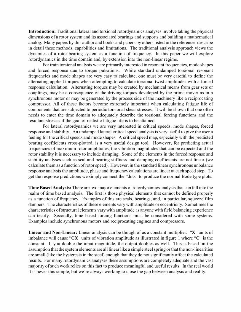
Figure 3 shows a 6-pole 5,500 HP synchronous motor driving an air compressor through a gear speedincreaser. Every synchronous motor generates alternating torque impulses during a startup. Thesepulses begin at twice line frequency (7,200 CPM in the US) and decline inversely with speed to zerowhen synchronous speed is reached. This means that every torsional resonance between 0 and 7,200CPM will be excited during each startup. Thus, any machine train with a synchronous motor mustbe evaluated with a transient torsional analysis. A transient analysis consists of creating a spring-mass model and defining all the torque producers (the motor and possibly the gear) and torqueabsorbers (the compressor). The torque information is generally available only from the motorvendor who must communicate with the manufacturer of the other machinery and produce a set oftorque curves similar to figure 4.

A forced response procedure is applied to the model simulating the startup. At time zero, thedriving, oscillatory, and load torques are applied simultaneously. This causes the train to acceleratein speed. The input torques are resisted by the polar inertia of the machines and the gas load fromthe compressor. Resistance from the bearings and gears is neglected. Then, at very small time steps,a new speed is calculated along with the torsional oscillation amplitude at every point in the train.Ultimately, the alternating torque amplitudes can be converted to the shear stresses in the shafts.One important calculation coming from this analysis is the time to reach full speed as seen in figure5. Typically, anything over 20 seconds could be damaging to the motor. After synchronization, thedelivered motor torque is balanced by the compressor load torque and there are no more alternatingtorque pulsations from the motor. Very low frequency oscillations often seen immediately aftersynchronization are due to interaction of the mechanical system with the electrical grid.

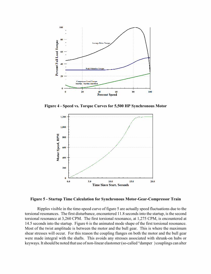
Figure 4 - Speed vs. Torque Curves for 5,500 HP Synchronous Motor

Figure 5 - Startup Time Calculation for Synchronous Motor-Gear-Compressor Train

Ripples visible in the time-speed curve of figure 5 are actually speed fluctuations due to thetorsional resonances. The first disturbance, encountered 11.8 seconds into the startup, is the secondtorsional resonance at 3,260 CPM. The first torsional resonance, at 1,275 CPM, is encountered at14.5 seconds into the startup. Figure 6 is the animated mode shape of the first torsional resonance.Most of the twist amplitude is between the motor and the bull gear. This is where the maximumshear stresses will occur. For this reason the coupling flanges on both the motor and the bull gearwere made integral with the shafts. This avoids any stresses associated with shrunk-on hubs orkeyways. It should be noted that use of non-linear elastomer (so-called “damper”) couplings can alter

these startup and response curves significantly. Elastomer couplings are not covered here.

Figure 6 - First Torsional Resonance Mode Shape for Example 3 - 1,275 CPM

Figure 7 is a plot of the alternating shaft shear stresses in the motor shaft section near the couplingduring a portion of the startup. The low-speed shaft always has higher torques and usually has thehighest steady and alternating torques from the synchronous motor startup.

Figure 7 - Shaft Stresses During Time Transient Startup of Synchronous Motor

The results of the time transient analysis produce a history of the number and magnitude of thealternating shear stresses in the shafting. In order to determine if these fatigue cycles will ultimatelybe a cause of failure, a fatigue analysis is performed. It is not possible for me to do this accuratelywithout a time transient analysis. In addition, derating factors are required such as stressconcentration factors, material composition and defect factors, surface finish factors, and other thingsthat may or may not apply to a given situation like a corrosion derating factor. Finally the timehistory is examined and the minimum and maximum shear stress values for the time period of highalternating stresses is examined and averaged to get a list of the maximum peak stresses.

Assuming the material specification is AISI 4140/4145 with an ultimate tensile strength(UTS) of 110,000 PSI and a yield strength of 85,000 PSI with a 40% reduction in area. A shearfatigue life plot for this material is shown in figure 8.

Figure 8 - Shear Fatigue Life Curve for Motor Shaft Material

In this particular analysis, failures that occur at less than 1000 cycles are called low cyclefatigue and high cycle fatigue after 1000 cycles to failure. Above 1 million cycles, the componentis assumed to have infinite life. Figure 8, for torsional shear stress, was derived from a plot of tensilefailure data by multiplying by 0.577 (von Mises theory) meaning that the shear endurance limit for

einfinite life is reduced from a tensile value of 30,000 PSI to S = 17,310 PSI. At the other end,

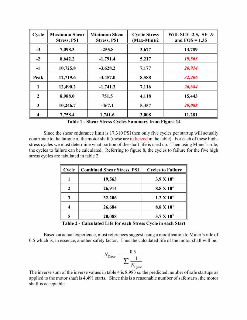
1000failure at 1000 cycles (S ) will occur at a shear stress level of 49,000 PSI. Table 1 is a listing ofthe calculated shaft shear stresses found in a plot of similar to figure 7. The stress concentrationfactor applied is 2.5 for the keyway and a factor of 1.35 is applied as a factor of safety. Also, asurface finish derating factor of 0.9 was used. A system modal damping factor was also applied oftwo percent of critical damping. The choice of this factor is critical since if it is too low, everysystem will calculate as a failure and if too high, every system will be indicated to be acceptable.Fatigue analysis is somewhat an art and must have a basis in experience.

Cycle Maximum ShearStress, PSI

Minimum ShearStress, PSI

Cyclic Stress(Max-Min)/2

With SCF=2.5, SF=.9and FOS = 1.35

-3 7,098.3 -255.8 3,677 13,789

-2 8,642.2 -1,791.4 5,217 19,563

-1 10,725.8 -3,628.2 7,177 26,914

Peak 12,719.6 -4,457.0 8,588 32,206

1 12,490.2 -1,741.3 7,116 26,684

2 8,988.0 751.5 4,118 15,443

3 10,246.7 -467.1 5,357 20,088

4 7,758.4 1,741.6 3,008 11,281

Table 1 - Shear Stress Cycles Summary from Figure 14

Since the shear endurance limit is 17,310 PSI then only five cycles per startup will actuallycontribute to the fatigue of the motor shaft (these are italicized in the table). For each of these high-stress cycles we must determine what portion of the shaft life is used up. Then using Miner’s rule,the cycles to failure can be calculated. Referring to figure 8, the cycles to failure for the five highstress cycles are tabulated in table 2.

Cycle Combined Shear Stress, PSI Cycles to Failure

1 19,563 3.9 X 105

2 26,914 8.8 X 104

3 32,206 1.2 X 104

4 26,684 8.8 X 104

5 20,088 3.7 X 105

Table 2 - Calculated Life for each Stress Cycle in each Start

Based on actual experience, most references suggest using a modification to Miner’s rule of0.5 which is, in essence, another safety factor. Thus the calculated life of the motor shaft will be:

The inverse sum of the inverse values in table 4 is 8,983 so the predicted number of safe startups asapplied to the motor shaft is 4,491 starts. Since this is a reasonable number of safe starts, the motorshaft is acceptable.

Reciprocating Compressor Train AnalysisThe second case of using time transient analysis involves steady state excitation from a

complicated alternating torque source. The compressor train illustrated here consists of a 600 HPinduction motor driving a 4-cylinder, double acting vertical piston reciprocating compressor withtwo 480mm and two 330mm cylinders. The motor is directly coupled to the gear by a disk typecoupling. The design full load motor speed is 593 RPM.

Figure 9 is a cross-section of the entire compressor train computer model. The providedphysical dimensions and other torsional information were translated into the finite element analysismodel used here. The motor rotor is shown in light red, the coupling in light blue, the flywheel isgreen and the compressor crankshaft is light magenta. The motor armature and the compressorreciprocating parts are indicated by the light orange disks on those shafts.

Figure 9 - Reciprocating Compressor Train Cross Section

The torsional resonance for this train has a direct torsional resonance interference with 4Xcompressor speed. Four times 593 RPM is the compressor excitation frequency of 2,372 CPM.Since there is significant 4X pulsation energy from the compressor, this is a resonance to be avoided.

The torsional resonance mode shape is plotted in figure 10. The horizontal axis is the axiallength of the shafting. The vertical axis is the non-dimensional relative twist amplitude. This isdimensionless since there is no forcing function defined in an undamped steady state torsional

analysis.Figure 10 - First Torsional Resonance Mode Shape - Original Coupling

In order to determine if the compressor pulsations are significant enough to cause any damageto the train components, a time transient forced response analysis is required. That means that allthe alternating torque harmonics must be consolidated into an equivalent complex alternating torquewaveform. This input is applied at the compressor shaft and the time based response of the shaftstresses in the train are determined.

Forced Response and Shaft Stress AnalysisThe primary torsional excitations in this system are generated by the compressor. The

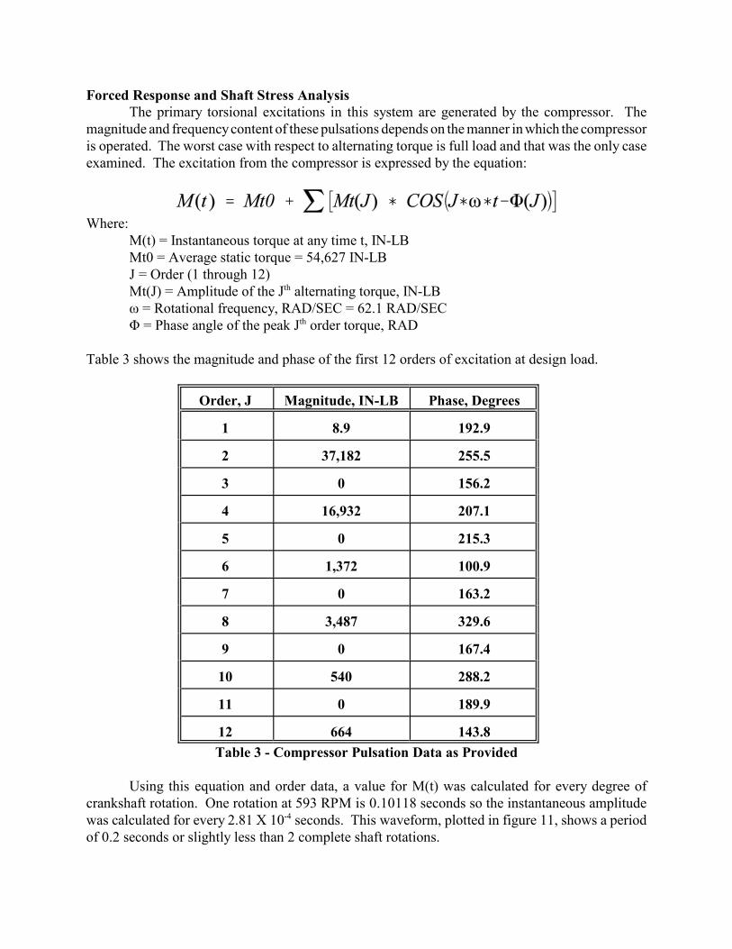
magnitude and frequency content of these pulsations depends on the manner in which the compressoris operated. The worst case with respect to alternating torque is full load and that was the only caseexamined. The excitation from the compressor is expressed by the equation:

Where:M(t) = Instantaneous torque at any time t, IN-LBMt0 = Average static torque = 54,627 IN-LBJ = Order (1 through 12)Mt(J) = Amplitude of the J alternating torque, IN-LBth

ω = Rotational frequency, RAD/SEC = 62.1 RAD/SECΦ = Phase angle of the peak J order torque, RADth

Table 3 shows the magnitude and phase of the first 12 orders of excitation at design load.

Order, J Magnitude, IN-LB Phase, Degrees

1 8.9 192.9

2 37,182 255.5

3 0 156.2

4 16,932 207.1

5 0 215.3

6 1,372 100.9

7 0 163.2

8 3,487 329.6

9 0 167.4

10 540 288.2

11 0 189.9

12 664 143.8

Table 3 - Compressor Pulsation Data as Provided

Using this equation and order data, a value for M(t) was calculated for every degree ofcrankshaft rotation. One rotation at 593 RPM is 0.10118 seconds so the instantaneous amplitudewas calculated for every 2.81 X 10 seconds. This waveform, plotted in figure 11, shows a period-4

of 0.2 seconds or slightly less than 2 complete shaft rotations.

Figure 11 - Periodic Alternating Torque Function from Table 3

Since only the most highly stressed shaft section needs to be used in the comparisons, theshaft stress at resonance for an arbitrary one degree of twist angle was calculated for all shaftsections. These stress levels, shown in figure 12, are not the actual predicted shaft stresses but ratherindicate that the smallest shaft diameter in the motor is the train location where the maximumtorsional shear stress will occur. This is indicated by the dark red color in this area and is designatedas element 8 in the finite element model.

Figure 12 - Location of Maximum Torsional Shear Stress at Resonance

Figure 13 is the calculated alternating shaft torque as a function of time (0.2 seconds). Figure14 then shows the equivalent shaft stresses in the motor shaft. These stresses are not high enoughto cause long-term fatigue damage and the design is acceptable.

Figure 13 - Alternating Torques in Motor Shaft

Figure 14 - Alternating Stresses in Motor Shaft

Instantaneous ChangesTime transient analysis is also required to evaluate what happens torsionally and laterally to

a machine train in the event something occurs instantaneously, or at least in a very short time period.From a torsional excitation standpoint there are several events that can trigger torsional oscillations.The most serious is an internal phase-to-phase or phase-to-ground short circuit. A short circuit inthe generator of a large turbine-generator train can be catastrophic. Another electrical fault that canbe an issue is sudden loss of power and almost immediate re-energizing as when a breaker wouldopen and close rapidly. A more common occurrence is a sudden load shed when the generator goesfrom full load to none. This does not happen instantaneously. It takes several cycles for themagnetic flux field to decay exponentially. By using this load change as the time transient inputfunction we can calculate the transient torsional response of the entire train.

Consider the turbine generator train shown in figure 15. This is an 850MW train consistingof an HP turbine, IP Turbine, two LP Turbines, a generator and the exciter all rigidly coupledoperating at 3,600 RPM. The torsional analysis was conducted to determine if a replacementgenerator was suitable and to investigate the effects of short circuits and load shed.

Figure 15 - 850MW Turbine-Generator Train

The shafting in this train is very large. The LP turbines have 21 inch diameter journals. Theentire train is 148 feet long and the combined rotor weight is nearly half a million pounds. Thesmallest diameter shaft is in the exciter section and this is where the highest shear stresses will bepresent right after a load shed. The first two torsional resonances will comprise nearly all of thetransient torsional energy. Figure 16 is a combination first torsional resonance mode shape andrelative stress plot. An arbitrary one degree of twist amplitude is assumed for the resonance. Thegreatest twist is in the exciter shafting and where the dark red coloration indicates the highest shearstresses at the first resonance (station 76).

Figure 16 - Combination 1 Torsional Resonance Modes Shape and Stress Plotst

The second torsional critical speed mode shape and stress plot, figure 17, indicates that thesame shaft section has the greatest relative shear stress at resonance. The torsional resonances higherin frequency are difficult to excite with this type of event and are not included in this analysis.

Figure 17 - Combination 2 Torsional Resonance Modes Shape and Stress Plotnd

The generator manufacturer stated that the magnetic field in the generator would collapseexponentially in 60 milliseconds (3.6 cycles). The input function that was used in the analysis isshown in figure 18. The torque starts at over 20 million inch-pounds, which is normal load on thegenerator, and decreases to a nominal residual value after the 60 millisecond decay time.

Figure 18 - Time Transient Torque Input to Turbine-Generator Set

The sudden release of torque causes the entire train of respond torsionally. All of thetorsional resonances are excited but only the first two contribute significantly to the shaft stressesin the exciter shafting. An FFT of the response at this section, figure 19, shows that the first modeat 1,240 CPM dominates and the second torsional resonance at 1,566 CPM has some effect. Thisplot is normalized to a maximum of unity because the machine owner did not want the actual valuesreleased.

Figure 19 - Spectrum Analysis of the Transient Torsional Response

The calculated maximum shaft stresses are plotted in figure 20. This sudden torque losscauses shaft shear stress oscillations that include primarily the first torsional resonance, some secondmode content and a small amount of higher mode content during the first few decay cycles.

Figure 20 - Torsional Shaft Shear Stress after Load Shed

Lateral Vibration Time Transient Analysis - Sudden ImbalanceHere we will evaluate what happens to the radial vibration of this same large turbine

generator train if a blade loss occurs. A blade loss is an instantaneous imbalance. While notcommon, this type of failure has occurred and nearly always results in a catastrophic failure andmany millions of dollars of loss. In the example shown in this paper, only a portion of a blade losswill be explored to increase the clarity of what is happening. Assume that the same turbine generatorset now has bearings and a random set of first and second mode imbalances indicated by the groupof three hollow red arrows pointing up from each machine as shown in figure 21. The solid redarrow at station 59, the last blade row of the second low pressure turbine indicates where the suddenblade loss simulation will occur.

Figure 21 - Turbine Generator Set with Imbalances and Blade Loss Indication

With the train operating at 3,600 RPM, the time transient analysis is started. There is aninitial transition period where the effects of the suddenly applied residual imbalances settle-out anda steady state synchronous response is established as in figure 22.

Figure 22 - Normal T-G Set Synchronous Vibration Prior to Blade Loss

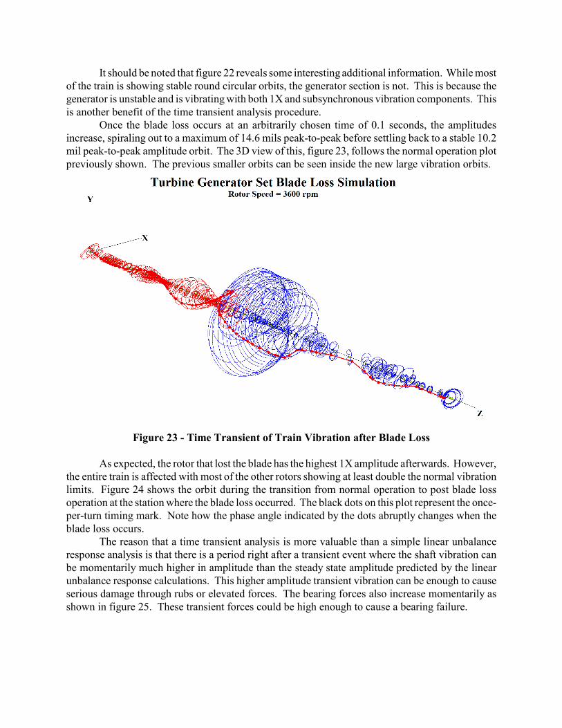
It should be noted that figure 22 reveals some interesting additional information. While mostof the train is showing stable round circular orbits, the generator section is not. This is because thegenerator is unstable and is vibrating with both 1X and subsynchronous vibration components. Thisis another benefit of the time transient analysis procedure.

Once the blade loss occurs at an arbitrarily chosen time of 0.1 seconds, the amplitudesincrease, spiraling out to a maximum of 14.6 mils peak-to-peak before settling back to a stable 10.2mil peak-to-peak amplitude orbit. The 3D view of this, figure 23, follows the normal operation plotpreviously shown. The previous smaller orbits can be seen inside the new large vibration orbits.

Figure 23 - Time Transient of Train Vibration after Blade Loss

As expected, the rotor that lost the blade has the highest 1X amplitude afterwards. However,the entire train is affected with most of the other rotors showing at least double the normal vibrationlimits. Figure 24 shows the orbit during the transition from normal operation to post blade lossoperation at the station where the blade loss occurred. The black dots on this plot represent the once-per-turn timing mark. Note how the phase angle indicated by the dots abruptly changes when theblade loss occurs.

The reason that a time transient analysis is more valuable than a simple linear unbalanceresponse analysis is that there is a period right after a transient event where the shaft vibration canbe momentarily much higher in amplitude than the steady state amplitude predicted by the linearunbalance response calculations. This higher amplitude transient vibration can be enough to causeserious damage through rubs or elevated forces. The bearing forces also increase momentarily asshown in figure 25. These transient forces could be high enough to cause a bearing failure.

Figure 24 - LP Turbine Shaft Orbit during Blade Loss Event

Figure 25 - LP Turbine Bearing Forces during Blade Loss Event

Non-Linear Bearing Effects

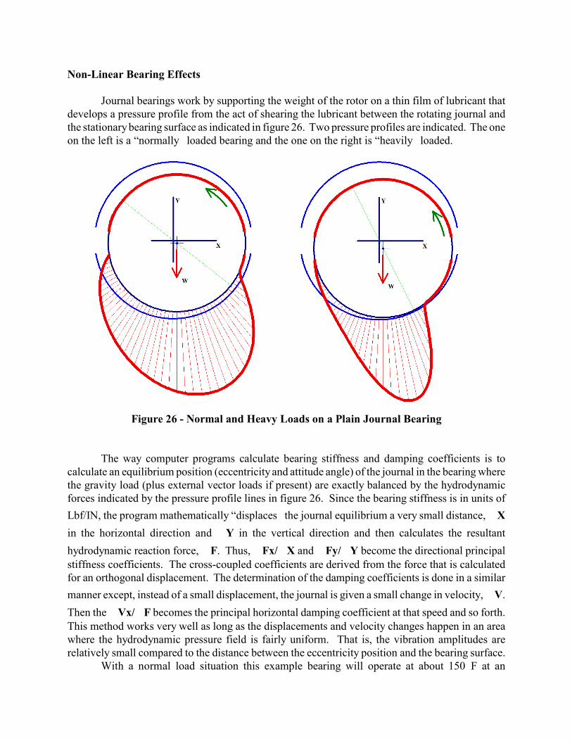
Journal bearings work by supporting the weight of the rotor on a thin film of lubricant thatdevelops a pressure profile from the act of shearing the lubricant between the rotating journal andthe stationary bearing surface as indicated in figure 26. Two pressure profiles are indicated. The oneon the left is a “normally” loaded bearing and the one on the right is “heavily” loaded.

Figure 26 - Normal and Heavy Loads on a Plain Journal Bearing

The way computer programs calculate bearing stiffness and damping coefficients is tocalculate an equilibrium position (eccentricity and attitude angle) of the journal in the bearing wherethe gravity load (plus external vector loads if present) are exactly balanced by the hydrodynamicforces indicated by the pressure profile lines in figure 26. Since the bearing stiffness is in units of

Lbf/IN, the program mathematically “displaces” the journal equilibrium a very small distance, ÎX

in the horizontal direction and ÎY in the vertical direction and then calculates the resultant

hydrodynamic reaction force, ÎF. Thus, ÎFx/ÎX and ÎFy/ÎY become the directional principalstiffness coefficients. The cross-coupled coefficients are derived from the force that is calculatedfor an orthogonal displacement. The determination of the damping coefficients is done in a similar

manner except, instead of a small displacement, the journal is given a small change in velocity, ÎV.

Then the ÎVx/ÎF becomes the principal horizontal damping coefficient at that speed and so forth.This method works very well as long as the displacements and velocity changes happen in an areawhere the hydrodynamic pressure field is fairly uniform. That is, the vibration amplitudes arerelatively small compared to the distance between the eccentricity position and the bearing surface.

With a normal load situation this example bearing will operate at about 150EF at an

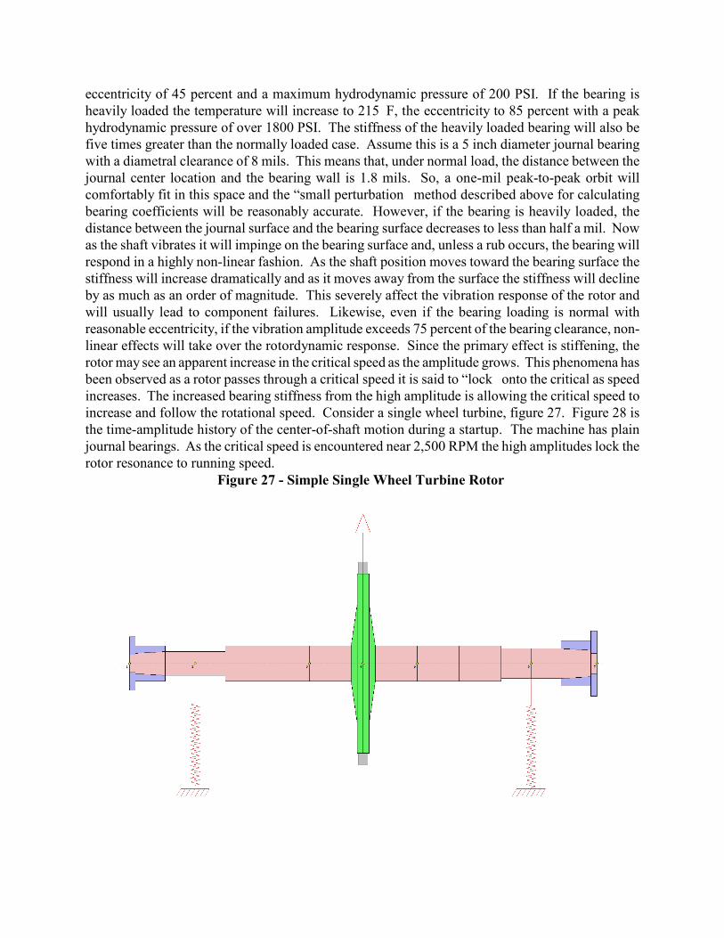
eccentricity of 45 percent and a maximum hydrodynamic pressure of 200 PSI. If the bearing isheavily loaded the temperature will increase to 215EF, the eccentricity to 85 percent with a peakhydrodynamic pressure of over 1800 PSI. The stiffness of the heavily loaded bearing will also befive times greater than the normally loaded case. Assume this is a 5 inch diameter journal bearingwith a diametral clearance of 8 mils. This means that, under normal load, the distance between thejournal center location and the bearing wall is 1.8 mils. So, a one-mil peak-to-peak orbit willcomfortably fit in this space and the “small perturbation” method described above for calculatingbearing coefficients will be reasonably accurate. However, if the bearing is heavily loaded, thedistance between the journal surface and the bearing surface decreases to less than half a mil. Nowas the shaft vibrates it will impinge on the bearing surface and, unless a rub occurs, the bearing willrespond in a highly non-linear fashion. As the shaft position moves toward the bearing surface thestiffness will increase dramatically and as it moves away from the surface the stiffness will declineby as much as an order of magnitude. This severely affect the vibration response of the rotor andwill usually lead to component failures. Likewise, even if the bearing loading is normal withreasonable eccentricity, if the vibration amplitude exceeds 75 percent of the bearing clearance, non-linear effects will take over the rotordynamic response. Since the primary effect is stiffening, therotor may see an apparent increase in the critical speed as the amplitude grows. This phenomena hasbeen observed as a rotor passes through a critical speed it is said to “lock” onto the critical as speedincreases. The increased bearing stiffness from the high amplitude is allowing the critical speed toincrease and follow the rotational speed. Consider a single wheel turbine, figure 27. Figure 28 isthe time-amplitude history of the center-of-shaft motion during a startup. The machine has plainjournal bearings. As the critical speed is encountered near 2,500 RPM the high amplitudes lock therotor resonance to running speed.

Figure 27 - Simple Single Wheel Turbine Rotor

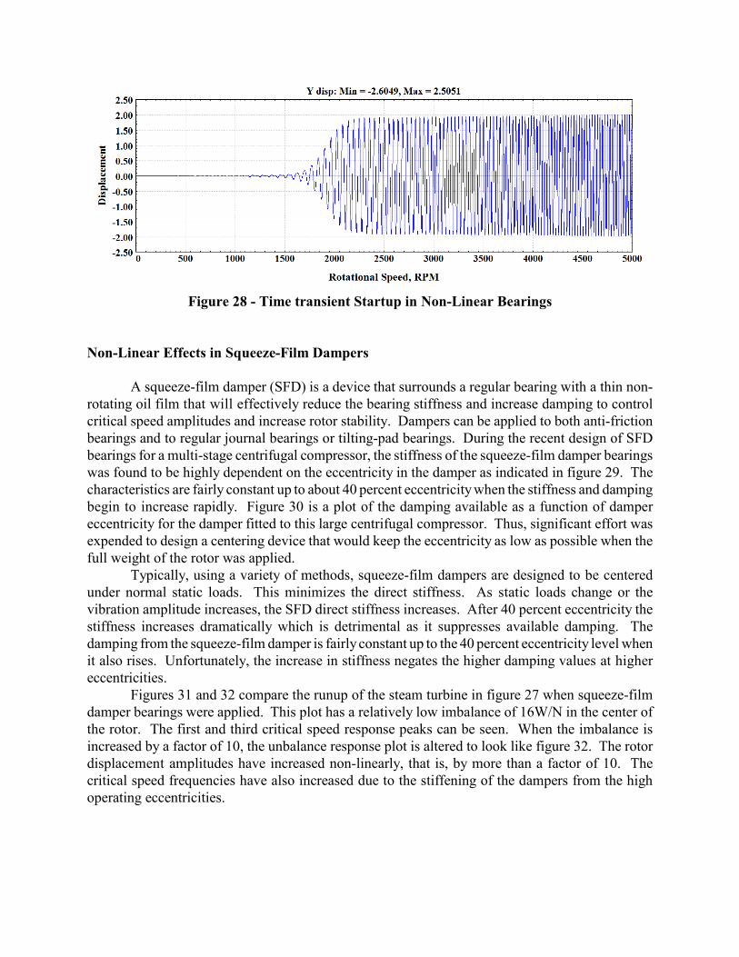
Figure 28 - Time transient Startup in Non-Linear Bearings

Non-Linear Effects in Squeeze-Film Dampers

A squeeze-film damper (SFD) is a device that surrounds a regular bearing with a thin non-rotating oil film that will effectively reduce the bearing stiffness and increase damping to controlcritical speed amplitudes and increase rotor stability. Dampers can be applied to both anti-frictionbearings and to regular journal bearings or tilting-pad bearings. During the recent design of SFDbearings for a multi-stage centrifugal compressor, the stiffness of the squeeze-film damper bearingswas found to be highly dependent on the eccentricity in the damper as indicated in figure 29. Thecharacteristics are fairly constant up to about 40 percent eccentricity when the stiffness and dampingbegin to increase rapidly. Figure 30 is a plot of the damping available as a function of dampereccentricity for the damper fitted to this large centrifugal compressor. Thus, significant effort wasexpended to design a centering device that would keep the eccentricity as low as possible when thefull weight of the rotor was applied.

Typically, using a variety of methods, squeeze-film dampers are designed to be centeredunder normal static loads. This minimizes the direct stiffness. As static loads change or thevibration amplitude increases, the SFD direct stiffness increases. After 40 percent eccentricity thestiffness increases dramatically which is detrimental as it suppresses available damping. Thedamping from the squeeze-film damper is fairly constant up to the 40 percent eccentricity level whenit also rises. Unfortunately, the increase in stiffness negates the higher damping values at highereccentricities.

Figures 31 and 32 compare the runup of the steam turbine in figure 27 when squeeze-filmdamper bearings were applied. This plot has a relatively low imbalance of 16W/N in the center ofthe rotor. The first and third critical speed response peaks can be seen. When the imbalance isincreased by a factor of 10, the unbalance response plot is altered to look like figure 32. The rotordisplacement amplitudes have increased non-linearly, that is, by more than a factor of 10. Thecritical speed frequencies have also increased due to the stiffening of the dampers from the highoperating eccentricities.

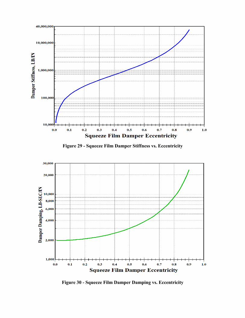
Figure 29 - Squeeze Film Damper Stiffness vs. Eccentricity

Figure 30 - Squeeze Film Damper Damping vs. Eccentricity

Figure 31 - Turbine Runup with Squeeze-Film Damper Bearings - Low Imbalance

Figure 32 - Turbine Runup with Squeeze-Film Damper Bearings - Large Imbalance

Acknowledgments: The author would like to thank Dr. Edgar J. Gunter for his counsel and insightover the last 35 years and in particular showing me how time transient and non-linear analysis canopen new methods of insight and solutions into machinery problems. I would also like to thank Dr.Wen Jeng Chen, the author of the suite of rotordynamics programs collectively called DyRoBeS.This set of tools has not only opened design and analysis methods to me that other rotordynamicsanalysis packages either do not have or are much more difficult to use. Dr Chen’s willingness toincorporate changes and additions to these programs is nothing short of phenomenal. The outputgraphics are a joy to incorporate into my papers and reports. Finally, I could not have come this farwithout the guidance of my mentor, Charlie Jackson. Charlie put the practical into rotordynamicsand vibration analysis and his contributions can not be overestimated.

REFERENCES

1. Leader, M.E., “Practical Rotor Dynamics,” Proceedings of the Vibration Institute 26 Annual Meeting, June, 2002th

2. Leader, M.E., “Rotor Dynamics as a Tool for Solving Vibration Problems ,“ Proceedings of the 27 Vibrationth

Institute Annual Meeting, July, 2003

3. Jackson, C., The Practical Vibration Primer, Gulf Publishing Co., Houston, TX., First Edition, 1979.

4. Kirk, R.G. and Gunter, E.J., “The Effect of Support Flexibility and Damping on the Synchronous Response of a Single

Mass Flexible Rotor,” ASME Journal of Engineering for Industry, 94(1), February, 1972

5. Nicholas, J.C., Whalen, J.K., and Franklin, S.D., “Improving Critical Speed Calculations Using Flexible Bearing

Support FRF Compliance Data,” Proceedings of the 15 Turbomachinery Symposium, Texas A&M University, pp. 69-th

80, 1986.

6. Lund, J.W., "Modal Response of a Flexible Rotor in Fluid-Film Bearings", ASME 73-DET-98, Cincinnati, September,

1973.

7. Prohl, M.A., "A General Method for Calculating Critical Speeds of Flexible Rotors", Transactions ASME, Volume

67, Journal of Applied Mechanics, Volume 12, Page A-142.

8. Tonnesen, J. and Lund, J.W., "Some Experiments on Instability of Rotors Supported in Fluid-Film Bearings", ASME

77-DET-23, Chicago, 1977.

9. Weaver, F.L., "Rotor Design and Vibration Response", AIChE 49C, September, 1971, 70th National Meeting.

10. API RP684, “Rotordynamics Tutorial: Lateral Critical Speeds, Unbalance Response, Stability, Train Torsionals, and

Rotor Balancing”, American Petroleum Institute, August, 2005.

11. Jackson, C., and Leader, M.E., "Rotor Critical Speed and Response Studies for Equipment Selection", Vibration

Institute Proceedings, April 1979, pp. 45-50. (reprinted in Hydrocarbon Processing, November, 1979, pp 281-284.)

12. Eshleman, R.L., "ASME Flexible Rotor-Bearing System Dynamics, Part 1 - Critical Speeds and Response of Flexible

Rotor Systems", ASME H-42, 1972.

13. Chen, W. J., and Gunter, E. J.,“Introduction to Dynamics of Rotor Bearing Systems”, Trafford Publishing, ISBN

1-4120-5190-8, 2005

14. Nestorides, E. J., B.I.C.E.R.A. Handbook of Torsional Vibration, Cambridge University Press, 1958

15. Walker, Duncan N., Torsional Vibration of Turbomachinery, McGraw-Hill, 2003 ISBN 0-07-143037-7

16. Corbo, Mark A. And Melanoski, Stanley B., Practical Design Against Torsional Vibration, Tutorial, 25 Texasth

A&M Turbomachinery Symposium pp 189-222, September, 1996

17. Ker Wilson, W., Practical Solution of Torsional Vibration Problems, Volumes 1 through 5, John Wiley & Sons,

1959

18. Jackson, C. And Leader, M.E., Design and Commissioning of Two Synchronous Motor-Gear-Air Compressor Trains,

13th Texas A&M Turbomachinery Symposium, November, 1983.

19. Holdrege, J., Subler, W., and Frasier, W., “AC Induction Motor Torsional Vibration Consideration – A Case Study”,

IEEE Transactions on Industry Applications, Vol. 1A-19, No.1, Jan/Feb 1983.