Time Series Cross Section Data

Anjali Thomas Bohlken∗

May 31, 2011

Time Series Cross Section Data analysis techniques are needed for datasets

consisting of a number of cross-sectional units (e.g. countries, dyads, provinces,

villages) with repeated observations over time (e.g. years, months, days).

Suppose you have a dataset with 20 countries each observed over 30 years. This

yields 600 observations, but in some sense this number is an artificial inflation.

Remember that the standard OLS assumption is that the error terms are

independent from each other (i.i.d.). In TSCS datasets, this assumption is clearly

violated for a number of reasons including but not limited to the following:

1. Observations from within the same unit over time are typically related to each

other in specific ways

2. Observations from nearby units may be related to each other

∗These notes are based to a large extent on Neal Beck’s lecture notes. I have also borrowed fromMatt Golder’s lecture notes and from many of the articles and texts referenced at the end of thenotes.

1

3. There may be differences across units that cannot be accounted for by the

independent variables in the model

The old-fashioned way of dealing with these issues was to treat them as a nuisance.

The new-fashioned(??) way of dealing with them is to consider them as part of the

model we specify. We will usually with the latter approach.

The main issues that come up when analyzing this kind of data are as follows:

• Between Unit Heterogeneity: Fixed Effects, Random Effects, Random

Coefficient Models

• Time Series Issues: Temporal Dependence, Dynamics

– Continuous Dependent Variable

– Dependent Variable

• Cross-Sectional Issues: Panel Heteroskedasticity, Spatial Correlation

1 Preliminaries

1.1 Notation

Number of cross-sectional units denoted by: N

Number of time-series units denoted by: T .

Thus, the total number of observations is NT .

2

In a pure cross-section dataset (e.g. a survey of N individuals), the basic model

assuming one independent variable is:

yi = α + xiβ + εi

In a pure time-series dataset (e.g. a series of daily world oil prices), the basic model

is:

yt = α + xtβ + εt

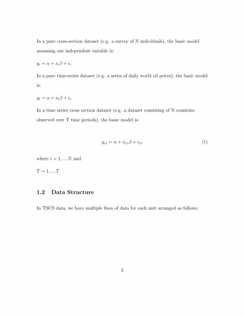
In a time series cross section dataset (e.g. a dataset consisting of N countries

observed over T time periods), the basic model is:

yi,t = α + xi,tβ + εi,t (1)

where i = 1, ....N and

T = 1, ....T

1.2 Data Structure

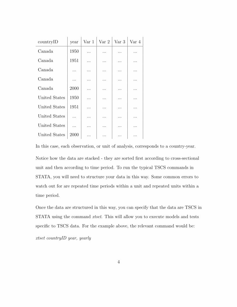
In TSCS data, we have multiple lines of data for each unit arranged as follows:

3

countryID year Var 1 Var 2 Var 3 Var 4

Canada 1950 ... ... ... ...

Canada 1951 ... ... ... ...

Canada ... ... ... ... ...

Canada ... ... ... ... ...

Canada 2000 ... ... ... ...

United States 1950 ... ... ... ...

United States 1951 ... ... ... ...

United States ... ... ... ... ...

United States ... ... ... ... ...

United States 2000 ... ... ... ...

In this case, each observation, or unit of analysis, corresponds to a country-year.

Notice how the data are stacked - they are sorted first according to cross-sectional

unit and then according to time period. To run the typical TSCS commands in

STATA, you will need to structure your data in this way. Some common errors to

watch out for are repeated time periods within a unit and repeated units within a

time period.

Once the data are structured in this way, you can specify that the data are TSCS in

STATA using the command xtset. This will allow you to execute models and tests

specific to TSCS data. For the example above, the relevant command would be:

xtset countryID year, yearly

4

1.2.1 TSCS vs. Panel Data

A key aspect of any dataset that must be considered is the size of N and T .

1. Time Series Cross Sectional Data (TSCS) refers to datasets with large T

and small or medium sized N . Examples include CPE datasets focusing on,

for example, the set of OECD countries or IR datasets with a large number of

dyads observed for 50 or more years. .

2. Panel Data refers to datasets with large N but small T such as a repeated

survey of a large number of individuals.

3. There is one other option of course! If your dataset falls in this category, you

are out of luck. You need to collect more data!

Techniques for TSCS data allow you to leverage the large T to (among other

things) model the time series structure of the data and to lend credence to your

inferences through the use of fixed effects.

How large is large? T should be large enough so that averages make sense. A rough

guideline is at least 10, but 20 or more is ideal.

2 Pooling/Between Unit Heterogeneity

Consider, again, Equation (1) above.

yi,t = α + xi,tβ + εi,t

5

A key assumption embedded in this model is that the intercept α does not vary.

This assumption is usually problematic when we think of units such as countries,

dyads or provinces that usually have key fixed characteristics not accounted for by

the independent variables. Running such a model amounts to ”pooling” your data.

2.1 Fixed Effects

One alternative to pooling is to include fixed effects in your model.

A fixed effect model is represented as follows:

yi,t = α + xi,tβ + δ1Z1 + δ2Z2 + ...+ δnZN−1 + εi,t (2)

It involves including dummy variables (Z1, Z2, ...., ZN−1) marking each

cross-sectional unit (e.g. country). If a constant term is included, then you must

include N − 1 dummy variables to avoid perfect collinearity.

Here, the Zi refer to dummy variables marking each cross-sectional unit. The δi

denote the coefficients associated with each cross-sectional unit. Thus, each

cross-sectional unit (minus one) has its own intercept.

Note that Equation (1) is a restricted form of Equation (2). Equation (1) assumes

that the coefficients associated with each cross-sectional unit are equal to zero or

that:

δ1 = δ2 = ..... = δN−1 = 0.

6

Not surprisingly, if the assumption above is violated, Equation (1) generates biased

estimates. As Green, Kim and Yoon (2001) note, ignoring fixed effects is a special

case of the general problem of omitted variable bias.

To see how ignoring fixed effects introduces bias, consider the following scenarios

and figures illustrated by Green, Kim and Yoon (2001):

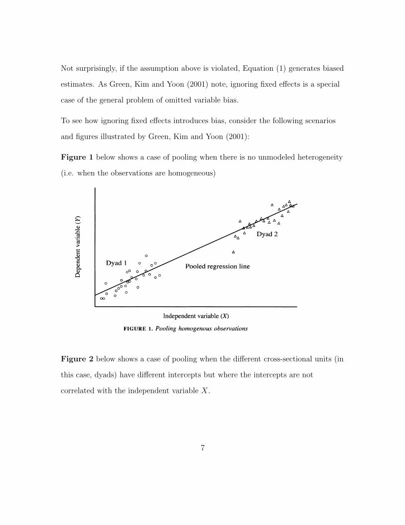
Figure 1 below shows a case of pooling when there is no unmodeled heterogeneity

(i.e. when the observations are homogeneous)444 International Organization

ADyad 2

AAA Dyad 2

A

Pooled regression line

Independent variable (X) FIGURE 1. Pooling homogenous observations

o o

line ? - -

0o ? o ? o0 0Q 0-

Independent variable (X) FIGURE 2. Pooling dyads with randomly varying intercepts

dyads have different intercepts, but there is no correlation between the intercepts and X. The average value of the independent variable is the same in each dyad. Again, pooled regression and regression with fixed effects give estimates with the same expected value. Figure 3 illustrates a situation in which pooled regression goes

Dyad 1 o

Figure 2 below shows a case of pooling when the different cross-sectional units (in

this case, dyads) have different intercepts but where the intercepts are not

correlated with the independent variable X.

7

444 International Organization

ADyad 2

AAA Dyad 2

A

Pooled regression line

Independent variable (X) FIGURE 1. Pooling homogenous observations

o o

line ? - -

0o ? o ? o0 0Q 0-

Independent variable (X) FIGURE 2. Pooling dyads with randomly varying intercepts

dyads have different intercepts, but there is no correlation between the intercepts and X. The average value of the independent variable is the same in each dyad. Again, pooled regression and regression with fixed effects give estimates with the same expected value. Figure 3 illustrates a situation in which pooled regression goes

Dyad 1 o

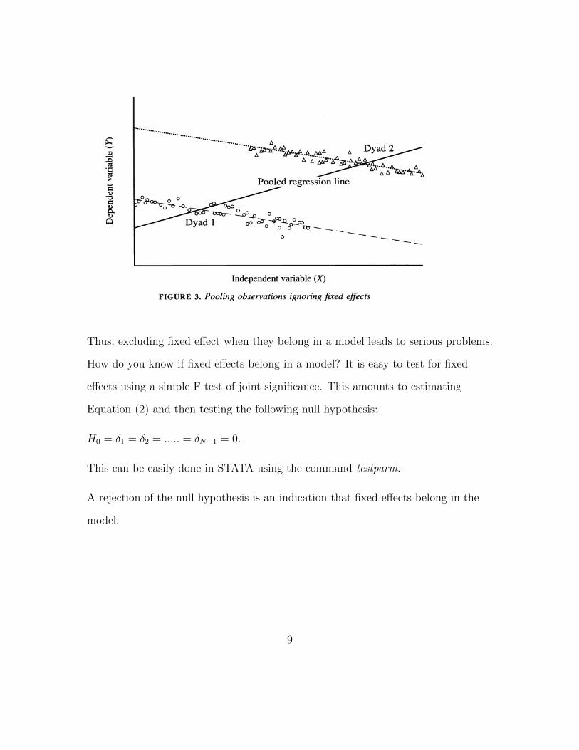
Figure 3 shows a case of pooling when the different cross-sectional units (in this

case, dyads) have different intercepts but where the intercepts are in fact correlated

with the independent variable X. Here, the pooled regression is particularly

problematic since it shows that the relationship between X and Y is positive, when

in fact it is negative. Because the dyad with the higher values of X also has a

higher intercept, this biases the pooled regression line upwards.

8

Dirty Pool 445

"5x` .........???....... ... A... A

A" A"' / A'A"...A. MA a Dyad2

3>^~~~~ ~~Pooled regression line

| ^ o0-0-.^ 0- * 0o ~ ~ ~ ~ 0

0

Independent variable (X)

Independent variable (X)

FIGURE 3. Pooling observations ignoring fixed effects

awry. Here, the causal relationship between X and Y is negative; in each dyad higher values of X coincide with lower values of Y. Yet when the dyads are pooled together, we obtain a spurious positive relationship. Because the dyad with higher values of X also has a higher intercept, ignoring fixed effects biases the regression line in the positive direction. Controlling for fixed effects, we correctly ascertain the true negative relationship between X and Y.

The foregoing examples suggest how fixed effects may be detected. By compar- ing alternative regression models, we obtain a sense of whether pooling causes estimation problems. This logic underlies statistical tests designed to check whether the assumptions behind Equation (1) are warranted. The most general null hypoth- esis is that all of the dyads have the same intercept (8g = 0). For a linear regression, this amounts to an F-test with (N - 1, NT) degrees of freedom. Rejecting the null hypothesis suggests that the dyads have different intercepts, a necessary but not sufficient condition for bias. To establish bias, one compares the estimates of the k generated by Equations (1) and (2) using a Hausman test (see the appendix), which gauges whether the dyad-specific intercepts are random or instead correlated with the model's regressors (Xkit). Under the null hypothesis, dyads have distinctive intercepts, but these intercepts are uncorrelated with the regressors and therefore produce no bias. In this case, controlling for fixed effects produces unbiased but inefficient slope estimates; the slew of dummy variables wastes degrees of freedom, making the estimates less precise than they could be. The alternative hypothesis is that the dyad-specific intercepts are correlated with the regressors, in which case pooled regression will be biased and fixed-effects regression remains unbiased. The

Thus, excluding fixed effect when they belong in a model leads to serious problems.

How do you know if fixed effects belong in a model? It is easy to test for fixed

effects using a simple F test of joint significance. This amounts to estimating

Equation (2) and then testing the following null hypothesis:

H0 = δ1 = δ2 = ..... = δN−1 = 0.

This can be easily done in STATA using the command testparm.

A rejection of the null hypothesis is an indication that fixed effects belong in the

model.

9

2.2 Cons of including Fixed Effects

Even if fixed effects belong in a model, including fixed effects can come with some

serious costs.

First, including fixed effects involves using up a large number of degrees of freedom

(i.e. N − 1) which makes estimation more difficult.

The issues occur if we have (1) variables that do not change over time or (2)

variables that change very slowly. Variables of type (1) will be dropped from your

model when you include fixed effects because they will be perfectly collinear with

the fixed effects. The coefficients on variables of type (2) will be very hard to

estimate precisely. Potential solutions are offered by Plumper and Troeger (2007)

and Beck (2001).

2.3 Random Effects

Another approach to dealing with between unit heterogeneity is to include random

effects. The key assumption made in random effects models is that the

unit-specific effects are uncorrelated with the independent variables. If

this assumption is true, then OLS will yield unbiased, consistent estimates (see

Figure 2 of Green, Kim and Yoon (2001) above). But the estimated standard errors

will be too small because, with a random effects model, we are ignoring the fact

that observations within the same unit are correlated.

Consider a reformulation of Equation (1) where we now have:

10

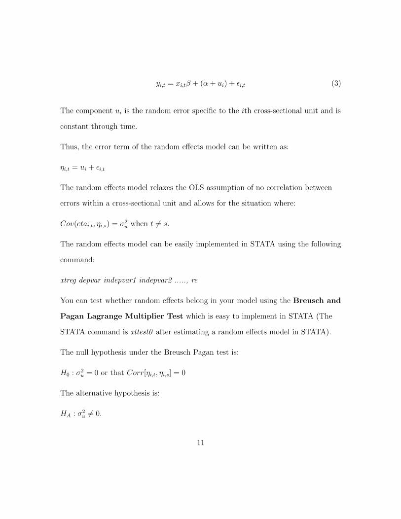
yi,t = xi,tβ + (α + ui) + εi,t (3)

The component ui is the random error specific to the ith cross-sectional unit and is

constant through time.

Thus, the error term of the random effects model can be written as:

ηi,t = ui + εi,t

The random effects model relaxes the OLS assumption of no correlation between

errors within a cross-sectional unit and allows for the situation where:

Cov(etai,t, ηi,s) = σ2u when t 6= s.

The random effects model can be easily implemented in STATA using the following

command:

xtreg depvar indepvar1 indepvar2 ....., re

You can test whether random effects belong in your model using the Breusch and

Pagan Lagrange Multiplier Test which is easy to implement in STATA (The

STATA command is xttest0 after estimating a random effects model in STATA).

The null hypothesis under the Breusch Pagan test is:

H0 : σ2u = 0 or that Corr[ηi,t, ηi,s] = 0

The alternative hypothesis is:

HA : σ2u 6= 0.

11

The resulting test statistic of the Breusch and Pagan Lagrange Multiplier Test is

distributed as Chi-Squared with one degree of freedom.

There are several assumptions embedded in a random effects model, but the key

ones are:

A. The unit specific effects are uncorrelated with the independent variables.

Cov[ui, xi,t] = 0

B. There is no correlation between the errors across units. Cov(ηi,t, ηi,s) = 0 for all

t and s if i 6= j.

The good news is that you can test Assumption (A) above using a Hausman

specification test. (The STATA command is hausman).1

Under the null hypothesis that Assumption (A) is true, the fixed effects and

random effects models are both consistent, but the random effects are more

efficient. (This is because FEs use up degrees of freedom).

Under the alternative hypothesis that Cov(ui, xi,t) 6= 0, the fixed effects estimator

is consistent (because it does not assume that Cov[ui, xi,t] = 0), but the random

effects estimator is not.

If the Hausman test does not reject the null hypothesis, it is advisable to use a

random effects model since this will be more efficient than a fixed effects model. If

1To carry out this test in STATA, you will need to estimate both a fixed effects model and arandom effects model in STATA using the command xtreg with the appropriate modification. Youwould then need to store each of the results under the names fixed and random respectively. Thecommand is estimates store fixed. You would then carry out the hausman specification test bytyping hausman fixed random. The order is important since the first model is consistent under boththe null and alternative, while the second model is efficient under both the null and alternative.

12

the null is rejected, however, it is advisable to use a fixed effects model since a

random effects model would be inconsistent.

2.4 Random Coefficient Models

A more flexible approach and one that is increasingly becoming the most preferred

by many researchers is a random coefficient model (RCMs). This allows for

heterogeneity of the coefficients as well as the intercepts in a nice way.

RCMs are a special case of a multi-level model. You have already covered

multi-level models, so we will not go into more detail here. For more on this refer

to: Beck and Katz (2007) or Beck’s lecture notes.

3 Time Series Issues

Let us go back, again, to the basic OLS model.

yi,t = α + xi,tβ + εi,t

A key assumption of this model is that: Cov(εi,t, εi,s) = 0 where t 6= s. Obviously,

this assumption is problematic since we expect events and phenomena to be

correlated across time.

Why might errors be correlated across time? There are features of the world that

are unobserved (i.e. not included in the model) that change slowly over time. If we

13

had perfect data availability (a utopian scenario), would we still need to model

time dependence?

It is useful to introduce some additional notation here pertaining to the lag

operator L.

L.yt = yt−1

L2.yt = yt−2 and so on.

It is also useful to introduce the first difference operator D or ∆:

D.y = yt − yt−1 (∆y = yt − yt−1)

This will be useful when we consider how to approach time series issues in STATA.

3.1 Continuous Dependent Variable

3.1.1 Huberized Standard Errors/Clustering

Clustering or Huberizing the standard errors allows for the errors of observations

within a single cross-sectional unit to be correlated and, for TSCS data, it is often

used to deal with temporal dependence. Clustering amounts to an ex post fix of the

standard errors and, thus, will affect your standard errors but not your coefficients.

A common approach used in the political science literature is to simultaneously

deal with non-independence of observations within a cross-sectional unit as well as

panel heteroskedasticity by estimating a regression model in STATA using

Huber-White standard errors (also known as heteroskedastic-consistent clustered

14

standard errors). If your cross-sectional unit is country (countryID), the command

in STATA is:

reg y x1 x2......, robust cluster(countryID)

Compared to the standard OLS variance covariance matrix given above, the robust

cluster command does the following:

1) It allows the error variance for each cross-sectional unit to be different. (i.e. the

diagonal terms are σ2i (where i is the cross-sectional unit) rather than σ2.

2) It allows the covariance between the error terms within the same unit to be

non-zero (e.g. σi,t,t+1 6= 0; σi,t,t+2 6= 0 etc.)

It retains the assumption that there is no correlation between errors across units

(i.e. σi,j,t = 0 for any t for all i 6= j.)

Why use clustering? Clustering is easily implemented in a maximum likelihood

framework where dealing with temporal dependence in other ways becomes

complicated. If you do not deal with temporal dependence in any other way, you

should at least use clustering as it is generally the more conservative approach in

expectation, but not necessarily in practice!.

3.1.2 Serial Correlation: AR1 Error Model

A model with an AR1 error process or, equivalently, first order serial correlation is

specified as follows:

15

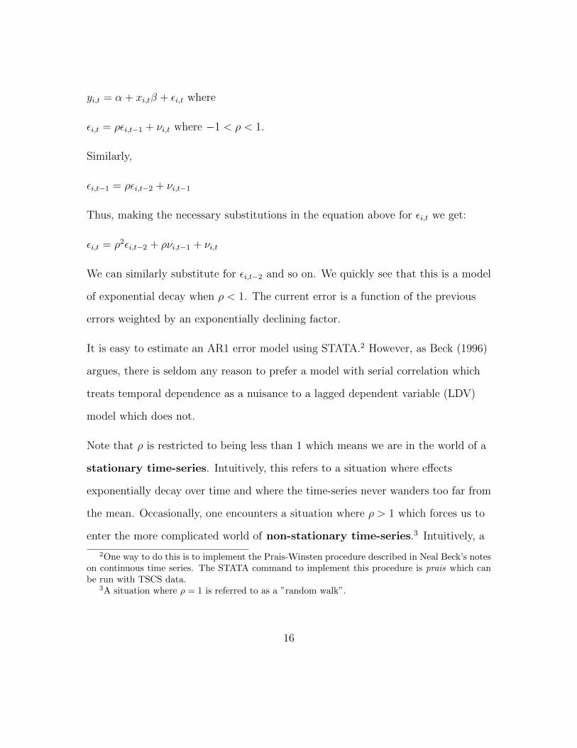
yi,t = α + xi,tβ + εi,t where

εi,t = ρεi,t−1 + νi,t where −1 < ρ < 1.

Similarly,

εi,t−1 = ρεi,t−2 + νi,t−1

Thus, making the necessary substitutions in the equation above for εi,t we get:

εi,t = ρ2εi,t−2 + ρνi,t−1 + νi,t

We can similarly substitute for εi,t−2 and so on. We quickly see that this is a model

of exponential decay when ρ < 1. The current error is a function of the previous

errors weighted by an exponentially declining factor.

It is easy to estimate an AR1 error model using STATA.2 However, as Beck (1996)

argues, there is seldom any reason to prefer a model with serial correlation which

treats temporal dependence as a nuisance to a lagged dependent variable (LDV)

model which does not.

Note that ρ is restricted to being less than 1 which means we are in the world of a

stationary time-series. Intuitively, this refers to a situation where effects

exponentially decay over time and where the time-series never wanders too far from

the mean. Occasionally, one encounters a situation where ρ > 1 which forces us to

enter the more complicated world of non-stationary time-series.3 Intuitively, a

2One way to do this is to implement the Prais-Winsten procedure described in Neal Beck’s noteson continuous time series. The STATA command to implement this procedure is prais which canbe run with TSCS data.

3A situation where ρ = 1 is referred to as a ”random walk”.

16

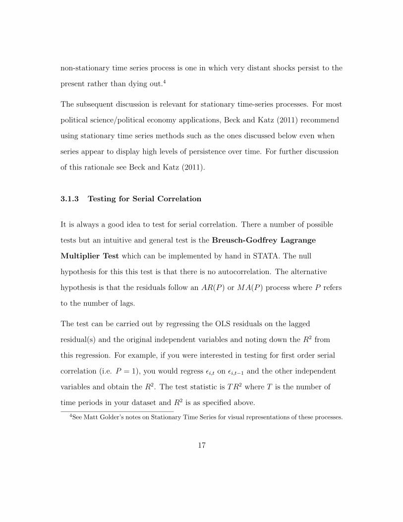
non-stationary time series process is one in which very distant shocks persist to the

present rather than dying out.4

The subsequent discussion is relevant for stationary time-series processes. For most

political science/political economy applications, Beck and Katz (2011) recommend

using stationary time series methods such as the ones discussed below even when

series appear to display high levels of persistence over time. For further discussion

of this rationale see Beck and Katz (2011).

3.1.3 Testing for Serial Correlation

It is always a good idea to test for serial correlation. There a number of possible

tests but an intuitive and general test is the Breusch-Godfrey Lagrange

Multiplier Test which can be implemented by hand in STATA. The null

hypothesis for this this test is that there is no autocorrelation. The alternative

hypothesis is that the residuals follow an AR(P ) or MA(P ) process where P refers

to the number of lags.

The test can be carried out by regressing the OLS residuals on the lagged

residual(s) and the original independent variables and noting down the R2 from

this regression. For example, if you were interested in testing for first order serial

correlation (i.e. P = 1), you would regress εi,t on εi,t−1 and the other independent

variables and obtain the R2. The test statistic is TR2 where T is the number of

time periods in your dataset and R2 is as specified above.

4See Matt Golder’s notes on Stationary Time Series for visual representations of these processes.

17

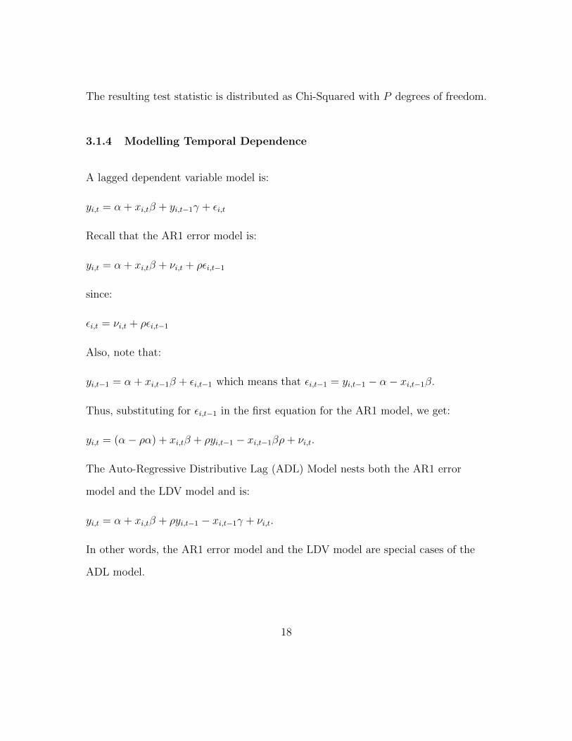
The resulting test statistic is distributed as Chi-Squared with P degrees of freedom.

3.1.4 Modelling Temporal Dependence

A lagged dependent variable model is:

yi,t = α + xi,tβ + yi,t−1γ + εi,t

Recall that the AR1 error model is:

yi,t = α + xi,tβ + νi,t + ρεi,t−1

since:

εi,t = νi,t + ρεi,t−1

Also, note that:

yi,t−1 = α + xi,t−1β + εi,t−1 which means that εi,t−1 = yi,t−1 − α− xi,t−1β.

Thus, substituting for εi,t−1 in the first equation for the AR1 model, we get:

yi,t = (α− ρα) + xi,tβ + ρyi,t−1 − xi,t−1βρ+ νi,t.

The Auto-Regressive Distributive Lag (ADL) Model nests both the AR1 error

model and the LDV model and is:

yi,t = α + xi,tβ + ρyi,t−1 − xi,t−1γ + νi,t.

In other words, the AR1 error model and the LDV model are special cases of the

ADL model.

18

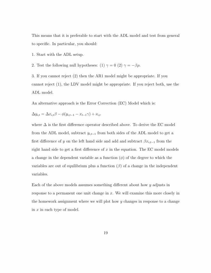
This means that it is preferable to start with the ADL model and test from general

to specific. In particular, you should:

1. Start with the ADL setup.

2. Test the following null hypotheses: (1) γ = 0 (2) γ = −βρ.

3. If you cannot reject (2) then the AR1 model might be appropriate. If you

cannot reject (1), the LDV model might be appropriate. If you reject both, use the

ADL model.

An alternative approach is the Error Correction (EC) Model which is:

∆yi,t = ∆xi,tβ − φ(yi,t−1 − xt−1γ) + νi,t

where ∆ is the first difference operator described above. To derive the EC model

from the ADL model, subtract yi,t−1 from both sides of the ADL model to get a

first difference of y on the left hand side and add and subtract βxi,t−1 from the

right hand side to get a first difference of x in the equation. The EC model models

a change in the dependent variable as a function (φ) of the degree to which the

variables are out of equilibrium plus a function (β) of a change in the independent

variables.

Each of the above models assumes something different about how y adjusts in

response to a permanent one unit change in x. We will examine this more closely in

the homework assignment where we will plot how y changes in response to a change

in x in each type of model.

19

3.1.5 The Inclusion of a Lagged Dependent Variable with Fixed Effects

When analyzing TSCS data we will often want to include a lagged dependent

variable along with fixed effects. It has been shown, however, that the inclusion of

fixed effects in a model with a lagged dependent variable introduces bias into the

coefficient estimates.5 It has been shown that this bias is of order 1T

and, hence,

decreases, as T gets large.

Based on simulations they ran, Beck and Katz (2011) recommend using OLS when

T is large enough (i.e. 20 or more) rather than alternative approaches. Other

approaches include using Generalized Method of Moments (GMM) as described by

Wawro (2002).

3.2 Binary Dependent Variable

A binary dependent variable is one which takes a value of either 0 or 1. Just as

with a continuous dependent variable, we would expect TSCS data with a binary

dependent variable to show temporal dependence.

Note, however, that using a lagged dependent variable in a BTSCS model is not

the same as using LDV in a continuous TSCS model. To see this, we need to

introduce the Markov transition framework.

5According to Beck and Katz (2011, p342), this bias arises because centering all variables bycountry introduces a correlation between the centered lagged dependent variable and the centerederror term.

20

3.3 Markov Transition framework

A first-order Markov process assumes that whether or not the dependent variable is

a 0 or 1 at time t is a function only of the value of the dependent and independent

variables at time t− 1.

With this assumption, we would estimate two different probits (or logits)

depending on the prior state:

P (yi,t|yi,t−1 = 0) = Probit(xi,tβ)

P (yi,t|yi,t−1 = 1) = Probit(xi,tα).

Note that we are allowing for the effects of the independent variables to differ

depending on the prior state.

We can combine these two separate equations into one model as follows:

P (yi,t = 1) = Probit(xi,tβ + yi,t−1 ∗ xi,tγ)

where γ = α− β.

You can test the hypothesis that the prior state does not matter by testing γ = 0.

A model with a lagged dependent variable is a special case of the above combined

model which assumes that the only thing that differs according to the prior state is

the intercept. This is an assumption that should be tested.

21

3.4 Duration Data framework

Beck, Katz and Tucker (1998) observe that binary TSCS data (BTSCS data) are

equivalent to grouped duration data.

Consider an example in which an “event” or “failure” is a conflict and the length of

time in between is a “spell” of peace.

BTSCS data are ”grouped” in the sense that we only know whether a unit has

failed in some discrete time interval (e.g. a year).6

Note that in this set-up we need to separate out conflict onset and conflict duration

and not lump them together in the same model. In the former case, a ”failure”

would be defined as the onset of conflict whereas in the latter, a ”failure” would be

defined as the onset of peace.

Recall (from last week?) that the hazard probability refers to the probability of

“dying” (or failing) in time t given alive at the start of the interval t.

Estimating the probability of failure using ordinary logit (or probit) assumes that

the hazard is time invariant:

hi,t = h(xi,t). (Notice the lack of subscript on the hazard function on the right

hand side of the equation).

To allow for duration dependence, we need to estimate a binary model in which:

hi,t = ht(xi,t). (Notice the subscript on the hazard function on the right hand side

6This is as opposed to a continuous duration model in which a unit can fail at any time.

22

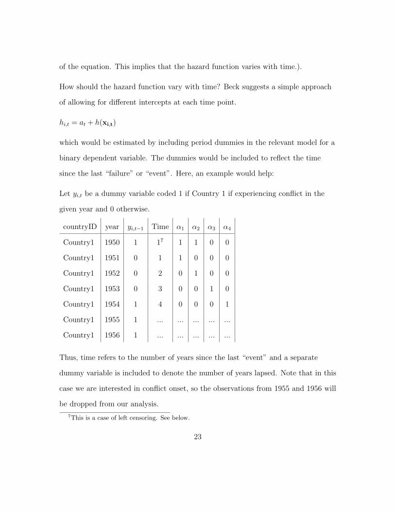
of the equation. This implies that the hazard function varies with time.).

How should the hazard function vary with time? Beck suggests a simple approach

of allowing for different intercepts at each time point.

hi,t = at + h(xi,t)

which would be estimated by including period dummies in the relevant model for a

binary dependent variable. The dummies would be included to reflect the time

since the last “failure” or “event”. Here, an example would help:

Let yi,t be a dummy variable coded 1 if Country 1 if experiencing conflict in the

given year and 0 otherwise.

countryID year yi,t−1 Time α1 α2 α3 α4

Country1 1950 1 17 1 1 0 0

Country1 1951 0 1 1 0 0 0

Country1 1952 0 2 0 1 0 0

Country1 1953 0 3 0 0 1 0

Country1 1954 1 4 0 0 0 1

Country1 1955 1 ... ... ... ... ...

Country1 1956 1 ... ... ... ... ...

Thus, time refers to the number of years since the last “event” and a separate

dummy variable is included to denote the number of years lapsed. Note that in this

case we are interested in conflict onset, so the observations from 1955 and 1956 will

be dropped from our analysis.

7This is a case of left censoring. See below.

23

One can test whether the dummy variables belong in the model (i.e. whether there

is duration dependence) using a standard F test in which the null hypothesis is that

all the period dummies (i.e. α1, α2...... are 0).

Including the period dummy variables often uses up a large number of degrees of

freedom. Beck, Katz and Tucker (1998) observe that this does not usually have

much of an effect on estimating the coefficients on the key independent variables,

but may lead to problems estimating the period dummies themselves. An

alternative approach is to use cubic splines which are essentially smoothed

functions of the ”Time” variable above. For more information on splines, see Beck,

Katz and Tucker (1998).

What is the appropriate model for binary dependent variables? It can be shown

that a Cox proportional hazard model for grouped duration data is mathematically

equivalent to a conditional logit model which involves using a cloglog function or

“link”8 rather than a logit function/link. Beck and Katz (1998) observe that, in

practice, there is almost no difference between these models when failure rates are

below 50% and recommend using logit in these situations for practical reasons.

Additional problems arise with these kind of data (e.g. how to deal with multiple

failures, left censoring etc.) See Beck, Katz and Tucker (1998) for recommendations

for how to deal with these issues.

8This terminology comes from the Generalized Linear Model approach.

24

4 Cross-Sectional Issues

4.1 Panel Corrected Standard Errors (PCSEs)

A key assumption entailed in OLS is that the off-diagonal terms of the

variance-covariance matrix are 0.

A standard error matrix for OLS looks like this:

VNTxNT =

σ2 0 . . . . 0

0 σ2 . . . . 0

0 . σ2 . . . 0

0 . . . . . 0

0 . . . . 0 σ2

One reason this assumption is unlikely to hold true for TSCS data is that there

may be a contemporaneous correlation of errors across cross-sectional units. In this

case, OLS is still consistent but the regular OLS standard errors are incorrect since

they incorrectly estimate the sampling variability.

PCSEs leave the coefficient estimates intact and fix the standard errors to allow for

contemporaneous correlation of errors (i.e. Cov(εi,t, εj,t) 6= 0 for i 6= j.).

PCSEs, however, assume that:

1. There is no temporal dependence in the errors. (i.e. Cov(εi,t, εi,t+1) = 0)

2. The covariance between errors of a pair of cross-sectional units (e.g. countries)

remains the same over time. (e.g. Cov(εi,t, εj,t) is the same for all t.)

25

PCSEs use the OLS estimates of the errors to generate estimates of the relevant

covariances (i.e. Cov(εi,t, εj,t). This works because, despite contemporaneous

correlation, the OLS estimates are still consistent.

4.2 Modeling Spatial Dependence

PCSEs treat spatial dependence between observations as a nuisance. As an

alternative, one could model the spatial dependence between units. Spatial

econometrics has become an important way of analyzing interdependence amongst

observations from “nearby” cross-sectional units. Beck, Gleditsch and Beardsley

(2006) note that one could not only incorporate geographic notions of distance but

also political economy notions of distance such as extent of trade between

countries. In such models, it is typically assumed that the structure of dependence

between observations is known by the researcher.

There are a number of possible specifications: a spatially lagged error model, the

spatially autoregressive model and so on. These are conceptually relatively easy to

understand, but in practice often hard to implement. See Beck, Gleditsch and

Beardsley (2006) for more details on this.

5 References

Beck, Nathaniel. 2001. Time-Series-Cross-Section Data: What Have We Learned inthe Past Few Years? Annual Review of Political Science Vol. 4: 271-293

26

Beck, Nathaniel, Kristian Skrede Gleditsch and Kyle Beardsley. 2006. ”Space isMore than Geography: Using Spatial Econometrics in the Study of PoliticalEconomy” International Studies Quarterly 50, 27-44.

Beck, Nathaniel and Jonathan Katz. 1995. What to do (and not to do) withTime-Series Cross-Section Data. American Political Science Review.

Beck, Nathaniel and Jonathan Katz. 1996. ”Nuisance vs. Substance: Specifyingand Estimating Time-Series-Cross-Section Models” Political Analysis 6 (1): pp1-36.

Beck, Nathaniel and Jonathan Katz. 2001. ”Throwing out the Baby with the BathWater: A Comment on Green, Kim, and Yoon” International Organization, Vol.55, No. 2 (Spring, 2001), pp. 487-495.

Beck, Nathaniel and Jonathan Katz. 2007. ”Random Coefficient Models forTime-Series-Cross-Section Data: Monte Carlo Experiments” Political Analysis 15:182-195.

Beck, Nathaniel and Jonathan Katz. 2011. ”Modeling Dynamics inTime-SeriesCross-Section Political Economy Data” Annual Review of PoliticalScience 14: 331-52.

DeBoef, Suzanna and Luke Keele. 2008. Taking Time Seriously American Journalof Political Science Vol. 52, No. 1 (Jan., 2008), pp. 184-200.

Green, Donald P. , Soo Yeon Kim and David H. Yoon. 2001. Dirty PoolInternational Organization Vol. 55, No. 2 (Spring, 2001), pp. 441-468.

Greene, William H. 2003. ”Econometric Analysis: Fifth Edition” New York:Pearson Education.

Plumper, Thomas and Vera E. Troeger. 2007. ”Efficient Estimation ofTime-Invariant and Rarely Changing Variables in Finite Sample Panel Analyseswith Unit Fixed Effects” Political Analysis 15: 124-139.

Wawro, Gregory. 2002. ”Estimating Dynamic Panel Data Models in PoliticalScience.” Political Analysis 10: 1, pp25-48.

Wilson, Sven and Daniel Butler. 2007. A Lot More to Do: The Sensitivity of Time-Series Cross-Section Analyses to Simple Alternative Specifications. PoliticalAnalysis. 15:101-123.

27