Time Series Analysis Using

Fractal Theory and Online

Ensemble Classifiers with

Application to Stock Portfolio

Optimization

Dalton Lunga

A dissertation submitted to the Faculty of Engineering and the Built Envi-

ronment, University of the Witwatersrand, Johannesburg, in fulfilment of the

requirements for the degree of Master of Science in Engineering.

Johannesburg, November 2006

Declaration

I declare that this dissertation is my own, unaided work, except where oth-

erwise acknowledged. It is being submitted for the degree of Master of Science

in Engineering to the University of the Witwatersrand, Johannesburg. It has not

been submitted before for any degree or examination in any other university.

Signed this day of 20

Dalton Lunga.

i

Abstract

Neural Network method is a technique that is heavily researched and used in ap-

plications within the engineering field for various purposes ranging from process

control to biomedical applications. The success of Neural Networks (NN) in en-

gineering applications, e.g. object tracking and face recognition has motivated its

application to the finance industry. In the financial industry, time series data is

used to model economic variables. As a result, finance researchers, portfolio man-

agers and stockbrokers have taken interest in applying NN to model non-linear

problems they face in their practice. NN facilitates the approach of predicting

stocks due to its ability to accurately and intuitively learn complex patterns and

characterizes these patterns as simple equations. In this research, a methodology

that uses fractal theory and NN framework to model the stock market behav-

ior is proposed and developed. The time series analysis is carried out using the

proposed approach with application to modelling the Dow Jones Average Index’s

future directional movement. A methodology to establish self-similarity of time

series and long memory effects that result in classifying the time series signal as

persistent, random or non-persistent using the rescaled range analysis technique is

developed. A linear regression technique is used for the estimation of the required

parameters and an incremental online NN algorithm is implemented to predict

the directional movement of the stock. An iterative fractal analysis technique is

used to select the required signal intervals using the approximated parameters.

The selected data is later combined to form a signal of interest and then pass it

to the ensemble of classifiers. The classifiers are modelled using a neural network

based algorithm. The performance of the final algorithm is measured based on

accuracy of predicting the direction of movement and also on the algorithm’s

ii

confidence in its decision-making. The improvement within the final algorithm

is easily assessed by comparing results from two different models in which the

first model is implemented without fractal analysis and the second model is im-

plemented with the aid of a strong fractal analysis technique. The results of the

first NN model were published in the Lecture Notes in Computer Science 2006

by Springer. The second NN model incorporated a fractal theory technique.

The results from this model shows a great deal of improvement when classifying

the next day’s stock direction of movement. A summary of these results were

submitted to the Australian Joint Conference on Artificial Intelligence 2006 for

publishing. Limitations on the sample size, including problems encountered with

the proposed approach are also outlined in the next sections. This document also

outlines recommendations that can be implemented as further steps to advance

and improve the proposed approach for future work.

iii

I would like to dedicate this work to my loving wife Makhosazana Thomo, my

mother, Jester Madade Hlabangana, my cousin, Khanyisile Hlabangana and

other family members: thank you for your prayers and support throughout this

demanding time.

iv

Acknowledgements

The work described in this dissertation was carried out at the University of Wit-

watersrand, in the School of Electrical and Information Engineering 2005/2006.

I would like to acknowledge the input from Professor Tshilidzi Marwala who has

been my source of inspiration, advisor, and a supervisor who made this thesis a

possibility by an extensive leadership as well as social support. Thank you for

putting so much insight into the development of the methodologies. Thank you

for conferences and expenses.

I would also like to thank the National Research Foundation for funding this

work.

v

Contents

Declaration i

Abstract ii

Acknowledgements v

1 Introduction 1

2 Time Series Analysis Using Fractal Theory and Online Ensemble

Classifiers 6

2.1 Introduction . . . . . . . . . . . . . . . . . . . . . . . . . . . . . . 6

2.2 Fractal Analysis . . . . . . . . . . . . . . . . . . . . . . . . . . . . 7

2.3 Rescaled Range Analysis . . . . . . . . . . . . . . . . . . . . . . . 8

2.3.1 The R/S Methodology . . . . . . . . . . . . . . . . . . . . 9

2.3.2 The Hurst Interpretation . . . . . . . . . . . . . . . . . . . 10

2.4 Incremental Online Learning Algorithm . . . . . . . . . . . . . . . 11

2.5 Confidence Measurement . . . . . . . . . . . . . . . . . . . . . . . 14

2.6 Forecasting Framework . . . . . . . . . . . . . . . . . . . . . . . . 15

2.6.1 Experimental Data . . . . . . . . . . . . . . . . . . . . . . 15

2.6.2 Model Input Selection . . . . . . . . . . . . . . . . . . . . 16

2.6.3 Experimental Results . . . . . . . . . . . . . . . . . . . . . 16

1

CONTENTS

2.7 Results Summary . . . . . . . . . . . . . . . . . . . . . . . . . . . 19

3 Main Conclusion 21

A Neural Networks 24

A.1 Introduction . . . . . . . . . . . . . . . . . . . . . . . . . . . . . . 24

A.2 What is a Neural Network . . . . . . . . . . . . . . . . . . . . . . 25

A.3 Back Propagation Algorithm . . . . . . . . . . . . . . . . . . . . . 27

A.3.1 Advantages of the Back Propagation Algorithm . . . . . . 28

A.3.2 Disadvantages of the Back Propagation Algorithm . . . . . 28

A.4 Neural Network Architectures . . . . . . . . . . . . . . . . . . . . 28

A.4.1 Selection of the Appropriate Training Algorithm . . . . . . 29

A.4.2 Selection of the System Architecture . . . . . . . . . . . . 29

A.4.3 Selection of the Learning Rule . . . . . . . . . . . . . . . . 30

A.4.4 Selection of the Appropriate Learning Rates and Momentum 30

A.5 Multi-Layer Perceptron . . . . . . . . . . . . . . . . . . . . . . . . 31

A.6 Conclusion . . . . . . . . . . . . . . . . . . . . . . . . . . . . . . . 32

B Learn++ 34

B.1 Ensemble of Classifiers . . . . . . . . . . . . . . . . . . . . . . . . 34

B.2 Strong and Weak Learning . . . . . . . . . . . . . . . . . . . . . . 36

B.3 Boosting the Accuracy of a Weak Learner . . . . . . . . . . . . . 37

B.4 Boosting for Two-class Problems . . . . . . . . . . . . . . . . . . 37

B.5 Boosting for Multi-class Problems . . . . . . . . . . . . . . . . . . 38

B.6 Connection to Incremental Learning . . . . . . . . . . . . . . . . . 42

B.7 Learn++: An Incremental Learning Algorithm . . . . . . . . . . . 44

B.7.1 Learn++ Algorithm . . . . . . . . . . . . . . . . . . . . . 46

2

CONTENTS

B.8 Conclusion . . . . . . . . . . . . . . . . . . . . . . . . . . . . . . . 48

C Fractals Theory 49

C.1 An Introduction to Fractals . . . . . . . . . . . . . . . . . . . . . 49

C.1.1 What is a fractal ? . . . . . . . . . . . . . . . . . . . . . . 49

C.1.2 Fractal Geometry . . . . . . . . . . . . . . . . . . . . . . . 49

C.2 Fractal Objects and Self-Similar Processes . . . . . . . . . . . . . 54

C.3 Mapping Real-World Time Series to Self-Similar Processes . . . . 60

C.4 Re-Scaled Range Analysis . . . . . . . . . . . . . . . . . . . . . . 61

C.4.1 The R/S Methodology . . . . . . . . . . . . . . . . . . . . 62

C.4.2 The Hurst Interpretation . . . . . . . . . . . . . . . . . . . 64

C.5 Conclusion . . . . . . . . . . . . . . . . . . . . . . . . . . . . . . . 65

References 69

D Published Paper 70

3

List of Figures

2.1 Fractal Brownian motion simulation-(1a) anti-persistent signal,(1b)

random walk signal,(1c) persistent signal . . . . . . . . . . . . . . 8

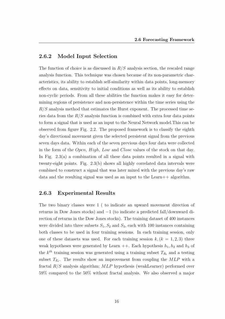
2.2 Model framework for fractal R/S technique and online neural net-

work time series analysis . . . . . . . . . . . . . . . . . . . . . . . 17

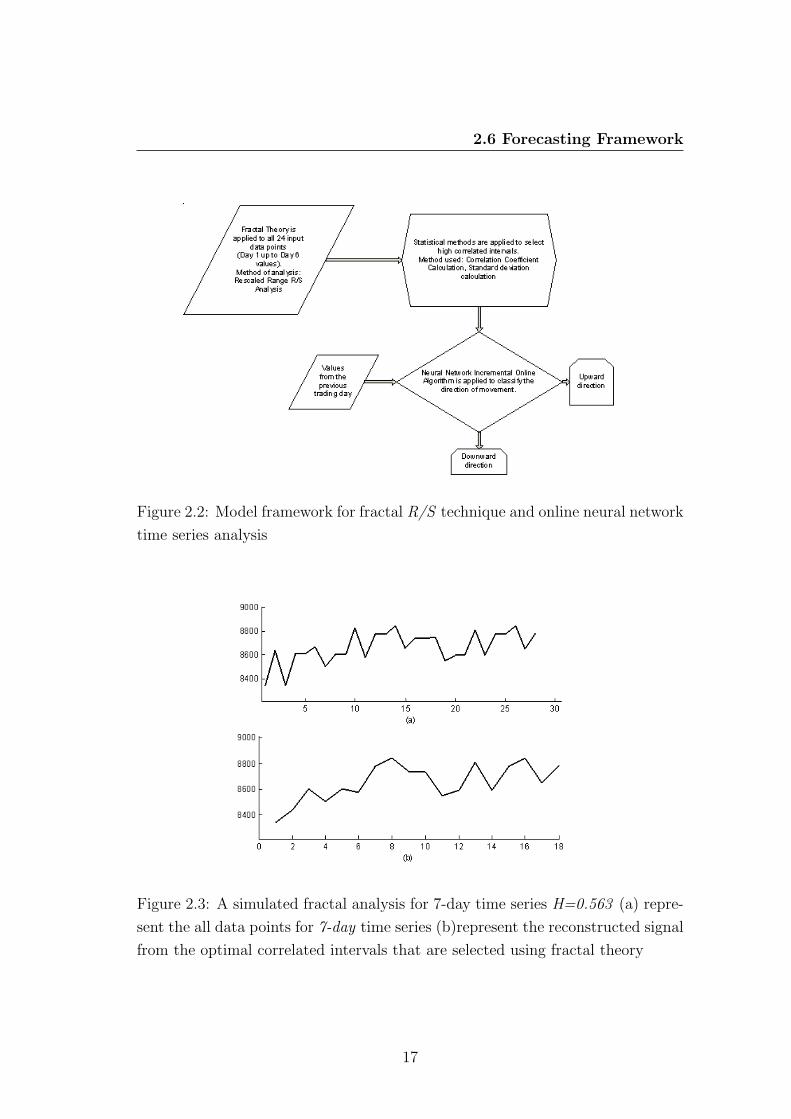
2.3 A simulated fractal analysis for 7-day time series H=0.563 (a)

represent the all data points for 7-day time series (b)represent the

reconstructed signal from the optimal correlated intervals that are

selected using fractal theory . . . . . . . . . . . . . . . . . . . . . 17

2.4 Log (R/S) as a function of log n for the 7-day data fractal analysis

The solid line for n > 3 is a linear fit to Actual R/S signal using

R/S = anH with h=0.557 and intercept a =-0.4077 . . . . . . . . 18

A.1 An example of a neural network model . . . . . . . . . . . . . . . 26

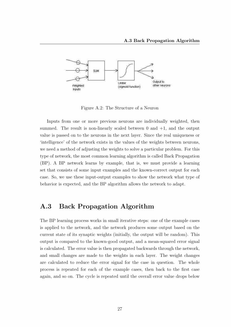
A.2 The Structure of a Neuron . . . . . . . . . . . . . . . . . . . . . . 27

A.3 A fully interconnected, biased, n-layered back-propagation network 32

B.1 Conceptual representation of combining classifiers . . . . . . . . . 42

B.2 Conceptual representation of combining classifiers . . . . . . . . . 43

C.1 Line dimension representation . . . . . . . . . . . . . . . . . . . . 50

C.2 Two dimension representation . . . . . . . . . . . . . . . . . . . . 50

C.3 Three dimension representation . . . . . . . . . . . . . . . . . . . 50

4

LIST OF FIGURES

C.4 Van Koch snowflake . . . . . . . . . . . . . . . . . . . . . . . . . 52

C.5 Multi Van Koch Snowflake shapes combined, Goldberger(2006) . . 52

C.6 Representative complex physiological fluctuations, Goldberger(2006) 56

C.7 Illustration of the concept of self-similarity for a simulated random

walk . . . . . . . . . . . . . . . . . . . . . . . . . . . . . . . . . . 59

C.8 A cardiac inter-heartbeat interval (inverse of heart rate) time series

is shown in (A) and a randomized control is shown in (B) . . . . . 61

5

List of Tables

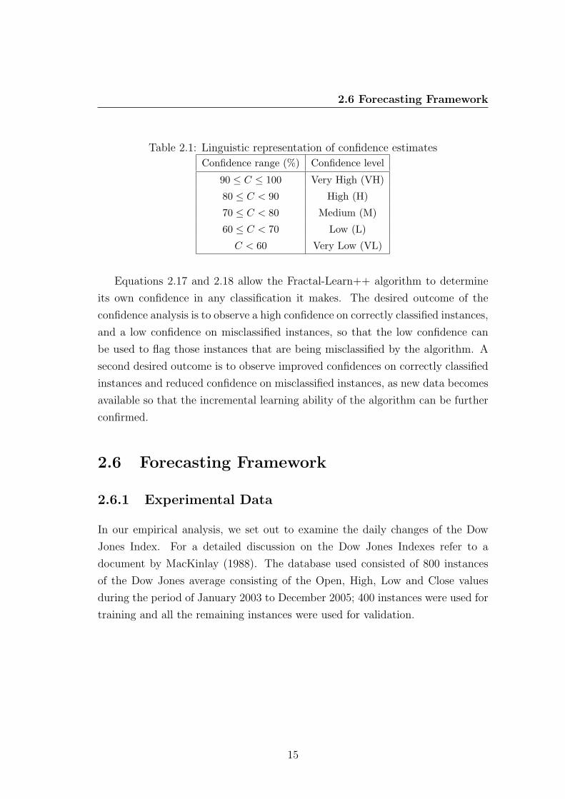
2.1 Linguistic representation of confidence estimates . . . . . . . . . . 15

2.2 Training and generalization performance of Fractal-Learn++ model 19

2.3 Algorithm confidence results on the testing data subset . . . . . . 19

2.4 Confidence trends for the time series: testing data subset . . . . . 19

C.1 Fractal vs. Euclidean geometries . . . . . . . . . . . . . . . . . . . 53

6

Nomenclature

Roman Symbols

F transfer function

∀ for all

p ulcorner

Greek Symbols

λ lambda

ι index

π ' 3.14 . . .

ε epsilon

δ delta

β beta

Σ summation symbol

Superscripts

j superscript index

Subscripts

0 subscript index

7

LIST OF TABLES

Acronyms

AJCAI2006 Australian Joint Conference on Artificial Intelligence 2006

ICONIP2006 International Conference on Neural Information Processing 2006

LNAIS2006 Lecture Notes in Artificial Intelligence Series 2006

LNCS2006 Lecture Notes in Computer Science 2006

Eq. Equation

NNs Neural Networks

8

Chapter 1

Introduction

Over the past two decades many important changes have taken place in the

environment of financial time series markets. The development of powerful com-

munication and trading facilities has enlarged the scope of selection for investors

to improve their day to day practices. Traditional capital market theory has also

changed and methods of financial analysis have improved. Forecasting stock mar-

ket returns or a stock index is an important financial subject that has attracted

researchers’ attention for many years. It involves an assumption that fundamen-

tal information publicly available in the past has some predictive relationships to

the future stock returns or indices.

The samples of such information include economic variables such as interest

rates and exchange rates, industry specific information such as growth rates of

industrial production and consumer price, and company specific information such

as income statements and dividend yields. This is opposed to the general percep-

tion of market efficiency as proved by McNelis (2005). In fact, the efficient market

hypothesis states that all available information affecting the current stock values

is constituted by the market before the general public can make trades based

on it, Skjeltorp (2000). Therefore, it is possible to forecast future returns since

they already reflect all information currently known about the stocks. This is

still an empirical issue because there is considerable evidence that markets are

not fully efficient, and it is possible to predict the future stock returns or indices

1

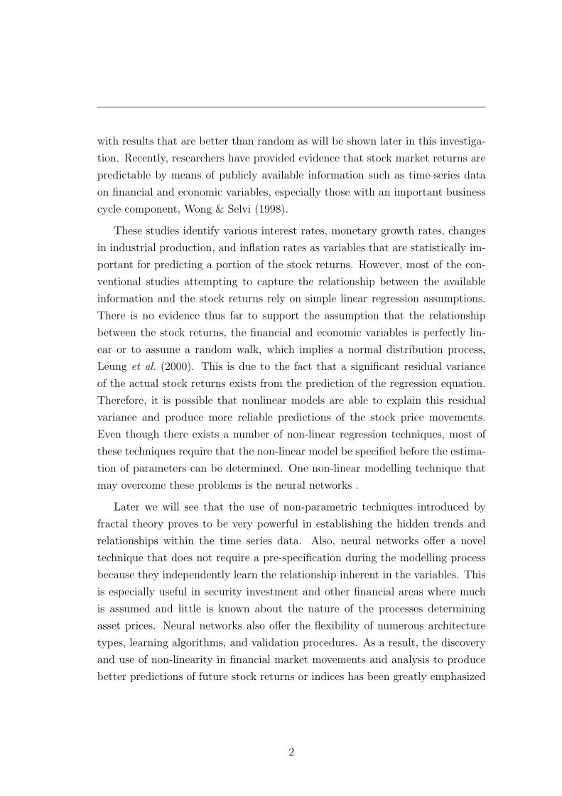
with results that are better than random as will be shown later in this investiga-

tion. Recently, researchers have provided evidence that stock market returns are

predictable by means of publicly available information such as time-series data

on financial and economic variables, especially those with an important business

cycle component, Wong & Selvi (1998).

These studies identify various interest rates, monetary growth rates, changes

in industrial production, and inflation rates as variables that are statistically im-

portant for predicting a portion of the stock returns. However, most of the con-

ventional studies attempting to capture the relationship between the available

information and the stock returns rely on simple linear regression assumptions.

There is no evidence thus far to support the assumption that the relationship

between the stock returns, the financial and economic variables is perfectly lin-

ear or to assume a random walk, which implies a normal distribution process,

Leung et al. (2000). This is due to the fact that a significant residual variance

of the actual stock returns exists from the prediction of the regression equation.

Therefore, it is possible that nonlinear models are able to explain this residual

variance and produce more reliable predictions of the stock price movements.

Even though there exists a number of non-linear regression techniques, most of

these techniques require that the non-linear model be specified before the estima-

tion of parameters can be determined. One non-linear modelling technique that

may overcome these problems is the neural networks .

Later we will see that the use of non-parametric techniques introduced by

fractal theory proves to be very powerful in establishing the hidden trends and

relationships within the time series data. Also, neural networks offer a novel

technique that does not require a pre-specification during the modelling process

because they independently learn the relationship inherent in the variables. This

is especially useful in security investment and other financial areas where much

is assumed and little is known about the nature of the processes determining

asset prices. Neural networks also offer the flexibility of numerous architecture

types, learning algorithms, and validation procedures. As a result, the discovery

and use of non-linearity in financial market movements and analysis to produce

better predictions of future stock returns or indices has been greatly emphasized

2

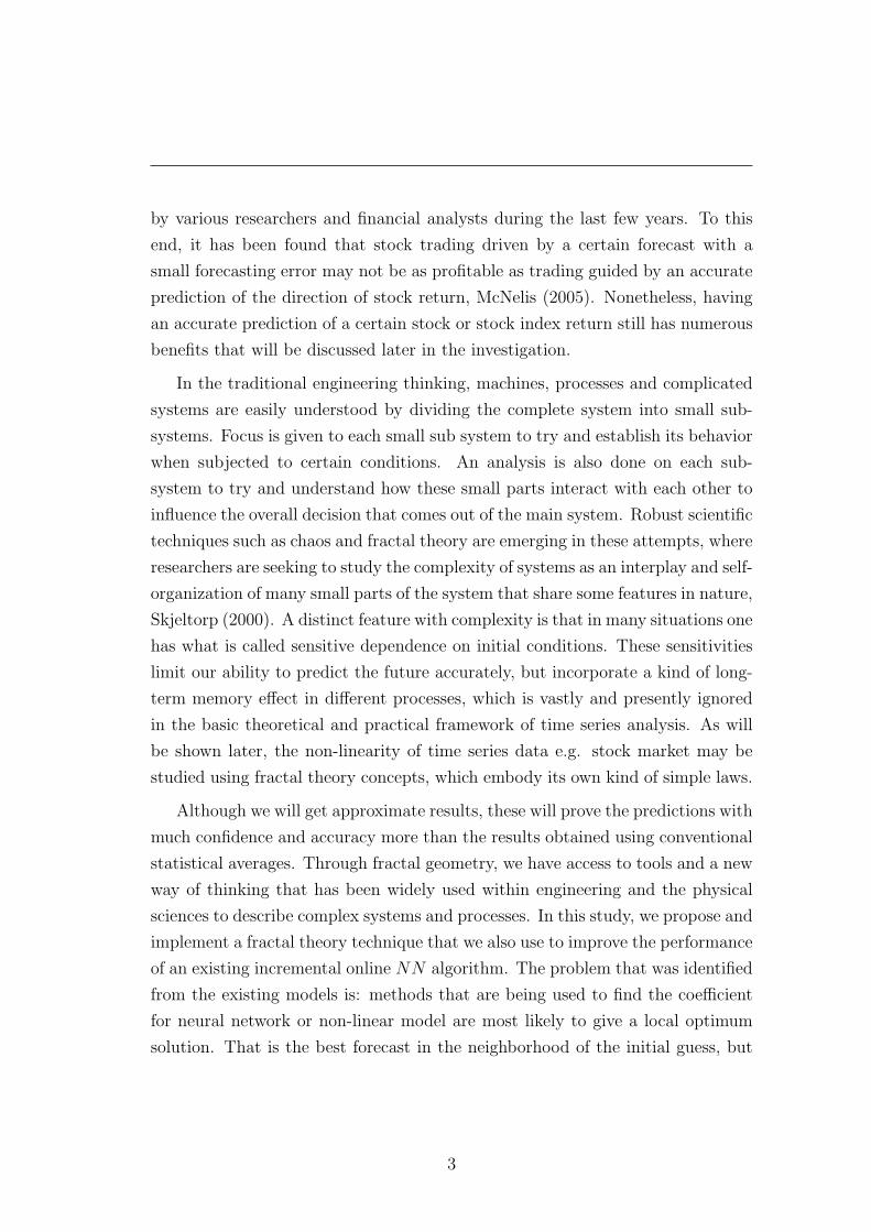
by various researchers and financial analysts during the last few years. To this

end, it has been found that stock trading driven by a certain forecast with a

small forecasting error may not be as profitable as trading guided by an accurate

prediction of the direction of stock return, McNelis (2005). Nonetheless, having

an accurate prediction of a certain stock or stock index return still has numerous

benefits that will be discussed later in the investigation.

In the traditional engineering thinking, machines, processes and complicated

systems are easily understood by dividing the complete system into small sub-

systems. Focus is given to each small sub system to try and establish its behavior

when subjected to certain conditions. An analysis is also done on each sub-

system to try and understand how these small parts interact with each other to

influence the overall decision that comes out of the main system. Robust scientific

techniques such as chaos and fractal theory are emerging in these attempts, where

researchers are seeking to study the complexity of systems as an interplay and self-

organization of many small parts of the system that share some features in nature,

Skjeltorp (2000). A distinct feature with complexity is that in many situations one

has what is called sensitive dependence on initial conditions. These sensitivities

limit our ability to predict the future accurately, but incorporate a kind of long-

term memory effect in different processes, which is vastly and presently ignored

in the basic theoretical and practical framework of time series analysis. As will

be shown later, the non-linearity of time series data e.g. stock market may be

studied using fractal theory concepts, which embody its own kind of simple laws.

Although we will get approximate results, these will prove the predictions with

much confidence and accuracy more than the results obtained using conventional

statistical averages. Through fractal geometry, we have access to tools and a new

way of thinking that has been widely used within engineering and the physical

sciences to describe complex systems and processes. In this study, we propose and

implement a fractal theory technique that we also use to improve the performance

of an existing incremental online NN algorithm. The problem that was identified

from the existing models is: methods that are being used to find the coefficient

for neural network or non-linear model are most likely to give a local optimum

solution. That is the best forecast in the neighborhood of the initial guess, but

3

not the coefficients for giving the best forecast if we look a bit further afield from

the initial guesses for the coefficients. This makes it very difficult to determine the

sign or direction of the stock/portfolio return value since a local minimum will rule

out other solutions (global minimum) that are more valid in the decision-making

process. Another shortfall that was discovered from the results of numerous

researches in this field is that input data is passed onto the NN in batch form

which results in the model having a requirement to go off-line every time new data

is presented to the network so that architecture optimization is achieved for the

new information. This means that the model will always be redesigned for all new

data that is presented on its input. This is time consuming and uneconomical.

A methodology is proposed for processing of input data before it is passed to the

NN algorithm. This is done using non-parametric methods discovered from the

study of fractal theory that are capable of eliminating noise random data points

from the sample spaces.

Making use of fractals will result in classifying the sample parts of the signal

as persistent, random signal or non-persistent. This approach has proven that the

application of fractal theory to analyzing financial time series data is the better

approach to providing robust solutions to this complex non-linear dynamic sys-

tem. The proposed methodology offers to develop a model that takes input data

in sequences and adapts (self-trains) to optimize its architecture without having

to change the architecture design. The first model framework seeks to convert

a weak learning algorithm implemented using the Multi-Layer Perceptron into a

strong learning algorithm. The model has the ability to identify unknown data

samples into correct categories and the results proves the incremental learning

ability of the proposed algorithm. In other words the strong learner identifies the

hard example and forces its capability to learn and adapt to these examples. The

first model is observed to classify known data samples into correct labelled classes

that give the predicted direction of movement of the future time series returns. A

summary of these results were published in the Lecture Notes in Computer Sci-

ence (LNCS) series by Springer 2006, Lunga & Marwala (2006a). The proposed

second model framework applies the theory of fractal analysis. The model pro-

cesses the input data in order to establish a form of a function that can identify

4

features e.g self-similarity, data persistence, random walk pattern, non-persistent

and the Hurst exponent. The relevance of these features in enabling predictions

for future time series data returns is explained in the next chapter. A summary of

fractal analysis framework results were submitted for publishing to the Australian

Joint Conference on Artificial Intelligence in 2006, Lunga & Marwala (2006b).

5

Chapter 2

Time Series Analysis Using

Fractal Theory and Online

Ensemble Classifiers

(Presented at the Australian Joint Conference on Artificial Intelligence 2006)

2.1 Introduction

The financial markets are regarded as complex, evolutionary, and non-linear dy-

namical systems, MacKinlay (1988). Advanced neural techniques are required

to model the non-linearity and complex behavior within the time series data,

Mandelbrot (1997). In this paper we apply a non-parametric technique to select

only those regions of the data that are observed to be persistent. The selected

data intervals are used as inputs to the incremental algorithm that predicts the

future behavior of the time series data. In the following sections we give a brief

discussion on the proposed fractal technique and the online incremental Learn++

algorithm. The proposed framework and findings from this investigation are also

discussed.

Fractal analysis is proposed as a concept to establish the degree of persistence

and self-similarity within the stock market data. This concept is implemented

6

2.2 Fractal Analysis

using the rescaled range analysis (R/S) method. The R/S analysis outcome is

applied to an online incremental algorithm (Learn++) that is built to classify

the direction of movement of the stock market. The use of fractal geometry in

this study provides a way of determining quantitatively the extent to which time

series data can be predicted. In an extensive test, it is demonstrated that the R/S

analysis provides a very sensitive method to reveal hidden long run and short run

memory trends within the sample data. The time series data that is measured to

be persistent is used in training the neural network. The results from Learn++

algorithm show a very high level of confidence of the neural network in classifying

sample data accurately.

2.2 Fractal Analysis

The fractal dimension of an object indicates something about the extent to which

the object fills space. On the other hand, the fractal dimension of a time series

shows how turbulent the time series is and also measures the degree to which the

time series is scale-invariant. The method used to estimate the fractal dimension

using the Hurst exponent for a time series is called the rescaled range (R/S) anal-

ysis, which was invented by Hurst (1951) when studying the Nile River in order

to describe the long-term dependence of the water level in rivers and reservoirs.

The estimation of the fractal dimension given the approximated Hurst exponent

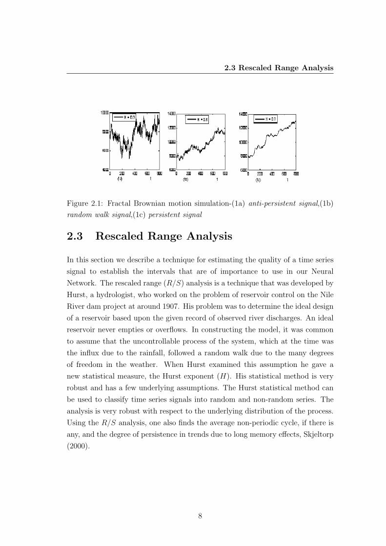
will be explained in the following sections. The simulated fractal Brownian mo-

tion time series in Fig. 2.1 was done for different Hurst exponents. In Fig. 2.1

(1a) we have an anti-persistent signal with a Hurst exponent of H = 0, 3 and

the resulting fractal dimension is Df = 1, 7. Fig. 2.1 (1b) shows a random walk

signal with H = 0, 5 and the corresponding fractal dimension is Df = 1, 5. In

Fig. 2.1 (1c) a persistent time series signal with H = 0, 7 and a corresponding

fractal dimension of Df = 1, 5 is also shown. From Fig. 2.1 we can easily note

the degree to which the data contain jagged features that needs to be removed

before the signal is passed over to the neural network model for further analysis

in uncovering the required information.

7

2.3 Rescaled Range Analysis

Figure 2.1: Fractal Brownian motion simulation-(1a) anti-persistent signal,(1b)

random walk signal,(1c) persistent signal

2.3 Rescaled Range Analysis

In this section we describe a technique for estimating the quality of a time series

signal to establish the intervals that are of importance to use in our Neural

Network. The rescaled range (R/S) analysis is a technique that was developed by

Hurst, a hydrologist, who worked on the problem of reservoir control on the Nile

River dam project at around 1907. His problem was to determine the ideal design

of a reservoir based upon the given record of observed river discharges. An ideal

reservoir never empties or overflows. In constructing the model, it was common

to assume that the uncontrollable process of the system, which at the time was

the influx due to the rainfall, followed a random walk due to the many degrees

of freedom in the weather. When Hurst examined this assumption he gave a

new statistical measure, the Hurst exponent (H). His statistical method is very

robust and has a few underlying assumptions. The Hurst statistical method can

be used to classify time series signals into random and non-random series. The

analysis is very robust with respect to the underlying distribution of the process.

Using the R/S analysis, one also finds the average non-periodic cycle, if there is

any, and the degree of persistence in trends due to long memory effects, Skjeltorp

(2000).

8

2.3 Rescaled Range Analysis

2.3.1 The R/S Methodology

The main idea behind using the R/S analysis for our investigation is to estab-

lish the scaling behavior of the rescaled cumulative deviations from the mean, or

the distance that the system travels as a function of time relative to the mean.

The intervals that display a high degree of persistence are selected and grouped

in rebuilding the signal to be used as an input to the NN model. A statistical

correlation approach is used in recombining the intervals. The approach of re-

combining different data intervals is inherited from the discovery that was made

by Hurst (1951) were it was observed that the distance covered by an independent

system from its mean increases on average, by the square root of time e.g. t2. If

the system under investigation covers a larger distance than this from its mean,

it cannot be independent by Hurst’s definition; the changes must be influencing

each other and therefore have to be correlated, Hutchinson & Poggio (1994). The

following is the approach used in the investigation: the first requirement is to

start with a time series in prices of length M . This time series is then converted

into a time series of logarithmic ratios or returns of length N = M − 1 such that

Eq.2.1 is

Ni = log(Mi+1

Mi

), i = 1, 2, ..., (M − 1) (2.1)

Divide this time period into T contiguous sub periods of length j, such that

T ∗ j = N . Each sub period is labelled It, with t = 1, 2...T . Then, each element

in It is labelled Nk,t such that k = 1, 2, , j. For each sub period It of length j the

average is calculated as shown in Eq.2.2

et =1

j

j∑k=1

Nk,t (2.2)

Thus, et is the average value of the Ni contained in sub-period It of length j.

We then calculate the time series of accumulated departures Xk,t from the mean

for each sub period It, defined in Eq.2.3

Xk,t =k∑

i=1

(Ni,t − et)k = 1, 2, ..., j (2.3)

9

2.3 Rescaled Range Analysis

Now, the range that the time series covers relative to the mean within each

sub period is defined in Eq.2.4

RIt = max(Xk,t)−min(Xk,t), 1 < k < j (2.4)

Next calculate the standard deviation of each sub-period as shown in Eq.2.5

Xk,t =

√√√√1

j

k∑i=1

(Ni,t − et)2 (2.5)

Then, the range of each sub period RIt is rescaled/normalized by the corre-

sponding standard deviation SIt . This approach is done for all the T sub intervals

we have for the series. As a result the average R/S value for length j is shown

in Eq.2.6

et =1

T

T∑t=1

(RIt

SIt

) (2.6)

Now, the calculations from the above equations were repeated for different

time horizons. This is achieved by successively increasing j and repeating the

calculations until we covered all j integers. After having calculated the R/S

values for a large range of different time horizons j, we plot log(R/S)j against

log(n). By performing a least squares linear regression with log(R/S)j as the

dependent variable and log(n) as the independent one, we find the slope of the

regression which is the estimate of the Hurst exponent (H). The relationship

between the fractal dimension and the Hurst exponent is modelled in Eq.2.7

Df = 2−H (2.7)

2.3.2 The Hurst Interpretation

If, H ∈ (0, 5; 1] it implies that the time series is persistent which is characterized

by long memory effects on all time scales, this is evident from a study done by

Gammel (1998). This also implies that all hourly prices are correlated with all

future hourly price changes; all daily price changes are correlated with all future

daily prices changes, all weekly price changes are correlated with all future weekly

10

2.4 Incremental Online Learning Algorithm

price changes and so on. This is one of the key characteristics of fractal time series

as discussed earlier. The persistence implies that if the series has been up or down

in the last period then the chances are that it will continue to be up and down,

respectively, in the next period. The strength of the trend reinforcing behavior,

or persistence, increases as H approaches 1. This impact of the present on the

future can be expressed as a correlation function G as shown in Eq.2.8

G = 22H−1 − 1 (2.8)

In the case of H = 0, 5 the correlation G = 0, and the time series is uncor-

related. However, if H = 1 we see that that G = 1, indicating a perfect positive

correlation. On the other hand, when H ∈ [0; 0, 5) we have an antipersistent time

series signal (interval). This means that whenever the time series has been up in

the last period, it is more likely to be down in the next period. Thus, an antiper-

sistent time series will be more jagged than a pure random walk as shown in Fig.

2.1. The intervals that showed a positive correlation coefficient were selected as

inputs to the Neural Network.

2.4 Incremental Online Learning Algorithm

An incremental learning algorithm is defined as an algorithm that learns new

information from unseen data, without necessitating access to previously used

data. The algorithm must also be able to learn new information from new data

and still retain knowledge from the original data. Lastly, the algorithm must be

able to teach new classes that may be introduced by new data. This type of

learning algorithm is sometimes referred to as a ‘memory less’ on-line learning

algorithm. Learning new information without requiring access to previously used

data, however, raises ‘stability-plasticity dilemma’, this is evident from a study

done by Carpenter et al. (1992). This dilemma indicates that a completely stable

classifier maintains the knowledge from previously seen data, but fails to adjust

in order to learn new information, while a completely plastic classifier is capable

of learning new data but lose prior knowledge. The problem with the Multi-Layer

Perceptron is that it is a stable classifier and is not able to learn new information

11

2.4 Incremental Online Learning Algorithm

after it has been trained. In this paper, we propose a fractal theory technique

and online incremental learning algorithm with application to time series data.

This proposed approach is implemented and tested on the classification of stock

options movement direction with the Dow Jones data used as the sample set

for the experiment. We make use of the Learn++ incremental algorithm in this

study. Learn++ is an incremental learning algorithm that uses an ensemble of

classifiers that are combined using weighted majority voting. Learn++ was de-

veloped by Polikar et al. (2002) and was inspired by a boosting algorithm called

adaptive boosting (AdaBoost). Each classifier is trained using a training subset

that is drawn according to a distribution. The classifiers are trained using a weak-

Learn algorithm. The requirement for the weakLearn algorithm is that it must be

able to give a classification rate of at least 50% initially and then the capability of

Learn++ is applied to improve the short fall of the weak MLP. For each database

Dk that contains training sequence, S, where S contains learning examples and

their corresponding classes, Learn++ starts by initializing the weights, w, ac-

cording to the distribution DT , where T is the number of hypothesis. Initially

the weights are initialized to be uniform, which gives equal probability for all

instances to be selected to the first training subset and the distribution is given

by Eq.2.9

D =1

m(2.9)

Where m represents the number of training examples in database Sk. The

training data are then divided into training subset TR and testing subset TE to

ensure weakLearn capability. The distribution is then used to select the training

subset TR and testing subset TE from Sk. After the training and testing subset

have been selected, the weakLearn algorithm is implemented. The weakLearner

is trained using subset, TR. A hypothesis, ht obtained from weakLearner is tested

using both the training and testing subsets to obtain an error,εt:

εt =∑

t:ht(xi) 6=yi

Dt(i) (2.10)

The error is required to be less than 12; a normalized error βt is computed

using:

12

2.4 Incremental Online Learning Algorithm

βt =εt

1− εt

(2.11)

If the error is greater than 12, the hypothesis is discarded and new training and

testing subsets are selected according to DT and another hypothesis is computed.

All classifiers generated so far, are combined using weighted majority voting to

obtain composite hypothesis, Ht

Ht = arg maxy∈Y

∑t:ht(x)=y

log1

βt

(2.12)

Weighted majority voting gives higher voting weights to a hypothesis that

performs well on its training and testing subsets. The error of the composite

hypothesis is computed as in Eq.2.13 and is given by

Et =∑

t:Ht(xi) 6=yi

Dt(i) (2.13)

If the error is greater than 12, the current composite hypothesis is discarded

and the new training and testing data are selected according to the distribution

DT . Otherwise, if the error is less than 12, the normalized error of the composite

hypothesis is computed as:

Bt =Et

1− Et

(2.14)

The error is used in the distribution update rule, where the weights of the

correctly classified instances are reduced, consequently increasing the weights of

the misclassified instances. This ensures that instances that were misclassified

by the current hypothesis have a higher probability of being selected for the

subsequent training set. The distribution update rule is given in Eq.2.15

wt+1 = wt(i) ·B[|Ht(xi) 6=yi|]t (2.15)

13

2.5 Confidence Measurement

Once the T hypotheses are created for each database, the final hypothesis is

computed by combining the composite hypothesis using weighted majority voting

given in Eq.2.16

Ht = arg maxy∈Y

K∑k=1

∑t:Ht(x)=y

log1

βt

(2.16)

2.5 Confidence Measurement

An intimately relevant issue is the confidence of the classifier in its decision,

with particular interest on whether the confidence of the algorithm improves as

new data become available. The voting mechanism inherent in Learn++ hints

to a practical approach for estimating confidence: decisions made with a vast

majority of votes have better confidence than those made by a slight majority,

Polikar et al. (2004). We have implemented weighted exponential voting based

confidence metric by McIver & Friedl (2001) with Learn++ as

Ci(x) = P (y = i|x) =expFi(x)∑N

k=1 expFk(x), 0 ≤ Ci(x) ≤ 1 (2.17)

Where Ci(x) is the confidence assigned to instance x when classified as class

i , Fi(x) is the total vote associated with the ith class for the instance x and N is

the number of classes. The total vote Fi(x) class received for any given instances

is computed as in Eq.2.18

Fi(x) =N∑

t=1

(log 1

βt, if ht(x) = i

0, otherwise

)(2.18)

The confidence of a winning class is then considered as the confidence of the

algorithm in making the decision with respect to the winning class. Since Ci(x)

is between 0 and 1, the confidences can be translated into linguistic indicators as

shown in Table 2.1. These indicators are adopted and used in interpreting our

experimental results.

14

2.6 Forecasting Framework

Table 2.1: Linguistic representation of confidence estimates

Confidence range (%) Confidence level

90 ≤ C ≤ 100 Very High (VH)

80 ≤ C < 90 High (H)

70 ≤ C < 80 Medium (M)

60 ≤ C < 70 Low (L)

C < 60 Very Low (VL)

Equations 2.17 and 2.18 allow the Fractal-Learn++ algorithm to determine

its own confidence in any classification it makes. The desired outcome of the

confidence analysis is to observe a high confidence on correctly classified instances,

and a low confidence on misclassified instances, so that the low confidence can

be used to flag those instances that are being misclassified by the algorithm. A

second desired outcome is to observe improved confidences on correctly classified

instances and reduced confidence on misclassified instances, as new data becomes

available so that the incremental learning ability of the algorithm can be further

confirmed.

2.6 Forecasting Framework

2.6.1 Experimental Data

In our empirical analysis, we set out to examine the daily changes of the Dow

Jones Index. For a detailed discussion on the Dow Jones Indexes refer to a

document by MacKinlay (1988). The database used consisted of 800 instances

of the Dow Jones average consisting of the Open, High, Low and Close values

during the period of January 2003 to December 2005; 400 instances were used for

training and all the remaining instances were used for validation.

15

2.6 Forecasting Framework

2.6.2 Model Input Selection

The function of choice is as discussed in R/S analysis section, the rescaled range

analysis function. This technique was chosen because of its non-parametric char-

acteristics, its ability to establish self-similarity within data points, long-memory

effects on data, sensitivity to initial conditions as well as its ability to establish

non-cyclic periods. From all these abilities the function makes it easy for deter-

mining regions of persistence and non-persistence within the time series using the

R/S analysis method that estimates the Hurst exponent. The processed time se-

ries data from the R/S analysis function is combined with extra four data points

to form a signal that is used as an input to the Neural Network model.This can be

observed from figure Fig. 2.2. The proposed framework is to classify the eighth

day’s directional movement given the selected persistent signal from the previous

seven days data. Within each of the seven previous days four data were collected

in the form of the Open, High, Low and Close values of the stock on that day.

In Fig. 2.3(a) a combination of all these data points resulted in a signal with

twenty-eight points. Fig. 2.3(b) shows all highly correlated data intervals were

combined to construct a signal that was later mixed with the previous day’s raw

data and the resulting signal was used as an input to the Learn++ algorithm.

2.6.3 Experimental Results

The two binary classes were 1 ( to indicate an upward movement direction of

returns in Dow Jones stocks) and −1 (to indicate a predicted fall/downward di-

rection of returns in the Dow Jones stocks). The training dataset of 400 instances

were divided into three subsets S1, S2 and S3, each with 100 instances containing

both classes to be used in four training sessions. In each training session, only

one of these datasets was used. For each training session k, (k = 1, 2, 3) three

weak hypotheses were generated by Learn ++. Each hypothesis h1, h2 and h3 of

the kth training session was generated using a training subset TRt and a testing

subset TEt . The results show an improvement from coupling the MLP with a

fractal R/S analysis algorithm; MLP hypothesis (weakLearner) performed over

59% compared to the 50% without fractal analysis. We also observed a major

16

2.6 Forecasting Framework

Figure 2.2: Model framework for fractal R/S technique and online neural network

time series analysis

Figure 2.3: A simulated fractal analysis for 7-day time series H=0.563 (a) repre-

sent the all data points for 7-day time series (b)represent the reconstructed signal

from the optimal correlated intervals that are selected using fractal theory

17

2.6 Forecasting Framework

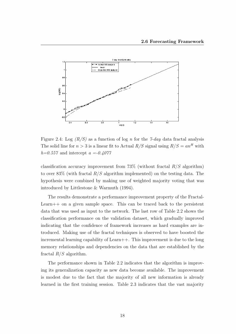
Figure 2.4: Log (R/S) as a function of log n for the 7-day data fractal analysis

The solid line for n > 3 is a linear fit to Actual R/S signal using R/S = anH with

h=0.557 and intercept a =-0.4077

classification accuracy improvement from 73% (without fractal R/S algorithm)

to over 83% (with fractal R/S algorithm implemented) on the testing data. The

hypothesis were combined by making use of weighted majority voting that was

introduced by Littlestone & Warmuth (1994).

The results demonstrate a performance improvement property of the Fractal-

Learn++ on a given sample space. This can be traced back to the persistent

data that was used as input to the network. The last row of Table 2.2 shows the

classification performance on the validation dataset, which gradually improved

indicating that the confidence of framework increases as hard examples are in-

troduced. Making use of the fractal techniques is observed to have boosted the

incremental learning capability of Learn++. This improvement is due to the long

memory relationships and dependencies on the data that are established by the

fractal R/S algorithm.

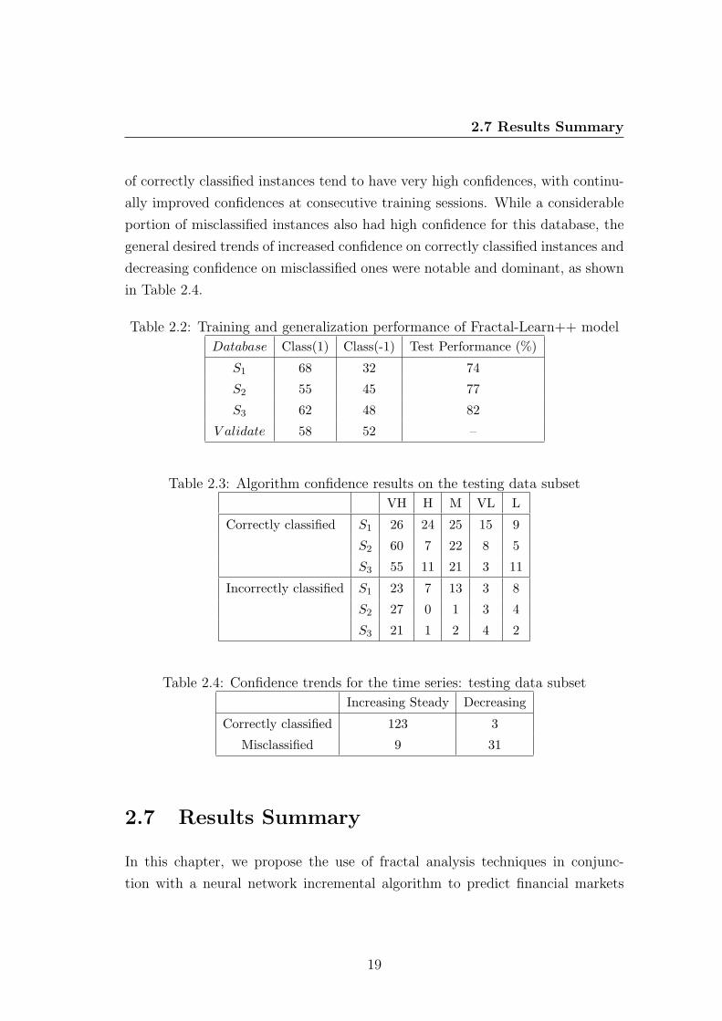
The performance shown in Table 2.2 indicates that the algorithm is improv-

ing its generalization capacity as new data become available. The improvement

is modest due to the fact that the majority of all new information is already

learned in the first training session. Table 2.3 indicates that the vast majority

18

2.7 Results Summary

of correctly classified instances tend to have very high confidences, with continu-

ally improved confidences at consecutive training sessions. While a considerable

portion of misclassified instances also had high confidence for this database, the

general desired trends of increased confidence on correctly classified instances and

decreasing confidence on misclassified ones were notable and dominant, as shown

in Table 2.4.

Table 2.2: Training and generalization performance of Fractal-Learn++ model

Database Class(1) Class(-1) Test Performance (%)

S1 68 32 74

S2 55 45 77

S3 62 48 82

V alidate 58 52 –

Table 2.3: Algorithm confidence results on the testing data subset

VH H M VL L

Correctly classified S1 26 24 25 15 9

S2 60 7 22 8 5

S3 55 11 21 3 11

Incorrectly classified S1 23 7 13 3 8

S2 27 0 1 3 4

S3 21 1 2 4 2

Table 2.4: Confidence trends for the time series: testing data subset

Increasing Steady Decreasing

Correctly classified 123 3

Misclassified 9 31

2.7 Results Summary

In this chapter, we propose the use of fractal analysis techniques in conjunc-

tion with a neural network incremental algorithm to predict financial markets

19

2.7 Results Summary

movement direction. As demonstrated in our empirical analysis, fractal re-scaled

range (R/S) analysis algorithm is observed to establish clear evidence of persis-

tence and long memory effects on the time series data. For any 7-day interval

analysis we find the Hurst exponent of H = 0, 563 for the range 7 < n < 28

(where n is the number of data points). A high degree of self-similarity is noted

in the daily time series data. These long-term memory effects observed in the

previous section are due to the rate at which information is shared amongst the

investors. Thus, the Hurst exponent can be said to be a measure of the impact

of market sentiment, generated by past events, upon future returns in the stock

market. The importance of using fractal R/S algorithm is noted in the improved

accuracy and confidence measures of the Learn++ algorithm. This is a very com-

forting outcome, which further indicates that the proposed methodology does not

only process and analyze time series data but it can also incrementally acquire

new and novel information from additional data. As a recommendation, future

work should be conducted to implement techniques that are able to provide stable

estimates of the Hurst exponent for small data sets as this was noted to be one

of the major challenges posed by time series data.

20

Chapter 3

Main Conclusion

In this document, a study is conducted to explore new ways in which time series

analysis can be carried out using emerging computational intelligence techniques

and physical sciences techniques. One of the observations that also emerged

from this investigation is an improvement on accurate performance of an existing

neural network model after the introduction of a fractal analysis technique. In

this study it is proven that the computational intelligence tools are essential for

describing and characterizing the dynamics of non-linear processes without any

intrinsic time scale.

The observations from this investigation are presented in the form of a pro-

ceedings paper in which the technique of converting a weak learning algorithm

into a strong classifier is introduced. This is done through the use of generating

an ensemble of hypotheses and later regrouping them using the weighted majority

voting technique. This study also introduces the concept of incremental learning

whereby the classifier is able to continuously identify data that it has not seen

before and group it into the respective categories thereby enforcing the ability of

adapting to learning new information without the need for retraining the model

with a new data set. A summary of the initial results were published in the Lec-

ture Notes in Computer Science 2006 by Springer, Lunga & Marwala (2006a), of

which a copy of the published paper is attached at the end of this document.

Although the results from the first proceedings paper indicated a success in

converting a weakLearner into a strong learning classifier, the initial proposed

21

framework faced some challenges. One of the major challenges that is observed

from the first model is the presents of noise samples that continuously biases

the initial guessing of the weakLearner hypothesis. The weak learning algorithm

is noted to constantly initialize its hypothesis to an average correct labelling

(classification) of 50%, which is a result of random guessing. This result indicates

the requirement for boosting the initial guessing of the weakLearner. A method

proposed in this study provides a very powerful approach in eliminating noise

samples from the data base.

In this section we propose the use of advanced fractal techniques to analyze

time series data. The objective of this new proposal is to establish regions of

persistent data, random data, and non-persistent data within the input signal

and later choose only a persistent portion of the signal to train the weakLearner.

The outcome has resulted in a improved algorithm that took less time in training

and also showed an increase in the algorithm’s confidence in decision making.

These findings imply that there are patterns and trends in the time series stock

returns that persist over time and different time scales. This provides a theoretical

platform supporting the use of technical analysis and active trading rules to

produce above average returns. The findings prove to be also useful in improving

the current models or to explore new models that implement the use of fractal

scaling. A summary of the results as presented in chapter 2 were submitted for

publishing to the Australian Joint Conference on Artificial Intelligence.

A continuation of this work would be to use multifractals, which is a kind

of generalized fractal analysis, and carries the analysis of dynamic non-linear

behavior even to greater analysis. The concept of multi-fractals has been applied

successfully in analyzing non-linear systems from a synthesis perspective. The

approach would improve on the challenges that we faced with our proposed model,

which are: the sensitivity of the proposed re-scaled range (R/S) analysis method

to short-term dependencies, which constantly biased our estimate of the Hurst

exponent H, which is in agreement to findings by other researchers. Another

shortfall that can be addressed by multifractals is the handling of very small

datasets (n < 8), where n is the number of data points, and very large datasets.

It is observed that for a very small n the Hurst exponent turns to be unstable.

22

Thus for the small sample sizes the approximation of the Hurst exponent are not

accurate. And also robust ways in which the lower bound sample size can be

defined are necessary to bring about an efficient algorithm.

23

Appendix A

Neural Networks

A.1 Introduction

This section covers the models that have been implemented in modelling the

financial markets. Neural Networks (NNs) are currently being applied to nearly

every field in the engineering and financial industries e.g. bio-medical equipment

and risk analysis, Zhang et al. (1998). NNs are used in the banking sector to

predict the issuing of bonds as well as the risk of issuing a loan to a new customer.

NNs are also used in the finance market to predict share prices which helps in

portfolio management. Furthermore, NNs are used in industry for predicting, the

life processes of products, optimization of business process, conflict management,

and the loss of information in databases as well as in most radar applications for

object identification, Bishop (1995).

Most of the conventional financial markets forecasting methods use time series

data to determine the future behavior of indicators. Wong & Selvi (1998) con-

ducted a survey which indicated that NNs are more appropriate for time-series

data rather than conventional regression methods. They also discovered that the

integration of neural networks with other technologies, such as decision support

systems (DSSs), expert systems, fuzzy logics, genetic algorithms, or robotics can

24

A.2 What is a Neural Network

improve the applicability of neural networks in addressing various types of finance

problems.

Quah & Srinivasan (1999) developed a methodology for improving returns on

stock investment through neural network selection. Their findings displayed the

generalization ability of the neural network in its application to financial markets.

This was evident through the ability to single out performing stock counters and

having excess returns in the basic stock selection system overtime. Moreover,

neural networks also showed its ability in deriving relationships in a constrained

environment in the moving window stock selection system thus making it even

more attractive for applications in the field of finance, Leke (2005).

Kuo et al. (2002) proposed a methodology that uses artificial neural networks

and fuzzy neural networks with fuzzy weight elimination for prediction of share

prices. Previously, statistical methods, which include regression methods and

moving average methods, were used for such predictions. These methods are lim-

ited in that they are efficient only for seasonal or cyclical data. Results obtained

by Kuo et al. (2002) proved to be more accurate than conventional statistical

methods. In the following section an investigation is conducted to try and explain

what a neural network is. The study goes on to investigate the back-propagation

neural network-training algorithm. The study also introduces the Multi-Layer

Perceptron neural network architecture

A.2 What is a Neural Network

The area of NNs is the intersection between the Artificial Intelligence and Ap-

proximation Algorithms. One could think of it as algorithms for ‘smart approxi-

mation’. These algorithms are used in (to name a few) universal approximation

(mapping input to the output), development of tools capable of learning hid-

den patterns from their environment, tools for finding non-evident dependencies

between data and so on.

The NNs structure models the human brain in how it processes information.

Neurolobiologists believe that the brain is similar to a massively parallel analog

25

A.2 What is a Neural Network

computer, containing about 1010 simple processors which each require a few mil-

liseconds to respond to input. The brain is a multi layer structure that works as

a parallel computer capable of learning from the ‘feedback’ it receives from the

world and changing its design by growing new neural links between neurons or

altering activities of existing ones. The brain is composed of neurons, which are

interconnected. With NNs technology, we can use parallel processing methods

to solve some real-world problems where it is difficult to define a conventional

algorithm. NNs possess the property of adaptive learning which is the ability to

learn how to do tasks based on the data given for training or initial experience and

this was shown in an investigation that was conducted by Vehtari & Lampinen

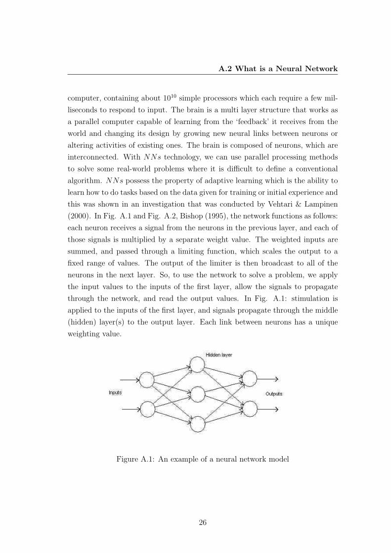
(2000). In Fig. A.1 and Fig. A.2, Bishop (1995), the network functions as follows:

each neuron receives a signal from the neurons in the previous layer, and each of

those signals is multiplied by a separate weight value. The weighted inputs are

summed, and passed through a limiting function, which scales the output to a

fixed range of values. The output of the limiter is then broadcast to all of the

neurons in the next layer. So, to use the network to solve a problem, we apply

the input values to the inputs of the first layer, allow the signals to propagate

through the network, and read the output values. In Fig. A.1: stimulation is

applied to the inputs of the first layer, and signals propagate through the middle

(hidden) layer(s) to the output layer. Each link between neurons has a unique

weighting value.

Figure A.1: An example of a neural network model

26

A.3 Back Propagation Algorithm

Figure A.2: The Structure of a Neuron

Inputs from one or more previous neurons are individually weighted, then

summed. The result is non-linearly scaled between 0 and +1, and the output

value is passed on to the neurons in the next layer. Since the real uniqueness or

‘intelligence’ of the network exists in the values of the weights between neurons,

we need a method of adjusting the weights to solve a particular problem. For this

type of network, the most common learning algorithm is called Back Propagation

(BP). A BP network learns by example, that is, we must provide a learning

set that consists of some input examples and the known-correct output for each

case. So, we use these input-output examples to show the network what type of

behavior is expected, and the BP algorithm allows the network to adapt.

A.3 Back Propagation Algorithm

The BP learning process works in small iterative steps: one of the example cases

is applied to the network, and the network produces some output based on the

current state of its synaptic weights (initially, the output will be random). This

output is compared to the known-good output, and a mean-squared error signal

is calculated. The error value is then propagated backwards through the network,

and small changes are made to the weights in each layer. The weight changes

are calculated to reduce the error signal for the case in question. The whole

process is repeated for each of the example cases, then back to the first case

again, and so on. The cycle is repeated until the overall error value drops below

27

A.4 Neural Network Architectures

some pre-determined threshold. At this point we say that the network has learned

the problem ‘well enough’ - the network will not exactly learn the ideal complex

function, but rather it will asymptotically approach the ideal function.

A.3.1 Advantages of the Back Propagation Algorithm

In the literature review it is found that NNs architectures, which were imple-

mented using the BP algorithm, displayed the algorithm’s strong generalization

ability to predict the performance of securities. This is evident through the ability

to single out performing stock and having excess returns in the basic stock selec-

tion system overtime from the results that were presented by Quah & Srinivasan

(1999).

A.3.2 Disadvantages of the Back Propagation Algorithm

The selection of the learning rate and momentum is very important when using

this type of algorithm. Failure to choose value for these to the required tolerance

will result in the output error oscillating and thus the system will become unstable

because it will not converge to a value (system will diverge). In the following

section a brief discussion is given on how to select the required optimal parameters

for this algorithm.

A.4 Neural Network Architectures

Most studies use the straightforward Multi-Layer Perceptron (MLP) networks

while others employ some variants of the MLP , Vehtari & Lampinen (2000).

The real uniqueness or intelligence of the MLP network exists in the values of

the weights between the neurons. Thus the best method to adjust these weights

in our study is the Back Propagation as discussed in the previous sections. There

is a criterion required to assist us in choosing the appropriate network structure

28

A.4 Neural Network Architectures

as proposed by Quah & Srinivasan (1999). There are four major issues in the

selection of the appropriate network:

• Appropriate training algorithm.

• Architecture of the ANN.

• The Learning Rule.

• The Appropriate Learning Rates and Momentum.

A.4.1 Selection of the Appropriate Training Algorithm

Since the sole purpose of this project is to predict the performance of the chosen

stock portfolio’s movement direction, the historical data that is used for the

training process will have a known outcome (whether it is considered moving up or

moving downwards). Among the available algorithms, the BP algorithm designed

by Rumelhart & McClelland (1986) is one of the most suitable methodologies

to be implemented as it is being intensively tested in finance. Moreover, it is

recognized as a good algorithm for generalization purposes.

A.4.2 Selection of the System Architecture

Architecture, in this context, refers to the entire structural design of the NNs

(Input Layer, Hidden Layer and Output Layer). It involves determining the

appropriate number of neurons required for each layer and also the appropriate

number of layers within the Hidden Layer. The logic of the Back Propagation

method is the hidden layer. The hidden layer can be considered as the crux of the

Back Propagation method. This is because hidden layer can extract higher-level

features and facilitate generalization, if the input vectors have low-level features

of a problem domain or if the outputinput

relationship is complex. The fewer the hidden

units, the better is the NNs is able to generalize. It is important not to over-fit

the NNs with large number of hidden units than required until it can memorize

29

A.4 Neural Network Architectures

the data. This is because the nature of the hidden units is like a storage device.

It learns noise present in the training set, as well as the key structures. No

generalization ability can be expected in these. This is undesirable, as it does not

have much explanatory power in an unseen environments.

A.4.3 Selection of the Learning Rule

The learning rule is the rule that the network will follow in its error reducing

process. This is to facilitate the derivation of the relationships between the in-

put(s) and output(s). The generalized delta rule developed by McClelland &

Rumelhart (1988) is mostly used in the calculations of weights. This particular

rule is selected in most researches as it proves to be quite effective in adjusting

the network weights.

A.4.4 Selection of the Appropriate Learning Rates and

Momentum

The Learning Rates and Momentum are parameters in the learning rule that aid

the convergence of error, so as to arrive at the appropriate weights that are rep-

resentative of the existing relationships between the input(s) and the output(s).

As for the appropriate learning rate and momentum to use, some neural network

software has a feature that can determine appropriate learning rate and momen-

tum for the network to start training with. This function is known as ‘Smart

Start’. Once this function is activated, the network will be tested using different

values of learning rates and momentum to find a combination that yields the

lowest average error after a single learning cycle. These are the optimum starting

values as using these rates improve error converging process, thus require less

processing time.

This function automatically adjusts the learning rates and momentum to en-

able a faster and more accurate convergence. In this function, the software will

sample the average error periodically, and if it is higher than the previous sample

30

A.5 Multi-Layer Perceptron

then the learning rate is reduced by 1%. The momentum is ‘decayed’ using the

same method but the sampling rate is half of that used for the learning rate. If

both the learning rate and momentum decay are enabled then the momentum

will decay slower than the learning rate. In general cases, where these features are

not available, a high learning rate and momentum (e.g. 0.9 for both the Learn-

ing Rates and Momentum) are recommended, as the network will converge at a

faster rate than when lower figures are used. However, too high a learning rate

and momentum will cause the error to oscillate and thus prevent the converging

process. Therefore, the choice of learning rate and momentum are dependent on

the structure of the data and the objective of using the NNs. The following

section introduces the Multi-Layer Perceptron neural network architecture that

is implemented in this study.

A.5 Multi-Layer Perceptron

A Multi-Layer Perceptron (MLP) is made up of several layers of neurons, each

layer is fully connected to the next one. Moreover, each neuron receives an addi-

tional bias input as shown in A.3. It is both simple and based on mathematical

grounds. Input quantities are processed through successive layers of ”neurons”.

There is always an input layer, with a number of neurons equal to the number

of variables of the problem, and an output layer, where the perceptron response

is made available, with a number of neurons equal to the number of quantities

computed from the inputs. The layers in between are called hidden layers. With

no hidden layer the perceptron can only perform linear tasks. Each neuron of a

layer other than the input layer computes a linear combination of the outputs of

the previous layer, plus the bias. The coefficients of the linear combinations plus

the biases are called the weights. Neurons in the hidden layer then compute a

non-linear function of their input. The non-linear function is the sigmoid func-

tion y(x) = 11−exp(−x)

. MLPs are probably the most widely used architecture

for practical applications.

• W kij = weight from unit i (in layer k) to unit j (in layer k + 1)

31

A.6 Conclusion

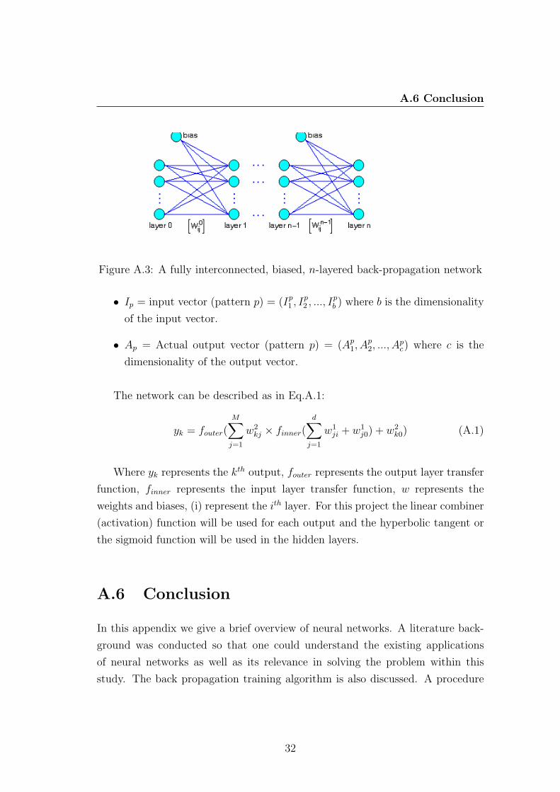
Figure A.3: A fully interconnected, biased, n-layered back-propagation network

• Ip = input vector (pattern p) = (Ip1 , Ip

2 , ..., Ipb ) where b is the dimensionality

of the input vector.

• Ap = Actual output vector (pattern p) = (Ap1, A

p2, ..., A

pc) where c is the

dimensionality of the output vector.

The network can be described as in Eq.A.1:

yk = fouter(M∑

j=1

w2kj × finner(

d∑j=1

w1ji + w1

j0) + w2k0) (A.1)

Where yk represents the kth output, fouter represents the output layer transfer

function, finner represents the input layer transfer function, w represents the

weights and biases, (i) represent the ith layer. For this project the linear combiner

(activation) function will be used for each output and the hyperbolic tangent or

the sigmoid function will be used in the hidden layers.

A.6 Conclusion

In this appendix we give a brief overview of neural networks. A literature back-

ground was conducted so that one could understand the existing applications

of neural networks as well as its relevance in solving the problem within this

study. The back propagation training algorithm is also discussed. A procedure

32

A.6 Conclusion

on how to choose the required parameters for the back propagation algorithm is

also explained in detail. An introduction of the neural network architecture that

is to be implemented in the study is given. The appendix ends by showing a

mathematical model of the multi-layer perceptron.

33

Appendix B

Learn++

B.1 Ensemble of Classifiers

Learn++ was developed by Polikar et al. (2002) from an inspiration by Freund

& Schapire (1997)’s ‘adaptive boosting‘ (AdaBoost) algorithm, originally pro-

posed for improving the accuracy of weak learning algorithms. In ‘Strength of

weak learning’, Freund & Schapire (1997) showed that for a two class problem,

a weakLearner that almost always achieves high errors can be converted into

a strong learner that almost always achieves arbitrarily low errors using a pro-

cedure called boosting. Both Learn++ and AdaBoost are based on generating

an ensemble of weak classifiers, which are trained using various distributions of

the training data and then combining the outputs (classification rules) of these

classifiers through a majority voting scheme. In the context of machine learning,

a classification rule generated by a classifier is referred to as a hypothesis. The

voting algorithm ”weighted majority algorithm” was developed by Littlestone &

Warmuth (1994), this algorithm assigns weights to different hypotheses based

on an error criterion. Weighted hypotheses are then used to construct a com-

pound hypothesis, which is proved to perform better than any of the individual

hypotheses.

34

B.1 Ensemble of Classifiers

Littlestone & Warmuth (1994), also showed that the error of the compound

hypothesis is closely linked to the error bound of the best hypothesis. Freund

& Schapire (1996) later developed AdaBoost extending boosting to multi-class,

learning problems and regression type problems. They continually improved their

work on boosting with statistical theoretical analysis of the effectiveness of voting

methods. Recently, they have introduced an improved boosting algorithm that

assigns confidences to predictions of decision tree algorithms. Their new boosting

algorithm can also handle multi-class databases, where each instance may belong

to more than one class.

Independent of Schapire and Freund, Breiman (1996) developed an algorithm

very similar to boosting in nature. Breiman’s bagging, short for ‘bootstrap ag-

gregating’, is based on constructing ensembles of classifiers through continually

retraining a base classifiers with bootstrap replicates of the training database. In

other words, given a training dataset S of m samples, a new training dataset S

is obtained by uniformly drawing m samples with replacement from S. This is

in contrast to AdaBoost where each training sample is given a weight based on

the classification performance of the previous classifier. Both boosting and bag-

ging require weak classifiers as their base classification algorithm because both

procedures take advantage of the so-called instability of the weak classifier.

This instability causes the classifiers to construct sufficiently different deci-

sion surfaces for minor modifications in their training datasets , this is observed

from the results presented by Schapire et al. (1998). Both bagging and boosting

have been used for construction of strong classifiers from weak classifiers, and

they have been compared and tested against each other by several authors. The

idea of generating an ensemble of classifiers is not new. A number of other re-

searchers have also investigated the properties of combined classifiers. In fact,

it was Wolpert (1992) who introduced the idea of combining hierarchical levels

of classifiers, using a procedure called ’stacked generalization’ and other authors

analyzed error sensitivities of various voting and combination schemes whereas

other researchers concentrated on the capacity of voting systems. Ji & Ma (1997)

proposed an alternative approach to AdaBoost for combining classifiers. Their

approach generates simple perceptrons of random parameters and then combines

35

B.2 Strong and Weak Learning

the perception outputs using majority voting. Ji & Ma (1997) also gave an ex-

cellent review of various methods for combining classifiers.

B.2 Strong and Weak Learning

Consider an instance space X, a concept class C = c : X → {0, 1}, a hypothesis

space H = h : X → {0, 1}, and an arbitrary probability distribution D over the

instance space X. In this setup, c is the true concept that we wish to learn, h is

the approximation of the learner to the true concept c. Although the following

definitions are for a two-class concept, they can be naturally generalized to the

n-class concept as was demonstrated by Polikar (2000) when he investigated the

application of Learn++ to the gas sensing problem . We assume that we have

access to an oracle, which obtains a sample x ∈ X, according to the distribution

D, labels it according to c, and outputs < x, c(x) >.

Definition (Strong Learning): A concept class C defined over an instance

space X is said to be potentially Probably Approximately Correct (PAC) learn-

able using hypothesis class H if for all target concepts c ∈ C, a consistent learner

L is guaranteed to output a hypothesis h ∈ H with error less than 12

observing

ε to be ε > 0 and probability of at least 1 − δ , δ > 0 after processing a finite

number of examples, obtained according to D. The learner L is then called a

PAC learning algorithm, or a stronglearner of the sample space. Note that

PAC learning imposes very stringent requirements on the learner L, since L is

required to learn all concepts within a concept class with arbitrarily low error

(approximately correct) and with an arbitrarily high probability (probably cor-

rect). A learner that satisfies these requirements may not be easy to implement

practically, hence such a learner is only a potentially PAC learning algorithm.

However, finding a learner L0 that can learn with fixed values of ε, (say ε0 ) and

δ , (say δ0 ) might be quite conceivable.

Definition (Weak Learning): A concept class C defined over an instance

space X is weakly learning using the hypothesis class H, if there exists a learning

algorithm L0 and constants ε0 > 12

and δ0 < 1 such that for every concept c ∈ C

36

B.3 Boosting the Accuracy of a Weak Learner

and for every distribution D on the instances space X, the algorithm L0, given

access to an example set drawn from (c, D), returns a hypothesis h ∈ H with

probability of at least 1− δ0 and Errorc, D(h). Note that unlike strong learning,

weak learning imposes the least possible stringent conditions, since it is required

to perform only slightly better than a random guess for a two class problem

Polikar (2000).

B.3 Boosting the Accuracy of a Weak Learner

Boosting is based on running the weak learning algorithm for a number of times

to obtain many weak hypotheses, and using a majority vote to determine the final

hypothesis whose error is less than any one of the individual weak hypotheses.

For the generation of each additional hypothesis, the learner is presented with a

different distribution of the training data, and it is forced to learn increasingly

misclassified examples.

B.4 Boosting for Two-class Problems

Let c be a boolean target concept and D1 = D, where D is the original distri-

bution of the training data. The weak learning algorithm L0 is ran with train-

ing examples from D1 and weak hypothesis h1 is obtained such that Errorc,

D1(h1) = ε1 < ε < 12. Attention is then focused on examples misclassified by h1.

A new set of training examples is obtained from a new distribution D2 as follows:

An oracle flips a fair coin; on heads, it returns an example < x, c(x) > such that

h1 = c(x). On tails the oracle returns an example < x, c(x) > such that h1 = c(x).

Therefore, the new distribution D2 picks up correctly classified examples with a

probability of 12

and picks up misclassified examples with probability of 12. Now

let h2 be the new hypothesis returned by the learner L0 on D2. This hypothesis

would also have an Errorc, D2(h2) = ε2 < ε1 < 12. The next hypothesis h3 is then

returned by L0 in which h1 and h2 disagree. The hypothesis h3 will then have

37

B.5 Boosting for Multi-class Problems

Errorc, D3(h3) = ε3 < ε1 < 12. Then the final hypothesis h is chosen from the

majority voting of the three hypotheses. Freund & Schapire (1997) showed that

Errorc, D(h) is bounded by 3× ε2 − 2× ε3, which is less than ε. Thus with each

iteration, the error of the final hypothesis decreases and can potentially converge

to an arbitrarily low value of error. Furthermore, it is proven that the error only

takes polynomial time to reach arbitrarily low values. Byorick & Polikar (2003)

gave an upper bound on the number of training examples required to reach these

low error levels.

B.5 Boosting for Multi-class Problems

AdaBoost algorithm is based on the belief that a large number of solvers, each

solving a simple problem, can be used to solve a very complicated problem when

the solutions to simple problems are combined in an appropriate form. Learn++

is an extension to the original boosting algorithm, which was developed to boost

the performance of multi-class weak learning classifiers by generating various

weak classification hypotheses and combining them through weighted majority

voting for the classes predicted by the individual hypotheses. These hypotheses

are obtained by retraining the classifier using a different subset of the training

dataset, chosen strategically based on the performance of the previous hypothe-

ses. In general terms, each instance in the training database is assigned a weight,

and these weights are updated based on the performance of the previous hypothe-

sis. Misclassified instances are assigned larger weight, whereas correctly classified

instances are smaller weights. The training dataset for the next hypothesis is

then chosen based on the current weights of the instances. Instances with higher

weights have higher chances of being selected into the next training set. Further-

more, the weights are normalized to satisfy the conditions to form a probability

distribution function, referred to as the distribution D of the training dataset.

This is observed in a study that was conducted by Carpenter et al. (1992). Con-

sistently misclassified instances are considered as hard examples of the dataset,

and the algorithm is designed to train subsequent classifiers with increasingly

harder instances of the dataset. Inputs to the AdaBoost algorithm are:

38

B.5 Boosting for Multi-class Problems

• Sequence of labelled examples (training data,S) drawn randomly from an

unknown distribution D,

• Weak learning algorithm, weakLearner

• An integer T that specifies the number of hypotheses (iterations) to be

generated by weakLearner.

The algorithm AdaBoost, which is given in the next section, proceeds as fol-

lows: In iteration t = 1, 2, ..., T , AdaBoost provides the weak learning algorithm,

weakLearner, with a training subset data drawn according to distribution Dt

from the original training data S = [(x1, y1), (x2, y2), ..., (xm, ym)] where x1 are

training data instances and y1 are the corresponding correct labels. weakLearner

then computes a hypothesis (classifier) ht : X → Y , which correctly classifies a

percentage of the training set. That is, weakLearner’s goal is to find a hypothesis

ht, which minimizes the training error as in Eq.B.1

εt =∑

t:ht(xt) 6=yt

Dt(i) (B.1)

The initial distribution Dt is typically chosen to be uniform over S, unless there

is prior knowledge to choose otherwise, that is, D1(i)=1m∀i . This gives equal

probability to all instances in S to be drawn into the initial data subset. The

distribution is updated using Eq.B.2

Dt+1 =Dt(i)

Zt

(B.2)

Where Zt =∑

i Dt(i) is a normalized constant chosen to ensure that Dt+1 will be

a distribution, and βt = εt

1−εt. The parameter β can be thought of as a normalized

error term, since for

0 < εt < 12,0 < β < 1. In fact, Schapire et al. (1998) showed that Eq.B.3 is

the optimum choice for the parameter

βt =εt

1− εt

(B.3)

39

B.5 Boosting for Multi-class Problems

The distribution update rule in Eq.B.2 ensures that weights for misclassified

instances are increased, whereas weights for correctly classified instances are re-

duced. Thus, AdaBoost focuses on examples that seem to be hardest for weak-

Learner to learn. At the end of T iterations, AdaBoost combines the weak hy-

potheses h1, ..., hT into a single final hypothesis hfinal by computing the weighted

majority of the weak hypothesis as in Eq.B.4

hfinal = argmaxy∈Y ×∑

t:ht(x)=y

log1

βt

(B.4)

Where the weight of hypothesis ht is defined to be log ( 1β) so that the greater

weight is given to a hypothesis with lower error. For a given instance x, Eq.??

outputs the label y, that maximizes the sum of the weights of the weak hypothesis

predicting that label. It should be noted that AdaBoost requires εt, error of each

hypothesis ht, to be less than 12. For a binary class problem, this is the least

restrictive requirement one could have, since an error of 12

for a binary class

problem is equivalent to random guessing.

Algorithm AdaBoost Input:

• Sequence of m examples S = [(x1, y1), (x2, y2), ..., (xm, ym)] with labels yi ∈Y = 1, ..., C drawn from a distribution D

• Weak learning algorithm weakLearner,

• Integer T specifying number of iterations.

Initialize D1(i) = 1m

,∀i

Do for t = 1, 2, ..., T

1. Call weakLearner, providing it with the distribution Dt

2. Get back a hypothesis ht : X → Y

3. Calculate the error of ht: εt =∑

i:ht(xi) 6=yiDt(i) if εt > 1

2, Then set T = t−1

and abort loop.

40

B.5 Boosting for Multi-class Problems

4. Set βt = εt

1−εt

5. Update distribution Dt: Dt+1(i)=Dt(i)

Zt× Bt if ht(xi) = yi Otherwise

Dt+1(i)=Dt(i)

Zt

Where Zt =∑

i Dt(i) is a normalized constant chosen to ensure that Dt+1 will

be a distribution function. The final hypothesis is

hfinal(x) = argmaxy∈Y

∑t:ht(x)=y

log(1

βt

) (B.5)

Note that any hypothesis with an error larger than 12

can be negated to ob-

tain an alternative hypothesis with an error less than 12. However, obtaining

a maximum error of 12

becomes increasingly difficult as the number of classes

increases, since for a k class problem the error for random guessing is proven

to be (k − 1) k by Freund & Schapire (1997). Therefore, the choice of a weak

learning algorithm with a classification performance of at least 50% may not be

very easy. Any classification algorithm can be substituted as a weak learner by

modifying appropriate parameters. For example, an MLP with a larger number

of nodes/layers and a smaller error goal is, in general, a stronger learner than the

one with smaller number of nodes and a higher error goal.

It should be noted that the use of strong learners that achieve high classifi-

cation performance on a particular training data are not recommended for use

with boosting since there is little to be gained from their combination, or they

may lead to over fitting of the data. One of the nice properties of the AdaBoost

algorithm is that it is less likely to encounter over fitting problems since only a

portion of the instances space is learned by individual hypothesis. In addition,

an ensemble of weak learners performs at least as well as a strong learner, but

in considerably less time, since strong learners spend most of the training time

during fine-tuning at lower error rates.

41

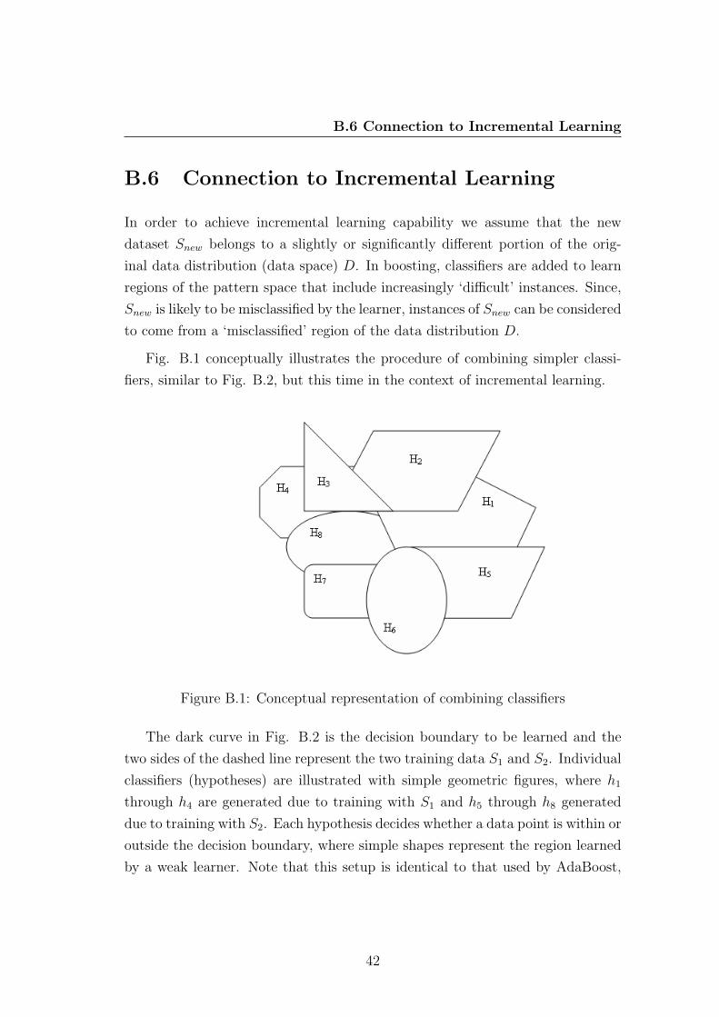
B.6 Connection to Incremental Learning

B.6 Connection to Incremental Learning

In order to achieve incremental learning capability we assume that the new

dataset Snew belongs to a slightly or significantly different portion of the orig-

inal data distribution (data space) D. In boosting, classifiers are added to learn

regions of the pattern space that include increasingly ‘difficult’ instances. Since,

Snew is likely to be misclassified by the learner, instances of Snew can be considered

to come from a ‘misclassified’ region of the data distribution D.

Fig. B.1 conceptually illustrates the procedure of combining simpler classi-

fiers, similar to Fig. B.2, but this time in the context of incremental learning.

Figure B.1: Conceptual representation of combining classifiers

The dark curve in Fig. B.2 is the decision boundary to be learned and the

two sides of the dashed line represent the two training data S1 and S2. Individual

classifiers (hypotheses) are illustrated with simple geometric figures, where h1

through h4 are generated due to training with S1 and h5 through h8 generated

due to training with S2. Each hypothesis decides whether a data point is within or

outside the decision boundary, where simple shapes represent the region learned

by a weak learner. Note that this setup is identical to that used by AdaBoost,

42

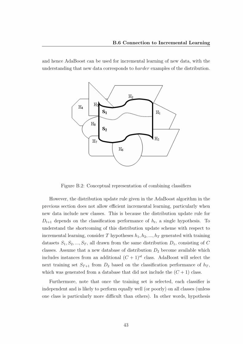
B.6 Connection to Incremental Learning

and hence AdaBoost can be used for incremental learning of new data, with the

understanding that new data corresponds to harder examples of the distribution.

Figure B.2: Conceptual representation of combining classifiers

However, the distribution update rule given in the AdaBoost algorithm in the

previous section does not allow efficient incremental learning, particularly when

new data include new classes. This is because the distribution update rule for

Dt+1 depends on the classification performance of ht, a single hypothesis. To

understand the shortcoming of this distribution update scheme with respect to

incremental learning, consider T hypotheses h1, h2, ..., hT generated with training

datasets S1, S2, ..., ST , all drawn from the same distribution D1, consisting of C

classes. Assume that a new database of distribution D2 become available which

includes instances from an additional (C + 1)st class. AdaBoost will select the

next training set ST+1 from D2 based on the classification performance of hT ,

which was generated from a database that did not include the (C + 1) class.

Furthermore, note that once the training set is selected, each classifier is

independent and is likely to perform equally well (or poorly) on all classes (unless

one class is particularly more difficult than others). In other words, hypothesis

43

B.7 Learn++: An Incremental Learning Algorithm

hT+1 will perform equally well on instances coming from (C+1)st class. Therefore,

patterns from the (C + 1)st class will not necessarily be selected into ST+1, and

they will have no advantage of being selected into the training dataset in the next

little iteration. Consequently, learners will not be forced to focus on the patterns

of the new class. The final weighted majority will then fail to recognize samples

from the new class for much iteration to come, increasing the time and space

complexity of the algorithm.

The distribution update rule can, however, be forced to focus on instances of

the new class, if the updated rule is based on the combined performance of all t

hypothesis generated during the previous t iterations. Let us call the weighted

majority voting of the previous t hypotheses the composite hypothesis Ht. Note

that when instances from a new class become available, they will be misclassified

by Ht, since none of the previous t training sessions have seen instances from the

new class. Therefore, updating the training dataset distribution based on the

classification results of Ht will ensure that the selection of instances from the new

class is favored. The Learn++ algorithm incorporates these ideas into a smarter

distribution update rules, this algorithm is described in the following section. As

will be shown in the following sections, Learn++ does not only allow the weak

learning algorithm to learn incrementally from new data, but at the same time

it converts the weak learning algorithm into a very powerful classifier.

B.7 Learn++: An Incremental Learning Algo-

rithm

Learn++ is an algorithm that allows any classifier to learn incrementally from

additional data, without forgetting what is previously learned, even when the

new data includes a new class. To achieve this rather ambitious task, Learn++

introduces a number of modifications to the basic ideas of AdaBoost. First, the

training error is redefined. In AdaBoost, the error εt is the training error of

the weak learner, calculated using the training patterns misclassified by ht. This

44

B.7 Learn++: An Incremental Learning Algorithm

constitutes a problem, when using neural network type classifiers such as MLPs

as base classifiers, since a converged neural network almost always performs close

to 100% on its training data for any nontrivial error goal. This is particularly true

for Radial Basis Functions, ARTMAP type algorithms, since these algorithms

guarantee 100% correct classification on their training database Byorick & Polikar

(2003).

In order to ensure weak learning and a nonzero εt, Learn++ first divides the

selected training dataset Tt into subsets TRt and TEt where TRt is the training

subset and TEt is the testing subset for the current training dataset Tt. During

the tth iteration, the weak learner is trained on TRt and tested on the entire

set T = TRt + TEt. For each iteration, different training and testing subsets

are selected based on previous performance. The error of tth hypothesis on the

combined TRt + TEt set is defined as εt. Eventually (almost) all patterns in the

original training dataset will be established by the weakLearner, and hence using

this definition of training error is justified.

Initially all instances have equal likelihood to be selected into the first training

dataset (unless there is prior knowledge to choose otherwise). In the following

discussion, new databases that become available for incremental learning are

denoted with the subscript k and the (unknown) distribution from which the kth

database is drawn will be denoted by the script Dk, whereas the distribution of

the current training dataset at tth iteration is denoted by Dt. In each iteration

t, the distribution Dt. is obtained by normalizing the current weights of the

instances in step 1. In step 2, training (TRt) and testing (TEt) subsets are

randomly generated from the current database Dk, according to the distribution

Dt. These subsets are used as inputs to WeakLearn in step 3, which return the

hypothesis ht in step 4. The error, εt, is then computed from the misclassified

patterns TRt + TEt. If εt > 12, ht is discarded, and new TRt and TEt are

generated. Instead of updating the distribution based on instances misclassified

by ht, Learn++ then calls the weighted majority voting in step 5 to compute the

composite hypothesis, Ht.

45

B.7 Learn++: An Incremental Learning Algorithm

B.7.1 Learn++ Algorithm

Input: For each database drawn from Dk, k = 1, 2, ..., K

• Sequence of m examples S = [(x1, y1), (x2, y2), ..., (xm, ym)] with labels yi ∈Y = 1, ..., C

• Weak learning algorithm weakLearner,

• Integer T specifying number of iterations.

Do for t = 1, 2..., T Initialize w1i = D(i) = 1

m∀i, unless there is prior

knowledge to select otherwise. Do for k = 1, 2, ...K

1. Set Dt=wt∑m

i=1 wt(i)so that Dt is a distribution

2. Randomly choose training TRt and testing TEt subsets according to Dt

3. Call weakLearner, providing it with TRt

4. Get back a hypothesis ht : X → Y , and. Calculate the error of ht:εt =∑i:ht(xi) 6=yi

Dt(i) on T = TRt + TEt if εt > 12

, set t = t− 1, discard ht and

go to step 2. Otherwise, compute normalized error as βt=εt

1−εt

5. Call weighted majority, obtain the overall hypothesis ht = argmaxy∈Y

∑t:ht(x)=y(log βt)

and compute the overall error Et =∑

i:Ht(Xi) 6=yiDt(i) =

∑mi=1 Dt(i) d|Ht(xi 6= yi|)e

if Et > 12, set t = t− 1, discard Ht and go to step 2.

6. Set βt=εt

1−εtand update the weights of the instances: wt+1 = wt(i) ×

B[|Ht(xi) 6=yi|]t

Call weighted majority on combined hypotheses Ht and Output the final hy-

pothesis Hfinal = argmaxy∈Y

∑Kk=1

∑t:Ht(x)=y(log βt) Note that the composite

hypothesis Ht is computed similar to the final hypothesis hfinal in AdaBoost,

that is Eq.B.6

ht = argmaxy∈Y

∑t:ht(x)=y

(log βt) (B.6)

46

B.7 Learn++: An Incremental Learning Algorithm

which makes the training error given in Eq.B.7 to be :

Et =∑

i:Ht(Xi) 6=yi

Dt(i) =m∑

i=1

Dt(i) d|Ht(xi 6= yi|)e | (B.7)

on misclassified instances, where d·e is 1 if the predicate holds true, and 0 other-

wise. From this error, we compute the normalized error as in Eq.B.8

βt =εt

1− εt

(B.8)

In step 6, the composite hypothesis, Ht , and its normalized error, Bt are then

used to update the distribution of the distribution of the instances to be used in

the next training session. The update rule is given by Eq.B.9

wt+1 = wt(i)×B[|Ht(xi) 6=yi|]t (B.9)

where wt(i) is simply the weights of the ith instance for the tth training session.

At the end of T iterations (for each database Dk), the final hypothesis is obtained

by combining the composite hypothesis Ht as in Eq.B.10

ht = argmaxy∈Y

∑t:ht(x)=y

(log βt) (B.10)

In this algorithm, when a new dataset contains new classes, the composite hy-

pothesis Ht will misclassify instances from the new class, and the algorithm will

be forced to learn these instances. A disadvantage of this approach is the large

storage capacity required to store all hypotheses generated to learn the additional

class. Addition of data with new classes results in generating a large number of

hypotheses in order to remove the bias of the combined classifier towards the

previous classes. This bias can be reduced significantly by changing the final

classification rule to Eq.B.11

Hfinal = argmaxy∈Y

K∑k=1

∑t:Ht(x)=y

(log βt) (B.11)

Which combines the original weak hypothesis ht It should be noted however that

subsequent hypotheses are still generated with training data selected according to

47

B.8 Conclusion

a distribution based on the performance of the composite hypotheses Ht, which,

along with other modifications, distinguishes Learn++ from AdaBoost. Exper-

imental results that are summarized in Chapter 2 and in Appendix D demon-

strate that both final classification rules given by equations Eq.B.10 and Eq.B.11

achieve the same performance level in incremental learning problems including

new classes.

B.8 Conclusion

This chapter introduced the incremental algorithm, Learn++, in detail focusing

more on its development from the AdaBoost algorithm. As shown in this study,

Learn++ displays its ability to learn from new data even when the data introduces

new classes. Learn++ makes no assumptions as to what kind of weak learning

algorithm is to be used. Any weak learning algorithm can serve as the base

classifier of Learn++, though the algorithm is optimized for supervised neural

network-type classifiers, whose weakness can be easily controlled via network

size and error goal. Learn++ is also intuitively simple, easy to implement,and

converges much faster that strong learning algorithms. This is because using weak

learners eliminates the problem of fine-tuning and over fitting, since each learner

only roughly approximates the decision boundary of the sample data. Initial

results using this algorithm looked promising, but because of the significant room

for improvement we proposed the use of fractal theory to eliminate non-persistent

data that introduced a huge margin of randomness in our initial results, Lunga

& Marwala (2006a). This results of this improvement are summarized in Lunga

& Marwala (2006b).

48

Appendix C

Fractals Theory

C.1 An Introduction to Fractals

C.1.1 What is a fractal ?

Definition: A rough or fragmented geometric shape that can be subdivided

into parts, each of which is (at least approximately) a reduced/size copy of the

whole. Mathematically: this is a set of points whose fractal dimension exceeds

its topological dimension.

C.1.2 Fractal Geometry

Almost all geometric forms used for building man made objects belong to Eu-

clidean geometry; they are comprised of lines, planes, rectangular volumes, arcs,

cylinders, spheres, etc. These elements can be classified as belonging to an in-

teger dimension 1, 2 or 3. This concept of dimensioning can be described both

intuitively and mathematically. Intuitively we say that a line is one-dimensional

because it only takes one number to uniquely define a point on it. That one

49

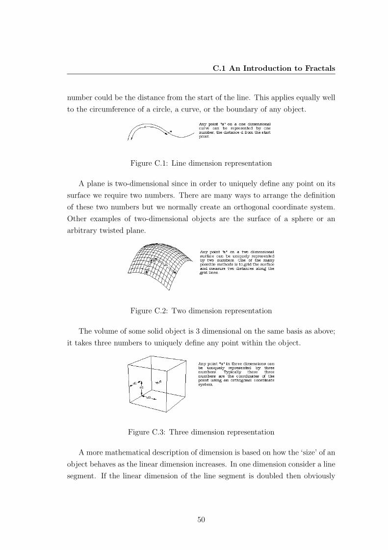
C.1 An Introduction to Fractals

number could be the distance from the start of the line. This applies equally well

to the circumference of a circle, a curve, or the boundary of any object.

Figure C.1: Line dimension representation

A plane is two-dimensional since in order to uniquely define any point on its

surface we require two numbers. There are many ways to arrange the definition

of these two numbers but we normally create an orthogonal coordinate system.

Other examples of two-dimensional objects are the surface of a sphere or an

arbitrary twisted plane.

Figure C.2: Two dimension representation

The volume of some solid object is 3 dimensional on the same basis as above;

it takes three numbers to uniquely define any point within the object.

Figure C.3: Three dimension representation

A more mathematical description of dimension is based on how the ‘size’ of an

object behaves as the linear dimension increases. In one dimension consider a line

segment. If the linear dimension of the line segment is doubled then obviously

50

C.1 An Introduction to Fractals

the length (characteristic size) of the line has doubled. In two dimensions, if the

linear dimension of a rectangle for example is doubled then the characteristic size,

the area, increases by a factor of 4. In three dimension, if the linear dimension of

a box are doubled then the volume increases by a factor of 8. This relationship

between dimension D, linear scaling L and the resulting increase in size S can be

generalized and written as

S = LD (C.1)

This is just telling us mathematically what we know from everyday experience.

If we scale a two-dimensional object for example, then the area increases by the

square of the scaling. If we scale a three dimensional object the volume increases

by the cube of the scale factor. Rearranging the above gives an expression for

dimension depending on how the size changes as a function of linear scaling,

namely

D =log(S)

log(L)(C.2)

In the examples above the value of D is an integer 1, 2 or 3 depending on the

dimension of the geometry, Feder (1988). This relationship holds for all Euclidean

shapes. There are, however, many shapes which do not conform to the integer

based idea of dimension given above in both the intuitive and mathematical

descriptions. That is, there are objects, which appear to be curves for example

(e.g. time series signals), but which a point on the curve cannot be uniquely

described with just one number. If the earlier scaling formulation for dimension

is applied the formula does not yield an integer. There are shapes that lie in a

plane but if they are linearly scaled by a factor L, the area does not increase by

L squared but by some non-integer amount. These geometries are called fractals.

One of the simpler fractal shapes is the von Koch snowflake in Fig. C.4. The

method of creating this shape is to repeatedly replace each line segment with

the following 4 line segments. The process starts with a single line segment and

continues forever. The first few iterations of this procedure are shown in Figure

C.5.

51

C.1 An Introduction to Fractals

Figure C.4: Van Koch snowflake

Figure C.5: Multi Van Koch Snowflake shapes combined, Goldberger(2006)

52

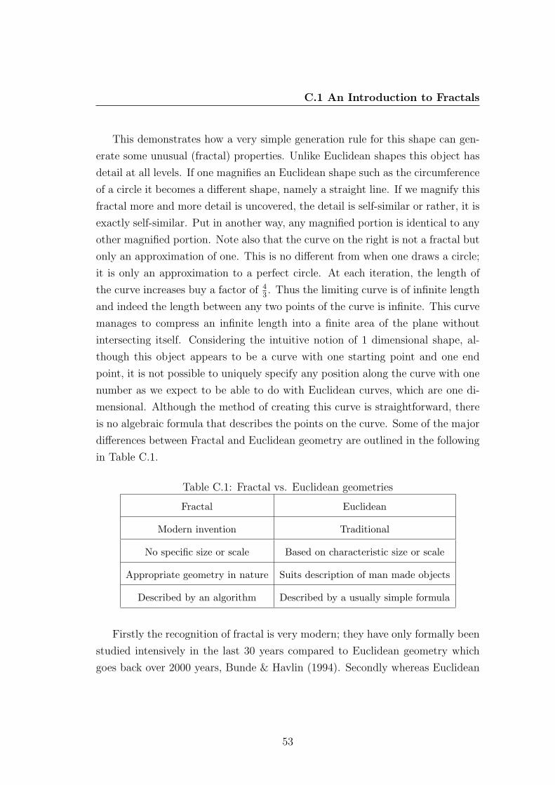
C.1 An Introduction to Fractals

This demonstrates how a very simple generation rule for this shape can gen-

erate some unusual (fractal) properties. Unlike Euclidean shapes this object has

detail at all levels. If one magnifies an Euclidean shape such as the circumference

of a circle it becomes a different shape, namely a straight line. If we magnify this

fractal more and more detail is uncovered, the detail is self-similar or rather, it is

exactly self-similar. Put in another way, any magnified portion is identical to any

other magnified portion. Note also that the curve on the right is not a fractal but

only an approximation of one. This is no different from when one draws a circle;

it is only an approximation to a perfect circle. At each iteration, the length of

the curve increases buy a factor of 43. Thus the limiting curve is of infinite length

and indeed the length between any two points of the curve is infinite. This curve

manages to compress an infinite length into a finite area of the plane without

intersecting itself. Considering the intuitive notion of 1 dimensional shape, al-

though this object appears to be a curve with one starting point and one end

point, it is not possible to uniquely specify any position along the curve with one

number as we expect to be able to do with Euclidean curves, which are one di-

mensional. Although the method of creating this curve is straightforward, there

is no algebraic formula that describes the points on the curve. Some of the major

differences between Fractal and Euclidean geometry are outlined in the following

in Table C.1.

Table C.1: Fractal vs. Euclidean geometries

Fractal Euclidean

Modern invention Traditional

No specific size or scale Based on characteristic size or scale

Appropriate geometry in nature Suits description of man made objects

Described by an algorithm Described by a usually simple formula

Firstly the recognition of fractal is very modern; they have only formally been

studied intensively in the last 30 years compared to Euclidean geometry which

goes back over 2000 years, Bunde & Havlin (1994). Secondly whereas Euclidean

53

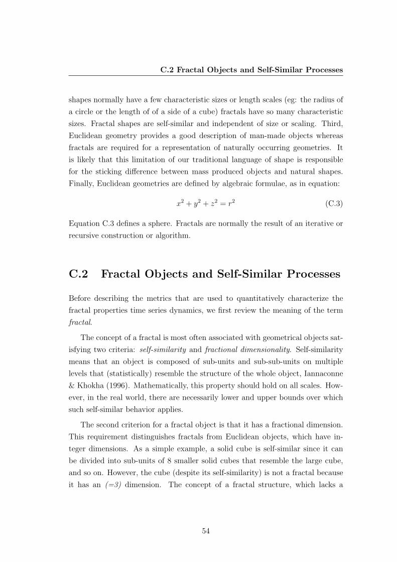
C.2 Fractal Objects and Self-Similar Processes

shapes normally have a few characteristic sizes or length scales (eg: the radius of

a circle or the length of of a side of a cube) fractals have so many characteristic

sizes. Fractal shapes are self-similar and independent of size or scaling. Third,

Euclidean geometry provides a good description of man-made objects whereas

fractals are required for a representation of naturally occurring geometries. It

is likely that this limitation of our traditional language of shape is responsible

for the sticking difference between mass produced objects and natural shapes.

Finally, Euclidean geometries are defined by algebraic formulae, as in equation:

x2 + y2 + z2 = r2 (C.3)

Equation C.3 defines a sphere. Fractals are normally the result of an iterative or

recursive construction or algorithm.

C.2 Fractal Objects and Self-Similar Processes

Before describing the metrics that are used to quantitatively characterize the

fractal properties time series dynamics, we first review the meaning of the term

fractal.

The concept of a fractal is most often associated with geometrical objects sat-

isfying two criteria: self-similarity and fractional dimensionality. Self-similarity

means that an object is composed of sub-units and sub-sub-units on multiple

levels that (statistically) resemble the structure of the whole object, Iannaconne

& Khokha (1996). Mathematically, this property should hold on all scales. How-

ever, in the real world, there are necessarily lower and upper bounds over which

such self-similar behavior applies.

The second criterion for a fractal object is that it has a fractional dimension.

This requirement distinguishes fractals from Euclidean objects, which have in-

teger dimensions. As a simple example, a solid cube is self-similar since it can

be divided into sub-units of 8 smaller solid cubes that resemble the large cube,

and so on. However, the cube (despite its self-similarity) is not a fractal because

it has an (=3) dimension. The concept of a fractal structure, which lacks a

54

C.2 Fractal Objects and Self-Similar Processes

characteristic length scale, can be extended to the analysis of complex temporal

processes. However, a challenge in detecting and quantifying self-similar scaling

in complex time series is the following: Although time series are usually plotted

on a 2-dimensional surface, a time series actually involves two different physical

variables.

For example, let us consider the study of time series analysis when applied

to heart rate and gait dynamics which is shown in Fig. C.6, the horizontal axis

represents ‘time’, while the vertical axis represents the value of the variable that

changes over time (in this case, heart rate). These two axes have independent

physical units, minutes and beats/minute, respectively. (Even in cases where the

two axes of a time series have the same units, their intrinsic physical meaning is

still different.) This situation is different from that of geometrical curves (such as

coastlines and mountain ranges) embedded in a 2-dimensional plane, where both

axes represent the same physical variable.

To determine if a 2-dimensional curve is self-similar, we can do the following

test: (i) take a subset of the object and rescale it to the same size of the original

object, using the same magnification factor for both its width and height; and

then (ii) compare the statistical properties of the rescaled object with the original

object. In contrast, to properly compare a subset of a time series with the original

data set, we need two magnification factors (along the horizontal and vertical

axes), since these two axes represent different physical variables. Fig. C.6 shows a

heart rate normal sinus rhythm time series of 30 min from (a) a healthy subject at

sea level,(b) a subject with congestive heart failure,(c) a subject with obstructive

sleep apnea, and (d) a sudden cardiac death subject who sustained a cardiac

arrest with ventricular fibrillation (V F ).

Note the highly non-stationary and “noisy” appearance of the healthy vari-

ability which is related in part to fractal (scale-free) dynamics. In contrast,

pathologic states may be associated with the emergence of periodic oscillations,

indicating the emergence of a characteristic time scale.

To put the above discussion into mathematical terms: A time-dependent pro-

55

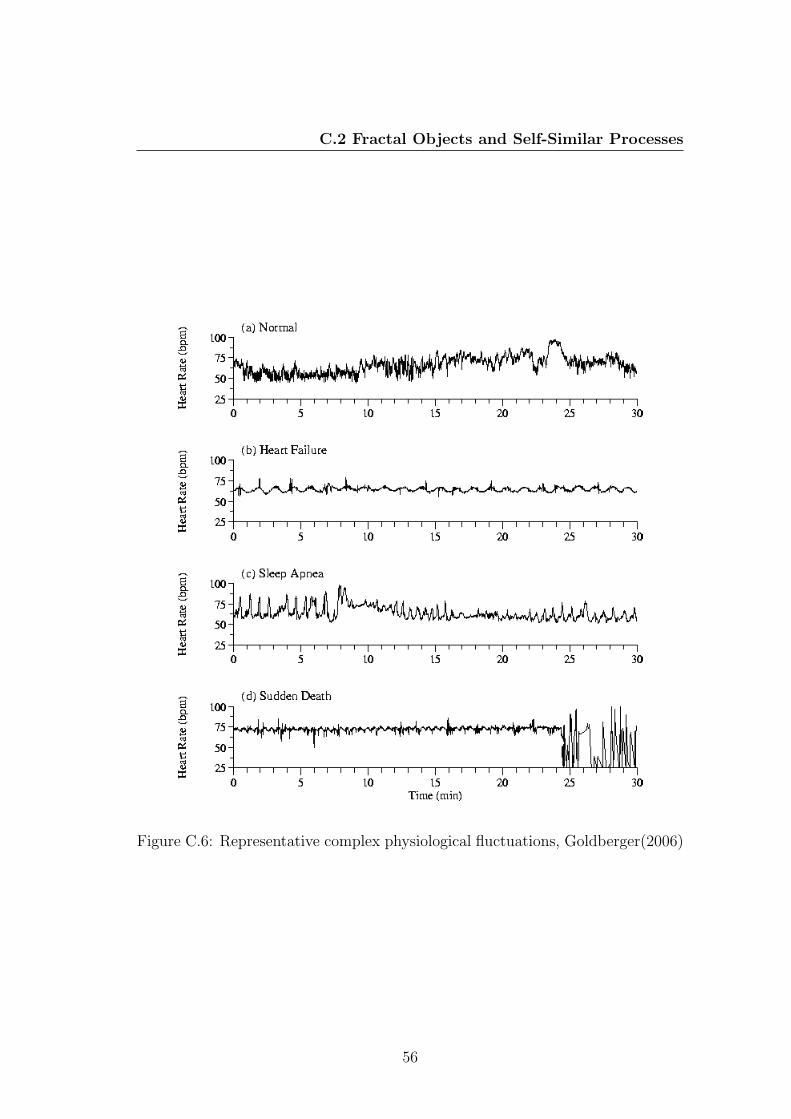
C.2 Fractal Objects and Self-Similar Processes

Figure C.6: Representative complex physiological fluctuations, Goldberger(2006)

56

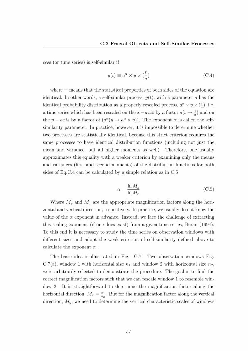
C.2 Fractal Objects and Self-Similar Processes

cess (or time series) is self-similar if

y(t) ≡ aα × y × (t

a) (C.4)

where ≡ means that the statistical properties of both sides of the equation are

identical. In other words, a self-similar process, y(t), with a parameter a has the

identical probability distribution as a properly rescaled process, aα × y× ( ta), i.e.

a time series which has been rescaled on the x−axis by a factor a(t → ta) and on

the y − axis by a factor of (aα(y → aα × y)). The exponent α is called the self-

similarity parameter. In practice, however, it is impossible to determine whether

two processes are statistically identical, because this strict criterion requires the

same processes to have identical distribution functions (including not just the

mean and variance, but all higher moments as well). Therefore, one usually

approximates this equality with a weaker criterion by examining only the means

and variances (first and second moments) of the distribution functions for both

sides of Eq.C.4 can be calculated by a simple relation as in C.5

α =ln My

ln Mx

(C.5)

Where My and Mx are the appropriate magnification factors along the hori-

zontal and vertical direction, respectively. In practice, we usually do not know the

value of the α exponent in advance. Instead, we face the challenge of extracting

this scaling exponent (if one does exist) from a given time series, Beran (1994).

To this end it is necessary to study the time series on observation windows with

different sizes and adopt the weak criterion of self-similarity defined above to

calculate the exponent α .

The basic idea is illustrated in Fig. C.7. Two observation windows Fig.

C.7(a), window 1 with horizontal size n1 and window 2 with horizontal size n2,

were arbitrarily selected to demonstrate the procedure. The goal is to find the

correct magnification factors such that we can rescale window 1 to resemble win-

dow 2. It is straightforward to determine the magnification factor along the

horizontal direction, Mx = n1

n2. But for the magnification factor along the vertical

direction, My, we need to determine the vertical characteristic scales of windows

57

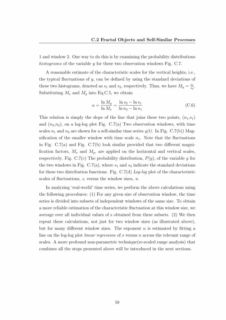
C.2 Fractal Objects and Self-Similar Processes

1 and window 2. One way to do this is by examining the probability distributions

histograms of the variable y for these two observation windows Fig. C.7.

A reasonable estimate of the characteristic scales for the vertical heights, i.e.,

the typical fluctuations of y, can be defined by using the standard deviations of

these two histograms, denoted as s1 and s2, respectively. Thus, we have My = s1

s2.

Substituting Mx and My into Eq.C.5, we obtain

α =ln My

ln Mx

=ln s2 − ln s1

ln n2 − ln n1

(C.6)

This relation is simply the slope of the line that joins these two points, (n1,s1)

and (n2,n2), on a log-log plot Fig. C.7(a) Two observation windows, with time

scales n1 and n2 are shown for a self-similar time series y(t). In Fig. C.7(b)) Mag-

nification of the smaller window with time scale n1. Note that the fluctuations

in Fig. C.7(a) and Fig. C.7(b) look similar provided that two different magni-

fication factors, Mx and My, are applied on the horizontal and vertical scales,

respectively. Fig. C.7(c) The probability distribution, P (y), of the variable y for

the two windows in Fig. C.7(a), where s1 and s2 indicate the standard deviations

for these two distribution functions. Fig. C.7(d) Log-log plot of the characteristic

scales of fluctuations, s, versus the window sizes, n.

In analyzing ‘real-world’ time series, we perform the above calculations using

the following procedures: (1) For any given size of observation window, the time

series is divided into subsets of independent windows of the same size. To obtain

a more reliable estimation of the characteristic fluctuation at this window size, we

average over all individual values of s obtained from these subsets. (2) We then

repeat these calculations, not just for two window sizes (as illustrated above),

but for many different window sizes. The exponent α is estimated by fitting a

line on the log-log plot linear regression of s versus n across the relevant range of

scales. A more profound non-parametric technique(re-scaled range analysis) that

combines all the steps presented above will be introduced in the next sections.

58

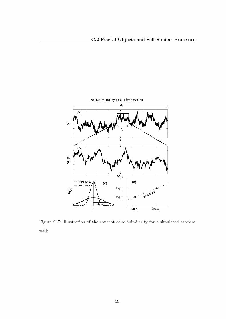
C.2 Fractal Objects and Self-Similar Processes

Figure C.7: Illustration of the concept of self-similarity for a simulated random

walk

59

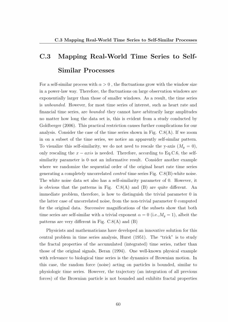
C.3 Mapping Real-World Time Series to Self-Similar Processes

C.3 Mapping Real-World Time Series to Self-

Similar Processes

For a self-similar process with α > 0 , the fluctuations grow with the window size

in a power-law way. Therefore, the fluctuations on large observation windows are

exponentially larger than those of smaller windows. As a result, the time series

is unbounded. However, for most time series of interest, such as heart rate and

financial time series, are bounded–they cannot have arbitrarily large amplitudes

no matter how long the data set is, this is evident from a study conducted by

Goldberger (2006). This practical restriction causes further complications for our

analysis. Consider the case of the time series shown in Fig. C.8(A). If we zoom

in on a subset of the time series, we notice an apparently self-similar pattern.

To visualize this self-similarity, we do not need to rescale the y-axis (My = 0),

only rescaling the x − axis is needed. Therefore, according to Eq.C.6, the self-

similarity parameter is 0–not an informative result. Consider another example

where we randomize the sequential order of the original heart rate time series

generating a completely uncorrelated control time series Fig. C.8(B)-white noise.

The white noise data set also has a self-similarity parameter of 0. However, it

is obvious that the patterns in Fig. C.8(A) and (B) are quite different. An

immediate problem, therefore, is how to distinguish the trivial parameter 0 in

the latter case of uncorrelated noise, from the non-trivial parameter 0 computed

for the original data. Successive magnifications of the subsets show that both

time series are self-similar with a trivial exponent α = 0 (i.e.,My = 1), albeit the

patterns are very different in Fig. C.8(A) and (B)

Physicists and mathematicians have developed an innovative solution for this

central problem in time series analysis, Hurst (1951). The “trick” is to study

the fractal properties of the accumulated (integrated) time series, rather than

those of the original signals, Beran (1994). One well-known physical example

with relevance to biological time series is the dynamics of Brownian motion. In

this case, the random force (noise) acting on particles is bounded, similar to

physiologic time series. However, the trajectory (an integration of all previous

forces) of the Brownian particle is not bounded and exhibits fractal properties

60

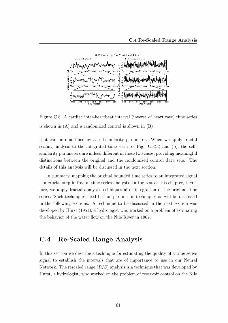
C.4 Re-Scaled Range Analysis

Figure C.8: A cardiac inter-heartbeat interval (inverse of heart rate) time series

is shown in (A) and a randomized control is shown in (B)

that can be quantified by a self-similarity parameter. When we apply fractal

scaling analysis to the integrated time series of Fig. C.8(a) and (b), the self-

similarity parameters are indeed different in these two cases, providing meaningful

distinctions between the original and the randomized control data sets. The

details of this analysis will be discussed in the next section.

In summary, mapping the original bounded time series to an integrated signal

is a crucial step in fractal time series analysis. In the rest of this chapter, there-

fore, we apply fractal analysis techniques after integration of the original time

series. Such techniques need be non-parametric techniques as will be discussed

in the following sections. A technique to be discussed in the next section was

developed by Hurst (1951), a hydrologist who worked on a problem of estimating

the behavior of the water flow on the Nile River in 1907.

C.4 Re-Scaled Range Analysis

In this section we describe a technique for estimating the quality of a time series

signal to establish the intervals that are of importance to use in our Neural

Network. The rescaled range (R/S) analysis is a technique that was developed by

Hurst, a hydrologist, who worked on the problem of reservoir control on the Nile

61

C.4 Re-Scaled Range Analysis

River dam project at around 1907. His problem was to determine the ideal design

of a reservoir based upon the given record of observed river discharges. An ideal

reservoir never empties or overflows. In constructing the model, it was common

to assume that the uncontrollable process of the system, which at the time was

the influx due to the rainfall, followed a random walk due to the many degrees

of freedom in the weather. When Hurst examined this assumption he gave a

new statistical measure, the Hurst exponent (H). His statistical method is very

robust and has a few underlying assumptions. The Hurst statistical method can

be used to classify time series signals into random and non-random series. The

analysis is very robust with respect to the underlying distribution of the process.

Using the R/S analysis, one also finds the average non-periodic cycle, if there is

any, and the degree of persistence in trends due to long memory effects, Skjeltorp

(2000).

C.4.1 The R/S Methodology

The main idea behind using the (R/S) analysis for our investigation is that

we establish the scaling behavior of the rescaled cumulative deviations from the

mean, or the distance that the system travels as a function of time relative to the

mean. The intervals that display a high degree of persistence are selected and

grouped in rebuilding the signal to be used as an input to the Neural Network

model. A statistical correlation approach is used in recombining the intervals.

From the discovery that was made by Hurst, the distance covered an independent

system increases, on average, by the square root of time. If the system covers a

larger distance than this, it cannot be independent by this definition; the changes

must be influencing each other and therefore have to be correlated, Hutchinson

& Poggio (1994). The following is the approach we used in our investigation:

we first start with a time series in prices of length M . This time series is then

converted into a time series of logarithmic ratios or returns of length N = M − 1

such that

Ni = log(Mi+1

Mi

), i = 1, 2, ..., (M − 1) (C.7)

62

C.4 Re-Scaled Range Analysis

We divide this time period into T contiguous sub periods of length j, such

that T ∗ j = N . Each sub period is labelled It, with t = 1, 2...T . Then, each

element in It is labelled Nk,t such that k = 1, 2, , j. For each sub period It of

length j the average is calculated as

et =1

j

j∑k=1

Nk,t (C.8)

Thus, et is the average value of the Ni contained in sub-period It of length j.

We then calculate the time series of accumulated departures Xk,t from the mean

for each sub period It, defined as

Xk,t =k∑

i=1

Ni,t − etk = 1, 2, ..., j (C.9)

Now, the range that the time series covers relative to the mean within each

sub period is defined as

RIt = max(X k, t)−min(X k, t, 1 < k < j (C.10)

Next we calculate the standard deviation of each sub-period as

Xk,t =

√√√√1

j

k∑i=1

(Ni,t − et)2 (C.11)

Then, the range of each sub period RIt is rescaled/normalized by the corre-

sponding standard deviation SIt . This approach is done for all the T sub intervals

we have for the series. As a result the average R/S value for length j is

et =1

T

T∑t=1

(RIt

SIt

) (C.12)

Now, the calculations from the above equations were repeated for different

time horizons. This is achieved by successively increasing j and repeating the

calculations until we covered all j integers. After having calculated the R/S

values for a large range of different time horizons j, we plot log(R/S)j against

63

C.4 Re-Scaled Range Analysis

log(n). By performing a least squares linear regression with log(R/S)j as the

dependent variable and log(n) as the independent one, we find the slope of the

regression which is the estimate of the Hurst exponent (H). The relationship

between the fractal dimension and the Hurst exponent is modelled as

Df = 2−H (C.13)

C.4.2 The Hurst Interpretation

If, H ∈ (0, 5; 1] it implies that the time series is persistent which is characterized

by long memory effects on all time scales, Gammel (1998). This also implies

that all hourly prices are correlated with all future hourly price changes; all daily

price changes are correlated with all future daily prices changes, all weekly price

changes are correlated with all future weekly price changes and so on. This is

one of the key characteristics of fractal time series as discussed earlier. The

persistence implies that if the series has been up or down in the last period then

the chances are that it will continue to be up and down, respectively, in the next

period. The strength of the trend reinforcing behavior, or persistence, increases

as H approaches 1. This impact of the present on the future can be expressed as

a correlation function G as in

G = 22H−1 − 1 (C.14)

In the case of H = 0, 5 the correlation G = 0, and the time series is uncor-

related. However, if H = 1 we see that that G = 1, indicating a perfect positive

correlation. On the other hand, when H ∈ [0; 0, 5) we have an antiperspirant

time series signal (interval). This means that whenever the time series has been

up in the last period, it is more likely to be down in the next period. Thus, an

nonpersistent time series will be more jagged than a pure random walk as shown

in Fig. C.8(b). The intervals that showed a positive correlation coefficient were

selected as inputs to the Neural Network.

64

C.5 Conclusion

C.5 Conclusion

In this section we introduce fractal analysis and its applications to time series

data. An example where fractal theory has been successfully used to extract

required features within data is also given. The example we introduce in this

chapter is that of estimating the inter-beat heartbeat interval which has been

proven by Goldberger (2006) to contain the same characteristics as financial time

series data. The reason for using this example in this study was due to the

availability of already successfully proven applications of fractal theory to time

series by, Hutchinson & Poggio (1994). The other reason was that this example

seeks to establish the self-similarity characteristics between the inter-beat heart-

beat interval of which these are same characteristic we seek to establish within

the financial time series data. Another example where fractal theory has been

applied successfully was that given by, Hurst (1951) in his study of the Nile River

in 1907. In the implementation of the proposed methodology the re-scaled range

analysis R/S is adapted.

65

References

Beran, J. (1994). Statistics for Long-Memory Processes . New York:Chapman

and Hall. 57, 60

Bishop, C., ed. (1995). Neural Networks for Pattern Recognition. Oxford Uni-

versity Press, Oxford-London. 24, 26

Breiman, L. (1996). Bagging predictors. Machine Learning , 24, 123–140. 35

Bunde, A. & Havlin, S. (1994). Fractals in Science. Berlin: Springer-Verlag.

53

Byorick, J. & Polikar, R. (2003). Confidence estimation using the incre-

mental learning algorithm. Lecture notes in computer science, 2714, 181–188.

38, 45

Carpenter, G., Grossberg, S., Marhuzon, N., Reynolds, J. & Rosen,

D. (1992). Artmap: A neural network architecture for incremental learning su-

pervised learning of analog multidi-mensional maps. In Transactions in Neural

Networks , vol. 3, 678–713, IEEE. 11, 38

Feder, J. (1988). Fractals . New York: Plenium Press. 51

Freund, Y. & Schapire, R. (1996). Experiments with a new boosting algo-

rithm. Proceedings of the13th International Conference on Machine Learning ,

2, 148–156. 35

66

REFERENCES

Freund, Y. & Schapire, R. (1997). A decision-theoretic generalization of on-

line learning and an application to boosting. Journal of Computer and System

Science. 34, 38, 41

Gammel, B. (1998). Hurst’s rescaled range statistical analysis for pseudoran-

dom number generators used in physical simulations. The American Physical

Society , 58, 2586. 10, 64

Goldberger, S. (2006). Nonstationery heartbeat time series.

http://www.physionet.org/tutorials/fmnc/node4.html . 60, 65

Hurst, H. (1951). Long-term storage of resevoirs. Transactions of American

Society for Civil Engineers , 166. 7, 9, 60, 61, 65

Hutchinson, J. & Poggio, T. (1994). A nonparametric approach to pricing

and hedging derivative securities via learning networks. Journal of Finance,

49, 851–889. 9, 62, 65

Iannaconne, P. & Khokha, M. (1996). Fractals Geometry in Biological Sys-

tems: An analytical Approach. Boca Raton: CRC Press. 54

Ji, C. & Ma, S. (1997). Combination of weak classifiers. IEEE Transactions on

Neural Networks , 8, 32–42. 35, 36

Kuo, R.J., Wu, P. & Wang, C. (2002). An intelligent sales forecasting system

through integration of artificial neural network and fuzzy neural networks with

fuzzy weight elimination. Neural Networks , 15, 909–925. 25

Leke, B. (2005). Optimal selection of stocks using computational intelligence

methods. In Proceedings of the IEEE International Conference on Service Op-

erations, Logistics and Informatics , 883–894. 25

Leung, M., Daouk, H. & Chen, A. (2000). Forecasting stock indices: a

comparison of classification and level estimation models. International Journal

of Forecasting , 16, 173–190. 2

Littlestone, N. & Warmuth, M. (1994). Weighted majority voting algo-

rithm. Information and Computer Science, 108, 212–216. 18, 34

67

REFERENCES

Lunga, D. & Marwala, T. (2006a). Online forecasting of stock movement

direction using the improved incremental algorithm. Lecture Notes in Computer

Science, to appear. 4, 21, 48, 70

Lunga, D. & Marwala, T. (2006b). Time series analysis using fractal theory

and online ensemble classifiers. Lecture Notes in Artificial Intelligence, submit-

ted. 5, 48

MacKinlay (1988). Stock market prices do not follow random walks: evidence

from a simple specification test. Review of Financial Studies , 41–66. 6, 15

Mandelbrot, B. (1997). Fractals and scaling in finance: Discontinuity.

Springer . 6

McClelland, J.L. & Rumelhart, D.E., eds. (1988). Explorations in parallel

distributed processing: A handbook of models, programs, and exercises.. MA:

MIT Press, Cambridge. 30

McIver, D. & Friedl, M. (2001). Estimating pixel-scale land cover classifica-

tion confidence using nonparametric machine learning methods. Transactions

on Geoscience and Remote Sensing , 39. 14

McNelis, P.D., ed. (2005). Neural Networks in Finance: Gaining the predictive

edge in the market . Elsevier Academic Press, Oxford-UK. 1, 3

Polikar, R. (2000). Algorithms for enhancing pattern separability, feature selec-

tion and incremental learning with applications to gas sensing electronic noise

systems . Ph.D. thesis, Iowa State University, Ames. 36, 37

Polikar, R., Byorick, J., Krause, S., Marino, A. & Moreton, M.

(2002). Learn++: A classifier independent incremental learning algorithm.

Proceedings of International Joint Conference on Neural Networks . 12, 34

Polikar, R., Udpa, L., Udpa, S. & Honavar, V. (2004). An incremental

learning algorithm with confidence estimation for automated identification of

nde signals. Transactions on Ul-trasonic Ferroelectrics, and Frequency control ,

51, 990–1001. 14

68

REFERENCES

Quah, T. & Srinivasan (1999). Improving returns on stock investment through

neural network selection. The Journal for Expert Systems with Applications ,

17, 295–301. 25, 28, 29

Rumelhart, D.E. & McClelland, J.L. (1986). Parallel distributed process-

ing: Explorations in the microstructure of cognition. MA: MIT Press , 1. 29

Schapire, R., Freund, Y., Bartlett, P. & Lee, W. (1998). Boosting

the margins: a new explanation for the effectiveness of voting methods. The

Annalysis of Statistics , 26, 1651–1686. 35, 39

Skjeltorp, J. (2000). Scaling in the norwergian stock market. Physica A, 283,

486. 1, 3, 8, 62

Vehtari, A. & Lampinen, J. (2000). Bayesian mlp neural networks for image

analysis. Journal of Pattern Recognition Letters , 21, 1183–1191. 26, 28

Wolpert, D. (1992). Stacked generalization. Neural Networks , 5, 241–259. 35

Wong, B.K. & Selvi, Y. (1998). Neural network applications in finance: A

review and analysis of literature. The Journal of Information and Management ,

34, 129–139. 2, 24

Zhang, G., Patuwo, B.E. & Hu, M. (1998). Forecasting with artificial neural

networks. International Journal of Forecasting , 14, 35–62. 24

69

Appendix D

Published Paper

A summary of the paper has been accepted for publishing and it will appear in

the Lecture Notes in Computer Science by Springer 2006. The full reference of

the paper in this document is Lunga & Marwala (2006a). A copy of the published

paper is attached with this document.

70