Embed Size (px)
Citation preview

Time Series Analysis of Domestic
Electricity Load ProfilesElectricity Load Profiles
Fintan McLoughlinSchool of Civil and Building Services Engineering
You Supervisors’ Names Here
Dr Aidan Duffy
Dr Michael Conlon
10th January 2012
Index
• Objective
• Characterising Load Profiles
• Time Series Methodologies
• Methodological Approach & Model Selection• Methodological Approach & Model Selection
• Fourier & Gaussian Processes
• Results
• Methodology continued
• Conclusion

Objective
Design of high time resolution models for domestic
electricity demand in Ireland
- Stochastic profiles at thirty minute intervals- Stochastic profiles at thirty minute intervals
- Capable of modelling individual dwelling types
- Other socio-economic variables (dwelling size, no. of
occupants, occupancy, appliance holdings)
- Used alongside renewable energy technology models

Characterising Domestic Electricity
Load Profiles
• Diurnal (over a 24hr period)
• Seasonal (days of the week to months/seasons) • Seasonal (days of the week to months/seasons)
• Customer type (number of occupants, dwelling size
etc..)


101 4820 30 400
1
2
3
4
101 4820 30 400
1
2
3
4
10 20 30 401 480
1
2
3
4
1
2
3
4
1
2
3
4
1
2
3
4
ElectricityConsumption(kW)
Monday Tuesday Wednesday
Thursday Friday Saturday
10 20 30 401 480
1
10 20 30 401 480
1
10 20 30 401 480
1
10 20 30 401 480
1
2
3
4
Sunday
Time of Day (half hour periods)

1 10 20 30 40 480
2
4
6
1 10 20 30 40 480
2
4
6
1 10 20 30 40 480
2
4
6
2
4
6
2
4
6
2
4
6
ElectricityConsumption(kW)
Customer 1 Customer 2 Customer 3
Customer 4 Customer 5 Customer 6
1 10 20 30 40 480
1 10 20 30 40 480
1 10 20 30 40 480
1 10 20 30 40 480
2
4
6
1 10 20 30 40 480
2
4
6
1 10 20 30 40 480
1
2
3
4
Time of Day (half hour periods)
Customer 7 Customer 8 Customer 9

3
4
5
6
Ele
ctr
icity C
on
su
mp
tio
n (
kW
)
y = 1.4e-016*x4 - 4.9e-012*x
3 + 5.1e-008*x
2 - 0.00014*x + 0.48
half hourly electricity consumption
4th degree polynomial
July August September October November December January February March April May June0
1
2
Time (Months)
Ele
ctr
icity C
on
su
mp
tio
n (
kW
)

Current Time Series Methodologies
• Fourier Transforms
• Neural Networks
• Gaussian Processes
• Autoregressive• Autoregressive
• Fuzzy Logic
• Wavelets
• Multiple Regression/Probabilistic

3
4D
om
estic E
lectric
ity C
onsum
ption (kW
)
3500
4000
Utilit
y E
lectric
ity C
onsum
prion (M
W)
Utility v’s Domestic Load Profile
0 5 10 15 20 25 30 35 40 45 500
1
2
Dom
estic E
lectric
ity C
onsum
ption (kW
)
0 5 10 15 20 25 30 35 40 45 502000
2500
3000
Utilit
y E
lectric
ity C
onsum
prion (M
W)

Methodology
• Apply a time series process that can accurately
characterise domestic electricity consumption
patterns
• The simpler the better (i.e. least number of
descriptors)
• Model must contain temporal and magnitude
components to determine the impact of dwelling and
occupant characteristics on the load profile shape

Models/Model
Attributes Advantages Disadvantages
Fourier Series
Some physical significance can be attached to the
coefficients of the series - e.g. cos or sin dtermines
more or less night time electricity consumption[1].
By definition are poor at approximating sharp spikes as
functions (sines and cosines stretch out to infinity) [33]
Neural Networks
Ability to handle non-linear relationships between
i/p and o/p. Combining neural networks (to model
seasonality) with fourier series can lead to a simpler
strucuture being chosen with the same
performance [3]
Black box approach. Unclear relationship between i/o and
o/p i.e very difficult to determine cause and effect
especially with an unknown dataset and hence there is a
possability to give unexpected results [21]
Gaussian Processes
Simplicity in modelling as a system can be
completely described by two moments (mean and
variance) [10]. Two more advantages in [12].
Models can be determined using a relatively small
number of points (unlike neural networks) [11].
Has difficulty modelling high peaks and troughs of a
domestic load profile. Computational load associated
with the need to invert the covariance matrix [12]. As
number of model parameters increases linearly, CPU time
increases exponentially [10].
Small number of parameters compared to other parameter values varied unpredictably with small changes
Autoregressive
Small number of parameters compared to other
models (for ARIMA) [1]
parameter values varied unpredictably with small changes
in profile shape [1]
Fuzzy Logic
Can use a large amount of input variables to model
output. Fuzzy model attractive in a sense that the
relationship between i/p and o/p is clariffied, unlike
the black-box method (i.e. NN) [21].
Complicated model structure. Not suitable for large-scale
complicated systems [21].
Wavelets
Can handle non-stationary discrete signals [24]. Are
well suited to approximating data with shap
discontinuities such as domestic load profiles [33].
Has advantage over the Fourier transform in that it
allows each frequency conponent to be considered
with an appropiate temporal resolution [24].
High frequency conponents are often treated as noise in
this model type [23]
Multiple Regression Large number of parameters required to model daily load profiles [34]
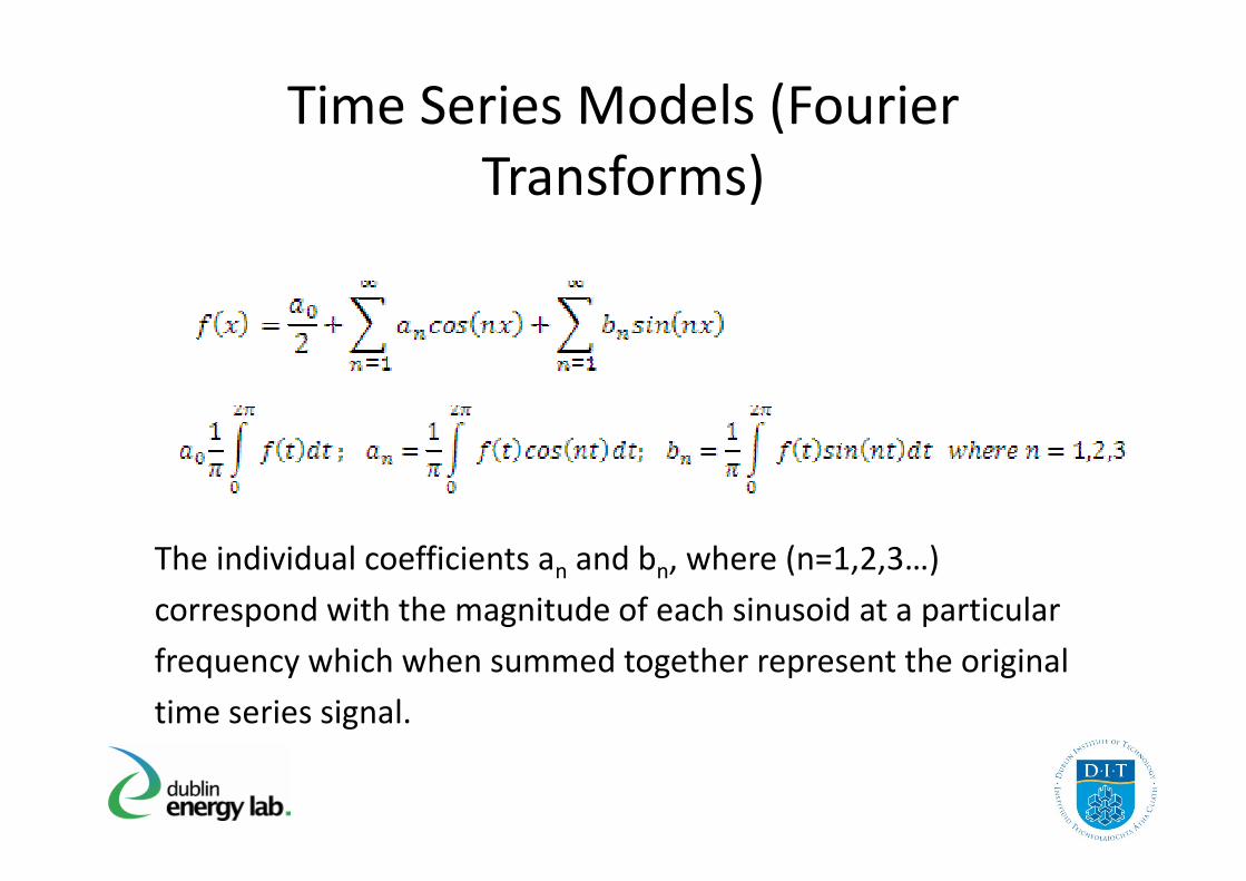
Time Series Models (Fourier
Transforms)
The individual coefficients an and bn, where (n=1,2,3…)
correspond with the magnitude of each sinusoid at a particular
frequency which when summed together represent the original
time series signal.

Time Series Models (Fourier
Transforms)

Time Series Models (Gaussian
Processes)
where Mc is the number of mixture components and wi is the
weight of the ith mixture component, subject to wi > 0 and . The
mean and variance of each density function is represented by µi
and respectively.

Results
Compared models using the following parameters
and functions:
– R2 and Descriptive Statistics
– Total Electricity Consumption– Total Electricity Consumption
– Maximum Demand
– Load Factor
– Time of Use (maximum electricity demand)
– Temporal and magnitude components
(autocorrelation and spectral components)

Results
0.8743 0.8761 0.0418 0.9878 0.6774
Model Mean Median
Standard
Deviation Maximum Minimum
Fourier
Transform
0.9931 0.7843Gaussian
Processes0.9447 0.9473 0.021
Transform
s

Results (Total Electricity Consumption)
Shape
Parameter
(β)
4,146kWh 4,008kWh 1,870kWh 9,651kWh 414kWh 4,687 2.38
4,146kWh 4,008kWh 1,870kWh 9,651kWh 414kWh 4,687 2.38
Targeted Time
Series
Scale
Parameter
(η)
Fourier
Model Mean Median
Standard
Deviation Maximum Minimum
4,146kWh 4,008kWh 1,870kWh 9,651kWh 414kWh 4,687 2.38
(0%) (0%) (0%) (0%) (0%) (0%) (0%)
4,047kWh 3,903kWh 1,835kWh 9,462kWh 413kWh 4,576 2.37
(-2.39%) (-2.62%) (-1.87%) (-1.96%) (-0.24%) (-2.37%) (-0.42%)
Fourier
Transforms
Gaussian
Processes

Results (Maximum Demand)
Shape
Parameter
(β)
2.34kW 2.29kW 0.92kW 6.18kW 0.14kW 2.6293 2.7425
1.68kW 1.66kW 0.68kW 3.89kW 0.09kW 1.8904 2.6885
Scale
Parameter
(η)
Fourier
Transforms
Targeted
Time Series
Model Mean Median
Standard
Deviation Maximum Minimum
(-28.21%) (-27.51%) (-35.29%) (-58.87%) (-55.56%) (-28.10%) (-1.97%)
2.23kW 2.20kW 0.88kW 5.99kW 0.13kW 2.5082 2.7394
(-4.70%) (-3.93%) (-4.35%) (-3.07%) (-7.14%) (-4.61%) (-0.11%)
Transforms
Gaussian
Processes

Results (Load Factor)
Shape
Parameter
(β)
23.23% 22.35% 5.76% 48.69% 11.29% -1.4935 0.1299
31.79% 30.76% 6.59% 66.72% 18.05% -1.1703 0.109
Scale
Parameter
(η)
Fourier
Targeted
Time Series
MinimumModel Mean Median
Standard
Deviation Maximum
31.79% 30.76% 6.59% 66.72% 18.05% -1.1703 0.109
(36.85%) (37.63%) (4.41%) (37.03%) (59.88%) (-21.64%) (-19.17%)
24.74% 23.74% 6.54% 51.76% 11.89% -1.434 0.138
(6.5%) (6.22%) (13.54%) (6.31%) (5.31%) (-3.98%) (6.24%)
Fourier
Transforms
Gaussian
Processes

Results (Time of Use)
Model Mean Median
Standard
Deviation
30.7 31.16 3.52Targeted Time Series
31.44 31.84 3.62
(2.41%) (2.18%) (2.84%)
29.63 29.91 3.3
(-3.49%) (-4.01%) (-6.25%)
Fourier Transforms
Gaussian Processes

Results (Time Series Plot)
02:00 04:00 06:00 08:00 10:00 12:00 14:00 16:00 18:00 20:00 22:00-0.5
0
0.5
1
1.5
2
2.5
3
3.5
Targeted Time Series
Fourier Model
Gaussian Model
ElectricityConsumption(kW)
Customer 1
02:00 04:00 06:00 08:00 10:00 12:00 14:00 16:00 18:00 20:00 22:00-0.5
0
0.5
1
1.5
2
2.5
3
3.5
Targeted Time Series
Fourier Model
Gaussian Model
(kW)
Time of Day
Customer 2

Results (Frequency Histogram)
-0.5 0 0.5 1 1.5 2 2.5 3 3.5 40
50
100
50
100
Fourier Transforms
Targeted Time Series
-0.5 0 0.5 1 1.5 2 2.5 3 3.5 40
50
-0.5 0 0.5 1 1.5 2 2.5 3 3.5 40
50
100
Gaussian Processes
Frequency
Electricity Consumption (kW)

Results (Autocorrelation)
0.1
0.2
0.3
0.4A
uto
co
rre
latio
n C
oe
ffic
ien
t
Targeted Time Series
Fourier Transforms
Gaussian Processes
0 50 100 150 200 250 300 350-0.4
-0.3
-0.2
-0.1
0
Time Lags (n)
Au
toc
orr
ela
tion
Co
eff
icie
nt
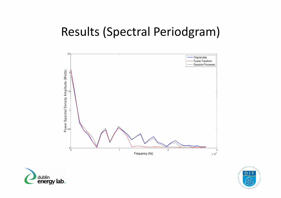
Results (Spectral Periodgram)
1.5
2
2.5
Po
we
r S
pe
ctr
al
De
ns
ity
Am
plit
ud
e (
Wa
tts
)
Original data
Fourier Transform
Gaussian Processes
0 1 2 3
x 10-4
0
0.5
1
Frequency (Hz)
Po
we
r S
pe
ctr
al
De
ns
ity
Am
plit
ud
e (
Wa
tts
)
Results Summary
• Fourier Transforms better at modelling customer
type 1 i.e. smoother load profiles
• Gaussian Processes better at modelling customer
type 2 i.e. fast changing load profiles

Methodology (cont)
• Both Fourier Transforms and Gaussian Processes
represent temporal and magnitude components in
their model descriptors
• Determine seasonality component and de-trend
model parametersmodel parameters
• Apply regression to each model descriptor with
dwelling and occupant characteristics for each day of
the year and determine influence per customer type
• Validate the results

a0 a1 b1 a2 b2 …. an bn
Electricity
Consumption
(kW)
12:0006:0000:00 18:00 Time of Day

• Time series approaches narrowed down to two most
appropriate - Fourier Transforms and Gaussian
Processes
• Fourier Transforms better at modelling smoother
Conclusions
• Fourier Transforms better at modelling smoother
domestic load profiles where as Gaussian Processes
superior at representing fast changing changing
profiles
• Methodology presented to model change in profile
shape by dwelling and occupant characteristics.

0.6
0.8
1
1.2
1.4
1.6
a0 F
ourier
Coeff
icie
nt
0 50 100 150 200 250 300 350 400-0.2
0
0.2
0.4
0.6
Day of Year
a0 F
ourier
Coeff
icie
nt