Time Series Analysis - Escuela Técnica Superior de ... · Time Series Analysis ... over time but rather with the level of the series: ... and the transformation of the data by means

Time Series Analysis

Identifying possible ARIMA models

Andres M. Alonso Carolina Garcıa-Martos

Universidad Carlos III de Madrid

Universidad Politecnica de Madrid

June – July, 2012

Alonso and Garcıa-Martos (UC3M-UPM) Time Series Analysis June – July, 2012 1 / 53

8. Identifying possible ARIMA models

Outline:

Introduction

Variance stabilizing transformation

Mean stabilizing transformation

Identifying ARMA structure

Recommended readings:

� Chapter 6 of Brockwell and Davis (1996).

� Chapter 17 of Hamilton (1994).

� Chapter 7 of Pena, Tiao and Tsay (2001).


Introduction

� We had studied the theoretical properties of ARIMA processes. Here we aregoing to analyze how to fit these models to real series. Box and Jenkins (1976)proposed carrying out this fit in three steps.

The first step consists of identifying the possible ARIMA model that theseries follows, which requires: (1) deciding what transformations to apply inorder to convert the observed series into a stationary one; (2) determining anARMA model for the stationary series.

Once we have provisionally chosen a model for the stationary series we moveon to the second step of estimation, where the AR and MA model parametersare estimated by maximum likelihood.

The third step is that of diagnosis, where we check that the residuals do nothave a dependence structure and follow a white noise process.


Introduction

� These three steps represented an important advancement in their day, since theestimation of the parameters of an ARMA model required a great deal ofcalculation time. Nowadays, estimation of an ARIMA model is straightforward,making it much simpler to estimate all the models we consider to be possible inexplaining the series and then to choose between them.

� This is the philosophy of the automatic selection criteria of ARIMA models,which work well in practice in many cases, and are essential when we wish tomodel and obtain predictions for a large set of series.

� Nevertheless, when the number of series to be modelled is small, it is advisableto carry out the identification step that we will look at next in order to betterunderstand and familiarize ourselves with the dynamic structure of the series ofinterest.

� The objective is not to choose a model now for the series, but rather to identifya set of possible models that are compatible with the series graph and its simpleand partial autocorrelation functions.


Introduction

� These models will be estimated and in the third phase, diagnosis, we ensurethat the model has no detectable deficiencies.

� Identification of the model requires identifying the non-stationary structure, ifit exists, and then the stationary ARMA structure:

The identification of the non-stationary structure consists in detecting whichtransformations must be applied to obtain a stationary ARMA process withconstant variance and mean:

to transform the series so that it has constant variance;

to differentiate the series so that it has constant mean.

Later we will identify the ARMA model for the stationary series and analyzethese aspects.



� In many series the variability is often greater when the series takes high valuesthan when it takes low ones.

Example 78

The figure shows the Spanish vehicle registration series and we observe that thevariability is much greater when the level of the series is high, which is whathappens at the end of the series, than when it is low.

0

40000

80000

120000

160000

200000

1960 1965 1970 1975 1980 1985 1990 1995

Number of registered vehicles

� The variability does not increaseover time but rather with the levelof the series: the variability around1975-1980 is high and corresponds toa maximum of the level, and this vari-ability decreases around 1980-1985,when the level drops.


� We can confirm this visual impression by plotting a graph between a measure ofvariability, such as the standard deviation, and a measure of level, such as thelocal mean.

� In order to make homogeneous comparisons since the series is seasonal we takethe 12 observations from each year and calculate the standard deviation and themean of the registrations in each year.

0

5000

10000

15000

20000

25000

30000

0 20000 40000 60000 80000 100000 140000

SERIESMEAN

SE

RIE

DS

D

� We can see that a clear linear-typedependence exists between both vari-ables.


� When the variable of the series increases linearly with the level of the series, asis the case with the vehicle registration, by taking logarithms we get a series withconstant variability.

Example 78

The figure shows the series in logarithms which confirms this fact. The series inlogs has constant variability.

7

8

9

10

11

12

13

1960 1965 1970 1975 1980 1985 1990 1995

LOG(REGISTRATION)Alonso and Garcıa-Martos (UC3M-UPM) Time Series Analysis June – July, 2012 8 / 53


� The dependency of the variability of the level of the series might be a result ofthe series being generated as a product (instead of sum) of a systematic orpredictable component, µt , times the innovation term, ut , that defines thevariability. Then:

zt = µtut . (156)

� Let us assume that the expectation of this innovation is one, such thatE (zt) = µt . The standard deviation of the series is:

σt =[E (zt − µt)

2]1/2

=[E (µtut − µt)

2]1/2

= |µt |[E (ut − 1)2

]1/2= |µt |σu

(157)and while the innovation ut has constant variability, the standard deviation of theobserved series zt is not constant in time and will be proportional to the level ofthe series.


� As we have seen, this problem is solved by taking logarithms, since then, lettingat = ln ut :

yt = ln zt = lnµt + at

and an additive decomposition is obtained for the variable yt , which will haveconstant variance.

� The above case can be generalized permitting the standard deviation to be apotential function of the local mean, using:

σt = kµαt , (158)

and if we transform variables zt into new variables yt by means of:

yt = x1−αt

these new variables yt have the same standard deviation.


� A more general way of describing this transformation is:

yt =x1−αt − 1

1− α(159)

which is part of the family of Box-Cox transformations and includes the powersand the logarithm of the variable.

� In the series, when a relationship is observed between the level and thevariability we can estimate the value of α needed to obtain constant variability bymaking consecutive groups of observations, calculating the standard deviation ineach group, si , and the mean x i and representing these variables in a graph.

� Taking logarithms in (158), the slope of the regression

log si = c + α log x i (160)

estimates the value of α, and the transformation of the data by means of (159)will lead to a series where the variability does not depend on the level.


Example 78

The figure gives the relationship between the logarithms of these variables for theregistration series. We observe that the slope is close to the unit and if weestimate regression (160) we have c = −2.17 and α = 1.04.

6.5

7.0

7.5

8.0

8.5

9.0

9.5

10.0

10.5

8.0 8.5 9.0 9.5 10.0 10.5 11.0 11.5 12.0

LOG(SERIESMEAN)

LO

G(S

ER

IED

SD

)

� As a result, a transformation us-ing α = 0, that is, by means of log-arithms, should produce a varianceconstant with the level.

� We had seen that the vehicle regis-tration series expressed in logarithmsand its variability is approximatelyconstant.

� It is advisable to plot graphs between variability and mean using groups of datathat are as homogeneous as possible.



� To stabilize the mean of the series we apply regular and seasonal differences.The decision to apply these differences can be based on the graph of the seriesand on the sample autocorrelation function, but we can also use formal tests.

Determining the order of regular difference

� If the series has a trend or shows changes in the level of the mean, wedifferentiate it in order to make it stationary. The need to differentiate is clearlyseen from the graph of the series. For example, the vehicle registration seriesclearly shows periodic behavior and non-constant mean.

� Note that

(1− B) ln zt = ln zt − ln zt−1 = ln

(1 +

zt − zt−1

zt−1

)≈ zt − zt−1

zt−1

where we have used ln(1 + x) ≈ x if x is small.

� Therefore, series ∇ ln zt is equivalent to the relative growth rates of zt .


Example 79

The figure shows the first difference of the registration series and we can see thatit contains very noticeable variations month to month, up to 0.8, that is 80% ofits value.

-.8

-.6

-.4

-.2

.0

.2

.4

.6

.8

1960 1965 1970 1975 1980 1985 1990 1995

D(LREG)

� This is due to the presence of strongseasonality, appearing in the graph assharp drops, which correspond to themonth of August of each year.

� As a result of this effect the seriesdoes not have a constant mean. Next,we will look at how to eliminate thispattern by means of a seasonal differ-ence.



� When the decision to differentiate is not clear from analyzing the graph, it isadvisable to study its autocorrelation function, ACF.

� We have seen that a non-stationary series has to show positive autocorrelations,with a slow and linear decay.

Example 80

The figure shows gives the ACF of the vehicle registration series: a slow lineardecay of the coefficients can be observed, which indicates the need to differentiate.

Corr

elo

gra

m o

f LR

EG

Date

: 02/1

2/0

8

Tim

e:

Sam

ple

: 1960M

01 1

999

Inclu

ded o

bserv

ations:

Auto

corr

ela

tion

1 2 3 4 5 6 7 8 910

11

12

13

14

15

16

17

18

19

20

21

22

23

24

25

26

27

28

29

30

31

32

33

34

35

36

37

38

39

40



� It is important to point out that the characteristic which identifies anon-stationary series in the estimated ACF is not autocorrelation coefficients closeto the unit, but rather the slow linear decay.

Example 81

In the IMA(1,1) process if θ is closeto one, then the expected value ofthe sample autocorrelationcoefficients is always less than 0.5.Nevertheless, a smooth lineardecrease is still to be expected.

5 10 15 20 25 30-0.2

-0.1

0

0.1

0.2

0.3

0.4

0.5

� To summarize, if the ACF does not fade for high values (more than 15 or 20) itis generally necessary to differentiate in order to obtain a stationary process.



� It is possible to carry out a test to decide whether or not the series should bedifferentiated.

� But, if the objective is forecasting, these tests are not very useful because incase of doubt it is always advisable to differentiate, since the negativeconsequences of overdifferentiating are much less that those ofunderdifferentiating.

� Indeed, if we assume that the series is stationary when it is not, the mediumterm prediction errors can be enormous because the medium term prediction of astationary period is its mean, whereas a non-stationary series can move away fromthis value indefinitely and the prediction error is not bounded.

� The undifferentiated model will also be non-robust and with little capacity toadapt in the presence of future values.

� However, if we overdifferentiate we always have adaptive predictors and, whilewe lose accuracy, this loss is limited.



� A further reason for taking differences in case of doubt is that it can be provedthat although the series is stationary, if the AR parameter is close to the unit weobtain better predictions by overdifferentiating the series than by using the truestationary model.

� When the aim is not to forecast, but rather to decide whether a variable isstationary or not, a common situation in economic applications, then we must usethe unit-root tests:

Dickey-Fuller test (with or without intercept, with trend and intercept)

Augmented Dickey-Fuller test

Phillips Perron test ...



Unit root tests

� These tests tell us whether we have to take an additional difference in a seriesin order to make it stationary.

� We will first present the simplest case of the Dickey-Fuller test. Let us assumethat we wish to decide between the non-stationary process:

∇zt = at , (161)

and the stationary:(1− ρB) zt = c + at . (162)

� The Dickey-Fuller test was developed because the traditional procedure forestimating both models and choosing the one with least variance is not valid inthis case.

� In fact, if we generate a series that follows a random walk, (161), and we fitboth models to this series, in model (161) we will not estimate any parameterwhereas in (162) we estimate parameters ρ and c so that the variance of theresiduals is minimum.


� To illustrate this aspect, the figure shows the distribution of the least squaresestimator of parameter ρ in samples of 100 which have been generated by randomwalk (161).

0.65 0.7 0.75 0.8 0.85 0.9 0.95 1 1.050

1000

2000

3000

4000

5000

0.55 0.6 0.65 0.7 0.75 0.8 0.85 0.9 0.95 10

500

1000

1500

2000

2500

3000

� The distribution is observed to bevery asymmetric and that it can bemuch smaller than the true value ofthe parameter which is one, especiallywith the second estimator, the esti-mated value, which is the one thatprovides the best fit.

� In conclusion, comparing the vari-ances of both models is not a goodmethod for choosing between themand, especially if we want to protectourselves with respect to the error ofnot differentiating.


Unit root tests

� One might think that a better way of deciding between two models is toestimate the stationary model (162) by least squares and test whether coefficientρ is one, comparing the estimator with its estimated standard deviation.

� The test would be H0 : ρ = 1 compared to the alternative H1 : ρ < 1, and thestatistic for the test:

tµ =ρ− 1

sρ(163)

where sρ is the estimated standard deviation of the least squares estimator.

� We could carry out the test comparing the value of tµ using the usual tables ofthe Student’s t with a unilateral test.

� Nevertheless, this method is not correct, since the distribution in the sample ofthe estimator ρ is not normal with a mean of one, which is necessary for thestatistic (163) to be a Student’s t.


� Furthermore, when the process is non-stationary the least squares estimationprovides an erroneous value of the variance of estimator ρ and statistic (163) doesnot follow a Student’s t-distribution.

� The reason is that when the null hypothesis is true the value of the parameteris found in the extreme of the parametric space (0,1) and the conditions ofregularity which are necessary for the asymptotic properties of the ML estimatorare not satisfied.

� To illustrate this fact the figuregives the result of calculating thestatistic (163) in 20000 samples of100 generated by random walks.

� Notice that the distribution of thestatistic differs greatly from that ofthe Students’s t and does not evenhave zero mean.

-5 -4 -3 -2 -1 0 1 2 3 40

500

1000

1500

2000

-5.5 -5 -4.5 -4 -3.5 -3 -2.5 -2 -1.5 -1 -0.50

500

1000

1500

2000

2500


Dickey-Fuller test

� In the Dickey-Fuller test, the null hypothesis of the test, H0, is that the seriesis non-stationary and it is necessary to differentiate, ρ = 1, and test whether thishypothesis can be rejected in light of the data.

� The statistic for the test is (163), but its value is compared with the truedistribution of the test, which is not that of the Student’s t

� A simple way of obtaining the value of this statistic (163) is to write the model(162) that we want to estimate subtracting zt−1 from both members of theequation and write:

∇zt = c + αzt−1 + at (164)

where α = ρ− 1.

� When we write a model including the variable in differences and in levels in theequation, ∇zt and zt−1, we call it an error correction model.


Dickey-Fuller test

� In model (164) if α = 0 we have a random walk and if α 6= 0 a stationaryprocess.

� The null hypothesis which states that the process is non-stationary and ρ = 1in this model becomes the null hypothesis H0 : α = 0, and the alternative, thatthe process is stationary, becomes H1 : α 6= 0.

� The test consists in estimating parameter α in (164) by least squares andrejecting that the process is stationary if the value of tµ is significantly small.

� The statistic (163) is now written:

tµ =α

sα(165)

where α is the least squares estimation of α in (164) and sα is its estimatedstandard deviation calculated in the usual way.


Dickey-Fuller test

� Under the hypothesis that α = 0 (which implies that ρ = 1) the distribution oftµ has been tabulated by Dickey and Fuller. An extract from their tables is:

Table: Critical values for the Dickey-Fuller unit-root test

T without constant with constant.01 .025 .05 .1 .01 025 .05 .1

25 -2.66 -2.26 -1.95 -1.60 -3.75 -3.33 -3.00 -2.6350 -2.62 -2.25 -1.95 -1.61 -3.58 -3.22 -2.93 -2.60100 -2.60 -2.24 -1.95 -1.61 -3.51 -3.17 -2.89 -2.58250 -2.58 -2.23 -1.95 -1.62 -3.46 -3.14 -2.88 -2.57500 -2.58 -2.23 -1.95 -1.62 -3.44 -3.13 -2.87 -2.57∞ -2.58 -2.23 -1.95 -1.62 -3.43 -3.12 -2.86 -2.57

� We observe that the estimation of α will be negative since ρ ≤ 1.


Dickey-Fuller test

� The distribution of the statistic is different when we include a constant or notin the model and, for greater security, it is always recommendable to include it,since the alternative is that the process is stationary but does not necessarily havezero mean.

� The decision of the test is:

Reject non-stationarity if tµ ≤ tc

where the value of tc is obtained from Table 1.

� We recommend carrying out the test with a low level of significance, .01, suchthat there is a low probability of rejecting that the process is non-stationary whenthis hypothesis is true.

� Since the negative consequences of underdifferentiating, we need to protectourselves against the risk of rejecting that the process is non-stationary when infact it is.



� The test we have studied analyzes whether there is a unit-root in an AR(1).This test is generalized for ARMA processes.

� We begin by studying the case in which we have an AR(p + 1) process and wewant to know if it has a unit root. That is, we have to choose between twomodels:

H0 : φp(B)∇zt = at , (166)

H1 : φp+1(B)zt = c + at . (167)

� The null hypothesis establishes that the largest root of an AR(p + 1) is equal toone, model (166), and the process is non-stationary. The alternative states that itis less than one, as in (167), and we will have a stationary process.

� The idea of the Augmented Dickey-Fuller test is to try to test the condition ofa unit root directly in the operator φp+1(B).



� To implement this idea, the operator φp+1(B) is decomposed

φp+1(B) = (1− α0B)− (α1B + ...+ αpBp)∇. (168)

� This decomposition can always be done, because in both sides of the equalitywe have a polynomial in B of order p + 1 with p + 1 coefficients. Thus byidentifying powers of B in both members we can obtain the p + 1 coefficientsα0, ..., αp, given φ1, ..., φp+1.

� We will see that this decomposition has the advantage of transferring thecondition of the unit root in the first member to a condition on a coefficient thatwe can estimate in the second member.

� Indeed, if φp+1(B) has a unit root, then φp+1(1) = 0, and if we make B = 1 in(168) the term (α2B + ...+ αp+1Bp)(1− B) is cancelled and it will have to beverified that (1− α0) = 0, that is α0 = 1.



� The unit root condition in φp+1(B) implies α0 = 1.

� We will see that α0 = 1 also implies a unit root: if α0 = 1, we can write thepolynomial on the left as (1− α1B − ...− αpBp)∇, and the polynomial has a unitroot.

� Therefore, we have proved that the two following statements are equivalent:(1) the polynomial φp+1(B) has a unit root and (2) the coefficient α0 indecomposition (168) is one.

� The model (167) can be written, utilizing (168)

φp+1(B)zt = (1− α0B)zt − (α1B + ...+ αpBp)∇zt = c + at , (169)

that is:

zt = c + α0zt−1 +

p∑i=1

αi∇zt−i + at



� To obtain the statistic of the test directly we can, as in the above case,subtract zt−1 from both members and write the model in the error correctionform, that is, with levels and differences as regressors.

� This model is:

∇zt = c + αzt−1 +∑p

i=1αi∇zt−i + at (170)

where α = (α0 − 1) .

� Equation (170) can be estimated by least squares and the test for whether theseries has unit root, α0 = 1 is equivalent to the test α = 0.

� The test utilizes the same statistic from above:

tµ =α

sα, (171)

where α is the least squares estimation of α in (170) and sα is its estimatedstandard deviation calculated in the usual way.



� The distribution of tµ when the hypothesis of a unit root ρ = 1 is true has beentabulated by Dickey and Fuller. Again, the distribution depends on whether or notwe have a constant in the model.

� In seasonal series we must be careful to introduce all of the necessary lags.

Example 82

The ADF unit-root test in the vehicle registration series logarithm:

Augmented Dickey-Fuller Unit Root Test on LREG

Null Hypothesis: LREG has a unit rootExogenous: NoneLag Length: 13 (Automatic based on SIC, MAXLAG=17)

t-Statistic Prob.*

Augmented Dickey-Fuller test statistic 2.498728 0.9972Test critical values: 1% level -2.569934

5% level -1.94150410% level -1.616243

*MacKinnon (1996) one-sided p-values.

Augmented Dickey-Fuller Unit Root Test on LREG

Null Hypothesis: LREG has a unit rootExogenous: ConstantLag Length: 13 (Automatic based on SIC, MAXLAG=17)

t-Statistic Prob.*

Augmented Dickey-Fuller test statistic -3.109254 0.0266Test critical values: 1% level -3.444158

5% level -2.86752210% level -2.570019



Example 82

Now, if we consider the seasonal differentiated series, we observe that it not haveconstant level, but it no longer shows any clear trend. The ACF of this series has alot of slowly decreasing positive coefficients, suggesting the need for a difference.

-.8

-.4

.0

.4

.8

1960 1965 1970 1975 1980 1985 1990 1995

D12LREG

Correlogram

of D

12LR

EG

Date: 02/11/08 T

im

e: 15:27

Sam

ple: 1960M

01 1999M

12

Included observations: 468

Autocorrelation

Partial C

orrelation

1 2 3 4 5 6 7 8 910

11

12

13

14

15

16

17

18

19

20

21

22

23

24

25

26

27

28

29

30

31

32

33

34

35

36

37

38

39

40


Example 82

The ADF unit-root test in theseasonal differentiated series:

Augmented Dickey-Fuller Unit Root Test on D12LREG

Null Hypothesis: D12LREG has a unit rootExogenous: ConstantLag Length: 13 (Automatic based on SIC, MAXLAG=17)

t-Statistic Prob.*


5% level -2.86768610% level -2.570107


Augmented Dickey-Fuller Test EquationDependent Variable: D(D12LREG)Method: Least SquaresDate: 02/12/08 Time: 19:15Sample (adjusted): 1962M03 1999M12Included observations: 454 after adjustments

Variable Coefficient Std. Error t-Statistic Prob.

D12LREG(-1) -0.198206 0.047686 -4.156481 0.0000D(D12LREG(-1)) -0.459689 0.058717 -7.828886 0.0000D(D12LREG(-2)) -0.195625 0.058645 -3.335761 0.0009D(D12LREG(-3)) -0.033722 0.059000 -0.571560 0.5679D(D12LREG(-4)) -0.026740 0.058813 -0.454659 0.6496D(D12LREG(-5)) 0.019417 0.058815 0.330134 0.7415D(D12LREG(-6)) 0.086480 0.058610 1.475510 0.1408D(D12LREG(-7)) 0.030257 0.057933 0.522285 0.6017D(D12LREG(-8)) 0.091939 0.057046 1.611664 0.1078D(D12LREG(-9)) 0.133196 0.056060 2.375975 0.0179

D(D12LREG(-10)) 0.071162 0.055130 1.290808 0.1974D(D12LREG(-11)) 0.097910 0.053822 1.819131 0.0696D(D12LREG(-12)) -0.257202 0.051574 -4.987043 0.0000D(D12LREG(-13)) -0.142624 0.045052 -3.165737 0.0017

C 0.014872 0.007203 2.064680 0.0395


Example 82

The ADF unit-root test in the seasonal differentiated series with different numberof lags


Null Hypothesis: D12LREG has a unit rootExogenous: ConstantLag Length: 9 (Fixed)

t-Statistic Prob.*


5% level -2.86763110% level -2.570077



Null Hypothesis: D12LREG has a unit rootExogenous: ConstantLag Length: 12 (Fixed)

t-Statistic Prob.*


5% level -2.86767210% level -2.570100


� This example illustrates the importance of including the right lags in the test.



Determining the order of seasonal differencing

� If the series has seasonality a seasonal difference, ∇s = 1− Bs , will have to beapplied in order to make the series stationary. Seasonality is shown:

In the series graph, which will show a repeating pattern of period s.

In the autocorrelation function, which shows positive coefficients that slowlydecrease in the lags s, 2s, 3s...

Example 83

The figure suggests a seasonalpattern because the value of theseries is systematically lower inAugust.

0

40000

80000

120000

160000

200000

1960 1965 1970 1975 1980 1985 1990 1995

Number of registered vehicles



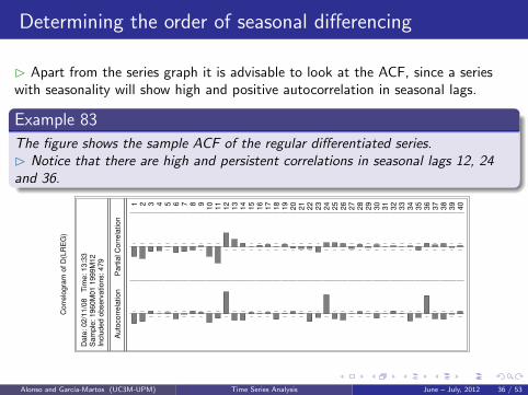
� Apart from the series graph it is advisable to look at the ACF, since a serieswith seasonality will show high and positive autocorrelation in seasonal lags.

Example 83

The figure shows the sample ACF of the regular differentiated series.� Notice that there are high and persistent correlations in seasonal lags 12, 24and 36.

Corr

elo

gra

m o

f D

(LR

EG

)

Date

: 02/1

1/0

8

Tim

e:

13:3

3S

am

ple

: 1960M

01 1

999M

12

Inclu

ded o

bserv

ations:

479

Auto

corr

ela

tion

Part

ial C

orr

ela

tion

1 2 3 4 5 6 7 8 910

11

12

13

14

15

16

17

18

19

20

21

22

23

24

25

26

27

28

29

30

31

32

33

34

35

36

37

38

39

40



� This suggests the need for taking a seasonal difference to obtain a stationaryseries.

� The figure gives the series with two differences, one regular and the otherseasonal.

-1.2

-0.8

-0.4

0.0

0.4

0.8

1960 1965 1970 1975 1980 1985 1990 1995

DDLREG


Identifying the ARMA structure

� Once we had determined the order of regular and seasonal differences, the nextstep is to identify the ARMA structure.

� Identification of the orders of p and q is carried out by comparing the estimatedpartial and simple autocorrelation functions with the theoretical functions of theARMA process.

� Letting ωt denote the stationary series, ωt = ∇d∇Ds zt , where in practice d

takes values in (0, 1, 2) and D in (0, 1), the autocorrelations are calculated by:

rk =

∑T−kt=d+sD+1 (ωt − ω) (ωt+k − ω)∑T

t=d+sD+1 (ωt − ω)2, k = 1, 2, ... (172)

� In order to judge when a coefficient rk is different from zero we need itsstandard error, whose determination depends on the structure of the process.



� One simple solution is to take 1/√

T as the standard error, which isapproximately the standard error of a correlation coefficient between independentvariables. If all the theoretical autocorrelation coefficients were null, the standarddeviations of estimation would be approximately 1/

√T .

� Therefore, we can place confidence bands at ±2/√

T and consider assignificant, in the first approximation, the coefficients which lie outside thosebands.

� The partial autocorrelations are obtained with the regressions:

ωt = αk1ωt−1 + ...+ αkk ωt−k ,

where ωt = ωt − ω. The sequence αkk (k = 1, 2, ...) of least squares coefficientsestimated in these regressions is the partial autocorrelation function.

� In the graphs of the PACF we will always use the asymptotic limits ±2/√

T ,and we will considered as approximate limits of reference.



� If the process is seasonal, we study the coefficients of the sample ACF andPACF in lags s, 2s, 3s, ..., in order to determine the seasonal ARMA structure.

� Identifying an ARMA model can be a difficult task. With large sample sizes andpure AR or MA processes, the structure of the sample ACF and PACF usuallyindicates the required order.

� Nevertheless, in general, the interpretation of the sample ACF and PACF iscomplex for three main reasons:

when autocorrelation exists the estimations of the autocorrelations are alsocorrelated, which introduces a pattern of random variation in the sample ACFand PACF that is superposed on the true existing pattern;

the limits of confidence that we use, 2/√

T , are asymptotic and not veryprecise for the first autocorrelations;

for mixed ARMA processes it can be extremely difficult to estimate the orderof the process, even when the theoretical values of the autocorrelations areknown.



� Fortunately, it is not necessary in the identification step to decide what theorder of the model is, but only to choose a set of ARMA models that seemsuitable for representing the main characteristics of the series.

� Later we will estimate this set of selected models and choose the most suitable.

� Identification with the simple and partial autocorrelation function of thepossible models can be done using the following rules:

1 Decide what the maximum order of the AR and MA part is from the obviousfeatures of the ACF and PACF.

2 Avoid the initial identification of mixed ARMA models and start with AR orMA models, preferably of low order.

3 Utilize the interactions around the seasonal lags, especially in the ACF, inorder to confirm the concordance between the regular part and the seasonal.



� In practice, most real series can be approximated well using ARMA models withp and q less than three, for non-seasonal series, and with P and Q less than twofor seasonal series.

� In addition to selecting the orders (p, q)(P,Q) of the model we have to decidein this step if the stationary series, ωt , has a mean different from zero:

ω =

∑ωt

Tc,

where Tc is the number of summands (normally Tc = T − d − sD). Its standarddeviation can be approximated by:

s (ω) ' sω√T

(1 + 2r1 + ...+ 2rk)1/2

where sω is the standard deviation of the stationary series, ωt , and ri theestimated autocorrelation coefficients.



� In this formula we are assuming that the first k autocorrelation coefficients aresignificant and that k/T is unimportant.

� If ω ≥ 2s (ω) we accept that the mean of the stationary process is differentfrom zero and we will include it as a parameter to estimate; in the opposite casewe assume that E (ωt) = 0.

Additionally

� There are automatic selection procedures, such as the one installed in theTRAMO program, which avoid the identification step and estimate all the possiblemodels within a subset, which is usually taken as p ≤ 3, q ≤ 2, P ≤ 2,Q ≤ 1.

� TRAMO also identify the mean, the log transformations, etcetera.


Example 84

Lets consider the regular and seasonal differentiated vehicle registration series.The most notable features of its ACF are: (i) a significant r1 coefficient; (ii)significant coefficients in the seasonal lags, r12, r24 and r36; (ii) interaction aroundthe seasonal lags, as shown by the positive and symmetric values of thecoefficients r11 and r13 as well as r23 and r25.

Corr

elo

gra

m o

f D

D12LR

EG

Date

: 02/1

1/0

8

Tim

e:

Sam

ple

: 1960M

01 1

999

Inclu

ded o

bserv

ations:

Auto

corr

ela

tion

1 2 3 4 5 6 7 8 910

11

12

13

14

15

16

17

18

19

20

21

22

23

24

25

26

27

28

29

30

31

32

33

34

35

36

37

38

39

40

� The regular part suggests an MA(1) model.

� The seasonal part is more complicated, since the observed structure iscompatible with that of an AR(1)12 with negative coefficient and with longer ARor ARMA(1,1) 12 models as well.


Example 84

The PACF of this series confirms the MA(1) structure for the regular part: ageometric decay is observed in the first lags and, by the interaction as well, whichrepeats after the seasonal lags.

Corr

elo

gra

m o

f D

D12LR

EG

Part

ial C

orr

ela

tion

1 2 3 4 5 6 7 8 910

11

12

13

14

15

16

17

18

19

20

21

22

23

24

25

26

27

28

29

30

31

32

33

34

35

36

37

38

39

40

� The two significant coefficients in the seasonal lags cause us to reject thehypothesis of an AR(1)12, but they are compatible with an AR(2)12 or with anARMA(1,1)12.

� Therefore, we move on to estimating models with MA(1) for the regular partand AR(2) or ARMA(1,1) for the seasonal part.


And TRAMO selects ...

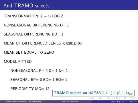
TRANSFORMATION: Z − > LOG Z

NONSEASONAL DIFFERENCING D= 1

SEASONAL DIFFERENCING BD= 1

MEAN OF DIFFERENCED SERIES -0.8281D-03

MEAN SET EQUAL TO ZERO

MODEL FITTED

NONSEASONAL P= 0 D= 1 Q= 1

SEASONAL BP= 0 BD= 1 BQ= 1

PERIODICITY MQ= 12TRAMO selects an ARIMA(0, 1, 1)× (0, 1, 1)12.


Example 85

We are going to identify a model for the Spanish work related accidents seriesfound in the accidentes.dat file. This file contains 20 years of monthly data fromJanuary 1979 to December 1998. The figure gives the graph of this series.

20000

40000

60000

80000

100000

120000

140000

160000

80 82 84 86 88 90 92 94 96 98

Work-related accidents in Spain

� The series seems to show an increase in variability with level.


Example 85

The figure gives the relationship between the logarithm of the standard deviationeach year and the logarithm of the mean for the year.

8.4

8.6

8.8

9.0

9.2

9.4

9.6

10.7 10.8 10.9 11.0 11.1 11.2 11.3 11.4 11.5 11.6 11.7

LOG(SERIESMEAN)

LO

G(S

ER

IES

SD

)

� A linear relationship is observed with a slope that is slightly less than the unit,thus we will take logarithms as a first approximation.


Example 85

The graph of the series in logarithms is shown in the figure. The logtransformation may be too strong because the variability of the first two years nowseems slightly greater than that of the last.

10.4

10.6

10.8

11.0

11.2

11.4

11.6

11.8

12.0

80 82 84 86 88 90 92 94 96 98

LWA

� We have tried using the square root as well, and the result is a little better, butfor ease of interpretation we will work with the series in logarithms.


Example 85

The graph of the series indicates the need for at least one regular difference forthe series to be stationary and the estimated ACF of the ∇ log zt transformationshows high coefficients and decays slowly in lags 12, 24, 36.

Corr

elo

gra

m o

f LW

A

Date

: 02/1

3/0

8

Tim

e:

Sam

ple

: 1979M

01 2

000

Inclu

ded o

bserv

ations:

Auto

corr

ela

tion

1 2 3 4 5 6 7 8 910

11

12

13

14

15

16

17

18

19

20

21

22

23

24

25

26

27

28

29

30

31

32

33

34

35

36

37

38

39

40

Corr

elo

gra

m o

f D

LW

A

Date

: 02/1

3/0

8

Tim

e:

Sam

ple

: 1979M

01 2

000

Inclu

ded o

bserv

ations:

Auto

corr

ela

tion

1 2 3 4 5 6 7 8 910

11

12

13

14

15

16

17

18

19

20

21

22

23

24

25

26

27

28

29

30

31

32

33

34

35

36

37

38

39

40

� So we take a regular and a seasonal difference.


Example 85

The figures give the simple and partial correlogram of the series ∇∇12 log zt . Inthe ACF we see significant coefficients in the regular lags 1 and 3, and in theseasonal lags 12, 24 and 36. Furthermore, several significant coefficients appeararound the seasonal lags.

Corr

elo

gra

m o

f D

D12LW

A

Date

: 02/1

1/0

8

Tim

e:

Sam

ple

: 1979M

01 1

998

Inclu

ded o

bserv

ations:

Auto

corr

ela

tion

1 2 3 4 5 6 7 8 910

11

12

13

14

15

16

17

18

19

20

21

22

23

24

25

26

27

28

29

30

31

32

33

34

35

36

Corr

elo

gra

m o

f D

D12LW

A

Part

ial C

orr

ela

tion

1 2 3 4 5 6 7 8 910

11

12

13

14

15

16

17

18

19

20

21

22

23

24

25

26

27

28

29

30

31

32

33

34

35

36


Example 85

Starting with the regular part, the ACF suggests an AR process for theregular part, which is supported by the numerous coefficients of interactionaround the seasonal lags.

As far as seasonality, there are significant lags in 12 and 24 and in the limitfor 36. The simplest hypothesis is an MA(2)12, but it could also be AR orARMA.

Regarding the PACF, two significant lags appear in the regular part, whichsuggests an AR(2) for this part.

In the seasonal lags there are significant coefficients in lags 12 and 36, whichsuggests that the seasonal structure might be either an MA or an AR greaterthan two, or, alternatively, ARMA.

� As a conclusion to this analysis, in the next section we will estimate anAR(2)×MA(2)12 as well as more complex models of typeARMA(2, 1)× ARMA(2, 1)12.


And TRAMO selects ...

TRANSFORMATION: Z − > LOG Z

NONSEASONAL DIFFERENCING D= 1

SEASONAL DIFFERENCING BD= 1

MEAN OF DIFFERENCED SERIES 0.5834D-03

MEAN SET EQUAL TO ZERO

MODEL FITTED

NONSEASONAL P= 2 D= 1 Q= 0

SEASONAL BP= 0 BD= 1 BQ= 1

PERIODICITY MQ= 12TRAMO selects an ARIMA(2, 1, 0)× (0, 1, 1)12.


Documents

Time Series Analysis - Escuela Técnica Superior de ... · Time Series Analysis ... over time but rather with the level of the series: ... and the transformation of the data by means