Embed Size (px)
Citation preview

TIME-RESOLVED X-RAY IMAGING OF
SPIN-TORQUE-INDUCED MAGNETIC VORTEX OSCILLATION
A DISSERTATION
SUBMITTED TO THE DEPARTMENT OF APPLIED PHYSICS
AND THE COMMITTEE ON GRADUATE STUDIES
OF STANFORD UNIVERSITY
IN PARTIAL FULFILLMENT OF THE REQUIREMENTS
FOR THE DEGREE OF
DOCTOR OF PHILOSOPHY
Xiaowei Yu
September 2009

c© Copyright by Xiaowei Yu 2009
All Rights Reserved
ii

I certify that I have read this dissertation and that, in my opinion, it
is fully adequate in scope and quality as a dissertation for the degree
of Doctor of Philosophy.
(Joachim Stohr) Principal Adviser
I certify that I have read this dissertation and that, in my opinion, it
is fully adequate in scope and quality as a dissertation for the degree
of Doctor of Philosophy.
(Yoshihisa Yamamoto)
I certify that I have read this dissertation and that, in my opinion, it
is fully adequate in scope and quality as a dissertation for the degree
of Doctor of Philosophy.
(Zhi-Xun Shen)
Approved for the University Committee on Graduate Studies.
iii

iv

Abstract
The spin transfer phenomenon provides a new method to manipulate magnetization
without applying an external magnetic field and a new playground to study the spin
degree of freedom of electrons. Two types of magnetic dynamics excited by the spin
transfer torque from a direct current were predicted in 1996: magnetization reversal
and steady-state precession. The physics of spin-torque-induced magnetization re-
versal of a single magnetic domain is now relatively well understood, but study of
spin-torque-induced high frequency oscillation is still at an early stage. The electronic
transport properties of this type of oscillation have been the subject of a lot of recent
work, but no direct imaging has been reported. Another trend in the research of
spin-torque dynamics is the focus shifting from the simplest uniform magnetization
distribution, the so-called “macrospin”, to non-uniform distributions, among which
magnetic vortices attract a lot of attention due to their rotational symmetry and
application possibilities.
This thesis describes the results of x-ray magnetic imaging recently carried out
to study spin-torque-induced steady-state oscillation of an inhomogeneous magnetiza-
tion distribution in a spin valve structure. Static magnetic images deduced from x-ray
transmission signals confirm that the ground state of the inhomogeneous magnetiza-
tion is a magnetic vortex and reveal an interesting vortex profile. Micromagnetic sim-
ulations were conducted to understand the nontrivial vortex profile we observed. To
study the vortex oscillation induced by a direct current, we developed a synchronous
detection technique using the injection locking of spin torque oscillators so that the
gigahertz sample oscillation is synchronized to the probing x-ray pulses. The imaging
results of the dynamic experiments confirm that the microwave frequency oscillation
v

observed in transport measurements comes from a translational vortex core motion.
A simple model is proposed to explain the observed dc-driven vortex oscillation.
vi

Acknowledgements
First of all I would like to thank my advisor Joachim Stohr. Jo has always been very
positive and supportive, especially during the more difficult parts of my project. He
also helped me develop a more intuitive way of doing physics: I used to rely heavily
on equations, and Jo taught me to think conceptually and develop simple pictures.
I would also like to thank my collaborators, both on my final project and through-
out my time at Stanford: Yves Acremann, Scott Andrews, John Paul Strachan,
Venkatesh Chembrolu, Ashwin Tulapurkar, Kang Wei Chou (LBNL), Tolek Tyliszczak
(LBNL), Vlad Pribiag (Cornell), Michael Scheinfein (Simon Fraser), Bjorn Bruer,
David Bernstein. Yves initiated the vortex project and provided many good ideas, as
well as teaching me many experimental techniques. I especially would like to thank
senior students, Scott Andrews, John Paul Strachan, Venkatesh Chembrolu, from
whom I inherited the spin-torque work. They were very kind and helpful, especially
in answering my questions early in our collaboration. We have also bonded over many
overnight beamtimes at ALS, and in the time since they have left I have sincerely
missed their company. I also had a great time working with Ashwin. He has a very
elegant way of thinking about physics, and I wish I could have learned more from
him. He was always patient and allowed me to do things myself, even when he could
have done them much more efficiently. Finally I’d like to thank Kang Wei, who joined
our project at a critical time. He regularly listened to my ideas with an open mind,
and provided both encouragement and constructive criticism.
I’d also like to thank the other members of the Stohr Group: Shampa Sarkar,
Suman Hossain, Andreas Scherz, Hendrik Ohldag, Suman Hossain, Bill Schlotter,
Ioan Tudosa, Sara Gamble, Mark Burkhardt, Ramon Rick, Diling Zhu, Benny Wu,
vii

Roopali Kukreja, Tianhan Wang, Cat Graves. Bill especially was very kind and funny,
he always made my day more pleasant, and he even taught me to drive! Shampa and
Sara were very supportive and willing to listen when things weren’t going well. I
think we all found comfort in each other in a field in which women remain a minority.
I’d like to give special thanks to Prof. Hans Christorph Siegmann, who passed
away only a few weeks before my thesis defense. Hans was the wisest and most
knowledgeable physicist I have ever worked with, and his perspectives on life and
the world were always deep and illuminating. He encouraged me both to be more
confident in my ability and to challenge my superiors when I felt they were in error.
He has been a great role model for me, and I will always remember him.
The administrators at SLAC, Stanford, and Berkeley were also very helpful,
in particular Paula Perron, Claire Nicholas, Irene Hu, Michelle Montalvo, Jennifer
Prindiville, Ellie Lwin, Yurika Peterman, Ping Feng, and Adriana Reza.
Finally I’d like to thank my family and friends for their love and support. Daniel
Harlow, Li Zhang, Lan Luan, Hui-Chun Chien, Ling Fu, Ningdong Huang, Congcong
Huang, Stan Brenner, Keyu Pi, Chunmei Shi, Julie Bert, and Greg Prisament all
were there to help me recharge and remember that sometimes there is life beyond
research. My parents especially have been very understanding and supportive, even
though my time here has made it very difficult for us to see each other. They have
always respected my decisions, and their wisdom and good advice have always been
available. I’m also very grateful to Daniel Harlow, for his encouragement, support,
company, and sweetness.
viii

Contents
Abstract v
Acknowledgements vii
1 Introduction 1
1.1 Introduction to spin torque . . . . . . . . . . . . . . . . . . . . . . . . 1
1.2 Introduction to magnetic vortices . . . . . . . . . . . . . . . . . . . . 5
1.2.1 Introduction to the statics of magnetic vortices . . . . . . . . 5
1.2.2 Introduction to the dynamics of magnetic vortices . . . . . . . 8
2 Experimental Setup 19
3 Results of Static Measurements 25
3.1 From transmission images to magnetic images . . . . . . . . . . . . . 25
3.2 Results of equilibrium magnetization . . . . . . . . . . . . . . . . . . 29
3.2.1 The size of the vortex core and the “dip” . . . . . . . . . . . . 30
3.2.2 Symmetry breaking . . . . . . . . . . . . . . . . . . . . . . . . 34
4 Results of Dynamic Measurements 39
4.1 Time-resolved images . . . . . . . . . . . . . . . . . . . . . . . . . . . 39
4.2 A simple picture . . . . . . . . . . . . . . . . . . . . . . . . . . . . . 47
5 Conclusions 51
Bibliography 53
ix

x

List of Tables
4.1 Effect of alignment on positions of the vortex core. . . . . . . . . . . 44
4.2 Static core positions and fluctuations. . . . . . . . . . . . . . . . . . . 45
4.3 Dynamic core positions. . . . . . . . . . . . . . . . . . . . . . . . . . 45
xi

xii

List of Figures
1.1 A schematic of the origin of the spin transfer torque. . . . . . . . . . 2
1.2 Spin-torque-induced magnetization dynamics in the macrospin model. 4
1.3 Micromagnetic simulation of a static magnetic vortex. . . . . . . . . . 6
1.4 Kerr signal of the low-frequency vortex mode. . . . . . . . . . . . . . 10
1.5 Time-resolved PEEM images of vortex gyration. . . . . . . . . . . . . 11
1.6 Fourier transform imaging of spin vortex eigenmodes. . . . . . . . . . 13
1.7 Comparison of experimental data, simulations and analytical theory
for the eigenfrequency of the vortex translational mode. . . . . . . . . 17
2.1 A schematic of the Scanning Transmission X-ray Microscope. . . . . . 20
2.2 Stroboscopic measurement with synchrotron radiation. . . . . . . . . 21
2.3 Schematic of our experimental setup. . . . . . . . . . . . . . . . . . . 23
3.1 From transmission images to magnetic images. . . . . . . . . . . . . . 26
3.2 Contour and surface plots of pillar transmission. . . . . . . . . . . . . 28
3.3 Convolution of sample topography with x-ray beam spot. . . . . . . . 29
3.4 Robustness of alignment. . . . . . . . . . . . . . . . . . . . . . . . . . 30
3.5 A magnetic image of the sample and linecuts along different directions. 31
3.6 Micromagnetic simulation of a vortex and its convolution with the x-
ray beam spot. . . . . . . . . . . . . . . . . . . . . . . . . . . . . . . 32
3.7 Dependence of the vortex core size on the sample thickness. . . . . . 32
3.8 Results of a vortex profile calculation. . . . . . . . . . . . . . . . . . . 33
3.9 X-ray data of the vortex in an equilibrium state. . . . . . . . . . . . . 35
3.10 Micromagnetic simulation of the 3D effect on a magnetic vortex. . . . 36
xiii

3.11 Comparison of data and simulation on a static vortex. . . . . . . . . . 37
4.1 Dynamic images of the vortex gyration. . . . . . . . . . . . . . . . . . 40
4.2 180◦ differential images of a vortex core gyration. . . . . . . . . . . . 41
4.3 Vortex core trajectory. . . . . . . . . . . . . . . . . . . . . . . . . . . 42
4.4 A simple picture of the spin-torque-induced vortex dynamics. . . . . . 48
4.5 A phenomenological toy model. . . . . . . . . . . . . . . . . . . . . . 48
xiv

Chapter 1
Introduction
1.1 Introduction to spin torque
The spin-transfer phenomenon [1, 2], where a spin-polarized current transfers spin
angular momentum to the magnetic moments of a ferromagnetic body, provides a
new method to manipulate magnetization without applying an external magnetic
field and a new playground to study the spin degree of freedom of electrons [3, 4].
It is closely related to the giant magnetoresistance effect (GMR) discovered by Fert
and Grunberg independently in 1988 [5, 6], for which they won the Nobel Prize in
physics in 2007. In the GMR effect, the resistance of a magnetic multilayer depends
strongly on the relative magnetization orientation in different magnetic layers. When
the magnetizations are parallel the resistance is small, and when the magnetizations
are antiparallel the resistance is higher. This influence of the magnetization on the
current flow suggests that there may also be a reverse influence from the current to
the magnetization.
In 1996, Slonczerski and Berger independently predicted this reverse effect of
GMR, which is now called the spin transfer effect, or spin transfer torque effect [1,2].
The origin of spin torque can be understood via the schematic in Fig. 1.1. Consider a
magnetic multilayer with two ferromagnetic layers, FM1 and FM2, separated by a thin
nonmagnetic metal layer B. Regions A and C are nonmagnetic metal leads. Assume
the spins in FM1 and FM2 are along directions S1 and S2. Now assume conduction
1

2 CHAPTER 1. INTRODUCTION
electrons are flowing from the left to the right. Usually conduction electrons in metals
are not spin polarized, i.e., their spins are randomly oriented as shown in region A. But
after they travel through the first ferromagnetic layer FM1, the current is polarized
to the S1 direction, and passing through the second ferromagnetic layer FM2, the
current is polarized to the S2 direction. So the net effect of the spin current before
and after going into FM2 is that it loses the angular momentum transverse to the
S2 direction. By the conservation of angular momentum, this angular momentum
loss of the spin current is transferred to the local magnetic moments in FM2. Thus
the absorption of the transverse component of the spin current can be viewed as an
effective torque, shown as a red arrow in the figure. Written in vector notation, the
spin torque direction on S2 is −s2× (s2× s1), where s1 and s2 are unit vectors along
the directions of S1 and S2. The size of the spin torque can be expressed as h2
JeP ,
which is the product of the magnitudes of the angular momentum of each conduction
electron, the electron number flux, and the polarization of the current. Note that the
polarization depends on transport properties of the whole structure and the relative
orientation of S1 and S2.
C
S2S1S1
Electron flow
FM1 FM2BA
Figure 1.1: A schematic of the origin of the spin transfer torque.
To understand spin-torque-induced magnetization dynamics, let’s consider the
dynamics without spin torque first. Usually magnetization dynamics is described by

1.1. INTRODUCTION TO SPIN TORQUE 3
the Landau-Lifshitz-Gilbert (LLG) equation:
M = −γ0M×Heff +α
Ms
M× M. (1.1)
where M is the magnetization, γ0 is the gyromagnetic ratio, Heff is the effective field
M feels, Ms is the saturation magnetization, and α is the Gilbert damping parameter.
Note that the effective field has contributions from both the external applied field and
internal fields, such as the demagnetizing field, the effective exchange field and the
effective magnetocrystalline anisotropy field. The LLG equation is very difficult to
solve analytically because it is nonlinear and nonlocal, thus micromagnetic simulations
are often used to study magnetization dynamics numerically.
With the existence of spin torque, the magnetization dynamics can be described
by the LLG equation plus Slonczewski’s spin torque term:
M = −γ0M×Heff +α
Ms
M× M− γ0βM× (M× p), (1.2)
where β is a dimensionless parameter describing the size of the spin torque and p is
the unit vector of the direction of the magnetization of the polarizer.
Though the LLG equation is very hard to solve, the basic spin torque dynamics
can be understood in a macrospin model. The macrospin model assumes that mag-
netization is uniform and stays uniform in dynamic processes and thus one can treat
the whole magnetization distribution as a single “macrospin”. In Slonczewski’s orig-
inal 1996 paper [1], he predicted two types of macrospin dynamics induced by spin
torque. One is the spin torque switching of the the direction of the macrospin without
applying an external magnetic field. Another one is persistent precession excited by a
dc spin-polarized current. The spin-torque dynamics in the macrospin model can be
understood in the schematic shown in Fig. 1.2. One of the magnetic layers in the spin
valve is “fixed” so that spin-torque-induced dynamics mainly happens in the “free”
layer. On the left hand side of Fig. 1.2, conduction electrons flow from the fixed layer
to the free layer and the magnetization in the free layer is antiparallel to that of the
free layer. In this configuration, spin-torque can be viewed as an “anti-damping”
torque and it can induce magnetization reversal or steady-state precession. On the

4 CHAPTER 1. INTRODUCTION
right hand side, conduction electrons also flow from the fixed layer to the free layer
but the magnetization is parallel. In this configuration, spin-torque can be viewed as
an “extra-damping” torque and it brings magnetization back to the equilibrium po-
sition faster. If conduction electrons flow from the free layer to the fixed layer, then
the reflected conduction electrons have the opposite spin polarization, thus in this
case, the spin torque works as an “anti-damping” torque when the two magnetization
layers are parallel.
Electron flow
Mfixed M
p
Electron flow
Mfixed M
p
Damping
Spin Torque
Heff
Heff
MDamping
Spin Torque
M
Damping
Spin Torque
M
Figure 1.2: Left: Conduction electrons flow from the fixed layer to the free layerand the magnetization in the free layer is antiparallel to that of the free layer. Inthis configuration, spin-torque can be viewed as an “anti-damping” torque and it caninduce magnetization reversal or steady-state precession. Right: Conduction electronsalso flow from the fixed layer to the free layer but the magnetization is parallel. Inthis configuration, spin-torque can be viewed as an “extra-damping” torque and itbrings magnetization back to the equilibrium position faster.
Spin-torque-induced switching has been proposed for use in spin-transfer magnetic
random access memory (ST-MRAM), and dc-spin-current-driven persistent preces-
sion might be used as nanoscale microwave sources [7–9]. However, so far, most

1.2. INTRODUCTION TO MAGNETIC VORTICES 5
understanding of spin-torque-induced dynamics is limited to the macrospin approx-
imation. A main purpose of this thesis is to study how spin torque interacts with
nonuniform magnetization and what types of dynamic motion it can excite in these
more complicated magnetic configurations. The simplest nonuniform magnetic state
is a magnetic vortex. In the next section I will give an introduction of the statics and
dynamics of magnetic vortices.
1.2 Introduction to magnetic vortices
1.2.1 Introduction to the statics of magnetic vortices
The magnetic vortex has recently received great attention in the field of magnetism
since it is often found to be the ground state of microscale and nanoscale magnetic
particles which have potential applications in magnetic storage and spin electronic
devices [10]. Though theoretically predicted many decades ago [11], a magnetic vortex
state has only been observed directly recently [12, 13]. Fig. 1.3 shows a magnetic
vortex as the ground state of a 175 × 175 × 21 nm permalloy disk calculated by the
“LLG Micromagnetic Simulator” developed by Michael R. Scheinfein. It contains a
curling in-plane magnetization and a “vortex core” in the center of the disk where
magnetization turns out of the plane. This section will discuss the micromagnetic
conditions under which a vortex state is stable in equilibrium, and also describe
vortex dynamics exited by an external magnetic field.
Generally speaking, the remnant magnetization of a ferromagnetic body is de-
termined by the competition of different contributions to the total magnetic energy,
such as exchange energy, magnetostatic energy, magnetocrystalline anisotropy, etc.
Micromagnetics treats this problem on an intermediate scale: “small enough to reveal
details of the transition regions between domains, yet large enough to permit the use
of a continuous magnetization vector rather than of individual atomic spins” [14]. It
assumes the magnitude of magnetization is constant throughout the sample and the
direction of magnetization varies slowly on the atomic scale [15]. The equilibrium

6 CHAPTER 1. INTRODUCTION
Figure 1.3: Micromagnetic simulation of a 175 × 175 × 21 nm permalloy disk con-taining a magnetic vortex. The white arrows are the magnetization direction at eachsimulated grid.
magnetic state corresponds to the smallest total energy:
Etotal =
∫
V
(εx + εK + εd + εH) d3r, (1.3)
where εx is the exchange energy, εK is the anisotropy energy, εd is the stray field
energy and εH is the Zeeman energy.
In the continuum approximation, the exchange interaction in the Heisenberg
model can be written as
εx = A(∇m)2 = A[(∇m2x) + (∇m2
y) + (∇m2z)], (1.4)
where m = M/Ms is the unit vector parallel to the magnetization and mx , my
and mz are the direction cosines of the magnetization. A is the so-called exchange
stiffness constant. It’s a material constant with a value of 10−11J/m in Fe, Co and
Ni [16]. It’s clear from Eq. 1.4 that exchange interaction favors uniform magnetization
distribution.
The most common anisotropy is the magnetocrystalline anisotropy caused by the

1.2. INTRODUCTION TO MAGNETIC VORTICES 7
spin-orbit interaction. In magnetic crystals, the energy of magnetic moments depends
on their direction relative to the crystallographic axes. The axis with the minimum
anisotropy energy is called the “easy axis” and that with the highest energy is called
the “hard axis”. Anisotropy energy is usually written as a power series expansion
which takes into account the crystal symmetry. Typically only the first one or two
terms are considered because higher order terms tend to be averaged out by thermal
fluctuations.
For uniaxial anisotropy, the first two terms can be written as
εK = K1 sin2 θ + K2 sin4 θ = K1(1−m2z) + K2(1−m2
z)2, (1.5)
where K1 and K2 are anisotropy constants and θ is the angle between magnetization
and the anisotropy axis. If K1 > 0 then the anisotropy axis corresponds to an energy
minimum, thus it’s an easy axis; if K1 < 0, this axis is a hard axis, with an easy plane
perpendicular to it.
For cubic anisotropy, the first two terms can be written as
εK = K1(m2xm
2y + m2
ym2z + m2
zm2x) + K2m
2xm
2ym
2z, (1.6)
where x, y, and z are defined along the crystallographic axes.
In cubic Fe and Ni, K1 is 4.8 × 10⁴ J/m3 and −5.7 × 10³ J/m3 respectively. In
hexagonal Co, K1 = 5× 10⁵ J/m3 [17].
The magnetostatic self-energy is sometimes called the demagnetizing field energy,
or stray field energy. It originates from the classical interactions among the mag-
netic dipoles. The so-called demagnetizing field, Hd, comes from the divergence of
magnetization, or “magnetic charges”. The energy density of the demagnetizing field
is
εd = −1
2µ0M ·Hd. (1.7)
In an ellipsoidal ferromagnet, the demagnetizing field has a simple form as Hd = NM
where N is the demagnetizing tensor. In this case, the demagnetizing field energy can
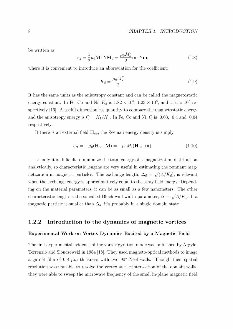
8 CHAPTER 1. INTRODUCTION
be written as
εd =1
2µ0M ·NMd =
µ0M2s
2m ·Nm, (1.8)
where it is convenient to introduce an abbreviation for the coefficient:
Kd =µ0M
2s
2. (1.9)
It has the same units as the anisotropy constant and can be called the magnetostatic
energy constant. In Fe, Co and Ni, Kd is 1.82 × 10⁶, 1.23 × 10⁶, and 1.51 × 10⁵ re-
spectively [16]. A useful dimensionless quantity to compare the magnetostatic energy
and the anisotropy energy is Q = K1/Kd. In Fe, Co and Ni, Q is 0.03, 0.4 and 0.04
respectively.
If there is an external field Hex, the Zeeman energy density is simply
εH = −µ0(Hex ·M) = −µ0Ms(Hex ·m). (1.10)
Usually it is difficult to minimize the total energy of a magnetization distribution
analytically, so characteristic lengths are very useful in estimating the remnant mag-
netization in magnetic particles. The exchange length, ∆d =√
(A/Kd), is relevant
when the exchange energy is approximatively equal to the stray field energy. Depend-
ing on the material parameters, it can be as small as a few nanometers. The other
characteristic length is the so called Bloch wall width parameter, ∆ =√
A/K1. If a
magnetic particle is smaller than ∆d, it’s probably in a single domain state.
1.2.2 Introduction to the dynamics of magnetic vortices
Experimental Work on Vortex Dynamics Excited by a Magnetic Field
The first experimental evidence of the vortex gyration mode was published by Argyle,
Terrenzio and Slonczewski in 1984 [18]. They used magneto-optical methods to image
a garnet film of 0.8 µm thickness with two 90◦ Neel walls. Though their spatial
resolution was not able to resolve the vortex at the intersection of the domain walls,
they were able to sweep the microwave frequency of the small in-plane magnetic field

1.2. INTRODUCTION TO MAGNETIC VORTICES 9
they applied and to locate the resonant vortex frequency (13 ∼ 24 MHz) by observing
the blurred motion of the domain walls. They found that no matter what direction
the in-plane field was applied, the vortex motion was always circular.
The first observation of the gyration mode in an isolated vortex was reported
by Park et al. in 2003 [19]. They used time-resolved Kerr microscopy as a local
spectroscopic probe. Their samples are Ni0.81Fe0.19 disks with thicknesses of 60 nm
and diameters of 0.5, 1, and 2 µm. The laser beam is focused to a full width half
maximum of 540 nm and is positioned near the center of each disk. The excitation is
an in-plane magnetic field pulse with an amplitude of ∼ 5 Oe and a temporal width
of ∼ 150 ps. The left panel of Fig. 1.4 shows the recorded time-domain polar Kerr
signal which corresponds to the out-of-plane magnetization near the center of each
disk. The low frequency component (0.6 GHz for the 500 nm disk) is attributed to
the vortex gyration mode.
The development of time-resolved x-ray imaging provides opportunities to study
the vortex dynamics with higher resolution. In 2004, Choe and coworkers reported
snapshots of gyration of Landau structures taken by photoemission electron micro-
scopes (PEEMs) [20]. The samples are rectangular CoFe microstructures with a
thickness of 20 nm and a lateral size of 1 ∼ 2 µm. The excitation is in-plane mag-
netic field pulses generated by current pulses in a Cu waveguide. The contrast in
Fig. 1.5 mainly comes from the in-plane magnetization of the four domains in the
Landau structure. Pattern II and pattern III shows that samples with the same in-
plane magnetization can have different directions of initial acceleration and opposite
gyration directions. Even though the out-of-plane magnetization is invisible in this
measurement, the authors were able to conclude by careful analysis that the direction
of the initial acceleration during the external field pulse depends on the chirality of
the vortex, and the direction of the vortex rotation depends on the polarization of
the vortex core.
In 2006, Waeyenberge and coworkers realized vortex core switching by small in-
plane magnetic field burst on top of an alternating in-plane magnetic field [21]. The
samples are 1.5µm x 1.5µm x 50 nm Ni80Fe20 squares and time-resolved images are
taken by a Scanning Transmission X-ray Microscope (STXM). The vortex core is

10 CHAPTER 1. INTRODUCTION
Figure 1.4: Figure 3 of Ref. [19]: (a) Magnetic force microscope image (left) andschematic of the vortex structure (right) of a 500 nm disk. The bright spot at thecenter of the disk in the image is due to the large z component of the magnetization.(b), (c),(d) Experimental (left) and simulated (right) time-domain polar kerr signalsfor vortex structures of diameters 2 µm, 1 µm and 500 nm near the center of eachdisk.
again invisible in this experiment, so they used the direction of the gyrotropic motion
to deduce the direction of the out-of-plane magnetization of the vortex core. A 0.1
mT continuous sinusoidal in-plane filed with a frequency of 250 MHz was applied to
the sample and the gyrotropic motion of the Landau structure can be clearly seen in
the domain images. After a 4 ns “single period” burst of magnetic field of 1.5 mT,

1.2. INTRODUCTION TO MAGNETIC VORTICES 11
Figure 1.5: Figure 1 of Ref. [20]: (Top) Domain images of the in-plane magnetizationof Pattern I (1 x 1 µm2), Patters II and III (1.5 x 1 µm2), and Pattern IV (2 x 1 µm2),taken at the specified delay times after the filed pulse. The images are part of a timeseries that extends over 8 ns and were chosen so that the horizontal displacement ofthe vortex has maximum amplitude. Hands illustrate the vortex handedness and theout-of-plane core magnetization as determined from the vortex dynamics. (Bottom)trajectories of the vortex core. the dots represent sequential vortex positions (in 100-ps steps). Lines represent time-averaged positions with a Gaussian weight function of100 ps (FWHM) for 0 to 1 ns and 400 ps (FWHM) for 1 to 8 ns. The progression intime is symbolized by the dot color. Red arrows show the trajectory during the filedpulses; black arrows show the direction of gyrotropic rotation after the pulse; and redstars show the vortex position for the shown domain images.))
the Landau structure changes its gyration direction. This experiments demonstrated
the possibility of switching the vortex core with a small magnetic field.
The first direct observation of the vortex core moving in the gyration mode was
reported in 2007 by Chou and coworkers [22]. Even though direct observation of a
static vortex core was reported as early as 2000 [12], time-resolved images of vortex
core motion were difficult to obtain due to the challenging requirement of both spatial
and temporal resolution. In Ref. [22], the out-of-plane magnetization of a 500 nm
x 500 nm x 40 nm Permalloy square was imaged by STXM. The excitation is an
in-plane ac magnetic field with a frequency of 437.5 MHz. Fig. 4 of this paper shows
12 CHAPTER 1. INTRODUCTION
that the trajectories of the vortex core of the same sample are different for different
core polarities. The authors attribute this asymmetry to the local imperfections and
rough surfaces in the thin films.
Besides the low-frequency gyrotropic mode, higher frequency eigenmodes of the
vortex dynamics have also been observed experimentally. Ref. [23] revealed both
axially symmetric modes and azimuthal modes by fourier transform of time-resolved
Kerr microscopy images. The samples are Permalloy disks with diameters of 3 µm,
4µm and 6µm and a thickness of 15 nm. The excitation is magnetic field pulses
perpendicular to the disk plane with maximum strength less than 50 Oe. A series
of polar Kerr microscopy images are taken with a time interval 30 ps. The contrast
of this experiment is the change of the out-of-plane magnetization with respect to
the equilibrium configuration. The fourier transform of these images are shown in
Fig. 1.6. Two types of modes were excited by the magnetic field pulses: (a) to (c)
are axially symmetric modes; (d) and (e) break the axial symmetry. Although the
azimuthal modes are exited by in-plane pulses, they also exist in this experiment with
perpendicular pulses due to the spatial inhomogeneity in the field distribution.
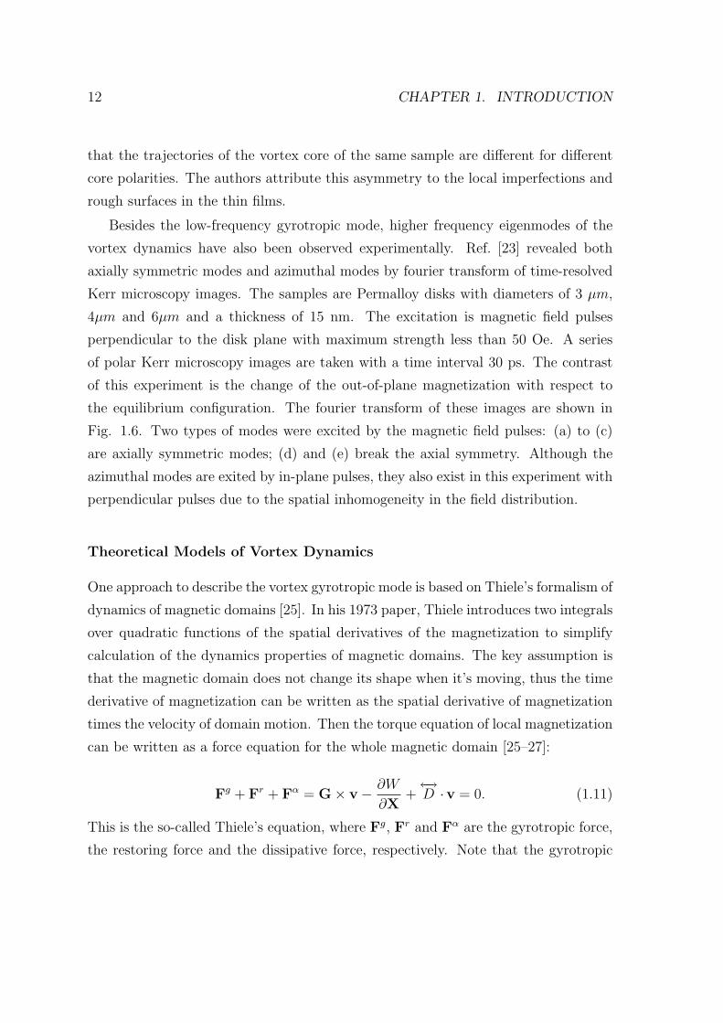
Theoretical Models of Vortex Dynamics
One approach to describe the vortex gyrotropic mode is based on Thiele’s formalism of
dynamics of magnetic domains [25]. In his 1973 paper, Thiele introduces two integrals
over quadratic functions of the spatial derivatives of the magnetization to simplify
calculation of the dynamics properties of magnetic domains. The key assumption is
that the magnetic domain does not change its shape when it’s moving, thus the time
derivative of magnetization can be written as the spatial derivative of magnetization
times the velocity of domain motion. Then the torque equation of local magnetization
can be written as a force equation for the whole magnetic domain [25–27]:
Fg + Fr + Fα = G× v− ∂W
∂X+←→D ·v = 0. (1.11)
This is the so-called Thiele’s equation, where Fg, Fr and Fα are the gyrotropic force,
the restoring force and the dissipative force, respectively. Note that the gyrotropic

1.2. INTRODUCTION TO MAGNETIC VORTICES 13
Figure 1.6: Figure 7 of chapter 4 of Ref. [24]: Fourier transform of spin vortex eigen-modes for a permalloy disk with a diameter of 6 µm and thickness of 15 nm. The toprow shows the absolute value of the amplitude of the Fourier amplitude at resonance,the bottom row the phase. The modal maps are composed from two half-images:the left from the micromagnetic simulation, the right from the experiment. (a)-(c):Axially symmetric modes showing concentric nodes (n = 1, 2, 3, m = 0). Mode (a) at2.80 GHz has the largest spectral weight. (b): 3.91 GHz and (c): 4.49 GHz are highermodes with regions exhibiting different phases. (d) and (e) are azimuthal modes. (d)m = 1, 2.08 GHz; (e) m = 2, 1.69 GHz.
force comes from the M term in the LLG equation (1.1), the restoring force comes
from the precessional torque term, and the damping force comes from the damping
torque term.
The derivation of the Thiele equation can be briefly summarized as follows [26].
Starting from the LLG equation, substituting
M = − 1
M2s
M× (M× M) (1.12)
to the left hand side and rearranging the equation, it can be written as
γ0M× (Hg + Hr + Hα) = 0, (1.13)

14 CHAPTER 1. INTRODUCTION
where the gyroscopic equivalent field and the dissipative equivalent field are
Hg = − 1
γ0M2s
M× dM
dt, (1.14)
Hg = Heff , (1.15)
Hα = − α
γ0Ms
dM
dt. (1.16)
Thus the LLG equation can be written as an equivalent field equation:
Hg + Hr + Hα = 0. (1.17)
Noting that the products (for a = g, r, α)
fai ≡ −Ha
j
∂Mj
∂xi
(1.18)
are force densities, the field equation 1.17 can be written as a force equation:
Fg + Fr + Fα = 0. (1.19)
Now the key step from the force equation to the Thiele equation is the rigid domain
assumption, i.e. the magnetization distribution moves as a whole without distortion:
M(x, t) = M0(x−X(t)), (1.20)
where x is the field position, X is the domain position, M(x,t) is the local magnetiza-
tion at position x and time t, and M0 is the equilibrium magnetization distribution.
Using the above rigid domain assumption, the time derivative of magnetization
can be written as the spatial derivative times the domain speed:
dMi
dt=
∂Mi
∂Xj
dXj
dt= vj
∂Mi
∂Xj
= −vj∂Mi
∂xj
. (1.21)
Substituting the alternative expression for the time derivative of magnetization

1.2. INTRODUCTION TO MAGNETIC VORTICES 15
(Equation 1.21) into the gyrotropic force density and dissipation force density (Equa-
tion 1.18) and integrating over the whole volume V, we get the total force terms
exerting on the magnetic domain:
Fg = G× v, (1.22)
Fα =←→D · v, (1.23)
Fr = −∂W (X)
∂X, (1.24)
where W(X) is the magnetostatic energy of the shifted magnetic domain, G is the
total gyrocoupling vector and←→D is the total dissipation tensor:
Gk =1
γ0M2s
εijkεlmn
∫Ml
∂Mm
∂xi
∂Mn
∂xj
dV (1.25)
Dij = − α
γ0Ms
∂Ml
∂xj
∂Ml
∂xi
dV (1.26)
In 1982 Huber [28] first applied the Thiele equation to a two-dimensional, three-
component magnetic vortex. Assuming the magnetization distribution of the vortex
takes the form given by Ref. [29], he obtained the two integrals for the gyrocoupling
vector and the dissipation tensor:
G = Gz = −2πqpz (1.27)
where q is the vorticity ( q = 1 for vortex and q = -1 for antivortex), and p = ±1 is
the vortex polarization.
Dxx = Dyy ≡ D = −απ ln(R/a) (1.28)
where R is the “outer radius” of the vortex, a is the lattice parameter, and all other
components of←→D are zero. Note that G and D are constants irrelevant of the position
of the vortex.
If we do not assume a specific magnetization distribution for the vortex, but only

16 CHAPTER 1. INTRODUCTION
assume the magnetization is uniform along the z direction, we will still have G = Gz.
If we further assume rotational symmetry of the magnetization, then we will also have
Dxx = Dyy ≡ D with other components of the dissipation tensor being zero.
Under the above assumptions plus the assumption that W (X) = W (0) + 1/2kX2
and v is in plane, the Thiele equation 1.11 becomes
Gz× X− kX + DX = 0, (1.29)
where X = (X, Y, 0). Eliminating the Y component, the above equation becomes
X + 2βX + ω20X = 0, (1.30)
where [26]
β = − kD
G2 + D2(1.31)
ω20 =
k2
G2 + D2. (1.32)
In Ref. [27], Guslienko and coworkers compared the vortex translational frequency
based on the “rigid-vortex” model and the “side-charge-free” model and found the
latter fits much better to micromagnetic simulations. In both of these models, the
gyroconstant is the same and the damping term is ignored. The difference is the stiff-
ness coefficient in the restoring force term, which results in a different eigenfrequency
ω0 = k/G.
In Ref. [30], the analytical results of the above“side-charge-free” model is com-
pared to experimental results. As shown in Fig. 1.7, the analytical results fit the
data well for small dot aspect ratio β = L/R, whereas for higher aspect ratio dots
discrepancies show up because the assumption that magnetization is uniform along
the z axis doesn’t hold any more and the surface charges at the side of the vortex de-
viate from the two limiting cases of the “rigid-vortex” and “side-charge-free” models.
Another approach in calculating the vortex gyration mode does not assume the
rigid structure of the vortex and is able to describe not only the low-frequency mode

1.2. INTRODUCTION TO MAGNETIC VORTICES 17
Figure 1.7: Figure 5 of Ref. [30]: Comparison of experimental data, simulations andanalytical theory for the eigenfrequency of the vortex translational mode vs the dotaspect ratio β = L/R.
but also other vortex dynamics modes with higher frequencies [31–33]. It assumes
small oscillations from the static vortex solutions and solves the LLG equation for
magnon normal modes.
The vortex ground state is assumed to be θ = θ0(r), φ = χ+π/2 for dot thickness
L much smaller than dot radius R. θ and φ are polar and azimuthal angles of the
magnetization, and in general they are functions of the space coordinates (z,r,χ) as
well as time (t). The magnetization is M = Ms(sin θ cos φ, sin θ sin φ, cos θ).
Assuming both the static and dynamic parts of the magnetization is uniform along
the z axis, the magnetization with small deviations from the vortex ground state can
be written as [33]
θ = θ0(r) + ϑ(r, χ, t), (1.33)
φ = χ + π/2 + ψ(r, χ, t). (1.34)
Then the magnetization is Ms[µr + (sin θ0 + ϑ cos θ0)χ + (cos θ0 − ϑ sin θ0)z], where

18 CHAPTER 1. INTRODUCTION
µ(r, χ, t) is defined as µ(r, χ, t) ≡ −ψ sin θ0.
The small deviations are assumed to have the following form [31,33]:
ϑ(r, χ, t) = fnm(r) cos(mχ + ωt), (1.35)
µ(r, χ, t) = gnm(r) sin(mχ + ωt), (1.36)
where n is the number of axially symmetric nodes and m is the number of the az-
imuthal nodes. (m = 1, n = 0) is the low-frequency gyrotropic mode.
Substituting the above assumption of M(r, t) into the LLG equation, if Heff is
known, the magnon modes can be solved. The difficulties come from the nonlocal
nature of the magnetostatic interaction and the inhomogeneous nature of the vortex
ground state. Usually the effective field needs to be evaluated numerically and the
ground state of the vortex magnetization is assumed to be axially symmetric with
θ0(r) taking the form of an exponential function or a power law function. The cal-
culated frequency also fits data well for low aspect ratio L/R ( ∼ 0.1) but deviates
from the experimental data for higher L/R values.
In this thesis, the aspect ratio L/R of the nanomagnet with an equilibrium vortex
state is high due to the small lateral size of spin-torque devices. Thus the vortex profile
based on the 2D assumption cannot be used anymore. In later sections, we’ll present
our imaging results of these non-traditional magnetic vortices and the consequences
of the 3D effects.

Chapter 2
Experimental Setup
The samples studied in this thesis are made by the Buhrman’s group in Cornell
University, and have a spin-valve nanopillar structure similar to those in Ref. [34].
The thick magnetic layer is 60 nm of Ni81Fe19, the thin magnetic layer is 5 nm of
Co60Fe20B20, and the spacer is 40 nm of Cu. The cross section is an ellipse with a
major axis of ∼ 170 nm and a minor axis of ∼ 120 nm. The transport properties
are similar to the measurements reported in Ref. [34], where persistent gigahertz-
frequency oscillations excited by direct current flowing from the thick magnetic layer
to the thin magnetic layer was detected in a spectrum analyzer. In our x-ray ex-
periments, the samples are excited by a direct current of 3 ∼ 8 mA and no external
magnetic field is applied.
To image the GHz magnetization dynamics in nanoscale multilayer structures
we need x-ray microscopy, because it provides us the desired elemental sensitivity,
combined high resolution in both the temporal and spatial spaces, and the magnetic
sensitivity. The elemental sensitivity of x-rays allows us to isolate the signals of the
thick magnetic layer from other layers in the sample by tuning the x-ray energy to the
nickel L3 absorption edge. The ability to probe fast dynamics comes from the fact that
modern synchrotrons produce sub-nanosecond x-ray pulses. The temporal resolution
of our experiment is about 70 ps, limited by the pulse-width of the x-ray pulses at
the Advanced Light Source (ALS) where we carried out our x-ray experiments. The
magnetic sensitivity comes from the X-ray Magnetic Circular Dichroism (XMCD)
19

20 CHAPTER 2. EXPERIMENTAL SETUP
effect [35, 36], where the absorption of circularly polarized x-rays depends on the
angle between the x-ray polarization and the sample magnetization. The Scanning
Transmission X-ray Microscope (STXM) [37] we use at beamline 11.0.2 of the ALS has
a spatial resolution of ∼ 30 nm, limited by the Fresnel zone plates [38]. A schematic
of the STXM is shown in Fig. 2.1. The zone plate focuses a monochromatic x-ray
beam to a small spot on the sample and the transmitted x-ray intensity through the
sample is recorded pixel by pixel as the sample is scanned.
X-ray
detector
Scanningsample stage
Zone plate
X-rays
STXM
S T X Mcanning ransmission -ray icroscopy
Figure 2.1: A schematic of the Scanning Transmission X-ray Microscope. Adaptedfrom Ref. [39]
The “Pump-probe” technique is often used to study fast magnetization dynamics
[40]. The first experiment of this kind was carried out in 1998 [41]. Based on the ratio
of the sample frequency fsample and the repetition rate of the x-ray pulses fx−ray pulses,
stroboscopic measurements with synchrotron radiation can be categorized in three
types ( Fig. 2.2): a) the sample frequency is the x-ray pulse repetition rate divided

21
by an integer N ; b) the sample frequency is the x-ray pulse repetition rate multiplied
by an integer N ; c) the sample frequency is an arbitrary rational number times the
x-ray pulse repetition rate, which I’ll express as the ratio of two integers, M/N .
0 1 2 3 4 5 6 7t (ns)
0 1 2 3 4 5 6 7 t (ns)
0 1 2 3 4 5 6 7t (ns)
a)
f fsample x-ray pulses= N x
f fsample x-ray pulses= x1N
b)b)
c) f fsample x-ray pulses= xMN
Figure 2.2: Three types of stroboscopic measurements using synchrotron radiation:a)the sample frequency is the x-ray pulse repetition rate divided by an integer. (N=2in the figure.) b)the sample frequency is the x-ray pulse repetition rate multipliedby an integer. (N=2 in the figure.) c) the sample frequency is an arbitrary numbertimes the x-ray pulse repetition rate. (M=67,N=32 in the figure.)
Type (a) is the most common scheme used to study magnetic dynamics. Typically,
magnetic system is excited by a “pump” which is synchronized to the “probe”, the x-
ray pulses. The “pump” can be either pulses or continuous signals. Both (repeatable)
transient and resonant dynamics can be studied in this scheme. Note that, in this
timing structure, only very limited phases can be probed by the x-ray pulses. For
example in Fig. 2.2, only two phases are probed simultaneously, thus the delay

22 CHAPTER 2. EXPERIMENTAL SETUP
between the “pump” and the “probe” is often varied to study more phases of the
sample dynamics. Type (b) is similar to type (a) but with a higher sample frequency.
Our experiment falls into type (c), because the sample oscillation is driven by an DC
current, thus the ratio between the sample frequency and the x-ray pulse repetition
rate is arbitrary.
Since the dynamics we want to study is driven by a direct current instead of
pulses or ac signals, the synchronization between the sample and the x-ray source
is nontrivial. Our solution is to use the “injection locking” method developed by
Rippard and colleagues [42] to phase lock the dc driven oscillation to a small ac current
isync. The amplitude of the phase-locking current isync is about 5% of the direct
current which drives the magnetization dynamics, and it has the same frequency as
the sample oscillation frequency fsample. A phase lock loop is used to synchronize isync
to the ALS x-ray pulses. The x-ray pulse repetition rate at the ALS is 499.642 MHz,
i.e., x-ray pulses come to the beamlines in about every 2 ns. Our sample frequency
ranges from 0.9 to 1.5 GHz, depending on intrinsic properties of the specific sample
and the amplitude of the DC current. This DC-driven oscillation is tunable within
10 ∼ 20 MHz.
Given the sample frequency and the x-ray pulse repetition rate, we chose N in 2.2
c) to be 32. Note that N has two meanings: 1) it is the number of phases we can record
simultaneously, assuming M and N do not have common factors; 2) fx−ray pulses/N
is the frequency grid on which sample frequency can vary. Thus by choosing N to
be 32, we allow the possibility to record 32 different phases of the sample dynamics
simultaneously and a frequency grid of fx−ray pulses/N = 499 MHz/32 ' 15 MHz,
which is within the tuning range of the sample frequency.
Now assume the ith x-ray pulse comes at t = i × 1fx−ray pulses
, then in Fig. 2.2 c)
the phase of the sample oscillation it is probing is
φ(t) = 2πfsamplet + φ0 = 2πfsamplei
fx−ray pulses
+ φ0 = 2πM
Ni + φ0, (2.1)
where M = fsample/(fx−ray pulses/N).
In our experiment, N = 32, M = 61 ∼ 99, and we are only recording every other

23
x-ray pulse, so i = 2,4, 6, 8,.... The photon counting system we used here is basically
the same as that used in [43, 44], except we increased the number of counters from
8 to 16. The schematic of the setup can be seen in Fig. 2.3. The left part is the
excitation (IDC) and synchronization(isync) of the sample, and the right part is the
photon counting system.
circularly polarizedx-ray pulses
x-raydetector
40 nm
60 nm
~ 170 nmx 120 nm
5 nm
synchronizedto x-ray pulses
photoncountingsystem
synchronizedto x-ray pulses
Idcisync
Figure 2.3: Schematic of our experimental setup.

24 CHAPTER 2. EXPERIMENTAL SETUP

Chapter 3
Results of Static Measurements
3.1 From transmission images to magnetic images
The raw data we got from the STXM is the transmitted intensity of x-rays at each
pixel. The contrast of these transmission images come from x-ray absorption: darker
area means less photons are transmitted through the sample and brighter area means
more photons are transmitted. To get magnetic information, we scan the same sample
area with opposite x-ray polarizations and record the transmission images I+ and I−.
Based on XMCD effect, we can get magnetic information about the scanned area
from the dichroic contrast defined as below:
Idich =I+ − I−
I+ + I−. (3.1)
Figure 3.1 shows a typical transmission image of our samples and the corresponding
magnetic image deduced from Equation 3.1.
The reason why the contrast we got using expression 3.1 is proportional to sample
magnetization is shown in the following derivation. Assume
I± = I0 Tother e−ρaσ0(1±αMkMs
)d, (3.2)
where I± is the transmitted intensity of right or left polarized x-rays at each pixel of
25

26 CHAPTER 3. RESULTS OF STATIC MEASUREMENTS
I-
50 nm
I+
I+ -
- I
I+ -
+I
Figure 3.1: Magnetic contrast deduced from transmission images I+ and I− usingequation 3.1.
the scanned images, I0 is the incident x-ray intensity, Tother is the total transmission
factor through other layers in the sample, ρa is the atomic intensity of the magnetic
element we are probing, σ0 is its cross-section with linearly polarized x-rays, α is
the percentage change of the cross-section with circularly polarized x-rays, Mk is the
magnetization of sample at this x-ray spot along the photon propagation direction,
Ms is the saturation magnetization, and d is the thickness of the interested magnetic
layer.
Then
I+ − I−
I+ + I−=
e−ρaσ0dαMkMs − e+ρaσ0dα
MkMs
e−ρaσ0dαMkMs + e+ρaσ0dα
MkMs
=e−
dλ
αMkMs − e+ d
λα
MkMs
e−dλ
αMkMs + e+ d
λα
MkMs
(3.3)
where λ = 1ρσ0
is the attenuation length with linearly polarized x-rays.
If the magnetic layer is very thin, i.e. d ¿ λ, then dλαMk
Ms¿ 1. The above equation
becomesI+ − I−
I+ + I−' −d
λα
Mk
Ms
. (3.4)
For example, at Ni L3 edge, λ ≈ 25 nm, α ≈ 13%, then for a thin layer with d = 2.5
nm and magnetization parallel to x-ray polarization (Mk = Ms), the dichroic contrast
is I+−I−I++I− ' 10−3.
Eq. 3.4 shows that given a certain magnetic material, the magnetic contrast in
dichroic STXM images depends on the thickness of the magnetic layer d, the direction
of the local magnetization Mk, and the x-ray energy through the XMCD contrast α.

3.1. FROM TRANSMISSION IMAGES TO MAGNETIC IMAGES 27
We will see soon that the contrast also depends on the size of the magnetic feature
due to the convolution with the spatial profile of the x-ray spot.
As we can see from Fig. 3.1, the magnetic contrast is much weaker than the topog-
raphy contrast, thus even very small drift between images can cause artifacts in the
dichroic images. To reduce the artifact caused by slow thermal drift, fast synchronous
detection technique is often used to measure nanoscale magnetic dynamics. For ex-
ample, [45,46] measures time differences M(ti) - M(t0) and then deduces M(ti) from
the differential images based on the information of M(t0) obtained from transport
measurement. However, this differential method does not apply for measurement of
static magnetization, hence image alignment is necessary to correct for the drifts of
the field of view [47].
Alignment of images usually requires the existence of a sharp and static feature
in the scanned sample area. In the case of our samples, the only feature we have in
the transmission images is the cross section of the spin torque pillar, as can be seen
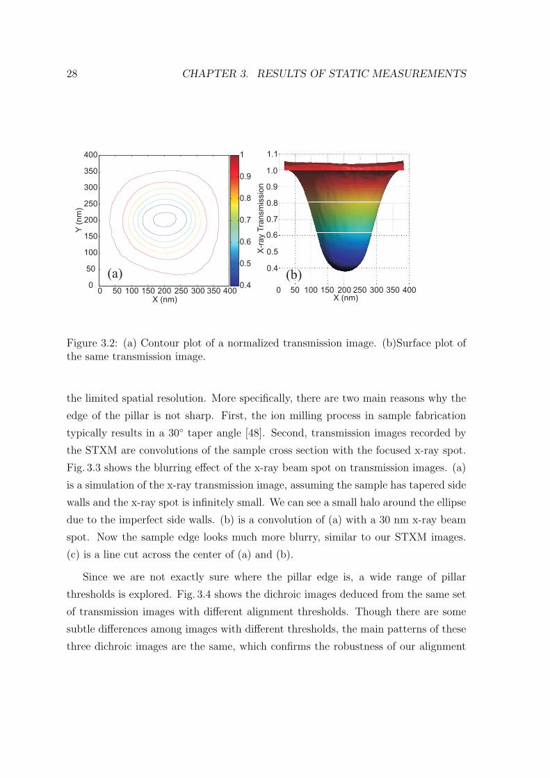
in Fig. 3.1. To depict the x-ray transmission through sample quantitatively, I show
the contour plot and surface plot of a typical transmission image in Fig. 3.2. The
transmission outside the pillar is normalized to one, thus we can see that the pillar
transmits about 60% less than its surrounding area.
Our alignment method is to align the center of the pillar image of each scan to
the center of the field of view. To find the center of the pillar, a threshold value
corresponding to the transmitted intensity at the edge of the pillar is assigned to the
whole image to generate a mask image of the pillar. In the mask image each pixel is
either 0 or 1, depending on whether the pixel is outside or inside the pillar. The center
of gravity of the mask is assumed to be the center of the pillar and the whole image
is shifted accordingly. Note that the transmission images I+ and I− have the same
topography component and different magnetic components, thus direct alignment
of them without removing the magnetic contribution will generate systematic error.
Hence the mask image of the pillar is essential for alignment.
The precision of the alignment depends on the topography contrast of each scan
and the reliability of the pillar edge thresholds. As we can see in Fig.3.2, it is not
very clear where the pillar edge is, due to imperfection in sample fabrication and
28 CHAPTER 3. RESULTS OF STATIC MEASUREMENTS
X (nm)
Y(n
m)
0 50 100 150 200 250 300 350 4000
50
100
150
200
250
300
350
400
0.4
0.5
0.6
0.7
0.8
0.9
1
(a) (b)
1.1
1.0
0.9
0.8
0.7
0.6
0.5
0.4
0 50 100 150 200 250 300 350 400X (nm)
X-r
ay
Tra
nsm
issio
n
Figure 3.2: (a) Contour plot of a normalized transmission image. (b)Surface plot ofthe same transmission image.
the limited spatial resolution. More specifically, there are two main reasons why the
edge of the pillar is not sharp. First, the ion milling process in sample fabrication
typically results in a 30◦ taper angle [48]. Second, transmission images recorded by
the STXM are convolutions of the sample cross section with the focused x-ray spot.
Fig. 3.3 shows the blurring effect of the x-ray beam spot on transmission images. (a)
is a simulation of the x-ray transmission image, assuming the sample has tapered side
walls and the x-ray spot is infinitely small. We can see a small halo around the ellipse
due to the imperfect side walls. (b) is a convolution of (a) with a 30 nm x-ray beam
spot. Now the sample edge looks much more blurry, similar to our STXM images.
(c) is a line cut across the center of (a) and (b).
Since we are not exactly sure where the pillar edge is, a wide range of pillar
thresholds is explored. Fig. 3.4 shows the dichroic images deduced from the same set
of transmission images with different alignment thresholds. Though there are some
subtle differences among images with different thresholds, the main patterns of these
three dichroic images are the same, which confirms the robustness of our alignment

3.2. RESULTS OF EQUILIBRIUM MAGNETIZATION 29
X (nm)
Y(n
m)
100 200 300 400
100
200
300
400 0.4
0.5
0.6
0.7
0.8
0.9
1
X (nm)
Y(n
m)
100 200 300 400
100
200
300
4000.4
0.5
0.6
0.7
0.8
0.9
1
a) b) c)0 100 200 300 400
0.4
0.5
0.6
0.7
0.8
0.9
1
X (nm)
transm
issio
n inte
nsity
sample
convolution
0
0 0
0
Figure 3.3: (a) Sample topography assuming sample is an ellipse of 92 nm × 178nm with a tapered side wall. (b)Convolution of sample topography with x-ray beamassuming the radius of beam spot is 30 nm. (c) Line cut along the easy axis of (a)and (b).
method.
The error bar of the alignment is about a few nanometers based on the following
estimation. Fig. 3.2 shows that the transmission intensity at the pillar edge changes
about 1% for every 3 nm (dI/dx ' (1 − 0.4)/200 nm). Assuming transmission
images I+ and I− are misaligned along x direction by about 3 nm, then we’ll have a
dichroic contrast of 0.7% at the right edge of the pillar and −0.7% at the left edge
( I+−I−I++I− = 1%
(1+0.4)/2+(1+0.4)/2' 0.7%). Since in our dichroic images we don’t see this
kind of strong and symmetric pairs of spots at the edges of the sample, our alignment
of the transmission images is good within a few nanometers.
3.2 Results of equilibrium magnetization
The “ideal” vortex profile in a circular disk calculated in a thin film limit is that the
magnetization curls around in the disk plane to form a flux-closure state and it goes
out of plane in the center, which is the vortex core. Typically, the size of the vortex
core is estimated to be only a few nanometers under the 2D assumption, and the
magnetization is in plane except in the core region. However in our data, we found
several interesting features in the observed magnetic vortex state, deviating from the
ideal 2D case. I will discuss these features in the following subsections.

30 CHAPTER 3. RESULTS OF STATIC MEASUREMENTS
-4
-2
0
2
4
6
8
10
12
a)
b)
c)
M (a.u.)z
100 nm
x 10-3
Figure 3.4: a) Dichroic images deduced from aligned transmission images assumingpillar edge is at transmission 0.6. b)Dichroic images deduced from aligned transmis-sion images assuming pillar edge is at transmission 0.7. c) Dichroic images deducedfrom aligned transmission images assuming pillar edge is at transmission 0.8.
3.2.1 The size of the vortex core and the “dip”
The line cuts in Fig. 3.5 show that the radius of the vortex core in our sample is about
27 nm, much bigger than that of an ideal vortex. Note that the x-ray spot size is also
about 30 nm, so I would like to first discuss whether the unusual core size is real or
due to experimental error.
In Fig. 3.6, I plot our results of the simulated magnetization distribution, the

3.2. RESULTS OF EQUILIBRIUM MAGNETIZATION 31
0 50 100 150 200 250 300 350 400-4
-2
0
2
4
6
8
10
12
14x 10
-3
X (nm)
Mz
(a.
u.)
0
p/4
p/2
3 /4p
2rc ~54 nm
M (a.u.)z
-4
-2
0
2
4
6
8
10
12
x 10-3
50 nm
Figure 3.5: a) A magnetic image of a typical sample. (b) Line cuts along differentdirections of the images.
convolution of this magnetization pattern with a x-ray spot, and the line cuts along
the horizontal axis across the center of the vortex core. We can see that the intensity
of the core is reduced a lot by convolution. In our experiment, the typical dichroic
contrast in the vortex core region using expression 3.1 is about 1%. It’s smaller than
expected (25%) due to the limited spatial resolution and energy resolution. Fig. 3.6
also shows that the core looks bigger after convolution with the x-ray beam spot. The
FWHM in the simulation is ∼ 33 nm and in the convolution it is ∼ 52 nm. However,
even taking into account the convolution with the x-ray beam spot, the measured
core size is still bigger than that in the 2D case.
To understand the vortex core broadening observed in our experimental data, I
conducted micromagnetic simulations to study the dependence of core size on the
sample thickness. I simulated the out-of-plane magnetization of three nanomagnets
which have the same material properties and later sizes but different thicknesses. The
results are shown in Fig. 3.7. It is clear in the simulation results that the size of the
vortex core increases as the thickness of the nanomagnet increases. So in a 2D vortex,
the vortex core is small to minimize the magnetostatic energy cost by the out-of-plane
component in the core region. However, as the film gets thicker, the out-of-plane
magnetization costs less magnetostatic energy due to the reduced demagnetizing field

32 CHAPTER 3. RESULTS OF STATIC MEASUREMENTS
X (nm)
100 200 300 400
100
200
300
400-0.05
0
0.05
0.1
0.15
0.2
0.25
X (nm)100 200 300 400
100
200
300
400 -0.2
0
0.2
0.4
0.6
0.8
c)b)a)Mz
Mz
Mz
2rc ~58 nm
2rs ~33 nm
00
0
100 200 300 400-0.2
0
0.2
0.4
0.6
0.8
1.0
X (nm)
simulation
convolution
0
0
Y (nm) Y (nm)
Figure 3.6: a) Micromagnetic simulation of a 180 nm x 90nm x 60 nm Py. Mz ofsurface. b)Its convolution with an x-ray beam spot with FWHM 30 nm. c) Line cutsalong the longer axis of the ellipse.
generated by surface “magnetic charges”. Thus in thicker films, the core gets larger
since exchange energy favors parallel configuration and magnetostatic energy cost is
small.
t = 2 nm t = 50 nm t = 1800 nm
x
y
Mz
Figure 3.7: Top: Average out-of-plane magnetization distributions of three magneticstructures with the same material and later sizes but different thicknesses. Bottom:the surface plots of the out-of-plane magnetization component.
In most papers on magnetic vortices, the vortex profile is assumed to be in plane

3.2. RESULTS OF EQUILIBRIUM MAGNETIZATION 33
except in the small core region. Thus we were surprised when we first saw in our
data that there is out-of-plane magnetization opposite to the core polarization at the
edge of the vortex, which we call the “dip”. Later we found that it was theoretically
predicted in the book [11], as shown in Fig. 3.8. The authors assumed the out-of-
Figure 3.8: Theoretic calculation of a vortex profile showing the “dip”. Taken fromRef. [11].
plane component is the sum of a few Gaussian functions and they optimized the
parameters in the trial function to minimize the energy. Their result shows that the
magnetization decays from the center of the core, and it overshoots to the opposite
out-of-plane direction before it goes back to zero. The reason that the magnetic
vortices have “dips” is because it partially compensates the flux from the vortex core.
A previous paper using spin-polarized STM to study the vortex core profile [13] hinted
at the existence of the “dip”. Our data are the first x-ray results that clearly show
that there are “dips” opposite to the vortex core in a magnetic vortex.

34 CHAPTER 3. RESULTS OF STATIC MEASUREMENTS
3.2.2 Symmetry breaking
As we mentioned before, most studies of micro- and nano- scale magnetic elements
have focused on two-dimensional (2D) structures. The thickness of these samples
are usually small compared to the exchange length so the magnetization is assumed
to be homogeneous along the sample normal axis. However, in many mesoscopic
magnetic structures with application possibilities, the lateral size and the thickness
are comparable and hence the thickness effect is not negligible.
The few works on three-dimensional (3D) magnetic particles studied soft rect-
angular prisms [49–51] and cylinders with rotational symmetry [52, 53]. The first
asymmetric magnetization pattern due to the bulk effect was reported in 1999 [49].
Their micromagnetic calculations on a 1 um x 500 nm x 250 nm Permalloy block
showed asymmetric flux-closure domains at the surfaces of the sample. The asymme-
try was attributed to the formation of an asymmetric central Bloch wall separating
the two major domains of the Landau structure. Later, this asymmetric Landau pat-
tern was observed in XMCD-PEEM experiments [50]. Recently, Ref. [51] reported
numeric study on the effect of the asymmetric Bloch wall in the 3d Landau struc-
ture (60 - 80 nm thick) on the vortex dynamics where they observed variants of the
gyrotropic vortex core modes due to the 3D nature of the sample.
Besides 3D landau structures, 3D effects were also studied numerically in cylinders
with rotational symmetry. Ref. [52] showed symmetry breaking of the y component
of the magnetization on the surfaces of an “onion state” in a Permalloy disk with
diameter 200 nm and thickness 10 nm at a 10 mT field along the x direction. This
asymmetric pattern was explained “to minimize the amount of poles created at the
perimeter of the disk”. They also showed out-of-plane component of the magneti-
zation near the“head” and the “tail” of the onion axis which differs on the top and
bottom surfaces. Both features are to achieve a better flux closure outside the sample.
In Ref. [53], a “twist” of the in-plane magnetization was observed numerically on the
two surfaces of a disk with thickness 80 nm and diameter 180 nm. The authors also
found a second vortex core mode originating from the nonuniform vortex structure
along the dot normal axis.
As far as we know, nobody has studied the 3D effect of a magnetic vortex with

3.2. RESULTS OF EQUILIBRIUM MAGNETIZATION 35
an elliptical cross section yet. Fig. 3.9 shows the schematic of our sample and the
experimental results of the out-of-plane component of the magnetization of the thick
magnetic layer. The pillar is elongated because we want to get polarized spin current
into the vortex for dynamic study. The vortex layer is thicker than the exchange length
because in an laterally confined nanostructure, if the thickness is too small then the
vortex state is not energetically favorable. The image of Mz is evidently different
from an ideal 2D vortex which maintains the sample topographical symmetry.
Cu 40 nm
Co Fe B 5 nm60 20 20
Py 60 nm
~ 170 nm x 120 nm M (a.u.)z
-4
-2
0
2
4
6
8
10
12
x 10-3
50 nm
x
z
x
y
Figure 3.9: Left: Schematic of the pillar and surface plot of the out-of-plane magne-tization. Right: Image of out-of-plane magnetization of a static vortex. The yellowellipse is added to the data to show the approximate position of the sample in the400 nm x 400 nm scan.
To better understand the origins of the asymmetric patter revealed in our x-
ray data, I conducted micromagnetic simulations using the LLG simulator. The
Permalloy element in the simulation has an elliptical cross section with the dimensions
of the major and minor axes to be 180 nm and 90 nm, respectively. The thickness
is 60 nm. We used the common parameters for Permalloy: A = 1.3; Ms = 800.
The grid is set to be 2 nm x 2nm x 2nm. Fig. 3.10 shows the simulations results of
the out-of-plane magnetization at the top, in the middle, at the bottom as well as
averaged over the whole sample. It is clear to see that the in-plane symmetry of the
magnetization on the surfaces is broken. The dark blue part is about 10 degrees from
the horizontal axis, and the light blue part is about 29 degrees from the horizontal
axis.

36 CHAPTER 3. RESULTS OF STATIC MEASUREMENTS
180 nm
60
nm 9
0nm
Mz
1.0
0.8
0.6
0.4
0.2
0
-0.2
Top slice
Middle slice
Bottom slice
Average
Figure 3.10: Micromagnetic simulation of a 180 nm x 90nm x 60 nm Py pillar. Colorcontrast corresponds to the out-of-plane magnetization.
Though the contrast of x-ray data corresponds to the averaged Mz across the
normal axis of the thick magnetic layer, we found our data is quite similar to the
magnetization on the top surface of the simulation result, as shown in Fig. 3.11.
Note that in the simulation, the averaged magnetization across the thickness is sym-
metric because the simulated structure has a symmetric environment along the z-axis.
However in our experiment, the symmetry along the z-axis is broken due to the layer
structures in the pillar. Thus the asymmetry we were able to detect in the x-ray
experiment comes from two steps: first the thickness effect breaks the symmetry
between the top and bottom surfaces; second, the symmetry of the averaged magne-
tization is broken due to the asymmetric magnetic environment in the pillar along
the z-axis, possibly coming from the tapered profile of the device sidewalls (induced

3.2. RESULTS OF EQUILIBRIUM MAGNETIZATION 37
by ion milling), interface anisotropy or magnetic coupling from the other magnetic
layer. The effect of symmetry breaking along the pillar z-axis will be shown again in
the next chapter where we discuss vortex dynamics.
Mz = 0
Experiment:average
Simulation:surface
Simulation:average
Figure 3.11: Comparison of data and simulation on a static vortex. The simulated Pypillar has a 170 nm x 120 nm elliptical cross section and a thickness of 60 nm. Top:out-of-plane magnetization distribution. Bottom: surface plots of the out-of-planemagnetic components.
The equilibrium magnetic pattern of a vortex is important because vortex dy-
namics depends strongly on its static configuration. An over simplified ideal vortex
picture can be misleading. Our x-ray data shows that the magnetization distribution
of a vortex sandwiched in a spin-torque device deviates strongly from that of an ideal
2D vortex. Thus, quantitative study of spin-torque-induced vortex dynamics should
take into account the realistic vortex profile to compare with experimental data.

38 CHAPTER 3. RESULTS OF STATIC MEASUREMENTS
Chapter 4
Results of Dynamic Measurements
4.1 Time-resolved images
Our synchronous detection setup allowed us to record time-resolved STXM images.
Fig. 4.1 are normalized difference images of the thick magnetic layer deduced from
the average of 12 images of I+ and the average of 13 images of I− using Equation 3.1.
The x-ray beam propagation direction is normal to the sample plane, so the black and
white contrast of these dichroic images corresponds to the out-of-plane magnetization
of the sample according to Equation 3.4. The black dot in the center is the core of
the vortex. The blue ellipse is the outline of the sample pillar estimated from the
transmission images. It is added to the data to guide our eyes where the sample is in
the 400 nm × 400 nm scan box. In these images, the sample is excited by a direct
current of 7.8 mA and it emits an oscillating voltage signal at 0.95 GHz. Our photon
counting system distributes every other transmitted x-ray pulse to 16 photon counters,
so that we record snapshots of the sample magnetization dynamics at 16 equally
distributed phases. In terms of time, these images are about (1000/0.95)/16 = 66
picosecond apart, similar to our time resolution of ∼70 ps which is limited by the
width of the x-ray pulses produced by the ALS. The magnetic images recorded by
the 16 photon counters are sorted to the right phase order according to Equation 2.1.
For f = 0.95 GHz, M in Equation 2.1 is 61. φ0 in this equation is unknown, so the
phases labeled in Fig. 4.1 have an arbitrary phase shift φ0.
39

40 CHAPTER 4. RESULTS OF DYNAMIC MEASUREMENTS
50 100 150 200 250 300 350 400
50
100
150
200
250
300
350
40050 100 150 200 250 300 350 400
50
100
150
200
250
300
350
40050 100 150 200 250 300 350 40050 100 150 200 250 300 350 400
50 100 150 200 250 300 350 400
50
100
150
200
250
300
350
40050 100 150 200 250 300 350 400
50
100
150
200
250
300
350
400
50 100 150 200 250 300 350 400
50
100
150
200
250
300
350
40050 100 150 200 250 300 350 400
50 100 150 200 250 300 350 400
50
100
150
200
250
300
350
40050 100 150 200 250 300 350 400
50
100
150
200
250
300
350
400
50 100 150 200 250 300 350 400
50
100
150
200
250
300
350
400
50 100 150 200 250 300 350 400
50
100
150
200
250
300
350
400
50
100
150
200
250
300
350
400
50
100
150
200
250
300
350
400
π/8
5 /8π
9 /8π
13 /8π
π/2
3 /2π
π
0 π/4
3 /4π
5 /4π
7 /4π
3 /8π
7 /8π
11 /8π
15 /8π
100 nm
Figure 4.1: Dynamic magnetic images of a sample excited by I = 7.8 mA and oscil-lating at f = 0.95 GHz.
A movie made of these 16 dichroic images clearly shows that the vortex core is
gyrating in the clockwise direction in a small orbit. However, since the displacement
of the vortex core in these images is so small, even smaller than the x-ray beam spot
size of ∼ 30 nm, the motion is difficult to see in these images. To reveal the core
dynamics, I plot Mz(φ) −Mz(φ + π) in Fig. 4.2. In these 180◦ differential images,
the common topography component remaining after the subtraction of the right- and

4.1. TIME-RESOLVED IMAGES 41
50 100 150 200 250 300 350 400
50
100
150
200
250
300
350
40050 100 150 200 250 300 350 400
50
100
150
200
250
300
350
400
50 100 150 200 250 300 350 400
50
100
150
200
250
300
350
400
50 100 150 200 250 300 350 400
50 100 150 200 250 300 350 400
50
100
150
200
250
300
350
40050 100 150 200 250 300 350 400
50
100
150
200
250
300
350
40050 100 150 200 250 300 350 400
50
100
150
200
250
300
350
400
50 100 150 200 250 300 350 400
50 100 150 200 250 300 350 400
50
100
150
200
250
300
350
400
50 100 150 200 250 300 350 400
50
100
150
200
250
300
350
40050 100 150 200 250 300 350 400
50
100
150
200
250
300
350
400
50 100 150 200 250 300 350 400
50
100
150
200
250
300
350
400
50
100
150
200
250
300
350
400
50
100
150
200
250
300
350
400
π/8
5 /8π
9 /8π
13 /8π
π/2
3 /2π
π
0 π/4
3 /4π
5 /4π
7 /4π
3 /8π
7 /8π
11 /8π
15 /8π
100 nm
Figure 4.2: 180◦ differential images of a vortex core gyration. The image of phase φis the difference of the images phase φ + π in Fig. 4.1.
left- circularly polarized transmission images is subtracted out, so the magnetization
component is enhanced. The black dots come from the vortex core at phase φ and the
white dots correspond to the core at phase φ + π. With the topography background
further suppressed, the clockwise gyration of the vortex core is revealed in these 180◦
differential images as the black dot moves from up of the ellipse in the first row, to
the right of the ellipse in the second row, then to the bottom, then to the left.

42 CHAPTER 4. RESULTS OF DYNAMIC MEASUREMENTS
-20 -10 0 10 20-20
-10
0
10
20
X (nm)
Y(n
m)
static core position
dynamic core position
sample A, core downI = 3.2 mAf = 1.23 GHz
sample B, core upI = 7.8 mAf = 0.95 GHz
sample B, core downI = 5.1 mAf = 1.26 GHz
-20 -10 0 10 20-20
-10
0
10
20
X (nm)
Y(n
m)
static core position
dynamic core position
-20 -10 0 10 20-20
-10
0
10
20
X (nm)
Y(n
m)
static core position
dynamic core position
Figure 4.3: Vortex core trajectories of two different samples, sample A and sample
B, which are nominally the same.

4.1. TIME-RESOLVED IMAGES 43
Fig. 4.3 shows the vortex core trajectories of the two nominally same samples.
The green dots are the static core positions recorded by the 16 photon counters. The
maximum time lag between these counters is 60 ns, so the different positions shown
on the figure result from fluctuations of the counters instead of from the slow drift of
the measurement system. The uncertainty of the core positions has several sources.
The x-ray spot size is ∼ 30 nm, the floor vibration is about ∼ 20 nm, the alignment
of the two sets of images taken with right and left circularly polarized x-rays is a few
nanometers, and the fluctuations of the photon counters also causes an uncertainty
of a few nanometers. The first three sources produce errors in the absolute core
positions, and the last source produce errors in the relative core positions, i.e., the
core position deduced from images recorded by one photon counter relative to that
of other photon counters.
As discussed in Section 3.1, to correct the slow drift between images, we align
each scan so that the center of the sample cross section is in the middle of the scan
box. Since the edge of the sample shape in our transmission images is not very sharp,
the alignment threshold has a relatively big range. In Table 4.1, we compare the
average vortex core positions over the 16 counters obtained from different alignment
thresholds. As we can see from the last row of the table, the variation of core position
caused by our image alignment is smaller than 3 nm. Note that the focused x-ray
spot size is about 30 nm and the scan step of STXM is 10 nm. Table 4.1 proves again
that the image alignment is robust. (Another demonstration of the robustness of the
alignment is Fig. 3.4.)
To estimate the uncertainty of the relative core position in vortex dynamics, we
measured the static vortex positions with the same photon counting system. Table
4.2 shows the average static core positions recorded by the 16 counters simultaneously
and the fluctuations of these counters. The alignment threshold is set to 0.7. The
average core positions show that within our experimental precision, the vortex core
at equilibrium is approximately at the center of the sample pillar. The fluctuations
across the photon counters are estimates by the standard deviation (times 2) and the
difference between the maximum and minimum values of the core position. The last
column is the accumulation time per pixel in each photon counter in units of millions

44 CHAPTER 4. RESULTS OF DYNAMIC MEASUREMENTS
of pulses. For example, the core position of sample A is deduced from 39 images, and
the dwell time of each pixel is 30 ms for this set of data, thus the number of photon
pulses incident to these samples is 39 x 30 ms / 64 ns = 18 million pulses.
The fluctuations of the static core positions provide us an estimate of the un-
certainty of the core trajectory. The accumulation time per pixel of the images for
dynamics measurements of sample A, sample B (core up), and sample B (core down)
in units of million photon pulses are 15, 8, 12. So the fluctuations caused by the
photon counters for the dynamic measurement are slightly bigger than those of the
static measurement.
alignment sample A sample B sample B sample A sample B sample Bthreshold core down core up core down core up core down
statics statics statics dynamics dynamics dynamics
0.6 (-5, -1) (3, -4) (1, -2) (-6, -3) (1, -5) (3, -1)
0.7 (-5 ,-2) (3, -3) (2, -2) (-6, -4) (2, -5) (5, -2)
0.8 (-6, -3) (3, -4) (3, -3) (-8, -5) (3 ,-6) (6, -2)
(∆x, ∆y) (1, 2) (0, 1) (1, 1) (2, 2) (2, 1) (3, 1)
Table 4.1: Average core positions obtained with different alignment threshold. The(X,Y) values in the middle three rows are average values of the 16 counters. Theunits are nanometers. The values in the last column is the deviations of the averagecore positions caused by alignment.
Due to the small size of the core displacement, it is very hard for us to detect
whether there is asymmetry in the core trajectory, even though in principle the spin
torque does break the up-down symmetry because the polarization of the spin current
is along the x axis. Table 4.3 shows the maximum distance in the core trajectory
∆(x)d, ∆(y)d, which is about 24 nm for sample A and about 15 nm for sample B,
and for comparison, the maximum distance in the static core positions due to the
fluctuations, ∆(x)s, and ∆(y)s. These numbers show that the elongation of the core
trajectory is smaller than the fluctuations. The distance between the center of the
core trajectory and the static core position is shown in xd−xs and xd−xs. Although

4.1. TIME-RESOLVED IMAGES 45
x 2δ(x) ∆(x) y 2δ(y) ∆(y) accumulation(nm) (nm) (nm) (nm) (nm) (nm) (million pulses)
sample A -5 4 7 -2 4 6 18(core down)sample B 3 2 4 -3 2 3 18(core up)sample B 2 2 5 -2 2 3 23
(core down)
Table 4.2: Static core positions and fluctuations.
the trajectories in Fig. 4.3 seem to be off-centered from the equilibrium position,
Table 4.3 shows that this offset is smaller than the experiment uncertainty. This is
also true for the asymmetry of the trajectory. For example, the maximum distance
in x between the core positions in the trajectory for sample B (core up) is 18 nm. A
reliable asymmetry should be bigger than the fluctuations of the static core positions
(∼ 4 nm), which means the bigger displacement has to be bigger than the smaller
displacement by ∼ 57%.
∆(x)d ∆(x)s xd − xs ∆(y)d ∆(y)s xd − xs
(nm) (nm) (nm) (nm) (nm) (nm)
sample A 24 7 -1 23 6 -1(core down)sample B 18 4 -1 15 3 -2(core up)sample B 15 5 3 15 3 0
(core down)
Table 4.3: Dynamic core positions.
The uncertainty in the temporal space has two major sources. One is the width
of the x-ray pulses, which is about 70 ps at the full width half maximum (FWHM).
Since we record 16 phases of the sample dynamics, the corresponding time grid of

46 CHAPTER 4. RESULTS OF DYNAMIC MEASUREMENTS
our measurement is 1/16 of the sample oscillation period, which is 50 ∼ 60 ps, com-
parable to the FWHM of the ALS pulses. Another major source is the jitter in the
synchronization between the x-ray pulses and the RF source which we use to phase
lock the vortex gyration. This synchronization is monitored in real time during the
imaging experiment on a 20 GHz real time oscilloscope. The trigger signal of the
scope is the synchrotron clock and the input signal displayed on the scope screen is
signal from a power splitter connected to the RF source. The jitter is about 1/16 of
the sine wave pattern on the screen.
Fig. 4.3 shows that the orbit size of the vortex gyration is very small. The radius
is only 5 ∼ 10 nm. However, in the previous studies of vortex dynamics excited by ac
magnetic field, the radius of the gyration orbit is usually a few hundred nanometers.
This difference is because that the size of the orbit depends on the strength of the
effective magnetic field. With sizeable ac magnetic field, the core can be “kicked”
into relatively large orbits. However, the spin torque doesn’t “kick” the core to a
certain orbit. It only balances the spin torque so that the core can contitue gyrating
on certain orbits decided by the initial shift and the size of the internal field. Thus the
orbit size of vortex dynamics excited by dc spin-polarized current without applying
a magnetic field is much smaller than the excitation excited by ac magnetic fields.
The measurement of sample B shows that the direction of gyration is determined
by the polarity of the vortex core. This observation agrees with previous studies on
field driven vortex dynamics [20]. In Ref. [20], a magnetic vortex in a Landau structure
was excited by an in-plane magnetic field pulse, the vortex core then gyrated a few
times with shrinking orbit size, eventually falling back to the equilibrium position.
The authors found that the direction the core gyrates does not depend on the direction
of the initial field pulse. It also does not depend on the vortex in-plane magnetization.
Instead, they found the direction of gyration is solely determined by the vortex core.
In our case, we do not apply any magnetic field, and the dc spin-polarized current we
apply does not change the energy landscape much, thus the direction of the gyration
is still determined by the core polarization.
As discussed in Section 1.2.2, the frequency of vortex gyration is determined by
the size of the effective magnetic field, thus in principle, the steady-state frequency of

4.2. A SIMPLE PICTURE 47
a magnetic vortex should not change when the core polarization changes. However,
we observed in our experiments that sample B’s steady-state frequency changed after
the vortex core flipped. This indicates that the magnetic environment felt by the
vortex core pointing up is different from that felt by the same vortex core pointing
down, which indicates again that the symmetry along the z-axis is broken in our
samples, agreeing with the symmetry breaking of the static magnetization distribution
discussed in Section 3.2.2.
4.2 A simple picture
The LLG equation is nonlinear and nonlocal, thus it is extremely difficult to solve
analytically. The “macrospin” model is usually a good starting point to provide
some useful intuition. However, in a strongly nonuniform magnetic state, such as
a magnetic vortex, the macrospin model which assumes the whole structure to be
uniformly magnetized is apparently too crude. Thus to develop some intuition for
the observed spin-torque-induced vortex dynamics, I made an approximation to use
two coupled macrospins to simplify the complicated magnetization distribution of a
magnetic vortex, as shown in Fig. 4.4a. The macrospin model of spin torque dynamics
tells us that M1 can be excited to persistent precession by the spin torque but M2
cannot, if both of them are isolated, as shown in Fig. 4.4b. Now the question is that
if they are coupled whether they can be excited into a steady state.
In the small angle dynamics for a macrospin, the LLG equation can be linearized
to a simple harmonic oscillator [54]. Here I use two coupled spring-mass systems to
further simplify the problem, as shown in Fig. 4.5.
In this coupled spring mass systems, the precession torque in the LLG equation
is described by the force exerted by the two springs connected to the walls:
F precession1,2 = kx1,2. (4.1)
The coupling between the two macrospins is described by the spring between the

48 CHAPTER 4. RESULTS OF DYNAMIC MEASUREMENTS
Conductionelectrons
p
M1 M2Damping
Spin Torque
M1eq
M1
M2eq
Damping
Spin Torque
M2
M2eq
Damping
Spin Torque
M2
a) b)
Figure 4.4: A simple picture of the spin-torque-induced vortex dynamics. a)Using2 “macrospins” to describe a magnetic vortex. b) The spin torques on these two“macrospins”.
m1 m
2
kk k’
m1 m
2
kk k’
Figure 4.5: A phenomenological toy model.
two masses:
F coupling1,2 = k′(x2,1 − x1,2). (4.2)
The damping torque in the LLG is described by the damping force
F damping1,2 = −αx1,2. (4.3)
The spin torque becomes βx1 for m1 and −βx2 for m2. Now this coupled spring-
mass system looks very similar to the coupled macrospin system: when α = β, m1
can have steady state oscillation, but m2 cannot. These equations are now much

4.2. A SIMPLE PICTURE 49
easier to solve than the nonlinear and nonlocal LLG equation. In fact this system
can have steady state oscillation if a critical condition is satisfied:
β2 = α2 +k′2
ω2(4.4)
The critical condition says that in order to have a steady state of this coupled
system, the spin torque has to be bigger than the damping torque by a certain amount
which depends on the coupling. If the coupling is very strong, then the spin torque
has to be very big to drag m2 to move. When the coupling is zero, it reduces to the
single macrospin case correctly.

50 CHAPTER 4. RESULTS OF DYNAMIC MEASUREMENTS

Chapter 5
Conclusions
In summary, we have presented results of the first direct imaging of the magneti-
zation dynamics in a dc driven spin-torque vortex oscillator. We have developed a
technique to synchronize the dc-driven GHz oscillation to x-ray pulses so that we
are able to do time-resolved x-ray imaging of the fast magnetization dynamics. We
studied both the statics and dynamics of the spin torque vortex oscillator. The static
images reveal a non-trivial vortex profile which strongly deviates from a circular 2D
vortex. This is due to the 3D nature of the thick magnetic layer, and possibly also
the interlayer coupling from the thin magnetic layer, as suggested in the symmetry
breaking of the magnetization distribution. To better understand the equilibrium
state of our sample, we analyzed the static data using micromagnetic simulations
and we observed most of the features revealed in experimental data in the simulation
results. Dynamic images show clear spin-torque driven vortex gyration, identifying
another spin-torque-induced dynamic mode, in additions to the spin-torque switch-
ing and persistent macrospin precession. To gain some insight into the underlying
dynamic process, we developed a simple phenomenological model, where two cou-
pled spring-mass systems with damping, “anti-damping”, and “extra-damping” show
steady-state oscillation if a critical condition relating the damping, the coupling and
the “spin torque” is satisfied.
The “non-ideal” magnetic vortex profile revealed by our x-ray data makes it very
challenging to model the magnetization dynamics reported here analytically. Most
51

52 CHAPTER 5. CONCLUSIONS
vortex dynamic models assume an “ideal” vortex profile where the magnetization is
uniform along the normal axis and the in-plane distribution maintains the sample
topographic symmetry [27, 31, 32, 55]; however, these models do not apply in our
case without taking into account the 3D nature of the magnetization distribution.
For example, Ref. [56] concludes, by using the Thiele equation [25, 28], that only
the perpendicular component of the spin polarization can sustain persistent vortex
gyration, while the in-plane component leads only to vortex core displacement. In
contrast, our x-ray data clearly shows that in our samples the vortex undergoes steady
state oscillation with in-plane spin-polarized current. One possible reason for the
discrepancy is the unusual profile of the vortex in our sample, since both the damping
force and the spin-torque force in the Thiele equation are strongly dependent on the
vortex magnetization distribution. Another possible reason is the periodic distortion
of the vortex core along the normal axis observed in simulations of the dynamics in
Ref. [34]. Such a periodic distortion of the core during the gyrotropic motion cannot
be described by the standard models of vortex dynamics. Our imaging results call
for better theoretical models of vortex dynamics which take into account the realistic
magnetization distribution.

Bibliography
[1] J. C. Slonczewski. Current-driven excitation of magnetic multilayers. J. Magn.
Magn. Mater., 159:L1, 1996.
[2] L. Berger. Emission of spin-waves by a magnetic multilayer traversed by a cur-
rent. Phys. Rev. B, 54:9353, 1996.
[3] D.C. Ralph and M.D. Stiles. Spin transfer torques. Journal of Magnetism and
Magnetic Materials, 320(7):1190 – 1216, 2008.
[4] Albert Fert. Nobel lecture: Origin, development, and future of spintronics. Re-
views of Modern Physics, 80(4):1517, 2008.
[5] M. N. Baibich, J. M. Broto, A. Fert, F. Nguyen Van Dau, F. Petroff, P. Eti-
enne, G. Creuzet, A. Friederich, and J. Chazelas. Giant magnetoresistance of
(001)fe/(001)cr magnetic superlattices. Phys. Rev. Lett., 61(21):2472–2475, Nov
1988.
[6] G. Binasch, P. Grunberg, F. Saurenbach, and W. Zinn. Enhanced magnetoresis-
tance in layered magnetic structures with antiferromagnetic interlayer exchange.
Phys. Rev. B, 39(7):4828–4830, Mar 1989.
[7] J.A. Katine and Eric E. Fullerton. Device implications of spin-transfer torques.
Journal of Magnetism and Magnetic Materials, 320(7):1217 – 1226, 2008.
[8] D.V. Berkov and J. Miltat. Spin-torque driven magnetization dynamics: Micro-
magnetic modeling. Journal of Magnetism and Magnetic Materials, 320(7):1238
– 1259, 2008.
53

54 BIBLIOGRAPHY
[9] T.J. Silva and W.H. Rippard. Developments in nano-oscillators based upon spin-
transfer point-contact devices. Journal of Magnetism and Magnetic Materials,
320(7):1260 – 1271, 2008.
[10] S. D. Bader. Colloquium: Opportunities in nanomagnetism. Rev. Mod. Phys.,
78:1, 2006.
[11] A. Hubert and R. Schaefer. Magnetic Domains. Springer, Berlin, 1998.
[12] T. Shinjo, R. Okuno, R. Hassdorf, K. Shigeto, and T. Ono. Magnetic vortex core
observation in circular dots of permally. Science, 289:930, 2000.
[13] A. Wachowiak, J. Wiebe, M. Bode, O. Pietzsch, M. Morgenstern, and R. Wiesen-
danger. Direct observation of internal spin structure of magnetic vortex cores.
Science, 298:577, 2002.
[14] W.F. Brown. Micromagnetics. Intersicence Publishers, Gouda, 1963.
[15] J. Miltat, G. Albuquerque, and A. Thiaville. An introduction to micromagnet-
ics in the dynamic regime. In B. Hillebrands and K. Ounadjela, editors, Spin
Dynamics in Confined Magnetic Structures, page 1, Berlin, 2002. Springer.
[16] M. Bode, O. Pietzsch, A. Kubetzka, W. Wulfhekel, D. McGrouther, S. McVitie,
and J. N. Chapman. Comment on “three-dimensional, spin-resolved structure of
magnetic vortex and antivortex states in patterned co films using scanning ion
microscopy with polarization analysis”. Physical Review Letters, 100(2):029703,
2008.
[17] S. Blundell. Magnetism in Condensed Matter. Oxford Univ. Press, New York,
2001.
[18] B. E. Argyle, E. Terrenzio, and J. C. Slonczewski. Magnetic vortex dynamics
using the optical cotton-mouton effect. Phys. Rev. Lett., 53:190, 1984.
[19] J. P. Park, P. Eames, D. M. Engebretson, J. Berezovsky, and P. A. Crowell.
Imaging of spin dynamics in closure domain and vortex structures. Phys. Rev.
B, 67:020403, 2003.
BIBLIOGRAPHY 55
[20] S.-B. Choe, Y. Acremann, A. Scholl, A. Bauer, A. Doran, J. Stohr, and H. A.
Padmore. Vortex core-driven magnetization dynamics. Science, 304:420, 2004.
[21] H. Stoll K. W. Chou T. Tyliszczak R. Hertel M. Fahnle H. Bruckl K. Rott G.
Reiss I. Neudecker D. Weiss C. H. Back B. Van Waeyenberge, A. Puzic and
G. Schutz. Magnetic vortex core reversal by excitation with short bursts of an
alternating field. Nature, 444:461, 2006.
[22] K. W. Chou, A. Puzic, H. Stoll, D. Dolgos, G. Schutz, B. Van Waeyenberge,
A. Vansteenkiste, T. Tyliszczak, G. Woltersdorf, and C. H. Back. Direct ob-
servation of the vortex core magnetization and its dynamics. Applied Physics
Letters, 90(20):202505, 2007.
[23] M. Buess, R. Hollinger, T. Haug, K. Perzlmaier, U. Krey, D. Pescia, M. R.
Scheinfein, D. Weiss, and C. H. Back. Fourier transform imaging of spin vortex
eigenmodes. Phys. Rev. Lett., 93(7):077207, Aug 2005.
[24] B. Hillebrands and K. Ounadjela, Editors. Spin Dynamics in Confined Magnetic
Structures III. Springer, Berlin, 2006.
[25] A. A. Thiele. Steady-state motion of magnetic domains. Phys. Rev. Lett.,
30(6):230–233, Feb 1973.
[26] J. Kim and S.-B. Choe. Simple harmonic oscillation of ferromagnetic vortex core.
2007.
[27] K. Yu. Guslienko, B. A. Ivanov, V. Novosad, Y. Otani, H. Shima, and
K. Fukamichi. Eigenfrequencies of vortex state excitations in magnetic
submicron-size disks. J. Appl. Phys., 91(10):8037–8039, 2002.
[28] D. L. Huber. Dynamics of spin vortices in two-dimensional planar magnets.
Phys. Rev. B, 26(7):3758–3765, Oct 1982.
[29] S. Hikami and T. Tsuneto. Phase Transition of Quasi-Two Dimensional Planar
System. Progress of Theoretical Physics, 63:387–401, February 1980.

56 BIBLIOGRAPHY
[30] V. Novosad, F. Y. Fradin, P. E. Roy, K. S. Buchanan, K. Yu. Guslienko, and
S. D. Bader. Magnetic vortex resonance in patterned ferromagnetic dots. Phys.
Rev. B, 72(2):024455, Jul 2005.
[31] B. A. Ivanov, H. J. Schnitzer, F. G. Mertens, and G. M. Wysin. Magnon modes
and magnon-vortex scattering in two-dimensional easy-plane ferromagnets. Phys.
Rev. B, 58(13):8464–8474, Oct 1998.
[32] B. A. Ivanov and C. E. Zaspel. Magnon modes for thin circular vortex-state
magnetic dots. Applied Physics Letters, 81(7):1261–1263, 2002.
[33] C. E. Zaspel, B. A. Ivanov, J. P. Park, and P. A. Crowell. Excitations in
vortex-state permalloy dots. Physical Review B (Condensed Matter and Ma-
terials Physics), 72(2):024427, 2005.
[34] V. S. Pribiag, I. N. Krivorotov, G. D. Fuchs, P. M. Braganca, O. Ozatay, J. C.
Sankey, D. C. Ralph, and R. A. Buhrman. Magnetic vortex oscillator driven by
d.c. spin-polarized current. Nat. Phys., 3:498, 2007.
[35] G. Schutz, W. Wagner, W. Wilhelm, P. Kienle, R. Zeller, R. Frahm, and
G. Materlik. Absorption of circularly polarized x rays in iron. Phys. Rev. Lett.,
58(7):737–740, Feb 1987.
[36] J. Stohr, Y. Wu, B. D. Hermsmeier, M. G. Samant, G. R. Harp, S. Koranda,
D. Dunham, and B. P. Tonner. Element-specific magnetic micoscopy with circu-
larly polarized x-rays. Science, 259:658, 1993.
[37] A. L. D. Kilcoyne, T. Tyliszczak, W. F. Steele, S. Fakra, P. Hitchcock, K. Franck,
E. Anderson, B. Harteneck, E. G. Rightor, G. E. Mitchell, A. P. Hitchcock,
L. Yang, T. Warwick, and H. Ade. Interferometer-controlled scanning transmis-
sion X-ray microscopes at the Advanced Light Source. Journal of Synchrotron
Radiation, 10(2):125–136, 2003.
[38] David Attwood. Soft X-Rays and Extreme Ultraviolet Radiation: Principles and
Applications. Cambridge University Press, Cambridge, 2000.

BIBLIOGRAPHY 57
[39] J. Stohr and H.C. Siegmann. Magnetism : from fundamentals to nanoscale
dynamics. Springer, Berlin, 2006.
[40] B. Hillebrands and K. Ounadjela, Editors. Spin Dynamics in Confined Magnetic
Structures II. Springer, Berlin, 2003.
[41] F. Sirotti, R. Bosshard, P. Prieto, G. Panaccione, L. Floreano, A. Jucha, J. D.
Bellier, and G. Rossi. Time-resolved surface magnetometry in the nanosecond
scale using synchrotron radiation. Journal of Applied Physics, 83(3):1563–1568,
1998.
[42] W. H. Rippard, M. R. Pufall, S. Kaka, T. J. Silva, S. E. Russek, and J. A. Katine.
Injection locking and phase control of spin transfer nano-oscillators. Phys. Rev.
Lett., 95(6):067203, Aug 2005.
[43] Y. Acremann, V. Chembrolu, J. P. Strachan, T. Tyliszczak, and J. Stohr. Soft-
ware defined photon counting system for time resolved x-ray experiments. Rev.
Sci. Instrum., 78:014702, 2007.
[44] J. P. Strachan, V. Chembrolu, X. W. Yu, T. Tyliszczak, and Y. Acremann.
Synchronized and configurable source of electrical pulses for x-ray pump-probe
experiments. Rev. Sci. Instrum., 78:054703, 2007.
[45] Y. Acremann, J.P. Strachan, V. Chembrolu, S.D. Andrews, T. Tyliszczak, J.A.
Katine, M.J. Carey, B.M. Clemens, H.C. Siegmann, and J. Stohr. Time-resolved
imaging of spin transfer switching: Beyond the macrospin concept. Phys. Rev.
Lett., 96:217202, 2006.
[46] J. P. Strachan, V. Chembrolu, Y. Acremann, X.W. Yu, A. A. Tulapurkar,
T. Tyliszczak, J. A. Katine, M. J. Carey, M. R. Scheinfein, H. C. Siegmann,
and J. Stohr. Direct observation of spin-torque driven magnetization reversal
through nonuniform modes. Phys. Rev. Lett., 100:247201, 2008.
[47] T. Tyliszczak E.G. Rightor G.E. Mitchell M.T. Dineen F. Hayes W. Lidy R.D.
Priester S.G. Urquhart A.P. Smith A.P. Hitchcock, I. Koprinarov and H. Ade.
58 BIBLIOGRAPHY
Optimization of scanning transmission x-ray microscopy for the identification and
quantitation of reinforcing particles in polyurethanes. Ultramicroscopy, 88:33,
2001.
[48] P. M. Braganca, O. Ozatay, A. G. F. Garcia, O. J. Lee, D. C. Ralph, and R. A.
Buhrman. Enhancement in spin-torque efficiency by nonuniform spin current
generated within a tapered nanopillar spin valve. Phys. Rev. B, 77:14423, 2008.
[49] Riccardo Hertel and Helmut Kronmuller. Computation of the magnetic domain
structure in bulk permalloy. Phys. Rev. B, 60(10):7366–7378, Sep 1999.
[50] R. Hertel, O. Fruchart, S. Cherifi, P.-O. Jubert, S. Heun, A. Locatelli, and
J. Kirschner. Three-dimensional magnetic-flux-closure patterns in mesoscopic fe
islands. Phys. Rev. B, 72(21):214409, Dec 2005.
[51] M. Yan, R. Hertel, and C.M. Schneider. Calculations of three-dimensional mag-
netic normal modes in mesoscopic permalloy prisms with vortex structure. Phys.
Rev. B, 76:094407, 2007.
[52] Jonathan Kin Ha, Riccardo Hertel, and J. Kirschner. Micromagnetic study
of magnetic configurations in submicron permalloy disks. Phys. Rev. B,
67(22):224432, Jun 2003.
[53] F. Boust and N. Vukadinovic. Micromagnetic simulations of vortex-state excita-
tions in soft magnetic nanostructures. Phys. Rev. B, 70(17):172408, Nov 2004.
[54] V. Chembrolu, J. P. Strachan, X. W. Yu, A. A. Tulapurkar, T. Tyliszczak, J. A.
Katine, M. J. Carey, J. Stohr, and Y. Acremann. Time-resolved x-ray imaging
of magnetization dynamics in spin-transfer torque devices. Physical Review B
(Condensed Matter and Materials Physics), 80(2):024417, 2009.
[55] K. Yu. Guslienko, X. F. Han, D. J. Keavney, R. Divan, and S. D. Bader. Magnetic
vortex core dynamics in cylindrical ferromagnetic dots. Physical Review Letters,
96(6):067205, 2006.

BIBLIOGRAPHY 59
[56] Q. Mistral, M. van Kampen, G. Hrkac, Joo-Von Kim, T. Devolder, P. Crozat,
C. Chappert, L. Lagae, and T. Schrefl. Current-driven vortex oscillations in
metallic nanocontacts. Physical Review Letters, 100(25):257201, 2008.