Time Integration - MCSpress3.mcs.anl.gov/.../08/...8-7_205pm_Woodward-Time_Integration.pdf · Time Integration Presented to ATPESC ... • Implicit vs. explicit methods ... (e.g

ATPESC Numerical Software Track

Time Integration

Presented to ATPESC 2017 Participants

Carol S. WoodwardSUNDIALS Project LeadLawrence Livermore National Laboratory

Q Center, St. Charles, IL (USA)Date 08/07/2017

ATPESC 2017, July 30 – August 11, 20172

Outline

• Software• Definition of ODEs and DAEs • Stability and stability restrictions• Implicit vs. explicit methods• Stiffness• Linear multistep methods• Multistage methods and additive

multistage methods

• Need for solvers• Adaptive methods• Rootfinding• Data use• SUNDIALS• Summary


High performance time integration software is available in the DOE in different forms that meet different needs

• PETSc: TS package, includes DAE and ODE integrators based on variable step multistage methods and additive multistage methods, C

• Trilinos: Rythmos and Chronos, include ODE and DAE integrators, C++

• SUNDIALS: Variable step and variable order linear multistep methods, variable step multistage and additive multistage methods, C

While there are numerous integration packages, this talk will emphasize the way SUNDIALS handles each of presented topics


ODEs and DAEs arise in numerous application areas

• Ordinary Differential Equations (ODEs)– Method of lines discretization of PDEs: f embeds all of the discrete spatial

operations– Chemical reactions: f includes terms for each reaction

• Differential Algebraic Equations (DAEs) 𝐹𝐹 (𝑡𝑡,𝑦𝑦, �̇�𝑦) = 0, y(0) = y0– Method of lines discretization of PDEs with algebraic constraints– Transmission power system models: F includes differential equations for

power generators and a large network-based algebraic system constraining power flow

– Circuit models– If is invertible, we solve for to obtain an ordinary differential

equation (ODE), but this is not always the best approach– Else, the system is a differential algebraic equation (DAE)

yF ∂∂ / y

Magnetic reconnection

US Transmission grid(Wikimedia Commons)


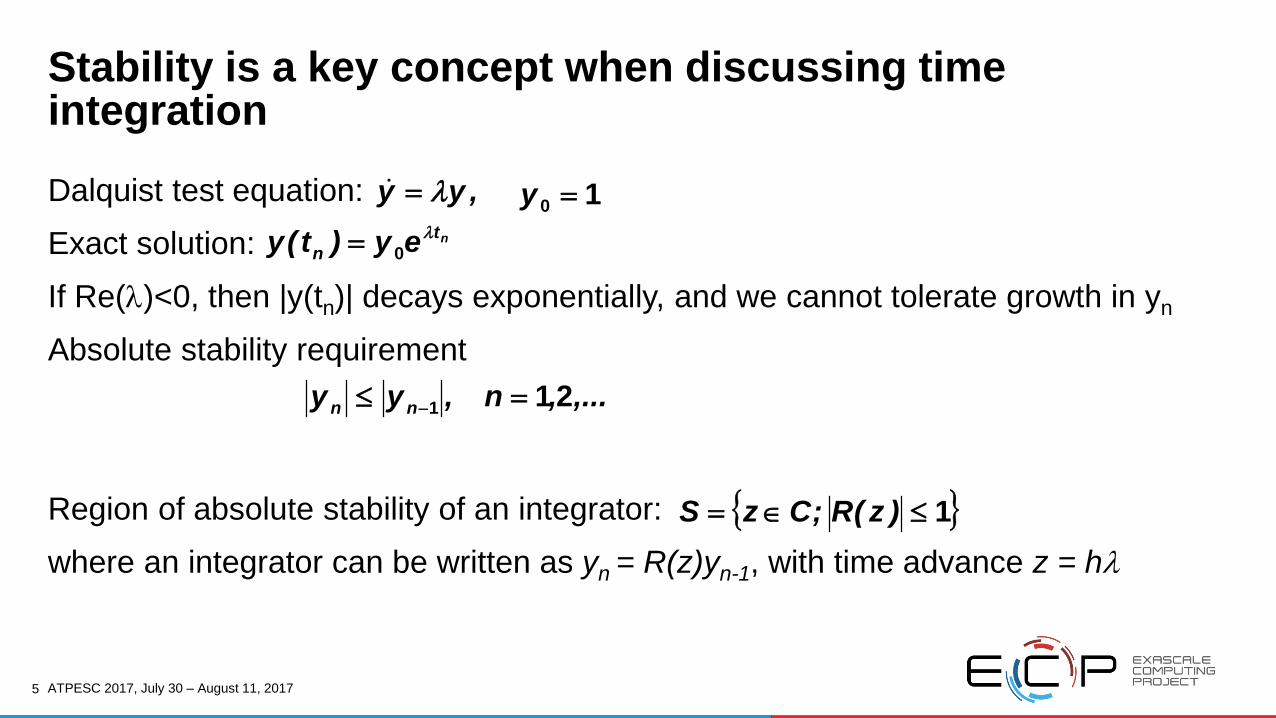
Stability is a key concept when discussing time integration

Dalquist test equation: Exact solution:

If Re(λ)<0, then |y(tn)| decays exponentially, and we cannot tolerate growth in yn

Absolute stability requirement

Region of absolute stability of an integrator:

where an integrator can be written as yn = R(z)yn-1, with time advance z = hλ

,yy λ= 10 =ynt

n ey)t(y λ0=

,...,n,yy nn 211 =≤ −

{ }1≤∈= )z(R;CzS


Forward and backward Euler show different stability restrictions

• Forward Euler:

So, if λ < 0, FE has the step size restriction:

• Backward Euler:

So, if λ < 0, BE has the step size restriction:

( ) λλ h)z(Ryhyy nnn +=⇒+= −− 111

λ−≤

2h

( )λ

λh

)z(Ryhyy nnn −=⇒+= − 1

11

0>h

Forward Euler is an explicit method

Backward Euler is an implicit method


Curtiss and Hirchfelder example demonstrates what can happen with failure to meet the stability step restriction

( )( ) 5050 −=−−= λtcosyy

Solution curvestime

y

Forward Euler h=2.01/50


Meeting the restriction with an explicit method or using an implicit method makes a difference!

( )( ) 5050 −=−−= λtcosyy

time

y

Implicit schemes h=0.5 for BEForward Euler


Explicit and implicit approaches should be selected based on needs of the problem

Explicit MethodsEasy to conceptualize

Easy to code

Do not require solversXStability limits on step sizes

XTracks fastest dynamics

Implicit MethodsLess or nonexistent stability limits

Steps over fastest dynamics

XRequire linear and/or nonlinear solversXSolvers generally require coupling over

all unknowns

XCode complexity higher

Implicit methods are most useful when fast dynamics of little interest are present, and accuracy requirements would dictate a much larger time step for resolution


• (Ascher and Petzold, 1998): If the system has widely varying time scales, and the phenomena that change on fast scales are stable, then the problem is stiff

• Stiffness depends on– Jacobian eigenvalues, λj

– System dimension– Accuracy requirements– Length of simulation

• In general a problem is stiff on [t0, t1] if

• Due to stability requirements, stiff problems generally require implicit approaches

For any time-dependent system, need to know if it is stiff before choosing a numerical solution approach

101 −<<ℜ− )(min)tt( jjλ

Implicit approaches for stiff problems often require a very robust nonlinear solver for each time step solution


Linear multistep methods construct approximations based on prior states• Linear Multistep Methods

• Nonstiff Implicit: Adams-Moulton– K1 = 1, K2 = k, k = 1,…,12

• Stiff: Backward Differentiation Formulas [BDF]– K1 = k, K2 = 0, k = 1,…,5

• Stiff integrators often use a predictor-corrector scheme:

Explicit predictor to give yn(0) Implicit corrector with yn(0) as initial iterate

Stability region is NOT shaded

Re(z)

Im(z

)


Multistage methods construct approximations based on estimates of derivatives at multiple points in a time step• Multistage methods employ multiple stage solutions

• The a’s, b’s, c’s, and s define the method, its order of accuracy, and its stability

• Codes with adaptivity in spatial systems or models cannot easily use multi-step methods due to need to interpolate prior step information

• Runge-Kutta (RK) methods are multistage so do not require prior states

• RK methods require multiple nonlinear solves per time step

• Additive RK methods can apply explicit and implicit methods to a split system allowing consistent approximations while using different methods on each

Butcher Tableau


Additive methods address systems with both stiff and nonstiff components• Split system into stiff, fI, and nonstiff, fE, components• M may be the identity or any nonsingular mass matrix (e.g. FEM)

• Variable step size additive Runge-Kutta Methods combine explicit (ERK) and diagonally implicit (DIRK) RK methods to enable an ImEx integrator

• Let tn,j = tn-1 + cj∆tn:

• Solve for stage solutions, zi, i= 1, …, s, sequentially


Implicit solutions result in nonlinear systems at each time step or stage

• Use predicted value as the initial iterate for the nonlinear solver• Nonstiff systems: Functional iteration or fixed point iteration

• Stiff systems: Newton iteration

ODE DAE


Adaptive methods choose time steps to minimize local truncation error and maximize efficiency

• User-defined tolerances:– Absolute tolerance on each solution component, ATOLi

– Relative tolerance for all solution components, RTOL

• Norm calculations are weighted by:

• Errors are measured with a weighted root-mean-square norm:

• Choose time steps to bound an estimate of the local truncation error; can do with both multistep and multistage methods


The choice of tolerances is critical to accuracy and efficiency for these adaptive methods• The relative tolerance controls error relative to the size of the solution

– RTOL = 10-4 means that errors are controlled to 0.01%– We do not recommend an RTOL above 10-3 nor one close to unit roundoff, 10-15

• The absolute tolerances control the absolute size of error when any solution component may be so small that pure relative error control is meaningless– Ex: solution starting at a nonzero value but decaying to a noise level, ATOL should be set to

the noise level– If different components have different noise levels then want ATOL to be a vector

• In general, want to be a bit conservative with these tolerances– Rule of thumb: use tolerances 0.01 below desired limits to ensure global errors are below limit

• But not too conservative as the integrator will work harder to meet tight tolerances

To use these adaptive methods effectively, choose tolerances carefully!


Rootfinding capabilities are critical in some applications

• Finds roots of solution-dependent user-defined functions, or • Important in applications where problem definition may change based on a

function of the solution

• Rootfinding is a critical feature for applications like power grid where solution-dependent system adaptations are common, e.g. voltage limit on a generator

• Roots are found by looking at sign changes, so only roots of odd multiplicity are found

• Checks each time interval for sign change

• When sign changes are found, apply a modified secant method with a tight tolerance to identify root

0),,( =yytgi 0),( =ytgi


Time integrator algorithms do not need to rely on specific data layouts

• All operations within the integrator can be conducted on vectors• Packages define a vector API; users can use their structures coded to this API• Within SUNDIALS, each vector implementation defines a content structure and

all implemented vector operations, along with routines to clone vectors• For an implicit method, data layouts are used in

– Specific vector implementations (streaming and reduction)

– Solvers (linear and/or nonlinear)

– Problem-defining function evaluations, f and F, and Jacobian evaluations

Using a time integrator on a given machine requires an efficient implementation of the problem-defining functions, as these typically are the dominant cost


SUNDIALS: SUite of Nonlinear and DIfferential / ALgebraic equation Solvers• ODE integrators:

– (CVODE/CVODES) variable order and step stiff BDF and non-stiff Adams– (ARKode) variable step implicit, explicit, and additive IMEX Runge-Kutta

• DAE integrators: (IDA/IDAS) variable order and step stiff integrators• CVODES and IDAS are equipped with forward and adjoint sensitivity analysis• Nonlinear Solver: (KINSOL) Newton-Krylov, Picard, and accelerated fixed point• Serial, MPI, openMP, and pthreads vectors; CUDA will be released this fall• Written in C with interfaces to Fortran• Designed to be easily incorporated into existing codes• Modular design allows users to supply their own data structures• CMAKE-based portable build system• Freely available (BSD license); >11,000 downloads/year from around the world• Active user community supported by sundials-users email list

http://www.llnl.gov/CASC/sundials

http://www.llnl.gov/CASC/sundials


SUNDIALS has been used worldwide in applications from research and industry• Power grid modeling (RTE France, LLNL, ISU) Simulation of clutches and power train parts (LuK GmbH & Co.) Magnetism at the nanoscale (Magpar, Nmag)• 3D parallel fusion (SMU, U. York, LLNL)• Spacecraft trajectory simulations (NASA)• Dislocation dynamics (LLNL)• Combustion and reacting flows (Cantera) Large-scale subsurface flows (Mines, LLNL) 3D battery simulation (ORNL - AMPERE) Computational modeling of neurons (NEURON) Micromagnetic simulations (U. Southampton) Released in third party packages: Red Hat Extra Packages for Enterprise Linux (EPEL SciPy – python wrap of SUNDIALS Cray Third Party Software Library (TPSL)

Magnetic reconnection

Core collapse supernova

Dislocation dynamics

Subsurface flow


Summary• When choosing a time integration method, need to understand

– What the time scales in the system are

– Whether the application requires resolving all time scales

– Whether the system is stiff

– Whether the system has adaptivity in the spatial or model components

– What the accuracy requirements are

• The choice of tolerances can impact both accuracy and performance• Multistep and multistage methods have different characteristics that may make

each better suited to an application• Implicit methods will need algebraic solvers (nonlinear and/or linear)• Time integrators can be implemented in a data agnostic way allowing for use of

application-specific data structures

Documents

Time Integration - MCSpress3.mcs.anl.gov/.../08/...8-7_205pm_Woodward-Time_Integration.pdf · Time Integration Presented to ATPESC ... • Implicit vs. explicit methods ... (e.g