Embed Size (px)
Citation preview

TIME-DEPENDENT SYSTEMS AND CHAOS IN STRING THEORY
DISSERTATION
A dissertation submitted in partial fulfillment of therequirements for the degree of Doctor of Philosophy in the
College of Arts and Sciencesat the University of Kentucky
By
Archisman Ghosh
Lexington, Kentucky
Director: Dr. Sumit R. Das, Professor of Department of Physics and Astronomy
Lexington, Kentucky
2012
Copyright c© Archisman Ghosh 2012
ABSTRACT OF DISSERTATION
TIME-DEPENDENT SYSTEMS AND CHAOS IN STRING THEORY
One of the phenomenal results emerging from string theory is the AdS/CFT corre-spondence or gauge-gravity duality: In certain cases a theory of gravity is equivalentto a “dual” gauge theory, very similar to the one describing non-gravitational inter-actions of fundamental subatomic particles. A difficult problem on one side can bemapped to a simpler and solvable problem on the other side using this correspondence.Thus one of the theories can be understood better using the other.
The mapping between theories of gravity and gauge theories has led to new ap-proaches to building models of particle physics from string theory. One of the impor-tant features to model is the phenomenon of confinement present in strong interactionof particle physics. This feature is not present in the gauge theory arising in the sim-plest of the examples of the duality. However this N = 4 supersymmetric Yang-Millsgauge theory enjoys the property of being integrable, i.e. it can be exactly solved interms of conserved charges. It is expected that if a more realistic theory turns out tobe integrable, solvability of the theory would lead to simple analytical expressions forquantities like masses of the hadrons in the theory. In this thesis we show that theexisting models of confinement are all nonintegrable – such simple analytic expressionscannot be obtained.
We moreover show that these nonintegrable systems also exhibit features of chaoticdynamical systems, namely, sensitivity to initial conditions and a typical route of tran-sition to chaos. We proceed to study the quantum mechanics of these systems andcheck whether their properties match those of chaotic quantum systems. Interest-ingly, the distribution of the spacing of meson excitations measured in the laboratoryhave been found to match with level-spacing distribution of typical quantum chaoticsystems. We find agreement of this distribution with models of confining strong in-teractions, confirming these as viable models of particle physics arising from stringtheory.KEYWORDS: String Theory, AdS/CFT Correspondence,
Integrable Systems, Chaos, Quantum Chaos.

Archisman Ghosh
12 June, 2012

TIME-DEPENDENT SYSTEMS AND CHAOS IN STRING THEORY
By
Archisman Ghosh
Dr. Sumit R. Das(Director of Dissertation)
Dr. Timothy Gorringe(Director of Graduate Studies)
12 June, 2012(Date)

Dedicated to the fond memories of mybrother Atri (Bhutu), whose untimelydemise left me with a changed perspectiveof life. A lot of my curiosity, that eventu-ally drove me to pursue physics, was devel-oped as a kid with my brother, when wewould go around the house taking aparthousehold gadgets and appliances, mixingtogether stuff that came in various bottlesand looking for things to set on fire.
ACKNOWLEDGEMENTS
I would like to begin by thanking Sumit Das and Al Shapere. Through the six long
years, they have been the very best advisors one could have, always encouraging, pa-
tient during unproductive times and ready to talk about anything – research, physics
and more importantly, stuff that is not even remotely related to physics. A few other
professors have also played a pivotal role in my graduate education, through courses
I have taken with them, or through individual discussions – I would like to like to
thank Ganpathy Murthy, Susan Gardner and Ribhu Kaul. I would like to thank my
fellow graduate students, Jae-Hyuk Oh, Joshua Qualls and Diptarka Das, for long
hours of useless and useful exchange of words and exchange of precious ideas every
once in a while. I would like to thank Adel Awad, Willie Merrell and Oleg Lunin –
their presence at UK has been very valuable to my research-career. I would like to
thank my other collaborators, initially Sandip Trivedi, and later, Leopoldo Pando-
Zayas and Dori Reichmann for very successful collaborations. I would like to end this
paragraph with a very special thanks to Pallab Basu. Without his intervention in my
graduate career, I might not have retained my interest in physics till this day.
The full list of people who have prepared me for a graduate education will not fit
in this page. I would still like to mention a few names from my undergraduate days –
Asok K. Mallick, Mahendra K. Verma, Jayanta K. Bhattacharjee, Sreerup Raychaud-
huri, Tapobrata Sarkar and Saurya Das – they have, in particular, been responsible
for building my interest in theoretical physics and in dynamical systems. The list
is incomplete without acknowledging another person – Mr. D. N. Bhattacharya, my
high-school physics teacher, who has been a constant source of encouragement for
sixteen years now.
I would like to thank all my friends in Lexington, who, with all the happy and
sad moments, have made the city a happening place to live in! I would like to end
by thanking my parents, who have through long and rough years, kept valuing my
education over their own well-being and peace of mind.
vi

Contents
Acknowledgements vi
List of Tables x
List of Figures xi
1 Overview 1
2 The AdS/CFT Correspondence 5
2.1 The AdS/CFT Correspondence . . . . . . . . . . . . . . . . . . . . . 5
2.2 Confinement in AdS/CFT . . . . . . . . . . . . . . . . . . . . . . . . 9
3 Integrability and Chaos 11
3.1 What is Integrability? . . . . . . . . . . . . . . . . . . . . . . . . . . 11
3.2 What is Chaos? . . . . . . . . . . . . . . . . . . . . . . . . . . . . . . 11
3.2.1 Lyapunov exponent . . . . . . . . . . . . . . . . . . . . . . . . 12
3.2.2 Transition to Chaos in Hamiltonian systems . . . . . . . . . . 13
3.3 Importance of Integrability in String Theory . . . . . . . . . . . . . . 16
3.4 Integrability in Sigma Models and Coset Spaces . . . . . . . . . . . . 17
4 Chaos in the AdS Soliton Background 19
4.1 The AdS soliton background . . . . . . . . . . . . . . . . . . . . . . . 19
4.2 Classical string in AdS-soliton . . . . . . . . . . . . . . . . . . . . . . 20
4.3 Dynamics of the system . . . . . . . . . . . . . . . . . . . . . . . . . 22
4.3.1 Poincare sections and the KAM theorem . . . . . . . . . . . . 22
4.3.2 Lyapunov exponent . . . . . . . . . . . . . . . . . . . . . . . . 25
vii

5 Analytic Nonintegrability 26
5.1 Analytic Integrability . . . . . . . . . . . . . . . . . . . . . . . . . . . 26
5.2 Nonintegrability in the AdS soliton background . . . . . . . . . . . . 28
5.2.1 Kovacic algorithm . . . . . . . . . . . . . . . . . . . . . . . . . 28
6 Nonintegrability in Generic Confining Backgrounds 32
6.1 Closed spinning strings in generic supergravity backgrounds . . . . . 32
6.1.1 Motion of the string with Ansatz I . . . . . . . . . . . . . . . 33
6.1.2 Motion of the string with Ansatz II . . . . . . . . . . . . . . . 35
6.2 Confining backgrounds . . . . . . . . . . . . . . . . . . . . . . . . . . 36
6.2.1 Regge trajectories from closed spinning strings in confining back-
grounds . . . . . . . . . . . . . . . . . . . . . . . . . . . . . . 36
6.3 Analytic Nonintegrability in Confining Backgrounds . . . . . . . . . . 37
6.3.1 With Ansatz I . . . . . . . . . . . . . . . . . . . . . . . . . . . 37
6.3.2 With Ansatz II . . . . . . . . . . . . . . . . . . . . . . . . . . 38
6.4 Explicit Chaotic Behavior in the MN Background . . . . . . . . . . . 39
7 Quantum Chaos in String Theory 41
7.1 What is Quantum Chaos? . . . . . . . . . . . . . . . . . . . . . . . . 41
7.1.1 Quantum chaos in the Hadronic Spectrum . . . . . . . . . . . 42
7.2 Quantum Chaos in the AdS soliton background . . . . . . . . . . . . 44
A Singularity Resolution in Cosmologies Using AdS/CFT 45
A.1 Motivation and Overview . . . . . . . . . . . . . . . . . . . . . . . . . 45
A.2 The AdS/CFT Correspondence . . . . . . . . . . . . . . . . . . . . . 46
A.3 Setup in Supergravity . . . . . . . . . . . . . . . . . . . . . . . . . . . 46
A.3.1 Supergravity Solution . . . . . . . . . . . . . . . . . . . . . . . 47
A.4 Field Theory Analysis . . . . . . . . . . . . . . . . . . . . . . . . . . 48
A.4.1 Standard Adiabatic Approximation . . . . . . . . . . . . . . . 48
A.4.2 Adiabatic Approximation with Coherent States . . . . . . . . 49
A.4.3 Results . . . . . . . . . . . . . . . . . . . . . . . . . . . . . . . 49
viii

A.5 Conclusions and Outlook . . . . . . . . . . . . . . . . . . . . . . . . . 50
B T p,q and Y p,q Backgrounds 51
B.1 Wrapped strings in general AdS5 ×X5 . . . . . . . . . . . . . . . . . 51
B.1.1 T p,q . . . . . . . . . . . . . . . . . . . . . . . . . . . . . . . . 52
B.1.2 NVE for T 1,1 . . . . . . . . . . . . . . . . . . . . . . . . . . . 54
B.1.3 Y p,q . . . . . . . . . . . . . . . . . . . . . . . . . . . . . . . . 54
B.1.3.1 θ straight line . . . . . . . . . . . . . . . . . . . . . . 55
B.1.4 The exceptional case: S5 . . . . . . . . . . . . . . . . . . . . . 55
B.1.4.1 θ straight line . . . . . . . . . . . . . . . . . . . . . . 56
B.1.4.2 µ straight line . . . . . . . . . . . . . . . . . . . . . . 57
C Straight-line Solution and NVE in Confining Backgrounds 58
C.1 The Klebanov-Strassler background . . . . . . . . . . . . . . . . . . . 58
C.1.1 The straight line solution in KS . . . . . . . . . . . . . . . . . 59
C.2 The Maldacena-Nunez background . . . . . . . . . . . . . . . . . . . 60
C.2.1 The straight line solution in MN . . . . . . . . . . . . . . . . . 60
C.3 The Witten QCD background . . . . . . . . . . . . . . . . . . . . . . 61
C.3.1 The straight line solution in WQCD . . . . . . . . . . . . . . . 61
Bibliography 63
Vita 70
ix
List of Tables
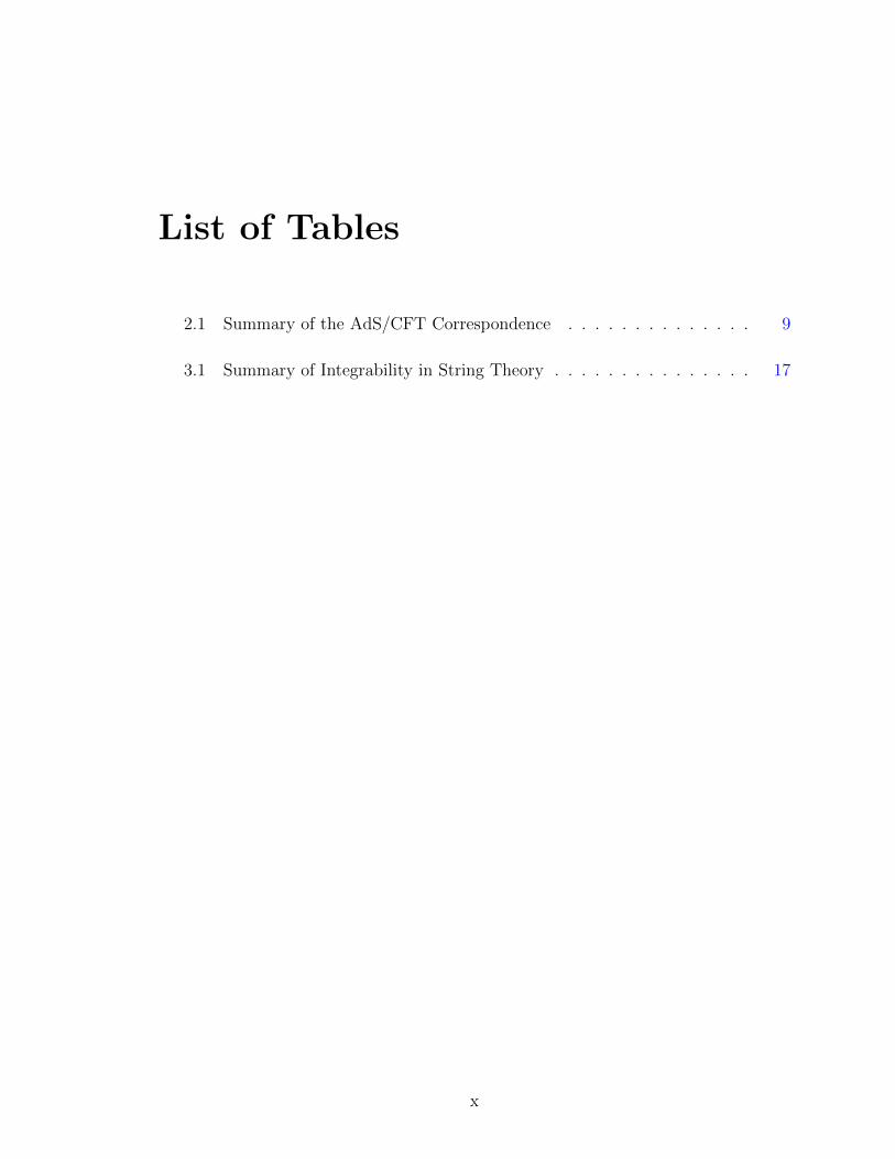
2.1 Summary of the AdS/CFT Correspondence . . . . . . . . . . . . . . 9
3.1 Summary of Integrability in String Theory . . . . . . . . . . . . . . . 17
x

List of Figures
2.1 AdS spacetime in global and Poincare coordinates. . . . . . . . . . . 6
2.2 Confinement from the bulk perspective . . . . . . . . . . . . . . . . . 10
3.1 Illustration of Poincare section of phase-space . . . . . . . . . . . . . 12
3.2 KAM tori breaking into elliptic and hyperbolic points. . . . . . . . . 14
3.3 Poincare sections for Henon-Heiles Equations . . . . . . . . . . . . . . 15
4.1 A classical string in the AdS soliton background. . . . . . . . . . . . . 20
4.2 Motion of a string in AdS soliton background . . . . . . . . . . . . . 23
4.3 Poincare sections for string motion in AdS soliton . . . . . . . . . . . 24
4.4 Lyapunov indices for string motion in AdS soliton . . . . . . . . . . . 25
6.1 String embeddings in a generic confining background . . . . . . . . . 34
6.2 Poincare sections for string motion in Maldacena-Nunez background . 40
6.3 Lyapunov index for string motion in Maldacena-Nunez background . 40
7.1 Quantum level-spacing distribution for integrable and chaotic systems 42
7.2 Level-repulsion in a quantum chaotic system . . . . . . . . . . . . . . 43
7.3 Wavefunction of a quantum chaotic system . . . . . . . . . . . . . . . 43
7.4 Signatures of quantum chaos in AdS soliton . . . . . . . . . . . . . . 44
A.1 A slowly-varying dilaton profile . . . . . . . . . . . . . . . . . . . . . 47
xi

Chapter 1
Overview
String theory is regarded as one of the most challenging frontiers of modern theoreticalphysics. In this theory the fundamental constituents of matter are open and closedstrings rather than particles, and these strings describe both matter and the forcesbetween them. Formulating a consistent quantum mechanical theory of gravitationhas been one of most important problems of the twentieth century. String theory is acandidate solution – at low energies the equations governing the dynamics of closedstrings reduce to Einstein’s equations of general relativity which describe all aspectsof classical gravitational physics. In addition string theory is also a candidate forbeing a unified theory describing all matter and forces in the universe.
One of the most important results that has emerged from String Theory in the lastdecade is the AdS/CFT correspondence, also known as the gauge-gravity duality. Thestatement of the correspondence is that in certain cases a string theory is equivalent toa “dual” gauge theory very similar to the one describing non-gravitational interactionsof fundamental particles. The gauge theory is in one lower dimension than than thegravity theory and since it captures all the physics of the gravity theory, the dualityis called holographic in analogy to how a two-dimensional hologram can reproducea three-dimensional image. When the interactions in the gauge theory are strongenough, the dual string theory can be replaced by classical general relativity. Animportant point here is that the strongly interacting gauge theory, which is difficultto analyze by itself, is mapped to a much simpler problem in gravity. There arealso regimes where gravity problem is no longer classical and does not admit a directanalysis, but is mapped to a simpler problem in a weakly interacting gauge theory –the duality can thus be used both ways.
The greatest triumph of gauge-gravity duality has been in the qualitative under-standing of the quantum properties of black holes. Hawking had shown that blackholes emit radiation like any other hot object and are characterized by thermody-namic quantities like temperature and entropy. General Relativity does not providean underlying microscopic structure to calculate these quantities. Here gauge-gravityduality has been able to provide a microscopic description of a large class of blackholes and has been able to reproduce their entropy and other thermodynamic quan-tities.
Applied in the other direction, gauge gravity has been able to make important
1

predictions in QCD. Quantum Chromodynamics or QCD is the theory of stronginteractions – the force that binds the nucleus of an atom together. At sufficiently hightemperatures nuclear matter undergoes a phase transition into a state where quarksand gluons which are normally confined within the nucleus are freed up. This “quark-gluon plasma” resembles a fluid that flows with a certain viscosity and supports soundwaves. Properties of this are difficult to calculate because of the very strong natureof the interactions. Here gauge-gravity duality can map the problem into a weaklycoupled problem in gravity in the presence of a black hole. A black hole is a naturalobject to introduce here, because it has a temperature just like a fluid. Although thefluid that is considered here is not exactly the quark-gluon plasma of QCD, the resultsobtained are in consistent with QCD experiments, perhaps indicating a broader rangeof applicability of the techniques.
In Chapter 2, we discuss the key concepts of the AdS/CFT correspondence andsome particular details that will be relevant to us in the rest of the thesis.
Nonintegrability in models of Confinement
The mapping between theories of gravity and gauge theories has led to new ap-proaches to building models of particle physics from string theory. One of the impor-tant features to model in this context, is the phenomenon of confinement in stronginteraction in particle physics. Unlike the force of electromagnetism which falls offwith the separation between two electromagnetically charged particles, the force ofinteraction between strongly interacting particles grows with the separation betweenthem. Thus it is not possible to separate and isolate strongly interacting particles– they remain clumped together forming composite entities called “hadrons”. Thisproperty is known as confinement.
This feature of confinement is not exhibited in the gauge theory arising in thesimplest of the examples of the duality, namely the correspondence between stringtheory in pure Anti-de Sitter spacetime and N = 4 supersymmetric Yang-Mills gaugetheory. However this N = 4 supersymmetric Yang-Mills theory enjoys the propertyof being integrable – the theory can be exactly solved in terms of conserved charges.It is expected that if a more realistic theory is integrable, solvability of the theorywould imply simple analytical expression for the quantities like masses of the hadronsin the theory. We discuss the definition and implications of integrability in greaterdetail in Chapter 3.
We move on to study gravitational theories whose gauge theory duals are morerealistic in the sense that they exhibit the phenomenon of confinement. It turnsout that such geometries cannot be infinite, but have to cap off like a cigar. Thefiniteness of the geometry sets a length scale to it, precisely the distance at whichthe cigar caps off, and this length scale in turn sets an energy scale in the dual gaugetheory. There is a minimum energy of excitations or a “mass gap” in the dual theory,again a desirable feature from the point of view of real QCD. Many such “confininggeometries” exist and we summarize some of the the more popular ones in AppendixC.
A main emphasis of this thesis is to study integrability in some of these confining
2

backgrounds. In Chapter 4, we begin with one such background, the AdS soliton,which we use an an example throughout this thesis. We study the dynamics of closedstrings of this geometry. A numerical analysis reveals that the system is chaotic. Itshows an exponential sensitivity to initial conditions that chaotic systems do, andshows a typical transition to chaos as a nonlinear parameter is varied. Chaotic dy-namical systems are known to be nonintegrable, and our analysis thus gives a negativeresult for integrability in the AdS soliton. In Chapter 5, we obtain the same conclusionusing analytical, as opposed to numerical methods. The full analysis of integrabilityinvolves sophisticated and relatively recently developed techniques from differentialGalois theory, however the demonstration of nonintegrability can be achieved withthe implementation of a small algorithm to the differential equations governing thedynamical system. In Chapter 6, we extend our result to a large class of confining ge-ometries, many of them being the most commonly cited ones. Our analysis thus rulesout integrability in a large number of backgrounds – thus simple analytic expressionsfor the hadron excitations in the dual theories cannot be obtained.
Quantum Chaos
A natural question to ask at this stage is “What is the full quantum spectrum ofthe systems that we are studying?” The distribution in spacing of energy levels inthe spectra of certain chaotic quantum systems have been observed to be qualita-tively different from the universal distribution the same spacing for integrable sys-tems. Interestingly, the distribution of the spacing of hadron excitations measured inthe laboratory is found to match with level-spacing distribution of typical quantumchaotic systems. In Chapter 7, we numerically obtain the spectrum for the AdS soli-ton background and find an agreement with the typical quantum chaotic level-spacingdistribution. The quantum analysis thus ends with a positive note confirming modelsof confinement coming from string theory as viable models of physics of the stronginteraction.
Cosmological singularities
We devote Appendix A to review a model that attempts to understand “singu-larities” in general relativity using the correspondence. In General Relativity, “sin-gularities” are regions where the theory itself breaks down and a quantum theory ofgravity is expected to take over. Since the universe is expanding, our present modelof cosmology tells us that at some very early time, the entire universe was containedin a very small region in space. In such a situation General Relativity would breakdown and such a singularity is known as the Big Bang. One can have models in cos-mology (although this is probably not true for our own universe) where the universestops expanding and begins to contract and shrinks to a very small region leadingto a Big Crunch. Big Bangs and Big Crunches are examples of cosmological singu-larities. These singularities are very disturbing to physicists because they represent
3

a “beginning of time” or “end of time”. There is no way for an observer to bypassthem.
A quantum theory of gravitation is expected to smooth out or resolve these singu-larities. It might also provide some interpretation of cosmological data from the veryearly universe. Before the advent of String Theory there was no consistent quantumtheory of gravity and and understanding of cosmological singularities had been a ma-jor theoretical problem. Recently there has been some progress in understanding thenature of singularities using String Theory and in particular gauge-gravity duality.As described above, the duality is between a gauge field theory and a string theory.When the gauge theory coupling is large, the string theory can be approximated byGeneral Relativity in a conventional spacetime. When the gauge theory coupling isweak, General Relativity breaks down and there is no conventional notion of spaceand time. The gauge theory however is defined for all values of coupling even whenGeneral Relativity has ceased to be valid in the dual theory.
Several groups have tried to use this and obtain toy models of cosmological singu-larities whose gauge theory duals have a time-dependent parameter like the coupling.One would like to see if we can use the gauge theory to calculate the time evolutionof the system in a regime where the gravitational description in terms of GeneralRelativity is no longer valid. We have constructed such a toy model where the gaugetheory coupling is slowly varying with time. It starts off with a large value in earlytimes and goes on to a large value at late times but is small at intermediate times.In the dual theory there is a good spacetime description in early times which breaksdown at intermediate times. The gauge theory however remains to be valid at alltimes and can be used to study the behavior of the dual gravity. The question thatwe ask is what happens at late times where a General Relativity description mightagain be applicable. There are two possibilities. One can be left with smooth space-time like the one we started out with, the energy that is pumped in to the systemduring the contracting phase is extracted out during the expanding phase. Alterna-tively, some of the energy pumped into the system might get distributed between thevarious modes of the system and get thermalized. In that case one is left with a blackhole in the gravity picture. Earlier attempts to obtain such “bouncing cosmologies”have often led to black holes that fill the universe.
We have developed a technique called “adiabatic approximation” in the field the-ory that is valid when the variation of the coupling is slow enough. In the regime ofparameters where our approximation is valid, we have shown that a big black hole isnever formed. If a black hole is formed, its size is small compared to the overall sizeof the universe. We are still trying to understand whether the energy is thermalizedor we have a perfectly smooth spacetime at late times. Our approach is one of thevery few methods where the question of bounce can be addressed in a controlled andself-consistent fashion.
4

Chapter 2
The AdS/CFT Correspondence
In Section 2.1, we discuss the AdS/CFT correspondence, an equivalence betweengauge theories and gravity, first introduced by Maldacena (1998) [1] and more ex-plicitly worked out by Gubser, Klebanov, Polyakov and Witten [2, 3] (for a standardreview, see [4]). In Section 2.2, we discuss the dual description of confinement in fieldtheories, that is going to be relevant to us.
2.1 The AdS/CFT Correspondence
The AdS/CFT correspondence relates a theory of gravity to a gauge theory withno dynamical gravity. In the simplest example of the correspondence the theory ofgravity is a Type IIB String Theory on the AdS5 × S5 background and the dualgauge theory is the N = 4 supersymmetric SU(N) Yang-Mills Theory. The AdS5
background is usually written out in either one of the two popular coordinate choices:
• Global AdS, that covers the entire AdS spacetime, and
• Poincare patch, does not cover the entire spacetime and has a coordinate horizonat r = 0.
The metric for AdS5 × S5 in the two coordinate systems is given below:
Global AdS: ds2 = −(1 +r2
R2AdS
)dt2 +dr2
1 + r2
R2AdS
+ r2 dΩ23 +R2
AdS dΩ25 . (2.1)
Poincare patch: ds2 =r2
R2AdS
(−dt2 + dx23) +
R2AdS
r2dr2 +R2
AdS dΩ25 . (2.2)
Here RAdS is the length scale associated with the geometry, which we will often setto unity. Ω5 are the coordinates of 5-sphere S5. For most of this thesis, this partof the geometry is also not going to be very important to us.1 We will call r theradial direction. The transverse directions are then Ω3 and x3 in the two cases, the
1We will not be dealing with fields dependent in the S5 directions. In other words, we will ignorethe Kaluza-Klein modes coming from the dependence of fields in these internal directions.
5
(a) Global coordinates
r=0horizon
r= 8
boundary
(b) Poincare patch
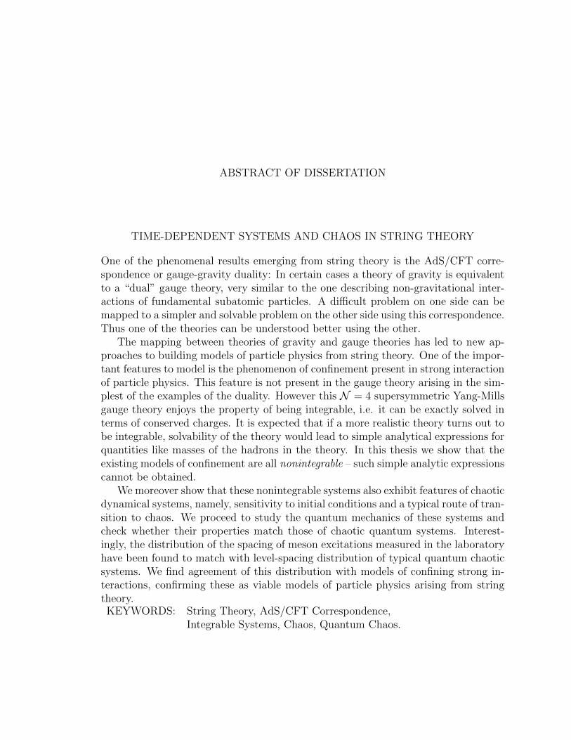
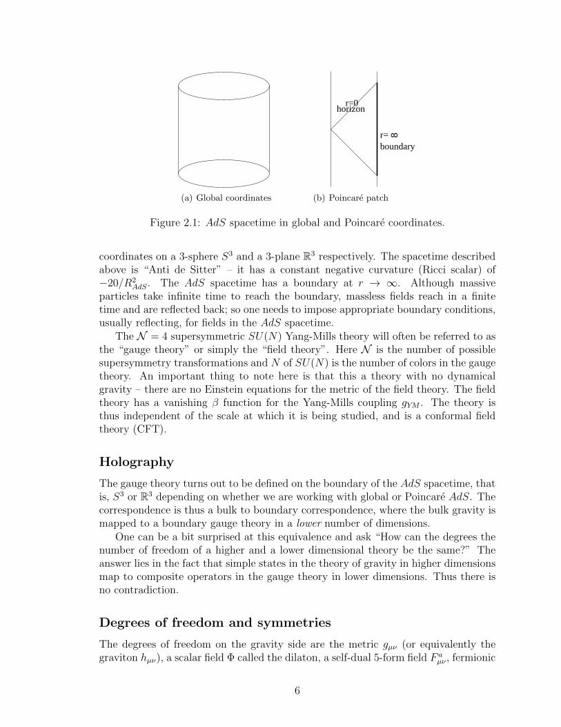
Figure 2.1: AdS spacetime in global and Poincare coordinates.
coordinates on a 3-sphere S3 and a 3-plane R3 respectively. The spacetime describedabove is “Anti de Sitter” – it has a constant negative curvature (Ricci scalar) of−20/R2
AdS. The AdS spacetime has a boundary at r → ∞. Although massiveparticles take infinite time to reach the boundary, massless fields reach in a finitetime and are reflected back; so one needs to impose appropriate boundary conditions,usually reflecting, for fields in the AdS spacetime.
The N = 4 supersymmetric SU(N) Yang-Mills theory will often be referred to asthe “gauge theory” or simply the “field theory”. Here N is the number of possiblesupersymmetry transformations and N of SU(N) is the number of colors in the gaugetheory. An important thing to note here is that this a theory with no dynamicalgravity – there are no Einstein equations for the metric of the field theory. The fieldtheory has a vanishing β function for the Yang-Mills coupling gYM . The theory isthus independent of the scale at which it is being studied, and is a conformal fieldtheory (CFT).
Holography
The gauge theory turns out to be defined on the boundary of the AdS spacetime, thatis, S3 or R3 depending on whether we are working with global or Poincare AdS. Thecorrespondence is thus a bulk to boundary correspondence, where the bulk gravity ismapped to a boundary gauge theory in a lower number of dimensions.
One can be a bit surprised at this equivalence and ask “How can the degrees thenumber of freedom of a higher and a lower dimensional theory be the same?” Theanswer lies in the fact that simple states in the theory of gravity in higher dimensionsmap to composite operators in the gauge theory in lower dimensions. Thus there isno contradiction.
Degrees of freedom and symmetries
The degrees of freedom on the gravity side are the metric gµν (or equivalently thegraviton hµν), a scalar field Φ called the dilaton, a self-dual 5-form field F a
µν , fermionic
6

superpartners of all the fields and the massive higher-string modes. Since supersym-metry is unbroken, one can consistently work in a basis where the fermionic fieldsare set to zero. The stringy excitations are characterized by an energy scale 1/
√α′.
If we can restrict ourselves to energy scales that are much smaller the string energyscale, we will not excite any of the higher-string modes, and we will be able to restrictourselves to the massless modes that are present in supergravity. This can be done ifthe length scale of our geometry RAdS is much larger than the string length ls ∼
√α′.
In that limit, the Type IIB string theory reduces to the Type IIB supergravity, withthe action:
SSUGRA5D =
1
2κ210
∫d5x
(R5D − 2Λ− 1
2∂µΦ∂µΦ− R2
AdS
8F aµνF
aµν + . . .
)(2.3)
The degrees of freedom on the gauge theory side are the gauge field, four Weylfermions and six real scalars, all in the adjoint representation of SU(N). The internalsymmetries of the gauge theory match the isometries of the dual spacetime. SYM in3 + 1 dimensions has a conformal group of SO(4, 2) and the R-symmetry group fora N = 4 theory is SU(4) which is same as SO(6). The isometry of AdS5 × S5 isSO(4, 2)× SO(6).
Relationship between parameters
An important insight about AdS/CFT comes from the relationship between the pa-rameters on either side of the correspondence. The parameters on the gravity sideare the length scale associated with the geometry RAdS, the string length ls and thestring coupling gs.
2 The parameters on the gauge theory side are the Yang-Mills cou-pling gYM and the N of the gauge group. It has been shown by ’t Hooft that in thelarge N limit of gauge theories (N → ∞, gYM → 0, g2
YMN =finite), the appropriatecoupling is the combination λ ≡ g2
YMN , now known as the ’t Hooft coupling. Theseparameters are related by
g2YM = 4πgs , λ ≡ g2
YMN =R4AdS
l4s. (2.4)
Thus the ’t Hooft large N limit of the gauge theory corresponds to a classical limitstring theory with the quantum corrections suppressed by 1/N . Moreover, the aboverelations tell us that the large ’t Hooft coupling limit (λ → ∞), corresponds to thelow-energy supergravity truncation of the string theory where the stringy modes aresuppressed by α′. In this limit, the AdS/CFT correspondence can be viewed as anequivalence between Type IIB supergravity in AdS to a large ’t Hooft coupling gaugetheory.
Correspondence between fields and operators
The AdS/CFT correspondence, can be formulated more mathematically in the super-gravity approximation. The mathematical statement of the correspondence is that
2In String Theory, the coupling gs is not an independent parameter, but is dynamically deter-mined by the value of the dilaton gs = Φ.
7

the partition function of the field theory in the presence of a source J coupled to theoperator O is same as the exponential of the classical action with the solution of theclassical field equations plugged in, where the boundary value of field Φ dual to theoperator O being the source J up to a scaling.
Z4D[J ] ≡∫DΦ exp
(iS + i
∫d4x JO
)= exp(iS[ΦCl]) (2.5)
with limr→∞
r∆ΦCl(r, x) = J(x) .
Here ∆ is just the scaling dimension of the operator O. For a scalar field in AdSd+1
for example, ∆ = ∆− where,
∆± =d
2±√d2
4+m2R2
AdS . (2.6)
With this prescription, the quantum correlation functions in the field theory can beobtained by taking repeated derivatives of the classical action in supergravity withrespect to the boundary value of the field. For example, for the simple case where∆ = 0, the two-point function reads:
iG(x− y) ≡ 〈T O(x)O(y)〉 =1
Zδ2Z4D
δJ(x)δJ(y)=
−iδ2S[ΦCl]
δΦCl(x)δΦCl(y). (2.7)
AdS/CFT at finite temperature
One can extend the AdS/CFT correspondence to a finite temperature. The dualof the N = 4 SYM at a finite temperature is a black three brane metric given (inRAdS = 1 units) by,
Global AdS: ds2 = −f(r)dt2 +dr2
f(r)+ r2 dΩ2
3 , f(r) = 1 + r2 − r2h(1 + r2
h)
r2.
(2.8)
Poincare patch: ds2 = −f(r)dt2 +dr2
f(r)+ r2dx2
3 , f(r) = r2
(1− r4
h
r4
). (2.9)
The Hawking temperature TH in the two cases is given by
TH =2r2
h + 1
2πand
rhπ
respectively. (2.10)
The temperature T of the field theory is same as the temperature TH of the geom-etry: T = TH . The entropy of the field theory can be obtained from the entropyof the horizon of the dual geometry, which using the area-entropy relation is simplyproportional to the area of horizon. The entropy density s of N = 4 SYM at strongcoupling is given by,
s =π2
2N2T 3 . (2.11)
8

Type II B String Theory inAdS5 × S5
⇐⇒ Large N limit of N = 4,SU(N) Super Yang Mills
Flux N ↔ Rank of SU(N)String coupling
gs = eΦ 4πgs = g2YM Yang Mills coupling
String length
ls ∼√α′
R4AdSl4s
= g2YMN ≡ λ ’t Hooft coupling
Type II B classical SUGRA ⇐= Large ’t Hooft couplingStringy corrections α′ Planar corrections
Quantum correctionslPlRAdS
1N corrections
e(iS[ΦCl]) = Z4D[J ]Pure AdS5 × S5 ↔ Vacuum of SYM
Normalizable modes ↔ Excited states of SYM
Non-normalizable modes ↔ Deformation of SYM action
Black-brane geometry ↔ SYM at finite temperature
Table 2.1: Summary of the AdS/CFT Correspondence
2.2 Confinement in AdS/CFT
In a confining theory, the vacuum expectation value of the Wilson loop has an arealaw behavior [5]
〈W (C)〉 ≡ Tr
[P exp
(i
∮C
A
)]' exp(−σA(C)) (2.12)
where A(C) is the area of the loop enclosed by the loop C. The constant σ is called thestring tension. The area law 2.12 is equivalent to the linear confining quark-antiquarkpotential V (L) ∼ σL. This can be seen simply by considering a rectangular loop Cwith sides of length T and L in Euclidean space as in Figure 2.2(a). For large valuesof T , we have, when V (L) ∼ σL and interpreting T as the time direction,
〈W (C)〉 ∼ exp(−TV (L)) (2.13)
The the dual description of a quark-antiquark pair on the boundary field theory is astring stretching into the bulk of the geometry. The dual of the expectation value ofthe Wilson loop operator is the area of the string that minimizes the action. In a thecase of pure AdS, the string can stretch freely into the bulk and finally gives a resultfor the minimum action worldsheet that is consistent with the conformal invarianceof N = 4 SYM. However if the geometry is capped off, like that in Figure 4.1, thenonce the string hits the cap, with further separation between q and q, the majorcontribution to the world sheet area comes from the “wall” sitting at the tip of thecap [Fig.2.2(b)]. Then with separation between q and q, the area of the worldsheetincreases linearly. This gives a linear dependence of the the expectation of the Wilsonloop with Lqq and thus we get a confining potential V (Lqq) ∼ Lqq.
9

T
L
(a) Wilson loop (b) Worldsheet in bulk
Figure 2.2: Confinement in a field theory is indicated by an area law for the Wilsonloop. In the gravity perspective this maps to the effective area of a string world sheetstretching into the bulk. For a geometry with a confining wall, the area of the worldsheet is essentially proportional to the separation between q and q.
10

Chapter 3
Integrability and Chaos
In this chapter we go over the basics of integrability and chaos. In Section 3.1 weintroduce the definition of an integrable systems and in Section 6.4 we introduce theproperties of a chaotic system. In Section 3.3 we discuss the importance of integrabil-ity in the context string theory and the AdS/CFT correspondence. In section 3.4 wereview the main results of [6], that 2-D sigma models and coset models are integrable.
3.1 What is Integrability?
In classical mechanics, a system is integrable when there are the same number ofconserved quantities as the pairs of canonical coordinates. One can then make acanonical transformation to a coordinate system where these conserved quantities arethe conserved momenta. In these “action-angle coordinates”, the conserved momentaare the action variables Ii and the corresponding coordinates are the angle variablesθi.
θi = Iit , Ii = constant . (3.1)
The theory is thus exactly solvable in terms of these constants of motion. For anonintegrable theory one can not write down a closed form analytic solution in general.
For a classical system with n degrees of freedom to be integrable, there are nconserved momenta pi, which have zero Poisson bracket with each other and with theHamiltonian H.
H, pi = 0 , pi, pj = 0 (3.2)
In quantum mechanics the Poisson brackets are replaced by the commutators. Wehave a net of n momenta that commute with themselves and the Hamiltonian.
[H, pi] = 0 , [pi, pj] = 0 (3.3)
3.2 What is Chaos?
Quoting from [7], “Chaos is the term used to describe the apparently complex be-havior of what we consider to be simple, well-behaved systems. Chaotic behavior
11

1
q2
q
Figure 3.1: Poincare section of phase-space for a 2-D dynamical system. As theparticle moves, it goes around the torus in the q1 direction and also winds around thetorus in the q2 direction. For each torus, the energies corresponding to each of thetwo degrees of freedom is conserved separately. For the tori of rational winding, theorbit goes around the torus q times and winds around it p times and comes back tothe same point.
when looked at casually, looks erratic and almost random . . . ”. The behavior is seenin systems that are complete deterministic and the apparent randomness is just amanifestation of a strong sensitivity to initial conditions the system has – with a veryslight change of initial conditions, a chaotic system can land up in a very differentstate. This sensitivity to initial conditions, whose meaning will be made more precisein §3.2.1, can be taken to be a working definition of chaos. Chaos is typically seenin nonlinear systems – dynamical systems governed by equations of motion that arenonlinear. One of the many universal properties of chaos is the universality of theroute to chaos a system takes as a nonlinear parameter is dialed. We look at theroute of transition to chaos for Hamiltonian systems in §3.2.2.
3.2.1 Lyapunov exponent
One of the trademark signatures of chaos is the sensitive dependence on initial con-ditions, which means that for any point X in the phase space, there is (at least) onepoint arbitrarily close to X that diverges from X. The separation between the twois also a function of the initial location and has the form ∆X(X0, τ). The Lyapunovexponent is a quantity that characterizes the rate of separation of such infinitesimallyclose trajectories. Formally it is defined as,
λ = limτ→∞
lim∆X0→0
1
τln
∆X(X0, τ)
∆X(X0, 0)(3.4)
12

3.2.2 Transition to Chaos in Hamiltonian systems
An integrable system has the same number of conserved quantities as degrees offreedom. A convenient way to understand these conserved charges is by looking atthe phase space. Let us assume that we have a system with N position variables qiwith conjugate momenta pi. The phase space is 2N -dimensional. Integrability meansthat there are N conserved charges Qi = fi(p, q) which are constants of motion. Oneof them is the energy. These charges define a N -dimensional surface in the phasespace which is a topological torus. The 2N -dimensional phase space is nicely foliatedby these N -dimensional tori. In terms of action-angle variables (Ii, θi) these torijust become surfaces of constant action. With each torus there are N associatedfrequencies ωi(Ii), which are the frequencies of motion in each of the action-angledirections. An illustration for a 2 dimensional system is given in Figure ??. Thetori which have rational ratios of frequencies, i.e. miωi = 0 with m ∈ Q are calledresonant tori. The total number of tori of rational winding is a set of Lebesguemeasure zero. However infinitesimally close to a torus of rational winding, there existtori of irrational winding. They are called the KAM (Kolmogorov-Arnold-Moser)tori.
It is interesting to study what happens to these tori when an integrable Hamilto-nian is perturbed by a small nonintegrable piece. The KAM theorem states that mosttori survive, but suffer a small deformation [8, 7]. However the resonant tori whichhave rational ratios of frequencies, i.e. miωi = 0 with m ∈ Q, get destroyed andmotion on them become chaotic. For small values of the nonintegrable perturbations,these chaotic regions span a very small portion of the phase space and are not readilynoticeable in a numerical study. As the strength of the nonintegrable interactionincreases, more tori gradually get destroyed. A nicely foliated picture of the phasespace is no longer applicable and the trajectories freely explore the entire phase spacewith energy as the only constraint. In such cases the motion is completely chaotic.
Henon-Heiles equations
The Henon-Heiles equation is a nonlinear nonintegrable Hamiltonian system. It isdescribed by the potential
V (x, y) =1
2
(x2 + y2 + 2x2y − 2
3y3
). (3.5)
Its equations of motion show typical characteristics of transition to chaos of a Hamil-tonian system. In Figure 3.3 we look at the Poincare section of phase space as theconserved energy E of the system is increased from 1/100 to 1/6. For small values ofE, the most tori are intact. with increasing E, the KAM tori near the resonant toristart breaking into smaller elliptic tori in accordance with KAM theorem. For largevalues of E all the tori break and fill the entire phase space (Arnold diffusion). Hereeach color represents a different initial condition and hence a different torus. Themixing of colors in the final picture indicates the filling up of phase space by the tori.
13
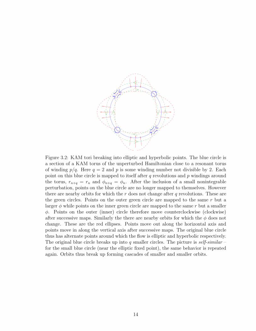
Figure 3.2: KAM tori breaking into elliptic and hyperbolic points. The blue circle isa section of a KAM torus of the unperturbed Hamiltonian close to a resonant torusof winding p/q. Here q = 2 and p is some winding number not divisible by 2. Eachpoint on this blue circle is mapped to itself after q revolutions and p windings aroundthe torus, rn+q = rn and φn+q = φn. After the inclusion of a small nonintegrableperturbation, points on the blue circle are no longer mapped to themselves. Howeverthere are nearby orbits for which the r does not change after q revolutions. These arethe green circles. Points on the outer green circle are mapped to the same r but alarger φ while points on the inner green circle are mapped to the same r but a smallerφ. Points on the outer (inner) circle therefore move counterclockwise (clockwise)after successive maps. Similarly the there are nearby orbits for which the φ does notchange. These are the red ellipses. Points move out along the horizontal axis andpoints move in along the vertical axis after successive maps. The original blue circlethus has alternate points around which the flow is elliptic and hyperbolic respectively.The original blue circle breaks up into q smaller circles. The picture is self-similar –for the small blue circle (near the elliptic fixed point), the same behavior is repeatedagain. Orbits thus break up forming cascades of smaller and smaller orbits.
14

- 0.10 - 0.05 0.05 0.10 0.15
- 0.10
- 0.05
0.05
0.10
e
1
100
- 0.15 - 0.10 - 0.05 0.05 0.10 0.15
- 0.15
- 0.10
- 0.05
0.05
0.10
0.15
e
1
80
- 0.15 - 0.10 - 0.05 0.05 0.10 0.15 0.20
- 0.15
- 0.10
- 0.05
0.05
0.10
0.15
e
1
60
- 0.2 - 0.1 0.1 0.2
- 0.2
- 0.1
0.1
0.2
e
1
40
- 0.2 - 0.1 0.1 0.2 0.3
- 0.2
- 0.1
0.1
0.2
e
1
25
- 0.2 0.2 0.4
- 0.4
- 0.2
0.2
0.4
e
1
12
- 0.4 - 0.2 0.2 0.4 0.6
- 0.4
- 0.2
0.2
0.4
e
1
8
- 0.4 - 0.2 0.2 0.4 0.6 0.8 1.0
- 0.6
- 0.4
- 0.2
0.2
0.4
0.6
e
1
6
Figure 3.3: Poincare sections for Henon-Heiles Equations. This demonstrate breakingof the KAM tori en route to chaos. Each color represents a different initial condition.For smaller values of E the sections of the KAM tori are intact curves, except for theresonant ones. The tori near the resonant ones start breaking as E is increased. Forvery large values of E all the colors get mixed – this indicates that all the tori getbroken and they fill the entire phase space.
15

3.3 Importance of Integrability in String Theory
The study of integrability has acquired a new importance in light of the AdS/CFTcorrespondence. For an excellent and relatively contemporary review refer to [9]. Aswe have already noted in Chapter 2, the AdS/CFT correspondence, in its simplestform maps Type II B String Theory in AdS5 × S5 to a maximally supersymmetricYang-Mills (N = 4 SYM) theory. In the small coupling limit (λ → 0) N = 4 SYMhas been shown to be integrable. The local operators of the theory have a one-to-one mapping with states of a certain quantum spin chain. The planar model is ageneralization of the Heisenberg spin chain and the Hamiltonian is of the integrablekind. This implies that the spectrum can be solved efficiently by the correspondingBethe Ansatz. The anomalous dimensions of the operators in the gauge theory canthus be calculated. Results have been obtained for one loop and higher loops andintegrability is believed to be true to all loops at small coupling.
In the strong coupling limit (λ → ∞), the dual string theory in AdS5 × S5 hasbeen shown to be integrable. The world sheet string theory maps to a sigma modelin PSU(2,2|4)
SO(4,1)×SO(5)and integrability has been established in the bosonic sector of the
sigma model in [10] and completed with the inclusion of fermions in [6]. One has toshow that string motion in AdS5 × S5 has an infinite number of conserved charges1. Following [6], we go through a sketch of the proof of integrability in maximallysymmetric coset spaces in Section 3.4.
The question now is what this integrability can be useful for. For one thing,integrability has allowed us to obtain many classical solutions of the theory thatwould otherwise have been impossible to find [11, 12]. Known to be solvable in theweak and strong coupling limits, one can now look into a finite coupling window inan integrable theory like N = 4 SYM. For certain states of the theory, one can finda complete and exact description of the spectrum far beyond what is possible usingjust ordinary QFT.
What exactly do we mean by solving a theory? In an example like the harmonicoscillator or the Hydrogen atom, one actually obtains the spectrum as a simple alge-braic expression. It would be too much to hope to expect such a simplistic behavior inour models. The best we can expect to find is a system of algebraic equations whosesolution determines the spectrum. What integrability achieves here, is that it vastlyreduces the complexity of the spectral problem by bypassing almost all the steps ofstandard QFT methods, Feynman graphs, loop integrals, regularization, etc. The in-tegrability approach should directly predict the algebraic equations determining thescaling dimension D: f(λ,D) = 0 – an equation that includes the coupling constantλ in a functional form. This is what we call a solution to a spectral problem.
An important open question is whether integrability can be extended to moreQCD-like theories.2 The original form of AdS/CFT duality was for conformally in-variantN = 4 SYM theory but this can be deformed in various ways to produce stringduals to confining gauge theories with less or no supersymmetry. The construction of
1Although established classically, the quantum commutator algebra of such charges is not fullyunderstood. However there are strong evidences to suspect that the full quantum theory is integrable
2This is one of the motivations discussed in the introduction of [6].
16

Any symmetric coset model
(Strings nonintegrable even at a classical level)
[Mandal, Suryanarayana, Wadia (2002)][Bena, Polchinski, Roiban (2003)](infinite set of conserved charges)
(numerical demonstration of chaos)[Pando-Zayas, Terrero-Escalante (2010)][Basu, Das, AG (2011)][Basu, Pando-Zayas (2011)](analytical techniques from differential Galois theory)
(class of confining backgrounds)[Basu, Das, AG, Pando-Zayas, (2012)]
Any symmetric coset model[Mandal, Suryanarayana, Wadia (2002)][Mandal, Suryanarayana, Wadia (2002)]
Table 3.1: Summary of Integrability in String Theory
[10, 6] does not readily generalize to these less symmetric backgrounds. One prime ex-ample of a confining background is the AdS soliton [13, 14]. Similar geometries havebeen used extensively to model various aspects of QCD in the context of holography[15]. Here we will look at the question of integrability of bosonic strings on an AdSsoliton background. Although it is much more interesting to explore full quantumintegrability, to begin with we may ask whether we can find enough conserved chargeseven at a purely classical level. The answer turns out to be negative. By choosing aclass of simple classical string configurations, we show that the Lagrangian reducesto a set of coupled harmonic and anharmonic oscillators that correspond to the sizefluctuation and the center of mass of motion of the string. The oscillators decouplein the low energy limit. With increasing energy the oscillators become nonlinearlycoupled. Many such systems are well known to be chaotic and nonintegrable [8, 7].It is no surprise that our system also shows a similar behaviour. Possibly chaotic be-haviour of a test string has been argued previously in black hole backgrounds [16, 17].However our problem is somewhat different as we are looking at a zero temperaturegeometry without a horizon. In [18] non-integrability of string theory in AdS5 × T 1,1
is discussed.
3.4 Integrability in Sigma Models and Coset Spaces
We consider a 2-D nonlinear sigma model where the field g(x) ∈ gauge group G, withthe Lagrangian L = Tr(dg−1∧∗dg). The following current, which corresponds to theglobal symmetry of left multiplication, can be regarded as a flat gauge connection inthe Lie algebra G.
j = −(dg)g−1 , d ∗ j = 0 , dj + j ∧ j = 0 . (3.6)
17

By taking linear combinations of j and ∗j, one can show that there are an infinitenumber of flat connections.
a = αj + β ∗ j , da+ a ∧ a = (α2 − α− β2)j ∧ j = 0 ,
if α =1
2(1± coshλ) , β =
1
2sinhλ . (3.7)
Given any flat connection, the equation dU = −aU is integrable: action on both sideswith d gives zero. On a simply connected space, given an initial value U(x0, x0) = 1,this defines a group element U(x, x0). This is just the Wilson line, defining the paralleltransport with the connection a,
U(x, x0) = P exp
(−∫C
a
), (3.8)
where C is any contour running from x0 to x, and P denotes path ordering. Theflatness of the connection implies that the Wilson line is invariant under continuousdeformations of C. Following [19, 20], one can immediately construct an infinitenumber of conserved charges by taking the outbound spatial Wilson line at fixedtime,
Qa(t) = Ua(∞, t;−∞, t) . (3.9)
An analogous construction of conserved charges for coset models G/H is carried out in[6]. The construction is also extended to the Green-Schwarz superstring on AdS5×S5.
18

Chapter 4
Chaos in the AdS SolitonBackground
In this chapter, we study the dynamics of closed strings in the AdS soliton back-ground. In Section 4.1, introduce the background. In Section 4.2, we set up thedynamics of the string in the background and obtain the equations of motion. InSection 4.3, we study the dynamics of the string numerically. In a certain regimeof parameter space the system shows a zigzag aperiodic motion characteristic of achaotic system. Then look at the phase space – integrability implies the existenceof a regular foliation of the phase space by invariant manifolds, known as KAM(Kolmogorov-Arnold-Moser) tori, such that the Hamiltonian vector fields associatedwith the invariants of the foliation span the tangent distribution. Our numericsshows how this nice foliation structure is gradually lost as we increase the energyof the system. To complete the discussion we also calculate Lyapunov indices forvarious parameter ranges and find large positive values in chaotic regimes indicatingan exponential sensitivity to initial conditions. The bulk of this chapter is based onthe work done in [21]1.
4.1 The AdS soliton background
The AdS soliton metric for an asymptotically AdSd+1 background is given by [13],
ds2 = L2α′e2u(−dt2 + T2π(u)dθ2 + dw2
i ) +1
T2π(u)du2
,
where T2π(u) = 1−(d
2eu)−d
. (4.1)
At large u, T2π(u) ≈ 1 and (4.1) reduces to AdSd+1 in Poincare coordinates. Howeverone of the spatial boundary coordinates θ is compactified on a circle. The remaining
1The convention employed in choosing the overall prefactors of the Hamiltonian is slightly differentin this thesis than in [21]. Also, we work with AdSd+1 with d = 4 here as opposed to d = 5 in [21].Therefore the numbers we see here are slightly different from that in our earlier work.
19

u=u0
w2
w1
θ
u, x
Figure 4.1: A classical string in the AdS soliton background.
boundary coordinates wi and t remain non-compact. The dual boundary theory maybe thought of as a Scherk-Schwarz compactification on the θ cycle. The θ cycle shrinksto zero at a finite value of u, smoothly cutting off the IR region of AdS. This cutoffdynamically generates a mass scale in the theory, very much like in real QCD. Theresulting theory is confining and has a mass gap.
Here we will work with2 d = 4 and make a coordinate transformation u = u0 +ax2
with u0 = log(2/d) and a = d/4, such that T2π(u0) = 0 and for small x the x-θ partof the metric looks flat, ds2 ≈ dx2 + x2 dθ2. In these coordinates the metric is
ds2 = L2α′e2u0+2ax2(−dt2 + T (x)dθ2 + dw2
i ) +4a2x2
T (x)dx2
,
where T (x) = 1− e−dax2 . (4.2)
4.2 Classical string in AdS-soliton
The motion of strings on the world-sheet is described by the Polyakov action [22]:
SP = − 1
2πα′
∫dτdσ
√−γγabGµν∂aX
µ∂bXν (4.3)
where Xµ are the coordinates of the string, Gµν is the spacetime metric of the fixedbackground, γab is the worldsheet metric, the indices a, b represent the coordinates onthe worldsheet of the string which we denote as (τ, σ). We work in the conformal gaugeγab = ηab and use the following embedding for a closed string (partially motivated by[16]):
t = t(τ), θ = θ(τ), x = x(τ),
w1 = R(τ) cos (φ(σ)) , w2 = R(τ) sin (φ(σ)) with φ(σ) = ασ . (4.4)
2The analysis for any other d ≥ 4 proceeds along the same lines and almost identical results canbe obtained.
20

The string is at located at a certain value of u and is wrapped around a pair ofw-directions as a circle of radius R. It is allowed to move along the potential in udirection and change its radius R. Here α ∈ Z is the winding number of the string.The test string Lagrangian takes the form:
L ∝ 1
2e2ax2
−t2 + T (x)θ2 + w2
i − w′2i
+d2a2x2
2T (x)x2
=1
2e2ax2
−t2 + T (x)θ2 + R2 − α2R2
+d2a2x2
2T (x)x2 , (4.5)
where dot and prime denote derivatives w.r.t τ and σ respectively. The coordinatest and θ are ignorable and the corresponding momenta are constants of motion. Thetest string Lagrangian differs from a test particle Lagrangian because of the potentialterm in R(τ). The coordinate R would be ignorable without a potential term. Ingeneral it can be easily argued that for a generic motion of a test particle in an AdSsoliton background, all the coordinates other than x are ignorable and the equationsof motion can be reduced to a Lagrangian dynamics in one variable x. This impliesintegrability.Here the conserved momenta conjugate to t and θ are,
pt = −e2ax2 t ,≡ −E , pθ = e2ax2T (x)θ ≡ k . (4.6)
The conjugate momenta corresponding to the other coordinates are:
pR = e2ax2R , px =d2a2x2
T (x)x . (4.7)
With these we can construct the Hamiltonian density:
H =1
2
(−E2 +
k2
T (x)+ p2
R
)e−2ax2 +
T (x)p2x
d2a2x2+ α2R2e2ax2
(4.8)
Hamilton’s equations of motion give:
R = pRe−2ax2 , pR = Rα2e2ax2 , x =
T (x)pxd2a2x2
,
px = −1
2
4ax
[(E2 − k2
T (x)− p2
R
)e−2ax2 + α2R2e2ax2
]−2T (x)p2
x
d2a2x3+
[p2x
d2a2x2− k2e−2ax2
T (x)2
]∂xT (x)
(4.9)
We also have the constraint equations:
Gµν (∂τXµ∂τX
ν + ∂σXµ∂σX
ν) = 0 ,
Gµν∂τXµ∂σX
ν = 0 . (4.10)
The first equation takes the form H = 0 3 and the second equation is automaticallysatisfied for our embedding.
3The Hamiltonian constraint could be tuned to a nonzero value by adding a momentum in adecoupled compact direction. For example if the space is M× S5 then giving a non-zero angularmomentum in an S5 direction would do the job. However we choose to confine the motion withinM here.
21

4.3 Dynamics of the system
At k = 0, an exact solution to the EOM’s is a fluctuating string at the tip of thegeometry, given by
x(τ) = 0 (4.11)
R(τ) = A sin(τ + φ). (4.12)
where A, φ are integration constants. No such solution with constant x(τ) existsfor k 6= 0. However one may construct approximate quasi-periodic solutions forsmall R(τ), pR(τ). It should be noted that with R, pR = 0 the zero energy conditionEqn.(4.10) becomes similar to the condition for a massless particle and the stringescapes from AdS following a null geodesic. For small nonzero values of R0, pR, themotion in the x-direction will have a long time period. However the fluctuationsin the radius will have a frequency proportional to the winding number which is ofO(1). This is a perfect setup to do a two scale analysis. In the equation for pRwe may replace R(τ)2 by a time average value. With this approximation, motion inthe x-direction becomes an anharmonic problem in one variable which is solvable inprinciple. The motion is also periodic [Fig.4.2(a)]. On the other hand to solve forR(τ) we treat x(τ) as a slowly varying field. In this approximation the solution forR(τ) is given by
R(τ) ≈ exp(−a x(τ)2)A sin(τ + φ). (4.13)
Hence R(τ) is quasi-periodic [Fig.4.2(a)]. We have verified that in the small R regime,the semi-analytic solution matches quite well with our numerics.
Once we start moving away from the small R limit the the above two scale analysisbreaks down and the nonlinear coupling between two oscillators gradually becomesimportant. In short the coupling between oscillators tends to increase as we increasethe energy of the string. Due to the nonlinearity, the fluctuations in the x- andR-coordinates influence each other and the motions in both coordinates become ape-riodic. Eventually the system becomes completely chaotic [Fig.4.2(c)]. The powerspectrum changes from peaked to noisy as chaos sets in [Fig.4.2]. As we discuss inthe next subsection, the pattern follows general expectations from the KAM theorem.
4.3.1 Poincare sections and the KAM theorem
We look at the Poincare section of the phase space of the system to investigatethe transition to chaos for Hamiltonian systems described in Section 3.2.2. For oursystem, the phase space has four variables x,R, px, pR. If we fix the energy we arein a three dimensional subspace. Now if we start with some initial condition andtime-evolve, the motion is confined to a two dimensional torus for the integrable case.This 2d torus intersects the R = 0 hyperplane at a circle. Taking repeated snapshotsof the system as it crosses R = 0 and plotting the value of (x, px), we can reconstructthis circle. Furthermore varying the initial conditions (in particular we set R(0) = 0,
22

0 200 400 600 800 1000
0.7
0.8
0.9
1.0
1.1
Τ
x@Τ
D
E=0.275, k =0.25, x H 0L =1.1
(a) Periodic motion showing R(τ) , x(τ).
0.00 0.01 0.02 0.03 0.04 0.05 0.06
10 - 4
0.001
0.01
0.1
Frequency
ÈFFT
2Hlo
gari
thm
icL
E=0.275, k =0.25, x H 0L =1.1
(b) Power spectrum of x(τ) for periodic mo-tion.
0 20 40 60 800.0
0.2
0.4
0.6
0.8
1.0
Τ
x@Τ
D
E=7.5, k =0.25, x H 0L =1.1
(c) Chaotic motion of string showing x(τ).
0.00 0.01 0.02 0.03 0.04 0.05 0.06
10 - 4
0.001
0.01
0.1
1
10
Frequency
ÈFFT
2Hlo
gari
thm
icL
E=7.5, k =0.25, x H 0L =1.1
(d) Power spectrum of x(τ) for chaotic mo-tion.
Figure 4.2: Numerical simulation of the motion of the string and the correspondingpower spectra for small and large values of E. The initial momenta px(0), pR(0) havebeen set to zero. For a small value of E = 0.22, we see a (quasi-)periodicity inthe oscillations. The power spectrum shows peaks at discrete harmonic frequencies.However for a larger value of E = 3.0, the motion is no longer periodic. We onlyshow x(τ) but R(τ) is similar. The power spectrum is white.
23

0.5 1.0 1.5
- 0.4
- 0.2
0.0
0.2
0.4
x
p x
E=0.375 , k =0.25
0.4 0.6 0.8 1.0 1.2
- 0.5
0.0
0.5
x
p x
E=0.5 , k =0.25
0.4 0.6 0.8 1.0-1.0
- 0.5
0.0
0.5
1.0
x
p x
E=0.625 , k =0.25
0.2 0.3 0.4 0.5 0.6 0.7 0.8 0.9
-1.0
- 0.5
0.0
0.5
1.0
x
p x
E=0.75 , k =0.25
0.2 0.4 0.6 0.8 1.0 1.2
-1.5
-1.0
- 0.5
0.0
0.5
1.0
1.5
x
p x
E=0.875 , k =0.25
0.2 0.4 0.6 0.8 1.0 1.2 1.4
-1.5
-1.0
- 0.5
0.0
0.5
1.0
1.5
x
p x
E=1. , k =0.25
0.5 1.0 1.5
- 2
-1
0
1
2
x
p x
E=1.25 , k =0.25
0.0 0.5 1.0 1.5 2.0
- 6
- 4
- 2
0
2
4
6
x
p x
E=3.75 , k =0.25
Figure 4.3: Poincare sections demonstrate breaking of the KAM tori en route tochaos.
24

0 500 1000 1500 2000
0.000
0.002
0.004
0.006
0.008
0.010
Iteration
Lyap
un
ovE
xpon
ent
E=0.275, k =0.25, x H 0L =1.1
(a) Lyapunov index for periodic motion.
0 500 1000 1500 2000
0.25
0.30
0.35
0.40
0.45
Iteration
Lyap
un
ovE
xpon
ent
E=7.5, k =0.25, x H 0L =1.1
(b) Lyapunov index for chaotic motion.
Figure 4.4: Lyapunov indices for the same values of parameters as in Fig.(4.2). ForE = 0.22, the Lyapunov exponent falls off to zero. For E = 3.0, the Lyapunovexponent converges to a positive value of about 0.38.
px(0) = 0, vary x(0) and determine pR(0) from the energy constraint), we can expectto get the foliation structure typical of an integrable system.
Indeed we see that for smaller value of energies, a distinct foliation structure ex-ists in the phase space [Fig.4.3(a)]. However as we increase the energy some tori getgradually dissolved [Figs.4.3(b)-4.3(f)]. The tori which are destroyed sometimes getbroken down into smaller tori [Figs.4.3(c)-4.3(d)]. Eventually the tori disappear andbecome a collection of scattered points known as cantori. However the breadths ofthese cantori are restricted by the undissolved tori and other dynamical elements.Usually they do not span the whole phase space [Figs.4.3(c)-4.3(f)]. For sufficientlylarge values of energy there are no well defined tori. In this case phase space trajec-tories are all jumbled up and trajectories with very different initial conditions comearbitrary close to each other [Fig.4.3(h)]. The mechanism is very similar to whathappens in well known nonintegrable systems like Henon-Heiles models [8, 7].
4.3.2 Lyapunov exponent
We next calculate the Lyapunov exponent defined in Section 3.2.1. We use an algo-rithm by Sprott [23], which calculates λ over short intervals and then takes a timeaverage. We should expect to observe that, as time τ is increased, λ settles down tooscillate around a given value. For trajectories belonging to the KAM tori, λ is zero,whereas it is expected to be non-zero for a chaotic orbit. We verify such expectationsfor our case. We calculate λ with various initial conditions and parameters. Forapparently chaotic orbits we observe a nicely convergent positive λ [Fig.4.4].
25

Chapter 5
Analytic Nonintegrability
In this chapter we review the features of analytic integrability that are required tounderstand Hamiltonian dynamical systems. In Section 5.1 we summarize the mainresults of [24, 25, 26]. The gist of the discussion is a theorem and an algorithm:
• The Ramis-Ruiz Theorem, that guarantees integrability of the Normal Varia-tional Equation (NVE) if the full set of equations is integrable, and
• The Kovacic Algorithm, that provides a systematic procedure of calculation ofthe first integral of the NVE, if it exists.
In Section 5.2 we obtain the NVE for the AdS soliton background introduced inChapter 4 and employ the Kovacic Algorithm to solve it. The algorithm fails, implyingnonintegrability of the system of equations1.
The algorithm was first used in the context of string theory in [27] where noninte-grability of strings in T p,q and Y p,q backgrounds was discussed. It was also shown howthe algorithm goes through for the integrable case of S5. These results are includedin Appendix (B).
5.1 Analytic Integrability
Consider a general system of differential equations ~x = ~f(~x). The general basis forproving nonintegrability of such a system is the analysis of the variational equationaround a particular solution x = x(t) which is called the straight line solution. Thevariational equation around x(t) is a linear system obtained by linearizing the vectorfield around x(t). If the nonlinear system admits some first integrals so does thevariational equation. Thus, proving that the variational equation does not admitany first integral within a given class of functions implies that the original nonlinearsystem is nonintegrable. In particular when one works in the analytic setting where
1Section 5.2 is part of an unpublished work done with Diptarka Das. An explicit application ofthe Kovacic algorithm in context of systems arising from string theory is not contained in any of theother papers. I would like to thank Diptarka Das for closely working out the steps of the algorithmwith me and for initially writing it up.
26

inverting the straight line solution x(t), one obtains a (noncompact) Riemann surfaceΓ given by integrating dt = dw/ ˙x(w) with the appropriate limits. Linearizing thesystem of differential equations around the straight line solution yields the NormalVariational Equation (NVE), which is the component of the linearized system whichdescribes the variational normal to the surface Γ.
The methods described here are useful for Hamiltonian systems, luckily for us,the Virasoro constraints in string theory provide a Hamiltonian for the systems weconsider. This is particularly interesting as the origin of this constraint is strictlystringy but allows a very intuitive interpretation from the dynamical system perspec-tive. One important result at the heart of a analytic nonintegrability are Ziglin’stheorems. Given a Hamiltonian system, the main statement of Ziglin’s theorems is torelate the existence of a first integral of motion with the monodromy matrices aroundthe straight line solution [28, 29]. The simplest way to compute such monodromiesis by changing coordinates to bring the normal variational equation into a knownform (hypergeometric, Lame, Bessel, Heun, etc). Basically one needs to compute themonodromies around the regular singular points. For example, in the case where theNVE is a Gauss hypergeometric equation z(1−z)ξ′′+(3/4)(1+z)ξ′+(a/8)ξ = 0, themonodromy matrices can be expressed in terms of the product of monodromy matri-ces obtained by taking closed paths around z = 0 and z = 1. In general the answerdepends on the parameters of the equation, that is, on a above. Thus, integrabilityis reduced to understanding the possible ranges of the parameter a.
Morales-Ruiz and Ramis proposed a major improvement on Ziglin’s theory byintroducing techniques of differential Galois theory [30, 31, 32]. The key observationis to change the formulation of integrability from a question of monodromy to aquestion of the nature of the Galois group of the NVE. In more classical terms, goingback to Kovalevskaya’s formulation, we are interested in understanding whether theKAM tori are resonant or not. In simpler terms, if their characteristic frequenciesare rational or irrational (see the pedagogical introductions provided in [25, 33]).This statement turns out to be dealt with most efficiently in terms of the Galoisgroup of the NVE. The key result is now stated as: If the differential Galois groupof the NVE is non-virtually Abelian, that is, the identity connected component is anon-Abelian group, then the Hamiltonian system is nonintegrable. The calculationof the Galois group is rather intricate, as was the calculation of the monodromies,but the key simplification comes through the application of Kovacic algorithm [34].Kovacic algorithm is an algorithmic implementation of Picard-Vessiot theory (Galoistheory applied to linear differential equations) for second order homogeneous lineardifferential equations with polynomial coefficients and gives a constructive answer tothe existence of integrability by quadratures. 2 So, once we write down our NVE in asuitable linear form it becomes a simple task to check their solvability in quadratures.An important property of the Kovacic algorithm is that it works if and only if thesystem is integrable, thus a failure of completing the algorithm equates to a proof of
2Kovacic algorithm is implemented in most computer algebra software including Maple and Math-ematica. It will be evident from the treatment in 5.2.1 that it is a little tedious but straightforwardto go through the steps of the algorithm manually.
27

nonintegrability. This route of declaring systems nonintegrable has been successfullyapplied to various situations, some interesting examples include: [35, 36, 37, 38]. Seealso [39] for nonintegrability of generalizations of the Henon-Heiles system [33]. Anice compilation of examples can be found in [25].
5.2 Nonintegrability in the AdS soliton background
We begin with the test string Lagrangian in the AdS soliton background (4.5), re-produced here for the convenience of the reader.
L =1
2e2ax2
−t2 + T (x)θ2 + R2 − α2R2
+d2a2x2
2T (x)x2 , (5.1)
In the following analysis, We set θ = 0. Expanding our Lagrangian to quadratic orderfor small x and R, we obtain,
L ≈ c0x2 + c1x
2 + c2(R2 − α2R2) + c3x2(R2 − α2R2)
where c0 =da
2, c1 = aE2 , c2 =
1
2, c3 = a . (5.2)
The Lagrangian is that of a pair of coupled harmonic oscillators, except for theopposite sign in the potential term for x. The equations of motion are are a setof second order differential equations in (x, px, R, pR). If we can consistently set(px = 0, x = constant), we can analytically obtain the straight line solution for Rwhich is just the harmonic oscillator solution,
R = A sinαt . (5.3)
We can obtain the normal variational equation (NVE) for x by plugging in the abovesolution into the e.o.m. for x:
c0x = x[c1 + c3(R2 − α2R2)]
=⇒ d2x
dR2− R
A2 −R2
dx
dR− c1 + c3α
2(A2 − 2R2)
c0α2(A2 −R2)x = 0 (5.4)
If there are two conserved quantities H and Q, then the NVE has a first integral. If theNVE does not have a first integral, the Ramis-Ruis theorem implies nonintegrabilityof the system of equations. The Kovacic algorithm provides a systematic procedurefor calculating the first integral of the NVE, if it exists. If a first integral does notexist, the Kovacic algorithm fails.
5.2.1 Kovacic algorithm
In order to employ the Kovacic algorithm, we need to cast the above equation to itsreduced invariant form, where prime now denotes derivative w.r.t. R,
ξ′′ + gξ = 0 (5.5)
28

And then g can be expressed as,
g = g(R) = −s(R)
t(R)(5.6)
For our case,
s(R) = 4c3α2(A4 − 3A2R2 +R4) + 4c1(A2 −R2) + α2R2
t(R) = 4c0(A2 −R2)2α2, (5.7)
In the following discussion, we closely follow the steps of the algorithm as describedin Section (2.7) of [25]. The algorithm is devoted to the computation of the minimalpolynomial Q(v). The degree n of Q(v) belong to the set
Lmax = 1, 2, 4, 6, 12
The following function h is defined on the set Lmax
h(1) = 1 , h(2) = 4 , h(4) = h(6) = h(12) = 12 .
The First Step of the algorithm determines the subset L of Lmax of the possiblevalues of n. The Second Step and Third Step are devoted to the computation ofQ(v), if it exists. If the polynomial does not exist, the algorithm fails indicating thatthe equation (5.5) is not integrable and that its Galois group is SL(2,C).
First Step
We factorize t(R) in relatively monic polynomials:
t(R) = (R− A)2(R + A)2 .
1.1 Let Γ′ be the set of roots of t(R): Γ′ = A,−A. Let Γ = Γ′ ∪∞ be the set ofsingular points: Γ = A,−A,∞. The order of a root at a singular point c ∈ Γ′ is, asusual, o(c) = i if c is a root of multiplicity i of t(x). The order at infinity is definedby o(∞) = max(0, 4 + deg(s)− deg(t)).
o(A) = o(−A) = 2 , o(∞) = 4 .
Now, m+ is defined to be the maximum value of the order that appears at the singularpoints in Γ and Γi the set of singular points of order i ≤ m+:
m+ = 4 , Γ2 = A,−A , Γ4 = ∞ .
1.2 If m+ > 2, we write γ2 = card(Γ2), else γ2 = 0. Then we compute γ = γ2 +card(
⋃k odd
3≤k≤m+Γk). For our case,
γ = γ2 = 2 .
29

1.3 For the singular points of order one or two, c ∈ Γ2∪Γ1, we compute the principalparts of g:
g = αc(R− c)−2 + βc(R− c) +O(1) if c ∈ Γ′ ,
and g = α∞R−2 + β∞R
−3 +O(R−4) for c =∞ .
We obtain the following coefficients,
αA = α−A =3
16, βA = −β−A = −α
2c0 − 8c1 + 8A2α2c3
16Aα2c0
.
1.4 We define the subset L′ (of possible values for the degree of the minimal polyno-mial Q(v)) as 1 ∈ L′ if γ = γ2, 2 ∈ L′ if γ′ ≥ 2 and 4, 6, 12 ∈ L′ if m+ ≤ 2.For us, the first two conditions are satisfied, but not the last one. So,
L′ = 1, 2 (5.8)
1.5 Since m+ > 2, L = L′ = 1, 2.1.6 Since L 6= Ø, the algorithm does not fail at this stage and we can move on to theSecond and the Third steps.
Second Step
We consider the cases n ∈ L, that is n = 1 and n = 2.2.1 For us ∞ does not have order 0. So we ignore this step.2.2 For us, there is no c with order 1. So we ignore this step.2.3 For n = 1, for each c of order 2, that is c ∈ A,−A, we define
Ec = 1
2(1 +
√1 + 4αc),
1
2(1−
√1 + 4αc).
Thus for n = 1 we get,
EA = E−A = 2 +√
7
4,2−√
7
4 .
2.4 For n ≥ 2, for each c of order 2 we define,
Ec = Z ∩ h(n)
2(1−
√1 + 4αc) +
h(n)
nk√
1 + 4αc : k = 0, 1, ..., n .
Thus for n = 2 we obtain;
EA = E−A = 2
2.5 For n = 1, for each singular point of order 2ν, with ν > 1, we compute thenumbers αcand βc. For c =∞, the prescription is to expand g as
g = α∞xν−2 +ν−3∑i=0
µi,∞xi2 − β∞xν−3 +O(xν−4) .
30
Then, upto a sign ε, that is irrelevant for our case,
Ec = 1
2(ν + ε
βcαc
)
Our expansion reads,
α2∞ = −2c3
c0
β∞ = 0 .
Thus for n = 1 we obtain,E∞ = 1
2.6 For n = 2, for each c of order ν, with ν > 3, we write Ec = ν. Thus for n = 2,
E∞ = 4 .
Summarizing the results of the Second step:
n = 1 : EA = E−A = 2 +√
7
4,2−√
7
4 , E∞ = 1 .
n = 2 : EA = E−A = 2 , E∞ = 4 . (5.9)
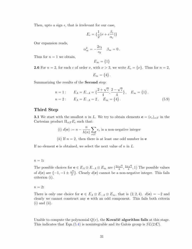
Third Step
3.1 We start with the smallest n in L. We try to obtain elements e = (ec)c∈Γ in theCartesian product Πc∈ΓEc such that:
(i) d(e) := n− n
h(n)
∑c∈Γ
ec is a non-negative integer
(ii) If n = 2, then there is at least one odd number in e
If no element e is obtained, we select the next value of n in L.
n = 1:
The possible choices for e ∈ EA ⊗ E−A ⊗ E∞ are (2±√
74, 2±
√7
4, 1) The possible values
of d(e) are −1,−1±√
72. Clearly d(e) cannot be a non-negative integer. This fails
criterion (i).
n = 2:
There is only one choice for e ∈ EA ⊗ E−A ⊗ E∞, that is (2, 2, 4). d(e) = −2 andclearly we cannot construct any e with an odd component. This fails both criteria(i) and (ii).
Unable to compute the polynomial Q(v), the Kovacic algorithm fails at this stage.This indicates that Eqn.(5.4) is nonintegrable and its Galois group is SL(2,C).
31

Chapter 6
Nonintegrability in GenericConfining Backgrounds
6.1 Closed spinning strings in generic supergravity
backgrounds
The Polyakov action and the Virasoro constraints characterizing the classical motionof the fundamental string are:
L = − 1
2πα′√−ggabGMN∂aX
M∂bXN , (6.1)
where GMN is the spacetime metric of the fixed background, Xµ are the coordinatesof the string, gab is the worldsheet metric, the indices a, b represent the coordinateson the worldsheet of the string which we denote as (τ, σ). We will use to work in theconformal gauge in which case the Virasoro constraints are
0 = GMNXMX ′N ,
0 = GMN
(XMXN +X ′MX ′N
), (6.2)
where dot and prime denote derivatives with respect to τ and σ respectively.We are interested in the classical motion of the strings in background metrics
GMN that preserve Poincare invariance in the coordinates (X0, X i) where the dualfield theory lives:
ds2 = a2(r)dxµdxµ + b2(r)dr2 + c2(r)dΩ2
d. (6.3)
Here xµ = (t, x1, x2, x3) and dΩ2d represents the metric on a d-dimensional sub-space
that, can also have r-dependent coefficients. In the case of supergravity backgroundsin IIB, we have d = 5 but we leave it arbitrary to also accommodate backgrounds in11-d supergravity in which case d = 6.
The relevant classical equations of motion for the string sigma model in this back-ground are
∂a(a2(r)ηab∂bx
µ) = 0,
32

∂a(b2(r)ηab∂br) =
1
2∂r(a
2(r))ηab∂axµ∂bxµ +
1
2∂r(b
2(r))ηab∂ar∂br.
(6.4)
They are supplemented by the Virasoro constraints. We will construct spinningstrings by starting with the following Ansatz (Ansatz I). The world-sheet coordinateσ wraps around the r direction. We will also call this the σ-embedding.
x0 = e τ,
x1 = f1(τ) g1(σ), x2 = f2(τ) g2(σ),
x3 = constant, r = r(σ). (6.5)
We will also consider a slight modification of the above Ansatz as follows (AnsatzII). Here the string does not wrap around the r direction, but the r coordinate is afunction of the world-sheet time τ . We will also call this the τ embedding.
x0 = e τ,
x1 = f1(τ) g1(σ), x2 = f2(τ) g2(σ),
x3 = constant, r = r(τ). (6.6)
An illustration of the two embeddings for a confining geometry is given in Fig.(6.1).
6.1.1 Motion of the string with Ansatz I
With Ansatz I (6.5) the equation of motion for x0 is trivially satisfied. Let us firstshow that the form of the functions fi is fairly universal for this Ansatz. The equationof motion for xi is
− a2 gifi + fi∂σ(a2g′i) = 0, (6.7)
where a dot denotes a derivative with respect to τ and a prime denotes a derivativewith respect to σ. Enforcing a natural separation of variables we see that
fi + (e ω)2fi = 0, ∂σ(a2 g′i) + (e ω)2a2gi = 0. (6.8)
The radial equation of motion is
(b2r′)′ =1
2∂r(a
2)[e2 − g2
i f2i + f 2
i g′2i
]+
1
2∂r(b
2)r′2. (6.9)
Finally the nontrivial Virasoro constraint becomes
b2r′2 + a2[− e2 + g2
i f2i + f 2
i g′2i
]= 0. (6.10)
We are particularly interested in the integrals of motion describing the energy andthe angular momentum
E =e
2πα′
∫a2dσ, (6.11)
33

r
0r=r
x2
x1
Ω
(a) Ansatz I: σ-embedding
r
0r=r
x2
x1
Ω
(b) Ansatz II: τ -embedding
Figure 6.1: σ and τ embeddings of a string in a generic confining background givenby Ansatze (6.5) and (6.6) respectively.
34

J =1
2πα′
∫a2[x1∂τx2 − x2∂τx1
]dσ =
1
2πα′
∫a2g1g2
[f1∂τf2 − f2∂τf1
]dσ (6.12)
The above system can be greatly simplified by further taking the following particularsolution:
f1 = cos eω τ, f2 = sin eω τ, and g1 = g2 = g. (6.13)
Under these assumptions the equation of motion for r and the Virasoro constraintbecome
(b2r′)′ − 1
2∂r(a
2)[e2 − (eω)2 g2 + g′2
]− 1
2∂r(b
2)r′2 = 0, (6.14)
b2r′2 + a2[− e2 + (eω)2 g2 + g′2
]= 0. (6.15)
The angular momentum is then
J =eω
2πα′
∫a2g2dσ. (6.16)
6.1.2 Motion of the string with Ansatz II
In this subsection we consider the Ansatz given in equation (6.6). Note that theanalysis given in the previous sections can be applied mutatis mutandis to this Ansatz.In particular, the separation of variables described in equation (6.8) can be performedin a symmetric way and one obtains:
g′′i + α2gi = 0, ∂τ (a2 ∂τfi) + α2a2 fi = 0. (6.17)
The Ansatz given in (6.6, 6.13) becomes
t = t(τ), r = r(τ),
x1 = R(τ) sinασ, x2 = R(τ) cosασ. (6.18)
The Polyakov action is:
L ∝ a2(r)[− t2 + R2 − α2R2
]+ b2(r)r2. (6.19)
The above Ansatz satisfies the first constraint automatically and the second constraintleads to a Hamiltonian constraint:
a2(r)[t2 + R2 + α2R2] + b2(r)r2 = 0 . (6.20)
We also have thatt = E/a2(r), (6.21)
where E is an integration constant. This gives
L ∝ − E2
a2(r)+ a2(r)
[R2 − α2R2
]+ b2(r)r2 . (6.22)
From the above Lagrangian density the equations of motion for r(τ) and R(τ) are
d
dτ
(b2(r)
d
dτr(τ)
)=
E2
a3(r)
d
dra(r) + a(r)
d
dra(r)
[R2 − α2R2
]+ b(r)
d
drb(r)(
d
dτr)2,
d
dτ
(a2(r)
d
dτR(τ)
)= −α2a2(r)R(τ). (6.23)
35

6.2 Confining backgrounds
Let us show that there exists a simple solution of the equations of motion (6.14)for any gravity background dual to a confining gauge theory. The conditions for aSUGRA background to be dual to a confining theory have been exhaustively explored[40, 41] using the fact that the corresponding Wilson loop in field theory shouldexhibit area law behavior. The main idea is to translate the condition for the vev ofthe rectangular Wilson loop to display an area law into properties that the metric ofthe supergravity background must satisfy through the identification of the vacuumexpectation value of the Wilson loop with the value of the action of the correspondingclassical string. It has been established that one set of necessary conditions is for g00 tohave a nonzero minimum at some point r0 usually known as the end of the space wall[40, 41]. Note that precisely these two conditions ensure the existence of a solution of(6.14). Namely, since g00 = a2 we see that for a point r = r0 = constant is a solutionif
∂r(g00)|r=r0 = 0, g00|r=r0 6= 0. (6.24)
The first condition solves the first equation in (6.14) and the second condition makesthe second equation nontrivial. Interestingly, the second condition can be interpretedas enforcing that the quark-antiquark string tension be nonvanishing as it determinesthe value of the string action. It is worth mentioning that due to the UV/IR cor-respondence in the gauge/gravity duality the radial direction is identified with theenergy scale. In particular, r ≈ r0 is the gravity dual of the IR in the gauge theory.Thus, the string we are considering spins in the region dual to the IR of the gaugetheory. Therefore we can conclude that it is dual to states in the field theory that arecharacteristic of the IR.
6.2.1 Regge trajectories from closed spinning strings in con-fining backgrounds
Since we are working in Poincare coordinates the quantity canonically conjugate totime is the energy of the corresponding state in the four dimensional theory. Theangular momentum of the string describes the spin of the corresponding state. Thusa spinning string in the Poincare coordinates is dual to a state of energy E and spinJ . In order for our semiclassical approximation to be valid we need the value of theaction to be large, this imply that we are considering gauge theory states in the IRregion of the gauge theory with large spin and large energy. In the cases we study,expressions (6.11) and (6.16) yield a dispersion relation that can be identified withRegge trajectories.
Let us now explicitly display the Regge trajectories. The classical solution isgiven by (6.5) with g(σ) solving the second equation from (6.14), that is, g(σ) =(1/ω) sin(eωσ). Imposing the periodicity σ → σ + 2π implies that eω = 1 and hence
x0 = e τ, x1 = e cos τ sin σ, x2 = e sin τ sin σ. (6.25)
36

The expressions for the energy and angular momentum of the string states are:
E = 4e g00(r0)
2πα′
∫dσ = 2πg00(r0)Tse, J = 4
g00(r0)e2
2πα′
∫sin2 σdσ = πg00(r0)Tse
2.
(6.26)Defining the effective string tension as Ts, eff = g00(r0)/(2πα′) and α′eff = α′/g00
we find that the Regge trajectories take the form
J =1
4πTs, effE2 ≡ 1
2α′eff t. (6.27)
Notice that the main difference with respect to the result in flat space dating backto the hadronic models of the sixties is that the slope is modified to α′eff = α′/g00.It is expected that a confining background will have states that align themselves inRegge trajectories.
6.3 Analytic Nonintegrability in Confining Back-
grounds
For confining backgrounds we have that the conditions on g00 described in (6.24)imply that:
a(r) ≈ a0 − a2(r − r0)2, (6.28)
where a0 is the nonzero minimal value of g00(r0) and the absence of a linear termsindicates that the first derivative at r0 vanishes.
6.3.1 With Ansatz I
In this region is easy to show that both equations above can be satisfied. The equationfor r(σ) is satisfied by r = r0 and dr/dσ = 0. The equation for R(σ) is simply
d2
dσ2R(σ) + ω2R(σ) = 0,−→ R(σ) = A sin(ωσ + φ0). (6.29)
We can now write down the NVE equation by considering an expansion around thestraight line solution, that is,
r = r0 + η(σ). (6.30)
We obtain
η′′ − a2E2
2b20a
30
[1− 2ω2A2a4
0
E2cos 2ωσ
]η = 0. (6.31)
The question of integrability of the system (6.23) has now turned into whether ornot the NVE above can be solved in quadratures. The above equation can be easilyrecognized as the Mathieu equation. The analysis above has naturally appeared inthe context of quantization of Regge trajectories and other classical string configura-tions. For example, [42, 43] derived precisely such equation in the study of quantum
37

corrections to the Regge trajectories, those work went on to compute one-loop cor-rections in both, fermionic and bosonic sectors. Our goal here is different, for us thesignificance of (6.31) is as the Normal Variational Equation around the dynamicalsystem (6.23) whose study will inform us about the integrability of the system. Thegeneral solution to the above equation is
η(σ) = c1 C(− α
ω2,− αβ
2ω2, ω σ) + c2 S(− α
ω2,− αβ
2ω2, ω σ), (6.32)
where c1 and c2 are constants and
α =a2E
2
2b20a
30
, β =2ω2A2a4
0
E2. (6.33)
Notice, crucially, that although the system obtain here is similar to the one dis-cussed in the main text there is a key difference. Namely, that the effective “time”variable σ is now periodic. This periodicity precludes us from talking about asymp-totic properties which lies at the heart of chaotic behavior. Most indicators of chaos,the largest Lyapunov exponent prominently, are based on the late time asymptoticsof the system.
6.3.2 With Ansatz II
In this region is easy to show that both equations in (6.23) can be satisfied. Theequation for r(τ) is satisfied by r = r0 and dr/dτ = 0. The straight line equation forR(τ) is simply
d2
dτ 2R(τ) + α2R(τ) = 0,−→ R(τ) = A sin(ατ + φ0). (6.34)
We can now write down the NVE equation by considering an expansion aroundthe straight line solution, that is,
r = r0 + η(τ). (6.35)
We obtain
η +a2E
2
2b20a
30
[1 +
2α2A2a40
E2cos 2ατ
]η = 0. (6.36)
The question of integrability of the system (6.23) has now turned into whether ornot the NVE above can be solved in quadratures. The above equation can be easilyrecognized as the Mathieu equation. The analysis above has naturally appeared inthe context of quantization of Regge trajectories and other classical string configura-tions. For example, [42, 43] derived precisely such equation in the study of quantumcorrections to the Regge trajectories, those work went on to compute one-loop cor-rections in both, fermionic and bosonic sectors. Our goal here is different, for us thesignificance of (6.36) is as the Normal Variational Equation around the dynamicalsystem (6.23) whose study will inform us about the integrability of the system.
38

The solution to the above equation (6.36) in terms of Mathieu functions is
η(τ) = c1 C(θ
α2,θβ
2α2, α τ) + c2 S(
θ
α2,θβ
2α2, α τ), (6.37)
where c1 and c2 are constants and
θ =a2E
2
2b20a
30
, β =2α2A2a4
0
E2. (6.38)
A beautiful description of a similar situation is presented in [44] where non-integrability of some Hamiltonians with rational potentials is discussed. In particular,the extended Mathieu equation is considered as an NVE equation
y = (a+ b sin t+ c cos t)y. (6.39)
Our equation 6.36 is of this form with 2ατ → t and b = 0. To aid the mathematicallyminded reader, and to make connection with our introduction to non-integrability inthe beginning of section 5.1, we show that the extended Mathieu equation can bebrought to an algebraic form using x = eit which leads to:
y′′ +1
xy′ +
(b+ c)x2 + 2ax+ c− b2x3
y = 0. (6.40)
The above equation is perfectly amenable to the application of Kovacic’s algorithm.It was shown explicitly in [44] that our case (b 6= −c above) corresponds to a non-integrable equation. More precisely, the Galois group is the connected componentof SL(2,C) and the identity component of the Galois group for (6.39) is exactlySL(2,C), which is a non-Abelian group.
6.4 Explicit Chaotic Behavior in the MN Back-
ground
To logically close the circle we should also show explicit chaotic behavior of stringmotion in confining backgrounds. In this section, we choose the Maldacena-Nunezbackground which belongs to the class of confining backgrounds we are interested in.String motion in the AdS soliton background, which also belongs to this class, hasalready been demonstrated to be chaotic in Chapter 4.
The expression for the functions a and b in the main dynamical system (6.23) canbe read directly from the MN background (C.10) (see Appendix C for details of thebackground).
a(r)2 = e−φ0√
sinh(2r)/2
(r coth 2r − r2
sinh2(2r)− 1
4)1/4
, b(r)2 = α′ gsNa(r)2. (6.41)
It is crucial thatlimr→0
a(r)2 → e−φ0 , (6.42)
39

Figure 6.2: Poincare sections for the Maldacena-Nunez background demonstratingbreaking of the KAM tori en route to chaos.
which is a nonzero constant that determines the tension of the confining string. Theequations of motion can be obtained by plugging the above expressions in Eqn.(6.23).
Following an analysis very similar to Section 4.3, we obtain the Poincare sections[Fig. 6.2], which show a KAM behavior of transition to chaos. A Lyapunov calcuatedin the chaotic regime [Fig. 6.3] is also found to converge to a positive value.
0 200 400 600 800 10000.10
0.15
0.20
0.25
Τ
LE
Lyapunov Exponent for E=3.21344
Figure 6.3: The Lyapunov Exponent converges to a positive value of about 0.2.
40

Chapter 7
Quantum Chaos in String Theory
In this chapter we look at the possible signatures of quantum chaos in confiningbackgrounds coming from string theory. In Section 7.1, we give an introduction toquantum chaos, with a special emphasis on observed signatures on quantum chaosin hadron spectra (§7.1.1). In Section 7.2 we look at the quantum level spacingdistribution in the AdS soliton background and find signatures of quantum chaos inthe distribution.
7.1 What is Quantum Chaos?
Quantum chaos is the study of quantum properties of systems whose classical limit ischaotic. For good books on the subject refer to [45, 46]. An interesting property tostudy turns out to be the distribution of the spacing of adjacent energy levels of thesystem. For a quantum system, whose Hamiltonian is classically integrable, it wasshown by Berry and Tabor (1977) [47] that this level-spacing distribution is same asthat for a sequence of uncorrelated levels, i.e. quite universally a Poisson distribution:
P (s) ' exp(−s) . (7.1)
The next question to ask is whether there is any such universal distribution for systemswhich are classically chaotic. The models most frequently studied in this contextare Billiard systems of Sinai, which also come up frequently while talking aboutclassically chaotic systems. It was shown by Berry (1981) [48] that the in the quantumspectrum of these systems small differences of eigenvalues are avoided (level repulsion,cf. Fig.7.2). It was further demonstrated by Bohigas, Giannoni and Schmit (1984)[49] that the level spacing distribution of eigenvalues calculated numerically perfectlyagree with that of a Gaussian orthogonal ensemble (GOE) of random matrices, firstdiscussed by Wigner (1958) [50].
P (s) ' πs
2exp
(−πs
2
4
). (7.2)
As seen from Figure (7.1), the principal qualitative difference between the levelspacing distributions for the integrable and chaotic systems is that P (s) goes to
41

0 10 20 30 40 50 600
50
100
150
200
250
s
PHs
L
N =64.
(a) Integrable potential
0 10 20 30 400
20
40
60
80
100
s
PHs
L
N =64.
(b) Nonintegrable potential
Figure 7.1: Distribution of level spacing for an integrable and a nonintegrable po-tential demonstrating Poisson and Wigner GOE distribution respectively. A boxof dimensions 4
√e × 1 and in the nonintegrable case, deformed by a potential
V (x, y) = exp (α(x− y − 1)) with α = 138.2. Eigenvalues have been calculatedusing pseudospectral method on a 64× 64 Tchebychef grid.
zero as s → 0 in the Wigner GOE distribution for the chaotic cases, but it has amaximum at s = 0 in the Poisson distribution for the integrable case. This is anindication of the phenomenon of level repulsion for nonintegrable systems [Figure(7.2)]. Since degeneracies are avoided, a system parameter is dialed, the levels tendto repel. Thus there are only a small number of eigenvalues with small s: P (0) ≈ 0for the nonintegrable case. For the integrable case, the eigenvalues coming from thedifferent separable sectors are independent of each other. Hence there is no suchrepulsion.
7.1.1 Quantum chaos in the Hadronic Spectrum
Signatures of chaos in the real hadron spectrum was discovered following Wigner’ssurmise. Experimental groups at Columbia and TUNL gathered data that permittedHaq, Pandey and Bohigan (1982) [51] to establish a statistically significant agreementbetween the measured fluctuations and Wigner’s random matrix model. The dataconsisted of 1407 resonance energies corresponding to 30 sequences of 27 differentnuclei. The Hydrogen atom in a magnetic field was also established to be quantumchaotic [52, 53]. The subject is thoroughly reviewed in [54, 55, 56, 57, 58]. Super-symmetric QCD at finite density [59] shows an even more exotic feature. While atzero chemical potential µ, the Wigner GOE distribution is obtained, for finite µ thelevel-spacing distribution agrees with the spacing of eigenvalues of non-Hermitianensembles like the Ginibre ensemble [60].
42

E
Parameter
(a) Integrable system
E
Parameter
(b) Nonintegrable system
Figure 7.2: Level repulsion in a nonintegrable quantum system. In an integrablesystem the eigenvalues can cross and have degeneracies. In a nonintegrable systemthe eigenvalues repel. Hence small differences between eigenvalues are avoided.
- 0.6 - 0.4 - 0.2 0.0 0.2 0.4 0.6
- 0.4
- 0.2
0.0
0.2
0.4
Figure 7.3: Contour plot of the wavefunction of a quantum chaotic system.
43

0.5 1.0 1.5
50
100
150
Figure 7.4: The distribution of level-spacings in the AdS soliton shows a strong level-repulsion and qualitative features of the Wigner distribution, indicating quantumchaos in this background. The eigenvalues of the Hamiltonian (7.4) with d = 4,a = 1, α = 1 have been numerically obtained using Fourier spectral method on a80× 80 grid between −12 < R < 12 and 0.047 < y < 1.180.
7.2 Quantum Chaos in the AdS soliton background
Recall:
H =1
2
(−E2 +
k2
T (x)+ p2
R
)e−2ax2 +
T (x)
d2a2x2p2x + α2R2e2ax2
(7.3)
We need to find the eigenvalues of E using,
E2ψ(x,R) =k2
T (x)ψ(x,R)− ∂2
Rψ(x,R)− f(x)∂2xψ(x,R) + V (x,R)ψ(x,R) , (7.4)
where,
f(x) =T (x)
d2a2x2, V (x,R) = α2R2e2ax2 . (7.5)
With a transformation dy = dx/√f(x), Eqn.(7.4) can be mapped to a canonical
form,
E2ψ(y,R) =k2
T (y)− ∂2
Rψ(y,R)− ∂2y ψ(y,R) + V (y,R)ψ(y,R) . (7.6)
Here,
T (y) = T (x(y)), V (y,R) = V (x(y), R) +1
2f ′′(x(y))
and ψ(y,R) = f(x(y))ψ(x(y), R) . (7.7)
We calculate the eigenvalues of the Hamiltonian (7.4) and plot the histogram ofthe difference of nearest eigenvalues [Fig.(7.4)]. The distribution shows a strong levelrepulsion and is quite similar to the Wigner distribution, indicating of quantum chaosin the AdS soliton background.
44

Appendix A
Singularity Resolution inCosmologies Using AdS/CFT
As an application of the AdS/CFT correspondence, in this appendix we review anexample in which a dual gauge theory helps better understand the gravitational dy-namics of a cosmological model.
A.1 Motivation and Overview
The theory of general relativity has a unique property of predicting its own failure –it breaks down at places called singularities. Our usual notions of spacetime breakdown near these singularities. At spacelike or null singularities, like those in theinteriors of neutral black holes, “time” begins or ends, the meaning of which is notclear. Particularly disturbing are cosmological singularities like the big bang or thebig crunch, which no observer can bypass.
Near these singularities, where the curvatures have become large compared tosome scale, a quantum theory of gravity is expected to take over.
Holographic correspondences like AdS/CFT arising from string theory provide anonperturbative formulation of quantum gravity. Here gravity in the bulk is an effec-tive description of a non-gravitational field theory in a lower number of dimensions.We ask the question whether the dual description following these correspondencescan give us some insight as to what happens near or past these singularities. In thesemodels the spectrum at late times can be interpreted as the primordial fluctuationsthat lead to structure formation in the early universe. An incomplete but long list ofattempts made in this direction is given in [61, 62, 63, 64, 65, 66, 67, 68, 69, 70]. Forreviews refer to [71, 72]. The bulk of this article is based on the work done in [73].
45

A.2 The AdS/CFT Correspondence
The simplest example of the correspondence relevant to our discussion. We work inglobal coordinates in which the AdS5 background has the metric [Eqn.(2.1)]:
ds2 = −(1 + r2)dt2 +dr2
1 + r2+ r2 dΩ2
3 + dΩ25 (A.1)
Here we are working with units where RAdS = 1. Recall the AdS/CFT relations[Eqn.(2.4)]
g2YM = 4πgs , λ ≡ g2
YMN =R4AdS
l4s. (A.2)
In the large N limit (N → ∞, gYM → 0, λ ≡ gNYM =finite), the dual description is aclassical string theory with the quantum corrections suppressed by 1/N . Moreover,the above relations tell us that the large ’t Hooft coupling limit (λ→∞), correspondsto the low-energy supergravity truncation of the string theory where the stringy modesare suppressed by α′. This is because, the massive string modes, which have massesof O(1/
√α′), are heavy compared to the energy scale of the theory 1/RAdS, and are
not excited. So we are left only with the massless supergravity modes.
A.3 Setup in Supergravity
We consider a Yang-Mills theory with a time-dependent ’t Hooft coupling λ(t). In thedual bulk (via AdS/CFT), this corresponds to a non-normalizable dilaton mode whoseboundary value Φ0(t) is being dialled. The dilaton evolves following the supergravityequations of motion and produces a non-trivial metric by backreaction. The equationsto solve are thus the Einstein-dilaton equations:
Rab = Λgab +1
2∂aΦ∂bΦ, (with Λ = −4), ∇2Φ = 0 . (A.3)
We choose a profile such that the ’t Hooft coupling λ is large at early and latetimes. The dual theory thus has a good gravity description at these times. We choosethe initial state to be the vacuum of the gauge theory, which in the bulk correspondsto pure AdS5 × S5. At intermediate times, λ is allowed to become O(1) – curvaturesin the bulk reach the string scale at this stage and supergravity description breaksdown. We fix N to remain large – the curvatures do not reach the Planck scaleand the system remains classical. Thus the singularities that we describe are ratherrestrictive.
Furthermore, we vary the ’t Hooft coupling, or equivalently the boundary valueof the dilaton slowly. The curvature scale of the AdS or equivalently the radius of S3
on which the field theory is defined sets a scale in the theory. We can quantify thisas
Φ0 = f(εt), ε 1 Φ0 = εf ′(εt) , (A.4)
where each time derivative comes with an additional power of ε.
46

λ=NeΦ
0
λmin
AdS5 × S5
YM vacuum at large λ
Supergravitycan be trusted
Supergravitybreaks down
What is the gravitydescription here???
Figure A.1: A slowly-varying dilaton profile.
Although the change is slow, the total change in the value of the dilaton accruesover time and we can eventually have a large change in the value of the dilaton. Oursolution therefore includes the case where the value of the dilaton becomes small, thebulk curvatures become large compared to the string scale and supergravity approx-imation in the bulk breaks down.
A.3.1 Supergravity Solution
We expand the dilaton and the bulk metric order by order in ε
Φ(r, t) = Φ0(t) + εΦ1(r, t) + ε2Φ2(r, t) + . . . ,
gab = g(0)ab + εg
(1)ab + ε2g
(2)ab + . . . , (A.5)
and plug them in the Einstein equations. Solving to the lowest non-trivial order in ε,we get
Φ2(r, t) = Φ0(t) + 14Φ0(t)
[1r2
log(1 + r2)− 12(log(1 + r2))2 − dilog(1 + r2)− π2
6
],
gtt = 1 + r2 − 112
Φ20
[3− 1
r2ln(1 + r2)
], grr = 1 + r2 − 1
12Φ2
0
[1− 1
r2ln(1 + r2)
].(A.6)
The solution is smooth everywhere – there are no horizons and no black holes areformed. This is a consequence of the slow variation. For a variation that is fastenough we can form black holes even within the supergravity approximation [74].
We will now consider the situation where the value of the dilaton has becomesmall at intermediate times and supergravity approximation has broken down. Weturn to the gauge theory to see if it can give us any clue as to what happens in thestringy regime and what happens afterwards when supergravity is restored.
47

A.4 Field Theory Analysis
The boundary gauge theory is a quantum mechanical system with a time dependentparameter – the coupling – that is slowly varying. For the field theory on S3, thespectrum has a gap of order 1/RAdS for all values of ’t Hooft coupling. 1 So we canuse the adiabatic approximation in quantum mechanics to study the system. Thestandard adiabatic approximation of quantum mechanics will turn out to be validonly if Nε 1, which is rather stringent. We will formulate an alternate adiabaticapproximation in terms of coherent states.
A.4.1 Standard Adiabatic Approximation
Consider a quantum mechanical system with Hamiltonian H(ζ(t)) that depends ona slowly-varying parameter ζ(t). In our case ζ(t) is the time dependent ’t Hooftcoupling λ(t) or equivalently the boundary value of the dilation field Φ0(t). Theinstantaneous eigenstates of the Hamiltonian are
H(ζ)|φm(ζ) >= Em(ζ)|φm(ζ) > . (A.7)
The evolution of the ground state |φ0 > of H(ζ0) in the adiabatic approximation issimply given by
|ψ0(t) >' |φ0(ζ) > e−i∫ t−∞ E0(ζ)dt , (A.8)
with first corrections of the form
|ψ1(t) > =∑n6=0
an(t)|φn(ζ) > e−i∫ t−∞ Endt,
an(t) = −∫ t
−∞dt′< φn(ζ)|∂H
∂ζ|φ0(ζ) >
E0 − Enζe−i
∫ t′−∞(E0−En)dt′ (A.9)
The approximation is good if the first corrections are small:
| < φn|∂H
∂ζ|φ0 > ζ| (∆E)2 (A.10)
where ∆E is the energy difference between the ground and the first excited states.In our case, ζ(t) = Φ0(t) ∼ O(ε) and using AdS/CFT 2,
< φn|∂H
∂Φ0
|φ0 >= − < φn|Ol=0|φ0 >∼ N . (A.11)
Thus, the adiabatic approximation is valid if Nε 1. This condition is however morestringent than the condition ε 1 that we had in the supergravity analysis.
1This follows from the fact that the states provide a unitary representation of the conformalgroup for any value of the coupling.
2Turning on a field Φ with a boundary value Φ0 corresponds the deformation of the gauge theoryaction by a gauge invariant operator O = δSCl
δΦ0where SCl is the classical supergravity action.
48

A.4.2 Adiabatic Approximation with Coherent States
A general coherent state has the form
|Ψ(t) >= exp
[∑n
λn(t)a†n
]|0 > , (A.12)
where a†n are the creation operators and λn(t) are the coherent state parameters. Forlarge values of λn, the system goes over to a classical configuration. In the large’t Hooft coupling regime they have a good description in terms of local fields. In ourproblem the creation and annihilation operators need to be replaced by the creationand annihilation parts O(±) of O. The evolution of λn(t) is determined by the algebra
of the operators O(±) and the Schrodinger equation. In general the operators O(±)
have a non-trivial operator algebra which mixes all of them and makes the evolutionof λn(t) and quite complicated. However, the situation drastically simplifies for a slowvariation. The expectation value of the three-point function taken in a coherent statecan be shown to be < ψ|O1O2O3|ψ >∼ ε. For ε 1, the operators O(±) decouple.The three and higher point functions are thus parametrically suppressed and all weare left with are the two point functions. Their algebra essentially reduces to that ofa free harmonic oscillator.
Ol=0 = N∞∑n=1
F (2n)[A2ne−i2nt + A†2ne
i2nt] with [A2m, A†2n] = δm,n′ (A.13)
We can now construct coherent states |ψ >= N(t)e(∑n λnA
†2n)|φ0 > and find the
Schrodinger evolution of the coherent state parameter.
λn(t) =e−i2ntNF (2n)
(2n)
∫ t
−∞Φ0(t′)ei2nt
′dt′ (A.14)
= −iNF (2n)Φ0(t)
(2n)2+ie−i2ntNF (2n)
(2n)2
∫ t
−∞dt′Φ0(t′)ei2nt
′(A.15)
= −iNF (2n)Φ0(t)
(2n)2+NF (2n)Φ0(t)
(2n)3+ . . . (A.16)
Subsequent integration by parts leads to a perturbative expansion for λn. The aboveexpansion is valid if the second and subsequent terms are small compared to the first
term i.e. | Φ0
2nΦ0| 1 ∀n. This is identical to the condition ε 1. Moreover the
state represents a “classical” deformation only when the coherent state parameter λis large. That holds when Nε 1.
A.4.3 Results
For small ’t Hooft coupling, the coupling between the oscillators are still individuallysuppressed by ε and most of the above analysis goes through. However now we haveO(N2) stringy modes whose frequencies are comparable to those of the supergravity
49

modes. So there is a possibility of thermalization. The energy that has been pumpedin might get distributed between the various modes. Then at late times one couldbe left with O(N2ε2) thermalized energy in the system. It is difficult to say whetherthermalization would indeed occur since the time scale of variation is same as thethermalization time scale.
However we can assume that all the energy left behind in the system has beenthermalized (EThermal ∼ N2ε2) and from entropic considerations in supergravity figureout the worst case scenarios for various values of ε. For ε λ5/4N−1, a gas ofsupergravity modes is favoured. For ε & λ5/4N−1 we can have a gas of massive stringmodes. For ε & λ−7/8 a small black hole can form. In order to form a large black holeone would require ε & 1. So a large black hole is never formed in our slowly varyingsolution.
A.5 Conclusions and Outlook
We have an example of a situation in which the gauge theory has a smooth time-evolution across a region whose dual bulk region has a singularity. An explicit calcu-lation of the final state is possible in principle, but made difficult in practice becausewe do not have a complete AdS/CFT dictionary in the stringy regime. Of the possi-ble outcomes, a thermal distribution at late times would imply a gaussian spectrumwhile formation of a black hole would source a nongaussianity.
50

Appendix B
T p,q and Y p,q Backgrounds
B.1 Wrapped strings in general AdS5 ×X5
The methods of analytic non-integrability can be applied to a large class of spaces instring theory. Let us start by considering a five-dimensional Einstein space X5, withRij = λgij, where λ is a constant. Any such Einstein space furnishes a solution tothe type IIB supergravity equations known as a Freund-Rubin compactification [75].Namely, the solution takes the form
ds2 = ds2(AdS5) + ds2(X5), F5 = (1 + ?)vol(AdS5), (B.1)
where vol is the volume five-form and ? is the Hodge dual operator. Basically F5 isa the sum of the volume forms on AdS5 and the Einstein space X5. Of particularinterest in string theory is the case when X5 is Sasaki-Einstein, that is, on top ofbeing Einstein it admits a spinor satisfying ∇µε ∼ Γµε. The case of Sasaki-Einsteinstructure is particularly interesting from the string theory point of view as it preservessupersymmetry which is a mechanism that provides extra computational power.
We consider spaces X5 that are a U(1) fiber over a four-dimensional manifold,again, this is largely inspired by the Sasaki-Einstein class but clearly goes beyondthat. In the case of topologically trivial fibration we are precluded from applying ourargument, those manifolds can be considered separately and probably on a case bycase basis.
The configuration that we are interested in exploring is a string sitting at thecenter of AdS5 and winding in the circles provided by the base space. More explicitly,consider the AdS5 metric in global coordinates
ds2 = − cosh2 ρ dt2 + dρ2 + sinh2 ρ dØ23. (B.2)
Then, our solutions is localized at ρ = 0. As noted before, in the search for solutions ofthe form (B.1) a prominent place is taken by deformations of S5 that preserve someamount of supersymmetry, they are given by Sasaki-Einstein spaces. The generalstructure of Sasaki-Eintein metrics is
ds2X5S−E
= (dψ +i
2(K,idz
i −K,idzi))2 +K,ijdz
idzj, (B.3)
51

where K is a Kahler potential on the complex base with coordinates zi with i = 1, 2.This is the general structure that will serve as our guiding principle but we will notbe limited to it. Roughly our Ansatz for the classical string configuration is
zi = ri(τ)eiαiσ (B.4)
where τ and σ are the worldsheet coordinates of the string. Note crucially we haveintroduced winding of the strings characterized by the constants αi. The goal is tosolved for the functions ri(τ).
A summary from the previous section instructs us to:
• Select a particular solution, that is, define the straight line solution.
• Write the normal variational equation (NVE).
• Check if the identity component of the differential Galois group of the NVEis Abelian, that is, apply the Kovacic’s algorithm to determine if the NVE isintegrable by quadrature.
Given this Ansatz above we can now summarize the general results. Namely, inthis section we prove that the corresponding effective Hamiltonian systems have twodegrees of freedom and admit an invariant plane Γ = r2 = r2 = 0 whose normalvariational equation around integral curves in Γ we study explicitly.
B.1.1 T p,q
These 5-manifolds are not necessarily Sasaki-Einstein, however, some of them areEinstein which allow for a consistent string backgrounds of the form described inequation (B.1). More importantly, some of these spaces provide exact conformalsigma models description [76] and are thus exact string backgrounds in all orders inα′. In this section we provide a unified treatment of this class for generic values of pand q. The metric has the form
ds2 = a2(dψ + p cos θ1dφ1 + q cos θ2dφ2)2 + b2(dθ21 + sin2 θ1dφ
21) + c2(dθ2
2 + sin2 θ2dφ22).
(B.5)The classical string configuration we are interested is
θ1 = θ1(τ), θ2 = θ2(τ), ψ = ψ(τ), t(τ),
φ1 = α1σ, φ2 = α2σ, (B.6)
where αi are constants quantifying how the string wounds along the φi directions.Recall that t is from AdS5. The Polyakov Lagrangian is
L = − 1
2πα′
[t2 − b2θ2
1 −−c2θ22 − a2ψ2
+ α21(b2 − a2p2) sin2 θ1 + α2
2(c2 − a2q2) sin2 θ2 + 2α1α2p q a2 cos θ1 cos θ2
].(B.7)
52

There are several conserved quantities, the corresponding nontrivial equations are
θ1 +α1
b2sin θ1
[α1(b2 − a2p2) cos θ1 − a2α2pq cos θ2
]= 0,
θ2 +α2
c2sin θ2
[α2(c2 − a2q2) cos θ2 − a2α1pq cos θ2
]= 0. (B.8)
There is immediately some insight into the role of the fibration structure. Note thatthe topological winding in the space which is roughly described by p and q intertwineswith the wrapping of the strings α1 and α2. The effective number that appears inthe interaction part of the equations is α1 p and α2q. For example, from the point ofview of the interactions terms, taking p = 0 or q = 0 is equivalent to taking one ofthe αi = 0 which leads to an integrable system of two non-interacting gravitationalpendula.
Following the structure of the discussion of section ??, we take the straight linesolution to be
θ2 = θ2 = 0. (B.9)
The equation for θ1 becomes
θ1 +α1
b2
[α1(b2 − a2p2) cos θ1 − a2α2pq
]sin θ1 = 0. (B.10)
Let us denote the solution to this equation θ1, it can be given explicitly but we will notneed the precise form. This solution also defines the Riemann surface Γ introducedin section ??. The NVE is obtained by considering small fluctuations in θ2 aroundthe above solutions and takes the form:
η +α2
c2
[α2(c2 − a2q2)− α1p q cos θ1
]η = 0. (B.11)
Our goal is to study the NVE. To make the equation amenable to the Kovacic’salgorithm we introduce the following substitution
cos(θ1) = z. (B.12)
In this variable the NVE takes a form similar to Lame equation (see section 2.8.4 of[25]),
f(z)η′′(z) +1
2f ′(z)η′(z) +
α2
c2
[α2(c2 − a2q2)− α1p qz
]η(z) = 0 (B.13)
where prime now denotes differentiation with respect to z.
f(z) = ˙θ21 sin2(θ1) =
(6E2 − 1
3(4α1α2z + α2
2(1− z2))
)(1− z2) (B.14)
Equation (B.13) is a second order homogeneous linear differential equation with poly-nomial coefficients and it is, therefore, ready for the application of Kovacic’s algo-rithm. For generic values of the parameters above the Kovacic’s algorithm does noproduce a solution meaning the system defined in equations (B.8) is not integrable.
53

B.1.2 NVE for T 1,1
It is worth taking a pause to discussed the case of T 1,1 explicitly. The NVE equationtakes a simpler form:
η +1
3(α2
1 − 2α1α2 cos(θ1(t))η = 0, (B.15)
where η, as above, is the variation in θ2. Substituting cos(y) = z this equation takesa form similar to Lame equation
f(z)η′′(z) +1
2f ′(z)η′(z) +
1
3(α2
1 − 2α1α2z)η(z) = 0 (B.16)
Similarly we can obtain an expression for the function f(z) as
f(z) = y2 sin2(y) =
(6E2 − 1
3(4α1α2z + α2
2(1− z2))
)(1− z2). (B.17)
Consequently, this system is also non-integrable.The case of T 1,1 is particularly interesting because in the case the supergravity
solution is supersymmetric and a lot of attention has been paid to extending config-urations of AdS5 × S5 to the case of AdS5 × T 1,1 [77, 78, 79, 80, 81, 82, 83].
B.1.3 Y p,q
These spaces have played a central role in developments of the AdS/CFT correspon-dence as they provided and infinite class of dualities. These spaces are Sasaki-Einsteinbut they are not coset spaces as was the case for the Y p,q discussed above. Followingthe general discussion of Sasaki-Einstein spaces above, we write the metric on thesespaces as
1
R2ds2 =
1
9(dψ−(1−cy) cos θdφ+ydβ)2+
1− cy6
(dθ2+sin2 θdφ2)+p(y)
6(dβ+c cos θdφ)2.
(B.18)
p(y) =a− 3y2 + 2c y3
3(1− c y). (B.19)
The classical string configuration is described by the Ansatz
θ = θ(τ), y = y(τ),
φ = α1σ, β = α2σ, (B.20)
The Polyakov Lagrangian is simply:
L = − 1
2πα′
[t2 − 1− cy
6θ2 − 1
6p(y)y2 − 1
9ψ2
+1− cy
6α2
1 sin2 θ +p(y)
6(α2 + c α1 cos θ)2 +
1
9(α2 y − α1(1− cy) cos θ)2
](B.21)
54

As in previous cases the equations of motion for t and ψ are integrated immediatelyleaving only two nontrivial equations for θ and y
θ − c
1− c yyθ + α1
(α1 cos θ − c p(y)
1− c y(α2 + c α1 cos θ)− 2
3(α2 y − α1(1− c y) cos θ)
)sin θ = 0.
y − p′
py2 +
p p′
2(α2 + c α1 cos θ)2 − c p
2α2
1 sin2 θ +2
3p(α2 + c α1 cos θ)(α2 y − α1(1− c y) cos θ) = 0.
B.1.3.1 θ straight line
The straight line solution ca be taken to be θ = θ = 0. Then the equation for y issimplified to
y − p′
py2 +
p p′
2(α2 + c α1)2 +
2
3p(α2 + c α1)(y(α2 + c α1)− α1) = 0. (B.22)
The Normal Variational Equation takes the form
η− c ys1− cys
η+α1
(α1 −
c p(ys)
1− c ys(α2 + c α1)− 2
3((α2 + c α1)ys − α1)
)η = 0. (B.23)
To be able to write it in a form conducive to the application of Kovacic’s algorithmwe subtitute ys(t) = y and the NVE takes the form
(y(t)(1− cy)− cy2(t)
) dηdy
+ (1− cy)y2(t)d2η
dy2+ q(y)n(y) = 0(B.24)
y2(t) = 6(E + p(y)V (y, 0)) = 6p(y)
(p(y)
6(α2 + cα1)2 +
1
9(α2y − α1(1− cy))
)y(t) = 3
d
dy(p(y)V (y, 0))
q(y) = α1 (1− cy)
(5/3α1 −
c (a− 3 y2 + 2 cy3) (α2 + cα1 )
(3− 3 cy) (1− cy)− 2/3 (α2 + cα1) y
)With this identifications we have rewritten the NVE as a homogeneous second orderlinear differential equation. The Kovacic’s algorithm again fails to yield a solutionpointing to the fact that the system is generically non-integrable.
B.1.4 The exceptional case: S5
In this section we provide an integrable example where the Kovacic’s algorithm shouldsucceed. To expose the Sasaki-Einstein structure of S5, it is convenient to write themetric as a U(1) fiber over P2. The round metrics on S5 may be elegantly expressed interms of the left-invariant one-forms of SU(2). For SU(2), the left-invariant one-formscan be written as,
σ1 =1
2(cos(dψ)dθ + sin(ψ) sin(θ)dφ),
55
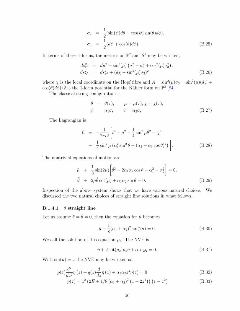
σ2 =1
2(sin(ψ)dθ − cos(ψ) sin(θ)dφ),
σ3 =1
2(dψ + cos(θ)dφ). (B.25)
In terms of these 1-forms, the metrics on P2 and S5 may be written,
ds2P2 = dµ2 + sin2(µ)
(σ2
1 + σ22 + cos2(µ)σ2
3
),
ds2S5 = ds2
P2 + (dχ+ sin2(µ)σ3)2 (B.26)
where χ is the local coordinate on the Hopf fibre and A = sin2(µ)σ3 = sin2(µ)(dψ +cos(θ)dφ)/2 is the 1-form potential for the Kahler form on P2 [84].
The classical string configuration is
θ = θ(τ), µ = µ(τ), χ = χ(τ),
φ = α1σ, ψ = α2σ, (B.27)
The Lagrangian is
L = − 1
2πα′
[t2 − µ2 − 1
4sin2 µθ2 − χ2
+1
4sin2 µ
(α2
1 sin2 θ + (α2 + α1 cos θ)2) ]. (B.28)
The nontrivial equations of motion are
µ +1
8sin(2µ)
[θ2 − 2α1α2 cos θ − α2
1 − α22
]= 0,
θ + 2µθ cot(µ) + α1α2 sin θ = 0. (B.29)
Inspection of the above system shows that we have various natural choices. Wediscussed the two natural choices of straight line solutions in what follows.
B.1.4.1 θ straight line
Let us assume θ = θ = 0, then the equation for µ becomes
µ− 1
8(α1 + α2)2 sin(2µ) = 0. (B.30)
We call the solution of this equation µs. The NVE is
η + 2 cot(µs)µsη + α1α2η = 0. (B.31)
With sin(µ) = z the NVE may be written as,
p(z)d2
dz2η (z) + q(z)
d
dzη (z) + α1α2z
2η(z) = 0 (B.32)
p(z) = z2(2E + 1/8 (α1 + α2)2 (1− 2z2
)) (1− z2
)(B.33)
56

q(z) = −1/8z(− 32E + 48Ez2 − 2α2
1 + 9α12z2 − 8α1
2z4 − 4α1α2
+ 18α1α2z2 − 16α1α2z
4 − 2α22 + 9α2
2z2 − 8α22z4)
This equation is now on the form conducive to Kovacic’s algorithm which succeedsand gives a solution. Since the above approach obscures the nature of integrability ofAdS5×S5 we consider another example which leaves no doubt about the integrability.
B.1.4.2 µ straight line
Let us assume the straight line is now given by µ = π/2, µ = 0. The the equation forθ becomes
θ + α1α2 sin θ = 0. (B.34)
Let us call the solution to this equation θs. Then the NVE is
η +1
4
(θ2s − 2α1α2 cos(θs)− α2
1 − α22
)η = 0. (B.35)
Note that the equation of motion for θs implies
θ + α1α2 sin θ = 0
→ d
dτ
(θ2s − 2α1α2 cos θs
)= 0,
→ θ2s − 2α1α2 cos θs = C0 (B.36)
Thus the NVE equation can be written as a simple harmonic equation
η +1
4
(C0 − α2
1 − α22
)η = 0. (B.37)
We do not require Kovacic’s algorithm to tell us that there is an analytic solution forthis equation. The power of differential Galois theory also guarantees that the resultis really independent of the straight line solution (Riemann surface) that one chooses.
We conclude this subsection with the jovial comment that we now know a veryprecise sense in which String theory in AdS5 × S5 is like a harmonic oscillator.
57
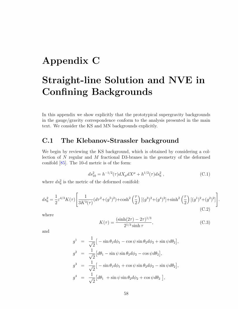
Appendix C
Straight-line Solution and NVE inConfining Backgrounds
In this appendix we show explicitly that the prototypical supergravity backgroundsin the gauge/gravity correspondence conform to the analysis presented in the maintext. We consider the KS and MN backgrounds explicitly.
C.1 The Klebanov-Strassler background
We begin by reviewing the KS background, which is obtained by considering a col-lection of N regular and M fractional D3-branes in the geometry of the deformedconifold [85]. The 10-d metric is of the form:
ds210 = h−1/2(τ)dXµdX
µ + h1/2(τ)ds26 , (C.1)
where ds26 is the metric of the deformed conifold:
ds26 =
1
2ε4/3K(τ)
[1
3K3(τ)(dτ 2+(g5)2)+cosh2
(τ2
)[(g3)2+(g4)2]+sinh2
(τ2
)[(g1)2+(g2)2]
].
(C.2)where
K(τ) =(sinh(2τ)− 2τ)1/3
21/3 sinh τ, (C.3)
and
g1 =1√2
[− sin θ1dφ1 − cosψ sin θ2dφ2 + sinψdθ2
],
g2 =1√2
[dθ1 − sinψ sin θ2dφ2 − cosψdθ2
],
g3 =1√2
[− sin θ1dφ1 + cosψ sin θ2dφ2 − sinψdθ2
],
g4 =1√2
[dθ1 + sinψ sin θ2dφ2 + cosψdθ2
],
58
g5 = dψ + cos θ1dφ1 + cos θ2dφ2. (C.4)
The warp factor is given by an integral expression for h is
h(τ) = α22/3
4I(τ) = (gsMα′)222/3ε−8/3I(τ) , (C.5)
where
I(τ) ≡∫ ∞τ
dxx cothx− 1
sinh2 x(sinh(2x)− 2x)1/3 . (C.6)
The above integral has the following expansion in the IR:
I(τ → 0)→ a0 − a2τ2 +O(τ 4) , (C.7)
where a0 ≈ 0.71805 and a2 = 22/3 32/3/18. The absence of a linear term in τ reassuresus that we are really expanding around the end of space, where the Wilson loop willfind it more favorable to arrange itself.
C.1.1 The straight line solution in KS
We consider the quadratic fluctuations and their influence on the Regge trajectories(6.27). In the notation used in the bulk of the paper we have:
a2(r) = h−1/2(r),
b2(r) =ε4/3
6K2(r)h1/2(r). (C.8)
Let us first consider the metric. The part of the metric perpendicular to the worldvolume, which is the deformed conifold metric, does not enter in the classical solutionwhich involves only world volume fields. Noting that the value r0 of section 6.2 isτ = 0, we expand the deformed conifold up to quadratic terms in the coordinates:
ds26 =
ε4/3
22/331/3
[1
2g2
5 + g23 + g2
4 +1
2dτ 2 +
τ 2
4(g2
1 + g22)
]. (C.9)
Let us further discuss the structure of this metric. It is known on very general groundsthat the deformed conifold is a cone over a space that is topologically S3×S2 [86]. Wecan see that the S3 roughly spanned by (g3, g4, g5) has finite size, while the S2 spannedby (g1, g2) shrinks to zero size at the apex of the deformed conifold. More importantlyfor us is the fact that if we do not allow non-trivial behavior in the directions (g1, g2)they cannot contribute to the NVE around the straight line solution characterized byτ = 0. Therefore, we have that the NVE equation for the spinning string in the KSbackground is precisely of the form (6.36).
59

C.2 The Maldacena-Nunez background
The MN background [87] whose IR regime is associated with N = 1 SYM theory isthat of a large number of D5 branes wrapping an S2. To be more precise: (i) thedual field theory to this SUGRA background is the N = 1 SYM contaminated withKK modes which cannot be de–coupled from the IR dynamics, (ii) the IR regime isdescribed by the SUGRA in the vicinity of the origin where the S2 shrinks to zerosize. The full MN SUGRA background includes the metric, the dilaton and the RRthree-form. It can also be interpreted as uplifting to ten dimensions a solution of sevendimensional gauged supergravity [88]. The metric and dilaton of the background are
ds2 = eφ[dXadXa + α′gsN(dτ 2 + e2g(τ)(e2
1 + e22) +
1
4(e2
3 + e24 + e2
5))
],
e2φ = e−2φ0sinh 2τ
2eg(τ),
e2 g(τ) = τ coth 2τ − τ 2
sinh2 2τ− 1
4,
(C.10)
where,
e1 = dθ1, e2 = sin θ1dφ1,
e3 = cosψ dθ2 + sinψ sin θ2 dφ2 − a(τ)dθ1,
e4 = − sinψ dθ2 + cosψ sin θ2 dφ2 − a(τ) sin θ1dφ1,
e5 = dψ + cos θ2 dφ2 − cos θ1dφ1, a(τ) =τ 2
sinh2 τ. (C.11)
where µ = 0, 1, 2, 3, we set the integration constant eφD0 =√gsN .
Note that we use notation where x0, xi have dimension of length whereas ρ andthe angles θ1, φ1, θ2, φ2, ψ are dimensionless and hence the appearance of the α′ infront of the transverse part of the metric.
C.2.1 The straight line solution in MN
The position referred to as r0 in section (6.1) is τ = 0. Therefore, we will expand themetric around that value. Let us first identify some structures in the metric that aresimilar to the deformed conifold considered in the previous subsection. Notice thate2
1 + e22 is precisely an S2. Moreover, near τ = 0 we have that e2g ≈ τ 2 +O(τ 4). Thus
(τ, e1, e2) span an R3 in the limit
dτ 2 + e2g(τ)(e21 + e2
2). (C.12)
This means that without exciting the KK modes corresponding to (e1, e2) in ourAnsatz II, the NVE equation is precisely of the form (6.36). Certainly e2
3 + e24 + e2
5
parametrizes a space that is topologically a three sphere fibered over the S2 spannedby (e1, e2). However, near τ = 0 we have a situation very similar to the structure
60

of the metric in the deformed conifold. Namely, at τ = 0 there we have that: e5 →g5, e3 →
√2g4, e4 →
√2g3 (up to a trivial identification θ1 → −θ1, φ1 → −φ1). This
allows us to identify this combination as a round S3 of radius 2 and therefore can notalter the form of the NVE (6.36).
C.3 The Witten QCD background
The ten-dimensional string frame metric and dilaton of the Witten QCD model aregiven by
ds2 = (u
R)3/2(ηµνdx
µdxν +4R3
9u0
f(u)dθ2) + (R
u)3/2 du
2
f(u)+R3/2u1/2dΩ2
4 ,
f(u) = 1− u30
u3, R = (πNgs)
13α′
12 ,
eΦ = gsu3/4
R3/4. (C.13)
The geometry consists of a warped, flat 4-d part, a radial direction u, a circle param-eterized by θ with radius vanishing at the horizon u = u0, and a four-sphere whosevolume is instead everywhere non-zero. It is non-singular at u = u0. Notice that inthe u → ∞ limit the dilaton diverges: this implies that in this limit the completionof the present IIA model has to be found in M-theory. The background is completedby a constant four-form field strength
F4 = 3R3ω4 , (C.14)
where ω4 is the volume form of the transverse S4.We will be mainly interested in classical string configurations localized at the
horizon u = u0, since this region is dual to the IR regime of the dual field theory. Inthis case the coordinate u is not suitable because the metric written in this coordinatelooks singular at u = u0. Then, as a first step, let us introduce the radial coordinate
r2 =u− u0
u0
, (C.15)
so that the metric expanded to quadratic order around r = 0 becomes
ds2 ≈ (u0
R)3/2[1 +
3r2
2](ηµνdx
µdxν) +4
3R3/2√u0(dr2 + r2dθ2) +R3/2u
1/20 [1 +
r2
2]dΩ2
4 .
(C.16)
C.3.1 The straight line solution in WQCD
In this section we consider the closed string configuration corresponding to the glueballRegge trajectories. The relevant closed folded spinning string configuration dual tothe Regge trajectories and constituting the straight line solution in our analysis is
61

X0 = kτ , X1 = k cos τ sinσ , X2 = k sin τ sinσ , (C.17)
and all the other coordinates fixed.To understand the NVE around the straight line solution given above, we need
only look at (C.16) and realize that the only possible contribution to the NVE givenin (6.36) can come only from KK modes in the S4 of equation (C.16). We concludethat, in this case, as well the NVE is precisely of the form given in (6.36).
62

Bibliography
[1] J. M. Maldacena, The Large N limit of superconformal field theories andsupergravity, Adv.Theor.Math.Phys. 2 (1998) 231–252, [hep-th/9711200].
[2] S. Gubser, I. R. Klebanov, and A. M. Polyakov, Gauge theory correlators fromnoncritical string theory, Phys.Lett. B428 (1998) 105–114, [hep-th/9802109].
[3] E. Witten, Anti-de Sitter space and holography, Adv.Theor.Math.Phys. 2 (1998)253–291, [hep-th/9802150].
[4] O. Aharony, S. S. Gubser, J. M. Maldacena, H. Ooguri, and Y. Oz, Large Nfield theories, string theory and gravity, Phys.Rept. 323 (2000) 183–386,[hep-th/9905111].
[5] K. G. Wilson, Confinement of Quarks, Phys.Rev. D10 (1974) 2445–2459.
[6] I. Bena, J. Polchinski, and R. Roiban, Hidden symmetries of the AdS(5) x S**5superstring, Phys.Rev. D69 (2004) 046002, [hep-th/0305116].
[7] R. Hilborn, Chaos and Nonlinear Dynamics: An Introduction for Scientists andEngineers. Oxford University Press, second edition ed., 2000.
[8] E. Ott, Chaos in Dynamical Systems. Cambridge University Press, secondedition ed., 2002.
[9] N. Beisert, C. Ahn, L. F. Alday, Z. Bajnok, J. M. Drummond, et al., Review ofAdS/CFT Integrability: An Overview, Lett.Math.Phys. 99 (2012) 3–32,[arXiv:1012.3982]. 31 pages, v2: reference added, references to other chaptersupdated, v3: footnote 1 on location of references added, v4: minor changes,references added, accepted for publication in Lett. Math. Phys, v5: minorcorrections, links to chapters updated, attached IntAdS.pdf with all chapters inone file, see http://arxiv.org/src/1012.3982/anc/IntAdS.pdf orhttp://www.phys.ethz.ch/ nbeisert/IntAdS.pdf.
[10] G. Mandal, N. V. Suryanarayana, and S. R. Wadia, Aspects of semiclassicalstrings in AdS(5), Phys.Lett. B543 (2002) 81–88, [hep-th/0206103].
[11] S. Gubser, I. Klebanov, and A. M. Polyakov, A Semiclassical limit of the gauge/ string correspondence, Nucl.Phys. B636 (2002) 99–114, [hep-th/0204051].
63
[12] A. Tseytlin, Review of AdS/CFT Integrability, Chapter II.1: Classical AdS5xS5string solutions, Lett.Math.Phys. 99 (2012) 103–125, [arXiv:1012.3986]. 23pages, see also overview article arXiv:1012.3982, v2: references to otherchapters updated/ v3: minor corrections and reference added.
[13] G. T. Horowitz and R. C. Myers, The AdS / CFT correspondence and a newpositive energy conjecture for general relativity, Phys.Rev. D59 (1998) 026005,[hep-th/9808079].
[14] E. Witten, Anti-de Sitter space, thermal phase transition, and confinement ingauge theories, Adv.Theor.Math.Phys. 2 (1998) 505–532, [hep-th/9803131].
[15] T. Sakai and S. Sugimoto, Low energy hadron physics in holographic QCD,Prog.Theor.Phys. 113 (2005) 843–882, [hep-th/0412141].
[16] L. A. Pando Zayas and C. A. Terrero-Escalante, Chaos in the Gauge / GravityCorrespondence, JHEP 1009 (2010) 094, [arXiv:1007.0277].
[17] A. V. Frolov and A. L. Larsen, Chaotic scattering and capture of strings byblack hole, Class.Quant.Grav. 16 (1999) 3717–3724, [gr-qc/9908039].
[18] P. Basu and L. A. Pando Zayas, Chaos Rules out Integrability of Strings inAdS5 × T 1,1, Phys.Lett. B700 (2011) 243–248, [arXiv:1103.4107].
[19] M. Luscher and K. Pohlmeyer, Scattering of Massless Lumps and NonlocalCharges in the Two-Dimensional Classical Nonlinear Sigma Model, Nucl.Phys.B137 (1978) 46.
[20] E. Brezin, C. Itzykson, J. Zinn-Justin, and J. Zuber, Remarks About theExistence of Nonlocal Charges in Two-Dimensional Models, Phys.Lett. B82(1979) 442–444.
[21] P. Basu, D. Das, and A. Ghosh, Integrability Lost, Phys.Lett. B699 (2011)388–393, [arXiv:1103.4101].
[22] J. Polchinski, String theory. Vol. 1: An introduction to the bosonic string.Cambridge University Press, 1998.
[23] J. C. Sprott, Chaos and Time-Series Analysis. Oxford University Press, 2003.
[24] A. T. Fomenko, Integrability and nonintegrability in geometry and mechanics,vol. 31 of Mathematics and its Applications (Soviet Series). Kluwer AcademicPublishers Group, Dordrecht, 1988. Translated from the Russian by M. V.Tsaplina.
[25] J. J. Morales Ruiz, Differential Galois theory and non-integrability ofHamiltonian systems, vol. 179 of Progress in Mathematics. Birkhauser Verlag,Basel, 1999.
64
[26] A. Goriely, Integrability and nonintegrability of dynamical systems, vol. 19 ofAdvanced Series in Nonlinear Dynamics. World Scientific Publishing Co. Inc.,River Edge, NJ, 2001.
[27] P. Basu and L. A. Pando Zayas, Analytic Non-integrability in String Theory,Phys.Rev. D84 (2011) 046006, [arXiv:1105.2540].
[28] S. L. Ziglin, Branching of solutions and non-existence of first integrals inHamiltonian mechanics I, Funct. Anal. Appl. 16 (1982) 181–189.
[29] S. L. Ziglin, Branching of solutions and non-existence of first integrals inHamiltonian mechanics II, Funct. Anal. Appl. 17 (1983) 617.
[30] J. J. Morales-Ruiz and C. Simo, Picard-Vessiot theory and Ziglin’s theorem, J.Differential Equations 107 (1994), no. 1 140–162.
[31] J. J. Morales-Ruiz and J. P. Ramis, Galoisian obstructions to integrability ofHamiltonian systems. I, II, Methods Appl. Anal. 8 (2001), no. 1 33–95, 97–111.
[32] J. J. Morales-Ruiz, J.-P. Ramis, and C. Simo, Integrability of Hamiltoniansystems and differential Galois groups of higher variational equations, Ann. Sci.Ecole Norm. Sup. (4) 40 (2007), no. 6 845–884.
[33] J. J. Morales-Ruiz, Kovalevskaya, Liapounov, Painleve, Ziglin and thedifferential Galois theory, Regul. Chaotic Dyn. 5 (2000), no. 3 251–272.
[34] J. J. Kovacic, An algorithm for solving second order linear homogeneousdifferential equations, J. Symbolic Comput. 2 (1986), no. 1 3–43.
[35] J. J. Morales-Ruiz and J. P. Ramis, A note on the non-integrability of someHamiltonian systems with a homogeneous potential, Methods Appl. Anal. 8(2001), no. 1 113–120.
[36] A. J. Maciejewski and M. Szyd lowski, Integrability and non-integrability ofplanar Hamiltonian systems of cosmological origin, J. Nonlinear Math. Phys. 8(2001), no. suppl. 200–206. Nonlinear evolution equations and dynamicalsystems (Kolimbary, 1999).
[37] P. B. Acosta-Humanez, D. Blazquez-Sanz, and C. A. Vargas-Contreras, OnHamiltonian potentials with quartic polynomial normal variational equations,Nonlinear Stud. 16 (2009), no. 3 299–313.
[38] R. Lakatos, On the Nonintegrability of Hamiltonian Systems with Two Degreeof Freedom with Homogeneous Potential, .
[39] S. L. Ziglin, An analytic proof of the nonintegrability of the ABC-flow forA = B = C, Funktsional. Anal. i Prilozhen. 37 (2003), no. 3 77–80.
[40] J. Sonnenschein, Stringy confining Wilson loops, hep-th/0009146.
65

[41] Y. Kinar, E. Schreiber, and J. Sonnenschein, Q anti-Q potential from strings incurved space-time: Classical results, Nucl.Phys. B566 (2000) 103–125,[hep-th/9811192]. Latex2e, 1+25 pages, 3 figures Report-no: TAUP-2536-98.
[42] L. A. Pando Zayas, J. Sonnenschein, and D. Vaman, Regge trajectories revisitedin the gauge / string correspondence, Nucl.Phys. B682 (2004) 3–44,[hep-th/0311190].
[43] F. Bigazzi, A. Cotrone, L. Martucci, and L. Pando Zayas, Wilson loop, Reggetrajectory and hadron masses in a Yang-Mills theory from semiclassical strings,Phys.Rev. D71 (2005) 066002, [hep-th/0409205].
[44] P. Acosta-Humanez and D. Blazquez-Sanz, Non-integrability of someHamiltonians with rational potentials, Discrete Contin. Dyn. Syst. Ser. B 10(2008), no. 2-3 265–293.
[45] M. C. Gutzwiller, Chaos in Classical and Quantum Mechanics. Springer, 1990.
[46] Stockmann, Hans-Jurgen, Quantum Chaos, An Introduction. CambridgeUniversity Press, 1999.
[47] M. V. Berry and M. Tabor, Level Clustering in the Regular Spectrum, Proc.Roy. Soc. (London) A 356 (1977) 375.
[48] M. V. Berry, Quantizing a classically ergodic system: Sinai’s billiard and theKKR method, Annals of Physics 131 (1981), no. 1 163–216.
[49] O. Bohigas, M. Giannoni, and C. Schmit, Characterization of chaotic quantumspectra and universality of level fluctuation laws, Phys.Rev.Lett. 52 (1984) 1–4.
[50] E. P. Wigner, On the distributions of the roots of certain symmetric matrices,Annals of Mathematics 67 (1958), no. 2 325–327.
[51] R. U. Haq, A. Pandey, and O. Bohigas, Fluctuation properties of nuclear energylevels: Do theory and experiment agree?, Phys.Rev.Lett. 48 (Apr, 1982)1086–1089.
[52] D. Delande and J. Gay, Scars of symmetries in quantum chaos, Phys.Rev.Lett.59 (1987) 1809–1812.
[53] H. Friedrich and D. Wintgen, THE HYDROGEN ATOM IN A UNIFORMMAGNETIC FIELD: AN EXAMPLE OF CHAOS, Phys.Rept. 183 (1989) 37.
[54] O. Bohigas and H. Weidenmuller, ASPECTS OF CHAOS IN NUCLEARPHYSICS, Ann.Rev.Nucl.Part.Sci. 38 (1988) 421–453.
[55] O. Bohigas and P. Leboeuf, Nuclear masses: Evidence of order - chaoscoexistence, Phys.Rev.Lett. 88 (2002) 092502, [nucl-th/0110025].
66
[56] V. Pascalutsa, A Statistical analysis of hadron spectrum: Quantum chaos inhadrons, Eur.Phys.J. A16 (2003) 149–153, [hep-ph/0201040].
[57] H. Markum, W. Plessas, R. Pullirsch, B. Sengl, and R. F. Wagenbrunn,Quantum chaos in QCD and hadrons, hep-lat/0505011.
[58] J. Gomez, K. Kar, V. Kota, R. A. Molina, A. Relano, and J. Retamosa,Many-body quantum chaos: Recent developments and applications to nuclei,Physics Reports 499 (2011), no. 45 103–226.
[59] E. Bittner, S. Hands, H. Markum, and R. Pullirsch, Quantum chaos insupersymmetric QCD at finite density, Prog.Theor.Phys.Suppl. 153 (2004)295–300, [hep-lat/0402015].
[60] J. Ginibre, Statistical Ensembles of Complex, Quaternion and Real Matrices,J.Math.Phys. 6 (1965) 440–449.
[61] T. Hertog and G. T. Horowitz, Towards a big crunch dual, JHEP 0407 (2004)073, [hep-th/0406134].
[62] B. Craps, S. Sethi, and E. P. Verlinde, A Matrix big bang, JHEP 0510 (2005)005, [hep-th/0506180].
[63] S. R. Das and J. Michelson, pp wave big bangs: Matrix strings and shrinkingfuzzy spheres, Phys.Rev. D72 (2005) 086005, [hep-th/0508068].
[64] S. R. Das and J. Michelson, Matrix membrane big bangs and D-braneproduction, Phys.Rev. D73 (2006) 126006, [hep-th/0602099].
[65] S. R. Das, J. Michelson, K. Narayan, and S. P. Trivedi, Time dependentcosmologies and their duals, Phys.Rev. D74 (2006) 026002, [hep-th/0602107].
[66] S. R. Das, J. Michelson, K. Narayan, and S. P. Trivedi, Cosmologies with NullSingularities and their Gauge Theory Duals, Phys.Rev. D75 (2007) 026002,[hep-th/0610053].
[67] N. Turok, B. Craps, and T. Hertog, From big crunch to big bang withAdS/CFT, arXiv:0711.1824.
[68] A. Awad, S. R. Das, K. Narayan, and S. P. Trivedi, Gauge theory duals ofcosmological backgrounds and their energy momentum tensors, Phys.Rev. D77(2008) 046008, [arXiv:0711.2994].
[69] B. Craps, T. Hertog, and N. Turok, Quantum Resolution of CosmologicalSingularities using AdS/CFT, arXiv:0712.4180.
[70] A. Awad, S. R. Das, S. Nampuri, K. Narayan, and S. P. Trivedi, GaugeTheories with Time Dependent Couplings and their Cosmological Duals,Phys.Rev. D79 (2009) 046004, [arXiv:0807.1517].
67

[71] S. R. Das, Gauge-gravity duality and string cosmology, .
[72] S. R. Das, AdS/CFT and cosmological singularities, PoS ISFTG (2009) 006.
[73] A. Awad, S. R. Das, A. Ghosh, J.-H. Oh, and S. P. Trivedi, Slowly VaryingDilaton Cosmologies and their Field Theory Duals, Phys.Rev. D80 (2009)126011, [arXiv:0906.3275].
[74] S. Bhattacharyya and S. Minwalla, Weak Field Black Hole Formation inAsymptotically AdS Spacetimes, JHEP 0909 (2009) 034, [arXiv:0904.0464].
[75] P. G. Freund and M. A. Rubin, Dynamics of Dimensional Reduction,Phys.Lett. B97 (1980) 233–235.
[76] L. A. Pando Zayas and A. A. Tseytlin, Conformal sigma models for a class ofT**(p,q) spaces, Class.Quant.Grav. 17 (2000) 5125–5131, [hep-th/0007086].
[77] L. A. Pando Zayas and J. Sonnenschein, On Penrose limits and gauge theories,JHEP 0205 (2002) 010, [hep-th/0202186].
[78] N. Itzhaki, I. R. Klebanov, and S. Mukhi, PP wave limit and enhancedsupersymmetry in gauge theories, JHEP 0203 (2002) 048, [hep-th/0202153].
[79] J. Gomis and H. Ooguri, Penrose limit of N = 1 gauge theories, Nucl.Phys.B635 (2002) 106–126, [hep-th/0202157].
[80] N. Kim, Multispin strings on AdS(5) x T**1,1 and operators of N=1superconformal theory, Phys.Rev. D69 (2004) 126002, [hep-th/0312113].
[81] X.-J. Wang, Spinning strings on deformed AdS(5) x T**1,1 with NS B-fields,Phys.Rev. D72 (2005) 086006, [hep-th/0501029].
[82] S. Benvenuti and M. Kruczenski, Semiclassical strings in Sasaki-Einsteinmanifolds and long operators in N=1 gauge theories, JHEP 0610 (2006) 051,[hep-th/0505046].
[83] S. Benvenuti and E. Tonni, Near-flat space limit and Einstein manifolds, JHEP0802 (2008) 022, [arXiv:0707.1676].
[84] A. Adams, K. Balasubramanian, and J. McGreevy, Hot Spacetimes for ColdAtoms, JHEP 0811 (2008) 059, [arXiv:0807.1111].
[85] I. R. Klebanov and M. J. Strassler, Supergravity and a confining gauge theory:Duality cascades and chi SB resolution of naked singularities, JHEP 0008(2000) 052, [hep-th/0007191].
[86] P. Candelas and X. C. de la Ossa, Comments on Conifolds, Nucl.Phys. B342(1990) 246–268.
68

[87] J. M. Maldacena and C. Nunez, Towards the large N limit of pure N=1superYang-Mills, Phys.Rev.Lett. 86 (2001) 588–591, [hep-th/0008001]. latex,12 pages. v2: Reference to a forthcoming paper added. v3 references andclarifications added.
[88] A. H. Chamseddine and M. S. Volkov, NonAbelian BPS monopoles in N=4gauged supergravity, Phys.Rev.Lett. 79 (1997) 3343–3346, [hep-th/9707176].
69

VITA
Archisman Ghosh
Date and place of birth5 March 1983, Calcutta, India.
Educational institutions attended and degrees awarded
August 2006 - presentUniversity of Kentucky, pursuing Ph.D. in Physics.
July 2001 - May 2006Indian Institute of Technology Kanpur, M.Sc. (Integrated) in Physics.
Professional positions held
Teaching Assistant, University of Kentucky, July 2010 - June 2011.
MacAdam Student Observatory Graduate Assistant, University of Kentucky, Au-gust 2007 - June 2009.
Teaching Assistant, University of Kentucky, August 2006 - July 2007.
Scholastic and professional honors
Dissertation Year Fellowship, University of Kentucky (2011–2012).
Presidential Fellowship, University of Kentucky (2009–2010).
Max Steckler Fellowship, University of Kentucky (2006, 2007).
Kishore Vaigyanik Protsahan Yojana (KVPY) Fellowship awarded by Departmentof Science and Technology, Government of India (2001–2006).
Institute Award for Academic Excellence, IIT Kanpur (2001–02).
National Talent Search (NTS) Scholarship awarded by National Council of Edu-cational Research and Training, India (1999–2001).
70

Professional publications
1. Archisman Ghosh, S. Shankaranarayanan, Saurya Das, “High frequency quasi-normal modes for black holes with generic singularities: II. Asymptotically non-flat spacetimes”, Class. Quant. Grav. 23 (2006) 1851-1874; [arXiv:hep-th/0510186].
2. Adel Awad, Sumit Das, Archisman Ghosh, Jae-Hyuk Oh, Sandip Trivedi, “Slowlyvarying dilaton cosmologies and their field theory duals”, Phys. Rev. D 80 (2009)126011; [arXiv:0906.3275[hep-th]].
3. Sumit R. Das, Archisman Ghosh, Alfred D. Shapere, Jae-Hyuk Oh, “On dumbholes and their gravity duals”, JHEP 40 (2011) 030; [arXiv:1011.3822[hep-th]].
4. Pallab Basu, Diptarka Das, Archisman Ghosh, “Integrability Lost: Chaotic dy-namics of classical strings on a confining holographic background”, Phys. Lett. B699 (2011) 388-393; [arXiv:1103.4101[hep-th]].
5. Pallab Basu, Diptarka Das, Archisman Ghosh, Leopoldo A. Pando-Zayas, “Chaosaround holographic Regge Trajectories”, JHEP 05 (2012) 077;[arXiv:1201.5634[hep-th]].
71


![Polynomial Chaos Expansions for Random Ordinary ...sites.science.oregonstate.edu/~gibsonn/Teaching/...spatially dependent soil properties [4]. Another example is the propagation](https://img.dokumen.tips/doc/110x75/5f39c6e7dd19362eb863bb84/polynomial-chaos-expansions-for-random-ordinary-sites-gibsonnteaching-spatially.jpg)