Time-Dependent Current-Density Functional Theory for Generalized Open Quantum Systems

CitationYuel-Zhou, Joel, Cesar Rodriquez-Rosario, and Alan Aspuru-Guzik. 2009. Time-dependent current-density functional theory for generalized open quantum systems. Physical Chemistry Chemical Physics 11:4509-4522.

Published Versiondoi:10.1039/b903064f

Permanent linkhttp://nrs.harvard.edu/urn-3:HUL.InstRepos:8344109

Terms of UseThis article was downloaded from Harvard University’s DASH repository, and is made available under the terms and conditions applicable to Other Posted Material, as set forth at http://nrs.harvard.edu/urn-3:HUL.InstRepos:dash.current.terms-of-use#LAA

Share Your StoryThe Harvard community has made this article openly available.Please share how this access benefits you. Submit a story .

Accessibility

This paper is published as part of a PCCP Themed Issue on: Time-Dependent Density-Functional Theory

Editorial

Time-dependent density-functional theory Phys. Chem. Chem. Phys., 2009 DOI: 10.1039/b908105b

Perspective

Time-dependent density functional theory of high excitations: to infinity, and beyond Meta van Faassen and Kieron Burke, Phys. Chem. Chem. Phys., 2009 DOI: 10.1039/b901402k

Papers

Time-dependent density functional theory versus Bethe–Salpeter equation: an all-electron study Stephan Sagmeister and Claudia Ambrosch-Draxl, Phys. Chem. Chem. Phys., 2009 DOI: 10.1039/b903676h TD-DFT calculations of electronic spectra of hydrogenated protonated polycyclic aromatic hydrocarbon (PAH) molecules: implications for the origin of the diffuse interstellar bands? Mark Hammonds, Amit Pathak and Peter J. Sarre, Phys. Chem. Chem. Phys., 2009 DOI: 10.1039/b903237a TDDFT diagnostic testing and functional assessment for triazene chromophores Michael J. G. Peach, C. Ruth Le Sueur, Kenneth Ruud, Maxime Guillaume and David J. Tozer, Phys. Chem. Chem. Phys., 2009 DOI: 10.1039/b822941d An ab initio and TD-DFT study of solvent effect contributions to the electronic spectrum of Nile Red Patrick Owen Tuck, Robert Christopher Mawhinney and Manit Rappon, Phys. Chem. Chem. Phys., 2009 DOI: 10.1039/b902528f

Towards a gauge invariant method for molecular chiroptical properties in TDDFT Daniele Varsano, Leonardo A. Espinosa-Leal, Xavier Andrade, Miguel A. L. Marques, Rosa di Felice and Angel Rubio, Phys. Chem. Chem. Phys., 2009 DOI: 10.1039/b903200b Second-order nonlinear optical properties of transition metal clusters [MoS4Cu4X2Py2] (M = Mo, W; X = Br, I) Qiaohong Li, Kechen Wu, Yongqin Wei, Rongjian Sa, Yiping Cui, Canggui Lu, Jing Zhu and Jiangang He, Phys. Chem. Chem. Phys., 2009 DOI: 10.1039/b903582f Absorption and fluorescence properties of oligothiophene biomarkers from long-range-corrected time-dependent density functional theory Bryan M. Wong, Manuel Piacenza and Fabio Della Sala, Phys. Chem. Chem. Phys., 2009 DOI: 10.1039/b901743g Time-dependent current-density functional theory for generalized open quantum systems Joel Yuen-Zhou, César Rodríguez-Rosario and Alán Aspuru-Guzik, Phys. Chem. Chem. Phys., 2009 DOI: 10.1039/b903064f Optical and magnetic properties of boron fullerenes Silvana Botti, Alberto Castro, Nektarios N. Lathiotakis, Xavier Andrade and Miguel A. L. Marques, Phys. Chem. Chem. Phys., 2009 DOI: 10.1039/b902278c Inhomogeneous STLS theory and TDCDFT John F. Dobson, Phys. Chem. Chem. Phys., 2009 DOI: 10.1039/b904385n Bound states in time-dependent quantum transport: oscillations and memory effects in current and density E. Khosravi, G. Stefanucci, S. Kurth and E.K.U. Gross, Phys. Chem. Chem. Phys., 2009 DOI: 10.1039/b906528h Time-dependent density functional theory for resonant properties: resonance enhanced Raman scattering from the complex electric-dipole polarizability Abdelsalam Mohammed, Hans Ågren and Patrick Norman, Phys. Chem. Chem. Phys., 2009 DOI: 10.1039/b903250a

Guest Editors:

Miguel A. L. Marques and Angel Rubio

Dow

nloa

ded

by H

arva

rd U

nive

rsity

on

02 M

arch

201

2Pu

blis

hed

on 1

1 M

ay 2

009

on h

ttp://

pubs

.rsc

.org

| do

i:10.

1039

/B90

3064

FView Online / Journal Homepage / Table of Contents for this issue

On the proton transfer mechanism in ammonia-bridged 7-hydroxyquinoline: a TDDFT molecular dynamics study Matteo Guglielmi, Ivano Tavernelli and Ursula Rothlisberger, Phys. Chem. Chem. Phys., 2009 DOI: 10.1039/b903136g Chemical and protein shifts in the spectrum of the photoactive yellow protein: a time-dependent density functional theory/molecular mechanics study Eneritz Muguruza González, Leonardo Guidoni and Carla Molteni, Phys. Chem. Chem. Phys., 2009 DOI: 10.1039/b902615k Excitation energies from ground-state density-functionals by means of generator coordinates E. Orestes, A. B. F. da Silva and K. Capelle, Phys. Chem. Chem. Phys., 2009 DOI: 10.1039/b902529d A time-dependent density-functional approach to nonadiabatic electron-nucleus dynamics: formulation and photochemical application Hirotoshi Hirai and Osamu Sugino, Phys. Chem. Chem. Phys., 2009 DOI: 10.1039/b901144g Wavepacket basis for time-dependent processes and its application to relaxation in resonant electronic transport Peter Bokes, Phys. Chem. Chem. Phys., 2009 DOI: 10.1039/b902501d Can phthalocyanines and their substituted -para-(methoxy)phenyl derivatives act as photosensitizers in photodynamic therapy? A TD-DFT study Angelo Domenico Quartarolo, Ida Lanzo, Emilia Sicilia and Nino Russo, Phys. Chem. Chem. Phys., 2009 DOI: 10.1039/b819064j Substituent effects on the light-induced C–C and C–Br bond activation in (bisphosphine)( 2-tolane)Pt0 complexes. A TD-DFT study Daniel Escudero, Mariana Assmann, Anne Pospiech, Wolfgang Weigand and Leticia González, Phys. Chem. Chem. Phys., 2009 DOI: 10.1039/b903603b Photodegradation mechanism of the common non-steroid anti-inflammatory drug diclofenac and its carbazole photoproduct Klefah A. K. Musa and Leif A. Eriksson, Phys. Chem. Chem. Phys., 2009 DOI: 10.1039/b900144a

Computation of accurate excitation energies for large organic molecules with double-hybrid density functionals Lars Goerigk, Jonas Moellmann and Stefan Grimme, Phys. Chem. Chem. Phys., 2009 DOI: 10.1039/b902315a Time-dependent current density functional theory via time-dependent deformation functional theory: a constrained search formulation in the time domain I. V. Tokatly, Phys. Chem. Chem. Phys., 2009 DOI: 10.1039/b903666k Photoabsorption spectra from adiabatically exact time-dependent density-functional theory in real time Mark Thiele and Stephan Kümmel, Phys. Chem. Chem. Phys., 2009 DOI: 10.1039/b902567g Double excitation effect in non-adiabatic time-dependent density functional theory with an analytic construction of the exchange–correlation kernel in the common energy denominator approximation Oleg V. Gritsenko and Evert Jan Baerends, Phys. Chem. Chem. Phys., 2009 DOI: 10.1039/b903123e Physical signatures of discontinuities of the time-dependent exchange–correlation potential Daniel Vieira, K. Capelle and C. A. Ullrich, Phys. Chem. Chem. Phys., 2009 DOI: 10.1039/b902613d Autoionizing resonances in time-dependent density functional theory August J. Krueger and Neepa T. Maitra, Phys. Chem. Chem. Phys., 2009 DOI: 10.1039/b902787d The polarizability in solution of tetra-phenyl-porphyrin derivatives in their excited electronic states: a PCM/TD-DFT study Roberto Improta, Camilla Ferrante, Renato Bozio and Vincenzo Barone, Phys. Chem. Chem. Phys., 2009 DOI: 10.1039/b902521a A new generalized Kohn–Sham method for fundamental band-gaps in solids Helen R. Eisenberg and Roi Baer, Phys. Chem. Chem. Phys., 2009 DOI: 10.1039/b902589h

Dow

nloa

ded

by H

arva

rd U

nive

rsity

on

02 M

arch

201

2Pu

blis

hed

on 1

1 M

ay 2

009

on h

ttp://

pubs

.rsc

.org

| do

i:10.

1039

/B90

3064

F

View Online

Time-dependent current-density functional theory for generalized open

quantum systems

Joel Yuen-Zhou, Cesar Rodrıguez-Rosario and Alan Aspuru-Guzik*

Received 13th February 2009, Accepted 31st March 2009

First published as an Advance Article on the web 11th May 2009

DOI: 10.1039/b903064f

In this article, we prove the one-to-one correspondence between vector potentials and particle and

current densities in the context of master equations with arbitrary memory kernels, therefore

extending time-dependent current-density functional theory (TD-CDFT) to the domain of

generalized many-body open quantum systems (OQS). We also analyse the issue of

A-representability for the Kohn–Sham (KS) scheme proposed by D’Agosta and Di Ventra for

Markovian OQS [Phys. Rev. Lett. 2007, 98, 226403] and discuss its domain of validity. We

suggest ways to expand their scheme, but also propose a novel KS scheme where the auxiliary

system is both closed and non-interacting. This scheme is tested numerically with a model system,

and several considerations for the future development of functionals are indicated. Our results

formalize the possibility of practising TD-CDFT in OQS, hence expanding the applicability of the

theory to non-Hamiltonian evolutions.

1. Introduction

A closed system is a quantum mechanical state that evolves

under Hamiltonian evolution, therefore obeying Schrodinger’s

equation. In practice, however, a quantum system is not

closed but interacts with the environment, and for many

physical situations of interest, this interaction must be

properly addressed. As an example, environmental effects

are central in quantum decoherence and quantum thermo-

dynamics, and the framework to study them is open quantum

systems (OQS).1,2 With the increasing possibility of designing,

manipulating and controlling objects at the nanoscale, many-

body OQS are becoming ubiquitous subjects of study in

current research spanning a broad range of disciplines in the

physical sciences from traditional condensed matter3 and

chemical physics,4 to the emerging fields of biophysics5

and quantum information science.6 In order to achieve a

substantial understanding of these systems, accurate yet

computationally tractable theoretical techniques to study

their time evolution are required. Over the last fifty years,

significant progress in many-body theory has resulted from the

introduction of density functional theory techniques both in

the time-independent (DFT)7,8 and dependent (TD-DFT)9

domains. In particular, incorporating the OQS formalism

into TD-DFT would provide a convenient set of tools for

studying a vast number of dynamical processes such as

excitations of molecules embedded in complex biological

environments,10 spin diffusion,11 molecular conductance,12

particle thermalization,13 and many other interesting

phenomena. In this article, we shall mostly concern ourselves

with TD-DFT and its variants, and therefore only mention

ground state DFT when needed.

Broadly speaking, TD-DFT reformulates time-dependent

quantum mechanics in terms of particle densities instead of

wavefunctions (or density matrices), thus allowing for more

affordable computational scaling than standard many-body

theories when it comes to the resources needed to study the

time evolution of a closed system. Whereas the calculation of

wavefunctions depends on 3N spatial variables (6N in the case

of density matrices) and time, with N being the number of

particles in the system, the calculation of particle densities

depends only on three spatial and one time variables.

However, we should emphasize that particle densities do not

render the many-body problem trivial. In fact, the accurate

reproduction of the original system’s particle densities using

auxiliary non-interacting systems, a strategy known as the

Kohn–Sham (KS) scheme, still requires considerable work

in the crafting of good functional approximations for the

effective scalar KS scalar potentials via the development of

the so-called exchange–correlation (xc) potentials.

So far, most of the development of TD-DFT has occurred in

the context of closed systems. We are only aware of a few

attempts to extend TD-DFT to the treatment of OQS.

Gebauer, Car, and Burke (GCB)14 have proved a Runge–

Gross (RG) theorem9 to include Markovian OQS of the

Kossakowski–Lindblad form into TD-DFT. Di Ventra and

D’Agosta (DADV)16 have performed a similar adaptation for

TD-CDFT in the context of stochastic Schrodinger equations.

From a slightly different perspective, Chen and co-workers15

have carried out a computational study of a dissipative

molecular device using regular TD-DFT; they justified the

validity of this formalism to treat OQS by invoking the

holographic electron density theorem. Our present investigation

is closely related to the first two efforts above. In particular,

we will devote this article to TD-CDFT since our study on

TD-DFT and OQS is carried out elsewhere.17

TD-CDFT differs from TD-DFT in the fact that it is a

theory based on current densities rather than particle densities.

Department of Chemistry and Chemical Biology, Harvard University,12 Oxford Street, Cambridge, 02138 MA, USA.E-mail: aspuru@chemistry.harvard.edu

This journal is �c the Owner Societies 2009 Phys. Chem. Chem. Phys., 2009, 11, 4509–4522 | 4509

PAPER www.rsc.org/pccp | Physical Chemistry Chemical Physics

Dow

nloa

ded

by H

arva

rd U

nive

rsity

on

02 M

arch

201

2Pu

blis

hed

on 1

1 M

ay 2

009

on h

ttp://

pubs

.rsc

.org

| do

i:10.

1039

/B90

3064

F

View Online

Whereas TD-DFT is formally exact, its most common practice

is based on spacially local functional approximations which

have been successful in many applications (see ref. 18 and 19),

but have also failed in some situations such as with the

description of charge transfer excited states.20 On the other

hand, TD-CDFT is a more expensive theory compared to

TD-DFT due to the intrinsic vectorial nature of the current

density (it requires 6 spacial variables plus time),21,22 but it has

been pointed out that the problems of ultranonlocality in

space that pervade TD-DFT do not appear in this theory.23

With this in mind, spacially local exchange correlation vector

potentials24 have been implemented within TD-CDFT to

successfully predict polymer polarizabilities,25 electronic

properties of weakly disordered systems,26 and recently,

charge and spin dynamics in ultracold gases,27 among many

other applications. Our goal is to generalize the framework of

TD-CDFT so that the set of problems consisting of either

Markovian or non-Markovian OQS can be studied within the

theory. We will do so by establishing formal results on the RG

theorem and on the representability of open systems with

auxiliary KS systems.

The remainder of this article is organized as follows: in the

next section, we generalize the RG theorem for arbitrary OQS,

comment on the implications it has with respect to TD-CDFT,

and note on the differences between standard TD-CDFT and

this OQS version. In section 3, we relate the construction given

in section 2 with the problem of continuity and master

equations, and thus conclude that the proof of the existence

of the KS scheme suggested by DADV might have a limited

applicability; however, we suggest a way to improve this

problem in section 4. In section 5, we suggest a novel KS

scheme where instead of using an open system as the auxiliary

KS system, we work with a closed one. This constitutes the

main result of our article, since we suggest not only switching

from an interacting to a non-interacting system, but also from

an open to a closed system. We comment on this strategy

comparing it with the previously suggested schemes, and on

issues related to the development of functionals for this

particular proposal. Finally, in section 5, we give a summary

of the article together with conclusions and comments about

future work.

2. Runge–Gross theorem for generalized open

quantum systems

The most standard way to treat OQS1 is through the density

matrix r(t) with the differential form of its evolution given by a

master equation of the form:

drðtÞdt¼ �i½HSðtÞ; rðtÞ� þ

Z t

0

dt0Kðt; t0Þrðt0Þ; ð1Þ

where the right hand side of the equation consists on a

closed-system evolution by the Hamiltonian HS(t), plus a

dissipative evolution characterized by a memory kernel

K(t,t0). We note that although any open quantum system

evolution can be written in the form (1),28,29 not every memory

kernel K(t,t0) denotes a valid physical evolution, and in fact,

additional constraints must be applied to it in order for it to

have any meaning.2,30 Although the exact dynamics can still be

recasted in this form, in practice, due to the impossibility in

most practical cases to characterize the bath and its interaction

with the system in an explicit way, one is resorted to simple

models for K(t,t0), thus rendering eqn (1) as a reasonable

approximation to the real evolution of the system of interest.

The simplest class of master equations has the semi-group

property under the Markov approximation;31,32 this class

assumes an ideal memoryless environment that does not act

back on the system. The most common example of this situation

is the Kossakowski–Lindblad (KL) form,31–33 where the action

of the memory kernel on the density matrix is given by

Kðt; t0Þrðt0Þ ¼Lðt0Þrðt0Þdðt� t0Þ

�XR2�1

i; j¼1aij �

1

2Lþj ðtÞLiðtÞrðt0Þ

�

� 1

2rðt0ÞLþj ðtÞLiðtÞ þ LiðtÞrðt0ÞLþj ðtÞ

�dðt� t0Þ

ð2Þ

describes the effects on the system of an ideal bath with Li(t)+

being a KL jump generator. Here aij are the real valued jump

rates and R is the dimension of the many-body Hilbert space of

the system in consideration.

On the other hand, there are also several formalisms for

treating non-Markovian equations in order to account for

more realistic environments with memory. The projector

operator method splits the evolution into the relevant part,

the system, and the rest, the environment in a manner that

makes it tractable to account for effects of the bath on the

system.28,29 This method can be applied to derive the so-called

time convolutionless master equations which incorporate

memory effects that are local in time.2 Their connection to

non-Markovian dynamical maps was studied in ref. 30. In any

case, in this investigation we only need to assume that K(t,t0)

will be of a form with a valid physical interpretation without

subscribing to a particular class of master equations.

Now, the unitary part of the evolution is characterized by

the many-body Hamiltonian HS(t) which contains both vector

and scalar potentials, ~A(~r,t) and ~V(~r,t), respectively, and an

interparticle pairwise symmetric potential U(~ri,~rj):

HSðtÞ ¼Xi

1

2mð~pi þ e~Að~ri; tÞÞ2 þ Vð~ri; tÞ

� �

þXioj

Uð~ri;~rjÞ: ð3Þ

Without loss of generality, we can set V(~r,t) = 0 via the

corresponding gauge transformation (see ref. 22), and we shall

assume that this transformation has been performed hereafter.

Also, just for nomenclature purposes, we define the particle

density operator as nð~rÞ ¼P

i dð~r� ~riÞ and the current density

operator as ~jð~r; tÞ ¼ 12

Pi fdð~r� ~riÞ;~við~ri; tÞg where the

canonical velocity operator ~við~ri; tÞ is explicitly time dependent

via the vector potential: ~við~r; tÞ ¼ 1mð~pi þ e~Að~ri; tÞÞ. The

expectation value for an arbitrary observable of the system

O(~r,t) will be computed as usual by taking the trace with

the density matrix r(t), hO(~r,t)it = Tr(O(~r,t)r(t)), where hit

4510 | Phys. Chem. Chem. Phys., 2009, 11, 4509–4522 This journal is �c the Owner Societies 2009

Dow

nloa

ded

by H

arva

rd U

nive

rsity

on

02 M

arch

201

2Pu

blis

hed

on 1

1 M

ay 2

009

on h

ttp://

pubs

.rsc

.org

| do

i:10.

1039

/B90

3064

F

View Online

indicates a trace with respect to r(t). We emphasize that

the time dependence of the expectation values hO(~r,t)itwill stem both from the explicit time dependence of the

operator O(~r,t) and from the evolution of r(t) due to the

master eqn (1).34

Now, just as in the original Runge and Gross (RG) article9

we shall define certain mappings in order to establish the

language of what will be our TD-CDFT for OQS (see

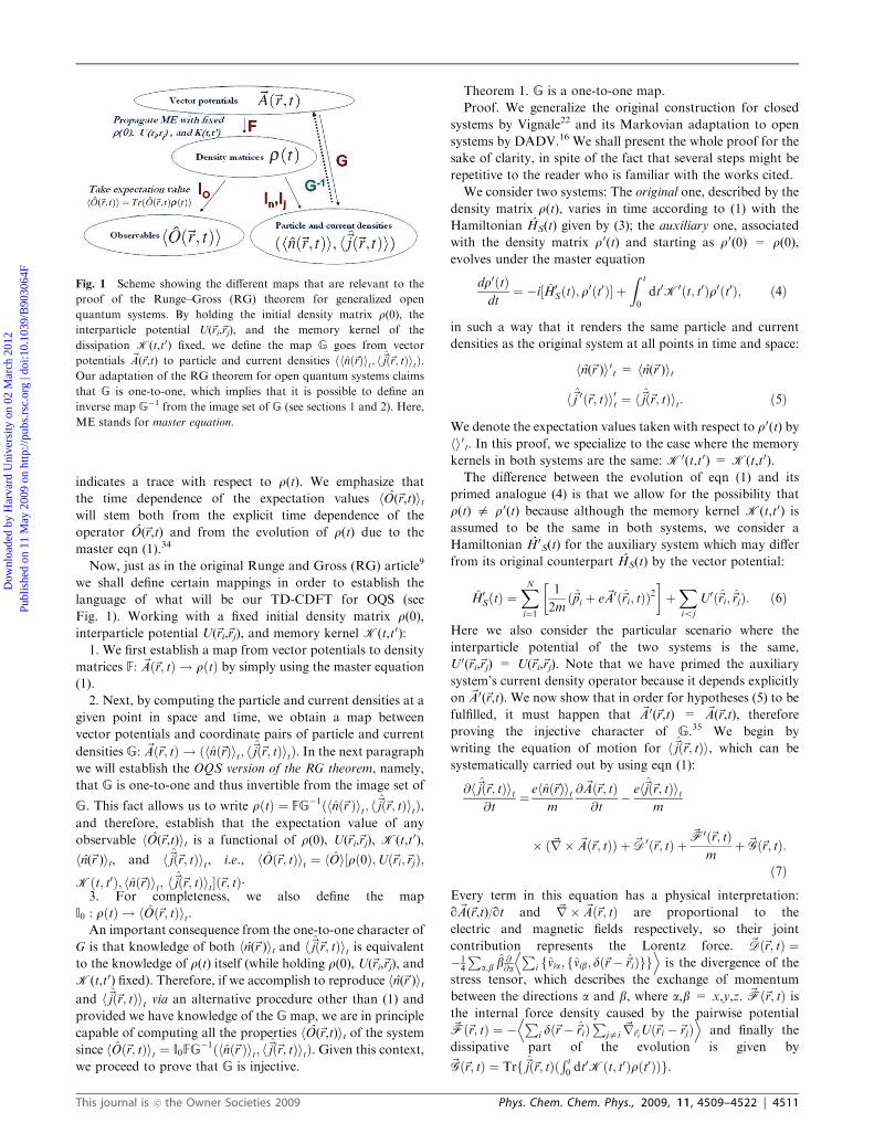
Fig. 1). Working with a fixed initial density matrix r(0),interparticle potential U(~ri,~rj), and memory kernel K(t,t0):

1. We first establish a map from vector potentials to density

matrices F: ~Að~r; tÞ ! rðtÞ by simply using the master equation

(1).

2. Next, by computing the particle and current densities at a

given point in space and time, we obtain a map between

vector potentials and coordinate pairs of particle and current

densities G: ~Að~r; tÞ ! ðhnð~rÞit; h~jð~r; tÞitÞ. In the next paragraph

we will establish the OQS version of the RG theorem, namely,

that G is one-to-one and thus invertible from the image set of

G. This fact allows us to write rðtÞ ¼ FG�1ðhnð~r Þit; h~jð~r; tÞitÞ,and therefore, establish that the expectation value of any

observable hO(~r,t)it is a functional of r(0), U(~ri,~rj), K(t,t0),

hn(~r )it, and h~jð~r; tÞit, i.e., hOð~r; tÞit ¼ hOi½rð0Þ;Uð~ri;~rjÞ;Kðt; t0Þ; hnð~rÞit; h~jð~r; tÞit�ð~r; tÞ.

3. For completeness, we also define the map

I0 : rðtÞ ! hOð~r; tÞit.An important consequence from the one-to-one character of

G is that knowledge of both hn(~r )it and h~jð~r; tÞit is equivalentto the knowledge of r(t) itself (while holding r(0), U(~ri,~rj), and

K(t,t0) fixed). Therefore, if we accomplish to reproduce hn(~r )itand h~jð~r; tÞit via an alternative procedure other than (1) and

provided we have knowledge of the G map, we are in principle

capable of computing all the properties hO(~r,t)it of the systemsince hOð~r; tÞit ¼ I0FG

�1ðhnð~r Þit; h~jð~r; tÞitÞ. Given this context,

we proceed to prove that G is injective.

Theorem 1. G is a one-to-one map.

Proof. We generalize the original construction for closed

systems by Vignale22 and its Markovian adaptation to open

systems by DADV.16 We shall present the whole proof for the

sake of clarity, in spite of the fact that several steps might be

repetitive to the reader who is familiar with the works cited.

We consider two systems: The original one, described by the

density matrix r(t), varies in time according to (1) with the

Hamiltonian HS(t) given by (3); the auxiliary one, associated

with the density matrix r0(t) and starting as r0(0) = r(0),evolves under the master equation

dr0ðtÞdt¼ �i½H0SðtÞ; r0ðt0Þ� þ

Z t

0

dt0K0ðt; t0Þr0ðt0Þ; ð4Þ

in such a way that it renders the same particle and current

densities as the original system at all points in time and space:

hn(~r )i0t = hn(~r )it

h~j 0ð~r; tÞi0t ¼ h~jð~r; tÞit: ð5Þ

We denote the expectation values taken with respect to r0(t) byhi0t. In this proof, we specialize to the case where the memory

kernels in both systems are the same: K0(t,t0) = K(t,t0).

The difference between the evolution of eqn (1) and its

primed analogue (4) is that we allow for the possibility that

r(t) a r0(t) because although the memory kernel K(t,t0) is

assumed to be the same in both systems, we consider a

Hamiltonian H0S(t) for the auxiliary system which may differ

from its original counterpart HS(t) by the vector potential:

H0SðtÞ ¼XNi¼1

1

2mð~pi þ e~A0ð~ri; tÞÞ2

� �þXioj

U0ð~ri;~rjÞ: ð6Þ

Here we also consider the particular scenario where the

interparticle potential of the two systems is the same,

U0(~ri,~rj) = U(~ri,~rj). Note that we have primed the auxiliary

system’s current density operator because it depends explicitly

on ~A0(~r,t). We now show that in order for hypotheses (5) to be

fulfilled, it must happen that ~A0(~r,t) = ~A(~r,t), therefore

proving the injective character of G.35 We begin by

writing the equation of motion for h~jð~r; tÞi, which can be

systematically carried out by using eqn (1):

@h~jð~r; tÞit@t

¼ ehnð~rÞitm

@~Að~r; tÞ@t

� eh~jð~r; tÞitm

� ð~r� ~Að~r; tÞÞ þ ~D 0ð~r; tÞ þ~F0ð~r; tÞ

mþ ~Gð~r; tÞ:

ð7Þ

Every term in this equation has a physical interpretation:

q~A(~r,t)/qt and ~r� ~Að~r; tÞ are proportional to the

electric and magnetic fields respectively, so their joint

contribution represents the Lorentz force. ~Dð~r; tÞ ¼�1

4

Pa;b b

@@a

Pi fvia; fvib; dð~r� ~riÞgg

D Eis the divergence of the

stress tensor, which describes the exchange of momentum

between the directions a and b, where a,b = x,y,z. ~Fð~r; tÞ isthe internal force density caused by the pairwise potential~Fð~r; tÞ ¼ �

Pi dð~r� ~riÞ

Pjai

~r~riUð~ri �~rjÞD E

and finally the

dissipative part of the evolution is given by

~Gð~r; tÞ ¼ Trf~jð~r; tÞðR t0 dt

0Kðt; t0Þrðt0ÞÞg.

Fig. 1 Scheme showing the different maps that are relevant to the

proof of the Runge–Gross (RG) theorem for generalized open

quantum systems. By holding the initial density matrix r(0), the

interparticle potential U(~ri,~rj), and the memory kernel of the

dissipation K(t,t0) fixed, we define the map G goes from vector

potentials ~A(~r,t) to particle and current densities ðhnð~rÞit; h~jð~r; tÞitÞ.Our adaptation of the RG theorem for open quantum systems claims

that G is one-to-one, which implies that it is possible to define an

inverse map G�1 from the image set of G (see sections 1 and 2). Here,

ME stands for master equation.

This journal is �c the Owner Societies 2009 Phys. Chem. Chem. Phys., 2009, 11, 4509–4522 | 4511

Dow

nloa

ded

by H

arva

rd U

nive

rsity

on

02 M

arch

201

2Pu

blis

hed

on 1

1 M

ay 2

009

on h

ttp://

pubs

.rsc

.org

| do

i:10.

1039

/B90

3064

F

View Online

Similarly, for the auxiliary system, we can analogously write

the equation of motion for h~j 0ð~r; tÞi0t:

@~j 0hð~r; tÞi0t@t

¼ ehnð~r Þi0tm

@~A0ð~r; tÞ@t

� eh~j 0ð~r; tÞi0tm

� ð~r� ~A0ð~r; tÞÞ

þ ~D0ð~r; tÞ þ~F0ð~r; tÞ

mþ ~G0ð~r; tÞ

ð8Þ

where the primed variables have their respective obvious

meanings. By subtracting eqn (8) from (7) and imposing

hypotheses (5) we can easily arrive to:

ehnð~r Þitm

@D~Að~r; tÞ@t

!¼ eh~jð~r; tÞit

m� ½~r� D~Að~r; tÞ�

þ ~Dð~r; tÞ þ~Fð~r; tÞm

þ ~Gð~r; tÞ !

� ~D0ð~r; tÞ þ~F0ð~r; tÞ

mþ ~G0ð~r; tÞ

!

ð9Þ

where we have defined the auxiliary system vector potential

with the original vector potential as the reference,~A(~r,t) = ~A(~r,t) + D~A(~r,t). Therefore, D~A(~r,t) is the unknown

function we are aiming to find.

At this point it may seem difficult to solve for D~A(~r,t)directly from eqn (9). However, progress can be made if one

assumes that the time-dependent functions are all analytic and

therefore admit a Taylor expansion about t = 0. If we denote

the Taylor coefficients byOk � 1k!@kOð~r;tÞ@tk

���t¼0

, once we collect the

terms of order tl we end up with the following identity:

eðlþ 1Þn0ð~r ÞD~Alþ1ð~r Þ ¼ � eXl�1k¼0ðkþ 1Þnl�kð~r ÞD~Akþ1ð~r Þ

þ eXlk¼0

~jl�kð~r Þ � ð~r� D~Akð~r ÞÞ

þ ðm~Dlð~r Þ þ ~Flð~r Þ þm~Glð~r ÞÞ

� ðm~Dl0ð~r Þ þ ~Fl

0ð~r Þ þm~Gl0ð~r ÞÞð10Þ

Note that all the Taylor coefficients are still position

dependent. We now claim that the right hand side of eqn (10)

does not contain any term D~Ak(~r ) for k4 l. This is obvious for

the terms that contain D~A(~r,t) explicitly. Let us study the other

terms. By definition, ~Dl0ð~rÞ can be written as:

~D0l ð~r Þ ¼ �1

4

Xls¼0

Xl�su¼0

Xa;b

b@

@aTr

XNi¼1

@uv0ia@tu

;@sv0ib@ts

; dð~r� ~riÞ� �� �

@l�r�sr0ðtÞ@tl�r�s

!

ð11Þ

We know that D~Ak(~r ) is the only coefficient of D~A(~r,t) that

appears in @kv 0ia@tk

, whereas the highest order coefficient in

@kr0ðtÞ@tk¼ @k�1

@tk�1@r0ðtÞ@t is D~Ak(~r ) (see eqn (1)). Based on these two

observations, it is straightforward to see that ~D0l ð~r Þ containsterms D~Ak�1(~r ) with k at the most being l. Similar arguments

allow us to conclude the same k r l condition for ~F0l ð~r Þ.Finally, for the term ~G0l ð~r Þ we have:

~D 0lð~r Þ ¼1

l!Tr

Xlk¼0

@k~j 0ð~r; tÞ@tk

@l�kðR t0 dt

0K0ðt; t0Þr0ðt0ÞÞ@tl�k

!

ð12Þ

Here, the dependence of@k~j 0ð~r; tÞ

@tk on ~A(~r,t) is only through

the k-th coefficient, D~A0k(~r ). For the integral term@kðR t

0dt0K0ðt;t0Þr0ðt0ÞÞ

@tk, we encounter two cases:

In the first case, K0(t,t0) is either a smooth function in t and

t0 or can be approximated as such, so we apply Leibniz rule

k times:

@kðR t0 dt

0K0ðt; t0Þr0ðt0ÞÞ@tk

¼Z t

0

dt0@kK0ðt; t0Þ

@tkr0ðt0Þ

þXk�1p¼0

Xk�1�pq¼0

k� 1� p

q

0@

1A

� @ pþqK0ðt; t0Þ@tpþq

@k�1�p�qr0ðt0Þ@tk�1�p�q

� �t0¼t

ð13Þ

If we evaluate this derivative at time t= 0, the first term in the

right vanishes. By examining the second term we conclude

that, by analogous reasons to the ones presented above,

this term only contains D~Ak�2(~r ) as its highest order

coefficient. In summary, for the first case, every D~Ak(~r ) in~Glð~r Þ has k r l � 2.

In the second case, whereK0(t,t0) is not an analytic function

in t and t0, it is not possible to anticipate a general conclusion.

However, the reader can easily check that as long as the

integralRt0dt0K0(t,t0)r0(t0) is analytic and does not contain

second derivatives of r0(t) with respect to t or higher, the

conclusion about the order of the coefficients D~Ak(~r ) in~Glð~r Þ still holds. For example, in the KL form, although

K0(t,t0) is not analytic due to the delta function it contains,Rt0dt0K0(t,t0)r0(t) = L(r) and ~G0l ð~r Þ ¼ Trð~j 0ð~r; tÞLðrÞÞ ¼PR2�1

i; j¼1 aijhLþj ~j 0ð~r; tÞLi � 12 Lþj Li

~j 0ð~r; tÞ � 12~j 0ð~r; tÞLþj Lii are both

analytic in t, and in fact, ~Glð~r Þ only contains terms

D~Ak(~r ) with k r l. We believe that physical memory

kernels are either smooth as in the first case, or if they belong

to the second case, they follow the conditions we have

outlined, in which case, we have finally proved the claim in

general.

The result above allows to regard eqn (10) as a recursion

relation to compute all the coefficients D~Ak(~r ) provided

we know D~A0(~r ). To obtain D~A0(~r ), we recognize that

4512 | Phys. Chem. Chem. Phys., 2009, 11, 4509–4522 This journal is �c the Owner Societies 2009

Dow

nloa

ded

by H

arva

rd U

nive

rsity

on

02 M

arch

201

2Pu

blis

hed

on 1

1 M

ay 2

009

on h

ttp://

pubs

.rsc

.org

| do

i:10.

1039

/B90

3064

F

View Online

D~A0(~r ) = D~A(~r,0) and that the constraints of eqn (5) at time

t = 0 yield:

D~A0ð~r Þ ¼Tr ðrð0Þ � r0ð0ÞÞ

Pi f~pi; dð~r�~riÞg

2ehnð~r; 0Þi ð14Þ

By hypothesis, r0(0) = r(0), so D~A0(~r ) = 0; however, eqn (10)

shows that given this initial condition, D~Ak(~r ) = 0 for all k,

which means that ~A0(~r,t) = ~A(~r,t) for all t A [0,tc1], where tc1 is

the largest time for which the analyticity of the functions is

ensured. However, the whole argument may be repeated by

expanding the time dependent functions about t= tc1 until the

radius of convergence in this interval is exhausted at t = tc2,36

and so on for the subsequent intervals, thus eventually proving

that ~A0(~r,t) = ~A(~r,t) for all times. This means that we

have finally showed the claim of Theorem 1. Obviously, this

argument fails in the pathological case where there is a

vanishing radius of convergence, in which case we cannot

iterate the procedure. However, just as in ref. 16 and 22, we

work under the assumption that the equations of motion we

are considering are smooth enough to rule this case out,

although we shall acknowledge that a more rigurous study

of this claim for the future would be of interest. Finally, one

could imagine extending this proof to piecewise analytic vector

potentials ~A(~r,t). We refer the reader to ref. 37 for more details

on this regard.

Before we close this section, we carry out a consistency

check. Just as we derived the equation of motion for the

current densities, we can prove from (1) and (4) that the

particle densities evolve as:

@hnð~r Þit@t

¼ �~r � h~jð~r; tÞit

þ Tr nð~r ÞZ t

0

dt0Kðt; t0Þrðt0Þ� �� �

ð15Þ

@hnð~r Þi0t@t

¼ �~r � h~j 0ð~r; tÞi0t

þ Tr nð~r ÞZ t

0

dt0K0ðt; t0Þr0ðt0Þ� �� �

ð16Þ

Interestingly, eqn (15) and (16) do not exhibit the continuity

form we are used to, but rather have leakage terms which are

related to the memory kernels K(t,t0) = K0(t,t0). We discuss

the implications about this issue in the next section. However,

this apparent anomaly does not interfere with the above

proof. The reason is that since we have concluded that

the vector potentials in both systems must be the same,~A0(~r,t) = ~A(~r,t), from eqn (6) and (3) the Hamiltonians must

satisfy H0S(t) = HS(t), and therefore, from eqn (4) and (1), we

conclude that the density matrices are equal at all times,

r0(t) = r(t). This means that eqn (16) and (15) are identical,

ensuring the consistency of our proof. Although the points we

are making in this paragraph might seem trivial, in the next

sections, they will be quite important for the establishment of a

KS scheme for TD-CDFT.

Notice that as opposed to standard TD-CDFT, the one-to-

one map G we have established goes from ~A(~r,t) to the

combination ðhnð~r Þit; h~jð~r; tÞitÞ as opposed to just h~jð~r; tÞit.The reader might wonder if there is any redundance in our

definition of the G map; for instance, we could imagine

just defining G: ~Að~r; tÞ ! h~jð~r; tÞit instead of considering

the codomain to be the set of Cartesian products

ðhnð~r Þit; h~jð~r; tÞitÞ. The map would in fact be redundant if

the continuity equation were satisfied:@hnð~r Þit

@t ¼ �~r � h~jð~r; tÞit,which is true for closed systems. The reason is because

knowing the function h~jð~r; tÞit would imply knowing@hnð~r Þit

@t ,

but since by hypothesis we know r(0), we can calculate hn(~r )i0and thus by integration over t, also compute hn(~r )it for all

~r and t. However, as shown explicitly in eqn (15) and (16),

continuity does not hold in general in the context we

are working on, so the claims we are making in this

article about the G map would not necessarily be true if we

consider h~jð~r; tÞit alone, rather than the combination

ðhnð~r Þit; h~jð~r; tÞitÞ, as the codomain of G.

3. On the problem of leakage and the

establishment of a Kohn–Sham scheme

The fact that (15) is not a continuity equation was pointed out

several years ago by Frensley,38 but has only recently been

extensively studied independently by Gebauer and Car (GC)39

and later on by Bodor and Diosi (BD).40 These authors have

focused on the case where a KL master equation is derived

microscopically from a system potential and a system-bath inter-

action both of which are local in the system coordinates. Let us

briefly comment on their work in light of our present study.

First of all, let us consider the total object composed

of the system S and the bath B with Hamiltonian

H = HS + HB + HSB. Here SB denotes the system-bath

interaction. If HSB and the potential in HS depend locally on

the coordinates of the system, it can be easily shown that the

exact particle and current densities (obtained from the unitary

evolution of the composite density matrix) do satisfy the

continuity equation and the leakage term vanishes. However,

depending on the level of description of the bath, which is

associated with the memory kernel K(t,t0), the leakage term

Tr{n(~r,)(Rt0dt0K(t,t0)r(t0))} might not necessarily be equal to

zero. In fact, for the particular case that GC and BD have

studied, which is the KL master equation derived micro-

scopically from H, the leakage term becomes

Tr nð~r ÞZ t

0

dt0Kðt; t0Þrðt0Þ� �� �

¼Trf nð~rÞLðrðtÞÞg

�XR2�1

i;j¼1aij Lj

þnð~r ÞLi�1

2LjþLinð~r Þ�

1

2nð~r ÞLj

þLi

� �t

;

ð17Þ

where the jump operators Li are in general non-local in space.

Therefore, n(~r,t) does not necessarily commute with these

operators and each of the traces in the right hand side of

eqn (17) might not vanish. Physically, leakage appears in the

KL formalism due to the imposition of the Born-Markov

approximation, which coarse-grains the events that occur at

the time-scale of the bath (see ref. 40).

The object h~jð~r; tÞit as calculated naively by taking the

expectation value of the current density operator h~jð~r; tÞi withrespect to the density matrix r(t) evolved through eqn (1) with

the memory kernel given by (2) might not necessarily correspond

to the total measured current in a nanodevice, since it misses

This journal is �c the Owner Societies 2009 Phys. Chem. Chem. Phys., 2009, 11, 4509–4522 | 4513

Dow

nloa

ded

by H

arva

rd U

nive

rsity

on

02 M

arch

201

2Pu

blis

hed

on 1

1 M

ay 2

009

on h

ttp://

pubs

.rsc

.org

| do

i:10.

1039

/B90

3064

F

View Online

the contribution that arises from the instantaneous redistribution

of position and momenta of the system due to collisions with

the bath. Therefore, the total current is composed of h~jð~r; tÞit,which is the object we have been studying throughout this

article and which GC and Piccinin (GCP)41 have called the

Hamiltonian current, plus the non-Markovian feedback we just

described, which has been named the collision current. It is

noteworthy, however, that the authors were able to derive an

explicit expression for the collision current operator ~jcolð~r; tÞwhich can be used to calculate the collision current by taking

the trace of its action on the (coarse-grained) density matrix

r(t) given by eqn (1), that is, by computing the quantity

h~jcolð~r; tÞi. In other words, it is still fine to use eqn (1)

but we need to keep in mind that if we are asked to

calculate the total current density we will need to compute

h~jð~r; tÞ þ ~jcolð~r; tÞit rather than just h~jð~r; tÞit. On the other

hand, h~jð~r; tÞit is not void of physical meaning, since it is

associated to the work done by the flow of particles.41 From a

more pragmatic perspective, even if we disregard the physical

meaning of h~jð~r; tÞit for a moment, Theorem 1 still guarantees

us that the knowledge of hn(~r,t)it and h~jð~r; tÞit for all ~r and t

amounts to the same information as r(t) for all t, which in turn

implies knowledge of h~jcolð~r; tÞit, and therefore of the total real

current. Obviously if instead of staying in the KL form, we use

the exact memory kernel K(t,t0) derived microscopically from

H, the continuity equation would be fully restablished. For the

intermediate case of non-Markovian memory kernels, it is not

very clear at this moment how would the ‘‘leakage’’ in eqn (15)

be affected and what h~jð~r; tÞit would precisely mean, though

these are definitely interesting questions to explore.

Going beyond the case studied by GCP, in many situations of

practical interest, master equations used to model relaxation

from non-equilibrium configurations will contain memory

kernels K(t,t0) that do not necessarily cause the rightmost term

in eqn (15) to vanish, in which case, an appropriate interpretation

for the object h~jð~r; tÞit is desirable. From a more general

perspective, the claim that Theorem 1 provides suffices to

regard h~jð~r; tÞit as a quantity that has computational merit

on its own, and this pragmatic approach will turn out to

be good enough to work through the rest of this article.

Hereafter, unless otherwise specified, the word current will

be used again to refer to h~jð~r; tÞit since we will not worry aboutthe other types of currents.

After this interlude, the reader might question why should

we care about leakage if our version of the RG theorem did

not seem to be affected by it. However, let us ask the following

question: Can we suggest a theorem whereby the same particle

and current densities hn(~r )it and h~jð~r; tÞit of the original systemcan be reproduced by a non-interacting open KS system with the

same memory kernel K(t,t0) and starting with a density matrix

r0(0) which may be different from r(0)? DADV have argued

that this is possible for the case of Markovian master

equations.16 If we follow their rationale, we just need to make

the following trivial modifications to the proof of Theorem 1:

(a) Set U0(~ri,~rj) = 0 in (6), and (b) lift the restriction that

r0(0) = r(0). At a first glance, it may seem that such a proof is

valid. Nevertheless, the problem manifests itself when we

arrive to the consistency check in (15) and (16). Let us analyse

the situation carefully: In constructing the KS vector potential

~A0(~r,t), we considered both the hypotheses in eqn (5) and the

set of eqn (7) and (8), which describe the motion for h~jð~r; tÞitand h~j 0ð~r; tÞi0t respectively. However, the constraints given by

eqn (15) and (16), were not used at all, but should be satisfied

by the respective particle and current densities. The only way

the constructed ~A0(~r,t) does what we want (which is to

reproduce hn(~r,t)t and h~jð~r; tÞit from the original system in

the auxiliary system, as expressed in (5)) is if the ‘‘leakage’’

terms in both systems are the same:

Tr{n(~r )(Rt0dt0K(t,t0)r(t0))}

= Tr{n(~r )(R0tdt0K0(t,t0)r0(t0))} (18)

If K0(t,t0) = K(t,t0), (18) becomes an additional restriction

which cannot be satisfied in general. DADV have suggested

that these terms normally vanish;42 however, as we have

commented before, based on the work of GCP39 and BD,40

these terms are in general not negligible: In fact, if the

system-bath interaction is local in the coordinates of the

system, from the microscopic derivation of the KL master

equation, it can be seen that La is a non-local function in

space, which then does not commute with n(~r ), and hence,

Tr{n(~r )L(r(t)) does not necessarily vanish). Interestingly how-

ever, due to the weaker conditions expected for TD-DFT, the

analogous KS scheme suggested by BCG14 is actually justified.

For a discussion of this case, we refer the reader to ref. 17.

The reason why Vignale did not encounter this problem for a

closed system (K(t,t0) = 0) in (ref. 22) is because in that case,

there are no ‘‘leakage’’ terms and the equations (15) and (16) are

just redundant with respect to (5). It seems, however, that the only

problem in DADV’s scheme is a matter of the restriction of two

variables to reproduce, but only constructing a single function.

We might imagine that lifting some of the assumptions in the

suggested KS scheme will give freedom to the mathematical

structure and will solve the problem. In fact, in the next section,

we show that by not assuming thatK0(t,t0) must equal toK(t,t0),

a KS scheme is actually possible. Additionally, in section 5, we

will prove that there is a simpler alternative KS scheme where the

auxiliary system is taken to be both closed and non-interacting.

4. A possible modification of D’Agosta and Di

Ventra’s Kohn–Sham scheme

Without more preamble, using the same language that we have

been employing before, we make the following claim:

Theorem 2. It is possible to reproduce both the particle and

current densities of the original many-body interacting OQS

(hn(~r )i0t = hn(~r )it, h~j 0ð~r; tÞi0t ¼ h~jð~r; tÞi0t for all~r and t) with an

auxiliary Markovian OQS with interparticle potential U0(~ri,~rj)

starting in the state r0(0) at the expense of a given vector

potential ~A0(~r,t) and a memory kernel K0(t,t0) of the KL form

with a single jump operator:

K0(t,t0) = L0(r(t0))d(t � t0)

= (�12L0+(t)L0(t)r0(t0)�1

2r0(t0)L0+(t)L0(t)

+ L0(t)r0(t0)L0+(t))d(t � t0) (19)

Comments. (a) As opposed to the proof for Theorem 1, here we

do not assume that in general r0(0) = r(0), K0(t,t0) = K(t,t0)

or U0(~ri,~rj) = U(~ri,~rj). (b) The corollary of Theorem 2 for the

4514 | Phys. Chem. Chem. Phys., 2009, 11, 4509–4522 This journal is �c the Owner Societies 2009

Dow

nloa

ded

by H

arva

rd U

nive

rsity

on

02 M

arch

201

2Pu

blis

hed

on 1

1 M

ay 2

009

on h

ttp://

pubs

.rsc

.org

| do

i:10.

1039

/B90

3064

F

View Online

non-interacting auxiliary system, i.e. U0(~ri,~rj) = 0 corresponds

to the KS case. (c) Note that the theorem claims that even if the

kernel of the original system K(t,t0) is non-Markovian, the

kernel in the KS system can be taken to be Markovian. (d) For

the case where the original system’s kernel K(t,t0) is of the KL

form, Theorem 1 becomes a fix for DADV’s KS scheme.

Proof. Compared to the proof given for Theorem 1, we need

to construct both ~A0(~r,t) andK0(t,t0) instead of just ~A0(~r,t). We

follow the same steps as in Theorem 1, except that we consider

the adaptations indicated in Comment (a). When we reach

eqn (10), we still follow all the arguments about how there are

no terms D~Ak(~r ) for k4 l in the right-hand side. However, we

do not proceed further to solve for each of the coefficients

D~Al+1(~r ) since ~G0l ð~r Þ containsK0(t,t0), which at the moment is

an unknown function since we have not constructed it. Having

this in mind, we combine eqn (10) and (18) in order to

solve for both D~A(~r,t) and K0(t,t0). There could be many

possibilities for K0(t,t0), but as we have specified in the claim,

we choose the simplest, namely, the KL form K0(t,t0)r(t0) =L0(r(t0))d(t � t0) with the respective generator L0+(t).

Let the leakage term be denoted by l(~r,t) � Tr{n(~r,t)Rt0K(t,t0)r(t)} so that (18) can be read as l(~r,t) = l0(~r,t). The

l-th time derivative of this equation evaluated at t = 0 reads

ll(~r ) = l0l(~r ). Here, we employ the same notation for the Taylor

expansion coefficients as before. This equation yields a possible

solution (there are many) for a matrix L0l in terms of the

appropriate time derivatives of ~A(~r,t), K(t,t0), ~jð~r; tÞ, r(t), r0(t),and lower order derivatives of L0 at t = 0. By similar arguments

as the ones presented in section II, one can show that the chosen

solution for L0l will only contain terms D~Ak(~r ) such that k r l.

On the other hand, the recursion of eqn (10) shows that the first

step in which L0l appears is on the right hand side of the solution

for D~Al+1(~r ) (inside of ~G0l ð~r Þ, see eqn (10)). With these observa-

tions in mind, the construction of the coefficients L0l and D~Al(~r )

for all l Z 0 is possible through a small modification of the

recursion (10). By using strong induction, we assume that right

before the lth step of the recursion, we already know D~Ak(~r ) and

Lk for all ko l. The lth step consists of (a) the solution of ll(~r ) =l0l(~r ) for Ll, followed by (b) the solution of (10) for D~Al+1(~r ).

Symbolically: � � �-D~Al(~r ) - Ll - D~Al+1(~r ) -� � �. Note that

D~A0(~r ) is still given by (14), and in fact, once we know its value,

we can solve l(~r,0) = l0(~r,0) (which depends on the already

obtained D~A0(~r )) for a possible L0, therefore building a base for

the recursion. This concludes the inductive proof.

With Theorem 2, we have not only provided a fix for

DADV’s KS scheme for Markovian OQS, but we have

also generalized it for their non-Markovian counterpart.

Although this scheme might be advantageous in some

practical applications, we believe that the alternative scheme

we propose in the next section offers a new perspective in the

formulation of KS schemes and might be more practical than

the one we considered here.

5. An alternative KS scheme for open systems

The next theorem constitutes our alternative proposal for KS

scheme to be used in the practice of TD-CDFT for an

arbitrary OQS:

Theorem 3. (A,C Kohn Sham scheme) There exists an

auxiliary closed KS system which starting in the state rKS(0)

evolves unitarily under a KS Hamiltonian HKS(t):

HKSðtÞ ¼Xi

~pi þ eð~AKSð~ri; tÞ þ ~Cð~ri; tÞÞ2m

!2

þXioj

Uð~ri;~rjÞ ð20Þ

producing particle and filtered current densities that are related

to the particle and current densities of the original many body

interacting open quantum system governed by (1) by:

hn(~r )iKS,t = hn(~r )it

h~jfiltð~r; tÞiKS;t ¼ h~jð~r; tÞit ð21Þ

where we have defined the filtered current operator as

~jfiltð~r; tÞ ¼P

i12f~vi;filtð~ri; tÞ; dð~r� ~riÞg with the filtered velocity

operator given by ~vi;filtð~ri; tÞ ¼ ~piþe~AKSð~ri;tÞm . Additionally, we

denote the expectation values in the KS system in the usual

form hO(~r,t)iKS,t = Tr(O(~r,t)rKS(t)). We shall call ~AKS(~r,t) the

KS vector potential, and ~C(~r,t) the leakage potential.

Proof. We proceed similarly to the proof in Theorem 1:

Given the master eqn (1), we evolve it to compute hn(~r )it andh~jð~r; tÞit for all positions and times. We explicitly ‘‘solve’’

for ~AKS(~r,t) and ~C(~r,t) such that the density matrix

rKSðtÞ ¼Tðe�iR t

0dt0HKSðt0ÞÞrð0ÞðTðe�i

R t

0dt0HKSðt0ÞÞÞþ, where T

denotes the time-ordering operator, renders the expectation

values hn(~r )iKS,t and h~jfiltð~r; tÞiKS;t which satisfy the relations

given in eqn (21). The explicit construction of ~AKS(~r,t) and~C(~r,t) implt their existence, and therefore prove the theorem.

We construct these potentials in two steps.

Step 1. (Construction of ~C(~r,t)). The equation of motion for

the particle density of the open system is just the pseudo-

continuity eqn (15). On the other hand, for the KS system, we

can write:

@hnð~r ÞiKS;t

@t¼ �~r � h~jfiltð~r; tÞiKS;t

� ~r � e~Cð~r; tÞm

hnð~r ÞiKS;t

! ð22Þ

By applying the constraints (21), it follows that ~C(~r,t) must be

given by

~Cð~r; tÞ ¼ � m

ehnð~r Þit

Zd3r

@hnð~r Þit@t

þ ~r � h~jð~r; tÞit� �

ð23Þ

where the addition of any function in time as an integration

constant is valid at this point. It is possible that a particular

way of choosing boundary conditions may enhance the

intuitive physical meaning of the leakage potential ~C(~r,t).

For instance, for the particular case studied by Gebauer,

Car, and Piccinin, we can choose ~C(~r,t) so thate~Cð~r;tÞ

m hnð~r ÞiKS;t is equal to what they have termed the collision

current41 (see discussion in Section III). However, this choice

is not formally necessary and ~C(~r,t) can simply be regarded as

a strategy that reestablishes the continuity equation via

This journal is �c the Owner Societies 2009 Phys. Chem. Chem. Phys., 2009, 11, 4509–4522 | 4515

Dow

nloa

ded

by H

arva

rd U

nive

rsity

on

02 M

arch

201

2Pu

blis

hed

on 1

1 M

ay 2

009

on h

ttp://

pubs

.rsc

.org

| do

i:10.

1039

/B90

3064

F

View Online

hn(~r )iKS,t. In fact, notice that the actual (unfiltered) KS

current density operator ~jð~r; tÞ ¼P

i12f~við~ri; tÞ; dð~r� ~riÞg where

~við~r; tÞ ¼ ~piþeð~AKSð~ri ;tÞþ~Cð~ri ;tÞÞm does satisfy the continuity

equation by construction since ~jð~r; tÞ ¼ ~jfilt þ em~Cð~r; tÞnð~r Þ.

Step 2. (Construction of ~AKS(~r,t)). The equation of motion

for h~jð~r; tÞit for the original system was given in (7). For the

closed KS system, we can analogously write an equation of

motion for h~jð~r; tÞiKS;t:

@h jð~r; tÞiKS;t

@t¼hnð~r ÞiKS;t

m

@ð~AKSð~r; tÞ þ ~Cð~r; tÞÞ@t

�h~jð~r; tÞiKS;t

m� ð~r� ð~AKSð~r; tÞ þ ~Cð~r; tÞÞÞ

þ ~DKSð~r; tÞ þ~FKSð~r; tÞ

m

ð24Þ

Note the absence of a dissipative ~GKSð~r; tÞ term due to the

unitarity of the evolution of the KS system. Combining the

constraints (21) with (7) and (24) yields:

ehnð~rÞitm

@D~Að~r;tÞ@t

!

¼� e

m

@ð~Cð~r;tÞhnð~rÞitÞ@t

þeh~jð~r;tÞitm

�½~r�ðD~Að~r;tÞþ ~Cð~r;tÞÞ�

þe~Cð~r;tÞhnð~rÞitm

�½~r�ðD~Að~r;tÞþCð~r;tÞÞ�

þ ~Dð~r;tÞþ~Fð~r;tÞmþ~Gð~r;tÞ

!

� ~DKSð~r;tÞþ~FKSð~r;tÞ

m

!:

ð25Þ

where as usual we have defined ~A = ~AKS(~r,t) + D~A(~r,t). Justas in (10), we write out the terms of (25) of order tl:

eðlþ1Þn0ð~rÞD~Alþ1ð~rÞ

¼�eXl�1k¼0ðkþ1Þnl�kð~rÞD~Akþ1ð~rÞ

�eXlk¼0ðkþ1Þ~Cl�kð~rÞnkþ1ð~rÞÞ

�eXlk¼0ðl�kþ1Þ~Cl�kþ1ð~rÞnkð~rÞÞ

þeXlk¼0

~jl�kð~rÞ�~r�ðD~Akð~rÞþ ~Ckð~rÞÞ

þeXlq¼0

Xl�qk¼0

~Cl�k�qð~rÞnqð~rÞ�½~r�ðD~Að~rÞþ ~Ckð~rÞÞ�

þðm~DKS;lð~rÞþ ~FKS;lð~rÞÞ�ðm~Dlð~rÞþ ~Flð~rÞþm~Glð~rÞÞ:ð26Þ

From analogous arguments to the ones in the proof for

Theorem 1, all the terms D~Ak in the right hand side of (26) are

such that k o l. This is a consequence of the linearity of the

master eqn (1). The recursion ladder can be solved if we

know the value of D~A0(~r ), which from the constraints (21)

for t = 0 yield D~A0ð~r Þ ¼Trððrð0Þ�r0ð0ÞÞð

Pifp!i;dð~r�~riÞgÞ

2ehnð~r;0Þiþ Cð~r; 0Þ.

Note that provided we decide on a systematic way to choose

the boundary conditions for ~C(~r,t), ~A(~r,t) is uniquely

defined. QED.

We call the reader’s attention to several features of Theorem 2:

INTERACTING TO NON-INTERACTING. Just as in the regular KS

schemes, we can set the auxiliary system to be non-interacting,

U0(~ri,~rj) = 0.

MIXED STATES TO PURE STATES. For practical applications, it

might be the case that sometimes it is easier to work with pure

states rather than mixed states. In fact, from a computational

perspective, the numerical propagation of a pure state in an

R-dimensional Hilbert space requires the propagation of

2(R � 1) real parameters of a vector, whereas for a mixed

state, it requires the evolution of R2 � 1 real parameters. If the

KS initial state is taken to be pure, i.e. rKS(0) =

|cKS(0)ihcKS(0)|, where |cKS(0)i is the initial KS wave-

function, Theorem 2 guarantees that the KS state will stay

pure at all times due to the unitary evolution via

jcKSðtÞi ¼Tfe�iR t

0HKSðt0Þdt0 jcKSð0Þig. There is however, the

subtle question of whether given any master eqn (1), |cKS(0)iwould always exist such that it can satisfy the constraints (21)

at t = 0. However, the first constraint with respect to the

particle densities can be trivially satisfied for bosons, and

by the so-called Harriman construction for the case of

fermions, which is a prescription to construct an N particle

single Slater determinant with a specified particle density.44

Once this initial wavefunction |cKS(0)i is constructed, the

constraint in the current density can always be satisfied by

choosing D~A(~r,0) as explained at the end of the proof for

Theorem 2.

OPEN SYSTEM TO CLOSED SYSTEM. Theorem 2 provides us with

the formal footing to calculate the particle and current

densities of an open system in a closed system. The artifact

involved in this mapping is the construction of the leakage

potential ~C(~r,t) and the definition of a filtered current operator

~jfiltð~r; tÞ. If there is no leakage, ~C(~r,t) vanishes identically for all

~r and t. This happens naturally for K(t,t0) = 0, which is the

case of closed systems, but might also happen in open systems

in the special case where the system-bath interaction is local in

the coordinates of the system. In such case, ~jfiltð~r; tÞ ¼ ~jð~r; tÞand we effectively have a map from an open to a closed system

without any additional artifact. However, as discussed in

section 3, this case might be an exception rather than a rule.

In any case, the use of a closed system as the auxiliary KS

system might turn out to have very important implications,

since at the present time, there are many more numerical

propagation schemes for closed quantum systems,43 than their

open counterpart.

An important feature associated with the use of a closed KS

system is that we do not need to worry about the propagation

of the Slater determinant as a whole, but rather evolve each

orbital unitarily and reconstruct the Slater determinant at all

points in time when needed, just as one might envision

performing real time TD-CDFT of closed systems. This

4516 | Phys. Chem. Chem. Phys., 2009, 11, 4509–4522 This journal is �c the Owner Societies 2009

Dow

nloa

ded

by H

arva

rd U

nive

rsity

on

02 M

arch

201

2Pu

blis

hed

on 1

1 M

ay 2

009

on h

ttp://

pubs

.rsc

.org

| do

i:10.

1039

/B90

3064

F

View Online

contrasts with the schemes of BCG and DADV, where the KL

master equation induces non-unitary quantum jumps between

different orbitals.

FUNCTIONALDEPENDENCEOF ~C(~r,t). The proof of the existence

of the potentials of the KS system is an explicit construction of

them. Since the expression (23) consists of an integral in space,~C(~r,t) must be a non-local functional in space of hn(~r 0)it andh~jð~r 0; tÞit, but we see that it is local in time since no other times

t0 appear in the expression. In summary we may write ~Cð~r; tÞ ¼~C½hnð~r 0Þit; h~jð~r 0; tÞit�ð~r; tÞ for all~r0 within the range of integra-

tion in (23).

FUNCTIONAL DEPENDENCE OF ~AKS(~r,t). On the other hand, the

construction of ~AKS(~r,t) is highly nonlocal in time due to the

complicated relations of the different Taylor coefficients

D~Al(~r ) in terms of nk(~r ) and ~jk(~r ) (see eqn (10)). However, it

is easy to see that except for the spacial non-locality that

comes from ~C(~r,t) (which by the way, we emphasize does not

carry time non-locality) all the other contributions for ~AKS(~r,t)

are local in space. Therefore, we may write

~AKSð~r; tÞ ¼ ~AKS½hnð~r Þit0 ; h~jð~r; t0Þit0 ;Uð~ri;~rjÞ;U0ð~ri;~rjÞ;

Kðt; t0Þ; ~Cð~r; tÞ; rð0Þ; rKSð0Þ�ð~r; tÞ

for all t0 A [0,t]. For the development of functionals, it may be

taken for granted that U(~ri,~rj) is always the same interaction,

such as the Coulomb potential Uð~ri;~rjÞ ¼ 1j~ri�~rjj, and the KS

interaction is null, U0(~ri,~rj) = 0. We could have absorbed the

functional dependence of ~C(~r,t) into hn(~r 0)it and h~jð~r 0; tÞit, butthat would have make the notation cumbersome. In fact, we

want to stress that in order to construct ~A(~r,t) for the

particular position ~r 0 and time t, it is not necessary to know

the values of ðhnð~r 0Þit0 ; h~jð~r 0; t0Þit0 Þ for all~r 0 in space and for all

t0 A [0,t]. In fact, it is only necessary to know

ðhnð~r 0Þit0 ; h~jð~r 0; t0Þit0 Þ for all the history t0 A [0,t] for fixed ~r,

plus an additional piece ðhnð~r 0Þit; h~jð~r 0; tÞitÞ00 for all~r 0 that lie

within the space integral given in (23), but just at the instant t.

INITIAL STATE DEPENDENCE. From the discussion above, the

initial state dependence for both the original and the KS

density matrices constitutes a problem in the practical

implementation of functionals. This situation has been

extensively studied by Maitra, Burke, and Woodward in the

context of regular TD-DFT.37 In our case, this difficulty can

be overcome if the initial state r(0) = |cground(0)ihcground(0)|

is taken to be the pure non-degenerate ground state of HS(0).

Then, by ground state C-DFT, cground(~r,0) is itself a functional

of the initial particle density hn(~r )i0 and paramagnetic current

density h~jpð~r; 0Þi0 � h~jð~r; 0Þi0 �e~Að~r;0Þhnð~r Þi0

m .46 Similarly, for the

KS initial state, one can choose the initial wavefunction to be

the actual ground state of the non-interacting Hamiltonian,

cKS,ground(~r,0), which being uniquely defined up to a phase

factor, is also a functional of hn(~r )iKS,0 and h~jpð~r; 0ÞiKS;0. For

longitudinal vector potentials, one can use the analogous

properties from ground state DFT47 or thermal ensemble

DFT.48 If r(0) cannot be taken to be the ground state of the

HS(0), then the method of pseudohistories may be applied.45

COMPARISON WITH STANDARD TD-CDFT. When K(t,t0) = 0,

our theory reduces to standard TD-CDFT, in which case~C(~r,t) = 0 and the functional dependence of ~AKS(~r,t) is time

non-local but spacially local. In our case, we still follow the

spirit of standard TD-CDFT in most part, but we cannot get

rid of the small space non-locality contribution given by ~C(~r,t).

However, compared to the ultranonlocality problem in

TD-DFT, we perform much better in the sense that the

non-locality in space does not affect ~AKS(~r,t) at times t0 o t.

We speculate that this is the small cost associated with

working with closed systems in the KS scheme.

6. Numerical simulation of a model system

To test the numerical aspects of Theorem 3, we have

considered a model system, namely, the evolution of a 1-D

harmonic oscillator, HS ¼ p2

2mþ mo2 x2

2 (we take �h = m =

o = 1), which starting in the superposition pure state

r(0) = 12(|3i+ |4i)(h3| + h4|) (|ni denoting the n-th eigenstate

of the oscillator) eventually decays to the ground state |0i viathe KL master equation,

drðtÞdt¼ �i½HS; rðtÞ�

þ � 1

2LþLrðtÞ � 1

2rðtÞLþLþ LrðtÞLþ

� �:

Here, L =P4

j=1z|0ihj| denotes the effect of the heat bath on

the system, and z characterizes the decay rate. We carried out

simulations for z = 0, 0.15, and 0.5. The results of these

simulations are summarized in Fig. 2–4, respectively.

The density matrix r(t) was expressed in the eigenstate basis

and propagated under the superoperator (1) with a time

step of Dt = 0.1. The particle and current densities

hn(x)it and h~jðx; tÞit were calculated at each time step by

analytically evaluating the eigenstates and their derivatives in

the position representation in terms of Hermite polynomials.

We used a grid spanning the position interval [�1,1] with

a spacing of Dx = 0.001. In every case, as time progresses

we notice that hn(x)it gradually approaches the Gaussian

form of the ground state. On the other hand we recognize

that the oscillations of h~jðx; tÞit slowly decay as the state

r(t) evolves towards an eigenstate, which has zero current

density.

In terms of the construction of the potentials, we first

inverted ~C(x,t) from hn(x)it and h~jðx; tÞit by numerically

implementing the integral in eqn (23) using the trapezoidal

rule, and taking the arbitrarily chosen boundary condition~C(0,t) = 0. From there, we computed the KS particle

and filtered current densities hn(x)iKS = hn(x,t)i and

h~jðx; tÞiKS;t ¼ h~jðx; tÞit þe~Cðx;tÞhnðxÞit

m . In order to invert~AKS(x,t), we found it convenient to work in the gauge where

the potential in the KS Hamiltonian is scalar,

HKSðtÞ ¼ p2

2 þ VKSðx; tÞ. This is possible since in one dimen-

sion, the vector potential is anyways purely longitudinal. We

first proceeded to reconstruct a possible KS wavefunction by

assuming the form cKSðx; tÞ ¼ eiyðx;tÞffiffiffiffiffiffiffiffiffiffiffiffiffiffihnðxÞit

p, so in this gauge

there is no vector potential, and therefore the current density

takes its familiar form, h~jðx; tÞit ¼ x=fc�KSðx; tÞ@cKSðx;tÞ

@x g. Theprevios assertion implies that h~jðx; tÞit ¼ xhnðxÞit

@yðx;tÞ@x .

The phase y(x,t) was extracted by an additional numerical

integration routine with the trapezoidal rule, and setting

This journal is �c the Owner Societies 2009 Phys. Chem. Chem. Phys., 2009, 11, 4509–4522 | 4517

Dow

nloa

ded

by H

arva

rd U

nive

rsity

on

02 M

arch

201

2Pu

blis

hed

on 1

1 M

ay 2

009

on h

ttp://

pubs

.rsc

.org

| do

i:10.

1039

/B90

3064

F

View Online

y(0,t) = 0 as the boundary condition. With cKS(x,t) in hand,

we finally attempted to solve for VKS(x,t) from the time-

dependent Schrodinger equation applied to the KS system:

VKSðx; tÞ ¼ 1cKSðx;tÞ

i @cKSðx;tÞ@t þ @2cKSðx;tÞ

2 @x2

� �. The latter numerical

task required the use of a least-squares fit routine such that

for each time t, VKS(x,t) was expanded as a 6-th degree

polynomial in x. In order to ensure the validity of this

numerical step, we computed Tðe�iR t

0dt0HKSðt0ÞcKSð~r; 0ÞÞ with

the polynomially fit VKS(x,t) in HKS by using the time-reversal

symmetry enforced propagator reported in ref. 43. We

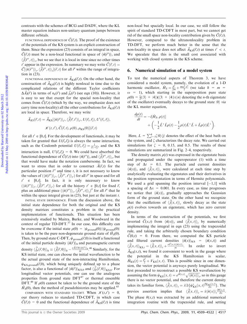
Fig. 2 1-D harmonic oscillator uncoupled to a heat bath. The particle (a) and current densities (b) were computed through the evolution of a density

matrix starting in the pure state r(0) = 12(|3i+ |4i)(h3| + h4|). The real and imaginary parts of the constructed Kohn–Sham wavefunction (c and d)

coincide with the unitary evolution of the density matrix of the original system up to a time-dependent phase factor which is physically irrelevant.

The constructed scalar (e) and vector (f) potentials exhibit the expected forms, which are parabolic and planar surfaces, respectively. The leakage

potential (g) is theoretically null for all points in position and time, but due to the numerical nature of the exercise, it exhibits negligible noise.

4518 | Phys. Chem. Chem. Phys., 2009, 11, 4509–4522 This journal is �c the Owner Societies 2009

Dow

nloa

ded

by H

arva

rd U

nive

rsity

on

02 M

arch

201

2Pu

blis

hed

on 1

1 M

ay 2

009

on h

ttp://

pubs

.rsc

.org

| do

i:10.

1039

/B90

3064

F

View Online

observed numerical consistency with the inverted wavefunction

cKS(~r,t). Going back to the gauge where the scalar potential

vanishes, by recognizing that the total vector potential~AKS(x,t) + ~C(x,t) in eqn (20) must equal to

x @@x

R t0 VKSðx; t0Þ dt0, we finally constructed ~AKS(x,t) by

performing another step of trapezoidal rule numerical integration

and substracting out the already constructed leakage potential~C(x,t). To gain more intuition on the problem, we have plotted

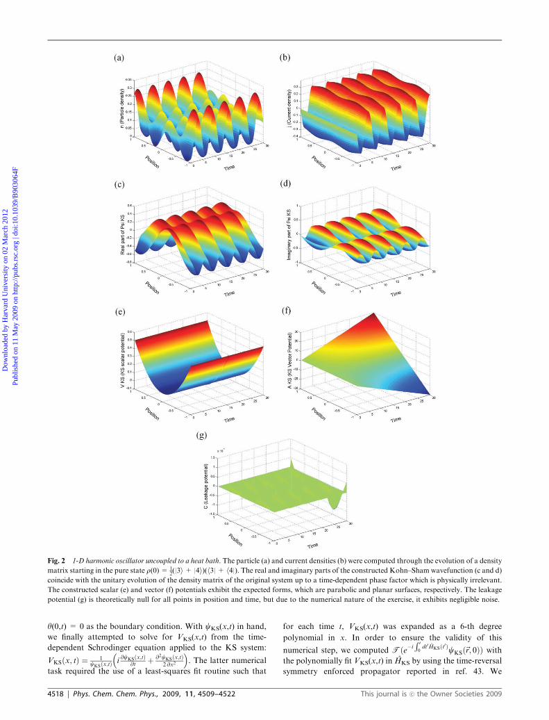
Fig. 3 1-D harmonic oscillator coupled to a heat bath that induces decays to the ground state with a rate z = 0.15. Just as in Fig. 1, the particle (a)

and current densities (b) were computed through the evolution of a density matrix starting in the pure state r(0) = 12(|3i+ |4i)(h3| + h4|). The real

part of the constructed Kohn–Sham wavefunction (c) slowly approaches the Gaussian function form as time progresses. The corresponding

imaginary part (d) gradually vanishes as expected. The inverted scalar potential (e) can be qualitatively described as a series of double well

potentials with time varying minima which accommodate most of the particle density in them (see (a)). The constructed vector potential (f) differs

considerably from its counterpart in Fig. 1. The intensity of the leakage potential (g) is very weak for this system and type of dissipation and has

non-negligible values only at the beginning of the evolution.

This journal is �c the Owner Societies 2009 Phys. Chem. Chem. Phys., 2009, 11, 4509–4522 | 4519

Dow

nloa

ded

by H

arva

rd U

nive

rsity

on

02 M

arch

201

2Pu

blis

hed

on 1

1 M

ay 2

009

on h

ttp://

pubs

.rsc

.org

| do

i:10.

1039

/B90

3064

F

View Online

cKS(~r,t), rather than the gauge-transformed wavefunction~cKS(~r,t) = eikx

2t/2cKS(~r ) since the latter exhibits slightly more

complicated beating patterns than the more familiar form

shown by cKS(~r,t) which was reconstructed in the gauge where

the external potential is purely scalar.

We discuss the results by referring to the plotted quantities. In

order to have a better visualization for the KS scalar potential

VKS(~r,t), we plotted the function with a time dependent shift

s(t):VKS(~r,t)-VKS(~r,t)+ s(t), so thatVKS(0,t)+ s(t)= 0 for all

t, which obviously does not change the dynamics of the system.

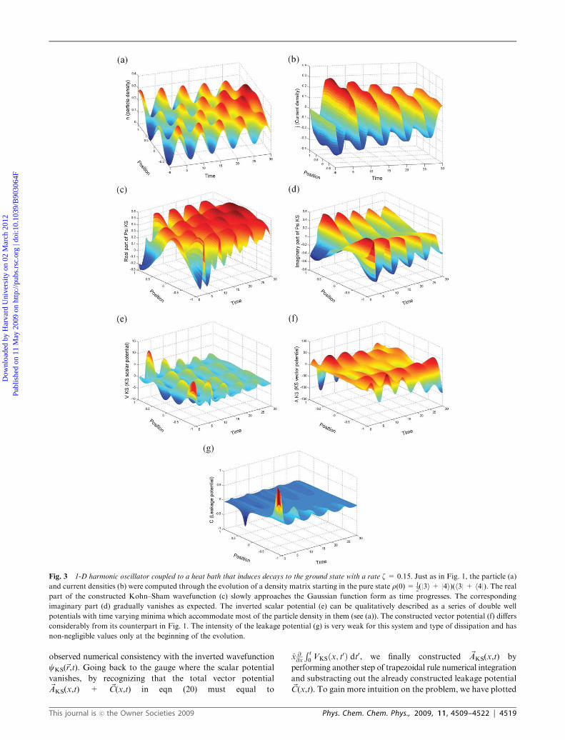
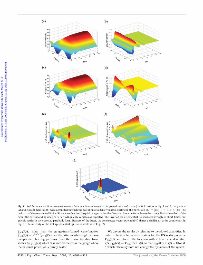
Fig. 4 1-D harmonic oscillator coupled to a heat bath that induces decays to the ground state with a rate z= 0.5. Just as in Fig. 1 and 2, the particle

(a) and current densities (b) were computed through the evolution of a density matrix starting in the pure state r(0) = 12(|3i+ |4i)(h3| + h4|). The

real part of the constructed Kohn–Sham wavefunction (c) quickly approaches the Gaussian function form due to the strong dissipative effect of the

bath. The corresponding imaginary part (d) quickly vanishes as expected. The inverted scalar potential (e) oscillates strongly at short times, but

quickly settles in the expected parabolic form. Because of the latter, the constructed vector potential (f) shares a similar tilt as its counterpart in

Fig. 1. The intensity of the leakage potential (g) is also weak as in Fig. (2).

4520 | Phys. Chem. Chem. Phys., 2009, 11, 4509–4522 This journal is �c the Owner Societies 2009

Dow

nloa

ded

by H

arva

rd U

nive

rsity

on

02 M

arch

201

2Pu

blis

hed

on 1

1 M

ay 2

009

on h

ttp://

pubs

.rsc

.org

| do

i:10.

1039

/B90

3064

F

View Online

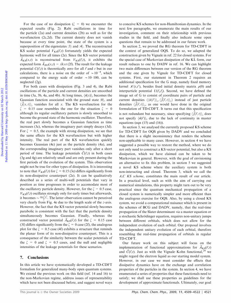
For the case of no dissipation (z = 0) we encounter the

expected results (Fig. 2): Rabi oscillations in time for

the particle (2a) and current densities (2b) as well as for the

wavefunction (2c,2d). The current density does not vanish

because at every time point, the state of the system is a

superposition of the eigenstates |3i and |4i. The reconstructedKS scalar potential VKS(~r,t) fortunately yields the expected

harmonic well for all times (2e). Since the KS vector potential~AKS(x,t) is reconstructed from VKS(~r,t), it exhibits the

expected form ~AHO(x,t) = xkxt (2f). The result for the leakage

potential C(~r,t) is theoretically zero for all ~r and t but in our

calculations, there is a noise on the order of B10�4, which

compared to the energy scale of order B10–100, can be

neglected (2g).

For both cases with dissipation (Fig. 3 and 4), the Rabi

oscillations of the particle and current densities are smoothed

in time (3a, 3b, 4a, and 4b). At long times, hn(x)it becomes the

Gaussian function associated with the ground state |0i, andh~jðx; tÞit vanishes for all x. The KS wavefunction for the

z = 0.15 case resembles the one for the situation z = 0

although its regular oscillatory pattern is slowly smoothed to

become the ground state of the harmonic oscillator. Therefore,

the real part slowly becomes a Gaussian function as time

increases (3c), whereas the imaginary part simply decays (3d).

For z = 0.5, the example with strong dissipation, we see that

the same effects for the KS wavefunction but with higher

intensity. The real part of the KS wavefunction quickly

becomes Gaussian (4c) just as the particle density (4a), and

the corresponding imaginary part vanishes only after a short

period of time. The leakage potentials ~C(~r,t) in both cases

(3g and 4g) are relatively small and are only present during the

first periods of the evolution of the system. This observation

might not be true for other types of dissipation. It is interesting

to note that VKS(~r,t) for z= 0.15 (3e) differs significantly from

its non-dissipative counterpart (2e). It can be qualitatively

described as a series of multi-well potentials that vary in

position as time progresses in order to accomodate most of

the oscillatory particle density. However, for the z = 0.5 case,

VKS(~r,t) oscillates strongly only for early times but afterwards,

it becomes mo2x2

2 . The latter observation cannot be perceived

very clearly from Fig. 4e due to the length scale of the z-axis.

However, the fact that the KS vector potential slowly becomes

parabolic is consistent with the fact that the particle density

simultaneously becomes Gaussian. Finally, whereas the

constructed vector potential ~AKS(~r,t) for the z = 0.15 case

(3f) differs significantly from the z= 0 case (2f), the analogous

plot for the z = 0.5 case (4f) exhibits a structure that reminds

the planar form of its non-dissipative counterpart. This is a

consequence of the similarity between the scalar potentials of

the z = 0 and z = 0.5 cases, and the null and negligible

intensities of the leakage potentials for these scenarios.

7. Conclusions

In this article we have systematically developed a TD-CDFT

formalism for generalized many-body open quantum systems.

We extend the previous work on this field (ref. 14 and 16) to

the non-Markovian regime, address issues of representability

which have not been discussed before, and suggest novel ways

to conceive KS schemes for non-Hamiltonian dynamics. In the

next few paragraphs, we enumerate the main results of our

investigation, comment on their relationship with previous

studies in the field, and finally also indicate some open

questions that remain to be addressed in our future work.

In section 2, we proved the RG theorem for TD-CDFT in

the context of generalized OQS. To do so, we adapted the

construction given by Vignale in ref. 22 for closed systems. For

the special case of Markovian dissipation of the KL form, our

result reduces to one by DADV in ref. 16. We can highlight

two main differences between our version of the RG theorem

and the one given by Vignale for TD-CDFT for closed

systems. First, our statement in Theorem 2 requires an

additional specification for the G map, namely fixed memory

kernel K(t,t0), besides fixed initial density matrix r(0) and

interparticle potential U(~ri,~rj). Second, we have defined the

image set of G to consist of coordinate pairs of particle and

current densities ðhnð~r Þit; h~jð~r; tÞitÞ instead of just particle

densities h~jð~r; tÞit, as one would have done in the original

formulation of TD-CDFT. It turns out that this specification

is not redundant but necessary, since specifying h~jð~r; tÞit doesnot specify hn(~r )it due to the lack of continuity in master

equations (eqn (15) and (16)).

In section 3, we analysed the currently proposed KS scheme

for TD-CDFT for OQS given by DADV and we concluded

that there is a slight inconsistency that renders the scheme

non-applicable to many cases. However, in section 4 we have

suggested a possible way to restore the method, where we do

not only need to construct a KS vector potential, but also a KS

dissipation, which we have claimed can be taken to be

Markovian in general. However, with the goal of envisioning

an alternative to fix this problem, in section 5 we suggested

a novel KS scheme where the auxiliary system is both

non-interacting and closed. Theorem 3, which we call the

A,C KS scheme, constitutes the main result of our article.

In a practical level, such as with the aim of carrying out

numerical simulations, this property might turn out to be very

practical since the quantum mechanical propagation of a

closed system is numerically simpler and more efficient than

the analogous exercise for OQS. Also, by using a closed KS

system, we avoid a computational nuisance which is present in

the schemes of BCG and DADV, namely, that the real-time

propagation of the Slater determinant via a master equation or

a stochastic Schrodinger equation, requires non-unitary jumps

between different orbitals, which does not allow for the

independent evolution of each orbital. Our proposal involves

the independent unitary evolution of each orbital, therefore

resembling the real-time propagation of orbitals in regular

TD-CDFT.

Our future work on this subject will focus on the

implementation of functional approximations for ~AKS(~r,t)

and ~C(~r,t). Just as with the Vignale–Kohn functional,24 we

might regard the electron liquid as our starting model system.

However, in our case we must consider the effects that

dissipative dynamics have on the exchange and correlation

properties of the particles in the system. In section 4, we have

enumerated a series of properties that these functionals need to

satisfy; we shall use these properties as guidelines for the

development of approximate functionals. Ultimately, our goal

This journal is �c the Owner Societies 2009 Phys. Chem. Chem. Phys., 2009, 11, 4509–4522 | 4521

Dow

nloa

ded

by H

arva

rd U

nive

rsity

on

02 M

arch

201

2Pu

blis

hed

on 1

1 M

ay 2

009

on h

ttp://

pubs

.rsc

.org

| do

i:10.

1039

/B90

3064

F

View Online

is to apply this formulation to a realistic system where the

non-Hamiltonian evolution is essential to understand its

function, such as excitation transfer in chromophores embedded

in a protein environment10 or resonant surface enhanced

Raman scattering.4 In summary, our work provides an

alternative tool to study generalized open quantum systems

within the realm of TD-CDFT.

Acknowledgements

We sincerely appreciate the suggestions and critical reading of

the manuscript by K. Burke. Stimulating discussions with

D. Tempel, I. Kassal, S. Saikin, P. Rebentrost, R. Olivares-

Amaya, and S. Shim, are greatly acknowledged. J.Y.Z. thanks

X. Andrade for referring him to the propagator technique in

ref. 43. J.Y.Z. also thanks the generous support of

Fundacion Mexico at Harvard and CONACYT. C.A.R.

thanks the Mary-Fieser Postdoctoral Fellowship program.

This work was carried out under the DARPA contract FA

9550-08-1-0285.

References

1 E. C. G. Sudarshan, P. M. Mathews and J. Rau, Phys. Rev., 1961,121, 920.

2 H. P. Breuer and F. Petruccione, The Theory of Open QuantumSystems, Oxford University Press, USA, 2002.

3 E. C. G. Sudarshan, P. M. Mathews and J. Rau, Phys. Rev., 1961,121, 920; B. Hackens, F. Martins, T. Ouisse, H. Sellier, S. Bollaert,X. Wallart, A. Cappy, J. Chevrier, V. Bayot and S. Huant, Nat.Phys., 2006, 2, 826.

4 L. Jensen, L. L. Zhao and G. C. Schatz, J. Phys. Chem. C, 2007,111(12), 4756.

5 J. Herek, W. Wohlleben, R. Cogdell, D. Zeidler and M. Motzkus,Nature, 2002, 417, 533.

6 M. Cramer, A. Flesch, I. P. McCulloch, U. Schollwock andJ. Eisert, Phys. Rev. Lett., 2008, 101, 063001.

7 P. Hohenberg and W. Kohn, Phys. Rev., 1964, 136, B864.8 W. Kohn and L. J. Sham, Phys. Rev., 1965, 140, A1133.9 E. Runge and E. K. U. Gross, Phys. Rev. Lett., 1984, 52, 997.

10 M. Mohseni, P. Rebentrost, S. Lloyd and A. Aspuru-Guzik,J. Chem. Phys., 2008, 129, 174106.

11 S. Saikin, J. Phys. Condens. Matter, 2004, 16, 5071.12 S. N. Yaliraki, M. Kemp and M. A. Ratner, J. Am. Chem. Soc.,

1999, 121(14), 3428.13 T. Klamroth andM.Nest, Phys. Chem. Chem. Phys., 2009, 11(2), 349.14 K. Burke, R. Car and R. Gebauer, Phys. Rev. Lett., 2005, 94,

146805.15 X. Zheng, F. Wang, C. Y. Yam, Y. Mo and G. H. Chen, Phys.

Rev. B, 2007, 75, 195127.16 M. Di Ventra and R. D’Agosta, Phys. Rev. Lett., 2007, 98,

226403.17 J. Yuen-Zhou, D. Tempel, C. Rodrıguez-Rosario and A.

Aspuru-Guzik, in preparation.18 M. A. L. Marques and E. K. U. Gross, Annu. Rev. Phys. Chem.,

2004, 55, 427.19 K. Burke, J. Werschnik and E. K. U. Gross, J. Chem. Phys., 2005,

122, 1.20 A. Dreuw and M. Head-Gordon, J. Am. Chem. Soc., 2004, 126,

4007.21 S. K. Ghosh and A. K. Dhara, Phys. Rev. A, 1988, 38, 1149.

22 G. Vignale, Phys. Rev. B, 2004, 70, 201102(R).23 G. Vignale, in Time-Dependent Density Functional Theory, ed.

M. A. L. Marques, C. A. Ullrich, F. Nogueira, A. Rubio,K. Burke and E. K. U. Gross, Springer, Berlin, 2006.

24 G. Vignale and W. Kohn, Phys. Rev. Lett., 1996, 77, 2037.

25 M. van Faasen, P. L. de Boeij, R. van Leeuwen, J. A. Berger andJ. G. Snijders, Phys. Rev. Lett., 2002, 88, 186401.

26 C. A. Ullrich and G. Vignale, Phys. Rev. B, 2002, 65, 245102.

27 X. L. Gao, M. Polini, D. Rainis, M. P. Tosi and G. Vignale, Phys.Rev. Lett., 2008, 101, 206402.

28 S. Nakajima, Prog. Theor. Phys., 1958, 20, 948.29 R. Zwanzig, J. Chem. Phys., 1960, 33, 1338.30 C. A. Rodrıguez-Rosario and E. C. G. Sudarshan, arXiv

0803.1183, 2008.31 A. Kossakowski, Rep. Math. Phys, 1972, 3, 247.32 G. Lindblad, Commun. Math. Phys., 1976, 48, 199.33 V. Gorini, A. Kossakowski and E. C. G. Sudarshan, J. Math.

Phys., 1976, 17, 821.34 The subscript t in hit denotes a trace taken with respect to r(t). For

instance, hn(~r )it is the expectation value of the particle densityoperator at time t. Although this may appear redundant forexplicitly time dependent operators, such as the current density,

where we write h~jð~r; tÞit instead of just h~jð~r; tÞi, we shall keep thenotation throughout the article for consistency and clarity.

35 At this point, it might seem that we are wasting symbols if many ofthe primed variables are equal to their unprimed counterparts (weassume that r0(0) = r(0), K(t,t0) = K(t,t0), and U0(~ri,~rj) =

U(~ri,~rj), we want hn(~r )i0t = hn(~r )it and h~j 0ð~r; tÞi0t ¼ h~jð~r; tÞit, andwe will try to show that ~A0(~r,t) = ~A(~r,t)) but we do this because insection 3, we will reconsider an adaptation for the proof foranother set of conditions on the primed system.

36 Suppose we have reached the radius of convergence located at tc1,so now we Taylor expand the time-dependent functions about t =tc a 0. We need to slightly modify the argument of why the right-hand side of (10) will not contain D~Ak(~r ) with k 4 l. The onlydifference is in the analysis of the ~Glð~r Þ term, and in particular, inthe first integral term in the right-hand side of (13),R t0 dt

0@kK0 ðt;t0Þ@tk

r0ðt0Þ, which vanishes in the case where we expand

about 0. However, by hypothesis, we already know D~A(~r,t) for allt o tc and hence we can propagate (1). This means that we cancompute r(t0) for that range of time values. Since K0(t,t0) =

K(t,t0), the integral term that is,R tc0 dt0@

kK0 ðt;t0Þ@tk

r0ðt0Þ can be calcu-

lated explicitly with the upper limit of the integral being tc. There-fore, we are left with the analysis of the second term in theright-hand side of (13), which is analogous to the one presentedin the body of the article.

37 N. T. Maitra, K. Burke and C. Woodward, Phys. Rev. Lett., 2002,89(2), 23002.

38 W. Frensley, Rev. Mod. Phys., 1990, 62, 3.39 R. Gebauer and R. Car, Phys. Rev. Lett., 2004, 93, 160404.40 A. Bodor and L. Diosi, Phys. Rev. A, 2006, 73, 064101.41 R. Gebauer, S. Piccinin and R. Car, ChemPhysChem, 2005, 6,

1727.42 R. D’Agosta and M. Di Ventra, Phys. Rev. B, 2008, 78,

165105.

43 A. Castro, M. A. Marques and A. Rubio, J. Chem. Phys., 2004,121(8), 3425.

44 J. E. Harriman, Phys. Rev. A, 1981, 24, 680.

45 N. T. Maitra, in Time-Dependent Density Functional Theory, ed.M. A. L. Marques, C. A. Ullrich, F. Nogueira, A. Rubio, K. Burkeand E. K. U. Gross, Springer, Berlin, 2006.

46 G. Vignale and M. Rasolt, Phys. Rev. Lett., 1987, 59, 2360–2363.

47 W. Kohn, Phys. Rev. Lett., 1983, 51, 1596.

48 N. D. Mermin, Phys. Rev., 1965, 137, A1441.

4522 | Phys. Chem. Chem. Phys., 2009, 11, 4509–4522 This journal is �c the Owner Societies 2009

Dow

nloa

ded

by H

arva

rd U

nive

rsity

on

02 M

arch

201

2Pu

blis

hed

on 1

1 M

ay 2

009

on h

ttp://

pubs

.rsc

.org

| do

i:10.

1039

/B90

3064

F

View Online