1

Technical Note

The Principle of Time-Correlated Single Photon Counting

Time-resolved fluorescence spectroscopy is a pow-erful analysis tool in fundamental physics as well as in the life sciences. Implementing it in the time do-main requires recording the time dependent inten-sity profile of the emitted light upon excitation by a short flash of light, typically a laser pulse. While in principle, one could attempt to record the time decay profile of the signal from a single excitation-emission cycle, there are practical problems preventing such a simple solution in most cases. First of all, the de-cay to be recorded is very fast. Typical fluorescence from commonly used organic fluorophores lasts only some hundred picoseconds to some tens of nano-seconds. In order to recover not only fluorescence lifetimes but also the decay shape, typically in or-der to resolve multi-exponential decays, one must be able to temporally resolve the recorded signal at least to such an extent, that the decay is represented by some tens of samples. For a decay lasting, e.g., 500 ps the signal would have to be sampled at time steps of say 10 ps.

At first glance it might seem reasonable to do this with a photo-diode and a fast oscilloscope or some similar electronic transient recorder. However, the re-quired temporal resolution is hard to achieve with or-dinary electronic transient recorders. Moreover, the emitted light may be simply too weak to create an an-alog voltage representing the optical flux. Indeed, the optical signal may consist of just a few photons per excitation/emission cycle. Then the discrete nature of the signal itself prohibits analog sampling. Even

if one has some reserve to increase the excitation power to obtain more fluorescence light, there will be limits, e.g., due to collection optic losses, spec-tral limits of detector sensitivity or photo-bleaching at higher excitation power. Ultimately, problems would arise when the observed sample consists of just a few or even single molecules, a situation that is ab-solutely real in confocal microscopy applications.

The solution for these problems is Time-Correlat-ed Single Photon Counting (TCSPC). With periodic excitation, e.g., from a laser, it is possible to extend the data collection over multiple cycles of excitation and emission. One can then accept the sparseness of the collected photons and reconstruct the fluores-cence decay profile from the multitude of single pho-ton events collected over many cycles.

The method is based on the repetitive, precisely timed registration of single photons of, e.g., a fluo-rescence signal[1],[2]. The reference for the timing is the corresponding excitation pulse. As a single pho-ton sensitive detector a Photomultiplier Tube (PMT), Micro Channel Plate (MCP), a Single Photon Ava-lanche Diode (SPAD) or Hybrid PMT can be used. Provided that the probability of registering more than one photon per cycle is low, the histogram of photon arrivals per time bin represents the time decay one would have obtained from a “single shot” time-re-solved analog recording. The precondition of single photon probability can (and must) be met by simply attenuating the light level at the sample if necessary.

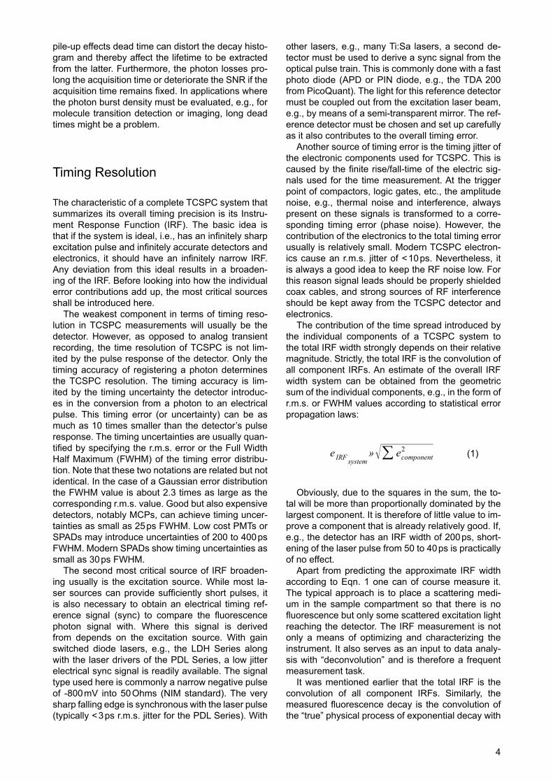
Figure 1 illustrates how the histogram is formed over multiple cycles. In the example, fluorescence is excited repetitively by short laser pulses. The time difference between excitation and emission is mea-sured by electronics that act like a stopwatch. If the

Time-Correlated Single Photon CountingMichael WahlPicoQuant GmbH, Rudower Chaussee 29, 12489 Berlin, Germany, info@picoquant.com

2

single photon probability condition is met, there will actually be no photons at all in many cycles. In the example this situation is shown after the second laser pulse. It should be noted that (by the laws of quan-tum physics) the occurrence of a photon or an empty cycle is entirely random and can only be described in terms of probabilities. Consequently, the same holds true for the individual stopwatch readings.

The stopwatch readings are sorted into a histo-gram consisting of a range of “time bins”. The width of the time bins typically corresponds to the resolu-tion of the stopwatch (some picoseconds) but may be chosen wider in order to cover a longer overall time span. The typical result in time-resolved fluo-rescence experiments is a histogram with an expo-nential drop of counts towards later times (Figure 2).

The reason why there typically is an exponential drop is very similar to that of nuclear decay. As quan-tum mechanics predict, we have no means of know-ing exactly when a nuclear decay will occur. All we can predict is the likelihood of an atomic species to decay in a given period of time. Similarly, all we can predict about the lifetime of an excited state is its sta-tistical expectation. The exponential drop of fluores-cence intensity in a single shot experiment with many molecules may be explained as follows: Suppose we begin with a population of 1000 excited molecules. Let the probability of each molecule returning to the ground state be 50 % in the first nanosecond. Then we have 50 % of the exited population after the first nanosecond. In the next nanosecond of observation we lose another 50 %, and so on. Since the intensity of light is determined by the number of photons emit-ted in any period of time, it is directly proportional to the surviving population of excited molecules. When the experiment is done with single molecules it is of course no longer meaningful to speak of populations. Nevertheless, by virtue of ergodicity, the likelihood of observing a photon, i.e., a molecule’s return to the ground state as a function of time follows the same exponential drop over time.

It is important to note that we can but need not actually do TCSPC with single molecules. Sufficient-ly attenuating the light, so that the detector receives only single photons, has the same effect. Indeed, in order to use TCSPC we must attenuate the light to this level. One may ask now, if we do have light from many molecules, why waste it by attenuation and use TCSPC? The good reason to do so is that a single photon detector can be built with much better time resolution than an analog optical receiver.

In practice, the registration of a photon in time-re-solved fluorescence measurements with TCSPC in-volves the following steps: First, the time difference between the photon event and the corresponding excitation pulse must be measured. For this purpose both optical events are converted into electrical puls-es. For the fluorescence photon this is done via the single photon detector mentioned before. For the ex-citation pulse it may be done via another detector (typically called trigger diode) if there is no electrical synchronization signal (sync) supplied directly by the laser. Obviously, all conversion to electrical pulses

Figure 1: Measurement of start-stop times in time-resolved fluorescence measurement with TCSPC.

Figure 2: Histogram of start-stop times in time-resolved fluores-cence measurement with TCSPC.

3

must preserve the precise timing of the signals as accurately as possible.

The actual time difference measurement is done by means of fast electronics which provide a digital timing result. This digital timing result is then used to address the histogram memory so that each possi-ble timing value corresponds to one memory cell or histogram bin. Finally, the addressed histogram cell is incremented. All steps are carried out by fast elec-tronics so that the processing time required for each photon event is as short as possible. When sufficient counts have been collected, the histogram memo-ry can be read out. The histogram data can then be used for display and, e.g., fluorescence lifetime cal-culation. In the following sections we will expand on the various steps involved in the method and associ-ated issues of importance.

Count Rates and Single Photon Statistics

It was mentioned that it is necessary to maintain a low probability of registering more than one photon per cycle. This is to guarantee that the histogram of photon arrivals represents the time decay one would have obtained from a single shot time-resolved an-alog recording. The reason for this is briefly the fol-lowing: Detector and electronics have a “dead” time for at least some nanoseconds after a photon event. During this time they cannot process another event. Because of these dead times TCSPC systems are usually designed to register only one photon per ex-citation cycle. If now the number of photons occurring in one excitation cycle were typically > 1, the system would very often register the first photon but miss the following ones. This would lead to an over-rep-resentation of early photons in the histogram, an ef-fect called ‘pile-up’. It is therefore crucial to keep the probability of cycles with more than one photon low (Figure 3).

To quantify this demand one has to set acceptable error limits for the lifetime measurement and apply some mathematical statistics. For practical purposes one may use the following rule of thumb: In order to maintain single photon statistics, on average only one in 20 to 100 excitation pulses should generate a count at the detector. In other words: the average count rate at the detector should be at most 1 to 5 % of the excitation rate. E.g., with a pulsed diode laser driver of PicoQuant’s PDL Series running at 80 MHz repetition rate, the average detector count rate should not exceed 4 MHz. This leads to another issue: the maximum count rate the system (of both detector and electronics) can handle.

Indeed, 4 MHz are stretching the limits of some detectors and certainly are way beyond the capabili-ties of old NIM based TCSPC systems. On the other hand, one wants high count rates in order to acquire fluorescence decay histograms quickly. This may be of particular importance where dynamic lifetime changes or fast molecule transitions are to be stud-ied or where large numbers of lifetime samples must be collected (e.g., in 2D scanning configurations). PMTs (dependent on the design) can handle count rates of up to 1 to 20 millions of counts per second (cps), passively quenched SPADs saturate at a few hundred kcps. Old-fashioned NIM based TCSPC electronics are able to handle a maximum of 50,000 to 500,000 cps. With modern integrated TCSPC de-signs, e.g. TimeHarp 260, count rates up to 40 Mcps can be achieved.

It is also worth noting that by virtue of quantum mechanics the actual count arrival times are random, so that there can be bursts of high count rate and periods of low count rates. Bursts of photons may well exceed the average rate. This should be kept in mind when an experiment is planned. Even if an in-strument can accommodate the average rate, it may drop photons in bursts. This is why the length of the dead time is of interest too. This quantity describes the time the system cannot register photons while it is processing a previous photon event. The term is applicable to both detectors and electronics. Through

Figure 3: Distortion of the TCSPC measurement by pile-up effect and dead time.

4

pile-up effects dead time can distort the decay histo-gram and thereby affect the lifetime to be extracted from the latter. Furthermore, the photon losses pro-long the acquisition time or deteriorate the SNR if the acquisition time remains fixed. In applications where the photon burst density must be evaluated, e.g., for molecule transition detection or imaging, long dead times might be a problem.

Timing Resolution

The characteristic of a complete TCSPC system that summarizes its overall timing precision is its Instru-ment Response Function (IRF). The basic idea is that if the system is ideal, i.e., has an infinitely sharp excitation pulse and infinitely accurate detectors and electronics, it should have an infinitely narrow IRF. Any deviation from this ideal results in a broaden-ing of the IRF. Before looking into how the individual error contributions add up, the most critical sources shall be introduced here.

The weakest component in terms of timing reso-lution in TCSPC measurements will usually be the detector. However, as opposed to analog transient recording, the time resolution of TCSPC is not lim-ited by the pulse response of the detector. Only the timing accuracy of registering a photon determines the TCSPC resolution. The timing accuracy is lim-ited by the timing uncertainty the detector introduc-es in the conversion from a photon to an electrical pulse. This timing error (or uncertainty) can be as much as 10 times smaller than the detector’s pulse response. The timing uncertainties are usually quan-tified by specifying the r.m.s. error or the Full Width Half Maximum (FWHM) of the timing error distribu-tion. Note that these two notations are related but not identical. In the case of a Gaussian error distribution the FWHM value is about 2.3 times as large as the corresponding r.m.s. value. Good but also expensive detectors, notably MCPs, can achieve timing uncer-tainties as small as 25 ps FWHM. Low cost PMTs or SPADs may introduce uncertainties of 200 to 400 ps FWHM. Modern SPADs show timing uncertainties as small as 30 ps FWHM.

The second most critical source of IRF broaden-ing usually is the excitation source. While most la-ser sources can provide sufficiently short pulses, it is also necessary to obtain an electrical timing ref-erence signal (sync) to compare the fluorescence photon signal with. Where this signal is derived from depends on the excitation source. With gain switched diode lasers, e.g., the LDH Series along with the laser drivers of the PDL Series, a low jitter electrical sync signal is readily available. The signal type used here is commonly a narrow negative pulse of -800 mV into 50 Ohms (NIM standard). The very sharp falling edge is synchronous with the laser pulse (typically < 3 ps r.m.s. jitter for the PDL Series). With

other lasers, e.g., many Ti:Sa lasers, a second de-tector must be used to derive a sync signal from the optical pulse train. This is commonly done with a fast photo diode (APD or PIN diode, e.g., the TDA 200 from PicoQuant). The light for this reference detector must be coupled out from the excitation laser beam, e.g., by means of a semi-transparent mirror. The ref-erence detector must be chosen and set up carefully as it also contributes to the overall timing error.

Another source of timing error is the timing jitter of the electronic components used for TCSPC. This is caused by the finite rise/fall-time of the electric sig-nals used for the time measurement. At the trigger point of compactors, logic gates, etc., the amplitude noise, e.g., thermal noise and interference, always present on these signals is transformed to a corre-sponding timing error (phase noise). However, the contribution of the electronics to the total timing error usually is relatively small. Modern TCSPC electron-ics cause an r.m.s. jitter of < 10 ps. Nevertheless, it is always a good idea to keep the RF noise low. For this reason signal leads should be properly shielded coax cables, and strong sources of RF interference should be kept away from the TCSPC detector and electronics.

The contribution of the time spread introduced by the individual components of a TCSPC system to the total IRF width strongly depends on their relative magnitude. Strictly, the total IRF is the convolution of all component IRFs. An estimate of the overall IRF width system can be obtained from the geometric sum of the individual components, e.g., in the form of r.m.s. or FWHM values according to statistical error propagation laws:

lu39c1s

size 12{e rSub { size 8{ ital "IRF"} rSub { size 8{ ital"system"} } } » sqrt { Sum {e rSub { size 8{ ital"component"} } rSup { size 8{2} } } } } {}

eIRF

system»√∑ e

component

2

(1)

Obviously, due to the squares in the sum, the to-

tal will be more than proportionally dominated by the largest component. It is therefore of little value to im-prove a component that is already relatively good. If, e.g., the detector has an IRF width of 200 ps, short-ening of the laser pulse from 50 to 40 ps is practically of no effect.

Apart from predicting the approximate IRF width according to Eqn. 1 one can of course measure it. The typical approach is to place a scattering medi-um in the sample compartment so that there is no fluorescence but only some scattered excitation light reaching the detector. The IRF measurement is not only a means of optimizing and characterizing the instrument. It also serves as an input to data analy-sis with “deconvolution” and is therefore a frequent measurement task.

It was mentioned earlier that the total IRF is the convolution of all component IRFs. Similarly, the measured fluorescence decay is the convolution of the “true” physical process of exponential decay with

5

the IRF. With this theoretical model it is possible to extract the parameters of the “true” decay process from the convoluted results in the collected histo-grams[3]. This is often referred to as “deconvolution” although it should be noted that the term is not math-ematically precise in this context. The procedure that most data analysis programs actually perform is an iterative reconvolution. If the detector’s temporal re-sponse shows a spectral dependency then it is not recommendable to measure the IRF at the excitation wavelength while the fluorescence will be mea-sured at a different wavelength. The deconvolution would then not be meaningful. In such cases the IRF should be measured at the target sample’s emission wavelength using strongly quenched fluorophores showing very short lifetimes.

Having established the role of the IRF and pos-sibly having determined it for a given instrument leads to the question what the actual lifetime mea-surement resolution of the instrument will be. Unfor-tunately, it is difficult to specify a general lower limit on the fluorescence lifetime that can be measured by a given TCSPC instrument. Apart from the instru-ment response function and noise, factors such as quantum yield, fluorophore concentration, and decay kinetics all affect the measurement. However, as a rule of thumb, one can assume that under favorable conditions, most importantly sufficient counts in the histogram, lifetimes down to 1/10 of the IRF width (FWHM) can still be recovered via iterative recon-volution.

A final time-resolution related issue worth noting here is the bin width of the TCSPC histogram. As outlined above, the analog electronic processing of the timing signals (detector, amplifiers, etc.) creates a continuous, e.g., Gaussian, distribution around the true value. In order to form a histogram, at some point the timing results must be quantized into dis-crete time bins. This quantization introduces another random error that can be detrimental if chosen too coarse. The time quantization step width, i.e., the bin width, must therefore be small compared to the width of the analog error distribution. As a minimum from the information theoretical point of view one would assume the Nyquist frequency. I.e., an analog signal should be sampled at least at twice the highest fre-quency contained in it. The high frequency content depends on the shape of the distribution. In a ba-sic approximation this can reasonably be assumed to be Gaussian and therefore having very little high frequency content. For practical purposes there is usually no point in collecting the histogram at time resolutions much higher than 1/10 of the width of the analog error distribution. Nevertheless, a good histogram resolution is helpful in data analysis with iterative reconvolution.

Photon Counting Detectors

General CharacteristicsWhat we expect of an ideal photon detector for TCSPC is an electrical output pulse upon each pho-ton arriving at the detector. In the real world there are various deviations from this ideal. As outlined in the section on timing resolution, one imperfection of real world detectors manifests itself in an uncertainty of time delay between photon arrival and electrical out-put. We describe it by the IRF width of the detector.

Furthermore, due to finite sensitivity we do not get an output pulse for each input photon. The most im-portant characteristic in this context is the quantum efficiency of the detector. It critically depends on ma-terial properties and incident wavelength. The peak quantum efficiency is between 5 and 90 % for typical detectors. There are other factors beyond quantum efficiency that may affect the overall conversion ef-ficiency of the detector but they are less dominant.

Because of noise from various sources in the de-tector, the output may contain pulses that are not related to the light input. These are referred to as dark counts. In terms of a characteristic of the detec-tor it is common to use the dark count rate (DCR) in counts per second. It can be close to zero for some specialized detectors but as high as some thousands of cps in other cases. Since it is mostly driven by thermal effects, it is typically higher in detectors with sensitivity in the near-infrared. For the same reason it can typically be reduced by cooling.

Another type of “false” output from a photon de-tector is due to so-called afterpulsing. The term de-scribes the observation that some time after a true photon event the detector emits another pulse. The internal reasons for such effects are different in the various types of detectors. As a common problem such false counts are temporally correlated with true photon events. The typical delay time is in the order of microseconds. The correlation is also weak, so that it does not show in many applications. In fact, in classical TCSPC with nanosecond time spans af-terpulses very often appear just like a background noise that increases with illumination. However, af-terpulsing can induce spurious effects when the typi-cal delay of the afterpulses is in the same time range as the photon correlation times to be observed in the experiment. This is typically the case in Fluores-cence Correlation Spectroscopy (FCS). Fortunately, there exist detectors with very little or even zero af-terpulsing.

Photomultiplier Tube (PMT)A PMT consists of a light-sensitive photocathode that generates electrons when exposed to light. These electrons are directed onto a charged elec-trode called a dynode. The collision of the electrons with the dynode produces additional electrons. Since each electron that strikes the dynode causes several electrons to be emitted, there is a multiplication ef-

6

fect. After further amplification by multiple dynodes, the electrons are collected at the anode of the PMT and output as a current. The current is directly pro-portional to the intensity of light striking the photo-cathode. Because of the multiplicative effect of the dynode chain, the PMT is a photoelectron amplifier of high sensitivity and remarkably low noise. PMTs have a wide dynamic range, i.e., they can also mea-sure relatively high levels of light. They furthermore are very fast, so rapid successive events can be reli-ably monitored. PMTs are also quite robust. The high voltage driving the tube may be varied to change the sensitivity of the PMT.

When the light levels are as low as in TCSPC, the PMT “sees” only individual photons. One photon on the photocathode produces a short output pulse con-taining millions of electrons. PMTs can therefore be used as single photon detectors. In photon counting mode, individual photons that strike the photocath-ode of the PMT are registered. Each photon event gives rise to an electrical pulse at the output. The number of pulses, or counts per second, is propor-tional to the light impinging upon the PMT. As the number of photon events increases at higher light levels, it will become difficult to differentiate between individual pulses and the photon counting detector will become non-linear. Dependent on the PMT de-sign this usually occurs at 1 to 10 millions of counts per second. The timing uncertainty between photon arrival and electrical output is small enough to permit time-resolved photon counting at a sub-nanosecond scale. In single photon counting mode the tube is typically operated at a constant high voltage where the PMT is most sensitive.

PMTs usually operate between the blue and red regions of the visible spectrum, with greater quan-tum efficiency in the blue-green region, depending upon photo-cathode materials. Typical peak quan-tum efficiencies are about 25 %. For spectrosco-py experiments in the ultraviolet and visible region of the spectrum, a photomultiplier tube is very well suited. In the near infrared the sensitivity drops off rapidly. Optimized cathode materials can be used to push this limit, which may on the other hand lead to increased noise. The latter can to some extent be reduced by cooling.

Because of noise from various sources in the tube, the output of the PMT may contain pulses that are not related to the light input. These are referred to as dark counts, as outlined previously. The detec-tion system can to some extent reject these spurious pulses by means of electronic discriminator circuitry. This discrimination is based on the probability that some of the noise generated pulses (those from the dynodes) exhibit lower signal levels than pulses from a photon event.

Microchannel Plate PMT (MCP)A microchannel plate PMT is also a sensitive photon detector. It consists of an array of glass capillaries

(10 to 25 µm inner diameter) that are coated on the inside with an electron-emissive material. The cap-illaries are biased at a high voltage applied across their length. Like in the PMT, an electron that strikes the inside wall of one of the capillaries creates an avalanche of secondary electrons. This cascading effect creates a gain of 103 to 106 and produces a current pulse at the output. Due to the confined paths the timing jitter of MCPs is sufficiently small to per-form time-resolved photon counting on a sub-nano-second-scale, usually outperforming PMTs. Good but also expensive MCPs can achieve timing uncer-tainties as low as 25 ps. Microchannel plates are also used as an intensifier for low-intensity light detection with array detectors.

Avalanche Photo Diode (APD)APDs are the semiconductor equivalent of PMTs. Generally, APDs may be used for ultra-low light de-tection (optical powers < 1 pW), and can be used in either “linear” mode (bias voltage slightly less than the breakdown voltage) at gains up to about 500, or as photon-counters in the so-called “Geiger” mode (biased slightly above the breakdown voltage). In the case of the latter, the term gain is meaningless. A single photon may trigger an avalanche of about 108 carriers but one is not interested in the output current or voltage because it carries no information other than “there was a photon”. Instead, in this mode the device can be used as a detector for photon count-ing with very accurate timing of the photon arrival. In this context APDs are referred to as Single Photon Avalanche Diodes (SPAD). Widespread commercial products attain timing uncertainties on the order of 400 ps FWHM. Single photon detection probabilities of up to approximately 50 % are possible. Maximum quantum efficiencies reported are about 80 %. More recent SPAD designs focus on timing resolution and can achieve timing accuracies down to 30 ps but are less sensitive at the red end of the spectrum. The dark count rate (noise) of SPADs strongly depends on the active area. In SPADs it is much smaller than in PMTs, which can make optical interfacing difficult.

Hybrid PMT detectorsBy combining a PMT front end with an APD amplifi-cation stage it is possible to design a hybrid detector that provides a very clean instrument response and virtually zero afterpulsing. The timing uncertainty is on the order of 50 to 100 ps and the distribution of timing error is nearly Gaussian. The PMT front end requires a very high voltage but the detectors are available as compact modules readily including the high voltage supply (PicoQuant’s PMA Hybrid). Due to the PMT front end their sensitivity follows the same fundamental dependency on cathode material and wavelength as in ordinary PMTs.

7

Other detectorsThe field of photon detectors is still evolving. Re-cent developments that are beginning to emerge as usable products include so called silicon PMTs, superconducting nanowire detectors and APDs with sufficient gain for single photon detection in analog mode. Each of these detectors has its specific ben-efits and shortcomings. Only a very brief overview can be given here. Silicon PMTs are essentially ar-rays of SPADs, all coupled to a common output. This has the benefit of creating a large area detector that can even resolve photon numbers. The drawback is increased dark count rate and relatively poor tim-ing accuracy. Superconducting nanowires, typically made from NbN, can be used to create photon de-tectors with excellent timing performance and high sensitivity reaching into the infrared spectrum. The shortcomings for practical purposes are the extreme cooling requirements and the low fill factor of the wire structures, making it difficult to achieve good collec-tion efficiencies. Another class of potentially interest-ing detectors are recently emerging APDs with very high gain. In combination with a matched electron-ic amplifier they have been shown to detect single photons. As opposed to Geiger mode, this avoids afterpulsing and allows very fast counting rates. The disadvantage is a high dark count rate, currently way too high for any practical TCSPC application.

Basic Principles Behind the TCSPC Electronics

PicoQuant’s TCSPC systems are quite advanced. To begin explanation, we start with traditional TCSPC systems. They typically consist of the building blocks shown in Figure 4.

The Constant Fraction Discriminator (CFD) is used to extract precise timing information from the electrical detector pulses that may vary in amplitude, typically those from a PMT or MCP detector. This way the overall system IRF may be tuned to become nar-rower. The same could not be achieved with a sim-ple level trigger (comparator). Particularly with PMTs and MCPs, constant fraction discrimination is very

important as their pulse amplitudes vary significantly. Figure 5 shows a comparison between level trigger and CFD operation. The pulses are shown with neg-ative voltages as typically delivered from PMTs.

The most common way of implementing a CFD is the comparison of the original detector signal with an amplified and delayed version of itself. The signal derived from this comparison changes its polarity ex-actly when a constant fraction of the detector pulse height is reached. The zero crossing point of this signal is therefore suitable to derive a timing signal independent from the amplitude of the input pulse. This is done by a subsequent comparison of this sig-nal with a settable zero level, the so called zero cross trigger. Making this level fixable allows to adapt to the noise levels in the given signal, since in principle an infinitely small signal could trigger the zero cross comparator.

It should be noted that modern CFDs, like in most of PicoQuant’s systems, work a little differently. They basically detect the vertex of each pulse and trigger on that point. Effectively this is like applying a con-stant fraction of 1. For practical purposes it makes no difference (we get a timing signal independent from the amplitude of the input pulse) and in terms of im-plementation it makes things easier.

Typical CFDs furthermore permit the setting of a so called discriminator level, determining the lower limit the detector pulse amplitude must pass. Ran-dom background noise pulses can thereby be sup-pressed. Particularly pulses originating from random electrons generated at the dynodes of the PMT can be suppressed as they had less time to amplify, so that their output pulses are small (Figure 6).

Similar as for the detector signal, the sync signal must be made available to the timing circuitry. Since the sync pulses are usually of well-defined amplitude and shape, a simple settable comparator (level trig-ger) is sufficient to adapt to different sync sources. In the classical design the signals from the CFD and SYNC trigger are fed to a Time to Amplitude Con-verter (TAC). This circuit is essentially a highly lin-ear ramp generator that is started by one signal and stopped by the other. The result is a voltage propor-tional to the time difference between the two signals (Figure 7).

The voltage obtained from the TAC is then fed

Figure 4: Block diagram of a traditional TCSPC system. CFD = Constant Fraction Discrimonator, TAC = Time to Amplitude Converter, ADC = Analog to Digital Converter

8

to an Analog to Digital Converter (ADC) which pro-vides the digital timing value used to address the histogrammer. The ADC must be very fast in order to keep the dead time of the system short. Further-more, it must guarantee a very good linearity, over the full range as well as differentially. These are cri-teria difficult to meet simultaneously, particularly with ADCs of high resolution, typically 12 bits, as desir-able for TCSPC over many histogram channels. Fur-thermore, the TAC range is limited.

The histogrammer has to increment each histo-gram memory cell whose digital address in the his-togram memory it receives from the ADC. This is commonly done by fast digital logic, e.g., in the form of Field Programmable Gate Arrays (FPGA) or a mi-croprocessor. Since the histogram memory at some point also must be available for data readout, the histogrammer must stop processing incoming data. This prevents continuous data collection. Sophisti-cated TCSPC systems solve this problem by switch-ing between two or more memory blocks, so that one is always available for incoming data.

While this section so far outlined the typical struc-ture of conventional TCSPC systems, it is now time to note that the tasks performed by TAC and ADC can be carried out by a single fully digital circuit, a so called Time to Digital Converter (TDC). These circuits can measure time differences based on the delay times of signals in semiconductor logic gates or the conductor strips between them[4]. The relative delay times in different gate chains can be used to deter-mine time differences well below the actual gate de-

lay. Other TDC designs use interpolation techniques between the pulses of a coarser clock. This permits exceptionally small, compact and affordable TCSPC solutions, as the circuits can be implemented as Ap-plication Specific Integrated Circuits (ASICs) at low cost and high reliability. All PicoQuant TCSPC sys-tems make use of such a state-of-the-art design.

In the simplest form of a TDC based TCSPC sys-tem the TAC and ADC of the classical approach are replaced by a TDC. However, this simple solution is no longer used in current systems. Modern TCSPC devices are fundamentally different in design. In-stead of operating like a stopwatch, they have inde-pendent TDCs for each input channel. The important detail is that the individual TDCs are running off the same crystal clock. If a timing difference is needed, like in classical histogramming, it can be obtained by simple arithmetics in hardware. Figure 8 shows this in a block diagram.

Observe the symmetry of the input channels, now both having a CFD. The symmetry as well as the separation of the input channels allow many ad-

Figure 5: Comparison between level trigger (left) and CFD operation (right).

Figure 6: Typical train of PMT pulses and the CFD’s discriminator level (red line).

Figure 7: Operation principle of a TAC (Time to Amplitude Converter) level (red line).

9

vanced TCSPC concepts and new applications that will be discussed further below. For the time being we will first take a look at a TCSPC set-up in the lab. This is fairly independent from the design of the TCSPC electronics used.

Experimental Set-up for Fluores-cence Decay Measurements with TCSPCFigure 9 shows a simple set-up for fluorescence life-time measurements with TCSPC. The picosecond diode laser is running on its internal clock. The driver box (PicoQuant’s PDL Series) is physically separate from the actual laser head (PicoQuant’s LDH Series), which is attached via a flexible lead. This permits to conveniently place the small laser head anywhere in the optical set-up.

The light pulses of typically 50 ps FWHM are di-

rected at the sample cuvette, possibly via some appropriate optics. A neutral density filter is used to attenuate the light levels to maintain single photon statistics at the detector. Upon excitation, the fluo-rescent sample will emit light at a longer wavelength than that of the excitation light. The fluorescence light is filtered out against scattered excitation light by means of an optical cut-off filter. Then it is direct-ed to the photon detector, again possibly via some appropriate collection optics, e.g., a microscope ob-jective or just a lens. For timing accuracies of 200 ps FWHM (permitting lifetime measurements even shorter than this via reconvolution), a economic PMT is sufficient. The electrical signal obtained from the detector, e.g., a small negative pulse of -20 mV, is fed to a pre-amplifier, and then to the TCSPC electronics via a standard 50 Ohms coax cable. In this example the complete TCSPC electronics are contained on a single PC board (TimeHarp 260). Other models are designed as separate boxes connected via USB.

The laser driver also provides the electric sync signal needed for the photon arrival time measure-

Figure 8: Block diagram of a modern TDC based TCSPC system running in classical histogramming mode.

Figure 9: Simple experimental set-up for fluorescence decay measurements with TCSPC.

10

ment. This signal (NIM standard, a narrow pulse of -800 mV) is fed to the TCSPC electronics via a stan-dard 50 Ohms coax cable.

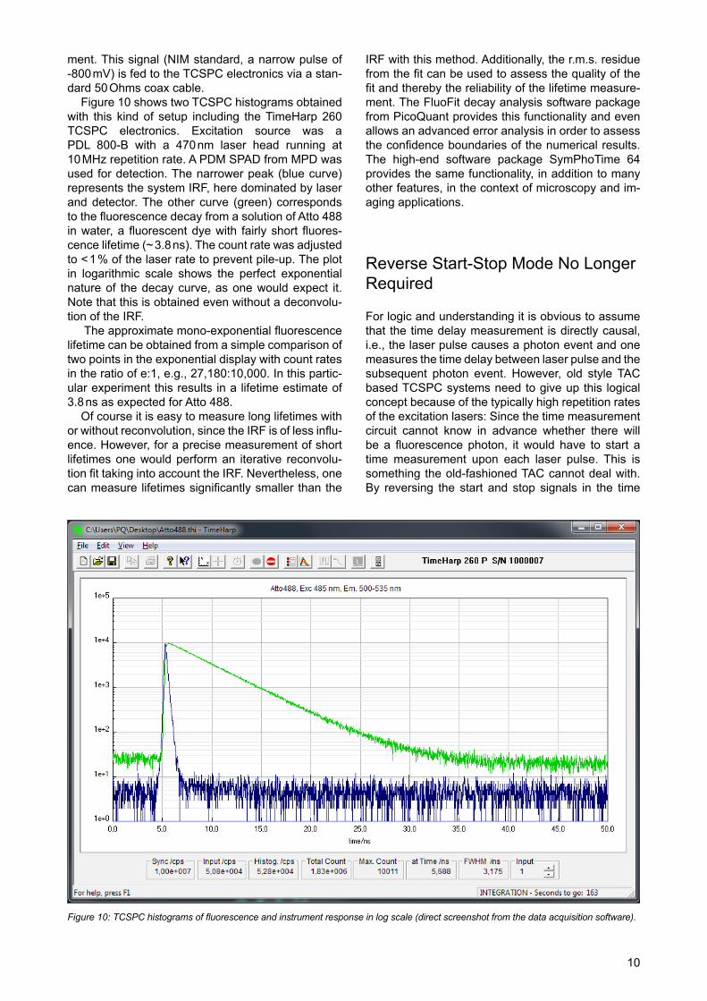
Figure 10 shows two TCSPC histograms obtained with this kind of setup including the TimeHarp 260 TCSPC electronics. Excitation source was a PDL 800-B with a 470 nm laser head running at 10 MHz repetition rate. A PDM SPAD from MPD was used for detection. The narrower peak (blue curve) represents the system IRF, here dominated by laser and detector. The other curve (green) corresponds to the fluorescence decay from a solution of Atto 488 in water, a fluorescent dye with fairly short fluores-cence lifetime (~ 3.8 ns). The count rate was adjusted to < 1 % of the laser rate to prevent pile-up. The plot in logarithmic scale shows the perfect exponential nature of the decay curve, as one would expect it. Note that this is obtained even without a deconvolu-tion of the IRF.

The approximate mono-exponential fluorescence lifetime can be obtained from a simple comparison of two points in the exponential display with count rates in the ratio of e:1, e.g., 27,180:10,000. In this partic-ular experiment this results in a lifetime estimate of 3.8 ns as expected for Atto 488.

Of course it is easy to measure long lifetimes with or without reconvolution, since the IRF is of less influ-ence. However, for a precise measurement of short lifetimes one would perform an iterative reconvolu-tion fit taking into account the IRF. Nevertheless, one can measure lifetimes significantly smaller than the

IRF with this method. Additionally, the r.m.s. residue from the fit can be used to assess the quality of the fit and thereby the reliability of the lifetime measure-ment. The FluoFit decay analysis software package from PicoQuant provides this functionality and even allows an advanced error analysis in order to assess the confidence boundaries of the numerical results. The high-end software package SymPhoTime 64 provides the same functionality, in addition to many other features, in the context of microscopy and im-aging applications.

Reverse Start-Stop Mode No Longer Required

For logic and understanding it is obvious to assume that the time delay measurement is directly causal, i.e., the laser pulse causes a photon event and one measures the time delay between laser pulse and the subsequent photon event. However, old style TAC based TCSPC systems need to give up this logical concept because of the typically high repetition rates of the excitation lasers: Since the time measurement circuit cannot know in advance whether there will be a fluorescence photon, it would have to start a time measurement upon each laser pulse. This is something the old-fashioned TAC cannot deal with. By reversing the start and stop signals in the time

Figure 10: TCSPC histograms of fluorescence and instrument response in log scale (direct screenshot from the data acquisition software).

11

measurement, the conversion rates are only as high as the actual photon rates generated by the fluores-cent sample. These can be handled by the TAC. The consequence of this approach, however, is that the times measured are not those between laser pulse and corresponding photon event, but those between photon event and the next laser pulse, unless a long cable delay is inserted. This still works (by software data reversing) but is inconvenient in various ways.

PicoQuant’s recent TCSPC electronics are very different in this respect, as they work in forward start stop mode, even with ultrafast lasers. This is facilitated by independent operation of the TDCs of all channels and a programmable divider in front of the sync input. The latter allows to reduce the input rate so that the period is at least as long as the dead time. Internal logic determines the sync period and re-calculates the sync signals that were divided out. It must be noted that this only works with stable sync sources that provide a constant pulse-to-pulse peri-od, but all fast laser sources known today meet this requirement within an error band of a few picosec-onds.

Advanced TCSPC

Historically, the primary goal of TCSPC was the de-termination of fluorescence lifetimes upon optical excitation by a short light pulse[1],[2]. This goal is still important today and therefore has a strong influence on instrument design. However, modifications and extensions of the early designs allow for the recovery of much more information from the detected photons and enable entirely new applications.

Classical TCSPC for fluorescence lifetime mea-surements only uses the short term difference be-tween excitation and emission. It was soon realized that other aspects of the photon arrival times were of equally great value in the context of single mol-ecule fluorescence detection and spectroscopy. For instance, in single molecule experiments in flow cap-illaries; an important option is to identify the mole-cules passing through the detection volume based

on their fluorescence lifetime. Each molecule transit is detected as a burst of fluorescence photons. Each time such a transit is detected its fluorescence decay time has to be determined.

Also in the area of single molecule detection and spectroscopy, photon coincidence correlation tech-niques were adopted to observe antibunching effects that can be used to determine the number of ob-served emitters as well as the fluorescence lifetime. Figure 11 shows an example for such a coincidence correlation experiment which can be performed with a stopwatch type TCSPC instrument and either pulsed or CW excitation since the laser sync is not used in photon timing.

Another important method that makes use of tem-poral photon density fluctuations over a wider time range is Fluorescence Correlation Spectroscopy (FCS). From the fluorescence intensity fluctuations of molecules diffusing through a confocal volume, one can obtain information about the diffusion con-stant and the number of molecules in the observed volume and calculate the molecular concentration. This allows sensitive fluorescence assays based on molecule mobility and interaction. Due to the small numbers of molecules, the photon count rates in FCS are fairly small. Therefore, the only practical way of collecting the data is by means of single pho-ton counting. In order to obtain the time resolution of interest for the diffusion processes, counting with microsecond resolution is required. Hardware cor-relators for FCS can be implemented very efficiently and recent designs are widely used. However, these instruments are dedicated to correlation with nano-second resolution at best, and cannot perform pico-second TCSPC.

The requirements of all these analytical tech-niques based on single photon timing data have much in common. Indeed, all of them can be imple-mented with the same experimental set-up and are based on photon arrival times. A first step towards unified instrumentation for this purpose was a modifi-cation of classical TCSPC electronics. The start-stop timing circuitry is used as previously, providing the required picosecond resolution for TCSPC. In order to maintain the information embedded in the tempo-ral patterns of photon arrivals the events are stored

Figure 11: Coincidence correlation for investigation of bunching/antibunching effects.

12

as separate records. In addition to that, a coarser timing (time tagging) is performed on each photon event with respect to the start of the experiment. This is called Time-Tagged Time-Resolved (TTTR) data collection[5]. Figure 12 shows a scheme of this data acquisition mode where the start-stop events (the so-called TCSPC times, t) are not sorted into a his-togram but stored directly along with an additional time information – the time tag (T). This time tag rep-resents the macroscopic arrival time of the photon with respect to the beginning of the experiment. Fur-thermore, channel information (CH) can be record-ed, that depending on the set-up, determines the wavelength or polarization of the detected photon. To synchronize the data acquisition with the move-ment of the scanner for, e.g., FLIM imaging, external marker signals (M) from the scanner are incorporat-ed into the file format. This enables to reconstruct 2D or even 3D images from the stream of TTTR records, since the relevant XY position of the scanner can al-ways be determined during the data analysis. The photon records are collected continuously and the data stream can be processed immediately for dis-play and analysis. Thus, within the generated TTTR file the complete photon dynamics are conserved and no information is lost.

In classical TTTR the different time scales are pro-cessed and used rather independently. However, it is of great interest to obtain high resolution timing on the overall scale, i.e., combining coarse and fine tim-

ing into one global arrival time figure per event, with picosecond resolution. In a most generic approach, without implicit assumptions on start and stop events, one would ideally just collect precise time stamps of all events of interest (excitation, emission, or others) with the highest possible throughput and temporal resolution, and then perform the desired analysis on the original event times (Figure 13).

Ideally this is done on independent channels, so that between channels even dead time effects can be eliminated. These requirements are met by the TimeHarp 260, PicoHarp 300, and HydraHarp 400 TCSPC systems from PicoQuant. Their radically new design enables temporal analysis from picosecond to second time scale, thereby covering almost all dy-namic effects of the photophysics of fluorescing mol-ecules. This is achieved by means of independent TDC timing channels allowing picosecond cross-cor-relations and very high throughput[6],[7],[8]. In addition to this enhanced functionality, the new designs elim-inate the need for operating in reverse start-stop mode. TTTR mode is a fairly powerful method with many aspects to consider, it is therefore covered in a separate technical note[5].

One last feature of advanced TDC based TCSPC systems to be covered here briefly is their multi-stop capability. While TAC based systems can process only one photon per excitation cycle, modern sys-tems with TDCs and independent channels can re-cord multiple photons per cycle, provided the cycle

Figure 12: TTTR (Time-Tagged Time-Resolved) data acquisition mode.

13

is longer than the dead time of the detector and the TDC. This is quite commonly the case in lumines-cence and phosphorescence measurements with lifetimes in the range of micro- or milliseconds. The TDC based system can then collect data much more efficiently. All recent TCSPC systems from PicoQuant support this multi-stop collection[6],[7],[8].

PicoQuant TCSPC Electronics and System Integration

In addition to the fast timing electronics for acqui-sition of, e.g., time-resolved fluorescence decays, PicoQuant provides pulsed diode lasers and other light sources, bringing the technology for such mea-

surements to a degree of compactness and ease of use unseen before. This permits the transfer of revolutionary methods from the lab to real life in-dustry applications, e.g., in quality control or high throughput screening. PicoQuant TCSPC systems outperform conventional systems in many param-eters. Due to a versatile design they support many useful measurement modes such as oscilloscope mode for on-the-fly optical alignment or continuous and time-tagging modes. Hardware synchronization pins permit real-time scanning set-ups with sub-milli-second stepping. DLL libraries as well as demo code are available for custom programming or system in-tegration. A powerful data analysis software for time-tagged data is also available and is being improved constantly to accommodate new methods and algo-rithms.

Figure 13: Ideal instrument for TCSPC.

14

Copyright of this document belongs to PicoQuant GmbH. No parts of it may be reproduced, translated or transferred to third parties without written permission of PicoQuant GmbH. All Information given here is reliable to our best knowledge. However, no responsibility is assumed for possible inaccuracies or ommisions. Specifications and external appearances are subject to change without notice.

PicoQuant GmbHRudower Chaussee 29 (IGZ)12489 BerlinGermany

Phone +49-(0)30-6392-6929Fax +49-(0)30-6392-6561Email info@picoquant.comWWW http://www.picoquant.com

© PicoQuant GmbH, 2014

References and Further Reading[1] Lakowicz, J. R. , “Principles of Fluorescence Spectroscopy”, 3rd Edition, Springer Science+Business Media, New York, 2006

[2] O’Connor, D.V.O., Phillips, D., “Time-correlated Single Photon Counting”, Academic Press, London, 1984

[3] O’Connor, D.V.O., Ware, W.R., Andre, J.C.,“Deconvolution of fluorescence decay curves. A critical com-parison of techniques”, J. Phys. Chem. 83, 1333-1343, 1979

[4] Kalisz, J., “Review of methods for time interval measurements with picosecond resolution”, Metrologia, 41(1), 17-32, 2004

[5] Wahl, M., Orthaus, S., Technical Note on TTTR, PicoQuant, 2014

[6] Wahl M., Rahn H.-J., Gregor I., Erdmann R., Enderlein J., “Dead-time optimized time-correlated photon counting instrument with synchronized, independent timing channels”, Review of Scientific Instruments, 78, 033106, 2007

[7] Wahl M., Rahn H.-J., Röhlicke T., Kell G., Nettels D., Hillger F., Schuler B., Erdmann R., “Scalable time-correlated photon counting system with multiple independent input channels”, Review of Scientific In-struments, 79, 123113, 2008

[8] Wahl M., Röhlicke T., Rahn H.-J., Erdmann , R., Kell G., Ahlrichs, A., Kernbach, M., Schell, A.W., Ben-son, O.: “Integrated Multichannel Photon Timing Instrument with Very Short Dead Time and High Through-put”, Review of Scientific Instruments, 84, 043102, 2013