TIMBER YIELD AND SPATIAL TRUNK ARRANGEMENT IN ARTIFICIAL FORESTS

EXPERIMENTS AND MODELING

Peter von HAHN, Rem KHLEBOPROS and Andrei ZINOVYEV

Institut des Hautes Études Scientifiques 35, route de Chartres 91440 – Bures-sur Yvette Octobre 2002

IHES/P/02/67

TIMBER YIELD AND SPATIAL TRUNK ARRANGEMENT IN ARTIFICIAL FORESTS

EXPERIMENTS AND MODELING

Peter von Hahn 3, Rem Khlebopros1,2, Andrei Zinovyev2

1 Institute of Biophysics, Russian Academy of Science 2 Institut des Hautes Études Scientifiques, France

3 Institute of Biology, Kirgizia Academy of Science

Email: zinovyev@ihes.fr, auranic@online.ru

ABSTRACT The problem of cooperative effect and competition between trees in forest has been considered. Special attention has been paid to the possibility of twofold increase in timber yield due to the dramatic decrease of intraspecific competition between individual trees. Use has been made of a large experimental area (about 50.000 hectares in mountainous Kirghizia) to demonstrate that the drastic increase in timber yield takes place if the number of trees in the planting unit, spacing between individuals within the planting unit and spacing between the planting units correlate with sufficient precision. The phenomenon has been analyzed by means of computer models developed. A theoretical interpretation of the phenomenon has been suggested.

I. INTRODUCTION Temporal-spatial structure of the forest is formed under the influence of many

factors. The main of them are trees competition for living area and the factor of cooperation of trees to provide better stability in competition with other plant communities (grass, bushes) and to defend from the destructive influence of wind. As a result of complicated interaction of trees a stand develops into one of the possible types.

In this work the formation of an artificial even-aged one-species forest stand is considered very generally. Though the conceptions to be developed are quite universal, we mainly have in mind even-aged pine artificial forests.

It is well known that there exists the definite minimum of local trees density (measured in the number of trees per a square unit) when a stand can develop into a normal forest. Otherwise, at the first stage of slow growth trees are so strongly influenced by the competition with grass and bushes that they just can’t develop into normal plants. On the other hand, this minimum density exceeds greatly the one in a grown-up (ripe) forest. Consequently, most of the trees participating in cooperative resistance to the influence from grass and bushes at the early stage (first 10-15 years), nevertheless, are doomed to death only because of the intraspecific competition before they reach 50-years of age. Competition among trees is very high; in natural and artificial forests only a small fraction of planted and young trees can survive. A great part of solar energy intended for plant growth is spent only for surviving in competition process. It is well-known that the competition strength can be reduced by the purposeful destruction of those trees that have no chance to survive (improvement felling).

Our aim in this paper mainly is to consider special arrangement of trees - planting

by means of dense groups, widely spaced. To our knowledge, the question of the group (or cluster) method of tree planting for

creating artificial forests has not been much discussed. Few authors have examined planting by means of dense groups, widely spaced. For example, in a rather detailed review [in “Analysis of structure of wood cenosis”, 1985], a conclusion has been made, horizontal structure of the coniferous forest having been analyzed, that it is necessary to draw attention to “elementary” tree groups, which play a significant role in creating and maintaining the ordered state of forest environment and other plants”.

In [Anderson, 1951] it was suggested that “if first-class timber is to be produced, trees must be grown as closely as possible, consistent with sound economy; that the best way of economizing is not to increase the planting distance from 3 feet to 6 feet (0.9 to 1.8 m.) or more... but simply to increase the average planting distance by an equivalent amount and to achieve this by instituting a method of planting in dense groups. The trees in the groups may be only from 2 to 3 feet (0.6 to 0.9 m.) apart, but there would be large gaps between the groups not planted at all”.

Very briefly and capaciously the statement about the spaced-group method of tree planting was formulated by Georgievsky N.P.: “Forest requires simultaneously dense and sparse conditions of growth”, i.e. dense in a group of trees and sparse between groups.

Studying artificial as well as natural forests, forestry specialists (even in the 19th century) believed that creating forests using dense tree groups provides better stability of their growth.

Optimization of the process of artificial forest growing can be considered from

different viewpoints. The first one is purely biophysical, in this case the function to be maximized is the total mass of the wood in a forest. The second one is economic, i.e. in this case one should optimize the total profit from growing of the timber and the sales at the forest market. One should take into account that these two aspects are generally different. The third variant is, expressed in a formal way, the degree of ecological value of a forest, i.e. the degree of diversity of trees and animal species inhabiting a forest, or, in other words, the number of ecological niches presented in a forest and many other ecological values such as possibility for developing recreation areas etc.

In this paper we will use the total timber mass as the optimality criterion disregarding economic and ecological aspects. Such consideration is the clearest and the simplest method. On the other hand, this aspect can be very important in respect of the problem of removing carbon from the atmosphere.

The general character of dependency of the total timber mass on the number of trees in a square unit for natural forests can be represented in a graph (see Fig.1). Some value of tree density corresponds to the maximum of the total timber mass. This value most of all depends on the characteristic size of the tree crown and root system and on the whole history of competition of trees at their growth time. Diversity in conditions of growth of forest stands leads to the dependence having a form of distribution.

Time history of every forest stand corresponds to the definite trajectory on the N×M plane (where N – is trees number and M is the total timber mass). The problem of growing forest in these terms is to set up initial conditions of the trajectory and to manage it in such a way that to the time of a ripe forest it should reach the top of the corresponding distribution or, if it is possible, be higher.

The question is: is it possible, in artificial forests, to set up such a trajectory that makes the total mass of wood (yield) in a ripe forest considerably bigger (say, 50-100%) than in natural forests? More exactly, we are interested only in reducing competition of trees using special initial spatial distribution of trunks without applying chemicals and special agriculture methods.

Fig.1. Forest trajectory on the plane N (number of trees) × M (total mass of trees). T1, T2, T3 – ages of forest.

The hatching means all possible states of natural forests at a certain age.

In this paper we will use both unique experimental data obtained by Peter von Hahn1 and simple modeling approach. We will show that the answer to the posed question is positive and will try to find out what general theoretical principles play the key role in the explanation of experimental results.

Peter von Hahn's experiments were conducted in the period from 1937 to 1984 in a mountain region of Kirghizia. In 1937 in this region trees plantings were undertaken using the group method (dense groups, widely spaced). The results of counting trees and evaluating the total timber yield in 1984 showed surprisingly high values (compared to the best Siberian natural forests). These results have only been published in Russian scientific literature and are practically unknown in modern forest science.

In early 30s, that is a bit earlier than the time Peter von Hahn's experiments were laid down, Professor Mark Anderson from the University of Edinburgh, Scotland being employed on research work by the Forestry Commission laid down a number of experiments and suggested the method of spaced-group planting [Anderson, 1930, 1931, 1951]. The planting was done by means of dense groups, widely spaced. Yet Prof. Anderson's main objective was to get timber of very high quality, free from knots and coarse branches. The trees were planted in such a way as to give the inner trees a better chance of survival while leaving the competition amongst the outer trees intense. Such

1 In 1981 in a private talk with R.Khlebopros Peter Hahn showed the documents witnessing that he was a direct descendant of a famous Russian family of the von Hahns who were invited to Russia during the reign of Catherine the Second. Here for the first time in a printed paper Peter Hahn is given back his family title.

N0

M

N

T1

T2

T3

T3 > T2 > T1

method of planting gave a better chance for 1 or several clean-stemmed dominants to develop. In contrast, Peter von Hahn's method allows the outer trees of the units develop more vigorously than the inner and become dominant. The method does not allow producing timber of very high quality, yet a ripe forest planted by von Hahn's method isn't worse than the best natural Siberian forests of the same species in stability and quality and exceeds them twice in productivity.

Even though there were plenty of such experiments made in Kirgizia and they show convincingly that the effect is real and possible, the data is not enough to understand deeply the key biophysical mechanisms of the phenomena. It is necessary to develop forest models.

One can distinguish dynamical and optimization approaches in forest modeling. Dynamical models can deal with distribution of species or can be individual-based, can be deterministic or use probabilistic approach. Some models are developed to be as much realistic as possible and can take into account enormous number of factors; others are intended only for qualitative modeling for better understanding of basic principles. One can find a lot of forest models in the Internet (for example, see Registry of Ecological Models: http://eco.wiz.uni-kassel.de/ecobas.html).

Trying to explain the results of Hahn’s observations we developed a very simple (and qualitative) individual-based deterministic dynamical forest model HAHN FOREST, in which we used a simple and clear conception of tree crowns interaction. We had in mind that it is not the competition of roots but the quality of soil and competition for light and living space that are the key processes. The analysis of the results of modeling showed that the special choice of the initial spacing of stems could lead to considerable changes in the forest dynamics and in the values of the resulting timber yield.

II. PETER VON HAHN’S EXPERIMENTS WITH GROUP PLANTINGS

In this section we will describe several experimental results, which belong to one of the authors, Peter von Hahn2, on the plantings of Pinus sylvestris in a mountain region of Kirgizia (north-east of middle Asia, mountain systems Tyan-Shan and Altai). We will give only one of the numerous experimental results described in his book [Hahn, 87].

In this work we will present the results of observations of tree mortality at the age of 20 to 50 years and tree diameter distributions3 for planting trees in the spaced - group method.

2 In 1954 Peter von Hahn came to Kirgizia to work as a forest specialist. Under his management unique experimental results described below were collected on the development of group plantings of Pinnus sylvestris. 3 The historical aspect of these plantings is rather interesting itself. It was Joseph Stalin, the head of the Soviet government, who commanded to plant trees in the mountains of Kirgizia. Seeds for planting were transported from Krasnoyarsk, Siberia. The number of saplings appeared not to be enough to make commonly used plantings in rows. The mistake was discovered too late and the person, who was in charge of the planting (master Petrov), was in a very risky situation (he could even find himself in prison). Being in a desperate situation, he tried to plant trees in dense groups, widely spaced which demanded less overall number of saplings. Unfortunately, a part of the saplings died, but 20 years later Peter von Hahn found that

Higher stability and productivity of group plantings in mountain regions of Kirghizia made them, starting from 1954, the main method of forest growing. First group plantings of pines in Kirghizia, and, in particular, in Teploklyuchenskoe forestry of the Forest Department of Kirghizian Academy of Science, were made by Petrov in 19372. He used 3 year-old pine saplings

The plantings were made at the north-north-east mountainside, at 2400m height above the sea level. The gradient of slope was 15-20°. The soils were deep and chernozem (black earth).

A year before the planting time, terrace-like squares were prepared on the mountainside. The squares were organized in rows themselves. Totally there were 25 rows with 20 squares in every row, 500 squares per hectare or 5000 trees per hectare.

In 1949 Peter von Hahn planted a permanent 1 ha experimental area with 15-year old trees. All trees were enumerated and every 5 years they were re-enumerated and measured which made it possible to take into account changes in the growth conditions of every tree.

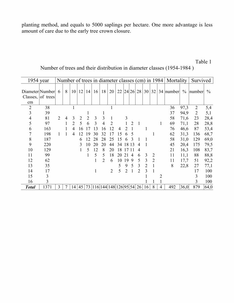
Here we give experimental results of the initial tree diameter distribution when trees are 20-years of age and of the tree mortality and the changes of tree numbers in diameter classes in 30 years (50-year old trees), see Table 1.

During this 30-year period, in 2cm diameter class (23% of the mean diameter), 97,3% of trees died, in 3cm diameter class (36% of the mean diameter) – 94,0%, in 4cm diameter class (48%) – 71,6%, in 5cm diameter class – 71,1%. Total tree mortality was about 36% of trees. Thus, we can state that in 20-year old artificial forest, trees with relative diameter less then 0,4 (of the mean diameter) are doomed to death. In the diameter classes with relative diameters 0,5-0,6 the mortality is still high: about 70%.

Thus, viability of trees is genetically determined and facilitates differentiation and self-thinning of the forest. Without this, the whole population would be suppressed and likely to perish. Those trees that lag behind in growth have the least viability, but even in higher diameter classes (with relative diameter > 1,3) there is 6-10% of trees which at 50 years of age accomplished their destination in the development of the population and died. While growing, those trees, which were initially in the same diameter class, were differentiated, and formed new diameter distribution, close to that of Gaussian.

The distribution inside every diameter class is bounded by the thinnest trees, which (in 4-10cm diameter classes) gave 2 cm diameter growth and the thickest trees in the same classes with 13-17cm diameter growth. In higher diameter classes, the minimum diameter growth was 4 cm, maximum – 17 cm. Thus, the trees were re-distributed.

As a result of high mortality of trees with the initial relative diameters 0,2-0,3, the number of trees with relative diameter 0,4-0,6 decreased considerably. Since thinner trees were eliminated, the average diameter became larger which resulted in disappearing of trees with relative diameter > 1,7. several planting regions contained a very good forest which excels the best natural forests in Siberia, where Pinnus sylvestris is widely spread.

We think that the most stable part of a young pine forest is the trees with relative diameter >0,8. They also are the most productive part of the forest, see Table 2.

Most of the trees (75,5%) in 1987 had relative diameter >0,8. In addition, 20 year old trees with relative diameter < 0,6, contribute only 3% in the diameter classes with relative diameter > 0,8 in 30 years. It means that they could be smoothly eliminated during improvement felling, if it would not result in strong sparsing of the forest and excessive lighting of the soil. Thus, the most of the trees (91%) in 1987, had relative diameter > 0,8.

It is very interesting that researchers of natural forests gave qualitatively very similar results. It allows to suggest that the both processes have universal character, regardless of the way of planting (artificial in groups or natural).

Let’s now consider how the tree elimination process proceeds in tree groups. In Table 3 we give the spacing of trees within a planting unit with respect of the number of trees per every unit (initially, 10 trees were planted on every unit) for 20, 30, 40 and 50 year old trees.

One can see from the data that the trees are eliminated in all squares, but more intensively in those, which had more than 7 trees. As a result of this natural mortality, the average number of trees per every unit decreased from 6,9 for 20-year old trees to 4,5 for 50-year old ones. Mortality level equals approximately 0,4-0,5 tree/square every 5 years and it does not change much during last 20 years. Planting units initially consisting of 1 or 2 trees had no trees at all (all trees were eliminated). It means that the most stable (in 20-50 year period) groups are those which initially (20-years of age) had > 3 trees/group density.

In order to determine how the number of trees in a group influences their growth, the average diameters of the three biggest trees were calculated for every group (see Table 3). As one can see from the data, for 50-year old trees the average diameter does not depend on the total number of trees in every group and varies in a very small interval (21,0 - 22,0 cm).

The most interesting point for us was to compare mortality level in artificial forests planted by the group method with natural pine forests.

Since the average tree diameters in the considered artificial establishments are almost identical to those given in the tree growth tables for the first-class pine forests, we will compare our results with these data (see Table 4). Thus, although 20-year old natural forest had more trees in comparison with the artificial one, but 50-year old artificial forest had 1,8 times more trees. The total mortality in a natural forest was 2770 trees/hectare, in the artificial – only 1119 trees.

Thus, we can claim that group tree plantings are more stable and self-thinning process proceeds much slower. This stability can be explained as a result of better lighting, which is formed due to the following reasons. First, because of big distance between groups, tree crown closure occurs only at the bottom. Upper crown parts are always open for every tree in the group. Second, this lighting increases due to the terrace-like arrangement of groups at the mountainside. Therefore, the main features of

group plantings growth are early crown closure and formation of appropriate forest environment. Absence of crown closures at the upper parts of trees promotes better lighting. Probably, the in-group distribution of trees, water supply conditions are also better. All these factors contribute to the fact that more trees can survive at the area of 1 hectare.

Lower mortality leads to bigger wood biomass value in group plantings. In Table 4 we give the results of observations of tree growth every 5 years for 500 groups on 1 hectare.

From graphs 1-4 one can see, that at the age of 20 total biomass in the artificial forest is less than in the natural forest of the same class, but then the situation changes mainly due to the lower mortality level in groups. As a result, at the age of 50, the artificial forest has twice bigger total biomass.

The given data allows making the following conclusions. The pine in the Tyan-Shan region has good biometrical parameters, which makes it

effective to create pine plantings in North Kirghizia. Possible height interval is 1900-2500 m above the sea level, without strong winds during the winter season.

Creating tree groups is recommended as the main method of initial tree arrangement with 500-1000 groups of 1x2m size per every hectare. The exact number of groups should be determined by the slope gradient.

In artificial pine forests where use is made of group planting method, mortality level is considerably lower in comparison with the first-class natural pine forests. As a result, by the age of 50 the total number of stems in artificial forests with group distribution is 80% bigger, and the total wood biomass is 65% bigger compared to the tree growth tables of the first-class natural pine forests.

High stability of groups does not only show itself in a bigger number of banded trees, but also in the fact that they are less prone to harmful effects of changing conditions (worsening of conditions due to the crown closure and so on).

From our point of view, this stability of strands with group distribution of trees can be explained by the ordered tree structure inside groups and between groups, and also by peculiar properties of group growth. Because of the order, the first tree crown closure happens at the age of 3 or 4 and it forms appropriate forest conditions, suppresses development of grass under the trees. Due to the big distance between groups, full crown closure does not happen even at the age of 50. This promotes better crown development, photosynthesis and better penetration of precipitation under the crown. But shading is nevertheless enough to suppress competing grass. On the other hand, trees planted in groups not only compete but provide mutual aid as well which leads to more stable group growth. In addition, genetically determined tree viability plays very important role in this process. In addition, it is appropriate to mention here that group plantings require much less efforts to create them. The square of cultivated soil in the case of 500 groups per hectare is only 0,1 ha. The number of saplings is also much less then in the case of, say, in-rows

planting method, and equals to 5000 saplings per hectare. One more advantage is less amount of care due to the early tree crown closure.

Table 1 Number of trees and their distribution in diameter classes (1954-1984 )

1954 year Number of trees in diameter classes (cm) in 1984 Mortality Survived

Diameter Classes,

cm

Number of trees

6

8

10

12

14

16

18

20

22

24

26

28

30

32

34

number

%

number

%

2 38 1 1 36 97,3 2 5,43 39 1 1 37 94,9 2 5,14 81 2 4 3 2 2 3 3 1 3 58 71,6 23 28,45 97 1 2 5 6 3 4 2 1 2 1 1 69 71,1 28 28,86 163 1 4 16 17 13 16 12 4 2 1 1 76 46,6 87 53,47 198 1 1 4 12 19 30 32 17 15 6 5 1 62 31,3 136 68,78 187 6 12 28 28 25 15 6 3 1 1 58 31,0 129 69,09 220 3 10 20 20 44 34 18 13 4 1 45 20,4 175 79,510 129 1 5 12 8 20 18 17 11 4 21 16,3 108 83,711 99 1 5 5 18 20 21 4 6 3 2 11 11,1 88 88,812 62 1 2 6 10 19 9 5 3 2 11 17,7 51 92,213 35 5 9 5 3 2 1 8 22,8 27 77,114 17 1 2 5 2 1 2 3 1 17 10015 3 1 2 3 10016 3 1 1 1 3 100

Total 1371 3 7 14 45 73 116 144 148 126 95 54 26 16 8 4 492 36,0 879 64,0

Table 2

Number of trees in diameter classes (1954-1979)

Number of trees in diameter class with relative diameter > 0,8 Initial

relative diameter at the age

of 20

Number of trees

Number ofsurvived

trees

Survived trees,

percentage number

% of trees from initial

number

% of trees with final diameter

class > 0,80,5 81 23 28,3 9 11,1 1,3 0,6 97 28 28,9 11 11,3 1,6 0,7 163 87 53,4 43 26,4 6,1 0,8 198 136 68,7 85 42,9 12,2 0,9 187 129 69,0 106 56,7 15,2 1,0 220 175 79,5 158 71,8 22,6

>1,0 348 297 84,8 287 82,5 41,0 Total 1294 875 67,8 699 54,0 100,0

Table 3

Distribution of number of trees (%) in groups

Number of trees in group Age

1 2 3 4 5 6 7 8 9 10

Ave

rage

nu

mbe

r of

trees

in

biog

roup

20 1,0 1,5 2,0 3,5 5,0 25,0 27,5 24,0 3,5 7,0 6,9 25 1,0 2,0 2,0 4,0 10,0 24,0 28,0 19,5 4,0 5,5 6,6 30 1,5 2,5 3,5 6,1 11,6 27,8 25,3 16,7 2,0 3,0 6,2 35 1,0 3,5 5,1 12,1 21,2 23,2 20,7 11,6 0,6 1,0 5,7 40 1,0 3,5 5,6 16,2 24,7 21,7 18,7 8,1 0,5 5,4 45 1,0 6,1 7,1 24,9 27,9 17,8 11,7 3,6 4,9 50 3,0 6,6 15,7 26,9 23,9 13,7 7,6 2,6 4,5

Average diameter of

the three biggest

trees in a group, 1984

23,7 21,4 21,6 22,0 21,6 21,7 21,0 21,1 21,1

Table 4 Number of trees per ha in group plantings and in regular pine first-class forests

(according to the tree growth tables)

Age

Number of trees

in natural forest

Mortality for 10 years

Number of trees in group

plantings

Mortality for 10 years

% of trees number in

group planting

relative to the natural

forest 20 3970 3425 86 30 2400 1570 3107 210 129 40 1640 760 2695 412 164 50 1200 440 2198 497 183

Total 2770 1119

Table 5

Tree growth in group pine planting without improvement felling

Percentage

Age Average height, m

Average diameter,

cm

Number of trees per 1 ha

Mortality in 5

years

Total wood

volume, m3

Mortality, in m3 of knots of

needles

15 3,6 5,8 3826 35 20 6,0 8,4 3425 401 65 25 8,0 11,5 3317 108 139 30 10,1 12,7 3107 210 202 0,3 35 12,0 15,1 2820 287 326 1,7 40 14,5 16,6 2695 125 428 3,2 10,4 13,7 45 16,1 18,5 2415 280 500 5,6 50 17,5 20,0 2197 232 582

Table 6 Tree growth in natural pine first-class forest

Age Number of trees

Average diameter,cm

Average height, m

Total wood volume, m3

20 4000 9,1 7,3 128 25 3100 11,1 9,4 177 30 2500 13,1 11,4 225 35 2050 14,8 13,3 266

Fig.2. Graphs of growth parameters for group planting (triangles) and for natural pine first-class forest (squares).

III. HORIZONTAL CROWN MOVING AND RADIAL-BASED FUNCTIONS METHOD

In this section we will consider the effect of horizontal crown moving. This effect plays the key role in forest modeling with the group method of spacing of stems. To our knowledge, in the most famous forest models this effect has not been considered at all. It can be explained by the fact that despite random (Poisson) trunk distribution the effect is compensated by many random crown “collisions” and, therefore, has second-order character. But in group plantings, as considered in the previous chapter, this effect leads to qualitatively new effects, as we will show with our forest model.

The effect of horizontal crown moving was considered in [Bouzikin, Gavrikov et al, 1985]. Here, in order to prove the existence of the effect, we will show how the

Average diameter, cm

02468

101214161820

20 25 30 35 40 45 50

Age

Diam

eter

Average height, m

02468

101214161820

20 25 30 35 40 45 50

Age

Heig

ht

Total wood volume, m3

0

100

200

300

400

500

600

700

20 25 30 35 40 45 50

Age

Vol

ume

Number of trees on 1 ha

0500

10001500200025003000350040004500

20 30 40 50

Age

Num

ber

radial-based function method can be applied to the analysis of spatial configuration of trunk positions in a real forest and compare it with the data on crown centers positions.

Initially the method of radial-based functions is widely applied in molecular physics for studying spatial configurations of atoms and molecules of different physical substances. The method was applied to the studying of spatial structure of tree crown and trunk positions based on the data obtained from the long-term observations of the pine forest, grown in Russia, Siberia, Angara-Irkutsk region. In this work we will formulate the method of radial-based functions and give the results of its application to the real data, according to [Bouzikin, Gavrikov et al, 1985].

Let’s consider 2D-distribution of objects inside a piece of plane with S square. The probability of object 1 to be situated inside the circle centered in R1 point and with S1 square, and the object 2 to be inside the circle centered in R2 point and with S2 square equals

SS

SS

RRgRRP 212121 ),(),(

∆∆= , (1)

where g(R1,R2) depends on the interaction between the objects. In case of non-

interacting objects we would have g ≡ 1. In the case of isotropic object interaction we have

)(),( 21 RgRRg = , (2)

where 21 RRR −= is a distance between trees. Then the probability of the object 2

to be inside the ring with internal radius R and external radius R+∆R, equals

SRRRgRP ∆= π2)()( . (3)

We denote g(R) as radial-based function of object distribution. It is easy to show

that

av

RRgρρ )()( = , (4)

where ρav is the average density of objects, i.e. ρav =

SN , where N is the overall

number of objects; ρ(R) =RR

RN∆π2

)( is the average density of objects in the [R;R + ∆R] ring,

i.e. N(R) is the average number of objects on the distance between R and R+∆R (here we average on all the objects).

Let’s consider four basic types of object distribution: 1) Random (Poisson) distribution. In this case we have ρ(R)= ρav and g(R)=1. It means that there are no preferred

distances between objects (all distances have equal probability). 2) Equidistant distribution. In this case the objects “avoid” being close to each other. This type of distribution

is due to the repulsion interaction (for example, free electron gas). Radial-based function in this case behaves as shown on the Fig.3.

3) Ordered structure. In this case we have crystal-like structure with distant order. This type of radial-

based distribution function is shown in Fig.3. 4) Group distribution. The objects are grouped, which means that the distances between objects inside a

group are much smaller then the distances between groups. The radial-based distribution function behaves as shown on Fig. 3.

In this form the method of radial-based function was applied to the real data of tree trunk and crown distributions. The results are shown on Fig.4.

The analysis of the results allowed to make the following conclusions: 1) Distribution of the trunk positions changes from the group one in a young

stand to the random (Poisson) one at the mature age (50-60 years). 2) Distribution of tree crown centers changes from the group one in young stand

to the equidistant at the mature age. In other words, this analysis shows that a young stand tends to form tree groups,

which helps to compete with grass and bushes. But at the mature age due to the random mortality, distribution of tree trunks is randomized. Nevertheless, tree crowns still interact with each other. It leads to the qualitatively different distribution of tree crown centers. The crowns repulse and cover, as a result, a larger area. In the next section, we will try to fix this effect in our simple forest model to explain the experimental results of Peter von Hahn.

1) 2) 3) 4)

Fig.3. Different typical distributions of objects and the corresponding radial-based distribution functions

1) Poisson; 2) Equidistant; 3) Ordered; 4) Group.

1

1

1

1

Fig.4. Radial-based distribution functions for pine forest grown in Russia, Siberia, Angara-Irkutsk. Distributions are calculated for three

different tree ages and separately for trunk positions and crown centers positions.

25 years, trunks

0

0.5

1

1.5

2

2.5

3

3.5

0 0.1 0.2 0.3 0.4 0.5 0.6 0.7 0.8

r

radi

al fu

nctio

n va

lue

25 years, crowns

0

0.5

1

1.5

2

2.5

3

0 0.1 0.2 0.3 0.4 0.5 0.6 0.7 0.8 0.9

r

radi

al fu

nctio

n va

lue

55 years, trunks

0

0.5

1

1.5

0 0.5 1 1.5 2 2.5 3 3.5 4 4.5

r

Radi

al fu

nctio

n

55 years, crowns

0

0.5

1

1.5

0 0.5 1 1.5 2 2.5 3 3.5 4 4.5

r

Radi

al fu

nctio

n

90 years, trunks

0

0.5

1

1.5

0 1 2 3 4 5 6 7 8

r

Radi

al fu

nctio

n

90 years, crowns

0

0.5

1

1.5

0 1 2 3 4 5 6 7 8

r

Radi

al fu

nctio

n

IV. FOREST HAHN MODEL DESCRIPTION We implemented a very simple forest model and do not pretend to give a highly

realistic description of forest dynamics. Here we underline the most important features of the model:

1) The model is geometrical. It means that we tried to develop a very simple geometrical conception of the interaction of tree crowns. We used several qualitative ideas on tree interaction and expressed them in the geometrical language.

2) The model deals with the aspect of trees’ growth only, with their intraspecific competition. We deliberately did not introduce in the model other very important factors (for example, interspecific competition with grass). It allowed us to consider effects in their “pure” form.

3) The model is individual-based, i.e. every tree has its own parameters and history. 4) The model is deterministic, i.e. given the initial distribution of trees the result of

modeling is unique. 1. Individual trees characteristics We used a “cylindrical” model of the tree, i.e. we think of a tree as of two joined

cylinders, one for the trunk and one for the crown. Here are the geometrical parameters of the tree (see Fig. 2a):

H – tree height; D – tree diameter; HC, C – crown height and diameter respectively.

Here are some additional derived characteristics:

VC = π HCC2/4 – crown volume; (5) µC = HC/H – relative crown height; (6) V = π HCD2/4 – tree (wood) volume. (7)

Dynamical variables for the ith tree are Dt(i) and )(itCµ , where t – time; other

characteristics are calculated with the following formulas:

H(i)= α(Dt(i))β (8) VC(i) = γ(Dt(i))δ (9) HC(i)= )(it

Cµ H(i) (10) C(i) = 4VC (i) /(πHC(i)) (11)

It means that we use allometry (see, for example, [Gould, 1966]) in calculating tree height and crown volume.

Equation of growth was chosen in the differential form of Korf [Korf, 1939] Dt+1 = Dt + kεDt/tη, (12) where Dt+1, Dt – new and old annual values of tree diameter, ε, η – constants, and

k∈[0,1] depends on the interaction with the neighbors (competitors) of the tree. Every tree position is described by two 2D - vectors: X and XC, where X is the

position of the trunk center, and XC is the position of the tree crown center. Vector X is the same during all tree lifetime and XC changes because of the interaction between crowns.

2. Trees interaction At every step of modeling, for every tree we determine a list of competitors.

Competitors are those trees whose crowns intersect the crown of the given tree. For every competitor discriminative relation is calculated:

i

jD D

DjiK =),( , (13)

where Dj is diameter of the jth tree, which is one of the competitors for the ith (current) tree.

All competitors for the ith tree are then divided into dominant and non-dominant competitors according to the definite threshold θD of the KD value. The jth competitor for the ith tree is dominant if KD(j,i)> θD, otherwise the competitor is non-dominant.

a) b) Fig.5. a) Geometrical characteristics of a tree (here H – tree height, C – crown

diameter, D – tree diameter, HC – crown height); b) Crown intersection.

H

C

D

HC S1 S2 ∆S

a) b)

Fig.6. a) Tree A is not in a crowded situation; b) Tree A is in a crowded situation;

Then we introduce the degree of competition for the ith tree with the jth

competitor: ( )

)()(),(min),(

),(iHS

jHiHjiSjiK

Ci

CCC ×

×∆= , (14)

where ∆S(i,j) is the square of crown intersection (see Fig.5), Si is the crown square of the ith tree, HC(i) and HC(j) are crown heights of the ith and jth tree. Actually, DC(i,j) is the relative volume of crown intersection.

3. Horizontal crown moving Competitors force each other to move crowns. We introduce a very simple law for

calculating crown displacement. At every step the vector of crown displacement is equal to

[ ]

[ ]∑

∑

=

=∆=)(

1

)(

1

),(),(

),(),()()()(

iN

jCC

iN

jCC

CC

C

jijiK

jijiKiiCi

n

n∆XC , (16)

where NC(i) is the number of competitors for the ith tree, and

)()()()(

),(jiji

jiCC

CCC XX

XXn

−−

= , (17)

<−

=∆else

iHiXiXifVi CC

C ,0)()()(,

)( maxα , (18)

Here VC is the annual crown speed (measured as fraction of C – tree crown diameter) and αmax is the maximum angle of the tree slope.

According to (18) competitors force neighbors to move their crowns proportionally to the relative crown intersection volume. Therefore, very small trees almost do not

A A

affect the big ones. Also because a tree trunk has natural limitations for the possibility of crown shift, we introduced the maximum shift, after which the crown does not move further.

3. Vertical crown moving The phenomenon considered can be explained if we take into account both

horizontal and vertical movements of the crown center. In our model the form of the tree crown depends highly on the environmental

conditions of a tree. If a tree stands alone then its crown has large height HC (see Fig. 2). In crowded environment a tree strives for raising branches and all green biomass to survive in the competition for light (if it does not do this, its bottom branches with leaves just become useless).

At every step of the calculation every tree is determined to be in crowded or free environment. In our model we determine this by analyzing configuration of competitors (see Fig. 3). If they form closed convex polygon and the tree is captured inside this polygon, then it is regarded to be in crowded environment. If the tree has at least one direction in which it could move its crown to get additional living space and light, then it is regarded to be in free environment.

If a tree is in crowded environment then, in our model, the growth mode changes its parameters. First, the crown form changes:

),max( min1 µµµµ crowded

CtC

tC ∆−=+ , (19)

where min, µµ crowdedC∆ are additional parameters of the model, t

CtC µµ ,1+ are the new and

old value of Cµ for the tree. If opposite (a tree is in free environment) then

),max( max1 µµµµ free

CtC

tC ∆+=+ . (20)

In our model we choose 10≈∆∆

freeC

crowdedC

µµ . It means that a tree quickly changes crown

form when it happens to be in crowded environment and then slowly changes it back when the situation becomes more favorable.

Note from (20) that the decrease of µC value leads to the increase of C value (crown diameter). Therefore, the effect of vertical crown moving introduces positive feed-back in the competition process (overcrowding leads to stronger competition and the latter leads to bigger overcrowding).

Fig.7. Excluding borde

4. Depression and mortality Tree growth speed is determined by equation

depending on the level of competition and environmen

−

−=

∑

∑

=

=

environcrowdedinjiK

tenvironmenfreeinjiKik

C

C

N

jCcrowded

N

jC

,)),(1,0max(

,)),(1,0max()(

1

1

σ

where σcrowded is the parameter of the model wdecrease of the growth speed) of a tree in the crowded

In formula (21) all NC competitors are taking parAs opposed to this, in mortality calculation only domaccount. We consider a tree doomed to death if the lecompetitors is higher than a definite threshold:

N

jCcrowded

N

jC

D

envirocrowdedinjiK

tenvironmenfreeinjiKik

D

D

σ

−

−=

∑

∑

=

=

,)),(1,0max(

,)),(1,0max()(

1

1

where ND is the number of dominant competitorsSo, in our model we introduce tree mortality

competition. Therefore, we deliberately exclude maanalyze only discriminative mortality.

real trees

fictive trees

r effects

(12), which contains parameter k tal conditions of the tree:

tmen, (21)

hich strengthens depression (the environment. t in decreasing the ith tree growth.

inant competitors are taken into vel of competition with dominant

M

tnmenθ> ,. (22)

. only as a result of intraspecific ny important factors in order to

5. Excluding the border effects Since we deal with a finite number of trees (100-2000 in our experiments on the

area of square S = 400m2), it is desirable to exclude border effects, i.e., the situations when outer trees, which are on the border of the area, have fewer competitors than others. These situations can distort results of modeling.

In our model we made opposite borders cyclic, as they often do in modeling of molecular interactions. Algorithmically, when calculating the competitor list for a tree, we consider a number of fictive trees in eight adjacent cells (see Fig.7), This trick is used for calculating crown moving as well as depression and mortality level.

6. Model algorithm We introduced above all the factors of our model. Here we combine them in one

algorithm. I. Initialization. Generate N trees. Set for every tree its individual parameters: D(i), X(i). Set initial values of relative crown height and crown position as µC(i)=µmax, XC(i)=X(i). For every tree set variable Doomed(i) to –1. Set time counter t=0. II. Allomerty calculation. For every tree calculate its characteristics H(i), C(i), HC(i), VC(i), V(i) using formulas (5-11). III. Competitors counting. For every ith tree calculate the list of competitors. Determine if the ith tree is in the crowded environment. IV. Moving crowns. For every tree (except those with variable Doomed(i)≠-1) calculate vector of crown shift, equation (16). Calculate new position of the crown XC(i). Calculate changing in crown height, (eq. 19,20). Calculate new value of µC(i). V. Depression and growth. For every tree (except those with variable Doomed(i)≠-1) calculate coefficient of growth speed k(i), (eq. 21). Calculate new value of tree diameter D(i) (eq. 12). VI. Mortality. For every tree check Doomed(i). If it is not equal to –1, then add unity to Doomed(i). If then Doomed(i) ≥ TDeath, then delete ith tree from the calculation. Calculate the value of kD(i). If kD(i) ≤ ηM then set Doomed(i)=0. VII. Cycle. Set t ⇒ t+1. If t<Tripe then go to the II step. Else finish. Table 7 summarizes all model parameters with short descriptions and the values

taken for the modeling.

Table 7

Model parameters and their values Sign Name and description Value

α, β

γ, δ

ε, η

θD

VC

αmax ,minµ maxµ

crowdedCµ∆ free

Cµ∆

σcrowded θM

TDeath TRipe

S

Allometrical coefficients for calculating tree height from diameter (eq. 8). Allometrical coefficients for calculating tree crown volume from diameter (eq. 9). Coefficients in the growth equation (12). Discriminative threshold. Determines whether a competitor is dominant for a tree (eq. 13). Annual crown speed (measured as fraction of C – tree crown diameter), (eq.18). The maximum angle of tree slope, (eq.18). Minimum and maximum values of µC, (equations 19,20). Speed of vertical crown moving when tree is in crowded environment, (eq.20). Speed of vertical crown moving when tree is in free environment, (eq.20). Degree of tree competition increasing in crowded environment, (eq.21). Mortality threshold. If competition level from dominant competitors is higher than θM, then tree is doomed to death. Tree death time (years). Age of ripe tree. Square of modeling area, m2

α = exp(4.93), β = 1.28

γ = exp(7.5), δ = 2.568

ε = 210, η = 2.6

θD = 1.5

VC =0.1

αmax = 30° minµ = 0.2,

maxµ = 0.5 crowdedCµ∆ = 0.1

free

Cµ∆ = 0.01

σcrowded = 3

θM = 0.4

TDeath = 10 TRipe = 100

S = 400

V. MODELING RESULTS We run our model for several types of planting: Poisson (random) planting,

equidistant planting and group planting. In Poisson (random) planting every tree is placed randomly on a region of square S.

In equidistant planting, trees form a kind of two-dimensional grid (hexagonal or rectangular). In group planting, trees are placed in bio-groups. The distance between trees in the group is much smaller then the distance between groups (see Fig.8).

a) b) c) Fig.8. Variants of tree planting; a) Poisson (random), b) equidistant, c) group.

In all our numerical experiments equidistant distribution showed essentially the

same dynamics as Poisson distribution, so we will compare results for Poisson and group distribution.

In Fig.4 we show trajectories of the artificial forests in the cases of Poisson and group distribution, starting from different initial values of tree numbers. For the modeling we took the area of square S = 1/25 ha2. The difference in forest dynamics is quite clear. Increasing number of trees in the case of Poisson distribution decreases the final yield monotonically, while in the case of group planting we have the maximum of final yield at some optimal initial number of trees. We underline here, that in the case of group planting we could start from any value of the initial number of trees because the density of trees in groups could be arbitrary high for providing saplings surviving.

In Fig.5 the results of visualizing forest dynamics for the same cases are shown. Every circle on the picture corresponds to a tree. The intensity of gray color of the circle corresponds to the degree of depression of the tree (how strong it is affected by intraspecific competition). The red border of the circle points out to the “crowded” condition of the competition for the tree. In the case of Poisson distribution of trunks most of trees during all their life are in the crowded situation. In contrast, in the case of group planting crowded situation is a very rare case, except for an early stage of tree growth, when the crowns of young trees are closured inside the group.

To demonstrate the phenomenon of discriminative death for the same run as shown in Fig. 5, we constructed diagrams of diameter distribution for both cases. On these diagrams red color denotes initial diameters distribution. Then for every diameter class we showed the number of survived trees (green bars). It is clear that in both cases thin trees are doomed for death.

Comparing Figures 4a and 4b, one can notice that the final number of trees is bigger in the case of Poisson distribution. It does not correspond to the observations of von Hahn (see Table 1). But we should notice that von Hahn obviously must have counted only good full-value trees, not very thin trunks. We plotted functions of the distribution for the diameter (number of trees with diameter bigger than d vs d) and for tree mass (number of trees with mass bigger than m vs m). From these plots it is clear that though the overall final number of trees in simulation is bigger in the case of

ay

ax

Poisson distribution, but if we count only full-value trees (say, with diameter bigger than 0.1) then the situation is quite opposite: we have the double number of trees in the case of group planting, which corresponds to the experimental observations of von Hahn.

To summarize, the results of modeling correspond well (of course, qualitatively, because the constructed model does not take into account many, many important factors; for example, it absolutely neglects stochastic tree death rate which is fairly equal for all trees, big and small ones) to the experimental observations. It means that the mechanisms of intraspecific competition introduced in the model (horizontal and vertical crown moving, discriminative death) reflect the real key processes that occur in nature.

a)

b)

Fig.9. Trajectories of forest dynamics on the N (number of trees) × M (total wood mass) in the case of Poisson initial trunk distribution (a) and group distribution (b); a) increasing the number of planted trees decreases the timber yield because of trees competition, but we can’t start the trajectory at small number of trees (because of the competition with grass and bushes); b) we can start with any number of trees and in some very narrow interval of initial values of N it is possible to reach high values of total wood mass, after this value the second closure of crowns leads to strong competition.

N

M Poisson distribution

Group distribution

N

M

0

2

4

6

8

10

12

0 500 1000 1500 2000

0

2

4

6

8

10

12

14

16

0 100 200 300 400 500 600

a) “Poisson” planting

5 years 15 years 25 years

35 years 60 years 90 years

b) Group planting

5 years 15 years 25 years

35 years 60 years 90 years

Fig.10. Comparing forest dynamics in the case of Poisson planting (a) and group planting (b); gray tint shows the degree of tree depression. Those trees which have red border color are in the “crowded” environment with stronger competition.

Fig.11. Discriminative mortality. Red blocks are the histogram of initial diameter’s distribution. Green blocks correspond to those trees, which survived at the age of 90. It is shown that the trees with initially small diameters have no chances to survive.

Poisson

0

50

100

150

200

250

300

350

0.001

7

0.002

9

0.004

1

0.005

3

0.006

4

0.007

6

0.008

8

0.010

0

0.011

2

0.012

4

tree diameter

num

ber o

f tre

es

Initial Survived

Group

05

1015202530354045

0.001

4

0.002

6

0.003

8

0.004

9

0.006

1

0.007

2

0.008

4

0.009

6

0.010

7

0.011

9

tree diameter

num

ber o

f tre

es

Initial Survived

Tree diameter

0

20

40

60

80

100

120

140

0 0.05 0.1 0.15 0.2 0.25 0.3tree diameter

num

er o

f tre

es w

ith d

iam

eter

>x

PoissonGroup

Tree mass

0

20

40

60

80

100

120

140

0 0.5 1 1.5 2 2.5tree mass

num

er o

f tre

es w

ith m

ass

>x

PoissonGroup

Fig.12. Distribution functions for tree diameter and tree mass (volume).

VI. CONCLUSION

The experiment of Peter von Hahn described in this paper shows that it is possible to affect considerably the dynamics of forest growth by choosing the initial spatial arrangement of tree saplings. As a result, it is possible to obtain a 50-100% gain in timber yield (total wood mass).

The modeling and conducted analysis showed that the first reason for von Hahn’s experimental results is purposeful excluding of intraspecific competition due to the special initial spatial trunk arrangement. The second one, and it may be even more important, is non-linear effect of tree cross-section crown size changing as a result of changing conditions of competition with neighbors (crowded and non-crowded conditions of growth). This effect introduces positive feed-back in the competition process (overcrowding leads to stronger competition and the latter leads to greater overcrowding). As a result, it means that at the same planting area it is possible to arrange more big full-value trees if every of them is not surrounded by competitors (not in the “crowded” situation).

Excluding intraspecific competition leads to the change in energy balance. The total energy that forest receives, in general case, is spent for the intraspecific and interspecific competition, and for the tree growth. The part of intraspecific competition in this balance is big enough, so excluding it, it is possible to gain in the energy spending for growth of total biomass. Excessive intraspecific competition leads usually to bigger quantity of small trees and if one considers only big full-valued trunks then in this case we can gain also in the number of trees (as can be seen from von Hahn’s experiment, see also Fig. 7).

Method of improvement felling is applied for the same reason, but the method described in this paper is cheaper, less laborious and more radical (intraspecific competition is excluded starting from a very early stage).

While modeling forest, we had in mind that the quality of soil is good enough to make crown competition the leading factor. Otherwise main competition would occur between tree roots. In this respect it is appropriate to mention here that applying fertilizers in the case of group method of trees planting gives much better results than in ordinary methods of equidistant plantings or plantings in rows. It occurs because of the fact that fertilization is then applied to the trees most of which will survive. In case of equidistant planting fertilizers help not only the trees with good chances, but also the doomed trees. In this case fertilization promotes, in fact, intraspecific competition.

In the model proposed the effect of gaining wood mass has resonance character. Setting groups of trees too distant from each other, we would lose in total wood mass because of excessive sparsity (in this case the number of trees will be insufficient for good timber yield). Setting groups of trees too close leads to the closure of tree crowns from different groups at mature age and to the emergence of strong intraspecific competition (which takes a lot of timber yield because in this case we have no excessive number of trees to sacrifice). Therefore a definite optimum in the spatial configuration

of trunks exists (optimal distance between groups of trees) which allows to obtain rich timber yield and to avoid strong intraspecific competition (see Fig. 4).

This text, software and other information are available on the web-server of one of the authors: http://www.ihes.fr/~zinovyev.

ACKNOWLEDGEMENTS

We would like to thank the directorate and management personnel of the Institut des Hautes Études Scientifiques (France) for the invitation and exclusively favorable conditions for creative work. We are thankful to Misha Gromov (professor of IHES) for paying attention to the work. We are also thankful to A. I. Bouzykin for his drawing attention of one of the authors to Fig.1 explaining the effect considered in the paper.

REFERENCES

1. Anderson, M. L. - A New System of Planting. Scottish Forestry Journal, Vol. 44 (2). 1930. pp. 7887.

2. Anderson, M. L. Planting in Dense Groups Spaced at Wide Intervals. Quarterly Journal of Forestry. Vol. XXV (4). 1931. pp. 312-316.

3. Anderson, M. L. Spaced Group-planting and Irregularity of stand structure. Empire Forestry Journal. Vol. XXX (4) 1951.

4. Bouzikin A.I., Gavrikov V.L., Sekretenko O.P., Khlebopros R.G. Analysis of structure of wood cenosis (in russian). Edited by Kireev D.M. Nauka Press, Novosibirsk, 1985.

5. Cameron, R. D. - A Study of the Development in Plantations of Small, Closely-planted Groups with Wide Interspaces. Manuscript in the Imperial Forestry Institute Library, Oxford. 1950.

6. Gould S. Allometry and size in ontogeny and phylogeny. – Biol. Rev., 1966, v.41, p.587-640.

7. Hahn P.A. Introduction and growing of coniferous forests in Kirgizia (in russian). Ilim Press, Frounze, 1987.

8. Jacquemin, A. - Le traitement de l'Epicea dans le Cantonnement de Vielsalm. Bulletin de la Société Royale Forestière de Belgique, Vol. XXXIX (1930), pp. 445-469, and Vol. XL (1931).

9. Kay, J., Anderson, M. L. Douglas Fir at Home and Abroad. Empire Forestry Journal, Vol. 7 (1).1928.

10. Korf V., Prispevek K matematicke definici vzrustoveho zakon hnot lesnich porostu. – Zesnicka prace, 1939, v.18, s. 339-379.

11. Niklas K.J. Plant Allometry: The Scaling of Form and Process (Univ.of Chicago Press, Chicago, 1994).

12. Ryle, G. B. Planting in Dense Groups Spaced at Wide Intervals. Quarterly Journal of Forestry Vol. XXVI. 1932. p. 46.

13. Space-time structure of forest biogeocenoses (in russian). Nauka Press, Novosibirsk, 1981.

14. Suhovolsky V.G. Economics of living (in russian). “Flat-limited” Press, Krasnoyarsk, 1999.

15. West, G.B., Brown, J.H. & Enquist, B.J. A general model for the origin of allometric scaling laws in biology. Science 276, 122-126 (1997).