Embed Size (px)
Citation preview

Tilburg University
Supplying to mom and pop: traditional retail channel selection in megacities
Ge, Jiwen; Honhon, Dorothee; Fransoo, Jan C.; Zhao, Lei
Published in:Manufacturing and Service Operations Management
DOI:10.1287/msom.2019.0806
Publication date:2021
Document VersionPeer reviewed version
Link to publication in Tilburg University Research Portal
Citation for published version (APA):Ge, J., Honhon, D., Fransoo, J. C., & Zhao, L. (2021). Supplying to mom and pop: traditional retail channelselection in megacities. Manufacturing and Service Operations Management, 23(1), 19-35.https://doi.org/10.1287/msom.2019.0806
General rightsCopyright and moral rights for the publications made accessible in the public portal are retained by the authors and/or other copyright ownersand it is a condition of accessing publications that users recognise and abide by the legal requirements associated with these rights.
• Users may download and print one copy of any publication from the public portal for the purpose of private study or research. • You may not further distribute the material or use it for any profit-making activity or commercial gain • You may freely distribute the URL identifying the publication in the public portal
Take down policyIf you believe that this document breaches copyright please contact us providing details, and we will remove access to the work immediatelyand investigate your claim.
Download date: 04. Apr. 2022

Supplying to mom and pop:
Traditional retail channel selection in megacities
Jiwen Ge
Institute of Supply Chain Analytics, Dongbei University of Finance and Economics
Tuck School of Business, Dartmouth College
Dorothee Honhon
University of Texas at Dallas, [email protected]
Jan C. Fransoo
Dapartment of Logistics, Kuehne Logistics University
Department of Industrial Engineering & Innovation Sciences, Eindhoven University of Technology
Lei Zhao
Dapartment of Industrial Engineering, Tsinghua University, [email protected]
June 2, 2019
Abstract
Problem definition: Nanostores are traditional, small and independent retailers that are
present in large numbers in the megacities of the developing world. CPG manufacturers can
choose to deliver to nanostores either directly - visiting thousands of stores per day - or via
wholesalers - saving on distribution cost but forfeiting the direct access to the store owners to
develop demand. We study a manufacturer’s channel strategy within a finite time horizon.
Academic / Practical Relevance: The channel strategy in emerging markets has both market-
ing and operational elements which lead to a newly formulated problem with novel characteris-
tics. High costs are involved in the nanostore distribution and the difference in wholesale price,
logistics cost, product availability and market growth leads to a multi-dimensional problem that
is not trivial to analyze.
Methodology: We develop an analytical model to derive the optimal channel policy. We
conduct a numerical study with parameters tuned by field data. We develop managerial insights
based on our formal results and our numerical analysis.
Results: The optimal channel policy structure depends mainly on two channel metrics: the
gross profitability, which is the gross margin at a particular moment in time and the growth-
adjusted profitability, which includes the growth potential of a particular channel strategy to de-
1

velop the market and realize future profits. With demand growth over time, we show that, in the
optimal policy, there is at most one switch between the wholesale and direct channel strategies
within the time horizon.
Managerial Implications: Depending on the two metrics, it may be optimal to first expand
the market using the direct channel and then switch to the wholesale channel to exploit the
expanded market. In other cases, it may be optimal to first expand the market slowly using
the wholesale channel then switch to the direct channel to benefit from high demand growth.
The optimal channel strategy is also dependent on the time horizon, with a longer time horizon
leading to relatively longer use of the direct channel.
Keywords: traditional retail, emerging markets, nanostores, distribution channel strategy
1 Introduction
Emerging markets have been the major growth driver for the world’s Consumer Packaged Goods
(CPG) industry in the past several decades. These markets, including China and India, will con-
tinue to see rapid growth in the next decade as new shoppers enter the market and the per capita
spending increases (Severin et al. 2011). Economic growth is especially substantial in the megaci-
ties in China, South and Southeast Asia, Latin America, and some parts of Africa and the Middle
East. Due to increasing levels of urbanization, the ability to sell and deliver in these large cities is
of increasing importance to the competitiveness of CPG manufacturers (Fransoo et al. 2017).
Although large retailers such as Walmart and Carrefour have entered these emerging markets in
the 1990s, the traditional retail channel remains a market force to be reckoned with. The traditional
channel is mostly composed of small family-operated stores that Fransoo et al. (2017) refer to as
nanostores. These small stores exist in large numbers in the megacities of the developing world. For
instance, Beijing counts about 60,000 nanostores serving about 20 million consumers; similarly, Bo-
gota counts about 100,000 nanostores serving about 8 million consumers. In India and sub-Saharan
Africa, the market share of nanostores can amount to more than 90% of CPG sales (Nielsen 2015a).
In further developed countries in East Asia and Latin America, this channel typically still serves
more than 40% of total CPG sales (Nielsen 2015a, Nielsen 2015b). Recent studies also show that
this channel has been growing faster in recent years than sales in hypermarkets (Nielsen 2015b).
For CPG manufacturers, it is therefore of high importance to have their products on the shelves
of nanostores in order to profit from the growth in consumer spending in the megacities of the
developing world.
Large multinational manufacturers such as Unilever, AB Inbev, and Nestle, and strong local
players such as Colombina in Colombia and Jarritos in Mexico, choose to serve nanostores by mak-
ing direct deliveries. By serving each store up to a few times per week, these CPG manufacturers
2

ensure that their products remain available for sale in the store. Manufacturers have significant
control over this channel. Price competition is virtually absent within a neighborhood due to nano-
stores not having any negotiating power over the price and manufacturers effectively controlling
the price. In some cases, this even happens explicitly since manufacturers may print the consumer
price on the products’ packaging. Sales and distribution agents help to drive sales by promoting
their products to the nanostore owners and offering enhanced product merchandising and display
on the nanostore shelves through promotional material. Obviously, these frequent store visits entail
a high cost to the manufacturers.
To avoid these costs, other manufacturers choose to sell their products via wholesalers instead:
they contract with local wholesalers to distribute their products to the nanostores. Wholesalers in
these markets also tend to be small. For instance, in a city like Beijing, there are several thousands
of small wholesalers, each serving three or four dozen nanostores. Using the wholesale channel
strategy reduces the cost of logistics, but prevents the manufacturers from reaching the store own-
ers directly to drive sales. Unlike in developed markets, the supplier is also the price setter in the
wholesale channel, since the negotiating power of these small wholesalers is barely more than that
of a nanostore: a small margin of a few percentage points is typically granted to such wholesalers.
We refer to Huang et al. (2017) for more details on the role of wholesalers in Beijing.
Typically, manufacturers deploy a one-size-fits-all strategy in a city; they either serve all nano-
stores directly or make use of wholesalers across the board. Some manufacturers are however more
sophisticated and make such trade-offs at a neighborhood level, choosing to serve one neighbor-
hood directly, while wholesalers may be used to serve the nanostores in another neighborhood. In
this paper, we study this channel selection decision at a neighborhood level. Neighborhoods in
emerging market megacities show substantial variation between them, and it is this variety that
we exploit. For instance, the nanostore density tends to be higher in poor communities than in
rich neighborhoods. In areas of high store density, the direct distribution may outperform whole-
sale distribution since the logistics costs can be justified by a higher sales volume; in areas of low
store density, the reverse may be true. Also on the commercial side, growth sensitivity to channel
choice may be different. In some areas, particularly the more underdeveloped areas of a city, this
difference in sensitivity between the two channels may be substantial. For instance, during a store
visit made in Casablanca (Morocco), one of the authors of this paper noted that certain personal
care products were nicely positioned in the front of the store, benefiting from daylight to be better
visible, while the products from the direct competitor were positioned in a far back corner of the
store, barely visible because of poor lighting. Unsurprisingly, the former group of products was
supplied directly, while the competing manufacturer made use of wholesalers.
Especially in first and second-tier cities in China, and in some neighborhoods of cities in South-
3

east Asia and Latin America, the modern retail channel is also present. Especially convenience
stores like 7-Eleven in Asia or Oxxo in Latin America have grown substantially. We do not consider
this channel in our study for several reasons. First, it is important to realize that there is a fairly
strong market segmentation between these channels, with the modern stores targeting the upper
middle and upper class consumers. In neighborhoods where these consumers are dominant, such
as for instance the (upmarket) Polanco district in Mexico City, few nanostores remain. However,
in the very same cities, there are populous neighborhoods where nanostores thrive and dominate
the market. In Mexico City, this is the case in lower middle class districts like Azcapotzalco or poor
districts like Ecatepec. In most of Latin America, for instance, about 75% of the urban population
lives in such neighborhoods, with little presence of the modern channel. Competition with the hy-
permarket channel may exist in some way from a consumer perspective, as some consumers may
choose to occasionally travel to a hypermarket such as a Walmart or Carrefour to buy certain goods.
This typically involves extensive travel on public transport to other neighborhoods. Furthermore,
for a consumer like this, the quantities bought in this channel will be limited as immediate payment
is due. In the nanostore channel, many consumers will make use of informal credit provided by
the store (Mejıa-Argueta et al. 2017). For these reasons, we do not study the impact of the modern
channel in our paper as it is not directly related to our problem at hand.
Research papers on distribution channel selection typically study the incentives of a supplier to
integrate or disintegrate the distribution function, or in essence, to reach the entire market directly
or indirectly. To date, substantial work has been conducted from the perspective of marketing and
economics, but little has been done that includes operations considerations. Given the significant
influence of the cost of logistics to nanostores in megacities, it appears appropriate to model this
explicitly.
Early conceptual and empirical work in the retail marketing literature on distribution channel
selection categorizes the factors that impact distribution channel selection. Cited relevant factors
include purchasing frequency (e.g., Aspinwall 1962, Miracle 1965), margin or value (e.g., Aspinwall
1962, Miracle 1965) and fixed investment costs or asset specificity (e.g., Anderson and Schmittlein
1984, Anderson and Coughlan 1987, John and Weitz 1988). Suppliers tend to use the direct channel
strategy for products with lower purchasing frequency, higher margin or value, and larger fixed
investment cost. For complete coverage, please refer to Coughlan (2006). Similarly, our paper
incorporates parameters such as channel-building fixed investment costs. Differently, we explicitly
model transportation cost parameters such as store density and distance (time) - based logistics
costs. Fundamentally, using a modeling approach, our paper derives relevant terms such as the
demand and margin as functions of the distribution channel policy.
Modeling work on distribution channel selection usually trades off disintegration versus inte-
4

gration in a competitive setting. For a monopoly supplier, the integration strategy dominates the
disintegration strategy since integration avoids double marginalization (e.g., see Lin et al. 2014).
For competing two-stage supply chains, the integration strategy loses the advantage of pricing con-
trol as it intensifies cross-chain price competition (e.g., see Coughlan 1985, Pun and Heese 2010).
However, integration is more favorable if the competing products are complements (Moorthy 1988,
Coughlan 1987), if the supplier is closer to the market or produces at a lower cost (Pun and Heese
2010), or if the suppliers also consider backward integration (Lin et al. 2014). In our paper, we study
the distribution channel strategies of a monopoly manufacturer who decides when to sell through
a wholesaler and when to eliminate the wholesaler through direct distribution where the wholesale
prices as considered as exogenous parameters. Our work also differs from these papers in that we
model the operations in more detail.
Our paper also relates to the new product diffusion literature which illustrates the evolving
nature of demand growth using the common framework of innovation adoption, imitation, and
word-of-mouth effect. Diffusion processes are normally modeled as the well-known logistic or
S-shape curve. Among all the functional forms, the most representative variants have been con-
structed by Bass (1969) and Mansfield (1961). New product diffusion processes are usually modeled
as functions of marketing and operations variables or parameters such as advertising (e.g., Mesak
et al. 2011, Dockner and Jorgensen 1988, Swami and Dutta 2010), pricing (e.g., Bass and Bultez 1982,
Liu et al. 2011), and most recent social network effect (e.g., Ho et al. 2012, Peres and Van den Bulte
2014). Among these, a few papers explicitly incorporate distribution in a product diffusion model.
In order to study the role of retailers in the diffusion of manufacturers’ products to consumers,
Jones and Ritz (1991) construct a two-stage diffusion process with retailers as the intermediary.
Empirically, Bronnenberg et al. (2000) characterize a positive relation between retailer coverage
and product diffusion. Alternatively, others study the influence of marketing variables and the
channel switch timing for a sequential two-channel strategy for services like movies entering into
a foreign market (e.g., Lehmann and Weinberg 2000, Elberse and Eliashberg 2003).
We model demand using a distribution channel dependent diffusion process. This generates an
S-shape demand growth curve for any channel policy to switch between channel strategies without
restricting any particular sequence. We model a one-stage product diffusion where nanostores as
retailers are fully covered by the manufacturer at the beginning of the time horizon regardless of
the channel strategy in use and the CPG manufacturer can use the direct channel to influence its
product diffusion positively through nanostores. There are three key aspects of nanostores that play
an important role in our model and that set it apart from organized retailers in a similar market.
First, the channel choice for distribution directly affects sales, so the sales channel choice and the
distribution channel choice are one and the same. In organized retail, this does not happen, even in
5

developing markets, as it is the retail chain that makes important decisions such as promotions and
planogram design, irrespective of whether the manufacturer supplies directly to the stores or via
a retail distribution center (DC). In organized retail, the decision of the retailer to negotiate direct
delivery by the manufacturer is purely driven by logistics efficiency and cost. Second, the number
of independent stores is considerably higher than the number of organized stores, allowing for the
type of continuous approximation of the distribution costs that we use. For instance, the number
of organized retail stores in Bogota (Colombia) is less than 1,000 (supermarkets and convenience
stores). The number of nanostores is about 100,000 (Mejıa-Argueta et al. 2017). Third, wholesalers
still play an important role in the supply to nanostores, while their role is absent in the organized
retail. In organized retail, typically manufacturers supply to the DC of the retailer, although in
some countries such as the US, it is also common to see large manufacturers supply directly to
(large) stores.
Note that, with the exception of the high density of stores that is important in this paper, the
problem studied in our work also exists in developed markets. For instance, so-called Direct Store
Delivery to independent stores is still common in the United States (see Grocery Manufacturers
Association 2008 and Grocery Manufacturers Association 2011).
Tang et al. (2017) also consider the distribution channel selection of micro-retailers. Like ours,
their paper considers a nanostore distribution setting, but the problem is modeled from the per-
spective of the (rural) micro-retailers. Instead of both buying independently from one manufac-
turer, one micro-retailer can buy in bulk and then act as a wholesaler by selling the product to the
other micro-retailer. At the same time, the store can sell as a retailer, which represents a “hybrid
channel”. With Cournot competition models, they show that the hybrid strategy is preferable with
high fixed costs and quantity discounts.
In our paper, we study the channel selection decision of a CPG manufacturer serving nanostores
in a densely populated megacity. We provide insights into the trade-offs that manufacturers face,
depending on characteristics such as the nanostore density and the demand growth rate. We first
analyze a static setting where the demand of each nanostore does not grow throughout the time
horizon. Then, we consider a demand growth setting where the demand growth rate is dependent
on the selected channel strategy. We model the growth of demand as an S-curve. We maximize
the manufacturer’s cumulative profit over the length of the time horizon and present the optimal
sequence of distribution channel strategies in each setting. We conduct numerical analyses with a
range of realistic parameter settings to provide further insights.
Our contribution is threefold. First, our model captures the operations dimensions explicitly in
the store density and the associated logistics costs; earlier channel choice models typically exclude
these important operational costs, potentially because the fraction of logistics costs in operations
6

in North America or Europe is small. However, in our setting, the logistics costs are substantial
because of deliveries in relatively high frequency and in relatively small drop size. We show that
the operations costs difference between channels plays a key role in the channel selection trade-
off. Second, the earlier literature assumes a single channel to be selected throughout while we
model the possibility of channel switching. We believe this is an important contribution since this
allows for strategies where new market entrants could decide between first going direct and then
wholesale, or the reverse; these types of strategies are not discussed in the prior literature. Third,
the prior literature has not studied the effect that the time horizon plays in the channel selection
decision. Our model helps to explain one important reason why some companies would choose
to use the wholesale channel throughout the horizon, i.e., because they are not prepared to take a
longer project evaluation time horizon.
The rest of the paper is structured as follows. We present the model in Section 2. We then
analyze both the static and the growth model in Section 3 and present the numerical study in
Section 4. We conclude in Section 5. All proofs can be found in Online Appendix C.
2 Model
A CPG manufacturer produces a non-perishable product at a cost of c per unit and has the option to
sell it to a cluster of identical nanostores located in a rectangular selling region over a well-defined
time horizon. In practice, the length of the time horizon, denoted by T, may correspond to the
decision making horizon of the company, i.e., the period for which the company normally evaluates
projects. If the manufacturer decides to sell to the region, she can use two channel strategies: she
can either use the direct channel strategy, i.e., she sells and delivers the product to the nanostores
using her own sales force and transportation fleet, or she can use the wholesale channel strategy,
i.e., she sells to a wholesaler located inside the region who then sells and delivers the product to
the nanostores. Let pD be the price at which the manufacturer sells its product to the nanostores
when using the direct channel strategy and let pW denote the price at which she sells her product
to the wholesaler when using the wholesale channel strategy. We assume that pD > pW , i.e., the
(wholesale) price is higher in the direct channel strategy, as the retail price is identical regardless of
the chosen channel strategy and the difference corresponds to the wholesaler’s cut.
When using the direct channel strategy, the manufacturer faces a demand rate of ωD(t) =
λ(t)βD per nanostore at time t where λ(t) corresponds to a nanostore’s market size for the man-
ufacturer’s product at time t and βD ∈ (0, 1] represents the availability multiplier when selling via
the direct channel strategy. This βD parameter captures the consumer access to the product at the
nanostores and it is a function of the amount of space allocated to the product on the nanostore
shelves as well as the actual product on-shelf availability which is high if the product is actively
7
replenished at the nanostores. Similarly, when using the wholesale channel strategy, the manu-
facturer faces a demand rate per nanostore at time t of ωW(t) = λ(t)βW where βW ∈ (0, 1] is the
availability multiplier when selling via the wholesale channel strategy. We assume that βD ≥ βW ,
that is, the manufacturer achieves higher availability and captures more consumer demand when
dealing directly with the nanostores.
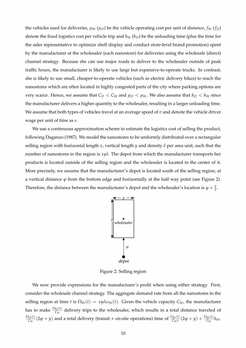
We model demand growth using models commonly used in the literature on product and inno-
vation diffusion (e.g., Bass 1969, Mansfield 1961). In those models, the growth curve is determined
based on the interaction between adopters and non-adopters of a new product and is represented
by an S-curve. In our case, once a consumer has adopted the product, he or she repeatedly pur-
chases the product as commonly observed with Consumer Packaged Goods. Following this mod-
eling perspective, we model the instantaneous adoption rate of the product at time t as:
∂λ(t)∂t
= αiλ(t)(1− λ(t)) (1)
which is the multiplication of the interaction intensity between adopters and non-adopters, i.e.,
λ(t)(1− λ(t)), and the average conversion rate αi for i = D, W of each interaction. For exposition
purpose, we term αD and αW as the market growth rates of using the direct and the wholesale channel
respectively. We assume that αD ≥ αW , i.e., the market grows at a faster pace when using the direct
channel strategy because of more specific and localized commercial activities at the nanostores. For
instance, the manufacturer’s sales representative who visits the store directly may ensure a better
quality shelf space, and use special product displays and other promotional material and activities
which promote the brand and lead to faster growth than if the product was replenished by the
wholesaler. Also, we assume that the market size does not grow if the manufacturer chooses not to
sell the product in the region over a certain period of time.
The manufacturer’s objective is to maximize total profits over a [0, T] time horizon by deciding
when to sell the product and, when doing so, whether to use the direct or the wholesale channel
strategy. More specifically, we define a channel policy as a sequence of N channel strategies (i,e.,
wholesale, direct or not-selling) and time thresholds denoted (S, t) where S = (S1, ..., SN) and
t = (t1, ..., tN) with Si ∈ W, D, ∅ for i = 1, ..., N, Si 6= Si+1 for i = 1, ..., N − 1 and 0 ≤ t1 ≤
... ≤ tN = T. Here, Si = ∅ means that the manufacturer does not sell to the region in time
interval [ti−1, ti), Si = W means that the manufacturer uses the wholesale channel strategy and
Si = D means that the manufacturer uses the direct channel strategy. In essence, the manufacturer
divides the time horizon [0, T] into N disjoint intervals so that channel strategy Si is used in time
interval [ti−1, ti) and a different channel strategy is used in adjacent intervals. Note that, in theory,
the same channel strategy can be used in non-adjacent intervals over the time horizon, that is, we
do not exclude situations where, for example, the manufacturer could enter the market using the
8

direct channel strategy, then switch to the wholesale strategy only to switch back later to the direct
channel strategy (however we show in Section 3 that such a case is never optimal).
We adapt the well-known logistic curve, which is a solution to Equation (1) and also has been
widely used to model new product diffusion, to illustrate the market dynamics over the time hori-
zon. Specifically, the market size in time interval t ∈ [ti−1, ti) is:
λ(t) =1
1 + e−αSi (t−ti−1)+b−∑i−1j=1 αSj (tj−tj−1)
(2)
where the market potential is normalized to be 1 and αSi is the market growth rate of using the
channel strategy Si for interval i = 1, ..., N. Herein, the term b is a positive constant which reflects
the difficulty of growing the market and 11+eb is the initial market size per nanostore at the beginning
of the time horizon. A product with a higher value of b diffuses at a lower pace and takes a longer
time to saturate the market. Given Equation (2), initially, the sales volume grows at an accelerating
rate. Later, after an inflection point, the sales volume grows in a decreasing rate until the entire
market potential is reached. This characterizes an S curve which is a common market growth
pattern. We also have conducted our analysis for a general exponential growth demand model;
this leads to similar results and insights.
Suppose, for example, that the manufacturer decides to sell her product via the direct channel
strategy from time 0 to time t1, then switches to the wholesale channel strategy from time t1 until the
end of the time horizon T. The demand rate per nanostore at time t is equal to ωD(t) = 11+e−αDt+b βD
for t ∈ [0, t1] and equal to ωW(t) = 11+e−αW (t−t1)+b−αDt1
βW for t ∈ (t1, T]. Figure 1 illustrates such a
policy.
T
λ(t)
inflection
poin
t
chan
nel switch
poin
t
<------------------------------------D------------------------------------->|<-------------------W-------------->
Figure 1: Market size growth curve of a channel policy switching from the direct to wholesale
The manufacturer uses vans to deliver to nanostores when using the direct channel distribu-
tion, which is common for the CPG sector in emerging markets. In this sales model, the sales
representative is also the vehicle driver who delivers products to nanostores, optimizes shelf dis-
play and conducts store-level brand promotion in a single trip. Let CW (CD) denote the capacity of
9
the vehicles used for deliveries, µW (µD) be the vehicle operating cost per unit of distance, fW ( fD)
denote the fixed logistics cost per vehicle trip and hW (hD) be the unloading time (plus the time for
the sales representative to optimize shelf display and conduct store-level brand promotion) spent
by the manufacturer at the wholesaler (each nanostore) for deliveries using the wholesale (direct)
channel strategy. Because she can use major roads to deliver to the wholesaler outside of peak
traffic hours, the manufacturer is likely to use large but expensive-to-operate trucks. In contrast,
she is likely to use small, cheaper-to-operate vehicles (such as electric delivery bikes) to reach the
nanostores which are often located in highly congested parts of the city where parking options are
very scarce. Hence, we assume that CD < CW and µD < µW . We also assume that hD < hW since
the manufacturer delivers a higher quantity to the wholesaler, resulting in a larger unloading time.
We assume that both types of vehicles travel at an average speed of v and denote the vehicle driver
wage per unit of time as s.
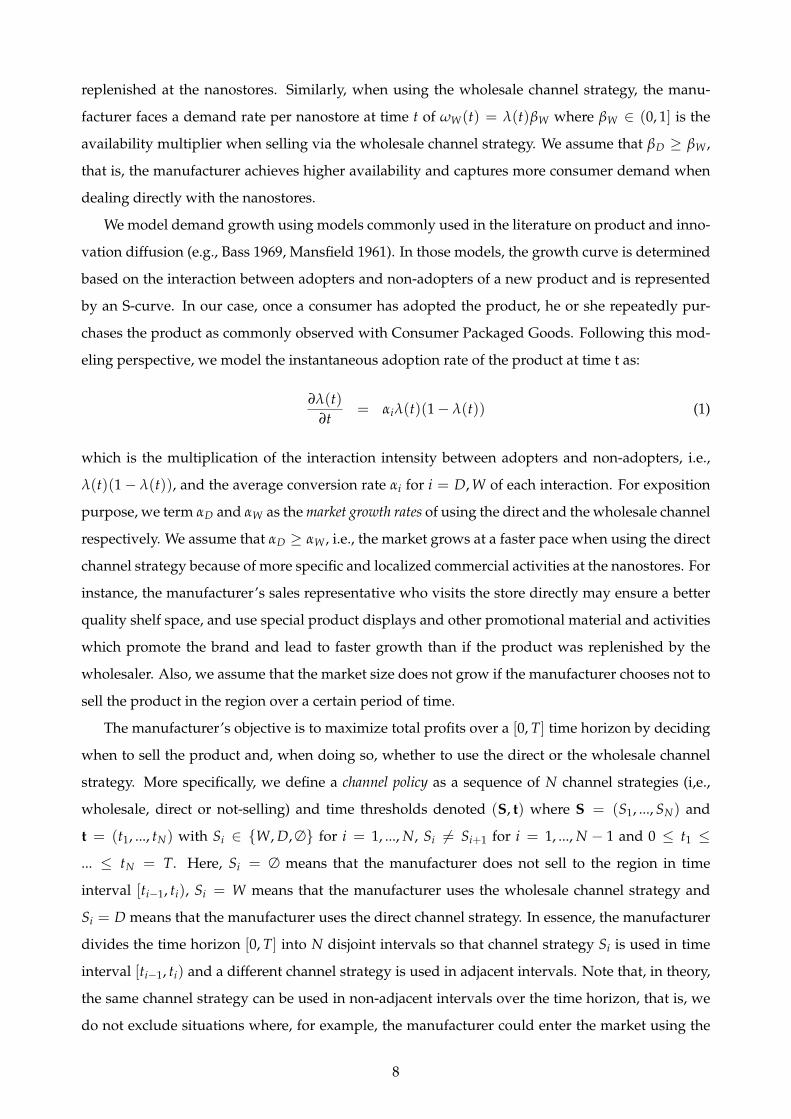
We use a continuous approximation scheme to estimate the logistics cost of selling the product,
following Daganzo (1987). We model the nanostores to be uniformly distributed over a rectangular
selling region with horizontal length x, vertical length y and density δ per area unit, such that the
number of nanostores in the region is xyδ. The depot from which the manufacturer transports her
products is located outside of the selling region and the wholesaler is located in the center of it.
More precisely, we assume that the manufacturer’s depot is located south of the selling region, at
a vertical distance ϕ from the bottom edge and horizontally at the half way point (see Figure 2).
Therefore, the distance between the manufacturer’s depot and the wholesaler’s location is ϕ + y2 .
depot
x
ywholesaler
Figure 2: Selling region
We now provide expressions for the manufacturer’s profit when using either strategy. First,
consider the wholesale channel strategy. The aggregate demand rate from all the nanostores in the
selling region at time t is ΩW(t) = xyδωW(t). Given the vehicle capacity CW , the manufacturer
has to make ΩW(t)CW
delivery trips to the wholesaler, which results in a total distance traveled ofΩW(t)
CW(2ϕ + y) and a total delivery (transit + on-site operations) time of ΩW(t)
CW v (2ϕ + y) + ΩW(t)CW
hW .
10

Note that we allow for fractional number of trips so as to avoid discreteness issues. As a result,
the instant profit (sales revenues minus logistics costs) at time t when using the wholesale channel
strategy is given by:
πW(t) = ΩW(t)(pW − c)− µW
(ΩW(t)
CW(2ϕ + y)
)− s
(ΩW(t)CWv
(2ϕ + y) +ΩW(t)
CWhW
)− ΩW(t)
CWfW
=
[(pW − c)− 1
CW
(fW + shW + (µW +
sv)(2ϕ + y)
)]︸ ︷︷ ︸
MW
ΩW(t).
In the first row, the first term is the sales revenue, the second term is the distance-based operating
cost, the third term is the labor cost and the last term is the fixed logistics cost. On the second row,
MW is the marginal return from selling an extra product unit using the wholesale channel strategy.
Note that we may have MW < 0.
Let us now consider the direct channel strategy. The aggregate demand rate from all the nano-
stores at time t is ΩD(t) = xyδωD(t). Given the vehicle capacity CD, the manufacturer has to makeΩD(t)
CDdelivery trips to serve the xyδ nanostores which are uniformly distributed over the selling
region (the average number of nanostores visited in one trip is xyδCDΩD(t)
= CDωD(t)
). Using the half-
width routing continuous approximation proposed by Daganzo (1987), we calculate that the total
distance traveled by all the delivery vehicles within the region at time t is equal to ΩD(t)CD
(2ϕ + y) +
y(
1 + x2δ6
)and that the corresponding total delivery time is ΩD(t)
CDv (2ϕ + y) + yv
(1 + x2δ
6
)+ xyδhD
(see derivations in Online Appendix A). As a result, the instant profit at time t using the direct
channel strategy is given by:
πD(t) = ΩD(t)(pD − c)− µD
[ΩD(t)
CD(2ϕ + y) + y
(1 +
x2δ
6
)]−s[
ΩD(t)CDv
(2ϕ + y) +yv
(1 +
x2δ
6
)+ xyδhD
]− ΩD(t)
CDfD
=
[(pD − c)− 1
CD
(fD + (µD +
sv)(2ϕ + y)
)]︸ ︷︷ ︸
MD
ΩD(t)−[(
µD +sv
)y(
1 +x2δ
6
)+ sxyδhD
]︸ ︷︷ ︸
kD
.
In the first row, the first term is the sales revenue, the second term is the distance-based operating
cost, the third term is the labor cost and the last term is the fixed logistics cost for all vehicle trips.
On the second row, MD is the marginal return from selling an extra product unit using the direct
channel strategy and kD is the fixed logistics cost. Note that we may have MD < 0. Also note that,
unlike with the wholesale channel, the instant profit at time t using the direct channel includes a
term which does not increase with the aggregate demand size. This is due to the fixed nature of
part of the logistics costs from serving a preset number of stores over the selling area.
On top of the costs already mentioned, we assume that the manufacturer incurs a fixed in-
11
vestment cost when she starts selling her product and every time she switches from one channel
strategy to the other channel strategy. Let FD and FW denote the channel-building fixed investment
costs when entering a period where the manufacturer uses the direct or wholesale channel strategy
respectively. We assume that FD ≥ FW since using the direct channel strategy is likely to require
larger initial investments than selling via the wholesaler as it entails hiring a larger sales force and
establishing business contacts with more clients.
Finally, for a given channel policy (S, t), the cumulative profit in the entire [0, T] horizon is:
Π(S, t) =N
∑i=1
∫ ti
ti−1
(πW(t)ISi=W + πD(t)ISi=D
)dt−
N
∑i=1
ISi=WFW −N
∑i=1
ISi=DFD.
Next, we study the optimal channel policy under the static demand model where αD = αW = 0
and the demand growth model where αD > αW > 0.
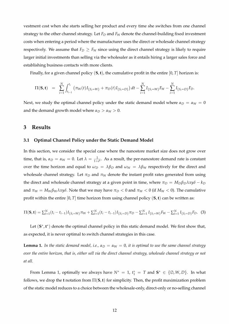
3 Results
3.1 Optimal Channel Policy under the Static Demand Model
In this section, we consider the special case where the nanostore market size does not grow over
time, that is, αD = αW = 0. Let λ = 11+eb . As a result, the per-nanostore demand rate is constant
over the time horizon and equal to ωD = λβD and ωW = λβW respectively for the direct and
wholesale channel strategy. Let πD and πW denote the instant profit rates generated from using
the direct and wholesale channel strategy at a given point in time, where πD = MDβDλxyδ− kD
and πW = MW βWλxyδ. Note that we may have πD < 0 and πW < 0 (if MW < 0). The cumulative
profit within the entire [0, T] time horizon from using channel policy (S, t) can be written as:
Π(S, t) = ∑Ni=1(ti − ti−1)ISi=WπW + ∑N
i=1(ti − ti−1)ISi=DπD −∑Ni=1 ISi=WFW −∑N
i=1 ISi=DFD. (3)
Let (S∗, t∗) denote the optimal channel policy in this static demand model. We first show that,
as expected, it is never optimal to switch channel strategies in this case.
Lemma 1. In the static demand model, i.e., αD = αW = 0, it is optimal to use the same channel strategy
over the entire horizon, that is, either sell via the direct channel strategy, wholesale channel strategy or not
at all.
From Lemma 1, optimally we always have N∗ = 1, t∗1 = T and S∗ ∈ ∅, W, D. In what
follows, we drop the t notation from Π(S, t) for simplicity. Then, the profit maximization problem
of the static model reduces to a choice between the wholesale-only, direct-only or no-selling channel
12
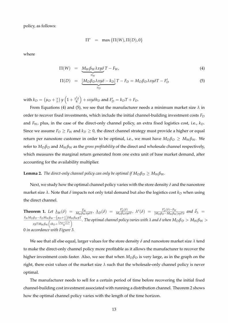
policy, as follows:
Π∗ = max Π(W), Π(D), 0
where
Π(W) = MW βWλxyδ︸ ︷︷ ︸πW
T − FW , (4)
Π(D) = [MDβDλxyδ− kD]︸ ︷︷ ︸πD
T − FD = MDβDλxyδT − F′D (5)
with kD =(µD + s
v
)y(
1 + x2δ6
)+ sxyδhD and F′D = kDT + FD.
From Equations (4) and (5), we see that the manufacturer needs a minimum market size λ in
order to recover fixed investments, which include the initial channel-building investment costs FD
and FW , plus, in the case of the direct-only channel policy, an extra fixed logistics cost, i.e., kD.
Since we assume FD ≥ FW and kD ≥ 0, the direct channel strategy must provide a higher or equal
return per nanostore customer in order to be optimal, i.e., we must have MDβD ≥ MW βW . We
refer to MDβD and MW βW as the gross profitability of the direct and wholesale channel respectively,
which measures the marginal return generated from one extra unit of base market demand, after
accounting for the availability multiplier.
Lemma 2. The direct-only channel policy can only be optimal if MDβD ≥ MW βW .
Next, we study how the optimal channel policy varies with the store density δ and the nanostore
market size λ. Note that δ impacts not only total demand but also the logistics cost kD when using
the direct channel.
Theorem 1. Let λW(δ) = FWMW βW xyδT , λD(δ) =
F′D(δ)MD βDxyδT , λe(δ) =
F′D(δ)−FW[MD βD−MW βW ]xyTδ
and δλ =
FW MD βD−FD MW βW−(µD+sv )MW βW yT
xyTMW βW
(shD+
(µD+ sv )x
6
) . The optimal channel policy varies with λ and δ when MDβD > MW βW >
0 in accordance with Figure 3.
We see that all else equal, larger values for the store density δ and nanostore market size λ tend
to make the direct-only channel policy more profitable as it allows the manufacturer to recover the
higher investment costs faster. Also, we see that when MDβD is very large, as in the graph on the
right, there exist values of the market size λ such that the wholesale-only channel policy is never
optimal.
The manufacturer needs to sell for a certain period of time before recovering the initial fixed
channel-building cost investment associated with running a distribution channel. Theorem 2 shows
how the optimal channel policy varies with the length of the time horizon.
13

WDe
( ) :s
d d v
w
F yT
d d w w Fa M M
WD
e
eDW
DD
( ) :s
d d v
w
F yT
d d w w Fb M M
W
W
(a) MD βDMW βW
≤ FD+(µD+ sv )yT
FW
WDe
( ) :s
d d v
w
F yT
d d w w Fa M M
WD
e
eDW
DD
( ) :s
d d v
w
F yT
d d w w Fb M M
W
W
(b) MD βDMW βW
>FD+(µD+ s
v )yTFW
Figure 3: Optimal channel policy as a function of λ and δ when MDβD > MW βW > 0.
Theorem 2. Let TW = FWπW
, TD = FDπD
and Te = FD−FWπD−πW
.
When πW ≤ 0 and πD ≤ 0, it is optimal not to sell to the region.
When πD > 0 and πW ≤ 0, it is optimal to use the direct-only channel policy if T ≥ TD; otherwise, it
is optimal not to sell.
When πW > 0 and πW ≥ πD, it is optimal to use the wholesale-only channel policy if T ≥ TW ;
otherwise, it is optimal not to sell.
When πD > πW > 0 and TW ≤ TD, it is optimal not to sell for T < TW , to use the wholesale-only
channel policy for T ∈ [TW , Te], and the direct-only channel policy for T ≥ Te.
When πD > πW > 0 and TW > TD, it is optimal not to sell for T < TD, and to use the direct-only
channel policy for T ≥ TD.
We see that, for relatively short time horizons, it may be optimal to use the wholesale-only
policy even in situations where the instant profit generated from the direct channel is greater than
the instant profit from the wholesale channel, i.e., πD > πW > 0. This is because it may take longer
to recoup the higher fixed cost investments which are necessary to serve the nanostores directly.
However, for long enough time horizons, it is optimal to use the direct-only policy when its instant
rate of profit is higher.
Next, we study how the optimal channel policy varies with the availability multipliers βD and
βW .
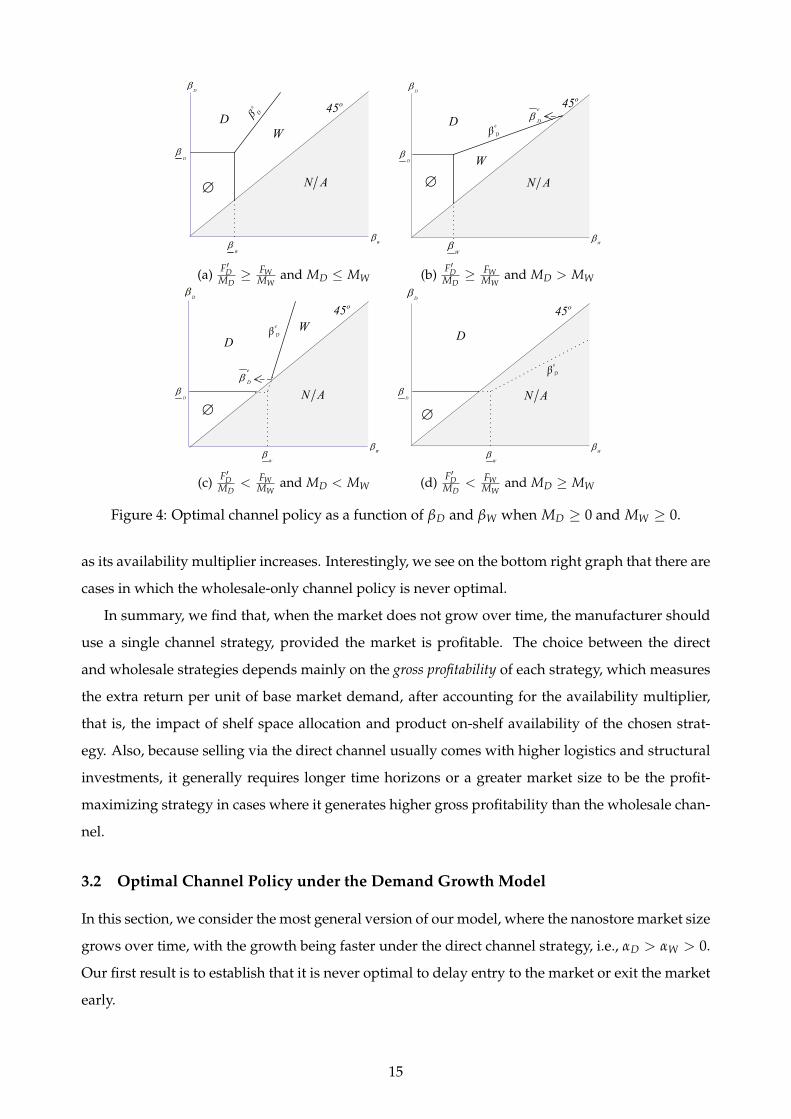
Theorem 3. Let βW
= FWMW xyλδT , β
D=
F′DMDxyλδT , βe
D(βW) = βD+ MW
MD(βW− β
W) and βe
D =F′D−FW
(MD−MW)xyδλT .
The optimal channel policy varies with βD and βD when MD ≥ 0 and MW ≥ 0 in accordance with Figure
4.
Note that, in all four graphs of Figure 4, the grey region is not to be considered since we have as-
sumed that βD ≥ βW , which is further because the careful re-shelving efforts of the manufacturer’s
sales force in the direct channel should guarantee sufficient shelf space allocation and higher on-
shelf product availability. We see that all else equal, each channel strategy becomes more attractive
14
'
( ) : WD
D W
FFD WM Ma and M M
eD
'
( ) : WD
D W
FFD WM Mb and M M
e
D
'
( ) : WD
D W
FFD WM Mc and M M
'
( ) : WD
D W
FFD WM Md and M M
WD
D
W
D
W
D
W
D
W
e
D
W
W
D
D D
N A
o45
N A
o45
N A
o45
N A
o45
D
D
W
W
W
W
e
D
e
D
e
D
D
D
(a) F′DMD≥ FW
MWand MD ≤ MW
'
( ) : WD
D W
FFD WM Ma and M M
eD
'
( ) : WD
D W
FFD WM Mb and M M
e
D
'
( ) : WD
D W
FFD WM Mc and M M
'
( ) : WD
D W
FFD WM Md and M M
WD
D
W
D
W
D
W
D
W
e
D
W
W
D
D D
N A
o45
N A
o45
N A
o45
N A
o45
D
D
W
W
W
W
e
D
e
D
e
D
D
D
(b) F′DMD≥ FW
MWand MD > MW
'
( ) : WD
D W
FFD WM Ma and M M
eD
'
( ) : WD
D W
FFD WM Mb and M M
e
D
'
( ) : WD
D W
FFD WM Mc and M M
'
( ) : WD
D W
FFD WM Md and M M
WD
D
W
D
W
D
W
D
W
e
D
W
W
D
D D
N A
o45
N A
o45
N A
o45
N A
o45
D
D
W
W
W
W
e
D
e
D
e
D
D
D
(c) F′DMD
< FWMW
and MD < MW
'
( ) : WD
D W
FFD WM Ma and M M
eD
'
( ) : WD
D W
FFD WM Mb and M M
e
D
'
( ) : WD
D W
FFD WM Mc and M M
'
( ) : WD
D W
FFD WM Md and M M
WD
D
W
D
W
D
W
D
W
e
D
W
W
D
D D
N A
o45
N A
o45
N A
o45
N A
o45
D
D
W
W
W
W
e
D
e
D
e
D
D
D
(d) F′DMD
< FWMW
and MD ≥ MW
Figure 4: Optimal channel policy as a function of βD and βW when MD ≥ 0 and MW ≥ 0.
as its availability multiplier increases. Interestingly, we see on the bottom right graph that there are
cases in which the wholesale-only channel policy is never optimal.
In summary, we find that, when the market does not grow over time, the manufacturer should
use a single channel strategy, provided the market is profitable. The choice between the direct
and wholesale strategies depends mainly on the gross profitability of each strategy, which measures
the extra return per unit of base market demand, after accounting for the availability multiplier,
that is, the impact of shelf space allocation and product on-shelf availability of the chosen strat-
egy. Also, because selling via the direct channel usually comes with higher logistics and structural
investments, it generally requires longer time horizons or a greater market size to be the profit-
maximizing strategy in cases where it generates higher gross profitability than the wholesale chan-
nel.
3.2 Optimal Channel Policy under the Demand Growth Model
In this section, we consider the most general version of our model, where the nanostore market size
grows over time, with the growth being faster under the direct channel strategy, i.e., αD > αW > 0.
Our first result is to establish that it is never optimal to delay entry to the market or exit the market
early.
15
Proposition 1. If it is optimal to sell the product in the region, then it is optimal to do so for the entire time
horizon.
Since we have assumed that the market for the manufacturer’s product does not grow if it is
not made available on the nanostores’ shelves, there is no benefit in delaying market entry. Also,
because we have assumed positive market growth when the product is sold, profitability only
improves over time so that it is never optimal to stop selling the product. However, it may be
optimal to sell the product initially at a loss, before the market reaches a critical mass, as will
be illustrated below. Also, it may be optimal to change channel strategy over time. Our next
result shows that, if it is optimal to sell, there should be at most one switch between the direct and
wholesale channel strategies during the time horizon.
Proposition 2. If the optimal channel policy includes both the direct and wholesale channel strategies, then it
is optimal to switch between them at most once. Also, the direct channel strategy is used before the wholesale
channel strategy if and only if MD βDαD
< MW βWαW
.
We refer to MD βDαD
and MW βWαW
as the growth-adjusted profitability of the direct channel and whole-sale channel strategy respectively. This measure is obtained by dividing the channel’s gross prof-itability (defined in §3.1) by the channel demand growth rate. According to Proposition 2, the man-ufacturer who uses both channel strategies over the time horizon should enter the market with thestrategy with the lowest growth-adjusted profitability then switch to the strategy with the highestgrowth-adjusted profitability. Mathematically, this condition emerges from the comparison of theprofit functions from two switching policies. First, consider the following channel policy: N = 2,S = (W, D) and t = (t1, T), that is, the manufacturer enters the market at time zero using thewholesale channel strategy then switches to the direct channel strategy at time t1 > 0 until the endof the time horizon. The profit of this policy can be written as:
Π(S, t) = xyδ
(MW βW
αWlog
[eb + eαW t1
1 + eb
]+
MDβDαD
log
[eb + eαW t1+αD(T−t1)
eb + eαW t1
])− kD(T − t1)− FW − FD.
Now consider the reverse channel policy: N = 2, S′ = (D, W) and t′ = (T − t1, T) such that themanufacturer enters the market at time zero using the direct channel strategy then switches to thewholesale channel strategy at time T − t1 until the end of the time horizon (the switching time ischosen so that the length of time to use each channel strategy is the same with policy (S, t)). Theprofit of this policy can be written as:
Π(S′, t′) = xyδ
(MDβD
αDlog
[eb + eαD(T−t1)
1 + eb
]+
MW βWαW
log
[eb+αD t1 + eαW t1+αD T
eαD T + eb+αD t1
])− kD(T − t1)− FW − FD.
The difference in profits between the two policies is given by:
Π(S, t)−Π(S′, t′) =
(MDβD
αD− MW βW
αW
)xyδ log
(
1 + eb) (
eb+αD t1 + eαD T+αW t1
)(eαD T + eb+αD t1
) (eb + eαW t1
)
where the logarithmic term is positive because the numerator is greater than the denominator with
a difference eb (eαDT − eαDt1) (
eαW t1 − 1). It follows that the first policy (W followed by D) yields a
16
higher cumulative profit than the second policy (D followed by W) if and only if MD βDαD
> MW βWαW
.
We further discuss the intuition beyond this inequality condition, with Propositions 3 to 5 below.
From Proposition 2, there are only five possible optimal channel policies: no selling (∅), direct-
only (D), wholesale-only (W), direct channel then switching to the wholesale channel (DW) and
wholesale channel then switching to the direct channel (WD).
Consider the DW channel policy and let tW denote the switching time between the direct and
wholesale channel strategies. The profit generated by the DW channel policy as a function of tW ∈
[0, T] is as follows:
ΠDW(tW) =∫ tW
0πD(t)dt +
∫ T
tW
πW(t)dt− FD ItW>0 − FW ItW<T
= xyδ
(MDβD
αDlog[
eb + eαDtW
1 + eb
]+
MW βW
αWlog
[eb + eαDtW+αW(T−tW)
eb + eαDtW
])− kDtW − FD ItW>0 − FW ItW<T.
Note that the W channel policy is obtained when tW = 0 and the D channel policy is obtained when
tW = T.
Consider the WD channel policy and let tD denote the switching time between the wholesale
and direct channel strategies. The profit generated by the WD channel policy as a function of
tD ∈ [0, T] is as follows:
ΠWD(tD) =∫ tD
0πW(t)dt +
∫ T
tD
πD(t)dt− FD ItD<T − FW ItD>0
= xyδ
(MW βW
αWlog[
eb + eαW tD
1 + eb
]+
MDβD
αDlog
[eb + eαW tD+αD(T−tD)
eb + eαW tD
])− kD(T − tD)− FW ItD>0 − FD ItD<T.
Note that the W channel policy is obtained when tD = T and the D channel policy is obtained when
tD = 0.
Though they are not necessarily concave, the two functions ΠDW(tW) and ΠWD(tD) are well-
behaved. In particular, we can show they have at most one or two interior local maxima on [0, T]
as stated in the following lemma.
Lemma 3. When MD βDαD
< MW βWαW
, ΠDW(tW) has at most one interior local maximum on [0, T]. WhenMD βD
αD≥ MW βW
αW, ΠWD(tD) has at most two interior local maxima on [0, T] and these two interior local
maxima exist only when αD > 2αW and MW < 0.
In both cases, the global maximum can be found by comparing the interior local maximum or
maxima (given existence) with the values of the profit function at 0 and T, which correspond to the
one-channel policies. Let t∗W denote the switching time which maximizes ΠDW(tW) for tW ∈ [0, T].
17

Let t∗D denote the switching time which maximizes ΠWD(tD) for tD ∈ [0, T]. From Proposition 2,
we get the following characterization of the optimal profit.
Corollary 1. If MD βDαD
< MW βWαW
, the optimal profit is maxΠDW(t∗W), 0; otherwise, it is maxΠWD(t∗D), 0.
Based on our previous discussion, MDβD − kDxyδ is the gross profitability after accounting for
the per-store fixed logistics cost of using the direct channel strategy, which can be interpreted as
the net profitability of using the direct channel strategy when the market size of 1 is fully realized.
When MDβD − kDxyδ ≤ MW βW , the wholesale channel strategy is more profitable in net terms than
the direct channel for every possible value of the market size; otherwise, there exists a threshold
demand value such that the wholesale channel is more profitable than the direct channel when
demand is below this threshold and less profitable when it is above. We compare the two channel
strategies in terms of gross profitability and growth-adjusted profitability in Table 1.
growth-adjusted profitability
MD βDαD≤ MW βW
αW
MD βDαD
> MW βWαW
grossprofitability
MDβD − kDxyδ ≤ MW βW Case I Case III
MDβD − kDxyδ > MW βW Case II Case IV
Table 1: Four possible cases by gross profitability and growth-adjusted profitability
The four cases we identify (remember that we have assumed αD > αW) are used to characterize
the optimal policy as a function of the length of the time horizon T. We build up intuition by
considering three settings sequentially: (i) no fixed channel-building investment costs and no direct
channel fixed logistics cost i.e., FD = FW = kD = 0; (ii) no fixed channel-building investment costs
but a positive direct channel fixed logistics cost, i.e., FD = FW = 0 and kD > 0 and (iii) positive
fixed channel-building investment costs and direct channel fixed logistics cost i.e., FD ≥ FW > 0
and kD > 0. We first study the setting with no fixed costs and present the solution in Proposition 3.
Proposition 3. Suppose that maxMW βW , MDβD > 0 and FD = FW = kD = 0. The optimal channel
policy varies with the length of the time horizon as shown in Figure 5.
ATW DW
D
T
Case I
Cases II, III & IV
W DW
D
Case I
Cases II & IV
T = 0
T = 0
IT
Figure 5: Optimal channel policy as a function of the length of the time horizon T when FD = FW =kD = 0.
18

Note that Case III does not occur when kD = 0. From Figure 5, we see that, when the direct
channel has lower gross profitability (Case I), the optimal policy differs based on the length of the
time horizon. For relatively short time horizons, it is optimal to follow the W channel policy, while
for relatively long time horizons, the optimal channel policy is DW, which we refer to as the “Grow
Fast then Back Down” policy: the manufacturer first expands the market at a fast pace using the
direct channel (possibly at a loss) then switches to the wholesale channel to exploit the expanded
market. In contrast, in Cases II and IV, the direct channel is more profitable in net terms and leads
to higher growth, so the D channel policy is optimal for any length of the time horizon.
Next, we consider the case of positive direct channel fixed logistics cost but zero fixed channel-
building investment costs, i.e., FD = FW = 0 and kD > 0. Proposition 4 shows how the optimal
policy varies with the length of the time horizon T.
Proposition 4. Suppose that maxMW βW , MDβD − kDxyδ > 0, FD = FW = 0 and kD > 0. The optimal
channel policy varies with the length of the time horizon as shown in Figure 6.
W
W DW
DW
D
T
WD D
W
: W WD D D
D W
MM kD D W WxyCase A and M M
: W WD D D
D W
MM kD D W WxyCase B and M M
: W WD D D
D W
MM kD D W WxyCase C and M M
1BT
2BT
AT
W
WD D1DT
2DT
1DT
2DT
: 0W WD D D
D W
MM kD D W WxyCase D and M M
: 0W WD D D
D W
MM kD D W WxyCase D and M M
W
W DW
DW
D
T
WD D
W
1BT
2BT
AT
W
WD D1DT
2DT
1DT
2DT
Case A
Case B
Case C
Case D with 0W WM
Case D with 0W WM
W
W DW
DW
D
WD D
W
W
WD D
T = 0
T = 0
0WM
0WM
T = 0
T = 0
T = 0
IT
1IIT
2IIT
1IVT
2IVT
1IVT
2IVT
Case I
Case II
Case III
Case IV
Figure 6: Optimal channel policy as a function of the length of the time horizon T when FD = FW =0 and kD > 0.
The existence of a positive fixed logistics cost kD lowers the appeal of the direct channel strategy,
which now requires a sufficient market size and gross profitability in order to be profitable. In
Cases I and III, when the wholesale channel strategy is always more profitable than the direct
channel strategy in net terms, the direct channel strategy should not be used as a single channel
throughout the entire horizon or as a post-switch channel prior to the end of the horizon because of
its poor net profitability. Instead, using the direct channel can add value to expand the market for
switching to the more profitable wholesale channel to accumulate a higher profit overall. However,
such a market expansion effect of the direct channel is only pronounced in Case I when the direct
channel growth potential exceeds the thresholdMD βDMW βW
αW. So, it is always optimal to use the wholesale
channel throughout the entire horizon for Case III. Further, for Case I, such a Grow Fast then Back
19
Down policy can only be optimal for relatively large horizons, which grant sufficient time for the
manufacturer not only to expand the market but also to exploit the expanded market.
In Cases II and IV, even though the direct channel strategy has higher gross profitability than
the wholesale channel, MDβD > MW βW , it requires fixed logistics investments and therefore could
have lower net profitability (defined as the gross profitability minus the fixed logistics costs then
divided by the demand) when the market size is small. Yet we see from Figure 6 that, when the
time horizon is very long, it is optimal to use only the direct channel strategy as there is enough
time to reap the benefits from growing the market at a fast pace, even if it means doing so initially at
a loss. In contrast, if the time horizon is very short, there is not enough time for the market to grow
sufficiently to make the direct channel profitable net of logistics costs; therefore, it is optimal to use
the W channel policy unless the wholesale channel gross profitability is negative (only possible in
Case IV). For time horizons of intermediate length, a switching channel policy may be optimal. In
Case II, the optimal channel policy is to Grow Fast then Back Down. In Case IV, the optimal policy
is WD, which we refer to as the “Grow Slow then Upgrade” policy where the manufacturer first
expands the market slowly using the wholesale channel at a small profit (as the direct channel is
not yet profitable due to the fixed logistics costs) then switches to the direct channel to benefit from
high demand growth and high gross profitability.
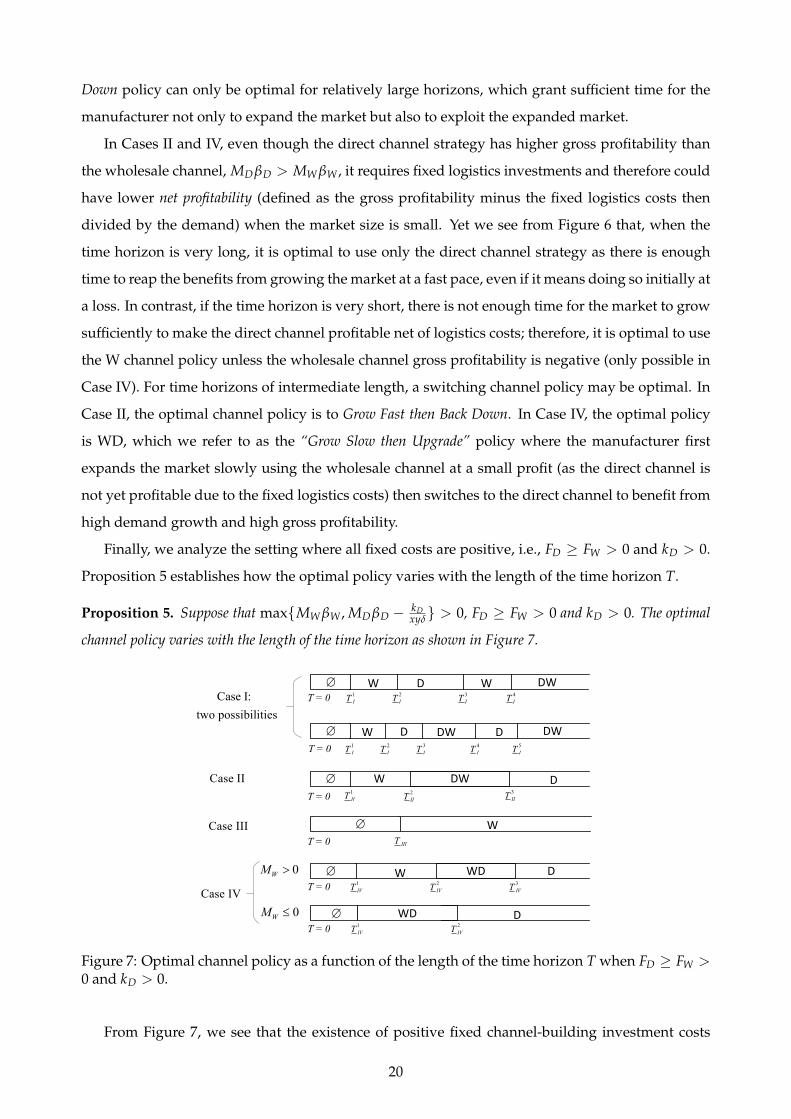
Finally, we analyze the setting where all fixed costs are positive, i.e., FD ≥ FW > 0 and kD > 0.
Proposition 5 establishes how the optimal policy varies with the length of the time horizon T.
Proposition 5. Suppose that maxMW βW , MDβD − kDxyδ > 0, FD ≥ FW > 0 and kD > 0. The optimal
channel policy varies with the length of the time horizon as shown in Figure 7.
DW
DW
D
T
WD D
W
: W WD D D
D W
MM kD D W WxyCase A and M M
: W WD D D
D W
MM kD D W WxyCase B and M M
: W WD D D
D W
MM kD D W WxyCase C and M M
1BT
2BT
WD D1DT
2DT
1DT
2DT
W D W1AT
2AT
3AT
4AT
DW W DW D1AT
2AT
3AT
4AT
W
W
3BT
CT
3DT
D5AT
: 0W WD D D
D W
MM kD D W WxyCase D and M M
: 0W WD D D
D W
MM kD D W WxyCase D and M M
DW
DW
D
T
WD D
W
1BT
2BT
WD D1DT
2DT
1DT
2DT
W D W1AT
2AT
3AT
4AT
DW W DW D1AT
2AT
3AT
4AT
W
W
3BT
CT
3DT
D5AT
Case A: two possibilities
Case B
Case C
Case D with 0W WM
Case D with 0W WM
DW
DW
D
WD D
W
WD D
W D W
DW W DW D
W
W
D
T = 0
T = 0
Case III
0WM
0WM
T = 0
T = 0
Case IV
Case II
T = 0
T = 0
Case I:
two possibilities
1IT
2IT
3IT
4IT
1IT
2IT
3IT
4IT
5IT
1IIT
2IIT
3IIT
IIIT
1IVT
2IVT
3IVT
1IVT
2IVT
Figure 7: Optimal channel policy as a function of the length of the time horizon T when FD ≥ FW >0 and kD > 0.
From Figure 7, we see that the existence of positive fixed channel-building investment costs
20

imposes a minimum time horizon length only beyond which it is profitable to enter the market:
in all four cases, if the time horizon is too short, it is not possible to recoup the fixed channel-
building investment costs of using either strategy and therefore the manufacturer does not sell her
product to the region. In Cases II, III and IV, we see that the structure of the optimal policy as a
function of T is the same as in the absence of fixed channel-building investment costs. In contrast,
in Case I, the existence of positive fixed channel-building investment costs may create situations
(for intermediate values of the time horizon) where the D policy is optimal. This occurs when
the time horizon is long enough to eventually make the direct channel sufficiently profitable (net
of logistics costs) but at the same time not long enough to justify incurring the channel-building
investment cost to switch to the wholesale channel strategy even if it is more (grossly) profitable.
To conclude our analysis, below we present a proposition to show how the optimal channel
switching time varies with the length of the time horizon T.
Proposition 6. For the DW policy, the optimal switching time from the direct channel to the wholesale
channel t∗W is increasing in T. For the WD policy, the optimal switching time from the wholesale channel to
the direct channel t∗D is decreasing in T and the proportion of time using the direct channel T−t∗DT is increasing
in T.
In both switching policies, as the time horizon T increases, the manufacturer should use the
direct channel strategy for a longer period of time as larger time horizons give the direct channel
strategy more opportunity to expand the market at a faster pace. For the DW policy, numerically, in
Case I, we consistently find that the optimal proportion of time using the direct channel t∗WT is first
increasing then decreasing in T. In this case, the direct channel is always less profitable in net terms
than the wholesale channel regardless of the horizon length such that the use of the direct channel
serves merely to expand the market. Intuitively, as T increases, the marginal market expansion
effect of using the direct channel is first intensifying then shrinking as the demand grows convexly
initially then concavely until saturation. Therefore, as T increases, the manufacturer should use
the direct channel for a larger proportion then for a smaller proportion of the time. In Case II,
numerically, we always observe that the optimal proportion of time using the direct channel t∗WT is
increasing in T. In this case, the direct channel eventually becomes more profitable as T increases
which renders the direct channel a dominant position against the wholesale channel in both de-
mand growth and profitability. Therefore, as T increases, the manufacturer should use the direct
channel for a larger proportion of time until the direct channel takes over the entire time horizon.
For the WD policy, as T increases, the manufacturer should always dedicate a larger proportion of
time to use the direct channel since the earlier the channel is switched, the market is expanded at a
higher growth rate again due to the S-shape growth curve.
Figure 8 illustrates Proposition 6 when FD = FW = 0 and kD > 0. In the first graph (Case I), the
21

region where the DW switching channel policy is optimal is to the right of the vertical dashed line.
On the second graph (Case II), it is between the two dashed lines. Finally, on the third graph, the
WD switching channel policy is also to be found for time horizon values which are between the two
vertical dashed lines. For Cases I and II, when the DW policy is optimal, t∗W(T) is increasing in T,
which means that it is optimal to switch from the direct channel to the wholesale channel strategy
relatively later as the length of the time horizon increases; for Case IV, when the WD policy is
optimal, t∗D(T) is decreasing in T, which means it is optimal to switch from the wholesale channel
to the direct channel proportionally sooner for longer horizons. We see, in Cases II and IV, as
the time horizon T increases, the manufacturer should use the direct channel strategy for a longer
proportion of the time, while in Case I, the proportion of time using the direct channel strategy is
increasing initially then decreasing.
0.0 0.5 1.0 1.5 2.0 2.5 3.00.0
0.5
1.0
1.5
2.0
2.5
3.0
T
t W*
-- -- -- - - - - - - - - - - - - - - - - - -
<--------- -----------
<------------------ -------------- | -------------- --------------
W D
W
(a) Case I
0.0 0.5 1.0 1.5 2.0 2.5 3.00.0
0.5
1.0
1.5
2.0
2.5
3.0
T
t W*
-- - - - - - - - - - - - --
-- -- -- - - - - - - - - - - - - - - - - - - - - - - - - - - - --
<---- -----
W
<------------------ ----------------- -------------- - - - - - - - - - - - - - - - -
D
<--- --- | -------- -----
D
W
(b) Case II
0.0 0.5 1.0 1.5 2.0 2.5 3.00.0
0.5
1.0
1.5
2.0
2.5
3.0
T
t D*
--- --- - - - - - - - - - - - - - - - - - - - - - - - - - - - -
- --- -- - - - - - - - - - - - - - - - - -- - - - - - - - - - - - - - - - - - - - - - - - - - - --
<---- - - - - - - - - - - ------
< - - - - - - - - - - - - - - - - - - - -| - - - - - - - - --
--- -------
D
---
<------------------ -----------------------------------
D
--- --------------- - - - - - - - - - - - - - - -
W W
(c) Case IV
Note: xy = 1, b = 2, δ = 50, MW = 5, αW = 1 for all cases, αD = 1.5 and kD = 15 for Cases I and II, αD = 1.2 and kD = 60 for Case IV,MD = 4 for Case I, MD = 5.5 for Case II, and MD = 8 for Case IV
Figure 8: Optimal switching time as a function of the length of the time horizon T when FD = FW =0 and kD > 0.
In summary, we see that the optimal channel policy depends on the relative values of the
growth-adjusted profitability and the gross profitability of both channels. Using these two prof-
itability measures, we are able to fully characterize the impact of the time horizon on the optimal
channel policy by considering Cases I, II, III and IV. We see that, for short time horizons, it is gen-
erally optimal to use the W channel policy as it has lower fixed costs. On the other hand, for long
time horizons, there is enough time to recoup the higher fixed costs required to implement the di-
rect channel strategy and benefit from the higher demand growth rate it generates. For the time
horizons with intermediate length, a switching channel policy may be optimal, that is, the firm
should use one channel then switch to the other. When the wholesale channel has higher growth-
adjusted profitability than the direct channel, the manufacturer who uses both channels should
Grow Fast then Back Down, that is, first expand the market at a fast pace using the direct channel
22

(possibly at a loss) then switch to the wholesale channel to exploit the expanded market. In con-
trast, when the direct channel has higher growth-adjusted profitability than the wholesale channel,
the manufacturer who uses both channels should Grow Slow then Upgrade , that is, first earn limited
profits while expanding the market slowly using the wholesale channel then switch to the direct
channel to benefit from high demand growth and high gross profitability.
4 Numerical Results
In this section, we numerically illustrate the parametric sensitivity of the optimal channel policy
and evaluate the performance of several heuristic policies. We use a base parameter set adapted
from the data of a CPG company in the city of Bogota, Colombia, to conduct the analysis. According
to the manufacturer’s data set, in the fiscal year 2014, the city-wide sales revenues from all the
products supplied directly to nanostores increased by 16.2% while sales by the wholesale channel
grew by 5%. However, the city-wide operating margin of the wholesale channel was 9.2% higher
than that of the direct channel strategy.
In Online Appendix B, we provide background on how we used the company’s numbers to set
the base parameter values: xy = 1, δ = 100, T = 2, b = 1, kD = 2000, αD = 3, αW = 1, MDβD = 300,
MW βW = 500, FD = 2000, FW = 1000. Under this base case, it takes around 1.07 years and 3.20
years to penetrate 90% of the market potential through using the direct channel and the wholesale
channel respectively.
Given these parameters, we have MD βDαD≤ MW βW
αWand MDβD − kD
xyδ ≤ MW βW (Case I from Table
1). After optimization, we see it is optimal for the manufacturer to switch from the direct channel
to the wholesale channel (the DW policy) and the switch occurs at t∗W = 0.69.
In Figure 9, we vary the gross profitability fraction MD βDMW βW
and the ratio of demand growth rateαDαW
by varying αD in [1, 3] and MDβD in [100, 900] while keeping all other parameters fixed. By
doing so, we generated 64,1601 instances which span all four cases listed in Table 1. Panels (a) and
(b) represent the optimal policy when the time horizon is equal to 1 and 2 respectively.
We see that the DW policy is optimal when the gross profitability of the wholesale channel is
larger than that of the direct channel but the direct channel provides a much higher demand growth
rate. In these instances, the role of the direct channel is to initially expand the market, then the firm
switches to the more profitable wholesale channel when facing a well-developed market. If the
direct channel is more profitable and offers a significantly higher growth rate, it should be used
exclusively. Finally, when the wholesale channel profitability is high and the difference in growth
rates is small, it is best to use only the wholesale channel. Note the “W is optimal” region includes
instances where the direct channel has both higher net profitability and demand growth rate (Cases
II and IV). This can be explained by the fixed-costs effect. Comparing Panels (a) and (b) of Figure
23

0.4 0.8 1 1.2 1.4 1.6 1.8
1.25
1.5
1.75
2
2.25
2.5
2.75
D is optimal
DW isoptimal
W is optimal
10.2
3
0.6
base case.
I
II
III IV
(a) T = 1
0.2 0.4 0.8 1 1.2 1.4 1.6
1.25
1.5
1.75
2
2.25
2.5
2.75
DW is optimal D is optimal
W is optimal
11.8
base case 3
I
II
III IV
.
0.60.6
(b) T = 2
Figure 9: Optimal policy map
9, we see that the region where the DW policy is optimal expands when the time horizon increases
as the firm has more time to develop the market through direct store visits.
Next, we consider four heuristic policies: (i) the W heuristic, by which the manufacturer uses
solely the wholesale channel, (ii) the D heuristic, by which she uses only the direct channel, (iii)
the WD half heuristic, where she switches from the wholesale channel to the direct channel at the
halfway point of the time horizon and (iv) the DW half heuristic, where she switches from the
direct channel to the wholesale channel at the halfway point of the time horizon.
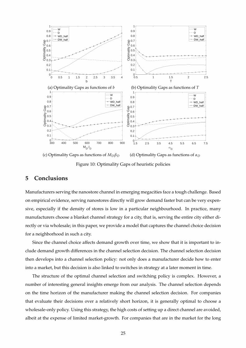
We vary parameters b, T, MDβD and αD one at a time in order to evaluate the optimality gap of
the heuristic policies, which is calculated as OG = Πopt−Πh
Πopt where Πopt represents the optimal profit
and Πh represents the profit of a heuristic policy, except when Πopt is equal to zero, in which case,
the optimality gap is equal to zero. The results are illustrated in Figure 10.
All the instances considered on Figure 10 fall into Case I from Table 1 so that the DW policy is
potentially optimal, i.e., the manufacturer should switch from the direct channel to the wholesale
channel if necessary. All four graphs show that the DW half heuristic generally performs best as it
chooses the right sequence of channel strategies; on the other hand, the WD half heuristic generally
performs worst as choosing the wrong sequence of channel strategies. In comparison, the two
single-channel policies tend to perform well for extreme instances but perform very poorly in the
opposite extreme instances because they fail to capture the trade-off between the two profitability
metrics. This shows that it is more critical to refer to the growth-adjust profitability metric to devise
the channel policy as it factors in both the gross profitability and also future growth potential.
24
0 0.5 1 1.5 2 2.5 3 3.5 4b
0
0.1
0.2
0.3
0.4
0.5
0.6
0.7
0.8
0.9
1
Opt
imal
ity G
ap
WDWD_half DW_half
(a) Optimality Gaps as functions of b
0.5 1 1.5 2 2.5T
0
0.1
0.2
0.3
0.4
0.5
0.6
0.7
0.8
0.9
1
Opt
imal
ity G
ap
WDWD_half DW_half
(b) Optimality Gaps as functions of T
300 400 500 600 700 800 900M
D D
0
0.1
0.2
0.3
0.4
0.5
0.6
0.7
0.8
0.9
1
Opt
imal
ity G
ap
WDWD_half DW_half
(c) Optimality Gaps as functions of MDβD
1.5 2.5 3.5 4.5 5.5 6.5 7.5
D
0
0.1
0.2
0.3
0.4
0.5
0.6
0.7
0.8
0.9
1
Opt
imal
ity G
ap
WDWD_half DW_half
(d) Optimality Gaps as functions of αD
Figure 10: Optimality Gaps of heuristic policies
5 Conclusions
Manufacturers serving the nanostore channel in emerging megacities face a tough challenge. Based
on empirical evidence, serving nanostores directly will grow demand faster but can be very expen-
sive, especially if the density of stores is low in a particular neighbourhood. In practice, many
manufacturers choose a blanket channel strategy for a city, that is, serving the entire city either di-
rectly or via wholesale; in this paper, we provide a model that captures the channel choice decision
for a neighborhood in such a city.
Since the channel choice affects demand growth over time, we show that it is important to in-
clude demand growth differences in the channel selection decision. The channel selection decision
then develops into a channel selection policy: not only does a manufacturer decide how to enter
into a market, but this decision is also linked to switches in strategy at a later moment in time.
The structure of the optimal channel selection and switching policy is complex. However, a
number of interesting general insights emerge from our analysis. The channel selection depends
on the time horizon of the manufacturer making the channel selection decision. For companies
that evaluate their decisions over a relatively short horizon, it is generally optimal to choose a
wholesale-only policy. Using this strategy, the high costs of setting up a direct channel are avoided,
albeit at the expense of limited market-growth. For companies that are in the market for the long
25

term, such as many local incumbents, it is often optimal to choose a direct-only policy. Our results
however also show a clear alternative, namely to switch between the two channel strategies at
some point in time, either starting in the direct channel and then switching to wholesale, or doing
this the other way around. Such a switching policy is optimal for intermediate time horizon, and
dependent on the so-called growth adjusted profitability. The growth adjusted profitability is based
on the gross profitability of a channel (determined by the gross margin and the logistics cost) but
adjusted for the demand growth pace of the channel. A manufacturer may hence choose to go
first direct and then wholesale, i.e., Grow Fast, then Back Down, that is, first expand the market at
a fast pace using the direct channel (possibly at a loss), and then switch to the wholesale channel
to exploit the developed market. This policy is generally optimal for intermediate time horizons
if the growth-adjusted profitability of the wholesale channel is larger than the growth-adjusted
profitability of the direct channel. In the reverse case, Grow Slow, then Upgrade is generally optimal,
that is, first earn limited profits while slowly growing the market using the wholesale channel, and
then switch to the direct channel to benefit from high demand growth and high gross profitability.
In general, our study provides insights into the channel strategies that manufacturers could
deploy when serving urban nanostores in emerging markets. Our work enables manufacturers
to develop distribution strategies where the channel changes after some time. Given the large
diversity in neighborhoods in terms of income and nanostores density, manufacturers could deploy
such strategies in a heterogeneous manner, making the key trade-off in different neighborhoods.
Acknowledgement
The authors thank the manufacturer in the city of Bogota for providing valuable data to conduct
this numerical study and also thank Dr. Christopher Mejia Argueta for spending valuable time
helping to collect data from this manufacturer. The authors are grateful to the entire editorial and
review team for their constructive comments which helped us improve the paper substantially. The
research has been funded through grants of The Netherlands Organisation for Scientific Research
(629.001.012) and The National Natural Science Foundation of China (71361130017).
References
Anderson, E. and Coughlan, A. T. (1987). International market entry and expansion via indepen-
dent or integrated channels of distribution. Journal of Marketing, 51(1):71–82.
Anderson, E. and Schmittlein, D. C. (1984). Integration of the sales force: an empirical examination.
The RAND Journal of Economics, 15(3):385–395.
26

Aspinwall, L. V. (1962). The characteristics of goods theory. In Kelley, E. J. and Lazar, W., editors,
Managerial marketing: perspectives and viewpoints, pages 633–643. Richard D. Irwin, Inc., Home-
wood, IL.
Bass, F. M. (1969). A new product growth for model consumer durables. Management Science,
15(5):215–227.
Bass, F. M. and Bultez, A. V. (1982). Technical note—a note on optimal strategic pricing of techno-
logical innovations. Marketing Science, 1(4):371–378.
Bronnenberg, B. J., Mahajan, V., and Vanhonacker, W. R. (2000). The emergence of market struc-
ture in new repeat-purchase categories: The interplay of market share and retailer distribution.
Journal of Marketing Research, 37(1):16–31.
Coughlan, A. T. (1985). Competition and cooperation in marketing channel choice: theory and
application. Marketing Science, 4(2):110–129.
Coughlan, A. T. (1987). Distribution channel choice in a market with complementary goods. Inter-
national Journal of Research in Marketing, 4(2):85–97.
Coughlan, A. T. (2006). Marketing Channels. Pearson/Prentice Hall, London, UK, 7th edition.
Daganzo, C. F. (1987). Modeling distribution problems with time windows: part i. Transportation
Science, 21(3):171–179.
Dockner, E. and Jorgensen, S. (1988). Optimal advertising policies for diffusion models of new
product innovation in monopolistic situations. Management Science, 34(1):119–130.
Elberse, A. and Eliashberg, J. (2003). Demand and supply dynamics for sequentially released prod-
ucts in international markets: The case of motion pictures. Marketing Science, 22(3):329–354.
Fransoo, J. C., Blanco, E. E., and Mejıa-Argueta, C. (2017). Reaching 50 million nanostores: Retail
Distribution in Emerging Megacities. CreateSpace Independent Publishing Platform, Scotts Valley,
California, United States.
Grocery Manufacturers Association (2008). Powering growth through direct store delivery. Ac-
cessed November 30, 2018, https://www.gmaonline.org/downloads/research-and-reports/
DSD_Final_111108.pdf.
Grocery Manufacturers Association (2011). Optimizing the value of fully integrated
dsd. Accessed November 30, 2018, https://www.gmaonline.org/file-manager/Logistics/
WP-DSD2011-9rev.pdf.
27

Ho, T., Li, S., Park, S., and Shen, Z. (2012). Customer influence value and purchase acceleration in
new product diffusion. Marketing Science, 31(2):236–256.
Huang, Y., Song, R., Zhao, L., and Fransoo, J. C. (2017). Beijing: where future meets history. In
Fransoo, J. C., Blanco, E. E., and Mejıa-Argueta, C., editors, Reaching 50 million nanostores, pages
41–71. CreateSpace Independent Publishing Platform.
John, G. and Weitz, B. A. (1988). Forward integration into distribution: an empirical test of trans-
action cost analysis. Journal of Law, Economics, and Organization, 4(2):337–355.
Jones, J. and Ritz, C. J. (1991). Incorporating distribution into new product diffusion models. Inter-
national Journal of Research in Marketing, 8(2):91–112.
Lehmann, D. R. and Weinberg, C. B. (2000). Sales through sequential distribution channels: An
application to movies and videos. Journal of Marketing, 64(3):18–33.
Lin, Y., Parlakturk, A. K., and Swaminathan, J. M. (2014). Vertical integration under competition:
Forward, backward, or no integration? Production and Operations Management, 23(1):19–35.
Liu, Y., Cheng, H. K., Tang, Q. C., and Eryarsoy, E. (2011). Optimal software pricing in the presence
of piracy and word-of-mouth effect. Decision Support Systems, 51(1):99–107.
Mansfield, E. (1961). Technical change and the rate of imitation. Econometrica, 29(4):741–766.
Mejıa-Argueta, C., Agudelo, I., Hidalgo-Carvajal, D. A., and Soto, M. A. (2017). Colombina: Shift-
ing from on-board to presales in bogota. In Fransoo, J. C., Blanco, E. E., and Mejıa-Argueta,
C., editors, Reaching 50 million nanostores, pages 197–215. CreateSpace Independent Publishing
Platform.
Mesak, H. I., Bari, A., Babin, B. J., Birou, L. M., and Jurkus, A. (2011). Optimum advertising policy
over time for subscriber service innovations in the presence of service cost learning and cus-
tomers’ disadoption. European Journal of Operational Research, 211(3):642–649.
Miracle, G. E. (1965). Product characteristics and marketing strategy. Journal of Marketing, 29(1):18–
24.
Moorthy, S. (1988). Strategic decentralization in channels. Marketing Science, 7(4):335–355.
Nielsen (2015a). Africa: how to navigate the retail distribution labyrinth. Accessed November 30,
2018, https://goo.gl/cgA3hE.
Nielsen (2015b). The future of grocery e-commerce, digital technology and changing shopping
preferences around the world. Accessed November 30, 2018, https://goo.gl/Tqo9TQ.
28

Peres, R. and Van den Bulte, C. (2014). When to take or forgo new product exclusivity: Balancing
protection from competition against word-of-mouth spillover. Journal of Marketing, 78(2):83–100.
Pun, H. and Heese, S. (2010). The value of losing control: competition in markets for complements.
Naval Research Logistics, 57(2):188–210.
Severin, C. B., Hirose, R., Kopka, U., Moulik, S., Nordheider, T., and Stul, F. (2011). Global
growth compass: locating consumer-industry growth opportunities in emerging mar-
kets. Accessed April 29, 2019, https://www.mckinsey.com/~/media/McKinsey/Business%
20Functions/Marketing%20and%20Sales/Our%20Insights/Finding%20profits%20and%
20growth%20in%20emerging%20markets/3-Finding%20profits%20and%20growth%20in%
20emerging%20markets.ashx.
Swami, S. and Dutta, A. (2010). Advertising strategies for new product diffusion in emerging
markets: Propositions and analysis. European Journal of Operational Research, 204(3):648–661.
Tang, C., Zhang, K., and Zhou, S. X. (2017). Replenishment strategies for micro-retailers in devel-
oping countries. Production and Operations Management, 26(12):2207–2225.
29
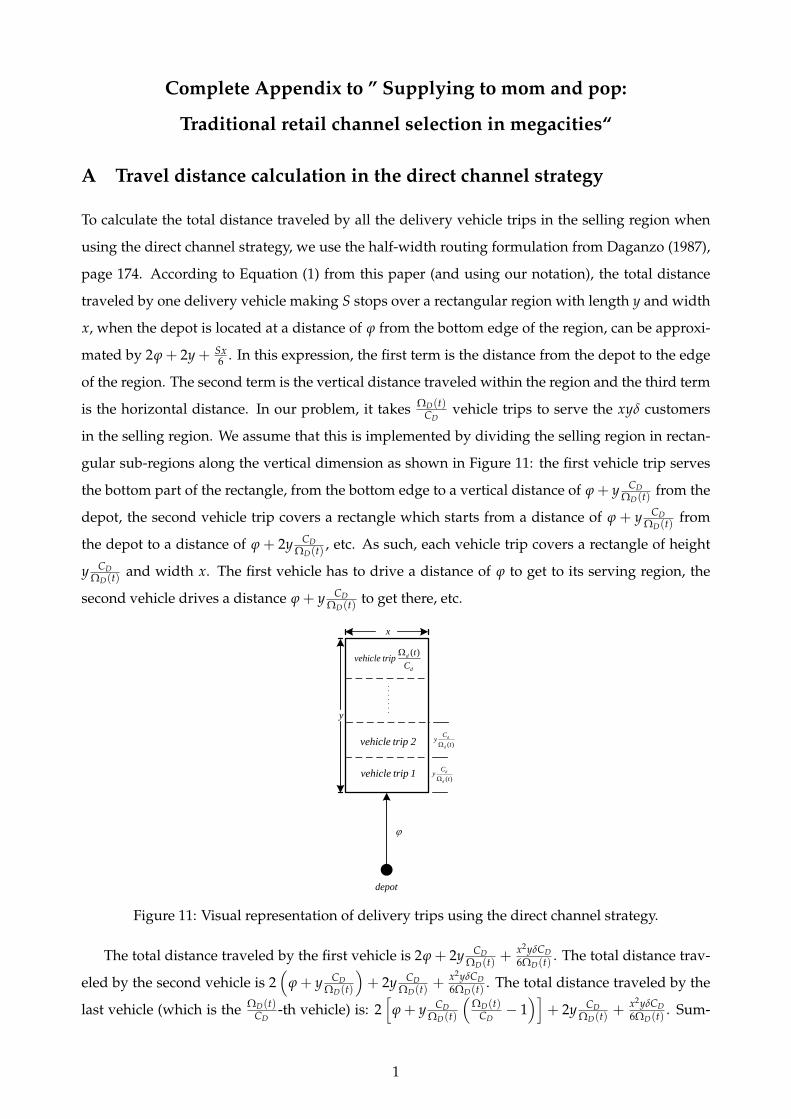
Complete Appendix to ” Supplying to mom and pop:
Traditional retail channel selection in megacities“
A Travel distance calculation in the direct channel strategy
To calculate the total distance traveled by all the delivery vehicle trips in the selling region when
using the direct channel strategy, we use the half-width routing formulation from Daganzo (1987),
page 174. According to Equation (1) from this paper (and using our notation), the total distance
traveled by one delivery vehicle making S stops over a rectangular region with length y and width
x, when the depot is located at a distance of ϕ from the bottom edge of the region, can be approxi-
mated by 2ϕ + 2y + Sx6 . In this expression, the first term is the distance from the depot to the edge
of the region. The second term is the vertical distance traveled within the region and the third term
is the horizontal distance. In our problem, it takes ΩD(t)CD
vehicle trips to serve the xyδ customers
in the selling region. We assume that this is implemented by dividing the selling region in rectan-
gular sub-regions along the vertical dimension as shown in Figure 11: the first vehicle trip serves
the bottom part of the rectangle, from the bottom edge to a vertical distance of ϕ + y CDΩD(t)
from the
depot, the second vehicle trip covers a rectangle which starts from a distance of ϕ + y CDΩD(t)
from
the depot to a distance of ϕ + 2y CDΩD(t)
, etc. As such, each vehicle trip covers a rectangle of height
y CDΩD(t)
and width x. The first vehicle has to drive a distance of ϕ to get to its serving region, the
second vehicle drives a distance ϕ + y CDΩD(t)
to get there, etc.
depot
x
y
( )
d
d
Cy
t
( )
d
d
Cy
t
vehicle trip 1
vehicle trip 2
( )d
d
tvehicle trip
C
Figure 11: Visual representation of delivery trips using the direct channel strategy.
The total distance traveled by the first vehicle is 2ϕ + 2y CDΩD(t)
+ x2yδCD6ΩD(t)
. The total distance trav-
eled by the second vehicle is 2(
ϕ + y CDΩD(t)
)+ 2y CD
ΩD(t)+ x2yδCD
6ΩD(t). The total distance traveled by the
last vehicle (which is the ΩD(t)CD
-th vehicle) is: 2[
ϕ + y CDΩD(t)
(ΩD(t)
CD− 1)]
+ 2y CDΩD(t)
+ x2yδCD6ΩD(t)
. Sum-
1

ming up the travel distances of all the vehicles, we get the total distance traveled as:
2[
ΩD(t)CD
ϕ + yCD
ΩD(t)
(0 + 1 + 2 + ... +
ΩD(t)CD
− 1)]
+ 2yCD
ΩD(t)ΩD(t)
CD+
x2yδCD
6ΩD(t)ΩD(t)
CD
= 2[
ΩD(t)CD
ϕ + yCD
ΩD(t)12
(ΩD(t)
CD− 1)
ΩD(t)CD
]+ 2y +
x2yδ
6
=
[2
ΩD(t)CD
ϕ + y(
ΩD(t)CD
− 1)]
+ 2y +x2yδ
6
= 2ΩD(t)
CDϕ + y
(ΩD(t)
CD+ 1)+
x2yδ
6
=ΩD(t)
CD(2ϕ + y) + y
(1 +
x2δ
6
).
B Base parameter values for the numerical study
According to Mejıa-Argueta et al. (2017), the city of Bogota counts about 100,000 stores in the urban
area of the city. The manufacturer who provided us with the dataset (and who cannot be named
for confidentiality reasons) is a relatively large publicly-traded company which operates mostly
in Latin America selling packaged food products such as candy, cookies, pasta, sauces, juices, ice
cream, etc. It sells to both modern and traditional retail stores. In 2014, the company’s share of rev-
enues in the city of Bogota generated from modern retail stores (e.g., convenience store chains and
large supermarkets) was 38% versus 62% for traditional retail stores. For the sales from traditional
retail, 15% directly came from 42,500 nanostores in the urban city area with an average density of
138 stores per km2, and 47% came from around 800 wholesalers. It is opaque how many nanostores
that each wholesaler is serving; however, a confident guess is the number ranges from 20 to 50, as
we have observed in most emerging markets that wholesalers in the CPG sector are small sized
and each wholesaler only serves a few dozens of nanostores in close proximity. Therefore, in this
numerical study, we use a base geographic region with an area of 1 km2 and a density of 100 stores
per km2; namely, the base values of xy and δ are 1 and 100 respectively.
According to the manufacturer’s data set, in the fiscal year 2014, the city-wide sales revenues
from all the products supplied directly to nanostores increased by 16.2% while sales by wholesalers
grew by 5%. Assuming the revenue increase was driven by market size growth, then the market
size grew three times faster when using the direct channel than using the wholesale channel. Given
an assumption of the product launch time, we can use a base value of b to induce the corresponding
values of αD and αW . However, in order to generate a full spectrum of product attributes, we loosely
use a base value of αD = 3 and a base value of αW = 1 as one third of αD. We also use the base
value of b as 1, at which it takes around 1.07 years and 3.20 years to penetrate 90% of the market
potential through using the direct channel and the wholesale channel respectively. Next, we use
these base values to estimate the margin and cost parameters.
2

For the city-wide direct channel operations, the manufacturer estimates the cost of goods sold at
56% of sales revenues and the (variable+fixed) cost of logistics at 5.1% of sales revenues. Hence, the
manufacturer calculates the operating margin as 38.9% of sales revenues. On average, the city-wide
operating margin of the wholesale channel is 9.2% higher than that of the direct channel strategy
on a monthly basis in the year of 2014. Further, according to a sample of 942 stores in 4 regions,
the annual per-store average revenue is around 384 US dollars so that the average annual per-store
net profit of using the direct channel is around 149 US dollars. Then, we can inflate this number
by 9.2% as the average annual per-store net profit of using the wholesale channel, which is 163 US
dollars. Assume the new product was launched at the beginning of the year 2014. Then, the annual
profit of using the wholesale channel was:
ΠW = MW βW xyδ∫ 1
0
11 + eb−αW t dt− FW .
Let FW = 1, 000 as the base value of the fixed investment cost to set up using the wholesale channel.
Then, the base value of MW βW is around 500 US dollars. When using the direct channel, the annual
profit was:
ΠD = [pD − c− z]︸ ︷︷ ︸MD
βDxyδ∫ 1
0
11 + eb−αDt dt− kD − FD
where z is the variable logistics cost and kD is the fixed logistics cost. For simplicity, let z = 0;
then as 5.1% of the sales revenues, we roughly take the base value of kD as 2,000. Further, let
FD = 2, 000; then we obtain the base value of MDβD as around 300. Note that the estimated base
values of MW βW and MDβD are the gross margins of per unit normalized demand. Finally, let the
base value of the time horizon T be 2.
C Proofs
Proof. Proof of Lemma 1
From Equation (3), we see that, if πW > πD (πW < πD), using the wholesale channel strategy
generates more (less) profit per unit of time than using the direct channel strategy. Since these
values do not vary over time, and switching channel policy is costly, it is never optimal to do so.
Selling via the wholesale channel strategy during the entire time horizon generates cumulative
profit Π(W) = TπW − FW while selling via the direct channel strategy during the entire time hori-
zon generates cumulative profit Π(D) = TπD − FD. The optimal channel policy is the channel
strategy which generates the highest cumulative profits, provided this value is positive; otherwise,
it is optimal not to sell the product. 2
3
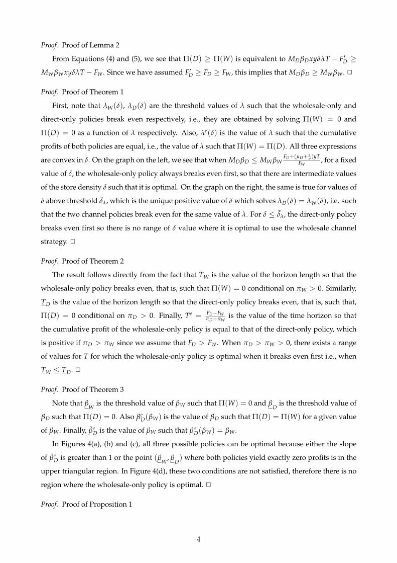
Proof. Proof of Lemma 2
From Equations (4) and (5), we see that Π(D) ≥ Π(W) is equivalent to MDβDxyδλT − F′D ≥
MW βW xyδλT − FW . Since we have assumed F′D ≥ FD ≥ FW , this implies that MDβD ≥ MW βW . 2
Proof. Proof of Theorem 1
First, note that λW(δ), λD(δ) are the threshold values of λ such that the wholesale-only and
direct-only policies break even respectively, i.e., they are obtained by solving Π(W) = 0 and
Π(D) = 0 as a function of λ respectively. Also, λe(δ) is the value of λ such that the cumulative
profits of both policies are equal, i.e., the value of λ such that Π(W) = Π(D). All three expressions
are convex in δ. On the graph on the left, we see that when MDβD ≤ MW βWFD+(µD+
sv )yT
FW, for a fixed
value of δ, the wholesale-only policy always breaks even first, so that there are intermediate values
of the store density δ such that it is optimal. On the graph on the right, the same is true for values of
δ above threshold δλ, which is the unique positive value of δ which solves λD(δ) = λW(δ), i.e. such
that the two channel policies break even for the same value of λ. For δ ≤ δλ, the direct-only policy
breaks even first so there is no range of δ value where it is optimal to use the wholesale channel
strategy. 2
Proof. Proof of Theorem 2
The result follows directly from the fact that TW is the value of the horizon length so that the
wholesale-only policy breaks even, that is, such that Π(W) = 0 conditional on πW > 0. Similarly,
TD is the value of the horizon length so that the direct-only policy breaks even, that is, such that,
Π(D) = 0 conditional on πD > 0. Finally, Te = FD−FWπD−πW
is the value of the time horizon so that
the cumulative profit of the wholesale-only policy is equal to that of the direct-only policy, which
is positive if πD > πW since we assume that FD > FW . When πD > πW > 0, there exists a range
of values for T for which the wholesale-only policy is optimal when it breaks even first i.e., when
TW ≤ TD. 2
Proof. Proof of Theorem 3
Note that βW
is the threshold value of βW such that Π(W) = 0 and βD
is the threshold value of
βD such that Π(D) = 0. Also βeD(βW) is the value of βD such that Π(D) = Π(W) for a given value
of βW . Finally, βeD is the value of βW such that βe
D(βW) = βW .
In Figures 4(a), (b) and (c), all three possible policies can be optimal because either the slope
of βeD is greater than 1 or the point (β
W, β
D) where both policies yield exactly zero profits is in the
upper triangular region. In Figure 4(d), these two conditions are not satisfied, therefore there is no
region where the wholesale-only policy is optimal. 2
Proof. Proof of Proposition 1
4

First, note that not selling the product leads to zero profit so that, if it is optimal to sell the
product at any time during the time horizon, this must mean that it is possible to earn positive
profit over the entire horizon. This, in turn, implies that the instant profit rate must be positive by
the end of the selling period given that the market size only grows over time when the product is
being sold (via either channel). As a result, it cannot be optimal to stop selling the product as it
would generate zero profit instead of positive profits. Also, remember that we have assumed that
the market does not grow when the product is not being sold by the manufacturer; this implies that
delaying entry to the market is equivalent to shortening the total time horizon and therefore this
cannot be optimal for the same reason. 2
Proof. Proof of Proposition 2
From Proposition 1, if it is optimal to sell to the region, the manufacturer only uses the whole-
sale and direct channel strategies, possibly switching multiple times between them throughout the
entire time horizon. So suppose we have a channel policy (S, t) with only these two selling channel
strategies, i.e., such that Si+1 = D and Si+2 = W for i = 0, ..., N − 2. In other words, the manufac-
turer uses the direct channel strategy from time ti to ti+1 then the wholesale channel strategy from
time ti+1 until ti+2 for some i ∈ 0, ..., N− 2. Let λ(ti) =1
1+eb−C where C = ∑ij=1 αSj(tj − tj−1). The
profit generated by this policy from time ti to time ti+2 is:
Π =∫ ti+1
ti
πD(t)dt +∫ ti+2
ti+1
πW(t)dt− FD − FW
=MW βW
αWlog
[eb+αDti + eC+αDti+1+αW(ti+2−ti+1)
eb+αDti + eC+αDti+1
]+ kD(ti+1 − ti)
+MDβD
αDlog
[eb + eC+αD(ti+1−ti)
eb + eC
]− FD − FW .
Now consider an alternative channel policy (S′, t′) such that t′k = tk for k = 1, ..., i, i + 2, ..., N,
t′i+1 = ti + ti+2 − ti+1, S′k = Sk for k = 1, ..., i, i + 3, ..., N, S′i+1 = W and S′i+2 = D. In other words,
the alternative channel policy switches the order of the wholesale channel strategy and the direct
channel strategy between time ti and ti+2, keeping the length of all intervals the same as in policy
(S, t). The profit generated by this policy from time ti to time ti+2 is:
Π′ =∫ ti+ti+2−ti+1
ti
πW(t)dt +∫ ti+2
ti+ti+2−ti+1
πD(t)dt− FD Ii=N−2 − FW Ii=0
=MDβD
αDlog
[eb+αW ti+1 + eC+αW ti+2+αD(ti+1−ti)
eb+αW ti+1 + eC+αW ti+2
]− kD(ti+1 − ti)
+MW βW
αWlog
[eb + eC+αW(ti+2−ti+1)
eb + eC
]− FD Ii=N−2 − FW Ii=0.
Note that we may save on the fixed costs because switching the order of the channel strategies
5

makes them coincide with the strategies used in intervals [ti−1, ti] when i > 0 and [ti+2, ti+3] when
i < N − 2. Since the profit generated before ti and after ti+2 are the same under both policies, we
have:
Π(S′, t′)−Π(S, t) ≥ xyδC log
[(eb + eC) (eb+αDti+αW ti+1 + eC+αDti+1+αW ti+2
)(eb+αDti + eC+αDti+1) (eb+αW ti+1 + eC+αW ti+2)
](MDβD
αD− MW βW
αW
)
where the logarithmic term is positive because the numerator is greater than the denominator of
the fraction with a difference eb+C (eαDti+1 − eαDti) (
eαW ti+2 − eαW ti+1). From this, we see that, when
MD βDαD
> MW βWαW
, the alternate policy generates more profit than the original policy.
We have shown that, for every pair of adjacent intervals, it is optimal for the manufacturer to
switch from the direct (wholesale) channel strategy to the wholesale (direct) channel strategy if and
only if MD βDαD
< (>)MW βWαW
. Hence, this directly implies that there can be at most one switch between
the two selling channel strategies, that is, it is optimal to have N ≤ 2. 2
Proof. Proof of Lemma 3
The second derivative of ΠDW(tW) is as follows:
∂2ΠDW(tW)
∂t2W
= xyδαDeαDtW−b
eαW(T−tW)MW βW (αD−αW )2
αW αD(1 + eαDtW+αW(T−tW)−b
)2 −αD
(MW βW
αW− MD βD
αD
)(1 + eαDtW−b)
2︸ ︷︷ ︸ADW
where the first derivative of the sign-determinant term ADW is given by:
∂ADW
∂tW=
eαW (T−tW )(
1 + e−b+αD tW
)(
1 + e−b+αD tW+αW (T−tW ))3
e(αD−αW )tW−2b(
αW eαD tW+αW T + eb(
eαW T − eαW tW)(αW − 2αD)
)− αW︸ ︷︷ ︸
BDW
.
Obviously, the number of sign changes of ∂2ΠDW(tW)∂t2
Wis determined by the term BDW . Note that
∂ADW
∂tWis negative at tW = 0 since at which BDW is decreasing in αD and it is negative at αD = αW .
The first derivative of BDW in tW is:
∂BDW
∂tW= e(αD−αW)tW−2b(2αD − αW)
(αDeαW tW+b + αWeαDtW+αW T − (αD − αW)eαW T+b
)where the third multiplying part (in brackets) is increasing in tW and is positive at tW = T, i.e.,∂BDW
∂tWis either positive for tW ∈ [0, T] or negative for low values of tW and positive for large values
of tW . This means BDW is either increasing in tW ∈ [0, T] or is decreasing in low values of tW
and increasing in large values of tW . Since ∂ADW
∂tWis negative at tW = 0, ∂ADW
∂tWis either negative
for tW ∈ [0, T] or is negative initially then positive in tW . Therefore, ADW is either decreasing
in tW ∈ [0, T] or is decreasing then increasing in tW , which implies ∂2ΠDW(tW)∂t2
Whas at most two sign
6

changes. When there is no sign change, ∂2ΠDW(tW)∂t2
Wis either positive or negative, so ΠDW(tW) is either
convex or concave in tW . In this case, there is at most one interior local maximum. When there is
one sign change, ∂2ΠDW(tW)∂t2
Weither switches from positive to negative or the other way around, which
implies ΠDW(tW) is either convex then concave in tW or the other way around. In this case, there
is at most one interior local maximum. When there are two sign changes, ∂2ΠDW(tW)∂t2
Wis positive
for low values of tW , negative for intermediate values of tW and positive for large values of tW ,
which indicates ΠDW(tW) is convex then concave and finally convex in tW . In this case, considering
possible existence of inflection points, there is at most one interior local maximum.Similarly, the second derivative of ΠWD(tD) is as follows:
∂2ΠWD(tD)
∂t2D
=xyδMDβD (αD − αW)2
αD(1 + eb−αW tD
)2 eαW tD−b
eαD(tD−T)
(1 + eb−αW tD
)2
(1 + eb−αD T+(αD−αW )tD
)2 −αW(MDβDαW −MW βW αD)
MDβD(αD − αW)2
︸ ︷︷ ︸AWD
where the first derivative of the sign-determinant term AWD in tD is given by:
∂AWD
∂tD=
eαD(tD−T)(
1 + eb−αW tD)
(1 + eb−αD T+(αD−αW )tD
)3
αD(1− e2b+αD(tD−T)−2αW tD ) + (αD − 2αW)eb−αD T−αW tD(
eαD T − eαD tD)
︸ ︷︷ ︸BWD
.
Obviously, the number of sign changes of ∂2ΠWD(tD)∂t2
Dis determined by the term BWD. The first
derivative of BWD in tD is:
∂BWD
∂tD= eb−αDT−2αW tD(2αW − αD)
(αDeb+αDtD + (αD − αW)e(αD+αW)tD + αWeαDT+αW tD
)which is negative if αD > 2αW and positive if αD < 2αW . Then, if αD 6= 2αW , BWD is either
decreasing or increasing in tD ∈ [0, T]. If αD = 2αW , we have BWD = 2(
1− e2(b−αW T))
αW , which
is either positive or negative. Therefore, ∂AWD
∂tDcan be positive, negative, positive then negative, or
negative then positive in tD ∈ [0, T]. This means AWD can be increasing, decreasing, increasing
then decreasing, or decreasing then increasing in tD ∈ [0, T], which implies ∂2ΠWD(tD)∂t2
Dcan have at
most two sign changes. If there is no or only one sign change, there is at most one interior local
maximum. Given two sign changes, considering possible inflection points, there is at most one
interior local maximum if ∂2ΠWD(tD)∂t2
Dis positive, negative then positive in tD ∈ [0, T]; there are at
most two interior local maxima if ∂2ΠWD(tD)∂t2
Dis negative, positive and then negative in tD ∈ [0, T].
When two such values exist, it must hold αD > 2αW and MW < 0 since under which AWD is
possibly increasing then decreasing in tD, and
∂2ΠWD(tD)
∂t2D
∣∣∣∣tD=T
=xyδeb−αW T(MW βWαW + MDβD(αD − 2αW))
(1 + eb−αW T)2
7

is possibly negative. 2
Proof. Proof of corollary 1
Proof omitted. 2
Proof. Proof of Proposition 3
When FD = FW = kD = 0, the cases to be considered are Case I where MDβDαD≤ MW βW
αWand
MDβD ≤ MW βW , Case II where MDβDαD≤ MW βW
αWand MDβD > MW βW and Cases IV where
MDβDαD
> MW βWαW
and MDβD ≥ MW βW .
In Cases III & IV, by Corollary 1, we need to consider ΠWD(tD). We have:
∂ΠWD(tD)
∂tD= xyδαW
( MD βDαD
αW−αDαW
1 + eb−αDT+(αD−αW)tD−
MD βDαD− MW βW
αW
1 + eb−αW tD
)
which is negative since MD βDαD
> MW βWαW
, MDβD > 0 (since maxMW βW , MDβD > 0) and αD > αW .
Therefore, ΠWD is decreasing in tD so that the unique optimal solution is t∗D = 0, that is, the D
policy is optimal for any length of the time horizon.
In Cases I and II, by Corollary 1, we need to consider ΠDW(tW). For Case II, we have:
∂ΠDW(tW)
∂tW= xyδαD
1+eαDtW+αW (T−tW )−b
1+eαDtW−b
(MW βW
αW− MD βD
αD
)− MW βW
αW
αD−αWαD
1 + eαDtW+αW(T−tW)−b+
MDβD −MW βW
αD
≥ xyδαD
( MW βWαW− MD βD
αD− MW βW
αW
αD−αWαD
1 + eαDtW+αW(T−tW)−b+
MDβD −MW βW
αD
)
=xyδ (MDβD −MW βW)
1 + eb−αW T−(αD−αW)tW> 0
where the first inequality is because MW βWαW≥ MD βD
αDand eαDtW+αW(T−tW)−b ≥ eαDtW−b and the second
inequality is because MDβD > MW βW . Therefore, ΠDW(tW) is increasing in tW so that the optimal
solution in Case II is t∗W = T, that is, the D policy is optimal for any length of the time horizon.
In Case I, where MDβD < MW βW , we evaluate the first derivative of ΠDW(tW) at tW = 0 and
tW = T as:
∂ΠDW(tW)
∂tW
∣∣∣∣tW=0
= xyδαD
( MW βWαW− MD βD
αD
1 + e−b −MW βW
αW
αD−αWαD
1 + eαW T−b +MDβD −MW βW
αD
)
> xyδαD
( MW βWαW− MD βD
αD
1 + e−b −MW βW
αW
αD−αWαD
1 + e−b +MDβD −MW βW
αD
)
=xyδ (MDβD −MW βW)
1 + eb
∂ΠDW(tW)
∂tW
∣∣∣∣tW=T
=xyδ (MDβD −MW βW)
1 + eb−αDT
8

where the inequality is because MW βW > 0 (due to MD βDαD≤ MW βW
αWand maxMW βW , MDβD >
0). We first see ∂ΠDW(tW)∂tW
∣∣∣tW=0
can be positive or negative. We also see ∂ΠDW(tW)∂tW
∣∣∣tW=T
is negative
for MDβD < MW βW . Therefore, the D policy is never optimal. Further since we always have∂ΠDW(tW)
∂tW
∣∣∣T=T2
> ∂ΠDW(tW)∂tW
∣∣∣T=T1
for tW ≤ T1 for any T1 and T2 > T1, the interior local maximum
tW(T) always exists for the time horizon beyond a certain threshold and tW(T) is increasing in T.
Next, we show that the first derivative of ΠDW(tW) increases in T faster at its interior local
maximum (if it exists) than at zero in Case I. We have:
∂ΠDW(tW(T))∂T
=xyδMW βW
1 + eb−αW T−(αD−αW)tW
∂ΠDW(0)∂T
=xyδMW βW
1 + eb−αW T
where ∂ΠDW(tW(T))∂T > ∂ΠDW(0)
∂T > 0 because MW βW > 0 as shown previously and eb−αW T >
eb−αW T−(αD−αW)tW . Because limT→0∂Π(tW)
∂tW= xyδ(MD βD−MW βW)
1+eb < 0 for MDβD < MW βW , for low
T, the first derivative in tW is always negative, implying that ΠDW(tW) is decreasing. After the
time horizon is beyond some certain threshold, the interior local maximum tW(T) always exists.
Initially, ΠDW(tW) may be maximized at 0 but since its first derivative increases in T faster at its
interior local maximum than at zero, there always exists a threshold value T I such that ΠDW(tW)
is maximized at zero for T ≤ T I and maximized at its unique interior local maximum for T ≥ T I .
Hence, the optimal channel policy is W for low values of T ≤ T I and is DW for T ≥ T I . 2
Proof. Proof of Proposition 4
When FD = FW = 0 and kD > 0, the first derivatives of ΠWD(tD) and ΠDW(tW) are as follows:
∂ΠWD(tD)
∂tD= xyδαW
( MD βDαD
αW−αDαW
1 + eb−αDT+(αD−αW)tD−
MD βDαD− MW βW
αW
1 + eb−αW tD
)+ kD
∂ΠDW(tW)
∂tW= xyδαD
( MW βWαW− MD βD
αD
1 + eαDtW−b −MW βW
αW
αD−αWαD
1 + eαDtW+αW(T−tW)−b+
MDβD −MW βW
αD
)− kD.
In Cases I and II, by Corollary 1, we need to consider ΠDW(tW). We have:
∂ΠDW(tW)
∂tW
∣∣∣∣tW=0
= xyδαD
( MW βWαW− MD βD
αD
1 + e−b −MW βW
αW
αD−αWαD
1 + eαW T−b +MDβD −MW βW
αD
)− kD
> xyδαD
( MW βWαW− MD βD
αD
1 + e−b −MW βW
αW
αD−αWαD
1 + e−b +MDβD −MW βW
αD
)− kD
=xyδ (MDβD −MW βW)
1 + eb − kD
∂ΠDW(tW)
∂tW
∣∣∣∣tW=T
=xyδ (MDβD −MW βW)
1 + eb−αDT − kD
9

where the inequality is because MW βW > 0 (due to MDβDαD≤ MW βW
αWand maxMW βW , MDβD −
kDxyδ > 0).
In Case I, the first derivative is always negative at tW = T for finite T since MDβD − kDxyδ ≤
MW βW by assumption. So, the D policy is never optimal for any finite time horizon. By arguments
similar to the proof of Proposition ??, we can prove that ΠDW(tW) increases in T faster at its interior
local maximum (if it exists) than at zero and conclude that the optimal channel policy is W for low
values of T ≤ T I and is DW for T ≥ T I .
In Case II, ∂ΠDW(tW)∂tW
∣∣∣tW=0
can be positive or negative and ∂ΠDW(tW)∂tW
∣∣∣tW=T
may be negative for low
values of T but is positive for large values of T. The interior local maximum tW(T) may not exist,
for example, when xyδ(MD βD−MW βW)1+eb − kD ≥ 0, we have:
∂ΠDW(tW)
∂tW= xyδαD
( MW βWαW− MD βD
αD
1 + eαDtW−b −MW βW
αW
αD−αWαD
1 + eαDtW+αW(T−tW)−b+
MDβD −MW βW
αD
)− kD
≥ xyδαD
( MW βWαW− MD βD
αD
1 + eαDtW−b −MW βW
αW
αD−αWαD
1 + eαDtW−b +MDβD −MW βW
αD
)− kD
=xyδ(MDβD −MW βW)
1 + eb−αDtW− kD >
xyδ(MDβD −MW βW)
1 + eb − kD ≥ 0
where the first inequality is because MW βW > 0 (due to MD βDαD≤ MW βW
αWand maxMW βW , MDβD −
kDxyδ > 0) and αD > αW , and the second inequality is because MDβD −MW βW > kD
xyδ > 0 by the
definition of Case II.
We follow up to claim, if tW(T) exists, it must exist within a continuous time horizon interval
and it is increasing in T. To prove this, we refer to the proof of Lemma 3 and characterize the impact
of T on the number of sign changes of the second derivative of ΠDW(tW) in tW :
∂2ΠDW(tW)
∂t2W
= xyδαDeαDtW−b
eαW(T−tW)MW βW (αD−αW )2
αW αD(1 + eαDtW+αW(T−tW)−b
)2 −αD
(MW βW
αW− MD βD
αD
)(1 + eαDtW−b)
2︸ ︷︷ ︸ADW
.
We begin to evaluate ∂2ΠDW(tW)∂t2
Wwhen T approaches 0 and at tW = T as follows:
limT→0
∂2ΠDW(tW)
∂t2W
=xyδeb(MDβDαD −MW βW(2αD − αW))
(1 + eb)2
∂2ΠDW(tW)
∂t2W
∣∣∣∣tW=T
=xyδeb+αDT(MDβDαD −MW βW(2αD − αW))
(eb + eαDT)2
of which the signs are determined by the term MDβDαD −MW βW(2αD − αW). Next, we split the
analysis into two scenarios: (i) MDβD < MW βW2αD−αW
αD, and (ii) MDβD ≥ MW βW
2αD−αWαD
.
10

For (i), ΠDW(tW) is concave in some small neighborhood with tW = T on the perimeter for
any T. According to the proof of Lemma 3, this is the only possible concave segment of the profit
function. We assume the unique interior local maximum tW(T) exists for horizon T′. Then, the
profit function is decreasing in (tW(T′), T′]. Since ∂ΠDW(tW)∂tW
is increasing in T for tW < tW(T′),
tW(T) keeps in existence and increases in T > T′ until the profit function is increasing in the
concave segment. Since T′ applies to any horizon such that tW(T) exists, tW(T) is increasing in a
continuous range of T given its existence.
For (ii), ΠDW(tW) is convex in tW for very low values of T because limT→0∂2ΠDW(tW)
∂t2W
≥ 0 and
∂ADW
∂T=
MW βW(αD − αW)2e2b+αW(tW+T) (eb+αW tW − eαDtW+αW T)αD (eαDtW+αW T + eb+αW tW )
3
is positive for very low values of T. Since the sign-determinant term of ∂ADW
∂T is decreasing in T, as
T increases, the profit function may become concave in a segment and stay concave in this segment
thereafter. If this occurs, according to the proof of Lemma 3, this is the only concave segment of the
profit function. Similar to (i), we can show tW(T) exists and increases in a continuous range of T
given its existence.
In Case II, in general, we consider all W, D and DW policies to be potentially optimal. We have:
∂ΠDW(tW(T))∂T
=xyδMW βW
1 + eb−αW T−(αD−αW)tW(6)
∂ΠDW(0)∂T
=xyδMW βW
1 + eb−αW T (7)
∂ΠDW(T)∂T
=xyδMDβD
1 + eb−αDT − kD (8)
where (8) may be less than (6) and (7) for low values of T but are greater than these two for large
values of T because MDβD − kDxyδ > MW βW > 0 as shown previously and b− αDT < b− αW T −
(αD − αW)tW < b− αW T. In addition, it is easy to see that ∂ΠDW(tW(T))∂T > ∂ΠDW(0)
∂T > 0 for any length
of the time horizon (given the existence of tW(T)). Therefore, there exist thresholds T1I I ≥ 0 and
T2I I ≥ T1
I I such that the W policy is optimal for T ≤ T1I I , the DW policy is optimal for T ∈ (T1
I I , T2I I ]
and the D policy is optimal for T > T2I I .
In Cases III and IV, by Corollary 1, we need to consider ΠWD(tD). When we evaluate the first
11

derivative at tD = 0 and tD = T, we get:
∂ΠWD(tD)
∂tD
∣∣∣∣tD=0
= kD + xyδαW
( MD βDαD
αW−αDαW
1 + eb−αDT −MD βD
αD− MW βW
αW
1 + eb
)
< kD + xyδαW
( MD βDαD
αW−αDαW
1 + eb −MD βD
αD− MW βW
αW
1 + eb
)
=xyδ (MW βW −MDβD)
1 + eb + kD
∂ΠWD(tD)
∂tD
∣∣∣∣tD=T
=xyδ (MW βW −MDβD)
1 + eb−αW T + kD
where the inequality is because MDβD > 0 (due to MD βDαD
> MW βWαW
and maxMDβD −kDxyδ , MW βW > 0) and αD > αW .
For Case III, we have ∂ΠWD(tD)∂tD
∣∣∣tD=T
> 0 for any finite T because MDβD − kDxyδ ≤ MW βW . For
tD < T, we have:
∂ΠWD(tD)
∂tD= xyδαW
( MD βDαD
αW−αDαW
1 + eb−αDT+(αD−αW)tD−
MD βDαD− MW βW
αW
1 + eb−αW tD
)+ kD
> xyδαW
( MD βDαD
αW−αDαW
1 + eb−αDT+(αD−αW)tD−
MD βDαD− MW βW
αW
1 + eb−αDT+(αD−αW)tD
)+ kD
=xyδ(MW βW −MDβD)
1 + eb−αDT+(αD−αW)tD+ kD
> xyδ(MW βW −MDβD) + kD ≥ 0
where the first inequality is because b − αDT + (αD − αW)tD < b − αW tD and MD βDαD
> MW βWαW
,
the second to the last inequality is because MDβD > MW βW as shown previously and the last
inequality is due to MDβD − kDxyδ ≤ MW βW in Case III. Therefore, ΠWD(tD) is increasing in tD and,
as a result, the W policy is optimal for any length of the horizon.
In Case IV, ∂ΠWD(tD)∂tD
∣∣∣tD=0
can be negative or positive, and ∂ΠWD(tD)∂tD
∣∣∣tD=T
may be positive initially
and then is negative for large values of T due to MDβD − kDxyδ > MW βW . The profit function
has at most two concave segments (see the proof of Lemma 3) either of which possibly admits
an interior local maximum for different length of the time horizon. However, the profit function
may not admit any interior local maximum for any length of the time horizon, for example, when
12
xyδ(MW βW−MD βD)1+eb + kD ≤ 0, we have:
∂ΠWD(tD)
∂tD= xyδαW
( MD βDαD
αW−αDαW
1 + eb−αDT+(αD−αW)tD−
MD βDαD− MW βW
αW
1 + eb−αW tD
)+ kD
≤ xyδαW
( MD βDαD
αW−αDαW
1 + eb−αW tD−
MD βDαD− MW βW
αW
1 + eb−αW tD
)+ kD
=xyδ (MW βW −MDβD)
1 + eb−αW tD+ kD
≤ xyδ (MW βW −MDβD)
1 + eb + kD ≤ 0
where the first inequality is because MDβD > 0 as shown previously, αD > αW and
eb−αDT+(αD−αW)tD < eb−αW tD , and the second inequality is because MDβD > MDβD − kDxyδ > MW βW .
Next, given existence, we show the property of the interior local maximum (maxima) in T andalso characterize the optimal policy change in T. We refer to the proof of Lemma 3 and characterizethe impact of T on the number of sign changes of the second derivative of ΠDW(tD) in tD:
∂2ΠWD(tD)
∂t2D
=xyδMDβD (αD − αW)2
αD(1 + eb−αW tD
)2 eαW tD−b
eαD(tD−T)
(1 + eb−αW tD
)2
(1 + eb−αD T+(αD−αW )tD
)2 −αW(MDβDαW −MW βW αD)
MDβD(αD − αW)2
︸ ︷︷ ︸AWD
.
We begin to evaluate ∂2ΠWD(tD)∂t2
Dwhen T approaches 0 and at tD = T as follows:
limT→0
∂2ΠWD(tD)
∂t2D
=xyδeb(MW βWαW + MDβD(αD − 2αW))
(1 + eb)2
∂2ΠWD(tD)
∂t2D
∣∣∣∣tD=T
=xyδeb−αW T(MW βWαW + MDβD(αD − 2αW))
(1 + eb−αW T)2
of which the signs are determined by the term MW βWαW + MDβD(αD − 2αW). Next, we split the
analysis in four scenarios: (i) αD ≤ 2αW and MW βWαW + MDβD(αD − 2αW) ≥ 0, (ii) αD ≤ 2αW and
MW βWαW + MDβD(αD − 2αW) < 0, (iii) αD > 2αW and MW βWαW + MDβD(αD − 2αW) ≥ 0, and
(iv) αD > 2αW and MW βWαW + MDβD(αD − 2αW) < 0.
For (i), according to the proof of Lemma 3, there is at most one concave segment, which pos-
sibly admits one interior local maximum. For low values of T, ΠWD(tD) is convex in tD because
limT→0∂2ΠWD(tD)
∂t2D
≥ 0 and
∂AWD
∂T=
αDeαD(tD+T) (eb + eαW tD)2 (eb+αDtD − eαDT+αW tD
)(eb+αDtD + eαDT+αW tD)
3 (9)
is positive for very low values of T. We see the sign of ∂AWD
∂T is determined by the term eb+αDtD −
eαDT+αW tD , which is decreasing in T. Therefore, AWD can become negative so that ΠWD(tD) can
13

become concave in one segment of tD. We assume the unique interior local maximum tD(T) exists
for horizon T′. This implies the profit function is increasing then decreasing in the neighborhoods
centered at tD(T′). Since ∂ΠWD(tD)∂tD
is decreasing in T > T′ for tD < tD(T′), tD(T) keeps in existence
and decreases in T > T′ until ΠWD(tD) is decreasing in the unique concave segment starting from
tD = 0. Since T′ applies to any horizon of T such that tD(T) exists, given its existence, tD(T) exists
and decreases in a continuous range of T.
For (ii), there also exists at most one concave segment since αD ≤ 2αW . Further, ΠWD(tD) is
concave in neighborhoods with tD = T on the perimeter and it is the only concave segment for any
length of the time horizon. Using the similar arguments to (i), we also can show, given its existence,
the unique interior local maximum tD(T) exists and decreases in a continuous range of T.
For (iii), if there are two concave segments, according to the proof of Lemma 3, ΠWD(tD) is
negative and increasing in low values of tD, then is positive and decreasing in intermediate values
of tD, and finally is negative in large values of tD. This contradicts with ∂2ΠWD(tD)∂t2
D
∣∣∣tD=T
≥ 0 which
defines (iii). Therefore, there exists at most one concave segment. Following similar arguments to
(i), we can show, given its existence, the unique interior local maximum tD(T) exists and decreases
in a continuous range of T.
For Scenarios (i) – (iii), there is at most one interior local maximum in a continuous range of T,
so there are three optimal policy candidates: the D policy, the W policy and the WD policy with
tD = tD(T). We have:
∂ΠWD(tD(T))∂T
=xyδMDβD
1 + eb−αDT+(αD−αW)tD− kD (10)
∂ΠWD(0)∂T
=xyδMDβD
1 + eb−αDT − kD (11)
∂ΠWD(T)∂T
=xyδMW βW
1 + eb−αW T . (12)
If MW βW > 0, (11) and (10) may be less than (12) for low values of T and are greater than (12) for
large values of T because MDβD − kDxyδ > MW βW . Further, (11) is greater than (10) for any length of
the horizon given the existence of tD(T). Therefore, there exist thresholds T1IV ≥ 0 and T2
IV ≥ T1IV
at which the W policy is optimal for T ≤ T1IV , the WD policy is optimal for T ∈ (T1
IV , T2IV ] and the
D policy is optimal for T > T2IV . If MW βW < 0, the W policy is never optimal so that there exist
two thresholds T1IV ≥ 0 and T2
IV ≥ T1IV at which the no-selling policy is optimal for T ≤ T1
IV , the
WD policy is optimal for T ∈ (T1IV , T2
IV ] and the D policy is optimal for T > T2IV . Overall, if the
switch policy is optimal, the optimal switch point t∗D(T) is decreasing in T. If there is no interior
local maximum for any length of the time horizon, there are two optimal policy candidates: the D
policy and the W policy. Then, we have T1IV = T2
IV .
Finally, we consider Scenario (iv), which can only occur when MW βW < 0 so the W only policy
14

is never optimal. According to Lemma 3, ΠWD(tD) possibly owns two concave segments each of
which admits an interior local maximum. If there is at most one interior local maximum, similar
to Scenarios (i) – (iii), we can show it exists and decreases in a continuous interval of T and the
optimal policy changes in T in the same fashion. In the following, we only focus on the possibility
of the existence of two interior local maxima t1D(T) and t2
D(T) > t1D(T) which may not co-exist for
any length of the time horizon.
Since ∂2ΠWD(tD)∂t2
D
∣∣∣tD=T
< 0, ΠWD(tD) is always concave in neighborhoods with tD = T on the
perimeter where t2D(T) emerges in a continuous interval T ∈ (T′2, T′′2). For low T, this is the
only concave segment since limT→0∂2ΠWD(tD)
∂t2D
< 0. As T increases, a new concave segment in the
neighborhoods with tD = 0 on the perimeter appears where t1D(T) emerges in a continuous interval
T ∈ (T′1, T′′1). Using similar arguments to (i) – (iii), we can show both t1D(T) and t2
D(T) decrease
in their respective interval of T.
The profit function is always increasing (decreasing) at tD = 0 before (after) t1D(T) disappears;
it is always increasing (decreasing) at tD = T before (after) t2D(T) appears. When t2
D(T) appears
earlier than t1D(T), i.e., T′2 < T′1, t2
D(T) must disappear after t1D(T) appears, i.e., T′′2 > T′1, because
otherwise the profit function is decreasing in tD for T′′2 < T < T′1, where t1D(T) never exists.
When t2D(T) appears no earlier than t1
D(T), i.e., T′2 ≥ T′1, t2D(T) may appear before and after t1
D(T)
disappears, which means these two values may not overlap in T. When t2D(T) and t1
D(T) co-exist
in the relevant continuous range of T, we have:
∂ΠWD(t1D(T))
∂T=
xyδMDβD
1 + eb−αDT+(αD−αW)t1D− kD >
xyδMDβD
1 + eb−αDT+(αD−αW)t2D− kD =
∂ΠWD(t2D(T))
∂T(13)
which means, as T increases, the early switch policy (with the switch point t1D(T)) approaches
(continues to outperform) its counterpart if it generates a less profit (it has already generated a
higher profit). In the following, we split the discussion in two sub-scenarios.
When t2D(T) appears earlier than or at the same time with t1
D(T), regardless the disappearance
sequence of these two values, given co-existence, the manufacturer realizes a higher profit at t2D(T)
than at t1D(T) initially and then possibly the other way around due to (13). This implies the manu-
facturer needs to trade off the D policy with the WD policy with tD = t2D(T) initially then possibly
with tD = t1D(T) where the relevant switch point in consideration is decreasing in T. Then, since
(11) is always greater than (10), the optimal policy changes in T in the same fashion as with Scenar-
ios (i) – (iii) with MW βW < 0.
When t2D(T) appears after t1
D(T), the first derivative of the profit function at tD = T′2 is exactly
zero for T = T′2. This implies, the profit of the second concave segment is negative for T ≤ T′2
because in which this segment is maximized at tD = T with a negative profit under the W policy.
Given that t2D(T) appears before t1
D(T) disappears, if the early switch policy (with the switch point
15

t1D(T)) generates a higher profit at T ≤ T′2, it will continue to do so due to (13). Then, the policy
candidates for the manufacturer are the no-selling policy, the D policy and the WD policy with the
switch point t1D(T). Otherwise, the early switch policy generates a negative profit for T ≤ T′2.
Then, for T > T′2, due to (13), the manufacturer only needs to trade off the D policy with the
switch policy with tD = t2D(T) initially and then possibly with tD = t1
D(T) where the switch point
in consideration is decreasing in T. Given that t2D(T) appears after t1
D(T) disappears, if the D
policy (with tD = 0) generates a less or the same profit with the late switch policy at tD = t2D(T)
for T = T′2, the no-selling policy is optimal for T ≤ T′2, and the manufacturer only needs to trade
off these two policies and the no-selling policy for T > T′2. Otherwise, the late switch policy is
never optimal for T > T′2 because the profit it generates is less and is increasing at a slower rate in
T than the switch policy with switch points close to tD = 0 in the first concave segment. Therefore,
the manufacturer only needs to trade off the D policy, the early switch policy and the no-selling
policy for any length of T. As a summary, optimal policy changes in T in the same fashion as with
Scenarios (i) – (iii) with MW βW < 0. 2
Proof. Proof of Proposition 5
Let ΠDW0 (tW) and ΠWD
0 (tD) represent the profit functions when FW = FD = 0 and kD > 0.
In Case I, by Corollary 1, we need to consider ΠDW(tW). For tW < T, we have:
∂ΠDW0 (tW)
∂T=
xyδMW βW
1 + eb−αW T−(αD−αW)tW
which is positive since MW βW > 0 (due to MW βW ≥ MDβD − kDxyδ and maxMDβD −
kDxyδ , MW βW > 0). This implies the value ΠDW
0 (tW) is increasing in T for tW < T. Therefore,
when FD > 0 and FW > 0, there exists a time horizon threshold T1I so that it is optimal not to sell
the product for T ≤ T1I and optimal to sell otherwise.
In the proof of Proposition 4, we have shown that ∂ΠDW0 (tW)∂tW
∣∣∣tW=T
< 0, which is to say, it is never
optimal to use the D policy when FD = FW = 0. Now, when FD > 0 and FW > 0, the D policy is
potentially optimal since it incurs a fixed cost less than the DW policy. For T > T1I , we have:
∂ΠDW0 (tW(T))
∂T=
xyδMW βW
1 + eb−αW T−(αD−αW)tW(14)
∂ΠDW0 (0)∂T
=xyδMW βW
1 + eb−αW T (15)
∂ΠDW0 (T)∂T
=xyδMDβD
1 + eb−αDT − kD (16)
where (15) is less than (14) as long as the interior local maximum tW(T) exists. Since MDβD −kDxyδ ≤ MW βW and b − αDT > b − αW T, (16) is less than (15) for low and high values of T and
possibly higher than (15) for intermediate values of T. Similarly, given the existence of tW(T), since
16
MDβD − kDxyδ ≤ MW βW , (16) is less than (14) for high values of T. Further because b − αDT <
b− αW T − (αD − αW)tW , if (16) is less than (14) right when tW(T) appears, (16) is less than (14) for
low values of T and possibly larger than (14) for intermediate values of T. Otherwise, (16) is larger
than (14) in T initially then it happens the other way around.
Given the above arguments and further because FW ≤ FD, the W policy is more likely to be opti-
mal for low and intermediate values of T, the D policy is more likely to be optimal for intermediate
values of T, and the DW policy is more likely to be optimal for high values of T. However, techni-
cally, for T > T1I , all these three can be the optimal policy candidate immediately following the no-
selling policy. We only consider the most general case where there exists horizon threshold T2I ≥ T1
I
such that the W policy is optimal for T ∈ (T1I , T2
I ] due to a lower fixed investment cost and the profit
function is decreasing in tW for very low T (due to limT→0∂Π(tW)
∂tW= xyδ(MD βD−MW βW)
1+eb − kD < 0). For
T > T2I , the D and DW are the next optimal policy candidates. Again, for generality, we only
consider the case where there exists horizon threshold T3I ≥ T2
I so that the D policy is optimal for
T ∈ (T2I , T3
I ] because the profit of the D policy is possibly increasing at a higher pace than the DW
policy for intermediate values of T and it incurs a less fixed investment.
We follow up to show the optimal policy structure in T under the most general case. Note that
it is very easy to show the results of the others are simply special cases of the general structure,
and, as a result, we omit the details.
For T > T3I , the W and DW are the optimal policy candidates. There are two scenarios: (i) the
W policy follows to be the next optimal policy and (ii) the DW follows to be the next optimal policy.
In (i), the profit growth rate of the W policy must have outpaced that of the D policy at T =
T3I , which implies the D policy is suboptimal for T > T3
I . Therefore, there must exist a horizon
threshold T4I such that the W policy is optimal for T ∈ (T3
I , T4I ] and the DW policy is optimal for
T > T4I . Note that the above results hold only if MDβD > 0. If MDβD ≤ 0, the D policy is never
optimal so that we must have T4I = T3
I = T2I .
In (ii), the W policy is suboptimal for T > T3I and the profit growth rate of the DW policy must
have been higher than that of the D policy at T = T3I . There are two possibilities. First, for T > T3
I ,
the profit growth rate of the DW policy in T continues to be higher then lower and finally higher
than that of the D policy, which implies there exist two additional thresholds T4I and T5
I so that the
DW policy is optimal for T ∈ (T3I , T4
I ], the D policy becomes optimal again for T ∈ (T4I , T5
I ] and,
then is outperformed again by the DW policy for T > T5I . Second, the profit growth rate of the DW
policy in T has been higher initially then lower and further higher for T ≤ T3I . Therefore, the profit
growth rate of the DW policy in T continues to be higher for T > T3I , which implies the DW policy
continues to be optimal so that we have T5I = T4
I = T3I . Note that the above results hold only if
MDβD > 0. If MDβD ≤ 0, the D policy is never optimal so that we must have T5I = T4
I = T3I = T2
I .
17

In Case II, we have MDβD − kDxyδ > MW βW > 0. Similar to Case I, we can show ΠDW
0 (tW) is
increasing in T for tW < T. Therefore, when FD > 0 and FW > 0, there exists a time horizon
threshold T1I I so that it is optimal not to sell the product for T ≤ T1
I I and optimal to sell otherwise.
We see (15) is still less than (14) as long as the interior local maximum tW(T) exists, and (16) is
possibly lower than (15) and (14) for low values of T and higher than these two for high values
of T. Further since FD ≥ FW > 0, there exist time horizon thresholds T2I I ≥ T1
I I and T3I I ≥ T2
I I
such that it is optimal to sell by the W policy for T ∈ (T1I I , T2
I I ] due to a lower fixed investment, it
is optimal to use the DW policy for T ∈ (T2I I , T3
I I ] because the profit growth rate of this policy is
possibly higher than that of the D policy for low values of T, and finally it is optimal to use the D
policy for T > T3I I .
In Case III, by Corollary 1, we need to consider ΠWD(tD). According to the proof of Proposition
4, ΠWD0 (tD) is increasing in tD. Since FD ≥ FW , the W policy is the only optimal policy candidate.
We have:
∂ΠWD0 (T)∂T
∣∣∣∣∣tD=T
=xyδMW βW
1 + eb−αW T
which is always positive since MDβW > 0 (due to MDβD − kDxyδ ≤ MW βW and minMDβD −
kDxyδ , MW βW > 0). Therefore, when FD > 0 and FW > 0, there exists a time horizon threshold T1
I I I
so that it is optimal not to sell the product for T ≤ T1I I I and optimal to use the W policy to sell
otherwise.
In Case IV, we have MDβD − kDxyδ > MW βW where MDβD − kD
xyδ is positive and MW βW can be
negative. We have:
∂ΠWD0 (tD)
∂T
∣∣∣∣∣tD<T
=xyδMDβD
1 + eb−αDT+(αD−αW)tD− kD
∂ΠWD0 (T)∂T
∣∣∣∣∣tD=T
=xyδMW βW
1 + eb−αW T
where the first term is positive for high values of T and the second term is positive if MW βW > 0.
Therefore, when FD > 0 and FW > 0, there exists a time horizon threshold T1IV so that it is optimal
not to sell the product for T ≤ T1IV and optimal to sell otherwise. For T > T1
IV , the W, D and DW
18

are optimal policy candidates. We have:
∂ΠWD0 (tD(T))
∂T
∣∣∣∣∣tD=tD(T)
=xyδMDβD
1 + eb−αDT+(αD−αW)tD− kD (17)
∂ΠWD0 (0)∂T
∣∣∣∣∣tD=0
=xyδMDβD
1 + eb−αDT − kD (18)
∂ΠWD0 (T)∂T
∣∣∣∣∣tD=T
=xyδMW βW
1 + eb−αW T (19)
where (18) is always greater than (17). If MW βW > 0, (19) may be greater than (17) and (18) for low
T and smaller than these two for large T. Then, when FD ≥ FW > 0, there exist horizon thresholds
T2IV ≥ T1
IV and T3IV ≥ T2
IV so that W is the optimal policy for T ∈ (T1IV , T2
IV ], WD is the optimal
policy for T ∈ (T2IV , T3
IV ] and D is the optimal policy for T > T3IV . If MW ≤ 0, the W policy is never
optimal so that the manufacturer only needs to consider the D and WD policy. Therefore, there
exists one threshold T2IV ≥ T1
IV such that WD is the optimal policy for T ∈ (T1IV , T2
IV ] and D is the
optimal policy for T > T2IV . 2
Proof. Proof of Proposition 6
According to the proof of Proposition 4, when the DW policy is optimal, the optimal switching
time t∗W is increasing in T. When the WD policy is optimal, the optimal switching time t∗D is de-
creasing in T, which further implies the proportion of time using the direct channel strategy T−t∗DT
is increasing in T. 2
19