Tide characteristics and tidal wave propagation in the

1

Tide characteristics and tidal wave propagation in the Persian Gulf

S. Mahya Hoseini1, Mohsen Soltanpour2

1Civil Engineering Department, K. N. Toosi University of Technology, Tehran, P.C. 19967-15433, Iran 2Civil Engineering Department, K. N. Toosi University of Technology, Tehran, P.C. 19967-15433, Iran

5

Correspondence to: S. Mahya Hoseini ([email protected])

Abstract. A 2D hydrodynamic model is employed to study the characteristics of tidal wave propagation in the Persian Gulf

(PG). The study indicates that tidal waves propagate from the Arabian Sea and the Gulf of Oman into the PG through the Strait

of Hormuz. The numerical model is first validated using the measured water levels and current speeds around the PG and the

principal tidal constituents of Admiralty tide tables. Considering the intermediate width of the PG, in comparison to Rossby 10

deformation radius, the tidal wave propagates like a Kelvin wave on the boundaries. Whereas the continental shelf oscillation

resonance of the basin is close to the period of diurnal constituents, the results show that the tide is mixed mainly semidiurnal.

A series of numerical tests is also developed to study the various effects of geometry and bathymetry of the PG, Coriolis force,

and bed friction on tidal wave deformation. Numerical tests reveal that the Coriolis force, combined with the geometry of the

gulf, results in generation of different amphidromic systems of diurnal and semidiurnal constituents. The configuration of the 15

bathymetry of the PG, with a shallow zone at the closed end of the basin that extends along its longitudinal axis in the southern

half (asymmetrical cross section), results in the deformations of incoming and returning tidal Kelvin waves and consequently

the shifts of amphidromic points (APs). The bed friction also results in the movements of the APs from the centerline to the

south border of the gulf.

1 Introduction 20

Understanding the dynamics of tides is essential to improve the performance of systems dealing with water level fluctuations,

e.g., navigation, coastal engineering projects, fishing, and generation of tidal energy. Tide-generating forces produced by

gravitational interaction between the moon, the sun, and the earth, result in the generation of the astronomical tides. Tides can

be described as the sum of two types of oscillations: (1) the co-oscillating tide, caused by tidal waves penetrating from the

adjacent ocean or sea. (2) the independent tide, generated directly by the tide generating forces that prevails where tidal waves 25

from adjacent basins cannot significantly penetrate the sea (Defant, 1961; Medvedev et al., 2019).

Tides have very different dynamics in shallow water depths compared to deep waters. Tidal propagation and ranges in shallow

waters of the continental shelves, gulfs, straits, and estuaries are severely affected by various factors such as the basin geometry,

friction, and Coriolis. The tidal range is increased by shoaling in a landward direction due to the gradual decrease of water

depth. Funneling also results in the increase of the tidal wave height in converging channels. In narrow gulfs, when the 30

https://doi.org/10.5194/os-2021-98Preprint. Discussion started: 16 November 2021c© Author(s) 2021. CC BY 4.0 License.

2

propagating tide meets the tide reflecting from the closed end of the gulf, a standing wave can be formed. Resonance occurs

when the length of the gulf is about one-quarter of the standing wavelength (or odd multiples of it), which results in a high

tidal range at the head of the gulf. Tidal wave heights are also damped due to bottom friction.

The Coriolis force deflects tidal waves across the gulf to the right in the northern hemisphere and to the left in the southern

hemisphere (Allen, 2009; Van Rijn, 2010). An amphidromic system develops as the result of the combined constraint of 35

Coriolis force effect and ocean basin geometry. During each tidal period, the tidal wave crest circulates around an

Amphidromic Point (AP) at high water. The tidal range is zero at each AP and increases away from it. Co-tidal lines connect

the points where the tide is at the same phase of its cycle, and co-range lines link the points where the tidal range is equal

(Wright et al., 1999).

Tides in the Persian Gulf (PG) co-oscillate with those in the narrow Strait of Hormuz, which opens into the deep Gulf of Oman, 40

where the tides co-oscillate with those in the Arabian Sea. The dimensions of the PG are such that resonance amplification of

the tides can occur. This results in two APs of semidiurnal constituents in the northwest and southeast ends and a single AP of

diurnal constituents in the center near Bahrain (Reynolds, 1993).

Krummel (1911) defined the tide in the PG as a progressive wave that penetrates through the Strait of Hormuz, clinging to the

land on the right side and traveling counter-clockwise around the whole PG. Defant (1961) also stated that the tide in the PG 45

is a standing wave in which the rotation of the earth deflects it and converts the nodal lines of different constituents to APs.

Reynolds (1993) interpreted the PG tides as complicated standing waves with the primarily semidiurnal and diurnal patterns

at different locations.

Literature shows a number of numerical studies of the tidal wave propagation in the PG. Elahi and Ashrafi developed a two-

dimensional numerical model to analyze the dynamics of the four major tidal constituents M2, S2, K1, and O1 in the PG (Elahi 50

and Ashrafi, 1994). They also presented the co-tidal/co-range charts and velocity fields of major tidal constituents. Najafi et

al. (1997) modelled the tides of the PG and presented the contour charts of tidal amplitudes and phases for the major tidal

constituents, tidal current ellipses, depth-averaged velocities, and residual tidal currents. Kämpf and Sadrinasab, (2006)

employed a three-dimensional hydrodynamic model (COHERENS) to study the circulation and water mass properties of the

Persian Gulf. Sabbagh‐Yazdi et al. (2007) applied the water level data of Admiralty tide tables (UKHO, 2005) at the open 55

boundary of Hormuz Strait in their model to extract the co-tidal charts of the PG. Pous et al. (2013) applied a 2D shallow-

water model over the northwestern Indian Ocean, forced by seven tidal components at the southern boundary, to derive the co-

tidal/co-range charts of harmonic constituents of the PG. They also presented velocities of tidal currents, residual tidal currents,

and form factor over the PG. Akbari et al. (2016) applied the finite volume model of FVCOM (Chen et al., 2003), forced by

eight tidal constituents at its southern boundary to study tidal amplitudes in an extended domain comprising of the PG, Gulf 60

of Oman, and the Arabian Sea and presented the co-tidal/co-range charts. Implementing the 2D shallow-water model of VOM-

SW2d (Backhaus, 2008), Mashayekh Poul (2016) presented the co-tidal/co-range charts, maximum velocities, tidal ellipses,

and kinetic power energy for the PG using 13 tidal constituents at the open boundary in the Gulf of Oman. They also studied

the resonance characteristics of the PG tide by a numerical model, ascertained with 33 runs with different periods. Using the


3

two-dimensional hydrodynamic model of MIKE21 software, Sohrabi Athar et al. (2019) presented a tidal model for the PG 65

with spatially variable bed friction coefficients, forced by satellite altimetry sea level data. Ranji and Soltanpour (2021) showed

that the spatially varying friction, as a function of water depth, mean velocity, vegetation, and bed sediment size, results in a

slight overall improvement of model outputs, compared to applying constant friction in the Persian Gulf.

Despite all past efforts, tidal modeling in the PG still needs to be improved, with comparisons to new water levels and current

speeds measurements at different locations. Moreover, unlike similar studies in other basins such as the Yellow Sea, China 70

Sea, and Gulf of Thailand (Su et al., 2015; Zu et al., 2008; Phan et al., 2019; Tomkratoke et al., 2015; Cui et al., 2019), here

the analysis of existing data and the behavior of the influencing factors on tidal wave dynamics are limited.

The present study aims to set up a comprehensive and precise tidal model in the PG to figure out the dominant physical

mechanisms required to reproduce the main features of the observed patterns of tide propagation in the PG. The high-resolution

bathymetry of the PG is introduced to the 2D hydrodynamic model, and the calibrations, as well as sensitivity analysis of 75

model inputs, are conducted by numerous measured water levels and tidal constituents around the PG. Different charts of co-

tidal, co-range, shallow-water constituents, maximum tidal range, shape factor, and effective resonance period are extracted

from the model results. The formation of the amphidromic system in the PG and the effects of important governing factors on

tidal behavior, i.e., the Coriolis force, friction, and bathymetry, are also studied.

2 Study area and field measurements 80

2.1 The Persian Gulf

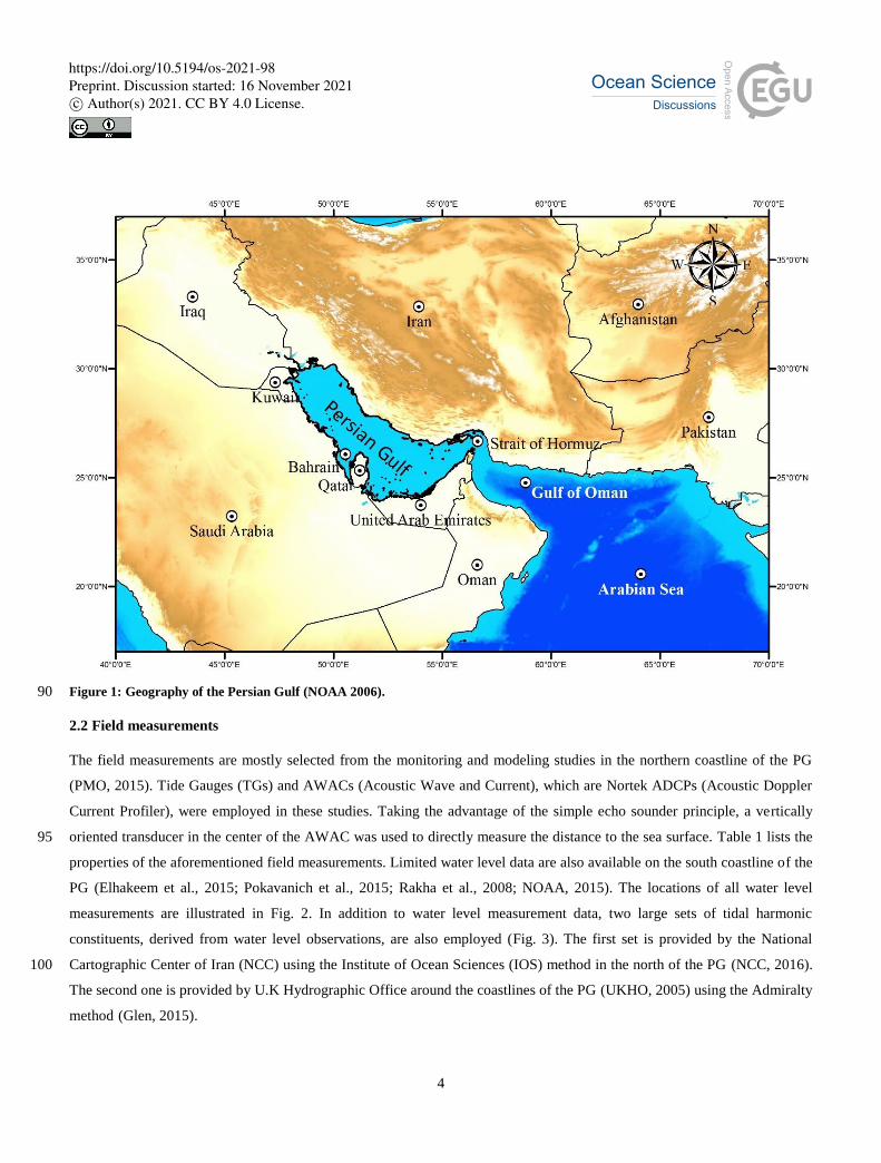
The shallow semi-enclosed basin of the PG locates in the south of Iran between latitudes 24°-30°N and longitudes 48 °-56 °E

(Fig. 1). The PG is connected to the Arabian Sea through the Gulf of Oman by the narrow Strait of Hormuz. Its average depth

is about 36 m with the maximum width and length of about 338 km and 1000 km, respectively. The tide in the PG is very

complicated, and the dominant pattern, i.e., primarily semidiurnal or diurnal, varies from one region to another (Reynolds, 85

1993).

The PG’s natural period of waves is calculated as 22.6 and 21.7 hours based on the Japanese and Chrystal methods, respectively

(Defant, 1961).


4

Figure 1: Geography of the Persian Gulf (NOAA 2006). 90

2.2 Field measurements

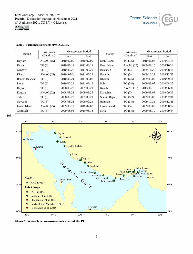
The field measurements are mostly selected from the monitoring and modeling studies in the northern coastline of the PG

(PMO, 2015). Tide Gauges (TGs) and AWACs (Acoustic Wave and Current), which are Nortek ADCPs (Acoustic Doppler

Current Profiler), were employed in these studies. Taking the advantage of the simple echo sounder principle, a vertically

oriented transducer in the center of the AWAC was used to directly measure the distance to the sea surface. Table 1 lists the 95

properties of the aforementioned field measurements. Limited water level data are also available on the south coastline of the

PG (Elhakeem et al., 2015; Pokavanich et al., 2015; Rakha et al., 2008; NOAA, 2015). The locations of all water level

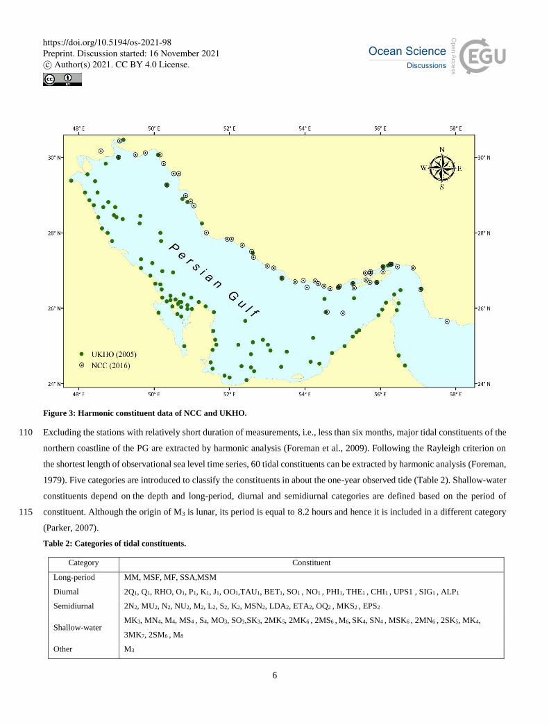
measurements are illustrated in Fig. 2. In addition to water level measurement data, two large sets of tidal harmonic

constituents, derived from water level observations, are also employed (Fig. 3). The first set is provided by the National

Cartographic Center of Iran (NCC) using the Institute of Ocean Sciences (IOS) method in the north of the PG (NCC, 2016). 100

The second one is provided by U.K Hydrographic Office around the coastlines of the PG (UKHO, 2005) using the Admiralty

method (Glen, 2015).


5

Table 1: Field measurements (PMO, 2015).

Measurement Period Instrument (Depth, m)

Station Measurement Period Instrument

(Depth, m) Station

End Start End Start

2010/04/14 2010/01/02 TG (3.5) Kish Island 2010/07/09 2010/07/09 AWAC (15) Deylam

2010/10/12 2009/09/10 AWAC (25) Farur Island 2011/08/11 2010/07/11 TG (3) Deylam

2010/08/18 2009/11/25 TG (4) Bustaneh 2011/08/20 2010/06/25 TG (3) Genaveh

2009/12/25 2009/10/22 TG (5) Basaidu 2011/07/29 2010/ 07/31 AWAC (25) Kharg

2009/09/11 2009/08/07 TG (4.5) Khamir 2011/08/07 2010/06/24 TG (3) Bandar Bushehr

2010/08/15 2009/08/07 TG (5.8) Pohl 2011/08/19 2010/06/24 TG (3) Lavar

2013/06/30 2013/06/16 AWAC (10) Kaveh 2009/09/21 2008/08/23 TG (3) Dayyer

2009/09/15 2009/08/08 TG (7) Dargahan 2009/09/25 2008/08/23 AWAC (22) Kangan

2010/02/01 2009/08/08 TG (5.2) Shahid Rajaee 2009/09/21 2008/08/23 TG (3) Taheri

2009/12/28 2009/10/21 TG (3.5) Bahman 2009/09/21 2008/08/23 TG (3) Nayband

2010/08/14 2009/08/09 TG (3) Larak Island 2010/07/08 2009/08/12 AWAC (25) Lavan Island

2010/09/04 2009/08/10 TG (5.8) Sirik 2010/08/18 2009/08/06 TG (5) Chiruyeh

105

Figure 2: Water level measurements around the PG.


6

Figure 3: Harmonic constituent data of NCC and UKHO.

Excluding the stations with relatively short duration of measurements, i.e., less than six months, major tidal constituents of the 110

northern coastline of the PG are extracted by harmonic analysis (Foreman et al., 2009). Following the Rayleigh criterion on

the shortest length of observational sea level time series, 60 tidal constituents can be extracted by harmonic analysis (Foreman,

1979). Five categories are introduced to classify the constituents in about the one-year observed tide (Table 2). Shallow-water

constituents depend on the depth and long-period, diurnal and semidiurnal categories are defined based on the period of

constituent. Although the origin of M3 is lunar, its period is equal to 8.2 hours and hence it is included in a different category 115

(Parker, 2007).

Table 2: Categories of tidal constituents.

Category Constituent

Long-period MM, MSF, MF, SSA,MSM

Diurnal 2Q1, Q1, RHO, O1, P1, K1, J1, OO1,TAU1, BET1, SO1 , NO1 , PHI1, THE1 , CHI1 , UPS1 , SIG1 , ALP1

Semidiurnal 2N2, MU2, N2, NU2, M2, L2, S2, K2, MSN2, LDA2, ETA2, OQ2 , MKS2 , EPS2

Shallow-water MK3, MN4, M4, MS4 , S4, MO3, SO3,SK3, 2MK5, 2MK6 , 2MS6 , M6, SK4, SN4 , MSK6 , 2MN6 , 2SK5, MK4,

3MK7, 2SM6 , M8

Other M3


7

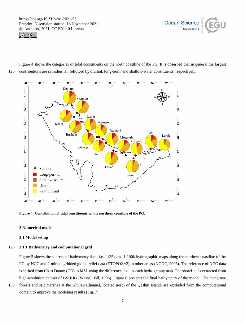
Figure 4 shows the categories of tidal constituents on the north coastline of the PG. It is observed that in general the largest

contributions are semidiurnal, followed by diurnal, long-term, and shallow-water constituents, respectively. 120

Figure 4: Contribution of tidal constituents on the northern coastline of the PG.

3 Numerical model

3.1 Model set up

3.1.1 Bathymetry and computational grid 125

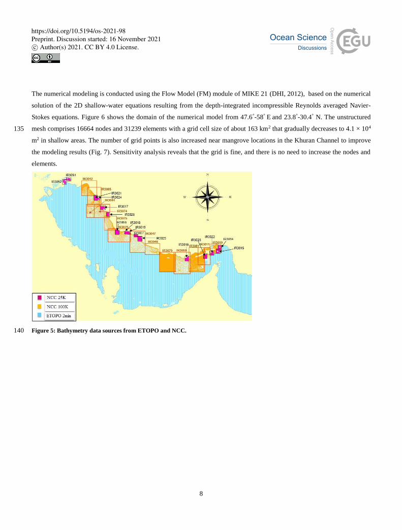
Figure 5 shows the sources of bathymetry data, i.e., 1:25k and 1:100k hydrographic maps along the northern coastline of the

PG by NCC and 2-minute gridded global relief data (ETOPO2 v2) in other areas (NGDC, 2006). The reference of NCC data

is shifted from Chart Datum (CD) to MSL using the difference level at each hydrography map. The shoreline is extracted from

high-resolution dataset of GSHHG (Wessel, Pål, 1996). Figure 6 presents the final bathymetry of the model. The mangrove

forests and salt marshes at the Khuran Channel, located north of the Qeshm Island, are excluded from the computational 130

domain to improve the modeling results (Fig. 7).


8

The numerical modeling is conducted using the Flow Model (FM) module of MIKE 21 (DHI, 2012), based on the numerical

solution of the 2D shallow-water equations resulting from the depth-integrated incompressible Reynolds averaged Navier-

Stokes equations. Figure 6 shows the domain of the numerical model from 47.6°-58° E and 23.8°-30.4° N. The unstructured

mesh comprises 16664 nodes and 31239 elements with a grid cell size of about 163 km2 that gradually decreases to 4.1 × 104 135

m2 in shallow areas. The number of grid points is also increased near mangrove locations in the Khuran Channel to improve

the modeling results (Fig. 7). Sensitivity analysis reveals that the grid is fine, and there is no need to increase the nodes and

elements.

Figure 5: Bathymetry data sources from ETOPO and NCC. 140


9

Figure 6: Bathymetry and computational grid.


10

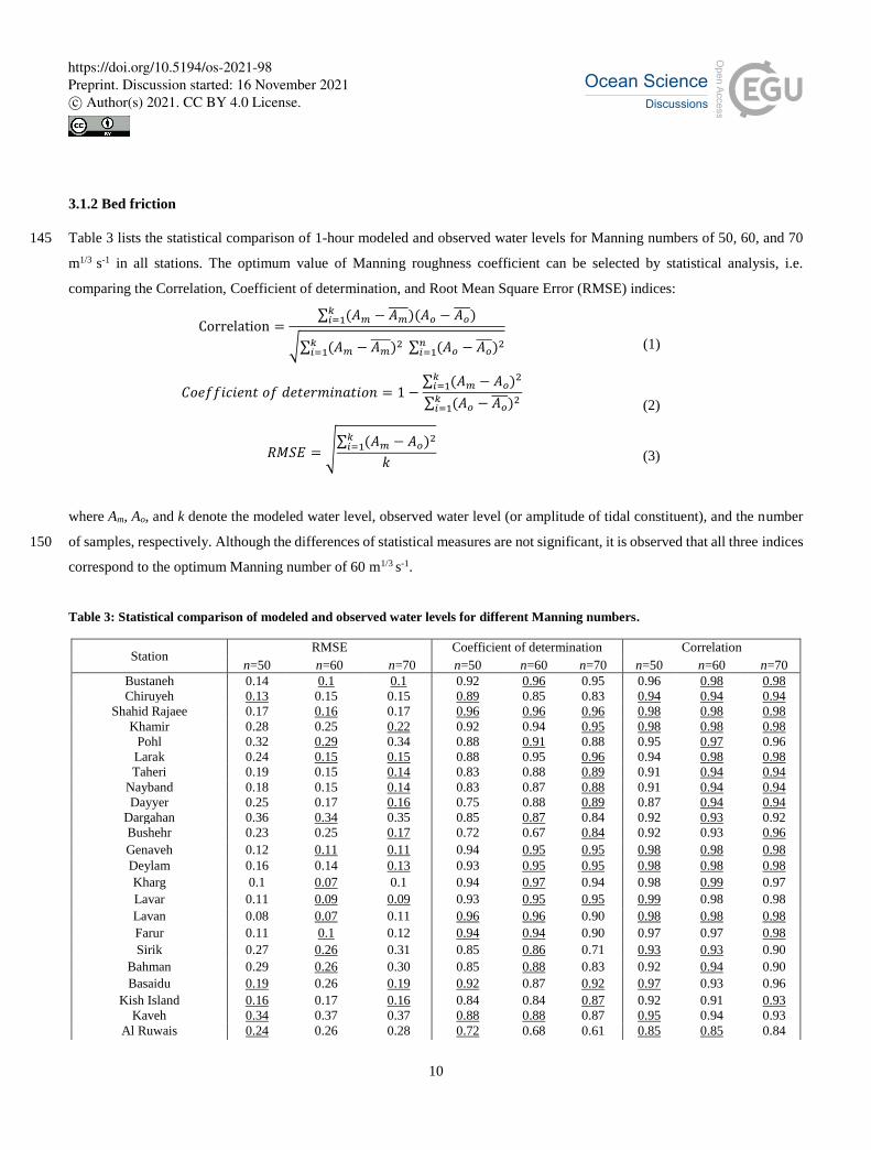
3.1.2 Bed friction

Table 3 lists the statistical comparison of 1-hour modeled and observed water levels for Manning numbers of 50, 60, and 70 145

m1/3 s-1 in all stations. The optimum value of Manning roughness coefficient can be selected by statistical analysis, i.e.

comparing the Correlation, Coefficient of determination, and Root Mean Square Error (RMSE) indices:

Correlation =∑ (𝐴𝑚 − 𝐴𝑚

)(𝐴𝑜 − 𝐴𝑜 )𝑘

𝑖=1

√∑ (𝐴𝑚 − 𝐴𝑚 )2 ∑ (𝐴𝑜 − 𝐴𝑜

)2𝑛𝑖=1

𝑘𝑖=1

(1)

𝐶𝑜𝑒𝑓𝑓𝑖𝑐𝑖𝑒𝑛𝑡 𝑜𝑓 𝑑𝑒𝑡𝑒𝑟𝑚𝑖𝑛𝑎𝑡𝑖𝑜𝑛 = 1 −∑ (𝐴𝑚 − 𝐴𝑜)2𝑘

𝑖=1

∑ (𝐴𝑜 − 𝐴𝑜 )2𝑘

𝑖=1

(2)

𝑅𝑀𝑆𝐸 = √∑ (𝐴𝑚 − 𝐴𝑜)2𝑘

𝑖=1

𝑘

(3)

where Am, Ao, and k denote the modeled water level, observed water level (or amplitude of tidal constituent), and the number

of samples, respectively. Although the differences of statistical measures are not significant, it is observed that all three indices 150

correspond to the optimum Manning number of 60 m1/3 s-1.

Table 3: Statistical comparison of modeled and observed water levels for different Manning numbers.

Station RMSE Coefficient of determination Correlation

n=50 n=60 n=70 n=50 n=60 n=70 n=50 n=60 n=70

Bustaneh 0.14 0.1 0.1 0.92 0.96 0.95 0.96 0.98 0.98

Chiruyeh 0.13 0.15 0.15 0.89 0.85 0.83 0.94 0.94 0.94

Shahid Rajaee 0.17 0.16 0.17 0.96 0.96 0.96 0.98 0.98 0.98

Khamir 0.28 0.25 0.22 0.92 0.94 0.95 0.98 0.98 0.98

Pohl 0.32 0.29 0.34 0.88 0.91 0.88 0.95 0.97 0.96

Larak 0.24 0.15 0.15 0.88 0.95 0.96 0.94 0.98 0.98

Taheri 0.19 0.15 0.14 0.83 0.88 0.89 0.91 0.94 0.94

Nayband 0.18 0.15 0.14 0.83 0.87 0.88 0.91 0.94 0.94

Dayyer 0.25 0.17 0.16 0.75 0.88 0.89 0.87 0.94 0.94

Dargahan 0.36 0.34 0.35 0.85 0.87 0.84 0.92 0.93 0.92

Bushehr 0.23 0.25 0.17 0.72 0.67 0.84 0.92 0.93 0.96

Genaveh 0.12 0.11 0.11 0.94 0.95 0.95 0.98 0.98 0.98

Deylam 0.16 0.14 0.13 0.93 0.95 0.95 0.98 0.98 0.98

Kharg 0.1 0.07 0.1 0.94 0.97 0.94 0.98 0.99 0.97

Lavar 0.11 0.09 0.09 0.93 0.95 0.95 0.99 0.98 0.98

Lavan 0.08 0.07 0.11 0.96 0.96 0.90 0.98 0.98 0.98

Farur 0.11 0.1 0.12 0.94 0.94 0.90 0.97 0.97 0.98

Sirik 0.27 0.26 0.31 0.85 0.86 0.71 0.93 0.93 0.90

Bahman 0.29 0.26 0.30 0.85 0.88 0.83 0.92 0.94 0.90

Basaidu 0.19 0.26 0.19 0.92 0.87 0.92 0.97 0.93 0.96

Kish Island

Kaveh

0.16

0.34

0.17

0.37

0.16

0.37

0.84

0.88

0.84

0.88

0.87

0.87

0.92

0.95

0.91

0.94

0.93

0.93

Al Ruwais 0.24 0.26 0.28 0.72 0.68 0.61 0.85 0.85 0.84


11

Mina Salman 0.23 0.22 0.21 0.78 0.81 0.82 0.94 0.94 0.93

Al Khiran 0.25 0.23 0.27 0.79 0.83 0.76 0.93 0.92 0.88

Kuwait 0.52 0.48 0.46 0.77 0.81 0.83 0.97 0.96 0.95

Average 0.217 0.201 0.204 0.864 0.881 0.872 0.944 0.950 0.946

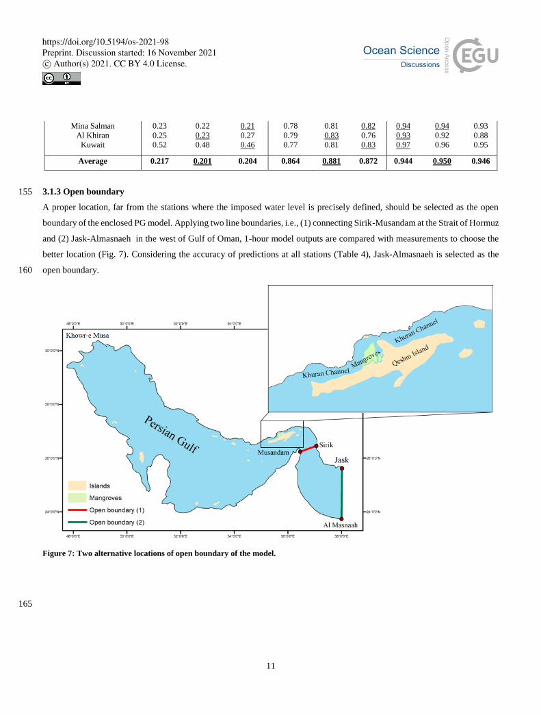
3.1.3 Open boundary 155

A proper location, far from the stations where the imposed water level is precisely defined, should be selected as the open

boundary of the enclosed PG model. Applying two line boundaries, i.e., (1) connecting Sirik-Musandam at the Strait of Hormuz

and (2) Jask-Almasnaeh in the west of Gulf of Oman, 1-hour model outputs are compared with measurements to choose the

better location (Fig. 7). Considering the accuracy of predictions at all stations (Table 4), Jask-Almasnaeh is selected as the

open boundary. 160

Figure 7: Two alternative locations of open boundary of the model.

165


12

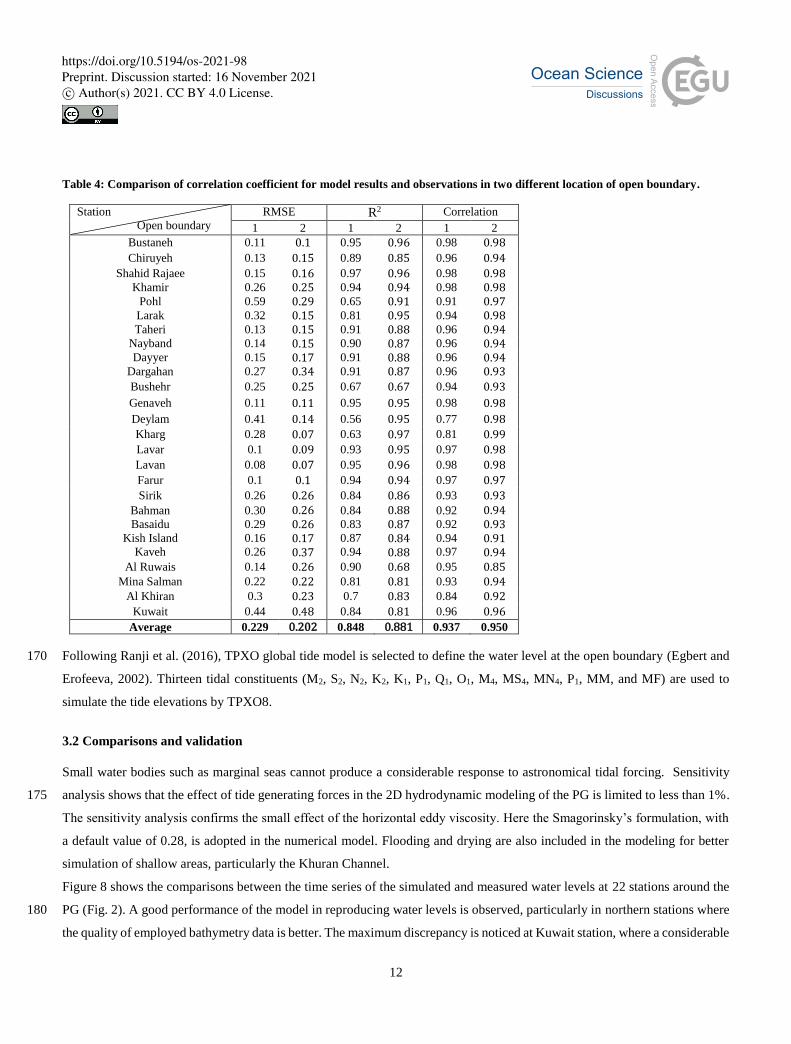
Table 4: Comparison of correlation coefficient for model results and observations in two different location of open boundary.

Station

Open boundary

RMSE R2 Correlation

1 2 1 2 1 2

Bustaneh 0.11 0.1 0.95 0.96 0.98 0.98

Chiruyeh 0.13 0.15 0.89 0.85 0.96 0.94

Shahid Rajaee 0.15 0.16 0.97 0.96 0.98 0.98 Khamir 0.26 0.25 0.94 0.94 0.98 0.98

Pohl 0.59 0.29 0.65 0.91 0.91 0.97 Larak 0.32 0.15 0.81 0.95 0.94 0.98 Taheri 0.13 0.15 0.91 0.88 0.96 0.94

Nayband 0.14 0.15 0.90 0.87 0.96 0.94 Dayyer 0.15 0.17 0.91 0.88 0.96 0.94

Dargahan 0.27 0.34 0.91 0.87 0.96 0.93

Bushehr 0.25 0.25 0.67 0.67 0.94 0.93

Genaveh 0.11 0.11 0.95 0.95 0.98 0.98

Deylam 0.41 0.14 0.56 0.95 0.77 0.98

Kharg 0.28 0.07 0.63 0.97 0.81 0.99

Lavar 0.1 0.09 0.93 0.95 0.97 0.98

Lavan 0.08 0.07 0.95 0.96 0.98 0.98

Farur 0.1 0.1 0.94 0.94 0.97 0.97

Sirik 0.26 0.26 0.84 0.86 0.93 0.93 Bahman

Basaidu

Kish Island

Kaveh

0.30

0.29

0.16

0.26

0.26 0.26 0.17 0.37

0.84

0.83

0.87

0.94

0.88 0.87 0.84 0.88

0.92

0.92

0.94

0.97

0.94 0.93 0.91 0.94

Al Ruwais 0.14 0.26 0.90 0.68 0.95 0.85 Mina Salman 0.22 0.22 0.81 0.81 0.93 0.94

Al Khiran 0.3 0.23 0.7 0.83 0.84 0.92

Kuwait 0.44 0.48 0.84 0.81 0.96 0.96

Average 0.229 0.202 0.848 0.881 0.937 0.950

Following Ranji et al. (2016), TPXO global tide model is selected to define the water level at the open boundary (Egbert and 170

Erofeeva, 2002). Thirteen tidal constituents (M2, S2, N2, K2, K1, P1, Q1, O1, M4, MS4, MN4, P1, MM, and MF) are used to

simulate the tide elevations by TPXO8.

3.2 Comparisons and validation

Small water bodies such as marginal seas cannot produce a considerable response to astronomical tidal forcing. Sensitivity

analysis shows that the effect of tide generating forces in the 2D hydrodynamic modeling of the PG is limited to less than 1%. 175

The sensitivity analysis confirms the small effect of the horizontal eddy viscosity. Here the Smagorinsky’s formulation, with

a default value of 0.28, is adopted in the numerical model. Flooding and drying are also included in the modeling for better

simulation of shallow areas, particularly the Khuran Channel.

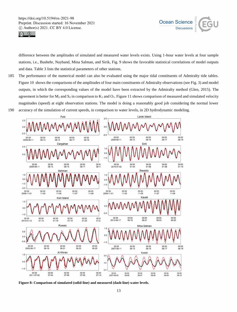
Figure 8 shows the comparisons between the time series of the simulated and measured water levels at 22 stations around the

PG (Fig. 2). A good performance of the model in reproducing water levels is observed, particularly in northern stations where 180

the quality of employed bathymetry data is better. The maximum discrepancy is noticed at Kuwait station, where a considerable


13

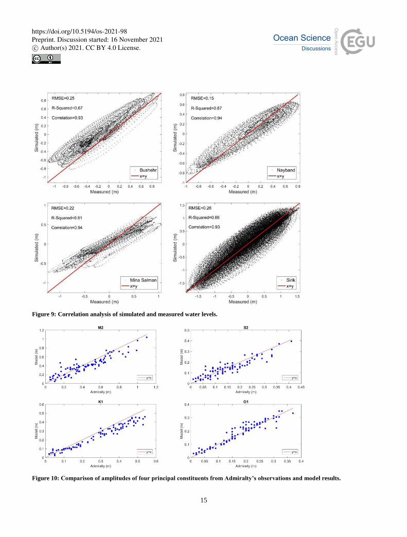
difference between the amplitudes of simulated and measured water levels exists. Using 1-hour water levels at four sample

stations, i.e., Bushehr, Nayband, Mina Salman, and Sirik, Fig. 9 shows the favorable statistical correlations of model outputs

and data. Table 3 lists the statistical parameters of other stations.

The performance of the numerical model can also be evaluated using the major tidal constituents of Admiralty tide tables. 185

Figure 10 shows the comparisons of the amplitudes of four main constituents of Admiralty observations (see Fig. 3) and model

outputs, in which the corresponding values of the model have been extracted by the Admiralty method (Glen, 2015). The

agreement is better for M2 and S2 in comparison to K1 and O1. Figure 11 shows comparison of measured and simulated velocity

magnitudes (speed) at eight observation stations. The model is doing a reasonably good job considering the normal lower

accuracy of the simulation of current speeds, in comparison to water levels, in 2D hydrodynamic modeling. 190

Figure 8: Comparison of simulated (solid-line) and measured (dash-line) water levels.


14

Figure 8: Comparison of simulated (solid-line) and measured (dash-line) water levels (continued).

195


15

Figure 9: Correlation analysis of simulated and measured water levels.

Figure 10: Comparison of amplitudes of four principal constituents from Admiralty’s observations and model results.


16

200

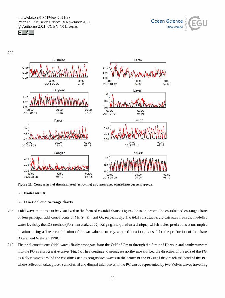
Figure 11: Comparison of the simulated (solid-line) and measured (dash-line) current speeds.

3.3 Model results

3.3.1 Co-tidal and co-range charts

Tidal wave motions can be visualized in the form of co-tidal charts. Figures 12 to 15 present the co-tidal and co-range charts 205

of four principal tidal constituents of M2, S2, K1, and O1, respectively. The tidal constituents are extracted from the modelled

water levels by the IOS method (Foreman et al., 2009). Kriging interpolation technique, which makes predictions at unsampled

locations using a linear combination of known value at nearby sampled locations, is used for the production of the charts

(Oliver and Webster, 1990).

The tidal constituents (tidal wave) firstly propagate from the Gulf of Oman through the Strait of Hormuz and southwestward 210

into the PG as a progressive wave (Fig. 1). They continue to propagate northwestward, i.e., the direction of the axis of the PG,

as Kelvin waves around the coastlines and as progressive waves in the center of the PG until they reach the head of the PG,

where reflection takes place. Semidiurnal and diurnal tidal waves in the PG can be represented by two Kelvin waves travelling


17

in opposite direction. It is observed that the waves rotate around a nodal point (AP) instead of oscillating about a nodal line

(discussed more in Sec.4.1) As the PG is located in the northern hemisphere, the tidal waves present a counter-clockwise 215

rotation, which can be observed in co-tidal curves of M2, S2, K1, and O1 (dash-lines in Fig. 12 to 15).

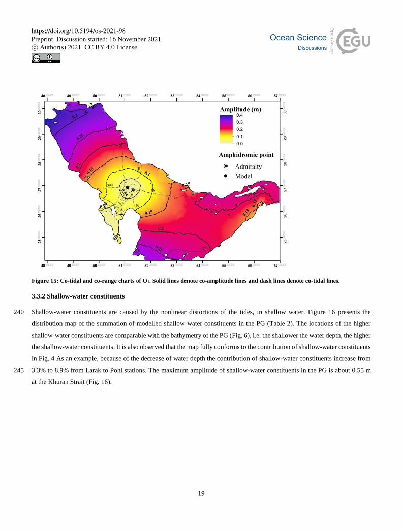
The semidiurnal constituents of M2 and S2 have two APs, located in the northwest and southern ends of the PG, but the diurnal

constituents, i.e., K1 and O1, have a single AP at the center part of the PG near Bahrain. The simulated co-tidal and co-range

charts of the model generally agree with the corresponding Admiralty charts (UK Hydrographic Office, 1999), which are based

on direct observations over the sea and shallow waters (Doodson and Warburg, 1941). The APs location of Admiralty charts 220

have also been plotted, to be compared with the derived APs from the numerical model.

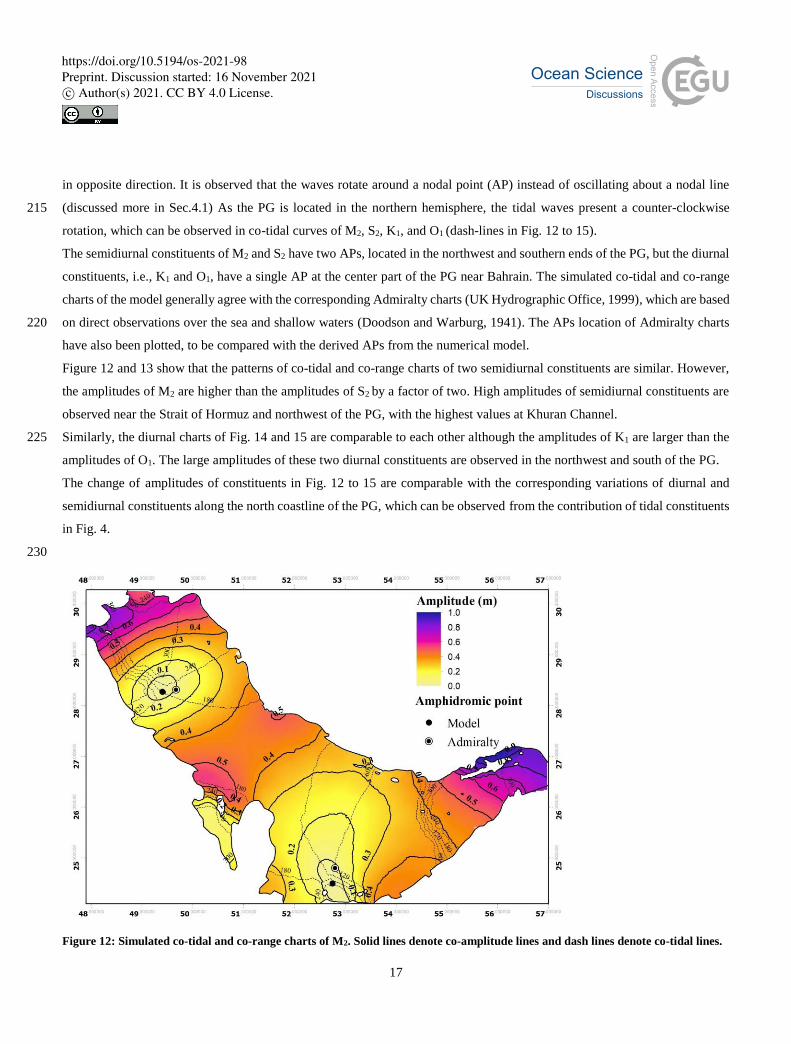
Figure 12 and 13 show that the patterns of co-tidal and co-range charts of two semidiurnal constituents are similar. However,

the amplitudes of M2 are higher than the amplitudes of S2 by a factor of two. High amplitudes of semidiurnal constituents are

observed near the Strait of Hormuz and northwest of the PG, with the highest values at Khuran Channel.

Similarly, the diurnal charts of Fig. 14 and 15 are comparable to each other although the amplitudes of K1 are larger than the 225

amplitudes of O1. The large amplitudes of these two diurnal constituents are observed in the northwest and south of the PG.

The change of amplitudes of constituents in Fig. 12 to 15 are comparable with the corresponding variations of diurnal and

semidiurnal constituents along the north coastline of the PG, which can be observed from the contribution of tidal constituents

in Fig. 4.

230

Figure 12: Simulated co-tidal and co-range charts of M2. Solid lines denote co-amplitude lines and dash lines denote co-tidal lines.


18

Figure 13: Co-tidal and co-range charts of S2. Solid lines denote co-amplitude lines and dash lines denote co-tidal lines.

235

Figure 14: Co-tidal and co-range charts of K1. Solid lines denote co-amplitude lines and dash lines denote co-tidal lines.


19

Figure 15: Co-tidal and co-range charts of O1. Solid lines denote co-amplitude lines and dash lines denote co-tidal lines.

3.3.2 Shallow-water constituents

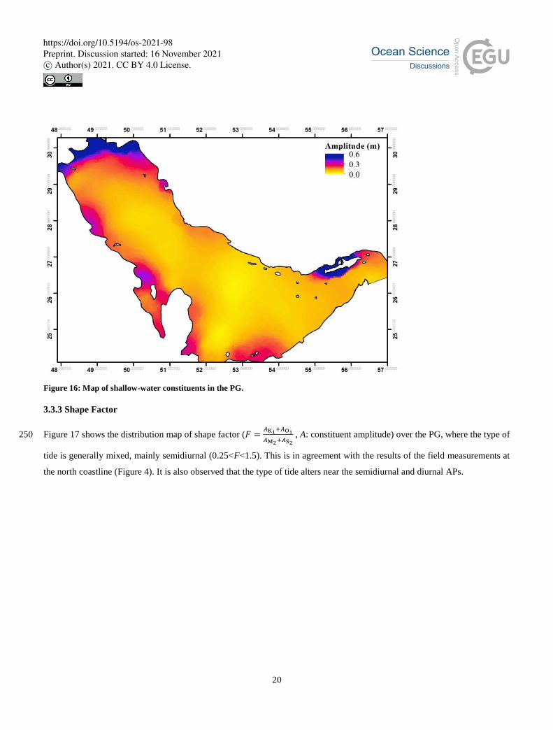
Shallow-water constituents are caused by the nonlinear distortions of the tides, in shallow water. Figure 16 presents the 240

distribution map of the summation of modelled shallow-water constituents in the PG (Table 2). The locations of the higher

shallow-water constituents are comparable with the bathymetry of the PG (Fig. 6), i.e. the shallower the water depth, the higher

the shallow-water constituents. It is also observed that the map fully conforms to the contribution of shallow-water constituents

in Fig. 4 As an example, because of the decrease of water depth the contribution of shallow-water constituents increase from

3.3% to 8.9% from Larak to Pohl stations. The maximum amplitude of shallow-water constituents in the PG is about 0.55 m 245

at the Khuran Strait (Fig. 16).


20

Figure 16: Map of shallow-water constituents in the PG.

3.3.3 Shape Factor

Figure 17 shows the distribution map of shape factor (𝐹 =𝐴K1+𝐴O1

𝐴M2+𝐴S2

, A: constituent amplitude) over the PG, where the type of 250

tide is generally mixed, mainly semidiurnal (0.25<F<1.5). This is in agreement with the results of the field measurements at

the north coastline (Figure 4). It is also observed that the type of tide alters near the semidiurnal and diurnal APs.


21

Figure 17: Classification of tides in the PG.

3.3.4 Resonance period 255

The effective period of resonance in the PG can be determined by its amplified response to various forcing periods. Assuming

similar input conditions in the developed numerical model, the sinusoidal waves with the constant amplitude of 1 m are applied

at the open boundary. An amplification factor is defined as the ratio between the wave height at the indicated location to the

wave height at the open boundary. Seven scenarios of input waves with different wave periods are considered to represent the

response of tidal constituents to resonance (Table 5). 260

Figure 18 shows the amplification factor for input wave periods of 24, 12, and 6 hours in the PG. It is observed that the

amplification factor is substantially higher in the Strait of Hormuz and Khuran Channel, northwest of the PG, and southeast

of Qatar.

Defining three numerical stations at these areas (1, 2, and 3 in Fig. 18), Table 5 presents the amplification factor of all modeled

scenarios. The diurnal and semidiurnal constituents show high amplification factors in three selected numerical stations and 265

in 1st and 2nd stations, respectively, which is in accordance with the study of Mashayekh Poul (2016). The shallow-water

constituents also resonate in some parts of the basin, particularly in Khuran Channel and Strait of Hormuz. It should be added

although various factors affect the increase of the tidal elevation in the numerical model, comparing the changes of similar

waves with different wave periods at checkpoints reveals that it is reasonable to relate the resonance phenomenon to the

amplification factor. 270


22

Table 5: Tidal amplification factor for different input wave periods at numerical stations 1, 2 and 3.

Period (h) Related constituents Amplification factor

Station 1 Station 2 Station 3

26 Q1, ρ1 1.25 1.54 1.21

24 K1, O1, P1 1.29 1.31 1.29

22 OO1, SO1 1.32 1.27 1.14

12 M2, S2, L2, N2 1.72 1.2 1.06

8 MK3, SO3, SK3, 2MK3 (MO3) 2.13 0.9 1.36

6 S4, MK4, MS4, SN4, M4, MN4 2.71 0.62 0.84

4 2MN6, M6, 2MS6, 2MK6, 2SM6 2.84 0.37 0.49

Figure 18: The tidal amplification factors for the wave periods of 6 h (top), 12 h (middle) and 24 h (bottom).


23

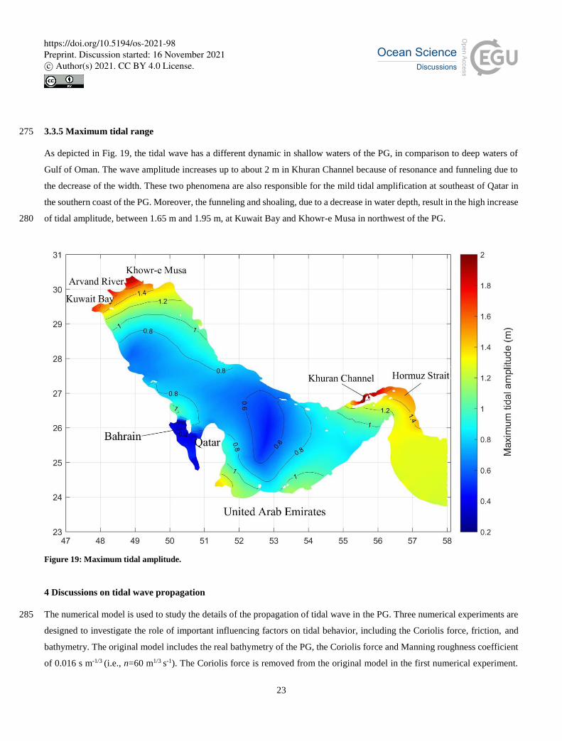
3.3.5 Maximum tidal range 275

As depicted in Fig. 19, the tidal wave has a different dynamic in shallow waters of the PG, in comparison to deep waters of

Gulf of Oman. The wave amplitude increases up to about 2 m in Khuran Channel because of resonance and funneling due to

the decrease of the width. These two phenomena are also responsible for the mild tidal amplification at southeast of Qatar in

the southern coast of the PG. Moreover, the funneling and shoaling, due to a decrease in water depth, result in the high increase

of tidal amplitude, between 1.65 m and 1.95 m, at Kuwait Bay and Khowr-e Musa in northwest of the PG. 280

Figure 19: Maximum tidal amplitude.

4 Discussions on tidal wave propagation

The numerical model is used to study the details of the propagation of tidal wave in the PG. Three numerical experiments are 285

designed to investigate the role of important influencing factors on tidal behavior, including the Coriolis force, friction, and

bathymetry. The original model includes the real bathymetry of the PG, the Coriolis force and Manning roughness coefficient

of 0.016 s m-1/3 (i.e., n=60 m1/3 s-1). The Coriolis force is removed from the original model in the first numerical experiment.


24

In the second case, a horizontal flat bed with constant water depth of 36 m is assumed as the bathymetry of the PG. The

constant water depth is also used in the third numerical test with the Manning coefficient of 0.002 s m-1/3, i.e., the smallest 290

value that does not make the model unstable, to concentrate on the effect of bottom friction.

4.1 Coriolis force

An amphidromic system develops as the result of the combined constraint of ocean basin geometry and the influence of the

Coriolis (Wright et al., 1999). The development of the amphidromic system in a gulf occurs when both standing and Kelvin

waves form. 295

If the gulf is sufficiently wide, in comparison to Rossby deformation radius (say W > 2RR, W; width of the gulf, RR; Rossby

deformation radius), the propagation of tide around the boundaries of a wide gulf is considered as a Kelvin wave since the

incoming and outgoing waves do not significantly overlap and interfere. On the other hand, rotation is insignificant in a narrow

gulf (say W < RR) and the standing wave is set up by reflecting the wave that entered from the open ocean (Hautala et al.,

2005; Vallis, 2006). The standing waves have nodes and antinodes, with zero and maximum amplitudes, respectively, 300

separated by a distance of 𝜆/4, where 𝜆 is the wavelength of the original progressive wave. The nodal line crosses the gulf at a

distance of λ/4 from its head (or iλ/4, i=3, 5, ...) (Pugh, 1987).

For an intermediate width, with respect to Rossby deformation radius, the tide will have the characteristics of both wide and

narrow gulfs. In this intermediate inlet, the tide will behave like the Kelvin wave on the boundaries. The amplitude of the

Kelvin wave increases in parallel to the wave crest because of the Coriolis acceleration, where in the northern hemisphere, the 305

amplitude increases to the right of the wave crest. The incoming wave from the ocean is thus amplified on the right towards

the coastline and the outgoing wave is similarly increased at the opposite coastline. The tide at the center axis of the gulf is

strongly similar to the case of a standing wave, i.e., low amplitude at the node and high amplitude at either side with an out of

phase relationship. The nodal line which extends across the channel when rotation is not important, turns into the nodal point

or AP in the center of the gulf around which the tide progresses (Hautala et al., 2005; Vallis, 2006). 310

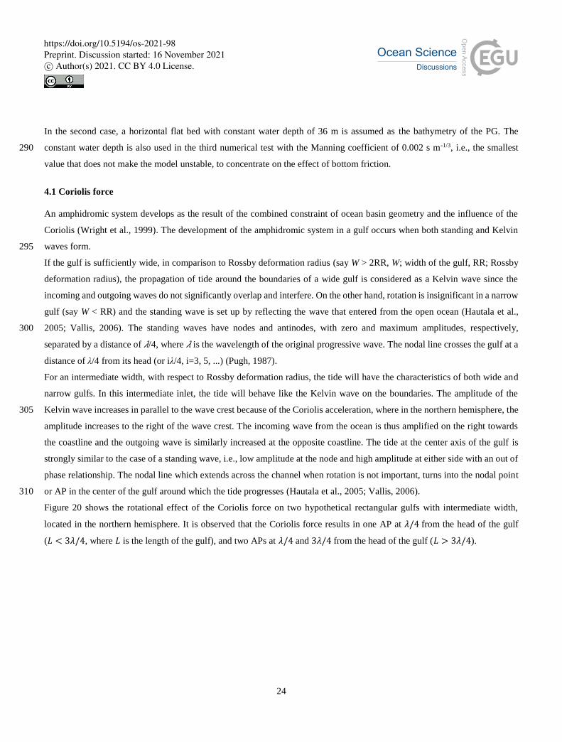
Figure 20 shows the rotational effect of the Coriolis force on two hypothetical rectangular gulfs with intermediate width,

located in the northern hemisphere. It is observed that the Coriolis force results in one AP at 𝜆/4 from the head of the gulf

(𝐿 < 3𝜆/4, where 𝐿 is the length of the gulf), and two APs at 𝜆/4 and 3𝜆/4 from the head of the gulf (𝐿 > 3𝜆/4).


25

315

Figure 20: Plan (cases (1) and (2)) and cross-section (bottom) views of a hypothetical rectangular gulf located in the northern

hemisphere. The Coriolis force is excluded on the left side (similar to first numerical experiment). The right side is similar to original

model, including the Coriolis force. Dash lines and solid lines in plan views denote co-range lines and co-tidal lines, respectively. In

plan views, blue and black arrows show incoming and reflected tidal wave directions, respectively. The solid line and dash line in

cross-section views respectively indicate the geometric locations of the crests of incoming and reflected Kelvin waves. Blank red 320 circles represent the APs.

The inertia period 𝑇𝑖 is 26.17 h (=2𝜋

𝑓 , f; the Coriolis parameter= 2𝜔𝑠𝑖𝑛𝜑, 𝜔; the angular velocity of the earth’s rotation, 𝜑;

the latitude= the average latitude is equal to 27° N in the PG). The Rossby deformation radius (𝑅𝑅 =√𝑔ℎ

𝑓 , ℎ; water depth) is

284 km using the estimated average depth of the PG of 36 m. Thus, the semidiurnal and diurnal tidal periods in the PG are in


26

order of the inertial period (26.17 h), and the maximum width of the PG (about 338 km) is more than the Rossby deformation 325

radius (but not much more, i.e., an intermediate case).

Figure 21 and 22 show the effect of Coriolis force on co-tidal charts of diurnal and semidiurnal constituents in the PG,

respectively. It is observed that the Coriolis force converts the nodal lines into nodal points, which results in forming

amphidromic systems for both semidiurnal and diurnal tides. Table 6 presents the wavelengths of the major tidal constituents

in the PG. Considering the PG length of about 1000 km, the modeling results in Fig. 21 and 22, i.e., one node (AP) for diurnal 330

constituents and two nodes (APs) for semidiurnal constituents, agree with the above theoretical discussion on rectangular gulfs

(Fig. 20).

Table 6: Wavelengths of tidal constituents and locations of nodal lines.

Constituent Period (h) 𝜆 = √𝑔ℎ × 𝑇 (km) 𝜆

4

3𝜆

4

M2 12.42 840 210 630

S2 12 812 203 609

K1 23.93 1596 399 1197

O1 25.82 1722 430 1290

335

Figure 21: The locations of the nodal line and node for diurnal constituents with the Coriolis force (right) and excluding the Coriolis

force (left).


27

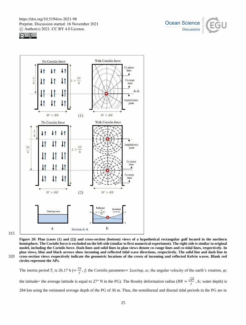
Figure 22: The locations of the nodal lines and nodes for semidiurnal constituents with the Coriolis force (right) and excluding the 340 Coriolis force (left).

4.2 Bathymetry

The second numerical test aims to study the effect of bathymetry and water depth differences on tidal wave transformation in

the PG. The bathymetry of the PG can be comprises a shallow zone at the closed end that extends along the southern part of

the basin, resulting in a highly asymmetrical cross-sectional longitudinal and transverse depth profiles (Fig. 6). 345

Figure 23 and 24 respectively present the numerical results of semi-diurnal and diurnal constituents on a hypothetical

bathymetry with constant water depth of 36 m, in comparison to the original model with real bathymetry. The background

color shows the change of amplitudes, i.e. the results of employing hypothetical bathymetry minus the original outputs. Co-

tidal lines and the locations of the APs are also presented. The different location of co-tidal lines in this test case can be related

to the changes of tidal wave speed as it travels faster in larger water depths, e.g. vicinity of the Strait of Hormuz. An obvious 350

shift of semidiurnal APs in the longitudinal direction of the PG is also observed (Fig. 23). The shifts of real southern

semidiurnal APs of the PG towards the open boundary, in comparison to the test model, can be explained by the local changes

of tidal wavelengths. The differences of locations are greater for the second southern APs because of the significant longer

wavelengths in that region, in comparison to the test model. It is also observed that the average water depth of 36 m in this

numerical test, and the consequent shorter wavelength in deeper waters, has resulted in the appearance of third AP of S2 in the 355

southeast of the PG.

The transverse movements of the single diurnal APs in Fig. 24 can also be explained by the tidal wave propagation in the

northern hemisphere. The shape of the PG between the head and AP of diurnal constituents can be approximated to a

rectangular basin, where the upper half (north) is deeper than the lower half (south). Due to Coriolis acceleration in the northern


28

hemisphere, the incoming Kelvin wave is bounded to the right of the direction of motion and increases in amplitude parallel 360

to the wave crest toward the right, i.e., the coastline of the north deeper part of the PG. Similarly, the reflected Kelvin wave

follows the coastline of the south shallower part of the PG and increases its amplitude toward the southern coastline. Since the

incoming and reflected Kelvin waves are banked up on the northern and southern sides of the PG, respectively, they are affected

by the larger depth of the northern half and lesser depth of the southern half, respectively. The associated change of wavelength

thus leads to a decreased amplitude in the deeper part of the basin and an increased amplitude in the returning tidal wave in 365

the shallower part, considering the wave energy conservation. On the other hand, the amplitude decreases by factor

exp (−𝑓𝑦

√𝑔ℎ) (Pugh and Woodworth, 2014). Assuming the constant Coriolis parameter (f) because of the slight change in

latitude in the cross section of the PG, the reflected wave should have a faster decrease of amplitude away from the coast than

the incoming wave.

Figure 25 shows the aforementioned explanations in a hypothetical rectangular gulf located in the northern hemisphere. 370

Comparing with the constant water depth, this pushes the AP away from the centerline into deeper north parts in the original

model of the PG (Fig. 24). These results are in accordance with conclusions derived from an idealized process-based model

for semi-enclosed basins by Roos & Schuttelaars (2011).

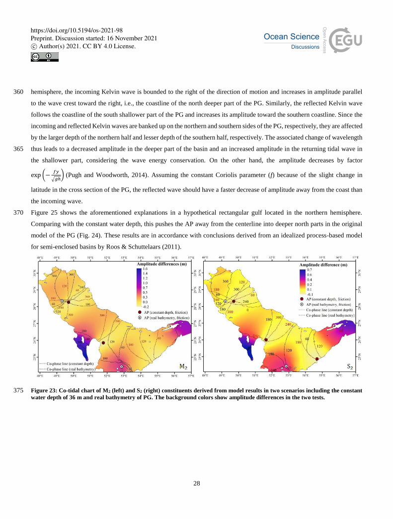
Figure 23: Co-tidal chart of M2 (left) and S2 (right) constituents derived from model results in two scenarios including the constant 375 water depth of 36 m and real bathymetry of PG. The background colors show amplitude differences in the two tests.


29

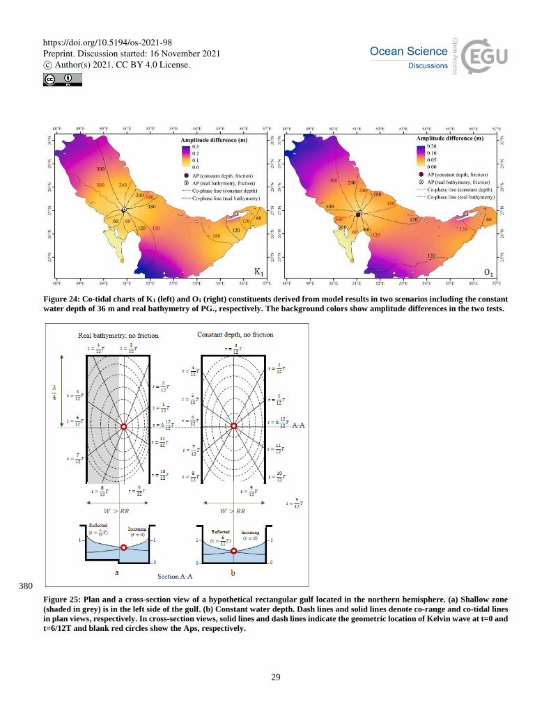
Figure 24: Co-tidal charts of K1 (left) and O1 (right) constituents derived from model results in two scenarios including the constant

water depth of 36 m and real bathymetry of PG., respectively. The background colors show amplitude differences in the two tests.

380

Figure 25: Plan and a cross-section view of a hypothetical rectangular gulf located in the northern hemisphere. (a) Shallow zone

(shaded in grey) is in the left side of the gulf. (b) Constant water depth. Dash lines and solid lines denote co-range and co-tidal lines

in plan views, respectively. In cross-section views, solid lines and dash lines indicate the geometric location of Kelvin wave at t=0 and

t=6/12T and blank red circles show the Aps, respectively.


30

4.3 Friction 385

The effect of friction is examined in the third numerical test, modeling the tidal wave propagation on the hypothetical constant

depth of the PG (second test) with and without bed roughness. The primary effect of friction is the exponential damping of

Kelvin wave amplitude in the direction of tide propagation (Rienecker and Teubner, 1980; Roos and Schuttelaars, 2009).

Furthermore, the reflected wave also dampens by the incomplete reflection from the head of the gulf, caused by the dissipation

in shallow water (Allen, 2009). 390

The incoming progressive (Kelvin) wave has a larger amplitude on the right-hand side of gulf in the northern hemisphere. The

Coriolis force also results in the greater amplitude of reflected wave on the left-hand side of the gulf. As the reflected wave is

weaker than the incoming wave due to dissipation damping, the APs are shifted from the centerline to the left side of the gulf.

Figure 26 illustrates this phenomenon in a hypothetical rectangular gulf, located in the northern hemisphere.

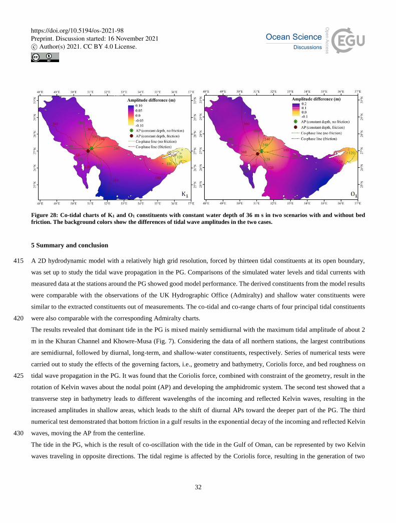
Figure 27 and 28 present modeling results of the propagations of M2, S2, K1, and O1 constituents. It is observed that the APs 395

move to the right side of the PG when the bottom friction is removed from the model. These results are in accordance with

conclusions of Roos & Schuttelaars (2011), derived from an idealized process-based model for semi-enclosed basins. However,

no displacement of the APs is observed in longitudinal axis of the PG.

Figure 27 and 28 show the increase of tidal amplitude all over the PG in modeling without friction. The change of tidal wave

height is larger in shallow areas, such as the northwest of the PG and south of Qatar and Bahrain, as well as narrow Strait of 400

Hormuz.


31

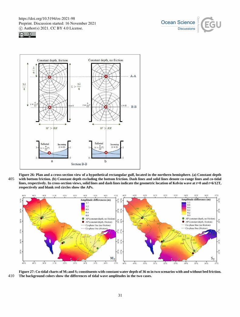
Figure 26: Plan and a cross-section view of a hypothetical rectangular gulf, located in the northern hemisphere. (a) Constant depth

with bottom friction. (b) Constant depth excluding the bottom friction. Dash lines and solid lines denote co-range lines and co-tidal 405 lines, respectively. In cross-section views, solid lines and dash lines indicate the geometric location of Kelvin wave at t=0 and t=6/12T,

respectively and blank red circles show the APs.

Figure 27: Co-tidal charts of M2 and S2 constituents with constant water depth of 36 m in two scenarios with and without bed friction.

The background colors show the differences of tidal wave amplitudes in the two cases. 410


32

Figure 28: Co-tidal charts of K1 and O1 constituents with constant water depth of 36 m s in two scenarios with and without bed

friction. The background colors show the differences of tidal wave amplitudes in the two cases.

5 Summary and conclusion

A 2D hydrodynamic model with a relatively high grid resolution, forced by thirteen tidal constituents at its open boundary, 415

was set up to study the tidal wave propagation in the PG. Comparisons of the simulated water levels and tidal currents with

measured data at the stations around the PG showed good model performance. The derived constituents from the model results

were comparable with the observations of the UK Hydrographic Office (Admiralty) and shallow water constituents were

similar to the extracted constituents out of measurements. The co-tidal and co-range charts of four principal tidal constituents

were also comparable with the corresponding Admiralty charts. 420

The results revealed that dominant tide in the PG is mixed mainly semidiurnal with the maximum tidal amplitude of about 2

m in the Khuran Channel and Khowre-Musa (Fig. 7). Considering the data of all northern stations, the largest contributions

are semidiurnal, followed by diurnal, long-term, and shallow-water constituents, respectively. Series of numerical tests were

carried out to study the effects of the governing factors, i.e., geometry and bathymetry, Coriolis force, and bed roughness on

tidal wave propagation in the PG. It was found that the Coriolis force, combined with constraint of the geometry, result in the 425

rotation of Kelvin waves about the nodal point (AP) and developing the amphidromic system. The second test showed that a

transverse step in bathymetry leads to different wavelengths of the incoming and reflected Kelvin waves, resulting in the

increased amplitudes in shallow areas, which leads to the shift of diurnal APs toward the deeper part of the PG. The third

numerical test demonstrated that bottom friction in a gulf results in the exponential decay of the incoming and reflected Kelvin

waves, moving the AP from the centerline. 430

The tide in the PG, which is the result of co-oscillation with the tide in the Gulf of Oman, can be represented by two Kelvin

waves traveling in opposite directions. The tidal regime is affected by the Coriolis force, resulting in the generation of two


33

amphidromic systems for M2 and S2 and one amphidromic system for K1 and O1. Numerical simulations and observational

data reveal that the natural oscillation period of PG is more or less diurnal.

More field measurements in the southern coast of the PG will be beneficial to improve the calibration and validation of the 435

present model. Including the wind force and the discharge of major rivers, in particular Arvand River at the northwest corner

of the PG, also increases the accuracy of the modeling, which is particularly important for the hindcast of water elevations and

currents across the PG. Moreover, in spite of shallow water depth of the PG that validates 2D modeling, the future extension

of present model to 3D will result in better simulation of hydrodynamics at Strait of Hormuz, with its pronounced vertical

salinity stratification, as well as the circulations near the land boundaries. 440

Data availability

The PMO and NCC provided us with the water level/current speed observational data and hydrography maps, respectively.

Both are national data which are not publicly accessible. They would be accessed by direct request from the owner. The PMO

website is available through https://www.pmo.ir/en/home and NCC website is available through https://www.ncc.gov.ir/en/.

The tidal constituent’s extraction code is available through https://github.com/CADWRDeltaModeling/vtide (Foreman et al., 445

2009).

Two-minute gridded global relief for both ocean and land areas (ETOPO2v2) are available through

https://www.ngdc.noaa.gov/mgg/global/relief/ETOPO2/ETOPO2v2-2006/ (NOAA, 2006).

Admiralty tide table volume 3 is available at https://wiac.info/docview.

Author contributions 450

This study was conducted as the master thesis of SMH under the supervision of MS. SMH did simulations, analysis,

visualization and drafted the manuscript. MS participated in the interpretation of the results and prepared a critical revision of

the manuscript.

Competing interests

The authors declare that they have no conflict of interest. 455

Acknowledgment

The authors acknowledge the PMO for providing tide measurements along the north coast of the PG. We are grateful to NCC

for hydrography maps and observation data. Thanks are also extended to Ms. Zahra Ranji, Ph.D. candidate at K. N. Toosi

University of Technology for her technical supports.


34

References 460

Akbari, P., Sadrinasab, M., Chegini, V. and Siadatmousavi, M.: Tidal constituents in the Persian Gulf, Gulf of Oman and

Arabian Sea: A numerical study, Indian J. Geo-Marine Sci., 45(8), 1010–1016, 2016.

Allen, P. A.: Earth surface processes, John Wiley & Sons., 2009.

Backhaus, J. O.: Improved representation of topographic effects by a vertical adaptive grid in vector-ocean-model (VOM).

Part I: generation of adaptive grids, Ocean Model., 22(3–4), 114–127, doi:https://doi.org/10.1016/j.ocemod.2008.02.003, 465

2008.

Chen, Changsheng; Liu, Hedong; Beardsley, R. C.: An Unstructured Grid, Finite-Volume, Three-Dimensional, Primitive

Equations Ocean Model: Application to Coastal Ocean and Estuaries., J. Atmos. Ocean. Technol., 20, 159–186,

doi:10.1175/1520-0426(2003)0202.0.CO;2, 2003.

Cui, X., Fang, G. and Wu, D.: Tidal resonance in the Gulf of Thailand, Ocean Sci., 15(2), 321–331, doi:10.5194/os-15-321-470

2019, 2019.

Defant, A.: Physical Oceanography, Pergamon Press, New York., 1961.

DHI: Mike 21 and 3 flow model FM, Hydrodynamic and Transport Module Scientific Documentation., 2012.

Doodson, A. T. and Warburg, H. D.: Admiralty manual of tides, HM Stationery Office., 1941.

Egbert, Gary D., and S. Y. E.: Efficient inverse modeling of barotropic ocean tides, J. Atmos. Ocean. Technol., 19(2), 183–475

204, doi:https://doi.org/10.1175/1520-0426(2002)019<0183:EIMOBO>2.0.CO;2, 2002.

Elahi, K. Z. and Ashrafi, R. A.: A two-dimensional depth integrated numerical model for tidal flow in the Arabian Gulf, Acta

Ocean. Taiwan, 32, 1–15, 1994.

Elhakeem, Abubaker, Walid Elshorbagy, and T. B.: Long-term hydrodynamic modeling of the Arabian Gulf, Mar. Pollut.

Bull., 94 (1–2), 19–36, doi:https://doi.org/10.1016/j.marpolbul.2015.03.020, 2015. 480

Foreman, Mike GG, J. Y. Cherniawsky, and V. A. B.: Versatile harmonic tidal analysis: Improvements and applications, J.

Atmos. Ocean. Technol., 26(4), 806–817, doi:https://doi.org/10.1175/2008JTECHO615.1, 2009.

Foreman, M. G. G.: Manual for tidal heights analysis and prediction, Institute of Ocean Sciences, Patricia Bay., 1979.

Glen, N.: The Admiralty method of tidal prediction, 2015.

K.A. Rakha, K. Al-Banaa, A. Al-Ragum, and F. A.-H.: Hydrodynamic Study on the Currents at an Intake Basin in Kuwait 485

Bay, in COPEDEC VII, p. 227, Dubai, UAE., 2008.

Kämpf, J. and Sadrinasab, M.: The circulation of the Persian Gulf: A numerical study, Ocean Sci., 2(1), 27–41, doi:10.5194/os-

2-27-2006, 2006.

Krummel, O.: Handbook of Oceanography, Engelhorn: Stuttgart, Germany., 1911.

Mashayekh Poul, H.: Modelling tidal processes in the Persian Gulf: With a view on Renewable Energy, Staats-und 490

Universitätsbibliothek Hamburg Carl von Ossietzky, Hamburg., 2016.

Medvedev, I., Kulikov, E. and Fine, I.: Numerical modelling of the tides in the Caspian Sea, Ocean Sci. Discuss., (July), 1–


35

21, doi:10.5194/os-2019-88, 2019.

Najafi, Hashem Saberi, and B. J. N.: Modelling Tides in the Persian Gulf using Dynamic Nesting, Adelaide., 1997.

National Geophysical Data Center (NGDC), NESDIS, NOAA, U. S. D. of C.: 2-minute Gridded Global Relief Data (ETOPO2) 495

v2, , doi:doi:10.7289/V5J1012Q, 2006.

NCC: National Cartographic Center of Iran, [online] Available from: https://www.ncc.gov.ir/en/, 2016.

Office, U. H. (UKHO): Admiralty Tide Tables., 2005.

Oliver, M. A. and Webster, R.: Kriging: a method of interpolation for geographical information systems, Int. J. Geogr. Inf.

Syst., 4(3), 313–332, 1990. 500

Parker, B. B.: Tidal analysis and prediction, NOAA, NOS Cent. Oper. Oceanogr. Prod. Serv. Silver Spring, MD, 378pp

(NOAA Special Publication NOS CO-OPS 3), doi:http://dx.doi.org/10.25607/OBP-191, 2007.

Phan, H. M., Ye, Q., Reniers, A. J. H. M. and Stive, M. J. F.: Tidal wave propagation along The Mekong deltaic coast, Estuar.

Coast. Shelf Sci., 220(February), 73–98, doi:10.1016/j.ecss.2019.01.026, 2019.

Pokavanich, T., Alosairi, Y., Graaff, R. D., Morelissen, R., Verbruggen, W., Al-Rifaie, K., Altaf, T. and Al-Said, T.: Three-505

dimensional Arabian Gulf Hydro-environmental modeling using DELFT3D, in Proceedings of the 36th IAHR World

Congress, The Hague, The Netherlands, vol. 28., 2015.

Port & Maritime Organization of Iran (PMO): Monitoring and modeling study of Iranian coasts, [online] Available from:

https://irancoasts.pmo.ir/en/home, 2015.

Pous, S., Carton, X. and Lazure, P.: A Process Study of the Wind-Induced Circulation in the Persian Gulf, Open J. Mar. Sci., 510

03(01), 1–11, doi:10.4236/ojms.2013.31001, 2013.

Pugh, D. and Woodworth, P.: Sea-level science: understanding tides, surges, tsunamis and mean sea-level changes, Cambridge

University Press., 2014.

Pugh, D. T.: Tides, surges and mean sea level., 1987.

Ranji, Zahra., Soltanpour, M.: Optimization of Bottom Friction Coefficient Using Inverse Modeling in the Persian Gulf, Ocean 515

Sci. J., doi:10.1007/s12601-021-00040-0, 2021.

Ranji, Z., Hejazi, K., Soltanpour, M. and Allahyar, M.: Inter-comparison of recent tide models for the Persian gulf and Oman

sea, Proc. Coast. Eng. Conf., 35(November), doi:10.9753/icce.v35.currents.9, 2016.

Reynolds, R. M.: Physical oceanography of the Gulf, Strait of Hormuz, and the Gulf of Oman—Results from the< i> Mt

Mitchell</i> expedition, Mar. Pollut. Bull., 27(August), 35–59, 1993. 520

Rienecker, M. M., and M. D. T.: A note on frictional effects in Taylor’s problem, J. Mar. Res., 38(2), 183–191, 1980.

Van Rijn, L. C.: Tidal phenomena in the Scheldt Estuary, Report, Deltares, 1–99 [online] Available from:

http://www.vliz.be/imisdocs/publications/214759.pdf, 2010.

Roos, P. C. and Schuttelaars, H. M.: Horizontally viscous effects in a tidal basin: Extending Taylor’s problem, J. Fluid Mech.,

640, 421–439, doi:10.1017/S0022112009991327, 2009. 525

Roos, P. C. and Schuttelaars, H. M.: Influence of topography on tide propagation and amplification in semi-enclosed basins,


36

Ocean Dyn., 61(1), 21–38, doi:10.1007/s10236-010-0340-0, 2011.

Sabbagh‐Yazdi, Saeed‐Reza, Mohammad Zounemat‐Kermani, and A. K.: Solution of depth‐averaged tidal currents in Persian

Gulf on unstructured overlapping finite volumes, Int. J. Numer. methods fluids, 55(1), 81–101,

doi:https://doi.org/10.1002/fld.1441, 2007. 530

Sohrabi Athar, M., Ardalan, A. A. and Karimi, R.: Hydrodynamic Tidal Model of the Persian Gulf Based on Spatially Variable

Bed Friction Coefficient, Mar. Geod., 42(1), 25–45, doi:10.1080/01490419.2018.1527799, 2019.

Su, M., Yao, P., Wang, Z. B., Zhang, C. K. and Stive, M. J. F.: Tidal Wave Propagation in the Yellow Sea, Coast. Eng. J.,

57(3), doi:10.1142/S0578563415500084, 2015.

Susan Hautala, Kathryn Kelly, L. T.: Tide Dynamics, Ocean420 [online] Available from: 535

https://faculty.washington.edu/luanne/pages/ocean420/notes/tidedynamics.pdf, 2005.

Tomkratoke, S., Sirisup, S., Udomchoke, V. and Kanasut, J.: Influence of resonance on tide and storm surge in the Gulf of

Thailand, Cont. Shelf Res., 109, 112–126, doi:10.1016/j.csr.2015.09.006, 2015.

UK Hydrographic Office: Admiralty Co-Tidal Atlas-Persian Gulf (NP 214), 2nd ed., UK Hydrographic Office., 1999.

Vallis, G. K.: Atmospheric and oceanic fluid dynamics, Cambridge University Press., 2006. 540

Wessel, Pål, and W. H. S.: A global, self-consistent, hierarchical, high-resolution shoreline database, J. Geophys. Res. Solid

Earth, 101(B4), 8741–8743, doi:doi:10.1029/96JB00104., 1996.

Wright, J., Colling, A. and Park, D.: Waves, tides and shallow-water processes, Gulf Professional Publishing., 1999.

Zu, T., Gan, J. and Erofeeva, S. Y.: Numerical study of the tide and tidal dynamics in the South China Sea, Deep. Res. Part I

Oceanogr. Res. Pap., 55(2), 137–154, doi:10.1016/j.dsr.2007.10.007, 2008. 545


Documents

Tide characteristics and tidal wave propagation in the