Tidal sea mathematical modelling: Current applications and future developments

CoastalEngineering, 11 (1987) 479-511 479 Elsevier Science Publishers B.V., Amsterdam - - Printed in The Netherlands

Tidal Sea Mathematical Modelling: Current Applications and Future Developments

Y. COEFFE, S. COURTIER and B. LATTEUX

Laboratoire National d'Hydraulique, E.D.F., B.P. 49, F-78401 Chatou, France

(Received May 21, 1986; revised and accepted February 5, 1987)

ABSTRACT

Co~ff6, Y., Courtier, S. and Latteux, B., 1987. Tidal sea mathematical modelling: current applications and future developments. In: P.P.G. Dyke (Editor), JONSMOD '86. Coastal Eng., 11: 479-511.

The purpose of this paper is to describe the contribution of the LNH/EDF, France, which work on the two following topics in sea modelling: (a) calibration and use of mathematical tools in order to perform numerical forecasts and simulation of sea patterns; and (b) important research effort, in order to develop ever more accurate numerical algorithms and to understand ever better the physical processes.

Simulating marine flows means in any case filtering of the sea-phenomenon on both time and space scales. The use of such filters related to the preponderant scales in each study leads to parameterize the unsolved scales through specific behaviour laws such as turbulence and dispersion.

Specific properties of sea modelling at LNH are based on the splitting-up technique applied to each term of the shallow water equations. The advective transport is solved through a Lagrangian method. The diffusive and propagative part is solved through two different algorithms depending on which method is used, a finite-difference method or a finite-element method.

The current applications of tidal computations are numerous and various, the examples given in this paper concern on one hand the simulations of uncovering tidal flats in the estuary of the River Canche and on the other hand of storm surge and tide interaction in the North Sea and English Channel. Some future developments among others are relative to the improvement of the properties of the solver of the advective term, and the treatment of uncovering and overcovering tidal areas. About the mixing properties of fluid, some research work concerns the better understanding and modelling of the big vortex shedding behind a hindrance cross a flow; therefore an experiment is done at this time which will provide a data collection useful to the calibration of a 2D-turbulence model.

Other simulations and research works are performed in fields connected to tidal current computations such as thermal impact or bed-load transport studies which lead to the problems of long term simulation and modelling of residual currents which are of a lower order of accuracy.

In order to conclude, the necessity is stressed of a double effort, scientific on one hand and algorithmic on the other hand.

0378-3839/87/$03.50 © 1987 Elsevier Science Publishers B.V.

480

INTRODUCTION

Two main features have to be considered in the choice of the studies to be carried on. The first of them is the calibration and the use of existing mathematical tools in order to be able to perform numerical forecasts and simulation of sea patterns. The second one is, within an important research effort, to develop new numerical models and to understand the physical processes in- volved in the aspects of the ocean motion we are interested in. The purpose of this paper is to give a description of the contribution of LNH/EDF, France to the two points described above with emphasis on the practical applications of the numerical products. The first part recalls a basic choice in sea modelling: the choice of time and space scales. The second part describes the specific properties and some results of tidal current modelling at LNH, useful for instance to the design of flood defence works or to the navigation help. The third part describes some current applications which use tidal current computations and are necessary to the design of shore protection works. The last part consists of technical and general reflections about future choices in sea modelling.

TIME AND SPACE SCALES IN SEA MODELLING

First reflections

A basic principle should never be forgotten when modelling a natural case: modelling marine flows means in any case filtering the sea-phenomenon.

The scales of the preponderant studied phenomenon have first to be known exactly. Then, depending on which scales one is interested in, one may model mathematically the sea-flow properties using a low-pass or a high-pass filter.

About the time scale, if studying a vivid evolution, the proper time step will be short n in a relative sense n and there is no need to take any slower prop- erty of the fluid into account. On the other hand, if studying a slow evolution, the proper time step will be rather large and modelling the faster scales of energy is required for a realistic and accurate modelling of the slow phenomenon.

About the different space scales, the same way of reduction of natural mechanisms can be applied to each one of the three directions. The possibility of simulating phenomenon with any time and space scales in mathematical modelling is a huge advantage with regard to reduced scale modelling which allows studying problems of long-term pollution or transport. Solving such problems requires indeed the determination of drift currents, or residual currents on large time scales.

Space scales

When simulating the tidal motion one can usually distinguish three scales of interest: large horizontal scale, mean one and small one. With regard to the

481

wave length of the tide each of these scales will imply different preponderant phenomenon.

Large-scale models which extend over a part of the continental shelf (like English Channel, North Sea) have similar dimensions as the tidal wave length. The horizontal tidal mechanisms are preponderant and do not depend on the effects of boundary layers or eddy shedding near shores. In this case one may integrate over the depth and keep a two-dimensional modelling without any need of taking into account the deviation to the mean horizontal velocity over the depth through a behaviour law - - dispersion in this case - - because its effect is small compared to the propagative effect.

In mean-scale models (like local and regional ones ) both the horizontal tidal propagation and the effect of boundary layers near bottom and shores are important. In this case the dispersion term plays an important part and has to be well introduced.

In small-scale models (like harbours, bays) the flow motion is governed by the local shape of currents mainly influenced by bed topography and boundary geometry; three-dimensional simulation can have to be done and behaviour laws - - turbulence modelling in this case - - introduced.

3D modelling: turbulence In a flow without any preponderant direction the shear stresses in the fluid

play a leading part in the motion. Modelling the evolution of these shear stresses, which connect velocity fluctuations in the three directions, is the so-called turbulence modelling. The location where the shear stresses are preponderant is near boundaries and one may speak of wall or bottom-generated turbulence. In fact, solving their evolution near boundaries would require to reduce the grid mesh and largely increase the number of discretization points and conse- quently the computational time and cost. This is not usually done for sea modelling at LNH. In this case, a behaviour law is assumed near bottom as a logarithmic law for mean velocity. We will come back to this point of turbulence modelling in a lower part of this paper.

2D modelling: dispersion Assuming a nearly uniform vertical profile of horizontal velocities V, ne-

glecting vertical acceleration with respect to gravity and integrating over the depth h lead from the general Navier-Stokes equations to the shallow water equations:

482

~ h+V .~h=O h h

ph[~-t~.ei÷'.V (V'ei)] = f -VP'eidz + IV'[vt:V (V"ei]dz o o ( 1 )

h

+ ~s-%+V.~p(V-r~)'ei(V-V)dz + 2p~×Vh 0

h

1 where I7= h f [ V- (V. e) z ez ] dz is the mean value over the vertical direction.

0

V denotes the two-dimensional differential operator; ei, i= 1,2 are the horizontal directions and ez the vertical one. P is the pressure of the fluid, p its density, vt the turbulent viscosity tensor and ~ is the earth rotation, rs and % are typical friction laws like a Ch~zy law for ~ and T b or a Strickler law for %.

Thus the integration over the depth of the Navier-Stokes equations leads to an additional transfer of momentum, expressed by the divergence of a tensor formed by the quadratic terms of the vertical variations in velocity:

h

V .Ip(V-lT).ei (V-IT) dz 0

Time scales

It can be usually distinguished between three specific types of sea-mechanisms which are directly related to different time scales. These types are the following ones:

(a) macroscale phenomenon, related to a large time scale - - with seasonal evolution for instance - - consisting of an almost steady residual current.

(b) mesoscale phenomenon, related to a much smaller time scale describing such processes as tide, storm, inertial oscillation or density stratification.

( c ) microscale phenomenon, related to very small time scales but described through turbulence modelling in order to be included in the range of the time step used to simulate the mesoscale phenomenon.

Mesoscale or microscale phenomena can be simulated through modelling of instantaneous parameters describing the state of the flow considered taking into account the limitation of computers. However, if one wants to simulate a macroscale phenomenon, it is not sufficient to take the mean of the mesoscale variation of the sea parameters over a long time in order to smooth for instance the transient effects of tide and storm because the obtained residual current

483

could be of the same order of magnitude as the error in the solution. This is avoided by taking the mean of the equations which introduces - - as for 2D space modelling m a kind of dispersion term representing the average effect of the non-linear interactions of tide and storm mesoscale phenomena which is then calculated on the basis of a pre-existing t ide/storm model, cf. Benque and Nihoul (1982) and Lomer (1978).

Figures 1, 2 and 3 show the value of residual currents in the English Channel with different computations: the residual current on Fig. 1 is issued from a classical computation over a complete tide. The residual current on Fig. 2 is obtained with the tide-filtered model, without the effect of the net flow discharge at the boundaries. The residual current on Fig. 3 is calculated with this same model, but accounting for the effect of the net flow discharge at the boundaries.

SPECIFIC PROPERTIES OF 2D SEA MODELLING AT LNH

Numerical methods associated with shallow-water equations

The two main modelling systems developed at LNH for tidal current computations are: (a) CYTHERE-ES 1 using a finite-difference method with rectangular or orthogonal curvilinear grids (jointly used and developed by LNH/EDF and SOGREAH ); and (b) CEFALO using a finite-element method. An overview of the numerical methods developed for those two systems will be given below. For further details reference is made to Benque et al. (1981, 1984 ), Esposito et al. (1984) and Labadie et al. (1982).

The splitting-up technique The main features of the fractional step method were introduced by Mar-

chuk and Yanenko (1966). The basic idea is to split the original equations into simpler parts according to physical interpretation thus allowing efficient sol- vers to be used for each mathematical operator. In the shallow water equations, the evolution mechanism of the discharge Q and free surface elevation Z can be interpreted as follows:

(~Q.e i - transport of Qby V : + V'V (Q.ei)=O (2) Ot

representing the time and space acceleration terms;

OQ.ei - diffusion of Q : Ot - K~Q.ei (3)

representing mainly turbulence effects;

484

j

i" i'" " % _ 2 l ° c ~

Fig. 1. English Channel. Residual current issued from the tidal model, no net flow discharge at the boundaries (from Lomer, 1978).

~,-.::-. w.-.:

~,:! ?iii!!:; •., .':'M'_ .:: : ::-.:-:.;;!ii-"

i ; i i; i i i i i !:: i ~ ~ ~.:,:;:,:-~],).'-),".:~)-~kT:!ii i i i i i; i i - : i i i i i i i i i i ~ : : : : : : : : : : : : : : : : : : : : : : : : : I , ' . ~ . Z . - ~ ' , ~ 2 X ; . 7 ~ : ; : : z : : , : : : ; f . : : : ' z _ . / -

Fig. 2. English Channel. Residual current computed from the tide-filtered model, no net flow discharge at the boundaries (from Lomer, 19?8).

• " ~ / ; ? ; h ~ 7 ~

~ ; .~_~-, :. " ...... ._~-i_L/~J/..'S ,

.............. , ............ . . • ~ ~ .......... --~_~1.>v.- +,'9"

. . . . . . . . . . . . . . . . . . . . . . . . . . . ,,- --- ....._.~,,~ ,]/, : -. . . . . . . . . . . . . . . . . . . . . . . . . " . ,' : • • " " z-_--~-- ~ : z - z - - z ~ z z ~ ' - " - ~ Z ~ ' - ' - ~ , '

..v ("

. . . : . . . . . . . . . . . . . . . . . , , . . . . ~ i : . , , . ~ . , ~ . . . . . . . ::::-:----------~-~"~

.............. • ....... . ~ I l~L , ~ ~ ' ' ' .... ' r - i ~ I . - _ . " - " ~2, ~

.~:'''.'' ..''~" ~ "', ,'' \\ Z''" "'~

" i ' • \' ,..... \

L Fig. 3. English Channel. Residual current computed from the tide-filtered model, with a net flow discharge at the boundaries (from Lomer, 1978).

485

/ /

A Pi | t n~l

Fig. 4. Upwinding of the velocity values along characteristics curves.

- propagation of Q and Z: OZco t + V. Q=O }

coQ'e------! +gh(V Z.ei) =$'i Ot

(4)

representing the continuity constraint and external force action. It should be noted that due to splitting, the method is of first-order approximation in time. Splitting up in space was used in the first models but as it introduces some inaccuracies, it is no more in use.

Transport by the current It is well known that a poor t reatment of the advective term not only implies

a poor reproduction of the non linearities of the shallow water equations, but generally introduces an artificial diffusion called numerical diffusion which "smooths" the flow field and cancels out any effort in the reproduction of boundary layers or turbulence effects. The methods in use in LNH are based on characteristics curves: these are unconditionally stable and provide very good results in terms of phase and amplitude errors.

For the CEFALO system, eqn. (2) is solved between time t"= nAt and t~+l= (n + 1 ) Atafter linearization by taking V at time t ~. It is solved "back- wards" along the characteristics curve ( C ) through the following system (see Fig. 4):

d M _ _ V" with t' = t ~ + l - t and M(t' =0) = P 1 dr' V~+'(P) =Vn(Q)

(5)

486

The time step has just to be small enough to catch the time variation of the velocity field V. The only significant error is made when performing the interpolation at the foot Q of the characteristics curve. The use of a high-order interpolation ensures a low numerical diffusion. The main drawback of the method is that strict conservativity is not ensured by this scheme. But as it will be seen later, a new approach using a weak formulation of eqn. (2) has been developed and will be used in the future.

For the CYTHERE-ES1 system a less sophisticated method is still in use, with the separation of each spatial direction.

Diffusion-propagation This step includes most of the time resolution of both the propagative term

and the diffusion term and continuity equation, and also the external forces (Coriolis force relevant on the Rossby number, and stresses issued from bottom friction and surface wind effect).

Concerning the finite-difference method, a "splitting up technique with co- ordination" is used. The equations are split over the two space directions, leading to two solutions, and an additional degree of freedom is introduced in the split equations ensuring the constraint of equality of the two solutions (see Benque et al., 1984 ).

Concerning the finite-element method (Labadie et al., 1982 ), eqns. ( 3 ) and (4) written in a finite-element way lead to the resolution of 3 symmetric definite matrix problems (one for the water level elevation Z and one for each component of the flow). At each time step the boundary condition for Z (which is required to solve the problem for Z) is computed through the resolution of 3 problems (similar to the 3 previous ones) and the resolution of a boundary problem (the size of its definite but not symmetrical matrix being the number of boundary points). The time scheme used is a semi-implicit scheme.

There are two kinds of boundary conditions: the flow discharge can be prescribed, with a particularly simple value along the coast: Q = o, or, on the open boundaries, a specific relation is prescribed which lets waves generated inside the domain leave it easily: an incident wave boundary condition (Labadie et al., 1982 ) which is written in the following way:

OQ)+cQ =(u-n)C2~ -C2Zn+ KTn (6)

where n denotes boundary outside normal direction, u is a unit vector indicat- ing the direction of the wave to specify and g] is a scalar function of space and time describing the incident wave entering the domain through the open boundary.

487

Current applications of tidal computations

Uncovering tidal areas in the estuary o[ the River Canche The river Canche estuary, located in the Northern French coast has been

subject for a very long time to a considerable erosion problem (5 m/year of average recession) of the northern shoreline. The estuary is subject to semi diurnal tidal movements of up to 10 m amplitude. The resulting strong currents appear to be responsible for the degradation of the north coast, forming a large bar. As the coast regression motivated studies for an evaluation of protection works, the tidal currents were computed using the CYTHERE-ES1 modelling system as to provide current field input to a sedimentation study. The boundary conditions were taken as discharges (two components) as functions of time. The t reatment of tidal flat assumes that for a small depth the flow is essentially controlled by bed resistance, and that inertial forces are negligible, leading to a relation:

hi+ ~/2 =flh~ + (1 - f l ) hd~ us = upstream ds = downstream ( 7 )

with the weighting coefficient fl such as to ensure that the discharge should always increase when the downstream level decreases (cf. Benque et al., 1981 ).

The results obtained for computed currents are shown on Fig. 5 at various time before and after high water. During flood tide the currents outside the estuary are oriented north to south; closer to the coast they induce a large eddy at the estuary entrance. The large peripheral velocities of the eddy cause the largest part of northern bank erosion while the small interior velocities allow deposition near the south coast. During ebb tide, currents leaving the estuary are deviated northwards by the exterior currents oriented south to north, in- ducing further erosion of the northern shoreline. Comparisons between computed and measured current intensity and direction are shown on Fig. 6.

Storm surge in the North Sea and English Channel Storm surges are particularly severe in the North Sea, due to the length and

the shape of this shallow basin and the strength of the winds blowing in this region. As an example, the height of observed surge can reach 4 m on the Dutch coast under exceptional circumstances. To avoid or at least reduce the possible damage of these storms it has seemed advisable to develop tools able to predict their dynamic evolution from meteorological forecasts. A series of storm surge computation models of the Northwest European Continental Shelf have been developed in most European States (group JONSMOD).

The LNH finite element model CEFALO was run on the surges from No- vember 4 to December 18, 1973, using the spherical coordinate mesh of Fig. 7, to examine the behaviour of the model.

488

I I I I I . . . . . . . . . . . . . . . ~ '¢~~! ; ' "

! . . . . . . . . . . . . . . . . . ~.. ~ ; ~ < :

I t i lh~ .... ~ . . . . . . . . . . . . . . . . . . . . . . ~m - , ~ ,

I I : : i i ! i i i~ ! !~ i !~ ! !~ ! ! !~ !? t : : : t ! : : : : : i ~ iN ~ , , , ~ , ~ , ~ . . . . . . . . . . . . . . , , .

I t d l l I 1 , , . , , , , , . . . . . . . . . . . . . . , . . . . . ( ( l l : l l [ l l | I I I . . . . . . . . . . . . . . . . . . . . . . . . . . / ' x : : , ! ! ! ~ k

H : ~ I ~ ~ " ~ .... : ~ ~

1 . . . . . . . . . ' ~ : ~ ~ . . . . . .

CURRENT FIELD AT 1:00 AFTER HW CURRENT FIELD AT 2;00 AFTER HW

: : : : ; : : : : ; : ; ; : : ; i ] ' , : i : : -

, : : ; , , l ' , , , " " , , t l t t I { i i i : !!!~t

l l f ~ i I l l J l l l l l l l l l ~ " •

I I I I I I l l l l l l l l l l # ' ~ " I I I l l l J l l l ~ l l l l l l l l l / * * ' ' J I I l l I I / / 1 1 1 1 1 1 " 1 ' ' " I I # ~ I l l / l / I l l / / I l l ' ' ' ' '

= I I I / l l l l l l l l l ' " • . . . . . . . . I l t t 1 / . . . . . . . . . . . . . I # l d l l l l 1 l l l l l l l l l l ' ' ' " . . . . . . . . I t t I , . . . . . . . . . . . . . . I I I I I I 1 1 1 1 1 1 1 I t l l l / " "

I t t l t . . . . . . . . . . . . . . . I I I I 1~ ~ l l l l l / / l l / / l ' * .

I I I I I I I I I I I I ~ ' ~ ' = . . . . J | | l i l t l t / . . . . . . . . " i i i I I I I I I 1 ~ " , , d l l l l l t l l b . . . . . . . I I I I I I I I I I * , , , l l I l l / I l l , , , . . . . . i I . I I I / , , l l l l l l l l l t l / . . . . . . . . ~1 II I / t 1 / / / 1! I I I ; . ' , I I I I I / /1 /1 /11, I11: : :~ ! ! /~HH~II i I : : : .., I I I1 , , ,11/ / t /1~=~II :11:" I J l I l t l t I I I I

I 1 ~l~t III I1'-

I' IIIIt i i ....... : t t i ~ l l j l " ,

, . . . . . I I I I , i i i i 1 - . . . . . . . . . I I 1 , - , , , .

I . . . . . . . . . . I I I I I / I W , . . . . i i i i i i i i i i i i I I I / I 1 " * I . . . . . . . . . . . I t l . . . . . . . .

I . . . . . . l t h l l , , . I I l I J I / ~ I ~ * II . . . . . . . . . I . . . . . . . . . . . . . . . ~lll t,,.

l . , . . . . . . . . . . . . , , , h ! ~ ,

CURRENT FIELD AT &00 AFTER HW

~ ! i i ~ i i i i ~ i ! i i ~ i i i / t l l . j j i , J l r , , ,u ~ i.- I t II II . . . . . . . . . , ~ 1 , .

Ht I l l " l l ; : l ; ' l ~ ; : : " I~ H I I * . H . ' ' II I l l l l l l l l l l l l l : :

I t l l l l l l l l l l l l l : : : It111 ,,I11: II/1111 It I W : : I t / t l I l l l :

I I : : .

iiiiiii.. i J I l l l ' ' ~ . .

, IH, ' : . , .

I l l ; " I I i t ': . . . . , , I l t l . . . .

I I I II . . . . . . . . . . .

CURRENT FIELD AT 6 00 AFTER HW

LENGTH SCALE ~ : ~ too,,, VELOUTY SCALE o..~-~,

i i 1 , , , i

, , I l l . . . . . . . . . . . . H~ , "

i j l l l l l , l / o l l . ~ [ 1 1 1 1 1 1 1 ~ o 1 ,

I l l . . . . . . . . . . ' I I I I I I I~ : : : :

} t . . . . . . . :

, I ::-

,,.o

[ I

,h, (! ,,,,, .... --'

CURRENT FIELD AT /*:00 BEFORE HW

: : : : : : : : : : : : : : : : : : : : : : : : : : : :

i~ i i i i i i i i i ! iiiiiiiiiii~ iiiiiiiiiii ii!iiiiii!!ii;i! ,?if!ill !ii!i!iiiiii!i~ !iiiii!i ?ilil;ii?ii!i~!~

iiiii;!!;;i!!!i~!i!~! ,, iiiiiiiiiiii!!iiiii~i~!!!:

: : : : : : : : : : : : : : : : : : : : : : : : :

iiiiiiii!!!!iiiiii~!!!~.. !iiiiii!iiiiiii!~i!iiiii~i~'

: : : : : : : : : : : : : : : : : : : : : : : : : : : :

iii!ii!iiiiiiiiiiiii!!!!!i '/ CURRENT FIELD AT 3:00 BEFORE HW

489

$'~ '~: : . ; . , , : ,z**~ ~ ; , [ ' , , , ~ .~.~ . . . . . ~ ~ . . . . . . . : ~ . , . ....

HIH!IIllllllllIllIIIIIili~(!~!i~i lil!llllilllllllill!llIIgIi '?

flfflf Iffil[tlrilrf frlff , t[

CURRENT FIELD AT 1:00 BEFORE HW

LENGTH SCALE em,==~$o0m

IIlllllllI!II!ii!il}!l!fi!iil i !ttt,,i,1 t' !

th~ t fl

J

CURRENT FIELD AT HW

VELOCITY SCALE ~,~ ~"~

Fig. 5. Tidal current configuration in the River Canche estuary.

On the open boundar ies , we fel t t h a t a specif ied flux condi t ion would be too reflexive. In order to specify a wave r a the r t h a n a flow ra te and above all to let waves gene ra t ed inside leave the doma in easily, an inc ident wave b o u n d a r y

490

,oo i/~" ~ ,oo i \ ! i l i i i l I ~ i ! ~ (1,, 'k!l l l I 71 !~ o i I I ' k . l ( ! I I I !

- 6 - 5 - t . - 3 - 2 - 1 1 2 ~, G - G - 5 - C - 3 - 2 - 1 0 I 2 3 I. S 6

: !: 1: !:i~ ~ : ~ ~ POINT E

1

till i : : , ; . : l , ! i i i i ! , l ~ i l ' , ~ r ~ s ~ : ~ = ~ - ' - ~ o~oll II11 I IXk I f " k ,oo

' i , ; ' t # } l { i7 : { ' , i i i [ } i i : i l7#~3~ o 1"4/i i i I I l i i l I o . . . . POINT F

: :: ZW#iii ~H:,;i!~::iH~!~;!i~

,:: ,~. f ~ ~ '-oo

o. M i l l I I t i l ~ l - 6 - 5 - A - 3 - 2 - ' 1 1 2 3 4 S G

. . . . . . . m e a s u r e d c u r r e n t s

c o m p u t e d c u r r e n t s

,i ,, ,

! I OP

°~° I IV~il\~ll ' ~ T i i ix..

O. ' ' -g-5-~-3-2 -I 0 1 2 ~ g 6

POINT J

; k i ' i "~ ; i i /

i ~ l i J l l ,oo : l i ~ l l '

- 6 ° 5 - ~ - 3 - 2 - 1 O 1 2 3 L 5 6

~OINT H

i°°l 7117 I, Ii',li -g-s-~-a-2-~ o i 3 ~. s g

Fig. 6. River Canche estuary. Comparison between computed and measured currents.

condition was used ( see above). Although the meteorological data have different origins, the results of this computation and previous results from Flather (1976) are very similar (Fig. 8).

Fine comparison between computed and measured storm surges shows that natural oscillations, within the range of tidal period, are not reproduced in the

491

# Ni.ck

~ ~ ( . J ~ ShLoLd J ~J~ e,'~en £sb 'm

y Nodes

Fig. 7. Finite-element mesh of the noz~h-west European contL~enta| shelf and position of ports.

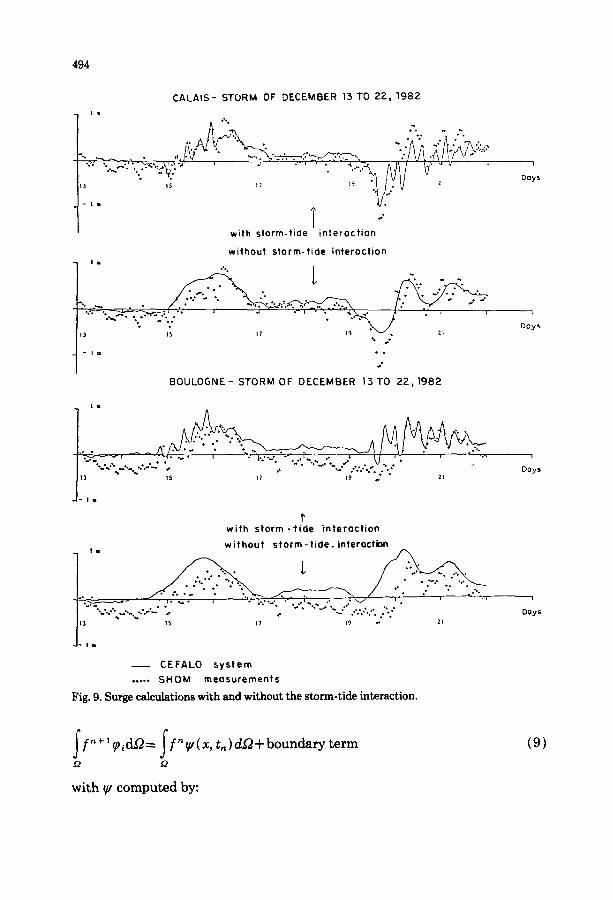
simulation: these oscillations result from difference in tide phases, and they are specially felt in the areas where strong current and small depth (vicinity of the Dover Straits) emphasize flow non-linearities and lead to a significant interaction between tide and storm surge. M2 tide has then been introduced and calibrated on the same domain, and the December 1982 storm surge was simulated together with the tide. First results exhibit significant improvement, revealing clearly the tide period oscillations (Fig. 9); further improvements are expected from a better tidal simulation (for example by considering other tidal harmonic components).

This finite-element method, specially well fitted for the simulation of hydrodynamics in complex domain, due to the great flexibility of mesh and to the accurate description of the domain geometry, has proved in this case to be furthermore of reasonable cost and core memory requirements.

Future developments in numerical methods

Solving the advection term through a weak formulation of the characteristics method

The foregoing developments on the subject of modelling the advective term are carried out in order to improve the qualities of a characteristic method in reducing the parasitic problems inherent in all numerical schemes: numerical

492

Dot Line : Observed surges

Fine Line : Results from FLATHER (l.O.S.)

Thick L~ne : ~inite elementeomputat~on

I . I1 ,

0 . 8 '

O . l l :

0 -0

• . J - . •

,. : " " . . : OSTEND I _ _ , ' , : . _ ' t ~ - _ ~, I - V V ~ / ~ ' ~ . ' . : - ~ - ; \ - ~ . . ; . . 2 " ~ , , - , - _ - - : - ~ . , . . ; , .

t , , ~ , r-, , , , , ~ . , , , , , : . ~ , , ~ ~ . . ~ . _--. . . . . . .

v v

'~"_", ~ _ X l - 7 . %.., ~. , " , . N ~ . , : . _ - . ~ . , " ."

.... : " " TERSCHELL~NG 1 : .~ .~. ] . / - ~_ > . , , % .~ . . . . \ _ , . . . ~ . ~ . ' - ~ . :

;'~. . . . . "", . ., CU~\VEN

: ' t " l i ' l ' l ' , i i a i , "l ~ > g ~ i I I i I I i , - - ) . .~i / . . •

- < j , , , , , , , , , , . ~ _ ~ . . . . . , , , . . ~ & : . . . . . . . . . . . . . - -

o. BERGEN • _ ~ ~ ~ - - - ~ _~.~-~ __ _- ..._

| 4 g l i / ' l ] I S l 1 ' 3 61 1~3 ? I t 17] O/ 1~1 $1 , g a Z U I I I I * a ~ l / l l l ' l ~ 2~/ / ] 211 /7 :3 ,4111/]:J

Fig. 8a. Storm surges at continental ports.

diffusion and phase shift• This has been done at L N H by using a weak formulation of the method of characteristics. A new step was taken (Hervouet, 1985) with the use of test fu.nctions that are variable over time and in space, supported by the characteristics themselves.

During each time-step the advecting field V is assumed to be constant over the time and the value f is sought at the nodes of a grid describing the domain to be studied. The weak formulation is then written as:

t n + l

tn

(s)

Dot Line : Observed surges Fine Line : Results from FLATIIER (I.O,S.

|.i I ~ ~ " Thick Line : Finite element computation

"01 o .-~ z - J ~ - _ ~ ~~0.4 WlCK

2~ ~ l ̂ ~ " - : ~ - ~ ' • . . . . . . ~ - - . , : j~ .~: ,~--~ ~ . . . . = - . .

:'- : ~ . -."

": ' 7 ' '; ' " " ' < " ~ / " ' ~ : ' ' * ~ "~'- . . . . -~ ":":~"" '

. : :~ , , . :, . ' ~ ' ~ - - ~ : ~ - " : ~

t \ - , , , - . ~ . WALTON-ON-NAZE

" •

SOUTHEND

• ' , f , I , ' i , T , I , _ _ I * # l z l ? 3 * l ~ x l l / ? 3 ' : 6 t H z ~ 3 ' l ~ / l ~ z T ~ ' [ e / l l z ? l ' l g l t l / ~ ) ' : o I N ~ 7 ~ ' : l l l l / : ~ ' : = , H l ? ~ ' : ~ J i l x ~ J ; ~ . ' l l l T ]

Fig. 8b. Storm surges at British ports.

4 9 3

w h e r e t n and tn+l are the limits of the time-step considered and ~ is a basis function which varies over time and in space.

The basis function ~, is chosen being equal to the test function ~i at tn+l with a value of one at node number i and zero elsewhere. The basis function is computed at time tn with following principle of advecting only the nodes of the grid. The weak formulation is written after integrating eqn. (8) by parts for any node function:

494

CALAIS- STORM OF DECEMBER 13 TO 22, 1982 I rl

• . ~ - : ~ . ~ ' , , .b , ., . : - , - . . . ~ . - Y ~ , ~ V 2 , . . . . - . . . _ ~ . . ....

with slorm.tide interact ion

without storm-t ide interaction I i

. .

• " " - . ' " ' " V " " " . % . . ? 13 I m 15 17 1 9 21

BOULOGNE- STORM OF DECEMBER 15TO 2 2 , 1 9 8 2

i

Days

Days

Im

t with s t o r m - t i d e in teract ion

wi thout s t o r m - t i d e , interaction

t . ! - i " : . - : - . - . : - - - - . . . . : " : : " ' " " : : " : - " : " -

- - CEFALO system .. . . . SHOM measurements

Fig. 9. Surge calculations with and without the storm-tide interaction.

i

Days

1

Days

f["+'¢idL-2= ff"fl(x, t . ) d~2+boundary term Y2

with ~, computed by:

(9)

INITIAL CONE

4 i.i

Ill

A 495

AFTER ONE ROTATION

@ Y (m)

AFTER TWO ROTATIONS AFTER FOUR ROTAT

Fig. 10. Rotating cone test (one rotation: 32 time steps). Weak formulation, Gauss quadrature.

~ ( X , t n + l ) =@i(X) } 0_~_~_ Ot F V.V ~,=0

(10)

n

As ~ @j = 1, then Z ~j = 1 and mass of f is preserved over between times tn ] ]

and t n + 1.

The resulting properties are unconditional stability, very low damping, no phase shift and conservativity. Following results are tests of the advection by a rotating field of a Gaussian cone of value exp [ - (x ~ +y2) /2 ] using the weak formulation and the Gaussian method of quadrature (Fig. 10). Under criterion of maximum height of the cone after 1, 2, 3 or 4 cycles, weak and strong advec- tions differ clearly: the first method indicates damping of the order of 5% at the first cycle whereas the strong method yields a damping of 50%. Under criterion of mass conservation the relative precision in one step using weak formulation remains lower than 0.01%.

Uncovering and overcovering tidal areas solved by an advection operator A most useful case being studied in the marine field is the extent of the

uncovering flat area at low tide which requires calculation of the change of the

496

,o] COT

X o 2C o

Fig. 11. Breaking dam.

~ W

x

maritime domain boundary together with that of tidal currents. Near the uncovering tidal flats the specific nature of the flow changes. A measure of this nature in this particular case can be the Froude number F= V / v / ~ which determines the importance of the advective motion with regard to the propagative motion. The usual specific values of tidal or surge studies lead to negligible values of the Froude number - - about 1071. When being interested in near-shore flows however the specific value of the Froude number varies from 0.1 to 2, the larger as nearer the shore. In these places the advective transport of the water elevation and of the flow velocity is then essential in the flow motion and has to be the better modelled. It has been proved recently (Cahouet and Goutal, 1985 ) that the usual writing with variables flow Q = Vh and water depth h can not solve a trans-critical flow motion, as writing with variables velocity V and water depth h does. The difficulty with this last writing is a splitting of the continuity equation which leads to some loss of mass. The classical test of a breaking dam was made under others. Figure 11 explains the case: a dam which impounds an unmoved water reservoir at a depth value of Yo is brought from its initial position Xo into motion and reaches a constant velocity w such as water always remains under touch with the dam. The shape of the water level is a parabolic curve at any time. Over the time, these different

4 parabolic curves are hinging upon the same point xo,y= ~Yo. In this plane the Froude number has the critical value of 1.

Figure 12 shows the numerical results. Figure 13 shows the first result of an uncovering beach with sloping bottom.

Mixing properties of fluid

Current application: momentum diffusion in the servicing harbour of the Euroroute road link

As mentioned previously, the integration over the depth of the non-linear momentum equation leads to an additional transfer of momentum. This effect of dispersion on hydrodynamics, generally considered through a Fick's law by analogy with molecular diffusion, is particularly perceptible when current pre-

o.

"~-÷x,i& -% ,%

X-QXIS

o o S~ARTING TI~ ~, . . . . -~ ~FT~R 0.SS x-------~ RFTER 1.255 + ......... + BFT~-R 25

Fig. 12. Test of a breaking dam (time step: 0.01 s).

c~

~ A ~ ~

~ x ~ x-w-x-x ~c .'c ~ .x ~ x . y ~ x "

-7. ~ ..

1.0 5.5 iO.O ! .5 Ig.O 23.5 2 .O 32.5 37.0 4 .S 46.0

X-RXIS

o o SLOPPING 80TTOM .... -~ AFTER 20S

x-------x AFTCR SOS ÷ ......... + AFTZR 70S

Fig. 13. Test o f a_, uncovering beach wi th a sloping bottom (time-step: I s).

497

498

°I o

o

~D

o

~ ~ 7 ~ ~ ~ - -

.~ o

~ ~ ~ 7 ~ - ~ ~ i : - ~ ~ : ' ~ ~ ~ ~ _ ~ ~ ~ _ - ~ - 7 ~ ~ ' ~ ~ - - - ~

~ ~ - ~ '~ .~.

499

sents strong spatial variability, i.e. for example in the case of small scale complex geometry: in that way flow pattern in harbours or in the vicinity of artificial structures is significantly affected by this dispersion. For such restricted areas, time and space discretization steps are small enough to bring numerical diffusion at a level far lower than the dispersion one; sensitivity analysis has to be performed around reasonable values of the dispersion coefficient, in order to appraise the range of accuracy of the numerical simulation. As an example, hydrodynamics has been computed in the vicinity of the planned servicing harbour of the Euroroute road link, for two values of the dispersion coefficient: 0.5 m 2 s -1 and5 m 2 s -1 (Fig. 14).

Adopting (too) large a value of this coefficient has the obvious effect of reducing the extent of flow separation and the eddy velocities; differences between both computations are restricted to the areas of separated flows.

However, some developments (Benque, 1980) show that the unknown term in the momentum equation due to non uniform values of the velocity over the depth appears equivalent not to a diffusion term - - like in the concentration equation - - but to an advective term.

Future developments: turbulence modelling in mean velocity equation The usual length scale of turbulent motion is very far smaller than the scale

of the flow domain and this type of motion can not be computed in three- dimensional cases, the current capacity of present-day computers being still not wide enough. Therefore, the marine flow modelling at LNH emphasizes the development of turbulent behaviour laws more especially where turbulent motion is generated, that means near bottom and shores, following the eddy- viscosity concept - - assuming that turbulent stresses V~ V~ are proportional to the mean-velocity gradients. The proportionality value vt appearing in such an expression is the turbulent or eddy viscosity. V} denotes the fluctuation of the velocity Vi around the mean value over the time tTi.

Future developments among others will be different kinds of relations defin- ing the mixing length l~ in a horizontal depth-integrated 2D model using a finite element method. One can indeed suggest to relate l~ to the distance to the wall, or to the mean-velocity profile, or to the grid mesh size as Smagorin- sky (1963) does. In any case such a kind of law enables to take into account the effect of large scale turbulent eddies upon the mean flow - - through the turbulent correlations Vi V i ~ of the same range of magnitude as /~ scale eddies. In order to take into account processes of convective or diffusive transport of turbulence, a k-e model is currently developed at LNH (Goussebaile et al., 1985) in a three-dimensional model using a finite-element method and will be in the near future inserted in its depth-integrated version in a 2D model.

The following experiment is carried out at the present time at LNH with the aim of better understanding and modelling the big vortex shedding behind a hindrance cross a flow, like groynes in harbour for instance.

500

i n l e t f \ a I " l i

, / tOm

Fig. 15. Rectangular hindrance cross a steady flow.

.7 ,7,

Figure 15 presents the reduced scale model which has been used. Many tests have been carried out in order to get some information about the influence of the hydraulics and geometrical parameters on the sizes and frequency of the vortex shedding. Thus different water depths have been chosen between 0.10 m and 0.40 m, different flows between 0.05 m 3 s - 1 and 0.50 m 3 s- 1 with different shapes of the obstacle, and over a smooth or rough bottom of the flume.

A data collection will be built with two kinds of measurements. Measure- ments of mean values describing the vortex shedding behind the hindrance have already been carried out at the present time using chronophotographs of floating balls as is shown on Fig. 16. Measurements of velocity fluctuations and turbulent stresses will be carried out with bidirectional hot-film anemo- meters. This data collection will then be used in order to calibrate a 2D turbulence model.

The numerical simulation of one of the experiments has already been made with a turbulence modelling of second order closure, meaning a k-e model with boundary conditions ensuring a logarithmic profile for the mean horizontal velocity very near the boundaries through friction at the walls. Figure 17 represents the mesh grid of finite-difference type used for the computations and Fig. 18 the velocity field obtained. The mean sizes of the eddy behind the groyne is well simulated but the k-e model used for turbulence modelling has the same effect upon the unstationary motion as a low pass frequency filter.

USE OF TIDAL CURRENT COMPUTATIONS IN CURRENT APPLICATIONS

Thermal impact sudies

A frequent problem at EDF is the study of heat dilution in the vicinity of power stations which implies an accurate measurement or simulation of cur-

at time at time at time

t o t o + 20 s t o + 40 s p O, lm/s

501

:÷,

Fig. 16. Vortex shedding behind a groyne placed cross a steady flow (water depth: 20 cm; flow discharge: O. 125 m 3 s - l ) .

502

>., m :lT~rlTtIlltlltltlJlflfll ~ 111111111111111111111111 ~. ll~iiilllllllillllllllItl ! -II~iiJlllllIllllllllllfl

h~;Jl!i[[ifl[ll[llll iI::!ll[[[lll[[l[lllll][I i L ~ L [ I t f [ J l l { [ ] l l l l l l l l [ ] [ : ! f l ] ] i l l ] H l ] [ l l l l l l

4~ i i ] : ! [ i i I t l ; [ l l l l [ I f f [ l [

" l~ili!ii!iiii? ~- - !i ? 9°S

I I H l l f t f l t l l l t l l I I I l i l i l i i l t i f l i t i l l I I I l l l i l l l l t l l t i l i l i i I I l l t i l l t l i i } l l l l i 1 i i

11111111 l l l l l l l l l [ I i l l l l l i i l l i l l i l [ l l l l I l i I I L I I i t l l J I I I I I l I l l i J l l t 1 I I [ l l l L I t I r ~ 1 I i I L I I 1 ~ L I t t z l l l l r l l [ i T I [ J I

~!iii?.!!!iiii i i i i i ~ i ] i i ] i ~ ! ] ! ! ~ ! ! f [ , ! ~

1 9 . 5

X [m) 2S.S

Fig. 17. Rectangular hindrance cross a steady flow. Mesh grid of the computation.

! ?.

9 .5 19.5 :~a.5 X (m}

m

v;"

~ o

~ ! ? ? ! i ! i i i i i i i i ! i ! i i ! - i ! 4 -" : . . . . . " - -- 9.5 19.S 29.S

X (m)

Fig. 18. Rectangular hindrance cross a steady flow. Stream lines and velocity field.

rents along the coasts (Fig. 19). Two kinds of such simulations are usually done: one of them is a three-dimensional modelling including a turbulence model closure for the stresses connecting the velocity fluctuations and the temperature fluctuations V'~T', V~T', W' T'; the other one is a depth-integrated version of the previous one including a dispersion term, which models the influence upon the mean value of temperature of the fluctuations of velocity and

503

Fig. 19. Location of some EDF power plants and results of heat dilution studies.

h h

temperature over the depth y V; T", f V'C T", which is much bigger than the 0 0

local turbulent diffusion. Under some assumptions (Warluzel and Benque, 1978) it has been proven

that the dispersion term in the mean temperature can be writ ten as a diffusion term like V- (K: V T) with K being a symmetric positive quadratic form depending on velocity disparities over the vertical direction and on the turbulent viscosity through the dimensionless expression:

1 z ' z '

I f Kij= V'[(u)du V;(v)dv 0 0 0

(11)

504

TABLE 1

Estimated value of cross dispersion coefficient K~2 (m 2 s- 1 )

Depth Untidal s e a Tidal sea

Chezy = 50 Chezy = 70 Chezy-- 50 Chezy-- 70

20 m 0.012 0.15 0.04 0.5 40 m 0.15 1.3 0.6 4.0

Both tidal and untidal seas were tested with classical expression of turbulent viscosity d t. For similar flows it is noticeable tha t a tidal sea increases the cross dispersion K22 with regard to a steady current, because of turbulent viscosity decreasing to zero with the current at slack periods (Table 1). Assuming a Prandtl number of one - - where Pr = v t / d t ~ some calculations were made and lead to the figures of Table 1 (Warluzel et al., 1978).

The equation for the depth-averaged temperature is:

Oh___T cOt ~-V.(VTh) =V. ( K V T ) - A - ( T - T E ) (12) c.

This equation is solved using a finite-difference method and an algorithm based upon a splitting method. The boundary conditions are chosen as follows: OT/On=O near a shore, T= TEquilibriu m o n open sea boundaries far from the outfall, and ±rP outletn+ 1 __ ~infalI = known value at the outlet.

The last term in the eqn. (12) specifies exchanges with the atmosphere. The value of the dispersion square tensor appears as very important for example on the case of Paluel. The estimated value (cf above ) is the following one:

K n =60 m 2 s -1 K12 = - 7 m 2 s -~ K22 =2 m 2 S - 1

where 1 denotes the direction parallel to the shore and 2 the cross direction. Figure 20 shows the results of two calculations, one of them being made with this estimated value and the other with isotropic values:

K1~--5 m 2 s -1 K12=0 m 2 s -1 K22=5 m 2 s -1

We can observe a totally different shape of the heated flows and a sensible decrease of the heated surface: a temperature excess greater than 1 °C covers about 11 km 2 in the first case and 20 km 2 in the second case (average values over the tidal period).

A three-dimensional computation is needed, however, in order to represent

505

6h before HT 0.25

3h before HT

High Tide

0.25

0.25 ~ " t ~ ~ 0 . 5 %,, I

rDxx : 5 m2/s . . . . | o . = 5

Loxy = Ore2/,

DDDXX : 60m2/s yy : 2m2 /s xy =-7 m 2/s

0.25

Oegres Celsius

3h after HT 0,25

lO.krn

Fig. 20. Influence of the dispersion coefficients over the tide (power plant of Paluel).

the buoyancy effects on the fluid when the vertical mixing is not strong enough to force the vertical homogenization of water. The buoyancy effect on turbulent diffusion is considered through the Richardson number:

g(OT/Oz) (13)

Results have been obtained with this model for the Gravelines power plant. Figure 21 shows some results over the tide for both horizontal and vertical current values and temperature profiles. Figure 22 is a comparison between measurements and calculations at one point and over the time.

506

iii!iii i iiiii iiiiiiiii ,,-

__ : : . . . . . . . . : ~

ii!iii!!iiii!!i ' !iiiiiii!iiiii!iliiiiii h iiiiiiiiiiiiii!! ept

z(~t, i

° I :~~'-~1_ I -20 I ~ / s

i i i ~ J b , ; , , ~ , - - , i ZSOo 3 o 0 0 : 3 5 o o 4 o o o m

a : J • z o

z ( . )

.,o}~.jj_~g__= _ ~ _

Z500 3000 3S00 m

Fig. 21. Three-dimensional heat dilution computation at Gravelines power plant. Velocity field and temperature excess at HW at different horizontal and vertical planes.

Sedimentation studies

Bed-load transport modelling Marine sediment motion depends both on their specific properties and on

the stress exerted by the surrounding flow. The shear stress on the bed can be derived from the determination of velocities close to the bed ( for example by three-dimensional modelling or from the depth-averaged velocity, water depth and friction coefficient). As sedimentation time scale is far longer than hydrodynamics one, morphological evolution can be determined after flow has been computed over a whole tide, without any short range coupling. Once hydrodynamic conditions are known, bed-load transport can be computed through empirical formula at each time step of the tide, leading then to the bed evolution by applying the continuity equation for the sediment:

v-2-~ +V .T=O with ~=bed elevation (14) Ot

507

~LOOO EBB FLOOD HT I ~T I HT

~" I ~ ' '

I I . I l l

E ~ . r

"_,

Time (s) (relO~qld to HT)

J ~'~ ~ top ~" x\ ~ ~ I/4 depth

. . . . ~ I . , .~_-- I/2 depth ~__J B7 ---~_~___ ~ . ~ - - ~ • top (Znd flood)

HT

D O L.

O. E

LT HT

I I I I I I I l l I l l

Time ( s ) ( r e l a t e d f o HT} .Jo'

POIIIT BT~(June 81)

Fig. 22. Temperature excess over the tide at Gravelines power plant. Comparison between computations and measurements.

Specific problem in bed-load transport modelling

Long-term simulation. A major problem when simulating morphological evolution is the time length of the simulation, compared with the elementary du- ration of the tide. Both the computation over a great number of tides and the continuous reaction of the bed evolution on the flow characteristics seem then to involve very heavy calculation costs. Fortunately, the difference between hydrodynamic and sedimentologic time scales allows some schematizations:

508

(a) Within the tide the bed evolution is very small and this evolution is almost identical on a few tides. It is then possible to extend to a group of tides the results obtained for one of them, or to lengthen the sedimentologic tide, just as it is made on scale models (a lengthened tide represents then several normal tides).

(b) The effect of morphological changes on flow modification is considered through schematic adjustment of the velocities, based on the flow discharge conservation (ensuring then the flow conservativity) in both direction and intensity, when this evolution is small compared with the water height. When the bed evolution becomes significant enough to induce an appreciable modification of the flow direction, a new complete hydrodynamic computation is then performed; more accurate tide filtering is now in progress.

Limiting factors of modelling accuracy. Accuracy of bed load transport simulation is limited by:

(a) The scattering of solid transport computed from the various formulas, even in their common validity field;

(b) the sharp aspect of the relation between instantaneous flow and morphological evolution, given that: (1) instantaneous solid discharge varies very quickly with respect to current velocity and friction coefficient; (2) net transport over the tide comes from the balance between two opposed components (flood and ebb transport) which can be of the same order of magnitude; (3) morphological changes are not directly connected to transport, but to its spatial derivative, which is of a lower order of accuracy.

So it appears obvious that an excellent accuracy is needed in hydraulic simulation to expect a satisfying quality of sedimentologic results, at least when flow gradients are weak. In that way, in case of natural evolution, when the bed is in dynamic equilibrium with regards to flow, quantitative simulation of morphological changes is rather uncertain; only calibration on past evolutions can ensure the ability of the model to predict future evolution, and gives then its range of accuracy. On the other hand when the flow pat tern is strongly modified by work creation, sedimentological changes, coming from first order effect, are more rapid and can more easily be predicted.

Application to the protection of River Canche Estuary The results of tidal simulation in River Canche estuary, described previ-

ously, have been used to evaluate the morphological changes with and without protection works. At first, a calibration phase consisted in running the bed- load transport model over one year in present state, using successively three different bed-load formulas (Meyer - Peter - Miiller; Engelund - Hansen; Bijker: Fig. 23). Results were compared to the existing data on the past evolutions, the conclusion of these comparisons was that: (a) the first two formulas give

o) MEYER-PETER b) EN GELUND-HANSEN

• .'i ~

c) BIJKER

509

I i I I 0 1 2 3km 0 50 100 150 crn

Fig. 23. River Canche estuary. Computed erosions using different bed-load transport formulae. Beach under erosion

j Area to be

j pro o,.d

/

/

/

~ J i

(not measured)

I N

Computed erosion over one year Measured erosion between

(1979 -1980 ) 1966 and 1979 , ,

1 2 3 km

Regions of erosion

Regions of strong erosion

Fig. 24. River Canche estuary. Comparison between measured and computed erosion.

similar global evolutions; and (b) the third one, including wave effect, leads to rather different results, closer to field data in the area to be protected.

In this area the qualitative agreement between observed and computed evolutions was felt to be good enough (Fig. 24) to think the model able to assess

510

~iiiiiii

Acc re t i on

0 - 0 ,5m

0 ,5 - lm

> lm

i!iiiii~: .:"

PRESENT STATE

Eros ion

o - O , 5 m

~ 0.5 - lm

U > lm

WITH GROINS

Fig. 25. River Canche estuary. Computed bed evolution over 5 years.

the effect of the protection works, given that the reproduction of natural evolutions is less easy and less accurate than the sedimentological impact of works.

Afterwards the bed evolution was computed over 5 years, with and without protection works (2 groynes 500 m long), in order to evaluate by difference their specific effect: it was found that the main result was the stopping of the erosion process along the more threatened beach (Fig. 25).

CHOICES AND PROBLEMS IN SEA MODELLING

The increase of computer power has developed the use of numerical models in hydraulics and fluid dynamics problems. Three main topics of the concept of a numerical model have to be pointed out. The first of them is the choice of the best mathematical model with regard to the study to be done. The second point is the development of efficient numerical methods which have to be as accurate as possible and have to limit the errors arising from discretization, i.e. numerical skew, damping, phase shift, boundary approximation. The last problem is the calibration of the parameters of the model which is reliable only after an experimental validation against measurements of the phenomenon.

Following these ideas the current developments at LNH lead to continuous improvement in the results of the numerical models. However, the lack of accuracy of numerical schemes remains connected with the power of the computers i.e. the cost of the computations and memory requirements.

A double effort has to be done in the future at LNH, scientific on one hand

511

and algorithmic on the other hand. The scientific effort mainly consists of a constant research in understanding and modelling such behaviour laws as turbulence, bed-load transport, boundary layers, residual currents or subgrid scale phenomenon.

The algorithmic effort has to be developed in order to provide reliable numerical tools which do not introduce any artificial numerical filtering.

REFERENCES

Benque, J.P., 1980. An attempt to generalize the shallow water equations. EDF Report HE41/80.14. Benque, J.P. and Nihoul, J.C., 1982. Modelling of hydrodynamic mechanisms of pollutant prop-

agation in coastal zones. IAEA - TECDOC - 274. Benque, J.P., Daubert, O., Goussebaile, J. and Hauguel, A., 1984. Splitting up techniques for

computations of industrial flows. EDF Report HE41/84.09. Benque, J.P., Cunge, J., Feuillet, J. and Hauguel, A., 1981. A new method for tidal current com-

putation. EDF Report HE41/81.26. Cahouet, J. and Goutal, N., 1985. Mod~lisation des ~quations de Saint-Venant en rggime tran-

scritique: applications aux bancs d~couvrants. EDF Report HE41/85.28. Esposito, P., Hauguel, A. and Latteux, B., 1984. A finite element method for storm surge and tidal

computation. EDF Report HE42/84.08. Flather, R.A., 1976. Practical aspects of the use of numerical models for surge prediction. IOS

Report Nr 30. Goussebaile, J., Jacomy, A., Hauguel, A. and Gr6goire, J.P., 1985. A finite element algorithm for

turbulent flow processing a k-e model. EDF Report HE41/85.12. Hervouet, J.M., 1985. Application of the method of characteristics in their weak formulation to

solving two-dimensional advection equations on mesh grids. EDF Report HE41/85.22. Labadie, G., Dalsecco, S. and Latteux, B., 1982. P~solution des ~quations de Saint-Venant par

une mSthode d'~l~ments finis. EDF Report HE/41/82.15. Lomer, J.F., 1978. La d~rive en mers ~ marSes. Thesis of the University Pierre et Marie Curie,

Paris VI. Marchuk, G.I. and Yanenko, N.N., 1966. The application of the splitting-up method { fractional

steps) to problems of mathematical physics except from some problems of numerical and applied mathematics. Novosibirsk.

Smagorinsky, J., 1963. General circulation experiments with the primitive equations. I. The basic experiments. Mon. Weather Rev.,: 91-99.

Warluzel, A. and Benque, J.P., 1978. Dispersion dans une mer ~ mar~e. EDF Report HE/041/78/09.

Documents

Tidal sea mathematical modelling: Current applications and future developments