Embed Size (px)
Citation preview
1
DATABASE MANAGEMENT SYSTEMS
Tibor Radványi PhD
It was made with support of the TÁMOP-4.1.2-08/1/A-2009-0038

2
INTRODUCTION ................................................................................................................................................ 6
BASIC ELEMENTS .............................................................................................................................................. 8
DATA AND INFORMATION ......................................................................................................................................... 8
DATABASE ............................................................................................................................................................. 9
DATABASE MANAGEMENT SYSTEM (DBMS) .............................................................................................................. 10
Local database ............................................................................................................................................. 12
File – server architecture ............................................................................................................................. 13
Client – server architecture .......................................................................................................................... 14
Multi-Tier ..................................................................................................................................................... 17
Thin client .................................................................................................................................................... 18
BASIC STRUCTURES ................................................................................................................................................ 18
IMPROVEMENT OF DATA MODELS ................................................................................................................. 20
HIERARCHICAL ...................................................................................................................................................... 20
NETWORK DATA MODEL ........................................................................................................................................ 21
RELATIONAL ......................................................................................................................................................... 22
DATABASE PLANNING AND ITS CONTRIVANCES ............................................................................................. 28
MAIN STEPS OF DATABASE DESIGNING ....................................................................................................................... 29
NORMALISATION ................................................................................................................................................... 31
Normal Forms: ............................................................................................................................................. 31
Dependences................................................................................................................................................ 32
Relation key ................................................................................................................................................. 33
DATA MODEL MISTAKES .......................................................................................................................................... 35
STOPPING THE REDUNDANCY ................................................................................................................................... 37
Normal forms: .............................................................................................................................................. 37
Third normal form: ...................................................................................................................................... 40
Boyce/Codd normal form (BCNF) ................................................................................................................. 41
THE RELATION’S THIRD NORMAL FORM AND THE DECOMPOSITION OF THE BOYCE/CODD NORMAL FORM ................................ 42
Fourth normal form (4NF)............................................................................................................................ 42
Fifth normal form (5NF) ............................................................................................................................... 43
PHYSICAL DESIGNING .............................................................................................................................................. 43
SUPPORTING THE DESIGN WITH SOFTWARE ................................................................................................................. 44
Designing requirements: .............................................................................................................................. 44
Design of the database, the database tables and their fields: .................................................................... 44
THE MYSQL WORKBENCH ..................................................................................................................................... 45
OPERATIONS OF RELATIONAL ALGEBRA ...................................................................................................................... 50
TASKS ................................................................................................................................................................. 55

3
LANGUAGE REFERENCE OF SQL ...................................................................................................................... 58
ELEMENTS OF DDL ................................................................................................................................................ 58
Create schemes, the creat ........................................................................................................................... 58
Changed the schema elements, the alter .................................................................................................... 60
.CONSTRAINT integrity constraint application ............................................................................................ 61
.ELEMENTS OF THE DML ........................................................................................................................................ 62
.New data entries, insert the command ...................................................................................................... 62
. Create table based on another table ......................................................................................................... 63
.Change data,the update ............................................................................................................................. 63
.Delete data, the delete ............................................................................................................................... 63
.RIGHTS AND USER MANAGEMENT, THE DCL .............................................................................................................. 64
.Privileges contribute ................................................................................................................................... 65
.Roles(ROLE) ................................................................................................................................................. 66
QUERIES AND THE QL ............................................................................................................................................ 68
The base of the select command ................................................................................................................. 68
Counted fields and aggregate functions ...................................................................................................... 69
Filters and the where clause ........................................................................................................................ 71
Aggregation queries, the usage of group by and having, and arrangement............................................... 75
Connecting Tables ........................................................................................................................................ 77
Embedded queries ....................................................................................................................................... 81
TASKS ................................................................................................................................................................. 84
VIEWS AND INDEXES .................................................................................................................................... 102
VIEW ................................................................................................................................................................ 102
Modifiable view tables ............................................................................................................................... 103
Structural terms of modifiability: ............................................................................................................... 103
Deleting a view table ................................................................................................................................. 104
Consequently, let’s look through the advantages of view tables: ............................................................. 104
INDEXES ............................................................................................................................................................ 104
Sparse indexes ........................................................................................................................................... 104
Searching ................................................................................................................................................... 105
Insertion ..................................................................................................................................................... 105
Deleting ..................................................................................................................................................... 105
Modifying: ................................................................................................................................................. 106
B*-trees as multilevel sparse indexes ........................................................................................................ 106
Searching: .................................................................................................................................................. 107
Insertion: .................................................................................................................................................... 107
Delete: ....................................................................................................................................................... 107
4
Modification: ............................................................................................................................................. 107
DENSE INDEXES: .................................................................................................................................................. 107
CONSTRAINTS, INTEGRITY RULES, TRIGGERS ................................................................................................ 110
Keys ............................................................................................................................................................ 110
Referential integrity constraint .................................................................................................................. 112
Constraints for attribute values ................................................................................................................. 113
Standalone assertions ................................................................................................................................ 113
Modifying constraints ................................................................................................................................ 114
TRIGGERS: (ORACLE 10G) ............................................................................................................................. 116
Triggers could triggered by: ....................................................................................................................... 116
We use them in the following cases: ......................................................................................................... 116
Row-level trigger: ...................................................................................................................................... 117
Statement-level trigger .............................................................................................................................. 117
Before and After triggers: .......................................................................................................................... 117
Instead of trigger ....................................................................................................................................... 119
System triggers .......................................................................................................................................... 119
Creating Triggers ....................................................................................................................................... 119
How triggers work: .................................................................................................................................... 120
TASKS ............................................................................................................................................................... 121
BASICS OF PL/SQL ........................................................................................................................................ 125
BASIC ELEMENTS OF PL/SQL ................................................................................................................................. 125
Character set ............................................................................................................................................. 125
Lexical units ............................................................................................................................................... 125
Symbolic names ......................................................................................................................................... 126
Reserved words .......................................................................................................................................... 127
Identifiers with quotation marks: .............................................................................................................. 127
Literals ....................................................................................................................................................... 127
Label .......................................................................................................................................................... 128
Nominated constants ................................................................................................................................ 128
Variable ..................................................................................................................................................... 128
Simple and complex types ......................................................................................................................... 129
NUMBER type ............................................................................................................................................ 130
Character family ........................................................................................................................................ 131
ROWID, UROWID Types ............................................................................................................................. 132
Date/interval types .................................................................................................................................... 132
Logical type ................................................................................................................................................ 133

5
Record type ................................................................................................................................................ 133
PROGRAMMING STRUCTURES ................................................................................................................................ 135
The CASE statement ................................................................................................................................... 136
Loops .......................................................................................................................................................... 138
Base loop ................................................................................................................................................... 138
While loop .................................................................................................................................................. 139
FOR loop .................................................................................................................................................... 140
The EXIT statement .................................................................................................................................... 141
MIXED TASKS ............................................................................................................................................... 142

6
Introduction
Data and information. These two things became leading factors through the past 50 years and
during the 20th and 21th century as these concepts play a significant part of our everyday life.
As in our society the role of the information is being valorised, we are getting more and more
pieces of information. We are continuously bombed with information from the outside world:
we get the news from the television, radio, and newspapers and we are being informed about
the latest happenings from the fellow human beings all day long. Of course we try to sort out
and concentrate on the most important ones from the quarry of information. It is especially
relevant as it seems to be impossible to memorize all the pieces of information. Sometimes we
simply can’t memorize or wouldn’t like to memorize them. Accordingly we have to find
another way of recording information instead of keeping them in mind. As the old Latin tag
has it - verba volant, scripta manent – spoken words fly away, written ones remain. In
addition everybody has a share in reaching the recorded information in a fast and easy way.
Information equals power as the proverb says. And actually it is right. I’m sure that explaining
the importance of keeping our bank card’s details at an appropriate place is not necessary.
That’s why it would be advisable to find the safest way of storing information. We should
find the best method to be able to reach them in an easy, simple, and fast way.
So, we can easily admit that students should acquire this bunch of learning during their
primary and secondary school studies (and of course during their lives). According to the
National Curriculum’s assumption in the field of developments, our educators should pay
more attention on teaching the basic computer skills. Indeed, in this field the number of the
lessons was raised. Because of the above-mentioned reasons cognition of databases and
database management systems play a particularly important role. Moreover, it is useful for
students (and of course for everyone) to keep up with the changes, aims, and reformations of
the developments of informatics. Furthermore the number of the people working with
informatics and the level of their qualification is rising mightily. Let’s keep up with both
aspects as the claim to well-qualified professionals is getting higher and higher.
One of the computer science’s main characteristics is the following: more and more users use
data, stored on more and more computers. Ready and applied software systems have to deal
with always rising amount of data. In our everyday life we meet the usage of computer
information systems more and more often. Computer information systems are frequently used

7
in factories to control different operations like production, finance, the staff’s work, storage,
and economization. We can mention some fields of usage in every part of our lives:
Commercialism: registration of the stock
Civil service: taxation
Hygiene: registration of the sick
Transport: system of reservations, timetables
Engineering: designer systems
Education: student’s registration
All of them have a common feature: they all maintain a large data set, there are complicated
relations between the data items, and these data sets have to be retained for a long period of
time.
Of course there are other main features of these systems, but there are requirements which
have to be fulfilled:
Maintaining a large amount of data
Supporting more users to be able to access at the same time
Keeping integrity
Protection
Effective software development

8
Basic Elements
The first databases were established from file control services in the early ‘60s. They were
extensive and expensive program systems which were run on large sized computers. The first
significant usage fields of them were the systems in which huge pieces of data were stored,
including numerous queries and modifies. For example: Companies’ card indexes, banks’
systems, flight booking systems.
Since 1970, the publication of Ted Codd’s article, in which he suggested that the database
management systems should present the data in tables for the user, database management
systems have appreciably changed.
The difference to the previously used systems is that in the relational system the user doesn’t
have to deal with the structure of data storage, as queries can be expressed with such a high-
level language, that its usage highly increases the efficiency of database programmers.
In this model there are no highlighted data, so the features registered about the items of the set
are equal. This way the system can be used more flexible as the search strings can be drawn
optionally.
The first corporation, selling both database systems supporting databases before relational
models and systems supporting relational models, was IBM.
Lately database systems based on relational models are as current computer tools as word
processors or spreadsheet programmes used to be.
Data and Information
Information plays the main role in our world. If we wanted to feature our society with an
attributive structure, it would be evident to name it information society. I wonder if we clearly
know what information means. A totally acceptable definition hasn’t been found yet, although
every speciality dealing with information has formed its entity, featured with marks being
important in their point of view; named information.
Information is the experienced, sensed, and understood data which is useful and new for the
taker, who construes it according to their previous store of learning.

9
Data means the appearance of a fact which we can record, store, modify, and send on. The
conception of data is not an exact idea. In the point of view of database designing, data is the
meaningless series of signs from which we can earn information after processing.
Although till then it is just a meaningless series of signs. If we collect some data and we store
them in a given place including the connections between them, we have created a database:
E.g.: the medical cards of the sick, details of cars at the police, notes of a telephone directory.
Database
A database is the whole bulk of integrated and logically connected pieces of information; the
system of data and connections between them; stored abreast. To be able to work with our
database effectively deliberate designing is essetial.
The concept of database system consists of the databases, the computer resources, moreover,
in a wider sense, the database-administrators, who are the ones who put through the designing
and programming of the database.
10
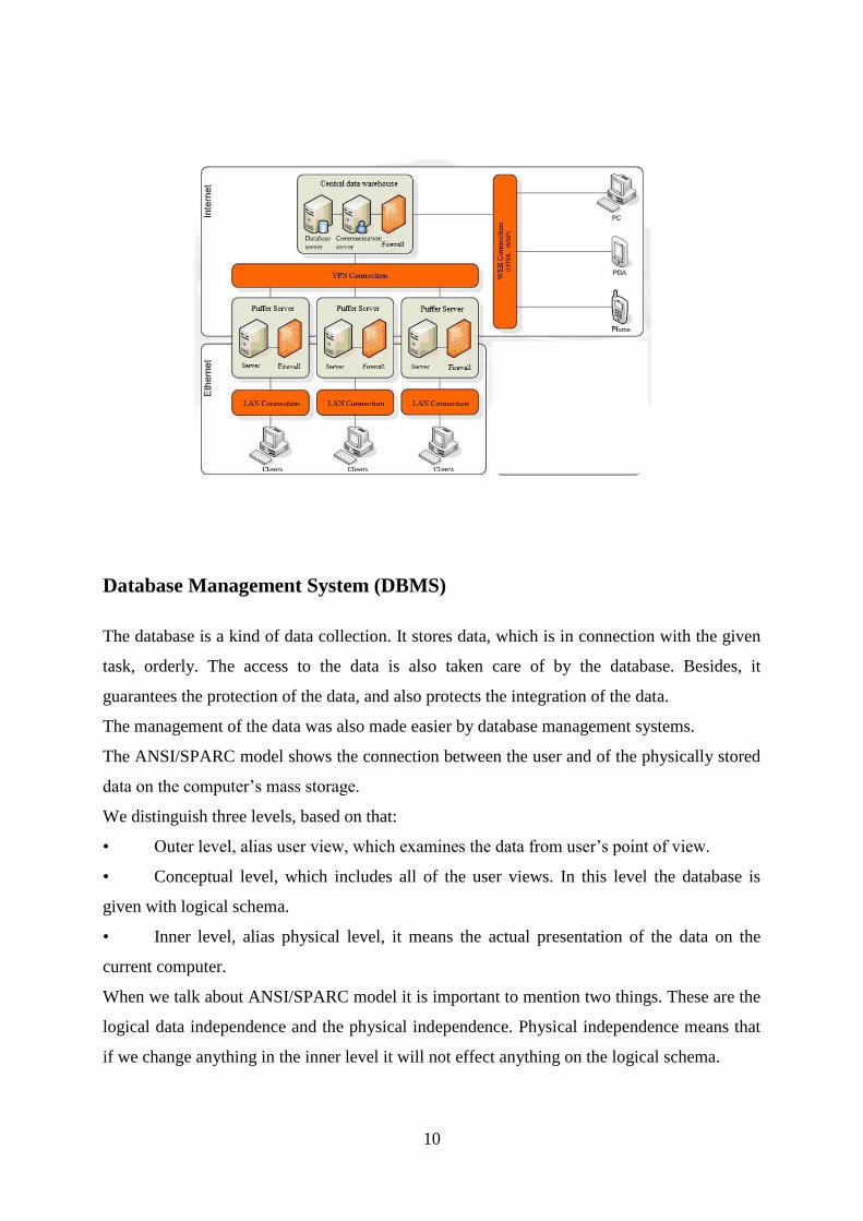
Database Management System (DBMS)
The database is a kind of data collection. It stores data, which is in connection with the given
task, orderly. The access to the data is also taken care of by the database. Besides, it
guarantees the protection of the data, and also protects the integration of the data.
The management of the data was also made easier by database management systems.
The ANSI/SPARC model shows the connection between the user and of the physically stored
data on the computer’s mass storage.
We distinguish three levels, based on that:
• Outer level, alias user view, which examines the data from user’s point of view.
• Conceptual level, which includes all of the user views. In this level the database is
given with logical schema.
• Inner level, alias physical level, it means the actual presentation of the data on the
current computer.
When we talk about ANSI/SPARC model it is important to mention two things. These are the
logical data independence and the physical independence. Physical independence means that
if we change anything in the inner level it will not effect anything on the logical schema.

11
So, we will not have to perform changes on them. If any changes occur in the storage of data
it will have no effect on the upper levels. The logical data independence is data independence
between outer level and conceptual level.
Those program systems which are responsible for guaranteeing access to the database are
called database management systems. Furthermore, the database management system takes
care of the tasks of the inner maintenance of the database such as
• Create database
• Defining the content of the database
• Data storage
• Querying data
• Data protection
• Data encryption
• Access rights management
• Physical organization of the data structure
We must keep in mind how the architecture of the database has changed. Furthermore, it is
also important how we can put these together. It is very important for the programmers,
because they are in a situation where they have to choose what they are going to working with
after they have got the order. Because, those are not good programmers or software
developers who can only use one database management system, or those who can write
programs only in one programming language. That is the expectation of an elementary school.
If you get a task it is good if you can decide which route is the one you have to start. What
database manager you should use and in which programming language you are going to write
your program. Of course, one could not say that know all of the existing programming
languages by heart. We will talk about two or three of them. But everybody knows who have
tried to make web pages that it might not be a good idea to start a webpage development for
example with an aspx.net. In one hand, it is possible in the case of a bigger task that aspx.net
is good. On the other hand, one could possibly do a smaller task with html code without
putting any dynamism in it, or maybe in php the things could be done easier. These are
specific things. Returning to the database architectures, now the question is in which
environment certain database managers can do good performance. Because, it is not true that
every database manager can satisfy our needs in all environments.

12
Local database
The first such architectural level is the local database: these are the “best”. It contains a
computer, a database, a user, nobody has any problem. The story started sometime around
1980s. Database managers have appeared in the computers. It was the world of the dBase,
which was based on the Dos. (From the beginning, DOS did not allow multi users and to run
on more paths.) Back then there were no such problems as web collusion or concurrent
access. Such database were dBase 3, 4, 5, the developed version of this were Paradox 4, 5, 7,
which had more stable data table management, but in return we have got a more damageable
index table. The following things were true for all of them: one database - one file; one index
- one file; one descriptor table - one file; one check term for a table – one file. If we had a
database with 100 tables then there was created 100 files in a directory. These were managed
by a database management engine. It worked on file levels, moved bytes and managed blocks.
As it worked on file level it was damageable. There were a lot of files. So, there were already
a big possibility of damage and big possibility of delete on the level of the operation system.
If there was a power shortage, it was necessary to call the programmer, because the whole
system has turned upside down. Something for something. I always say that these are
dangerous systems, especially, if we do not use them in local database system. Nowadays, it
would be very hard to use local database. The MS Access is also belonging to there. It is only
more modern, because of the fact that all of the tools, data and descriptive tools are stored in
the same file. From there it knows it knows the same as Paradox or dBase. It could become
very damageable if we want to use under bigger stress. They are perfect for teaching (ECDL,
for final examination). The LibreOffice also has the Base database. That is similar to Access.
It is also free, and it is good for familiarization and teaching. These database managers have
limits. In a traffic table the numbers of records are continuously growing. It can easily reach
the quantity of 100000. It may seem to be more, however if somebody write a system that is
also being used, it turns out to be few. One could not say that up to 100000 it works well, but
at 100001 the whole system fall apart. It works well two to three hundred-thousand, but after
it more and more error occurs. The system is start slowing down and index damages are
coming up. So, the efficiency of the local, file-based systems has the volume of 100000. If we
know that and if we know the kind of work they want to give us then it is not a problem to use
them. if we have to make a database for Marika’s flower shop where she would put her data.
For example, she wants to store that she has got 10 tulips and 30 roses and that she has sold 9

13
tulips and 34 roses, and nothing more. In this case the Access is more than enough for her.
Don’t try to convince her that she needs Oracle.
File – server architecture
Of course, the world has developed. There is cable so we can connect any number of
computers. But the problem was that the database management was young at that time. So,
they have developed this wonderful file – server architecture. I have to mention it in
parentheses that although the use of the Novell server is not exclusive, but its best time was
then. That hasn’t been so long, about 15 years. But in the information technology that had
been a long time. They were worked out very well. They were robust systems, but “file-
server”. It is already in its name that it is for to share documents and files as source of energy.
The Novell was forced to database management. They have grasped these put them under the
Novell or Windows server in shared folders, and then the operation system will grant that who
could reach them and who could not. After that, of course it had not worked, because it has no
rights to write. So, that right has to been added. But it turned out that it had worked only then
if we gave admin right to that directory. We started to share the local database files on the
network. The problems have started from here. The users wanted to modify the same record
of the same table for one occasion. The time of the problem of the concurrent access has
come. This problem had to be solved. We started to patch database managers. We made a new
programming interface for the dBase, which could say that they sequester the data table or the
whole database. it is mine and no one else’s. I work on it and when I’m finished, I will free it
and then you may also touch it. Oh, I have forgotten. I will free it tomorrow. The source of
lots of problem was the inappropriate fine granulated sequester. On top of that, it was not part
of the system. It was controlled by programmers. Despite of the fact it was used for many
years. In certain circumstances it was quite fast during the characteristic interface
programming. But, of course the reliability of it leaves much to ask for. The concept of the
consistent database that still has been locally, we can forget about that. (So, the empty
database was consistent). Simply, there was not any tool for handling the concurrent access.
Although, there were tries when one of the users working with it then it copies the whole
database for itself, and it worked in there. It logged the differences that itself made and when
it loaded it back it only carried the differences as it was in the log. But that could only been
done at night when nobody has touched the database.

14
Client – server architecture
It has two sides. The first one is the hardware architecture. That is when I say that I have a
server and there are clients. The server offers some kind of service and the client is using it.
However, we are talking about database. In general, everybody think of a huge computer,
which is the server, and some little laptops, which are the clients. But it is not true in the case
of database management. Here the server is the one that offers service and the client is the one
that makes use of it. If there is an MS SQL server Steve’s and I would log in to his computer
and use it to reach the database that was ordered to it then his laptop would be the server and
mine would be the client. I remember that he has done something wrong. I tell him to look at
mine. Now he will log in to my SQL server. At this point my computer is the server his
computer is the client. So, it depends on the service that who is the server, who is the client.
There are examples, but when we will work for a big company there the services are adjust to
the hardware. It is simply, because the bigger source of energy is needed for a server to serve
the requests of the few hundred or few thousands of people. Because of this an SQL server is
running on the server computer, as service and here client programs are running. We are still
in abstract level: What the SQL server is? Somebody is going to the MS Windows 2008
server and asking a service from it. Then the answer of the Windows is: What? I have no such
15
a thing. Then this person is going to the Unix and the answer is the same as it was in the case
of Windows. I have no such a thing. There is no such thing in the operation systems. It is
another tale that what software, what servers, and what services we are installing. I would like
to put it in two big groups that are capable of doing this. It is an interesting thing that in
Hungary the Oracle is the most famous “database manager”. Although, in Romania they say
that yes, there is Oracle, but the IBM DB2 is the “database manager”. It is nothing more than
marketing. Because one has to pay for it - and not little – I write here the MS SQL. it is a very
nice SQL server. I always say that this is the best product of Microsoft. It can be robust, and it
can work well. Therefore, I also count the IBM DB2 and Sybase among them. I have to count
the Interbase among the paywares. Only the 6th version was freeware. It is the Borland
Company’s emphasized partner. It may be perfect SQL server of Delphi and C++ Builder.
These SQL servers can be purchased for a big amount of money. The price of these can be
from a couple of 100000 to manifold of 10 million. So, when we write a store management
program to Mary’s small shop and we tell her that we will make it to her for a couple of
cakes, but she has to buy an Oracle for it, which is for 15 million. She will not want that. It is
very important that when we choose SQL server we have to look for the one that is the best
mach for the size of the task.
The expansion software and the manager interface that are given to the SQL servers are
greatly influence their price. Of course, we get a lot and often indispensable product
assistance for our money. So, these are paywares. They give service for money. If we are
making a sharp system for a big company then this is important. The other group is the
freeware softwares’ group. A tend to count here the MYSQL, too. From the version of 5.1 it
can manage stored procedures (it is a very good and it was missed from the previous ones).
So, my only problem with the MYSQL was that it cannot manage transactions, and other
small things that it should. So, there is a big probability that the banks will not use them,
because it is not suitable for collecting money from ATM. It can’t handle. But it is almost
free. Another possibility is the PostgreSQL. The PostreSQL also know the stored procedures
for a long time. It can handle nicely the triggers. It can also serve transactions (there are not
just auto transactions in it), but it is not as wide-spread as MySQL. But it is a free system
which very good. It is worth a look (I recommend it.) There is still a very interesting system
by the name of Firebird. It is equal to Interbase, and it is an SQL server that is 100%
compatible with it.

16
The Firebird is fit perfectly for the data storage and the management of the records system of
a small or middle enterprise. It is not suitable where there is big data replication. These
systems such as Firebird has the advantage of that if we have written a system and we would
like to sell it to – small or middle enterprises the these will save them. We can also sell them
in local systems without changes. So, when Mary opens a flower shop an she says she has to
invoice or maybe she has to make out a bill for example five times a week and she has to
make income. In this case, the Firebird would serve her well. Id doues not need a computer
with 5 cores and with 100 gigabytes, because it runs on a simple laptop. The installer of the
Firebird is not even having manager interface. So, it runs with six or seven megabytes. Its
transaction manager is excellent. From the 6th version it also contains triggers and stored
procedures. Practically, it knows everything just not in monumental scale, but in the level of
the small or middle companies. I would recommend it for those who has sense for such
things.

17
Multi-Tier
Multy-layer architecture. Here w are not only thinking to hardware, but to logical layers.
There is a SQL server and there are client programs. This is the client-server architecture for
sure.
One or two inner layers were put between them with the condition that the clients are sending
their requests to these layer and they will also receive answer from there. Only this layer can
make contact with the SQL server, and only this layer can ask questions from the SQL
system. The client program can’t make contact with the SQL server directly. In the server-
client architecture the client program can reach the SQL server directly. There, I call the
stored procedure in the database that was managed by the SQL server. But not in the multi-
tier. In it there is an inner layer that is called business intelligence. It is a collection of
procedure, function, method that were called by clients. The BL (Business Logic Layer) is
responsible for the communication with the SQL system. The BL cannot be evaded. It was
developed from the fact that how pleasant is that when a program does not have to be installed
on the client. Instead of the installation the client says that, I already have an explorer. We
write a web address and then we communicate that way. Some kind if data will appear on the
web place. Of course it is extreme, because we could say many systems that cannot be served
by an explorer. At serious systems it is sure that there are two hardware tools and there are
two servers. So, that is not serious system when the web server and the database server are on
the same computer. From the view of data protection that is not system. Due to the safe things

18
we always say that one of the computers is the database server that is placed in a so called
DMZ (Demilitarized zone) that is surrounded by many firewalls. Simply, it is about that the
data are values. So, these data can cause tremendous damage for a company if they are lost, or
if they are leaking out. The following is a very simple example, when we have doing the
EGERFOOD system (http://ektf.hu/ret/fo_profil/ and http://egerfood.eu/). They are six
companies each with one product. They are all food producing companies. The factory of
Detk biscuit is in Halmajugra. They have entered the EGERFOOD system with the simplest
product. It is called rich tea biscuits. When we have went to the company to consult that what
system we will create, how the data connections will be, the first and more important question
was the data protection. We sat down. The boss came in. We have not even spoken for
minutes of what we would like to when she made us stop. Then she said: Boys! Tell me that
how you can assure that the recipes and the data, which we use and send through the internet
between Halmajugra and the college, would not get in others’ hands. We have shown them
that we are using VPN (Virtual Private Network) and the encrypting system of WCF
(Windows Communication Foundation). Besides, we are encoding everything with AS 128.
We have showed them a three layer protection system what we have nicely drawn it for them.
It has turned to reality. So, we have not spoken in vain. But the plan was plan at that time. She
said that it was good, applicable, she said thanks and that we shall go. IN the industry the data
protection is extremely required from the developers. Of course, when it turns out that it costs
a million more for them then they grimace, but it is something they have to invest. So,
nowadays is really that the database server – demilitarized zone and business logic is a
separate computer. It is another computer if it is a web structure. The access to it can be made
by pda, mobile phone, laptop, anyhow.
Thin client
The thin client is a client minimal tool. This type of client uses the required sources of energy
at remote (host) computers. The task of the thin client is mainly get exhausted in showing
graphic data send by the application server.
Basic structures
Schema: every database has an inner structure that includes the description of all data
elements and the connection among them. This structure is called the schema of the database.

19
The most significant metadata contains the definition of the data’s type and references to
what connections and relations are between data. Furthermore, they contain information in
connection with the administration of the database. So, with their help can store structural
information besides the actual data.
The construction of the database be different. It depends on the applied model. However,
there are some general principles which are almost used in every application based on
database. These are:
The table, or data table is a two dimensional table which demonstrate logically closely
connected data. The table consists of columns and rows.
The record is a row of the database. We store in a record those data which are depending on
each other. The rows of the table contain the concrete values of single features.
The field is a column of the table. Every single column means the feature of the certain thing
which has name and type.
The elementary data are the values in cell of the table that are the concrete attributes of the
entity.
The entity is what we would like to describe and whose data we would like to store and
collect in the database. We consider entity for example a person. We call those things or
objects entity that can be well separated from and from which we store data, and what we
feature with attributes. For example, entity can be the payment of a worker, a material, a
person, etc. In this form the entity function as abstract notion.
We can also say that the entity is the abstraction of concrete things. It is a habit to use the
expression of entity type to abstract entities.
The attribute is one of the features of the entity. The entity can be featured by the sum of
attributes. For example, the name of a person can be a feature.
The entity type is the sum of given features related to entity. For example, a person can be
described jointly by name, date of birth, height, the color of hair and the color of eyes.
The entity occurrence is the given concrete features of entity. For example, Koltai Lea Kiara
is 5 years old. She has brown hair, blue eyes, her height is 110 cm, and she is in nursery
schools. The occurrences of the entity are corresponding to the records. In practice, the entity
type also can be called record type (record type or structure type).
When we store data in more than one place then we talk about data redundancy. Because, it
is almost impossible to avoid the redundancy we have to endeavor to minimize the multiple
occurrences. The method of that is to pick the repeated data out during the designing of the
database, and store them separately referring to it in the right place.

20
Improvement of data models
Making a model is a common method among the scientists for recognising the base of the
problem. In informatics we call models data models which are to describe the structure of the
data.
During database designing plenty types of data models have been evolved, three of them have
gained currency. Although we must mention that, thank for the new programming methods, a
new type of data model is getting in shape – the object-oriented model.
Hierarchical
This one is the most ancient data model. Datas are stored in a hierarchical structure which is
similar to a tree. Every intersection of the tree refers to one type of record. There is parent-
children relationship between the datas. Every data can have infinite number of children but
only one parent. This model can be used to one-to-one and one-to-many relationships as well.
Lately this model has been absolutely displaced by the relational model.
A database might consist of more trees which are not connected to each other. Datas are
situated in the intersections and the leaves of the tree. The relationship between them equals
with parent-child relationship so we can only make 1:n relationships. The 1:n relationship
means that one type of data in the data structure is only connected with datas under it.
By its nature, we can’t express n:m relationships with the hierarchical data model (as you can
see in the net model). Moreover its other disadvantage is that datas can be only accessed in
one given order which equals the order of the stored hierarchy.
The best example for the usage of the hierarchical data model is the family tree. But the
employer-employee relationship or the structure of a school can be described in this model. In
case of a school we can design more types of hierarchies. On the one hand the system of the

21
school is separated into classes which consist of students. On the other hand the school is led
by a headmaster whose employees are the teachers, who teach one or more subject(s).
Hierarchical cast of the school in the students’ point of view.
Hierarchical cast of the school in the teachers’ point of view.
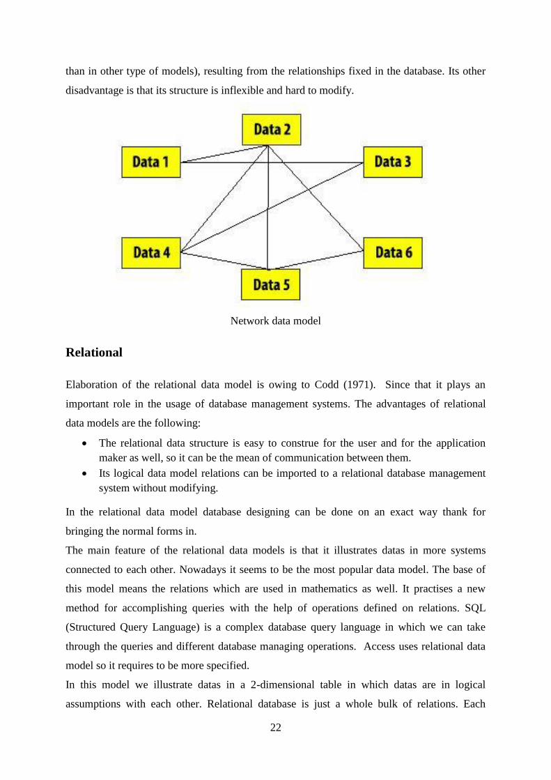
Network Data Model
This model is the developed version of the hierarchical model. The main difference between
them is that as in the hierarchical data model the graph could be only tree-shaped; in the
network model we can create every kind of graphs. So an item can have more parents, and we
can create every type of relationship between the datas. We can deal with more-to-more
relationships. Its disadvantage is that it requires a lot of storage space. It can be found in
environments with huge computers. Nowadays this model became outmoded.
In case of a network data model the relationship between single equivalent or different pieces
of data (records) can be expressed with a graph. The graph is a system of intersections, and
runners connecting them to each other; where there is connection between two intersections
providing that they are connected with two runners. Infinite number of runners can go from
one intersection but one runner can connect only two intersections to each other. It means that
every piece of data can be connected to infinite number of pieces of data. In this model n:m
relationships can be described as well as 1:n ones. In case of hierarchical or network data
model, only stored relationships can be used effectually to data-retrieval (more effectively
22
than in other type of models), resulting from the relationships fixed in the database. Its other
disadvantage is that its structure is inflexible and hard to modify.
Network data model
Relational
Elaboration of the relational data model is owing to Codd (1971). Since that it plays an
important role in the usage of database management systems. The advantages of relational
data models are the following:
The relational data structure is easy to construe for the user and for the application
maker as well, so it can be the mean of communication between them.
Its logical data model relations can be imported to a relational database management
system without modifying.
In the relational data model database designing can be done on an exact way thank for
bringing the normal forms in.
The main feature of the relational data models is that it illustrates datas in more systems
connected to each other. Nowadays it seems to be the most popular data model. The base of
this model means the relations which are used in mathematics as well. It practises a new
method for accomplishing queries with the help of operations defined on relations. SQL
(Structured Query Language) is a complex database query language in which we can take
through the queries and different database managing operations. Access uses relational data
model so it requires to be more specified.
In this model we illustrate datas in a 2-dimensional table in which datas are in logical
assumptions with each other. Relational database is just a whole bulk of relations. Each

23
relation has a unique name. In the columns datas refer to the same quantities. Columns are
named as well, which have to be unique within a relation, but there can be columns named the
same in other relations. We store datas logically belong together in the rows of the relation.
The sequence of the rows is disregardful but two rows can’t be the same. In the cut of a row
and a column there is a field which contains the datas. Fields contain different type of
quantities (numeric, written) in different columns. We often say tables or charts instead of
relations, records instead of rows, attributes instead of columns.
The following example shows a relation including personal details:

24
Does this chart remain a relation if we leave the ID number column out of account?
As we can’t pass by the chance that there can be two people who have the same name,
profession, and live in the same city; without the ID number column we would have two equal
rows, which is not allowed in a relation. It is suggested to name the columns of the relation to
refer to their content even if it goes with more type work. Its usefulness is shown in this
example:
These two charts contain the same pieces of data, but in case of the first one addition of more
notes to describe the contents of the column will be necessary.
In usual it is require in case of relations not to contain any information which could be
calculated from other details. For example, in the material relation (chart 2.3) it would be
completely unnecessary to add a column named value as it can be calculated by multiplying
the in stock and the one-price columns. This way if we have an ID number column it is
needless to make a column named date of birth as this detail can be figured out from the ID
number.
Basic requirements in connection with the charts:
Every chart has a unique identifier

25
Details in the cut of the columns and rows are single-valued; these are called primary
data fields
Datas stored in a column are connatural
Every column has a unique name
There is the same amount of data in the rows of a chart
A chart mustn’t contain two rows which are the same
The sequence of columns and rows is disregardful
KEY.
Those properties play important role, which determine the values of other properties clearly.
That means, when we give such properties value that defines an occurrence clearly. Those
properties, which determine clearly an element of an individual type, we call key. Keys are
playing an important role during the creation of the data model. During design, in general we
imply which attributes are making the keys. Theoretically an individual could have more
keys, but in the most cases it is common to choose one, which is the best suitable to the clear
identification. We call this primary key.
Key-featured property could always be found. If there is no such property among the real
data, we can introduce a new property which values are ordinal numbers, codes, special
identifiers. This can play the role of the primary key. We can see, the identifiers, codes can be
found almost every application. Due to the nature of the computer, these are suitable to
determine the occurrences precisely. In particular cases for a non-advanced user could be
difficult to pay attention for slight mistypes. This could cause a significantly different output
or results. Who works with computers should be extra careful about codes, and should work
accurately.
Relations
The third important elements of the data model are the connections. We call a relation the
affairs and contexts between the individuals. For example in the well-known payroll system
there is a natural relation between the employee and the payment individuals. This tells us,
which payments relate to the individual employees.

26
Like this way relations can be made between the elements of the individual sets. We can
classify the relations according to how many elements belongs for each element. This is
significant in the computer representation aspect of the relation.
It is way simple to implement a relation where to one individual belong only one another
individual occurrence, than another one, where there could be more. In the first case a pointer
could do the job, but in the second case we need a complex data structure for example a set or
list. Relationships can be organized into three groups:
• One-to-one
• One-to-many
• Many-to-many
In case of one-to-one relation for one individual occurrence belongs only one occurrence of
another individual. One-to-one relation is for example between a man and a women
individuals the marriage relationship.
The next group is made of the one-to-many relations. In this one for an individual occurrence
can belong more occurrences of another individual.
27
For example in the payroll system there is one-to-more relationship between the employees
and the payments. The base of the relation is which payment belongs to which employee. It is
clear, for one employee can belong more payments, but one payment can belong for only one
employee.
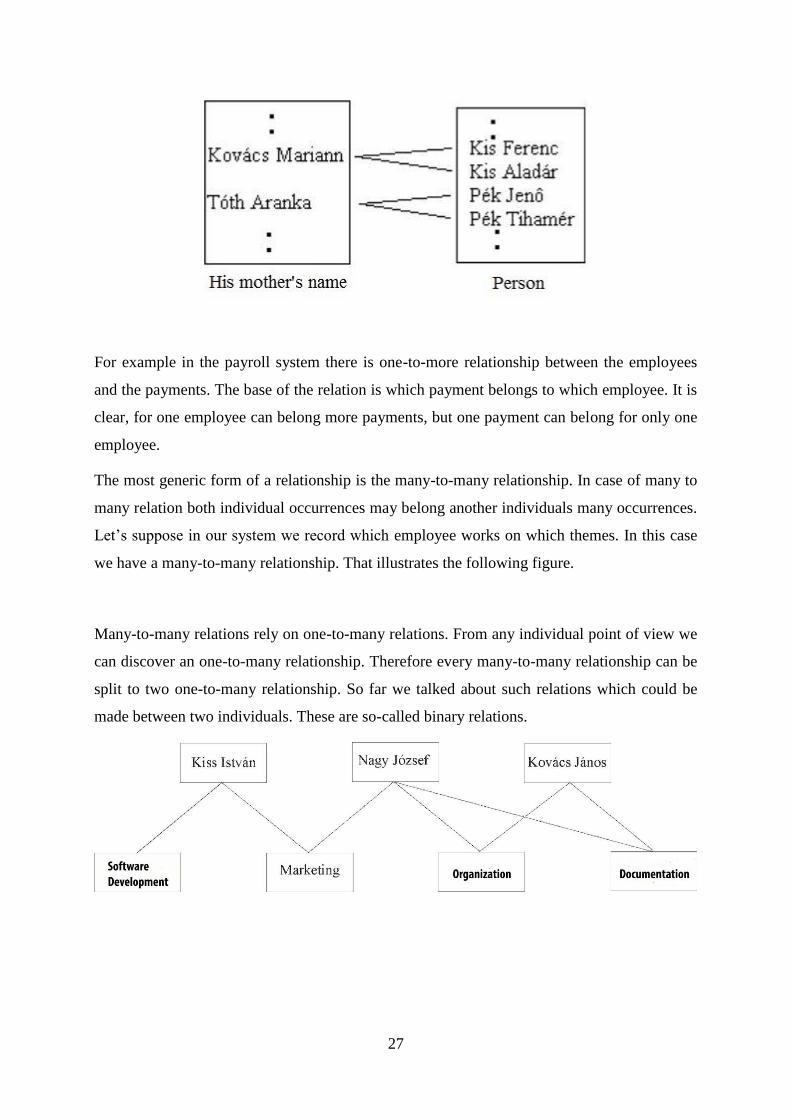
The most generic form of a relationship is the many-to-many relationship. In case of many to
many relation both individual occurrences may belong another individuals many occurrences.
Let’s suppose in our system we record which employee works on which themes. In this case
we have a many-to-many relationship. That illustrates the following figure.
Many-to-many relations rely on one-to-many relations. From any individual point of view we
can discover an one-to-many relationship. Therefore every many-to-many relationship can be
split to two one-to-many relationship. So far we talked about such relations which could be
made between two individuals. These are so-called binary relations.

28
Database planning and its contrivances
The very first step of database designing is that we have to know what type of database
management system we use. The use of Access database management system goes with
subdividing data into groups, taking the items being close to each other into one table, then
specifying the relations between the tables – just like in relational database management
systems. So designing and creating a database is a quite complicated job and it requires some
creativity as well. During designing a database we have to pay attention to make our database
be able to fulfil some requirements like minimizing data redundancy or proving all data
independences to be expressed, ect. There is no general method which can be used during
designing all kinds of databases but there’s a procession which is advisable to be followed.
Above all, we have to determine our aims which have to stand close to the user’s demands.
Meanwhile designing it is essential for the planner to have the required knowledge in
connection with the field the user deals with. This is the section of defining the information
needs as well as developing the details, formats and algorithms. In usual designing is not
brought off by the programmer but the organizer who is familiar with designing and who will
investigate the exact demands of the user. The organizer will do a well-founded research with
the help of different reports and documents which can be used as sources during designing.
Therefore we can go on with the logical database designing. In this section the data and the
relations between them are highlighted. Now comes defining the database objects, describing
their features, and mapping the relations between them while taking care of minimizing the
data redundancy. The physical database designing is separated from the first two steps as in
this section the databases are created on the computer according to our previous plans. After
all we are done with the prototype, which is only the first version of the system as a lot of
changes and improvements are still needed.

29
Main steps of database designing
1. Analyzing the requirements: First of all we have to determine the aim of the database.
We have to do some research to be of use for designing the database. We also have to
think over what kind of information we would like to get from the database, and which
are the details should be stored in connection with the objects.
2. Determining the objects and tables: the collected data have to be sorted into an
information system. This information system is dealing with objects. Physically the
objects are stored in tables, where the objects go to the lines (records) and attributes go
to the columns (record’s fields). It is advisable to keep one piece of data in only one
table – this way later if we have to modify it; we will be able to do it at one place.
Information referring to one topic has to be stored in one table.
3. Determining fields and attributes: this is the concrete section of designing. Here we
design the tables and determine the tables including the fields. We can sort the
attributes according to these aspects:
a) simple attributes, which can’t be divided anymore ; and composite ones which
consist of simple attributes
b) equivalent: it has one value at its every occurrence. Multivalued ones have
more values at their occurrences.
c) the stored attribute’s values are stored by the database. Its derived value is
determined by right of other attributes.
30
4. Determining identifiers: It is significant to identify the data stored in tables clearly.
Using primary keys is necessary in every table in which we would like to identify the
records one by one. The primary key is a kind of identifier, which’s values can’t be
repeated within a table. Primary keys have an important role in the relational database
management systems. By the help of them we can increase the level of efficacy, fasten
searching and collecting data.
Three types of primary keys are applicable:
a) auto-number primary key: this is the simplest primary key. We only have to create
an auto number field. Then the Access will generate a unique ordinal number for
every new record.
b) single field primary key: the key isn’t counter-type if it doesn’t consist of any
recurring values (e.g. VAT number)
c) multi-field primary key: we make this key with the use of more fields. This one
comes on when we can’t insure any of the field’s uniqueness.
5. Determining relationships: Relate the records of the tables with the help of the primary
keys. Relationship means that two objects belong together.
We can subdivide relationships into three groups in the view of multiplicity (we will deal
with them later):
a) one-to-one relationship
b) one-to-many relationship
c) many-to-many relationship
6. Control: After designing the fields, tables, and relationships we have to check the plan
whether there is a mistake or not. It is easier to modify our database directly after
designing than if it is filled in with details.
7. Data input: Since we are done with the needed corrections and controls we can entry
the data into the previously prepared tables. Furthermore we have a chance to create
other objects like forms, reports and queries (we will deal with them later)
31
Normalisation
The base of the relational database management system is the normalisation –meaning a
method which gives the optimum way of the data’s placement. In case of an inefficiently
designed database there will be contradictions and anomalies in the data structure.
Normalisation allows you to structure data appropriately, and it helps you to eliminate the
anomalies and lower data redundancy.
Anomalies:
Insertion anomaly: Adding a record wishes another record’s enrolment which is not
logically related to the record.
Deletion anomaly: During deleting the item some instance of data is removed as well
Update anomaly: Because of a change of a data we have to update it at its every place
of occurrence
Normal Forms:
First Normal Form: there are no repeating elements or groups of elements. In every row of
the relations one and only one value takes place in a column, the order of the values is the
same in every row, and every row is different. There is always at least one or more feature(s)
which make(s) the rows individually distinguishable.
Second Normal Form: the relation is in first normal form, and none of its secondary
attributes depend on any of the genuine subset of its keys. (Primary attributes are the ones
which belong to a key; in case of secondary attributes this is not true.)
Third Normal Form: the relation is in second normal form and there is no functional
dependence among the secondary attributes. If the value of “B” attribute depends on the value
of “A” attribute, and the value of “C” attribute transitively depends on the value of “A”
attribute. Elimination of these transitively dependences is an essential requirement of the third
normal form. If the table of the database is not in third normal form we have to divide it into
two tables, each of them in third normal form.

32
Dependences
Functional dependency: when any values of a feature of the system can be assigned to only
one value of another feature. E.g.: one personal identity number can be connected to one
person but a person is able to have more personal identity numbers.
One-to-many relationship.
Mutual Functional Dependency: when the above-mentioned requirements come true in both
directions. e.g.: registration number- number of the engine. One-to-one relationship.
Functionally Independents: when the above-mentioned requirements don’t come true. e.g.:
the colour of the student’s eyes – the place of their school.
Transitive Functional Dependency: when some concrete values of a describing feature of an
element determine other values of a describing feature.

33
Relation key
The relation key unambiguously identifies a row of the relation. The relation – as it is in the
definition – cannot include two identical rows. Therefore, there is a key in every relation. The
relation key must carry out the following terms:
• it is a group of such attributes, that identifies only one row (unambiguously)
• none of the attributes that are included in the key can form subset
• the value of attributes that are included in the key cannot undefined (NULL)
The storage of undefined (NULL) values is being specially solved by the relation database
managers. In case of numerical values, the value of NULL and 0 are not equals.
Let’s keep a record of the personal data of students of the class in a relation.
Id number Date of birth Name
PERSONAL_DATA=({ ID_NUMBER, DATE_OF_BIRTH, NAME}).
In the PERSONAL_DATA relation the ID_NUMBER attribute is a key. It is, because there
cannot be two different people with same id numbers. The date of birth or the name cannot
identify unambiguously a row of the relation, because there have been born students on the
same day or there may be students with same names in the class. Together they identify a row
of the relation. But they cannot satisfy the condition related to the keys that the subset of the
attribute, that is included in them, cannot be a key. In this case, the id number is already a key.
This way, combined it with any other attribute it cannot form key already.
There might also be such relation that in it the key can be formed by connecting more value
for the attributes. Let’s make a record of the given marks the students got with the following
relation:
DIARY=({ID_NUMBER, SUBJECT, DATE, MARK)}
Id number Subject Date Mark

34
In the DIARY relation the ID_NUMBER does not identify a row, because there can be marks
for a student, even from the same subject. Because of this, even the ID_NUMBER and the
SUBJECT cannot form key. Even the ID_NUMBER, SUBJECT and the DATE can only
form key if we preclude the possibility of that that a student can get two marks from the same
subject on the same day. In this case, if that condition could not be kept, then there must be
stored not only the acquisition date of the mark, but also its point of time. In such cases the
DIARY relation has to be extended with that new column. There are not just complex keys
that can take place in the relation. There are also such relations that in it there can be found
not just one, but more keys. To illustrate this let’s see the next relation.
Consultation=({Teacher, POINT_OF_TIME, STUDENT)}
Teacher Point of time Student
Relation with more keys
In the CONSULTATION relation we imagine such identifier in the teacher and student
columns that unambiguously identify the person (for example ID number). Every single
student can take part in more consultation, and every teacher can hold more consultations.
What is more, the same student can take part in the same teacher’s consultation in different
points of time. As a consequence, neither the TEACHER nor the STUDENT nor the two
identifiers together are keys of the relation. But one person in one time can only be in one
place. As a consequence the TEACHER, POINT_OF_TIME attributes are forming key, and
with the same reasons the STUDENT, POINT_OF_TIME attributes are forming key as well.
We have to notice that the keys are not being made by as a result of arbitrary decisions, but
they come from the nature of the data as well as the functional dependence or the polyvalent
dependence. In the relation we differentiate foreign/outer key, too. These attributes form key
not in the certain relation, but in another relation of the database. For example, in the
CONSULTATION relation if we use the ID number to the identification of the STUDENT
then it is a foreign key to the relation record personal data.

35
Data model mistakes
Anomalies:
They are mistakes, because of inadequately designed data model. They may lead to the
inconsistency of the database (because we are not storing only one entity’s features or we
store certain features multiple times).
Types
- insertion anomaly: The entry of new record cannot be done to one table, because in the table
there are such attribute values which are available during entry or not available even later.
- modification anomaly: We store one in more tables, but during the modification of the
attribute values we have not done the modification everywhere, or we have not done it the
same way.
- deletion anomaly: We are deleting in a table and we are losing such important information
that we would need later.
Redundancy:
It means overlap. In practice we refer physical overlapping to it – multiple data storage in the
database – at designing it is also important paying attention to the logical overlaps.
Types
- Logical overlap:
Open logical overlap: the same attribute type with the same name is included in more entities.
It results multiple storage. They may be necessary due to safety or efficiency, or for example
to carry out connections (as foreign key). The lack of the logical overlap is also count as a
mistake.
Hidden logical overlap (synonym phenomenon): We mark the same attribute with different
name.
Apparent logical overlap (homonym phenomenon): We use the same name to different
attributes.
- Physical overlap: the multiple store of the same attribute or – with synonym name –
entity in the database.
Let’s see the next relation.
36
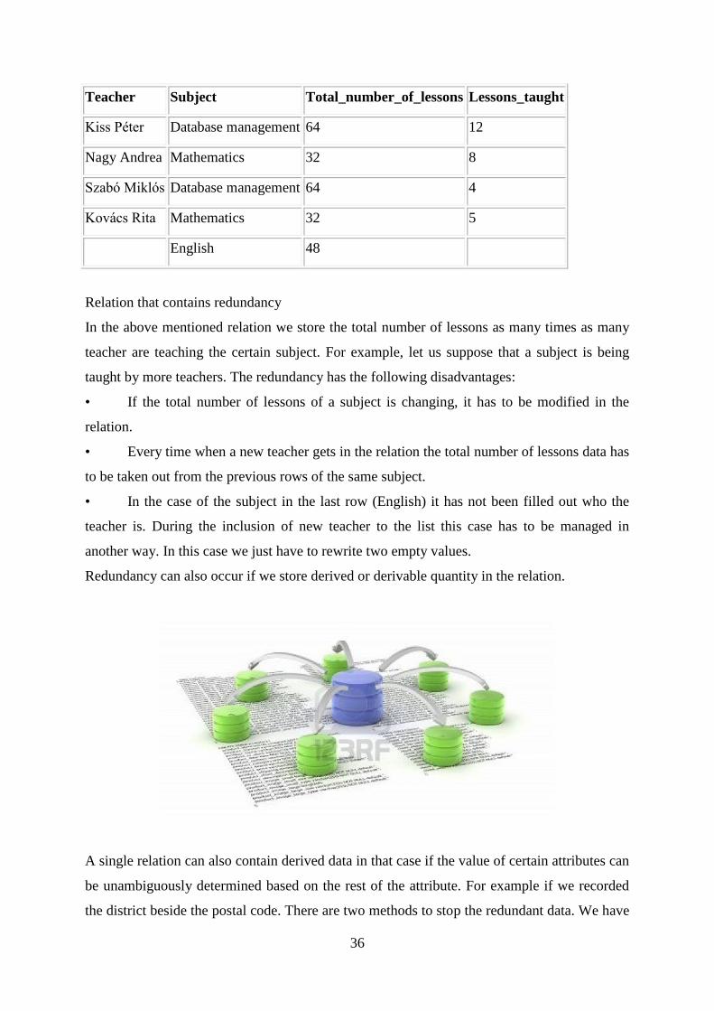
Teacher Subject Total_number_of_lessons Lessons_taught
Kiss Péter Database management 64 12
Nagy Andrea Mathematics 32 8
Szabó Miklós Database management 64 4
Kovács Rita Mathematics 32 5
English 48
Relation that contains redundancy
In the above mentioned relation we store the total number of lessons as many times as many
teacher are teaching the certain subject. For example, let us suppose that a subject is being
taught by more teachers. The redundancy has the following disadvantages:
• If the total number of lessons of a subject is changing, it has to be modified in the
relation.
• Every time when a new teacher gets in the relation the total number of lessons data has
to be taken out from the previous rows of the same subject.
• In the case of the subject in the last row (English) it has not been filled out who the
teacher is. During the inclusion of new teacher to the list this case has to be managed in
another way. In this case we just have to rewrite two empty values.
Redundancy can also occur if we store derived or derivable quantity in the relation.
A single relation can also contain derived data in that case if the value of certain attributes can
be unambiguously determined based on the rest of the attribute. For example if we recorded
the district beside the postal code. There are two methods to stop the redundant data. We have

37
to leave those relations or attributes that contain derived data. The redundant facts that are
being stored in relations can be ended by taking the table apart, but we are doing it with its
composition. We take to two pieces the relation that is in the 3.10 example
Lessons = {Teacher, Subject, Lessons_taught} and Total_number_of_lessons = {Subject,
Total_number_of_lessons }
Stopping the redundancy
The goal of the logical design is a relation system, relation database without redundancy. The
relation theory contains methods to stop redundancy with the help of the so called normal
forms. From now on we will shot the definition of normal forms of the relations through
examples. We will use notion of functional dependence, multivalued dependence and the
relation key to make normal forms. During forming of normal form the goal is simply to write
down such relations that we store facts which are related to the relation key. We differentiate
five normal forms. The different normal forms build upon each other. The relation in the
second normal form is also in first normal form. During designing the goal is to reach the
biggest normal form. The first three normal forms concentrate on stopping redundancies in
functional dependences. The fourth and fifth normal forms concentrate on stopping
redundancies in multivalued dependences.
We have to get acquainted with two new notions that are connected to the relations. We call
primary attributes that are at least in one relation key. The other attributes are called not
primary.
Normal forms:
First normal form: All values are elementary in the relation. The relation cannot include data
group. In every row per column of the relation there can be only one value. In every row the
order of values are the same. All rows are different. There is at least one or more attribute that
the rows can be unambiguously differentiated from each other.
For example, let it be here such kind of a relation that the attributes of it are also relations.
Study group Teacher Students
Computer technology Nagy Pál Name Class

38
Kiss Rita III.b
Álmos Éva II.c
Video Gál János
Name Class
Réz Ede I.a
Vas Ferenc II.b
Study group Teacher Student Class
Computer technology Nagy Pál Kiss Rita III.b
Computer technology Nagy Pál Álmos Éva II.c
Video Gál János Réz Ede I.a
Video Gál János Vas Ferenc II.b
Second normal form: The relation is n first normal form. Furthermore, none of its secondary
attributes depend on any of its key’s subset. (The primary attributes are those attribute that
belonging to some of the keys. Those attributes, which are not belonging to any of the keys,
are secondary attributes.)
Conference
Room Point of time Presentation Place
B 10:00 Mythology 250
A 8:30 Literature 130
B 11:30 Theater 250
A 11:00 Painting 130
A 13:15 Archeology 130
Conference
Room Point of time Presentation
B 10:00 Mythology
A 8:30 Literature

39
B 11:30 Theater
A 11:00 Painting
A 13:15 Archeology
Conference
Room Point of time Presentation
B 10:00 Mythology
A 8:30 Literature
B 11:30 Theater
A 11:00 Painting
A 13:15 Archeology
Dependency diagram
Let’s see another example for the relation that breaks the term of the second normal form. For
the check of the energy management of a building the temperature in the certain rooms is
being regularly measured. For the evaluation of the measured results we are also recording the
number of radiators in the certain rooms.
Temperature
Room Point of time Temperature Radiator
213 98.11.18 23 2

40
213 98.11.24 22 2
213 98.12.05 21 2
214 98.12.05 21 3
214 98.12.15 20 3
Conference
Room Point of time Temperature
213 98.11.18 23
213 98.11.24 22
213 98.12.05 21
214 98.12.05 21
214 98.12.15 20
Rooms
Room Radiator
213 2
214 3
Third normal form:
The relation is in second normal form. Furthermore, there are not any functional dependence
among the secondary attributes. If the value of attribute “B” depends on the value of attribute
“A” as well as the value of attribute “C” transitively depends on the value of “A”. The
elimination of such transitive dependences is inevitable requirements of the third normal
form. If the table of the database is not in third normal form then it must be broken to two
tables so that the certain tables separately are in third normal form.
This will be demonstrated with the help of an example again.

41
Study groups
Study group Teacher Date of birth
Képzőművész Sár Izodor 1943
Iparművész Sár Izodor 1943
Karate Erős János 1972
Study groups
Study group Teacher
Képzőművész Sár Izodor
Iparművész Sár Izodor
Karate Erős János
Teachers
Teacher Date of birth
Erős János 1972
Sár Izodor 1943
Boyce/Codd normal form (BCNF)
During the discussion of the normal forms we showed examples to such relations which only
have one relation key. Of course, the definition of the normal forms can be applied to those
relations that have more keys. In this case, every attribute that is part some of the keys are
primary attribute. But this attribute can depend on another key that does not include it as part
of the key. If that is the case then the relation contains redundancy. The recognition of this led
to a more strict definition of the third normal form that is called Boyce/Codd normal form.

42
• All primary attributes are in complete functional dependence with those keys that this
is not part of it.
As an example, let’s see the following relation:
Subjects
Teacher Point_of_time Subject Semester Number_of_students
Kiss Pál 93/1 Database 1 17
Jó Péter 93/1 Unix 1 21
Kiss Pál 93/2 Database 2 32
Jó Péter 93/1 Unix 2 19
Kiss Pál 93/1 Database 3 25
The relation’s third normal form and the decomposition of the Boyce/Codd normal form
Let us suppose that every teacher is teaching only one subject, but they are teaching it in
different semesters. Based on this the following functional dependence can be written down:
Teacher, Semester Subject, and Semester Teacher. The relation has two keys. They are the
(Teacher, Point of time, Semester) and the (Subject, Point of time, Semester). In the relation
there is only one non-primary attribute which is the Number_of_students. That is complete
functional dependence with both of the relation keys. There is no dependence relation
between the primary attributes. Based on these the relation is in third normal form. However,
it contains redundancy, because beside the same teacher we store the subject multiple times in
the same points of time. The reason for the redundancy is due to the fact that the teacher
attribute depends on the relation key that does not include the teacher attribute (Subject, Point
of time, Semester) only the part of it (Subject, Semester).
Fourth normal form (4NF)
Unfortunately, even the Boyce/Codd normal form can contain redundancy. Up to this point
we have only examined the functional dependences, but not the polyvalent dependences. The
following two normal forms serve to eliminate the redundancy from polyvalent dependences.
A relation is in fourth normal form if in an XY polyvalent dependence it only contains those
attributes that can be found in X and Y.

43
Fifth normal form (5NF)
For a long time the fourth normal form was considered the last step of the normalization.
However, we can lose information due to the storage of the polyvalent dependences in
separate relations. Let’s see an example to show this. An Ltd, which is specialized in teaching
computer knowledge, has more, well qualified teachers. The teachers are suitable for educate
in various courses. The courses are being held in different parts of the country.
Let’s make the Teacher-Course-Place relation based on these facts.
The only relation key contains all of the attributes (Teacher, Course, Place). It comes from
that the relation is in Boyce/Codd normal form, but despite of that, it contains redundancy.
For example, there can be found in two rows that Kiss Pál is teaching Database 1 course. By
breaking the relation down in two - that only contains one polyvalent dependence – relation
(Teacher, Course) and (Teacher, Place). If we stop the redundancy, that would also lead to
information loss. After the break down we already do not know which subject is being taught
in the certain place by the teacher. For example, is Kiss Éva holding database I. or database II.
course in Pécs. Breaking the original relation in three, we will get the fifth normal form. The
original relations can be produced from the connection of three relations that we have got as a
result, but the connection of any of the two relations is not enough. At the end of the
discussion of the normal forms we mention that it is recommended to normalize the relations
by all means up to the third normal form. This eliminates much of the redundancy. Those
cases are rarer that requires the use of the fourth and fifth normal form. In the case of the fifth
normal form, it is possible to stop the redundancy we use bigger storage space. So, the
designer of the database can decide whether he/she choose the fifth normal form and the
bigger database, or the redundancy and the more complicated refresh and modification
algorithms.
Physical designing
In case of the relation database, during the logical designing the relations can already adopt
their final form which can be easily formed down in the database manager. During the
physical designing we are rather concentrating on that, is the logical structure suitable for the
terms of the effective implementation, and what indexes should we summon to the certain
relation. The jointly implemented operations on the relation are called transaction. In general,
we would like to reach fast implementation of transactions.
44
During the physical design it may occur that we build redundancies intentionally in relations
for more efficient transaction management. It may seem a step back compared to the
redundancy stop manipulations that was followed during the logical design. But the most
important difference is that the redundancy is getting in the relation in a checked mode, and it
was not just left there, because of the incomplete designing. For example, it often occurs that
we store frequently together necessary data in one relation, because of the fastest possible
check.
Supporting the design with software
Designing does not differ from the well-known practices. In every case it follows the
software-developing standards which are the following:
1. Designing the requirements
2. Design of the database, the database tables and their fields
3. Defining the tables between the database
4. Stress and normal tests
Designing requirements:
Before this section we determined the requirements. It is important that requirements should
determine those expectations that should meet the database. If there is any difference between
the requirements and design, one should not go further in process until every difference was
not thought through and fixed.
Design of the database, the database tables and their fields:
When we determine a requirement, comparing the information and the aim of the database,
we can determine the kind of the table structure to create. So everytime we should consider
that the data - what is necessary to achieve the requirements – should create a structure that
meets the foundations of general database theorem. When we can project the structure we can
go on with creating the fields of the database. In this phase we mark the primary keys too. In
this particular task the primary key in every case is the table (uid) identifier which identifies
the series. On the other hand introducing the historic data handling model we identify the
individual by the reference identifier (rid). Like this, we can achieve that in the system we

45
have more rid yet they made unique records. The uniqueness should made of understanding
together the rid and the dtm_ValidTo fields.
Defining the tables between the database:
When we use the technical identifier (uid) the individual and the historic data handling will be
lost. Therefore the relationships in every case should assigned to the reference identifier.
When we don’t do this, the historic data-handling could not be realized.
Stress and normal tests:
Testing is a key part of the development. Since in the data structure there could be found
multiple records on the same time, it is important after the development part during the
physical implementation we should testing the database structure continuously. The database
structure should be tested by not only with normal data input, modifying, delete methods, but
with stress tests too. That means we should do an intensive data input, in order to set the
limits. Those limits could be the following:
• An interface in what detail could be computed?
• Connection between the quantity of data and quickness of the queries
• Input the proper data
For the stress test we use the JMeter application which could queries run in multiple threads.
The MySQL WorkBench
First steps: Introducing the user interface
Data Modeling

46
In the model there are tables, connections keys and so on.
When Create New EER Model clicked, a window appears:
Here are the created models. They
could be reopened and changed.
Here we can create a new model
In model view we could design
easily the tables in database and
the relationships, and field types.

47
Here we can create a new model

48
Designing fields:
Editing a table properties
We can define the types of the fields and its other detalis
The primary key of the ‘dolgozo’ table is the ‘id’ fileld with type of ‘int’.
After naming the fields we select their types.
A field properties could be the following:

49
PK – PrimaryKey
NN – NotNull – The field could not be empty
UQ
BIN
UN
ZF
AI
By ticking the corresponding checkboxes we can define the further properties of the field.
Creating relationships:
We select the kind of the relationship, and we connect the desired fields considered the
relations ‘one’ side always linked for the primary key, the ‘many’ side for the foregin key.
We should pay attention for the keyed fields types must be the same. Creating many-to-many
relationship is done by switching tables. In the name of the table we name that it will be a
switched table, then, we indicate the switched fields names. The rule, - keyed fileds types
must be the same - applies here too.
Deleting relationships:
In this case the program asks, if the connected fields should be deleted too, or keep them.
When we hover the cursor above the line which indicates the relationship, we can see, what
fields are involved in the relationship.

50
The well-developed database design could be exported in some picture formats in order to use
in a presentation easily.
Operations of relational algebra
Connected with relations a whole branch developed in mathematics. Mathematicians defined
operations for the relations and they applied set operations for the relations. In the following
let’s see these operations in brief.
Selection
In the operation of selection we just keep rows in the result relation satisfying a certain
condition.

51
Projection
During the operation of projection we just keep particular columns in the result relation
Cartesian product
The Cartesian product puts two relations rows next to each other in every combination in the
output relation.

52
Natural join
The operation of join connects two or more relations by comparing attribute values. The most
common case when we examine the match of the attributes, that we call natural join.
This is a special product which could be described as the follows:
1. Take a row from the first relation
2. Examine the joining condition for the second tables all row. If it is true, add both
relations rows to the result.
3. Continue with the 1st step until there is any row in the first relation.
In the result relation appear those rows from the first relation where could be found a
satisfying condition in the second relation. In many cases it is necessary that the first relation
every row appear at least once in the result relation. This kind of outer join we call outer join.
Set operations
The basic operations with sets – union, intersection, complement – we can interpret to the
relations too. Every interpreted set operation is needed at least two operands, in the case of
complement there could not be more. Set operations can executed only between relations with
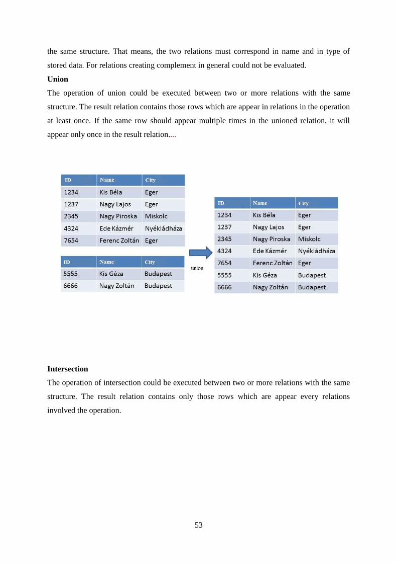
53
the same structure. That means, the two relations must correspond in name and in type of
stored data. For relations creating complement in general could not be evaluated.
Union
The operation of union could be executed between two or more relations with the same
structure. The result relation contains those rows which are appear in relations in the operation
at least once. If the same row should appear multiple times in the unioned relation, it will
appear only once in the result relation....
Intersection
The operation of intersection could be executed between two or more relations with the same
structure. The result relation contains only those rows which are appear every relations
involved the operation.

54
Complement
The operation of complement could be executed between two or more relations with the same
structure. The result relation contains only those rows which are appear only the first relation
but not in the second one.

55
Tasks
1. Work – Artist
We know about the work in which year was created, what is its kind (sculpture, painting,
sketchbook, etc.) how much it worth in forints, we know its title, the artist, the year the artist
born, and his/her nationality. One work always belongs to one kind, and the artist can have
only one nationality. We should process the complete work of an artist. The task is to create
the design of the database in drawing including table names, field names, field types.
2. The “Stupido-Gigantic GmbH Ltd Kft S.A.” company deals mostly with commerce.
Accordingly orders are coming in from costumers, which are delivered by transporters. One
product is being delivered by only one transporter. We record the actual balance of the
costumers. In one order there could be more items, the content of an item is the name of the
product and the quantity. The transporters, products and the city names are identical, but the
costumer names are only among the city identical. We suppose every city has only one zip
code.
Stored data in bulk:
TransporterZipCode, CostumerZipCode, TransporterName, OrderNumber, OrderDate,
CostumerCity, Balance, UnitPrice, ProductName, TransporterCity, CostumerName,
ProductName.
Create the logical database model of the “Stupido-Gigantic GmbH Ltd Kft S.A.” company
until the third normal form.
3. Design a database where we can store the results of a problem-solving competition. We
know the competitor name, his/her school name, the detailed address of the school, the class
of the competitor, the points earned in the competition, what we get in task number, earned
points form. It is no restriction how many competitors can come from a school.
4. An Arabic sheikh would like to maintain the data related to his crude oil commerce. would
like to see the following data in the registry: Oil well (Name, Capacity) Refinery(Name,
Address, Capacity), Costumers (Name, Address). The sheikh deals with selling both refined
and crude oil. Therefore he wants to track every costumer purchase. Selling crude oil is done
by the oil wells, the refined oil is being sold by the refineries. The sheikh would like to know

56
the quantity of each costumers order, and the deadline. Refineries are process the oil from the
sheikh’s oil wells. The sheikh would like to track the particular oil wells transfer oil to which
refineries, the deadline of the transfer, and the quantity.
5. We examine the records of a video rental. The rental rents films only, about films there is a
registry which contains the title of the film, the star, and the director. Each film has an
identifying number, the title is not always identical. A film could be appear in more cassette,
copies created by the rental. Cassettes also have an identical identifier, and its type is also
recorded. From the rental the members may rent. The members name, address, and his
identifier is recorded. Members rent film(s), we should track the rental dates, and the bring
back dates accurately. The rental buys the films from a distributor, every order has a number
and the order date is recorded in order to the easier tracking. In one particular order there
could be more films. The documents at the video rental are contain the following data in
different data sheets:
From those document we should create the logical database model.
Cassette number
Cassette type
Film title
Film number
Order number
Order date
Rental number
Member number
Member name
Member address
Rental date
Bring-back date
Film star
Film director
6. Create a database which contain the following details about school students: name, address,
home telephone number, mothers name, pocket money, when started the school, what is his
major, (PE, music, English, German) language certificates, (English, German, French,
57
Russian…). Pay attention to the details of the address, and the recurrence of the city. Design
the most general case. To be submitted the database design in third normal form.
7. A hotel would like to track the expenses of its guests. The guests would stay in rooms for a
particular period. The important detail about a room is its area, number of beds and its price
per day. Guests can stay in many rooms, or one room, even at the same time. Important
information about room usage by guests is the time of checking in and checking out. Of
course there could be a room where haven’t stayed any guest yet. Guests can book rooms in
advance; important information about booking is the planned date of arrival and the leaving.
Guest can resort different services in the hotel (internet, meal, sauna) related information to
the service is its name, price, description. Guests can take up many services, and there could
be such services which were never used.
8. Design a database for storing a swimming tournament results. Swimmers competed in
different tournaments. The database should contain:
swimming association data
swimmers data
data of the tournament
data of tournament places
the records
58
Language Reference of SQL
Elements of DDL
Create schemes, the creat
Create the tables by CREATE TABLE command.We can use lot of data types (here),but
practically we just need some of them.
NUMBER (h, t) - numeric data, length <= 38, h - number contains the length, the number of
decimal places;
DATE - date and time types;
VARCHAR2(size) – character types, the length of variable (maxlength<=4000);
CHAR(size)- character types, fixed length (max length<=2000);
NCHAR(size) – same as the character types, but the max size depending on the character set,
LOB (large objects) – binary or text format. It may be an image, audio or large text file.
Include the LOB types:
LONG – text data, max length<=2 Gbyte;
LONG RAW – binary data, max length<=2 Gbyte;
The LONG and LONG RAW types used only simple data processing operations.
CLOB, NCLOB, BLOB – internal LOB types,because they are stored in the AB , max
length<=4 Gbyte;
CLOB – the data stored in AB Character set;
NCLOB –stores the data in the national character set
The Oracle puts a Pseudocolumn, calls ROWID to every table automaticly, but it’s rarely
used by Programmers.
ROWID – pseudocolumn that contain the logically individual title of the line. The ROWID
does not need to be changed,but you can search in the SELECT command:
SELECT rowid FROM tabel_1;
The Sequential number of the Line - a number that is assigned to the line when it is added to
the table.This number is part of the ROWID.
Only the user can create tables, who has privileges to CREATE TABLE or CREATE ANY
TABLE.

59
The applicationof the STORAGE parameters on CREATE TABLE command.
We can create a table without the STORAGE memory-parameters. In that case the table get
the default value, but it is not always the good solution. The memory storage(segments), are
stored in the table calls extent. The first extent name’s INITIAL, the rest of the extent are
secondary extent
CREATE TABLE testtab
(col1 VARCHAR2(10))
STORAGE (INITIAL 100K
NEXT 50K
MINEXTENTS 1
MAXEXTENTS 99
PCINCREASE 20);
The first extent gets 100K memory, the second – 50K. By the PCINCREASE 20 values of
every extent grow with 20% compared to the previous. MINEXTENTS 1 MEANS, the table
gets in first time 1extent, the MAXEXTENTS 99 – the table get 99 extent maximum.
The tables may be partitioned as like the index tables. The partitioning gives the possibility of
the very large tables and index tables for the treatment of. During the partitioning of the large
table, the system divides into that to smaller and it more manageable.
Partitioned table - This is a table where, the rows are smaller but identical construction with
boards, partitions, they share. The partitions can be stored on different physical locations.
The benefits of partitioning:
Better distribution of I/O-load
Backup and restore is a simple.
Minimize the possibility of data corruption.
Help to the archiving process.
For example:
CREATE TABLE large_table
(col1 VARCHAR2(10),
(col2 VARCHAR2(10))
)
PARTITION BY RANGE (col1, col2)
(PARTITION p1 VALUES LESS THEN (…) TABLESPACE p1,
PARTITION p2 VALUES LESS THEN (…) TABLESPACE p2);

60
Changed the schema elements, the alter
The length of the column can be increase even if the table contains data. But the length of the
column can only be reduced if the table is empty.
ALTER TABLE testtab ADD col2 VARCHAR2(100);
ALTER TABLE testtab MODIFY col2 VARCHAR2(150);
ALTER TABLE testtab STORAGE ( NEXT 10K
MAXEXTENTS 50);
ALTER TABLE testtab DROP col1;
We can rename the tables:
RENAME testtab TP testtab1;
and we can delete it:
DROP TABLE testtab;
For example:
CREATE TABLE students(
idNUMBER(5) PRIMARY KEY,
first_nameVARCHAR2(20),
last_name VARCHAR2(20),
majorVARCHAR2(30), -- professional
current_credits NUMBER(3)); -- cast the number of exams
The ORACLE-system contains a presentation scheme, that owner is Scott:
CREATE TABLE scott.dept
(deptno NUMBER(2) NOT NULL,
dname VARCHAR2(14),
loc VARCHAR2(13),
CONSTRAINT pk_dept PRIMARY KEY (deptno));
CREATE TABLE scott.emp
(empno NUMBER(4) NOT NULL,
ename VARCHAR2(10),
job VARCHAR2(9),
mgr NUMBER(4),
hiredate DATE,
sal NUMBER(7,2),
comm NUMBER(7,2),
sal NUMBER(7,2),
deptn NUMBER(2),
CONSTRAINT pk_emp PRIMARY KEY (empno));

61
When we refer to the table(or other Oracle-object),what we does not the owner, that time we
must give the really owner name too. owner.table_name
.CONSTRAINT integrity constraint application
Referential integrity ensures that a specific column values to which appear in another column.
Integrity can be imposed austerity.
Constraint – a rule or restriction, on a part of the data will be checked.
Integrity constraint – a rule, comprising one or more columns is limited by the possible range
of values. The constraint when creating the table can be assigned to the columns.
You can use the CONSTRAINT clause of the CREATE TABLE or ALTER TABLE
commands. Lots of constraints can be approved without the CONSTRAINT clause.
Exists:
table constraints
column constraints
Table constraints–that integrity constraints, what we apply for one or more column to the
table.
Column constraints – one integrity constraints what we apply to one column of the table.
List of the table constains:
UNIQUE
PRIMARY KEY
FOREIGN KEY
REFERENCES
ON DELETE CASCADE
CHECK
ENABLE VALIDATE
DISABLE
The column contains:
NULL
NOT NULL
The other column constraints and the table constraints are the same.
The DISABLE options is the integrity constraints or we can use to turn off the trigger.(but not
delete it) Most of the time applied it in the ALTER TABLE order.

62
ALTER TABLE tabla DISABLE UNIQUE oszlop, column,..
ALTER TABLE tabla DISABLE PRIMARY KEY
ALTER TABLE tabla DISABLE CONSTRAINT constraint_name
DISABLE ALL TRIGGERS
.Elements of the DML
INSERT – insert a new line
UPDATEupdate existing records of data
DELETE – delete records
TRUNCATE– fast delete of all records
.New data entries, insert the command
For the first time check the SQL * Plus structure of testtab table:
DESCRIBE testtab;
NAME NULL? TYPE
--------- ---------- --------
COL1 VARCHAR2(10)
COL2 NUMBER(38)
INSERT INTO testtab(col1, col2) VALUES(’text’, 123);
Although this result is obtained if the
INSERT INTO testtab VALUES (’szöveg’, 123);
we use the command.
The insert nulls
INSERT INTO testtab (col1, col2) VALUES (’text’, NULL);
or
INSERT INTO testtab (col1) VALUES (’text’);
It is also possible that the INSERT command insert one in time more rows to the table. (use
for this purpose an embedded SELECT command)
INSERT INTO testtab (col1, col2) SELECT e_name, emp_no FROM
emp;

63
. Create table based on another table
CREATE TABLE emp_copy AS
SELECT * FROM emp;
CREATE TABLE emp_copy2 AS
SELECT emp_no, e_name FROM emp
WHERE e_name LIKE ’%a%’;
.Change data,the update
The UPDATE command modifies all rows for which the WHERE condition is met. If the
UPDATE command has WHERE condition, that time the modify executed every rows. It is
very rare.
For example:.
UPDATE emp_copy2 SET e_name=’Kovacs’ WHERE emp_no=7499;
UPDATE emp_copy2 ec SET (emp_no, e_name) =
(SELECT emp_no, e_name FROM emp e WHERE e.emp_no=ec.emp_no)
WHERE e_name LIKE ’I%’;
In the last command, the secondary names of the table ec and e. The last WHERE condition
includes the entire command(to UPDATE) and enter the rows that you want to modify. The
nested SELECT command edits the values that are entered in the table emp_copy2.The
WHERE condition in the SELECT is linked to the appropriate rows of the two tables.
.Delete data, the delete
DELETE FROM emp_copy2 WHERE emp_no=7876;
DELETE FROM emp_copy2 WHERE emp_no IN
(SELECT emp_no FROM emp_copy);
We can use functions in every SQL commands.
For exampla:

64
UPDATE emp_copy SET e_name=UPPER( SUBSTR(e_name, 1, 1)) ||
LOWER(SUBSTR(e_name, 2, LENGTH(e_name)-1));
We get the same results if we use the INITCUP function.
Deleting data quickly.
The table’s all rows can delete quickly with the TRUNCATE command.
TRUNCATE TABLE emp_copy;
After the command executed, the table structure will remain, but it will not contain single
rows.
.Rights and user management, the DCL
Privilege (entitlement) allows the user to be able to carry out certain actions in AB.
The privilege can be two types:
system privilege;
object privilege.
The system privileges allow data definition and data control commands from and to enter into
the AB.The object privilege give privilege to operation with AB object. After the create the
user has not privilege, and just later got it from AB admin. When the user gets a privilege,
then the authorized work to enforce AB-listed objects.
In general case can attach more user to one AB. Every object have user attribute in Oracle. If
the user not owner: he can not do operation just when he get the relevant privilege. There are
more relevant privileges than 80.
ALTER
DELETE
EXECUTE
INDEX
INSERT
REFERENCES
SELECT
UPDATE
…
The next table contains some privileges and contact between the AB objects.
privileges Table View Sequence Procedure
ALTER + +
DELETE + +
EXECUTE +

65
INDEX +
INSERT + +
REFERENCES +
SELECT + + +
UPDATE + +
We can deal the INSERT, UPDATE and REFERENCES privileges to the column of the table.
If we want to know, which system privileges may to use, we must execute the next command:
SELECT UNIQUE privilege FROM dba_sys_priv;
.Privileges contribute
The AB admin to get the privilages with GRANT command for the users:
GRANT privilages_list ON object_list TO user_list
[WITH GRANT OPTION];
GRANT privilage_list ON object_list TO role_list
[WITH GRANT OPTION];
GRANT privilage_list ON object_list TO PUBLIC
[WITH GRANT OPTION];
When we use the WITH FANT OPTION, the user can get move the privilages to the other
usres.
For examples.
GRANT SELECT, UPDATE ON emp_copy TO test_user;
The test_user user can excuse the SELECT and the UPDATE command with the emp_copy
command.In this table not enough to get the table name: emp_copy because we must get the
name of the owner the table. For examples, if the scott user is the owner of the emp_copy
table, the right reference:
SELECT * FROM scott.emp_copy;

66
In some, cases the requirement make some problem. For examples if the owner of the table
changed between the creation and the execution time we have to be considered all of the table
references. In such cases approve use the table’s synonim:
CREATE SYNONIM test FOR scott.emp_copy;
The scott.emp_copy table got the test synonim.If after that change the owner,we can referce
the table with the synonim.
SELECT * FROM test;
When we use the PUBLIC options ,the privileges allow all of the users, so the objects are
public. The Public object available, visible all of the users.
GRANT SELECT, UPDATE ON emp_copy TO PUBLIC;
If the privilages contains the ANY options, the AB allow all of the tables. Like that privileges:
DELETE ANY TABLE
UPDATE ANY TABLE
INSERT ANY TABLE,
the user can move all of the AB’s table, even if the user not the owner of the table. This is the
largest potential eligibility and the just the admin level’s user get this.
In the SESSION_PRIVS view can find the actual privileges. For the ALL_TAB_PRIVS and
ALL_COL_PRIVS view we can find the users which privileges has.
.Roles(ROLE)
Role –privileges ensemble, the chances of creating the users’ group. The users can assigned
one group, and in the group every users have the same privileges. For examples, we create the
role:
CREATE ROLE common;
after we can get some privileges to the role.
GRANT INSERT ON table_a TO common;
GRANT INSERT ON table_b TO common;
GRANT INSERT, DELETE ON table_c TO common;
GRANT UPDATE ON table_d TO common;
GRANT DELETE ON table_e TO common;
GRANT SELECT ON table_f TO common;

67
If the user_1 and the user_2 users get the common role:
GRANT common TO x;
GRANT common TO y;
that time they has all of the common role’s privilege
Undercover roles
There are some undercover roles in the Oracle too:
CONNECT-
ALTER SESSION
CREATE CLUSTER
CREATE DATABASE LINK
CREATE SEQUENCE
CREATE SESSION
CREATE SYNONIM
CREATE TABLE
CREATE VIEW
RESOURSE-
CREATE CLUSTER
CREATE PROCEDURE
CREATE SEQUENCE
CREATE TABLE
.Privileges of the system’s executions
Stored in AB.
Procedure
Package
Function
The objects are allowed when the user has EXECUTE privilage.
For example:
GRANT EXECUTE ON my_package TO PUBLIC;
GRANT EXECUTE ON my_func TO user_2;
GRANT EXECUTE ON my_proc TO user_1;
Withdrawal of the privileges.
The AB admin can withdrawal the privileges of the users with REVOKE command:
REVOKE privilege ON object FROM user
[CASCADE CONSTRAINTS];

68
The CASCADE CONSTRAINTS deletes all the REFERENCES integrity limitations in case
of withdrawal of the preferences privelege which were created by the user.
REVOKE UPDATE ON emp_copy FROM test_user;
After this command the test_user user can not modify the emp_copy table,but he can use the
SELECT command.
REVOKE SELECT ON classes FROM user_1;
REVOKE ALTER TABLE, EXECUTE ANY PROCEDURE FROM user_2;
REVOKE common FROM user_1;
Queries and the QL
The most basic SQL command is used to query a whole table or a column of a table. Exactly
it is the real algebraic method of projection.
The base of the select command
The main syntax of the command is the following:
SELECT [ALL|DISTINCT] * | <coulmnnamelist> FROM <tablename>
In the first part of the command the * mark means that the query refers to the whole table, and
we would like to see all the columns and fields in the query.
In case we would not like to use all the columns, with the help of the <coulmnnamelist> we
can give the name of the columns we would like to get as the result of the query.
We have the chance to make other modifications, e.g. we can rename or make new
expressions from the items on the list. Its method is putting an AS keyword after the name of
the field and then we give the alias name. This only exists for the time period of the query.
SELECT name as „NAME” …
We can use other functions, which’s first parts are the aggregate functions, and their other
parts are functions which are proved by the host language for the SQL environment.
In this command ALL and DISTINCT keywords have a special meaning. It can occur that
after taking through the query the same record occurs more than one times.
If we used the ALL option, and according to the basic settings, all the same incidence will
occur more times on the result table.
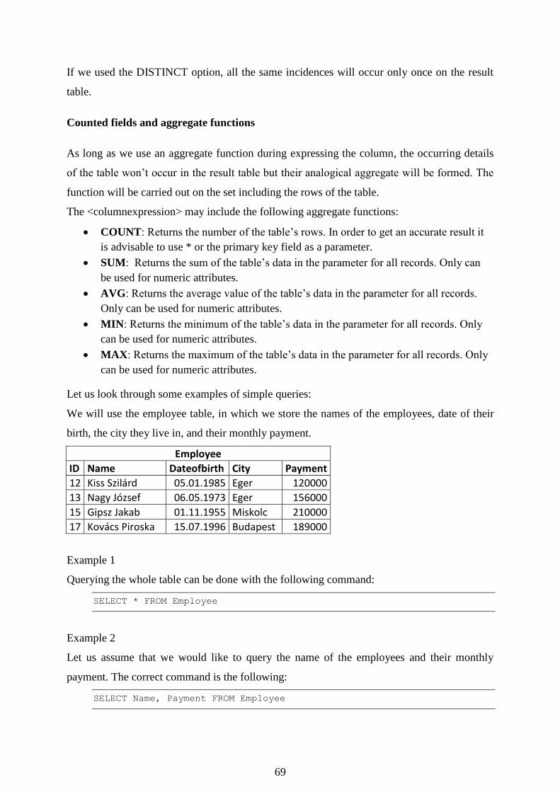
69
If we used the DISTINCT option, all the same incidences will occur only once on the result
table.
Counted fields and aggregate functions
As long as we use an aggregate function during expressing the column, the occurring details
of the table won’t occur in the result table but their analogical aggregate will be formed. The
function will be carried out on the set including the rows of the table.
The <columnexpression> may include the following aggregate functions:
COUNT: Returns the number of the table’s rows. In order to get an accurate result it
is advisable to use * or the primary key field as a parameter.
SUM: Returns the sum of the table’s data in the parameter for all records. Only can
be used for numeric attributes.
AVG: Returns the average value of the table’s data in the parameter for all records.
Only can be used for numeric attributes.
MIN: Returns the minimum of the table’s data in the parameter for all records. Only
can be used for numeric attributes.
MAX: Returns the maximum of the table’s data in the parameter for all records. Only
can be used for numeric attributes.
Let us look through some examples of simple queries:
We will use the employee table, in which we store the names of the employees, date of their
birth, the city they live in, and their monthly payment.
Employee
ID Name Dateofbirth City Payment
12 Kiss Szilárd 05.01.1985 Eger 120000
13 Nagy József 06.05.1973 Eger 156000
15 Gipsz Jakab 01.11.1955 Miskolc 210000
17 Kovács Piroska 15.07.1996 Budapest 189000
Example 1
Querying the whole table can be done with the following command:
SELECT * FROM Employee
Example 2
Let us assume that we would like to query the name of the employees and their monthly
payment. The correct command is the following:
SELECT Name, Payment FROM Employee

70
Our results are going to be the following:
Name Payment
Kiss Szilárd 120000
Nagy József 156000
Gipsz Jakab 210000
Kovács Piroska 189000
Example 3
Let us make a result table which contains the name of the employees, their payment, and their
new payment which is raised by 20%. Let’s name the new column Raised Payment. We can
solve the problem with the following command:
SELECT Name, Payment, 1.2*Payment AS „Raised Payment” FROM Employee
Our results are going to be the following:
Name Payment Raised Payment
Kiss Szilárd 120000 144000
Nagy József 156000 187200
Gipsz Jakab 210000 252000
Kovács Piroska 189000 226800
Example 4
Let us make a table of the city the employees live in avoiding to have two same values.
We can solve the task with the following command:
SELECT DISTINCT City FROM Employee
Our results are going to be the following:
City
Eger
Miskolc
Budapest
Example 5
Let us make a chart in which shows the number of the employees, the summation of the
payments, the average, the smallest and the largest payments.

71
We can solve the problem with the following method:
SELECT COUNT(id) as „Number of employees”,
SUM(payment) as „Summed payment”,
AVG(payment) as „Average payment”,
MIN(payment) as „Smallest payment”,
MAX(payment) as „Largest payment”
FROM Employee
Our results are going to be the following:
Number of Employees
Summed payment
Average payment
Smallest payment
Largest payment
4 675000 168750 120000 210000
Example 6
Let us make a chart which shows the name and date of birth of the employees. The new
column which contains the date of birth might be named ‘Date of birth’
We can solve the problem with an Oracle function.
SELECT Name, TO_CHAR(Dateofbirth, ’yyyy’) as „Date of Birth” FROM
Employee
Here the TO_CHAR function transfers the date-type value stored in the Dateofbirth field into
the given form, in this case, into a four-figure.
Our results are going to be the following:
Name Date of birth
Kiss Szilárd 1985
Nagy József 1973
Gipsz Jakab 1955
Kovács Piroska 1996
Filters and the where clause
In case of a command which takes through the selects, we can use the sub-command after the
FROM command as you can see below:
[WHERE <assumption>]
In the assumption we can use operand uses and operators.

72
Operators are comparative (<,>,<=,>=,<>), arithmetical (+,-,*,/), and logical procedures
(AND, OR, NOT), while operand uses can be constant, relation attributes viz. column names,
and function references.
For these operations the usual precedence rules are valid. Of course they can be overwritten
with brackets. We have to pay attention to make expressions serve logical values, as only the
existences will get to the result table which are true for the expression.
There are some great predicate functions:
The first one is the BETWEEN predicate function, which is used on the following way:
[<columnexpression> BETWEEN <value1> AND <value2>]
<value1> and <value2> are constants, equal with some of the known basic types (numeric,
date).
The <columnexpression> is an expression, formed from column names, having the same
type as the ones mentioned below. Records, on which the value of the expression will be
between the two constants, will fulfil the conditions. Thus, BETWEEN expresses a closed
interval.
So the condition only makes a sense if the constant given in the <value1> parameter is smaller
than the one given in the <value2>parameter.
The predicate can be definitely replaced with a logical expression containing comparative
operators:
payment between 100000 and 200000
means the same as
(payment >= 100000) and (payment <= 200000)
The following IN predicate can be used this way:
[<columnexpression> [NOT] IN <valuelist>]
As an effect of this expression, the following examination will be taken through: whether the
<columnexpression>’s value is on the given value list, or not. As far as the expression’s value
exists, it will be true. If we use the NOT keyword, the expression will be true so far as its
value is not on the list. So in the <valuelist> parameter we have to list the values fitting the
type of the expression.
The role of the predicate is highlighted in the embedded queries.

73
The third type of the predicates goes with the character chain type expressions. Its average
form is the following:
[<columnexpression> LIKE <characterchain>]
In the <characterchain> constant we can give the chain of characters between quotation
marks. Two characters have special meanings: these are the % and the _ marks. Characteristic
value has to be served to the <columnexpression> parameter which will be compared to the
constant. As long as they are equal, the condition will be true. If we use the % mark in the
constant, the two chains of characters have to match till the mark. So the % can replace an
arbitrary number of characters. The _ mark replaces only one character.
Example 7
Let’s make a chart which gives the name and the payment of the employees who earn more
than 150000 Ft.
We can solve the problem with the following order:
SELECT Name, Payment FROM Employee
WHERE Payment >= 150000
The results will look like the following one:
Name Payment
Nagy József 156000
Gipsz Jakab 210000
Kovács Piroska 189000
Example 8
Let’s make a chart which shows the name and the payment of the employees who live in Eger
and their payment is more than 150 000 Ft.
We can solve the problem with the following order:
SELECT Name, Payment FROM Employee
WHERE (City = ’Eger’) AND (Payment >= 150000)
The results will be the following:
Name Payment
Nagy József 156000
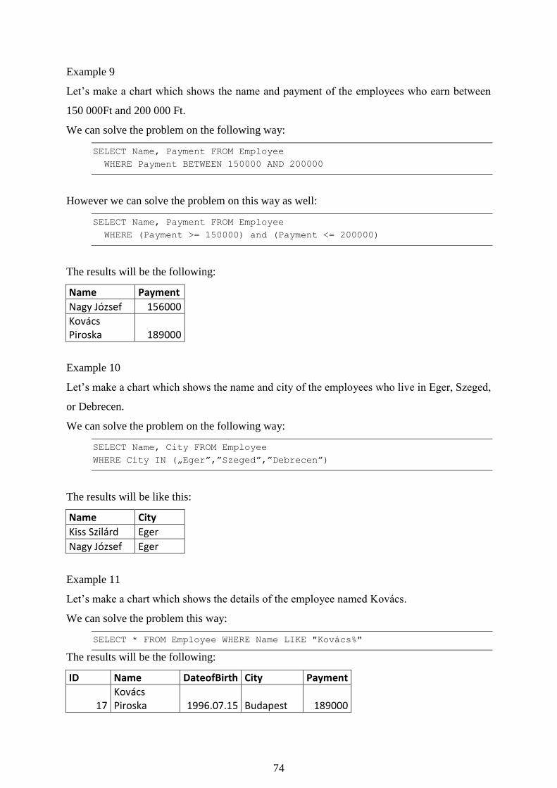
74
Example 9
Let’s make a chart which shows the name and payment of the employees who earn between
150 000Ft and 200 000 Ft.
We can solve the problem on the following way:
SELECT Name, Payment FROM Employee
WHERE Payment BETWEEN 150000 AND 200000
However we can solve the problem on this way as well:
SELECT Name, Payment FROM Employee
WHERE (Payment >= 150000) and (Payment <= 200000)
The results will be the following:
Name Payment
Nagy József 156000
Kovács Piroska 189000
Example 10
Let’s make a chart which shows the name and city of the employees who live in Eger, Szeged,
or Debrecen.
We can solve the problem on the following way:
SELECT Name, City FROM Employee
WHERE City IN („Eger”,”Szeged”,”Debrecen”)
The results will be like this:
Name City
Kiss Szilárd Eger
Nagy József Eger
Example 11
Let’s make a chart which shows the details of the employee named Kovács.
We can solve the problem this way:
SELECT * FROM Employee WHERE Name LIKE "Kovács%"
The results will be the following:
ID Name DateofBirth City Payment
17 Kovács Piroska 1996.07.15 Budapest 189000

75
Aggregation queries, the usage of group by and having, and arrangement
Aggregation means that we group records according to the values of one or more fields. After
that we can do different operations with the records in the groups, or we can use the
aggregation functions we have discussed before. We also may use selecting operations for the
groups.
We can group with this command:
GROUP BY <columnname>,[<columnname>]…
Grouping will go according to the equal values of the column names. As far as we give more
columns, it will make groups within the first column according to the second column’s equal
values, and according to the third column’s, etc. The system puts the values belong to the
single fields in the sequence given below. It makes group according to the scheme we get this
way.
After taking through the operation there will be one row for every group in the result table. As
it is a special command, during its usage we’ll have to make restrictions for other parts of the
SELECT command.
This way we’ll have to use an aggregation operator for the data of the column. Otherwise the
column has to be among the columns in the grouping, so after the GROUP BY command.
The SQL language proves us the possibility to make conditions for the data incurred by the
aggregation. In this case we have to use the HAVING command.
The form of the subcommand is the following:
HAVING <groupcondition>
In the <groupcondition> condition we can give conditions on the traditional way, except that
the column names in the conditions must include an aggregation operator, and this also have
to be after the SELECT command.
The SQL language proves us a possibility to visualise the results of our queries on a trimmed
way. We can use the ORDER BY subcommand:
ORDER BY <columnname|columnnumber> [ASC|DESC], <columnname|
columnnumber> [ASC|DESC]]…
Ordering goes according to the columns given before. First aspect will be the first column,
and the following aspect will be the following given columns. Columns can be defined on two
ways.

76
Firstly, with their original name, and secondly, with a number which is the line number of the
column in the chart. Numbering starts at 1 according to the sequence determined in the header
of the chart. It is important to have the column which represents the ordering aspect after the
SELECT command. The meaning of the ASC and the DESC keywords are also essential.
ASC is the default what means that ordering goes by an ascending order. As far as we use the
DESC keyword the ordering will go by a descending order.
Let’s look through some examples for the usage of grouping and ordering SQL commands.
Example 12
Let’s make a list which gives that how many employees live in each city.
We will use the following command:
SELECT City, COUNT(id) as „Piece” FROM Employee
GROUP BY City
The results are going to be like this:
City Piece
Eger 2
Miskolc 1
Budapest 1
Example 13
Let’s make a list which gives the sum and the average of the employee’s payment in each
city.
We will use the following command:
SELECT City, sum(Payment) as „Summed”, avg(Payment) as „Average”
FROM Employee
GROUP BY City
The results are going to be the following:
City Summed Average
Eger 276000 138000
Miskolc 210000 210000
Budapest 189000 189000
Example 14
Let’s make a list which gives the cities which are true for the condition that the employees
living there have a maximum of 150 000Ft payment.
We will use the following command:

77
SELECT City, avg(payment) as „Average”
FROM Employee
GROUP BY City
HAVING avg(Average) <= 150000
As a result we will get this table:
City Average
Eger 138000
Example 15
Let’s make a list which gives the name and payment of the employees by their payment in
descending order. In case there are same payments let’s order by name in an alphabetic
sequence.
We might use the following command:
SELECT Name, Payment FROM Employee
ORDER BY Payment DESC, Name
The results are going to be the following:
Name Payment
Gipsz Jakab 210000
Kovács Piroska 189000
Nagy József 156000
Kiss Szilárd 120000
Connecting Tables
In most of the cases the database is designed the way that details we need are stored in more
tables. It is especially true if we use normalized relations, as we all know that the base of
normalization is separating into more relations. So in this case we need all the tables, thus
queries have to be extended into multiple table queries. The SQL language provides us to take
the real algebraic operation of connection through directly. It means that there are previously
made special commands which give the different types of connections.
The first command from this group creates the Descartes product itself. During making the
command we only define the part which comes after the FROM keyword.
<tablename> CROSS JOIN <tablename>

78
As the effect of the command the system creates the Descartes product of the two tables. As
we all know, the connection based on conditions are far more natural.
Its form is the following:
<tablename> INNER JOIN <tablename> ON <condition>
As a condition we can give any of the conditions which can be used after the WHERE
command. In most of the cases one of the two connected tables’ (named master) primary key
field equals with the other table’s (named detail) unknown key field. As relational database
management systems don’t treat directly the more-to-more connections, this compliance is
clear.
This connection is called close inner connection, too.
Let’s examine the following Disbursal table which contains the paying-outs for the
employees. It has a one-to-many relationship with the (previously mentioned) Employee
table.
Employee
ID Name DateofBirth City Payment
12 Kiss Szilárd 1985.01.05 Eger 120000
13 Nagy József 1973.05.06 Eger 156000
15 Gipsz Jakab 1955.11.01 Miskolc 210000
17 Kovács Piroska 1996.07.15 Budapest 189000
Disbursal
ID Date Money Employee
101 2012.01.05 120000 12
102 2012.01.05 160000 13
103 2012.01.05 200000 15
104 2012.02.05 123000 12
105 2012.02.05 240000 15
The Employee table’s ID primary key and the Disbursal table’s unknown key field form the
relationship between the two tables.
Example 16
Let’s make a list which contains the name of the employees and the amount of money they
had been paid. The date of the disbursal should be given in alphabetic order according to the
names.
We have to use the following command:

79
SELECT Employee.name as „Name”,
Disbursal.money as „Money”,
Disbursal.date as „Date”
FROM Employee INNER JOIN Disbursal ON employee.id = disbursal.employee
ORDER BY 1
The results are going to be the following:
Name Money Date
Gipsz Jakab 200000 2012.01.05
Gipsz Jakab 240000 2012.02.05
Kiss Szilárd 120000 2012.01.05
Kiss Szilárd 123000 2012.02.05
Nagy József 160000 2012.01.05
As you can see Kovács Piroska hasn’t got her salary yet, so she wasn’t returned. As far as we
would like to add records which aren’t connected to any record, we have to use outer joins.
They are used to treat the problem which occurs when there is a row from the two tables
which isn’t connected to any items of the other table. In this case, according to the definition
of the connection, this row can’t get into the result table. In practice we might need these
occurrences in the connected relation. An outer join differs from the standard in that every
row gets into the result even the ones which aren’t connected to any other rows of the other
table. An outer join can be taken through on three ways. The first way is when all the non-
matching rows of both tables can get into the result. On the two other ways only the left or the
right sided table’s non-matching rows can.
Owing to this the following cases can exist:
<táblanév> FULL OUTER JOIN <táblanév> ON <feltétel>
In this case both table’s non-matching rows are returned.
<táblanév> LEFT OUTER JOIN <táblanév> ON <feltétel>
In this case only the non-matching rows of the table given in the first <tablename> parameter
are returned.
<táblanév> RIGHT OUTER JOIN <táblanév> ON <feltétel>
In this case only the non-matching rows of the table given in the second <tablename>
parameter are returned.
Example 17
Let’s make a list which solves the task, we were dealing in the previous example with,
returning the employees who didn’t get their salary, too.
The solution is the following:

80
SELECT employee.name as „Name”,
disbursal.money as „Money”,
disbursal.date as „Date”
FROM employee LEFT OUTER JOIN disbursal
ON employee.id = disbursal.employee
ORDER BY 1
It can occur that we have to connect more tables. In this case our method will be the same.
Every connection is a JOIN command. Like if we wanted to connect five tables we would
have four JOINs in our query.
Let’s have a look on the attendance of the employees in the corporate projects. It’s a more-to-
more relationship so we will need a connection table. In this case our database will look like
this:
Example 18
81
Let’s order the names of the employees taking part in the projects.
The solution is the following:
SELECT p.pName, e.Name
FROM employee e
INNER JOIN EmpProj ep ON e.id = dp.employee
INNER JOIN project p ON ep.project = p.idProject
ORDER BY p.pName, e.name
As you can see I have used the shorter form of the table names. The employee table was put
in as ‘e’. It is to use a shorter way of writing within the query. The rule is if we shorten the
name of a table we have to use the shorter form in the whole query.
Embedded queries
The SQL language provides us the facility of using the SQL query command in the condition
of the select queries. In this case we separate inner and outer SELECT command, and name
these queries embedded queries.
The syntax of the SELECT commands equals with the forms we have already discussed, we
only have to pay attention to make some requirements fulfilled in connection with the inner
queries. We separate more cases in accordance with the type of the inner query.
They are the following:
1. The inner query serves only one value. This is the simpler case as at this time
everything happens on the standard way except that the system serves the value given
in the expression as a condition.
2. The inner query serves a one column relation. This time we can give conditions which
use the data of the column served by the inner query. In this case we might use
different predicates:
The following predicate do exists:
<columnexpression> [NOT] IN <inner query>
Dealing with this type the system will decide if it is in the generated column’s data examining
the value of the expression given in the <columnexpression> parameter. If the condition’s
value is yes, it’ll be true; if it is not, it’ll be false. If we use the NOT keyword we have to read
the condition reversed.
The form of the forthcoming predicates is the following:
[NOT] <columnexpression> <relation> ALL|ANY <inner query>
At this type the system will examine whether the relation is fulfilled with the data of the
column created by the inner query, referring to the value of the expression given in the
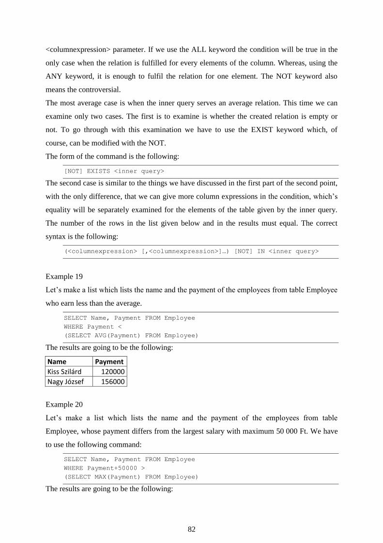
82
<columnexpression> parameter. If we use the ALL keyword the condition will be true in the
only case when the relation is fulfilled for every elements of the column. Whereas, using the
ANY keyword, it is enough to fulfil the relation for one element. The NOT keyword also
means the controversial.
The most average case is when the inner query serves an average relation. This time we can
examine only two cases. The first is to examine is whether the created relation is empty or
not. To go through with this examination we have to use the EXIST keyword which, of
course, can be modified with the NOT.
The form of the command is the following:
[NOT] EXISTS <inner query>
The second case is similar to the things we have discussed in the first part of the second point,
with the only difference, that we can give more column expressions in the condition, which’s
equality will be separately examined for the elements of the table given by the inner query.
The number of the rows in the list given below and in the results must equal. The correct
syntax is the following:
(<columnexpression> [,<columnexpression>]…) [NOT] IN <inner query>
Example 19
Let’s make a list which lists the name and the payment of the employees from table Employee
who earn less than the average.
SELECT Name, Payment FROM Employee
WHERE Payment <
(SELECT AVG(Payment) FROM Employee)
The results are going to be the following:
Name Payment
Kiss Szilárd 120000
Nagy József 156000
Example 20
Let’s make a list which lists the name and the payment of the employees from table
Employee, whose payment differs from the largest salary with maximum 50 000 Ft. We have
to use the following command:
SELECT Name, Payment FROM Employee
WHERE Payment+50000 >
(SELECT MAX(Payment) FROM Employee)
The results are going to be the following:

83
Name Payment
Kiss Szilárd 120000
Nagy József 156000
Gipsz Jakab 210000
Kovács Piroska 189000 Example 21
Let’s make a list with the help of the Disbursal table we dealt with below which lists the name
and the number who haven’t got their salary yet.
We will have to use the following command:
SELECT Name, ID FROM Employee
WHERE ID NOT IN
(SELECT ID FROM Disbursal)
Another solution might be the following:
SELECT Name, ID FROM Employee
WHERE NOT EXISTS
(SELECT ID FROM Disbursal
WHERE Disbursal.employee = Employee.ID)
You might recognise that the second way of solving the problem includes a special case when
we use a field of the table of the outer query in the inner query.
The results are the following:
Name ID
Kovács Piroska 17
Example 22
Let’s make a list which lists the details of the employees who earn more than all the
employees living in Eger or Szeged.
We will use the following command:
SELECT * FROM Employee
WHERE Payment > ALL
(SELECT Payment FROM Employee
WHERE City = "Eger" OR City = "Szeged")
ID Name DateofBirth City Payment
15 Gipsz Jakab 1955.11.01 Miskolc 210000
17 Kovács 1996.07.15 Budapest 189000

84
Piroska
Tasks
Task 1.
Artwork- Artificer
We know several things about a piece of artwork like the year of the creation, its genre
(sculpture, painting, art book, etc.) its value in HUF, its title, and the name, date of birth, and
nationality of the artist. One piece of artwork always belongs to one type of genre, and the
artists belong to one nationality as well. We are able to process the whole life and work of the
artist.
The drawn plan of the database including the names of the tables, names of the fields, types of
the fields, and relationships should be delivered.
The DDL commands which are creating the table.
The DML commands doing the data upload.
The QL, DDL, and DML commands which are giving answers.
1. Design a database at least in 3NF to solve the problem mentioned above.
2. Add at least 5 artificers and 10 artworks. Create at least 3 kinds of genres and
nationalities. Upload the created data tables in the given sequence.
3. Answer the following questions with SQL queries.
a. List the name of the artworks made in the 20th century and order them by the name
of their creator in cumulative sequence.
b. List all the details of the sculptures.
c. List the details of the Hungarian artists in an alphabetical order in decreasing
sequence
d. Figure out the summed value of all the artworks for each nationality.
e. List the Italian artworks and the name of their creator which worth more than the
average.
f. List the name of the genres but pay attention to have every genre only once in the
result.
g. List the number of the artworks in each nation with the name of the nations but
visualise only the nations which have more than 3 pieces of artwork.
h. Add a new field to the appropriate table which contains the number of the
artificer’s international awards.
Solutions for the SQL queries:
A.
select ar.title, sz.name

85
from artwork ar
inner join K1 on ar.ar_id = K1.ar_id
inner join artificer sz on k1.a_id = sz.a_id
where ar.ar_year between 1901 and 2000
order by sz.name;
A/2
select ar.title, sz.name
from artwork ar, K1, artificer sz
where
(ar.ar_id = K1.ar_id) and
(k1.a_id = sz.a_id) and
(ar.ar_year between 1901 and 2000)
order by sz.name;
B.
select sz.name, aa.*, n.n_name
from artwork ar
inner join K1 on ar.ar_id = K1.ar_id
inner join artificer sz on k1.a_id = sz.a_id
inner join nation n on n.n_id = sz.n_id
inner join genre g on g.g_id = ar.g_id
where g.g_name = "sculpture"
order by ar.ar_name
C.
select sz.*
from artificer sz
inner join nation n on n.n_id = sz.n_id
where n.n_name = "Hungarian"
order by sz.a_name desc;
D.
select n.n_name as nation, sum(ar.ar_value) as summed
from artwork ar
inner join K1 on ar.ar_id = K1.ar_id
inner join artificer sz on k1.a_id = sz.a_id
inner join nation n on n.n_id = sz.n_id
group by n.n_name;
E.
select ar.ar_name, sz.a_name
from artwork ar
inner join K1 on ar.ar_id = K1.ar_id
inner join artificer sz on k1.a_id = sz.a_id
where
ar.ar_value >
(
select avg(ar.ar_value)
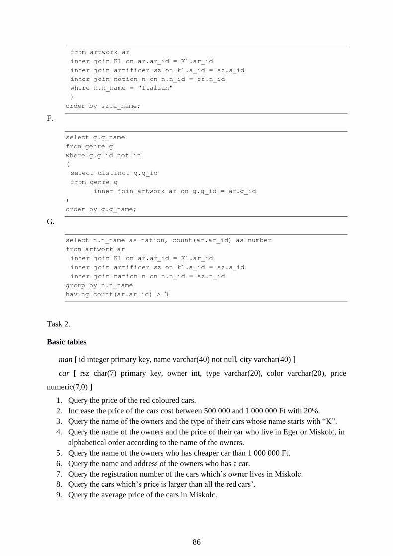
86
from artwork ar
inner join K1 on ar.ar_id = K1.ar_id
inner join artificer sz on k1.a_id = sz.a_id
inner join nation n on n.n_id = sz.n_id
where n.n_name = "Italian"
)
order by sz.a_name;
F.
select g.g_name
from genre g
where g.g_id not in
(
select distinct g.g_id
from genre g
inner join artwork ar on g.g_id = ar.g_id
)
order by g.g_name;
G.
select n.n_name as nation, count(ar.ar_id) as number
from artwork ar
inner join K1 on ar.ar_id = K1.ar_id
inner join artificer sz on k1.a_id = sz.a_id
inner join nation n on n.n_id = sz.n_id
group by n.n_name
having count(ar.ar_id) > 3
Task 2.
Basic tables
man [ id integer primary key, name varchar(40) not null, city varchar(40) ]
car [ rsz char(7) primary key, owner int, type varchar(20), color varchar(20), price
numeric(7,0) ]
1. Query the price of the red coloured cars.
2. Increase the price of the cars cost between 500 000 and 1 000 000 Ft with 20%.
3. Query the name of the owners and the type of their cars whose name starts with “K”.
4. Query the name of the owners and the price of their car who live in Eger or Miskolc, in
alphabetical order according to the name of the owners.
5. Query the name of the owners who has cheaper car than 1 000 000 Ft.
6. Query the name and address of the owners who has a car.
7. Query the registration number of the cars which’s owner lives in Miskolc.
8. Query the cars which’s price is larger than all the red cars’.
9. Query the average price of the cars in Miskolc.

87
10. Query that how much cars are in each cities.
11. Query the registration number and the name of the owners of the cars which are more
expensive than the average.
12. Query the owners who have only one car grouped and ordered by the city they live in.
Solutions for the SQL queries:
1. Query the price of the red coloured cars.
SELECT price FROM car WHERE color = ’red’;
2. Increase the price of the cars cost between 500 000 and 1 000 000 Ft with 20%
UPDATE car SET price=price*1.2 WHERE price BETWEEN 500000 AND 1000000
3. Query the name of the owners and the type of their cars whose name starts with “K”.
SELECT m.name, c.type
FROM man m inner join
car c on m.id = c.owmner
WHERE m.name LIKE 'K%';
4. Query the name of the owners and the price of their car that lives in Eger or Miskolc,
in alphabetical order according to the name of the owners.
SELECT man.name, car.price
FROM man m inner join
car c on m.id = c.owner
WHERE city IN ('Miskolc', 'Eger')
ORDER BY man.name;
5. Query the name of the owners who has cheaper car than 1 000 000 Ft.
SELECT man.name
FROM man m inner join
car c on m.id = c.owner
WHERE car.price < 1000000;
6. Query the name and address of the owners who has a car.
SELECT name, city
FROM man
WHERE id IN (SELECT owner FROM car);
7. Query the registration number of the cars which’s owner lives in Miskolc.
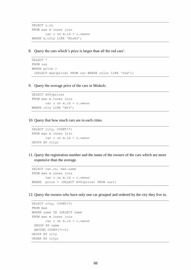
88
SELECT c.rn
FROM man m inner join
car c on m.id = c.owner
WHERE m.city LIKE ’Misk%’;
8. Query the cars which’s price is larger than all the red cars’.
SELECT *
FROM car
WHERE price >
(SELECT max(price) FROM car WHERE color LIKE ‘red’);
9. Query the average price of the cars in Miskolc.
SELECT AVG(price)
FROM man m inner join
car c on m.id = c.owner
WHERE city LIKE ’Mi%’;
10. Query that how much cars are in each cities.
SELECT city, COUNT(*)
FROM man m inner join
car c on m.id = c.owner
GROUP BY city;
11. Query the registration number and the name of the owners of the cars which are more
expensive than the average.
SELECT car.rn, man.name
FROM man m inner join
car c on m.id = c.owner
WHERE price > (SELECT AVG(price) FROM car);
12. Query the owners who have only one car grouped and ordered by the city they live in.
SELECT city, COUNT(*)
FROM man
WHERE name IN (SELECT name
FROM man m inner join
car c on m.id = c.owner
GROUP BY name
HAVING COUNT(*)=1)
GROUP BY city
ORDER BY city;

89
Task 3.
Video rental store
We are examining a video rental store’s registration. The lender rents only videos, and all the
videos are registered including the title of the film, the main character, and the director. Every
film has a unique identity number but we can’t be sure if its title is unique or not. One film
can be stored on more cassettes as the video rental store can make copies. Every cassette has
its unique identity number and their type is registered. Only the members of the video rental
store are allowed to rent a video. The members’ name, address, and identity number are also
registered. Members are allowed to lend films, so the date of the lending and the date of the
return are registered as well. The video rental store purchases videos from a wholesaler. Every
order has an identity number and to make orders easy to follow, they register the date of the
order. One order may include more films. Documents at the video rental store are the
following, stored on different pages. These items have to be used during designing the logical
database model:
Number of the Cassette
Type of the Cassette
Title of the Film
Number of the Film
Number of the Order
Date of the Order
Number of the Lending
Identity number of the Member
Name of the Member
Address of the Member
Date of the Lending
Date of the Return
Main Character of the Film
Director of the Film
Queries
1. List the details of the members who haven’t borrowed anything but own a
membership.
2. List all the main characters of the films available.

90
3. List the title and the director of all the films available.
4. Visualize the number of the cassettes and the name of the films which haven’t been
borrowed ever.
5. List the name of the members borrowed something today.
6. List the films have to be returned today.
7. List the films which should have been returned till today.
Solutions for the SQL queries:
1.
select * from tag
where tag_snumber not in
(select tag_snumber from borrow)
order by name
2.
select e.name from employee e
inner join film_emp fe on e.em_id = fe.em_id
inner join emp_type et on et.et_id = fe.et_id
where et.description = "main character"
order by e.name
3.
select f.filmtitle, e.name from employee e
inner join film_emp fe on e.em_id = fe.em_id
inner join dolg_tipus dt on dt.dt_id = fd.dt_id
inner join film f on f.filmnumber = fe.filmnumber
where et.description = "director"
order by e.name
4.
select f.filmtitle, c.cassettenumber
from film f
inner join cassette c on f.filmnumber = c.filmnumber
where c.cassettenumber not in
(select disctinct c2.cassettenumber from cassette c2
inner join borrow bo
on c2.cassettenumber = bo.cassettenumber)
5.
select t.name from tag t inner join borrow b
on b.tag_snumber = t.tag_snumber
where borrow_date = '2005.11.21'
6.
select f.filmtitle, c.cassettenumber
from film f
inner join cassette c on f.filmnumber = c.filmnumber

91
inner join borrow bo
on c.cassettenumber = bo.cassettenumber
where bo.return_date = '2005.11.21'
order by f.filmtitle
7.
select f.filmtitle, c.cassettenumber
from film f
inner join cassette c on f.filmnumber = c.filmnumber
inner join borrow bo
on c.cassettenumber = bo.cassettenumber
where bo.return_date < '2005.11.21'
order by f.filmtitle
8.
select filmtitle from film order by filmtitle
Task 4.
Kings
We would like to store and work with the period of their reign. We know the name of the
kings, the starting and ending date of their reign.
Table:
KING (THE, Name, Begin, End)
THE The ID of the king (counter) this is the key
Name The name of the king (text)
Begin The first year of his reign (number)
End The last year of his reign (number)
1. List the kings in alphabetical order. (nominal roll)
2. List the name and the period of their reign of the kings named László. Don’t add the
kings named Ulászló. (László)
3. List the name of the kings ordered according to the length of their reign in descending
sequence. (LengthOrder)
4. Query the number of the kings named István. (Number of Istváns)
5. In 1347 the court of the king temporarily moved from Visegrád to Buda. Who was the
king at that time? (Buda court)
6. List the name of the kings who owned the throne for more than 10 years in
alphabetical order. (10 years)
7. How many kings reigned from 1300 till 1399 in Hungary? Don’t forget that only a
part of the reign of a king might belong to this period. (Number of kings)
8. Identify that how many kings reigned before Mátyás with the help of a subquery.
(before Mátyás)
9. Who owned the throne for the longest period of time? (MaxKing)

92
Task 5.
Borrowing water sports equipment
During our holiday nearby the cost we can borrow sport equipment for more hours a day
several times. Let’s make a database for the rental service.
The database stores the tools which can be lent, their type (like paddle boat, kayak, surf, ect.)
and how much the rent costs for an hour. Borrowers have to pay for every hour as it begins.
The clients (borrowers) must be stored and the details that which client borrowed the tool and
when. The head of the rental service trusts the clients so the clients have to pay at the end of
the day in sum.
To solve this you should create four tables, which have to contain the following attributes and
relationships (we mark the primary keys with a *)
Tooltype *Type (text), Price_hour (number)
Tool *Tidentifyer (number), Type (text), Brand (text)
Client *Cidentifyer (number), Name (text), Address (text), Pay (number)
Borrow Cidentifyer (number), Tidentifyer (number), Period (number) Start
(time) End (time
1. Create the data tables based on the information given above. Choose the optimal field
size during defining the fields. Set the unknown keys (the relationships) to make the
database management system keep integrity.
2. Invert to the tables the details given in the borrow.xls worksheet.
3. Make a query which returns the contains of the Borrow table in the way that the
Identifier is replaced with the name of the client and the Identifier is replaced with the
type and the brand of the tool.
4. List the type of all the tools which were borrowed at 12 am.
5. Query all the tool types (once) which were borrowed once at least for 2 hours.
6. List all the details of the tools which haven’t been borrowed yet.
7. Make a query what counts how much a client will have to pay at the end of the day,
based on the number of the daily borrows, their period of time, and the price of the
borrowed tools.
Task 6.
Competition
Create a database for registering the result of a problem-solving competition answering the
following data structure. (We mark the primary keys with a *)
Tables:
COMPETITOR (CompetitorAZ, Name, SchoolAZ, Class)
*CompetitorAZ ID of the competitor (text)

93
Name Name of the competitor (text)
SchoolAZ The ID of the competitor’s school (text)
Class Class of the competitor (number)
RESULT (CompetitorAZ, TaskNumber, Points)
*R_id (number)
CompetitorAZ ID of the competitor (text)
TaskNumber The number of the task (text)
Points The points the competitor achieved in that task (number)
SCHOOL (SchoolAZ, SchoolName, PostCode, City, Street, Number)
*SchoolAZ The ID of the school
SchoolName The name of the school
PostCode The post code of the school (number)
City The city the school is situated in (text)
Street The street of the school (text)
Number The number of the school (text)
Relationships between the tables:
SCHOOL-COMPETITOR : one-to-many type
COMPETITOR-RESULT : one-to-many type
Tasks
1. Crate a COMPETITON database matching the table structures discussed above.
2. Fulfil the tables according to this scheme:

94

95
CompetitorAZ TaskNumber Points
1 I 12
1 II 8
1 III 11
1 IV 3
10 I 2
10 II 5
10 III 0
10 IV 6
11 I 4
11 II 9
11 III 13
11 IV 2
And so on
All the competitors have to solve four tasks. The tasks are marked with roman numbers.
Make a query to answer the following questions! Mark the name of the solutions with the
letters in brackets.
3. Query the name and the points of the competitors in increasing sequence. (A)
4. Identify the largest point for each task. (B)
5. How many students entered the competition from each school (school’s name and
city)? (C)
6. Order the name of the competitors in alphabetical order that got 0 points for any task.
One name can be there only once. (D)
7. Query the name, school’s name and address of the students who got more than 10
points for a task.
8. Who got the maximum points for the first task from the students living in the country?
Query his name and his school’s name. (F)
Task 7.

96
Products
Make the structure of Products table according to this scheme:
Products (ProductCode, ProductName, CategoryCode, Size, Color, Price, InStock)
ProductCode (Counter)
ProductName (text)
CategoryCode (number)
Size (text)
Color (text)
Price (number)
InStock (number)
Set the key of the tables.
Change the form of the Price field of the Products table to make the prices appear as full
currencies.
During solving the tasks pay attention for the relationships between the tables.
Tasks:
Solve the following tasks. Save the solutions as the name given in brackets.
1. Which are the products and in which colors are they on sale which are sized L and
there are at least 5 ones in stock? Order the list to make the product with the largest
price to be at the first place. (A)
2. What’s the average price of the products in each category? (B)
3. What is the actual stock value of the cotton and canvas trousers? The name, color,
category, and the stock value of the products should be listed in alphabetical order. (C)
4. List the black tops which are in stock? In which size and price are they for sale? (D)
5. Sum the number of the pullovers which are in stock. (E)
6. List the products and the number of them which are in stock which’s price is between
5000 and 10 000 HUF. Order the list in increasing sequence according to the stock. In
case of a same stock, list them in alphabetical order.
Task 8.
Epee
Examine the details of the ones who won a medal in men’s individual epee at the modern
Olympic Games with the help of a database management system. These pieces of information
are stored in a data table. Create a new database named duel.
The structure of the table:
INDIVIDUAL (ID, Year, Location, Name, Country)
ID The ID of the athlete (counter). This is the key.
Year Date of the Olympics (number)

97
Location The city where the Olympics took place (text)
Place The place the athlete achieved (number)
Name The name of the athlete (text)
Country The shorter form of the country the athlete represents (text)
Tasks
Solve the following problems.
1. List the name of the athletes who earned a gold medal, the date, and the location of the
Games. Order them by date in increasing sequence. (A)
2. In which Olympics and what place did Kulcsár Győző achieved? (B)
3. List the name and place of the athletes who won a medal in the Olympics in Atlanta.
(C)
4. How many medals have the Hungarians earned? (D)
5. Who were the ones who won a medal representing Hungary? Every athlete should be
on the list only once. (E)
6. Who won the most gold medals? (F)
7. Sum the number of the gold medals earned by each country. (G)
8. In which city was the Olympic Games organised the most times? (H)
Task 9.
Course
Name of the data table: EMPLOYEE
Name of the data table: COURSE

98
Name of the data table: ATTENDANCE
The employees of a company take part in different courses. One employee might attend more
courses.
1. Create the data tables you’ve seen above, and define the field types.
2. Create logically the primary keys and acceptable relationships between the tables.
3. Query the employees who attend the informatics course.
4. How many employees attend the informatics course?
5. Query the courses which cost between 4500 HUF and 6500 HUF.
6. Lower all the fees by 50%.
7. Query all the fees the attendees have paid ever.
Task 10.
Statistics
One of the local schools in Budapest from distinct VII makes a database for its statistical
registries.
1. Design a database named statistics.
2. Create a table named student on the way to be able to answer the following questions
after the uploading.
What is the number of the boys, the girls, and the private students in the class?
What is the number of the students who are aged 14, 15, 16, 17, and 18?

99
Who has two or more siblings?
How many students live in another distinct or city, and what is the number of the
local students?
How many students live in a college?
What is the number of the students who have a resort to the school canteen or to
the prep room?
What is the number of the families where monthly income per capita is less than
30 000 HUF?
3. Give a key field in the data table.
4. Load up the data table fulfilled with 5 records with details of fictitious people.
Answer the following questions due to these details. Save your answers with the name
in brackets at the end of the question.
5. Who has two or more siblings? Order the name of the students, the number of their
siblings, and the monthly income per capita in increasing sequence according to their
income. (sibling)
6. Who are the ones who live in another distinct or city than the seat of the school? (other
place)
Task 11.
Nobel Prize
Process the details of the ones who earned a Nobel Prize with the help of a database
management system.
Create a new database named nobel.
The structure of the table should be the following:
year The year of the remuneration (number)
name The name of the one who got the prize (text)
country The country the one who got the prize lived in (text)
prize The type of the prize (text)
1. Kertész Imre’s Nobel Prize in Literature which he got in 2002 is missed out of the
database. Fulfil the database.
2. Make the list of the Hungarian Nobel Prizes. (Hungarian)
3. What kind of prize did Bárány Róbert get? Which country did he represent? (Bárány)
4. What kind of prize did Wigner Jenő get? Which country did he represent? (Wigner)
5. Who were the Dutch Nobel Prize winners (its mark: NL)? (NL)
6. Which prize was given the most of the times? Whom was the prizes given to?(prizes)
7. In which year what kind of prizes weren’t given to anyone? (miss)
8. Which countries’ reps got only one Nobel Prize? (once)
9. List the number of the Nobel Prizes in each country. Only real countries can be on the
list. They have to be listed hierarchically. (hierarchy)
10. List the prizes, winners, and their country that got a Nobel Prize between 1901 and
1939. (1939)

100
12.
1. The Stupido-Gigantic GmbH Ltd Kft S.A. is mainly dealing with commercialism.
According to this they get orders from their customers who are served by the deliverers. One
product is delivered by one deliverer and one deliverer delivers only one product. We register
the customer’s momentary remainder. One order may include more items – an item consists
of the name of the product and the amount of the ordered item(s). The name of the deliverers,
products, and cities are unique but the names of the customers are only unique within a city.
We can assume that every city has only one post code.
The stored datas:
DelivererPostCode, CustomerPostCode, DelivererName, OrderNumber, Quantity, OrderDate,
CustomerCityName, Remainder, OnePrice, ProductName, DelivererCityName,
CustomerName, ProductName.
Tasks:
1. Create the logical database model of the Stupido-Gigantic GmbH Ltd Kft S.A.
company’s trade. (Till the 3NF form)
2. Put the model into practical.
3. Make the following queries:
the post code of the deliverer who delivers the “gummy bear” item
the names of the customers in the year 1998
the remainder of the customers living in Ajka
the name and location of the customer having the largest remainder
from which deliverer have the most loyal customer ordered the most of the
times?
Task 13.
Basic tables
man [ id integer primary key, name varchar(40) not null, city varchar(40) ]
car [ rsz char(7) primary key, owner int, type varchar(20), color varchar(20), price
numeric(7,0) ]
1. Query the price of the red coloured cars.
2. Increase the price of the cars cost between 500 000 and 1 000 000 Ft by 20%.
3. Query the name of the owners and the type of their cars whose name starts with “K”.
4. Query the name of the owners and the price of their cars that live in Eger or Miskolc,
in alphabetical order according to the name of the owners.
5. Query the name of the owners who has cheaper car than 1 000 000 Ft.
6. Query the name and address of the owners who has a car.
7. Query the registration number of the cars which’s owner lives in Miskolc.
8. Query the cars which’s price is larger than all the red cars’.
9. Query the average price of the cars in Miskolc.

101
10. Query that how much cars are in each cities.
11. Query the registration number and the name of the owners of the cars which are more
expensive than the average.
12. Query the owners who have only one car grouped and ordered by the city they live in.
13. Query the registration number of the cars which are more expensive than the cheapest
car in Miskolc.

102
Views and Indexes
View
Some groups of the users don’t see the whole database, or they might see some parts
differently from they are built up in the conceptual model.
For example, this case obtains when a group can’t see the Payment field of the record of the
Personal Details table, while another group can’t see the Date of Birth field. So planning the
views is one of our duties during designing a database. We can sort the data model into three
levels:
– User level: describes the way the users see the database
– Logical level: illustrates the whole conceptual structure of the database
– Physical level: Writes down the physical position and the access path of the datas
Due to the strong severance of the logical and the physical level, data independence became
the most important requirement of database designing. We distinguish logical and physical
data independence:
Metadata provide us the logical data independence, viz. not only data but the features of the
data and descriptions of the connections between data groups are stored as well.
Database management systems (DBMS) provide logical data independence basically. A
change in the data structure doesn’t mean that we have to rewrite the user program as it means
a change just among the metadata. We are able to make changes on the logical level without
making a change on the user level.
DBMS provides physical data independence as well. A change in the structure of data storage
or the way of access – in one word: the physical database – doesn’t mean a change in the
logical scheme or in the user level. For example the only thing a user recognises from
indexing is that they can reach some data faster than before.
The aim in every well-designed system built up according to the layering conception is that
layers have to be changeable without reference to each other, providing that the interfaces
between the layers remain the same.
Two types of data independence are distinguished:
Physical data independence, which is meant between the physical and the logical database
Logical data independence, which is meant between the logical database and the views

103
When we talk about physical data independence, we think of a requirement that the changes
taken through the physical database shouldn’t affect the logical database. If it is realized (in
most of the cases) then the physical data medium can be exchanged to another with different
parameters (in case of a breakdown or a technical improvement) without experiencing any
changes in the logical database.
We talk about logical data independence when a change in the logical database doesn’t go
with a change in the views which belong to the users. This requirement isn’t fulfilled in all
cases.
We can create a view with the following order:
CREATE VIEW <view_name> [(<column_name1>, …)] AS <query>
There is only one restriction for queries: they mustn’t contain orderings. If we don’t name the
columns, the columns of the view equals with the names of the columns listed after SELECT.
However, if the SELECT creates counted values, we’ll have to name the columns.
For example:
CREATE VIEW dept_sal (deptno, avg salary) AS SELECT deptno, AVG (sal) FROM emp
GPOUP BY deptno
Modifiable view tables
During modifying a view table we also modify the content of the data tables behind
them
Basically not all the view tables are modifiable
Modifiability can be gained on two ways:
– The view table has an originally a more simple structure
– We make an INSTEAD OF type trigger
Structural terms of modifiability:
The definition of the view table mustn’t contain:
– set procedures
– DISTINCT, GROUP BY, ORDER BY keywords
– cumulative functions
– sub-queries
Columns, which’s value come from a monomial, can’t be modified
In case of views referring to more tables
– Modifying can affect only one table
– In case of INSERT or UPDATE the keys and unique values of the modified
table have to be unique in the view as well

104
For modifying the structure of the view table we use CREATE OR REPLACE VIEW.
Deleting a view table
Form:
DROP VIEW view_name
Example:
DROP VIEW customers_budapest_vw
Data aren’t deleted! They are in the tables!
Consequently, let’s look through the advantages of view tables:
First of all safety: they allow access to the chosen data
– e.g. every employer can see only their employees
– In the data dictionary we only see the view tables (e.g. USER_TABLES or
ALL_USERS). It is advantageous as the user can see what they are allowed
to see but nothing else.
They simplify the orders the users have to give out
– e.g. users don’t have to connect tables
They make applications independent from the structure of the tables
– e.g. new columns can be added to the data tables and their names can be
modified as well
They increase safety
– e.g. complicated queries which are used frequently can be saved as a view
table
Data can be “served” due to the different user’s demands.
– e.g. users can see data which are useful for them
Indexes
Pointers in index records can identify the record on two ways:
– Clustered indexing, when we put indexes on every single data record
– Sparse indexing, when we put indexes on groups of data stored in blocks
Sparse indexes
Index records locate the block the records of the data file are stored in. Within a block, data
records can be treated as free records. In case of a sparse index the data file has to be stored
on a trimmed way; viz. all the records having their keys in one interval have to be stored in
one block.

105
Searching
Let’s put the case that we are searching a k1 type key. Within the index file we look up the
record whiches k2 type key is the largest out of the ones which are smaller than k1. The
pointer of the k2 key of the index record will name the block in which you’ll find the k1 key.
Insertion
Let’s put the case that we would like to store the record having the k1 type key. Firstly we
have to find the block in which the record must be stored. If it were in the data file, let’s name
it Bi block.
After that two cases can exist.
It depends on whether there is enough space for the k1 key in the Bi block or not.
If there is, we don’t have much to do only to write it into the Bi block as a record.
If there is no space, we’ll have to make. We have to make a new empty block.
Deleting
Let us assume that we wish to delete the record with the k1 key. First of all, we have to look
up the block the record is stored in. Here it is called Bi. If the k1 key is not the smallest key in

106
the block we can delete it smoothly, and abolish the empty space in the place of the deleted
key with moving the records inside the block.
Modifying:
In case of modifying two cases can exist. It can be simple, if the modifiction didn’t affect the
key of the record. In this case we just look up the record, take through the modifiction, and
rewrite it to the storage device.
Alhtough it can be complicated, if the modifiction affects a key field. In this case deleting can
be taken through with deleting and inserting followed by each other.
B*-trees as multilevel sparse indexes
With indexed searching searching time commensurate with log2N can be reached, which is
less than the heap organising’s but more, than the hash organizing’s. In exchange, the amount
of the usage of the storage device can be handled in case of a database with a changing size.
A k-ponter imaged in an intersection can be stored with only a k-1 key as the meaning of this
key is the smallest key value in the given part of the tree. This way the first key value of the
index blocks wouldn’t contain any information. This indexing is called B*-tree indexing.

107
Searching:
The procedure is similar to those studied on rare indexes, only the index file searching is
carried out in several steps.
Suppose that v1 key records are required. Find the record, in the top block of indexes, which
has the highest v2 key but lower v1 keys. This record’s pointer directs to the lower level
block, in which the search should be continued for a record that has the largest v3 key of those
with smaller v1 keys. This process continues until the last indicator identifies a block of the
database in which the key must be a record.
Insertion:
The main deviation from inserting rare indexes is the added requirement of managing
the original tree-system and it’s equilibrium.
Delete:
Find and delete the appropriate entry. Data blocks should be merged if possible. When
merging, or when a record’s last data block is deleted, the block’s keys are to be removed
from the concerned index.
Modification:
Same as mentioned during rare indexes.
Dense indexes:
The disadvantage of rare indexing is that the data files have to be stored orderly. Therefore,
there is no way to insert a new record for any available position, thus storage utilization is
reduced.

108
One solution could be if all data records have index record. The index records continue to
only identify the block containing the record. This way, the search time within the block can
be reduced.
Dense indexing primarily helps the use of the main database and makes searching by multiple
keys possible.
Disadvantages:
● More space required
● Requires an extra data access to read records
● Extra administration to maintenance
Advantages:
● No need for organized storage,thus space savings
● Faster access to the record
● Multiple key search
● Database records can be freed if all other records of the calls are made through a dense
indexes.
Search:
Find the key in the index database, access the record using the connected pointer.
Delete:
We find the record, set the signal to unused, the key is removed from the index file and
compact the index stocks.

109
Insertion:
Look for an empty space for the record, if it’s not found, add it to the end of the file.
Set the signal, and enter the data.
Modification:
We find the data block containing the record, then re-enter the amended record to the
database. If a key field has been modified rearrange the indexes.

110
Constraints, integrity rules, triggers
The constraints are such regulations we can provide our expectations related to the content of
the database. When we make these statements for the database system in one place once, it
will make sure to force them. If we happen to design them in the user-interface, we would
modify and declare them in many places.
Constraints are checked after every action which would change the content of the database in
a way that the content would not satisfy the constraints. Constraints are valid since we declare
them. They do not have a retrospective effect. Execute a delayed check by the keyword
DEFFERRED.
Keys
Used for identify the individual clearly. As a constraint it means to check that in the relation
should not occur two rows, where the value of the key attributes would be the same for a pair.
In one relation there might be more keys. It is a custom to declare one primary key form them.
At the CREATE TABLE statement it could be defined. When the key has one attribute, we
can declare it by the PRIMARY KEY or the UNIQUE keywords, or at the end of the
statement after the above keywords in brackets as an enumeration. If it has more attributes, at
the end of the table only.
In the following example we create tables with the same constraints, illustrating how to define
constraints in two possible ways.
CREATE TABLE hallgatok(
neptun_kod CHAR(6) PRIMARY KEY,
nev VARCHAR2(30) NOT NULL,
szul_ev NUMBER(4) CHECK (szul_ev > 1900),
telefonszam NUMBER(10) UNIQUE);
CREATE TABLE atlagok(
neptun_kod CHAR(6) REFERENCES hallgatok(neptun_kod),
atlag NUMBER(3,2));
CREATE TABLE hallgatok2(
neptun_kod CHAR(6),
nev VARCHAR2(30) NOT NULL,
szul_ev NUMBER(4),

111
telefonszam NUMBER(10),
PRIMARY KEY (neptun_kod),
CHECK (szul_ev > 1900),
UNIQUE (telefonszam)
);
CREATE TABLE atlagok2(
neptun_kod CHAR(6),
atlag NUMBER(3,2),
FOREIGN KEY (neptun_kod) REFERENCES hallgatok2(neptun_kod)
)
Above attributes have the following constraints.
• in tables ‘hallgatok’ and ‘hallgatok2’ the a ‘neptun_kod’ is the primary key, so in every row
must have different values, and none of them could be null.
• the ‘név’ field could not contain null value;
• ‘szul_ev’ must be greater than 1900;
• there could not be two same telephone numbers, but it could happen that we do not know
somebody’s telephone number;
• to the tables ‘átlagok’ and ‘átlagok2’ could go only such record where the value of
‘neptun_kod’ field is appearing in the ‘hallgatok’ table’s ‘neptun_kod’ attribute values.
Let’s see an example, how else to define an attribute set as a primary key. (UNIQUE and
FOREIGN KEY could be defined similarly for an attribute set.
CREATE TABLE hallgatok(
nev VARCHAR2(30),
szul_datum DATE,
anyja_neve VARCHAR2(30),
lakcim VARCHAR2(100),
PRIMARY KEY(nev, szul_datum, anyja_neve));
In this table the ‘nev’, ‘szul_datum’ and ‘anyja_neve’ attributes could take same value in two
records one by one, but there is a slight chance to all three attributes would be the same, so in
practice they are used as primary key often.

112
Referential integrity constraint
~ that means that certain attributes in a relation could be just such values which are in a given
table occurring primary key values. (foreign keys) Definig the referential integrity constraint
there are two ways. When the foreign key is one-attributed then during the definition:
REFERENCES table (attribute) or in the end of the statement CREATE TABLE in this way:
FOREGIN KEY attributes REFERENCES table (attributes). If the foreign key has multiple
attributes we have just the second way.
The referential integrity could be harmed in the following way: the referring table get a such
value during modification or inserting which does not appear in the referred table at the
named attributes. Or we do modifications or deleting from the referred table, or delete rows
which were pairs of earlier right references.
When the referential integrity harmed, database systems not only could deny these actions but
they offer two ways of reaction:
Denying modifications
Cascading procedure
When in the referred place we modify the two references then in the referring
places the referring values will be modified also by the database system
recovering the reference.
SET NULL procedure
When the reference would be harmed due to a change in the referred place,
then in the referring place the referring value will be set to NULL.NULL
értékre állítás módszere, (SET NULL).
In case of harming the referential integration the reaction of the database system could be set
at the CREATE TABLE statement setting the reference which creates the referring table.
ON DELETE SET NULL: harm due to delete the referring value will be set to NULL.
ON UPDATE CASCADE in the event of modification in the referring place should happen
the change of the values in order to keep the reference valid.
Referential Integrity Constraints: We can define that one or an attribute-set values must occur
an another relation’s any row’s primary key attribute(s). This could be set defining the
relation scheme by the REFERENCES or the FOREIGN KEY keyword.
When the foreign key is the only attribute:
REFERENCES <table> (<attribute>)
When the foreign key is set of multiple attributes:
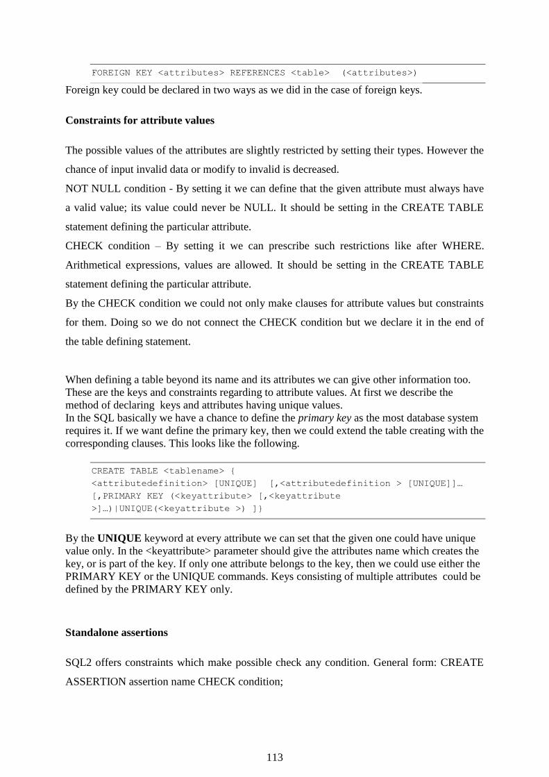
113
FOREIGN KEY <attributes> REFERENCES <table> (<attributes>)
Foreign key could be declared in two ways as we did in the case of foreign keys.
Constraints for attribute values
The possible values of the attributes are slightly restricted by setting their types. However the
chance of input invalid data or modify to invalid is decreased.
NOT NULL condition - By setting it we can define that the given attribute must always have
a valid value; its value could never be NULL. It should be setting in the CREATE TABLE
statement defining the particular attribute.
CHECK condition – By setting it we can prescribe such restrictions like after WHERE.
Arithmetical expressions, values are allowed. It should be setting in the CREATE TABLE
statement defining the particular attribute.
By the CHECK condition we could not only make clauses for attribute values but constraints
for them. Doing so we do not connect the CHECK condition but we declare it in the end of
the table defining statement.
When defining a table beyond its name and its attributes we can give other information too.
These are the keys and constraints regarding to attribute values. At first we describe the
method of declaring keys and attributes having unique values.
In the SQL basically we have a chance to define the primary key as the most database system
requires it. If we want define the primary key, then we could extend the table creating with the
corresponding clauses. This looks like the following.
CREATE TABLE <tablename> {
<attributedefinition> [UNIQUE] [,<attributedefinition > [UNIQUE]]…
[,PRIMARY KEY (<keyattribute> [,<keyattribute
>]…)|UNIQUE(<keyattribute >) ]}
By the UNIQUE keyword at every attribute we can set that the given one could have unique
value only. In the <keyattribute> parameter should give the attributes name which creates the
key, or is part of the key. If only one attribute belongs to the key, then we could use either the
PRIMARY KEY or the UNIQUE commands. Keys consisting of multiple attributes could be
defined by the PRIMARY KEY only.
Standalone assertions
SQL2 offers constraints which make possible check any condition. General form: CREATE
ASSERTION assertion name CHECK condition;

114
Contingencies of standalone assertions are expanded in SQL3. Checkings are triggered by the
events given by the programmer, furthermore the assertion could be applied for particular
rows of a table or tables not just for a whole table.
Modifying constraints
In order to modify or delete an assertion we have to name it at the creation. Giving a name
could be done at the time of definition after the CONSTRAINT keyword. For example:
CONSTRAINT title CHECK (parameters).
If we want to delete the named constraint we could do that by the ALTER TABLE tablename
DROP CONSTRAINT constraintname statement.
New constraint: ALTER TABLE table name ADD CONSTRAINT constraint name define
constraint;
Table-level constraint:
ALTER TABLE <tablename> ADD CONSTRAINT <name> <type> <column>;
Example:
Let’s add an constraint to the tTeacher table, causing we cannot store two teachers by the
same name.
ALTER TABLE tTeacher ADD CONSTRAINT uq_tTeacher UNIQUE (Name);
Checking:
INSERT INTO tTeacher VALUES (1, ’ Example John’);
Deleting a constraint:
ALTER TABLE <tablename> DROP CONSTRAINT <constraintname>;
Example:
Let’s drop the above constraint:
ALTER TABLE tTeacher DROP CONSTRAINT uq_tTeacher;

115
Checking:
INSERT INTO tTeacher VALUES (1, ’ Example John’);
Keeping the consistence of the database
Consistence sequences

116
Triggers: (Oracle 10g)
The trigger defines an activity which executed automatically when a table or a view is being
modified or other user- or system events should occur. So, any change in the database starts a
trigger. The trigger is a database object.
Triggers are working transparent from the angle of the user.
Triggers could triggered by:
- An INSERT, DELETE or an UPDATE statement executed on a table or a view
- Some DLL statements
- Server errors
- User logon or logoff
- Starting or stopping a database
We use them in the following cases:
- generating inherited column value
- prevent an invalid transaction
- protection
- defining referential integrity constraints
- handling complex business rules
- event logging
- trace
- collect table statistics
- multiplying data
Triggers could be sorted by different angles. At a trigger we should declare that when and
how many times should it being executed regarding to the event. According to the above, we
could talk about the following triggers.
- row- and statement level trigger
- Before and After trigger
- Instead Of trigger
- System triggers

117
Row-level trigger:
Briefly it is being executed everytime when the table data is being modified. For example
after a Delete statement every deleted row activates the trigger. But when none of the rows
modify the trigger will not executed neither.
The trigger counts the new employees having less salary than 100 000.
CREATE TRIGGER empl_count
AFTER INSERT ON employee
FOR EACH ROW
WHEN (NEW.salary < 100000)
BEGIN
UPDATE counter SET value=value+1;
END;
Statement-level trigger
This trigger opposite its row-level peer just executed only once, and it is being executed even
the database has not been changed.
One element support table:
CREATE TABLE counter (value NUMBER);
INSERT INTO counter VALUES (-1);
We define two triggers to enroll multiple new employees. The first resets the counter to zero:
CREATE TRIGGER dolg_kezdo
BEFORE INSERT ON dolgozo
BEGIN
UPDATE szamlalo SET ertek=0;
END;
Before and After triggers:
They could be equally at row- and statement levels. They can be attached for a table only not
for a view, however a trigger connected to a base table executes on a view in a case of an
executed DLM statement.

118
The Before trigger executes before the linked statement, and the After trigger executes after
the statement as we can see it from its name.
Before:
CREATE OR REPLACE TRIGGER emp_alert_trig
BEFORE INSERT ON emp
BEGIN
DBMS_OUTPUT.PUT_LINE('New employees are about to be
added');
END;
Let’s insert a row!
INSERT INTO emp(empno, ename, deptno) VALUES(8000, ’valaki’,
40);
After:
Let’s create the new table where we will store the modifications!
CREATE TABLE empauditlog (
audit_date DATE,
audit_user VARCHAR2(20),
audit_desc VARCHAR2(20)
);
Let’s create the trigger!
CREATE OR REPLACE TRIGGER emp_audit_trig
AFTER INSERT OR UPDATE OR DELETE ON emp
DECLARE
v_action VARCHAR2(20);
BEGIN
IF INSERTING THEN
v_action := 'Added employee(s)';
ELSIF UPDATING THEN
v_action := 'Updated employee(s)';
ELSIF DELETING THEN
v_action := 'Deleted employee(s)';
END IF;
INSERT INTO empauditlog VALUES (SYSDATE, USER, v_action);
END;

119
Instead of trigger
This trigger executes instead of its linked statement. It can be defined views, and it could be
row-level only. When we want to modify a view, but we cannot do that directly by DML
statements, the we use the Instead Of trigger.
System triggers
Their aim is inform the subscribers about the database events.
Now we know what are the triggers, when they are executed, and what kinds of do we have.
However we do not know yet how to create them. The next section this is about.
Creating Triggers
In own schema ----- CREATE TRIGGER
In other user’s schema ----- CREATE ANY TRIGGER
Creating in a database ----- ADMINISTER DATABASE TRIGGER
Rights are needed.
Creating statement:
CREATE [OR REPLACE] TRIGGER [schema. ] triggername
{ BEFORE | AFTER | INSTEAD OF }
{dml_trigger | { ddl_event [OR ddl_ event] …|
Ab_esemény [OR db_e event]…}
ON {DATABASE | [schema. ] SCHEMA}
[WHEN (condition) ] {plsql_block | procedurecall}
Where
Dml_trigger::=
{INSERT | DELETE | UPDATE [OF column [ , column]…}
[OR {INSERT | DELETE | UPDATE [OF column [ , column]…} ]….

120
ON { [ schema. ] tábla |
[ NESTED TABLE bát_column OF ] [schema. ] nézet}
[REFERENCING {OLD [AS] old | NEW [AS] new | PARENT [AS] parent}
[ { OLD [AS] old | NEW [AS] new | PARENT [AS] parent} ]…
[FOR EACH ROW]
Let’s summarize the above:
The OR REPLACE is a redefinition of an existing trigger, without its previous abolishment.
The schema trigger containing schema’s name. If it is missing, then the trigger is being
created in the user’s schema who executed the command, therefore not the place we want it.
The trigger name is the trigger’s name what is being created.
The BEFORE, AFTER, INSTEAD OF sets the type of the trigger.
The INSERT, DELETE, UPDATE defines that SQL statement causing the trigger executed.
The ON statement part gives the database object, the trigger will be created on.
A REFERENCING statement part determines correlating names (old, new, parent)
A NEW gives the names after the modification.
A FOR EACH ROW creates row-level triggers.
The dll_event determines a DLL statemet, the db_event a determines a database event, what
activates the trigger.
There is only one question left related to triggers. How do they work?
How triggers work:
A trigger can have two statuses: enabled and disabled. Disabled trigger does not start even if
the related event happens. In case of enabled trigger the Oracle executes the following events
automatically.
- Executes the trigger, if more similar trigger is defined for the same statement, then
their order is not determined.
- Checks the constraints and supervises the triggers not to harm them.
- Provides reading consistency for queries.
- Handles the depedicities between scheme objects and triggers.
121
- In case of divided database, when the trigger has modified a remote table, applies
two-phased finalization.
The CREATE statement enables the trigger automatically.
We can disable and enable a trigger by the ALTER TRIGGER and ALTER TABLE
statements.
We know already, when on the same statement there are same triggers there is no specific
order. But what is the case, when they are not similar?
Oracle follows one execution order:
- Executes all statement-level BEFORE triggers
- Involved by the DML statement cyclically for every row:
a, executes the row-level triggers
b, locks and changes the row and checks the integrity constraints.
the lock opens only in the end of the transaction,
c, executes row-level AFTER triggers.
- Checks delayed integrity constraints.
- Executes the statement-level AFTER triggers.
The execution model is recursive. During execution a trigger could be another triggers
start.
Tasks
Task 1
There is a database with the following structure.

122
1. Create the database tables in your own database.
2. Fill to the tables 5-5 corresponding records.
3. List the students names, pocket money ordered by name in reversed alphabetic order.
4. List the name of the majors, with the student’s names. Order by name of the major,
within student name.
5. Count how many student studies in the school by counties.
6. Who are those students who have less pocket money than the average? List their
names, descending order by pocket money.
7. Write an own stored procedure, which determines the most difference between pocket
moneys, and decreases the greatest pocket money value by this value.
8. Write a stored procedure, which increases the students pocket money living in Eger,
by 10% if it is greater than the average, and by 15% when it is smaller.
2. feladat
There is a database with the following structure.

123
1. Write the statement creating the cinemas table.
2. Add a new cinema to the table. Its data: name: Csillag, Address, Eger, Leányka út 4,
3300, the phone number we do not know. The primary key is identity type.
3. Modify the movie Blade genre to romantic and the length to 135 minutes.
4. Cancel all Sunday (22 April) shows due to blackout.
5. Create a show-list from April movies.
6. How many shows were in March in the Uránia cinema?
7. List all the films which are shorter than the average movie length.
8. Which cinema shows the most movies?
9. How many movies can be found by nationality? Show them descending order.
10. In 2012 Harry Potter 7 part two in how many cinemas is being showed?
11. Write a stored procedure which sums up all longer movies than 120 minutes length in
minutes.
Task 3
There is a database with the following structure.

124
1. Write the statement creating the table Students.
2. There is a new student in class. His data should stored in the database. (class.mdb) The
data is the following: name: Kovács Péter, place of birth: Budapest, date of birth, 1992. jun
12, address: 2120 Dunakeszi, Munkácsy u. 12. (the identifier consist of the initial letter of
surname and forname, and a number, which indicates the order of the student with the same
initials.)
3. Vágó László (VL1) place of birth was recorded wrong by the headteacher, he was born
in Pécs instead of Bécs. Correct the place of birth in the class’s database table.
4. Kovács Péter (KP1) parents decided that they will take him to another school so
Kovács Péter should be removed from the class.
5. Filter from the students table those, who born in a place beginning with B or V and
order them ascending by birth date.
6. Count each language how many students does have a certificate.
7. Create the list containing all of the incomes by student. Order it alphabetically, then
descending by the income.
8. How many students income is above the average income?
9. The most students which city came from?
10. Which students did not make any income?
11. Write a stored procedure that selects the students with English and German certificate,
and compares their average income.

125
Basics of PL/SQL
Basic elements of PL/SQL
Character set
A PL/SQL program’s source code –like every source code – the smallest elements are the
characters. The A PL/SQL language’s character set elements are the following:
• letters, the English small- and capital letters: A—Z and a—z;
numbers: 0—9;
• other characters: ()+-/<>=!~^;:.@%,#$&{}?[]
• space, tabulator, carriage return
The PL/SQL is not case sensitive except inside string literals.
Lexical units
In the text of a PL/SQL program the following lexical units may be used:
• delimiters,
• symbolic names,
• comments,
• literals.
These will detailed in the following section.
Delimiters

126
Symbolic names
Identifiers: begins with a letter and followed by numbers or $ _ # characters.
These are non-case sensitive.
hallgato, HALGGATO, Hallgato
means the same
Further symbols:
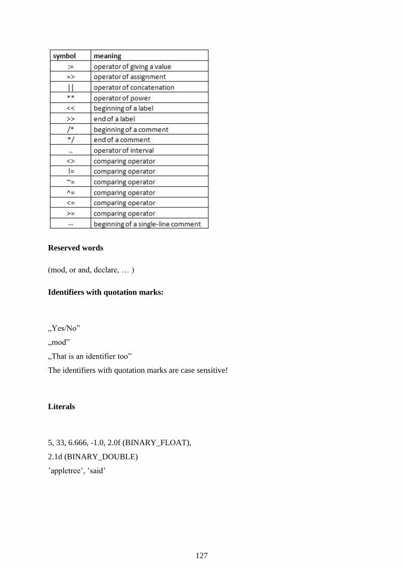
127
Reserved words
(mod, or and, declare, … )
Identifiers with quotation marks:
„Yes/No”
„mod”
„That is an identifier too”
The identifiers with quotation marks are case sensitive!
Literals
5, 33, 6.666, -1.0, 2.0f (BINARY_FLOAT),
2.1d (BINARY_DOUBLE)
’appletree’, ’said’

128
Label
<< label >>
Could occur in any row. Identifier!
Nominated constants
name CONSTANT type [NOT NULL] {:=|DEFAULT} expression;
Variable
name type [NOT NULL] {:=|DEFAULT} expression;
Example:
DECLARE
-- NOT NULL at a declaration giving a value is compulsory
v_Szam1 NUMBER NOT NULL := 10;
-- v_Szam2 initial value will be NULL
v_Szam2 NUMBER;
BEGIN
v_Szam1 := v_Szam2; -- causes VALUE_ERROR exception
END;
-- declaration of nominated constant, the value-giving expression is a
function call
c_Now CONSTANT DATE := SYSDATE;
-- declaration a variable without giving initial value
v_Egeszszam PLS_INTEGER;
v_Logikai BOOLEAN;
-- declaration a variable with giving an initial value
v_Pozitiv POSITIVEN DEFAULT 1;
v_Idopecset TIMESTAMP := CURRENT_TIMESTAMP;
-- giving initial value for a record type field
TYPE t_Kiserlet IS RECORD (
leiras VARCHAR2(20),
probalkozas NUMBER := 0,
sikeres NUMBER := 0 );
-- record fields can get initial value only in type declaration
v_Kiserlet t_Kiserlet;

129
Simple and complex types
Literals, nominated constants, variables all have a data-type component which determines for
them not only the values, but the operators, and how the values represented in the memory.
The data types could be system-defined or user types.
Scalar types:
SCALAR TYPES
Numeric family Character family Date/interval family
BINARY_DOUBLE CHAR DATE
BINARY_FLOAT CHARACTER INTERVAL DAY TO SECOND
BINARY_INTEGER LONG INTERVAL YEAR TO MONTH
DEC LONG RAW TIMESTAMP
DECIMAL NCHAR TIMESTAMP WITH TIME
DOUBLE PRECISION
NVARCHAR2 ZONE
FLOAT RAW TIMESTAMP WITH LOCAL
INT ROWID TIME ZONE
INTEGER STRING
NATURAL UROWID
NATURALN VARCHAR
NUMBER VARCHAR2
NUMERIC
PLS_INTEGER
POSITIVE
POSITIVEN Logikacal family
REAL BOOLEAN
SIGNTYPE
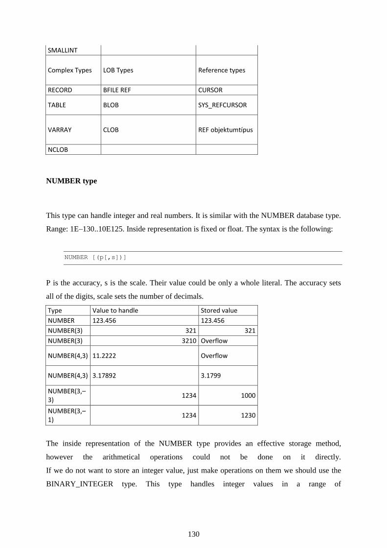
130
SMALLINT
Complex Types LOB Types Reference types
RECORD BFILE REF CURSOR
TABLE BLOB SYS_REFCURSOR
VARRAY CLOB REF objektumtípus
NCLOB
NUMBER type
This type can handle integer and real numbers. It is similar with the NUMBER database type.
Range: 1E–130..10E125. Inside representation is fixed or float. The syntax is the following:
NUMBER [(p[,s])]
P is the accuracy, s is the scale. Their value could be only a whole literal. The accuracy sets
all of the digits, scale sets the number of decimals.
Type Value to handle Stored value
NUMBER 123.456 123.456
NUMBER(3) 321 321
NUMBER(3) 3210 Overflow
NUMBER(4,3) 11.2222 Overflow
NUMBER(4,3) 3.17892 3.1799
NUMBER(3,–3)
1234 1000
NUMBER(3,–1)
1234 1230
The inside representation of the NUMBER type provides an effective storage method,
however the arithmetical operations could not be done on it directly.
If we do not want to store an integer value, just make operations on them we should use the
BINARY_INTEGER type. This type handles integer values in a range of

131
–2147483647..2147483647. These values are stored with fixed decimal point, so operations
are faster.
The restricted basic types of BINARY_INTEGER are the followings:
NATURAL 0..2147483647
NATURALN 0..2147483647 and NOT NULL
POSITIVE 1..2147483647
POSITIVEN 1..2147483647 and NOT NULL
SIGNTYPE –1,0,1
Character family
The elements of character types are arbitrary character sequences. Their representation
CHAR TYPE
It can handle fixed-length strings.
Syntax:
CHAR [(h [CHAR|BYTE])]
where h is a whole literal from the range 1..32767 by default 1. Value of h understood in bytes
(BYTE), or characters(CHATR). The default is character. For the strings always that amount
of byte will be reserved. When the string to be stored is shorter, then it will be filled with
spaces from the right.
VARCHAR2 Type
It handles strings with variable width. Syntax is the following:
VARCHAR2(h [CHAR|BYTE])
where h is a whole literal from the range 1..32767 and it sets the maximum length. Its value is
in characters when CHAR was given, in bytes when BYTE was given, or in case of nothing
was given, it is in characters. The maximum length is 32767 byte.
Within the maximum length the strings to be threated just take up the necessary bytes.

132
ROWID, UROWID Types
Every database table has a pseudo column named ROWID which stores a binary value the
row identifier. Every row identifier based on its storage address. The physical row identifier
identifies “normal table” the logical row identifier an associative arrays. The ROWID
datatype’s domain there are physical identifiers. On the other hand the UROWID data type
can handle physical, logical, and foreign (non-Oracle) row identifiers.
Date/interval types
In this family there are three basic types: DATE, TIMESTAMP és INTERVAL.
DATE TYPE
This type makes possible to handle the date and time information. Every value is stored on 7
bytes, which are in order the century, year, month, day, hour, minute, second.
The range is between 4712 BC 1st January and AD 9999 31st December. Applying the Julian
calendar the date contains the number of the days past from 4712 BC 1st January.
The actual date and time can be requested by the return value of the SYSDATE function.
TIMESTAMP TYPE
This type’s range contains the year, month, day, hour, second and fragment of second. It can
handle timestamp. Syntax:
TIMESTAMP[(p)] [WITH [LOCAL] TIME ZONE]
where p is the number of digits of the second fragment. By default it is 6. Giving the WITH
TIME ZONE the values contains the user’s timezone data. Giving LOCAL the database’s
timezone will be used instead of the user’s.
INTERVAL TYPE
With the INTERVAL type we can handle the difference between two timestamps.
Syntax:
INTERVAL {YEAR[(p)] TO MONTH|DAY[(np)] TO SECOND[(mp)]}

133
The YEAR[(p)] TO MONTH the interval giving in years and months. The p is the number of
digits in year. By default it is 2.
The DAY[(np)] TO SECOND [(mp)] gives the interval in days and seconds. np is the days,
mp is the number of the seconds digits. np is by default 2, second is 6.
Logical type
Only one type belongs here, the BOOLEAN, which range consists of logical true, false, and
NULL. There is not logical type literal, but in the Oracle interprets three Logical types. TRUE
is the logical true, FALSE is the logical false, and the NULL is NULL.
Record type
The record is a group of logically together-belonging data where every data is stored in a
field. The field has its own name and type. The record type provides us the feature, the
different data could be handled together as a single logical unit. By the record data type we
could declare such program tools which can handle database rows directly. The record type
declaration is the follows:
TYPE name IS RECORD(
fieldname type [[NOT NULL] {:=|DEFAULT} expression]
[,mezőnév típus [[NOT NULL] {:=|DEFAULT} expression]]…);
The name is the created record type in the further declaration we use it for set the record type.
The field name is name of the record fields, elements. The type could be any PL/SQL type
except the REF CURSOR. Setting NOT NULL the given field cannot have the NULL value.
During runtime should occur such assignment the VALUE_ERROR exception will be raised.
When setting NOT NULL the initiation is compulsory
A :=|DEFAULT statement part is used for initiation the field. The expression determines the
field initial value. Form of a record declaration:

134
record type recordtype_name;
DECLARE
TYPE cikk IS RECORD (
cikkkod NUMBER NOT NULL := 0,
cikknev VARCHAR2(20),
afa_kulcs NUMBER := 0.27
);
Between data types we use converting functions to convert. They are summarized in the table
below:
Function Desciption Convertible families
TO_CHAR
Converts the given parameter to VARCHAR2, the format could be set optionally.
Numeric, date
TO_DATE
Converts the given parameter to DATE, the format could be set optionally.
Character
TO_TIMESTAMP
Converts the given parameter to TIMESTAMP, the format could be set optionally.
Character
TO_TIMESTAMP_TZ
Converts the given parameter to TIMESTAMP WITH TIMEZONE, the format could be set optionally.
Character
TO_DSINTERVAL
Character
TO_YMINTERVAL
Converts the given parameter to INTERVAL YEAR TO MONTH, the format could be set optionally.
Character
TO_NUMBER
Converts the given parameter to NUMBER, the format could be set optionally.
Character, Numeric
TO_BINARY_DOUBLE
Converts the given parameter to BINARY_DOUBLE, the format could be set optionally.
Character, Numeric

135
TO_BINARY_FLOAT
Converts the given parameter to BINARY_FLOAT, the format could be set optionally.
Character, Numeric
RAWTOHEX Returns the hexadecimal representation of the given value.
Raw
HEXTORAW Returns the given hexadecimal-represented value in binary format.
Character
(should contain a hexadecimal representation).
CHARTOROWID Returns the inside-binary format of the ROWID represented by characters.
Character ( should contain a 18-character rowid format).
ROWIDTOCHAR
Rowid
Programming structures
Selection
Selection selects one from conversely excluded logical conditions, then based on this executes
one or more statements.
Form:
IF condition THEN statement [statement]…
[ELSIF condition THEN statement [statement]…]…
[ELSE statement [statement]…]
END IF;
Selection has three forms:
IF-THEN
IF-THEN-ELSE
IF-THEN-ELSIF

136
At the simplest form we close the activity by a statement sequence between the THEN and
END IF reserved words. These are executed when the condition value is true. At false and
NULL conditions the IF statement does not do anything.
At the IF-THEN-ELSE form one activity given by between the THEN and ELSE, the other
between the ELSE and END IF statement sequence. When the condition is true, then the
statement sequence will be executed after the THEN, if the condition is false or NULL, then
the statement sequence will be executed after the ELSE. The third form contains a condition
sequence. This condition sequence will be evaluated in the written order. If one of them is
true, then the statement sequence will be executed after the next THEN.
If all condition are false, or NULL, then the execution will be continued by the statement
sequence after the next ELSE reserved word, if there is not ELSE part, then this is an empty
statement. In case of the IF statement after execution any activity (if there was not GOTO) the
program continues on the statement after the IF.
Between the THEN and ELSE reserved words could be a newer IF statement. The depth of
the encapsulation is arbitrary.
declare
x number;
y number;
greater number;
if y > x then greater = y else greater = x;
The CASE statement
CASE is a kind of selection-statement, where the program can choose only one form
conversely excluded activities depending on the values of an expression or cases of
conditions. Its form:
CASE [selector_expression]
WHEN {expression | condition} THEN statement [statement]…
[WHEN { expression | condition } THEN statement [statement]…]…
[ELSE statement [statement]…]
END CASE;
If a CASE statement is labeled, then the given label is can be shown after the END CASE.
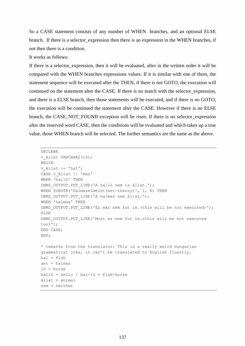
137
So a CASE statement consists of any number of WHEN branches, and an optional ELSE
branch. If there is a selector_expression then there is an expression in the WHEN branches, if
not then there is a condition.
It works as follows:
If there is a selector_expression, then it will be evaluated, after in the written order it will be
compared with the WHEN branches expressions values. If it is similar with one of them, the
statement sequence will be executed after the THEN, if there is not GOTO, the execution will
continued on the statement after the CASE. If there is no match with the selector_expression,
and there is a ELSE branch, then those statements will be executed, and if there is no GOTO,
the execution will be continued the statement after the CASE. However if there is no ELSE
branch, the CASE_NOT_FOUND exception will be risen. If there is no selector_expression
after the reserved word CASE, then the conditions will be evaluated and which takes up a true
value, those WHEN branch will be selected. The further semantics are the same as the above.
DECLARE
v_Allat VARCHAR2(10);
BEGIN
v_Allat := 'hal';
CASE v_Allat || 'maz'
WHEN 'halló' THEN
DBMS_OUTPUT.PUT_LINE('A halló nem is állat.');
WHEN SUBSTR('halmazelmélet(set-theory)', 1, 6) THEN
DBMS_OUTPUT.PUT_LINE('A halmaz sem állat.');
WHEN 'halmaz' THEN
DBMS_OUTPUT.PUT_LINE('Ez már nem fut le.(this will be not executed)');
ELSE
DBMS_OUTPUT.PUT_LINE('Most ez sem fut le.(this will be not executed
too)');
END CASE;
END;
* remarks from the translator: This is a really weird Hungarian
grammatical joke, it can’t be translated to English fluently.
hal = fish
set = halmaz
ló = horse
halló = hello / hal-ló = fish-horse
állat = animal
sem = neither
138
Loops
Loops are such programming tools which make possible repeat a particular activity as much
as we want. It is possible to execute zero times if it is needed. The repetitive activity is closed
by an executable statement sequence, this is called the core of the loop.
PL/SQL knows four kind of loops
base loop (or infinite loop)
WHILE loop (or pre-test loop )
FOR loop (or explicit number of steps loop);
cursor FOR loop.
Related information (if there is any) to repeating the loop core we should give before the core,
in the head of the loop. This information is identical for the particular kind of loop. A loop
can begin its work with the execution the first statement of the core. A loop could end, if
the information related with the repeating forces the end;
we exit from the core by the statement GOTO;
we finish the loop by the statement EXIT;
an exception should raise.
Base loop
Form of the base loop is the following:
[label] LOOP statement [statement]…
END LOOP [label];
In the base loop we not provide information related to repetition so if in the core we not force
to exit the loop by one of the three statements, it will be repeat infinite times.
For example here is a seemingly infinite loop. However it will end due to an exception since
the value of factor will be greaters than 5 digits.
DECLARE
v_Fact NUMBER(5);
i PLS_INTEGER;

139
BEGIN
i := 1;
v_ Fact := 1;
LOOP
v_ Fact := v_ Fact * i;
i := i + 1;
END LOOP;
EXCEPTION
WHEN VALUE_ERROR THEN
DBMS_OUTPUT.PUT_LINE(v_ Fact
|| ' is the greatest maximum 5-digited factorial');
END;
/
While loop
Form of a while loop is the following
[label] WHILE condition
LOOP statement [statement]…
END LOOP [label];
In this kind of loop the repetition is controlled by a condition. The loop starts with the
evaluation of the expression. If the value of the condition is false or NULL the execution
ends, and the program continues on the next statement after the loop.
Operation of the WHILE loop has two extreme cases. If the condition in the first case is false
or NULL, the core of the loop will never execute (empty loop). If the condition is true in the
first case, and in the core does not happen anything what would change this value, the
repetition will not stop. (infinite loop).
The above example could be solved without handling exceptions.
DECLARE
v_Fact NUMBER(5);
i PLS_INTEGER;
BEGIN
i := 1;
v_ Fact := 1;
WHILE v_ Fact * i < 10**5 LOOP
v_Faktorialis := v_ Fact * i;
i := i + 1;

140
END LOOP;
DBMS_OUTPUT.PUT_LINE(v_ Fact
|| ' is the greatest, maximum 5 digit factorial');
END;
/
FOR loop
This kind of loop execute once for every value of an integer range. Its form:
[címke] FOR loopvariable IN [REVERSE] under_boundary..upper_boundary
LOOP statement [statement]...
END LOOP [label];
The loop variable (loop index, loop counter) implicitly is a PLS_INTEGER type variable, its
scope the loop core. This variable takes up in order every value from under_boundary to
upper_boundary and the core will execute for every value. The upper_boundary and the
under_boundary have to be an integer-value expression. The expressions evaluated once,
before the loop starts to operate.
Giving the REVERSE keyword, the loop variable takes up the values of the range descending,
without it ascending. Note that in case of REVERSE we should determine the under boundary
of the range.
FOR i IN REVERSE 1..10 LOOP …
In the loop core the loop variable could not be assigned with a new value. We can just use its
actual value in an expression. If the under_boundary is greater than the upper_boundary, the
loop will be never executed (empty loop). A FOR loop cannot be an empty loop.
DECLARE
v_Sum PLS_INTEGER;
BEGIN
v_ Sum := 0;
FOR i IN 1..100 LOOP
v_ Sum := v_ Sum + i;
END LOOP;

141
DBMS_OUTPUT.PUT_LINE(' 1 + 2 + ... + 100 = ' || v_ Sum || '.');
END;
/
The EXIT statement
The EXIT statement could be in any loops core, but outside the core it cannot be used. Due to
its effect the loop finishes its work. Its form:
EXIT [label] [WHEN condition];
On EXIT the loop breaks, the program will continue on the next statement.

142
Mixed Tasks
There is the following data table:
DOLGOZO(id integer not null primary key, nev varchar (50), szdatum date, fizu
numeric(12,2), sz_hely varchar (30), belep_ev int, neme char(1));
id: identifier, nev: name of the employee, szdatum: birth date, fizu: salary of the employee,
sz_hely: city where he born, belep_ev: admission to the company, neme: F- male, N-female.
Select the right SQL sentences, which provide the answer to the questions! At least one
answer should be chosen for each question.
1. All data of Kovács:
A. SELECT * FROM dolgozo WHERE nev LIKE „Kovács%”;
B. SELECT * FROM dolgozo WHERE nev = „Kovács%”;
C. SELECT * FROM dolgozo WHERE nev = Kovács ;
D. SELECT * FROM dolgozo WHERE nev LIKE Kovács%;
2. Salaries between 100 000 and 120 000 Ft salaries:
A. SELECT nev, fizu FROM dolgozo WHERE fizu BETWEEN 100000 AND 120000;
B. SELECT nev, fizu FROM dolgozo WHERE fizu BETWEEN „100000 Ft” AND
„120000 Ft”;
C. SELECT nev, fizu FROM dolgozo WHERE (fizu >= 100000) AND (fizu <= 120000);
D. SELECT nev, fizu FROM dolgozo WHERE (fizu >= 100000) OR (fizu <= 120000);
3. Employee names and salaries greater than 100000 Ft and born after 1970.01.01.
A. SELECT nev, fizu FROM dolgozo WHERE (sz_datum > ’1970.01.01’) OR (fizu >
100000);
B. SELECT nev, fizu FROM dolgozo WHERE sz_datum > ’1970.01.01’ AND fizu >
100000;
C. SELECT nev, fizu FROM dolgozo WHERE sz_datum IN ’1970.01.01’ AND fizu <
100000;
D. SELECT DISTINCT nev, fizu FROM dolgozo WHERE sz_datum > ’1970.01.01’
AND fizu < 100000;
4. The number of the employee ordered by city.

143
A. SELECT sz_hely AS Hely, COUNT(id) as Törzsszám FROM dolgozo ORDER BY
sz_hely;
B. SELECT sz_hely AS Hely, COUNT(id) as Törzsszám FROM dolgozo Where sz_hely
in dolgozo;
C. SELECT sz_hely AS Hely, COUNT(id) as Törzsszám FROM dolgozo GROUP BY
sz_hely;
D. SELECT sz_hely AS Hely, SUM(id) as Törzsszám FROM dolgozo GROUP BY
sz_hely;
5. Which are the cities, where the average salary is less than 120000Ft?
A. SELECT sz_hely AS Hely, AVG(fizu) as átlag FROM dolgozo GROUP BY sz_hely
HAVING fizu < 120 000;
B. SELECT sz_hely AS Hely, AVG(fizu) as átlag FROM dolgozo Where fizu <
120 000 GROUP BY sz_hely ;
C. SELECT sz_hely AS Hely, AVG(fizu) as átlag FROM dolgozo GROUP BY sz_hely
HAVING AVG(fizu) < 120 000;
D. SELECT nev AS Hely, AVG(fizu) as átlag FROM dolgozo GROUP BY sz_hely
HAVING AVG(fizu) < 120 000;
6. List the woman joined to the company last year descending order!
.......................................................................................................
.......................................................................................................
.......................................................................................................
.......................................................................................................
7. Who earns more than the average from the men working here at least 5 years?
.......................................................................................................
.......................................................................................................
.......................................................................................................
.......................................................................................................
8. How many men and women born in Eger?
.......................................................................................................
.......................................................................................................
.......................................................................................................
.......................................................................................................

144
9. We can list the raised by 10% salary near the actual salary with the name of the employee,
because the query can select data from more tables.
A. True-True-There is correlation B. True-True-No correlation
C. True-False-No correlation D. False-True-No correlation
E. False-False-No correlation
10. The having clause filters the grouped records, because it has greater priority then the
where.
A. True-True-There is correlation B. True-True-No correlation
C. True-False-No correlation D. False-True-No correlation
E. False-False-No correlation
11. The property occurrence is a … of the data table
A. Record C. Field
B. Field value D. Field type
12. The modification anomaly is:
A. When modifying a record, modification of another record will be necessary.
B. When modifying a record, the modification will be unsuccessful.
C. When inserting a record, insertion of other will be necessary.
D. When inserting a record, the insertion will be unsuccessful.
13. Which are the types containing integer numbers?
A. SmallInt B. Integer
C. BigInt D. Char
14. Which are the types containing real numbers?
A. VarChar B. Real
C. Boolean D. Float
15. Raising the salary in the fizetes table by 10% for every employee is like this:
A. insert fizetes set fiz = 1.1*fiz;

145
B. Update fizetes set fiz = 1.1*fiz;
C. Update fizetes from fiz = 1.1*fiz;
D. Update fizetes set fiz = 10% * fiz;
16. Let’s change the city of the employees named Kis to Eger:
A. Update dolgozo set varos = ’Eger’ having nev like ’Kis’;
B. Update dolgozo from varos = ’Eger’ where nev like ’Kis’;
C. Update dolgozo set varos = ’Eger’ where nev like ’Kis’;
17. By which clause can we order?
A. Where B. Broup by
C. Order by D. Having
18. The system fills the empty spaces in case of fix-length text by what?
A. Nothing B. Space
C. Underscores D. the character #9
19. How do we create the tanulo data table
A. create new table tanulo (id int primary key, nev char(30));
B. alter table tanulo add nev char (30);
C. create table tanulo (id int primary key, nev char(30));
D. alter table tanulo tanulo (id int primary key, nev char(30));
20. Write the definition of the 3rd normal form. Define the necessary concepts too.
.....................................................................................................
.....................................................................................................
.....................................................................................................
.....................................................................................................
.....................................................................................................
.....................................................................................................
.....................................................................................................
.....................................................................................................

146
21. Write the following steps by SQL statements:
a. Create the STUDENT table, where there is a integer type field ID, as primary key, the name
of the student, birth date.
b. Insert as a new record the new student named Kiss Ferenc with the ID 17, born in 19th of
March, 1983.
c. Correct the ID 17 student to Kiss Mátyás.
d. Expand the table with the CITY field, where you will store the place of birth.
22. Answer the following questions by one query:
a) Create a list ordered by name, from the students living in Budapest, and one of the
forenames is Zsolt.
b) Calculate the average canteen money for every place of birth, and list it ordered by
place of birth descending.
c) List the names and birth dates and canteen money, who pay more than the average
canteen money ascending.
d) Let’s suppose there is the following table near the STUDENT table.
BEFIZ(nr int PK, sum int, student int, date date)
List all of the payed sums, ascending by name.
e) Create a list from the payments of students from Budapest, which made in the last
month of 2009.
23. Base tables.
ember [ id integer primary key, nev varchar(40) not null, varos varchar(40) ]
auto [ rsz char(7) primary key, tulaj integer, tipus varchar(20), szin varchar(20), ar
numeric(7,0) ]
Create the two data tables.
Tasks:
1. Query the price of the red colored cars.
2. Increase the car prices valued between 500000 and 1000000 Ft by 20%.
3. Query the owner names beginning with K, and their car types.
4. Query the owners names, and car prices from the city Eger and Miskolc,
ordered by the owner names.
5. Query those names who has cheaper car than 1 million Ft.

147
6. Query those car owners name and address, who own a car.
7. Query those number plates, which owner is from Miskolc.
8. Query those cars, which price is greater than any other red cars.
9. Query what types of the cars occur in the car tables without repetition.
10. Query the average price of the cars from Miskolc.
11. Query how many cars in each city.
12. Query the number plate of the cars more expensive than the average and their
owner names.
13. Query the number plates of the more expensive car from the cheapest car from
Miskolc.
24. Create the DOLGOZOK table with the following structure:
KOD VARCHAR2(4) NOT NULL
NEV VARCHAR2(30) NOT NULL
FIZETES NUMBER
SZUL DAT DATE
25. Extend the DOLGOZOK table with the COM column, which type is VARCHAR2(30).
Modify the length of the NEV to 40.
26. Create the table UJ_RESZL1 which structure is the same of the table RESZLEG.
27. Create the table which has the same structure and content with the RESZLEG.
28. Rename the table UJ_RESZL2 to RESZLEG2.
29. Create the table NEZET which contains only those employees name and address whose
post is ‘ELADO’ from the tables ALKALMAZOTT and RESZLEG.
30. Create those viewtable named VIDEK which contains all the division data except from
Budapest.
31. Create the ATLAG viewtable, which contains the code of the divisions and the employee
average salary. Create a list by the created viewtable, where there is the emplolyee name,
salary, division code, and the average salary of the division.
32. Using the ATLAG viewtable created in the previous task, list the name, salary, the address
and nema of the division, and the average salary of the division.
33. Create the UJ_RENDELES viewtable based on the RENDELES and AUTOK, which
columns are costumer number, car group, type of the rented car, order date, costumer name,
rental date and duration, and method of payment. List the content of the table!

148
34. Modify the structure of the viewtable created in the last task in a way one column shows
the ran kilometers during the rental time.
35. Create the UJ_UGYFEL viewtable, based on UGYFELEK, TIPUSOK, AUTO_CSOP and
RENDELES tables which contains the following columns: costumer number, name, contact
person name, rented car name, type, number plate, ran kilometers during rental, rental price
for kilometers, and days.
36. Create the KOLCSON_SZAM viewtable, based on the RENDELES table, which contains
the rentals for every number plate. List using the content of the viewtable the number plates,
type, count of rentals from the AUTOK table. The number of the rentals should be 0 at the
non-rented cars.
37. Create the table, which contains the number plate, the actual mileage, the mileage at the
last service, and the service period. The table name should be KARBANTART!
38. Create the ELADO_AUTOK table based on the AUTOK table, which contains the
following columns: numberplate, type, purchased date, mileage. (with new column names)
39. In the table KARBANTART increase the mileage column length to 8.
40. Broaden the table KARBANTART with the service period column. Its length is 8, type
numeric.
41. Create an index to the table AUTOK for the number plate.
42. Create an index to the table RENDELES for the costumer number and car type name.
43. Enter the data of the code 80 division to the RESZLEG2 table. Division name:
AUTOKOLCSONZO, address: SZEGED.
44. Enter the data of the rental offices to the table RESZLEG2 from the table.
45. Enter the code 99 division to the table VIDEK with the name FORD --- AUTO, address
DEBRECEN then check if the row is in the table RESZLEG and to the viewtable.
46. Modify in the table RESZLEG2 the 'KOZPONT' division name to 'IRODAK'.
47. Increse the salary of the employees in the code 10 division by 15%.
48. Increase the premium of the 'ELADO' post employees by 10000 Ft.
49. Delete the Debrecen divisions from the RESZLEG2 table.
50. Enter the newly purchased car data to the table AUTOK
Number plate: CAR-342
Type: RENAULT ESPACE
Group: LUXUS
Purchase date: 1994. június 23.
Price: 1.400.000 Ft

149
Mileage: 100
Last service: at 0 km
Condtion: rentable (A)
Division20
51. Enter to the ELADO_AUTOK table those cars which mileage is greater than
52. Increase in the table AUTO_CSOP the rental price by 10%.
53. Modify the service period to 12000 km in the NORMAL car group.
54. Delete the cars from the AUTOK table which you have been entered to the
ELADO_AUTOK (task 175)
55. Delete from the table AUTOK the car with the number plate ABC-022.
56. Write an INSERT statement which inserts all data from the car group EXTRA to the
newly created, but empty EX AUTOK table.
57. Write an UPDATE statement, which modifies in the table EX_AUTOK all 'OPEL
ASTRA' type car division code to '99'.
58. Delete the content of EX AUTOK table except the cars with the code '99'.
59. Move the data from the AUTOK table to the ELADO_AUTOK table those cars which ran
more than 50% of their car group.
60. You have to enter a new costumer to the table UGYFELEK
(Create a sequence with the initial value 351)
Costumer number: the next value in the table.
Name: Karát KFT.
Address: 4025 Debrecen, Nyugati utca 7.