D-AiB5 336 THE POLAR IONOSPHERE AND INTERPLANETARY FIELD(U) ALASKA t/iUNIV FAIRBANKS GEOPHYSICAL INST B J WATKINS ET ALAUG S7 AFOSR-TR-87-1342 SAFOSR-85-8258

UNCLASSIFIED F/G 4/1 NL

loll sonlIlMINES1E

10.1211

iAD- A185 386 ,CUMENTATION__ PAGE F (L Q~FrmApoe-- ] y Forrm Approved -

8 8 . OMB No. 0704-0188

Un.-c--- 1b. RESTRICTIVE MARKINGS

2a. SECURITY CLASSIFICATION A-3. DISTRIBUTION /AVAILABILITY OF REPORTApproved for public release;

2b. DECLASSIFICATION/DO Distribution Unlimited

.'" 4. PERFORMING ORGANIZATION IW .NUMBER(S) S. MONITORING ORGANIZATION REPORT NUMBER(S)

C" tr. I FOSR-TR. 87- 1 3426a. NAME OF PERFORMING ORGANIZATIOfi 6b. OFFICE SYMBOC 7a. NAME OF MONITORING ORGANIZATION• l (If applicable) AORN

Geophysical Institute I(fapibl) AFOSR/NC

6c. ADDRESS (City, State, and ZIP Code) ,. 7b. ADDRESS (City, State, and ZIP Code)

University of Alaska Bldg. 410Fairbanks, AK 99775-0800 Bolling AFB, DC 20332-6448

8a. NAME OF FUNDING/SPONSORING 8b. OFFICE SYMBOL 9. PROCUREMENT INSTRUMENT IDENTIFICATION NUMBERORGANIZATION (If applicable)

AFOSR NC AFOSR-85-02588c. ADDRESS(City, State, and ZIP Code) 10. SOURCE OF FUNDING NUMBERS

Bldg. 410 PROGRAM PROJECT TASK_ IWORK UNITBolling AFB ELEMENT NO. NO. NO ACCESSION NO.DC 20332-6448 61102F 2310 A2

11. TITLE (Include Security Classification)

The Polar Ionosphere and Interplanetary Field12. PERSONAL AUTHOR(S)

B.J. Watkins and S-I. Akasofu13a. TYPE OF REPORT 13b. TIME COVERED 14. DATE OF REPORT (Year, Month, Day) 15. PAGE COUNT

Final Technical FROM 1 Jul 85To30 Jun o7 August 1987 4016. SUPPLEMENTARY NOTATION

17. COSATI CODES 18. SUBJECT TERMS (Continue on reverse if necessary and identify by block number)

FIELD GROUP I SUB-GROUP Ionosphere, Magnetosphere, Interplanetary Magnetic Field,

Model, geomagnetic storm, polar F-region

19. ABSTRACT (Continue on reverse if necessary and identify by block number)

The model ionosphere was developed that is coupled to a magnetospheric model

for investigating time dependent behavior of the Polar F-region ionosphere in

response to varying interplanetary magnetic field (IMF) configurations. The

numerical ionospheric model covers a latitude range from 50 to 90 degrees and

an altitude range of 150 to 600 KM. The purpose of the magnetospheric model

is to define the location and gefometry of the polar cap, which is defined as

the region of open field lines. The polar cap configuration has been coupled --

20. DISTRIBUTION /AVAILABILITY OF ABSTRACT 21 ABSTRACT SECURITY CLASSiFICATIONCrUNCLASSIFIED/UNLIMITED 0 SAME AS RPT DTC ,SERS Unclassified

22a. NAME OF RESPONSIBLE INDIVIDUAL 22b TELEPHONE (Include Area Code) 22c OFFCE SYMBOLJAMES P. KOERMER, Lt Col, USAF (202) 767-49I NC

DD Form 1473, JUN 86 Previous edi ions are obsolete. SECURITY CLASSIFICATION OF -HIS PAGE

87 9 .4 309-'

- *.- .

to a model electric field pattern that in turn may vary in size and strength

in response to the IMF. The ionosphere model assumes only oxygen. ions; the

- ion density is solved vertically along many magnetic field lines as they move

horizontally under the influence of the large-scale convective electric

fields. The lower boujpdary..:.is:defined by the local chemistry and the upper

boundary condition has been set by applying an outward flux of ions

appropriate for open field line conditions. The model has been used to

illustrate ionospheric behavior during geomagnetic storms conditions. Future

model applications may include ionospheric prediction using IMF inputs

improved understanding of polar ionization structuros.

- '"

44

* I ~ 2

, . .° , '. ' **** Q** 4 ** *.~

SEPI

AFOSR.TR. 8 7 -1 34 2

FINAL REPORT

Grant AFOSR-85-0285

THE POLAR IONOSPHERE AND INTERPLANETARY FIELD

BJ.Watkins and S.-I.AkasofuGeophysical InstituteUniversity of Alaska

15 C ( 1 P:F 1

V O~l

114SPEJ ..... - ----

August 1987

,6iiiioi. apublio relea6s

-9tiuin niie

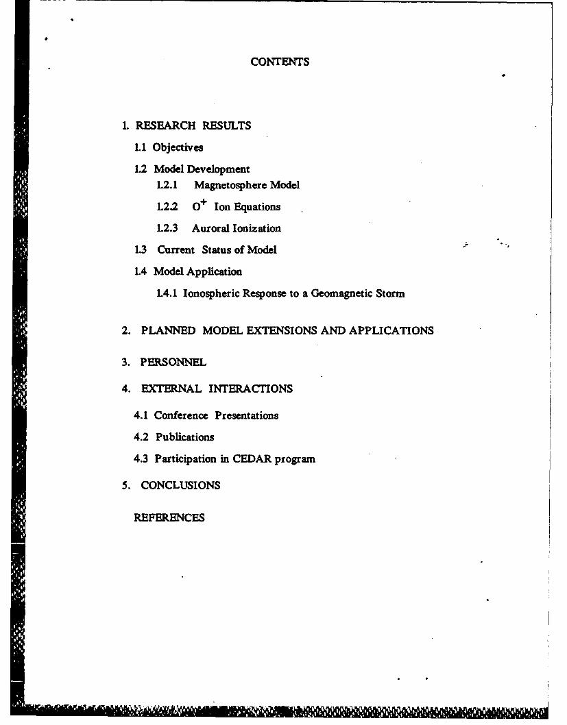
CONTENTS

1. RESEARCH RESULTS

Li Objectives

1.2 Model Development

12.1 Magnetosphere Model

1.2.2 O+ Ion Equations

1.2.3 Auroral Ionization

1.3 Current Status of Model

1.4 Model Application

L4.1 Ionospheric Response to a Geomagnetic Storm

2. PLANNED MODEL EXTENSIONS AND APPLICATIONS

3. PERSONNEL

4. EXTERNAL INTERACTIONS

4.1 Conference Presentations

4.2 Publications

4.3 Participation in CEDAR program

5. CONCLUSIONS

REFERENCES

SUMARY

We have developed a model ionosphere that is coupled to a magnetosphere model forinvestigating time dependent behavior of the polar F-region ionosphere in response tovarying interplanetary magnetic field (IMF) configurations. The numerical ionosphericmodel covers a latitude range from 50 to 90 degrees, and an altitude range 150 to 600km.The purpose of the magnetosphere model is to define the location and geometry of the polarcap,which is defined as the region of open field lines. The polar cap configuration has beencoupled to a model electric field pattern that in turn may vary in size and strength inresponse to the IMF. The ionosphere model assumes only oxygen ions, the ion density issolved vertically along many magnetic field lines as they move horizontally under theinfluence of the large-scale convective electric fields. The lower boundary is defined by thelocal chemistry, the upper boundary condition has been set by applying an outward flux ofions (which is appropriate for open field line conditions). The model has been applied toillustrate ionospheric behavior during geomagnetic storm conditions. Future use of thismodel may have applications in predicting ionospheric conditions using IMF inputs, and toenhance basic understanding of polar ionization structures.

)

I

1. RESEARCH RESULTS

1.1 O I VES

This grant period began with a simple subroutine that computed the ion density along fieldlines, and a first attempt at combining this with a model electric field structure. The overallobjective was to build on this basis to develop a new three-dimensional time dependentmodel of the polar ionosphere. In doing this, it was planned to incorporate as much of thebasic physics and chemistry as possible, but to omit secondary effects. Since computerresources,no matter how abundantnever seem adequate, it has been our philosophy to onlymodel the basic processes responsible for the F-region structure and to keep an appropriatebalance between modeling from first principles and parameterization; thus computer timehas been minimized. This has been achieved by carefully constructing our computer codes,and to keep the modeled processes about equal in importance. For example, it is wasteful to

-id considerable effort and precision in calculating one quantity such as auroral ionization,if other equally important production functions such as photoionization can not bedetermined with a high degree of certainty. Thus, a number of compromises have been madeto keep the computational times reasonable; these can be adjusted in future as betterexperimental inputs are incorporated.

There are still some minor ob)ectives that could not be accomplished in the grant period andthese are mentioned in section 2 . The major goal of coupling an ionospheric model tomagnetospheric inputs has been accomplished. We are now able to study the time dependentbehavior of the polar ionosphere in response to varying interplanetary field (IMF) values. Itneeds to be clearly stated however, that this is a first attempt and several improvements arestill possible. It was not an objective to predict or simulate a real ionosphere; there havebeen no comparisons with re data. However, further development and application of thiswork should be useful for future comparisons with data, using the model to investigate basicphysical processes, and to predict ionospheric conditions with magnetospheric inputs. Themain objectives accomplished were:

• Set up a magnetospheric model to compute the polar cap sizeand position. The model of Akasofu and Roederer(1984) has beenadopted and modified for our purposes.

• Define a model for the large scale convective electric fields.This model is scaled to match the polar cap configuration thatresults from the magnetospheric model.

* Write new code to compute ion densities vertically alongmagnetic field lines.

* Devise an efficient method to track individual field lines asthey move horizontally under the influence of the convectiveelectric fields.

0 Write code to compute auroral ionization from particle fluxdata.

" Write efficient code to compute photoionization rates.

" Combine all computer codes into a package that responds toIMF inputs and generate a time sequence of ionospheric structures.

-eN

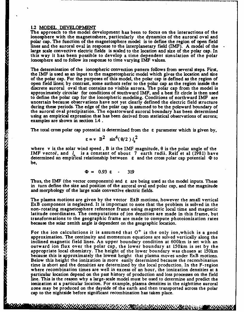
1.2 MODEL DEVELQPMENTThe approach to the model development has been to focus on the interactions of theionosphere with the magnetoshere, particularly the dynamics of the auroral oval andpolar cap. The function of the magnetosphere model is to define the region of open fieldlines and the auroral oval in response to the interplanetary field (IMF). A model of thelarge scale convective electric fields is scaled to the location and size of the polar cap. Inthis way it has been possible to develop a time dependent simulation of the polarionosphere and to follow its response to time varying IMF values.

The determination of the ionospheric convection pattern follows from several steps. First,the IMF is used as an input to the magnetospheric model which gives the location and sizeof the polar cap. For the purposes of this model, the polar cap is defined as the region ofopen field lines; by contrast, some authors refer to the polar cap as the region inside thediscrete auroral oval that contains no visible aurora. The polar cap from the model isapproximately circular for conditions of southward IMF, and a best fit circle is then usedto define the polar cap for the ionospheric modeling. Conditions of northward IMF areuncertain because observations have not yet clearly defined the electric field structureduring these periods. The edge of the polar cap is assumed to be the poleward boundary ofthe auroral oval precipitation. The equatorward auroral boundary has been determinedusing an empirical expression that has been derived from statistical observations of aurora;examples are shown in section 1.4.

The total cross polar cap potential is determined from the F parameter which is given by,

e=v B2 sin4 (0/2) 02

where v is the solar wind speed , B is the IMF magnitude, 0 is the polar angle of theIMF vectoi, and I is a constant of about 7 earth radii. Reif et al (1981) havedetermined an empiical relationship between E and the cross polar cap potential 0 tobe,

0 = 0.93e - 319

Thus, the IMF (the vector components) and E are being used as the model inputs. Thesein turn define the size and position of the auroral oval and polar cap, and the magnitudeand morphology of the large scale convective electric fields.

The plasma motions are given by the vector ExB motions, however the small verticalExB component is neglected. It is important to note that the problem is solved in thenon-rotating magnetosphere reference frame using magnetic local time and magneticlatitude coordinates. The computations of ion densities are made in this frame, buttransformations to the geographic frame are made to compute photoionization ratesbecause the solar zenith angle is dependent on the geographic location.

For the ion calculations it is assumed that 0+ is the only ion,which is a goodapproximation. The continuity and momentum equations are solved vertically along theinclined magnetic field lines. An upper boundary condition at 600km is set with anoutward ion flux over the polar cap, the lower boundary at 150km is set by theappropriate local chemistry. The height of the lower boundary was chosen at 150kmbecause this is approximately the lowest height that plasma moves under ExB motions.Below this height the ionization is more easily determined because the recombinationtime is short and the densities are determined by the local production. In the F-regionwhere recombination times are well in excess of an hour, the ionization densities at aparticular location depend on the past history of production and loss processes on the fieldle. This is the reason why a large-scale model must be used to determine and predict theionization at a particular location. For example, plasma densities in the nighttime auroralzone may be produced on the dayside of the earth and then transported across the polarcap to the nightside before significant recombination has taken place.

The approach used to simulate a time varying ionosphere is to first generate a reasonablestarting value ionosphere. This is done by back-tracking each location in time to determinewhere the plasma originated from 4 hours earlier. Then,from this earlier location, a fieldline is time stepped to its position of interest. The ion equation is solved about everyminute along the field line. This procedure is repeated for many locations (ie different fieldlines) to build up a three-dimensional structure. This three-dimensional structure is thenstored and allowed to evolve in time by further tracking field lines. For the exampleshown in section 1.4.1 the ionospheric structure is plotted every hour, however the timesteps for indivdually solving the ion equations are very short, typically a minute or less.

In the next three sections more aspects of the magnetosphere model, ion equationsolutions, and auroral inputs are discussed.

1.2.2 MAGNETOSPHERE MODELExamples of this magnetospheric model have been shown by Akasofu and Roederer(1984).The model has been adapted for compatibility and rapid computational time when used inconjunction with the ionospheric model. The major remaining question with the model isthe behavior under northward IMF conditions. There remains some uncertainty fromspacecraft observations (mainly due to the paucity of data) about the northward IMFstructure for both open field line and electric field structures.

There is an important point regarding the application of the upper boundary conditionflux that is relevant to the magnetosphere model. Over the polar cap, field lines are openand a continual outward flux has been used; this should be an excellent assumption.However, on closed field lines in the plamasphere this is not the case. The field-alignedflow in or out of the ionosphere depends on the ionization densities in the plasmasphere,which in turn depends on the past history of field line filling/emptying for perhaps a dayor more. Other researchers with large scale ionospheric models seem to have avoided thisproblem. This is very important on the nightside post-midnight auroral zone whereionospheric densities are low and magnetic field lines are closed. The modeling work so farhas assumed a zero flux in the closed field line region. This is an area that must beaddressed in future work because ionospheric densities may easily be affected by factorsof 2 or 3 depending on the particular time and geophysical conditions.

4

'C

:? - -;'~.'!~

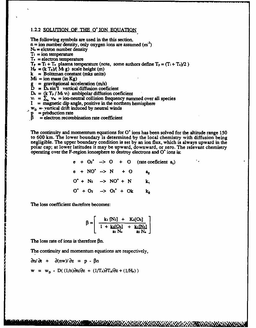
1.2.2 SOLUTION OF THE Q ION EQUATION

The following symbols are used in the this section.n = ion number density, only oxygen ions are assumed (m 3)

N. = elctron number densityTi =ion temperatureT. = electron temperatureT= = Ti + T. plasma temperature (note, some authors define Tp = (Ti + T.)/2)Hp = (k Tp)/( M g) scale height (m)k = Boltzman constant (mks units)Mi = ion mass (in Kg)g = gravitptional acceleration (m/s)D D sin='I vertical diffusion coeficient

= -k TP / M/ vi) ambipolar diffusion coeficientV1i 1. = ion-neutral collision frequency summed over all speciesI =magnetic dip angle, positive in the northern hemisphereWD =- vertical drift induced by neutral winds

= prbduction rate• = electron recombination rate coefficient

The continuity and momemtum equations for 0 ions has been solved for the altitude range 150to 600 km. The lower boundary is determined by the local chemistry with diffusion beingnegligible. The upper boundary condition is set by an ion flux, which is always upward in thepolar cap; at lower latitudes it may be upward, downward, or zero. The relevant chemistryoperating over the F-region ionosphere to destroy electrons and 0 ions is:

e + 02+ -- > 0 + 0 (rate coeficient a,)

e + NO+ -- >N + 0 a2

0+ N2 ->NO+ N k

0 +02 -> 2 + Ok k2

The loss coefficient thtrefore becomes:

P-[ ki [N2] + K[02]

I l+k2[Q21 + kIjMWL at N. a2 N.J

The loss rate of ions is therefore 3n.

The continuity and momentum equations are respectively,

cn/at + a(nw)/az= p- Pn

w = wD - D( (l/n)anl/z + (lfIrp)dITp/az + (I/H))

lllllH~'li -

Thie momentum and continuity equations may be combined to yield a diffusion equation,

~n+ ~[nwD -D& z(D n/ T) d7/az - (D n)/H. ] /dz = p -Pn

Taking derivatives, the following are obtained,

d20?= fi tV + fi an/az + fin + f

whereft = -(1/DaD/at -(lfrP)a'TP/az - /Hp + wD/D

f2 -( (1f~)T 1,/a) ( (1/D)aD/a) - ( rr))T /

+( (IrrP)'Frp/a& - (1IHpX (lID) aD/az)

+( (1/Hp)( (lIHp)(aHpI) + ((l/D)(CWD/&z

f3 = -p/D

f4= ltD

With the equations in this format, the Crank-Nicholson method with a predictor-corrector typemodification has been used for their solution. The predictor is given by,

A2 n...= f4U At2(n.,,2 -nj) + fijAnij + fij n1 +

where A&2 n= (n. 41 2n, + n,), (Ax 2

and Axn; r(n.1 n.)/2Ax

Rearranging, then substituting the difference operators that operate on the n+, results in,

(1/Az )2 n1,,+, - 2( (1Az 2 + fij / At) ) nj,, + (I/ Az)2 n,,,+,,2 (0a)

( (f~i - (2fsw /At) ) nj, + fi Azn, + fi

The corrector is given by,

1/t2) A 2 (n,. 2 + nj) f4y,j 2, (I/At) ( n~j- nij)

+ ( 1/2) fiLJ+, 2 At ( nj,1+n%)

+ f~j,2n., + f

This results in,

((l/Az) 2 + (1/2 Az) fij+,1 ) " 2 (1/Az) 2 + f~, / At )ni ,, 2 (0b)

+ ((1/Az) 2 - (1/(2 Az)) fart ) nlJt

= 2( fztjnghajjj2 + fz~w+14 (f4j nil, )/At)

+ fIiAAzn - A2

The right hand side of the predictor is completely known, therefore the left-hand side defines atridiagonal system in the n,+,/ variable. Similarly, the corrector defines a tridiagonal system inthe nr, variable once the nj+,r, variables are known.

Both the predictor and corrector are of the form,

cln,., + bAn, + aln,, = di (1)

There are N of these equations in the system, where N is the number of solution points on thefield line. A recursion relatiois'defined as,

1 = Ep4h. 1 + F, (2)

where EB and F, are quantities to be determined. If the above recursion relation holds,then n-, = E .j + F,Substitution into (1) gives,

cAE .n, + cF., + bn, + an ., = di

Solving for n the following is obtained,

n, = [-a/( b, + c,E,.,)]n,+, + '(di - ciFi_,)/(b, + cE,,)

Then by comparison with the defined recursion relation,

-a, d,- cF .+- =F, = (3)b, + cE,., bi + cE .1

Before discussing the solution of the tridiagonal system, the method of handling the boundaryconditions must be mentioned.At the lowgounda=, chemical equilibrium is imposed by setting production equal to loss,

p = On (4)

Therefore, the ionization density is,

n=p/3= [ (p+ '4 p (p+ 4wIW2)w (5)

L,-.,2wJ

where

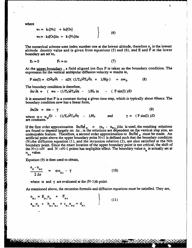
wi = ki[N2] + k202] } (6)

w2=- k2[02]/ai + ki[N2]/a2

The numerical scheme uses index number one at the lowest altitude, therefore n is the lowestaltitude density value and is given from equations (5) and (6), and E and F at the lowerboundary are set to,

Ei =0 Fi = ni (7)

At the upper bounday, a field aligned ion flux F is taken as the boundary condition. Theexpression for the vertical ambipolar diffusion velocity w results in,

F sin(I) = -DOn/)t - nD( (1,T,)cTp/z + 1/Hp) + nw, (8)

The boundary condition is therefore,&/at = ( wD - (lfr)aTp/az - I/Hp )n - (Fsin(I) )/D

It is assumed that F is a constant during a given time step, which is typically about 60secs. Theboundary condition now has a linear form,

= an- (9)

where a w/D - (1/TP)'/lz - 1/Hp and = (Fsin(I) )/Dare constants.

If the first order approximation &i/zN = (nN - n-,1 )/Az is used, the resulting solutionsare found to depend largely on Az , ie the solutions are dipendent on t1e vertical step size, anundesirable feature. Therefore, a second order approximation to 8n/&J N must be made. Anartificial point above the upper boundary point N+1 is defined such that the boundary condition(9),the diffusion equation (1), and the recursion relation (2), are also satisfied at the Nthboundary point. Since the exact location of the upper boundary point is not critical, the shift ofthe N+1-,N and N -*N-1 points has negligible effect. The boundary value nN is actually set atn value.N-1

Equation (9) is then used to obtain,

n -nN N-2 = an - (10)2 Az N-I

where a and y are evaluated at the (N-1)th point.

As mentioned above, the recursion formula and diffusion equations must be satisfied. They are,

=E n + Fn-~I N-I N N-I (1

a n + b n +c n =dN-i N N.I N-I N-I N-2 N-I

. v. ..

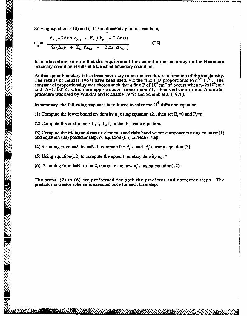
Solving equations (10) and (11) simultaneously for nNresults in,

dN.l -2Az ycN.l - FN.I( bN.I 2 Az a)n = (12)

N 2/(Az)2 + EN.l(bN.l - 2Az acN.)

It is interesting to note that the requirement for second order accuracy on the Neumannboundary condition results in a Dirichlet boundary condition.

At this upper boundary it has been necessary to set the ion flux as a function of the ion density.The results of Geisler(1967) have been used, viz the flux F is proportional to n-"I Tit 2 . Theconstant of proportionality was chosen such that a flux F of 10' cnr 2 s- 1 occurs when n=2xl0'cm- 3

and Ti=1500*K, which are approximate experimentally observed conditions. A similarprocedure was used by Watkins and Richards(1979) and Schunk et al (1976).

In summary, the following sequence is followed to solve the 0 + diffusion equation.

(1) Compute the lower boundary density n, using equation (2), then set E-0 and F-n,

(2) Compute the coefficients f,, f2, f3, f, in the diffusion equation.

(3) Compute the tridiagonal matrix elements and right hand vector components using equation(l)and equation (0a) predictor step, or equation (0b) corrector step.

(4) Scanning from i=2 to i=N-1, compute the Ei's and F,'s using equation (3).

(5) Using equation(12) to compute the upper boundary density nN.'"

(6) Scanning from i--N to i-- 2, compute the new n,'s using equation(12).

The steps (2) to (6) are performed for both the predictor and corrector steps. Thepredictor-corrector scheme is executed once for each time step.

' ",

Mi.

NO],pPBU I

1.2.3 AURORAL IONIZATION

Ionization from precipitating auroral particles is not as important as photoionization inmagnitude, but plays an important role in defining the ionization structure on thenightside of the earth when photoionization is absent or minimal.

On the dayside auroral oval, the average energies are several hundred eV, resulting inionization that peaks at altitudes 250 to 300 km. The results of Banks et al (1974) for450eV electrons with a total flux of 1.5x 106 cm "2 s" have been used. The use of theseresults is a somewhat empirical approach, however it is quite time comsuming to computeionization rates from such low energy particles. In essence, we have directly adopted theionization production rate from Banks et al for the low energy dayside auroral h put. Theionization rate per unit flux for 450eV electrons has been scaled up for the flux mentionedabove. The flux was chosen to give a peak density value about 10 cm "3. Usually, thedayside auroral oval is at least partially sunlit, and auroral effects are very small comparedto the background. The only exception is near mid-winter at longitudes near 100 degreeseast where there is maximum separation the geographic and magnetic poles.

On the night side auroral oval, the characteristic energies are much higher,typically about4 to 5keV. Code has been written that will determine the ionization profile from anyarbitrary energy spectrum for energies down to a minimum of 500eV. For this initialwork, a Maxwellian energy distribution with 5keV characteristic energy was used.

The following text summarizes the derivation of the production rate due to energeticelectron precipitation, and the soft electron production rates that have been used.

(a) ENERGETIC ELECTRONS ( > 500 eV )(i) Definitions

E electron energyE(E) electron energy distribution functionF0 total electron fluxz altitudep(z) mass densitys(z) scattering depth = I p(z') dz'R(E) range function, see Bhrrett and Hays(1976) for valuesA( s(z)/R(E) ) energy dissipation function£(z) energy deposition rate per unit volumeq(z) total ionization rate of all species due to energetic electronsqo(z) ionization rate of 0 due to energetic electrons,the subscript denotes the species

(ii) DerivationThe differential rate of energy deposition per unit volume by the electron population z(E)is,de = E A[s(z)/R(E)] p(z)/R(E) dF

The differential flux is dF = F, g(E) dE , therefore

d. -- F, E c(E) A[ s(z)/ R(E)] p(z) / R(E) dE

The total rate of energy deposition per unit volume at altitude z is therefore,

F pz) (E) A[ s(z)/R(E)] / R(E) dEEh

where Emin is the minimum contributing energy.

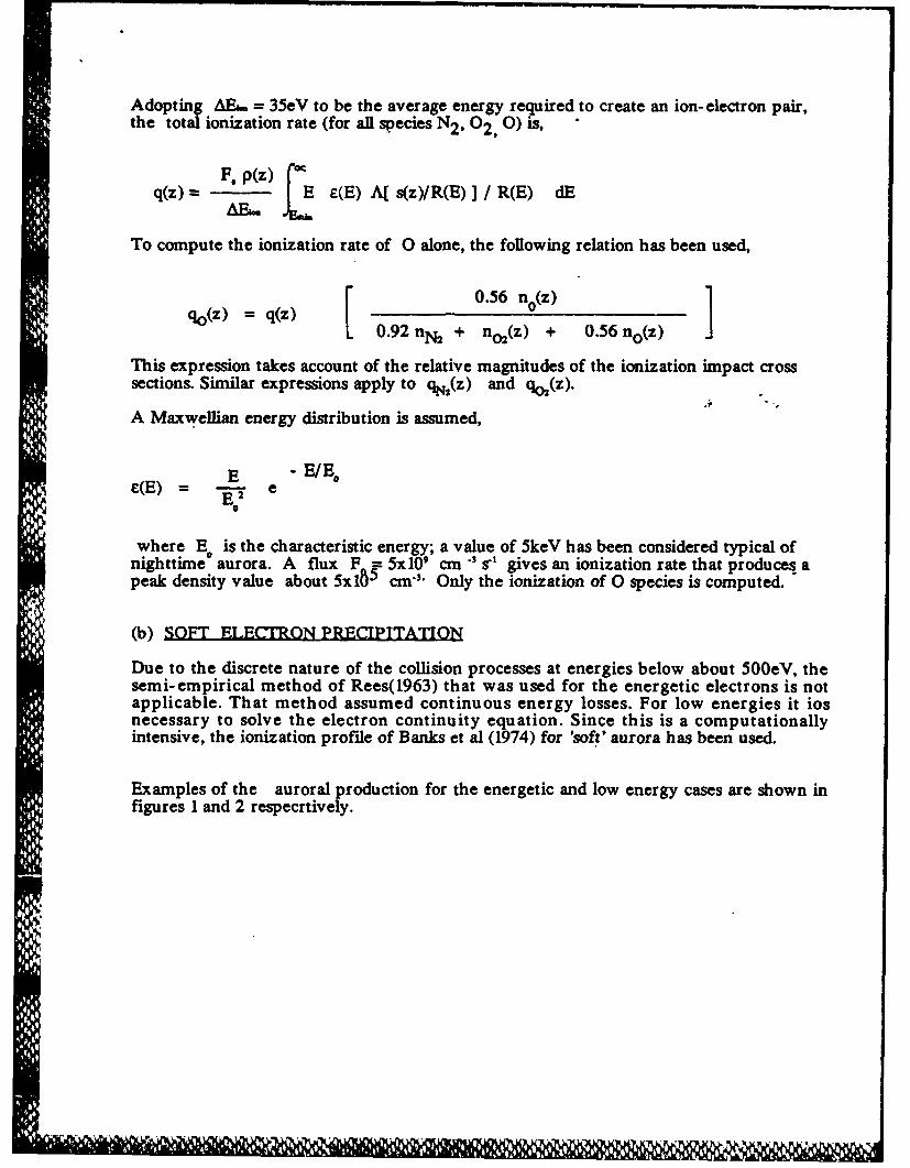
Adopting AE. = 35eV to be the average energy required to create an ion-electron pair,the total ionization rate (for all species N2 , 02, 0) is,

F, p(z) .q(z) = FE e(E) A[ s(z)/R(E)] / R(E) dE

To compute the ionization rate of 0 alone, the following relation has been used,

( 0.92 nN2 + n 0(z) + 0.56 no(z)

This expression takes account of the relative magnitudes of the ionization impact crosssections. Similar expressions apply to q,(z) and qo,(Z).

A Maxwellian energy distribution is assumed,

E(E)= E e -E/E

0

where E is the characteristic energy; a value of 5keV has been considered typical ofnighttime0 aurora. A flux F = 5x10' cm s"' gives an ionization rate that produces apeak density value about 5xl65 cm"" Only the ionization of 0 species is computed.

(b) SOFT ELECTRON PRECIPITATION

Due to the discrete nature of the collision processes at energies below about 500eV, thesemi-empirical method of Rees(1963) that was used for the energetic electrons is notapplicable. That method assumed continuous energy losses. For low energies it iosnecessary to solve the electron continuity equation. Since this is a computationallyintensive, the ionization profile of Banks et al (1974) for 'soft' aurora has been used.

Examples of the auroral production for the energetic and low energy cases are shown infigures 1 and 2 respecrtively.

550

500

400

300

200

100

so109 0- 1071-

0+ PRODUCTION RRTE (CMu-3 Son-I)

Figure 1: Production rate of 0+ ions for a typical nightime, aurora. This is the production ratefor unit flux. A Maxwellian energy spectrum with a 5keV characteristic energy has beenassumed

600

550

500

450

400

~350

-Z:300

250

200

ISO

100

50 IC * pI. I ~ I

10-* 0- 10.'1-9I-

0- PROOLICTION RATE (CMum-3 Saw-Il

Figtir6-2: ProaIuction rate of 0+ ions for a typical daytime aurora This is the production rate forunit flux, and is the production tha results from an O.42keV monoenergetic energy spectrum.

1.3 CURRENT STATUS OF MODELThe current version of the model incorporates the following processes.

* A magnetospheric model that determines the open field line regionandauroral oval precipitation region with the inteplanetary magnetic fieldas input.

" A simple two cell convection pattern is used to define the large scaleelectric fields. The input may be defined with the magnitude of thecross polar cap potential, or the E parameter (energy input from solarwind to the magnetosphere). The size of the electric field pattern isscaled to the size of the polar cap.

* The momentum and continuity equations for the major ion 0+ issolved vertically along inclined magnetic field lines. The MAGSATmagnetic field model that is based on spacecraft data has been used.The horizontal neutral wind is assumed equal to the horizantal ExBion motion. The MSIS-86 neutral model that is derived fromincoherent scatter radar and spacecraft data has been used fordetermining the neutral composition.

* The Air Force Geophysics Lab code is used to transform from themagnetic local time and magnetic latitude system, to the geographicsystem. In the geographic system, efficient code has been written todetermine the solar zenith angle for any location at any time, and thephotoionization rate as a function of altitude.

" Auroral precipitation may be determined on the nightside of theauroral oval from any input energy spectrum with energies down to500eV. On the dayside auroral oval where energies are lower than500eV the ionization rate is assumed to be f:om a mono-energetic450eV flux of particles. The flux may be arbitrarily varied.

" Command files have been written for the VAX computer to run longsimulations that compute the time varying iorosphere in response totime varying interplanetary field values.

4!

._1_

1.4 MODEL..APPfLCA'I'IONTo illustrate the use of the model for time dependent applications, the ionosphericresponse to a large geomagnetic storm has been modeled over a 16 hour period and hourlyresults plotted.

1.4.1 IONOSPHERIC RESPONSE TO A GEOMAGNETIC STORMAkasofu and Fry(1986) have developed a numerical solar wind code and applied it toexamine the propagation of a major solar flare disturbance to the earth. The solar windparameters at the earth several days after the flare are plotted in figure 3; the IMF andsolar wind speed and density are shown. Using these solar wind parameters, the rate ofenergy input to the magnetosphere from the solar wind may be estimated from the eparameter that was discussed in section 1.2 . The total cross polar cap potential 40 isrelated statistically to e by the relation that was also presented in section 1.2 . The IMFcoordinate system is shown in figure 4 because polar coordinates are used in thecomputations and plotted in figure 3; their relation to the more popular cartesian useage(BxBy Bz) is shown.

The results of the ionospheric response to the disturbance was computed and plotted eachhour. This storm simulation was done for a day in January, and for a year in mid solarcycle. As the IM changes the polar cap position and area changes; for the times 0200 to1600 UT the positions are shown in figure 5. Each plot has magnetic latitude circles at50,60,70,80 degrees, midnight (OOMLT) is at the bottom, with 1200MLT at the top of eachplot. The area of the polar cap expands to a maximum at about 0700UT when the]B.component of the IMP is most southward. The polar cap movements left and right on the

* figures results from the varying By component of the IMF.

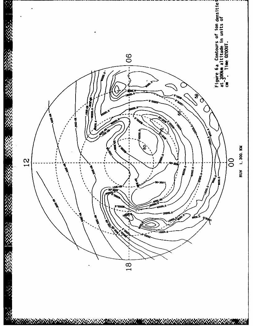
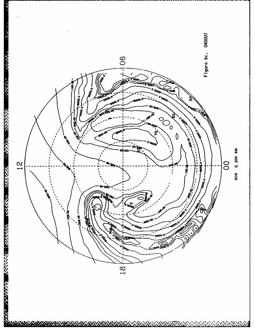
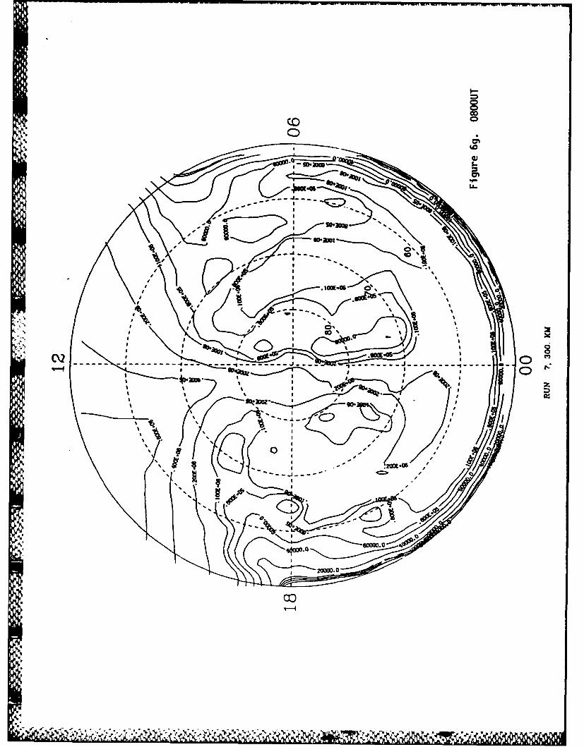
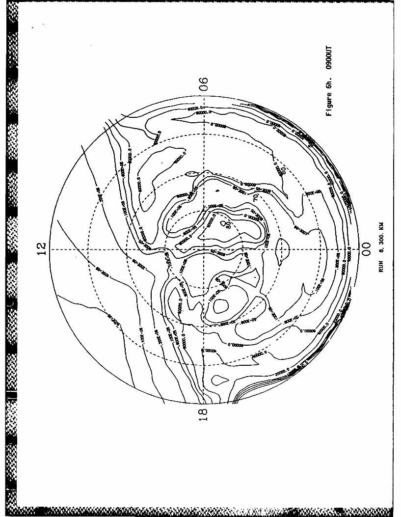
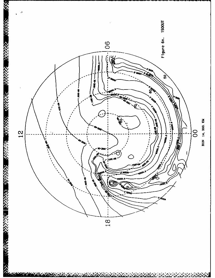
*The ion equations are solved in one minute time steps, and each individual field line isstepped in 3 minute increments along plasma convection paths. The entire threedimensional ionization structure is stored at hourly intervals and the data at 300kmaltitude is contoured and plotted. These hourly plots, which are shown in figures 6a to 6o,span the same time period as the figure 5. Initially in figure 6a, dayside ionizationextends partially over the central polar cap, and on the nightside south of the auroral ovalthere is an ion density depletion (trough) with densities as low as 6x 10 cm"3 at 1900MLTand 62 degrees magnetic latitude. During most of the nighttime jeriod the trough islocated at 55-60 degrees latitude with density values about 8x10 cm "3 . The peaks inionization density from 0200 to 050OMLT at 70 degrees latitude, and 1900 to 2100MLT at75 degrees latitude are caused by auroral precipitation. Although most auroral ionizationoccurs at about 110km altutude, there is sufficient production up to 250km that diffusesupward to enhance the F region densities at 300km and higher; this can occur because theconvection velocities are parallel to the auroral oval at those locations and there issufficient time for ions to diffuse upward. The decrease in this auroral 'hill' occurs nearmidnight because the convection there tends to be perpendicular to the auroral oval andthere is less time for vertical diffusion of auroral ionization to take place.

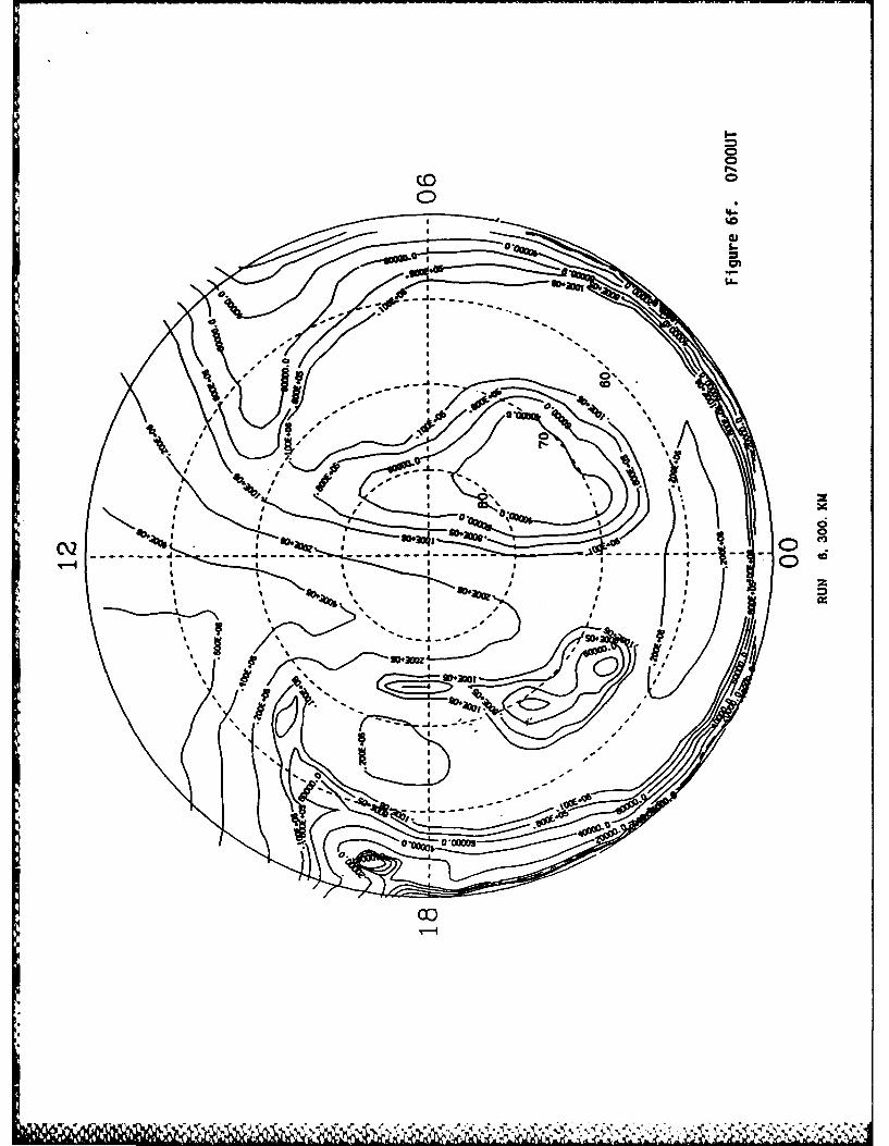
In the following time sequence of plots there is a great deal of structure. As the cross polarcap potential increases it tends to rapidly transport plasma from the dayside across to thenightside auroral zone. This becomes quite extreme in figure 6f for exmple where thedensities at 60 degeres latitude have increased by a factor of about ten, and the nightsidetrough formerly at 50 to 65 degrees latitude has dissappeared. The densities equatorwardof 52 degrees drop rapidly into the region where corotating magnetic field lines that havebeen relatively unaffected by the disturbance and recombination has had sufficient time toact so that densities as low as lxl0 4cm "3 are present.

oil.

(Ergs/Sc) 10'

200

VEL 95

(Km/Sec) 450200 _ _ _ _ _ _ _ _ _ _ _ _ _ _4-0

Dens '-(CMr 3 )

( 00

( 0)

8) 91101(d0s

Figure ~ 30Mdlgoanei tr aaetr rmAaof n r(96

ththvebe ue oriptst hei3spei0mdlTh owr5 aaetr aesla2in elct0dnit-n

Figure magnetic geield.eThe tompatoratrmetrsm aeomutend from18

the solar wind data.These values are plotted for 5 days after a solar flare.

t~b SU

Figure- 4.Temgei oriaessemue o h oa iddt

infiur3.Th ert i te mal phre

ALJKJL

.* .. .. . ..... . .

0200 0300 0400 0500

4.---

140 150 1600

Fiur 5. Time.. deenen beavo ofteplr a.nrspnet h

vayn inepantr manei fil nfiue3

-- 4- ~ Th time are4 UT on day10 shw in.j. fiur ..- a..

41'

IA

C

0-1

CO %%

CD~ C .'C%% % %% S; lool,

4 0 (.~%

200002

0o

CD

(0=00

4aa

001

0%

-v -- - - ----- - - f -

C.0

v-4-

I I

%W a- I

%' U~%I

<= Alp

2000

CI

he

% %-0%0

CD %0

Was

CO -

4 -- -- -- -- - -- -- - -- -- -- -- --

.10-4

co-

- - - - - - -~ -

I-9

0 d

16(0d co0

61 J%-

/SD-

WNW~

% %

0 a S S

7 5 cc

(00

goo

00 %S

4roft,1.1'

C\2I

-- - -- - -- - -

Q0-

00

(06

#463

02 o

I t6

* C

I IOD

'SC>

CC

90

CQ'

% %

% 4b ~

r-I-

C

o %'

C\ -

* I

.4o

A 1N&

4WWI-

0 0OL

CIO.

ch

01

C\ ---

-wi I

Sz

08

GCD% '-4

'Sn

(.0 4)

00

........... . .

020000

%0 %doI~

% %

%I a al

'I. . I

2. PLANNED MODEL EXTENSIONS AND APPLICATIONS

During the latter portion of the grant period some planning had been made for extendingthe model. There are three limitations that must be addressed before the model can beused for realistic comparisons with data or for predictive purposes.

(i)EktricEildsThe simple two cell convection pattern that has been used is a reasonable representation ofthe actual average situation. However, a model based on real data has been kindly given tous by Dr Heelis at University of Texas. It is based on data from the Dynamics Explorerspacecraft and represents the statistical results of comparisons with the interplanetary field.It was only acquired in July 1987 and therefore there was insufficient time to incorporateit into the current version of the model.

(ii) Multiple Ion SpeciesThe current effort only solves for 0+ ions. There are two other minor ions in the F region,02+ and NO + that should be incorporated. The NO+ ions are particularly importantduring magnetically disturbed periods because their production is enhanced to the levelwhere their concentration may significantly affect the recombination rate.

The dynamics on the neutral gas should be self consistently computed with the ionmotions. The particular situation that occurs when the neutral wind is north-south with amagnitude that is different to the ion drift motion will affect ionospheric densities. When aneutral wind is blowing from north to south, ion drag forces tend to move ions up or downthe inclined magnetic field lines. For an upward drift, ions are moved to higher altitudeswhere the recombination time is longer and this results in higher ion densities and ahigher altitude peak in the density height profile. For a downward drift the reverseoccurs, ie movement of ions to lower altitudes resulting in greater recombination andlower ion densities.

With regard to applications of the model, it is planned to concentrate on comparisons withreal data, probably incoherent- scatter radar density and electric fields, and spacecraftparticle data 1o determine the auroral particle input fluxes. The polar cap region isparticularly interesting because of the complex ionization structures that have beenobserved. With greater spatial resolution understanding of the formation and evolution ofpolar cap structures should be possible.

3. PERSONEL

The initial work on this grant was performed by the principal investigators; ProfessorAkasofu developed the magnetospheric model and Dr Watkins was responsible for theconvection electric field model, coupling the magnetospheric model to the convectionmodel, developing code to step along equipotentials,and the initial code to solve the ionequations. In July 1986 we recruited a new PhD student, Mr Chris Grimm. He has spent alarge amount of time learning to use the existing code, has greatly enhanced the efficiencyof the ion equation code, and has written code for computing the auroral ionization. MrGrimm is a very competant programmer and has also been of assistance in packaging thevarious programs to run from a command file on the Geophysical Institute's VAXcomputer. He has also taken the Aeronomy course at the Geophysical Institute and hasbegun to contribute scientifically to our effort. It is anticipated that this research willcontinue and subsequent results will form the basis for Mr Grimm's thesis. The grant hasbeen very valuable in introducing a new researcher to the field.

-a'a

a'.

A

4. EXTEIRNAL INTERACTIQNS

4.1 CONFERENCE PRESENTATIONS

Four conferences have been attended and papers presented.

(a) NATO Advisory Group for Aerospace Research, 36th Symposium, Fairbanks, Alaska,June 1985.Paper titled 'Progrss in Modeling the Polar Ionosphere from Solar and MagnetosphericParameters'

(b) Ionospheric Effects Symposium on 'The Effects of the Ionosphere on Communication,Navigation, and Surveillance Systems', May 1987.Paper titled 'A Numerical Prediction of Ionospheric Conditions After an Intense SolarFlare'

(c) XXII General Assembly of the International Union of Radio Science.Paper titled 'Dynamic Ionospheric Models'

4.2 PUBLICATIONS

The following are in various stages of the publication process.

(a) 'Progress in Modeling the Polar Ionosphere from Solar and MagnetosphericParameters', NATO Advisory Group for Aerospace Research, Report No 382, 1986, byWatkins,Akasofu andd Fry.

(b) 'A Numerical Prediction of Ionospheric Conditions After an Intense Solar Flare', inpress, in proceedings of symposium on The Effect of the Ionosphere on Communication,Navigation, and Surveillance Systems, 1987, by Watkins and Akasofu.

(c) 'Numerical Modeling of Magnetic Storm Effects on the Polar F-Region Ionosphere',in preparation for special issue of Radio Science, by Watkins, Akasofu and Grimm.

4.3 PARTICIPATION IN THE 'CEDAR' PROGRAM

The CEDAR (Coupling, Energetics, and Dynamics of Atmospheric Regions) science effortis an NSF initiated program with three major goals. These are, first to study the dynamicsand energetics of the upper atmosphere from the mesopause upward to the exobase (about80 to 150km altitude), second to study mesospheric-thermospheric coupling, and third tostudy ionosphere- magnetosphere- thermosphere coupling.

Within the CEDAR program there are a number of individual smaller efforts that willcontribute to the overall objectives. One of these, organized by Dr S. Basu at Air ForceGeophysics Lab, called HLPS (High Latitude Plasma Structures), is directed towardunderstanding the physical processes responsible for the formation and evolution of polarcap ionization structures. This modeling effort will be an important contribution.

'.

5.0 CONCLUSIONS

This grant has been very successful and is the first attempt to couple a magnetosphericmodel to a large-scale ionospheric model. The codes are quite efficient and may be runefficiently on a VAX computer of the 780 size or larger when the horizontal grid spacingis at least 5 degrees of latitude and 5 degrees of longitude; the vertical grid size is now10km which should remain fixed. If better spatial resolution could be realized by usinggreater computing resources, it should be possible to study small-scale polar capstructures,both their formation and evolution. Time dependent simulations of a largemagnetic storm show very complex time dependent behavior of the ionosphere.

In future, further extensions of the model to include neutral wind effects and multiple ionsshould permit many useful insights into the physical processes operating in the polarionosphere. Comparisons with real data, and the application of the model for predictivepurposes should then be possible.

SI .

.11

S.,

4.-.

i,

REFERENCS

Akasofu, S.- I., and M.Roederer, Dependence of the polar cap geometry on the IMF,Planet. Space Sci., ULp 111,1984

Barrett, J.C., and P.R.Hays, J. Chem Phys., fA, 2, 1976.

Banks, P.M., C.R.Chappell, and A.F.Nagy, J. Geophys. Res., 2-2, p1459, 1974.

Geisler, L.E., J. Geophys. Res., 7-2, p81, 1967.

Rees, M.H., Planet. Space Sci., 11, p 1209, 1963.

Reif, R.J., R.W.Spiro, and T.W.Hili, Dependence of Polar Cap Potential Drop onInterplanetary Parameters, J. Geophys. Res., 86, p7639, 1981.

Schunk,R. W., P.M. Banks, and WJ.Raitt, J. Geophys. Res., B1, p3 2 7 1, 1976.

Watkins, B. J., and P. G. Richards, J. Atmos. Terres. Phys., 4.1, p 179, 1979.

.F .

4i