TI-89 WORKBOOK

for

HONORS CALCULUS

by

Professor James Keesling Department of Mathematics

University of Florida

Table of Contents Introduction………………………………………………………………… 2 1. Elementary Calculations..................................................................... 4 2. Functions and Graphs………………………………………………. 5 3. Limits……………………………………………………………….. 6 4. The Derivative and Tangent Lines………………………………….. 7 5. Applications of the Derivative………………………………………. 9 6. Integrals as Limits…………………………………………………… 12 7. Antidifferentiation and the Fundamental Theorem…......................... 15 8. Numerical Integration……………………………………………….. 17 9. Applications of Integration………………………………………….. 19 10. Remarks…........................................................................................... 20

2

Introduction. In recent years the design, speed, and power of modern computers have increased significantly. Along with the increased capabilities, computers have been assigned new tasks. These tasks are beyond anything conceived a few years ago. Until recently, computers were seen as powerful calculators whose sole contribution to mathematics was to work out complicated numerical examples with great precision and speed. However, with the advent of Macsyma, Mathematica, Maple, Derive and other computer programs capable of symbolic calculations, the computer has become an indispensable help in performing logical functions and algorithms as well as numerical calculations. Now the computer can solve algebraic equations exactly, can compute derivatives and integrals symbolically, and can even compute exact limits. For almost the whole history of calculus, these have been the skills that students learned in calculus courses. Now there is danger that those skills may become outmoded. No one uses tables of logarithms or trigonometric functions or learns manual methods of approximating these functions. Calculators and computer determine the values of these functions with greater accuracy than these tables would give us anyway. In the same way some would argue that the techniques of differentiation and integration may be on the way to being antiquated. This is not to say that there is no need for calculus or a course in calculus. It is just that the skills that were taught in the past need to be reevaluated. One still needs to understand the principles of calculus even to make use of one of the symbolic programs and apply it properly. If we make proper use of the new technology our calculus courses can be more interesting and relevant. There will be less emphasis on mastering certain algorithms and more concentration on understanding the underlying principles of calculus. Would one say that word processing has eliminated the need to learn to write and spell properly? Not at all! However, one would be disappointed if word processing technology were not incorporated in a modern course in creative writing. Where would we be without cut and paste and spell checking? Even with these advances we need to learn to organize and discipline our thoughts and express them in a coherent and cogent fashion. Word processing technology can be a help, but there are still skills to be learned to make effective use of this technology. The same can be said for the new technology in mathematics. It is without value if one lacks the understanding to make proper use of it. For the past five years I have made use of the computer in all of my classes. In calculus I have taken the students to a computer laboratory once a week to learn Maple, one of the advanced symbolic languages. This has worked very well except that access to the computer has been limited. The students could not make use of the computer at all times. It was not seen as an integral part of the course or of calculus. It was a technology which was seen by the students as useful for advanced applications, but not for everybody. The TI-89 has provided an opportunity for this perception to change. The TI-89 is programmed with a version Derive, an advanced symbolic computer language similar to Maple. It has many of the powerful capabilities of Maple and the full-fledged version of Derive. However, it is portable and inexpensive. The student can have the calculator in class to work examples. It can be used to do homework problems. It can be used to

3

work out the details of a complicated practical problem. And, most practical of all, it can be available for tests as well. What better way to demonstrate the usefulness of this new technological advance than to show that it can lead to a better grade! This workbook gives you an opportunity to savor the capabilities of the TI-89. It can solve equations; it can do symbolic calculations; it can compute derivatives and integrals exactly; and it can produce superb graphs of functions of one and two variables. It can also do numerical calculations using floating point approximation. All of this is packaged in a very intuitive menu-driven format so that it is quite natural to use. It is time to try out your TI-89. This manual contains some examples that introduce the TI-89 and show what a powerful device it is. We will not burden you in this manual with how each calculation is made. The owner’s manual does a good job of that. Through these examples and constant use in the classroom we hope that the features of the TI-89 will become second nature to you with time. Glance through this manual periodically and work a few problems. This should help you develop and maintain your skills with your TI-89.

4

1. Elementary Calculations. The TI-89 is a calculator, so it will do the calculations that you expect from such a device. However, it will do much more than produce a floating point approximation of the answer to your problem. It can give an exact answer. If the answer is a fraction, it will give it in reduced form. If the answer is a radical or a multiple of! , that will be the form of the answer. One can get a floating point approximations to any answer. This is especially helpful when the exact answer is particularly complicated to view or beyond the capability of the calculator. However, there is no substitute for the exact answer in mathematics. The exact answer conveys a certain satisfaction in the mathematical precision of the result. In many applications it is not clear how much precision is needed in the answer. Having the exact answer guarantees that you have as much precision as could ever be asked. Make the following elementary calculations on your TI-89. You should be able to do them by hand, but perhaps with some difficulty.

(a) 1

5+3

7 (b) sin

!4

"#$

%&'

(c) sin!3

"#$

%&'

(d) 25! (e) 35

14

!

"#$

%&=

35C14

(f) 1+ 5

2

!

"#$

%&

3

(g) 3+ 2 i

4 ! i3

(h) sin! i3

"#$

%&'

(i) 25

3

!

"#$

%&1

3( )

32

3( )

22 (j) k3

k=1

20

!

5

2. Functions and Graphs. The notion of function is perhaps the most important of all concepts in modern mathematics. One can create functions several different ways with the TI-89. The simplest is to use the “Y=” screen and let the function be one of the yn= functions on that screen. There are more complicated ways to do this, but it is best to use the elementary features of this calculator until more sophisticated ones become necessary. The graphics on the TI-89 are superb. As you gain more familiarity with the options available you will be able to manipulate functions in one window and have a graphical display in another window on the same screen. You will be able to go between a graphical analysis of a problem and relevant analytical calculations with natural ease. Here are a few examples of functions that produce some interesting graphs.

(a) sin(x) on[0, 4! ] (b) sin 1x( )on[0,1] (c) x

2sin 1

x( ), x2 ,!x2{ } on [!1,1]

(d) x3 +10x2 + 3x ! 5 (e) sin(x)

x (f) x

3,(x + 1

10)3 ! x3

110

"#$

%&'

on [!2,2]

In (d) determine all of the real roots of the polynomial graphically. You will have to adjust the interval until you are certain that all the roots are included in it. Once you have approximated the roots graphically, you can get a numerical approximation of each root using one of the menu items on the graphing screen. Also, with each of the functions, determine the tangent lines at various points on the graph of the function using the graphical tools on the menus available on the TI-89 graphing screen. It is also possible to determine the area under the curve using tools in the graphing menus. You may want to experiment with other features as well.

6

3. Limits. Although the most important concept in mathematics is that of function, the most import concept in calculus itself is that of limit. The limit is the foundation of all other concepts in calculus. This includes the derivative and the integral as well as continuity. We now go through a number of examples to show the capabilities of the TI-89 to calculate limits. We first start with limits of infinite sums. What does it mean to add an infinite number of terms together? We take it to mean that the sequence of finite sums using a larger and larger number of the terms gets closer and closer to a number, the limit. This limit of the sequence of partial sums is taken to be the value of the infinite “sum”. Such an infinite sum is said to be a series and when the series converges to L we say that its sum (or limit) is L. Here are a few exercises to determine limits using the TI-89. Because of the limitations of memory this aspect of the TI-89 is not as full-featured as one of the computer versions of Derive or Maple. Nevertheless, it is a powerful tool in a handy package.

(a) 1

n( )

2

n=1

!

" (b) limx!0

sin(x)

x (c) lim

x!a

x3 (d) lim

h!0

(x + h)3" x

3

h

(e) limh!0

sin(x + h) " sin(x)

h (f)

2392

10000n

n=1

!

" = .2392 (g) 1

3( )

n

n=0

!

"

7

(h) limx!1

x2"1

x "1 (i) lim

x!1

x4"1

x "1 (j) lim

x!1

xn"1

x "1 (k) 1

10( )

n

n=1

!

"

4. The Derivative and Tangent Lines. The Greeks understood the idea of a line tangent to a geometric figure. They determined the tangent lines to many of the shapes known at the time. However, it was only after René Descartes developed analytic geometry that tangents to general figures were studied and their analysis became an interesting subject. This development became important in the development of the calculus. Differentiation became the main tool in finding tangent lines. The inverse of this operation became the principal method in determining areas. How does one find the line tangent to a circle through one of its points? How would you define a tangent to another curve? This takes some thought and is not immediately apparent. Certainly the line tangent to the graph of a function at the point (x, f (x)) should go through the point (x, f (x)) . It could not possibly be tangent otherwise. The tangent line is completely resolved when we know its slope. We determine the precise slope at the point (x, f (x)) by taking a limit. Suppose that we have a line which passing through the point (x, f (x)) and a nearby point (y, f (y)) . If y is very close to x, then this secant line should be very close to the line tangent to the graph of f at the point (x, f (x)) . Determine this for f(x) = x3 at x = 2 . Let y = 2 + h . Use the TI-89

8

to make the calculation. The slope of the tangent line is determined by taking the limit of the slopes of these secant lines as h! 0 . The formula for a general function f is

df

dx= lim

h!0

f (x + h) " f (x)

h.

The TI-89 is expert in calculating derivatives of functions. Use the differentiate command to determine the derivatives of the following functions. Also, make the same calculation using the limit command. It is encouraging to get the same answer in both cases. This is one of the ways of checking an answer. Make the calculation by a different method to be sure that the answer is the same in both cases.

(a) x2 (b) sin(x) (c) x2 sin 1x( ) (d)

x2! 3x + 2

x3+ 2x

2+ 4x !1

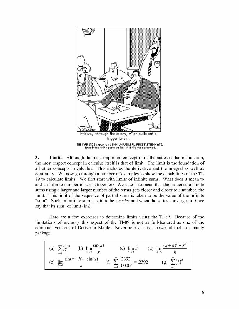
(e) cos(x) (f) tan(x) (g) ex (h) ax (i) xa Let us determine the tangent line to a circle at a certain point using this approach. Consider the circle centered at the origin with radius one, x2 + y2 = 1. The graph of the

function f (x) = 1! x2 is the top half of this circle. Let us find and plot the tangent line

over x =1

4. With the proper window settings the graph should look like this.

Work through a few more examples while this one is fresh in your mind. Find the equation for and then graph the line tangent to the graph of the function f (x) through the point x = a . Graph the function and the tangent line together.

(a) f (x) = sin(x), a = 0 (b) f (x) = sin(x), a =!

4 (c) f (x) = x

2, a = !1

(d) f (x) =1

x, a = 2 (e) f (x) = x5 + 2x2 ! 5x + 3, a = 1

9

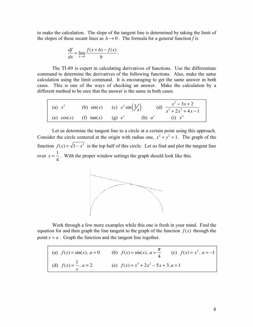
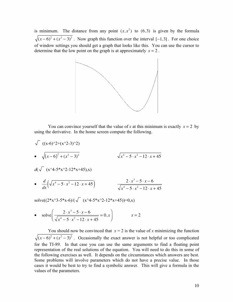
5. Applications of the Derivative. In this section we apply the derivative to solve a few problems. There are many applications of the derivative. Some of these are simply mathematical. For instance, the derivative gives the instantaneous rate of change of a function. Using this fact one can use the derivative to approximate the value of a function near a known value. This can be especially handy when a calculator or computer is not readily available. Another mathematical application of the derivative is to determine the maximum and minimum of a function. At a point where a function takes on one of these extrema, the derivative either vanishes or does not exist. This purely mathematical principle is used in optimization which is widely employed in business to maximize profits or minimize costs of a business operation. It is also used in risk analysis to minimize risk or maximize the probability of a favorable outcome in some undertaking. In physics, tangent lines are the direction that a particle would travel if no forces were applied to constrain it to a prescribed path. The list would be much too long if we tried to compile a comprehensive inventory of all applications. One advantage of using the TI-89 as a teaching tool is that the calculations required in examples do not need to be simple or routine. Very often solving a real world problem involves calculations that are brutal. We can leave that hard work to the calculator. We just need to be sure that we are assigning the precise calculations that need to be done. As a first example consider the distance of the point (6, 3) from the graph of the function x2 . We would like to determine the point on the graph whose distance to (6, 3)

10

is minimum. The distance from any point (x, x2 ) to (6, 3) is given by the formula

(x ! 6)2+ (x

2! 3)

2 . Now graph this function over the interval [!1,3] . For one choice of window settings you should get a graph that looks like this. You can use the cursor to determine that the low point on the graph is at approximately x = 2 .

You can convince yourself that the value of x at this minimum is exactly x = 2 by using the derivative. In the home screen compute the following.

((x-6)^2+(x^2-3)^2) • x ! 6( )

2+ (x

2! 3)

2 x4! 5 " x

2!12 " x + 45

d( (x^4-5*x^2-12*x+45),x)

• d

dxx4! 5 " x

2!12 " x + 45( ) 2 ! x

3" 5 ! x " 6

x4" 5 ! x

2"12 ! x + 45

solve((2*x^3-5*x-6)/( (x^4-5*x^2-12*x+45))=0,x)

• solve2 ! x3 " 5 ! x " 6

x4 " 5 ! x2 "12 ! x + 45

= 0, x#

$%&

'( x = 2

You should now be convinced that x = 2 is the value of x minimizing the function (x ! 6)

2+ (x

2! 3)

2 . Occasionally the exact answer is not helpful or too complicated for the TI-89. In that case you can use the same arguments to find a floating point representation of the real solutions of the equation. You will need to do this in some of the following exercises as well. It depends on the circumstances which answers are best. Some problems will involve parameters which do not have a precise value. In those cases it would be best to try to find a symbolic answer. This will give a formula in the values of the parameters.

11

In working the following problems, keep a scratch pad handy. The TI-89 can do the calculations, but only you can organize your thinking. You have to take the English version of the problem and determine what computations you need from the TI-89 to solve the problem. You also have to interpret the results of these computations to be sure that they solve the original problem.

(a) Find the point on the ellipse x2

4+y2

12= 1 which has the minimum distance

to the point (10,20). (b) Find the point on the ellipse such that the line joining the point and the

point (10,20) is tangent to the ellipse. (c) Find the equation of the line passing through the point (10,20) and

tangent to the ellipse. (d) Find the maximum area enclosed by a rectangle whose perimeter is 100

feet. (e) Find the shortest path from a point P to a point Q which touches the line

L.

12

(f) Find the path taking the least time from the point P to the point Q.

Assume that there is a straight line between P and Q and that the speed traveled on the P side of the line is v

1 and the speed traveled on the Q side

of the line is v2

. (g) A cylindrical tank is to have volume V. What should its dimensions be to

have minimum surface area. Include the top and bottom as part of the surface.

6. Integrals as Limits. After you become familiar with the Fundamental Theorem of Calculus, you are likely to forget the formal definition of the definite integral. It is so much easier to compute integrals by using antiderivatives that one tends to forget that this was only a means to an end. For approximately two thousand years the only method of determining area was by the method of exhaustion. This was analogous in modern methods and terminology to computing an integral by means of the definition using limits. The Fundamental Theorem of Calculus was seen as a great advance because it simplified these calculations. It also brought unity to a field which had developed many diverse and fragmented algorithms to compute areas and volumes. With the advent of calculus one only needed an antiderivative in order to compute the area under the curve of a function.

13

On the other hand, if the TI-89 were available at the time of Newton, perhaps mathematicians would not have seen calculus as such an impressive advance. You will see in the following exercises that determining integrals using limits is not so difficult with modern tools of technology. Here are a few calculations that you can do on your TI-89 to illustrate the method without the frustration experienced by many previous generations of mathematicians. ! (j/n/n,j,1,n)

• j

n

n

!

"#$

%&j=1

n

' n +1

2 !n

limit((n+1)/(2*n),n,∞)

• limn!"

n +1

2 #n$%&

'()

12

! ((j/n)^2/n,j,1,n)

• j

n( )2

n

!

"##

$

%&&j=1

n

' (n +1) ! (2 !n +1)

6 !n2

limit((n+1)*(2*n+1)/(6*n^2),n,∞)

• limn!"

(n +1) # (2 #n +1)6 #n2

$%&

'()

13

! ((j/n)^3/n,j,1,n)

• j

n( )3

n

!

"##

$

%&&j=1

n

' (n +1)

2

4 !n2

limit((n+1)^2/(4*n^2),n,∞)

• limn!"

(n +1)2

4 #n2$%&

'()

14

The above computations determined the values of the integrals xdx0

1

! , x2dx

0

1

! ,

and x3dx

0

1

! , respectively. To see this observe that the functions x, x2, and x3 are all

14

increasing on the interval [0,1]. The upper Riemann sum for the partition with n +1 equally spaced points for each of these functions is just j

n( ) 1

n( )j=1

n

! , j

n( )2

1

n( )j=1

n

! , and

j

n( )3

1

n( )j=1

n

! , respectively. The first task was to compute these sums. The result gave a

greatly simplified formula. The next task was to take the limit of these respective sums as n!" . The final result was the value of each of the respective integrals. Now you can see that even though the calculations would have been imposing by hand, the results were quite simple. The first to calculate the area under these curves by this method was Bonaventura Cavalieri. He discovered the method around 1626. He determined the areas under the curve xk for k up to about 7. You could easily do this for k = 7 . Cavalieri was a gifted geometer. Some of his methods of determining volumes and areas are still easier and give more geometric insight than the methods using calculus. We will cover Cavalieri’s Method later in the course. He was a contemporary of Galileo Galilei who thought that he was the most brilliant geometer that ever graced the earth.

(a) x4dx

0

1

! (b) xdxa

b

! (c) x2dx

a

b

! (d) sin2(x)dx

0

!

"

(e) sin(!)d!0

x

" (f) x!2dx

1

2

"

15

7. Antidifferentiation and the Fundamental Theorem. We now give some examples using the Fundamental Theorem of Calculus in evaluating integrals. You need to observe some caveats in applying the Fundamental Theorem. You can even fool (or rather be fooled by) the TI-89 if you do not observe these warnings. The Fundamental Theorem of Calculus has several elements which we will separate here for clarity.

Theorem. Let f (x) be a continuous function on the interval [a,b] . Let F(x) be

defined by the formula F(x) = f (!)d!a

x

" . Then F(x) is differentiable on [a,b]

and dFdx x

= f (x) for all x ![a,b] .

This version of the Fundamental Theorem states that an antiderivative for a continuous function always exists and can be defined by the definite integral. On the other hand we may not be able to come up with a “nice” formula for this antiderivative. When we are able, then we can compute the definite integral of the function over any appropriate interval by a trivial computation.

Theorem. Let f (x) be a continuous function on the interval [a,b] . Suppose that F(x) is an antiderivative for the function f (x) on the interval [a,b] . Then

f (!)d!a

x

" = F(x) # F(a) .

Lastly, we note that antiderivatives are in a certain sense unique. Any two must differ by a constant on an interval [a,b] where the function f (x) is continuous.

Theorem. Let f (x) be a continuous function on the interval [a,b] . Suppose that F(x) and G(x) are both antiderivatives for the function f (x) on the interval [a,b] . Then there is a constant C such that for all x ![a,b] , F(x) !G(x) " C .

You need to know some standard antiderivatives and how to derive formulas for others. The methods involved are techniques of integration. These have been formalized and programmed so that the TI-89 and advanced symbolic computer languages will perform these algorithms faster and more reliably than possible for a human. Try the fol-lowing commands on the home screen of your TI-89. (! x^2,x)

• x2( )! dx

x3

3

The answer bears some explanation. Our function x2 is continuous and certainly 1

3x3 is an antiderivative. However, it is not the only one. Any function of the form

16

1

3x3+ C is also an antiderivative for any constant C. The TI-89 assumes that you know

that adding a constant will give you another antiderivative. The Fundamental Theorem of Calculus guarantees that as you add all possible constants you get the whole family of antiderivatives for x2 . Again, the TI-89 assumes that you have this background knowledge and that you will use the answer it has given appropriately. Find antiderivatives for the following functions.

(a) xn (b) x4 (c) x!2 (d) x!1 Notice that there is there something wrong with the formula in (a). It does not work for n = !1 . You will see that (d) gives a different answer than you might have expected from the answer in (a). Can you see what the problem is? Now find the definite integrals for the same functions above on the intervals [a,b] = [1,2], [0,1], [-1,1], and [-2,-1].

(a) xndx

a

b

! (b) x4dx

a

b

! (c) x!2dx

a

b

" (d) x!1dx

a

b

"

Now find the antiderivatives of the following functions.

(a) sin(x) (b) x sin(x) (c) cos(x)sin(x) (d) sin2 (x) (e) sin3(x)

(f) exp(x) (g) x exp(x) (h) x2 exp(x) (i) x2+1

x2!1

(j) x2+1

x2!1( )

2

(k) x2!1

x2+1

(l) arcsin(x) (m) x arcsin(x)

17

8. Numerical Integration. There are occasions when a closed formula for an antiderivative of a given function cannot be found. For instance, there is no such formula for the function f (x) = e! x

2

. Did you have trouble with a similar example in the last set of exercises? This example comes up quite frequently in probability theory. The normal distribution is based on the function f (x) = e! x

2

. In dealing with such functions there are several options. If one is only interested in the numerical value of a definite integral involving the given integrand, then there are numerical techniques for getting excellent approximations for this value. First we consider the Trapezoidal Rule. We will then consider Romberg Integration as a method of error correction. Romberg integration has excellent accuracy with minimal computation. Let us first give the formula for the Trapezoidal Rule. We can estimate the integral of a function f(x) on an interval [a,b] using either the Upper Riemann Sum or the Lower Riemann Sum using a partition of the interval into n equal segments. However,

the error using this estimate is usually on the order of b ! a

n. If f is monotone on [a,b],

then you can easily show that the difference between the Upper Riemann Sum and the

Lower Riemann Sum is exactly b ! a

nf (b) ! f (a) . Thus, either of these estimates is

within b ! a

nf (b) ! f (a) of the correct value of the integral. On the other hand, if f is

18

twice differentiable, then the Trapezoidal Rule gives an estimate of the integral whose

error is K

n2

for some K which depends on the second derivative of f. Here is the formula

for the Trapezoidal Rule using a partition with n equal segments

(b ! a)

2nf (a) + 2 f ((b ! a)i + a)

i=1

n!1

" + f (b)( ) .

Let f(x) = x4 for now and estimate the integral x

4dx

0

1

! using the Trapezoidal Rule.

g:=n -> 1/(2*n)*(sum(2*(j/n)^4, j=1..(n-1))+1); limit(g, n=infinity); Notice that this limit is the value of the integral. Now compare the error in using a particular value for n. Define h(n) the following way. h:=n -> limit(g(n),n=infinity)-g(n); h(1); h(2); h(3); limit(h(n)*n^2, n=infinity); So we see that h(n) goes to zero very fast as n → ∞. It goes so fast that when we multiply h(n) by n2, the limit is finite. If we multiplied by n rather than by n2, the limit would be zero. If we multiplied by n3 instead, the limit would be infinity. We can express the precise relationship between the Trapezoidal Rule and the the integral by the following formula.

x4dx

0

1

! =1

2n2

i

n( )

i=1

n"1

#4

+14( ) " 1

3

1

n( )

2

+ o 1

n( )

2( )

The last term is a standard representation for a function o which has

n!"

lim

o1

n( )

2( )1

n( )

2= 0 .

(a) Repeat the above procedure for the function x5 .

19

(b) Repeat the above procedure using the Upper Riemann Sum rather than the Trapezoidal Rule for the functions x4 and x5 . You will have to modify the procedure to get an estimate of the error in this case.

One can show that if f(x) is especially “nice” (namely, analytic) on the interval [a,b], then there is a nice formula for the error in the Trapezoidal Rule as a function of n.

f (x)dx =a

b

!(b " a)

2nf (a) + 2 f ((b " a)i + a)

i=1

n"1

# + f (b)( ) + e(n) In the above equation the function e(n) is the difference between the Trapezoidal Rule and the exact integral. This is the error in using the Trapezoidal Rule to represent the integral. It can be shown e(n) can be given by a power series in b!a

n( )

2 . The general for-mula is the following.

e(n) = a2i

b!a

n( )

i=1

"

#2i

The foregoing exercise determined the value of a2 for the functions x4 and x5 on the interval [0,1]. The constants a2i will not depend on n for a given function f. Our error function would be smaller if we could make a2 be zero since that makes the biggest contribution to the error for large values of n. A method for doing this is called Romberg Integration. Now define T(n) as the nth-stage Trapezoidal Rule.

T (n) =(b ! a)

2nf (a) + 2 f ((b ! a)i + a)

i=1

n!1

" + f (b)( )

Then define S(n) by the next formula.

S(n) =4T (2n) ! T (n)

3

This will be a better estimate of the integral. Determine the error for this estimate of the integral. Express it as a power series in 1

n( )

2 . Show that the first constant in the series is now zero. Use this formula on a few examples. Can you think of a way of eliminating other coefficients in the power series representing the error? S(n) is known as Simpson’s Rule. If you want to know what more can be done, pick up a book on numerical analysis. You will probably find a section on Romberg Integration. It is a very powerful method for numerical integration. This has been a brief introduction to that method. 9. Applications of Integration. The applications of integration fall into several cate-gories. One is the determination of areas and volumes of geometric figures. Another is

20

the determination of arc length and the area of surfaces. In physics energy and other quantities are often determined by integration. In probability theory many probabilities are represented by integrals. The normal curve is such an example. The probability that an event will lie in the interval [a,b] is given by

1

! 2"a

b

# e1

2

x$µ!( )

2

dx .

It takes some doing to calculate this integral and we have to be content with a numerical estimate. There are some very accurate algorithms for this. Archimedes could find some areas by methods similar to taking Riemann sums. Now that we have the TI-89 and other symbolic calculators and computer programs, we can leave Archimedes, the greatest mathematician in the ancient world, far behind in the dust.

(a) The area of a circle given by the inequality x2 + y2 ! 1 .

(b) The area of an ellipse given by x2

a2+y2

b2! 1 .

(c) The area of a general triangle in the plane. (d) The area bounded above by the parabola y = ax2 , below by the x-axis and

on the right by the vertical line x = 1 . (Archimedes knew this one.) (e) What is the probability that an event will occur within σ of the mean µ in

the normal distribution? (f) What is the probability of occurring within 2σ of µ? (g) Determine the area bounded by a regular polygon with n sides. (h) Determine the volume of a tetrahedron. (i) Determine the volume of the ellipsoid given by the inequality

x2

a2+y2

b2+z2

c2! 1 .

10. Remarks. You now have a good start in the use of The TI-89 in solving problems in calculus. I hope that it has made calculus more enjoyable. You have been able to avoid much of what previous generations of students have considered drudgery. Perhaps learning the TI-89 commands and their syntax has become a new form of tedium. On the other hand, you now have a new source of power. Calculations that would have been impossible by the best mathematical minds ten years ago can now be done by freshmen in calculus. The computer will not replace human reasoning. You still need your analytical powers to make proper use of The TI-89. You actually have to perform at a higher level in this subject now than previous generations of students have had to. You can no longer muddle through calculus just knowing a few calculations. Now nothing short of clear understanding should be acceptable.

21

Make good use of your new skills.