Embed Size (px)
Citation preview


Threshold Bipower Variation
and the Impact of Jumps on Volatility Forecasting∗
Fulvio Corsi† Davide Pirino‡ Roberto Reno§
June 22, 2010
Abstract
This study reconsiders the role of jumps for volatility forecasting by showing that jumps have
a positive and mostly significant impact on future volatility. This result becomes apparent once
volatility is separated into its continuous and discontinuous component using estimators which
are not only consistent, but also scarcely plagued by small-sample bias. To this purpose, we
introduce the concept of threshold bipower variation, which is based on the joint use of bipower
variation and threshold estimation. We show that its generalization (threshold multipower vari-
ation) admits a feasible central limit theorem in the presence of jumps and provides less biased
estimates, with respect to the standard multipower variation, of the continuous quadratic varia-
tion in finite samples. We further provide a new test for jump detection which has substantially
more power than tests based on multipower variation. Empirical analysis (on the S&P500 index,
individual stocks and US bond yields) shows that the proposed techniques improve significantly
the accuracy of volatility forecasts especially in periods following the occurrence of a jump.
Keywords: volatility estimation, jump detection, volatility forecasting, threshold estimation,
financial markets
JEL Classification codes: G1,C1,C22,C53
∗A previous version of this paper circulated with the title Volatility forecasting: the jumps do matter. All the
code used for implementing threshold multipower variation and the C-Tz is available by the authors upon request.
We wish to acknowledge Federico Bandi, Anna Cieslak, Dorislav Dobrev, Loriano Mancini, Cecilia Mancini, Juri
Marcucci, Mark Podolskij, Elvezio Ronchetti, Vanessa Mattiussi, the associate editor and two anonymous referees
for useful suggestions. All errors and omissions remain our own.†University of Lugano and Swiss Finance Institute, E-mail: [email protected]‡CAFED and LEM, Scuola Superiore Sant’Anna, Pisa, Italy, E-mail: [email protected]§Dipartimento di Economia Politica, Universita di Siena, E-mail: [email protected]
1

1 INTRODUCTION 1
1 Introduction
The importance of jumps in financial economics is widely recognized. A partial list of recent studies
on this topic includes test specification of Aıt-Sahalia (2004), Jiang and Oomen (2008), Barndorff-
Nielsen and Shephard (2006), Lee and Mykland (2008) and Aıt-Sahalia and Jacod (2009), as well
as the empirical studies of and Maheu and McCurdy (2004); Bollerslev et al. (2009); Andersen
et al. (2007); Cartea and Karyampas (2010); nonparametric estimation in the presence of jumps,
as in Bandi and Nguyen (2003); Johannes (2004); Mancini and Reno (2009); option pricing as in
Duffie et al. (2000); Eraker et al. (2003); Eraker (2004); applications to bond and stock market, as
in Das and Uppal (2004); Wright and Zhou (2007). Interesting references for a review are Cont and
Tankov (2004) and Barndorff-Nielsen and Shephard (2007). However, while jumps have been shown
to be relevant in economic and financial applications, previous research has not found evidence that
jumps help in forecasting volatility.
In this study we start from an apparent puzzle contained in the studies of Andersen et al. (2007)
(henceforth ABD), Forsberg and Ghysels (2007), Giot and Laurent (2007) and Busch et al. (2009):
these works find a negative (or null) impact of jumps on future volatility. We find this result
puzzling in at least two respects. First, visual inspection of realized variance time series reveals
that bursts in volatility are usually initiated by a large and unexpected movement of asset prices,
suggesting that jumps should have a forecasting power for volatility. Second, it is well known that
volatility is associated with dispersion of beliefs and heterogeneous information, see e.g. Shalen
(1993); Wang (1994) and Buraschi et al. (2007). If the occurrence of a jump increases the un-
certainty on fundamental values, it is likely to have a positive impact on future volatility. Why,
then, jumps have been found to be irrelevant? Our first contribution is to show that this puzzle is
spuriously due to the small-sample bias of bipower variation, a very popular measure of continuous
quadratic variation introduced by Barndorff-Nielsen and Shephard (2004). We show by realistic
simulations that, even if bipower variation is consistent, in finite samples it is largely upper biased
in the presence of jumps, and this implies a large underestimation of the jump component. Un-
fortunately, this problem cannot be accommodated by simply shrinking the observation interval,
since market microstructure effects would jeopardize the estimation in an unpredictable way.1
The second contribution of this paper is then to introduce an alternative estimator of integrated
powers of volatility in the presence of jumps which is less affected by small-sample bias. We intro-
duce (Section 2) the concept of threshold multipower variation, which can be viewed as combination
1Attempts to study and correct bipower variation under microstructure noise can be found in Podolskij and Vetter
(2009), and Christensen et al. (2008). ABD and Huang and Tauchen (2005) propose a staggered version of bipower
variation. Fan and Wang (2007) study jumps and microstructure noise with wavelet methods. Jacod et al. (2007)
pre-average the data to get rid of microstructure noise. The impact of microstructure noise on threshold estimation
of Mancini (2009) is instead unknown. Directly incorporating microstructure noise can improve volatility forecasting,
see e.g. Aıt-Sahalia and Mancini (2008).

2 THRESHOLD MULTIPOWER VARIATION 2
of multipower variation and the threshold realized variance of Mancini (2009). We show consistency
and asymptotic normality in the presence of jumps of the newly proposed estimator (a central limit
theorem for bipower variation has been recently proved by Vetter, 2010). Moreover, using realistic
simulation of asset prices (Section 4), we show that threshold bipower variation is nearly unbiased
on continuous trajectories and, importantly, also in the presence of jumps. Finally, it is robust
to the choice of the threshold function, in the sense that the impact of the threshold choice on
estimation is marginal. Thus, it is an ideal candidate to estimate models of volatility dynamics in
which we use separately the continuous and discontinuous volatility as explanatory variables.
Our third contribution is the introduction of a novel test for jump detection in time series (Section
3). Our C-Tz test is basically a correction of the z statistics of Barndorff-Nielsen and Shephard
(2006) which softens the finite-sample bias in estimating the integral of the second and fourth power
of continuous volatility in the presence of jumps. We show, by using simulated data (Section 4),
that the two tests are equally sized under the null, but that in the presence of jumps the C-Tz test
has substantially more power than the z test, especially when jumps are consecutive, a situation
which is quite frequent in high-frequency data.
Empirical results (Section 5) constitute our fourth contribution. We work with stock index futures,
individual stocks and Treasury bond data. We find that lagged jumps have a positive and highly
significant impact on realized variance, a result which cannot be observed when bipower variation
is employed because of its inherent bias. We also document, uniformly on our data sets, that it
is possible to get higher R2 (especially in days following a jump) and generally significant lower
relative root mean square error, just by using measures based on threshold multipower variation
instead of measures based on multipower variation, with no other changes in the model used for
volatility forecasting. Concluding remarks are in Section 6.
2 Threshold Multipower Variation
2.1 Introductory concepts
We work in a filtered probability space (Ω, (Ft)t∈[0,T ], F , P), satisfying the usual conditions
(Protter, 2004). We assume that an economic variable Xt, for example the logarithmic price of a
stock or an interest rate, satisfies the following assumption:
Assumption 2.1 (Xt)t∈[0,T ] is a real-valued process such that X0 is measurable with respect to F0
and
dXt = µtdt + σtdWt + dJt (2.1)
where µt is predictable, σt is cadlag; dJt = ctdNt where Nt is a non-explosive Poisson process whose

2 THRESHOLD MULTIPOWER VARIATION 3
intensity is an adapted stochastic process λt, the times of the corresponding jumps are (τj)j=1,...,NT
and cj are i.i.d. adapted random variables measuring the size of the jump at time τj and satisfying,
∀t ∈ [0, T ], P(cj = 0) = 0.
Typically, a time window T is fixed, e.g. one day, and we define the quantities of interest on a time
span of length T . Quadratic variation of such a process over a time window is defined as:
[X]t+Tt := X2
t+T − X2t − 2
∫ t+T
tXs−dXs, (2.2)
where t indexes the day. It can be decomposed into its continuous and discontinuous component
as:
[X]t+Tt = [Xc]t+T
t + [Xd]t+Tt (2.3)
where [Xc]t+Tt =
∫ t+Tt σ2
sds and [Xd]t+Tt =
∑Nt+T
j=Ntc2j . To estimate these quantities, we divide the
time interval [t, t + T ] into n subintervals of length δ = T/n. On this grid, we define the evenly
sampled returns as:
∆j,tX = Xjδ+t − X(j−1)δ+t, j = 1, . . . , n (2.4)
For simplicity, in what follows we omit the subscript t and we simply write ∆jX. A popular
estimator of [X]t+Tt is realized variance, defined as:
RVδ(X)t =n∑
j=1
(∆jX)2 , (2.5)
which converges in probability to [X]t+Tt as δ → 0. To disentangle the continuous quadratic
variation from the discontinuous one, multipower variation has been introduced by Barndorff-
Nielsen and Shephard (2004). It is defined as:
MPVδ(X)[γ1,...,γM ]t = δ1− 1
2(γ1+...+γM )
[T/δ]∑
j=M
M∏
k=1
|∆j−k+1X|γk , (2.6)
and it converges in probability, as δ → 0, to∫ t+Tt σγ1+...+γM
s ds times a suitable constant. Asymp-
totic properties of multipower variation have been studied by Barndorff-Nielsen et al. (2006) in the
absence of jumps, and by Barndorff-Nielsen, Shephard and Winkel (2006) and Woerner (2006) in
the presence of jumps. For practical applications, multipower variation is used for the estimation
of∫ t+Tt σ2
sds and∫ t+Tt σ4
sds. Bipower variation is defined as:
BPVδ(X)t = µ−21 MPVδ(X)
[1,1]t = µ−2
1
[T/δ]∑
j=2
|∆j−1X| · |∆jX|, (2.7)
with µ1 ≃ 0.7979, and it converges in probability, as δ → 0, to∫ t+Tt σ2
sds. For estimators of∫ t+Tt σ4
sds based on multipower variation, see Appendix A.

2 THRESHOLD MULTIPOWER VARIATION 4
Based on a threshold function Θ(δ), Mancini (2009) provides alternative estimators of squared and
fourth power integrated volatility. Threshold realized variance is defined as follows:
TRVδ(X)t =
[T/δ]∑
j=1
|∆jX|2I|∆jX|2≤Θ(δ) (2.8)
where I· is the indicator function and the threshold function has to satisfy
limδ→0
Θ(δ) = 0, limδ→0
δ log 1δ
Θ(δ)= 0, (2.9)
that is it has to vanish slower than the modulus of continuity of the Brownian motion in order
to have convergence in probability of TRVδ(X)t, as δ → 0, to∫ t+Tt σ2
sds. Mancini (2009) also
establishes a central limit theorem for TRV and provides a similar quarticity estimator, which is
defined in Eq. (A.3) in Appendix A.
2.2 Definition and asymptotic theory
We now introduce our family of estimators. In what follows, we use a strictly positive random
threshold function ϑs : [t, t + T ] → R+. For brevity, we write ϑj := ϑjδ+t.
Definition 2.2 Let γ1, . . . , γM > 0. We define the realized threshold multipower variation as:
TMPVδ(X)[γ1,...,γM ]t = δ1− 1
2(γ1+...+γM )
[T/δ]∑
j=M
M∏
k=1
|∆j−k+1X|γkI|∆j−k+1X|2≤ϑj−k+1(2.10)
The intuition behind the concept of threshold multipower variation is the following. Suppose
|∆jX| contains a jump. In the case of bipower variation, it multiplies |∆j−1X| and |∆j+1X|.Asymptotically, both these returns have to vanish and bipower variation converges to integrated
continuous volatility. However, for finite δ these returns will not vanish, causing a positive bias
which will be larger as |∆jX| increases. This consideration suggests that the bias of multipower
variation will be extremely large in case of consecutive jumps. For estimators (2.10) instead, if
|∆jX| contains a jump larger than ϑj , the corresponding indicator function vanishes, thus correcting
for the bias. This intuition is supported by the analysis in the subsequent sections.
Importantly, threshold multipower variation admits a central limit theorem in the presence of
jumps, which is stated as follows.
Theorem 2.3 Let Assumption 2.1 hold, and let ϑt = ξtΘ(δ), where Θ(δ) is a real function sat-
isfying conditions (2.9) and ξt is a stochastic process on [0, T ] which is a.s. bounded and with a

2 THRESHOLD MULTIPOWER VARIATION 5
strictly positive lower bound. Then, as δ → 0:
TMPVδ(X)[γ1,...,γM ]t
p−→(
M∏
k=1
µγk
)∫ t+T
tσγ1+...+γM
s ds (2.11)
where the above convergence is in probability, and
δ−1
2
(TMPVδ(X)t −
(M∏
k=1
µγk
)∫ t+T
tσγ1+...+γM
s ds
)−→ cγ
∫ t+T
tσγ1+...+γM
s dW ′s (2.12)
where W ′ is a Brownian motion independent on W , the above convergence holds stably in law and:
c2γ =
M∏
k=1
µ2γk− 2(M − 1)
M∏
k=1
µ2γk
+ 2M−1∑
j=1
j∏
k=1
µγk
M∏
k=M−j+1
µγk
M−j∏
k=1
µγk+γk+j
(2.13)
Proof. Write
X = Y + Z
where Yt =∫ t+Tt µsds +
∫ t+Tt σsdWs. If Z = 0, the Theorem has been proved by Barndorff-Nielsen
et al. (2006) for multipower variation. Since Z is a finite activity jump process and Y is a Brownian
semimartingale, by virtue of Theorem 1 in Mancini (2009) and Remark 3.4 in Mancini and Reno
(2009) we can write, for δ small enough:
TMPVδ(X)[γ1,...,γM ]t = δ1− 1
2(γ1+...+γM )
[T/δ]∑
j=M
M∏
k=1
|∆j−k+1Y |γk −[T/δ]∑
j=M
I∗j,M
M∏
k=1
|∆j−k+1Y |γk
where I∗j,M is 1 if there has been a single jump between tjδ and tj+Mδ, and zero otherwise. Thus,
using the modulus of continuity of the Brownian motion,
TMPVδ(X)[γ1,...,γM ]t − MPVδ(Y )
[γ1,...,γM ]t = δ1− 1
2(γ1+...+γM )Op
(NT (δ log |δ|) 1
2(γ1+...+γM )
)
= Op
(δ (log |δ|) 1
2(γ1+...+γM )
)
which is op(δ1
2 ), thus TMPV(X) has the same limit of MPV(Y ) both in probability and distribution.
In Theorem 2.3 we could also allow for infinite activity jumps under suitable conditions on the
coefficients γ1, . . . , γM , see e.g. Jacod (2008); Mancini (2009).
A simple special case of TMPV is threshold bipower variation, obtained with γ1 = γ2 = 1 and
multiplying by a suitable constant:
TBPVδ(X)t = µ−21 TMPVδ(X)
[1,1]t = µ−2
1
[T/δ]∑
j=2
|∆j−1X| · |∆jX|I|∆j−1X|2≤ϑj−1I|∆jX|2≤ϑj. (2.14)

3 JUMP DETECTION TEST 6
For estimators of the integrated fourth-power of volatility using threshold multipower variation,
see Appendix A. Alternative estimators of the integrated variance, with the aim of reducing the
bias induced by jumps, have been recently proposed by Andersen et al. (2008), using the minimum
of |∆j−1X| · |∆jX| or the median value of |∆j−1X| · |∆jX| · |∆j+1X|. Their estimators also admit
a central limit theorem in the presence of jumps, and have the advantage of not needing the
specification of the threshold function, but the disadvantage of a larger asymptotic variance with
respect to TBPV. Related work can be found in Christensen et al. (2008) and Boudt et al. (2008).
For applications, it is important to note that our central limit theorem holds even with a stochastic
threshold ϑt fulfilling the assumptions of the Theorem. This can be important since it is natural
to scale the threshold function with respect to the local spot variance, which is estimated with the
data themselves. In this paper, we write
ϑt = c2ϑ · Vt, (2.15)
where Vt is an auxiliary estimator of σ2t and cϑ is a scale-free constant. The dimensionless parameter
cϑ can be used to change the threshold, and by varying it we can test the robustness of proposed
estimators with respect to the choice of the threshold. As we show below by simulations, the choice
of the auxiliary estimator Vt, among unbiased estimators of the local variance, is immaterial for our
purposes. The estimator of the local variance used in this paper with simulated and actual data is
described in Appendix B.
In addition to provide a feasible asymptotic theory, the newly proposed threshold multipower vari-
ation is expected to perform better in finite sample. Indeed, bipower variation is largely biased by
big jumps but is less affected by small jumps. On the other hand, threshold realized variance is
problematic with small jumps while much more effective with large ones. Thus, the joint combi-
nation of bipower variation and threshold is doubly effective in disentangling diffusion from jumps
since each method tends to compensate the weakness of the other. We provide evidence of the
benefit of this “double sword” technique below, using simulated data.
3 Jump detection test
The test we propose for jump detection is a modification of the test proposed by Barndorff-Nielsen
and Shephard (2006) based on the difference between RV and BPV, which is expected to be small
in the absence of jumps (the null) and large in the presence of the jumps (the alternative): we
modify it by replacing estimators based on multipower variation with estimators based on thresh-
old multipower variation. However, when using the latter for finite δ, when |∆jX|2 > ϑj the
corresponding return is annihilated. This is a potential issue when testing for the presence of
jumps, since variations larger than the threshold exist even in the absence of jumps and anni-
hilating them is a source of negative bias for threshold multipower variation. This issue can be

3 JUMP DETECTION TEST 7
attenuated if, when |∆jX|2 > ϑj , we replace |∆jX|γ with its expected value under the assumption
that ∆jX ∼ N (0, σ2), which is given by:
E[|∆jX|γ
∣∣(∆jX)2 > ϑ]
=Γ(
γ+12 , ϑ
2σ2
)
2N(−√
ϑσ )
√π
(2σ2) 1
2γ, (3.1)
where N(x) is the standard normal cumulative function and Γ(α, x) is the upper incomplete gamma
function.2 Then, writing ϑ = c2ϑσ2, we define the corrected realized threshold multipower estimator
as:
C-TMPVδ(X)[γ1,...,γM ]t = δ1− 1
2(γ1+...+γM )
[T/δ]∑
j=M
M∏
k=1
Zγk(∆j−k+1X, ϑj−k+1) (3.2)
where the function Zγ(x, y) is defined as:
Zγ(x, y) =
|x|γ if x2 ≤ y
1
2N(−cϑ)√
π
(2
c2ϑ
y
) γ2
Γ
(γ + 1
2,c2ϑ
2
)if x2 > y
(3.3)
Relevant cases which will be examined in what follows are γ = 1, 2, 4/3. In these special cases we
have, with cϑ = 3 and x2 > y, Z1(x, y) ≃ 1.094 ·y 1
2 , Z4/3(x, y) ≃ 1.129 ·y 2
3 , and Z2(x, y) ≃ 1.207 ·y.
For example, the corrected version of (2.14) is the corrected threshold bipower variation defined as:
C-TBPVδ(X)t = µ−21 C-TMPVδ(X)
[1,1]t = µ−2
1
[T/δ]∑
j=2
Z1(∆Xj , ϑj)Z1(∆Xj−1, ϑj−1) (3.4)
The test statistics we propose is based on this correction and it is defined by:
C-Tz = δ−1
2
(RVδ (X)T − C-TBPVδ (X)T ) · RVδ (X)−1T√(
π2
4 + π − 5)
max
1,
C-TTriPVδ(X)T
(C-TBPVδ(X)T )2
, (3.5)
where C-TTriPVδ (X)T is a quarticity estimator which is a subcase of threshold multipower variation
and is precisely defined in Eq. (A.5) in Appendix A. It is immediate to prove the following:
Corollary 3.1 Under the assumptions of Theorem 2.3 we have that if dJt = 0 then C-Tz → N (0, 1)
stably in law as δ → 0.
Proof. The correction, for small δ, affects only the jumps which are a finite number. Then we
use the delta-method as in Barndorff-Nielsen and Shephard (2004) and Theorem 2.3, which implies
2See Abramowitz and Stegun (1965). The funcion N(·) and Γ(·, ·) are defined by
N(x) =
Z x
−∞
1√2π
e−1
2s2
ds, Γ(α, x) =
Z
+∞
x
sα−1e−sds.
When α = 1, Γ(1, x) = e−x. For large γ, it is useful the integration by parts formula Γ(α+1, x) = αΓ(α, x)+xα e−x.

4 SIMULATION STUDY 8
that the denominator converges in probability to the integrated quarticity, with thus yielding the
desired result.
Simulations in the next section show that the C-Tz test is correctly sized in finite samples under
the null.3
4 Simulation study
To assess the small sample properties of concurrent estimators we use Monte Carlo simulations of
realistic stochastic processes which have been extensively used to model stock index prices. The
purpose of this section is to show that, in finite samples, bipower variation is a biased estimator
of integrated volatility in the presence of jumps, while threshold-based estimator are much less
sensitive to jumps and accordingly less biased. Moreover, we show that while threshold realized
variance (2.8) is particularly sensitive to the choice of the threshold, threshold bipower variation
(2.14) is instead largely robust to this choice. This latter feature is particularly important, since it
suggests that the results obtained in our empirical applications using threshold multipower variation
do not depend crucially on the threshold employed.
The model we simulate is a one-factor jump-diffusion model with stochastic volatility, described by
the couple of stochastic differential equations:
dXt = µ dt +√
vtdWx,t + ctdNt,
d log vt = (α − β log vt) dt + ηdWv,t,(4.1)
where Wx and Wv are standard Brownian motions with corr (dWx, dWv) = ρ, vt is a stochastic
volatility factor, ctdNt is a compound Poisson process with random jump size which is Normally
distributed with zero mean and standard deviation σJ . We use the model parameters estimated by
Andersen et al. (2002) on S&P500 prices: µ = 0.0304, α = −0.012, β = 0.0145, η = 0.1153, ρ =
−0.6127, σJ = 1.51, where the parameters are expressed in daily units and returns are in percent-
ages. Similar estimates have been obtained by Bates (2000); Pan (2002); Chernov et al. (2003). The
numerical integration of the system (4.1) is performed with the Euler scheme, using a discretization
step of ∆ = 1 second. Each day, we simulate 7 · 60 · 60 steps corresponding to seven hours. We
then use δ = 5 minutes, that is 84 returns per day. The threshold is set as in Eq. (2.15), with the
local variance estimator Vt defined in Appendix B and cϑ = 3.
We generate samples of 1, 000 “daily” replications in the following way. In the first sample (no
jumps), we do not generate jumps at all. In the second sample (one jump), we generate a single
3Under the alternative, the corrected version of threshold multipower variation is subject to a source of upper
bias. Indeed, suppose that there is a jump J such that ∆jX = ∆jXc + J . If (∆jX)2 > ϑj , we replace |∆jX|γ with
Eˆ
|∆jXc|γ
˛
˛(∆jXc)2 > ϑ
˜
, which is much larger than E [|Xc|γ ], which is our estimation target.

4 SIMULATION STUDY 9
Quantity Estimator Relative bias (%)
no jumps one jump two jumps two consecutive jumps
BPV -1.00 ( 0.53) 48.04 ( 1.74) 102.03 ( 3.36) 595.57 ( 21.07)
stag − BPV -1.20 ( 0.53) 47.60 ( 1.72) 114.77 ( 6.32) 97.07 ( 2.43)
TRV -5.56 ( 0.49) -5.95 ( 0.52) -7.00 ( 0.53) -6.93 ( 0.52)R
σ2sds C-TRV -1.39 ( 0.46) 9.40 ( 0.55) 18.69 ( 0.61) 18.94 ( 0.61)
TBPV -4.15 ( 0.56) -4.83 ( 0.60) -5.65 ( 0.58) -4.70 ( 0.58)
C-TBPV -0.58 ( 0.53) 7.87 ( 0.62) 15.26 ( 0.66) 24.57 ( 0.74)
QPV -1.53 ( 1.33) 101.90 ( 5.41) 272.32 ( 22.79) 1601.81 ( 88.71)
TQV -16.32 ( 0.91) -15.98 ( 0.94) -16.47 ( 1.00) -16.31 ( 1.00)
C-TQV -4.10 ( 1.01) 37.75 ( 1.53) 75.96 ( 2.00) 77.10 ( 2.06)R
σ4sds TQPV -7.39 ( 1.28) -8.92 ( 1.36) -12.04 ( 1.32) -9.10 ( 1.36)
C-TQPV -1.18 ( 1.33) 16.52 ( 1.71) 30.44 ( 1.94) 57.50 ( 2.88)
TriPV -1.66 ( 1.24) 210.32 ( 11.64) 687.56 ( 94.69) 7841.87 ( 468.15)
TTriPV -7.94 ( 1.21) -8.47 ( 1.28) -10.76 ( 1.25) -8.87 ( 1.28)
C-TTriPV -1.41 ( 1.25) 18.12 ( 1.69) 34.42 ( 1.95) 77.61 ( 3.16)
Table 1: Reports the mean percentage relative error in estimatingR
σ2sds and
R
σ4sds
in the case of no jumps, one jump, two jumps and two consecutive jumps when
simulating model (4.1). The estimators we compare are: the bipower variation used
by ABD (BPV) and its staggered version (stag − BPV); the threshold estimator of
Mancini (2009) (TRV) and its corrected version (C-TRV); threshold bipower variation
(TBPV) proposed in this paper and defined in equation (2.14), and its correction
(C-TBPV); and the corresponding estimators for quarticity, see Appendix A. For all
estimators, the usual small-sample correction N/(N − (M − 1)− k) is applied, where
N = [T/δ] and k is the number of excluded addends because of the threshold. In
parenthesis, the standard error of the mean is reported.
jump for each day which is located randomly within the day. In the third sample (two jumps),
we generate exactly two jumps per day which are located randomly within the day. In the fourth
sample (two consecutive jumps), we generate two jumps per day and we force them to be consecutive
(i.e., the first is located randomly and the second jump is forced to occur 300 seconds after the
first). This procedure allows us to compute the expected value conditional to the presence of zero,
one, two jumps and two consecutive jumps. For every simulated daily trajectory, we compute
the estimates of BPV (and its staggered version, see ABD) and their fourth-power counterparts
QPV,TriPV as well as threshold estimators TRV, TQV, TTriPV and threshold multipower estimators
TBPV, TQPV,TTriPV (precise definitions of these estimators are given in Appendix A). We compute
daily percentage estimation error and compute averages and standard deviations across the sample.
Results reported in Table 1 are compelling. Bipower variation is substantially biased if there is
one jump in the trajectory (+48.04%) and largely biased (+102.03%) if there are two jumps in the
trajectory. If the two jumps are consecutive, the bias is huge (+595.57%) and can only marginally
be softened by using staggered bipower variation (+97.07%, similar to the case of two jumps). The

4 SIMULATION STUDY 10
bias of multipower variation in estimating integrated quarticity is even larger.
Threshold-based estimators, instead, are much more robust to the presence of jumps. The bias
of threshold realized variance in estimating integrated squared volatility is around −5% in the
absence of jumps and ranges from −6% to −7% in the presence of one and two jumps, consecutive
or not. The same happens when estimating quarticity, the bias being around −16%. The presence
of a negative bias is due to the fact that, by their proper definitions, threshold estimators remove
completely observations larger than the threshold. When we correct for this as indicated in Section
3, the bias turns out to be positive since, when an observation is above the threshold, we replace it
with its expected value under the assumption that the observation was actually above threshold;
which is true under the null of no jumps, but needs not to be true under the alternative, see footnote
3.
The estimators based on threshold multipower variation, introduced in this study, yield equally
good results. Threshold bipower variation has a bias of −4.15% in the case of no jumps, of −4.83%
with a single jump, of −5.65% in the case of two jumps, and of −4.70% in the case of two consecutive
jumps. When estimating quarticity, these biases range between −9% and −15% according to the
number of jumps and the estimator used. Again, the corrected versions largely correct the bias
under the null of no jumps, but turn the negative bias in a positive one in the case of jumps.
However, from our simulated experiment we can conclude that threshold-based estimators perform
much better than multipower variation in the presence of jumps.
Between the two competing threshold estimators (threshold realized volatility and threshold bipower
variation), our simulation experiments highlight a substantial advantage in using the second: as
shown in Figure 1 integrated volatility measures are much more robust with respect to the pa-
rameter cϑ. Bipower variation does not depend on the value of the threshold but it is largely
biased. Threshold estimators are less biased, however we can see that threshold bipower variation
is less sensitive to the choice of the threshold than threshold power variation. This is basically
due to the fact that, even if both TBPV and TRV converge to [Xc] as δ → 0, for fixed δ we have
TBPVδ −→cϑ→∞
BPVδ while TRVδ −→cϑ→∞
RVδ.
We also use Monte Carlo experiments to evaluate the size and power of the z statistiscs constructed
with multipower variation methods (Barndorff-Nielsen and Shephard, 2006, see Eq. (A.7) in Ap-
pendix A for its precise definition), and the C-Tz statistics (3.5). Results with different confidence
levels are reported in Table 2 in the case of no jumps, a single jump, and two consecutive jumps.
The C-Tz (with cϑ = 3) has the largest power in detecting jumps, still preserving a size which is
virtually identical to that of the z statistics. With higher confidence level, the advantage in using
C-Tz statistics increases. Such an advantage is very large if the jumps in the simulated trajectory
are consecutive. In this case, the power of the z test at the 99.99% confidence level is just 42.4%,
while the corresponding power of the C-Tz test is 93.1%. We conclude that, on our simulations,
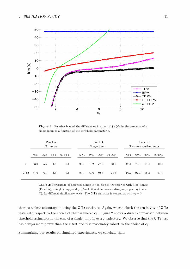
4 SIMULATION STUDY 11
2 4 6 8 10−50
−40
−30
−20
−10
0
10
20
30
40
50
cϑ
bias
(%)
TRVBPVTBPVC−TBPVC−TRV
Figure 1: Relative bias of the different estimators ofR
σ2sds in the presence of a
single jump as a function of the threshold parameter cϑ.
Panel A Panel B Panel C
No jumps Single jump Two consecutive jumps
50% 95% 99% 99.99% 50% 95% 99% 99.99% 50% 95% 99% 99.99%
z 53.0 5.7 1.4 0.1 93.4 81.2 77.6 68.6 98.1 79.1 64.4 42.4
C-Tz 54.0 6.0 1.6 0.1 93.7 83.6 80.6 74.6 99.2 97.3 96.3 93.1
Table 2: Percentage of detected jumps in the case of trajectories with a no jumps
(Panel A), a single jump per day (Panel B), and two consecutive jumps per day (Panel
C), for different significance levels. The C-Tz statistics is computed with cϑ = 3.
there is a clear advantage in using the C-Tz statistics. Again, we can check the sensitivity of C-Tz
tests with respect to the choice of the parameter cϑ. Figure 2 shows a direct comparison between
threshold estimators in the case of a single jump in every trajectory. We observe that the C-Tz test
has always more power than the z test and it is reasonably robust to the choice of cϑ.
Summarizing our results on simulated experiments, we conclude that:

4 SIMULATION STUDY 12
2 4 6 8 1070
72
74
76
78
cϑ
Det
ectio
n ef
ficie
ncy
(%)
C−TBPVBPV
Figure 2: Jump detection power for the model (4.1) in the presence of a single jump,
as a function of the threshold parameter cϑ.
1. When measuring integrated volatility in the presence of jumps, bipower variation is largely
upward biased, while threshold-based estimators are slightly downward biased (with the cor-
rected versions being upward biased, though much less than bipower variation).
2. When measuring integrated variance, threshold bipower variation is nearly insensitive to the
choice of the threshold for cϑ ≥ 3 while threshold realized variance is more sensitive to this
choice.
3. When testing for the presence of jumps, tests based on threshold multipower variation yield
a substantial advantage with respect to those based on multipower variation.
Thus, in our empirical analysis we will use threshold bipower variation as an estimator of integrated
volatility, and C-Tz statistics as jump detection test.

5 EMPIRICAL ANALYSIS 13
5 Empirical Analysis
Our data set covers a long time span of almost 15 years of high frequency data for the S&P
500 futures and US Treasury Bond with maturity 30 years, and nearly 5 years of six individual
stocks. The purpose of this section is mainly to analyze the impact of jumps on future volatility
when threshold bipower variation is employed as jump measure. We will focus not only on the
impact of jumps on future realized variance, but also on the performance of models which explicitly
incorporate lagged jumps in the volatility dynamics.
All the analysis presented in this section is based on measures of threshold multipower variation
with the threshold defined as in Eq. (2.15), with cϑ = 3 and Vt defined as in Appendix B. When
not differently specified, jumps are detected using the C-Tz statistics. Our tables are built at
confidence level α = 99.9% but the most interesting quantities will be computed and plotted for
different values of α as well. Further results with cϑ = 4, 5 are qualitatively very similar and can
be provided upon request.
5.1 The forecasting model
Empirical evidence on strong temporal dependence of realized volatility has been already found
for instance in Andersen, Bollerslev, Diebold and Labys (2001) and Andersen, Bollerslev, Diebold
and Ebens (2001). This evidence, together with our empirical results reported below, suggests that
realized variance series should be described by models allowing for slowly decaying autocorrelation
and possibly long-memory, see Andersen et al. (2003); Banerjee and Urga (2005); McAleer and
Medeiros (2008). These features are displayed by the HAR model of Corsi (2009), which has been
extended by ABD to allow for the separation of quadratic variation in its continuous part and jumps.
We then borrow the model of ABD to forecast realized variance. However, when implemented in
finite sample, we use the newly proposed measures based on threshold multipower variation.
Let t = 1, . . . be the day index and write RVt = RVδ(X)t. For two days t1 and t2 ≥ t1, define:
RVt1:t2 =1
t2 − t1 + 1
t2∑
t=t1
RVt . (5.1)
The HAR model reads:
RVt:t+h−1 = β0 + βd RVt−1 +βw RVt−5:t−1 +βm RVt−22:t−1 +εt. (5.2)

5 EMPIRICAL ANALYSIS 14
ABD proposed the HAR-CJ model:4
RVt:t+h−1 = β0 + βdCt−1 + βwCt−5:t−1 + βmCt−22:t−1 + βj Jt−1 + εt. (5.3)
The daily jump is defined as:
Jt = Izt>Φα · (RVt −BPVt)+ , (5.4)
with zt given by Eq. (A.7) in Appendix A and Φα being the cumulative distribution function of the
Normal distribution at confidence level α; x+ = max(x, 0). The continuous part of the quadratic
variation is defined by:
Ct = RVt −Jt. (5.5)
Finally, Ct−5:t−1 and Ct−22:t−1 are the weekly and monthly aggregation of Ct as in Eq. (5.1). Using
model (5.3), ABD estimate βj to be not significant and negative, and a very similar conclusion has
been reached by Forsberg and Ghysels (2007), Giot and Laurent (2007) and Busch et al. (2009);
see also the analysis of Ghysels et al. (2006).
By the light of the above sections, it is natural to define the HAR-TCJ model as:
RVt:t+h−1 = β0 + βdTCt−1 + βwTCt−5:t−1 + βmTCt−22:t−1 + βjT J t−1 + εt (5.6)
where we employ the threshold bipower variation measure to estimate the jump component
T J t = IC-Tz>Φα · (RVt −TBPVt)+ (5.7)
and the corresponding continuous part TCt = RVt −T J t.
The square-root and logarithmic counterparts of the model read:
RV1
2
t:t+h−1 = β0 + βdTC1
2
t + βwTC1
2
t−5:t−1 + βmTC1
2
t−22:t−1 + βj T J1
2
t−1 + εt (5.8)
and
log RVt:t+h−1 = β0 + βd log TCt−1 + βw log TCt−5:t−1 + βm log TCt−22:t−1 + βj log(T J t−1 + 1
)+ εt
(5.9)
and the same transformations will be estimated for model (5.2) and (5.3). Everywhere we use
annualized volatility measures (one year = 252 days).
To evaluate the forecasting performance of the different models, we use: a) the R2 of Mincer-
Zarnowitz forecasting regressions; b) the heteroskedasticity adjusted root mean square error sug-
gested in Bollerslev and Ghysels (1996):
HRMSE =
√√√√ 1
T
T∑
t=1
(RVt −RVt
RVt
)2
(5.10)
4ABD also consider weekly and monthly aggregation of the jump component. In this paper, we focus on the daily
component only to better evaluate the impact of a single jump on future volatility. Weekly and monthly components
are considered in Corsi and Reno (2010), together with an heterogeneous leverage component.

5 EMPIRICAL ANALYSIS 15
where RVt is the ex-post value of realized variance and RVt is the forecast; c) since the HRMSE is
not a robust loss function (see Patton, 2008), we also employ the QLIKE loss function, defined as:
QLIKE =1
T
T∑
t=1
(log RVt +
RVt
RVt
). (5.11)
The QLIKE loss function is robust, in the sense defined by Patton (2008). Significant difference
among competing forecasting models are evaluated through the Diebold and Mariano (1995) test
at the 5% confidence level.
5.2 Stock index futures S&P500 data
The first and most important data set we analyze is the S&P500 futures time series. We have
all high-frequency transactions from January 1990 to December 2004 (3,736 days). In order to
mitigate the impact of microstructure effects on our estimates, we choose, as in ABD, a sampling
frequency of δ = 5 minutes, corresponding to 84 returns per day.
Figure 3 is an example in which using the C-Tz statistics is effective. It displays the S&P 500
time series on one specific day, in which there is an abrupt price change. However, in this day,
the z statistics, which is based on multipower variation, is negative and does not reveal a jump at
any reasonable significance level; while the C-Tz statistics, which is based on threshold multipower
variation, does reveal a very significant jump. Our interpretation for this day is that, since the jump
appears in the form of two consecutive and very large returns, this creates a huge bias (especially
in the quarticity estimates) which makes the z statistics very noisy. This bias is instead completely
removed by the corrected threshold estimators.
Figure 4 shows the number of jumps detected in the sample by the conditions C-Tz > Φα and
z > Φα as a function of α. We see that with the statistics based on threshold multipower variation,
we detect an higher number of jumps, reflecting the greater power of the C-Tz test.
We then estimate and compare the HAR-TCJ model (5.6) and the HAR-CJ model (5.3). We also
estimate the standard HAR model (5.2) as a benchmark. Results are reported in Table 3, 4 and 5
for daily, weekly and monthly volatility forecasts respectively.
Results are unambiguous. When the jump component is measured by means of bipower variation, as
in the HAR-CJ model, its coefficient is significantly negative for the square model and insignificant
for the log and square root model in explaining future volatility. This result, although consistent
with the literature, is rather surprising in our opinion, being at odd with the economic intuition
which would suggest an increase in volatility after a jump in the price process. Moreover, this
result is even more puzzling, given that the unconditional correlations between realized variation
and jumps lagged by one day is significantly positive and around 20% for the variances, 30% for

5 EMPIRICAL ANALYSIS 16
0 10 20 30 40 50 60 70 8099
100
101
102
0 10 20 30 40 50 60 70 80−1
0
1
2
Figure 3: Rescaled time series (top) and 5-minutes logarithmic returns (bottom) of
the S&P500 on 4th December 1990. The solid and the dashed line are our estimated
threshold with cϑ = 3 and cϑ = 5 respectively. The jump statistics are z = −0.2545,
C-Tz = 4.5055 with cϑ = 3, C-Tz = 4.4745 with cϑ = 5.
the volatilities and 25% for the log volatilities. However, the simulated experiments in Section 4
suggest that when the jump component is estimated via Eq. (5.4) it is largely downward biased
because of the large upward bias of bipower variation in the presence of jumps. As a consequence,
the continuous component Ct estimated using bipower variation is still contaminated by the jump
component and hence the impact of jumps is also passing through the positive coefficients of the
other regressors.
When instead the jump component is measured by means of threshold bipower variation, the
estimated coefficients βj are positive and highly significant for the square root and log model.
Most importantly, the HAR-TCJ model yields an higher R2 and a significantly lower HRMSE
and QLIKE (as witnessed by the Diebold-Mariano test at the 5% confidence level), which implies a
better forecasting power. To better understand this point, we divide the sample in days immediately
following the occurrence of a jump and the remainder. On these two samples, we compute the R2,
HRMSE and QLIKE statistics separately, denoting them by J −R2, J −HRMSE, J −QLIKE
and C − R2, C − HRMSE, C − QLIKE respectively. The results in Table 3 show that the
TCJ models largely and significantly improves the forecasting power on realized variance in days

5 EMPIRICAL ANALYSIS 17
99 99.1 99.2 99.3 99.4 99.5 99.6 99.7 99.8 99.9 1000
50
100
150
200
250
300
350
400
450
500
zC−Tz
Figure 4: Number of days which contain jumps in the S&P500 sample obtained with
the C-Tz statistics (3.5), as a function of the confidence level α. The total number of
days is 3, 736.
immediately following a jump, and it is still slightly more performing in days that do not follow a
jump. Our interpretation of this result is that, since we are better measuring the jump component,
we are also removing noise from the continuous component in the explanatory variables; and thus,
we also get slightly better results on days in which there were no jumps before.
Figure 5 displays the most important quantities as a function of the confidence interval α. It shows
that the jump component of the HAR-TCJ model, as measured by the t−statistics of the coefficient
βj , is always positive for all models and highly significant for square root and log transformations;
while the jump component of the HAR-CJ model is mainly significantly negative or not significant.
Importantly, it shows that the HAR-TCJ model provides superior forecasts when measured in terms
of R2 and the HRMSE, irrespective of the confidence level used and model employed.
When forecasting weekly and monthly volatility, the βj of the HAR-CJ model tends to be negative,
sometimes significantly. Instead, for the HAR-TCJ model, the βj are largely positive and significant
in the square root and log model, and insignificant in the square model. Again, the R2 and the
HRMSE confirm, in days following a jump, the better forecasting ability of the HAR-TCJ model,
which is not worse than HAR-CJ in days not following a jump.5
5The analysis with higher values of cϑ reveals that the βj coefficient of the TCJ specification is mildly significant
for cϑ = 4 and not significant for cϑ = 5. This is not surprising, since as we increase cϑ we get closer to the results
obtained with bipower variation. We also estimated the HAR-CJ model using the jumps detected via the z statistics
(A.7) and compare it with the HAR-TCJ model estimated with the jumps detected via the C-Tz statistics (3.5).
The results indicate that in this case the difference between the two models is even more pronounced in favor of the
HAR-TCJ.

5 EMPIRICAL ANALYSIS 18
tstat − βj − RV
99 99.2 99.4 99.6 99.8 100−4
−3
−2
−1
0
1
2
HAR−CJHAR−TCJ
tstat − βj − RV1
2
99 99.2 99.4 99.6 99.8 100−4
−2
0
2
4
6
HAR−CJHAR−TCJ
tstat − βj − log RV
99 99.2 99.4 99.6 99.8 100−2
0
2
4
6
8
10
HAR−CJHAR−TCJ
R2 − RV
99 99.2 99.4 99.6 99.8 1000.32
0.34
0.36
0.38
0.4
0.42
0.44
HARHAR−CJHAR−TCJ
R2 − RV1
2
99 99.2 99.4 99.6 99.8 100
0.58
0.585
0.59
0.595
0.6
0.605
0.61
HARHAR−CJHAR−TCJ
R2 − log RV
99 99.2 99.4 99.6 99.8 1000.679
0.68
0.681
0.682
0.683
0.684
0.685
0.686
HARHAR−CJHAR−TCJ
HRMSE (%) − RV
99 99.2 99.4 99.6 99.8 1000.7
0.75
0.8
0.85
0.9
0.95
HARHAR−CJHAR−TCJ
HRMSE (%) − RV1
2
99 99.2 99.4 99.6 99.8 1000.6
0.61
0.62
0.63
0.64
0.65
0.66
HARHAR−CJHAR−TCJ
HRMSE (%) − log RV
99 99.2 99.4 99.6 99.8 1000.535
0.54
0.545
0.55
0.555
0.56
0.565
HARHAR−CJHAR−TCJ
Figure 5: Reports the t statistics of the coefficient βj measuring the impact of jumps
on future volatility, the R2 and the HRMSE for the three models estimated on S&P
500 data for daily forecasting, for both the HAR-CJ and HAR-TCJ versions, as a
function of the confidence level used for detecting jumps with the C-Tz statistics.

5 EMPIRICAL ANALYSIS 19
Daily (h = 1) S&P500 Regressions
HAR: RVt:t+h−1 = β0 + βd RVt−1 +βw RVt−5:t−1 +βm RVt−22:t−1 +εt
HAR-CJ: RVt:t+h−1 = β0 + βdbCt−1 + βw
bCt−5:t−1 + βmbCt−22:t−1 + βj
bJt−1 + εt
HAR-TCJ: RVt:t+h−1 = β0 + βddTCt−1 + βw
dTCt−5:t−1 + βmdTCt−22:t−1 + βj
cTJt−1 + εt
RVt RV1/2
t log RVt
HAR HAR-CJ HAR-TCJ HAR HAR-CJ HAR-TCJ HAR HAR-CJ HAR-TCJ
β0 34.266 26.823 23.312 0.986 0.906 0.771 0.254 0.274 0.286
(3.779) (3.373) (2.760) (3.973) (3.817) (3.318) (4.498) (4.906) (5.206)
βd 0.220 0.378 0.420 0.323 0.371 0.421 0.335 0.336 0.356
(2.329) (5.736) (6.171) (6.348) (8.961) (11.958) (13.143) (13.146) (14.838)
βw 0.321 0.263 0.298 0.336 0.317 0.308 0.359 0.356 0.342
(3.820) (3.156) (2.608) (6.077) (5.812) (5.427) (9.489) (9.420) (9.441)
βm 0.313 0.288 0.253 0.268 0.260 0.237 0.256 0.256 0.252
(4.814) (4.783) (3.850) (6.820) (6.704) (6.081) (8.829) (8.916) (9.028)
βj -0.581 0.045 -0.101 0.096 0.007 0.055
(-2.968) (0.925) (-1.627) (2.653) (0.680) (6.386)
R2 0.339 0.374 0.387 0.583 0.592 0.604 0.679 0.681 0.684
HRMSE 0.867 0.794* 0.749*† 0.652 0.630 0.605*† 0.555 0.552* 0.537*†
QLIKE 6.429 6.390* 6.371*† 6.228 6.223* 6.216*† 6.139 6.139 6.136
J-R2 0.320 0.363 0.386 0.573 0.596 0.626 0.685 0.691 0.707
J-HRMSE 1.137 0.955* 0.778*† 0.799 0.729* 0.624*† 0.644 0.611* 0.530*†
J-QLIKE 6.513 6.405* 6.317*† 6.265 6.214* 6.149*† 6.148 6.114* 6.054*†
C-R2 0.341 0.375 0.388 0.584 0.592 0.603 0.679 0.680 0.682
C-HRMSE 0.846 0.782* 0.747*† 0.640 0.623 0.604 0.548 0.547 0.537
C-QLIKE 6.423 6.389* 6.375*† 6.226 6.224 6.220 6.139 6.140 6.142
Table 3: OLS estimate for daily (h = 1) HAR, HAR-CJ and HAR-TCJ volatility
forecast regressions for S&P500 futures from January 1990 to December 2004 (3,736
observations). The significant daily jumps are computed using a critical value of
α = 99.9% and the C-Tz statistics computed with cϑ = 3. Reported in parenthesis are
the t-statistics based on Newey-West correction with order 5. Performance measures
are the Mincer-Zarnowitz R2, the HRMSE as in equation (5.10) and the QLIKE as in
(5.11), computed unconditionally, conditionally on having had a jump at time t − 1
(J-R2, J-HRMSE, J-QLIKE) and conditionally on no jump at time t − 1 (C-R2, C-
HRMSE, C-QLIKE). Using the Diebold-Mariano test at the 5% confidence level, a ∗denotes significant improvement in the forecasting performance with respect to the
HAR model, and a † with respect to the HAR-CJ model.

5 EMPIRICAL ANALYSIS 20
Weekly (h = 5) S&P500 Regressions
HAR: RVt:t+h−1 = β0 + βd RVt−1 +βw RVt−5:t−1 +βm RVt−22:t−1 +εt
HAR-CJ: RVt:t+h−1 = β0 + βdbCt−1 + βw
bCt−5:t−1 + βmbCt−22:t−1 + βj
bJt−1 + εt
HAR-TCJ: RVt:t+h−1 = β0 + βddTCt−1 + βw
dTCt−5:t−1 + βmdTCt−22:t−1 + βj
cTJt−1 + εt
RVt:t+4 RV1/2
t:t+4log RVt:t+4
HAR HAR-CJ HAR-TCJ HAR HAR-CJ HAR-TCJ HAR HAR-CJ HAR-TCJ
β0 47.320 41.284 37.873 1.541 1.465 1.348 0.407 0.426 0.438
(4.335) (3.987) (3.384) (4.334) (4.252) (3.966) (4.843) (5.118) (5.384)
βd 0.097 0.190 0.210 0.176 0.213 0.244 0.205 0.211 0.229
(1.892) (4.858) (4.403) (5.360) (7.927) (9.395) (11.744) (12.132) (13.821)
βw 0.367 0.351 0.393 0.369 0.356 0.353 0.360 0.353 0.333
(4.677) (4.299) (3.564) (6.157) (6.006) (5.869) (8.245) (8.148) (8.070)
βm 0.335 0.320 0.304 0.342 0.337 0.329 0.353 0.355 0.359
(4.897) (4.371) (3.702) (6.361) (6.174) (6.028) (8.548) (8.728) (9.159)
βj -0.394 0.007 -0.105 0.040 -0.005 0.031
(-2.571) (0.379) (-2.427) (2.466) (-0.693) (6.193)
R2 0.499 0.534 0.554 0.690 0.700 0.709 0.767 0.770 0.772
HRMSE 0.634 0.589* 0.566*† 0.439 0.425* 0.417*† 0.377 0.372* 0.369*
QLIKE 6.401 6.376* 6.366*† 6.194 6.190* 6.187 6.098 6.097 6.097
J-R2 0.489 0.539 0.567 0.656 0.684 0.712 0.742 0.751 0.766
J-HRMSE 0.761 0.652* 0.545*† 0.526 0.465* 0.397*† 0.415 0.391* 0.355*†
J-QLIKE 6.456 6.377* 6.300*† 6.220 6.173* 6.114*† 6.101 6.069* 6.019*†
C-R2 0.503 0.536 0.553 0.693 0.701 0.709 0.769 0.771 0.773
C-HRMSE 0.625 0.584* 0.568*† 0.432 0.423* 0.418* 0.373 0.371* 0.369*
C-QLIKE 6.397 6.376* 6.371* 6.193 6.191 6.192 6.098 6.099 6.102
Table 4: OLS estimate for weekly (h = 5) HAR, HAR-CJ and HAR-TCJ volatility
forecast regressions for S&P500 futures from January 1990 to December 2004 (3,736
observations). The significant daily jumps are computed using a critical value of α =
99.9%. Reported in parenthesis are the t-statistics based on Newey-West correction
with order 10. Performance measures are the Mincer-Zarnowitz R2, the HRMSE as in
equation (5.10) and the QLIKE as in (5.11), computed unconditionally, conditionally
on having had at jump a time t − 1 (J-R2, J-HRMSE, J-QLIKE) and conditionally
on no jump at time t − 1 (C-R2, C-HRMSE, C-QLIKE). Using the Diebold-Mariano
test at the 5% confidence level, a ∗ denotes significant improvement in the forecasting
performance with respect to the HAR model, and a † with respect to the HAR-CJ
model.

5 EMPIRICAL ANALYSIS 21
Monthly (h = 22) S&P500 Regressions
HAR: RVt:t+h−1 = β0 + βd RVt−1 +βw RVt−5:t−1 +βm RVt−22:t−1 +εt
HAR-CJ: RVt:t+h−1 = β0 + βdbCt−1 + βw
bCt−5:t−1 + βmbCt−22:t−1 + βj
bJt−1 + εt
HAR-TCJ: RVt:t+h−1 = β0 + βddTCt−1 + βw
dTCt−5:t−1 + βmdTCt−22:t−1 + βj
cTJt−1 + εt
RVt:t+21 RV1/2
t:t+21log RVt:t+21
HAR HAR-CJ HAR-TCJ HAR HAR-CJ HAR-TCJ HAR HAR-CJ HAR-TCJ
β0 78.538 73.578 70.785 2.883 2.808 2.699 0.758 0.771 0.778
(5.909) (5.638) (4.962) (5.892) (5.967) (5.883) (5.292) (5.492) (5.702)
βd 0.061 0.124 0.129 0.109 0.135 0.149 0.126 0.130 0.138
(2.555) (5.292) (4.876) (5.915) (8.410) (9.183) (10.055) (10.519) (11.717)
βw 0.219 0.206 0.243 0.281 0.273 0.281 0.269 0.265 0.253
(4.279) (3.746) (4.350) (5.579) (5.385) (5.405) (6.171) (6.093) (5.927)
βm 0.385 0.385 0.385 0.399 0.397 0.395 0.454 0.456 0.462
(4.595) (4.310) (4.022) (6.358) (6.291) (6.373) (9.144) (9.246) (9.728)
βj -0.284 -0.002 -0.092 0.018 -0.010 0.016
(-2.892) (-0.114) (-3.278) (1.444) (-1.746) (3.658)
R2 0.471 0.500 0.517 0.649 0.659 0.667 0.739 0.742 0.746
HRMSE 0.680 0.649* 0.639*† 0.438 0.429* 0.425* 0.376 0.373* 0.370*
QLIKE 6.483 6.467* 6.462* 6.227 6.224 6.222 6.106 6.105 6.105
J-R2 0.438 0.476 0.513 0.651 0.672 0.692 0.746 0.755 0.761
J-HRMSE 0.753 0.690* 0.653*† 0.475 0.443* 0.420*† 0.389 0.375* 0.367*
J-QLIKE 6.520 6.465* 6.416*† 6.237 6.200* 6.156*† 6.096 6.069* 6.033*†
C-R2 0.474 0.502 0.517 0.650 0.658 0.666 0.738 0.742 0.745
C-HRMSE 0.675 0.647* 0.638* 0.435 0.428* 0.425 0.374 0.372* 0.370*
C-QLIKE 6.481 6.467* 6.465* 6.227 6.226 6.227 6.107 6.108 6.110
Table 5: OLS estimate for monthly (h = 22) HAR, HAR-CJ and HAR-TCJ volatility
forecast regressions for S&P500 futures from January 1990 to December 2004 (3,736
observations). The significant daily jumps are computed using a critical value of α =
99.9%. Reported in parenthesis are the t-statistics based on Newey-West correction
with order 44. Performance measures are the Mincer-Zarnowitz R2, the HRMSE as in
equation (5.10) and the QLIKE as in (5.11), computed unconditionally, conditionally
on having had a jump at time t − 1 (J-R2, J-HRMSE, J-QLIKE) and conditionally
on no jump at time t − 1 (C-R2, C-HRMSE, C-QLIKE). Using the Diebold-Mariano
test at the 5% confidence level, a ∗ denotes significant improvement in the forecasting
performance with respect to the HAR model, and a † with respect to the HAR-CJ
model.

5 EMPIRICAL ANALYSIS 22
5.3 Individual stocks
We analyze a sample of six individual stocks, chosen among the most liquid stocks of S&P500. The
stocks are Alcoa (aa), Citigroup (c), Intel (intc), Microsoft (msft), Pfeizer (pfe) and Exxon-Mobil
(xom). Our sample starts on 2 January 2001 and ends on 30 December 2005, containing 1, 256
days per stock. Since these stocks are traded very actively, we still use a sampling frequency of
δ = 5 minutes, corresponding to 78 returns per day. To save space, we focus on the most important
quantities (the significance of the jump and the R2, HRMSE and QLIKE of the forecasting
model conditional to days after the occurrence of a jump), which are reported in Table 6 for the
logarithmic model. We report results for α = 99% and α = 99.9%.
Despite the smaller sample size and increased idiosyncratic noise, jumps still have a substantial
impact in determining future volatility which can be revealed by using threshold bipower variation.
The t statistics of the βj coefficient is always larger for the HAR-TCJ model than for the HAR-CJ
model, and always significant. On the whole sample, the performance of the two models is virtually
the same but, conditioned on the occurrence of a jump, there is significant advantage in using
the HAR-TCJ model, especially when significance is evaluated by the robust QLIKE. Thus, the
results obtained on the S&P500 portfolio are qualitatively replicated on its most liquid constituents,
indicating that the impact of jumps on future volatility is not peculiar to the S&P500 returns
considered in the previous Section, and suggesting that it may simply come from aggregation, at
the portfolio level, of the same effect at the individual stock level.
5.4 Bond data and the no-trade bias
Finally, we use a sample of 30-years US Treasury Bond futures from January 1990 to October 2003
for a total of 3, 231 daily data points. All the relevant volatility and jump measures are computed
again with five-minutes returns, corresponding to 84 returns per day.
The first thing we note on bond data is a surprisingly high number of jumps. At the 99.9%
confidence level, the C-Tz statistics detects 570 jumps, corresponding to the 17.6 % of our sample.
Visual inspection of time series data reveals that in most of these days there are many intervals
with zero return instead.
The problem hinges from what we could call the no-trade bias of bipower variation. This can
be explained as follows. Suppose that data are not recorded continuously but, more realistically,
that they are recorded discretely. Denote by δ the minimum distance between two subsequent
observations. By construction, if δ < δ, then MPVδ = 0 identically! Clearly, also TMPVδ = 0.
This simple reasoning also explains why the presence of null returns caused by absence of trading
(stale price) in that interval induces a downward bias in multipower variation measures. Note that

6 CONCLUSIONS 23
realized variance is immune from this bias instead. Moreover, this bias has a larger impact on the
jump detecting statistics, pointing toward rejection of the null. For example, when considering the
z statistics, this bias lowers both the BPV and TriPV measure, with the joint effect of increasing
the numerator and decreasing the denominator, thus increasing the statistics considerably.
In our paper, this problem does not affect the S&P500 index, neither the stocks considered in our
empirical analysis. However, it may affect US bond data, which are largely less liquid. Indeed, the
percentage of zero 5-minutes return in bond data is very high, nearly 30%. We accommodate this
problem as follows: for bond data, we compute the C-Tz statistics using only returns different from
zero. Clearly, this biases the test toward the null, meaning that the detected jumps are those which
have a larger impact for the statistics. With this correction the number of significant jumps with
α = 99.9% reduced to 112 representing 3.4% of the sample. Further analysis and different possible
corrections for this problem are discussed in Schulz (2010).
Relevant estimation results for bond data when forecasting daily, weekly and monthly volatility are
shown in Table 7 for α = 99.9%. We find that the HAR-TCJ model outperforms the HAR-CJ model
(significantly after a jumps) while both significantly outperform the HAR model. Also the impact
of the jump on future volatility in the HAR-TCJ model is generally insignificant, but nevertheless
not negatively significant as for the HAR-CJ estimates. An explanation for this finding might be
that jumps in the bond market are less “surprising” with respect to those in the stock markets, since
most of them are related to scheduled macroeconomic announcements. Indeed, related studies, for
example Bollerslev et al. (2000), find two intraday spikes at hours in which announcements are
released.
Summarizing, our empirical findings further corroborate the theoretical and simulation results in the
previous sections on the superior performance of the threshold method in separating and estimating
the continuous and jump components of the price process. Moreover, they show that, once the two
components are correctly measured and separated, the impact of past jumps on future realized
variance is positive and significant, and the ability to forecast volatility increases significantly.
6 Conclusions
This paper shows that dividing volatility into jumps and continuous variation yields a substantial
improvement in volatility forecasting, because of the positive impact of past jumps on future volatil-
ity. This important result has been obscured in the literature since, in finite samples, measures
based on multipower variation are largely biased in the presence of jumps. We uncover this effect
by modifying bipower variation with the help of threshold estimation techniques. We show that the
newly defined estimator is robust to the presence of jumps and quite inelastic with respect to the
choice of the threshold. The class of TMPV estimators introduced in this paper admits a central

6 CONCLUSIONS 24
limit theorem in presence of jumps.
Our empirical results, obtained on US stock index, individual stocks and Treasury bond data, also
show that jumps can be effectively detected using the newly proposed C-Tz statistics, which is based
on TMPV estimators. The models we propose provide a significantly superior forecasting ability,
especially in days which follow the occurrence of a jump. Clearly, these findings can be of great
importance for risk management and other financial applications involving volatility estimation.
Moreover, the correlation between jumps and future volatility can be helpful not only for practical
applications, but also for a deeper comprehension of the asset price dynamics. We consider this
line of research as an interesting direction for future studies.

6C
ON
CLU
SIO
NS
25
Stock α (%) Jumps βj t-stat J-R2 J-HRMSE J-QLIKE
HAR-CJ HAR-TCJ HAR HAR-CJ HAR-TCJ HAR HAR-CJ HAR-TCJ HAR HAR-CJ HAR-TCJ
aa 99.0 242 0.829 3.378 0.551 0.560 0.546 0.495 0.466* 0.450* -1.589 -1.623* -1.665*†99.9 121 0.373 2.671 0.607 0.628 0.614 0.455 0.416* 0.399* -1.582 -1.627* -1.685*†
c 99.0 196 0.746 3.677 0.827 0.830 0.835 0.538 0.520 0.486 -2.045 -2.073* -2.104*†99.9 105 -0.410 3.967 0.842 0.847 0.851 0.457 0.435* 0.418*† -2.091 -2.127* -2.164*†
intc 99.0 155 3.471 5.572 0.784 0.786 0.784 0.512 0.485 0.463* -1.472 -1.506* -1.535*†99.9 78 3.112 4.935 0.831 0.827 0.821 0.474 0.460* 0.430 -1.401 -1.443* -1.485*†
msft 99.0 202 -0.305 2.899 0.807 0.813 0.815 0.604 0.547 0.506 -2.030 -2.060* -2.087*†99.9 92 0.252 2.190 0.799 0.805 0.810 0.755 0.673 0.602 -2.020 -2.058* -2.102*†
pfe 99.0 239 0.524 2.469 0.600 0.617 0.609 0.655 0.570 0.560 -1.956 -1.988* -2.013*†99.9 131 0.391 2.979 0.591 0.628 0.612 0.715 0.564 0.551 -1.953 -2.001 -2.033*†
xom 99.0 193 1.424 3.224 0.732 0.735 0.721 0.500 0.475* 0.464* -2.296 -2.324* -2.360*†99.9 98 0.472 2.656 0.695 0.702 0.695 0.523 0.479* 0.454*† -2.305 -2.348* -2.394*†
Table 6: Reports number of jumps, t-stat on βj , J − R2, J − HRMSE and J −QLIKE for daily (h = 1) logarithmic version of HAR, HAR-CJ and HAR-TCJ
volatility forecast regressions on six individual stocks . The significant daily jumps
are computed using a critical value of α = 0.99 and α = 0.999 as reported, with
the C-Tz statistics. Using the Diebold-Mariano test at the 5% confidence level, a ∗denotes significant improvement in the forecasting performance with respect to the
HAR model, and a † with respect to the HAR-CJ model.

6 CONCLUSIONS 26
US Bond Regressions (C-Tz statistics)
HAR: RVt:t+h−1 = β0 + βd RVt−1 +βw RVt−5:t−1 +βm RVt−22:t−1 +εt
HAR-CJ: RVt:t+h−1 = β0 + βdbCt−1 + βw
bCt−5:t−1 + βmbCt−22:t−1 + βj
bJt−1 + εt
HAR-TCJ: RVt:t+h−1 = β0 + βddTCt−1 + βw
dTCt−5:t−1 + βmdTCt−22:t−1 + βj
cTJt−1 + εt
RVt:t+h−1 RV1/2
t:t+h−1log RVt:t+h−1
HAR HAR-CJ HAR-TCJ HAR HAR-CJ HAR-TCJ HAR HAR-CJ HAR-TCJ
Daily forecasts (h = 1)
βj -0.108 0.030 -0.041 0.029 -0.012 0.016
(-2.633) (1.445) (-1.932) (1.798) (-1.393) (2.015)
R2 0.124 0.144 0.143 0.204 0.216 0.214 0.250 0.256 0.252
HRMSE 0.907 0.872* 0.866* 0.754 0.737* 0.733* 0.657 0.649* 0.645*
QLIKE 5.508 5.491* 5.492* 5.362 5.356* 5.356* 5.256 5.254 5.254
J-R2 0.096 0.119 0.108 0.160 0.169 0.161 0.200 0.201 0.192
J-HRMSE 1.326 1.053 0.890*† 1.113 0.906 0.763† 0.934 0.796 0.677*†J-QLIKE 5.537 5.455* 5.398*† 5.355 5.294* 5.236*† 5.222 5.175* 5.125*†C-R2 0.129 0.144 0.142 0.209 0.218 0.216 0.255 0.261 0.256
C-HRMSE 0.888 0.865* 0.866* 0.738 0.731* 0.732 0.645 0.642 0.643
C-QLIKE 5.502 5.499 5.512 5.364 5.370 5.382 5.264 5.271 5.282
Weekly forecasts (h = 5)
βj -0.063 0.028 -0.030 0.029 -0.010 0.018
(-3.119) (2.794) (-2.625) (3.582) (-2.010) (4.036)
R2 0.295 0.333 0.332 0.415 0.438 0.436 0.472 0.486 0.480
HRMSE 0.445 0.422* 0.419* 0.363 0.353* 0.351* 0.331 0.327* 0.325*
QLIKE 5.370 5.361* 5.363 5.250 5.248 5.249 5.162 5.162 5.163
J-R2 0.197 0.233 0.232 0.330 0.351 0.344 0.400 0.411 0.400
J-HRMSE 0.629 0.498* 0.417*† 0.469 0.386* 0.338*† 0.367 0.326* 0.306*
J-QLIKE 5.364 5.310* 5.270*† 5.221 5.181* 5.144*† 5.115 5.086* 5.056*†C-R2 0.315 0.347 0.347 0.428 0.448 0.446 0.482 0.493 0.488
C-HRMSE 0.437 0.419* 0.420* 0.358 0.352* 0.352* 0.329 0.326* 0.325*
C-QLIKE 5.371 5.372 5.383 5.257 5.262 5.271 5.173 5.178 5.186
Monthly forecasts (h = 22)
βj -0.058 0.010 -0.034 0.010 -0.013 0.006
(-3.986) (1.586) (-3.871) (1.743) (-3.259) (1.875)
R2 0.333 0.387 0.395 0.433 0.473 0.481 0.488 0.514 0.519
HRMSE 0.321 0.305* 0.303* 0.264 0.258* 0.257* 0.262 0.260 0.260
QLIKE 5.351 5.344 5.345 5.233 5.231 5.231 5.144 5.143 5.144
J-R2 0.296 0.353 0.365 0.403 0.442 0.452 0.461 0.484 0.484
J-HRMSE 0.398 0.313* 0.271*† 0.281 0.240* 0.235* 0.234 0.229 0.250
J-QLIKE 5.342 5.300* 5.267*† 5.204 5.173* 5.142*† 5.100 5.077* 5.052*†C-R2 0.339 0.387 0.393 0.436 0.471 0.478 0.489 0.513 0.517
C-HRMSE 0.318 0.305* 0.304* 0.263 0.259* 0.258* 0.262 0.260 0.260
C-QLIKE 5.353 5.354 5.361 5.240 5.243 5.250 5.153 5.158 5.164
Table 7: OLS (partial) estimates for daily (h = 1), weekly (h = 5), monthly (h = 22)
HAR, HAR-CJ and HAR-TCJ volatility forecast regressions for US Bond from Jan-
uary 1990 to December 2004 (3,736 observations). The significant daily jumps are
computed using a critical value of α = 99.9% and the C-Tz statistics. Reported in
parenthesis are the t-statistics based on Newey-West correction. Performance mea-
sures are the Mincer-Zarnowitz R2, the HRMSE as in equation (5.10) and the QLIKE
as in (5.11), computed unconditionally, conditionally on having had a jump at time
t−1 (J-R2, J-HRMSE, J-QLIKE) and conditionally on no jump at time t−1 (C-R2,
C-HRMSE, C-QLIKE). Using the Diebold-Mariano test at the 5% confidence level, a
∗ denotes significant improvement in the forecasting performance with respect to the
HAR model, and a † with respect to the HAR-CJ model.

REFERENCES 27
References
Abramowitz, M. and I. Stegun (1965). Handbook of mathematical functions. Courier Dover Publications.
Aıt-Sahalia, Y. (2004). Disentangling diffusion from jumps. Journal of Financial Economics 74, 487–528.
Aıt-Sahalia, Y. and J. Jacod (2009). Testing for jumps in a discretely observed process. Annals of Statis-
tics 37, 184–222.
Aıt-Sahalia, Y. and L. Mancini (2008). Out of sample forecasts of quadratic variation. Journal of Econo-
metrics 147 (1), 17–33.
Andersen, T., L. Benzoni, and J. Lund (2002). An empirical investigation of continuous-time equity return
models. Journal of Finance 57, 1239–1284.
Andersen, T., T. Bollerslev, F. Diebold, and H. Ebens (2001). The distribution of realized stock volatility.
Journal of Financial Economics 61, 43–76.
Andersen, T., T. Bollerslev, F. Diebold, and P. Labys (2001). The distribution of realized exchange rate
volatility. Journal of the American Statistical Association 96, 42–55.
Andersen, T., T. Bollerslev, and F. X. Diebold (2003). Parametric and nonparametric volatility measurement.
In L. P. Hansen and Y. Ait-Sahalia (Eds.), Handbook of Financial Econometrics. Amsterdam: North-
Holland.
Andersen, T., T. Bollerslev, and F. X. Diebold (2007). Roughing it up: Including jump components in
the measurement, modeling and forecasting of return volatility. Review of Economics and Statistics 89,
701–720.
Andersen, T., T. Bollerslev, and D. Dobrev (2007). No-arbitrage semi-martingale restrictions for continuous-
time volatility models subject to leverage effects, jumps and iid noise: Theory and testable distributional
implications. Journal of Econometrics 138 (1), 125–180.
Andersen, T., D. Dobrev, and E. Schaumburg (2008). Jump robust volatility estimation. Working Paper.
Bandi, F. and T. Nguyen (2003). On the functional estimation of jump-diffusion models. Journal of Econo-
metrics 116, 293–328.
Banerjee, A. and G. Urga (2005). Modelling structural breaks, long memory and stock market volatility: an
overview. Journal of Econometrics 129 (1-2), 1–34.
Barndorff-Nielsen, O. E., E. Graversen, J. Jacod, M. Podolskij, and N. Shephard (2006). A central limit
theorem for realised power and bipower variations of continuous semimartingales. In From Stochastic
Analysis to Mathematical Finance, Festschrift for Albert Shiryaev, pp. 33–68.
Barndorff-Nielsen, O. E., E. Graversen, J. Jacod, and N. Shephard (2006). Limit theorems for bipower
variation in financial econometrics. Econometric Theory 22, 677–719.
Barndorff-Nielsen, O. E. and N. Shephard (2004). Power and bipower variation with stochastic volatility
and jumps. Journal of Financial Econometrics 2, 1–48.
Barndorff-Nielsen, O. E. and N. Shephard (2006). Econometrics of testing for jumps in financial economics
using bipower variation. Journal of Financial Econometrics 4, 1–30.
Barndorff-Nielsen, O. E. and N. Shephard (2007). Variation, jumps, market frictions and high frequency
data in financial econometrics. In Advances in Economics and Econometrics. Theory and Applications,
Ninth World Congress, pp. 328–372. Cambridge University Press.
Barndorff-Nielsen, O. E., N. Shephard, and M. Winkel (2006). Limit theorems for multipower variation in
the presence of jumps. Stochastic Processes and Their Applications 116, 798–806.

REFERENCES 28
Bates, D. (2000). Post-’87 crash fears in the S&P 500 futures option market. Journal of Econometrics 94,
181–238.
Bollerslev, T., J. Cai, and F. Song (2000). Intraday periodicity, long memory volatility and macroeconomic
announcement effects in the US Treasury bond market. Journal of Empirical Finance 7, 37–55.
Bollerslev, T. and E. Ghysels (1996). Periodic autoregressive conditional heteroscedasticity. Journal of
Business & Economic Statistics 14 (2), 139–151.
Bollerslev, T., U. Kretschmer, C. Pigorsch, and G. Tauchen (2009). A Discrete-Time Model for Daily S&P500
Returns and Realized Variations: Jumps and Leverage Effects. Journal of Econometrics 150 (2), 151–166.
Bollerslev, T., T. H. Law, and G. Tauchen (2008). Risk, jumps and diversification. Journal of Economet-
rics 144, 234–256.
Boudt, K., C. Croux, and S. Laurent (2008). Outlyingness Weighted Quadratic Covariation. Working Paper.
Buraschi, A., F. Trojani, and A. Vedolin (2007). The Joint Behavior of Credit Spreads, Stock Options and
Equity Returns when Investors Disagree. Working paper.
Busch, T., B. Christensen, and M. Nielsen (2009). The role of implied volatility in forecasting future realized
volatility and jumps in foreign exchange, stock, and bond markets. Journal of Econometrics. Forthcoming.
Cartea, A. and D. Karyampas (2010). The relationship between the volatility of returns and the number of
jumps in financial markets. Working paper.
Chernov, M., R. Gallant, E. Ghysels, and G. Tauchen (2003). Alternative models for stock price dynamics.
Journal of Econometrics 116 (1), 225–258.
Christensen, K., R. Oomen, and M. Podoslkij (2008). Realised quantile-based estimation of the integrated
variance. Journal of Econometrics. Forthcoming.
Cont, R. and P. Tankov (2004). Financial Modelling with Jump Processes. Chapman & Hall - CRC.
Corsi, F. (2009). A simple approximate long-memory model of realized volatility. Journal of Financial
Econometrics 7, 174–196.
Corsi, F. and R. Reno (2010). Discrete-time volatility forecasting with persistent leverage effect and the link
with continuous-time volatility modeling. Working paper.
Das, S. and R. Uppal (2004). Systemic Risk and International Portfolio Choice. The Journal of Fi-
nance 59 (6), 2809–2834.
Diebold, F. and R. Mariano (1995). Comparing predictive accuracy. Journal of Business & Economic
Statistics 13 (3), 253–263.
Duffie, D., J. Pan, and K. Singleton (2000). Transform analysis and asset pricing for affine junp-diffusions.
Econometrica 68, 1343–1376.
Eraker, B. (2004). Do Stock Prices and Volatility Jump? Reconciling Evidence from Spot and Option Prices.
The Journal of Finance 59 (3), 1367–1404.
Eraker, B., M. Johannes, and N. Polson (2003). The impact of jumps in equity index volatility and returns.
Journal of Finance 58, 1269–1300.
Fan, J. and Y. Wang (2007). Multi-scale jump and volatility analysis for high-frequency financial data.
Journal of the American Statistical Association 102, 1349–1362.
Fan, J. and Q. Yao (2003). Nonlinear time series. Springer.
Forsberg, L. and E. Ghysels (2007). Why do absolute returns predict volatility so well? Journal of Financial
Econometrics 5, 31–67.
Ghysels, E., P. Santa-Clara, and R. Valkanov (2006). Predicting volatility: getting the most out of return

REFERENCES 29
data sampled at different frequencies. Journal of Econometrics 131 (1-2), 59–95.
Giot, P. and S. Laurent (2007). The information content of implied volatility in light of the jump/continuous
decomposition of realized volatility. Journal of Future Markets 27 (4), 337.
Huang, X. and G. Tauchen (2005). The relative contribution of jumps to total price variance. Journal of
Financial Econometrics 3 (4), 456–499.
Jacod, J. (2008). Asymptotic properties of realized power variations and associated functionals of semi-
martingales. Stochastic processes and their applications 118, 517–559.
Jacod, J., Y. Li, P. Mykland, M. Podolskij, and M. Vetter (2007). Microstructure noise in the continuous
case: the pre-averaging approach. Stochastic Processes and Their Applications. Forthcoming.
Jiang, G. and R. Oomen (2008). Testing for jumps when asset prices are observed with noise–a ”swap
variance” approach. Journal of Econometrics 144 (2), 352–370.
Johannes, M. (2004). The statistical and economic role of jumps in continuous-time interest rate models.
Journal of Finance 59, 227–260.
Lee, S. and P. Mykland (2008). Jumps in financial markets: A new nonparametric test and jump dynamics.
Review of Financial studies 21 (6), 2535.
Maheu, J. and T. McCurdy (2004). News arrival, jump dynamics and volatility components for individual
stock returns. Journal of Finance 59 (2), 755–793.
Mancini, C. (2009). Non-parametric threshold estimation for models with stochastic diffusion coefficient and
jumps. Scandinavian Journal of Statistics 36 (2), 270–296.
Mancini, C. and R. Reno (2009). Threshold estimation of Markov models with jumps and interest rate
modeling. Journal of Econometrics. Forthcoming.
McAleer, M. and M. Medeiros (2008). Realized volatility: a review. Econometric Reviews 27 (1), 10–45.
Pan, J. (2002). The jump-risk premia implicit in options: Evidence from an integrated time series study.
Journal of Financial Economics 63, 3–50.
Patton, A. (2008). Volatility forecast comparison using imperfect volatility proxies. Journal of Econometrics.
Forthcoming.
Podolskij, M. and M. Vetter (2009). Estimation of volatility functionals in the simultaneous presence of
microstructure noise and jumps. Bernoulli 15 (3), 634–668. Working Paper.
Protter, P. (2004). Stochastic Integration and Differential Equations. Springer.
Schulz, F. C. (2010). Robust estimation of integrated variance and quarticity under flat price and no trading
bias. Working paper.
Shalen, C. T. (1993). Volume, volatility and dispersion of beliefs. Review of Financial Studies 6, 405–434.
Vetter, M. (2010). Limit theorems for bipower variation of semimartingales. Stochastic Processes and their
Applications 120 (1), 22–38.
Wang, J. (1994). A model of competitive stock trading volume. Journal of Political Economy 102, 127–168.
Woerner, J. (2006). Power and multipower variation: inference for high frequency data. In A. N. Shiryaev,
M. do Rosario Grossinho, P. Oliveira, and M. Esquivel (Eds.), Stochastic Finance, pp. 343–364. Springer.
Wright, J. and H. Zhou (2007). Bond risk premia and realized jump volatility. Working paper, Federal
Reserve Board.

A QUARTICITY ESTIMATORS AND JUMP DETECTION STATISTICS 30
A Quarticity estimators and jump detection statistics
For estimation of the integrated quarticity∫ t+Tt σ4
sds, the literature focused on the following quan-
tities:
QPVδ(X)t = µ−41 · MPVδ(X)
[1,1,1,1]t = µ−4
1
1
δ
[T/δ]∑
j=4
|∆j−3X| · |∆j−2X| · |∆j−1X| · |∆jX| (A.1)
TriPVδ(X)t = µ−34
3
· MPVδ(X)[ 43, 43, 43]
t = µ−34
3
1
δ
[T/δ]∑
j=3
|∆j−2X| 43 · |∆j−1X| 43 · |∆jX| 43 (A.2)
where µ 4
3
≃ 0.8309, and
TQVδ(X)t =1
3δ
[T/δ]∑
j=1
|∆jX|4I|∆jX|2≤Θ(δ) (A.3)
where Θ(δ) satisfies (2.9). We propose the counterparts TQPV = µ−41 ·TMPVδ(X)
[1,1,1,1]t , TTriPV =
µ−34
3
· TMPVδ(X)[ 43, 43, 43]
t , see equation (2.10), and their corrected version
C-TQVδ(X)t = µ−41 · C-TMPVδ(X)
[1,1,1,1]t (A.4)
C-TTriPVδ(X)t = µ−34
3
· C-TMPVδ(X)[ 43, 43, 43]
t (A.5)
see definition (3.2). We also define a corrected version of (A.3):
C-TQVδ(X)t =1
3δ
[T/δ]∑
j=1
Z4(∆jX, ϑj) (A.6)
A feasible jump test can be constructed using multipower estimators of the integrated quarticity
given by equations (A.1)-(A.2). In their study, ABD use the test:
z = δ−1
2
(RVδ (X)T − BPVδ (X)T ) · RVδ (X)−1T√
ϑ max
1,
TriPVδ(X)T
(BPVδ(X)T )2
, (A.7)
with ϑ = π2
4 + π − 5.

B AUXILIARY ESTIMATION OF LOCAL VARIANCE 31
B Auxiliary estimation of local variance
We estimate local variance with a non-parametric filter of length 2L + 1 (Fan and Yao, 2003)
adapted for the presence of jumps by iterating in Z:
V Zt =
L∑
i=−L, i6=−1,0,1
K
(i
L
)(∆t+iX)2 I(∆t+iX)2≤c2V ·bV Z−1
t+i
L∑
i=−L, i6=−1,0,1
K
(i
L
)I(∆t+iX)2≤c2V ·bV Z−1
t+i
, Z = 1, 2, . . . (B.1)
with the starting value V 0 = +∞, which corresponds to using all observations in the first step,
and cV = 3. At each iteration, large returns are eliminated by the condition (∆tX)2 > c2V · V Z−1
t ;
each estimate of the variance is multiplied by c2V to get the threshold for the following step. For
estimation of the local variance at time t, we do not use the adjacent observations (i 6= −1, 0, 1). The
iterations stop when no further large returns are removed. With high frequency data, this typically
happens with Z = 2, 3 iterations. The bandwidth parameter L determines the number of adjacent
returns included in the estimation of the local variance around point t. In our application, its
choice is not crucial and we set L = 25. We use a Gaussian kernel K (y) =(1/√
2 π)
exp(−y2/2
).
Alternatively, one may use the approach proposed by Lee and Mykland (2008) to detect and remove
individual jumps and subsequently estimate the local variance with the remaining observations.
Mancini and Reno (2009) use instead a GARCH(1,1) process.