Three Flavor Oscillations of Atmospheric Neutrinos in ...raw22/SK/wendell.cu.t2k.20090403.pdf · Neutrinos are included in the Standard Model, but are massless. However, there is

Three Flavor Oscillations of Atmospheric Neutrinos in Super Kamiokande

Roger Wendell, Duke University 20090403

Tokai, J-PARC

Outline

Super – Kamiokande Neutrino Oscillations

Incorporating three actvive flavors Signatures of θ

13

Pure ProbabilitiesEffects of Reconstruction

Oscillation FittingFits in θ

13 for SK-I, SK-II and SK-I+ SK-II

Results Conclude

Introduction

Neutrinos are included in the Standard Model, but are massless. However, there is now a lot of compelling evidence to suggest that in fact, neutrinos are massive

We want to constrain the last unknown mixing angle in neutrino oscillation physics by searching for evidence of electron neutrino appearance in atmospheric neutrinos

Much of this evidence comes in the form of neutrino oscillation experiments which have constrained several of the parameters governing the behavior of neutrinos.

50 kiloton Water Cherenkov Detector

11,146 Photomultiplier TubesInner Detector (ID):

22.5 kt fiducial volume

Under Mt. Ikenoyama, western Japan,at depth of 2700 m.w.e

In operation since 1996

Outer Detector (OD):Cylindrical Shell ~ 2m

1885 PMTs

Super-Kamiokande

Phases of Super-KamiokandeOn November 12th 2001 a PMT imploded creating a shock wave that destroyed ~60% of PMTs

The run period prior to July 2001 is termed SK-I (1489 days) Detector was rebuilt from 2001 - 2003

Half as many PMTs were installed in the IDID are covered in a fiber reinforced plastic (FRP) shell with an acrylic windowAll damaged OD tubes were replaced

Data taken from 2003 – 2005 in this configuration is known as SK-II (804 days) Both run periods are used in this talk

...fully reconstructed and took data from June 2006 ~ August 2008

The ν news at SuperK

Electronic upgrade complete Fall 2008,Now running as SK-IV

Atmospheric Neutrinos

Neutrinos produced in the decay products of cosmic ray interactions with air nuclei

p N air

e e

Two νµ's and one ν

e

Flux is isotropic about the EarthLarge variation in ν path lengths - 15 ~ 1.5 x 104 km

Large variation in energy 100 MeV – 1 TeV

Very useful for studying neutrino oscillations....

Two Types of Rings

e-likee-like µ-like

Electrons have low mass and multiply scatter and may produce e+e- pairsCollection of Cherenkov light produces a diffuse ring pattern ⇒ e-like

Muons are more massive and pass relatively undeflected Produce Cherenkov rings with well defined edges ⇒ µ-like

Neutrino Oscillations

Super-K data is well described by standard two flavor νµ disappearance

What about sub-leading oscillation effects?

High Energy Atmospheric Neutrinos at Super-K

Deficit seen in µ-like events coming from below the detector (long baselines ) Electron-like event rate is consistent with expectation

disappearance

Cosine Zenith Angle

Upward-going Downward-going

(preliminary)

P =sin2 2sin2 1.27m2LE [ eV

2 kmGeV ] m2

≡m22−m1

2

Energy [ GeV ]

Co

sin

e Z

enit

h A

ng

le

νµ → ν

τ

Long Pathlengths

Short Pathlengths

⇒ data well described by dominant two-flavor νµ

→ ν

τ oscillations with

maximal mixing

Two-flavor Result: sin22θ = 1.0 , ∆m2 = 2.1 x 10-3 eV2

Two Flavor Oscillations at Super-K

What about sub-leading effects?.....

(preliminary)

Three Active Flavors• s

ij ≡ sin θ

ij and c

ij ≡ cos θ

ij

With three ν flavors there are3 Mixing angles : θ

12 , θ

23 , θ

13

3 Mass states : m1, m

2, m

3

2 Mass differences : ∆m2

12 , ∆m2

31

1 cp violating phase: δcp

If all of these angles are non-zero it becomes possible to measure CP-violation in leptons...

Atmospheric Solar

Pieces of the mixing matrix (MNS matrix) are rotations among two states Oscillation probabilities in vacuum can be written in a closed form and

maintain an L/E type dependence in each mass splitting

Current Experimental Knowledge ( Maltoni - arXiv:0812.3161 )

Solar :

∆m2

127.6 x 10-5 eV2 [ 7.0 , 8.3 ] x 10-5 eV2 KamLAND, SNO...

sin2 θ12

0.30 [ 0.23, 0.37 ] Atmospheric :

| ∆m2

31 | 2.4 x 10-3 eV2 [ 2.07, 2.75 ] x 10-3 eV2

Super-K, MINOS..

sin2 θ23

0.50 [ 0.36, 0.67 ] Other :

sin2 θ13

0.01 [ 0.00, 0.056] Chooz δ

cp ???

Parameter Best-Fit 3 σ C.L. Experiments

Normal Hierarchy

∆m2

sol

∆m2

atmmn

n3

n2n1

Inverted Hierarchy

n3

n2n1

∆m2

atm

∆m2

solOR ?

Searching for θ13

Look for the appearance of νe against the main disappearance of ν

µ

Matter Effects Neutrinos traveling through matter are subject to additional scattering

amplitudes:

Z0 exchange flavor blind, no net effect

W± ExchangeOnly ν

e

⇒ Effective potential added to the hamiltonian

⇒ Alters νe → ν

α oscillations....

neutrino

anti-neutrino

Matter Effects (2)

neutrinoanti-neutrino

( ∆m2 > 0 )

Density [g/cm3]

sin

2 2θ M

P e = sin2 2M sin2 1.27M2 LE

Resonance depends on sign of ∆m2 and whether neutrino or anti-neutrino Exists for a given set of oscillation parameters at some density Ideas carry over well to three neutrino flavors

Leads to a resonance condition

For two flavors: replace vacuum variables with “matter” variables

“Matter” variables

neutrino

anti-neutrino

PREM ModelThisAnalysis

Extend νµ→ν

τ oscillations to include ν

µ→ν

e

Three flavor oscillation probabilities in matter cannot be written in a simple form

But constant density evolution is solvable Same resonant features are present

Under the normal hierarchy: ν's and notν's Under the inverted hierarchy:ν's and not ν's Magnitude of the effect is regulated by θ

13

sin2θ13

= 0

sin2θ13

= 0 sin2θ

13 = 0.01

sin2θ

13 = 0.03

Energy [ GeV ]

Co

sin

e Z

enit

h A

ng

le

Radius [ km ]

Den

sity

[g

/cm

3 ]Three-Flavors and Matter Effect in the Earth

⇒ Use these properties to look for non-zero θ13

and test the hierarchy

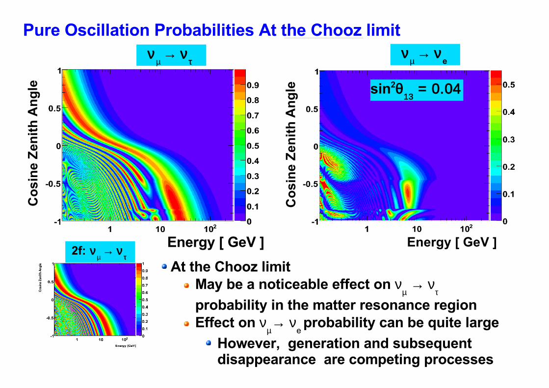
Pure Oscillation Probabilities At the Chooz limitν

µ → ν

τ ν

µ → ν

e

At the Chooz limitMay be a noticeable effect on ν

µ → ν

τ

probability in the matter resonance regionEffect on ν

µ→ ν

e probability can be quite large

However, generation and subsequent disappearance are competing processes

sin2θ13

= 0.04

Energy [ GeV ] Energy [ GeV ]

Co

sin

e Z

enit

h A

ng

le

Co

sin

e Z

enit

h A

ng

le

2f: νµ → ν

τ

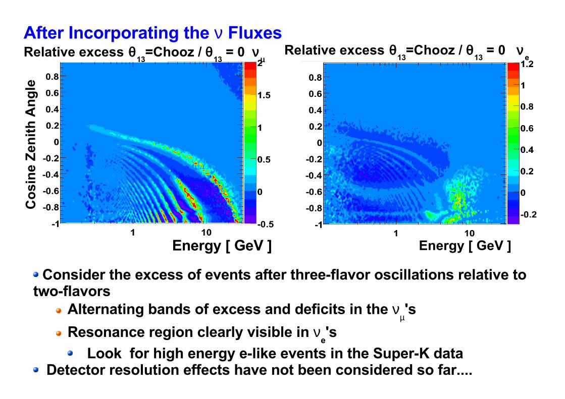
Consider the excess of events after three-flavor oscillations relative to two-flavors

Alternating bands of excess and deficits in the νµ's

Resonance region clearly visible in νe's

Look for high energy e-like events in the Super-K data Detector resolution effects have not been considered so far....

Energy [ GeV ] Energy [ GeV ]

After Incorporating the ν FluxesC

os

ine

Zen

ith

An

gle

Relative excess θ13

=Chooz / θ13

= 0 νµ


=Chooz / θ13

= 0 νe

The Reconstructed bins

Matter resonance is visible but now represents only a 20% excess Fortunately, the bins in the resonance area are well populated For the inverted hierarchy there is only an 8% excess in the resonance µ-like samples(not shown) show a lower effect ± 4% in just a few bins

Evis

[ log MeV ]Evis

[ log MeV ]


=Chooz / θ13

= 0

Multi-Ring e-like

Multi-Ring e-like Bin Contents

Co

sin

e Z

enit

h A

ng

le

Co

sin

e Z

enit

h A

ng

le

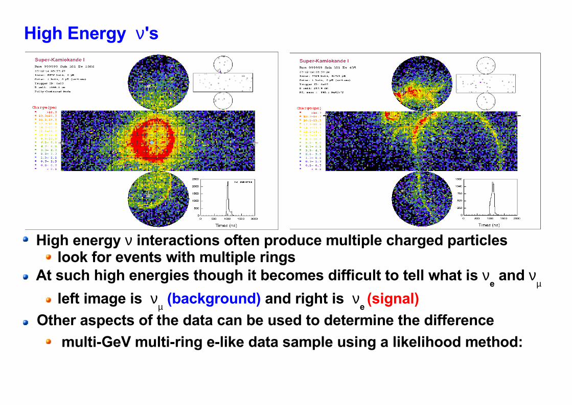
High Energy ν's

High energy ν interactions often produce multiple charged particleslook for events with multiple rings

At such high energies though it becomes difficult to tell what is νe and ν

µ

left image is νµ (background) and right is ν

e (signal)

Other aspects of the data can be used to determine the difference

multi-GeV multi-ring e-like data sample using a likelihood method:

Likelihood: Multi-ring e-like sample

Likelihoods for 5 energy bins in 4 variables,(applied to multi-ring events)Most Energetic Ring's PID and momentum fractionNumber of decay elections and maximum distance to them

Background to this sample is νµ or NC-π production

Resulting sample signal purity: SK-I 75% , SK-II 73%

Signal: CC νe

BG: CC νµ

/ NC - π

Oscillation Fitting

Analysis Structure

Oscillation Space Over 3 oscillation parametersSolar oscillations are neglected -- ≤ 5% effect on the main resonance

Computationally intensive to use all 5 Fits to SK-I, SK-II and SK-I+SK-II Fits to MC for both hierarchies

sin2θ13

sin2θ23

∆m2

Systematic Uncertainties90 sources of uncertainty, 32 common between SK-I and SK-II

ν flux uncertainties (18) ν interaction uncertainties (14) Event reduction uncertainties (10 SK-I + 10 SK-II ) Event reconstruction uncertainties (19 SK-I + 19 SK-II )

Look for evidence of non-zero θ13

and the mass hierarchy by comparing

data with several oscillation models

About the Fitting Method

Fit is done using the “Pull” method of systematic uncertaintyMC expectation is adjusted directly during the fit to minimize χ2

Adjustment is controlled by εε is constrained by penalty term

χ2 is based on a poisson likelihood n indexes bins and i indexes systematic errors

χ2 is minimized over εi by inverting a matrix equation obtained by

differentiatingFast fitting methodEquivalent to fitting using a covariance method

sin2θ13

sin2θ23

∆m2 ∆m2

sin2θ13

sin2θ13

sin2θ23

sin2θ23

∆m2

Drawing Contours from a 3-dimensional χ2 surface

Easier to visualize in two-dimensionsso “project” χ2 surface onto each 2-variable planeminimize over the 3rd variable

Results: Normal Hierarchy

SK-I + SK-II: Normal Hierarchy

99% C.L. 90% C.L. (preliminary)

Similarly for SK-I and SK-II

Normal Hierarchy: Chooz Limit

99% C.L. 90% C.L.

Chooz Exclusion

SK-II SK-I +SK-II

Chooz Exclusion

SK-I

Chooz Exclusion

Best fit point for SK-I+SK-II agrees with the recent Two-Flavor result All contours enter the Chooz exclusion region SK-II and SK-I+SK-II have smaller contours than their expected sensitivity

(preliminary)∆m2 = 2.1 x 10-3 eV2

sin2 θ23

= 0.5

sin2 θ13

= 0.00

χ2 = 841 / 745

∆m2 = 2.6 x 10-3 eV2

sin2 θ23

= 0.5

sin2 θ13

= 0.00

χ2 = 413 / 347

∆m2 = 2.6 x 10-3 eV2

sin2 θ23

= 0.5

sin2 θ13

= 0.00

χ2 = 413 / 347

SK-I + SK-II

99% C.L. 90% C.L.

SK-I + SK-IISensitivity

Normal

Sensitivity computed as average contour of 1000 Toy MC sets generated at the best fit of the two-flavor analysis and randomly fluctuated Data's contour is roughly half of the sensitivity in terms of its extent in

the θ13

direction

(preliminary)

Contour Overlay at 90% C.L.

SK-I

SK-II

SK-I + SK-II 90% C.L.

SK-I

SK-II

Size of the SK-I + SK-II contour is dominated by the small size of SK-II However, SK-II has roughly half of the statistics of SK-I

Why is its θ13

contour so small?

Is the C.L. Cut value correct?Checking the critical values using the Feldman-Cousins (FC) method shows that the 90% C.L. Value of 4.6 is close to the FC value near and beyond the data's contour

SK-I + SK-II 90% c.l. (cut 4.6)

First Checks

Systematic Errors?Increasing systematic errors like background contamination in the high evergy e-like samples by a factor of two does not significantly expand the contour

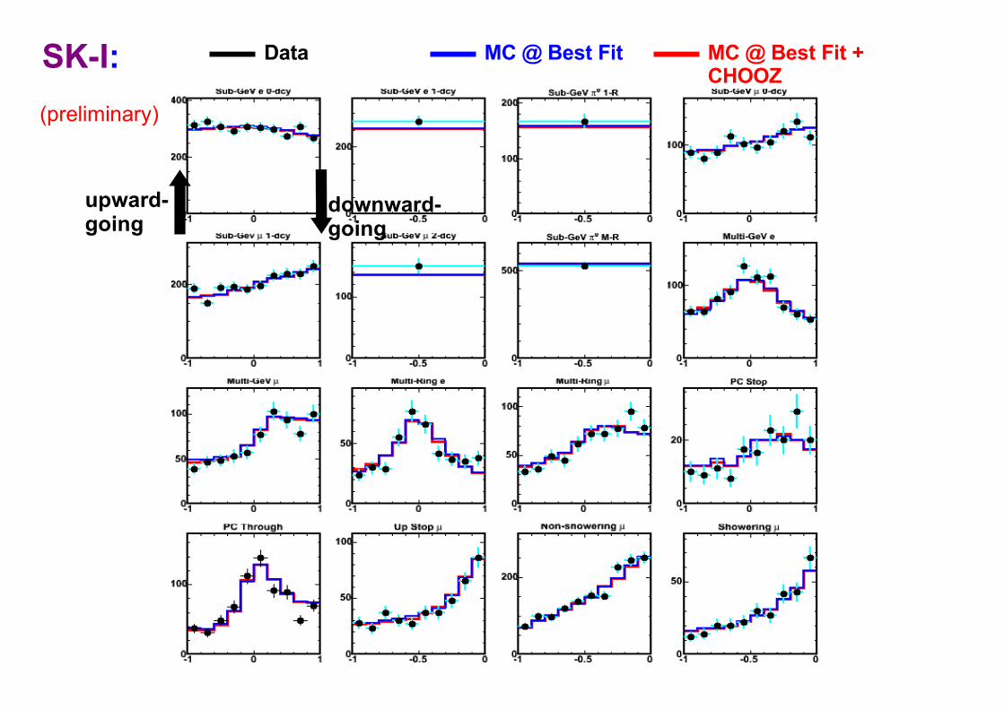
SK-I: MC @ Best Fit MC @ Best Fit + CHOOZ

Data

upward-going

downward-going

(preliminary)

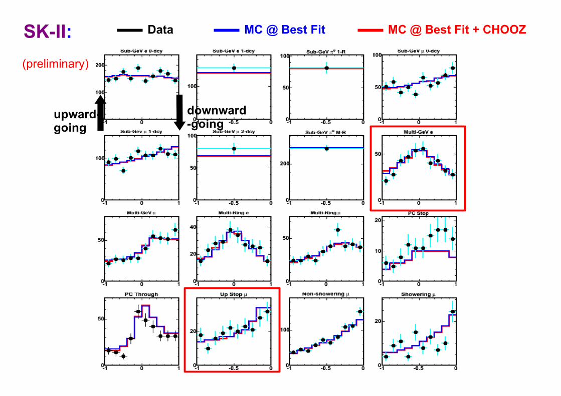
SK-II: MC @ Best Fit MC @ Best Fit + CHOOZData

upward-going

downward-going

(preliminary)

Signal Sample: Multi-GeV e-like

In these bins the effect of non-zero θ13

is apparent and strong

However, the data lies consistently below the MC expectation, a disparity that is aggravated as θ

13 becomes larger

This provides a strong portion of the constraint SK-I does not show such disparities in this sample

MC @ Best Fit MC @ Best Fit + CHOOZData

Cosine Zenith Angle Cosine Zenith Angle

(preliminary)

Do these bins provide a real constraint? : Remove them and refit

sensitivity

SK-II 90% full data Set SK-II 90% with bins removed

Without these bins the size of the contour balloons out towards the expected sensitivity and the constraint on θ

13 is relaxed

(The best fit point is the same in both cases θ13

= 0)

In this case the SK-I contour would provide the dominant constraint on the SK-I+SK-II result

Results: Inverted Hierarchy

SK-I + SK-II: Inverted Hierarchy

99% C.L. 90% C.L.

This Fit∆m2 = 2.1 x 10-3 eV2

sin2 θ23

= 0.5

sin2 θ13

= 0.00

χ2 = 841 / 745

SK-I + SK-II

(preliminary)

Inverted Hierarchy: Chooz Limit

99% C.L. 90% C.L.

CHOOZ Exclusion

SK-II SK-I +SK-II

CHOOZ Exclusion

SK-I

All contours enter the Chooz exclusion region SK-II and SK-I+SK-II have smaller contours than the expected sensitivity

the reason is the same as in the normal hierarchy case

CHOOZ Exclusion

(preliminary)

Conclusions

Fits for SK-I, SK-II, and SK-I + SK-II performed SK-I Atmospheric variables are consistent with two-flavor analysis SK-II results are consistent with SK-I

Slightly larger/shifted Atmospheric variablesSmaller θ

13

Results from discrepancies between Data and MC in a few bins

SK-I + SK-II results

Atmospheric contours are consistent with other data sets and slightly improved over SK-I aloneθ

13 contour is smaller than either SK-I or SK-II alone

Inverted Hierarchy fits are similar

All fits are consistent with θ13

= 0

No preference in the data for either mass hierarchy

Measuring θ13

is a goal of the next generation oscillation experiments

The Future of θ13

ν's from reactors

T2KNOνA

Double Chooz Daya Bay

ν beamline experiments

Super-K Taking data as SK-IV Improvements to reconstruction algorithms and MC Gd in Super-K?

Improved measurement of θ

13...

Supplements

Neutrino Oscillations Neutrino mass eigenstates , | ν

i ⟩ , under which they propagate, are

different than their eigenstates of the weak interaction, | να ⟩

For two flavors α and β, U is a rotation, parameterized by a `mixing angle`, θ

∣ ⟩=∑iU i

∗ ∣i ⟩

Probability of starting as a and being b after traveling L with energy E:

U= cos sin

− sin cos

P =sin2 2sin2 1.27m2LE [ eV

2 kmGeV ] m2

≡m22−m1

2

Non-zero ifU is not diagonal , ie θ ≠ 0m

i ≠ 0

mi ≠ m

j

Amplitude ~ sin2 2θ , Frequency ~ ∆ m2

Large range of L/E is useful ⇒ Atmospheric νLook for appearance of β or disappearance of α

SK-I: Normal Hierarchy

99% C.L. 90% C.L.

This Fit∆m2 = 2.2 x 10-3 eV2

sin2 θ23

= 0.52

sin2 θ13

= 0.01

χ2 = 429 / 397

SK-I

(preliminary)

SK-II: Normal Hierarchy

99% C.L. 90% C.L.

This Fit∆m2 = 2.6 x 10-3 eV2

sin2 θ23

= 0.5

sin2 θ13

= 0.00

χ2 = 413 / 347

SK-II

(preliminary)

SK-I + SK-II: Normal Hierarchy

99% C.L. 90% C.L.

∆m2 = 2.1 x 10-3 eV2

sin2 θ23

= 0.5

sin2 θ13

= 0.00

χ2 = 841 / 745

SK-I + SK-II

(preliminary)

Total s

νµ

Above ~2 GeV CC 1-π production and DIS are important CCQE still present

⇒ Look at high energy single-ring and multi-ring e-like events for signs of θ

13

What to look for?

Matter resonance

νe

CC Quasi-elasticCC Single πDeep InelasticNC Single πNC Elastic

θ

Detection With Cherenkov Radiation

cos=1n

Charged particles traveling faster than the speed of light in a medium emit Cherenkov radiation A cone of light is formed with opening

angle

photons

Light is projected onto the Super-K PMTs as a ring

(n is refractive index, β is the particle velocity)

θmax

= 42° in water

Charge and time information from the PMTs is used to reconstruct a vertex, direction and momentum of the particle

About Neutrinos

Neutral, Spin-1/2, lepton Undergo weak interactions

Only three light active neutrinos (LEP) One neutrino flavor for each charged

leptonDetermined by lepton accompanying reaction

νε , ν

µ , ν

τ

νl

p

l

CC reactions can occur if there is enough energy to produce l

Charged current quasi-elastic ( CCQE )

ν

l + n → p + l

νl + p → n + l+

Neutral current ( NC )

νx + n(p) → n(p) + ν

x

Charged current quasi-elastic ( CC1π )

ν

l + n → p +π+ l

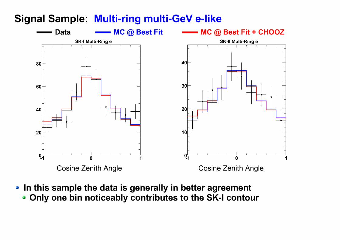
Signal Sample: Multi-ring multi-GeV e-like

In this sample the data is generally in better agreementOnly one bin noticeably contributes to the SK-I contour

Cosine Zenith Angle Cosine Zenith Angle

MC @ Best Fit MC @ Best Fit + CHOOZData

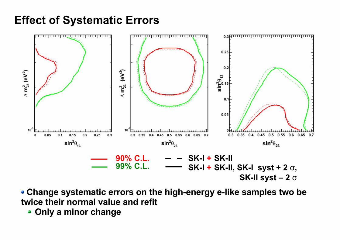
99% C.L. 90% C.L.

SK-I + SK-II, SK-I syst + 2 σ, SK-II syst – 2 σ

Effect of Systematic Errors

SK-I + SK-II

Change systematic errors on the high-energy e-like samples two be twice their normal value and refit

Only a minor change

Fitting Scheme

Data and MC are binned SK-I (1489 days data and 100 yr. MC ) SK-II ( 804 days data and 60 yr. MC )

The MC is oscillated at each point on a grid in an oscillation space Data is then fit to the oscillated MC at each point

“Fit” is achieved when the χ2 is minimized The MC point returning the smallest χ2 is deemed the “best fit” point Contours are then drawn expressing the level of agreement between the

data and MC at all of the oscillation points relative the “best fit” point.

Fits to SK-I, SK-II and SK-I+SK-II Fits to MC for both hierarchies

Look for evidence of non-zero θ13

and the mass hierarchy by comparing

data with several oscillation models

Binning

Multi-ring multi-GeV e-like

Multi-GeV e-like

Sub-GeV e-like

Multi-ring multi-GeV µ-like

Multi-GeV µ-like

Sub-GeV µ-like

PC Stopping

PC Through-going

Upward Stopping µ

Upward Through-going µ

Lo

g P

SK-I 32 x 10 = 320 bins SK-II 27 x 10 = 270 bins

Binning is different due to differences in livetimes

= 10 Zenith angle bins

About the Contour Plots:

Contours are not a simple projection Contours are drawn around all points that satisfy

90 % C.L. : χ2( x, y, zmin

) ≤ χ2

min + 4.6

99 % C.L. : χ2( x, y, zmin

) ≤ χ2

min + 9.2

The third variable in each of the two-variable plots has been minimized at each (x,y) pair in the space

x

y

z y

x

Systematic Uncertainties

A Bin A Bin at + 1 σ ~ 10% more CCQE events

Systematics are taken to have a linear effect on the contents of the bins A given systematic may affect only a subset of a bin's events Example:

CCQE ν interaction cross-section 10%

% Change in red is f i

n

Coefficients are computed using the MCDuring fitting the MC expectation is adjusted by the error parameters, ε

PC Sample is composed of mostly νµ

Regions of excess and deficit presentConfined to a few binsMagnitude of the difference is smallLower bin populations

Similar effect in other µ-like samples


=CHOOZ / θ13

= 0

PC Through-going

PC Through-going Bin Contents

Now looking at reconstructed binning

Evis

[ log GeV ]Evis

[ log GeV ]

Co

sin

e Z

enit

h A

ng

le

Co

sin

e Z

enit

h A

ng

le

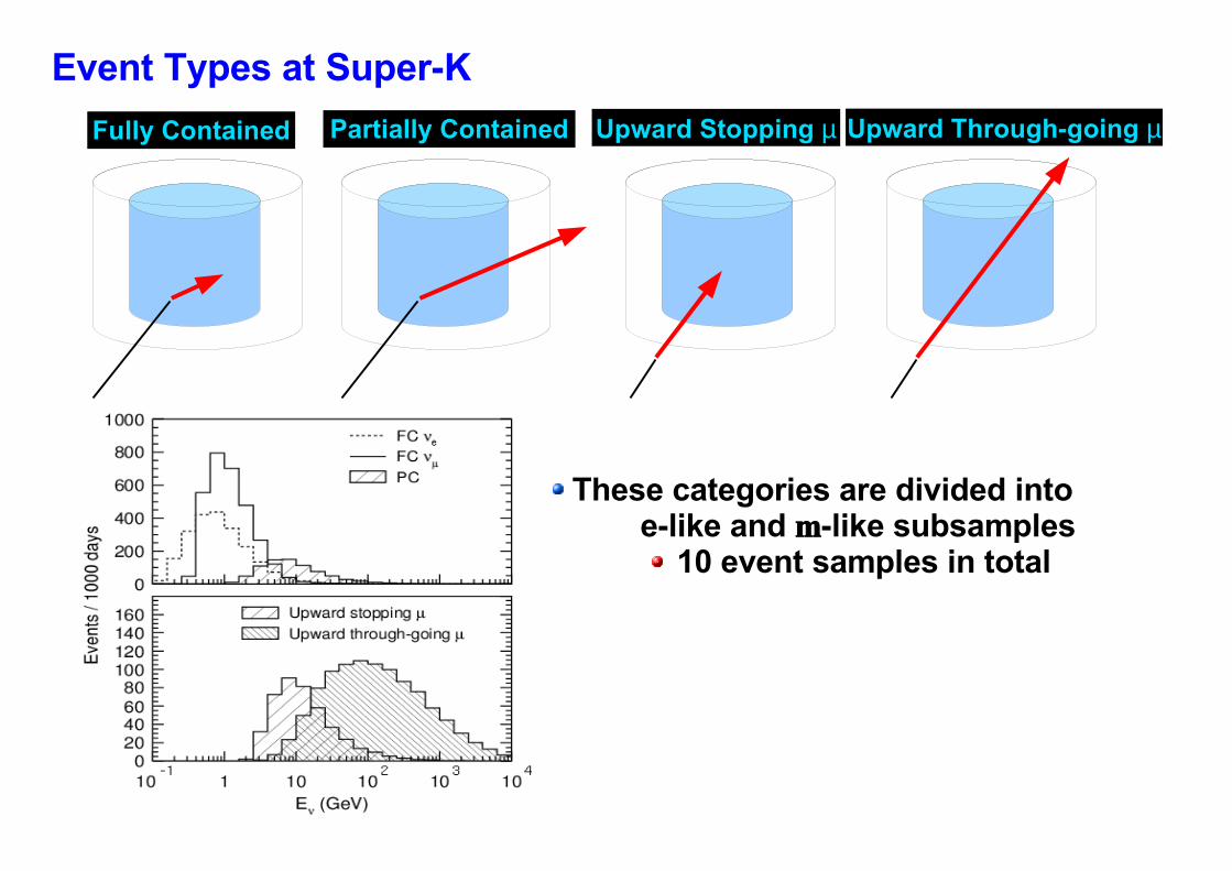
Event Types at Super-K

Fully Contained Partially Contained Upward Stopping µ Upward Through-going µ

These categories are divided into e-like and m-like subsamples

10 event samples in total

2 D.o.F - Restricted to the plane

Feldman-Cousins Critical values : 400 Toy MC

Generated at: sin2 θ13

= 0.092

Critical value is slightly lower than the usual cut at 4.6 Both methods exclude this point

2 D.o.F cut 90% C.L. ∆χ2 = 4.612 D.o.F cut 99% C.L. ∆χ2 = 9.2

Feldman-Cousins Map: Constrain to ∆m2 x sin2 θ13

plane

When restricted to the plane, the distribution of critical values is consistent with the usual 2 D.o.F cut on ∆χ2 . But its not clear that the prescription for this analysis' plots is truly 2

D.o.F

FC – plane minimization

Testing Coverage with Feldman-Cousins

Objective is to determine whether or not the contours that have been drawn have proper coverage Currently the contours are drawn

using a cut on ∆χ2 for 2 D.o.F ∆χ2 = 4.61 at 90% C.L. ∆χ2 = 9.2 at 99% C.L.

Test with Feldman-Cousins MethodBut to save time, consider only a few representative points around the 90% C.L. drawn in the usual way

F.C. 90% Critical Value is computed using 400 Toy MC at each of 6 points (lines above)

Statistics are a little low, but saves computation timeFull F.C. method might entail 1000 Toy MC for each of the 80,000 points in the analysis

Feldman-Cousins Critical values : 400 Toy MC, minimized to plane


=

0.07

Critical value is slightly higher than the usual cut at 4.6 Both methods include this point




=

0.08

Critical value is slightly higher than the usual cut at 4.6 Both methods may exclude this point

even with Feldman-cousins, the size of the contour would only increase nominally




=

0.10

Critical value is slightly higher than the usual cut at 4.6 Both methods exclude this point




=

0.13

Critical value is the same as usual cut at Both methods exclude this point


Feldman-Cousins Map: Minimize to ∆m2 x sin2 θ13

plane

Feldman-Cousins critical values are near the usual 2 D.o.F cut at 4.6Size of the contour would not change appreciably even with a full F-C treatment

90% of 400 Toy MC generated at the Data's best fit point fall within 90% C.L of the sensitivity. ( 98.5% fall within its 99% C.L. )

Sensitivity 99% C.L.

Sensitivity 90% C.L.

SK-I + SK-II 90% c.l. (cut 4.6)

SK-I SK-II

Up / Down Ratio Single Ring E-like Events

Data

MC at Best FitMC at Best Fit w/ CHOOZ Limit

Looking for clues as to why SK-II θ13

contour is smaller than SK-I

SK-I SK-II

Up / Down Ratio Multi-Ring E-like Events

Data

MC at Best FitMC at Best Fit w/ CHOOZ Limit

99% C.L. 90% C.L.

SK-I + SK-II, SK-I syst + 2 σ, SK-II syst – 2 σ

Normal Bins : + Sensitivitites

SK-I + SK-II

Small effect seen in both χ2 methods

Documents

Three Flavor Oscillations of Atmospheric Neutrinos in ...raw22/SK/wendell.cu.t2k.20090403.pdf · Neutrinos are included in the Standard Model, but are massless. However, there is