Embed Size (px)
Citation preview

Three Essays on the Syndicated Loan Market
D I S S E R T A T I O N
zur Erlangung des akademischen Gradesdoctor rerum politicarum
(Doktor der Wirtschaftswissenschaft)
eingereicht an derWirtschaftswissenschaftlichen Fakultät
der Humboldt-Universität zu Berlin
vonDiplom-Volkswirt Daniel Streitz
Präsident der Humboldt-Universität zu Berlin:Prof. Dr. Jan-Hendrik Olbertz
Dekan der Wirtschaftswissenschaftlichen Fakultät:Prof. Dr. Ulrich Kamecke
Erstgutachter ZweitgutachterProf. Tim R. Adam, PhD Prof. Dr. Sascha SteffenRudolf von Bennigsen-Förder Professor of Finance Karl-Heinz Kipp Chair in ResearchHumboldt-Universität zu Berlin European School of Management & TechnologyDorotheenstr. 1 Schlossplatz 110117 Berlin 10178 Berlin
Tag des Kolloquiums: 06.02.2015

Acknowledgments
I am indebted to my thesis advisor Tim Adam for his advice and encour-agement. Tim has been extremely supportive and contributed greatly to mydevelopment as a researcher. I would like to express my sincere gratitude tomy second advisor, Sascha Steffen, for his guidance and advice. I would liketo thank Tobias Berg for his mentoring and support. I am extremely thankfulto my colleagues Valentin, Tobias, Laurenz, Simon, and Dominika, for makingmy time at the institute an unforgettable experience. I am extremely thankfulto Hanna for her support and encouragement and for enduring endless discus-sions about my research :) Finally, but not least, I want to thank my belovedparents and friends for their continuous support.

Contents
Introduction 1
An Introductory Summary .................................................................. 1References.......................................................................................... 5
Loan Sales versus Credit Default Swaps — The Promiseand Perils of Financial Innovation 6
1 Introduction .................................................................................... 72 Theoretical Framework..................................................................... 123 Data............................................................................................... 144 Loan Sales, Syndicate Structure, and CDS Trading ............................. 18
4.1 Baseline Specification .................................................................... 184.2 Endogeneity ................................................................................ 204.3 CDS Market Liquidity................................................................... 22
5 CDS Trading, Monitoring, and Moral Hazard ..................................... 236 Robustness...................................................................................... 27
6.1 CDS Introduction Dates ................................................................ 276.2 Secondary Market Trading ............................................................. 27
7 Conclusion ...................................................................................... 28References.......................................................................................... 30Appendix........................................................................................... 34
A.1 Figures ...................................................................................... 34A.2 Tables ....................................................................................... 35A.3 Variable Definitions...................................................................... 45
Managerial Optimism and Debt Contract Design 49
1 Introduction .................................................................................... 502 Hypothesis Development................................................................... 543 Data Description ............................................................................. 57
3.1 Managerial Optimism.................................................................... 573.2 Loan Sample ............................................................................... 583.3 Descriptive Statistics..................................................................... 60
4 Managerial Optimism and Performance-Sen-sitive Debt....................... 614.1 Performance-Sensitive vs. Straight Debt ........................................... 614.2 PSD Pricing-Grid Structure ........................................................... 624.3 Post-Issue Performance.................................................................. 644.4 Endogeneity ................................................................................ 66
I

5 Robustness...................................................................................... 685.1 Other Optimism Measures ............................................................. 685.2 CEO Characteristics ..................................................................... 70
6 Conclusion ...................................................................................... 72References.......................................................................................... 73Appendix........................................................................................... 77
A.1 Figures ...................................................................................... 77A.2 Tables ....................................................................................... 80A.3 Optimism Classification ................................................................ 91A.4 Variable Definitions...................................................................... 95
Hold-Up and the Use of Performance-Sensitive Debt 98
1 Introduction .................................................................................... 992 Hypothesis Development................................................................... 1043 Data Description ............................................................................. 107
3.1 Performance-sensitive Debt Contracts .............................................. 1073.2 Measuring Relationship Strength..................................................... 1083.3 Measuring the Tightness of Covenants.............................................. 1093.4 Descriptive Statistics..................................................................... 110
4 Results ........................................................................................... 1114.1 Lending Relationships and the Use of Performance-sensitive Debt ......... 1114.2 Performance-sensitive Debt and Covenants........................................ 117
5 Robustness: Hold-up vs. Signaling .................................................... 1196 Conclusion ...................................................................................... 120References.......................................................................................... 122Appendix........................................................................................... 127
A.1 Figures ...................................................................................... 127A.2 Tables ....................................................................................... 129A.3 Variable Definitions...................................................................... 139
II

Introduction
An introductory summary
Syndicated loans are an important source of external financing for large cor-
porations. This thesis studies three important aspects of the syndicated loan
market: (i) the impact of the ability to unload loan risk via traded credit de-
fault swap (CDS) contracts on the fraction of loans retained by lead banks, (ii)
the impact of managerial traits on the design of syndicated loan contracts, and
(iii) the impact of long-term lending relationships on the decision to include
contract provisions in loan contracts that stipulate that the coupon paid rises
if the firm’s financial performance deteriorates and/or vice versa.
The first paper, "Loan Sales versus Credit Default Swaps — The Promise
and Perils of Financial Innovation", analyzes the impact of the ability to un-
load loan risk via traded CDS contracts on primary loan market allocation.
Theoretically, there is a clear prediction on how CDS trading will affect loan
sales: Banks are less likely to sell loans once credit protection via CDS is avail-
able. However, there are different economic mechanisms that can lead to this
conjecture. Duffee and Zhou (2001) argue that tailor-made CDS are a flexible
tool to temporarily lay off credit risk and hence (partially) replace loan sales.
Parlour and Winton (2013) argue that CDS trading has a detrimental effect
on loans sales as banks can no longer commit to monitor borrowers if credit
risk can be laid off via CDS. Hence, loan sales become more difficult/costly
and originating banks are forced to retain larger shares in their loans.
I compare loans to firms before and after CDS are actively traded on a
borrower’s debt with loans to firms that never have actively traded CDS on
their debt. The results indicate that banks retain significantly larger shares
of loans after CDS trading becomes available. The effects is also meaningful
1

economically, that is, banks retain on average 7% more of a loan if hedging via
CDS is possible. In the next step, I explicitly disentangle the risk management
from the moral hazard effect by analyzing the effect of CDS trading on syn-
dicate structure for different types of firms and lenders. Overall, the findings
do not support the claim that the moral hazard effect is a significant concern
in the syndicated loan market. The results suggest that banks actively use
CDS as a risk management tool and therefore rely less on other risk sharing
mechanisms.
The second paper, "Managerial Optimism and Debt Contract Design"
(co-authored with Tim R. Adam, Valentin Burg, and Tobias Scheinert), an-
alyzes how managerial traits impact debt contract design. In particular, we
analyze performance-sensitive debt contracts (PSD), that is, debt contracts
with coupon payments that deterministically follow an underlying measure of
borrower quality. If borrower quality decreases, coupon rates are increased to
pre-agreed levels. This option, which is valuable for the lender, is reflected
in a lower initial spread paid by the borrower on performance-sensitive loans
when compared to straight debt. Manso, Strulovici, and Tchistyi (2010) pre-
dict that PSD serves as a screening device for lenders: high quality borrowers
select PSD contracts as they perceive the risk of having to pay a higher spread
in the future as low, and low quality borrowers select straight debt contracts.
In their model, Manso et al. (2010) assume that the manager of a firm correctly
assesses the quality of his/her firm and chooses the optimal debt contract given
his/her expectations. However, the recent literature questions this assumption
(e.g., Malmendier and Tate (2005)). In particular, overly optimistic managers
could persistently overestimate the firms’ quality, while rational managers cor-
rectly assess the firms’ quality on average. We argue that firms with overly
optimistic managers are more likely to issue PSD contracts than their rational
counterparts.
2

Our empirical evidence confirm this prediction. Firms with optimistic
managers are more likely to choose debt contracts with performance-pricing
features than rational managers. Further, within the set of PSD contracts, op-
timistic managers choose PSD contracts that contain more risk-compensation
than rational managers. Consistent with an overestimation of firm quality,
we find that firms with optimistic managers are significantly more likely to
experience a performance deterioration after a PSD issue than firms with ra-
tional managers. Overall, our findings indicate that managerial optimism is
an important determinant of debt contract design.
The third paper, "Hold-Up and the Use of Performance-Sensitive Debt"
(co-authored with Tim R. Adam), examines whether PSD is used to reduce
hold-up problems in long-term lending relationships. A lender acquires reusable,
proprietary information on the borrower over the course of a lending relation-
ship and hereby gains an informational advantage vis-à-vis other potential
lenders. Sharpe (1990) and Rajan (1992) argue that the non-verifiable in-
side information that the lender acquires can generate hold-up problems. The
information advantage by the relationship lender makes it difficult for the bor-
rower to switch to another, less well informed, lender due to adverse selection.
This can be strategically exploited by the relationship lender, for example,
by raising the interest rate. Von Thadden (1995) shows that a solution to
this problem is to specify contract terms ex ante, thereby limiting the dis-
cretion of the lender. One can view PSD contracts as limiting the discretion
of lenders because by pre-specifying the loan contract terms if a borrower’s
performance deteriorates or improves PSD avoids debt renegotiation in these
states. For example, rather than renegotiate a loan after a covenant violation,
the performance-pricing provision specifies the outcome of such renegotiation
ex ante and thus avoids the situation of a technical default.
3

Our results indicate that PSD contracts are more likely to be used in
repeated lending relationships. We further document that the use of PSD
varies systematically across different types of borrowers. Santos and Winton
(2008) argue that the costs of relationship lending are higher for companies,
which do not have access to other financing sources (e.g., bond market access).
In line with this argument, we find that PSD contracts are more common in
relationship lending arrangements with smaller firms, firms that do not have
a long-term issuer credit rating at the time of the loan origination, and firms
with lower analyst coverage. Overall, our results are indicative of PSD being
used to mitigate hold-up concerns in long-term lending relationships.
The three thesis chapters contribute to the literature on bank and firm
behavior in the syndicated loan market.
4

References
Duffee, G. R. and C. Zhou (2001). Credit derivatives in banking: Useful tools
for managing risk? Journal of Monetary Economics 48, 25–54.
Malmendier, U. and G. Tate (2005). Does overconfidence affect corporate in-
vestment? ceo overconfidence measures revisited. European Financial Man-
agement 11, 649–659.
Manso, G., B. Strulovici, and A. Tchistyi (2010). Performance-sensitive debt.
Review of Financial Studies 23, 1819–1854.
Parlour, C. A. and A. Winton (2013). Laying off credit risk: Loan sales versus
credit default swaps. Journal of Financial Economics 107, 25–45.
Rajan, R. G. (1992). Insiders and outsiders: The choice between informed and
arm’s-length debt. The Journal of Finance 47, 1367–1400.
Santos, J. A. C. and A. Winton (2008). Bank loans, bonds, and information
monopolies across the business cycle. The Journal of Finance 63, 1315–1359.
Sharpe, S. A. (1990). Asymmetric information, bank lending and implicit
contracts: A stylized model ofcustomer relationships. The Journal of Fi-
nance 45, 1069–1087.
Von Thadden, E.-L. (1995). Long-term contracts, short-term investment and
monitoring. Review of Economic Studies 62, 557–575.
5

Loan Sales versus Credit Default Swaps —The Promise and Perils of Financial
Innovation
Daniel Streitz
Abstract:
This study analyzes the impact of credit default swap (CDS) trading on loansales and the structure of loan syndicates. Theoretically, CDS can have bothpositive and negative effects on the loan market. One the one hand, CDSare a flexible risk management tool and can therefore (partially) replace loansales (risk management effect). On the other hand, lenders can no longercredibly commit to monitor a borrower if laying off credit risk anonymouslyvia CDS is possible making loan sales costly (moral hazard effect). We find thatlenders retain significantly higher shares of loans once CDS are actively tradedon a borrower’s debt and the overall syndicate becomes more concentrated.These effects are stronger if CDS liquidity is higher. Disentangling the riskmanagement from the moral hazard effect, we find that potentially negativeeffects of CDS trading are of minor importance in the syndicated loan market.The results are robust to controlling for the potential endogeneity of CDSintroduction.
Keywords: Loan Sales, Credit Default Swaps, Syndicate Structure, SyndicatedLoans
JEL-Classification: G21, G32
6

1 Introduction
Despite the growing importance of credit derivatives in recent years, the im-
pacts of this financial innovation on the nature and operation of credit markets
are not yet fully understood. While the majority of CDS have corporate bonds
as underlying instruments, credit derivatives can also be used to trade other-
wise non-marketable credit risks such as bank loans (Duffee and Zhou (2001),
Instefjord (2005)). Theoretically, the enhanced risk sharing via CDS can al-
leviate credit supply frictions with potentially positive effects on firm’s credit
terms and overall credit supply. However, empirical evidence so far does not
confirm this prediction.1 Also empirical research on how and to what extent
banks use CDS to manage credit risk is scarce.
One important determinant of the effects of CDS on credit markets is
the interplay with bank’s existing risk management tools such as loan sales. A
bank can limit the exposure to a borrower to comply with regulatory capital
requirements and diversify the loan portfolio by (partially) selling loans (Den-
nis and Mullineaux (2000)) — e.g. via syndication. Theoretically the effect of
CDS trading on loan sales is unambiguous: Banks are less likely to sell loans
once credit protection via CDS is available. However, there are different eco-
nomic mechanisms that can lead to this conjecture. Duffee and Zhou (2001)
argue that tailor-made CDS are a flexible tool to temporarily lay off credit
risk and hence (partially) replace loan sales. Parlour and Winton (2013) argue
that CDS trading has a detrimental effect on loans sales as banks can no longer
commit to monitor borrowers if credit risk can be laid off via CDS. Hence, loan
sales become more difficult/costly and originating banks are forced to retain
larger shares in their loans.
1 For example, Hirtle (2009) shows that CDS trading has only limited effects on bank loansupply. Ashcraft and Santos (2009) show that CDS trading does not affect the spreadsthat firms pay to raise funding via loans or bonds.
7

We empirically analyze the impacts of CDS trading on primary2 loan
sales using a large sample of syndicated loans3 and explicitly disentangle risk
management from moral hazard effects. In particular, we compare the syndi-
cate structure of loans to borrowers before and after CDS are actively traded
on the borrower’s debt with the syndicate structure of loans to borrowers that
never have actively traded CDS on their debt during the sample period.
We start by establishing a general link between CDS trading, loan sales
and syndicate structure. Consistent with existing theories, lead banks sell
seven percentage points less of a loan once credit protection via CDS is avail-
able, which is economically important given an average lead share of 38%.
However, consistent with the argument that the flexibility of the underlying
CDS contract matters, lead arrangers only sell a lower fraction of the loan if
CDS liquidity is sufficiently high, i.e. the bid-ask spread is low.
This evidence is both consistent with the idea that CDS are a substitute
for loan sales and the idea that CDS increase moral hazard problems in loan
syndicates. We disentangle both effects empirically by analyzing the effect of
CDS trading on syndicate structure for different types of firms and lenders.
If the moral hazard effect is the dominant effect, then this problem should be
especially severe for borrowers that require intensive monitoring, e.g. riskier,
more opaque firms. However, we do not find any empirical support for this
conjecture. The effect of CDS trading on syndicate structure does not differ
for low or high risk borrowers and for more or less opaque borrowers. We
further test, if the effect of CDS trading is different for relationship loans. Sufi
(2007) argues that previous lending relationships between the borrower and
the lead arranger can serve as a measure of the information advantage of the
2 We control for a possible effect of secondary market trading in the robustness section.3 In a syndicated loan, the originating bank (lead bank) negotiates the deal with the bor-
rower and then decides upon which fraction of the loan to sell to other participatinglenders. Primary loan sales are mainly done via syndication. We therefore use the termssyndication and loan sales synonymously in this study when we analyze the share retainedby the lead arranger.
8

lead arranger with respect to participant lenders. Moral hazard should be less
severe if a lending relationship exists because the lead arranger has already
put in the effort required to learn about the firm. Again, we do not find
different effects for relationship vs. non relationship loans. Finally, we test
the effect of lender reputation. As shown theoretically by Parlour and Winton
(2013), moral hazard problems arising from CDS trading are less severe if the
lender’s reputation is high. Our results show that effect of CDS trading on
syndicate structure is not significantly different for lenders with different levels
of reputation.
We further analyze which banks end up as syndicate members and whether
the syndicate participant selection process is different after CDS are actively
traded on the borrowers debt. The main argument is that the degree of infor-
mation asymmetry between a potential participant and the lead bank is not
the same for all potential participants. Hence, moral hazard concerns are more
severe for some banks compared to others. For example, a bank that already
knows the borrower from previous deals is less dependent on the information
generation and monitoring by the lead bank. Therefore, this bank may decide
to participate in a syndicate even if CDS availability prevents the lead bank
from credibly committing to monitor the borrower. On the contrary, banks
that do not know the borrower and the lead arranger should be especially re-
luctant to invest in a syndicated loan if the lead bank cannot credibly commit
to monitor the borrower. We find — consistent with Sufi (2007) — that in gen-
eral banks that already know the borrower from prior deals and banks that are
located in the same region as the borrower are significantly more likely to end
up as syndicate members compared to other banks. Further, also banks that
already know the lead arranger from prior deals are more likely to participate
in a syndicate compared to other banks. However, the syndicate participant
selection process is not significantly different for loans in which CDS are ac-
tively traded on the borrowers debt which is unsupportive of the conjecture
9

that CDS trading amplifies moral hazard problems. Overall, the results show
that an increase in moral hazard caused by CDS introduction is not a major
concern in the syndicated loan market.
CDS trading and the timing of CDS inception is clearly endogenous,
hence this problem needs to be addressed in order to make causal inferences
about the effect of CDS trading on the structure of loan syndicates and loan
sales. Firms that have actively traded CDS on their debt are different from
firms that do not have actively traded CDS on their debt, therefore, unob-
servable differences could drive both CDS introduction, as well as changes
in the loan syndicate structure. Further, as noted by Subrahmanyam, Tang,
and Wang (2014), the timing of CDS inception may be endogenous. We ad-
dress these concerns by constructing a model to predict CDS trading and
use this model to run an instrumental variable estimation. Minton, Stulz,
and Williamson (2008) show that banks that use foreign exchange derivatives
are more likely to be net buyers of CDS, i.e. are more prone to use deriva-
tives in general. Therefore, foreign exchange derivatives holdings are likely to
be correlated with investor demand for credit protection via CDS. We follow
Saretto and Tookes (2013) and Subrahmanyam et al. (2014) and use the aver-
age amount of foreign exchange derivatives held by all the lead arrangers that
lend money to a company in the previous five years as a fraction of the total
loans of the lead arrangers as an instrument for CDS trading. This variable
is constructed at the firm level for each year. As foreign exchange hedges are
macro hedges, it is unlikely that this variable is directly related to the loan
(and borrower) specific syndicate structure. Overall, our results are robust to
potential endogeneity concerns.
We contribute to the literature by providing novel evidence that banks
actively use CDS as a risk management tool and therefore rely less on other
risk sharing mechanisms. Understanding the trade-off between different risk
10

management tools is important to better understand under which conditions
CDS trading reduces credit supply frictions. If CDS trading replaces existing
risk management tools it is unlikely to have a strong impact on credit supply by
banks and loan contract terms. This is consistent with existing studies, which
find limited effects of CDS trading on credit markets (Hirtle (2009), Ashcraft
and Santos (2009)).4 We further show that potentially negative effects of CDS
trading — increased moral hazard problems — are of minor importance.5
We also add to the literature on loan syndicate structure by showing that
the availability of other risk management tools significantly affects syndicate
composition. Sufi (2007) and Dennis and Mullineaux (2000) show that lenders
form more concentrated syndicates when borrowers are more opaque. Bharath,
Dahiya, and Hallak (2012) show that an increase in shareholder rights makes
loan syndicates more concentrated as firm’s risk shifting incentives increase.
Gatev and Strahan (2009) show that commercial banks dominate the market
for lines of credit as they have an advantage over other investors in managing
liquidity risk. Gopalan, Nanda, and Yerramilli (2011) show that banks ability
to syndicate loans decreases after a negative shock to their reputation.
The rest of the paper is organized as follows. In Section 2, we discuss the
theoretical background and derive empirical hypothesis. Section 3 describes
our sample selection process. The main empirical analysis, demonstrating a
link between CDS trading, loan sales and the structure on loan syndicates,
4 Several studies analyze the effect of CDS trading on the bond market. E.g., Das, Kalim-ipalli, and Nayak (2014) find no evidence for an increase in bond market liquidity or areduction in pricing errors. Chava, Ganduri, and Ornthanalai (2012) show that creditratings become less important when a market price for the risk of a company can beobserved. Saretto and Tookes (2013) analyze how the capital structure of companies isaffected by CDS trading and find that firms maintain higher leverage ratios and longerdebt maturities once CDS are available.
5 Ashcraft and Santos (2009) also analyze the effect of CDS trading on the share retainedby the lead arranger in an earlier version of the paper (Ashcraft and Santos (2007)). Wediffer from this analysis in several fundamental ways. First, and most importantly, weexplicitly distinguish between moral hazard and risk management effects. Second, weaddress the endogeneity of CDS introduction. Third, we analyze a much larger sample —the analysis by Ashcraft and Santos (2007) is based on a sample of 291 loan contracts.
11

is presented in Section 4. We disentangle the moral hazard from the risk
management effect in Section 5. Section 6 presents robustness tests and Section
7 concludes.
2 Theoretical Framework
In a Modigliani-Miller world, bank risk management does not increase firm
value as shareholders can manage risks more efficiently by holding a well-
diversified portfolio. However, market frictions such as moral hazard and ad-
verse selection problems lead banks to acquire borrower specific private infor-
mation that can make bank loans illiquid and loan sales difficult. The existence
of private information makes bank failures costly (see e.g. Goderis, Marsh,
Castello, and Wagner (2007), Cebenoyan and Strahan (2004)). Further, banks
are required by regulation (e.g. the Basel Accords) to implement risk man-
agement tools and hold equity capital to back-up risky assets. Overall, banks
have strong incentives to actively manage the risk of their loan portfolio.6
One way how banks can manage credit risk is syndication. In a syn-
dicated loan, the lead bank negotiates the deal with the borrower and then
decides upon which fraction of the loan to sell to other participating lenders.
Thereby, the bank can limit the size of any single loan to comply with regu-
latory capital requirements and diversify the loan portfolio by taking smaller
shares in multiple syndicated loans (Dennis and Mullineaux (2000)).7
Recently more and more firms that borrow from banks have actively
traded CDS on their debt. The CDS market is an over-the-counter derivative
market where default protection for corporate bonds and loans can be bought.
Banks that have access to credit derivatives therefore have an alternative tool
6 See also Froot and Stein (1998) and Froot, Scharfstein, and Stein (1993).7 Consistent with the risk sharing motive for loan syndication, Dennis and Mullineaux
(2000) find that banks are more likely to syndicate larger loans and loans with longermaturities.
12

to manage the risk associated with a loan. The question that arises is whether
and how a market in which loan sales/syndication exist is affected by the
availability of CDS?
Duffee and Zhou (2001) show theoretically that CDS can be a more flexi-
ble tool to manage credit risk compared to loan sales if the banks informational
advantage is non constant over the life of the loan. The lead bank is considered
an ”informed lender” that knows more about the true credit quality of the bor-
rower than the potential participants (Diamond (1984)). The arising adverse
selection problems make loan sales costly. Gorton and Pennachi (1995) show
that banks will only sell loans if the banks’ internal funding cost are sufficiently
high and/or the cost of funding loans via loan sales is sufficiently small (e.g.
high quality borrowers). If the banks informational advantage varies over the
life of a loan as in Duffee and Zhou (2001), it is therefore optimal for the bank
to lay off a larger (smaller) part of the credit risk when information asymmetry
is low (high). Thereby, the bank can minimize the costs of adverse selection.
Duffee and Zhou (2001) show that tailor-made CDS are a flexible tool to tem-
porarily lay off credit risk. Loan sales on the other hand are less flexible as
the loan is no longer on the bank’s balance sheet. CDS can therefore be value
creating and (partially) replace loan sales.
Hypothesis 1: Risk management via CDS is more flexible than risk man-
agement via loans sales. Therefore, banks retain larger shares of a loan once
credit derivatives are actively traded on a borrower’s debt.
Sufi (2007) argues (building on the models of Holmstrom (1979), Holm-
strom and Tirole (1997), and Gorton and Pennachi (1995)) that moral hazard
problems exist in syndicated loans. The ”informed” lead arranger is able to
monitor and learn about the borrower through unobservable and costly effort.
Participants, on the other hand, are ”uninformed lenders” who rely on the
monitoring effort by the lead arranger. The lower the share of a loan that is
13

retained by the lead arranger, the lower are the incentives to actively monitor
the borrower. As potential participants are aware of this problem, they are
only willing to invest if the lead arranger retains a large enough fraction of
the loan to credibly commit to monitor the borrower. As shown by Parlour
and Winton (2013), retaining a larger share of the loan is no longer a credible
signal by the bank if CDS are available. The lead arranger can lay off credit
risk anonymously via CDS which effectively reduces the incentive to monitor.
Without a credible signal by the lead arranger, potential investors are less
willing to participate in a syndicated loan. Hence, syndication becomes less
likely and the lead arranger has to retain a larger share of the loan.
Hypothesis 2: A commitment to monitor the borrower is less credible if
laying off credit risk via CDS is possible, hence investors are less willing to
participate in a syndicated loan. Therefore, banks retain larger shares of a
loan once credit derivatives are actively traded on a borrower’s debt.
Note that both Hypothesis 1 and Hypothesis 2 predict that the lead
lender will sell a smaller fraction of the loan. However, the reasons differ: Hy-
pothesis 1 predicts that the lender will (partially) substitute loan sales via the
purchase of CDS. Hypothesis 2 predicts that loan sales become more difficult
because the lender can no longer credibly commit to monitor the borrower if
CDS are available. Which effect prevails is an empirical question that will be
addressed in the following analysis.
3 Data
We follow Saretto and Tookes (2013) and use all USD denominated CDS
spreads for all maturities obtained from Bloomberg to identify firms that have
actively traded CDS on their debt. For robustness checks, we additionally use
USD denominated CDS spreads from the CMA database. We manually match
all reference entity names to the borrower names in the Thomson Reuters Loan
14

Pricing Corporation Dealscan database (LPC Dealscan), that contains detailed
information on corporate loan contracts. We restrict the sample to loans to
(non financial) US borrowers originated between 2000 and 2010.8 We fur-
ther exclude loans with missing information on the maturity, the all-in-drawn
spread, or the deal amount. We also exclude all loans by firms that have ac-
tively traded CDS on its debt at any time during the sample period but only
issue loans before or after the CDS introduction. Note that, as common in the
literature (e.g. Berg, Saunders, and Steffen (2013), Bharath, Dahiyab, Saun-
ders, and Srinivasan (2007)), the loan panel is created on the facility (tranche)
level. Following Sufi (2007), we classify a lender as a lead-lender if the variable
called "Lead Arranger Credit" (provided by LPC’s Dealscan) takes on the value
"Yes" or if the lender is the only lender specified in the loan contract. Finally,
we merge the loan data to Standard and Poor’s Compustat North America
database to obtain financial information on the borrowers.9
Dedependent Variables: Syndicate Structure Indicators
Following Sufi (2007), we use the percent of the total loan held by the
lead bank (% Held By Lead) as the main characteristic of the syndicate. %
Held By Lead is larger (lower) if the lead arranger sells a lower (larger) fraction
of the loan. We use two additional variables to also capture any effects on the
overall syndicate structure, i.e. including particiapting banks. Herfindahl, a
measure for the syndicate concentration, is calculated by squaring the shares
of the loan for each syndicate member and summing up the squared shares
for all the lenders in each particular facility. The Herfindahl index can take
on values between (nearly) 0 (a large number of banks holding small shares
of the loan) to 10,000 (one bank holds the entire loan amount). Additionally,
8 Loans issued prior to 2000 are excluded as the vast majority of CDS introduction dates areafter 2000. However, not imposing this restriction and using all loans originated between1990 and 2010 yields qualitatively similar results.
9 We use Michael Robert’s Dealscan-Compustat Linking Database to merge Dealscan withCompustat (see Chava and Roberts (2008) for details).
15

as in Bharath et al. (2012), we also use the number of members in the loan
syndicate.
Main Independent Variables: CDS Trading Indicators
We follow Ashcraft and Santos (2009) and Subrahmanyam et al. (2014)
and construct two CDS trading variables. One is CDS Traded, a dummy that
equals one if a firm has actively traded CDS on its debt at any point in time
during the sample period and zero otherwise. This dummy is a firm fixed
effect that is used to control for unobservable differences between firms with
and without CDS. The other variable is CDS Trading, a dummy that equals
one if a firm has active CDS trading at the time of the loan origination date and
zero otherwise. CDS Trading is the primary variable of interest as it captures
the marginal impact of CDS introduction on the syndicate structure.
Control Variables
Throughout the analysis we control for various firm characteristics and
loan characteristics. Included are the firm size, specified as ln(Total Assets),
the market-to-book asset ratio (Market-To-Book), and proxies for firm risk and
profitability. We further control for the maturity of the loan (ln(Maturity)),
the loan amount (ln(Facility Amount)), and other loan characteristics. All
control variables are defined in more detail in the Appendix Table A.I.
Table 1 presents descriptive statistics for the final panel. The sample
comprises 14,190 facilities to 3,265 distinct borrowers. Thereof 288 companies
have actively traded CDS at some point in time during the sample period.
Panel A reports descriptives for two CDS trading indicators. 19% of loans are
issued by borrowers that have CDS trading at some point in time during the
sample period. For 9% of the loans the borrower has actively traded CDS at the
time of the loan issue. Panel B reports descriptives for the syndicate structure
indicators. The median share of the loan retained by the lead arranger is 28%
16

which consistent with prior studies (e.g. Bharath et al. (2012)). The median
syndicate Herfindahl index is 1,547 and the median number of lenders is 5.
The number of observations is reduced for the variables % Held By Lead and
Herfindahl, as the individual shares retained by the lenders are not reported
for all loans that are included in the Dealscan database.10 Panel C reports loan
characteristics, which are consistent with prior studies (e.g. Sufi (2007)). For
example, the mean/median loan amount is $343/$135 million, the mean loan
maturity is 3.6 years, and the mean all-in-drawn spread is 220 basis points.
Panel D reports borrower characteristics. The mean/median book value of
assets is $4,470/$884 million. 24% of loans are issued by borrowers that have
an investment grade rating. In 51% of cases, the borrowers do not have a
credit rating at all.
[Table 1 here]
Table 2 presents descriptive statistics distinguishing between firms that
have CDS trading at some point in time during the sample period and firms
that never have actively traded CDS during the sample period. Panel A re-
ports descriptives for two CDS trading indicators. 46% of the loans issued by
CDS firms are issued before CDS inception. Panel B reports descriptives for
the syndicate structure indicators. Overall, CDS firms have more diverse syn-
dicates. The mean/median share retained by the lead arranger is 42%/32% for
Non-CDS firms and 26%/19% for CDS firms. The median number of lenders
is 5 for Non-CDS firms and 12 for CDS firms. Panel C reports loan char-
acteristics. Loans issued by CDS firms are larger with a mean/median size
of $980/$600 million compared to the mean/median of $198/$100 million for
Non-CDS firms. Also the loan maturity is shorter for CDS firms when com-
pared to Non-CDS firms. Panel D reports borrower characteristics. CDS firms
10 Potential reporting biases are discussed in Ivashina (2009) and are unlikely to affect ourresults.
17

are much larger that Non-CDS firms. The mean/median book value of assets
is $1,624/$598 million for Non-CDS firms and $16,985/$10,488 million for CDS
firms. Almost all borrowers, which have CDS trading at some point in time
during the sample period, have an S&P rating at the time of the loan issue
(97%).
[Table 2 here]
4 Loan Sales, Syndicate Structure, and CDS
Trading
4.1 Baseline Specification
We start by establishing a general link between CDS trading, loan sales and
syndicate structure. An explicit distinction between Hypothesis 1 and Hypoth-
esis 2 is made in Section 5. Figure 1 shows the average loan share retained by
the lead bank before and after CDS are actively traded on the borrowers debt.
[Figure 1 here]
We find that the share retained by the lead arranger strongly increases
from 21% to 26% after CDS are actively traded on a borrower’s debt. This
increase is statistically significant at the 1% level. Only the change from year
zero (CDS introduction year) to year one is statistically significant, indicating
that there is indeed a structural break. This univariate comparison is consis-
tent with Hypothesis 1 and Hypothesis 2, however, other firm characteristics
may have changed at the CDS introduction date and firms with actively traded
CDS may be different from firms that never have actively traded CDS during
our sample period. We follow Ashcraft and Santos (2009) and Subrahmanyam
18

et al. (2014) and address these issues by comparing firms before and after
CDS are actively traded on the firm’s debt with firms that never have actively
traded CDS at any point in time during the sample period, using the following
regression framework:
Syndicate Structureit =α + β1 ∗ CDS Traded i + β2 ∗ CDS Tradingit
+ X′
it ∗ γ + ϵit.
(1)
Syndicate Structure is a syndicate structure indicator. As discussed earlier, we
construct three different specifications for this variable, with the main variable
being the share of the loan retained by the lead arranger. CDS Traded is
a dummy that equals one if a firm has actively traded CDS on its debt at
any time during the sample period and zero otherwise. CDS Trading is a
dummy that equals one if a firm has active CDS trading at the time of the
loan origination date and zero otherwise. The regression further includes a set
of firm and loan characteristics, X. All control variables are defined in detail
in the Appendix Table A.I. Also included are time fixed effects, industry fixed
effects, and indicator variables for the different loan purposes and loan types.
We use OLS to estimate the regressions, however, all results reported in this
paper remain qualitatively unchanged if we use a Tobit specification in the
models that have % Held By Lead or Herfindahl as dependend variables.
[Table 3 here]
The results reported in Table 3 provide evidence that banks sell a lower
fraction of the loan once credit protection via CDS is available. The share
retained by the lead arranger increases by 7 percentage points and the effect
is highly statistically significant. This effect is also economically important
as compared to the median value of 27%, this change implies an increase in
magnitude of about 25%. The effects for Herfindahl and ln(# Lenders) are
19

similar. Loan syndicates are more concentrated after CDS are traded on a
borrower’s debt when measured by the Herfindahl index and the number of
lenders in the syndicate declines. Again the effects are highly statistically
significant.
Turning to the control variables, we find similar effects as Sufi (2007).
The lead arranger retains a lower share of the loan if the borrower is larger,
if the loan is larger, and if the maturity is longer. This evidence is consistent
with the idea that larger firms are less opaque, therefore moral hazard and
adverse selection problems are lower in loans to these borrowers, hence the
lead arranger can sell a larger fraction of the loan. We further find that lead
arrangers retain larger shares in secured loans.
One potential concern is that borrowers may switch to different banks af-
ter CDS are traded on a borrower’s debt. If banks have different risk attitudes,
then the effect reported in Table 3 could be driven by borrowers who switch
to banks that hold larger shares in all loans in their portfolios. We address
this issue by including bank fixed effects in the regressions. The results are
reported in Table 4.
[Table 4 here]
While the effects are economically weaker, they remain statistically highly
significant, indicating that the change in syndicate structure after CDS are
traded on a borrower’s debt cannot be explained by variations across banks.
4.2 Endogeneity
Another concern is that the selection of firms for CDS trading and the timing of
CDS inception may be endogenous. Unobserved differences between CDS firms
and non-CDS firms could influence both CDS inception and the structure of
loan syndicates. We follow Ashcraft and Santos (2009), Subrahmanyam et al.
20

(2014), and Saretto and Tookes (2013) and address this issue by constructing
a model to predict CDS trading for individual firms. As in Subrahmanyam
et al. (2014) and Saretto and Tookes (2013) we use Lender FX Usage as an
instrument for CDS Trading. Lender FX Usage is constructed at the firm level
for each year as the average amount of foreign exchange derivatives held by all
the lead arrangers that lend money to the company in the previous five years
as a fraction of the total loans of the lead arrangers.11 Minton et al. (2008)
show that banks that use foreign exchange derivatives are more likely to be net
buyers of CDSs, hence Lender FX Usage is correlated with investors demand
for CDS. As foreign exchange hedges are macro hedges, it is unlikely that
this variable is directly related to the loan (and borrower) specific syndicate
structure.
The economic intuition for using Lender FX Usage as an instrument for
CDS Trading is that market participants that are overall more ”derivative-
affine” also have a higher demand for credit protection via CDS. Ideally one
would like to use both bond and loan market information to determine investors
demand for CDS. However, as argued by Saretto and Tookes (2013) the hedging
activity of firms’ lead banks is expected to impact both the loan and bond
components of firms’ debt. Lead lenders are also likely to underwrite and hold
firms’ bonds. Yasuda (2005) shows that lead arrangers of a firm are also likely
to be chosen as the bond underwriters. Goldstein and Hotchkiss (2007) find
that lead underwriters also tend to hold significant fractions in the bonds.
We use the model to predict CDS trading for each company in each year
to employ an instrumental variable estimation. Thereby, the probability of
CDS trading as predicted by the first stage is used as an instrument for CDS
trading in the second stage. Table 5 reports the results of the instrumental
variable estimation. Column 1 reports the model that is used to predict CDS
11 As in Saretto and Tookes (2013) we use the foreign exchange derivatives used for hedging(not trading) purposes.
21

trading. The results are similar to Subrahmanyam et al. (2014) and Saretto
and Tookes (2013). Lender FX Usage is significantly positively related to CDS
Trading confirming the validity of the inclusion restriction. The second stage
results show that, the effect of CDS trading on the share retained by the lead
arranger remains highly significant after addressing the endogeneity of CDS
inception.12
[Table 5 here]
4.3 CDS Market Liquidity
Duffee and Zhou (2001) theoretically show that CDS can replace loan sales as
CDS are a flexible way to temporarily lay off credit risk. However, the flexi-
bility of CDS is likely to be determined by the liquidity in the CDS market.
If the CDS that are traded on the borrowers debt are illiquid, CDS trading is
unlikely to have an effect on loan sales and general syndicate structure. We ad-
dress this issue and use the borrowers CDS bid-ask spread in the month before
the loan origination as a proxy for the liquidity. We divide CDS Trading intro
three subsets: CDS Trading*Low Liquidity, CDS Trading*Medium Liquidity,
and CDS Trading*High Liquidity. Low, medium, and high liquidity are indica-
tor variables for three CDS bid-ask spreads quantiles. The results reported in
Table 6 show that CDS trading does only have an effect on syndicate structure
if the liquidity is sufficiently high. The coefficients CDS Trading*Low Liquidity
and CDS Trading*High Liquidity are significantly difference from each other
at the 1% level in all reported regression. The lead arranger especially sells a
lower fraction of the loan if CDS liquidity is high, i.e. the bid-ask spread is low.
Also the syndicate concentration and the number of lenders is predominantly
affected by trading of liquid CDS contracts.
12 The results for the other syndicate structure indicators are qualitatively similar but notreported to save space. The results are available from the author upon request.
22

[Table 6 here]
5 CDS Trading, Monitoring, and Moral Haz-
ard
The evidence so far is consistent with both Hypothesis 1 and Hypothesis 2.
Lead arrangers may sell a lower fraction of the loan because loan sales are
(partially) replaced by CDS. Alternatively, lead arrangers may sell a lower
fraction of the loan because investors are less willing to invest in syndicated
loans if the lender can no longer credible commit to monitor the borrower. We
disentangle the effects empirically by analyzing different types of borrowers and
lenders. If the moral hazard effect (the lead arranger can no longer credibly
commit to monitor the borrower if anonymous hedging via CDS is possible) is
the dominant effect, then this problem should be especially severe for borrowers
that require extensive monitoring. Therefore, we analyze if the effect of CDS
trading on the share retained by the lead arranger is especially pronounced
for more risky borrowers, and more opaque borrowers. We use leverage and
interest coverage as proxies for borrower risk. We further use the number of
analysts covering the firm as firms with higher analyst coverage are typically
less opaque. Results are reported in Table 7.
[Table 7 here]
The results show that the effect of CDS trading on the share retained
by the lead arranger does not differ between borrowers with different required
monitoring intensities, which is unsupportive of Hypothesis 2. The fraction
of the loan sold by the lead arranger is, if anything, larger for more opaque
borrowers. The effect however, is only statistically significant at the 10% level.
23

Sufi (2007) argues that previous lending relationships between the bor-
rower and the lead arranger can serve as a measure of the information advan-
tage of the lead arranger with respect to participant lenders. Moral hazard
should be less severe if a lending relationship exists because the lead arranger
has already put in the effort required to learn about the firm. We therefore test
if the effect of CDS trading on the share retained by the lead arranger is more
severe if the lead arranger and the borrower do not have a previous lending
relationship. Following Bharath, Dahiya, Saunders, and Srinivasan (2011), we
construct a dummy variable, Rel(Dummy), which equals one if the firm bor-
rowed from the same lead lender in the previous five years and zero otherwise
and interact this variable with CDS Trading. Results reported in Table 7 show
that the effect of CDS Trading on % Held By Lead is not significantly different
for relationship loans. The lead arranger sells, if anything, a larger fraction
of the loan if no prior lending relationship exists. This is again unsupportive
of Hypothesis 2. The general effect of Rel(Dummy) is significantly negative,
confirming the results of Sufi (2007).
Finally, we test the effect of lender reputation. As shown theoretically by
Parlour and Winton (2013), moral hazard problems arising from CDS trading
are less severe if the lenders reputation is higher. Following Sufi (2007), we
measure lead arranger reputation, Lead Reputation, by the market share (by
amount) of the lead arranger in the year prior to the loan in question. Results
reported in Table 7 show that the effect of CDS Trading on % Held By Lead
is not significantly different for lenders with different reputations. The general
effect of Lead Reputation is significantly negative, confirming the results of Sufi
(2007).13
The analysis so far focuses on borrower and lead bank characteristics,
however, if CDS trading amplifies moral hazard problems in loan syndicates,
13 The effect of CDS Trading on Herfindahl and ln(# Lenders) does also not differ betweendifferent types of borrowers and lenders (not tabulated to save space).
24

this should also have an effect on the overall syndicate structure. We therefore
additionally analyze which banks end up as syndicate members and whether
the syndicate participant selection process is different after CDS are actively
traded on the borrowers debt. The main argument is that the degree of infor-
mation asymmetry between a potential participant and the lead bank is not
the same for all potential syndicate participants. Therefore also moral hazard
problems will be more severe for some banks compared to others. For example,
a bank that already knows the borrower from previous deals is less dependent
on the information generation and monitoring by the lead arranger. Hence,
this bank may decide to participate in a syndicate even if CDS availability
prevents the lead arranger from credibly committing to monitor the borrower.
We follow Sufi (2007) and model the choice of loan syndicate members.
For each deal the ”potential” participant choice set consists of all financial
institutions that are active in the U.S. syndicated loan market in the year
of the loan in question.14 We relate a dummy variable, Participantij, which
equals one if bank j participated in loan i and zero otherwise, to proxies for
the degree of information asymmetry between bank j and the lead arranger
of deal i. We use three different measures for information asymmetry: (i)
Former Deal With Borrower is a dummy variable, which equals one if bank
j is a former lender of the borrowing firm, and zero otherwise. (ii) Same
Region As Borrower is a dummy variable, which equals one if bank j is in the
same region as the borrowing firm, and zero otherwise. (iii) Former Deal With
Lead Arranger is a dummy variable, which equals one if bank j has made a
deal in the past where the lead arranger of loan i was also involved, and zero
otherwise. We exclude all lead arrangers from the estimation and restrict our
sample to firms that have actively traded CDS on their debt at any point in
time during the sample period to compare the same set of firms before and
14 Sufi (2007) focuses on banks with a market share of at least 0.5%. Imposing this additionalrestriction does not affect our results.
25
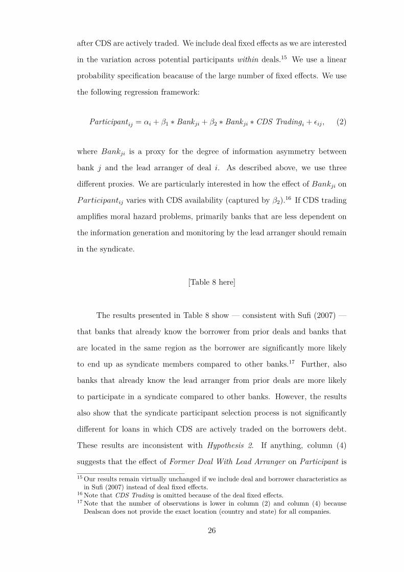
after CDS are actively traded. We include deal fixed effects as we are interested
in the variation across potential participants within deals.15 We use a linear
probability specification beacause of the large number of fixed effects. We use
the following regression framework:
Participantij = αi + β1 ∗ Bankji + β2 ∗ Bankji ∗ CDS Tradingi + ϵij, (2)
where Bankji is a proxy for the degree of information asymmetry between
bank j and the lead arranger of deal i. As described above, we use three
different proxies. We are particularly interested in how the effect of Bankji on
Participantij varies with CDS availability (captured by β2).16 If CDS trading
amplifies moral hazard problems, primarily banks that are less dependent on
the information generation and monitoring by the lead arranger should remain
in the syndicate.
[Table 8 here]
The results presented in Table 8 show — consistent with Sufi (2007) —
that banks that already know the borrower from prior deals and banks that
are located in the same region as the borrower are significantly more likely
to end up as syndicate members compared to other banks.17 Further, also
banks that already know the lead arranger from prior deals are more likely
to participate in a syndicate compared to other banks. However, the results
also show that the syndicate participant selection process is not significantly
different for loans in which CDS are actively traded on the borrowers debt.
These results are inconsistent with Hypothesis 2. If anything, column (4)
suggests that the effect of Former Deal With Lead Arranger on Participant is
15 Our results remain virtually unchanged if we include deal and borrower characteristics asin Sufi (2007) instead of deal fixed effects.
16 Note that CDS Trading is omitted because of the deal fixed effects.17 Note that the number of observations is lower in column (2) and column (4) because
Dealscan does not provide the exact location (country and state) for all companies.
26

weaker if CDS are available. This is consistent with the conjecture that CDS
availability attracts new investors.
Overall, the results reported in this section show that an increase in moral
hazard is unlikely to be the dominant effect on the fraction of a loan sold by
the lead arranger.
6 Robustness
6.1 CDS Introduction Dates
One potential problem is that exact CDS introduction dates are hard to iden-
tify and several data sources containing CDS spreads are available. Since CDS
are not traded on centralized exchanges, not all databases necessarily contain
the exact same information. For robustness purposes, we use all CDS spreads
from the CMA Datavision database to identify CDS introduction dates and
additionally report the baseline regressions using this database. Results are
reported in Table 9.
[Table 9 here]
The results using CMA data to identify CDS introduction dates are sim-
ilar to those using Bloomberg data. Again, all syndicate structure indicators
show that lenders form a more concentrated syndicate after CDS are avail-
able on a borrower’s debt. Also the magnitudes are comparable to the results
reported in Table 3.18
6.2 Secondary Market Trading
Another potential concern is that an increasing number of loans are traded
in the secondary market. It could be that the availability of credit protec-18 Also combining CMA and Bloomberg data yields similar results.
27

tion via CDS also increases the likelihood of secondary market trading. The
lead arranger may initially agree to retain a larger fraction of the loan but
immediately sell the loan after the origination. Unfortunately, Dealscan only
provides loan information as of origination so one cannot track the syndicate
composition over time. However, Ivashina and Sun (2011) show (using a hand
collected sample of loan amendments) that lead arrangers almost never sell
their stakes in the loan.
We additionally address this issue by excluding all companies from the
sample that issued loans that are traded on the secondary market during the
sample period.19 The results remain qualitatively unchanged.20
7 Conclusion
This study provides empirical evidence on how credit derivative trading affects
loan sales and the structure of loan syndicates. Using CDS trading data and
a large sample of syndicated loans issued between 2000 to 2010, we show that
lenders sell significantly lower fractions of loans once credit protection via CDS
is possible. Further, the syndicate concentration (measured by the Herfindahl
index) increases, and the number of lenders in the syndicate declines. These
effects are stronger if CDS liquidity is higher and the results are robust to
controlling for the potential endogeneity of CDS introduction. The reduction
in loan sales and the increase in syndicate concentration is consistent with
diversification benefits of the CDS market, which reduces the need for risk-
sharing via syndication.
However, a reduction in loan sales after CDS introduction is also consis-
tent with Parlour and Winton (2013), who show theoretically that lenders can
19 We classify traded loans as loans that have a Loan Identification Number (LIN). TheLIN is the main identifier in secondary loan market databases. E.g. Drucker and Puri(2009) use the LIN to merge Dealscan with the Loan Syndications and Trading Association(LSTA) Mark-to-Market Pricing database.
20 The results are not reported to save space but available from the author upon request.
28

no longer credible commit to monitor a borrower if laying off credit risk anony-
mously via CDS is possible. Without a credible signal by the lead arranger,
investors willingness to participate in a syndicate declines. Disentangling the
risk management from the moral hazard effect empirically, we find that poten-
tially negative effects of CDS trading are of minor importance in the syndicated
loan market.
This study helps to understand the impact of CDS trading on the nature
and operation of credit markets. Though the importance of credit derivatives
has grown enormously in recent years, these effects are not fully understood.
We provide evidence that is consistent with CDS being a flexible risk man-
agement tool that (partially) replaces loan sales and the need for a diverse
syndicate structure.
29

References
Ashcraft, A. B. and J. A. C. Santos (2007). Has the cds market lowered the
cost of corporate debt? Working Paper .
Ashcraft, A. B. and J. A. C. Santos (2009). Has the cds market lowered the
cost of corporate debt? Journal of Monetary Economics 56, 514–523.
Berg, T., A. Saunders, and S. Steffen (2013). The total costs of corporate
borrowing: Don’t ignore the fees. Working Paper .
Bharath, S., S. Dahiyab, A. Saunders, and A. Srinivasan (2007). So what
do i get? the bank’s view of lending relationships. Journal of Financial
Economics 85, 368–419.
Bharath, S. T., S. Dahiya, and I. Hallak (2012). Do shareholder rights affect
syndicate structure? evidence from a natural experiment. Working Paper .
Bharath, S. T., S. Dahiya, A. Saunders, and A. Srinivasan (2011). Lending
relationships and loan contract terms. The Review of Financial Studies 24,
1142–1203.
Cebenoyan, A. S. and P. E. Strahan (2004). Risk management, capital struc-
ture and lending at banks. Journal of Banking & Finance 28, 19–43.
Chava, S., R. Ganduri, and C. Ornthanalai (2012). Are credit ratings still
relevant? Working Paper .
Chava, S. and M. R. Roberts (2008). How does financing impact investment?
the role of debt covenants. Journal of Finance 63, 2085 – 2121.
Das, S., M. Kalimipalli, and S. Nayak (2014). Do cds markets improve the mar-
ket efficiency of corporate bonds? Journal of Financial Economics (forth-
coming).
30

Dennis, S. A. and D. J. Mullineaux (2000). Syndicated loans. Journal of
Financial Intermediation 9, 404–426.
Diamond, D. W. (1984). Financial intermediation and delegated monitoring.
Review of Economic Studies 51, 393–414.
Drucker, S. and M. Puri (2009). On loan sales, loan contracting, and lending
relationships. Review of Financial Studies 22 (7), 2835–2872.
Duffee, G. R. and C. Zhou (2001). Credit derivatives in banking: Useful tools
for managing risk? Journal of Monetary Economics 48, 25–54.
Froot, K. A., D. S. Scharfstein, and J. C. Stein (1993). Risk management:
Coordinating corporate investment and financing policies. The Journal of
Finance 48, 1629–1658.
Froot, K. A. and J. C. Stein (1998). Risk management: Capital budgeting, and
capital structure policy for financial institutions: An integrated approach.
Journal of Financial Economics 47, 55–82.
Gatev, E. and P. E. Strahan (2009). Liquidity risk and syndicate structure.
Journal of Financial Economics 93, 490–504.
Goderis, B., I. W. Marsh, J. V. Castello, and W. Wagner (2007). Bank be-
haviour with access to credit risk transfer markets. Working Paper .
Goldstein, M. A. and E. S. Hotchkiss (2007). Dealer behavior and the trading
of newly issued corporate bonds. Working Paper .
Gopalan, R., V. Nanda, and V. Yerramilli (2011). Does poor performance
damage the reputation of financial intermediaries? evidence from the loan
syndication market. Journal of Finance 66, 2083–2120.
Gorton, G. B. and G. G. Pennachi (1995). Banks and loan sales: Marketing
nonmarketable assets. Journal of Monetary Economics 35, 389–411.
31

Hirtle, B. (2009). Credit derivatives and bank credit supply. Journal of Fi-
nancial Intermediation 18, 125–150.
Holmstrom, B. (1979). Moral hazard and observability. Bell Journal of Eco-
nomics 10, 74–91.
Holmstrom, B. and J. Tirole (1997). Financial intermediation, loanable funds,
and the real sector. Quarterly Journal of Economics 112, 663–691.
Instefjord, N. (2005). Risk and hedging: Do credit derivatives increase bank
risk? Journal of Banking & Finance 29, 333–345.
Ivashina, V. (2009). Asymmetric information effects on loan spreads. Journal
of Financial Economics 92, 300–319.
Ivashina, V. and Z. Sun (2011). Institutional stockt rading on loan market
information. Journal of Financial Economics 100, 284–303.
Minton, B. A., R. Stulz, and R. Williamson (2008). How much do banks use
credit derivatives to hedge loans? Journal of Financial Services Research 35,
1–31.
Parlour, C. A. and A. Winton (2013). Laying off credit risk: Loan sales versus
credit default swaps. Journal of Financial Economics 107, 25–45.
Saretto, A. and H. Tookes (2013). Corporate leverage, debt maturity and credit
supply: The role of credit default swaps. Review of Financial Studies 26,
1190–1247.
Subrahmanyam, M. G., D. Y. Tang, and S. Q. Wang (2014). Does the tail
wag the dog? the effect of credit default swaps on credit risk. Review of
Financial Studies (forthcoming).
Sufi, A. (2007). Information asymmetry and financing arrangements: Evidence
from syndicated loans. The Journal of Finance 62, 629–668.
32

Yasuda, A. (2005). Do bank relationships affect the firms underwriter choice
in the corporate-bond underwriting market? Journal of Finance 60, 1259–
1292.
33

Appendix
A.1 Figures
Figure 1: Loan Share Retained by Lead Bank: Before vs. After CDS Intro-duction
This figures shows the average loan share retained by the lead bank beforeand after CDS are actively traded on the borrowers debt ([-2,+2] yearssurrounding the CDS introduction).
34

A.2 Tables
35

Tab
le1:
Des
crip
tive
Stat
istic
sT
his
tabl
ere
port
ssu
mm
ary
stat
istic
sfo
rC
DS
trad
ing
indi
cato
rs,s
yndi
cate
stru
ctur
ein
dica
tors
,loa
nch
arac
teris
tics
and
borr
ower
char
acte
ristic
s.A
llva
riabl
esar
ede
fined
inth
eA
ppen
dix
Tabl
eA
.I.m
ean
p25
p50
p75
sdco
unt
Pan
elA
:C
DS
Tra
ding
Indi
cato
rsC
DS
Trad
ed(0
/1)
0.19
0.00
0.00
0.00
0.39
1374
4C
DS
Trad
ing
(0/1
)0.
090.
000.
000.
000.
2813
744
Pan
elB
:Sy
ndic
ate
Stru
ctur
eIn
dica
tors
%H
eld
byLe
adA
rran
ger
38.1
517
.50
28.0
050
.00
27.9
238
42So
leLe
nder
(0/1
)0.
180.
000.
000.
000.
3913
744
#Le
nder
s7.
732.
005.
0010
.00
8.12
1374
4H
erfin
dahl
2676
.67
863.
6815
61.6
334
22.2
227
01.1
234
26P
anel
C:
Loan
Cha
ract
eris
tics
Faci
lity
Am
ount
(mill
ion
USD
)34
2.45
40.0
013
2.05
350.
0081
5.61
1374
4M
atur
ity(M
onth
s)44
.05
24.0
048
.00
60.0
023
.09
1374
4Se
cure
d(0
/1)
0.56
0.00
1.00
1.00
0.50
1374
4A
llIn
Spre
adD
raw
n(b
p)22
0.03
100.
0020
0.00
300.
0015
9.74
1374
4P
anel
D:
Bor
row
erC
hara
cter
isti
csTo
talA
sset
s(m
illio
nU
SD)
4469
.83
259.
6087
4.08
2937
.25
1098
5.77
1374
4Le
vera
ge0.
300.
130.
270.
410.
2413
744
Cov
erag
e17
.68
2.64
5.40
12.2
949
.90
1374
4Pr
ofita
bilit
y0.
140.
070.
130.
210.
2013
744
Tang
ibili
ty0.
340.
140.
280.
510.
2413
744
Cur
rent
Rat
io1.
771.
051.
502.
161.
1313
744
Mar
ket-
To-B
ook
1.66
1.09
1.36
1.86
0.96
1374
4In
vest
men
tG
rade
(0/1
)0.
240.
000.
000.
000.
4313
744
Not
Rat
ed(0
/1)
0.50
0.00
1.00
1.00
0.50
1374
4
36

Tab
le2:
Des
crip
tive
Stat
istic
s:N
oC
DS
Trad
edvs
.C
DS
Trad
edT
hist
able
repo
rtsd
escr
iptiv
est
atist
icsf
orC
DS
trad
ing
indi
cato
rs,s
yndi
cate
stru
ctur
ein
dica
tors
,loa
nch
arac
teris
ticsa
ndbo
rrow
erch
arac
teris
tics.
CD
ST
rade
din
dica
tes
that
the
borr
ower
has
activ
ely
trad
edC
DS
onits
debt
atan
ypo
int
intim
edu
ring
the
sam
ple
perio
d.A
llva
riabl
esar
ede
fined
inth
eA
ppen
dix
Tabl
eA
.I.C
DS
Tra
ded
=0
CD
ST
rade
d=
1
mea
np5
0sd
coun
tm
ean
p50
sdco
unt
Pan
elA
:C
DS
Tra
ding
Indi
cato
rsC
DS
Trad
ed(0
/1)
0.00
0.00
0.00
1119
01.
001.
000.
0025
54C
DS
Trad
ing
(0/1
)0.
000.
000.
0011
190
0.47
0.00
0.50
2554
Pan
elB
:Sy
ndic
ate
Stru
ctur
eIn
dica
tors
%H
eld
byLe
adA
rran
ger
42.0
032
.00
28.7
929
3725
.62
18.8
320
.40
905
Sole
Lend
er(0
/1)
0.22
0.00
0.41
1119
00.
030.
000.
1625
54#
Lend
ers
6.34
5.00
7.09
1119
013
.83
12.0
09.
4425
54H
erfin
dahl
3126
.84
2008
.89
2830
.33
2635
1177
.04
750.
0014
12.3
379
1P
anel
C:
Loan
Cha
ract
eris
tics
Faci
lity
Am
ount
(mill
ion
USD
)19
6.42
100.
0035
0.96
1119
098
2.25
600.
0015
93.1
625
54M
atur
ity(M
onth
s)45
.36
48.0
022
.69
1119
038
.30
36.0
023
.94
2554
Secu
red
(0/1
)0.
641.
000.
4811
190
0.20
0.00
0.40
2554
All
InSp
read
Dra
wn
(bp)
243.
3022
5.00
158.
1811
190
118.
0970
.00
122.
2125
54P
anel
D:
Bor
row
erC
hara
cter
isti
csTo
talA
sset
s(m
illio
nU
SD)
1617
.26
586.
2645
49.8
711
190
1696
8.01
1048
8.25
1915
7.49
2554
Leve
rage
0.30
0.26
0.26
1119
00.
310.
300.
1625
54C
over
age
19.4
35.
1854
.79
1119
010
.00
6.22
13.1
425
54Pr
ofita
bilit
y0.
130.
120.
2111
190
0.20
0.17
0.14
2554
Tang
ibili
ty0.
320.
250.
2411
190
0.41
0.40
0.22
2554
Cur
rent
Rat
io1.
861.
591.
2011
190
1.34
1.21
0.62
2554
Mar
ket-
To-B
ook
1.65
1.36
0.98
1119
01.
671.
390.
8625
54In
vest
men
tG
rade
(0/1
)0.
110.
000.
3211
190
0.77
1.00
0.42
2554
Not
Rat
ed(0
/1)
0.61
1.00
0.49
1119
00.
030.
000.
1825
54
37

Tab
le3:
The
Impa
ctof
CD
STr
adin
gon
the
Stru
ctur
eof
Loan
Synd
icat
esT
his
tabl
ere
por
tsdi
ffer
ence
-in-
diff
eren
ces
OL
Sre
gres
sion
resu
lts
anal
yzin
gth
eim
pact
ofC
DS
trad
ing
onth
est
ruct
ure
oflo
ansy
ndic
ates
.T
hede
pen
dent
vari
able
sar
esy
ndic
ate
stru
ctur
ein
dica
tors
:th
ep
erce
ntag
eof
the
loan
held
byth
ele
adar
rang
er,
the
Her
find
ahl-
inde
xfo
rth
esy
ndic
ate
conc
entr
atio
n,an
dth
enu
mb
erof
lend
ers.
The
key
inde
pen
dent
vari
able
isC
DS
Tra
ding
,a
dum
my
vari
able
,w
hich
equa
lson
eif
CD
Sar
eac
tive
lytr
aded
onth
eb
orro
wer
’sde
btat
the
tim
eof
the
loan
orig
inat
ion,
and
zero
othe
rwis
e.C
DS
Tra
ded
isa
dum
my
vari
able
,w
hich
equa
lson
eif
CD
Sar
etr
aded
onth
eb
orro
wer
’sde
btat
any
poi
ntof
tim
edu
ring
the
sam
ple
per
iod,
and
zero
othe
rwis
e.A
llva
riab
les
are
defi
ned
inth
eA
ppen
dix
Tab
leA
.I.
Stan
dard
erro
rsar
ehe
tero
sked
asti
city
robu
stan
dcl
uste
red
atth
efi
rmle
vel
toac
coun
tfo
rno
n-in
dep
ende
ntob
serv
atio
nsw
ithi
nfi
rms.
*,**
,***
Indi
cate
stat
isti
cal
sign
ifica
nce
atth
e10
%,5
%,1
%le
vel.
(1)
(2)
(3)
(4)
(5)
(6)
%H
eld
By
Lea
d%
Hel
dB
yL
ead
Her
find
ahl
Her
find
ahl
ln(#
Len
ders
)ln
(#L
ende
rs)
Pan
elA
:C
DS
Tra
din
gIn
dic
ato
rsC
DS
Tra
ding
11.0
8∗∗
∗6.
70∗
∗∗
1014
.89∗
∗∗
551.
05∗
∗∗
-0.0
6∗-0
.07∗
∗
(1.5
7)(1
.61)
(130
.40)
(126
.91)
(0.0
3)(0
.04)
CD
ST
rade
d7.
76∗
∗∗
813.
33∗
∗∗
0.02
(1.4
7)(1
31.6
2)(0
.03)
Pan
elB
:L
oan
Ch
arac
teri
stic
sln
(Fac
ilit
yA
mou
nt)
-8.6
6∗∗
∗-8
.66∗
∗∗
-102
1.63
∗∗
∗-1
020.
17∗
∗∗
0.22
∗∗
∗0.
22∗
∗∗
(0.5
8)(0
.58)
(60.
84)
(60.
56)
(0.0
1)(0
.01)
ln(M
atur
ity)
-5.3
0∗∗
∗-5
.29∗
∗∗
-576
.35∗
∗∗
-574
.94∗
∗∗
0.14
∗∗
∗0.
14∗
∗∗
(0.7
8)(0
.78)
(68.
57)
(67.
79)
(0.0
1)(0
.01)
Secu
red
4.44
∗∗
∗4.
31∗
∗∗
341.
75∗
∗∗
323.
34∗
∗∗
-0.0
1-0
.01
(1.1
1)(1
.09)
(95.
90)
(94.
48)
(0.0
2)(0
.02)
Pan
elC
:B
orr
ower
Ch
arac
teri
stic
sln
(Tot
alA
sset
s)-2
.79∗
∗∗
-3.4
3∗∗
∗-3
36.9
9∗∗
∗-4
03.9
1∗∗
∗0.
11∗
∗∗
0.11
∗∗
∗
(0.5
9)(0
.61)
(59.
10)
(60.
36)
(0.0
1)(0
.01)
Lev
erag
e-2
.87
-3.4
2-4
74.9
3∗-5
23.1
5∗0.
000.
00(3
.36)
(3.3
8)(2
75.2
7)(2
73.7
1)(0
.04)
(0.0
4)C
over
age
0.01
0.01
0.86
0.88
-0.0
0∗∗
-0.0
0∗∗
(0.0
1)(0
.01)
(0.9
1)(0
.90)
(0.0
0)(0
.00)
Pro
fita
bili
ty-4
.65
-4.2
1-6
36.4
0∗∗
-594
.80∗
∗0.
09∗
∗0.
09∗
∗
(2.8
7)(2
.83)
(267
.23)
(262
.98)
(0.0
4)(0
.04)
Tan
gibi
lity
-1.9
8-1
.93
-139
.94
-135
.07
-0.1
0∗∗
∗-0
.10∗
∗∗
(2.7
4)(2
.75)
(241
.96)
(242
.15)
(0.0
4)(0
.04)
Cur
rent
Rat
io0.
410.
4522
.18
27.0
2-0
.02∗
∗∗
-0.0
2∗∗
∗
(0.5
4)(0
.54)
(47.
92)
(47.
45)
(0.0
1)(0
.01)
Mar
ket-
To-
Boo
k-0
.67
-0.6
8-2
0.67
-22.
490.
01∗
0.01
∗
(0.4
8)(0
.47)
(44.
18)
(44.
16)
(0.0
1)(0
.01)
Inve
stm
ent
Gra
de0.
60-0
.71
328.
15∗
∗18
7.35
0.04
0.03
(1.6
5)(1
.61)
(144
.79)
(142
.86)
(0.0
3)(0
.03)
Not
Rat
ed-1
.95
-1.9
614
.18
10.9
0-0
.06∗
∗-0
.06∗
∗
(1.7
0)(1
.70)
(144
.71)
(143
.99)
(0.0
2)(0
.02)
Inte
rcep
t25
4.82
∗∗
∗26
0.28
∗∗
∗26
801.
07∗
∗∗
2744
8.73
∗∗
∗-3
.25∗
∗∗
-3.2
4∗∗
∗
(15.
56)
(15.
64)
(108
8.65
)(1
123.
61)
(0.1
5)(0
.15)
Obs
.38
4238
4234
2634
2613
744
1374
4A
dj.
R2
0.37
70.
382
0.51
50.
521
0.52
00.
520
Tim
eF
ixed
Eff
ects
Yes
Yes
Yes
Yes
Yes
Yes
Indu
stry
Fix
edE
ffec
tsY
esY
esY
esY
esY
esY
esL
oan
Pur
pos
eF
ixed
Eff
ects
Yes
Yes
Yes
Yes
Yes
Yes
Loa
nT
ype
Fix
edE
ffec
tsY
esY
esY
esY
esY
esY
es
38

Tab
le4:
The
Impa
ctof
CD
STr
adin
gon
the
Stru
ctur
eof
Loan
Synd
icat
es-C
ontr
ollin
gfo
rBa
nkFi
xed
Effec
tsT
his
tabl
ere
por
tsdi
ffer
ence
-in-
diff
eren
ces
OL
Sre
gres
sion
resu
lts
anal
yzin
gth
eim
pact
ofC
DS
trad
ing
onth
est
ruct
ure
oflo
ansy
ndic
ates
.T
hede
pen
dent
vari
able
sar
esy
ndic
ate
stru
ctur
ein
dica
tors
:th
ep
erce
ntag
eof
the
loan
held
byth
ele
adar
rang
er,
the
Her
find
ahl-
inde
xfo
rth
esy
ndic
ate
conc
entr
atio
n,an
dth
enu
mb
erof
lend
ers.
The
key
inde
pen
dent
vari
able
isC
DS
Tra
ding
,a
dum
my
vari
able
,w
hich
equa
lson
eif
CD
Sar
eac
tive
lytr
aded
onth
eb
orro
wer
’sde
btat
the
tim
eof
the
loan
orig
inat
ion,
and
zero
othe
rwis
e.C
DS
Tra
ded
isa
dum
my
vari
able
,w
hich
equa
lson
eif
CD
Sar
etr
aded
onth
eb
orro
wer
’sde
btat
any
poi
ntof
tim
edu
ring
the
sam
ple
per
iod,
and
zero
othe
rwis
e.A
llva
riab
les
are
defi
ned
inth
eA
ppen
dix
Tab
leA
.I.
Stan
dard
erro
rsar
ehe
tero
sked
asti
city
robu
stan
dcl
uste
red
atth
efi
rmle
vel
toac
coun
tfo
rno
n-in
dep
ende
ntob
serv
atio
nsw
ithi
nfi
rms.
*,**
,***
indi
cate
stat
isti
cal
sign
ifica
nce
atth
e10
%,5
%,1
%le
vel.
(1)
(2)
(3)
(4)
(5)
(6)
%H
eld
By
Lea
d%
Hel
dB
yL
ead
Her
find
ahl
Her
find
ahl
ln(#
Len
ders
)ln
(#L
ende
rs)
Pan
elA
:C
DS
Tra
din
gIn
dic
ato
rsC
DS
Tra
ding
7.92
∗∗
∗3.
95∗
∗∗
882.
20∗
∗∗
436.
70∗
∗∗
-0.0
7∗∗
-0.0
8∗∗
(1.3
8)(1
.43)
(121
.52)
(124
.02)
(0.0
3)(0
.04)
CD
ST
rade
d7.
35∗
∗∗
812.
60∗
∗∗
0.01
(1.3
4)(1
23.2
6)(0
.03)
Pan
elB
:L
oan
Ch
arac
teri
stic
sln
(Fac
ilit
yA
mou
nt)
-8.6
6∗∗
∗-8
.66∗
∗∗
-942
.53∗
∗∗
-942
.50∗
∗∗
0.20
∗∗
∗0.
20∗
∗∗
(0.5
7)(0
.57)
(58.
78)
(58.
75)
(0.0
1)(0
.01)
ln(M
atur
ity)
-5.7
2∗∗
∗-5
.74∗
∗∗
-549
.33∗
∗∗
-550
.26∗
∗∗
0.13
∗∗
∗0.
13∗
∗∗
(0.6
9)(0
.69)
(64.
82)
(64.
13)
(0.0
1)(0
.01)
Secu
red
1.86
∗1.
71∗
152.
7313
1.29
0.03
0.03
(1.0
4)(1
.03)
(97.
48)
(96.
08)
(0.0
2)(0
.02)
Pan
elC
:B
orr
ower
Ch
arac
teri
stic
sln
(Tot
alA
sset
s)-3
.64∗
∗∗
-4.2
4∗∗
∗-3
23.9
0∗∗
∗-3
90.5
9∗∗
∗0.
10∗
∗∗
0.09
∗∗
∗
(0.5
6)(0
.57)
(56.
59)
(58.
30)
(0.0
1)(0
.01)
Lev
erag
e-6
.87∗
∗-7
.40∗
∗∗
-702
.79∗
∗∗
-749
.31∗
∗∗
0.02
0.01
(2.7
4)(2
.75)
(247
.43)
(246
.80)
(0.0
4)(0
.04)
Cov
erag
e0.
010.
010.
390.
42-0
.00∗
∗-0
.00∗
∗
(0.0
1)(0
.01)
(0.8
9)(0
.88)
(0.0
0)(0
.00)
Pro
fita
bili
ty-1
.81
-1.4
5-2
89.6
4-2
48.3
60.
050.
05(3
.05)
(3.0
1)(2
93.7
4)(2
89.0
4)(0
.04)
(0.0
4)T
angi
bili
ty-1
.51
-1.4
0-1
20.3
7-1
11.3
3-0
.06
-0.0
6(2
.38)
(2.3
8)(2
25.9
3)(2
26.1
8)(0
.04)
(0.0
4)C
urre
ntR
atio
0.10
0.13
7.60
12.2
8-0
.02∗
∗-0
.02∗
∗
(0.4
8)(0
.48)
(46.
00)
(45.
76)
(0.0
1)(0
.01)
Mar
ket-
To-
Boo
k-0
.69
-0.7
2-2
1.40
-25.
460.
01∗
0.01
∗
(0.4
7)(0
.47)
(43.
85)
(43.
75)
(0.0
1)(0
.01)
Inve
stm
ent
Gra
de0.
12-1
.11
254.
12∗
118.
410.
020.
02(1
.52)
(1.4
7)(1
40.8
9)(1
37.2
5)(0
.03)
(0.0
3)N
otR
ated
-1.3
4-1
.35
-7.2
6-9
.45
-0.0
5∗∗
-0.0
5∗∗
(1.4
8)(1
.48)
(137
.86)
(137
.22)
(0.0
2)(0
.02)
Inte
rcep
t23
6.56
∗∗
∗24
1.99
∗∗
∗25
075.
71∗
∗∗
2582
7.42
∗∗
∗-2
.90∗
∗∗
-2.8
9∗∗
∗
(14.
06)
(14.
17)
(127
2.54
)(1
313.
80)
(0.1
3)(0
.13)
Obs
.38
4238
4234
2634
2613
744
1374
4A
dj.
R2
0.50
80.
512
0.56
50.
571
0.55
90.
559
Tim
eF
ixed
Eff
ects
Yes
Yes
Yes
Yes
Yes
Yes
Indu
stry
Fix
edE
ffec
tsY
esY
esY
esY
esY
esY
esL
oan
Pur
pos
eF
ixed
Eff
ects
Yes
Yes
Yes
Yes
Yes
Yes
Loa
nT
ype
Fix
edE
ffec
tsY
esY
esY
esY
esY
esY
esB
ank
Fix
edE
ffec
tsY
esY
esY
esY
esY
esY
es
39

Table 5: The Impact of CDS Trading on the Structure of Loan Syndicates -IV-Estimation
This table reports instrumental variable regressions analyzing the impact of CDS tradingon the structure of loan syndicates. The instrument for CDS trading is the amount offoreign exchange derivatives held by the lead arranger for hedging purposes (not trading)as a fraction of the total assets of the lead arranger. A logit model is used to obtain theprobability of CDS trading for each loan (column 1). The predicted probability is used asthe instrumental variable in the models reported in column 2 and column 3. The dependentvariable in the models reported in column 2 and column 3 is the percentage of the loan heldby the lead arranger. All variables are defined in the Appendix Table A.I. Standard errorsare heteroskedasticity robust and clustered at the firm level to account for non-independentobservations within firms. *,**,*** Indicate statistical significance at the 10%,5%,1% level.
(1) (2) (3)CDS Trading % Held By Lead % Held By Lead
Panel A: CDS Trading IndicatorsInstrumented CDS Trading 25.30∗∗∗ 18.30∗∗∗
(5.02) (5.09)CDS Traded 8.38∗∗∗
(1.50)Panel B: Loan Characteristicsln(Facility Amount) -8.18∗∗∗ -8.18∗∗∗
(0.65) (0.64)ln(Maturity) -5.28∗∗∗ -5.34∗∗∗
(0.88) (0.86)Secured 3.83∗∗∗ 3.79∗∗∗
(1.18) (1.16)Panel C: Borrower Characteristicsln(Total Assets) 0.37∗∗∗ -2.32∗∗∗ -3.21∗∗∗
(0.03) (0.71) (0.72)Leverage 0.04 -3.67 -4.74
(0.08) (3.44) (3.43)Coverage -0.00 0.01 0.01
(0.00) (0.01) (0.01)Profitability 0.30 -0.90 -0.22
(0.18) (3.46) (3.39)Tangibility 0.00 -0.07 0.25
(0.17) (2.88) (2.89)Current Ratio -0.07∗∗ 1.30∗∗ 1.28∗∗
(0.03) (0.63) (0.62)Market-To-Book 0.10∗∗∗ -1.62∗∗∗ -1.43∗∗∗
(0.02) (0.56) (0.54)Investment Grade 0.44∗∗∗ -2.31 -3.21∗
(0.08) (1.82) (1.73)Not Rated -0.52∗∗∗ -2.02 -2.49
(0.08) (1.72) (1.71)Panel D: Lender CharacteristicsLender FX Usage 0.30∗∗
(0.13)Obs. 28404 3106 3106Adj. R2 0.314 0.323Pseudo R2 0.382Time Fixed Effects Yes Yes YesIndustry Fixed Effects Yes Yes YesLoan Purpose Fixed Effects Yes YesLoan Type Fixed Effects Yes Yes
40

Tab
le6:
The
Impa
ctof
CD
STr
adin
gon
the
Stru
ctur
eof
Loan
Synd
icat
es-C
DS
Mar
ket
Liqu
idity
Thi
sta
ble
repo
rts
diffe
renc
e-in
-diff
eren
ces
OLS
regr
essio
nre
sults
anal
yzin
gth
eim
pact
ofC
DS
trad
ing
onth
est
ruct
ure
oflo
ansy
ndic
ates
.T
hede
pend
ent
varia
bles
are
synd
icat
est
ruct
ure
indi
cato
rs:
the
perc
enta
geof
the
loan
held
byth
ele
adar
rang
er,t
heH
erfin
dahl
-inde
xfo
rth
esy
ndic
ate
conc
entr
atio
n,an
dth
enu
mbe
rof
lend
ers.
The
key
inde
pend
ent
varia
bles
are
CD
STr
adin
g*Lo
wLi
quid
ity,
CD
STr
adin
g*M
ediu
mLi
quid
ityan
dC
DS
Trad
ing*
Hig
hLi
quid
ity.
CD
STr
adin
gis
adu
mm
yva
riabl
ew
hich
equa
lson
eif
CD
Sar
eac
tivel
ytr
aded
onth
ebo
rrow
er’s
debt
atth
etim
eof
the
loan
orig
inat
ion,
and
zero
othe
rwise
.Lo
wLi
quid
ity/M
ediu
mLi
quid
ity/H
igh
Liqu
idity
isa
dum
my
varia
ble
whi
cheq
uals
one
ifth
ebo
rrow
er’s
CD
Sbi
d-as
ksp
read
isin
the
low
/med
ium
/hig
hqu
antil
ein
the
mon
thpr
ior
toth
elo
aniss
uean
dze
root
herw
ise.
CD
STr
aded
isa
dum
my
varia
ble,
whi
cheq
uals
one
ifC
DS
are
trad
edon
the
borr
ower
’sde
btat
any
poin
tof
time
durin
gth
esa
mpl
epe
riod,
and
zero
othe
rwise
.A
llva
riabl
esar
ede
fined
inth
eA
ppen
dix
Tabl
eA
.I.St
anda
rder
rors
are
hete
rosk
edas
ticity
robu
stan
dcl
uste
red
atth
efir
mle
velt
oac
coun
tfo
rno
n-in
depe
nden
tob
serv
atio
nsw
ithin
firm
s.*,
**,*
**in
dica
test
atist
ical
signi
fican
ceat
the
10%
,5%
,1%
leve
l.(1
)(2
)(3
)%
Hel
dB
yLe
adH
erfin
dahl
ln(#
Lend
ers)
CD
STr
adin
g*Lo
wLi
quid
ity3.
3618
1.46
0.00
(2.3
7)(1
86.8
8)(0
.04)
CD
STr
adin
g*M
ediu
mLi
quid
ity7.
16∗∗
∗54
9.20
∗∗∗
-0.0
0(2
.35)
(182
.80)
(0.0
5)C
DS
Trad
ing*
Hig
hLi
quid
ity10
.08∗∗
∗95
9.25
∗∗∗
-0.2
2∗∗∗
(2.0
1)(1
53.2
7)(0
.05)
CD
STr
aded
7.90
∗∗∗
832.
46∗∗
∗0.
01(1
.47)
(130
.98)
(0.0
3)O
bs.
3836
3420
1372
9A
dj.
R2
0.38
20.
522
0.52
1T
ime
Fixe
dEff
ects
Yes
Yes
Yes
Indu
stry
Fixe
dEff
ects
Yes
Yes
Yes
Loan
Purp
ose
Fixe
dEff
ects
Yes
Yes
Yes
Loan
Typ
eFi
xed
Effec
tsYe
sYe
sYe
sha
scon
trYe
sYe
sYe
s
41

Tab
le7:
CD
STr
adin
g,M
onito
ring,
and
Mor
alH
azar
dT
his
tabl
ere
por
tsdi
ffer
ence
-in-
diff
eren
ces
OL
Sre
gres
sion
resu
lts
anal
yzin
gth
eim
pact
ofC
DS
trad
ing
onth
est
ruct
ure
oflo
ansy
ndic
ates
dist
ingu
ishi
ngb
etw
een
diff
eren
tty
pes
ofb
orro
wer
san
dle
nder
s.T
hede
pen
dent
vari
able
isth
ep
erce
ntag
eof
the
loan
held
byth
ele
adar
rang
er.
The
key
inde
pen
dent
vari
able
sis
CD
ST
radi
ng,
adu
mm
yva
riab
le,
whi
cheq
uals
one
ifC
DS
are
acti
vely
trad
edon
the
bor
row
er’s
debt
atth
eti
me
ofth
elo
anor
igin
atio
n,an
dze
root
herw
ise
CD
ST
rade
dis
adu
mm
yva
riab
le,
whi
cheq
uals
one
ifC
DS
are
trad
edon
the
bor
row
er’s
debt
atan
yp
oint
ofti
me
duri
ngth
esa
mpl
ep
erio
d,an
dze
root
herw
ise.
Leve
rage
isth
era
tio
ofb
ook
valu
eof
tota
lde
btto
boo
kva
lue
ofas
sets
.C
over
age
isth
era
tio
ofE
BIT
DA
toin
tere
stex
pen
ses.
#A
naly
sts
isth
enu
mb
erof
anal
ysts
cove
ring
the
bor
row
erat
the
tim
eof
the
loan
orig
inat
ion.
Rel
(Dum
my)
isa
dum
my
vari
able
whi
cheq
uals
one
ifth
efi
rmb
orro
wed
from
the
sam
ele
adle
nder
inth
epr
evio
usfi
veye
ars
and
zero
othe
rwis
e.Le
adR
eput
atio
nis
the
mar
ket
shar
e(b
yam
ount
)of
the
lead
arra
nger
inth
eye
arpr
ior
toth
elo
anin
ques
tion
.A
llit
ems
are
defi
ned
inth
eA
ppen
dix
Tab
leA
.I.
Stan
dard
erro
rsar
ehe
tero
sked
asti
city
robu
stan
dcl
uste
red
atth
efi
rmle
vel
toac
coun
tfo
rno
n-in
dep
ende
ntob
serv
atio
nsw
ithi
nfi
rms.
*,**
,***
indi
cate
stat
isti
cal
sign
ifica
nce
atth
e10
%,5
%,1
%le
vel.
(1)
(2)
(3)
(4)
(5)
%H
eld
By
Lea
d%
Hel
dB
yL
ead
%H
eld
By
Lea
d%
Hel
dB
yL
ead
%H
eld
By
Lea
dC
DS
Tra
ding
3.09
∗∗
∗0.
850.
472.
70∗
2.73
∗∗
∗
(1.0
1)(0
.54)
(0.7
6)(1
.61)
(0.9
4)C
DS
Tra
ding
*Lev
erag
e-6
.55∗
∗
(2.7
7)C
DS
Tra
ding
*Cov
erag
e0.
04(0
.03)
CD
ST
radi
ng*#
Ana
lyst
s0.
07(0
.05)
CD
ST
radi
ng*R
el(D
umm
y)-1
.68
(1.6
0)C
DS
Tra
ding
*Lea
dR
eput
atio
n-1
1.34
∗
(6.6
3)L
ever
age
1.13
0.94
0.74
1.05
0.92
(1.6
6)(1
.62)
(1.6
2)(1
.62)
(1.6
2)C
over
age
0.01
0.01
0.01
0.01
0.01
(0.0
1)(0
.01)
(0.0
1)(0
.01)
(0.0
1)#
Ana
lyst
s-0
.07∗
∗∗
(0.0
3)R
el(D
umm
y)-0
.79
(0.5
5)L
ead
Rep
utat
ion
-1.1
8(3
.69)
CD
ST
rade
d-0
.95∗
-0.9
4∗-0
.72
-0.9
8∗-0
.88∗
(0.5
2)(0
.52)
(0.5
2)(0
.52)
(0.5
3)O
bs.
3842
3842
3842
3842
3704
Adj
.R
20.
191
0.19
00.
191
0.19
10.
196
Tim
eF
ixed
Eff
ects
Yes
Yes
Yes
Yes
Yes
Indu
stry
Fix
edE
ffec
tsY
esY
esY
esY
esY
esL
oan
Pur
pos
eF
ixed
Eff
ects
Yes
Yes
Yes
Yes
Yes
Loa
nT
ype
Fix
edE
ffec
tsY
esY
esY
esY
esY
esC
ontr
ols
For
Bor
row
erC
hara
cter
isti
csY
esY
esY
esY
esY
esC
ontr
ols
For
Loa
nC
hara
cter
isti
csY
esY
esY
esY
esY
es
42

Table 8: Participant Choice EstimationThis table presents coefficient estimates for a linear probability specification estimating how bank characteristics affect the probability of being chosen as aparticipant in a syndicated loan. Estimations include deal fixed effects. The choice set includes all banks that are active in the syndicated loan market in the yearof the loan. Firms that never have actively traded CDS on their debt during the sample period are excluded. CDS Trading is a dummy variable, which equalsone if CDS are actively traded on the borrower’s debt at the time of the loan origination, and zero otherwise. Former Deal With Borrower is a dummy variable,which equals one if the bank is a former lender of the borrowing firm, and zero otherwise. Same Region As Borrower is a dummy variable, which equals one if thebank is in the same region as the borrowing firm, and zero otherwise. Former Deal With Lead Arranger is a dummy variable, which equals one if the bank hasmade a deal in the past where the current lead arranger was also involved, and zero otherwise. All items are defined in the Appendix Table A.I. Standard errorsare heteroskedasticity robust and clustered at the firm level to account for non-independent observations within firms. *,**,*** indicate statistical significance atthe 10%,5%,1% level.
(1) (2) (3) (4)Participant Participant Participant Participant
Former Deal With Borrower 0.287∗∗∗ 0.300∗∗∗
(0.016) (0.013)Former Deal With Borrower*CDS Trading 0.021 0.015
(0.018) (0.015)Same Region As Borrower 0.017∗∗∗ 0.008∗∗∗
(0.003) (0.002)Same Region As Borrower*CDS Trading -0.001 -0.001
(0.003) (0.003)Former Deal With Lead Arranger 0.016∗∗∗ 0.008∗∗∗
(0.001) (0.000)Former Deal With Lead Arranger*CDS Trading -0.000 -0.004∗∗∗
(0.001) (0.001)Intercept 0.003∗∗∗ 0.016∗∗∗ -0.000 -0.000
(0.000) (0.000) (0.000) (0.000)Obs. 3,082,122 1,712,577 3,082,122 1,712,577Adj. R2 0.217 0.008 0.011 0.232Deal Fixed Effects Yes Yes Yes Yes
43

Table 9: Robustness: CDS Trading - CMA DataThis table reports difference-in-differences OLS regression results analyzing the impact ofCDS trading on the structure of loan syndicates. The difference to Table 2 is that datafrom CMA instead of Bloomberg data is used to identify which borrowers have activelytraded CDS on their debt. The dependent variables are syndicate structure indicators: thepercentage of the loan held by the lead arranger, the Herfindahl-index for the syndicateconcentration, and the number of lenders. The key independent variable is CDS Trading, adummy variable, which equals one if CDS are actively traded on the borrower’s debt at thetime of the loan origination, and zero otherwise. CDS Traded is a dummy variable, whichequals one if CDS are traded on the borrower’s debt at any point of time during the sampleperiod, and zero otherwise. All items are defined in the Appendix Table A.I. Standard errorsare heteroskedasticity robust and clustered at the firm level to account for non-independentobservations within firms. *,**,*** indicate statistical significance at the 10%,5%,1% level.
(1) (2) (3)% Held By Lead Herfindahl ln(# Lenders)
Panel A: CDS Trading IndicatorsCDS Traded 6.44∗∗∗ 807.75∗∗∗ 0.07∗∗
(1.48) (127.42) (0.03)CDS Trading 6.60∗∗∗ 416.85∗∗∗ -0.16∗∗∗
(1.60) (135.50) (0.04)Panel B: Loan Characteristicsln(Facility Amount) -8.46∗∗∗ -999.58∗∗∗ 0.22∗∗∗
(0.57) (59.68) (0.01)ln(Maturity) -5.58∗∗∗ -593.31∗∗∗ 0.15∗∗∗
(0.76) (65.53) (0.01)Secured 4.63∗∗∗ 350.00∗∗∗ -0.02
(1.08) (93.41) (0.02)Panel C: Borrower Characteristicsln(Total Assets) -3.16∗∗∗ -379.08∗∗∗ 0.10∗∗∗
(0.59) (58.79) (0.01)Leverage -3.39 -574.56∗∗ 0.00
(3.34) (272.41) (0.04)Coverage 0.01 0.71 -0.00∗∗
(0.01) (0.90) (0.00)Profitability -4.02 -569.96∗∗ 0.10∗∗∗
(2.81) (261.95) (0.04)Tangibility -2.33 -163.85 -0.10∗∗∗
(2.70) (238.93) (0.04)Current Ratio 0.50 25.38 -0.02∗∗∗
(0.53) (46.87) (0.01)Market-To-Book -0.52 -13.28 0.01
(0.47) (43.34) (0.01)Investment Grade 0.58 204.90 0.03
(1.55) (134.88) (0.03)Not Rated -0.93 60.49 -0.07∗∗∗
(1.67) (141.68) (0.02)Intercept 240.38∗∗∗ 26747.35∗∗∗ -3.42∗∗∗
(13.92) (1105.22) (0.16)Obs. 4020 3586 14339Adj. R2 0.381 0.519 0.520Time Fixed Effects Yes Yes YesIndustry Fixed Effects Yes Yes YesLoan Purpose Fixed Effects Yes Yes YesLoan Type Fixed Effects Yes Yes Yes
44

A.3
Var
iabl
eD
efini
tion
s
Tab
leA
.I:
Varia
ble
Defi
nitio
ns
Var
iabl
eN
ame
Defi
niti
onSo
urce
CD
ST
radi
ngIn
dica
tors
:
CD
STr
adin
gA
dum
my
varia
ble,
whi
cheq
uals
one
ifC
DS
are
activ
ely
trad
edon
the
borr
ower
’sde
btat
the
time
ofth
elo
anor
igin
atio
n,an
dze
root
herw
ise.
Blo
ombe
rg&
CM
A
CD
STr
aded
Adu
mm
yva
riabl
e,w
hich
equa
lson
eif
CD
Sar
etr
aded
onth
ebo
rrow
er’s
debt
atan
ypo
int
oftim
edu
ring
the
sam
ple
perio
d,an
dze
root
herw
ise.
Blo
ombe
rg&
CM
A
Low
Liqu
idity
Adu
mm
yva
riabl
ew
hich
equa
lson
eif
the
borr
ower
’sC
DS
bid-
ask
spre
adis
inth
ehi
gh
quan
tile
inth
em
onth
prio
rto
the
loan
issue
and
zero
othe
rwise
.
Blo
ombe
rg
Med
ium
Liqu
idity
Adu
mm
yva
riabl
ew
hich
equa
lson
eif
the
borr
ower
’sC
DS
bid-
ask
spre
adis
inth
em
ediu
m
quan
tile
inth
em
onth
prio
rto
the
loan
issue
and
zero
othe
rwise
.
Blo
ombe
rg
Hig
hLi
quid
ityA
dum
my
varia
ble
whi
cheq
uals
one
ifth
ebo
rrow
er’s
CD
Sbi
d-as
ksp
read
isin
the
low
quan
tile
inth
em
onth
prio
rto
the
loan
issue
and
zero
othe
rwise
.
Blo
ombe
rg
Synd
icat
eSt
ruct
ure
Indi
cato
rs:
%H
eld
byLe
adA
rran
ger
The
shar
eof
the
loan
reta
ined
byth
ele
adar
rang
erin
%.
Dea
lscan
Con
tinue
don
next
page
45

Tab
leA
.I–
cont
inue
dfr
ompr
evio
uspa
ge
Var
iabl
eN
ame
Defi
niti
onSo
urce
Her
finda
hlT
heH
erfin
dahl
-Ind
exfo
rth
esy
ndic
ate
conc
entr
atio
nm
easu
red
asth
esu
mof
the
squa
red
shar
esre
tain
edby
the
diffe
rent
lend
ers
ina
loan
.
Dea
lscan
#Le
nder
sT
henu
mbe
rof
dist
inct
lend
ers
ina
loan
cont
ract
.D
ealsc
an
Bor
row
er/I
ssue
rch
arac
teri
stic
s:
Tota
lAss
ets
Firm
’sto
tala
sset
sin
$mill
ion.
Com
pust
at
Leve
rage
Long
-ter
mde
btdi
vide
dby
tota
lass
ets.
Com
pust
at
Mar
ket-
to-B
ook
Mar
ket
valu
eof
the
firm
divi
ded
byth
ebo
okva
lue
ofas
sets
.C
ompu
stat
Tang
ibili
tyN
etpr
oper
typl
ant
and
equi
pmen
tdi
vide
dby
tota
lass
ets.
Com
pust
at
Cov
erag
eIn
tere
stex
pens
esdi
vide
dby
EBIT
DA
.C
ompu
stat
Profi
tabi
lity
EBIT
DA
divi
ded
byto
tala
sset
s.C
ompu
stat
Cur
rent
Rat
ioC
urre
ntas
sets
divi
ded
bycu
rren
tlia
bilit
ies.
Com
pust
at
Not
Rat
edA
dum
my
varia
ble,
whi
cheq
uals
one
ifth
ebo
rrow
erw
asno
tra
ted
byS&
Pat
the
time
of
the
debt
issue
.
Com
pust
at
Inve
stm
ent
Gra
deA
dum
my
varia
ble,
whi
cheq
uals
one
ifth
ebo
rrow
erw
asra
ted
BB
B-
orbe
tter
byS&
Pat
the
time
ofth
ede
btiss
ue.
Com
pust
at
#A
naly
sts
The
num
ber
ofan
alys
tsco
verin
gth
ebo
rrow
erat
the
time
ofth
elo
anor
igin
atio
n.I/
B/E
/S
Loan
/Len
der
char
acte
rist
ics:
Con
tinue
don
next
page
46

Tab
leA
.I–
cont
inue
dfr
ompr
evio
uspa
ge
Var
iabl
eN
ame
Defi
niti
onSo
urce
Faci
lity
Am
ount
Ove
rall
faci
lity
volu
me
in$m
illio
n.D
ealsc
an
Mat
urity
Tim
eto
mat
urity
inm
onth
s.D
ealsc
an
Secu
red
Adu
mm
yva
riabl
e,w
hich
equa
lson
eif
the
loan
isse
cure
dan
dze
root
herw
ise.
Dea
lscan
Sole
Lend
erA
dum
my
varia
ble,
whi
cheq
uals
one
ifth
elo
anis
not
synd
icat
edan
dze
root
herw
ise.
Dea
lscan
All
InSp
read
Dra
wn
The
faci
lity
All
InSp
read
Dra
wn
(bps
).D
ealsc
an
Lend
erFX
Usa
geT
heav
erag
eam
ount
offo
reig
nex
chan
gede
rivat
ives
held
byal
lthe
lead
arra
nger
sth
atle
nd
mon
eyto
the
com
pany
inth
epr
evio
usfiv
eye
ars
asa
frac
tion
ofth
eto
tall
oans
ofth
ele
ad
arra
nger
s.
Cal
lRep
orts
Lead
Rep
utat
ion
The
mar
kets
hare
(by
amou
nt)o
fthe
lead
arra
nger
inth
eye
arpr
iort
oth
elo
anin
ques
tion.
Dea
lscan
Rel
(Dum
my)
Adu
mm
yva
riabl
ew
hich
equa
lson
eif
the
firm
borr
owed
from
the
sam
ele
adle
nder
inth
e
prev
ious
five
year
san
dze
root
herw
ise.
Dea
lscan
Form
erD
ealW
ithB
orro
wer
Adu
mm
yva
riabl
e,w
hich
equa
lson
eif
the
bank
isa
form
erle
nder
ofth
ebo
rrow
ing
firm
,
and
zero
othe
rwise
.
Dea
lscan
Sam
eR
egio
nA
sB
orro
wer
Adu
mm
yva
riabl
e,w
hich
equa
lson
eif
the
bank
isin
the
sam
ere
gion
,i.e
.in
the
sam
e
coun
try
and
inth
esa
me
stat
e,as
the
borr
owin
gfir
m,a
ndze
root
herw
ise.
Dea
lscan
Form
erD
ealW
ithLe
adA
rran
ger
Adu
mm
yva
riabl
e,w
hich
equa
lson
eif
the
bank
has
mad
ea
deal
inth
epa
stw
here
the
curr
ent
lead
arra
nger
was
also
invo
lved
,and
zero
othe
rwise
.
Dea
lscan
Con
tinue
don
next
page
47

Table A.I – continued from previous page
Variable Name Definition Source
Participantij A dummy variable, which equals one if bank j participated in loan i, and zero otherwise. Dealscan
48

Managerial Optimism and Debt ContractDesign
Tim R. Adam Valentin Burg Tobias Scheinert Daniel Streitz
Abstract:
We examine the impact of managerial optimism on the inclusion of performance-pricing provisions in debt contracts (PSD). Given their upwardly biased ex-pectations about the firm’s future cash flow, optimistic managers may viewPSD as a relatively cheap form of financing. Indeed, we find that optimisticmanagers are more likely to issue PSD, and choose contracts with greater risk-compensation than rational managers. Consistent with their biased expecta-tions, firms with optimistic managers perform worse than firms with rationalmanagers after issuing PSD. Our results suggest that behavioral aspects canaffect debt contract design.
Keywords: Optimism, Performance-Sensitive Debt, Debt Contracting, Syndi-cated Loans
JEL-Classification: G02, G30, G31, G32
49

1 Introduction
The recent literature shows that managerial optimism can have significant ef-
fects on a firm’s financing strategies. For example, Graham, Harvey, and Puri
(2012) and Hackbarth (2008) argue that optimistic managers view external
funds as unduly costly, which according to Heaton (2002) and Malmendier,
Tate, and Yan (2011) can lead to a preference for issuing debt over equity.
In this paper we show that besides a firm’s capital structure, managerial opti-
mism can also affect certain debt contract design features such as performance-
pricing provisions. These specify that the coupon rate on a loan rises if the
borrower’s performance deteriorates and falls if the borrower’s performance
improves.
Manso, Strulovici, and Tchistyi (2010) hypothesize that performance-
sensitive debt (PSD) can be used to signal a firm’s unobservable information
about its credit quality to potential lenders. Lenders, who cannot distinguish
between high and low quality firms, offer borrowers a menu of contracts, which
includes fixed-rate debt and risk-compensating PSD. High quality firms choose
PSD because the initial coupon rate is lower compared to fixed-rate debt. The
potential for coupon rate increases in PSD is of little importance as high quality
firms do not expect their performance to deteriorate. Low quality firms, on the
other hand, will not mimic high quality firms as low quality firms expect their
credit qualities to deteriorate in the future, which would trigger coupon rate
increases and thus higher borrowing costs compared to straight debt contracts.
In the resulting separating equilibrium high quality firms issue PSD, while low
quality firms issue straight debt.
We argue that optimistic managers, who persistently overestimate their
firms’ future expected cash flow, may (irrationally) decide to mimic high qual-
ity firms and issue PSD in order to benefit from the relatively low initial coupon
50
rate offered by lenders on PSD. This possibility gives rise to a number of new
testable hypotheses, which we evaluate in this paper. First, optimistic man-
agers should exhibit a greater likelihood of using PSD than rational managers
as they overestimate their firms’ credit quality.1 Second, extending the Manso
et al. (2010) framework to continua of credit qualities and performance-pricing
provisions predicts that optimistic managers choose PSD contracts with more
risk-compensation, that is, contracts with a higher sensitivity of the coupon
rate to performance changes, than rational managers on average. This is be-
cause contracts with more risk-compensation offer lower initial coupon rates.
Finally, the post-issue performance of PSD-issuing firms led by optimistic man-
agers should be worse than the post-issue performance of PSD-issuing firms
led by rational managers.
We examine these hypotheses using a sample of syndicated and non-
syndicated loan tranches issued between 1992 and 2010, obtained from the
LPC Dealscan database. Asquith, Beatty, and Weber (2005) report that the
use of performance-pricing provisions has become widespread since the early
1990s. In Adam and Streitz (2013) 47% of loans reported in Dealscan contain
performance-pricing provisions.
The terms managerial optimism and overconfidence have been used in-
consistently in the literature. We define managerial optimism to mean that
the executive persistently overestimates the firm’s future expected cash flow.
Of course, future cash flow expectations are not observable. We therefore fol-
low the methodology discussed in Malmendier and Tate (2005a) and classify
CEOs as optimistic if they ever hold an option until maturity, which is at
1 Managers do at times seem to overestimate their firms’ credit qualities. In 1990, JohnBowen, CFO of Morton International Inc., commented on their recent performance-sensitive debt issue, "[...] the market was giving us a reduction in basis points onthe coupon, and we felt there was no probability of violating the covenants [i.e., theperformance-pricing thresholds]." During the life of this PSD, Morton International Inc.experienced several downgrades, from AA to BBB. (Investment Dealers’ Digest, June1990)
51

least 40% in-the-money at the year-end prior to maturity. The rationale be-
hind this measure is that CEOs who typically have a large fraction of personal
wealth tied to their companies and only limited diversification abilities across
alternative investments should rationally exercise an option once it is in-the-
money and exercisable. Only executives who are extremely confident about
their firm’s future return would decide not to exercise their stock options in
these situations. In addition, we construct the Holder67, Pre-/Post-Optimistic
and the optimism variable proposed by Sen and Tumarkin (2009) to test for
robustness of our results.
Our results are consistent with the above empirical predictions. Op-
timistic CEOs are 6% more likely to issue PSD than rational CEOs. This
is economically significant given an overall mean of about 50%. Optimistic
managers also sell more risk-compensation to lenders than rational managers.
Finally, we find that the performance of firms with optimistic managers is more
likely to deteriorate after the issuance of PSD compared to firms led by ratio-
nal managers. This result rules out the possibility that the managers, which
we classify as optimistic, possess positive inside information about their com-
pany’s future performance. If this were true, issuing PSD could be a rational
choice driven by different information sets and not by differences in opinions.
In fact, our result suggests that the issue of PSD may have been harmful for
firms run by optimistic managers.
A potential concern with our analysis is that a firm’s choice to hire an
optimistic CEO is endogenous. This decision might be correlated with the
same variables that also affect the decision to issue PSD. We address this
issue in two ways. First, we model the firm’s choice to hire an optimistic
CEO using a propensity score matching approach, that is, we match one firm
that is managed by an optimistic CEO to a firm that is equally likely to be
managed by an optimistic CEO but is indeed managed by a rational CEO. Our
52

results are qualitatively unaffected. The main drawback of this procedure is
that we can only match based on observable characteristics. In a second step,
we therefore control for unobservable (time-invariant) firm characteristics by
testing whether the policy to issue PSD changes after CEO turnover with
optimistic successors. We find that optimistic CEOs increase the issuance of
PSD after being hired while incoming rational CEOs decrease the fraction of
PSD issues. The difference between these two groups is highly significant.
In summary, we show that (i) optimistic managers are more likely to
issue PSD than rational managers, (ii) optimistic managers issue PSD with
more risk-compensation than rational managers, and (iii) firms with optimistic
managers perform worse after issuing PSD than firms with rational managers.
These results are robust to controlling for the endogenous choice of employing
an optimistic manager.
We make two contributions to the literature. First, we show that man-
agerial traits can have a measurable impact on debt contract design. In partic-
ular, we document a positive relationship between managerial optimism and
the inclusion of performance-pricing provisions in loan contracts, which have
become widespread since the early 1990s. This result extends the existing lit-
erature on the impact of managerial traits on corporate financing decisions.
For example, Malmendier et al. (2011) and Graham et al. (2012)) show that
managerial optimism affects firms’ capital structure decisions, while Landier
and Thesmar (2009) focus on the effect of debt maturity.2
Second, we contribute to the literature on performance-pricing provisions
in corporate debt contracts. Asquith et al. (2005) argue that PSD is used to
2 This list is not intended to be exhaustive. See also Ben-David, Graham, and Harvey(2013), Campbell, Gallmeyer, Johnson, Rutherford, and Stanley (2011), Deshmukh, Goel,and Howe (2010), Ferris, Jayaraman, and Sabherwal (2013), Galasso and Simcoe (2011),Gervais, Heaton, and Odean (2011), Goel and Thakor (2008), Hirhsleifer, Low, and Teoh(2012), Lowe and Ziedonis (2006), Malmendier and Zheng (2012) and Otto (2014). Baker,Ruback, and Wurgler (2004) provide an excellent survey on behavioral corporate finance.
53

reduce debt renegotiation costs, while Manso et al. (2010) show that PSD
can be used as a signaling device for a firm’s credit quality. Other studies
document a link between PSD and earnings management (Beatty and Weber
(2003)), manager equity incentives (Tchistyi, Yermack, and Yun (2011)), and
relationship lending (Adam and Streitz (2013)). Our paper is the first to
establish a link between the use of PSD and managerial optimism.
The remainder of the paper proceeds as follows. Section 2 presents our
hypotheses, while Section 3 describes the sample. Section 4 contains the em-
pirical analysis of the impact of managerial optimism on PSD contract terms.
In Section 5 we test the robustness of our results, and Section 6 concludes.
2 Hypothesis Development
In performance-sensitive debt (PSD) the coupon rate is a deterministic func-
tion of the issuer’s performance. The coupon rises if the borrower’s perfor-
mance deteriorates and/or falls if the borrower’s performance improves. Manso
et al. (2010) show that PSD can be used as a screening device in a setting with
asymmetric information between borrower and lender. In their model, the
growth rate of the cash-flow process of a firm is private information and de-
pends on the firm’s quality. The lender, who cannot observe the true quality
(cash-flow growth rate) of a potential borrower, offers a menu of contracts,
which includes fixed-rate debt and risk-compensating PSD. In the resulting
separating equilibrium low-growth firms choose to issue fixed-rate debt while
high-growth firms choose to issue risk-compensating PSD. The low-growth firm
has no incentive to deviate from this equilibrium because despite the initially
low coupon rate offered on PSD, PSD subjects the low-growth firm to coupon
rate increases in the future when its true type is revealed. Thus, low-growth
firms would face higher borrowing costs overall if they were to issue PSD rather
than regular debt.
54

In their model, Manso et al. (2010) assume that the manager of a firm
correctly assesses the cash-flow growth rate of his firm and chooses the debt
contract according to this expectation. However, the recent literature ques-
tions this assumption (e.g., Malmendier and Tate (2005a)). In particular, op-
timistic managers could persistently overestimate the firms’ cash-flow growth
rate, while rational managers correctly assess the firms’ cash-flow growth rate
on average. As a result, optimistic managers of low-growth firms may now de-
cide to pool with rational managers of high-growth firms.3 This implies that
optimistic managers are more likely to issue PSD than rational managers.
Hypothesis 1: Optimistic managers are more likely to issue risk-compen-
sating PSD than rational managers.
Note that for Hypothesis 1 to hold, we do not require the assumption
that the average quality of the firms managed by optimistic managers is less
than the quality of firms managed by rational managers. We only require that
there are firms for which it is optimal to issue PSD and firms for which it is
optimal to issue fixed-rate debt in both groups. Then some low-growth firms
that are managed by optimistic managers will issue PSD, as the optimistic
manager overestimates the firms’ cash-flow growth rate. Firms with a com-
parable quality that are managed by rational managers will choose fixed-rate
debt instead.
Manso et al. (2010) assume for simplicity that there are only two types
of firms: low-growth firms and high-growth firms. This assumption can be
relaxed without affecting the separating equilibrium. Under the assumption
that a continuous distribution of cash-flow growth rates exists, PSD screens
different types through different levels of risk-compensation. Fixed-rate debt
can simply be considered as a PSD contract with a pricing grid that is flat.
3 The pooling of optimistic managers with rational managers of high-growth firms preservesthe equilibrium as long as the coupon rate increases of PSD adequately compensate thelender for the increase in credit risk due to the presence of some low-growth borrowers.
55

Consider, for example, a setting with three different types of firms: low-
growth, medium-growth, and high-growth. In this situation a separating equi-
librium can still be achieved: Low-growth firms choose PSD contracts with no
(or low) rate-increase potential, medium growth firms choose PSD contracts
with some rate-increase potential, and high-growth firms choose PSD con-
tracts with the highest rate-increase potential. This implies that there must
be cross-sectional variation within PSD contracts if one allows for a range of
different firm types. If optimistic managers generally overestimate the cash-
flow growth rate of their firms, this implies that — conditional on choosing
PSD — optimistic managers will choose PSD with a higher risk-compensation
than rational managers within the same group.
Hypothesis 2: Optimistic managers choose PSD with more risk-compen-
sation than rational managers.
Our theory builds on the fact that optimistic managers mimic firms with
higher quality by using PSD. If this is the case, then the post-issue firm perfor-
mance of optimistic managers is expected to be worse than the post-issue firm
performance of rational managers using PSD. Hypothesis 1 stipulates that
some low-growth firms with optimistic managers choose PSD contracts and
pool with high-growth firms that have a rational manager. Therefore, the set
of firms with rational managers that have issued PSD contracts solely consists
of high-growth firms, while the set of firms with optimistic managers that have
issued PSD contracts consists of both high-growth and low growth firms. This
gives rise to our third hypothesis.
Hypothesis 3: The performance following a PSD issue is worse for
firms managed by optimistic managers than for firms managed by rational
managers.
56

3 Data Description
3.1 Managerial Optimism
We start by classifying CEOs as either rational or optimistic following
Malmendier and Tate (2005a), that is, we measure optimism based on execu-
tive option holdings. We use ExecuComp to obtain information on executive
stock option grants, exercised options, and option holdings. We restrict our
sample to the 1992 to 2010 period and exclude financial firms (SIC codes 6000-
6999). As ExecuComp contains option exercises only in an aggregated form
and not on the grant level, we follow Hall and Liebman (1998) and apply a
FIFO-algorithm to construct the option portfolios in a given year.4 Thereby
executives are classified as optimistic if they ever hold an option until maturity,
which is at least 40% in-the-money at the year-end prior to maturity.5 Thus,
optimism is considered as an inherent, time-invariant personal characteristic
of an executive.
The intuition for relying on the executives’ option exercise behavior as
a means of classification into rational or optimistic managers is the following:
Executives face a trade-off between exercising their options or keeping the
options for later exercise. By keeping the options, they maintain the right
to purchase company stock at potentially more favorable conditions in the
future. The downside of this strategy is that it involves substantial costs for the
executive in terms of exposure to idiosyncratic risk. Executive stock options
typically have a maturity of ten years and become vested after two to four
years. Furthermore, diversifying this exposure is problematic as executives
are legally prohibited from short-selling their company’s stock. Given the
4 See Appendix A.3 for further details.5 The threshold is derived according to Hall and Murphy (2002) by using a constant risk
aversion parameter of 3 and 67% of wealth in company stock. The original Malmendierand Tate (2005b) classification does not require a minimum threshold for in-the-moneynessand solely requires option holding until maturity.
57

large fraction of personal wealth tied to their company, diversification abilities
across alternative investments are also limited. Lastly, besides the financial
exposure, also a substantial fraction of the executive’s human capital is tied to
the company (Malmendier and Tate (2008)). Consequently executives can be
considered as under-diversified investors, who have a large exposure to their
company’s risk. Thus, rational executives should divest as soon as the option is
sufficiently in-the-money because the cost of delayed exercise typically exceeds
its option value. In contrast, executives who are optimistic and therefore
overestimate the firm’s future return may fail to exercise their stock options
in these situations.
3.2 Loan Sample
We obtain loan contract information from LPC Dealscan for all compa-
nies for which the CEO of the borrowing firm can be classified as optimistic
or rational.6 We additionally merge our loan deal panel to COMPUSTAT to
obtain financial information on the borrowers.7 We refer to the Appendix for
a detailed description of the control variables used.
Dealscan reports information on performance pricing provisions included
in loan contracts. In particular, Dealscan reports the pricing grid, that is, a
step function schedule linking the interest payments to a measure of finan-
cial performance.8 We define a dummy variable, PSD, which equals one if
a loan contract includes a performance-pricing provision and zero otherwise.
We further distinguish between interest-increasing PSD, that is, contracts in
6 As common in the literature the loan panel is created on the facility (tranche) level (e.g.,Berg, Saunders, and Steffen (2013), and Bharath, Dahiyab, Saunders, and Srinivasan(2007)).
7 We use the link provided by Michael Roberts to merge Dealscan with COMPUSTAT (seeChava and Roberts (2008) for details). We obtain borrower information from the lastavailable fiscal year before the loan issue.
8 The most common financial measure used in PSD contracts reported in Dealscan is thedebt-to-EBITDA ratio (∼ 50% of all PSD loans issued by US borrowers) followed bythe senior debt rating (∼ 25%). Other less commonly used measures are the interestcoverage ratio, the fixed charge ratio or leverage. A minority of PSD deals uses multipleperformance criteria.
58

which the coupon rate on the loan increases if the borrower’s creditworthiness
declines, and interest-decreasing PSD, that is, contracts in which the coupon
rate on the loan decreases if the borrower’s creditworthiness improves. In
particular, we define the following ratio:
Rate De-/Increase = (SInitial − SMin)(SMax − SMin) . (1)
SInitial is the interest rate paid at contract inception and SMax (SMin) is
the highest (lowest) interest rate defined in the pricing grid. Rate De-/Increase
is zero (one) if the pricing grid allows for interest increases (decreases) only.
Contracts with a ratio between zero and one allow for both interest rate
increases and interest rate decreases. We define indicator variables for ter-
ciles of this ratio to categorize PSD contracts into (mainly) rate-increasing,
mixed, and (mainly) rate-decreasing.9 Disentangling rate-increasing and rate-
decreasing PSD is important as our main hypotheses are derived for rate-
increasing PSD.10
Figure 1 shows the pricing grid of a loan issued by IBM in March 2004
as an example. In this contract, the interest rate changes with IBM’s senior
debt rating. Since IBM’s senior debt rating at the time of the issue was A+,
this loan is an example of a mixed PSD contract.
[Figure 1 here]
9 For robustness we replicated all our specifications defining only contracts as rate-increasing(rate-decreasing) if Rate De-/Increase is exactly equal to zero (one). The remaining PSDcontracts, that is, contracts with Rate De-/Increase between zero an one, are defined asmixed. All our results remain qualitatively unchanged if we use this alternative definition.
10 The use of rate-decreasing PSD can be motivated by other reasons. For example, Asquithet al. (2005) argue that rate-decreasing PSD is a prepayment option for the borrower,which does not require renegotiation. The interest rate is automatically reduced if thereare unanticipated improvements in the borrower’s performance, thereby lowering renego-tiation costs.
59

3.3 Descriptive Statistics
We provide descriptive statistics for borrower and loan characteristics in
Table 1. We divide the sample into firms managed by optimistic and rational
managers. Panel A reports descriptives for borrower characteristics. Unsur-
prisingly, the companies in our sample are large. By relying on information
from the ExecuComp database, which covers all companies listed in the S&P
1,500, we effectively restrict our sample to large public US companies. Borrow-
ers with CEOs that are classified as optimistic are on average smaller compared
to borrowers with CEOs that are classified as rational. The mean/median size
is $7,452/$2,225 million USD for rational borrowers and $6,502/$2,136 million
USD for optimistic borrowers. The other borrower characteristics are similar.
Panel B.1 provides descriptive statistics for general loan characteristics. Con-
sistent with Hypothesis 1, we find that the fraction of PSD contracts is four %
higher in the sample of loans issued by borrowers with optimistic CEOs when
compared with loans issued by borrowers with rational CEOs (57% vs. 53%).
The median loan amount is $250 for both groups and also the median maturity
is similar (about 5 years). Panel B.2 provides descriptive statistics for the sub-
set of performance-sensitive loans. Within PSD contracts firms managed by
optimistic managers in particular issue more rate-increasing PSD if compared
to firms managed by rational managers.
[Table 1 here]
60

4 Managerial Optimism and Performance-Sen-
sitive Debt
4.1 Performance-Sensitive vs. Straight Debt
In this section, we analyze the relationship between managerial optimism
and the use of PSD. We begin by estimating the following Probit regression
specification:
PSDit = α + β ∗ Optimisticit + γ ∗ X ′it−1 + δ ∗ Y ′
it + ϵit. (2)
The dependent variable, PSD, is a dummy variable, which equals one if
the loan contract includes a performance-pricing provision and zero otherwise.
Optimistic indicates whether the borrowing firm is managed by an optimistic
CEO. X is a set of borrower characteristics and Y a set of loan characteristics.11
We also include industry, time, and rating fixed effects.
[Table 2 here]
The results reported in Table 2 indicate that managerial traits may sig-
nificantly impact the firms’ decision to issue PSD. Loans issued by optimistic
CEOs are about six % more likely to contain performance-pricing provisions
than loans issued by rational CEOs. Smaller firms are also more likely to
issue PSD than larger firms. Furthermore, larger loans and loans that have
a longer maturity are more likely to contain performance-pricing provisions.
These findings are consistent with the existing literature, which argues that
PSD can be used to overcome asymmetric information problems (see Asquith
11 As noted in the data section, we obtain borrower information from the last available fiscalyear before the loan issue (t − 1).
61

et al. (2005), Manso et al. (2010)), which are more significant in larger loans
and loans of longer maturities.
Next, we examine whether the higher likelihood of using PSD by opti-
mistic managers is driven by rate-increasing or rate-decreasing PSD. To do so,
we estimate a multinomial logit model, in which the dependent variable can
take on four values: 0 for straight debt, 1 for (mainly) rate-increasing PSD, 2
for mixed PSD, and 3 for (mainly) rate-decreasing PSD.
[Table 3 here]
Table 3 shows that the effect reported in Table 2 is solely driven by a pref-
erence of optimistic managers for rate-increasing PSD contracts. Optimistic
managers are about five % more likely to use rate-increasing PSD, while we
find no significant correlation between optimism and mixed or rate-decreasing
PSD. Overall, these findings are consistent with Hypothesis 1.
4.2 PSD Pricing-Grid Structure
Hypothesis 2 stipulates that optimistic managers choose PSD with more
risk-compensation than rational managers. To test this hypothesis we analyze
the structure of the PSD pricing grids in more detail. Figure 2, shows the
average pricing grid for firms with optimistic and rational CEOs. The graph
indicates that the difference between the maximum and the minimum interest
rate is on average higher if the CEO of the PSD-issuing firm is optimistic than
if the CEO is rational.12 Of course, the graphical evidence serves as a first
indication only, as borrowers with optimistic CEOs and borrowers with rational
CEOs are not unconditionally comparable as borrower and loan characteristics
may differ.
12 The median credit rating at the time of the loan issue is BBB+ for both optimistic andrational CEOs, suggesting that the differences in the pricing grids are not driven bydifferences in the riskiness of the issuing firms.
62

[Figure 2 here]
To test Hypothesis 2 in a more refined way, we follow Tchistyi et al. (2011)
and calculate slope measures to proxy for the risk of a PSD contract. These
slope measures relate interest rate changes that result from a credit rating
change (as defined in the pricing grid) to the difference in market interest
rates over the same rating notches.13 A slope of one implies that the pricing
grid simply reflects the market interest rate structure at the time of the loan
issue. A slope measure greater than one indicates that the borrower "overpays"
for downgrades and/or receives a larger interest rate reduction compared to
the market for upgrades. To disentangle the up- and downgrade effects we
further calculate the slope measure separately over the rate-increasing and the
rate-decreasing regions of the pricing grid. Similar to Tchistyi et al. (2011), we
also calculate the slope measures "locally" (pricing steps directly adjacent to
the initial interest rate) and as averages (average over the entire pricing grid).
The local slope measure is formally defined as:
LocalSlope = 0.5 ∗
(Si+1 − Si)(Bondi+1 − Bondi)
+ (Si − Si−1)(Bondi − Bondi−1)
, (3)
where Si is the coupon rate that the borrower pays at the initial rating i. Si+1
(Si−1) is the coupon rate, which the borrower has to pay if the company is
downgraded (upgraded) and the next pricing step at the rating i + 1 (i − 1)
is reached.14 Bondi, Bondi+1, and Bondi−1 are the levels of the bond market
index for the respective rating notches at the time of the loan issue. We use
the level of the Bloomberg Bond Market Index for each rating notch at the
time of loan issue. As noted above the average slope is calculated similarly by
13 Note that we can only calculate the slope measures for the subset of PSD contracts thatrelate interest rate changes to the borrower’s credit rating.
14 Note that we are interested in the risk arising from interest rate changes. For the majorityof the PSD contracts the next pricing step is at the next rating notch but this does nothave to be the case. Sometimes the same interest rate is defined for more than one ratingnotch. We only relate actual interest rate changes to changes in the bond market index.
63

using all interest rate changes defined in the pricing grid. Figure 3 illustrates
this procedure.
[Figure 3 here]
The OLS regression results relating the slope of rating-based PSD con-
tracts to managerial optimism are reported in Table 4. We follow Tchistyi
et al. (2011) and define the slope of fixed rate debt to be zero.15 We address
skewness in the slope measure by using ln(Slope) in the regressions.
[Table 4 here]
As shown in Table 4, we find — consistent with Hypothesis 2 — that
loans issued by optimistic CEOs have significantly larger local slopes over
regions of rating downgrades. This means that optimistic CEOs choose pricing
provisions that allow for larger interest rate increases (relative to the market
yield) than PSD contracts chosen by rational CEOs. Results for the average
slope measures are similar to those for the local slope measures. To summarize,
consistent with our hypotheses, optimistic CEOs choose pricing grids with
steeper slopes compared with the slopes of the pricing grids chosen by rational
CEOs.
4.3 Post-Issue Performance
In this subsection, we test whether firms with optimistic managers per-
form worse after issuing rate-increasing PSD relative to firms with rational
managers (Hypothesis 3 ). In particular, we estimate the following model:
∆Performanceit+k = α + β1 ∗ Optimisticit + γ ∗ X ′it−1 + δ ∗ Y ′
it + ϵit. (4)
15 We obtain qualitatively the same results if we use a Tobit specification with zero as thelower bound.
64

∆Performanceit+k is the change in financial performance of the bor-
rower between the year of the loan issue (t) and k years after the issue (k =
1, 2).16 We use two different measures of firm performance: the debt-to-
EBITDA ratio and the firm’s credit rating. These two measures are the two
most commonly used performance measures in PSD contracts.17 The regres-
sion includes rate-increasing PSD contracts only.18 We focus on rate-increasing
PSD because as shown in Table 3, managerial optimism is related to the use
of rate-increasing PSD only. Table 5 presents the regression results.
[Table 5 here]
The results in Columns 1 and 2 show that the debt-to-EBITDA ratio of
firms with optimistic CEOs increases in the years following a PSD issue relative
to firms with rational CEOs. This effect is economically large. A change of 0.4
(Column 1) represents about one half of the standard deviation of the debt-to-
EBITDA ratio. This suggests that the performance (here: leverage) of these
firms deteriorates significantly after the loan issue, leading to higher interest
payments. In Columns 3 and 4, the dependent variable is a dummy variable,
which equals one if the issuer is downgraded following the loan issue and zero
otherwise. The results show that the credit rating of firms with optimistic
CEOs is about five % more likely to be downgraded following a PSD issue
than the credit rating of firms managed by rational CEOs. Again, this result
is consistent with the hypothesis that following PSD issues, the performance
of firms with optimistic CEOs is worse than the performance of firms with
rational CEOs.16 Note that, as we are interested in the post-issue performance, we ensure that we measure
the firm performance relative to the first financial statement after the loan issue to ensurethat we do not simply capture the effect of the loan issue itself. t + 1 (t + 2) thereforerefers to the 2nd (3rd) financial statement after the loan issue, that is, to a point in timethat is on average more than one (two) calendar year(s) after the loan issue.
17 More than 75% of all PSD contracts are written on either the issuer’s credit rating or theissuer’s debt-to-EBITDA ratio.
18 Using both PSD and straight debt contracts and interacting Optimistic with a PSDindicator variable yields qualitatively similar results.
65

Note that the results in Table 5 also rule out a possible alternative expla-
nation of our results. Delaying the exercise of an in-the-money option can be a
rational strategy if the manager possesses positive inside information. There-
fore, being optimistic may capture positive inside information of a manager
and not only irrational over-optimism. In this case, "optimistic" managers may
issue PSD simply because they possess positive inside information about the
firm’s future performance. However, if this were the case, we would expect
firm performance to be better than that of rational managers following a PSD
issue. Our findings show that the opposite is the case.
4.4 Endogeneity
A potential concern with our analysis is that managerial optimism may
be an endogenous choice by the firm’s owners when selecting a CEO. The
same factors that drive the choice of the CEO could in principle also deter-
mine the use of PSD. In order to address this problem we use a propensity
score matching approach and estimate the probability that a firm is managed
by an optimistic CEO. For example, Hirhsleifer et al. (2012) argue that a rea-
son for hiring optimistic CEOs might be that optimistic managers are more
likely to invest in more innovative and riskier projects and can thereby benefit
shareholders. We explicitly control for firm age in the first stage regression
because innovations are more important in younger firms.19 Furthermore, we
use several firm characteristics, such as total assets, leverage, market-to-book,
asset tangibility, interest coverage, profitability, current ratio, and industry-
, year- and credit rating (notch level) fixed effects as additional explanatory
variables. In untabulated results we find that firms with lower leverage ratios,
higher market-to-book ratios, lower interest coverage ratios, and younger firms
are more likely to be managed by optimistic CEOs. In the next step we match
19 We compute firm age based on the data provided by Laura Field and Jay Ritter availableon http://bear.warrington.ufl.edu/ritter/foundingdates.htm. The data is described in de-tail in Loughran and Ritter (2004). Firm founding dates are only available for roughly50% of our sample, which leads to a sample reduction in Table 6.
66

firms based on the probability to be managed by an optimistic CEO, that is,
we match one firm that is managed by an optimistic CEO to a firm that is
predicted to be managed by an optimistic CEO but is indeed managed by a
rational CEO.
[Table 6 here]
In Table 6 we report results of a probit regression specification as in
Table 2 for the matched sample. We find that optimistic CEOs are eight to
nine % more likely to issue performance-sensitive debt contracts (compared
to rational CEOs). Thus, our results are even stronger after accounting for a
possibly endogenous selection of optimistic CEOs.
A drawback of the propensity score matching technique is that the choice
to hire an optimistic CEO can only be modeled based on observable firm
characteristics. To control for unobservable time-invariant firm characteristics
that might be correlated with the use of PSD and managerial optimism, we
examine PSD issuance after CEO turnover.
In particular, we compare the use of PSD of incoming optimistic CEOs
with the use of PSD of incoming rational CEOs three years before and three
years after the turnover event.20 We are forced to disregard the type of the
outgoing CEOs due to sample size restrictions. Since we can only classify a
fraction of all CEOs as either optimistic or rational,21 further conditioning
our analysis on the type of outgoing CEO would render the sample size to
be too small for statistical inference. Not conditioning on the type of the
outgoing CEO, however, is conservative as it biases our tests against finding a
statistically significant relationship.
20 The results are qualitatively similar if we vary the event window and use, for example,five years before and after the turnover.
21 Cf. section 3.1.
67

We estimate two separate linear probability models with a dummy vari-
able equal to one if the company issues a loan with a performance-pricing
provision and zero otherwise as dependent variable. The first column includes
only observations where the incoming CEO is optimistic, the second column
only observations where the incoming CEO is rational. Both regressions in-
clude the same control variables as in Table 2. To see whether optimistic
CEOs pursue a different policy with respect to the use of PSD we estimate a
difference-in-differences model. The first difference is calculated as the differ-
ence between the fraction of loans with a performance-pricing feature before
and after the CEO turnover, represented by the coefficient Post Turnover. The
second difference is the difference in the coefficient Post Turnover between op-
timistic and rational CEOs.
[Table 7 here]
Our results are presented in Table 7. We find that optimistic CEOs sig-
nificantly increase the fraction of loans with a performance-pricing provision
while rational CEOs seem to decrease the fraction of PSD (although not sig-
nificantly). The difference between both coefficients is significantly different
from zero suggesting that optimistic CEOs are more likely to issue PSD rel-
ative to rational CEOs even after controlling for unobservable, time-invariant
firm effects.
5 Robustness
5.1 Other Optimism Measures
In this section, we analyze whether our results are robust to alternative
methods to identify optimistic managers. In particular, we consider different
moneyness thresholds for the original optimism classification, distinguish be-
68

tween Pre- and Post-Optimistic, and consider alternative methods to identify
optimism.
[Table 8 here]
Table 8 replicates Table 2 but uses alternative optimism measures. In
Columns 1 and 2 we use more conservative moneyness thresholds than in
our original optimism classification. In particular, we identify executives as
optimistic if they ever hold an option until one year prior to expiration, which is
at least 70% in-the-money (Column 1) or at least 100% in-the-money (Column
2). The original classification uses a moneyness threshold of 40%. The results
in Table 8 confirm our previous findings. Firms managed by optimistic CEOs
are significantly more likely to include a performance-pricing provision in their
loan contracts than firms managed by rational CEOs. Thus, our results are
not sensitive to the choice of the moneyness parameter, which is also consistent
with the robustness checks in Malmendier and Tate (2008).
Next, we follow Malmendier and Tate (2008) and distinguish between
the time before and after an optimistic manager has ever shown evidence of
being optimistic. The motivation for this separation is to justify the treatment
of optimism as a time-invariant, personal characteristic. Pre-Optimistic refers
to the time period before the respective executive first holds an option that is
at least 40% in-the-money until the final maturity year, and Post-Optimistic
refers to the time period thereafter. Table 8 shows that optimistic CEOs are
significantly more likely to use PSD than rational CEOs, both before and after
they are classified by our algorithm. This finding supports the notion that
optimism is a time-invariant, personal characteristic.
In Column 4 we employ a different identification method of optimism,
suggested by Malmendier and Tate (2005b). According to this method, CEOs
are classified as optimistic if they hold stock options that are at least 67% in
69

the money five years after the respective option grants. A CEO needs to show
this behavior at least twice during his tenure to be classified as optimistic.
Malmendier and Tate (2005b) refer to this measure as Holder 67.22 Using the
Holder 67 measure instead of the original optimism variable, our results are
even stronger than before.
In Column 5, we use a new identification method of optimism first pro-
posed by Sen and Tumarkin (2009). Instead of analyzing executives’ option
exercise behavior, this method examines the executives’ stock holdings. An
executive is classified as optimistic if his total stock holdings relative to his
salary exceed the median stock holdings to salary ratio. The intuition for this
classification is similar to the Optimistic classification. Executives are gen-
erally poorly diversified and have a large idiosyncratic risk exposure to their
firms. Consequently, they should hold as little of their companies’ stock as
possible. If executives voluntarily hold more stock, they are likely to be overly
optimistic with respect to the future performance of their firms. According
to Core and Larcker (2002), many firms have a minimum stock holding re-
quirement for their top executives in place, which often is stated in terms of
multiples of the executives’ salary. Like Sen and Tumarkin (2009) we use the
median of this stock holdings-to-salary multiple as our threshold to distinguish
between rational and optimistic executives. Again, the results in Table 8 con-
firm our previous findings that firms with optimistic CEOs are more likely to
use performance-pricing provisions than firms managed by rational CEOs. In
summary, our findings are robust to several alternative optimism specifications.
5.2 CEO Characteristics
Bertrand and Schoar (2003) show that managerial style, which is likely
to be affected by manager characteristics such as age, gender or educational
background, significantly affects corporate financial policy. For example, Be-
22 We are grateful to Rik Sen for providing us with this measure.
70
ber and Fabbri (2010) find that CEO age and education is correlated with
speculation in the FX market. Huang and Kisgen (2013) find that male exec-
utives make riskier financial and investment decisions than female executives.
Kaplan, Klebanov, and Sorensen (2012) find that general CEO ability and ex-
ecution skills matter in buyout and venture capital transactions. To address
the concern that our optimism measure may be correlated with CEO charac-
teristics that also affect risk-taking and therefore the decision to issue PSD, we
explicitly control for CEO age, tenure, gender, and education in this section.
In addition to personal managerial characteristics, executive compensa-
tion plans are likely to also affect risk-taking behavior. In the context of PSD,
Tchistyi et al. (2011) document that managers whose compensation is more
sensitive to stock return volatility choose riskier pricing grids. To rule out the
possibility that our results are driven by a correlation between the optimism
measures and the delta/vega of the CEOs stock option portfolio, we explicitly
control our analysis for these sensitivities. We follow Core and Guay (2002) in
calculating delta and vega. The results are reported in Table 9.
[Table 9 here]
Besides optimism, the only variable that is significantly correlated with
the decision to issue PSD is age, that is, the age of the CEO at the time of the
debt issue (in years). Older CEOs are less likely to issue loans that contain
performance-pricing provisions than younger CEOs. The other personal char-
acteristics, as well as the delta and the vega of the CEO’s stock and option
portfolio are not significantly related to the decision to issue PSD. As noted
above, controlling for delta and vega mitigates concerns that our optimism
measure is positively correlated with a larger general risk preference by those
executives.
71

6 Conclusion
This paper explores the impact of managerial optimism on debt contract
design. In particular, we investigate whether optimistic CEOs, that is, man-
agers who persistently overestimate their firms’ future expected cash flow, are
more likely to issue performance-sensitive debt (PSD) than rational managers.
This possibility arises when optimistic managers decide to pool with rational
managers who signal their credit worthiness using PSD.
We find that optimistic managers are indeed more likely to issue PSD
than rational managers. We further find that within the subset of PSD issuing
firms, optimistic managers choose contracts with larger risk-compensation to
lenders, that is, pricing grids with more coupon rate increase potential in re-
sponse to performance deterioration. Finally, we find that firms managed by
optimistic managers perform worse after a PSD issue compared to firms man-
aged by rational managers. This result confirms that our results are not simply
driven by optimistic managers possessing some information advantage relative
to rational managers. Our results are robust to the endogenous choice of the
CEO as well as several robustness checks. Overall, our results suggest that
managerial optimism can have a significant impact on a firm’s debt contract
design.
72

References
Adam, T. R. and D. Streitz (2013). Bank lending relationships and the use of
performance sensitive debt. Working Paper .
Asquith, P., A. Beatty, and J. Weber (2005). Performance pricing in bank
debt contracts. Journal of Accounting and Economics 40, 101–128.
Baker, M., R. S. Ruback, and J. Wurgler (2004, November). Behavioral corpo-
rate finance: A survey. Working Paper 10863, National Bureau of Economic
Research.
Beatty, A. and J. Weber (2003). The effects of debt contracting on voluntary
accounting method changes. The Accounting Review, 78, 119–142.
Beber, A. and D. Fabbri (2010). Who times the foreign exchange market?
corporate speculation and ceo characteristics. Working Paper .
Ben-David, I., J. R. Graham, and C. R. Harvey (2013). Managerial miscali-
bration. The Quarterly Journal of Economics 128, 1547–1584.
Berg, T., A. Saunders, and S. Steffen (2013). The total costs of corporate
borrowing: Don’t ignore the fees. Working Paper .
Bertrand, M. and A. Schoar (2003). Managing with style: The effect of man-
agers on firm policies. Quarterly Journal of Economics 118, 1169–1208.
Bharath, S., S. Dahiyab, A. Saunders, and A. Srinivasan (2007). So what
do i get? the bank’s view of lending relationships. Journal of Financial
Economics 85, 368–419.
Campbell, T. C., M. Gallmeyer, S. A. Johnson, J. Rutherford, and B. W.
Stanley (2011). Ceo optimism and forced turnover. Journal of Financial
Economics 101, 695–712.
73

Chava, S. and M. R. Roberts (2008). How does financing impact investment?
the role of debt covenants. Journal of Finance 63, 2085 – 2121.
Core, J. and W. Guay (2002). Estimating the value of employee stock option
portfolios and their sensitivities to price and volatility. Journal of Accounting
Research 40, 613–630.
Core, J. E. and D. F. Larcker (2002). Performance consequences of manda-
tory increases in executive stock ownership. Journal of Financial Eco-
nomics 64 (3), 317–340.
Deshmukh, S., A. Goel, and K. Howe (2010). Ceo overconfidence and dividend
policy. Working Paper .
Ferris, S. P., N. Jayaraman, and S. Sabherwal (2013). CEO overconfidence
and international merger and acquisition activity. Journal of Financial and
Quantitative Analysis 48, 137–164.
Galasso, A. and T. S. Simcoe (2011). CEO overconfidence and innovation.
Management Science 57, 1469–1484.
Gervais, S., J. B. Heaton, and T. Odean (2011). Overconfidence, compensation
contracts, and capital budgeting. The Journal of Finance 66, 1735–1777.
Goel, A. and A. Thakor (2008). Overconfidence, ceo selection, and corporate
governance. Journal of Finance 63, 2737–2784.
Graham, J. R., C. R. Harvey, and M. Puri (2012). Managerial attitudes and
corporate actions. Journal of Financial Economics, forthcoming.
Hackbarth, D. (2008). Managerial traits and capital structure decisions. Jour-
nal of Financial and Quantitative Analysis 43, 843–882.
Hall, B. and J. Liebman (1998). Are ceos really paid like bureaucrats? Quar-
terly Journal of Economics 113, 653–691.
74

Hall, B. J. and K. J. Murphy (2002). Stock options for undiversified executives.
Journal of Accounting and Economics 33 (1), 3–42.
Heaton, J. B. (2002, Summer). Managerial optimism and corporate finance.
Financial Management 31 (2), pp. 33–45.
Hirhsleifer, D., A. Low, and S. H. Teoh (2012). Are overconfident ceos better
innovators? The Journal of Finance 67 (4), 1457–1498.
Huang, J. and D. J. Kisgen (2013). Gender and corporate finance: Are male
executives overconfident relative to female executives? Journal of Financial
Economics 108, 822–839.
Kaplan, S. N., M. M. Klebanov, and M. Sorensen (2012). Which CEO char-
acteristics and abilities matter? Journal of Finance 67, 973–1007.
Landier, A. and D. Thesmar (2009). Financial contracting with optimistic
entrepreneurs. Review of Financial Studies 22 (1), 117–150.
Loughran, T. and J. Ritter (2004). Why has ipo underpricing changed over
time? Financial Management 3, pp. 5–37.
Lowe, R. A. and A. A. Ziedonis (2006). Overoptimism and the performance
of entrepreneurial firms. Management Science 52, 173–186.
Malmendier, U. and G. Tate (2005a). Ceo overconfidence and corporate in-
vestment. Journal of Finance 60, 2661–2700.
Malmendier, U. and G. Tate (2005b). Does overconfidence affect corporate in-
vestment? ceo overconfidence measures revisited. European Financial Man-
agement 11, 649–659.
Malmendier, U. and G. Tate (2008). Who makes acquisitions? ceo overconfi-
dence and the market’s reaction. Journal of Financial Economics 89, 20–43.
75

Malmendier, U., G. Tate, and J. Yan (2011). Overconfidence and early-life
experiences: The effect of managerial traits on corporate financial policies.
Journal of Finance 66, 1687–1733.
Malmendier, U. and H. Zheng (2012). Managerial duties and managerial biases.
Working Paper .
Manso, G., B. Strulovici, and A. Tchistyi (2010). Performance-sensitive debt.
Review of Financial Studies 23, 1819–1854.
Otto, C. (2014). CEO optimism and incentive compensation. Journal of
Financial Economics, forthcoming.
Sen, R. and R. Tumarkin (2009). Stocking up: Executive optimism and share
retention. Working Paper .
Tchistyi, A., D. Yermack, and H. Yun (2011). Negative hedging: Performance-
sensitive debt and ceos’ equity incentives. Journal of Financial and Quan-
titative Analysis 46, 657–686.
76

Appendix
A.1 Figures
Figure 1: PSD Pricing Grid ExampleThis figure exemplary shows the pricing grid embedded in the loan contractnegotiated by International Business Machines Corporation (IBM) in March2004. Information are taken from the Dealscan database. The black line showsthe interest rate contingent upon the issuers credit rating. IBM’s credit ratingat the time of the loan issues was A+, the initial interest rate LIBOR + 12bp.
77

Figure 2: PSD Pricing Grids - Optimistic vs. Rational CEOsThis figure shows pricing grids for firms with optimistic CEOs (straight line)and rational CEOs (dashed line). The pricing grid is calculated by taking theaverage spread over LIBOR for each rating notch relative to the spread paidwhen the rating is AAA. These calculations are performed for both groupsindividually.
78

Figure 3: Slope of the PSD Pricing GridThis figure shows a hypothetical rating-based performance pricing grid thatlinks the borrower’s credit rating to the interest rate S over a benchmark (e.g.LIBOR). Interest payments increase if the rating deteriorates and decline if therating improves. This hypothetical pricing grid is defined over the ratings AA-to BBB. The rating as of loan issue is A-. The local measures are calculatedover the pricing steps adjacent to the initial rating while the average measuresare calculated over the entire pricing grid. The definitions of the local slopemeasures for this hypothetical performance pricing grid are:
Local Slope = 0.5 ∗
(SBBB+ − SA−)(BondBBB+ − BondA−) + (SA− − SA+)
(BondA− − BondA+)
Local Slope ↑ = (SA− − SA+)(BondA− − BondA+)
Local Slope ↓ = (SBBB+ − SA−)(BondBBB+ − BondA−)
The average slopes are calculated similar to the local slope measure but usingall pricing steps that are defined in the grid.
79

A.2 Tables
80

Tab
le1:
Des
crip
tive
Stat
isti
cs:
Rat
iona
lvs
.O
ptim
isti
cC
EO
sT
his
tabl
ere
port
sde
scrip
tive
stat
istic
sfo
rlo
anan
dbo
rrow
erch
arac
teris
tics.
The
sam
ple
isdi
vide
din
tofir
ms
with
ratio
nala
ndop
timist
icC
EOs.
All
varia
bles
are
defin
edin
App
endi
xA
.4.
Rat
iona
lC
EO
sO
ptim
isti
cC
EO
s
Mea
nM
edia
nSt
d.D
ev#
Mea
nM
edia
nSt
d.D
ev#
Pan
elA
:B
orro
wer
Cha
ract
eris
tics
Tota
lAss
ets
(mill
ion
USD
)7,
452.
152,
224.
8814
,060
.66
4,50
06,
501.
622,
135.
6313
,205
.37
2,43
4Le
vera
ge0.
270.
260.
194,
500
0.25
0.24
0.16
2,43
4M
arke
t-To
-Boo
k1.
781.
480.
954,
500
1.87
1.60
0.95
2,43
4Ta
ngib
ility
0.35
0.29
0.23
4,50
00.
330.
260.
242,
434
Cov
erag
e22
.11
7.10
52.1
14,
500
22.4
29.
1949
.37
2,43
4Pr
ofita
bilit
y0.
180.
150.
154,
500
0.17
0.14
0.13
2,43
4C
urre
ntR
atio
1.75
1.50
1.05
4,50
01.
771.
570.
992,
434
Not
Rat
ed(0
/1)
0.31
0.00
0.46
4,50
00.
310.
000.
462,
434
Inve
stm
ent
Gra
de(0
/1)
0.43
0.00
0.50
4,50
00.
460.
000.
502,
434
Pan
elB
.1:
Gen
eral
Loan
Cha
ract
eris
tics
Faci
lity
Am
ount
(mill
ion
USD
)53
7.39
250.
0098
7.89
4,50
053
9.44
250.
001,
021.
552,
434
Mat
urity
(mon
ths)
44.1
650
.00
23.0
84,
500
43.9
955
.00
22.5
82,
434
Mul
tiple
Tran
ches
(0/1
)0.
420.
000.
494,
500
0.44
0.00
0.50
2,43
4Te
rmLo
an(0
/1)
0.20
0.00
0.40
4,50
00.
180.
000.
382,
434
Secu
red
0.37
0.00
0.48
4,50
00.
330.
000.
472,
434
PSD
(0/1
)0.
531.
000.
504,
500
0.57
1.00
0.49
2,43
4
Pan
elB
.2:
PSD
Cha
ract
eris
tics
PSD
(Rat
ing)
(0/1
)0.
430.
000.
502,
367
0.44
0.00
0.51
1,39
7PS
D(A
ccou
ntin
g)(0
/1)
0.58
1.00
0.49
2,36
70.
571.
000.
501,
397
PSD
(Inc
reas
ing)
(0/1
)0.
120.
000.
332,
367
0.14
0.00
0.35
1,39
7PS
D(M
ixed
)(0
/1)
0.67
1.00
0.47
2,36
70.
651.
000.
481,
397
PSD
(Dec
reas
ing)
(0/1
)0.
190.
000.
392,
367
0.18
0.00
0.39
1,39
7#
Pric
ing
Step
s4.
735.
001.
302,
367
4.71
5.00
1.31
1,39
7
81

Table 2: Performance-Sensitive vs. Straight DebtThis table reports the marginal effects for a probit regression using a dummy as the depen-dent variable that equals one whenever a loan includes a performance pricing provision andzero otherwise. The main variable of interest is Optimistic, which is an indicator variablethat equals one if the CEO of the borrower is classified as optimistic and zero otherwise. Allvariables are defined in Appendix A.4. Marginal effects for each covariate are constructedas the difference in predicted probabilities for a particular outcome computed at their meanvalues holding all other covariates constant. For factor levels it is computed as a discretechange from the base level. The regressions include time, industry, and rating (notch level)dummies when indicated. Standard errors are heteroskedasticity robust and clustered atthe firm level to account for non-independent observations within firms. *, **, *** indicatestatistical significance at the 10%, 5% and 1% level, respectively.
(1) (2) (3) (4)
Panel A: Optimism ClassificationOptimistic 0.063∗∗∗ 0.061∗∗∗ 0.058∗∗∗ 0.057∗∗∗
(0.022) (0.022) (0.022) (0.022)
Panel B: Borrower Characteristicsln(Total Assets) −0.032∗∗∗ −0.097∗∗∗
(0.011) (0.013)Leverage −0.088 −0.096
(0.069) (0.069)Market-to-Book −0.003 −0.004
(0.012) (0.012)Tangibility −0.092 −0.043
(0.072) (0.075)Coverage 0.000 0.000
(0.000) (0.000)Profitability 0.124 −0.002
(0.090) (0.089)Current Ratio −0.017 −0.011
(0.012) (0.012)
Panel C: Loan Characteristicsln(Facility Amount) 0.136∗∗∗
(0.010)ln(Maturity) 0.119∗∗∗
(0.012)Multiple Tranches 0.073∗∗∗
(0.017)Term Loan −0.233∗∗∗
(0.020)Secured 0.154∗∗∗
(0.022)
Observations 6,749 6,703 6,703 6,703Pseudo R2 0.060 0.074 0.078 0.154Year Fixed Effects Yes Yes Yes YesIndustry Fixed Effects No Yes Yes YesCredit Rating Fixed Effects Yes Yes Yes Yes
82

Table 3: Interest Increasing vs. Interest Decreasing PSDThis table reports the marginal effects for a multinominal logit regression using a dummyas the dependent variable, which equals one for PSD contracts that contain mainly spreadincrease features (Column 1), two for PSD contracts that contain both spread increase andspread decrease features (Column 2), three for PSD contracts that contain mainly spread de-crease features (Column 3) and zero for non-PSD contracts (base group). The main variableof interest is Optimistic, which indicates the probability of optimistic CEO to choose a loancontract with the respective spread change feature. The regressions furthermore include allcontrol variables used in Table 2. All variables are defined in Appendix A.4. Marginal effectsfor each covariate are constructed as the difference in predicted probabilities for a particularoutcome computed at their mean values holding all other covariates constant. For factorlevels it is computed as a discrete change from the base level. The regressions include time,industry, and rating (notch level) dummies. Standard errors are heteroskedasticity robustand clustered at the firm level to account for non-independent observations within firms. *,**, *** indicate statistical significance at the 10%, 5% and 1% level, respectively.
(1) (2) (3)Optimistic 0.044∗∗∗ 0.007 0.007
(0.017) (0.012) (0.005)
Observations 6,718Pseudo R2 0.182Firm Characteristics YesLoan Characteristics YesYear Fixed Effects YesIndustry Fixed Effects YesCredit Rating Fixed Effects Yes
83

Tab
le4:
Man
ager
ial
Opt
imis
man
dth
eSl
ope
ofP
SDC
ontr
acts
Thi
sta
ble
repo
rts
OLS
regr
essio
ns,r
elat
ing
the
slope
ofth
epe
rfor
man
cepr
icin
ggr
ids
toC
EO,b
orro
wer
and
loan
char
acte
ristic
s.T
hesa
mpl
ein
clud
esst
raig
htde
btco
ntra
cts
and
ratin
g-ba
sed
PSD
cont
ract
s.T
hede
pend
ent
varia
bles
are
slope
mea
sure
sfo
rth
ePS
Dpr
icin
ggr
ids.
The
loca
lslo
peis
defin
edas
follo
ws.
Loca
lSlo
pe=
0.5
∗
(Si+
1−
Si)
(Bon
di+
1−
Bon
di)
+(S
i−
Si−
1)(B
ond
i−
Bon
di−
1)
S
iis
the
spre
adth
atth
ebo
rrow
erpa
ysat
the
initi
alra
ting
i.S
i+1
(Si−
1)is
the
spre
adha
tthe
borr
ower
has
topa
yw
hen
the
com
pany
isdo
wng
rade
d(u
pgra
ded)
and
the
next
pric
ing
step
atth
era
ting
i+
1(i
−1)
isre
ache
d.B
ond
i,B
ond
i+1,
and
Bon
di−
1ar
eth
ele
vels
ofth
ebo
ndm
arke
tin
dex
for
the
resp
ectiv
era
ting
notc
hes
atth
etim
eof
the
loan
issue
.T
heslo
peof
stra
ight
debt
is0.
Whi
leth
eLo
calS
lope
isde
fined
over
the
pric
ing
step
sdi
rect
lyad
jace
ntto
the
initi
alpr
icin
gst
epon
ly,t
heA
vera
geSl
ope
isca
lcul
ated
asa
mea
nov
eral
lpric
ing
step
sde
fined
inth
egr
id.
Loca
lSlo
pe↑
and
Ave
rage
Slop
e↑
are
defin
edov
eral
lcre
dit
ratin
gsab
ove
the
firm
’sra
ting
atth
etim
eof
cont
ract
ince
ptio
n,i.e
.fo
rra
ting
upgr
ades
.Lo
calS
lope
↓an
dA
vera
geSl
ope
↓ar
ede
fined
over
allc
redi
tra
tings
belo
wth
efir
m’s
ratin
gat
the
time
ofco
ntra
ctin
cept
ion,
i.e.
for
ratin
gdo
wng
rade
s.T
hem
ain
inde
pend
ent
varia
ble
ofin
tere
stis
Opt
imis
tic,w
hich
isan
indi
cato
rva
riabl
e,w
hich
equa
lson
eif
the
CEO
ofth
ebo
rrow
eris
clas
sified
asop
timist
ican
dze
root
herw
ise.
The
regr
essio
nsfu
rthe
rmor
ein
clud
eal
lcon
trol
varia
bles
used
inTa
ble
2.A
llva
riabl
esar
ede
fined
inA
ppen
dix
A.4
.T
here
gres
sions
incl
ude
time,
indu
stry
,and
ratin
g(n
otch
leve
l)du
mm
ies.
Stan
dard
erro
rsar
ehe
tero
sked
astic
ityro
bust
and
clus
tere
dat
the
firm
leve
lto
acco
unt
for
non-
inde
pend
ent
obse
rvat
ions
with
infir
ms.
*,**
,***
indi
cate
stat
istic
alsig
nific
ance
atth
e10
%,5
%an
d1%
leve
l,re
spec
tivel
y.
(1)
(2)
(3)
(4)
(5)
(6)
Loca
lSlo
peLo
calS
lope
↑Lo
calS
lope
↓Av
erag
eSl
ope
Aver
age
Slop
e↑
Aver
age
Slop
e↓
Opt
imist
ic0.
014∗∗
0.00
60.
018∗∗
∗0.
012∗
0.00
90.
014∗∗
(0.0
07)
(0.0
06)
(0.0
07)
(0.0
07)
(0.0
06)
(0.0
07)
Obs
erva
tions
4,50
24,
365
4,42
84,
502
4,36
64,
430
Adj
.R
20.
228
0.20
60.
210
0.22
90.
230
0.20
8Fi
rmC
hara
cter
istic
sYe
sYe
sYe
sYe
sYe
sYe
sLo
anC
hara
cter
istic
sYe
sYe
sYe
sYe
sYe
sYe
sYe
arFi
xed
Effec
tsYe
sYe
sYe
sYe
sYe
sYe
sIn
dust
ryFi
xed
Effec
tsYe
sYe
sYe
sYe
sYe
sYe
sC
redi
tR
atin
gFi
xed
Effec
tsYe
sYe
sYe
sYe
sYe
sYe
s
Con
tinue
don
next
page
84

Table 4 – continued from previous page(1) (2) (3) (4) (5) (6)
Local Slope Local Slope ↑ Local Slope ↓ Average Slope Average Slope ↑ Average Slope ↓
85

Table 5: Post-PSD-Issue PerformanceThis table reports OLS regressions showing the change in Debt-to-EBITDA between the year of the loan issue (t) and k years after the issue (k = 1,2). Thesample is restricted to PSD contracts with a spread-increase potential. This table further reports marginal effects of probit regressions using a dummy as thedependent variable, which equals one if the borrowing firm was downgraded k years after the issue of PSD. Again, the sample is restricted to PSD contracts with aspread-increase potential. Marginal effects for each covariate are constructed as the difference in predicted probabilities for a particular outcome computed at theirmean values holding all other covariates constant. For factor levels it is computed as a discrete change from the base level. Standard errors are heteroskedasticityrobust and clustered at the firm level to account for non-independent observations within firms. *, **, *** indicate statistical significance at the 10%, 5% and1% level, respectively. The regressions include time, rating, and insdustry fixed effects, as well as loan, and borrower characteristics. All variables are defined inAppendix A.4.
(1) (2) (3) (4)∆ Debt-to-EBITDA Rating Downgrade
k = 1 k = 2 k = 1 k = 2
Optimistic 0.401∗∗ 0.350∗ 0.052∗ 0.021(0.155) (0.185) (0.028) (0.042)
Observations 2,341 2,193 941 913Adjusted R2 0.032 0.042Pseudo R2 0.105 0.057Control Variables Yes Yes Yes YesYear Fixed Effects Yes Yes Yes YesIndustry Fixed Effects Yes Yes Yes YesCredit Rating Fixed Effects Yes Yes Yes Yes
86

Table 6: Propensity Score Matching - PSD vs. Straight DebtThis table reports the marginal effects for the second stage of a propensity score matchingmodel using a dummy as the dependent variable that equals one whenever a loan includesa performance-pricing provision and zero otherwise. The propensity scores are estimated inthe first stage by a probit regression using a dummy as the dependent variable that equalsone if the firm is managed by an optimistic CEO and zero otherwise. Optimistic is anindicator variable that equals one if the CEO of the borrower is classified as optimistic, i.e.,if the CEO ever held an option until the final maturity year, which is at least 40% in themoney and zero otherwise. The regressions furthermore include all control variables used inTable 2. All variables are defined in Appendix A.4. Marginal effects for each covariate areconstructed as the difference in predicted probabilities for a particular outcome computedat their mean values holding all other covariates constant. For factor levels it is computedas a discrete change from the base level. The regressions include time, industry, and rating(notch level) dummies. Standard errors are heteroskedasticity robust and clustered at thefirm level to account for non-independent observations within firms. *, **, *** indicatestatistical significance at the 10%, 5% and 1% level respectively.
(1) (2)Optimistic 0.090∗∗∗ 0.082∗∗
(0.033) (0.033)
Observations 1,716 1,716Pseudo R2 0.127 0.219Firm Characteristics Yes YesLoan Characteristics No YesYear Fixed Effects Yes YesIndustry Fixed Effects Yes YesCredit Rating Fixed Effects Yes Yes
87

Table 7: CEO Turnover - PSD vs. Straight DebtThis table reports results for fixed effects linear probability models using a dummy as thedependent variable which is equal to one whenever a loan includes a performance pricingprovision and zero otherwise. The sample solely includes loans issued during the three yearsbefore and after CEO turnover. Further, it includes only observations where the new CEOcan be classified as optimistic or rational. In total, the sample comprises 161 CEO changes.Post Turnover is an indicator variable which equals one if the loan was issued in the threeyears following CEO turnover. In model (1), loan issues are included where the incomingCEO was classified as optimistic. In model (2), we include loan issues where the incomingCEO was classified as rational. The regressions furthermore include all control variablesused in Table 2. All variables are defined in Appendix A.4. The regressions include time,rating (notch level), and firm fixed effects. *, **, *** indicate statistical significance at the10%, 5% and 1% level respectively.
(1) (2)Post Turnover 0.295∗∗ −0.058
(0.148) (0.082)
Observations 236 620Adj. R2 0.530 0.449Firm Characteristics Yes YesLoan Characteristics Yes YesYear Fixed Effects Yes YesCredit Rating Fixed Effects Yes YesFirm Fixed Effects Yes Yes
Test if coefficients are equal in both models:
Post Turnover (Optimistic) = Post Turnover (Rational)χ2(1) = 5.15Prob > χ2 = 0.0233**
88

Table 8: Alternative Optimism ClassificationsThis table reports the marginal effects for probit regressions using a dummy as the dependentvariable that equals one whenever a loan includes a performance pricing provision and zerootherwise. Optimism 70 and Optimism 100 are indicator variables that equal one if theCEO of the borrower is classified as optimistic, i.e. if the CEO ever held an option until thefinal maturity year, which is at least 70 or 100% in the money and zero otherwise. Holder67is an indicator variable that is equal to one if CEOs did not exercise options that were atleast 67% in the money in their fifth year at least twice during their tenure. Pre-Optimisticand Post-Optimistic indicate the time period before an executive ever held an option untilthe final maturity year, which is at least 40% in the money and the the time period afterthis activity, respectively. Voluntary Holder is an indicator variable that equals one if CEOsvoluntarily holds more stocks of their company than required by company constitutions. Theregressions furthermore include all control variables used in Table 2. All other variables aredefined in Appendix A.4. Marginal effects for each covariate are constructed as the differencein predicted probabilities for a particular outcome computed at their mean values holdingall other covariates constant. For factor levels it is computed as a discrete change fromthe base level. The regressions include time, industry, and rating (notch level) dummies.Standard errors are heteroskedasticity robust and clustered at the firm level to account fornon-independent observations within firms. *, **, *** indicate statistical significance at the10%, 5% and 1% level respectively.
(1) (2) (3) (4) (5)Optimistic (70) 0.050∗∗
(0.024)Optimistic (100) 0.055∗∗
(0.025)Pre-Optimistic 0.062∗∗
(0.028)Post-Optimistic 0.050∗
(0.027)Holder 67 0.077∗∗∗
(0.027)Voluntary Holder 0.062∗∗∗
(0.023)
Observations 6,703 6,703 6,703 3,379 6,417Pseudo R2 0.153 0.153 0.154 0.167 0.147Firm Characteristics Yes Yes Yes Yes YesLoan Characteristics Yes Yes Yes Yes YesYear Fixed Effects Yes Yes Yes Yes YesIndustry Fixed Effects Yes Yes Yes Yes YesCredit Rating Fixed Effects Yes Yes Yes Yes Yes
89

Table 9: CEO CharacteristicsThis table reports the marginal effects for probit regressions using a dummy as the dependentvariable that equals one whenever a loan includes a performance pricing provision and zerootherwise. Optimisticis and indicator variables that equal one if the CEO of the borroweris classified as optimistic, i.e. if the CEO ever held an option until the final maturity year,which is at least 40% in the money and zero otherwise. Female is a dummy variable thatis equal to one if the CEO is female. Ph.D. is a dummy variable if the CEO holds aPh.D. degree. Tenure is the time in days since the executive became CEO. Delta measuresthe sensitivity of the CEO’s overall option and stock portfolio to price movements of thecompany’s stock. Vega measures the sensitivity of the CEO’s overall option and stockportfolio to volatility changes of the company’s stock. The regressions furthermore includeall control variables used in Table 2. All variables are defined in Appendix A.4. Marginaleffects for each covariate are constructed as the difference in predicted probabilities for aparticular outcome computed at their mean values holding all other covariates constant. Forfactor levels it is computed as a discrete change from the base level. The regressions includetime, industry, and rating (notch level) dummies. Standard errors are heteroskedasticityrobust and clustered at the firm level to account for non-independent observations withinfirms. *, **, *** indicate statistical significance at the 10%, 5% and 1% level respectively.
(1) (2) (3)Optimistic 0.057∗∗ 0.053∗∗ 0.050∗∗
(0.023) (0.023) (0.023)Female −0.023 −0.041
(0.080) (0.084)Ph.D. 0.016 −0.001
(0.057) (0.059)Age −0.003∗∗ −0.003∗
(0.001) (0.002)Tenure 0.001 0.002
(0.002) (0.002)Delta −0.150 −0.133
(0.271) (0.275)Vega −0.002 −0.001
(0.005) (0.005)
Observations 6,567 6,139 6,008Pseudo R2 0.154 0.149 0.150Firm Characteristics Yes Yes YesLoan Characteristics Yes Yes YesYear Fixed Effects Yes Yes YesIndustry Fixed Effects Yes Yes YesCredit Rating Fixed Effects Yes Yes Yes
90

A.3 Optimism Classification
We follow Malmendier and Tate (2005a) and classify executives as opti-
mistic if they ever hold an option until one year before expiration even though
the option is at least 40% in the money. Therefore, to identify executives as
optimistic we need detailed information about the portfolio of executive stock
option holdings for each executive at different points in time. Before 2006,
ExecuComp contains information on option holdings only in an aggregated
form and not detailed for each position of the option portfolio. Therefore, we
use information on option grants and option exercises in order to infer detailed
information on option portfolios including time to maturity and strike price.
Option grants are provided in a detailed manner in the ExecuComp tables
STGRTTAB and PLANBASEDAWARDS. Option exercises are given in an
aggregated form in the table ANNCOMP. Thus, ExecuComp does only state
how many options were exercised but not from which option grant. There-
fore, we follow Hall and Liebman (1998) and assume a first-in first-out (fifo)
allocation rule in order to infer the option holdings per year.
In doing so, we follow Hall and Liebman (1998) and make the following
assumptions:
1. Missing information on option grants.
For each option grant we require the number of options granted, the ex-
piration date and the exercise price. Information on option grants is given in
the ExecuComp tables STGRTTAB (until 2006) and PLANBASEDAWARDS
(from 2006 onwards). Information on the expiration date of the grant is con-
tained in the table OUTSTANDINGAWARDS. When exercise dates are miss-
ing, we assume that the option expires ten years after the grant date as the
median maturity for all option grants is ten years. When the grant date is
missing, we assume that the options are granted at fiscal year end. When the
91

exercise price is missing, we assume that the options are granted at the money
and thus replace missing exercise prices with the stock price of the company
at the grant date.23
2. Inconsistencies in granted options between PLANBASEDAWARDS
& STGRTTAB and ANNCOMP
We compare whether the number of options granted reported in the ta-
bles STGRTTAB and PLANBASEDAWARDS matches with the information
given in the annual compensation table ANNCOMP. In approximately 95%
of observations this is the case. For the remaining observations only general
information on granted options is given in ANNCOMP but no detailed infor-
mation is available in STGRTTAB or PLANBASEDAWARDS. In these cases,
we assume that the options are granted in a single grant at the money at fiscal
year end.
3. Missing years in compensation reporting
We check whether there are missing years in the compensation reporting
for managers in ExecuComp (for example if compensation is reported for a
manager in 1994 and 1996 but not in 1995). If this is the case, we do not
know how many options were granted or exercised in the missing years and we
only observe the total number of options held in the year following the missing
years. When there is only a gap of one year, the missing information can be
obtained by comparing the option holdings of the year before the gap and the
year following the gap. When the number of options held is larger in the year
following the gap we assume that the additional options are granted in a single
grant at the money at fiscal year end of the missing year. When the number
of options in the following year is smaller than in the year before the gap, we
23 The stock price at the grant date is included in the ExecuComp database as the variable"mktpric". If this variable is not available we use instead the CRSP stock price of thecompany at the grant date.
92

assume that the difference is exercised in the missing year. Thereby we apply
the first-in first-out principle and assume that the oldest options are exercised
first.
4. Initial option holdings
ExecuComp contains data on executive compensation starting in 1992.
We follow Hall and Murphy (2002) and restrict our sample to managers that
are included in ExecuComp ten years after ExecuComp’s initial year, that
is, 2002, and the years thereafter. This ensures that we can backtrack option
grants and exercises for managers for a sufficient period of time. The reasoning
behind this is that executive stock options typically have a maturity of ten
years and including only executives in 2002 or thereafter makes sure that the
option portfolios that we compute using the fifo technique are not biased by
imposing too many assumptions on initial option holdings. Hereby, we ensure
that the option portfolios we analyze include reliable information on maturity
and strike price.
However, also managers that appear in ExecuComp for the first time
after 2002 sometimes already have initial stock option holdings for which we
do not have information on the strike price and the maturity. We follow Hall
and Liebman (1998) and assume that these options are granted three years
earlier and have seven years left until expiration (i.e., they are granted with
a ten year maturity). We further assume that the options are granted at the
money at fiscal year end.
5. Inconsistencies in option holdings between fifo-algorithm & AN-
NCOMP
Sometimes the fifo-algorithm results in a different number of options held
by the executive than the number reported in the annual compensation table
ANNCOMP. If this is the case, we follow Hall and Liebman (1998) and impose
93

the following assumptions to the option holdings. (i) When the number of
options held by the executive given in ANNCOMP is smaller than the num-
ber computed by the fifo-algorithm, we assume that either some exercises are
missing in ExecuComp or that some options expired. Therefore, we subtract
the difference from the oldest option grants. (ii) When the number of options
held given in ANNCOMP is larger than the number computed by the fifo-
algorithm, we assume that too many options were exercised and add back the
exercised options until both numbers match. If it is insufficient to add back
the exercised options to reach the number reported in ANNCOMP, the option
holdings are rescaled proportionally such that they match with the number of
options held given in ANNCOMP.
6. Adjustment for stock splits
The number of options held and the exercise price need to be adjusted for
stock splits. We obtain information on stock splits directly from ExecuComp.
When this information is missing we assume that there is no stock split in the
given year.
7. Chance to reveal optimism
As discussed above, an executive needs to hold options until one year
before expiration in order to be classified as optimistic. If ExecuComp does
not cover this time period or if the manager leaves the firm before, there is no
chance that optimism can be identified. Therefore, we exclude all executives
that have no chance to reveal themselves as being optimistic.
94

A.4 Variable Definitions
Variable Name Definition
Managerial Characteristics:
Optimistic A dummy variable which equals one if a manager holds executive
stock options until the last year of maturity that are at least 40%
in-the-money and zero otherwise.
Pre-Optimistic A dummy variable which equals one in the time period before a
manager ever held an option until the final maturity year, which
is at least 40% in the money and zero otherwise.
Post-Optimistic A dummy variable which equals one in the time period after a
manager ever held an option until the final maturity year, which
is at least 40% in the money and zero otherwise.
Holder67 A dummy variable which equals one if a manager holds options five
years after the option grant that are at least 67% in-the-money.
This behavior has to be shown at least twice by the manager.
Voluntary Holder A dummy variable, which equals one ifStock Holdings
Salary >= Median( Stock HoldingsSalary ) and zero otherwise,
where:
Stock holdings is the value of company stock held by the CEO in
$million.
Salary is the CEO salary in $million.
Delta Overall delta of the option and stock portfolio held by the CEO
divided by total shares outstanding. The individual stock delta is
one per definition, the delta of an individual option is defined as
e−dT N(Z).
Vega e−dT N′(Z)ST 1/2 ∗ (0.01). In our regressions we use log(1 + vega)
to correct for the skewness of vega.
where:
Z =ln (S/X) + T
r − d + σ2/2
/σT 1/2
N = cumulative probability function for the normal distribution
N′ =normal density function.
S = price of the underlying stock
X = exercise price of the option
Continued on next page
95

continued from previous page
Variable Name Definition
σ = expected stock-return volatility over the life of the option
r = natural logarithm of the risk-free rate
T = time to maturity of the option in years
d = natural logarithm of expected dividend yield over the life of
the option
Female A dummy variable, which equals one if the CEO is female.
Ph.D. A dummy variable, which equals one if the CEO holds a Ph.D.
degree.
Age Age of the CEO in years at the time of the debt issue.
Tenure Time in days since the executive became CEO.
Borrower/Issuer characteristics:
Total Assets Firm’s total assets in $million.
Leverage Long-term debt divided by total assets.
Market-to-Book Market value of the firm divided by the book value of assets.
Tangibility Net property plant and equipment divided by total assets.
Coverage Interest expenses divided by EBITDA.
Profitability EBITDA divided by total assets.
Current Ratio Current assets divided by current liabilities.
Loan characteristics:
Facility Amount Overall facility volume in $million.
Maturity Time to maturity in months.
Multiple Tranches A dummy that equals one if the deal consists of more than one
tranche and zero otherwise.
Term Loan A dummy variable, which equals one if the loan type is defined as
"Term Loan", "Term Loan A ... Term Loan H", or "Delay Draw
Term Loan", and zero otherwise.
Secured A dummy variable, which equals one if the loan contains collateral
PSD grid characteristics:
PSD A dummy variable, which equals one if the loan contract includes
a performance pricing provision and zero otherwise.
Continued on next page
96

continued from previous page
Variable Name Definition
PSD(Rating) A dummy variable, which equals one if the loan contract includes
a performance pricing provision based on the issuer’s credit rating
and zero otherwise.
PSD(Increasing) A dummy variable, which equals one if (Si−SMin)(SMax−SMin) < 1
3 and zero
otherwise.
PSD(Mixed) A dummy variable, which equals one if 13 >= (Si−SMin)
(SMax−SMin) < 23
and zero otherwise.
PSD(Decreasing) A dummy variable, which equals one if (Si−SMin)(SMax−SMin) >= 2
3 and
zero otherwise.
# Pricing Steps Number of pricing steps defined in the pricing grid.
Local Slope 0.5 ∗
(Si+1−Si)(Bondi+1−Bondi) + (Si−Si−1)
(Bondi−Bondi−1)
Local Slope ↑ (Si−Si+1)
(Bondi−Bondi+1)
Local Slope ↓ (Si−1−Si)(Bondi−1−Bondi)
where:
i is the borrower’s long-term credit rating as of contract inception
i + 1 is the borrower’s long-term credit rating as of contract in-
ception plus one notch (upgrade)
i − 1 is the borrower’s long-term credit rating as of contract in-
ception minus one notch (downgrade)
Si is the spread that the borrower has to pay given rating i
Si+1 is the spread that the borrower has to pay given rating i + 1
Si−1 is the spread that the borrower has to pay given rating i − 1
SMin is the lowest spread defined in the pricing grid
SMax is the highest spread defined in the pricing grid
Bond refers to the market spread for the respective rating notch
Average Slope Calculated as Local Slope but over all rating notches defined in
the pricing grid.
Average Slope ↑ Calculated as Local Slope ↑, but over all credit ratings above the
firm’s rating at the time of contract inception.
Average Slope ↓ Calculated as Local Slope ↓, but over all credit ratings below the
firm’s rating at the time of contract inception.
97

Hold-Up and the Use of Performance-SensitiveDebt
Tim R. Adam Daniel Streitz
Abstract:
We examine whether performance-sensitive debt (PSD) is used to reduce hold-up problems in long-term lending relationships. We find that the use of PSDis more common in the presence of a long-term lending relationship and ifthe borrower has fewer financing alternatives available. In syndicated deals,however, the presence of a relationship lead arranger reduces the use of PSD,which is consistent with hold-up being of lesser concern in such cases. Finally,we find a substitution effect between the use of PSD and the tightness offinancial covenants. This result also supports our hypothesis that hold-upconcerns motivate the use of PSD.
Keywords: Performance-Sensitive debt, Relationship Lending, Hold-Up, Hold-out, Syndicated Debt, Covenants
JEL-Classification: G21, G31, G32
98

1 Introduction
Since the early 1990s, many bank loans contain performance pricing provisions,
which stipulate that the coupon paid rises if the firm’s financial performance
deteriorates and/or vice versa. Financial performance is measured either by
the borrower’s credit rating or a financial ratio such as leverage. The theoret-
ical literature has linked the use of performance-sensitive debt (PSD) to debt
renegotiation costs, signaling, and asset substitution considerations. Asquith,
Beatty, and Weber (2005) argue that PSD reduces debt renegotiation costs
due to adverse selection, moral hazard, or unanticipated changes in the bor-
rower’s credit risk. Manso, Strulovici, and Tchistyi (2010) demonstrate that
PSD can be used as a signaling device for a firm’s credit quality in a setting
with adverse selection. Finally, Koziol and Lawrenz (2010) show that PSD can
mitigate risk-shifting incentives, but Bhanot and Mello (2006) argue that PSD
is an inefficient method to reduce incentives for asset substitution.
In this paper we explore a new explanation for the use of PSD. We hy-
pothesize that PSD can be used to mitigate hold-up problems, which, for ex-
ample, can arise in long-term lending relationships. Sharpe (1990) and Rajan
(1992) show that a cost of relationship lending is the potential for hold-up by
the lender. The potential for hold-up arises from the information advantage,
which the lender acquires in the course of the lending relationship. This infor-
mation advantage makes it difficult for the borrower to switch to another, less
well informed, lender due to adverse selection, which is especially relevant for
opaque borrowers with fewer financing alternatives. If the borrower is "locked
in", the bank could exploit the situation by charging higher interest rates or by
denying interest rate reductions when the borrower’s performance improves.
Schmidt (2006) argues that the use of covenants, which is common in private
debt contracts, further exacerbates the hold-up problem because covenants
shift bargaining power from borrowers to lenders. Von Thadden (1995) shows
99

that a solution to this hold-up problem is to pre-specify contract terms ex
ante, thereby limiting the discretion of the lender. Indeed, one can view PSD
contracts as limiting the discretion of lenders because by pre-specifying the
loan contract terms if a borrower’s performance deteriorates or improves PSD
avoids debt renegotiation in these states. For example, rather than renegotiate
a loan after a covenant violation, the performance-pricing provision specifies
the outcome of such renegotiation ex ante and thus avoids the situation of a
technical default. This argument also implies a substitution effect between the
use of PSD and the tightness of covenants.
In syndicated deals, the presence of a relationship lead-arranger is likely
to reduce the use of PSD. In the decision to hold-up a client a lender needs
to weigh the short-term gains from hold-up against the long-term costs of
jeopardizing the relationship. In a syndicated deal, the short-terms gains from
hold-up would be shared by all syndicate members, while the long-term costs
of jeopardizing the relationship would be borne mostly by the relationship
lender. Thus, a relationship lead-arranger should always favor to continue
the relationship and benefit from its information advantage relative to other
lenders rather than to hold-up a client.
Our paper is the first to explicitly analyze the link between the hold-
up problem in repeated lending relationships and the use of PSD contracts.
A particular advantage of focusing on lending relationships is that it allows
us to differentiate the hold-up from the signaling motivation. This is because
signaling is less important in lending relationships, as the relationship lender al-
ready has an information advantage (see for example Menkhoff, Neuberger, and
Suwanaporn (2006)), while the potential for hold-up rises in lending relation-
ships. Using a large sample of private debt contracts issued by non-financial
U.S. borrowers between 1993 and 2011, we show that accounting-based PSD
contracts, i.e., PSD based on a financial ratio, are about 25% more likely to
100

be used in repeated lending relationships after we control for the endogeneity
of the lending relationship. Following Bharath, Dahiya, Saunders, and Srini-
vasan (2011), we use the spherical distance between the borrower’s and the
lender’s headquarters as an instrument for relationship strength. In contrast,
we find that the use of rating-based PSD is negatively related to the presence
of a repeated lending relationship. Thus, these initial results suggest that
accounting-based PSD are used to address hold-up while rating-based PSD is
used for signaling.
We further analyze whether the use of PSD varies systematically across
different types of borrowers because the potential for hold-up is also a function
of borrower characteristics. For example, Santos and Winton (2008) argue that
the costs of relationship lending are higher for companies, which do not have
access to other financing sources (e.g., bond market access). In line with this
argument, we find that accounting-based PSD contracts are more common in
relationship lending arrangements with smaller firms, firms that do not have a
long-term issuer credit rating at the time of the loan origination, and firms with
lower analyst coverage. If a loan is syndicated, performance pricing provisions
are more likely, which is consistent with the renegotiation cost argument by
Asquith et al. (2005). However, the presence of a lending relationship between
the borrower and the lead arranger reduces the use of PSD. This is consistent
with the argument that in a syndicate the lead arranger cannot capture all
rents from hold-up, causing hold-up to be a less attractive strategy for the
lead arranger than to preserve the relationship with the client.
Next, we examine the structure of covenants in PSD because if perfor-
mance pricing provisions are used to mitigate hold-up problems, then there
should be a substitution effect between the pricing grid of rate-increasing
PSD1 and covenant tightness. Covenants should be less tight compared to
1 PSD that allows for interest rate increases only.
101

covenants of regular debt.2 This is what we find. Firstly, the majority of
PSD have covenants on the same performance measure as the one used in the
performance-pricing provision, with covenant thresholds typically set directly
at the end of the pricing grid. Secondly, Debt-to-EBITDA covenants, the most
common covenant type in our loan sample, are less tight in PSD contracts
that also use Debt-to-EBITDA as a measure of the borrower’s performance
compared with non-PSD debt contracts. Consistent with the substitution hy-
pothesis, this effect exists only for interest-increasing PSD contracts.3
Finally, we examine the evolution of the borrower’s credit rating and
the borrower’s leverage ratio up to 2 years following the issue of PSD, to
differentiate hold-up from the possibility that PSD is used to signal credit
quality, as proposed by Manso et al. (2010). Under the signaling hypothesis,
the firm’s performance should improve following a PSD issue, while the hold-up
hypothesis makes no prediction about the firm’s post-issue performance. We
find that borrowers’ credit ratings tend to improve and leverage ratios decline
1-2 years following the issue of rating-based PSD, but not for accounting-based
PSD. These results further support our conclusion that accounting-based PSD
is used to address hold-up problems in repeated lending relationships, while
rating-based PSD is more likely used to signal credit quality.
We make two contributions to the literature. Firstly, we offer a new
explanation for the use of PSD, namely that PSD reduces potential hold-up
problems in repeated lending relationships. In contrast, Manso et al. (2010)
argue that borrowers use PSD to signal their credit quality, while Koziol and
Lawrenz (2010) argue that PSD reduces moral hazard. The study that is
closest to our own is Asquith et al. (2005), who argue that the use of PSD
2 Small deteriorations in a borrower’s performance, which would otherwise trigger a techni-cal default now automatically lead to interest rate increases as determined by the pricinggrid.
3 Nikolaev (2012) shows that PSD contracts are less likely to be renegotiated than regulardebt, which is also consistent with the substitution hypothesis.
102

reduces debt renegotiation costs. In contrast to renegotiation costs, however,
hold-up does not arise in all situations and implies a wealth transfer between
borrower and lender.
Secondly, we add to the literature on hold-up in repeated lending rela-
tionships. Several authors find evidence that is consistent with the presence of
hold-up. Saunders and Steffen (2011) find that private firms pay higher loan
spreads than public firms if borrowing from a relationship bank. Hale and
Santos (2009) show that banks reduce the interest rates on loans after a client
successfully issued its first public bond. Santos and Winton (2008) find that
(all else equal) loan spreads of bank-dependent borrowers rise more during re-
cessions than loan spreads of borrowers who have access to public debt markets.
Mattes, Steffen, and Wahrenburg (2012) find that capital-constrained (Euro-
pean) banks charge borrowers with high switching costs higher loan spreads
than well-capitalized banks. This effect prevails only during recessions. De-
gryse and Cayseele (2000) find evidence for a deterioration of contract terms
over the duration of the lending relationship for a sample of European firms.4
As argued by Boot (2000), maintaining multiple bank relationships can be one
potential solution for this problem.5 However, Ongena and Smith (2000) show
that this may reduce the availability of credit, because increased competition
reduces the value of information acquisition and hence the incentive to lend
4 There is also considerable evidence of the benefits of lending relationships. Petersen andRajan (1994) find that the duration of a bank-firm relationship does not influence the con-tracted loan rate, but Berger and Udell (1995) document that rates on lines of credit andcollateral requirements decrease with the duration of the bank-firm relationship. Bharathet al. (2011) find that repeated borrowing from the same lender translates into a 10-17bps lowering of loan spreads, and that relationships are especially valuable when borrowertransparency is low. See Boot and Thakor (2000), Elsas and Krahnen (1998), Freudenberg,Imbierowicz, Saunders, and Steffen (2013), Berlin and Mester (1998), Bharath, Dahiyab,Saunders, and Srinivasan (2007), Bharath et al. (2011), and Schenone (2010) for furtherempirical evidence on the benefits of lending relationships.
5 Houston and James (1996) find that firms with a single bank relationship use less bankdebt, as growth opportunities are higher. Farinha and Santos (2002) find that firms withhigher growth opportunities or greater bank dependence are more likely to switch tomultiple bank relationships. All of the above-mentioned evidence is consistent with thenotion that multiple bank relationships reduce the hold-up problems.
103

to "young" firms.6 We extend this literature by linking the use of PSD to the
hold-up problem in repeated lending relationships.
The remainder of the paper proceeds as follows. Section 2 presents our
hypotheses. Section 3 describes the sample selection process, outlines the
construction of variables, and presents some descriptive findings. Section 4
contains the main empirical analysis, which demonstrates a link between re-
lationship lending and the use of performance pricing provisions. Section 5
explores alternative explanations, and Section 6 concludes.
2 Hypothesis Development
Sharpe (1990) and Rajan (1992) show that a long-term lending relation-
ship creates an information asymmetry between the relationship lender and
other potential lenders, which can be costly for the borrower. Adverse selec-
tion can make it difficult for the borrower to switch to another lender. In this
case the relationship lender could take advantage of its information monopoly
and extract some rents from the borrower, especially in the event of covenant
violations, when much bargaining power rests with the lender (see Chava and
Roberts (2008)). Von Thadden (1995) argues that one way of reducing this
hold-up problem is to limit the discretion of the lender by using pre-specified
contract terms. PSD can be interpreted as such a pre-specification of contract
terms. PSD contracts specify higher (lower) interest payments if the borrower’s
performance deteriorates (improves) in the future. A performance deteriora-
tion could trigger a covenant violation, which would subject the borrower to
hold-up. In the case of PSD, however, there would be no technical default
situation since interest rate increases have been negotiated ex ante in the case
of performance deteriorations. Similarly, a performance improvement could
6 The availability of funds to young firms without a track record is one potential benefitof relationship lending as shown by Petersen and Rajan (1995). Banks can "subsidize"borrowers in earlier periods in return for higher rents in future periods when the bankshave an information monopoly.
104

cause the borrower to request improved loan terms. A relationship lender may
hold-up the borrower and deny any changes to the loan terms knowing that
the borrower is locked in the relationship. In the case of PSD, however, there
would be an automatic adjustment to the loan terms if the borrower’s perfor-
mance changes. Thus, a PSD contract limits the discretion of the lender and
therefore can reduce hold-up in long-term lending relationships.7 This gives
rise to our first hypothesis:
Hypothesis 1a Relationship loans are more likely to include performance-
pricing provisions than non-relationship loans.
In contrast, Manso et al. (2010) argue that PSD is used to signal a firm’s
credit quality. Relationship lending provides an excellent setting to disentangle
the two hypotheses because hold-up is more likely in repeated relationship
lending, while the need for signaling is less likely. There is little need to signal
if the lender possesses an information advantage already (see Menkhoff et al.
(2006)). Thus, if the use for PSD is motivated by signaling considerations, we
expect a negative relation between relationship lending and the use of PSD.
Hypothesis 1b Relationship loans are less likely to include performance-
pricing provisions than non-relationship loans.
Santos and Winton (2008) argue that the severity of the hold-up problem
can vary systematically across different types of borrowers. For example, the
degree to which a borrower is "locked-in" in a lending relationship depends on
the availability of other financing sources, such as public bond market access,
and the opaqueness of the borrower. This gives rise to our second hypothesis:
Hypothesis 2 Firms with fewer outside financing alternatives, which borrow
from a relationship lender are more likely to use performance-sensitive debt.
7 A performance pricing provision can also be valuable for a lender who is trying to at-tract high quality borrowers because PSD is a commitment device not to expropriate theborrower ex post.
105

When renegotiating a loan, a relationship lender must weigh the short-
term benefits of holding-up the borrower against the long-term benefits of
maintaining the relationship. In syndicated deals the lead arranger must share
the benefits of hold-up with the rest of the syndicate, while the benefits of
the relationship accrue mostly to the relationship lender. Thus, in a syndicate
a relationship lead arranger is less likely to hold-up a borrower, so that the
inclusion of performance-pricing provisions should be less likely compared to
non-relationship loans. We therefore expect that
Hypothesis 3 Syndicated relationship loans are less likely to include perfor-
mance-pricing provisions than syndicated non-relationship loans.
Covenants especially present an opportunity for hold-up, because af-
ter covenant violations, lenders have much bargaining power vis-a-vis their
borrowers. The most common consequence of covenant violations is that
the coupon the borrower has to pay is revised upward. To eliminate hold-
up in these situations, the interest increases could be pre-contracted using
performance-pricing provisions. The threshold at which a covenant ultimately
kicks in would then have to be set higher than in the absence of a performance-
pricing provision. Thus, there is a substitution effect between the use of a
pricing grid and the tightness of the respective covenant. We therefore test
the following hypothesis.
Hypothesis 4 Interest-increasing performance-sensitive loans have less tight
covenants on the same performance measure, which is also used in the pricing
grid.
Manso et al. (2010) argue that PSD is used to signal a firm’s credit
quality. If so, a firm’s credit quality should improve on average following
the issuance of PSD. In contrast, the hold-up hypothesis makes no prediction
106

with respect to the borrower’s post issue performance. We therefore test the
following hypothesis.
Hypothesis 5 The issuer’s performance improves (does not improve) follow-
ing the issue of PSD.
3 Data Description
We obtain our loan sample from the Thomson Reuters Loan Pricing
Corporation Dealscan (LPC’s Dealscan) database, which contains detailed in-
formation on corporate loan issues. We restrict our sample to loans issued
by U.S. non-financial borrowers between 1993 and 2011.8 Consistent with
the prior literature (e.g., Berg, Saunders, and Steffen (2013), Bharath et al.
(2007)), we conduct our analysis on the facility (tranche) level. We obtain
information on loan characteristics such as maturity, the loan amount (scaled
by total assets), number of covenants, as well as the loan purpose and loan
type. In addition, we record whether a loan is secured or not. We then merge
our loan data with borrower-specific information obtained from Standard and
Poor’s Compustat North America database, such as firm size, market-to-book
etc., from the last available fiscal quarter before the loan issue.9 The Appendix
contains the definitions of all variables used in our analysis.
3.1 Performance-sensitive Debt Contracts
The most common performance measure used in PSD contracts is the
Debt-to-EBITDA ratio (∼ 48% of all PSD loans issued by U.S. borrowers)
followed by the issuer’s senior debt rating (∼ 26%). Dealscan also reports
the exact pricing grid, i.e., the function, which links the coupon payments to
8 Prior to 1993, virtually no contracts include a performance-pricing provision according toDealscan. As PSD clearly existed prior to 1993, we conclude that Dealscan’s data qualitywith respect to PSD is insufficient prior to 1993.
9 We use Michael Robert’s Dealscan-Compustat Linking Database to merge Dealscan withCompustat (see Chava and Roberts (2008)).
107

the performance measure. Figure 1 shows the pricing grid of a loan issued by
Urban Outfitters Inc. in September 2007. The spread paid by Urban Outfitters
increases with its Debt-to-EBITDA ratio (an accounting-based PSD). Urban
Outfitter’s Debt-to-EBITDA ratio at the time of the issue was 4, implying
that this loan is an example of a rate-increasing contract. Figure 2 shows
the pricing grid of a loan issued by IBM in March 2004. In this contract,
the loan spread changes with IBM’s senior debt rating (a rating-based PSD).
Since IBM’s senior debt rating at the time of the issue was A+, this loan is an
example of a rate-increasing and rate-decreasing contract.
[Figures 1 & 2 here]
3.2 Measuring Relationship Strength
We follow Bharath et al. (2011) and construct three proxies for the
strength of the lending relationship between borrower and lender. To con-
struct these proxies, we first need to identify the lead lender(s) for each loan
contract. As in Sufi (2007), we classify a lender as the lead lender if the vari-
able "Lead Arranger Credit" (provided by LPC’s Dealscan) takes on the value
"Yes", or if the lender is the only lender specified in the loan contract. Next, we
search the borrowing record of the borrower over the past five years. The first
proxy for the strength of the lending relationship, Rel(Dummy), is a dummy
variable, which equals one if the firm borrowed from the same lead lender in
the previous five years and zero otherwise.10 If there are multiple lead lenders
in a loan, we calculate the proxy separately for each lender and assign the high-
est value to the loan. The second proxy, Rel(Number), measures the relative10 Dealscan often classifies borrowers at the subsidiary level, e.g., General Electric Capital
Canada and General Electric Capital Corp of Puerto Rico are two distinct borrowersin Dealscan. By using the Michael Robert’s Dealscan-Compustat Linking Database, allwholly-owned subsidiaries are effectively aggregated under the ultimate parent. We applythe same procedure to lenders. This procedure is important to ensure that, e.g., a switchfrom Lehman Brothers Inc [Frankfurt] to Lehman Brothers Asia is not classified as anactual lender switch. Not aggregating the borrowers and lenders under the ultimateparent, however, does not affect our results qualitatively.
108

number of loans obtained from the relationship lender. For bank m lending to
borrower i, it is calculated as follows.
Rel(Number)m = # loans by bank m to borrower i (last 5 years)Total # loans by borrower i (last 5 years) (1)
Again, the highest value is assigned to a loan if there are multiple lead
lenders. The third proxy, Rel(Amount), measures the relative loan amounts
(in $) obtained from the relationship lender. For bank m lending to borrower
i, it is calculated as follows.
Rel(Amount)m = Loan amount by bank m to borrower i (last 5 years)Total loan amount by borrower i (last 5 years) (2)
Again, the highest value is assigned to a loan if there are multiple lead
lenders.
3.3 Measuring the Tightness of Covenants
As noted by Demiroglu and James (2010), covenant slack, i.e., the differ-
ence between the covenant variable at the initiation of the loan agreement and
the covenant threshold, is an intuitive measure of covenant tightness. However,
the degree of tightness also depends on the volatility of the covenant variable
and is thus firm-specific. We therefore follow Dichev and Skinner (2002) and
define covenant tightness as the difference between the covenant variable at
the initiation of the loan agreement and the covenant threshold, normalized
by the standard deviation of the covenant variable over the previous 8 years.11
11 The tightness of covenants can also be measured by a covenant intensity index that rangesfrom zero to six, with higher values indicating stricter covenants as proposed by Bradleyand Roberts (2003). The index is constructed by summing indicator variables on dividendrestrictions, equity sweep, asset sweep, debt sweep, securitization and a binary variablethat equals one if the contract includes two or more financial covenants. Murfin (2012)further considers covariation between the different covenant variables when measuringcontract strictness. We do not use these indices because we are interested in the tightnessof a particular covenant rather than general covenant tightness.
109

Since various definitions of leverage and liquidity ratios are used in practice,
we restrict our analysis to covenants on the Debt-to-EBITDA ratio, which, as
Dichev and Skinner (2002) note, has the most consistently used definition.
3.4 Descriptive Statistics
Table 1 presents descriptive statistics for our sample consisting of 25,900
loan tranches issued by 4,958 distinct borrowers between 1993 and 2011. Fol-
lowing Bharath et al. (2011), the data are winsorized at the 1% and 99%
levels to remove outliers. Panel A reports loan characteristics, which are con-
sistent with prior studies (e.g. Sufi (2007)). For example, the mean/median
tranche amounts in our sample are $314/$110 million, which is large given the
mean/median book value of assets of $3,287/$657 million and an average lever-
age ratio of 29%. The average all-in-drawn spread is 204 basis points, and the
average maturity is 3.75 years. 74% of loan tranches are credit lines. Consistent
with Manso et al. (2010), roughly 47% of loans include a performance-pricing
provision. Panel B reports borrower characteristics. In 55% of cases, borrow-
ers do not have a credit rating, but if a rating exists it tends to be around
the investment grade threshold. Panel C reports descriptive statistics on the
three relationship lending proxies. A lending relationship exists in 62% of all
loan contracts. On average, 42% of the total capital raised over the course of
5 years was raised from the same lead lender.
[Table 1 here]
Table 2 shows the various performance measures used in PSD contracts.
The most common performance measure is the Debt-to-EBITDA ratio (48%),
followed by the senior debt rating (26%). The remaining performance measures
are mostly other leverage ratios. In at least 4% of cases, multiple performance
measures are used. We define PSD as accounting-based PSD whenever a fi-
nancial ratio is used as a measure of firm performance. Rating-based PSD
110

comprise all PSD contracts, which use the borrower’s credit rating as a per-
formance measure.
[Table 2 here]
4 Results
4.1 Lending Relationships and the Use of Performance-
sensitive Debt
We begin by analyzing the interaction between lending relationships and
the choice between PSD and straight debt. As noted in Section II, we distin-
guish between accounting-based and rating-based PSD. We therefore estimate
a multinomial logistic regression.
PSDit = α + αInd + αt + αRat + β ∗ Rel(M)it + γ ∗ Xit + ϵit (3)
The dependent variable, PSD, is a discrete variable, which equals one if
the loan contract contains a performance pricing provision on an accounting
measure, two if the loan contract includes a performance pricing provision on
the borrower’s credit rating, and zero in the case of straight debt (control
group). Rel(M) represents one of our three measures of relationship strength,
and X are control variables to control for heterogeneity in borrower and loan
characteristics. We use firm size, measured by the log of total assets, the
market-to-book ratio of assets, leverage, tangibility, profitability, the current
ratio, the loan amount (scaled by total assets), the deal maturity, and an
indicator variable for secured loans as control variables. We also include loan
purpose and loan type indicators, time fixed effects, industry fixed effects, and
dummy variables for each rating level. We cluster the standard errors at the
111

firm level to account for non-independent observations within firms. Table 3
reports the regression results.
[Table 3 here]
Consistent with Hypotheses 1a and 1b, we find that relationship strength
is positively and significantly correlated with the use of accounting-based PSD
and negatively related to the use of rating-based PSD. These results suggest
that accounting-based PSD may be used to address hold-up, while rating-
based PSD may be used for signaling. This conclusion is intuitive on two
accounts. First, there are virtually no covenants on a borrower’s credit rating,
while covenants on accounting ratios are common. Since covenant violations
are a cause for hold-up, any PSD that is to reduce the potential for hold-up
must be accounting-based rather than rating-based. Second, there is less need
for signaling in the presence of a lending relationship because the relationship
lender already has an information advantage with respect to other lenders.
Therefore, any PSD that is used for signaling should be observed less frequently
in the presence of lending relationships.12
Consistent with the existing literature on PSD (e.g., Tchistyi, Yermack,
and Yun (2011)), larger loan amounts are more likely to include a performance-
pricing provision. Loan maturity is positively correlated with the use of
accounting-based PSD, which is consistent with Asquith et al. (2005)’s hypoth-
esis that performance-pricing provisions are used in contracts with a higher
renegotiation likelihood. Loan contracts are more likely to be renegotiated the
longer the maturity. Larger borrowers are less likely to include an accounting-
based performance-pricing provision in the loan contract, possibly because
large borrowers have more financing alternatives and therefore are less subject
12 When further distinguishing between interest-increasing, interest-decreasing, and mixedPSD, we find that all three types of accounting-based PSD are positively correlated withrelationship strength. These results are available from the authors upon request.
112

to hold-up. These initial results show that it is accounting-based PSD con-
tracts, which may be motivated by hold-up due to lending relationships, while
rating-based PSD are unlikely to be motivated by hold-up considerations. In
the following analysis, we therefore exclude rating-based PSD and return to
the issue of signaling in Section IV.
The analysis so far presents mostly cross-sectional evidence. However,
our control variables may not fully capture all differences between relationship
and non-relationship borrowers. If unobservable differences between borrower
types are correlated with the use of PSD, our estimates are biased. We there-
fore include firm-fixed effects to control for unobservable time-invariant differ-
ences across firms, and analyze the use of PSD across loans within firms. The
results of linear probability models relating the use of accounting-based PSD
to measures of relationship strength are reported in Table 4.13
[Table 4 here]
Confirming our previous findings, relationship strength is positively and
significantly correlated with the use of accounting-based PSD, even after con-
trolling for time-invariant differences across firms. The economic magnitude
is slightly lower when compared to the cross-sectional results. We include
firm-fixed effects in all of the remaining analysis. However, all results remain
qualitatively similar if we exclude firm-fixed effects and focus purely on the
cross-sectional differences.
The decision to form and stay in a lending relationship is clearly an en-
dogenous choice, which has been recognized in a number of recent studies, e.g.
Agarwal and Hauswald (2010), Bharath et al. (2011), Coval and Moskowitz
(2001), Dass and Massa (2011), Degryse and Ongena (2005), Norden and We-
ber (2010), and Petersen and Rajan (2002). We follow this literature and use13 We use linear probability models because of the large number of fixed effects. However,
all results reported in this paper remain virtually unchanged if we use logit models.
113

the geographic distance between the borrower and the lead lender as an in-
strument for relationship strength. This instrument is likely to be correlated
with the decision to form a lending relationship but unlikely to be correlated
with the decision to include a performance-pricing provision in the loan con-
tract. Lenders that are physically closer to a borrower are more likely to have
better information about a borrower, and are hence more likely to become
a relationship lender. We match the location of the borrowers’ and lenders’
headquarters, provided by Dealscan, to the MaxMind World Cities Database
to obtain information on the longitude and latitude.14 We are always able to
identify the lender and the borrower location in MaxMind if the information
on the location is provided by Dealscan. We treat observations as missing if
the exact location of the lender or the borrower is not specified in Dealscan,
which reduces the sample by 2,804 observations. We calculate the distance
in miles between the borrower and the lead lender for each deal.15 We follow
Petersen and Rajan (2002) and address skewness in the distance measure by
using ln(1 + Distance) in the regressions.
Table 5 reports the results of the IV-estimation using linear probabil-
ity models in computing 2SLS estimates and correcting the standard errors
for heteroskedasticity.16 Consistent with Bharath et al. (2011), we find that
ln(1 + Distance) is significantly negatively correlated to all three proxies for
lending relationship strength, confirming the validity of the inclusion restric-
tion. The results of the second stage regressions confirm our previous results
that PSD contracts are more likely to be used in the presence of bank lending
relationships. In fact, PSD contracts are about 25% more likely to be used in
14 The MaxMind database contains geographical information for about 3 million places in234 countries and is publicly available at http://www.maxmind.com/app/worldcities.
15 We use the same estimation formula as in Dass and Massa (2011). We assign the minimumdistance to the deal in case of multiple lead lenders. See the Appendix for further details.
16 Angrist and Pischke (2009) argue that this procedure yields consistent estimates. Severalstudies find that linear probability models produce results similar to partial effects frommore precise models (see e.g., Angrist and Pischke (2009) and Katz, Kling, and Liebman(2001)). However, our results are not sensitive to the question of whether we use linearprobability models or bivariate probit models as advocated by Heckman (1978).
114

repeated lending relationships after we control for the endogeneity of the lend-
ing relationship, which is statistically and economically highly significant.17
[Table 5 here]
Our results so far show that relationship lending is positively correlated
with the use of accounting-based PSD. To establish whether this positive cor-
relation is due to hold-up, we make use of the fact that the severity of the
hold-up problem is likely to vary systematically across different types of bor-
rowers. For example, more opaque borrowers have fewer financing alternatives,
so that these borrowers are more subject to hold-up. Following Bharath et al.
(2011), we use firm size as well as a dummy variable which equals one if the
borrower does not have a S&P rating (and zero otherwise) as proxies for firm
opacity. Another proxy for opacity is the number of analysts following the firm.
Larger firms, rated firms, and firms with larger analyst coverage are more likely
to have multiple financing alternatives, and are thus less "locked-in" in a bank
lending relationship.
To test for the cross-sectional variation in the severity of the hold-up
problem induced by lending relationships, we estimate the following model.
PSDit = αi + αt + αRat + β1 ∗ Rel(M)it + β2 ∗ BorrowerOpacityit
+ β3 ∗ Rel(M)it ∗ BorrowerOpacityit + γ ∗ Xit + ϵit
(4)
BorrowerOpacity stands for the above-mentioned proxies for borrower
opacity. We include interaction variables of relationship strength and Borrower
17 As in other studies that use instruments in relationship lending settings, the economicsignificance strongly increases in the IV-estimation. For example, Bharath et al. (2011)use IV regressions to examine the impact of lending relationships on loan spreads and findthat the effect is more than 5 times stronger when using the distance between borrowerand lender as an instrument for relationship lending. Berger, Miller, Petersen, Rajan, andStein (2005) use IV regressions to examine the relationship between bank size and theexclusivity of bank-borrower relationships. Instrumenting bank size, they show a largeincrease in economic importance of bank size when compared to the OLS estimates.
115

Opacity to test for the joint effect of these two variables. Due to the high cor-
relation of the interaction variables, we include one variable at a time in the
regressions. The results are reported in Table 6.
[Table 6 here]
The coefficients of all interaction variables of borrower opacity are neg-
ative and statistically significant, which supports our hypothesis that opacity
in the presence of a lending relationship increases the severity of hold-up, and
hence the likelihood of using PSD.18
A significant portion of our sample consists of syndicated loans. Asquith
et al. (2005) argues that the use of PSD should be more likely in syndicated
loans because their renegotiation costs are higher. As reported in Table 6, we
find the use of performance-pricing provisions is indeed more likely in syndi-
cated deals. According to Hypothesis 3, a relationship lead arranger should
find it less beneficial to hold-up a borrower compared to a single lender be-
cause the gains from hold-up would have to be shared with the rest of the
syndicate. As a result, the use of performance-pricing provisions should be
less likely if the lead arranger is a relationship bank. The results reported in
Table 6 confirm this hypothesis. The coefficient on Rel(Dummy)*Syndication
is negative and statistically highly significant.
A potential concern is that the syndication results are driven by the
largest banks in the syndicated loan market. The market for syndication is
dominated by three large banks (see Ross (2010)). Performance-sensitive debt
should be less frequently used if the lending relationship is with one of these
banks, because the top 3 banks are mostly transaction-oriented, so that hold-
up problems are less severe in relationships with these lenders. We find that18 Our results are robust to using our other measures of relationship strength and to exclud-
ing all syndicated loans from the sample. These results are available from the authorsupon request.
116

our results still hold if we exclude all loans made by the top 3 banks from our
sample.19
4.2 Performance-sensitive Debt and Covenants
In this section, we investigate whether there is a substitution effect
between the use of performance pricing grids and the tightness of financial
covenants. In particular, Hypothesis 4 states that PSD contracts should have
less tight covenants because the pricing grid pre-specifies the consequences
of small changes in a borrower’s performance, while only large performance
deteriorations trigger a renegotiation due to covenant violations.
[Table 7 here]
Table 7 compares the covenant threshold levels used in PSD and non-PSD
contracts. We find that PSD contracts have leverage and liquidity covenants
with lower default thresholds than non-PSD contracts. For example, the me-
dian Debt-to-EBITDA covenant level for PSD contracts is 3.55, and 4 for
non-PSD contracts. This appears not to be supportive of Hypothesis 4. How-
ever, PSD and non-PSD are not unconditionally comparable, since borrower
characteristics differ. A multivariate analysis is called for.
Furthermore, we now need to distinguish between interest-increasing and
interest-decreasing PSD, because only interest-increasing PSD contracts should
have an effect on covenant tightness. Interest-decreasing performance-pricing
provisions matter only if a borrower’s performance improves. To ensure that
covenants and a loan’s performance-pricing grid are based on the same variable,
we restrict our analysis to covenants on the Debt-to-EBITDA ratio, which is
the most frequently used performance measure in our sample.
19 These results are available from the authors upon request.
117

Following Dichev and Skinner (2002), we calculate the covenant tightness
as the absolute difference between the Debt-to-EBITDA ratio at the initiation
of the loan agreement and the Debt-to-EBITDA covenant threshold, normal-
ized by the standard deviation of the borrower’s Debt-to-EBITDA ratio over
the previous 8 years.20 A lower ratio indicates a tighter covenant. We then
estimate the following regression by OLS.
Tightnessit = αi + αt + αRat + β1 ∗ IncreasingPSDit
+ β2 ∗ MixedPSDit + β3 ∗ DecreasingPSDit + γ ∗ Xit + ϵit
(5)
The dependent variable, Tightness, is the tightness of the Debt-to-
EBITDA covenant as defined above. X represents loan and borrower char-
acteristics. As before, we control for firm, time, loan purpose, loan type, and
rating fixed effects. IncreasingPSD is a dummy variable which equals one if
the loan contains a pricing grid on Debt-to-EBITDA that only allows for in-
terest rate increases. DecreasingPSD is a dummy variable which equals one
if the loan contains a pricing grid on Debt-to-EBITDA that allows for interest
rate decreases only, and MixedPSD is a dummy variable which equals one
if the loan contains a pricing grid on Debt-to-EBITDA that allows for both
interest rate increases and decreases.
[Table 8 here]
As shown in Table 8, we find that interest-increasing PSD contracts have
significantly less tight Debt-to-EBITDA covenants than straight debt. This
is consistent with our hypothesis that performance-pricing affects covenant
tightness: small changes in the credit risk of the borrower are regulated by
performance-pricing provisions and not by tight covenants. We further find20 We lose observations because we require 8 years before the loan issue with non-missing
observations on the Debt-to-EBITDA ratio to calculate the Debt-to-EBITDA standarddeviation.
118

that more highly levered borrowers have tighter Debt-to-EBITDA covenants.
Borrowers with more growth opportunities have less tight covenants.21
5 Robustness: Hold-up vs. Signaling
Manso et al. (2010) show that PSD can be used as a signaling device to
signal a firm’s credit quality. Only borrowers who expect their credit ratings
not to deteriorate are willing to enter into contracts that stipulate interest
rate increases should the firm’s credit rating decline. To test whether signaling
explains the use of PSD, Manso et al. (2010) analyze the post-issue credit rating
development for firms that issue PSD vs. firms that issue straight debt. We use
a similar methodology and further analyze the post-issue development of the
firm’s leverage ratio. We use the Debt-to-EBITDA ratio to measure leverage as
this is the most common performance measure used in accounting-based PSD
contracts. We distinguish between accounting-based and rating-based PSD in
all specifications, because the signaling hypothesis should predominantly apply
to rating-based PSD, while the hold-up hypothesis predominantly applies to
accounting-based PSD. In particular, we estimate the following regression.
∆Performanceit+1 = αi + αt + β1 ∗ PSD(Rating)it + β2 ∗ PSD(Accounting)it
+ γ ∗ Xit + ϵit
(6)
∆Performancei is a dummy variable that equals 1 if the borrower’s
credit rating improves in the first k quarters after the loan issue and 0 otherwise
(k = 4, 8). In an alternative specification, ∆Performancei is the difference
between the firm’s Debt-to-EBITDA ratio k quarters after the loan issue and
the firm’s Debt-to-EBITDA ratio at the time of the loan issue (k = 4, 8).21 The accuracy and coverage of covenants reported in the Dealscan database has improved
over time. However, our results are not sensitive to this issue and remain virtually un-changed if we restrict the sample to loans issued after 2000. These results are availableupon request.
119

PSD(Rating) is a dummy variable, which equals one if the loan contains a
pricing grid on the borrower’s credit rating, while PSD(Accounting)i is a
dummy variable which equals one if the loan contains a pricing grid on an
accounting measure. The regression results are reported in Table 9.
[Table 9 here]
Consistent with the results reported by Manso et al. (2010), we find
that firms are more likely to experience a rating improvement up to two years
after issuing rating-based PSD relative to borrowers who issued regular debt.
Furthermore, firms that issue rating-based PSD see their leverage ratios decline
by more than borrowers who issue straight debt. However, these results do not
hold for accounting-based PSD. Neither credit ratings nor leverage ratios vary
systematically after firms had issued accounting-based PSD. Accounting-based
PSD contracts are thus unlikely to be motivated by signaling considerations.
6 Conclusion
Von Thadden (1995) argues that pre-specifying loan contract terms can
be an efficient way to mitigate hold-up problems in long-term lending relation-
ships. An example is performance-sensitive debt (PSD), which pre-specifies
loan contract terms in events that would otherwise trigger debt renegotiations.
In this paper, we test the hypothesis that PSD is used to reduce potential hold-
up problems in bank lending relationships.
Consistent with this hypothesis, we find that accounting-based PSD con-
tracts are 25% more likely to be used in relationship lending arrangements,
after controlling for the endogeneity of the lending relationship. This is espe-
cially the case if the borrower is opaque and/or has fewer financing alternatives,
both of which imply a greater potential for hold-up. Syndicated deals are more
likely to include performance-pricing provisions, which is consistent with the
120

renegotiation cost argument by Asquith et al. (2005). However, relationship
lenders as lead arrangers should find it less beneficial to hold-up a borrower
as the gains from hold-up would have to be shared with the other syndicate
members. This reduces the need for PSD. Indeed, we find that in syndicated
relationship lending the use of PSD is less likely.
We also find a substitution effect between the pricing grid and the tight-
ness of covenants. The Debt-to-EBITDA covenants of interest rate increasing
PSD contracts are less tight than the covenants of non-PSD contracts. This
substitution effect is consistent with the recommendation by Von Thadden
(1995) to pre-specify contract terms to mitigate hold-up.
In contrast to accounting-based PSD, we find no evidence that the use
of rating-based PSD is motivated by hold-up considerations. In fact, several
results are consistent with rating-based PSD used for signaling. Therefore we
conclude that hold-up is likely an important determinant in the decision to
issue accounting-based PSD, while signaling motivates the decision to issue
rating-based PSD.
121

References
Agarwal, S. and R. Hauswald (2010). Distance and private information in
lending. Review of Financial Studies 23, 2757–2788.
Angrist, J. D. and J.-S. Pischke (2009). Mostly Harmless Econometrics: An
Empiricists Companion. Princeton University Press.
Asquith, P., A. Beatty, and J. Weber (2005). Performance pricing in bank
debt contracts. Journal of Accounting and Economics 40, 101–128.
Berg, T., A. Saunders, and S. Steffen (2013). The total costs of corporate
borrowing: Don’t ignore the fees. Working Paper .
Berger, A. N., N. H. Miller, M. A. Petersen, R. G. Rajan, and J. C. Stein
(2005). Does function follow organizational form? evidence from the lending
practices of large and small banks. Journal of Financial Economics 72, 237–
69.
Berger, A. N. and G. F. Udell (1995). Relationship lending and lines of credit
in small firm finance. The Journal of Business 68, 351–381.
Berlin, M. and L. J. Mester (1998). On the profitability and cost of relationship
lending. Journal of Banking & Finance 22, 873–897.
Bhanot, K. and A. S. Mello (2006). Should corporate debt include a rating
trigger? Journal of Financial Economics 79, 69–98.
Bharath, S., S. Dahiyab, A. Saunders, and A. Srinivasan (2007). So what
do i get? the bank’s view of lending relationships. Journal of Financial
Economics 85, 368–419.
Bharath, S. T., S. Dahiya, A. Saunders, and A. Srinivasan (2011). Lending
relationships and loan contract terms. The Review of Financial Studies 24,
1142–1203.
122

Boot, A. W. A. (2000). Relationship banking: What do we know? Journal of
Financial Intermediation 9, 7–25.
Boot, A. W. A. and A. V. Thakor (2000). Can relationship banking survive
competition? The Journal of Finance 55, 679–713.
Bradley, M. and M. R. Roberts (2003). The structure and pricing of corporate
debt covenants. Working Paper .
Chava, S. and M. R. Roberts (2008). How does financing impact investment?
the role of debt covenants. Journal of Finance 63, 2085 – 2121.
Coval, J. D. and T. J. Moskowitz (2001). The geography of investment: In-
formed trading and asset prices. Journal of Political Economy 109, 811–841.
Dass, N. and M. Massa (2011). The impact of a strong bank-firm relationship
on the borrowing firm. Review of Financial Studies 24, 1204–1260.
Degryse, H. and P. V. Cayseele (2000). Relationship lending within a bank-
based system: Evidence from european small business data. Journal of
Financial Intermediation 9, 90–109.
Degryse, H. and S. Ongena (2005). Distance, lending relationships, and com-
petition. The Journal of Finance 60, 231–266.
Demiroglu, C. and C. M. James (2010). The information content of bank loan
covenants. Review of Financial Studies 23, 3700–3737.
Dichev, I. D. and D. J. Skinner (2002). Large-sample evidence on the debt
covenant hypothesis. Journal of Accounting Research 40, 1091–1123.
Elsas, R. and J. P. Krahnen (1998). Is relationship lending special? evidence
from credit-file data in germany. Journal of Banking & Finance 22, 1283–
1316.
123

Farinha, L. A. and J. A. C. Santos (2002). Switching from single to multi-
ple bank lending relationships: Determinants and implications. Journal of
Financial Intermediation 11, 124–151.
Freudenberg, F., B. Imbierowicz, A. Saunders, and S. Steffen (2013). Covenant
violations and dynamic loan contracting. Working Paper .
Hale, G. and J. A. C. Santos (2009). Do banks price their informational
monopoly? Journal of Financial Economics 93, 185–206.
Heckman, J. J. (1978). Dummy endogenous variables in a simultaneous equa-
tion system. Econometria 46, 931–959.
Houston, J. F. and C. M. James (1996). Bank information monopolies and
the mix of private and public debt claims. The Journal of Finance 51,
1863–1899.
Katz, L. F., J. R. Kling, and J. B. Liebman (2001). Moving to opportunity in
boston: Early results of a randomized mobility experiment. The Quarterly
Journal of Economics 116, 607–654.
Koziol, C. and J. Lawrenz (2010). Optimal design of rating-trigger step-up
bonds: Agency conflicts versus asymmetric information. Journal of Corpo-
rate Finance 16, 182–204.
Manso, G., B. Strulovici, and A. Tchistyi (2010). Performance-sensitive debt.
Review of Financial Studies 23, 1819–1854.
Mattes, J. A., S. Steffen, and M. Wahrenburg (2012). Do information rents in
loan spreads persist over the business cycles? Journal of Financial Services
Research, 1–21.
Menkhoff, L., D. Neuberger, and C. Suwanaporn (2006). Collateral-based
lending in emerging markets: Evidence from thailand. Journal of Banking
& Finance 30, 1–21.
124

Murfin, J. (2012). The supply-side determinants of loan contract strictness.
The Journal of Finance 67, 1565–1601.
Nikolaev, V. V. (2012). Scope for renegotiation and debt contract design.
Working Paper .
Norden, L. and M. Weber (2010). Credit line usage, checking account activity,
and default risk of bank borrowers. Review of Financial Studies 23, 3665–
3699.
Ongena, S. and D. C. Smith (2000). What determines the number of bankre-
lationships? cross-country evidence. Journal of Financial Intermediation 9,
26–56.
Petersen, M. and R. Rajan (1995). The effect of credit market competition on
lending relationships. Journal of Quarterly Economics 110, 406–443.
Petersen, M. A. and R. G. Rajan (1994). The benefits of lending relationships:
Evidence from small business data. The Journal of Finance 49, 3–37.
Petersen, M. A. and R. G. Rajan (2002). Does distance still matter? the
information revolution in small business lending. The Journal of Finance 57,
2533–2570.
Rajan, R. G. (1992). Insiders and outsiders: The choice between informed and
arm’s-length debt. The Journal of Finance 47, 1367–1400.
Ross, D. G. (2010). The ”dominant bank effect:” how high lender reputation
affects the information content and terms of bank loans. Review of Financial
Studies 23, 2730–2756.
Santos, J. A. C. and A. Winton (2008). Bank loans, bonds, and information
monopolies across the business cycle. The Journal of Finance 63, 1315–1359.
Saunders, A. and S. Steffen (2011). The costs of being private: Evidence from
the loan market. Review of Financial Studies 24, 4091–4122.
125

Schenone, C. (2010). Lending relationships and information rents: Do banks
exploit their information advantages? Review of Financial Studies 23, 1149–
1199.
Schmidt, K. M. (2006). The economics of covenants as a means of efficient
creditor protection. European Business Organization Law Review 7, 89–94.
Sharpe, S. A. (1990). Asymmetric information, bank lending and implicit
contracts: A stylized model ofcustomer relationships. The Journal of Fi-
nance 45, 1069–1087.
Sufi, A. (2007). Information asymmetry and financing arrangements: Evidence
from syndicated loans. The Journal of Finance 62, 629–668.
Tchistyi, A., D. Yermack, and H. Yun (2011). Negative hedging: Performance-
sensitive debt and ceos’ equity incentives. Journal of Financial and Quan-
titative Analysis 46, 657–686.
Von Thadden, E.-L. (1995). Long-term contracts, short-term investment and
monitoring. Review of Economic Studies 62, 557–575.
126

Appendix
A.1 Figures
Figure 1: Accounting-Based PSDThis figure shows the pricing grid of a loan issued by Urban Outfitters Inc in2007. The spread is contingent on the issuer’s Debt-to-EBITDA ratio. TheDebt-to-EBITDA ratio at the time of loan issue was 4. The initial spreadpaid was LIBOR + 150bp.
127

Figure 2: Rating-Based PSDThis figure shows the pricing grid of a loan issued by IBM in March 2004.The loan spread is a function of IBM’s S&P senior debt rating. IBM’s seniordebt rating at the time of loan issue was A+. The initial spread paid wasLIBOR + 12bp.
128

A.2 Tables
129

Tab
le1:
Sum
mar
ySt
atist
ics
Thi
sta
ble
rep
orts
sum
mar
yst
atis
tics
for
asa
mpl
eof
25,9
00lo
antr
anch
esis
sued
by4,
958
non-
fina
ncia
lfi
rms
bet
wee
n19
93an
d20
11.
All
item
sar
ede
fine
din
the
App
endi
x,T
able
A.I
.M
ean
Med
ian
Std
Min
Max
NP
SD(R
atin
g)0.
130.
000.
340.
001.
0025
900
PSD
(Acc
ount
ing)
0.34
0.00
0.47
0.00
1.00
2590
0F
acil
ity
Am
ount
(mil
l.U
SD)
313.
8311
0.00
745.
930.
0430
000.
0025
900
All
-in-
draw
nSp
read
(bp)
203.
6617
5.00
147.
552.
7016
55.0
025
900
Fac
ilit
yM
atur
ity
(mon
ths)
45.1
148
.00
24.0
51.
0027
6.00
2590
0T
erm
Loa
n0.
260.
000.
440.
001.
0025
900
Secu
red
0.55
1.00
0.50
0.00
1.00
2590
0So
leL
ende
r0.
110.
000.
320.
001.
0025
900
Pur
pos
e:G
ener
al0.
310.
000.
460.
001.
0025
900
Pur
pos
e:R
efina
nce
0.20
0.00
0.40
0.00
1.00
2590
0P
urp
ose:
Tak
eove
r0.
130.
000.
330.
001.
0025
900
Pur
pos
e:W
orki
ngC
apit
al0.
180.
000.
380.
001.
0025
900
Pan
elB
:B
orr
ower
Ch
arac
teri
stic
sT
otal
Ass
ets
(mil
l.U
SD)
3287
.02
657.
2066
53.3
810
.35
3200
9.00
2590
0L
ever
age
0.29
0.26
0.23
0.00
4.35
2590
0M
arke
t-to
-Boo
k1.
711.
410.
960.
686.
3825
900
Tan
gibi
lity
0.34
0.28
0.24
0.00
0.91
2590
0P
rofi
tabi
lity
0.14
0.13
0.20
-1.2
00.
7325
900
Cur
rent
Rat
io1.
861.
571.
210.
258.
1725
900
#A
naly
sts
4.38
0.00
6.65
0.00
42.0
025
900
Rat
ing
AA
A0.
000.
000.
060.
001.
0025
900
Rat
ing
AA
0.01
0.00
0.12
0.00
1.00
2590
0R
atin
gA
0.08
0.00
0.28
0.00
1.00
2590
0R
atin
gB
BB
0.13
0.00
0.33
0.00
1.00
2590
0R
atin
gB
B0.
130.
000.
340.
001.
0025
900
Rat
ing
B0.
090.
000.
280.
001.
0025
900
Rat
ing
C(o
rb
elow
)0.
010.
000.
080.
001.
0025
900
Rat
ed0.
450.
000.
500.
001.
0025
900
Pan
elC
:R
elat
ion
ship
Len
din
gP
rox
ies
Rel
(Dum
my)
0.62
1.00
0.49
0.00
1.00
2590
0R
el(N
umb
er)
0.39
0.38
0.37
0.00
1.00
2590
0R
el(A
mou
nt)
0.42
0.45
0.39
0.00
1.00
2590
0
130

Table 2: PSD Contract TypesThis table reports the types and frequencies of performance-pricing provisions used in oursample of PSD.
Frequency ObservationsPanel A: Accounting-Based PSDDebt-to-EBITDA 0.48 5859User Condition 0.06 727Multiple 0.04 518Leverage 0.04 461Senior Debt to Cash Flow 0.03 384Fixed Charge Coverage 0.02 267Other Accounting Measures 0.02 242Outstandings 0.02 219Debt-to-Tangible Net Worth 0.01 178Interest Coverage 0.01 148Panel B: Rating-Based PSDSenior Debt Rating 0.26 3094Other Credit Rating 0.00 21Total 1.00 12134
131

Table 3: Lending Relationships and the Use of Performance-Sensitive DebtThis table reports the marginal effects of multinominal logit regressions to evaluate the likelihoods of using rating-based or accounting-based PSD. The dependent variable equals one if theloan includes a performance pricing provision based on the credit rating of the borrower, two if the loan includes a performance pricing provision based on an accounting measure and zerofor non performance-sensitive loan contracts. Marginal effects for each covariate are constructed as the difference in predicted probabilities for a particular outcome computed at their meanvalues holding all other covariates constant. All items are defined in the Appendix Table A.I. Standard errors are heteroskedasticity robust and clustered at the firm level to account fornon-independent observations within firms. *,**,*** Indicate statistical significance at the 10%, 5%, 1% level.
(1) (2) (3)
PSD(Accounting) PSD(Rating) PSD(Accounting) PSD(Rating) PSD(Accounting) PSD(Rating)Rel(Dummy) 0.061∗∗∗ -0.002
(0.009) (0.002)Rel(Number) 0.078∗∗∗ -0.007∗∗
(0.011) (0.003)Rel(Amount) 0.072∗∗∗ -0.008∗∗∗
(0.011) (0.003)ln(Total Assets) -0.022∗∗∗ -0.003 -0.020∗∗∗ -0.003 -0.020∗∗∗ -0.003
(0.005) (0.002) (0.005) (0.002) (0.005) (0.002)Leverage -0.086∗∗∗ -0.016∗∗ -0.078∗∗∗ -0.017∗∗ -0.078∗∗∗ -0.017∗∗
(0.021) (0.008) (0.021) (0.008) (0.021) (0.008)Market-to-Book 0.003 0.003 0.003 0.003 0.003 0.003
(0.004) (0.002) (0.004) (0.002) (0.004) (0.002)Tangibility -0.024 0.007 -0.025 0.007 -0.026 0.007
(0.023) (0.008) (0.023) (0.008) (0.023) (0.008)Profitability 0.227∗∗∗ 0.027∗∗ 0.226∗∗∗ 0.027∗∗ 0.227∗∗∗ 0.027∗∗
(0.027) (0.011) (0.027) (0.011) (0.027) (0.011)Current Ratio 0.005 0.000 0.005 0.000 0.005 0.000
(0.004) (0.001) (0.004) (0.001) (0.004) (0.001)ln(Facility Maturity) 0.175∗∗∗ 0.001 0.174∗∗∗ 0.001 0.175∗∗∗ 0.001
(0.010) (0.002) (0.010) (0.002) (0.010) (0.002)ln(Facility Amount) 0.069∗∗∗ 0.017∗∗∗ 0.070∗∗∗ 0.017∗∗∗ 0.070∗∗∗ 0.017∗∗∗
(0.005) (0.001) (0.005) (0.001) (0.005) (0.001)Secured 0.177∗∗∗ -0.020∗∗∗ 0.178∗∗∗ -0.020∗∗∗ 0.178∗∗∗ -0.020∗∗∗
(0.010) (0.003) (0.010) (0.003) (0.010) (0.003)Obs. 25900 25900 25900Adj. R2 0.33 0.33 0.33Industry Fixed Effects Yes Yes YesTime Fixed Effect Yes Yes YesCredit Rating Fixed Effects Yes Yes YesLoan Purpose Fixed Effects Yes Yes YesLoan Type Fixed Effects Yes Yes Yes
132

Table 4: Lending Relationships and the Use of Accounting-Based PSD - Borrower Fixed EffectsThis table reports linear probability models to evaluate the likelihood of using accounting based PSD. The dependent variable equals one if the loan includes a performance pricing provisionbased on an accounting measure and zero for non performance-sensitive loan contracts. All items are defined in the Appendix Table A.I. Standard errors are heteroskedasticity robust andclustered at the firm level to account for non-independent observations within firms. *,**,*** Indicate statistical significance at the 10%, 5%, 1% level.
(1) (2) (3) (4) (5) (6)PSD(Accounting) PSD(Accounting) PSD(Accounting) PSD(Accounting) PSD(Accounting) PSD(Accounting)
Rel(Dummy) 0.056∗∗∗ 0.024∗∗
(0.008) (0.010)Rel(Number) 0.067∗∗∗ 0.025∗∗
(0.010) (0.013)Rel(Amount) 0.063∗∗∗ 0.025∗∗
(0.010) (0.012)ln(Total Assets) -0.013∗∗∗ 0.008 -0.011∗∗ 0.009 -0.011∗∗ 0.009
(0.005) (0.011) (0.005) (0.011) (0.005) (0.011)Leverage -0.076∗∗∗ -0.123∗∗∗ -0.070∗∗∗ -0.121∗∗∗ -0.070∗∗∗ -0.121∗∗∗
(0.018) (0.031) (0.018) (0.031) (0.018) (0.031)Market-to-Book 0.004 0.009 0.003 0.009 0.003 0.009
(0.004) (0.008) (0.004) (0.008) (0.004) (0.008)Tangibility -0.017 0.070 -0.018 0.069 -0.018 0.069
(0.021) (0.068) (0.021) (0.068) (0.021) (0.068)Profitability 0.196∗∗∗ 0.133∗∗∗ 0.195∗∗∗ 0.133∗∗∗ 0.195∗∗∗ 0.133∗∗∗
(0.019) (0.044) (0.019) (0.044) (0.019) (0.044)Current Ratio 0.005 0.004 0.005 0.004 0.005 0.004
(0.004) (0.006) (0.004) (0.006) (0.004) (0.006)ln(Facility Maturity) 0.137∗∗∗ 0.101∗∗∗ 0.137∗∗∗ 0.101∗∗∗ 0.137∗∗∗ 0.101∗∗∗
(0.007) (0.009) (0.007) (0.009) (0.007) (0.009)ln(Facility Amount) 0.067∗∗∗ 0.048∗∗∗ 0.068∗∗∗ 0.048∗∗∗ 0.067∗∗∗ 0.048∗∗∗
(0.004) (0.004) (0.004) (0.004) (0.004) (0.004)Secured 0.171∗∗∗ 0.221∗∗∗ 0.171∗∗∗ 0.221∗∗∗ 0.171∗∗∗ 0.221∗∗∗
(0.009) (0.012) (0.009) (0.012) (0.009) (0.012)Obs. 22519 22519 22519 22519 22519 22519Adj. R2 0.288 0.455 0.288 0.455 0.288 0.455Firm Fixed Effects No Yes No Yes No YesIndustry Fixed Effects Yes No Yes No Yes NoTime Fixed Effect Yes Yes Yes Yes Yes YesCredit Rating Fixed Effects Yes Yes Yes Yes Yes YesLoan Purpose Fixed Effects Yes Yes Yes Yes Yes YesLoan Type Fixed Effects Yes Yes Yes Yes Yes Yes
133

Table 5: IV-Estimation: Lending Relationships and the Use of Accounting-Based PSDThis table reports the results of instrumental variable (IV) estimations, using Distance as an instrument for lending relationships. The sample consists of straight loans and accounting-based performance sensitiveloans. The dependent variables in the first stage regressions (Columns (1a)-(3a)) are Rel(Dummy), Rel(Number), and Rel(Amount) respectively. The dependent variable in the second stage regression (Columns (1b)-(3b))is a dummy, which equals one if the loan contract includes an accounting-based performance pricing provision and zero otherwise. All other variables are defined in the Appendix Table A.I. Standard errors areheteroskedasticity robust and clustered at the firm level to account for non-independent observations within firms. *,**,*** Indicate statistical significance at the 10%, 5%, 1% level.
(1a) (2a) (3a) (1b) (2b) (3b)First Stage Regressions Second Stage Regressions
Rel(Dummy) Rel(Number) Rel(Amount) PSD(Accounting) PSD(Accounting) PSD(Accounting)ln(1+Distance) -0.019∗∗∗ -0.019∗∗∗ -0.020∗∗∗
(0.003) (0.002) (0.002)Rel(Dummy) 0.251∗
(0.146)Rel(Number) 0.254∗
(0.146)Rel(Amount) 0.235∗
(0.135)ln(Total Assets) 0.065∗∗∗ 0.018∗∗∗ 0.024∗∗∗ 0.000 0.012 0.011
(0.008) (0.006) (0.007) (0.012) (0.008) (0.008)Leverage 0.039 -0.043∗∗ -0.046∗∗ -0.142∗∗∗ -0.121∗∗∗ -0.121∗∗∗
(0.024) (0.020) (0.020) (0.024) (0.024) (0.024)Market-to-Book -0.001 -0.002 -0.005 0.013∗∗ 0.013∗∗ 0.014∗∗
(0.006) (0.005) (0.005) (0.006) (0.006) (0.006)Tangibility 0.015 0.015 0.025 0.143∗∗∗ 0.143∗∗∗ 0.141∗∗∗
(0.051) (0.041) (0.042) (0.049) (0.049) (0.049)Profitability 0.091∗∗∗ 0.097∗∗∗ 0.082∗∗∗ 0.115∗∗∗ 0.113∗∗∗ 0.119∗∗∗
(0.035) (0.028) (0.030) (0.037) (0.037) (0.035)Current Ratio -0.012∗∗ -0.010∗∗∗ -0.013∗∗∗ 0.010∗∗ 0.010∗∗ 0.010∗∗
(0.005) (0.004) (0.004) (0.005) (0.005) (0.005)ln(Facility Maturity) -0.031∗∗∗ -0.025∗∗∗ -0.026∗∗∗ 0.111∗∗∗ 0.110∗∗∗ 0.110∗∗∗
(0.006) (0.004) (0.005) (0.007) (0.007) (0.007)ln(Facility Amount) 0.039∗∗∗ 0.015∗∗∗ 0.025∗∗∗ 0.027∗∗∗ 0.033∗∗∗ 0.031∗∗∗
(0.004) (0.003) (0.003) (0.007) (0.004) (0.005)Secured -0.036∗∗∗ -0.030∗∗∗ -0.035∗∗∗ 0.228∗∗∗ 0.226∗∗∗ 0.227∗∗∗
(0.009) (0.007) (0.007) (0.010) (0.010) (0.010)Obs. 19715 19715 19715 19715 19715 19715Adj. R2 0.376 0.313 0.314 0.144 0.160 0.163Firm Fixed Effects Yes Yes Yes Yes Yes YesTime Fixed Effect Yes Yes Yes Yes Yes YesCredit Rating Fixed Effects Yes Yes Yes Yes Yes YesLoan Type Fixed Effects Yes Yes Yes Yes Yes YesLoan Purpose Fixed Effects Yes Yes Yes Yes Yes Yes
134

Table 6: Borrower Opacity and Loan SyndicationThis table reports linear probability models, relating the use of accounting-based PSD to measures of borrower opaqueness. The dependent variable is a dummy variable, which equals one if a loan includes an accounting-based performance pricing provision and zero otherwise. All items are defined in the Appendix Table A.I. Standard errors are heteroskedasticity robust and clustered at the firm level to account for non-independentobservations within firms. *,**,*** Indicate statistical significance at the 10%, 5%, 1% level.
(1) (2) (3) (4)PSD(Accounting) PSD(Accounting) PSD(Accounting) PSD(Accounting)
Rel(Dummy)*ln(Total Assets) -0.016∗∗∗
(0.005)Rel(Dummy)*Rated -0.039∗
(0.020)Rel(Dummy)*#Analysts -0.003∗
(0.002)Rel(Dummy)*Syndication -0.080∗∗∗
(0.026)Rel(Dummy) 0.124∗∗∗ 0.042∗∗∗ 0.024∗∗ 0.093∗∗∗
(0.034) (0.013) (0.012) (0.025)ln(Total Assets) 0.016 0.004 0.001 0.006
(0.011) (0.011) (0.011) (0.010)Rated -0.016
(0.024)#Analysts 0.008∗∗∗
(0.002)Syndication 0.140∗∗∗
(0.021)Obs. 22519 22519 22519 22519Adj. R2 0.456 0.453 0.457 0.458Firm Fixed Effects Yes Yes Yes YesTime Fixed Effect Yes Yes Yes YesCredit Rating Fixed Effects Yes Yes Yes YesLoan Purpose Fixed Effects Yes Yes Yes YesLoan Type Fixed Effects Yes Yes Yes YesLoan Characteristics Yes Yes Yes YesBorrower Characteristics Yes Yes Yes Yes
135

Tab
le7:
Cov
enan
tT
hres
hold
sin
PSD
vs.
Non
-PSD
Con
trac
tsT
his
tabl
ere
por
tssu
mm
ary
stat
isti
csfo
rth
ein
itia
lra
tios
ofco
vena
nts
typ
esus
edin
acco
unti
ng-b
ased
PSD
and
non-
PSD
cont
ract
sb
etw
een
1993
and
2011
.P
SD(A
ccou
ntin
g)N
on-P
SD
Mea
nM
edia
nSt
dN
Mea
nM
edia
nSt
dN
Pan
elA
:L
ever
age
Cov
enan
tsM
ax.
Deb
t-to
-Tan
gibl
eN
etW
orth
2.32
2.00
1.66
495
2.57
1.60
5.15
1052
Max
.D
ebt-
to-E
BIT
DA
3.98
3.55
1.54
5816
4.49
4.00
2.42
2316
Max
.Se
nior
Deb
t-to
-EB
ITD
A3.
383.
251.
3412
363.
443.
252.
0458
1
Max
.D
ebt-
to-E
quit
y1.
361.
000.
9140
3.08
1.57
4.84
68
Max
.Se
nior
Lev
erag
e0.
670.
600.
227
0.72
0.72
0.20
4
Max
.L
ever
age
0.58
0.55
0.21
906
0.62
0.60
0.36
487
Max
.L
oan-
to-V
alue
1.89
2.25
1.30
70.
840.
750.
5915
Pan
elB
:C
over
age
Cov
enan
tsM
ax.
Cas
hIn
tere
stC
over
age
2.02
1.75
0.89
113
1.72
1.40
0.75
69
Min
.D
ebt
Serv
ice
Cov
erag
e1.
481.
250.
7068
81.
451.
250.
5871
8
Min
.F
ixed
Cha
rge
Cov
erag
e1.
371.
250.
5242
281.
321.
200.
5518
76
Min
.In
tere
stC
over
age
2.56
2.50
0.85
3487
2.40
2.25
1.27
1767
Pan
elC
:L
iqu
idit
yC
oven
ants
Min
.C
urre
ntR
atio
1.27
1.15
0.38
945
1.37
1.25
0.50
775
Min
.Q
uick
Rat
io1.
091.
000.
5214
51.
291.
250.
5031
6
Pan
elD
:O
ther
Cov
enan
tsM
ax.
Cap
ex57
.79
20.0
014
4.89
2249
50.0
710
.00
135.
5216
72
Min
.E
BIT
DA
35.8
715
.00
80.4
276
831
.95
5.50
110.
8883
1
136

Table 8: Debt-to-EBITDA Covenant TightnessThis table presents OLS regressions relating Debt-to-EBITDA covenant tightness to the use of PSD. The sample includes contracts, only which have a covenant on the Debt-to-EBITDAratio. We further require that all PSD contracts use the Debt-to-EBITDA ratio as a measure of the borrowers performance. All variables are defined in the Appendix Table A.I. Standarderrors are heteroskedasticity robust and clustered at the firm level to account for non-independent observations within firms. *,**,*** Indicate statistical significance at the 10%, 5%, 1%level.
(1) (2) (3) (4)Covenant Tightness Covenant Tightness Covenant Tightness Covenant Tightness
Increasing PSD 2.112∗∗∗ 1.581∗∗∗ 0.932∗∗ 0.742∗
(0.534) (0.522) (0.450) (0.441)Mixed PSD -0.0249 -0.212 0.335 0.284
(0.253) (0.250) (0.247) (0.244)Decreasing PSD 0.137 0.172 0.0604 0.0817
(0.285) (0.283) (0.226) (0.230)Debt-to-EBITDA -0.371∗∗∗ -0.332∗∗∗ -0.203∗∗∗ -0.181∗∗∗
(0.0413) (0.0390) (0.0349) (0.0312)ln(Total Assets) 0.234 0.263
(0.149) (0.313)Market-to-Book 0.890∗∗∗ 0.785∗∗∗
(0.182) (0.278)Tangibility 0.393 1.858
(0.580) (2.103)Profitability -0.491 1.161
(1.036) (1.487)Current Ratio 0.266∗ 0.503∗
(0.142) (0.273)ln(Facility Amount) 0.179∗ 0.0547
(0.103) (0.0718)ln(Facility Maturity) 0.247 0.229
(0.227) (0.164)Secured -0.812∗∗ 0.0266
(0.318) (0.291)Obs. 4996 4996 4996 4996Adj. R2 0.200 0.226 0.778 0.784Firm Fixed Effects No No Yes YesIndustry Fixed Effect Yes Yes No NoTime Fixed Effect Yes Yes Yes YesCredit Rating Fixed Effects Yes Yes Yes YesLoan Purpose Fixed Effects Yes Yes Yes YesLoan Type Fixed Effects Yes Yes Yes Yes
137

Table 9: Post Issue PerformanceThis table reports linear probability models to examine credit rating changes of the borrower after the issue of PSD. The dependent variable equals 1 if the borrower’s credit rating improved in the first 4 or 8 quartersafter the loan issue and zero otherwise. This table further reports OLS regressions to examine the change in the Debt-to-EBITDA 4 or 8 quarters after the issue of PSD. All variables are defined in the Appendix TableA.I. Standard errors are heteroskedasticity robust and clustered at the firm level to account for non-independent observations within firms. *,**,*** Indicate statistical significance at the 10%, 5%, 1% level.
(1) (2) (3) (4)Rating Upgrade (+4) Rating Upgrade (+8) ∆ Debt-to-EBITDA (+4) ∆ Debt-to-EBITDA (+8)
PSD(Rating) 0.037∗∗∗ 0.026∗ -0.134 -0.063(0.012) (0.014) (0.092) (0.085)
PSD(Accounting) 0.008 0.011 0.071 0.029(0.016) (0.020) (0.087) (0.091)
ln(Total Assets) -0.006 -0.008 0.040 0.075(0.018) (0.025) (0.104) (0.107)
Leverage -0.183∗∗∗ -0.174∗∗ -0.972∗∗∗ -0.998∗∗∗
(0.067) (0.077) (0.023) (0.018)Market-to-Book 0.096∗∗∗ 0.100∗∗∗ -0.312∗∗∗ 0.002
(0.012) (0.013) (0.057) (0.074)Tangibility -0.062 -0.016 -0.037 -0.037
(0.096) (0.118) (0.721) (0.612)Profitability 0.437∗∗∗ 0.339∗∗∗ 0.315 0.222
(0.097) (0.113) (0.602) (0.619)Current Ratio -0.003 -0.015 -0.028 0.045
(0.010) (0.012) (0.070) (0.058)ln(Facility Maturity) 0.005 0.003 -0.007 0.000
(0.010) (0.012) (0.071) (0.066)ln(Facility Amount) 0.012∗∗∗ 0.008 0.067∗∗ 0.097∗∗∗
(0.005) (0.006) (0.031) (0.031)Secured -0.050∗∗∗ -0.080∗∗∗ 0.422∗∗∗ 0.205∗∗
(0.015) (0.018) (0.088) (0.082)Obs. 11,057 9,707 24,459 21,839Adj. R2 0.308 0.406 0.729 0.758Firm Fixed Effects Yes Yes Yes YesTime Fixed Effect Yes Yes Yes YesCredit Rating Fixed Effects Yes Yes Yes YesLoan Purpose Fixed Effects Yes Yes Yes YesLoan Type Fixed Effects Yes Yes Yes Yes
138

A.3
Var
iabl
eD
efini
tion
s
Tab
leA
.I:
Varia
ble
Defi
nitio
ns
Var
iabl
eN
ame
Defi
niti
on(C
ompu
stat
Item
#)
Sour
ce
Loan
char
acte
rist
ics
PSD
(Rat
ing)
Adu
mm
yva
riabl
ew
hich
equa
lson
eif
the
loan
tran
che
incl
udes
ape
rfor
man
cepr
icin
g
prov
ision
base
don
the
firm
’scr
edit
ratin
g.
Dea
lscan
PSD
(Acc
ount
ing)
Adu
mm
yva
riabl
ew
hich
equa
lson
eif
the
loan
tran
che
incl
udes
ape
rfor
man
cepr
icin
g
prov
ision
base
don
anac
coun
ting
mea
sure
.
Dea
lscan
Incr
easin
gPS
DA
dum
my
varia
ble
whi
cheq
uals
one
ifth
epr
icin
ggr
idal
low
sfor
inte
rest
rate
incr
ease
s
only
.
Dea
lscan
Mix
edPS
DA
dum
my
varia
ble
whi
cheq
uals
one
ifth
epr
icin
ggr
idal
low
sfo
rbo
thin
tere
stra
te
incr
ease
san
din
tere
stra
tede
crea
ses.
Dea
lscan
Dec
reas
ing
PSD
Adu
mm
yva
riabl
ewhi
cheq
uals
onei
fthe
pric
ing
grid
allo
wsf
orin
tere
stra
tede
crea
ses
only
.
Dea
lscan
Faci
lity
Am
ount
Faci
lity
amou
ntin
mill
ion
USD
.D
ealsc
an
All-
in-d
raw
nSp
read
Initi
alal
lin
draw
nsp
read
over
LIB
OR
.D
ealsc
an
Faci
lity
Mat
urity
Tim
eto
mat
urity
inM
onth
s.D
ealsc
an
Con
tinue
don
next
page
139

Tab
leA
.I–
cont
inue
dfr
ompr
evio
uspa
ge
Var
iabl
eN
ame
Defi
niti
on(C
ompu
stat
Item
#)
Sour
ce
Term
Loan
Adu
mm
yva
riabl
ew
hich
equa
lson
eif
the
type
ofth
elo
antr
anch
eis
spec
ified
as
"Ter
mLo
an",
"Ter
mLo
anA
...H
",or
"Del
ayD
raw
Term
Loan
".
Dea
lscan
Secu
red
Adu
mm
yva
riabl
ew
hich
equa
lson
eif
the
loan
isse
cure
d.D
ealsc
an
Cov
enan
tT
ight
ness
(Deb
t-to
-EB
ITD
A-D
ebt-
to-E
BIT
DA
-Cov
enan
t-T
hres
hold
)di
vide
dby
the
stan
dard
devi
atio
nof
Deb
t-to
-EB
ITD
Aov
erth
epr
evio
us8
year
s.
Dea
lscan
&C
ompu
stat
Purp
ose:
Gen
eral
Adu
mm
yva
riabl
ew
hich
equa
lson
eif
the
loan
purp
ose
issp
ecifi
edas
"cor
pora
te
purp
ose"
.
Dea
lscan
Purp
ose:
Refi
nanc
eA
dum
my
varia
ble
whi
cheq
uals
one
ifth
elo
anpu
rpos
eis
spec
ified
as"d
ebt
repa
y-
men
t".
Dea
lscan
Purp
ose:
Take
over
Adu
mm
yva
riabl
ew
hich
equa
lson
eif
the
loan
purp
ose
issp
ecifi
edas
"tak
eove
r"of
"acq
uisit
ion"
.
Dea
lscan
Purp
ose:
Wor
king
Cap
ital
Adu
mm
yva
riabl
ew
hich
equa
lson
eif
the
loan
purp
ose
issp
ecifi
edas
"wor
king
capi
tal".
Dea
lscan
Synd
icat
ion
Adu
mm
yva
riabl
ew
hich
equa
lson
eif
the
dist
ribut
ion
met
hod
ofth
elo
antr
anch
eis
defin
edas
"Syn
dica
tion"
acco
rdin
gto
Dea
lscan
.
Dea
lscan
Sole
Lend
erA
dum
my
varia
ble
whi
cheq
uals
one
ifth
elo
antr
anch
eis
nots
yndi
cate
d(S
yndi
catio
n
=0)
.
Dea
lscan
Con
tinue
don
next
page
140

Tab
leA
.I–
cont
inue
dfr
ompr
evio
uspa
ge
Var
iabl
eN
ame
Defi
niti
on(C
ompu
stat
Item
#)
Sour
ce
Dist
ance
The
sphe
rical
dist
ance
betw
een
theb
orro
wer
’she
adqu
arte
rand
the
lend
er’s
head
quar
-
ter
inm
iles.
The
dist
ance
betw
een
bank
ian
dbo
rrow
erj
isca
lcul
ated
asfo
llow
s:
di,
j=
arc
cos(
deg
latl
on)∗
r,w
here
:
Dea
lscan
&M
axM
ind
r=
the
radi
usof
Eart
hin
mile
s,an
d
deg
latl
on
=co
s(la
t i)∗
cos(
lon
i)∗
cos(
lat j
)∗co
s(lo
nj)
+co
s(la
t i)∗
sin
(lon
i)∗
cos(
lat j
)∗si
n(l
onj)+
sin
(lat i
)∗si
n(l
at j
)
lat
and
lon
refe
rto
the
latit
ude
and
long
itude
inra
dian
s(c
onve
rted
from
degr
ees
by
mul
tiply
ing
with
π/1
80).
Bor
row
erch
arac
teri
stic
s
Tota
lAss
ets
Firm
’sto
tala
sset
sin
mill
ion
USD
.C
ompu
stat
Leve
rage
Long
-ter
mde
btdi
vide
dby
tota
lass
ets.
Com
pust
at
Mar
ket-
to-B
ook
Mar
ket
valu
eof
the
firm
divi
ded
byth
ebo
okva
lue
ofas
sets
.C
ompu
stat
Tang
ibili
tyN
etpr
oper
typl
ant
and
equi
pmen
tdi
vide
dby
tota
lass
ets.
Com
pust
at
Profi
tabi
lity
EBIT
DA
divi
ded
byto
tala
sset
s.C
ompu
stat
Cur
rent
Rat
ioC
urre
ntas
sets
divi
ded
bycu
rren
tlia
bilit
ies.
Com
pust
at
#A
naly
sts
The
num
ber
ofan
alys
tsco
verin
gth
ebo
rrow
erat
the
time
ofth
elo
anor
igin
atio
n.I/
B/E
/S
Con
tinue
don
next
page
141

Table A.I – continued from previous page
Variable Name Definition (Compustat Item #) Source
Rating AAA ... C(or below) A dummy variable which equals one if the borrower has an S&P rating of AAA ... C
(or below) at the time of the loan issue.
Compustat
Rated A dummy variable which equals one if the borrower has an S&P rating at the time
of the loan issue.
Compustat
Debt-to-EBITDA Total debt divided by EBITDA. Compustat
Relationship Lending Proxies
Rel(Dummy) A dummy variable which equals one if the firm borrowed from at least one of the lead
lenders in the five years before the present loan.
Dealscan
Rel(Number) The number of loans from the same lead bank(s) over the total number of loans issued
in the last five years before the present loan.
Dealscan
Rel(Amount) The dollar value of loans from the same lead bank(s) over the total dollar value of all
loans issued in the last five years before the present loan.
Dealscan
142