THREE ESSAYS ON MARKET TRANSPARENCY

BY

CHEN YAO

DISSERTATION

Submitted in partial fulfillment of the requirements

for the degree of Doctor of Philosophy in Finance

in the Graduate College of the

University of Illinois at Urbana-Champaign, 2013

Urbana, Illinois

Doctoral Committee:

Professor Timothy Johnson, Chair

Assistant Professor Mao Ye

Professor Neil Pearson

Professor Louis Chan

ii

ABSTRACT

This is an empirical study of the market transparency on the U.S. equity market. The

dissertation is composed of three essays. Using two unique data sets on NASDAQ stocks, the

first essay studies the influence and informational role of hidden orders in the U.S. equity

markets. I find that as much as 20 percent of trading volume is executed against hidden orders in

NASDAQ, and 16 percent of time the best bid and offer is represented by hidden orders. The

observed bid-ask spread is 34 percent larger than the true spread because of invisible orders.

Hidden orders are more likely to be used by informed traders. At intraday day level, hidden

orders can generate 13 basis point return (33 percent annually), but the return of displayed orders

is zero. On a two-day horizon, the portfolio of stocks with trades heavily executed against hidden

buy orders outperforms the portfolio of stocks with trades heavily executed against hidden sell

orders at an annualized 18-percent rate for small firms, but outperformance decreases with

market capitalizations. Beyond two-day level, the hidden order return predictability disappears,

indicating that the information in hidden orders is quickly incorporated into stock prices. Since

there exists no return reversal, the return predictability is not due to price pressure.

The second essay investigates the role and usage of odd lot trades in equity markets. Odd

lots are increasingly used in algorithmic and high frequency trading, but are never reported to the

consolidated tape or to data bases derived from it such as TAQ (Trades and Quotes). The essay

finds the median fraction of missing odd lot trades per stock is 24% but some stocks have more

than 60 % missing trades. Odd lot trades contribute 35% of price discovery, consistent with

informed traders splitting orders into odd-lots to avoid detection. The omission of odd-lot trades

leads to significant inaccuracies in empirical measures such as order imbalance and sentiment

measures. The exclusion of odd lots from the consolidated tape raises important regulatory issues.

iii

The third essay shows that two exogenous technology shocks that increase the speed of

trading from microseconds to nanoseconds do not lead to improvements on quoted spread,

effective spread, trading volume or variance ratio. However, cancellation/execution ratio

increases dramatically from 26:1 to 32:1, short term volatility increases and market depth

decreases. This essay finds evidence consistent with quote stuffing hypothesis (Biais and

Woolley, 2011), which involves submitting an extraordinarily large number of orders followed

by immediate cancellation in order to generate order congestion. The stock data are handled by

six independent channels in the NASDAQ based on alphabetic order of ticker symbols. The

essay documents abnormally high levels of co-movement of message flows for stocks in the

same channel using factor regression, a discontinuity test and diff-in-diff test. Results suggest

that an arms race in speed at the sub-millisecond level is a positional game in which a trader’s

pay-off depends on her speed relative to other traders. This game leads to positional externality

(Frank and Bernanke, 2012), in which private benefit leads to offsetting investments on speed, or

effort to slow down other traders or the exchange, with no observed social benefit.

iv

TABLE OF CONTENTS

CHAPTER 1: HIDDEN AGENDAS: A STUDY OF THE INFORMATIVENESS OF

CONCEALED ORDERS………………………………………………………………………....1

CHAPTER 2: WHAT’S NOT THERE: ODD-LOTS AND MARKET DATA…………………25

CHAPTER 3: THE EXTERNALITIES OF HIGH-FREQUENCY TRADING………………...56

CHAPTER 4: TABLES AND FIGURES…………………………..............................................85

REFERENCES………………………………………………………………………….……...125

APPENDIX A: THE IMPACT OF ODD LOT TRUNCATION ON PREVIOUS

LITERATURE………………………………………………………………………………….134

1

CHAPTER 1

HIDDEN AGENDAS: A STUDY OF THE INFORMATIVENESS OF CONCEALED

ORDERS

I Introduction

The major U.S. stock markets are now organized as limit order books. In this market,

traders either supply liquidity by posting non-marketable limit orders that specify prices and total

order sizes, or they demand liquidity by submitting market orders or marketable limit orders,

which yield immediate executions. The option of hiding one’s order has also become an

important feature of equity markets. Nowadays, virtually all exchanges permit traders to choose

the extent to which their orders are displayed in the system, allowing all, some or none of their

orders to be visible. Like a regular limit order, a hidden limit order must specify the sign (buy or

sell), size and the price level of the order. However, this information is not visible to other

market participants. Thus, the information of the hidden orders cannot be found in the limit order

book.

A direct consequence of hidden orders is that the visible prices in the market are not real

because of the large amount of hidden orders, and many trades are executed against hidden

orders. Based on two proprietary datasets from NASDAQ, I find hidden orders are strikingly

important. About 16.47 percent of the time, the best bid or offer price we observe is not true

because the best price is established by hidden orders. Over 20 percent of executions are against

hidden orders, which account for about 19 percent of daily volume. Despite the importance of

hidden orders in the United States, the empirical research on hidden orders is sparse due to the

availability of the data. This paper aims to fill this gap.

2

The question of first order importance is whether hidden orders have information, or

alternatively, whether informed traders are more likely to use hidden orders. On one hand, an

informed trader may use hidden orders to conceal their information. This concern is supported by

a recent Wall Street Journal article stating that sophisticated traders use hidden orders to exploit

less sophisticated traders.1 In addition, brokerage firms for retail traders (Schwab, e-trade,

Scottrade, etc) usually do not provide interfaces for customers to submit hidden orders, whereas

some institutional trading algorithms, for example, one called “guerrilla,” involve submitting

only hidden orders. All the evidence suggests that hidden orders are more likely to be used by

informed traders. On the other hand, there exist arguments suggesting informed trader should not

use hidden orders. The long tradition in market microstructure is that informed traders should use

market orders but not limit orders, or they should demand instead of supplying liquidity.2 The

intuition is that infrequently monitored limit orders are susceptible to being picked off by better

informed subsequent investors (Copeland and Galai (1983), Rock (1990) and Glosten (1994)).

Because hidden orders are also limit orders, they suffer from the same risk as regular limit orders;

therefore, hidden orders should not have information. Using data in the earlier period outside the

United States, Aitken et al. (2001), Bessembinder et al. (2008) and De Winne and D.Hondt (2007)

find that hidden orders do not have information.

Based on a large cross-section of stocks from January 2010 to November 2011, I find that

traders who use hidden orders can make intraday profits and the same pattern is not found for

displayed orders, implying that hidden orders are more likely to be used by informed traders in

the United States. The return predictability is most striking at the intraday level. Following the

1 For Superfast Stock Traders, a Way to Jump Ahead in Line. Wall Street Journal, September 19, 2012

2 This prior has recently been challenged theoretically ((Kaniel and Liu, 2005) and Goettler, Parlour and

Rajan (2007), empirically ( Biais, Hillion and Spatt (1995) and Griffiths, Smith, Turnbull and White (2000) and

experimentally (Bloomfield, O’Hara and Saar (2005)).

3

methodology in Linnainmaa (2010), I measure the intraday return as follows: for each executed

buy hidden order, the return is defined as the logarithm of the closing price over the execution

price; for each executed sell hidden order, the return is defined as the logarithm of the execution

price over the closing price. I find that the return of hidden orders is as high as 13 basis point per

day, or 33 percent annually.

One alternative explanation for the return of hidden orders is that they provide liquidity.

In other words, traders submitting hidden orders earn returns by providing liquidity to market

orders. My result rules out this alternative explanation. Applying the same methodology to

calculate the intraday return for displayed orders, I find the return is close to zero. The result is

consistent with competing for providing liquidity in the current market structure. Market makers

or specialists in the traditional sense no longer exist. Every trader nowadays can post limit orders

to provide liquidity in the NASDAQ, though most liquidity is provided by 26 or more high

frequency traders. Biais, Bisiere and Spatt (2003) test the hypothesis that liquidity supply is

perfectly competitive, and they find the hypothesis that liquidity suppliers that do not earn rents

cannot be rejected after decimalization. The competition in providing liquidity is very similar to

the perfect competitive market described by Stigler (1995): there are many providers of the

goods (liquidity), the goods (liquidity) they provide are identical; entrant into a market is free

and there is no collusion in providing liquidity. As a result, profits in providing liquidity result in

price cuts or new entrants. Traders competing on speed stand as evidence that traders can no

longer undercut the price (Gai, Yao and Ye, 2012). Furthermore, exchanges now provide rebates

for limit orders that provide liquidity, implying liquidity providers can make profits even when

they slightly suffer losses before rebates. Indeed, I find that for medium and large cap stocks, the

returns for displayed orders are negative before rebates. As a result, regular liquidity providing

4

orders do not have significant returns. The abnormal returns of hidden orders do not stem from

regular liquidity providing. As a group, the submitters of hidden orders have better information

than the submitters of displayed orders.

I then study how long this information lasts. To address this question, I sort stocks into

portfolios based on hidden order activities, and I examine whether the portfolio of stocks with

trades heavily executed against hidden buy orders outperforms the portfolio of stocks with trades

heavily executed against hidden sell orders. After adjusting for risk factors, I find this long-short

strategy can generate abnormal returns for up to two days. The outperformance decreases with

market capitalizations. The abnormal return is as high as 18 percent for small stocks and the

return is only 2 percent for large stocks. At monthly level, the return predictability disappears,

implying that the information contained in the hidden orders is short lived. Taking together, the

above evidence suggests that the information contained in hidden orders is quickly impounded

into securities prices.

My paper contributes to the literature by providing empirical evidence for the

assumptions in theoretical models. An ideal model on hidden liquidity allows both informed

traders and uninformed traders to submit market or limit orders and allows that when they submit

limit orders, they can choose to display or hide orders. However, a model with above properties

is hardly tractable.3 Therefore, theoretical works on hidden liquidity are usually highly structured

with strong restrictions on who can submit hidden orders.4 For example, Moinas (2007) proposes

a sequential signaling game where hidden orders are used by one insider to trade large volume

but the model does not allow uninformed traders to hide orders. Boulatov and George (2012)

3 In a model with informed and uninformed traders, the price should be uncertain. Limit orders usually have

execution uncertainty. Ye (2012) discuss the difficulty to build a model to tract both price and execution uncertainty.

In fact, models where informed traders can place limit orders are usually not tractable. When traders can hide limit

orders, the problem becomes even more complex.

5

also assume that uninformed traders cannot submit hidden orders. On the other hand, based on

early evidence from non-U.S. markets, hidden orders are used by uninformed traders (Harris

(1996), Aitken et al. (2001), Bessembinder et al. (2008) and De Winne and D. Hondt (2007)).

Buti and Rindi (2012) build a model that assumes hidden orders are used by uninformed traders.

These papers generate different predictions that are important for policy making. My paper does

not aim to test the predictions of these models. Instead, I test whether their assumptions hold for

the current U.S. market. Due to the difficulty to model informed trading, Bloomfield, O’Hara

and Saar (2012) adopt an experimental approach. They find that both informed and uninformed

traders use hidden orders, but the informed traders submit hidden orders more than liquidity

traders do. Gozluklu (2012) illustrates an attempt to link informed trading and hidden orders

through distributing questionnaires to professional traders.

The previous empirical literatures using non-U.S. data generally support that hidden

orders are more likely to be used by uninformed traders (Aitken et al. (2001), Bessembinder,

Panayides and Venkataraman (2009), De Winne and D’Hondt (2007), Frey and Sanda (2009)).

The key elements to reconcile my results and the previous literatures are the changes in the

market structure and the blurring between market and limit orders. Traditionally, hidden orders

are passive orders that are subject to adverse selections when the market moves. Currently, the

proliferation of high frequency and algorithm trading significantly changes the landscape of

trading. Traders are able to manage hidden orders, add or cancel them in a matter of micro or

nanoseconds, and send fleeting orders to the market (Hasbrouck and Saar (2009), and Gai, Yao

and Ye (2012)). In this sense, hidden orders are less subject to the adverse selection problem than

that they were before, and the invisibility feature of such orders can be incorporated into

sophisticated trading strategies. The Wall Street Journal reports that high-frequency traders

6

sometimes use a special type of order known as “Hide Not Slide” to step in front of ordinary

investors to buy and sell stocks. These maneuvers are executed in a fraction of second.5 Recent

work by Foley, Malinova and Park (2012) also suggests that hidden orders in the current market

are quite different from the hidden orders several years ago. For example, one of the main results

in Bessembinder, Panayides and Venkataraman (2009) using samples in year 2003 is that hidden

orders are associated with lower probability of execution, but Foley, Malinova and Park (2012)

find that the fill rate of hidden orders is three times as large as displayed orders. The proliferation

of algorithm and high frequency trading brings an important new role to hidden orders.

The paper is organized as follows: section II illustrates the institutional details of hidden

orders and describes the data. Section III examines the magnitude and pattern of hidden orders.

Section IV explores the intraday return of hidden as well as displayed orders. Section V

examines the information content of hidden orders at daily and monthly level. Section VI

concludes the paper.

II Institutional Details and Data

This section illustrates the concept of hidden orders and provides examples of their

execution sequences under different scenarios. This section also describes the dataset used to

study hidden orders.

A. Hidden orders and Execution Priority

Hidden orders are limit orders invisible to other market participants. The NASDAQ

market provides options for traders to hide all or part of their orders. For example, a non-

5

This news was reported on September 19, 2012 in the Wall Street Journal: http://online.wsj.com/article/SB10000872396390443989204577599243693561670.html?mod=WSJ_hppMIDDLEN

exttoWhatsNewsSecond

7

displayed order allows a trader to hide the size of an entire order, whereas a reserved order

allows a trader to display only a fraction of the order. Hidden orders can also be embedded in

more complicated order types, such as Price-To-Comply Orders, Supplemental Orders,

Minimum Quantity Orders and Discretionary Orders6. Those types of orders are commonly used

by highly sophisticated traders. However, NASDAQ’s core matching engine accepts limit orders

of only two types: displayed and hidden. Complex orders are pre-processed into these two order

types before being sent to the core matching engine. For example, iceberg orders are broken into

different types of orders based on their displayed and reserved sizes. Since the data I use is

directly from the core matching engine, I can only observe trades executed from displayed and

hidden orders but not the specific type of hidden orders used.

In regards to limit orders awaiting execution, NASDAQ’s core matching engine

determines their execution sequences based on a priority rule.7 Orders at the best prices receive

the highest priority.8 For orders at the same prices, displayed orders have execution priority over

hidden orders; display status trumps time as the third priority factor. Currently, the market

fragmentation allows a stock to be traded in more than 40 venues (O’Hara and Ye, 2011). The

priority across exchanges is even more complex. Regulation NMS prohibits “Trade Through,”

that is, an execution occurred not at the best possible price based on quoted prices at other

exchanges. This regulation, known as the Order Protection Rule, establishes price priority among

6 NASDAQ allows for additional order types other than displayed or hidden orders. A complete

description of these orders is available at “Routing Strategy and Order Types Guide” published by

NASDAQ:

http://www.NASDAQtrader.com/content/ProductsServices/Trading/Workstation/rash_strategy.pdf 7 NASDAQ does not allow market orders; all orders must come with intended prices. Orders that

are intended to be executed immediately are made possible by marketable limit orders, for which buy

orders are submitted at prices at least as good as the best ask prices and sell orders are submitted at prices

at least as good as the best bid prices in order to ensure executions. 8 The best prices here refer to the highest price for buy orders and the lowest ask price for sell

orders.

8

displayed orders among different exchanges. However, the hidden orders are not protected by

this rule because they are not visible. For example, suppose that there is a displayed buy order in

the NYSE with the price $20.00 and there is a displayed buy order at price $20.01 in the

NASDAQ. Next, a marketable sell order enters the NYSE. The order will be routed to the

NASDAQ because the order in the NASDAQ is at a better price. However, the order in the

NASDAQ will not be protected if it is a hidden order. As a result, the order loses price priority.

As my analysis is concentrated in the NASDAQ, I focus on the execution priority in the

same market. Figure 1 Panel A shows a limit order book snapshot that contains both displayed

orders and hidden orders. Hidden order prices and depths are grey in color and displayed order

prices and depths are black in color. Market participants observe the best bid at $1.01 and the

best ask at $1.06. Although the total depth of the best bid is 5500 shares, market participants can

observe only the displayed 4000 shares. The same holds true for the depth of the best ask. In this

example, best bid and ask prices are provided by hidden orders. The true best bid and true best

ask prices, which take into account both displayed and hidden orders, are $1.03 for 850 shares

and $1.04 for 900 shares, respectively.

Panel B, C and D provide three examples which illustrate the execution priority of hidden

orders. The execution priority has three levels: price, displayed status and time. Panel B

illustrates the scenario following an arrival of a 300-share sell market order. The 300-share sell

market order will be matched to hidden orders placed at $1.03 because $1.03 is the highest bid

price. Market participants do not see any depths at $1.03 but are able to observe trades that occur

at $1.03 for 300 shares once they are reported. Panel C illustrates the scenario following an

arrival of a 1500-share sell market order. The order will initially be matched to hidden orders

placed at $1.03 and will wipe out the 850-share depth, and then get matched to hidden orders

9

placed at $1.02 and wipe out the 500-share depth. The remaining 150 shares will be matched to

displayed orders placed at $1.01, because at the same price level, displayed orders have

execution priority over hidden orders. Trades occurred at $1.03 with a total of 850 shares, at

$1.04 with a total of 500 shares, and at $1.05 with a total of 150 shares being reported. Panel D

illustrates the scenario following an arrival of a 6000-share sell market order. As in the previous

example, the order will first wipe out all depths for hidden orders placed at $1.03 and $1.02. It

will then be matched to displayed orders placed at $1.01 and will wipe out all displayed depths.

The remaining 650 shares will be matched to buy hidden orders at $1.01. Market participants

observe that trades occurred at $1.03 with a total of 850 shares, at $1.04 with a total of 500

shares, at $1.05 with a total of 4650 shares. Among the 4650 shares, 650 shares are executed

against hidden orders.

B Data Description

The analyses in this paper are based on messages I find in two unique datasets, NASDAQ

TotalView-ITCH and NASDAQ Model View. NASDAQ TotalView-ITCH consists of a series of

messages that describe orders added to, removed from and executed on the NASDAQ. The data

is in the form of daily binary files with order instructions. The first step is to separate the order

instructions into different message types. This paper focuses on message P, which contains

executions of hidden orders. A complete list of message types can be found in the NASDAQ

TotalView-ITCH data manual.9 The timestamps for all of the different types of messages have

two parts: one concerns the number of seconds since midnight; the other concerns the number of

nanoseconds (which is accurate to 10-9

second) since the most recent second message.

9 The NADAQ TotalView-ITCH data manual can be found at

http://www.nasdaqtrader.com/content/technicalsupport/specifications/dataproducts/nqtv-itch-v4_1.pdf

10

Table 1 presents a sample of the NASDAQ TotalView-ITCH message P, which includes

executions against hidden orders. The dataset contains the trade prices, volume and timestamps

for trades that occurred. It also indicates the signs for executed limit orders. The signs here are

measured from the passive side. In this example, all of the trades were executed against the same

limit order, which was assigned the unique order reference number 61224737 when the order

was added to the book.10

Sections III in this paper use two unique data sets, NASDAQ

TotalView ITCH and NASDAQ Modelview. They cover the same 2156 common stocks that

were listed on the NASDAQ. The sample period for NASDAQ TotalView ITCH is from

January 4, 2010 to November 18, 2011, and sample period for NASDAQ ModelView is from

February 28, 2012 to March 16, 2012. NASDAQ Modelview dataset contains one-second snap

shots of the limit order book for displayed and hidden order depths at each price level.

The CRSP dataset was used to retrieve the information on daily stock returns, market

capitalizations and volume. Section III uses three factors: MKT, SMB, and HML for the asset

pricing tests. These are obtained from the Fama/French website data library.

III Summary Statistics

This Section provides summary statistics demonstrating the importance of hidden orders.

I show that 20 percent of executions in the NASDAQ are made against hidden orders and for 16

percent of the time they represent the best prices.

A Market share of Executions Against Hidden Orders

Table 2 Panel A presents the cross sectional distributions for executed shares against

hidden orders over the total trading volume. On average, over 19 percent of trading volume

10

Effective December 6, 2010, NASDAQ OMX filled the order reference number field within the P

message as zero.

11

comes from executions made against hidden orders. Small stocks have a significantly higher

percentage of shares executed against hidden orders (28.71 percent) than large stocks (13.85

percent), and this number monotonically decreases in tandem with size quintiles. Panel B shows

that on average, nearly 18 percent of trades are executions against hidden orders. Panel B

displays the same pattern as in Panel A, such that the small stocks have higher executions against

hidden orders over total trades, and this number decreases with market size quintiles.

The key variable in my study is the imbalance of executed hidden orders, which is

defined as, for each stock in each day11

Panel C provides cross-sectional distributions for the executed hidden order imbalances.

The mean of the imbalance measures is negative, which suggests that there are more executions

made against sell hidden orders than against hidden buy orders. Small stocks have a higher order

imbalance (-1.31%) than large stocks (-0.08%), and the mean decreases with the size quintiles.

Stock size may be correlated with illiquidity. In order to disentangle the size effect from

the illiquidity effect, Table 3 examines the cross-sectional distributions of hidden orders double

sorted for size and illiquidity. The illiquidity measure follows Amihud (2002), for which the

illiquidity is calculated as daily return over daily dollar volume. Stocks are sorted horizontally

for size and vertically for illiquidity. Panel A shows that, after controlling for firm size, illiquid

stocks have a higher percentage of shares that are executed against hidden orders than is the case

for liquid stocks. The same pattern holds true for the percentage of executions against hidden

orders in illiquidity quintiles as Panel B indicates.

B Which factors determine executions against hidden orders?

11

I also calculate the imbalance based on volume and dollar volume, and the results are similar.

12

In this section, I examine the factors correlated with executions made against hidden

orders. Because it is hard to establish the causality without clean identification, I present the

result based on partial correlations instead of the regression analysis. Variable hidtrdpct is the

number of executions made against hidden orders over total trades. logprc is the log value of the

price level, range is the daily highest price minus the lowest price over the closing price, and

illiquidity is the Amihud (2002) illiquidity measure multiplied by 106. The results are in Table 4.

High price stocks have a higher percentage of trades that come from executions against hidden

orders. High price stocks are likely to have large displayed bid-ask spreads, which provide more

discrete price levels such that hidden orders can be placed at. Small stocks and highly illiquid

stocks have a larger percentage of executions against hidden orders, which is consistent with

Table 3. The daily price range, which is used as a proxy for volatility, is positively correlated

with the percentage of executions made against hidden orders. This finding is consistent with

Hasbrouck and Saar (2001), which reflects that higher volatility is associated with a higher

probability of limit order executions.

C Where are hidden orders placed?

Another important question is where hidden orders are placed. Though the main dataset,

NASDAQ ITCH, is unable to address this question, NASDAQ ModelView, which provides a

glimpse of the order book with hidden orders, is able to serve this purpose. Columns (1) and (2)

of Table 5 show the observable quoted spread and true quoted spread for each market quintile.

True quoted spread is the difference between the true best ask and the true best bid. It is

calculated as follows:

13

The table shows that the observable quoted spread is larger than the true quoted spread

for each market size quintile. In the aggregate, the observable spread is 34 percent larger than the

true market spread. Small stocks have larger observable quoted spreads as well as larger true

quoted spreads than large stocks.

Columns (3), (4) and (5) of Table 5 show the percentages of hidden time orders that are

placed between, at and away from observable spreads for each market capitalization quintile.

The observable spread is calculated as the difference between the best bid and best ask prices for

displayed orders, which are also the prevailing bid and ask prices that market participants

observe. In the aggregate, hidden orders are placed between the observable spread 16.47 percent

of the time. Hidden orders have lower execution priorities than displayed orders at the same price

level, so one way to gain execution priorities is to place hidden orders between the observable

bid and ask prices. If hidden orders improve the prevailing visible bid or ask prices, they will be

executed ahead of displayed orders. Column (3) also shows that small stocks have a higher

percentage of time (35.72 percent) than large stocks (15.92 percent) for hidden orders to be

placed between the observable bid and ask prices.

Column (4) shows that hidden orders are placed at the prevailing observable bid or ask

prices 55.47 percent of time. Hidden orders are placed at the observable bid and ask prices at a

lower percentage of time (31.13 percent) for small stocks than is the case for large stocks (56.86

percent). Column (5) shows that hidden orders are placed away from the observable spread 28.06

percent of time. Placing hidden orders at or away from observable bid or ask prices mitigates the

cost of being picked-off by fast traders in the event of an asset value shock or the cost of being

adversely selected by informed traders. Hidden orders will not be executed when the counterpart

14

submits a large size order equal to the displayed depth, and intend to wipe out the depth at

certain price levels.

D Intraday spread patterns

It is well documented in the literature that the intraday minute-by-minute spread exhibits

a reversed J-shaped pattern, and the liquidity is high in the morning and decreases as the day

progresses. Figure 2 shows that the trend of the hidden order spread is the reverse. In other words,

the spread is narrower in the morning and increases during the day. The gradual increase of the

hidden order spread suggests the possibility of high levels of hidden liquidity existing in the

morning, and the traders switch to displayed orders when the hidden orders do not get filled as

the day moves on. The results may also reflect the case that the hidden orders placed in the

morning get filled. When no new hidden orders come in, the spread widens. Without order level

information for hidden orders, it is not possible for this paper to distinguish between the two

scenarios. The figure also shows that the hidden order spread experiences a sudden drop five

minutes before the market closes. The sudden narrowing of bid and ask prices may be the result

of the fact that orders that are intended to be executed, but are not filled, wind up getting sent to

the closing call auction, where the closing prices, depending on the supply and demand schedule,

are uncertain. Traders improve their bid and ask prices in order to obtain better chances of

executions.

The figure shows that in the aggregate, the hidden order spread is larger than the

displayed order spread. The result is consistent with Table 5 to the effect that the percentage of

time that hidden orders are placed away from the observable spread is larger than the percentage

of time that hidden orders are placed between the observable spread.

15

Given that the true ask is the minimum of the displayed ask and hidden ask prices, and

the true bid is the maximum of displayed bid and hidden bid prices, the true spread is smaller

than either the displayed order spread or the hidden order spread. The concentration of hidden

liquidity in the morning is insufficiently strong to offset the low displayed liquidity. Therefore,

the displayed liquidity and the true liquidity still exhibit the classical reversed J-shaped pattern.

IV Test for Information: Intraday Return

The standard test for the information content of different order types is based on high

frequency return predictability (Parlour and Seppi, 2009). The benchmark price I choose to

calculate intraday return is the closing price of the day.12

The calculation follows Linnainmaa

(2010). I first compute the intraday return for executed hidden orders and I find that on average,

executed hidden orders have an on average of 13 basis points (33 percent annually) intraday

return. I then calculate the intraday return for displayed orders and find that the return is close to

zero. These findings demonstrate that 1) providing liquidity by using displayed orders is almost

perfectly competitive, which further strengths the results by Biasis Bisiere and Spatt (2003); 2)

hidden orders have larger return compared to the liquidity providing displayed orders, consistent

with the information hypothesis.

Intraday executed hidden order return is defined as follows, and intraday executed

displayed order return is defined similarly. For each executed buy hidden order, the return is

measured as the logarithm of the closing price divided by the execution price. For each executed

12

Previous studies have adopted other benchmark prices such as the midpoint price five minutes after

transaction. The difference between the trade price and midpoint five minutes letter is called realized spread, which

is the temporary price impact. The difference between the midpoint at the time of trade and midpoint five minutes

letter is called (permanent) price impact, which measures the information content of trade. A recent paper by Wahal

(2012) challenges this methodology for any arbitrary fixed horizon after the trade in the era of algorithmic trading.

According to his paper, studies that use fixed-horizon realized spreads, without accounting for the speed of trading

and quote movement, are often unreliable.

16

sell hidden order, the return is the log of the sell price divided by the closing price. More

specifically, let be the return for the k

th execution of hidden orders on day t for stock i,

which is computed as follows:

(1)

where is the closing bid and the ask price midpoint; is the execution price

for the kth

execution of hidden orders for stock i on day t.

The return per trade is then aggregated for each stock and each day. Within each trading

day, the return for each stock is share weighted across different trades. The return for each stock

is the average daily return.

(2)

where is the share weight for the k

th execution of hidden orders, and T is the number of

total trading days.

The return for displayed orders for stock i is similarly defined:

where

(3)

is the execution price for the k

th execution of displayed orders for stock i on day t, and

is the share weight for the k

th execution of displayed orders.

Table 6 reports the share weighted intraday returns for executed hidden and displayed

orders, as well as their return differences. Results show that executed hidden orders have high

17

return. On average, the return from hidden orders is as large as 13 basis points, which is about 33

percent annually. I further divide stocks into three groups: small, medium and large based on

market cap of the stock. For small stocks the intraday return is as large as 29.2 basis points. The

return decreases with the market size categories, and it is 7.6 basis points for medium stocks and

2.1 basis points for large stocks. There are two possible causes for the return differences for

different-sized firms. First, as has been documented in the literature, small stocks have higher

returns than large stocks due to their size effects. Second, small stocks tend to have wider

spreads than large stocks. Sophisticated traders can undercut displayed orders by using hidden

orders more frequently when spread is wide. In the extreme case, the advantage of hidden orders

diminishes when the spread is one penny. Hidden orders across all market size categories have

significantly positive returns, and T-values are computed from stock-clustered residuals.

On the contrary, the intraday return for displayed orders is close to zero. Surprisingly, the

return is positive only for small stocks. The intraday returns for medium and large stocks are

negative. Nevertheless, the profit computed here has not taken liquidity rebate into account, and

the liquidity rebate for providing liquidity, which is typically around 0.295 cent per 100 shares in

the NASDAQ, may possibly balance their costs.13

The exact magnitude depends on how much

liquidity they provide. As a result, large liquidity providers can provide liquidity even when they

slightly lose money before rebate. For example, a liquidity providing strategy called “scratch for

the rebate” involves buying and selling one stock at the same price, or buying at a price even

slightly higher than the selling price. Early results of Biais, Bisiere and Spatt (2003) find that the

hypothesis that liquidity suppliers do not earn rents cannot be rejected after decimalization. My

13

The complete adding and removing liquidity rates are found in

http://www.nasdaqtrader.com/content/ProductsServices/PriceList/pricesheet.pdf

18

evidence is consistent with intense competition in the current market: liquidity providers can

provide liquidity to a point that they slightly lose money before rebate.

The striking difference between the profit level of displayed and hidden orders suggest

that hidden orders are significantly different from the regular liquidity providing provision. On

average, hidden orders can generate 11.7 basis points return benchmarked to displayed orders.

The return difference for small stocks is the largest, and the difference decreases with market

size categories. As a group, the submitters of hidden orders have better information than the

submitters of displayed orders.

Trading firms commonly use closing price as a benchmark for measuring traders’

execution performances, and traders have strong incentive to beat the daily closing price. Results

in Table 6 suggest that traders who use hidden orders are informed about the intraday level in the

sense that they have superior order exposure and execution strategies. Their strategies allow

them to execute orders with profitable prices that beat the closing price. One natural strategy for

them is to open positions using hidden orders (buy or short sell), and close the position (sell or

buy back) at the end of day. The strategy generates a 13 basis points intraday return on average,

and ends with a zero daily inventory.14

V How Quickly Does Information Incorporated Into the Price?

Having established the presence of informed trading in hidden orders at intraday level, I

turn my attention to longer horizons. I sort stocks into five portfolios based on the imbalance

between buy and sell hidden trades from daily level to monthly level (20 trading days). These

14 Although hidden orders can generate positive intraday returns, the trading strategy is hardly

implementable by general investors. First, investors need access to direct data feeds, which provide instant updates

for executions and message flows. Second, hidden orders do not have guaranteed executions; orders may not get

filled and prices may drift away. Third, it is hard to define the time intervals upon which trading decisions and

initiatives should be based. The benefits of hidden orders are mostly utilized by sophisticated traders with

complicated algorithms.

19

tests serve two purposes. First, returns on longer horizon can be used to examine whether the

intraday return are due to price pressure instead of information. Results show no return reversals

for the executed hidden orders, indicating that returns by using hidden orders do not arise from

price pressure. One the other hand, I find that the return predictability from hidden trades is

short-lived. The return predictability only lasts for two days, mostly for small stocks. I do not

find the return predictability for large stocks at daily level. This indicates that the information

contained in the hidden trades is quickly incorporated into the stock price.

I conduct the test based on portfolio approach. This approach has two advantages: first, it

is translated into an implementable trading strategy; second, aggregation into portfolios reduces

the impact of outliers and relaxes the assumption of heteroskedasticity within portfolios

compared to a regression approach. More specifically, I measure the aggregate imbalance of

trades executed against hidden orders during the previous five trading days. I define for

stock i on day t as

(4)

where

In order to confirm that hidden order activities do not contain the same information set as

market sizes, I conduct double sorts such that stocks are first sorted into three market

capitalization categories. Then, within each category, stocks are sorted for the second time into

quintiles based on . The result is a set of stocks that differ in hidden order activities but are

20

of similar size. Stocks with the smallest are sorted into quintile 1, and stocks with the

largest are sorted into quintile 5 within the same market capitalization category. In other

words, quintile 1 contains stocks with trades executed most heavily against hidden sell orders

and quintile 5 contains stocks with trades executed most heavily against hidden buy orders. In

order to reduce the effect of outliers, a stock was selected into a portfolio on the portfolio

formation date only if it had at least 10 executions against hidden orders during at least one of

the previous five trading days.15

After stocks are sorted into 3x10 portfolios, I hold a value-

weighted portfolio for 2 trading days. This process was repeated each day, so there are

overlapping 2-day holding period returns. Each trading day’s portfolio return is the simple

average of 2 different daily portfolio returns, and one portfolio is rebalanced each day. I then roll

forward one day and repeat the portfolio formation and return calculation process.

In order to ensure that portfolio returns are not driven by differences in risk and

characteristics, I calculate abnormal returns using Fama and French’s (1993) three-factor,

Carhart (1997) momentum factor, and Pastor and Stambaugh (2003) liquidity factor model. The

estimated abnormal returns are the constant alphas in the following regressions:

(5)

(6)

(7)

where is the excess return over the risk-free rate of a portfolio over time t, and , ,

, and are the excess return on the market portfolio and the excess return on the

long/short portfolios that captured size, book-to-market, momentum. is the Pastor and

Stambaugh (2003) liquidity factor.

15

Highly illiquid stocks are likely to be filtered out using this selection criterion.

21

Table 7 Panel A presents abnormal returns for each of the double-sorted portfolios with

the two-day holding horizon. The results are strongest for the small-sized firm category. For the

three-factor model, stocks with trades heavily executed against hidden buy orders (quintile 5)

outperform stocks for which traders heavily executed against hidden sell orders (quintiles 1) by

an annualized 17.7 percent rate (t-statistics 3.05). The outperformance of small stocks under the

four-factor model and the five-factor model is at an annualized 17.4 percent and 17.8 percent

respectively. Abnormal returns decrease with market sizes. In regards to medium market size

portfolios, stocks in quintile 5 outperform stocks in quintile 1 by 7.2 percent annually (t-statistics

1.83) under the three-factor model. Abnormal returns for medium stocks under the four-factor

and the five-model are of similar magnitude as the three-factor model. In regards to large market

size portfolios, the return difference between quintile 5 and quintile 1 is insignificant across all

model types.

Although portfolios sorted on hidden order activities can generate excess returns,

transaction costs are of considerable magnitude, given that half of the portfolios are rebalanced

each day. The transaction cost is roughly estimated to be 12 percent annually, following the

methodology in Boehmer, Jones and Zhang (2009). Without careful monitoring of the

transaction costs, a large proportion of the abnormal returns will be wiped out. Trading strategies

that are constructed based on observing hidden order executions without careful monitoring of

transaction costs are less likely to generate profitable trading outcomes.

Table 7 Panel B repeats the analyses in Panel A, but instead uses the imbalance of trades

executed against displayed orders during the previous five trading days as the portfolio sorting

criterion. Portfolios are held for two trading days. Different from Panel A, the return

predictability disappears across all market size categories.

22

I then examine whether hidden orders contain information on the monthly level by

extending the portfolio holding period to 20 trading days. As is the case in previous analyses, I

first sort stocks into three market capitalization categories and then into five quintiles.

This process is repeated each day, so there are overlapping 20-day holding period returns. Each

trading day’s portfolio return is the simple average of 20 different daily portfolio returns, and the

1/20 portfolio is rebalanced each day. I then roll forward one day and repeat the portfolio

formation and the return calculation process. The results are presented in Table 8 Panel A.

Abnormal returns are insignificant across all market size categories and under all model types.

The results suggest that hidden orders do not contain information on the fundamental level.

Panel B in Table 8 presents the abnormal returns for portfolios constructed with 20-day

holding period using displayed order activities. Results show that there exists no return

predictabilities. Taken together, this section suggests that submitters of hidden orders have

information that is rapidly impounded into securities prices. Display orders do not have

information either at the short term or on the monthly level.

V Conclusion

This paper documents that a significant proportion of U.S. liquidity is hidden. Over 16

percent of the time, the best bid and offer are established by hidden orders which are invisible to

the general public, and one out of five shares are executed against hidden orders. This

demonstrates the importance of hidden orders in the current U.S. market.

Hidden orders are informationally important. Executed hidden orders can generate an

average of a 13 basis points intraday return. The return cannot be justified by liquidity providing,

because the return of displayed orders is close to zero. Since market orders are on the other side

23

of limit orders, we can infer that market orders lose to hidden orders, while they generally break

even when executed against displayed orders. The return forecastability suggests that submitters

of hidden orders, as a group, are more informed than submitters of market and displayed limit

orders.

The results by double sorting stocks into portfolios based on their market sizes and

hidden order activities at both daily and monthly levels reveal two additional facts. First, hidden

order submitters have short-lived information. The return predictability lasts for one to two days,

and abnormal return completely disappears at the monthly level. Second, the return of hidden

orders does not reverse, which is consistent with information explanation and inconsistent with

the price pressure explanation.

Because hidden orders are important and informative, it will be interesting to see the

impact of hidden orders on traditional liquidity measures based on the displayed market and

whether the differences in the liquidity measures affect results in the previous literature. For

example, previous studies may sort stocks into different portfolios based on the bid-ask spread of

the displayed market. The existence of hidden orders may affect portfolio sorting. It will be

interesting to see whether the effect is large enough to change conclusions in the current

literature. This paper examines the informativeness of hidden orders using return predictabilities.

The weakness of this approach, according to a recent critique of Parlour and Seppi (2009), is that

it is unclear what (hidden) limit orders are informative about. Fully exploring this question may

need identities of different traders, but a parsimonious approach is to investigate hidden orders

around events prone to private information (e.g. earnings announcements) and examines the

patterns of hidden orders around these events. This paper shows that hidden liquidity has

24

information, and the next step is to show the type of information they have. I defer it to future

work.

25

CHAPTER 2

WHAT’S NOT THERE: ODD-LOTS AND MARKET DATA

Odd-lots are trades for less than 100 shares of stock. In the market, such trades were

traditionally viewed as irrelevant: odd lot trades and volumes were small, and they were thought

to originate from retail traders and so would have little information content with respect to future

price movements. On the NYSE, odd lots even had their own trading system. The convention

followed by all market centers was (and still is) that only round-lot trades of 100 shares and

mixed-lot trades of greater than 100 shares are reported to the consolidated tape. 16

Times have changed. The median trade size on the NASDAQ is 100 shares, and a large

fraction of trades are odd-lots. Algorithmic trading routinely slices and dices orders into smaller

pieces, creating a new clientele of odd-lot traders. Allocation protocols for crossing networks can

result in odd-lot fills, as can clearing rules associated with particular order types (such as market-

at-close orders).17

The emergence of high-priced stocks such as Google or Apple, where trading

a round-lot requires an investment of $60,000 or more, results in odd-lots constituting a

significant fraction of trade for a subset of important stocks in the market. And the fact that odd

lots are not reported to the tape provides incentives for informed traders to transact via odd-lots

rather than use more visible trade sizes.

16

The consolidated tape was established as part of the national market system in 1975. Currently, there

are approximately 2.5 million subscribers and it reaches more than 200 million households. The price updates in

financial news TV programs, for example, use consolidated tape data. 17

The increased incidence of index trading also leads to increases in odd lot trades due to rebalancing, as

does more extensive use of hedging techniques for option trades.

26

Yet, none of this is apparent to either market watchers or researchers because neither the

consolidated tape, nor the TAQ data derived from it, include odd-lot trades.18

That odd lot trades

are now an important fraction of the market is undeniable: in our sample, we find the average

number of odd lot trades per stock is now 24% but for some stocks odd lots are as high as 60%

of total transactions. Perhaps more disquieting is that these trades are not innocuous: we

demonstrate that odd lot trades have higher information content than round lot or mixed lot

trades. Moreover, we find that odd lots as a percentage of trades are growing over time. As we

discuss, these findings have important implications for the current regulatory debates regarding

market transparency and high frequency trading, as well as for the design and interpretation of

academic studies relying on market data.

Our analysis focuses on a special data set of 120 stocks provided to us by NASDAQ.

This data set, which was originally intended to facilitate studies of high frequency trading,

includes trades, inside quotes, and the order book on NASDAQ for the period 2008-2009. Trades

are also identified by trader identity (specifically, whether the buyer or seller are high frequency

traders), by trade type (buy or sell), and by which side of the trade was the maker or taker of

liquidity. The 120 stocks in the sample were selected to provide a stratified sample of securities

representing different market capitalizations and listing venues.19

We supplement this data set

with more recent data on trade executions from 2010-2011 to show how odd lot trading has

continued to grow for the stocks in our sample.

Our analysis focuses on three questions. First, how important is odd lot trading across

stocks and what determines its incidence? To address this issue, we analyze the trading patterns

18

Even regulators face a blind spot with respect to odd lots in much of the data they collect. For example,

the SEC requires each market center to provide on a monthly basis the execution rates of limit orders on those

markets (referred to as SEC Rule 605 market quality statistics), but these statistics do not include odd-lot trades. 19

The sample was constructed by Terrence Hendershott and Ryan Riordan, and details on the data can be

found in Brogaard, Hendershott and Riordan (2013).

27

of odd-lots, the scale of odd-lot trading across stocks, the types of stocks more frequently traded

in odd-lots, and the identity of odd-lot traders. Second, what are the informational properties of

odd-lot trades? Here we calculate Weighted Price Contribution measures of odd-lot trades and

VAR analyses to investigate how the information content differs across trade sizes and across

trader types. Third, how does the exclusion of odd lot trades affect researchers? We address this

issue by showing how these missing odd lot trades influence a variety of measures used by

finance researchers.

Why does it matter that 52.9% of trades in Google are not visible to the market? Or that

25% of trades in small stocks (and almost 20% of trades in large stocks) are missing from TAQ

data? Or that 85% of price discovery on NASDAQ is now coming from trades of 100 shares or

less? Or that odd lots are most frequently used by high frequency traders? We believe there are

some very important reasons to care about these odd lot trades.

First, odd lots provide an important lens through which to view the new world of high

frequency trading. While odd lots are still used by retail traders, they are more likely to arise

from high frequency or algorithmic traders. Our results are consistent with algorithms now

slicing and dicing larger orders into odd lot-sized pieces. The fact that 35%-39% of price

discovery is coming from odd lots is consistent with this being done to “hide” such trades from

the market. Our results here contribute to a growing literature on the impact of high frequency

and algorithmic trading on markets (see, Hendershott, Jones and Menkveld (2011); Chaboud,

Hjalmarsson, Vega and Chiquoine (2009); Hasbrouck and Saar (2011); Easley, Lopez de Prado,

and O’Hara (2012); Baron, Brogaard, and Kirilenko (2012)).

Second, the U. S. Securities and Exchange Commission (SEC), and regulators throughout

the globe, are increasingly concerned about market transparency. Much of this concern has

28

focused on pre-trade transparency in the context of hidden orders or dark pools (see Bloomfield,

O’Hara, and Saar (2012); Ye (2011); Buti and Werner (2011). But post-trade transparency is

equally important, and seeing all trades gives traders important information about the current

state of the market.20

Omitting odd-lots from the consolidated tape, but not from the proprietary

data feeds sold by exchanges, means that U.S. markets are becoming increasingly opaque (at

least to most of us).

Third, and perhaps most pertinent for finance researchers, the exclusion of odd-lot trades

can affect a variety of market data-based measures, as well as the interpretation of previous

research results. Order imbalance measures, for example, are greatly affected by missing trades,

with incorrect classification rates in our sample of 11%.21

The missing trade problem is also

particularly acute for behavioral finance studies imputing retail trading behavior and sentiment

(see, for example, Barber, Odean and Zhu (2009); Lamont and Frazzini (2007); Hvidkjaer

(2008)).22

We show that, depending upon the time period, up to 15% of all stocks in our sample

have zero imputed retail trades because of this missing data problem. Our findings raise red flags

in using particular data measures in future research and in interpreting some existing results in

the literature.

This missing data issue should concern all researchers using TAQ data. We also believe it

raises important regulatory issues for the SEC. While policies surrounding odd lots may have

been sensible in the past, fragmentation, high frequency trading, and the widespread use of

20

It is important to stress that trades involving hidden orders and trades in dark pools are reported to the

consolidated tape, so that post-trade transparency issues do not arise in these context (unless these trades are odd lots

in which case they are also not reported). 21

The microstructure literature uses order imbalances to impute the existence of asymmetric information

and to calibrate liquidity effects; asset pricing research has used order imbalances to investigate stock returns,

momentum, volatility, and market efficiency; and behavioral finance has used order imbalances to test for

disposition effects in trading. 22

Behavioral finance studies often rely on dollar trade size cut-offs to determine retail participation and

sentiment (see Lee and Radhakrishna (2000)). For higher price stocks, this approach will bias participation rates

downward.

29

algorithms have changed markets in fundamental ways. Our results reveal that odd-lot trades

have changed as well, and they now play a new, and far from irrelevant, role in the market. It is

time for regulatory policies with respect to odd lots to reflect these new realities.

The paper is organized as follows. Section I provides a short history of odd lot trading.

Section II describes the data; provides summary statistics; gives results on the composition and

cross-sectional properties of odd-lot trading; investigates how odd lots are used in high

frequency trading; and controls for other factors affecting the growth of odd lots. Section III

explores the information content of odd-lot trades and computes price discovery measures for

trades of different sizes. Section IV provides a variety of robustness checks, including time

aggregation of trades, a VAR analysis of information content, and evidence from more recent

data on price discovery. Section V evaluates qualitatively the potential bias for research studies

arising from missing trades. Section VI concludes the paper and discusses its policy implications.

An Internet Appendix provides additional evidence of research biases arising from odd lot

truncation.

I. A Short History of Odd Lot Trading

Odd-lots have undoubtedly existed since the beginning of trading, but their role in

modern markets has generally been of limited importance.23

Starting in 1976, the NYSE formally

allowed trading by specialists in odd-lots but required that odd-lots be handled via a separate

odd-lot trading system. The rationale for this separate system was to afford customers “an

inexpensive and efficient order execution system compatible with the traditional odd-lot

23

Odd lots were important from late 1950s to early 1970s. For a review of the history of odd lots from 1958

to 1976, see the lecture by Paul Miranti and Phil Bradford “Finance Technology and Organization: Automating

Odd-Lot trading at the NYSE, 1958-1976” in American Finance Association (AFA) history of finance thought series.

30

investing practices of small, retail customers.”24

The odd-lot system featured different reporting

rules in that odd-lot trades were segregated from round lot volume and were not reported to the

consolidated tape. The odd-lot trading system also featured different order handling rules, and it

essentially required the specialist to price the odd-lot at the price of the next executed round-lot.

The ability to get a “better” price in the odd-lot system created incentives for abuse, and over the

years the NYSE instituted disciplinary actions against a number of member firms.25

For the most

part, however, odd-lot trading became increasingly less important, and Figure 3 shows that by

1990 it accounted for less than 1% of NYSE volume (for discussion of the decline of odd-lot

trading, see Wu (1972)).

Because institutions rarely, if ever, traded odd-lots, researchers often used odd-lots as a

proxy for individual trades (see, for example, Lakonishok and Maberly (1990), Ritter (1988),

Rozeff (1985) and Dyl and Maberly (1992)). This individual investor linkage was also the basis

for “odd-lot theory”, a popular technical analysis strategy based on the belief that one could

outperform the stock market by identifying the least-informed investors and making investments

opposite to them. As Malkiel (1981) notes, “the odd-lotter is precisely that person …, and

[according to this theory] success is assured by buying when the odd-lotter sells and selling when

the odd-lotter buys.” While apparently popular in the 1960’s and 1970’s, this theory found little

empirical support and so fell out of common use.

More recently, changes in markets have led to changes in odd-lot trading as well. In July

2010, the NYSE decommissioned its separate odd-lot trading system, requiring henceforth that

odd-lot orders and trades be handled by the same trading system as all other orders and trades.26

24

See NYSE (2007) “Odd Lot Order Requirements”, Information Memo 07-60. 25

See “NYSE Moves to Prevent Abuses in Odd-Lot Trades,” Wall Street Journal, Nov. 14, 2007. 26

See Securities and Exchange Commission Release No. 34-62302; File No. SR-NYSE-2010-43 (June 16,

2010) for details on the new order handling and reporting rules for odd-lot trades.

31

Some distinctive features to odd-lot trading remain, however, particularly with respect to

reporting rules. In particular, odd-lots trades are not reported to the consolidated tape, meaning

that an odd-lot trade remains invisible to the broader market.27

Odd-lot limit orders are also

treated differently in the quote montage. An odd-lot order that would better the existing quote is

not included in the quote montage, although an odd-lot that adds depth at an existing displayed

quote can be included in the reported depth.28

II. Data and Analysis

A Data

The data in this paper are from a variety of sources. Information on price, volume, daily

volatility and market cap are from CRSP. The main datasets we use for transactions data are

TAQ, the NASDAQ high frequency dataset (denoted NASDAQ HF), and NASDAQ ITCH data.

The NASDAQ HF data contain trades, inside quotes of the NASDAQ market, and the order

book for a sample of 120 U.S. stocks. These stocks were selected to provide a stratified sample

of securities representing differing market capitalization levels and listing venues.29

Table 9

provides sample statistics on the firms in our study. The trade file for NASDAQ HF data

contains each trade done on the Nasdaq exchange, excluding trades done in the opening, closing,

and intraday crosses, for the sample period 2008-2009. To provide evidence on the growth and

incidence of odd lot trading over time, we use data on trade executions (including odd lots) for

27

As an example, suppose a trader wished to sell 143 shares. If this order were executed in a single trade,

then the order to sell 143 shares would be printed to the tape. An order to sell 143 shares that was executed in two

trades (say a 100 share trade and a 43 share trade) would appear on the tape as a single trade of 100 shares (the 43

share trade would not appear). If the 143 share order were split into 143 orders for 1 share each, then none of the

trades would appear on the tape. 28

The history of odd lot trading on Nasdaq differs from that of the NYSE in that until 1997 Nasdaq was a

quotation system and not an actual trading platform. Quotes could only be made for 100 shares or above, so by

definition odd-lots were not quoted on Nasdaq. After 1997, market makers could post quotes on Nasdaq but again

there was a minimum quote size of a round lot. Since 2003, market makers and other firms can post orders to

Nasdaq but only round lots were reported to the securities information processor (SIP). 29

Brogaard, Hendershott and Riordan (2013) shows these stocks are representative of the universe of listed

stocks trading in U.S. markets.

32

our sample stocks from NASDAQ Historical ITCH database for the period January 2, 2010 –

November 18, 2011.30

The NASDAQ HF data have a number of unique features, three of which are particularly

important for our study. First, the HF data include all trades (including odd-lot trades) occurring

on the NASDAQ exchange during regular trading hours in 2008 and 2009. This allows us to

determine the incidence of odd lot trading in this period. Second, the data include buy/sell

indicators, allowing us to compute trade and imbalance measures without resorting to standard

trade classification algorithms.31

Third, the HF data provide information on whether the traders

involved in each trade are high frequency traders or non-high frequency traders. In particular,

trades in the dataset are categorized into four types: HH stands for high frequency traders take

liquidity from high frequency traders; HN: high frequency trader takes liquidity from non-high

frequency traders; NH: non-high frequency trader takes liquidity from high frequency trader; and

NN: non-high frequency traders take liquidity from non-high frequency traders. These

designations allow us to investigate the role and use of odd lots in high frequency trading

strategies. The NASDAQ ITCH data do not include information on HF status or signed trades,

and so are not used for analyses needing such inputs.32

The NASDAQ data have some limitations. The data include only trades executing on the

NASDAQ and not those executing elsewhere in the market. In the past, this would have raised

30

Two stocks from the original 120 stock sample were no longer trading in the later sample period. For

simplicity, we refer to the ITCH data as covering 2010-2011, but note that our data actually ends in mid-November

and not at year end. The NASDAQ HF data also carries information for NASDAQ best quote and offer for 1) the

first full week of the first month of each quarter during 2008 and 2009; 2) Sept 15 – 19, 2008 and Feb 22 – 26, 2010.

We use this quote information to compute the Hasbrouck’s (1991 a and b) permanent price impact measure as a

robustness check. 31

The buy/sell indicator refers to the liquidity seeking side of the trade. 32

NASDAQ TotalView-ITCH is a series of messages that describes orders added to, removed from, and

executed on the NASDAQ. This dataset provides much less information than the NASDAQ high-frequency dataset.

For example, it does not provide trader type, nor does the dataset directly carry information on the best bid and ask.

This restricts the type of test we can conduct using the dataset. Fortunately, ITCH data does include all the trades,

which allows us to calculate the market share of odd lots as well as the weighted price contribution.

33

concerns regarding selection bias across market centers, but O’Hara and Ye (2011) show that

competition between market centers has effectively removed this bias in the current fragmented

market structure. In particular, markets now trade stocks irrespective of listing locale, and

NASDAQ executes a large fraction of trade in both its listed stocks and stocks listed on the

NYSE.

Trades do occur off exchange, however, due to practices such as preferencing and

internalization.33

Such trades are reported to Trade Reporting Facilities (TRFs), which in turn

report those trades to the consolidated tape, but again odd lot trades are not reported. Because

many retail trades are subject to preferencing arrangements, it is likely that odd lots are more

common on TRFs, although data to determine this are not available. SEC (2010) reported that

odd lot share volume for the market as a whole was 4% of total share volume, a number that

closely tracks what we find in the NASDAQ HF data. It seems reasonable to assume, therefore,

that odd-lot behavior in NASDAQ is typical of that in the larger market, but to the extent that

TRF odd lot trading is larger our results on the incidence of odd lot trading will be understated.34

B. Odd-lot trades and volume: How much is missing?

Figure 4 demonstrates the time series pattern of odd lot trades and volume for the period

2008-2011. Panel A of Figure 4 shows that in January 2008 about 14% of total trades were odd

lot trades and so are missing from the consolidated tape and TAQ data, and this number

increases to about 25% by the November 2011. Panel B shows that odd lot share volume is about

2.25% of total share volume in January 2008, and it rises to about 6 % at the end of 2011. While

the number and volume of odd lot trades are highly variable, both series show a clear increasing

33

Trading also takes place in crossing networks, but trades there are batched so odd lots are uncommon.

Crossing networks also report trades to TRFs. 34

The NASDAQ TRF is the largest of the active trade reporting facilities, and correspondence with Jeffrey

Smith of NASDAQ indicated that TRF odd lot trading there was similar to that found in the HF data base.

34

trend over time. Other variables, such as stock price levels and liquidity, may also influence the

incidence of odd lots, and we investigate these factors later in this section.

Table 10 gives the level of odd lot trades and volumes for the 15 largest stocks in our

sample (Panel A), and for the 15 stocks with the largest increase in odd lot trades over the 2008-

2011 period (Panel B). Figure 5 present further detail on the cross–sectional variation of odd lot

trading.

A number of large, well-known firms have substantial numbers of odd lot trades, and

these appear to be growing over time. Google, for example, had almost 31% odd lot trades in

2008 and this had grown to 52.9% by 2011. Amazon’s odd lot trades went from approximately

22% to 46% of trades, while Apple’s increased from 17% to 38% over this interval. Some firms,

for example GE and Cisco, had little change in odd lots over this period. For the largest stocks,

odd lot transactions grew from 12.65% to 20.5% over this period; for the stocks with the greatest

odd lot growth, odd lots went from 21.5 % of trades to 43.00% of trades.

Institutions are generally thought to trade larger stocks, so odd-lots may be more

prevalent in the smaller stocks favored by retail traders. We divided the 120 stocks into 40 large,

40 medium and 40 small market capitalization groups, and we calculated odd lot percentages by

aggregating the NASDAQ HF sample and the ITCH sample. Panel A of Table 11 shows that this

conjecture is correct: odd-lots in the large firm sample are 19.6% of trades, and this increases to

22.2% of trades for the medium firm sample, and to 25% for small firms. The difference between

the small and large samples is strongly statistically significant, but we cannot reject the

hypothesis that odd-lots trading in the small and medium samples is the same.

Historically, retail traders used odd-lots to purchase small quantities of high-priced stocks,

so we would also expect to find a relationship between missing trades and price levels. We

35

divided the 120 stocks into 40 low, 40 medium and 40 high stock price groups. Panel B of Table

11 shows that high-priced stocks are more likely to have odd lot trades, with 26.9% transaction

in odd lots. The percentage of odd lot trades in low-priced and medium-priced stocks varies over

time, but even in low priced stocks we find odd-lots of more than 19% in our sample. This

result suggests that the motivations for odd-lot trades may be more complex than in times past.

C. Who is trading odd lots and how?

Understanding current odd lot usage requires recognizing the new role played in markets

by high frequency trading. HF traders follow a variety of trading strategies, but virtually all of

these strategies involve the use of algorithms to slice, dice, and send massive numbers of orders

to trading venues. As noted earlier, the NASDAQ HF dataset differentiates traders into high

frequency and non-high frequency categories, and it also distinguishes who was the maker or

taker of liquidity in each trade. This data allows us to investigate more carefully the question of

who is trading odd lots and how.

Figure 6 - Panel A provides the ratio of odd lot trades relative to the total number of

trades for each trader type (HH stands for high frequency traders take liquidity from high

frequency traders; HN: high frequency trader takes liquidity from non-high frequency traders;

NH: non-high frequency trader takes liquidity from high frequency trader; and NN: non-high

frequency traders take liquidity from non-high frequency traders). The figure shows that odd

lots are more likely to occur when trades are initiated by high frequency traders. About 20-25%

of trades of HH and HN type trades are odd-lots. On the other side, odd-lots are least likely when

non-high frequency traders take liquidity from high frequency traders. Less than 15% of NH type

trades are odd-lots. Panel B demonstrates a similar pattern for volume and the rankings. Order

splitting entails additional trading commissions, and so we would expect odd lots to be more

36

common for HF traders who generally face much lower trading costs than retail traders. The

results here are consistent with that hypothesis.

The histograms of odd-lot trades in Figure 7 show a clear pattern of clustering on

particular trade sizes. Two facts are particularly salient. First, trades in a multiple of 10 are more

likely than other trades, with 50 shares being the most frequent trade size. Second, trades at 1

share are the second most frequent trade size in 2008-2009 sample and third largest in 2010-2011

sample. That trade clusters at particular price increments has long been observed in equity

markets (see for example Harris (1991); Christie and Schultz (1994)). Our finding that odd-lot

quantities cluster raises a variety of questions as to how odd lots are being used in markets and

by whom.35

We can get more insight into these strategies by determining who is trading various odd

lot sizes, which is given in Figure 8. Focusing on trades initiated by high frequency traders, the

data show two interesting patterns. First, the market share of HN and HH traders decreases in

odd lot size, implying that high frequency traders are more likely to initiate very small odd lot

trades. Indeed, almost 60% of 1-share odd lot trades are initiated by HF traders. Second, the

market share of high frequency traders dips down for round lot numbers such as 10, 25, 50, while

correspondingly it jumps up for non-high frequency usage. This pattern reflects the new reality

in markets that “silicon traders” (i.e. machines) are not predisposed to favor one number over

another, unlike human traders who prefer to trade in round numbers. This greater tendency of

humans to use round numbers also means that silicon traders can exploit the predictable

tendencies of their live counterparties (see Easley et al (2012b) for more discussion).

35

For related work on trade clustering in equities see Alexander and Peterson (2007) and in foreign

exchange see Moulton (2005).

37

Odd lots can also be generated by mechanical reasons due to order mismatching. For

example, suppose the first order of the day is a 50-share buy and that subsequently sell and buy

orders of 100 shares appear alternatively. Then, the 50 share buy may result in a trade of 50

shares, the sell order has 50 shares remaining, which may then execute against half of the next

buy order, and so on. To investigate the importance of this effect, we calculated the incidence of

sequences of odd lot trades in the data. Figure 9 presents the histogram of these sequences, where

each sequence is defined as a group of odd lots without a round lot trade between them36

. More

than 60% of odd lot sequences have only 1 odd lot, while another 20% have 2 odd lots. More

than 99% of odd lot sequences have less than 9 odd lots. The data suggest that the “odd lot

cascade” is not strong enough to explain the large number of odd lots in the data.

Finally, odd lots can originate for less benign reasons. A round-lot trade can be split into

smaller trade sizes to escape reporting requirements. Splitting the order into a 99-share trade and

a 1-share trade is consistent with this practice, as of course, is splitting orders into other trade

sizes. Interestingly, we find that most odd-lot trades below 50 shares fall into the 1-5 share bin,

and most odd lot trades above 50 shares fall into the 95-99 share bin.

Table 12 gives an example for Apple (AAPL) trades on June 20, 2008. At 13:59:01:107,

111 odd-lot trades occurred in the same millisecond with the same direction and price, all of

which are HN type trades (high frequency traders taking liquidity from non-high frequency

traders). The total volume for all these trades is only 2995 shares. Three milliseconds later, we

see another 102 odd-lot trades of the HN type with the same direction and price, which result in

volume of 2576 shares. Such patterns are consistent with sophisticated traders (high frequency

traders, in this particular case) who are able to slice and dice their orders and hide from the

36

Figure 7 displays the histogram up to 99 percentile of the observations, since the graph has a very long

right hand tail.

38

consolidated tape. This also suggests that odd-lot trades may have information content, an issue

we address in more detail in the next section.

D Odd-lot Regression Results

As an additional diagnostic to understand the incidence of odd-lot trades, we ran

between-effect, random and within-effect (fixed-effect) regressions on a panel containing

information on the percentage of odd lotstrades and odd lots volume, and daily price, volume and

volatility. The between-effect regression allows us to explore cross-sectional variation in odd lots

trades and volume. We regress the cross-sectional mean level of odd-lot trades and volume on

the price level and the proportional effective spread, which we use as a proxy for liquidity. Daily

price range is included to control for volatility. We also include the Probability of Informed

Trade (PIN) to consider whether stocks with more information-based trading are more likely to

have greater odd-lot trading.37

Finally, we include the dummy variable NYSE to control for

listing venue effects. We use both time and stock subscripts, but because we run between-effect

regressions the coefficient is actually defined over the mean of each variable for each stock. Our

estimating equation is given by:

(8)

(9)

The results are given in Table 13. As expected, high-price stocks have more odd lot

trades and odd lot volumes. Neither daily price ranges relative to price nor stock listing venue

have explanatory power for cross-sectional variation of odd lot trades and odd lot volume. The

level of liquidity, however, does affect odd-lot trading. We find that the number of odd lot trades

37

PIN can be estimated based on all trades and or based on the trades of 100 shares or more in NASDAQ.

We estimated both measures, and we report the PIN measure based on trades greater than 100 shares (results here

are very similar with either calculation). Nevertheless, missing trades also pose a challenge for estimating PIN

measures with TAQ data.

39

and volume increases in the proportional spread, suggesting that stocks with lower liquidity have

greater odd-lot trading. We also find that stocks with higher PINs have higher levels of odd lot

trades. This latter result is consistent with informed traders breaking trades into odd-lots so as to

better hide their information. The regression R2 is 64.6%, meaning that about 2/3 of cross-

sectional variation of odd lot volume is explained by these variables.

We also ran equations (3) - (4) using the random effects model. The regression takes the

following form:

(10)

(11)

The results are very similar, except we now find that higher volatility as measured by

daily price range results in lower odd lot trades and volume. Engle, Ferstenberg and Russell

(2007) model the decision to split orders as the trade-off between execution cost and the

volatility of execution cost. Breaking trades into small pieces may lead to a lower transaction

cost, however, splitting trades across time leads to execution risk because it is hard to predict

future price changes. This risk is certainly higher when volatility is high, so our results here are

consistent with their result.

Finally, we ran the following two regressions using a fixed effect model. Since PIN and

listing venue do not vary across time and are captured by the dummy coefficients, they are not

included in the following regressions.

(12)

(13)

40

The findings reported in Columns (5) and (6) are similar: higher price, lower liquidity

and low volatility lead to more odd lot trades and volume.

III. Do Odd-Lot Trades Move Prices?

The results of the previous section show that odd-lot trades are now part of a variety of

trading strategies used by high frequency and algorithmic traders. Such trades may well have

information content for future price movements.38

To investigate the informativeness of odd-lot

trades, we follow the literature using weighted price contribution (WPC), which measures how

much of a stock’s cumulative price change or return change is attributable to trades in particular

trade-size categories (see, e.g., Barclay and Warner (1993), Chakravarty (2001) Choe and

Hansch (2005) and Alexander and Peterson(2007)). In this section, we provide results using the

HF data set. We provide robustness checks using the ITCH data as well as an alternative price

informativeness measure proposed in Hasbrouck (1991) in the next section.

A Weighted Price Contribution

Suppose there are N trades for a stock s on day t, and each trade falls in one of the J size

categories. Price contribution of the trade belonging to category j for stock s on day t is defined

as:

(14)

δn,j is an indicator variable which takes the value of 1 if the n-th trade belongs to size category j,

and zero otherwise.

38

There is a large literature in microstructure looking at the informativeness of stock trades, with the

general focus being that trades from informed traders permanently move prices, while trades from uninformed

traders have more transient price effects (see Hasbrouck (1986)).

41

Barclay and Warner (1993) define

as the difference between the price of trade n and

n-1.39

The weighted cross-sectional average price contribution following Barclay and Warner

(1993) is calculated as follows. The weight for stock s on day t for the WPC measure is the ratio

of its absolute cumulative price change to the sum of all stocks’ absolute cumulative price

changes on day t.40

We weigh each stock’s price contribution to mitigate the problem of

heteroskedasticity, which may be severe for firms with small cumulative changes. Suppose there

are N trades for a stock s on day t, the weight for stock s on day t is defined as

(15)

The WPC of trades in size category j on day t is defined as

(16)

Suppose there are T days in total, the WPC of trades in size category j is defined as

(17)

Table 14 presents results on price discovery by trade size.41

Several results are striking.

First, approximately 80 - 85% of price discovery is accounted for by trades of 100 shares or less.

Barclay and Warner found that it was medium–sized trades that were most informative, but that

is clearly no longer the case. It is the smaller trades that are moving the markets. Second, the

less-than-100-share trade category is responsible for 35% of weighted price contribution in the

2008-2009 period. Since odd lots over this period were in aggregate only 16% of trades and 3.3%

39 Choe and Hansch (2005) define

as the log return between the price of trade n and n-1. We calculated

the weighted price contribution based on Choe and Hansch (2005) and the result is similar. 40

One difference between our WPC measure and the WPC measures by Barclay and Warner (1993), and

Choe and Hansch (2005) is that we first find the daily WPC for each size category and then take the arithmetic

averages across all days. The difference in approaches arises because our data lacks daily opening and closing

trades while they have continuous datasets. Our WPC measure resembles Barclay and Hendershott (2003) in that

they measure WPC from close-to-open while we measure WPC from open-to-close. 41

Market opens are often viewed as times of high information content so we ran our analysis both

including and excluding the first 15 minutes of trading. The results are virtually identical.

42

of volumes, the information content of odd lots far exceeds their incidence, consistent with odd

lot trades being used by informed traders.

C Sources of Cumulative Price Changes: Formal Tests

The stealth trading hypothesis by Barclay and Warner (1993) states that informed traders

are concentrated in particular size categories and that price movements are due mainly to

informed trader’s private information. Two alternative hypotheses, the public information

hypothesis and the trading volume hypothesis, also address the relation between price

contribution and percentage of transactions or total trading volume in each trade-size category.

The public information hypothesis claims the release of public information causes most stock

price change. The testable implication of this theory is that the price contribution in a trade size

category is proportional to the percentage of trades in that category. The stealth trading

hypothesis implies the price contributions would not be proportional.

Following Barclay and Warner (1993), we run weighted-least-squares regressions of the

price contribution on two trade-size category dummies and the percentage of transactions in that

category. The regression equation is as follows:

(18)

is the price contribution for stock s on day t of trade size category j. Trades are classified

into two categories: less than 100 shares, and equal or greater than 100 shares.

and

denote the two indicator variables that take the value one if

falls into their trade categories,

and zero otherwise; and represent coefficients for the two indicator variables. is

the coefficient for the percentage of transactions for stock s on day t of trade size category j. The

regression weight is the ratio of the absolute cumulative price change of stock s on day t to the

43

sum of all stocks’ absolute cumulative price changes on day t. Regression (1) in Table 15 reports

the result.

If the public information hypothesis holds, the coefficient on percentage of transactions

or percentage of trading volume in that category should equal one and the coefficient of the

dummy variable should equal 0. The t-statistics for of 1.98 means that the public

information hypothesis can be rejected at 0.047 level of significance. The results also show that

the coefficient of less-than-100 trade size is positive and significantly different from zero, while

the indicator coefficient of equal-or-greater-to-100 trade size is insignificant. This indicates that

odd lot trades contribute disproportionally to the price discovery process. The hypothesis that the

coefficients for the two indicator variables are equal can be rejected at the 0.001 level of

significance. These transactions-based results are consistent with the stealth trading hypothesis.

An alternative trading volume hypothesis states that large trades move stock prices more

than small trades. The price contribution in a trade size category is proportional to the percentage

of trading volume in that category. Regression (2) in Table 15 reports weighted-least-squares

regression of the price contribution on two trade-size category dummies and the percentage of

trading volume in that category. The regression equation is as follows:

(19)

where

, ,

, follow the definitions in the previous regression. is the

coefficient for percentage of trading volume for stock s on day t of trade size category j.

Table 15 indicates that the hypothesis for coefficient of the percentage of trading volume

in that category should equal to one can be rejected at the 0.001 level of significance. The

hypothesis that the coefficients for the two indicator variables are equal can be rejected at the

44

0.0001 level of significance. The volume-based results suggest that odd lot trades are embedded

with more private information, again consistent with the stealth trading hypothesis.

IV. Robustness Checks

In this section, we provide a number of robustness checks of our results on the incidence

and informational content of odd lot trades. First, we aggregate trades occurring in the same

millisecond with the same active side, the same directions (buy or sell) and the type (HH, HN,

NH and NN) to one large trade. This aggregation addresses the concern that odd lot trades may

come from a single active order interacting with multiple passive orders on the book. Second,

we examine an alternative measure of price impact following Hasbrouck (1991 a and b). This

analysis is designed to address concerns that the weighted price contribution methodology is not

appropriate for current high frequency markets. Finally, we investigate the price informativeness

of trades in the ITCH data, allowing us to examine how this measure is changing over time.

These analyses show that our main results that odd lots are now a substantial fraction of market

activity and that odd trades are informative of future price movements are robust.

A. Aggregate Trades in the Same Millisecond

If a large active order interacts with multiple passive orders on the book, then the

resulting trade prints may overstate the actual incidence of odd lots in the market. To address

this concern, we combine reported trades within the same millisecond and with the same active

side, same direction (buy or sell) and type (HH, HN, NH and NN) to one large trade. Note that

this aggregation, while allaying concerns regarding over-estimation of odd lot trades, is also

likely to underestimate both the incidence and price impact of odd lots. To see why, recall the

example in Table 12 where 111 odd lot trades executed at 13:59:01:107 on June 20, 2008,

45

followed by another 102 odd lots executed at 13:59:01:110. After aggregation, these trades will

be treated as two large trades instead of a number of small trades. If algorithms slice the original

parent order into odd lot child orders to reduce price impacts of trading, then aggregation will

obliterate this effect. Moreover, if traders slice orders into odd lots at the sub-milliscond level to

escape trade reporting requirements, then aggregation will similarly underestimate the true price

impact of the odd lots. Gai, Yao and Ye (2012) finds that high frequency traders could cancel

their orders at 2-6 microseconds in January, 2010, so it seems sensible that they could slice

trades in less than 1 millisecond in our sample period.

As expected, aggregation leads to a dramatic decrease in odd lot trades and volumes.

Table 16 shows that while odd lots fall to 5.94% of trades and 0.14% of volume, they still

contribute 20.36% in weighted price contribution. It may seem odd that so few trades can have

such a large price contribution, but it arises because the weighted price contribution is a signed

measure in which individual trades can have a positive and negative weighted price contribution.

The reference is the open to close return. Therefore, trades moving the price in the same

direction as the daily return contribute positively to weighted price contribution, whereas trades

moving the price in the opposite direction of the daily price movement contribute negatively to

the weighted price contribution. As a result, price impact for a trade size category can be 0 if buy

and sell trades are equal in number and they move the price by the same magnitude. The outsized

effects of odd lot trades arise because these trades are more likely to be on the correct side of the

price movement.

B The Hasbrouck Price Impact Measure

The original stealth trading hypothesis in Barclay and Warner (1993) only uses weighted

price contribution to measure the informativeness of the trade. Here we support our results using

46

an alternative measure of price impact: Hasbrouck’s (1991a; 1991b) permanent price measure.

Using this approach, we can measure whether executed odd lots or round and mixed lots have a

more permanent impact on prices. To this end, we estimate the return and executed orders

dynamics in a structural vector autoregressive (VAR) framework.. We follow the method of

Barclay, Hendershott and McCormick (2003) and Chaboud, Chiquoine, Hjalmarsson and Vega

(2009) and estimate the impulse response function.

Specially, we estimate the following system of equations. Here is the midpoint return

during the 1-minute interval, is the sum of the signed odd lot volume (buy initiated volume

minus sell initiated volume) during the 1-minute interval, and

is the sum of the signed

round and mixed lots volume during the 1-minute interval. We follow Hasbrouck (1996) to

calculate the price impact for half an hour, that is, we estimate the VAR system with 30 lags.

(20)

In this specification, the contemporaneous odd lot trading variable, , appears in the

quote and round and mixed lot trade equations. Thus, we assume that odd lot volume causes

contemporaneous quote changes and volume of round and mixed lots. We then reverse the

assumption by removing the contemporaneous odd lot volume and add the contemporaneous

round or mix lot volume. These two specifications provide upper and lower bounds for the price

impact of odd lots.

47

We estimate the three equations for each stock and each day, and then determine the

arithmetic average of the impulse coefficients which are given in basis points. Statistical

inference is conducted using each stock date as an observation. We calculate the impulse

response function to a 100 share shock to odd lot volume and round and mixed lot volume. We

calculate the cumulative long-run response of minute-by-minute returns, which is the cumulative

impact of the shock after 30 minutes. Panel A of Table 17 shows that the lower bound of an odd

lot shock is 3.56 basis points, which is about three times higher than the upper bound of round

lots (1.13 basis points). The difference between these two price impacts is 2.44 basis points, with

a t-statistics of 7.00. The upper bound for an odd lot shock (5.19 basis points) is about five times

as large as the lower bound of Mixed and Round Lots (1.05 basis points). The difference is 4.15

basis points, with a t-statistics of 11.24. These data provide confirming evidence that odd lots are

more informative than mixed and round lots.

As a robustness check, we also compute the result for a one-trade shock using Hasbrouck

method. Therefore, we estimate the equation (20) again, except that is the sum of the

signed odd lot trades (buy initiated trades minus sell initiated trades) during the 1-minute interval,

and

is the sum of the signed round and mixed lots trades during the 1-minute interval.

Compared to the results using volume, the price impact per trade is smaller for odd lots and

larger for round and mixed lots, but Panel B of Table 17 shows that the price impact of odd lots

is still higher than that of the round and mixed lots. The lower bound of one trade odd lot shock

is 2.16 basis points, which is higher than the upper bound of one trade round or mixed shock

(2.02 basis points). The upper bound for an odd lot shock (3.19 basis points) is higher than the

lower bound of mixed and round Lots (1.74 basis points). The difference is 1.45 basis points,

with a t-statistics of 3.01.

48

C Price Informativeness Over Time

As a final robustness check, we estimated weighted price contribution measures for the

2010-2011 period covered in the Nasdaq ITCH data. The estimation process is as described in

the previous section, and the results are given in Table 18. As in our earlier period, we find that

odd lots are clearly informative, but now we also find this informativeness is increasing over

time. Odd lots alone contribute 39% to price discovery in the 2010-2011 period. The data also

show that almost 86% of price discovery is accounted for by trades of 100 shares or less.

Coincident to this finding is that trades greater than 500 shares now contribute only about 2% of

price discovery. Thus, price discovery is shifting to smaller trade sizes, with odd-lot trades

playing a very important role in this process.

V. Why Does It Matter? The Impact of Missing Trades on Empirical Research

For researchers, the fact that a large, and growing, fraction of trades are missing from the

data bases generally used for academic studies is cause for concern. In this section, we discuss

how these missing trades can affect the design and interpretation of research. First, we show that

several widely used empirical measures have significant bias because of odd lot truncation,

implying that researchers should be cautious in using these measures in the future. Second, we

show that odd-lot truncation can also affect the interpretation of results in the previous literature.

One important application of TAQ data is to calculate order imbalances. The literature

uses buy and sell imbalance as a proxy for information asymmetry, price pressure and sentiment

of investors. The measure has been used to explain stock returns (Chordia, Roll and

Subrahmanyam (2002), Chordia, and Subrahmanyam (2004)), momentum (Hvidkjaer, 2006),

herding (Jame and Tong (2010) and Christoffersen and Tang (2009)), disposition effect,

49

(Chordia, Goyal, and Jegadeesh, 2011), and volatility (Chan and Fong, 2000). Busse and Green

(2002) use order imbalance to test market efficiency, and Barber, Odean and Zhu (2009) use

order imbalance to study whether retail trades move price.

Order imbalance can be measured in three ways. Busse and Green (2002) and Chan and

Fong (2000) use the number of buyer-initiated trades minus the number of seller-initiated trades.

Hvidkjaer (2006) and Sias (1997) use the volume of trades to define order imbalance. Chordia,

Roll and Subrahmanyam (2002) and Chordia and Subrahmanyam (2004) use the dollar volume

in addition to the first two definitions.

Missing trades not only affect order imbalance measures quantitatively, but also affect

these measures qualitatively. Because of missing trades, we may falsely identify a buy imbalance

as a sell imbalance, and conversely. If order imbalance is then used as an independent variable in

regression analysis, the sign of the coefficient may be reversed.

Table 19 demonstrates the degree of misclassification of order imbalance based on the

number of trades (OIBNUM), the number of shares (OIBSH) and the dollar volume (OIBDOL).

We consider a trading day for each stock as one observation. The HF data identifies buys

and sells, so we can calculate the true order imbalance of all trades as true buy imbalance, true

balance and true sell imbalance. TAQ data only records trades of 100 shares or more, so using

those trades we define observed buy imbalance, observed balance and observed sell imbalance.

The TAQ data do not indicate buys and sells, but for our purposes here we will use the true

buy/sell information from the HF data. In general, however, users of TAQ data will need to use

a signing algorithm such as Lee-Ready which will lead to greater errors in calculating

imbalances.

50

Order imbalance based on number of trades suffers the most from missing odd-lot trades.

Altogether, we observe about 11% misspecification due to missing odd-lot trades. This error

arises from 5.42% of imbalances classified as buys when they are actually sell imbalances or no

imbalance. We also find 5.52% of imbalances classified as sells when they are buy imbalances or

no imbalance. Finally, there are also days classified as no imbalance when they are actually buy

or sell imbalance days (approximately .23%). Chordia, Roll, and Subrahmanyam (2002)

recommended using the number of trade imbalance measure for empirical work, but this is

clearly not advisable: the OBINUM measure is seriously biased by missing trades.

Table 19 shows that using volume-based order imbalance or dollar-volume based order

imbalance greatly reduces the misclassification problem. This improvement occurs because,

while the number of missing trades can be large, the amount of missing volume is often small.

Altogether, only 3.33% of order imbalances are misclassified when volume measures are used.

We suggest that researchers use such volume or dollar–volume based measures for order

imbalance measurement.

Missing odd-lots have much a larger impact for order imbalances of small trades, which

is often used as a proxy for sentiment of individual traders. TAQ data do not reveal a trader’s

identity, so Lee and Radhakrishna (2000) proposed a $5000 cut-off value to identify individual

(or retail) trades. This method is used extensively in the literature to study individual trader’s

behavior (see, e.g. Shanthikumar (2004); Barber, Odean and Zhu (2009); Frazzini and Lamont

(2006); Jame and Tong (2010); and Christoffersen and Tang (2009)).

The absence of odd lot trades means that the $5,000 dollar cut-off generates a second,

potentially more severe bias in the data. Because TAQ data do not have trades less than 100

shares, a stock with price above $50 dollars will have zero imputed retail trading. These stocks

51

are then either defined as having no individual trade imbalance, or are truncated unintentionally

from the sample when order imbalance is defined as the ratio of buy orders to the sum of buy and

sell orders. (Barber, Odean and Zhu, 2009) As a result, any paper that uses the $5,000 dollars is

actually based on stocks with price below $50.

This bias can be substantial. We calculated the incidence of zero imputed retail trades for

stock using TAQ data and the 5000 dollar trade cutoff for the period 1983-2011. Figure 10

shows that, depending upon the time period, up to 15% of stocks have zero imputed retail trades.

Those stocks, however, tend to be both larger and more actively traded, so that looking at the

percentage of zero individual trading weighted by market capitalization results in almost 70% of

the value-weighted index having zero imputed retail trades.

Table 20 presents evidence on the magnitude of these two types of biases for our sample

stocks. Based on order numbers, 9.61% of imbalances are mis-classified, with 4.77% of buy

imbalances classified as sell imbalances and 4.58% of sell imbalances classified as buy

imbalances; 0.11% of stock day are classified as buy imbalance although there is a balance of

trades; and 0.15% of stock day are misclassified as sell imbalance though there is a true balance.

Again, the problem is less severe for volume and dollar volume-based imbalance measures

where in total about 4% of orders are misclassified.

The problem is much more severe when we observe zero individual trades. Across all the

three measures, we observe 17% balanced trades that are actually buy or sell imbalances. If order

imbalances from individual traders are used to explain other variables such as stock return, this

can cause either one of two problems. If order imbalance is treated as missing because there are

no observed trades, it leads to a 17% truncation of the regression sample. If order imbalance is

52

treated as zero because zero buy and zero sell implies zero order imbalance, it results in 17% of

the sample with zero values in individual trading.

Summing the two types of errors together, about 27% of imbalance is misclassified in

terms of transaction and 21% in terms of volume or dollar volume. These errors are significant,

because randomly assigning buy as sell order imbalances has a 50% chance of being correct.

These results strongly suggest that researchers avoid using investor sentiment proxies based on

order imbalances or trade size cut-offs in future work.

One interesting fact about this truncation is that it is independent of the actual magnitude

of odd lots – we do not even use the level of odd lot activity in the replication! The truncation is

actually based on price level. But it is because there are no odd lot trades in TAQ/ISSM that

using cut-offs for retail trades leads to the removal of high price stocks that constitute a

significant part of the value-weighted portfolio. The truncation then generates significant return

patterns by truncating high price stocks.

These results demonstrate why it is important for all researchers to be aware of the fact

that TAQ/ISSM data do not have trades for less than 100 shares. This omission will bias any

study using arbitrary trade size cut-offs to proxy particular trader groups. We also suggest

caution in interpreting existing results due to the sample selection biases that may have been

present. In the on-line appendix of this paper, we show that odd lot truncation can reconcile the

differences in results between two papers on retail trading (Barber, Odean and Zhu (2009) and

Hvikjaer (2008)). Given the increasing incidence of odd lot trades, these truncation problems

may become an even greater problem going forward.

VI. Conclusion

In this research we investigated the changing role and incidence of odd-lot trades in

equity markets. We demonstrated that odd lot trades are a large, and growing fraction of trades,

53

reflecting the new dynamics of high frequency markets. While traditionally used by retail

traders, odd lot trades are now much more likely to come from high frequency traders, and their

incidence is increased by practices such as pinging and order shredding. Moreover, we showed

that these odd lot trades are highly informative, contributing 39% to price discovery. With round

lot trades contributing 50% of price discovery, the vast majority of price discovery is now taking

place in very small trades.

Due to traditional trade reporting rules, however, none of these odd lot trades are visible

to the market due to their exclusion from the consolidated tape. Because TAQ data are derived

from the tape, these missing trades are also a large and pervasive problem in TAQ data. That

trade sizes are truncated below 100 shares means there is a censored sample problem for all

stocks. For some stocks, this problem is acute, with 50% or more of trades missing from the data.

Equally important, measures such as order imbalance or imputed trader identity or sentiment

measures can be severely biased, and analyses of issues related to return or market efficiency are

also subject to error. As we have shown, these biases can result in spurious inferences being

drawn from the data.

Our analysis shows that odd-lot trades are now far from unusual, and market practices

such as algorithmic trading and high frequency trading are only increasing their incidence. For

researchers using TAQ and other market data, these trends highlight the need to choose empirical

measures carefully. Trade-based measures of order imbalance, for example, are more affected by

this bias than are volume-based measures, suggesting a preferred approach for such research.

Standard imputations regarding retail trades, or trader sentiment, however, appear to be flawed.

A firm-varying cut-off based on firm price, such as used in Hvidkjaer [2008], may mitigate the

problem by ensuring that small trades exist for all stocks. In addition, the development of new,

54

more complete data bases such as the consolidated audit trail may be needed for continued

research in this area.

We believe our results also have important policy and regulatory implications. The recent

SEC Concept Release (2010) raised a number of questions regarding odd lot trades. In

particular, the SEC queried:

“Why is the volume of odd lots so high? Should the Commission be concerned

about this level of activity not appearing in the consolidated trade data? Has there been

an increase in the volume of odd lots recently? If so, why? Do market participants have

incentives to strategically trade in odd lots to circumvent the trade disclosure or other

regulatory requirements? Would these trades be important for price discovery if they

were included in the consolidated trade data? Should these transactions be required to

be reported in the consolidated trade data? Why?”

Our paper provides answers to these important questions and is, to our knowledge, the

first paper to do so. As we have demonstrated, market data are biased because of the reporting

rules. When odd-lots were a trivial fraction of market activity, this omission was of little

consequence. But new market practices mean that these missing trades are both numerous and

informationally important. Particularly unsettling is that while these trades are invisible to the

2.5 million subscribers to the consolidated tape, they are not invisible to all market participants.

NASDAQ ITCH data contains odd-lots, and other market venues also sell proprietary data that

allow purchasers to see all market activity (see Easley, O’Hara and Yang (2010) for an analysis

of the detrimental effects of differential access to market information).42

The market thus looks

very different to those relying on the consolidated tape than it does to those buying proprietary

42

These data feeds are not inexpensive. Nasdaq Itch data, for example, costs from $500 per port/per month

for the basic data to $2500 per port/per month for the multicast ITCH/FPGA feed.

55

data feeds. Even the SEC faces challenges knowing the true state of the market because the SEC

also does not include odd-lots in other market reporting requirements. Rule 605, for example,

requires market centers to report market quality statistics on a monthly basis, but these reports

are based on trades of various size categories starting at 100 shares and above.

Our results suggest that odd-lot trades now play a new, and far from irrelevant, role in the

market. The SEC should recognize this new role and change the reporting rules regarding odd-lot

trades for the consolidated tape and other regulatory data.

56

CHAPTER 3

THE EXTERNALITIES OF HIGH FREQUENCY TRADING

I Introduction

“High frequency trading presents a lot of interesting puzzles. The Booth faculty lunchroom has

hosted some interesting discussions: ‘what possible social use is it to have price discovery in a

microsecond instead of a millisecond?’ ‘I don't know, but there's a theorem that says if it's

profitable it's socially beneficial.’ ‘Not if there are externalities’ ‘Ok, where's the externality?’

At which point we all agree we don't know what the heck is going on.”

-John Cochrane

The professional trading field is witnessing an arms race in the speed of trading.

Recently, The Wall Street Journal stated that trading entered the nanosecond age when Fixnetix,

a London-based trading technology company, announced “it has the world’s fastest trading

application, a microchip that prepares a trade in 740 billionths of a second, or nanoseconds.”

Since “investment banks and proprietary trading firms spend millions to shave ever smaller

slivers of time off their activities, ...the race for the lowest ‘latency’ [continues], some market

participants are even talking about picoseconds — trillionths of a second.”43

The empirical literature on the speed of trading before the sub-millisecond era finds the

social value of increases in speed. For example, Hendershott, Jones and Menkveld (2011) find

that the automated quote dissemination in the NYSE reduces the spread and enhances the

43

Wall Street’s Need for Trading Speed: The Nanosecond Age. The Wall Street Journal, June 14, 2011.

57

informativeness of quotes in 2003. In contrast to the previous work, this paper shows that such a

benefit has ceased when the speed improvement proceeds to the micro or nano second level. Two

exogenous technology shocks that increase the speed of trading from microseconds to

nanoseconds do not lead to improvements on market quality measures. Quoted spread, effective

spread, trading volume and variance ratio stay at the about the same level after the shocks.

However, an increase in trading speed lead to a dramatic increase in the cancellation/execution

ratio from 26:1 to 32:1 and an increase in short term volatility as well as a decrease of market

depth.

Our result elicits an intuitive economic interpretation. The level of bid-ask spread is

related to the liquidity providing function of high frequency trading. Current U.S. stock markets

observe price, display and time priority.44

The fierce competition in speed implies the failed

competition in price. The fact that an increase in speed does not change the bid-ask spread

supports this hypothesis. In other words, high frequency traders cannot undercut each other by

price, but the faster trader can eventually provide liquidity because of his earlier arrival than

other traders. In the standard definition of Walrasian equilibrium and the proof of Fundamental

Theorem of Welfare Economics, price is infinitely divisible but time is not; all agents are

assumed to arrive the market at the same time. The reality in the financial market, however, is

exactly the opposite, where time becomes divisible at the nanosecond level but price is restricted

by tick size. Therefore, suppose that zero profit (or equilibrium) bid-ask spread is 1.5 cents.

Then, the liquidity provider will lose money if he chooses a bid-ask spread of 1 cent, but there

exists abnormal profit if he sets the bid-ask spread to be 2 cents. The 0.5 cent rent per share

provides incentive for competing in speed.

44

Orders that offer a better price have the highest execution priority. For orders with the same price,

displayed orders have priority over non-displayed orders. For orders with the same displayed status, orders arriving

first have the highest priority.

58

More importantly, speed competition imposes negative externalities to traders who are

not in the speed game. An increase in speed decreases the quoted depth and increases short term

volatility of price. In addition, order cancellation increases despite of steady trading volume,

which implies that the size of the data increases. We believe that the increase in speed leads to

more discrete time periods for a fixed calendar time, which increases the number of possible

moves for a trading game among high frequency traders. The game among high-frequency

traders becomes more complex, but the aggregated opportunity for actual trading with non-high

frequency traders is unlikely to increase. As a result, we witness an increase in cancellation and

short-term volatility. Depth also decreases, probably because it becomes more risky to expose a

large size order when increases in speed increase pick-off risk. We show that order cancellations

now consume 97% of computer system resources, which the entire market has to bear.45

The

high levels of cancellations force stock exchanges and traders to continually upgrade trading

systems and bandwidth to accommodate higher message flows. In addition, most stock

exchanges only charge fees for executions but not cancellations. This worsens the externality

problem because traders who actually execute orders are subsidizing those traders with excessive

cancellations.

As the speed provides private value to a trader, it is equally valuable to slow down her

competitors. Biais and Woolley (2011) discuss a trading strategy called “[quote] stuffing,” a type

of externality-generating behavior, which involves submitting a profuse number of orders to the

market to generate congestions on purpose. Though regulators classify quote stuffing as a type of

market manipulation,46 the behavior itself is hard to identify. For example, Egginton, Van Ness,

45

According to Wharton Research Data Services, the Trade and Quote Data (TAQ) is more than 10

terabytes per year, the same size as the digitized versions of all prints in the Library of Congress. 46

In the Dodd-Frank Act, Section 747 specifically prohibits “bidding or offering with the intent to cancel

the bid and offer before execution.” On December 14, 2011, the NYSE and NYSE ARCA proposed rule 5210,

59

and Van Ness (2011) find that intense quoting activity is correlated with short-term, but it lacks

convincing evidence of their causal relationship. It is even less clear to identify whether the

intense episodic spikes of quoting activity are generated through manipulative “quote stuffing”

or they are natural responses to a market with higher short-term volatility.

This paper provides evidence consistent with quote stuffing hypothesis based on channel

assignments of NASDAQ-listed stocks. Trading data for NASDAQ listed stocks are splitted into

six identical but independent channels based on the first character of the issue symbol. 47

The

channel assignment is close to random with respect to firm fundamentals, thus providing us with

a clean identification scheme for one possible type of quote stuffing, which is to slow down the

consolidated feed. Most traders in the market use a consolidated data feed. High frequency

traders may subscribe faster direct feed. According to Durbin (2010), however, even the most

aggressive high-frequency trader still listens to consolidated feeds.48 Because of the channel

assignment, excessive message flow of a stock stifles the trading of stocks in the same channel,

but it does not have the same effect on stocks in a different channel. Suppose a trader intends to

slow down the information dissemination for stock A, he can achieve the goal by submitting

messages for stock A as well as for any stock with a ticker symbol beginning with A or B.

However, message flow for stock Z will not have the same effect. As a result, abnormal co-

movement of message flow for stocks in the same channel is consistent with quote stuffing.

which prohibits “quotation for any security without having reasonable cause to believe that such quotation is a bona

fide quotation, is not fictitious and is not published or circulated or caused to be published or circulated for any

fraudulent, deceptive or manipulative purpose.” 47

According to the UTP plan Quotation Data Feed Interface Specification, Version 13.0e, dated Febuary 22,

2013. Each channel has a bandwidth allocation of 29,166,666 bits per second. Channel 1 handles ticker symbols

from A to B; Channel 2 handles ticker symbols from C to D; Channel 3 handles ticker symbols from E to I; Channel

4 handles ticker symbols from J to N; Channel 5 handles ticker symbols from O to R; and Channel 6 handles ticker

symbols from S to Z. 48

For one, no market data feed is perfect; the direct feed can sometimes lose packages. Multiple sources of

data help to verify that an unusual market data tick is genuine by comparing it to a second source. Also, in some

cases it is possible to receive a price change from a consolidated feed sooner than a direct feed.

60

We test the quote stuffing behavior based three methodologies: first we show the

existence of abnormal message flow co-movement for stocks handled by the same channel

through factor regressions. The idea is analogous to the literature of international finance that

examines the existence of country-specific factors after controlling for the global market co-

movement [Lessard (1974, 1976), Roll (1992), Heston and Rouwenhorst (1994), Griffin and

Karolyi (1998), Cavaglia, Brightman, and Aked (2000), and Bekaert, Hodrick, and Zhang

(2009)]. In our application, the six channels in total resemble a “global market,” whereas each

channel represents a “country”. The factor regression reveals a diagonal effect: after controlling

for the message flow of the “global” market, the message flow of a stock has an abnormal

positive correlation with the total message flow of other stocks in its own channel. Our second

identification method, a discontinuity test, also demonstrates the positive abnormal correlations

of message flows of stocks handled by the same channel. We find that the first and the last stock

in a channel, the order of which is based on an alphabetic sequence, have a 4.74% abnormal

correlation of message flow with its own channel but zero abnormal correlations with the

adjacent channels.49 Our third identification method, a diff-in-diff regression, further strengthens

the results. Stocks that change ticker symbols are separated into two groups. The control group

changes their ticker names but not the channel assignments. The treatment group changes ticker

symbols as well as the channel assignments. We find that the correlation between the treatment

group’s message flow and their old channels’ message flow, has decreased 3% after the symbol

change. The correlation between the control group’s message flow and their corresponding

channels’ message flow has remained the same after the symbol change.

49

For the first stock in the channel, the adjacent channel is the channel immediately before. For the last

stock in a channel, the adjacent channel is the channel immediately after.

61

Quote stuffing provides evidence that competition in speed is a positional game, in which

a trader’s pay-off depends on his speed relative to other traders. The traders who generate

stuffing may also delay themselves, but they still have the economic incentive for stuffing as

long as it slows other traders to a greater extent. Recent work by Frank (2003, 2005, 2008) and

Bernanke and Frank (2010) argue that positional games lead to positional externality, because

any step that improves one side's relative position necessarily worsens the other's ranking. In our

case, quote stuffing creates benefit to the initiator, but there is no social benefit associated such

activity.

Surprisingly, even without the negative effects such as increased cancellation, increased

volatility and quote stuffing, competition in speed but not price, by itself, matches the definition

of externality (Laffont, 2008).50

By increasing its own speed, a high frequency trader directly

harms the production set of liquidity of his competitors. The private benefit of speed advantage

for one high frequency trader is higher than the social benefit, because part of profit earned by

the faster trader is “stolen” from slower high frequency traders. Aghion and Howitt (1992) term

this externality “business stealing effect.” A more general discussion of the consequence of this

externality can be found in the canonical textbook by Tirole (1988).51

Most important of all,

competition in speed does not work through the price system. In fact, it is the failure of price

competition that leads to speed competition. Competition working through price system does not

lead to externality, because the loss to producers is precisely offset by the gain to consumers

(Laffont, 2008). Competition in speed, however, does not have such effect unless the consumer

50

Externalities are indirect effects of consumption or production activity; that is, effects on agents other

than the originator of such activity which do not work through the price system. In a private competitive economy,

equilibria will not be in general Pareto optimal since they will reflect only private (direct) effects and not social

(direct plus indirect) effects of economic activity. (New Palgrave Dictionary of Economics, second edition) 51

Answer for exercise 10.5 in page 416 of the book demonstrates mathematically the magnitude of the

externality and also offers the economic intuition.

62

of liquidity cares directly about the difference between micro and nanoseconds. This paper

contributes to the literature on the impact of algorithmic and high-frequency trading. We contrast

our results with the current literature that uses second or millisecond level data, which finds that

high-frequency trading improves liquidity and price efficiency (Chaboud, Chiquoine,

Hjalmarsson, and Vega, 2009; Hendershott and Riordan, 2009, 2011; Brogaard, 2011 a and b;

Hasbrouck and Saar, 2011; and Hendershott, Jones, and Menkveld, 2011). The theoretical work

on the speed of trading by Biais, Foucault, and Moinas (2011), Jovanovic and Menkveld (2010),

and Pagnotta and Philippon (2012) is based on the following trade-off: on one side, high-

frequency traders may detect new trading opportunities, which increases social welfare; on the

other side, high-frequency trading may cause an adverse selection problem and generate negative

externalities to traditional traders and investors. While an increase in speed from seconds to

milliseconds may result in more trading opportunities, our results cast doubt on the social value

of increasing speed from micro to nano or pico seconds. The literature cannot assess the value of

nanosecond trading due to two constraints: identification and computation.52

We address the

identification issue based on two exogenous technology shocks and NASDAQ channel

assignments. These two identification strategies are implemented by two supercomputers from

the National Science Foundation’s Extreme Science and Engineering Discovery Environment

(XSEDE) program. To our knowledge, our empirical investigation is one of largest computing

efforts ever conducted in academic finance.

More broadly, our paper is related to the literature of overinvestment in research and

development, information acquisition, professional services, and financial expertise. Hirshleifer

(1971) models two types of information: foreknowledge of states of the world that will be

52

A joint report by the Securities and Exchange Commission (SEC) and the U.S. Commodity Futures

Trading Commission (CFTC) of the Flash Crash illustrates the difficulty of constructing two hours of data.

63

revealed by nature itself (e.g., earning announcements), and the discovery of hidden properties of

nature that can only be laid bare by action. We conjecture that the information existing at the

microsecond or nanosecond level is more of the former. The distributive aspect of speed

provides a motivation for investing in speed that is quite apart from — and may even exist in the

absence of — any social usefulness of speed. As a result, an externality emerges. The general

notion that agents may overinvest to compete in a zero-sum game links back to Ashenfelter and

Bloom (1993). A more recent work by Glode, Green, and Lowery (2011) examines the arms race

for financial expertise.

This paper is organized as follows. Section 2 describes the data. Section 3 provides the

summary statistics and preliminary results. Section 4 examines quote stuffing based on the

channel assignment of the NASDAQ. In Section 5, we use event studies to compare the market

quality before and after the system enhancements of speed. Section 6 concludes the paper and

discusses possible policy implications.

II Data

A NASDAQ TotalView-ITCH Data

The main dataset for this paper is the NASDAQ TotalView-ITCH, which is a series of

messages that describe orders added to, removed from, and executed on the NASDAQ. The data

come as a daily binary file and the first step is to separate order instructions into different types.

To conserve space, we focus on seven types of messages: A, F, U, E, C, X, and D. A complete

list of message types can be found in the NASDAQ TotalView-ITCH data manual. The

messages come with a timestamp measured in nanoseconds (10-9

seconds).

64

Table 21 presents a sample of each type of message from the daily file of May 24, 2010.

The daily file contains the order instructions for all the NASDAQ-listed stocks. To save space,

some order instructions, such as order deletion, do not indicate the stock symbol but only the

reference number of the order to be deleted. It is essential to fill in the redundant details to group

the order instructions based on ticker symbol, which is the foundation for the construction of the

limit order book for each stock.

Messages A and F include the new orders accepted by the NASDAQ system and added to

the displayable book. NASDAQ assigns each message a unique reference number. Messages A

and F include the timestamp, buy or sell reference number, price, amount of shares, and the stock

symbol. The only difference between messages A and F is that F indicates the market participant

identification associated with the entered order. The first message in Table 21 is an A message

with a reference number 335531633 to sell 300 shares of EWA at $19.50 per share. Time is

measured as the number of seconds past midnight. Therefore, this order is input at second

53435.759668667, or 14:50:35:759668667. The F message shows a 100-share buy order for

NOK at a price of $9.38 per share with UBSS as the market participant. A U message means that

the previous order is deleted and replaced with a new order. The update can be on the share price

or quantity of shares. In our example, order 335531633 has a change in price from $19.50 to

$19.45, generating a new order with reference number 336529765. To conserve space, message

U does not indicate the ticker symbol and the buy/sell reference number. Only after the trader

finds the reference number for the first time the updated message was deleted can she link the

updated message back to message A or message F to locate its ticker symbol and buy/sell

reference number. In our example, we can link order 336529765 to the original order 335531633

and know that it is a sell order for EWA. We find that a message can be deleted and replaced

65

69,204 times using a U message. In short, new orders can originate from three message files:

messages A, F, and U.

A message X provides quantity information when an order is partially cancelled. Orders

with multiple partial cancellations share the same reference number. Message X only contains a

timestamp, order number, and the quantity of shares cancelled. We need to link the X message to

the original A or F message in order to find the stock in our sample and update its limit order

book. In our example, the X instruction deletes 100 shares from order 336529765. The U

message with reference number 336529765 implies that the size of the order is reduced to 200

shares at a price of $19.45 per share. However, we need to link the U message to the A message

to know that new order is to sell EWA.

An E message is generated when an order in the book is executed in whole or in part.

Multiple executions originated from the same order share the same reference number. An E

message also only has the order reference number and the quantity of shares executed. Therefore,

we need to trace the order to the original A or F message to find the stock and the buy/sell

information. In our example, the order reference number first points to a U message

(336529765), which then tracks to an A message. Now we know that a sell order for EWA is

executed; however, the price information is from the U message, where the price has been

updated from $19.50 to $19.45 per share. After matching, the system will generate a matching

number of 7344037. If the order is executed at a price that is different from the original order, a

C message is generated and the new price is demonstrated in the price field.

A message D provides information when an order is deleted. All remaining shares are

removed from the order book once message D is sent. In our example, all the remaining shares of

order 336529765 are deleted. The order uses to have 300 shares, and an X message deletes 100

66

shares from the book, while an E message leads to an execution for a sale of 76 shares.

Therefore, a D message deletes 124 shares from the book. The price level is $19.45 per share,

which is known from the U message, and the stock and the buy/sell indicator can be found at the

A message.

B Sample Stocks and Periods

We construct two samples of stocks for our study. The test for quote stuffing uses the

message flow of all 2,377 common stocks listed on the NASDAQ. The construction of message-

by-message limit order books requires a large amount of computing power and storage space.

Therefore, we start from the same 120 stocks selected by Hendershott and Riordan (2011a, b) for

their NASDAQ high-frequency dataset. These stocks provide a stratified sample of securities

representing differing market capitalization levels and listing venues. The sample of stocks has

been used by a number of recent studies, such as those by Brogaard (2011 a, and b), Hendershott

and Riordan (2011a, b), and O’Hara, Yao, and Ye (2011). Since our sample period extends to

2011 and Hendershott and Riordan picked the stocks in early 2010, 118 of the 120 stocks remain

in the sample.

With the help of the NASDAQ and an anonymous firm, we identify two structural breaks

in latency. We use these two structural breaks as an identification strategy to examine the impact

of speed on market quality. Interestingly, both of these structural changes happened on

weekends, which is usually when both the exchanges and traders test new technology. The first

structural break happened between Friday, April 9, 2010 and Monday, April 12, 2010. A more

dramatic change happened between Friday, May 21, 2010 and Monday, May 24, 2010. These

technology shocks are exogenous because they are not correlated with the level of liquidity or

price discovery in the market. The private benefit to become the fastest exchange and the fastest

67

trader is so large that it is beneficial to implement and use the innovation once it is mature.

Figure 11 shows the impact of these two technology shocks on latency. Panel A demonstrates the

result on the minimum timestamp difference between two consecutive messages across the day.

These two messages do not need to come from the same trader. For example, it can be the time

difference between one trader’s execution and another trader’s cancellation. The figure shows

that there is a decrease from about 950 nanoseconds to 800 nanoseconds between April 9, 2010

and April 12, 2010 and a dramatic decrease from 800 nanoseconds to 200 nanoseconds between

May 21, 2010 and May 24, 2010. Panel B of Figure 11 demonstrates, for each day, the quickest

execution and cancellation. As the ITCH data track the life of each individual order, we know the

cancellation and execution are from the same trader. Panel B shows that the level of the fastest

cancellation and execution does not change much for the April structural break, although the

volatility of the fastest cancellation and execution drastically decreases. The structural break in

May, however, has a dramatic impact on latency. The fastest cancellation and execution time

difference decreases from about 1.2 microseconds to 500-600 nanoseconds and stays below one

microsecond for all but seven days after the break. Therefore, NASDAQ enters the realm of

nanosecond trading after May 24, 2010.

C Construction of the Variables

Our test on quote stuffing is based on the time-series pattern of aggregated message flow.

The aggregated message flow is defined as the sum of the 7 types of NASDAQ messages. Other

types of messages are mostly stock symbol directory information and administrative information,

such as trading halt and trading resumption. We use the stock directory information to link the

NASDAQ messages to each stock and the administrative information when we construct the

limit order book, but we do not count the stock symbol and administrative information in the

68

total message flow. The result is similar even if they are added because there are less than 10

observations per stock per day.

The cancellation ratio can be defined in two ways. The first measure of cancellation is

based on the number of entered orders. We define the cancellation ratio as 1 minus the number of

trades divided by the number of entered orders, that is:

Cancellation_ratio =

(21)

The second measure is based on cancelled orders. We define the cancellation and execution ratio

as:

Cancellation_execution =

(22)

The U type message is in both definitions because a U message involves a deletion plus an

addition. These two measures are not exactly the same because of such issues as partial

cancellation or multiple executions from the same order, but certainly they are very highly

correlated.

We define the order life as the difference between order entry through A, F or U

messages and order deletion through D, X or U messages. We also compute the life for orders

that are executed, but we focus on orders that are cancelled or updated unless otherwise

indicated. The results are very similar if executed orders are included because the number of

executed orders is much less than the number of cancelled or updated orders.

We also use A, F, U, E, C, X, and D messages to construct the limit order book with

nanosecond resolution. The traditional way to construct limit order books is based on Kavajecz

(1999). The idea is to construct a snapshot of limit order books on a fixed time interval such as 5

69

minutes or 30 minutes. We examine the impact of fleeting orders, thus a lot of information is lost

if the analysis is based on snapshots. Therefore, we construct a message-by-message limit order

book where the book is updated whenever there is a new message. That is, any order addition,

execution or cancellation leads to a new order book. For example, Microsoft has about 1.08

million messages on an average trading day, and we generate and store all the resulting 1.08

million order books. This provides the most accurate view of the limit order book at any point in

time.

The message-by-message order book enables us to compute a number of metrics for

market quality. We calculate four measures of liquidity. Two are spread measures: the time-

weighted quoted spread and the size-weighted effective spread. The other two are depth

measures: the depth at the best bid and ask and the depth within 10 cents of the best bid and ask.

Since we construct a full limit order book, the quoted spread is measured as the difference

between the best bid and ask at any time. Each quoted spread is weighted based on the life of the

quoted spread to obtain the daily time-weighted quoted spread for each stock per day. The

effective spread for a buy is defined as twice the difference between the trade price and the

midpoint of the best bid and ask price. The effective spread for a sell is defined as twice the

difference between the midpoint of the best bid and ask and the trade price. Size-weighted

effective spread is defined as the size-weighted effective spread of all the trades for each stock

and each day. The two depth measures, the depth at the best bid and ask and the depth within 10

cents of the best bid and ask, are weighted using the time for each stock per day. 53

We also calculate two measures of price efficiency. We take the one-minute snapshot for

the limit order book and calculate the minute-by-minute return based on the midpoint of the limit

53

The 10 cent cutoff is used by Hasbrouck and Saar (2011).

70

order book. We then measure volatility as the standard deviation of the one-minute return. We

also conduct a variance ratio for price efficiency at the one-minute level. Following Lo and

MacKinlay (1988), the variance ratio is defined as the variance of a two-minute return divided by

two one-minute returns. In an efficient market, prices should approximate a random walk with no

positive or negative correlation. Therefore, a ratio closer to 1 implies higher price efficiency.

III Preliminary Results

Table 22 presents the order cancellation ratio. NACCO Industries (Ticker NC) has the

highest cancellation ratio, with 99.57% of submitted orders cancelled. Some of the most liquid

stocks have very high cancellation ratios. For example, 96.09% orders of Apple (AAPL) are

cancelled and 95.92% of Google (GOOG) orders are cancelled. The high cancellation ratio

means that, on average, there is only one trade for every 30 orders, while the ratio is 232 to 1 for

ERIE. The median level of cancellation is 96.5%, which implies an execution ratio of 28 to 1.

Figure 12 provides a histogram of quote life for cancelled orders with a life less than one second,

with each bin in the graph representing five milliseconds. The sample includes 118 stocks for

which we construct the limit order books. 30% of the observations fall into the bin with the

shortest quote life. This result has the following implication. Regulators across the Atlantic are

proposing minimum quote life policy to slow down the trading process. In Europe, the Review of

the Markets in Financial Instruments (MiFID) solicits comments on “How should the minimum

period be prescribed?”54

In the United States, “The likely minimum duration for a quote under

such a proposal could be 50 milliseconds, which has been suggested by several sources.”55

54

European Commission Public Consultation: Review of the Markets in Financial Instruments Directive

(MiFID), February, 2011, page 7. 55

Minimum Quote Life Faces Hurdles. Traders Magazine, November 15, 2010.

71

Currently, the minimum quote life for most actively traded foreign exchange currency pair is 250

milliseconds.56

Our paper does not directly address the minimum quote life policy, but we define

order with a quote life less than 50 milliseconds as fleeting orders. Figure 12 demonstrates that a

minimum quote life of 50 or 250 milliseconds would not generate a significant difference in

market outcome because there are few observations in-between.

Table 23 demonstrates the position of fleeting orders. Hasbrouck and Saar (2009) find

that most fleeting orders are placed inside best bid and offer (BBO) in 2004, which is consistent

with the strategy of detecting hidden liquidity. In our sample, however, only 11.25% of fleeting

orders are placed inside BBO, while 52.23% are placed at the BBO and 36.53% are placed

outside the BBO,57 which suggests that fleeting orders are placed for different purposes in 2010

than in 2004.

IV Test for Quote Stuffing

Biais and Woolley (2011) define quote stuffing as submitting an unwieldy number of

orders to the market to generate congestion. Quote stuffing is certainly an externality-generating

activity, like noise or pollution in the financial market. We believe that quote stuffing is perfectly

incentive compatible in positional arms races. In the microsecond or nanosecond trading

environment, it is not the absolute speed, but the relative speed to competitors and stock

exchanges that matters. As speed leads to profit, it would also be equally profitable to slow down

your competitors, the exchanges, or both. The economic incentives for enhancing speed and

delaying others should be the same, if it is relative speed that is important. According to

56

Thomson Reuters Spot Matching: Changes to Minimum Quote Life and Transaction to Match Ratio,

October 17, 2012. 57

Fleeting orders are defined as orders with a life less than two seconds in Hasbrouck and Saar (2009). In our

sample, they are defined as orders with a life less than 50 milliseconds.

72

Brogaard (2011c), the speed differences caused by quote stuffing are only microseconds or

milliseconds, but that is enough time for a trader to gain an advantage. The traders who generate

stuffing may also delay themselves, but they still have the economic incentive for stuffing as

long as it slows other traders more. This is generally the case because the generators of stuffing

do not need to analyze the data they generate and they know exactly when stuffing will occur.

The other possibility raised by Brogaard (2011c) is that a malevolent trader may attempt to slow

down an entire exchange. If the trader can extend the time delay between how fast an exchange

can update quotes, post trades, and report data, then the trader will have more time to capitalize

on cross-exchange price differences. This kind of stuffing is more harmful than the previous one

because it might effectively cause the breakdown of inter-market linkages, leading to sharp price

movements (Madhavan, 2011).

We find evidence consistent with quote stuffing based on the following identification

strategy. The outflow messages on NASDAQ-listed stocks are distributed and processed across

six different channels in “unlisted trading privileges” (UTP).58 The six channels have the same

breakout for the UTP Quotation Data Feed (UQDF) and the UTP Trade Data Feed (UTDF). In

total there are 2,377 stocks reported to UTP in our sample period. The channel assignment

provides an ideal identification for quote stuffing. Note that quote stuffing the UTP feed is not

the only way to accomplish quote stuffing. As explained by footnotes 8 and 9, quote stuffing

may also happen at the exchange gateway or the matching engine, and attacking the UTP feed

may not even be the most efficient way of quote stuffing. We focus on quote stuffing the

distribution of the UTP data because the channel assignment provides us with the identification

strategy.

58

Although the NASDAQ also trades stocks listed in other exchanges, the outflow messages of other

exchanges is handled by different systems. Quote data from other exchanges are handled by the Consolidated Quote

System (CQS), and the trade data of other exchanges is handled by the Consolidated Tape System (CTS).

73

Suppose, for example, a trader has information for Stock A. One way he can delay the

data distribution, and thereby the trading of Stock A, is to send messages only to Stock A.

However, this strategy involves thousands of messages per second for one particular stock,

which increases the likihood of detection by exchanges and regulators. One way to avoid

detection is to send messages to multiple tickers. A stock has an asymmetric relationship

between stocks in the same channel and stocks in a different channel. For example, sending

messages to ticker B will delay the trading for ticker A, but sending messages to ticker Z will

minutely impact stock A. It is because A is in the same channel as stock B but not stock Z.

Therefore, we test quote stuffing based on abnormal correlations of message flows for tickers in

the same channel.

A Factor Regression

We obtain the channel assignments for NASDAQ-listed stocks from the NASDAQ. In

our sample period, there are six channels for NASDAQ-listed stocks. Channel 1 handles ticker

symbols from A to B; Channel 2 handles ticker symbols from C to D; Channel 3 handles ticker

symbols from E to I; Channel 4 handles ticker symbols from J to N; Channel 5 handles ticker

symbols from O to R; Channel 6 handles ticker symbols from S to Z. The testing strategy follows

the literature on international stock market co-movement by Lessard (1974, 1976), Roll (1992),

Heston and Rouwenhorst (1994), Griffin and Karolyi (1998), Cavaglia, Brightman, and Aked

(2000), and Bekaert, Hodrick, and Zhang (2009). The idea is that we consider each channel as a

“country” and all six channels as the “global market.” The literature on country factor examines

whether there is a country specific factor after controlling for the global market co-movement.

Using the same method, we find evidence of a “channel” factor, that is, message flows for stocks

74

in the same channel co-move with each other. This co-movement is consistent with “quote

stuffing.”

We divide each trading day into one-minute intervals and count the number of messages

in each interval for all 2,377 stocks in the 55 trading days between March 19, 2010 and June 7,

2010. For each stock i, the channel message flow is the sum of all messages for stocks in

Channel j minus the message flow of stock i, if stock i is in Channel j. We make this adjustment

to avoid mechanical upward bias to find that a stock has higher correlations with message flows

in its own channel. The market message flow is the sum of the messages for all stocks.59 For

each stock i, we run the following two stage regressions following Bekaert, Hodrick, and Zhang

(2009)60:

We first regress the total number of messages of Channel j on the market message flow:

(23)

We save the residual of this regression as a new variable, . In the second step,

we run the following six regressions for each stock i:

(24)

where stands for the number of messages for stock i at time t. measures the channel-

level effect after controlling for the market-wide effect. We are particularly interested in

when stock i belongs to Channel j. However, we also run the regression for stock i on other

channels as a falsification test. Due to the large number of stocks, we do not present the

59

We also compute the market message flow as the sum of message flows for all stocks except stock i. The

result is similar. 60

As is discussed in Bekaert, Hodrick, and Zhang (2009), the first stage of orthogonalization does not

change the results but only simplifies the interpretation of the coefficients. We can simply run the second stage

regression and get the same result.

75

coefficients for individual regressions, but the results are available upon request. Table 24

provides the summary statistics of all these regressions. A cell in the kth

column and the jth

row in

the table presents the average of the coefficient if stock i in Channel k is regressed on the

residual message flow of Channel j. For example, the coefficient in the first row and the second

column, -0.00115, means that the average regression coefficients of Channel 1 stocks on the

residual message flow in Channel 2 is -0.00115. The t-statistics are based on the null hypothesis

that these coefficients are zero. Table 24 shows a strong diagonal effect: all the diagonal

elements in the matrix are significantly positive. This means that a stock’s message flow has

strong positive correlation with the message flow for the channel even after controlling for the

market message flow. We also find that this type of co-movement does not exist between stocks

in different channels: the coefficients are negative for message flow in different channels, and

most of them are statistically significant.

B Discontinuity Test

We also supplement our regression using a discontinuity test. For each of the two

adjacent channels, alphabetically, we pick the last stock in the previous channel and the first

stock in the next channel with at least one message in each minute. In other words, for Channels

2-5, we use both the first and the last stock in the channel; for Channel 1, we use the last stock,

and for Channel 6, we use the first stock.61 Panel A of Table 25 presents the ten stocks we

examine. We then compare the correlation of the message flow for each stock with its own

channel and the channel immediately after (before) if the stock is the last (first) one in the

channel. For each stock, we first run the following regression:

61

The first stock in Channel 1 and the last stock in Channel 6 do not have immediate alphabetic neighbors

under our specification.

76

(25)

where is the number of messages for stock i at time t, and is the number

of messages for the entire market at time t. We save the residual of the regression, which is the

message flow after controlling for the market. We then construct two correlation variables for

each stock per day: In_correlation measures the correlation between the selected stock’s order

flow residual with the order flow residual for stocks in the same channel, and Out_correlation

measures the correlation between the selected stock’s order flow residual with the order flow

residual for stocks in the adjacent channel. For example, BUCY is the last stock in Channel 1.

In_correlation is the correlation with Channel 1, while Out_correlation is the correlation with

Channel 2. CA is the first stock in Channel 2. In_correlation is the correlation with Channel 2,

while Out_correlation is the correlation with Channel 1. Panel B of Table 25 presents the results

based on 550 observations (10 stocks for 55 days). We find that Out_correlation is only 0.47%

and is not statistically significant; In_correlation is about 4.64%, which is 10 times as large as

Out_correlation and is statistically significant. The difference between In_correlation and

Out_correlation is 4.17%, with t-statistics equal to 5.11. The results based on discontinuity also

suggest abnormal correlation of message flows for stocks in the same channel.

C Diff-in-diff Regression

Our final test for abnormal co-movement for message flow is based on diff-in-diff

regression. We find 55 NASDAQ stocks that switch ticker symbol from January, 2010 to

November 18, 2011, and we separate these stocks into two groups. The control group changes

ticker symbols but remains in the same channel; the treatment group changes ticker symbol as

well as the channel. The control group has 13 stocks and the treatment group has 42 stocks.

77

We use the correlation of the stock with the channel before switching ticker as the dependent

variable. For the control group, the channel assignment before and after the ticker change is the

same. If a stock switch ticker from A to Z, the channel assignment will move from 1 to 6, but we

always use the correlation with channel 1 as dependent variable. The purpose of the test is to

examine whether the treatment group has a decrease of correlation in message flow with the

original channel after the change of ticker symbol. For each stock, we use the 30 days before

the ticker change as before period and 30 days after the ticker change as after period.

Table 26 shows that the treatment group has a 4% decrease in correlation with the original

channel after the ticker change and result is significant at 1 percent level. However, the control

group does not have a statistically significant reduction in correlations in message flow with the

original channel. The difference between the treatment and control group reveals the channel

effect: stocks have a 3% decrease in correlations with message flow after they leave a channel.

V Natural Experiment

To evaluate the effects of the technology shocks on liquidity, price efficiency and trading

volume, we follow the approach of Boehmer, Saar, and Yu (2005) and Hendershott, Jones, and

Menkveld (2011), who run regressions on the event dummy and control variables. We compare

the market liquidity and price efficiency before and after these two technology shocks. These

two structural breaks, particularly the one happened in May 21, 2010, dramatically increases the

trading speed. It also increases the cancellation ratio. For the event days before and after these

structural changes, the mean cancellation/execution ratio increases from 25.82 to 32.04, while

the cancellation/execution ratio increases from 20.30 to 33.56 between March 2010 and June

2010.

78

A Effects of the Technology Shocks on Liquidity

Following the approach of Boehmer, Saar, and Yu (2005) and Hendershott, Jones, and

Menkveld (2011), we regress the liquidity measure on the event dummy and a number of

controls. Our liquidity measure includes (time weighted) quoted spread, (size weighted) effective

spread, and (time weighted) depth that at the best bid and ask and (time weighted) depths within

10 cents of the best bid and ask.

(26)

is the log of the daily volume for stock i at day t. controls for volatility for

stock i at day t, which is equal to day high minus day low in the CRSP data. is the price

level of the stock and is the stock fixed effect. We want to examine whether α, the coefficient

for the event dummy, is significant after we control for volume, volatility, and price level.\

Table 27 shows that these technology shocks do not have a statistically and economically

significant impact on spread. The quoted spread decreases by -0.0394 cent and the effective

spread increases by 0.00115 cent, but both results are not statistically significant. The depths at

the best bid and ask also do not change, but we find a 2015-share decrease of market depth

within 10 cents of the best bid and ask. Overall, we find that these two technology shocks neither

increases nor decreases spread but slightly decrease the depth.

The fact that speed does not decrease spread has two natural explanations. First, the

exchange follows price time priority. The competition to provide liquidity is first at price level.

Time priority has a secondary role only after the price. The fact that there are intensive

competitions in speed implies that there very little room for competition for price at the best bid

79

and asks. As a result, spread can barely decrease when speed increases. Second, one argument

that speed may increase liquidity is that traders with high speed can maintain tighter bid-ask

spread because they can quickly update the stale quotes before other traders can adversely select

them. This argument, however, confirms that only relative speed matters: the trader with the

highest speed may be able to post the tightest quotes. If the speed of all the traders increases

twice, the equilibrium level of spread may not change at all. If the fastest trader is surpassed by

the second fastest trader, the latter may have the ability to quote the tightest spread but the level

of spread may be the same as the original. To summarize, intensive competition in speed implies

that there may be little room for further improvement in the best bid and offer. Traders with the

highest speed may be able to maintain the best bid and ask spread, but the level of bid and ask

are unlikely to change. We also find that market depth slightly decrease, probably because it is

more risky to expose a large position when speed is higher.

B Effects of Technology Shocks on Market Efficiency and Volume

For market efficiency, we follow Boehmer, Saar, and Yu (2005) and compare the mean

of the volatility and variance ratio before and after the shocks without control variables. We also

add the trading volume into this regression to see whether there is an increase in trading volume

after these two technology shocks.

(27)

Therefore, we run the fixed effect regression with the dummy variable equal to 1 after the

shocks. is the price efficiency measure such as one minute volatility and two minute to one

minute variance ratio and market volume. The variable of interest is λ, which measures the

impact of these two exogenous technology improvements.

80

Table 28 shows that the variance ratio at 1 minute level does not have a statistically

significant change before and after the technology shocks. The change of trading volume is also

not statistically significant. However, volatility slightly increases after the technology shocks.

C Summary

We find that two exogenous technology shocks do not affecting volume, spread and

variance ratio. However, it dramatically increases cancellation/execution ratio and increases

short term volatility and decreases market depth. We believe that an increase in trading speed

increases the number of periods for the trading game played between high-frequency traders.

Therefore, we see more order cancellations, probably because a more complex game leads to

higher cancellations. For example, the quote stuffing strategy may need increasingly more orders

to generate congestion. However, an increase in speed does not improve liquidity or price

efficiency.

As a result, speed may create several externalities. Quote stuffing is certainly one type of

externality-generating events. Even without quote stuffing, we argue that investment in speed

with sub-millisecond accuracy may provide a private benefit to traders without consummate

social benefit; therefore, there may be an overinvestment in speed. Finally, the exchanges

continually makes costly system enhancements to accommodate higher message flow, but these

enhancements facilitate further order cancellations, not increases in trading volume. Since the

current exchange fee structure only charges executed trades and not order cancellations,

legitimate traders and investors subsidize high-frequency traders who purposefully cancel orders,

reflecting a wealth transfer from low frequency traders to high-frequency traders.

VI Conclusion

81

Identification and computing power impose a strict constraint for us to understand the

consequence of speed competition below microsecond level. With two identification strategies

and supporting supercomputing power, we provide the first glimpse into the world of

nanosecond trading.

We find that stocks randomly grouped into the same channel have an abnormal

correlation in message flow, which is consistent with the quote stuffing hypothesis. If the

message flows of stocks are driven by market-wide information, they should affect stocks in all

channels. If these message flows are driven by stock-specific information, they should be

independent across different stocks. The abnormal correlation for stocks in the same channel

implies that there is a “channel-level shock,” which is consistent with the quote stuffing

hypothesis. Since the message flow of a stock delays the trading of stocks in the same channel,

but not stocks in other channels, the message flows in the same channel are more likely to co-

move.

We also find that two specific technology shocks, which exogenously increase the speed

of trading from the microsecond level to the nanosecond level, lead to dramatic increases in

message flow. However, the increases in message flow are due largely to increases in order

cancellations without any real increases to actual trading volume. Spread does not decrease

following increase in speed and the variance ratio does not improve. However, we find evidence

that market depth decreases and short term volatility increases, probably as a consequence of

more cancellations. Therefore, a fight for speed increases high-frequency order cancellation but

not real high-frequency order execution. Because the function of the stock market is to provide

liquidity and to facilitate trading and share of risk, our results doubt the social value of

decreasing latency to nanoseconds or any further decreases. We believe that investing in trading

82

speed above some threshold should be a zero-sum game, but players may continually invest to

play. Therefore, the aggregate payoff is negative even among high-frequency traders. For low-

frequency traders, the externality is even more obvious. An increase in speed increases order

cancellations, which generates more noise to the message flow. Low-frequency traders then

subsidize the high-frequency traders because only executed trades are charged a fee. We also

find a decrease of market depth and an increase of short term volatility after the technology

shocks. These finding is consistent with the observations from the market on the accumulative

effects of a series of enhancement in speed. U.S. Securities and Exchanges Commission (2010)

reveals that the average trade size has decrease from 724 shares in 2005 to 268 shares as a

consequence of the decrease in market depth. The increase in short term volatility can be

demonstrated by the recent plan of “Limit Up-Limit Down” to dampen volatility.

Since competition on speed is a positional arms race among high frequency traders that

creates externalities to non-high frequency traders, it is important to discuss possible solutions to

this inefficiency. One solution to this problem is to decrease tick size, which will force

competition to focus more on price. Interestingly, from an economics point of view, this would

be deregulation instead of regulation, because the current one cent tick size for stocks with a

price above one dollar is imposed by regulation. The other solution is to decrease the importance

of time priority below the millisecond level, where orders that arrive at the same millisecond

share priority.

In the positional arms race of speed, investment tends to be mutually offsetting: suppose

one high frequency trader invests to increase the speed from micro to nanosecond, other high

frequency traders have a strong incentive to follow. When all traders have nanosecond

technology, the pay-off would not be different from the case where all traders are in

83

microseconds. Collectively, the high frequency traders may be better off by not investing in

speed, but the individual rationale of each trader provides a strong incentive to deviate. The

private solution to this problem is called positional arms control agreement (Bernanke and Frank,

2012), in which market participants agree not to engage in mutually offsetting investments or

activities. One challenge to this solution is the difficulty for a trader to verify the actions of his

competitors. As a result, the consolidated audit trail to be created by the SEC is the first step for

this type of solution. A Pigovian tax can also help to correct this externality. The tax can be

imposed on any investments in speed (Biais, Foucault, Moinas, 2011). Cabral (2000) discusses

the tax on entry when there is a business stealth effect. The other alternative is to tax rapid order

cancellation, which is accomplished through a cancellation fee. Also, when a trader’s investment

in speed can be neutralized by the same investment by his competitors in a positional game, a

restriction on this type of investment may benefit all traders in the market as long as the

restriction does not change the relative ranking of speed.62

For example, on March 29, 2012, a

300 million dollar project was announced to build a transatlantic cable to reduce the current

transmission time from 64.8 milliseconds to 59.6 milliseconds. According to the project’s

financier, “that extra five milliseconds could be worth millions every time they hit the button.”63

However, the cable may simply lead to a wealth transfer from non-subscribers to subscribers.

Individual rationale makes certain high frequency traders in the transatlantic market subscribe to

the cable, but when all high frequency traders subscribe to the cable, the private benefit

disappears. Traders may be better off if none of them invests in the cable. Unfortunately, this

cannot be sustained as equilibrium due to the private incentive to deviate. As a result, a

62

In this sense, our paper does not provide a direct answer to minimum quote life policy, because minimum

quote life increases the speed of execution relative to cancellation. 63

Stock Trading Is About to Get 5.2 Milliseconds Faster. Businessweek, March 29, 2012

84

restriction on trading speed can only be imposed by an outside authority, which can benefit all

traders.

85

CHAPTER 4

TABLES AND FIGURES

Table 1: Sample Data

This table presents a sample of the NASDAQ TotalView-ITCH message P, which includes all executions

against hidden orders. It is possible to receive multiple trade messages for the same order if that order is

executed in several parts. In this table, all transactions were executed against the same hidden order,

which was assigned a unique order reference number 61224737 when the order was added to the book. In

regards to the Time variable, the digits that appear before the decimal point reflect the number of seconds

past midnight; digits that appear after the decimal point reflect the number of nanoseconds since the most

recent second timestamp. Buy/Sell indicates the direction of the limit order when it is added to the book.

Order

Reference

Number

Time (Nanoseconds) Buy/Sell Shares Stock Price

61224737 36888.426197129 S 1 DELL 14.57

61224737 36888.426524809 S 725 DELL 14.57

61224737 36888.426632973 S 400 DELL 14.57

61224737 36888.426697769 S 400 DELL 14.57

61224737 36888.426701583 S 100 DELL 14.57

61224737 36888.427005536 S 274 DELL 14.57

86

Table 2: Summary Statistics of Executed Hidden Orders

The sample of the stocks in this table consists of all of the common stocks listed on the NASDAQ from

January 4, 2010 to November 18, 2011, with records in NASDAQ TotalView-ITCH. There are 2156

stocks in the sample. In Panel A, I compute the time-series means of executed shares against hidden

orders over the total trading volume for each stock. I then sort the stocks into five market capitalization

quintiles and present the cross-sectional summary statistics for five size quintiles. In Panel B, I compute

the time-series means of number executions against hidden order over total trades for each stock during

the sample period and present the cross-sectional summary statistics for five size quintiles. In Panel C, I

compute the time-series means of executed hidden order imbalance for each stock and present the cross-

sectional summary statistics for five size quintiles. The imbalance measure is calculated as the number of

executions against hidden buy orders minus the number of executions against hidden sell orders on day t

over the total trades on day t.

Panel A: Executed Shares Against Hidden orders / Total Trading Volume (%)

Size Mean Std. Dev Min 25% Median 75% Max

Q1 (small) 28.71% 10.95% 6.39% 20.17% 26.87% 37.32% 64.39%

Q2 20.89% 8.99% 5.72% 15.36% 18.57% 23.99% 79.06%

Q3 18.12% 6.14% 6.33% 14.29% 17.29% 20.61% 50.49%

Q4 16.31% 4.84% 5.16% 12.90% 15.99% 19.00% 42.12%

Q5 (large) 13.85% 6.25% 4.78% 8.69% 13.03% 17.22% 39.41%

All 19.58% 9.29% 4.78% 13.63% 17.48% 22.52% 79.06%

Panel B: Number of Executions Against Hidden orders / Total Trades (%)

Size Mean Std. Dev Min 25.00% Median 75.00% Max

Q1 (small) 28.98% 13.24% 6.39% 18.36% 26.30% 38.96% 63.80%

Q2 18.19% 10.44% 5.53% 11.72% 15.03% 20.49% 77.11%

Q3 15.84% 8.11% 5.17% 11.14% 13.73% 17.73% 61.20%

Q4 13.81% 5.36% 5.31% 10.29% 13.27% 16.54% 49.85%

Q5 (large) 11.72% 6.48% 2.63% 6.45% 10.38% 15.05% 41.64%

All 17.71% 10.97% 2.63% 10.69% 14.60% 20.46% 77.11%

Panel C: Executed Hidden Order Imbalance (%)

Size Mean Std. Dev Min 25.00% Median 75.00% Max

Q1 (small) -1.31% 3.13% -14.83% -2.81% -0.98% 0.33% 9.55%

Q2 -0.43% 3.02% -7.11% -1.26% -0.37% 0.25% 46.01%

Q3 -0.35% 1.58% -12.92% -0.70% -0.08% 0.36% 3.83%

Q4 -0.06% 0.84% -5.38% -0.32% 0.02% 0.34% 2.17%

Q5 (large) -0.08% 0.64% -4.26% -0.25% -0.01% 0.17% 4.80%

All -0.45% 2.17% -14.83% -0.81% -0.10% 0.26% 46.01%

87

Table 3: Executed Hidden Orders over Size and Illiquidity

The sample of the stocks in this table consists of all of the common stocks listed on the NASDAQ from

January 4, 2010 to November 18, 2011, with the records in NASDAQ TotalView-ITCH. There are 2156

stocks in the sample. In Panel A, I compute the time-series means of executed shares against hidden

orders over total trading volume for each stock. I sort the stocks into five market capitalization quintiles

and among each market capitalization quintile, I sort the stock into five Amihud (2002) illiquidity

quintiles. I then present the cross-sectional averages for five size quintiles over five Amihud (2002)

illiquidity quintiles. In Panel B, I compute the time-series means of number executions against hidden

orders over total trades for each stock over the sample period and present the cross-sectional average for

five size quintiles over five Amihud (2002) illiquidity quintiles.

Panel A: Executed Shares Against Hidden orders/Total Trading Volume by Size and Illiquidity

Q1(small) Q2 Q3 Q4 Q5(Large)

Q1(Low) 19.09% 17.23% 16.70% 15.71% 11.96%

Q2 23.10% 18.23% 16.78% 16.93% 12.65%

Q3 27.91% 20.23% 17.13% 15.87% 13.50%

Q4 35.83% 20.87% 18.02% 16.25% 14.53%

Q5(High) 37.72% 27.93% 22.03% 16.78% 16.64%

Panel B: Number of Executions Hidden Orders / Total Trades by Size and Illiquidity

Q1(small) Q2 Q3 Q4 Q5(Large)

Q1(Low) 16.63% 13.23% 13.50% 12.82% 9.70%

Q2 22.08% 15.25% 13.87% 14.18% 10.88%

Q3 26.88% 17.19% 14.46% 13.35% 11.19%

Q4 37.37% 18.77% 15.51% 14.16% 12.10%

Q5(High) 42.07% 26.58% 21.93% 14.57% 14.76%

88

Table 4: Factors Correlated with Executions Against Hidden Orders

This table provides factors that correlate with executions against hidden orders. The sample of the stocks

in this table consists of all of the common stocks listed in the NASDAQ from January 4, 2010 to

November 18, 2011, with records in NASDAQ TotalView-ITCH. hidtrdpct is the number of executions

against hidden orders over total trades and hidvolpct is the executed shares against hidden orders. logprc

is the log value of the price level; range is the daily highest price minus the lowest price over the closing

price, illiquidity is the Amihud (2002) illiquidity measure multiplied by 106. *** indicates significance at

the 1% level and p-values appear in parentheses.

hidtrdpct 1

logprc 0.034*** 1

(<.0001)

logmktcap -0.291*** 0.676***

(<.0001) (<.0001)

range 0.137*** -0.342*** 0.045*** 1

(<.0001) (<.0001) (<.0001)

illiquildity 0.009*** -0.017*** -0.019*** 0.018*** 1

(<.0001) (<.0001) (<.0001) (<.0001)

89

Table 5: Positions’ Hidden Orders Are Placed for Market Size Quintiles Column (1) calculates the displayed quoted spread, which is the difference between the best bid and ask

for displayed orders, and column (2) shows the true quoted spread, which is the difference between the

true bid and true ask. Column (3) shows the percentage of time that hidden orders place between the

displayed spread; column (4) shows the percentage of time that hidden orders place at the displayed bid

for buy orders and the displayed ask for sell orders; column (5) show the percentage of time that hidden

orders are placed away from the observable spread.

(1) (2) (3) (4) (5)

Size Observable

quoted spread

True quoted

spread Between At Away

Q1 (small) 0.0375 0.0274 35.72% 31.13% 33.15%

Q2 0.0144 0.0110 23.78% 40.89% 35.33%

Q3 0.0067 0.0052 20.03% 44.51% 35.46%

Q4 0.0029 0.0023 19.24% 47.11% 33.65%

Q5 (large) 0.0012 0.0009 15.92% 56.86% 27.22%

All 0.0126 0.0094 16.47% 55.47% 28.06%

90

Table 6: Intraday Returns for Executed Hidden and Displayed Orders in Percentage

This table reports intraday returns in percentage for executed hidden and displayed orders. The sample of

the stocks in this table consists of all common stocks listed on the NASDAQ from January 4, 2010 to

November 18, 2011, with records in NASDAQ TotalView-ITCH. Each intraday executed buy order

return is computed as the log-return measured from the transaction price to the closing price of the day,

and the signs are reversed for each sell order return. For each stock on each day, I compute the share

weighted average returns for all executions based on their order types, then I average hidden and

displayed order returns across all days for each stock. *** indicates significance at the 1% level and t-

statistics appear in parentheses.

MktCap Hidden Displayed Difference

Small 0.292*** 0.069*** 0.223***

N = 719 (25.05) (8.31) (24.10)

Medium 0.076*** -0.017*** 0.094***

N = 719 (18.29) (-5.00) (20.82)

Large 0.021*** -0.011*** 0.032***

N = 718 (11.71) (-6.56) (15.47)

All 0.130*** 0.012 0.117***

N = 2156 (26.65) (1.38) (25.18)

91

Table 7: Portfolio Based on Size and Executed Trade Imbalances with Two-Day Holding Period

The sample of the stocks in this table consists of all of the common stocks listed on the NASDAQ from

January 4, 2010 to November 18, 2011, with records in NASDAQ TotalView-ITCH. In Panel A, firms

are sorted into quintile based on executed hidden order imbalances during the previous five trading days.

In Panel B, firms are sorted into quintile based on executed displayed order imbalances during the

previous five trading days. Value-weighted portfolios are held for two trading days. This process is

repeated each trading day, so that trading day’s portfolio return is an average of two different portfolios

with one portfolio rebalanced each day. Fama and French (1993) three-factor alphas, Carhart (1997)

momentum factor alphas, and Pastor and Stamabaugh (2003) liquidity factor alphas multiplied by 250 are

reported to reflect an appropriate yearly return. ***, **, and * indicates significance at the 1%, 5%, and

10% level and t-statistics appear in parentheses.

Panel A: Abnormal Returns for Portfolios with 2 Holding Days (Sorted by Hidden Order Activities)

Three-Factor Four-Factor Five-Factor

P1 P5 P5-P1 P1 P5 P5-P1 P1 P5 P5-P1

Small -0.033 0.144 0.177*** -0.035 0.140 0.174*** -0.068 0.110 0.178***

(3.05)

(3.01)

(2.86)

Medium -0.037 0.035 0.072* -0.030 0.045 0.074* -0.034 0.041 0.075*

(1.83)

(1.90)

(1.76)

Large -0.015 0.007 0.021 -0.021 0.005 0.025 -0.036 -0.005 0.029

(0.41) (0.48) (0.53)

Panel B: Abnormal Returns for Portfolios with 2 Holding Days (Sorted by Displayed Order

Activities)

Three-Factor Four-Factor Five-Factor

P1 P5 P5-P1 P1 P5 P5-P1 P1 P5 P5-P1

Small 0.005 0.135 0.128* 0.009 0.127 0.117 -0.013 0.080 0.092

(1.79)

(1.68)

(1.23)

Medium 0.003 0.042 0.038 0.013 0.049 0.035 0.016 0.040 0.023

(0.88)

(0.81)

(0.49)

Large -0.036 0.026 0.063 -0.036 0.024 0.061 -0.037 0.007 0.044

(1.32) (1.27) (0.86)

92

Table 8: Portfolio Based on Size and Executed Trade Order Imbalances with Twenty-Day Holding

Period The sample of the stocks in this table consists of all of the common stocks listed on the NASDAQ from

January 4, 2010 to November 18, 2011, with records in NASDAQ TotalView-ITCH. In Panel A, firms

are sorted into quintile based on executed hidden order imbalances during the previous five trading days.

In Panel B, firms are sorted into quintile based on executed displayed order imbalances during the

previous five trading days. Value-weighted portfolios are held for twenty trading days. This process is

repeated each trading day, so that trading day’s portfolio return is an average of twenty different

portfolios with 1/20 of the portfolio rebalanced each day. Fama and French (1993) three-factor alphas,

Carhart (1997) momentum factor alphas, and Pastor and Stamabaugh (2003) liquidity factor alphas

multiplied by 250 are reported to reflect an appropriate yearly return. ***, **, and * indicates significance

at the 1%, 5%, and 10% level and t-statistics appear in parentheses.

Panel A: Abnormal Returns for Portfolios with 20 Holding Days (Sorted by Hidden Order Activities)

Three-Factor Four-Factor Five-Factor

P1 P5 P5-P1 P1 P5 P5-P1 P1 P5 P5-P1

Small 0.023 0.036 0.012 0.021 0.034 0.012 -0.011 0.007 0.017

(0.33)

(-0.49)

(0.45)

Medium -0.004 -0.014 -0.011 0.004 -0.005 -0.01 0.006 -0.016 -0.023

(-0.49)

(-0.45)

(-0.92)

Large 0.017 -0.004 -0.014 0.01 -0.006 -0.01 -0.011 -0.016 -0.003

(-0.53) (-0.37) (-0.12)

Panel B:Abnormal Returns for Portfolios with 20 Holding Days (Sorted by Displayed Order

Activities)

Three-Factor Four-Factor Five-Factor

P1 P5 P5-P1 P1 P5 P5-P1 P1 P5 P5-P1

Small 0.023 0.045 0.022 0.024 0.034 0.01 -0.014 -0.003 0.011

(0.61)

(0.52)

(0.16)

Medium -0.014 0.009 0.023 -0.018 0.016 0.034 -0.007 0.016 0.023

(1.46)

(1.07)

(1.09)

Large -0.012 0.02 0.032 -0.004 0.033 0.037 -0.015 0.009 0.024

(1.52) (1.26) (0.51)

93

Table 9: Summary Statistics of the 120 Firms in the HF Sample

Table 9 provides summary statistics for the 120 firms in the NASDAQ High Frequency data set. Large

firms contain the 40 firms with the largest market cap. Small firms contain the 40 firms with the smallest

market cap. Medium firms are the remaining 40. Spread is the average trade weighted effective half

spread, which is the absolute difference between the trade price and the quote midpoint; PIN is the

probability of informed trading for each stock; Range is defined as the daily high price minus daily low

price divided by the daily close price; Volume is the daily volume; Price is the closing price of the trading

day from CRSP; MarketCap is the market capitalization of the stock on each the trading day. Volume and

Marketcap are in the unit of one million. Rankings are based on market caps of December 31, 2007.

Variable Mean StdDev Max Min Type

MarketCap 46760.98 51461.22 383602.92 3349.12 large

Spread 0.04 0.07 0.87 0.01 large

Range 0.04 0.03 0.68 0.00 large

Volume 16.61 24.34 752.91 0.17 large

Price 56.72 76.76 685.33 5.22 large

PIN 0.07 0.02 0.12 0.02 large

MarketCap 1554.53 667.15 4110.46 98.90 medium

Spread 0.04 0.03 0.55 0.01 medium

Range 0.05 0.04 0.87 0.00 medium

Volume 1.00 1.28 23.51 0.02 medium

Price 28.39 18.34 114.17 0.90 medium

Pin 0.15 0.04 0.25 0.02 medium

MarketCap 422.75 248.14 1797.76 19.13 small

Spread 0.10 0.24 4.40 0.01 small

Range 0.06 0.05 1.59 0.00 small

Volume 0.28 0.36 15.37 0.00 small

Price 19.44 19.84 169.00 0.24 small

Pin 0.18 0.05 0.33 0.02 small

94

Table I0: Sample stocks and odd lot trades and volumes

This table demonstrates the odd lots as a percent of all trades and trading volume for the 15 largest stock

as well as for the 15 stocks with the highest growth in odd lots in our 120 stock sample. The result for

2008-2009 is based on NASDAQ HF data and the result for 2010-2011 is based on the NASDAQ ITCH

data from January 2, 2010-November 18, 2011.

Panel A: Large Market Cap Stock Odd Lots Percentage

2008 2009 2010 2011

stock Trades Volume Trades Volume Trades Volume Trades Volume

GE 8.80% 1.58% 7.73% 0.93% 8.31% 0.84% 8.85% 1.01%

PG 10.93% 3.62% 17.59% 5.88% 15.43% 5.21% 17.23% 5.71%

AAPL 17.12% 5.65% 23.88% 8.61% 26.34% 9.50% 38.47% 13.92%

CSCO 9.96% 1.26% 8.95% 1.28% 7.60% 0.86% 8.00% 0.66%

GOOG 30.92% 11.78% 38.94% 16.99% 44.63% 19.68% 52.95% 22.96%

PFE 8.57% 1.11% 9.51% 1.36% 8.31% 0.91% 8.22% 0.97%

INTC 8.95% 1.05% 9.19% 1.16% 7.93% 0.85% 9.56% 0.93%

HPQ 10.90% 3.39% 14.21% 4.16% 11.33% 3.26% 15.01% 4.32%

DIS 9.04% 2.53% 15.40% 4.14% 12.50% 3.73% 16.66% 5.82%

AXP 12.65% 3.94% 17.34% 4.80% 15.03% 5.61% 21.84% 8.18%

MMM 16.19% 5.75% 24.58% 8.96% 28.76% 11.29% 29.71% 12.34%

DELL 10.25% 1.79% 10.06% 1.43% 9.62% 1.25% 10.28% 1.39%

AMGN 14.52% 4.13% 19.90% 6.35% 19.85% 6.49% 26.38% 9.39%

HON 10.87% 3.64% 17.52% 5.76% 17.50% 6.49% 24.31% 10.43%

EBAY 10.07% 2.27% 11.28% 2.21% 10.09% 2.17% 20.78% 6.51%

Average 12.65% 3.57% 16.40% 4.93% 16.21% 5.21% 20.55% 6.97%

95

Table 10: (Continued)

Panel B: Stocks with Most Odd-lot Trade Growth

2008 2009 2010 2011

stock Trades Volume Trades Volume Trades Volume Trades Volume

ISRG 34.39% 13.97% 34.96% 13.82% 49.06% 22.46% 65.67% 30.88%

AMZN 16.23% 5.02% 28.67% 8.77% 26.44% 9.70% 46.03% 17.97%

CTSH 11.72% 3.70% 18.50% 5.44% 25.83% 9.00% 37.60% 14.51%

SJW 17.63% 4.76% 42.19% 12.44% 50.46% 17.96% 39.89% 17.29%

GOOG 30.92% 11.78% 38.94% 16.99% 44.63% 19.68% 52.95% 22.96%

CRVL 30.20% 10.69% 61.34% 24.47% 63.76% 26.09% 51.81% 22.16%

AAPL 17.12% 5.65% 23.88% 8.61% 26.34% 9.50% 38.47% 13.92%

LANC 21.45% 9.18% 28.16% 11.17% 37.63% 15.42% 41.54% 18.83%

CELG 16.96% 5.75% 21.52% 7.15% 27.48% 9.94% 36.58% 13.51%

GAS 16.59% 5.07% 38.91% 12.63% 34.16% 14.13% 35.59% 16.39%

BIIB 18.71% 6.64% 26.39% 9.15% 23.09% 7.79% 36.94% 15.11%

NC 32.97% 13.19% 49.93% 15.84% 58.05% 29.43% 51.01% 22.56%

AGN 18.63% 5.73% 26.77% 8.58% 31.72% 11.91% 36.61% 15.19%

AZZ 17.52% 6.34% 33.74% 12.01% 37.85% 14.53% 34.65% 14.01%

PPD 22.76% 7.51% 37.92% 13.05% 39.50% 15.16% 39.73% 16.26%

Average 21.59% 7.67% 34.12% 12.01% 38.40% 15.51% 43.00% 18.10%

96

Table 11: Odd-lot trades by market cap and price

This table presents the odd-lot trades based on market cap and price groups. Panel A divide the 120 stocks

into large, medium and small market cap group, each of which contains 40 stocks. Panel B divide the 120

stocks into high, medium and low price group, each of which has 40 stocks. We aggregate the NASDAQ

HF data from 2008-2009 and ITCH data from January 2, 2010- November 18, 2011 in this calculation.

The table also tests the hypothesis that the average level of odd-lots is equal across different group. The t-

statistics of the test are presented in the parentheses. t statistics in parentheses. ***, ** and * means the

significance at 1%, 5% and 10% level.

Panel A : By Market Capitalization

Large Medium Small

Small -

Medium

Medium -

Large

Small -

Large

Ratio of Missing

Trades

0.196 0.222 0.250 0.029 0.026 0.055***

(1.39) (1.42) (2.62)

Ratio of Missing

Volume

0.062 0.076 0.087 0.011 0.014* 0.025***

(1.36) (1.75) (2.76)

Panel B: By Price

High Medium Low

Low -

Medium

Medium -

High

Low -

High

Ratio of Missing

Trades

0.269 0.203 0.196 -0.007 -0.067*** -

0.074***

(-0.40) (-3.06) (-3.91)

Ratio of Missing

Volume

0.097 0.065 0.064 -0.001 -0.032*** -

0.033***

(-0.16) (-3.48) (-4.22)

97

Table 12: Example of odd-lot pattern

This table demonstrates an example of a sequence of odd-lots trading that happened in February, 6, 2008.

The patterns are generated by high frequency traders taking liquidity from non-high frequency traders.

There are 111 odd lot sells at 13:59:01:107, which have a total of 2995 shares. Another 102 odd lot sells

happened 3 milliseconds later, which have a total of 2576 shares. The first letter in the type variable

symbolizes the liquidity taker and the second one is the liquidity maker. Letter H designates High

frequency traders and N designates non high frequency traders.

Sequence Symbol Hour Minute Second Millisecond Shares BuySell Price Type

1 AAPL 13 59 1 107 20 S 125 HN

2 AAPL 13 59 1 107 10 S 125 HN

3 AAPL 13 59 1 107 50 S 125 HN

4 AAPL 13 59 1 107 25 S 125 HN

5 AAPL 13 59 1 107 12 S 125 HN

6 AAPL 13 59 1 107 35 S 125 HN

7 AAPL 13 59 1 107 10 S 125 HN

8 AAPL 13 59 1 107 12 S 125 HN

9 AAPL 13 59 1 107 24 S 125 HN

10 AAPL 13 59 1 107 6 S 125 HN

11 AAPL 13 59 1 107 4 S 125 HN

12 AAPL 13 59 1 107 75 S 125 HN

13 AAPL 13 59 1 107 1 S 125 HN

14 AAPL 13 59 1 107 15 S 125 HN

15 AAPL 13 59 1 107 50 S 125 HN

………

108 AAPL 13 59 1 107 50 S 125 HN

109 AAPL 13 59 1 107 50 S 125 HN

110 AAPL 13 59 1 107 30 S 125 HN

111 AAPL 13 59 1 107 3 S 125 HN

112 AAPL 13 59 1 110 47 S 125 HN

113 AAPL 13 59 1 110 80 S 125 HN

114 AAPL 13 59 1 110 80 S 125 HN

115 AAPL 13 59 1 110 8 S 125 HN

116 AAPL 13 59 1 110 8 S 125 HN

117 AAPL 13 59 1 110 60 S 125 HN

118 AAPL 13 59 1 110 8 S 125 HN

119 AAPL 13 59 1 110 32 S 125 HN

120 AAPL 13 59 1 110 30 S 125 HN

……

210 AAPL 13 59 1 110 5 S 125 HN

211 AAPL 13 59 1 110 25 S 125 HN

212 AAPL 13 59 1 110 50 S 125 HN

213 AAPL 13 59 1 110 12 S 125 HN

98

Table 13: Variation of Odd lot Trades and Volume

This table explains the variation of missing trades and volume. We run the between, random and fixed

effect regression on the panel of miss trades and volume for each stocks on each day. OLTrade% and

OLVol% are percentage of missing trades and volume; logprc is the price level; spread is the bid-ask

spread; pinge100 is the probability of informed trading for each stock for trades greater than 100 shares;

range is daily price range; NYSE equals to 1 if the stock is listed in NYSE and 0 if it list in NASDAQ.

The sample period is 504 trading days from 2008 to 2009.

(1) (2) (3) (4) (5) (6)

VARIABLES OLTrade% OLVol% OLTrade% OLVol% OLTrade% OLVol%

logprc 0.068*** 0.035*** 0.008*** 0.007*** 0.012*** 0.009***

(7.26) (8.48) (5.20) (9.34) (6.90) (11.24)

Pinge100 0.555*** 0.267*** 0.543*** 0.283***

(5.75) (6.29) (4.87) (5.40)

spread 12.918*** 7.79*** 0.221*** 0.074*** 0.062*** 0.027***

(3.21) (4.41) (3.39) (2.42) (10.59) (9.91)

range 0.039 -0.017 -0.248*** -0.123*** -0.287*** -0.140***

(0.07) (-0.07) (-18.24) (-19.29) (-18.81) (-19.56)

NYSE -0.002 -0.004 -0.008 -0.007

(-0.16) (-0.67) (-0.52) (-0.95)

constant -0.098** -0.082*** 0.136*** 0.028*** 0.220*** 0.061***

(-2.00) (-3.79) (7.00) (3.06) (19.67) (11.66)

Effect Between Between Random Random Fixed Fixed

Observations 60,412 60,412 60,412 60,412 60,412 60,412

R-squared 0.482 0.561 0.008 0.011 0.583 0.563

Number of

tickers 120 120 120 120 120 120

99

Table 14: Price Discovery, Share on Number of Trades and Volume for each Size Category

This table demonstrates the weighted price contribution for each order size category using individual

trades. WPC return change is the weighted price contribution using returns; WP price change is the

weighted price contribution using price changes. Share of trades (volume) gives the percentage of trades

(volume) in each size category. The data is from the Nasdaq HF data base and is for the 2008- 2009

sample period.

Trade size category WPC Shares of Trades Shares of Volume

<100 0.354 0.158 0.034

100 0.497 0.54 0.281

200 0.041 0.117 0.121

300 0.01 0.041 0.065

400 0.016 0.025 0.053

500 0.006 0.024 0.062

100-500 0.615 0.791 0.633

501-900 0.012 0.027 0.099

901-1900 0.011 0.017 0.109

1901-4900 0.008 0.005 0.078

4901-9999 0.000 0.001 0.028

501-9999 0.031 0.051 0.313

>=10000 0.000 0.000 0.019

100

Table 15: Test for price discovery

This table reports the weighted least square regressions of price contribution on dummy of less-than-100-

share category, dummy of equal-or-greater-than-100-share category, and percentage of transactions or

percentage of trading volume in that category. The dependent variable, price contribution for stock s on

day t of category j, is the sum of stock s price changes belonging to category j on day t divided by the

total cumulative stock s price changes on day t. The regression is weighted by the ratio of stock s absolute

cumulative price change to the sum of all stocks’ absolute cumulative price changes on day t. The null

hypothesis is the coefficients of dummies in each category equal to zero and the coefficient of percentage

of transactions or percentage of trading volume in that category equal to one. T-statistics are given in

parentheses.

regression

(1) (2)

Trade Size

< 100 shares 0.120*** 0.175***

( 7.31) ( 12.39)

>= 100 Shares -0.023 -0.997***

(-0.60) (-11.15)

Percent of Transactions 0.903**

(1.98)

Percent of Volume

1.821***

(8.34)

Adj R2 0.043 0.043

Tests on Dummy Variables

p-value p-value

Dummy<100 shares = Dummy of >= 100

Shares <.0001 <.0001

t-statistics in parentheses *** p<0.01, ** p<0.05, *p<0.1

101

Table 16: Weighted Price Contribution by Aggregating Trades within the Same Millisecond

This paper calculates the weighted price contribution of odd lots by aggregating trades within the same

millisecond with the same trade direction (buy or sell) and same type (HH, HN, NH, and NN) as a single

trade. The sample period is from 2008 to2009.

Trades within one millisecond are aggregated as one trade

Trade Size Category WPC Share of Trades Share of Volume

<100 20.36% 5.94% 0.14%

100 35.26% 24.53% 1.48%

200 8.63% 12.36% 1.49%

300 6.46% 7.00% 1.27%

400 3.63% 5.12% 1.24%

500 2.22% 4.11% 1.24%

100-500 66.79% 58.71% 7.57%

501-900 6.75% 9.82% 4.23%

901-1900 3.16% 9.70% 7.66%

1901-4900 2.04% 7.56% 14.03%

4901-9999 0.46% 4.07% 16.91%

501-9999 12.42% 31.15% 42.82%

>=10000 0.44% 4.20% 49.47%

102

Table 17: Permanent Price Impact by Odd lots and Mixed and Round Lots

This table shows the impulse response function for returns for odd lot trades and round and mixed lot

trades. Panel A presents the result based on 100 share shock, and Panel B presents the result for 1 trade

shock. We calculate the cumulative long-run response of minute-by-minute returns, which is the

cumulative impact of the shock after 30 minutes. Odd lots upper bound and mixed and round lots lower

bound assume that odd lots cause contemporaneous mixed and round lots and vice versa. The

coefficients (in basis points) are the average price impact across each stock for each day and t-statistics

for the differences are also presented.

*** p<0.01, ** p<0.05, *p<0.1

Hasbrouck (1991a and b) VAR

Panel A: 100 share shock

Odd Lots Mixed and

Round Lots Difference

T-statistics for the

difference

Odd lots lower, Mixed and round lots upper

3.57 1.13 2.44*** 7.00

Odd lots Upper, Mixed and round lots lower

5.20 1.05 4.15*** 11.24

Panel B: 1 trade shock

Odd Lots Mixed and

Round Lots Difference

T-statistics for the

difference

Odd lots lower, Mixed and round lots upper

2.16 2.02 0.14 0.30

Odd lots Upper, Mixed and round lots lower

3.19 1.74 1.45*** 3.01

103

Table 18: Weighted Price Contribution in ITCH Data

This table demonstrates the weighted price contribution for each order size category using individual

trades. WP price change is the weighted price contribution using price changes. Share of trades (volume)

gives the percentage of trades (volume) in each size category. The data is from the Nasdaq ITCH data

base for the 2010- 2011 sample period.

Trade Size Category WPC Share of Trades Share of Volume

<100 39.02% 19.96% 4.29%

100 47.45% 53.27% 27.59%

200 4.76% 9.25% 9.59%

300 1.49% 3.61% 5.61%

400 0.79% 2.28% 4.73%

500 0.70% 1.79% 4.63%

100-500 58.77% 74.46% 57.03%

501-900 1.04% 2.63% 9.20%

901-1900 0.71% 2.09% 13.30%

1901-4900 0.24% 0.72% 10.31%

4901-9999 0.04% 0.11% 3.60%

501-9999 2.20% 5.92% 38.49%

>=10000 0.01% 0.03% 2.27%

104

Table 19: Correctly Signed Order Imbalance

This table demonstrates the percentage of correctly signed buy and sell imbalance and the PIN estimated

through all trades and trades greater or equal to 100 shares. The table provides a conservative estimation

because it is based on the assumption that Lee and Ready (1991) makes no mistakes in assigning buy and

sell trades. True Buy Imbalance, True Balance and True Sell Imbalance are the true daily order

imbalances. Observed Buy Imbalance, Observed Balance, and Observed Sell Imbalance are daily

imbalances we would observe through the TAQ data, if all the buy and sells are correctly signed.

OIBNUM is the defined as the number of buy trades minus the number of sell trades. OIBSH is defined

as the number of buy volume minus sell volume. OIBDOL is defined as the buy dollar volume minus sell

dollar volume.

OIBNUM Total incorrectly assigned imbalance: 11.37%

Observed Buy Observed Balance Observed Sell Sum

True Buy Imbalance 43.60% 0.23% 5.34% 49.16%

True Balance 0.13% 0.02% 0.18% 0.33%

True Sell Imbalance 5.29% 0.00% 45.02% 50.31%

Sum 49.02% 0.25% 50.54% 100%

OIBSH Total incorrectly assigned imbalance: 3.33%

Observed Buy Observed Balance Observed Sell Sum

True Buy Imbalance 47.84% 0.04% 1.62% 49.50%

True Balance 0.00% 0.00% 0.00% 0.00%

True Sell Imbalance 1.64% 0.02% 48.84% 50.50%

Sum 49.49% 0.06% 50.46% 100%

OIBDOL Total incorrectly assigned imbalance: 3.27%

Observed Buy Observed Balance Observed Sell Sum

True Buy Imbalance 47.95% 0.00% 1.64% 49.59%

True Balance 0.00% 0.00% 0.00% 0.00%

True Sell Imbalance 1.62% 0.00% 48.79% 50.41%

Sum 49.57% 0.00% 50.43% 100%

105

Table 20: The Percentage of Correctly Signed Order Imbalance for Individual Trades

This table demonstrates the percentage of correctly signed buy and sell imbalance based on Lee and

Radhakrishna’s 5,000 dollars cut-off for individual trades. True Buy Imbalance, True Balance and True

Sell Imbalance are the true daily order imbalances. Observed Buy Imbalance, Observed Balance, and

Observed Sell Imbalance are daily imbalances we would observe through the TAQ data, if all the buy and

sells are correctly signed. OIBNUM is the defined as the number of buy trades minus the number of sell

trades. OIBSH is defined as the number of buy volume minus sell volume. OIBDOL is defined as the buy

dollar volume minus sell dollar volume. The sample period is from 2008-2009, where each observation is

the imbalance of each 120 stocks on each day.

OIBNUM Total incorrectly assigned imbalance: 26.82%

Observed Buy Observed Balance Observed Sell Sum

True Buy Imbalance 35.71% 8.11% 4.77% 48.59%

True Balance 0.11% 0.12% 0.15% 0.38%

True Sell Imbalance 4.58% 9.11% 37.34% 51.03%

Sum 40.39% 17.35% 42.26% 100%

OIBSH Total incorrectly assigned imbalance: 20.72%

Observed Buy Observed Balance Observed Sell Sum

True Buy Imbalance 38.45% 7.96% 1.82% 48.23%

True Balance 0.00% 0.01% 0.00% 0.01%

True Sell Imbalance 1.86% 9.07% 40.83% 51.76%

Sum 40.31% 17.04% 42.65% 100%

OIBDOL Total incorrectly assigned imbalance: 20.70%

Observed Buy Observed Balance Observed Sell Sum

True Buy Imbalance 38.55% 7.93% 1.86% 48.34%

True Balance 0.00% 0.00% 0.00% 0.00%

True Sell Imbalance 1.89% 9.02% 40.76% 51.66%

Sum 40.44% 16.95% 42.62% 100%

106

Table 21: The Seven Types of Messages Used to Construct the Limit Order Book

This table provides the format of the seven types of messages used to construct the limit order book. The

sample is from May 24, 2010.

Message Timestamp Order

Reference

Number

Buy/

Sell Shares Stock Price

Original

Order

Reference

Number Type (nanoseconds)

A 53435.759668667 335531633 S 300 EWA 19.5

F 40607.031257842 168914198 B 100 NOK 9.38

U 53520.367102587 336529765

300

19.45 335531633

E 53676.740300677 336529765

76

C 57603.003717685 625843333

100

32.25

X 53676.638521222 336529765

100

D 53676.740851701 336529765

107

Table 22: Percentage of Fleeting orders and the level of Cancellation

This table presents the percentage of orders cancelled (Cancel Ratio).

Stock Cancel

Ratio Stock

Cancel

Ratio Stock

Cancel

Ratio Stock

Cancel

Ratio

NC 99.57 PTP 97.43 MAKO 96.42 PBH 94.83

ERIE 99.56 AGN 97.42 CNQR 96.35 HPQ 94.8

CRVL 99.49 ROC 97.4 NUS 96.34 ADBE 94.75

ROG 99.42 DCOM 97.39 KMB 96.32 CPWR 94.73

AZZ 99.29 ROCK 97.37 LPNT 96.3 RIGL 94.71

PPD 99.22 GAS 97.36 MMM 96.25 FULT 94.66

SJW 99.04 CBT 97.31 MXWL 96.14 CMCSA 94.59

EBF 98.91 MANT 97.29 AAPL 96.1 FMER 94.46

CKH 98.75 JKHY 97.22 AMED 96.05 GE 94.35

BW 98.69 MELI 97.21 FRED 95.95 GLW 94.18

MFB 98.61 APOG 97.17 GOOG 95.92 BIIB 94.15

IPAR 98.49 CB 97.1 CTSH 95.8 IMGN 94.07

MRTN 98.43 FCN 97.1 ABD 95.79 AINV 94.02

LECO 98.37 NSR 97.09 CBZ 95.79 INTC 93.92

SFG 98.32 ISRG 97.04 ESRX 95.75 CSCO 93.91

LANC 98.3 ANGO 96.95 CBEY 95.59 PFE 93.86

CPSI 98.3 RVI 96.87 AXP 95.57 BRCM 93.77

AYI 98.24 KTII 96.82 BAS 95.55 BZ 93.74

DK 98.08 CCO 96.75 COST 95.54 GENZ 93.7

FFIC 98.02 MOD 96.74 FL 95.31 DELL 93.68

CTRN 97.8 BRE 96.72 ARCC 95.17 CELG 93.68

FPO 97.75 AMZN 96.68 EWBC 95.11 ISIL 93.57

KNOL 97.73 CRI 96.65 SWN 95.1 AMAT 93.22

SF 97.71 CETV 96.62 GPS 95.1 EBAY 93.1

CSL 97.67 HON 96.61 CDR 95.09 CSE 93

CR 97.61 LSTR 96.61 DOW 95.01 AMGN 92.95

PNY 97.6 NXTM 96.56 PG 94.99 MDCO 92.92

COO 97.58 MIG 96.47 KR 94.95 GILD 92.05

BXS 97.47 BHI 96.44 AA 94.92

PNC 97.43 MOS 96.44 DIS 94.87

108

Table 23: Position of Fleeting Orders

This table presents the position of order placement for orders with a life of 50 milliseconds or less.

Position of Fleeting Orders Percentage

Inside the bid and ask 11.25

At the best bid and ask 52.23

Less than 10 cents away from the best bid and ask 29.57

10 cents away from bid and ask but not stub quotes 6.93

Stub quotes (buy with a price less than 75% of the bid and sell with a price greater than

125% of ask 0.03

109

Table 24: Channel Factor Regression

This table presents the summary of the results on channel factor regression. For each stock in Channel i,

we run six regressions:

, where i denotes the stock label, represents one of the six channel indices of the NASDAQ. stands for the

number of the message flow for each stock at time t. is the message flow for all NASDAQ-listed stocks

at time t, is the residual for regressing message flow of Channel j on the market message flow. We run

six regressions for each of the 2,377 stocks. A cell in kth column and the j

th row in the table presents the

average of the regression coefficient for those stocks belonging to Channel k on residuals of Channel j.

Therefore, the diagonal elements present the stock’s co-movement with the same channel, while the off-

diagonal elements present the stock’s co-movement with a different channel. The t-statistics for the

hypothesis are in the parentheses. ***, **, * represent the statistical significance at the 1%, 5%, and 10%

levels, respectively.

Dependent Channel 1

Message

Flow

Channel 2

Message

Flow

Channel 3

Message

Flow

Channel 4

Message

Flow

Channel 5

Message

Flow

Channel 6

Message

Flow

Variable

Independent

Variable

Channel 1Residual 0.00304** -0.00115** -0.00079* -0.00087* -0.00082*** -0.00105*

(2.267) (-2.132) (-1.696) (-1.848) (-3.049) (-1.753)

Channel 2 Residual -0.00049*** 0.00300*** -0.00017 -0.00034*** -0.00032*** -0.00028

(-6.219) (4.340) (-1.532) (-2.425) (-2.768) (-1.480)

Channel 3 Residual -0.00039*** -0.00020* 0.00209*** -0.00043*** -0.00052*** -0.00045**

(-4.810) (-1.708) (5.553) (-2.687) (-3.005) (-1.962)

Channel 4 Residual -.00049*** -0.00045** -0.00049** 0.00266*** -0.00054*** -0.00031

(-3.979) (-2.092) (-2.256) (3.869) (-2.348) -1.297

Channel 5 Residual -0.00074** -0.00068 -0.00094* -0.00085*** 0.00310* -0.00072

(-2.273) (-1.492) (-1.868) (-3.869) (1.738) (-1.158)

Channel 6 Residual -.00042*** -0.00026** -0.00036*** -0.00022*** -0.00032*** 0.00186***

(-8.172) (-2.191) (-3.448) (-2.790) (-4.794) (6.227)

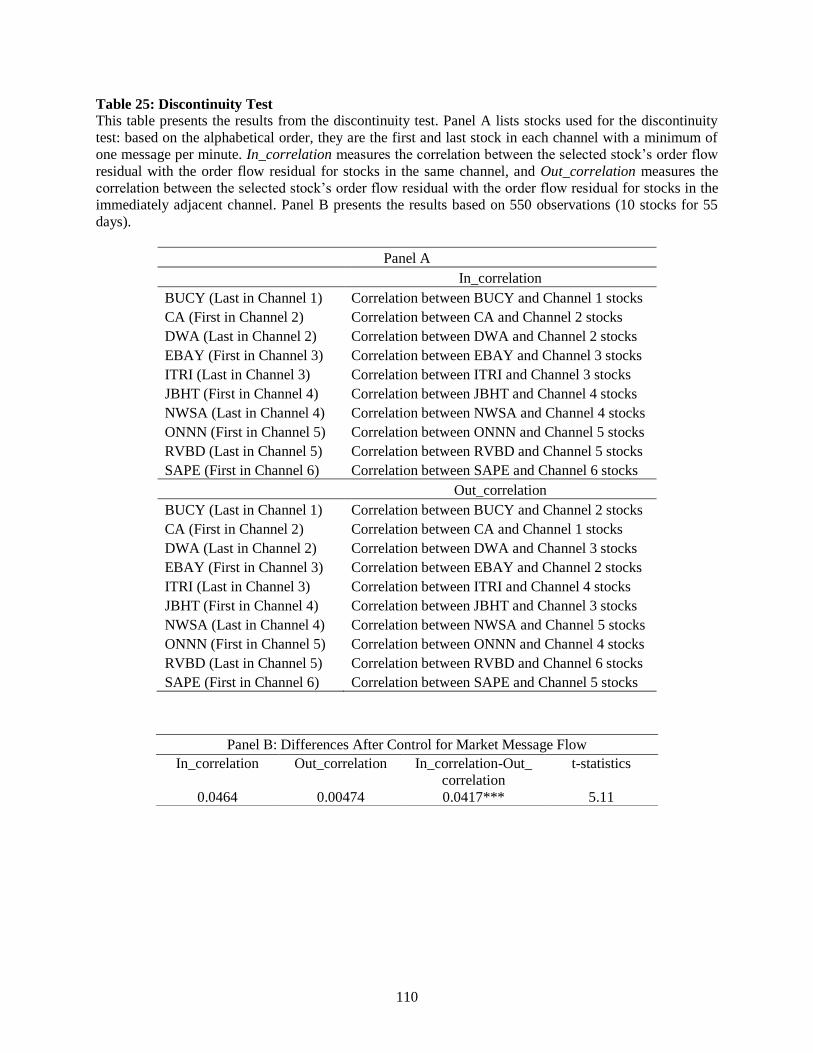
110

Table 25: Discontinuity Test

This table presents the results from the discontinuity test. Panel A lists stocks used for the discontinuity

test: based on the alphabetical order, they are the first and last stock in each channel with a minimum of

one message per minute. In_correlation measures the correlation between the selected stock’s order flow

residual with the order flow residual for stocks in the same channel, and Out_correlation measures the

correlation between the selected stock’s order flow residual with the order flow residual for stocks in the

immediately adjacent channel. Panel B presents the results based on 550 observations (10 stocks for 55

days).

Panel A

In_correlation

BUCY (Last in Channel 1) Correlation between BUCY and Channel 1 stocks

CA (First in Channel 2) Correlation between CA and Channel 2 stocks

DWA (Last in Channel 2) Correlation between DWA and Channel 2 stocks

EBAY (First in Channel 3) Correlation between EBAY and Channel 3 stocks

ITRI (Last in Channel 3) Correlation between ITRI and Channel 3 stocks

JBHT (First in Channel 4) Correlation between JBHT and Channel 4 stocks

NWSA (Last in Channel 4) Correlation between NWSA and Channel 4 stocks

ONNN (First in Channel 5) Correlation between ONNN and Channel 5 stocks

RVBD (Last in Channel 5) Correlation between RVBD and Channel 5 stocks

SAPE (First in Channel 6) Correlation between SAPE and Channel 6 stocks

Out_correlation

BUCY (Last in Channel 1) Correlation between BUCY and Channel 2 stocks

CA (First in Channel 2) Correlation between CA and Channel 1 stocks

DWA (Last in Channel 2) Correlation between DWA and Channel 3 stocks

EBAY (First in Channel 3) Correlation between EBAY and Channel 2 stocks

ITRI (Last in Channel 3) Correlation between ITRI and Channel 4 stocks

JBHT (First in Channel 4) Correlation between JBHT and Channel 3 stocks

NWSA (Last in Channel 4) Correlation between NWSA and Channel 5 stocks

ONNN (First in Channel 5) Correlation between ONNN and Channel 4 stocks

RVBD (Last in Channel 5) Correlation between RVBD and Channel 6 stocks

SAPE (First in Channel 6) Correlation between SAPE and Channel 5 stocks

Panel B: Differences After Control for Market Message Flow

In_correlation Out_correlation In_correlation-Out_

correlation

t-statistics

0.0464 0.00474 0.0417*** 5.11

111

Table 26: Diff-in-diff Test

This table presents the diff-in-diff regression for 55 stocks that switch ticker symbol from January, 2010

to November 18, 2011. The control group changes ticker symbol but remain in the same channel; the

treatment group changes ticker symbol as well as the channel. The before period has 30 days before the

ticker change and the after period has 30 days after the ticker change. The dependent variable is the

message flow correlation with the original channel.

Diff-in-Diff Table

Treatment Group Control Group Diff

Before 0.485*** 0.507*** -0.0222**

(0.00519) (0.00916) (0.0106)

After 0.444*** 0.495*** -0.0513***

(0.00523) (0.00921) (0.0106)

Diff -0.0414*** -0.0123 -0.0291*

(0.151) (0.013) (0.015)

112

Table 27: Effect of Technology Shocks for Liquidity

The table presents the event study of the technology shocks for the four liquidity measures. For each stock

per day, qt_spread is the time-weighted quoted spread, sz_wt_eff_spread is the trade size-weighted

effective spread, depth is the depth at the best bid and ask, depth10 is the cumulative depth for orders 10

cents below the best bid and 10 cents above the best ask, after is a dummy variable, logvol is the log of

the daily volume, price is the daily price level of the stock, and range equals to highest trading price

minus the lowest trading price on each day for each stock. Standard errors are in parentheses, and ***, **

and * represent significance at the 1%, 5%, and 10% levels, respectively.

(1) (2) (3) (4)

Variables qt_spread sz_wt_eff_spread depth depth10

after -0.000394 0.0000115 -68.31 -2,015***

(0.00124) (0.000301) (93.46) (736.50)

logvol -0.00418*** -0.000713** -114.60 -5,317***

(0.00147) (0.000358) (111.30) (877.20)

prc 0.000907*** 0.000234*** 25.42** 118.3

(0.000141) (0.0000343) (10.66) (83.98)

range 0.0167*** 0.00441*** 126.90** -1,057**

(0.000793) (0.000193) (59.91) (472.10)

Constant 0.0596*** 0.0127** 5,001*** 118,697***

(0.0211) (0.00512) (1,590) (12,527)

Observations 5,858 5,858 5,858 5,858

R-squared 0.077 0.092 0.003 0.012

Number of ticker 118 118 118 118

113

Table 28: Effect of Technology Shocks on Price Efficiency and Volume

The table presents the event study of the technology shocks on price efficiency and volume. For each

stock per day, volatility is the one-minute volatility, variance is the one-minute variance ratio, and volume

is the daily volume.

(1) (2) (3)

Variables sigma_all all_ratio volume

after 0.0000249 * -0.00289 131,609

(0.0000128) (0.00332) (142,487)

Constant 0.00114*** 0.951*** 5.971e + 06***

(9.04e-06) (0.00234) (100,625)

Observations 5,858 5,856 5,860

R-squared 0.001 0.000 0.000

Number of ticker 118 118 118

Standard errors are in parentheses.

*** p < 0.01, ** p < 0.05, * p < 0.1

114

Figure 1: Example of Hidden orders and their executions

This diagram provides an example of hidden orders which are invisible to market participants. Hidden

order prices and depths appear in grey and displayed order prices and depths appear in black. Market

participants observe that the best bid is $1.01 and the best ask is $1.06. Although the total depths for the

best displayed bid are 5500 shares, market participants can only observe the displayed 4000 shares. The

same holds for the total depths at the best displayed ask. In this example, the best bid and ask prices are

provided by hidden orders. The true best bid is $1.03 for 850 shares, and the true best ask is $1.04 for 900

shares.

Panel A: Diagram of a limit order book

Panel B: A 300-share sell market order comes to the market

115

Figure 1: (Continued)

Panel C: A 1500-share sell market order comes to the market

Panel D: A 6000-share sell market order comes to the market

116

Figure 2: Intraday Spread in Percentage

The solid line displays the intraday spread for hidden orders, the dashed line shows the intraday spread for

displayed orders, and the dotted lines exhibit the true spread, for which the true ask is the minimum of all

of the hidden and displayed sell order prices, and the true bid is the maximum of all of the hidden and

displayed buy order prices.

117

Figure 3: Historical volume of odd-lots

This graph shows the historical market shares of NYSE odd-lots from 1950-2004 in terms of volume. The

data are from the NYSE fact book.

118

Figure 4: Time Series Variation of Odd Lot Trades

This figure illustrates total level of odd lot trades and volume from January 2008 to November 2011.

Panel A demonstrates the number of odd lot trades as a percentage of total transactions. Panel B

demonstrates the odd lot trade volume as a percentage of total trades.

119

Figure 5: Cross-Sectional Variation of Odd-lot Trades

This figure illustrates the level of missing trades across the 120 stocks. Panel A demonstrates the

percentage the number of odd lot trades in 2008-2009 NASDAQ HF sample and Panel B demonstrates

the percentage of odd lot volume in 2008-2009 NASDAQ HF sample. Panel C demonstrates the

percentage the number of odd lot trades in 2010-2011 NASDAQ ITCH sample and Panel D demonstrates

the percentage of odd lot volume in 2010-2011 NASDAQ ITCH sample.

120

Figure 6: Odd-Lot Trades by Trader Type

This figure displays the time series odd-lots percentage breaking down to four different trade types. The

first letter symbolizes the liquidity taker and the second one is the liquidity maker. Letter H stands for

higher liquidity traders and N stands for non liquidity traders. For example, an HN trade means that a high

frequency trader takes liquidity from a non-high frequency trader.

121

Figure 7: Histogram of Odd-lot Trades

122

Figure 8: Odd-lot Trades by Trader Type

This figure displays the usage of specific odd-lot sizes by the four different trade types. The first letter

symbolizes the liquidity taker and the second one is the liquidity maker. Letter H stands for higher

liquidity traders and N stands for non liquidity traders. For example, an HN trade means that a high

frequency trader takes liquidity from a non-high frequency trader. The sample period is from 2008-2009.

123

Figure 9: Length of consecutive Odd Lot Sequences

This is the histogram on the number of consecutive odd-lots in each odd-lot sequence, which is defined as

a sequence of odd lots without round or mixed lots between them.

124

Figure 10: Stocks Shows Zero Individual Trading as A Result of 5000-dollar Cut-off Value

This figure demonstrates the percentage of stocks showing 0 individual trades by applying Lee and

Radhakrishna’s 5,000 dollars dollar cut-off to the TAQ data. Because TAQ does not report trades less

than 100 shares, we observe 0 trading for individual trades for stocks with a price higher than $50. The

graph is computed through CRSP. Panel A is the percentage of stocks with zero individual trades. Panel B

weights each stock by their dollar volume and Panel C provides value weighted average.

125

REFERENCES

Aitken, Michael J., Henk Berkman, and Derek Mak, 2001, The use of undisclosed limit orders

on the Australian stock exchange, Journal of Banking and Finance 25, 1589-1603.

Aghion, Philippe and Peter Howitt, 1992, A model of growth through creative destruction,

Econometrica 60, 323-351.

Alexander, Gordon J., and Mark A. Peterson, 2007, An analysis of trade-size clustering and its

relation to stealth trading, Journal of Financial Economics 84, 435-471.

Amihud, Yakov, 2002, Illiquidity and stock returns: cross-section and time series effects,

Journal of Financial Markets 5, 31-56.

Anand, Amber, and Daniel G. Waver, 2004, Can order exposure be mandated? Journal of

Financial Market 7, 405- 426.

Ashenfelter, Orley and David Bloom, 1993, Lawyers as agents of the devil in a prisoner's

dilemma game, NBER Working paper, Princeton University and Columbia University.

Barber, Brad M., Terrance Odean, and Ning Zhu, 2009, Do noise traders move markets? Review

of Financial Studies 22, 151–186.

Barclay, Michael J., and Jerold B. Warner, 1993, Stealth trading and volatility: which trades

move prices? Journal of Financial Economics 34, 281-305.

Baron, Matthew, Jonathan, Brogaard, and Andrei Kirilenko, 2012, The trading profits of high

frequency traders, Working paper, Princeton University, University of Washington and

MIT Sloan School of Management.

Bekaert, Geert, Robert J. Hodrick and Xiaoyan Zhang, 2009, International stock return

comovements, Journal of Finance 64, 2591-2626.

Belter, Klaus, 2007, Partial vs. full display limit orders: the order display choice and its effects

on order management and execution quality, Working paper, Aarhus School of Business.

Bessembinder, Hendrik, and Marios Panayides, and Kumar Venkataraman, 2009, Hidden

liquidity: an analysis of order exposure strategies in electronic stock market, Journal of

Financial Economics 94, 361-383.

Biais, Bruno, Christopher Bisière and Chester S. Spatt, 2003, Imperfect competition in financial

markets: ISLAND vs. NASDAQ, GSIA Working paper 2003-E41, Carnegie Mellon

University, Tepper School of Business.

Biais, Bruno, Thierry Foucault, and Sophie Moinas, 2013, Equilibrium High-Frequency Trading,

Working paper, Toulouse School of Economics, HEC Paris and Toulouse School of

Economics.

126

Biais, Bruno, and Paul Woolley, 2011, High-frequency trading, Working paper, Toulouse

University and London School of Economics.

Bloomfield, Robert, Maureen O’Hara and Gideon Saar, 2011, Hidden liquidity: some new light

on dark trading, Working paper, Cornell University.

Boehmer, Ekkehard, Charles M. Jones and Xiaoyan Zhang, 2008, Which shorts are informed?,

Journal of Finance, 63 491-527.

Boehmer, Ekkehart, Gideon Saar, and Lei Yu, 2005, Lifting the Veil: An analysis of pre-trade

transparency at the NYSE, Journal of Finance 60, 783-815.

Boulatov, Alex and Thomas J. George, 2011, Hidden and displayed liquidity in securities

markets with informed liquidity providers, Working paper, Moscow State University and

University of Houston.

Brogaard, Jonathan, 2011a, The activity of high-frequency traders, Working paper, University of

Washington.

Brogaard, Jonathan, 2011b, High-frequency trading and volatility, Working paper, University of

Washington.

Brogaard, Jonathan, 2011c, High frequency trading, information, and profits, Working paper,

University of Washington.

Brogaard, Jonathan, Terrence Hendershott and Ryan Riordan, 2013, High frequency trading and

price discovery, Working paper, University of Washington, University of California,

Berkley, and University of Ontario Institute of Technology.

Busse, Jeffrey A., and T. Clifton Green, 2002, Market efficiency in real time, Journal of

Financial Economics 65, 415-437.

Buti, Sabrina, and Barbara Rindi, 2011, Undisclosed orders and optimal submission strategies in

a dynamic limit order market, Working paper, University of Toronto and Bocconi

University.

Campbell, John Y., Tarun Ramadorai, and Allie Schwartz, 2009, Caught on tape: institutional

trading, stock returns, and earnings announcements, Journal of Financial Economics 92,

66-91.

Carhart, Mark M., 1997, On persistence in mutual fund performance, Journal of Finance 52, 57-

82.

Cavaglia, Stefano, Brightman Chris, and Michael Aked, 2000, The increasing importance of

industry factors, Financial Analyst Journal 56, 41-54.

Chaboud, Alain, Benjamin Chiquoine, Erik Hjalmarsson, and Clara Vega, 2009, Rise of the

machines: algorithmic trading in the foreign exchange market, Working paper, Board of

Governors of the Federal Reserve System.

127

Chakravarty, Sugato, 2001, Stealth-trading: which traders' trades move stock prices? Journal of

Financial Economics 61, 289-307.

Chakravarty, Sugato, Pankaj Jain, James Upson, and Robert Wood, 2011, Clean sweep: informed

trading through inter-market sweep orders, Working paper, Purdue University and

University of Memphis.

Chan, K.C. and William G. Christie, 1995, Market structural and the intraday pattern of bid-ask

spreads for NASDAQ securities. Journal of Business 68, 35-60.

Chan, Kalok, and Wai-Ming Fong, 2000, trade size, order imbalance, and the volatility-volume

relation, Journal of Financial Economics 57, 247-273.

Chen, Qi, Itay Goldstein, and Wei Jiang, 2007, Price informativeness and investment sensitivity

to stock price, Review of Financial Studies 20, 619-650.

Choe, Hyuk, and Oliver Hansch, 2005, which trades move stock prices in the internet age?

Working paper, Pennsylvania State University and Seoul National University.

Chordia, Tarun, Amit Goyal, and Narasimhan Jegadeesh, 2011, Buyers versus sellers: who

initiates trades and when? Working paper, Emory University and University of Lausanne.

Chordia, Tarun, Richard. Roll and Avanidhar Subrahmanyam, 2002, Order imbalance, liquidity,

and market returns, Journal of Financial Economics 65, 111-130.

Chordia, Tarun, and Avanidhar Subrahmanyam, 2004, Order imbalance and individual stock

returns: theory and evidence, Journal of Financial Economics 72, 485-518.

Christie, William G., and Paul H. Schulz, 1994, Why do NASDAQ market makers avoid odd-

eighth quotes? Journal of Finance 49, 1813-1840.

Christoffersen, Susan Kerr, and Ya Tang, 2009, Institutional herding and information cascades:

evidence from daily trades, Working paper, McGill University.

Copeland, Thomas E., and Dan Galai, 1983, Information effects on the bid-ask spread, The

Journal of Finance 38, 1457-1469.

De Winne, Ruby and D’Hondt, 2007, Hide-and-seek in the market: placing and detecting hidden

orders, Review of Finance 11, 663-692.

Dyl, Edward A., and Edwin D. Maberly, 1992, Odd-lot transactions around the turn of the year

and the January effect, Journal of Financial and Quantitative Analysis 27, 591-604.

Easley, David, Marcos M. Lopez de Prado, and Maureen O’Hara, 2011a, The microstructure of

the flash crash: flow toxicity, liquidity crashes and the probability of informed trading,

Journal of Portfolio Management 37, 118-128.

128

Easley, David, Marcos M. Lopez de Prado, and Maureen O’Hara, 2012a, Flow toxicity and

liquidity in a high frequency world, Review of Financial Studies 25, 1457-1493.

Easley, David, Marcos M. Lopez de Prado, and Maureen O’Hara, 2012b, The Volume Clock:

Insights into the High Frequency Paradigm, Journal of Portfolio Management, Winter.

Easley, David., Soeren Hvidkjaer, and Maureen O'Hara, 2002, Is information risk a determinant

of asset returns? Journal of Finance 57, 2185-2221.

Easely, David, Maureen O’Hara, and Joseph B. Paperman, 1996, Liquidity, information and

infrequently traded stocks, Journal of Finance 51, 1405-1436.

Easley, David, Maureen O’Hara, and Liyan Yang, 2010, Differential access to price information

in financial markets, work paper, Cornell University.

Egginton, Jared, Bonnie F. Van Ness and Robert A. Van Ness, 2011, Quote stuffing, Working

paper, Louisiana Tech University, University of Mississippi and University of

Mississippi.

Engle, Robert F., Robert Furstenberg, and Jeffery Russell, 2006, Measuring and modeling

execution cost and risk, Working paper, New York University.

Fama, Eugene F., and Kenneth R. French, 1993, Common risk factors in the returns on stocks

and bonds, Journal of Financial Economics 33, 3–56.

Fleming, Michael and Bruce Mizrach, 2009, The microstructure of a U.S. treasury ECN: the

BrokerTec platform, Working paper, Federal Reserve Bank of New York and Rutgers

University.

Foley, Sean, Katya Malinova, and Andreas Park, 2012, Dark trading on public exchanges,

working paper.

Frank, Robert, 2003, Are positional externalities different from other externalities? Working

paper, Cornell University.

Frank, Robert, 2005, Positional externalities cause large and preventable welfare losses,

American Economic Review 95, 137-141.

Frank, Robert, 2008, Should public policy respond to positional externalities? Journal of Public

Economics 92, 1777-1786.

Frank, Robert, and Ben Bernanke, 2010, Principles of Economics, McGraw-Hill.

Frey, Stefan, and Patrik Sandas, 2009, The impact of Iceberg orders in limit order books,

Working paper, University of Tubingen and University of Virginia.

Gai, Jiading, Chen Yao, and Mao Ye, 2012, The externalities of high frequency trading, Working

paper, University of Illinois at Urbana-Champaign.

129

Getry, William M., Deen Kemsley, and Christopher J. Mayer, 2003, Dividend taxes and share

prices: evidence from real estate investment trusts, Journal of Finance 58, 261-282.

Glode, Vincent, Richard C. Green and Richard Lowery, 2012, Financial expertise as an arms

race, Journal of Finance 67, 1723-1759.

Glosten, L., 1994. Is the electronic open limit order book inevitable? Journal of Finance 49,

1127-1161.

Gozluklu, Arie, 2010, Pre-trade transparency and informed trading: an experimental approach to

hidden liquidity, Working paper, Bocconi University.

Griffin, John. M. and George Andrew Karolyi, 1998, Another look at the role of the industrial

structure of markets for international diversification strategies, Journal of Financial

Economics 50, 351-373.

Grossman, Gene M. and Elhanan Helpman, 1991, Quality ladders in the theory of growth,

Review of Economics Studies 58, 43-61.

Hasbrouck, Joel and Gideon Saar, 2002, Limit orders and volatility in a hybrid market: the Island

ECN, Working paper, New York University and Cornell University.

Harris, Lawrence, 1991, Stock price clustering and discreteness, Review of Financial Studies 4,

389-415.

Harris, Lawrence, 1996, Does a large minimum price variation encourage order exposure?

Working paper, University of Southern California.

Harris, Lawrence, 1997, Order exposure and parasitic traders, Working paper, University of

Southern California.

Hasbrouck, Joel, 1991a, Measuring the Information Content of Stock Trades, Journal of Finance

46, 179-207.

Hasbrouck, Joel. 1991b. The summary informativeness of stock trades: An econometric analysis.

Review of Financial Studies 4, 571-595.

Hasbrouck, Joel. 1996. Order characteristics and stock price evolution an application to program

trading. Journal of Financial Economics 41, 129-149.

Hasbrouck, Joel, and Gideon Saar, 2009, Technology and liquidity provision: the blurring of

traditional definitions, Journal of Financial Markets 12, 143-172.

Hasbrouck, Joel, and Gideon Saar, 2011, Low-latency trading, Working paper, New York

University and Cornell University.

Hendershott, Terrence, Charles M. Jones, and Albert J. Menkveld, 2011, Does algorithmic

trading improve liquidity? Journal of Finance 66, 1-33.

130

Hendershott, Terrence, and Ryan Riordan, 2011, Algorithmic trading and information, Working

paper, University of California, Berkeley and University of Ontario Institute of

Technology.

Heston, Steven L., and K. Geert Rouwenhorst, 1994, Does industrial structure explain the

benefits of international diversification? Journal of Financial Economics 36, 3-27.

Hirshleifer, J.,1971. The private and social value of information and the reward to inventive

activity, American Economic Review 61, 561-574.

Hirschey, Nicholas H., 2012, Do High-Frequency Traders Anticipate Buying and Selling

Pressure? Working paper, London Business School.

Hvidkjaer, Soeren, 2006, A trade-based analysis of momentum, Review of Financial Studies 19,

457.

Hvidkjaer, Soeren, 2008, Small Trades and the Cross-Section of Stock Returns, Review of

Financial Studies 21, 1123-1151.

Jame, Russell, and Qing Tong, 2009, Retail investor industry herding, Working paper, Emory

University.

Jones, Charles I., and John C. Williams, 2000, Too much of a good thing? The economics of

investment in R&D, Journal of Economic Growth 5, 65-85.

Jovanovic, Boyan, and Albert J. Menkveld, 2011, Middlemen in limit order markets, Working

paper, VU University Amsterdam.

Kaniel, Ron, and Hong Liu, 2006, So what orders do informed traders use?, Journal of Business,

79, 1867-1913.

Kavajecz, Kenneth A., 1999, A specialist's quoted depth and the limit order book, Journal of

Finance 54, 747-771.

Kelley, Eric K., and Paul C. Paul, 2011, How wise are crowds? Insights from retail orders and

stock returns, Working paper, University of Arizona and Columbia University.

King, Benjamin F., 1966, Market and Industry factors in stock price behavior, Journal of

Business 39, 139-190.

Kirilenko, Andrei, Albert S. Kyle, Mehrdad Samadi, and Tuzun Tuzun, 2011, The flash crash:

The impact of high-frequency trading on an electronic market, Working paper, MIT

Sloan School of Management, University of Maryland, University of North Carolina at

Chapel Hill, and Federal Reserve Board.

Krigman, L., W. H. Shaw, and K. L. Womack, 1999, The persistence of IPO mispricing and the

predictive power of flipping, Journal of Finance 54, 1015-1044.

Kumar, K. Kiran, Ramabhadran S. Thirumalai, and Pradeep K. Yadav, 2009, Hiding Behind the

Veil: Pre-Trade Transparency, Informed Traders and Market Quality, Working paper,

131

National Institute of Securities Markets, Mumbai, India, Indian School of Business and

University of Oklahoma.

Kyle, Albert S., Anna A. Obizhaeva, and Tugkan Tuzun, 2010, Trading game invariance in the

TAQ dataset, Working paper, University of Maryland.

Hendershott, Terrence, and Charles M. Jones, 2005, Island goes dark: transparency,

fragmentation and Regulation, Review of Financial Studies 18, 743-793.

Lakonishok, Josef, and Edwin Maberly, 1990, The weekend effect: trading patterns of individual

and institutional investors, Journal of Finance 49, 231-243.

Lee, Charles M.C., and Balkrishna Radhakrishna, 2000, Inferring investor behavior: evidence

from TORQ data, Journal of Financial Markets 3, 83-111.

Lessard, Donald, 1974, World, national, and industry factors in equity returns, Journal of

Finance 29, 379-391.

Lessard, Donald, 1976, World, country, and industry relationships in equity returns: implications

for risk reduction through international diversification. Financial Analysts Journal 32,

32-38.

Linnainmaa, Juhani T., 2010, Do limit orders alter inferences about investor performance and

behavior?, Journal of Finance 65, 1473- 1506.

Livingston, Miles, 1977, Industry movements of common stocks. Journal of Finance 32, 861-

874.

Lo, Andrew W., A. Craig MacKinlay, 1988, Stock market prices do not follow random walks:

Evidence from a simple specification test, Review of Financial Studies 1, 41-66.

Malkiel, Burton, 1981, A random walk down wall street, Norton, New York.

Malmendier, Ulrike, and Devin Shanthikumar, 2007, Are small investors naive about incentives?

Journal of Financial Economics 85, 457-489.

McInish, Thomas H., and Robert A. Wood, 1992, An analysis of intraday patterns in bid/ask

spread for NYSE stocks, Journal of Finance 47, 753-764.

McInish, Thomas H., and Robert A. Wood, 1995, Hidden orders on the NYSE, Journal of

Portfolio Management 21, 19-26.

Moinas, Sophie, 2010, Hidden orders and liquidity in order driven markets, Working paper,

Toulous University.

Moulton, Pamela C. 2005, You can't always get what you want: trade-size clustering and

quantity choice in liquidity, Journal of Financial Economics 78, 89-119.

132

Myers, Stephen L., 1973, A re-examination of market and industry factors in stock price

behavior, Journal of Finance 28, 695-705.

Nimalendran, Mahen, Jay R. Ritter, and D. Zhang, 2007, Do today's trades affect tomorrow's

IPO allocations? Journal of Financial Economics 84, 87-109.

O’Hara, Maureen, 2010, What is a quote?, Journal of Trading 5, 10-16.

O’Hara, Maureen, and Mao Ye, 2011, Is market fragmentation harming market quality? Journal

of Financial Economics 100, 459-474.

O'Hara, Maureen, Chen Yao, and Mao Ye, 2011, What's not there: The odd-lot bias in market

data, Working paper, Cornell University, University of Illinois at Urbana-Champaign,

and University of Illinois at Urbana-Champaign.

Pagnotta, Emiliano and Thomas Philippon, 2012, Competing on speed, Working paper, New

York University.

Pan, Jun, and Allen M. Poteshman, 2006, The information in option volume for future stock

prices, Review of Financial Studies 19, 871–908.

Parlour, Christine, and Duane J. Seppi, 2008, Limit order markets: a survey handbook of

financial intermediation & banking.

Pastor, Lubos, and Robert F. Stambaugh, 2003, Liquidity risk and expected stock returns,

Journal of Political Economy 111, 642-685.

Patterson, Scott, 2012, Crown Business, New York.

Ritter, Jay R., 1988, The buying and selling behavior of individual investors at the turn of the

year, Journal of Finance 43, 701-717.

Rock, K., 1990. The specialist's order book and price anomalies. Unpublished working paper,

Graduate School of Business, Harvard University.

Roll, Richard., 1992, Industrial structure and the comparative behavior of international stock

market indices, Journal of Finance 47, 3-41.

Rozeff, Michael S., 1985, The tax-loss selling hypothesis: new evidence from share shifts,

Working paper, University of Iowa.

Sadka, Ronnie, 2006, Momentum and post-earnings-announcement drift anomalies: the role of

liquidity risk, Journal of Financial Economics 80, 309-349.

Sias, Richard W., 1997, Price pressure and the role of institutional investors in closed-end funds,

Journal of Financial Research 20, 211-229.

Stigler, George J., 1957, Perfect competition, historically contemplated, Journal of Political

Economy 65, 1-17.

133

Tirole, Jean, 1988, The theory of industrial organization, MIT press.

Tuttle, Laura, 2003, Hidden orders, trading costs and information, Working paper, University of

Kansas.

Wahal, Sunil, 2012, Electronic markets and trading algorithms, The Journal of Trading 7, 26-36.

Wooldridge, Jeffery M., 2002, Econometric analysis of cross section and panel data, MIT press.

Wu, Hsiu-Xwang, 1972, Odd lot trading in the stock market and its market impact, Journal of

Financial and Quantitative Analysis 7, 1321-1344.

134

APPENDIX A

THE IMPACT OF ODD LOT TRUNCATION ON PREVIOUS LITERATURE

One natural question is whether odd lot truncation affects the conclusion of any previous

studies. Addressing this question is challenging because our sample containing odd lot trades is

recent, while most published work is based on older data with longer time horizons. Fortunately,

under some specifications, we can evaluate the impact of odd lot truncation even without

knowing the exact magnitude of odd lot trading. In this section, we illustrate this point by

showing how odd lot truncation can reconcile differences between two papers on retail trading

and the cross-section of stock return (Barber, Odean and Zhu (2009) and Hvidkjaer (2008)).64

Barber, Odean and Zhu (2009) and Hvidkjaer (2008) are two closely related papers

examining the relationship between buy/sell pressure for retail traders and future stock returns.

They employ the same dataset: TAQ data and Institute for the Study of Security Markets

(ISSM).65

They both use small trades in TAQ/ISSM data as a proxy for individual sentiments,

and they construct portfolios based on the relative frequency of small buyer- and seller-initiated

transactions. However, despite the similarity of methods, these two papers find different results

on whether stocks with small-trade selling pressure outperform stocks with small-trade buying

pressure in short time horizons.

While technical differences can account for part of this discrepancy, these authors

acknowledge that their results are different at one-month horizons66

. Hvidkjaer (2008) finds that

64

We are grateful to Soeren Hvidjkaer for providing us with his computer code. 65

As a predecessor of the TAQ data, ISSM data also does not carry the information on odd lots. 66

See Barber, Hvidkjaer, Odean and Zhu(2006) for discussion of how their results differ and possible

explanations.

135

monthly returns of stocks with buying pressure over the past one month are significantly lower

than those with past selling pressures, but Barber, Odean and Zhu do not. The puzzle is why does

Hvidkjaer (2008) produce a faster reversal than Barber, Odean and Zhu (2009)?

We believe the differences in their results are driven by odd lot truncation. To understand

why, consider how each paper forms its sample. Barber, Odean and Zhu (2009) apply a $5,000

cut-off for individual trades. An unintended consequence of this cut-off value is that they

eliminate any stock with a price above $50 from their sample. For example, the stock price of

Atlantic Richfield Company (ticker symbol: ARC) is around $115 in 1991. Because there are no

odd lots reported to ISSM, the minimum dollar value of the trades for ARC is around $11,500.

This is greater than the $5,000 cut-off value, so, Barber, Odean and Zhu (2009) observe zero

individual trades for ARC and the stock is eliminated from their sample.67

Hvidkjaer (2008), alternatively, ensures that small trades exist in all stocks by the

following two adjustments. First, firms have different cut-off values based on size. Each month s,

firms are sorted into quintiles based on firm size. Within each size quintile j, the 99th

stock price

percentile (P99js) is found, and P99j is compute as the average of P99js across all months in the

sample. Small-trade cut-off points are then set as 100* P99j rounded to the nearest $100. The

cut-off value is then based on firm-size quintiles, which ensures that 99 percent of stocks will

have small trades in the TAQ dataset. To ensure that the other 1 percent has small trades,

Hvidkjaer (2008) sets the share cut-off points as the ratio of the dollar cut-off point to the share

price rounded up to the nearest round-lot. For example, Capital Cities/ABC (ticker symbol:

CCB), has a stock price of $450. Therefore, even a $16, 400 dollar cut-off will generate a share

cut-off less than 100 shares. However, Hvidkjaer (2008) rounds the ratio of the dollar cut-off to

the share price up to the nearest round lot, which means that Hvidkjaer (2008) treats 100 shares

67

Barber, Odean and Zhu (2009) also eliminate any stock with less than 10 individual trades

136

in CCB as individual trades, while Barber, Odean and Zhu (2009) eliminate the stock from their

sample.

In summary, Barber, Odean and Zhu (2009) eliminate high price stocks in their sample

using fixed dollar cut-offs, whereas Hvidkjaer (2008) keeps all the stocks in the sample. These

sampling differences lead to fundamental differences in the value-weighted returns because

stocks above $50 constitute a significant proportion of the market cap. In particular, applying the

$5,000 dollar cut-off to the sample used in Hvidkjaer (2008), we find that up to 65 percent of

market cap is coming from stocks with prices above $50, despite their representing only 6

percent of stocks.68

Consequently, Barber, Odean and Zhu (2009)’s $5,000 cut-off cannot detect

return reversal for any stock with a price above $50, but Hvidkjaer’s cut-off can document this

reversal. The stocks with price above $50 tend to be large stocks, and Hvidkjaer (2008) also

shows that larger stocks have quicker reversal whereas the reversal for small stocks can last as

long as three years. As a result, Barber, Odean and Zhu (2009) eliminate some stocks with

quicker reversal out of their sample. We conjecture that it is this difference that produces

Hvidkjaer’s (2008) quicker reversal.

To test this conjecture, we obtained all the codes and data from Hvidkjaer (2008), and

then modified his code in two ways. First, we changed the cut-off value to $5,000. Second,

instead of rounding the share cut-off up to the closest round lot, we simply kept the original share

cut-off. With these new cut-offs, we find that stocks favored by individual traders do not

underperform stocks with high selling pressure (i.e. the return of quintile 1 and 5 are not

68

Market cap equals price*shares outstanding. As a result, high price stocks have a natural trend to have

higher impact on market cap and, in unreported results; we also find that stocks with higher prices tend to have a

larger number of shares outstanding.

137

statistically significant and neither is their difference).69

The result is demonstrated in Table A.1.

Thus, we can reproduce Barber, Odean and Zhu’s (2009) results in Hvidkjaer’s analysis. The

dichotomy in their results is thus due to odd lot truncation and its effects on sample selection.

One interesting fact about this truncation is that it is independent of the actual magnitude

of odd lots – we do not even use the level of odd lot activity in the replication! The truncation is

actually based on price level. But it is because there are no odd lot trades in TAQ/ISSM that

using cut-offs for retail trades leads to the removal of high price stocks that constitute a

significant part of the value-weighted portfolio. The truncation then generates significant return

patterns by truncating high price stocks.

These results demonstrate why it is important for all researchers to be aware of the fact

that TAQ/ISSM data do not have trades for less than 100 shares. This omission will bias any

study using arbitrary trade size cut-offs to proxy particular trader groups. We also suggest

caution in interpreting existing results due to the sample selection biases that may have been

present. Given the increasing incidence of odd lot trades, these truncation problems may become

an even greater problem going forward.

69

The magnitude is slightly different from the Barber, Odean and Zhu’s result (Barber, Odean, Hvidkjaer

and Zhu, 2006), probably because of other slight differences in their methodology. For example, they use a slightly

different measure of order imbalance and slightly different variation of Lee and Ready (1991) mechanism to sign the

trades in NASDAQ.

138

Table A.1: Abnormal Returns by Applying $5,000 cut-off to Hvidkjaer (2008)

This table presents monthly percent abnormal return for value-weighted portfolios. Portfolios are formed

each month, January 1983 to December 2000 based on monthly measures of small trade imbalance.

Portfolio 1 has the highest sell imbalance, and portfolio 5 has the highest buy imbalance. The table

presents intercepts from a time series regression of portfolio excess return (raw return less risk free) on

four factors: market, size, value and momentum. The result for Hvidkjaer (2008) firm varying cut-off and

Barber, Odean and Zhu (2009) $5,000 cut-off are adapted from the joint note by Barber, Hvidkjaer,

Odean and Zhu (2006). The last column adopts the $5,000 cut-off to Hvidkjaer (2008) sample.

Monthly Four-Factor Alphas (%)

Order Imbalance

Quintile

Hvidkjaer (2008)

firm varying cut-off

Barber, Odean and

Zhu (2009) $5,000

cut-off

Hvidkjaer (2008)

with $5,000 cut-off

1 (Sold) 0.429 0.049 0.036

(2.58) (0.42) (0.32)

2 0.27 0.176 0.174

(2.4) (1.88) (1.33)

3 -0.025 0.022 0.215

(-0.36) (0.24) (1.76)

4 0.13 0.087 0.129

(1.9) (1.01) (1.06)

5 (Bought) -0.021 0.040 -0.050

(-0.17) (0.37) (-0.32)

B-S (5-1) -0.45 -0.009 0.086

(-1.98) (-0.05) (0.49)