Three Essays on Current International Financial Markets

Three Essays on Current International Financial Markets

Seungho Lee

A Thesis

In

The John Molson School of Business

Presented in Partial Fulfillment of the Requirements

For the Degree of

Doctor of Philosophy (Business Administration - Finance) at

Concordia University

Montreal, Quebec, Canada

March 2019

© Seungho Lee, 2019

ii

CONCORDIA UNIVERSITY

SCHOOL OF GRADUATE STUDIES

This is to certify that the thesis prepared

By: Seungho Lee

Entitled: Three Essays on Current International Financial Markets

and submitted in partial fulfillment of the requirements for the degree of

Doctor of Philosophy (Business Administration - Finance)

complies with the regulations of the University and meets the accepted standards with respect to

originality and quality.

Signed by the final examining committee:

Chair

Prof. Mahesh Sharma

External Examiner

Dr. Marie-Claude Beaulieu

External to Program

Dr. Bryan Campbell

Examiner

Dr. Sandra Betton

Examiner

Dr. Ramzi Ben-Abdallah

Thesis Supervisor

Dr. Lorne N. Switzer

Approved by

Dr. Kathleen Boies, Graduate Program Director

April 24, 2019

Dr. Anne-Marie Croteau, Dean

John Molson School of Business

iii

ABSTRACT

Three Essays on Current International Financial Markets

Seungho Lee, Ph. D.

Concordia University, 2019

This dissertation consists of three essays that address recent developments in international

financial markets that have been of concern for scholars, policymakers, and practitioners. The first

essay examines how cultural factors can influence individual investors’ trading behavior in

response to risk in nine Eurozone countries. The markets studied were particularly affected by the

global financial crisis, the subsequent European banking crisis, and the European sovereign debt

crisis. Using mutual fund flows as proxy of investors’ trading behavior, our evidence indicates that

a country culture variable significantly affects investors’ trading responsiveness to risk.

Specifically, the impact of risk on fund flows is significantly positive and is larger in scale in

countries with individualist cultures.

The second essay attempts to investigate the effects of negative interest rate policies (NIRP)

on foreign exchange and equity markets of eight European countries and Japan. To see the impacts

of these policies, event studies and regime-switching vector autoregressive regression analyses are

conducted for the nine countries that implement NIRP. The results provide valid evidence that the

announcement of NIRP has a transitory effect on currency depreciation; long term effects are less

evident. On the day of NIRP implementation, both currency and equity market returns reacted in

response to the event efficiently and negatively, especially in Switzerland’s case. These outcomes

suggest that simulative monetary policy by lowering interest rates below zero might have counter-

effects from those observed when interest rates are lowered, but to rates that remain positive.

Additionally, findings from the long term analyses explain that interest rate term structure and

cointegration level of local and the U.S. equity index may be related to effectiveness of NIRP in

currency and equity markets, respectively.

The last essay examines the determinants of the price of the leading cryptocurrency,

Bitcoin. The analyses identify a number of factors that significantly affect the returns to

investments in Bitcoin including: trading volume, high-low price spread, and extreme price change

in the previous period. The latter result supports the assertion that recent severe price fluctuations

in Bitcoin markets are primarily due to speculative investment activities. Furthermore, evidences

suggested in this study explain possibility of market compromise and inefficiency of the

cryptocurrency market, implying pivotal risks for Bitcoin market participants.

iv

Acknowledgements

I cannot express enough thanks to my supervisor Dr. Lorne N. Switzer for his continued

support and encouragement. It was a great privilege and honor to work and study under his

guidance. I would also like to thank the other members of the dissertation committee: Dr. Sandra

Betton and Dr. Ramzi Ben-Abdallah for their priceless advices. Besides, I appreciate Dr. Ernest J.

Scalberg for providing me invaluable supports over the period of my graduate studies.

I am extremely grateful to my parents, Keyhyun Lee and Jin-Kyung Kim, for their love,

caring and sacrifices for educating and preparing me for my future. They sacrificed their own

happiness, just so that I could be happy. It may take a lifetime, but I’ll do everything to repay for

what they have done for me. I also express my thanks to Taekho and Minji for being very

supportive brother and sister in law.

Last but not least, to my caring, loving, and supportive wife Kaori: my deepest gratitude.

Thank you for being there by my side at my hour of crisis. The journey through the difficult time

was easy as you all were there with me.

v

Contribution of Authors

Part of this thesis is published work with Lorne N. Switzer and Jun Wang.

Lee, S., Switzer, L.N. and Wang, J. (2018). “Risk, culture and investor behavior in small (but

notorious) Eurozone countries.” Journal of International Financial Markets, Institutions and

Money. (In Press)

The manuscript has been reformatted and reorganized according to the requirements set out in

the guideline of the School of Graduate Studies

vi

Table of Contents

List of Tables .............................................................................................................................................. vii

Chapter 1: Introduction ................................................................................................................................. 9

Chapter 2: Risk, Culture and Investor Behavior in Small (but notorious) Eurozone Countries ................. 16

2.1 Literature Review: ............................................................................................................................ 16

2.2. Sample Construction ........................................................................................................................ 17

2.2.1. Traditional Risk (bases on Standard Deviations) and Extreme Risk Estimation ...................... 18

2.3. Comparison of Two Risk Measures ................................................................................................. 20

2.4. Results Based on Individual Countries ............................................................................................ 22

2.5. Country Culture and Panel Regressions ........................................................................................... 25

Chapter 3: The Effects of Negative Interest Rates on Equity and Currency Markets ................................ 30


3.2 Hypotheses ........................................................................................................................................ 33

3.3 Data Description ............................................................................................................................... 35

3.4 Research Methodology ..................................................................................................................... 37

3.4.1 Definition of Currency and Index Return .................................................................................. 37

3.4.2. Event Study ............................................................................................................................... 39

3.4.3. Regime-Switching Vector Autoregressive Regression Model.................................................. 40

3.5. Results .............................................................................................................................................. 42

Chapter 4: Speculation, Overpricing, and Arbitrage in the Bitcoin Spot and Futures Markets .................. 52


4.2 Data Description ............................................................................................................................... 53

4.3 Research Methodology ..................................................................................................................... 56

4.4. Results .............................................................................................................................................. 63

4.4.1. Bitcoin Overpricing................................................................................................................... 64

4.4.2. Bitcoin Price Determinants ....................................................................................................... 65

4.4.3. Market Efficiency of Bitcoin Market ........................................................................................ 67

4.4.4. Further Discussion on Bitcoin Market Efficiency ................................................................. 72

Chapter 5: Conclusions ............................................................................................................................... 77

References ................................................................................................................................................... 80

Figures ........................................................................................................................................................ 86

Tables ........................................................................................................................................................ 102

vii

List of Tables

Table 1: Hofstede’s Cultural Dimension Score (Individualism vs Collectivism) ..................................... 102

Table 2. Statistics of Indices ..................................................................................................................... 103

Table 3. Summary Statistics of Daily/Weekly/Monthly Logarithmatic Percent Changes (i.e. returns) of

Indices ............................................................................................................................................... 104

Table 4. The Top 15-year Rankings of Volatility as Measured by Standard Deviation and by the

Percentage of Extreme Days for Each of the Nine European Countries ........................................... 107


Percentage of Extreme Weeks for Each of the Nine European Countries ........................................ 110


Percentage of Extreme Months for Each of the Nine European Countries ....................................... 113

Table 7. Regression Results of Equity Mutual Fund Net Flows on Risk Measures for Small Eurozone

Countries ........................................................................................................................................... 116

Table 8. Pooled regression results of equity mutual fund net flows on risk measures ............................. 121

Table 9. Simultaneous Regression Results (2 Groups: Individualism vs Collectivism), 2SLS Estimates 123

Table 10. Overview of Central Banks with Negative Policy Rates .......................................................... 124

Table 11. Reference Index and Currency for Countries that Implement NIRP ........................................ 124

Table 12. Summary Statistics of Daily Currency Return Logarithmatic Percent Changes ...................... 125

Table 13. Summary Statistics of Daily Index Return Logarithmatic Percent Changes ............................ 126

Table 14. Abnormal Return Analysis for Currency Exchange Markets ................................................... 127

Table 15. Abnormal Return Analysis for Equity Markets ........................................................................ 129

Table 16. Portfolio Average Abnormal Return Analysis for Currency Exchange Markets...................... 131

Table 17. Descriptive Statistics of Currency Mispricing Terms ............................................................... 133

Table 18. Panel Error Term Unit Root Test Results (July 2011 – July 2017) .......................................... 133

Table 19. By-country Error Term Unit Root Test Results (Before and After NIRP) ............................... 134

Table 20. Portfolio Average Abnormal Return Analysis for Equity Markets .......................................... 135

Table 21. Regression Results of Currency Return Analysis ..................................................................... 137

Table 22. Regression Results of Index Return Analysis ........................................................................... 138

Table 23. Comparison of Average Term Structure of Interests ................................................................ 139

Table 24. Indexes Cointegration with the U.S. Equity Market ................................................................. 139

Table 25. Results of VIX Volatility Index Regression Models ................................................................ 140

Table 26. Test Results for Equality of Variance and Mean ...................................................................... 141

viii

Table 27. GARCH Results for the Currency and Equity Returns ............................................................. 143

Table 28. Descriptive Statistics (May 2014 – December 2018, Monthly Data) ....................................... 145

Table 29. The Chronology of Government Regulations about Bitcoin Transaction................................. 146

Table 30. Correlation Matrix of Relevant Variables ................................................................................. 147

Table 31. Statistic Measures of Detrend Ratios of Bitcoin and Indexes ................................................... 148

Table 32. Regression Results with Monthly Data (April 2014 – December 2018) .................................. 149

Table 33. Regression Result with Daily Data (11 April 2014 – 30 January 2019) ................................... 154

Table 34. Unit Root Test Statistics for Fama (1984) Model ..................................................................... 157

Table 35. Results of Fama (1984) Model ................................................................................................. 157

Table 36. Wald Test Results of Fama (1984) Model ................................................................................ 158

Table 37. Descriptive Statistics of Mispricing Term and Absolute Value of Mispricing Term ............... 158

Table 38. Results of Bitcoin Futures Contracts Mispricing Term Unit Root Tests .................................. 159

Table 39. Chronology of Major Bitcoin Exchange Hacks ........................................................................ 159

Table 40. Top 10 Cryptocurrencies by Market Capitalization .................................................................. 160

Table 41. Estimates of Daily Futures Mispricing Regression with Dummy Variables ............................ 160

Table 42. EGARCH Results of Daily Futures Mispricing Regression with Dummy Variables ............... 161

9

Chapter 1: Introduction

My dissertation consists of three essays studying current issues on international financial

markets, covering diverse topics that include: a) the influence of culture on risk taking, b) the

impact of negative interest rate policies, and c) the behavior of cryptocurrency markets. These

topics are relatively new in finance, and the literature is still in a nascent stage. However, given

the increased recognition of the pertinence of these topics for global financial markets, we believe

that they are worthy areas for investigation.

The first essay investigates how culture moderates the impact of risk on small investors’

investment behavior in certain European countries. In this study, we look at investor responses to

risk, using both traditional and extreme risk measures for countries particularly affected by the

global financial crisis, the subsequent European banking crisis, and the European sovereign debt

crisis. Specifically, we construct standard risk measures based on the logarithmic percentage

changes of stock prices over different holding periods, with the assumptions of normality and

symmetry of return distribution and risk averse investors. The standard deviation of returns is also

an essential component of the traditional value-at-risk (VaR) measure. Such risk has been the

focus of regulators in seeking to establish how much financial institutions should put aside to

guard against the types of financial and operational risks banks (and the whole economy) face.

However, because the standard deviation does not capture the risk to the investor when the

distribution is non-symmetric, the traditional methods of calculating conventional value-at-risk

(VaR) measures that are based on a normal distribution are problematic and need to be interpreted

cautiously. Our second measure of risk that focuses on the distribution around the tail falls under

the rubric of extreme value theory. Extreme risk observations are identified as the mild outliers

in our samples, using the Tukey (1977) definition. They are computed using the percentage of

10

extreme days, weeks, and months over a specific year. One advantage of this extreme measure is

that we can decompose the total risk measure into a positive shock component and a negative

shock component, so that we can observe accurately the behavior such investors whose utility

responses to stock price change are asymmetric. Comparing the risks based on those two measures,

our results show that the extreme measures do not always cohere with the classical standard

deviation measure of risk for the countries considered.

Previous studies that examine these issues on large developed countries. In this study, we

examine nine relatively small European countries that have been exposed to several external

financial shocks over the past decade. More specifically, during the Global Financial crisis of

2007-08 and its aftermath, as G-7 countries generally recovered, relatively small economies such

as Belgium, Greece, Ireland, and Portugal became the main epicenters of continued instability.

For example, two of Belgium’s largest banks: Fortis and Dexia, underwent reorganization and

restructuring in order to survive. Fortis was spun off into two parts, while the Dutch group was

nationalized and the Belgian component was sold to the French bank BNP Paribas. Ireland and

Greece also went into a debt crisis in 2010. Allied Irish Bank and the Bank of Ireland received a

€7 billion rescue package in 2009 and went into recapitalization. The four largest banks of Greece,

National Bank of Greece SA, Piraeus Bank SA, Euro-bank Ergasias SA, and Alpha Bank AE,

have been the regular recipients of emergency loans from the European Central Bank (ECB).

Portugal applied for bail-out programs to cover its insolvent sovereign debt, drawing a €79 billion

from the International Monetary Fund (IMF), the European Financial Stabilization Mechanism

(EFSM), and the European Financial Stability Facility (EFSF). The debt crises of Ireland, Greece

and Portugal marked the start of the European sovereign debt crisis. One might posit that the

behavior of investors in such countries experiencing protracted financial instability may not be

11

consistent with those in larger countries that have more or less recovered. Therefore, in this paper,

we focus on individual investors’ response to the two aforementioned risk measures in those nine

relatively small Eurozone countries: Austria, Belgium, Denmark, Finland, Greece, Ireland,

Norway, Portugal, and Sweden that were epicenters of continued instability. By using mutual

fund flow as proxy of individual investor’s trading behavior, our results show significantly

different behavior of investors in those countries in terms of their sensitivity to risks.

We use the Hofstede (2001) culture dimension score on individualism vs. collectivism, as

the culture factor. The detailed score for each country can be found in Table 1. Based on

Hofstede’s classification, a country with higher cultural dimension score is classified more as

individualism culture. Individualism cultures describes societies that emphasize the moral worth

of the individuals, the exercise of individuals’ goals, desires, freedom, independence, and self-

reliance, and advocate that interests of individuals should be priority. Considering these culture

characteristics, we hypothesize that subjective assessments among individuals may explain the

differential or contrasting behaviors to risk: individual investors are more likely to take the

initiative in actively trading in response to market signals. In addition, investors may have high

risk tolerance, or are even adventuresome so exhibit “flight to risk” preferences, in the sense that

they invest more, rather than liquidating their investments when they sense risk. On the other

hand, societies with collectivist traditions emphasize cohesiveness amongst members, and

individuals in these societies are more likely to adjust their behavior with that of their cohorts,

rather than maximizing their own private benefits. Therefore, we propose that more collectivist

cultures constrain the initiative for investors to actively trading in response to market signals, and

individual investors with these cultural attributes are more likely to exhibit herding behavior and

are less sensitive to variations in the risk environment.

12

Our results support our hypothesis. We find that small investors’ responses to risk (both

traditional and extreme risks) in those small Eurozone countries are significantly influenced by

country culture. In other words, the culture variable affects the impact of risk on investor’s trading

behavior. The impact of risk on fund flow is significantly positive and are larger from countries

with more individualistic cultures. This implies that individual investors from these countries are

more sensitive to variations in risk, in terms of engaging in active trading in response to risk

changes. On the other hand, when controlling for the culture variable, small investors trading

behavior is not directly affected by risk. Our results emphasize the importance of cultural factors

in determining individual investor’s behavior in response to risk in small Eurozone countries. To

the best of our knowledge, our research is the first study that provides a detailed examination of

individual investor’s trading behavior and its key determinants in relatively small Eurozone

countries that were particularly affected by the European banking and European sovereign debt

crisis.

My second essay studies the impact of the negative-interest-rate-policies (NIRP) on

foreign exchange and equity markets of eight European countries and Japan. Recently, several

countries lowered their policy rates below zero percent as a means to emerge from severe

recessionary conditions. One could argue that Japan provides the archetypical case of NIRP

implementation. The country’s long recession, the so-called “Lost 20 Years,” has been one of the

most troublesome episodes for the world economy in recent decades. In order to stimulate the

Japanese economy, after unsuccessful attempts through public sector spending, quantitative

easing, and deregulation, the Japanese government went beyond its long-standing zero-interest-

rate policy as the Bank of Japan (BOJ) announced that the deposit rate for its accounts would be

-0.1 percent from February 16, 2016.

13

The execution of NIRP was not unprecedented. Prior to the Japanese experiment, several

European countries including Denmark, Norway, Sweden, and Switzerland implemented

negative interest policies at various times. Bosnia and Herzegovina, Bulgaria, and Hungary joined

the negative-interest-rate group in 2016. These three countries lowered their interest rates below

the zero bound to maintain the interest rate differentials between themselves and the eurozone

region, which were narrowing, as a result of the quantitative easing policy conducted by the ECB.

Policymakers in other countries have also considered NIRP as one of their monetary policy

options in order to overcome the possible recession or even stagflation.

Most studies on the economic effects of interest rate changes on financial markets have

been conducted for regimes characterized by positive interest rate bounds. The empirical literature

aimed at assessing how negative interest rates actually affect markets is still relatively limited.

Moreover, numerous questions about the negative interest rate concept still remain to be clarified.

This study aims to shed new light on the impact of NIRP on financial markets, and in turn enhance

our understanding of the limitations of stimulative monetary policies through lower interest rates.

I provide new evidence on the impact of negative interest rates on country exchange rates and

equity markets over various time horizons. Specifically, I analyze cases of Europe and Japan

using standard event studies as well as regime-switching vector autoregressive regression models.

The results suggest that NIRP has transitory effects on local currency returns. Longer term effects

are observed for only a few countries.

My last essay is an empirical analysis of the market for the world’s leading cryptocurrency,

Bitcoin. Bitcoin’s unprecedented price appreciation in 2017 was deemed by many observers of

international financial markets to represent a modern analogue to the Dutch tulip mania of the 17th

century. It is difficult to infer an appropriate/efficient market price for virtual currencies such as

14

Bitcoin. Simple expectations models are confounded by the limited historical data series available

since its inception, which hampers even rudimentary backtesting exercises.1 Bitcoin and other

cryptocurrencies that have emerged have achieved notoriety for several reasons including: a)

allowing transactions among parties in a transparent manner; b) providing liquidity without

arbitrary bounds set by centralized governmental authorities; and c) global compatibility. However,

the acceptability of Bitcoin and other cryptocurrencies remains a matter of controversy due to

factors that include: a) anonymity of wallet ownership permitting its use for money laundering and

other criminal activities; b) security issue of the virtual exchange system; and c) market instability,

reflected by extraordinary levels of volatility through time. These latter features are often used as

a key deterrent to widespread adoption of cryptocurrencies such as Bitcoin in the real economy.

Public pricing for Bitcoin commenced with the launch of the platform: BitcoinMarket.com in

March 2010. The price of Bitcoin at the outset of trading was a mere $0.003. After16 months, it

soared to $31. From that time forth, Bitcoin’s price has experienced periods of extreme volatility

characterised by episodes of explosive appreciations and depreciations, unhampered by regulated

price limits or circuit breakers such as prevail in many organized exchanges. Bitcoin’s appreciation

from under $1,000 to over $18,000 in 2017-18 has been viewed by numerous market

commentators as clear evidence of a classic irrational bubble.

As of December 31, 2017, the total market capitalization of Bitcoin was $237,466,518,547,

and its 24 hours trading volume recorded $12,136,306,688 with circulating supply of 16,774,450

BTCs.2 The sheer magnitude of this market has served as lightening rod for government regulators

1 The origin of Bitcoin remains nebulous. In October 2008, an unknown developer, Satoshi Nakamoto presented a

nine-page paper explaining the principal of a peer-to-peer electronic money system with blockchain technology. The

program named Bitcoin Core was opened to the public in 2009 which inaugurated the world’s biggest cryptocurrency

to date. This virtual currency was expected to become an attractive medium of exchange to compete with and even

supersede extant government-issued currencies. 2 Bitcoin Transaction Volume Data from coinmarketcap.com:

https://coinmarketcap.com/historical/20171231/

https://coinmarketcap.com/currencies/bitcoin/#markets

15

concerned with the integrity of international financial markets. Monetary authorities have begun

to address several questions in this regard including: a) the potential for Bitcoin and other

cryptocurrencies to substitute for and perhaps replace government-issued currencies; b) weakening

the ability of central banks to conduct monetary policy; and c) exposure to excessive speculative

behavior apart from that could creating instability in global financial markets.

Our contribution in this paper concerns c). Our focus is on whether Bitcoin prices are

determined in an efficient market. We address this issue from several perspectives. First, we

examine whether the pricing of Bitcoin can be explained by fundamental factors, as opposed to

technical perturbations reflected by excess speculative behavior. Our focus here is on markets in

which the cryptocurrency’s trading volume is highest: the U.S. Dollar, Chinese Yuan, Japanese

Yen, Euro, and South Korean Won, respectively. The study also examines the impact of several

macroeconomic drivers in the pricing of Bitcoin. Overall, the results support the assertion that

speculation can be considered the decisive factor underlying extreme volatility in the market. We

also test for pricing efficiency based on deviations from no-arbitrage between spot and futures

markets, using all CBOE and CME contracts traded from January 2018 contracts to March 2019.

The findings are not consistent with market efficiency for the futures prices. Furthermore, we find

that deviations from no-arbitrage prices widen during episodes of hackings, frauds issues and new

alternative cryptocurrency releases.

Chapters 2 to 4 correspond to my three essays and I conclude in Chapter 5.

16

Chapter 2: Risk, Culture and Investor Behavior in Small (but notorious) Eurozone

Countries

2.1 Literature Review:

How investors respond to risk has been a fundamental question in finance over the past

several decades. Most studies that use the traditional volatility measure (standard deviation of

stock returns) as it relates to investors’ trading behavior find mixed results. For instance, Sirri and

Tufano (1998), Barber, Odean, and Zheng (2005), Spiegel and Zhang (2013), and Kim (2017)

assert that fund flows are negatively related to risk. On the other hand, O’Neal (2004) and

Cashman et al. (2014) show a positive relation between fund inflows and risk. In a related vein,

Clifford et al. (2013) show that fund inflows from small investors are positively related to

unsystematic risk, while its relation to market risk is an open question. In a recent paper, Switzer

et al. (2017) examine the responses of investors to both an extreme risk measure, and the

traditional risk measure. They find that individual investors in G-7 countries have different

reactions and sensitivities to these two types of risk.

Why investors from those countries exhibit different responses to the same risk measures?

This is a critical important research question addressed in this study. Previous literature in this

line of research show cross-country investor behavioral variations. For example, Statman (2008)

investigates twenty-two countries and identifies significant differences in stated propensities for

risk taking of investors. Grinblatt and Keloharju (2001) emphasis culture variables in explaining

stockholder’s behavior. Eun, Wang, and Xiao (2015) find that culture influences stock price

synchronicity by affecting correlations in investors' trading activities and a country's information

environment.

While these studies typically show that individualism plays a significant role, they do not

explore the actual trading behavior of market participants across different countries. Several

17

researchers endeavor to ascertain the influence of such cultural dimension’s influence on

performance of financial markets. For example, by using use Hofstede’s culture dimension score

of 26 developed countries’ data, Chui et al. (2010) assert that country individualist score is

positively related to trading volume, volatility, and the magnitude of momentum profits.

Schmeling (2009) examines the impacts of investor sentiment on stock returns over 18

industrialized countries and finds that sentiment negatively forecasts aggregate stock returns.

Chang and Lin (2015) provide comparable results. According to their findings, national cultures

are associated with investor herding behavior. Such herding behavior is particularly observed in

countries where Confucianism is dominant and in less sophisticated stock markets. Although

these studies provide insights about how cultural factors influence overall investing activities in

equity markets, they do not consider investors’ attitudes against risk. Our paper provides new

evidence on this issue, as we examine individual investor’s trading behavior directly, as reflected

in portfolio position changes in response to changing risk, and how culture factor plays a role in

deterring investor’s trading behavior based on different risk levels.

2.2. Sample Construction

The data of mutual fund net flows used in this study are obtained from Thomson Reuters

DataStream and Thomson ONE. For each of the countries in this study, we choose the equity

index with the longest history as the major stock index to use in this study. The historical prices

for those indices are collected from Bloomberg and Thomson Reuters DataStream. Table 2

presents the details of the indices, including the time period and the number of observations for

each country when we use daily, weekly, and monthly data to calculate risk variables.

[Insert Table 2 here]

18

The index for our sample countries start from as early as 1987, including Finland’s OMS

Helsinki Index, Ireland’s Irish Overall Index, and Sweden’s Stockholm All-Share Index, to as late

as 1995, including Norway’s OMX Oslo All Share Index. The index for each country covers more

than 18 years, from as short as 225 months (19 years) to as long as 445 months (37 years).

Therefore, our sample period covers major historical events and business cycles, allowing for a

broad perspective for investigating investors’ behavior across different market conditions.

2.2.1. Traditional Risk (bases on Standard Deviations) and Extreme Risk Estimation

2.2.1.1. Traditional risk measure

In order to calculate both the standard and extreme risk measure, we need to calculate

returns from index prices first. Following previous literature, we use the logarithmic percentage

change (L%) of the stock index closing price to estimate returns on a daily, weekly, and monthly

basis, respectively. The summary statistics of logarithmic percentage changes for each country is

shown in Table 3. Panels A, B, and C in Table 3 provide the statistics of returns based on daily,

weekly, and monthly index prices, respectively. Panel D of Table 3 show the statistics during the

crisis period of 2008-09, in addition to the whole sample period.


As shown in Table 3, Greece has the lowest average returns during over its sample period

with -0.47% daily return, while Norway and Sweden have the highest returns during the sample

period. For all countries, significant departures from normality are observed for all data

frequencies, based on the Jarque-Bera statistics. At daily, weekly, and monthly frequencies, for

all nine countries, the markets show negative skewness and leptokurtosis. Jarque-Bera test rejects

19

the normality of the return distribution, implying that extreme measure of risk which does not

assume normal distribution may be better than standard risk measure. However, in this study we

compare and use both measures comprehensively to check investor’s response.

We then annualize the returns to get annualized geometric returns before calculating

traditional and extreme risks, assuming 252 effective trading days over a year. The traditional risk

measure is calculated as the annualized geometric standard deviation of the annualized return of

index for each country.

2.2.1.2. Extreme risk measure

The extreme measure of volatility is estimated as the percentage of extreme days, weeks

or months over a given period. Most researchers define the extreme value as the lowest or the

highest daily return of a stock market index observed over a given period (see e.g. Longin, 1996).

Jones, Walker and Wilson (2004) use the statistical distribution of annualized geometric return to

arbitrarily assign the distribution percentiles of 5% and 95% as cut-off points to distinguish

extreme values. In our study, we define the extreme dates as the observations that are less than

the difference between the lower quartile (Q1) and the value of 1.5 times of the interquartile range

(IQR, aka. the lower inner fence), or greater than the sum of the upper quartile (Q3) and the value

of 1.5 times of the interquartile range (IQR, aka. the upper inner fence), following the traditional

outlier classification methodology suggested by Tukey (1977):

Extreme Observation < Q1 - 1.5 × IQR, or Extreme Observation > Q3 + 1.5 × IQR

The range suggested by Tukey’s fence is slightly narrower than ±3σ in normally

distributed dataset, which declares about 1% of outliers. The extreme risk for a given year is

20

determined as the percentage of outliers during a given interval over that year, i.e. Percentage of

Extremes = No. of Outliers / Annual Trading Days (Weeks or Months).

2.3. Comparison of Two Risk Measures

One weakness of the traditional risk measure is that it is treats positive and negative price

changes symmetrically. However, the extreme volatility method provides both positive and

negative measures, and can be used to more accurately predict the behavior of risk-averse

investors who responses are more dramatic to negative changes than to the positive changes of

equity prices.

Figure 1 portrays the time series of the extreme measure of risk for Belgium, Greece,

Ireland, and Portugal from 1986-2016. As shown in these graphs, 35.8% of Ireland’s trading days

were characterized by extreme volatility in 2008; Belgian and Portuguese markets experienced

extreme volatility on more than 25% of their trading days in the same year, reflecting the strong

and persistent influence of the Global financial crisis in 2008-2009. Greece has 16% of extreme

days in 2015, somewhat higher than its experience in 2008, when 13% of annual trading days are

identified as extreme. In sum, the countries of this sample display some commonalities as well as

differences in regards to the timing and magnitude of their exposure to extreme volatility over the

sample period.

[Insert Figure 1 here]

In Table 4 to Table 6, we compare the traditional risk and extreme risk as measured by

the percentage of extreme days, weeks, or months by each country, respectively. As Table 4

shows, estimated from daily data, volatility rankings of conventional risk measure are similar to

21

those of extreme measures. In particular, the most volatile year and top ranked extreme years for

each country are almost identical for all the nine countries.


Using weekly data to measure risk, as shown in Table 5, both methodologies almost

cohere as well. In most countries, the most volatile 2 or 3 years are identical across risk measures.

However, Greece and Sweden are exceptional cases. Traditional risk measure shows 1998, 2015,

and 2014 as the most volatile years, while extreme measure suggests 2009, 1999, and 2011 in

Greece. For Sweden, extreme measure approach indicates 2001, 2000, and 2002 are the most

volatile years, whereas standard deviation catches 2008, 1998, and 2000 as the most unstable

periods.


Using monthly data, we observe that in the majority of cases, the most volatile years based

on extreme measure rankings also shown to be the most volatile based on traditional standard

deviation analysis ranking.


According to Switzer et al (2017), for G-7 countries of their study, volatility as captured

by the extreme measure shows similar patterns as the traditional volatility measure for most years.

Many commonalities in the attribution of high risk by both measures are observed, consistent

with Longin and Solnik (2001). However, differences are also observed, therefore, in our formal

test, we use both risk measures in our analyses of investor behavior.

22

2.4. Results Based on Individual Countries

In this research, our objective is to explain investor’s reaction to both risk variables by

measuring net flows to equity mutual funds against changes in both extreme volatility and

standard deviation changes. In our initial specifications, our dependent variables is the net flow

to equity mutual funds, with the risk measures lagged by one period in separate specifications.

Our control variables include returns (GeoMean), linear time trend (Time) to account for possible

secular growth in such funds, as well as a financial market crisis dummy variable (Crisis) in our

following models.

NetFlows(t) = α + βGeoMean(t-1) + γGeoStdDev(t-1) + δTime +λCrisis+ ε(t) Model 1

NetFlows(t) = α + βGeoMean(t-1) + γTotalExtr(t-1) + δ Time + λCrisis+ ε(t) Model 2

NetFlows(t) = α + βGeoMean(t-1) + γNegExtr(t-1) + ζPosExtr(t-1) + δ Time + λCrisis +ε(t)

Model 3

The variable NetFlow refers to the net flows to equity mutual funds, which are defined as

new sales plus reinvestment of income less withdrawals and transfers; TotalExtr denotes the

percentage of the number of extreme days over the measure horizon; NegExtr and PosExtr

represent the percentages of number of negative and positive extreme days over the measure

horizon, respectively; Crisis is a dummy variable to indicate the global financial crisis in 2008-9.

We expect that regression coefficients for mean returns are positive, and for market volatility are

negative, using the traditional or extreme day risk measures. In addition, when volatility is divided

into negative and positive components, the coefficient for the negative extreme days should be

negative since when stock market is negatively volatile, loss averse investors tend to hold less

equity, and the coefficient for the positive extreme days probably positive.

23

In order to anticipate the effect of the crisis variable, we compare summary statistics

during the financial crisis and the full sample period, based on Panel D of Table 3. In most

countries, the average monthly logarithmic percentage changes are negative, ranging between -

4.53 to -8.86 percent in 2008, and between -0.08 to 1.00 percent across the whole sample period.

The standard deviations also increase, during the financial crisis years, while Kurtosis decreases

in both 2008 and 2009. To prevent possible “overfitting” using the crisis dummy variable, we

also estimate our above three models with crisis dummy variable excluded.

In Table 7, we provide the regression results for the nine countries. Panel A (B) shows the

results for models 1-3 (4-6) that include (exclude) the crisis dummy variable.


There is no major difference in the results between Models 1-3 and Models 4-6, except

for the case of Belgium. The regression data shows significant statistic values for the traditional

measure of the risk in Austria’s case. Austrian retail investors also respond to extreme risk

measures, according to the result of Model 2. Furthermore, they move into markets subsequent to

negative extreme event. It is interesting to observe Austria’s case since the country is classified

as a relatively less individualistic culture according to Hofstede (2001). The only other country

in which investors respond to risk/extreme risk is Belgium, which is one of central figures of the

European banking crisis, suffering from the default of its two largest banks. As shown in Model

3, small investors in Belgium exhibit “flight to risk” behavior with increased negative extreme

measures, while there was fund outflow when there are positive extreme outliers. This gives us a

scenario that Belgian investors are attracted to negative extreme events (buying the dips) and exit

the markets on positive extreme events (sell at the high). However, when we run regression

24

without financial crisis dummy variable, such behavior is no longer observable in Models 4, 5

and 6.

For both Portugal and Ireland, the crisis dummy variable plays significant role, though in

different directions. With the crisis dummy included, funds flow out of the Portuguese market

while the opposite happens in Ireland. Hofstede’s individualism vs. collectivism score classifies

Portugal as a highly collectivist and Ireland as a highly individualistic culture. Indeed, investors

in highly individualistic cultures such as Ireland show high risk tolerance or even risk loving

proclivities. Hence, during the crisis period, they are more inclined to exhibit “flight to risk”

behavior. However, as we see from the separate country results, the impacts of risks on fund flow

are not monotonic with respect to increases of Hofstede’s individualism score. For example, at

the same level of individualism score, countries such as Sweden and Norway do not show

consistent result. Mutual fund flows of Greece, Norway, and Sweden are not significantly

responsive to changes in with any of the variables in the models. Norway and Sweden show high

levels of the individualism index. So far, the influence of culture on investor responsiveness to

risk is not clear-cut.

[Insert Figure 2 here]

These results are also depicted in Figure 2, where the relationship between investors’

behavior vs. extreme risk is shown for Belgium, Greece, Ireland, and Portugal. Figure 2.1 graphs

the case of Belgium, which is classified as an individualistic. The investors’ tendency of “flight

to risk” is evident in the graph, as it is observed that the increased risk of the equity market has

the negative relationship with the equity market’s mutual fund inflow, especially in 2002, 2005,

and 2008. In collectivist cultures, the relation between risk and fund flow is mixed. For example,

Figure 2.2 shows that in Greece, the equity market volatility moves in the same trend with the

25

equity market’s mutual fund inflow. However, for another collectivist culture country, Portugal,

the relation between risk and fund flow is negative, as shown in Figure 2.4. For Ireland, the mutual

fund flow is not responsive to changes in equity market volatility. Therefore, we cannot conclude

decisively that the cultural variable has monotonic impact on the relation between fund flow and

extreme risk.

The drawback of the regression based on individual countries is that we cannot incorporate

the culture variable directly in the regression, since it is a highly persistent/time-invariant. As a

consequence, in order to clearly understand the impact of culture in the relation between extreme

risk and fund flow, in the next section, we perform a serious of panel regressions including all the

nine countries with culture dummy variable added.

2.5. Country Culture and Panel Regressions

One important research focus of this study is on the effects of cultural factors on small

investors’ behavior in response to both traditional and extreme risks. In order to examine the

influence of individualism or collectivism in the market, we import Hofstede’s cultural dimension

score. As discussed in the previous section, according to the results of individual country analyses,

investors’ reaction against risks by country are non-monotonic, considering the cultural

dimension score. This may due to the fact the impact of cultural factors on the relation between

investors’ response to risk factors are regime dependent, or there is a threshold level of culture

score that affect such impact. Thus, in order to obtain distinct and intuitive outcomes, we separate

the nine Eurozone countries into two groups: countries with individualistic cultures vs. countries

with collectivist cultures, based on the median of Hofstede’s cultural dimension score. Countries

with Hofstede’s score above the median are classified as individualistic, and we use a dummy

variable, Individualism =1 to indicate this group. For our sample countries, Belgium, Denmark,

26

Sweden, Ireland and Norway are members of this group. On the other hand, Finland, Austria,

Greece, and Portugal are classified as collectivist societies (Individualism =0).

With this country classification, we perform panel regressions using the country specific,

time invariant cultural variables, and consider the interaction between the culture variable and the

risk variable to determine how culture moderates the impact of risk on investor’s trading behavior.

The maintained hypothesis of delayed responses of investors is carried forth from the previous

regression models. In order to control for economic development for each country, we also add

GDP per capita (GDP) to the analysis. The specific models follow:

NetFlows(t) = α + β1GeoMean(t-1)+ β2GeoStdDev(t-1)+β11GDP(t-1 )+ β12Crisis+ ε(t) 1’

NetFlows(t) = α + β1GeoMean(t-1)+β2GeoStdDev(t-1)+β3Individualism +β11GDP(t-1) +

β12Crisis + ε(t)

2’

NetFlows(t) = α + β1GeoMean(t-1)+β2GeoStdDev(t-1)+β4Individualism*GeoStdDev(t-

1)+β11GDP(t-1) +β12Crisis+ε(t) 3’

NetFlows(t) = α + β1GeoMean(t-1)+β5TotalExtr(t-1) + β11GDP(t-1)+β12Crisis+ε(t) 4’

NetFlows(t) = α + β1GeoMean(t-1)+ β3Individualism + β5TotalExtr(t-1) + β11GDP(t-

1)+β12Crisis+ε(t)

5’

NetFlows(t) = α + β1GeoMean(t-1) +β5TotalExtr(t-1)+ β6Individualism*TotalExtr(t-

1)+β11GDP(t-1) +β12Crisis+ ε(t) 6’

NetFlows(t) = α + β1GeoMean(t-1) + β7NegExtr(t-1) +β8PosExtr(t-1)+ β11GDP(t-1)+β12Crisis+

ε(t) 7’

NetFlows(t) = α + β1GeoMean(t-1) + β3Individualism + β7NegExtr(t-1) +β8PosExtr(t-1)+

β11GDP(t-1) +β12Crisis+ ε(t) 8’

NetFlows(t) = α + β1GeoMean(t-1) +β7 NegExtr(t-1)+β8 PosExtr(t-1)+

β9Individualism*NegExtr(t-1)+ β10Individualism*PosExtr(t-1)+β11GDP(t-1)+β12Crisis+ ε(t) 9’

27

In the regression models, Individualism is the cultural dummy variable. GDP represents

for GDP per capita of each country at specific time point t. The definitions of the other variables

are identical to the regression models in section 3. We also implement panel regressions that

incorporate controls for year fixed effects. Table 8 below reports the results. Panel A provides

results for models 1’to 9’ without country fixed effects and Panel B reports results that include

country fixed effects in the analyses.


We observe positive coefficients for the interaction variables Individualism*Geo StdDev

and Individualism*Total Extr., as shown in models 3’ and 6’ in both Panels A and panel B.

However, it is interesting to note that neither the traditional risk nor the extreme risk measure

affects fund flow directly, as shown by the insignificant coefficient of Geo.Std.Deviation(t-1) and

coefficient of Total Extreme Value (t-1) in models 1’, 2’, 4’ and 5’ for both panels. We note that

the culture-risk interaction variables show a significantly positive impact on fund flow (e.g., 0.163

in model 3’ and 0.112 in model 6’) at the 1% significant level. This finding can explain why our

previous tests in section 3, based on risk variables only, does not systematically predict investors

trading behavior. Further looking at the sign of the interaction terms in models 3’ and 6’ in both

panels, in contrast to investors from collectivist cultures, investors based in individualistic

cultures are more responsive to changes in both traditional and extreme risk. In addition, the

positive sign of the interaction terms shows that investors from individualistic societies exhibit

“flight to risk” behavior, performing like risk seekers with high risk tolerance. We use country

size, as measured by GDP per capita as a control variable in the regressions. However, it is not

found to be a significant determinant of investors’ trading behavior.

28

Another noteworthy point is that when we further look at whether the positive extreme

shock and negative extreme shock have different impact on investor’s response to risk, we find

out that investors are actually indifferent in this regard. For example, for each of the negative and

positive extreme risk variables, the coefficients are not significant, shown in the results for models

7’ and 8’. Similar results are also shown with the interaction terms (models 3’, 6’, and 9’).

As a robustness check, we also separate sample countries into three groups based on

Hofstede’s culture score, with individualism in the top tercile group, neutral in the middle tercile

group and collectivism in the bottom tercile group. 3 Our results based on this alternative

classification are qualitatively and quantitatively consistent with the previous findings: the

culture-risk interaction term has a significantly positive impact on fund flows. In addition, small

investors with individualism (or neutral) cultural backgrounds exhibit flight to risk behavior.


We also conduct a further robustness check using simultaneous equations to account for

the possibility that both risk and fund flows are determined simultaneously. Table 9 present the

results of the simultaneous regression analyses using 2SLS. The results are consistent with our

previous findings that there is a significant positive impact of the traditional risk-individualism

interaction term on fund flow, as shown in model 3’ that the coefficient of Individualism*Geo

StdDev is 0.143 with 95% level. When we use extreme risk measure, the results are similar: the

coefficient of Individualism*Total Extr in model 6’ is 0.101 with 5% level. Therefore, our results

are robust to alternative classification of the culture dummy variable as well as simultaneous

model specification.

3 Full sample results provide qualitatively and quantitatively similar findings, are available on request, and are

omitted for brevity.

29

30

Chapter 3: The Effects of Negative Interest Rates on Equity and Currency Markets


Since Gesell (1891) suggested an idea of taxing on cash in the late 19th century, the

concept of negative interest rate had not been broadly discussed until Japan’s long recession

started in early 1990s. The global economy has been growing consistently for a century, except

for several crisis periods. Therefore, it was deemed to be a natural phenomenon that money grows

over time, and thus inflation and interest rates are positive in general. Is stimulative monetary

policy through lower interest rates effective? This is a basic question that has been debated in the

literature for decades. Most of the empirical work on this question has been conducted in an

environment where nominal interest rates have a zero lower bound. Negative nominal interest

rates as a policy instrument are a fairly new phenomenon, and might be viewed as a consequence

of the persistence of recessionary conditions in several countries, despite attempts by central

banks to stimulate the affected economies through stimulative monetary policies such as

quantitative easing.4

In the aftermath of severe financial crises and recessions, several governments cut their

interest rate to the “lower bound” of zero. After experiencing the Global Financial Crisis in 2007-

08, the Federal Reserve introduced the zero-interest-rate policy (ZIRP) in 2008, and the BOJ cut

its deposit rate to zero in 2010. Subsequently, the ECB also decided to lower their deposit rate

and maintain them to be pinned at zero percent in 2012. However, due to unsatisfactory outcomes

of ZIRP and other expansionary policies, monetary authorities in some countries decided to

pursue negative-interest-rate strategy as a viable alternative to stimulate their economies.

4 Federal Reserve of St. Louis, Economic Research:

https://fred.stlouisfed.org/categories/32242?t=nation&ob=pv&od=desc

https://fred.stlouisfed.org/categories/32242?t=nation&ob=pv&od=desc

31

The analysis of NIRP in the literature is not unprecedented. Flemming and Garbade (2004)

analyze negative interest rates on certain U.S. Treasury security repurchase agreements. Redding

(2000) observes that some U.S. Treasury bills generate a liquidity premium due to their heavy

trading frequency. He shows that this liquidity premium is sufficient to lower the forward nominal

interest rate below zero under certain conditions. Coenen (2003) asserts that the zero-interest-rate

bound is economically insignificant under the Taylor’s interest rate rule. Correspondingly, Jarrow

(2013) shows that requirement of a zero-lower bound on interest rates in markets is not a valid

constraint. He asserts that in a competitive and nearly frictionless market, a negative risk-free

nominal interest rate can be consistent with an arbitrage free term structure evolution. Buiter

(2009) analyzes three specific methodologies for lowering the nominal interest rates to negative

realm and tests their feasibility. His study shows that the interest rates can be dropped below zero

percent by abolishing currency, paying negative interest on currency by taxing money, and

separating the numéraire from the currency. Among them, the methodology of taxing currency is

the approach of monetary authorities in most countries examined in this study. Danthine (2017)

moves the possibility beyond just below the zero bound, suggesting that the nominal interest rate

can be significantly lower than zero.

Since employing and maintaining NIRP for a considerable period of time is a relatively

recent practice adopted by a few central banks to date, extant evidence on its impact remains

limited. On the other hand, the few empirical findings pertaining to this subject have shown that

the effects of adopting a negative interest rate strategy can be significantly different in terms of

direction, magnitude, and efficiency, not only across countries, sectors, and time horizons, but

also across studies. The discrepancies in the results may be attributed to the differences in the

objectives and motivations behind implementing NIRP, its launch date, as well as those in the

32

countries’ economic situations. These findings can also differ because of the various

methodologies used in the literature to assess the impacts of the introduction of NIRP.

Tokic (2016) discusses the rationale for setting negative interest rates. Through the

analysis based on the yield curve, the author explains that central banks are compelled to go below

the zero bound for the policy interest rate in order to maintain the curve spread (the differential

between long- and short-term yields) at a certain level allowing to increase bank profitability and

stimulate the economy during a recession. The author also analyzes the repercussions of NIRP on

investors in the stock, fixed-income, real estate, or commodity markets. Jurksas (2017) examines

the motives and the impacts of NIRP implementations on various markets and economic sectors

in the Euro Area. The author conducts statistical analyses that show that NIRP’s effects are

significant and could be either positive or negative, depending on the sector and the time horizon

over which these effects are assessed, while the local currency depreciates in short-term following

NIRP. Siegel and Sexaue (2017) address the potential problems created by NIRP, as well as assess

their impacts; they also put forward their recommendations on how to make and adjust investment

decisions in such environments. Hameed and Rose (2017) investigate the effects of negative

nominal interest rates on exchange rates (effective and bilateral). Their empirical findings imply

that the behavior of exchange rates (e.g., volatility, deviations from uncovered interest parity)

have not been substantially influenced by negative interest rates. Arteta, Kose, Stocker, and

Taskin (2018) implements an event study to evaluate the effects of NIRP domestically in the five

major economies that introduce the policy (the Euro Area, Japan, Switzerland, Sweden, and

Denmark), as well as their potential global spillover impacts on several emerging and developing

economies. These effects are examined over a 1-day event window around the implementation of

33

NIRP 5 on seven chosen variables, including interbank rates and bond yields with different

maturities, swap rates, equity prices, and the nominal effective exchange rate. Their empirical

results show that the effects of NIRP is in the expected direction of conventional monetary policy

mechanisms. The authors argue, however, that financial stability could be threatened if these rates

become more negative or should the governments need to continue applying the NIRP for longer

periods of time.

3.2 Hypotheses

Manipulating the nominal interest rate has been a popular policy measure for central banks.

The mechanism of the traditional monetary policy is based on the conventional economics theory:

cutting the interest rate increases the aggregate amount of money in the market, and as the supply

of money in the economy increases, more investment and consumption are expected as a primary

following-up consequence. Unlike most historical cases, however, the nine central banks

executed the policy by putting their steps into the negative interest territory. To identify the

validity of the negative-interest-rate strategy as an expansionary monetary policy on the currency

market returns, I set following hypothesis:

H1: The announcement (or implementation) of NIRP results in statistically significant

changes in the value of the local currency in international markets. Whether a currency

appreciates or depreciates depends on country specific factors.

5 The authors argue that the event study is restricted to a 1-day window in order to ensure that the data is not influenced by

factors other than the introduction of a NIRP. When a 1-month window is considered instead, the authors obtain larger effects but

qualitatively similar.

34

Lowering interest rates in general, with high capital mobility and flexible exchange rates

can be viewed as a means to depreciate a currency, due to the short term violation of covered

interest arbitrage conditions, which will create currency flows out of the country, as per the

Mundell-Fleming Model.6 Negative interest rates should be particularly undesirable for investors

who expect positive returns as a norm. Currency flights therefore might be observed in less

developed countries with weak economic fundamentals which will be reflected as significant

depreciation of the local currency vis-à-vis foreign currency benchmark. For developed countries

with stronger economic fundamentals, investors might perceive that negative interest rates will

be particularly stimulative to GDP; higher GDP will be reflected in higher cash flows for investors,

which would cause the domestic currency to appreciate in value.

The effects of NIRP on equity markets are another aspect that I attempt to verify.

Corresponding to the currency exchange market analyses, I suggest the following hypothesis for

the equity market analyses:

H2: The announcement (or implementation) of NIRP results in statistically significant

change of the stock market returns. The direction of market reaction depends on country specific

factors.

Analogous to the argument for currency responses, we might expect that for developed

countries with stronger economic fundamentals, investors might perceive that negative interest

rates will be particularly stimulative to GDP; higher GDP will be reflected in higher cash flows

6 See e.g. Mundell(1963) and Fleming (1962). "Capital mobility and stabilization policy under fixed and flexible

exchange rates." Canadian Journal of Economic and Political Science. 29 (4): 475–485. DOI:10.2307/139336.

Reprinted in Mundell, Robert A. (1968). International Economics. New York: Macmillan.

Fleming, J. Marcus (1962). "Domestic financial policies under fixed and floating exchange rates." IMF Staff Papers.

9: 369–379. DOI:10.2307/3866091. Reprinted in Cooper, Richard N., ed. (1969). International Finance. New York:

Penguin Books.

35

for investors, which would cause the domestic currency to appreciate in value. For emerging

economies, for which investors are leerier, capital flight might occur, which would serve as a

retardant to GDP and equity markets.

This study also investigates the influences of NIRP on the volatilities of both currency

and equity returns. The question I address here is: Do the market participants accept this monetary

policy as the same when it is executed in the negative territory? While most central banks

introduce NIRP as a type of expansionary monetary policies, there exist some possible risks

associated with the policy, according to previous literatures. For instance, Jobst and Lin (2016)

point out that the negative interest rate may weigh on banks’ profitability. Correspondingly,

Taskin (2018) asserts that maintaining negative rate considerably lower than zero or extended

time period may undermine financial stability of the economy. Under such environment, if NIRP

strategies are deemed to be undesirable events in the financial markets, the volatilities of financial

market returns may be amplified, and investors can face higher risks than the past. To verify

whether or not this assertion is valid, I suggest the following two hypotheses:

H3: There is statistically significant change in the volatility of currency returns after NIRP.

H4: There is statistically significant change in the volatility of equity returns after NIRP.

3.3 Data Description

Breaking the long belief that zero percent is the lower bound of the nominal interest rates,

the ECB announced a negative deposit rate in 2014 and Japan decided to eliminate the zero bound

of the central bank’s interest-rate policy in early 2016. Switzerland and Nordic countries such as

Denmark, Norway, and Sweden introduced the policy a few years earlier than the Euro Area,

36

while Bosnia and Herzegovina, Bulgaria, and Hungary announced the negative interest in 2016.

Table 10 provides brief chronology of NIRP history for those nine countries.

[Please insert Table 10 about here]

In order to investigate NIRP’s influences on both currency and stock markets of the nine

countries, their historical daily equity index prices and spot exchange rates are collected. (See

Table 11 for the list of reference indices and currencies.)


The U.S. Dollar is solely set as the reference currency throughout this analysis, as it is

widely recognized as the largest key currency in the global economy. Kwok and Brooks (1990)

show that the U.S. Dollar functions fair as a numeraire in general foreign exchange analysis.

Alongside with the U.S. Dollar, the EURO was considered as another reference currency for the

study. The majority of countries in this research, however, are located in Europe, and some of

them such as Bosnia and Herzegovina, Bulgaria, and Denmark have pegged their currency to the

EURO. In addition, most European currencies have relatively diminutive changes against the

EURO over the time. Therefore, the EURO is not analyzed as a numeraire currency in this study.

Table 12 presents the summary statistics of the data.


To investigate NIRP’s effects in longer term, I implement the regime-switching vector

autoregressive regression analyses, defining regime 0 as pre-NIRP and 1 as ex-NIRP period. For

the analyses, more than 2 years of historical daily index price data of the nine economies, the S&P

500, and the EUROSTOXX50 are collected from Bloomberg, same as the source of currency spot

37

exchange rates. For the Euro Area, the German DAX Index is used as a proxy of the Euro Area

Index. While the EUROSTOXX50 index serves as the representative equity market index of the

Euro Area, it is not used as a proxy of the equity market. Since the EUROSTOXX50 is used as

an explanatory variable, use of the index data causes collinearity problem in the regression models.

Moreover, the index does not meet the comparability condition since this study is country by

country analysis.

Add to the equity index prices, historical policy rates data of the nine governments are

obtained from FactSet and Thomson Reuter DataStream. Table 13 provides the summary statistics.


In order to estimate an appropriate value of the U.S. Dollar against another international

key currencies, 6 years of Bloomberg Dollar Spot Index (BBDXY) data is obtained from

Bloomberg. From the same source, 2 years of the nine countries’ overnight deposit rate, 5- year

CDS spread, 2-year and 10-year national bond yields data are collected for the analysis. The yield

curve of the sovereign bonds is defined as the differential between 2-year and 10-year bond yields.

VIX currency index data is gathered from Chicago Board of Option Exchange (CBOE), in order

to see the event’s impact on currency volatility change. Due to its availability, only Euro VIX and

Japanese Yen VIX data are obtained.

3.4 Research Methodology

3.4.1 Definition of Currency and Index Return

While the equity returns are computed with natural logarithm, it is not applicable for

calculating the currency returns, recalling the Fisher effect. According to Fisher (1930), since

38

each currency’s value is relative to the numeraire currency, the interest rate differentials of local

countries and numeraire country should be considered for appropriate calculation of currency

returns. Kwok and Brooks (1990) suggest a relevant example of currency return estimation,

considering the spot exchange rates and interest rates of the two countries compared. They define

a currency return as currency exchange rate change less the interest rate differential between the

numeraire economy and the objective economy:

��𝑗,𝑡 =𝐸(��𝑗,𝑡−𝑆𝑗,𝑡−1)

𝑆𝑗,𝑡−1− (𝑟𝑛,𝑡−1 − 𝑟𝑗,𝑡−1) (1)

Where 𝑅𝑗,𝑡 is the expected daily returns of currency j on date t; 𝑆𝑗,𝑡 is a spot exchange rates

with respect to the numeraire currency n (U.S. Dollar). The daily interest rates of country j at time

t is defined as 𝑟𝑗,𝑡, while the rates of the numeraire economy (the United State) at time t is 𝑟𝑛,𝑡.

This model is using the arithmetic percentage in calculating returns of currency exchange rates

from time t-1 to t. However, throughout this paper, we are using logarithmic returns for equity

market returns. To be consistent with equity return computation, following equation is suggested

to calculate currency returns.

𝑅𝑗,𝑡 = 𝑙𝑛 (𝑆𝑗,𝑡

𝑆𝑗,𝑡−1) − (𝑟𝑛,𝑡−1 − 𝑟𝑗,𝑡−1) (2)

Over the period covered in this study, the policy rate of the U.S. Federal Reserve had

several changes since 2015, subsequent to a long stable period. It had been 0.25% since 2009,

and raised to 0.5% on December 16, 2015, and again on December 14, 2016 to 0.75%.

39

3.4.2. Event Study

The fundamental research methodology of this paper is conventional short-term event

study with constant mean model. The primary event date is defined as the day of NIRP

announcement. For comparison, the day when the policy rates were turned from zero (or positive)

to a negative number is also considered as the secondary event date. In this study, the primary

event window for the analysis is defined as 21 days [-10, +10], uniformly. This gives two trading

weeks before and after the event date, and it is a generally fair event window as suggested by

Kwok and Brooks (1990). For accurate event study results, a year of estimation window is used.

The first model considered for measuring abnormal returns (AR) was the CAPM for

equity market analyses. However, as I use the equity index returns as a proxy of stock market

returns in this study, the equity indexes cannot represent the market. Thus, I lose the common

proxy of the market variable for the analysis. The alternative model I suggest is the one factor

model with constant mean return. According to Brown and Warner (1980 and 1985), despite its

simplicity and restrictiveness, the results based on the constant mean model are as appropriate as

those of other more complex models. Thus, it is used to find the significance of abnormal returns:

𝑅𝑗,𝑡 = ��𝑗 + 𝛽𝑗𝜇 + 𝜀��,𝑡 (3)

𝜇 =1

𝑁∑ 𝑅𝑗,𝜏

𝑇1𝑇0+1 (4)

𝑅𝑗,𝑡 represents the daily returns of currency and equity index of country j; 𝜇 is the constant

average return of the estimation window.

40

3.4.3. Regime-Switching Vector Autoregressive Regression Model

In order to see more general and longer-term effects of NIRP of each government, 1 year

before and after NIRP data are tested by regression models with regime-switching dummy

variable. The day of NIRP implementation was set as the regime-switching moment, and the pre-

event year is defined as regime 0, and post-event year is considered as regime 1. The length of

each regime is 365 calendar days, 261 days after excluding Saturdays and Sundays. By using this

methodology, it is feasible to verify whether there exists any evidence that the policy had a

statistically valid change on each economy’s stock and currency exchange market in the longer

period. The models for currency exchange rates and equity market yields are formulated as

follows:

𝑐𝑟𝑗,𝑡 = 𝛼𝑗𝑒𝑥 + 𝛽1,𝑗

𝑒𝑥𝑐𝑟𝑗,𝑡−1 + 𝛽2,𝑗𝑒𝑥𝑠𝑚𝑦𝑗,𝑡−1 + 𝛽3,𝑗

𝑒𝑥𝑂𝑁𝐷𝑅𝑗,𝑡−1 + 𝛽4,𝑗𝑒𝑥2𝑦𝑏𝑦𝑗,𝑡−1 +

𝛽5,𝑗𝑒𝑥10𝑦𝑏𝑦𝑗,𝑡−1+ 𝛽6,𝑗

𝑒𝑥𝐴𝑏𝑠_𝑌𝐶𝑆 + 𝛽7,𝑗𝑒𝑥5𝑌𝐶𝐷𝑆_𝑆𝑝𝑟𝑒𝑎𝑑𝑡−1 + 𝛽8,𝑗

𝑒𝑥𝐵𝐵𝐷𝑋𝑌𝑡−1 +

𝛽9,𝑗𝑒𝑥𝑆&𝑃500𝑡−1 + 𝛽10,𝑗

𝑒𝑥 𝐸𝑈𝑅𝑂𝑆𝑇𝑂𝑋𝑋50𝑡−1 + 𝛽11,𝑗𝑒𝑥 𝑆𝑇𝐴𝑇𝐸 + 𝜀𝑗

𝑒𝑥 (5)

𝑒𝑟𝑗,𝑡 = 𝛼𝑗𝑒𝑞 + 𝛽1,𝑗

𝑒𝑞𝑐𝑟𝑗,𝑡−1 + 𝛽2,𝑗𝑒𝑞𝑒𝑟𝑗,𝑡−1 + 𝛽3,𝑗

𝑒𝑞𝑂𝑁𝐷𝑅𝑗,𝑡−1 + 𝛽4,𝑗𝑒𝑞2𝑦𝑏𝑦𝑗,𝑡−1 +

𝛽5,𝑗𝑒𝑞10𝑦𝑏𝑦𝑗,𝑡−1+ 𝛽6,𝑗

𝑒𝑞𝐴𝑏𝑠_𝑌𝐶𝑆 + 𝛽7,𝑗𝑒𝑞5𝑌𝐶𝐷𝑆_𝑆𝑝𝑟𝑒𝑎𝑑𝑡−1 + 𝛽8,𝑗

𝑒𝑞𝐵𝐵𝐷𝑋𝑌𝑡−1 +

𝛽9,𝑗𝑒𝑞𝑆&𝑃500𝑡−1 + 𝛽10,𝑗

𝑒𝑞 𝐸𝑈𝑅𝑂𝑆𝑇𝑂𝑋𝑋50𝑡−1 + 𝛽11,𝑗𝑒𝑞 𝑆𝑇𝐴𝑇𝐸 + 𝜀𝑗

𝑒𝑞 (6)

In the models above, variables 𝑒𝑟𝑗,𝑡 and 𝑐𝑟𝑗,𝑡refer currency and equity market return of

country j at time t; 𝑂𝑁𝐷𝑅 , 2yby and 10yby are overnight deposit rate, 2-year and 10-year

government bond’s yield, respectively; Abs_YCS refers absolute value of yield curve slope, which

is defined as the difference between 10-year and 2-year bond yields; 5YCDS_Spread is 5-year

CDS spread, and 𝑆𝑇𝐴𝑇𝐸𝑗,𝑡 is regime dummy variable of country j at time t. Due to unavailability

41

of the data, the two national bond yield variables are omitted for the analysis of Bosnia and

Herzegovina. For Hungary as well, 3-year national government bond yields are used instead of

the 2-year bond returns.

As previously mentioned, NIRP’s impact on the currency and equity market volatilities is

another topic to be investigated in this paper. While the models suggested above considers

appropriate variables which can potentially influence the dependent variable, they do not capture

volatilities of the currency and equity index returns. In order to see the effects on currency return

volatilities, I run the regression with VIX index variable for European and Japanese currency

markets.

𝐸𝑈(𝐽𝑌)𝑉𝐼𝑋𝑗,𝑡 = 𝛼𝑗𝑣𝑖𝑥 + 𝛽1,𝑗

𝑣𝑖𝑥𝐸𝑈(𝐽𝑌)𝑉𝐼𝑋𝑗,𝑡−1 + 𝛽2,𝑗𝑣𝑖𝑥𝑐𝑟𝑗,𝑡−1 + 𝛽3,𝑗

𝑣𝑖𝑥𝑠𝑚𝑦𝑗,𝑡−1 + 𝛽4,𝑗𝑣𝑖𝑥2𝑦𝑏𝑦𝑗,𝑡−1 +

𝛽5,𝑗𝑣𝑖𝑥10𝑦𝑏𝑦𝑗,𝑡−1 + 𝛽6,𝑗

𝑣𝑖𝑥10𝑦𝑏𝑦𝑗,𝑡−1+ 𝛽7,𝑗𝑣𝑖𝑥𝐴𝑏𝑠_𝑌𝐶𝑆 + 𝛽8,𝑗

𝑣𝑖𝑥5𝑌𝐶𝐷𝑆_𝑆𝑝𝑟𝑒𝑎𝑑𝑡−1 +

𝛽9,𝑗𝑣𝑖𝑥𝐵𝐵𝐷𝑋𝑌𝑡−1 + 𝛽10,𝑗

𝑣𝑖𝑥 𝑆&𝑃500𝑡−1 + 𝛽11,𝑗𝑣𝑖𝑥 𝐸𝑈𝑅𝑆𝑇𝑋50𝑡−1 + 𝛽12,𝑗

𝑣𝑖𝑥 𝑆𝑇𝐴𝑇𝐸11,𝑡𝑣𝑖𝑥 + 𝜀𝑗

𝑒𝑥 (7)

𝐸𝑈(𝐽𝑌)𝑉𝐼𝑋𝑗,𝑡 = 𝛼𝑗𝑣𝑖𝑥 + 𝛽1,𝑗

𝑣𝑖𝑥𝑐𝑟𝑗,𝑡−1 + 𝛽2,𝑗𝑣𝑖𝑥𝑠𝑚𝑦𝑗,𝑡−1 + 𝛽3,𝑗

𝑣𝑖𝑥2𝑦𝑏𝑦𝑗,𝑡−1 + 𝛽4,𝑗𝑣𝑖𝑥10𝑦𝑏𝑦𝑗,𝑡−1 +

𝛽5,𝑗𝑣𝑖𝑥10𝑦𝑏𝑦𝑗,𝑡−1+ 𝛽6,𝑗

𝑣𝑖𝑥𝐴𝑏𝑠_𝑌𝐶𝑆 + 𝛽7,𝑗𝑣𝑖𝑥5𝑌𝐶𝐷𝑆_𝑆𝑝𝑟𝑒𝑎𝑑𝑡−1 + 𝛽8,𝑗

𝑣𝑖𝑥𝐵𝐵𝐷𝑋𝑌𝑡−1 +

𝛽9,𝑗𝑣𝑖𝑥𝑆&𝑃500𝑡−1 + 𝛽10,𝑗

𝑣𝑖𝑥 𝐸𝑈𝑅𝑆𝑇𝑋50𝑡−1 + 𝛽11,𝑗𝑣𝑖𝑥 𝑆𝑇𝐴𝑇𝐸11,𝑡

𝑣𝑖𝑥 + 𝜀𝑗𝑒𝑥 (8)

However, these models cover volatilities of the EURO and Japanese Yen returns only.

Therefore, in addition to the VIX regression analyses above, I conduct F-test and Bartlett’s test

to verify equality of variances between before and after NIRP, for both currency and equity

market returns. Since these tests might not catch the homogeneity of the variance when the

samples are not normally distributed, I also implement the Levene’s test as an alternative test

methodology.

42

3.5. Results

The outcomes of this study provide clues for the two main questions: a) are the effects of

NIRP consistent with those of interest cut in positive territory, and b) how the volatilities of

currency and equity returns are influenced by NIRP. As the first step, the short-term event studies

are implemented for the currency and equity markets of the nine economies.


Panel A of Table 14 displays abnormal return analyses with primary event days (NIRP

announcement day). It is observable that Danish Krone, Japanese Yen, and Norwegian Krone

show significant depreciations of its own currency against the U.S. Dollar, while the others do

not. If NIRP implementation date is considered as the event day (secondary event day), somewhat

different results come out. Cumulative abnormal returns (CAR) analyses within the short-term

event window (-10, 10) are presented in Panel B of the table. Over the primary event window,

currencies of Bosnia and Herzegovina, Bulgaria, the Euro Area, Japan, Norway, and Sweden have

negative returns and value appreciations. Panels C and D of the table show ARs and CARs of the

currencies with the secondary event days (NIRP implementation day). Reviewing Panel C, on the

days, Danish Krone, and Norwegian Krone experience currency depreciations, while Swiss Franc

is appreciated. Swiss Franc shows following two days of bounce-ups after the secondary event

day.


Table 15 shows the short-term effects of NIRP on the equity markets. The announcements

of NIRP are significant events in the equity markets of Bosnia and Herzegovina, Sweden and

Switzerland. Meanwhile the impacts are negative in Bosnia and Herzegovina, and positive in the

43

other two countries, according to Panels A and B of the table. Panels C and D display the impacts

of NIRP on the secondary event days. The case of Switzerland is notable, since it is observable

that the significant fluctuation in its own currency exchange market may influence the equity

market returns. The country’s equity index also has significant two drops from the event day, with

following bounce up on D+2. This consequence is understandable, recalling the economy

structure of Switzerland. Since over 70% of the country’s GDP rely on exports of goods and

services, the significantly negative impacts on the equity market returns are possibly derived from

the turmoil in its currency market. Moreover, the country has unique financial industry with its

reputation of a safe heaven for money savings. Therefore, it is possible inference that the shock

on the equity market is an inevitable consequence of 25% of its own currency appreciation against

the U.S. Dollar on January 15, 2015.


If the event study is conducted with aggregated data by pooling all the countries as a

portfolio, several more noteworthy outcomes are generated. From Panel A of Table 16, it is

observable that the local currencies are depreciated on the event day, consistent with Jurksas

(2017). Besides, Panel B of the table shows more apparent evidence that supports the impact is

valid in favor of the central banks’ aim. On the days when actual policy rates go below the

negative bound, the exchange rates are bounced up. According to Panels C and D of Table 16,

average value of local currencies of the nine countries is significantly appreciated. However, one

possible discussion about these results is that this appreciation may be led by Swiss Franc. The

currency market of Swiss Franc had been compromised since the Swiss National Bank (SNB) had

pegged exchange rate policy in September 2011 to depreciate its own currency. However, the

SNB abolished the lower limit of its currency exchange rate, one euro per 1.2 Swiss Franc on

44

January 15, 2015, simultaneously with NIRP implementation. These actions of the SNB result in

the unprecedented appreciation of the currency in short period of time, deriving pivotal impacts

on its own economy.

The results explained above imply that the currency markets may react efficiently against

NIRP execution, consistent with the efficient market hypothesis (EMH) of Fama (1998). However,

those currency markets’ efficiencies over the time is not statistically verified in the previous

models. Therefore, investigating whether those currency markets are efficient may provide

additional implication about the monetary policy. According to covered interest parity (CIP),

currency arbitrage opportunities with nominal interest rate differentials can be diminished, if

currency exchange markets are efficient. Holmes and Wu (1997) provide relevant example to test

market efficiency with CIP using the panel unit root test methodologies. Following conventional

CIP equation, the deviation from CIP vis-à-vis the U.S. Dollar is defined as follows:

𝑢𝑡 = 𝑟𝑗,𝑡 − 𝑟𝑛,𝑡 − (𝑓𝑡 − 𝑠𝑡)

Using this error term, 𝑢𝑡, a number of unit root tests are implemented to verify covered

interest arbitrage in the financial markets of the nine countries. Presence of unit root process in

the error term can be interpreted as violation of no-arbitrage condition. The descriptive statistics

of currency market mispricing term is presented in Table 17.


Table 18 shows the results of the panel unit root tests with various relevant types of tests:

Levin, Lin, and Chu test, Im, Pesaran, and Shin test, Fisher-Choi Augmented Dickey-Fuller (ADF)

test, and Fisher-Choi Phillips-Perron (PP) test. Due to the data availability, six currencies are

considered: Denmark Krone, the Euro, Japanese Yen, Norwegian Krone, Swedish Krona, and

45

Swiss Franc. Among these currencies, several have mixed backgrounds; Danish Krone and

Swedish Krone are independent currencies, while those countries are members of the European

Union (EU). Norway and Switzerland are classified as European countries due to their

geographical location, whereas they are not members of the EU. Considering that the EU is

representative economic and political union of European nations sharing monetary policies,

investigating EU-specific factors may provide comprehensive insight about NIRP’s effects.

Therefore, the tests are conducted with two subgroups: EU (Denmark, the Euro Area, Sweden),

and non-EU (Japan, Norway, and Switzerland). Reviewing the test results of all the six countries,

I cannot reject unit roots for CIP based on the Levin, Lin and Chu (2002) tests, which assume

homogeneous panels.


By assuming heterogeneity of panel countries, Im, Persaran and Shin (2003) W-statistic

also provide evidences of unit root process for CIP in those countries. The statistics are different

once the tests are executed in different subgroups. According to the outcomes, there is no apparent

covered interest arbitrage opportunities in the currency markets of the EU countries during the

period of NIRP, while that is not the case for non-EU group. It is notable to see that Switzerland

is included in non-EU group. As previously introduced, the country experienced abnormal

exchange rate impacts during the days surrounding NIRP execution.


Table 19 presents the unit root test results with structural period break, before and after

NIRP by country. By setting NIRP implementation as the breakpoint, unit root processes of before

and after NIRP are tested. The test statistics imply different effects of NIRP on each currency. At

46

5% level of p-value, ADF statistics show unit root process in both pre-year and post-year of NIRP

for the Euro, Japanese Yen, and Norwegian Krone, implying covered interest arbitrage of those

currencies. Denmark Krone and Swedish Krona have unit root processes after NIRP

implementation, while Switzerland presents unit root process in pre-NIRP period. The PP test

results show substantial similarity with minor differences.


The effects of NIRP on equity markets stand in contrast to those on currency exchange

markets, showing relatively undistinguishable outcomes. Table 20 provides the portfolio event

study analyses results of the equity returns. While it does not show significant ARs on the primary

event days according to Panels A and B of the table, the equity returns on the secondary event

days and D+2 have significant negative ARs. Despite presence of significant and positive ARs

on D-2 and D+7, narrowing down the event window, the negative impacts of the policy

implementations are observable in Panel D.

If the policies are sufficiently effective to increase aggregate amount of money in the

economies, the local currencies are expected to be depreciated and equity indexes have positive

returns with capital inflows. The outcomes from the event study show significant depreciations

of local currencies on the days of NIRP announcement, while the currency appreciations and

outflows from the equity markets are observed on NIRP implementation days.


Somewhat different outcomes are obtained if pre- and ex-year of NIRP are compared.

Table 21 delivers the results of the currency return analyses using the suggested regression models.

According to the table, significant differences of currency returns between before and after NIRP

47

are captured with STATE variable in Bosnia and Herzegovina, Denmark, Hungary and

Switzerland. Another noteworthy point is that bond yields and its absolute yield curve variables

have significant coefficient in case of Bulgaria and Denmark. Moreover, 2-year bond yields are

correlated with the currency returns in Bulgaria, Denmark, Hungary, Japan, Sweden and

Switzerland. These indicate that bond yields and yield curve variables may also be decisive

factors for local currency returns of those countries.


The regression results of the index return analyses are displayed in Table 22. For most

countries’ equity market returns, NIRP is not a considerable event, as Switzerland solely has a

significant coefficient on its regime dummy variable. However, consistent with the currency

market analyses, Switzerland may need to be considered as an exceptional case in the equity

return analyses as well, due to the extraordinary exchange rate shock occurred in the event day.

Instead of the state variable, it is observable that national bond yields and its interest term structure

have significant influence on the equity returns in Denmark, Norway, the Euro Area and

Switzerland. Furthermore, the S&P500 index return variable is also significant in most developed

economies including Denmark, the Euro Area, Japan, Norway, Sweden and Switzerland. These

outcomes imply that possible cointegrations with the U.S. equity markets have stronger impacts

on the domestic equity returns than the stimulative monetary policy by the central banks.

The results of both currency and stock market return analyses generate additional issues

to be addressed. For currency return regression analyses, I found evidence that currency return

changes are possibly led by the interest term structures. However, the relation between the

dependent variable and the interest rate curve is not clearly shown in the models. To investigate

this issue, term structures of nominal interest rates of each country are compared. Table 23

48

provides the average bond yield curve slopes of the eight countries. Due to data unavailability,

Bosnia and Herzegovina is excluded in this comparison. The term structure is defined as the

differential of 10-year and 2-year government bond yields.


According to the table, Bulgaria, Hungary, and Denmark have relatively steeper slopes of

the bond yield curves, while NIRP’s effects are notable in Hungary and Denmark. These results

imply that NIRP may be more effective in economies which have less flat yield curves of

government bonds with exception of Bulgaria. Switzerland, where NIRP is significant event, has

relatively flattened slope of the government bond yield curve. One might argue that Switzerland’s

case is a counterevidence of the relationship between the term structures and effectiveness of

NIRP. However, as previously introduced, the country needs to be deemed as an exceptional case

considering its currency market chaos on the event day (NIRP Implementation) caused by sudden

exchange rate policy change announcement of the SNB on the same day.

The results from equity market analyses also generate additional inquiries to be clarified.

If NIRP is not the decisive event for those stock market returns, which factors drive changes of

equity returns? As the coefficients indicate, the U.S. equity market may explain changes of the

local equity index returns of the nine countries. To observe the linkage between the local and the

U.S. equity market, I test degrees of market cointegration of the nine individual indexes and the

S&P500.


Table 24 shows how those local indexes are cointegrated with the U.S. stock market, using

the S&P as the benchmark index. Column 2) provides test results of period, covered by the equity

49

market return regression analyses. The Trace statistics of SOFIX, OSEAX, and SMI show

cointegration of those indexes with the S&P500. If the period is narrowed down to the event

window, somewhat different outcomes are shown. According to column 1), the Trace statistics of

DAX, NIKKEI, OSEAX, and SMI are statistically significant, implying that those indexes are

cointegrated with the U.S. equity market over the period. These outcomes are partially overlapped

with the previous equity return analyses results, recalling those indexes have significant

influences of the interest rate regime change in the longer-term regression analyses. On the other

hand, with the extended period of time, the cointegrations of those indexes and the S&P500 are

not captured. Japan’s NIKKEI solely and significantly cointegrated with the U.S. equity market,

consistent with Switzer and Tahaoglu (2015)’s analyses of equity market cointegration.

Although the analyses above provide comprehensive perspective about the effects of

NIRP on currency and equity returns, its volatility factors are not captured by those models. I

implement additional regressions with VIX currency volatility index data to examine the volatility

changes by the negative policy rates. Although data of only the Euro Area and Japan are available

for VIX currency index, it is noteworthy since they are only countries with no significant

coefficient on its state variable in their currency markets returns. Meanwhile, EUVIX index has

been influenced by 10-year bond yield and yield curve slope, and JYVIX analysis shows

significant coefficients on the variable of BBDXY and S&P500.


Table 25 shows results of regression models on EUVIX and JYVIX. According to the

table, no significant coefficient on variable STATE is observed for both EUVIX and JYVIX. This

can be interpreted that no pivotal changes in volatility are captured in the models, questioning the

effects of NIRP implementations in those two currency markets.

50

Subsequently, to have more comprehensive investigation for the other markets’ volatility

changes, several tests for equality of variance for all objective currencies and index returns. The

F-test, Bartlett’s test, and Levene’s test are executed in order to see NIRP’s effects on return

volatility in currency and equity markets. Table 26 shows variances, standard deviations, and test

results of the nine countries comparing before and after the policies.


At first glance, for both currency and index return, only Bulgaria displays a significant

change in variance with the regime-switching according to F-test results. Bartlett’s test results for

currency returns show that none of these countries has significant statistics. The results are similar

in stock market returns, showing that only Bulgaria and Switzerland are the two counties which

have significant Bartlett’s test statistics. However, Levene’s test results suggest that there are

statistical differences in variance between the two regimes. Considering currency return data, all

the countries have significant Levene’s test statistics at 5% standard error level. For index return

data as well, except for Bosnia and Herzegovina, Bulgaria and Japan, all the others have critical

value. These results provide firm evidence in favour of the negative interest rate policy’s

potentially influencing volatility of currency returns. Yet, its general direction is in ambiguity.

Panel A of Table 26 shows Bosnia and Herzegovina, Bulgaria, Denmark, Hungary, Norway, and

Switzerland have a decrease of volatility from regime 0 to regime 1, while variance of the

eurozone, Japan, and Sweden move the opposite direction. Panel B exhibits mixed results as well,

as the standard deviation and variance of four countries, Bosnia and Herzegovina, Denmark,

Japan have decrease in volatility over the period, whereas the other six countries experience

increases in the volatility.

51

In order to verify whether NIRP affects the structure of the volatility processes for

currencies and equities, I implement GARCH models for all the currency and equity return data

set. The GARCH (1,1) model is applied for currency returns consistent with the literature,7 while

the EGARCH model is used for the equity returns, considering asymmetric characteristic of stock

market return data.


The volatility test results of GARCH (1,1) model for currency returns are presented in

Panel A of Table 27. According to the table, for the 2-year of overall period, which covers before

and after year of NIRP, all the sums of ARCH and GARCH terms of GARCH (1,1) model are

less than 1, implying volatility persistence is not apparent after NIRP for the currency markets.

In order to investigate the period-specific volatility of the currency returns, two GARCH (1,1)

tests covering different periods are conducted for each by splitting the period with the breakpoint

of NIRP. Consistent with the previous results, the impact on currency returns’ volatility

persistence is not indicated with an exception of Euro. Similar results are shown in the equity

markets with the EGARCH model. Reviewing the corresponding EGARCH coefficient C(5) of

Panel B, none of the equity indexes has a value more than 1 over the time. Overall, we can infer

that the structure of the volatility process, is not affected by NIRP.

7 See e.g. https://files.stlouisfed.org/files/htdocs/publications/review/02/05/43-54NeelyWeller.pdf and the references

cited therein.

https://files.stlouisfed.org/files/htdocs/publications/review/02/05/43-54NeelyWeller.pdf

52

Chapter 4: Speculation, Overpricing, and Arbitrage in the Bitcoin Spot and Futures

Markets


The extraordinary appreciation of Bitcoin value over the year of 2017 is often considered

as a result of speculative investment activities. However, it can be controversial to conclude the

cryptocurrency as a speculative vehicle without relevant empirical evidence for the underlying

determinants of the price of Bitcoin. In fact, several researchers argue that speculation is not a

decisive factor of in the pricing of Bitcoin and regard the virtual currency as a type of commodity

that is priced by interaction of supply and demand on the market. Bartos (2015) provides evidence

that the pricing of Bitcoin is consistent with the efficient market hypothesis, and the speculations

of investors do not significantly affect the price. Instead, he argues that positive and negative

news for the cryptocurrency are key factors in Bitcoin pricing. Other papers examine a variety of

external and internal factors that may influence the price of Bitcoin. Ciaian et al (2014) presents

evidence that its price changes are affected by its attractiveness and vulnerability for investors,

and the supply-demand fundamentals of the cryptocurrency. Bouoiyour and Seli (2016) show that

geopolitical chaos such as China’s deepening slowdown, Brexit, India’s demonetization, anxiety

over the U.S. President Donald Trump are significant determinants of Bitcoin price, using

Bayesian quantile regression models. Jaroslav (2016) insists that emotional factors explain

Bitcoin’s price volatility better than rational factors.

Since mining of the cryptocurrency is quantitatively limited, its price behavior may be

related to basic demand/supply factors. Its aggregate supply is constrained to be 21 million BTCs

by its mining system, and no more Bitcoins will be mined beyond the amount. As of 29th

December 2017, 16,770,512 BTCs have been mined, and its mining process is designed be slow

down as time passes by. Tapscott (2016) anticipates that all the 21 million BTCs will be mined

53

by the year of 2150. Because of this structural limitation of Bitcoin’s supply in the market, as

long as the speed of its demand upsurge is faster than its supply increase, the cryptocurrency’s

price must be escalated as a consequence.

On the other hand, Baek and Elbeck (2015) explain that the Bitcoin price movements are

due to the behavior of pure speculators since they are significantly responsive to high-low price

differentials. Yermack (2015) questions the function of Bitcoin as an appropriate currency in the

real economy, showing that its returns are not correlated with any of key assets in the real world.

Baur et al (2017) also provide similar results. They find the price of Bitcoin is not correlated with

traditional asset classes, and thus conclude that Bitcoin trading is mainly executed as a speculative

investment and do not function as a currency in current global economic system.

In a more recent study, Baur and Dimpfl (2018) look at the linkages between the spot and

futures prices for Bitcoin. They show evidence that the futures price of Bitcoin is led by its spot

price. This outcome is in contrast with most studies for financial and commodity futures whereby

futures lead the spot, consistent with the informational advantages accorded to futures traders.

They do not explore whether this result provides distinct arbitrage opportunities for traders,

however. Such opportunities would be inconsistent with efficient markets. Our paper will provide

new evidence on this score.

4.2 Data Description

This paper attempts to identify the determinants of the price of Bitcoin, and the pricing

efficiency for the Bitcoin market from the onset of the market in March 2014. Throughout this

study, the spot price of Bitcoin is defined as the spot exchange rate of Bitcoin against the U.S.

Dollar. Using this benchmark, daily and monthly high, low, bid, ask and closings prices of Bitcoin

54

are collected from Bloomberg. The trading volume data of the cryptocurrency is from

data.bitcoinity.org, which covers data of 39 Bitcoin exchanges, including Bit-x, Bitfinex, Bitflyer,

Bitstamp, Btcchina, Coinbase, Gemini, Kraken, and Okcoin. Considering the data availability, the

daily data from April 2014 to January 2019 are obtained. Monthly data span the period from May

2010 to December 2018.

Since Bitcoin transactions occur globally with various currencies, we use the data of

several major Bitcoin trading countries. More specifically, the analysis focuses on markets in

which Bitcoin’s trading volume is highest in the period of extreme volatility. Although the

statistics have minor differences by the exchange venues, trading volumes in these five objective

currencies in 2017 are reported the largest in the most statistic reports. Representatively,

according to statistics by Bloomberg, as of January 10, 2018, 46.3% of Bitcoin transactions are

by the U.S. Dollar, 38.4% are by Japanese Yen, 7.2% are by Euro, and 5.6% are by South Korean

Won. Chinese Yuan had occupied the major part of overall Bitcoin transactions before the initial

coin offering (ICO) ban was announced by the Chinese government at the end of January 2017.

Based on these facts, four years of daily and monthly spot exchange rates data of Chinese Yuan,

Japanese Yen, Euro, and South Korean Won against the U.S. Dollar are collected from the same

source, to see the correlations of these currency rates on the price of Bitcoin.

This paper also tests correlations of Bitcoin and equity markets. Therefore, the

abovementioned five economies’ five-year historical equity index price data are obtained from

Bloomberg. For the Euro Zone, the EUROSTOXX index is considered as the representative index

of the economy. We also investigate the macro-economic indicators to capture their effects on the

price of Bitcoin. For the five countries studied, economic statistics data including consumer price

index, industrial production, and unemployment rate are gathered from the source of Thomson

55

Reuter One, the U.S. Bureau of Labor Statistics, the Bank of Japan, the European Central Bank,

and the Bank of Korea. The descriptive statistics of the aforementioned variables are displayed in

Table 28.


Lastly, we incorporated a governmental regulation factor of the five major bitcoin

currency areas in the models as risk factor. The validity and acceptability of Bitcoin as a medium

of exchange is still not a settled matter agreed among many government authorities. China

provides the archetypical case. The People’s Bank of China’s ICO ban for its financial institutions

had a notable influence in Bitcoin exchanges in terms of its price and transactions. This regulation

was influential since Chinese Yuan had an overwhelming volume of transactions at that time.

According to the Morgan Stanley’s statistics, As of February 2016, 90% of the cryptocurrency

was implemented in Chinese Yuan. However, this rate dropped to one-digit number immediately

after the announcement. Along with such changes of transaction pattern, the price of Bitcoin

dropped by $200 in major Bitcoin exchanges.8 Please see Table 29 for the chronology of recent

government retardants for the cryptocurrency markets. We capture the effects of these events in

the analysis with dummy variables in the analyses.


Both the Chicago Mercantile Exchange (CME) and the CBOE introduced futures

contracts on Bitcoin in December 2017. Our analyses of spot-futures pricing efficiency use all

8 See Cermak, L., (2018). “Morgan Stanley report: The Bitcoin thesis is rapidly morphing, cryptos highly

correlated” J.P. Morgan Stanley.

Graham, L., (2016). “Bitcoin price drops $200 after new ruling from Chinese regulators.” CNBC.

56

contracts on these exchanges from January 2018 contracts to March 2019. The CBOE data are

obtained from the exchange’s website and the CME contracts are obtained from Bloomberg.

4.3 Research Methodology

As the first step to verify whether or not Bitcoin has been overpriced since 2017, an

appropriate price of the cryptocurrency has to be defined and compared with the realized value.

Abraham (1983) and Chatfield (2001, 2004) provide exponential smoothing methodology to

estimate relevant price trends of the asset in the time series. In this paper, the single exponential

trend values and the actual values are visually compared to see how much Bitcoin is overpriced

over the period. The relation between actual value and trend value is defined as follows:

𝑎𝑣𝑡 = 𝛼 ∙ 𝑡𝑣𝑡−1(1 − 𝛼) ∙ 𝑎𝑣𝑡−1, 𝑡 = 1,2, … , 𝑇

and thus,

𝑎𝑣𝑡 = 𝛼 ∑(𝑎 − 1)𝑘

𝑇−1

𝑘=0

∙ 𝑡𝑣𝑇−𝑘 + (1 − 𝛼) ∙ 𝑎𝑣0

𝑎𝑣𝑡 is the actual value of the asset at time t, and 𝑡𝑣𝑡 refers the exponential trend value; 𝛼

defines the smoothing parameter, which minimize the in-sample sum-of-squared forecast errors.

With the definitions of actual value and trend value explained above, the residual 𝜀𝑡 is defined as

the differential of the two values:

𝑎𝑣𝑡 = 𝑡𝑣𝑡 − 𝜀𝑡

As previously introduced, this study implements a number of regression analyses with

macroeconomic indicators, index prices, and currency exchange rates to see the effects of related

57

international factors. More specifically, variables reflecting inflation, production, and

unemployment rate data of the five economies are analyzed with conventional regression models.

Add to these variables, the equity market indexes and currency exchange rates are also examined.

The other important factors to be defined are variables reflecting speculative investment

activities. One relevant example is a variable of high-low price spread of the Bitcoin. According

to Baek and Elbeck (2015) the gap between monthly high and low price can represent an internal

driver of the Bitcoin price changes. In this study, monthly and daily bid-ask spreads are brought

as independent variables in order to observe the effects of liquidity of the asset. Add to these,

trading volume of Bitcoin and notable price changes in the previous period are examined. Pooling

all these explanatory variables, we suggest a model as follows:

∆ 𝑟𝑡𝐵𝑇𝐶 = 𝛼 + 𝛽0∆ 𝑟𝑡−1

𝐵𝑇𝐶 + 𝛽1∆ 𝑆𝑝𝑟𝑒𝑎𝑑𝑡−1 + 𝛽2∆ 𝐵𝑖𝑑𝐴𝑠𝑘𝑡−1 + 𝛽3∆ 𝑉𝑜𝑙𝑢𝑚𝑒𝑡−1 +

𝛽4 𝑅𝑒𝑔𝑢𝑙𝑎𝑡𝑖𝑜𝑛 + 𝛽5𝑛∆ 𝐶𝑃𝐼𝑡−1

𝑛 + 𝛽6𝑛∆𝐼𝑃𝑡−1

𝑛 + 𝛽7𝑛∆ 𝑈𝑛𝑒𝑚𝑝𝑡−1

𝑛 + 𝛽8𝑛∆ 𝐼𝑛𝑑𝑒𝑥𝑡−1

𝑛 +

𝛽9𝑛∆ 𝑋𝑟𝑎𝑡𝑒𝑡−1

𝑛 + 𝛽10𝑆𝑜𝑎𝑟𝑡−1 + 𝛽11𝐶𝑟𝑎𝑠ℎ𝑡−1 + 𝜀𝑡 Model (1)

∆𝑟𝐵𝑇𝐶 refers change of exchange rate for Bitcoin to the U.S. Dollar; ∆𝑆𝑝𝑟𝑒𝑎𝑑 is the

monthly change in gap of monthly high and low price; ∆𝑉𝑜𝑙𝑢𝑚𝑒 measures monthly changes of

trading volume; ∆𝐵𝑖𝑑𝐴𝑠𝑘 is the monthly bid-ask spread change, and ∆𝑅𝑒𝑔𝑢𝑙𝑎𝑡𝑖𝑜𝑛 is

governmental regulation dummy variable; ∆ 𝐶𝑃𝐼𝑡𝑛, ∆ 𝐼𝑃𝑡

𝑛, and ∆ 𝑈𝑛𝑒𝑚𝑝𝑡𝑛 are monthly changes

in the consumer price index, industrial production, and unemployment rate of country n in time t,

respectively. In the model, 𝑆𝑜𝑎𝑟𝑡−1 and 𝐶𝑟𝑎𝑠ℎ𝑡−1 are dummies referring the price appreciation

and depreciation larger than the upper fence and lower than the bottom fence. The definition of

the upper and bottom fences follows Tukey (1977), who explains the positive and negative

extreme values using interquartile range. Following the literature, the upper and bottom fences

are described as follows:

58

The upper fence > Q3 + 1.5 × IQR, and the bottom fence < Q1 - 1.5 × IQR

While this idea of extreme outliers provides comprehensive and reasonable definitions of

extraordinary price appreciation and depreciation, it is difficult to have an intuitive snapshot

among models since the IQR values varies depends on the dataset. Thus, we also use a number

of different dummy variables for price changes, including 𝑆𝑜𝑎𝑟_10%, 𝑆𝑜𝑎𝑟_20%, 𝑆𝑜𝑎𝑟_30%,

𝐶𝑟𝑎𝑠ℎ_10%, 𝐶𝑟𝑎𝑠ℎ_20%, and 𝐶𝑟𝑎𝑠ℎ_30%, each refers the cases of 10%, 20% and 30% of price

appreciations and depreciations in the previous months, respectively. By taking these variables,

we also suggest model (2) as follows:







𝑛 +


𝑛 + 𝛽12𝑆𝑜𝑎𝑟_10%𝑡−1 + 𝛽13𝑆𝑜𝑎𝑟_20%𝑡−1 + 𝛽14𝑆𝑜𝑎𝑟_30%𝑡−1 +

𝛽15𝐶𝑟𝑎𝑠ℎ_10%𝑡−1 + 𝛽16𝐶𝑟𝑎𝑠ℎ_20%𝑡−1 + 𝛽17𝐶𝑟𝑎𝑠ℎ_30%𝑡−1 + 𝜀𝑡 Model (2)

Additionally, to see the effects of price rises and drops independently, each of 10%, 20%,

and 30% cases are separately regressed with the other explanatory variables. Therefore, we have

six more subordinate models:







𝑛 +


𝑛 + 𝛽12𝑆𝑜𝑎𝑟_10%𝑡−1 + 𝜀𝑡 Model (2-1)







𝑛 +



59







𝑛 +



These models regress price soar dummies individually by the percentage of price increase.

On the other hand, for crash dummy variables, we suggest following regressions:







𝑛 +


𝑛 + 𝛽15𝐶𝑟𝑎𝑠ℎ_10%𝑡−1 + 𝜀𝑡 Model (2-4)







𝑛 +









𝑛 +



Models (1), (2) and their subordinate models are aggregate models which generate

coefficients for all the key explanatory variables. However, we also put additional efforts to test

for the robustness of the results considering the correlation structure of variables. According to

correlation matrix for each variable presented in Table 30, it is observed that some index and

exchange rate variables present significant correlations to each other.


60

In order to mitigate the effects of collinearity problems for the regressors, we designed

models which concentrate only on macroeconomic indicators, indexes values, and exchange rates.

Firstly, to see the influences of the macroeconomic factors separately, we suggest the following

models:






𝑛 + 𝛽10𝑆𝑜𝑎𝑟𝑡−1 + 𝛽11𝐶𝑟𝑎𝑠ℎ𝑡−1 +

𝜀𝑡 Model (3)






𝑛 + 𝛽12𝑆𝑜𝑎𝑟_10%𝑡−1 +

𝛽13𝑆𝑜𝑎𝑟_20%𝑡−1 + 𝛽14𝑆𝑜𝑎𝑟_30%𝑡−1 + 𝛽15𝐶𝑟𝑎𝑠ℎ_10%𝑡−1 + 𝛽15𝐶𝑟𝑎𝑠ℎ_20%𝑡−1 +

𝛽15𝐶𝑟𝑎𝑠ℎ_30%𝑡−1 + 𝜀𝑡 Model (4)

Considering the transactions of Bitcoin are implemented with various international

currencies, it is pivotal to see how the cryptocurrency’s price is correlated with the currency

exchange rates distinctly:



𝛽4 𝑅𝑒𝑔𝑢𝑙𝑎𝑡𝑖𝑜𝑛 + 𝛽8𝑛∆ 𝐼𝑛𝑑𝑒𝑥𝑡−1





𝑛 + 𝛽12𝑆𝑜𝑎𝑟_10%𝑡−1 + 𝛽13𝑆𝑜𝑎𝑟_20%𝑡−1 +

𝛽14𝑆𝑜𝑎𝑟_30%𝑡−1 + 𝛽15𝐶𝑟𝑎𝑠ℎ_10%𝑡−1 + 𝛽15𝐶𝑟𝑎𝑠ℎ_20%𝑡−1 + 𝛽15𝐶𝑟𝑎𝑠ℎ_30%𝑡−1 + 𝜀𝑡

Model (6)

61

Likewise, the index prices of the five countries are regressed separately in the additional

models as well. The impacts of currency and equity returns are investigated with the models (7)

and (8) as follows:



𝛽4 𝑅𝑒𝑔𝑢𝑙𝑎𝑡𝑖𝑜𝑛 + 𝛽9𝑛∆ 𝑋𝑟𝑎𝑡𝑒𝑡−1





𝑛 + 𝛽12𝑆𝑜𝑎𝑟_10%𝑡−1 + 𝛽13𝑆𝑜𝑎𝑟_20%𝑡−1 +

𝛽14𝑆𝑜𝑎𝑟_30%𝑡−1 + 𝛽15𝐶𝑟𝑎𝑠ℎ_10%𝑡−1 + 𝛽15𝐶𝑟𝑎𝑠ℎ_20%𝑡−1 + 𝛽15𝐶𝑟𝑎𝑠ℎ_30%𝑡−1 + 𝜀𝑡

Model (8)

For models (4), (6) and (8), we also implement additional six subordinate models with

individual Soar_% and Crash_% dummies with the same methodologies used for subordinates of

model (2). It was inevitable to use the monthly data for abovementioned models since the macro-

economic statistics are announced monthly.

However, Bitcoin transactions are implemented continuously without any stoppage, and

its price changes show higher level of daily volatility than any other financial instruments. Thus,

it is meaningful to conduct the analyses with the daily data, which is relatively continuous.

Excluding the macroeconomic variables, we regress the Bitcoin price changes on all the

abovementioned independent variables with the daily data.




𝑛 + 𝛽6𝑛∆ 𝑋𝑟𝑎𝑡𝑒𝑡−1


62





𝑛 + 𝛽9𝑆𝑜𝑎𝑟_10%𝑡−1 + 𝛽10𝑆𝑜𝑎𝑟_20%𝑡−1 +

𝛽11𝐶𝑟𝑎𝑠ℎ_10%𝑡−1 + 𝛽12𝐶𝑟𝑎𝑠ℎ_20%𝑡−1 + 𝜀𝑡 Model (10)

Unlike the models with monthly data, Soar and Crash of 30% dummies are excluded

because there was no case of more than 30% of Bitcoin daily value rise or fall in the U.S. Dollar

according to Bloomberg data. We also suggest subordinate models of model (10), which regress

the price change dummy variables separately:










𝑛 + 𝛽10𝑆𝑜𝑎𝑟_20%𝑡−1 + 𝜀𝑡 Model (10-2)











In addition to these, models (11) - (14) are suggested in order to see the impacts of the

equity market index returns and exchange rate changes, minimizing possible collinearity of

variables:





63




𝑛 + 𝛽9𝑆𝑜𝑎𝑟_10%𝑡−1 + 𝛽10𝑆𝑜𝑎𝑟_20%𝑡−1 +









𝑛 + 𝛽9𝑆𝑜𝑎𝑟_10%𝑡−1 + 𝛽10𝑆𝑜𝑎𝑟_20%𝑡−1 +


Similar to the previous models, we regress the price soar and crash dummy variables

separately for models (12) and (14), generating additional four subordinates for each model.

Another issue to be addressed in this study is efficiency of Bitcoin market.

4.4. Results

The results of this study are categorized by three parts. First, we generate graphs that show

abnormality of Bitcoin price volatility. More specifically, the cryptocurrency’s trend values and

actual prices in the market are compared by using the detrended ratio and single exponential

residuals. Similar comparisons are also made with the five countries’ equity index prices.

Secondly, we attempt to identify drivers of Bitcoin price changes by testing the relevant

explanatory variables with both monthly and daily data. Lastly, several evidences of inefficiency

of Bitcoin market are presented.

64

4.4.1. Bitcoin Overpricing

As the first step to find evidence of Bitcoin overpricing, its trend value and detrended ratio

are computed and analyzed. For the trend value analyses, the results are shown in Figures 3 to 5.

[Please insert Figure 3 about here]

Figure 1 presents the notable increases and decreases of the price of Bitcoin over the time,

in comparison to the five countries’ equity index prices. As the figure shows, the recent

fluctuations of the cryptocurrency are most remarkable among those of six different assets.

[Please insert Figures 4 and 5 about here]

Figures 4 and 5 provide another viewpoint of Bitcoin’s price volatility. The y-axis of the

graph is index returns, while its x-axis refers those of the cryptocurrency. By matching the two

dataset, volatility level of the five analysed indexes and Bitcoin returns are compared in Figure 2.

Figure 3 presents comparisons of Bitcoin and each individual equity market index returns. As the

shape of scattered plots are horizontally wide, those outcomes can be deemed as an evidence of

relatively high volatility level of Bitcoin returns.

[Please insert Figures 4-1 and 5-1 about here]

Figures 4-1 and 5-1 compare volatility levels of Bitcoin during 2017-18 period with that

of the period before the year of 2017. As observed in these figures, scattered plots form more

flattened shapes before 2017 than the subsequent period.


Figures 6 and 7 show single exponential residuals of Bitcoin and the five indexes from

March 2010 to June 2018. Referring Figure 6, although the trend values of Bitcoin are similar to

65

those of the indexes until the end of 2016, its residuals fluctuate thereafter. Figure 7 presents the

by-country comparisons. The single exponent residuals in the graphs support that Bitcoin’s price

changes over the year of 2017 are beyond the relevant or traditional volatility level.

Such excessive volatility of recent Bitcoin prices can be shown also by degree of detrend.

Following Baek and Elback (2015), we define the detrended ratio as follows, in order to quantitate

abnormality of the cryptocurrency and index prices.

Detrended Ratio = Actual Value / Trend Value

By calculating the detrended ratio, Bitcoin’s distinguished detrend ratio can be displayed

quantitatively, by comparing its standard deviation with those of the suggested index price

changes.


Table 31 compares summary statistics of the Bitcoin’s detrended ratios and the five

indexes. As the table presents, the standard deviation of Bitcoin’s detrended ratio is about seven

times of S&P500 over the period. The detrended ratios of other indexes shows about one fifth of

the cryptocurrency’s detrended ratio. Therefore, it is fair to consider that recent price appreciation

of the electronic coin is an abnormal phenomenon compare to the equity markets.

4.4.2. Bitcoin Price Determinants

The other issue of this paper addresses is the determinants of Bitcoin price changes. As

previously explained, we suggest number of models which contain the possible explanatory

variables. In order to see the effects of the relevant variables, number of regression models are

implemented with both monthly and daily data. The models (1) to (8) are the analyses with

monthly data and their results are shown in Table 32.

66


The outcomes above provide clues to infer factors affecting on the price of Bitcoin. Model

(1) shows no significant coefficient for any variables. However, for model (2), Bitcoin(USD) (t-

1), IP (China), SHSZ300 (t-1), NIKKEI (t-1), XRate CNY-USD (t-1), and XRate JPY-USD (t-1)

have significant effect on Bitcoin price change. Additionally, 10% Crash (t-1), 20% Crash (t-1),

and 30% Crash (t-1) are also significant in the model. If the soar and crash dummy variables are

regressed separately, it generates somewhat different results. Except for Bitcoin(USD) (t-1) and

XRate CNY-USD (t-1) in model (2-4), all the other external explanatory variables are not

significant.

If the analyses are focused on macro-economic factors corresponding models (3) and (4),

China’s CPI shows significant effects on the cryptocurrency’s price change, except model (4-1).

All the other explanatory variables do not explain the dependent variable. This result is consistent

with Yermack (2015), showing that most real economy variables, especially macroeconomic

factors are not correlated with Bitcoin price.

Models (5) and (6) provide analyses focusing on index prices of suggested equity markets.

Interestingly, the European stock price and trading volume index have significant coefficients in

common, while NIKKEI (t-1) is significant in models (6), (6-1), (6-4), (6-5), and (6-6). Bitcoin’s

price change and 10% Crash at t-1 are significant in model (6), while S&P500 (t-1) is shown as a

decisive variable in model (6-6).

Models (7) and (8) contain exchange rate variables while macroeconomic factors and

index prices are excluded. According to the results, trading volume at t-1 is significant in all the

models except for model (8). It is noteworthy to observe that trading volume is commonly

significant in most of models (5)-(8) and its subordinate models.

67

Additional analyses are implemented with the daily data excluding the macro economic

variables as previously introduced in models (9) to (14). The results are tabulated in Table 33.


The regression analyses with daily data show that daily high-low price spread plays a

significant role in Bitcoin price change. Also, Chinese and Japanese stock market indexes are also

significant explanatory variables, according to models (9) to (12). Additionally, models (9), (11),

and (13) show crashes in the previous period have negative impact on the dependent variable.

These results of daily data analyses are consistent of Baek and Elback (2015) showing that the

high-low price spread may be the pivotal driver of Bitcoin price change.

In summary, the regression analyses of Bitcoin volatility levels and its detrended ratio

provide evidence that its price volatility is out of appropriate and traditional range. More

importantly, according to the regression analyses results, the variables related to speculative

investment behavior such as trading volume, high-low price spread and price crash in the previous

period are significantly related to the price of Bitcoin. Furthermore, most of the suggested

macroeconomic factor variables are insignificant in the regression models. These results imply

that Bitcoin has limited linkage to the real economy.

4.4.3. Market Efficiency of Bitcoin Market

One of the key discussions in this chapter is whether or not Bitcoin is overpriced. One of

the reasons for this perception is the unprecedented speed of its value appreciation. However, if

Bitcoin market is efficient, even with such fast value changes, the market price of the

cryptocurrency reflects its essential fair value and therefore no remarkable mispricing exists. The

issue, then is whether or not market participants regard the cryptocurrency market as an efficient

68

market. Our results so far are not supportive of the efficient market hypothesis, however.

Reviewing the regression results, several past price change variables are correlated with the price

of Bitcoin. These coefficients imply that the Bitcoin traders may take signals from the historical

data as information which influences on the market price of Bitcoin. In other words, Bitcoin

market may not be deemed as an efficient market in a weak-form sense, since traders can take

advantage from the historical price data of the cryptocurrency.

Other arguments can be used to support the view that the price of Bitcoin does not fairly

reflect its intrinsic value. Under the assumption that cryptocurrency markets are examples of the

perfect competition market, analyzing the marginal mining cost of Bitcoin may provide the

outline to find its appropriate intrinsic value. According to Loery and Chang (2018), the lowest

mining cost of 1 BTC is measured as about $3,200. Also, J.P. Morgan analyzes that the worldwide

weighted averaged cash cost to mine 1 BTC is about $4,060, and this can be dropped to $1,260

or less in near future.9 Supposing that the price determination mechanism is same as that of the

perfect competition market, the marginal cost of mining 1 BTC can be a rational price of the

cryptocurrency. However, significant gap between the marginal mining cost and the actual price

is observed in late 2017 to early 2018, as 1 BTC is about $18,000 in December 2017.

Reviewing the considerable gap between the market price and mining cost of Bitcoin, one

can argue that there are some other factors which constitute intrinsic value of the cryptocurrency,

and the gap can be explained by the factor. However, the results of the study raise serious

questions regarding the appropriateness or viability of Bitcoin as a medium of exchange. Bitcoin’s

extreme volatility shown in the previous sections renders it as problematic in this regard, to say

9 Eric Lam, Bitcoin is worth less than the cost to mine it, JPMorgan Says, Bloomberg, Jan 25, 2019,

https://www.bloomberg.com/news/articles/2019-01-25/bitcoin-is-worth-less-than-the-cost-to-mine-it-jpmorgan-

says, Accessed on Feb 4, 2019

https://www.bloomberg.com/news/articles/2019-01-25/bitcoin-is-worth-less-than-the-cost-to-mine-it-jpmorgan-says

https://www.bloomberg.com/news/articles/2019-01-25/bitcoin-is-worth-less-than-the-cost-to-mine-it-jpmorgan-says

69

the least. As the value of Bitcoin changes continuously and dramatically in the market without

any discrete time segmentation, it is difficult to relate it to a basket of real goods or services in a

certain period of time. Pricing of goods and services in Bitcoin may at some point be viable, to

the extent that exchange rates between Bitcoin and fiat currencies become stable. Since its

issuance and trading is largely outside the jurisdiction of monetary authorities, this is most

unlikely. Fundamentally, one cannot expect Bitcoin to serve as a liquid store of value and have

extra intrinsic value other than its marginal mining cost. Of course, the mining cost vary over the

world, and the time-series data of marginal cost of Bitcoin mining is not available. However,

considering the estimated worldwide weighted average marginal mining cost and absence of

factors which give intrinsic value for Bitcoin, it is possible to infer that the rational value of the

cryptocurrency was not fairly and efficiently reflected in the market price.

Evidence of inefficiency of Bitcoin market can be inferred from derivatives markets. A

number of recent studies provide explanations about Bitcoin’s mispricing by explaining the lack

of synchronization between spot markets and futures markets. For example, Baur and Dimpfl

(2018) show evidence that the futures price of Bitcoin is led by its spot price. This outcome is in

contrast with most studies for financial and commodity futures whereby futures lead the spot.

Problems in identifying the trading activity reflected in the spot markets are severe, however; this

does not undercut the potential importance of futures in pricing or in arbitrage.10 The futures

markets for Bitcoin have shown some resilience, since its introduction, especially the CME

10 As Young (2010) notes: “According to Bitwise, more than 95 percent of the reported bitcoin volume is inflated or

faked, which leaves the futures market responsible for around 35 percent of global bitcoin volume.” See

https://www.ccn.com/cme-sees-meteroic-bitcoin-demand-546m-in-1-day, accessed on April 13, 2019

https://www.ccn.com/cme-sees-meteroic-bitcoin-demand-546m-in-1-day

70

contract. One of the leading cryptocurrency exchanges, Bakkt plans to launch the world’s first

physically delivered Bitcoin futures contracts.11

Can futures prices serve as valid predictors of spot prices? To address this question, we

implement Fama’s (1984) regression approach. The two equations to be estimated are following:

𝑃𝑡+1 − 𝑃𝑡 = 𝛼1 + 𝛽1(𝐹𝑡 − 𝑃𝑡) + 𝜀1,𝑡+1 (1)

and

𝐹𝑡 − 𝑃𝑡+1 = 𝛼2 + 𝛽2(𝐹𝑡 − 𝑃𝑡) + 𝜀2,𝑡+1 (2)

where 𝑃𝑡 and 𝐹𝑡 are the spot and future price of Bitcoin at time t, respectively. 𝐹𝑡 − 𝑃𝑡+1 defines

the risk premium and (𝐹𝑡 − 𝑃𝑡) refers the basis at time t. Estimations of these two equations may

provide evidence that the differentials between spot ands future prices contain information about

future spot prices or risk premium at the expiration of the future contract. The prerequisite

condition of relevant estimation of these two equations is stationarity of the data series. In order

to test for stationarity of the dataset, we conducted three different unit root tests including: Dickey

and Fuller (1979, 1981), augmented Dickey-Fuller (ADF), and Phillips-Perron (PP) tests.


The results reported in the table show the basis, the risk premium, and the change in the

future spot prices data series are stationary, rejecting existence of unit root process. Therefore,

we can infer that the regression models are not subject to the spurious inference issues associated

with time series.


11 Jeremy Wall, Bakkt raises $182.5 million and its launch may be delayed again, January 1, 2019,

https://www.investinblockchain.com/bakkt-raises-182-5-million-launch-delayed-again, accessed on April 13, 2019

https://www.investinblockchain.com/bakkt-raises-182-5-million-launch-delayed-again

71

Table 35 presents the results of the estimation of the equations. Given the significance of

the coefficients 𝛽1 for both CBOE and CME contracts in the equation (1), we can infer that the

basis, (𝐹𝑡 − 𝑃𝑡) contains some information about the spot price change of Bitcoin in the future.

The results of estimation of the equation (2) are consistent with those of the equation (1). From

the estimated coefficients 𝛽2, we can also conclude that the basis at time t can be a predictor of

the risk premium. However, the Wald tests do not support unbiasedness of the predictors, since

the joint tests for α1=0, β1=1 and α2=0, β2=1 are significant for all the contracts examined, as

shown in Table 36.


Do the futures markets facilitate efficient pricing through arbitrage? We address this issue

using the cost-of-carry model as in MacKinlay and Ramaswamy (1988), Bhatt and Cakici (1990),

and Switzer, Varson, and Zghidi (2000). Mispricing is based on the deviation of the futures price

prevailing in the market at time t for a contract with a maturity of T: F(t,T) and the arbitrage free

expected Futures price Fe(t,T):

𝑥𝑡 = (𝐹(𝑡,𝑇) − 𝐹(𝑡,𝑇)𝑒 )/𝑃𝑡

where 𝐹(𝑡,𝑇) is Bitcoin future price at time t with the maturity date of T, and 𝐹(𝑡,𝑇)𝑒 = 𝑃𝑡𝑒𝑟𝑓∗(𝑡−𝑇),

where rf is risk free rate. Deviations from no-arbitrage are identified using panel unit root tests

on xt. Since both Chicago Mercantile Exchange (CME) and CBOE introduced the futures in

December 2017, data consisting of all contracts from January 2018 contracts to March 2019

contracts are used in the tests. The CBOE data are obtained from the exchange’s website and the

CME contracts are obtained from Bloomberg. Descriptive statistics of the mispricing term and

absolute value of the mispricing term are presented in Table 37.

72


In order to investigate existence of arbitrage opportunity in the Bitcoin market, we

conducted two different unit root tests for the mispricing term data series. Evidence of unit root

processes in the mispricing term data can support chance persistence of arbitrage opportunities

through time, which would be indicative of inefficiency.


As shown in Panel A of Table 38, using the CBOE’s futures contracts data of both monthly

nearby-contracts and rolled over 7 days before expiration, the test statistics indicate the presence

of unit root processes of the mispricing term. The test results with CME’s futures contracts data

are similar. According to Panel B of Table 38, we cannot reject the unit roots hypothesis at the 5%

level, which indicates that the hypothesis of no-arbitrage is not supported. Furthermore, the signs

of the t-statistics provide clues for direction of price change of Bitcoin. As we see the signs are

negative for all the cases, we can see the mispricing terms are significantly negative, which

indicates that futures prices exceed efficient prices based on the cost of carry. Why do these

arbitrage opportunities persist?

4.4.4. Further Discussion on Bitcoin Market Efficiency

Several factors might serve as sources of inefficiency in the markets. Such factors would

include trading frictions due to the extreme volatility of the markets, and failures of significant

spot exchanges would adversely affect both long and short trading of spot Bitcoins. Regarding

the latter, given the lack of physical delivery of the physical product at expiration combined with

an illiquid spot market may inhibit short selling.12 Although Bitcoin has been touted for the

12 A number of exchanges do market contracts for short selling. See: https://99bitcoins.com/short-sell-bitcoin/

73

integrity of its security system, a number of cases highlight its actual vulnerabilities: indeed, a

number of hacking and fraud events have taken place since its initial release to the latest case of

Quadriga.13 The chronology of major Bitcoin exchange security issues is shown in Table 39 and

Figure 8.

[Please insert Table 39 and Figure 8 about here]

Theoretically and practically, Bitcoin itself is secure from hacking attacks due to the

blockchain technology. However, exchanges and wallet service providers are not. Especially,

centralized cryptocurrency exchanges are vulnerable to such hacks and frauds, and the security

of the coin owners are not guaranteed by the service provider. As long as the concerns about hacks

and frauds remain, the virtual currency’s stability and function as a store of value is remained to

be jeopardized.

While Bitcoin is the leading cryptocurrency market, it does not have a monopoly on the

market, as numerous virtual currencies have been released in the last several years. Table 40

shows the list of major alternative cryptocurrencies and their release dates.


As those cryptocurrencies may serve as alternatives or substitutes of Bitcoin, releases of

competitive virtual monies are reviewed to capture the possible impacts on the price of Bitcoin.

Figure 9 provides a snapshot of such alternative coin releases and corresponding changes of the

price of Bitcoin since April 2010.

13 Doug Alexander, Quadriga Crypto Mystery Deepens With ‘Cold Wallets’ Found Empty, Bloomberg, March 1,

2019, https://www.bloomberg.com/news/articles/2019-03-01/quadriga-has-6-cold-wallets-but-they-don-t-hold-any-

crypto, accessed on April 13, 2019

https://www.bloomberg.com/news/articles/2019-03-01/quadriga-has-6-cold-wallets-but-they-don-t-hold-any-crypto

https://www.bloomberg.com/news/articles/2019-03-01/quadriga-has-6-cold-wallets-but-they-don-t-hold-any-crypto

74

[Please insert Figure 9 about here]

While the alternative coins have been released over the time, their impacts on Bitcoin

prices is not clear-cut. For example, Litecoin, Stellar, Ripple, Tether, and Ethereum were

launched before 2017: a casual glance at notable Bitcoin price appreciation or depreciation during

the time. Subsequently, EOS, Bitcoin Cash, and TRON were launched during bullish period of

Bitcoin market, and Bitcoin SV was introduced in the bearish period. However, those releases do

not show any uniformed impact on Bitcoin’s price. One explanation is that Bitcoin is still the

dominant player among the cryptocurrencies. In fact, the market capitalization of Bitcoin is five

times larger than Ripple, which is the second biggest cryptocurrency market as of January 30,

2019. This distinguishable market capitalization of Bitcoin imply that the alternatives may not

have sufficient market shares to influence Bitcoin’s price.

A casual glance at Figures 9 and 10 and Tables 39 and 40 in the period up to 2017 suggests

that the impacts of Bitcoin security concerns and new coin releases on the price of Bitcoin were

muted. One could argue that up until 2017, the legitimacy of the market was still in question.

This changed with the launching of futures contracts on Bitcoin in December 2017, on both the

CBOE and the CME. Figures 9 and 10 provide graphs of the mispricing term and absolute value

of mispricing term since the inception of futures trading on these major exchanges.


As can be seen, mispricing and absolute mispricing the price crash exhibit a significant

spike in the first week of November 2018. This month was particularly bearish, with bitcoin

exhibiting a monthly decline of about 37%. Was the jump in Bitcoin mispricing attributable to

security concerns related to hacking and other forms of fraud? Notable events, for example were

75

the thefts of Bithumb and Zaif which resulted in losses of There might be several reasons for such

bearish market, and one possible cause is concern about Bitcoin security, which might be

triggered by a number of Bitcoin hacks and frauds continuously occurred in 2018. Especially,

amount of Bitcoin stolen in the cases of Bithumb and Zaif are several thousands BTCs, reflecting

losses of 31 million and 60 million U.S. dollar, respectively.

To formally capture impacts of these issues on Bitcoin price, we regress the mispricing

term, 𝑥𝑡 on dummy variables that represent events of identified Bitcoin hacks/frauds issue as

well as alternative coin releases. The model as follows:

𝑥𝑡 = 𝛼 + 𝛽1 ∗ 𝐻𝑎𝑐𝑘_𝐶𝑢𝑚t + 𝛽2 ∗ 𝑁𝑒𝑤𝐶𝑜𝑖𝑛t + 𝜀 𝑡

where 𝐻𝑎𝑐𝑘_𝐶𝑢𝑚t is cumulative amount of stolen Bitcoin by the time t, and 𝑁𝑒𝑤𝐶𝑜𝑖𝑛t is dummy

variable indicating on D-1 to D+5 of new cryptocurrency releases. For 𝑁𝑒𝑤𝐶𝑜𝑖𝑛t, only top 50

cryptocurrencies in market capitalization are considered, as of April 11, 2019.14 The results are

shown in Table 41.


Reviewing the results, we can conclude that hacks and frauds of Bitcoin are pivotal issues

which may amplify the mispricing term. Alternative coin release variable also shows significant

coefficients except for CBOE’s futures contract with nearby rollover data series. Overall, both

Bitcoin security concerns and new cryptocurrency releases may lead considerable gap between

the futures price and spot price in the future.

14 Data Source: https://coinmarketcap.com/

76

Additionally, in order to verify persistency of effects captured above, we conducted

GARCH test for the model. Considering asymmetric characteristic of the data series, EGARCH

model is implemented. Table 42 shows the results of EGARCH estimation.


According to the table, all the EGARCH coefficient C(7) are less than one, implying that

the effect of the independent dummy variables are not persistent. Thus, we can infer that the

volatility structure of Bitcoin mispricing term is not affected by the two dummy variables: Bitcoin

hacks and alternative cryptocurrency releases.

77

Chapter 5: Conclusions

In this thesis, I study three aspects of recent international financial markets and explore

their implications for policy making and investment decisions. These three aspects include a)

cultural factor’s impact on investment behavior; b) effects of negative interest rate policies on

financial markets; and c) pricing of the leading cryptocurrency, Bitcoin. The first essay addresses

the issue of culture and risk behavior focuses on nine small European countries over a long-time

frame and show that two different risk measures, i.e. the traditional risk measure and the extreme

risk measure, capture different responses from investors in those countries. More importantly, we

find that a country culture factor plays a critical role in explaining small stockholders’ behavior,

and in particular the trading responses of such investors to changes in the risk environment. In

country specific regressions, with the exception of Austria, small investors domiciled in

collectivist countries do not show much responsiveness to changes in the risk environment, which

implies that collectivism constrains the initiative for investors to actively trade in response to

market signals. In a pooled panel regression where we can control for the highly persistent and

time invariant country variable, we find that the culture-risk interaction variable has a

significantly positive impact on fund flows. In addition, small investors from individualistic

societies exhibit “flight to risk” behavior, consistent with high risk tolerance.

I investigate the effects of negative interest rate policies (NIRP) on the financial markets

of the eight European countries and Japan in my second essay. The results from Chapter 3 explain

that the consequences of NIRP might not correspond to its policy objective. By implementing the

event study analyses, I find the evidences of transitory effects of the policy announcements on

the currency returns, while insufficient impacts are found in the equity markets. In extended term

analyses with regression models, the effects on currency market returns are not in the direction of

78

the traditional expansionary monetary policy mechanism. The analyses provide evidences for

NIRP’s limited reverse-effects on the currency returns, and the effects are more observable in the

countries with steeper yield curves of sovereign bonds. Furthermore, for the equity markets, the

S&P500 index variable plays significant role in most cases of developed economies, rather than

interest regime switching variable. More specifically, the Euro Area, Japan, Norway, and

Switzerland show notable cointegrations between the U.S. and those equity markets during the

event window. Throughout the analyses, Switzerland presents notable differences from the other

economies due to the SNB’s pegged exchange rate abolishment along with NIRP execution.

Overall, findings of this study suggest that lowering policy rate under the zero bound as a

stimulative monetary policy may cause unfavorable consequences, unlike conventional interest

rate cuts during periods in which interest rates remain bounded from above by zero. I believe this

research contributes to the literature of interest rate risk by delivering significant new evidence

on the impact of NIRP.

The last essay attempts to show the abnormality of recent severe Bitcoin price instability

and to investigate possible drivers of recent price changes of the cryptocurrency by analyzing its

historical price data and relevant explanatory variables. We visualize that the cryptocurrency’s

recent price ascents and descents are anomalous and not consistent with efficient markets. The

outcomes of the analyses portray that the realized prices of Bitcoin have notable gaps with its

exponential trend values, having unprecedented volatility level and abnormal detrended ratios.

One could support the assertion that Bitcoin is overpriced. Its instability certainly renders it as

unviable as a medium of exchange. The analyses show that the price of Bitcoin is significantly

related to its daily trading volume, monthly high-low price spread, and value crash in the previous

trading day, while most of the other explanatory variables are significant. These results of

79

regression analyses are in favor of the argument that the price of Bitcoin has mainly moved with

internal speculative investing activities. This study also provides evidence of inefficiency of

Bitcoin market and presence of external risks which may influence the cryptocurrency’s essential

value. Finally, the results also show significant and persistent mispricing of the Bitcoin spot prices

in relation to futures prices, that represent deviations from no-arbitrage bounds. Moreover, we

show that such mispricing may be amplified by hackings and alternative cryptocurrency releases.

Identifying the precise causes of these apparent arbitrage opportunities remains a topic for future

research.

80

References

Abraham, B., and J. Ledolter., (1983). Statistical methods for forecasting. New York: Wiley.

Anderson, R. and Liu, Y., (2013). “How low can you go? negative interest rates and investors’ flight to

safety.” Regional Economist. January 2013. 12-13. Federal Reserve Bank of Saint Louise.

Arteta, C., Kose, M., Stocker, M., and Taskin, T., (2018). “Implication of negative interest rate policies:

an early assessment.” Pacific Economic Review. 23: 8-16. DOI: 10.1111/1468-0106.12249.

Baek, C., and Elbeck, M., (2015). “Bitcoins as an investment or speculative vehicle? a first look.” Applied

Economics Letters. 22 (1): 30-34. DOI: 10.1080/13504851.2014.916379

Bhatt, S., and Cakici, N. (1990). “Premiums on stock index futures: some evidence.” Journal of Futures

Markets. 10: 367-375

Barber, B. M., Odean, T., and Zheng L., (2005). “Out of sight, out of mind: the effects of expenses on

mutual fund flows.” Journal of Business. 78: 2095-2119.

Barberis, N., Schleifer, A., and Vishny, R., (1998). “A model of investor sentiment.” Journal of Financial

Economics. 49: 307-343.

Baur, D.G., and Dimpfl, T., (2018). “Price discovery in bitcoin spot or futures?” Journal of Futures

Markets. 2019:1-15.

Bean, C., (2013). “Note on negative interest rates for treasury committee.” Bank of England. June 2013.

1-8.

Bank for International Settlements. (2011). “Interpretive issues with respect to the revisions to the market

risk framework.” Basel, Switzerland.

Bartos, J., (2015). “Does Bitcoin follow the hypothesis of efficient market?” International Journal of

Economic Sciences. 4(2): 10-23, DOI: 10.20472/ES.2015.4.2.00210

Baur, D., Hong, K., and Lee, A., (2017). “Bitcoin: medium of exchange or speculative assets?” Journal of

International Financial Markets, Institutions & Money. 54: 177-189

Beechey, M. and Elmér, H., (2009). “The lower limit of the riksbank’s repo rate.” Riksbank Economic

Commentaries. 11.

Benartzi, S. and Thaler R.H., (1995). “Myopic loss aversion and the equity premium puzzle.” Quarterly

Journal of Economics. 110: 73-92.

Bouoiyour, J. and Selmi, R., (2016). “The Bitcoin price formation: beyond the fundamental sources.”

University of Pau

Brown, S. and Warner, J., (1985). “Using daily stock returns: the case of event studies.” Journal of

Financial Economics. 14:3-31.

Buiter, W., (2009). “Negative nominal interest rates: three ways to overcome the zero lower bound.”

North American Journal of Economics and Finance. 20(3): 213-238.

Bukovina, J., Martiček, M., (2016). “Sentiment and Bitcoin volatility.” Mendel University in Brno. 58.

Working paper.

http://www.sciencedirect.com/science/journal/10629408/20/3

81

Burnie, D. A., and De Ritter, A., (2009). “Fat tail or extreme day returns, mutual fund cash flows and

investment behaviour.” Gotland University. Working paper.

Campbell, C. J., et al. (2010). “Multi-country event-study methods.” Journal of Banking & Finance.

34(12): 3078–3090.

Cashman, G. D., Deli, D. N., Nardari, F., and Villupuram, S. V., (2014). “Investor behavior in the mutual

fund industry: evidence from gross flows.” Journal of Economics and Finance. 38:541-567.

Chamonikolas, K. and Gokoluk, S., (2016). “Czech central banker says negative rates may help end

Koruna cap.” Bloomberg. December 8, 2016. https://www.bloomberg.com/news/articles/2016-12-

08/czech-central-banker-says-negative-rates-may-help-end-koruna-cap-iwgjoc4f.

Chang, C., and Lin, S., (2015). “The effects of national culture and behavioral pitfalls on investors’

decision-making: herding behavior in international stock markets.” International Review of Economics

and Finance. 37:380-392.

Chatfield, C., (2001). Time-Series Forecasting. London: Chapman & Hall/CRC

Chatfield, C., (2004). The Analysis of Time Series: An Introduction (6th ed.). Boca Raton, FL: Chapman

& Hall/CRC.

Chaudhuri, K. and Wu, Y., (2003). “Random walk versus breaking trend in stock prices: evidence from

emerging markets.” Journal of Banking and Finance. 27(4):575-592.

Chui, A.C., Titman, S., and Wei, K.C., (2010). “Individualism and momentum around the world.”

Journal of Finance. 65(1):361-392.

Ciaian, P., Rajcaniova, M., and Kancs, D., (2014). “The economics of Bitcoin price formation.”

Economics and Econometrics Research Institute. 48(19): 1799-1815

Clifford, C.P., Fulkerson, J.A., Jordan, B.D., and Waldman, S., (2013). “Risk and fund flows.” University

of Kentucky. Working paper.

Coenen, G., (2003). “Zero lower bound: is it a problem in the Euro Area?” ECB Working Paper Series

269. European Central Bank

Cohen, J., Cohen, P., West, S. G. et al. (2003). Applied Multiple Regression/Correlation Analysis for the

Behavioral Sciences. London: Lawrence Erlbaum Associates.

Conrad, J., (2000). “A non-random walk down Wall Street: book review.” Journal of Finance. 55 (1):

515-518.

Cornell, B., and French, K. R. (1983). “Taxes and the pricing of stock index futures.” Journal of Finance.

38: 675-694

Danthine, J., (2017). “Is interest rate unbound?” Comparative Economic Studies. 59:129–148.

Derby, M., (2019). “Negative rates would have sped up economic recovery, Fed paper says.” Wall Street

Journal. February 4, 2019, https://www.wsj.com/articles/negative-rates-would-have-sped-up-economic-

recovery-fed-paper-says-11549314837

DiTraglia, F. J., and Gerlach, J. R., (2012). “Portfolio Selection: an extreme value approach.” University

of Pennsylvania. Working paper.

82

Donier, J. and Bouchaud, J. P., (2015). “Why do markets crash? Bitcoin data offers unprecedented

insights.” PLoS ONE. 10(10): e0139356. DOI:10.1371/journal.pone.0139356

Eun, C. S., Wang, L., and Xiao, S.C., (2015). “Culture and R2.” Journal of Financial Economics.

115:283-303.

Evans, P. (2015)., “Negative interest rates an option in Canada, Stephen Poloz says.” CBC News.

December 8, 2015, http://www.cbc.ca/news/business/stephen-poloz-monetary-policy-1.3355704.

Evans-Pughe, C. C., (2012). “From megabytes to megabucks [e-currency].” Engineering & Technology.

7: 59–61. DOI:10.1049/et.2012.0408.

Fama, E. F., (1965). “The behaviour of stock market prices.” Journal of Business. 38: 34-106.

Fama, E. F., (1970). “Efficient capital markets: a review of theory and empirical work.” Journal of

Finance. 25(2): 383-417.

Fama, E. F., (1984). “Forward and spot exchange rates.” Journal of Monetary Economics. 34: 157-170

Fama, E. F., (1998). “Market efficiency, long-term returns, and behavioural finance.” Journal of

Financial Economics. 49(3): 283-306.

Fisher, I., (1930). The Theory of Interest. New York: MacMillan.

Fleming, J. M., (1962). "Domestic financial policies under fixed and floating exchange rates." IMF Staff

Papers. 9: 369–379. DOI:10.2307/3866091. Reprinted in Cooper, Richard N., ed. (1969). International

Finance. New York: Penguin Books.

Fleming, J. and Garbade, K., (2004). “Repurchase agreements with negative interest rates.” Current

Issues in Economics and Finance. 10(5). Federal Reserve Bank of New York.

Frazzini, A. and Lamont, O. A., (2008). “Dumb money: mutual fund flows and the cross-section of stock

returns.” Journal of Financial Economics. 88: 299-322.

Gelfand, M., Raver, J., Nishii, L., Leslie, L., Lun, J., et al. (2011). “Differences between tight and loose

societies.” Science. 33: 1100-1104.

Gesell, S., (1891). Die Reformation des Münzwesens als Brücke zum sozialen Staat. Buenos Aire:

Selbstverlag.

Girard E, and Biswas, R., (2007). “Trading volume and market volatility: developed versus emerging

stock markets.” Financial Review. 42: 429-459.

Grinblatt, M., and Kelaoharju, M., (2001), “How distance, language, and culture influence stockholdings

and trades.” Journal of Finance. 56: 1053-1071.

Hainz, C., Marjenko, A. and Wildgruber, S., (2017). “How the ECB’s low-interest policy impacts firms:

Result of the ifo business survey on the effects of negative interest rates for bank deposits.” CESifo

Forum. 3(18): 21-24.

Hameed, A. and Rose, A. (2017). “Exchange rate behavior with negative interest rates: Some early

negative observations.” ADBI Working Paper. 699. Asian Development Bank Institute.

83

Heider, F., Saidi, F., and Schepens, G., (2018). “Life below zero: bank lending under negative policy

rates.” Working Paper Series. 2173. European Central Bank.

Hofstede, G., (2001). Culture’s consequences: comparing values, behaviors, institutions, and

organizations across nations (2nd ed.). Beverly-Hills, CA: Sage Publication.

Holmes, M. J., and Wu, Y., (1997). “Capital controls and covered interest parity in the EU: evidence from

a panel-data unit root test.” Weltwritschaftliches Archiv. 133(1): 76-89

Hong, G. and Kandarac, J., (2018). “Pushed past the limit? How Japanese banks reacted to negative

interest rates.” IMF Working Paper. 131, International Monetary Fund

Hyung, N., and De Vries, C., (2005). “Portfolio diversification effects of downside risk.” Journal of

Financial Econometrics. 3: 107-125.

Hyung, N., and De Vries, C., (2007). “Portfolio selection with heavy tails.” Journal of Empirical

Finance. 14 (3): 383-400.

Ilgmann, C. and Menner, M., (2011). “Negative nominal interest rates: history and current proposals.”

International Economic Policy. 8: 383-405.

Ivkovic, Z., and Weisbenner, S., (2009). “Individual investor mutual fund flows.” Journal of Financial

Economics. 92: 223-237.

Jobst, A. and Lin, H., (2016). “Negative interest rate policy (NIRP): implications for monetary

transmission and bank profitability in the Euro Area.” IMF Working Paper. 172. International Monetary

Fund.

Jones, C. P., Walker, M. D., and Wilson, J. W., (2004). “Analyzing stock market volatility using extreme-

day measures.” Journal of Financial Research. 27: 585-601

Jones, C. P., and Wilson, J.W., (1989). “Is stock price volatility increasing?” Financial Analysts Journal.

45: 20-26

Jurksas, L., (2017). “An impact assessment of negative interest rates of central banks.” Ekonomika. 96(1):

2424-6166. DOI: https://doi.org/10.15388/Ekon.2017.1.10662.

Karafiath, I., (1988). “Using dummy variables in the event methodology.” The Financial Review. 23(3):

351- 357.

Kim, M. S., (2017). “Changes in mutual fund flows and managerial incentives.” University of New South

Wales. Working paper.

Kothari, S.P., and Warner, J. B., (1996). “Measuring long-horizon security price performance.” Journal of

Financial Economics. 43: 301-339.

Kwok, C.Y., and Brooks, L.D., (1990). “Examining event study methodologies in foreign exchange

markets.” Journal of International Business Studies. 21(2): 189-224.

Lee, S., Switzer, L.N., and Wang, J., (2018). “Risk, culture and investor behavior in small (but notorious)

Eurozone countries.” Journal of International Financial Markets, Institutions and Money. (In Press)

Lietaer, B., (2001). The future of money: creating new wealth, work and a wiser world. London: Random

House

84

Loeys, J., and Chang, J., (2018). “Decrypting cryptocurrencies: technology, applications and challenges.”

J.P. Morgan Perspectives. J.P. Morgan Chase.

Longin, F. M., (1996). “The asymptotic distribution of extreme stock returns.” Journal of Business. 69:

383-408.

Longin, F. M., and Solnik. B., (1981). “Extreme correlation of international equity markets.” Journal of

Finance. 56: 649-676.

Longin, F. M., (2005). “The choice of the distribution of asset returns: how extreme value theory can

help?” Journal of Banking and Finance. 29(4): 1017-1035.

Lopez, J., Rose, A., and Spiegel, M., (2018). “Why have negative nominal interest rates had such a small

effect on bank performance? cross country evidence.” Working Paper Series. 2018(7). Federal Reserve

Bank of San Francisco.

MacKinlay, A. C., (1997). “Event studies in economics and finance.” Journal of Economic Literature. 35:

13–39.

Mankiw, G., (2009). “It may be time for the Fed to go negative.” New York Times, 19 April 2009.

Moore, T. and Christin, N., (2013). “Beware the middleman: empirical analysis of Bitcoin-exchange risk,

in Financial Cryptography, Sadeghi.” Lecture Notes in Computer Science. 7859: 25–33.

Mundell, Robert A., (1963). "Capital mobility and stabilization policy under fixed and flexible exchange

rates." Canadian Journal of Economic and Political Science. 29 (4): 475–485.

Nakamoto, S., (2008). “Bitcoin: a peer-to-peer electronic cash system.” www.bitcoin.org

Neely, C. J., (2005). “An analysis of recent studies of the effect of foreign exchange intervention.”

Federal Reserve Bank of St. Louis Review. 87 (6): 685-717. Federal Reserve Bank of St. Louis.

Ober, M., Katzenbeisser, S. and Hamacher, K., (2013). “Structure and anonymity of the Bitcoin

transaction graph.” Future Internet. 5: 237–50. DOI:10.3390/fi5020237.

Okina, K. and Shiratsuka, S., (2004). “Policy commitment and expectation formation: Japan’s experience

under zero interest rates.” North American Journal of Economics and Finance. 15 (1): 75–100.

O’Neal, E. S., (2004). “Purchase and redemption patterns of U.S. equity mutual funds.” Financial

Management. 33: 63-90.

Plassaras, N. A., (2013). “Regulating digital currencies: bringing Bitcoin within the reach of the IMF.”

Chicago Journal of International Law. 14: 377– 407.

Redding, L., (2000). “Negative nominal interest rates and the liquidity premium.” Economics Letters.

62(2): 213–216.

Roll, R. and Solnik, B., (1977). “A pure foreign exchange asset pricing model.” Journal of International

Economics. 7: 161-179.

Schmeling, M., (2009). “Investor sentiment and stock returns: some international evidence.” Journal of

Empirical Finance. 16 (3): 394-408.

http://www.sciencedirect.com/science/journal/10629408

http://www.sciencedirect.com/science/journal/01651765

https://ideas.repec.org/p/han/dpaper/dp-407.html

85

Schwert, G. W., (1990). “Indexes of U.S. stock prices from 1802 to 1987.” Journal of Business. 63: 399-

427.

Siegel, L. and Sexauer, S., (2017). “Five mysteries surrounding low and negative interest rates.” Journal

of Portfolio Management. 43 (3): 77-86.

Sirri, E. R., and Tufano, P., (1998). “Costly search and mutual fund flows.” Journal of Finance. 53: 1589-

1622.

Spiegel, M., and Zhang, H., (2013). “Mutual fund risk and market share-adjust fund flows.” Journal of

Financial Economics. 108: 506–528.

Statman, M., (2008)., “Countries and culture in behavioral finance.” CFA Institute. 25(3): 38-44.

Stokes, R., (2012). “Virtual money laundering: the case of Bitcoin and the linden dollar.” Information &

Communications Technology Law. 21: 221–36.

Switzer, L. N., and El-Khoury, M., (2007). “Extreme volatility, speculative efficiency, and the hedging

effectiveness of the oil future markets.” Journal of Futures Markets. 27(1): 61-84

Switzer, L. N., and Tahaoglu, C., (2015). “The benefit of international diversification: market

development, corporate governance, market cap, and structural change effects.” International Review of

Financial Analysis. 42: 76-97

Switzer, L. N., Varson, P. L., and Zghidi, S., (2000). “Standard and Poor’s depository receipts and the

performance of the S&P500 index futures market.” Journal of Futures Markets. 20(8): 705-716

Switzer, L. N., Wang, J., and Lee, S., (2017). “Extreme risk and small investor behavior in developed

markets.” Journal of Asset Management. 18 (6): 457-475.

Tapscott, D., and Tapscott, A., (2016). Blockchain revolution: how the technology behind Bitcoin is

changing money, business, and the world. London: Random House. ISBN: 0670069973

Tokic, D., (2016). “Negative interest rates: Causes and consequences.” Journal of Asset Management.

18(4): 243-254.

Tukey, J. W., (1977). Exploratory Data Analysis. Boston, MA: Addison-Wesley. ISBN: 020107616-0

Ueda, K., (2011). “The effectiveness of non-traditional monetary policy measures: the case of the Bank of

Japan.” CARF F-Series. 252. University of Tokyo.

Yermack, D., (2015). “Is Bitcoin a real currency? an economic appraisal.” In Handbook of Digital

Currency: Bitcoin, Innovation, Financial Instruments and Big Data (first ed.). 31-43. Cambridge, MA:

Academic Press

https://en.wikipedia.org/wiki/International_Standard_Book_Number

86

Figures

Figure 1. Extreme Risk Measure (in %) for Belgium, Greece, Ireland, and Portugal during 1983-

2016

Figure 1.1. Extreme Risk Measure (in %) for Belgium, 1988-2016

Figure 1.2. Extreme Risk Measure (in %) for Greece, 1992-2016

0

5

10

15

20

25

30

35

40

1 9 8 5 1 9 9 0 1 9 9 5 2 0 0 0 2 0 0 5 2 0 1 0 2 0 1 5Belgium Greece Ireland Portugal

0

5

10

15

20

25

30

19

87

19

88

19

89

19

90

19

91

19

92

19

93

19

94

19

95

19

96

19

97

19

98

19

99

20

00

20

01

20

02

20

03

20

04

20

05

20

06

20

07

20

08

20

09

20

10

20

11

20

12

20

13

20

14

20

15

20

16

0

2

4

6

8

10

12

14

16

18

19

87

19

88

19

89

19

90

19

91

19

92

19

93

19

94

19

95

19

96

19

97

19

98

19

99

20

00

20

01

20

02

20

03

20

04

20

05

20

06

20

07

20

08

20

09

20

10

20

11

20

12

20

13

20

14

20

15

20

16

87

Figure 1.3. Extreme Risk Measure (in %) for Ireland, 1987-2016

Figure 1.4. Extreme Risk Measure (in %) for Portugal, 1988-2016

0

5

10

15

20

25

30

35

401

98

7

19

88

19

89

19

90

19

91

19

92

19

93

19

94

19

95

19

96

19

97

19

98

19

99

20

00

20

01

20

02

20

03

20

04

20

05

20

06

20

07

20

08

20

09

20

10

20

11

20

12

20

13

20

14

20

15

20

16

0

5

10

15

20

25

30

19

87

19

88

19

89

19

90

19

91

19

92

19

93

19

94

19

95

19

96

19

97

19

98

19

99

20

00

20

01

20

02

20

03

20

04

20

05

20

06

20

07

20

08

20

09

20

10

20

11

20

12

20

13

20

14

20

15

20

16

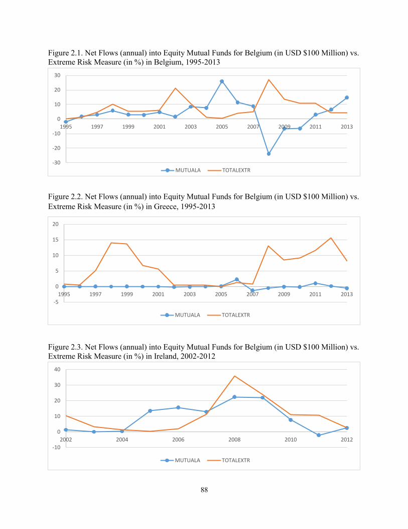
88

Figure 2.1. Net Flows (annual) into Equity Mutual Funds for Belgium (in USD $100 Million) vs.

Extreme Risk Measure (in %) in Belgium, 1995-2013


Extreme Risk Measure (in %) in Greece, 1995-2013


Extreme Risk Measure (in %) in Ireland, 2002-2012

-30

-20

-10

0

10

20

30

1995 1997 1999 2001 2003 2005 2007 2009 2011 2013

MUTUALA TOTALEXTR

-5

0

5

10

15

20

1995 1997 1999 2001 2003 2005 2007 2009 2011 2013

MUTUALA TOTALEXTR

-10

0

10

20

30

40

2002 2004 2006 2008 2010 2012

MUTUALA TOTALEXTR

89

Figure 2.4.

Net Flows (annual) into Equity Mutual Funds for Belgium (in USD $100 Million) vs. Extreme

Risk Measure (in %) in Portugal, 1995-2013

-20

-10

0

10

20

30

1995 1997 1999 2001 2003 2005 2007 2009 2011 2013

MUTUALA TOTALEXTR

90

Figure 3. Comparison of Bitcoin and Index Prices (Mar 2010 – Jun 2018)

91

Figure 4. Scatter Plot Chart of Bitcoin and Indexes Returns

Figure 4-1. Scatter Plot Chart of Bitcoin and Indexes Returns Before and After 2017

92

Figure 5. Scatter Plot Chart of Bitcoin and Index Returns by Country

93

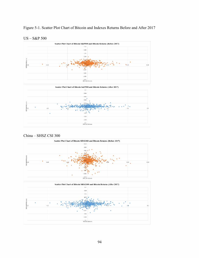
94

Figure 5-1. Scatter Plot Chart of Bitcoin and Indexes Returns Before and After 2017

US – S&P 500

China – SHSZ CSI 300

95

Japan – Nikkei 225

Euro Zone – EUROSTOXX50

96

Korea – KOSPI 200

97

Figure 6. Comparison of Single Exponential Residuals of Bitcoin and Index Price (March 2010 –

January 2019)

98

Figure 7. Comparison of Single Exponential Residuals of Bitcoin and Index Price by Country

(March 2010 – January 2019)

99

Figure 8. BitCoin Price Changes and Major Exchange Hacks (March 2010 – January 2019)

Figure 9. BitCoin Price Changes and Release of Alternative Coins (March 2010 – January 2019)

Figure 9. Bitcoin Futures Mispricing Terms (CBOE: December 2017 – March 2019, CME: January 2018 – March 2019)

101

Figure 10. Absolute Value of Bitcoin Futures Mispricing Terms (CBOE: December 2017 – March 2019, CME: January 2018 –

March 2019)

102

Tables

Table 1: Hofstede’s Cultural Dimension Score (Individualism vs Collectivism)

Rank Country Score

(Individualism)

For our study

Dummy =

individualism (1)

vs. Collectivism (0)

1 United States 91 N/A

2 United Kingdom 89 N/A

3 Canada 80 N/A

3 Netherland 80 N/A

5 Italy 76 N/A

6 Belgium 75 Individualism

7 Denmark 74 Individualism

8 France 71 N/A

8 Sweden 71 Individualism

10 Ireland 70 Individualism

11 Norway 69 Individualism

12 Switzerland 68 N/A

13 Germany 67 N/A

14 Finland 63 Collectivism

15 Austria 55 Collectivism

16 Spain 51 N/A

17 Japan 46 N/A

18 Greece 35 Collectivism

19 Portugal 27 Collectivism

[dataset] Hofstede, G., 2001. The 6-D model of national culture: country comparison.

https://www.hofstede-insights.com/country-comparison/

103

Table 2. Statistics of Indices

We focus on nine relatively small Eurozone countries in this study: Austria, Belgium, Denmark, Finland, Greece, Ireland, Norway, Portugal, and Sweden

that were epicenters of European banking crisis, and the European sovereign debt crisis. For each country, we choose the equity index with the longest

history as the major stock index to use in this study. The historical prices for those indices are collected from Bloomberg and Thomson Reuters DataStream.

This table presents the details of _the nine indices, including time period and the number of observations for each country when we use daily, weekly, and

monthly data to calculate risk variables.

No. Country Index

Daily Data Weekly Data Monthly Data

Time Period Obs. Time Period Obs. Time Period Obs.

1 Austria Austrian Traded Index (ATX) June 5, 1992 - March 24, 2017

6150 June 5, 1992 - March 24, 2017

1295 June 30, 1992 - February 28, 2017

297

2 Belgium Belgium All Share Index (BELAS) October 3, 1988 -

March 24, 2017 7162 October 7, 1988 -

March 24, 2017 1486 October 7, 1988 -

February 28, 2017 341

3 Denmark OMX Copenhagen 20 Index (KFX) December 4, 1989 -

March 24, 2017 6837 December 8, 1989 -

March 24, 2017 1425 December 29, 1989 -

February 28, 2017 327

4 Finland OMS Helsinki Index (HEX) January 30, 1987 -

February 28, 2017 7549 January 30, 1987 -


January 31, 2017 361

5 Greece Athens Stock Exchange (ASE) Index Jun 30, 1992 -

February 28, 2017 6140 July 3, 1992 - February

24, 2017 1282 July 31, 1992 - January

31, 2017 294

6 Ireland Irish Overall Index (ISEQ) January 2, 1987 - March 24, 2017

7609 February 4, 1983 - February 24, 2017

1786 January 31, 1983 - February 28, 2017

410

7 Norway OMX Oslo All Share Index (OSEAX) December 29, 1995 - March 24, 2017

5331 December 29, 1995 - March 24, 2017

1109 December 29, 1995 - February 28, 2017

255

8 Portugal Portugal All Share Index (PSI) January 5, 1988 -

March 24, 2017 7154 January 9, 1988 -

March 24, 2017 1520 January 29, 1988 -

February 28, 2017 350

9 Sweden Stockholm All-Share Index (SAX) January 2, 1987 -



January 31, 2017 445

104

Table 3. Summary Statistics of Daily/Weekly/Monthly Logarithmatic Percent Changes (i.e. returns) of Indices

Country Mean Median StdDev Skewness Kurtosis Jarque-

Bera

Percentile

1% 5% 10% 90% 95% 99%

Panel A. Daily Data

Austria 0.0168 0.0600 1.3605 -0.3699 7.0939 13033.5632 -4.1698 -2.1652 -1.4002 1.4208 1.9056 3.4388

Belgium 0.0296 0.0599 1.0437 -0.1100 7.6207 17342.4548 -2.9831 -1.6847 -1.0868 1.0716 1.5673 2.7324

Denmark 0.0312 0.0596 1.1896 -0.2878 5.4294 8490.7097 -3.3404 -1.8812 -1.2997 1.3315 1.8244 3.0799

Finland 0.0283 0.0560 1.6216 -0.2981 7.6116 18332.9331 -4.6496 -2.5136 -1.6873 1.6915 2.4616 4.5382

Greece -0.0047 0.0115 1.8742 -0.2601 5.6020 8096.5801 -5.4298 -2.9842 -2.0064 2.0397 2.8572 5.1334

Ireland 0.0238 0.0495 1.2607 -0.8218 10.5498 36138.0111 -3.8700 -1.8522 -1.2400 1.3019 1.7842 3.3301

Norway 0.0381 0.1043 1.3554 -0.5958 6.0898 8551.5429 -4.1378 -2.1205 -1.4159 1.4479 2.0026 3.3202

Portugal 0.0131 0.0140 1.0759 -0.3667 9.7827 28683.4787 -3.1829 -1.6620 -1.0920 1.1272 1.6241 2.8246

Sweden 0.0342 0.0801 1.3225 -0.1239 5.3008 8884.3645 -3.8125 -2.0677 -1.4092 1.4066 1.9700 3.5672

Panel B. Weekly Data

Austria 0.0801 0.2580 3.0910 -1.4792 14.4433 11719.3723 -8.2113 -4.5514 -3.4394 3.2815 4.3767 6.7723

Belgium 0.1420 0.3113 2.3731 -1.4583 14.9052 14272.7576 -6.7343 -3.9823 -2.4188 2.6087 3.4002 5.7797

Denmark 0.1512 0.3175 2.6330 -0.9537 6.6591 2846.9231 -7.0802 -4.1158 -2.8720 3.0625 3.8407 5.8779

Finland 0.1362 0.2652 3.5620 -0.5548 3.6421 947.6775 -10.1309 -5.5977 -4.0108 4.0295 5.6184 8.7303

Greece -0.0185 0.0574 4.2358 -0.1996 3.3167 595.6637 -12.0981 -6.9053 -4.8627 4.6592 6.1885 10.9949

Ireland 0.1702 0.3937 2.8646 -1.5298 12.7169 12724.0204 -8.5059 -4.1356 -2.8895 3.2471 4.2346 6.6763

Norway 0.1834 0.5046 2.9096 -1.1327 7.3826 2753.1451 -8.3526 -4.8245 -2.9110 3.0252 3.8062 6.8770

Portugal 0.0528 0.1028 2.5132 -0.7780 6.2558 2630.1025 -8.2099 -3.7179 -2.7498 2.7429 3.9139 6.5868

Sweden 0.1646 0.4128 2.8486 -0.6693 5.4360 2054.1876 -7.6722 -4.5096 -3.1517 3.1939 4.2327 7.1231

105

Panel D. Whole sample period vs. crisis period.

Period Observation Mean Median StdDev Skewness Kurtosis Jarque-

Bera

Percentile

1% 5% 10% 90% 95% 99%

Austria

Jun 1992 -

Feb 2017 296 0.3615 1.0892 6.1555 -1.1407 3.7602 238.5806 -18.5845 -10.1973 -6.9855 7.5428 8.8351 12.4084

2009 12 2.9535 3.3022 8.5102 -0.8379 0.7025 1.6508 -14.7698 -10.4303 -5.4879 12.0763 12.8230 13.4021

2008 12 -7.8906 -5.1448 12.6039 -0.6202 0.3061 0.8161 -31.9413 -29.3298 -25.6027 2.7774 7.2486 11.4020

Belgium

Oct 1988 -

Feb 2017 340 0.6137 1.0386 4.6288 -1.0080 2.4974 145.9397 -14.5691 -8.1971 -4.6983 5.3307 6.7679 9.5863

2009 12 2.0548 3.2581 6.0660 -0.4587 -0.3349 0.4768 -9.1809 -6.9306 -4.5274 9.2403 10.0677 10.5426

2008 12 -5.3790 -3.6539 9.0788 -0.2209 -1.2006 0.8183 -20.1941 -17.5311 -14.7823 5.2510 6.3431 7.1137

Denmark

Dec 1989 -

Feb 2017 326 0.6637 0.9758 5.3089 -0.5545 1.3498 41.4537 -14.8811 -8.1400 -6.0569 6.9451 8.2421 11.6878

2009 12 2.5572 1.8970 7.0328 0.7288 1.3946 2.0348 -7.8010 -6.7073 -5.3600 7.3126 12.3817 17.2850

2008 12 -5.2324 -3.8184 8.9896 -0.4373 -0.6429 0.5892 -20.5937 -19.7455 -18.2835 5.1821 6.4481 7.2954

Panel C. Monthly Data

Austria 0.3615 1.0892 6.1555 -1.1407 3.7602 238.5806 -18.5845 -10.1973 -6.9855 7.5428 8.8351 12.4084

Belgium 0.6137 1.0386 4.6288 -1.0080 2.4974 145.9397 -14.5691 -8.1971 -4.6983 5.3307 6.7679 9.5863

Denmark 0.6637 0.9758 5.3089 -0.5545 1.3498 41.4537 -14.8811 -8.1400 -6.0569 6.9451 8.2421 11.6878

Finland 0.5861 0.6732 7.4341 -0.2154 1.6876 45.5041 -19.1259 -11.3699 -8.3427 8.8410 11.4745 20.3757

Greece -0.0887 0.4265 9.0829 -0.2345 1.3781 25.8701 -25.3191 -15.4895 -11.8359 10.4745 14.0990 20.0462

Ireland 0.7458 1.3983 6.0320 -1.0131 3.2589 250.9545 -17.6699 -9.1039 -6.3349 7.1754 9.5612 12.6107

Norway 0.8019 1.3902 5.9166 -1.3484 4.4471 286.2679 -22.8869 -8.3305 -5.5780 7.3036 8.8279 11.1287

Portugal 0.2573 0.3602 5.4960 -0.4136 2.3449 89.9131 -16.1342 -8.3648 -5.9919 6.6518 8.8381 14.5988

Sweden 1.0082 1.2433 5.9358 -0.4064 2.0092 86.9052 -15.3517 -9.3336 -6.1547 7.7278 10.2612 14.0407

106

Finland

Jan 1987 -

Jan 2017 360 0.5861 0.6732 7.4341 -0.2154 1.6876 45.5041 -19.1259 -11.3699 -8.3427 8.8410 11.4745 20.3757

2009 12 1.4832 2.5201 8.6403 0.1700 1.4814 1.1552 -14.0734 -10.4541 -6.6444 7.7624 13.2955 18.4713

2008 12 -6.3652 -6.1905 6.8957 -0.6141 -0.4420 0.8520 -19.5638 -16.3998 -13.0412 0.5285 0.8950 1.2246

Greece

Jul 1992 -

Jan 2017 293 -0.0887 0.4265 9.0829 -0.2345 1.3781 25.8701 -25.3191 -15.4895 -11.8359 10.4745 14.0990 20.0462

2009 12 1.7204 2.6189 10.7347 -0.3204 -0.1370 0.2147 -16.8673 -15.8082 -13.7705 12.1840 15.8038 19.0224

2008 12 -8.8693 -6.1391 10.3716 -1.0793 1.3006 3.1757 -31.2140 -25.3777 -19.1827 -0.9396 2.0115 4.8559

Ireland

Jan 1983 -

Feb 2017 409 0.7458 1.3983 6.0320 -1.0131 3.2589 250.9545 -17.6699 -9.1039 -6.3349 7.1754 9.5612 12.6107

2009 12 1.9889 3.4268 9.0016 -0.4051 0.5340 0.4708 -14.9858 -12.9271 -9.9477 10.1154 13.7264 17.0055

2008 12 -9.0412 -5.9859 8.7199 -0.1941 -1.2916 0.9095 -22.9332 -20.3369 -17.6670 1.9485 2.6709 2.7593

Norway

Dec 1995

- Feb 2017 254 0.8019 1.3902 5.9166 -1.3484 4.4471 286.2679 -22.8869 -8.3305 -5.5780 7.3036 8.8279 11.1287

2009 12 3.6776 4.0228 5.2600 0.1802 0.6893 0.3025 -5.3866 -4.1903 -2.5998 9.6991 11.8826 13.5900

2008 12 -6.2202 -5.2617 12.8421 -0.4010 -0.9388 0.7624 -27.0131 -25.6363 -23.9752 7.6412 9.4098 11.0751

Portugal

Jan 1988 -

Feb 2017 349 0.2573 0.3602 5.4960 -0.4136 2.3449 89.9131 -16.1342 -8.3648 -5.9919 6.6518 8.8381 14.5988

2009 12 2.8017 2.6839 4.9600 -0.0534 -0.6464 0.2146 -5.5719 -3.9126 -2.1452 8.1656 9.3783 10.5464

2008 12 -5.7293 -2.5220 8.6310 -0.8762 0.0096 1.5356 -22.6329 -19.3963 -16.0307 2.2100 3.8644 5.2217

Sweden

Jan 1980 -

Jan 2017 444 1.0082 1.2433 5.9358 -0.4064 2.0092 86.9052 -15.3517 -9.3336 -6.1547 7.7278 10.2612 14.0407

2009 12 3.1910 1.9663 5.6680 1.2865 3.1955 8.4160 -5.3646 -2.7040 0.0672 9.1543 13.0364 16.3422

2008 12 -4.5332 -1.3914 8.3117 -0.7971 -1.0682 1.8412 -19.2165 -17.2613 -15.0661 3.0916 3.3752 3.5383

107


Percentage of Extreme Days for Each of the Nine European Countries

Austria Belgium

Rank

Geometric Standard

Deviation Percentage of

Extreme Days Geometric Standard


Extreme Days

Rank Year GeoStdDev(%) Year L(%) Year GeoStdDev(%) Year L(%)

1 2008 47.9863

2008 28.4000

2008 35.7265

2008 35.7265 1

2 2009 35.7144

2009 24.1935

2002 25.6784

2002 25.6784 2

3 2011 29.1925

2011 13.3065

2009 22.5379

2009 22.5379 3

4 1998 24.3126

1992 8.4507

2011 21.2453

2011 21.2453 4

5 2010 23.8813

2012 7.6923

2015 20.5910

2015 20.5910 5

6 2016 21.8380

1998 7.6613

2003 19.8203

2003 19.8203 6

7 2012 21.7115

2010 7.6305

2010 19.5069

2010 19.5069 7

8 2006 20.5959

2016 5.622

2016 18.9441

2016 18.9441 8

9 2007 20.2668

1997 5.2632

1998 18.6076

1998 18.6076 9

10 1997 20.1104

2007 4.4534

1999 16.0590

1999 16.0590 10

11 2015 20.0032

2015 4.0323

2014 15.8120

2014 15.8120 11

12 1992 18.5516

2006 3.6585

2000 15.6013

2000 15.6013 12

13 2014 16.8607

2000 3.2520

2007 15.2289

2007 15.2289 13

14 1993 16.6748

1993 3.2129

2001 14.7436

2001 14.7436 14

15 1999 16.2005

2014 2.8340

2013 14.5637

2013 14.5637 15

Denmark Finland

Rank

Geometric Standard




Extreme Days


1 2008 38.4943

2008 23.2000

2000 54.7089

2000 35.4582 1

2 2009 26.6886

2009 12.4498

2001 51.0954

2001 33.3333 2

3 2002 24.4199

2002 10.0402

2002 39.1523

2002 24.8996 3

4 1998 23.3034

1998 9.6000

2008 37.5657

2008 15.4150 4

5 2016 22.0259

2001 8.8353

1998 33.0828

1999 13.5458 5

6 2000 21.8666

2011 8.3333

1999 31.0529

1998 12.8000 6

7 2011 21.2402

2016 7.5397

2009 29.9125

2011 12.6482 7

8 2015 20.4903

2000 7.1713

2011 28.2242

2009 12.3506 8

9 2001 19.9714

2015 6.0241

2003 27.8146

2003 9.2000 9

10 2010 19.8851

1992 5.6000

1997 23.4500

1992 4.3825 10

11 2003 17.9649

2010 5.5777

1995 22.5236

1997 4.0161 11

12 2007 17.6929

2007 4.8193

1992 22.0537

2007 3.2000 12

13 1992 17.4694

2003 4.0161

2012 20.8853

2006 3.1873 13

14 2012 16.0330

2006 3.9683

1993 20.3695

2012 2.8000 14

15 2006 15.8967

2012 3.6145

2004 20.1625

2010 2.7778 15

108

Table 4. Cont'd

Greece Ireland

Rank

Geometric Standard




Extreme Days


1 2015 46.4653

2015 16.1435

2008 47.8976

2008 35.8268 1

2 2012 39.9886

2012 15.6627

2009 32.6774

2009 23.7154 2

3 2008 38.8718

1998 13.9442

1987 30.7513

2007 11.4173 3

4 1998 38.4077

1999 13.6000

2010 25.2077

2010 11.0236 4

5 1999 37.6695

2008 12.9555

2007 23.2181

2011 10.6719 5

6 2011 37.0962

2011 11.5538

2011 22.8458

1987 10.3586 6

7 2014 34.6443

2010 9.1270

2016 22.7368

2002 10.2767 7

8 2010 34.1359

2009 8.4677

1998 22.5521

1998 10.0000 8

9 2009 33.2648

2013 8.1301

2002 22.0552

2001 7.1146 9

10 2000 32.4245

2014 7.2581

2001 19.4826

2016 6.2992 10

11 2016 32.0999

2000 6.7460

2015 18.8086

2000 5.2209 11

12 1997 31.0177

2016 6.4257

2000 17.6076

2015 5.1181 12

13 2013 30.4778

2001 5.6000

1990 16.7002

1990 4.3825 13

14 2001 28.6758

1997 5.0980

1999 16.4688

1988 3.9841 14

15 1993 26.0297

1993 4.3307

2014 16.2031

2014 3.9370 15

Norway Portugal

Rank

Geometric Standard




Extreme Days


1 2008 46.8717

2008 24.2063%

2008 32.8977

2008 25.3906% 1

2 2009 31.7568

2009 17.5299%

1998 26.4106

1998 21.8623% 2

3 1998 25.2844

2011 9.0909%

2010 22.3970

2011 18.2879% 3

4 2011 24.6472

1998 8.3665%

2011 22.0392

2015 16.7969% 4

5 2006 24.0700

2006 6.7729%

2015 22.0009

2014 14.9020% 5

6 2010 21.1818

2002 6.0241%

2014 20.0170

2010 13.9535% 6

7 2002 20.7336

2016 5.5336%

2000 19.3877

2000 13.9344% 7

8 2016 20.3397

2010 5.1587%

2016 19.3550

2016 12.4514% 8

9 2007 19.7297

2000 4.7809%

1989 18.0892

1988 12.1827% 9

10 2000 19.3475

2001 3.6290%

1988 17.9535

2009 9.7656% 10

11 2001 19.1654

2005 3.5573%

2009 17.5111

2012 8.9844% 11

12 2015 17.6858

2014 3.2000%

2012 17.2451

2013 8.6275% 12

13 2005 17.5407

2007 3.2000%

2001 16.9526

2001 8.0972% 13

14 2012 16.5922

2012 3.1873%

2013 16.8674

1999 7.6613% 14

15 1999 16.0560

1999 1.9841%

1997 16.3335

2002 6.9106% 15

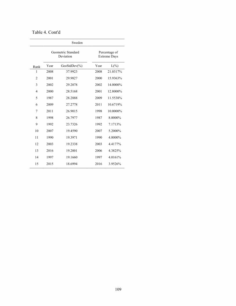
109

Table 4. Cont'd

Sweden

Rank

Geometric Standard


Extreme Days

Year GeoStdDev(%) Year L(%)

1 2008 37.9923

2008 21.0317%

2 2001 29.9827

2000 15.9363%

3 2002 29.2078

2002 14.0000%

4 2000 28.5168

2001 12.8000%

5 1987 28.2888

2009 11.5538%

6 2009 27.2778

2011 10.6719%

7 2011 26.9015

1998 10.0000%

8 1998 26.7977

1987 8.0000%

9 1992 23.7326

1992 7.1713%

10 2007 19.4590

2007 5.2000%

11 1990 19.3971

1990 4.8000%

12 2003 19.2338

2003 4.4177%

13 2016 19.2001

2006 4.3825%

14 1997 19.1660

1997 4.0161%

15 2015 18.6994

2016 3.9526%

110


Percentage of Extreme Weeks for Each of the Nine European Countries

Austria Belgium

Rank

Geometric Standard


Extreme Weeks Geometric Standard


Extreme Weeks


1 2008 51.7178

2008 59.6154

2008 37.2575

2008 63.4615 1

2 2009 36.6474

2009 57.6923

2009 24.4423

2011 53.8462 2

3 2011 29.6846

1992 48.2759

2011 22.1039

2009 51.9231 3

4 2010 25.6182

2010 45.2830

2001 21.4142

1997 50.0000 4

5 1998 23.8982

1998 44.2308

1998 21.3581

2002 46.1538 5

6 1992 23.2436

2011 38.4615

2002 20.7649

1999 45.2830 6

7 2006 21.5954

2014 36.5385

2003 19.4470

1998 44.2308 7

8 2012 19.5731

2012 34.6154

2015 17.9414

2015 42.3077 8

9 2016 19.5607

1997 34.6154

2010 17.8058

2010 41.5094 9

10 2007 19.4641

2015 32.6923

1990 17.6666

2014 36.5385 10

11 1999 19.4486

1999 32.0755

1999 17.5854

2013 36.5385 11

12 1997 19.1372

1993 32.0755

2016 17.4139

2003 36.5385 12

13 2014 19.0307

2016 30.1887

2007 16.4739

1990 36.5385 13

14 2015 18.4312

2007 28.8462

1997 16.3341

2016 35.8491 14

15 1993 18.1802

2006 28.8462

2000 16.1972

2007 34.6154 15

Denmark Finland

Rank

Geometric Standard




Extreme Weeks


1 2008 40.6063

2009 51.9231

2000 52.3659

2000 67.3077 1

2 2009 28.7925

2008 46.1538

2001 48.5823

2002 61.5385 2

3 2001 23.9041

1998 42.3077

2008 35.3267

2001 61.5385 3

4 2016 21.4325

2000 40.3846

2002 34.4546

2008 50.0000 4

5 2011 21.2590

1997 40.3846

1998 32.4487

1999 49.0566 5

6 2010 21.1865

2015 36.5385

2011 29.8203

2009 48.0769 6

7 2002 20.6397

2001 36.5385

2009 29.0908

1998 44.2308 7

8 2000 19.3637

2002 34.6154

2003 28.0922

2011 42.3077 8

9 1998 19.2449

2016 33.9623

1999 27.9954

2003 42.3077 9

10 1992 19.2035

2003 32.6923

1992 27.5150

1992 40.3846 10

11 1997 18.3778

1992 32.6923

1995 25.5737

1993 37.7358 11

12 2015 17.5312

1999 32.0755

1993 24.5855

1995 36.5385 12

13 1999 16.9973

2011 30.7692

2004 23.4496

1991 34.6154 13

14 1990 16.6178

2010 30.1887

1997 21.7572

1997 32.6923 14

15 2007 16.6049

1993 30.1887

2012 20.6029

1994 28.8462 15

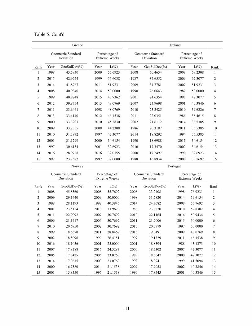
111

Table 5. Cont'd

Greece Ireland

Rank

Geometric Standard




Extreme Weeks


1 1998 45.5930

2009 57.6923

2008 50.4654

2008 69.2308 1

2 2015 42.9724

1999 56.6038

1987 37.6552

2009 67.3077 2

3 2014 41.8967

2011 51.9231

2009 34.7781

2007 51.9231 3

4 2008 40.9340

2014 50.0000

1998 26.0643

1987 50.0000 4

5 1999 40.8248

2015 48.9362

2001 24.6354

1998 42.3077 5

6 2012 39.8754

2013 48.0769

2007 23.9698

2001 40.3846 6

7 2011 33.6441

1998 48.0769

2010 23.3425

2010 39.6226 7

8 2013 33.4140

2012 46.1538

2011 22.0351

1986 38.4615 8

9 2000 33.3201

2010 45.2830

2002 21.6112

2014 36.5385 9

10 2009 33.2355

2008 44.2308

1986 20.3187

2011 36.5385 10

11 2010 31.3972

1997 42.3077

2014 18.8292

1994 36.5385 11

12 2001 31.1299

2000 34.6154

1990 18.6988

2015 34.6154 12

13 1997 30.6134

2001 32.6923

2016 17.3470

2002 34.6154 13

14 2016 28.9728

2016 32.0755

2000 17.2497

1990 32.6923 14

15 1992 23.2622

1992 32.0000

1988 16.8934

2000 30.7692 15

Norway Portugal

Rank

Geometric Standard




Extreme Weeks


1 2008 45.8560

2008 55.7692

2008 33.2408

1998 76.9231 1

2 2009 29.1440 2009 50.0000

1998 31.7820 2014 59.6154 2

3 1998 28.1193 1998 40.3846

2014 24.7682 2008 55.7692 3

4 2001 23.5154

2010 33.9623

1988 23.6870

2010 52.8302 4

5 2011 22.9092 2007 30.7692

2010 22.1164 2016 50.9434 5

6 2006 21.1417 2006 30.7692

2011 21.2006 2015 50.0000 6

7 2010 20.6750

2002 30.7692

2015 20.5779

1997 50.0000 7

8 1999 18.6570 2011 28.8462

2016 19.3491 2009 48.0769 8

9 2002 18.5096

1999 26.4151

1997 19.1329

2011 46.1538 9

10 2016 18.1036

2001 25.0000

2001 18.8394

1988 43.1373 10

11 2007 17.8288 2016 24.5283

2000 18.7302 2007 42.3077 11

12 2005 17.3425 2005 23.0769

1989 18.6647 2000 42.3077 12

13 2014 17.0615

2003 23.0769

1999 18.0941

1999 41.5094 13

14 2000 16.7580 2014 21.1538

2009 17.9053 2002 40.3846 14

15 2003 15.8350 1997 21.1538

1990 17.8543 2001 40.3846 15

112

Table 5. Cont'd

Sweden

Rank

Geometric Standard


Extreme Weeks


1 2008 38.0421

2001 57.6923

2 1998 28.6410

2000 55.7692

3 2000 27.3161

2002 53.8462

4 2001 27.0393

2008 48.0769

5 2002 26.8213

2009 44.2308

6 2011 26.7513

1998 44.2308

7 1990 26.5180

2011 36.5385

8 1987 25.8891

1990 34.6154

9 1992 25.7377

1992 32.6923

10 2009 25.5469

1991 32.6923

11 1991 18.6649

1987 31.3725

12 2010 18.6029

1999 30.1887

13 2007 18.5062

2003 26.9231

14 1994 18.0107

1994 26.9231

15 1997 17.9156

1993 24.5283

113


Percentage of Extreme Months for Each of the Nine European Countries

Austria Belgium

Rank

Geometric Standard


Extreme Months Geometric Standard


Extreme Months


1 2008 43.6612

1993 91.6667

2008 31.4498

1998 91.6667 1

2 2009 29.4802

2008 83.3333

1998 23.5242

1997 91.6667 2

3 1998 29.1508

2005 83.3333

2002 21.6430

2009 83.3333 3

4 1997 23.1339

2016 75.0000

1990 21.2586

2005 83.3333 4

5 1993 21.8066

2015 75.0000

2009 21.0132

2004 83.3333 5

6 2010 21.5577

1997 75.0000

2003 20.1805

2015 75.0000 6

7 1992 21.3587

2012 66.6667

2015 19.1744

2008 75.0000 7

8 1999 20.8975

2010 66.6667

2000 17.0880

1989 75.0000 8

9 2015 20.4569

2009 66.6667

1997 16.5425

2014 66.6667 9

10 2011 20.3502

2004 66.6667

1991 15.0907

2012 66.6667 10

11 2012 18.0167

2002 66.6667

1989 13.9651

2010 66.6667 11

12 2016 17.9077

1999 66.6667

2010 13.5704

1993 66.6667 12

13 2001 17.7594

1998 66.6667

2001 13.3557

1990 66.6667 13

14 2006 17.4930

1994 66.6667

1992 12.2344

2011 58.3333 14

15 1996 16.8506

1992 66.6667

1999 12.0797

2007 58.3333 15

Denmark Finland

Rank

Geometric Standard




Extreme Months


1 2008 31.1409

2016 83.3333

2001 58.8500

2001 100.0000 1

2 2009 24.3624

2002 83.3333

1992 39.5677

2004 91.6667 2

3 1998 23.1493

1997 83.3333

2002 35.0402

2002 91.6667 3

4 2001 22.9897

1992 83.3333

1999 34.1264

1998 91.6667 4

5 2002 22.8876

2009 75.0000

1998 33.2609

1997 83.3333 5

6 2003 21.2062

1990 75.0000

2009 29.9307

1994 83.3333 6

7 1990 21.1136

2015 66.6667

1991 28.2831

1993 83.3333 7

8 1992 20.2355

2010 66.6667

1995 26.0440

1987 81.8182 8

9 2011 19.0249

2008 66.6667

2004 25.1911

2015 75.0000 9

10 1997 18.5076

2005 66.6667

1994 24.9458

2011 75.0000 10

11 2015 18.3247

2003 66.6667

2003 24.3057

2009 75.0000 11

12 1994 17.1399

2001 66.6667

1997 24.2671

2000 75.0000 12

13 2000 17.0473

1999 66.6667

2008 23.8874

1999 75.0000 13

14 1993 16.0979

1993 66.6667

2000 21.2439

1992 75.0000 14

15 2012 15.3780

2011 58.3333

1990 20.9775

1991 75.0000 15

114

Table 6. Cont'd

Greece Ireland

Rank

Geometric Standard




Extreme Months


1 1998 56.6405

2010 91.6667

1987 45.1398

2008 100.0000 1

2 2012 43.5045

2000 83.3333

2009 31.1825

2001 91.6667 2

3 2015 40.4667

1997 83.3333

2008 30.2065

1992 91.6667 3

4 1997 37.4118

2012 75.0000

1998 27.0171

2005 83.3333 4

5 2009 37.1860

2009 75.0000

2002 26.6785

2002 83.3333 5

6 2008 35.9283

2008 75.0000

1990 25.1560

1997 83.3333 6

7 2013 35.1912

2003 75.0000

2010 23.3673

1990 83.3333 7

8 2011 34.6977

2001 75.0000

1986 22.2488

1987 83.3333 8

9 2000 33.8414

1999 75.0000

1991 22.1082

1985 83.3333 9

10 2010 32.2309

2015 72.7273

2001 22.0702

1983 81.8182 10

11 2001 31.0690

2016 66.6667

1988 21.2369

2009 75.0000 11

12 2016 30.6310

2013 66.6667

2016 20.1764

1994 75.0000 12

13 2003 27.3089

1998 66.6667

1984 19.1826

1986 75.0000 13

14 2014 26.9293

2014 58.3333

2000 19.0909

1984 75.0000 14

15 1993 23.9730

2011 58.3333

1985 18.7222

2016 66.6667 15

Norway Portugal

Rank

Geometric Standard




Extreme Months


1 2008 44.4863

2005 91.6667

1998 38.1811

1988 100.0000 1

2 1998 32.4518

2008 83.3333

2008 29.8985

1998 91.6667 2

3 2002 22.4656

2007 83.3333

1989 25.1228

1997 91.6667 3

4 2001 21.7071

2003 83.3333

1988 24.5670

1994 91.6667 4

5 2010 20.4839

2002 83.3333

2002 23.0465

2002 83.3333 5

6 2003 20.1908

2001 83.3333

2000 21.9241

1999 83.3333 6

7 2005 19.1972

2010 75.0000

1997 19.6740

1993 83.3333 7

8 2009 18.2212

2009 75.0000

2015 19.2287

2015 75.0000 8

9 1999 17.9293

2004 66.6667

2010 19.1633

2014 75.0000 9

10 2011 16.7016

2000 66.6667

2014 18.4535

2012 75.0000 10

11 2006 16.6438

1998 66.6667

2001 17.8566

2010 75.0000 11

12 2000 16.5380

2006 58.3333

1994 17.1879

2009 75.0000 12

13 2004 15.6969

1999 58.3333

2009 17.1818

2003 75.0000 13

14 2012 13.8440

2015 50.0000

2007 16.3367

1989 75.0000 14

15 1997 13.8072

1997 50.0000

1999 16.2677

2016 66.6667 15

115

Table 6. Cont'd

Sweden

Rank

Geometric Standard


Extreme Months


1 1987 37.0711

1997 91.6667

2 1992 32.3222

2002 83.3333

3 2002 31.7092

1987 83.3333

4 2001 30.5038

2015 75.0000

5 1990 29.5851

2001 75.0000

6 1983 28.8175

1989 75.0000

7 2008 28.7925

1988 75.0000

8 1998 25.9940

1983 75.0000

9 1994 21.7047

1981 75.0000

10 1993 21.0375

2005 66.6667

11 2000 20.9825

2003 66.6667

12 1981 20.2546

1998 66.6667

13 1997 19.9931

1994 66.6667

14 1991 19.8585

1993 66.6667

15 2009 19.6344

1992 66.6667

116

Table 7. Regression Results of Equity Mutual Fund Net Flows on Risk Measures for Small

Eurozone Countries

Austria (1996-2012) Belgium (1995-2013)

Model (1) Model (2) Model (3) Model (1) Model (2) Model (3)

Panel A: Annual Observation with Financial Crisis Dummy Variable (Austria: n=17; Belgium: n=19)

Constant 2.4426 7.7979 6.9923 2.4233 2.8781 0.3985 0.77 3.98 3.88 0.63 0.65 0.10

GeoMean(t-1) 9.5968 8.1307 26.7668 0.0000 -6.0533 -1.5173 0.81 0.82 2.08 - -0.20 -0.06

GeoStdDev(t-1) 0.4081 -1.7749

2.20 -0.08

TotalExtr(t-1) 0.1976 -0.0345

2.85 -0.23

NegExtr(t-1) 0.7464 1.1290 2.65 2.22

PosExtr(t-1) -0.4502 -1.7044 -1.36 -2.38

Time -0.5968 -0.6136 -0.7059 0.3782 0.4107 0.5843 -2.15 -2.52 -3.17 1.13 1.09 1.75

Dummy Variable -9.7441 -9.3226 -10.7261 -23.4073 -23.4763 -28.1261 -2.43 -2.55 0.00 -3.24 -3.14 -4.16

Adjusted R Square 0.3863 0.4860 0.0596 0.3307 0.3567 0.5162

Austria (1996-2012) Belgium (1995-2013) Model (4) Model (5) Model (6) Model (4) Model (5) Model (6)

Panel B: Annual Observation without Financial Crisis Variable (Austria: n=17; Belgium: n=19)

Constant 3.1549 7.9911 7.4769 1.2937 1.4899 0.1372 0.85 3.42 3.13 0.27 0.27 0.02

GeoMean(t-1) 20.5567 19.7462 33.2442 0.0000 38.4154 44.9684 1.60 1.87 1.96 - 1.13 1.27

GeoStdDev(t-1) 0.3679 40.2214

1.69 1.65

TotalExtr(t-1) 0.1914 -0.0150

2.31 -0.08

NegExtr(t-1) 0.5542 0.5583 1.51 0.78

PosExtr(t-1) -0.2382 -0.8332 -0.55 -0.83

Time -0.7288 -0.7640 -0.8402 0.1343 0.1481 0.2078 -2.28 -2.71 -2.89 0.32 0.32 0.44

Adjusted R^2 0.1541 0.2681 0.2698 -0.0235 -0.0246 -0.0467

117

Table 7. Cont’d Denmark (2003-2013) Finland (1995-2012)


Panel A: Annual Observation with Financial Crisis Dummy Variable (Denmark: n=11; Finland: n=19)

Constant -1.9165 -1.3322 -1.9737 3.8327 2.4267 3.5382

-1.03 -1.32 -1.58 0.75 0.69 0.90

GeoMean(t-1) -2.0470 -0.7117 5.0563 -9.5690 -9.3994 -17.6914

-0.34 -0.12 0.56 -0.89 -0.88 -1.09

GeoStdDev(t-1) 0.0597 -1.2308

0.64 -0.61

TotalExtr(t-1) 0.0407 -0.0322

0.91 -0.58

NegExtr(t-1) 0.2428 -0.3713

1.05 -0.75

PosExtr(t-1) -0.1350 0.2691 -0.67 0.61

Time 0.5586 0.5399 0.5130 0.4734 0.4853 0.4990

3.98 3.88 3.54 1.69 1.74 1.75

Dummy Variable

-1.0069 -1.0615 -0.9845 -7.3596 -7.5456 -8.2332

-0.77 -0.84 -0.76 -1.61 -1.63 -1.70

Adjusted R Square 0.6288 0.6509 0.6385 0.0880 0.0857 0.0474

Denmark (2003-2013) Finland (1995-2012)


Panel B: Annual Observation without Financial Crisis Variable (Denmark: n=11, Finland: n=18)

Constant

-1.8887 -1.4059 -2.0784 3.3158 2.0470 2.5779

-1.04 -1.43 -1.73 0.62 0.55 0.62

GeoMean(t-1)

-0.5161 0.8002 6.7826 -5.1050 -4.3124 -8.1711

-0.09 0.14 0.81 -0.47 -0.40 -0.50

GeoStdDev(t-1)

0.0510 -0.8899

0.57 -0.42

TotalExtr(t-1)

0.0355 -0.0161

0.82 -0.28

NegExtr(t-1)

0.2496 -0.1825

1.12 -0.35

PosExtr(t-1)

-0.1499 0.1332

-0.77 0.29

Time

0.5475 0.5297 0.5020 0.3662 0.3778 0.3797

4.04 3.91 3.61 1.27 1.32 1.28

Adjusted R^2 0.6502 0.6658 0.6638 -0.0149 -0.0220 -0.0917

118

Table 7. Cont’d Greece (2003-2013) Ireland (1995-2012)


Panel A: Annual Observation with Financial Crisis Dummy Variable (Greece: n=19, Ireland: n=11)

Constant 0.2781 0.0801 0.0839 7.1932 5.6588 10.3754

0.51 0.21 0.21 0.97 1.24 0.84

GeoMean(t-1) -0.4488 -0.3883 -0.3515 22.5714 27.4193 -11.3329

-0.42 -0.37 -0.29 0.69 0.93 -0.12

GeoStdDev(t-1) -0.0110 -1.8291

-0.59 -0.27

TotalExtr(t-1) -0.0057 -0.0120

-0.42 -0.08

NegExtr(t-1) -0.0006 -0.7822

-0.01 -0.42

PosExtr(t-1) -0.0113 0.6076 -0.14 0.41

Time 0.0110 0.0097 0.0096 0.0117 -0.0972 -0.0750

0.31 0.27 0.26 0.01 -0.12 -0.09

Dummy Variable -0.4872 -0.4651 -0.4999 25.1384 25.4558 24.9086

-0.79 -0.75 -0.61 2.82 2.87 2.58

Adjusted R Square -0.2057 -0.2200 -0.3134 0.4184 0.4120 0.3181

Greece (2003-2013) Ireland (1995-2012)


Panel B: Annual Observation without Financial Crisis Variable (Greece: n=19, Ireland: n=11)

Constant

0.2541 0.0804 0.0633 10.8503 6.9073 15.5529

0.47 0.21 0.16 1.05 1.07 0.92

GeoMean(t-1)

-0.2048 -0.1601 -0.4038 -36.2552 -26.9905 -96.2743

-0.20 -0.16 -0.34 -1.03 -0.84 -0.75

GeoStdDev(t-1)

-0.0098 -4.8519

-0.53 -0.51

TotalExtr(t-1)

-0.0054 -0.0479

-0.40 -0.23

NegExtr(t-1)

-0.0289 -1.4663

-0.49 -0.57

PosExtr(t-1)

0.0195 1.0958

0.31 0.53

Time

0.0050 0.0044 0.0068 0.6344 0.4075 0.4284

0.15 0.12 0.19 0.54 0.36 0.36

Adjusted R^2 -0.1757 -0.1849 -0.2548 -0.1613 -0.1959 -0.3268

119

Table 7. Cont’d Norway (1997-2013) Portugal (1995-2013)


Panel A: Annual Observation with Financial Crisis Dummy Variable (Norway: n=17; Portugal: n=19)

Constant 0.6241 0.2738 0.4143 4.2220 4.3452 4.1639

0.76 0.59 0.63 1.28 1.79 1.64

GeoMean(t-1) -0.5150 -0.1188 -0.9350 -19.0232 -19.4260 -13.6505

-0.22 -0.05 -0.27 -1.58 -1.58 -0.74

GeoStdDev(t-1) -0.3677 0.0066

-0.57 0.04

TotalExtr(t-1) -0.0065 -0.0025

-0.33 -0.04

NegExtr(t-1) -0.0335 0.1693

-0.37 0.42

PosExtr(t-1) 0.0274 -0.1721 0.25 -0.43

Time 0.0244 0.0190 0.0173 -0.2368 -0.2334 -0.2657

0.49 0.38 0.33 -1.18 -1.16 -1.21

Dummy Variable -1.3454 -1.4294 -1.4458 -9.5473 -9.5090 -10.5338

-1.70 -1.84 -1.78 -2.56 -2.57 -2.35

Adjusted R Square 0.0908 0.0751 -0.0002 0.2496 0.2496 0.2033

Norway (1997-2013) Portugal (1995-2013)


Panel B: Annual Observation without Financial Crisis Variable (Norway: n=17, Portugal: n=19)

Constant 0.9339 0.2795 0.3672 5.1340 4.3824 4.7160

1.09 0.55 0.51 1.33 1.54 1.63

GeoMean(t-1) 0.2369 1.1121 0.6116 -11.6650 -11.0451 -23.6160

0.10 0.49 0.17 -0.85 -0.79 -1.14

GeoStdDev(t-1) -0.6878 -0.0786

-1.03 -0.37

TotalExtr(t-1) -0.0128 -0.0207

-0.62 -0.26

NegExtr(t-1) -0.0297 -0.3403

-0.31 -0.87

PosExtr(t-1) 0.0083 0.3022

0.07 0.76

Time 0.0167 0.0051 0.0040 -0.3115 -0.3185 -0.2403

0.32 0.10 0.07 -1.34 -1.37 -0.95

Adjusted R^2 -0.0409 -0.0943 -0.1824 -0.0273 -0.0320 -0.0535

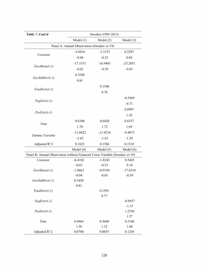
120

Table 7. Cont’d Sweden (1995-2013)

Model (1) Model (2) Model (3)

Panel A: Annual Observation (Sweden: n=19)

Constant

-5.6016 -1.3133 0.2287

-0.60 -0.25 0.04

GeoMean(t-1)

-17.1531 -16.9401 -25.2051

-0.62 -0.59 -0.83

GeoStdDev(t-1)

0.3240

0.81

TotalExtr(t-1)

0.1506

0.76

NegExtr(t-1)

-0.5469

-0.71

PosExtr(t-1)

0.8997

1.10

Time

0.6340 0.6420 0.6337

1.70 1.72 1.69

Dummy Variable

-11.8822 -11.9234 -9.4073

-1.63 -1.63 -1.20

Adjusted R^2 0.1623 0.1586 0.1518

Model (4) Model (5) Model (6)

Panel B: Annual Observation without Financial Crisis Variable (Sweden: n=19)

Constant -6.4102 -1.8243 0.5465

-0.65 -0.33 0.10

GeoMean(t-1) -1.0663 -0.9150 -17.6518

-0.04 -0.03 -0.59

GeoStdDev(t-1) 0.3450

0.81

TotalExtr(t-1) 0.1591

0.77

NegExtr(t-1) -0.8457

-1.15

PosExtr(t-1) 1.2330

1.57

Time 0.4964 0.5049 0.5346

1.30 1.32 1.44

Adjusted R^2 0.0700 0.0655 0.1245

121

Table 8. Pooled regression results of equity mutual fund net flows on risk measures

Panel A: Pooled regression results of equity mutual fund net flows on risk measures, with no country fixed effect controlled.

The countries examined are separated into two groups, individualism and collectivism, based on Hofstede’s culture dimension score of

individualism vs. collectivism.

(1) (2) (3) (4) (5) (6) (7) (8) (9)

VARIABLES Model 1’ Model 2’ Model 3’ Model 4’ Model 5’ Model 6’ Model 7’ Model 8’ Model 9’

Geometric Mean (t-1) -9.045** -9.740** -9.053** -8.035 -8.224* -1.432 -6.569 -7.738 -5.112

(4.157) (4.025) (3.909) (5.072) (4.859) (4.079) (5.242) (4.963) (4.874)

Geo. Std. Deviation (t-1) 0.00983 0.00239 -0.0907

(0.0561) (0.0573) (0.0697)

Individualism 4.196*** 4.647*** 4.082***

(1.456) (1.414) (1.503)

Individualism*Geo StdDev (t-1) 0.163***

(0.0553)

Total Extreme Value (t-1) -0.0632 -0.0780* -0.112**

(0.0435) (0.0418) (0.0511)

Individualism*Total Extr (t-1) 0.112***

(0.0399)

Negative Extreme Value (t-1) 0.0608 0.0580 0.105

(0.127) (0.123) (0.163)

Positive Extreme Value (t-1) 0.00169 -0.0250 -0.220

(0.134) (0.133) (0.205)

Individualism*Neg Extr (t-1) 0.0157

(0.217)

Individualism*Pos Extr (t-1) 0.221

(0.255)

GDP (t-1) 2.60e-05 -4.34e-05 -3.10e-05 1.99e-05 -5.86e-05** -1.60e-05 2.52e-05 -4.33e-05 -7.64e-06

(2.18e-05) (2.85e-05) (2.61e-05) (2.20e-05) (2.87e-05) (2.40e-05) (2.31e-05) (3.09e-05) (2.69e-05)

Crisis -5.446* -5.240 -5.334* -3.034 -2.269 -1.459 -5.691* -5.460* -5.765*

(3.145) (3.186) (3.146) (2.726) (2.797) (2.689) (3.119) (3.180) (3.182)

Constant 2.888* 3.486** 5.336*** 4.296*** 5.065*** 5.078*** 2.417** 3.142*** 3.860***

(1.608) (1.600) (1.850) (1.274) (1.193) (1.344) (1.139) (1.112) (1.296)

Fixed Effect No No No No No No No No No

Observations 141 141 141 141 141 141 141 141 141

R-squared 0.058 0.111 0.108 0.080 0.143 0.144 0.065 0.113 0.095 Robust standard errors in parentheses

*** p<0.01, ** p<0.05, * p<0.1

122

Panel B: Pooled regression results of equity mutual fund net flows on risk measures, with country fixed effect controlled. (1) (2) (3) (4) (5) (6) (7) (8) (9) VARIABLES Model 1’ Model 2’ Model 3’ Model 4’ Model 5’ Model 6’ Model 7’ Model 8’ Model 9’

Geometric Mean (t-1) -8.278 -9.594 -10.10* -8.839 -9.429 -7.362 -9.733 -10.79 -8.674

(6.087) (5.644) (5.793) (6.681) (6.512) (6.883) (7.284) (7.062) (6.795)

Geo. Std. Deviation (t-1) 0.0165 -0.00314 -0.105

(0.0581) (0.0604) (0.0782)

Individualism 4.396*** 4.446*** 4.258***

(1.278) (1.333) (1.385)

Individualism*Geo StdDev (t-1) 0.182***

(0.0450)

Total Extreme Value (t-1) 0.0197 -0.00766 -0.0411

(0.0366) (0.0395) (0.0432)

Individualism*Extreme Measure (t-1) 0.103***

(0.0207)

Negative Extreme Value (t-1) -0.0477 -0.0631 -0.0514

(0.151) (0.114) (0.0873)

Positive Extreme Value (t-1) 0.142 0.0952 -0.0620

(0.174) (0.136) (0.191)

Individualism*Neg Extr (t-1) 0.106

(0.129)

Individualism*Pos Extr (t-1) 0.134

(0.218)

GDP (t-1) 1.66e-05 -5.95e-05* -5.02e-05* 1.86e-05 -6.11e-05 -1.41e-05 2.45e-05 -5.22e-05 -1.77e-05

(1.93e-05) (3.20e-05) (2.61e-05) (2.11e-05) (3.67e-05) (2.40e-05) (2.18e-05) (3.66e-05) (2.49e-05)

Crisis = o, - - - - - - - - -

Constant 2.455 3.524* 5.595** 2.342 3.646** 3.630** 1.858 3.177** 3.902**

(1.763) (1.962) (2.204) (1.369) (1.617) (1.618) (1.159) (1.416) (1.539)

Fixed Effect Yes Yes Yes Yes Yes Yes Yes Yes Yes

Observations 141 141 141 141 141 141 141 141 141

R-squared 0.011 0.084 0.088 0.012 0.085 0.065 0.021 0.087 0.066

Number of year 18 18 18 18 18 18 18 18 18

Robust standard errors in parentheses

*** p<0.01, ** p<0.05, * p<0.1

123

Table 9. Simultaneous Regression Results (2 Groups: Individualism vs Collectivism), 2SLS Estimates

Model (2’) Model (3’) Model (4’) Model (5’) Model (6’)

VARIABLES Net Flow Geo.StDev Net Flow Geo.StDev Net Flow Total Extr. Net Flow Total Extr. Net Flow Total Extr.

Geometric Mean (t-1) -2.872 8.552 -2.405 8.599 -2.158 15.76 -3.657 16.06 -2.196 16.05

(5.514) (5.950) (5.513) (5.946) (5.419) (11.63) (5.299) (11.52) (5.335) (11.60)

Geo. StdDev (t-1) 0.212** 0.125

(0.0851) (0.0951)

Individualism 4.012*** -0.571 3.555** 4.321

(1.505) (1.881) (1.497) (3.642)

Net Flow(t-1) 0.230** 0.219* 0.539** 0.461** 0.509**

(0.115) (0.114) (0.224) (0.223) (0.219) Individualism*Geo StdDev (t-1) 0.143**

(0.0559)

Total Extr. (t-1) 0.106*** 0.0896** 0.0313

(0.0372) (0.0365) (0.0495) Individualism*Total Extr. (t-1) 0.101**

(0.0451)

GDP (t-1) -4.46e-05 -1.97e-05 -2.82e-05 -2.89e-05 2.78e-05 -0.000109 -3.13e-05 -0.000180* -1.48e-06 -0.000109

(3.96e-05) (4.87e-05) (3.63e-05) (3.78e-05) (3.10e-05) (7.39e-05) (3.91e-05) (9.44e-05) (3.32e-05) (7.37e-05)

Crisis -5.773*** 17.60*** -5.857*** 17.59*** -6.036*** 39.42*** -5.782*** 39.37*** -5.849*** 39.33***

(1.949) (2.404) (1.948) (2.403) (1.962) (4.699) (1.913) (4.655) (1.936) (4.689)

Constant -0.944 19.88*** 0.758 0.219* 0.887 17.71*** 1.603 18.35*** 0.0313 17.79***

(2.331) (1.854) (2.529) (0.114) (1.679) (3.590) (1.657) (3.589) (0.0495) (3.582)

Var(e.netflow) 44.53*** 44.51*** 45.20*** 42.82*** 43.92***

(5.851) (5.836) (5.607) (5.304) (5.450)

Var(e.risk) 67.22*** 67.11*** 256.6*** 252.0*** 255.8***

(8.188) (8.162) (31.250) (30.590) (31.02)

Covariance -21.94*** -21.35*** -39.22*** -37.81*** -38.99***

(6.760) (6.778) (11.910) (11.340) (11.53)

Observations 141 141 141 141 141 141 141 141 141 141

Standard errors in parentheses

*** p<0.01, ** p<0.05, * p<0.1

124

Table 10. Overview of Central Banks with Negative Policy Rates

Year Country Date Rate Announcement Measures

2012 Denmark July 5, 2012

January 2013

April 2014

September 2014

January 19, 2015

January 22, 2015

January 29, 2015

February 5, 2015

January 8, 2016

-0.20%

-0.10%

+0.05%

-0.05%

-0.20%

-0.35%

-0.50%

-0.75 %

-0.65 %

July 5, 2012 Certificates of deposit

(CD)

2014 Euro Area

June 11, 2014

September 10, 2014

December 9, 2015

March 16, 2016

-0.10%

-0.20%

-0.30%

-0.40%

June 5, 2014 Deposit rate

2015 Switzerland January 15, 2015 -0.75%

December 18, 2014 Sight deposits at SNB

(with an exemption

threshold)

Sweden February 12, 2015

March 18, 2015

July 2, 2015

February 11, 2016

-0.10%

-0.25%

-0.35%

-0.50%

February 12, 2015 Reverse repo rate

Norway September 24, 2015

March 17, 2016

-0.25%

-0.50%

September 24, 2015 Reserve rate

2016 Bulgaria January 4, 2016

March 16, 2016

-0.30%

-0.40%

November 26, 2015 Deposit rate

Japan February 16, 2016 -0.10% January 29, 2016 Deposit rate

Hungary March 23, 2016 -0.05% March 22, 2016 Deposit rate

Bosnia and Herzegovina July 1, 2016 -0.20% April 18, 2016 Deposit rate

Table 11. Reference Index and Currency for Countries that Implement NIRP

Country Currency Currency

Symbol Index

Index

Symbol

Bosnia and

Herzegovina

Bosnia and Herzegovina

Convertible Mark BAM MSCI Bosnia and Herzegovina MXBAH

Bulgaria Bulgarian Lev BGN SOFIX Index SOFIX

Denmark Danish Krone DKK OMX Copenhagen Index KAX

Euro Area EURO EUR Deutsche Boerse AG German Stock Index DAX

Hungary Hungarian Forint HUF Budapest Stock Exchange Budapest Stock Index BUX

Japan Japanese Yen JPY Nikkei 225 NKY

Norway Norwegian Krone NOK Oslo Stock Exchange All Share Index OSEAX

Switzerland Swiss Franc CHF Swiss Market Index SMI

Sweden Swedish Krona SEK OMX Stockholm 30 Index OMX

125

Table 12. Summary Statistics of Daily Currency Return Logarithmatic Percent Changes

Country Mean Median StdDev Skewness Kurtosis Jarque-Bera Percentile

1% 5% 10% 90% 95% 99%

Panel A. Overall Period

Bosnia & Herzegovina -0.0001 0.0000 0.0055 -0.3255 3.0781 215.71 -0.0153 -0.0089 -0.0067 0.0065 0.0084 0.0130

Bulgaria 0.0003 0.0002 0.0064 -0.1889 1.9942 89.77 -0.0167 -0.0101 -0.0073 0.0078 0.0105 0.0167

Denmark 0.0002 0.0000 0.0059 0.0481 0.9560 20.12 -0.0147 -0.0093 -0.0064 0.0074 0.0102 0.0159

Euro Area 0.0003 0.0000 0.0053 -0.0515 2.6968 158.72 -0.0143 -0.0083 -0.0048 0.0064 0.0084 0.0144

Hungary 0.0000 0.0000 0.0067 0.1515 1.9815 87.56 -0.0182 -0.0106 -0.0080 0.0081 0.0110 0.0165

Japan -0.0001 0.0002 0.0067 -0.7692 4.3611 466.03 -0.0173 -0.0108 -0.0076 0.0070 0.0101 0.0176

Norway 0.0004 0.0006 0.0081 0.1310 0.2790 3.19 -0.0181 -0.0132 -0.0098 0.0103 0.0144 0.0212

Sweden 0.0005 0.0005 0.0063 -0.2999 1.0602 32.33 -0.0164 -0.0112 -0.0064 0.0082 0.0113 0.0148

Switzerland 0.0002 0.0008 0.0105 -12.2975 227.9075 1145080.63 -0.0173 -0.0091 -0.0063 0.0070 0.0107 0.0162

Panel B. Regime 0 – Ex-Event

Bosnia & Herzegovina 0.0000 0.0000 0.0063 -0.3526 3.1160 111.00 -0.0179 -0.0094 -0.0073 0.0073 0.0091 0.0136

Bulgaria 0.0004 0.0003 0.0076 -0.2615 1.2049 18.76 -0.0202 -0.0121 -0.0085 0.0094 0.0133 0.0183

Denmark 0.0005 0.0001 0.0068 0.0735 0.5891 4.01 -0.0158 -0.0098 -0.0081 0.0085 0.0115 0.0165

Euro Area -0.0001 -0.0001 0.0037 -0.2337 1.3714 22.83 -0.0107 -0.0057 -0.0040 0.0047 0.0066 0.0074

Hungary -0.0001 0.0004 0.0074 -0.1510 0.8669 9.16 -0.0196 -0.0118 -0.0091 0.0085 0.0126 0.0170

Japan -0.0001 0.0002 0.0053 -0.9397 4.8040 289.40 -0.0154 -0.0092 -0.0061 0.0054 0.0065 0.0118

Norway 0.0010 0.0010 0.0086 0.0515 -0.0895 0.20 -0.0179 -0.0136 -0.0104 0.0124 0.0150 0.0212

Sweden 0.0010 0.0008 0.0054 0.0001 1.8121 35.71 -0.0150 -0.0066 -0.0046 0.0080 0.0097 0.0168

Switzerland 0.0005 0.0004 0.0042 0.0134 1.9020 39.35 -0.0096 -0.0062 -0.0042 0.0051 0.0070 0.0125

Panel C. Regime 1 – Post-Event


Bulgaria 0.0001 0.0000 0.0051 0.0111 2.3926 62.26 -0.0149 -0.0081 -0.0053 0.0067 0.0078 0.0112

Denmark -0.0001 -0.0002 0.0048 -0.2513 0.5164 5.65 -0.0127 -0.0075 -0.0056 0.0062 0.0079 0.0102

Euro Area 0.0007 0.0004 0.0065 -0.1327 1.5924 28.34 -0.0154 -0.0110 -0.0062 0.0083 0.0125 0.0162

Hungary 0.0001 -0.0003 0.0060 0.7214 3.9048 188.45 -0.0123 -0.0084 -0.0068 0.0075 0.0095 0.0143

Japan 0.0000 -0.0001 0.0079 -0.6871 3.2291 133.93 -0.0253 -0.0116 -0.0082 0.0088 0.0121 0.0183

Norway -0.0002 0.0001 0.0074 0.1290 0.7860 7.44 -0.0182 -0.0121 -0.0094 0.0080 0.0134 0.0170

Sweden 0.0000 -0.0001 0.0070 -0.3416 0.4060 6.87 -0.0177 -0.0129 -0.0089 0.0084 0.0118 0.0145

Switzerland -0.0001 0.0012 0.0142 -9.8289 133.7825 198840.42 -0.0207 -0.0126 -0.0085 0.0097 0.0123 0.0215

126

Table 13. Summary Statistics of Daily Index Return Logarithmatic Percent Changes

Country Mean Median StdDev Skewness Kurtosis Jarque-Bera Percentile

1% 5% 10% 90% 95% 99%

Panel A. Overall Period


Bulgaria 0.0002 0.0000 0.0067 -0.1501 8.2602 1488.84 -0.0147 -0.0087 -0.0066 0.0073 0.0103 0.0168

Denmark 0.0003 0.0007 0.0109 -0.4441 2.3843 141.07 -0.0300 -0.0182 -0.0129 0.0120 0.0168 0.0275

Euro Area 0.0006 0.0006 0.0104 -0.2281 0.9295 23.37 -0.0275 -0.0177 -0.0122 0.0136 0.0182 0.0255

Hungary 0.0010 0.0004 0.0105 -0.3667 3.9674 354.73 -0.0260 -0.0159 -0.0110 0.0140 0.0167 0.0265

Japan 0.0001 0.0002 0.0148 -0.1713 5.4977 661.20 -0.0411 -0.0246 -0.0155 0.0142 0.0208 0.0384

Norway 0.0000 0.0000 0.0124 -0.0432 1.7438 66.43 -0.0302 -0.0181 -0.0146 0.0141 0.0208 0.0328

Sweden 0.0001 0.0002 0.0108 -0.3022 1.5954 63.43 -0.0277 -0.0198 -0.0124 0.0128 0.0180 0.0262

Switzerland -0.0001 0.0001 0.0106 -1.5978 12.7995 3792.63 -0.0256 -0.0154 -0.0112 0.0108 0.0148 0.0264

Panel B. Regime 0 – Ex-Event

Bosnia & Herzegovina -0.0001 0.0000 0.0076 0.0817 10.4053 1177.73 -0.0216 -0.0106 -0.0057 0.0064 0.0093 0.0271

Bulgaria 0.0010 0.0007 0.0069 -0.0900 12.4257 1679.44 -0.0115 -0.0075 -0.0060 0.0085 0.0111 0.0173

Denmark 0.0005 0.0009 0.0081 -1.1168 6.2101 473.66 -0.0209 -0.0138 -0.0082 0.0094 0.0124 0.0192

Euro Area 0.0005 0.0009 0.0116 -0.0846 0.3168 1.40 -0.0282 -0.0194 -0.0151 0.0155 0.0192 0.0268

Hungary 0.0008 0.0002 0.0096 -0.1421 2.9906 98.14 -0.0235 -0.0129 -0.0098 0.0122 0.0164 0.0239

Japan 0.0008 0.0002 0.0139 -0.6829 7.2384 590.08 -0.0364 -0.0174 -0.0132 0.0142 0.0228 0.0373

Norway 0.0004 0.0000 0.0132 -0.0054 1.1255 13.78 -0.0308 -0.0177 -0.0150 0.0160 0.0241 0.0313

Sweden -0.0006 0.0000 0.0127 -0.2842 0.9645 13.63 -0.0312 -0.0232 -0.0176 0.0142 0.0197 0.0285

Switzerland -0.0001 0.0000 0.0118 -0.5503 3.0551 114.68 -0.0347 -0.0184 -0.0141 0.0142 0.0172 0.0285

Panel C. Regime 1 – Post-Event


Bulgaria -0.0005 0.0000 0.0065 -0.2859 3.0858 107.11 -0.0188 -0.0121 -0.0076 0.0064 0.0091 0.0146

Denmark 0.0000 0.0005 0.0131 -0.2083 0.8247 9.28 -0.0306 -0.0247 -0.0168 0.0152 0.0210 0.0340

Euro Area 0.0007 0.0004 0.0089 -0.4992 1.7962 45.93 -0.0244 -0.0155 -0.0092 0.0111 0.0162 0.0205

Hungary 0.0011 0.0005 0.0115 -0.5044 4.1965 202.58 -0.0279 -0.0170 -0.0121 0.0152 0.0170 0.0275

Japan -0.0004 0.0002 0.0156 0.2114 4.4776 219.98 -0.0437 -0.0274 -0.0198 0.0139 0.0190 0.0418

Norway -0.0004 0.0000 0.0115 -0.1411 2.6746 78.66 -0.0282 -0.0181 -0.0139 0.0120 0.0161 0.0335

Sweden 0.0007 0.0003 0.0085 -0.0271 1.2934 18.23 -0.0218 -0.0128 -0.0093 0.0105 0.0150 0.0239

Switzerland 0.0003 0.0003 0.0072 -0.1022 2.3620 61.13 -0.0217 -0.0116 -0.0076 0.0085 0.0114 0.0212

127

Table 14. Abnormal Return Analysis for Currency Exchange Markets

Panel A: Abnormal Returns (AR) (Event Date: NIRP Announcement Day) Day USD / BAM USD / BGN USD / DKK USD / EUR USD / HUF USD / JPY USD / NOK USD / SEK USD / CHF

D-10 -0.050% -0.568% 1.311% ** 0.187% 1.282% -0.921% -0.490% -0.293% -0.655%

-0.085 -0.879 2.232 0.349 1.204 -1.389 -0.605 -0.470 -0.617

D-9 0.060% 0.225% -0.275% 0.173% 0.267% 0.288% -0.421% 0.062% 0.751%

0.102 0.349 -0.469 0.323 0.251 0.435 -0.520 0.099 0.707

D-8 -0.114% 0.783% 0.519% -0.181% -0.450% 0.271% 0.290% 0.329% -0.295%

-0.193 1.212 0.884 -0.338 -0.423 0.408 0.358 0.527 -0.278

D-7 0.247% 0.370% 0.074% 0.091% 1.302% -0.599% 0.134% -1.260% ** -0.501%

0.417 0.572 0.126 0.170 1.223 -0.903 0.166 -2.021 -0.472

D-6 -0.260% -0.192% 0.181% 0.268% -0.090% 0.646% -0.694% 0.775% -0.535%

-0.439 -0.297 0.308 0.500 -0.085 0.974 -0.857 1.243 -0.504

D-5 -0.045% -0.734% 0.159% -0.099% -0.090% 0.912% -0.959% -0.514% 0.137%

-0.075 -1.136 0.271 -0.185 -0.085 1.375 -1.184 -0.824 0.129

D-4 0.119% 0.791% -1.767% *** -0.277% -0.070% -0.407% 1.111% 1.747% *** -0.443%

0.201 1.225 -3.008 -0.516 -0.066 -0.614 1.371 2.802 -0.417

D-3 0.982% * 0.059% 0.708% 0.241% 0.520% 0.100% 0.692% -0.489% 0.168%

1.660 0.091 1.205 0.449 0.489 0.150 0.854 -0.784 0.158

D-2 0.192% -0.105% -0.268% -0.263% 0.559% 0.217% 0.722% -0.447% -0.611%

0.325 -0.162 -0.456 -0.490 0.526 0.328 0.890 -0.717 -0.575

D-1 -0.228% 0.146% 0.644% 0.187% -0.501% 0.116% -0.253% 0.516% 1.347%

-0.386 0.225 1.096 0.348 -0.471 0.175 -0.312 0.827 1.269

D-0 -0.229% 0.096% 1.140% * -0.481% 0.089% 1.932% *** 2.112% *** 0.763% 0.678%

-0.387 0.149 1.940 -0.897 0.083 2.914 2.606 1.223 0.639

D+1 -0.491% 0.129% 0.775% 0.064% -0.792% -0.126% 0.799% -0.279% 0.430%

-0.830 0.199 1.320 0.120 -0.744 -0.190 0.986 -0.447 0.405

D+2 0.622% 0.231% -0.211% 0.350% -1.074% -0.849% 0.071% -0.113% -0.069%

1.052 0.358 -0.360 0.653 -1.009 -1.280 0.088 -0.181 -0.065

D+3 0.025% -0.668% 0.476% 0.322% -0.090% -1.742% *** -0.729% -1.170% * 0.387%

0.043 -1.034 0.811 0.600 -0.085 -2.629 -0.900 -1.877 0.365

D+4 0.589% 0.156% 0.075% 0.091% -0.090% -0.956% 0.411% 0.415% -0.201%

0.996 0.242 0.127 0.169 -0.085 -1.443 0.507 0.666 -0.189

D+5 -0.331% -3.080% *** 0.277% -0.207% 1.048% 0.075% -1.096% 0.664% -0.242%

-0.560 -4.767 0.471 -0.387 0.985 0.113 -1.352 1.065 -0.228

D+6 -0.252% 0.580% -0.371% 0.064% 2.127% ** -0.879% -0.698% -0.511% 0.357%

-0.425 0.897 -0.632 0.118 1.998 -1.325 -0.862 -0.820 0.336

D+7 -0.229% 0.305% -0.192% -0.275% 0.428% -0.643% 0.337% 0.300% 0.214%

-0.387 0.471 -0.328 -0.514 0.402 -0.970 0.415 0.482 0.202

D+8 -0.398% -0.545% -0.188% 0.172% -0.622% -1.543% ** -1.611% ** -0.045% -0.110%

-0.673 -0.843 -0.320 0.321 -0.584 -2.327 -1.988 -0.072 -0.103

D+9 -0.814% -1.244% * 0.045% -0.398% 0.294% -0.826% -0.803% -1.408% ** 0.526%

-1.377 -1.925 0.077 -0.742 0.276 -1.246 -0.991 -2.257 0.496

D+10 -0.614% 0.730% -0.003% -0.113% -0.857% 0.734% -0.892% 1.187% * -0.059%

-1.039 1.129 -0.005 -0.211 -0.805 1.107 -1.101 1.904 -0.055

Panel B: Cumulative Abnormal Returns (CAR) (Event Date: NIRP Announcement Day)

(-10,10) -1.220% -2.536% 3.108% -0.085% 3.188% -4.200% -1.969% 0.230% 1.274%

(-10,0) 0.902% 0.775% 1.286% 0.328% 2.728% 0.623% 0.131% 0.426% -0.637%

(0,10) -2.122% -3.311% 1.822% -0.413% 0.460% -4.822% -2.100% -0.195% 1.911% *** p<0.01, ** p<0.05, * p<0.1

128

Table 14. Cont’d

Panel C: Abnormal Returns (AR) (Event Date: NIRP Implementation Day) Day USD / BAM USD / BGN USD / DKK USD / EUR USD / HUF USD / JPY USD / NOK USD / SEK USD / CHF

D-10 -0.347% -0.460% 1.312% ** 0.267% -0.185% -0.851% -0.490% -0.293% -0.075%

-0.637 -0.703 2.238 0.495 -0.275 -1.289 -0.605 -0.470 -0.130

D-9 -0.221% -0.411% -0.275% -0.101% -0.948% -1.745% *** -0.421% 0.062% 0.747%

-0.406 -0.629 -0.468 -0.186 -1.407 -2.644 -0.520 0.099 1.303

D-8 0.494% 0.377% 0.520% -0.278% -0.137% -0.959% 0.290% 0.329% 0.484%

0.905 0.577 0.887 -0.515 -0.203 -1.453 0.358 0.527 0.843

D-7 -0.434% -0.490% 0.075% 0.240% 0.351% 0.073% 0.134% -1.260% ** 0.293%

-0.796 -0.749 0.127 0.445 0.521 0.111 0.166 -2.021 0.511

D-6 -0.698% -0.171% 0.182% -0.264% 0.207% -0.881% -0.694% 0.775% 0.371%

-1.279 -0.262 0.311 -0.490 0.307 -1.335 -0.857 1.243 0.646

D-5 2.566% *** 0.087% 0.160% 0.185% -0.883% -0.645% -0.959% -0.514% 0.369%

4.704 0.133 0.273 0.344 -1.311 -0.977 -1.184 -0.824 0.644

D-4 0.722% 0.321% -1.766% *** -0.482% -1.171% * -1.545% ** 1.111% 1.747% *** -0.438%

1.323 0.492 -3.012 -0.895 -1.739 -2.341 1.371 2.802 -0.763

D-3 -0.567% 0.030% 0.709% 0.063% 0.320% -0.828% 0.692% -0.489% 0.015%

-1.039 0.046 1.209 0.117 0.475 -1.255 0.854 -0.784 0.026

D-2 -0.206% 0.476% -0.267% 0.349% 0.438% 0.732% 0.722% -0.447% 0.487%

-0.378 0.727 -0.455 0.647 0.651 1.109 0.890 -0.717 0.848

D-1 0.061% -0.076% 0.645% 0.320% 0.519% 1.181% * -0.253% 0.516% -0.172%

0.111 -0.116 1.100 0.594 0.771 1.790 -0.312 0.827 -0.299

D-0 -0.332% 0.312% 1.141% * 0.089% 0.773% -0.468% 2.112% *** 0.763% -19.418% ***

-0.609 0.477 1.946 0.166 1.148 -0.709 2.606 1.223 -33.856

D+1 -0.185% 0.746% 0.776% -0.209% 0.277% 0.022% 0.799% -0.279% 2.263% ***

-0.339 1.141 1.324 -0.387 0.411 0.033 0.986 -0.447 3.945

D+2 0.804% -0.335% -0.210% 0.062% 0.070% -0.761% 0.071% -0.113% 2.371% ***

1.475 -0.512 -0.359 0.116 0.104 -1.153 0.088 -0.181 4.133

D+3 -0.286% -1.431% ** 0.477% -0.277% -0.443% -0.545% -0.729% -1.170% * -0.479%

-0.524 -2.188 0.814 -0.513 -0.658 -0.825 -0.900 -1.877 -0.835

D+4 0.355% 0.030% 0.075% 0.171% -0.775% 0.253% 0.411% 0.415% -1.820% ***

0.650 0.045 0.129 0.317 -1.151 0.383 0.507 0.666 -3.174

D+5 0.105% 0.570% 0.277% -0.399% -0.062% -0.733% -1.096% 0.664% 1.248% **

0.193 0.871 0.473 -0.740 -0.092 -1.111 -1.352 1.065 2.176

D+6 -0.036% -0.004% -0.370% -0.114% -0.658% 0.067% -0.698% -0.511% 0.971% *

-0.066 -0.006 -0.631 -0.212 -0.977 0.102 -0.862 -0.820 1.692

D+7 -0.042% -0.210% -0.192% 0.036% -0.229% 0.724% 0.337% 0.300% 2.523% ***

-0.077 -0.321 -0.327 0.066 -0.340 1.097 0.415 0.482 4.400

D+8 -0.263% 0.063% -0.187% -0.073% -0.459% 0.877% -1.611% ** -0.045% -0.034%

-0.482 0.096 -0.319 -0.136 -0.682 1.329 -1.988 -0.072 -0.060

D+9 -0.190% -0.500% 0.046% -0.060% 0.367% -1.160% * -0.803% -1.408% ** 0.198%

-0.348 -0.764 0.078 -0.111 0.545 -1.758 -0.991 -2.257 0.345

D+10 0.429% 0.197% -0.002% -0.182% -0.449% 1.160% * -0.892% 1.187% * 2.022% ***

0.786 0.301 -0.003 -0.338 -0.666 1.758 -1.101 1.904 3.525

Panel D: Cumulative Abnormal Returns (CAR) (Event Date: NIRP Implementation Day)

(-10,10) 1.728% -0.880% 3.127% -0.656% -3.078% -6.031% -1.969% 0.230% -8.075%

(-10,0) 1.369% -0.317% 1.295% 0.300% -1.489% -5.467% 0.131% 0.426% 2.081%

(0,10) 0.360% -0.563% 1.832% -0.956% -1.589% -0.564% -2.100% -0.195% -10.156%

*** p<0.01, ** p<0.05, * p<0.1

129

Table 15. Abnormal Return Analysis for Equity Markets

Panel A: Abnormal Returns (AR) (Event Date: NIRP Announcement Day) Day MXBAH SOFIX KAX DAX BUX NKY OSEAX OMX SMI

D-10 -1.715% ** -0.139% -0.336% 0.184% 0.034% 0.325% -1.968% 0.505% -0.023%

-2.248 -0.195 -0.308 0.173 0.050 0.016 -1.603 0.462 -0.022

D-9 0.203% -0.567% -0.289% 0.430% -0.179% -0.253% -1.099% 0.327% -0.023%

0.267 -0.793 -0.264 0.405 -0.264 -0.012 -0.895 0.299 -0.022

D-8 -0.365% -0.490% -1.462% 1.216% -0.941% 1.417% -0.692% 0.240% -0.591%

-0.479 -0.686 -1.337 1.145 -1.388 0.069 -0.564 0.220 -0.569

D-7 0.347% 0.922% -0.862% 0.431% -0.131% -2.908% 0.625% 0.964% 0.120%

0.455 1.291 -0.788 0.405 -0.193 -0.141 0.509 0.882 0.115

D-6 0.547% -0.296% 1.017% -0.070% 0.358% -1.589% 1.594% -0.603% -0.023%

0.717 -0.414 0.930 -0.066 0.527 -0.077 1.298 -0.552 -0.022

D-5 -0.810% 0.025% 0.037% -0.056% 0.213% 6.581% 0.694% 0.656% -0.023%

-1.061 0.035 0.034 -0.053 0.315 0.320 0.565 0.600 -0.022

D-4 0.204% -0.587% 2.506% ** -0.010% -0.877% 1.765% -1.306% 0.833% -0.023%

0.267 -0.821 2.291 -0.009 -1.294 0.086 -1.064 0.762 -0.022

D-3 -0.145% 0.788% 1.114% 0.015% -1.165% * -1.507% 0.386% -0.416% -0.153%

-0.190 1.103 1.019 0.014 -1.719 -0.073 0.314 -0.380 -0.148

D-2 -2.331% *** -0.808% 1.427% -0.359% 0.326% 3.558% -1.201% 0.828% 0.612%

-3.056 -1.130 1.305 -0.338 0.482 0.173 -0.978 0.757 0.590

D-1 -0.086% -1.328% * 0.219% 0.016% 0.445% 0.155% -0.615% -0.433% -0.433%

-0.113 -1.859 0.201 0.015 0.656 0.008 -0.501 -0.396 -0.417

D-0 -1.273% * 0.194% 0.459% 0.159% 0.526% 3.631% -1.407% 2.067% * 2.644% **

-1.669 0.271 0.419 0.150 0.775 0.177 -1.146 1.891 2.548

D+1 -0.781% 0.553% -0.663% 0.341% 0.780% 2.832% 2.314% * 0.945% -0.242%

-1.024 0.773 -0.606 0.321 1.151 0.138 1.885 0.865 -0.233

D+2 0.394% -0.529% -0.453% 0.161% 0.284% 0.228% -1.634% 0.176% 0.917%

0.517 -0.740 -0.414 0.152 0.419 0.011 -1.330 0.161 0.884

D+3 0.413% 0.283% 1.187% 0.148% 0.077% -2.332% 0.161% -0.883% -2.096% **

0.542 0.395 1.085 0.139 0.113 -0.113 0.131 -0.807 -2.020

D+4 -0.333% -0.164% -0.671% -0.844% -0.436% 0.016% 1.804% 1.370% -1.844% *

-0.436 -0.230 -0.614 -0.795 -0.644 0.001 1.469 1.254 -1.777

D+5 0.019% -0.204% -0.379% -0.165% -0.769% -0.460% 0.875% 0.498% 0.397%

0.025 -0.285 -0.346 -0.156 -1.134 -0.022 0.713 0.456 0.383

D+6 -0.063% -0.032% 0.536% -0.314% -0.055% 1.963% -0.630% 0.019% -0.361%

-0.082 -0.044 0.490 -0.295 -0.082 0.095 -0.513 0.017 -0.348

D+7 0.029% -0.041% 1.052% -0.345% -0.652% -4.684% 3.319% *** 0.874% -1.447%

0.038 -0.057 0.962 -0.325 -0.961 -0.228 2.703 0.800 -1.395

D+8 1.573% ** -0.153% 0.284% 0.313% -0.223% -1.469% 2.063% * 0.276% -0.367%

2.063 -0.215 0.259 0.295 -0.328 -0.071 1.680 0.252 -0.353

D+9 0.029% -0.294% 0.626% 0.047% -0.453% 0.871% 1.851% -0.179% 1.010%

0.038 -0.412 0.573 0.045 -0.668 0.042 1.508 -0.164 0.973

D+10 0.029% -0.212% 1.410% 0.686% 0.374% -4.092% -1.471% 0.356% -0.572%

0.038 -0.296 1.289 0.646 0.552 -0.199 -1.198 0.325 -0.551

Panel B: Cumulative Abnormal Returns (CAR) (Event Date: NIRP Announcement Day)

(-10,10) -4.111% -3.079% 6.758% 1.983% -2.463% 4.046% 3.662% 8.420% -2.520%

(-10,0) -4.150% -2.479% 3.370% 1.796% -1.917% 7.544% -3.583% 2.901% -0.560%

(0,10) 0.039% -0.600% 3.387% 0.187% -0.547% -3.498% 7.245% 5.520% -1.960%

*** p<0.01, ** p<0.05, * p<0.1

130

Table 15. Cont’d

Panel C: Abnormal Returns (AR) (Event Date: NIRP Implementation Day) Day MXBAH SOFIX KAX DAX BUX NKY OSEAX OMX SMI

D-10 -0.152% 0.163% -0.336% 0.184% 1.282% -3.228% ** -1.968% 0.505% -0.004%

-0.206 0.243 -0.308 0.174 1.204 -2.298 -1.603 0.462 -0.004

D-9 -0.385% 1.107% * -0.289% 0.431% 0.267% -0.880% -1.099% 0.327% -0.004%

-0.522 1.650 -0.264 0.406 0.251 -0.627 -0.895 0.299 -0.004

D-8 -0.363% -0.022% -1.462% 1.217% -0.450% -1.357% -0.692% 0.240% -0.501%

-0.492 -0.033 -1.337 1.147 -0.423 -0.966 -0.564 0.220 -0.543

D-7 0.113% -0.022% -0.862% 0.431% 1.302% 1.066% 0.625% 0.964% -0.727%

0.153 -0.033 -0.788 0.407 1.223 0.759 0.509 0.882 -0.788

D-6 -0.883% 0.503% 1.017% -0.070% -0.090% -5.581% *** 1.594% -0.603% 0.293%

-1.197 0.750 0.930 -0.066 -0.085 -3.974 1.298 -0.552 0.318

D-5 -2.094% *** 2.249% *** 0.037% -0.056% -0.090% -2.366% * 0.694% 0.656% 2.644% ***

-2.839 3.354 0.034 -0.052 -0.085 -1.685 0.565 0.600 2.868

D-4 -0.170% 0.002% 2.506% ** -0.009% -0.070% -0.026% -1.306% 0.833% -0.376%

-0.230 0.002 2.291 -0.008 -0.066 -0.018 -1.064 0.762 -0.408

D-3 0.026% -0.022% 1.114% 0.016% 0.520% -4.989% *** 0.386% -0.416% 0.514%

0.035 -0.033 1.019 0.015 0.489 -3.552 0.314 -0.380 0.558

D-2 0.221% -0.022% 1.427% -0.359% 0.559% 6.885% *** -1.200% 0.828% 1.435%

0.300 -0.033 1.305 -0.338 0.526 4.902 -0.978 0.757 1.557

D-1 1.765% ** -0.826% 0.219% 0.017% -0.501% 0.173% -0.615% -0.433% -0.950%

2.392 -1.232 0.201 0.016 -0.471 0.123 -0.501 -0.396 -1.030

D-0 1.597% ** 0.010% 0.459% 0.160% 0.089% -1.394% -1.407% 2.067% * -9.074% ***

2.165 0.015 0.419 0.151 0.083 -0.992 -1.146 1.891 -9.843

D+1 -0.068% 0.052% -0.663% 0.342% -0.792% 2.225% 2.315% * 0.945% -6.153% ***

-0.092 0.077 -0.606 0.322 -0.744 1.584 1.885 0.865 -6.674

D+2 -4.636% *** -1.187% * -0.453% 0.162% -1.074% -1.454% -1.633% 0.176% 3.151% ***

-6.285 -1.770 -0.414 0.152 -1.009 -1.035 -1.330 0.161 3.418

D+3 0.026% 0.989% 1.187% 0.148% -0.090% 0.871% 0.161% -0.883% 0.316%

0.035 1.475 1.085 0.140 -0.085 0.620 0.131 -0.807 0.343

D+4 -1.568% ** -0.622% -0.671% -0.844% -0.090% -0.393% 1.804% 1.370% -2.109% **

-2.126 -0.927 -0.614 -0.795 -0.085 -0.280 1.469 1.254 -2.287

D+5 0.026% -0.009% -0.379% -0.165% 1.048% -0.878% 0.875% 0.498% -0.117%

0.035 -0.014 -0.346 -0.155 0.985 -0.625 0.713 0.456 -0.127

D+6 0.826% -0.727% 0.536% -0.313% 2.127% ** 1.375% -0.630% 0.019% 1.997% **

1.120 -1.084 0.490 -0.295 1.998 0.979 -0.513 0.017 2.166

D+7 -0.069% 0.044% 1.052% -0.345% 0.428% 0.272% 3.319% *** 0.874% 1.640% *

-0.094 0.066 0.962 -0.325 0.402 0.193 2.703 0.800 1.779

D+8 0.026% -0.284% 0.284% 0.314% -0.622% -1.030% 2.063% * 0.276% 1.270%

0.035 -0.424 0.259 0.296 -0.584 -0.733 1.680 0.252 1.378

D+9 -0.951% -0.948% 0.626% 0.048% 0.294% 0.340% 1.852% -0.179% -1.096%

-1.289 -1.414 0.573 0.045 0.276 0.242 1.508 -0.164 -1.189

D+10 -1.033% -0.092% 1.410% 0.686% -0.857% 4.001% *** -1.471% 0.356% 1.475%

-1.400 -0.137 1.289 0.647 -0.805 2.849 -1.198 0.325 1.600

Panel D: Cumulative Abnormal Returns (CAR) (Event Date: NIRP Implementation Day)

(-10,10) -7.744% 0.334% 6.758% 1.997% 3.188% -6.368% 3.667% 8.420% -6.374%

(-10,0) -1.921% 3.107% 3.370% 1.803% 2.728% -10.303% -3.580% 2.901% 2.325%

(0,10) -5.824% -2.774% 3.387% 0.194% 0.460% 3.936% 7.247% 5.520% -8.699%

*** p<0.01, ** p<0.05, * p<0.1

131

Table 16. Portfolio Average Abnormal Return Analysis for Currency Exchange Markets

Panel A: Average Abnormal Returns (AAR) (Event Date: NIRP Announcement Day)

Day AAR z Std Error Minimum Maximum CAAR

D-10 -0.022% -0.8067 0.0082 -0.921% 1.311% -0.0220%

D-9 0.126% 0.4257 0.0034 -0.421% 0.751% 0.1036%

D-8 0.128% 0.7193 0.0041 -0.450% 0.783% 0.2315%

D-7 -0.016% -0.2407 0.0072 -1.260% 1.302% 0.2157%

D-6 0.011% 0.2813 0.0050 -0.694% 0.775% 0.2267%

D-5 -0.137% -0.5717 0.0055 -0.959% 0.912% 0.0896%

D-4 0.089% 0.3257 0.0103 -1.767% 1.747% 0.1789%

D-3 0.331% 1.4244 0.0044 -0.489% 0.982% 0.5101%

D-2 0.000% -0.1104 0.0045 -0.611% 0.722% 0.5098%

D-1 0.219% 0.9238 0.0056 -0.501% 1.347% 0.7290%

D-Day 0.678% 2.7568 *** 0.0092 -0.481% 2.112% 1.4066%

D+1 0.057% 0.2729 0.0055 -0.792% 0.799% 1.4632%

D+2 -0.116% -0.2482 0.0055 -1.074% 0.622% 1.3475%

D+3 -0.354% -1.5687 0.0077 -1.742% 0.476% 0.9930%

D+4 0.054% 0.3299 0.0046 -0.956% 0.589% 1.0473%

D+5 -0.321% -1.5535 0.0120 -3.080% 1.048% 0.7259%

D+6 0.046% -0.2383 0.0091 -0.879% 2.127% 0.7721%

D+7 0.027% -0.0752 0.0037 -0.643% 0.428% 0.7992%

D+8 -0.543% -2.1965 ** 0.0064 -1.611% 0.172% 0.2561%

D+9 -0.514% -2.5634 ** 0.0068 -1.408% 0.526% -0.2581%

D+10 0.013% 0.3079 0.0074 -0.892% 1.187% -0.2456%

Panel B: Cumulative Average Abnormal Returns (CAAR) (Event Date: NIRP Announcement Day)

Window CAAR z

[-10,10] -0.246% 0.367814

[-10,0] 0.014066 1.763108 *

[0,10] -0.009746 -1.440100

[-5,5] 0.004992 0.597290

[-5,0] 0.011799 1.938641 *

[0,5] -0.000031 -0.004433

[-3,3] 0.008141 1.304215

[-3,0] 0.012277 2.497336 **

[0,3] 0.00264 0.606396

[-2,2] 0.008374 1.607700

[-2,0] 0.008966 2.061282 **

[0,2] 0.006185 1.605909

[-1,1] 0.009534 2.825540 ***

[-1,0] 0.008968 2.602609 ***

[0,1] 0.007342 2.142314 **

*** p<0.01, ** p<0.05, * p<0.1

132

Table 16. Cont’d

Panel C: Average Abnormal Returns (AAR) (Event Date: NIRP Implementation Day)


D-10 -0.125% -0.4590 0.0062 -0.851% 1.312% -0.1247%

D-9 -0.368% -1.6192 0.0069 -1.745% 0.747% -0.4927%

D-8 0.125% 0.6424 0.0049 -0.959% 0.520% -0.3682%

D-7 -0.113% -0.5619 0.0052 -1.260% 0.351% -0.4813%

D-6 -0.130% -0.5718 0.0056 -0.881% 0.775% -0.6117%

D-5 0.041% 0.5999 0.0107 -0.959% 2.566% -0.5711%

D-4 -0.167% -0.9209 0.0122 -1.766% 1.747% -0.7379%

D-3 -0.006% -0.1164 0.0054 -0.828% 0.709% -0.7439%

D-2 0.254% 1.1076 0.0044 -0.447% 0.732% -0.4903%

D-1 0.305% 1.4885 0.0046 -0.253% 1.181% -0.1857%

D-Day -1.670% -9.2027 *** 0.0670 -19.418% 2.112% -1.8555%

D+1 0.468% 2.2227 ** 0.0080 -0.279% 2.263% -1.3877%

D+2 0.218% 1.2370 0.0091 -0.761% 2.371% -1.1699%

D+3 -0.542% -2.5018 ** 0.0055 -1.431% 0.477% -1.7123%

D+4 -0.098% -0.5426 0.0074 -1.820% 0.415% -1.8108%

D+5 0.064% 0.4940 0.0073 -1.096% 1.248% -1.7470%

D+6 -0.151% -0.5938 0.0051 -0.698% 0.971% -1.8976%

D+7 0.361% 1.7983 * 0.0087 -0.229% 2.523% -1.5368%

D+8 -0.193% -0.7714 0.0065 -1.611% 0.877% -1.7293%

D+9 -0.390% -1.7536 * 0.0062 -1.408% 0.367% -2.1192%

D+10 0.386% 2.0550 ** 0.0092 -0.892% 2.022% -1.7337%

Panel D: Cumulative Average Abnormal Returns (CAAR) (Event Date: NIRP Implementation Day)

Window CAAR z

[-10,10] -1.734% -1.739111 *

[-10,0] -1.856% -2.898560 ***

[0,10] -1.548% -2.279071 **

[-5,5] -1.135% -1.849640 *

[-5,0] -1.244% -2.875653 ***

[0,5] -1.561% -3.385738 ***

[-3,3] -0.974% -2.178954 **

[-3,0] -1.118% -3.361446 ***

[0,3] -1.527% -4.122365 ***

[-2,2] -0.426% -1.407307

[-2,0] -1.112% -3.814271 ***

[0,2] -0.984% -3.315709 ***

[-1,1] -0.897% -3.170491 ***

[-1,0] -1.365% -5.454711 ***

[0,1] -1.202% -4.935589 ***

*** p<0.01, ** p<0.05, * p<0.1

133

Table 17. Descriptive Statistics of Currency Mispricing Terms

Denmark Euro Japan Norway Sweden Switzerland

Mean 1.60E-05 -1.82E-05 1.45E-06 -2.64E-05 7.02E-06 2.48E-05

Median 0.00015 9.91E-06 -0.000135 -0.000112 3.59E-05 5.96E-05

Maximum 0.00146 0.00162 0.00157 0.00120 0.00098 0.00101

Minimum -0.00110 -0.00120 -0.00178 -0.00046 -0.00060 -0.00053

Std. Dev. 0.00066 0.00075 0.00095 0.00036 0.00035 0.00033

Skewness 0.00857 0.37056 -0.13364 1.76422 0.64728 0.62192

Kurtosis 2.42268 2.64539 1.92494 6.49143 3.78373 4.67819

Jarque-Bera 0.34749 0.70313 1.27832 25.66657 2.38554 4.54529

Observations 25 25 25 25 25 25

Table 18. Panel Error Term Unit Root Test Results (July 2011 – July 2017)

Considering the data availability, currencies of six economies are considered: Denmark, the Euro Area, Japan, Norway, Sweden, and Switzerland. Here, the

sample of countries are divided into two groups: EU (Denmark, the Euro Area, Sweden), and non-EU (Japan, Norway, and Switzerland).

Method Levin, Lin, and Chu Im, Pesaran, and Shin Fisher-Choi ADF Fisher-Choi PP

Fisher Chi-sq Choi Z-stat Fisher Chi-sq Choi Z-stat

Stat. Prob. Stat. Prob. Stat. Prob. Stat. Prob. Stat. Prob. Stat. Prob.

Overall

Level 0.74430 0.7717 -1.3735 0.0848* 27.3460 0.0069*** -1.5500 0.0606* 44.4956 0.0000*** -2.7164 0.0033***

1st Diff. -7.2319 0.0000*** - - - - - - - - - -

EU Countries

Level -2.2430 0.0124** -3.0292 0.0012*** 15.0670 0.0198** -2.2067 0.0137** 35.8004 0.0000*** -4.6902 0.0000***

1st Diff. - - - - - - - - - - - -

non-EU Countries

Level 1.3884 0.9175 1.0868 0.8614 7.0898 0.3126 0.8775 0.8099 8.6952 0.1915 0.8487 0.8020

1st Diff. -2.9725 0.0015*** -6.3024 0.0000*** 45.9695 0.0000*** -5.5717 0.0000*** 45.9695 0.0000*** -5.5717 0.0000***

*** p<0.01, ** p<0.05, * p<0.1

134

Table 19. By-country Error Term Unit Root Test Results (Before and After NIRP)

Considering the data availability, six economies are considered: Denmark, the Euro Area, Japan, Norway, Sweden, and Switzerland. The unit root tests are implemented by

country, with periodic breakpoint of NIRP. For each country, pre- and post-year of NIRP implementation are compared.

Method

Denmark (DKK) Euro Area (EUR) Japan (JPY)

ADF PP ADF PP ADF PP


Overall

Level -2.3897 0.3750 -2.3277 0.4046 -5.9491 0.0003*** -5.9450 0.0003*** -2.0571 0.5422 -2.1166 0.5113

1st Diff. -5.4625 0.0011*** -5.4625 0.0011*** - - - - -4.8311 0.0042*** -4.8314 0.0041***

Pre-NIRP

Level -3.7964 0.0562* -3.8528 0.0517* -3.4927 0.0865* -3.4936 0.0864* -1.7926 0.6454 -1.8234 0.6312

1st Diff. - - - - - - - - -2.7467 0.2450 -5.0712 0.0107**

Post-NIRP

Level -2.9801 0.1850 -2.6389 0.2742 -3.8637 0.0552* -6.0330 0.0033*** -1.1749 0.8622 -0.6970 0.9432

1st Diff. -3.9609 0.0600** -5.0982 0.0128** - - - - -3.1109 0.1639 -4.7663 0.0191**

Method

Norway (NOK) Sweden (SEK) Switzerland (CHF)

ADF PP ADF PP ADF PP


Overall

Level -3.3270 0.0859* -3.3129 0.0881* -2.7962 0.2118 -2.7962 0.2118 -2.6513 0.2636 -2.6449 0.2656

1st Diff. - - - - -6.5860 0.0001*** -6.8250 0.0001*** -3.2842 0.0974* -6.7760 0.0001***

Pre-NIRP

Level -1.7926 0.6454 -1.8234 0.6312 -3.7805 0.0575* -5.5847 0.0045*** -1.2350 0.8529 -0.9333 0.9148

1st Diff. -2.7467 0.2450 -5.0712 0.0107** - - - - -2.6885 0.2609 -2.6937 0.2571

Post-NIRP

Level -2.7214 0.2516 -3.6560 0.0732* -3.4580 0.0950* -3.4587 0.0949* -4.0240 0.0444** -4.4943 0.0233**

1st Diff. -4.7781 0.0232** - - - - - - - - - -

*** p<0.01, ** p<0.05, * p<0.1

135

Table 20. Portfolio Average Abnormal Return Analysis for Equity Markets

Panel A: Average Abnormal Returns (AAR) (Event Date: NIRP Announcement Day)


D-10 -0.3482% -1.2248 0.0088 -1.9682% 0.5049% -0.3482%

D-9 -0.1610% -0.4267 0.0048 -1.0988% 0.4298% -0.5092%

D-8 -0.1854% -1.1963 0.0097 -1.4622% 1.4166% -0.6946%

D-7 -0.0547% 0.8449 0.0121 -2.9079% 0.9639% -0.7493%

D-6 0.1038% 0.7806 0.0093 -1.5893% 1.5938% -0.6455%

D-5 0.8131% 0.2442 0.0221 -0.8095% 6.5812% 0.1676%

D-4 0.2784% 0.0656 0.0124 -1.3060% 2.5058% 0.4460%

D-3 -0.1203% -0.0201 0.0085 -1.5067% 1.1142% 0.3258%

D-2 0.2281% -0.7321 0.0170 -2.3311% 3.5576% 0.5538%

D-1 -0.2290% -0.8023 0.0054 -1.3283% 0.4448% 0.3249%

D-Day 0.7777% 1.1390 0.0170 -1.4073% 3.6305% 1.1026%

D+1 0.6755% 1.0900 0.0124 -0.7809% 2.8318% 1.7781%

D+2 -0.0505% -0.1135 0.0073 -1.6335% 0.9173% 1.7276%

D+3 -0.3380% -0.1782 0.0119 -2.3315% 1.1867% 1.3896%

D+4 -0.1225% -0.5906 0.0111 -1.8439% 1.8038% 1.2671%

D+5 -0.0208% -0.1224 0.0052 -0.7686% 0.8751% 1.2462%

D+6 0.1181% -0.2539 0.0076 -0.6303% 1.9630% 1.3644%

D+7 -0.2105% 0.5125 0.0215 -4.6844% 3.3191% 1.1539%

D+8 0.2552% 1.1938 0.0105 -1.4693% 2.0625% 1.4090%

D+9 0.3899% 0.6452 0.0075 -0.4526% 1.8513% 1.7989%

D+10 -0.3881% 0.2018 0.0161 -4.0920% 1.4096% 1.4109%

Panel B: Cumulative Average Abnormal Returns (CAAR) (Event Date: NIRP Announcement Day)

Window CAAR z

[-10,10] 1.4109% 0.2306

[-10,0] 1.1026% -0.4004

[0,10] 1.0860% 1.0624

[-5,5] 1.8917% -0.0062

[-5,0] 1.7481% -0.0431

[0,5] 0.9214% 0.4998

[-3,3] 0.9435% 0.1447

[-3,0] 0.6565% -0.2077

[0,3] 1.0647% 0.9686

[-2,2] 1.4018% 0.2599

[-2,0] 0.7768% -0.2283

[0,2] 1.4027% 1.2214

[-1,1] 1.2243% 0.8237

[-1,0] 0.5488% 0.2381

[0,1] 1.4533% 1.5761

*** p<0.01, ** p<0.05, * p<0.1

136

Table 20. Cont’d

Panel C: Average Abnormal Returns (AAR) (Event Date: NIRP Implementation Day)


D-10 -0.3950% -0.7786 0.0137 -3.2283% 1.2815% -0.3950%

D-9 -0.0584% 0.0981 0.0069 -1.0986% 1.1065% -0.4534%

D-8 -0.3767% -0.9971 0.0081 -1.4622% 1.2167% -0.8301%

D-7 0.3211% 0.7744 0.0077 -0.8624% 1.3019% -0.5090%

D-6 -0.4244% -0.8589 0.0208 -5.5811% 1.5940% -0.9334%

D-5 0.1861% 0.9205 0.0168 -2.3661% 2.6444% -0.7473%

D-4 0.1537% 0.4203 0.0104 -1.3058% 2.5058% -0.5936%

D-3 -0.3167% -0.5118 0.0181 -4.9887% 1.1142% -0.9103%

D-2 1.0861% 2.6658 *** 0.0233 -1.2002% 6.8854% 0.1758%

D-1 -0.1280% -0.2995 0.0083 -0.9498% 1.7647% 0.0478%

D-Day -0.8325% -2.4185 ** 0.0330 -9.0741% 2.0671% -0.7847%

D+1 -0.1997% -1.1277 0.0250 -6.1531% 2.3145% -0.9844%

D+2 -0.7721% -2.7042 *** 0.0205 -4.6362% 3.1510% -1.7565%

D+3 0.3029% 0.9791 0.0064 -0.8825% 1.1867% -1.4536%

D+4 -0.3469% -1.4636 0.0126 -2.1086% 1.8040% -1.8005%

D+5 0.0999% 0.3069 0.0061 -0.8784% 1.0481% -1.7006%

D+6 0.5789% 1.6261 0.0108 -0.7270% 2.1265% -1.1217%

D+7 0.8017% 2.1622 ** 0.0113 -0.3448% 3.3193% -0.3201%

D+8 0.2552% 0.7199 0.0094 -1.0295% 2.0627% -0.0648%

D+9 -0.0017% -0.4709 0.0094 -1.0959% 1.8515% -0.0665%

D+10 0.4973% 1.0566 0.0168 -1.4706% 4.0014% 0.4308%

Panel D: Cumulative Average Abnormal Returns (CAAR) (Event Date: NIRP Implementation Day)

Window CAAR z

[-10,10] 0.4308% 0.0217

[-10,0] -0.7847% -0.2971

[0,10] 0.3830% -0.4022

[-5,5] -0.7672% -0.9747

[-5,0] 0.1487% 0.3171

[0,5] -1.7484% -2.6242 ***

[-3,3] -0.8600% -1.2915

[-3,0] -0.1911% -0.2820

[0,3] -1.5015% -2.6357 ***

[-2,2] -0.8462% -1.7370 *

[-2,0] 0.1256% -0.0302

[0,2] -1.8043% -3.6087 ***

[-1,1] -1.1602% -2.2203 **

[-1,0] -0.9605% -1.9220 *

[0,1] -1.0323% -2.5076 **

*** p<0.01, ** p<0.05, * p<0.1

137

Table 21. Regression Results of Currency Return Analysis

VARIABLES Bosina

(USD/BAM)

Bulgaria

(USD/BGN)

Denmark

(USD/DKK)

Euro Area

(USD/EUR)

Hungary

(USD/HUF)

Japan

(USD/JPY)

Norway

(USD/NOK)

Sweden

(USD/SEK)

Switzerland

(USD/CHF)

Index Return (t-1) -0.055 -0.019 0.071 ** 0.244 *** -0.032 0.010 -0.082 -0.032 -0.169 **

0.15 0.68 0.03 0.00 0.37 0.69 0.16 0.51 0.02

Currency Return (t-1) 0.272 ** 0.052 -0.055 -0.239 ** 0.146 ** -0.077 -0.093 -0.134 ** -0.108 *

0.01 0.59 0.56 0.01 0.03 0.28 0.30 0.03 0.07

O/N Deposit Rate (t-1) 0.014 * -0.016 *** 0.004 0.000 -0.001 -0.008 -0.001 -0.002

0.09 0.00 0.38 0.57 0.30 0.30 0.54 0.49

2-Yr Bond Yield (t-1) 0.008 *** 0.006 ** 0.007 0.004 ** 0.020 * 0.004 0.007 ** -0.028 ***

0.00 0.02 0.30 0.01 0.07 0.77 0.02 0.00

10-Yr Bond Yield (t-1) -0.014 ** 0.020 *** -0.001 0.000 0.000 0.024 ** 0.004 -0.003

0.02 0.00 0.86 0.86 0.97 0.03 0.12 0.41

Abs Yield Curve Slope 0.012 * -0.025 *** 0.000 0.000 -0.001 -0.011 -0.003 0.002

0.06 0.00 1.00 0.87 0.30 0.15 0.20 0.48

5-Yr CDS Spread (t-1) 0.001 0.016 ** 0.005 0.007 -0.005 -0.005 -0.001 0.001

0.95 0.04 0.57 0.64 0.66 0.63 0.91 0.84

BBDXY (t-1) -0.286 * -0.104 0.017 -0.042 -0.053 0.113 0.313 * 0.136 0.278 **

0.06 0.45 0.90 0.73 0.64 0.25 0.06 0.19 0.05

S&P500 Return (t-1) -0.030 0.060 0.103 *** 0.022 -0.005 0.057 0.001 0.023 0.047

0.53 0.18 0.00 0.59 0.91 0.22 0.99 0.55 0.46

EURSTX 50 Return (t-1)

0.038 0.004 -0.041 * -0.233 *** 0.066 * 0.031 0.070 0.021 0.147 **

0.21 0.88 0.09 0.00 0.06 0.35 0.21 0.63 0.01

STATE -0.004 *** -0.002 -0.003 *** 0.000 -0.002 ** 0.001 -0.002 -0.002 -0.035 ***

0.00 0.22 0.00 0.65 0.04 0.76 0.33 0.13 0.00

Constant -0.002 *** -0.001 0.005 -0.003 ** -0.008 -0.003 -0.028 *** -0.002 -0.005 ***

0.00 0.74 0.23 0.05 0.10 0.15 0.01 0.20 0.01

Observations 324 459 485 489 486 472 225 488 487

R-squared 0.192 0.207 0.505 0.058 0.182 0.073 0.133 0.321 0.195

Robust pval in brackets *** p<0.01, ** p<0.05, * p<0.1

138

Table 22. Regression Results of Index Return Analysis

VARIABLES Bos&Herz

(MXBAH)

Bulgaria

(SOFIX)

Denmark

(KAX)

Euro Area

(DAX)

Hungary

(BUX)

Japan

(NIKKEI)

Norway

(OSEAX)

Sweden

(SAX)

Switzerland

(SMI)

Index Return (t-1) -0.052 -0.048 -0.076 0.127 -0.100 * -0.279 *** -0.200 ** -0.247 *** -0.246 ***

0.42 0.32 0.24 0.29 0.06 0.00 0.02 0.00 0.00

Currency Return (t-1) -0.034 0.067 0.221 0.283 0.041 0.038 0.149 0.295 *** 0.366 ***

0.86 0.51 0.23 0.14 0.69 0.79 0.26 0.01 0.00

O/N Deposit Rate (t-1) -0.001 0.032 *** 0.010 0.000 -0.003 0.052 *** 0.006 -0.003

0.91 0.00 0.29 0.82 0.30 0.00 0.23 0.29

2-Yr Bond Yield (t-1) -0.002 -0.009 * 0.010 -0.001 0.013 0.003 0.005 -0.020 ***

0.56 0.09 0.44 0.57 0.54 0.86 0.24 0.00

10-Yr Bond Yield (t-1) -0.007 -0.030 *** -0.018 ** -0.004 0.005 -0.054 *** -0.016 *** -0.003

0.31 0.00 0.04 0.16 0.61 0.00 0.00 0.33

Abs Yield Curve Slope 0.004 0.037 *** 0.015 * 0.000 -0.005 0.052 *** 0.011 ** 0.003

0.53 0.00 0.07 1.00 0.13 0.00 0.01 0.20

5-Yr CDS Spread (t-1) -0.005 0.034 ** -0.002 0.022 0.011 -0.012 0.009 0.008

0.77 0.02 0.89 0.30 0.64 0.41 0.29 0.24

BBDXY (t-1) 0.061 -0.111 -0.092 -0.500 ** -0.092 0.725 *** -0.249 -0.326 * -0.237 *

0.83 0.45 0.73 0.04 0.58 0.00 0.32 0.06 0.08

S&P500 Return (t-1) 0.010 0.052 0.177 *** 0.358 *** 0.066 0.657 *** 0.549 *** 0.418 *** 0.400 ***

0.90 0.26 0.01 0.00 0.34 0.00 0.00 0.00 0.00

EURSTX 50 Return (t-1) 0.030 -0.014 0.108 ** -0.318 *** 0.075 0.222 *** -0.010 -0.033 0.022

0.57 0.65 0.02 0.01 0.15 0.00 0.90 0.65 0.69

STATE 0.000 -0.001 0.000 0.000 -0.003 0.003 0.001 -0.003 -0.018 ***

0.91 0.66 0.90 0.90 0.13 0.34 0.71 0.14 0.00

Constant -0.002 0.008 ** -0.008 0.005 0.017 ** 0.000 0.001 0.008 *** -0.001

0.14 0.03 0.27 0.12 0.03 0.91 0.95 0.01 0.51

Observations 267 457 473 479 476 448 219 473 476

R-squared 0.005 0.042 0.142 0.064 0.024 0.281 0.234 0.140 0.211

Robust pval in brackets

*** p<0.01, ** p<0.05, * p<0.1

139

Table 23. Comparison of Average Term Structure of Interests

The yield curve slopes are calculated by differentials of 10-year government bond yields and 2-year government bond yields. For

Hungary, due to availability issue, 3-year government bond yields are used instead of 2-year yields. Each value is average of the

differentials over the period from 1 year before to 1 year after the NIRP.

Bulgaria Hungary Denmark Euro Area Sweden Norway Switzerland Japan

Avg. Term Structure 2.0276% 1.6212% 1.4116% 1.3212% 1.1629% 0.9263% 0.7865% 0.2606%

Rank 1 2 3 4 5 6 7 8

Table 24. Indexes Cointegration with the U.S. Equity Market

For those nine countries' indexes, Johansen cointegration tests are implemented, using the S&P500 as the benchmark index. Daily

data of each equity index returns are used for the test, and Linear deterministic trends are assumed. The data covers three different

period of time. 1) the primary event window is D-10 to D+10 of the event day. 2) Regime 0+1 is two years of data, before and

after NIRP. 3) to see the longer-term cointegration, 6 years of longer-term period, which covers all the analyses data in this study

is considered.

1) Primary Event Window 2) Regime 0+1 (2 years) 3) July 5, 2011 - July 1, 2017

Country Index Trace Stat. Prob. Trace Stat. Prob. Trace Stat. Prob.

Bos & Herz MXBAH 13.33255 0.1032 8.666291 0.3972 6.615036 0.6228

Bulgaria SOFIX 12.87747 0.1194 18.86822 0.0149 ** 3.606961 0.9326

Denmark KAX 12.87747 0.1194 12.2596 0.1449 8.059453 0.4591

Euro Area DAX 25.02436 0.0014 *** 3.29829 0.9517 9.189588 0.3482

Hungary BUX 7.152566 0.5600 7.378296 0.5341 11.49918 0.1826

Japan NIKKEI 13.99046 0.0832 * 11.52513 0.1812 20.00238 0.0098 ***

Norway OSEAX 22.58429 0.0036 *** 18.72791 0.0157 ** 7.091516 0.5670

Sweden OMX 5.380235 0.7672 12.30256 0.1430 6.171222 0.6753

Switzerland SMI 17.79775 0.0221 ** 22.99693 0.0031 *** 2.881643 0.9720

140

Table 25. Results of VIX Volatility Index Regression Models

Euro Japanese Yen

VARIABLES Model (E2) Model (E4) Model (J2) Model (J4)

EUVIX (t-1) -0.084

[0.25]

JYVIX (t-1) -0.055

[0.38]

Index Return (t-1) -0.085 -0.203 -0.228 -0.202

[0.87] [0.70] [0.22] [0.28]

Currency Return (t-1) -0.561 -0.636 0.415 0.381

[0.46] [0.40] [0.55] [0.58]

Overnight Deposit rate (t-1) -0.012 -0.011 -0.003 -0.002

[0.71] [0.74] [0.67] [0.68]

2-Yr Bond Yield (t-1) 0.113 0.11 -0.129 -0.126

[0.14] [0.15] [0.50] [0.51]

10-Yr Bond Yield (t-1) -0.113** -0.110** 0.071 0.069

[0.04] [0.05] [0.67] [0.68]

Abs Yield Curve Slope 0.108** 0.105* -0.115 -0.113

[0.04] [0.05] [0.49] [0.50]

5-Yr CDS Spread (t-1) -0.068 -0.073 -0.013 -0.009

[0.26] [0.23] [0.89] [0.93]

BBDXY (t-1) 0.985 0.947 1.785** 1.825**

[0.34] [0.35] [0.04] [0.04]

S&P500 Return (t-1) -0.41 -0.308 -1.045** -0.958*

[0.22] [0.33] [0.03] [0.05]

EURSTX 50 Return (t-1) -0.288 -0.193 0.006 0.082

[0.60] [0.72] [0.98] [0.79]

STATE 0.001 0.001 -0.022 -0.021

[0.86] [0.88] [0.28] [0.30]

Constant 0.007 0.007 0.014 0.014

[0.68] [0.68] [0.33] [0.33]

Observations 475 475 457 457

R-squared 0.036 0.031 0.057 0.055

Robust pval in brackets

*** p<0.01, ** p<0.05, * p<0.1

141

Table 26. Test Results for Equality of Variance and Mean

Panel A: Equality of Variance and Mean of Currency Returns

Variance Bos&Herz Bulgaria Denmark Euro Area Hungary Japan Norway Switzerland Sweden

Regime 0

(Est. Window) 4.24E-05 5.79E-05 6.30E-05 1.49E-05 6.54E-05 3.00E-05 7.93E-05 1.65E-04 3.63E-05

Event Window 1.80E-05 7.45E-05 4.12E-05 6.10E-06 2.91E-05 7.61E-05 7.84E-05 2.67E-05 6.40E-05

Regime 1 2.50E-05 2.64E-05 2.41E-05 4.00E-05 3.95E-05 6.31E-05 5.86E-05 7.26E-05 5.04E-05

Standard Deviation Bos&Herz Bulgaria Denmark Euro Area Hungary Japan Norway Switzerland Sweden

Regime 0

(Est. Window) 0.0065 0.0076 0.0079 0.0039 0.0081 0.0055 0.0089 0.0128 0.0060

Event Window 0.0042 0.0086 0.0064 0.0025 0.0054 0.0087 0.0089 0.0052 0.0080

Regime 1 0.0050 0.0051 0.0049 0.0063 0.0063 0.0079 0.0077 0.0085 0.0071

F-Test Bos&Herz Bulgaria Denmark Euro Area Hungary Japan Norway Switzerland Sweden

Test Statistic 0.0340 0.1350 1.7110 2.9710 0.0580 0.0470 2.6560 0.1220 3.4780

df 511 516 519 505 512 520 521 509 521

p-value 0.4554 0.0062 0.6209 0.9684 0.5490 0.7299 0.5060 0.5473 0.1666

***

Bartlett's Test Bos&Herz Bulgaria Denmark Euro Area Hungary Japan Norway Switzerland Sweden

Test Statistic 0.584 1.665 0.840 0.425 0.005 0.165 0.089 0.145 0.766

df 1 1 1 1 1 1 1 1 1

p-value 0.445 0.197 0.359 0.514 0.943 0.684 0.765 0.703 0.381

Levene's Test Bos&Herz Bulgaria Denmark Euro Area Hungary Japan Norway Switzerland Sweden

Test Statistic 10.864 14.211 20.428 26.131 8.497 25.024 6.033 51.374 15.179

df1 1 1 1 1 1 1 1 1 1

df2 510 515 518 504 511 519 520 508 520

p-value 0.001 0.000 0.000 0.000 0.004 0.000 0.014 0.000 0.000

*** *** *** *** *** *** ** *** ***

142

Panel B: Equality of Variance and Mean of Equity Returns

Variance Bos&Herz Bulgaria Denmark Euro Area Hungary Japan Norway Switzerland Sweden

Regime 0

(Est. Window) 0.00007664 0.00004335 0.00017783 0.00008612 0.00012216 0.00024400 0.00013348 0.00005473 0.00007402

Event Window 0.00026284 0.00002830 0.00009371 0.00001865 0.00006669 0.00105758 0.00022367 0.00005050 0.00014793

Regime 1 0.00007514 0.00005372 0.00006878 0.00013450 0.00020720 0.00009357 0.00017450 0.00014415 0.00016148

Standard Deviation Bos&Herz Bulgaria Denmark Euro Area Hungary Japan Norway Switzerland Sweden

Regime 0

(Est. Window) 0.0088 0.0066 0.0133 0.0093 0.0111 0.0156 0.0116 0.0074 0.0086

Event Window 0.0162 0.0053 0.0097 0.0043 0.0082 0.0325 0.0150 0.0071 0.0122

Regime 1 0.0087 0.0073 0.0083 0.0116 0.0144 0.0097 0.0132 0.0120 0.0127

F-Test Bos&Herz Bulgaria Denmark Euro Area Hungary Japan Norway Switzerland Sweden

Test Statistic 0.5584 7.5508 0.2450 0.0016 0.3596 0.1194 0.4430 0.3626 1.9193

df 340 476 486 493 489 466 521 491 484

p-value 0.4554 0.0062 0.6209 0.9684 0.5490 0.7299 0.5060 0.5473 0.1666

***

Bartlett's Test Bos&Herz Bulgaria Denmark Euro Area Hungary Japan Norway Switzerland Sweden

Test Statistic 0.023 8.248 1.278 0.636 0.005 2.218 2.157 2.830 0.968

df 1 1 1 1 1 1 1 1 1

p-value 0.880 0.004 0.258 0.425 0.943 0.136 0.142 0.093 0.325

*** **

Levene's Test Bos&Herz Bulgaria Denmark Euro Area Hungary Japan Norway Switzerland Sweden

Test Statistic 0.479 0.358 35.438 9.409 5.717 0.712 3.645 32.342 24.426

df1 1 1 1 1 1 1 1 1 1

df2 339 475 485 492 488 465 520 490 483

p-value 0.489 0.550 0.000 0.002 0.017 0.399 0.057 0.000 0.000

*** *** ** * *** ***

*** p<0.01, ** p<0.05, * p<0.1

143

Table 27. GARCH Results for the Currency and Equity Returns

Panel A: Results for Currency Returns – GARCH (1,1)

GARCH = C(2) + C(3)*RESID(-1)^2 + C(4)*GARCH(-1)

1. Overall Period

VARIABLES BAM / USD BGN / USD DKK / USD EUR / USD HUF / USD JPY / USD NOK / USD SEK / USD CHF / USD

C 1.71E-07 1.44E-07 2.76E-07 1.79E-07 6.77E-07 7.63E-07 1.05E-05 2.00E-06 1.60E-06

α: RESID(-1)^2 -0.013725 0.0156641 -0.012954 0.0571653 0.024806 0.0448262 0.051859 0.048223 -0.001119

β: GARCH(-1) 1.0073425 0.9791945 1.00157 0.9387652 0.961045 0.9434469 0.821851 0.918212 0.988795

α + β 0.9936179 0.9948585 0.9886158 0.9959305 0.985851 0.9882731 0.87371 0.966435 0.987676

R-squared -0.008742 -0.035196 -0.077495 -0.001992 -0.021797 -0.017556 -0.00208 -0.003266 -0.004532

2. Pre-NIRP Year


C 4.28E-05 2.27E-05 6.27E-07 2.18E-07 6.55E-07 4.61E-06 1.71E-05 6.54E-06 3.77E-07

α: RESID(-1)^2 0.103486 0.090867 0.040644 -0.034892 -0.027967 0.154794 0.059911 0.10649 0.048103

β: GARCH(-1) -0.125225 0.513729 0.943554 1.011889 1.021612 0.698613 0.726931 0.717688 0.926772

α + β -0.021739 0.604596 0.984198 0.976997 0.993645 0.853407 0.786842 0.824178 0.974875

R-squared -0.00011 -0.000001 -0.046789 -0.000223 -0.006985 -0.005906 -0.000122 -0.000355 -0.000024

3. Post-NIRP Year


C 4.19E-07 7.24E-06 4.98E-06 3.58E-08 4.00E-05 6.33E-05 3.37E-05 3.37E-05 7.03E-06

α: RESID(-1)^2 0.033959 0.013898 -0.037763 -0.014563 0.132307 0.067455 0.152735 0.152735 0.024824

β: GARCH(-1) 0.964802 0.702362 0.825747 1.02472 -0.165633 -0.06925 0.239623 0.239623 0.831818

α + β 0.998761 0.71626 0.787984 1.010157 -0.033326 -0.001795 0.392358 0.392358 0.856642

R-squared -3.015418 -0.000024 -0.000022 -0.003489 -0.000062 -0.000012 -0.000271 -0.000271 -0.007088

144

Panel B: Results for Equity Returns - EGARCH

LOG(GARCH) = C(2) + C(3)*ABS(RESID(-1)/@SQRT(GARCH(-1))) + C(4)*RESID(-1)/@SQRT(GARCH(-1)) + C(5)*LOG(GARCH(-1))

1. Overall Period

VARIABLES Bos&Herz (MXBAH)

Bulgaria (SOFIX)

Denmark (KAX)

Euro Area (DAX)

Hungary (BUX)

Japan (NIKKEI)

Norway (OSEAX)

Sweden (SAX)

Switzerland (SMI)

C(2) -0.39815 -1.67294 -0.61323 -0.80373 -0.41791 -0.667310 -0.21709 -0.83335 -2.06753

C(3) 0.113871 0.166386 0.147225 0.15294 0.11682 0.072953 0.01367 0.15067 0.458703

C(4) 0.055591 0.105444 -0.042980 -0.14810 -0.11044 -0.282890 -0.15698 -0.19254 -0.30395

C(5) 0.965552 0.846417 0.944802 0.925073 0.963868 0.930218 0.97638 0.921458 0.815726

R-squared -0.00153 -1.60E-05 -0.00017 -0.0004 -0.00144 -2.20E-05 -0.00214 -0.00071 -0.00154

2. Pre-NIRP Year


Bulgaria (SOFIX)

Denmark (KAX)

Euro Area (DAX)

Hungary (BUX)

Japan (NIKKEI)

Norway (OSEAX)

Sweden (SAX)

Switzerland (SMI)

C(2) -6.570981 -13.7528 -1.15E+01 -0.520557 -13.13213 -0.751651 -1.090929 -1.240111 -1.240111

C(3) 0.587399 0.138494 -0.132133 -0.155938 0.130958 0.085573 0.002378 0.17849 0.17849

C(4) 0.224617 0.089592 -0.086002 -0.292603 0.044777 -0.28552 -0.238962 -0.172011 -0.172011

C(5) 0.368005 -0.351723 -0.341272 0.932073 -0.457563 0.922213 0.879515 0.884593 0.884593

R-squared -0.000207 -0.000341 -0.000152 -0.005839 -0.000183 -0.001382 -0.000158 -0.002724 -0.002724

3. Post-NIRP Year


Bulgaria (SOFIX)

Denmark (KAX)

Euro Area (DAX)

Hungary (BUX)

Japan (NIKKEI)

Norway (OSEAX)

Sweden (SAX)

Switzerland (SMI)

C(2) -18.50785 -1.30E+00 -7.93699 -0.217151 -0.546783 -0.452892 -0.353236 -0.658590 -1.170406

C(3) 0.062831 0.291976 -0.04483 -0.055505 0.107688 -0.014376 0.095905 -0.042432 0.010951

C(4) 0.536980 0.196786 0.027519 -0.055804 -0.211022 -0.312554 -0.192732 -0.244562 -0.273735

C(5) -0.822353 0.896221 0.172379 0.970096 0.950489 0.946172 0.968321 0.922189 0.874033

R-squared -0.001269 -0.000836 -0.000022 -0.001157 -0.000936 -0.004528 -0.006824 -0.000017 0.000000

145

Table 28. Descriptive Statistics (May 2014 – December 2018, Monthly Data)

Panel A: Monthly Data (March 2014 – December 2018)

Variables BTC-USD Spread Bid-Ask CPI (US) CPI (CHN) CPI (JPN) CPI (EUR) CPI (KOR) IP (US)

Mean 0.0376 0.0194 2.0831 0.1196 0.1518 0.0333 0.0696 0.0875 0.0804

St. Dev. 0.2245 0.7691 2.8489 0.2075 0.4585 0.2612 0.5059 0.3237 0.5050

Skewness 0.0497 0.6952 2.7017 -0.6900 0.6683 0.3433 -0.7861 0.2298 0.4506

Kurtosis -0.0436 3.0267 9.6547 1.9963 1.8263 -0.0624 2.0908 0.6764 -0.0392

Variables IP (CHN) IP (JPN) IP (EUR) IP (KOR) Unemp. Rate

(US)

Unemp. Rate

(CHN)

Unemp. Rate

(JPN)

Unemp. Rate

(EUR)

Unemp. Rate

(KOR)

Mean 0.5075 0.1271 0.1143 0.0196 -0.0429 -0.0027 -0.0179 -0.0661 0.0018

St. Dev. 0.1349 1.4442 1.0289 1.7955 0.1248 0.0258 0.1081 0.0668 0.1940

Skewness 0.3356 -0.5822 0.5360 -0.0423 -0.1104 1.1869 -1.0654 -0.1378 0.6403

Kurtosis 1.9003 1.7863 0.9608 -0.7242 -0.4312 8.9882 2.2254 -0.2958 0.2095

Variables CNY-USD JPY-USD EUR-USD KRW-USD S&P500 SHSZ300 NIKKEI EUROSTOX KOSPI

Mean -0.0016 -0.0009 0.0010 -0.0011 0.0051 0.0043 0.0046 -0.0046 -0.0007

St. Dev. 0.0114 0.0290 0.0233 0.0251 0.0319 0.0771 0.0385 0.0418 0.0481

Skewness -0.3988 0.3357 0.3989 0.6343 -0.7234 -0.3141 -0.5273 0.0395 -0.4698

Kurtosis 0.6597 1.6848 0.5090 0.7860 1.6489 2.2481 0.7849 -0.6738 2.0174

Panel B: Daily Data (April 2014 – January 2019)

Variables BTC-USD Spread Bid-Ask CNY-USD JPY-USD EUR-USD

Mean 0.0024 0.0004 2.0075 -0.0001 -0.0001 0.0000

St. Dev. 0.0432 0.6287 6.8885 0.0022 0.0056 0.0054

Skewness 0.0900 0.5467 19.5408 -0.2907 0.5601 -0.1178

Kurtosis 4.8345 1.3685 480.5404 6.7355 5.2741 2.3406

Variables KRW-USD SP500 SHSZ300 NIKKEI EUROSTOXX KOSPI

Mean 0.0000 0.0003 -0.0012 -0.0034 0.0002 0.0001

St. Dev. 0.0053 0.0083 0.0560 0.1345 0.0127 0.0082

Skewness -0.0893 -0.4191 -31.3190 -34.6839 3.0356 -0.4403

Kurtosis 1.3451 4.0344 1058.5476 1213.2091 55.5101 2.3779

146

Table 29. The Chronology of Government Regulations about Bitcoin Transaction

Date Country Description

June 4, 2018 The United States The Securities and Exchange Commission announced that Valerie A.

Szczepanik has been named Associate Director of the Division of

Corporation Finance and Senior Advisor for Digital Assets and

Innovation for Division Director Bill Hinman, the newly created

branch to manage cryptocurrency.

January 22, 2018 South Korea South Korea brought in a regulation that requires all the bitcoin

traders to reveal their identity, thus putting a ban on anonymous

trading of bitcoins

January 19, 2018 The United States The Commodities Futures Trading Commission (CFTC) filed charges

against two cryptocurrency fraud cases.

December 27, 2017 South Korea Korea’s government announced that it will impose additional

measures to regulate speculation in cryptocurrency trading within the

country.

December 6, 2017 South Korea Korea's Financial Services Commission issued a ban on the trading of

bitcoin futures, prompting several securities firms to cancel seminars

scheduled in December for bitcoin future investors

November 11, 2017 The United States Treasury Secretary Steven Mnuchin mentioned he had established

working-groups at treasury looking at bitcoin and that it is something

they will be watching "very carefully."

September 29, 2017 The United States The U.S. Securities and Exchange Commission (the SEC) filed a

civil complaint in the U.S. District Court for the Eastern District of

New York against the sponsors of two “initial coin offerings” (ICOs)

for alleged violations of U.S. securities laws

September 4, 2017 China China banned all companies and individuals from raising funds

through ICO activities, reiterating that ICOs are considered illegal

activity in the country

July 25, 2017 The United States The SEC issued an investor bulletin about initial coin offerings,

saying they can be “fair and lawful investment opportunities” but can

be used improperly. The SEC has issued three enforcement actions

against ICO sponsors- one halt and exposure of two alleged frauds.

SEC Chairman Clayton has also expressed concern about market

participants who extend to customers credit in U.S.

July 1, 2017 The United States The National Conference of Commissioners on Uniform State Laws

voted to approve a model act providing for the regulation of digital

currency business at state level

[Source 1: www.marketwatch.com / Here’s how the U.S. and the world regulate bitcoin and other cryptocurrencies by Francine

McKenna, accessed on February 9, 2018]

[Source 2: https://www.sec.gov/news/press-release/2018-102 / [Press Release] SEC Names Valerie A. Szczepanik Senior

Advisor for Digital Assets and Innovation, accessed on Jan 31, 2019]

http://www.marketwatch.com/

147

Table 30. Correlation Matrix of Relevant Variables

Panel A: Variables with Monthly Data

BTC-

USD

BTC-

USD

(t-1)

Spread

(t-1)

Bid-

Ask

(t-1)

Vol CPI

US

CPI

CHN

CPI

JPN

CPI

EUR

CPI

KOR

IP

US

IP

CHN

IP

JPN

IP

EUR

IP

KOR

Unem

US

Unem

CHN

Unem

JPN

Unem

EUR

Unem

KOR

S&P5

(t-1)

SS3

(t-1)

NKY

(t-1)

EUS

(t-1)

KSP

(t-1)

CNY

USD

(t-1)

JPY

USD

(t-1)

EUR

USD

(t-1)

KRW

USD

(t-1)

BTC-USD 1.00

BTC-USD (t-1) 0.06 1.00

Spread (t-1) 0.08 0.02 1.00

Bid-Ask (t-1) 0.04 0.00 -0.02 1.00

Volume -0.21 0.09 0.20 -0.05 1.00

CPI (US) 0.24 0.13 0.07 0.18 -0.15 1.00

CPI (CHN) -0.18 -0.01 -0.07 -0.03 -0.03 0.03 1.00

CPI (JPN) 0.11 0.05 0.11 0.26 0.14 0.27 0.12 1.00

CPI (EUR) 0.13 -0.01 0.07 -0.06 -0.19 0.10 -0.12 0.10 1.00

CPI (KOR) 0.06 -0.20 -0.09 -0.01 0.10 0.16 0.41* 0.09 -0.21 1.00

IP (US) 0.16 0.07 -0.05 0.42* -0.10 0.04 -0.10 0.09 -0.02 -0.18 1.00

IP (CHN) 0.01 -0.02 0.24 0.05 -0.02 -0.02 -0.01 -0.19 0.03 0.03 -0.02 1.00

IP (JPN) 0.12 -0.02 0.18 -0.13 0.00 -0.17 -0.02 -0.12 0.05 0.02 0.21 0.05 1.00

IP (EUR) 0.10 0.18 -0.01 -0.12 0.15 0.17 0.06 0.16 -0.11 -0.10 0.03 0.07 0.13 1.00

IP (KOR) 0.07 -0.08 0.19 0.12 -0.07 0.15 0.07 0.03 0.01 0.00 -0.02 0.36* -0.35* 0.00 1.00

Unemp (US) 0.04 -0.08 0.11 0.03 -0.08 0.05 0.06 0.13 -0.12 0.15 -0.06 -0.26 0.14 -0.08 -0.32 1.00

Unemp (CHN) 0.07 -0.01 -0.02 -0.19 -0.02 -0.05 0.12 -0.33 0.09 0.01 0.12 -0.07 0.26 0.07 0.02 -0.23 1.00

Unemp (JPN) 0.06 0.05 0.18 -0.07 -0.11 -0.19 -0.02 -0.21 0.03 -0.21 0.19 0.07 0.30 -0.18 0.04 -0.04 -0.01 1.00

Unemp (EUR) -0.01 -0.04 0.10 -0.03 0.08 -0.01 0.02 -0.12 -0.05 0.11 -0.09 0.00 0.07 0.00 -0.18 0.41* -0.11 0.06 1.00

Unemp (KOR) -0.02 -0.06 -0.17 -0.13 -0.15 0.07 0.51* 0.10 0.18 0.19 -0.18 0.04 0.13 0.11 -0.06 -0.01 0.25 -0.20 -0.23 1.00

S&P500 (t-1) 0.25 0.21 0.39* -0.07 -0.06 -0.05 -0.03 -0.04 0.02 -0.04 0.01 0.26 0.35* 0.10 0.10 0.19 -0.06 0.25 0.20 0.04 1.00

SHSZ300 (t-1) 0.14 0.05 0.19 -0.11 -0.06 -0.14 -0.01 0.19 0.11 -0.20 0.11 -0.06 0.03 -0.03 0.01 0.11 -0.09 0.06 0.08 0.04 0.45* 1.00

NIKKEI (t-1) 0.26 0.21 0.28 -0.12 -0.13 -0.08 0.02 0.06 0.23 -0.11 0.03 0.11 0.38* 0.08 0.00 0.14 0.04 0.15 0.00 0.17 0.72* 0.50* 1.00

ESTX (t-1) 0.04 0.22 0.20 -0.13 -0.18 -0.20 0.10 -0.02 0.13 -0.06 -0.15 0.14 0.43* 0.12 -0.11 0.23 -0.13 0.19 0.14 0.23 0.66* 0.29 0.70* 1.00

KOSPI (t-1) 0.14 0.16 0.25 -0.12

-

0.35* -0.05 0.13 0.05 0.14 -0.17 0.09 0.12 0.25 -0.05 0.13 0.18 -0.05 0.25 -0.09 0.26 0.55* 0.49* 0.63* 0.58* 1.00

CNY-USD (t-1) 0.16 0.08 0.10 0.05 -0.19 -0.07 0.16 0.10 -0.04 -0.13 0.12 0.18 0.12 -0.05 -0.03 0.07 -0.16 0.20 0.04 0.14 0.27 0.41* 0.34* 0.31 0.55* 1.00

JPY-USD (t-1) 0.10 -0.01 -0.24 -0.03 -0.17 0.01 -0.12 0.02 -0.01 -0.06 0.13 0.00 0.05 -0.10 -0.02 0.02 -0.07 0.09 -0.22 -0.03 -0.15 -0.11 0.03 -0.06 0.24 0.29 1.00

EUR-USD (t-1) -0.19 -0.15 0.09 -0.20 0.25 -0.06 0.07 -0.09 -0.19 -0.01 -0.22 -0.03 -0.11 0.21 0.17 -0.11 0.05 -0.09 -0.03 -0.02 -0.10 0.04 -0.03 -0.14 -0.20 -0.18

-

0.39* 1.00

KRW-USD (t-1) 0.12 0.13 0.08 0.08

-

0.41* 0.05 0.14 0.09 0.10 -0.08 0.16 0.12 0.13 -0.24 0.13 0.25 -0.03 0.05 -0.06 0.17 0.32 0.36* 0.32 0.30 0.75* 0.40* 0.39*

-

0.36* 1.00

148

Panel B: Variables with Daily Data

BTC-

USD

BTC-

USD

(t-1)

Spread

(t-1)

Bid-Ask

(t-1) Volume

S&P500

(t-1)

SHSZ300

(t-1)

NIKKEI

(t-1)

EURSTX

(t-1)

KOSPI

(t-1)

CNY-

USD

(t-1)

JPY-

USD

(t-1)

EUR-

USD

(t-1)

KRW-

USD

(t-1)

BTC-USD 1.00

BTC-USD (t-1) 0.03 1.00

Spread (t-1) -0.04 -0.07 1.00

Bid-Ask (t-1) 0.04 0.00 0.29* 1.00

Volume -0.01 -0.09* 0.12* 0.01 1.00

S&P500 (t-1) 0.05 0.04 0.00 -0.01 -0.07 1.00

SHSZ300 (t-1) 0.05 -0.01 -0.01 0.01 0.04 0.10* 1.00

NIKKEI (t-1) -0.01 0.07 -0.08* -0.03 -0.05 0.05 0.02 1.00

ESTX (t-1) 0.04 -0.01 0.01 0.00 0.01 0.46* 0.07* -0.43* 1.00

KOSPI (t-1) 0.03 0.00 -0.02 -0.04 0.01 0.24* 0.10* 0.51* 0.32* 1.00

CNY-USD (t-1) 0.01 -0.04 0.01 0.00 0.07* 0.08* 0.11* 0.04 0.08* 0.18* 1.00

JPY-USD (t-1) -0.03 0.02 -0.01 -0.02 0.00 -0.37* -0.03* -0.02 -0.34* -0.16* 0.17* 1.00

EUR-USD (t-1) 0.05 0.01 -0.05 0.02 0.04 0.12* 0.01 0.02 0.23* 0.11* -0.07 -0.32* 1.00

KRW-USD (t-1) 0.00 0.02 0.03 -0.02 0.02 0.27* 0.07 -0.03 0.18* 0.28* 0.37* 0.25* -0.29* 1.00

Table 31. Statistic Measures of Detrend Ratios of Bitcoin and Indexes

Statistic Measure Bitcoin S&P500 SHSZ NIKKEI EUSTOXX KOSPI

Standard Deviation 0.067925 0.009203 0.014968 0.013133 0.013951 0.01235

Skewness 1.090718 -0.42525 -0.60099 -2.66675 -0.15835 -0.27621

Kurtosis 14.87181 4.657465 4.638201 39.4934 4.442844 3.034228

149

Table 32. Regression Results with Monthly Data (April 2014 – December 2018)

VARIABLES Model 1 Model 2 Model 2-1 Model 2-2 Model 2-3 Model 2-4 Model 2-5 Model 2-6

Bitcoin (USD) (t-1) 0.038 1.641* 0.066 0.011 -0.081 0.443* 0.028 0.144

[0.848] [0.093] [0.830] [0.977] [0.828] [0.086] [0.921] [0.601]

Spread (t-1) -0.008 -0.051 -0.011 -0.010 -0.004 -0.002 -0.012 -0.011

[0.928] [0.479] [0.895] [0.906] [0.962] [0.983] [0.881] [0.893]

Bid-Ask Spread (t-1) -0.002 0.002 -0.002 -0.003 -0.006 -0.001 -0.001 -0.007

[0.929] [0.910] [0.933] [0.900] [0.784] [0.925] [0.942] [0.789]

Trading Volume (t-1) -0.059 -0.013 -0.057 -0.059 -0.067 -0.069 -0.056 -0.057

[0.471] [0.880] [0.474] [0.490] [0.450] [0.402] [0.476] [0.474]

Regulation -0.099 -0.167 -0.099 -0.116 -0.164 -0.216 -0.093 -0.158

[0.496] [0.445] [0.491] [0.541] [0.451] [0.219] [0.594] [0.441]

CPI (US) 0.095 0.258 0.096 0.093 0.127 0.140 0.097 0.113

[0.707] [0.245] [0.706] [0.719] [0.616] [0.508] [0.699] [0.648]

CPI (China) -0.169 -0.095 -0.169 -0.174 -0.187 -0.157 -0.169 -0.181

[0.189] [0.523] [0.190] [0.197] [0.164] [0.192] [0.191] [0.161]

CPI (Japan) 0.015 0.120 0.007 0.013 -0.003 0.026 0.006 0.026

[0.953] [0.596] [0.976] [0.961] [0.992] [0.926] [0.980] [0.913]

CPI (Euro Zone) 0.040 0.107 0.041 0.038 0.021 0.033 0.043 0.027

[0.713] [0.406] [0.697] [0.734] [0.850] [0.724] [0.688] [0.804]

CPI (Korea) 0.167 0.057 0.167 0.168 0.188 0.187 0.167 0.152

[0.360] [0.747] [0.371] [0.355] [0.338] [0.270] [0.361] [0.421]

IP (US) 0.017 -0.019 0.021 0.020 0.030 -0.003 0.021 0.030

[0.877] [0.865] [0.848] [0.850] [0.783] [0.973] [0.847] [0.787]

IP (China) -0.264 -1.264** -0.262 -0.238 -0.220 -0.301 -0.272 -0.294

[0.436] [0.047] [0.444] [0.592] [0.544] [0.386] [0.443] [0.398]

IP (Japan) -0.004 -0.058 -0.001 -0.005 -0.015 -0.030 -0.001 -0.016

[0.931] [0.425] [0.981] [0.930] [0.795] [0.541] [0.990] [0.800]

IP (Euro Zone) 0.051 0.056 0.050 0.051 0.044 0.052 0.050 0.049

[0.287] [0.350] [0.302] [0.322] [0.384] [0.264] [0.309] [0.318]

IP (Korea) 0.019 0.002 0.020 0.017 0.018 0.007 0.020 0.016

[0.570] [0.962] [0.552] [0.676] [0.571] [0.806] [0.551] [0.640]

Unemp Rate (US) 0.189 -0.211 0.209 0.217 0.204 0.160 0.206 0.182

[0.679] [0.564] [0.637] [0.613] [0.642] [0.693] [0.643] [0.688]

Unemp Rate (China) -0.235 3.921 -0.347 -0.429 -1.103 -0.831 -0.287 -0.374

[0.933] [0.243] [0.900] [0.872] [0.717] [0.758] [0.921] [0.890]

Unemp Rate (Japan) 0.262 0.387 0.245 0.254 0.302 0.519 0.238 0.234

[0.618] [0.440] [0.630] [0.630] [0.575] [0.328] [0.651] [0.645]

Unemp Rate (Euro) -0.058 -1.942 -0.084 -0.080 0.078 -0.038 -0.129 -0.069

[0.925] [0.133] [0.894] [0.896] [0.914] [0.950] [0.842] [0.909]

Unemp Rate (Korea) 0.083 -0.312 0.092 0.096 0.139 0.070 0.082 0.119

[0.804] [0.413] [0.781] [0.769] [0.693] [0.815] [0.791] [0.707]

S&P500 (t-1) 1.840 3.431 1.844 1.776 1.902 1.385 1.875 2.121

[0.364] [0.120] [0.380] [0.420] [0.353] [0.511] [0.351] [0.296]

SHSZ300 (t-1) -0.220 -1.379* -0.215 -0.216 -0.127 -0.222 -0.228 -0.285

[0.761] [0.092] [0.777] [0.765] [0.861] [0.693] [0.751] [0.717]

NIKKEI (t-1) 2.042 4.563** 1.995 2.106 1.938 3.102 1.994 2.025

[0.277] [0.047] [0.279] [0.280] [0.304] [0.109] [0.280] [0.280]

EURO STOXX50 (t-1) -1.889 -2.231 -1.949 -1.994 -1.704 -2.167 -1.929 -1.889

[0.410] [0.386] [0.385] [0.374] [0.478] [0.292] [0.403] [0.395]

KOSPI (t-1) -1.127 -4.119 -0.964 -1.027 -1.136 -1.521 -0.970 -1.424

[0.647] [0.103] [0.675] [0.656] [0.625] [0.485] [0.671] [0.567]

XRate CNY-USD (t-1) 6.767 15.189** 6.773 7.007 5.866 8.158* 6.855 6.927

[0.140] [0.028] [0.175] [0.126] [0.283] [0.060] [0.136] [0.121]

150

XRate JPY-USD (t-1) -0.554 -5.345* -0.572 -0.662 -0.088 -0.695 -0.600 -0.991

[0.786] [0.093] [0.792] [0.745] [0.972] [0.694] [0.768] [0.662]

XRate EUR-USD (t-1) -1.449 -4.023 -1.492 -1.638 -1.513 -1.800 -1.508 -1.921

[0.545] [0.152] [0.531] [0.573] [0.530] [0.423] [0.526] [0.492]

XRate KRW-USD (t-1) 0.521 8.053 0.262 0.251 -0.184 0.987 0.261 0.935

[0.899] [0.108] [0.950] [0.951] [0.964] [0.783] [0.949] [0.833]

10% Soar (t-1) 0.141 -0.008

[0.557] [0.958]

20% Soar (t-1) -0.298 0.034

[0.246] [0.899]

30% Soar (t-1) -0.720 0.170

[0.153] [0.648]

10% Crash (t-1) 0.730** 0.258

[0.013] [0.126]

20% Crash (t-1) -0.605* -0.019

[0.097] [0.923]

30% Crash (t-1) 0.894** 0.146

[0.035] [0.670]

Soar (t-1) 0.061

[0.824]

Crash (t-1) = o, -

Constant 0.169 0.393 0.169 0.155 0.153 0.116 0.171 0.187

[0.390] [0.118] [0.400] [0.524] [0.450] [0.571] [0.406] [0.367]

Observations 55 55 55 55 55 55 55 55

R-squared 0.384 0.593 0.383 0.384 0.389 0.453 0.383 0.389

p-value in parentheses *** p<0.01, ** p<0.05, * p<0.1

151

Table 32. Cont’d


Bitcoin (USD) (t-1) 0.092 0.930 0.247 0.233 -0.056 0.297 0.062 0.132

[0.632] [0.251] [0.349] [0.376] [0.819] [0.268] [0.796] [0.546] Spread (t-1) 0.023 0.018 0.022 0.019 0.021 0.026 0.021 0.022

[0.655] [0.745] [0.658] [0.704] [0.684] [0.604] [0.667] [0.664]

Bid-Ask Spread (t-1) -0.003 0.000 -0.003 -0.001 -0.007 -0.003 -0.002 -0.004 [0.879] [0.998] [0.871] [0.959] [0.673] [0.859] [0.893] [0.840]

Trading Volume (t-1) -0.090 -0.083 -0.077 -0.085 -0.088 -0.098 -0.087 -0.089

[0.141] [0.158] [0.174] [0.154] [0.140] [0.113] [0.151] [0.134] Regulation -0.030 -0.060 -0.021 0.017 -0.106 -0.078 -0.016 -0.046

[0.853] [0.803] [0.897] [0.924] [0.617] [0.671] [0.925] [0.791]

CPI (US) 0.123 0.198 0.114 0.137 0.151 0.142 0.125 0.131 [0.578] [0.377] [0.590] [0.534] [0.490] [0.502] [0.565] [0.550]

CPI (China) -0.172* -0.158 -0.180** -0.159* -0.209** -0.164* -0.175* -0.176*

[0.051] [0.176] [0.044] [0.082] [0.045] [0.067] [0.052] [0.053] CPI (Japan) 0.155 0.112 0.132 0.124 0.123 0.175 0.145 0.155

[0.487] [0.655] [0.545] [0.573] [0.574] [0.468] [0.511] [0.475]

CPI (Euro Zone) 0.022 0.026 0.019 0.031 0.005 0.023 0.026 0.020 [0.802] [0.793] [0.822] [0.721] [0.952] [0.788] [0.765] [0.818]

CPI (Korea) 0.190 0.199 0.200 0.180 0.228 0.196 0.195 0.188

[0.255] [0.265] [0.242] [0.284] [0.195] [0.225] [0.239] [0.261] IP (US) 0.045 0.038 0.052 0.050 0.055 0.042 0.050 0.051

[0.594] [0.615] [0.495] [0.520] [0.438] [0.565] [0.513] [0.499]

IP (China) -0.029 -0.289 -0.049 -0.115 -0.010 -0.028 -0.049 -0.032 [0.917] [0.498] [0.865] [0.714] [0.974] [0.924] [0.871] [0.908]

IP (Japan) 0.004 0.004 0.012 0.017 -0.010 -0.006 0.008 0.002

[0.921] [0.938] [0.713] [0.692] [0.804] [0.877] [0.839] [0.960] IP (Euro Zone) 0.027 0.011 0.027 0.024 0.027 0.024 0.027 0.026

[0.521] [0.810] [0.505] [0.582] [0.520] [0.559] [0.523] [0.547]

IP (Korea) 0.010 0.023 0.015 0.020 0.009 0.004 0.011 0.009 [0.636] [0.426] [0.512] [0.489] [0.691] [0.861] [0.623] [0.697]

Unemp Rate (US) 0.049 0.025 0.093 0.042 0.055 0.036 0.050 0.049

[0.869] [0.941] [0.745] [0.883] [0.849] [0.910] [0.865] [0.869] Unemp Rate (China) 1.203 1.094 1.017 1.239 0.097 0.995 1.218 1.134

[0.628] [0.704] [0.675] [0.597] [0.971] [0.687] [0.621] [0.643]

Unemp Rate (Japan) 0.236 0.315 0.223 0.214 0.324 0.332 0.219 0.222 [0.597] [0.528] [0.629] [0.631] [0.484] [0.495] [0.624] [0.622]

Unemp Rate (Euro) 0.138 0.043 0.110 0.073 0.280 0.125 0.036 0.131

[0.798] [0.956] [0.826] [0.879] [0.621] [0.804] [0.947] [0.806] Unemp Rate (Korea) 0.047 0.045 0.076 0.053 0.106 0.042 0.047 0.062

[0.863] [0.865] [0.758] [0.835] [0.650] [0.866] [0.844] [0.797]

10% Soar (t-1) -0.076 -0.083 [0.665] [0.475]

20% Soar (t-1) -0.255 -0.108

[0.220] [0.506] 30% Soar (t-1) 0.050 0.195

[0.841] [0.361]

10% Crash (t-1) 0.233 0.122 [0.155] [0.347]

20% Crash (t-1) -0.091 -0.037

[0.662] [0.810] 30% Crash (t-1) 0.224 0.035

[0.388] [0.865]

Soar (t-1) 0.062 [0.802]

Crash (t-1) = o, -

Constant 0.052 0.146 0.089 0.096 0.054 0.015 0.060 0.053

[0.735] [0.476] [0.588] [0.586] [0.730] [0.930] [0.715] [0.729]

Observations 55 55 55 55 55 55 55 55 R-squared 0.245 0.314 0.254 0.251 0.258 0.263 0.245 0.245


152

Table 32. Cont’d


Bitcoin (USD) (t-1) 0.019 1.165* 0.112 0.121 0.038 0.296 0.072 0.112

[0.913] [0.084] [0.624] [0.542] [0.844] [0.178] [0.752] [0.586]

Spread (t-1) 0.001 -0.011 -0.004 -0.008 -0.004 0.002 -0.004 -0.007

[0.987] [0.775] [0.903] [0.803] [0.899] [0.961] [0.899] [0.850]

Bid-Ask Spread (t-1) 0.003 0.007 0.003 0.005 0.003 0.003 0.003 0.002

[0.796] [0.540] [0.773] [0.716] [0.818] [0.714] [0.791] [0.837]

Trading Volume (t-1) -0.086** -0.084** -0.077** -0.079* -0.084** -0.096** -0.083** -0.086**

[0.023] [0.038] [0.033] [0.051] [0.038] [0.013] [0.027] [0.019]

Regulation -0.018 -0.065 -0.029 -0.013 -0.033 -0.058 -0.032 -0.046

[0.900] [0.680] [0.839] [0.930] [0.824] [0.676] [0.823] [0.745]

S&P500 (t-1) 2.316 2.185 2.232 2.372 2.267 1.891 2.249 2.391*

[0.102] [0.182] [0.117] [0.102] [0.110] [0.182] [0.110] [0.098]

SHSZ300 (t-1) -0.065 -0.036 -0.106 -0.130 -0.075 0.018 -0.066 -0.043

[0.868] [0.927] [0.780] [0.730] [0.843] [0.962] [0.869] [0.915]

NIKKEI (t-1) 1.982 2.388* 2.024* 1.941 1.937 2.245* 1.933* 1.834*

[0.100] [0.098] [0.100] [0.110] [0.118] [0.068] [0.092] [0.098]

EURO STOXX50 (t-1) -2.083* -2.596** -2.072* -2.130* -2.073* -2.196** -2.082* -2.128*

[0.075] [0.032] [0.076] [0.072] [0.081] [0.042] [0.073] [0.081]

KOSPI (t-1) -0.476 -0.104 -0.290 -0.141 -0.346 -0.425 -0.308 -0.414

[0.516] [0.907] [0.676] [0.841] [0.611] [0.537] [0.652] [0.551]

10% Soar (t-1) -0.108 -0.037

[0.425] [0.700]

20% Soar (t-1) -0.169 -0.061

[0.179] [0.634]

30% Soar (t-1) -0.139 0.020

[0.517] [0.912]

10% Crash (t-1) 0.287* 0.148

[0.086] [0.159]

20% Crash (t-1) -0.013 0.015

[0.938] [0.901]

30% Crash (t-1) 0.230 0.071

[0.329] [0.683]

Soar (t-1) 0.173

[0.179]

Crash (t-1) = o, -

Constant 0.000 -0.043 0.016 0.009 0.003 -0.042 0.002 0.000

[0.992] [0.351] [0.746] [0.811] [0.930] [0.302] [0.961] [1.000]

Observations 55 55 55 55 55 55 55 55

R-squared 0.203 0.289 0.196 0.198 0.195 0.230 0.194 0.197


153

Table 32. Cont’d


Bitcoin (USD) (t-1) 0.056 0.912 0.103 0.048 0.018 0.318 0.140 0.094

[0.737] [0.252] [0.649] [0.843] [0.923] [0.130] [0.503] [0.653]

Spread (t-1) 0.040 0.037 0.040 0.038 0.041 0.040 0.038 0.036

[0.387] [0.419] [0.402] [0.392] [0.376] [0.353] [0.397] [0.418]

Bid-Ask Spread (t-1) 0.002 0.004 0.002 0.002 0.001 0.003 0.001 0.002

[0.884] [0.801] [0.888] [0.914] [0.938] [0.844] [0.938] [0.919]

Trading Volume (t-1) -0.077* -0.076 -0.075* -0.077* -0.080* -0.087** -0.077* -0.076*

[0.056] [0.106] [0.067] [0.059] [0.065] [0.027] [0.055] [0.063]

Regulation -0.040 -0.085 -0.045 -0.051 -0.057 -0.083 -0.062 -0.053

[0.771] [0.577] [0.736] [0.725] [0.679] [0.507] [0.644] [0.701]

XRate CNY-USD (t-1) 2.723 3.247 2.721 2.959 2.562 3.634 3.102 2.750

[0.412] [0.383] [0.399] [0.363] [0.458] [0.248] [0.314] [0.412]

XRate JPY-USD (t-1) 0.431 0.289 0.472 0.393 0.528 0.473 0.295 0.315

[0.735] [0.845] [0.735] [0.760] [0.667] [0.704] [0.819] [0.830]

XRate EUR-USD (t-1) -1.275 -1.185 -1.299 -1.397 -1.357 -1.393 -1.343 -1.432

[0.432] [0.573] [0.423] [0.476] [0.417] [0.389] [0.406] [0.451]

XRate KRW-USD (t-1) -1.022 -0.513 -1.017 -1.109 -1.215 -1.272 -0.961 -1.023

[0.442] [0.787] [0.440] [0.480] [0.396] [0.344] [0.477] [0.441]

10% Soar (t-1) -0.085 -0.020

[0.555] [0.866]

20% Soar (t-1) -0.098 0.019

[0.556] [0.912]

30% Soar (t-1) -0.103 0.061

[0.666] [0.759]

10% Crash (t-1) 0.227 0.158

[0.156] [0.142]

20% Crash (t-1) 0.060 0.064

[0.724] [0.603]

30% Crash (t-1) 0.102 0.035

[0.622] [0.852]

Soar (t-1) 0.071

[0.578]

Crash (t-1) = o, -

Constant 0.038 -0.001 0.046 0.039 0.037 -0.007 0.033 0.038

[0.365] [0.992] [0.333] [0.340] [0.357] [0.890] [0.439] [0.331]

Observations 55 55 55 55 55 55 55 55

R-squared 0.106 0.166 0.105 0.105 0.108 0.146 0.109 0.105


154

Table 33. Regression Result with Daily Data (11 April 2014 – 30 January 2019)

VARIABLES Model 9 Model 10 Model 10-1 Model 10-2 Model 10-3 Model 10-4

Bitcoin (USD) (t-1) -0.024 0.051 0.086* 0.035 0.025 0.030

[0.747] [0.367] [0.071] [0.457] [0.632] [0.518]

Spread (t-1) 0.005** 0.005** 0.004** 0.004** 0.004** 0.004**

[0.013] [0.019] [0.027] [0.046] [0.032] [0.045]

Bid-Ask Spread (t-1) 0.000 -0.000 0.000 -0.000 0.000 -0.000

[0.804] [0.948] [0.976] [0.983] [0.956] [0.980]

Trading Volume (t-1) 0.001 0.000 -0.001 -0.002 -0.001 -0.001

[0.775] [0.982] [0.880] [0.689] [0.825] [0.853]

Regulation -0.011 -0.023 -0.015 -0.022 -0.017 -0.017

[0.724] [0.390] [0.652] [0.409] [0.580] [0.576]

S&P500 (t-1) 0.379 0.339 0.347 0.340 0.334 0.348

[0.101] [0.143] [0.134] [0.146] [0.150] [0.136]

SHSZ300 (t-1) 0.033*** 0.035*** 0.035*** 0.035*** 0.034*** 0.035***

[0.004] [0.002] [0.003] [0.002] [0.004] [0.003]

NIKKEI (t-1) 0.350** 0.381** 0.400*** 0.372** 0.376** 0.373**

[0.022] [0.011] [0.008] [0.016] [0.015] [0.016]

EURO STOXX50(t-1) -0.180 -0.188 -0.197 -0.171 -0.169 -0.180

[0.265] [0.257] [0.237] [0.298] [0.300] [0.273]

KOSPI (t-1) -0.095 -0.127 -0.140 -0.110 -0.115 -0.105

[0.667] [0.559] [0.520] [0.620] [0.603] [0.635]

XRate CNY-USD (t-1) 0.026 -0.062 -0.031 0.022 0.038 0.034

[0.972] [0.935] [0.967] [0.977] [0.960] [0.964]

XRate JPY-USD (t-1) 0.142 0.117 0.076 0.078 0.081 0.078

[0.673] [0.718] [0.817] [0.815] [0.807] [0.813]

XRate EUR-USD (t-1) 0.436 0.532* 0.504 0.469 0.460 0.458

[0.192] [0.098] [0.121] [0.163] [0.170] [0.173]

XRate KRW-USD (t-1) -0.082 -0.020 -0.024 -0.064 -0.059 -0.077

[0.811] [0.954] [0.943] [0.851] [0.862] [0.823]

10% Soar (t-1) -0.036* -0.030

[0.060] [0.103]

20% Soar (t-1) 0.059 0.027

[0.218] [0.561]

10% Crash (t-1) -0.008 -0.015

[0.537] [0.256]

20% Crash (t-1) -0.042 -0.052

[0.387] [0.279]

Soar (t-1) -0.007

[0.579]

Crash (t-1) -0.024***

[0.007]

Constant 0.004*** 0.003* 0.002 0.002 0.002 0.002

[0.009] [0.073] [0.101] [0.190] [0.126] [0.154]

Observations 993 993 993 993 993 993

R-squared 0.035 0.034 0.028 0.023 0.024 0.025

p-value in parentheses

*** p<0.01, ** p<0.05, * p<0.1

155

Table 33. Cont’d


Bitcoin (USD) (t-1) -0.028 0.050 0.086* 0.037 0.026 0.031

[0.695] [0.371] [0.072] [0.442] [0.628] [0.509]

Spread (t-1) 0.005** 0.005** 0.004** 0.004** 0.004** 0.004**

[0.012] [0.019] [0.027] [0.047] [0.032] [0.046]

Bid-Ask Spread (t-1) 0.000 0.000 0.000 0.000 0.000 0.000

[0.730] [0.967] [0.900] [0.940] [0.881] [0.945]

Trading Volume (t-1) 0.001 0.000 -0.000 -0.001 -0.001 -0.001

[0.730] [0.927] [0.933] [0.740] [0.880] [0.905]

Regulation -0.011 -0.022 -0.015 -0.022 -0.017 -0.017

[0.727] [0.402] [0.650] [0.419] [0.581] [0.576]

S&P500 (t-1) 0.340 0.310 0.325 0.313 0.307 0.319

[0.120] [0.159] [0.142] [0.160] [0.165] [0.151]

SHSZ300 (t-1) 0.033*** 0.034*** 0.034*** 0.034*** 0.033*** 0.034***

[0.003] [0.001] [0.002] [0.001] [0.002] [0.002]

NIKKEI (t-1) 0.332** 0.362*** 0.386*** 0.361** 0.363** 0.362**

[0.018] [0.009] [0.006] [0.011] [0.010] [0.011]

EURO STOXX50 (t-1) -0.147 -0.140 -0.148 -0.128 -0.127 -0.138

[0.344] [0.368] [0.344] [0.411] [0.411] [0.374]

KOSPI (t-1) -0.082 -0.104 -0.120 -0.098 -0.101 -0.095

[0.685] [0.600] [0.548] [0.627] [0.616] [0.637]

10% Soar (t-1) -0.034* -0.029

[0.070] [0.114]

20% Soar (t-1) 0.056 0.025

[0.252] [0.590]

10% Crash (t-1) -0.008 -0.016

[0.508] [0.244]

20% Crash (t-1) -0.042 -0.052

[0.390] [0.283]

Soar (t-1) -0.006

[0.633]

Crash (t-1) -0.025***

[0.004]

Constant 0.004** 0.002* 0.002 0.002 0.002 0.002

[0.010] [0.083] [0.115] [0.206] [0.138] [0.169]

Observations 995 995 995 995 995 995

R-squared 0.032 0.030 0.024 0.020 0.020 0.021


*** p<0.01, ** p<0.05, * p<0.1

156

Table 33. Cont’d


Bitcoin (USD) (t-1) -0.036 0.026 0.058 0.014 0.011 0.011

[0.605] [0.642] [0.216] [0.759] [0.828] [0.808]

Spread (t-1) 0.005** 0.005** 0.004** 0.004** 0.004** 0.004**

[0.011] [0.018] [0.023] [0.036] [0.028] [0.037]

Bid-Ask Spread (t-1) 0.000 -0.000 0.000 -0.000 0.000 -0.000

[0.797] [0.950] [0.956] [0.997] [0.944] [0.999]

Trading Volume (t-1) -0.001 -0.002 -0.002 -0.003 -0.003 -0.002

[0.904] [0.702] [0.563] [0.435] [0.537] [0.585]

Regulation -0.010 -0.022 -0.013 -0.021 -0.015 -0.015

[0.765] [0.411] [0.696] [0.428] [0.634] [0.633]

XRate CNY-USD (t-1) 0.147 0.085 0.125 0.160 0.164 0.173

[0.836] [0.906] [0.861] [0.821] [0.818] [0.808]

XRate JPY-USD (t-1) -0.144 -0.146 -0.195 -0.188 -0.194 -0.190

[0.602] [0.574] [0.463] [0.480] [0.470] [0.479]

XRate EUR-USD (t-1) 0.442 0.519* 0.484 0.477 0.462 0.462

[0.150] [0.080] [0.109] [0.124] [0.136] [0.137]

XRate KRW-USD (t-1) 0.123 0.138 0.132 0.117 0.120 0.105

[0.657] [0.615] [0.633] [0.674] [0.665] [0.705]

10% Soar (t-1) -0.032* -0.024

[0.091] [0.179]

20% Soar (t-1) 0.064 0.035

[0.183] [0.451]

10% Crash (t-1) -0.005 -0.011

[0.709] [0.405]

20% Crash (t-1) -0.051 -0.057

[0.308] [0.250]

Soar (t-1) -0.007

[0.585]

Crash (t-1) -0.022**

[0.010]

Constant 0.004*** 0.003* 0.003* 0.002 0.002* 0.002*

[0.006] [0.051] [0.069] [0.125] [0.084] [0.096]

Observations 1,039 1,039 1,039 1,039 1,039 1,039

R-squared 0.019 0.019 0.012 0.010 0.009 0.011


*** p<0.01, ** p<0.05, * p<0.1

157

Table 34. Unit Root Test Statistics for Fama (1984) Model

Panel A: CBOE BTC Futures Contracts

Rollover Nearby 7 Days

Unit Root Test ADF DF-GLS PP ADF DF-GLS PP

Change in spot -9.8827*** -4.8564*** -16.6816*** -9.5041*** -9.2639*** -16.6831***

Basis -5.7320*** -0.3320 -5.9340*** -5.6850*** -0.3601 -5.8364***

Risk premium -5.2160*** -0.4326 -5.9993*** -5.7349*** -0.3320 -5.9359***

Panel B: CME BTC Futures Contracts


Unit Root Test ADF DF-GLS PP ADF DF-GLS PP

Change in spot -9.2851*** -9.0732*** -16.3040*** -9.3170*** -9.1029*** -16.3587***

Basis -3.9440*** -0.7803 -4.0684 -3.9631*** -0.7873 -4.0850***

Risk premium -4.2704*** -0.8501 -4.4147 -4.2883*** -0.7139 -4.4295***

*** p<0.01, ** p<0.05, * p<0.1

Table 35. Results of Fama (1984) Model



Equation (1): Pt-1-Pt=α1+β1*(Ft-Pt)+ε1,t+1

α1 β1 F-Stat α1 β1 F-Stat

Coefficient 97.3997** 0.0606*** 13.7553*** 102.3019** 0.0625*** 15.4107***

Standard Error 42.8474 0.0163 - 42.3927 0.0159 -

Probability 0.0237 0.0002 0.0002 0.0164 0.0001 0.0001

Equation (2): Ft- Pt+1 =α2+β2*(Ft - Pt)+ε2,t+1


Coefficient -97.3997** 0.9394*** 3308.2470*** -102.3019** 0.9375*** 3462.0300***

Standard Error 42.8474 0.0163 - 42.3927 0.0159 -

Probability 0.0237 0.0000 0.0000 0.0164 0.0000 0.0000





Coefficient 132.2801*** 0.0663*** 15.8842*** 133.3589*** 0.0665*** 16.1867***

Standard Error 48.3904 0.0166 - 48.1787 0.0165 -

Probability 0.0066 0.0001 0.0001 0.0060 0.0001 0.0001

Equation (2): Ft- Pt+1 =α2+β2*(Ft - Pt)+ε2,t+1


Coefficient -132.2801*** 0.9337*** 3151.8007*** -133.3589*** 0.9335*** 3187.6110***

Standard Error 48.3904 0.0166 - 48.1787 0.0165 -

Probability 0.0066 0.0000 0.0000 0.0060 0.0000 0.0000

*** p<0.01, ** p<0.05, * p<0.1

158

Table 36. Wald Test Results of Fama (1984) Model




α1=0, β1=1 α1=0 β1=1 α1=0, β1=1 α1=0 β1=1

F-statistic 3484.2530*** 5.1673** 3308.2470*** 3616.0850*** 5.8235** 3462.0300***

df (2, 313) (1, 313) (1, 313) (2, 314) (1, 314) (1, 314)

Probability 0.0000 0.0237 0.0000 0.0000 0.0164 0.0000

Equation (2): Ft- Pt =α2+β2*(Ft - Pt)+ε2,t+1

α2=0, β2=1 α2=0 β2=1 α2=0, β2=1 α2=0 β2=1

F-statistic 6.9956*** 5.1673*** 13.7553*** 7.8213*** 5.8235** 15.4107***

df (2, 313) (1, 313) (1, 313) (2, 314) (1, 314) (1, 314)

Probability 0.0011 0.0237 0.0002 0.0005 0.0164 0.0001




α1=0, β1=1 α1=0 β1=1 α1=0, β1=1 α1=0 β1=1

F-statistic 4000.8910*** 7.4726*** 3151.8007*** 4069.5259*** 7.6619*** 3187.6109***

df (2, 300) (1, 300) (1, 300) (2, 302) (1, 302) (1, 302)

Probability 0.0000 0.0066 0.0000 0.0000 0.0060 0.0000

Equation (2): Ft- Pt =α2+β2*(Ft - Pt)+ε2,t+1

α2=0, β2=1 α2=0 β2=1 α2=0, β2=1 α2=0 β2=1

F-statistic 8.0422*** 7.4726*** 15.8842*** 8.1939*** 7.6619*** 16.1867***

df (2, 300) (1, 300) (1, 300) (2, 302) (1, 302) (1, 302)

Probability 0.0004 0.0066 0.0001 0.0003 0.0060 0.0001

*** p<0.01, ** p<0.05, * p<0.1

Table 37. Descriptive Statistics of Mispricing Term and Absolute Value of Mispricing Term

Exchange CBOE CME

Rollover Nearby 7 Days Nearby 7 Days

Error Term x abs (x) x abs (x) x abs (x) x abs (x)

Mean -0.2939 0.3082 -0.3440 0.3567 -0.3193 0.3297 -0.3701 0.3794

Median -0.2741 0.2779 -0.3169 0.3238 -0.3072 0.3101 -0.3413 0.3444

Maximum 0.6466 0.7049 0.6466 0.7630 0.3705 0.7121 0.3705 0.7629

Minimum -0.7049 0.0021 -0.7630 0.0119 -0.7121 0.0050 -0.7629 0.0050

Std. Dev. 0.2060 0.1838 0.2185 0.1971 0.1909 0.1724 0.1987 0.1802

Skewness 0.3613 0.3385 0.3667 0.2875 0.2200 0.3021 0.2797 0.2661

Kurtosis 4.1289 2.0015 4.0265 1.8848 3.2911 2.1240 3.4094 2.0116

Jarque-Bera 23.7310 19.2207 21.0208 20.7939 3.5141 14.2957 6.1069 16.0157

Probability 0.0000 0.0001 0.0000 0.0000 0.1726 0.0008 0.0472 0.0003

Observations 317 317 317 317 303 303 305 305

159

Table 38. Results of Bitcoin Futures Contracts Mispricing Term Unit Root Tests

The error term used for these unit root tests is defined following methodology suggested by MacKinlay and

Ramaswamy (1988), Bhatt and Cakici (1990), and Switzer, Varson and Zghidi (2000). Both CME and CBOE's

futures contracts daily data are used for the tests and the daily rate of 4-week U.S. T-bill is used for risk-free rate.

Panel A: CBOE Futures Contracts (December 18, 2017 – March 22, 2019)

Nearby Contracts Roll-over 7 days before expiration

ADF PP ADF PP

Level 1st Diff. Level 1st Diff. Level 1st Diff. Level 1st Diff.

Stat. -1.80451* -18.3530*** -1.85708* -18.3528*** -1.638196* -17.1532*** -1.7274* -17.1472***

Prob. 0.0677 0.0000 0.0604 0.0000 0.0957 0.0000 0.0798 0.0000

Panel A: CME Futures Contracts (January 2, 2018 – March 22, 2019)

Nearby Contracts Roll-over 7 days before expiration

ADF PP ADF PP

Level 1st Diff. Level 1st Diff. Level 1st Diff. Level 1st Diff.

Stat. -1.28480 -17.7733*** -1.233471 -17.8079*** -0.792969 -19.8856*** -0.860488 -19.9025***

Prob. 0.1833 0.0000 0.1996 0.0000 0.3719 0.0000 0.3425 0.0000 *** p<0.01, ** p<0.05, * p<0.1

Table 39. Chronology of Major Bitcoin Exchange Hacks

Year Month Exchange Amount Stolen (BTC)

2012 March Bitcoinica 46,703

2012 May Bitcoinica 18,000

2012 August Bitcoin Ponzi 265,678

2012 September Bitfloor 24,000

2014 February Mt. Gox 850,000

2014 July Cryptsy 13,000

2015 January Bitstamp 19,000

2015 February BTER 7,170

2016 August Bitfinex 120,000

2017 December NiceHash 4,736

2018 April CoinSecure 438

2018 June Bithumb 2,016

2018 September Zaif 5,966

2018 October MapleChange 919

2019 February Quadriga 154

160

Table 40. Top 10 Cryptocurrencies by Market Capitalization

Rank Name Market Capitalization

(As of January 30, 2019) Initial Release

1 Bitcoin $60,329,884,225 January 9, 2009

2 Ripple (XRP) $12,444,402,901 August 11, 2013

3 Ethereum $11,041,665,977 July 30, 2015

4 EOS $2,098,395,149 June 26, 2017

5 Tether $2,034,826,407 October 6, 2014

6 Bitcoin Cash $1,983,990,236 August 1, 2017

7 Litecoin $1,889,854,900 October 7, 2011

8 TRON $1,653,533,859 September 12, 2017

9 Stellar $1,551,518,489 July 31, 2014

10 Bitcoin SV $1,119,643,115 November 25, 2018

[Source 1: CoinMarketCap / https://coinmarketcap.com, accessed on Jan 31, 2019]

[Source 2: coinbase / https://www.coinbase.cm/price, accessed on Jan 31, 2019]

Table 41. Estimates of Daily Futures Mispricing Regression with Dummy Variables

Estimation equation: x = α1+β1*hack_cum+ β2*newcoin

hack_cum constitutes cumulative amount of stolen Bitcoin from December 2017. newcoin variable refers dummy

variable of new cryptocurrency release. The dummy variable has value of 1 from D-1 to D+5 of new coin releases,

otherwise 0. The datasets have two different types of rollover methodologies: nearby and 7 days before expiration,

and each methodology is presented in Nearby and 7 Days rows, respectively.

Exchange Rollover Variable Coefficient Std. Error t-Stat Prob

CBOE Nearby Constant -0.0706 *** 0.0259 -2.7314 0.0067

Cumulative Hack -2.4E-05 *** 0.0000 -9.6612 0.0000

New Coin -0.0325 0.0252 -1.2868 0.1991 R-square 0.2292 7 Days Constant -0.0869 *** 0.0268 -3.2424 0.0013


New Coin -0.0538 ** 0.0265 -2.0330 0.0429 R-square 0.2636

CME Nearby Constant -0.1288 *** 0.0257 -5.0207 0.0000 Cumulative Hack -1.9E-05 *** 0.0000 -7.8814 0.0000

New Coin -0.0709 *** 0.0243 -2.9113 0.0039 R-square 0.1781 7 Days Constant -0.1402 *** 0.0265 -5.2922 0.0000


New Coin -0.0645 *** 0.0246 -2.6260 0.0091 R-square 0.2276

*** p<0.01, ** p<0.05, * p<0.1

161

Table 42. EGARCH Results of Daily Futures Mispricing Regression with Dummy Variables

Estimation equation: X=C(1)+C(2)*hack_cum+C(3)*newcoin

Variance equation: LOG(GARCH) = C(4) + C(5)*ABS(RESID(-1)/@SQRT(GARCH(-1))) + C(6)*RESID(-

1)/@SQRT(GARCH(-1)) + C(7)*LOG(GARCH(-1))

hack_cum constitutes cumulative amount of stolen Bitcoin from December 2017. newcoin variable refers dummy

variable of new cryptocurrency release. The dummy variable has value of 1 from D-1 to D+5 of new coin releases,

otherwise 0. The datasets have two different types of rollover methodologies: nearby and 7 days before expiration,

and each methodology is presented in Nearby and 7 Days columns, respectively.

Exchange CBOE CME

Rollover Nearby 7 Days Nearby 7 Days

C(1) -0.0633 -0.0191 -0.1175 -0.0855

C(2) -3.0E-05 -3.8E-05 -2.8E-05 -3.4E-05

C(3) -0.0198 -0.0791 -0.0825 -0.0512

C(4) -2.2871 -1.9803 -2.2689 -2.2445

C(5) 1.1256 1.1214 1.3440 1.2886

C(6) 0.1823 0.1375 0.2019 0.1737

C(7) 0.6922 0.7620 0.7555 0.7411

Prob. (C(7)) 0.0000 0.0000 0.0000 0.0000

*** *** *** ***

R-squared 0.1742 0.1977 0.0186 0.1443

*** p<0.01, ** p<0.05, * p<0.1

Documents

Three Essays on Current International Financial Markets