Embed Size (px)
Citation preview

THREE ESSAYS IN APPLIED FINANCIAL ECONOMICS
AND MACROECONOMICS
by
FAROOQ MALIK, B.A., M.A.
A DISSERTATION
IN
ECONOMICS
Submitted to the Graduate Faculty of Texas Tech University in
Partial Fulfillment of the Requirements for
the Degree of
DOCTOR OF PHILOSOPHY
Approved
August, 2000

ACKNOWLEDGEMENTS
I would like to express my most sincere gratitude to Bradley T. Ewing as
chairman of the committee for his guidance and supervision during the preparation of this
dissertation. He has always been there for me and this dissertation would not have been
possible without him. I would also like to thank Jamie B. Kruse and Thomas L.
Steinmeier for their input as committee members. Additional thanks go to Kristen Keith
from University of Toledo and William Levemier from Georgia Southern University for
their helpful comments on the second essay.
11

TABLE OF CONTENTS
ACKNOWLEDGEMENTS ii
UST OF TABLES vi
USTOFHGURES vii
CHAPTER
L INTRODUCTION 1
n. SECTOR INDEX RETURNS AND THE MARKET: A NEW STUDY OF BETA STABILITY 5
Abstract 5
Introduction 5
Risk, Return, and the Meaning of Beta 8
General Description of Methodology and Data 10
Estimation of Sector Index Betas in Pre- and Post-Crash Periods 12
Recursive Estimation of Sector Index Betas 17
Recursive Estimates for Capital Goods Sector 19
Recursive Estimates for Financial Sector 20
Recursive Estimates for Industrial Sector 21
Recursive Estimates for Transportation Sector 21
Recursive Estimates for Utilities Sector 22
Rolling Regression Estimation of Sector Index Betas 23
Rolling Regression Estimates for Capital Goods Sector 24
Rolling Regression Estimates for Financial Sector 24
iii
Rolling Regression Estimates for Industrial Sector 25
Rolling Regression Estimates for Transportation Sector 25
Rolling Regression Estimates for Utilities Sector 26
Implications of the Sector Index Betas for Financial Market Participants..26
Concluding Remarks 28
m. DIFFERENTIAL EFFECTS OF OUTPUT SHOCKS ON
UNEMPLOYMENT RATES BY RACE AND GENDER 71
Abstract 71
Introduction 72
Related Literature 74
A Brief Digression on the Equilibrium Rate of Unemployment 76
Unemployment Rates and Demographic Groups 79
A Brief Digression on Okun's Law 82
Data 84
Empirical Methodology 85
Discussion of Results 90
Concluding Remarks and Policy Implications 92
IV. THE INFORMATION CONTENT OF THE PAPER-BILL SPREAD:
THE CASE OF CANADA 102
Abstract 102
Introduction and Related Literature 103
Data 106
iv
Methodology and Results 107
Concluding Remarks 112
UST OF REFERENCES 120
APPENDIX
A. DESCRIPTIVE STATISTICS FOR INDEX RETURNS 126
B. UNIT ROOT TESTS FOR INDEX RETURNS 128
C. BETAS FOR FULL SAMPLE PERIOD 130
D. DIMSON BETAS 132
E. UNIT ROOT TESTS FOR UNEMPLOYMENT RATES 134
F. PARTIAL DERIVATIVES OF UNEMPLOYMENT RATES 136
G. RESULTS OF UNH ROOT TESTS FOR FINANCL^L VARL\BLES ..138

UST OF TABLES
2.1 Pre- and Post-Stock Market Crash: Investment Betas for S&P Sector Indexes 29
2.2 Pre- and Post-Stock Market Crash: Tests of Inter-Period Sector Beta Stability 30
3.1 Descriptive Statistics of Unemployment Rates by Race and Gender 96
4.1 Descriptive Statistics 114
4.2 Results of Granger-CausaUty Tests 115
4.3 Generalized Forecast Error Variance Decompositions of Canadian Real Output Growth 116
A. 1 Descriptive Statistics for Index Returns 127
B.l Results of Unit Root Tests 129
C. 1 Investment Betas for Full sample period 131
D. 1 Dimson Betas 133
F.l ADF Unit Root Test Statistics 137
G. 1 Results of Unit Root Tests for Financial Variables 139
VI

UST OF HGURES
2.1 Recursive estimate of alpha for the full period for the Capital Goods Sector with two standard error bands 31
2.2 Recursive alpha for the Pre-1987 crash period for the Capital Goods Sector with two standard error bands 32
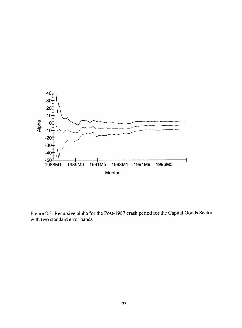
2.3 Recursive alpha for the Post-1987 crash period for the Capital Goods Sector with two standard error bands 33
2.4 Recursive beta for the Full period for the Capital Goods Sector with two standard error bands 34
2.5 Recursive Beta for the Pre-1987 crash period for the Capital Goods Sector with two standard error bands 35
2.6 Recursive Beta for the Post-1987 crash period for the Capital Goods Sector with two standard error bands 36
2.7 Recursive alpha for the full period for Financial Sector with two standard error bands 37
2.8 Recursive alpha for the Pre-1987 crash period for Financial Sector with two standard error bands 38
2.9 Recursive alpha for the Post-1987 crash period for Financial Sector with two standard error bands 39
2.10 Recursive Beta for the full period for Financial Sector with two standard error bands 40
2.11 Recursive Beta for the Pre-1987 crash period for Financial Sector with two standard error bands 41
vii

2.12 Recursive Beta for the Post-1987 crash period for Financial Sector with two standard error bands 42
2.13 Recursive alpha for the full period for Industrial Sector with two standard error bands 43
2.14 Recursive alpha for the Pre-1987 crash period for Industrial Sector with two standard error bands 44
2.15 Recursive alpha for the Post-1987 crash period for Industrial Sector with two standard error bands 45
2.16 Recursive Beta for the full period for Industrial Sector with two standard error bands 46
2.17 Recursive Beta for the Pre-1987 crash period for Industrial Sector with two standard error bands 47
2.18 Recursive Beta for the Post-1987 crash period for Industrial Sector with two standard error bands 48
2.19 Recursive alpha for the full period for the Transportation Sector with two standard error bands 49
2.20 Recursive alpha for the Pre-1987 crash period for the Transportation Sector with two standard error bands 50
2.21 Recursive alpha for the Post-1987 crash period for the Transportation Sector with two standard error bands 51
2.22 Recursive Beta for the full period for the Transportation Sector with two standard error bands 52
Vll l

2.23 Recursive Beta for the Pre-1987 crash period for the Transportation Sector 53
2.24 Recursive Beta for the Post-1987 crash period for the Transportation Sector with two standard error bands 54
2.25 Recursive alpha for the full period for the Utilities Sector with two standard error bands 55
2.26 Recursive alpha for the Pre-1987 crash period for the Utilities Sector with two standard error bands 56
2.27 Recursive alpha for the Post-1987 crash period for the Utilities Sector with two standard error bands 57
2.28 Recursive Beta for the full period for the Utilities Sector with two standard error bands 58
2.29 Recursive Beta for the Pre-1987 crash period for the Utilities Sector with two standard error bands 59
2.30 Recursive Beta for the Post-1987 crash period for the Utilities Sector with two standard error bands 60
2.31 Rolling alpha for the full period for the Capital Goods Sector with two standard error bands 61
2.32 Rolling beta for the full period for the Capital Goods Sector with two standard error bands 62
2.33 Rolling Alpha for the full period for the Financial sector with two standard error bands 63
2.34 Rolling Beta for the full period for the Financial sector with two standard error bands 64
ix

2.35 Rolling Alpha for the full period for the Industrial sector with two standard error bands 65
2.36 Rolling Beta for the full period for the Industrial sector with two standard error bands 66
2.37 Rolling Alpha for the full period for the Transportation sector with two standard error bands 67
2.38 Rolling Beta for the full period for the Transportation sector with two standard error bands 68
2.39 Rolling Alpha for the full period for the Utilities sector with two standard error bands 69
2.40 Rolling Beta for the full period for the Utilities sector with two standard error bands 70
3.1 Unemployment Rates by Race and Gender (1972:01-1999:08) 97
3.2 Generalized Impulse Responses to Shock to Growth in Industrial Production on white female unemployment rate 98
3.3 Generalized Impulse Responses to Shock to Growth in Industrial Production on white Male unemployment rate 99
3.4 Generalized Impulse Responses to Shock to Growth in Industrial Production on Black Male unemployment rate 100
3.5 Generalized Impulse Responses to Shock to Growth in Industrial Production on Black Female unemployment rate 101
4.1 Paper-Bill Spread inCanada 117
X

4.2 Industrial Production in Canada 118
4.3 Growth in Industrial Production in Canada 119
XI

CHAPTER I
INTRODUCTION
This dissertation is comprised of three essays in the areas of financial economics
and macroeconomics. The general equilibrium nature of the macroeconomy is seen
through the ways in which firms, govemments, and households interact in the labor,
output, financial, and money markets. This dissertation focuses on two of the markets
that comprise the macroeconomy; namely, the financial markets and the labor market.
The essays examine how different sectors within the financial sector react to changes in
the overall financial market, how movements in financial variables such as interest rates
provide information on changes in economic activity, and how labor market conditions
respond to unanticipated changes in real economic activity. Each essay also incorporates
time series econometric techniques that allow me to analyze the interactions and
responses of some macroeconomic variable(s) to changes in other macroeconomic
variables. Following is a brief synopsis of each essay.
The first essay is entitled "Sector Index Returns and the Market: A New Study of
Beta Stability." A number of studies have estimated beta's for a variety of securities and
examined their stability over time, however, no study has focused on the betas of
individual sector indexes. This is quite surprising given the proliferation of index
investing over the last decade. I estimate betas for the returns on the S&P capital goods
index, financial index, industrials index, transportation index, and utilities index, using
the composite index as a proxy for the market. An underlying assumption of CAPM is
that beta is inter-temporally stable. However, the underlying stmcture of markets may

change over time for a number of reasons (e.g., financial innovation, money supply
shocks, deregulation, stock market crash, etc.). Some studies have suggested betas may
be time-varying (Fabozzi and Francis, 1978; Brooks, Faff, and Ariff, 1998; Stokes and
Neuburger, 1998). I perform a series of tests to check both the inter-pehod and intra-
period stability of these sector index betas over time. The analysis involves obtaining
recursive and rolling regression estimates of the betas, and a number of diagnostic tests to
detect stmctural breaks and auto-regressive conditional heteroscedasticity. The results
enable me to identify periods of instability and stability, as well as changes in beta over
time. I am able to attribute most of the major changes in sector index betas to particular
economic events and, as such, provide investors with useful information about how future
events are likely to affect these index returns.
The second essay is entitled "Differential Effects of Output Shocks on
Unemployment Rates by Race and Gender" and focuses on how unanticipated changes in
real output are transmitted to unemployment rates of different demographic groups. A
common feature in many macroeconomic models is the connection between departures
from some equilibrium rate of unemployment and the business cycle. The output gap can
be related to the difference between the equilibrium (or "baseline") rate of unemployment
and the actual unemployment rate using Okun's Law and, in fact, most empirical studies
in this area use this as a starting point. Studies of these types include Evans (1989) and
Koop et al. (1996), both of which incorporate vector autoregressions in their analyses.
Hyclak and Stewart (1995) and Lynch and Hyclak (1984) are among the few studies that
examine unemployment rates by race and gender. The former uses micro-data while the
latter focuses on estimates of the natural rate. Through the use of the newly developed

technique of generalized impulse response analysis (Pesaran and Shin, 1998), I measure
the extent to which the behavior of unemployment rates for white males, black males,
black females, and white females differ in response to real output shocks. My results
suggest that these responses are larger and more persistent for blacks than whites, and for
males than females. The findings are particularly important for understanding the impact
of policy initiatives aimed at reducing the adverse effects of changes in output on
employment.
Examining U.S. data, the evidence suggests that the spread between the
commercial paper rate and the Treasury bill rate may contain useful information about
future changes in real output (Friedman and Kuttner, 1992; Estrella and Mishkin, 1998;
and Weber, 1998). Increases in the U.S. paper-bill spread are often associated with
downturns in real economic activity, although recent evidence casts doubt on the spread's
ability to predict recessions (Friedman and Kuttner, 1998; Thoma and Gray, 1998). The
final essay of this dissertation is entitled "The Information Content of the Paper-Bill
Spread: The Case of Canada." In this essay, I examine whether or not the paper-bill
spread is a robust predictor of real activity by considering the case of Canada. If there is
something inherently informative about this yield spread then, in Canada, where these
variables are similarly defined, we should find similar results. To date, only a handful of
studies have looked at the ability of financial spreads to predict recessions in Canada.
Recently, Atta-Mensah and Tkacz (1998) concluded that the spread between the long
bond and the paper rate portends recessions in Canada. This essay focuses on the
information content of the paper-bill spread for the case of Canada and is unique in two
respects. First, by studying the Canadian paper-bill spread I am able to directly compare

the results to the U.S. studies and determine the robustness of this interest rate spread
variable in terms of its ability to predict output. Second, many of the studies used vector
autoregression (VAR) models and forecast error variance decompositions and are,
therefore, subject to the "orthogonality" critique (Lutkenpohl, 1991). In the standard
methodology, results are sensitive to the order in which the variables are entered in the
VAR. I employ the newly developed technique of generalized forecast error variance
decomposition (Pesaran and Shin, 1998). This method provides robust results regardless
of the ordering of the variables in the VAR. I estimate a VAR model of real Canadian
output growth, the paper-bill spread, and money growth. The VAR is then re-estimated
with the addition of U.S. real output growth. Generally speaking, the results presented in
this essay suggest that the paper-bill spread does indeed contain some information about
future movements in Canadian output. Another interesting finding is that the growth rate
of U.S. industrial production does not predict the growth rate of Canadian industrial
production based on Granger-causality tests, but a shock to U.S. real output growth is
found to be important in terms of explaining the forecast error variance of Candian real
output growth. This suggests that unanticipated changes in U.S. real output growth are
important indicators of future real Canadian economic activity. Thus, Canadian
economic activity is not tied directly to how well the U.S. is performing per se, but is
instead significantly affected by unexpected changes (i.e., shocks) to the growth rate of
U.S. real output.

CHAPTER n
SECTOR INDEX RETURNS AND THE MARKET: A NEW STUDY
OFBETASTABUJTY
Abstract
Reliance on stock market sector indexes for investment purposes makes it
essential to understand how various sectors behave relative to the market. Of particular
importance is whether or not these relationships are stable or if they have changed over
time. This paper examines the risk/return characteristics of five S&P sector indexes over
the 1970:01-1997:07 period. The analysis involves tests of inter-period and intra-period
stability, and includes recursive and rolling regression techniques. The results suggest
that the volatility of some sectors, relative to the market, may change following major
economic events. In particular, changes in relative volatility follow or coincide with
events such as the 1987 stock market crash and recessions. Sector volatility also appears
to have responded to the major Federal Reserve tightening of 1994. The findings suggest
that portfolios involving index-based investing should not be thought of as totally passive
strategies. In light of these changing relationships, financial market participants need to
re-evaluate their investments following major economic news.
Introduction
One ingredient to successfully obtaining financial goals is an adequate
understanding of the risk/return characteristics of financial instmments comprising a

portfolio. In order to achieve retirement or savings goals many investors have turned to
various forms of "index investing."' The popularity of index fund investing is evident in
the amount of attention that the financial media devotes to the tracking of equity indexes.
Including an index fund (or group of funds) in one's portfolio may have several
advantages over holding only individual stocks. These advantages include a reduction in
trading costs and management fees, postponement of taxable gains (i.e., market winners
will not be sold as quickly thereby saving on taxes), and obtaining market predictability
(i.e., in the sense that you earn what the market or sector does). Whether or not to
include in a portfolio financial instmments that track particular sectors of the economy or
mirror particular composites, depends on a number of factors including how, and to what
extent, the various indexes are related to the market.
While the index approach to investing has generally been thought of as a passive
strategy, it may not be pmdent to simply invest and "forget about it." Indeed, it may be
wise to periodically re-visit the composition of a portfolio comprised of index funds or
index-based investments particularly after major market changes occur (e.g., a stock
market crash, monetary policy shocks, etc.). This research examines whether or not the
fundamental relation between volatility in several major sector indexes and the volatility
of the overall market has changed over time. By being aware of the potential for certain
sectors of the economy and, therefore, the tendency for index-based investments to
' A number of mutual fund companies offer index funds and index-linked products. In fact, more than 50 companies issue S&P 500 index-linked annuities (http://www.spglobal.com/index.html).
^ Other factors that investors consider when making their investment decision include their level of risk tolerance, investment horizon, goals, etc. Clearly, for diversification purposes, the decision to include a particular asset in a portfolio may also depend on how that asset behaves relative to other assets and/or the market.

behave differently in relation to the market following economic news (e.g., unanticipated
events), financial market participants can constmct portfolios in line with their needs.
Given that financial market participants are turning to index-based investments as a major
part of their portfolio allocation decision, it is imperative that we understand how these
indexes behave, especially in relation to the market. This paper seeks to provide
information on the subject by looking at how returns in various sectors have responded to
fluctuations in overall market returns over a time period that includes a number of major
economic events. Certainly, some sectors are traditionally more volatile than the market
and some are less volatile than the market. However, do these responses of certain
sectors to changes in market returns remain intact following an event such as a stock
market crash or monetary surprise? If they do, then one can simply determine their
relationships once and forget about them. On the other hand, if these relationships
change, then it would be wise to use this information when attempting to constmct
portfolios geared towards investment objectives. In order to examine this issue we focus
attention on five major S&P stock indexes, each representing a major sector of the overall
U.S. market, and each proxying for particular types of index funds and index-based
investments. The Standard and Poor's indexes are especially important to examine
because financial professionals use S&P indexes more than any others to follow
movements of industry groups (Mennis, 1999). We examine these indexes over the
1970:01-1997:07 period in order to discern whether or not the relationships between
these S&P sector indexes and the market have changed.

Risk. Return, and the Meaning of Beta
One method of measuring risk is to use the popular systematic risk measure
known as an investment beta. For instance, the beta of an index (or a stock or portfolio)
tells us how the return on the index responds to changes in the overall market return.
Traditionally, investment betas have been estimated for a number of individual stocks
and a variety of portfolios and the information is often used by financial market
participants for diversification purposes. However, no study has yet examined the betas
for sector indexes like those represented by the S&P. This is surprising given the
popularity of index investing and the importance of sector based indexes."^
The role of the investment beta has become a mainstay of modem financial
economics and has been the subject of much research. The capital asset pricing model
(CAPM) has allowed researchers "to quantify risk and the reward for bearing it".
(Campbell, Lo, and MacKinley, 1997, p. 181). An underlying assumption of CAPM is
that investment betas are constant or stable over time. However, there is some evidence
to suggest otherwise (see, for instance, Fabozzi and Francis, 1978; Sunder, 1980; Stokes
and Nueburger, 1998). Does this mean betas are not useful and that they should be
ignored? Probably not, especially if it is possible to identify how and under what
circumstances betas change. It may very well be that betas are fairiy stable for even
^ The early, seminal work in this area was conducted by Markowitz (1959), Sharpe (1964), and Lintner(1965).
" It is interesting to note that S&P now makes available beta estimates for a variety of sectors based on the S&P Depository Receipts (SPDRs). These figures can be obtained free of charge via the S&P Internet website. This provides financial market participants with a way to quickly reference these figures and use that information to help construct portfolios.

some extended periods of time, but that major events^ may alter the market and thus the
beta values. Exactly how and when betas change, if they do, should be particularly
important to investors and financial market participants.
One important component of the capital asset pricing model is the way in which
the risk-return tradeoff for portfolios is measured. This measure is called beta. Consider
the following equation.
E(rj) = rf+Pj[E(rJ-rfl (2.1)
where rj denotes the return on asset j (in our case the return on an S&P sector index), rm is
the market return (or the return on the S&P composite index), rf is the return on the risk-
free asset (e.g., the 3-month Treasury bill rate), and £(•) is the expectations operator.
The beta of a security is a measure of its systematic risk and is non-diversifiable. In the
context of our study, Pj is the ratio of the covariance between the return on S&P index j
and the market return to the variance of the market return. Thus, beta represents the
volatility of index j relative to the overall market. If P > 1, the index has more risk than
the market and, thus, requires more than the market return. On the other hand, if 0 < P <1
then the index has less risk than the market and requires less than the market return. For
the case when P =1, the index and the market have the same amount of risk and will
require the market return. According to CAPM, an investor is only compensated for
taking on systematic risk and beta can be seen as a measure of the risk that a particular
index brings to a well-diversified portfolio, such as that represented by the S&P 500
composite index. Typically, estimated betas are used by investors in determining and
^ Chen, Roll, and Ross (1986) use the phrase "economic news" to describe major events. Both phrases are used to refer to unanticipated events.
9

analyzing their stock market positions.^ Though a number of studies have estimated
beta's for a variety of securities, and others have examined beta stability over time, no
study has focused on the investment betas of individual sector S&P indexes. This paper
attempts to fill this gap in the literature and to provide the investment professional with
useful information about the behavior of sector indexes relative to the market.
General Description of Methodology and Data
To determine the sector index investment betas, the following equation is
estimated using ordinary least squares regression.
(rj - rf)t = a+ Pj(rm - rf)t + e, (2.2)
The term on the left-side of (2.2), (rj - rf), represents the total risk premium of index j ,
while (rm - rf) represents the market risk premium. The stochastic disturbance term, e ,
reflects the effects of specific (i.e., nonsystematic) and, thus, diversifiable risk. The
estimated coefficient Pj is then taken as the beta for the sector index. Beta enables one to
calculate what the required return on index j might be. One major issue of concern is
whether or not beta is stable over the time period studied (i.e., Pjt = pjt+k, for k = 1,2,...,
n). In our analysis, several tests regarding both mrra-period and inter-pehod stability are
conducted based on the estimation of equation (2.2).
We estimate betas for the returns on the S&P capital goods index, financial index,
industrials index, transportation index, and utilities index. For the overall market return
^ Investors'decisions are also effected by the amount of nonsystematic risk and, therefore, risk related decisions may not be based solely on the value of beta.
10

we use the S&P composite index.^ The three-month Treasury bill proxies the risk-free
rate. The estimated betas provide information as to which indexes are relatively more or
less volatile than the market. Furthermore, examination of the sector index betas in the
pre- and post-crash periods provides information about the stability of these betas in lieu
of major market events.
The data for the study are obtained from the DRI/Citibase data bank and are
monthly observations covering the period from January 1970 through July 1997. The
return on each index was constmcted by annualizing the monthly growth rate.^
The CAPM assumes that beta is inter-temporally stable. However, as mentioned
above, the underlying stmcture of financial markets may change over time for a number
of reasons (e.g., financial innovation, money supply shocks, deregulation, stock market
crash, etc.). Additionally, some studies have suggested betas and/or their variance may
be time-varying (Fabozzi and Francis, 1978; Brooks, Faff, and Ariff, 1998; Stokes and
Neuburger, 1998). Thus, a series of tests are performed to check both inter-pehod and
mrra-period stability of these sector index betas over time. The analysis involves
obtaining recursive and rolling regression estimates of the betas, as well as diagnostic
' Fortune (1998) contends that the S&P 500 composite more closely tracks the (theoretically unobservable) market than do other indexes.
^ Yields are quoted on a discount basis and each monthly observation represents the average of daily values for the whole month.
' The annualized return for index j = {[(1+ ((rj - rj.,/ rj.i))'^]-l }xlOO. Descriptive statistics for index returns are presented in Appendix A. Because ordinary least squares regression requires that the variables under investigation are stationary, unit root tests on each of the constructed return less Treasury bill rate series were conducted. Each was found to be stationary based on findings from augmented Dickey-Fuller unit root tests. Appendix B describes the unit root test and presents the results. Note that the findings of stationarity of index returns is consistent with the weak-form efficient markets hypothesis (Campbell, Lo, and MacKinleay, 1997).
11

tests to detect stmctural changes and tests of auto-regressive conditional
heteroscedasticity (ARCH). The results allow for the identification of periods of
instability and stability, as well as changes in beta over time. We then link some of these
changes in beta to well-known economic events. Below, we describe the methodology
associated with each of these procedures in more detail and present the empirical results
from each.
Estimation of Sector Index Betas in Pre- and Post-Crash Periods
As a starting point for the examination of sector index beta stability, we first
consider the possibility that these betas may have changed following the 1987 stock
market crash. The pre-crash period is defined as 1970:01-1987:09, while the post-crash
period is defined to be 1988:01-1997:07. The stock market crash of October 1987 was
arguably one of the biggest financial market events since World War n and, thus, it
provides us with a natural place to begin our investigation.'°
The results from estimating equation (2.2) for each sector index in both the pre-
and post-crash periods are presented in Table 2.1.' ' Specifically, the third column reports
'° Some people refer to this event as a stock market correction. However, in keeping with much of the literature (e.g., Thorbecke, 1997; Stokes and Neuburger, 1998; Ewing, Payne, and Sowell, 2000), we use the term crash.
" Full sample period results are presented in Appendix C. An alternative method for estimating beta was put forth by Dimson (1979) and subsequently used by Brooks et al. (1998) in a study of the Singapore stock market. The "Dimson beta" technique augments equation (2.2) with lead(s) and lag(s) of the market risk premium, (r^ - rf), in addition to the contemporaneous market risk premium. It is argued that these leads and lags will capture the effects of market risk premium on thinly traded portfolios. While we do not expect the stocks that comprise each of the sector indexes in this study to be thinly traded, we do not rule out the possibility that many index investors "trade" infrequently. Thus, to be sure, we examine the findings using this alternative procedure. Appendix D presents estimated Dimson betas for each sector index. The results were qualitatively identical to the standard beta model. The magnitude of the Dimson beta is slightly larger than the standard estimated beta. This is due to the fact that that the former allows the current total risk premium of a portfolio (i.e., sector index) to depend on changes in the market over a
12

the value of the estimated sector index beta and the fourth column presents the result of a
test to see if the estimated beta is significantly different from one (HQ: P = 1). As
menfioned above, a beta value equal to one implies that the index and the market have the
same amount of risk and should provide similar returns. If the sector index beta is greater
than (less than) one, then a move in the overall market will tend to raise (lower) the index
proportionately more (or less) than the market. Thus, volatile sectors are those sectors
with betas significantly greater than one, while sectors that are less volatile than the
market have betas significantly less than one.
Focusing on the capital goods index it is found that both the pre- and post-crash
period betas are significantly greater than one, with the latter period having the highest
value (1.40 vs. 1.21). This indicates that the capital goods index is more volatile than the
market overall and that this volatility may have increased following the crash. In both
cases, the R^ value is high, suggesting that around 83-85% of the total risk in capital
goods index returns is systematic in nature. Thus, only a relatively small proportion of
the total risk of capital index returns is diversifiable. One way of checking to see if the
estimated beta relationship spelled out in equation (2.2) is stable within the sample
period, i.e. testing for intra-period stability, is to conduct the Lagrange multiplier test for
the presence of autoregressive conditional heteroscedasticity (ARCH).'^ The null
prolonged period. As long as the total risk premium responds in the same direction, independently but not necessarily significantly, in the period(s) immediately preceding and following the current period, then the Dimson beta may be larger since it equals the sum of the coefficients on the lead(s), lag(s), and current market risk premium.
' According to Hildreth and Houck (1968), the effect of a time-varying beta is to alter the properties of the disturbance term in equation (2) so as to become heteroscedastic. In analyzing time series data, heteroscedasticity generally takes the form of what is called autoregressive conditional heteroscedasticity or ARCH effects. A discussion of ARCH and ways to test for its presence is given in Engle(1982).
13

hypothesis of this test assumes that the variance of the esfimated residuals is constant. A
violation of this assumption is detected if the ARCH statistic is significant and is
suggestive of a time-varying variance of the beta model. For capital goods, it is found
that the variance of the beta equation may indeed have been time-varying during the pre-
crash period but no evidence of these ARCH effects are found in the post-crash period.
Thus, we can be more confident using the post-crash beta in constmcting portfolios.
The financial index is also found to have beta estimates significantly greater than
one in both periods studied. Similar to capital goods, the beta value for the financial
index is found to be higher in the post-crash period (1.86) than in the pre-crash period
(1.13). The volatility of financial index returns relative to the overall market appears to
be greater following the stock market crash. The R 's suggest there has been an increase
in the measured amount of total risk that is systematic, i.e., attributable to the market,
since the 1987 crash. No evidence of any intra-period instability is found via the test for
ARCH effects.
Of all the indexes studied, the industrial index most closely resembles the overall
market as measured by beta. In fact, while the estimated betas are found to be
significantly greater than one in both periods, they are both approximately equal in value
and found to be about 1.03. The R 's are .99 and .98, suggesting that almost all of the
movement in industrial index returns can be explained by movements in the market.
Some caution should be used when interpreting the pre-crash beta, however, as evidence
of instability in this period is suggested by the presence of ARCH effects.
The beta values for the transportation index in the pre- and post-crash periods
were found to be 1.29 and 1.07, respectively. However, only the earlier estimate of beta
14
was found to be significantly greater than one. Thus, the volatility of transportation
relative to the market dramatically fell after the stock market crash. In fact, in the latter
period, there appears to be no difference between the transportation beta and the market
beta of one. No significant ARCH effects were detected, providing evidence that these
estimates of beta were stable within each period.
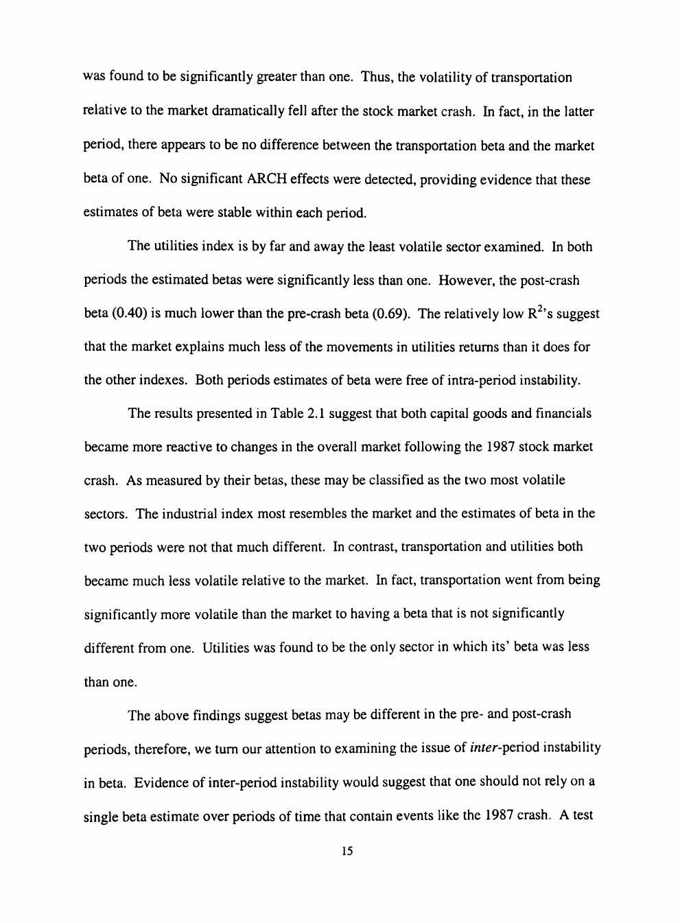
The utilities index is by far and away the least volatile sector examined. In both
periods the estimated betas were significantly less than one. However, the post-crash
beta (0.40) is much lower than the pre-crash beta (0.69). The relatively low R^'s suggest
that the market explains much less of the movements in utilities returns than it does for
the other indexes. Both periods estimates of beta were free of intra-period instability.
The results presented in Table 2.1 suggest that both capital goods and financials
became more reactive to changes in the overall market following the 1987 stock market
crash. As measured by their betas, these may be classified as the two most volatile
sectors. The industrial index most resembles the market and the estimates of beta in the
two periods were not that much different. In contrast, transportation and utilities both
became much less volatile relative to the market. In fact, transportation went from being
significantiy more volatile than the market to having a beta that is not significantly
different from one. Utilities was found to be the only sector in which its' beta was less
than one.
The above findings suggest betas may be different in the pre- and post-crash
periods, therefore, we turn our attention to examining the issue of inter-pehod instability
in beta. Evidence of inter-period instability would suggest that one should not rely on a
single beta estimate over periods of time that contain events like the 1987 crash. A test
15

was conducted to examine if there was a significant change in the regression coefficients
between the two periods. The results of the Chow breakpoint test are presented in Table
2.2. In four cases (capital goods, financial, transportation, and utilities) we find
evidence of inter-period instability in beta.'"* The Chow test did not detect any instability
between the pre- and post-crash regressions for the case of the industrial index.
Table 2.2 also presents the results of an additional test designed to see if the
estimated value of beta in the post-crash period was any different from that of the pre-
crash period. The third column of the table shows the findings of a test where the null
hypothesis is that the post-crash beta equals the pre-crash beta. Consistent with the
findings of the Chow test, we find significant differences between pre- and post-crash
sector index betas in all cases except the industrial index. This suggests that estimated
sector index betas have changed in value and in this sense suffer from inter-period
instability. Thus, while sector index betas may be stable within particular periods, it is
important to re-examine their values periodically and especially following a major event
like a stock market crash.
' To conduct the Chow test, one simply fits the equation separately for both the pre- and post-crash periods and constructs an F-statistic to see whether there are significant differences in the estimated equations. A significant difference indicates a structural change in the relationship.
"* Caution should be used when interpreting results of Chow breakpoint tests. A significant test statistic does not necessarily imply that a structural break took place at precisely the time of the crash. For example, it is possible that there were multiple structural breaks or that the structure changed gradually over time. However, a significant Chow test statistic does indicate that the process in the post-crash period is different than the process in the pre-crash period.
16

Recursive Estimation of Sector Index Betas
In order to determine if the sector index investment betas were stable over the
time period studied (1970-97), recursive estimates of the sector index betas were
obtained.*^ As explained by Stokes and Neuburger (1998) this method can be used to
determine if, and when, changes in the estimated beta values occurred. Plotting the
recursive coefficient estimates allows us to see the development of the betas through
time. Equation (2.2) was estimated recursively using ordinary least squares. The
recursive procedure involves successively re-estimating the model by adding one
observation at a time until the final estimation contains the full set of observations. We
began the estimations of equation (2.2) using a minimum sample size of 3 observations
and then observations were added one at a time as we moved through the sample. Thus,
in all, each of the recursive sector estimations involves a total of N-3 regressions, where
N is the number of observations. The first couple of years in all cases are not significant,
most likely reflective of small sample size, and are not meaningful in an economic sense.
Thus, any appearance (or non-appearance) of volatility in the first part of these plots
would be misleading. However, once the sample size gets sufficiently large so as to
produce consistent estimates (i.e., increases to, say, n=30), we can begin to see
meaningful results and make inferences based on those results. A caveat of using
recursive estimation technique is that this method is biased toward giving the appearance
that the betas are becoming more stable through time as the sample size increases. Thus,
evidence contrary to stability would be all the more convincing.
' For details on the recursive estimation method see Brown, Durbin, and Evans (1975).
17

While our focus is on the estimation of beta in equation (2.2), the constant term
(a) also has a financial market interpretation. According to finance theory the value of
"alpha" is expected to be zero (or not statistically significantly different from zero).
Thus, a significant positive value of alpha indicates that the realized return of the
portfolio is greater than the predicted return. A practice in some brokerage/investment
houses is to base a portfolio managers compensation, often in the form of a bonus, on this
value of a, with those portfolio managers able to generate positive alpha's being in high
demand.*^
Market analysts suggest that if a portfolio has an alpha which is positive and
significant then that implies investors expect a positive return for that portfolio (equal to
the value of alpha) even if the market as a whole provides zero return (Stokes and
Nueburger, 1998). The value of beta provides information as to how market participants
view the volatility of a sector (or, more formally, a portfolio) relative to the market. High
betas suggest that investors view that sector as more volatile than the market, while low
beta values indicate less volatility than the market. Furthermore, if the recursive plot of
beta shows instability then that is taken as an indication that market participants are
repeatedly changing their expectations about that sector.
Figures 2.1-2.30 show the plots of estimated recursive sector index betas as well
as the estimated recursive alphas for the full, pre-1987 crash and post-1987 crash periods.
Below we discuss each of the plots by sector index.
'** See Malkiel (1996).
18

Recursive Estimates for Capital Goods Sector
The plot of the recursive alpha for the full sample period (Figure 2.1) indicates
that alpha was positive most of the time, although it was not significantiy different from
zero. A slight decline in the value of alpha since the late 1980's can be seen in the plot
where the alpha approaches a value of zero, implying adherence to CAPM theory. The
pre-crash period (Figure 2.2) shows alpha to be positive but not significantly different
from zero. However, in the post crash period (Figure 2.3), alpha was negative and
marginally significant during the early 1990s. This latter results indicates that after the
crash, investors in the capital sector were expecting losses (negative return) even if the
market gave a zero return. This is contrary to their belief before the crash.
The plot of the recursive sector beta for the full sample period (Figure 2.4)
indicates that beta was significantly greater than one and exhibited a slight upward trend
over time. This implies that, over time, investors adjusted their beliefs and that capital
sector has become more volatile. Thus, market participants expected a higher than
market return for this sector. A slight jump around 1975 corresponds to the 1974-75
recession. Another jump, though less pronounced, occurred around the beginning of the
1990 recession. Bad economic news appears to make the capital sector more volatile and
thus investors require higher returns. Note that the jump in 1974-75 period is especially
revealed when examining the pre-crash period (Figure 2.5). In the post-crash period
(Figure 2.6) the beta jumped in the 1990-91 recession and remained high until the late
1990s, signifying that investors required a higher return than the market. However, there
is a slight downward trend during the last part of the post-crash period.
19

Recursive Estimates for Financial Sector
The plot of the recursive alpha for the full sample period (Figure 2.7) indicates
that alpha had a positive value and was marginally significant after the early 1980s. The
plot of alpha for the pre-1987 crash period (Figure 2.8) shows that the value of alpha was
marginally significant during the eighties. Following the 1987 crash (Figure 2.9), the
value of alpha was not significantly different from zero. This indicates that after the
crash, investors expected a zero return for the financial sector if the market were to yield
a zero return. A slight dip in the alpha value during the 1990-91 recession, as indicated
in the post-crash figure, shows that this recession appeared to make investors more
pessimistic about expected returns.
The recursive beta plot for the full sample period (Figure 2.10) reveals that the
financial sector exhibited greater volatility in returns as compared to the other sectors.
The financial sector beta shows an upward trend after the 1970s. It also shows a jump
and then a dip around the recession period of 1975, similar to that which the capital
sector experienced. The 1990-91 recession had a similar effect in the financial sector as
it had in the capital goods sector with beta becoming higher. The pre-crash period
(Figure 2.11) exemplifies the 1975 recession. It also shows a higher beta value after
1982 following the 1980-82 recession. The post-crash beta plot (Figure 2.12) shows the
1990-91 jump and then beta remaining high (with a value exceeding 2) until the late
1990s. In the late 1990s, the sector beta began to trend down slightiy. This type of trend
is consistent with what one would expect given the financial innovation and continued
deregulation of financial markets in the 1990s. Thus, following the crash of 1987, the
financial sector beta has been higher.
20

Recursive Estimates for Industrial Sector
The plot of the recursive alpha for the full sample period (Figure 2.13) indicates
that the alpha had a positive but insignificant value throughout much of the entire
estimation period. The alpha value became marginally significant in the 1990s indicative
of market participants that expected the sector to produce a positive return even if the
market produced a zero return. The estimated value for alpha in the pre-crash period
(Figure 2.14) was positive but never significant. The alpha value in the post-crash period
(Figure 2.15) was always close to zero, as is expected by CAPM theory.
Looking at the recursive beta plot of the full sample period (Figure 2.16) shows
that the industrial sector was the least volatile of the sectors, indicating that market
participants viewed this sector as more stable in terms of returns and, since the beta value
has been close to one, believed it should yield returns similar to those of the market. This
is consistent with the higher R-square values for the industrial sector as reported in Table
2.1. A downward spike around late 1974, a recessionary period, stands out in the full
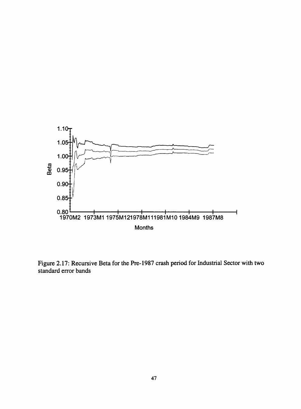
sample estimation and in the pre-crash period (Figure 2.17). The post crash plot (Figure
2.18) of the beta shows the beta value to have stabilized since the slight jump experienced
during the 1990-91 recession.
Recursive Estimates for Transportation Sector
The plot of the recursive alpha for the full sample period (Figure 2.19) indicates
that alpha had a positive and significant value almost throughout the sample. This is the
only sector for which a significant value for alpha was detected. The implication is
21

investors were always optimistic about transportation returns. Even if the market were to
perform badly, this sector anticipated a better return than the market. The pre-crash
period (Figure 2.20) shows a positive and (most of the time) significant value for alpha.
However, after the crash (Figure 2.21) it was not significantiy different from zero. Thus,
the 1987 crash may have made investors realize that if the market does not perform well
(yields zero retum), the transportation sector will also yield zero returns.
The recursive beta plot of the full sample period (Figure 2.22) reveals that the
transportation sector beta rose in the early 1970s and then experienced a substantial drop
in value around the middle of 1974 near the start of the recession. This beta exhibited a
slight rise in the 1970s but since the mid-1980s has been trending down somewhat. The
pre- and post-crash periods (Figure 2.23-2.24) tell a similar story.
Recursive Estimates for Utilities Sector
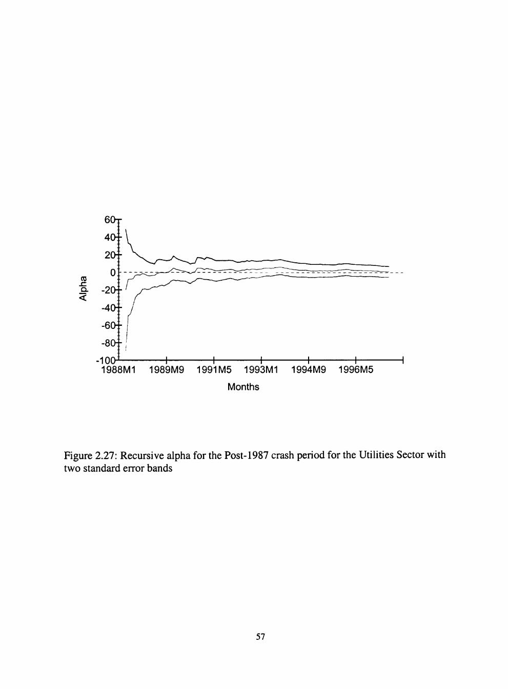
The plot of the recursive alpha for the full sample period (Figure 2.25) indicates
that alpha had a value very close to zero and was insignificant all through the full sample,
pre-crash (Figure 2.26) and post crash period (Figure 2.27). This finding is consistent
with CAPM.
Lx)oking at the recursive beta plot of the full sample period (Figure 2.28) we see
that the utilities sector has had a beta less than one, possibly trending down through the
sample period. However, the beta value went up in the middle of 1975 close to the end of
the recession. The pre-crash period (Figure 2.29) revealed that the beta has gone down in
value. The post-crash period (Figure 2.30) shows that after the crash beta was high and
exhibited volatility, but since the 1990-91 recession subsided the beta has been lower.
22

Rolling Regression Estimation of Sector Index Betas
To begin the rolling regression analysis we initially estimated equation (2.2) over
the first thirty observations of the sample period for each sector and then re-estimated
equation (2.2) where one observation was added to the end of the sample and
simultaneously one observation was dropped from the beginning of the sample. This
procedure was repeated until we moved, or rolled, entirely through the sample. The key
to the rolling regression is that each regression is conducted with an identical sample size,
called the sample size window. Thus, as we rolled through the sample, the sample size
was kept constant. The results presented here are for the case with a sample size window
of 30 observations; however, experiments with windows of 40 and 50 produced
qualitatively similar results and the conclusions based on the alternative window sizes are
unchanged. The rolling regressions show how the sector index betas change over time
and allow one to identify particular periods of instability as well as periods of stability.
The major benefit from using the rolling regression method is that it provides results that
are robust to changes in starting and ending period. The method can detect outliers in the
sample and allows one to determine the extent to which a particular outlier may have
influenced the results and thus the inference drawn from those results. While a
significant jump in the regression estimate indicates the possible presence of an outiier, a
corresponding jump of similar magnitude in the opposite direction is likely to occur after
thirty months (the window size) when the outlier observation is dropped from the sample.
This should be kept in mine when interpreting the rolling regression results.
23

Figures 2.31-2.40 show the plots of estimated rolling regression sector index betas
and alphas for the full sample period. In the interest of brevity, we do not report or
discuss the recursive regression findings based on the pre- and post-1987 stock market
crash sub-periods as no additional information was contained in them. ^ Below we
discuss each of the plots by sector index.
Rolling Regression Estimates for Capital Goods Sector
For the full sample period (Figure 2.31) the rolling alpha for the capital goods
index had a positive value until the middle of the 1980s and then became negative for
around ten years before becoming positive again during the middle 1990s. However,
throughout the sample period, the estimated value of alpha was not significantly different
from zero. The rolling beta (Figure 2.32) estimates for the full sample period appear to
be unstable. The capital goods index rolling beta had a value greater than one throughout
the sample, except for two short periods during 1975 and 1995 when it was actually less
than one. The sudden increase that occurred around 1991 stands out and corresponds the
1990-91 recession.
Rolling Regression Estimates for Financial Sector
Similar to the experience of the capital goods sector, the rolling alpha for the
financial sector index (Figure 2.33) was positive until the late 1980s and then became
negative for a couple of years before returning to positive territory during the early
' ' These results are available upon request.
24

1990s. This behavior of alpha implies that financial market participants expected the
financial sector would yield negative returns when the overall market yields zero retum
during these years following the crash of 1987. However, the rolling alpha was not
significantly different from zero during the sample period. The rolling beta estimates
were greater than one throughout most of the sample (Figure 2.34). This implies that the
financial sector has been regarded as more volatile than the market by the participants
and they expect a retum higher than the overall market. The rolling financial sector beta
did go up during late 1990-early 1991 (a recession period) and was actually greater than
two until early 1993. In general, the rolling beta was higher after the 1987 crash.
Rolling Regression Estimates for Industrial Sector
The rolling alpha for the industrial sector was not significantly different from zero
throughout the sample period (Figure 2.35). The value of alpha had been hovering
around zero except right after the October 1987 crash when it was around two. The
implication is that financial market participants realized retums higher than expected
after the crash. The rolling beta for the industrial sector was not significantly different
from one for most of the sample period (Figure 2.36). It shows far more stability than the
other sector indexes. However, the rolling beta for the industrial sector index has shown
some relative instability after the 1987 crash.
Rolling Regression Estimates for Transportation Sector
The rolling alpha for the transportation sector was not significantly different from
zero throughout the sample period except for a brief period coinciding with the 1982
25

recession (Figure 2.37). The sharp rise in the rolling alpha during 1982 indicates that
market participants were expecting a positive retum from transportation sector even if the
market yielded a zero retum. The rolling regression for the transportation sector index is
indicative of a fairly unstable beta (Figure 2.38). Unlike the financial and capital goods
sectors, the transportation sector showed greater volatility in beta during the pre-crash
period. The post-crash period reveals a smooth downward trend in the value of beta,
except for a small dip in the middle of 1995, about a year after the monetary policy
tightening of 1994.
Rolling Regression Estimates for Utilities Sector
The rolling alpha for the utilities sector was not significantiy different from zero
throughout the sample period (Figure 2.39). Similar to the transportation sector, these
alpha estimates show more stability following the 1987 crash. The rolling regression
estimates of beta (Figure 2.40) for the utilities sector indicates signs of instability,
especially in the pre-crash period. There is a noticeable jump in the rolling beta around
1975 and this may be attributed to the 1974-75 recession. However, from 1975 until the
1987 crash there was a upward trend in the value of beta.
Implications of the Sector Index Betas for Financial Market Participants
The main contribution of this paper is the documentation of changes in sector
index betas over the time period studied. First, we documented changes in sector index
betas between the pre- and post-1987 stock market crash periods. Second, through the
use of recursive estimation, it is shown that volatility as measured by sector index betas
26

has gone through a number of changes over time. These changes appear to be linked to
major economic events such as recessions and monetary policy, in addition to the stock
market crash. In fact, the latter event appears to have had a lingering and somewhat
persistent effect that has worked to raise (most of) the betas over time. The rolling
regression results are suggestive of an increase in sector index beta volatility over the full
sample period. This increased volatility is especially evident during the 1990's. These
sector betas jumped upward around the 1990-91 recession in all cases except the utilities
sector. Also, there is a noticeable drop in the sector index beta values for the financial,
capital, and industrial sectors in (or following) 1994, corresponding to a period of
substantial monetary tightening by the Federal Reserve. Generally speaking, sector index
betas have not remained constant over time and in this sense exhibit characteristics of
instability. The instabilities appear more abmpt and pronounced during and inmiediately
following major economic events.
A key point of these results is that relationships between sectors and the market
are not set in stone. These relationships do change and financial market participants need
to know that portfolios constmcted today with certain expected diversification benefits in
mind may not necessarily provide those same benefits in the future.
An important practical implication of this research is the valuable and timely
information that the estimated sector index betas provide to investors, market
participants, and financial planners and counselors. For instance, if the beta for a
particular index is close to one, then those seeking to diversify would not experience the
expected benefits from allocating between a market index fund and that sector index-
based investment.
27

An important lesson from this research is that viewing index-based investing as a
totally passive strategy may lead to a false sense of security for investors. It is necessary
for those who make use of index-based investments to be aware of the potential for
changing relationships between sectors and the overall market, and to carefully watch and
monitor these relationships in the wake of economic events.
Concluding Remarks
Today's investors are utilizing various forms of index-based investing to achieve
long term financial goals. Proper financial planning is, of course, essential to the success
of any investor's portfolio. The results presented in this paper strongly suggest that index
investing should not be thought of as being a completely passive strategy. We find that
the relative responsiveness of various sectors in relation to the market has changed. We
attribute many of these changes in the behavior of sector betas to major economic events
such as the 1987 stock market crash, Federal Reserve actions such as the monetary
tightening of 1994, deregulation of financial markets and financial innovation. Given
these tendencies for changes in sector investment betas, financial market participants will
want to make appropriate portfolio allocation decisions. In fact, the occurrence of major
market changes, economic news, and other potential shocks to the world economy is
inevitable and it is especially important for investors to re-visit their financial positions
and perhaps alter their allocation decisions accordingly, regardless of whether or not they
are taking an index-based investing approach.
28

Table 2.1. Pre- and Post-Stock Market Crash: Investment Betas for S&P Sector Indexes
Capital goods
Financial
Industrial
Transportation
Utilities
Sample Period
Pre-crash
Post-crash
Pre-crash
Post-crash
Pre-crash
Post-crash
Pre-crash
Post-crash
Pre-crash
Post-crash
P
1.2066
1.4015
1.1257
1.8571
1.0283
1.0262
1.2873
1.0727
0.6854
0.3991
H o : p = l
34.03'
44.69'
3.10 =
70.05'
16.55'
3.0703'
16.73'
0.66
25.38'
75.03'
R^
.85
.83
.54
.74
.99
.98
.61
.56
.36
.23
ARCH
24.91'
1.63
1.89
0.32
36.24'
0.00
0.75
0.85
0.00
0.37
Notes: The superscripts a, b, c denote significance at less than the 1%, 5%, and 10% levels, respectively. ARCH denotes a Lagrange Multiplier test, distributed x^d), designed to check for the presence of autoregressive heteroscedasticity in the error terms. A significant ARCH value suggests that the estimate of beta may not be stable within the particular sample period.
29

Table 2.2. Pre- and Post-Stock Market Crash: Tests of Inter-Period Sector Beta Stability
Capital goods
Financial
Industrial
Transportation
Utilities
Chow
3.2994*
[0.038]
14.9619'
[0.000]
0.1918
[0.826]
2.7211'
[0.067]
3.4788^
[0.032]
Ho: pP^' = pP '
10.5316'
[0.001]
51.0117'
[0.000]
0.0196
[0.889]
5.7302'
[0.017]
17.0333'
[0.000]
Notes: The superscripts a, b, c denote significance at less than the 1%, 5%, and 10% levels, respectively. Chow denotes the F-statistic that tests the stability of the regression coefficients. HQ: pP°'* = pP' is the null hypothesis from a Wald test, distributed x^d), and is used to check if the estimated value of beta in the post-crash period equals the value of beta from the pre-crash period. Actual probability values are given in brackets.
30

CD
a. <
1970M2 1974M4 1978M6 1982M8 1986M10 1990M12 1995M2 Months
Figure 2.1: Recursive estimate of alpha for the full period for the Capital Goods Sector with two standard error bands
31

30r
CD x: Q.
1970M2 1973M1 1975M121978M111981M101984M9 1987M8 Months
Figure 2.2: Recursive alpha for the Pre-1987 crash period for the Capital Goods Sector with two standard error bands
32
CO SI
<
1988M1 1989M9 1991M5 1993M1
Months
1994M9 1996M5
Figure 2.3: Recursive alpha for the Post-1987 crash period for the Capital Goods Sector with two standard error bands
33

2.0T
1970M2 1974M4 1978M6 1982M81986M101990M121995M2
Months
Figure 2.4: Recursive beta for the Full period for the Capital Goods Sector with two standard error bands
34

2.aT
C D * . < 0
CO
1970M2 1973M1 1975M121978M111981M10 1984M9 1987M8 Months
Figure 2.5: Recursive Beta for the Pre-1987 crash period for the Capital Goods Sector with two standard error bands
35

2.(>T
B CO
1988M1 1989M9 1991M5 1993M1 1994M9 1996M5 Months
Figure 2.6: Recursive Beta for the Post-1987 crash period for the Capital Goods Sector with two standard error bands
36

CD
a. <
1970M2 1974M4 1978M6 1982M81986M101990M121995M2
Months
Figure 2.7: Recursive alpha for the full period for Financial Sector with two standard error bands
37

CD
a. <
1970M2 1973M11975M121978M111981M101984M9 1987M8 Months
Figure 2.8: Recursive alpha for the Pre-1987 crash period for Financial Sector with two standard error bands
38

60r
CD sz a. <
-40--
-60--
1988M1 1989M9 1991M5 1993M1 1994M9 1996M5
Months
Figure 2.9: Recursive alpha for the Post-1987 crash period for Financial Sector with two standard error bands
39

2.5T
C D ^-> Q)
CO
1970M2 1974M4 1978M6 1982M8 1986M101990M12 1995M2
Months
Figure 2.10: Recursive Beta for the full period for Financial Sector with two standard error bands
40

1970M2 1973M11975M121978M111981M101984M9 1987M8 Months
Figure 2.11: Recursive Beta for the Pre-1987 crash period for Financial Sector with two standard error bands
41

1988M1 1989M9 1991M5 1993M1 1994M9 1996M5
Months
Figure 2.12: Recursive Beta for the Post-1987 crash period for Financial Sector with two standard error bands
42

CD sz a. <
1970M2 1974M4 1978M6 1982M8 1986M101990M12 1995M2 Months
Figure 2.13: Recursive alpha for the full period for Industrial Sector with two standard error bands
43

CD
a. <
-4--I
-6"
1970M2 1973M1 1975M121978M111981M10 1984M9 1987M8
Months
Figure 2.14: Recursive alpha for the Pre-1987 crash period for Industrial Sector with two standard error bands
44

CD
<
1988M1 1989M9 1991M5 1993M1
Months
1994M9 1996M5
Figure 2.15: Recursive alpha for the Post-1987 crash period for Industrial Sector with two standard error bands
45

1.10r
CD
I 0.9
1970M2 1974M4 1978M6 1982M8 1986M101990M12 1995M2 Months
Figure 2.16: Recursive Beta for the full period for Industrial Sector with two standard error bands
46
1.10T
CD
I 0.9
0.85--
1970M2 1973M1 1975M121978M111981M101984M9 1987M8
Months
Figure 2.17: Recursive Beta for the Pre-1987 crash period for Industrial Sector with two standard error bands
47

CD 0)
m
1.5T
1988M1 1989M9 1
1991M5 1993M1 Months
+ + 1994M9 1996M5
Figure 2.18: Recursive Beta for the Post-1987 crash period for Industrial Sector with two standard error bands
48

1970M2 1974M4 1978M6 1982M8 1986M101990M12 1995M2
Months
Figure 2.19: Recursive alpha for the full period for the Transportation Sector with two standard error bands
49

8Ch-
1970M2 1973M1 1975M121978M111981M10 1984M9 1987M8
Months
Figure 2.20: Recursive alpha for the Pre-1987 crash period for the Transportation Sector with two standard error bands
50

CD
<
1988M1 1989M9 1991M5 1993M1
Months
1994M9 1996M5
Figure 2.21: Recursive alpha for the Post-1987 crash period for the Transportation Sector with two standard error bands
51

CD *-> 00
1970M2 1974M4 1978M6 1982M8 1986M101990M12 1995M2 Months
Figure 2.22: Recursive Beta for the full period for the Transportation Sector with two standard error bands
52

3.0r
CD ••-< 0)
CO
1
1
0
1970M2 1973M1 1975M121978M111981M10 1984M9 1987M8
Months
Figure 2.23: Recursive Beta for the Pre-1987 crash period for the Transportation Sector
53

CO
1988M1 1989M9 1991M5 1993M1
Months
+ 1994M9 1996M5
Figure 2.24: Recursive Beta for the Post-1987 crash period for the Transportation Sector with two standard error bands
54

150T
1970M2 1974M4 1978M6 1982M8 1986M101990M12 1995M2
Months
Figure 2.25: Recursive alpha for the full period for the Utilities Sector with two standard error bands
55

15C>T
1970M2 1973M1 1975M121978M111981M10 1984M9 1987M8 Months
Figure 2.26: Recursive alpha for the Pre-1987 crash period for the Utilities Sector with two standard error bands
56
CD SI Q.
-100 1988M1 1989M9 1991M5 1993M1 1994M9 1996M5
Months
Figure 2.27: Recursive alpha for the Post-1987 crash period for the Utilities Sector with two standard error bands
57

B CO
1970M2 1974M4 1978M6 1982M8 1986M101990M12 1995M2 Months
Figure 2.28: Recursive Beta for the full period for the Utilities Sector with two standard error bands
58

1970M2 1973M1 1975M121978M111981M10 1984M9 1987M8 Months
Figure 2.29: Recursive Beta for the Pre-1987 crash period for the Utilities Sector with two standard error bands
59

B 0)
CD
1988M1 +
1989M9 1991M5 1993M1
Months
\ 1 1994M9 1996M5
Figure 2.30: Recursive Beta for the Post-1987 crash period for the Utilities Sector with two standard error bands
60

CD sz Q.
1972M7 1976M4 1980M1 1983M10 1987M7 1991M4 1995M1 Months
Figure 2.31: Rolling alpha for the full period for the Capital Goods Sector with two standard error bands
61

2.Ch-
1972M7 1976M4 1980M1 1983M10 1987M7 1991M4 1995M1 Months
Figure 2.32: Rolling beta for the full period for the Capital Goods Sector with two standard error bands
62

8 0 T
CD
a. <
1972M7 1976M4 1980M1 1983M10 1987M7 1991M4 1995M1
Months
Figure 2.33: Rolling Alpha for the full period for the Financial sector with two standard error bands
63

3.0j
2.5"
CD * ^ CD
CO
-0.5 1972M7 1976M4 1980M1 1983M10 1987M7 1991M4 1995M1
Months
Figure 2.34: Rolling Beta for the full period for the Financial sector with two standard error bands
64

1972M7 1976M4 1980M1 1983M10 1987M7 1991M4 1995M1 Months
Figure 2.35: Rolling Alpha for the full period for the Industrial sector with two standard error bands
65

1.3T
B CO
1972M7 1976M4 1980M1 1983M10 1987M7 1991M4 1995M1 Months
Figure 2.36: Rolling Beta for the full period for the Industrial sector with two standard error bands
66

CD
a. <
1972M7 1976M4 1980M1 1983M10 1987M7 1991M4 1995M1
Months
Figure 2.37: Rolling Alpha for the full period for the Transportation sector with two standard error bands
67

2 .5T
2.0--
B m
1972M7 1976M4 1980M1 1983M10 1987M7 1991M4 1995M1
Months
Figure 2.38: Rolling Beta for the full period for the Transportation sector with two standard error bands
68

60r
CD
Q.
<
1972M7 1976M4 1980M1 1983M10 1987M7 1991M4 1995M1 Months
Figure 2.39: Rolling Alpha for the full period for the Utilities sector with two standard error bands
69

2.5T
B CO
1972M7 1976M4 1980M1 1983M10 1987M7 1991M4 1995M1
Months
Figure 2.40: Rolling Beta for the full period for the Utilities sector with two standard error bands
70

CHAPTER m
DIFFERENTIAL EFFECTS OF OUTPUT SHOCKS ON
UNEMPLOYMENT RATES BY RACE
AND GENDER
Abstract
This paper employs a recentiy developed time series econometric technique to
examine the magnitude and persistence of unanticipated changes in real output on
unemployment rates by race and gender. Through the use of generalized impulse
response analysis (Koop et al. 1996; Pesaran and Shin, 1998), we measure the extent to
which the behavior of unemployment rates for white males, black males, black females,
and white females differ in response to real output shocks. The results suggest that while
real output growth reduces the unemployment rate of all demographic groups, the effect
is larger and more persistent for blacks than whites, and for males than for females. The
findings are particularly important for understanding the impact of policy initiatives
aimed at dampening the employment effects of unanticipated changes in real output
growth.
71

Introduction
The issues of unemployment and output are central to many macroeconomic
policy debates. A major source of disagreement among policymakers deals with the
maximum sustainable level of output growth that is consistent with the absence of
inflation. When the economy's rate of output growth exceeds the maximum sustainable
rate, there will be upward pressure on the economy's overall price level. Traditional
macroeconomic theory emphasizes the role that tight labor markets play in this
inflationary pressure. The commonly held belief is that in a tight labor market firms must
bid workers away from other firms if they wish to expand the size of their workforce.
Hence, labor costs in the economy will tend to rise. Since labor is a major input in the
production of virtually all goods and services, an increase in labor costs will tend to
increase the economy's overall price level. Conversely, when the economy contracts, if
wages are downward flexible, labor costs in the economy will tend to fall, inducing a
downward movement in the economy's overall price level. The labor market is therefore
linked to changes in economic activity.
A common feature in many macroeconomic models is the connection between
departures from the equilibrium rate of unemployment (i.e., the natural or normal rate)
and the business cycle. These macroeconomic models suggest that unanticipated
departures from a steady state in the output market should be related to departures of the
actual unemployment rate from the normal rate. However, the economy's aggregate
unemployment rate is really a weighted-average of the unemployment rates of various
demographic groups. The rate of each demographic group is influenced by each group's
72

flows into and out of unemployment. Thus, the unemployment rates of different
demographic groups may respond differently to aggregate output shocks. In fact, since
many of the factors that determine the flows into and out of unemployment have been
found to differ by demographic group, it is expected that a given output shock may have
differential effects on the unemployment rates of various groups.
This paper focuses on how unanticipated changes in real output affect the
unemployment rate of different demographic groups. We examine the time series
behavior of black male, white male, black female, and white female monthly
unemployment rates, over the January 1972 (1972:01) to August 1999 (1999:08) period.
Specifically, we estimate a vector autoregression (VAR) and then conduct simulations in
the form of impulse responses to determine the extent to which each of these
unemployment rates is affected by an aggregate output shock (i.e., an unanticipated
change in output). We compare and contrast both the magnitude and the persistence of
these responses across the groups. Because the traditional impulse response function
generated from a VAR is sensitive to how the researcher chooses to order the variables,
with different orderings often giving vastiy different results, we employ the recentiy
developed generalized impulse response function (Pesaran and Shin, 1998; Koop et al.,
1996). This technique allows researchers to examine impulse responses that are robust to
changes in ordering. In the following sections we highlight the major literature that this
paper builds upon and then we discuss the basics behind the nature of the relationship
between unemployment and output. A discussion of the data, the methodology, and the
results follows. The paper closes by offering some concluding remarks.
73

Related Literature
A number of studies have examined racial differences in unemployment rates and
in factors that may affect unemployment rates. Using data on displaced workers, Fairiie
and Kletzer (1998) examine racial differences in job displacement over the years 1984-
1992. They find that black males experienced greater rates of job displacement and
lower rates of re-employment than white males. Petterson (1998) uses data from the
National Longitudinal Survey of Youth for the 1979-1986 period to examine the
reservation wages of black males compared to those of white males and, contrary to
earlier research, argues that these differences do not explain much (if any) of the racial
employment gap. Keith and McWilliams (1995, 1999) document differences in job
mobility between men and women, as well as differences in the degree of on-the-job
search. Generally speaking, if there are differences in the underlying factors that affect
the flows into or out of unemployment by demographic group, then differences in
unemployment rates may exist.
Bartlett and Haas (1997) contend that the natural rate of unemployment varies by
demographic group. They argue that an economic policy geared towards changing the
aggregate natural rate could, therefore, have positive effects on the unemployment
situations of some groups while having adverse effects on other groups. Schwartzman
(1997) documents the effects of government policies on the unemployment rate of black
males over the last half century. Fairiie and Sundestrom (1999) use Census Bureau
micro-data from 1880-1990 (exclusive of 1920 and 1930) to examine the racial
unemployment rate gap and, through the use of decomposition analysis, they uncover
74

three trends. First, black gains in human capital (e.g., education) have helped reduce the
gap. Second, since World War n regional shifts in the economy, mostly the migration of
blacks from the mral south, have attributed to a widening of the gap. Third, relative
decreases in demand for less-skilled workers have added to the gap since 1970.
The time-series relationship between aggregate output and the aggregate
unemployment rate was examined by Evans (1989), using vector autoregressions (VAR)
and employing innovation accounting techniques. Evans documented the relationship
and provided some evidence to suggest a persistent effect of output shocks on aggregate
unemployment consistent with what is to be expected by Okun's Law.
While a number of studies have examined the aggregate output-unemployment
rate relationship, few have looked specifically at the effects of output changes on the
unemployment rates of various demographic groups. Hyclak and Stewart (1995)
examined the effects of changes in aggregate demand on unemployment rates by
demographic group, using establishment-level data and longitudinal/panel data
techniques. They found that unemployment rates of blacks were significantly more
responsive to demand growth than unemployment rates of whites. A time series analysis
by Lynch and Hyclak (1984) found that unemployment rates of blacks and males are
more adversely affected by downturns in the economy than the rates of whites and
females. The latter paper was based on the relationship spelled out by Okun's Law. The
present paper fills a gap in the literature by using advanced time-series techniques to
study the question posed by Lynch and Hyclak (1984) about differential effects of output
shocks on unemployment rates of various demographic groups.
75

A Brief Digression on the Equilibrium Rate of Unemplovment
In the absence of macroeconomic shocks, the unemployment rate that the
economy tends to gravitate towards is the equilibrium rate of unemployment. This
"natural" rate can be thought of as the normal rate of unemployment or the baseline.
When the economy is at its equilibrium unemployment rate, three conditions will exist.'^
1. The flow of employed workers into unemployment will equal the flow of
unemployed workers into employment.
2. The flow of people from not-in-the-labor-force status (i.e., non-
participants) to unemployment equals the flow of workers from
unemployment to not-in-the-labor-force status.
3. The flow of non labor-force participants to the labor force equals the flow
of workers from the labor-force to not-in-the-labor-force status.
To mathematically derive the above equilibrium conditions, we develop a model
that describes the stock-flow analysis of Barron et al. (1989). To derive the first
condition for the equilibrium unemployment rate; define a to be the fraction of employed
workers who become unemployed each month; define p to be the fraction of unemployed
workers who become employed each month; define N to be the number of workers
employed at the beginning of each month; and define U to be the number of workers
unemployed at the beginning of each month. The first equilibrium condition, that the
flows into unemployment equal the flows out of unemployment, can be written as:
' Technically, all that is required is the sum of inflows to be equal to the sum of outflows for total labor force and unemployment pool.
76

ocN = pu. (3.1)
If we further let L = total number of workers in the labor force, then N = L-U.
Thus, in equilibrium we have:
a(L-U) = PU.
Solving for the equilibrium unemployment level, U, U = [(x/(a+P)]L. The equilibrium
unemployment rate is then given by:
u* = U/L = [a/(a+P)]
The second condition for equilibrium implies that entry into and out of the labor
force by unemployed workers also affects the unemployment rate. Therefore, if we let n
denote the fraction of non-participants who enter the labor force each month but who
don't become employed during the month, K denote the number of individuals not
participating in the labor force each month, and r|u denote the fraction of unemployed
workers who drop out of the labor force each month, then the second equilibrium
condition is 7iK = r|uU. Adding this to the first equilibrium condition, equation (3.1),
yields:
oN + 7iK = (P+Tiu)U (3.2)
The third condition states that the number of non-participants entering the labor
force (some who become employed and some who become unemployed) equals the
number exiting the labor force (from the ranks of both the unemployed and employed). K
we denote Tie as the fraction of employed workers who leave the labor force each month
and p denote the fraction of the non-participants who enter the labor force each month as
employed, then in equilibrium
77
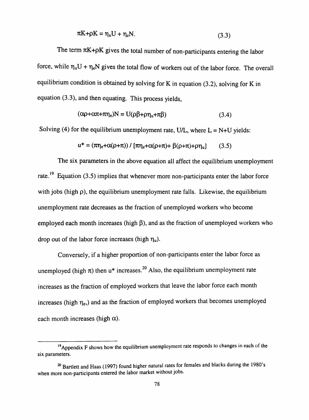
7iK+pK = TluU + TleN. (3.3)
The term 7iK+pK gives the total number of non-participants entering the labor
force, while TiuU -i- TieN gives the total flow of workers out of the labor force. The overall
equilibrium condition is obtained by solving for K in equation (3.2), solving for K in
equation (3.3), and then equating. This process yields,
(ocp+oai+7rne)N = U(pP+pTiu+7cP) (3.4)
Solving (4) for the equilibrium unemployment rate, U/L, where L = N+U yields:
U* = (TCne+a(p+7l)) / [7nie+a(P+7l)+ P(p-H7l)+pTlul (3 .5)
The six parameters in the above equation all affect the equilibrium unemployment
rate. Equation (3.5) implies that whenever more non-participants enter the labor force
with jobs (high p), the equilibrium unemployment rate falls. Likewise, the equilibrium
unemployment rate decreases as the fraction of unemployed workers who become
employed each month increases (high P), and as the fraction of unemployed workers who
drop out of the labor force increases (high T U).
Conversely, if a higher proportion of non-participants enter the labor force as
unemployed (high n) then u* increases.^^ Also, the equilibrium unemployment rate
increases as the fraction of employed workers that leave the labor force each month
increases (high r|e,) and as the fraction of employed workers that becomes unemployed
each month increases (high a).
"Appendix F shows how the equilibrium unemployment rate responds to changes in each of the six parameters.
^ Bartlett and Haas (1997) found higher natural rates for females and blacks during the 1980's when more non-participants entered the labor market without jobs.
78

One point to note is that the labor force drop out rate of employed workers. Tie,
plays a role in determining u*. If this rate differs by demographic group then tiie
unemployment rate will also vary by demographic group. There is no a priori
expectation about whether Tie is likely to fall or rise during a recession. However, it is
likely that the other parameters (p, 71, a, p, TIU) are sensitive to current macroeconomic
conditions. Typically, the labor market is characterized by higher values of p and P
during an economic expansion, while recessions are associated with higher values of 7i,
a, and Tiu. For example, during a recession there are typically a number of layoffs, which
causes a to rise and P to fall, relative to their normal values. Together, these parameter
changes work to increase the unemployment rate during a recession or economic
downturn. The opposite is tme during a recovery or period of economic growth. Since
the equilibrium unemployment rate is affected by the values of the above parameters, any
differences in these parameters between demographic groups can potentially lead to
differences in the response of the unemployment rate to changes in output. Thus, there
may be differences in the response of the unemployment rate to an output shock between
race and gender groups.
Unemplovment Rates and Demographic Groups
The aggregate unemployment rate is actually a weighted-average comprised of
the unemployment rates of various demographic groups that, at any point in time, diverge
widely. If there are differences between demographic groups in the factors underlying
the flows into and out of unemployment, then there will be differences in the equilibrium
79

unemployment rate of each group. Thus, it should not surprise us to find that the
unemployment rate response to an output shock varies across demographic groups.
As discussed above, a particular demographic group's unemployment rate may be
high for any number of reasons. For example, Barron et al. (1989) suggest that if
unemployed workers in a group require an unusually long time to obtain employment
after becoming unemployed (low P), or if after becoming employed they have a high
probability of becoming unemployed again (high a), or if they frequently quit their jobs
to pursue non-labor market activities (high Tie), then the unemployment rate of the group
will be high. '
Similarly, blacks would have higher unemployment rates than whites if blacks
have a higher probability of moving from employment to unemployment (i.e., a high a).
Additionally, the median unemployment duration is longer for blacks than for whites,
which implies that this might be the case if unemployed blacks face poorer job prospects
than whites (i.e., a low P).
A lower labor force attachment (i.e., high r|e) for females may be part of the
reason that females have higher unemployment rates than males. ^ Over time the labor
force attachment of females has become stronger, though, and given the median
unemployment duration may be lower for females than males (a higher value of P for
' The seminal article on this subject is Hall (1982).
" The percent of weeks individuals 18-34 years old were unemployed during 1978-1998 for whites was 4.5% compared to 10.2 % for blacks. The percent of weeks unemployed was higher for blacks in all education classes. See Bureau of Labor Statistics, National longitudinal surveys, (http://stats.bls.gov/news.release/nlsoy.t02.htm).
^^ For evidence on this see Marston (1976) and Hall (1982).
80

24 females). The unemployment rate for females has been lower than that of males i m
25 some years. As with blacks, females may face poorer job prospects (a low P).
Several factors may cause the value for the P parameter to vary across
demographic groups and are noted by Barron et al. (1989). For example, the intensity of
the job search by unemployed workers and their reservation wage, which may vary across
demographic groups, influences P and the average duration of unemployment. The
expected duration of unemployment should depend negatively on search intensity and
positively on reservation wage. Government policies, such as unemployment benefits
(e.g., unemployment insurance), also affect search behavior by increasing or decreasing
the marginal cost of an unsuccessful search (i.e., a search that does not yield a job offer
which is accepted), which will affect reservation wages. Together, a low intensity search
and a high reservation wage will decrease the probability of moving from unemployment
to employment (lower P). If the reservation wage or the search intensity differs by
demographic group, then average unemployment duration and unemployment rate will
also differ by group.
The success that people in a particular demographic group have in finding a job
and their attachment to the labor force will also affect the equilibrium unemployment rate
^ The percent of weeks individuals 18-34 years old were unemployed during 1978-1998 for females was 4.7% compared to 6.0% for males. The percent of weeks unemployed was higher for males in all education classes. See Bureau of Labor Statistics, National longitudinal surveys, (http://stats.bls.gov/news.release/nlsoy.t02.htm).
" During the 1972-1999 period, the period covered in this study, the average annual unemployment rate of females that are 20 years of age or older has been lower than the unemployment rate of males that are 20 years of age or older six times (1982, 1983, 1990, 1991, 1992, and 1993). The unemployment rates were equal in 1987 and 1994. (U.S. Bureau of Labor Statistics, Labor force statistics from the current population survey (http://www.bls.gov/webapps/legacy/cpsatabl.htm)
^^ See Barron and Mellow (1979, 1981).
81

for the group. If blacks and females, for example, face more trouble in finding jobs when
they enter labor force than whites and males, (i.e., high n and low p), either because of
discrimination or because of a lower investment in human capital, then the equilibrium
unemployment rate for blacks and females will be higher than that for whites and males.
If recessions lead to higher rates of exit from the labor force for some demographic
groups than others (high Tiu), then the unemployment rates of different group will vary in
response to changes in real output.
Historically, actual unemployment rates have differed across demographic groups,
particularly by race and gender (refer to Table 3.1 and Figure 3.1). Taken together,
differences in the underlying factors that comprise the model of unemployment discussed
in the previous section can lead to vast differences in both the equilibrium and actual
unemployment rate of each demographic group. Thus, we would not necessarily expect
each group's unemployment rate to respond in precisely the same way to a given output
shock. To examine this issue, we will determine how the magnitude and persistence of
the unemployment rate for each demographic group is affected by an unanticipated
change in real output. Before proceeding to the empirical analysis, however, we discuss
the link between output and the labor market.
A Brief Digression on Okun's Law
A relationship between the output gap (i.e., departures from the full employment
level of output) and the deviation of the actual unemployment rate from the natural rate is
summarized in Okun's Law:
4' = k(u - u*)
82

where u denotes the actual unemployment rate, u* denotes the equilibrium rate of
unemployment, and 4 denotes the output gap given by (Y-Y*)A'*, where Y is real
output and Y* is the full employment level of real output. According to Okun's Law,
k<0. Note that when u = u*, economy-wide output is equal to the full employment level
of output.
Rearranging Okun's Law gives:
u-u* = (1/k)^
In equilibrium u = u* and Y = Y*. If u* and Y* are assumed to be constant,^^ then we
can examine departures from equilibrium by focusing on:
Au = A,Ay
where X < 0 and y is the natural logarithm of Y. A convenient and appealing way to
examine the dynamics of this equation is through the use of impulse response functions
(IRF) generated from a vector autoregression (VAR). The appeal of the impulse response
functions is that they measure how one series (e.g., Au) responds to (standardized) shocks
to another series (e.g., Ay), based on the deviation of the former series from its baseline
(i.e., equilibrium) value. The IRF then allows one to examine both the magnitude and
persistence of the response. The VAR technique has the additional advantage of treating
all the variables in the model as endogenous, consistent with the treatment of output and
unemployment outlined above.
What is required is that u* and Y* are inter-temporally stable.
83
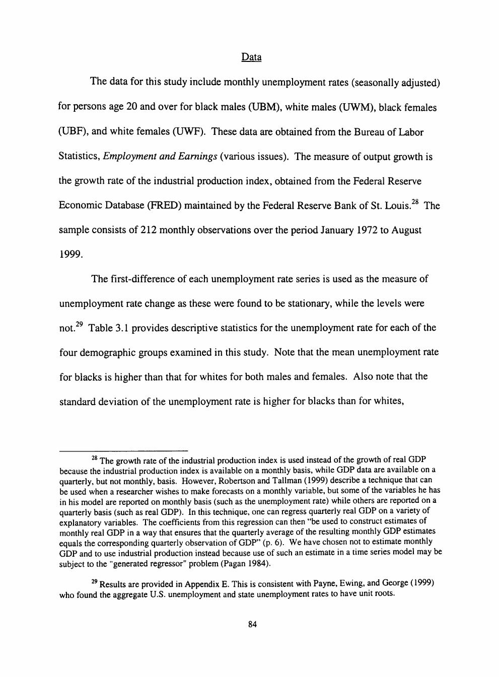
Data
The data for this study include monthly unemployment rates (seasonally adjusted)
for persons age 20 and over for black males (UBM), white males (UWM), black females
(UBF), and white females (UWF). These data are obtained from the Bureau of Labor
Statistics, Employment and Earnings (various issues). The measure of output growth is
the growth rate of the industrial production index, obtained from the Federal Reserve
Economic Database (FRED) maintained by the Federal Reserve Bank of St. Louis.^^ The
sample consists of 212 monthly observations over the period January 1972 to August
1999.
The first-difference of each unemployment rate series is used as the measure of
unemployment rate change as these were found to be stationary, while the levels were
not. Table 3.1 provides descriptive statistics for the unemployment rate for each of the
four demographic groups examined in this study. Note that the mean unemployment rate
for blacks is higher than that for whites for both males and females. Also note that the
standard deviation of the unemployment rate is higher for blacks than for whites,
^ The growth rate of the industrial production index is used instead of the growth of real GDP because the industrial production index is available on a monthly basis, while GDP data are available on a quarterly, but not monthly, basis. However, Robertson and Tallman (1999) describe a technique that can be used when a researcher wishes to make forecasts on a monthly variable, but some of the variables he has in his model are reported on monthly basis (such as the unemployment rate) while others are reported on a quarterly basis (such as real GDP). In this technique, one can regress quarterly real GDP on a variety of explanatory variables. The coefficients from this regression can then "be used to construct estimates of monthly real GDP in a way that ensures that the quarterly average of the resulting monthly GDP estimates equals the corresponding quarterly observation of GDP" (p. 6). We have chosen not to estimate monthly GDP and to use industrial production instead because use of such an estimate in a time series model may be subject to the "generated regressor" problem (Pagan 1984).
^' Results are provided in Appendix E. This is consistent with Payne, Ewing, and George (1999) who found the aggregate U.S. unemployment and state unemployment rates to have unit roots.
84

regardless of gender, and it is lower for females than for males within race.^° These
patterns can also be clearly seen in Figure 3.1, which plots the unemployment rates for
white males, black males, white females, and black females. These rather large
differences in unemployment rates by race and gender motivate an examination as to
whether the unemployment rate for each demographic group responds differently to a
shock to aggregate output.
Empirical Methodology
One way to examine the dynamic relationship among economic time series is to
estimate a vector autoregression (VAR) model and then conduct impulse response
analysis (Sims, 1980). However, this traditional method has been criticized for what is
called the "orthogonality assumption" because results from impulse response analysis
may differ markedly depending on the ordering of the variables in the VAR (Lutkenpohl,
1991). An altemative to the orthogonalized impulse response function has recently been
developed by Pesaran and Shin (1998) and Koop et al. (1996). This new technique is
called the generalized impulse response function and it is invariant to the ordering of the
variables in the underiying VAR. Unlike the orthogonalized version proposed by Sims
(1980), the generalized method does not impose the constraint that the underiying shocks
° One characteristic of the standard deviation of a variable is that it tends to increase as the mean of the variable increases. A measure that controls for the size of the mean is the coefficient of variation. Therefore, we also calculated the coefficient of variation for each demographic group. We find that the coefficient of variation for males is larger than that of females. Further, we find the coefficient of variation is approximately the same for white males as for black males. Also, the coefficient of variation for white females is higher than that for black females, but only slightly.
85

to the VAR model are orthogonalized before impulse responses are computed.^^ As a
result, inferences based on generalized impulse responses are robust to changes in the
ordering of the variables in the VAR while those from orthogonalized responses are not.
The ensuing discussion briefly outlines the methodology developed by Pesaran
and Shin (1998) as it is described in Pesaran and Pesaran (1997)^^ and is meant to provide
a brief summary of the generalized impulse response analysis as it applies to the VAR
model we estimate. First, consider the standard VAR(p) model as in Pesaran and Pesaran
(1997).
Xt = ao + 2i=iPOiXt.i + Ut, t = 1, 2 , . . .n (3.6)
where Xt is an mxl vector of the variables under investigation. In the present paper the
33
vector x contains the four different unemployment rate series and the real output senes.
The VAR can be rewritten in matrix notation as:
Xt = A'gt + Ut (3-7)
where gt = (1, XM, Xt.2, ..., Xt-p) and A' contains coefficients. It is assumed that the
disturbances are well-behaved white-noise processes, the variables in the VAR are
stationary, and the right-hand-side variables are not perfectly collinear.
An impulse response function traces out the effect of shocks at time t on the
expected future values of the variables in the system. Two types of impulse response
' Pesaran and Shin (1998) present an empirical illustration that shows how results may differ between the orthogonalized and generalized impulse response functions.
2 For a more detailed discussion, including proofs, see Pesaran and Shin (1998). Additional background material on the development of generalized impulse response analysis can be found in Koop et al. (1996).
'' If the series are found to be nonstationary, i.e., 1(1). variables then x would be specified in first-
differences.
86

functions can be computed from the VAR: the traditional orthogonalized impulse
response function (Sims, 1980) and the recentiy developed generalized impulse response
function of Pesaran and Shin (1998) and Koop et al. (1996). To facilitate our discussion
of the impulse response analysis, we rewrite the VAR in its infinite moving average
representation:
Xt = 2j=o"AjUt.j (3.8)
where Aj = 0,Aj.i + OjAj.z + ... + OpAj.p, j = 1,2,..., with AQ = Im and Aj = 0 for j < 0.
The traditional orthogonalized impulse responses employ a Cholesky decomposition of
the positive definite mxm covariance matrix, 2, of the shocks (Ut). " Letting T represent
a lower triangular matrix, we have S = XT'. Rewriting (3.8) gives:
Xt = Ej=o"A*jet-j (3.9)
where A*j = AjT and et = T' Ut, E(ete't) = Im, and the shocks Et = (eu, e2t,..., emt)' are
orthogonal to each other. The orthogonalized impulse response of a one standard error
shock at time t to En on the jth variable at time t+N is given by:
A V i = ANTei (3.10)
where ei is an mxl vector with the ith element equal to one and all other elements equal
to zero. The orthogonalized impulse response function (OIRF) to the /th variable
(equation) is:
0//?Fij.N = CjAwTci, i,j = 1, 2, ..., m (3.11)
^ For a description of the Cholesky decomposition, see Patellis (1997).
87

The orthogonalized impulse responses computed from (3.11) may vary depending on the
ordering of the variables in the VAR and will only be invariant to the ordering if the
covariance matrix is (at least almost) diagonal (Lutkenpohl, 1991).
Let us now denote the generalized impulse response function (GIRF) for a shock
to the entire system, u°t, as:
GlRFr (N, VL\, Q\.I) = E(xt+N I Ut = u^ , Q^.i) - E(Xt N I ^Vi) (3.12)
where the history of the process up to t-1 is denoted by the information set Q°t.i. Assume
Ut ~ N(0, 2), and E(ut | Ujt = 6j) = (aij, a2j,..., ainj)'Gr"'jj6j, where 6j = (ajy)''^ denotes a one
standard deviation shock. The GIRF for a one standard deviation shock to the ith
equation in the VAR model on theyth variable at a horizon of N is:
G//?Fij.N = (CJANSCO / (Qii)*'' , i,j = l ,2 , ...,m (3.13)
Perasan and Shin (1998) note that "the generalized impulse responses are
invariant to the reordering of the variables in the VAR, but this is not the case with the
orthogonalized ones" (p. 20). They further caution the researcher about using
orthogonalized impulse responses since there is typically no clear guidance as to which of
many possible parameterizations to employ. "In contrast, the generalized impulse
responses are unique and fully take account of the historical pattems of correlations
observed amongst the different shocks" (p. 20).
As mentioned above, we use the first-differences of UBM, UWM, UWF and
UBF, and the growth rate in industrial production (GIP) in the VAR estimations to
^ The generalized and orthogonalized impulse responses coincide only for the case where the covariance matrix is diagonal.
88

generate the generalized impulse responses in the empirical analysis. We denote the first
difference operator by "D".
We begin by estimating a vector autoregression containing five equations
corresponding to the five variables GIP, DUBM, DUWM, DUWF, and DUBF in addition
to a constant term. The optimal order of the VAR was determined to be six lags based on
Akaike's information criterion and likelihood ratio tests. As discussed above, one of the
major concerns and potential drawbacks of using orthogonalized impulse responses is
that results are likely to be sensitive to the ordering of the variables. Indeed, if the shocks
to the respective equations in a VAR are contemporaneously correlated, then the
orthogonalized and generalized impulse responses may be quite different. Moreover, a
re-ordering of the variables may lead to a number of markedly different conclusions
based on the orthogonalized responses. If, on the other hand, shocks are not
contemporaneously correlated, then the two types of responses would probably not be
substantially different and the orthogonalized responses would probably be relatively
insensitive to a re-ordering of the variables. Thus, before proceeding to an examination
of the dynamic responses of the respective unemployment rates to unanticipated changes
in real output growth, we performed a test to determine if shocks in the individual
equations that make up the VAR were contemporaneously correlated. The null
hypothesis is that the off-diagonal elements in the covariance matrix equal zero, and the
altemative hypothesis is that none of the off-diagonal elements is equal to zero. The log-
likelihood ratio test statistic is computed as LR = 2(LLu - LU) where LLu and LU are the
maximized values for the log-likelihood functions for the unrestricted and restricted
89
36 models, respectively. The LR statistic is distributed -^ with 5 degrees of freedom and
was 71.34, significant at less than the 1% level. Thus, the null that the off-diagonal
elements in the covariance matrix are zero is rejected for the VAR and we proceed to
examine generalized impulse response functions.^^
Discussion of Results
Figures 3.2-3.5 presents the generalized impulse response functions to a shock in
real output growth for each of the unemployment rates in the five-equation VAR.
Figures 3.2-3.5 show how the unemployment rates for white female, white male, black
male and black female, respectively, respond to the output shock. These graphs trace out
the response of changes in each of the unemployment rates to a positive one standard
error shock to real output growth.^^ Responses are plotted out to the eighteenth month.
Note that in all cases the unemployment rate initially deviates from the baseline level
following the output shock but eventually subsides, returning to its equilibrium value.
Although the initial impact is actually larger in absolute value for white females
than for black females, the response of black females is larger in magnitude once lags are
considered, and it is also more variable and lasts longer than the response of white
'^ LLu is the system log-likelihood from the VAR and LL is computed as the sum of the log-likelihood values from the individual equations in the VAR.
" For comparison purposes we computed orthogonalized impulse responses and they were, in fact, quite different from the generalized responses reported in this paper. The OIRFs are available upon request.
^ We do not distinguish between the different possible sources of output shocks, such as monetary and fiscal policies. Certainly, the source may matter. For example, if sources effect various sectors differently and if these sectors differ in their composition of labor market participants by race and gender, it is possible that the responses of unemployment rates by race and gender generated by output shocks of similar magnitude may also differ depending on the origin of the shock.
90

females. The response of black females ranges from -0.062 after the first month to 0.03
at a two-month horizon. The maximum response of white females is found to be -0.057,
which occurs at a one-month horizon. The output shock effect dies out after about 6-7
months for white females, but lingers on to around 10 months for black females. Thus,
an unanticipated increase in the economy's real output tends to reduce the unemployment
rate of black females more strongly than that of white females.
The initial impact of an output growth shock on black males and white males are
about the same. However, as with females, the black unemployment rate is affected
much more than the white unemployment rate in terms of magnitude, especially at
periods several months removed from the shock. The variability of the black male
response is also much greater than that of the white male response. The output shock has
a much more persistent affect on black males than on white males, with the effect dying
out around 13 months for black males, as compared to around 9-10 months for white
males. The response of black males is greatest after one month at about -0.137. For
white males the maximum response is -0.078 at initial impact. Thus, an unanticipated
increase in the economy's real output tends to reduce the unemployment rate of black
39
males more strongly than that of white males.
The generalized impulse responses presented here indicate that an unanticipated
change in the growth of real output has a contemporaneous impact on the unemployment
^' It should be noted that an othogonalized or generalized impulse response function of the unemployment rate to an output shock for a particular demographic group is necessarily symmetric. Thus, the magnitude (in absolute value) and persistence of the unemployment rate response will be the same for an increase in real output as it will be for an equivalent decrease in real output. The direction of the unemployment rate response will, of course, differ between an output increase and an output decrease. Consequently, we can make an inference about the influence on the different unemployment rates arising
91

rates of each of the four demographic groups examined in this study. However, the
overall magnitude of the shock is much larger and more persistent for blacks than for
whites, and for males than females.
Concluding Remarks and Policv Implications
This paper has examined the effect that unanticipated changes in real output
growth have on the unemployment rate for various demographic groups. The paper adds
to the literature by specifically documenting these findings and, by implication, provides
information to policymakers as to how the unemployment rates of different demographic
groups are likely to respond to policy actions and events that affect output growth. We
find that the responses of unemployment rates by race and gender are different both in
terms of magnitude and persistence. The paper employs a generalized impulse response
analysis that, unlike the traditional orthogonalized version, allows the error terms in the
equations comprising the underlying vector autoregression to be contemporaneously
correlated. By not relying on the Cholesky decomposition to compute impulse responses,
we are able to make direct and robust comparisons about the relative responsiveness of
the unemployment rates for different demographic groups to an unanticipated output
shock.
Our results indicate that male unemployment rates experience a stronger and more
persistent response to an unanticipated output shock than female unemployment rates. In
addition, black unemployment rates experience a greater and more persistent response to
from contractions in the economy based on the results of the impulse responses generated from an expansionary shock.
92

an unanticipated output shock than white unemployment rates. As such, an unanticipated
output shock affects different demographic groups differentiy, which supports the earlier
findings of Lynch and Hyclak (1984) and Hyclak and Stewart (1995).
Although the purpose of the study is not to determine the factors that cause the
unemployment rate response to an output shock to be stronger for males than females,
and to be stronger for blacks than whites, we can offer some possible reasons why this is
the case. One possible reason is that male and black workers are disproportionately
employed in cyclically sensitive industries compared to female and white workers. As
such, when the economy experiences a contraction, the unemployment rates of males and
blacks would be more affected than the unemployment rates of females and whites.
A second possible reason is that non-working blacks may require a longer search
to obtain employment than whites (high n). If the search duration is longer for people in
a given demographic group, then the unemployment rate will tend to be higher for that
group than another group. When the economy contracts, causing previously employed
workers to become unemployed, it may take blacks longer to find replacement
employment than whites. This could be due to a variety of reasons, such as
discrimination against blacks, lower human capital investment by blacks, or blacks
having less developed job networks than whites.
A possible explanation for the weaker unemployment rate response by females is
that they may have a higher propensity to exit the labor force than males when they
become unemployed (high Tiu). This is most likely to be tme for married females whose
husband is the primary wage eamer for the family. When these women exit the labor
force they are no longer counted as unemployed, even though they do not have a job. If
93

females have a higher propensity to exit the labor force than males during a recession, the
"official" unemployment rate of females will tend to be less affected by a recession than
the "official" unemployment rate of males.
While the reduced-form nature of the vector autoregression does not answer the
question of which of the underlying factors in the unemployment rate are responsible for
the differential responses to output changes, the results do have important and practical
implications. In implementing macroeconomic policies, government and Federal
Reserve policymakers should be aware of the demographically diverse effects on the
unemployment rate that an expansionary or contractionary fiscal or monetary action is
likely to have. As expected, our results indicate that an expansionary (contractionary)
policy will reduce (increase) the unemployment rate for both males and females, and for
both blacks and whites. Fiscal and monetary policies will have a stronger and more
persistent effect on the black unemployment rate than the white unemployment rate, and
on the male unemployment rate than on the female unemployment rate, however. Thus, a
particular expansionary (contractionary) policy is likely to reduce (increase) the
unemployment rate of blacks more than that of whites, and is likely to reduce the
unemployment rate of males more than females.
The findings regarding the unemployment rate response of different demographic
groups to an output shock imply that an expansionary (contractionary) policy aimed at a
particular group may have some unexpected effects. An expansionary (contractionary)
policy aimed at reducing (increasing) female unemployment, for example, may also
reduce (increase) the unemployment rate gap between blacks and whites, since the
reduction (increase) in the unemployment rate of black females will be greater than that
94

of white females. As such, the black unemployment rate will decrease (increase) by more
than the white unemployment rate, even though the policy was aimed toward females. In
order to insure that macroeconomic policies have the desired effects, our findings suggest
that govemment policymakers must consider the differential responses of unemployment
rates to changes in output when constmcting economic policy.
95

Table 3.1. Descriptive Statistics of Unemployment Rates by Race and Gender
Mean
Max.
Min.
Std. Dev.
Coefficient of Variation
Black Males
10.95
20.70
5.20
3.04
27.76
White Males
4.83
9.00
2.70
1.32
27.32
Black Females
10.99
18.20
6.40
2.26
20.56
White Females
5.15
8.30
3.20
1.12
21.75
Notes: All unemployment rates are for workers 20 years of age and older and seasonally adjusted. The coefficient of variation is expressed in percentage terms. Data are obtained from Bureau of Labor Statistics. Sample period is from 1972:01 to 1999:08.
96

25 -,
Vi 0)
"CD CC
c
E
Q. E <]> c D
72 74 76 78 80 82 84 86 88 90 92 94 96 98
Years
UW20M UW20F
UBM20 UBF20
Figure 3.1: Unemployment Rates by Race and Gender (1972:01-1999:08)
Notes: All unemployment rates(U) are for workers 20 years of age and older and seasonally adjusted. Data obtained from Bureau of Labor Statistics. BM = black male, WM = white male, BF = black female, WF = white female.
97

0.05T
/ DUWF
Horizon
Figure 3.2: Generalized Impulse Responses to Shock to Growth in Industrial Production on white female unemployment rate.
Notes: The five equation VAR used to generate the responses contained six lags and a constant. Generalized impulse responses are to a one standard error shock to the equation for growth in industrial production.
98

0) (/) c o Q . CO 0)
O.O&r
0.00
-0.05--
-0.10-
/ DUWM
0 . 1 5 ' I I I I I I I I I I I I I I I I I I 0 8 1 0 1 2 1 4 16 1 8
Horizon
Figure 3.3: Generalized Impulse Responses to Shock to Growth in Industrial Production on white Male unemployment rate.
Notes: The five equation VAR used to generate the responses contained six lags and a constant. Generalized impulse responses are to a one standard error shock to the equation for growth in industrial production.
99

0 . 0 5 T
0
/ DUBM
I I I I I I I I I I I I I I 6 8 10
Horizon
12 14 16 18
Figure 3.4: Generalized Impulse Responses to Shock to Growth in Industrial Production on Black Male unemployment rate.
Notes: The five equation VAR used to generate the responses contained six lags and a constant. Generalized impulse responses are to a one standard error shock to the equation for growth in industrial production.
100

0.05T
-0.1 &
/ DUBF
0 2 4 6 8 10
Horizon
I I I I I I I 12 14 16 18
Figure 3.5: Generalized Impulse Responses to Shock to Growth in Industrial Production on Black Female unemployment rate.
Notes: The five equation VAR used to generate the responses contained six lags and a constant. Generalized impulse responses are to a one standard error shock to the equation for growth in industrial production.
101

CHAPTER IV
THE INFORMATION CONTENT OF THE PAPER-BILL
SPREAD: THE CASE OF CANADA
Abstract
Considerable attention has been given to examine the information content of the
paper-bill spread in terms of predicting U.S. real economic activity. However, the
results have been mixed. This paper examines the robustness of the paper-bill spread as
an indicator variable of real output growth by studying Canadian data. A unique feature
of this study is the use of the newly developed generalized forecast error variance
decomposition technique (Koop et al., 1996; Pesaran and Shin, 1998). The results
indicate that the information content of the paper-bill spread in Canada is non-trivial
even when the performance of the U.S. economy is taken into account. Moreover, we
provide evidence that Canadian economic activity may not be tied directly to how well
the U.S. is performing per se, but is instead significantiy effected by unexpected changes
(i.e., shocks) to the growth rate of U.S. real output.
102

Introduction and Related Literature
Examining U.S. data, a number of researchers have suggested that the spread
between the commercial paper rate and the Treasury bill rate contains information about
future changes in real output (Friedman and Kuttner, 1992; Estrella and Mishkin, 1998;
Weber 1998). An increase in the paper-bill spread is generally found to be associated
with a downtum in real economic activity, although recently some evidence has cast
doubt on the spread's ability to predict recessions (Friedman and Kuttner, 1998; Thoma
and Gray, 1998). There are several reasons usually given as to why the spread may
predict real output. Ferderer et al. (1998) summarize the general consensus by saying
that the spread contains information about: (1) the stance of monetary policy, (2) the
probability of bankmptcies and (3) the cash flow needs of firms who often must issue
paper to finance inventories.
The mixed findings of past research make it meaningful to see if the paper-bill
spread is a robust predictor of real activity by examining the case of Canada. If there is
something intrinsically special about this particular yield spread's ability to forecast
economic activity then, in a country such as Canada where these variables are similarly
defined, we should find similar results. Our paper adds to the literature on the forecasting
power of the paper-bill spread by examining the information content of the paper-bill
spread in Canada and thus providing a test of robustness. A unique feature of this study
is the use of the newly developed generalized forecast error variance decomposition
technique (Koop et al., 1996; Pesaran and Shin, 1998).
103

Given the attention that the paper-bill spread has received in the U.S., it is
surprising that no one has explicitiy focused on the information content of the paper-bill
spread in Canada. There have, however, been several related papers which examined die
predictive power of other yield spreads to forecast Canadian output. Among these,
Clinton (1994) provided evidence that the slope of the yield curve (i.e., term stmcture)
has been a better predictor of future real economic activity than other leading indicators
in Canada. In particular, Clinton (1994) determined that while the U.S. and Canadian
term stmctures often move together, the Canadian term stmcture contains additional
information, above and beyond that which is contained in the U.S. term stmcture, about
movements in Canadian real output. Cozier and Tkacz (1994) studied twelve different
Canadian yield spreads to see how well these spreads predict real economic activity.
They concluded that the spread between the rates on the Canadian Treasury bond and
commercial paper is a good predictor of Canadian real output. Among the handful of
studies that have looked at the ability of financial spreads to predict recessions in Canada
is a recent Bank of Canada working paper by Atta-Mensah and Tkacz (1998). Their
study differs from previous work in this area mainly in terms of econometric
methodology." ' Atta-Mensah and Tkacz (1998) conclude that the spread between the long
bond and the paper rate portends recessions in Canada.
^ Papers finding a relationship between the paper-bill spread and real output also include Stock and Watson (1989), Bemanke (1990) and Kashyap, Stein, and Wilcox (1993). Among the studies that find evidence to the contrary are Hess and Porter (1993) and Emery (1996).
"*' Unlike the approach taken by other researchers that examine the ability of yield spreads to forecast output using vector autoregressions (VAR) and innovation accounting, Atta-Mensah and Tkacz (1998) utilize a probit analysis.
104

Our focus on the information content of the paper-bill spread for the case of
Canada is unique in two major respects. First, by studying the Canadian paper-bill spread
(as opposed to other yield spreads) we can more directly compare our results to the
studies on the U.S. and determine the robustness of this variable with respect to
forecasting real economic activity. Second, we use the recently developed generalized
forecast error variance decomposition technique of Koop et al. (1996) and Pesaran and
Shin (1998) to determine the information content of the paper-bill spread. Whereas each
of the U.S. studies that used VAR models and innovation accounting techniques is
subject to the "orthogonality" critique of Lutkenpohl (1991), the generalized method
provides superior results as compared to the standard technique and also allows us to
determine the initial impact that unanticipated changes in the paper-bill spread have on
A O
the growth rate of Canadian real output.
In the standard methodology, results are typically sensitive to the order in which
the variables are entered into the VAR. Unfortunately, a problem arises if the variables
in the VAR are contemporaneously correlated. Because the Cholesky decomposition is
used to orthogonalize the shocks, the researcher is forced to restrict the VAR in such a
way that at least one variable has no contemporaneous effect on another. The extent to
which this assumption (i.e., the restriction) is violated determines how sensitive the
results are to a re-ordering of the variables in the VAR. The new method developed by
Koop et al. (1996) and Pesaran and Shin (1998) provides robust results regardless of how
^^ Friedman and Kuttner (1992) mention that one important criterion that has been used for judging the dynamic relationships among financial variables and real activity is the "ability of money (or other variables) to account for the forecast error variance of income at horizons of interest in a business cycle context" (p. 477). Thus, decomposition of real output variance can provide important insight into the relationship between the paper-bill spread and real output.
105

the variables are ordered in the model. These generalized decompositions tiien allow us
to make robust comparisons about the extent of information contained in the shocks to
each of the variables in the system about the forecast error variance of real output growth
at different forecasting horizons.
Data
In order to see if the paper-bill spread contains significant information about
future movements in Canadian real output we examine data over the period from 1975:01
to 1998:12. All data are monthly observations.'^ The Canadian paper-bill spread (CPB)
is defined as the difference between the rates on three-month corporate paper and three-
month Treasury bills (weekly auction). Data for both the paper and bill rates are from the
Bank of Canada. Industrial production is used as the measure of real output for Canada
and the United States. Industrial production indexes for both countries were obtained
from the Intemational Financial Statistics (IFS) CD-ROM database (series 66..IZF...).' ^
For the measure of Canadian money supply we use seasonally adjusted Ml obtained from
the Bank of Canada." ^ Table 4.1 provides descriptive statistics for the variables used in
this study.
^'^ According to Cozier and Tkacz (1994) the Canadian Treasury market was extremely thin prior to 1975. Thus, we chose to start the sample at 1975:01.
'^ The earlier Canadian studies used quarterly data. The use of monthly observations has the obvious advantage of providing additional degrees of freedom.
'* Industrial production is seasonally adjusted with a base year of 1990.
^ Ml is series B1627 from the Bank of Canada and includes currency and demand deposits.
106

Figure 4.1 presents a plot of the Canadian paper-bill spread over the sample
period, while Figure 4.2 and Figure 4.3 plot the time series behavior of Canadian
industrial production and its growth rate, respectively. Casual observation suggests that
real output falls immediately preceding periods of a widening paper-bill spread. In order
to determine if the spread can be used as an indicator of real output in Canada we turn our
attention to several econometric tests.
Methodology and Results
Our analysis will proceed in two steps. First, we estimate a vector autoregression
that contains each of the Canadian variables (CGIP, CPB, and CGMl) and conduct
Granger-causality tests to determine if past values of CPB and CGMl help explain
movements in the growth rate of Canadian real output." ^ We refer to this specification as
VARl. A second vector autoregression is also estimated that includes an additional
variable to detect if the results are sensitive to a measure of how the U.S. economy is
performing. Thus, VAR2 contains CGIP, CPB, CGMl, and USGIP. The second step in
our study is then to examine forecast error variance decompositions of real output growth
(CGIP) to determine the extent to which the paper-bill spread plays a role.
" Unit root tests were conducted on each of the variables used in the analyses. Based on these unit root tests we use the growth rate of industrial production (CGIP) and money (CGMl), and the level of the paper-bill spread (CPB). Results of the unit root tests are given in the Appendix G.
'** A time-series (x) is said to Granger-cause another time-series (y) if the prediction error of current y declines by using past values of x in addition to past values of y. We thus test the null hypothesis that all of the coefficients of the lagged values of x are jointly insignificant. Rejection of the null hypothesis implies that movements in past values of x Granger-cause y. A standard Wald test, distributed as a chi-square statistic, is used to determine significance.
107

The results of the first step in our study are presented in Table 4.2. The Granger-
causality tests provide evidence as to the information content of the paper-bill spread in
Canada. The first column in the table lists the "causal variable" under investigation,
while the second and third columns show the results from the estimation of VARl and
VAR2, respectively."^^ In this part of the study we are testing to see whether or not the
causal variable (e.g., CPB) helps to predict changes in Canadian real output. The entries
m the table are the x statistics, along with their corresponding probability values, from
Wald tests of the joint insignificance of the lagged values of the causal variable in the
equation for CGIP. A significant % allows us to infer the variable under investigation
Granger-causes CGIP. The results based on VARl indicate that past values of the paper-
bill spread contain additional information about real output growth beyond that which is
contained in lagged values of CGIP and CGMl. Specifically, for the real output growth
equation, the % statistic for the null hypothesis that all the coefficients of lagged values
of CPB are zero was 12.96, significant at less than the 1% level. Thus, CPB is said to
Granger-cause CGIP. Additionally, it is found that CGMl Granger-causes CGIP (x^ =
7.11, probability value = 0.028). The results from the estimation of VAR2 are presented
in the third column of Table 4.2. Recall that VAR2 includes the additional variable
USGIP. We find that both the paper-bill spread (x^ = 6.46, probability value = 0.039)
and money growth (x^ = 7.23, probability value = 0.027) Granger-cause CGIP. This
result holds even in the presence of a variable that proxies how the U.S. economy is
performing. It is interesting to note that USGIP does not Granger-cause CGIP (x^ = 3.59,
"*' The order of both VARl and VAR2 was determined to be 2 based on Akaike's information
108

probability value = 0.166) suggesting that the Canadian Economy may not directiy follow
the U.S. economy. This is contrary to what is often suggested in the popular media.
The second step in our investigation is to compute the newly developed
generalized forecast error variance decompositions of Koop et al. (1996) and Pesaran and
Shin (1998). Forecast error variance decompositions illustrate the proportion of the
movements in a sequence due to its "own" shocks versus shocks to the other variables in
the system. However, the traditional method has been criticized for the "orthogonality
assumption" as results may differ considerably depending on the ordering of the variables
in the VAR. Furthermore, if shocks to one equation in the VAR have little
contemporaneous effect on some variable but affect the sequence with a lag then one
expects only a small proportion of the forecast error variance to be explained by these
shocks in short horizons and a greater proportion in longer horizons. The orthogonalized
method often indicates that a variable explains almost all of its own forecast error
variance at very short horizons and a smaller proportion at longer horizons. The
traditional method uses a Cholesky decomposition to orthogonalize shocks and, by
design, necessitates that all the one-period forecast error variance of a variable is due to
"own" shocks. At longer horizons, if variables are correlated, then the problem is
reduced since decompositions should converge. However, when considering shorter
horizons the use of the traditional orthogonalized method is more troublesome.
The generalized forecast error variance decomposition developed by Pesaran and
Shin (1998) and Koop et al. (1996) is invariant to the ordering of the variables and does
not impose the constraint that the underiying shocks to the VAR are orthogonalized
criterion (AIC) and likelihood ratio tests, results available on request.
109

before decompositions are computed. The generalized method explicitly takes into
account the contemporaneous correlation of the variables under investigation. The
method provides meaningful results at all horizons including initial impact (or time t=0).
The ensuing discussion is attributed to Pesaran and Pesaran (1997) and provides a
brief summary of the generalized decomposition methodology. A VAR(p) model is
typically written as yt = A'xt + Ut, where t = 1, 2, ...n, yt is an mxl vector, and Xt = (1, yt-
h yt-2,-.-, yt-p). It is assumed the disturbances are well-behaved white-noise processes
with covariance matrix Z, the variables are stationary, and the regressors are not perfectly
collinear. The infinite MA representation of the VAR is given by:
yt = Ej=o"AjUt.j (4.1)
where Aj = OiAj.i + O2AJ.2 + ... + OpAj.p, j = 1,2,..., with AQ = Im and Aj = 0 for j < 0.
Two types of forecast error variance decompositions can be computed - the
traditional orthogonalized decomposition and the recently developed generalized
decomposition.^^ In the interest of brevity and because the orthogonalized decomposition
method is well-known, only the generalized version is described here. The forecast error
of predicting yt+N conditional on information at t-1 is given by ^t(N) = 2k=o AkUt+N-k»
where ^t(N) is mxl, and the total forecast error covariance matrix is Cov[^t(N)] =
Sk=o^Ak2Ak'. Now, consider the forecast error covariance matrix of predicting yt+N
conditional on information at t-1 and given values of the shocks to the i^ equation (Ui.t,
Ui.t+i, ..., Ui.t+N), ^/'^(N) = Zk=o' Ak(ut+N-k - E(ut+N-k I Ui,t+N-k)). Assume Ut ~ N(0,2) and
E(ut I Ui,t = 6i) = (au, G2i,..., ami)'a"*ii6i, where 6i = (GH)'^'^ denotes a one standard
^ See Ewing (forthcoming) for an application of this technique using stock retum data.
110

deviation shock. Thus, E(ut+N-k | Ui.t+N-k ) = (au'' Sci) Ui,t+N-k for k=l,2,...N and
i=l,2,.. .m, with ei being mxl with all elements equal to zero except for the i*** element
which equals one. Substitution and taking conditional expectations yields:
Cov[^t ')(N)] = Ek=o''AkIAk' - Oii-' (Zk=o''AkE ei ei' SAk') (4.2)
The decline in the N-step forecast error variance of yt can be obtained from conditioning
on the future shocks to the i"* equation and is given by:
AiN = Cov[^(N)l - Cov[^t^'\N)l = Gii' Sk=o''Ak2 ej Ci' SAk' (4.3)
Scaling the j'** element by the N-step ahead forecast error variance of the i* variable in yt,
gives the generalized forecast error variance decomposition as reported in Pesaran and
Pesaran (1997):
ij.N = [ Gv;' Xk=o''(ej'Ak2ei) ] / [ Sk=o\'AkE Ak'Ci ] (4.4)
The generalized decomposition outlined in equation (4.4) has two important advantages
over the standard orthogonalized decomposition when dealing with contemporaneously
correlated variables: (1) They are invariant to the order in which the variables appear in
the VAR and (2) they provide information about initial impact effects (i.e., at a horizon of
t=0).
The results for the generalized forecast error variance decompositions are shown
in Table 4.3. For VARl (see Panel A), it is interesting to note that both the paper-bill
spread (CPB) and the growth of Ml money supply (CGMl) each explain slightiy more
than .02 (i.e., 2%) of the forecast error in CGIP at the 9-month horizon. Thus, the
predictive power of the paper-bill spread is about the same as that of money, and the
information content of each of these variables is non-trivial. Furthermore, unlike
111

orthogonalized decompositions, the generalized method allows us to determine the initial
impact effects. Both shocks to CPB and CGMl provide at least some information as to
the forecast error variance of CGIP at initial impact.
Panel B of Table 4.3 shows the results of the generalized forecast error variance
decompositions for VAR2. Note that CPB, CGMl, and USGIP explain approximately
.02, .02, and .14 of the forecast error of CGIP at a 9-month horizon, respectively. Thus,
the addition of the U.S. variable does not appear to change the importance of either CPB
or CGMl in terms of explaining the forecast error of CGIP. The initial impact effects for
CPB and CGMl are again greater than zero.
Concluding Remarks
This paper examined the information content of the paper-bill spread for the case
of Canada, and by doing so provides an important test of the robustness of the paper-bill
spread as an indicator variable. Granger-causality tests reveal that, in addition to money
growth, the Canadian paper-bill spread helps predict movements in Canadian real output.
This result holds even when we include a proxy for the performance of the U.S.
economy. The paper further adds to the literature on the subject by using the recently
developed generalized forecast error variance decomposition technique of Koop et al.
(1996) and Pesaran and Shin (1998). This robust method for examining how shocks to
different variables explain the variance in future forecast errors of real output reveals
several important findings. First, we find that both the paper-bill spread and money
growth shocks are non-trivial when it comes to forecasting future real activity. Second,
each of these indicator variables also provides at least some information about the
112

forecast error variance of Canadian real output growth at initial impact. Generally
speaking, the results presented in this paper suggest that the paper-bill spread does
indeed contain some information about future movements in Canadian output. Another
interesting finding is that the growth rate of U.S. industrial production does not predict
the growth rate of Canadian industrial production based on Granger-causality tests, but a
shock to USGIP is found to be important in terms of explaining the forecast error
variance of CGIP. This suggests that unanticipated changes in U.S. real output growth
are important indicators of future real Canadian economic activity. Thus, Canadian
economic activity is not tied directiy to how well the U.S. is performing p^r 5e, but is
instead significantly effected by unexpected changes (i.e., shocks) to the growth rate of
U.S. real output.
113

Table 4.1. Descriptive Statistics
Mean
Max.
Min.
Std. Dev.
CCP
9.18
22.2
2.90
3.57
CTB
8.92
20.8
2.69
3.50
CPB
0.25
1.64
-0.22
0.23
CIP
93.90
125.0
69.00
14.75
CGIP
0.18
7.10
-4.40
1.30
CMl
39445
89300
15400
18359
CGMl
0.61
5.47
-3.50
1.39
USIP
93.32
132.5
61.34
17.43
USGIP
0.24
3.30
-2.60
0.73
Notes: There are 288 observations over the sample period 1975:01 to 1998:12. Variables are defined using the following notation: C = Canada, US = United States, CP = commercial paper rate, TB = Treasury bill rate, PB= commercial paper rate - Treasury bill rate, IP = industrial production Index, Ml = money, and G denote growth rate.
114

Table 4.2. Results of Granger-Causality Tests
Causal Variable
CPB
CGMl
USGIP
VARl
12.95 (0.002)
7.11 (0.028)
VAR2
6.46 (0.039)
7.23 (0.027)
3.59 (0.166)
Notes: VARl contains three variables (CGIP, CPB, and CGMl) and a constant and VAR2 contains four variables (CGIP, CPB, CGMl, and USGIP) and a constant. The entries in the table are the y^ (chi-square) statistic that tests the null hypothesis that the coefficients on the lagged values of x (i.e., the variable listed in the first column as "causal variable") are not jointiy significant in the equation for CGIP. The order of VAR was 2 in both cases, thus each VAR contains two lags of each variable. The x is distributed with 2 degrees of freedom for both VARl and VAR2. Actual probability values for the Granger-causality test are given in parentheses. Independent Variable is CGIP.
115

Table 4.3. Generalized Forecast Error Variance Decompositions of Canadian Real Output Growth
PANEL A: VARl
Horizon
0
1
2
3
4
5
6
7
8
9
CGIP
1.00000
.97825
.96199
.96115
.96033
.96025
.96023
.96022
.96022
.96022
CPB
.006904
.017285
.022754
.023520
.023633
.023713
.023719
.023723
.023724
.023724
CGMl .001979
.008630
.021229
.021272
.022031
.022031
.022052
.022054
.022054
.022054
PANEL B:VAR2
Horizon
0
1
2
3
4
5
6
7
8
9
CGIP
1.00000
.97750
.95913
.95780
.95672
.95654
.95650
.95649
.95649
.95649
CPB
.007472
.014858
.017521
.018956
.019096
.019249
.019265
.019272
.019273
.019274
CGMl .003077
.010300
.023195
.023177
.024194
.024232
.024260
.024263
.024264
.024264
USGIP
.14277
.13557
.14126
.14097
.14088
.14085
.14085
.14084
.14084
.14084
Notes: The forecast horizon is measured in months. The order of both VARl and VAR2 was determined to be 2 in each case based on Akaike's information criterion and Likelihood ratio tests (available on request).
116

2.0 -,
~ 1 1 r — I 1 1 1 I I I 1 I I 1 — I 1 — I 1 1 1 1 — I 1 r
76 78 80 82 84 86 88 90 92 94 96 98
Years
Figure 4.1: Paper-Bill Spread in Canada
117
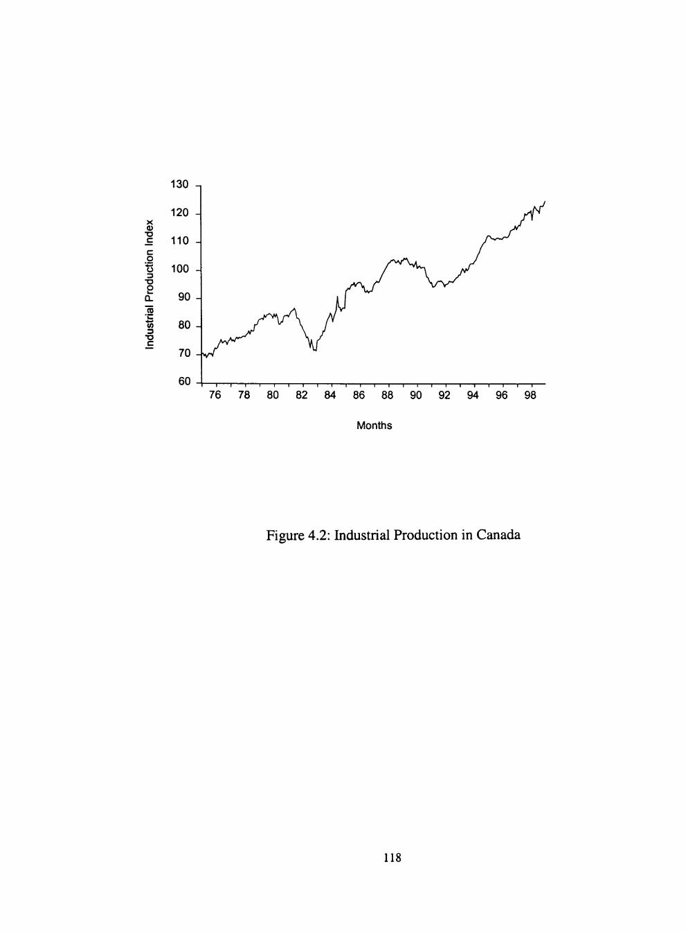
X 0)
•a c c o
••s 3
T3 O
CD ' C
tn 3
X3 C
I I 1 1 1—I 1 1 1 1 1 1—I r
76 78 80 82 84 86 88 90 1 1 1 r
92 94 96 98
Months
Figure 4.2: Industrial Production in Canada
118

8 -,
1 I I
76 78 80 82 84 86 88 90 92 94 96 98
Months
Figure 4.3: Growth in Industrial Production in Canada
119

UST OF REFERENCES
Atta-Mensah, J. and G. Tkacz. April 1998. Predicting Canadian recessions using financial variables: A probit approach. Bank of Canada working paper 98-5.
Barron, J. M., M. Lowenstein, and G. J. Lynch. 1989. Macroeconomics. Reading, MA: Addison-Wesley.
Barron, J. M. and W. Mellow. 1979. Search effort in the labor market. Journal of Human Resources. 14: 9-17.
Barron, J. M. and W. Mellow. 1981. Changes in labor force status among the unemployed. Journal of Human Resources. 16: 427-41.
Bartlett, R. L. and P. Haas. 1997. The natural rate of unemployment by race, gender, and class. Challenge. 40: 85-98.
Bemanke, B. S. 1990. On the predictive power of interest rates and interest rate spreads. New England Economic Review. Nov/Dec: 51-68.
Brooks, R. D., R. W. Faff, and M. Ariff. 1998. An investigation into the extent of beta instability in the Singapore stock market. Pacific-Basin Finance Journal. 6: 87-101.
Brown, R. L., J. Durbin, and J. M. Evans. 1975. Techniques for testing the constancy of regression relationship over time. Journal of the Royal Statistical Society, series B, 37: 149-192.
Campbell, J. Y., A. W. Lo, and A. C. MacKinley. 1997. The Econometrics of Financial Markets. Princeton, NJ: Princeton University Press.
Chen, Roll, and Ross. 1986. Economic forces and the stock market. Journal of Business. 59: 383-403.
120

Clinton, K. 1994-1995. The term stmcture of interest rates as a leading indicator of economic activity: a technical note. Bank of Canada Review. Winter: 23-40.
Cozier, B. and G. Tkacz. 1994. The term stmcture and real activity in Canada. Bank of Canada working paper 94-3.
Dimson, E. 1979. Risk management when shares are subject to infrequent trading. Journal of Financial Economics. 7: 197-226.
Emery, K. M. 1996. The information content of the paper-bill spread. Journal of Economics and Business. A%\ 1-10
Engle, R. F. 1982. Autoregressive conditional heteroscedasticity with estimates of the variance of United Kingdom inflation. Econometrica. 50: 987-1007.
Estrella, A. and F. S. Mishkin. 1998. Predicting U.S. recessions: Financial variables as leading indicators. Review of Economics and Statistics. 80 (1): 45-61.
Evans, G. W. 1989. Output and unemployment dynamics in the United States: 1950-1985. Journal of Applied Econometrics. 4: 213-237.
Ewing, B.T. forthcoming. Monetary policy and stock retums. Bulletin of Economic Research.
Ewing, B. T., J.E. Payne, and C. Sowell. 2000. NAFTA and North American stock market linkages: an empirical note. North American Journal of Economics and Finance. 10: 443-452.
Fabozzi, F. J. and J. C. Francis. 1978. Beta as a random coefficient. Journal of Financial and Quantitative Analysis. 13: 101-115.
Fairiie, R. B. and L. G. Kletzer. 1998. Jobs lost, jobs regained: An analysis of black/white differences in job displacement in the 1980s. Industrial Relations. 37: 461-475.
121

Fairiie, R. B. and W. A. Sundstrom. 1999. The emergence, persistence, and recent widening of the racial unemployment gap. Industrial and Labor Relations Review. 52: 252-270.
Ferderer, J. P., S. C. Vogt and R. Chahil. 1998. Increasing liquidity and the declining informational content of the paper-bill spread. Journal of Economics and Business. 50: 361-377
Fortune, P. 1998. A primer on U.S. stock price indices. Federal Reserve Bank of Boston, New England Economic Review. Nov.-Dec. 25-40.
Friedman, B. M., and K. N. Kuttner. 1992. Money, income, prices and interest rates. American Economic Review. 82 (3): 472-492.
Friedman, B. M., and K. N. Kuttner. 1998. Indicators properties of the paper-bill spread: lessons from recent experience. The Review of Economics and Statistics. 80: 34-44.
Hall, R. B. 1982. The importance of lifetime jobs in the U.S. economy. American Economic Review. 72: 716-724.
Hess, G. D. and R. D. Porter. 1993. Comparing interest-rate spreads and money growth as predictors of output growth: Granger causality in the sense Granger intended. Journal of Economics and Business. 45: 247-268.
Hildreth, C. and J. P. Houck. 1968. Some estimators for a linear model with random coefficients. Journal of the American Statistical Association. 63: 584-595.
Hyclak, T. and J. B. Stewart. 1995. Racial differences in the unemployment response to stmctural changes in local labor markets. Review of Black Political Economy. 23: 29-42.
Kashyap, A. K., J. C. Stein, and D. W. Wilcox. 1993. Monetary policy and credit conditions: evidence from the composition of external finance. American Economic Review. 83: 78-98.
122

Keith, K. and A. Mc Williams. 1995. The wage effects of cumulative job mobility. Industrial and Labor Relations Review. 49: 121-137.
Keith, K. and A. Mc Williams. 1999. The retums to mobility and job search by gender. Industrial and Labor Relations Review. 52: 460-477.
Koop, G., M. H. Pesaran and S. M. Potter. 1996. Impulse response analysis in nonlinear multivariate models. Journal of Econometrics. 74: 119-147.
Lintner, J. 1965. The valuation of risky assets and the selection of risky investments in stock portfolios and capital budgets. Review of Economics and Statistics. 47: 13-17.
Lutkenpohl, H. 1991. Introduction to Multiple Time Series Analysis. Springer-Verlag, Berlin.
Lynch, G. J. and T. Hyclak. 1984. Cyclical and noncyclical unemployment differences among demographic groups. Growth and Change. 15: 9-17.
MacKinnon, J. G. 1991. Critical Values for Cointegration Tests. Chapter 13 in Long-mn Economic Relationships: Readings in Cointegration, edited by R. F. Engle and C. W. J. Granger, Oxford University Press.
Malkiel, B. G. 1996. A Random Walk Down Wall Street. New York. W. W. Norton and Company.
Markowitz, H. 1959. Portfolio Selection: Efficient Diversification of Investments. New York: John Wiley.
Marston, S. T. 1976. Employment instability and high unemployment rates. Brookings Papers on Economic Activity. 1: 169-203.
Mennis, E. A. 1999. How the Economy Works: An Investor's Guide to Tracking the Economy. 2" * edition. New York. New York Institute of Finance.
123

Pagan, A. 1984. Econometric issues in the analysis of regressions with generated regressors. Intemational Economic Review. 25: 221-247.
Patellis, A. 1997. Stock retum predictability and the role of monetary policy. Journal of Finance. 52: 1951-1972.
Payne, J. E., B. T. Ewing, and E. George. 1999. Time series dynamics of U.S. state unemployment rates. AppZ/ec? Econom/c^. 31: 1503-1510.
Pesaran H.M. and Y. Shin. 1998. Generalized impulse response analysis in linear multivariate models. Economics Letters. 58: 17-29.
Pesaran, M. H. and B. Pesaran. 1997. Working with Microfit 4.0. Camfit Data LTD., Cambridge, England.
Petterson, S. M. 1998. Black-white differences in reservation wages and joblessness: A replication: comment. Journal of Human Resources. 31: 758-770.
Robertson, J. C. and E. W. Tallman. 1999. Vector autoregressions: Forecasting and reality. Federal Reserve Bank of Atlanta Economic Review. 84: 4-18
Schwartzman, D. 1997. Black male unemployment. The Review of Black Political Economy. 25: 77-93
Sharpe, W. 1964. Capital asset prices: A theory of market equilibrium under conditions of risk. Journal of Finance. 19: 425-442.
Sims, C. 1980. Macroeconomics and reality. Econometrica. 48: 1-48.
Stock, J. and M. W. Watson. 1989. New indexes of coincident and leading indicators. NBER Macroeconomic Annual Edited by O. Blanchard and S. Fischer. Cambridge, MA: MIT Press. 351-393.
124

Stokes, H. H. and H. M. Neuburger. 1998. New Methods in Financial Modeling: Explorations and Applications. Westport, CT: Quomm Books.
Sunder, S. 1980. Stationarity of market risk: random coefficient tests for individual stocks. Journal of Finance. 35: 883-896.
Thoma, M. A. and J. A. Gray. 1998. Financial market variables do not predict real activity. Economic Inquiry. 36 (4): 522-39.
Thorbecke, W. 1997. On stock market retums and monetary policy. Journal of Finance. 52: 638-654.
U.S. Bureau of Labor Statistics. Employment and earnings, (various issues).
U.S. Bureau of Labor Statistics. Table A-1: Employment status of the civilian population by sex and age. Labor force statistics from the current population survey. (http://www.bls.gov/webapps/legacy/cpsatabl.htm). accessed on April 27, 2000.
U.S. Bureau of Labor Statistics. Table 2: Percent of weeks individuals were employed, unemployed, or not in the labor force from age 18 to 34 in 1978-98 by educational attainment, sex, race, and hispanic origin. National longitudinal surveys. (http://stats.bls.gov/news.release/nlsoy.t02.htm). accessed on April 27, 2000.
Weber, C. E. 1998. Consumption spending and the Paper-bill spread: theory and evidence. Economic Inquiry. 36 (4): 575-89.
125

APPENDIX A
DESCRIPTIVE STATISTICS FOR INDEX RETURNS
126

Table A.l: Descriptive Statistics for Index Retums
Index Retums Composite Index Retum Capital goods Index Retum Financial Index Retum Industrial Index Retum Transportation Index Retum Utility Index Retum
Mean 18.44
22.55
29.30
19.21
29.40
14.13
Max. 275.44
462.81
757.62
293.89
471.18
509.49
Min. -79.98
-84.51
-85.13
-81.99
-89.13
-74.03
Std. Dev. 49.62
67.89
84.90
51.32
78.84
52.63
Kurtosis - 3 4.61
9.99
18.94
5.27
4.86
23.58
Skewness 1.48
2.40
3.07
1.59
1.76
3.15
Note: There are 288 observations over the sample period 1970:02 to 1997:07.
127

APPENDDC B
A BRIEF DESCRIPTION AND RESULTS OF THE UNIT ROOT
TESTS FOR INDEX RETURNS
128

Table B.l: Results of Unit Root Tests
Variable Capital goods Index Retum less Treasury bill rate
Transportation Index Retum less Treasury bill rate Financial Index Retum less Treasury bill rate
Utility Index Retum less Treasury bill rate
Industrial Index Retum less Treasury bill rate Composite Index Retum less Treasury bill rate Financial Index Retum Composite Index Retum Transportation Index Retum Utility Index Retum Capital goods Index Retum Industrial Index Retum
ADF statistic -5.0114(11)*
-15.0623 (0) * -14.7558 (0) * -4.7019 (12) *
-13.8066 (0) * -13.8465 (0) * -14.7889 (0) *
-13.9513 (0) * -15.0539 (0) * -4.7338 (12) * -5.0221(11)* -13.9081 (0) *
Notes: The optimal lag lengths on the augmenting terms (given in parentheses) were determined by Akaike's information criterion. The augmented Dickey-Fuller (ADF) regressions include an intercept but no trend term. The 95% critical value for the augmented Dickey-Fuller statistic is -2.8708. * denotes significance at 5% level as determined by critical values in MacKinnon (1991). 317 observations were used in the estimation of all ADF regressions. Sample period from March 1971 through July 1997.
A Brief Description of the (Augmented) Dickey Fuller Test:
Consider the following AR (1) process
Yt= a-HpYt-i +et
Where a and p are parameters, et is assumed to be white noise process. If the value of p is 1 then the data generating process is non-stationary and is referred to as a series with unit root. The hypothesis of unit root is tested against the altemative hypothesis of p being less than 1, since a value of p greater than 1 indicates explosive series. Lagged difference terms are added on the right hand side in order to take care of serial correlation and the test is then called Augmented Dickey Fuller (ADF) Test. A trend and/or an intercept term is included in the regressions only if the data plot strongly suggests. Since the t-statistics under the null hypothesis does not follow a conventional t-distribution so simulated critical values from MacKinnon (1991) are used. If ADF statistic is more than the critical value then the null hypothesis of a unit root is rejected and one can conclude that the process is stationary. More detailed discussion of the unit root test can be found in MacKinnon (1991).
129

APPENDDC C
BETAS FOR FULL SAMPLE PERIOD
130

Table C.l: Investment Betas for Full sample period
Index Capital
Financial
Industrial
Transport
Utility
a 1.2245 (.78503) 7.2267 (2.3588) .46072 (1.3872) 8.3414 (2.9601) .22369 (.09156)
3 1.2491 (41.0286) 1.3132 (21.9604) 1.0273 (158.479) 1.2261 (22.2908) .60910 (12.7742)
Adj-R' .83643
.59396
.98707
.60115
.33019
R .83692
.59519
.98711
.60237
.33222
3=1 66.9562[.000]
27.4356[.000]
17.7981 [.000]
16.8920 [.0(X)] 67.2105 [.000]
LM test 14.5873[.265]
25.4362[.013]
35.7350[.000
31.9803[.001]
24.2961 [.019]
Notes: Standard errors in parenthesis. P=l indicates the results from a Wald test(% ) where the null hypothesis is that beta is equal to 1. LM denotes the value of the Lagrange multiplier statistic where the null hypothesis is that there is no serial correlation. P-values are in brackets.
131

APPENDK D
DIMSON BETAS
132

Table D.l: Dimson Betas
Index Capital(full-sample) Capital(pre-crash)
CapitaKpost-crash) Financial(full-sample) Financial(pre-sample) FinanciaKpost-sample) Industrial(Full-sample) Industrial(pre-crash) IndustriaKpost-crash) Transport(Full-sample) Transport(pre-sample) Transport(post-sample) Utility(full-sample) Utility(pre-sample) Utility(post-sample)
a 1.3095
(1.6080) 1.7498
(1.9106) -1.7121 (2.9734) 7.7164 (3.1756) 7.0396
(3.9579) 3.0667
(5.0190) .44963
(.34041) .53789
(.37581) .25633
(.74307) 9.1983 (2.9263) 12.0385 (3.8953) 4.8990 (4.4725 .53920 (2.4563) 1.2374 (3.3190) 2.6898 (3.3985)
P 1.2415
1.2564
1.3081
1.2722
1.1568
1.8284
1.0288
1.0332
1.0195
1.1535
1.1777
1.0645
.57759
1.3471
.28800
Adj-R^ .8373
.8539
.8232
.5941
.5394
.7459
.9872
.9908
.9754
.5990
.6126
.5419
.3705
.4132
.2313
R .8388
.8560
.8279
.5979
.5459
.7527
.9873
.9910
.9761
.6027
.6181
.5540
.3763
.4215
.2517
3=1 27.4271 [.000]
24.6459[.000]
9.3142[.002]
8.9354[.003]
2.1557[.142]
23.6307[.000]
8.7153[.003]
10.7052[.001]
.56737[.451]
3.4780[.062]
2.8493[.091]
.18051[.671]
35.9447 [.000]
15.4452[.000]
38.0684[.000]
LMtest 13.6717[.322]
19.3361[.081]
15.0200[.240]
26.1403[.010]
31.7106[.002]
4.4380[.974]
32.2982[.001]
32.4655[.001]
16.8272[.156]
32.3769[.001]
31.4879[.002]
14.0582[.297]
18.9901 [.089]
16.6638[.163]
8.9068[.711]
Notes: Standard errors in parenthesis. P=l indicates the results of a Wald test with a null hypothesis that the dimson beta equals to 1. LM shows the Lagrange multiplier statistic where the null hypothesis is no serial correlation. P-values are in brackets.
133

APPENDIX E
PARTIAL DERIVATIVES OF UlSfEMPLO YMENT RATES
134
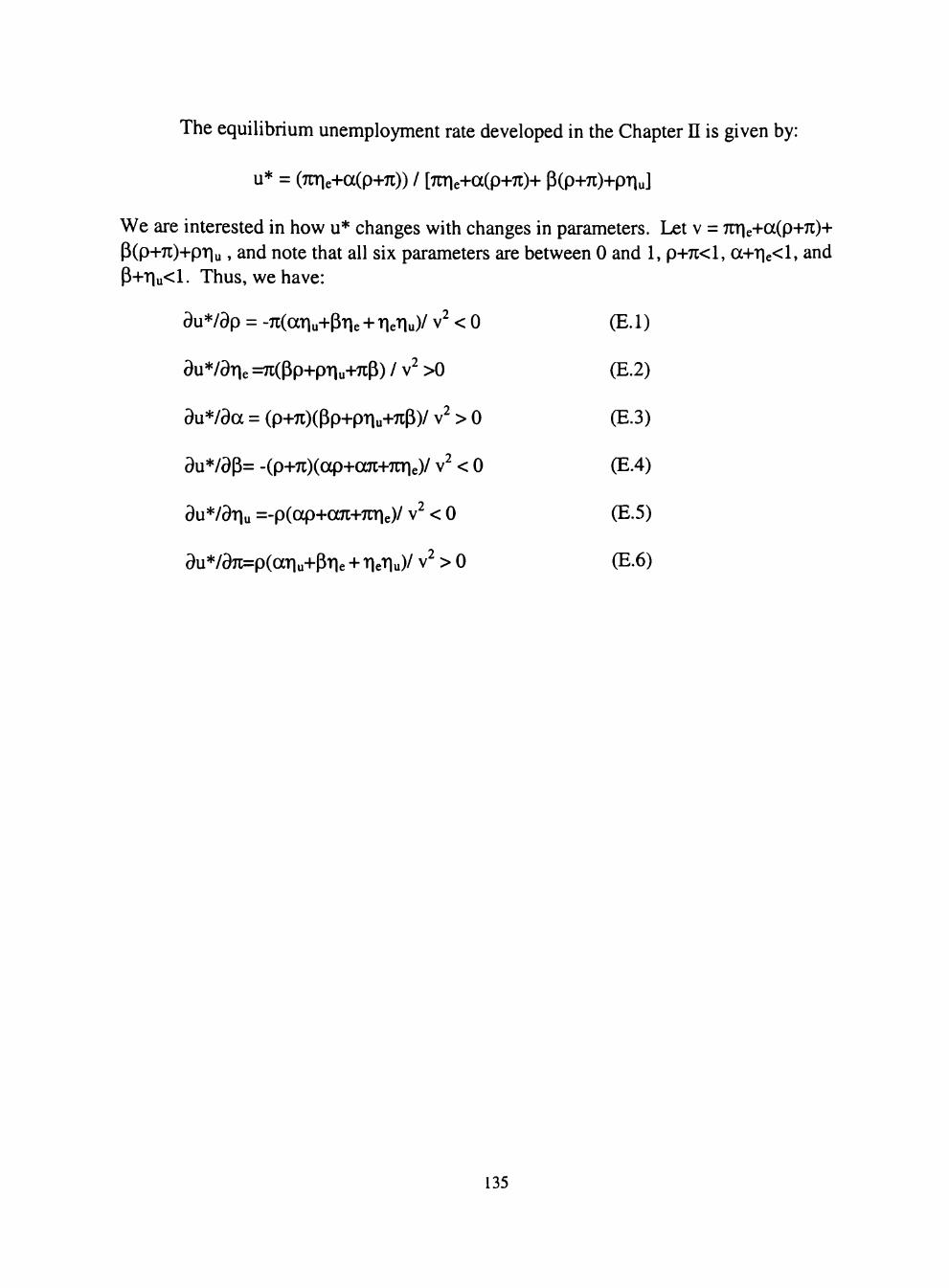
The equilibrium unemployment rate developed in the Chapter n is given by:
u* = (7rne+a(p+7i)) / [7rrie+a(p+7i)+ P(p+7c)+pTiuJ
We are interested in how u* changes with changes in parameters. Let v = 7rne+oc(p+7i)+ P(p-i-7i)-i-pTiu, and note that all six parameters are between 0 and 1, p-i-7i<l, a+'ne<l, and P-i-r|u<l. Thus, we have:
3 u * / 3 p = -7l(aTlu+3'ne + TleTlu)/ V^ < 0 (E. 1)
aU*/aTle =7l(Pp+pTlu+7lp) / V^ > 0 (E.2)
au*/aa = (p-i-7i)(Pp+pTiu+7ip)/ v S 0 (E.3)
au*/ap= -(p-i-7i)(otp-i-a7i+7nie)/ v < 0 (E.4)
3u*/aTiu =-p(ap+a7i-i-Tcrie)/ v < 0 (E.5)
au*/37t=p(aTlu+PTle + TleTlu)/ V^ > 0 (E.6)
135

APPENDIX F
UNIT ROOT TESTS FOR UNEMPLOYMENT SERIES
136

Table F.l: ADF Unit Root Test Statistics
Unemployment Rates White Male Black Male Black Female White Female
Level -2.6391 [3]
-2.2963 [12]
-2.0365 [10]
-1.4446 [3]
1 ' difference -5.4357 [3] *
-4.7103 [12] *
-4.9224 [11]*
-8.9445 [2] *
Notes: The number of lags used in the Dickey Fuller equation is given in brackets and was determined by the Akaike Information Criterion (AIC). The Dickey-Fuller regressions include an intercept but not a trend. * denotes significance at 5% level as determined by critical values in MacKinnon (1991). Appendix B provides a description of the unit root test.
137

APPENDDC G
RESULTS OF UNIT ROOT TESTS FOR FINANCL\L VARIABLES
138

Table G.l: Results of Unit Root Tests for Financial Variables
Variable CPB CGMl CGIP USGIP
ADF statistic -2.9412(3) * -6.1394(12)* -5.2597(7) * -7.7802(4) *
Notes: The optimal lag lengths on the augmenting terms (given in parentheses) were determined by Akaike's information criterion. The augmented Dickey-Fuller (ADF) regressions include an intercept but no trend term. The 95% critical value for the augmented Dickey-Fuller statistic is -2.8708. * denotes significance at 5% level as determined by critical values in MacKinnon (1991). 455 observations used in the estimation of all ADF regressions. Sample period from 1961:02 to 1998:12. Variables are defined in the text. Appendix B provides a description of the unit root test.
139