THREE ESSAYS IN APPLIED ECONOMETRICS

By

Monthien Satimanon

A DISSERTATION

Submitted to

Michigan State University

in partial fulfillment of the requirements

for the degree of

Economics - Doctor of Philosophy

2013

ABSTRACT

THREE ESSAYS IN APPLIED ECONOMETRICS

By

Monthien Satimanon

The three essays are self-contained and are the combination of applied and empirical

econometrics. They are “Comparisons of Approaches in Measuring Willingness to Pay for

Environmental Services”, “Comparisons of Approaches in Measuring Causes of Wage

Inequality”, and “Estimation of Binary Response Model with Endogeneity and Hetero-

skedasticity.”

The first essay proposes a comparison of both parametric and semiparametric estimation

of willingness to pay (WTP) for environmental services. In order to solve for problem of

inconsistency of estimation since heteroskedasticity, several conventional and new methods are

used in the analysis. The methods are Probit (Probit), Heteroskedasticy Probit (HP), Turnbull

(T), Watnabe (2010), Ahn (2000), and sieve semiparametric estimator (S). The comparison

includes the estimated parameters as well as the estimated standard errors since the WTP is

derived from these parameters. Monte Carlo simulations have been used to compare finite

sample properties of each estimating methods. The empirical application comes from a study of

the demand for payment for environmental services, water quality preservation, in eastern Costa

Rica. By Monte Carlo Simulation, we found out that neglecting heteroskedasticity could lead to

over estimation of WTP by almost 100 percent. In the empirical study, we found out that WTP

for water conservation program in villages in eastern Costa Rica is about 2400 Colones that is

about two times of the current monthly water cost program. This estimate is consistent with

previous studies in the water conservation program.

The second essay proposes a comparison of both parametric and semiparametric

estimation of causes of income equality. In quantile regression setting, this paper analyzes the

determinants of wage inequality with endogenous categorical regressors. The framework of Lee

(2007) has been extended to cover the case where control function comes from generalized

residuals of ordered probit models. We found out that the proposed method yields not only

consistent but also efficient estimated parameters when there is a present of both endogeneity

and heteroskedasticity while the conventional estimators led to overestimated parameters. In

addition, we use all the proposed to estimate the return to education on wage using the data from

Current Population Survery (CPS). We found out that returns to education are not monotonically

increase throughout the wage distribution.

The third essay analyzes the binary response model that encounters the problems of

endogeneity and heteroskedasticity that lead to inconsistent estimated parameters. Our model

allows both heteroskedasticity in structural and reduced formed equation. To handle both

problems, we employ control function estimation with sieve estimator. The first step generates

control function with flexible form of multiplicative exponential heteroskedasticity. The second

step employs the use of maximum likelihood method to find the average partial effects with the

adjusted standard errors based on Ackerberg et.al. (2012). Monte Carlo simulations are

conducted to study the performance of this new estimator comparing to standard binary choice

models. Then, the estimator is applied to estimation of female labor supply.

iv

For my parents, Montri Satimanon and Ream Chairuengsri, and my wife Thasanee

Satimanon

v

ACKNOWLEDGMENTS

I would like to express my deepest appreciation to my advisor, Professor Jeffrey

Wooldridge for his valuable advice, guidance, suggestion, and support throughout every stage of

completing this dissertation. My work would not have been possible without his comment and

support. I am grateful for the assistance and lively discussion with Professor Timothy (Tim)

Volgelsang. I wish to thank Professor Todd Elder and Professor Robert Myers for their

encouragement and his fruitful discussions.

I would like to express my deepest gratitude for Thammasat University for financial

support throughout my academic years. I am also indebted to Center for Statistical Training and

Consulting, Michigan State University that have not only offered life-changing experience but

also support for my dissertation. I would like to thank the Economics department staff for their

help throughout my study here, especially Ms. Jennifer Carducci and Ms. Lori Jean Nichols.

Finally yet importantly, my deepest blessing and gratitude goes to my family. I would

never be who I am today without their encouragement and unconditional love from my parents.

In addition, I would like to thank my parent-in-law for their support. Last but not least, I would

like to thank my wife, Thasanee (my little Yui), who shared with me every moment of this

dissertation throughout the thick and thin. I would not be this better self without her

encouragement, love and support. Thank you very much, N’Yui.

All ambiguities, deficiencies, and mistakes in this dissertation are solely my own

responsibility.

vi

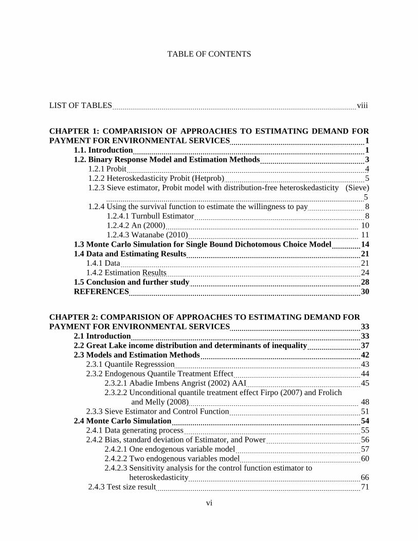
TABLE OF CONTENTS

LIST OF TABLES viii

CHAPTER 1: COMPARISION OF APPROACHES TO ESTIMATING DEMAND FOR

PAYMENT FOR ENVIRONMENTAL SERVICES 1

1.1. Introduction 1

1.2. Binary Response Model and Estimation Methods 3

1.2.1 Probit 4

1.2.2 Heteroskedasticity Probit (Hetprob) 5

1.2.3 Sieve estimator, Probit model with distribution-free heteroskedasticity (Sieve)

5

1.2.4 Using the survival function to estimate the willingness to pay 8

1.2.4.1 Turnbull Estimator 8

1.2.4.2 An (2000) 10

1.2.4.3 Watanabe (2010) 11 1.3 Monte Carlo Simulation for Single Bound Dichotomous Choice Model 14

1.4 Data and Estimating Results 21

1.4.1 Data 21

1.4.2 Estimation Results 24

1.5 Conclusion and further study 28

REFERENCES 30

CHAPTER 2: COMPARISION OF APPROACHES TO ESTIMATING DEMAND FOR

PAYMENT FOR ENVIRONMENTAL SERVICES 33

2.1 Introduction 33

2.2 Great Lake income distribution and determinants of inequality 37

2.3 Models and Estimation Methods 42

2.3.1 Quantile Regresssion 43

2.3.2 Endogenous Quantile Treatment Effect 44

2.3.2.1 Abadie Imbens Angrist (2002) AAI 45

2.3.2.2 Unconditional quantile treatment effect Firpo (2007) and Frolich

and Melly (2008) 48

2.3.3 Sieve Estimator and Control Function 51

2.4 Monte Carlo Simulation 54

2.4.1 Data generating process 55

2.4.2 Bias, standard deviation of Estimator, and Power 56

2.4.2.1 One endogenous variable model 57

2.4.2.2 Two endogenous variables model 60

2.4.2.3 Sensitivity analysis for the control function estimator to

heteroskedasticity 66

2.4.3 Test size result 71

vii

2.5 Data and Estimating Results 75

2.6 Concluding Remarks and Further Study 84

REFERENCES 86

CHAPTER 3: BINARY RESPONSE MODEL WITH CONTINUOUS ENDOGENOUS

VARIABLE AND HETEROSKEDASTICITY 90

3.1 Introduction 90

3.2 Model and Estimation Method 94

3.3 Monte Carlo Simulation 98

3.3.1 Data generating process (DGP) 98

3.3.1.1 The data generating process contains only exogenous variables 99

3.3.1.2 The data generating process contains only endogeneity 100

3.3.1.3 Data generating process with endogeneity and heteroskedasticity in

reduced form 102

3.3.1.4 Data generating process with endogeneity and heteroskedasticity in

both equations 103

3.4 Empirical Study: Application to female labor supply 104

3.5 Conclusion 107

APPENDICES 124

APPENDIX A: Asymptotic Variance for the two-step estimators 125

APPENDIX B: Asymptotic Variance for the APEs 136

REFERENCES 141

viii

LIST OF TABLES

Table 1.1 Basic willingness to pay model 17

Table 1.2 Heteroskedastic Probit willingness to pay model 18

Table 1.3 Heteroskedastic Probit with square exponenetial variance willingness to pay

model 22

Table 1.4 Communities in the study 23

Table 1.5 Data description and descriptive statistics (N=1141) 26

Table 1.6 Estimated coefficients 27

Table 2.1 Monte Carlo Simulation for Mean without endogeneity 58

Table 2.2 Monte Carlo Simulation for Mean with 0.1 degree of correlation 58

Table 2.3 Monte Carlo Simulation for Mean with 0.5 degree of correlation 59

Table 2.4 Monte Carlo Simulation for Mean with 0.9 degree of correlation 60

Table 2.5 Monte Carlo Simulation for Mean with 0 degree of correlation 63

Table 2.6 Monte Carlo Simulation for Mean with 0.1 degree of correlation 64

Table 2.7 Monte Carlo Simulation for Mean with 0.5 degree of correlation 65

Table 2.8 Monte Carlo Simulation for Mean with 0.9 degree of correlation 66

Table 2.9 Monte Carlo Simulation for the case of Heteroskedasticity and Endogeneity with

0.1 degree of correlation 68

Table 2.10 Monte Carlo Simulation for the case of Heteroskedasticity and Endogeneity with

0.5 degree of correlation 69

Table 2.11 Monte Carlo Simulation for the case of Heteroskedasticity and Endogeneity with

0.9 degree of correlation 70

Table 2.12 Test size based on model with two ordered endogenous variables 72

Table 2.13 Test size based one binary endogenous variable 73

ix

Table 2.14 Test size with 1000 observations and variance of (9, 1) 74

Table 2.15 Percentiles, cut-off level of nominal household income ($) 76

Table 2.16 Summary statistics for the year 2001-2009 76

Table 2.17 Estimate result assuming education attainments are conditionally exogenous

(n = 349,825) 80

Table 2.18 Estimate result assuming education attainments are endogenous (n = 349,825) 81

Table 3.1 The correct model is Probit with 1000 observations 109

Table 3.2 The correct model is Probit with 3000 observations 110

Table 3.3 The correct model is IVprobit with 1000 observations and 50225021 .,.

111

Table 3.4 The correct model is IVprobit with 3000 observations and 50225021 .,.

112

Table 3.5 The correct model is IVprobit with 1000 observations and 10221021 .,.

113

Table 3.6 The correct model is IVprobit with 3000 observations and 10221021 .,.

114

Table 3.7 The correct model is IVprobhet with 1000 observations and 50225021 .,.

115

Table 3.8 The correct model is IVprobhet with 3000 observations and 50225021 .,.

116

Table 3.9 The correct model is IVprobhet with 1000 observations and 10221021 .,.

117

Table 3.10 The correct model is IVprobhet with 3000 observations and 10221021 .,.

118

Table 3.11 The correct model is HetIVprobhet with 1000 observations and

50225021 .,. 119

Table 3.12 The correct model is HetIVprobhet with 3000 observations and

50225021 .,. 120

x

Table 3.13 Data description 121

Table 3.14 Estimation of Reduced form equation 121

Table 3.15 Empirical Result of APEs with analytical standard errors 122

Table 3.16 Empirical Result of APEs with analytical standard errors and Bootstrap

standard errors 123

1

CHAPTER 1: COMPARISION OF APPROACHES TO ESTIMATING

DEMAND FOR PAYMENT FOR ENVIRONMENTAL SERVICES

1.1. Introduction

This paper proposes a comparison of both parametric and semiparametric

estimation of willingness to pay (WTP) for environmental services. Payment for

environmental services (PES) is an approach that uses economic incentives either

provided by public or private sector to protect natural resources. PES programs range

from classical soil and water conservation to the new areas such as drinking and farming

water supply and carbon sequestration. Hence, PES programs have been of recent interest

globally and have led to an increasing number of empirical studies. Two important

questions for PES studies are what determine the willingness to pay (WTP) or demand

for PES? and what determines participation in PES programs by payment recipients?.

Both of these questions have been answered by estimating the dichotomous choice

(binary choice) models by using standard Probit or Logit estimation. The standard

procedure of this contingent valuation can be found in the work of Haneman (1984) and

Haab and McConnell (2003). In this binary response valuation models, WTP usually

refers to conditional mean that is derived from estimated parameters under given

underlying distributional assumption. The problem with this set up is that the welfare

evaluations will crucially depend on these specific distributions. Unlike the linear

probability model, the consistencies of estimated parameters depend on the underlying

distribution as well as the conditional variance of the estimated model. In this context,

semiparametric estimation provides an interesting alternative since it allows flexible

functional form for conditional variance.

2

Semiparametric methods have been used in estimation of binary choice model for

a long period of time, as summarized in Li and Racine (2008). In most theoretical studies,

the semiparametric models have been compared with parametric binary choice model by

simulation. Horowitz (1992) found that semiparametric models will be more robust when

the estimated model contains heteroskedasticity. Klein and Spady (1993) and Li (1996)

also found strong support for the semiparametric model. In empirical application of

semiparametric methods to welfare measurement in binary choice model, Chen and

Randall (1997), Creel and Loomis(1997), An (2000), Cooper (2002), and Huang et.al

(2009) found out that the semipametric results are robust and can be used as a

complementary procedure along with the parametric estimation. In addition, it can be

used to check whether the parametric model encounters any inconsistency problems

because of underlying distribution, unobserved heterogeneity, and heteroskedasticity.

The comparing methods of estimation for the binary choice models are Probit

(Probit), Heteroskedasticy Probit (Hetprob), Turnbull, Watnabe (2010), An (2000), and

sieve semiparametric estimator (Sieve). The sieve method assumes exponential

heteroskedasticity of the normal distribution with flexible functional form. Hence,

comparison includes the estimated parameters as well as the estimated variances since the

WTP derives from these parameters.

The data used for the comparison of welfare measures comes from a study of the

demand for payment for environmental services (PES) in eastern Costa Rica. The data set

come from the extended surveys of Ortega-Pacheco et.al. (2009). The respondents are

asked to vote “Yes” or “No” in the response to additional payment for the people who

live in the upstream and mountainous area to preserve the quality as well as quality of

3

water sources that will be used in the lower area. The bid value has been provided in

standard referendum contingent valuation. The goods here are clearly defined since the

people who live along the downstream self-financed their existing water supply and

already pay the water fees monthly. With the new estimation methods and extended data

from previous study, the results show that the choice of methods and models can

influence the mean willingness to pay.

1.2 Binary Response Model and Estimation Methods

The estimated model in this study is specified as exponential willingness to pay

function as in Haab and McConnell (2003). The exponential willingness to pay with

linear combination of attributes and additional stochastic term is

iizeiWTP

(1.1)

where i is a stochastic error with mean zero and unknown variance 2 .The probability

that individual ‘i’ will answer “yes” for the corresponding offered bid it will be

determined whether the random willingness to pay is greater than the offered bid.

)()( itiWTPPiziyP 1 (1.2)

= ))(exp( itiizP

= ))ln(( izitiP

By assuming that the unknown standard errors is , equation can be standardized to

izitiPiziyP)ln(

)( 1 = )*)ln(( izitiP (1.3)

4

The conventional process in estimating the parameters of the model in (1.3) is to

specifying the distribution of the error terms. In most of the studies, i are independently

and identically distributed (IID) with mean zero and variance 1. Then, either the

underlying distribution of normal and/or logistic will be assumed as in the case of Probit

and Logit estimation. For comparison in this study, only the basic Probit will be used.

1.2.1 Probit

In Probit model, the probability of “yes” will be model in term of latent variable that

1iy if 0 iitiziy )ln(** and probability of “no” will be defined as 0iy

if 0 iitiziy )ln(** . Or, binary response model is in the form of index

function 01 iitiziy )ln(* .Also, for the errors term, it is assumed to be

),(~20 Ni and ),(~ 10Ni . Hence the distribution is assumed to be as followed.

))ln(*()( itiziziyP 1 (1.4)

where )(x is the cumulative standard normal distribution. Then, the parameters can be

estimated up to a scale as well as the marginal effects. In order to estimate this model, the

maximum likelihood estimation will be used. Defining a new )( 11 m parametric vector

*,B where )( 1m is the dimension of covariates including constant terms, and

define the data vector itiziX , the likelihood function will be

})'()'({),( iyBiXiyBiXniiXiyBL 11 (1.5)

Then, the familiar log likelihood function is

)]}'(ln[)()'(ln{),(ln BiXiyBiXiyniiXiyBL 11 (1.6)

5

1.2.2 Heteroskedasticity Probit (Hetprob)

The simple estimation will be modified with the unobserved heterogeneity by

incorporating the heteroskedasticity into standard Probit model. The variance 2 will be

varying as a function of attributes. The variance will be a multiplicative function of iz as

followed

)exp( izi (1.7)

Substituting this variance into equation (1.3) yields multiplicative heteroskedastic probit

model.

)exp()exp(

)ln(

)exp()(

iz

iz

iz

it

iz

iPiziyP

1

= )**)ln(**( izitiP (1.8)

Defining a new )( 11 m parametric vector *}*,*{* B where 1m is the

dimension of covariates including constant terms. Then, the log likelihood function will

become

*)]'(ln[)(*)'(ln),(ln BiXiyBiXiyniiXiyBL 11 (1.9)

The result of estimation from equation (1.6) and (1.9) will be useful in positing

whether our estimated model contain heteroskedasticity or not. Furthermore, the other

assumptions that can be relaxed is functional specification of i .

1.2.3 Sieve estimator, Probit model with distribution-free heteroskedasticity

(Sieve)

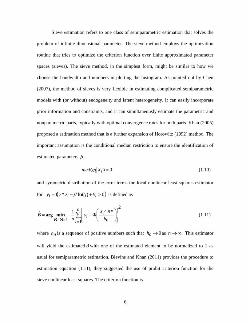
6

Sieve estimation refers to one class of semiparametric estimation that solves the

problem of infinite dimensional parameter. The sieve method employs the optimization

routine that tries to optimize the criterion function over finite approximated parameter

spaces (sieves). The sieve method, in the simplest form, might be similar to how we

choose the bandwidth and numbers in plotting the histogram. As pointed out by Chen

(2007), the method of sieves is very flexible in estimating complicated semiparametric

models with (or without) endogeneity and latent heterogeneity. It can easily incorporate

prior information and constraints, and it can simultaneously estimate the parametric and

nonparametric parts, typically with optimal convergence rates for both parts. Khan (2005)

proposed a estimation method that is a further expansion of Horowitz (1992) method. The

important assumption is the conditional median restriction to ensure the identification of

estimated parameters .

0)( iXimed (1.10)

and symmetric distribution of the error terms the local nonlinear least squares estimator

for 01 iitiziy )ln(* is defined as

2

1

1

1

n

i nh

BiXiy

nBB

*'minargˆ (1.11)

where nh is a sequence of positive numbers such that 0nh as n . This estimator

will yield the estimated B with one of the estimated element to be normalized to 1 as

usual for semiparametric estimation. Blevins and Khan (2011) provides the procedure to

estimation equation (1.11), they suggested the use of probit criterion function for the

sieve nonlinear least squares. The criterion function is

7

n

iizlBiXiy

nlBi

21))(exp(*')*,( (1.12)

where )( izl is finite dimensional scaling parameter and is a finite vector of parameters.

Then, they introduce a finite-dimensional approximation of )( izl using a linear-in-

parameters sieve estimator as in Chen (2007). They define the estimator as followed. Let

)( izjb0 denotes a sequence of known basis function and )(),...,()( izn

bizjbiznb

00

for some integer n . Then, the function )(exp izl will be estimated by the following

sieve estimator

niz

nb

)'(exp where n is a vector of constants. Let

nAnn ),( where nA is the sieve space. The estimator can be defined by

n

iizngBiXiy

nnA

n1

21)(*'minargˆ

(1.13)

The choice of )( izng is arbitrary and can be any possible series such as power

and polynomial series, and spline. In this study, we estimate the )( izng by exponential

function that contains the power series of )( iz as a domain. Chen (2007) proved that the

estimated parameters from sieve estimation will be asymptotically normal and consistent

when the estimated number of sieve parameters grows with respect to number of

observations. However, in this paper we are interested in the estimation of willingness to

pay so we have to apply further step in estimation. From estimation of equation (1.12),

we can get the estimation of )( izng , and then we will plug this one in the probit

estimation of equation (1.3). The main reason that we proceed in two step estimation is

that we can apply the results from Ackerberg et.al. (2012) in order to estimate the

8

asymptotic variance by using parametric approximation since it requires less computation

power to get the variance of the estimate of *B and willingness to pay. Moreover, the

first step estimation of equation (1.12) can be conduct by using Sieve-M estimator that

comprises of both non-linear least squares as in Blevins and Khan (2011) and the use of

standard maximum likelihood with flexible function Chen (2007). They should yield the

same asymptotic result; however, their finite sample properties will be examined through

Monte Carlo study among the nested models. Then, the usual delta method or Krinsky

and Robb will easily compute the willingness to pay and its variance.

1.2.4 Using the survival function to estimate the willingness to pay

Consider a PES project as in our study, villagers are asked to pay a given bid for

either there will be conservation or not, hence the willingness to pay, iWTP , may be

viewed as a survival time in a survival analysis. By giving a particular bid across

individual, we can get a one to one response between the binary choice models as in

1.2.1-1.2.3 to the survival model. In this context we can define the general failure-time

distribution as )()( izitiWTPPizit , given fixed it , it is the simple model of survival

probability )()( izitFizitS 1 . In this study, three estimators will be used to illustrated

and compared with the given binary choice models. They are Turnbull estimator, An

(2000) estimator, and Watanabe (2010) estimator.

1.2.4.1 Turnbull estimator

Turnbull estimator is a distribution-free estimator that relies on asymptotic

properties. When there are large number of observations and the offered bid increases,

9

the proportion of “no” responses will be higher and the survival function is decreasing in

bid. That is, the survival function supposed to mimic the real survival function when

observations are large and it assumed to decrease monotonically. The steps in which

Turnbull estimation are carried are as followed:

- For each bid indexed mjjt ,...,, 1 calculate the proportions, jF , of “no”

responses. For example, if the first bid is 10 and has been given to 100

villagers and 10 villagers answered “no”. This proportion, 1F , will be 0.1. If

the second bid is 20 and has been given to 100 villagers and 20 villagers

answered “no”. This proportion, 2F , will be 0.2.

- Calculate this proportion for all of the bids level j .

- If jFjF 1 , there is no need for adjustment.

- If jFjF 1 , there is need to pool bid j and 1j together and then calculate

the proportions of “no” with the observations from both of the bid categories.

For example, if the second bid is 20 and has been given to 100 villagers and

20 villagers answered “no”. This proportion, 2F , will be 0.2. In addition, if

third bid is 30 and the has been given to 100 villagers and 15 villagers

answered “no”. This proportion, 3F , will be 0.15. Then, we have to merge

second and third bid to one category and calculate the new 2F that is equal to

(20 + 15) /(100 +100) = 0.175

- Continue this process of merging to allow for monotonicity in survival

function.

10

- Set 11 mF , or there is no one who will pay after the last bid, survival

function = 0.

- Calculating probability distribution for each bid level as follows:

jFjFjf 1 .

- The expected lower bound of willingness to pay will be mj jfjt

0*

In this study the expected lower bound and upper bound as in Haab and

McConnnell (1997) will be calculated to find the mid-point which will be compared with

other estimators.

1.2.4.2 An (2000)

He introduced a semiparametric model that has the same property as Cox

Proportional hazard model with discrete time and unobserved heterogeneity as in Jenkins

(1995). Willingness to pay is represented by the link function as follows

iiizfiWTP ),( (1.14)

where f can be generalized by generic link function that is assumed to be continuous

and differentiable with 00 )( and )(lim iWTPmiWTP . i is assumed to follow

a Type-I extreme value distribution. This lead to the conditional survivor function as

same as Cox proportional hazard model of the form

))(exp()()( izeiWTPizitiWTPPiziWTPS

(1.15)

Then, by pursuing the double bound dichotomous contingent valuation model and

unobserved heterogeneity with unit-mean Gamma density, he formulated the same log

11

likelihood function as in Jenkins (1995) that is called discrete choice proportional hazard

model with shared frailty.

),(ln iziyBL

)}/)exp(*)'exp({}/)exp(*)'exp(({log

ni

lnj

l lBizlBizni 1

11

(1.16)

However, in this study with single bound dichotomous choice model, it is not possible to

assume shared frailty since there is only one bid or failed time per one individual. In

addition, there is no data grouping mechanism. Hence, the likelihood function in equation

(1.16) is not suitable for this study. Stripping off both shared frailty and data grouping

mechanism, the log-likelihood in (1.16) will become the same as standard Cox

proportional hazard model in survival analysis with the mean willingness to pay equal to

area under the curve of survival function.

m

dizeiiziWTPE

0

)))((exp()( (1.17)

where i is defined as in equation (1.14). Following approximation as in An (2000)’s

equation (1.17), it will be

][))(exp()( 11

jtjtmj

izeiiziWTPE

(1.18)

1.2.4.3 Watanabe (2010)

The paper presented the nonparametric model to find mean willingness to pay

with modeling it as the survival function as in the case of Turnbull and An(2000).

The survival function is defined as

12

)()( itiWTPPitS (1.19)

And the support of willingness to pay need to be in the range of offering bid ],[ mt0 .

Given the observed “yes” and “no” answer in standard single bound dichotomous choice

model, the probability of answering “yes” will be assumed to follow Bernoulli random

variable with the conditional probability of )()( itiWTPPitiyP 1 and expected value

of )()( itSitiyE 1 . Then he assume the distribution of the the bid it follows

- A bid it follows a continuous distribution )( itf over the range of ],[ mt0 ,

and 0)( itf in the range.

- The range of support of bid and willingness to pay are equal to ],[ mt0 .

Under these two assumptions the expected willingness to pay of single bound

dichotomous choice willingness to pay condition on observe attributes will be equal to

mt dtizitiWTPPiziWTPE0

)()(

mt dtizitiyE

0),(

izit

itf

iyE ,

)( (1.20)

In order to estimate equation (1.20), the following assumption is required,

),,( izitiy is independent and identically distributed. Then, the consisted estimator of the

minimum mean-squared errors linear approximation of equation (1.20) is iz where

13

are estimated coefficients from running linear regression )( itf

iy on intercepts and

attributes iz .

These three estimators share similar characteristics in order to get better precision

of estimating mean willingness to pay. First, the support of willingness to pay has to lies

within the support of bid distribution. Second, number of distinct bids (ideally bid should

continuously distributed as in case of survival time) matters in achieving the less

interpolation errors of willingness to pay. Though, An and Watanabe claims that their

estimator are non/semiparametric; however, they need to assume certain form of

distribution either on unobserved heterogeneity or bid distribution. Lastly, for

nonparametric estimators, the need for independent and identical assumption is required

for estimation in Turnbull and Watanabe.

To conclude this section, there are certain insights that might be gained from

comparing these six methods of estimation. The probit and heteroskedastic probit models

are computationally simple and should be more efficient if the underlying distributions

are correctly specified. On the other hands, the four nonparametric and semiparametric

models in this paper are not nested with each corresponding probit and heteroskedastic

probit, but heuristic comparison can be made as in Beluzzo (2004). Results of Probit,

Hetprob, and Sieve can be compared to see whether the underlying normal distribution is

a valid assumption or not. In addition, results from Probit, Hetprob and Sieve can be

compared to see whether the there is a problem of heteroskedasticity in the data

generating process or not.

14

1.3 Monte Carlo Simulation for Single Bound Dichotomous Choice Model

Monte Carlo simulations were carried out to compare the finite sample properties

of six estimators with respect to varying conditional variances. The sample size is 500

and the number of simulation trials is 1000 at each simulation. First we consider the case

where data generating process followed Watanabe (2010). That is true willingness to pay

(WTP) follow the linear exponential function as )exp( iziWTP 121 , where

1z is considered to be individual attribute, i is random errors term and 1 and 2 are

parameters. The data generating process are as followed:

Case 1: 31 , 502 . , ).,(~ 64001 Nz , and ).,(~ 6400Ni , the bids are set

up following process as in Watanabe (2010). There are 20 equal bid levels

ranging from 0 to 400 assigned randomly to 500 observations with 25

observations facing the same bid level.

In case 1), the sieve estimator and heteroskedasticity probit model use the same variance

adjustment term that is exponential of 1z .

First, when the standard probit specification is true for estimating the WTP, the

result are as expected, the probit estimator performs best not only in terms of bias but

also variance of estimation. The three estimators under survival function analysis yield

similar results. They under predict the mean WTP by almost 50 percent. However, their

variances are quite low compared to the dichotomous choice models. The lower variance

can be attributed to assuming the smoothness of survival function that make the extreme

value less affect the mean WTP. In addition, for each underlying survival function, they

are multiplied with corresponding bid points that further lead to lower variances of

estimated mean willingness to pay. For the case of heteroskedasticity probit and Sieve

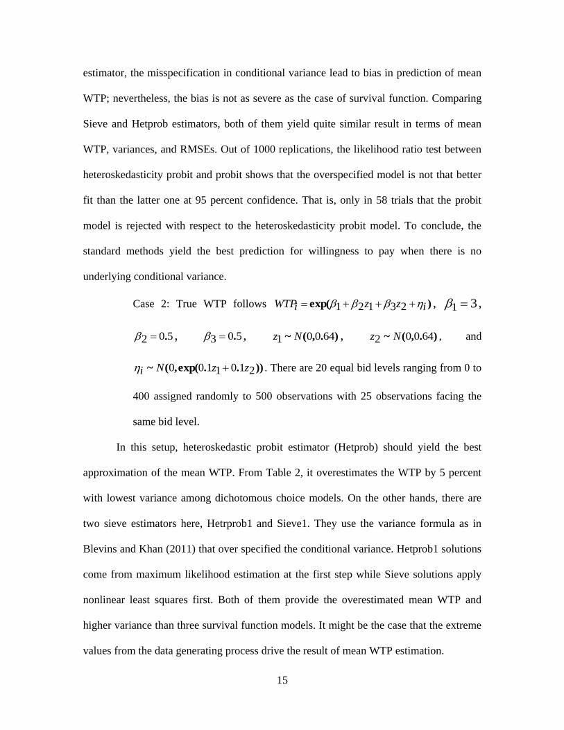
15

estimator, the misspecification in conditional variance lead to bias in prediction of mean

WTP; nevertheless, the bias is not as severe as the case of survival function. Comparing

Sieve and Hetprob estimators, both of them yield quite similar result in terms of mean

WTP, variances, and RMSEs. Out of 1000 replications, the likelihood ratio test between

heteroskedasticity probit and probit shows that the overspecified model is not that better

fit than the latter one at 95 percent confidence. That is, only in 58 trials that the probit

model is rejected with respect to the heteroskedasticity probit model. To conclude, the

standard methods yield the best prediction for willingness to pay when there is no

underlying conditional variance.

Case 2: True WTP follows )exp( izziWTP 23121 , 31 ,

502 . , 503 . , ).,(~ 64001 Nz , ).,(~ 64002 Nz , and

))..exp(,(~ 2101100 zzNi . There are 20 equal bid levels ranging from 0 to

400 assigned randomly to 500 observations with 25 observations facing the

same bid level.

In this setup, heteroskedastic probit estimator (Hetprob) should yield the best

approximation of the mean WTP. From Table 2, it overestimates the WTP by 5 percent

with lowest variance among dichotomous choice models. On the other hands, there are

two sieve estimators here, Hetrprob1 and Sieve1. They use the variance formula as in

Blevins and Khan (2011) that over specified the conditional variance. Hetprob1 solutions

come from maximum likelihood estimation at the first step while Sieve solutions apply

nonlinear least squares first. Both of them provide the overestimated mean WTP and

higher variance than three survival function models. It might be the case that the extreme

values from the data generating process drive the result of mean WTP estimation.

16

Sieve1 yields similar result to probit estimator while Hetprob1, though having

same explanatory variables for the conditional variance as Sieve1, yields similar results

to Hetprob. It is important to note that Sieve1 estimator provide highest variance than

Hetrprob1 given the highest maximum WTP estimated is 221 that is 100 percent higher

than all estimates from other methods. We suspect that nonlinear least squares estimation

of over specified model might be more biased and less efficient than maximum

likelihood.

Comparing across the nested model of Probit, Hetprob and Hetprob1 by using

likelihood ratio test, there are only 125 trials that reject Probit against correctly specified

Hetprob. In addition, there are only 213 trials that reject correctly specified Hetprob

against over-specified Hetprob1. Hence, adding three more explanatory terms to

conditional variance to Hetprob1 compared to Hetprob does not change the likelihood

ratio between the two methods that much. This might help in explaining why there is

more increase in bias and variance of estimation from using nonlinear least squares Sieve

compared to using maximum likelihood Sieve.

It is surprising that in this case Turnbull estimator yields the best result with

lowest bias and RMSE among the all estimators. Moreover, An and Watanabe estimators

still underestimate the mean willingness to pay by 25-30 percent with low variances.

17

Table 1.1 Basic willingness to pay model

True Model mean willingness to pay = 47.746

Turnbull Watanabe An Probit Hetprob Sieve

Mean willingness to pay 28.920 19.990 23.970 48.008 37.292 36.048

Bias 18.556 27.486 23.506 -0.532 10.184 11.428

Variance 10.910 11.029 8.209 60.203 40.590 40.918

Root mean squared errors(RMSE) 18.848 27.686 23.680 7.777 12.013 13.096

Maximum WTP 41.400 32.000 44.085 77.511 164.072 57.258

Minimum WTP 19.800 10.400 19.812 18.569 12.557 12.870

Frequency of rejection 58

Note: Monte Carlo Bias and Root mean square errors are measure with respect to true model willingness to pay.

18

Table 1.2 Heteroskedastic Probit willingness to pay model

True Model mean willingness to pay = 37.773

Turnbull Watanabe An Probit Hetprob Hetprob1 Sieve1

Mean willingness to pay 38.395 30.178 27.682 52.035 39.223 42.193 53.327

Bias 0.622 -7.595 -10.091 14.262 1.450 4.420 15.554

Variance 23.394 18.050 11.958 98.292 57.737 82.785 403.976

Root mean squared errors(RMSE) 4.877 8.702 10.667 17.369 7.736 10.115 25.415

Maximum WTP 55.927 46.400 48.711 89.358 66.803 80.388 221.391

Minimum WTP 19.800 18.400 21.107 22.335 12.557 14.122 12.896

Frequency of rejection 125 213

Note: 1) Monte Carlo Bias and Root mean square errors are measure with respect to true model willingness to pay.

2) Hetprob represents heteroskedasticity model with correctly specified errors Hetprob1 represents heteroskedasticity model

with overspecified standard errors as in Blevins and Khan (2011) with maximum likelihood estimation.

3) Sieve represents Blevins and Khan (2011) non-linear least squares estimation.

19

Case 3: True WTP follows )exp( izziWTP 23121 , 31 ,

502 . , 503 . , ).,(~ 64001 Nz , ).,(~ 64002 Nz , and

))...exp(,(~22

10212021

100 zzzzNi . There are 20 equal bid levels ranging

from 0 to 400 assigned randomly to 500 observations with 25 observations facing

the same bid level.

In Table 1.3, only the Sieve1 and Hetprob1 estimator assumes the correct form of

conditional variance, where the normal Sieve2 and Hetprob2 estimator assumes the

conditional variances as in Blevins and Khan (2011). As expected the misspecification of

conditional various affect the estimated mean WTP for all of the dichotomous choice

models. The Probit and Hetprob1 models those are under specified the conditional

variance lead to higher level of WTP than expected by 20 percent or more. Although, the

Sieve1 and Hetprob1 estimator should yield lower bias; however, their RMSEs are still

higher than the comparable Turnbull model but lower than An and Watanabe. Comparing

across nested models, only Probit without conditional variance leads to considerable

biased estimator that overshoots willingness to pay by 18 percent. At least by inserting

conditional variance terms either correctly specified (Sieve1 and Hetprob1), over

specified (Hetprob2 and Sieve2) helps in reducing the bias of estimated mean WTP.

Using nonlinear least squares is precise with low variance when only the conditional

variances are correctly specified. Considering the survival function models, all of them

underestimate mean WTP with lower variances and Turnbull estimators yields the least

biased result.

20

Comparing across the nested model of Probit, Hetprob, Hetprob1, and Hetprob2

by using likelihood ratio test, there are only 124 trials that reject Probit against under

specified Hetprob. There are only 177 trials that reject under-specified Hetprob against

correctly specified Hetprob1 and there are 135 that reject Hetprob1 in favors of Hetprob2.

This comparison points out that given unknown form of conditional variances, it is better

to flexibly model them rather than ignore them. Adding conditional variance terms will

help not only reduced bias but also make estimated results more efficient. Nevertheless,

over fitting the conditional variances tend to increase the variances compared to under

fitting model.

To conclude, comparing across six estimators yield interesting results, first, the

survival function models give less variance than all of the dichotomous choice models

that might come as a result of smoothing and interpolation. Out of three survival

functions, Turnbull estimator midpoint might be the best among three estimators.

However, in these setups, survival function models always yield inconsistent results that

mean WTP will not converge to the true one even in large sample. We suspect that the

result from Table 1.2) where Turnbull estimator outperforms all other estimators might

comes out of data generating process. On the contrary, the dichotomous choice models

perform better in term of less bias when conditional variances are prevalent either

misspecified or not. For sieve estimator with maximum likelihood that assumes flexible

conditional variance function, it performs best comparing to the rest of the models.

However, since it shares the same feature as the other two dichotomous choice models, it

always yields higher variance than survival function models. Hence, sieve estimator

provides the middle ground in which we can compromise between assuming underlying

21

distribution with flexible conditional variance and give less bias willingness to pay when

form of conditional variances is unknown.

1.4 Data and Estimating Results

1.4.1 Data

The data in this study came from eastern Costa Rica. The research sites contain

not only the two communities as in Ortega-Pacheco et.al. (2009) but also four

communities within the region that were recently surveyed as presented in Table 4. The

communities’ local water supply is too polluted for drinking water usage due to heavy

use of chemical substances in nearby pineapple and banana plantation. Their drinking

water supply comes from aqueducts that pipe in water from the forested upper reaches of

their watershed. The communities have local water boards that oversee the construction

and maintenance of these water systems and levy monthly fees for water. However,

changes in land use in the upper reaches of the watersheds threaten the quality of the

communities’ drinking water. To protect their water, the communities are considering

PES programs to keep land uses from changing in the upper watershed. The surveys

assess local resident’s willingness to pay to finance these PES programs. The payment

vehicle is a monthly surcharge on their water bill. There are 1179 completed interviews

from the surveys.

22

Table 1.3 Heteroskedastic Probit with square exponenetial variance willingness to pay model

True Model mean willingness to pay = 44.986

Turnbull Watanabe An Probit Hetprob Hetprob1 Hetprob2 Sieve1 Sieve2

Mean willingness to pay 37.552 29.390 26.541 52.253 39.138 41.885 42.1929 43.341 51.120

Bias -7.434 -15.596 -18.445 7.267 -5.848 -3.101 -2.793 -1.645 6.134

Variance 20.129 17.015 11.853 92.106 53.508 69.425 82.785 111.529 342.966

Root mean squared errors(RMSE) 8.683 16.133 18.764 12.038 9.365 8.891 9.518 10.688 19.509

Maximum WTP 53.787 44.800 54.703 90.071 66.606 87.964 80.388 131.567 149.185

Minimum WTP 24.051 18.400 20.391 15.155 14.495 17.343 14.122 20.212 12.896

Frequency of rejection 124 177 135

Note: 1) Monte Carlo Bias and Root mean square errors are measure with respect to true model willingness to pay.

2) Hetprob represents heteroskedasticcity model with under specified conditional variance as in case 2 with only and .

Hetprob1 represents heteroskedasticity model with correctly specified conditional variance. Hetprob2 represents heteroskedasticity

model with overspecified standard errors as in Blevins and Khan (2011) with maximum likelihood estimation.

3) Sieve1 represents non-linear least squares estimation with correctly specified conditional variance.

Sieve 2 represents Blevins and Khan (2011) non-linear least squares estimation with overspecified conditional variance

23

Table 1.4 Communities in the study

Community Herediana Cairo-

Francia

Florida Alegría Milano Iberia

Interviews 397 164 248 131 136 103

The dependent variable is the binary choice variable of voting “Yes” or “No” for

the program for a particular fee (cost) in addition to the current water bill. The

independent variables are the fee (cost) of the program, female dummy, age, high school

dummy, household income, and other household characteristics. In the Table 5, summary

statistics of variables used in estimation are presented along with their description. In

total, there are 1141 observations to be used after using respondent with reported income.

The respondents are asked to Vote “Yes” or no for the proposed increase in the

monthly water fee. From, the observations about 66 percent of people voted “Yes”. This

variable will be the dependent variable in the estimated model. The bid value for each

respondent will range from 400 to 2400 Colones, this represents the additional water fee

that each respondent has to pay for the PES program. This additional fee is a direct

payment to people who manage land upstream. The recipient of the fee payment will in

return conserve the resources in the surrounding catchments. This will ensure the

preservation of both water quality and quantity. The other dependent variables are female

which indicates the sex of respondents, age of respondents, number of household

members under age 18, and education level of respondent. Average monthly income is

142,364 Colones that is slightly higher than national average household income of

140,000 Colones and slightly lower than household incomes in urbanized and

metropolitan areas of Costa Rica’s Central Valley (Ortega-Pachego et al, 2009).

24

1.4.2 Estimation Results

The methods presented in Section 2 were estimated using Vote “yes” as

dependent variable. The set of other covariates are monthly cost, income, female, age,

number of member less than 18, and education. Table 6 gives coefficient estimate

obtained from Probit, Heteroskedastic Probit, sieve estimator as well as mean willingness

to pay. For the An’s method and Turnbull, only the mean willingness to pay will be

presented since the parameters estimated from An’s method is clearly not comparable to

the previous four methods and Turnbull estimator does not use covariates in calculating

willingness to pay.

Overall, the key variables in the model are significant and yield expected signs.

The additional monthly cost has a negative impact on the probability of voting “Yes” in

all four estimation methods. If the sex of respondent is female, then it will have led to

lower probability of voting yes to the PES. Furthermore, the age of respondents and

number of household member under age 18 both have negative effects on the probability

of voting for the program. For the education variable, if the respondent has high school

degree, it might lead to higher chance of voting. The monthly income also has a positive

effect on probability of voting "yes".

Regarding the estimated willingness to pay, as expected, the mean willingness to

pay from survival function models, Turnbull, Watanabe, and An yield lower estimates

compares to the Probit, Heteroskedastic Probit, and Sieve as presented in Table 1.6. The

estimated results from dichotomous choice models exhibit similar results to the previous

studies where WTP for water conservation is approximately two times the current cost of

monthly water usage. The estimated mean willingness to pay from the dichotomous

25

choice models is roughly 28 percent higher than survival models. On the other hands, the

differences between Probit, Heteroskedastic Probit and Sieve estimators are only about 5

percent. This is similar to the case 2 in Monte Carlo simulation where estimation from the

dichotomous choice models yields willingness to pay that is higher than survival

functions model. That is, at least including flexible conditional variances or parametric

conditional variances will increase the precision of estimating willingness to pay. In

addition, including unobserved heterogeneity by conditional variances might be

complement to modeling it as in An (2000) where there is a need for double bound

dichotomous question that might suffer from framing issue. However, including the

conditional variance come at a cost of increasing the variance of estimation since extreme

value can significantly affect Sieve estimator as observed in simulation study.

Our findings have some implications for the use of discrete choice and survival

functions in contingent valuation study. First, modeling unobserved heterogeneity is

important either by modeling conditional variance in the single bound questions. Also, if

the questionnaire can incorporate double bound question there is possibility of using

survival function model with censored discrete time as in An (2000). In addition, future

developing of the survival model that includes cluster and heterogeneity in form of

spatial location might be of interest. Secondly, each proposed estimator contains

information that helps in better approximation of willingness to pay and is rather

complement than substitute. Given that underlying willingness distribution is unknown

along with actual differences between bid design and distribution, the survival function

model at least can provide the lower bound of mean willingness to pay while

dichotomous choice can capture the effect of extreme value.

26

Table 1.5 Data description and descriptive statistics (N=1141)

Description Measurement Mean Std. Dev. Min Max

Response to " Would you vote for or

against the program if you would have

to pay [cost] Colones more on your

water bill (yes or for = 1, no or

against = 0) 1 Or 0 0.659 0.474 0 1

Monthly cost of program (on top of

current water bill) from the vote

question. Defined in the preamble to

the vote question and varied across

respondents Colones 1243.087 758.098 400 2400

A dummy for sex of the respondent

(female = 1 male = 0) 1 Or 0 0.725 0.447 0 1

Age of respondents 43.176 15.113 18 93

Number of household member under

age 18 1.515 1.418 0 9

A dummy for schooling (high school

or more = 1 otherwise = 0) 1 Or 0 0.120 0.326 0 1

Monthly household income Colones 142364.4 141374.8 7000 2000000

27

Table 1.6 Estimated coefficients

Dependent variable =1 if respondent

vote "Yes",

0 if the vote is "No".

Probit HP Sieve Watanabe Turnbull An

Monthly Cost -0.0004*** -0.0007*** -0.0003*** -0.3552***

(-8.29) (-3.10) (-2.36) (-8.42)

Female -0.2420*** -0.2250 -0.1298 -198.4140***

(-2.53) (-1.41) (-0.56) (-2.82)

Age -0.0150*** -0.0203*** -0.2490*** -13.3100***

(-4.85) (-3.19) (-2.63) (-5.73)

Household members -0.0608** -0.0363 -0.0860*** -45.5040**

(-1.95) (-0.33) (-2.53) (-1.81)

Education 0.0955 0.7335

121.4693

(0.65) (0.94)

(-1.22)

Income 2.56E-06*** 6.60E-06*** 4.31E-06*** 0.0011***

(4.95) (2.10) (3.37) (4.53)

Intercept 1.5679*** 1.9731*** 1.3856** 2643.5690***

(7.02) (3.58) (1.82) (17.58)

Mean Willingness to Pay 2340.69 2492.7 2426.02 1592.29 1630.99 1407.28

Note: 1)*** is significant at 99%, ** is significant at 95%, and * is significant a 90% confidence interval

2) The number in parenthesis is t-statistic

3) Sieve estimator assumed parameter of education to be normalized to 1.

4) For Watanabe estimator, the value of dependent variable is 2400 times dependent variable.

28

Lastly, for the use of Watanabe‘s method in calculating willingness to pay, the

method relies on the crucial that the bid construction is uniformly distributed. This is

assumption is certainly violated in this empirical application and other empirical papers

where the bid designed is setting up as a discrete cut-off point, or possesses the discrete

distribution structure. Therefore, our use of Watanabe’s estimator might be only a special

case. It leads to underestimation of WTP since we offered the bid at a lower end more

than the upper end of bid design.

1.5. Conclusion and further study

This study has presented a comparison of approaches of estimation for the

willingness to pay in the contingent valuation set up. The standard exponential

willingness to pay model has been estimated by Probit, heteroskedastitc probit, and

semiparametric estimators. In addition, at the time of study, this paper is the first one that

applied sieve estimator to estimate willingness to pay. The estimation results come from

the contingent valuation study of payment for environmental services in Costa Rica. The

referendum of the study is asking respondent to vote “Yes” or “No” to an additional

monthly water fee to pay for conservation of water resources by the group of people who

live upstream.

Regarding Monte Carlo simulation, the difference between survival function

models and dichotomous choice models show the significant effect of conditional

variance on WTP. It is possible that the low WTP form survival function models might

come as a result of assuming monotonicity and the estimator heavily filtered out the

effect of extreme value. We might need to further explore this issue and the use of better

29

semiparametric estimators that can be more flexible. Also, the use of quantile regression

might be of interest. The empirical results from the dichotomous choice models yield

similar results as the previous study in term of WTP; however, the estimation from the

survival function models give significantly lower estimation of WTP when there is

relaxation of underlying distribution assumption. On the other hand, if the model allows

only a flexible functional form of conditional variance(Sieve), the estimated WTP is

slightly higher by 5 percent compared to the standard Probit model.

Nevertheless, there is still more work to be done within this area of research.

Given, single bound dichotomous choice model, the current sieve estimation model still

has no canned package that empirical researchers can easily use. For double bound

dichotomous choice model, controlling the unobserved heterogeneity by spatial

correlation of known and unknown form might be interesting.

30

REFERENCES

31

REFERENCES

Ackerberg, Daniel, Xiaohong Chen, and Jinyong Hahn. “A Practical Asymptotic Variance

Estimator for Two-step Semiparametric Estimators.” Review of Economics and Statistics

94, no. 2 (2012): 481–498.

An, Mark Yuying. “A Semiparametric Distribution for Willingness to Pay and Statistical

Inference with Dichotomous Choice Contingent Valuation Data.” American Journal of

Agricultural Economics 82, no. 3 (2000): 487–500.

Belluzzo Jr, Walter. “Semiparametric Approaches to Welfare Evaluations in Binary Response

Models.” Journal of Business & Economic Statistics 22, no. 3 (2004): 322–330.

Blevins, Jason R., and Shakeeb Khan. Distribution-Free Estimation of Heteroskedastic Binary

Response Models in Stata. mimeo, 2011.

Boyle, Kevin J. “Contingent Valuation in Practice.” In A Primer on Nonmarket Valuation,

111–169. Springer, 2003.

Chen, Heng Z., and Alan Randall. “Semi-nonparametric Estimation of Binary Response

Models with an Application to Natural Resource Valuation.” Journal of Econometrics 76,

no. 1 (1997): 323–340.

Chen, Xiaohong. “Large Sample Sieve Estimation of Semi-nonparametric Models.” Handbook

of Econometrics 6 (2007): 5549–5632.

Cooper, Joseph C. “Flexible Functional Form Estimation of Willingness to Pay Using

Dichotomous Choice Data.” Journal of Environmental Economics and Management 43,

no. 2 (2002): 267–279.

Costa, María A. Máñez, and Manfred Zeller. “Calculating Incentives for Watershed

Protection. A Case Study in Guatemala.” In Valuation and Conservation of Biodiversity,

297–314. Springer, 2005.

Creel, Michael, and John Loomis. “Semi-nonparametric Distribution-free Dichotomous

Choice Contingent Valuation.” Journal of Environmental Economics and Management

32, no. 3 (1997): 341–358.

Haab, T. C „and KE McConnell. 2003. Valuing Environmental and Natural Resources: The

Econometrics of Nonmarket Valuation. Edward Elgar Publishing, Massachusetts .

Haab, Timothy C., and Kenneth E. McConnell. “Referendum Models and Negative

Willingness to Pay: Alternative Solutions.” Journal of Environmental Economics and

Management 32, no. 2 (1997): 251–270.

32

Hanemann, W. Michael. “Welfare Evaluations in Contingent Valuation Experiments with

Discrete Responses.” American Journal of Agricultural Economics 66, no. 3 (1984):

332–341.

Horowitz, Joel L. “A Smoothed Maximum Score Estimator for the Binary Response Model.”

Econometrica: Journal of the Econometric Society (1992): 505–531.

Huang, Ju-Chin, Douglas W. Nychka, and V. Kerry Smith. “Semi-parametric Discrete Choice

Measures of Willingness to Pay.” Economics Letters 101, no. 1 (2008): 91–94.

Jenkins, Stephen P. “Easy Estimation Methods for Discrete‐time Duration Models.” Oxford

Bulletin of Economics and Statistics 57, no. 1 (1995): 129–136.

Khan, Shakeeb. “Distribution Free Estimation of Heteroskedastic Binary Response Models

Using Probit/Logit Criterion Functions.” Journal of Econometrics (2012).

Klein, Roger W., and Richard H. Spady. “An Efficient Semiparametric Estimator for Binary

Response Models.” Econometrica: Journal of the Econometric Society (1993): 387–421.

Li, Chuan-Zhong. “Semiparametric Estimation of the Binary Choice Model for Contingent

Valuation.” Land Economics (1996): 462–473.

Li, Qi, and Jeffrey Scott Racine. Nonparametric Econometrics: Theory and Practice.

Princeton University Press, 2007.

Ortega-Pacheco, Daniel V., Frank Lupi, and MichAel D. Kaplowitz. “Payment for

Environmental Services: Estimating Demand Within a Tropical Watershed.” Journal of

Natural Resources Policy Research 1, no. 2 (2009): 189–202.

33

CHAPTER 2: COMPARISON OF APPROACHES TO MEASURING THE

CAUSES OF INCOME INEQUALITY

2.1 Introduction

This paper proposes a comparison of both parametric and semiparametric

estimation of causes of income equality. In the United States of America, income

inequality had followed the Kuznets’ hypothesis of an inverse-U shape over the

developmental process since the Great depression until the early 1950s. That is, the

inequality rising with industrialization and then declining, as more and more workers join

the high-productivity sectors of the economy (Kuznets 1955). There was a remarkable

decrease in relative gap between high-income Americans and low-income American.

From about 1950 until the early 1970s, this narrowing gap stayed constant (Ballard and

Menchik 2008). However, since the late 1970s, the income distribution has followed a U-

shaped pattern. Piketty and Saez (2003) argue that it is just a remake of the previous

Kuznets’ curve relationship between income inequality and income. A new industrial

revolution or wave of development had taken place in service and digital industries,

thereby leading to increasing inequality. Inequality will decline again at some point in

time as more and more workers benefit from innovations and market mechanism in

which it will shift the worker from industrial sector to service sector. That is, income can

be more equalized when labor can leap the benefit from education, new technology, and

innovation. However, since the early 1980s, there is no sign of reducing inequality. In

United States, the share of top 10 percentile income bracket has risen from 32.87 percent

in 1980 to 45.60 percent in 2008 (Saez 2008).

34

Despite abundant literature on the income distribution at the national and

international level, there has been relatively little attention to the causes of income

inequality in the regional as well as state level. In addition, most of the inequality

literature in the United States and developing countries has focused on average treatment

effect of education and fringe benefit provided by government as determinants of income

inequality. However, most of the analysis of the causes of income inequality has

employed the conditional mean estimation in either cross-section or panel data setup that

ignores the possibility of various effects of education or government policies on income

distribution.

It has been well recognized that the resulting estimates of effects of education on

the conditional mean of income are not necessary indicative of size and nature of the

return to education on the upper and lower tail of income distribution Abadie, Angrist

and Imbens (2002). In addition, the partial effects of government policies such as

Medicaid, Medicare, and food stamp on income fall under the same context. Quantile

regression offers a complementary mode of analysis and gives a more complete picture of

covariate effects by estimating the conditional quantile functions.

Furthermore, in the recent development literature, it has been pointed out that

there exists the endogeneity issue regarding the causality of income and education

attainment. Hence, the estimating results of treatment effect might be inconsistent.

Taking advantages of the newly developed quantile regression with control function, this

study compares the result from conventional quantile regression to the results of this new

estimation method.

35

Semiparametric methods have been used in estimation of quantile regression for

quite some time, as summarized in Koenker (2005). The main different between the two

methods is either to assume parametric or nonparametric conditional quantile function.

In most studies, the semiparametric models have been compared with parametric quantile

regression model by simulation. Koenker (2005) point out that semiparametric model will

be more robust when the parametric specifications fail and data analysis must require

flexible conditional quantile function. Frolich and Melly (2008) have categorized the

estimation of quantile treatment effect into four different cases. There are conditional and

unconditional treatment effects and whether the selection is “on observables” or “on

unobservables”. Selection on observables is referred to the case of exogenous treatment

choice and selection on unobservable is referred to the case of endogenous treatment

choice.

If the quantities of interest are conditional quantile treatment effects with

exogenous regressors, the parametric method as in Koenker (2005) can be used.

However, if the conditional treatment is binary and endogenous, the method suggested by

AAI may be used. This method contains the semiparametric element in the estimation of

instrumental variables in a reduced form equation. AAI found out that the semipametric

results are robust and can be used as a complementary procedure along with the

parametric estimation. Firpo (2007) developed semiparametric estimation for the quantile

treatment effect that is unconditional. This method consists of two steps estimation that

consists of nonparametric estimation of the propensity score and computation of the

difference between the solutions of two separate minimization problems. Frolich and

Melly (2008) (FM) developed the binary instrumental variable method for unconditional

36

quantile treatment effects that reaches the semiparametric efficiency lower bound. Lee

(2007) considers conditional endogenous treatment effect with the use of control function

rather than IV estimation. This method is easier to compute than the IV methods

described above and can be extend to cover more flexible estimation since it is a special

case of sieve estimation.

In this paper, we try to apply and extend the control function method as in Lee

(2007) to cover the case of discrete endogenous variables that are ordinal. We

approximate the controlled function by using concept of generalized residuals with

flexible functional forms. Then, viewing these residuals as an approximation of control

function, we use these residuals in the estimation of quantile treatment effects. Our

findings reveal a way to improve the robustness of estimation results and provide a case

study for more complete picture of the covariate effects, when the endogenous regressors

are ordered outcome. In addition, this method can be used to check whether the

parametric model encounters any inconsistency problems because of endogeneity.

The methods that will be in this paper for Monte Carlo simulation of quantile

regression are Koenker (K), Abadie, Angrist, and Imbens (AAI), Firpo (F), Frolich and

Melly (FM) and control function with sieve semiparametric estimator (S). The

comparison includes the estimated treatment effects as well as the simulated standard

errors. However, the first four methods are not applicable to the case where there are

ordered binary regressors. Therefore, in this study, only the control function with sieve

estimator can correct for such endogenity problem.

In section two, I provide the background of Great Lakes state regarding income

distribution within the Great Lake Region and USA from 2000-2009 given there are two

37

recessions within this period: Dot com meltdown of 2001 and financial crisis of 2008.

This can help in choosing the independent variables to use in comparison of both

parametric and semiparametric models. In section three, I present detail of each

methodology. Monte Carlo Simulation will be discussed in section four while section five

presents data empirical results, and section six provides concluding remarks.

2.2 Great Lake income distribution and determinants of inequality

The Great Lake states comprises of Michigan, Illinois, Indiana, Ohio and

Wisconsin that is based on Bureau of Economic Analysis (BEA) regions in 2009. These

states share certain economic characteristics as well as had been most severely hit by

financial crisis of 2008. In 2009, real gross domestic product of the whole region fall by

3.4 percent. At the bottom of the region is Michigan with 5.2 percent reduction followed

by 3.6 percent in Indiana, 3.4 percent in Illinois, 2.7 percent in Ohio and 2.1 percent in

Wisconsin. Moreover, the real per capita GDP of the Great Lakes are the second lowest

in the country at the value of 38,856 dollars. Among these states, Michigan has the lowest

real per capita GDP of 34,157 dollars.

Despite the facts that financial meltdown and housing price bubble lead to the

national wide reduction in real GDP in 2009. Great Lakes states suffered from the decline

of manufacturing goods sector since 2005. On average, this industry has been accounted

for about 20 percent of this regional GDP. In 2009, the durable-goods manufacturing (i.e.

automobile), contributed to more than 2 percentage points to the decline in real GDP in

Michigan and Indiana, and more than 1 percentage point in Ohio and Wisconsin. That is,

these states are facing contraction of their main industry.

38

On the income distribution side, by using the Current Population Survey data

(CPS), this region share similar story particularly regarding the change in income of the

top 10 percentile and 50 percentile(median). In Michigan, for the household at 50

percentile, real income grew by only 3.4 percent over the period of 1976-2006. While the

top 10 per centile real income grew by 31.6 percent over the same time. In Ohio, the

situation is quite similar; the top 10-percentile income grew by 37.2 percent while the

median group income grew by 18.3 percent. In Illinois, the top 10-percentile income

grew by 36.5 percent and the median income grew only 10.1 percent. Certainly, the

worsening income distribution across the region makes leaping the benefit of innovation

to become more crucial if they want to reduce such inequality.

In summary, over the past 30 years, the income growth rates of these states have

been lower than the national average as well as exhibit the pattern of income distribution

that is worse than the national level. Given that and combined with population of these

five states that is approximately 50 million, the causes of inequality in this region is well

worth studied since there are numerous literature that points out to the adverse effects

income inequality.

Conventionally, the main explanation for household income inequality has been

driven by an increase in gap of labor-market earnings or wage. The neoclassical

explanation is that there has been a sharp increase in the demand for highly skilled labor

due to globalization, innovation, and changing in demand based on Engle curve.

Following agricultural product and food, the income elasticities of demand for

manufacturing product, both durable and non-durable, have been declined. These led to

changes in corporate-governance procedures. The wage gaps between those with more

39

education and those with less education and experience have increased greatly given the

shift in consumer demand and need to minimize the cost of operation.

Other explanations include the decline in the relative strength of labor unions

either in public and private setup, the decrease in the real value of the minimum wage,

and the increase in immigration of low-skilled workers. These explanations are well

understood and certainly affect people more at the bottom of income distribution. For

discussion of these trends, see Levy and Murnane (1992), Bound and Johnson (1992),

Saez and Piketty (2003), Autor et.al. (2008), and Bakija and Heim (2009). Empirical

results of these studies come from finding the average relationship between indexes of

income inequality to the interested regressors.

However, the staggering fact is that in 2007 the incomes share of the richest first

percentile reached a staggering 18.3%. The last time America was such an unequal place

was in 1929, when the equivalent figure was 18.4% (Economist 2011). Also, the income

(excluding capital gains) of the richest one percentile is approximately 3 times of the

richest 10 percent while including the capital gain the results is 5 times (Saez 2008).

Applying the neoclassical growth theory that the main hypotheses for the different in

income will tell a story that the group of top 1 percent is three times more skilled,

educated, and productive than the top 10 percent might seems questionable.

One way to explain this phenomenon might be looking at the Endogenous Growth

Theory (Acemoglu 2008). In the age of innovation where growth have been highly

associated with investment in human capital and endogenous creation of new products

and technology, the real returns to labor with lower skilled than the frontier will be

reduced. While only labor at the highest possible frontier or with diversified skill and

40

capital holders will leap more benefit out of the growth. In order to capture this

phenomena, quantile regression might give a better picture than standard average

treatment effects model.

Why should we worry about income inequality? There are two important

economic concerns. First line of thought opting from the possibility of social fairness and

conflicts. There are the effects of income inequality on the mortality in US. The papers

by Kaplan et.al (1996) and Kawachi et.al. (1997) found the positive correlation between

income inequality and mortality. Moreover, there are several studies pointed out that

region with high income inequality are more prone to adverse effects of natural disaster

than the other. Kahn (2005) found that area with higher income inequality measured by

Gini coefficient suffer more deaths and damage in the wake of natural disasters. Anbarci

et.al. (2005) discussed how the number of fatalities from earthquake positively response

to income inequality. Shaughnessy et.al. (2010) provided the evidences of effects of

Hurricane Katrina on income inequality and vice versa.

In the neoclassical economic idea, the quote of “That (inequality) it is not a big

concern if the rich are getting richer so long as the poor are doing well too.”(Economist

2011) is still relevant. However, in recent, the incorporation of political economy and

endogenous growth model, Acemoglu (2008), Rajan (2010), and Ritchie (2010) pointed

out the adverse effect of income inequality on the prospect of economic growth via

political policy and innovation process of the economy.

Rajan (2010) reckoned that technological progress increased the relative demand

for skilled workers. This led to a widening gap in wages between them and the lower-

41

skilled workforce. He argued that this growing gap lays the ground for the housing credit

boom that precipitated the financial crisis. The US government put on the two state

enterprises, Fannie Mae and Freddie Mac, to lend more to poorer people as instruments

of public policy. Subprime mortgages rose from less than 4% in 2000 to a peak of around

15% in 2008. This credit boom led to an enormous housing bubble and the worst

financial crisis since great depression. According to this, he argued that well-intentioned

political responses to the rise in inequality might lead to devastating side effects.

On the innovation and technological development part, Ritchie (2010) argues that

country with high level of natural resources, distributional alliances of political party and

ruling elites, education systems that has political priorities rather than economic and

technology priorities, and high income inequality will lead to low levels of technical

intellectual capital. That is, it might be suitable to explain lower level of higher education

attainment by in the U.S. For example, percentage of bachelor's degrees awarded in

mathematics and science of USA in 2006 is lowest among the OECD average, even

lower than Mexico (http://nces.ed.gov). Also, if we look at the latest U.S. Census Bureau

(2010), out of 226,793 observations of people with the age over 18, only 17.7 percent got

there bachelor degree, and only 9.3 percent attained the degree higher than bachelor.

Following the argument in Acemoglu (2008) and Murray (2008), when income is not

normally distributed and more skewed to the right (evidence of high income inequality),

it is harder for household with average income to attain college not to mention higher

education. In addition, if the students inherited skill is normally distributed, given such

income structure, cost, and benefit of college and higher degree, the rate of attainment for

higher education will be lowered. In turn, this will lead to lower prospect of growth since,

42

at the current stage of economic development, innovation and technological adoption

relies heavily on human capital.

Given that, inequality might be detrimental to the overall economy; this study will

use new estimation method to test whether the root cause of wage inequality is still

education attainment. In addition, from simulation study, we want to be certain that the

estimated return to education is no biased. Finally, for empirical study, we will analyze

the return to education for each level of them simultaneously in order to see which level

of education can contribute the most to wage.

2.3 Models and Estimation Methods

The estimated model in this study is specified as system of equations as followed:

),,( iuixiDQiy (2.1)

),,( ivixizGiD (2.2)

Where (.)Q is quantile function; iy is continuous outcome; iD are individual ordered

treatment effects in form of dummy variables that represent each ordered outcome;

izixiD ,; are exogenous covariates; iu and iv are possibly related unobservable; and,

(.)G is known or unknown function. For example, if there is only one endogenous

binary treatment iDiD 1 . If there are two ordered endogenous treatment effects

),( iDiDiD 21 , ),( 101 iD as well as ),( 102 iD and ),,( 210iD in equation (2.2).

43

When treatment is exogenous and conditional upon given covariates, then the use of

standard quantile regression is appropriate. That is, equation (2.2) is not relevant, the

standard Koenker method as in section 2.3.1 can be used.

2.3.1 Quantile Regression

Koenker’s Quantile regression (K) exhibits a more complete picture of

relationship between iy and ix at the different points in the conditional distribution of iy .

The q th quartile estimator of q and q minimizes over q and q on the objective

function

)'(,minarg)ˆ,ˆ( qixlqiDiyqlqq (2.3)

Where q lies between 0 and 1 and )}({* 01 uquq as in Koenker (2005). Then,

lq and q represent the choices of quantile that will estimate for the different value of

and . For example, if 90.q , much more weight will be put at the income at 90

percentile and when 50.q , the estimated result is the same as least absolute deviation

estimators. Let )',( ixiDX and )'',( qlqq , the asymptotic distribution of

estimator defined in (2.3) is given by

),()ˆ( q qJqJNqqn 110 (2.4)

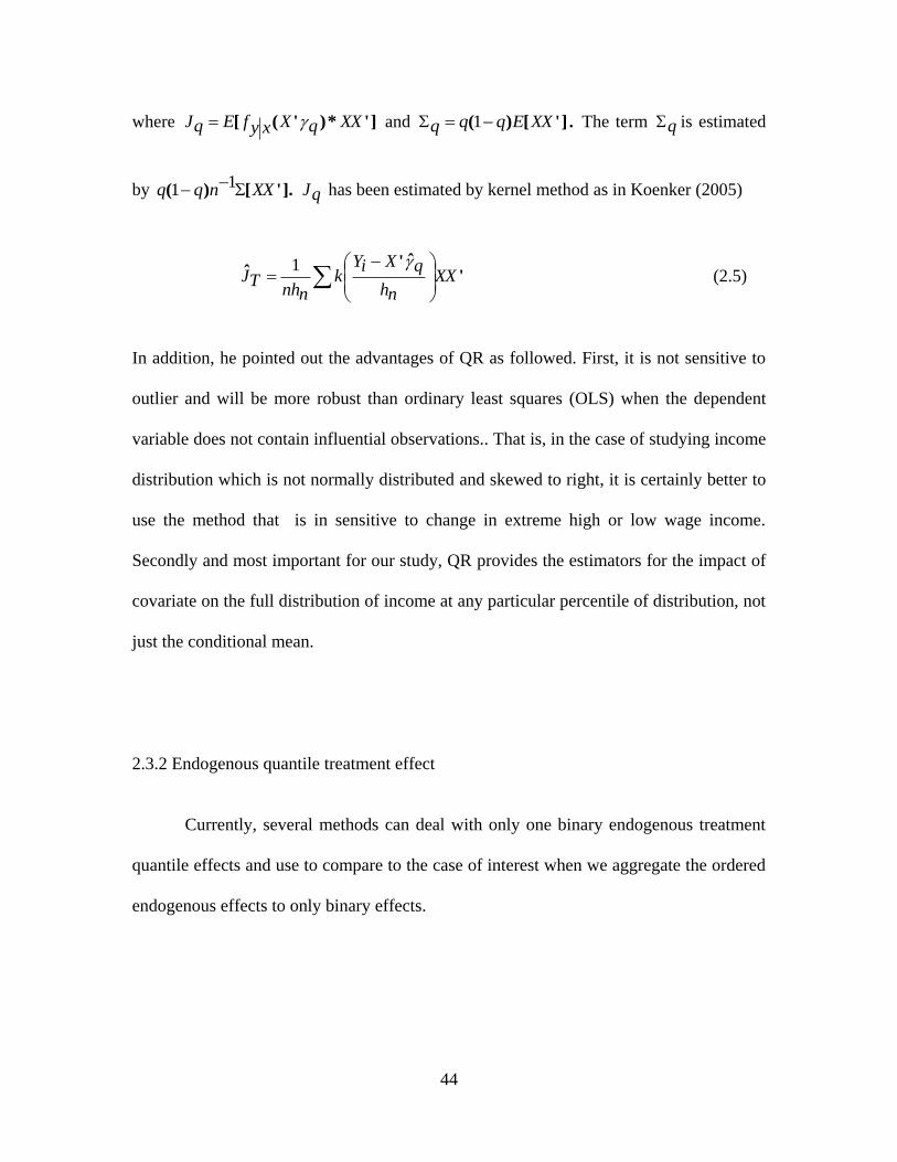
44

where ]'*)'([ XXqXxyfEqJ and ]'[)( XXEqqq 1 . The term q is estimated

by ].'[)( XXnqq 11 qJ has been estimated by kernel method as in Koenker (2005)

'ˆ'

ˆ XXnh

qXiYk

nnhTJ

1 (2.5)

In addition, he pointed out the advantages of QR as followed. First, it is not sensitive to

outlier and will be more robust than ordinary least squares (OLS) when the dependent

variable does not contain influential observations.. That is, in the case of studying income

distribution which is not normally distributed and skewed to right, it is certainly better to

use the method that is in sensitive to change in extreme high or low wage income.

Secondly and most important for our study, QR provides the estimators for the impact of

covariate on the full distribution of income at any particular percentile of distribution, not

just the conditional mean.

2.3.2 Endogenous quantile treatment effect

Currently, several methods can deal with only one binary endogenous treatment

quantile effects and use to compare to the case of interest when we aggregate the ordered

endogenous effects to only binary effects.

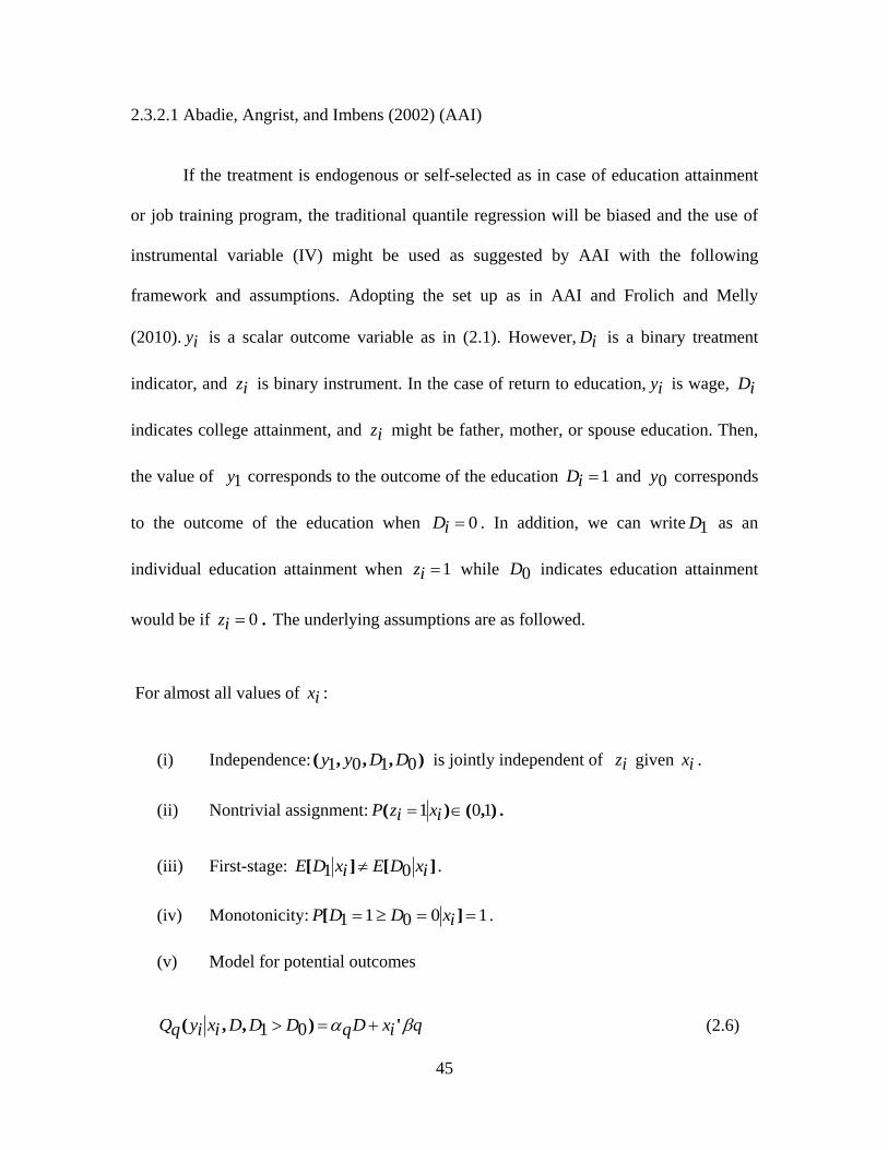
45

2.3.2.1 Abadie, Angrist, and Imbens (2002) (AAI)

If the treatment is endogenous or self-selected as in case of education attainment

or job training program, the traditional quantile regression will be biased and the use of

instrumental variable (IV) might be used as suggested by AAI with the following

framework and assumptions. Adopting the set up as in AAI and Frolich and Melly

(2010). iy is a scalar outcome variable as in (2.1). However, iD is a binary treatment

indicator, and iz is binary instrument. In the case of return to education, iy is wage, iD

indicates college attainment, and iz might be father, mother, or spouse education. Then,

the value of 1y corresponds to the outcome of the education 1iD and 0y corresponds

to the outcome of the education when 0iD . In addition, we can write 1D as an

individual education attainment when 1iz while 0D indicates education attainment

would be if 0iz . The underlying assumptions are as followed.

For almost all values of ix :

(i) Independence: ),,,( 0101 DDyy is jointly independent of iz given ix .

(ii) Nontrivial assignment: ),()( 101 ixizP .

(iii) First-stage: ][][ ixDEixDE 01 .

(iv) Monotonicity: 10011 ][ ixDDP .

(v) Model for potential outcomes

qixDqDDDixiyqQ '),,( 01 (2.6)

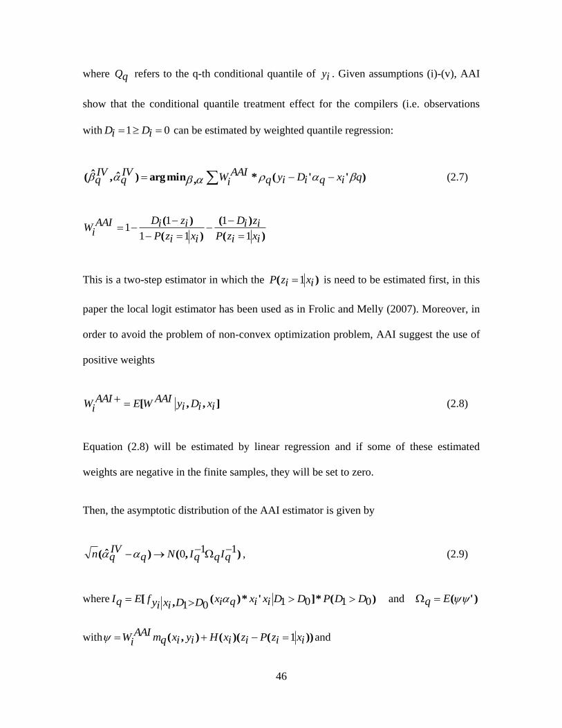
46

where qQ refers to the q-th conditional quantile of iy . Given assumptions (i)-(v), AAI

show that the conditional quantile treatment effect for the compilers (i.e. observations

with 01 iDiD can be estimated by weighted quantile regression:

)''(*,minarg)ˆ,ˆ( qixqiDiyqAAI

iWIVq

IVq (2.7)

)(

)(

)(

)(

ixizP

iziD

ixizP

iziDAAIiW

1

1

11

11

This is a two-step estimator in which the )( ixizP 1 is need to be estimated first, in this

paper the local logit estimator has been used as in Frolic and Melly (2007). Moreover, in

order to avoid the problem of non-convex optimization problem, AAI suggest the use of

positive weights

],,[ ixiDiyAAIWEAAIiW (2.8)

Equation (2.8) will be estimated by linear regression and if some of these estimated

weights are negative in the finite samples, they will be set to zero.

Then, the asymptotic distribution of the AAI estimator is given by

),()ˆ(110 qIqqINq

IVqn , (2.9)

where )(*]'*)(,[ 010101DDPDDixixqixDDixiyfEqI and )'(Eq

with ))()((),( ixizPizixHiyixqmAAIiW 1 and

47

Xqixiyqiyixqm ))'((),( 01 and

])(

)(

))((

)(),([)( ix

ixizP

iziD

ixizP

iziDiyixqmEixH

21

1

211

1.

qI will be estimated by kernel estimation that uses Epanechnikov kernel as suggested by

Abadie et.al. (2002)

'ˆ'

*ˆˆixix

nh

IVqixiy

kAAIiW

nnhqI

1

(2.10)

Where AAIiW are estimates of the projected weights. )(ˆ ixH is estimated by regressing

21

1

211

101

))(ˆ(

)(

))(ˆ(

)())ˆ'((

ixizP

iziD

ixizP

iziDixIV

qixiyq on ix . Lastly,

))(ˆ)((ˆ))ˆ'((ˆ ixZPZlxHXIVqixiyqAAI

iW 101 (2.11)

)'ˆˆ(ˆ Eq (2.12)

As stated before, AAI method can only be applied to endogenous treatment

effects where the iD is only binary. That is, the model can estimate the case where

observation of interest attains certain level of education, high school, or not. So, it is not

possible to use the iD , that are ordered outcome as endogenous regressors.

48

2.3.2.2 Unconditional quantile treatment effect Firpo (2007) and Frolich and Melly

(2008)

The unconditional treatment effect for quantile can be defined as

01 yqQ

yqQq (2.13)

The distinct feature between the conditional and unconditional treatment effects is

that the unconditional effect, by definition, will not change with respect to the different

set of covariates ix . Also, unconditional effects can be estimated consistently at the

n rate without any parametric restrictions. That is, these estimators will be entirely

nonparametric, and the assumption (i) will not be needed. Also, in estimating this

nonparametric model, it is needed to assume that the support of the covariates ix is the

same independently of the treatment. For almost all values of ix ,

110 )( ixiDP (2.14)

However, the unconditional method still needs the inclusion of covariates ix for various

reasons. First, ix are needed to make the identification plausible. Secondly, including

ix will improve efficiency. Following Frolich and Melly (2008), it is better to explain

the endogenous treatment with a binary instrumental variable iz first. Given

assumption(iv), the estimator for q is as followed:

)(*,minarg)ˆ,ˆ( iDiyqFM

iWIVq

IV (2.15)

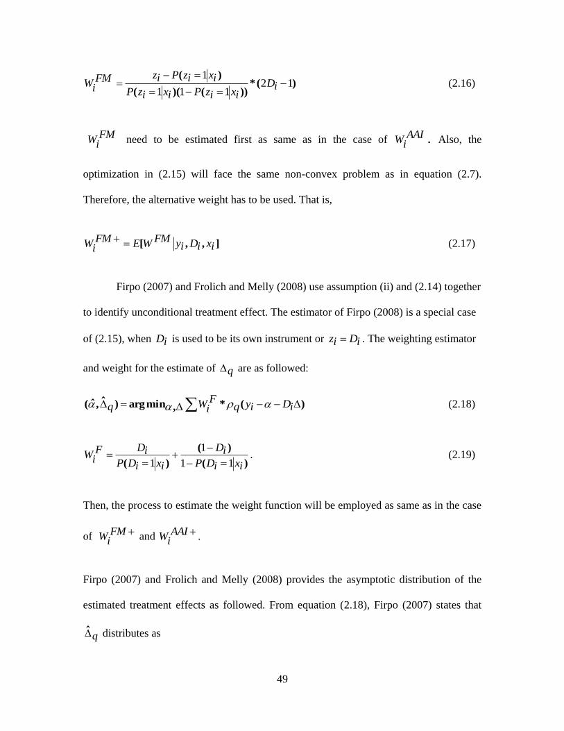
49

)(*))()((

)(12

111

1

iD

ixizPixizP

ixizPizFMiW (2.16)

FMiW need to be estimated first as same as in the case of AAI

iW . Also, the

optimization in (2.15) will face the same non-convex problem as in equation (2.7).

Therefore, the alternative weight has to be used. That is,

],,[ ixiDiyFMWEFMiW (2.17)

Firpo (2007) and Frolich and Melly (2008) use assumption (ii) and (2.14) together

to identify unconditional treatment effect. The estimator of Firpo (2008) is a special case

of (2.15), when iD is used to be its own instrument or iDiz . The weighting estimator

and weight for the estimate of q are as followed:

)(*,minarg)ˆ,ˆ( iDiyqF

iWq (2.18)

)(

)(

)( ixiDP

iD

ixiDP

iDFiW

11

1

1

. (2.19)

Then, the process to estimate the weight function will be employed as same as in the case

of FMiW and AAI

iW .

Firpo (2007) and Frolich and Melly (2008) provides the asymptotic distribution of the

estimated treatment effects as followed. From equation (2.18), Firpo (2007) states that

q distributes as

50

),()ˆ( vNqqn 0 (2.20)

)(

))(,)((,

)( ixiDP

yqQxiDYF

yqQ

ixiDYFE

yqQ

yf

v1

111

11

121

1

)(

))(,)((,

)( ixiDP

yqQxiDYF

yqQxiDYF

EyqQ

yf 11

001

00

020

1

])}()([{2

01 ixXE ,

where )(

)(,)(

YdqQYdf

Ydd

QixdDYFq

Xd

. 1YqQ and 0Y

qQ have been estimated by qˆ

and . The densities )(YdqQYdf are estimated by kernel estimators with Epanecnikov

kernel function and Silverman bandwidth choice.

diDnh

YdqQiy

kFiW

nnh

YdqQYdf ˆ)ˆ(ˆ 1

(2.21)

)(,ydqQXdiDYF is estimated by local logit estimator. In addition, the density will

be estimated by kernel regression as in the case of the exogenous treatment. These two

methods also suffer the same setback as in the case of AAI, where binary instrument will

be required for only on binary endogenous variable.

51

In addition, there is other IV method suggested by Chernokuzhov and Hansen

(2005), (2006), and (2008) that does not require binary instrument; however, in this

study, we do not employ their method for comparison since it is more computationally

intensive than the other proposed methods. In addition, it can deal with the case where

there are more than one endogenous variable but we need to fully understanding and

define the relationship between those endogenous variables. If not, it will entail bias

problem similar to the case of instrumental variable regression.

2.3.3 Sieve estimator and control function

Sieve estimation refers to one class of semiparametric estimation that solves the

problem of infinite dimensional parameter. The sieve method employs the optimization

routine that tries to optimize the criterion function over finite approximated parameter

spaces (sieves). The sieve method, in the simplest form, might be similar to how we

choose the bandwidth and numbers in plotting the histogram. As pointed out by Chen

(2007), the method of sieves is very flexible in estimating complicated semiparametric

models with (or without) endogeneity and latent heterogeneity. It can easily incorporate

prior information and constraints, and it can simultaneously estimate the parametric and

nonparametric parts, typically with optimal convergence rates for both parts.

The main reason that this paper employs the sieve estimator is that it can simplify

semiparametric inference for the quantile treatment effects. So far, the four methods of

estimation employs at least certain degree of semiparametric estimation for their

respective variances with relatively complicated formulation and computationally

52

intensive. In addition, the estimated variance varies with not only choice of kernel

function but also bandwidth selection.

Following the results in Ackerberg et.al. (2012), it has established the numerical

equivalence between two estimators of asymptotic variance for two-step semiparametric

estimators when the first-step nonparametric estimation is implemented. That is, in the

first stage, the sieve M-estimator (Sieve maximum likelihood, Sieve minimum distance,

series estimator) will be applied to the model of interest, and then in the second stage,

estimation can be set up as if the problem is completely parametric for the purpose of

inference on treatment effects.

Secondly, in this method, the endogeneity will be treated as omitted variable case

as in equation (2.1) and (2.2) since wage will certainly depend on unobserved personal

characteristics that linked to education attainment. In addition, we can allow more than

one endogenous variables that can be either categorical or ordered that is drawback for

previous methods of estimation. In addition, even the instrumental variables that allow

more than one endogenous variables as in Chernokuzhov and Hansen (2005, 2008)

cannot cover the case of endogenous categorical and ordered regressors. The paper

corrects for endogeneity by adopting the control function approach, as in case of Lee

(2007) but there is a different in first stage and second stage estimation.

We newly propose that the first step is to construction of estimated generalized

residuals irg a ordered-probit of iD on ),( izix . This step is approximation of control

function that help in solving the endogenous problem. The idea of generalized residual

for the group or ordered outcome can be found in Chesher and Irish (1987) and

Gourieroux et.al. (1987). The generalized residuals is as equation (2.22)

53

1

1 1

111L

l izlcizlc

izlcizlcliDigr

)()(

)()(][

(2.22)

lc is the estimated cut points or threshold parameters, for example, if there are

three values of iD , 210 ,,iD there will be ),( iDiDliD 21 , 21,l , then there will be

two cut points, 1c and 2c given that 01lc and 31lc . After getting the

estimated irg from equation (2.22), it will be plug in to the (2.3) as an additional

independent variables. The second step of estimation is partially linear quantile

regression of iY on iZ , iD and igr . However, it is difficult to assume the stochastic

relationship between igr and i (the errors terms from the main equation), so we use the

sieve estimator for putting the linear combination of power series of irg as regressors in

the equation of

))ˆ('()ˆ,,(,minarg)ˆ,ˆ( irgfnqizlqliDiyqirgizliDtlqq

(2.23)

where t is the trimming function that is set to equal to 1 and irg and its power function

even interacting the residuals with other regressors. In addition, we can use other form of

control functions such as fourier, spline or Taylor series approximation in the second

stage of quantile regression. Moreover, practitioner can assume other form of distribution

in the first stage given that there is the correct form for generalized residuals.

Then, the variance of the treatment effects can be estimated by either bootstrap or

finding the solution of inverse quantile functions analytically. In this paper, we choose

the bootstrap method for inference since the inverse function will mainly depend on the

54

control function that we choose. Moreover, this leads complicated analytical formula and

computationally intensive procedure. The reason that bootstrap estimator for variance is

valid that we proceed in two step estimation as in Ackerberg et.al. (2012). Also,

estimating the asymptotic variance by using parametric approximation and bootstrap

requires less restrict assumptions in order to get establish consistency and asymptotic

normality as in the case of Lee (2007).

To conclude this section, there are certain insights that might be gained from

comparing these five methods of estimation. The conditional treatment effect models are

computationally simple and should be unbiased if there is no underlying endogeneity. On

the other hands, the four semiparametric models in this paper have each own advantages

and heuristic comparison can be made to see differences in treatment effects across

income distribution. In addition, results from unconditional treatment effects, it might be

helpful for policy makers and applied economists since they capture the effects in the

entire population rather than a large number of effects for different covariate

combinations.

2.4. Monte Carlo Simulation

This section presents the Monte Carlo simulation result for comparing finite

sample properties of sieve control function estimator with the methods described in

section 2.3 given that we have not developed its asymptotic property. There are three

focuses in the simulation: the changes in root mean squared errors of the parameters with

varying degree of endogeneity, robustness to heteroskedasticity for quantile endogenous

treatment effects, and size of the test for statistical inference given varying of

55

endogeneity. In addition, we report the mean of estimated coefficients as well as bias and

standard deviation.

2.4.1 Data generating process

The data generating process (DGP) is given by

iuixixiDiDiy 22112211 )()( , ni ,...,,21

ivizizixixiD 24132211 * , ni ,...,,21

),,( 210iD

For the sake of simplicity, we assume that the exogenous variables have

homogenous effects throughout the entire distribution. However, for endogenous

covariates we can follow Melly (2007) and Lee (2007) that assume homogenous marginal

effects in their Monte Carlo Simulations or follow Chernokuzhov et.al. (2005) that allows

the marginal effects to be monotonically increases with respect to quantile.

The DGP for each variable is given by

)(~ 221 iX , ),(~ 102 NiX , )(~ 12

1 iz , ),(~ 102 Niz

1

10

,~),( Niviu

56

For one endogenous variable

iviziziXiXiD 21150250150 **.*.*.* , ni ,...,,21 ,

iuiXiXiDiy 2211121 **)(* , ni ,...,,21

),( 10iD

For two endogenous variables

iviziziXiXiD 21150250150 **.*.*.* , ni ,...,,21 ,

iuiXiXiDiDiy 2211251111 **)(*.)(* , ni ,...,,21

The )( is the th percentile value of normal cumulative density function for

example at .5 quantile the value of ).( 50 is 0.5. The endogeneity problem comes from

the correlation between errors term from ),( iviu . We assume that there are only three

categories of ordered endogenous variables. Simulation results are based on 1000

replications with number of observations of 10,000 since we are interest in all part of

income distribution especially to capture the treatment effects at the tails of distribution.

2.4.2 Bias, standard deviation of Estimator, and Power

In this section, we present results from Monte Carlo simulation with varying

degree of endogeneity in two main cases. The first case, we compare the model where

57

there is only one binary endogenous variable. The second, we compare the model where

there are two ordered endogenous variables. In the first case, we compare the estimate by

the method proposed in third section. The second case control function method is

compared with standard quantile regression, two-stage least squares with strong

instruments, and regression with predicted probability from Probit as instrumental

variables.

2.4.2.1 One endogenous variable model

In this section, we compare the finite sample properties of sieve estimator with

the well-established estimator of the quantile treatment effects that can only take care of

one endogenous variable. When there is no endogeneity, as presented in Table 2.1,

standard quantile regression yields the lowest bias and variance for the coefficient

estimated. However, Firpo yields least precise estimate as expected by unconditional

quantile treatment effects. For, the unconditional quantile regression, the bias is higher

along with variance. Moreover, mean rejection for FM is closest to the 0.05 level that we

set up.

By introducing mild degree of endogeneity in table 2.2, the methods that does not

take in to account, endogeneity tends to slightly overestimate the quantile treatment effect

at the median. The Sieve estimator still yield less bias with higher variance compared to

the standard quantile regression. The FM and AAI methods do slightly overestimate the

parameter but come out with higher variance than the rest.

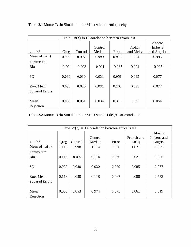
58

Table 2.1 Monte Carlo Simulation for Mean without endogeneity

True )( is 1 Correlation between errors is 0

= 0.5 Qreg Control

Control

Median Firpo

Frolich

and Melly

Abadie

Imbens

and Angrist

Mean of )( 0.999 0.997 0.999 0.913 1.004 0.995

Parameters

Bias -0.001 -0.003 -0.001 -0.087 0.004 -0.005

SD 0.030 0.080 0.031 0.058 0.085 0.077

Root Mean 0.030 0.080 0.031 0.105 0.085 0.077

Squared Errors

Mean 0.038 0.051 0.034 0.310 0.05 0.054

Rejection

Table 2.2 Monte Carlo Simulation for Mean with 0.1 degree of correlation

True )( is 1 Correlation between errors is 0.1

= 0.5 Qreg Control

Control

Median Firpo

Frolich and

Melly

Abadie

Imbens and

Angrist

Mean of )( 1.113 0.998 1.114 1.030 1.021 1.005

Parameters

Bias 0.113 -0.002 0.114 0.030 0.021 0.005

SD 0.030 0.080 0.030 0.059 0.085 0.077

Root Mean 0.118 0.080 0.118 0.067 0.088 0.773

Squared Errors

Mean 0.038 0.053 0.974 0.073 0.061 0.049

Rejection

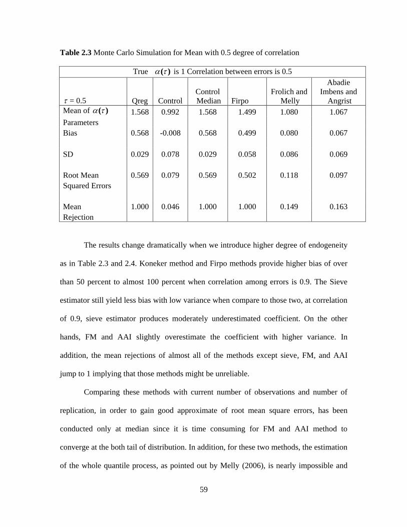
59

Table 2.3 Monte Carlo Simulation for Mean with 0.5 degree of correlation

True )( is 1 Correlation between errors is 0.5

= 0.5 Qreg Control

Control

Median Firpo

Frolich and

Melly

Abadie

Imbens and

Angrist

Mean of )( 1.568 0.992 1.568 1.499 1.080 1.067

Parameters

Bias 0.568 -0.008 0.568 0.499 0.080 0.067

SD 0.029 0.078 0.029 0.058 0.086 0.069

Root Mean 0.569 0.079 0.569 0.502 0.118 0.097

Squared Errors

Mean 1.000 0.046 1.000 1.000 0.149 0.163

Rejection

The results change dramatically when we introduce higher degree of endogeneity

as in Table 2.3 and 2.4. Koneker method and Firpo methods provide higher bias of over

than 50 percent to almost 100 percent when correlation among errors is 0.9. The Sieve

estimator still yield less bias with low variance when compare to those two, at correlation

of 0.9, sieve estimator produces moderately underestimated coefficient. On the other

hands, FM and AAI slightly overestimate the coefficient with higher variance. In

addition, the mean rejections of almost all of the methods except sieve, FM, and AAI

jump to 1 implying that those methods might be unreliable.

Comparing these methods with current number of observations and number of

replication, in order to gain good approximate of root mean square errors, has been

conducted only at median since it is time consuming for FM and AAI method to

converge at the both tail of distribution. In addition, for these two methods, the estimation

of the whole quantile process, as pointed out by Melly (2006), is nearly impossible and

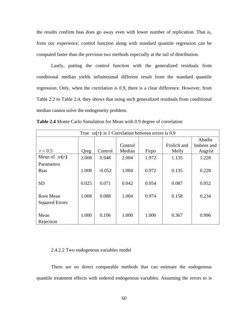
60

the results confirm bias does go away even with lower number of replication. That is,

from our experience, control function along with standard quantile regression can be

computed faster than the previous two methods especially at the tail of distribution.

Lastly, putting the control function with the generalized residuals from

conditional median yields infinitesimal different result from the standard quantile

regression. Only, when the correlation is 0.9, there is a clear difference. However, from

Table 2.2 to Table 2.4, they shows that using such generalized residuals from conditional

median cannot solve the endogeneity problem.

Table 2.4 Monte Carlo Simulation for Mean with 0.9 degree of correlation

True )( is 1 Correlation between errors is 0.9

= 0.5 Qreg Control

Control

Median Firpo

Frolich and

Melly

Abadie

Imbens and

Angrist

Mean of )( 2.008 0.948 2.004 1.972 1.135 1.228

Parameters

Bias 1.008 -0.052 1.004 0.972 0.135 0.228

SD 0.025 0.071 0.042 0.054 0.087 0.052

Root Mean 1.008 0.088 1.004 0.974 0.158 0.234

Squared Errors

Mean 1.000 0.106 1.000 1.000 0.367 0.996

Rejection

2.4.2.2 Two endogenous variables model

There are no direct comparable methods that can estimate the endogenous

quantile treatment effects with ordered endogenous variables. Assuming the errors to is

61

normally distributed, we can use Monte Carlo simulation to compare the property of

control function estimator to the standard two-stage least squares method that can take

care of two endogenous regressors properly. We compare sieve estimator with quantile

regression, two-staged least squares with strong instruments and two-staged least square

with predicted probabilities as instrument.

In addition, as same as in section 2.4.2.1, we present the result with varying

degree of endogeneity. When there is no endogeneity, the quantile regression, sieve, and

2SLS with probabilities yield the best estimate of coefficients as expected, however,

putting the power series or probabilities to control for endogeneity yields higher variance

of estimation. However, the drawback of standard instrumental variable (Z) persists both

in the case where there is more than one endogenous variable. For simulation and

estimation, the relationship between these two variables has to be established. Assuming

that both of these variables are not related is plausible but not valid in almost all of the

case. Hence, even with no endogeneity, the results from third column in Table 5 yield

bias and high variance since we do not have information on the relationship such that we

can estimate the model with full information maximum likelihood or GMM.

When we introduce mild degree of endogeneity, the Koenker estimation yield

overestimated results for both coefficients with low level of mean rejection. The sieve

and 2SLS with probabilities produce less biased results with similar level of mean

rejection implying more precise and robust results. Moreover, introducing the corrected

terms, series of generalized residuals or predicted probabilities always increase the Monte

Carlo standard deviations. At 0.5 level of correlation, neglecting endogeneity, leads to

62

almost 100 percent increase in median treatment effects as well as still accepting that the

estimated effects is statistically different from zero. On the contrary, the sieve and 2SLS

with probabilities are really closed and reliable. For standard IV results, the bias is not

getting better as well as standard deviation. We might conclude that dealing with more

than one endogenous variable is quite problematic in terms of not only finding the strong

instrumental variables but also modeling relationship between them.

In table 2.8, we present the result where the correlation is 0.9, sieve estimation

yield more biased results compared to two-stage least squares with predicted probabilities

though the Monte Carlo variance is lower. Moreover, for the other two methods, the

results are certainly biased. However, one caution is in the case of two-stage least squares

with instrumental variables, this method yield the highest bias among the entire

estimators with high variances. That is, we certainly will fail to reject that the estimated

coefficient will be different from zero and led to the worse estimators of all the methods.

To conclude, sieve estimator, though might not be the best estimator to control for

endogeneity, at least can reduce the bias as well as give a valid estimate for quantile

treatment effect when there is one or more endogenous variables. That is, without

calculating analytical asymptotic theory for this sieve estimator, the proposed procedures

constitute a probable approximation for estimating quantiles treatment effects and for

making reliable inference for this two-step estimation.

63

Table 2.5 Monte Carlo Simulation for Mean with 0 degree of correlation

True )(1 is 0.5 Correlation between errors is 0

= 0.5 Qreg Control 2SLS with Z 2SLS with Prob

Mean of )(1 0.499 0.499 -0.772 0.501

Parameters

Bias -0.001 -0.001 -1.272 0.001

SD 0.034 0.049 36.110 0.095

Root Mean 0.034 0.049 36.132 0.095

Squared Errors

Mean 0.044 0.049 0.017 0.051

rejection

True )(2 is 0.75 Correlation between errors is 0

= 0.5 Qreg Control 2SLS with Z 2SLS with Prob

Mean of )(2 0.749 0.750 1.203 0.748

Parameters

Bias -0.001 0.000 0.453 -0.002

SD 0.037 0.071 13.424 0.052

Root Mean 0.037 0.071 13.432 0.052

Squared Errors

Mean 0.040 0.055 0.017 0.047

rejection

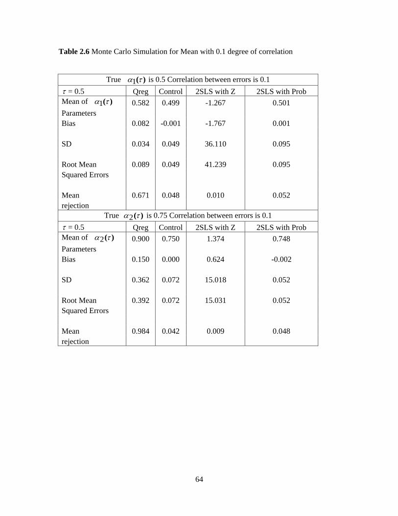
64

Table 2.6 Monte Carlo Simulation for Mean with 0.1 degree of correlation

True )(1 is 0.5 Correlation between errors is 0.1

= 0.5 Qreg Control 2SLS with Z 2SLS with Prob

Mean of )(1 0.582 0.499 -1.267 0.501

Parameters

Bias 0.082 -0.001 -1.767 0.001

SD 0.034 0.049 36.110 0.095

Root Mean 0.089 0.049 41.239 0.095

Squared Errors

Mean 0.671 0.048 0.010 0.052

rejection

True )(2 is 0.75 Correlation between errors is 0.1

= 0.5 Qreg Control 2SLS with Z 2SLS with Prob

Mean of )(2 0.900 0.750 1.374 0.748

Parameters

Bias 0.150 0.000 0.624 -0.002

SD 0.362 0.072 15.018 0.052

Root Mean 0.392 0.072 15.031 0.052

Squared Errors

Mean 0.984 0.042 0.009 0.048

rejection

65

Table 2.7 Monte Carlo Simulation for Mean with 0.5 degree of correlation

True )(1 is 0.5 Correlation between errors is 0.5

= 0.5 Qreg Control 2SLS with Z 2SLS with Prob

Mean of )(1 0.918 0.494 2.996 0.502

Parameters

Bias 0.418 -0.006 2.496 0.002

SD 0.324 0.046 53.678 0.095

Root Mean 0.529 0.047 41.239 0.095

Squared Errors

Mean 1.000 0.052 0.013 0.052

rejection

True )(2 is 0.75 Correlation between errors is 0.5

= 0.5 Qreg Control 2SLS with Z 2SLS with Prob

Mean of )(2 1.503 0.741 -0.281 0.749

Parameters

Bias 0.753 -0.009 -1.031 -0.001

SD 0.338 0.072 22.547 0.052

Root Mean 0.825 0.072 22.571 0.052

Squared Errors

Mean 1.000 0.053 0.012 0.046

rejection

66

Table 2.8 Monte Carlo Simulation for Mean with 0.9 degree of correlation

True )(1 is 0.5 Correlation between errors is 0.9

= 0.5 Qreg Control 2SLS with Z 2SLS with Prob

Mean of )(1 1.244 0.469 -0.569 0.502

Parameters

Bias 0.744 -0.032 -1.069 0.002

SD 0.027 0.038 76.284 0.095

Root Mean 0.744 0.049 41.239 0.095

Squared Errors

Mean 1.000 0.133 0.009 0.046

rejection

True )(2 is 0.75 Correlation between errors is 0.9

= 0.5 Qreg Control 2SLS with Z 2SLS with Prob

Mean of )(2 2.095 0.690 1.046 0.749

Parameters

Bias 1.345 -0.060 0.296 -0.001

SD 0.029 0.062 29.145 0.052

Root Mean 1.345 0.086 29.147 0.052

Squared Errors

Mean 1.000 0.174 0.009 0.044

rejection

2.4.2.3 Sensitivity analysis for the control function estimator to heteroskedasticity

Unlike normal regression, the estimated parameters from quantile regression can

be effected by heteroskedasticity. Suppose the true data generating process depicts linear

quantile regression where there are only exogenous variables ),( 21 XX and there is only

67

one exogenous variable )( 1X that enter in to both conditional quantile equation as well

as multiplicative heteroskedasticity, then we expect that estimated coefficient of 1X will

vary with the value of quantile. Moreover, even if we add one additional binary

endogenous variable )( iD1 to estimation, we suspect that heteroskedasticity will further

lead to bias estimation of both coefficients of ),( iDX 11 . However, control function

might provide flexible way to estimate the model by interacting generalized residuals

with 1X as more control variables. The data generating process come from part 2.4.1, we

focus on the case where there are one binary endogenous variable as the following

iviziziXiXiD 211502501501 **.*.*.* , ni ,...,,21

iwiXiXiDiy 22121111 **)()( , ni ,...,,21

where iuiXiw *)..( 15010

The only difference from section 2.4.1 is the new DGP contains

heteroskedasticity problem in exogenous independent variable and might exacerbate the

biases of both endogenous treatment effect and coefficient of iX1 . The simulation

contains the same 1,000 replications with 10,000 observations. Then, we compute Monte

Carlo mean, standard deviation, and root mean squares error as before.

The result in Table 2.9 shows that even with mild endogeneity, correlation at 0.1,

control function without interaction term can let to a biased result of about 10 percent for

the estimated parameters of binary endogenous variable. However, for the estimation of

68

coefficient of iX1 , the bias is not that severe. Only at the 90 percentile where the bias is

large for the case of control function.

Table 2.9 Monte Carlo Simulation for the case of Heteroskedasticity and Endogeneity

with 0.1 degree of correlation

True )(1 is 0.2 Correlation between errors is 0.1

= 0.1 Qreg Control

Control with

Interaction

Frolich and

Melly

Abadie Imbens and

Angrist

Mean of

)(1 0.252 0.212 0.200 0.444 0.229

Parameters

Bias 0.052 0.012 0.000 0.244 0.029

SD 0.018 0.061 0.035 0.099 0.031

Root Mean 0.055 0.062 0.035 0.264 0.042

Squared

Errors

Mean .811 0.051 0.039 0.691 0.152

rejection

True )(2 is 0.36 Correlation between errors is 0.1

= 0.1 Qreg Control

Control with

Interaction

Frolich and

Melly

Abadie Imbens and

Angrist

Mean of

)(2 0.366 0.362 0.360 0.386

Parameters

Bias 0.006 0.002 0.000 0.026

SD 0.018 0.019 0.033 0.041

Root Mean 0.019 0.019 0.033 0.049

Squared

Errors

Mean 0.039 0.020 0.048 0.093

rejection

69

Table 2.10 Monte Carlo Simulation for the case of Heteroskedasticity and Endogeneity

with 0.5 degree of correlation

True )(1 is 1 Correlation between errors is 0.5

= 0.5 Qreg Control

Control with

Interaction

Frolich and

Melly

Abadie Imbens and

Angrist

Mean of

)(1 1.259 1.029 0.995 1.069 1.145

Parameters

Bias 0.259 0.029 -0.005 0.069 0.145

SD 0.017 0.044 0.027 0.096 0.029

Root Mean 0.260 0.052 0.028 0.118 0.148

Squared

Errors

Mean 1.000 0.094 0.032 0.121 0.999

rejection `

True )(2 is 1 Correlation between errors is 0.5

= 0.5 Qreg Control

Control with

Interaction

Frolich and

Melly

Abadie Imbens and

Angrist

Mean of

)(2 1.037 0.999 1.001 1.115

Parameters

Bias 0.037 -0.001 0.001 0.115

SD 0.013 0.013 0.024 0.036

Root Mean 0.039 0.013 0.024 0.121

Squared

Errors

Mean 0.719 0.019 0.045 0.891

rejection

70

Table 2.11 Monte Carlo Simulation for the case of Heteroskedasticity and Endogeneity

with 0.9 degree of correlation

True )(1 is 1.8 Correlation between errors is 0.9

= 0.9 Qreg Control

Control with

Interaction

Frolich and

Melly

Abadie Imbens

and Angrist

Mean of

)(1 2.057 1.759 1.798 1.304 1.981

Parameters

Bias 0.257 -0.041 -0.002 -0.497 0.181

SD 0.019 0.049 0.032 0.216 0.028

Root Mean 0.257 0.064 0.032 0.541 0.183

Squared

Errors

Mean 1.000 0.121 0.038 0.668 1.000

rejection

True )(2 is 1.64 Correlation between errors is 0.9

= 0.9 Qreg Control

Control with

Interaction

Frolich and

Melly

Abadie Imbens

and Angrist

Mean of

)(2 1.656 1.559 1.496 1.711

Parameters

Bias 0.016 -0.081 -0.144 0.071

SD 0.016 0.018 0.028 0.030

Root Mean 0.023 0.083 0.147 0.077

Squared

Errors

Mean 0.122 0.996 0.996 0.697

rejection

In sum, from simulation results, control function can correct the bias problem

from the heteroskedasticity and endogeneity to a certain degree. When, the

71

heterskedasticity is multiplicative, putting interaction term between generalized residuals

and independent variables might help. In addition, from sieve estimator perspective,

increasing the number of interaction or creating better sieve approximation function with

more terms is necessary when the number of observations is large.

2.4.3 Test size result

We present the test size results from three methods to correct for endogeneity

problems. The first one is control function estimation of median regression by using

generalized residuals as control. The second one is two-stage least squares with 2

instrumental variables and the last one is two-stage least squares with predicted

probabilities from ordered probit as instrumental variables. The test size has been

calculated based on 1000 replications for both the data generating process with two

endogenous variables and one endogenous variable. Generally, in order to adopt control

functions of ordered outcome method for quantile regression, we worry about its finite-

sample size property comparing to standard mean regression whether it should report

lower p-value than the true size, so we reject the null hypothesis more often than we

should when there is no endogeneity or low degree of endogeneity.

For our example with given DGP, we want to simulate the size of a 0.05 level test

of endogeneity based on Hausman-type statistics. The null hypothesis for the first method

is 00 :H against 00 :H where is the coefficient of the control function.

Under the null, we have use the naïve estimator for standard errors of . For the other

two instrumental variables method we perform the test based on standard Hausman test.

72

Then, we obtain their respective valuep and compare it to true size. The results are in

the following table.

When 0 , or there is no endogeneity, the actual test size is 0.065 for control

function, it is reasonably close to the nominal size of 0.05. However, it is a little higher

than the cases where we use two-stage least squares. That is, we fail the null hypothesis a

little more often than the other two methods. However, out of 1,000 replications, the

difference is only 15, it make us become less concern about the validity of employing the

control function. Moreover, when there is slight degree of endogeneity at 10. , the

size of the test is larger, we almost certainly reject the null hypothesis of no endogeneity

in case of control function and two-stage least squares with predicted probabilities.

However, with the case of standard instrumental variables, it does not reject the

hypothesis of no endogeneity as often as other two methods; only about 600 out of 1,000

that it rejects. When we increase the correlation )( to 0.5 and 0.9, all of the tests

perform well; they always reject the case of no endogeneity.

Table 2.12 Test size based on model with two ordered endogenous variables

Test Size Two ordered endogenous variables

= 0 = 0.1 = 0.5 = 0.9

Control 0.065 0.951 1 1

with

generalized

residuals

Ivregress 0.047 0.597 1 1

with

Instrumental

Variables

Ivregress 0.058 0.978 1 1

with predicted

probabilites

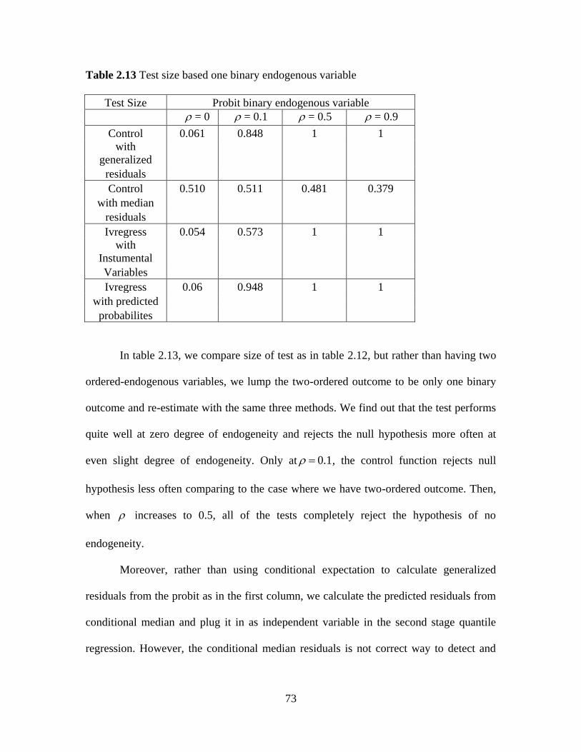
73

Table 2.13 Test size based one binary endogenous variable

Test Size Probit binary endogenous variable

= 0 = 0.1 = 0.5 = 0.9

Control 0.061 0.848 1 1

with

generalized

residuals

Control 0.510 0.511 0.481 0.379

with median

residuals

Ivregress 0.054 0.573 1 1

with

Instumental

Variables

Ivregress 0.06 0.948 1 1

with predicted

probabilites

In table 2.13, we compare size of test as in table 2.12, but rather than having two

ordered-endogenous variables, we lump the two-ordered outcome to be only one binary

outcome and re-estimate with the same three methods. We find out that the test performs

quite well at zero degree of endogeneity and rejects the null hypothesis more often at

even slight degree of endogeneity. Only at 1.0 , the control function rejects null

hypothesis less often comparing to the case where we have two-ordered outcome. Then,

when increases to 0.5, all of the tests completely reject the hypothesis of no

endogeneity.

Moreover, rather than using conditional expectation to calculate generalized

residuals from the probit as in the first column, we calculate the predicted residuals from

conditional median and plug it in as independent variable in the second stage quantile

regression. However, the conditional median residuals is not correct way to detect and

74

correct endogeneity since it does not reject the null hypothesis of endogeneity for almost

all level of . Thus, we should use conditional expected residuals rather than median.

Table 2.14 Test size with 1000 observations and variance of (9, 1)

Test Size Two ordered endogenous variables

= 0 = 0.1 = 0.5 = 0.9

Control 0.054 0.213 1 1

with

generalized

residuals

Ivregress 0.047 0.091 0.958 1

with Z

Ivregress 0.059 0.227 1 1

with predicted

probabilites

Test Size Probit binary endogenous variable

= 0 = 0.1 = 0.5 = 0.9

Control 0.061 0.151 0.998 1

with

generalized

residuals

Control 0.508 0.494 0.481 0.494

with median

residuals

Ivregress 0.058 0.199 0.919 1

with

Instumental

Variables

Ivregress 0.059 0.199 1 1

with predicted

probabilites

Next, we consider the case where the variance of ),( iviu change to (9, 1). Also,

we will reduce number of observation to 1,000. Increasing the variance from 1 to 9 will

certainly reduce the imply R-squared of the data generating process. For example, when

75

the variance is 1, without considering the variation in endogenous terms, the implied R-

squared equals to (4+4)/(4+4+1) = 0.89 or 89 percent. When we change it to 9, the

implied R-squared is (4+4)/(4+4+9) = 0.47 or 47 percent that is closed to normal cross

sectional data R-squared. In table 3, we represent the test sized based on two and one

endogenous variable with 1000 observations and variance of (9, 1).

To conclude, from the test size simulations, adopting control functions for the

model of quantile regression at median with ordered endogenous variables might be a

valid way to control for endogeneity and perform statistical inference in order to check

whether we really face endogeneity problem.

2.5. Data and Estimating Results

In this paper, we apply the methods described in section 3 and 4 to estimating the

causes of income inequality in USA and Great Lake States. The data is Currently

Population Survey (CPS) from the period of 2001 to 2009. During this period, two shocks

potentially affect household income in the top quantile. They are the dot-com crisis of the

2001 and the Financial Crisis of 2008. The measurement of log wage of the person with

highest education will be used as dependent variable while household characteristics,

education, union coverage, and age are used as dependent variables in finding quantile

treatment effect. In the case that there are two same level of highest education in the

household, we will use person with highest wage income.

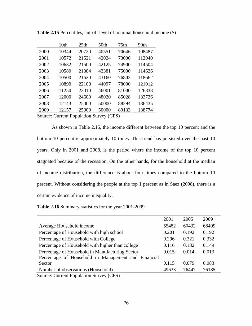
76

Table 2.15 Percentiles, cut-off level of nominal household income ($)

10th 25th 50th 75th 90th

2000 10344 20720 40551 70646 108487

2001 10572 21521 42024 73000 112040

2002 10632 21500 42125 74900 114504

2003 10580 21384 42381 75000 114626

2004 10500 21620 43160 76803 118662

2005 10890 22108 44097 78000 121012

2006 11250 23010 46001 81000 126838

2007 12000 24600 48020 85028 133726

2008 12143 25000 50000 88294 136435

2009 12157 25000 50000 89133 138774

Source: Current Population Survey (CPS)

As shown in Table 2.15, the income different between the top 10 percent and the

bottom 10 percent is approximately 10 times. This trend has persisted over the past 10

years. Only in 2001 and 2008, is the period where the income of the top 10 percent

stagnated because of the recession. On the other hands, for the household at the median

of income distribution, the difference is about four times compared to the bottom 10

percent. Without considering the people at the top 1 percent as in Saez (2008), there is a

certain evidence of income inequality.

Table 2.16 Summary statistics for the year 2001-2009

2001 2005 2009

Average Household income 55482 60432 68409

Percentage of Household with high school 0.201 0.192 0.192

Percentage of Household with College 0.296 0.321 0.332

Percentage of Household with higher than college 0.116 0.132 0.149

Percentage of Household in Manufacturing Sector 0.015 0.014 0.013

Percentage of Household in Management and Financial

Sector 0.115 0.079 0.083

Number of observations (Household) 49633 76447 76185

Source: Current Population Survey (CPS)

77

Table 2.16 contains statistics of some key variables that will be used in

estimation. The average income shows a steady growth despite two recessions during the

period of sample. On the education attainment, household with the high school education

refers to the case where the most educated person in the household achieve high school

degree where the household with college refers to most educated person in the household

holds bachelor degree. It is clear that for the past ten years, the household with high

school degree from the survey stays at about 20 percent of total population. There is a

growth of household with college degree from 29 percent to 33 percent and household

with higher than college degree from 11 to 14 percent.

The linear quantile effects model of income determination with the interested

explanatory as discussed in section 2 will be as follows:

)ln(wage covunAgeMcollegecollegehighschool 543210

iuGreatlakeMaFiManuwhite 9876 (2.25)

where )ln(wage is the log wage of most educated person in the household

highschool = 1 if household member of highest education got high school degree = 0

otherwise.

college = 1 if household member of highest education got bachelor degree = 0 otherwise

Mcollege = 1 household member of highest education got high degree than bachelor = 0

otherwise

78

Age is age of person in the household with highest education.

uncov = 1 if household member of highest education is under union coverage = 0

otherwise

white = 1 if household member of highest education is white = 0 otherwise

Manu = 1 if household member of highest education worked in Manufacturing sector

last year = 0 otherwise

MaFi = 1 if household member of highest education worked in Management and

Financial sector last year = 0 other wise.

Greatlake = 1 if the household lives in the Great Lake States

First, we assume that education attainment is exogenous at first in order to

provide a quick picture of what are the determinants of income or return to education.

The linear model will be estimated by qreg command in STATA® as well as regression

with robust standard errors. We pool the data from CPS survey from year 2001 to 2009 to

be one data set. We choose the household with positive wage income that has more than

2 members. Then, we keep only the case where the second most educated member is

either wife, husband, partner, or parents. The results are in the following Table 17.

At a first glance, not taking in to account the possibility of endogeneity in

education attainment, the effects of education attainment on the wage income are

significant across all the quantile as well as from standard regression. The results show

that higher level of education always lead to higher wage income no matter what point of

79

income distribution. In addition, all of the coefficients are significant at 1 percent. These

result are more in line with classical economic theory, the relative differences in wage

can be explain by the education. Moreover, at quantile 90 and 99, the return to education

seems to be highest especially for the people with degree higher than college. One way of

looking at this high value of Mcollege is that it might be possible to look through one of

the most popular graduate level program, Master in Business Administration (MBA).

According to http://www.businessweek.com/interactive_reports/roi_rankings.html, the

average salary of the newly graduate top 20 business school is about 100,000 dollars for

the graduate of 2008 class.

80

Table 2.17 Estimate result assuming education attainments are conditionally exogenous

(n = 349,825)

Estimation OLS Quantile10 Quantile50 Quantile90 Quantile99

highschool 0.2303*** 0.2578*** 0.2341*** 0.1923*** 0.2485***

(0.0038) (0.0082) (0.0033) (0.0058) (0.0224)

college 0.4957*** 0.5500*** 0.4619*** 0.4685*** 0.9190***

(0.0032) (0.0071) (0.0028) (0.0050) (0.0189)

Mcollege 0.8623*** 0.8990*** 0.7610*** 0.9687*** 1.247***

(0.0045) (0.0092) (0.0037) (0.0066) (0.0251)

Age 0.1145*** 0.1757*** 0.0976*** 0.0725*** 0.0612***

(0.0010) (0.0015) (0.0006) (0.0011) (0.0041)

Age2 -0.0013*** -0.0021*** -0.0017*** -0.0007*** -0.0006***

(0.00001) (0.00001) (0.00006) (0.00002) (0.00004)

uncov 0.0042** 0.01351*** -0.007*** -0.0190*** -0.0234**

(0.0017) (0.0041) (0.0016) (0.0029) (0.0112)

white 0.1197*** 0.1484*** 0.1081*** 0.1253*** 0.1110***

(0.0036) (0.0078) (0.0031) (0.0055) (0.0211)

Manu -0.01669*** -0.3526*** -0.0910*** 0.0083*** 0.1540**

(0.0140) (0.024) (.0010) (0.0167) (0.0646)

MaFi 0.3918*** 0.4131*** 0.3336*** 0.4040*** 0.4010***

(0.0037) (0.0083) (0.0033) (.0058) (0.0224)

Greatlake -0.0323*** 0.0823*** 0.0336*** -0.014** -0.0448*

(0.0038) (0.0086) (0.0034) (0.0061) (0.0233)

Notes: (i) The standard errors for the coefficients are in parenthesis

(ii) *, **, and *** denote significance at the 10,5, and 1% level respectively

For the case of age, it forms a quadratic relationship with the wage that is wage is

growing with age at a decreasing rate for all of the quantile distribution. On the union

coverage, it might be positively relates to wage at the lower end of income spectrum but

not for the quantile 50, 90 and 99.

81

Table 2.18 Estimate result assuming education attainments are endogenous (n = 349,825)

Estimation 2SLS Quantile10 Quantile50 Quantile90 Quantile99

highschool 0.0142 -0.0794*** 0.0499*** 0.0853*** 0.5910***

(0.0117) (0.0235) (0.0100) (0.0056) (0.0670)

college 0.1528*** 0.0133 0.1628*** 0.2534*** 1.1502***

(0.0163) (0.3275) (0.0150) (0.0175) (0.1204)

Mcollege 0.0747** -0.2109*** 0.0906*** 0.2553*** 0.3381**

(0.0268) (0.0490) (0.0256) (0.0200) (0.2024)

Age 0.1298*** 0.1968*** 0.1100*** 0.0807*** 0.0576***

(0.0011) (0.0020) (0.0001) (0.0004) (0.0042)

Age2 -0.0014*** -0.0023*** -0.0012*** -0.0008*** -0.0005***

(0.00001) (0.00002) (0.000001) (0.000005) (0.00004)

uncov 0.0069** 0.0176*** -0.0056*** -0.0169*** -0.0136***

(0.0017) (0.0035) (0.0012) (0.0012) (0.0112)

white 0.1148*** 0.1435*** 0.1047*** 0.1223*** 0.0624***

(0.0036) (0.0081) (0.0038) (0.0015) (0.0211)

Manu -0.1134*** -0.2613*** -0.0426*** 0.0463*** 0.2022***

(0.0140) (0.0278) (.0011) (.0011) (0.0868)

MaFi 0.5006*** 0.5707*** 0.4244*** 0.4772*** 0.5287***

(0.0058) (0.0102) (0.0051) (0.0086) (0.0567)

Greatlake 0.0286*** 0.0783*** 0.0311*** -0.0141** -0.0353***

(0.0038) (0.0078) (0.0030) (0.0078) (0.0107)

Notes: (i) The standard errors for the coefficients are in parenthesis

(ii) Standard errors come from bootstrap with 200 replications.

(iii) *, **, and *** denote significance at the 10, 5, and 1% level respectively

Being white yield the same positive and significant effect on wage throughout

regression and quantile regression. As expected for the decline in industrial sector,

working in manufacturing gives less wage at a lower part of income while at a higher

income distribution, the coefficients is still positive. In addition working in financial

82

service sector always yield higher wage. Lastly, working in great lake state is on average

associate with lower income; however, it is not true for quantile 10 and 50.

Secondly, when we treat the education attainments as endogenous ordered

variables and we should, the estimated results are starkly different. The first column from

Table 2.18 describes the case where we correct for endogeneity by first calculating the

generalized residuals and then use the standard regression. By looking at the average

effects of education attainment, we found out that return to education is not as high as in

Table 2.17. Getting high school yields positive return to wage but not significant at 10

quantile. Moreover, earning college degree leads to higher return to wage comparing to

earning more than high school. This result is the clear when we focus on the 10 quantile

and 50 quantile; the return to education of bachelor degree is higher than both high

school and even graduate degree. At 90 quantile, it is the place where the wage is

increasing, as the level of education attainment is higher, but only at this quantile is

where the return to education of graduate becomes higher than college. Then, at 99

quantile the return to education of graduate degree is highest but is still lower than the

bachelor degree. That is, the return to education is not monotonically increases with the

level of education attainment. By correcting for endogeneity, it reveals that returns of

education on wages do not always increase throughout the income distribution.

Specifically, attaining high school though positively related to higher wage than

not getting high school degree, the coefficients are quite small throughout the wage

distribution compared to other education degrees. Next attaining college degree leads to

highest impact on wage. We might be able to say that bachelor degree is a must-have for

83

higher wage. The low coefficients of high school education even at 90 and 99 quantile

point out that high school degree is not sufficient anymore. In addition, for the higher

than college degree (graduate degree), the impact on wage is still positive but

incrementally less than the college degree. The lower return of graduate degree might be

a good indicator of why only 10 percent of observations from the survey pursued

graduate degree.

One explanation for such lower return to graduate degree is Neoclassical Growth

theory; the reduction for the return of graduate degree might be related to skill-set

demanded in the current world economy. Globalization makes outsourcing of the

graduate skill-set possible. That is, not only the US corporation can conduct foreign

direct investment abroad to lower the cost of low-skill labor(high school) but also firm

can lower the cost of high-skill labor, too. Wan (2008) pointed out that the cost of hiring

US engineer to design computer chip is approximately three times higher than cost of

hiring Chinese engineer and two times higher than hiring Korean engineer of the same

caliber. In addition, Endogenous Growth theory predicts the economy where only people

at the high end of human capital spectrum and capital holder will leap more benefit from

economy. That is, at the 99 quantile, education attainment alone might not be enough in

explaining the different in wage. People with graduate degree earn higher wage than

people without high school education. However, it might not be true if we compare to the

bachelor degree.

84

2.6 Concluding Remarks and Further Study

Unlike previous studies on income distribution, this empirical study examines the

relationship between determinants of income throughout entire distribution by using

quantile regression. Although, various methods of quantile treatment effects that are

robust to endogeneity have been examined, but none of them has taken into account the

ordered endogenous regressors. We propose the use of control function with sieve

estimator to correct for the endogeneity problem. The Monte Carlo simulation shows that

our proposed method is usable and works well against other method. Correcting for

endogeneity reveals interesting results, the different levels of education attainment

significantly increases wage. However, ignoring endogeneity leads to overestimate of the

return to education. In addition, wages are not monontonically increasing with education

throughout wage distribution. At the both low and high wage spectrum, it proves out that

bachelor degree is not enough for the current state of the economy. Moreover, focusing

on graduate degree attainment might not be the key in improving wage, their coefficients

are increasing throughout the income distribution but it can be lower than bachelor

degree attainment even at the 99 quantile. Moreover, only at the 90 quantile is where the

returns to graduate degree is slightly higher than bachelor degree.

Regarding policy implications, on the surface, it might be suitable to say that

government should promote higher education attainment; however, there are issues that

are more concerned. At first, higher education is not cheap and given the current state of

income inequality and economy, only the people at the higher end of the spectrum will be

able to leap the benefit. In addition, some might argue the definition of education whether

85

the university should provide knowledge that can be practically used and related to the

economy or being holistic. Also, there is a differences opinion regarding the education

system, in the East Asian countries, it is a belief that judgementalism and incentive

system are an important elements in leading the student to study science and technology

as well as pursuing higher education than bachelor degree Wan (2008).

Future research into this issue might be beneficial by either conducting Monte

Carlo simulation or empirical study of endogenous effect of education on income (not

only wage) inequality of people at the higher end of income spectrum (higher than 90

percent). In addition, the choices of control function, sieve estimator, as well as

instrumental variable do really affect the estimated results. Further sensitivity analysis

and asymptotic theory are of interest in order to ensure the robustness of estimator.

86

REFERENCES

87

REFERENCES

Abadie, Alberto, Joshua Angrist, and Guido Imbens. “Instrumental Variables Estimates of the

Effect of Subsidized Training on the Quantiles of Trainee Earnings.” Econometrica 70,

no. 1 (2002): 91–117.

Acemoglu, Daron. Introduction to Modern Economic Growth. Princeton University Press,

2008.

Anbarci, Nejat, Monica Escaleras, and Charles A. Register. “Earthquake Fatalities: The

Interaction of Nature and Political Economy.” Journal of Public Economics 89, no. 9

(2005): 1907–1933.

Autor, David H., Lawrence F. Katz, and Melissa S. Kearney. “Trends in US Wage Inequality:

Revising the Revisionists.” The Review of Economics and Statistics 90, no. 2 (2008):

300–323.

Bakija, Jon, Adam Cole, and Bradley T. Heim. “Jobs and Income Growth of Top Earners and

the Causes of Changing Income Inequality: Evidence from US Tax Return Data.”

Williamstown: Williams College (2010) Mimeo.

Ballard, Charles L., and Paul L. Menchik. “Informing the Debate” (2008) Mimeo.

Bound, John, and George Johnson. “Changes in the Structure of Wages in the 1980’s: An

Evaluation of Alternative Explanations.” The American Economic Review (1992): 371–

392.

Chen, Xiaohong. “Large Sample Sieve Estimation of Semi-nonparametric Models.” Handbook

of Econometrics 6 (2007): 5549–5632.

Chernozhukov, Victor, and Christian Hansen. “An IV Model of Quantile Treatment Effects.”

Econometrica 73, no. 1 (2005): 245–261.

———. “Instrumental Quantile Regression Inference for Structural and Treatment Effect

Models.” Journal of Econometrics 132, no. 2 (2006): 491–525.

———. “Instrumental Variable Quantile Regression: A Robust Inference Approach.” Journal

of Econometrics 142, no. 1 (2008): 379–398.

Firpo, Sergio. “Efficient Semiparametric Estimation of Quantile Treatment Effects.”

Econometrica 75, no. 1 (2007): 259–276.

Frölich, Markus. “Nonparametric IV Estimation of Local Average Treatment Effects with

Covariates.” Journal of Econometrics 139, no. 1 (2007): 35–75.

88

———. “Propensity Score Matching Without Conditional Independence Assumption—with

an Application to the Gender Wage Gap in the United Kingdom.” The Econometrics

Journal 10, no. 2 (2007): 359–407.

Frölich, Markus, and Blaise Melly. “Estimation of Quantile Treatment Effects with Stata.”

Stata Journal 10, no. 3 (2010): 423.

———. “Unconditional Quantile Treatment Effects Under Endogeneity.” Journal of Business

& Economic Statistics no. just-accepted (2013).

Kahn, Matthew E. “The Death Toll from Natural Disasters: The Role of Income, Geography,

and Institutions.” Review of Economics and Statistics 87, no. 2 (2005): 271–284.

Kahn, Robert S., Paul H. Wise, Bruce P. Kennedy, and Ichiro Kawachi. “State Income

Inequality, Household Income, and Maternal Mental and Physical Health: Cross

Sectional National Survey.” BMJ: British Medical Journal 321, no. 7272 (2000): 1311.

Kawachi, Ichiro, Bruce P. Kennedy, Kimberly Lochner, and Deborah Prothrow-Stith. “Social

Capital, Income Inequality, and Mortality.” American Journal of Public Health 87, no. 9

(1997): 1491–1498.

Koenker, Roger. Quantile Regression. Cambridge university press, 2005.

Kuznets, Simon. “Economic Growth and Income Inequality.” The American Economic Review

45, no. 1 (1955): 1–28.

Levy, Frank, and Richard J. Murnane. “US Earnings Levels and Earnings Inequality: A

Review of Recent Trends and Proposed Explanations.” Journal of Economic Literature

30, no. 3 (1992): 1333–1381.

Murray, Charles. Real Education: Four Simple Truths for Bringing America’s Schools Back to

Reality. Random House Digital, Inc., 2009.

Piketty, Thomas, and Emmanuel Saez. “Income Inequality in the United States, 1913–1998.”

The Quarterly Journal of Economics 118, no. 1 (2003): 1–41.

Rajan, Raghuram G. Fault Lines: How Hidden Fractures Still Threaten the World Economy

(New in Paper). Princeton University Press, 2011.

Ritchie, Bryan K. Systemic Vulnerability and Sustainable Economic Growth: Skills and

Upgrading in Southeast Asia. Edward Elgar Publishing, 2010.

Saez, Emmanuel. “Striking It Richer: The Evolution of Top Incomes in the United States

(update with 2007 Estimates)” (2009).

89

Shaughnessy, Timothy M., Mary L. White, and Michael D. Brendler. “The Income

Distribution Effect of Natural Disasters: An Analysis of Hurricane Katrina.” Journal of

Regional Analysis and Policy 40, no. 1 (2010).

90

CHAPTER 3: BINARY RESPONSE MODEL WITH CONTINUOUS ENDOGENOUS

VARIABLE AND HETEROSKEDASTICITY

3.1 Introduction

This paper describes a simple estimator for the binary choice model with continuous

endogenous regressors and heteroskedasticity in both the structural and reduced form equations.

As pointed out in Wooldridge (2010), either endogeneity or heteroskedasticity can lead to the

problem of inconsistency in the estimation of both binary choice model coefficient as well as

average partial effects (APEs).

Many approaches have been proposed to handle the endogeneity in the binary responses

model including full information maximum likelihood, limited information maximum likelihood,

special regressor, instrumental variables, and control functions. Applying instrumental variables

to a Linear Probability Model (LPM) is the easiest approach to implement and the estimated

coefficients are equal to (approximate) APEs. There are two main drawbacks for using LPM.

First, by construction, it ignores the bounded nature of the binary response. That is, it does not

guarantee the fitted values – which are supposed to be probabilities – lie with the interval of zero

and one. Secondly, its functional form may not be general enough to well approximate all

response probabilities, thereby leading to poor estimates of APEs, especially for subgroups in the

population.

Full information maximum likelihood is the most common estimation method to deal

with either endogeneity or heteroskedasticity in the binary response model. The popular

econometrics package Stata® has commands to deal with each problem separately (called

91

“ivprobit” and “hetprob,” respectively.) But we may want to allow both features in the same

time, and for flexibility reason, we might want to allow heteroskedasticity in both the structural

and reduced form equations. One can use full maximum likelihood, but that is computationally

intenstive. Instead, a two-step control function approach is attractive.

Recently, several studies include flexible form of hetreoskedastitcity into binary

response model without taking into account endogeneity. Khan (2013) proves the equivalence

results of the maximum score estimator of Manski (1985) and Horowitz (1992). The proposed

estimator used sieve nonlinear least squares for estimating the distribution free form of

heteroskedasiticity with the Probit criterion function. Chesher (2009) and Holderlin (2009) used

the index restriction along the line of quantile regression to estimate the binary model with

heteroskedasticity in the form of unobserved heterogeneity in the structural equation. Their

methods are complicated and required semiparametric estimation of conditional distribution

function. Moreover, in Chesher (2009), he focused on the identification of ratios of derivatives of

the index while Holderlin (2009) focused on median interpretation of the result. None of these

papers allows consistent estimation of the average partial effect, which is a focus in this paper.

There are group of papers that can deal with both endogeneity and heteroskedasticity

problems. They are using “special regressor” proposed by Lewbel (2000) and applied to binary

choice model in Dong et.al. (2012). The special regressor must satisfy three assumptions. It is

conditionally independent of the error, additive with the model error in the binary response

model, and continuous with the large supports. In practice, these assumptions essentially require

that the special regressor is independent of other observable explanatory variables, as well as the

error. Plus, the special regressor approach can deal with only the case of heteroskedasticity in

the special regressor only. In addition, their marginal effects come from Average Index Function

92

as in Lewbel et.al. (2012). This function is easy to compute but is not the same an average partial

effect. In addition, it appears sensitive to outliers as well choice of bandwidth and kernel to

approximate the index function.

The last method is control function. The general approach is standard and can be found

in textbooks such as Wooldridge (2010) and Greene (2008). The method was first used by

Heckman (1976) to correct for endogeneity in a linear model with a binary endogenous

explanatory variable. For the simple binary response model and continuous endogenous

explanatory variables, it was first proposed by Rivers and Vuong (1988) and Blundell and Smith

(1989). For the semiparametric estimation, the example is Blundell and Powell (2004) and Klein

and Vella (2008).

The previous literature on control functions has assumed that, when applied to standard

model such as probit and Tobit, or semiparametric index functions, that heteroskedasticity is

either absent or of a very restrictive form. In this paper, we adopt the use of control function

approach to address endogeneity and hetersoskedasticity problem since it can incorporate both

heteroskedasticity in reduced form equation and structural equation. The advantage of the

control function is that for the first stage estimation, we can specify flexible functional form of

heteroskedasticity; for example, exponential heteroskedasticity. Then, we can apply the

asymptotic property of sieve estimator from Ackerberg et.al. (2012). It leads to valid statistical

inference for second-stage parameters. For the second step of estimator, we assumed also the

heteroskedasticity in the probit model as in Wooldridge (2005). Hence, we can easily estimate

APEs and find their standard errors by mean value expansion theorem or bootstrapping.

93

This paper does not cover analytical and asymptotic theory of the control function with

sieve estimator as in Chen (2007) and Ackerberg et.al. (2012). From the perspective of regularity

conditions, the problem here is standard, so there should be no surprises when it comes to the

asymptotic theory. Instead, we conduct Monte Carlo simulations to investigate how the proposed

estimation works when the true data generating process contains only endogeneity, endogeneity

with heteroskedasticity in reduced form equation, and endogeneity with heteroskedasticity in

both equations. The performance is measured by Monte Carlo bias and root mean square errors

of the estimated APES, as well as mean of standard errors from the simulation.

The simulation results show the considerable benefit of modeling heteroskedasticity in

either the first stage estimation or the second stage estimation. Without incorporating

heteroskedascity, the linear model of endogenous regressor yields biased and insignificant

results. In addition, the standard two-step estimation leads to upward-biased APEs. For, the

empirical study, we apply the proposed method to the model of female labor supply decision

making, that is binary probit model. The only endogenous variable will be non-wife income as in

study of Mroz (1987)

The rest of the paper is organized as followed. Section 2 describes the model and APEs.

Section 3 contains the results from Monte Carlo Simulation that compares control function with

the LPM, probit, hetprob, and ivprobit from Stata®. Section 4 demonstrates the application to

female labor supply. And, Section 6 is conclusion.

94

3.2 Model and Estimation Method

In this paper, I consider the binary response model where one of the explanatory variables is

correlated with the error term in the latent variable model.

}*

{ 0111 iyiy (3.1)

where the latent variable *iy1 is assumed to be in the linear in parameter model of the form

iiyiiy 121β1z1 * (3.2)

iεiiy 22βz2 (3.3)

iiiiii 1z1z2zz1z11z , (3.4)

From structural equation (3.1) and (3.2), the binary response model contains continuous

endogenous variable iy2 and exogenous variables i1z . Then, equation (3.3) is the reduced form

equation of iy2 . The subset of exogenous variable in (3.4) is used in the identification of model

with heteroskedasticity as well as endogeneity in structural equation. Furthermore, I assume that

the error terms in (3.2) and (3.3) contain multiplicative heteroskedasticity of the form

))(,(~| 11121

011z1 izhNii and ))(,(~| 2iz22

0iz2 hNi

To deal with heteroskedasticity in the reduced form equation, I divide equation (3.2) and

(3.3) by their respective standard deviation )( 111z1 ih and )( 2iz2 h . We can write equation

(3.2) and (3.3) as follows:

iiyiiy 1211z1 ~~~*~ (3.5)

95

iiiy 221z2 ~~~ (3.6)

where the tilde refers to transformed data.

In order to take care of endogeneity problem, we must make a strong assumptions that

governs the relationship between the standardized errors i1~ and i2

~ .For identification, i1~ and

i2~ is conditional independent of iz . Next, we assume that )~,~( ii 21 has zero mean, bivariate

normal distribution with the following variance covariance structure,

11

11

0

0

2

1

,~~

~

Ni

i (3.7)

We can write the linear projection of i1~ on i2

~

1211 eii ~~ (3.8)

where 1 is correlation between i1~ and i2

~ . Given that i2~ is normally distributed, then in this

case iy2 conditional on iz has features of a normal random variable. This model cannot solve

the endogeneity problem when *iy1 appears in the reduced form equation (3.3). As pointed out by

Wooldridge (2010). The model is applicable when iy2 poses the endogeneity problem that

comes from omitted variables or measurement error. The normalization of variance of i2~ is

necessary in estimating the parameters in (3.5) up to scale and obtaining average partial effects

(APEs). Then, I employ the control function approach similar to Rivers and Vuong (1988), it

includes extra regressions in the structural equation (3.5) such that the remaining variation in

iy2~ will not be correlated with i1 and i1

~ . Under joint normality assumption in (3.7), we can

rewrite (3.8) as

96

ieihiiih 1111z1211z1111iz1 )(~)(~)( (3.9)

where )()( 111iz1111iz h . Also, because or assumption in (3.8), 1e is normally distributed

with 01 )( ieE and variance ))((21

1111iz21

h . Therefore, we can now get the structural

equation with control function as

iehiiyiy 1111iz1211iz211iz1 )(~)(~~*~ (3.10)

)))((,(~~,~,|)(21

1111iz21

0221111iz1 hNiiyizieh (3.11)

Using equation (3.9) to rewrite the structural equation in term of normal distribution, we get

]))((/~)(~~[()~,~,|(21

1111iz21211iz211iz2211 hiiyiiyiziyP (3.12)

If there is no endogeneity of iy2 or iy2~ then estimation of (3.12) will be the same as standard

heteroskedasticity probit model. If we do observe i2~ , we can estimate each respective parameter

with the maximum likelihood estimation of (3.12). However, i2~ is not observed, we can replace

it with the consistent estimator of i2~ , i2

~ . Hence, we suggest the following procedure.

Step 1. Obtain the standardized residual i2~ from the maximum likelihood estimation of iy2 on

iz . Also, we do not have to specifically identify the specific form of )( 2iz2 h . We propose the

use exponential function that can allow for the interaction and power series that we can flexibly

increase their terms with respect to the number of observations.

97

Step 2. Apply maximum likelihood estimation of equation (3.12). However, we have to specify

the functional form of )( 111iz21

h . I suggest the use of exponential standard deviation as same

as in hetprob command in Stata®.

This two-step estimator is easy to implement; however, we need to adjust the second-

stage standard errors by taking into account the first-stage estimation. This procedure is common

as in the chapter 12 of Wooldridge (2010). We proceed in two-step estimation as in Ackerberg

et.al. (2012) such that the corrected standard errors of ),( 1 are asymptotically equivalent to

that of Murphy and Topel (1985). I show the adjustment procedure in the appendix A.

In order to obtain the APEs, we adopt the average structural function (ASF) defined by

Blundell and Powell (2004), and is similar to Wooldridge (2005). From (3.12), ASF is defined as

]

))((

)([,),(

21

1111iz21

211iz211z11221z

h

iyizi

EyASF (3.13)

By assumption that i2 is normally distributed, a consistent estimator of the average structural

function is

Ni

h

iy

N 1 21

1111iz21

211iz211z1

)ˆ)(ˆ(

ˆ)(ˆˆˆ

(3.14)

For the continuous covariate in iz and iy2 , their APEs are partial differentiate of (3.13)

with respect to each parameter and averaging out with respect to both i2 and 11iz as in (3.15).

98

The APEs for binary exogenous variable is the differences of ASF in (3.14) when the exogenous

variable is set to one and zero.

/

)ˆ)(ˆ(

ˆ)(ˆˆˆNi

h

iy

N 1 21

1111iz21

211iz211z1 (3.15)

Then, we calculate the APEs standard error based on their corrected two-step estimation.

The standard errors of the APEs will be derived the procedure as in question 12.17 in

Wooldridge (2010). The detail is in the appendix B.

3.3 Monte Carlo Simulation

The purpose of this section is to compare the proposed estimators’ APEs, (HetIVhetprob), with

standard estimators: regression(OLS), two-stage least squares(2SLS), Probit, instrumental

variables probit(IVprob), heteroskedasticity probit(Hetprob), and instrumental variable probit

with heteroskedasticity(IVhetprob). These estimators are evaluated under correct model

specification under different scenarios. There are four main scenarios. Firstly, all of the

dependent variables are exogenous. Secondly, there is only one endogenous variable in the probit

model. Thirdly, there will be one endogenous variable in the probit model and heteroskedasticity

in the first stage estimation. Lastly, there is only one endogenous variable in the probit model

and heteroskedasticity in both first and second stage estimation.

99

3.3.1 Data generating process (DGP)

3.3.1.1 The data generating process contains only exogenous variables

The number of observation and the number of iteration are set to be 1000 and 1000,

respectively. The data generating process (DGP) for the first scenario is given by

Niiixixixiyiy ,...,,,* 21131321211121101 (3.16)

Niiiziziy ,...,,, 212222121202 (3.17)

The parameters are setting as follows:

1221211202135012501131210 ,,,,.,.,,

The DGP for each variable is given by

),(~),,(~),(~),,(~),,(~ 1021011231021031 NizNizixNixuix

The error terms are randomly drawn from normal distribution with mean 1 and covariance 0.

11

11

0

0

2

1

,~ N

i

i. Hence, probit and regression should be the best estimator. The true

APEs are obtained from plugging in the correct parameters to the APEs formula, then averaging

the estimates out across them sample and simulate 1000 times with respective number of

observations, 1,000 and 3,000. That is, it is equal to

100

sj ijxijxijxijy

s 1 322501502321

*)..( (3.18)

where represents each true respective parameters. The results are in table 3.1 and 3.2. The

tables report the means of the APEs over 1000 replications, the standard deviations (SD) of

Monte Carlo simulation, and the mean of the adjusted standard errors (SE). When there is no

heteroskedasticity and endogeneity, all of the estimation methods work really well. All of them

have very low bias and variance that leads to low root mean squares errors (RMSE). In addition,

the relative values of SD and SE are close for all of the estimators, this indicates that the adjusted

standard errors method, by mean value expansion theorem, work well when the data generating

process is not complicated. Moreover, by over fitting the model, the standard deviations of the

nonlinear models are slightly higher than the linear one. Therefore, the simulations under the first

condition suggest that nonlinear and linear model are comparable and can be use alongside with

each other when there are no endogeneity and heteroskedasticity problem.

3.3.1.2 The data generating process contains only endogeneity

To examine whether the proposed estimators work under endogeneity, the data

generating process incorporate moderate endogeneity through the covariance matrix of errors

terms

11

11

0

0

2

1

,~ N

i

iand 501 . . Then, the linear projection of i1 on i2 is

1211 eii . The instrument’s predictive power is 0.5 that is strong instrument by setting

50225021120 .,., . The rest of the parameters and data generating process is the same

101

as in section 3.3.1.1. The true value of APEs for each variable is generated from the mean of the

APEs from Monte Carlo simulations as same as in 3.3.1.1. For example, the true APE of 2y is

approximated from simulations by first computing the derivative of (3.14) with respect to 2y ,

and then taking the average across the distribution of i1 :

N

i

ieiixixixiy

NAPE

12501

2503225015023212

.

... (3.19)

These approximated true values of the APEs with respect to both endogenous and exogenous

variables are the benchmark for comparing the estimated APEs across the models. Table 3.3 and

3.4 report simulation results when there are 1000 and 3000 observations. As expected with

strong instrument, the nonlinear two-step models that takes into account endogeneity provide

less biased results than the linear model (2SLS) and the other models that do not take into

account endogeneity. However, 2SLS yields less bias than either normal probit or

heteroskedastic probit. On the volatility of each estimator, the linear and one-step model

provides less standard deviation than the two-step model. Overall, the root mean squares errors

of the two-step models with endogeneity are still less than the one-step model. In Table 3.5 and

3.6, they represent the results when the instruments are weak. With the two-stage least squares

and other one-step estimators, they are biased upward while the two-step estimators with

endogenetiy are biased downward. Comparatively, all of them yield similar root mean square

errors. Interestingly, by using IVhetprob and HetIVhetprob to estimate the only endogenous

probit model, the Monte Carlo standard deviations are not much different from the correctly

specified Ivprobit results.

102

3.3.1.3 Data generating process with endogeneity and heteroskedasticity in reduced form

In this scenario, all other parameters are the same as in 3.3.1.2, except, the

heteroskedasticity in the first stage estimation will be in the form of multiplicative

heteroskedasticity with exponential functional form. It changes the first stage estimation error

term to ))exp((,(~| 2iz120z2 Nii and the covariance matrix of the errors term change to

11

11

0

0

2

1

,~~ N

i

iwhere i2

~ is ).exp(/ 2iz5012 i . Hence, in the first stage estimation,

if we suspect that the error terms contain heteroskedaticity, we will estimate it first and then

standardized such errors and use it in the second stage estimation. While holding other

parameters to be the same as before, table 3.7 and 3.8 present very interesting result.

With strong instruments of 0.5 predictive powers, the last two estimators IVhetprob and

HetIVhetprob that take into account heteroskedasticity outperform the other four estimators not

only in term of less bias but also comparable standard errors. In addition, the linear model

performs poorly; it heavily under estimate APEs of the endogenous variable while over estimates

the rest of the APEs for exogenous variables. Interestingly, regarding the bias, it is even worse

than the nonlinear models that do not take into account endogeneity and heteroskedasticity

problem.

With weak instruments of 0.1 predictive powers, the IVhetprob, and HetIVhetprob lead

to more positive biased of the APEs for the endogenous variables. However, the bias is still less

than the other nonlinear models. On the contrary, the two-stage least squares suffered the most

from weak instrument. It not only yields biased APEs for endogenous variables, but also the sign

is in correct with high standard deviations and standard errors. This certainly will lead to

103

rejection of the significant result when applying the linear model to the nonlinear setup. More

importantly, even the observations increases from 1000 to 3000, the bias does not go away. The

increase in number of observations slightly reduces only standard deviation and standard errors.

3.3.1.4 Data generating process with endogeneity and heteroskedasticity in both

equations

For the last condition, the first stage estimation contains heteroskedasticity as in 3.3.1.3,

then, the errors term in the second stage estimation is the same as in equation 3.10. Then,

)( 111iz1 h defines as multiplicative heteroskedasticity with exponential of the form )exp( ix21

while the other parameter for data generating process are the same as in 3.3.1.3. The derivations

of APEs as well as adjusted standard errors are in the appendix. From Table 3.11, the linear

estimator still yields biased result for all estimated APEs. For the APEs of endogenous

explanatory variable, the estimators those do not take in to account the heteroskedasticity in the

structural equation yields downward biased result while the standard heteroskedastic probit leads

to upward bias. Even though, the proposed HetIVhetprob leads to upward bias result for the

APEs of endogenous variables, it provides some advantages over other estimation methods that

do not model heteroskedasticity, the APEs for 2x of linear model, probit, and Ivprobit not only

are biased but also negative rather than being positive. One last important note is that the APE of

endogenous explanatory variable from probit estimation has lower bias than the HetIVhetprob;

however, its APEs of other exogenous variables are more bias than HetIVhetprob.

104

Lastly, the mean rejection rate of the APEs from the proposed method is certainly lower

than both linear instrumental variables model and the heteroskedastic model as seen in table

13.12. Using linear model leads to mean rejection rate of 1 while using the heteroskedastic probit

model alone lead to mean rejection rate of 0.967. That is, out of 1,000 simulations, we are almost

certainly rejecting the estimated APEs from both of the models. The mean rejection rate of

HetIVhetprob is about 0.14 or 14 percent given its complicated variance structure and higher

simulated variance than the other methods.

3.4. Empirical Study: Application to female labor supply

In this section, we apply the above procedure in estimation of female labor force

participation that is binary choice model. The female decision to join labor force may be affected

by endogeneity as suggested by Mroz (1987). In addition, it might contain the heteroskedasticity

problem, too. This makes the response probability and the APEs depend on the form of variance

and need to be incorporated into estimation of female decision model.

In the static decision making model with continuous endogenous variable, the estimation

focus on non-wife income as a sole endogenous variable. The non-wife income might be related

to certain unobserved individual female characteristics as well as her husband characteristics. For

heteroskedasticity, in order to be comparable to the Monte Carlo simulation, the

heteroskedasticity in reduce form equation has exponential form with husband experience and

education )exp( huseduc21experhus 21 . In the second stage estimation, only female

experience and its square are in the exponential heteroskedastic term

105

)exp(2

1211 experδexperδ . Later on, the flexible form of the heteroskedasticity can be

introduced in both stage of estimation. Then, the analytical standard errors from the delta method

will be hard to derive and become too cumbersome as pointed out in Wooldridge (2005). The

standard errors of APEs will come from bootstrapping.

The data set for the application comes from Wooldridge (2012) book; it contains

information for female labor participation from Current Population Survey (CPS) in 1991. There

are 5634 observations. Table 3.13 provides the summary of the 5634 observations. In the

reduced form equation, the husband education and experience are instrumental variable for non-

wife income, where both the husband experience and experience enters into the exponential

heteroskedasticity. Table 3.14 provides the result from reduced form equation estimation. The

high value of t-statistics suggests that both husband education and experience is strong

instrument. In addition, the estimation of the conditional variance terms are also significant.

The specification of structural equation is

iexperikidgeikidltieduci

inlf 146136121110 *

iinwifeinciexper 12

15 (3.20)

The reduced form equation is

ihusexperhuseducinwifeinc 22121 (3.21)

Then, the structural equation is

iexperikidgeikidltieduciinlf 1461361211101 [

106

]012

15 iinwifeinciexper (3.22)

This specification is similar to example in Wooldridge (2010) and (2012) textbook; however, I

drop the age out since it is highly correlated with experience; the correlation coefficient is

0.9682.

At first, in order calculate the analytical standard errors, only the wife experience and

experience square enter into the exponential heteroskedasticity term. Table 3.15 and 3.16 report

the estimated APEs. The results for estimated APEs are interesting and provide a comparable

result to Monte Carlo simulation. From table 3.15, ignoring endogeneity will lead to over-

estimation of APEs for non-wife income; however, when the standard instrumental variable

regression is used, the partial effects will be much smaller. In contrast, if researcher believe that

instrumental variable probit needed to be used in order to control for both engogenity and

nonlinearity; the partial effects of -0.00328 will be really close to regression of 0.00331. This

might lead to the conclusion that estimating partial effects from linear model is usable and

comparable to what seems to be right underlying model of Ivprobit. However, the result from

heteroskedastic probit model lead to the starkingly different with APEs of -0.00696, it is almost

two times higher than the result from regression and Ivprobit and about four times higher than

two stage least squares (2SLS).

Then, from the significant of the heteroskedastic term in both first stage and second stage

estimation, table 3.16 provides the APEs of non-wife income. They shows that considering the

heteroskedasticity in the first stage is not enough, the APEs from IVhetrprob is similar to two-

stage least squares but it is not significant. Then, by simply modeling the heteroskedasticity in

the second stage, the APEs turn out to be -0.00459 for the basic Hetivhetprob model that has

107

wives’ experience and square of experience in the conditional variance terms. This result is

similar to simulation when the HetIVhetprob is correctly specified in table 3.11 and 3.12. That is,

the conditional variance both in first stage and in second stage influences the estimated APEs not

only in terms of their values but also in terms of standard errors of endogenous variable. Also,

when we allow flexible functional form of predicted errors and predicted errors square to be in

the conditional variance function, the results are in column 3 and 4 in table 3.16, we can see that

the APEs for non-wife income turns out to be -0.0054 and -0.0049. These APES are higher than

the other estimated APEs from models that do not take into account heteroskedasticity.

On the other exogenous variables, the estimated APEs from heteroskedasticity

(HetIVHetprob) model show a different story, especially the APEs for education and having kid

in the age greater than 6. The APEs of education are more negatively affected the probability of

labor supply in such model than the rest. In addition, APEs of having kid in the age greater than

six become positive and significant while the other model show only positive but not significant

result. These results are consistent with the Monte Carlo simulation study.

3.5 Conclusion

This paper proposes a two-step estimation method for the binary model with

heteroskedasticity and continuous endogenous variable. The method employed is the used of

control function that allow the flexible functional form of the conditional variance in the first

stage estimation that still yield a valid second stage variance estimation and adjustment. The

Monte Carlo simulations study is conducted to test whether the proposed estimation is better or

not under different data generating process that start from the simple binary model. The binary

108

model with endogeneity is correct, and the binary model with heteroskededaticity and

endogeneity is correct. The results elucidate that not taking into account all of the either

endogeneity or heteroksedasticity in both steps of estimation might lead to biased result. Most

importantly, using the linear probability model to estimate APEs is not always the best or

considered just fine approximation in various situations. The application to female labor supply

from CPS data yields similar conclusion to Monte Carlo simulation. Estimating the APEs by

using the linear model yield lower APEs than the model that taken into account

heteroskedasticity. In addition, the estimation of the model with heteroskedasticity yields APEs

that is statistically significant compared to the models that do not put the heteroskedasticity in

the estimation.

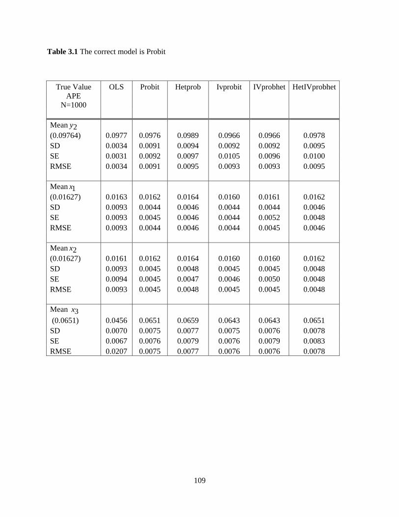
109

Table 3.1 The correct model is Probit

True Value OLS Probit Hetprob Ivprobit IVprobhet HetIVprobhet

APE

N=1000

Mean 2y

(0.09764) 0.0977 0.0976 0.0989 0.0966 0.0966 0.0978

SD 0.0034 0.0091 0.0094 0.0092 0.0092 0.0095

SE 0.0031 0.0092 0.0097 0.0105 0.0096 0.0100

RMSE 0.0034 0.0091 0.0095 0.0093 0.0093 0.0095

Mean 1x

(0.01627) 0.0163 0.0162 0.0164 0.0160 0.0161 0.0162

SD 0.0093 0.0044 0.0046 0.0044 0.0044 0.0046

SE 0.0093 0.0045 0.0046 0.0044 0.0052 0.0048

RMSE 0.0093 0.0044 0.0046 0.0044 0.0045 0.0046

Mean 2x

(0.01627) 0.0161 0.0162 0.0164 0.0160 0.0160 0.0162

SD 0.0093 0.0045 0.0048 0.0045 0.0045 0.0048

SE 0.0094 0.0045 0.0047 0.0046 0.0050 0.0048

RMSE 0.0093 0.0045 0.0048 0.0045 0.0045 0.0048

Mean 3x

(0.0651) 0.0456 0.0651 0.0659 0.0643 0.0643 0.0651

SD 0.0070 0.0075 0.0077 0.0075 0.0076 0.0078

SE 0.0067 0.0076 0.0079 0.0076 0.0079 0.0083

RMSE 0.0207 0.0075 0.0077 0.0076 0.0076 0.0078

110

Table 3.2 The correct model is Probit

True Value OLS Probit Hetprob Ivprobit IVprobhet HetIVprobhet

APE

N=3000

Mean 2y

(0.09762) 0.0977 0.0976 0.0978 0.0972 0.0972 0.0975

SD 0.0020 0.0050 0.0050 0.0050 0.0050 0.0051

SE 0.0018 0.0051 0.0051 0.0047 0.0052 0.0052

RMSE 0.0020 0.0050 0.0050 0.0050 0.0050 0.0051

Mean 1x

(0.01627) 0.0165 0.0164 0.0164 0.0163 0.0163 0.0164

SD 0.0053 0.0024 0.0024 0.0024 0.0024 0.0024

SE 0.0054 0.0026 0.0026 0.0025 0.0026 0.0026

RMSE 0.0053 0.0024 0.0024 0.0024 0.0024 0.0024

Mean 2x

(0.01627) 0.0164 0.0163 0.0163 0.0162 0.0162 0.0162

SD 0.0053 0.0025 0.0026 0.0025 0.0025 0.0026

SE 0.0054 0.0026 0.0026 0.0025 0.0028 0.0028

RMSE 0.0053 0.0025 0.0026 0.0025 0.0025 0.0026

Mean 3x

(0.0651) 0.0458 0.0652 0.0654 0.0650 0.0650 0.0651

SD 0.0040 0.0042 0.0042 0.0042 0.0042 0.0042

SE 0.0038 0.0042 0.0043 0.0041 0.0043 0.0044

RMSE 0.0197 0.0042 0.0042 0.0042 0.0042 0.0042

111

Table 3.3 The correct model is Ivprobit with 50225021 .,.

True

Value 2SLS Probit Hetprob Ivprobit

IVprobhe

t HetIVprobhet

APE

N=1000

Mean 2y

(0.09158) 0.1062 0.1114 0.1126 0.0928 0.0929 0.0935

SD 0.0070 0.0097 0.0103 0.0124 0.0124 0.0129

SE 0.0059 0.0098 0.0104 0.0109 0.0113 0.0126

RMSE 0.0162 0.0221 0.0234 0.0125 0.0125 0.0130

Mean 1x

(0.01526) 0.0180 0.0178 0.0180 0.0156 0.0156 0.0158

SD 0.0086 0.0051 0.0053 0.0045 0.0045 0.0046

SE 0.0084 0.0048 0.0049 0.0043 0.0045 0.0063

RMSE 0.0090 0.0057 0.0059 0.0045 0.0045 0.0047

Mean 2x

(0.01526) 0.0174 0.0174 0.0177 0.0153 0.0153 0.0154

SD 0.0083 0.0050 0.0054 0.0044 0.0044 0.0047

SE 0.0084 0.0048 0.0051 0.0045 0.0038 0.0080

RMSE 0.0086 0.0051 0.0055 0.0045 0.0045 0.0048

Mean 3x

(0.06106) 0.0359 0.0706 0.0713 0.0620 0.0620 0.0624

SD 0.0055 0.0090 0.0094 0.0096 0.0096 0.0099

SE 0.0060 0.0091 0.0094 0.0097 0.0107 0.0115

RMSE 0.0257 0.0131 0.0139 0.0096 0.0096 0.0100

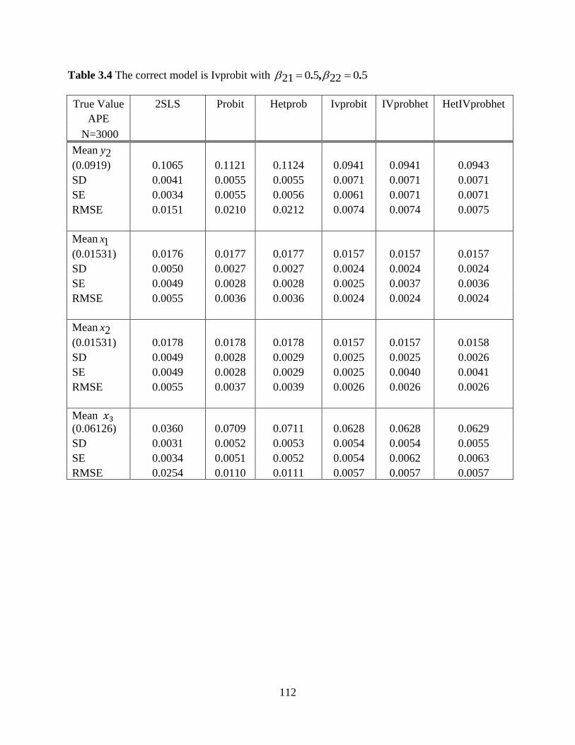
112

Table 3.4 The correct model is Ivprobit with 50225021 .,.

True Value 2SLS Probit Hetprob Ivprobit IVprobhet HetIVprobhet

APE

N=3000

Mean 2y

(0.0919) 0.1065 0.1121 0.1124 0.0941 0.0941 0.0943

SD 0.0041 0.0055 0.0055 0.0071 0.0071 0.0071

SE 0.0034 0.0055 0.0056 0.0061 0.0071 0.0071

RMSE 0.0151 0.0210 0.0212 0.0074 0.0074 0.0075

Mean 1x

(0.01531) 0.0176 0.0177 0.0177 0.0157 0.0157 0.0157

SD 0.0050 0.0027 0.0027 0.0024 0.0024 0.0024

SE 0.0049 0.0028 0.0028 0.0025 0.0037 0.0036

RMSE 0.0055 0.0036 0.0036 0.0024 0.0024 0.0024

Mean 2x

(0.01531) 0.0178 0.0178 0.0178 0.0157 0.0157 0.0158

SD 0.0049 0.0028 0.0029 0.0025 0.0025 0.0026

SE 0.0049 0.0028 0.0029 0.0025 0.0040 0.0041

RMSE 0.0055 0.0037 0.0039 0.0026 0.0026 0.0026

Mean

(0.06126) 0.0360 0.0709 0.0711 0.0628 0.0628 0.0629

SD 0.0031 0.0052 0.0053 0.0054 0.0054 0.0055

SE 0.0034 0.0051 0.0052 0.0054 0.0062 0.0063

RMSE 0.0254 0.0110 0.0111 0.0057 0.0057 0.0057

113

Table 3.5 The correct model is Ivprobit with 10221021 .,.

True Value 2SLS Probit Hetprob Ivprobit IVprobhet HetIVprobhet

APE

N=1000

Mean 2y

(0.0705) 0.0797 0.0918 0.1124 0.0607 0.0612 0.0610

SD 0.0479 0.0107 0.0055 0.0293 0.0297 0.0302

SE 0.0458 0.0111 0.0056 0.0259 0.0258 0.0271

RMSE 0.0488 0.0238 0.0422 0.0309 0.0311 0.0317

Mean 1x

(0.01176) 0.0130 0.0132 0.0177 0.0095 0.0096 0.0096

SD 0.0063 0.0043 0.0027 0.0044 0.0044 0.0045

SE 0.0065 0.0041 0.0028 0.0052 0.0052 0.0053

RMSE 0.0064 0.0045 0.0065 0.0049 0.0049 0.0050

Mean 2x

(0.01176) 0.0132 0.0132 0.0178 0.0096 0.0096 0.0095

SD 0.0067 0.0042 0.0029 0.0044 0.0045 0.0049

SE 0.0065 0.0041 0.0029 0.0052 0.0051 0.0055

RMSE 0.0069 0.0044 0.0067 0.0049 0.0049 0.0054

Mean 3x

(0.04702) 0.0178 0.0536 0.0711 0.0390 0.0392 0.0391

SD 0.0034 0.0109 0.0053 0.0149 0.0150 0.0157

SE 0.0046 0.0106 0.0052 0.0185 0.0183 0.0190

RMSE 0.0294 0.0127 0.0246 0.0169 0.0169 0.0176

114

Table 3.6 The correct model is Ivprobit with 10221021 .,.

True Value 2SLS Probit Hetprob Ivprobit IVprobhet HetIVprobhet

APE

N=3000

Mean 2y

(0.0713) 0.0798 0.0924 0.0927 0.0673 0.0676 0.0675

SD 0.0260 0.0063 0.0066 0.0228 0.0227 0.0230

SE 0.0258 0.0062 0.0065 0.0112 0.0113 0.0115

RMSE 0.0274 0.0220 0.0223 0.0231 0.0230 0.0233

Mean 1x

(0.0119) 0.0133 0.0133 0.0133 0.0110 0.0110 0.0110

SD 0.0037 0.0025 0.0025 0.0030 0.0030 0.0031

SE 0.0037 0.0024 0.0024 0.0031 0.0031 0.0032

RMSE 0.0040 0.0029 0.0029 0.0031 0.0031 0.0032

Mean 2x

(0.0119) 0.0134 0.0133 0.0133 0.0109 0.0109 0.0109

SD 0.0038 0.0024 0.0025 0.0029 0.0029 0.0030

SE 0.0037 0.0024 0.0025 0.0031 0.0031 0.0033

RMSE 0.0041 0.0027 0.0029 0.0030 0.0030 0.0031

Mean 3x

(0.04756) 0.0179 0.0533 0.0534 0.0438 0.0439 0.0439

SD 0.0019 0.0059 0.0061 0.0098 0.0098 0.0100

SE 0.0026 0.0059 0.0060 0.0108 0.0108 0.0109

RMSE 0.0297 0.0082 0.0085 0.0105 0.0104 0.0106

115

Table 3.7 The correct model is Ivprobhet with 50225021 .,.

True Value 2SLS Probit Hetprob Ivprobit IVprobhet HetIVprobhet

APE

N=1000

Mean 2y

(0.0893) 0.0188 0.1109 0.1122 0.1065 0.0896 0.0900

SD 0.0249 0.0097 0.0101 0.0129 0.0203 0.0210

SE 0.0177 0.0100 0.0106 0.0117 0.0225 0.0220

RMSE 0.0748 0.0237 0.0250 0.0215 0.0203 0.0211

Mean 1x

(0.01488) 0.0172 0.0175 0.0177 0.0172 0.0150 0.0150

SD 0.0125 0.0049 0.0050 0.0048 0.0049 0.0050

SE 0.0124 0.0047 0.0047 0.0046 0.0060 0.0060

RMSE 0.0127 0.0055 0.0057 0.0053 0.0049 0.0050

Mean 2x

(0.01488) 0.0175 0.0172 0.0174 0.0168 0.0147 0.0147

SD 0.0124 0.0046 0.0048 0.0046 0.0046 0.0048

SE 0.0124 0.0047 0.0048 0.0046 0.0062 0.0060

RMSE 0.0127 0.0051 0.0054 0.0050 0.0046 0.0048

Mean 3x

(0.05953) 0.0451 0.0698 0.0706 0.0686 0.0592 0.0595

SD 0.0067 0.0080 0.0083 0.0082 0.0120 0.0124

SE 0.0088 0.0080 0.0083 0.0085 0.0186 0.0178

RMSE 0.0159 0.0131 0.0139 0.0122 0.0120 0.0124

116

Table 3.8 The correct model is Ivprobhet with 50225021 .,.

True Value 2SLS Probit Hetprob Ivprobit IVprobhet HetIVprobhet

APE

N=3000

Mean 2y

(0.0896) 0.0164 0.1108 0.1111 0.1075 0.0911 0.0913

SD 0.0141 0.0056 0.0056 0.0070 0.0123 0.0124

SE 0.0101 0.0056 0.0056 0.0062 0.0115 0.0117

RMSE 0.0745 0.0220 0.0222 0.0192 0.0124 0.0126

Mean 1x

(0.01492) 0.0176 0.0173 0.0173 0.0172 0.0152 0.0152

SD 0.0073 0.0027 0.0028 0.0027 0.0028 0.0028

SE 0.0071 0.0027 0.0027 0.0027 0.0037 0.0037

RMSE 0.0078 0.0036 0.0037 0.0035 0.0028 0.0028

Mean 2x

(0.01492) 0.0168 0.0171 0.0172 0.0170 0.0150 0.0150

SD 0.0071 0.0027 0.0027 0.0027 0.0028 0.0029

SE 0.0071 0.0027 0.0027 0.0027 0.0035 0.0036

RMSE 0.0074 0.0035 0.0035 0.0034 0.0028 0.0029

Mean 3x

(0.05971) 0.0453 0.0698 0.0699 0.0693 0.0607 0.0607

SD 0.0039 0.0046 0.0047 0.0047 0.0072 0.0072

SE 0.0050 0.0045 0.0045 0.0046 0.0102 0.0103

RMSE 0.0149 0.0111 0.0112 0.0107 0.0072 0.0073

117

Table 3.9 The correct model is Ivprobhet with 10221021 .,.

True Value 2SLS Probit Hetprob Ivprobit IVprobhet HetIVprobhet

APE

N=1000

Mean 2y

(0.08054) -0.0841 0.0982 0.0993 0.0784 0.0798 0.0801

SD 0.6349 0.0092 0.0094 0.0286 0.0175 0.0181

SE 0.6699 0.0095 0.0100 0.0495 0.0159 0.0168

RMSE 0.6559 0.0199 0.0210 0.0286 0.0176 0.0181

Mean 1x

(0.01342) 0.0131 0.0155 0.0156 0.0117 0.0132 0.0132

SD 0.0687 0.0045 0.0046 0.0051 0.0044 0.0045

SE 0.0815 0.0044 0.0045 0.0064 0.0048 0.0049

RMSE 0.0687 0.0049 0.0051 0.0054 0.0044 0.0045

Mean 2x

(0.01342) 0.0161 0.0155 0.0157 0.0117 0.0132 0.0133

SD 0.0589 0.0044 0.0047 0.0050 0.0044 0.0046

SE 0.0724 0.0044 0.0046 0.0065 0.0048 0.0050

RMSE 0.0589 0.0048 0.0052 0.0053 0.0044 0.0046

Mean 3x

(0.05369) 0.0415 0.0624 0.0632 0.0474 0.0526 0.0528

SD 0.0383 0.0076 0.0077 0.0159 0.0111 0.0113

SE 0.0505 0.0077 0.0080 0.0214 0.0125 0.0131

RMSE 0.0402 0.0116 0.0122 0.0171 0.0111 0.0114

118

Table 3.10 The correct model is Ivprobhet with 10221021 .,.

True Value 2SLS Probit Hetprob Ivprobit IVprobhet HetIVprobhet

APE

N=3000

Mean 2y

(0.0809) -0.2341 0.0986 0.0988 0.0869 0.0822 0.0823

SD 0.5626 0.0051 0.0051 0.0227 0.0108 0.0109

SE 0.4575 0.0053 0.0053 0.0374 0.0083 0.0084

RMSE 0.6448 0.0184 0.0186 0.0235 0.0109 0.0110

Mean 1x

(0.01348) 0.0170 0.0156 0.0157 0.0123 0.0137 0.0137

SD 0.0412 0.0026 0.0026 0.0038 0.0026 0.0026

SE 0.0404 0.0025 0.0026 0.0042 0.0028 0.0028

RMSE 0.0413 0.0034 0.0034 0.0039 0.0026 0.0027

Mean 2x

(0.01348) 0.0130 0.0156 0.0157 0.0123 0.0137 0.0138

SD 0.0472 0.0027 0.0028 0.0039 0.0027 0.0028

SE 0.0512 0.0025 0.0026 0.0042 0.0028 0.0028

RMSE 0.0472 0.0034 0.0035 0.0040 0.0027 0.0028

Mean 3x

(0.05393) 0.0416 0.0631 0.0632 0.0498 0.0549 0.0550

SD 0.0317 0.0043 0.0043 0.0132 0.0067 0.0067

SE 0.0329 0.0043 0.0043 0.0144 0.0070 0.0070

RMSE 0.0340 0.0101 0.0102 0.0138 0.0067 0.0068

119

Table 3.11 The correct model is HetIVprobhet with 50225021 .,.

True Value 2SLS Probit Hetprob Ivprobit IVprobhet HetIVprobhet

APE

N=1000

Mean 2y

(0.12227) 0.0220 0.1103 0.1661 0.1035 0.0896 0.1389

SD 0.0241 0.0065 0.0210 0.0128 0.0203 0.0324

SE 0.0177 0.0064 0.0208 0.0108 0.0225 0.0645

RMSE 0.1035 0.0140 0.0482 0.0230 0.0388 0.0362

Mean 1x

(0.02045) 0.0168 0.0167 0.0263 0.0165 0.0150 0.0230

SD 0.0120 0.0067 0.0070 0.0066 0.0049 0.0071

SE 0.0124 0.0066 0.0067 0.0065 0.0060 0.0135

RMSE 0.0126 0.0077 0.0091 0.0077 0.0073 0.0075

Mean 2x

(0.02045) -0.0058 -0.0101 0.0133 -0.0099 0.0147 0.0114

SD 0.0126 0.0086 0.0080 0.0085 0.0046 0.0074

SE 0.0124 0.0062 0.0071 0.0062 0.0062 0.0111

RMSE 0.0291 0.0317 0.0107 0.0315 0.0074 0.0117

Mean 3x

(0.08186) 0.0452 0.0659 0.1053 0.0653 0.0592 0.0913

SD 0.0069 0.0090 0.0158 0.0090 0.0120 0.0198

SE 0.0088 0.0078 0.0151 0.0079 0.0186 0.0465

RMSE 0.0373 0.0183 0.0283 0.0188 0.0256 0.0220

120

Table 3.12 The correct model is HetIVprobhet with 50225021 .,.

True Value 2SLS Probit Hetprob Ivprobit IVprobhet HetIVprobhet

APE

N=3000

Mean 2y

(0.123) 0.0201 0.1105 0.1604 0.1045 0.0881 0.1386

SD 0.0136 0.0038 0.0106 0.0069 0.0108 0.0181

SE 0.0101 0.0036 0.0105 0.0061 0.0068 0.0255

RMSE 0.1038 0.0130 0.0389 0.0198 0.0365 0.0239

Mean

Rejection

Rate 1 0.917 0.947 0.814 .881 0.140

Mean 1x

(0.0205) 0.0174 0.0168 0.0256 0.0167 0.0152 0.0232

SD 0.0072 0.0039 0.0037 0.0039 0.0036 0.0038

SE 0.0071 0.0038 0.0035 0.0038 0.0085 0.0060

RMSE 0.0079 0.0054 0.0063 0.0054 0.0065 0.0047

Mean 2x

(0.0205) -0.0067 -0.0105 0.0140 0.0104 -0.0095 0.0125

SD 0.0075 0.0051 0.0043 0.0051 0.0047 0.0043

SE 0.0071 0.0036 0.0035 0.0036 0.0132 0.0044

RMSE 0.0282 0.0314 0.0078 0.0313 0.0304 0.0091

Mean 3x

(0.082) 0.0456 0.0660 0.1025 0.0658 0.0591 0.0922

SD 0.0039 0.0052 0.0081 0.0052 0.0062 0.0109

SE 0.0050 0.0044 0.0077 0.0045 0.0117 0.0203

RMSE 0.0367 0.0168 0.0220 0.0170 0.0237 0.0149

121

Table 3.13 Data description

Variable Definition Mean

Standard

deviations

inlf 1 if wife is in labor force 0.583 0.493

nwifeinc non-wife income, $1000s 30.269 27.212

educ wife's year of schooling 12.984 2.165

6kidlt 1 if have child age <6 years 0.279 0.449

6kidge 1 if have child age >=6 years 0.308 0.462 exper experience(age - education - 6) 20.444 10.445

2exper exper squared 527.042 468.289

huseduc husband's year of schooling 13.147 2.977

husexper

husband age - huseduc-6 23.305 11.761

Table 3.14 Estimation of Reduced form Equation

nwifeinc Coefficient SE z P>z

Mean Equation

husexper 0.360 0.032 11.340 0

huseduc 3.454 0.121 28.520 0

constant -23.500 1.952 -12.040 0

Variance

Equation

huseduc 0.101 0.003 30.270 0

husexper 0.016 0.001 16.400 0

constant 1.464 0.057 25.620 0

122

Table 3.15 Empirical Result of APEs with analytical standard errors.

OLS 2SLS Probit Hetprob Ivprobit

inlf inlf inlf inlf inlf

VARIABLES

nwifeinc -0.00331*** -0.00195** -0.00328*** -0.00696*** -0.00316***

[0.00023] [0.00095] [0.00023] [0.00115] [0.00084]

educ 0.0353*** 0.0318*** 0.03607*** 0.07641*** 0.03579***

[0.00257] [0.00356] [0.00261] [0.01165] [0.00324]

exper 0.00245 0.00077 -0.00611*** -0.00875*** -0.00615***

0.00261 0.00289 0.00077 0.00170 0.00255

expersq -0.00021*** -0.00018***

[0.00006] [-0.00006]

kidlt6 -0.171*** -0.175*** -0.17416*** -0.14538*** -0.17413***

[0.01794] [0.01860] [0.01827] [0.03763] [0.01827]

kidge6 0.01660 0.01330 0.01467 0.01310 0.01473

[0.0166] [0.01690] [0.01852] [0.04340] [0.00550]

Observations 5,634 5,634 5,634 5,634 5,634

*, **, ***: significant at 10%, 5% and 1% level respectively.

Adjusted analytical standard errors are in the [ ].

123

Table 3.16 Empirical Result of APEs with analytical standard errors and Bootstrap standard

errors

IVprobhet HetIVprobhet1 HetIVprobhet2 HetIVprobhet3

inlf inlf inlf inlf

VARIABLES

nwifeinc -0.00205 -0.00459* -0.00534*** -0.00490***

[0.00210] [0.00285]

(0.001614) (0.001509) ( 0.001913)

educ 0.03372*** 0.07002*** 0.07183*** 0.08265***

[0.00442] [0.01434]

(0.012299) (0.012102) (0.013432)

exper -0.00653 -0.00924*** -0.00927*** -0.01048***

[0.00528] [0.00287]

(0.001761) (0.001819) (0.002094)

kidlt6 -0.17357*** -0.19280** -0.19262*** -0.17163***

[0.03848] [0.05996]

(0.026883) (0.001819) (0.025359)

kidge6 0.01546 0.06580** 0.06123** 0.07777**

[0.01123] [0.02353]

(0.038130) (0.037438) (0.034927)

Observations 5,634 5,634 5,634 5,634

*, **, ***: significant at 10%, 5% and 1% level respectively.

Adjusted analytical standard errors are in the [ ]. Bootstrap standard errors are in the ( ).

124

APPENDICES

125

APPENDICES

APPENDIX A: Asymptotic Variance for the two-step estimators

In order to obtain the standard errors for estimated APEs, first we need to compute the

adjusted standard errors of the estimated parameters. Our estimator is a common two-step M-

estimator, where the first stage estimation is maximum likelihood estimation. Then, the

estimated standardized residuals are plugged in to the maximum likelihood estimation(MLE) in

the second stage. The adjustment of asymptotic variance is well known and explained in

textbooks as Greene (2008) and Wooldridge (2010) with minor differences in either using outer

product of the score to approximate the information matrix or using the information matrix

directly. In this paper, it follows the step as in Murphy and Topel (1985) for the adjustment. That

is, it uses the outer product approximation to the information matrix.

The standardized residuals come from the first stage MLE that solves

)ˆ,ˆ( 22

ni i1 22

22

),(,

maxargˆ

. (A.1)

In the second step, the estimated standardized residuals i2~ are plugged in the other MLE

estimation. Hence, the first stage problem is

)ˆ,ˆ,ˆ,ˆ( 11

ni il1 11

11

)ˆ;,,,(,,

maxargˆ

, (A.2)

and this objective function depends on the estimated parameters from the first stage. Let

)0,0( be the true value of the estimated parameters. Then, the following score, outer product

of the score and Hessian matrix terms are

)(

i

)(i , and

),( il

),(il . (A.3)

126

Outer products of the score are

O )',(),(lim 001 001

il

ni ilnn

p

, (A.4)

O )'(),(lim 01 001

i

ni ilnn

p

, (A.5)

O '),()(lim

ni ilinn

p1 000

1

, (A.6)

O ')()(lim

ni iinn

p1 00

1

. (A.7)

Hessian matrices are

H

ni

il

nnp

100

21

'

),(lim

, (A.8)

H

ni

il

nnp

100

21

'

),(lim

, (A.9)

H

ni

il

nnp

100

21

'

),(lim

, (A.10)

H

ni

i

nnp

10

21

'

)(lim

. (A.11)

Then, let assume that the sample scores are normally distributed asymptotically with the

following mean zero and variance covariance matrix:

OO

OON

dn

i i

il

n,

)(

),(0

1 0

001. (A.12)

127

From the first step maximum likelihood estimation of normal distribution with exponential

heteroskedasticity, the mean value expansion theorem around 0 and gives

)()ˆ()()ˆ( 101

01

1

10 ponH

n

iin

n

iin

. (A.13)

That is the same as the asymptotic result under standard regularity condition

)ˆ( 0 n )()( 11 0

11po

ni in

H

. (A.14)

Then, applying the same mean value expansion to the second-step estimation of its first-order

conditions around 0 and gives the required result for variance adjustment:

ni iln 1

10 )ˆ,ˆ(

,

)()ˆ()ˆ(),( 101 0001

ponHni

nHiln

. (A.15)

Then,

n

ipoin

Hn

i

HilnnH

1

1011

100

10 )()(*),()ˆ(

(A.16)

and

)()(

),()*,()ˆ( 1

10

001110 po

ni

i

il

nHHIHn

. (A.17)

Hence,

VNd

n ,)ˆ( 00 , (A.18)

where

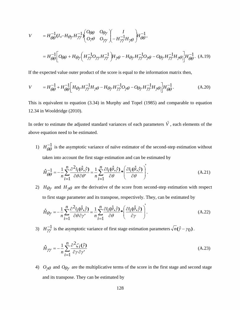
128

V 11

11

HHH

I

OO

OOHHIH ),( ,

111111

HHHOOHHHHOHHOH . (A.19)

If the expected value outer product of the score is equal to the information matrix then,

V 111111

HHHOOHHHHHHH . (A.20)

This is equivalent to equation (3.34) in Murphy and Topel (1985) and comparable to equation

12.34 in Wooldridge (2010).

In order to estimate the adjusted standard variances of each parameters V , each elements of the

above equation need to be estimated.

1) 1

H is the asymptotic variance of naïve estimator of the second-step estimation without

taken into account the first stage estimation and can be estimated by

')ˆ,ˆ(

*)ˆ,ˆ(

'

)ˆ,ˆ(ˆ

iln

i

il

n

n

i

il

nH

1

1

1

211 . (A.21)

2) H and H are the derivative of the score from second-step estimation with respect

to first stage parameter and its transpose, respectively. They, can be estimated by

')ˆ,ˆ(

*)ˆ,ˆ(

'

)ˆ,ˆ(ˆ

iln

i

il

n

n

i

il

nH

1

1

1

21

. (A.22)

3) 1H is the asymptotic variance of first stage estimation parameters )ˆ( 0 n .

n

i

i

nH

1

21

'

)ˆ(ˆ

(A.23)

4) O and O are the multiplicative terms of the score in the first stage and second stage

and its transpose. They can be estimated by

129

n

i

ili

nO

1

1

)ˆ,ˆ(*

)ˆ(ˆ . (A.24)

This estimated adjusted variance might not be robust when the underlying distribution is not

correctly specified. However, Hardin (2002) showed that the robust version of Murphy Topel

estimation. This paper doses not adopt such formula since it will not be equivalent to result of

Ackerberg et.al. (2012).

To obtain score and Hessian from first-step estimation, the log likelihood in matrix form is as

follows

)()'()(

))(ln()ln( 2z22z22z2

22

12z2

222

2

yy

hh

NN. (A.25)

Hence, the score function can be represented by gradient vector

0

2

20

)(

)(

)( , (A.26)

2'

2z22

1

2

zzyz

h

'

)(

)(. (A.27)

For 2

)(, assume that the heteroskedasticity term is multiplicative with exponential function

)exp( 2z2 ,

2

)( )()'(

)exp(

)'*(' 2z22z2

2z2

z2

yyZ . (A.28)

From the gradient matrix, the Hessian matrix is

130

)(H

'

)(

'

)(

'

)(

'

)(

)(

22

2

22

222

2

22

2

, (A.29)

'

)(

22

2

zz'

2z2

1-

)exp( , (A.30)

'

)(

22

2

)exp(

'z)'*(

22

2'z2

z

zzy , (A.31)

'

)(

22

2

)exp(

'')'*(

2z2

2zz'zz2

y, (A.32)

'

)(

22

2

)()'(

)exp(

)*(2z22z2

2z2

zz'4

yy . (A.33)

The information matrix is the negative of the expectation of the Hessian ])([)( z HEI .

Then, the estimation of )ˆ( 0 Avar

1H

1

1

22

2

22

222

2

22

2

1

n

i ii

ii

n

'

)ˆ(

'

)ˆ(

'

)ˆ(

'

)ˆ(

. (A.34)

In the second step, the estimation of )'/(),','(2111 θ comes from the

heteroskedastic probit of iy1 on )~,,( iiy 221iz , where i2~ is the standardized error from the

first stage estimation and )( 111iz21

h is the heteroskedastic variance. Assuming that

)exp()( 111iz2111iz21

h . The log-likelihood function for each individual observation i is

131

i

iyiyil 2

21111iz

211iz111

~

)exp(

log)ˆ;,,,(

i

iyiy 2

21111iz

211iz111

~

)exp(

log)( . (A.35)

The score function and gradient vector is

)ˆ,( il 0

1

1

'

/)ˆ,(

/)ˆ,(

/)ˆ,(

/)ˆ,(

)ˆ,(

il

il

il

il

il . (A.36)

Define

i

iyA 2

21111iz

211iz

ˆ

)exp(

, ),( iy21iziW , and )','( 1 then

1 /)ˆ,(il

21111iz1

2'1iz

)exp())()((

)()(

AΦAΦ

AΦiyA, (A.37)

/)ˆ,(il

21111iz1

22

)exp())()((

)(')(

AΦAΦ

AΦiyiyA, (A.38)

/)ˆ,(il

))()((

)('ˆ)(

AΦAΦ

AΦiyiA

1

22, (A.39)

1 /)ˆ,(il

21111iz1

2iw'11iz

)exp())()((

)()(

AΦAΦ

AΦiyA. (A.40)

The inverse of Hessian 1

H for the heteroskedastic probit is a mess as pointed out in

Wooldridge (2010). Hence, we adopt the result from his example 13.1, iz0)(iE H is a 4x4

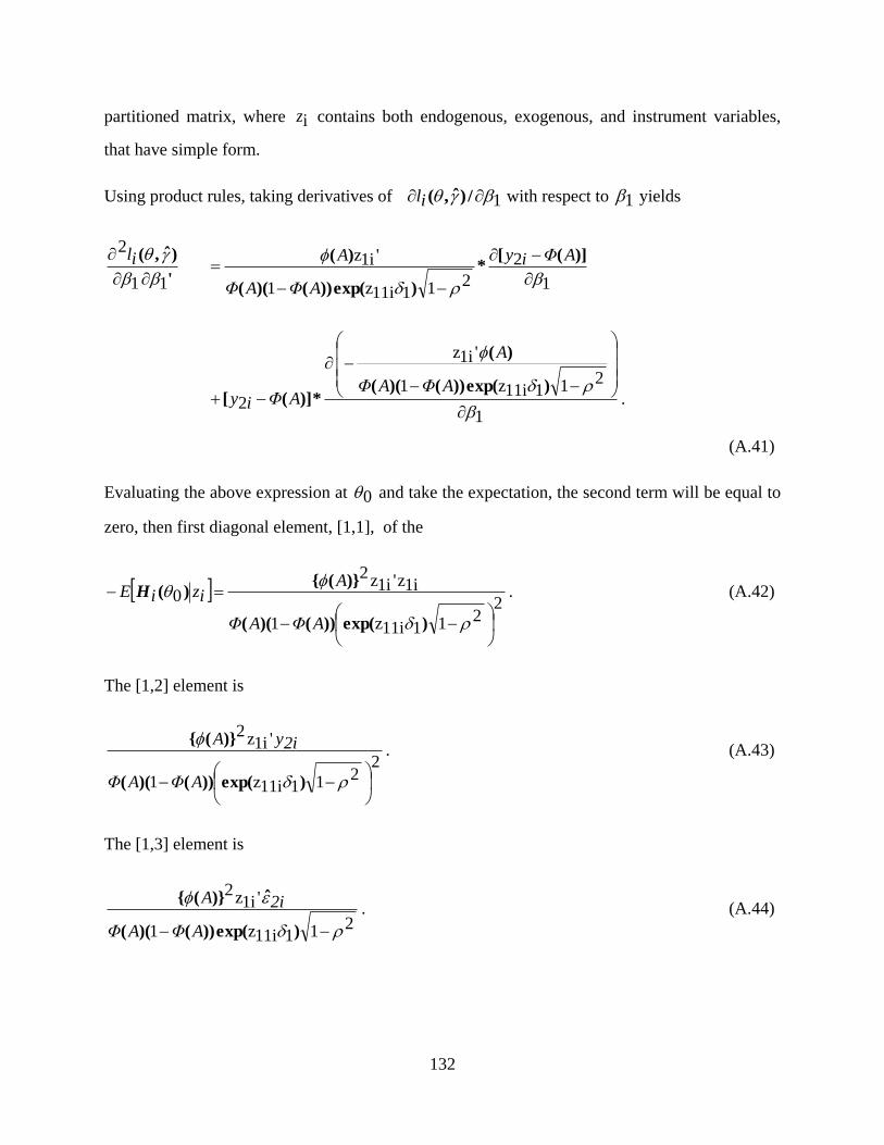
132

partitioned matrix, where iz contains both endogenous, exogenous, and instrument variables,

that have simple form.

Using product rules, taking derivatives of 1 /)ˆ,(il with respect to 1 yields

'

)ˆ,(

11

2

il 1

2

21111iz1

'1iz

)]([

*

)exp())()((

)( AΦiy

AΦAΦ

A

1

21111iz1

'1iz

2

)exp())()((

)(

*)]([AΦAΦ

A

AΦiy .

(A.41)

Evaluating the above expression at 0 and take the expectation, the second term will be equal to

zero, then first diagonal element, [1,1], of the

2

21111iz1

1iz'1iz2

0

)exp())()((

)}({)(

AΦAΦ

AiziE H . (A.42)

The [1,2] element is

221111iz1

'1iz2

)exp())()((

)}({

AΦAΦ

2iyA. (A.43)

The [1,3] element is

21111iz1

'1iz2

)exp())()((

ˆ)}({

AΦAΦ

2iA. (A.44)

133

The [1,4] element is

221111iz1

11iziw'1iz2

)exp())()((

)}({

AΦAΦ

A. (A.45)

The [2,1] element is

221111iz1

1iz2

)exp())()((

)}({

AΦAΦ

'2iyA. (A.46)

The [2,2] element is

221111iz1

2

)exp())()((

)}({

AΦAΦ

2iy'2iyA. (A.47)

The [2,3] element is

21111iz1

2

)exp())()((

ˆ)}({

AΦAΦ

2i'2iyA. (A.48)

The [2,4] element is

221111iz1

11iz2

)exp())()((

)}({

AΦAΦ

'2iyA iw. (A.49)

The [3,1] element is

21111iz1

1iz2

)exp())()((

ˆ)}({

AΦAΦ

'2iA. (A.50)

The [3,2] element is

134

21111iz1

22

)exp())()((

ˆ)}({

AΦAΦ

iy'2iA. (A.51)

The [3,3] element is

))()((

ˆˆ)}({

AΦAΦ

2i'2iA

1

2 . (A.52)

The [3,4] element is

21111iz1

11iz2

)exp())()((

ˆ)}({

AΦAΦ

'2iA iw. (A.53)

The [4,1] element is

221111iz1

1iz11iziw2

)exp())()((

)}({

AΦAΦ

)'(A. (A.54)

The [4,2] element is

221111iz1

11iziw2

)exp())()((

)}({

AΦAΦ

2iy)'(A. (A.55)

The [4,3] element is

21111iz1

11iziw2

)exp())()((

ˆ)}({

AΦAΦ

2i)'(A. (A.56)

135

The [4,4] element is

221111iz1

11iziw11iziw2

)exp())()((

)}({

AΦAΦ

)'(A. (A.57)

Finally, the last element need for the two-step adjustment is

)ˆ,(il

2

2

/)ˆ,(

/)ˆ,(

il

il, (A.58)

2

)ˆ,(il )exp())()((

)]([)(

2iz1

2'i

AΦAΦ

AΦiyzA

, (A.59)

2

)ˆ,(il )exp())()((

)]([)-()(

2iz1

2'iz2iz2

AΦAΦ

AΦiyyA

. (A.60)

Plugging in the estimated coefficient of , , and 1 yields the estimated variance V .

136

Appnedix B: Asymptotic Variance for the APEs

B.1 Standard errors for the continuous explanatory variables.

First, we need to obtain asymptotic variance of )ˆ( ηη -N , where )),(,2y,( ˆˆˆ 1zgη is

partial derivative of )2y,(fFSA 1zˆ with respect to 1z , 2y and )),(,2y,( 1zgη is

partial derivative of )2y,(fASF 1z with respect to 1z , 2y . For example the APEs for

continuous 2y is

ni y

AA

N2y 12

1*)(ˆ η . (A.61)

Then, we can insert the interesting value of 2y or further average out 2iy . Moreover, this set up

leads to the dilemma as stated in Wooldridge (2010) chapter 15, if either 2iy , subset of 1iz , or

i2~ enters into the heteroskedastic function, the sign and magnitude of APEs might not be the

same as estimated parameters. Forη , its value depends on where the value of 1iz , 2iy , i2

evaluates, so in order to get single number for each variable, we average them over 11iz and i2 .

ni

ni y

AA

NN2y 1 12

11*)(ˆ η . (A.62)

Using problem 12.17 and 15.15 in Wooldridge (2010), by applying mean value expansion

theorem,

)),(,2y,(n

1iN

ˆˆ1z

1g

)(ˆ

ˆ* 1

0

01z

1po

n

1i

N)),(,2y,(N

Gg , (A.63)

where ][ )),(,2y,()),(,2y,( 1z1z ggEG .

For example, assumed that 2iy does not enter into the variance, the Jacobian of )),(,2y,( 1zg

of 2y or APE of 2y with respect to second-step parameter θ is

137

21z

y

AA

)),(,2y,(

*)(

g , (A.64)

1

*)(

1 βgβ

21z

y

AA

)),(,2y,(

, (A.65)

21z

y

AA

)),(,2y,(

*)(

g , (A.66)

1

21z

1

y

AA

)),(,2y,(

*)(

g . (A.67)

The Jacobian of APE of 2y with respect to first-step parameter γ is

2

*)(

2 βgβ

21z

y

AA

)),(,2y,(

, (A.68)

2

21z

2

y

AA

)),(,2y,(

*)(

g . (A.69)

For

0

0

ˆ

ˆ*N , it is just a stack of the both equation

)()(

),()*,()ˆ( 11

0

001110 po

ni

i

il

nHHIHn

and

)()()ˆ( 11 011

0 poni in

Hn

.

Hence, we can write,

138

)(),(ˆ

ˆ* 11 00

1

0

0po

nin

N

ie . (A.70)

Thus,

)},ˆˆ{)ˆ( 001z (iGe-η-)),(,2y,(Varη-ηNAvarC g (A.71)

A consistent estimator for the asymptotic variance of APEs is

)]}',ˆˆˆˆˆ}{),ˆˆˆˆˆ{[ˆ001z

1001z

1 (ieG-η-)),(,2y,(

N

i

(ieG-η-)),(,2y,(N

C igig

(A.72)

By construction, the conditional expected values of the score function of both first and second

stage estimation equals to zero, then, )),(,2y,( ˆˆ1zg will not be correlated with ), 00 (iGe ,

which means

'GNAvarG)VarC ˆˆ

ˆ*ˆˆ(ˆ

0

0

ig (A.73)

Hence, asymptotic variance of APEs depends on variance of itself plus positive definite matrix

of the adjustment term. For standard error for any particular APE, it will be the square root of

corresponding diagonal element of the above equation, divided by N .

B.2 Standard errors for the binary exogenous explanatory variables.

Assumed, that there is one element of 1z is binary exogenous variables 1z with

coefficient . Hence, the APE of 1z can be written as

)]()([,)( 1iz2111z AAiizEAPEh (A.74)

For the estimate of )( 1zAPE ,it is

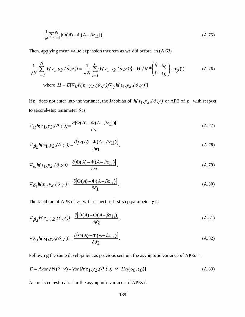
139

Ni

AAN 1 1iz1

])ˆ()([ (A.75)

Then, applying mean value expansion theorem as we did before in (A.63)

)),(,2y,(N

1iN

ˆˆ1z

1h

)(ˆ

ˆ* 1

0

01z

1po

n

1i

N)),(,2y,(N

Hh (A.76)

where ][ )),(,2y,()),(,2y,( 1z1z hhEH

If 1z does not enter into the variance, the Jacobian of ),(,2y,( ˆˆ1zh or APE of 1z with respect

to second-step parameter is

)]ˆ()([ 1iz1z

AA)),(,2y,(h , (A.77)

1

)ˆ()(

1 βhβ

1iz

1z

AA

)),(,2y,( , (A.78)

)ˆ()( 1iz1z

AA)),(,2y,(h , (A.79)

1

1iz1z

1

)ˆ()( AA)),(,2y,(h . (A.80)

The Jacobian of APE of 1z with respect to first-step parameter γ is

2

)ˆ()(

2 βhβ

1iz

1z

AA

)),(,2y,( , (A.81)

2

1iz1z

2

)ˆ()( AA)),(,2y,(h . (A.82)

Following the same development as previous section, the asymptotic variance of APEs is

)},ˆˆ{)ˆ( 001z (iHe--)),(,2y,(Var-NAvarD h (A.83)

A consistent estimator for the asymptotic variance of APEs is

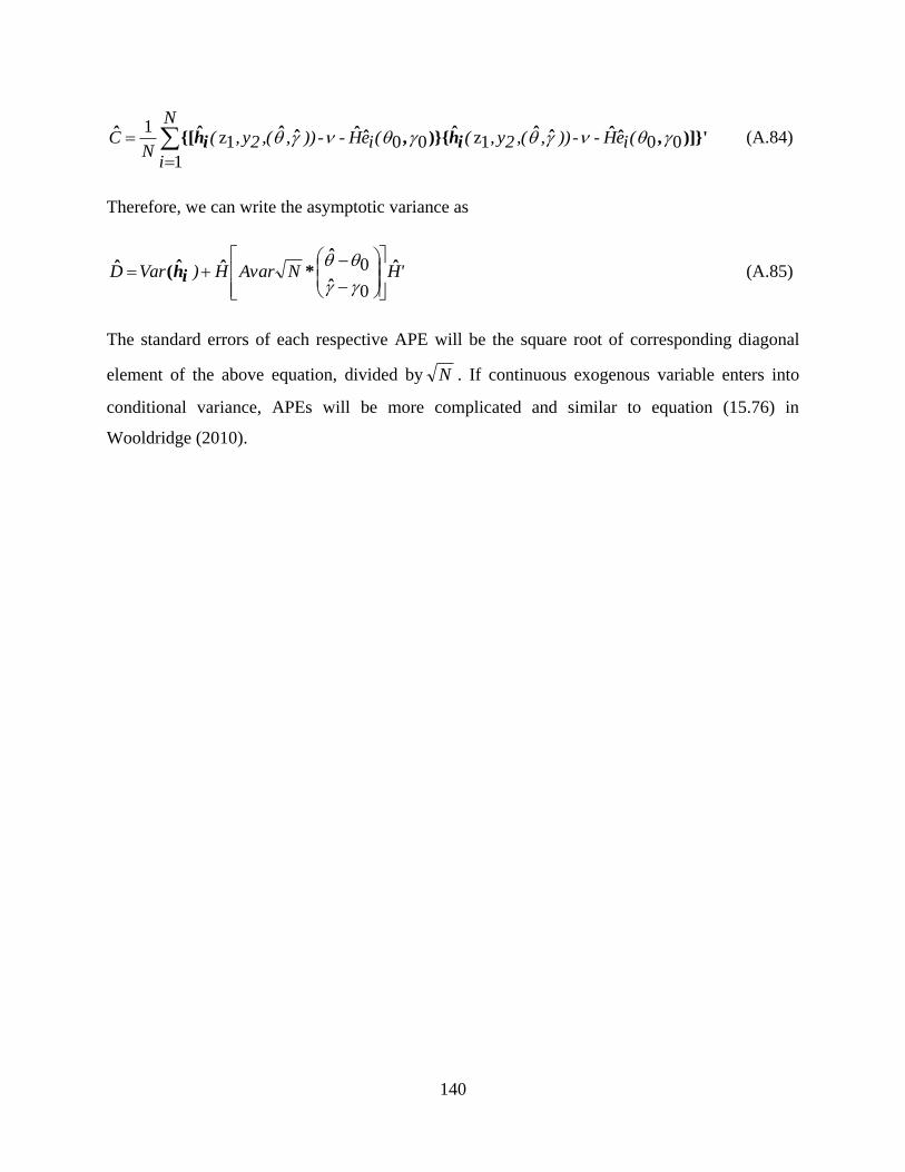
140

)]}',ˆˆˆˆˆ}{),ˆˆˆˆˆ{[ˆ001z

1001z

1 (ieH--)),(,2y,(

N

i

(ieH--)),(,2y,(N

C ihih

(A.84)

Therefore, we can write the asymptotic variance as

'HNAvarH)VarD ˆˆ

ˆ*ˆˆ(ˆ

0

0

ih (A.85)

The standard errors of each respective APE will be the square root of corresponding diagonal

element of the above equation, divided by N . If continuous exogenous variable enters into

conditional variance, APEs will be more complicated and similar to equation (15.76) in

Wooldridge (2010).

141

REFERENCES

142

REFERENCES

Ackerberg, Daniel, Xiaohong Chen, and Jinyong Hahn. “A Practical Asymptotic Variance

Estimator for Two-step Semiparametric Estimators.” Review of Economics and Statistics

94, no. 2 (2012): 481–498.

Angrist, Joshua D., and William N. Evans. Children and Their Parents’ Labor Supply: Evidence

from Exogenous Variation in Family Size. National Bureau of Economic Research, 1996.

Averett, Susan L., and Julie L. Hotchkiss. “Female Labor Supply with a Discontinuous,

Nonconvex Budget Constraint: Incorporation of a Part-time/full-time Wage

Differential.” Review of Economics and Statistics 79, no. 3 (1997): 461–470.

Blundell, Richard, and James L. Powell. “Endogeneity in Nonparametric and Semiparametric

Regression Models.” ECONOMETRIC SOCIETY MONOGRAPHS 36 (2003): 312–357.

Blundell, Richard W., and James L. Powell. “Endogeneity in Semiparametric Binary Response

Models.” The Review of Economic Studies 71, no. 3 (2004): 655–679.

Blundell, Richard W., and Richard J. Smith. “Estimation in a Class of Simultaneous Equation

Limited Dependent Variable Models.” The Review of Economic Studies 56, no. 1 (1989):

37–57.

Card, David. “Estimating the Return to Schooling: Progress on Some Persistent Econometric

Problems.” Econometrica 69, no. 5 (2001): 1127–1160.

Chen, Xiaohong. “Large Sample Sieve Estimation of Semi-nonparametric Models.” Handbook

of Econometrics 6 (2007): 5549–5632.

Chesher, Andrew. “Instrumental Variable Models for Discrete Outcomes.” Econometrica 78, no.

2 (2010): 575–601.

Cruces, Guillermo, and Sebastián Galiani. “Fertility and Female Labor Supply in Latin America:

New Causal Evidence.” Labour Economics 14, no. 3 (2007): 565–573.

Dong, Yingying, and Arthur Lewbel. “A Simple Estimator for Binary Choice Models with

Endogenous Regressors.” Econometrics Reviews, Forthcoming (2012).

Florens, Jean-Pierre, James J. Heckman, Costas Meghir, and Edward Vytlacil. “Identification of

Treatment Effects Using Control Functions in Models with Continuous, Endogenous

Treatment and Heterogeneous Effects.” Econometrica 76, no. 5 (2008): 1191–1206.

Gourieroux, Christian, Alain Monfort, and Alain Trognon. “Pseudo Maximum Likelihood

Methods: Theory.” Econometrica: Journal of the Econometric Society (1984): 681–700.

143

Greene, William H. “Econometric Analysis, 5th.” Ed.. Upper Saddle River, NJ (2003).

Heckman, James J. “The Common Structure of Statistical Models of Truncation, Sample

Selection and Limited Dependent Variables and a Simple Estimator for Such Models.” In

Annals of Economic and Social Measurement, Volume 5, Number 4, 475–492. NBER,

1976.

Heckman, James J., and Edward Vytlacil. “Structural Equations, Treatment Effects, and

Econometric Policy Evaluation1.” Econometrica 73, no. 3 (2005): 669–738.

Heckman, James, and Edward Vytlacil. “Instrumental Variables Methods for the Correlated

Random Coefficient Model: Estimating the Average Rate of Return to Schooling When

the Return Is Correlated with Schooling.” Journal of Human Resources (1998): 974–987.

———. “Instrumental Variables Methods for the Correlated Random Coefficient Model:

Estimating the Average Rate of Return to Schooling When the Return Is Correlated with

Schooling.” Journal of Human Resources (1998): 974–987.

Hoderlein, Stefan. Endogenous Semiparametric Binary Choice Models with Heteroscedasticity.

cemmap working paper, 2009.

Honoré, Bo E., and Arthur Lewbel. “Semiparametric Binary Choice Panel Data Models Without

Strictly Exogeneous Regressors.” Econometrica 70, no. 5 (2002): 2053–2063.

Horowitz, Joel L. “A Smoothed Maximum Score Estimator for the Binary Response Model.”

Econometrica: Journal of the Econometric Society (1992): 505–531.

Imbens, Guido, and Jeffrey Wooldridge. “Control Function and Related Methods.” What’s New

in Econometrics (2007).

Khan, Shakeeb. “Distribution Free Estimation of Heteroskedastic Binary Response Models

Using Probit/Logit Criterion Functions.” Journal of Econometrics 172, no. 1 (2013):

168–182.

Klein, Roger, Chan Shen, and Francis Vella. “Triangular Semiparametric Models Featuring Two

Dependent Endogenous Binary Outcomes.” Unpublished Manuscript (2010).

Lewbel, A., and Y. Dong. “T. Yang (2012),‘ Comparing Features of Convenient Estimators for

Binary Choice Models With Endogenous Regressors,’ Forthcoming.” Canadian Journal

of Economics.

Lewbel, Arthur. “Semiparametric Latent Variable Model Estimation with Endogenous or

Mismeasured Regressors.” Econometrica (1998): 105–121.

———. “Semiparametric Qualitative Response Model Estimation with Unknown

144

Heteroscedasticity or Instrumental Variables.” Journal of Econometrics 97, no. 1 (2000):

145–177.

Manski, Charles F. “Maximum Score Estimation of the Stochastic Utility Model of

Choice.” Journal of Econometrics 3, no. 3 (1975): 205–228.

Mroz, Thomas A. “The Sensitivity of an Empirical Model of Married Women’s Hours of Work

to Economic and Statistical Assumptions.” Econometrica (1987): 765–799.

Murtazashvili, Irina, and Jeffrey M. Wooldridge. “Fixed Effects Instrumental Variables

Estimation in Correlated Random Coefficient Panel Data Models.” Journal of

Econometrics 142, no. 1 (2008): 539–552.

Newey, Whitney K., and James L. Powell. “Instrumental Variable Estimation of Nonparametric

Models.” Econometrica 71, no. 5 (2003): 1565–1578.

Newey, Whitney K., James L. Powell, and Francis Vella. “Nonp arametric Estimation of

Triangular Simultaneous Equations Models.” Econometrica 67, no. 3 (1999): 565–603.

Papke, Leslie E., and Jeffrey M. Wooldridge. “Panel Data Methods for Fractional Response

Variables with an Application to Test Pass Rates.” Journal of Econometrics 145, no. 1

(2008): 121–133.

Petrin, Amil, and Kenneth Train. “A Control Function Approach to Endogeneity in Consumer

Choice Models.” Journal of Marketing Research 47, no. 1 (2010): 3–13.

Rivers, Douglas, and Quang H. Vuong. “Limited Information Estimators and Exogeneity Tests

for Simultaneous Probit Models.” Journal of Econometrics 39, no. 3 (1988): 347–366.

Staiger, Douglas, and James H. Stock. “Instrumental Variables Regression with Weak

Instruments.” Econometrica 65, no. 3 (1997): 557–586.

Vella, Francis, and Marno Verbeek. “Two-step Estimation of Panel Data Models with Censored

Endogenous Variables and Selection Bias.” Journal of Econometrics 90, no. 2 (1999):

239–263.

Wooldridge, Jeffrey M. Econometric Analysis Cross Section Panel. 2nd

MIT press, 2010.

Wooldridge, Jeffrey M. Introductory Econometrics: a Modern Approach. Cengage Learning,

2012.

Wooldridge, Jeffrey M. “Unobserved Heterogeneity and Estimation of Average Partial Effects.”

Identification and Inference for Econometric Models: Essays in Honor of Thomas

Rothenberg (2005): 27–55.