THREE-DIMENSIONAL RECONSTRUCTION OF

POINTS AND LINES WITH UNKNOWN

CORRESPONDENCE ACROSS IMAGES�

Y-Q Cheng�, E.M. Riseman, X.G. Wang, R.T. Collins

���and A.R. Hanson

Village Networks, Inc100 Village CourtHazlet, NJ 07730

�

Department of Computer ScienceUniversity of Massachusetts

Amherst, MA 01003Email:

�riseman � @cs.umass.edu

Robotics Institute, NSHCarnegie Mellon University

5000 Forbes AvePittsburgh, PA 15213

���

�This work was funded by the RADIUS project under DARPA/Army TEC contract number

DACA76-92-C-0041, the DARPA/TACOM project under contract number DAAE07-91-C-R035,and the National Science Foundation (NSF) under grant number CDA8922572).

Abstract

Three-dimensional reconstruction from a set of images is an important and dif-ficult problem in computer vision. In this paper, we address the problem of de-termining image feature correspondences while simultaneously reconstructing thecorresponding 3D features, given the camera poses of disparate monocular views.First, two new affinity measures are presented that capture the degree to whichcandidate features from different images consistently represent the projection ofthe same 3D point or 3D line. An affinity measure for point features in two dif-ferent views is defined with respect to their distance from a hypothetical projected3D pseudo-intersection point. Similarly, an affinity measure for 2D image linesegments across three views is defined with respect to a 3D pseudo-intersectionline. These affinity measures provide a foundation for determining unknown cor-respondences using weighted bipartited graphs representing candidate point andline matches across different images. As a result of this graph representation, astandard graph-theoretic algorithm can provide an optimal, simultaneous match-ing and triangulation of points across two views, and lines across three views.Experimental results on synthetic and real data demonstrate the effectiveness ofthe approach.

1 Introduction

Three-dimensional model acquisition remains a very active research area in com-puter vision. One of the key questions is how to reconstruct accurate 3D mod-els from a set of calibrated 2D images via multi-image triangulation. The basicprinciples involved in 3D model acquisition are feature correspondence determina-tion and triangulation, with the two commonly used types of image features beingpoints and lines. Usually, 2D features are extracted first, such as corners, curvaturepoints, and lines from each image. Then, the correspondence of these features isestablished between any pair of images, usually referred to as “the correspondenceproblem”. Finally, the 3D structure is triangulated from these 2D correspondences.

Many reconstruction papers assume the correspondence problem has beensolved [2, 7, 35, 39, 50, 51, 53]. Unfortunately, in many applications, this infor-mation is not available and mechanisms to achieve correspondence are unreliable.This has caused serious criticism of feature-based methods [6, 22, 33, 52, 60, 61].The process of finding ��� image feature correspondences can be computationallyexpensive and difficult to implement reliably, requiring subsequent algorithms toemploy robust mechanisms for detecting outliers due to mismatches [46, 49].

Even if the image feature correspondences are known, robust triangulation ofthe 3D models using noisy image data is still a non-trivial problem and an on-going

2

research topic. Extensive research has been devoted to developing robust algo-rithms in this area [5, 8, 23, 37, 46, 49, 66, 67], including processing of monocularmotion sequences, stereo pairs, and sets of distinct views. Although both point-based and line-based triangulation are commonly employed, more attention hasbeen paid to line-based triangulation since it generally provides more accurate re-constructions.

In this paper, we address the problem of determining image feature correspon-dences given known camera poses, while simultaneously computing the corre-sponding 3D features. We restrict our attention to simultaneous determination ofimage feature correspondences and recovery of their 3D structure using matchingand triangulation of noisy 2D image points and lines. Our approach assumes a setof calibrated images, for which both intrinsic (lens) parameters and either absoluteor relative poses are known. Therefore these approaches are well-suited for pho-togrammetric mapping applications where extrinsic parameters are already known,such as 3D aerial reconstruction in cultural settings [4], for wide-baseline multi-camera stereo systems, or for model extension applications where a previous partialmodel has been used to determine camera pose for a set of new views, from whichpreviously unmodeled scene features are now to be recovered [18, 19, 21, 46].

This paper is organized as follows. Section 2 reviews previous related workin the area of 3D reconstruction with unknown apriori correspondences. Section 3introduces two new affinity measures for determining image point and line corre-spondences across images, and uses them to construct weighted bipartite graphs.Section 4 formulates the image feature matching problem as the general maximum-weight bipartite matching problem and develops two algorithms to simultaneouslymatch and reconstruct 3D points and lines from noisy 2D image points and lines,respectively. Finally, Section 5 and Section 6 present and analyze experimentalresults from synthetic and real image data sets. Section 7 gives our conclusions.

2 Previous Work

2.1 Motion Estimation without Correspondences

Aggarwal et al [2] reviewed the correspondence problem two decades ago. Inrecent years, a variety of correspondence problems [2, 6, 13, 14, 16, 33, 39, 51,52, 61, 63] have been studied. In addition, many researchers have worked on theproblem of motion estimation without pre-specified correspondences [3, 22, 33,39, 50, 52, 63].

Aloimonos, et al [3], presented an algorithm to estimate 3D motion withoutapriori correspondences by combining motion and stereo matching. Huang andhis research group [33, 50, 52] presented a series of algorithms to estimate rigid-

3

body motion from ��� data without matching point correspondences. Goldgof etal [33] presented moment-based algorithms for matching and motion estimationof 3D point or line sets without correspondences and applied these algorithms toobject tracking over the image sequences. The basic idea is to find two coordinatesystems based on relative positions of 3D points/lines before and after the motion,then compute the motion parameters (rotation and translation) that make these co-ordinate systems coincide. The disadvantages of the approach include sensitivityto noise and to missing or false points or lines.

Lee et al [52] proposed an algorithm to deal with the correspondence problemin image sequence analysis. This method is based on the following three assump-tions: (1) the objects undergo a rigid motion; (2) a perspective projection cameramodel can be used; (3) the translation vector is small compared to the distance ofthe object.

Recently, we presented a mathematical symmetry in the solutions of rotationparameters and point correspondences, derived a closed-form solution based oneigenstructure decomposition for correspondence recovery in ideal cases with nomissing points, and developed a weighted bipartite matching algorithm to deter-mine the correspondences in general cases where missing points occur [63]

2.2 Determination of Correspondences from Nonrigid Objects

Objects in the world can be nonrigid, and an object’s appearance can deform as theviewing geometry changes. Consequently, research has been carried out to addressthe problem of correspondence and description using deformable models [56, 57,59, 60, 61].

Scott and Longuet-Higgins [60] developed an algorithm to determine the pos-sible correspondences of 2D point features across a pair of images without use ofany other information (in particular, they had no information about the poses of thecameras). They first incorporated a proximity matrix description which describesGaussian-weighted distances between features (based on inter-element distances)and a competition scheme allowing candidate features to contest for best matches.Then they used the eigenvectors of this matrix to determine correspondences be-tween two sets of feature points.

Shapiro and Brady [61] also proposed an eigenvector approach to determin-ing point-feature correspondence based on a modal shape description. Recently,Sclaroff and Pentland [59] described a modal framework for correspondence anddescription. They first developed a finite element formulation using Gaussian basisfunctions as Galerkin interpolants, then used these interpolants to build stiffnessand mass matrices. Correspondences were determined by decomposing the stiff-ness and mass matrices into a set of eigenvectors.

4

2.3 Determination of Correspondences among Disparate, MonocularImages

Methods based on tracking features such as points and line segments through asequence of closely-spaced image frames cannot be applied in our present domain,since they are based on small-motion approximations, while we are presented witha set of discrete, disparate, monocular views. Furthermore, heuristic measuresbased on similarity of image feature appearance across multiple images will alsofail, since widely disparate viewpoints, taken at different times of day and underdifferent weather conditions can lead to corresponding image features of signif-icantly different appearance. Gruen and Baltsavias [35] describe a constrainedmulti-image matching system where intensity templates extracted from one ref-erence image are affine-warped and correlated along epipolar lines in each otherimage. Kumar et al [48] present a multi-image plane+parallax matching approachwhere they compensate for the appearance of a known 3D surface between a refer-ence view and each other view, then search for corresponding points along lines ofresidual parallax.

Collins [16] introduces the term ”true multi-image” matching and present anew space-sweep approach to multi-image matching that make full and efficientuse of the geometric relationships between multiple images and the scene to simul-taneously determine 2D feature correspondences and the 3D positions of featurepoints in the scene.

Bedekar and Haralick [7] first pose the triangulation problem as that of findingthe Bayesian maximum a posteriori estimate of the 3D point, given its projectionsin N images, assuming a Gaussian error model for the image point coordinatesand the camera parameters. Then, they consider the correspondence problem asa statistical hypothesis verification problem and solve this problem by an iterativesteepest descent method.

Graph theoretic methods also have been applied [13, 14, 30, 34, 43, 58, 63,64, 65]. Gold and Rangarajan [30] presented a new algorithm for graph matching,which uses graduated assignment. They applied “softassign”, a novel constraintsatisfaction technique, to a new graph matching energy function that uses a robust,sparse distance measure between the links of the two graphs. Wu and Leon [64]proposed a two-pass greedy bipartite matching algorithm to determine the approx-imate solution of the stereo correspondence problem. Griffin [34] presented a bi-partite graph matching method to determine the correspondences between 2-D pro-jections of a 3-D scene. Roy and Cox [58] described a algorithm for solving theN-camera stereo correspondence problem.

5

2.4 Our Approach

The work in this paper is based on an optimal graph theoretic approach using aresidual error function defined on the image plane to construct a bipartite graph, acorresponding flow network, and finally a maximum network flow that determinesthe correspondences between two images [13]. Unlike many other matching tech-niques, our method of network flow ensures that a maximal matching can be found.From the point of view of implementation, this matching technique can be imple-mented efficiently and in parallel, and has been successfully applied by others tomatching problems involving graphs of large size (about 100,000 vertices) [41].

What is needed for correspondence matching among disparate, monocular im-ages is a description of the affinity (or 2D/3D spatial relationship ) between imagefeatures. The term ”affinity” is first introduced by Ullman in [62] as a measureof the pairing likelihood of two objects in two sets. Here, we define the affinityas a measure of the degree to which candidates from different images consistentlyrepresent the projection of the same 3D point or the same 3D line.

Traditionally, two separate processing phases are employed to reconstruct 3Dscene structure: feature matching and 3D triangulation. With this division of pro-cessing, it is very difficult to employ 3D information to measure the affinity be-tween image features during the matching phase. We argue that it is better tocombine matching and triangulation in an integrated manner. This is accomplishedby introducing an affinity measure between image point and line features basedon their distance from a hypothetical projected 3D pseudo-intersection point orline, respectively [14]. The ideas developed in this paper are an extension of ourprevious work [13, 14].

The challenge in combining matching and triangulation for image line featuresis that it is more difficult to describe the affinity between image lines than it isfor image points. Line segment endpoints are not meaningful since there may ex-ist significant fragmentation and occlusion in image line data, and therefore onlythe position and orientation of the infinite image line passing through a given linesegment can be considered reliable. Moreover, this implies that at least three im-ages are necessary to describe line affinity, since the projection planes for any pairof image lines in two images always intersect in a 3D line (Note: if parallel, theplanes are said to intersect at infinity). Thus, no conclusive evidence about pos-sible correspondences between infinite image lines may be derived from only twoimages.

One of the contributions of our work is an affinity measure for lines based onthe rapid computation of a 3D pseudo-intersection line from a set of possibly corre-sponding image lines during the matching process. This approach leads to generalmaximum-weight bipartite matching techniques to deal with the 3D reconstruction

6

problem without apriori specification of known image feature correspondences.

3 Measuring 2D Image Point amd Line Affinity

3.1 Measuring 2D Image Point Affinity from Two Images Via a 3DPseudo-Intersection Point

Given a point ��� in image � � , we seek its match ��� in another image � � . Point ���necessarily belongs on an epipolar line of image � � determined completely by � � ,and vice versa. Most of the existing matching algorithms e.g. [5] directly utilizethis 2D epipolar line constraint to determine the image point correspondences fromtwo images. However, it is very difficult to employ 3D information to measure theaffinity between image features from this 2D epipolar line constraint. We arguethat it is better to combine matching and triangulation in an integrated manner.

The key observation is that for any pair of image points � � and � � from twoimages � � and � � , there exists a ��� pseudo-intersection point, defined as the pointwith the smallest sum of squared distances from it to the two projection lines of� � and � � . The physical meaning of the pseudo-intersection point is that ideally,if � � and � � are corresponding image points from � � and � � , then their pseudo-intersection point is a real ��� point recovered by the traditional triangulation con-straint.

Given any pair of image points chosen at random, one from each image, thepair may or may not truly correspond to a single 3D point in the scene. The twoimage points always yield a 3D pseudo-intersection point in either case, but whenthis 3D point is projected back into each image it will only coincide reasonablywell with the original pair of 2D image points if the points are a true correspon-dence, and will yield a very poor fit otherwise. Therefore, the distance betweenthe projected pseudo-intersection point and the original pair of image points yieldsan affinity measure that signifies whether that pair of points forms a compatiblecorrespondence.

Let us now provide a formal specification of the affinity measure, with thereader referring to Figure 1. Given two poses ����� ���� and ������� ����� from twoimages �� and ��� , any pair of ��� points � � and � �� ( ������� ��� ... , � ; !"�#��� ��� ... , �$� )from �% and ��� , define two ��� lines & � and & � such that & � passes through points� � and �� , and & � passes through points � �� and ��� . & � and & � are the projectionlines of points � � and � �� , respectively.

Suppose each projection line &(' ( )*�+��� � ) is written as

7

P

L L

τ τ

q

21

i

l r

j

l r

p p

Figure 1: A triangulation process for a pair of images.����� '��� ' ������ '�� ' �

��� '�� ' (1)

with unit direction vector � ' = � ��� ' � �� ' � �� ' � ���Consider first how to compute an optimal ��� pseudo-intersection point��� � � � � � � � � � with the smallest sum of distances from

���to the two lines & � and

& � . The error function can be defined [33] as� � � � � � ��� ' � �� ' � � � � ��� '�� ��� '�� �� � � � � ��� '�� �� ' � � � �� ' � ��� '�� �� � � � � ��� '�� �� ' � � � �� ' � �� '�� � (2)

After setting ���� �! � ���� " � ���� # �%$ , we obtain the optimal ��� pseudo-intersection point

�&�[33]'() � �� � � *,+- �/. �0

'!1 �32 '!465 � '() �0'!1 �879:�2 ' '() � '� ' '*,+-<;>=? *,+- (3)

where

2 ' � '() � � ' � � � ' �@��� ' �� ' �@��� ' �� '�@��� ' �� ' � �� ' � � � ' �@�� ' �� '�@��� ' �� ' �@�� ' �� ' � �� ' � � � '*,+-

8

τ τ

L L

Pe

l r

1 2

i

l

j

rp p

Figure 2: A wrong “negative” 3D point corresponding to a pair of image points thatintersect behind one or both cameras. This is a detectable condition, even thoughit satisfies the definition of pseudo-intersection.

As mentioned before, if � � and � �� are true corresponding image points, then� �is the real ��� point to be recovered. However, there are four cases that are

exceptions: (1) no ��� point could be obtained for � � and � �� , because the two ���lines & � and & � are parallel; (2) an incorrect “negative” ��� point could be obtainedfor � � and � �� , due to the two ��� lines & � and & � intersecting behind one or bothcameras, as shown in Figure 2; (3) a wrong “epipolar” ��� point

���is obtained

due to ambiguous correspondences, e.g. a typical problem with � � correspondingto either � �� or � �� is shown in Figure 3. This case shows that a point � � in image�� could intersect with the projection line of more than one image point in image��� ; (4) a pseudo-intersection 3D point

� �is computed although � � and � �� don’t

correspond at all.The first case, with parallel projection lines, is exceedingly rare, but is easily

detected by examining whether a solution exists for Eq. 3. It also can be detectedby examining whether the directions of the projection lines & � and & � are thesame.

For the second case, as all pairs of image points from two images are con-sidered initially as possible correspondences, some of those will intersect in theirnegative directions and satisfy the minimal distance condition to lines & � and & � ,

9

τ τ

P

P

l r

q

r

jr

wi

l

l

w

w

pp

pp

Figure 3: An error in correspondence produces a wrong 3D Pseudo-intersectionpoint

� �, or ambiguity in pairs of correspondences.

� �is the correct pseudo-

intersectionpoint, but an incorrect correspondence using� �� along the correct

epipolar line produces� �

as an incorrect psuedo-intersection point. If� �

is anexisting candidate correspondence, then two pairs of ambiguous correspondencescan be successfully resolved.

10

but are incorrect. Fortunately, it is easy to detect this kind of “negative” ��� pointby examining the directions of rays from � to � � and from �� to

���or rays from

��� to � �� and from ��� to� �

to make sure that they are the same.The third case is the interesting one, caused by an incorrect correspondence,

due to ambiguity. For example, as shown in Figure 3, suppose � � corresponds to� �� with

�&�as the correct ��� point. However, the known poses specify epipolar

lines, and since � �� lies on the known epipolar line of � � in image ��� , then bothare plausible but ambiguous candidates for a correspondence match. Thus � � and� �� would intersect at a ��� point

� �. However, this kind of ambiguity might be

detected because � � might correspond to another existing point� �� appearing in

image ��� . For this case, the true (maximum) correspondences could be detectedfor the two sets of points, i.e., � � corresponds to � �� and � � corresponds to � �� .Unfortunately, if the point � � doesn’t appear in the first image, it is difficult toresolve this inherent ambiguity. In such situations, a third image would greatlyreduce such ambiguities.

For the fourth case, since it is an incorrect correspondence, the pseudo-intersection point

� �is located far from the two projection lines. This case is

easily detected by its 2D affinity function defined below.For any pair of image points (� � ,� �� ), we project the “pseudo-intersection” point� �into the two images � and � � , to get the two projected image points �

�� � ���� ��� �� �and � �

�� � � �� ��� �� � . Finally, we compute the error functions� � � and

� �� � :� � � � � � � � � �� � � � � �� � � � � �� � � � �� � � (4)

and define a 2D point affinity function ��� � � � � � �� � is defined as

��� � � � � � �� ����� 5 ���� ��� ���� ����� � (5)

The criterion underlying ����� � � � � �� � is that the best estimate for any 3Dpseudo-intersection point is the point that minimizes the sum of the squareddistances between the predicted image location of the computed 3D point and itsactual image locations in the first and second images. If ����� � � � � �� � = $ , it meansthat � � is not a possible match for � �� ; if ��� � � � � � �� � = 1, it means that � � is aperfect match for � �� .

3.2 Measuring 2D Line Affinity from Three Images via a 3D Pseudo-Intersection Line

Here, we develop an analagous line pseudo-intersection measure, similar to the2D affinity measure between image point features in the last subsection. Given

11

the poses of three images, a 2D affinity measure among image line segments isdeveloped for the problem of determining image line correspondences, while si-multaneously computing the corresponding ��� lines. The challenge in combiningmatching and triangulation for image line features is that it is more difficult to de-scribe the affinity between image line segments. Since it is well-known that linesegment endpoints are prone to error due to fragmentation and unreliable termi-nations in image line data, only the position and orientation of the infinite imageline passing through a given line segment of sufficient length can be consideredreliable. Moreover, this implies that at least three images are necessary to describeaffinity, since the projection planes for any pair of image lines in two images al-ways intersect in a 3D line (if parallel, the planes are said to intersect at infinity),and thus no conclusive evidence about possible correspondences between infiniteimage lines may be derived from only two images.

Given three images and their corresponding camera poses, we assume that threeline segments are chosen at random, one from each image, so that the set mayor may not truly correspond to a single 3D line in the scene. For any triplet ofimage lines from three images, there exists a 3D pseudo-intersection line � withthe smallest sum of squares of the mutual moments of � with respect to the twoprojection lines of the two endpoints for each image line. As this computationwill be performed many times on images with large numbers of line segments aswe search for correct correspondences, we need it to be computationally efficient,even if this speed is achieved at the expense of accuracy. Here, the linear linereconstruction algorithm presented in [12] is employed to achieve a closed-formsolution for the best 3D pseudo-intersection line. It has been shown in [12] that thealgorithm is fast and efficient.

For any triplet of image line segments from three images, we wish to computean affinity value that measures the degree to which these lines are consistent withthe hypothesis that they are all projections of the same linear 3D scene structure. Todo this, we first use the line reconstruction algorithm presented in [12] to computetheir pseudo-intersection line � , and then project & back into each image to getthree infinite image lines � � � ���+��� � � � � � � .

Suppose � � is represented by the equation

� � � ��� � � ��� � � $in pixel coordinates � � ��� � , and that the endpoints of the original 2D line segmentin image � � are � ��� ��� � � and � ��� ��� � � . A natural measure of the distance from theline segment to the projected pseudo-intersection line � is the sum of absolute pixel

12

distances from the line segment endpoints to � , that is

� � �� � � ��� ��� � � � ��� � � � � � � � � ��� � � � ��� � ��

� �� � � �� �(6)

If the three image line segments actually are a true correspondence of a singlelinear 3D structure, we can expect all of them to lie “close” to their respectivereprojections of the pseudo-intersection line, where closeness is judged based onour knowledge of the error characteristics of the line segment extraction processand the level of noise in the image. On the other hand, if the image line segments donot correspond to a linear scene structure, their distance from the projected pseudo-intersection line will be large, which is true of most of the line triplets (barringaccidental alignments). The distance is greater to the extent that the chosen linesare truly geometrically incompatible.

Based on the above distance measure, the ��� line affinity value ��� � � � � � � � ��� �for a triplet of image line segments from three images is defined as

��� � � � � � � � ���%����� 5 ����� � � � � ��� (7)

where� �� 1 � � ����� can be interpreted as the average distance from the set of image

line segment endpoints to their respective projected pseudo-intersection lines.If ��� � � � � � � � � � � = 0, it means that � � , � � , and � � are not compatible at all; if��� � � � � � � � � � � = 1, it means tha � � , � � , and � � are perfectly compatible.

4 3D Reconstruction Algorithms without Correspon-dences Based on the Weighted Bipartite MatchingTechnique

Traditional correspondence matching techniques use only 2D pixel-level informa-tion. These 2D image analysis techniques encounter significant difficulty in re-covering correct correspondences of image features, since they do not consider theimportant 3D information captured via our pseudo-intersection points or lines.

In the previous section, we developed two affinity measures between imagefeatures, ��� � � � � � �� � in Eq. 5 for image points and ��� � � � � � � � � � � in Eq. 7 for im-age lines. The two affinity measure functions contain significant information aboutpotential correspondences between image features. The important question thatimmediately follows is how to use this information in a reliable process to deter-mine image feature correspondences. Weighted bipartite matching [41, 42] is amature mathematical framework for solving matching problems using our affinitymeasure.

13

In this section, we will show how the problem of image feature matching can beformulated as a maximum-weight bipartite matching problem by using the 2D im-age point affinity function in Eq. 5 and the 2D image line affinity function in Eq. 7.An efficient graph-based algorithm for matching and reconstruction is developedto determine image feature correspondences while simultaneously recovering 3Dfeatures.

4.1 Formulation as a Maximum-Weight Bipartite Matching Problem

Given the two sets of image points L = � � � � � � ��� ��� � � � � �$�� from image �%and � = � � �� � ! � ��� ��� � � � � � ��� from image ��� , an undirected weighted graph� � ����� � � can be constructed as follows: �#� ���� � � = ��� � � � . Each edge � � �( ��� ��� ��� ..., � ; ! � ��� ��� ..., � � ) corresponds to a weighted link between � � in ��and � �� in � � , whose weight "� � � � � is equal to the affinity between � � and � �� , i.e."� � � � � = ����� � � � � �� � . Obviously, the graph arising in such a case is a weighted bi-partite graph by construction, since two points in the same image cannot be linked.

Given a set of line segments ��� , �� , and ��� in a triplet of images � � , � � and� � , two undirected bipartite graphs

� � � ��� � � � � � and� � � ��� � � � � � can be

constructed as follows. First, generate two vertex sets � � and � � such that � � �� � � � � and � � � � � � � � . Next, for all feasible matches among any three image lines� � , �� and � � , one from each image, generate their edges � �� �� � � and � � � � � �with weights equal to the affinity measure ��� � � � � �� � � � � , as defined in the lastsection, i.e. "� � �� � ��"� � � � � = ��� � � � � �� � � � � . Note that in general this couldinvolve taking all triplets of image line segments, one from each image, unlessdomain specific information is used to prune the set of possible matches down toa smaller feasible set. Often such information should be available through domainconstraints.

It should be noted that due to the fragmentation of image lines, multiple com-peting edges could exist between the same two nodes in either graph. For example,suppose there exists a possible correspondence among the line segments � � , �� ,and � � from the three images respectively, and another possible correspondencebetween � � , � � , and � � . It would seem then, that two edges between � � and �� areneeded, one to store the weight for ��� � � � � �� � � � � and one for ��� � � � � �� � � �� � . Inpractice, we remove these trivial conflicts at graph creation time by checking if anedge already exists between two nodes before adding a new one. If the affinityvalue of the new edge is larger than the edge already there, then the old edge isreplaced by the new one, otherwise it is left alone.

From the previous subsections, we know that for any pair of image points � �and � �� , there is a weighted link � � � between � � and � �� in the weighted bipartitegraph

�. Similarly, for any triplet of image line segments � � , �� , and � � , there

14

is a weighted link � �� between � � and �� in the first bipartite graph� � and a

weighted link � � � between �� and � � in the second bipartite graph� � . Ideally, if the

image features (points/lines) are in true correspondence then their weights � � � � � ,or � � �� � and "� � � � � should be equal to the maximum weight of 1; thus theysignificantly contribute to the final matching to be determined, and the number oftotal image feature (point/line) correspondences is equal to the size of the matching.Due to the errors in some of the camera poses and the locations of the extractedimage points or line segments, however, the weights � � � � � , or "� � � � and � � � �will be below 1, but often can be expected to be high (i.e. approach 1).

On the other hand, from graph theory, we know that given an undirected graph,a matching is a subset of edges

� � �such that for all vertices � � � , at most

one edge of�

is incident on � . A vertex � � � is matched by�

if some edgein�

is incident on � ; otherwise, � is unmatched. The maximum-weight matchingis a matching

� �of size

� � � �such that the sum of the weights of the edges

in� �

is maximum over all possible matchings. Therefore, the image featurecorrespondences to be determined correspond to the maximum-weight matchingin the bipartite graphs

�for determination of image point correspondences, or

� �and

� � for determination of image line correspondences.

4.2 Reduction to the Maximum-Flow Problem

As discussed from Subsection 4.1, the correspondence problem of image points andlines can be considered as the problem of finding the maximum-weight matching inthe weighted bipartite graphs. The remaining question is how to find the maximum-weight matching in the weighted bipartite graphs.

If each edge has a unit weight in the bipartite graph, then we get the un-weighted bipartite matching problem, which is to find a matching of maximumcardinality. The above image feature matching problem for image points and linescould be reduced to the unweighted matching problem by setting all the weightsin the bipartite graph to be 1 if ��� � � � � � �� ������� for image points � � and � �� , orif ��� � � � � �� � � � ��� for image line segments � � � �� , and � � . Here, the thresholds��� and � would be chosen empirically. For the weighted bipartite graph shown inFigure 4(a), its unweighted counterpart is shown in Figure 4(a) by setting all theweights in the bipartite graph to be 1 if ��� � � �� � � �� ��� ��� � $ ��� .

The problem of image feature matching seems on the surface to have little todo with flow networks, but it can in fact be reduced to a maximum-flow prob-lem. By relating the unweighted matching problem for bipartite graphs to the max-flow problem for simple networks, the matching problem becomes simpler, and thefastest maximum flow algorithm can be used to find the maximum matching, whichwas discussed in [13]. In order to reduce the problem of a maximum matching in

15

1

2

3

4

5

a

b

c

d

e

0.95

0.97

0.95

0.92

0.930.85

(a)

1

2

3

4

5

a

b

c

d

e

1

1

1

1

11

(b)

Figure 4: The weighted and unweighted bipartite graphs: (a) weighted bipartitegraph; (b) unweighted bipartite graph.

the bipartite graph�

to a maximum flow problem in the flow network� � , the trick

is to construct a flow network in which flows represent correspondences. We builda corresponding flow network

� � � ��� � � � � � for the bipartite graph�

as follows:Let the source � and sink � be new vertices not in � , let � � � � � ��� ��� � , and letthe directed edges of

� � be given by� � � � � � ��� �� ��� � �� � � � �� � � �� ��� �� ��� � �� � � ��� �� � � �� � �� ��� �� � � � � �� � � �� ��� ��� � � � �

and finally, assign unit flow capacity to each edge in�

.Further, it has been shown that a maximum matching

� �in a bipartite graph�

corresponds to a maximum flow in its corresponding flow network� � . There-

fore, the unweighted image feature correspondence problem is exactly equivalentto finding the maximum flow in

� � � ��� � � � � � , and we can compute a maximummatching in

�by finding a maximum flow in

� � . The main advantage of for-mulating the image feature correspondence problem as the unweighted bipartitematching problem is that there exist very fast algorithms (e.g. Goldberg’s algo-rithm is � � � � ��� � � �� � � � � � ), which can be implemented in an efficient and parallelway to find the maximum matching in the unweighted bipartite graph.

16

4.3 Solving for the Maximum-Weight Bipartite Match

The main disadvantage of the unweighted bipartite matching formulation is that itis crucial to choose an appropriate value for the threshold � � for the image pointcorrespondence problem and � for the image line segment correspondence prob-lem before the unweighted bipartite matching algorithm is performed. If � � or � istoo small, more outliers will be created; if � � or � is too large, it will filter out toomany correct correspondences. For example, as shown in Figure 4(a), if we choose��� = 0.9, then the correct correspondence ����� � � could be filtered. In this case,we would miss the matching ����� ��� and could not then disambiguate the matchings��� ����� and ��� � ��� for the left image point “4”. Therefore, it is necessary to dealwith the general maximum-weight bipartite matching problem, which is the gen-eralization of the unweighted bipartite matching problem. Although the weightedmatching problem is not characterized by maximum flows in terms of augmentingpaths, it indeed can be solved based on exactly the same idea: start with any emptymatching, and repeatedly discover augmenting paths. In the following, we focuson how to find the maximum-weight matching in the weighted bipartite graph.

Consider the matching�

shown in Figure 5(a). The edges � ����� � , � ������� , � ����%� ,and ��� � � � are matched, and the edges ��� ��� � and ����� � � are unmatched. Given amatching

�in a bipartite graph

� � ����� � � , a simple path in�

is called an aug-menting path with respect to matching

�if its two endpoints are both unmatched,

and its edges alternate between� � � and in

�. The augmenting path =

� ����� � � � � � ��� � � ��� ����� � with respect to matching�

is shown in Figure 5(b). End-points 5 and d are unmatched, and the path consisting of alternating edges (5,e) in� � � , (4,e) in

�, and finally (4,d) in

� � � .Let denote an augmenting path with respect to matching

�, and denote

the set of edges in , then� is called the symmetric difference of

�and

.� is the set of elements that are in one of

�or , but not both, i.e.�� � � � � � � �� � � � . It can be shown that

�� has the followingproperties: (1) it is a matching; (2)

� �� �=� � �

+1. The symmetric difference�� is shown in Figure 5(c), i.e.�� � � � ����� � � � ������� � � ����%� � ��� � � � � ��� ��� � � ,

and� �� �

= 4+1=5.For the matching

�, its total weight of matching

�is defined as

"� � ���0�����

� � �

Let� � be a set of edges; then an incremental weight � � � is defined as the total

weight of the unmatched edges in� � minus the total weight of the matched edges

in� � :

� � � � "� � � � � � � "� � ��� � �

17

1

2

3

4

5

a

b

c

d

e

0.95

0.97

0.95

0.92

0.930.85

(a)

4

5

d

e

0.92

0.930.85

(b)

1

2

3

4

5

a

b

c

d

e

0.95

0.97

0.95

0.92

0.85

(c)

Figure 5: The symmetric difference operator of�

and : (a) matching�

; (b)augmenting path wrt.

�; (c)

� .

From the definition of incremental weight, we know that for an augmenting path with respect to

�, then � gives the net change in the weight of the matching

after augmenting :

� �� ��� "� � � � � Intuitively, we can use an iterative algorithm to construct a maximum-weight

matching. Initially, the matching�

is empty. At each iteration, the matching�

isincreased by finding an augmenting path of maximum incremental weight. This isrepeated until no augmenting path with respect to matching

�can be found. It has

been proven that repeatedly performing augmentations using augmenting paths ofmaximum incremental weight, yields a maximum-weight matching

� �[41].

The remaining problem is how to search for augmenting paths with respect tomatching

�in a systematic and efficient way. Naturally, a search for augmenting

paths must start by constructing alternating paths from the unmatched points. Be-cause an augmenting path must have one unmatched endpoint in � and the otherin � , without loss of generality, we can start growing alternating paths only fromunmatched vertices of � . We may search for all possible alternating paths fromunmatched vertices of � simultaneously in a breadth-first manner. Here, an effi-cient Gabor’s N-cubed weighted matching algorithm [41] is used to compute themaximum-weight matching in the weighted bipartite graph. This algorithm has two

18

basic steps: (1) to find a shortest path augmentation from a subset of left vertices in� to a subset of right vertices in � ; (2) to perform the shortest augmentation. Thealgorithm is very efficient; more implementation are discussed in [41].

Since the number of matched vertices increases by two each time, this takesat most

� � augmentations. It has been shown that for a matching�

of size ) ofmaximum weight among all matchings of size at most ) , if there exists a matching� �

of maximum weight among all matchings in�

, and � � � � � � � � , then�has an augmenting path of positive incremental weight. Therefore, the image

feature correspondence problem can be exactly reduced to finding the maximum-weight matching in the weighted bipartite graph.

In summary, the general matching and reconstruction algorithm for image pointcorrespondences can be achieved by the following steps:

Step 1: compute a pseudo-intersection point for each pair of image points � �and � �� .

Step 2: calculate the value of ����� � � � � �� � in Eq. 5 for each pair of image points� � and � �� .

Step 3: remove the pair from further graph-based matching analysis if its��� � � � � � �� � value is less than certain predefined threshold.

Step 4: determine if the pair should not be added into a weighted bipartitegraph in Step 5 with respect to incorrect Cases 1 and 2, which were discussed inSection 3.1.

Step 5: construct a weighted bipartite graph� �#����� � � for image points.

Step 6: find the maximum weighted matching� �

for�

.Step 7: determine image point correspondences and their corresponding 3D

points from the maximum matching� �

.Similarly, the general matching and reconstruction algorithm for image line

correspondences can be achieved by the following steps:Step 1: compute a pseudo-intersection line for each triplet of image lines � � � � � ,

and ��� .Step 2: calculate the value of ��� � � � � � � � � � � in Eq. 7 for each triplet of image

lines � � � � � , and ��� .Step 3: remove the triplet from further graph-based matching analysis if its

��� � � � � � � � � � ) value is less than certain predefined threshold.Step 4: construct two weighted bipartite graphs

� � � ��� � � � � � and� � �

��� � � � � � for image line segments.Step 5: find the maximum weighted matching

� �for

� � and� � .

Step 6: determine image line correspondences and their corresponding 3D linesfrom the maximum matching

� �.

It should be noted that Step 3 in the above two matching algorithms is not nec-

19

essary, but can filter out a great number of incorrect correspondences thus improv-ing computational efficiency, since it can reduce the size of the bipartite graphs.

5 Experimental Results for Correspondence of ImagePoints

In this section, we present experiments to characterize the performance of our ap-proach to 3D point reconstruction while simultaneously determining correspon-dences, based on the affinity function defined in Eq. 5. We will examine the per-formance in terms of the number of the recovered image point correspondences,and the distance between each triangulated 3D pseudo-intersection point and itsactual 3D point. In all the experiments, we assume that both the intrinsic cameraparameters and poses are known. The algorithm uses two sets of image pointsseparately extracted from two images as input, and produces a set of image pointcorrespondences and their corresponding triangulated 3D points.

5.1 Synthetic Data

The synthetic experiments are performed on a set of synthesized 3D points repre-senting a rigid object. To evaluate performance with known ground truth, a set of40 3D points were randomly generated from the object and projected into two im-ages. The image point locations for each image were corrupted by Gaussian noise.Noise for each image point location was assumed to be zero-mean, identically dis-tributed, and independent. The standard deviation ranges from 1.0 pixel to 5.0pixels. In order to examine how the robustness of matching is affected by missingpoints (i.e. no correct correspondence in the other image), 16 sets were generatedwith different percentages of missing points ranging from

�� ��� to

���� ��� . For each ofthese reduced point sets, 100 trials of noisy samples were used to spatially perturbthe remaining points for each of the five levels of noise. For each sample of thesame set, the number of missing points is the same, i.e. the same percentage of im-age points were randomly deleted. The algorithm was run on each of the samples,and the number of incorrect image point correspondences was computed for eachsample run. Figure 6 shows the average number of incorrect correspondences foreach noise level.

As shown in Figure 6, the algorithm works very well if the number of missingpoints is 0, i.e. each 3D point to be recovered is visible in both images. On av-erage, there is only one incorrect correspondence even for the highest noise levelof 5 pixels. For lower levels of noise ranging from 1 pixel to 3 pixels, there islittle effect on the performance of the algorithm for different numbers of missing

20

0

1

2

3

4

5

6

0 2 4 6 8 10 12 14 16

Avera

ge n

um

ber

of in

corr

ect po

int

corr

espondences

Number of missing points

"noise_free""noise_level_1""noise_level_2""noise_level_3""noise_level_4""noise_level_5"

Figure 6: Performance of the image point matching algorithm against five levels ofnoise with different numbers of missing points. The average number of incorrectcorrespondences is shown for the true set of 3D points. Noise level ) means allpoints were perturbed with Gaussian noise of standard deviation ) .

points. For the higher levels of noise, the number of incorrect correspondencesincreases linearly as the difference in the sizes of image points from two imagesincreases. From Figure 6, we can see that on average, the number of incorrect cor-respondences rises about 3% at any of the noise levels. Therefore, our experimentshave shown that the algorithm can tolerate a significant difference in the numberof image points from two images and is robust against a reasonable level of noise.

21

5.2 PUMA Sequence

The 3D point reconstruction algorithm with unknown correspondences is applied tothe set of real images referred to as the UMass PUMA sequence originally collectedby R. Kumar [49], since the images were acquired by a camera mounted on aPUMA robot arm. The image sequences were captured with a SONY B/W AVCD-1 camera with an effective field of view of 41.7 � (fovx: field of view x-axis) by39.5 � (fovy: field of view y-axis) and the image resolution is � � ��� � � � . Thirtyframes were taken over a total angular displacement of 116 degrees. The maximumdisplacement of the camera in these twenty frames is approximately 2 feet alongthe world y-axis and 1 foot along the world x-axis.

For each image, line segments were first extracted by the Boldt algorithm [9],and then 2D corner image points were computed by calculating the intersectionpoint between any pair of nearby image line segments. Figure 7 shows two setsof extracted and unmatched image points from the 1 � � frame and the 10 � � frame,respectively. There is a difference in the number of image points from the twoimages, since the 1 � � frame has 113 image points while the 10 � � frame has 107image points. There are two kinds of error sources: the 2D image point locationsand the estimated camera parameters. The noise in the image points is due to manytypical factors such as camera distortion and errors in the image line extractionalgorithm. The noise in the camera parameters is mainly due to errors in cameracalibration. As seen in Figure 7, some image points were extracted in the 1 � �frame, but not in the 10 � � frame, and vice versa. Thus, it is a general 3D pointreconstruction problem with unknown image point correspondences.

Figure 8 shows a subset of 43 correct image point correspondences determinedfrom the two frames. The corresponding 3D points reconstructed by the algorithmare reported in Table 1. This experiment uses the ground truth 3D data suppliedin Kumar’s thesis [49]. Note that here we only reported the comparisons betweenthe reconstructed 3D points and their ground truth data for those 3D points whoseground truth coordinates are available. As shown in Table 1, there is only oneincorrect correspondence labeled 21, where the correspondence is of two differentimage points from the 1st frame and 10 � � frame. Point 21 in Frame 1 is on thelower of two rectangles (the upper left corner), while Point 21 in Frame 10 is on theupper rectangle (the lower left corner). Although they are very close in the images,the absolute error between the triangulated 3D point recovered by this incorrectcorrespondence and the original 3D point associated with image point 21 in thefirst frame has large error, 9.69 feet. For the other 42 correct correspondences, theaverage distance between the triangulated 3D points and ground truth data is 0.43feet.

22

Table 1: 3D point reconstruction error for the PUMA ROOM data (average 3Derror: 0.43 feet without incorrect point 21.

LineActual 3D point Computed 3D points Error� �

(feet)1 -6.06 -0.47 13.70 -5.94 -0.52 13.48 0.262 -6.06 -0.47 11.56 -5.89 -0.55 11.18 0.433 -6.06 -0.47 16.81 -6.87 -0.50 16.62 0.834 -6.06 -0.47 14.68 -6.88 -0.49 14.50 0.845 -8.58 -0.47 16.81 -8.53 -0.48 16.64 0.186 -8.58 -0.47 14.68 -8.54 -0.45 14.59 0.117 0.00 4.05 20.82 0.20 4.04 18.89 1.948 0.00 8.13 13.51 0.13 8.21 13.32 0.259 0.00 6.81 14.91 0.17 6.89 14.64 0.33

10 0.00 7.31 13.51 0.15 7.38 13.28 0.2811 0.00 7.00 13.89 0.19 7.09 13.60 0.3612 0.00 7.00 11.76 0.18 7.11 11.47 0.3613 0.00 5.36 13.89 0.11 5.39 13.76 0.1714 0.00 4.69 14.89 0.18 4.72 14.66 0.3015 0.00 4.66 16.00 0.27 4.72 16.19 0.3316 0.00 4.98 11.95 0.25 5.07 11.58 0.4617 0.00 4.92 14.11 0.23 4.98 13.77 0.4118 0.00 4.25 11.96 0.34 4.22 11.42 0.6419 -3.32 9.01 7.03 -3.17 9.23 6.35 0.7320 -1.45 9.01 3.13 -1.08 9.18 2.27 0.9521 -3.02 3.80 11.28 0.68 4.26 2.33 9.6922 -6.32 8.11 0.00 -6.13 8.27 -0.85 0.8823 -4.20 8.07 0.00 -4.00 8.19 -0.64 0.6824 -6.35 6.49 0.00 -6.20 6.56 -0.55 0.5825 -1.77 2.86 0.00 -1.52 2.87 -0.68 0.7326 -7.26 8.09 0.00 -7.11 8.17 -0.47 0.5027 -7.26 6.45 0.00 -7.15 6.50 -0.25 0.2728 -4.82 -0.47 17.82 -4.68 -0.52 17.64 0.2329 -4.81 -0.47 14.82 -4.67 -0.54 14.56 0.3030 -4.81 -0.47 16.95 -4.66 -0.52 16.73 0.2731 -4.43 -0.47 11.63 -4.22 -0.55 11.30 0.4033 -6.44 -0.47 16.95 -6.35 -0.52 16.74 0.2334 -6.94 -0.47 19.45 -6.86 -0.52 19.24 0.2335 -6.94 -0.47 17.82 -6.88 -0.50 17.66 0.1836 -7.53 -0.47 17.54 -7.48 -0.49 17.38 0.1637 -3.32 9.01 15.03 -3.42 9.04 15.08 0.1238 0.00 5.37 11.76 0.35 5.48 11.17 0.7039 0.00 4.10 14.09 0.24 4.15 13.76 0.4140 -1.43 3.64 0.00 -1.21 3.67 -0.55 0.5941 -4.23 6.45 0.00 -4.05 6.53 -0.61 0.6443 -6.87 0.11 13.75 -6.84 0.09 13.71 0.05

23

5.3 RADIUS Image Set

The 3D point reconstruction algorithm without apriori correspondences is also ap-plied to the RADIUS image set. This experiment uses data supplied through theARPA/ORD RADIUS project(Research and Development for Image Understand-ing Systems) [4]. The images and camera parameters used in this experiment werethe ”model board 1” data set distributed with version 1.0 of the RCDE (RADIUSCommon Development Environment) software package [54]. The image size isapproximate � � � $ � �!$ � � pixels. Unlike the PUMA image sequence used in lastsubsection, each pair of images from this data set were taken from two disparateviews. Eight images were provided in this data set.

Again, for each image, line segments and 2D corner points were extracted aspart of an automated building detection algorithm [17]. These 2D corner pointsare thus extracted in a different manner than those in the PUMA sequence. Herethe points to be matched are the corners of building polygons. Figures 9 and 10show two sets of extracted and unmatched image points from images J3 and J7,respectively. It should be noted that J3 and J7 have two different numbers of miss-ing points although they have exactly the same number of image points, i.e. 186points. Again, both the 2D image points and the camera parameters are noisy. Thenoise in the image points is again due to errors in point localization and cameracalibration.

Our algorithm recovered 61 correspondence rooftop polygon points, all of themcorrect (Figures 11 and 12). The corresponding 3D points reconstructed by the al-gorithm are reported in Table 2. This experiment uses the ground truth 3D datasupplied in the “model board 1” data set Here we only reported the comparisonsbetween the reconstructed 3D points and their ground truth data for those 3D pointswhose ground truth coordinates are available. From Table 2, we can see that forsome image correspondences such as 20, 21, 34, 35, 36, 49, 50, and 57, the trian-gulated 3D points have large errors although their correspondences are determinedcorrectly by our algorithm. This is due mainly to the errors in the locations ofrooftop polygon points, since it is well known that these 2D errors have a significanteffect on the triangulated 3D data, especially when there are only two images [17].Some of the increased size of errors can be attributed to 2D corners being ”moved”due to shadows in one of the views (e.g. point 49 which produced the largest er-ror). In order to improve overall accuracy, more images are required. Nevertheless,the results are quite good, with the average distance between the triangulated 3Dpoints and ground truth data across 61 correct image point correspondences being0.45 feet.

24

Table 2: 3D point reconstruction error for the RADIUS image data.

LineActual 3D point Computed 3D points Error

� � � � � � (feet)1 15.79 22.79 -1.15 16.12 22.79 -0.87 0.442 15.77 16.40 -1.15 16.01 16.51 -1.33 0.323 20.51 16.39 -1.15 20.74 16.48 -1.39 0.344 20.52 22.78 -1.15 20.83 22.76 -0.93 0.385 9.90 39.36 -1.21 10.45 39.46 -1.32 0.566 9.90 40.13 -1.21 10.45 40.16 -1.29 0.557 5.89 40.13 -1.21 6.26 40.17 -1.00 0.438 5.89 39.35 -1.21 6.26 39.44 -1.01 0.43

15 17.55 7.14 -0.16 17.79 7.17 0.46 0.6716 17.52 0.76 -0.16 17.77 0.88 0.46 0.6817 20.08 0.75 -0.16 20.32 0.80 -0.35 0.3118 20.11 7.13 -0.16 20.34 7.14 -0.18 0.2320 17.26 10.35 -0.22 17.53 10.48 1.06 1.3121 17.27 13.36 -0.22 17.56 13.56 1.05 1.3222 20.29 13.35 -0.22 20.52 13.52 0.06 0.4023 22.92 11.25 -0.97 22.98 11.49 -0.86 0.2724 1.60 23.56 -0.43 1.86 23.44 -1.06 0.6925 1.61 26.53 -0.43 1.85 26.61 -1.21 0.8226 -4.41 26.55 -0.43 -4.04 26.69 -0.65 0.4527 -4.42 23.58 -0.43 -4.04 23.47 -0.49 0.4028 1.64 27.16 -0.78 1.86 27.21 -1.29 0.5629 1.61 23.38 -0.78 1.86 23.40 -1.04 0.3630 4.49 26.52 -0.55 4.75 26.55 -0.60 0.2731 4.34 16.55 -0.55 4.62 16.57 -0.53 0.2832 14.33 16.40 -0.55 14.60 16.45 -0.65 0.2933 14.49 26.31 -0.94 14.75 26.35 -1.06 0.3034 14.45 24.56 -0.55 13.07 24.90 -2.01 2.0335 12.88 26.39 -0.55 13.12 26.38 -1.98 1.4536 20.47 26.36 1.71 20.91 26.42 -0.19 1.9649 20.65 32.76 -1.19 20.13 35.10 -0.05 2.6550 20.72 35.92 -1.19 20.16 35.92 -0.10 1.2251 12.80 36.09 -1.19 13.09 36.17 -0.73 0.5552 12.78 35.26 -1.19 13.05 35.34 -0.86 0.4355 13.16 33.77 -1.47 13.46 33.78 -1.23 0.3856 13.16 33.01 -1.47 13.42 33.16 -1.43 0.3057 19.01 33.74 -1.47 19.59 33.04 -0.93 1.0558 19.01 32.97 -1.47 19.59 33.66 -1.05 0.99

25

6 Experimental Results for Image Lines

In this section, we will demonstrate the performance of the 3D line reconstructionalgorithm with unknown correspondences. It should be noted that the accuracyof the triangulated 3D lines depends upon the performance of the line reconstruc-tion algorithm employed. Here, we use a fast line reconstruction algorithm withcomputational efficiency and robustness against noise [12]. Therefore, in the fol-lowing, we will simply report a comparison between the triangulated 3D lines andtheir ground-truth data, and concentrate instead on characterizing the performanceof the algorithm for determining the 2D line correspondences that are used for 3Dline reconstruction. Thus, more detailed experiments are reported in terms of thenumber of the recovered image line correspondences. In all the experiments pre-sented here, we again assume that both the intrinsic camera parameters and posesare known. Unlike the previous section, image lines are extracted directly as imagefeatures, and the algorithm uses three sets of image lines across three images asinput, computing the image line correspondences and their corresponding triangu-lated 3D lines as output.

6.1 Synthetic Data

Simulations were performed on a set of synthetic 3D lines representing a rigidbody. A set of 40 3D lines were randomly generated from an object, and projectedinto three images. The two endpoints of each image line segment in three imageswere corrupted by Gaussian noise. Noise for each image line segment endpoint wasassumed to be zero-mean, identically distributed, and independent. The standarddeviation of line endpoint noise ranges from 1.0 pixel to 5.0 pixels. In order toexamine how the number of incorrect correspondences is affected by the numberof missing image line segments, 16 sets of 100 noisy line samples were created foreach level of noise, in terms of 16 different percentages of missing lines rangingfrom

�� � � to

���� � � . For each sample of the same set, the number of missing linesis the same, i.e. the same percentage of image lines were randomly deleted. Thealgorithm was run on each of the samples, and the average number of incorrectimage line correspondences was computed across samples used. Figure 13 shows16 different average numbers of incorrect correspondences for each noise level,respectively.

As shown in Figure 13, the algorithm works very well if the number of missinglines is 0, i.e. each 3D line is visible in all three images. For example, on average,there are only about 0.5 incorrect correspondences for the noise level of 5 pixels.For the lower levels of noise ranging from 1 pixel to 3 pixels, there is little effecton the performance of the algorithm for different numbers of missing points. For

26

the higher levels of noise, the number of incorrect correspondences increases asthe number of missing image lines increases. From Figure 13, we can see that onthe average, the number of incorrect correspondences rises about 0.5 lines (about2 � ) at any of the noise levels. Therefore, our experiments have shown that thealgorithm can tolerate a difference in the number of image lines from three imagesand is robust against a reasonable level of noise.

6.2 PUMA Sequence

In this subsection, we test on the indoor PUMA image sequence again. For eachimage, 2D image line segments were extracted by the accurate Boldt line extractionalgorithm [9]. Figures 14 shows a triplet of the extracted line sets from the 1 � � ,10 � � , and 20 � � frames in the sequence with 196, 185, and 189 image line segments,respectively. Here, the three images have more accurate image line segments, butalso more line segments are extracted than in the previous set shown in Figure13. Figure 15 shows 76 correct image line segment correspondences. Again, thisexperiment uses the ground truth 3D data supplied in Kumar’s thesis [49]. Here weonly reported the comparisons between the reconstructed 3D lines and their groundtruth data for those 3D lines whose ground truth coordinates of two endpoints areavailable. Table 3 and Table 4 report a comparison between the triangulated 3Dlines and their ground-truth data. For the 35 line correspondences, the averageorientation error is 3.36 degree, and the average distance error is 0.11 feet.

6.3 RADIUS Image Set

The goal of this experiment is to test the performance of correspondence processfor larger size images and a huge line data set, and we will not attempt evaluationof 3D accuracy here. Again, this experiment uses the RADIUS image data set (J1-J8) supplied through the ARPA-ORD RADIUS project [4]. Each image containsapproximately 1320 � 1035 pixels, with about 11 bits of grey level informationper pixel. The dimensions of each image vary slightly because the images havebeen resampled, and unmodeled geometric and photometric distortions have beenintroduced to more accurately reflect actual operating conditions.

Here, the Boldt line algorithm [9], was run on all of the eight images J1-J8.To reduce the number of lines to a computationally manageable size these imageswere first reduced in resolution to half their original size before line extraction.After line extraction, the segments found were rescaled back into original imagecoordinates, then filtered so that each line segment in the final set has a length ofat least 10 pixels and a contrast (difference in average grey level across the line)of at least 15 grey levels. This procedure produced more than 2000 line segments

27

Table 3: 3D line reconstruction error for the PUMA Sequence frames using Boldtline algorithm: Processing of Frames 1,10,20 produces an average orientation errorof 3.36 degree, and average distance error of 0.11 feet (Part 1).

Line Actual 3D Lines Computed 3D Lines Orient. Distance��� ��� ��� ��� ��� ��� Error Error��� ��� ��� ��� ��� ���

4 -0.00 -0.00 1.00 0.08 0.02 1.00-8.19 -0.00 -0.00 -7.98 -0.91 0.66 4.74 0.05

5 -0.00 -0.01 1.00 0.00 -0.02 1.00-7.01 -0.00 -0.00 -7.13 0.16 0.03 0.21 0.19

7 0.00 0.00 1.00 0.01 0.01 1.00-7.25 0.00 0.00 -7.30 0.04 0.09 0.71 0.05

8 -0.00 -0.00 1.00 0.02 -0.00 1.00-7.03 -0.00 -0.00 -7.15 -0.09 0.17 1.38 0.12

9 0.00 1.00 0.00 0.12 0.97 -0.2013.89 0.00 0.00 14.50 -1.65 0.62 13.41 0.01

10 0.00 -0.02 1.00 -0.01 -0.01 1.00-5.02 0.00 0.00 -4.84 0.35 -0.04 0.95 0.22

11 -0.00 -0.03 1.00 0.02 -0.04 1.00-5.34 -0.00 -0.00 -5.49 -0.09 0.12 1.39 0.12

12 1.00 -0.00 -0.00 1.00 -0.02 0.10-0.00 -7.03 9.01 -1.05 -6.71 9.10 5.90 0.09

15 1.00 0.01 0.00 1.00 0.00 0.060.14 -11.28 4.17 -0.23 -11.09 4.16 3.60 0.03

17 0.00 1.00 0.00 0.06 0.99 -0.1611.28 0.00 2.94 12.63 -0.09 3.44 9.58 0.00

18 1.00 0.01 0.00 1.00 0.01 -0.040.14 -11.28 2.79 0.16 -10.87 2.74 2.09 0.02

23 -0.00 -0.00 1.00 0.01 0.00 1.000.47 -4.82 -0.00 0.51 -4.90 0.00 0.63 0.04

24 -0.00 -0.00 1.00 -0.03 0.02 1.000.47 -4.43 -0.00 0.72 -3.95 0.09 1.93 0.02

29 0.00 0.00 1.00 0.02 -0.02 1.000.47 -6.94 0.00 0.09 -7.35 -0.16 1.91 0.01

30 -0.00 -0.00 1.00 0.01 -0.00 1.000.47 -7.53 -0.00 0.38 -7.63 -0.03 0.41 0.02

33 1.00 -0.00 -0.00 1.00 0.00 -0.04-0.00 -15.03 9.01 0.45 -14.65 9.14 2.48 0.10

34 0.00 1.00 0.01 0.02 1.00 -0.0414.85 0.00 0.00 15.24 -0.31 0.20 3.31 0.03

35 0.00 0.00 1.00 0.00 0.01 1.00-9.01 -3.32 0.00 -9.05 -3.34 0.07 0.49 0.04

28

Table 4: 3D line reconstruction error for the PUMA Sequence frames using Boldtline algorithm: Processing of Frames 1,10,20 produces an average orientation er-ror of 3.36 degree, and average distance error of 0.11 feet (Part 2)(continue fromTable 3).

Line Actual 3D Lines Computed 3D Lines Orient. Distance� � � � � � � � � � � � Error Error� � � � � � � � � � � �

36 0.00 1.00 -0.00 -0.10 0.98 0.1811.78 0.00 0.00 10.56 1.21 -0.54 11.93 0.01

37 0.00 -0.00 1.00 -0.00 -0.02 1.00-5.40 0.00 0.00 -5.65 0.26 -0.00 0.90 0.22

39 0.00 -0.07 1.00 0.00 -0.03 1.00-5.05 0.00 0.00 -4.55 0.19 0.02 2.17 0.21

44 1.00 0.02 -0.00 1.00 0.01 -0.020.28 -11.28 5.26 0.21 -10.99 5.28 1.45 0.19

50 1.00 -0.02 0.00 0.99 -0.03 0.130.00 0.00 6.37 -0.81 0.15 6.35 7.34 0.01

56 1.00 0.00 0.01 1.00 -0.01 0.010.00 -14.85 -0.47 -0.19 -14.59 -0.60 0.74 0.25

58 1.00 0.01 0.00 1.00 -0.06 0.010.19 -13.75 1.57 -0.83 -13.51 1.00 4.27 0.31

59 1.00 -0.05 0.00 1.00 -0.05 0.06-0.74 -13.73 0.37 -0.77 -13.85 0.32 3.44 0.04

60 1.00 -0.00 0.00 1.00 -0.00 0.07-0.06 -13.75 0.08 -0.08 -13.91 0.02 3.95 0.06

61 1.00 0.00 0.00 1.00 0.01 0.080.00 -16.81 -0.47 0.20 -17.14 -0.43 4.74 0.01

63 1.00 0.00 0.05 1.00 -0.00 0.030.02 -17.92 -0.47 -0.08 -17.52 -0.54 1.25 0.02

64 1.00 0.00 0.00 1.00 -0.02 0.060.00 -11.13 9.01 -0.71 -10.82 9.06 3.48 0.03

65 0.00 1.00 0.00 -0.10 0.99 0.1316.00 0.00 0.00 15.73 1.67 -0.47 9.26 0.34

66 0.00 0.00 1.00 -0.00 0.01 1.00-9.01 -1.45 0.00 -9.11 -1.04 -0.01 0.47 0.42

71 1.00 0.00 0.00 1.00 -0.01 -0.050.00 -19.48 -0.47 -0.31 -18.98 -0.59 3.20 0.01

72 1.00 0.00 0.00 1.00 -0.01 -0.010.00 -17.82 -0.47 -0.15 -17.59 -0.57 0.65 0.12

73 1.00 -0.00 -0.00 1.00 -0.00 -0.00-0.00 -16.95 -0.47 -0.08 -16.73 -0.54 0.29 0.20

29

per image. Figures 16, 17, and 18 show three sets of line segments produced fromimages J1, J2, J3, respectively.

As shown in Figures 16, 17, and 18, the three line sets are huge, and the num-bers of image line segments from the three images are different, since J1, J2, and J3have 2662, 2772, and 2734 image line segments, respectively. Both the 2D imagelines and the camera parameters are noisy. Clearly, there exists significant frag-mentation in the three image line data sets. Due to this fragmentation, there maybe several line segment correspondences that correspond to the same 3D line. Ge-ometrically, each finite image line segment corresponds to a finite line segment inits corresponding 3D line. Due to fragmentation, each of three line segments in animage line correspondence often is from a different part of the actual 3D line triple.In order to reduce some unnecessary correspondences obtained by the line match-ing and reconstruction algorithm, a ”common part” constraint was imposed. Thisconstraint ensures that any line segment correspondence must have an overlappingcommon part in their 3D intersection line. Another advantage of this constraint isthat it can eliminate some incorrect correspondences which have no common ele-ment in their corresponding 3D pseudo-intersection lines, although they have smallaffinity values. The result of the algorithm was 232 line segment correspondencesacross three images, shown in figures 19, 20, and 21.

7 Conclusions

This paper addresses the problems of determining image feature correspondenceswhile simultaneously computing the corresponding 3D features, for images withknown camera pose. Our novel contribution is the development and applicationof an affinity measure between image features (points and lines), i.e. a measureof the degree to which candidates from different images consistently represent theprojection of the same 3D point or the same 3D line. We utilize optimal bipartitegraph matching to solve the problem of simultaneous recovery of correspondenceand 3D reconstruction. The matching mechanism is general and robust since itensures that a maximal matching can be found based upon proven graph theoreticalalgorithms. From the point of view of implementation, this graph-based matchingtechnique can be implemented efficiently and in parallel, and has been successfullyapplied to matching problems involving graphs of quite large size.

Experiments with both synthetic and real image data sets were conducted toevaluate performance of the point and line matching algorithms. The experimentshave shown that the algorithms are robust in the presence of significant amounts ofmissing points and lines, and noise in the camera parameters and in the extractedimage point and line features. The presented integrated matching and triangulation

30

methods are well-suited for photogrammetric mapping applications where cam-era pose is already known, for wide-baseline multi-camera stereo systems, and formodel extension where a set of known features are tracked. Also, these techniquespotentially have a wider application domain than traditional matching and recon-struction algorithms, since our matching mechanism is general-purpose and onlythe affinity measures would need to be redefined. They could also be extended todeformable 3D matching and reconstruction problems.

Some remaining issues associated with generalization to multi-image analysisover larger numbers of images are subject for further study. In order to perform3D reconstruction from � images, the point matching and triangulation algorithmcould be repeated for each image pair of

������ , and the integrated line matching and

triangulation algorithm could be repeated for each image triplet of� �� � . This is

not true multi-image matching, since all images are not used together, and the twoaffinity measures are not able to describe the affinity among image features (pointsand lines) over multiple images. The development of a new multi-image matchingalgorithm based on more general affinity measures is left for future work. Finally,it is desirable to develop a unified matching and reconstruction algorithm based onboth image points and image lines, combining the advantages of both.

References

[1] Amerinex Artificial Intelligence, The KBVision System User’s Guide. AAI,Amherst, MA, 1991.

[2] Aggarwal, J. K., Davis, L. S. and Martin, W. N., Correspondence processesin dynamic scene analysis. In Proc. of IEEE 69, 1981.

[3] Aloimonos, J., and Rigoutsos, I., Determining 3-D motion of a rigid sur-face patch without correspondences under perspective projection. In Proc. ofAAAI, August 1986.

[4] ARPA, RADIUS, Section III, In Arpa Image Understanding Workshop. Mon-terey, CA, 1994.

[5] Ayache, N., Artificial vision for mobile robots: stereo vision and multisensoryperception. The MIT Press, 1991.

[6] Basu, A., and Aloimonos J., A robust algorithm for determining the transla-tion of a rigidly moving surface without correspondence for robotics applica-tions. In Proc. of IJCAI, August 1987.

31

[7] Bedekar, A. S., and Haralick, R. M., Finding corresponding points based onBayesian triangulation. In Proc. of CVPR’96, San Francisco, CA, 1996.

[8] Blostein, S. D., and Huang, T. S., Quantization errors in stereo triangulation.In Proc. of First International Conf. on Computer Vsion, 1987.

[9] Boldt, M., Weiss, R., and Riseman, E. M., Token-based extraction of straightlines. IEEE Trans. SMC, Vol. 19(6), 1989.

[10] Burns, J. B., Hanson, A. R., and Riseman, E. M., Extracting straight lines.IEEE Trans. PAMI, Vol. 8(4), July 1986.

[11] Chang, S. F., and McCormick, S. T., A fast implementation of a bipar-tite matching algorithm, Technical Report, Columbia University, New York,1989.

[12] Cheng, Y. Q., Acquisition of 3D Models from a Set of 2D Images. Ph.D. The-sis, CMPSCI TR96-91, Computer Science Department, University of Mas-sachusetts, August 1996.

[13] Cheng, Y. Q., Collins, R., Hanson, A. R., and Riseman, E. M., Triangulationwithout correspondences. Arpa Image Understanding Workshop, Monterey,CA, 1994.

[14] Cheng, Y. Q., Wu, V., Collins, R. T., Hanson, A. R. and Riseman, E. M.Maximum-weight bipartite matching technique and its application in imagefeature matching. In Proc. SPIE VCIP, 1996.

[15] Cheriyan, J., and Maheshwari, S. N., Analysis of preflow push algorithms formaximum network flow. SIAM J. Comput. 18, 1989.

[16] Collins, R. T., A space-sweep approach to true multi-image matching. InProc. of CVPR’96, San Francisco, CA, 1996.

[17] Collins, R.T., Cheng, Y.Q., Jayes, C., Stolle, F., Wang, X.G., Hanson,A.R., and Riseman, E.M., The ASCENDER system automated site model-ing from multiple aerial images. Computer Vision and Image Understanding,Vol 72(2), pp. 143-162, 1998.

[18] Collins, R. T., Cheng, Y. Q., Jayes, C., Stolle, F., Wang, X.G., Hanson, A. R.,and Riseman, E. M., Site model acquisition and extension from aerial images.In Proc. ICCV IEEE, 1996.

[19] Collins, R. T., Hanson, A. R., Riseman, E. M., and Cheng, Y. Q., Modelmatching and extension for automated 3D modeling. In Proc. IUW, 1993.

32

[20] Collins, R. T., Hanson, A. R., Riseman, E. M., Jayes, C. O., Stolle, F., Wang,X. G., and Cheng, Y. Q., UMass progress in 3D building model acquisition.In Arpa Image Understanding Workshop, Palm Springs, CA, Feb. 1996.

[21] Collins, R. T., Jayes, C. O., Stolle, F., Wang, X. G., Cheng, Y. Q., Hanson,A. R., Riseman, E. M., A system for automated site model acquisition. InIntegrating Photogrammetric Techniques with Scene Analysis and MachineVision II, SPIE Proceeding. Vol. 7617, Orlando, FL, April, 1995.

[22] Chou, T. C., and Kanatani, K., Recovering 3D rigid motions without corre-spondences. In Proc. ICCV, June 1987.

[23] Deriche, R., Vaillant, R., and Faugeras, O. D., From noisy edge points to 3Dreconstruction of a scene: a robust approach and its uncertainty analysis. InProc. of the Second Europeian Conf. on Computer Vision, 1992.

[24] Edmonds, J., Maximum matching and polyhedron with 0,1 vertices. J. Re-search of the National Bureau of Standards, Vol. 69B, 1965.

[25] Edmonds, J., and Karp, R. M. Karp, Theoretical improvements in algorithmicefficiency for network flow problems. J. Assoc. Comput. Math., Vol 19, 1972.

[26] Ford, L. R., and Fulkerson, E., Flows in networks. Princeton Univ. Press,Princeton NJ, 1962.

[27] Gabow, H. N., A scaling algorithm for weighted matching on general graphs.In Proc. 26th Annual Symp. of the Foundations of Computer Science, 1985.

[28] Gabow, H. N., Data structure for weighted matching and nearest commonancestors with linking. 1990.

[29] Ganapathy, S., Decomposition of transformation matrices for robot vision. InProc. IEEE Int. Conf. Robotics and Automation, Atlanta, GA, Mar. 1984.

[30] Gold, S., and Rangarajan, A., Graph matching by graduated assignment. InProc. of CVPR’96, San Francisco, CA, 1996.

[31] Goldberg, A. V., and Tarjan, R. E., A new approach to the maximum-flowproblem. J. Assoc. Comput. Mach., Vol. 35, 1988.

[32] Goldberg, A. V., Efficient graph algorithms for sequential and parallel com-puters. Ph.D thesis, MIT, Cambridge, Mass, January, 1987.

33

[33] Goldgof, D. B., Lee, H., and Huang, T. S., Matching and motion estimationof three-dimensional point and line sets using eigenstructure without corre-spondences. Pattern Recognition, Vol.25, No. 3, 1992.

[34] Griffin, P.M., Correspondence of 2-D projections by bipartite matching. Pat-tern Recognition Letter, No. 9, pp.361-366, 1989.

[35] Gruen, A., and Baltsavias, E., Geometrically constrained multiphoto match-ing. Photogrammetric Engineering and Remote Sensing, Vol. 54(6), 1988,pp.633-641.

[36] Hao, J., and Kocur, G., An implementation of a shortest augmenting pathalgorithm for the assignment problem. Network flows and matching: first DI-MACS implementation challenge, Series in DIMACS, Vol. 12, pp. 453-468,1993.

[37] Hartley, R. I., Triangulation. In Proc. IUW, 1994.

[38] Hopcroft, J. E., and Karp, R. M., An � ��� � algorithm for maximum matchingin bipartite graphs. J. ACM, Vol. 23, pp. 225-231, 1973.

[39] Ito, E., and Aloimonos, J., Is correspondence necessary for the perceptionof structure from motion?. In Image Understanding Workshop, pp. 921-929,April 1988.

[40] Jaynes, C., Stoll, F., and Collins, R., Task driven perceptual organization forextraction of rooftop polygons. In Proceeding ARPA Image UnderstandingWorkshop, Monterey, CA, Nov. 1994.

[41] Johnson, D. S., and McGeoch, C. C., Network flows and matching: first DI-MACS implementation challenge. Series in DIMACS, Vol. 12, 1993.

[42] Jonker, R., and Volgenant, A., A shortest augmenting path algorithm fordense and sparse linear assignment problems. Computing, Vol. 38, pp. 325-340, 1987.

[43] Kim, W., and Kak, A., 3D object recognition using bipartite matching em-bedded in discrete relaxation. IEEE PAMI, 13(3), pp. 224-251, March 1991.

[44] Kahn, P., Kitchen, L., and Riseman, E., Real-time feature extraction: a fastline finder for vision-guided robot navigation. IEEE Pattern Analysis and ma-chine Intelligence, Vol.12, No.11, pp.1098-1102, Nov. 1990.

[45] Kuhn, H. W., The Hungarian method for assignment problem. Naval Re-search Logistics, Quarterly 2, pp. 83-97, 1955.

34

[46] Kumar, R., and Hanson, A., Model Extension and Refinement Using PoseRecovery Techniques. Journal of Robotic Systems, 9(6):753-771, 1992.

[47] Kumar, R., and Hanson, A. R., Application of Pose Determination Tech-niques to Model Extension and Refinement. Proceedings Darpa Image Un-derstanding Workshop, San Diego, CA, pp. 727–744, January 1992.

[48] Kumar, R., Anandan, P., and Hanna, K., Shape recovery from multiple views:a parallax based approach. In Proc. of ARPA Image Understanding, Monterey,CA Nov. 1994.

[49] Kumar, R. Model Dependent Inference of 3D Information from a Sequence of2D Images. Ph.D. Thesis, CMPSCI TR92-04, Computer Science Department,University of Massachusetts, February 1992.

[50] Lee, H., Lin, Z., and Huang, T. S., Finding 3-D point correspondences inmotion estimation. In Proc. of Eighth Int. Conf. on Pattern Recognition, pp.303-305, 1986.

[51] Lee, C-H., and Joshi, A., Correspondence problem in image sequence analy-sis. Pattern Recognition, Vol. 26, No. 1, pp. 47-61, 1993.

[52] Lee, H., Lin, Z., and Huang, T. S., Estimating rigid-body motion from three-dimentional data without matching point correspondences. Int. J. ImagingSystems Technol. Vol. 2, pp. 55-62, 1990.

[53] Lessard, R., Rousseau, J.-M., and Minoux, M., A new algorithm for generalmatching problems using network flow subproblems. Networks, Vol. 19, pp.459-479, 1989.

[54] Martin Marietta and SRI International, RCDE User’s Guide. Martin Marietta,Management and Data Systems, Philadelpha, PA, 1993.

[55] Micali, S., and Vazirani, V., An �*� � � � ��� � � � � algorithm for finding maxi-mum matchings in general graphs. In Proc. 21st Symp. Foundations of Com-puter Science, pp. 17-27, 1980.

[56] Pentland, A., and Sclaroff, S., Closed-form solutions for physically-basedshape modeling and recognition. IEEE PAMI, 13(7), pp. 715-729, July 1991.

[57] Pentland, A., and Horowitz, B., Recovery of non-rigid motion and structure.IEEE PAMI, 13(7), pp. 730-742, July 1991.

[58] Roy, S. and Cox, I.J., A maximum-flow formulation of the N-camera stereocorrespondence problem. ICCV98, pp. 492-499, 1998.

35

[59] Sclaroff, S., and Pentland, A., A modal framework for correspondence anddescription. In Proc. of IEEE, pp. 308-313, 1993.

[60] Scott, G. L., and Longuet-Higgins, H. C., An algorithm for associating thefeatures of two patterns. In Proc. Roy Soc Lond, Vol. B244, pp. 21-26, 1991.

[61] Shapiro, L. S., and Brady, J. M., Feature-based correspondence: an eigen-vector approach. Image and Vision Computing, Vol. 10, No. 5, pp. 283-288,June, 1992.

[62] Ullman, S., The interpretation of visual motion. MIT Press, 1979.

[63] Wang, X., Cheng, Y. Q., Collins, R. T., and Hanson, A. R., Determiningcorrespondences and rigid motion of 3-D point sets with missing data. InProc. CVPR IEEE, 1996.

[64] Wu, M.S. and Leou, J.J., A bipartite matching approach to feature correspon-dence in stereo vision. Pattern Recognition Letter, No.16, pp. 23-31, 1995.

[65] Wu, Z., and Leahy, R., An optimal graph theoretic approach to data cluster-ing: theory and its application to image segmentation. IEEE PAMI, 13(7), pp.1101-1113, Nov. 1993.

[66] Zhang, Z., and Faugeras, O. D., Building a 3D world model with a mobilerobot: 3D line segment representation and integration. In Proc. of the IEEEInternational Conf. on Pattern Recognition, Atlantic City, New Jersy, June,1990.

[67] Zhang, Z., and Faugeras, O. D., Tracking and grouping 3D line segemnts.In Proc. of 3rd International Conf. on Computer Vision, pp. 577-580, Osaka,Japan, 1990.

36

(a)

(b)

Figure 7: PUMA sequence data for matching experiments: (a) extracted imagepoints (113 points) in the 1 � � frame; (b) extracted image points (107 points) in the10 � � frame.

37

(a)

(b)

Figure 8: (a) 43 matched image points in the 1 � � frame; (b) 43 matched imagepoints in the 10 � � frame.

38

Figure 9: Extracted image points in image J3. The 186 points are a result of gen-erating 2D building polygons via the ASCENDER system.

39

Figure 10: Extracted image points (186 points) in image J7.

40

Figure 11: Experiments with RADIUS detect 61 matched image points in imageJ3.

41

Figure 12: Experiments with RADIUS detect 61 matched image points in imageJ7.

42

0

0.5

1

1.5

2

2.5

3

3.5

4

0 2 4 6 8 10 12 14 16

Avera

ge n

um

ber

of in

corr

ect line c

orr

esponde

nces

Number of missing lines

"noise_free""noise_level_1""noise_level_2""noise_level_3""noise_level_4""noise_level_5"

Figure 13: Performance of the image line matching algorithm against 5 levels ofnoise with different numbers of missing points.

43

(a) (b)

(c)

Figure 14: Boldt lines in PUMA sequence. Three sets of image line segmentsextracted by the Boldt algorithm: (a) 196 image line segments in frame 1; (b) 185image line segments in frame 10; (c) 189 image line segments in frame 20.

44

(a) (b)

(c)

Figure 15: 76 matched line segments from Boldt lines in PUMA sequence: (a)frame 1; (b) frame 10; (c) frame 20.

45

Plot of j1.tks Sat Feb 3 13:48:43 1996

Figure 16: RADIUS model board image J1. The Boldt straight line extractionalgorithm produced 2662 lines.

46

Plot of j2.tks Sat Feb 3 13:49:28 1996

Figure 17: RADIUS model board image J2. The Boldt straight line extractionalgorithm produced 2772 lines.

47

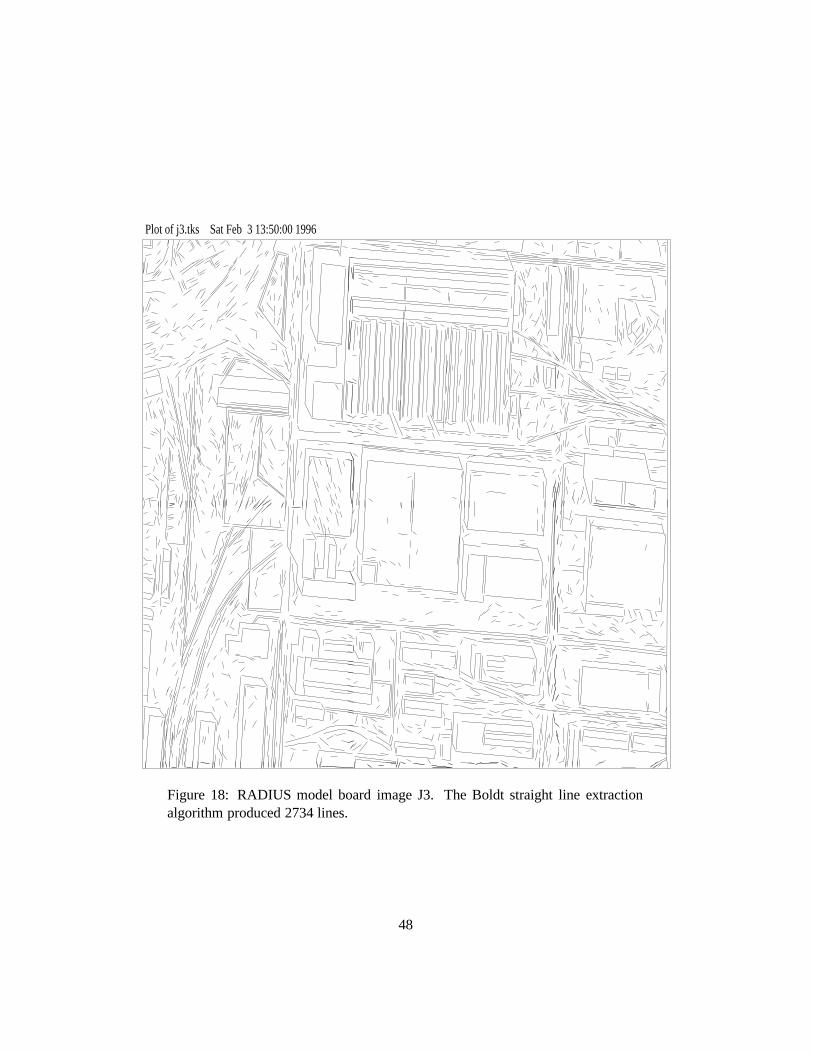
Plot of j3.tks Sat Feb 3 13:50:00 1996

Figure 18: RADIUS model board image J3. The Boldt straight line extractionalgorithm produced 2734 lines.

48

12

3

4

567

8

91011

12

13

14

15

1617

1819

20

2122

23

2425 26

27

28

29

30

3132

33

34

35

36

37

38

3940

41

42

43

44 45

4647

4849

50

51

52535455

5657585960

6162636465666768 69

7071 72

73

74

75

76

77

7879

80

8182

8384 85

8687

8889

9091

929394

9596

9798

99

100

101

102

103104

105

106 107

108109

110

111

112

113

114

115

116

117

118

119120

121

122123

124

125126127128

129

130 131

132

133

134

135

136137138

139

140

141

142143

144145

146

147148

149

150151

152

153

154 155

156

157

158

159

160

161

162 163

164

165

166

167

168169

170171

172173

174175176177

178 179180

181182

183184 185 186

187

188

189

190

191

192

193

194

195196

197

198

199200201202

203204205

206207

208209210211

212

213214

215

216217

218219

220

221

222

223

224

225

226

227

228

229

230

231

232

Plot of j1.tks Tue Jan 23 20:09:30 1996

Figure 19: 232 matched line segments for RADIUS model board image J1.

49

12

3

4

56

7

89

10

11

12

13

14

15

16

17

1819

20

2122

23

2425

26

27

28

29

30

3132

33

34

35

36

37

38

39

40

41

42

43

44

45

46

47

48

49

50

51

52

535455

56

5758

59

60

6162

6364

6566

6768

69

7071

72

73

74

75

76

77

7879

80

81

82

8384

85

8687

88

89

9091

929394

9596

97

98

99

100

101

102

103104

105

106

107

108

109

110

111 112

113

114

115

116117

118

119120

121

122

123

124

125

126127

128

129

130

131132133

134135

136

137

138

139

140141142

143

144

145

146

147

148

149

150

151

152

153

154

155

156

157

158

159

160

161

162

163

164

165

166

167

168

169 170

171

172

173

174

175176177

178

179180

181182

183

184

185

186

187188

189

190

191

192

193

194

195

196

197

198

199

200

201

202

203204

205

206207

208

209210

211212

213

214

215216

217

218

219

220

221222

223

224

225

226

227

228

229

230231

232

Plot of j2.tks Tue Jan 23 20:10:16 1996

Figure 20: 232 matched line segments for RADIUS model board image J2.

50

12

3

4

56

7

8

9

10

11

12

13

14

15

16

171819

20

2122

232425

2627

28

29

30

31

32

33

34

35

36

37

38

39

40

41

42

43

44

45

4647

4849

50

51

52

535455565758 596061626364656667 68 697071 72

73

74

75

76

77

78

79

80

81

82

8384 85

868788 899091929394

9596

97

98

99

100

101

102

103104 105

106

107

108109

110

111

112

113

114

115

116

117

118

119120

121

122

123124

125

126127

128

129

130

131

132

133

134

135

136

137138139

140

141

142143

144

145

146147

148

149

150

151

152

153

154

155

156

157

158

159

160

161

162163

164

165

166

167

168169

170

171

172

173

174

175176177

178

179

180181182

183

184

185

186

187

188

189

190191

192

193

194

195

196

197

198

199

200

201

202

203

204

205206207

208

209210211

212

213

214

215216

217

218219

220

221 222

223

224

225

226

227

228

229

230

231

232

Plot of j3.tks Tue Jan 23 20:10:16 1996

Figure 21: 232 matched line segments for RADIUS model board image J3.

51