Three-dimensional MHD simulation of a flux rope driven CME

Three-dimensional MHD simulation of a flux rope driven CME

Ward B. Manchester IV, Tamas I. Gombosi, Ilia Roussev, Darren L. De Zeeuw,

I. V. Sokolov, Kenneth G. Powell, and Gabor Toth1

Center for Space Environment Modeling, University of Michigan, Ann Arbor, Michigan, USA

Merav OpherJet Propulsion Laboratory, California Institute of Technology, Pasadena, California, USA

Received 6 September 2002; revised 21 August 2003; accepted 11 September 2003; published 6 January 2004.

[1] We present a three-dimensional (3-D) numerical ideal magnetohydrodynamics(MHD) model, describing the time-dependent expulsion of plasma and magnetic flux fromthe solar corona that resembles a coronal mass ejection (CME). We begin by developing aglobal steady-state model of the corona and solar wind that gives a reasonable descriptionof the solar wind conditions near solar minimum. The model magnetic field possesseshigh-latitude coronal holes and closed field lines at low latitudes in the form of a helmetstreamer belt with a current sheet at the solar equator. We further reproduce the fast andslow speed solar wind at high and low latitudes, respectively. Within this steady-stateheliospheric model, conditions for a CME are created by superimposing the magnetic fieldand plasma density of the 3-D Gibson-Low flux rope inside the coronal streamer belt. TheCME is launched by initial force imbalance within the flux rope resulting in its rapidacceleration to a speed of over 1000 km/s and then decelerates, asymptoticallyapproaching a final speed near 600 km/s. The CME is characterized by the bulk expulsionof �1016 g of plasma from the corona with a maximum of �5 � 1031 ergs of kineticenergy. This energy is derived from the free magnetic energy associated with the cross-field currents, which is released as the flux rope expands. The dynamics of the CME arefollowed as it interacts with the bimodal solar wind. We also present synthetic white-lightcoronagraph images of the model CME, which show a two-part structure that can becompared with coronagraph observations of CMEs. INDEX TERMS: 7513 Solar Physics,

Astrophysics, and Astronomy: Coronal mass ejections; 7524 Solar Physics, Astrophysics, and Astronomy:

Magnetic fields; 7509 Solar Physics, Astrophysics, and Astronomy: Corona; 7531 Solar Physics,

Astrophysics, and Astronomy: Prominence eruptions; KEYWORDS: magnetohydrodynamics, Sun, coronal

mass ejection

Citation: Manchester, W. B., IV, T. I. Gombosi, I. Roussev, D. L. De Zeeuw, I. V. Sokolov, K. G. Powell, G. Toth, and M. Opher

(2004), Three-dimensional MHD simulation of a flux rope driven CME, J. Geophys. Res., 109, A01102, doi:10.1029/2002JA009672.

1. Introduction

[2] Coronal mass ejections (CMEs) have traditionallybeen defined as large-scale expulsions of plasma from thecorona seen as bright arcs in coronagraphs that recordThomson scattered light. These events are the moststunning activity of the solar corona in which typically1015–1016 g of plasma is hurled into interplanetary spacewith a kinetic energy of the order 1031–32 ergs. Extensiveobservations with the SMM coronagraph have shown thatthe majority of CMEs originate from the disruption oflarge-scale coronal structures known as helmet streamers[Hundhausen, 1988, 1993]. Helmet streamers are arcade-like structures commonly found in coronagraph images

that possess a three-part structure composed of a high-density shell covering a low-density cavity, at the base ofwhich lies a filament. That CMEs originate from helmetstreamers is strongly suggested by the appearance ofmany CMEs possessing a dense bright leading shell witha cavity containing a bright core, which can be inter-preted as the corresponding three-part structure of the ofthe preevent helmet streamer as shown by Hundhausen[1999] and Howard et al. [1997]. It is now believed thatthe breakup of helmet streamers may result from a loss ofequilibrium following a slow, nearly quasi-static evolution[Low, 1983]. A slow growth followed by eruption isconsistent with the observations of the swelling andbrightening of large coronal helmet streamers severaldays before they produce CMEs [Hundhausen, 1993].[3] Central to understanding the dynamics of CMEs is the

nature of the preevent magnetic field, about which muchcan be inferred from both theory and observations. For ahelmet streamer to be in static equilibrium, the underlying

JOURNAL OF GEOPHYSICAL RESEARCH, VOL. 109, A01102, doi:10.1029/2002JA009672, 2004

1Also at Department of Atomic Physics, Eotvos University, Budapest,Hungary.

Copyright 2004 by the American Geophysical Union.0148-0227/04/2002JA009672$09.00

A01102 1 of 17

magnetic field must be in a closed configuration to confinethe dense plasma that would otherwise be carried out withthe solar wind. Observations show that the photosphericmagnetic field associated with helmet streamers is in abipolar configuration where opposite polarities are largelyseparated by a neutral line. Furthermore, in the corona,X-ray loops are clearly found to coincide with the helmetstreamers, indicating a dominant loop-type magnetic fieldconfiguration [Sterling and Hudson, 1997]. A significantfeature of the field configurations associated with CMEs ismagnetic shear, which is observed at the photosphere withvector magnetograms [Wang and Sheeley, 1994] and isstrongly suggested in the corona by the presence of X-raysigmoids [Moore et al., 2001]. Thus the magnetic fieldconfiguration of preevent helmet streamers is a shearedarcade possibly containing a flux rope as suggested byLow [1994] and Low and Hundhausen [1995] coincidingwith the plasma cavity. It is believed that CMEs are theresult of a global magnetohydrodynamic (MHD) processand represent a significant restructuring of the globalcoronal magnetic field [Low, 1996].[4] Observational limitations combined with the com-

plexity of CME structure and dynamics have lead to adiverse number of models that capture various aspects of theeruption process. Early theories of initiation suggested thatthermal pressure associated with solar flares was the drivingmechanism [Dryer et al., 1979]. However, this model fellfrom favor when observations revealed that flares oftenoccur after CME initiation [Hundhausen, 1999]. Morerecent observations have shown that soft X-ray emissionsincrease with CME initiation, particularly for fast CMEs[Zhang et al., 2002]. It is now believed that only the solarmagnetic field is capable of driving CMEs [Forbes, 2000].Nearly all magnetic-driven models of CMEs have employedpreevent coronal magnetic fields of two distinct topologies:sheared magnetic arcades or magnetic flux ropes oftencontained within an arcade. Examples of flux rope modelsinclude Mouschovias and Poland [1978], Chen [1996], Wuand Guo [1997], Wu et al. [1999], and Wu et al. [2000].CME models with simple arcade configurations includeWolfson [1982], Mikic et al. [1988], Steinolfson [1991],Choe and Lee [1996], Mikic and Linker [1994], and Linkerand Mikic [1995]. Flux ropes offer some advantages overarcades in that they offer a structure that more naturallysupports prominence material and explains the cavity andcore of the three part density structure commonly observedin CMEs. In addition, flux ropes detached from the solarsurface can store free magnetic energy capable of poweringCMEs [Low, 2001]. However, while flux ropes may betheoretically appealing there is still little direct observationalevidence supporting the existence of preevent coronal fluxropes while arcade type structures are commonly observedin the corona before and after CMEs.[5] Regardless of topology, the preevent magnetic fields

are usually taken to be either potential or force-free. Thepotential field has zero free energy while the force-free fieldhas been shown by Aly [1991] and Sturrock [1991] topossess less energy than the open state, greatly limiting itsability to erupt. To induce an eruption from such magneticstates, several mechanisms have been invoked. In the caseof flux ropes, the injection of azimuthal magnetic flux hasbeen used to drive eruptions as in the works of Chen [1996]

and Wu et al. [1999]. Localized magnetic reconnection hasbeen selectively introduced to sever field lines and relievemagnetic tension to allow a portion of the system (typicallya flux rope) to expand rapidly upwards. Examples ofreconnection-driven CME models are those by Forbesand Priest [1995], Lin and Forbes [2000], and Chen andShibata [2000]. Also, a combination of system driving andmagnetic reconnection has been used to model the initiationof CMEs. In the most common example, two-dimensional(2-D) magnetic arcades are made to approach an open stateby way of prescribed footpoint motions that shear themagnetic field. Reconnection when applied within theshearing arcade results in eruption [Steinolfson, 1991; Choeand Lee, 1996; Linker and Mikic, 1995]. Antiochos et al.[1999] have produced a new variation of this modelemploying a quadrupole field that allows magnetic recon-nection to occur higher in the corona, which removes theunsheared field above a low-lying sheared core.[6] Only recently have CME models been produced that

allow for fully three-dimensional (3-D) spatial variation.Gibson and Low [1998] gives an analytical description ofthe expansion of a flux rope as a CME while Amari et al.[2000] perform a numerical MHD simulation of the forma-tion of a flux rope within an arcade and its subsequenteruption. Lately, a numerical model of coronal arcadesresponding to rotating photospheric flows has been pro-duced by Tokman and Bellan [2002]. In this case, theauthors find that the evolving magnetic field mimics thethree-part structure of CMEs.[7] The approach we take to modeling CMEs is to start

with a system that is initially out of equilibrium andsimulate its subsequent time evolution. We begin bynumerically forming a steady-state model of the coronaalong with a bimodal solar wind. The model coronalmagnetic field is representative of a solar minimum config-uration with open polar field lines and low-latitude closedfield lines forming a streamer belt. Having attained thissteady-state, we then place a 3-D magnetic flux rope withinthe streamer belt, which is tied at both ends to the innerboundary. The flux rope we use is taken from a family of 3-Danalytical solutions derived by Gibson and Low [1998,hereinafter referred to as GL], which provide time-depen-dent, self-similar MHD models of CMEs. In the case of GL,the flux rope is initially in equilibrium in which radiallyoutward directed Lorentz force is balanced by the weight andpressure of contained plasma. The flux rope then expands asa result of an applied velocity field, which is prescribed sothat the flux rope expands in a self-similar fashion resem-bling a CME. Here, we have superimposed both the mag-netic field and density of the GL flux rope onto the steady-state corona. Rather than imparting an initial outward flow,we leave the system at rest but insert the flux rope within thesystem with reduced mass and insufficient external pressurefor the system to be in equilibrium. This configurationallows the system to contain substantial free energy andcircumvents the constraint of Aly [1991] and Sturrock [1991]by virtue of a nonzero cross-field component of the electriccurrent. In the subsequent time evolution of the system, wefind that the flux rope expands rapidly, driving a strongshock ahead of it as it is expelled from the corona along withlarge amounts of plasma mimicking a CME. With ourinclusion of this flux rope to a numerical, steady-state model

A01102 MANCHESTER ET AL.: CORONAL MASS EJECTION

2 of 17

A01102

of the corona and solar wind, we can extend the Gibson Lowmodel to address its limitations such as CME accelerationand interaction with a background solar wind, as well asallowing for magnetic reconnection.[8] The organization of the paper is as follows. We give a

brief description of the conservative form of the equationsof MHD and the scheme used to solve them in section 2.Details of the steady-state corona and solar wind are givenin section 3, while an outline of the Gibson-Low flux rope isgiven in section 4. Results of the numerical simulation ofthe flux rope driven CME are given in section 5, whichincludes a discussion of the energy budget and velocityprofile. In addition, synthetic, Thomson-scattered, whitelight images of the CME are presented as seen from threedifferent perspectives. Finally, in section 6, we discuss thesimulation results and their significance in demonstratingmagnetic flux ropes as a possible driver of CMEs.

2. Governing Equations of the MHD Model

[9] In our model of the corona, solar wind, and CME, weassume that the systems are composed of magnetizedplasma that behaves as an ideal gas with a polytropic index,g = 5/3. The plasma is assumed to have infinite electricalconductivity so that the magnetic field is ‘‘frozen’’ into theplasma. Gravitational forces on the plasma are included butonly forces due to the Sun; there is no self-gravitation of theplasma. Finally, volumetric heating of the plasma of achosen form is assumed to occur in the corona. With theseassumptions, the evolution of the system may be modeledby the ideal MHD equations written in conservative form:

@r@t

þr � ruð Þ ¼ 0 ð1Þ

@ ruð Þ@t

þr � ru uþ pþ B2

8p

� �I BB

4p

� �¼ rg ð2Þ

@B

@tþr � uB B uð Þ ¼ 0 ð3Þ

@e@t

þr � u eþ pþ B2

8p

� � u � Bð ÞB

4p

� �;

¼ rg � uþ ðg 1ÞQ; ð4Þ

where r is the plasma mass density, u is the plasma velocity,B is the magnetic field, and p is the plasma pressure (sum ofthe electron and ion pressures). The volumetric heatingterm, Q, parameterizes the effects of coronal heating as wellas heat conduction and radiation transfer (see section 3).Thegravitational acceleration is definedasg=g(r/r)(R/r)

2,where R is the solar radius and g is the gravitationalacceleration at the solar surface. The total energy density, e,is given by

e ¼ ru2

2þ p

g 1þ B2

8p: ð5Þ

This system of eight equations details the transport of mass,momentum, and energy with three equations describing the

evolution of the magnetic field given by Faraday’s Lawassuming infinite electrical conductivity. These equations arethenput indimensionless form, usingvaluesof thedensity andion-acoustic wave speed from a suitable part of the physicaldomain (in this case the low corona) in addition to a referencelength scale (in this case the solar radius). The dimensionlessequations are then solved, using the block-adaptive tree solarwindRoe-type upwind scheme (BATS-R-US) code [Powell etal., 1999; Groth et al., 2000]. This code is designed to runefficiently on massively parallel computers and solves theequations of MHD with the use of block adaptive meshrefinement (AMR).This feature of thegrid allows for orders ofmagnitude variation in numerical resolution within thecomputational domain. Such resolution is necessary forglobalcoronal models, which strive to resolve structures such asshocks and electric current sheets in a domain that extends tomany solar radii.

3. Steady-State Model of the Solar Wind

[10] In order to simulate the time-dependent behavior of aCME propagating from the low corona through the solarwind, a representative MHD model of the steady-statebackground solar wind is required. With such a model,the evolution of a CME is then formulated as a propagationproblem with the initial condition of the corona and solarwind specified by the steady-state solution.[11] In this section, we describe our steady-state model of

the corona and solar wind that is designed to reproduceconditions near solar minimum. The essential features ofthis model are (1) open magnetic field lines forming coronalholes at high latitude; (2) closed magnetic field linesforming a streamer belt near the Sun at low latitudes;(3) the bimodal nature of the solar wind is reproduced withfast wind over the poles and slow wind at low latitudes. Athin current sheet forms at the tip of the streamer belt andseparates opposite directed magnetic flux originating fromthe two poles. The model is simplified by alignment ofthe magnetic axis with the z axis so the solution isaxisymmetric. Also, solar rotation is neglected since thedomain extends only to 32 solar radii. At this distance fromthe Sun, the azimuthal component of the Parker [1963]spiral is negligible. While the magnetic field structure ofthis steady-state solution is simple, future models willeventually incorporate synoptic magnetogram observationsas well as a rotating Sun to form much more realisticmagnetic field configurations.[12] The corona is composed of high-temperature (T >

106 K), low-density (r � 1016 gm cm3) plasma composedprimarily of ionized hydrogen. The temperature and pres-sure of the corona are such that it can not be held inequilibrium by solar gravity or the pressure of the interstel-lar medium. Consequently, it expands outward at supersonicspeeds and in doing so forms the solar wind [Parker, 1963].The fast solar wind originates from coronal holes and ispossibly driven to high velocity by additional heating thatoccurs close to the Sun [cf. Axford and McKenzie, 1996]. Itis also thought that momentum deposited by Alfven wavesmay accelerate this component of the wind [cf. Hollweg etal., 1982; Usmanov et al., 2000]. The fast wind lies atheliolatitudes >30� at solar minimum and has an averagevelocity of the approximately 750 km s1. The slow wind


3 of 17

A01102

by contrast is confined close to the global heliosphericcurrent sheet, which lies near the equator at solar minimum.This component of the wind is highly variable with speedsthat lie between 300 and 450 km s1. The source of the slowwind may be highly expanded plasma traveling downmagnetic flux tubes that originate near coronal hole bound-aries. It has also been suggested that opening of closed fluxtubes by interchange reconnection with open flux mayrelease plasma to form the slow solar wind [Fisk et al.,1999].[13] The steady-state model of the corona and solar wind

described here was first developed by Groth et al. [2000].However, we have made significant modifications to theoriginal steady-state model to suit our purposes. First, oursimulation is performed in the inertial frame rather than thecorotating frame. Second, the magnetic axis is aligned withthe z axis in our model rather than having a tilted intrinsicmagnetic field topology. Third, we have slightly modifiedthe inner boundary condition to allow for the flux rope to beline-tied to the coronal surface. Finally, our model of thesolar wind only extends to 32R compared to 224R ofthe original model with a different numerical grid and withthe absence of solar rotation. In all other ways, our steady-state model is identical to Groth et al. [2000], of which webriefly outline here.[14] The steady-state numerical model is made with the

assumption that the base of the corona is at the innerboundary and acts as a reservoir of hot plasma with anembedded magnetic field. The plasma temperature (the sumof the ion and electron temperatures) is taken to be Ts = Tp +Te = 2.85 � 106 K with Tp/Te � 2. For the remainderof the text, we will refer only to the plasma temperature, Ts.The plasma density is taken to be r = 2.5 � 1016 gm cm3.The intrinsic magnetic field at the solar surface, B0, may bewritten as a multipole expansion of the following form:

B0k ¼ 3Miri

r4rk

rMk

r3þ 7

Qijlrirjrl

r8rk

r 3

Qijkrirj

r7; ð6Þ

where Mi (i = 1, 2, 3) are the components of the dipolemoment vector and Qijk are the octupole moment tensorcomponents with the octupole aligned with the z axis (thereis no quadrupole moment in this model). We have takenthe dipole aligned with the z axis so that Mx = My = 0 andMz = b0. The dipole and octupole moments are chosen suchthat the maximum field strength at the poles is 8.4 Gaussand 2.2 Gauss at the equator.[15] Volumetric heating of the model corona is introduced

in a way that attempts to mimic the effects of energyabsorption above the transition region, thermal conduction,and radiative losses as well as satisfying known constraintsof coronal heating. The heating function has the followingform,

Q ¼ rq0 T0 gp

r

� �exp ðr RÞ2

s20

" #; ð7Þ

where the target temperature, T0, is 5.0 � 106 K polewardfrom a critical angle q0(r) which defines the coronal holeboundary, while T0 = 2.85 � 106 K equatorward of q0(r) inthe streamer belt. The heating function is defined with q0 =

106 ergs g1 s1 K1, where R is equal to the solar radiusand r is the heliocentric radius. The function q0(r) is definedas follows: for the region R < r < 7R,

sin2 ðqoÞ ¼ sin2 ð17:5�Þ þ ð1 sin2 ð17:5�ÞÞðr 1Þ8

; ð8Þ

which is equal to 17.5� at the solar surface and increases to avalue of qo = 61.5� at r = 7R. Beyond this radius, qoincreases more slowly as

sin2 ðqoÞ ¼ sin2 ð61:5�Þ þ ð1 sin2 ð61:5�ÞÞðr 7Þ40

; ð9Þ

reaching a value of qo = 90� at r = 47R, which is then heldfixed at 90� for r > 47R. The heating scale height functionis kept constant in the streamer belt with s0(r, q) = 4.5, andincreases inside the coronal hole as

s0ðr; qÞ ¼ 4:5 2 sin2 ðqÞsin2 ðqoÞ

� �; ð10Þ

which gives a scale height for the volumetric heating thatvaries from 4.5R near to equator to 9R at the poles. It isimportant to mention that this heating function was designedwith several free parameters with the desire of reproducingobserved features of the fast and slow solar wind.

3.1. Computational Mesh

[16] The computational domain for the simulation extendsfrom 32R < x < 32R, 32R < y < 32R, and 32R <z < 32R with the Sun placed at the origin with themagnetic axis aligned with the z axis. The system is initiallyresolvedwith 15,555 self-similar 4� 4� 4 blocks containinga total of 995,520 cells. The blocks are distributed in size overseven levels of refinement with each subsequent level ofrefinement using cells half the size of the previous level (ineach dimension). In this case, cells range in size from 1/32Rto 2R and are spatially positioned to highly resolve thecentral body and the flux rope as well as the heliosphericcurrent sheet. The grid is refined every 200 iterations withoutcoarsening for the first 10,000 iterations to increase the totalnumber of cells to 1.9 million. Beyond 10,000 iterations, thegrid is refined and coarsened such that the total number ofcells is held nearly constant. AMR criteria are chosen so thatblocks close to the y axis with large time variations in densityare preferentially refined. In this way, the high-resolutionmesh tracks the shock directly in front of the flux rope as wellas the central part of the flux rope.

3.2. Boundary Conditions

[17] To pose a physically meaningful system subject tothe equations of ideal MHD, it is necessary to specifyappropriate boundary conditions at the inner boundary(the spherical surface r = R) and the outer boundary (theouter surfaces of the rectangular domain). The coronalboundary conditions are a function of heliospheric latitude.In the coronal holes poleward of q0, the following values areprescribed just inside r = R: r = 2.5 � 1016 gm cm3, p =5.89 � 102 dynes cm2, u = 0, and B = B0. These valuesare then allowed to interact with the solution inside our


4 of 17

A01102

physical domain through the r = R boundary; this ap-proach ensures that the appropriate information from the‘‘solar’’ values is propagated into the solution domain bythe numerical flux function used in the scheme. Theseconditions set up a pressure gradient that drives plasmaaway from the Sun and permits plasma to pass through theboundary as the mass source for the solar wind. Themagnetic field at the surface is specified by the time-independent multipole expansion for the intrinsic fieldgiven by equation (6). In the streamer belt equatorward ofq0, the following values are prescribed just inside r = R:@r/@r = 0, @p/@r = 0, u = uoutside, B = Boutside, where thesubscript outside refers to the values just outside r = R,which are computed by the flow solution scheme. Theseconditions strictly enforce a zero flow at the boundary, bothin the radial and tangential directions; they also enforcecontinuity of the magnetic field across r = R. Thisprovision allows the magnetic field of the flux rope (pre-scribed in the streamer belt) to pass through the interfacewhere the footpoints are effectively ‘‘line tied.’’ At the outerboundary of the domain, the flow is super-fast. Thus allwaves are exiting the domain, and no information fromoutside the domain propagates into the domain.

3.3. Steady-State Solar Wind Solution

[18] The solar wind solution is produced by the timeevolution of the system subject to the described heatingfunction, intrinsic magnetic field, and boundary conditions.An initial plasma flow is taken to have mass density fallingoff as 1/r3, constant temperature, and a radial outflow withthe velocity proportional to r. Local time stepping is used tospeed up convergence, achieving a near steady-state solu-tion after 84,000 iterations, with AMR periodically appliedwith an emphasis on resolving the heliospheric currentsheet. Figure 1 depicts a two-dimensional (2-D) cut throughthe 3-D steady-state solar wind model in the meridional

plane close to the Sun. The false color image indicates thevelocity magnitude, juj, of the plasma while the magneticfield is represented by solid while lines. Inspection reveals abimodal outflow pattern with slow wind leaving the Sunbelow 400 km/s near the equator and high-speed wind above700 km/s found above 30� latitude. In this model, we find thatthe source of the slow solar wind is cooler plasma originatingfrom the coronal hole boundaries that overexpands and failsto accelerate to high speed as it fills the volume of spaceradially above the streamer belt. Thismodel has similarities tothe empirical model of the solar wind proposed byWang andSheeley [1994] that explains solar wind speeds as beinginversely related to the expansion of contained magnetic fluxtubes. The magnetic field remains closed at low latitude closeto the Sun forming a streamer belt. At high latitude, themagnetic field is carried out with the solar wind to achieve anopen configuration. Closer to the equator, closed loops aredrawn out and (at a distance of r > 3R), collapse into a fieldreversal layer. The resulting field configuration has a neutralline and a current sheet originating at the tip of the streamerbelt similar to numerical solution originally obtained byPneuman and Kopp [1971].

4. Flux Rope of Gibson and Low

[19] To initiate a CME within this coronal model, wesuperimpose a 3-D magnetic flux rope and its entrainedplasma into the streamer belt of our steady-state coronalmodel (see Figure 2). The flux rope we employ comes fromthe GL family of analytical solutions of the ideal MHDequations describing an idealized, self-similar expansion ofa magnetized cloud resembling a CME. We briefly describehere the mathematical form of the GL solutions while morecomplete derivations and descriptions of the solutions canbe found in their original paper [Gibson and Low, 1998].

4.1. Self-Similar Flux Ropes

[20] The CME models of GL are developed by finding a3-D analytical solution to the equation

1

4pr� Bð Þ � Brp rg ¼ 0 ð11Þ

and Maxwell’s equation, r � B = 0, that describe a globalmagnetostatic corona containing a magnetic flux rope inforce balance with the pressure and weight of the plasma.[21] The solution for this flux rope is derived by applying a

mathematical stretching transformation r ! r a to anaxisymmetric, spherical ball of twisted magnetic flux inequilibrium with plasma pressure. The transformation, per-formed in spherical coordinates (r, q, f), draws space towardthe origin while holding angular coordinates q and f fixed.This mathematical procedure serves two important purposes.First, it generates a geometrically complex solution by dis-torting the originally spherical, axisymmetric flux rope (cen-tered away from the heliocentric origin) into a tear-drop shapewith full 3-D spatial variation. Themagnetic structure, seen asa 3-D representation in Figure 2, possesses a toroidal coreshown in solid blue lines surrounded by flux becomingprogressively more twisted closer to the flux rope surfaceshown as solid red lines. The computational grid is seen inFigure 2 as black lines superimposed upon a false color image

Figure 1. Magnetic structure and velocity for the steady-state solar wind solution. Solid white lines are magnetic‘‘streamlines’’ drawn in the y – z plane superimposed upona false color image of the velocity magnitude. Note thebimodal nature of the solar wind.


5 of 17

A01102

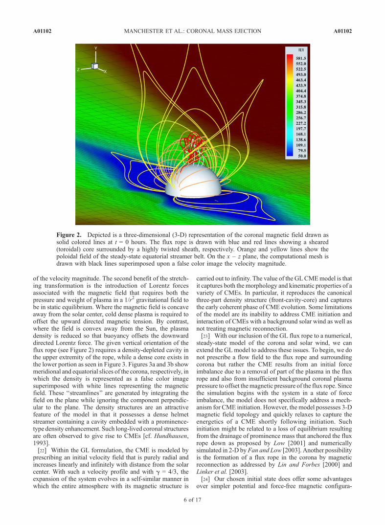
of the velocity magnitude. The second benefit of the stretch-ing transformation is the introduction of Lorentz forcesassociated with the magnetic field that requires both thepressure and weight of plasma in a 1/r2 gravitational field tobe in static equilibrium. Where the magnetic field is concaveaway from the solar center, cold dense plasma is required tooffset the upward directed magnetic tension. By contrast,where the field is convex away from the Sun, the plasmadensity is reduced so that buoyancy offsets the downwarddirected Lorentz force. The given vertical orientation of theflux rope (see Figure 2) requires a density-depleted cavity inthe upper extremity of the rope, while a dense core exists inthe lower portion as seen in Figure 3. Figures 3a and 3b showmeridional and equatorial slices of the corona, respectively, inwhich the density is represented as a false color imagesuperimposed with white lines representing the magneticfield. These ‘‘streamlines’’ are generated by integrating thefield on the plane while ignoring the component perpendic-ular to the plane. The density structures are an attractivefeature of the model in that it possesses a dense helmetstreamer containing a cavity embedded with a prominence-type density enhancement. Such long-lived coronal structuresare often observed to give rise to CMEs [cf. Hundhausen,1993].[22] Within the GL formulation, the CME is modeled by

prescribing an initial velocity field that is purely radial andincreases linearly and infinitely with distance from the solarcenter. With such a velocity profile and with g = 4/3, theexpansion of the system evolves in a self-similar manner inwhich the entire atmosphere with its magnetic structure is

carried out to infinity. The value of the GLCMEmodel is thatit captures both the morphology and kinematic properties of avariety of CMEs. In particular, it reproduces the canonicalthree-part density structure (front-cavity-core) and capturesthe early coherent phase of CME evolution. Some limitationsof the model are its inability to address CME initiation andinteraction of CMEs with a background solar wind as well asnot treating magnetic reconnection.[23] With our inclusion of the GL flux rope to a numerical,

steady-state model of the corona and solar wind, we canextend the GLmodel to address these issues. To begin, we donot prescribe a flow field to the flux rope and surroundingcorona but rather the CME results from an initial forceimbalance due to a removal of part of the plasma in the fluxrope and also from insufficient background coronal plasmapressure to offset themagnetic pressure of the flux rope. Sincethe simulation begins with the system in a state of forceimbalance, the model does not specifically address a mech-anism for CME initiation. However, the model possesses 3-Dmagnetic field topology and quickly relaxes to capture theenergetics of a CME shortly following initiation. Suchinitiation might be related to a loss of equilibrium resultingfrom the drainage of prominence mass that anchored the fluxrope down as proposed by Low [2001] and numericallysimulated in 2-D by Fan and Low [2003]. Another possibilityis the formation of a flux rope in the corona by magneticreconnection as addressed by Lin and Forbes [2000] andLinker et al. [2003].[24] Our chosen initial state does offer some advantages

over simpler potential and force-free magnetic configura-

Figure 2. Depicted is a three-dimensional (3-D) representation of the coronal magnetic field drawn assolid colored lines at t = 0 hours. The flux rope is drawn with blue and red lines showing a sheared(toroidal) core surrounded by a highly twisted sheath, respectively. Orange and yellow lines show thepoloidal field of the steady-state equatorial streamer belt. On the x – z plane, the computational mesh isdrawn with black lines superimposed upon a false color image the velocity magnitude.


6 of 17

A01102

tions in that it possesses substantial free magnetic energythat is liberated as the flux rope expands. As the CMEleaves the corona, it strongly interacts with the highlystructured solar wind ahead of it, most notably, by theformation of an MHD shock running ahead of the fluxrope. Our MHD simulation also allows us to mimic mag-netic reconnection, in this case, through numerical resistiv-ity. We will show in the next section, that reconnectionplays a significant role in the restructuring of the coronalmagnetic field following the CME.

4.2. Mathematical Form of the GL Flux Rope

[25] The flux rope is obtained by transforming a toroidalmagnetic rope contained in a sphere of radius r0. The centerof the sphere is located at a radial distance of r1 on the y

axis. The plasma pressure in the flux rope is proportional tothe free parameter a1

2, which also controls the magnetic fieldstrength in the flux rope through pressure balance.[26] Mathematically, the flux rope magnetic field is

written in terms of a scalar function A in spherical coor-dinates (r0, q0, f0) as

b ¼ 1

r0 sin q0ð Þ1

r0@A

@q0r0 @A

@r0q0a0Af0

� �; ð12Þ

where

A ¼ 4pa1

a20

r20

gða0r0Þg a0r

0ð Þ r02� �

sin2 q0ð Þ ð13Þ

Figure 3. The initial coronal plasma density is depicted in Figures 3a and 3b with false color images inthe y – z meridional plane and the x – y equatorial plane respectively. Figures 3c and 3d show the initialfield strength and plasma b respectively in false color in the y – z meridional plane. In all panels, themagnetic field is represented by ‘‘streamlines’’ drawn as solid white lines.


7 of 17

A01102

and

gða0r0Þ ¼ sin a0r

0ð Þa0r0

cos a0r0ð Þ: ð14Þ

The pressure inside the flux rope necessary for equilibriumis � = a1A, where a1 is a free parameter that determines themagnetic field strength and plasma pressure in the flux rope.Here, r0 is the diameter of the spherical ball of flux and a0 isrelated to r0 by a0r0 = 5.763459 (this number is the smallesteigenvalue of the spherical Bessel function, J5/2). Thecoordinate (r0, q0, p0) is centered relative to the heliosphericcoordinate system on the y axis at y = r1 and oriented suchthat the circular axis of the flux rope is in the heliosphericequatorial plane.[27] In the next step, this axisymmetric flux rope is sub-

jected to the mathematical transformation r ! r a thatdraws space toward the heliospheric origin and distorts thesphere containing the rope to a tear-drop shape. Followingthis transformation, the magnetic field takes the form:

Brðr; q;fÞ ¼�

r

� �2

br �; q;fð Þ; ð15Þ

Bqðr; q;fÞ ¼�

r

d�

dr

� �bq �; q;fð Þ; ð16Þ

Bfðr; q;fÞ ¼�

r

d�

dr

� �bf �; q;fð Þ; ð17Þ

where � = r + a and (r, q, f) are the heliospheric sphericalcoordinates. Equilibrium within this transformed statedemands that the plasma pressure be of the form

p ¼ �

r

� �2

1 �

r

� �2 !

b2r8p

� �þ �

r

� �2

� ð18Þ

and that density be of the form

r ¼ 1

FðrÞ �

r

� �2

1 �

r

� �2 !

d

d��þ b2

8p

� �"

þ 2��a

r3þ �a

4pr31 2

�

r

� �2 !

b2rþ�

r

� �2a2

r2þ 2a

r

� �

�b2q þ b2f

4p�

!#; ð19Þ

where F(r) = GM/r2, with G being the gravitational constantand M being the solar mass. It is interesting to note thatequation (19) does not depend on the density of thepretransformed state because without gravity, density is notspecified, since there is no force associated with it. Onlyafter gravity is introduced in the transformed state is densityspecified, and then it is done so to provide force balance inthe radial direction.[28] For this simulation, the flux rope is specified by

setting a = 0.3, r0 = 1.0, r1 = 1.6 and a1 = 0.4. The flux rope

and contained plasma are superimposed upon the exitingcorona, the results of which can be seen in Figures 2 and 3.The density of mass contained in the flux rope is furthermultiplied by a factor of 0.8, leaving the prominencebuoyant. In addition, the equilibrium state of GL requiresa significant outward increasing plasma pressure to offsetthe magnetic pressure in the upper portion of the magneticflux rope. The background corona is insufficient to providethis pressure and results in a negative pressure when the GLsolution is superimposed on the corona. To avoid negativepressure, we limit the depletion of pressure and density inthe coronal cavity to 25 percent of the initial coronal values,which leaves the upper portion of the flux rope withunbalanced magnetic pressure.[29] By introducing the GL solution to the corona, we

have added 9.0 � 1031 ergs of magnetic and 4.8 �1029 ergs of thermal energy, as well as 4.9 � 1014 gm ofplasma to the corona. The added plasma is concentrated in aprominence-type core at the base of the flux rope that isapproximately 10 times denser than the ambient corona.The magnetic field strength of the flux rope is quiteconservative with a maximum value of only 5 Gauss, whichis consistent with field measurements in quiescent prom-inences [Leroy et al., 1983]. However, the magnetic field ofthe rope completely dominates the corona, being consider-ably stronger than the ambient coronal field and alsodominating the plasma pressure as seen in Figures 3cand 3d. These figures show meridional slices of the coronawith false color images of the field strength and plasma b,respectively, with solid white lines representing themagnetic field.

5. Simulation of the CME Event

[30] In this section, we present the results of a 3-Dnumerical simulation designed to study the evolution of aflux rope placed in the corona out of equilibrium. We findthat the flux rope is expelled from the corona in a convinc-ing fast CME-like eruption. The front of the rope rapidlyachieves a maximum speed over 1000 km/s before decel-erating and asymptotically approaching a terminal velocitynear 600 km/s. A strong MHD shock front forms ahead ofthe flux rope as it travels through the solar wind. We willpresent an energy budget, which clearly shows the CME ismagnetically driven with an interesting interaction with theplasma thermal energy. A current sheet forms at the base ofthe expanding flux rope where magnetic reconnectionpartially severs the rope from the line-tied coronal bound-ary. Finally, we present synthetic images of the Thomson-scattered white light showing how the CME would appearin a coronagraph.

5.1. CME Morphology

[31] Figure 4 presents a 3-D view of the CME as seen att = 2.0 hours, from a perspective looking down and aheadfrom above the y axis, along which the CME is traveling.The false color image shows the velocity magnitude alongwith the numerical grid (shown in grey lines) on theequatorial (x – y) plane. A shock front is clearly visiblepreceding the flux rope in the color image as is the adaptivemesh tracking the shock. The magnetic field in the interiorof the flux rope is represented by solid colored magenta


8 of 17

A01102

lines. The field close the the axis of the flux rope clearly hasa strong toroidal component while the field at the surface isnearly poloidal. Grey lines show the open field lines of thesolar wind some of which pass through the shock frontwhere the lines bend sharply to wrap around the expandingflux rope. Black and green lines show closed field lines ofthe streamer belt.[32] The time evolution of the CME is displayed in

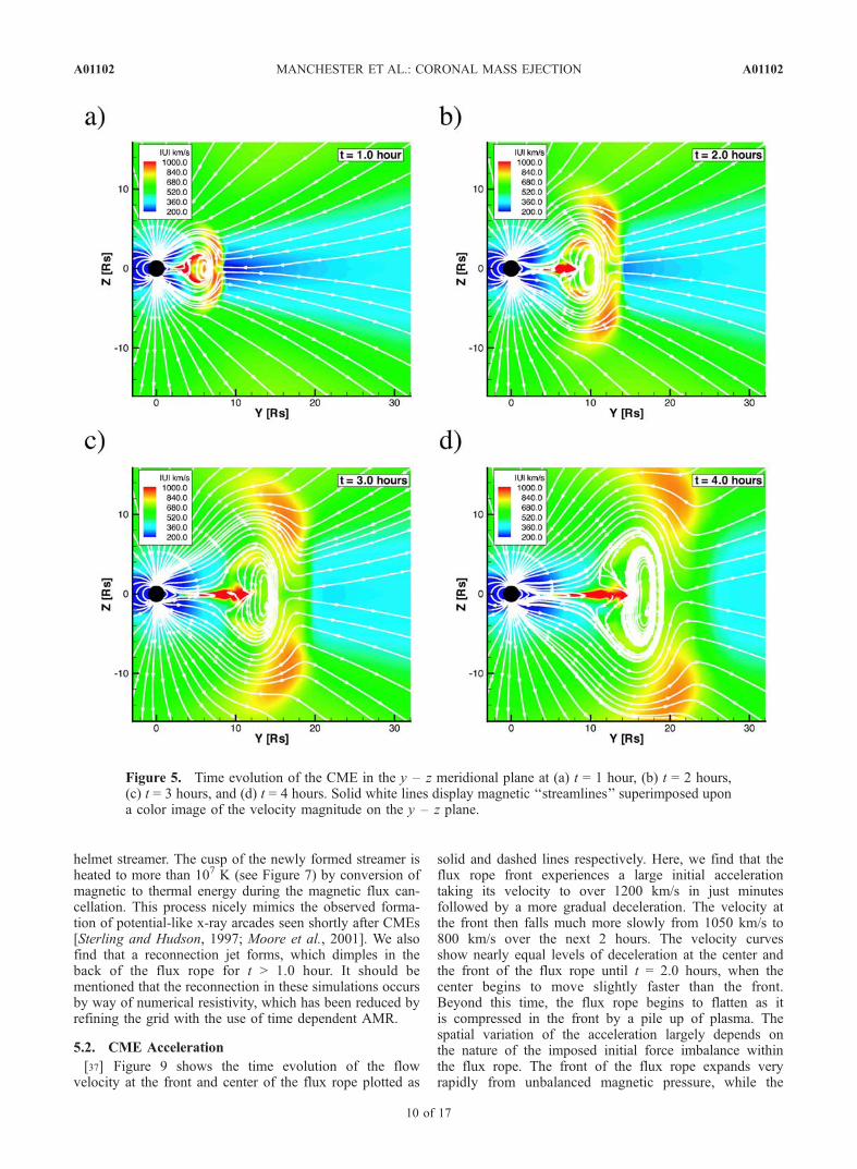
Figures 5 and 6 with a time series of figures showing thesystem at t = 1.0, 2.0, 3.0, and 4.0 hours. Figure 5 depictsthe system in 2D meridional slices (y – z plane), whileFigure 6 shows equatorial slices (x – y plane). In both cases,false color images show the plasma velocity magnitudeupon which solid while lines are superimposed representingthe magnetic field.[33] We find the flux rope rapidly expanding and being

expelled from the corona while decelerating. An MHDshock front moves ahead of the flux rope, traveling atnearly the same speed as the rope on the y axis whilepropagating far ahead to the sides of the rope. In effect, theshock front moves at relatively uniform speed, initiallyforming a spherical bubble, while the flux rope inside thefront moves forward faster than it expands to the sides. Wealso find that the structure of the ambient solar wind has aprofound influence on the shock front. The wind andmagnetosonic speeds are minimal in the heliospheric currentsheet, and both grow with heliospheric latitude. As a result,the shock travels at higher latitude in the fast solar windwith a lower Mach number than found at low latitude. Forexample, at t = 1.0 hour, the shock travels at approximately1100 km/s through the current sheet with a magnetosonic

Mach number of 6.04 while at this same time, the magneto-sonic Mach number at 30� latitude is only 1.86.[34] The variation in Mach number is clearly reflected in

the temperature structure of shock heated plasma shown inFigure 7. This figure depicts a 2-D meridional slice at t =1.0 hour where solid white lines representing the magneticfield are superimposed upon a false color image of thetemperature. Inspection of Figure 7 reveals that the temper-ature of the shock-heated plasma is greatest at the helio-spheric current sheet where the Mach number is the largestand the temperature reaches 2.1 � 107 K. The temperaturebehind the shock then rapidly decreases with latitude,reaching a value of 1.3 � 107 K at 30� heliolatitude. Thetemperature behind the shock rapidly falls with radialdistance, as the CME moves from the Sun as is seen inFigure 8. This line plot shows the temperature as a functionof height behind the shock front where it travels along thecurrent sheet.[35] There is a clear dimple (concave-outward) in the

shock front very near the heliospheric current sheet seen inthe meridional slices for t > 1.0 hour. At this location theplasma b is high and the shock speed is super-fast and isabove the critical speed defined by

v2crit ¼gþ 1

g 1

� �c2a

2

g 1

� �c2s ; ð20Þ

where ca and cs are the Alfven speed and sound speed,respectively, defined as ca =

ffiffiffiffiffiffiffiffiffiffiffiffiffiffiffiB2=4pr

pand cs =

ffiffiffiffiffiffiffiffiffiffiffiffiffiffiffiffiffiffigkBT=mi

p.

Here, kB is Boltzmann’s constant and mi is the ion mass. Theshock speed is outside the switch-on regime, indicating a fastmode along the leading shock front except at the current sheetwhere the shock is hydrodynamic in nature. Close inspectionof Figure 5 reveals that at high latitude, the magnetic fieldlines bend at the shock to deflect around the flux rope. At lowlatitude, where the shock front forms a dimple, the field linesdeflect toward the equatorial plane and only bend to goaround the flux rope well behind the shock. Previous studieshave found that in the switch-on regime, the shock is of theintermediate type in the concave region, becoming a fastshock in the convex portion of the front [Steinolfson andHundhausen, 1990; DeSterck et al., 1998; Fan and Low,2003]. However, in our case, the shock dimple is largely theresult of spatial variations in the background solar wind nearthe heliospheric current sheet. Close to the Sun, the shocktravels faster away from current sheet where the magneto-sonic speed increases relative to the current sheet itself whereB = 0. On a larger scale, the shock travels faster at higherlatitudes in the higher temperature and higher speedwind thancompared with the low-latitude wind. This effect leads to thedimple becoming a very broad indentation in the shock frontby t = 4.0 hours. This same large-scale concave feature of theshock front has been found in earlier work such asOdstrcil etal. [1996] and Riley et al. [2002].[36] We also find that magnetic reconnection plays a

significant role in the evolution of the CME. At t = 1.0 hour,the magnetic topology of the system is nearly identical tothat of the initial state. As time progresses, we find that acurrent sheet forms between field lines attaching the fluxrope to the coronal boundary. Examination of Figures 5 and6 reveals that reconnection at this current sheet partiallysevers the flux rope from the boundary and reforms the

Figure 4. 3-D representation of the magnetic field lines2 hours after the initiation of the CME. The color coderepresents the velocity magnitude in the x – y plane andgrey lines depict the computational mesh. Magenta linesshow magnetic field lines of the flux rope while black andgreen lines show magnetic lines of the helmet streamer.Grey lines represent the open magnetic flux extending fromthe pole.


9 of 17

A01102

helmet streamer. The cusp of the newly formed streamer isheated to more than 107 K (see Figure 7) by conversion ofmagnetic to thermal energy during the magnetic flux can-cellation. This process nicely mimics the observed forma-tion of potential-like x-ray arcades seen shortly after CMEs[Sterling and Hudson, 1997; Moore et al., 2001]. We alsofind that a reconnection jet forms, which dimples in theback of the flux rope for t > 1.0 hour. It should bementioned that the reconnection in these simulations occursby way of numerical resistivity, which has been reduced byrefining the grid with the use of time dependent AMR.

5.2. CME Acceleration

[37] Figure 9 shows the time evolution of the flowvelocity at the front and center of the flux rope plotted as

solid and dashed lines respectively. Here, we find that theflux rope front experiences a large initial accelerationtaking its velocity to over 1200 km/s in just minutesfollowed by a more gradual deceleration. The velocity atthe front then falls much more slowly from 1050 km/s to800 km/s over the next 2 hours. The velocity curvesshow nearly equal levels of deceleration at the center andthe front of the flux rope until t = 2.0 hours, when thecenter begins to move slightly faster than the front.Beyond this time, the flux rope begins to flatten as itis compressed in the front by a pile up of plasma. Thespatial variation of the acceleration largely depends onthe nature of the imposed initial force imbalance withinthe flux rope. The front of the flux rope expands veryrapidly from unbalanced magnetic pressure, while the

Figure 5. Time evolution of the CME in the y – z meridional plane at (a) t = 1 hour, (b) t = 2 hours,(c) t = 3 hours, and (d) t = 4 hours. Solid white lines display magnetic ‘‘streamlines’’ superimposed upona color image of the velocity magnitude on the y – z plane.


10 of 17

A01102

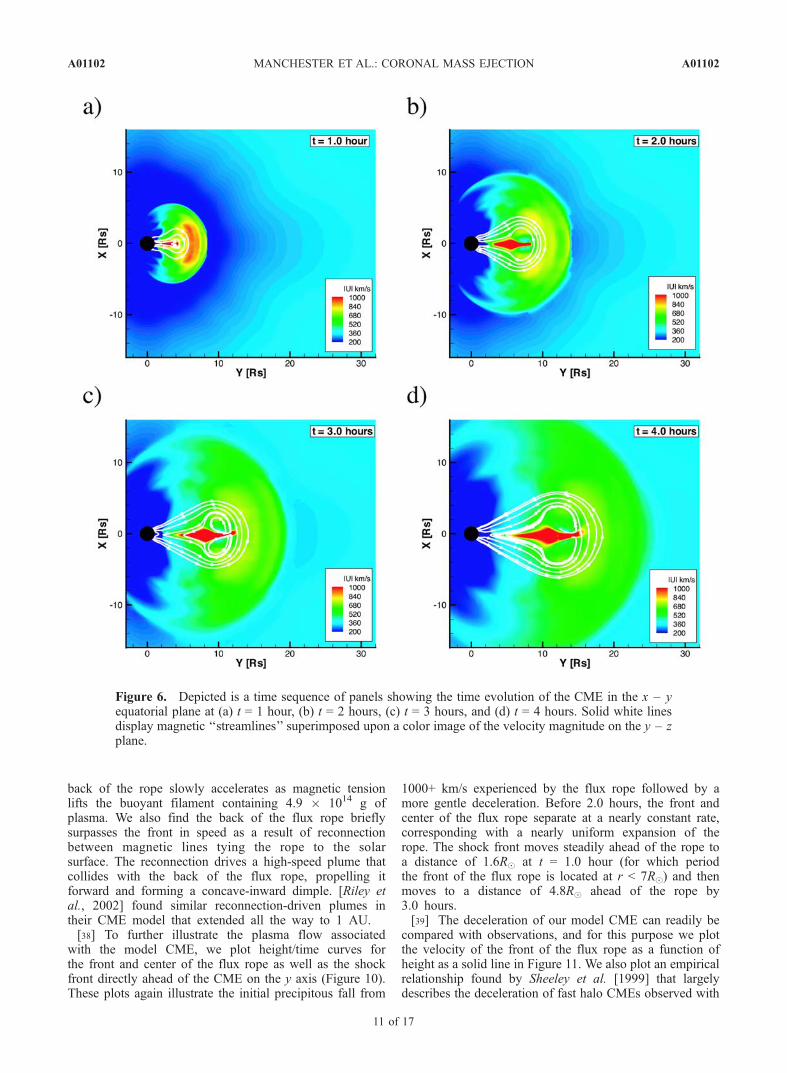
back of the rope slowly accelerates as magnetic tensionlifts the buoyant filament containing 4.9 � 1014 g ofplasma. We also find the back of the flux rope brieflysurpasses the front in speed as a result of reconnectionbetween magnetic lines tying the rope to the solarsurface. The reconnection drives a high-speed plume thatcollides with the back of the flux rope, propelling itforward and forming a concave-inward dimple. [Riley etal., 2002] found similar reconnection-driven plumes intheir CME model that extended all the way to 1 AU.[38] To further illustrate the plasma flow associated

with the model CME, we plot height/time curves forthe front and center of the flux rope as well as the shockfront directly ahead of the CME on the y axis (Figure 10).These plots again illustrate the initial precipitous fall from

1000+ km/s experienced by the flux rope followed by amore gentle deceleration. Before 2.0 hours, the front andcenter of the flux rope separate at a nearly constant rate,corresponding with a nearly uniform expansion of therope. The shock front moves steadily ahead of the rope toa distance of 1.6R at t = 1.0 hour (for which periodthe front of the flux rope is located at r < 7R) and thenmoves to a distance of 4.8R ahead of the rope by3.0 hours.[39] The deceleration of our model CME can readily be

compared with observations, and for this purpose we plotthe velocity of the front of the flux rope as a function ofheight as a solid line in Figure 11. We also plot an empiricalrelationship found by Sheeley et al. [1999] that largelydescribes the deceleration of fast halo CMEs observed with

Figure 6. Depicted is a time sequence of panels showing the time evolution of the CME in the x – yequatorial plane at (a) t = 1 hour, (b) t = 2 hours, (c) t = 3 hours, and (d) t = 4 hours. Solid white linesdisplay magnetic ‘‘streamlines’’ superimposed upon a color image of the velocity magnitude on the y – zplane.


11 of 17

A01102

the Large-Angle Spectrometric Coronagraph (LASCO). Theempirical relationship is given by the equations:

rðtÞ r0 þ v1t þ 1 et=t� �

v0 v1ð Þt ð21Þ

vðtÞ ¼ v1 þ v0 v1ð Þet=t: ð22Þ

For our model, we find r0 = 3.0R, v0 = 1033.0 km/s, andv1 = 583.0 km/s and t = 2.25 hours gives a close fit to ournumerical simulation for velocities less than 1030 km/s. In

comparison, Sheeley et al. [1999] give examples of thedeceleration of fast CMEs that can be described with thefollowing parameters: r0 = 2.6R, v0 = 1098 km/s, v1 =598 km/s and t = 2.1 hours, r0 = 5.6R, v0 = 945 km/s, andv1 = 595 km/s and t = 2.1 hours. Clearly, our simulationproduces a height/time curve that is very similar to theobserved deceleration of these fast CMEs. The exception is

Figure 7. The plasma temperature is displayed in falsecolor at t = 1 hour on the y – z meridional plane. Solid whitelines show magnetic ‘‘streamlines’’ on the same plane. Notethe appearance of hot plasma at the center of the shock frontand at the point magnetic reconnection where the helmetstreamer reforms.

Figure 8. The temperature at the center of the shock front(on the y axis) is plotted as a function of height.

Figure 9. The radial velocity, ur, along the y axis, isplotted as a function of time for both the front and center ofthe flux rope in solid and dashed lines, respectively.

Figure 10. The height, r, along the y axis, is plotted as afunction of time for the shock front along with the front andcenter of the flux rope.


12 of 17

A01102

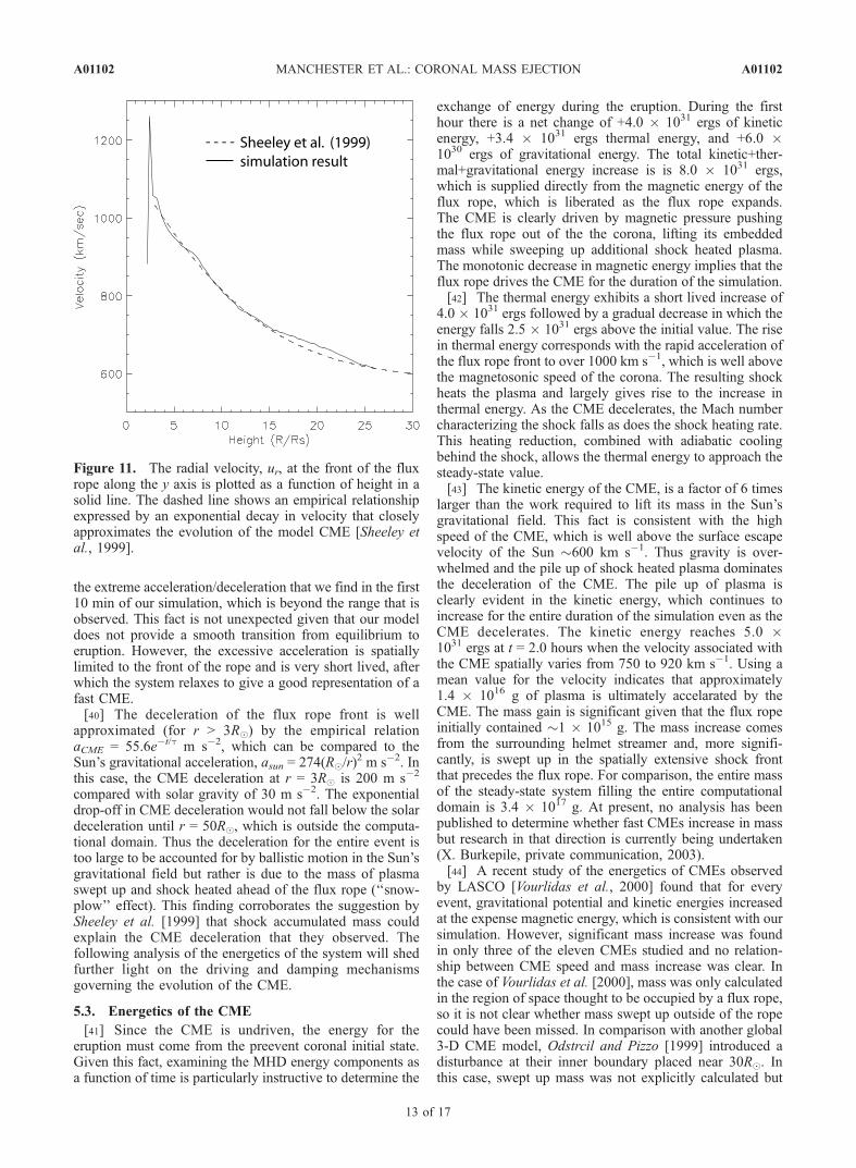
the extreme acceleration/deceleration that we find in the first10 min of our simulation, which is beyond the range that isobserved. This fact is not unexpected given that our modeldoes not provide a smooth transition from equilibrium toeruption. However, the excessive acceleration is spatiallylimited to the front of the rope and is very short lived, afterwhich the system relaxes to give a good representation of afast CME.[40] The deceleration of the flux rope front is well

approximated (for r > 3R) by the empirical relationaCME = 55.6et/t m s2, which can be compared to theSun’s gravitational acceleration, asun = 274(R/r)

2 m s2. Inthis case, the CME deceleration at r = 3R is 200 m s2

compared with solar gravity of 30 m s2. The exponentialdrop-off in CME deceleration would not fall below the solardeceleration until r = 50R, which is outside the computa-tional domain. Thus the deceleration for the entire event istoo large to be accounted for by ballistic motion in the Sun’sgravitational field but rather is due to the mass of plasmaswept up and shock heated ahead of the flux rope (‘‘snow-plow’’ effect). This finding corroborates the suggestion bySheeley et al. [1999] that shock accumulated mass couldexplain the CME deceleration that they observed. Thefollowing analysis of the energetics of the system will shedfurther light on the driving and damping mechanismsgoverning the evolution of the CME.

5.3. Energetics of the CME

[41] Since the CME is undriven, the energy for theeruption must come from the preevent coronal initial state.Given this fact, examining the MHD energy components asa function of time is particularly instructive to determine the

exchange of energy during the eruption. During the firsthour there is a net change of +4.0 � 1031 ergs of kineticenergy, +3.4 � 1031 ergs thermal energy, and +6.0 �1030 ergs of gravitational energy. The total kinetic+ther-mal+gravitational energy increase is is 8.0 � 1031 ergs,which is supplied directly from the magnetic energy of theflux rope, which is liberated as the flux rope expands.The CME is clearly driven by magnetic pressure pushingthe flux rope out of the the corona, lifting its embeddedmass while sweeping up additional shock heated plasma.The monotonic decrease in magnetic energy implies that theflux rope drives the CME for the duration of the simulation.[42] The thermal energy exhibits a short lived increase of

4.0 � 1031 ergs followed by a gradual decrease in which theenergy falls 2.5 � 1031 ergs above the initial value. The risein thermal energy corresponds with the rapid acceleration ofthe flux rope front to over 1000 km s1, which is well abovethe magnetosonic speed of the corona. The resulting shockheats the plasma and largely gives rise to the increase inthermal energy. As the CME decelerates, the Mach numbercharacterizing the shock falls as does the shock heating rate.This heating reduction, combined with adiabatic coolingbehind the shock, allows the thermal energy to approach thesteady-state value.[43] The kinetic energy of the CME, is a factor of 6 times

larger than the work required to lift its mass in the Sun’sgravitational field. This fact is consistent with the highspeed of the CME, which is well above the surface escapevelocity of the Sun �600 km s1. Thus gravity is over-whelmed and the pile up of shock heated plasma dominatesthe deceleration of the CME. The pile up of plasma isclearly evident in the kinetic energy, which continues toincrease for the entire duration of the simulation even as theCME decelerates. The kinetic energy reaches 5.0 �1031 ergs at t = 2.0 hours when the velocity associated withthe CME spatially varies from 750 to 920 km s1. Using amean value for the velocity indicates that approximately1.4 � 1016 g of plasma is ultimately accelarated by theCME. The mass gain is significant given that the flux ropeinitially contained �1 � 1015 g. The mass increase comesfrom the surrounding helmet streamer and, more signifi-cantly, is swept up in the spatially extensive shock frontthat precedes the flux rope. For comparison, the entire massof the steady-state system filling the entire computationaldomain is 3.4 � 1017 g. At present, no analysis has beenpublished to determine whether fast CMEs increase in massbut research in that direction is currently being undertaken(X. Burkepile, private communication, 2003).[44] A recent study of the energetics of CMEs observed

by LASCO [Vourlidas et al., 2000] found that for everyevent, gravitational potential and kinetic energies increasedat the expense magnetic energy, which is consistent with oursimulation. However, significant mass increase was foundin only three of the eleven CMEs studied and no relation-ship between CME speed and mass increase was clear. Inthe case of Vourlidas et al. [2000], mass was only calculatedin the region of space thought to be occupied by a flux rope,so it is not clear whether mass swept up outside of the ropecould have been missed. In comparison with another global3-D CME model, Odstrcil and Pizzo [1999] introduced adisturbance at their inner boundary placed near 30R. Inthis case, swept up mass was not explicitly calculated but

Figure 11. The radial velocity, ur, at the front of the fluxrope along the y axis is plotted as a function of height in asolid line. The dashed line shows an empirical relationshipexpressed by an exponential decay in velocity that closelyapproximates the evolution of the model CME [Sheeley etal., 1999].


13 of 17

A01102

their CME rapidly decelerated as it passed through a denseheliospheric plasma sheet while driving a shock. Thisbehavior is qualitatively similar to the deceleration andshock formation that we find.

5.4. Synthetic Coronagraph Images of the CME

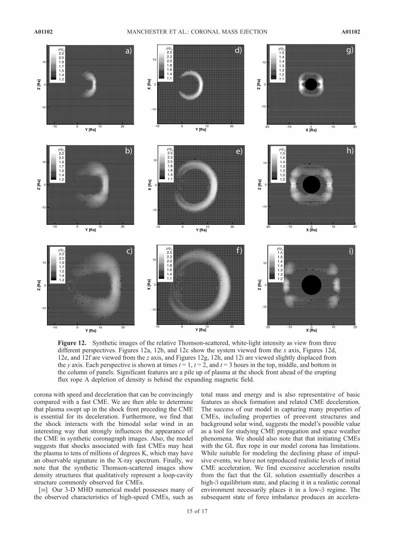
[45] We have produced a CME model with speeds that arecharacteristic of fast CMEs and we have found that in thiscase, strong shocks are driven in the low corona. It is rarethat features of CMEs observed in the corona in Thomson-scattered white light are interpreted as signatures of shocks.As an example, Sime and Hundhausen [1987] observed abright loop at the front of a CME that they identified as acandidate for a coronal shock. In this case, the presenceof a shock was inferred from the high speed of the loop(1070 km/s) and the absence of any deflections precedingthe CME; also the expanding loop did not cease its lateralmotion to form stationary legs. More recent observations bymultiple instruments on SOHO along with radio observa-tions have made clear cases for shocks that appear as visiblecomponents of CMEs in LASCO images. In two reports,Raymond et al. [2000] and Mancuso et al. [2002], shockswere observed simultaneously in the low corona (r < 3R)by LASCO, the Ultraviolet Coronagraph Spectrometer(UVCS) and as type II radio burst. UVCS gave clearspectroscopic evidence for the presence of shock frontsassociated with CMEs while radio bursts indicated thepresence of shock-accelerated electrons. The shock frontsobserved with LASCO by Raymond et al. [2000] andMancuso et al. [2002] were representative of fast CMEswith speeds of 1200 km/s and 1100 km/s, respectively,which is comparable to the speed observed by Sime andHundhausen [1987].[46] A discussion of our work would be incomplete

without mentioning the evolution of the plasma densityassociated with the shock front. Rather than simply display-ing 2-D representations of the density in various planes, it isfar more instructive to present the density as it would appearin a coronagraph image. To that end, we produce syntheticThomson-scattered white-light images from three perspec-tives at three different times, which are displayed inFigure 12. Here, Figures 12a, 12b, and 12c show the coronaviewed from the x axis at time t = 1.0, 2.0, 3.0 hours,respectively (‘‘side view’’). The same time sequence ispresented in Figures 12d, 12e, and 12f, as viewed fromthe polar axis (‘‘top view’’), while a halo CME representa-tion is given in Figures 12g, 12h, and 12i, viewed slightlyoff center from the y axis (‘‘front view’’). Each figure showsa gray scale image of the total scattered intensity ofradiation, I = It + Ir, where It and Ir are radiation intensitiespolarized tangential to the solar limb and radial to the Sun,respectively. The intensities are found by the line-of-sightintegration of the density multiplied by a scattering functionthat takes into account the extended light source of the limb-darkened solar disk as summarized by Billings [1966]. Forthese images, we have divided the background steady-stateintensity to form a relative brightness.[47] In the side view images, we find that the dense

core of plasma (see Figures 3a and 3b) is not present inthe line-of-sight images. The modest mass enhancement atthe base of the flux rope has expanded to such an amount by1.0 hour that its density is very near the background value.

We find that a dense shell of plasma exists between theshock front and the flux rope followed by a density depletedcavity. The shock front has the same basic features, as firstdescribed by Sime and Hundhausen [1987], namely a brightloop expanding in the corona at super-Alfvenıc velocity(>1000)km/s that expands laterally without forming station-ary legs. A more rarefied region forms between the coronalboundary and the rear of the flux rope reflecting the largedegree to which plasma is removed from the corona by theCME. There is also a narrow dark lane in the center of theejecta that is seen in Figure 12a at t = 1.0 hour. This is aconsequence of the CME passing through the plasma sheetand is qualitatively very similar to density images in thework of Wu et al. [1999].[48] The polar view of the CME shows a surprisingly

different morphology than is viewed from the side. Here,the enhanced density associated with the shock front standsout much more prominently and is seen to partially encirclethe Sun. For the synthetic images, the line-of-sight integralis dominated by density over the limb of the Sun, near theplane of the sky. Consequently, the polar view preferentiallyshows the density structure in the heliospheric current sheet.As we mentioned before, the low magnetosonic speeds nearthe current sheet lead to considerably higher Mach numbersthan are found at higher heliospheric latitude. Associatedwith the higher Mach number is a higher density compres-sion [Kabin, 2001], which results in the brighter shock frontin the polar view. The final column of Figures 12g, 12h, and12i shows a dramatic view of the CME directed toward theobserver as a halo event. In this case, we find that theintensity reflects a density structure strongly effected bythe MHD shock interaction with the bimodal solar wind.Here, the front has an oval shape aligned with the polar axis,which is indented and brightened at the sides near where thefront crosses the x axis. This morphology results from theenhanced density behind the shock front, which propagateswith enhanced speed and lower Mach number in the high-latitude fast wind relative to the lower speed and higherMach number of the shock (and greater density compres-sion) in the low-latitude slow wind.

6. Discussion and Conclusions

[49] We have investigated the time evolution of a 3-DMHD model of a CME driven by the magnetic pressure andbuoyancy of a flux rope in an initial state of force imbal-ance. The ensuing eruption originates in the low corona anddevelops as the flux rope and plasma are expelled throughthe solar wind. The model eruption possesses many featuresassociated with fast CMEs. First, the preevent structure ofour model, a dense helmet streamer possessing a cavity anddense core threaded by a six Gauss magnetic flux rope. Incomparison, observations show that the majority of CMEsoriginate from helmet streamers that overlie quiescentprominences [cf. Hundhausen, 1993] thought to be sup-ported by flux ropes [Low, 2001]. Second, the energy for theeruption comes from the preevent magnetic configurationand yields �5 � 1031 ergs of kinetic and gravitationalenergy to drive �1016 g of plasma from the corona. Boththe energy and mass that characterize the eruption are withinthe limits commonly observed for CMEs. The CME prop-agates to 32R through a realistic steady-state model of the


14 of 17

A01102

corona with speed and deceleration that can be convincinglycompared with a fast CME. We are then able to determinethat plasma swept up in the shock front preceding the CMEis essential for its deceleration. Furthermore, we find thatthe shock interacts with the bimodal solar wind in aninteresting way that strongly influences the appearance ofthe CME in synthetic coronagraph images. Also, the modelsuggests that shocks associated with fast CMEs may heatthe plasma to tens of millions of degrees K, which may havean observable signature in the X-ray spectrum. Finally, wenote that the synthetic Thomson-scattered images showdensity structures that qualitatively represent a loop-cavitystructure commonly observed for CMEs.[50] Our 3-D MHD numerical model possesses many of

the observed characteristics of high-speed CMEs, such as

total mass and energy and is also representative of basicfeatures as shock formation and related CME deceleration.The success of our model in capturing many properties ofCMEs, including properties of preevent structures andbackground solar wind, suggests the model’s possible valueas a tool for studying CME propagation and space weatherphenomena. We should also note that that initiating CMEswith the GL flux rope in our model corona has limitations.While suitable for modeling the declining phase of impul-sive events, we have not reproduced realistic levels of initialCME acceleration. We find excessive acceleration resultsfrom the fact that the GL solution essentially describes ahigh-b equilibrium state, and placing it in a realistic coronalenvironment necessarily places it in a low-b regime. Thesubsequent state of force imbalance produces an accelera-

Figure 12. Synthetic images of the relative Thomson-scattered, white-light intensity as view from threedifferent perspectives. Figures 12a, 12b, and 12c show the system viewed from the x axis, Figures 12d,12e, and 12f are viewed from the z axis, and Figures 12g, 12h, and 12i are viewed slightly displaced fromthe y axis. Each perspective is shown at times t = 1, t = 2, and t = 3 hours in the top, middle, and bottom inthe column of panels. Significant features are a pile up of plasma at the shock front ahead of the eruptingflux rope A depletion of density is behind the expanding magnetic field.


15 of 17

A01102

tion that is too large but ultimately yields an appropriateamount of energy. For the background pressure of ourmodel corona and our choice of GL parameters, we findthe flux rope can only be near equilibrium if the rope’s fieldstrength is near one Gauss. At two Gauss, the GL flux ropeproduces a low speed event in which magnetic reconnectionprovided a secondary, long-lasting acceleration for theCME.[51] In the future, our research will explore the MHD

processes by which CMEs make their way from thelow-b corona to the high-b solar wind with emphasis onshock structure. Advanced AMR techniques will beapplied to highly resolve shocks and allow us to capturehighly structured, multiple shock fronts [DeSterck et al.,1998] that may form. Larger-scale simulations willinvestigate the long-term fate of CMEs in interplanetaryspace. Fundamental questions need to be addressedconcerning the interaction of the flux rope with thesolar wind, including current sheet formation/dissipation,plasma swept up by the CME, and evolution of the 3-Ddensity structure. Finally, we will investigate the spaceweather phenomena associated with CMEs by couplingour model to a magnetospheric model of the Earth. Forsuch studies, we will introduce a much more realisticcoronal magnetic field configuration based on synopticmagnetograms. Improvements to the solar wind modelwill follow, as we include nonthermal momentum termsassociated with an Alfven wave driven wind. These aresome of the possibilities we will treat in our futureinvestigations.

[52] Acknowledgments. We thank B. C. Low, Sarah Gibson, ThomasZurbuchen, Tom Holzer, and Yuhong Fan for discussion and commentsconcerning the this research. The simulations reported here were carried outon an Origin2000 supercomputer at White Sands Missile Range DistributedCenter. The research for this manuscript was supported by DoD MURIgrant F49620-01-1-0359, NSF KDI grant NSF ATM-9980078, NSF CISEgrant ACI-9876943, and NASA AISRP grant NAG5-9406 at the Universityof Michigan. G. Toth is partially supported by the Education Ministry ofHungary (grant FKFP-0242-2000). M. Opher’s research was performed atthe Jet Propulsion Laboratory of the California Institute of Technologyunder a contract with NASA.[53] Shadia Rifai Habbal thanks both referees for their assistance in

evaluating this paper.

ReferencesAly, J. J. (1991), How much energy can be stored in a three-dimensionalforce-free magnetic field?, Astrophys. J. Lett., 375, L61–L64.

Amari, T., J. F. Luciani, Z. Mikic, and J. Linker (2000), A twisted flux ropemodel for coronal mass ejections and two-ribbon flares, Astrophys. J.Lett., 529, L49–L52.

Antiochos, S. K., C. R. DeVore, and J. A. Klimchuk (1999), A model forsolar coronal mass ejections, Astrophys. J., 510, 485–493.

Axford, W. I., and J. F. McKenzie (1996), The acceleration of the solarwind, in Solar Wind Eight, edited by D. Winterhalter et al., AIP Conf.Proc. Ser. 382, 72–75.

Billings, D. W. (1966), A Guide to the Solar Corona, Academic, San Diego,Calif.

Chen, J. (1996), Theory of prominence eruption and propagation: Interpla-netary consequences, J. Geophys. Res., 101, 27,499.

Chen, P. F., and K. Shibata (2000), An emerging flux trigger mechanism forcoronal mass ejections, Astrophys. J., 545, 524–531.

Choe, G. S., and L. C. Lee (1996), Evolution of solar magnetic arcades. II.Effects of resistivity and solar eruptive processes, Astrophys. J., 472,372–388.

DeSterck, H., B. C. Low, and S. Poedts (1998), Complex magnetohydro-dynamic bow shock topology in field-aligned low-b flow around a per-fectly conducting cylinder, Phys. Plasmas, 6, 4015–4027.

Dryer, M., S. Wu, R. S. Steinolfson, and R. M. Wilson (1979), Magneto-hydrodynamic models of coronal transients in the meridional plan. II.

Simulation of the coronal transient of 1973 August 21, Astrophys J.,227, 1059.

Fan, Y., and B. C. Low (2003), Dynamics of CME driven by a Buoy-antProminence flux tube, in Proceedings of the 21st InternationalNSO/SacPeak Workshop, ASP Conf. Ser., vol. 286, edited by A. A.Pevtsov and H. Uitenbroek, p. 347, Astron. Soc. of the Pacific, SanFransisco, Calif..

Fisk, L. A., N. A. Schwadron, and T. H. Zurbuchen (1999), Acceleration ofthe fast solar wind by the emergence of new magnetic flux, J. Geophys.Res., 104, 19,765–19,772.

Forbes, T. G. (2000), A review on the genesis of coronal mass ejections,J. Geophys. Res., 105, 23,153–23,165.

Forbes, T. G., and E. R. Priest (1995), Photospheric magnetic field evolu-tion and eruptive flares, Astrophys. J., 446, 377–389.

Gibson, S., and B. C. Low (1998), A time-dependent three-dimensionalmagnetohydrodynamic model of the coronal mass ejection, Astrophys. J.,493, 460–473.

Groth, C. P. T., D. L. De Zeeuw, T. I. Gombosi, and K. G. Powell (2000),Global three-dimensional MHD simulation of a space weather event:CME formation, interplanetary propagation, and interaction with themagnetosphere, J. Geophys. Res., 105, 25,053–25,078.

Hollweg, J. V., S. Jackson, and D. Galloway (1982), Alfven waves in thesolar atmosphere. III. Nonlinear waves on open flux tubes, Sol. Phys., 75,35–61.

Howard, R. A., et al. (1997), Observations of CMEs from SOHO/LASCO,in Coronal Mass Ejections, Geophys Monogr. Ser., vol. 99, edited byN. Crooker, J. A. Joselyn, and J. Feynman, pp. 17–26, AGU,Washington,D. C.

Hundhausen, A. J. (1988), The origin and propagation of coronal massejections, in Solar Wind Six, edited by V. J. Pizzo, T. E. Holzer, andD. G. Sime, Tech. Note NCAR/TN-306+Proc, pp. 181–214, Natl. Cent.for Atmos. Res., Boulder, Colo.

Hundhausen, A. J. (1990), Coronal Mass Ejections: A summary of SMMobservations from 1980 and 1984–1989, in The Many Faces of the Sun,edited by K. Strong, J. Saba, and B. Haisch, pp. 143–200, Springer-Verlag, New York.

Hundhausen, A. J. (1993), Sizes and locations of coronal mass ejections:SMM observations from 1980 and 1984–1989, J. Geophys Res., 98,13,177–13,200.

Kabin, K. (2001), A note on the compression ratio in MHD shocks,J. Plasma Phys., 66, 259–274.

Leroy, J. L., V. Bommier, and S. Sahal-Brechot (1983), The magnetic fieldin the prominences of the polar crown, Sol. Phys., 83, 135–142.

Lin, J., and T. G. Forbes (2000), Effects of reconnection on the coronalmass ejection process, J. Geophys. Res., 105, 2375–2392.

Linker, J. A., and Z. Mikic (1995), Disruption of a helmet streamer byphotospheric shear, Astrophys. J. Lett., 438, L45–L48.

Linker, J. A., Z. Mikic, R. Lionello, P. Riley, T. Amari, and D. Odstrcil(2003), Flux cancellation and coronal mass ejections, Phys. Plasmas, 10,1971–1978.

Low, B. C. (1983), Expolsion of magnetized plasmas from coronae, inSolar and Stellar Magnetic Fields: Origins and Coronal Effects,pp. 467–471, D., Reidel, Norwell, Mass.

Low, B. C. (1994), Magnetohydrodynamic processes in the solar corona:Flares, coronal mass ejections, and magnetic helicity, Phys. Plasmas, 1,1684–1690.

Low, B. C. (1996), Solar activity and the corona, Sol. Phys., 167, 217–265.Low, B. C. (2001), Coronal mass ejections, magnetic flux ropes, and solarmagnetism, J. Geophys. Res., 106, 25,141–25,163.

Low, B. C., and J. R. Hundhausen (1995), Magnetostatic structures of thesolar corona. II. the magnetic topology of quiescent prominences, Astro-phys. J., 443, 818–836.

Mancuso, S., J. C. Raymond, J. Kohl, Y.-K. Ko, M. Uzzo, and R. Wu(2002), UVCS/SOHO observations of a CME-driven shock: Conse-quences on ion heating mechanisms behind a coronal shock, Astron.Astrophys., 383, 267–274.

Mouschovias, T. C., and A. I. Poland (1978), Expansion and broadening ofcoronal loop transients: A theoretical explanation, Astrophys. J., 220,675–682.

Mikic, Z., and J. A. Linker (1994), Disruption of coronal magnetic fieldarcades, Astrophys. J., 430, 898–912.

Mikic, Z., D. C. Barnes, and D. Schnack (1988), Dynamical evolution of asolar coronal magnetic field arcade, Astrophys. J., 328, 830–847.

Moore, R. L., A. C. Sterling, H. S. Hudson, and R. J. Lemen (2001), Onsetof the magnetic explosions in solar flares and coronal mass ejections,Astrophys J., 552, 833.

Odstrcil, D., and V. J. Pizzo (1999), Three-dimensional propagation ofcoronal mass ejections (CMEs) in a structured solar wind flow: 1.CME launched within the streamer belt, J. Geophys. Res., 104,483–492.


16 of 17

A01102

Odstrcil, D., M. Dryer, and Z. Smith (1996), Propagation of an interplane-tary shock along the heliosphere plasma sheet, J. Geophys. Res., 101,19,973–19,986.

Parker, E. N. (1963), Interplanetary Dynamical Processes, Wiley-Inter-science, New York.

Pneuman, G. W., and R. A. Kopp (1971), Gas-magnetic field interactions inthe solar corona, Sol. Phys., 18, 258–270.

Powell, K. G., P. L. Roe, T. J. Linde, T. I. Gombosi, and D. L. De Zeeuw(1999), A solution-adaptive upwind scheme for ideal magnetohydrody-namics, J. Comput. Phys., 154, 284.

Raymond, J. C., B. J. Thompson, O. C. St.Cyr, N. Gopalswamy, S. Kahler,M. Kaiser, A. Lara, A. Ciaravella, M. Romoli, and R. ONeal (2000),SOHO and radio observations of a CME shock wave, Geophys. Res.Lett., 27, 1439–1442.

Riley, P., J. A. Linker, Z. Mikic, D. Odstrcil, V. J. Pizzo, and D. F. Webb(2002), Evidence of posteruption reconnection associated with coronalmass ejections in the solar wind, Astrophys. J., 578, 972–978.

Sheeley, N. R., J. H. Walters, Y.-M. Wang, and R. A. Howard (1999),Continuous tracking of coronal outflows: Two kinds of coronal massejections, J. Geophys Res., 104, 24,739–24,767.

Sime, D. G., and A. J. Hundhausen (1987), The coronal mass ejection ofJuly 6, 1980: A candidate for interpretation as a coronal shock wave,J. Geophys Res., 92, 1049–1055.

Steinolfson, R. S. (1991), Coronal evolution due to shear motion, Astro-phys. J., 382, 677.

Steinolfson, R. S., and A. J. Hundhausen (1990), MHD intermediate shocksin coronal mass ejections, J. Geophys. Res., 95, 6389–6401.

Sterling, A. C., and H. S. Hudson (1997), X-ray dimming in halo coronalmass ejections, Astrophys. J. Lett., 491, L55.

Sturrock, P. A. (1991), Maximum energy of semi-infinite magnetic fieldconfigurations, Astrophys. J., 380, 655.

Tokman, M., and P. M. Bellan (2002), Three-dimensional model of thestructure and evolution of coronal mass ejections, Astrophys. J., 567,1202–1210.

Usmanov, A. V., M. L. Goldstein, B. P. Besser, and J. M. Fritzer (2000), Aglobal MHD solar wind model with WKB Alfven waves: Comparisonwith Ulysses data, J. Geophys. Res., 105, 12,675–12,696.

Vourlidas, A., P. Subramanian, K. P. Dere, and R. A. Howard (2000),Large-angle spectrometric coronagraph measurements of the energeticsof coronal mass ejections, Astrophys. J., 534, 456–467.

Wang, Y.-M., and N. R. Sheeley Jr. (1994), Global evolution of the inter-planetary sector structure, coronal holes, and solar wind streams during1976–1993: Stackplot displays based on magnetic observations, J. Geo-phys. Res., 99, 6597–6608.

Wolfson, R. (1982), Equilibria and stability of coronal magnetic arcades,Astrophys. J., 255, 774.

Wu, S. T., and W. P. Guo (1997), A self-consistent numerical magnetohy-drodynamic (MHD) model of helmet streamer and flux-rope interactions:Initiation and propagation of Coronal Mass Ejections (CMEs), in CoronalMass Ejections, Geophys. Monogr. Ser., vol. 99, edited by N. Crooker,J. A. Joselyn, and J. Feynman, pp. 83–89, AGU, Washington, D. C.

Wu, S. T., W. P. Guo, D. J. Michels, and L. F. Burlaga (1999), MHDdescription of the dynamical relationships between a flux rope, streamer,coronal mass ejection, and magnetic cloud: An analysis of the January1997 Sun-Earth connection event, J. Geophys. Res., 104, 14,789 –14,801.

Wu, S. T., W. P. Guo, S. P. Plunkett, B. Schmieder, and G. M. Simnett(2000), Coronal mass ejections (CMEs) initiation: Models and observa-tions, J. Atmos. Sol. Terr. Phys., 62, 1489–1498.

Zhang, M., L. Golub, E. DeLuca, and J. Burkepile (2002), The timing offlares associated with the two dynamical types of coronal mass ejections,Astrophys. J. Lett., 574, L97–L100.

W. B. Manchester IV, T. I. Gombosi, I. Roussev, D. L. De Zeeuw, I. V.

Sokolov, and K. G. Powell, Center for Space Environment Modeling,University of Michigan, 2455 Hayward Street, Ann Arbor, MI 48109, USA.([email protected]; [email protected]; [email protected]; [email protected]; [email protected]; [email protected])G. Toth, Department of Atomic Physics, Eotvos University, Pazmany

setany 1/A, Budapest 1117, Hungary. ([email protected])M. Opher, Jet Propulsion Laboratory, California Institute of Technology,

Pasadena, CA 91109-8099, USA. ([email protected])


17 of 17

A01102

Documents

Three-dimensional MHD simulation of a flux rope driven CME