Three-Dimensional Mapping of Fluorescent Dye Using a

Three-Dimensional Mapping of Fluorescent Dye Using a Scanning, Depth-ResolvingAirborne Lidar

M. A. SUNDERMEYER

School for Marine Science and Technology, University of Massachusetts, Dartmouth, New Bedford, Massachusetts

E. A. TERRAY AND J. R. LEDWELL

Department of Applied Ocean Physics and Engineering, Woods Hole Oceanographic Institution, Woods Hole, Massachusetts

A. G. CUNNINGHAM, P. E. LAROCQUE, AND J. BANIC

Optech Incorporated, Vaughan, Toronto, Ontario, Canada

W. J. LILLYCROP

Joint Airborne LIDAR Bathymetry Technical Center of Expertise, U.S. Army Corps of Engineers, Mobile, Alabama

(Manuscript received 28 October 2005, in final form 3 July 2006)

ABSTRACT

Results are presented from a pilot study using a fluorescent dye tracer imaged by airborne lidar in theocean surface layer on spatial scales of meters to kilometers and temporal scales of minutes to hours. Thelidar used here employs a scanning, frequency-doubled Nd:YAG laser to emit an infrared (1064 nm) andgreen (532 nm) pulse 6 ns in duration at a rate of 1 kHz. The received signal is split to infrared, green, andfluorescent (nominally 580–600 nm) channels, the latter two of which are used to compute absolute dyeconcentration as a function of depth and horizontal position. Comparison of dye concentrations inferredfrom the lidar with in situ fluorometry measurements made by ship shows good agreement both qualita-tively and quantitatively for absolute dye concentrations ranging from 1 to �10 ppb. Uncertainties associ-ated with horizontal variations in the natural seawater attenuation are approximately 1 ppb. The resultsdemonstrate the ability of airborne lidar to capture high-resolution three-dimensional “snapshots” of thedistribution of the tracer as it evolves over very short time and space scales. Such measurements offer apowerful observational tool for studies of transport and mixing on these scales.

1. Introduction

a. Overview and background

For decades, dye release experiments in the upperocean and pycnocline have been used to study the dis-persal and transport of passive tracers in natural waters(e.g., Kullenberg 1971; Okubo 1971; Vasholz and Craw-ford 1985). The naturally integrating properties ofLagrangian tracers in both space and time allow slowbut persistent motions to be detected on a variety of

time and space scales. One of the difficulties of usingLagrangian tracers, however, is that quantitative esti-mates of dye concentrations have traditionally requiredin situ measurements of the dye patch. Yet conven-tional shipboard measurements are time consumingand often lack the spatial and/or temporal coveragerequired to understand the underlying physics. This isparticularly true for small scales, that is, spatial scales ofmeters to kilometers and temporal scales of minutes tohours.

Of particular interest here are both vertical and hori-zontal mixing processes in the ocean surface layer, andalong and across its base. These processes are central tounderstanding and modeling how the mixed layer andthe deeper ocean communicate, and are central issuesin a number of fundamental questions in oceanography,

Corresponding author address: M. A. Sundermeyer, School forMarine Science and Technology, University of Massachusetts,Dartmouth, 706 Rodney French Blvd., New Bedford, MA 02744-1221.E-mail: [email protected]

1050 J O U R N A L O F A T M O S P H E R I C A N D O C E A N I C T E C H N O L O G Y VOLUME 24

DOI: 10.1175/JTECH2027.1

© 2007 American Meteorological Society

JTECH2027

such as the contribution of atmospheric forcing to mix-ing and circulation in the ocean interior, the transportof nutrients across the base of the mixed layer, and theobserved patchiness of biological organisms in thephotic zone. Despite the importance of mixing and lat-eral dispersion on these scales, however, little is knownfrom direct observations, mainly due to the inability tomake observations with the requisite spatiotemporalresolution and coverage.

One approach that offers considerable promise inthis regard is the coupling of fluorescent dye releaseswith the mapping capability of airborne lidar operatingat low altitude (on the order of several hundredmeters). In combination, these two approaches offer apowerful tool for studying mixing and stirring processesin the upper ocean. Particularly because of the rela-tively short temporal and spatial scales characteristic ofthese processes, the ability of an airborne lidar to non-intrusively capture high-resolution three-dimensional“snapshots” of the distribution of the tracer patch as itevolves over time represents a unique observational ca-pability.

Specialized lidar systems have been developed foroceanographic use by a number of organizations, in-cluding the National Aeronautics and Space Adminis-tration (NASA), the Unites States Navy, and the Na-tional Oceanographic and Atmospheric Administration(NOAA). These systems have been shown to be veryeffective for their intended uses: bathymetric surveys(e.g., Irish and Lillycrop 1999), chlorophyll mapping(e.g., Hoge and Swift 1983; Yoder et al. 1993), and fishstock assessment (e.g., Squire and Krumboltz 1981;Churnside et al. 1997). Despite efforts in these otherareas, however, there have been few studies using lidarin conjunction with the fluorescent dye releases tostudy small-scale mixing in the ocean. In fact, we areaware of only three other studies in the published lit-erature in which airborne lidar was used to obtainquantitative estimates of dye concentration in the up-per ocean. These studies differ from the present work,however, in that they reported only depth-integratedconcentrations of dye, whereas here we estimate dyeconcentration as a function of depth.

One of the prior studies, reported by Hoge and Swift(1981), used NASA’s Airborne Oceanographic lidar(AOL). The AOL employs a conically scanning laser,with a multispectral time-gated receiving capability. Inthat study, the observed ratio of fluorescence to waterRaman backscatter was calibrated with similar mea-surements in the laboratory and used to infer absolutedye concentrations in the field. A major advantage tothis approach is that it enabled absolute dye concentra-tions to be inferred from airborne measurements with-

out the need for in situ water column sampling. Despitethe time gating capability of AOL, however, Hoge andSwift (1981) did not report on depth dependence of thedye patch. Still, their study was significant in that theytracked the dye for approximately 2 h after release,with horizontal resolutions of better than 10 m (abso-lute positioning accuracy of the airborne measurementswas not reported) and a minimum detectable single-pulse integrated water column dye concentration of ap-proximately 2 ppb.

A second published study, by Franz et al. (1982),mapped the distribution of Rhodamine B over a periodof 2 days using an airborne lidar flown in a helicopter.In that study, the lidar system used was a nonscanningflashlamp-pumped laser operated by the University ofOldenburg, Germany. There the authors relied on si-multaneous in situ measurements of dye concentrationand attenuation depth to determine dye concentrationfrom the lidar signal. They also used a comparativelyhigh-powered laser (1 J compared to the AOL’s 1 mJ),which presumably enabled them to detect dye deeper inthe water column. They reported being able to map dyeconcentrations ranging from less than 1 ppb up to 30ppb along individual flight tracks of the aircraft, with anestimated positioning accuracy of about 100 m (basedon the Decca radio-location system). However, theirdetector did not have time-resolving capability, so thatlike Hoge and Swift (1981), although for different rea-sons, they also did not resolve depth-dependent dyeconcentrations.

Finally, a third study was conducted by a group fromthe Johns Hopkins University Applied Physics Labora-tory (Mack et al. 1997). They used a lidar operated bythe Naval Air Warfare Command to track the horizon-tal and vertical spreading of dye streaks injected in theSargasso Sea. Their lidar measurements did providedepth resolution of their dye patch. However, they ul-timately used the towed fluorometer chain to infer thediapycnal diffusivity of the dye. They did not reportestimates of the horizontal diffusivity.

b. Scope and outline

Here we revisit the idea of using airborne lidar forsurveying dye release experiments in the upper oceanand pycnocline. Advances in navigational systems, im-provements in airborne lidar technology, and the ad-vent of new airborne and in situ observational capabili-ties (e.g., shipboard ADCP) all lend themselves to bet-ter observing of the physics of ocean mixing on shorttime and space scales. The most notable advance of thepresent study compared with previous experiments ofthis type (with the possible exception of Mack et al.1997) is the ability to obtain depth-resolved dye con-

JUNE 2007 S U N D E R M E Y E R E T A L . 1051

centrations with a vertical resolution on the order of1 m and an absolute horizontal position accuracy of2.5 m. We also present a different method for convert-ing measured intensity in the laser and dye wave bandsto absolute dye concentration. This is done using boththe backscatter and dye fluorescence. Detailed in situobservations are also used to compare the airbornemeasurements with more traditional shipboard surveysusing towed conductivity–temperature–depth (CTD)and fluorometer observations.

The present paper is organized as follows: in section2 we describe the field experiments and the methodol-ogy used to inject and sample the dye patch, as well asthe methods used to invert the measured backscatterand fluorescence intensity to dye concentration. Re-sults are described in section 3, including both the insitu and airborne measurements. Similarities and dif-ferences between the in situ and airborne measure-ments are described in section 4, along with possiblesources of errors and uncertainties and considerationsfor future studies. Section 5 summarizes and concludes.

2. Description of field experiments

Two dye releases were conducted in the near-surfacewaters approximately 5 km due east of Ft. Lauderdale,

Florida, one on 2 June and the other on 3 June 2004(Fig. 1). The study site was chosen in part because ofthe favorable optical qualities of the water in this regionand in part to coincide with scheduled activities of theU.S. Army Corps of Engineers (USACE) Joint Air-borne Lidar Bathymetry Technical Center of Expertise(JALBTCX) group. The dye injections and in situ sam-pling were carried out using the Florida Atlantic Uni-versity research vessel, R/V Stephan. Both experimentswere performed in approximately 200-m water depth,far enough offshore to be outside the nearshore band ofhigher chlorophyll and suspended particulates, but notso far as to be subjected to significant currents associ-ated with the Gulf Stream. On each of the 2 days, 5 kgof Rhodamine WT were injected in a single streak andsubsequently mapped over a period of 1–2 h using afluorometer/CTD system towed from the ship, as wellas airborne lidar. For reasons described below, we focushere on results from the second of these two releases.

a. Dye injection and in situ sampling

The 3 June dye release was conducted at approxi-mately 0900 local time. A 20% solution of 5 kg ofRhodamine WT was first mixed with isopropyl alcoholto match the density of the dye mixture with that of thenear-surface waters at the injection site to within

FIG. 1. Chlorophyll concentration inferred from satellite sea surface color over the FloridaStraits (Feldman and McClain 2004). Inset to the figure shows the ship track during the 3 Junedye surveys—red, green, and magenta curves indicate the first transect, the zigzag survey, andthe final transect, respectively. Bold lines indicate the ship’s location at times correspondingto the lidar overflights.


Fig 1 live 4/C

0.001 kg L�1. The resulting solution was then dilutedwith surface seawater to obtain a total volume of dyesolution of approximately 200 L. The dye mixture waspumped at a rate of approximately 0.2 L s�1 down agarden hose to the injection sled, where it was releasedthrough a T-shaped pvc diffuser. The injection sled,which was also used for subsequent sampling of the dye,consisted of the diffuser, an Ocean Sensors OS200CTD, and two Chelsea fluorometers, one for dye andone for chlorophyll.

The injection was performed at a ship speed of ap-proximately 3.6 kt. The total injection time for the ex-periment was approximately 15 min. This resulted in aninjection streak length of approximately 1600 m, withan average initial dye concentration based on estimatesof the size of the patch on the order of 40 ppb. The dyewas injected in a stairstep profile, starting at a depth of2.5 m for approximately 1 min, followed by a deepersegment at 5 m, followed by an even deeper segment at10 m, then returning to the surface and repeating (Fig.2). This resulted in a series of surface segments of thepatch, interspersed with progressively deeper segmentsat discrete depths. The pumping rate of the dye washeld constant throughout the injection, which allowedquantitative assessment of the depth-resolving capabili-ties of the airborne lidar using similar dye concentra-tions at various depths. The surface segments of thepatch provided the additional advantage of enablingthe aircraft to visually align with the axis of the tracerstreak during successive lidar passes.

Ship-based sampling of the dye patch commencedimmediately after injection and continued for 1–2 hthereafter. Surveys of the patch consisted of a singleline transect along the major axis of the dye streak,followed by a zigzag survey, followed by another linetransect (see inset to Fig. 1). Ship speed during thesurveys varied between 2 and 4 kt, while the depth ofthe tow sled was cycled between the surface and 10–20m with the winch. This resulted in an oblique up–downprofile approximately every 1 min, or 50–100 m, de-

pending on the ship speed at the time. The CTD andfluorometers all sampled at a rate of 6 Hz, which, for awinch speed of approximately 0.5 m s�1, resulted in avertical sample resolution of approximately 10 cm. Inaddition to the tow sled, the ship was equipped with a300-kHz RD Instruments Workhorse acoustic Dopplercurrent profiler. The ADCP was set to sample at a rateof 1 Hz, with a vertical bin size of 2 m. Data from theADCP were logged nearly continuously during the in-jection and sampling.

b. Measurements from airborne lidar

Overflights of the dye patches were conducted usingan airborne lidar. We used a SHOALS-1000T lidarmanufactured by Optech Incorporated and operated byJALBTCX (Irish and Lillycrop 1999; Günther et al.1996). The SHOALS-1000T system uses a frequency-doubled Nd:YAG laser to produce 1064- and 532-nmpulses 6 ns in duration. The laser pulses at a rate of 1kHz, and scans approximately transverse to the direc-tion of flight at a rate of 10–15 Hz through a conical arcwith a constant incidence angle of 20°. In its bathymet-ric configuration, the system has four receive chan-nels—one at 1064 nm [infrared (IR)], two at 532 nm(green), and one at 650 nm to measure Raman back-scatter. The transmit pulses at both 532 and 1064 nmare approximately linearly polarized, while the receiv-ers are essentially unpolarized. The infrared and Ra-man channels are used to obtain redundant estimates ofthe location of the sea surface, while the two greenchannels (one for shallow returns and one for deep) arenormally used to detect the bottom. Following eachpulse, the received waveforms of all four channels aredigitized at a rate of 1 GHz and recorded for postflightprocessing. Measurements are georeferenced usingGPS, using inertial sensors to measure the aircraft’sattitude. At an aircraft altitude of 200 m, horizontalresolution is on the order of 3–4 m over a swath widthof 100 m. The range resolution within the water col-umn, which is set by the pulse length, is approximately

FIG. 2. Injection time series showing the staircase of different depths where the dye was injected. Theinjection was performed while the ship was headed southward, hence, early times correspond to thenorthernmost extent of the patch, while later times are at the southern extent.


1 m, although higher resolutions are possible for map-ping bottom bathymetry.

To measure dye fluorescence, we used a slight modi-fication of the SHOALS-1000T bathymetric configura-tion. Namely, we replaced the receiver optics of theexisting Raman channel with a narrowband filter cen-tered around the peak emission wavelength of the dye(i.e., centered at 580 nm with cutoffs at 560 and 600nm). This receive channel was then routed to the highgain electronics of the shallow green channel. The latterspanned a wider range of depths than the Raman chan-nel, typically down to about 20 m, compared to only 5–8m in the Raman. The reconfiguration took about 20min on the ground. In dye sampling mode, we recordedthe fluorescence (nominally 580 nm), the infrared, andthe deep green channels. The latter used a photomul-tiplier (PMT) detector and was the most sensitive of thethree channels. The fluorescence channel used an ava-lanche photo detector (APD).

c. Method of inversion for dye concentration

We use the measured profiles of backscatter at 532nm and fluorescence at 580 nm to estimate dye concen-tration as a function of depth. The inversion approachis described briefly here. Additional details are given inTerray et al. (2005).

We make the simplifying assumption that the onlyunknowns are the dye concentration C(z) and the lightintensity in the water just below the surface. To invertthe measured intensity profiles directly, one approachwould be to condition the problem further by estimat-ing C(z) on a coarser grid than the depth resolution ofthe measurements. Alternatively, in the interest ofachieving a fast inversion, we can reduce the problem tojust two dimensions by using an exact inversion of ourfluorescence model (Klett 1981, 1985). The latter allowsus to parameterize the concentration profile in terms ofan unknown constant of proportionality P, which is re-lated to the incident intensity just below the surface,and the dye concentration Cr � C(zr) at some referencedepth zr. These parameters can then be determined bya joint least squares fit to the fluorescence intensityprofile and to the backscatter-derived concentrationprofile over a limited region where the signal-to-noiseratio is high.

Before discussing the general inversion, we reviewthe use of the backscatter profile at 532 nm to infer dyeconcentration. This approach is based on the fact thatthe dye absorption/fluorescence process removes pho-tons from the incident 532-nm beam. The measuredprofiles of backscatter outside the patch in dye-free wa-ter are approximately exponential and give a mean li-dar attenuation coefficient of k � 0.085 � 0.003 m�1.

Meanwhile, the absorption coefficient of RhodamineWT at the laser wavelength of 532 nm is approximately�D532 � 0.03 m�1 ppb�1, so that a dye concentration ofa few ppb will lead to an O(1) contribution to the total(dye plus water) attenuation. The received backscat-tered intensity I532 from the range gate at depth z canthus be modeled as

I532�z� � IS532�z� exp��2�0

z

�D532C�z�� dz��,

�1�

where IS532 is the attenuation profile associated with theambient seawater, and the exponential accounts for theadditional absorption by the dye. The dye concentra-tion C(z) (ppb) can then be estimated as

C�z� �1

2�D532

d

dzln�IS532�z�

I532�z� �. �2�

Note that if the “background” backscatter due to ev-erything but the dye is stationary and homogeneousover the time and space scales of our experiment, thenIS532 can be estimated from measurements outside thedye patch. For our experiments, we have checked thatthis is a good approximation by comparing mean pro-files of I�1

532dI532/dz taken in dye-free water to the northand south of the dye streaks (the locations were sepa-rated by roughly 1 km, and the aircraft flew at a con-stant altitude throughout the experiment). The profilesare essentially indistinguishable over the upper 30 m ofthe water column. Thus, (2) provides a local estimate ofC(z) based entirely (apart from the specific dye attenu-ation coefficient �D532) on measured backscatter pro-files in the 532-nm “green” channel.

Our model for the received signal in the 580-nm“fluorescence” channel is based on the backscattermodels of Gordon (1982) and Phillips and Koerber(1984), extended to include fluorescence and attenua-tion by the dye. We write it as

I�z� � PC�z� exp��0

z

��DC�z�� kS� dz��, �3�

where �D is the sum of the specific dye absorption co-efficients in the 532- and 580-nm bands, and kS(z)(m�1) denotes the sum of the lidar attenuation coeffi-cients in those two bands due to scattering and absorp-tion by everything but the dye. Subsumed in P are theincident intensity of the laser light and the transmissiv-ity of the surface to ingoing and outgoing radiation, aswell as a number of system-dependent constants such asthe receiver aperture, aircraft altitude, and pulselength. The P also contains a factor (nh |z|)�2 de-scribing the diminution of the intensity due to geo-


metrical spreading, where n is the index of refraction ofseawater and h is the aircraft altitude. However, in thisexperiment, h 200 m and zmax 10 m, and thereforethis factor varies by less than 10%. Consequently, whilewe permit P to vary from profile to profile, we assumehere that it is independent of depth.

Following Klett (1981), (3) can be used to relate theconcentration at any depth to the concentration at adeeper depth. Differentiating (3), we obtain the non-linear differential equation

dC

dz� �DC2 � g�z�C � 0, �4�

where g(z) � I�1580 dI580/dz kS(z) is given by observa-

tion. Equation (4) can be integrated to give the con-centration at any depth in terms of the concentration atanother “reference depth” zr. The solution can be writ-ten as

C � C �z|Cr, �D, kS�z�, I580�z��, �5�

where Cr � C(zr) and I580(z) is the measured intensityprofile. As noted by Klett (1981), the integration isstable if z zr, although in practice it is possible tointegrate to depths somewhat deeper than zr. Substitut-ing the solution for C(z) back into (3), we obtain amodel for I(z) that depends on the two unknown valuesCr and P, and functionally on the observed I580 profile.

Combining the above approaches for both the back-scatter and fluorescence channels, we estimate Cr and Pby fitting the measured I580 profile and part of the con-centration profile C532 estimated from the excess at-tenuation in the 532-nm channel [Eq. (2)]. Here we usethe cost function

�2 � ||I � I580||2 w||C � C532||2. �6�

This function has been shown in simulations to providea reasonably shaped error surface (Terray et al. 2005).The weight w is adjusted to balance the contributionsfrom the two error terms, and only the part of the C532

profile that is well above the noise floor is used.In this procedure, both �D and the lidar attenuation

coefficient kS, which may be depth-dependent, must beknown. From laboratory measurements, we take �D ��D532 �D580 � 0.035 m�1 ppb�1. Similarly, kS can bewritten as the sum kS � k532 k580. We estimate k532

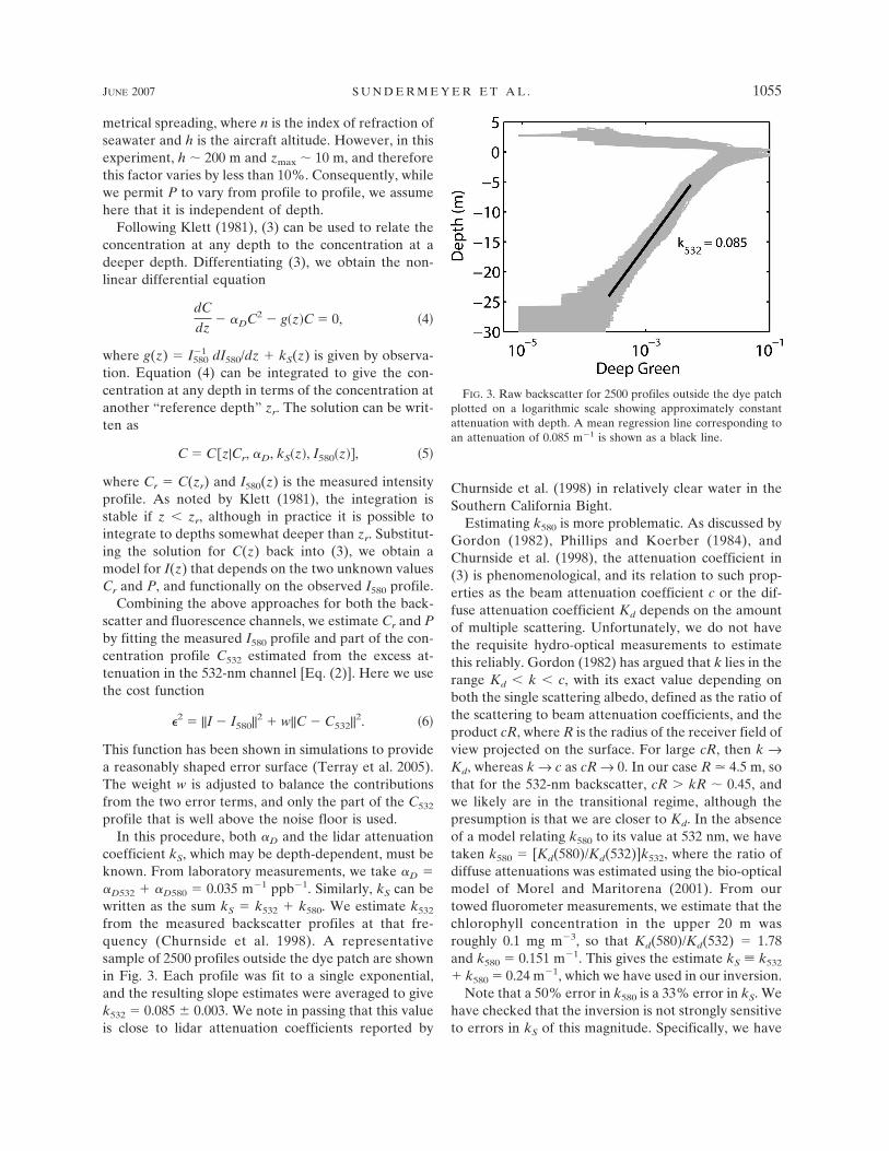
from the measured backscatter profiles at that fre-quency (Churnside et al. 1998). A representativesample of 2500 profiles outside the dye patch are shownin Fig. 3. Each profile was fit to a single exponential,and the resulting slope estimates were averaged to givek532 � 0.085 � 0.003. We note in passing that this valueis close to lidar attenuation coefficients reported by

Churnside et al. (1998) in relatively clear water in theSouthern California Bight.

Estimating k580 is more problematic. As discussed byGordon (1982), Phillips and Koerber (1984), andChurnside et al. (1998), the attenuation coefficient in(3) is phenomenological, and its relation to such prop-erties as the beam attenuation coefficient c or the dif-fuse attenuation coefficient Kd depends on the amountof multiple scattering. Unfortunately, we do not havethe requisite hydro-optical measurements to estimatethis reliably. Gordon (1982) has argued that k lies in therange Kd k c, with its exact value depending onboth the single scattering albedo, defined as the ratio ofthe scattering to beam attenuation coefficients, and theproduct cR, where R is the radius of the receiver field ofview projected on the surface. For large cR, then k →Kd, whereas k → c as cR → 0. In our case R � 4.5 m, sothat for the 532-nm backscatter, cR � kR 0.45, andwe likely are in the transitional regime, although thepresumption is that we are closer to Kd. In the absenceof a model relating k580 to its value at 532 nm, we havetaken k580 � [Kd(580)/Kd(532)]k532, where the ratio ofdiffuse attenuations was estimated using the bio-opticalmodel of Morel and Maritorena (2001). From ourtowed fluorometer measurements, we estimate that thechlorophyll concentration in the upper 20 m wasroughly 0.1 mg m�3, so that Kd(580)/Kd(532) � 1.78and k580 � 0.151 m�1. This gives the estimate kS � k532

k580 � 0.24 m�1, which we have used in our inversion.Note that a 50% error in k580 is a 33% error in kS. We

have checked that the inversion is not strongly sensitiveto errors in kS of this magnitude. Specifically, we have

FIG. 3. Raw backscatter for 2500 profiles outside the dye patchplotted on a logarithmic scale showing approximately constantattenuation with depth. A mean regression line corresponding toan attenuation of 0.085 m�1 is shown as a black line.


found that for a typical overflight, increasing or de-creasing kS by 33% leads to an approximately 0.5-ppbrms change in inferred dye concentration in the upper 5m, increasing to approximately 3.0 ppb at a depth of 15m. We attribute the general increase in rms error withdepth to the lack of stability of our inversion deeper inthe water column. Meanwhile, the lack of a strong sen-sitivity to kS, particularly higher in the water column, isdue to the fact that our least squares fit is constrainedby the dye concentration profile inferred from the at-tenuation measurements at 532 nm, which is indepen-dent of any assumptions concerning kS.

In all of the above, we have not dealt explicitly withthe lidar system response. Specifically, the measuredlidar backscatter in both the 532- and 580-nm receivechannels is the convolution of 1) the water columnbackscatter/fluorescence and 2) the laser pulse, receiverdetector, amplifier, and digitizer bandwidth. For bothchannels, the latter was estimated on the ground byfiring the system at a flat target from a distance of 80 m.For these measurements, attenuation filters were usedon the outgoing laser beam to reduce the backscattersignals so that they would not saturate the various de-tectors in the system. In addition, a 532-nm filter wasused in place of the 580-nm narrowband fluorescencefilter to permit a backscatter measurement in the fluo-rescence channel. Regarding the latter, we note that theresponse time of the APD used in the fluorescencechannel did not depend strongly on wavelength, so thatusing 532 nm rather than 580 nm for our flat-target testsof the APD resulted in only a small difference in therise and fall response times, less than 10% of the totalwidth of the flat-target response.

The pulse widths of the flat-target responses for boththe backscatter and fluorescence channels were on theorder of 10 ns, or about 1 m in depth (accounting forround-trip travel), with the backscatter channel show-ing a slightly wider peak than the fluorescence channel(not shown). Relevant here is that the vertical distribu-tion of our dye patch was of comparable or greaterscale, on the order of 2–5 m (e.g., see both the in situand the lidar inversion results in Figs. 7, 8, and 11).Comparing power spectra of the flat-target responseswith typical spectra from the raw received waveforms,we thus find that the bandwidths of both flat-targetresponses tend to be greater than those of their respec-tive channel’s raw waveforms (Fig. 4). We also notethat the raw waveform spectra for both channels dropto near or below the noise floor of our measurementsbefore their concomitant flat-target spectra roll-off(e.g., frequencies greater than approximately 0.5–0.7cycles per meter in Fig. 4). These two factors combinedimply that deconvolving the flat-target response from

the total received waveforms would amplify the noisebut would not provide much signal gain (e.g., seedashed lines in Fig. 4).

In the above inversion procedure, even without per-forming the deconvolution, it was necessary to smooththe raw waveform data with an approximately 2-msmoothing filter to help reduce the noise. To addressthe increased noise that would accompany a deconvo-lution, in principle we could apply an additional low-pass filter to the deconvolved water column response.The precise shape of such a filter would likely differsomewhat from that of the flat-target response (e.g., itmight be flatter). However, its effect would still be simi-lar to that of the flat-target response we just decon-volved. Important here is that the amplitude of the lidarresponse is immaterial since our backscatter inversionis insensitive to amplitude, and our fluorescence inver-

FIG. 4. (a) Power spectra of normalized lidar flat target response(thick solid), raw backscatter (solid), and deconvolved backscatter(dashed) for a single waveform within the dye patch. (b) Same asin (a), but for corresponding fluorescence channel waveform.


sion fits for amplitude. Also, given the approximatelyGaussian shape of the flat-target response, based ontheoretical considerations and tests using actual decon-volved waveforms, the slope of the deconvolved pro-files and hence our estimate of the lidar attenuationcoefficient ks is not sensitive to whether we use theconvolved or deconvolved signals. With these consid-erations in mind, in the interest of simplicity and speedof our inversion, we thus choose not to perform such adeconvolution, but rather simply note that the resolu-tion of our inverted dye profiles, whether it be due tothe bandwidth of the lidar system response or due tothe inherent bandwidth of the water column response,is limited to approximately 2 m.

3. Results

a. Experimental setting

The study site was located along the narrow portionof the East Florida Shelf, along the inshore edge of theregion known as Miami Terrace. As with much of theEast Florida Shelf, this area is strongly influenced bythe Florida Current, which meanders back and forthacross the region and varies in total transport, with pe-riods ranging from 2 to 20 days, to seasonal and annualtime scales (e.g., Lee and Williams 1988). At the loca-tion of our study site, east of Miami and Ft. Lauderdale,the inner edge of the Florida Current is typically about10 miles from the coast (e.g., Gyory et al. 2005). Attimes, northward alongshore currents can exceed 2 ms�l within a few miles of the coast, while at other times,when the current is farther offshore, the nearshore flowcan be significantly reduced or even reversed (south-ward). Tidal currents in the region are generally smallcompared to the Florida Current and furthermorewould not have contributed significant variability overthe time scale of our experiments (less than 2 h).

Weather for the week prior as well as during theexperiments was generally fair, except for occasionalthunderstorms during the afternoon and/or eveninghours, although no thunderstorms passed over our fieldsite during either of our experiments. Meteorologicaldata were not available from the ship; however, datacollected at the nearby Ft. Lauderdale airport weregenerally consistent with conditions observed at thestudy site, namely, scattered to partly cloudy with windsgenerally less than 10 kt out of the south-southeast.Waves at the study site throughout the experimentwere generally small (i.e., on the order of 0.5 m or less).

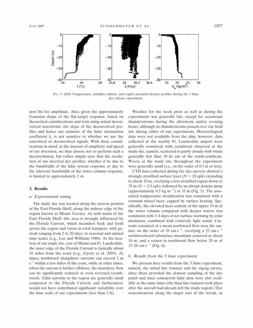
CTD data collected during the dye surveys showed astrongly stratified surface layer (N � 10 cph) extendingto about 10 m, overlying a less stratified region down to35 m (N � 3.5 cph), followed by an abrupt density jump(approximately 0.5 kg m�3) at 35 m (Fig. 5). The asso-ciated temperature stratification was consistent with aremnant mixed layer, capped by surface heating. Spe-cifically, the elevated heat content of the upper 10 m ofthe water column compared with deeper waters wasconsistent with 3–4 days of net surface warming by solarinsolation, combined with relatively light winds. Cur-rents consisted of a mean northward flow near the sur-face on the order of 10 cm s�1, overlying a 25 cm s�1

northwestward subsurface maximum centered at about10 m, and a return to northward flow below 20 m of15–20 cm s�1 (Fig. 6).

b. Results from the 3 June experiment

We present here results from the 3 June experiment,namely, the initial line transect and the zigzag survey,since these provided the densest sampling of the dyepatch and since concurrent lidar data were also avail-able at the same times (the final line transect took placeafter the aircraft had already left the study region). Dyeconcentrations along the major axis of the streak, as

FIG. 5. (left) Temperature, (middle) salinity, and (right) potential density profiles during the 3 Junedye release experiment.


measured during the initial transect, are shown in Fig. 7.The transect shows three distinct patches of dye. Fromright to left (note, the x axis in Fig. 7 is reversed com-pared to Fig. 2, since the dye was injected from north tosouth), the northernmost (rightmost) segment of thedye patch starts near the surface, then deepens to ap-proximately 5 m; the middle segment starts at 5 m,shoals to the surface, then deepens again to 5 m; andthe southernmost (leftmost) segment starts at 5 m, andshoals to the surface. This pattern of surface and deepsegments agrees well with the injection segments shownin Fig. 1, with the exception of the two 10-m sections ofthe patch, which by the time of the transect had alreadybeen advected to the west of the major axis of the sur-face patches and hence were not sampled by the linetransect (recall that the subsurface shear would haveadvected the deeper dye westward compared to thesurface patch; see Fig. 6). That dye concentrations mea-sured at the southern end of the patch were somewhatless than those at the northern end is consistent with thefact that the injection was performed while steamingsouthward, while the initial sampling transect was donewhile heading northward. Thus, the time between in-jection and sampling was larger for the northern por-tion of the dye streak.

Cross-streak sections of the dye patch taken duringthe zigzag survey are shown in Fig. 8, starting from thenorthern end of the patch and progressing southward.(Note, for compactness of presentation, lidar-derivedsections are also shown in Fig. 8, although we defercomparison between the lidar and in situ results untilsection 3d. Also, since corresponding airborne lidardata were only available for the early part of the survey,

we show here only sections occupied during the firsthalf of the survey.) In all sections, particularly thosepassing through the surface segments of the patch, evi-dence of an east–west shear in the upper portion of thewater column is again visible in the dye data. Assumingan elapsed time of 1–1.5 h (the time between the injec-tion and the zigzag survey) and a westward velocity of0.1 m s�1 at 5-m depth (see Fig. 6), we would expect atotal differential displacement on the order of 350–550m between the surface and 5-m portions of the patch.This is roughly consistent with the observed displace-ments, most notably the two transects taken throughthe surface segments of the patch (i.e., Figs. 8a,d).Transects taken across the deeper segments of thepatch, well away from the near-surface segments (Figs.8b,c), show relatively little dye near the surface, with aweak maximum at 5-m depth toward the western edgeof the survey. These displacements are again consistentwith a stronger westward current at depth.

c. Results from airborne lidar

Overflights of the dye patch using airborne lidarcommenced at the start of the dye injection and con-tinued for 1.5 h (i.e., about halfway through the zigzagsurvey). A total of 21 flight lines over the dye patchwere carried out: 12 in the north–south direction (i.e.,along the axis of the dye streak) and 9 in the east–westdirection (across the axis of the dye streak). The aver-age time between successive overflights was about 4.5min.

A subset of the raw lidar waveforms (intensity ofbackscatter versus time/depth) both inside and outsidethe dye patch for the infrared, green, and fluorescencechannels is shown in Fig. 9. A peak in backscatter fromthe ocean surface is clearly visible in the IR and greenchannels. The IR signal is confined to the near surface,while the green channel shows a more gradual expo-nential decay with depth. Peaks in the fluorescent chan-nel are also evident in profiles through the dye patch,distinct from profiles outside the patch. These corre-spond to profiles in the green channel in which theattenuation rate was significantly enhanced comparedto ones where no dye was found.

The inversion procedures for both the green andfluorescence channels were applied for each of the lidaroverflights per (2) and (5). In the case of the greenchannel, data collected well to the north and south ofthe dye patch were used to compute a mean I�1

532 dI532/dz outside of the patch. Results of the two inversionsteps for an overflight made approximately 0.5 h afterthe injection are shown in Fig. 10. The results show aclear signal in both channels. Noteworthy, however, arethe differences between C computed from (2) and that

FIG. 6. Mean velocity profiles during the 3 June dye releaseexperiment: eastward (solid) and northward (dashed). Dottedlines indicate one standard deviation about the means.


from (5). Specifically, the noise level in the green chan-nel is more evident than the noise in the fluorescencechannel. Meanwhile, though the fluorescence channelappears cleaner, this is at the expense of a higher de-tectability threshold. These differences stem from dif-ferences in the two inversion procedures. Specifically,in the case of the green channel, attenuation profileswithin the dye patch are compared to the mean profileoutside the patch, per (2). As such, the noise in theinverted solution is the result of small spatial variationsin the ambient attenuation profile, combined with in-strument noise at low signal-to-noise levels. Both ofthese can result in spurious dye peaks, as well as zero oreven negative dye concentrations. By contrast, thenoise in the dye channel is primarily instrumental noise.To identify peaks in the dye channel that are clearlyabove the noise floor, we have chosen a threshold in-tensity, below which we set the inverted dye signalequal to zero. This results in an apparently cleaner sig-nal with fewer spurious peaks but also with a higherdetectability threshold. Despite these differences, how-ever, the surface segments of the dye streak are clearlyvisible in both the green and fluorescence channel in-versions. Also visible in the green channel inversion arethe two southernmost 5-m segments of the dye patch.The northernmost 5-m segment and the two 10-m seg-ments do not appear, possibly because they had alreadybeen advected westward out of the field of view of thelidar.

d. Comparison with in situ results

The results of the lidar surveys can be compared di-rectly to those from the towed fluorometer data. The

lidar data corresponding to the first transect along themajor axis of the dye streak are shown in Fig. 11. Re-sults from both channels show good qualitative agree-ment with the in situ data (see also Fig. 7) in terms ofthe locations and mean depths of the dye patch, as wellas the amplitude of the dye concentrations. Again, how-ever, significant noise is visible in the green channel C,particularly below regions where dye was found. Bycontrast, C from the fluorescence channel shows lessnoise at depth, but also fewer dye peaks overall, par-ticularly for lower peak concentrations.

Similar comparisons can be made between the zigzagtransects of the airborne versus the in situ observations(Fig. 8). Again, the lidar results show good agreementwith the in situ data, both qualitatively and quantita-tively, although the same differences between the lidarresults and the in situ data, as well as between the twolidar channels, also exist.

A final check of the lidar inversions can be made bycomparing the total mass of dye inferred from each ofthe inversions to the total amount that was actuallyinjected. Taking an average over the 9 north–southoverflights following the injection (3 of the 12 north–south overnights were done during the injection, beforeit was complete), the total dye mass accounted for inthe lidar signal was 1.7 kg for the green channel and 1.4kg for the fluorescent channel. These can be comparedto the 5 kg of dye that were actually injected. There arethree major reasons for these underestimates. The firstreason, which would lead to both channels underesti-mating the total dye, particularly during later over-flights, is that because of vertical shear in the watercolumn, the deeper segments of the patch were ad-

FIG. 7. In situ dye concentration [log10(C/ppb)] as measured during the first transect along the major axis of the dye streak showingthe three near-surface (centered at about 2.5-m depth) segments of the dye patch, interspersed with deeper (5 m) segments. Two gapswhere no dye was found (approximately 25.944° and 25.95°N) correspond to the portions of the streak that were injected at 10 m, which,due to a strong vertical shear, had already been advected westward of the surface patch. Black triangles indicate locations of thedowncast portions of the surveys.


Fig 7 live 4/C

vected westward, out of the field of view of the lidar.Because the lidar overflights were aligned with the sur-face segments of the dye patch, they generally did notcapture these deeper dye segments. Taking this intoconsideration, and noting that about 60% of the totaldye was injected in the near-surface segments of thestreak, we would expect that approximately 3 kg of thedye would be contained in the near-surface segments.As the deeper portions of the surface dye segmentswere likely also advected westward, due to the strongvertical shears (e.g., Fig. 8), the actual amount of dyesampled by the lidar may have been even less than this.A second reason, particularly relevant to the earliersurveys when dye concentrations were much higher (upto 40 ppb peak concentration), was that the attenuationof the incident laser light due to absorption by dye, plus

that due to the water itself, would have led to a morethan 100-fold reduction in the intensity of the incomingpulse over the first (upper) 2 m of the dye patch [e.g.,see Eq. (1)]. Such strong attenuations would have rap-idly reduced the lidar signal to the noise floor of ourmeasurement, and hence led to our inability to detectdye deeper in the water column. Although our inver-sion approach generally takes both the dye and watercolumn absorption into account, it cannot overcomethe extreme situation in which the laser pulse is attenu-ated away before it has fully traversed the dye patch.As a result, absorption by the upper portion of the dyepatch could have led to the “shadowing” of dye atdeeper depths, and hence an underestimate of the over-all dye mass. Relevant to the fluorescence channel in-version, a third reason contributing to the underesti-

FIG. 8. Dye concentration observed during the 3 June zigzag survey showing the vertical and cross-streak structure of the dye patch1–1.5 h after injection. (a)–(d) Four transects consist of the (top) in situ, (middle) green channel, and (bottom) fluorescent channel withplan view of ship track and corresponding lidar overflight on the rhs. Color scale is log10(C/ppb). Note, in situ concentration estimatesnear the sea surface (uppermost 1–2 m) may be artificially elevated due to the sampling sled breaching the surface.


Fig 8 live 4/C

mate of the dye concentration is that whenever the sig-nal for an entire profile fell below a prespecified level,the signal was deemed indistinguishable from noise andthe entire dye profile was assumed to be zero. As aresult, profiles that had a very weak signal (i.e., near orbelow the noise level) underestimated the dye. Thisalso explains why less of the dye was accounted for bythe fluorescence channel inversion than the green chan-nel, since the signal to noise was generally less in thefluorescence channel.

4. Discussion

a. Comparison of green and dye channel results

Comparing the lidar data to the in situ data, we findthat the green channel inversion is better able to de-tect lower concentrations of dye but that it also has agreater amount of noise, including spurious but coher-ent peaks that are not in the in situ data. This isparticularly so below regions where significant dyeconcentrations (on the order of 10 ppb or greater)were found. Meanwhile, the fluorescence channelshows only the higher concentration peaks in the dye,but with less noise otherwise. As noted previously, thelatter is the result of constraints imposed by the inver-sion itself.

The results of the lidar inversions suggest that for

both the green and fluorescence channels, dye concen-trations on the order of 1–2 ppb are readily resolved,with the possibility of detections as low as 0.5 ppb in thegreen channel. Particularly noteworthy is that the dyeconcentrations inferred from the lidar agree as well asthey do with the in situ data, despite the fact that thetwo sets of measurements were made independently ofone another. This suggests that our inversion proce-dures capture at least the major attenuation, scattering,and absorption characteristics so as to yield robust re-sults. A more thorough treatment of the inversion willlikely lead to further improvements in the dye concen-tration estimates.

One of the difficulties of comparing the lidar datawith in situ data is the problem of space–time aliasing.Specifically, the lidar measurements are nearly instan-taneous compared to the in situ measurements (e.g., 20s to complete an overflight versus 20 min for a singleline transect). We have addressed this to some extent inour comparisons in section 3, inasmuch as we comparemeasurements from the two platforms for times andlocations that are as close as is practically possible. Nev-ertheless, the fact that the dye patch is constantly evolv-ing because of both advection and diffusion means thatany mismatch in time inevitably translates to a mis-match in space as well. Still, the results shown in Figs. 7,8 offer a reasonable comparison.

FIG. 9. (left) Raw IR, (middle) green, and (right) fluorescence backscatter lidar signalsobserved (top) during a pass over the near-surface segment of the dye patch and (bottom) fora series of profiles outside the dye patch. Each panel contains 100 profiles.


b. Errors and uncertainties

Neglecting possible errors and uncertainties associ-ated with the model itself, the dominant source of errorin the green channel inversion is natural variation in thebackground attenuation. The error associated with suchvariation can be estimated directly. Specifically, takingthe two standard deviation limit of I�1

532dI532/dz outsidethe dye patch, the uncertainty in the attenuation in theupper 10 m of the water column is about 0.07 m�1,

increasing to 0.14 m�1 at 15 m. Dividing by 2�D532, thistranslates to an uncertainty in the dye concentration of1 ppb from 0- to 10-m depth, increasing to 2 ppb at 15-mdepth. This increase in uncertainty with depth is a directresult of the decreasing signal-to-noise ratio.

Uncertainties in the fluorescence channel dye esti-mates are more difficult to quantify, in part because ofour use of an a priori noise threshold in the inversionbut also because of the least squares fitting methodused to constrain the integration constants, plus other

FIG. 10. Dye concentration [log10(C/ppb)] inferred from airborne lidar: (top) green channel and (bottom)fluorescence channel. Vertical slices are approximately every 2 m starting from the surface down to 12 m.


Fig 10 live 4/C

assumptions such as that of a constant lidar attenuationcoefficient. In the present analysis, we have set thenoise threshold at 1.0 � 10�4 in the raw fluorescenceintensity (see Fig. 9). This translates to a noise floor inabsolute dye concentration again of about 1 ppb be-tween 0- and 10-m depth, increasing to about 2 ppb at15-m depth. Meanwhile, if variations in background at-tenuation as a function of depth were similar in the twochannels, the uncertainty due to such variations in thefluorescence channel would also have been on the or-der of 1 ppb between 0 and 10 m, increasing to 2 ppb at15-m depth.

One possible approach to attaining a greater dynamicrange in the observations in future studies would be toincrease the total amount of dye released in each ex-periment, thus increasing the overall signal to noise.The problem with this approach, however, is the self-shadowing of the dye described in section 3d, which fora given level of incoming radiation (e.g., a given laserpulse power) sets an upper limit on the total amount ofdye the laser can penetrate. Based on the present in-

version results, we estimate this limit to be approxi-mately equivalent to a 3–4-m-thick layer of dye withconcentration on the order of 10 ppb, or about 3.5 ppbof dye averaged over the upper 10 m of the water col-umn.

Putting the above uncertainties into perspective,the minimum detectable level for Rhodamine WTin clear water using a commercial fluorometer isapproximately 0.01 ppb. Given that the uncertaintiesin the lidar inversions are set in part by variations inthe background attenuation, a more refined inver-sion approach will thus be required to come close tothe in situ detection level. Nevertheless, the verylarge number of observations made by the lidar (onthe order of 30 000 profiles during a single overflightcompared to 200 in situ profiles for the entire ex-periment) provides a wealth of information aboutthe overall dye distribution, which would otherwise notbe obtainable from in situ measurements alone. Thetwo types of observations are complementary in thisregard.

FIG. 11. Dye concentration [log10(C/ppb)] as measured by lidar during an overflight approximately 10 min intothe first line transect along the major axis of the dye streak based on the green channel and fluorescent channelinversions, respectively. Data shown correspond to averages of profiles taken within 10 m of the ship-based transectpositions. An offset in the longitudinal position has been applied to the lidar positions, corresponding to approxi-mately 0.5 m s�1 to account for the westward advection of the patch between the in situ and lidar data samplingtimes.


Fig 11 live 4/C

5. Summary and conclusions

The results here are from a pilot study using airbornelidar to survey dye release experiments in the upperocean on spatial scales of meters to kilometers and tem-poral scales of minutes to days. Dye concentrations as afunction of horizontal position and depth from two in-version approaches are compared to ship-based obser-vations using an in situ fluorometer. Results showqualitative as well as quantitative agreement betweendye distributions inferred from the two lidar channelsversus the in situ measurements. Dye concentrationsdetected by the airborne lidar ranged from 1 ppb togreater than 10 ppb, with the lower limit set by varia-tions in the background (ambient) attenuation coeffi-cient and the upper limit set by self-shadowing of thedye.

The present results represent a significant advance inthe use of airborne lidar for surveying dye release ex-periments insofar as this is the first time, to our knowl-edge, that depth-dependent dye concentrations havebeen reported in the peer-reviewed literature. A sec-ond novel aspect of this work is the method used toinvert the raw lidar signal for absolute dye concentra-tion. Specifically, the method used here requires no apriori knowledge of in situ dye concentration, althoughwe used such measurements to provide validation ofthe technique.

While the present study shows the basic capabilitiesof airborne lidar for obtaining three-dimensional mapsof dye release experiments in the upper ocean, there isstill considerable room for improvement in terms ofsignal to noise, dye detection limits, and depth penetra-tion. Given the relative success of the simple inversionapproach applied here, however, it is likely that amore sophisticated inversion procedure that takesadvantage of known characteristics of the backgroundattenuation, instrument and environmental noise,and the dye signal could lead to significant improve-ment in the accuracy of the dye concentration esti-mates. On the instrumentation side, it should be notedthat the system used here was a slight modification of abathymetric system. A system designed specificallywith the above issues in mind, including possibly theuse of more sensitive detectors, would also greatly en-hance the capability of airborne lidar for surveying dyerelease experiments. Given the very high resolution,both temporally and spatially, provided by airborne li-dar, we believe measurements such as those presentedhere hold great promise for significant advances in ourunderstanding of small-scale dispersion in the upperocean.

Acknowledgments. Support was provided by theCecil H. and Ida M. Green Technology InnovationFund under Grant 27001545, the Office of Naval Re-search Grant N00014-01-1-0984, and the Woods HoleOceanographic Institution Coastal Ocean Institute.The authors thank E. Culpepper and C. Wiggins of theU.S. Army Corps of Engineers Joint Airborne LIDARBathymetry Technical Center of Expertise for their as-sistance with the airborne measurements. We are grate-ful to Captains R. Franks and M. Andrews and FloridaAtlantic University for use of the R/V Stephan, and T.Donoghue and S. Bohra for assistance with staging anddeployment related to the ship-based portion of thefield work. We also thank F. Hoge, J. Churnside, J.Buck, and H. Sosik for helpful discussions.

REFERENCES

Churnside, J. H., V. V. Tatarskii, and J. W. Wilson, 1997: Lidarprofiles of fish schools. Appl. Opt., 36, 6011–6020.

——, ——, and ——, 1998: Oceanographic lidar attenuation co-efficients and signal fluctuations measured from a ship in theSouthern California Bight. Appl. Opt., 37, 3105–3112.

Feldman, G., and C. R. McClain, cited 2004: Ocean Color Web,SeaWiFS Reprocessing Level 2. NASA Goddard SpaceFlight Center. [Available online at http://oceancolor.gsfc.nasa.gov/.]

Franz, H., U. Gehlhaar, K. P. Günther, A. Klein, J. Luther, R.Reuter, and H. Weidemmann, 1982: Airborne fluorescenceLIDAR monitoring of trace dye patches—A comparisonwith shipboard measurements. Deep-Sea Res., 29, 893–901.

Gordon, H. R., 1982: Interpretation of airborne oceanic lidar: Ef-fects of multiple scattering. Appl. Opt., 21, 2996–3001.

Günther, G. C., R. W. L. Thomas, and P. E. LaRoque, 1996: De-sign considerations for achieving high accuracy with theshoals bathymetric LIDAR system. Laser Remote Sensing ofNatural Waters: From Theory to Practice, V. Feigels and Y.Kopilevich, Eds., SPIE, 54–71.

Gyory, J., E. Rowe, A. J. Mariano, and E. H. Ryan, cited 2005:The Florida current. [Available online at http:/ /oceancurrents.rsmas.miami.edu/atlantic/florida.html.]

Hoge, F. E., and R. N. Swift, 1981: Absolute tracer dye concen-tration using airborne laser-induced water raman backscat-ter. Appl. Opt., 20, 1191–1202.

——, and ——, 1983: Airborne dual laser excitation and mappingof phytoplankton photopigments in a Gulf Stream warm corering. Appl. Opt., 22, 2272–2281.

Irish, J. L., and J. W. Lillycrop, 1999: Scanning laser mapping ofthe coastal zone; the shoals system. ISPRS J. Photogramm.Remote Sens., 54, 123–129.

Klett, J. D., 1981: Stable analytical inversion solution for process-ing LIDAR returns. Appl. Opt., 20, 211–220.

——, 1985: Lidar inversion with variable backscatter/extinctionratios. Appl. Opt., 24, 1638–1643.

Kullenberg, G., 1971: Vertical diffusion in shallow waters. Tellus,23, 129–135.

Lee, T., and E. Williams, 1988: Wind-forced transport fluctuationsof the Florida current. J. Phys. Oceanogr., 18, 937–946.

Mack, S. A., D. P. Vasholz, E. C. Larson, D. J. Scheerer, J. Cal-man, and H. C. Schoeberlein, 1997: Estimation of diapycnal


diffusivity from a dye tracer study in the upper seasonal ther-mocline. Eos, Trans. Amer. Geophys. Union, 78 (Fall Meet-ing Suppl.), Abstract F374.

Morel, A., and S. Maritorena, 2001: Bio-optical properties ofoceanic waters: A reappraisal. J. Geophys. Res., 106, 7163–7180.

Okubo, A., 1971: Oceanic diffusion diagrams. Deep-Sea Res., 18,789–802.

Phillips, D. M., and B. W. Koerber, 1984: A theoretical study of anairborne laser technique for determining sea water turbidity.Aust. J. Phys., 37, 75–90.

Squire, J. L., and H. Krumboltz, 1981: Profiling pelagic fish

schools using airborne optical lasers and other remotes sens-ing techniques. Mar. Technol. Soc. J., 15, 27–31.

Terray, E. A., and Coauthors, 2005: Airborne fluorescence imag-ing of the ocean mixed layer. Proc. Eighth Working Conf. onCurrent Measurement Technology, Southampton, UK, IEEE/OES, 76–82.

Vasholz, D. P., and L. J. Crawford, 1985: Dye dispersion in theseasonal thermocline. J. Phys. Oceanogr., 15, 695–711.

Yoder, J. A., J. Aiken, R. N. Swift, F. E. Hoge, and P. M. Steg-man, 1993: Spatial variability in near-surface chlorophyll-afluorescence measured by the Airborne Oceanographic Lidar(AOL). Deep-Sea Res., 40, 37–53.


Documents

Three-Dimensional Mapping of Fluorescent Dye Using a