Three-Dimensional Flow of a Vortex Drop Shaft Spillway

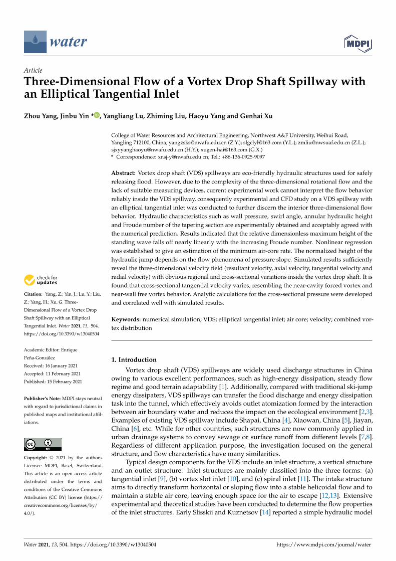
water

Article

Three-Dimensional Flow of a Vortex Drop Shaft Spillway withan Elliptical Tangential Inlet

Zhou Yang, Jinbu Yin * , Yangliang Lu, Zhiming Liu, Haoyu Yang and Genhai Xu

��

Citation: Yang, Z.; Yin, J.; Lu, Y.; Liu,

Z.; Yang, H.; Xu, G. Three-

Dimensional Flow of a Vortex Drop

Shaft Spillway with an Elliptical

Tangential Inlet. Water 2021, 13, 504.

https://doi.org/10.3390/w13040504

Academic Editor: Enrique

Peña-González

Received: 16 January 2021

Accepted: 11 February 2021

Published: 15 February 2021

Publisher’s Note: MDPI stays neutral

with regard to jurisdictional claims in

published maps and institutional affil-

iations.

Copyright: © 2021 by the authors.

Licensee MDPI, Basel, Switzerland.

This article is an open access article

distributed under the terms and

conditions of the Creative Commons

Attribution (CC BY) license (https://

creativecommons.org/licenses/by/

4.0/).

College of Water Resources and Architectural Engineering, Northwest A&F University, Weihui Road,Yangling 712100, China; [email protected] (Z.Y.); [email protected] (Y.L.); [email protected] (Z.L.);[email protected] (H.Y.); [email protected] (G.X.)* Correspondence: [email protected]; Tel.: +86-136-0925-9097

Abstract: Vortex drop shaft (VDS) spillways are eco-friendly hydraulic structures used for safelyreleasing flood. However, due to the complexity of the three-dimensional rotational flow and thelack of suitable measuring devices, current experimental work cannot interpret the flow behaviorreliably inside the VDS spillway, consequently experimental and CFD study on a VDS spillway withan elliptical tangential inlet was conducted to further discern the interior three-dimensional flowbehavior. Hydraulic characteristics such as wall pressure, swirl angle, annular hydraulic heightand Froude number of the tapering section are experimentally obtained and acceptably agreed withthe numerical prediction. Results indicated that the relative dimensionless maximum height of thestanding wave falls off nearly linearly with the increasing Froude number. Nonlinear regressionwas established to give an estimation of the minimum air-core rate. The normalized height of thehydraulic jump depends on the flow phenomena of pressure slope. Simulated results sufficientlyreveal the three-dimensional velocity field (resultant velocity, axial velocity, tangential velocity andradial velocity) with obvious regional and cross-sectional variations inside the vortex drop shaft. It isfound that cross-sectional tangential velocity varies, resembling the near-cavity forced vortex andnear-wall free vortex behavior. Analytic calculations for the cross-sectional pressure were developedand correlated well with simulated results.

Keywords: numerical simulation; VDS; elliptical tangential inlet; air core; velocity; combined vor-tex distribution

1. Introduction

Vortex drop shaft (VDS) spillways are widely used discharge structures in Chinaowing to various excellent performances, such as high-energy dissipation, steady flowregime and good terrain adaptability [1]. Additionally, compared with traditional ski-jumpenergy dissipaters, VDS spillways can transfer the flood discharge and energy dissipationtask into the tunnel, which effectively avoids outlet atomization formed by the interactionbetween air boundary water and reduces the impact on the ecological environment [2,3].Examples of existing VDS spillway include Shapai, China [4], Xiaowan, China [5], Jiayan,China [6], etc. While for other countries, such structures are now commonly applied inurban drainage systems to convey sewage or surface runoff from different levels [7,8].Regardless of different application purpose, the investigation focused on the generalstructure, and flow characteristics have many similarities.

Typical design components for the VDS include an inlet structure, a vertical structureand an outlet structure. Inlet structures are mainly classified into the three forms: (a)tangential inlet [9], (b) vortex slot inlet [10], and (c) spiral inlet [11]. The intake structureaims to directly transform horizontal or sloping flow into a stable helicoidal flow and tomaintain a stable air core, leaving enough space for the air to escape [12,13]. Extensiveexperimental and theoretical studies have been conducted to determine the flow propertiesof the inlet structures. Early Slisskii and Kuznetsov [14] reported a simple hydraulic model

Water 2021, 13, 504. https://doi.org/10.3390/w13040504 https://www.mdpi.com/journal/water

https://www.mdpi.com/journal/water

https://www.mdpi.com

https://orcid.org/0000-0002-8364-237X

https://doi.org/10.3390/w13040504

https://doi.org/10.3390/w13040504

https://creativecommons.org/

https://creativecommons.org/licenses/by/4.0/

https://creativecommons.org/licenses/by/4.0/

https://doi.org/10.3390/w13040504

https://www.mdpi.com/journal/water

https://www.mdpi.com/2073-4441/13/4/504?type=check_update&version=1

Water 2021, 13, 504 2 of 23

study for the Medo dam with a tangential inlet. A depth-discharge theoretical modelwas first proposed by Jain [9] to predict the flow depth for the tangential inlet. Yu andLee [15] demonstrated that the hydraulic stability in the vortex inlet was strongly relatedto the geometry of the inlet and vertical shaft, and a comprehensive theoretical designguideline for the tangential slot intake was proposed. Del Giudice [16] recommendedthe improved design of the inlet in which proper reduction of the bottom length couldprevent hydraulic jump and congestion phenomenon. Pfister and Crispino [13] presentedan applicable concept to a novel junction chamber combining with several inlet channels.In addition, Hager [11], Crispino and Pfister [17], and Wu et al. [18] theoretically andexperimentally analyzed the performance of the standing wave at the intake structure,mainly characterized by the relative height, the location and the extent.

The vertical structure is next to the inlet structure, where the flow clings to the wall andswirls down along the wall at the mercy of centrifugal force and gravity [19]. Moreover,there are remarkable energy dissipation and air entrainment associated with the flowpattern alteration. According to the experimental results of Jain, flow in the vertical dropshaft can be distinguished into three regions, annular jet flow, transition flow, and watercushion region [20]. The investigation of the aeration and the deaeration processes isextremely necessary when the vertical shaft structure is considered. Dynamic change ofthe air entrainment in the high drop shaft would generate system pressurization and thenrelease foul-smelling air [21]. Li et al. [22] emphasized the need for an aerator in the middleof the shaft, and a calculation method for aeration cavity length was presented. However,both experimental and numerical simulation results on the air entrainment differed fromprototype values [23,24]. Although a model with gravity similarity criterion could simulatewell the water flow, it did not adequately simulate the entrainment and transport of theair [25]. Other studies focused on energy loss found that depth of energy dissipation wellhas little effect on total energy dissipation rate and that the energy dissipation rate of therotational flow is much smaller than that of the annular hydraulic jump in dissipationwell [26,27]. Generally, the total energy dissipation ratio can exceed 70% under a reasonabledesign [26,28,29]. In other studies, the characteristics of velocity and pressure on a levelswirling flow discharge tunnel were theoretically analyzed based on the combined vortexrule [30–33].

The outlet structure is mainly set to alter the flow pattern from annular flow tohorizontal flow without severe water surface fluctuations. Nevertheless, limited laboratorystudies had been done for outlet structure. Del Giudice and Gisonni [7] carried out somepreliminary exploration in terms of both optimizing outlet shape and improving energydissipation. Zhang et al. [34] developed a novel type of submerged outlet for the VDSspillways, where the flow transit smoothly and favorably from non-pressure flow topressure flow.

Overall, it can be said that previous advance made on the different parts and researchaspects of the VDS was considerable. However, unlike the previous VDS with a tangentialslot inlet [9,15,29], widely applied in an urban drainage system, the hydraulic behaviorof a VDS spillway equipped with an elliptical tangential inlet has not been detailed ad-dressed. Such shape originated in China, and it is generally considered superior with betterdischarge capacity and flow pattern than the former [1]. On the one hand, the ellipticaltangential inlet can promote the formation of a stable rotational flow under various flowconditions, while for the tangential slot inlet, the overfall flow phenomenon will directlyoccur under small flow conditions. On the other hand, the flow in the elliptical intakeis smoother because of the elliptical guiding wall, and it is not prone to cause backwa-ter and negative pressure. Benefiting from the above, a similar VDS spillway with theelliptical tangential inlet has already been built in China, such as Xiaowan and Jilintai.Previously Wei et al. [35] have theoretically proposed the design criteria for this shape.Moreover, due to the complexity of the three-dimensional rotational flow and the lack ofsuitable measuring devices, detailed information such as the three-dimensional velocityfield inside the VDS spillway is hitherto lacking. Fortunately, numerical simulation is

Water 2021, 13, 504 3 of 23

able to reproduce the experimental flow phenomena while straightforward obtaining thedetailed hydraulic parameter inside the VDS. Recently, Liu et al. [2] have reported thesuccessful use of the RNG k-ε turbulence model on a newly developed VDS spillway withthe spiral-flow-generating piers. However, there are also no detailed three-dimensionalflow characteristics.

Hence, in the present study, physical model experiments with corresponding numer-ical simulation were conducted to further discern the three-dimensional flow behaviorof a VDS spillway, comprising a tangential vortex intake with 1/4 ellipse guiding wall,and the relevant computational results are verified by experimental data. Meanwhile,experimental and simulated results such as the performance of the standing wave, air-coreratio, cross-sectional pressure and three-dimensional velocity were comprehensively ana-lyzed. Furthermore, the combined vortex rule was introduced to predict the cross-sectionalpressure distribution of the swirling flow in the VDS. The outcomes of the current researchcan provide comprehensive insights for the research and application of similar engineering.

2. Physical Model and Measurement

A 1:40 Froude model fabricated from transparent plexiglass was made in the Collegeof Water Resources and Architectural Engineering, Northwest A&F University, to providea useful reference for future prototype VDS spillways serving in China. Generally, the scaleeffect can be ignored for some time-averaged hydraulic characteristics [36]. The physicalmodel consists of an elliptical tangential inlet (include a tapering section and a vortexchamber), a gradient (contracted) section, a vertical shaft, an energy dissipation well, apressure slope and an outlet tunnel, as shown in Figure 1, in which the vortex chamber,gradient section, vertical shaft, dissipation well can be collectively referred to as the VDS.

Water 2021, 13, x FOR PEER REVIEW 3 of 24

lack of suitable measuring devices, detailed information such as the three-dimensional velocity field inside the VDS spillway is hitherto lacking. Fortunately, numerical simula-tion is able to reproduce the experimental flow phenomena while straightforward ob-taining the detailed hydraulic parameter inside the VDS. Recently, Liu et al. [2] have re-ported the successful use of the RNG k–ε turbulence model on a newly developed VDS spillway with the spiral-flow-generating piers. However, there are also no detailed three-dimensional flow characteristics.

Hence, in the present study, physical model experiments with corresponding nu-merical simulation were conducted to further discern the three-dimensional flow be-havior of a VDS spillway, comprising a tangential vortex intake with 1/4 ellipse guiding wall, and the relevant computational results are verified by experimental data. Mean-while, experimental and simulated results such as the performance of the standing wave, air-core ratio, cross-sectional pressure and three-dimensional velocity were comprehen-sively analyzed. Furthermore, the combined vortex rule was introduced to predict the cross-sectional pressure distribution of the swirling flow in the VDS. The outcomes of the current research can provide comprehensive insights for the research and applica-tion of similar engineering.

2. Physical Model and Measurement A 1:40 Froude model fabricated from transparent plexiglass was made in the Col-

lege of Water Resources and Architectural Engineering, Northwest A&F University, to provide a useful reference for future prototype VDS spillways serving in China. Gener-ally, the scale effect can be ignored for some time-averaged hydraulic characteristics [36]. The physical model consists of an elliptical tangential inlet (include a tapering section and a vortex chamber), a gradient (contracted) section, a vertical shaft, an energy dissi-pation well, a pressure slope and an outlet tunnel, as shown in Figure 1, in which the vortex chamber, gradient section, vertical shaft, dissipation well can be collectively re-ferred to as the VDS.

Figure 1. (a) Side view of the experimental setup; and (b) elliptical inlet configuration (all dimen-sions are in meters).

Unlike the previous tangential slot inlet where the tapering section and the vortex chamber are directly tangential connected in a straight line is widely applied in urban drainage systems. In this study, an elliptical tangential inlet equipped with a 1/4 ellipti-cal guiding wall ( 2 2 2 2/10.5 /18.5 1x y+ = ) was applied, as shown in Figure 1. Additional-ly, a deflector was set in the vortex chamber to prevent the backwater phenomenon. The

Figure 1. (a) Side view of the experimental setup; and (b) elliptical inlet configuration (all dimensions are in meters).

Unlike the previous tangential slot inlet where the tapering section and the vortexchamber are directly tangential connected in a straight line is widely applied in urbandrainage systems. In this study, an elliptical tangential inlet equipped with a 1/4 ellipticalguiding wall (x2/10.52 + y2/18.52 = 1) was applied, as shown in Figure 1. Additionally,a deflector was set in the vortex chamber to prevent the backwater phenomenon. Theinclination angle (β) of the tapering section is 5.71 degrees, and the entrance width (E) ofthe vortex chamber is 0.162 m. The diameter of the vortex chamber (D1) and vertical shaft(D2) is 0.275 m and 0.2 m separately. The total height of the VDS is 1.91 m. A more detaileddimension is shown in Figure 1. In order to better understand the hydraulic behavior, atotal of five experimental flow rates were considered, namely 45.46 L/s, 40.52 L/s, 24.11L/s, 20.26 L/s and 17.59 L/s, corresponding to flood frequency P = 0.05%, P = 0.1%, P = 1%,

Water 2021, 13, 504 4 of 23

P = 2% and P = 3.3%, respectively, and the first 3 test-runs (P = 0.05%, 0.1%, 1%, respectively)were simulated.

In this experiment, a steady discharge generated by a recirculating flow system wasprovided to guarantee the rigor and repeatability of the experiments, as simply shown inFigure 1. The discharge was measured by a rectangular weir. Piezometers were used foracquiring time–average pressure values of the wall. Due to the pulsation of water flow atdissipation well, a possibly largest pressure error of ±10% was estimated, and the errorrange of the remaining points was estimated to be within plus or minus 3%. The location ofmeasuring points is as shown in Figure 1. The velocity at the tapering section was detectedusing a propeller-type current meter (relative error ≤ ±5%). The measuring points are,respectively, taken at a distance of about 1.5 cm from the water surface and the bottom andtaken in the middle. The average velocity can be obtained through the above three sets ofdata. The near-wall swirl angle was measured by the tracer method with a protractor, andthe accuracy is 1 degree. Given the available measuring devices and laboratory limitations,three sets of measurements were taken, and the experimental data were averaged.

Inside the VDS, the hydraulic behavior of the numerical model is similar. However,in that region, the laboratory measurements such as the pitot tube may be affected by theturbulently uneven water thickness and misaligned direction, which might result in anerror up to 20–30% [31]. Hence, the flow velocity in this research was supplemented bynumerical simulation.

3. Numerical Simulation3.1. Governing Equations

Although the k-ε turbulent models have been widely applied to flow simulationsbecause of the fine convergence and computational efficiency [37–39], the RNG k-ε tur-bulence model proposed by Yakhot and Orzag, by providing an additional coefficientcorrecting the turbulent viscosity and taking into account the average rotational motion,can effectively process the strong swirling flow or curved wall jet under high Reynoldsnumber [40]. Furthermore, regarding to previous research [2,24,41] were found that theRNG k-ε turbulence model can give the best prediction of the jet flow in such shaft spillway.Accordingly, this turbulence model was utilized to model the intricate flow in the VDSspillways via ANSYS 16.0 software, Fluent. The basic control equations are as follows:

Continuity Equation:∂ui∂xi

= 0 (1)

Momentum Equation:

∂ui∂t

+ uj∂ui∂xj

= −1ρ

∂P∂xi

+ v∂2

∂xi

∂ui∂xj

+ fi (2)

k Equation:∂(ρk)

∂t+

∂(ρuik)∂xi

=∂

∂xj

(αkµe f f

∂k∂xj

)+ Gk + ρε (3)

ε Equation:

∂(ρε)

∂t+

∂(ρuiε)

∂xi=

∂

∂xj

(αεµe f f

∂ε

∂xj

)+

C∗1ε

kGk − C2ερ

ε2

k(4)

where ui is the velocity component in xi direction; t is the time; ρ and v are the density andthe kinematic viscosity coefficient of water, respectively. P is the corrected pressure; fi is theexternal volume force component; ∂k and ∂ε are the turbulent Prandtl constant; Gk is theturbulent kinetic energy generated by the velocity gradient; µe f f is the corrected effective

turbulent viscosity. µe f f = µ + µt µt = ρCµk2

ε Gk = µt

(∂ui∂xj

+ ∂ui∂xi

)∂ui∂xj

C∗1ε = C1ε − η(1−η/η0)

1+βη3

Water 2021, 13, 504 5 of 23

η =(2Eij × Eij

)1/2 kε Eij =

12

(∂ui∂xj

+∂uj∂xi

)αk = αε = 1.39 Cµ = 0.0845 C1ε = 1.42 C2ε = 1.68

η0 = 4.377 β = 0.012 [42].The VOF method presented by Hirt and Nichols [43] was used to catch the free surface

of the high-speed flow, which is achieved by resolving the following Equation:

∂aw

∂t+ ui

∂aw

∂xi= 0 (5)

where aw is the volume fraction of water.

3.2. Mesh and Boundary Conditions

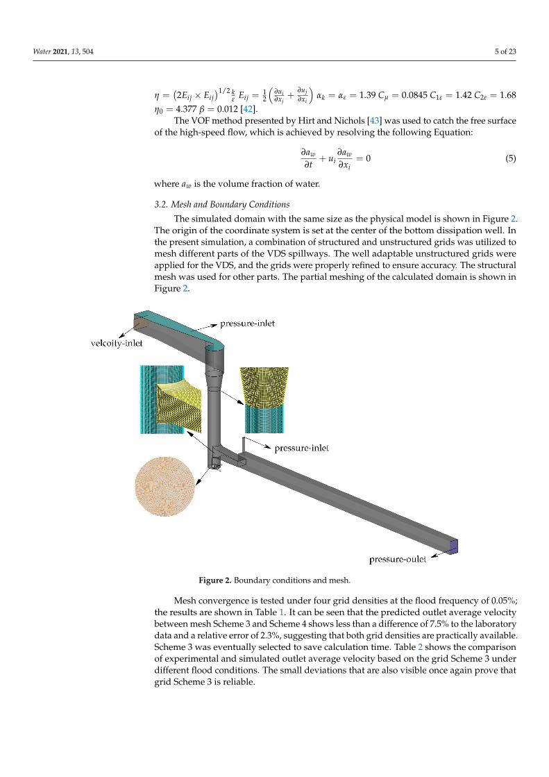
The simulated domain with the same size as the physical model is shown in Figure 2.The origin of the coordinate system is set at the center of the bottom dissipation well. Inthe present simulation, a combination of structured and unstructured grids was utilized tomesh different parts of the VDS spillways. The well adaptable unstructured grids wereapplied for the VDS, and the grids were properly refined to ensure accuracy. The structuralmesh was used for other parts. The partial meshing of the calculated domain is shown inFigure 2.


Figure 2. Boundary conditions and mesh.

Table 1. The test of fine-grid selection (P = 0.05%).

Mesh Scheme

Mesh Number Mesh Size Range Outlet Average

Velocity (m/s) Relative Error Experimental Aver-

age Velocity (m/s)

1 374, 240 12.5–25.0 mm 3.44 −

2.82 2 530, 853 8.0–20.0 mm 3.18 0.076 3 781, 526 5.0–15.0 mm 3.05 0.041 4 131, 3582 2.5–10.0 mm 2.98 0.023

Table 2. Simulation cases.

Flood Frequency Inlet Water Depth (m)

Inlet Velocity (m/s)

Outlet Velocity (m/s) Deviation

Simulation Experiment 1% 0.108 0.812 2.12 2.03 4.26%

0.1% 0.155 0.951 2.89 2.71 6.23% 0.05% 0.173 0.956 3.05 2.82 7.54%

The boundary conditions are set as shown in Figure 2. For the water inlet, the flow depth and velocity were selected while the pressure-outlet prescribed with 0 gauge pressure was defined. Additionally, the pressure-inlet was adopted for the two air vents. The wall boundary was based on no-slip conditions, and a standard wall function was used for processing the area near the wall.

The governing equations are solved using the finite volume method; the pressure–velocity coupling adopts the well-established PISO algorithm; a quick scheme is used for momentum, a geo-reconstruct scheme for the volume fraction, and a second-order up-wind scheme for the turbulent kinetic energy. The density and the kinematic viscosity coefficient of water are 998.2 kg/m3 and 1.003 10−3 N·s/m2, respectively. A transient simu-lation using a variable time step was performed until the residual error was within 10−4. A group of successful simulation required about 50–60 s (approximately runs for 12

Figure 2. Boundary conditions and mesh.

Mesh convergence is tested under four grid densities at the flood frequency of 0.05%;the results are shown in Table 1. It can be seen that the predicted outlet average velocitybetween mesh Scheme 3 and Scheme 4 shows less than a difference of 7.5% to the laboratorydata and a relative error of 2.3%, suggesting that both grid densities are practically available.Scheme 3 was eventually selected to save calculation time. Table 2 shows the comparisonof experimental and simulated outlet average velocity based on the grid Scheme 3 underdifferent flood conditions. The small deviations that are also visible once again prove thatgrid Scheme 3 is reliable.

Water 2021, 13, 504 6 of 23

Table 1. The test of fine-grid selection (P = 0.05%).

Mesh Scheme Mesh Number Mesh Size Range Outlet AverageVelocity (m/s) Relative Error Experimental Average

Velocity (m/s)

1 374, 240 12.5–25.0 mm 3.44 −

2.822 530, 853 8.0–20.0 mm 3.18 0.0763 781, 526 5.0–15.0 mm 3.05 0.0414 131, 3582 2.5–10.0 mm 2.98 0.023

Table 2. Simulation cases.

Flood Frequency Inlet Water Depth (m) Inlet Velocity (m/s)Outlet Velocity (m/s)

DeviationSimulation Experiment

1% 0.108 0.812 2.12 2.03 4.26%0.1% 0.155 0.951 2.89 2.71 6.23%

0.05% 0.173 0.956 3.05 2.82 7.54%

The boundary conditions are set as shown in Figure 2. For the water inlet, the flowdepth and velocity were selected while the pressure-outlet prescribed with 0 gauge pressurewas defined. Additionally, the pressure-inlet was adopted for the two air vents. The wallboundary was based on no-slip conditions, and a standard wall function was used forprocessing the area near the wall.

The governing equations are solved using the finite volume method; the pressure–velocity coupling adopts the well-established PISO algorithm; a quick scheme is used formomentum, a geo-reconstruct scheme for the volume fraction, and a second-order upwindscheme for the turbulent kinetic energy. The density and the kinematic viscosity coefficientof water are 998.2 kg/m3 and 1.003 10−3 N·s/m2, respectively. A transient simulationusing a variable time step was performed until the residual error was within 10−4. A groupof successful simulation required about 50–60 s (approximately runs for 12 days), and threesets of stable computational results were averaged for different parameters.

4. Results and Discussion4.1. Flow Pattern in the Vortex Drop Shaft4.1.1. Standing Shock Wave

Experimental observation and numerical prediction for flow state in the ellipticaltangential inlet are shown in Figure 3. The figure reveals that the flow at long taperingsection can be viewed as the rectangular open channel flow. The Froude number (Fr)calculated by Fr = v/

√gh is also plotted in Figure 4, which reduces with increasing

discharge. It can be noted that the experimental results are in acceptable agreement withthe numerical prediction (percentage error less than 9.12%). For all flow cases, the approachflow is supercritical within the entire tapering section, where Fr is larger than 1.

Water 2021, 13, 504 7 of 23


days), and three sets of stable computational results were averaged for different param-eters.

4. Results and Discussion 4.1. Flow Pattern in the Vortex Drop Shaft 4.1.1. Standing Shock Wave

Experimental observation and numerical prediction for flow state in the elliptical tangential inlet are shown in Figure 3. The figure reveals that the flow at long tapering section can be viewed as the rectangular open channel flow. The Froude number (Fr) calculated by F /r v gh= is also plotted in Figure 4, which reduces with increasing discharge. It can be noted that the experimental results are in acceptable agreement with the numerical prediction (percentage error less than 9.12%). For all flow cases, the ap-proach flow is supercritical within the entire tapering section, where Fr is larger than 1.

(a)

(b)

Figure 3. Flow pattern for the elliptical tangential inlet (a) predicted flow state(b) experimental flow observation. Figure 3. Flow pattern for the elliptical tangential inlet (a) predicted flow state (b) experimental flowobservation.


Figure 4. Froude number in the tapering section.

After the flow entered the vortex chamber with a 1/4 elliptical guiding wall, the water surface elevation had a rising process due to flow deflection, generating one visi-ble standing shock wave along the guiding wall, as observed in Figure 3. According to the experimental data in previous research [11], the shock wave was characterized by the maximum shock wave elevation (hm) for the spiral inlet, whereas few experimental data are available for the elliptical tangential intake. In the present investigation, the performance of the maximum height of the standing wave is expressed as a dimension-less parameter ηm (relative maximum height ( )0 1/mm h h Dη = − , where hm, h0 and D1 is the maximum standing wave elevation, the water depth at the beginning of the elliptical guiding wall and the diameter of the vortex chamber, respectively, as shown in Figure 5.

Figure 5. Standing wave along the guiding wall.

The dimensionless parameter ηm at the elliptical tangential inlet is plotted as a func-tion of Fr0 at the beginning of the elliptical guiding wall in Figure 6. It is shown from this figure that with increasing the Fr0 (approximately Fr0 = 1–4) or equivalently the decrease of discharge, the ηm tends to linearly reduce. The linear regression is presented in Equa-tion (6) with R2 = 0.987. For spiral inlet with the supercritical flow, Crispino [17] stated that the shock wave maxima also depends on the Fr0 with a linear trend when not con-sidering other geometric parameters, expressed as 0 0/ 2.3mh h Fr= . Interestingly, as the experimental discharge increases from 17.59 L/s (Fr0 = 4.02) to 45.46 L/s (Fr0 = 1.29) about 2.5 times, the increasing effect of ηm is insignificantly improved, which increases 35% from 0.212–0.286.


After the flow entered the vortex chamber with a 1/4 elliptical guiding wall, thewater surface elevation had a rising process due to flow deflection, generating one visible

Water 2021, 13, 504 8 of 23

standing shock wave along the guiding wall, as observed in Figure 3. According to theexperimental data in previous research [11], the shock wave was characterized by themaximum shock wave elevation (hm) for the spiral inlet, whereas few experimental data areavailable for the elliptical tangential intake. In the present investigation, the performanceof the maximum height of the standing wave is expressed as a dimensionless parameterηm (relative maximum height ηm = (hm − h0)/D1, where hm, h0 and D1 is the maximumstanding wave elevation, the water depth at the beginning of the elliptical guiding walland the diameter of the vortex chamber, respectively, as shown in Figure 5.



After the flow entered the vortex chamber with a 1/4 elliptical guiding wall, the water surface elevation had a rising process due to flow deflection, generating one visi-ble standing shock wave along the guiding wall, as observed in Figure 3. According to the experimental data in previous research [11], the shock wave was characterized by the maximum shock wave elevation (hm) for the spiral inlet, whereas few experimental data are available for the elliptical tangential intake. In the present investigation, the performance of the maximum height of the standing wave is expressed as a dimension-less parameter ηm (relative maximum height ( )0 1/mm h h Dη = − , where hm, h0 and D1 is the maximum standing wave elevation, the water depth at the beginning of the elliptical guiding wall and the diameter of the vortex chamber, respectively, as shown in Figure 5.


The dimensionless parameter ηm at the elliptical tangential inlet is plotted as a func-tion of Fr0 at the beginning of the elliptical guiding wall in Figure 6. It is shown from this figure that with increasing the Fr0 (approximately Fr0 = 1–4) or equivalently the decrease of discharge, the ηm tends to linearly reduce. The linear regression is presented in Equa-tion (6) with R2 = 0.987. For spiral inlet with the supercritical flow, Crispino [17] stated that the shock wave maxima also depends on the Fr0 with a linear trend when not con-sidering other geometric parameters, expressed as 0 0/ 2.3mh h Fr= . Interestingly, as the experimental discharge increases from 17.59 L/s (Fr0 = 4.02) to 45.46 L/s (Fr0 = 1.29) about 2.5 times, the increasing effect of ηm is insignificantly improved, which increases 35% from 0.212–0.286.


The dimensionless parameter ηm at the elliptical tangential inlet is plotted as a functionof Fr0 at the beginning of the elliptical guiding wall in Figure 6. It is shown from thisfigure that with increasing the Fr0 (approximately Fr0 = 1–4) or equivalently the decrease ofdischarge, the ηm tends to linearly reduce. The linear regression is presented in Equation (6)with R2 = 0.987. For spiral inlet with the supercritical flow, Crispino [17] stated that theshock wave maxima also depends on the Fr0 with a linear trend when not considering othergeometric parameters, expressed as hm/h0 = 2.3Fr0. Interestingly, as the experimentaldischarge increases from 17.59 L/s (Fr0 = 4.02) to 45.46 L/s (Fr0 = 1.29) about 2.5 times, theincreasing effect of ηm is insignificantly improved, which increases 35% from 0.212–0.286.

ηm = −0.028Fr0 + 0.323 (6)


0m 0.028 0.323Frη = − + (6)

Equation (6) is based on the present geometric model and data, and it can be used to provide a reference for the tangential inlet with an elliptical guiding wall. Meanwhile, more experimental work by varying discharge, bottom slope and elliptical form is nec-essary to further discern this behavior.

Figure 6. Relative maximum height against Fr0.

4.1.2. Air Core The vortex chamber forces the approach flow to the spiral down and adheres to the

wall, forming a stable cavity along the vertical axis. Figure 7 shows the experimental and predicted air core. The numerical prediction is able to overcome the test limitation inside the VDS and clearly capture the vertical variation, as shown in Figure 7b. The air core was hardly to be symmetrical because of the non-axisymmetric tangential inlet, resulting in uneven distribution of water layers in different cross-sections. Accordingly, the rotary flow can be divided into the main flow with thicker water layers and the non-main flow with the relatively thin water layers. According to the location change of the main flow in Figure 7b, it can be estimated that water rotated close to about 1 circle in the VDS. Overall, the simulation was able to reproduce the experimental flow phenomena while straightforward showing the flow regime of the rotary flow inside the VDS.

(a) (b)

Figure 7. Air core in the vortex drop shaft (P = 0.05%). (a) Rotary flow for test (b) predicted air core of cross-sections.


Equation (6) is based on the present geometric model and data, and it can be used toprovide a reference for the tangential inlet with an elliptical guiding wall. Meanwhile, moreexperimental work by varying discharge, bottom slope and elliptical form is necessary tofurther discern this behavior.

Water 2021, 13, 504 9 of 23

4.1.2. Air Core

The vortex chamber forces the approach flow to the spiral down and adheres to thewall, forming a stable cavity along the vertical axis. Figure 7 shows the experimentaland predicted air core. The numerical prediction is able to overcome the test limitationinside the VDS and clearly capture the vertical variation, as shown in Figure 7b. Theair core was hardly to be symmetrical because of the non-axisymmetric tangential inlet,resulting in uneven distribution of water layers in different cross-sections. Accordingly, therotary flow can be divided into the main flow with thicker water layers and the non-mainflow with the relatively thin water layers. According to the location change of the mainflow in Figure 7b, it can be estimated that water rotated close to about 1 circle in the VDS.Overall, the simulation was able to reproduce the experimental flow phenomena whilestraightforward showing the flow regime of the rotary flow inside the VDS.


0m 0.028 0.323Frη = − + (6)

Equation (6) is based on the present geometric model and data, and it can be used to provide a reference for the tangential inlet with an elliptical guiding wall. Meanwhile, more experimental work by varying discharge, bottom slope and elliptical form is nec-essary to further discern this behavior.


4.1.2. Air Core The vortex chamber forces the approach flow to the spiral down and adheres to the

wall, forming a stable cavity along the vertical axis. Figure 7 shows the experimental and predicted air core. The numerical prediction is able to overcome the test limitation inside the VDS and clearly capture the vertical variation, as shown in Figure 7b. The air core was hardly to be symmetrical because of the non-axisymmetric tangential inlet, resulting in uneven distribution of water layers in different cross-sections. Accordingly, the rotary flow can be divided into the main flow with thicker water layers and the non-main flow with the relatively thin water layers. According to the location change of the main flow in Figure 7b, it can be estimated that water rotated close to about 1 circle in the VDS. Overall, the simulation was able to reproduce the experimental flow phenomena while straightforward showing the flow regime of the rotary flow inside the VDS.

(a) (b)

Figure 7. Air core in the vortex drop shaft (P = 0.05%). (a) Rotary flow for test (b) predicted air core of cross-sections. Figure 7. Air core in the vortex drop shaft (P = 0.05%). (a) Rotary flow for test (b) predicted air core of cross-sections.

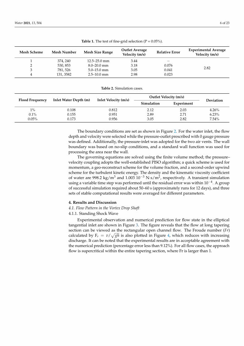
Figure 8 shows the predicted air-core ratio λ (ratio of the air-core area to cross-sectionalarea) in the contracted section and vertical shaft, showing an increasing trend of λ withdecreasing discharge. It can be seen that λ was the smallest around the junction witha value larger than the minimum engineering requirement of 0.25, indicating that thestructure can meet the maximum flood discharge requirements and ensure sufficientaeration conditions [7,26]. With the rapid rotation and diffusion of flow in the vertical shaft,the water thickness decreases and equivalently λ increases. However, the increasing effectseems to flatten off remarkably as decreasing level z.

The minimum λ (λm), a vital design parameter, can be plotted against a dimension-less discharge parameter Fa (Fa = 4(Q2e/(gπ3D1

6 cos β))1/3/(1 − e/D1)) on previous

experimental investigations [15] for the tangential slot inlet. Figure 9 shows the numericalpredictions of λm against Fa (according to [1], a value of e should be given as 0.9E for theelliptical tangential intake); the data of Yu and Lee [15] and Jain [7] are also extracted. It isseen that the results nearly match on one line. To estimate the minimum air-core ratio forthe tangential intake, nonlinear regression was founded to fit collective data and proposedas follows:

λm = 0.153Fa2 − 0.797Fa + 1 (7)

Water 2021, 13, 504 10 of 23


Figure 8 shows the predicted air-core ratio λ (ratio of the air-core area to cross-sectional area) in the contracted section and vertical shaft, showing an increasing trend of λ with decreasing discharge. It can be seen that λ was the smallest around the junction with a value larger than the minimum engineering requirement of 0.25, indi-cating that the structure can meet the maximum flood discharge requirements and en-sure sufficient aeration conditions [7,26]. With the rapid rotation and diffusion of flow in the vertical shaft, the water thickness decreases and equivalently λ increases. However, the increasing effect seems to flatten off remarkably as decreasing level z.

Figure 8. Air core ratio along the shaft.

The minimum λ (λm), a vital design parameter, can be plotted against a dimen-sionless discharge parameter aF ( 2 3 6 1/3

1 14( / ( cos )) / (1 / )= −aF Q e g D e Dπ β ) on previous experimental investigations [15] for the tangential slot inlet. Figure 9 shows the numeri-cal predictions of λm against Fa (according to [1], a value of e should be given as 0.9E for the elliptical tangential intake); the data of Yu and Lee [15] and Jain [7] are also extracted. It is seen that the results nearly match on one line. To estimate the minimum air-core ra-tio for the tangential intake, nonlinear regression was founded to fit collective data and proposed as follows:

2m 0.153 0.797 1a aF Fλ = − + (7)

Equation (7) can be expected to give a satisfactory estimation of the minimum air-core rate for the VDS spillway with the tangential inlet.

Figure 8. Air core ratio along the shaft.


Figure 9. Minimum air-core rate against Fa.

4.1.3. Annular Hydraulic Jump

Finally, the helicoidal jet dropped into the milky hydraulic jump and formed a wa-ter cushion, consuming much energy, as shown in Figure 10. In the present experimental discharge, the pressure slope was not always submerged by the air–water mixture flow, showing a changing performance in relation to the discharge. The experimental observa-tion shows that the condition of flow in pressure slope altering from weir flow (P = 3.33%, Q = 17.59 L/s) to orifice flow phenomenon (P = 1%, Q = 24.11 L/s). With a further increase in discharge, the free surface profile of the hydraulic jump is on the rise.

(a) (b) (c)

Figure 10. Experimental observation for annual hydraulic jump (a) P = 0.05% (b) P = 1% (c) P = 3.3%.

To examine the flow behavior of the annular hydraulic jump in more detail, the normalized height of the hydraulic jump 2/jh D (where jh is the elevation of the hy-

draulic jump, 2D is the diameter of the vertical shaft.) is plotted against 52/Q gD in

Figure 11. In the numerical test, the annular hydraulic jump occurred at 2/jh D = 3.60 (P = 0.05%), 3.01 (P = 0.1%) and 2.4 (P = 1%), which agreed well with experimental data under a negligible percentage error (2.1–3.6%). For different discharges, 2/jh D increases

as the 52/Q gD increases. However, 2/jh D does not shows a monotonic increasing

tendency with respect to 52/Q gD . It seems that 2/jh D initially increases slowly re-


Equation (7) can be expected to give a satisfactory estimation of the minimum air-corerate for the VDS spillway with the tangential inlet.


Finally, the helicoidal jet dropped into the milky hydraulic jump and formed a watercushion, consuming much energy, as shown in Figure 10. In the present experimentaldischarge, the pressure slope was not always submerged by the air–water mixture flow,showing a changing performance in relation to the discharge. The experimental observationshows that the condition of flow in pressure slope altering from weir flow (P = 3.33%,Q = 17.59 L/s) to orifice flow phenomenon (P = 1%, Q = 24.11 L/s). With a further increasein discharge, the free surface profile of the hydraulic jump is on the rise.

Water 2021, 13, 504 11 of 23




Finally, the helicoidal jet dropped into the milky hydraulic jump and formed a wa-ter cushion, consuming much energy, as shown in Figure 10. In the present experimental discharge, the pressure slope was not always submerged by the air–water mixture flow, showing a changing performance in relation to the discharge. The experimental observa-tion shows that the condition of flow in pressure slope altering from weir flow (P = 3.33%, Q = 17.59 L/s) to orifice flow phenomenon (P = 1%, Q = 24.11 L/s). With a further increase in discharge, the free surface profile of the hydraulic jump is on the rise.

(a) (b) (c)


To examine the flow behavior of the annular hydraulic jump in more detail, the normalized height of the hydraulic jump 2/jh D (where jh is the elevation of the hy-

draulic jump, 2D is the diameter of the vertical shaft.) is plotted against 52/Q gD in

Figure 11. In the numerical test, the annular hydraulic jump occurred at 2/jh D = 3.60 (P = 0.05%), 3.01 (P = 0.1%) and 2.4 (P = 1%), which agreed well with experimental data under a negligible percentage error (2.1–3.6%). For different discharges, 2/jh D increases

as the 52/Q gD increases. However, 2/jh D does not shows a monotonic increasing

tendency with respect to 52/Q gD . It seems that 2/jh D initially increases slowly re-


To examine the flow behavior of the annular hydraulic jump in more detail, thenormalized height of the hydraulic jump hj/D2 (where hj is the elevation of the hydraulicjump, D2 is the diameter of the vertical shaft.) is plotted against Q/

√gD25 in Figure 11. In

the numerical test, the annular hydraulic jump occurred at hj/D2 = 3.60 (P = 0.05%), 3.01(P = 0.1%) and 2.4 (P = 1%), which agreed well with experimental data under a negligiblepercentage error (2.1–3.6%). For different discharges, hj/D2 increases as the Q/

√gD25

increases. However, hj/D2 does not shows a monotonic increasing tendency with respectto Q/

√gD25. It seems that hj/D2 initially increases slowly resembling with a state of

weir flow when the discharge is lower than the critical value (near Q/√

gD25 = 0.42,Q = 24.11 L/s, P = 1%), whereas this increase becomes quickly with a trait of parabolicshape for discharge larger than these ranges. This means that the face of orifice flow isgenerated. The results are exactly as shown in Figure 10.


sembling with a state of weir flow when the discharge is lower than the critical value

(near 52/ =0.42Q gD , Q = 24.11 L/s, P = 1%), whereas this increase becomes quickly with

a trait of parabolic shape for discharge larger than these ranges. This means that the face of orifice flow is generated. The results are exactly as shown in Figure 10.

Figure 11. Relation between the normalized height of the hydraulic jump and discharge.

4.2. Distribution of Pressure in the Vortex Drop Shaft 4.2.1. Wall Pressure Distribution

The pressure corresponding to the shaft wall is one of the vital parameters to eval-uate the operation safety of the VDS spillways. In order to prevent cavitation occurrence and cavitation erosion, the negative pressure area should be avoided or reduced as much as possible [24]. Figure 12 shows the measured data with corresponding simulated data of wall pressure in the VDS. It can be clearly seen that the experimental and pre-dicted pressure show similar behavior with an acceptable deviation (mean error is equal to 8.07%), which further verifies the accuracy of the numerical prediction. However, there is a significant deviation below the elevation of the annular hydraulic jump (a per-centage error of 5.89–33.69%). A reasonable explanation for this phenomenon was the measurement error caused by the rapidly up and down fluctuation of the hydraulic jump. Another explanation lied in the limitations of the VOF method for simulating vig-orous air–water mixed-flow [2].

Figure 11. Relation between the normalized height of the hydraulic jump and discharge.

4.2. Distribution of Pressure in the Vortex Drop Shaft4.2.1. Wall Pressure Distribution

The pressure corresponding to the shaft wall is one of the vital parameters to evaluatethe operation safety of the VDS spillways. In order to prevent cavitation occurrence andcavitation erosion, the negative pressure area should be avoided or reduced as much aspossible [24]. Figure 12 shows the measured data with corresponding simulated dataof wall pressure in the VDS. It can be clearly seen that the experimental and predicted

Water 2021, 13, 504 12 of 23

pressure show similar behavior with an acceptable deviation (mean error is equal to8.07%), which further verifies the accuracy of the numerical prediction. However, there is asignificant deviation below the elevation of the annular hydraulic jump (a percentage errorof 5.89–33.69%). A reasonable explanation for this phenomenon was the measurementerror caused by the rapidly up and down fluctuation of the hydraulic jump. Anotherexplanation lied in the limitations of the VOF method for simulating vigorous air–watermixed-flow [2].


(a) (b)

Figure 12. Experimental and predicted wall pressure in the vortex drop shaft (VDS) (a) pressure on the left wall (b) pressure on the right wall.

There was no negative pressure on the wall; the pressure distribution was asym-metrical because of uneven water thickness. The pressure initially increased from the vortex chamber to the transition section; this is due to the reason that the tapered gradi-ent section shrinks, resulting in the increase of water thickness and tangential velocity. After this, the wall pressure above the annular hydraulic jump reduced, and the overall value was small. Finally, owing to the thickness and impingement of the water cushion, the pressure below the hydraulic jump sharply increased until the pressure reached its maximum value in the bottom of the well. The maximum value in the test was 10.76 kPa on the left wall (P = 0.05%) and 9.82 kPa on the right wall (P = 0.05%), corresponding to the simulated values of 12.34 kPa and 9.23 kPa. After being converted to prototype, it was a relatively large value and should be paid attention to. This tendency recorded was similar to the result obtained by He et al.[27] who simulated a large-scale vortex shaft spillway with superhigh water head and large flood discharge (Q > 1400 m3/s).

4.2.2. Cross-Sectional Pressure Distribution Pressure results for the different parts were obtained based on the three representa-

tive cross-sections, which are located in the vortex chamber (z = 1.55 m), the gradient section (z = 1.40 m), and the vertical shaft (z = 1.10 m), respectively. The general radial variation of the pressure cannot be obtained by experiment work but successfully cap-tured by the numerical simulation. Figure 13 shows the cloud diagram of cross-sectional pressure, and Figure 14 drawn from the extracted node data, is the pressure distribution on the right side of the shaft axis. To avoid redundancy, the left side result that has the same variation as the right side is not considered. It can be seen from Figure 14 that the variation of pressure distribution is represented as being the smallest at the air core, ap-proximately 0, then gradually increasing with the increasing radius for the rotary water, and finally reaching the maximum value on the wall. Additionally, the pressure of the same cross-section with the same radius is not symmetrical because of the uneven dis-tribution of water thickness, as seen in Figure 13. Interestingly, the pressure isoline den-sity near the cavity is slightly larger than that near the shaft wall. This rather complicated behavior can be explained in terms of the adequately turbulent mixed flow at the air–water interface.

Figure 12. Experimental and predicted wall pressure in the vortex drop shaft (VDS) (a) pressure on the left wall (b) pressureon the right wall.

There was no negative pressure on the wall; the pressure distribution was asymmet-rical because of uneven water thickness. The pressure initially increased from the vortexchamber to the transition section; this is due to the reason that the tapered gradient sectionshrinks, resulting in the increase of water thickness and tangential velocity. After this,the wall pressure above the annular hydraulic jump reduced, and the overall value wassmall. Finally, owing to the thickness and impingement of the water cushion, the pressurebelow the hydraulic jump sharply increased until the pressure reached its maximum valuein the bottom of the well. The maximum value in the test was 10.76 kPa on the left wall(P = 0.05%) and 9.82 kPa on the right wall (P = 0.05%), corresponding to the simulatedvalues of 12.34 kPa and 9.23 kPa. After being converted to prototype, it was a relativelylarge value and should be paid attention to. This tendency recorded was similar to theresult obtained by He et al. [27] who simulated a large-scale vortex shaft spillway withsuperhigh water head and large flood discharge (Q > 1400 m3/s).

4.2.2. Cross-Sectional Pressure Distribution

Pressure results for the different parts were obtained based on the three representativecross-sections, which are located in the vortex chamber (z = 1.55 m), the gradient section(z = 1.40 m), and the vertical shaft (z = 1.10 m), respectively. The general radial variationof the pressure cannot be obtained by experiment work but successfully captured by thenumerical simulation. Figure 13 shows the cloud diagram of cross-sectional pressure, andFigure 14 drawn from the extracted node data, is the pressure distribution on the right sideof the shaft axis. To avoid redundancy, the left side result that has the same variation as theright side is not considered. It can be seen from Figure 14 that the variation of pressuredistribution is represented as being the smallest at the air core, approximately 0, thengradually increasing with the increasing radius for the rotary water, and finally reachingthe maximum value on the wall. Additionally, the pressure of the same cross-section withthe same radius is not symmetrical because of the uneven distribution of water thickness,as seen in Figure 13. Interestingly, the pressure isoline density near the cavity is slightly

Water 2021, 13, 504 13 of 23

larger than that near the shaft wall. This rather complicated behavior can be explained interms of the adequately turbulent mixed flow at the air–water interface.


(a) (b) (c)

Figure 13. Pressure in different cross-section (P = 0.05%). (a) z = 1.55 m (b) z = 1.40 m (c) z = 1.10 m.

Figure 14. Pressure distribution in the radial direction.

4.3. Three-Dimensional Velocity Field in the Vortex Drop Shaft The flow velocity is an important parameter when analyzing the energy dissipation

effect and calculating the cavitation number. The laboratory measurement such as pitot tube has great limitations on measuring the resultant velocity in the VDS. However, Nan et al.[31] has validated the reliability for simulated velocity field When the numerical results are able to well predicts the flow pattern, the pressure, and the swirl angle (men-tioned below). For this reason, the following analysis is based on numerical results.

4.3.1. Velocity Field Near the Wall Generally, the rotational motion within the VDS not only depends on geometric

parameters such as the shape of the inlet structure, the shrinkage degree of the gradient section and the size of the vertical shaft, but also is closely linked to the turbulence and shear of flow, the mixing of the air and water, and the centrifugal force. Previous studies [2,24,27] focused more on the resultant velocity rather than each velocity component. As a typical three-dimensional motion, the rotary flow motion can be decomposed into axi-al motion, tangential motion and radial motion, satisfying the expression as follows:

2 2 2 2= z t rv v v v+ + (8)

where v denotes the resultant velocity, zv , tv and rv are the axial velocity, the tan-gential velocity and the radial velocity, respectively.



(a) (b) (c)



4.3. Three-Dimensional Velocity Field in the Vortex Drop Shaft The flow velocity is an important parameter when analyzing the energy dissipation

effect and calculating the cavitation number. The laboratory measurement such as pitot tube has great limitations on measuring the resultant velocity in the VDS. However, Nan et al.[31] has validated the reliability for simulated velocity field When the numerical results are able to well predicts the flow pattern, the pressure, and the swirl angle (men-tioned below). For this reason, the following analysis is based on numerical results.

4.3.1. Velocity Field Near the Wall Generally, the rotational motion within the VDS not only depends on geometric

parameters such as the shape of the inlet structure, the shrinkage degree of the gradient section and the size of the vertical shaft, but also is closely linked to the turbulence and shear of flow, the mixing of the air and water, and the centrifugal force. Previous studies [2,24,27] focused more on the resultant velocity rather than each velocity component. As a typical three-dimensional motion, the rotary flow motion can be decomposed into axi-al motion, tangential motion and radial motion, satisfying the expression as follows:

2 2 2 2= z t rv v v v+ + (8)

where v denotes the resultant velocity, zv , tv and rv are the axial velocity, the tan-gential velocity and the radial velocity, respectively.


4.3. Three-Dimensional Velocity Field in the Vortex Drop Shaft

The flow velocity is an important parameter when analyzing the energy dissipa-tion effect and calculating the cavitation number. The laboratory measurement such aspitot tube has great limitations on measuring the resultant velocity in the VDS. However,Nan et al. [31] has validated the reliability for simulated velocity field When the numer-ical results are able to well predicts the flow pattern, the pressure, and the swirl angle(mentioned below). For this reason, the following analysis is based on numerical results.

4.3.1. Velocity Field near the Wall

Generally, the rotational motion within the VDS not only depends on geometricparameters such as the shape of the inlet structure, the shrinkage degree of the gradientsection and the size of the vertical shaft, but also is closely linked to the turbulence and shearof flow, the mixing of the air and water, and the centrifugal force. Previous studies [2,24,27]focused more on the resultant velocity rather than each velocity component. As a typicalthree-dimensional motion, the rotary flow motion can be decomposed into axial motion,tangential motion and radial motion, satisfying the expression as follows:

v2 = vz2 + vt

2 + vr2 (8)

Water 2021, 13, 504 14 of 23

where v denotes the resultant velocity, vz, vt and vr are the axial velocity, the tangentialvelocity and the radial velocity, respectively.

Figure 15 shows the resultant velocity with corresponding velocity components of theswirling flow cling to the wall (the velocity extracting points are about 5–8 mm from thewall, and elevation corresponds to the pressure measurement point). With the exception oflocal fluctuation caused by shrinkage effects in the gradient section, the changing trend onboth sides is basically similar under the tested discharge. The unequal values on both sidesat a fixed elevation are probably due to the flow thickness and the wall friction. It is wellknown that with decreasing shaft elevation, gravity potential energy is gradually convertedinto kinetic energy, resulting in the increase in v and vz. However, once the helicoidal jetis distant from the top of the vertical shaft, the increasing rate of v and vz is no longerobvious. Following Hager [19], the rotational flow starts maintaining quasi-uniform flowwith a constant maximum velocity. This behavior seems to occur for the small discharge(P = 1%), in which a stable velocity value is around 3.8 m/s, as shown in Figure 15. Dong [1]provided an approximation of maximum velocity vm, as

vm =

(8gQ

nπD2

)1/3(9)


Figure 15 shows the resultant velocity with corresponding velocity components of the swirling flow cling to the wall (the velocity extracting points are about 5–8 mm from the wall, and elevation corresponds to the pressure measurement point). With the ex-ception of local fluctuation caused by shrinkage effects in the gradient section, the changing trend on both sides is basically similar under the tested discharge. The unequal values on both sides at a fixed elevation are probably due to the flow thickness and the wall friction. It is well known that with decreasing shaft elevation, gravity potential en-ergy is gradually converted into kinetic energy, resulting in the increase in v and zv . However, once the helicoidal jet is distant from the top of the vertical shaft, the increas-ing rate of v and zv is no longer obvious. Following Hager [19], the rotational flow starts maintaining quasi-uniform flow with a constant maximum velocity. This behavior seems to occur for the small discharge (P = 1%), in which a stable velocity value is around 3.8 m/s, as shown in Figure 15. Dong [1] provided an approximation of maxi-mum velocity mv , as

1/3

2

8=m

gQv

n Dπ

(9)

Herein n is the roughness coefficient; it is generally considered to be greater than the value calculated by the Manning formula [26]. This coefficient was also experimen-tally summarized by Dong [1] as:

( )1/32=0.09+0.04Exp 0.2 /n z D− (10)

(a) (b)

Figure 15. Velocity trends along the wall (a) left velocity (b) right velocity.

With respect to the tangential velocity, its value roughly increases at the gradient section but decreases at the vertical shaft. The reason for this increased behavior was at-tributed to the blocking and shrinkage effect of the gradient section, leading to the cen-trifugal force increases to maintain the conservation of angular momentum. After this, the tangential velocity behaves to decrease because of wall friction. In addition, it can be noted from Figure 15 that the radial velocity is negligible. Alternatively speaking, the rotational flow field in the VDS is dominated by axial and tangential movement.

Figure 15. Velocity trends along the wall (a) left velocity (b) right velocity.

Herein n is the roughness coefficient; it is generally considered to be greater than thevalue calculated by the Manning formula [26]. This coefficient was also experimentallysummarized by Dong [1] as:

n= 0.09 + 0.04Exp(−0.2z/D2)1/3 (10)

With respect to the tangential velocity, its value roughly increases at the gradientsection but decreases at the vertical shaft. The reason for this increased behavior wasattributed to the blocking and shrinkage effect of the gradient section, leading to thecentrifugal force increases to maintain the conservation of angular momentum. After this,the tangential velocity behaves to decrease because of wall friction. In addition, it canbe noted from Figure 15 that the radial velocity is negligible. Alternatively speaking, therotational flow field in the VDS is dominated by axial and tangential movement.

4.3.2. Swirl Angle

So far, few analytical approaches for rotational flow angle (α) are available up to theauthors’ knowledge [2,17]. The swirl angle can be estimated as α = arctan(vt/vz) for the

Water 2021, 13, 504 15 of 23

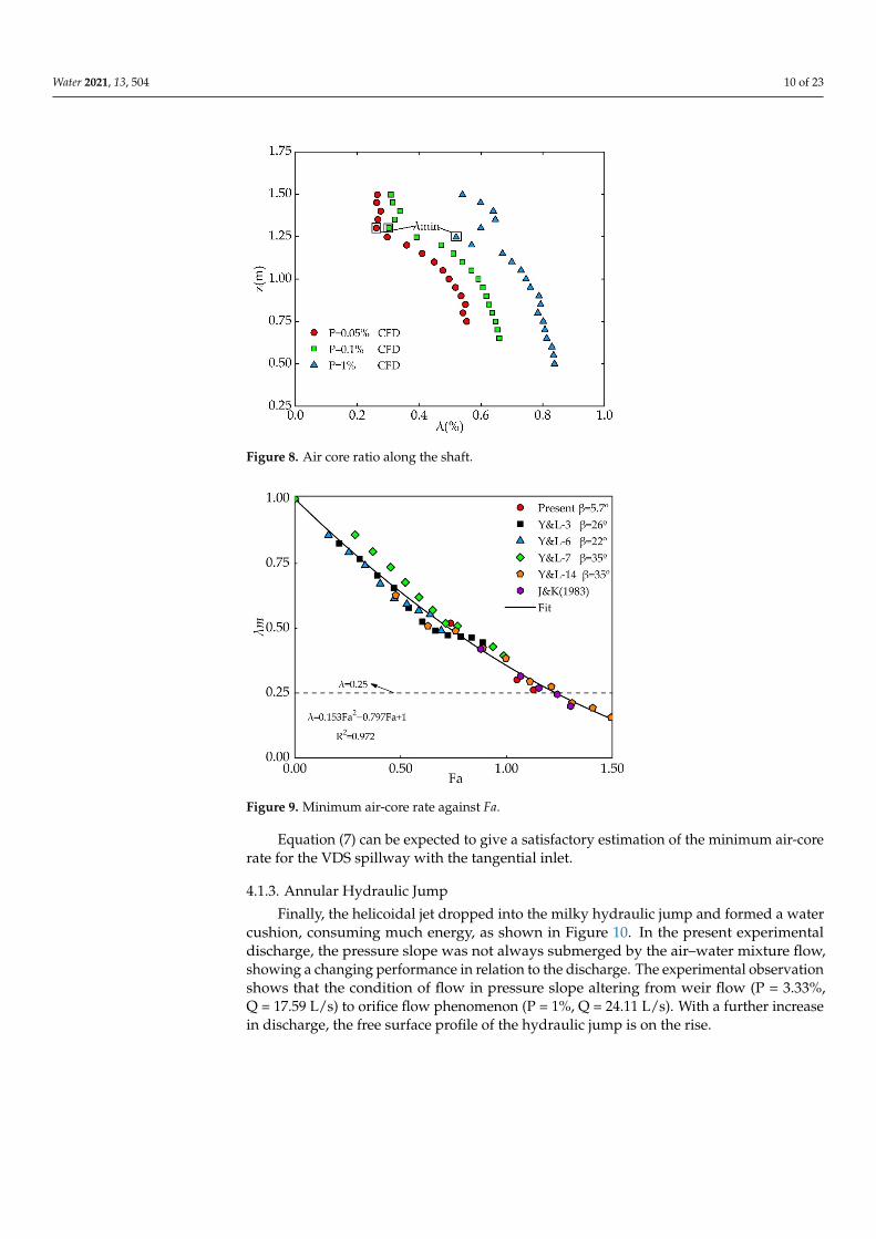
reason that vr the aforementioned is negligible. According to the results of swirl angle, asshown in Figure 16, the simulated values are very close to those actually obtained in thelaboratory, with an acceptable error of 3.3–11.5%. The swirl angle decreases with increasingthe incoming discharge at a fixed elevation and varied approximately in the range of 15–80◦.Specifically, the patterns of swirl angle distribution are as follows:

(1) The large swirl angle appeared at the vortex chamber, where the tangential velocitywas much larger than the axial flow velocity, according to Figure 15. As the initialtangential dominant movement was transformed into a compound movement of thetangential and axial direction, the swirl angle gradually decreased along the wall;

(2) The swirl angle in the gradient section tended to fluctuate due to the complex and un-stable flow field herein. This phenomenon corresponded to the noticeable fluctuationof vt and vz in Figure 15, which was beneficial to increase the local water head loss toimprove the energy dissipation rate;

(3) In the vertical shaft, the tangential velocity along the shaft was gradually consumeddue to friction effects, whereas the axial velocity increased because of gravity, whichtogether reduced the swirl angle.


4.3.2. Swirl Angle So far, few analytical approaches for rotational flow angle (α) are available up to the

authors’ knowledge [2,17]. The swirl angle can be estimated as arctan( / )α t zv v= for the reason that rv the aforementioned is negligible. According to the results of swirl angle, as shown in Figure 16, the simulated values are very close to those actually obtained in the laboratory, with an acceptable error of 3.3–11.5%. The swirl angle decreases with in-creasing the incoming discharge at a fixed elevation and varied approximately in the range of 15–80º. Specifically, the patterns of swirl angle distribution are as follows:

(1) The large swirl angle appeared at the vortex chamber, where the tangential velocity was much larger than the axial flow velocity, according to Figure 15. As the initial tangential dominant movement was transformed into a compound movement of the tangential and axial direction, the swirl angle gradually decreased along the wall;

(2) The swirl angle in the gradient section tended to fluctuate due to the complex and unstable flow field herein. This phenomenon corresponded to the noticeable fluctu-ation of tv and zv in Figure 15, which was beneficial to increase the local water head loss to improve the energy dissipation rate;

(3) In the vertical shaft, the tangential velocity along the shaft was gradually consumed due to friction effects, whereas the axial velocity increased because of gravity, which together reduced the swirl angle.

(a)

(b)

Figure 16. Swirl angle along the wall (a) left swirl angle (b) right swirl angle. Figure 16. Swirl angle along the wall (a) left swirl angle (b) right swirl angle.

4.3.3. Cross-Sectional Velocity Field

(1) Resultant velocity distribution

The example representing the resultant velocity distribution along the radial directionis shown in Figure 17 at the flood frequency of 0.5%. Figure 18 shows the velocity distribu-

Water 2021, 13, 504 16 of 23

tion of the rotational flow (fraction of water accounting for 80% is taken as the air–waterinterface). Due to the similar variation of left side, only the right results are shown. It canbe seen that the velocity behavior in the swirling flow area and the air core area exhibitobvious spatial variations.


4.3.3. Cross-Sectional Velocity Field (1) Resultant velocity distribution

The example representing the resultant velocity distribution along the radial direc-tion is shown in Figure 17 at the flood frequency of 0.5%. Figure 18 shows the velocity distribution of the rotational flow (fraction of water accounting for 80% is taken as the air–water interface). Due to the similar variation of left side, only the right results are shown. It can be seen that the velocity behavior in the swirling flow area and the air core area exhibit obvious spatial variations.

For the rotational flow area, the resultant velocity gradient is much smaller than that of the air in Figure 17. On one hand, for the vortex chamber and gradient section with a thick water layer, the velocity distribution is represented as that it linearly decreases from the air–water interface due to viscous dissipation, subsequently plummets to 0 rapidly near the wall affected by the boundary condition, as shown in Figure 18. On the other hand, the distribution of resultant velocity at the vertical shaft where the water layer is relatively thin is distinctly different from that aforementioned. The resultant ve-locity value no longer declines at first. Instead, its value first increases and then decreases with an insignificant variation, which persuasively proves why it is reasonable to use the near-wall velocity to replace average velocity at the vertical shaft regarding the previous studies [2,24].

With respect to the air, its movement is mainly caused by the entrainment of swirl-ing water [33]. The density of velocity isoline is the largest near the air–water interface, probably because of the highly turbulent and violently mixed air and water here. Addi-tionally, the air velocity in the cavity approximates the maximum at the center, as seen in

(a) (b) (c)

Figure 17. Resultant velocity in different cross-sections (P = 0.5%) (a) z = 1.55 m (b) z = 1.40 m (c) z = 1.10 m.

Figure 18. Resultant velocity of rotational flow along the radial direction.



4.3.3. Cross-Sectional Velocity Field (1) Resultant velocity distribution

The example representing the resultant velocity distribution along the radial direc-tion is shown in Figure 17 at the flood frequency of 0.5%. Figure 18 shows the velocity distribution of the rotational flow (fraction of water accounting for 80% is taken as the air–water interface). Due to the similar variation of left side, only the right results are shown. It can be seen that the velocity behavior in the swirling flow area and the air core area exhibit obvious spatial variations.

For the rotational flow area, the resultant velocity gradient is much smaller than that of the air in Figure 17. On one hand, for the vortex chamber and gradient section with a thick water layer, the velocity distribution is represented as that it linearly decreases from the air–water interface due to viscous dissipation, subsequently plummets to 0 rapidly near the wall affected by the boundary condition, as shown in Figure 18. On the other hand, the distribution of resultant velocity at the vertical shaft where the water layer is relatively thin is distinctly different from that aforementioned. The resultant ve-locity value no longer declines at first. Instead, its value first increases and then decreases with an insignificant variation, which persuasively proves why it is reasonable to use the near-wall velocity to replace average velocity at the vertical shaft regarding the previous studies [2,24].

With respect to the air, its movement is mainly caused by the entrainment of swirl-ing water [33]. The density of velocity isoline is the largest near the air–water interface, probably because of the highly turbulent and violently mixed air and water here. Addi-tionally, the air velocity in the cavity approximates the maximum at the center, as seen in Figure 17.

(a) (b) (c)


Figure 18. Resultant velocity of rotational flow along the radial direction. Figure 18. Resultant velocity of rotational flow along the radial direction.

For the rotational flow area, the resultant velocity gradient is much smaller than thatof the air in Figure 17. On one hand, for the vortex chamber and gradient section with athick water layer, the velocity distribution is represented as that it linearly decreases fromthe air–water interface due to viscous dissipation, subsequently plummets to 0 rapidly nearthe wall affected by the boundary condition, as shown in Figure 18. On the other hand,the distribution of resultant velocity at the vertical shaft where the water layer is relativelythin is distinctly different from that aforementioned. The resultant velocity value no longerdeclines at first. Instead, its value first increases and then decreases with an insignificantvariation, which persuasively proves why it is reasonable to use the near-wall velocity toreplace average velocity at the vertical shaft regarding the previous studies [2,24].

With respect to the air, its movement is mainly caused by the entrainment of swirlingwater [33]. The density of velocity isoline is the largest near the air–water interface, probablybecause of the highly turbulent and violently mixed air and water here. Additionally, theair velocity in the cavity approximates the maximum at the center, as seen in Figure 17.

(2) Tangential velocity distribution

The tangential velocity distribution on a level rotary flow discharge tunnel is similarto that of the hydrocyclone, which is basically in line with the combined vortex distribution

Water 2021, 13, 504 17 of 23

that inside and outside swirling flow are corresponding to the forced vortex distributionand free vortex distribution, respectively [30,31,33]. Whereas such phenomena for the VDSspillway is not clear. Therefore, the author tried to analyze and discuss the tangentialvelocity distribution of the rotational flow in the VDS. According to the test of Bradleyand Pulling [44], the tangential velocity distribution of the forced vortex accords with thefollowing law:

vt

rk = C (11)

The distribution of free vortex conforms to the following expression:

vtrk = C (12)

where the k is an index reflecting the degree to which the swirling flow conforms to theabsolute forced vortex or free vortex behavior, 0 < k < 1, the closer k is to 1, the moreconsistent it is. C is a constant on the same cross-section, but different-in-different cross-sections.

Figure 19 visualizes the distribution of the tangential velocity of the swirling flow. Forthe vortex chamber and the contracted section, the tangential velocity increases first, withan increasing radius near the cavity, which is suggestive of a forced vortex behavior, thentends to fall off resembling a free vortex distribution near the wall, ultimately plummets to0 affected by boundary condition. Moreover, it can be remarkably noted that the range ofincrease in the tangential velocity is smaller than that of decrease of the tangential velocity.This means that the tangential velocity mainly presents the free vortex distribution here.For instance, in the case of P = 0.05%, the ratio of increasing range to decreasing range is1.75:1 (z = 1.55 m) and 1.83:1 (z = 1.40 m). However, for the vertical shaft, this trend remainsopposite; the forced vortex area is wide because of the relatively large range of increase inthe tangential velocity. For instance, in the case of P = 0.05%, the ratio of increasing range todecreasing range is 0.54:1 (z = 1.10 m). This finding is contrary to the previous assumptionestablished by Jain [20], who considered the tangential velocity distribution at the verticalshaft as a free vortex region.


(2) Tangential velocity distribution The tangential velocity distribution on a level rotary flow discharge tunnel is simi-

lar to that of the hydrocyclone, which is basically in line with the combined vortex dis-tribution that inside and outside swirling flow are corresponding to the forced vortex distribution and free vortex distribution, respectively [30,31,33]. Whereas such phe-nomena for the VDS spillway is not clear. Therefore, the author tried to analyze and discuss the tangential velocity distribution of the rotational flow in the VDS. According to the test of Bradley and Pulling [44], the tangential velocity distribution of the forced vortex accords with the following law:

tk

v Cr

= (11)

The distribution of free vortex conforms to the following expression: k

tv r C= (12)

where the k is an index reflecting the degree to which the swirling flow conforms to the absolute forced vortex or free vortex behavior, 0< k <1, the closer k is to 1, the more con-sistent it is. C is a constant on the same cross-section, but different-in-different cross-sections.

Figure 19 visualizes the distribution of the tangential velocity of the swirling flow. For the vortex chamber and the contracted section, the tangential velocity increases first, with an increasing radius near the cavity, which is suggestive of a forced vortex behav-ior, then tends to fall off resembling a free vortex distribution near the wall, ultimately plummets to 0 affected by boundary condition. Moreover, it can be remarkably noted that the range of increase in the tangential velocity is smaller than that of decrease of the tangential velocity. This means that the tangential velocity mainly presents the free vor-tex distribution here. For instance, in the case of P = 0.05%, the ratio of increasing range to decreasing range is 1.75:1 (z = 1.55 m) and 1.83:1 (z = 1.40 m). However, for the vertical shaft, this trend remains opposite; the forced vortex area is wide because of the relatively large range of increase in the tangential velocity. For instance, in the case of P = 0.05%, the ratio of increasing range to decreasing range is 0.54:1 (z = 1.10 m). This finding is contrary to the previous assumption established by Jain [20], who considered the tan-gential velocity distribution at the vertical shaft as a free vortex region.

Figure 19. Tangential velocity along the radial direction.

It is significant to say that the behavior of the tangential velocity changing from quasi-forced vortex to quasi-free vortex is probably due to the reason that the violent

Figure 19. Tangential velocity along the radial direction.

It is significant to say that the behavior of the tangential velocity changing fromquasi-forced vortex to quasi-free vortex is probably due to the reason that the violentturbulence and full mixing of the air and water at the air–water interface, making the near-cavity rotational flow more affected by the air, consequently presenting a forced vortexdistribution, especially obvious when the water layer is thinner, and the cavity is larger.Hence, the tangential velocity at the vertical shaft is mainly presented as the forced vortex

Water 2021, 13, 504 18 of 23

distribution. Whereas the wall friction and the water layer shear will cause the tangentialvelocity to be consumed, thus the near-wall tangential velocity decays freely and presentsa free vortex distribution.

4.3.4. Theoretical Analysis between Cross-Sectional Pressure and Tangential Velocity

Herein, a predicted approach for the relationship between tangential velocity andpressure is proposed. The following calculations and results refer to the present geometryof the VDS spillway, with an elliptical tangential intake at the drop shaft head. Now usinga swirling micro-surface, as shown in Figure 20. The motion Equation along the radialdirection is established as follows:

(p +∂p∂r

× dr2)rdθ − ρdrdθvt

2 − (p − ∂p∂r

× dr2)rdθ = ρrdθdr

dvr

dt(13)

where r is the radius of micro rotary flow, dr is the thickness of micro rotary flow, ∂p∂r is the

pressure change, dvr/dt is the radial acceleration, and ρ is the density of water. Since theradial velocity is extremely small and can be ignored, Equation (13) can be simplified to:

dpdr

= ρvt

2

r(14)Water 2021, 13, x FOR PEER REVIEW 20 of 24

Figure 20. Analysis of the micro swirling flow.

The k value of different positions was calculated by the simulated tangential veloc-ity. Then combined with Equations (17) and (18), the theoretical pressure at each position can be obtained. The comparison of pressure between the theoretical value and the sim-ulated value is shown in Figure 21, where the dotted line indicates the boundary between the forced vortex and the free vortex region. It can be seen that there is a significant dif-ference between the calculated value and the simulated value near the boundary and that the deviation within the forced vortex region is greater than that within the free vortex region. The possible reason lies in that there is a rapid adjustment of kinetic energy and pressure energy in the forced vortex region [32].

(a) (b)

(c)

Figure 21. Comparison of the simulated values with theoretical values of the radial pressure. (a) z = 1.55 m (b) z = 1.40 m (c) z = 1.10 m.


For the near-cavity swirling flow resembling forced vortex behavior, C is a constant ofthe same section, the Formula (11) can be expressed as:

vt = vtc(rrc)

k(15)

where vtc is the tangential velocity of the swirling flow at the air–water interface, and rc isthe corresponding radius.

Substituting Formula (15) into Formula (14) and performing integration yields:

p =ρvtc

2

rc2k

∫r2k−1dr =

ρvtc2

2k(

rrc)

2k+ C1 (16)

where C1 is the integral constant. When r = rc, pressure is equal to 0, Calculate C1 =−ρvtc

2/2k, and substitute it into Equation (16) to obtain the pressure expression of theforced vortex distribution area as follows:

p =ρvtc

2

2k

[(

rrc)

2k− 1]

(17)

Water 2021, 13, 504 19 of 23

For the near-wall rotational flow resembling free vortex behavior, only Equation (12)needs to be expressed as vt = vtR(R/r)k. Meanwhile, the boundary conditions thatr = R, p = pR are adopted, then the pressure expression can be obtained as:

p = pR +ρvtR

2

2k

[1 − (

Rr)2k]

(18)

where pR is the wall pressure, vtR is the corresponding tangential velocity, and R is theradius of the VDS.

The k value of different positions was calculated by the simulated tangential velocity.Then combined with Equations (17) and (18), the theoretical pressure at each position canbe obtained. The comparison of pressure between the theoretical value and the simulatedvalue is shown in Figure 21, where the dotted line indicates the boundary between theforced vortex and the free vortex region. It can be seen that there is a significant differencebetween the calculated value and the simulated value near the boundary and that thedeviation within the forced vortex region is greater than that within the free vortex region.The possible reason lies in that there is a rapid adjustment of kinetic energy and pressureenergy in the forced vortex region [32].



The k value of different positions was calculated by the simulated tangential veloc-ity. Then combined with Equations (17) and (18), the theoretical pressure at each position can be obtained. The comparison of pressure between the theoretical value and the sim-ulated value is shown in Figure 21, where the dotted line indicates the boundary between the forced vortex and the free vortex region. It can be seen that there is a significant dif-ference between the calculated value and the simulated value near the boundary and that the deviation within the forced vortex region is greater than that within the free vortex region. The possible reason lies in that there is a rapid adjustment of kinetic energy and pressure energy in the forced vortex region [32].

(a) (b)

(c)

Figure 21. Comparison of the simulated values with theoretical values of the radial pressure. (a) z = 1.55 m (b) z = 1.40 m (c) z = 1.10 m. Figure 21. Comparison of the simulated values with theoretical values of the radial pressure. (a) z = 1.55 m (b) z = 1.40 m(c) z = 1.10 m.

The simulated and theoretical results exhibit a very similar pattern with an acceptableoverall deviation at the vortex chamber (z = 1.55 m) and the gradient section (z = 1.40 m).The mean error between the calculated and simulated values was 6.96% and 7.92%, respec-tively, while for the vertical shaft (z = 1.10 m), The mean error is 15.11%, suggesting that

Water 2021, 13, 504 20 of 23

the theoretical formula based on the combined vortex rule is feasible for the cross-sectionalpressure prediction in the VDS spillway, especially in the free vortex region.

5. Conclusions

The complex flow field of a VDS spillway with an elliptical tangential inlet is testedexperimentally and simulated. The results of the model experiment with correspondingnumerical prediction were similar in terms of the flow pattern. The wall pressure andthe swirl angle flow regime of the VDS spillway is characterized by the standing shockwave, the air core and the annular hydraulic jump. One standing wave was detectedunder supercritical flow conditions with a moderate Froude number. The dimensionlessmaximum wave height tends to linearly grow with increasing discharge, but the increasingeffect is insignificantly improved. A high-axisymmetric air core along the shaft can be wellcaptured by numerical prediction. On the basis of previous studies, a quadratic equationwas fitted to give an estimation of the minimum air-core rate for the VDS spillway with thetangential inlet. As regards the annular hydraulic jump, its dimensionless height, showingvariation performance of first increasing slowly and then rapidly increasing with increasingdischarge, was related to the pressure slope where the flow condition varies from weir flowto orifice flow simultaneously.

The swirling flow velocity is decomposed into the three-dimensional components fordetailed research. The end rotational flow seems to start maintaining quasi-uniform flowwith the constant maximum resultant velocity for small discharge. The cross-sectionalresultant velocity value linearly decreases with an increasing radius for the vortex chamberand gradient section while initially increases and then decreases with an insignificantvariation for the vertical shaft. Moreover, the rotational flow field in the VDS is dominatedby the axial and tangential movement because radial velocity with an extremely small valueis negligible. The cross-sectional tangential velocity distribution accords with the combinedvortex behavior. The free vortex region is wider in the vortex chamber and gradient section,but the vertical is opposite. The theoretical calculation for the cross-sectional pressurebased on the combined vortex rule was developed, especially feasible in the free vortexregion. Considering that the eco-friendly VDS spillway has become an important researchhotspot in the field of flood discharge and energy dissipation, the current work can provideuseful insights for future research and application of similar engineering. Furthermore, therelevant prototype measurements work is necessary to conduct in the future.

Author Contributions: Physical experiment, Z.Y., G.X. and H.Y.; computer and numerical simulation,Z.Y., J.Y. and Y.L.; methodology and Chart, Z.Y., J.Y. and G.X.; writing—review and editing, Z.Y.,J.Y. and Z.L.; funding support, Z.L. All authors contributed to the overall framing and revision ofthe manuscript at multiple stages. All authors have read and agreed to the published version of themanuscript.

Funding: This research was funded by the National Natural Science Foundation of China, grantnumber (No. 51509212).

Institutional Review Board Statement: Not applicable.

Informed Consent Statement: Informed consent was obtained from all subjects involved in thestudy.

Data Availability Statement: All data, models, or code generated or used during the study areavailable from the corresponding author by request.

Conflicts of Interest: The authors declare no conflict of interest.

Water 2021, 13, 504 21 of 23

Abbreviations

aw Volume of fluid functionC Constant of combined eddyC1 Integral constantD1 Diameter of the vortex chamber (m)D2 Diameter of the vertical shaft (m)E Entrance width of the vortex chamber (m)Fa A dimensionless discharge parameterFr Froude numberFr0 Froude number at the beginning of the elliptical guiding wallε Turbulent dissipation rate (m2·s−3)fi Gravity component (m·s−2)g Gravity acceleration (m·s−2)Gk Turbulent kinetic energy generated by the velocity gradienth0 Water depth at the beginning of the elliptical guiding wall (m)hm Maximum standing wave elevation (m)hj Elevation of the hydraulic jump (m)k Index of combined eddyn Roughness coefficientP Pressure (kPa)pR Wall pressure (kPa)P Flood frequencyρ Density of water (kg·m−3)Q Discharge (m3·s)r Radius of swirling flow (m)R Radius of the VDS (m)t Time (s)ui Velocity component (m/s)µ Coefficient of dynamic viscosity (kg·m−1·s−1)µeff Revisionary coefficient of dynamic viscosity (kg·m−1·s−1)v Resultant velocity (m·s−1)vm Maximum velocity (m·s−1)vt Tangential velocity (m·s−1)vtc Tangential velocity of the air–water interface (m·s−1)vtR Tangential velocity of the wall (m·s−1)vz Axial velocity (m·s−1)vr Radial velocity (m·s−1)α Swirl angleβ Inclination angle of the tapering sectionηm Relative maximum heightλ Air-core ratioλm Minimum air-core ratioxi Coordinate componentz Elevation (m)

References1. Dong, X.L. Spillway with Swirling Flow; The Yellow River Water Conservancy Press: Zhengzhou, China, 2011.2. Liu, Z.P.; Guo, X.L.; Xia, Q.F.; Fu, H.; Wang, T. Experimental and Numerical Investigation of Flow in a Newly Developed Vortex

Drop Shaft Spillway. J. Hydraul. Eng. 2018, 144. [CrossRef]3. Lian, J.J.; He, J.L.; Guo, W.J.; Ran, D.J. Effects of Bucket Type and Angle on Downstream Nappe Wind Caused by a Turbulent Jet.

Int. J. Environ. Res. Public Health 2019, 16, 1360. [CrossRef] [PubMed]4. Dong, X.L.; Guo, J. Report on Model Study of Retrofitting a Diversion Tunnel into a Vortex Dropshaft Spillway in Shapai Power Station;

IWHR Research Rep, China Institute of Water Resources and Hydropower Research: Beijing, China, 1995.5. Sun, S.K.; Liu, Z.P.; Zhou, S.; Yang, J.W. Study on the rebuild of large-sized diversion tunnel into flood releasing tunnel in the

Xiaowan Hydropower Station. Water Power 2001, 1, 26–31, 68.6. Dong, X.L.; Yang, K.l.; Guo, X.L.; Guo, Y.X. Hydraulic mechanism and application of swirling device in morning glory shaft

spillway. J. Hydraul. Eng. 2011, 42, 14–18. (In Chinese)

http://doi.org/10.1061/(ASCE)HY.1943-7900.0001444

http://doi.org/10.3390/ijerph16081360

http://www.ncbi.nlm.nih.gov/pubmed/31014021

Water 2021, 13, 504 22 of 23

7. Jain, S.C.; Kennedy, J.F. Vortex-flow Drop Structures for the Milwaukee Metropolitan Sewerage District Inline Storage System.In Proceedings of IIHR Rep.264; Iowa Institute of Hydraulic Research, University of Iowa: Iowa City, IA, USA.

8. Rhee, D.S.; Park, Y.S.; Park, I. Effects of the bottom slope and guiding wall length on the performance of a vortex drop inlet. WaterSci. Technol. 2018, 78, 1287–1295. [CrossRef]

9. Jain, S.C. Tangential Vortex-Inlet. J. Hydraul. Eng. 1984, 110, 1693–1699. [CrossRef]10. Quick, M.C. Analysis of Spiral Vortex and Vertical Slot Vortex Drop Shafts. J. Hydraul. Eng. 1990, 116, 309–325. [CrossRef]11. Hager, W.H. Vortex Drop Inlet for Supercritical Approaching Flow. J. Hydraul. Eng. 1990, 116, 1048–1054. [CrossRef]12. Chan, S.N.; Qiao, Q.S.; Lee, J.H.W. On the three-dimensional flow of a stable tangential vortex intake. J. Hydro-Environ. Res. 2018,

21, 29–42. [CrossRef]13. Pfister, M.; Crispino, G.; Fuchsmann, T.; Ribi, J.M.; Gisonni, C. Multiple Inflow Branches at Supercritical-Type Vortex Drop Shaft.

J. Hydraul. Eng. 2018, 144, 9. [CrossRef]14. Slisskii, S.M.; Kuznetsov, E.B.; Akhmedov, T.K. Multistage whirlpool shaft spillways. Hydrotech. Constr. 1980, 14, 892–895.

[CrossRef]15. Yu, D.; Lee, J.H.W. Hydraulics of Tangential Vortex Intake for Urban Drainage. J. Hydraul. Eng. 2009, 135, 164–174. [CrossRef]16. Del Giudice, G.; Gisonni, C. Vortex dropshaft retrofitting: Case of Naples city (Italy). J. Hydraul. Res. 2011, 49, 804–808. [CrossRef]17. Crispino, G.; Pfister, M.; Gisonni, C. Hydraulic design aspects for supercritical flow in vortex drop shafts. Urban Water J. 2019, 16,

225–234. [CrossRef]18. Wu, J.H.; Ren, W.C.; Ma, F. Standing wave at dropshaft inlets. J. Hydrodyn. 2017, 29, 524–527. [CrossRef]19. Hager, W.H.; Kellenberger, M.H. Die Dimensionierung Des Wirbelfallschachtes [The Design of the Vortex Drop]. Gas-und

Wasserfach. Wasser Abwasser 1987, 128, 582–590.20. Jain, S.C. Air Transport in Vortex-flow Drop Shafts. J. Hydraul. Eng. 1988, 114, 1485–1497. [CrossRef]21. Edwini-Bonsu, S.; Steffler, P.M. Dynamics of air flow in sewer conduit headspace. J. Hydraul. Eng. 2006, 132, 791–799. [CrossRef]22. Li, Y.; Zhang, F.X.; Deng, J.; Xu, W.L. Calculation of the Cavity Length of Annular Aerator in the Vortex Drop Shaft Spillway. J.

Sichuan. Univ. 2011, 43, 28–33.23. Gualtieri, C.; Chanson, H. Interparticle arrival time analysis of bubble distributions in a dropshaft and hydraulic jump. J. Hydraul.

Res. 2013, 51, 253–264. [CrossRef]24. Zhang, W.C.; Wang, J.X.; Dong, Z.S.; Zhou, Z.; Yang, X. Characteristics of energy dissipation and cavitation of vertical swirling

spillway. J. Zhongnan Univ. 2018, 49, 3011–3019.25. Camino, G.A.; Zhu, D.Z.; Rajaratnam, N. Flow Observations in Tall Plunging Flow Dropshafts. J. Hydraul. Eng. 2015, 141, 7.

[CrossRef]26. Zhao, C.H.; Zhu, D.Z.; Sun, S.K.; Liu, Z.P. Experimental study of flow in a vortex drop shaft. J. Hydraul. Eng. 2006, 132, 61–68.

[CrossRef]27. He, J.L.; Yin, J.B.; Jiang, Q.F.; Wu, B.Q. Numerical simulation study on vortex shaft spillway with superhigh water head and large

flood discharge. J. Hydroelect. Eng. 2016, 35, 45–51.28. Guo, Y.; Ni, H.G. Study on the water flow characteristics of the vortex shaft spillway. J. Hydrodyn. Ser. A 1995, 1, 97–105.29. Mahmouth-Rad, M.; Khanjani, M.J. Energy Dissipation of Flow in the Vortex Structure: Experimental Investigation. J. Pipel. Syst.

Eng. Pract. 2019, 10, 16. [CrossRef]30. Cao, S.L.; Niu, Z.M.; Yang, J.; Lu, H.B. Velocity and pressure distributions in discharge tunnel of rotary-obstruction composite

inner energy dissipation. Sci. Chin. Technol. Sci. 2011, 54, 111–117. [CrossRef]31. Nan, J.H.; Niu, Z.M.; Zhang, D. Study on Velocity Characteristics of Cavity Gyrating Flow in Gyrating Discharge Tunnel. J. Sichuan

Univ. 2016, 48, 41–47.32. Niu, Z.M.; Zhang, M.Y. Wall Stress of Horizontal Rotary Cavity Flow. J. Chin. J. Appl. Mech. 2004, 4, 110–114, 174.33. LI, Q.L.; Niu, Z.M.; Wang, J. Analysis of Rotary Flow in Spillway Tunnel with Blocking Based on Quasi-free-vortex Rules.

J. Sichuan Univ. 2014, 46, 49–57.34. Zhang, J.M.; Ren, C.Y.; Xu, W.L.; LI, Z.; HU, X.Y. Novel type of revolving-flow drop-shaft with submerged outlet. J. Hydroelect.

Eng. 2012, 31, 96–101.35. Wei, Y.; Shi, Z.J.; Chang, X.Q. Hydraulic design of vertical vortex spillway tunnel. J. Hydroelect. Eng. 2007, 26, 88–92.36. Chen, J.G.; Zhang, J.M.; Xu, W.L.; Wang, Y.R. Scale Effects of Air-Water Flows in Stiling Basin of Multi-Horizontal Submerged Jets.

J. Hydrodyn. 2010, 22, 788–795. [CrossRef]37. Galvan, S.; Reggio, M.; Guibault, F. Assessment Study of k-epsilon Turbulence Models and Near-Wall Modeling for Steady State

Swirling Flow Analysis in Draft Tube Using Fluent. Eng. Appl. Comput. Fluid. 2011, 5, 459–478. [CrossRef]38. Li, S.; Zhang, J. Numerical Investigation on the Hydraulic Properties of the Skimming Flow over Pooled Stepped Spillway. Water

2018, 10, 1478. [CrossRef]39. Qi, Y.; Wang, Y.; Zhang, J. Three-Dimensional Turbulence Numerical Simulation of Flow in a Stepped Dropshaft. Water 2019, 11,

30. [CrossRef]40. Yakhot, V. Renormalization group analysis of turbulence: Basic theory. J. Sci. Comput. 1986, 1, 3–51. [CrossRef]41. Jalil, S.A.; Hussein, B.S.; Sarhan, S.A. Visualization of elbow flow performance as shaft spillway. Ain Shams Eng. J. 2020, 11,

865–873. [CrossRef]

http://doi.org/10.2166/wst.2018.397

http://doi.org/10.1061/(ASCE)0733-9429(1984)110:12(1693)

http://doi.org/10.1061/(ASCE)0733-9429(1990)116:3(309)

http://doi.org/10.1061/(ASCE)0733-9429(1990)116:8(1048)

http://doi.org/10.1016/j.jher.2018.07.001


http://doi.org/10.1007/BF02305443

http://doi.org/10.1061/(ASCE)0733-9429(2009)135:3(164)

http://doi.org/10.1080/00221686.2011.622148

http://doi.org/10.1080/1573062X.2019.1648531

http://doi.org/10.1016/S1001-6058(16)60765-5

http://doi.org/10.1061/(ASCE)0733-9429(1988)114:12(1485)

http://doi.org/10.1061/(ASCE)0733-9429(2006)132:8(791)

http://doi.org/10.1080/00221686.2012.762430


http://doi.org/10.1061/(ASCE)0733-9429(2006)132:1(61)

http://doi.org/10.1061/(ASCE)PS.1949-1204.0000398

http://doi.org/10.1007/s11431-011-4633-4

http://doi.org/10.1016/S1001-6058(09)60117-7

http://doi.org/10.1080/19942060.2011.11015386

http://doi.org/10.3390/w10101478

http://doi.org/10.3390/w11010030

http://doi.org/10.1007/BF01061452

http://doi.org/10.1016/j.asej.2020.03.017

Water 2021, 13, 504 23 of 23

42. Launder, B.E.; Spalding, D.B. A Mathematical Model Illustrating the Theory of Turbulence; Academic Press: London, UK, 1972.43. Hirt, C.W.; Nichols, B.D. Volume of fluid (VOF) method for the dynamics of free boundaries. J. Comput. Phys. 1981, 39, 201–225.44. Bradley, D.; Pulling, D.J. Flow pattern in the hydraulic cyclone and their interpretation in terms of performance. Trans. Inst. Chem.

Engrs. 1959, 37, 34–45.

Documents

Three-Dimensional Flow of a Vortex Drop Shaft Spillway