THREE DIMENSIONAL ANALYSIS OF

EXTRUSION

THROUGH TAPER DIE

A THESIS SUBMITTED IN PARTIAL FULFILMENT OF THE

REQUIREMENTS FOR THE DEGREE OF

Master of Technology

in

Mechanical Engineering By

Mithun Kumar Murmu

Department of Mechanical Engineering National Institute of Technology Rourkela MAY, 2009

THREE DIMENSIONAL ANALYSIS OF EXTRUSION THROUGH TAPER DIE

A THESIS SUBMITTED IN PARTIAL FULFILMENT OF THE

REQUIREMENTS FOR THE DEGREE OF

Master of Technology

in Mechanical Engineering

[Specialization: Production Engineering]

By

Mithun Kumar Murmu

Under the Guidance of

Dr. Susanta Kumar Sahoo

Department of Mechanical Engineering

Department of Mechanical Engineering National Institute of Technology

Rourkela May, 2009

NATIONAL INSTITUTE OF TECHNOLOGYROURKELA- 769008INDIA

CERTIFICATE

This is to certify that the thesis entitled ee Dimensional Analysis of Extrusion

To the best of my kno\Vledg~~ embodied in the thesis has not been

submitted to any other University/Htstityte for the a\Vard.ofany degree or diploma.

Date:

Dr.SusantaKumarS~Departmentof MechanicalEngineering

I

National Institute of Technology

Rourkela - 769008

NATIONAL INSTITUTE OF TECHNOLOGYROURKELA - 769008INDIA

ACKNOWLEDGEMENT

I avail this opportunity to extend my .indebtedness to my guide Dr.S.K.Sahoo,

Professor, Mechanical Engineering for his constant encouragement and

kind help at different stages for the execution of this dissertation work.! am extremely

thankful to Prof. R. K. Sahoo Head, Departmentof MechanicalEngineeringand Prof. S.S.

Mohapatra, Course CdPrqip their helpand !1te;;course ofthis work.

I am also thankful to Mr.Y.AJj, Technical assistant of cental workshop for their help during

the execution of experiment. Myff'iends ShuV't3nSu, L. N. Patra(Ph D Scholar) and

Sontosh sahoo deserve my special thanks for their help and support throughout this work.

I am also thankful to all my well wishers, class mates and friends for their inspiration and

help.

Date:- dS/O 5'(~t'I1C:1-h~1) \(</ MW(~.

Mithun KumarM"urmu

Roll No.-207ME202

ABSTRACT

An upper bound solution for extrusion of “triangular” sectioned product through taper die from

round sectioned billet has been developed. A simple discontinuous kinematically admissible

velocity field with optimization parameter is proposed. From the proposed velocity field the

upper bound solution on non-dimensional extrusion pressure are determined with respect to

chosen process parameters. The theoretical results are compared with experimental result to

check the validity of the proposed velocity fields.

The reformulated SERR technique is used to find out the kinematically admissible velocity field

applied to deformation zone surrounded by flat surfaces. This velocity field is used to compute

upper bound extrusion pressure at various area of reduction.

The triangular sectioned product from round sectioned billet through taper die is taken for upper

bound analysis using SERR technique. As this section is symmetry about one axis with round

sectioned billet only one half of section is taken as domain interest for deformation zone to

calculate the velocity field. Detailed formulations of models are presented.

To validate the proposed model/analysis experiments are carried out taking lead as the working

material. An experimental set-up is designed and fabricated with four split type taper dies for this

purpose. Experiments are carried out at dry and lubricated condition of the dies to check the

friction effect.

The results obtained indicate that the predictions both in extrusion load and the deformed

configuration are in good agreement with the experiment under different lubrication conditions.

 

CONTENTS

 

*******

   

Chapter 1 Introduction 1-10

Chapter 2 Theoretical Analysis 11-21

Chapter 3 Upper bound Analysis For Extrusion OF Triangular Section Through Taper Dies

22-39

Chapter 4 Experimental Investigation 40-58

Chapter 5 Conclusions & Future works 59-60

References 61-62

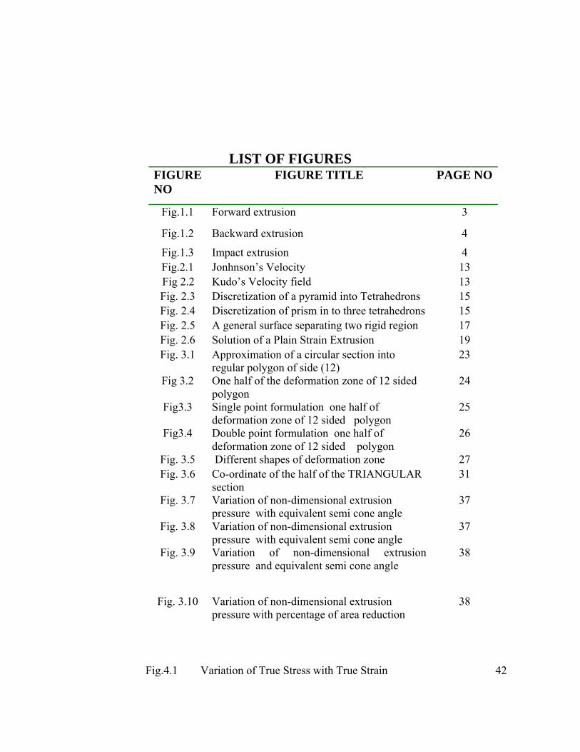
LIST OF FIGURES FIGURE NO

FIGURE TITLE PAGE NO

Fig.1.1 Forward extrusion 3

Fig.1.2 Backward extrusion 4

Fig.1.3 Impact extrusion 4 Fig.2.1 Jonhnson’s Velocity 13

Fig 2.2 Kudo’s Velocity field 13 Fig. 2.3 Discretization of a pyramid into Tetrahedrons 15 Fig. 2.4 Discretization of prism in to three tetrahedrons 15 Fig. 2.5 A general surface separating two rigid region 17 Fig. 2.6 Solution of a Plain Strain Extrusion 19 Fig. 3.1 Approximation of a circular section into

regular polygon of side (12) 23

Fig 3.2 One half of the deformation zone of 12 sided polygon

24

Fig3.3 Single point formulation one half of deformation zone of 12 sided polygon

25

Fig3.4 Double point formulation one half of deformation zone of 12 sided polygon

26

Fig. 3.5 Different shapes of deformation zone 27 Fig. 3.6 Co-ordinate of the half of the TRIANGULAR

section 31

Fig. 3.7 Variation of non-dimensional extrusion pressure with equivalent semi cone angle

37

Fig. 3.8 Variation of non-dimensional extrusion pressure with equivalent semi cone angle

37

Fig. 3.9 Variation of non-dimensional extrusion pressure and equivalent semi cone angle

38

Fig. 3.10 Variation of non-dimensional extrusion pressure with percentage of area reduction

38

Fig.4.1 Variation of True Stress with True Strain 42

Fig.4.2 Ring before compression 44 Fig. 4.3 Ring after compression 44

Fig. 4.4 Theoretical calibration curve for standard ring 6:3:2 45 Fig. 4.5 UTM (INSTRON 600 KN) and close view 46 Fig. 4.6 Assembly setup(photograph) 46 Fig. 4.7 Shcematic view of Experimental setup 46 Fig. 4.8 Disassemle parts of setup(photograph 47 Fig. 4.9 Experimental setup for extrusion 47

Fig. 4.10(a) One half Schematic view of die 49 Fig. 4.10(b) Top view of die TYPE 1 49

Fig. 4.11(a) Top view of die TYPE 2 49

Fig. 4.11(b) Bottom view of die 49

Fig.4.12 Photograph of different type of die 50Fig.4.13 Variation of Compressive Load with Extension at

Lubricated Condition

 

52

Fig.4.14 Variation of Compressive Load with Extension at dry condition

52

Fig.4.15 Variation of Compressive Load with Extension at wet condition

53

Fig.4.16 Variation of Compressive Load with Extension at Wet Condition

53

Fig.4.17 Variation of Compressive Load with Extension at Dry Condition

54

Fig.418 Photograph Extruded product at wet condition 54 Fig.4. 19 Photograph of Extruded product at dry condition 55

Fig .4.20 Photograph of Shape of product inside die 55

 

TABE NO. TABLE TITLE PAGE NO

Table.2.1 Conversion of Prism and Pyramid into Tetrahedron

15

Table.2.2 Lines. The zone they separated and velocity vector

on their sides.

19

Table.3.1 Half extrusion zone(domain of interest) divided into

prism, pyramid and tetrahedron

27

Table 3.2 Number of planes and ways of discritization

27

Table.3.3 Total number of planes derived from Prism, Pyramid and Tetrahedrons

28

Table. 3.4 Co-ordinates of points in deformation zone

31

Table. 3.5 Various surfaces, types and their velocity

33

Table4.1 Dimension of different Dies

50

Table. 4.2 Experiment result 56

Table. 4.3 Theoretical result of non-dimensional extrusion pressure

57

NOMENCLATURE

                    J = Upper bound energy consumption 

J1 = Internal power of deformation

J2 = Power of shear deformation

J3 = Frictional power

σ 0 = Yield stress in uniaxial tension

εij = Components of strain tensor

V = Volume of deformation zone

Si = The surface of velocity discontinuity

Sj = The surface of die/work

                  SiV∇ = Velocity discontinuity along with surface

SjV∇ = Velocity discontinuity along Sj surface

nΛ

= Unit normal vector

a = half width

L = Optimization parameter

W = Half width of billet

Vx ,Vy, Vz = Components of velocity in Cartesian co-opdinate

Vb = Billet velocity

VP = Product velocity

JMIN = Minimum value of upper bound energy consumption

R = Radius of billet

N = Number of sides

L = Length of deformation zone

H = Height of the triangle(of triangular section)

B = Side of triangle

X,Y Z = Axis of general cartesianco-ordinate A x, Ay, Az = Area of X, Y, Z projection of triangle in space

Pavg = avg pressurwe.

                                     

 

 

 

 

 

 

CHAPTER ONE 

 

INTRODUCTION 

 

 

 

 

 

 

 

 

 

 

1  

 

   

CHAPTER 1

1.1 INTRODUCTION

Extrusion is an often-used forming process among the different metal forming operations and

its industrial history dates back to the 18th century. A billet is placed in the container and

pressed by the punch, causing the metal to flow through a die with an opening. In the process

of extrusion, a billet is placed in an enclosed chamber. The chamber has an opening through

which the excess material escapes as the volume of chamber is reduced when pushed by ram.

The escaped material has a uniform cross section identical with that of the opening. In general

extrusion is used to produce cylindrical bars or hollow tubes. A large variety of irregular cross

sections are also produced by this process using dies of complex shapes. The process has

definite advantage over rolling for production of complicated section having re-entrant

corners. In this process large reduction achieved even at high strain rates has made it one of

the fastest growing metal working methods.

Because of large force required in extrusion most metals are extruded hot when the

deformation resistance of metal is low. However cold extrusion is also possible for many

metals and has become an important commercial process. The reaction of the billet with the

container and the die results in high compressive stresses that effectively reduce cracking of

materials during primary breakdown from ingot. This is an important reason for increased

commercial adoption of extrusion in the working of metals difficult to form such as stainless

steel, nickel, nickel based alloys and other high temperature materials.

More than ten years ago, researchers started to be attracted by three-dimensional problems in

metal forming. Today three-dimensional modeling is still regarded as a highlighted and

difficult problem. Different methods of analysis have been extended to three dimensional,

among which the finite element analysis is most commonly used. Most of the results that have

2  

been published on three dimensional finite element method simulations are based on different

software package like DEFORM-3D (ALGOR).

1.2 Metal Forming                             

Forming is defined as the plastic deformation of a billet between tools (dies) to obtain the

final configuration. It may be classified roughly into five categories: mechanical working,

such as forging, extrusion rolling, drawing, and various sheets forming process; casting;

powder and fiber metal forming; and joining process. Forming is generally employed for

those components, which require high strength, high resistance to shock and vibration, and

uniform properties.

With the rapid advancement of new technologies like aerospace, aircraft, missile and

automobile, the need for light and high strength, anti corrosion products are observed. Now a

day the main constrain is the amount material resources, which is depleting at an alarming

rate. So considering all the aspects, industries mostly depend on metal forming operations to

minimize the material losses. The advantages of metal forming processes are:                

                                                                                                                                    

1.The desired size and shape are obtained through the plastic deformation of materials.

2. It’s a very economical process where the desired size, shape and surface can be obtained

without any significance loss of material.

3. The input energy can be fruitfully utilized in improving the strength.

4. Strain and hardness are increased due to strain hardening.             1.3 Extrusion Process                   The forcing of solid metal through a suitably shaped orifice under compressive forces.

Extrusion is somewhat analogous to squeezing toothpaste through a tube, although some cold

extrusion processes more nearly resemble forging, which also deforms metals by application

of compressive forces. Most metals can be extruded, although the process may not be

economically feasible for high-strength alloys. The most widely used method for producing

extruded shapes is the direct, hot extrusion process. In this process, a heated billet of metal is

placed in a cylindrical chamber and then compressed by a hydraulically operated ram. The

 

extrus

extrus

steel f

Advan

finish

machi

The e

directi

and im

1.3.1Forwa

to the

 

 

 

 

 

 

 

sion of cold m

sion pressing

fabrication in

ntages of co

and dimen

ining require

extrusion pr

ion in relatio

mpact extrus

Forward ard extrusion

ram. Steppe

   

 

   

   

metal is vari

g, and impac

ndustry, whi

old extrusion

nsional accur

e.

rocess is ba

on to the pu

ion.

Extrusionn, reduces sl

ed shafts and

 

Fig.1.1 For

 

 

iously terme

ct extrusion.

ile impact ex

n are higher

racy, and ec

asically clas

nch movem

n  lug diameter

d cylinders a

     

rward extrus

             

 

3 

ed cold press

The term c

xtrusion is m

r strength be

conomy due

sified into

ent. This cla

r while incre

are typical ex

       

sion            

 

 

sing, cold for

cold extrusio

more widely

ecause of se

e to fewer o

three catego

assification i

easing length

xamples of th

          

rging, cold e

on has becom

used in the

evere strain-

operations a

ories accord

is namely fo

             

h. Metal flow

his process. 

   

   

   

   

extrusion for

me popular i

nonferrous

-hardening,

and minimu

ding to the

orward, back

               

ws same dire

              

 

 

 

 

rging,

in the

field.

good

um of

flow

kward

                

ection

      

               

           

           

 

1.3.2Backw

ram in

1.3.3

Backwarward extrusio

n the opposit

                    

   

      

Impact ex

d extrusioon produces

te direction.

          

  

xtrusion 

 

on s hollow part

Fig. 1.2 B

   

 

Fig. 1.3 Imp

4 

 ts. Here, the

Backward ex

 

 

pact Extrusio

metal flows

xtrusion

on

     s back aroun

       

   

     

         nd the descen

  

 

   

 nding

                         

5  

                      Advantages Extrusion processes are:

1. The desired size and shape are obtained through the plastic deformation of material.

2. it’s a very economical process where the desired size, shape and surface finish can be obtained without any significance loss of material.

3. The input energy can be fruitfully utilized in improving the strength.

4. Strain and hardness are increased due to strain hardening.                              

Among the different metal forming processes, extrusion has definite advantages over others

for the production of three dimensional section shapes. Now it is becoming essential to pay

greater attention to the extrusion of section rod from round stock, as this operation offers the

promises of an economic production route. The process is also attractive because press

machines are readily available and the necessity to purchase expensive section stock

corresponding to a multiplicity of required sections is eliminated.

The analysis of the stresses in the metal working process has been an important area of

plasticity for the past few years. Since the forces and the deformations generally are quite

complex.

It is usually useful to use simplifying assumptions to obtain a traceable solution. The principal

use of analytical study of metalworking process is for determining the forces required to

produce a given deformation for a certain geometry prescribed by the process and is the

ability to make an accurate prediction of the stress, strain, and velocity at every point in the

deformed region of the work piece.

For the extrusion of sections, converging dies with lubricants are more preferred to flat dies,

as the former provide a gradual change in shape and reduction of area simultaneously. The

flat-faced or square die has the disadvantage of not providing any work hardening effect, thus

requiring high extrusion energy.

The upper-bound technique appears to be a useful tool for analyzing 3D metal forming

problems when the objective of such an analysis is limited to prediction of the deformation

6  

load and study of metal flow during the process. This is so because the classical slip line field

solution is not applicable to this class of problem and the finite element method (FEM) is

constrained by computational difficulties to achieve accuracy in these cases.

Different methods are there to solve the metal forming problems

1. Severity solution

2. Slip line solution

3. Upper bound solution

4. Lower bound solution

5. Finite element analysis

1.4 Upper bound solution.

An upper bound analysis provides an overestimation of the required deformation force. It is

more accurate because it will always result in an overestimation of the load that the press or

the machine will be called upon to deliver. In this case factor of safety will be automatically

built in. In this analysis, the deformation is assumed to take place by rigid body movement of

triangular blocks in which all particles in a given element moves with the some velocity.

A kinematically admissible velocity should satisfy the

• Continuity equation

• Velocity boundary condition

• Volume constancy condition

The power of deformation calculated from this is higher than the actual one, called upper

bound. When applying upper bound, the first step is to conceive of a velocity field for the

deforming body.

• The field can be easily imagined and related to our visual experience.

• Velocity can be measured directly and is easily displayed in a physical manner.

• In this case factor of safety is automatically in built

• It is comparatively easy to analyze.

7  

There exists an infinite no stress field that satisfy the prescribed condition for a lower bound

solution and an infinite number of velocity that satisfy the upper bound condition. It is

generally assumed that velocity field that the highest lower bound that provides the highest

lower bound is closest in characteristics to the actual velocity. Likewise, generally assume a

stress field that provides highest lower bound the closest to the actual stress distribution.

Theoretical consideration of this process has been neglected as simple analytical techniques

can not yield valid relationships. Therefore, it has been very difficult to determine the

appropriate working conditions of extrusion and to design the optimum die shape and

dimensions for the required product. For a long time, those matters have been based on

empirical knowledge.

8  

1.4 LITERATURE REVIEW

Now it is becoming essential to pay greater attention to the extrusion of section rod from

round stock, as this operation offers the promise of an economic production route. Despite the

advantage of converging dies, only a few theoretical approaches to the extrusion or drawing

processes for 3D shapes have been published.

Nagpal and Altan (1) introduced the concept of dual stream functions to express 3D flow in

the die and analyzed the force of extrusion from round billet to elliptical bars.

Basily and Sansome (2)made an upper-bound analysis of drawing of square sections from

round billets by using triangular elements at entry and exit of the die.

Yang and Lee (3) proposed kinematically admissible velocity fields for the extrusion of billets

having generalized cross-sections, where the similarity in the profile of cross-section was

assumed to be maintained throughout deformation. They analyzed the extrusion of

polynomial billet with rectilinear and curvilinear sides.

Johnson and Kudo (4) have proposed upper bound for plain strain axis-symmetry extrusion,

for extrusion through smooth square dies. in this case materials was assumed to be rigid,

perfectly plastic and work hardening effect being neglected.

Hill et al.(5) proposed the first genuine attempt to develop a general method of analysis of

three dimensional metal deformation problem choosing a class of velocity field that nearly

satisfies the statistically requirements, by using the virtual work principle for the continuum.

Prakash and Khan (6) made an upper-bound analysis of extrusion and drawing through dies

of polygonal cross-sections with straight stream lines, where the similarity in shape was

maintained. The upper-bound technique appears to be a useful tool for analyzing 3D metal

forming problems when the objective of such an analysis is limited to prediction of the

deformation load and study of metal flow during the process.

A method employing a discontinuous velocity field was proposed by Gatto and Giarda (7).

This method is based on discretizing the deformation zone into elementary rigid regions. In

such a scenario, the rigid regions have a constant internal velocity vector and the deformation

9  

is assumed to occur at the interfaces of these regions. The rigid element assumption limits the

use of this technique to problems with flat boundaries. Formulation appears suitable for

problems where billet and product sections are similar.

P.K. Kar and N.S Das (8) modified this technique to solve problems with dissimilar billet

and product sections. However, their formulation was also limited to problems with flat

boundaries and, as such; the analysis of extrusion from round billets is excluded from their

formulation.

However P.K. Kar and S.K. Sahoo (9) used the reformulated spatial elementary rigid region 

(SERR) technique for the analysis of round-to-square extrusion by approximating the circle

into a polygon and successively increasing the number of sides of this approximating polygon

until the extrusion pressure converged by using tapper dies

S.K. Sahoo a, P.K. Kar and K.C. Singh a (10) also used the reformulated SERR technique for

the analysis of round-to-hexagonal section, channel section, triangular section extrusion

through converging dies.

Narayanasamy et al. (11) proposed an analytical method for designing the streamlined

extrusion have the cosine profile and an upper bound analysis is proposed for the extrusion of

circular section from circular billets.

Hosino and Gunasekara (12) made an upper bound solution for extrusion and drawing of

square section from round billets through converging dies formed by an envelope of straight

lines.

Boer et al. (13) applied the upper bound approach to drawing of square rods from round

stock, by employing a method of co-ordinate transformation.

Kim et al. (14) proposed the velocity field, based on upper bound analysis, for the prediction

of the extrusion load in the square die forward extrusion of circular shaped bars from regular

polygonal billets.

10  

1.5 OBJECTIVE OF THESIS

The objective of the work is to find an upper bound solution using three dimensional

discontinuous kinematically admissible velocity field for the configuration under

consideration.

1. To find out a class of kinematically admissible velocity discontinuous field based on the

reformulated SERR technique.

2. To find the optimum velocity from velocity field.

3. Computation of upper bound extrusion pressure at various area reductions to get triangular

section extruded product through taper die from round section billet using optimum velocity

field.

4. Analysis of stresses distribution in the deformation process.

5. To design and develop an extrusion setup (Dies)  

 

 

 

 

 

CHAPTER TWO 

 

THEORETICAL ANALYSIS 

 

 

 

 

 

 

  

11  

CHAPTER 2

2.1 THEORETICAL ANALYSIS For many metals working operation exact solution for the load to cause plastic deformation

are either non-existent or too difficult to compute. The Upper bound solution is constructed on

what is known as kinematically admissible velocity field. A velocity field is said to be

kinematically admissible if it is consistent with the velocity boundary condition both in rigid

as well as the plastic zone. Upper bound solution is the best method for calculating the

extrusion pressure.

The principal use of analytical study of metalworking process is for determining the forces

required to produce deformation for a certain geometry prescribed by the process and is the

ability to make an accurate prediction of the stress, strain, and velocity at every point in the

deformed region of the work piece. Since the calculation are useful for selecting or designing

the equipment to do a particular job. While an analytical method is only possible if a

sufficient number of boundary conditions are specified, the mathematical difficulties in

general solutions are formidable. The most of analysis of actual metal working process is

limited to two dimensional, symmetrical problems. Upper bound solution can be applied to

three dimensional problems.

The formal statement of the upper-bound theorem is that the power of deformation calculated

in kinematically admissible velocity fields, is greater than the actual. The power of

deformation calculated from this is higher than the actual one, called upper bound. When

applying upper bound, the first step is to conceive of a velocity field for the deforming body.

An upper bound analysis provides an overestimation of the required deformation force. It is

more accurate because it will always result in an overestimation of the load that the press or

the machine will be called upon to deliver. In this analysis, the deformation is assumed to take

place by rigid body movement of triangular blocks in which all particles in a given element

moves with the some velocity. For continuum deforming plastically in contact with a die, the

rate of energy dissipated, J, is given by

12  

J=J1+J2+J3 ……………………... …………………….. (2.1) where J1 is the power dissipated for internal plastic deformation

J2 is the power dissipated at surfaces of velocity discontinuity (shear deformation)

J3 is the power dissipated due to friction at the die–work piece interface

For a material obeying Levy-Misses flow rule the internal power J1 is given by

1 0 i j i jV

J = ( 2 σ / 3 ) [ ( 1 / 2 ) ε ε ] d v∫ ...………... (2.2)

Where, 0σ is the yield stress in uniaxial tension and i jε is the strain rate tensor. The internal

Power is computed by integrating Von-Misses equation over total volume V0.

i j i j j iε = 1 /2 [ V / X + V / X ]∂ ∂ ∂ ∂ ………………….. (2.3)

The power of shear deformation, J2 along the velocity discontinuity surface Si present in

the deformation zone is given by,

2 0 iS i

S i

J = ( σ / 3 ) d SΔ V∫ ……………… (2.4)

The friction power J3 is dissipated at the tool/work piece is determined from the relation

3 0 jS j

S j

J = (m σ / 3 ) dSΔV∫ ……………… (2.5)

Where m is the friction factor and Si

ΔV , SjΔV are the magnitude of velocity discontinuity at

the surfaces Si and Sj respectivel. If the kinematically admissible velocity field postulated for

the forming process under consideration is the actual one, the power J calculated from

equation (2.1) is the exact value. It is different from the actual equation (2.1) yields and upper

bound to the power necessary for forming operation in question. .

 

2.2 S

The

proble

techni

discon

In pla

along

unkno

mass

region

known

extrus

zone

three

for a t

techni

square

sugge

discre

metho

limita

by pla

SERR tech

SERR tech

ems was fir

ique is that

ntinuous velo

Fig.2.1 Jon

ane strain so

two mutual

own and two

continuity c

n is always

n velocity fi

sion. In a thr

has three un

equations fr

three deform

ique as prop

e section thr

sted method

etized into e

od is suitable

ation of this t

anner faces.

hnique

hnique is a

rst proposed

the deform

ocity field in

nhnson’s Ve

olution, the

ly perpendic

o equations

condition on

a triangle a

fields by Joh

ree dimensio

nknown com

rom the mas

mation probl

posed by Gat

rough wedg

d by which

elementary

e for the up

technique ap

method fo

d by Gotta

mation zone

n the deform

elocity velocity in

cular directio

necessary t

n two faces b

and this has

hnson and K

onal deforma

mponents an

ss continuity

lem must be

tto and Giar

e shaped die

complex g

tetrahedrons

pper bound a

ppears to be

13 

or analyzing

and Giarda

is discretiz

mation zone.

F

a rigid regi

ons are know

to determine

bordering th

s formed the

Kudo shown

ation problem

nd their dete

y condition.

e tetrahedral

rda [5]. The

es with the

geometrical

s. As illustr

analysis of s

applied only

g there dim

a [5].The di

zed into rigi

Fig 2.2 Kudo

ion is determ

wn. Thus, th

e them are

his rigid reg

e basis for t

n in Fig 2.1

m, however,

ermination n

Thus the sp

in shape. T

above autho

help of the

shapes like

rated in sub

section invol

y when the d

mensional m

istinguishing

id regions t

o’s Velocity

mined when

he problem in

obtained by

ion. Hence

the construc

and Fig 2.2

the spatial v

necessities t

patial elemen

This is the ba

ors analyzed

SEER tech

prism and

bsequent ch

lving re-entr

deformation

etal deform

g feature of

thus providi

field n its compo

nvolves only

y considering

the planner

ction of the

2 for plane s

velocity in a

the setting u

ntary rigid re

asis of the S

d the extrusi

nique. They

pyramid ca

hapter the a

rant corners

n zone is bou

mation

f this

ing a

nents

y two

g the

rigid

well

strain

rigid

up of

egion

SERR

on of

y also

an be

above

. The

unded

14  

The SERR is based upon discretizing the deformation zone into basic tetrahedral rigid blocks,

with each block being separated from the others by planes of velocity discontinuity. Each

rigid block has its own internal velocity vector consistent with the bounding conditions.Thus,

if there are N rigid blocks, then the number of unknown internal velocity vectors are also N

(thus, 3N spatial velocity components). The velocity at entry to the deformation zone (the

billet velocity) is considered to be prescribed and the velocity at the exit has a single

component, since its direction is known from the physical description of the problem. The

total number of unknown velocity components can be uniquely determined if an equal number

of equation so generated become consistent and determinate if and only if the SERR blocks

are tetrahedral in shape, so that the number of triangular bounding faces automatically

becomes 3N+1. To illustrate the application of the above principles, let the ith bounding face

in the assembly of tetrahedrons be:

Φ= f(x,y,z) = a1ix+a2iy+a3iz+1=0 ……………………………. (2.6)

The coefficients a1i, a2i and a3i in above eqn. can be determined by specifying the co-

ordinates of the three vertices of this triangular face. Then the unit normal vector to this face

is given by the relation.

/n φ φ∧

= ∇ ∇ …………. (2.7)

 

2.3 D

The d

triang

in cas

discre

have t

veloci

Discretizat

Fig

deformation z

ular section

se of triangu

etized into tw

two internal

ity can be re

tion of Def

Fig. 2.3

g 2.4 Discret

zone in extru

during takin

ular section e

wo tetrahed

l velocity ve

epresented by

formation  

3 Discretizat

tization of pr

usion may c

ng one float

extrusion du

drons as dem

ectors one f

y a single co

15 

zone in E

tion of a pyra

rism in to th

onsist of sim

ting point or

uring taking

monstrated i

for each regi

omponent by

Extrusion

amid into Te

ree tetrahedr

mply a pyram

r combinatio

double float

in Fig2.3.Th

ion having s

y choosing a

etrahedrons

rons

mid as in cas

on of pyrami

ting point. A

hese two tet

six compone

a coordinate

se of extrusi

ids and prism

A pyramid ca

trahedral reg

ents and the

frame. Whe

on of

ms as

an be

gions

e exit

en the

16  

inlet velocity for this pyramidal zone is prescribed, there are seven unknown velocity

components to be determined to establish the velocity field. Thus seven equations are

necessary and sufficient to determine the velocity field. The two tetrahedrons of pyramidal

region have a common face. Thus there are seven independent bounding faces which on

applying the continuity condition, generate a set of seven equations which contain the

unknown velocity components on solving this set of seven velocity equations, the velocity

field is uniquely determined. In similar fashion, a prism can be discretized into three

tetrahedrons with ten independent bounding faces that can generate a set of ten velocity

equation for establishing the corresponding velocity field. The discretization of a prism into

tetrahedrons shown in Fig2.4. When a deformation zone consists of a combination of pyramid

and prisms the discretization of the combined region into tetrahedrons and subsequently

application of continuity condition to all the independent bounding faces, generate a system of

determinate velocity components. The prism and pyramid can be discretized into 3

tetrahedron and 2 tetrahedron in 6 and 2 different ways respectively shown in table 2.1.

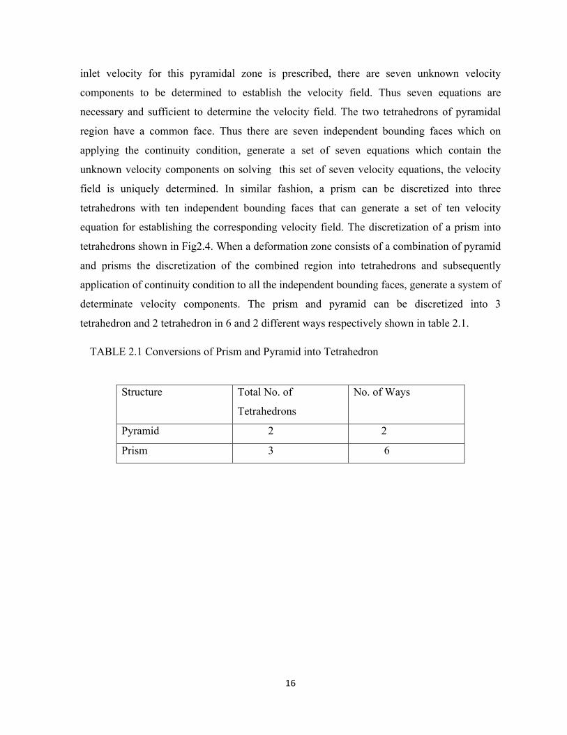
TABLE 2.1 Conversions of Prism and Pyramid into Tetrahedron

Structure Total No. of

Tetrahedrons

No. of Ways

Pyramid 2 2

Prism 3 6

 

2.

 

 The

vec

φ  a

 

 

If A

then

con

inco

Fro

equ

.4 The Con

    

Fig 2.5 A

e Fig 2.5 Sh

tor on both

are given by

1 nV =ur

2 nV n=ur

A and ρ den

n the mass f

ntinuity cond

ompressible)

1(ρA ) .V

m above eq

ual, so;

ntinuity of

 

A general sur

hows a surfa

sides. The c

the equation

1n .V (∧

=uur

2n .V (∧

= ∇uur

notes the sur

flow rate acr

dition (also

) i.e.

1 nV (ρ=

quation canc

f a Discon

 

rface separat

ce separatin

omponents o

n (2.8) and (2

( /φ∇ ∇

/φ φ∇ ∇

rface area of

ross the surf

known as

2 2 nA ) .V

celing φ∇

17 

ntinuous V

 

ting two rigi

ng two spatia

of these two

2.9) 

1) .Vφuur

 …

2).Vφuur

  …

f the segmen

face segmen

volume con

……………

which is sc

Velocity Fie

d region

al region wi

o vectors nor

………………

………………

nt and the m

nt taken from

nstancy cond

…………

calar quantit

eld  

   

   th v1 and v2

rmal to the s

………     

………..

material den

m both sides

dition, since

ty so that V

 

 

               

2 as the vel

eparating su

             

sity respecti

s. Thus the

e the mater

(2.10)

V1n and V2n

   

      locity

urface

(2.8)

(2.9)

ively,

mass

ial is

)

must

18  

1 2. V . Vφ φ∇ = ∇ur ur

……………………… (2.11)

It is to be pointed out that the regions on both sides of the surface φ in Fig (2.5) are rigid if

1Vur

and 2Vur

are constant velocity vectors if equation (2.10) is linear. The linearity of equation

(2.10) is assured when the surface φ is a plane. Thus the bounding faces of the spatial

elementary rigid region can only be planner. Some of this bounding face may lie on the die

surfaces or planes of symmetry. Since no material flow occurs across faces. Equation (2.10)

takes the following form;

1.V 0φ∇ =ur

………………………………………. (2.12)

The equation of each of the triangular faces can be determined when the co-ordinates of three

vertices are specified. Then the velocity equation can be formed by applying the mass

continuity condition either in the form of equation (2.10) or (2.11) as appropriate. The

velocities of material in the zones are V1 and V2 respectively are not identical. The

components of velocity in the normal and tangential direction of the surface are Vn1, Vn2 and

Vt1,Vt2. The normal velocity Vn1 should be equal to Vn2 for the continuity of the material. The

tangential velocity Vt1 and Vt2 need not be equal. The difference is called the velocity

discontinuity ∆V and is given by equation (2.13).

∆V=Vt1-Vt2 ……………………………… (2.13)

 

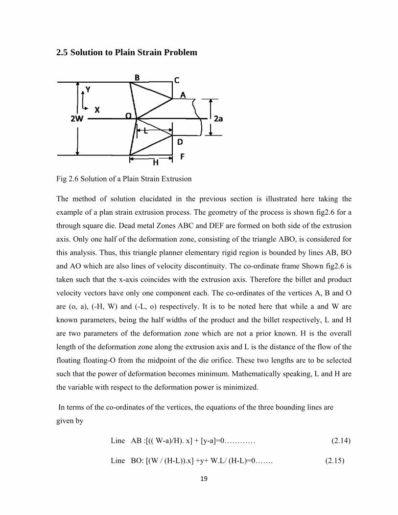
2.5 S

Fig 2.

The m

examp

throug

axis. O

this an

and A

taken

veloci

are (o

known

are tw

length

floatin

such t

the va

In ter

given

Solution to

6 Solution o

method of s

ple of a plan

gh square die

Only one ha

nalysis. Thu

AO which are

such that th

ity vectors h

o, a), (-H, W

n parameter

wo paramete

h of the defo

ng floating-O

that the powe

ariable with r

rms of the co

by

L

L

o Plain Str

of a Plain Str

solution elu

n strain extru

e. Dead met

lf of the def

us, this triang

e also lines o

he x-axis coi

have only on

W) and (-L,

s, being the

ers of the de

rmation zon

O from the m

er of deform

respect to th

o-ordinates o

Line AB :[(

Line BO: [(

rain Proble

rain Extrusio

ucidated in t

usion proces

al Zones AB

formation zo

gle planner e

of velocity d

incides with

ne componen

o) respectiv

half widths

eformation z

ne along the e

midpoint of

mation becom

e deformatio

of the vertice

(( W-a)/H). x

(W / (H-L)).

19 

em

on

the previou

ss. The geom

BC and DEF

one, consistin

elementary r

discontinuity

h the extrusio

nt each. The

vely. It is to

s of the prod

zone which

extrusion ax

the die orifi

mes minimum

on power is m

es, the equati

x] + [y-a]=0

.x] +y+ W.L

s section is

metry of the p

F are formed

ng of the tria

rigid region

y. The co-ord

on axis. The

e co-ordinate

o be noted h

duct and the

are not a pr

xis and L is th

ice. These tw

m. Mathema

minimized.

ions of the th

0…………

L/ (H-L)=0…

s illustrated

process is sh

on both side

angle ABO,

is bounded

dinate frame

erefore the b

es of the ver

here that wh

e billet respe

rior known.

he distance o

wo lengths a

atically speak

hree boundin

…….

here taking

hown fig2.6

e of the extru

is considere

by lines AB

e Shown fig2

billet and pro

rtices A, B a

hile a and W

ectively, L a

H is the ov

of the flow o

are to be sel

king, L and H

ng lines are

(2

(2.1

g the

for a

usion

ed for

B, BO

2.6 is

oduct

and O

W are

and H

verall

of the

ected

H are

2.14)

15)

20  

Line OA = ((a/l).x) + y –a = 0………….. (2.17)

If the billet velocity Vb is prescribed, there are three unknown velocity component in this

case. These components are Vp, the product velocity, and Vx and Vy, the x- and y-

components of the velocity vector in the elementary rigid region.

The line AB in fig2.6 is the limiting line for the dead metal zone. Material enters the

deformation zone across line BO and the product leaves the deformation zone through line

AB. Table2.2 shows these lines and the corresponding velocity vectors on both side of the

line. The physical description of side of each line is also known this table.

Employing the mass continuity condition given equation (2.11) and (2.12) as appropriate to

these lines, the three velocity equations are obtained as given below:

[(W-a) / H]. Vx + Vy = 0 (2.18)

[W /(H-L)] . Vx + Vy = [W / (H-L)] . Vb (2.19)

TABLE 2.2

Lines. The zone they separated and velocity vector on their sides.

Lines and their equations

Side 1 Velocity vector on side 1

Side 1 Velocity vector on side 1

AB φ=[(w-a).x]/L+ [y-a] =o

Deformation zonei x j yV + V

Dead metal zone

0

BO φ=Wx/(H-L)+y+ WL/(H-L)=0

Deformation zonei x j yV + V

Billet iVb

OA φ=[ax/L]+y-a=0

Deformation zonei x j yV + V

product iVp

                       (-a/L) . Vx + Vy = - (a/L) 0. Vp…………….. (2. 20) 

On solving this set of linear equation Vx, Vy and Vp, the velocity vectors are obtained as shown in equations (2.21) (2.22) (2.23).

Vx= ( H. w. Vb ) / ( H.a + L.W-a.L )……………………… . (2.21)

21  

Vy = [(W-a) W. Vb ) ] / [ H.a = L.W-a.L )…………………. (2.22)

V p= W Vb / a ………………………………………………… (2.23)

Since the elementary region is rigid, the strain rate tensor in region is zero. Therefore the

power for internal deformation, J1 is zero. Further, the dead metal zone separates the

deformation zone from the die surface and as such, there is no relative motion between the

two. Therefore there is no dissipation power due to the friction at the diameter faces i.e. J3=0).

Thus the power consumed for deformation is dissipated only at the lines of velocity

discontinuity. Therefore in this case, equation (2.1) reduces to the following form.

J=J1……………… (2.24)

In the present analysis, all the lines of velocity discontinuity separate rigid regions. Hence the

absolute values of the velocity discontinuities at each line are constant. If ,

denote the length of the line segment AB, BO and OA respectively and, BO

VΔ ,and OAV| Δ |

represents the corresponding absolute values of the velocity discontinuities, the value of J

becomes as

  ( )[ ]0 AB AB BO OAJ= / 3 V S V S V Sσ ΒΟ ΟΑ| Δ | + + | Δ | + | Δ |               …………….              (2.25)

 

The upper bound to the deforming power can be calculated using equation. (2.25) the upper

bound so obtained can be optimized with respect to the parameter H and L and the minimum

upper bound, Jmin, to the deformation power can be obtained corresponding to this velocity

field. The average extrusion pressure, non-dimensional zed by σo, c then can be calculated

form the equation.

  avg 0 mm b oP / J / WVσ σ=        ……………………………                                          (2.26) 

 

                                                                                         

                                                                               

 

 

 

 

 

 

 

CHPTER THREE 

 

UPPER  BOUND  ANALYSIS  FOR  EXTRUSION  OF ‘TRIANGULAR’ SECTION THROUGH TAPER DIES 

 

 

  

22  

                                                                                 CHAPTER 3 

UPPER BOUND ANALYSIS FOR EXTRUSION

OF TRIANGULAR SECTION THROUGH TAPER DIES

3.1 Introduction                         Triangular section bars are produced by extrusion using taper dies. Softer metal like lead

aluminum are easily extruded such sections are widely used for commercially and house

hold items because their decorative value. Extrusion is carried out with the help of taper

dies. For extrusion of sections taper dies with lubricant is more preferred as it provides

gradual change in shape and reduction of area simultaneously.

However upper bound solution for extrusion of triangular section from round billet using

taper wall with re-entrant corner received the attention of many investigators. The SERR

technique is further modified for analyzing the extrusion process from round billets. In

present work the circular section of round billet is approximated to 12 sides of regular

polygon.

Here number of sides of polygon is increased continuously up to the limit when after

increasing the sides there will be no effect on result of extrusion pressure. Here to

approximate a circular section into regular polygon, sectional area must be maintained

constant as shown in Fig.3.1 and by using formula given in equation (3.1).   

         

23  

Fig 3.1 Approximation of a circular section into regular polygon of side (12)

( )2 21R M L c o t / 24

θπ = ……………………. (3.1)

From considerations of symmetry, only one half of the deformation zone is considered for

this analysis. Where R= Radius of the round billet

M=No. of polygon sides

L=Die length

θ=Equivalent cone angle

The upper bound load has been computed using discontinuous velocity field. The

discontinuous velocity field has been obtained by discritizing the deformation zone into

tetrahedral blocks using reformulated SERR technique.

3.2 SERR Method Analysis

As discussed in the previous chapter, it was pointed out that in the SERR method of

analysis, the deformation zone is discritized into rigid region thus leading to a

discontinuous velocity field. When these rigid region are in shape of tetrahedron a

determinate set of equation is obtained (by application of continuity condition to individual

 

face

be c

bille

of t

velo

long

trian

deli

sect

sing

12 s

Fig

es defining t

calculated. I

et axis. This

he die orific

ocity field (z

g as it is k

ngular secti

ineated in d

tion two floa

gle floating p

sides for ana

3.2 One hal

the rigid regi

In present an

s assumption

ce. It is appro

zone of zero

kinamatically

on because

domain of in

ating point f

point formul

alysis.

lf of the defo

ion) from wh

nalysis it is a

n is necessar

opriate to m

o velocity) an

y admissibl

symmetry a

nterest by ta

formulation g

lation. The F

ormation zon

24 

hich the velo

assumed the

ry so that pr

mention that f

nd upper bou

le. For one

about one pl

aking suitabl

gives the mo

Fig 3.2 show

ne of 12 side

ocity compo

e centre of g

roduct remai

friction surfa

und theorem

half of the

lane. The su

le located fl

ore upper bo

ws the one ha

ed polygon

onent in such

gravity of die

ins straight a

ace zone are

m admits any

e deformatio

ub zones of

loating point

ound solution

alf of the def

h rigid region

e aperture li

as it is come

part of purp

y velocity fie

on geometry

f deformatio

ts. For trian

n as compar

formation zo

n can

es on

es out

posed

eld as

y for

n are

ngular

red to

one of

 

3.3

Fig

In F

The

12–

11–

sche

3.4 D

As

only

ana

roun

at la

3 Single flo

.3.3 Single p

Fig.3.3 analy

e deformatio

–8–7–9–11)

–7and 7–12–

emes of disc

Double floa

mentioned e

y one half o

alysis. As it

nd cross sec

ast it conver

oating poi

point formul

ysis is done b

on zone is to

& five tetra

–11–8).Henc

critizing of d

ating poin

earlier the T

of the extrus

is discussed

ction of billet

ges to give a

int formul

ation

by taking on

be descritiz

ahedral subz

ce it results

different zon

nt formula

Traingular-se

sion geometr

d earlier that

t, the upper

a constant re

25 

lation

ne floating fo

zed into two

zones (11–12

s in nine te

es.

tion

ections have

ry may be c

t, if we incr

bound soluti

esult.

or the as dom

pyramidal s

2–10–2, 3–1

etrahedrons

symmetry a

considered a

rease the sid

ion falls tow

main interest

subzones (12

12–10–4, 4–

and the nu

about one ax

as domain of

des of the re

wards the min

t for discretiz

2–5–6–11–10

–12–10–5, 6

umber of g

xes and ther

f interest for

gular polygo

nimum valu

zatio.

0 and

6–12–

global

refore

r this

on of

e and

 

Hen

is b

pert

Fig.3.

In thi

point

deform

known

zones

3.1 fo

nce for simp

being taken

tinent co-ord

4 Double po

is, formulati

(13) is tak

mation zone

n as floating

, one prism,

r classifying

plicity in exp

for the con

dinate system

oint formulat

ion floating

en any whe

is delineate

g points. By

, two pyram

g the differen

plaining the d

nsideration,

m.

tion

point (12) i

ere inside d

ed by joining

y this proce

mids and four

nt planes.

26 

double point

Fig3.4 show

is taken alon

deformation

g corner poin

ss the defor

r tetrahedron

t formulation

ws the one

ng symmetry

zone as sh

nts of entry

rmation zon

ns shown in

n, a 12 sided

half of the

y plane and

own in abo

and exist pl

e is divided

Fig 3.5 and

d regular pol

e die cavity

d another flo

ove Fig 3.4.

lane to the p

d into seven

d shown in T

lygon

with

oating

. The

points

sub-

Table

 

Fig

3.5 differennt shape of deeformation z

27 

zone

28  

TABLE 3.1

Half extrusion zone (domain of interest) divided into prism, pyramid and tetrahedron

.

Each prism can be subdivided into three tetrahedron in six different ways and each pyramid

can be divided into two tetrahedron in two different ways as discussed earlier. Hence the total

deformation zone can be subdivided into 11 numbers of tetrahedrons in 24 different ways i.e.

(2×2×6) shown in Table 3.2 and total number of plane derived from the prism, pyramid and

tetrahedron shown in Table 3.3 .

TABLE3.2

Number of planes and ways of discritization

No. of Tetrahedrons No. of Planes No. of Ways

1×3+2×2+1+1+1+1=11 11×4-10(common plane)=34 6×2×2

Sub-zones Model numbering system No. of plane faces

1.Prism

2.Pyramid

3.Pyramid

4.Tetrahedron

5.Tetrahedron

6.Tetrahedron

7. Tetrahedron

1-8-9-11-12-13

2-3-10-12-13

5-6-10-11-13

3-4-10-13

4-5-10-13

6-7-11-13

7-8-13-11

10

7

7

4

4

4

4

29  

TABLE 3.3

Total number of planes derived from Prism, Pyramid and Tetrahedrons;

Subzones Model numbering system

Numbering of different planes

No. of planes

Total no.of common planes

Total no. of planes

Prism 1-8-9-11-12-13 1-12-9 1-9-8 1-9-11 1-8-12 1-8-11 8-9-12 8-11-13 8-9-11 8-9-13 9-11-13

10

7-13-11 4-10-13 8-13-11 3-10-13 5-10-13 6-11-13 (6 Common planes) 

(10+7+7+4+4+4+4) - 6 =34

Pyramid 2-3-10-12-13 2-3-13 3-10-13 10-12-13 2-12-13 3-12-13 2-12-13 3-10-12

7

Pyramid 5-6-10-11-13 5-6-13 6-10-13 6-11-13 10-11-13 5-13-10 5-6-10 6-10-11

7

Tetrahedron 3-4-10-13 3-4-10 3-4-13 3-10-13 4-10-13

4

Tetrahedron 4-5-10-13 4-5-13 4-5-10 4-10-13 5-10-13

4

Tetrahedron 6-7-11-13 6-7-11 6-7-13 6-11-13 7-11-13

4

Tetrahedron 7-8-13-11 7-8-11 7-8-13 7-13-11 8-11-13

4

30  

3.5 Calculation of velocity components

Each tetrahedron move with a unique velocity. The internal velocity of each tetrahedron is V1,

V2, and V3 …….. V11 (as there are 11 numbers of tetrahedrons) when resolved into

components along the co-ordinate axis V1, V2, V3 …….. V11 together have 33. The billet

and product velocity vector, Vb, Ve are along the extrusion axis (z-axis) and so can be

consider to have one non-zero component each. With prescribed billet velocity Vb, the

product velocity Ve is taken as unknown thus there are 34 unknown velocity components.

When mass continuity condition is applied to all 34 bounding faces of these 11 tetrahedrons,

then 34 equations are obtained. These 34 equations being a determinate set are solved

simultaneously to give the all unknown velocity components.

Here the floating point (12) has 2 unknown co-ordinate whereas (13) has 3 unknown co-

ordinates. Using these co-ordinates, the equation of plane containing 34 triangular faces under

consideration can be determined. Since a velocity discontinuity is permissible only along the

tangential direction the normal component on side of faces must be equal. A validity of

equation carried out under following consideration (velocity on both side of each face is given

in table3.5)

(a)Normal velocity in friction surface is zero.

(b) Normal velocity in symmetry plane is same.

With this theoretical approach a matrices of (34×35) with suitable sub-program is solved to

get required unknown velocity component (V1x, V1y, V1z) ………….( V11x ,V11y, V11z)and Ve

along Z-direction . After getting the velocity components, the resultant velocity at each plane

faces are then carried out.

V1= [V1x2+V1y2+V1z2] (3.2)

V2= [V2x2+V2y2+V2z2] (3.3)

31  

V11= [V11x2+V11y2+V11z2] ( 3.4)

Fig 3.6 Co-ordinate of the half of the TRIANGULAR section

 

TABL

Co-or

Points

1

2

3

4

5

6

7

8

9

10

11

12

13

Know

for sim

as mat

LE3.4

rdinates of po

s

wing the co-o

mplicity a m

trices of (4×

oints in defo

X-co-

-R

R

R C

R C

R C

R C

R C

R C

-H/3

-2H/

-H/3

0

X13

ordinates of p

mathematical

×4)

ormation zon

-ordinate

Cos(π/12)

Cos(π/4)

Cos(5π/12)

Cos(7π/12)

Cos(9π/12)

Cos(11π/12)

/3

point’s equa

approach fo

32 

ne

Y-co-

0

0

R Si

R Si

R Si

R Si

R Si

R Si

0

0

B/2

Y12

Y13

ation of all tr

or equation o

-ordinate

in(π/12)

in(π/4)

in(5π/12)

in(7π/12)

in(9π/12)

in(11π/12)

2

2

3

riangular fac

of triangular

Z-co

L

L

L

L

L

L

L

L

0

0

0

Z12

Z13

es (34) can b

face 4-5-10

-ordinate

be found out

can be expr

t. But

ess

33  

Similarly equation for all 34 planes can be set up. With this theoretical approach a matrices of

(34×35) with suitable sub-program is solved to get required unknown velocity components

i.e. ( V1x,V1x, V1z )(V2x, V2y, V2z)………………………………… (V11x,V11y,V11z) and Ve

along Z-direction. After getting the velocity components, the resultant velocity at each plane

is then carried out.

3.6 Calculation of area of triangular faces in deformation zone

Knowing the co-ordinates of each plane face in deformation zone then area of triangle is

calculated. Co-ordinate of these vertices of triangle in the space are (X1,Y1,Z1), (X2,Y2,Z2)

(X3,Y3,Z3)

Area of triangle is

2 2 2( A )y zXA A A= + + …………………….. (3.5)

( )x 1 2 2 1 2 3 3 2 1 31A = y z -y z +y z -y z +y z2      ………………….. (3.6)

( )y 1 2 2 1 2 3 3 2 1 31A = x z -x z +x z -x z +x z2 …………………. (3.7)

( )z 1 2 2 1 2 3 3 2 2 31A = x y -x y +x y -x y +x y2 …………………… (3.8)

Using the above equation the area of the bounding faces is calculated,

An = (A1 +A2 + A3+ A4 + A5 +……………..+ A34)………………….. (3.9)

When An is total area of bounding faces and n is the number of bounding faces of triangular

shape which is taken as 34 in our assumption. Table 3.5 shows the various surfaces, types and

their velocities for deformation zone of Fig 3.4.

34  

TABLE 3.5

Various surfaces, types and their velocity

Surface Category Normal velocity in that surface

2-3-12-13 Entry surface Billet velocity(Vb)

2-3-13 Entry surface Billet velocity (Vb)

5-6-13 Entry surface Billet velocity (Vb)

6-7-13 Entry surface Billet velocity (Vb

7-8-13 Entry surface Billet velocity (Vb)

4-5-13 Entry surface Billet velocity (Vb)

4-5-10 Friction surface 0

3-4-10 Friction surface 0

2-3-10 Friction surface 0

5-6-10-11 Friction surface 0

6-7-10-11 Friction surface 0

7-8-10-11 Friction surface 0

4-5-10 Friction surface 0

3-4-10 Friction surface 0

2-3-10 Friction surface 0

1-2-9-10 Symmetry surface Equal on both sides

12-13-10-11 Exit surface Product velocity (Vp)

12-13-9-11 Exit surface Product velocity (Vp)

12-13-9-10 Exit surface Product velocity (Vp)

35  

3.7 Calculation of Non-dimensional Extrusion Pressure

Deformation power consists of power of shear deformation at the plane of velocity

discontinuity and friction power at die/work piece may be determined using relation.

         0 n n 0 n nJ σ / 3 V A σ m / 3 V A= √ ∇ + √ ∇∑ ∑ ……………….. (3.10)

Where n= Total no. of bounding faces

nV∇ = is the velocity discontinuity at nth faces whose area is An

The non-dimensional extrusion pressure (Pav/ 0σ ) is optimized with respect to seven

unknown adjustable or variable parameter of deformation zone and written as

a v 0 b b 0P / σ J / A V σ= …………………………… (3.11)

Where Ab = Area of Billet

Vb = Billet Velocity

σ0= Uniaxial Stress in Compression

3.8 Computation:

Using a suitable analytical model, computation is carried out. It consists of following steps:

(a) Determine the co-efficient of equation of the planes containing bounding faces of

tetrahedral block.

(b) Determine the co-efficient of velocity equation by applying the mass continuity

condition to respective planes.

(c) Magnitude of velocity discontinuity is found out by algorithm. This solution also

determines exit velocity, with serves as check on computation. Since exit velocity can

be independently calculated using billet velocity and the area reduction.

(d) Computing deformation work by equation(3.10) and non-dimensional extrusion pressure

by equation(3.11)

36  

(e) Optimizing non-dimensional extrusion pressure with respect to variable parameter L,

Y12, Z12, X13, Y13, Z13 , using multivariable unconstraint routine.

(f) All the computation is carried out with a suitable subroutine of tetrahedron, pyramid,

and prism imposed with different alternatives. Figs 3.7, 3.8 and 3.9 show the variation

of non-dimensional extrusion pressure with equivalent cone angle at area reduction

75%, 80% and 85% for different friction factor respectively. Fig 3.10 shows the

variation of non-dimensional extrusion pressure with percentage of area reduction at

equivalent semi-cone angle 20˚ for different friction factor.

3.9 Optimization parameter

For a double point formulation one floating point lies on plane of symmetry having two

undetermined co-ordinates Y12 and Z12. Second floating point lies any where inside

deformation zone having three undetermined co-ordinates X13, Y13, Z13. Height of

deformation zone an additional optimizing parameter.

37  

Fig.3.7 Variation of non-dimensional extrusion pressure with equivalent semi cone angle

Fig.3.8 Variation of non-dimensional extrusion pressure with equivalent semi cone angle

0

1

2

3

4

5

6

0 10 20 30 40 50 60

FF = 0.1

FF = .3

FF = 0.38

FF = 0.5

FF = 0.76

FF = 0.9

Equivalent semi cone angle

Non

-dim

ensi

onal

extru

sion

pres

sure

Pav

g/σ 0

Reduction of area=70 %

0

1

2

3

4

5

6

7

0 10 20 30 40 50 60

FF = 0.1

FF = 0.3

FF=0.38

FF = 0.5

FF = 0.76

FF = 0.9

Equivalent semi cone angle (in˚)

Non

-dim

ensi

onal

ext

rusi

on

pres

sure

Pav

g/σ 0

Reduction of area = 80 %

38  

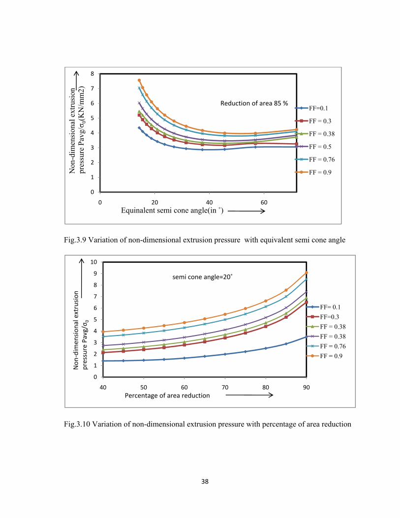
Fig.3.9 Variation of non-dimensional extrusion pressure with equivalent semi cone angle

Fig.3.10 Variation of non-dimensional extrusion pressure with percentage of area reduction

0

1

2

3

4

5

6

7

8

0 20 40 60

FF=0.1

FF = 0.3

FF = 0.38

FF = 0.5

FF = 0.76

FF = 0.9

Equinalent semi cone angle(in ˚)

Non

-dim

ensi

onal

ext

rusi

on

pres

sure

Pav

g/σ 0

(KN

/mm

2)

Reduction of area 85 %

0

1

2

3

4

5

6

7

8

9

10

40 50 60 70 80 90

FF= 0.1FF=0.3FF = 0.38FF = 0.38FF = 0.76FF = 0.9

Percentage of area reduction

Non

‐dim

ension

al extrusion

pressure Pavg/σ 0

semi cone angle=20˚

39  

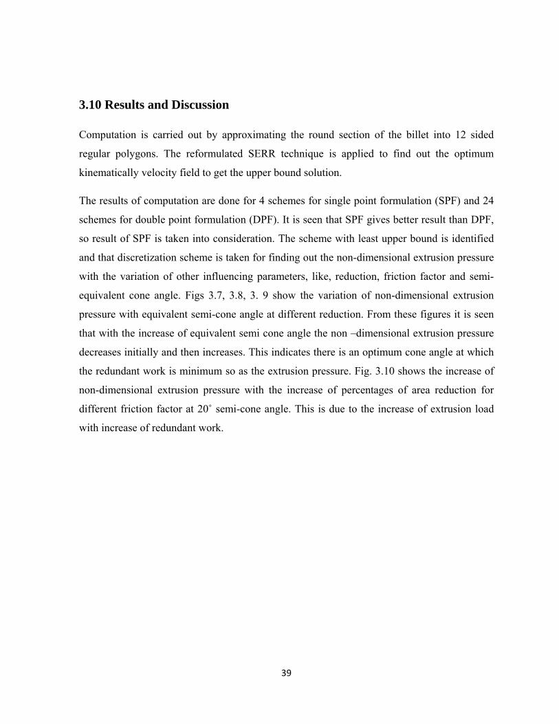
3.10 Results and Discussion

Computation is carried out by approximating the round section of the billet into 12 sided

regular polygons. The reformulated SERR technique is applied to find out the optimum

kinematically velocity field to get the upper bound solution.

The results of computation are done for 4 schemes for single point formulation (SPF) and 24

schemes for double point formulation (DPF). It is seen that SPF gives better result than DPF,

so result of SPF is taken into consideration. The scheme with least upper bound is identified

and that discretization scheme is taken for finding out the non-dimensional extrusion pressure

with the variation of other influencing parameters, like, reduction, friction factor and semi-

equivalent cone angle. Figs 3.7, 3.8, 3. 9 show the variation of non-dimensional extrusion

pressure with equivalent semi-cone angle at different reduction. From these figures it is seen

that with the increase of equivalent semi cone angle the non –dimensional extrusion pressure

decreases initially and then increases. This indicates there is an optimum cone angle at which

the redundant work is minimum so as the extrusion pressure. Fig. 3.10 shows the increase of

non-dimensional extrusion pressure with the increase of percentages of area reduction for

different friction factor at 20˚ semi-cone angle. This is due to the increase of extrusion load

with increase of redundant work.

 

 

 

 

 

 

 

CHPTER FOUR 

 

EXPERIMENTAL INVESTIGATION 

 

  

40  

CHAPTER 4 EXPERIMENTAL INVESTIGATION 4.1 Introduction In the upper bound analysis idealized assumptions made regarding the nature of deformation

and material properties. Consequently, before applying the theoretically result to any practical

situation, their adequacy needs experimental verification. The objective of present work is to

compare theoretically predicted extrusion load with experimental value. Experiments are

performed for TRIANGULAR section using tapper die. Commercially available tellurium

lead was chosen as the working material for the experiments (extrusion). Different shape of

same circular entry face and various reduction of triangular exit face were made

(72.78%, 80.78%, and 87.41%).

4.2 Determination of Material Behavior A serious limitation of the tensile test even for cold working is that fracture occurs at a

moderate strain; so that it is not possible to use this test for determination of yield stress, after

very heavy deformation. The fracture is most easily avoided by adopting some compressive

form of test. The average stress state during testing is similar to that in much bulk deformation

process, without introducing the problems of necking or material orientation.

Therefore, in compression test, a large amount of deformation can be achieved before

fracture. By controlling the barreling of the specimen ends and the anvils with lubricants the

strain can be varied under limits.

4.2.1 Compression Test The simplest of these tests is the axial compression of a cylinder between smooth platens. If

the platens are well lubricated, this gives essentially the same yield stress at a tensile test with

small strains. As the strain is increased, the specimen spreads and thinning of the lubricant

occurs, so that the frictional component at the die face increases .The increase in the load

41  

required causing yielding. It can be overcome to a large extent by removing the sample after

small increments in strain and relubricating each time. The main disadvantage of this tests is

conducted at a constant true stress strain rate require special equipment. Compression testing

has developed into a highly sophisticated test of workability extrusion and is a common

quality control test in extrusion operation. Compression loads are applied to many engineering

structures that vary in dimension from massive suspension bridge piers to the thin sheets of

aircraft wings. In addition, metal forming processes involve large deformation. Analysis of

metal forming processes requires knowledge of stress strain properties. The following

assumptions are made in stress strain testing.

•In any test, used to obtain uniform axial compression stress strain properties, the

measured quantities are generally load and strain. If a strain gage is used or

displacement is measured at the surface of the specimen, the longitudinal and

transverse strain is assumed to be uniform along the entire gage length.

• The cross sectional area is constant over the gage length

• The stress is uniaxial and uniform in each cross section along the gage length

• The loading forces must maintain initial alignment throughout the entire loading

process

• The measured surface strain is assumed to be same as internal strain.

An error in stress or strain occurs, if the assumptions of uniformity do not exist in a test.

Buckling, distributions, and elimination of these phenomena in the compression test leads to

more accurate stress strain data.

To determine the uniaxial yield tress of the billet material for any given reduction, R the

corresponding strain imparted to the billet material during the extrusion process must be

known a prior. For the same reduction the stain imparted to the billet during the extrusion

process is always higher than that imparted to the billet during compression because of

redundant work done during extrusion process. Following Johnson (4) the above strain in the

present case was calculated from the empirical relation.

ε = 0 .8 + 1 .5 L n (1 / (1 -R ) ) ……………………….. (4.1)

Where R is the fractional reduction. The average yield stress of the extruded billet was then

calculated by dividing the area under the stress-strain curve.

42  

4.2.2 Experimental Procedure of compression test

Cylinders with a 50.20mm × 31.77 mm (H/D = 1.5 to 2) were used to obtain the stress-strain

curve by a compression test using UTM (INSTRON 600 KN) at room temperature. The

compression rate is maintained same as that adapted for the experiments. The specimen has

oil grooves on both the ends to entrap lubricant during the compression test. The compression

load is recorded at every 0.5 mm of punch ravel. After compressing the specimen to about 10

mm it is taken out of the press, re-machined to cylindrical shape with original diameter, and

tested in compression till the specimen is reduced to about 10mm. The stress-strain diagram is

drawn and the curve is extrapolated beyond a natural strain 0.5. To simulate a rigid plastic

material, the wavy portion is approximated by smooth line (Fig. 4.1). The average flow stress

of the used lead is found to be 25460 KN/m2.

Fig 4.1 Variation of True Stress with True Strain

12660.8

14660.8

16660.8

18660.8

20660.8

22660.8

24660.8

26660.8

0.00909 0.01909 0.02909 0.03909

True

stre

ss in

KN

/m2

True strain

3.21 3.9082.75

   

43  

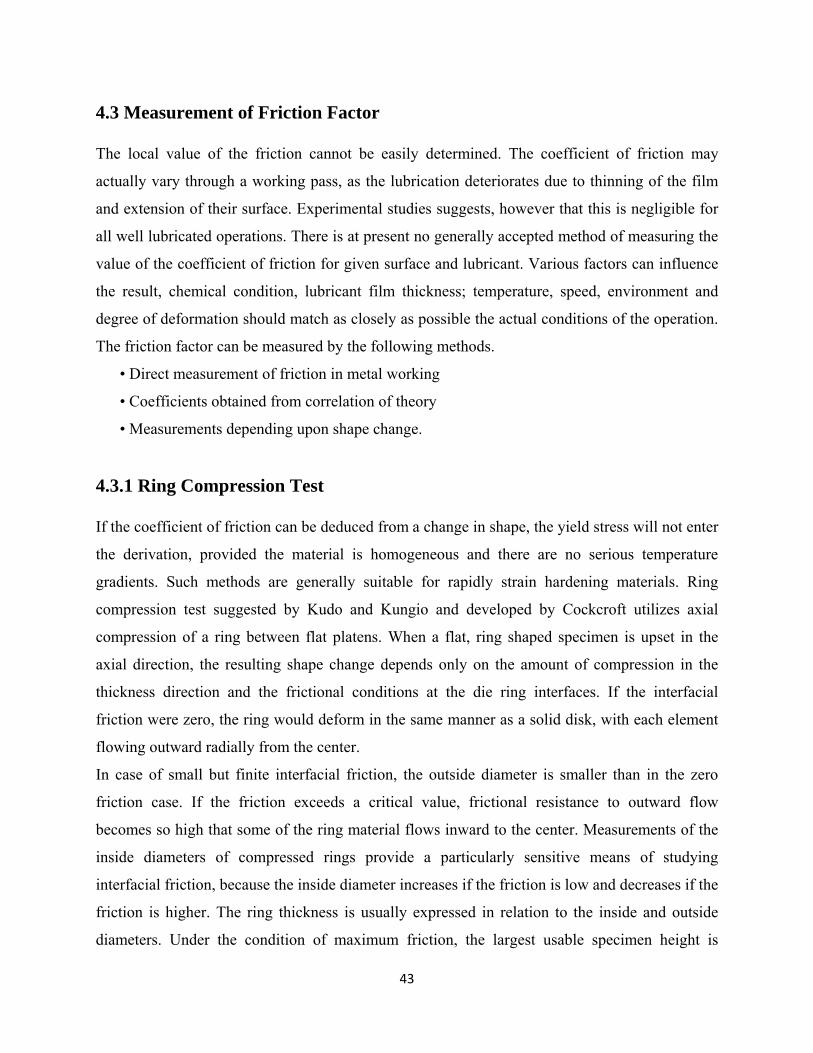
4.3 Measurement of Friction Factor The local value of the friction cannot be easily determined. The coefficient of friction may

actually vary through a working pass, as the lubrication deteriorates due to thinning of the film

and extension of their surface. Experimental studies suggests, however that this is negligible for

all well lubricated operations. There is at present no generally accepted method of measuring the

value of the coefficient of friction for given surface and lubricant. Various factors can influence

the result, chemical condition, lubricant film thickness; temperature, speed, environment and

degree of deformation should match as closely as possible the actual conditions of the operation.

The friction factor can be measured by the following methods.

• Direct measurement of friction in metal working

• Coefficients obtained from correlation of theory

• Measurements depending upon shape change.

4.3.1 Ring Compression Test

If the coefficient of friction can be deduced from a change in shape, the yield stress will not enter

the derivation, provided the material is homogeneous and there are no serious temperature

gradients. Such methods are generally suitable for rapidly strain hardening materials. Ring

compression test suggested by Kudo and Kungio and developed by Cockcroft utilizes axial

compression of a ring between flat platens. When a flat, ring shaped specimen is upset in the

axial direction, the resulting shape change depends only on the amount of compression in the

thickness direction and the frictional conditions at the die ring interfaces. If the interfacial

friction were zero, the ring would deform in the same manner as a solid disk, with each element

flowing outward radially from the center.

In case of small but finite interfacial friction, the outside diameter is smaller than in the zero

friction case. If the friction exceeds a critical value, frictional resistance to outward flow

becomes so high that some of the ring material flows inward to the center. Measurements of the

inside diameters of compressed rings provide a particularly sensitive means of studying

interfacial friction, because the inside diameter increases if the friction is low and decreases if the

friction is higher. The ring thickness is usually expressed in relation to the inside and outside

diameters. Under the condition of maximum friction, the largest usable specimen height is

   

 

obtained

For norm

results o

measure

ratio of in

possible

with rings o

mal lubricate

f sufficient

the flow str

nternal, exte

to obtain a m

Fig

of dimension

ed condition

accuracy fo

ress under h

ernal diamete

measure of th

g 4.2 Ring b

Fig 4.3Rin

ns in the rati

ns, geometry

or most appl

high strain pr

ers after axia

he friction.F

efore compr

ng after com

44 

o of 6:3:1 i.

y of 6:3:2, s

lications. Th

ractical form

al compressi

Fig.4.3 shows

ression

mpression

e. outer diam

shown in Fig

he ring com

ming conditi

ion of a ring

s rings after

meter: inner

g 4.2, can b

mpression tes

ons. Thus, b

g of standard

compression

diameter: he

be used to o

st can be us

by measurin

d dimensions

n.

eight.

obtain

ed to

ng the

s, it is

   

45  

4.3.2 Experimental Procedure for ring test

A ring compression test was carried out at dry condition and commercially available grease

lubrication condition. The rings were compressed upto the 4 mm inner diameter, at each 0.5 mm

of punch travel inner diameter and height was recorded. The friction factors were found to be

0.76 for dry condition and 0.38 for the lubricated condition by comparing our result with the

calibration curve of Male and Cockcroft (Fig. 4.4). 

Fig 4.4 Theoretical calibration curve for standard ring 6:3:2

4.4 Experimental Setup

The following section deals with the brief description of apparatus, dies. The present studies on tapper die entry as circular and exit as a triangle. The output product is like a triangular section. The main parts namely.

(1) punch (3)die (5) base plate (2) container (4)die hold

   

46  

Fig 4.5UTM (INSTRON 600 KN) and UTM with close view

         Fig 4.6Assembly setup (photo copy)     Fig 4.7Shcematic view of Experimental setup        

   

 

                  

 

 

    Fig4.9 Ex

Fig.4.5 sh

photogra

cross sec

      

F

         xperimental

hows the UT

aphs of assem

ctional parts

Fig 4.8 Disas

                  setup for ex

TM in which

mble parts, s

of the exper

ssemle parts

                  xtrusion

h the experim

chematic vie

rimental setu

47 

s of setup(ph

                  

ments were c

ew of parts,

up respective

 

hotograph) 

                  

carried out. F

photograph

ely.

                   

Figs 4.6, 4.7,

of disassemb

                  

, 4.8and 4.9

ble parts and

                  

are

d

            

   

48  

4.4.1 Different Parts of the Set-up                                     Container with extrusion chamber                   

Material: MS

Properties: tensile strength – 320 N/mm2

Hardness - 100 BHN Die plate

Material: MS

Properties: tensile strength – 320 N/mm2

Hardness- 100 BHN Punch &supporting plate Material: MS Properties: tensile strength – 320 N/mm2 Hardness- 100 BHN

Die Material: MS

Properties: tensile strength -320 N/mm2

Hardness-100BHN

Taper dies are manufactured split type for easy removal of the product. Three dies of reductions

72.78%, 80.78% and 87.41% (Table 4.1) are made for the experiments (marked type-1 in

Fig.4.10 (b)). To check the effect of orientation of inclined surface from entry to exit one number

of other type (72.78% reduction), marked type-2 in Fig.4.11 (b), is made. Photograph of the dies

made and used is shown in Fig 4.12. Fig 4.11(b) shows the bottom view of die which is same for

both types of dies through which the triangular products are comes out.

   

 

Fig 4

Fig4.10 (b)

F

4.10 (a) One

) Top view o

Fig4.11 (b) B

e half Schem

of die TYPE

Bottom view

49 

matic view of

E 1

w of die

f die

Fig4.11(a)T

Top view of d

die TYPE 2

   

 

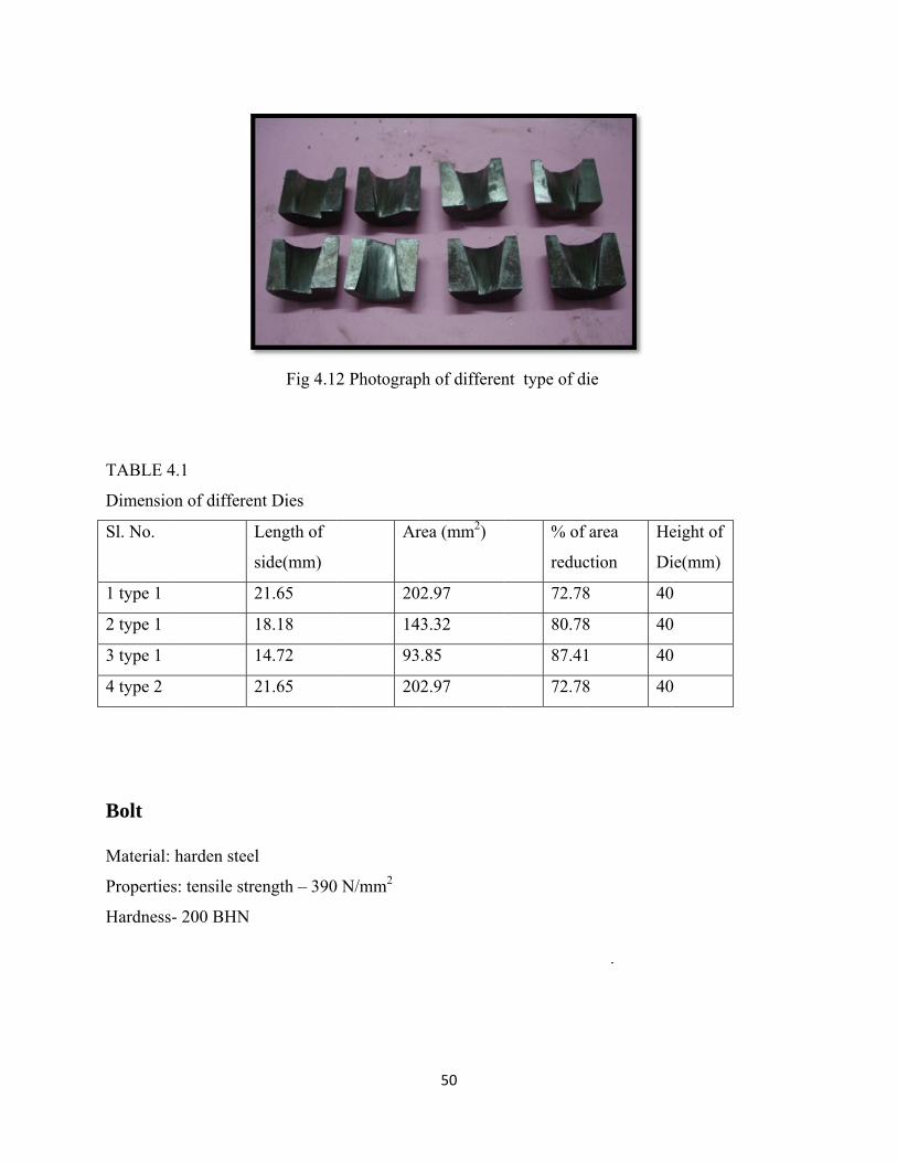
TABLE 4

Dimensio

Sl. No.

1 type 1

2 type 1

3 type 1

4 type 2

Bolt Material:

Propertie

Hardness

4.1

on of differe

: harden stee

es: tensile str

s- 200 BHN

Fig 4.1

ent Dies

Length of

side(mm)

21.65

18.18

14.72

21.65

el

rength – 390

2 Photograp

Ar

20

14

93

20

0 N/mm2

50 

ph of differen

rea (mm2)

2.97

3.32

.85

2.97

nt type of di

% of

reduc

72.78

80.78

87.41

72.78

ie

area

ction

He

Di

8 40

8 40

1 40

8 40

eight of

ie(mm)

0

0

0

0

   

51  

Extrude metal Material: lead

Properties: tensile strength – 20 N/mm2

Melting point –327 ° C density -11330Kg/m3

 

4.5 Experimental procedure

Before starting the test the die sets, die holder and inside face of extrusion chamber were

cleaned. The two halves of the die set were then push fitted into die holder and total assembly

were secured by screwing four bolts. The full assembly was then placed in the placed between

the base plate of UTM ( Instron 600 KN ) in upside down position. It was done so that extruded

product would get enough clearance, when it comes out from the die. For carrying out an

extrusion test the side of lead specimen was placed in side extrusion chamber. The punch was

then inserted into its position. After centering the apparatus under machine lower table, Machine

was started and extrusion process was continued. The speed of movement of punch being given

1.5 mm per minute to avoid rate effect and to account for uniformity in results. Punch load was

recorded at every 1.5 mm movement of punch travel, which was read from computer fitted to the

UTM. The application of load was continued till it reaches the steady state and up to certain

length of product comes out side. At this position Machine was stopped and test was terminated

the die holder was then separated from extrusion chamber and finally die halves with extruded

product were pushed out from die holder and extrusion chamber. Experiments were conducted

for three different reductions (72.78%, 80.78%, and 87.41%) to get triangular section product at

two different friction condition (dry-.76 friction factor, wet-.38 friction factor) from round cross-

section billet. The variation of extrusion load with punch displacement is shown in Figs 4.13,

4.14, 4.15, 4.16, 4.17 and calculated results are summarized in Table 4.2. The extrapolated

theoretical values at experiment conditions and comparison between experimental and theoretical

results are depicted in Table 4.3. Photograph of the extruded product is shown in Figs. 4.18, 4.19

are at wet and dry condition respectively. Fig. 4.20 shows the inclined surfaces marked in the

last end of the product.

   

52  

 

 

Fig 4.13 Variation of Compressive Load with Extension at Lubricated Condition

 

 

Fig 4.14Variation of Compressive Load with Extension

0

20

40

60

80

100

120

140

160

0 10 20 30 40 50 60 70 80 90

72.78% reduction

80.78% reduction

87.41% reduction

Compressive extension (mm)

Com

pres

sive

load

in(K

N)

0

20

40

60

80

100

120

140

160

180

0 20 40 60 80 100

72.78 %Reduction at dry condition

80.78 %Rreduction at Dry condition

87.41 % Reduction at dry condition

Compressive extension(mm)

Com

pres

sive

load

(KN

)

   

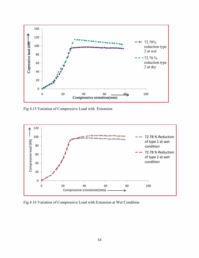
53  

 

Fig 4.15 Variation of Compressive Load with Extension

 

 

Fig 4.16 Variation of Compressive Load with Extension at Wet Condition

 

0

20

40

60

80

100

120

140

0 20 40 60 80 100

72.78% reduction type 2 at wet

72.78 % reduction type 2 at dry

Compressive extention(mm)

Cop

ress

ivelaod (KN)

Compressive extention(mm)

Cop

ress

ivelaod (KN)

0

20

40

60

80

100

120

0 20 40 60 80 100

72.78 % Reduction of type 1 at wet condition

72.78 % Reduction of type 2 at wet condition

Compressive extension(mm)

Compressive

load

 (KN)

   

 

Fig 4.17

F

1

1

1C

ompr

essi

veload(KN)

Variation of

ig 4.18 Phot

0

20

40

60

80

100

120

140

0

f Compressiv

tograph Extr

20Com

ve Load with

ruded produc

40mpressive ext

54 

h Extension

ct at wet con

60tension(mm)

at Dry Cond

ndition

80

dition

100

72.7typecond

72.7typecond

8 % Reductie1 at dry dition

8 % Reductie 2 at dry dition

on 

on 

   

 

Fig

Fig 4.20

4.19 Photog

Photograph

graph of Extr

of Shape of

ruded produc

f product insi

55 

ct at dry con

ide die

ndition

   

56  

TABLE. 4.2

Experiment results

Area of billet (Ab) = (π/4). (Db) 2

= (π/4) (31)2

= 754.76 mm2

Pavg = (F/ Ab)

Experiment %Red Friction

Factor

ε

Strain

Load F

(KN)

Pavg

(KN/m2) 0σ

(KN/m2)

Pavg /σ0 Eqvt.cone

Angle

1. type 1 dry

72.78 0.76 2.75 109.9560 145683 25560 5.69 21.12

2. type 1 dry

80.78 0.76 3.28 132.7793 175922 25560 6.80 24.66

3. type 1 dry

87.41 0.76 3.908 147.340 195214 25560 7.63 28.18

4 .type 2 dry

72.78 0.76 2.75 104.3480 151502 25560 5.61 21.12

5. type 1 wet

78.78 0.38 3.28 90.041 119297 25560 4.99 21.12

6. type 1 wet

80.78 0.38 3.28 103.52 137156 25560 5.36 24.66

7. type 1 wet

72.78 0.38 3.908 124.01 164290 25560 6.42 28.18

8. type 2 wet

72.78 0.38 2.75 89.76 118925 25560 4.65 21.12

   

57  

TABLE 4.3

Theoretical result of non-dimensional extrusion pressure

%Red Friction

Factor

Eq. Semi cone

Angle

Pavg/σ0

(Theoretical) Pavg/σ0

(Experimental) Error

72.78 0.76 10.56 5.72 5.69 0.52 %

80.78 0.76 12.33 6.51 6.80 -4.45 %

87.41 0.76 14.09 7.65 7.63 0.26 %

72.78 0.38 10.56 4.69 4.99 -6.39

80.78 0.38 12.33 5.38 5.36 0.37 %

87.41 0.38 14.09 6.45 6.42 0.46 %

   

58  

4.6 Result and Discussion The variation of compressive load with extension was determined from the extrusion test for

TRIANGULAR cross section taper dies shown in fig4.12. Referring to the Figs 4.13, 4.14, 4.15,

4.16 and 4.17 seen that a typical diagram consists of two stages; namely

(1) A coining stage in which load increases gradually and reaches peak value due to initial

compression of billet.

(2) A steady stage of extrusion in which load maintains approximately a constant value upto

the end of the extrusion.

The average load corresponding to the second stage consider as the extrusion load. The value of

uniaxial yield stress in compression σ0 , is calculated from stress strain characteristics plot of

lead and non- dimensional mean extrusion pressure (Pavg/σ0 ) is calculated.

Referring to Figs 4.13, 4.14, 4.15, 4.16 and 4.17 the extrusion load decreases marginally with

punch displacement for lubricated condition during steady state stage, but it is more prominent

for dry condition. This may be attributed to the high friction exist between billet and container in

dry condition, which decreases with the length of the billet. In case of type 2 die the requirement

of load for same reduction the load is marginally in dry condition but prominent in wet

condition. In case of type 2 die the requirement of load for same reduction the load is more as

compared to type 1 die in wet condition .This may probably due to decrease of work hardening

of material by changing the direction of flow.

The comparison of experimental values with that of theoretical results shows the error remains

within 10 percent.

                       

                                                                              

 

 

 

 

 

 

 

 

CHPTER FIVE 

 

CONCLUSION & FUTURE WORKS 

 

  

   

59  

                                                                                                CHAPTER 5

5.1 CONCLUSION

From the present study the following conclusions may be drawn:

• The upper bound analysis of extrusion of different sections taper dies can carry out by using discontinuous velocity field (modified SERR technique). These techniques provided a better method of analysis for this type of section extrusion, which are difficult by the continuous velocity field formulation.

• Increasing the percentage of reduction accompanying with increase in extrusion loads.

• Using this solution, the optimal die geometry (equivalent semi-cone angle) can be obtained for different area reductions and friction conditions.

• Comparison made with existing theoretical and experimental results shows that the present solution can predict reasonable upper-bound extrusion pressure.

• The present method can be extended to obtain the solution of generalized problems of non-axisymetric extrusion or drawing through taper dies.

   

   

60  

5.2 FUTURE WORKS                                        

1. Theoretical prediction of non-dimensional extrusion pressure for different formulation like triple point formulation.                                                                            2. Experimental validation for the different shapes (L-Section. Channel section).   

                                                                                                                                                                          3. Equivalent semi cone angle compared with experimental and identified the optimum one.                    

 

 

 

 

 

 

 

 

 

REFFERNCES  

   

61  

REFERENCES   

                                     

[1] V. Nagpal, T. Altan, Analysis of the three-dimensional metal flow in extrusion of shapes.

With the use of dual stream function, in: Proceedings of the Third North American Metal

Research Conference, Pittsburgh, PA, 1975, pp. 26–40.

[2] B.B. Basily, D.H. Sansome, Some theoretical considerations for the direct drawing of section

rod from round bar, Int. J. Mech. Sci. 18 (1979) 201–209.

[3] D.Y. Yang, C.H. Lee, Analysis of three-dimensional extrusion of sections through curved

dies by conformal transformations, Int. J. Mech. Sci. 20 (1978) 541–552.

[4] W. Johnson, H. Kudo, The Mechanics of Metal Extrusion.(1963)

[5] Hill, Analysis metal working process, mechanics of physical solids flow rule(1963)

[6] R. Prakash, O.H. Khan, An analysis of plastic flow through polygonal converging dies with

generalised boundaries of the zone of plastic deformation, Int. J. Mach. Tool Des. Res. 19 (1979)

1–9.

[7] F. Gatto, A. Giarda, The characteristics of three-dimensional analysis of plastic

deformation according to the SERR method, Int. J. Mech. Sci. 23 (1981) 129–148.

   

62  

[8] P.K. Kar, N.S. Das, Upper bound analysis of extrusion of I-section bars from

square:rectangular billets through square dies, Int. J. Mech. Sci. 39 (8) (1997) 925–934.

[9] P.K. Kar, R.K. Sahoo, Application of the SERR technique to the analysis of extrusion of

sections from round billets, J. Inst. Engrs. (India) 78 (1997) 15

[10] S.K. Sahoo, P.K. Kar , K.C. Singh a. A numerical application of the upper-bound technique

for round-to-hexagon extrusion through linearly converging dies,Int. J. Mat. Pro. Tec. 91 (1999)

105–110

[11] Narayanasamy R, Ponalagusamy R, Venkatesan R, Srinivasan P (2006) An upper bound

solution to extrusion of circular billet to circular shape through cosine die. Mater Des 27(5):411–

415. doi:10.1016/j.matdes.2004.11.026

[12] J.S. Gunasekera, S. Hosino, Analysis of extrusion or drawing ofpolygonal sections through

straightly conversing dies, J. Engng. Ind.Trans. ASME 104 (1982) 38–43.

[13] C.B. Boer, W.R. Schneider, B. Avitzur, An upper bound approach forthe direct drawing of

square section rod from round bar, in: Proceedings of the 20th International Machine Tool

Design and Research Conference, Birmingham, 1980, pp. 149–155

[14] D.Y. Yang, M.U. Kim, C.H. Lee, A new approach for generalized three-dimensional

extrusion of sections from round billets by conformal transformation, IUTAM Symp. Metal

Forming Plasticity, Germany, 1979, pp. 204–221.

[15] B, Vvitzur, Metal forming process and analysis, capter10 (1977)

[16] Geoffrey W. Rowe, Introduction to the principle of metal working, Chapter-8

[17] V. Gopinathan, Plasticity Theory and its Application in Metal Forming, Chapter 7