Embed Size (px)
Citation preview
Journal of Machine Learning Research 22 (2021) 1-66 Submitted 520 Revised 821 Published 921
Thompson Sampling Algorithms for Cascading Bandits
Zixin Zhong zixinzhongunuseduDepartment of MathematicsNational University of Singapore119076 Singapore
Wang Chi Chueng isecwcnusedusgDepartment of Industrial Systems and ManagementNational University of Singapore117576 Singapore
Vincent Y F Tan vtannusedusg
Department of Electrical and Computer Engineering and
Department of Mathematics
National University of Singapore
117583 Singapore
Editor Csaba Szepesvari
Abstract
Motivated by the important and urgent need for efficient optimization in online recom-mender systems we revisit the cascading bandit model proposed by Kveton et al (2015a)While Thompson sampling (TS) algorithms have been shown to be empirically superior toUpper Confidence Bound (UCB) algorithms for cascading bandits theoretical guaranteesare only known for the latter In this paper we first provide a problem-dependent upperbound on the regret of a TS algorithm with Beta-Bernoulli updates this upper bound istighter than a recent derivation under a more general setting by Huyuk and Tekin (2019)Next we design and analyze another TS algorithm with Gaussian updates TS-CascadeTS-Cascade achieves the state-of-the-art problem-independent regret bound for cascad-ing bandits Complementarily we consider a linear generalization of the cascading banditmodel which allows efficient learning in large-scale cascading bandit problem instances Weintroduce and analyze a TS algorithm which enjoys a regret bound that depends on thedimension of the linear model but not the number of items Finally by using information-theoretic techniques and a judicious construction of cascading bandit instances we derivea nearly-matching lower bound on the expected regret for the standard model Our paperestablishes the first theoretical guarantees on TS algorithms for a stochastic combinato-rial bandit problem model with partial feedback Numerical experiments demonstrate thesuperiority of the proposed TS algorithms compared to existing UCB-based ones
Keywords Multi-armed bandits Thompson sampling Cascading bandits Linear ban-dits Regret minimization
1 Introduction
Online recommender systems seek to recommend a small list of items (such as moviesor hotels) to users from a larger ground set [L] = 1 L of items Optimizing theperformance of these systems is of fundamental importance in the e-service industry where
ccopy2021 Zixin Zhong Wang Chi Cheung and Vincent Y F Tan
License CC-BY 40 see httpscreativecommonsorglicensesby40 Attribution requirements are providedat httpjmlrorgpapersv2220-447html
Zhong Cheung and Tan
companies such as Yelp and Spotify strive to maximize usersrsquo satisfaction by catering totheir taste The model we consider in this paper is the cascading bandit model (Kvetonet al 2015a) which models online learning in the standard cascade model by Craswellet al (2008) The latter model (Craswell et al 2008) is widely used in information retrievaland online advertising
In the cascade model a learning agent offers a list of items to a user The user thenscans through it in a sequential manner The user looks at the first item and if she isattracted by it she clicks on it If not she skips to the next item and clicks on it if she findsit attractive This process stops when she clicks on one item in the list or when she comesto the end of the list in which case she is not attracted by any of the items The items thatare in the ground set but not in the chosen list and those in the list that come after theattractive one are unobserved Each item i is associated with a click probability w(i) isin [0 1]which in general varies across different items The event that a user is attracted to an itemis independent of the events that she is attracted to other items The learning agentrsquosobjective is to maximize the cumulative rewards
In the cascading bandit model which is a multi-armed bandit version of the cascademodel by (Craswell et al 2008) the click probabilities w = w(i)Li=1 are not known to thelearning agent and should be learnt over time Based on the lists previously chosen and theobservations obtained thus far the agent tries to learn the click probabilities (exploration)in order to adaptively and judiciously recommend other lists of items (exploitation) tomaximize his overall reward over T time steps
Apart from the cascading bandit model where each itemrsquos click probability is learntindividually (we call it the standard cascading bandit problem) we also consider a lineargeneralization of the cascading bandit model which is called the linear cascading banditproblem proposed by (Zong et al 2016) In the linear model each click probability w(i)is known to be equal to x(i)gtβ isin [0 1] where the feature vector x(i) is known for eachitem i but the latent β isin Rd is unknown and should be learnt over time The featurevectors x(i)Li=1 represents the prior knowledge of the learning agent When d lt L thelearning agent can potentially harness the prior knowledge x(i)Li=1 to learn w(i)Li=1 byestimating β which is more efficient than by estimating each w(i) individually
11 Main Contributions
First we analyze the Thompson sampling algorithm with the Beta-Bernoulli update whichis an application of the Combinatorial Thompson Sampling (CTS) algorithm (Russo et al2018 Huyuk and Tekin 2019) in the cascading bandit setting We provide a concise analysiswhich leads to a tighter upper bound compared to the original one reported in Huyuk andTekin (2019)
Our next contribution is the design and analysis of TS-Cascade a Thompson samplingalgorithm (Thompson 1933) for the standard cascading bandit problem Our motivation isto design an algorithm that can be generalized and applied to the linear bandit setting sinceit is not as natural to design a linear generalization of the CTS algorithm The variationof TS-Cascade for the linear setting is presented in Section 5 Our design involves twonovel features First the Bayesian estimates on the vector of latent click probabilities ware constructed by a univariate Gaussian distribution Consequently in each time step
2
Thompson Sampling Algorithms for Cascading Bandits
Ts-Cascade conducts exploration in a suitably defined one-dimensional space Secondinspired by Audibert et al (2009) we judiciously incorporate the empirical variance of eachitemrsquos click probability in the Bayesian update The allows efficient exploration on item iwhen w(i) is close to 0 or 1
We establish a problem-independent regret bound for our proposed algorithm TS-Cascade Our regret bound matches the state-of-the-art regret bound for UCB algorithmson the standard cascading bandit model (Wang and Chen 2017) up to a multiplicative log-arithmic factor in the number of time steps T when T ge L Our regret bound is the firsttheoretical guarantee on a Thompson sampling algorithm for the standard cascading ban-dit problem model or for any stochastic combinatorial bandit problem model with partialfeedback (see literature reviewin Section 12)
Our consideration of Gaussian Thompson sampling is primarily motivated by Zonget al (2016) who report the empirical effectiveness of Gaussian Thompson sampling oncascading bandits and raise its theoretical analysis as an open question In this paper weanswer this open question under both the standard setting and its linear generalizationand overcome numerous analytical challenges We carefully design estimates on the latentmean reward (see inequality (42)) to handle the subtle statistical dependencies betweenpartial monitoring and Thompson sampling We reconcile the statistical inconsistency inusing Gaussians to model click probabilities by considering a certain truncated version ofthe Thompson samples (Lemma 45) Our framework provides useful tools for analyzingThompson sampling on stochastic combinatorial bandits with partial feedback in othersettings
Subsequently we extend TS-Cascade to LinTS-Cascade(λ) a Thompson samplingalgorithm for the linear cascading bandit problem and derive a problem-independent upperbound on its regret According to Kveton et al (2015a) and our own results the regret onstandard cascading bandits grows linearly with
radicL Hence the standard cascading bandit
problem is intractable when L is large which is typical in real-world applications Thismotivates us to consider linear cascading bandit problem (Zong et al 2016) Zong et al(2016) introduce CascadeLinTS an implementation of Thompson sampling in the linearcase but present no analysis In this paper we propose LinTS-Cascade(λ) a Thompsonsampling algorithm different from CascadeLinTS and upper bound its regret We arethe first to theoretically establish a regret bound for Thompson sampling algorithm on thelinear cascading bandit problem
Finally we derive a problem-independent lower bound on the regret incurred by anyonline algorithm for the standard cascading bandit problem Note that a problem-dependentone is provided in Kveton et al (2015a)
12 Literature Review
Our work is closely related to existing works on the class of stochastic combinatorial bandit(SCB) problems and Thompson sampling In an SCB model an arm corresponds to a subsetof a ground set of items each associated with a latent random variable The correspondingreward depends on the constituent itemsrsquo realized random variables SCB models withsemi-bandit feedback where a learning agent observes all random variables of the items ina pulled arm are extensively studied in existing works Assuming semi-bandit feedback
3
Zhong Cheung and Tan
Anantharam et al (1987) study the case when the arms constitute a uniform matroidKveton et al (2014) study the case of general matroids Gai et al (2010) study the case ofpermutations and Gai Chen et al (2013) Combes et al (2015) and Kveton et al (2015b)investigate various general SCB problem settings More general settings with contextualinformation (Li et al 2010 Qin et al 2014) and linear generalization (Wen et al 2015Agrawal and Goyal 2013b) are also studied When Wen et al (2015) consider both UCBand TS algorithms Agrawal and Goyal (2013b) focus on TS algorithms all other worksabove hinge on UCBs
Motivated by numerous applications in recommender systems and online advertisementSCB models have been studied under a more challenging setting of partial feedback wherea learning agent only observes the random variables for a subset of the items in the pulledarm A prime example of SCB model with partial feedback is the cascading bandit modelwhich is first introduced by Kveton et al (2015a) Subsequently Kveton et al (2015c)Katariya et al (2016) Lagree et al (2016) and Zoghi et al (2017) study the cascadingbandit model in various general settings Cascading bandits with contextual information(Li et al 2016) and linear generalization (Zong et al 2016) are also studied Wang andChen (2017) provide a general algorithmic framework on SCB models with partial feedbackAll of the works listed above only involve the analysis of UCB algorithms
On the one hand UCB has been extensively applied for solving various SCB problemsOn the other hand Thompson sampling (Thompson 1933 Chapelle and Li 2011 Russoet al 2018) an online algorithm based on Bayesian updates has been shown to be empir-ically superior compared to UCB and ε-greedy algorithms in various bandit models Theempirical success has motivated a series of research works on the theoretical performanceguarantees of Thompson sampling on multi-armed bandits (Agrawal and Goyal 2012 Kauf-mann et al 2012 Agrawal and Goyal 2017ba) linear bandits (Agrawal and Goyal 2013a)generalized linear bandits (Abeille and Lazaric 2017) etc Thompson sampling has alsobeen studied for SCB problems with semi-bandit feedback Komiyama et al (2015) studythe case when the combinatorial arms constitute a uniform matroid Wang and Chen (2018)investigate the case of general matroids and Gopalan et al (2014) and Huyuk and Tekin(2019) consider settings with general reward functions In addition SCB problems withsemi-bandit feedback are also studied in the Bayesian setting (Russo and Van Roy 2014)where the latent model parameters are assumed to be drawn from a known prior distribu-tion Despite existing works an analysis of Thompson sampling for an SCB problem in themore challenging case of partial feedback is yet to be done Our work fills in this gap in theliterature and our analysis provides tools for handling the statistical dependence betweenThompson sampling and partial feedback in the cascading bandit models
This paper serves as a significant extension of Cheung et al (2019) which was pre-sented at the 22nd International Conference on Artificial Intelligence and Statistics in April2019 The additional materials contained herein include the analysis of the CTS algorithmLinTS-Cascade(λ) an algorithm designed for the linear cascading bandit setting a lowerbound on the regret over all cascading bandit algorithms and extensive experimental re-sults
4
Thompson Sampling Algorithms for Cascading Bandits
13 Outline
In Section 2 we formally describe the setup of the standard and the linear cascading banditproblems In Section 3 we provide an upper bound on the regret of CTS algorithm and aproof sketch In Section 4 we propose our first algorithm TS-Cascade for the standardproblem and present an asymptotic upper bound on its regret Additionally we com-pare our algorithm to the state-of-the-art algorithms in terms of their regret bounds Wealso provide an outline to prove a regret bound of TS-Cascade In section 5 we designLinTS-Cascade(λ) for the linear setting provide an upper bound on its regret and theproof sketch In Section 6 we provide a lower bound on the regret of any algorithm in thecascading bandits with its proof sketch In Section 7 we present comprehensive experimen-tal results that compare the performances of all the algorithms including new ones such asCTS and LinTS-Cascade(λ) We discuss future work and conclude in Section 8 Detailsof proofs as given in Appendix C
2 Problem Setup
Let there be L isin N ground items denoted as [L] = 1 L Each item i isin [L] isassociated with a weight w(i) isin [0 1] signifying the itemrsquos click probability In the standardcascading bandit problem the click probabilities w(1) w(L) are not known to the agentThe agent needs to learn these probabilities and construct an accurate estimate for eachof them individually In the linear generalization setting the agent possesses certain linearcontextual knowledge about each of the click probability terms w(1) w(L) The agentknows that for each item i it holds that
w(i) = βgtx(i)
where x(i) isin Rd is the feature vector of item i and β isin Rd is a common vector sharedby all items While the agent knows x(i) for each i he does not know β The problemnow reduces to estimating β isin Rd The linear generalization setting represents a settingwhen the agent could harness certain prior knowledge (through the features x(1) x(L)and their linear relationship to the respective click probability terms) to learn the latentclick probabilities efficiently Indeed in the linear generalization setting the agent couldjointly estimate w(1) w(L) by estimating β which could allow more efficient learningthan estimating w(1) w(L) individually when d lt L This linear parameterization is ageneralization of the standard case in the sense that when x(i)Li=1 is the set of (d = L)-dimensional standard basis vectors β is a length-L vector filled with click probabilities ieβ = [w(1) w(2) w(L)]gt then the problem reverts to the standard case This standardbasis case actually represents the case when the x(i) does not carry useful information
At each time step t isin [T ] the agent recommends a list of K le L items St =(it1 i
tK) isin [L](K) to the user where [L](K) denotes the set of all K-permutations of
[L] The user examines the items from it1 to itK by examining each item one at a time untilone item is clicked or all items are examined For 1 le k le K Wt(i
tk) sim Bern
(w(itk)
)are
iid and Wt(itk) = 1 iff user clicks on itk at time t
5
Zhong Cheung and Tan
The instantaneous reward of the agent at time t is
R(St|w) = 1minusKprodk=1
(1minusWt(itk)) isin 0 1
In other words the agent gets a reward of R(St|w) = 1 if Wt(itk) = 1 for some 1 le k le K
and a reward of R(St|w) = 0 if Wt(itk) = 0 for all 1 le k le K
The feedback from the user at time t is defined as
kt = min1 le k le K Wt(itk) = 1
where we assume that the minimum over an empty set is infin If kt lt infin then the agentobserves Wt(i
tk) = 0 for 1 le k lt kt and also observes Wt(i
tk) = 1 but does not observe
Wt(itk) for k gt kt otherwise kt = infin then the agent observes Wt(i
tk) = 0 for 1 le k le K
The agent uses an online algorithm π to determine based on the observation history the armSt to pull at each time step t in other words the random variable St is Ftminus1-measurablewhere Ft = σ(S1 k1 St kt)
As the agent aims to maximize the sum of rewards over all steps the expected cumu-lative regret is defined to evaluate the performance of an algorithm First the expectedinstantaneous reward is
r(S|w) = E[R(S|w)] = 1minusprodiisinS
(1minus w(i))
Note that the expected reward is permutation invariant but the set of observed items isnot Without loss of generality we assume that w(1) ge w(2) ge ge w(L) Consequentlyany permutation of 1 K maximizes the expected reward We let Slowast = (1 K)be the optimal ordered K-subset that maximizes the expected reward Additionally welet items in Slowast be optimal items and others be suboptimal items In T steps we aim tominimize the expected cumulative regret
Reg(T ) = T middot r(Slowast|w)minusTsumt=1
r(St|w)
while the vector of click probabilities w isin [0 1]L is not known to the agent and therecommendation list St is chosen online ie dependent on the previous choices and previousrewards
3 The Combinatorial Thompson Sampling (CTS) Algorithm
In this section we analyze a Thompson sampling algorithm for the cascading bandit prob-lem and consider the posterior sampling based on the Beta-Bernoulli conjugate pair Thealgorithm dubbed CTS algorithm was first proposed as Algorithm 6 in Section 73 ofRusso et al (2018) and analyzed by Huyuk and Tekin (2019) We derive a tighter boundon the regret than theirs The algorithm and the bound are as follows
6
Thompson Sampling Algorithms for Cascading Bandits
Algorithm 1 CTS Thompson Sampling for Cascading Bandits with Beta Update
1 Initialize αB1 (i) = 1 and βB1 (i) = 1 for all i isin [L]
2 for t = 1 2 do3 Generate Thompson sample θBt (i) sim Beta(αB
t (i) βBt (i)) for all i isin [L]4 for k isin [K] do5 Extract itk isin argmaxiisin[L]it1itkminus1
θBt (i)
6 end for7 Pull arm St = (it1 i
t2 i
tK)
8 Observe click kt isin 1 Kinfin9 For each i isin [L] if Wt(i) is observed define αB
t+1(i) = αBt (i) + Wt(i) β
Bt+1(i) =
βBt (i) + 1minusWt(i) Otherwise αBt+1(i) = αB
t (i) βBt+1(i) = βBt (i)10 end for
Theorem 31 (Problem-dependent bound for CTS) Assume w(1) ge ge w(K) gtw(K + 1) ge ge w(L) and ∆ij = w(i)minus w(j) for i isin Slowast j isin Slowast the expected cumulativeregret of CTS is bounded as
Reg(T ) le LminusK + 16 middotLsum
i=K+1
(1
∆2Ki
+log T
∆Ki
)+
Lsumi=K+1
Ksumj=1
∆ji
+ α2 middotKsumj=1
∆jL
(1[∆jK+1 lt
14
]∆3jK+1
+log T
∆2jK+1
)
where α2 is a constant independent of the problem instance
We remark that it is common to involve a problem-independent constant such as α2
in Theorem 31 in the upper bound (Wang and Chen 2018) In fact the bounds inTheorems 34 41 and 51 also involve problem-independent constants
Table 1 Problem-dependent upper bounds on the T -regret of CTS CascadeUCB1 andCascadeKL-UCB the problem-dependent lower bound apply to all algorithmsfor the cascading bandit model In the table we use the notation KL(a b) todenote the Kullback-Leibler divergence between two Bernoulli distributions withparameters a and b
AlgorithmSetting Reference Bounds
CTS Theorem 31 O(L(log T )∆ + L∆2
)CTS Huyuk and Tekin (2019) O
(KL(log T )[(1minus w(L))Kminus1w(L)∆]
)CascadeUCB1 Kveton et al (2015a) O
((LminusK)(log T )∆ + L
)CascadeKL-UCB Kveton et al (2015a) O
((LminusK)∆(log T )log(1∆)KL(w(L) w(1))
)Cascading Bandits Kveton et al (2015a) Ω
((LminusK)(log T )∆
)(Lower Bd)
7
Zhong Cheung and Tan
Next in Table 1 we compare our regret bound for the CTS algorithm to those in theexisting literature Note that the upper bound for CTS in Huyuk and Tekin (2019) can bespecified to the cascading bandits as above and the two other algorithms are based on theUCB idea (Kveton et al 2015a) To present the results succinctly we consider the problemwhere w(1) = w(2) = = w(K) w(K + 1) = w(K + 2) = = w(L) ie ∆ = ∆ji
for any optimal item j and any suboptimal item i In other words the gap between anyoptimal item j and any suboptimal item i is ∆ which does not depend on i and j Theparameter ∆ measures the difficulty of the problem
Table 1 implies that our upper bound grows like log T similarly to the other boundsfor the other algorithms When log T ge 1∆ since L(log T )∆ is the dominant termin our bound we can see that L(log T )∆ is smaller than the term KL(log T )[(1 minusw(L))Kminus1w(L)∆] in the bound by Huyuk and Tekin (2019) In addition the dominantterm L(log T )∆ in our bound matches that in CascadeUCB1 in the term involvinglog T However we note that it is incomparable to the one for CascadeKL-UCB (Kvetonet al 2015a) due to the following two reasons
(i) on the one hand
1
∆ middotminw(1) 1minus w(1)le ∆
KL(w(L) w(1))le 2
∆
by Pinskerrsquos inequality (see Section 6 for the definition of the KL divergence andPinskerrsquos inequality)
(ii) on the other hand CascadeKL-UCB involves an additional log(1∆) term
Furthermore the dominant term involving log T in our bound matches the lower boundprovided in Kveton et al (2015a) when L K Therefore our derived bound on CTSthe Thompson sampling algorithm with Beta-Bernoulli update is tight
Moreover apart from the problem-dependent bound we also notice that it is valuableto derive a problem-independent bound for CTS However in the cascading bandit modelit cannot be trivially reduced from a problem-dependent one and hence we leave it as anopen question For instance Kveton et al (2015a) (the first paper on cascading bandits)provided an problem-dependent regret bound but left the problem-independent bound asan open question
To derive an upper bound the analytical challenge is to carefully handle the partialfeedback from the user in the cascading bandits Though our analysis has similarity tothose in Wang and Chen (2018) (semi-bandit feedback) and Huyuk and Tekin (2019) (partialfeedback) the difference is manifested in the following aspects
(i) To handle the partial feedback from the user we handcraft the design of eventsAt(` j k) At(` j k) At(` j) in (31) and apply the property of the reward to de-compose the regret in terms of the observation of a suboptimal items in Lemma 32and 33
(ii) Additionally our algorithm crucially requires the items in St to be in the descend-ing order of θBt (i) (see Line 4ndash7 of Algorithm 1) which is an important algorithmicproperty that enables our analysis (see Lemma 33)
8
Thompson Sampling Algorithms for Cascading Bandits
Our analytical framework which judiciously takes into the impact of partial feedback issubstantially different from Wang and Chen (2018) which assume semi-feedback and do notface the challenge of partial feedback Besides since Huyuk and Tekin (2019) consider a lessspecific problem setting they define more complicated events than in (31) to decompose theregret Moreover we carefully apply the mechanism of CTS algorithm to derive Lemma 33which leads to a tight bound on the regret Overall our concise analysis fully utilizes theproperties of cascading bandits and Algorithm 1
Now we outline the proof of Theorem 31 some details are deferred to Appendix CNote that a pull of any suboptimal item contributes to the loss of expected instantaneousreward Meanwhile we choose St according to the Thompson samples θBt (i) instead of theunknown click probability w(i) We expect that as time progresses the empirical meanwt(i) will approach w(i) and the Thompson sample θBt (i) which is drawn from Bern(θBt (i))will concentrate around w(i) with high probability In addition this probability dependsheavily on the number of observations of the item Therefore the number of observationsof each item affects the distribution of the Thompson samples and hence also affects theinstantaneous rewards Inspired by this observation we decompose the the regret in termsof the number of observations of the suboptimal items in the chain of equations including(35) to follow
We first define πt as follows For any k if the k-th item in St is optimal we placethis item at position k πt(k) = itk The remaining optimal items are positioned arbitrarilySince Slowast is optimal with respect to w w(itk) le w(πt(k)) for all k Similarly since St isoptimal with respect to θBt θBt (itk) ge θBt (πt(k)) for all k
Next for any optimal item j and suboptimal item ` index 1 le k le K time step twe say At(` j k) holds when suboptimal item ` is the k-th item to pull optimal item j isnot to be pulled and πt places j at position k We say At(` j k) holds when At(` j k)holds and item ` is observed Additionally At(` j) is the union set of events At(` j k) fork = 1 K We can also write these events as follows
At(` j k) =itk = ` πt(k) = j
At(` j k) =itk = ` πt(k) = jWt(i
t1) = = Wt(i
tkminus1) = 0
=itk = ` πt(k) = jObserve Wt(`) at t
At(` j) =K⋃k=1
At(` j k) =exist1 le k le K st itk = ` πt(k) = jObserve Wt(`) at t
(31)
Then we have
r(Slowast|w)minus r(St|w)
= r(πt(1) πt(K)|w)minus r(St|w) (32)
=
Ksumk=1
[kminus1prodm=1
[1minus w(itm))
]middot [w(πt(k))minus w(itk)] middot
[Kprod
n=k+1
(1minus w(πt(n))]
](33)
leKsumk=1
[kminus1prodm=1
(1minus w(itm))
]middot [w(πt(k))minus w(itk)]
9
Zhong Cheung and Tan
leKsumk=1
Ksumj=1
Lsum`=K+1
E
[[ kminus1prodm=1
(1minus w(itm))]middot [w(πt(k))minus w(itk)] | At(` j k)
]middot E [1 At(` j k)]
=Ksumj=1
Lsum`=K+1
Ksumk=1
∆j` middot E[1Wt(i
t1) = = Wt(i
tkminus1) = 0
|At(` j k)
]middot E [1 At(` j k)]
=
Ksumj=1
Lsum`=K+1
∆j` middotKsumk=1
E[1At(` j k)
]
=Ksumj=1
Lsum`=K+1
∆j` middot E [1 At(` j)]
Line (32) results from the fact that any permutation of 1 K maximizes the expectedreward and (πt(1) πt(K)) is one permutation of 1 K Line (33) applies theproperty of the reward (Lemma C4) The subsequent ones follow from the various eventsdefined in (31)
Let NB(i j) denote the number of time steps that At(i j) happens for optimal item jand suboptimal item i within the whole horizon then
NB(i j) =
Tsumt=1
E [1 At(i j)] (34)
Reg(T ) = T middot r(Slowast|w)minusTsumt=1
r(St|w) leKsumj=1
Lsumi=K+1
∆ji middot E[NB(i j)] (35)
We use
wt(i) =αBt (i)minus 1
αBt (i) + βBt (i)minus 2
=
sumtminus1τ=1 1item i is observed at time step τsumtminus1τ=1 1item i is pulled at time step τ
(36)
to denote the empirical mean of item i up to and including time step tminus 1 To bound theexpectation of NB(i j) we define two more events taking into account the concentration ofThompson sample θBt (i) and empirical mean wt(i)
Bt(i) = wt(i) gt w(i) + εi Ct(i j) =θBt (i) gt w(j)minus εj
1 le j le K lt i le L
with
εi =1
2middot(
∆K+1i +∆KK+1
2
) εj =
1
2middot(
∆jK +∆KK+1
2
) 1 le j le K lt i le L
Then εi ge ∆Ki4 εj ge ∆jK+14 εi + εj = ∆ji2 and we have
E[NB(i j)
]= E
[Tsumt=1
1 [At(i j)]
]
le E
[Tsumt=1
1 [At(i j) and Bt(i)]
]+ E
[Tsumt=1
1 [At(i j) and notBt(i) and Ct(i j)]
]
+ E
[Tsumt=1
1 [At(i j) and notCt(i j)]
] (37)
10
Thompson Sampling Algorithms for Cascading Bandits
Subsequently we bound the three terms in (37) separately Since we need to count thenumber of observations of items in the subsequent analysis we also use Nt(i) to denote oneplus the number of observations of item i before time t (consistent with other sections)
The first term We first derive a lemma which facilitates us to bound the probabilitythe event At(i j) and Bt(i)
Lemma 32 For any suboptimal item K lt i le L
E
[Tsumt=1
1[i isin St |wt(i)minus w(i)| gt εiObserve Wt(i) at t ]
]le 1 +
1
ε2i
Next summing over all possible pairs (i j) and then applying Lemma 32 the regretincurred by the first term can be bounded as follows
Ksumj=1
Lsumi=K+1
∆ji middot E
[Tsumt=1
1 [At(i j) and Bt(i)]
]
leLsum
i=K+1
E
Tsumt=1
Ksumj=1
1 [At(i j) and Bt(i)]
le
Lsumi=K+1
E
[Tsumt=1
1 [Bt(i)Observe Wt(i) at t]
]
leLsum
i=K+1
E
[Tsumt=1
1[i isin St |wt(i)minus w(i)| gt εiObserve Wt(i) at t ]
]
le LminusK +Lsum
i=K+1
1
ε2ile LminusK +
Lsumi=K+1
16
∆2Ki
(38)
The second term Considering the occurrence of At(i j)andnotBt(i)andCt(i j) we boundthe regret incurred by the second term as follows (see Appendix C2 for details)
Lsumi=K+1
Ksumj=1
∆ji middot E
[Tsumt=1
1 [At(i j) and notBt(i) and Ct(i j)]
]le
Lsumi=K+1
16 log T
∆Ki+
Lsumi=K+1
Ksumj=1
∆ji
(39)
The third term We use θB(minusi) to denote the vector θB without the i-th elementθB(i) For any optimal item j let Wij be the set of all possible values of θB satisfying thatAij(t) and notCt(i j) happens for some i and Wiminusj =
θB(minusj) θB isinWij
We now state
Lemma 33 whose proof depends on a delicate design of Algorithm 1 to pull items in theirdescending order of Thompson samples θBt (i)
Lemma 33 For any optimal item 1 le j le K we have
E
[Tsumt=1
Pr[existi st θBt isinWij Observe Wt(i) at t |Ftminus1
]]le c middot
(1[εj lt 116]
ε3j+
log T
ε2j
)
where c is a constant which does not depend on the problem instance
11
Zhong Cheung and Tan
Recalling the definition of Wij we bound the regret incurred by the third term
Lsumi=K+1
Ksumj=1
∆ji middot E
[Tsumt=1
1 [At(i j) and notCt(i j)]
]
leKsumj=1
∆jL middot E
[Tsumt=1
Lsumi=K+1
1 [At(i j) and notCt(i j)]
]
=Ksumj=1
∆jL middot E
[Tsumt=1
Lsumi=K+1
1[θBt isinWij Observe Wt(i) at t
]]
=
Ksumj=1
∆jL middot E
[Tsumt=1
1[existi st θBt isinWij Observe Wt(i) at t
]]
le c middotKsumj=1
∆jL middot(1[εj lt 116]
ε3j+
log T
ε2j
)le α2 middot
Ksumj=1
∆jL middot(1[∆jK+1 lt 14]
∆3jK+1
+log T
∆2jK+1
)(310)
with α2 = 64c (a constant which does not depend on the problem instance)Summation of all the terms Overall we derive an upper bound on the total regret
Reg(T ) le LminusK +Lsum
i=K+1
16
∆2Ki
+Lsum
i=K+1
16 log T
∆Ki+
Lsumi=K+1
Ksumj=1
∆ji
+ α2 middotKsumj=1
∆jL
(1[∆jK+1lt
14
]∆3jK+1
+log T
∆2jK+1
)
le LminusK + 16 middotLsum
i=K+1
(1
∆2Ki
+log T
∆Ki
)+
Lsumi=K+1
Ksumj=1
∆ji
+ α2 middotKsumj=1
∆jL
(1[∆jK+1lt
14
]∆3jK+1
+log T
∆2jK+1
)
The previous upper bound on the regret of the CTS algorithm in Theorem 31 isproblem-dependent ie it depends on the gaps ∆ijij We now present a problem-independent bound on the regret of CTS
Theorem 34 (Problem-independent bound for CTS) Assume that w(1) = w(2) = = w(K) Algorithm CTS incurs an expected regret at most
O(KT 34 + LradicT +K
radicT log T )
where the big O notation hides a constant factor that is independent of KL Tw
We remark that if all variables other than T are kept fixed the expected regret then scalesas O(KT 34) The proof of Theorem 34 can be found in Appendix C4
12
Thompson Sampling Algorithms for Cascading Bandits
Theorem 34 is established by following a case analysis on whether ∆1i le ε or ∆1i gt εfor each suboptimal item i and then tuning the parameter ε to optimize the bound Thecase analysis is in a similar vein to the reduction from problem-dependent regret bounds toproblem-independent regret bounds in the classical stochastic MAB literature (for examplesee Theorem 6 in Kveton et al (2015b)) While this reduction approach does not yield anoptimal bound in terms of T in the subsequent section we study a Thompson sampling-likealgorithm TS-Cascade which enjoys a regret bound that scales with T as
radicT In addition
TS-Cascade also naturally generalizes to a linear contextual setting
4 The TS-Cascade Algorithm
The CTS algorithm cannot be applied directly to the linear generalization setting sincethe Beta-Bernoullli update is incompatible with the linear generalization model on the clickprobabilities (see detailed discussions after Lemma 44 for an explanation) Therefore wepropose a Thompson sampling-like algorithm In the rest of the paper we call our algorithmTS-Cascade with a slight abuse of terminology as we acknowledge that it is not a bonafide Thompson sampling algorithm that is based on prior posterior updates Instead of theBeta distribution TS-Cascade designs appropriate Thompson samples that are Gaussiandistributed and uses these in the posterior sampling steps We design a variation of TS-Cascade for the linear setting in Section 5
Our algorithm TS-Cascade is presented in Algorithm 2 Intuitively to minimize theexpected cumulative regret the agent aims to learn the true weight w(i) of each itemi isin [L] by exploring the space to identify Slowast (ie exploitation) after a hopefully smallnumber of steps In our algorithm we approximate the true weight w(i) of each item iwith a Bayesian statistic θt(i) at each time step t This statistic is known as the Thompsonsample To do so first we sample a one-dimensional standard Gaussian Zt sim N (0 1) definethe empirical variance νt(i) = wt(i)(1 minus wt(i)) of each item and calculate θt(i) Secondlywe select St = (it1 i
t2 i
tK) such that θt(i
t1) ge θt(i
t2) ge ge θt(i
tK) ge maxj 6isinSt θt(j) this
is reflected in Line 10 of Algorithm 2 Finally we update the parameters for each observeditem i in a standard manner by applying Bayes rule on the mean of the Gaussian (withconjugate prior being another Gaussian) in Line 14The algorithm results in the followingtheoretical guarantee
Theorem 41 (Problem-independent) Consider the cascading bandit problem Algo-rithm TS-Cascade presented in Algorithm 2 incurs an expected regret at most
O(radicKLT log T + L log52 T )
In practical applications T L and so the regret bound is essentially O(radicKLT )
Besides we note that in problem-independent bounds for TS-based algorithms the impliedconstants in the O(middot)-notation are usually large (see Agrawal and Goyal (2013b 2017b))These large constants result from the anti-concentration bounds used in the analysis Inthis work we mainly aim to show the dependence of regret on T similarly to other paperson Thompson Sampling in which constants are not explicitly shown Hence in the spiritof those papers on Thompson Sampling we made no further attempt to optimize for thebest constants in our regret bounds Nevertheless we show via experiment that in practice
13
Zhong Cheung and Tan
Algorithm 2 TS-Cascade Thompson Sampling for Cascading Bandits with GaussianUpdate
1 Initialize w1(i) = 0 N1(i) = 0 for all i isin [L]2 for t = 1 2 do3 Sample a 1-dimensional random variable Zt sim N (0 1)4 for i isin [L] do5 Calculate the empirical variance νt(i) = wt(i)(1minus wt(i))6 Calculate standard deviation of the Thompson sample
σt(i) = max
radicνt(i) log(t+ 1)
Nt(i) + 1log(t+ 1)
Nt(i) + 1
7 Construct the Thompson sample θt(i) = wt(i) + Ztσt(i)8 end for9 for k isin [K] do
10 Extract itk isin argmaxiisin[L]it1itkminus1θt(i)
11 end for12 Pull arm St = (it1 i
t2 i
tK)
13 Observe click kt isin 1 Kinfin14 For each i isin [L] if Wt(i) is observed define wt+1(i) = Nt(i)wt(i)+Wt(i)
Nt(i)+1 and Nt+1(i) =
Nt(i) + 1 Otherwise (if Wt(i) is not observed) wt+1(i) = wt(i) Nt+1(i) = Nt(i)15 end for
TS-Cascadersquos empirical performance outperforms what the finite-time bounds (with largeconstants) suggest We elaborate on the main features of the algorithm and the guarantee
In a nutshell TS-Cascade is a Thompson sampling algorithm (Thompson 1933) basedon prior-posterior updates on Gaussian random variables with refined variances The use ofthe Gaussians is useful since it allows us to readily generalize the algorithm and analyses tothe contextual setting (Li et al 2010 2016) as well as the linear bandit setting (Zong et al2016) for handling a large L We consider the linear setting in Section 5 and plan to studythe contextual setting in the future To this end we remark that the posterior update of TScan be done in a variety of ways While the use of a Beta-Bernoulli update to maintain aBayesian estimate on w(i) is a natural option (Russo et al 2018) we use Gaussians insteadwhich is in part inspired by Zong et al (2016) this is for ease of generalization to the linearbandit setting Indeed the conjugate prior-posterior update is not the only choice for TSalgorithms for complex multi-armed bandit problems For example the posterior updatein Algorithm 2 in Agrawal et al (2017) for the multinomial logit bandit problem is notconjugate
While the use of Gaussians is useful for generalizations the analysis of Gaussian Thomp-son samples in the cascading setting comes with some difficulties as θt(i) is not in [0 1]with probability one We perform a truncation of the Gaussian Thompson sample in theproof of Lemma 45 to show that this replacement of the Beta by the Gaussian does notincur any significant loss in terms of the regret and the analysis is not affected significantly
14
Thompson Sampling Algorithms for Cascading Bandits
We elaborate on the refined variances of our Bayesian estimates Lines 5ndash7 indicatethat the Thompson sample θt(i) is constructed to be a Gaussian random variable withmean wt(i) and variance being the maximum of νt(i) log(t + 1)(Nt(i) + 1) and [log(t +1)(Nt(i) + 1)]2 Note that νt(i) is the variance of a Bernoulli distribution with mean wt(i)In Thompson sampling algorithms the choice of the variance is of crucial importance Weconsidered a naıve TS implementation initially However the theoretical and empiricalresults were unsatisfactory due in part to the large variance of the Thompson samplevariance this motivated us to improve on the algorithm leading to Algorithm 2 Thereason why we choose the variance in this manner is to (i) make the Bayesian estimatesbehave like Bernoulli random variables and to (ii) ensure that it is tuned so that the regretbound has a dependence on
radicK (see Lemma 44) and does not depend on any pre-set
parameters We utilize a key result by Audibert et al (2009) concerning the analysisof using the empirical variance in multi-arm bandit problems to achieve (i) In essence inLemma 44 the Thompson sample is shown to depend only on a single source of randomnessie the Gaussian random variable Zt (Line 3 of Algorithm 2) This shaves off a factor ofradicK vis-a-vis a more naıve analysis where the variance is pre-set in the relevant probability
in Lemma 44 depends on K independent random variables In detail if instead of Line 3ndash7in Algorithm 2 we sample independent Thompson samples as follows
θt(i) sim N(wt(i)
K log(t+ 1)
Nt(i) + 1
)foralli isin [L]
a similar analysis to our proof of Theorem 41 leads to an upper bound O(KradicLT log T )
which isradicK worse than the upper bound for TS-Cascade Hence we choose to design
our Thompson samples based on a single one-dimensional Gaussian random variable Zt
Table 2 Problem-independent upper bounds on the T -regret of CTS TS-Cascade andCUCB the problem-independent lower bound apply to all algorithms for thecascading bandit model
AlgorithmSetting Reference Bounds
CTS () Theorem 34 O(KT 34)
TS-Cascade Theorem 41 O(radicKLT log T + L log52 T )
CUCB Wang and Chen (2017) O(radic
KLT log T)
Cascading Bandits Theorem 61 Ω(radic
LTK)
(Lower Bd)
Next in Table 2 we present various problem-independent bounds on the regret forcascading bandits The () in Table 2 indicates that our bound for CTS in Theorem 34 isderived for a special instance in which all the optimal items have the same click probabilityie w(1) = w(2) = = w(K) while the remaining bounds are for any general cascadingbandit instances We observe that the bound for CTS is larger than the remaining boundsin the term involving T by a factor of approximately 4
radicT While we believe that it is
possible to establish a tighter problem-independent bound for CTS the derivation could
15
Zhong Cheung and Tan
potentially involve analysis significant from the proof of CTS in Theorems 31 and 34 Weleave the possible refinement as an interesting future direction Subsequently we focus oncomparing the remaining bounds Table 2 shows that our upper bound for TS-Cascadegrows like
radicT just like the other bounds Our bound for TS-Cascade also matches the
state-of-the-art UCB bound (up to log factors) by Wang and Chen (2017) whose algorithmwhen suitably specialized to the cascading bandit setting is the same as CascadeUCB1in Kveton et al (2015a) For the case in which T ge L our bound for TS-Cascade is aradic
log T factor worse than the problem-independent bound in Wang and Chen (2017) butwe are the first to analyze Thompson sampling for the cascading bandit problem
Moreover Table 2 shows that the major difference between the upper bound in Theo-rem 41 and the lower bound in Theorem 61 is manifested in their dependence on K (thelength of recommendation list) (i) On one hand when K is larger the agent needs tolearn more optimal items However instead of the full feedback in the semi-bandit settingthe agent only gets partial feedback in the cascading bandit setting and therefore he is notguaranteed to observe more items at each time step Therefore a larger K may lead to alarger regret (ii) On the other hand when K is smaller the maximum possible amountof observations that the agent can obtain at each time step diminishes Hence the agentmay obtain less information from the user which may also result in a larger regret Intu-itively the effect of K on the regret is not clear We leave the exact dependence of optimalalgorithms on K as an open question
Sequentially we present a proof sketch of Theorem 41 with several lemmas in orderwhen some details are postponed to Appendix C
During the iterations we update wt+1(i) such that it approaches w(i) eventually To doso we select a set St according to the order of θt(i)rsquos at each time step Hence if wt+1(i)θt(i) and w(i) are close enough then we are likely to select the optimal set This motivatesus to define two ldquonice eventsrdquo as follows
Ewt = foralli isin [L] |wt(i)minus w(i)| le gt(i) Eθt = foralli isin [L] |θt(i)minus wt(i)| le ht(i)
where νt(i) is defined in Line 5 of Algorithm 2 and
gt(i) =
radic16νt(i) log(t+ 1)
Nt(i) + 1+
24 log(t+ 1)
Nt(i) + 1 ht(i) =
radiclog(t+ 1)gt(i)
Lemma 42 For each t isin [T ] Ht isin Ewt we have
Pr [Ewt] ge 1minus 3L
(t+ 1)3 Pr [Eθt|Ht] ge 1minus 1
(t+ 1)3
Demonstrating that Ewt has high probability requires the concentration inequality inTheorem B1 this is a specialization of a result in Audibert et al (2009) to Bernoulli randomvariables Demonstrating that Eθt has high probability requires the concentration property
of Gaussian random variables (cf Theorem B2)To start our analysis define
F (S t) =Ksumk=1
kminus1prodj=1
(1minusw(ij))
(gt(ik)+ht(ik)) (41)
16
Thompson Sampling Algorithms for Cascading Bandits
and the the set
St =S = (i1 iK) isin πK(L) F (S t) ge r(Slowast|w)minus r(S|w)
Recall that w(1) ge w(2) ge ge w(L) As such St is non-empty since Slowast = (1 2 K) isinSt
Intuition behind the set St Ideally we expect the user to click an item in St for everytime step t Recall that gt(i) and ht(i) are decreasing in Nt(i) the number of time steps qrsquosin 1 tminus 1 when we get to observe Wq(i) Naively arms in St can be thought of as armsthat ldquolack observationsrdquo while arms in St can be thought of as arms that are ldquoobservedenoughrdquo and are believed to be suboptimal Note that Slowast isin St is a prime example of anarm that is under-observed
To further elaborate gt(i)+ht(i) is the ldquostatistical gaprdquo between the Thompson sampleθt(i) and the latent mean w(i) The gap shrinks with more observations of i To balanceexploration and exploitation for any suboptimal item i isin [L] [K] and any optimal itemk isin [K] we should have gt(i) + ht(i) ge w(k)minusw(i) However this is too much to hope forand it seems that hoping for St isin St to happen would be more viable (See the forthcomingLemma 43)
Further notations In addition to set St we define Ht as the collection of observationsof the agent from the beginning until the end of time t minus 1 More precisely we define
Ht = Sqtminus1q=1 cup (iqkWq(i
qk))minktinfink=1
tminus1q=1 Recall that Sq isin πK(L) is the arm pulled
during time step q and(iqkWq(i
qk))minktinfink=1
is the collection of observed items and theirrespective values during time step q At the start of time step t the agent has observedeverything in Ht and determine the arm St to pull accordingly (see Algorithm 2) Notethat event Ewt is σ(Ht)-measurable For the convenience of discussion we define Hwt =Ht Event Ewt is true in Ht The first statement in Lemma 42 is thus Pr[Ht isin Hwt] ge1minus 3L(t+ 1)3
The performance of Algorithm 2 is analyzed using the following four Lemmas To beginwith Lemma 43 quantifies a set of conditions on microt and θt so that the pulled arm St belongsto St the collection of arms that lack observations and should be explored We recall fromLemma 42 that the events Ewt and Eθt hold with high probability Subsequently we willcrucially use our definition of the Thompson sample θt to argue that inequality (42) holdswith non-vanishing probability when t is sufficiently large
Lemma 43 Consider a time step t Suppose that events Ewt Eθt and inequality
Ksumk=1
kminus1prodj=1
(1minus w(j))
θt(k) geKsumk=1
kminus1prodj=1
(1minus w(j))
w(k) (42)
hold then the event St isin St also holds
In the following we condition on Ht and show that θt is ldquotypicalrdquo wrt w in the senseof (42) Due to the conditioning on Ht the only source of the randomness of the pulledarm St is from the Thompson sample Thus by analyzing a suitably weighted version of theThompson samples in inequality (42) we disentangle the statistical dependence between
17
Zhong Cheung and Tan
partial monitoring and Thompson sampling Recall that θt is normal with σ(Ht)-measurablemean and variance (Lines 5ndash7 in Algorithm 2)
Lemma 44 There exists an absolute constant c isin (0 1) independent of wK L T suchthat for any time step t and any historical observation Ht isin Hwt the following inequalityholds
Prθt
[Eθt and (42) hold | Ht] ge cminus1
(t+ 1)3
Proof We prove the Lemma by setting the absolute constant c to be 1(192radicπe1152) gt 0
For brevity we define α(1) = 1 and α(k) =prodkminus1j=1(1 minus w(j)) for 2 le k le K By the
second part of Lemma 42 we know that Pr[Eθt|Ht] ge 1 minus 1(t + 1)3 so to complete thisproof it suffices to show that Pr[(42) holds|Ht] ge c For this purpose consider
Prθt
[Ksumk=1
α(k)θt(k) geKsumk=1
α(k)w(k)
∣∣∣∣Ht
]
= PrZt
[Ksumk=1
α(k)[wt(k)+Ztσt(k)
]ge
Ksumk=1
α(k)w(k)
∣∣∣∣ Ht
](43)
ge PrZt
[Ksumk=1
α(k) [w(k)minus gt(k)] + Zt middotKsumk=1
α(k)σt(k) geKsumk=1
α(k)w(k)
∣∣∣∣ Ht
](44)
= PrZt
[Zt middot
Ksumk=1
α(k)σt(k) geKsumk=1
α(k)gt(k)
∣∣∣∣ Ht
]
gesumK
k=1 α(k)σt(k)
4radicπ middotsumK
k=1 α(k)gt(k)middot exp
minus1
2
[Ksumk=1
α(k)gt(k)
Ksumk=1
α(k)σt(k)
]2 (45)
ge 1
192radicπe1152
= c (46)
Step (43) is by the definition of θt(i)iisinL in Line 7 in Algorithm 2 It is important tonote that these samples share the same random seed Zt Next Step (44) is by the Lemmaassumption that Ht isin Hwt which means that wt(k) ge wt(k) minus gt(k) for all k isin [K] Step(45) is an application of the anti-concentration inequality of a normal random variable inTheorem B2 as gt(k) ge σt(k) Step (46) is by applying the definition of gt(k) and σt(k)
We would like to highlight an obstacle in deriving a problem-independent bound for theCTS algorithm In the proof of Lemma 44 which is essential in deriving the bound forTS-Cascade step (44) results from the fact that the TS-Cascade algorithm generatesThompson samples with the same random seed Zt at time step t (Line 3 ndash 8 in Algorithm2) However CTS generate samples for each item individually which hinders the derivationof a similar lemma Therefore we conjecture that a problem-independent bound for CTScannot be derived using the same strategy as that for TS-Cascade
18
Thompson Sampling Algorithms for Cascading Bandits
Combining Lemmas 43 and 44 we conclude that there exists an absolute constant csuch that for any time step t and any historical observation Ht isin Hwt
Prθt
[St isin St
∣∣ Ht
]ge cminus 1
(t+ 1)3 (47)
Equipped with (47) we are able to provide an upper bound on the regret of our Thomp-son sampling algorithm at every sufficiently large time step
Lemma 45 Let c be an absolute constant such that Lemma 44 holds Consider a timestep t that satisfies c minus 2(t + 1)3 gt 0 Conditional on an arbitrary but fixed historicalobservation Ht isin Hwt we have
Eθt [r(Slowast|w)minus r(St|w)|Ht] le(
1 +2
c
)Eθt
[F (St t)
∣∣ Ht
]+
L
(t+ 1)3
The proof of Lemma 45 relies crucially on truncating the original Thompson sampleθt isin R to θt isin [0 1]L Under this truncation operation St remains optimal under θt (asit was under θt) and |θt(i) minus w(i)| le |θt(i) minus w(i)| ie the distance from the truncatedThompson sample to the ground truth is not increased
For any t satisfying cminus 2(t+ 1)3 gt 0 define
Fit = Observe Wt(i) at t G(StWt) =Ksumk=1
1(Fitkt
)middot (gt(itk) + ht(i
tk)))
we unravel the upper bound in Lemma 45 to establish the expected regret at time step t
E r(Slowast|w)minus r(St|w) le E [Eθt [r(Slowast|w)minus r(St|w) | Ht] middot 1(Ht isin Hwt)] + E [1(Ht 6isin Hwt)]
le(
1 +2
c
)E[Eθt
[F (St t)
∣∣ Ht
]1(Ht isin Hwt)
]+
1
(t+ 1)3+
3L
(t+ 1)3
le(
1 +2
c
)E [F (St t)] +
4L
(t+ 1)3(48)
=
(1 +
2
c
)E[EWt [G(StWt)
∣∣Ht St]]
+4L
(t+ 1)3
=
(1 +
2
c
)E [G(StWt)] +
4L
(t+ 1)3 (49)
where (48) follows by assuming t is sufficiently large
Lemma 46 For any realization of historical trajectory HT+1 we have
Tsumt=1
G(StWt) le 6radicKLT log T + 144L log52 T
Proof Recall that for each i isin [L] and t isin [T + 1] Nt(i) =sumtminus1
s=1 1(Fis) is the number ofrounds in [t minus 1] when we get to observe the outcome for item i Since G(StWt) involvesgt(i) + ht(i) we first bound this term The definitions of gt(i) and ht(i) yield that
gt(i) + ht(i) le12 log(t+ 1)radicNt(i) + 1
+72 log32(t+ 1)
Nt(i) + 1
19
Zhong Cheung and Tan
Subsequently we decomposesumT
t=1G(StWt) according to its definition For a fixed butarbitrary item i consider the sequence (Ut(i))
Tt=1 = (1 (Fit) middot (gt(i) + ht(i)))
Tt=1 Clearly
Ut(i) 6= 0 if and only if the decision maker observes the realization Wt(i) of item i at t Lett = τ1 lt τ2 lt lt τNT+1
be the time steps when Ut(i) 6= 0 We assert that Nτn(i) = nminus 1for each n Indeed prior to time steps τn item i is observed precisely in the time stepsτ1 τnminus1 Thus we have
Tsumt=1
1 (Fit) middot (gt(i) + ht(i)) =
NT+1(i)sumn=1
(gτn(i) + hτn(i)) leNT+1(i)sumn=1
12 log Tradicn
+72 log32 T
n
(410)
Now we complete the proof as follows
Tsumt=1
Ksumk=1
1(Fitkt
)middot (gt(itk) + ht(i
tk)) =
sumiisin[L]
Tsumt=1
1 (Fit) middot (gt(i) + ht(i))
lesumiisin[L]
NT+1(i)sumn=1
12 log Tradicn
+72 log32 T
nle 6
sumiisin[L]
radicNT+1(i) log T + 72L log32 T (log T + 1)
(411)
le 6
radicLsumiisin[L]
NT+1(i) log T + 72L log32 T (log T + 1) le 6radicKLT log T + 144L log52 T
(412)
where step (411) follows from step (410) the first inequality of step (412) follows from theCauchy-Schwarz inequalityand the second one is because the decision maker can observeat most K items at each time step hence
sumiisin[L]NT+1(i) le KT
Finally we bound the total regret from above by separating the whole horizon into twoparts with time step t0 = d 3
radic2c e We bound the regret for the time steps before t0 by 1
and the regret for time steps after t0 by (49) which holds for all t gt t0
Reg(T ) lelceil
3
radic2
c
rceil+
Tsumt=t0+1
E r(Slowast|w)minus r(St|w)
lelceil
3
radic2
c
rceil+
(1 +
2
c
)E
[Tsumt=1
G(StWt)
]+
Tsumt=t0+1
4L
(t+ 1)3
It is clear that the third term isO(L) and by Lemma 46 the second term isO(radicKLT log T+
L log52 T ) Altogether Theorem 41 is proved
5 Linear generalization
In the standard cascading bandit problem when the number of ground items L is largethe algorithm converges slowly In detail the agent learns each w(i) individually and the
20
Thompson Sampling Algorithms for Cascading Bandits
knowledge in w(i) does not help in the estimation of w(j) for j 6= i To ameliorate thisproblem we consider the linear generalization setting as described in Section 1 Recallthat w(i) = x(i)gtβ where x(i)rsquos are known feature vectors but β is an unknown universalvector Hence the problem reduces to estimating β isin Rd which when d lt L is easierthan estimating the L distinct weights w(i)rsquos in the standard cascading bandit problem
We construct a Thompson Sampling algorithm LinTS-Cascade(λ) to solve the cas-cading bandit problem and provide a theoretical guarantee for this algorithm
Algorithm 3 LinTS-Cascade(λ)
1 Input feature matrix XdtimesL = [x(1)gt x(L)gt] and parameter λ Set R = 122 Initialize b1 = 0dtimes1 M1 = Idtimesd ψ1 = Mminus11 b13 for t = 1 2 do4 Sample a d-dimensional random variable ξt sim N (0dtimes1 Idtimesd)
5 Construct the Thompson sample vt = 3Rradicd log t ρt = ψt + λvt
radicKM
minus12t ξt
6 for k isin [K] do7 Extract itk isin argmaxiisin[L]it1itkminus1
x(i)gtρt
8 end for9 Pull arm St = (it1 i
t2 i
tK)
10 Observe click kt isin 1 Kinfin11 Update Mt Bt and ψt with observed items
Mt+1 = Mt +
minktKsumk=1
x(ik)x(ik)gt bt+1 = bt +
minktKsumk=1
x(ik)Wt(ik)
ψt+1 = Mminus1t+1bt+1
12 end for
Theorem 51 ( Problem-independent bound for LinTS-Cascade) Assuming the l2norms of feature parameters are bounded by 1
radicK ie x(i) le 1
radicK for all i isin [L]1
Algorithm LinTS-Cascade(λ) presented in Algorithm 3 incurs an expected regret at most
O(
minradicdradic
logL middotKdradicT (log T )32
)
Here the big O notation depends only on λ
The upper bound in Theorem 51 grows with g(λ) = (1 + λ) middot (1 + 8radicπe7(2λ
2)) Recallthat for CascadeLinUCB Zong et al (2016) derived an upper bound in the form ofO(Kd
radicT ) and for Thompson sampling applied to linear contextual bandits Agrawal and
Goyal (2013a) proved a high probability regret bound of O(d32radicT ) Our result is a factorradic
d worse than the bound on CascadeLinUCB However our bound matches that of
1 It is realistic to assume that x(i) le 1radicK for all i isin [L] since this can always be ensured by rescaling
the feature vectors If instead we assume that x(i) le 1 as in Gai Wen et al (2015) Zong et al(2016) the result in Lemma 57 will be
radicK worse which would lead to an upper bound larger than the
bound stated in Theorem 51 by a factor ofradicK
21
Zhong Cheung and Tan
Thompson sampling for contextual bandits with K = 1 up to log factors While Zong et al(2016) proposed CascadeLinTS they did not provide accompanying performance analysisof this algorithm Our work fills this gap by analyzing a Thompson sampling algorithm forthe linear cascading bandit setting The tunable parameter σ in CascadeLinTS (Zonget al 2016) plays a role similar to that of λvt
radicK in LinTS-Cascade(λ) However the
key difference is that vt depends on the current time step t which makes it more adaptivecompared to σ which is fixed throughout the horizon As shown in Line 5 of Algorithm 3we apply λ to scale the variance of Thompson samples We see that when the given set offeature vectors are ldquowell-conditionedrdquo ie the set of feature vectors of optimal items andsuboptimal items are far away from each other in the feature space [0 1]d then the agentshould should choose a small λ to stimulate exploitation Otherwise a large λ encouragesmore exploration
Now we provide a proof sketch of Theorem 51 which is similar to that of Theorem 41More details are given in Appendix C
To begin with we observe that a certain noise random variable possesses the sub-Gaussian property (same as Appendix A1 of Filippi et al (2010)) and we assume x(i) isbounded for each i
Remark 52 (Sub-Gaussian property) Define ηt(i) = Wt(i)minusx(i)gtβ and let R = 12The fact that EWt(i) = w(i) = x(i)gtβ and Wt(i) isin [0 1] yields that Eηt(i) = EWt(i)minusw(i) =0 and ηt(i) isin [minusw(i) 1minus w(i)] Hence ηt(i) is 0-mean and R-sub-Guassian ie
E[exp(ληt)|Ftminus1] le exp(λ2R2
2
)forallλ isin R
During the iterations we update ψt+1 such that x(i)gtψt+1 approaches x(i)gtβ eventuallyTo do so we select a set St according to the order of x(i)gtρtrsquos at each time step Henceif x(i)gtψt+1 x(i)gtρt and x(i)gtβ are close enough then we are likely to select the optimalset
Following the same ideas as in the standard case this motivates us to define two ldquoniceeventsrdquo as follows
Eψt =foralli isin [L]
∣∣∣x(i)gtψt minus x(i)gtβ∣∣∣ le gt(i)
Eρt =foralli isin [L]
∣∣∣x(i)gtρt minus x(i)gtψt
∣∣∣ le ht(i) where
vt = 3Rradicd log t lt = R
radic3d log t+ 1 ut(i) =
radicx(i)gtMminus1t x(i)
gt(i) = ltut(i) ht(i) = minradicdradic
logL middotradic
4K log t middot λvtut(i)
Analogously to Lemma 42 Lemma 53 illustrates that Eψt has high probability Thisfollows from the concentration inequality in Theorem B3 and the analysis is similar tothat of Lemma 1 in Agrawal and Goyal (2013a) It also illustrates that Eρt has highprobability which is a direct consequence of the concentration bound in Theorem B2
22
Thompson Sampling Algorithms for Cascading Bandits
Lemma 53 For each t isin [T ] we have
Pr[Eψt
]ge 1minus 1
t2 Pr [Eρt|Ht] ge 1minus d+ 1
t2
Next we revise the definition of F (S t) in equation (41) for the linear generalizationsetting
F (S t) =
Ksumk=1
kminus1prodj=1
(1minusx(ij)gtβ)
(gt(ik) + ht(ik)) (51)
St =S = (i1 iK) isin πK(L) F (S t) ge r(Slowast|w)minus r(S|w)
(52)
Further following the intuition of Lemma 43 and Lemma 44 we state and prove Lemma 54and Lemma 55 respectively These lemmas are similar in spirit to Lemma 43 and Lemma 44except that θt(k) in Lemma 43 is replaced by x(k)gtρt in Lemma 54 when inequality (42)and c in Lemma 44 are replaced by inequality (53) and c(λ) in Lemma 55 respectively
Lemma 54 Consider a time step t Suppose that events Eψt Eρt and inequality
Ksumk=1
kminus1prodj=1
(1minus w(j))
x(k)gtρt geKsumk=1
kminus1prodj=1
(1minus w(j))
w(k) (53)
hold then the event St isin St also holds
Lemma 55 There exists an absolute constant c(λ) = 1(4radicπe72λ
2) isin (0 1) independent
of wKL T such that for any time step t ge 4 and any historical observation Ht isin Hψtthe following inequality holds
Prρt
[Eρt and (53) hold | Ht] ge c(λ)minus d+ 1
t2
Above yields that there exists an absolute constant c(λ) such that for any time step tand any historical observation Ht isin Hψt
Prρt
[St isin St
∣∣ Ht
]ge c(λ)minus d+ 1
t2 (54)
This allows us to upper bound the regret of LinTS-Cascade(λ) at every sufficientlylarge time step The proof of this lemma is similar to that of Lemma 45 except that θt(k)in Lemma 45 is replaced by x(k)gtθt We omit the proof for the sake of simplicity
Lemma 56 Let c(λ) be an absolute constant such that Lemma 55 holds Consider a timestep t that satisfies c(λ) gt 2(d+1)t2 t gt 4 Conditional on an arbitrary but fixed historicalobservation Ht isin Hψt we have
Eρt [r(Slowast|w)minus r(St|w)|Ht] le(
1 +4
c(λ)
)Eρt
[F (St t)
∣∣ Ht
]+d+ 1
t2
23
Zhong Cheung and Tan
For any t satisfyingc(λ) gt 2(d+ 1)t2 t gt 4 recall that
Fit = Observe Wt(i) at t G(StWt) =
Ksumk=1
1(Fitkt
)middot (gt(itk) + ht(i
tk)))
we unravel the upper bound in Lemma 56 to establish the expected regret at time step t
E r(Slowast|w)minus r(St|w) le E[Eρt [r(Slowast|w)minus r(St|w) | Ht] middot 1(Ht isin Hψt)
]+ E
[1(Ht 6isin Hψt)
]le(
1 +2
c(λ)
)E[Eρt
[F (St t)
∣∣ Ht
]1(Ht isin Hψt)
]+d+ 1
t2+
1
t2
(55)
=
(1 +
2
c(λ)
)E [G(StWt)] +
d+ 2
t2 (56)
where step (55) follows by assuming t is sufficiently large
Lemma 57 For any realization of historical trajectory HT+1 we have
Tsumt=1
G(StWt) le 40R(1 + λ) minradicdradic
logL middotKdradicT (log T )32
Note that here similarly to Lemma 46 we prove a worst case bound without needingthe expectation operatorProof Recall that for each i isin [L] and t isin [T + 1] Nt(i) =
sumtminus1s=1 1(Fis) is the number of
rounds in [t minus 1] when we get to observe the outcome for item i Since G(StWt) involvesgt(i) + ht(i) we first bound this term The definitions of gt(i) and ht(i) yield that
gt(i) + ht(i) = ut(i)[lt + minradicdradic
logL middot λradic
4K log t middot vt]
= ut(i)[Rradic
3d log t+ 1 + minradicdradic
logL middot λradic
4K log t middot 3Rradicd log t]
le 8R(1 + λ)ut(i) log tradicdK middotmin
radicdradic
logL
Further we have
Tsumt=1
G(StWt) =Tsumt=1
Ksumk=1
1(Fitkt
)middot [gt(itk) + ht(i
tk)] =
Tsumt=1
ktsumk=1
[gt(itk) + ht(i
tk)]
le 8R(1 + λ) log TradicdK middotmin
radicdradic
logLTsumt=1
ktsumk=1
ut(itk)
Let x(i) = (x1(i) x2(i) xd(i)) yt = (yt1 yt2 ytd) with
ytl =
radicradicradicradic ktsumk=1
xl(itk)
2 foralll = 1 2 d
then Mt+1 = Mt + ytygtt yt le 1
24
Thompson Sampling Algorithms for Cascading Bandits
Now we have
Tsumt=1
radicygtt M
minus1t yt le 5
radicdT log T (57)
which can be derived along the lines of Lemma 3 in Chu et al (2011) using Lemma C5 (seeAppendix C10 for details) Let M(t)minus1mn denote the (mn)th-element of M(t)minus1 Note that
ktsumk=1
ut(itk) =
ktsumk=1
radicx(itk)
gtM(t)minus1x(itk) (58)
le
radicradicradicradickt middotktsumk=1
x(itk)gtM(t)minus1x(itk) (59)
leradicK
radicradicradicradic sum1lemnled
M(t)minus1mn
[ktsumk=1
xm(itk)xn(itk)
]
leradicK
radicradicradicradicradic sum1lemnled
M(t)minus1mn
radicradicradicradic[ ktsumk=1
xm(itk)2
]middot
[ktsumk=1
xn(itk)2
](510)
=radicK
radic sum1lemnled
M(t)minus1mnytmytn =radicK
radicygtt M
minus1t yt
where step (58) follows from the definition of ut(i) (59) and (510) follow from Cauchy-Schwartz inequality
Now we complete the proof as follows
Tsumt=1
G(StWt) le 8R(1 + λ) log TradicdK middotmin
radicdradic
logLTsumt=1
ktsumk=1
ut(itk)
le 8R(1 + λ) log TradicdK middotmin
radicdradic
logL middotTsumt=1
radicK middot
radicygtt M
minus1t yt
le 40R(1 + λ) minradicdradic
logL middotKdradicT (log T )32
Finally we bound the total regret from above by separating the whole horizon into twoparts with time step t(λ) =
lceilradic8(d+ 1)c(λ)
rceil(noting c(λ) gt 2(d + 1)t2 t gt 4 when
t ge t(λ)) We bound the regret for the time steps before t(λ) by 1 and the regret for timesteps after t(λ) by (56) which holds for all t gt t(λ)
Reg(T ) lelceil
2
c(λ)
rceil+
Tsumt=t(λ)+1
E r(Slowast|w)minus r(St|w)
lelceil
2
c(λ)
rceil+
(1 +
2
c(λ)
)E
[Tsumt=1
G(StWt)
]+
Tsumt=t(λ)+1
d+ 2
t2
25
Zhong Cheung and Tan
It is clear that the first term is O(1) and the third term is O(d) and by Lemma 57 thesecond term is O
(min
radicdradic
logL middotKdradicT (log T )32
) Altogether Theorem 51 is proved
6 Lower bound on regret of the standard setting
We derive a problem-independent minimax lower bound on the regret of any algorithmπ (see definition in Section 2) in the standard cascading bandit problem following theexposition in Bubeck et al (2012 Theorem 35)
Theorem 61 (Problem-independent lower bound) The following regret lower boundholds for the cascading bandit problem
infπ
supI
Reg(T π I) = Ω(radic
LTK)
where π denotes an algorithm and I denotes a cascading bandit instance The Ω notationhides a constant factor that is independent of KL Tw
Now we outline the proof of Theorem 61 the accompanying lemmas are proved in Ap-pendix C The theorem is derived probabilistically we construct several difficult instancessuch that the difference between click probabilities of optimal and suboptimal items is sub-tle in each of them and hence the regret of any algorithm must be large when averagedover these distributions
The key difference from the analysis in Bubeck et al (2012) involves (i) the differencebetween instance 0 and instance ` (1 le ` le L) involves different distributions of k items (ii)the partial feedback from the user results in a more delicate analysis of the KL divergencebetween the probability measures of stochastic process Sπt Oπt Tt=1 under instances 0 andinstance ` (1 le ` le L) (see Lemmas 64 and 65)
Notations Before presenting the proof we remind the reader of the definition of theKL divergence (Cover and Thomas 2012) For two probability mass functions PX and PYdefined on the same discrete probability space A
KL(PX PY ) =sumxisinA
PX(x) logPX(x)
PY (x)
denotes the KL divergence between the probability mass functions PX PY (We abbreviateloge as log for simplicity) Lastly when a and b are two real numbers between 0 and 1KL(a b) = KL (Bern(a)Bern(b)) ie KL(a b) denotes the KL divergence between Bern(a)and Bern(b)
First step Construct instances
Definition of instances To begin with we define a class of L+ 1 instances indexed by` = 0 1 L as follows
bull Under instance 0 we have w(0)(i) = 1minusεK for all i isin [L]
bull Under instance ` where 1 le ` le L we have w(`)(i) = 1+εK if i isin ` `+ 1 `+K minus 1
where a = a if 1 le a le L and a = a minus L if L lt a le 2L We have w(`)(i) = 1minusεK if
i isin [L] ` `+ 1 `+K minus 1
26
Thompson Sampling Algorithms for Cascading Bandits
1 2 3 4 5 6
Slowast1
Slowast3
Slowast2
Slowast4
Slowast5
L minus 2 L minus 1 L 1 2
SlowastLminus1
SlowastLminus2
SlowastL
Figure 1 An example of instances with K = 3
where ε isin [0 1] is a small and positive number such that 0 lt (1minus ε)K lt (1 + ε)K lt 14The expected reward of a list S under instance `(0 le ` le L) is
r(S|w(`)) = 1minusprodiisinS
(1minus w(`)(i))
Under instance 0 every list S isin [L](K) is optimal while under instance ` (1 le ` le L)a list S is optimal iff S is an ordered K-set comprised of items ` `+ 1 `+K minus 1Let Slowast` = (` `+ 1 `+K minus 1) be an optimal list under instance ` for ` isin 0 LEvidently it holds that r(Slowast`|w(`)) = 1minus[1minus(1+ε)K]K if ` isin 1 L and r(Slowast0|w(0)) =1minus [1minus (1minus ε)K]K Note that Slowast1 SlowastL lsquouniformly coverrsquo the ground set 1 Lin the sense that each i isin 1 L belongs to exactly K sets among Slowast1 SlowastL InFigure 1 we give an example of Slowast1 Slowast2 SlowastL to illustrate how we construct theseinstances
Notations regarding to a generic online policy π A policy π is said to bedeterministic and non-anticipatory if the list of items Sπt recommended by policy π attime t is completely determined by the observation history Sπs Oπs tminus1s=1 That is π isrepresented as a sequence of functions πtinfint=1 where πt ([L](K)times0 1 K)tminus1 rarr [L](K)and Sπt = πt(S
π1 O
π1 S
πtminus1 O
πtminus1) We represent Oπt as a vector in 0 1 K where 0 1
represents observing no click observing a click and no observation respectively For examplewhen Sπt = (2 1 5 4) and Oπt = (0 0 1 ) items 2 1 5 4 are listed in the displayed orderitems 2 1 are not clicked item 5 is clicked and the response to item 4 is not observed Bythe definition of the cascading model the outcome Oπt = (0 0 1 ) is in general a (possiblyempty) string of 0s followed by a 1 (if the realized reward is 1) and then followed by apossibly empty string of s
Next for any instance ` we lower bound the instantaneous regret of any arm S withthe number of suboptimal items within the arm
Lemma 62 Let ε isin [0 1] integer K satisfy 0 lt (1 minus ε)K lt (1 + ε)K lt 14 Considerinstance ` where 1 le ` le L For any order K-set S we have
r(Slowast`|w(`))minus r(S|w(`)) ge2∣∣S Slowast`∣∣ εe4K
Second step Pinskerrsquos inequality
After constructing the family of instances we consider a fixed but arbitrary non-anticipatorypolicy π and analyze the stochastic process Sπt Oπt Tt=1 For instance ` isin 0 L we
27
Zhong Cheung and Tan
denote P(`)
Sπt Oπt Tt=1as the probability mass function of Sπt Oπt Tt=1 under instance ` and
we denote E(`) as the expectation operator (over random variables related to Sπt Oπt Tt=1)under instance ` Now Lemma 62 directly leads to a fundamental lower bound on theexpected cumulative regret of a policy under an instance ` isin 1 L
E(`)
[Tsumt=1
R(Slowast`|w(`))minusR(Sπt |w(`))
]ge 2ε
e4Kmiddot
sumjisin[L]Slowast`
E(`)
[Tsumt=1
1(j isin Sπt )
] (61)
To proceed we now turn to lower bounding the expectation of the number of times thatsuboptimal items appear in the chosen arms during the entire horizon We apply Pinskerrsquosinequality in this step
Lemma 63 For any non-anticipatory policy π it holds that
1
L
Lsum`=1
sumjisin[L]Slowast`
E(`)
[Tsumt=1
1(j isin Sπt )
]
ge KT
1minus K
Lminus
radicradicradicradic 1
2L
Lsum`=1
KL(P
(0)
Sπt Oπt Tt=1 P
(`)
Sπt Oπt Tt=1
)
Recall that under the null instance 0 each item has click probabilities 1minusεK and the only
difference between instance 0 and instance ` (1 le ` le L) is that the optimal items underinstance ` have click probabilities 1minusε
K under instance 0 but 1+εK under instance ` Since the
difference between optimal and suboptimal items under instance ` is small it is difficultto distinguish the optimal items from suboptimal ones Therefore the set of chosen armsand outcomes under instance ` would be similar to that under the null instance 0 Moreprecisely the distributions of the trajectory Sπt Oπt Tt=1 and that of Sπ`t Oπ`t Tt=1 wouldbe similar which implies that the KL divergence is small and hence the lower bound on theregret would be large This intuitively implies that we have constructed instances that aredifficult to discriminate and hence maximizing the expected regret
Third step chain rule
To lower bound the regret it suffices to bound the average of KL(Sπ0t Oπ0t Tt=1 S
π`t Oπ`t Tt=1
)(over `) from above Observe that the outcome Oπ`t in each time step t must be one of thefollowing K + 1 possibilities
o0 = (1 ) o1 = (0 1 ) oKminus1 = (0 0 1) and oK = (0 0)
We index each possible outcome by the number of zeros (no-clicks) which uniquely defineseach of the possible outcomes and denote O = okKk=0 The set of all possible realization
of each (Sπ`t Oπ`t ) is simply [L](K) timesOWith these notations we decompose the KL divergence according to how time pro-
gresses In detail we apply the chain rule for the KL divergence iteratively (Cover and
Thomas 2012) to decompose KL(Sπ0t Oπ0t Tt=1 S
π`t Oπ`t Tt=1
)into per-time-step KL
divergences
28
Thompson Sampling Algorithms for Cascading Bandits
Lemma 64 For any instance ` where 1 le ` le L
KL(P
(0)
Sπt Oπt Tt=1 P
(`)
Sπt Oπt Tt=1
)=
Tsumt=1
sumstisin[L](K)
P (0)[Sπt = st] middotKL(P
(0)Oπt |Sπt
(middot | st)∥∥∥P (`)
Oπt |Sπt(middot | st)
)
Fourth step conclusion
The design of instances 1 to L implies that the optimal lists cover the whole ground setuniformly and an arbitrary item in the ground set belongs to exactly K of the L op-timal lists This allows us to further upper bound the average of the KL divergence
KL
(P
(0)
Oπ0t |Sπ0t
(middot | st)∥∥∥P (`)
Oπ`t |Sπ`t
(middot | st))
as follows
Lemma 65 For any t isin [T ]
1
L
Lsum`=1
sumstisin[L](K)
P (0)[Sπt = st] middotKL(P
(0)Oπt |Sπt
(middot | st)∥∥∥P (`)
Oπt |Sπt(middot | st)
)le K
L
[(1minus ε) log
(1minus ε1 + ε
)+ (K minus 1 + ε) log
(K minus 1 + ε
K minus 1minus ε
)]
Substituting the results of Lemma 64 and Lemma 65 into inequality (C35) we have
1
L
Lsum`=1
E
[Tsumt=1
R(Slowast`|w(`))minusR(Sπ`t |w(`))
]
ge 2εT
e4
(1minus K
L
)minus
radicradicradicradicradic 1
2L
Tsumt=1
Lsum`=1
sumstisin[L](K)
P (0)[Sπt = st] middotKL(P
(0)Oπt |Sπt
(middot | st)∥∥∥P (`)
Oπt |Sπt(middot | st)
) = Ω
(εT
(1minus K
Lminus εradicTK
2L
))= Ω(
radicLTK)
The first step in the last line follows from the fact that
(1minus ε) log
(1minus ε1 + ε
)+ (K minus 1 + ε) log
(K minus 1 + ε
K minus 1minus ε
)= O(ε2)
when ε is a small positive number and the second step follows from differentiation Alto-gether Theorem 61 is proved
7 Numerical experiments
We evaluate the performance of our proposed algorithms TS-Cascade LinTS-Cascade(λ)analyzed algorithm CTS (Huyuk and Tekin 2019) as well as algorithms in some ex-isting works such as CascadeUCB1 CascadeKL-UCB in Kveton et al (2015a) and
29
Zhong Cheung and Tan
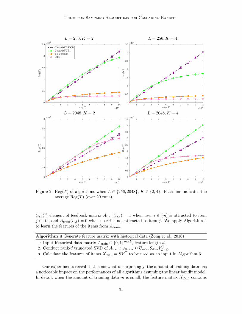
CascadeLinUCB CascadeLinTS RankedLinTS in Zong et al (2016) The pur-pose of this section is not to show that the proposed algorithms mdash which have strongtheoretical guarantees mdash are uniformly the best possible (for all choices of the param-eters) but rather to highlight some features of each algorithm and in which regime(s)which algorithm performs well We believe this empirical study will be useful for prac-titioners in the future The codes to reproduce all the experiments can be found athttpsgithubcomzixinzh2021-JMLRgit
71 Comparison of Performances of TS-Cascade and CTS to UCB-basedAlgorithms for Cascading Bandits
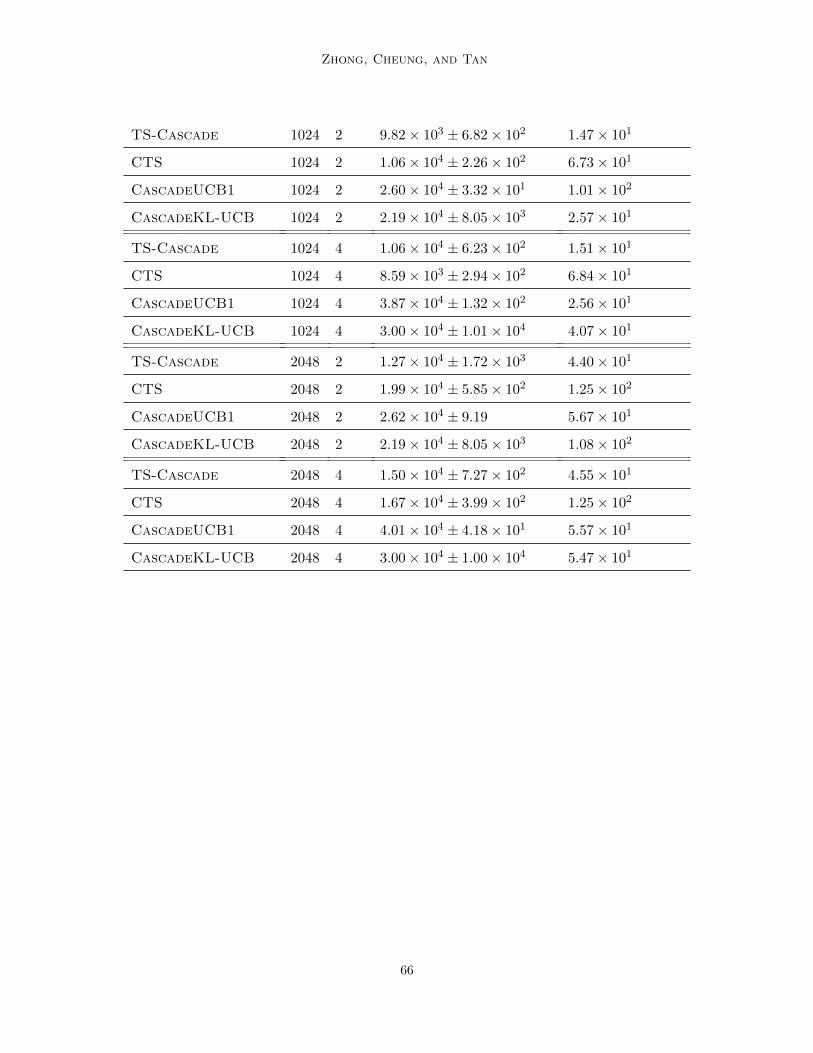
To demonstrate the effectiveness of the TS algorithms TS-Cascade and CTS we com-pare their expected cumulative regrets to CascadeKL-UCB and CascadeUCB1 (Kvetonet al 2015a) Since there are many numerical evaluations of these algorithms in the exist-ing literature (Cheung et al 2019 Huyuk and Tekin 2019) here we only present a briefdiscussion highlighting some salient features
For the L items we set the click probabilities of K of them to be w1 = 02 the proba-bilities of another K of them to be w2 = 01 and the probabilities of the remaining Lminus 2Kitems as w3 = 005 We vary L isin 16 32 64 256 512 1024 2048 and K isin 2 4 Weconduct 20 independent simulations with each algorithm under each setting of L K Wecalculate the averages and standard deviations of Reg(T ) and as well as the average runningtimes of each experiment
Our experiments indicate that the two TS algorithms always outperform the two UCBalgorithms in all settings considered (see Table 4 in Appendix D) and Figure 2 NextCascadeKL-UCB outperforms CascadeUCB1 when L ge 512 while CascadeUCB1 out-performs CascadeKL-UCB otherwise Similarly TS-Cascade outperforms CTS whenL ge 2048 while CTS outperforms TS-Cascade otherwise Thus for a large number ofitems TS-Cascade is preferred to CTS again demonstrating the utility of the Gaussianupdates over the seemingly more natural Bernoulli updates For simplicity we only presenta representative subset of the results in Figure 2 These observations imply that the bestchoice of algorithm depends on L the total number of items in the ground set
72 Performance of LinTS-Cascade(λ) compared to other algorithms for linearcascading bandits
In this subsection we compare Algorithm 3 (LinTS-Cascade(λ)) to other competitors us-ing numerical simulations Note that the three competitors for cascading bandits with lineargeneralization CascadeLinUCB CascadeLinTS RankedLinTS (Zong et al 2016) in-volve tuning parameters (called σ) Thus to be fair to each algorithm we also tune theparameters for each of the algorithms to ensure that the best performances are obtained sothat the comparisons are fair
We now describe how we set up these experiments In real-world applications goodfeatures that are extracted based on a large number of items are rarely obtained directlybut rather learnt from historical data of usersrsquo behaviors (Koren et al 2009) One commonlyused method to obtain the features of items is via low-rank matrix factorization In detaillet Atrain isin 0 1mtimesL be the matrix representing feedback of L items from m users The
30
Thompson Sampling Algorithms for Cascading Bandits
L = 256K = 2 L = 256K = 4
1 2 3 4 5 6 7 8 9 10
104
0
05
1
15
2
25104
1 2 3 4 5 6 7 8 9 10
104
0
05
1
15
2
25
3
35104
L = 2048K = 2 L = 2048K = 4
1 2 3 4 5 6 7 8 9 10
104
0
05
1
15
2
25
3104
1 2 3 4 5 6 7 8 9 10
104
0
05
1
15
2
25
3
35
4
45104
Figure 2 Reg(T ) of algorithms when L isin 256 2048 K isin 2 4 Each line indicates theaverage Reg(T ) (over 20 runs)
(i j)th element of feedback matrix Atrain(i j) = 1 when user i isin [m] is attracted to itemj isin [L] and Atrain(i j) = 0 when user i is not attracted to item j We apply Algorithm 4to learn the features of the items from Atrain
Algorithm 4 Generate feature matrix with historical data (Zong et al 2016)
1 Input historical data matrix Atrain isin 0 1mtimesL feature length d2 Conduct rank-d truncated SVD of Atrain Atrain asymp UmtimesdSdtimesdV gtLtimesd3 Calculate the features of items XdtimesL = SV gt to be used as an input in Algorithm 3
Our experiments reveal that somewhat unsurprisingly the amount of training data hasa noticeable impact on the performances of all algorithms assuming the linear bandit modelIn detail when the amount of training data m is small the feature matrix XdtimesL contains
31
Zhong Cheung and Tan
Table 3 The performances of CascadeUCB1 CascadeLinTS(100) CascadeKL-UCB CTS TS-Cascade RankedLinTS(001) CascadeLinUCB(01) andLinTS-Cascade(001) when L = 2048 K = 4 The first column displays themean and the standard deviation of Reg(T ) and the second column displays theaverage running time in seconds Algorithms which are analyzed in this work arehighlighted in bold
Reg(T ) Running time
CascadeUCB1 401times 104 plusmn 418times 101 557times 101
CascadeLinTS(100) 283times 104 plusmn 206times 103 236times 101
CascadeKL-UCB 300times 104 plusmn 100times 104 547times 101
CTS 167times 104 plusmn 399times 102 125times 102
TS-Cascade 150times 104 plusmn 727times 102 455times 101
RankedLinTS(001) 132times 104 plusmn 503times 103 264times 102
CascadeLinUCB(01) 771times 101 plusmn 257times 102 419times 103
LinTS-Cascade(001) 712times 101 plusmn 229times 102 508times 101
a small amount of noisy information of the latent click probabilities and thus taking intoaccount the paucity of information any algorithm assuming the linear bandit model cannotreliably identify the optimal items and hence suffers from a large (and often linear) regretConversely when m is large Atrain contains a significant amount of information about thelatent click probabilities w(i)Li=1 Thus Algorithm 4 is likely to successfully project theunknown feature vectors x(i)Li=1 sub Rd onto an informative low-dimensional subspace andto learn a linear separator in this subspace to classify the optimal and suboptimal itemsThis enables the algorithms assuming the linear bandit model with a small d to quicklycommit to the optimal set Slowast after small amount of exploration However in real-worldapplications since the historical data is limited we may not get sufficient training data butmay require the algorithm itself to explore the items Hence for this problem setting toillustrate the typical behavior of the algorithms under consideration we set m = 200 sothat the amount of information contained in Atrain is ldquoappropriaterdquo However obviouslyother choices of m will lead to other experimental outcomes but since our objective is tocompare the algorithms for the linear bandit model and not to scrutinize their performancesas functions of m we do not investigate the effect of m any further
To begin with we generate independent Bernoulli random variables with click prob-abilities w1 w2 or w3 for each item to produce the matrix Atrain isin 0 1mtimesL in whichm = 200 Next we vary the tuning parameters for each algorithm under consideration on alogarithmic scale We present the best performance of each algorithm for cascading banditswith linear generalization with tuning parameters in the finite set 001 01 1 10 100
Table 3 displays the means and the standard deviations of Reg(T ) as well as the averagerunning times The algorithms are listed in descending order of the average cumulative
32
Thompson Sampling Algorithms for Cascading Bandits
1 2 3 4 5 6 7 8 9 10
104
0
50
100
150
200
250
300
1 2 3 4 5 6 7 8 9 10
104
0
100
200
300
400
500
600
700
Figure 3 Left Reg(T ) of algorithms when L = 1024 K = 2 d = 3 Right Reg(T )of LinTS-Cascade(004) when L = 1024 K = 2 d isin 1 2 3 4 Each lineindicates the average Reg(T ) (over 20 runs) and the length of each errorbarabove and below each data point is the scaled standard deviation
regrets Note that we set d = 3 for the algorithms based on the linear bandit model Wewill explain this choice later
In the left plot of Figure 3 we present the average cumulative regrets of the algorithmsSince CascadeUCB1 CascadeKL-UCB CTS CascadeLinTS(100) incur much largerregrets compared to the remaining algorithms we omit their regrets in the plot for clarityFor the algorithms assuming the linear bandit model and for this dataset our experimentsindicate that d = 3 is the most appropriate choice For clarity we only display the regretsof the proposed LinTS-Cascade(λ) algorithm as d varies from 1 to 4 in the right plotof Figure 3 Figure 3 is a representative plot for all considered algorithms based on thelinear bandits It can be seen that d = 3 results in the best performance in terms of theexpected cumulative regret ie d = 3 minimizes the average regret among the values ofd considered here Roughly speaking this implies that the optimal and suboptimal itemscan be separated when the data is projected onto a three-dimensional subspace (comparedto subspaces of other dimensions) When d gt 3 the matrix that contains the extractedfeatures XdtimesL overfits to the historical data and due to this overfitting our algorithmmdashas well as other algorithmsmdashincurs a larger regret Hence in our comparison to otheralgorithms for linear bandits we only consider d = 3 features
Among the algorithms designed for linear bandits CascadeLinUCB requires signifi-cantly more time to run (as compared to other algorithms) as suggested by Table 3 whileRankedLinTS lacks theoretical analysis The reason why CascadeLinUCB is less com-
putationally efficient is that x(i)gtMminus12t x(i) needs to be calculated for each item i isin [L]
(the definition of Mt in Zong et al (2016) is slightly different from that in our paper see
Algorithm 2 therein) whereas we only calculate vtradicKM
minus12t ξt once for all items at each
time step t (see Line 5 of Algorithm 3) Our proposed LinTS-Cascade(λ) algorithm isthe only efficient algorithm with theoretical guarantees
33
Zhong Cheung and Tan
For LinTS-Cascade(λ) it is essential to pick an appropriate λ to balance explorationand exploitation Varying λ is equivalent to tuning the variance of the Thompson sam-ples (see Line 5 of Algorithm 3) We note that other algorithms such as CascadeLinUCBand CascadeLinTS (Zong et al 2016) also contain tuning parameters (called σ) andthus our algorithm is similar to these other competing algorithms in this aspect Howeverin Figure 3 we have displayed results in which the hyperparameters of all algorithms aretuned on a logarithmic scale to be fair
Lastly we submit that our LinTS-Cascade(λ) algorithm does not outperform otheralgorithms under all problem settings Indeed the performances of all algorithms basedon the linear bandit model are sensitive to the amount of training data Atrain isin 0 1mtimesL(ie the number of rows m) and the choice of d However it is worth emphasizing thatour proposed algorithm is computationally efficient and possesses appealing (asymptotic)theoretical guarantees cf Theorem 51 Indeed it is the only Thompson sampling algorithmfor linear cascading bandits that admits such theoretical guarantees
8 Summary and Future work
This work presents a comprehensive theoretical analysis of various Thompson samplingalgorithms for cascading bandits under the standard and linear models Firstly we providea tighter upper bound on the regret of CTS compared to Huyuk and Tekin (2019) Secondlythe upper bound on the expected regret of TS-Cascade we derived in Theorem 41 matchesthe state-of-the-art bound based on UCB by Wang and Chen (2017) (which is identical toCascadeUCB1 in Kveton et al (2015a)) Thirdly we propose LinTS-Cascade(λ) for thelinear generalization of the problem and upper bound its regret in Theorem 51 by refiningproof techniques used for TS-Cascade Finally in Theorem 61 we also derive a problem-independent lower bound on the expected cumulative regret using the information-theoretictechnique of Auer et al (2002) as well as a judicious construction of bandit instance Lastlywe also demonstrate the computational efficiency and efficacy in terms of regret of LinTS-Cascade(λ)
In Section 1 we analyze the Thompson sampling algorithm with Beta-Bernoulli updateand provide a tighter bound than Huyuk and Tekin (2019) in the cascading bandit settingOur analysis can be readily generalized to the matroid bandit setting which is also widelyconsidered in current literature as in Kveton et al (2014) Although the CTS algorithmcannot be easily generalized in a straightforward way to a linear cascading bandit setting itmay be a worthy endeavor to extend the other TS-based algorithms (such as TS-Cascade)introduced in this paper to other generalized linear bandit settings (such as logistic bandits)Next since the attractiveness of items in real life may change with time it is reasonable toconsider the cascading bandit model with unknown change points of latent click probabil-ities (Garivier and Moulines 2011) There are practical real-life implications in designingand analyzing algorithms that take into account the non-stationarity of the latent clickprobabilities eg the attractiveness of hotels in a city depending on the season Furtheranother interesting topic within the realm of multi-armed bandit problems concerns bestarm identification (Audibert and Bubeck 2010) In the cascading model since an arm isa list of items the objective here is to minimize the total number of pulls of all arms toidentify items that are ldquoclose tordquo or exactly equal to the optimal ones with high probability
34
Thompson Sampling Algorithms for Cascading Bandits
In the future we plan to design and analyze an algorithm for this purpose assuming thecascading bandit model
Acknowledgements
We thank the reviewers for their meticulous reading and insightful comments This workis partially funded by a National University of Singapore Start-Up Grant (R-266-000-136-133) a Singapore National Research Foundation (NRF) Fellowship (R-263-000-D02-281)and a Singapore Ministry of Education AcRF Tier 1 Grant (R-263-000-E80-114) Thisresearch is also supported by the National Research Foundation Singapore under its AISingapore Programme (AISG Award No AISG2-RP-2020-018) Any opinions findingsand conclusions or recommendations expressed in this material are those of the author(s)and do not reflect the views of National Research Foundation Singapore
References
Yasin Abbasi-Yadkori David Pal and Csaba Szepesvari Improved algorithms for linearstochastic bandits In Proceedings of the 24th Advances in Neural Information ProcessingSystems pages 2312ndash2320 2011
Marc Abeille and Alessandro Lazaric Linear Thompson sampling revisited In Proceedingsof the 20th International Conference on Artificial Intelligence and Statistics pages 176ndash184 2017
Milton Abramowitz and Irene A Stegun Handbook of Mathematical Functions with For-mulas Graphs and Mathematical Tables Dover New York ninth edition 1964
Shipra Agrawal and Navin Goyal Analysis of Thompson sampling for the multi-armedbandit problem In Proceedings of the 25th Annual Conference on Learning Theorypages 391ndash3926 2012
Shipra Agrawal and Navin Goyal Thompson sampling for contextual bandits with lin-ear payoffs In Proceedings of the 30th International Conference on Machine Learningvolume 28 pages 127ndash135 2013a
Shipra Agrawal and Navin Goyal Further optimal regret bounds for Thompson sampling InProceedings of the 16th International Conference on Artificial Intelligence and Statisticspages 99ndash107 2013b
Shipra Agrawal and Navin Goyal Near-optimal regret bounds for Thompson sampling JACM 64(5)301ndash3024 September 2017a
Shipra Agrawal and Navin Goyal Near-optimal regret bounds for Thompson samplingJournal of the ACM (JACM) 64(5)1ndash24 2017b
Shipra Agrawal Vashist Avadhanula Vineet Goyal and Assaf Zeevi Thompson samplingfor the MNL-bandit arXiv preprint arXiv170600977 2017
35
Zhong Cheung and Tan
Venkatachalam Anantharam Pravin Varaiya and Jean Walrand Asymptotically efficientallocation rules for the multiarmed bandit problem with multiple plays-Part I IIDrewards IEEE Transactions on Automatic Control 32(11)968ndash976 November 1987
Jean-Yves Audibert and Sebastien Bubeck Best arm identification in multi-armed banditsIn Proceedings of the 23th Conference on Learning Theory pages 41ndash53 2010
Jean-Yves Audibert Remi Munos and Csaba Szepesvari Explorationndashexploitation tradeoffusing variance estimates in multi-armed bandits Theoretical Computer Science 410(19)1876 ndash 1902 2009 Algorithmic Learning Theory
Peter Auer Nicolo Cesa-Bianchi Yoav Freund and Robert E Schapire The nonstochasticmultiarmed bandit problem SIAM Journal of Computing 32(1)48ndash77 2002
Sebastien Bubeck Nicolo Cesa-Bianchi et al Regret analysis of stochastic and nonstochas-tic multi-armed bandit problems Foundations and Trends Rcopy in Machine Learning 5(1)1ndash122 2012
Olivier Chapelle and Lihong Li An empirical evaluation of Thompson sampling In Proceed-ings of the 24th Advances in Neural Information Processing Systems pages 2249ndash22572011
Wei Chen Yajun Wang and Yang Yuan Combinatorial multi-armed bandit Generalframework and applications In Proceedings of the 30th International Conference onMachine Learning volume 28 of Proceedings of Machine Learning Research pages 151ndash159 2013
Wang Chi Cheung Vincent Tan and Zixin Zhong A Thompson sampling algorithm forcascading bandits In Proceedings of the 22nd International Conference on ArtificialIntelligence and Statistics pages 438ndash447 2019
Wei Chu Lihong Li Lev Reyzin and Robert Schapire Contextual bandits with linear payofffunctions In Proceedings of the 14th International Conference on Artificial Intelligenceand Statistics pages 208ndash214 2011
Richard Combes M Sadegh Talebi Alexandre Proutiere and Marc Lelarge Combina-torial bandits revisited In Proceedings of the 28th International Conference on NeuralInformation Processing Systems - Volume 2 pages 2116ndash2124 2015
Thomas M Cover and Joy A Thomas Elements of information theory John Wiley amp Sons2012
Nick Craswell Onno Zoeter Michael Taylor and Bill Ramsey An experimental comparisonof click position-bias models In Proceedings of the 1st ACM International Conference onWeb Search and Data Mining pages 87ndash94 2008
Sarah Filippi Olivier Cappe Aurelien Garivier and Csaba Szepesvari Parametric banditsThe generalized linear case In Proceedings of the 23rd Advances in Neural InformationProcessing Systems pages 586ndash594 2010
36
Thompson Sampling Algorithms for Cascading Bandits
Yi Gai Bhaskar Krishnamachari and Rahul Jain Learning multiuser channel allocationsin cognitive radio networks A combinatorial multi-armed bandit formulation In 2010IEEE Symposium on New Frontiers in Dynamic Spectrum (DySPAN) pages 1ndash9 2010
Aurelien Garivier and Eric Moulines On upper-confidence bound policies for switchingbandit problems In Proceedings of the 22nd International Conference on AlgorithmicLearning Theory pages 174ndash188 Springer 2011
Aditya Gopalan Shie Mannor and Yishay Mansour Thompson sampling for complex onlineproblems In Proceedings of the 31st International Conference on Machine Learning pages100ndash108 2014
Alihan Huyuk and Cem Tekin Analysis of Thompson sampling for combinatorial multi-armed bandit with probabilistically triggered arms In Proceedings of Machine LearningResearch pages 1322ndash1330 2019
Sumeet Katariya Branislav Kveton Csaba Szepesvari and Zheng Wen DCM banditsLearning to rank with multiple clicks In Proceedings of the 33rd International Conferenceon Machine Learning pages 1215ndash1224 2016
Emilie Kaufmann Nathaniel Korda and Remi Munos Thompson sampling An asymptot-ically optimal finite-time analysis In Proceedings of the 23rd International Conferenceon Algorithmic Learning Theory pages 199ndash213 2012
Junpei Komiyama Junya Honda and Hiroshi Nakagawa Optimal regret analysis of Thomp-son sampling in stochastic multi-armed bandit problem with multiple plays In Proceed-ings of The 32nd International Conference on Machine Learning pages 1152ndash1161 2015
Yehuda Koren Robert Bell and Chris Volinsky Matrix factorization techniques for recom-mender systems Computer (8)30ndash37 2009
Branislav Kveton Zheng Wen Azin Ashkan Hoda Eydgahi and Brian Eriksson Ma-troid bandits Fast combinatorial optimization with learning In Proceedings of the 30thConference on Uncertainty in Artificial Intelligence pages 420ndash429 2014
Branislav Kveton Csaba Szepesvari Zheng Wen and Azin Ashkan Cascading banditsLearning to rank in the cascade model In Proceedings of the 32nd International Confer-ence on Machine Learning pages 767ndash776 2015a
Branislav Kveton Zheng Wen Azin Ashkan and Csaba Szepesvari Tight regret boundsfor stochastic combinatorial semi-bandits In Proceedings of the 18th International Con-ference on Artificial Intelligence and Statistics pages 535ndash543 2015b
Branislav Kveton Zheng Wen Azin Ashkan and Csaba Szepesvari Combinatorial cascad-ing bandits In Proceedings of the 28th International Conference on Neural InformationProcessing Systems pages 1450ndash1458 2015c
Paul Lagree Claire Vernade and Olivier Cappe Multiple-play bandits in the position-basedmodel In Proceedings of the 29th Advances in Neural Information Processing Systemspages 1597ndash1605 Curran Associates Inc 2016
37
Zhong Cheung and Tan
Lihong Li Wei Chu John Langford and Robert E Schapire A contextual-bandit approachto personalized news article recommendation In Proceedings of the 19th InternationalConference on World Wide Web pages 661ndash670 2010
Shuai Li Baoxiang Wang Shengyu Zhang and Wei Chen Contextual combinatorial cas-cading bandits In Proceedings of the 33rd International Conference on Machine Learningpages 1245ndash1253 2016
Lijing Qin Shouyuan Chen and Xiaoyan Zhu Contextual combinatorial bandit and itsapplication on diversified online recommendation In Proceedings of the 14th SIAM In-ternational Conference on Data Mining pages 461ndash469 SIAM 2014
Daniel Russo and Benjamin Van Roy Learning to optimize via posterior sampling Math-ematics of Operations Research 39(4)1221ndash1243 2014
Daniel Russo Benjamin Van Roy Abbas Kazerouni Ian Osband and Zheng Wen Atutorial on Thompson sampling Foundations and Trends in Machine Learning 11(1)1ndash96 2018
William R Thompson On the likelihood that one unknown probability exceeds another inview of the evidence of two samples Biometrika 25(3ndash4)285ndash294 1933
Qinshi Wang and Wei Chen Improving regret bounds for combinatorial semi-bandits withprobabilistically triggered arms and its applications In Proceedings of the 30th Advancesin Neural Information Processing Systems pages 1161ndash1171 2017
Siwei Wang and Wei Chen Thompson sampling for combinatorial semi-bandits In Pro-ceedings of the 35th International Conference on Machine Learning pages 5114ndash51222018
Zheng Wen Branislav Kveton and Azin Ashkan Efficient learning in large-scale combina-torial semi-bandits In Proceedings of the 32nd International Conference on InternationalConference on Machine Learning - Volume 37 pages 1113ndash1122 2015
Masrour Zoghi Tomas Tunys Mohammad Ghavamzadeh Branislav Kveton Csaba Szepes-vari and Zheng Wen Online learning to rank in stochastic click models In Proceedingsof the 34th International Conference on Machine Learning pages 4199ndash4208 2017
Shi Zong Hao Ni Kenny Sung Nan Rosemary Ke Zheng Wen and Branislav KvetonCascading bandits for large-scale recommendation problems In Proceedings of the 32ndConference on Uncertainty in Artificial Intelligence pages 835ndash844 2016
38
Thompson Sampling Algorithms for Cascading Bandits
Appendix A Notations
[L] ground set of size L
w(i) click probability of item i isin [L]
x(i) feature vector of item i in the linear generalization
β common latent vector in the linear generalization
T time horizon
d number of features of any item in the linear generalization
K size of recommendation list
St recommendation list at time t
iti i-th recommended item at time t
[L](K) set of all K-permutations of [L]
Wt(i) reflection of the interest of the user in item t at time t
R(St|w) instantaneous reward of the agent at time t
kt feedback from the user at time t
r(St|w) expected instantaneous reward of the agent at time t
Slowast optimal ordered K-subset for maximizing the expected instan-
taneous reward
Reg(T ) expected cumulative regret
wt(i) empirical mean of item i at time t
Nt(i) number of observations of item i before time t plus 1
Zt 1-dimensional random variable drawn from the standard nor-
mal distribution at time t
νt(i) empirical variance of item i at time t
σt(i) standard deviation of Thompson sample of item i at time t in
TS-Cascade
θt(i) Thompson sample of item i at time t in TS-Cascade
αBt (i) βBt (i) statistics used in CTS
θBt (i) Thompson sample from Beta distribution at time t in CTS
39
Zhong Cheung and Tan
∆ij gap between click probabilities of optimal item i and subopti-
mal item j
∆ = ∆KK+1 minimum gap between click probabilities of optimal and sub-
optimal items
πt a permutation of optimal items used in the analysis of CTS
At(` j k) At(` j k) At(` j) events defined to help decompose the regret of CTS
NB(i j) number of time steps that At(i j) happens for optimal item j
and suboptimal item i within the whole horizon
Bt(i) Ct(i j) events that measure the concentration of θBt (i) wt(i) around
w(i) as CTS processes
θB(minusi)Wij Wiminusj variables used in the analysis of CTS
Ewt Eθt ldquonice eventsrdquo in TS-Cascade
gt(i) ht(i) functions used to define ldquonice eventsrdquo
St ldquounsaturatedrdquo set at time t
F (S t) function used to define ldquounsaturatedrdquo set
α determined by click probabilities w(i)rsquos used in the analysis
Hwt Fit G(StWt) used in the analysis of TS-Cascade
λ parameter in LinTS-Cascade(λ)
X collection of feature vector x(i)rsquos
bt Mt vt statistics used in LinTS-Cascade(λ)
ξt d-dimensional random variable drawn from standard multi-
variate normal distribution at time t in LinTS-Cascade(λ)
ψt empirical mean of latent vector β at time t
ρt Thompson sample at time t in TS-Cascade
ηt(i) random variable in the linear generalization
Eψt Eρt ldquonice eventsrdquo in LinTS-Cascade(λ)
lt ut(i) functions used to define ldquonice eventsrdquo in LinTS-Cascade(λ)
w(`)(i) click probability of item i isin [L] under instance ` (0 le ` le L)
r(St|w(`)) expected instantaneous reward of the agent at time t under
instance `
40
Thompson Sampling Algorithms for Cascading Bandits
Slowast` optimal ordered K-subset under instance `
π deterministic and non-anticipatory policy
Sπ(`)t recommendation list at time t (under instance `) by policy π
Oπ(`)t stochastic outcome by pulling S
π(`)t at time t (under instance
`) by policy π
A feedback matrix extracted from real data
yt Qt ζt σt variables used in the analysis of LinTS-Cascade(λ)
Q Jπ`t Υ`t(S) variables used in the analysis of the lower bound
Appendix B Useful theorems
Here are some basic facts from the literature that we will use
Theorem B1 (Audibert et al (2009) specialized to Bernoulli random variables)Consider N independently and identically distributed Bernoulli random variables Y1 YN isin0 1 which have the common mean m = E[Y1] In addition consider their sample meanξ and their sample variance V
ξ =1
N
Nsumi=1
Yi V =1
N
Nsumi=1
(Yi minus ξ)2 = ξ(1minus ξ)
For any δ isin (0 1) the following inequality holds
Pr
∣∣∣ξ minusm∣∣∣ leradic
2V log(1δ)
N+
3 log(1δ)
N
ge 1minus 3δ
Theorem B2 (Abramowitz and Stegun (1964) Formula 7113) Let Z sim N (micro σ2)The following inequalities hold
1
2radicπ
exp
(minus7z2
2
)le Pr (|Z minus micro| gt zσ) le exp
(minusz
2
2
)forallz gt 0
1
2radicπz
exp
(minusz
2
2
)le Pr (|Z minus micro| gt zσ) le
radic2radicπz
exp
(minusz
2
2
)forallz ge 1
Theorem B3 (Abbasi-Yadkori et al 2011 Agrawal and Goyal 2013a) Let (F primet t ge 0) bea filtration (mt t ge 1) be an Rd-valued stochastic process such that mt is (F primetminus1)-measurable(ηt t ge 1) be a real-valued martingale difference process such that ηt is (F primet)-measurable Fort ge 0 define ξt =
sumtτ=1mτητ and Mt = Id +
sumTτ=1mτm
gtτ where Id is the d-dimensional
identity matrix Assume ηt is conditionally R-sub-GaussianThen for any δprime gt 0 t ge 0 with probability at least 1minus δprime
ξtMminus1tle R
radicd log
( t+ 1
δprime)
where ξMminus1t
=radicξgtt M
minus1t ξt
41
Zhong Cheung and Tan
Appendix C Proofs of main results
In this Section we provide proofs of Lemmas 32 33 Theorem 34 Lemmas 42 43 45 63 64 65as well as derivations of inequalities (39) and (57)
C1 Proof of Lemma 32
Proof We let τ1 τ2 be the time slots such that i isin S(t) and Wt(i) is observed defineτ0 = 0 and abbreviate εi as ε for simplicity Then
E [ existt 1 le t le T i isin St |wt(i)minus w(i)| gt εObserve Wt(i) at t ]
= E
[Tsumt=1
1 [i isin St |wt(i)minus w(i)| gt εObserve Wt(i) at t]
]
le E
[Tsums=0
E
[τs+1minus1sumt=τs
1 [i isin St |wt(i)minus w(i)| gt εObserve Wt(i) at t]
]]
le E
[Tsums=0
Pr [wt(i)minus w(i)| gt εNt(i) = s]
]
le 1 +Tsums=1
Pr [|wt(i)minus w(i)| gt εNt(i) = s]
le 1 +Tsums=1
exp [minuswKL (w(i) + ε w(i))] +Tsums=1
exp [minuswKL (w(i)minus ε w(i))]
le 1 +
infinsums=1
exp [minusKL (w(i) + ε w(i))])s +
infinsumw=1
exp [minusKL (w(i)minus ε w(i))]s
le 1 +exp [minusKL (w(i) + ε w(i) )]
1minus exp [minusKL (w(i) + ε w(i))]+
exp [minusKL (w(i)minus ε w(i))]
1minus exp [minusKL (w(i)minus ε w(i))]
le 1 +1
KL (w(i) + ε w(i))+
1
KL (w(i)minus ε w(i))
le 1 +1
ε2
42
Thompson Sampling Algorithms for Cascading Bandits
C2 Upper bound on the regret incurred by the second term of (37) inSection 3
To derive the inequality (39) for any 0 lt ε lt ∆KK+12
Lsumi=K+1
Ksumj=1
∆ji middot E
[Tsumt=1
1 [At(i j) and notBt(i) and Ct(i j)]
]
le 4 log T middotLsum
i=K+1
∆Ki minus ε(∆Ki minus 2ε)2
+
Lsumi=K+1
Ksumj=1
∆ji
we use the following result
Lemma C1 (Implied by Wang and Chen (2018) Lemma 4) In Algorithm 1for anybase item i we have the following two inequalities
Pr
[θBi (t)minus wt(i) gt
radic2 log T
Nt(i)
]le 1
T Pr
[wt(i)minus θBi (t) gt
radic2 log T
Nt(i)
]le 1
T
Note that
εi =1
2middot(
∆K+1i +∆KK+1
2
)and εj =
1
2middot(
∆jK +∆KK+1
2
)implies εi + εj = ∆ji2 Let
Mij =2 log T
(∆ji minus εi minus εj)2=
8 log T
∆2ji
then when Nt(i) gt Mij ∆jiminus εiminus εj gtradic
2 log TNt(i)
Thus in expectation the time steps that
At(i j) and notBt(i) and Ct(i j) occurs can be decomposed as follows
E
[Tsumt=1
1 [At(i j) and notBt(i) and Ct(i j)]
]
= E
[Tsumt=1
1 [At(i j) and notBt(i) and Ct(i j) Nt(i) leMij ]
]
+ E
[Tsumt=1
1 [At(i j) and notBt(i) and Ct(i j) Nt(i) gt Mij ]
]
And further
E
[Tsumt=1
1 [At(i j) and notBt(i) and Ct(i j) Nt(i) gt Mij ]
]
le E
[Tsumt=1
1[wt(i) le w(i) + εi θ
Bt (i) gt w(j)minus εj Nt(i) gt Mij Observe Wt(i) at t
]]
43
Zhong Cheung and Tan
le E
[Tsumt=1
1[θBt (i) gt wt(i) + ∆ji minus εi minus εj Nt(i) gt Mij Observe Wt(i) at t
]](C1)
le E
[Tsumt=1
1
[θBt (i) gt wt(i) +
radic2 log T
Nt(i)
]](C2)
le 1
To derive line (C1) we observe that when wt(i) le w(i) + εi θBt (i) gt w(j)minus εj we have
θBt (i) gt w(j)minus εj = w(i) + ∆ji minus εj ge wt(i) + ∆ji minus εi minus εj
Besides line (C2) follows from the definition of Mij Hence
Ksumj=1
∆ji middot E
[Tsumt=1
1 [At(i j) and notBt(i) and Ct(i j)]
]
leKsumj=1
∆ji middot E
[Tsumt=1
1 [At(i j) Nt(i) leMij ]
]︸ ︷︷ ︸
(lowast)
+
Ksumj=1
∆ji
Note that (i) Nt(i) of suboptimal item i increases by one when the event Aijt happens forany optimal item j (ii) the event At(i j) happens for at most one optimal item i at anytime t and (iii) M1i le leMKi Let
Yij =
Tsumt=1
1 [ At(i j) Nt(i) leMij ]
Based on these facts it follows that Yij le Mij almost surely and moreoversumK
j=1 Yij leMKi almost surely Therefore (lowast) can be bounded from above by
max
Ksumj=1
∆jiyij 0 le yij leMij
Ksumi=1
yij leMKj
Since the gaps are decreasing ∆1i ge ∆2i ge ∆Ki the solution to the above problem isylowast1i = M1i y
lowast2i = M2i minusM1i y
lowastKi = MKi minusMKminus1i Therefore the value of (lowast) is
bounded from above by
8 log T
∆1i1
∆21i
+
Ksumj=2
∆ji
(1
∆2ji
minus 1
∆2jminus1i
) Further we use the following result
Lemma C2 (Kveton et al (2014) Lemma 3) Let ∆1 ge ge ∆K be a sequence ofK positive numbers then[
∆11
∆21
+Ksumk=2
∆k
(1
∆2k
minus 1
∆2kminus1
)]le 2
∆K
44
Thompson Sampling Algorithms for Cascading Bandits
Therefore
Ksumj=1
∆ji middot E
[Tsumt=1
1 [At(i j) and notBt(i) and Ct(i j)]
]le 16 log T
∆Ki+
Ksumj=1
∆ji
Lastly the total regret incurred by the second term in equation (37) can be boundedas follows
Lsumi=K+1
Ksumj=1
∆ji middot E
[Tsumt=1
1 [At(i j) and notBt(i) and Ct(i j)]
]le 16 log T middot
Lsumi=K+1
1
∆Ki+
Lsumi=K+1
Ksumj=1
∆ji
C3 Proof of Lemma 33
Proof We abbreviate εj as ε for simplicity By the definition of Wij and Wiminusj θBt isin Wj
yields that there exists i such that θBt (i) le w(j)minus ε θBt (minusj) isinWiminusj thus we can use
E
[Tsumt=1
Pr[existi st θBt (i) le w(j)minus ε θBt (minusj) isinWiminusj Observe Wt(i) at t | Ftminus1
]]
as an upper bound Since θBt isinWj indicates θBt (i) ge θBt (j) we have
Pr[existi st θBt (i) le w(j)minus ε θBt (minusj) isinWiminusj Observe Wt(i) at t | Ftminus1
]le Pr
[existi st θBt (j) le w(j)minus ε θBt (minusj) isinWiminusj Observe Wt(i) at t | Ftminus1
]
Denote the value pjt as Pr[θBt (j) gt w(j)minus ε|Ftminus1
] Notice that according to the cas-
cading model given Ftminus1 the value θBt (j) and the set of values θBt (minusj) are independentBesides note that notCij(t) = θBt (i) le w(j)minus ε holds when θBt (minusj) isinWiminusj If we furtherhave θBt (j) gt w(j)minus ε then j isin St
Observation of fixed i Fix θBt (minusj) isinWiminusj let
bull St = it1 it2 itK itk1 = i when θBt (j) le w(j)minus ε
bull St = it1 it2 itK itk2 = j when θBt (j) changes to θBt(j) such that θBt(j) gt w(j)minusε
Since θBt (iti) ge θBt (it2) ge θBt (it1) ge θBt (it2) ge according to Algorithm 1
θBt(j) gt w(j)minus ε ge θBt (i) = θBt (itk1) ge θBt (itk1+1) ge
Therefore k2 le k1 and itl = itl for 1 le l lt k2 Besides the observation of item i or j isdetermined by θBt (minusj)
With the observation and notation above we have
Pr[θBt (j) le w(j)minus ε θBt (minusj) isinWiminusj Observe Wt(i) at t
∣∣ Ftminus1]= (1minus pjt) middot Pr
[θBt (minusj) isinWiminusj |Ftminus1
]middot Pr
[Observe Wt(i) at t
∣∣ θBt ]= (1minus pjt) middot Pr
[θBt (minusj) isinWiminusj |Ftminus1
]middot E
[k1minus1prodl=1
(1minus w(itl))∣∣ θBt (minusj)
]
45
Zhong Cheung and Tan
and
Pr[j isin St θBt (minusj) isinWiminusj Observe Wt(j) at t|Ftminus1
]ge Pr
[θBt (j) gt w(j)minus ε θBt (minusj) isinWiminusj Observe Wt(j) at t|Ftminus1
]= pjt middot Pr
[θBt (minusj) isinWiminusj |Ftminus1
]middot Pr
[Observe Wt(j) at t
∣∣ θBt (minusj)]
= pjt middot Pr[θBt (minusj) isinWiminusj |Ftminus1
]middot E
[k2minus1prodl=1
(1minus w(itl))∣∣ θBt (minusj)
]
ge pjt middot Pr[θBt (minusj) isinWiminusj |Ftminus1
]middot E
[k1minus1prodl=1
(1minus w(itl))∣∣ θBt (minusj)
]
This leads to
Pr[θBt isinWij Observe Wt(i) at t | Ftminus1
]le (1minus pjt) middot Pr
[θBt (minusj) isinWiminusj
∣∣ Ftminus1] middot E[k1minus1prodl=1
(1minus w(itl))∣∣ θBt (minusj)
]
le 1minus pjtpjt
middot Pr[j isin St θBt (minusj) isinWiminusj Observe Wt(j) at t
∣∣ Ftminus1] Observation in the whole horizon By definition Wij are disjoint sets for different
i Hence
E
[Tsumt=1
Pr[existi st θBt isinWij Observe Wt(i) at t | Ftminus1
]]
=
Lsumi=K+1
E
[Tsumt=1
Pr[θBt isinWij Observe Wt(i) at t | Ftminus1
]]
leTsumt=1
E
[Lsum
i=K+1
E[
1minus pjtpjt
middot Pr[j isin St θBt (minusj) isinWiminusj Observe Wt(j) at t
∣∣ Ftminus1]]]
=Tsumt=1
E[
1minus pjtpjt
middot Pr[existi st j isin St θBt (minusj) isinWiminusj Observe Wt(j) at t
∣∣ Ftminus1]]
leTsumt=1
E[
1minus pjtpjt
middot Pr[j isin StObserve Wt(j) at t
∣∣ Ftminus1]]
=Tsumt=1
E[
1minus pjtpjt
middot 1 [j isin StObserve Wt(j) at t | Ftminus1]]
46
Thompson Sampling Algorithms for Cascading Bandits
Let τjq is the time step that item j is observed for the q-th time Then
E
[Tsumt=1
Pr[existi st θBt isinWij Observe Wt(i) at t | Ftminus1
]]
leTminus1sumq=0
E
1minus pjτjq+1
pjτjq+1
τjq+1sumt=τjq+1
1 [j isin StObserve Wt(j) at t | Ftminus1]
(C3)
=
Tminus1sumq=0
E[
1minus pjτjq+1
pjτjq+1
]
Line (C3) follows from the fact that the probability Pr[θBt (j) gt w(j)minus ε|Ftminus1
]only changes
when we get a feedback of item j but during time steps in [τjq + 1 τjq+1 minus 1] we do nothave any such feedback
Next we apply a variation of Lemma 29 in Agrawal and Goyal (2017b)
Lemma C3 (Implied by Agrawal and Goyal (2017b) Lemma 29) For any j pjtis Pr
[θBt (j) gt w(j)minus ε|Ftminus1
] and τjq is the time step that item j is observed for the q-th
time Then 2
E[
1
pjτjq+1minus 1
]le
3
εif q lt
8
ε
Θ
(eminusε
2q2 +1
(q + 1)ε2eminusDjq +
1
eε2q4 minus 1
)else
where Dj = KL(w(j) w(j)minus ε) = [w(j)minus ε] middot log[w(j)minusεw(j)
]+ [1minus w(j) + ε] middot log
[1minusw(j)+ε1minusw(j)
]
According to Pinskerrsquos and reverse Pinskerrsquos inequality for any two distributions P andQ defined in the same finite space X we have
δ(PQ)2 le 1
2KL(PQ) le 1
αQδ(PQ)2
where δ(PQ) = sup|P (A)minusQ(A)|∣∣A sub X and αQ = minxisinXQ(x)gt0Q(x) Therefore
Dj ge 2w(j)minus [w(j)minus ε]2 = 2ε2
Hence there exists a constant 0 lt c1 ltinfin such that
Tminus1sumq=0
E[
1minus pjτjq+1
pjτjq+1
]le
sum0leqlt8ε
3
ε+
sumTminus1geqge8ε
c1 middot[eminusε
2q2 +1
(q + 1)ε2eminus2ε
2q +1
eε2q4 minus 1
]
le 24
ε2+ c1 middot
int Tminus1
8εminus1eminusε
2x2 +1
(x+ 1)ε2eminus2ε
2x +1
eε2x4 minus 1dx
2 A (non-negative) function f(T ) = O(T ) if there exists a constant 0 lt c lt infin (dependent on w but notT ) such that f(T ) le cT for sufficiently large T Similarly f(T ) = Ω(T ) if there exists c gt 0 such thatf(T ) ge cT for sufficiently large T Finally f(T ) = Θ(T ) if f(T ) = O(T ) and f(T ) = Ω(T )
47
Zhong Cheung and Tan
Note the Taylor series of ex ex =suminfin
n=0 xnn (0 = 1) We have
(i)
int Tminus1
8εminus1eminusε
2x2 dx = minus 2
ε2eminusε
2x2
∣∣∣∣Tminus1x=8εminus1
=2
ε2eε
22 middot[eminusε
2T2 minus eminusε2(8ε)2]le 2radice
ε2
(ii)
int Tminus1
8εminus1
1
(x+ 1)ε2eminus2ε
2x dx = eε22 middot
int Tminus1
8εminus1
1
(x+ 1)ε2eminus2ε
2(x+1) dx
= eε22 middot
int T
8ε
1
xε2eminus2ε
2x dx = eε22 middot
int 2Tε2
16ε
eminusx
x2d( x
2ε2
)=eε
22
ε2middotint 2Tε2
16ε
eminusx
xdx
le eε22
ε2middotint 1
16ε
eminusx
xdx middot 1[16ε lt 1] +
eε22
ε2middotint 2Tε2
1
eminusx
xdx
le eε22
ε2middotint 1
16ε
1
16εdx middot 1[16ε lt 1] +
eε22
ε2middotint 2Tε2
1eminusx dx
le eε22
ε2middot 1
16εmiddot 1[16ε lt 1] +
eε22
ε2middot 1
e
(iii)
int Tminus1
8εminus1
1
eε2x4 minus 1dx le
int Tminus1
8εminus1
1
ε2x4dx =
4
ε2middot log x
∣∣∣Tminus18εminus1
le 4
ε2middot log T
Let c = c1 middot (2radice+ 5) + 24 then (i) if ε lt 116
Tminus1sumq=0
E[
1minus pjτjq+1
pjτjq+1
]le 24
ε2+ c1 middot
(2radice
ε2+
2radice middot ε3
+4
ε2middot log T
)le c middot
(1
ε3+
log T
ε2
)
(ii) else we have ε ge 116 and
Tminus1sumq=0
E[
1minus pjτjq+1
pjτjq+1
]le 24
ε2+ c1 middot
(2radice
ε2+
1radice middot ε2
+4
ε2middot log T
)le c log T
ε2
C4 Proof of Theorem 34
Proof We assume that w(1) = w(2) = = w(K) The problem-independent bound forCTS can be derived with a similar analysis as the problem-dependent bound in Theorem 31The key difference is to divide the items into two sets according to the gaps ∆1iLi=K+1
which were defined in the statement of Theorem 31
For any ε isin (0 1) we let S1 = i isin [L] 0 lt ∆1i le ε and S2 = i isin [L] ∆1i gt εThen S1 cap S2 = empty and S1 cup S2 = [L] Slowast According to the definition of NB(i j) in (34)sum
iisinS1
∆ji middot E[NB(i j)] le T forall1 le j le K lt i le L
48
Thompson Sampling Algorithms for Cascading Bandits
Recall from the decomposition of the expected regret in (35) that we have
Reg(T ) leKsumj=1
Lsumi=K+1
∆ji middot E[NB(i j)] =Ksumj=1
sumiisinS1
∆ji middot E[NB(i j)] +Ksumj=1
sumiisinS2
∆ji middot E[NB(i j)]
le εKT +Ksumj=1
sumiisinS2
∆ji middot E[NB(i j)]
Now we focus on the second part of the regret Similarly to before we define two moreevents taking into account the concentration of Thompson sample θBt (i) (see Line 3 ofAlgorithm 1) and empirical mean wt(i) (see (36) for definition)
Bprimet(i) =wt(i) gt w(i) + εprimei
Cprimet(i j) =
θBt (i) gt w(j)minus εprimej
j isin Slowast i isin S2
with
εprimej =ε
4forallj isin Slowast εprimei =
∆1i
2minus ε
4ge ε
4foralli isin S2
Then εprimei + εprimej = ∆ji2 Subsequently we separate the second part of the regret similarly to(37) and bound the three terms separately as follows
(i)Ksumj=1
sumiisinS2
∆ji middot E
[Tsumt=1
1[At(i j) and Bprimet(i)
]]le LminusK +
sumiisinS2
1
(εprimei)2le (LminusK) middot
(1 +
16
ε2
)
(ii)sumiisinS2
Ksumj=1
∆ji middot E
[Tsumt=1
1[At(i j) and notBprimet(i) and Cprimet(i j)
]]lesumiisinS2
16 log T
∆Ki+sumiisinS2
Ksumj=1
∆ji
le 16(LminusK) log T
ε+K(LminusK)
(iii)sumiisinS2
Ksumj=1
∆ji middot E
[Tsumt=1
1[At(i j) and notCprimet(i j)
]]
le c middotKsumj=1
∆jL middot(1[εprimej lt 116]
(εprimej)3
+log T
(εprimej)2
)le 2α2K middot
(4 middot 1[ε lt 14]
ε3+
log T
ε2
)
with α2 = 8c (a constant that does not depend on the problem instance which appeared in(310) for the first time) Similarly to (38) the first bound above results from Lemma 32The second one is derived similarly to (39) We apply Lemma 33 to derive the final boundsimilarly to (310) Overall we can derive an upper bound on the total regret as a functionof ε as follows
Reg(T ) le εKT + (LminusK) middot(
1 +16
ε2
)+
16(LminusK) log T
ε+K(LminusK)
+ 2α2K middot(
4 middot 1[ε lt 14]
ε3+
log T
ε2
)= εKT +
16(LminusK) log T
ε+
16(LminusK) + 2α2K log T
ε2+
8α2K
ε3+ (K + 1)(LminusK)
49
Zhong Cheung and Tan
If we let ε = Tminus14 we have
Reg(T ) le (1 + 8α2) middotKT 34 + 32(LminusK)(radicT +K + 1) + 2α2K
radicT log T
This bound is of order O(KT 34 + LradicT +K
radicT log T )
C5 Proof of Lemma 42
Proof Bounding probability of event Ewt We first consider a fixed non-negativeinteger N and a fixed item i Let Y1 YN be iid Bernoulli random variables with thecommon mean w(i) Denote ξN =
sumNi=1 YiN as the sample mean and VN = ξN (1 minus ξN )
as the empirical variance By applying Theorem B1 with δ = 1(t+ 1)4 we have
Pr
∣∣∣ξN minus w(i)∣∣∣ gt
radic8VN log(t+ 1)
N+
12 log(t+ 1)
N
le 3
(t+ 1)4 (C4)
By an abuse of notation let ξN = 0 if N = 0 Inequality (C4) implies the followingconcentration bound when N is non-negative
Pr
∣∣∣ξN minus w(i)∣∣∣ gt
radic16VN log(t+ 1)
N + 1+
24 log(t+ 1)
N + 1
le 3
(t+ 1)4 (C5)
Subsequently we can establish the concentration property of wt(i) by a union bound ofNt(i) over 0 1 tminus 1
Pr
(|wt(i)minus w(i)| gt
radic16νt(i) log(t+ 1)
Nt(i) + 1+
24 log(t+ 1)
Nt(i) + 1
)
le Pr
∣∣∣ξN minus w(i)∣∣∣ gt
radic16VN log(t+ 1)
N + 1+
24 log(t+ 1)
N + 1for some N isin 0 1 tminus 1
le 3
(t+ 1)3
Finally taking union bound over all items i isin L we know that event Ewt holds true withprobability at least 1minus 3L(t+ 1)3
Bounding probability of event Eθt conditioned on event Ewt Consider anobservation trajectory Ht satisfying event Ewt By the definition of the Thompson sampleθt(i) (see Line 7 in Algorithm 2) we have
Pr (|θt(i)minus wt(i)| gt ht(i) for all i isin L|Hwt)
= PrZt
(∣∣∣∣∣Zt middotmax
radicνt(i) log(t+ 1)
Nt(i) + 1log(t+ 1)
Nt(i) + 1
∣∣∣∣∣ gtradic
log(t+ 1)
[radic16νt(i) log(t+ 1)
Nt(i) + 1+
24 log(t+ 1)
Nt(i) + 1
]for all i isin [L]
∣∣∣∣ wt(i) Nt(i)
)
50
Thompson Sampling Algorithms for Cascading Bandits
le Pr
(∣∣∣∣∣Zt middotmax
radicνt(i) log(t+ 1)
Nt(i) + 1log(t+ 1)
Nt(i) + 1
∣∣∣∣∣ gtradic
16 log(t+ 1) max
radicνt(i) log(t+ 1)
Nt(i) + 1log(t+ 1)
Nt(i) + 1
for all i isin [L]
∣∣∣∣ wt(i) Nt(i)
)le exp [minus8 log(t+ 1)] le 1
(t+ 1)3 (C6)
The inequality in (C6) is by the concentration property of a Gaussian random variable seeTheorem B2 Altogether the lemma is proved
C6 Proof of Lemma 43
Proof To start we denote the shorthand θt(i)+ = maxθt(i) 0 We demonstrate that if
events Ewt Eθt and inequality (42) hold then for all S = (i1 iK) isin St we have
Ksumk=1
kminus1prodj=1
(1minus w(ij))
middotθt(ik)+ (Dagger)lt
Ksumk=1
kminus1prodj=1
(1minus w(j))
middotθt(k)+(dagger)le
Ksumk=1
kminus1prodj=1
(1minus w(itj))
middotθt(itk)+(C7)
where we recall that St = (it1 itK) in an optimal arm for θt and θt(i
t1) ge θt(it2) ge ge
θt(itK) ge maxiisin[L]it1itK θt(i) The inequalities in (C7) clearly implies that St isin St To
justifies these inequalities we proceed as followsShowing (dagger) This inequality is true even without requiring events Ewt Eθt and
inequality (42) to be true Indeed we argue the following
Ksumk=1
kminus1prodj=1
(1minus w(j))
middot θt(k)+ leKsumk=1
kminus1prodj=1
(1minus w(j))
middot θt(itk)+ (C8)
leKsumk=1
kminus1prodj=1
(1minus w(itj))
middot θt(itk)+ (C9)
To justify inequality (C8) consider function f πK(L)rarr R defined as
f((ik)
Kk=1
)=
Ksumk=1
kminus1prodj=1
(1minus w(j))
middot θt(ik)+We assert that St isin argmaxSisinπK(L)f(S) The assertion can be justified by the following twoproperties First by the choice of St we know that θt(i
t1)
+ ge θt(it2)
+ ge ge θt(itK)+ ge
maxiisin[L]St θt(i)+ Second the linear coefficients in the function f are monotonic and non-
negative in the sense that 1 ge 1minusw(1) ge (1minusw(1))(1minusw(2)) ge geprodKminus1k=1 (1minusw(k)) ge 0
Altogether we have f(St) ge f(Slowast) hence inequality (C8) is shownNext inequality (C9) clearly holds since for each k isin [K] we know that θt(i
tk)
+ ge 0
andprodkminus1j=1(1 minus w(j)) le
prodkminus1j=1(1 minus w(itj)) The latter is due to the fact that 1 ge w(1) ge
w(2) ge ge w(K) ge maxiisin[L][K]w(i) Altogether inequality (dagger) is established
51
Zhong Cheung and Tan
Showing (Dagger) The demonstration crucially hinges on events Ewt Eθt and inequality(42) being held true For any S = (i1 iK) isin St we have
Ksumk=1
kminus1prodj=1
(1minus w(ij))
θt(ik)+le
Ksumk=1
kminus1prodj=1
(1minus w(ij))
(w(ik) + gt(ik) + ht(ik)) (C10)
lt
Ksumk=1
kminus1prodj=1
(1minus w(ij))
w(ik)
+ r(Slowast|w)minus r(S|w) (C11)
= r(Slowast|w) =
Ksumk=1
kminus1prodj=1
(1minus w(j))
w(k)
leKsumk=1
kminus1prodj=1
(1minus w(j))
θt(k) leKsumk=1
kminus1prodj=1
(1minus w(j))
θt(k)+ (C12)
Inequality (C10) is by the assumption that events Ewt Eθt are true which means that forall i isin [L] we have θt(i)
+ le micro(i) + gt(i) +ht(i) Inequality (C11) is by the fact that S isin StInequality (C12) is by our assumption that inequality (42) holds
Altogether the inequalities (dagger Dagger) in (C7) are shown and the Lemma is established
C7 Proof of Lemma 45
The proof of Lemma 45 crucially uses the following lemma on the expression of the differencein expected reward between two arms
Lemma C4 (Implied by Zong et al (2016) Lemma 1) Let S = (i1 iK) Sprime =(iprime1 i
primeK) be two arbitrary ordered K-subsets of [L] For any wwprime isin RL the following
equalities holds
r(S|w)minus r(Sprime|wprime) =
Ksumk=1
kminus1prodj=1
(1minus w(ij))
middot (w(ik)minus wprime(iprimek)) middot
Kprodj=k+1
(1minus wprime(iprimej))
=
Ksumk=1
kminus1prodj=1
(1minus wprime(iprimej))
middot (w(ik)minus wprime(iprimek)) middot
Kprodj=k+1
(1minus w(ij))
While Lemma C4 is folklore in the cascading bandit literature we provide a proof in
Appendix C11 for the sake of completeness Now we proceed to the proof of Lemma 45
Proof In the proof we always condition to the historical observation Ht stated in theLemma To proceed with the analysis we define St = (it1 i
tK) isin St as an ordered
52
Thompson Sampling Algorithms for Cascading Bandits
K-subset that satisfies the following minimization criterion
Ksumk=1
kminus1prodj=1
(1minus w(ij))
(gt(ij) + ht(ij)) = minS=(i1iK)isinSt
Ksumk=1
kminus1prodj=1
(1minus w(ij))
(gt(ij) + ht(ij))
(C13)We emphasize that both St and the left hand side of (C13) are deterministic in the currentdiscussion where we condition on Ht To establish tight bounds on the regret we considerthe truncated version θt isin [0 1]L of the Thompson sample θt For each i isin L define
θt(i) = min1max0 θt(i)
The truncated version θt(i) serves as a correction of θt(i) in the sense that the Thompsonsample θt(i) which serves as a Bayesian estimate of click probability w(i) should lie in[0 1] It is important to observe the following two properties hold under the truncatedThompson sample θt
Property 1 Our pulled arm St is still optimal under the truncated estimate θt ie
St isin argmaxSisinπK(L) r(S|θt)
Indeed the truncated Thompson sample can be sorted in a descending orderin the same way as for the original Thompson sample3 ie θt(i
t1) ge θt(i
t2) ge
ge θt(itK) ge maxiisin[L]it1itK θt(i) The optimality of St thus follows
Property 2 For any t i if it holds that |θt(i)minus w(i)| le gt(i)+ht(i) then it also holds that|θt(i)minusw(i)| le gt(i)+ht(i) Indeed we know that |θt(i)minusw(i)| le |θt(i)minusw(i)|
Now we use the ordered K-subset St and the truncated Thompson sample θt to de-compose the conditionally expected round t regret as follows
r(Slowast|w)minus r(St|w) =[r(Slowast|w)minus r(St|w)
]+[r(St|w)minus r(St|w)
]le[r(Slowast|w)minus r(St|w)
]+[r(St|w)minus r(St|w)
]1(Eθt) + 1(notEθt)
le[r(Slowast|w)minus r(St|w)
]︸ ︷︷ ︸
(diams)
+[r(St|θt)minus r(St|θt)
]︸ ︷︷ ︸
(clubs)
+[r(St|θt)minus r(St|w)
]1(Eθt)︸ ︷︷ ︸
(hearts)
+[r(St|w)minus r(St|θt)
]1(Eθt)︸ ︷︷ ︸
(spades)
+1(notEθt)
(C14)
We bound (diamsclubsheartsspades) from above as followsBounding (diams) By the assumption that St = (it1 i
tK) isin St with certainty we have
(diams) leKsumk=1
kminus1prodj=1
(1minus w(itj))
(gt(itj) + ht(i
tj)) (C15)
3 Recall that that θt(it1) ge θt(it2) ge ge θt(itK) ge maxiisin[L]it
kKk=1
θt(i) for the original Thompson sample
θt
53
Zhong Cheung and Tan
Bounding (clubs) By Property 1 of the truncated Thompson sample θt we know thatr(St|θt) = maxSisinπK(L) r(S|θt) ge r(St|θt) Therefore with certainty we have
(clubs) le 0 (C16)
Bounding (hearts) We bound the term as follows
1(Eθt)[r(St|θt)minus r(St|w)
]= 1(Eθt)
Ksumk=1
kminus1prodj=1
(1minus w(itj))
middot (θt(itk)minus w(itk)) middot
Kprodj=k+1
(1minus θt(itj))
(C17)
le 1(Eθt)Ksumk=1
kminus1prodj=1
(1minus w(itj))
middot ∣∣∣θt(itk)minus w(itk)∣∣∣ middot Kprodj=k+1
∣∣∣1minus θt(itj)∣∣∣
le 1(Eθt)Ksumk=1
kminus1prodj=1
(1minus w(itj))
middot [gt(itk) + ht(itk)]
(C18)
leKsumk=1
kminus1prodj=1
(1minus w(itj))
middot [gt(itk) + ht(itk)] (C19)
Equality (C17) is by applying the second equality in Lemma C4 with S = Sprime = St as wellas wprime larr w w larr θt Inequality (C18) is by the following two facts (1) By the definition
of the truncated Thompson sample θ we know that∣∣∣1minus θt(i)∣∣∣ le 1 for all i isin [L] (2)
By assuming event Eθt and conditioning on Ht where event Ewt holds true Property 2implies that that |θt(i)minus w(i)| le gt(i) + ht(i) for all i
Bounding (spades) The analysis is similar to the analysis on (hearts)
1(Eθt)[r(St|w)minus r(St|θt)
]= 1(Eθt)
Ksumk=1
kminus1prodj=1
(1minus w(itj))
middot (w(itk)minus θt(itk)) middot
Kprodj=k+1
(1minus θt(itj))
(C20)
le 1(Eθt)Ksumk=1
kminus1prodj=1
(1minus w(itj))
middot [gt(itk) + ht(itk)]
(C21)
leKsumk=1
kminus1prodj=1
(1minus w(itj))
middot [gt(itk) + ht(itk)] (C22)
Equality (C20) is by applying the first equality in Lemma C4 with S = Sprime = St andw larr w wprime larr θt Inequality (C21) follows the same logic as inequality (C18)
54
Thompson Sampling Algorithms for Cascading Bandits
Altogether collating the bounds (C15 C16 C19 C22) for (diamsclubsheartsspades) respectivelywe bound (C14) from above (conditioned on Ht) as follows
r(Slowast|w)minus r(St|w) le 2Ksumk=1
kminus1prodj=1
(1minus w(itj))
(gt(itj) + ht(i
tj))
+Ksumk=1
kminus1prodj=1
(1minus w(itj))
middot [gt(itk) + ht(itk)]
+ 1(notEθt) (C23)
Now observe that
Eθt
Ksumk=1
kminus1prodj=1
(1minus w(itj))
(gt(itj) + ht(i
tj))∣∣∣ Ht
ge Eθt
Ksumk=1
kminus1prodj=1
(1minus w(itj))
(gt(itj) + ht(i
tj))∣∣∣ Ht St isin St
Prθt
[St isin St
∣∣∣∣ Ht
]
ge
Ksumk=1
kminus1prodj=1
(1minus w(ij))
(gt(ij) + ht(ij))
middot(cminus 1
(t+ 1)3
) (C24)
Thus taking conditional expectation Eθt [middot|Ht] on both sides in inequality (C23) gives
Eθt [R(Slowast|w)minusR(St|w)|Ht]
le
(1 +
2
cminus 1(t+1)3
)Eθt
Ksumk=1
kminus1prodj=1
(1minus w(itj))
middot [gt(itk) + ht(itk)] ∣∣∣∣ Ht
+ Eθt [1(notEθt)|Ht]
Finally the lemma is proved by the assumption that c gt 2(t + 1)3 and noting fromLemma 42 that Eθt [1(notEθt)|Ht] le 1(t+ 1)3
C8 Proof of Lemma 53
Proof Bounding probability of event Eψt We use Theorem B3 with ηt(i) = Wt(i)minusx(i)gtw F primet = Sqtminus1q=1cup
(iqkWq(i
qk))minktinfink=1
tminus1q=1cupStcup(x(i))Ki=1 (Note that effectively F primethas all the information including the items observed until time t+1 except for the clicknessof the selected items at time t+1) By the definition of F primet x(i) is (F primetminus1)-measurable and ηtis F primet-measurable Also ηt is conditionally R-sub-Gaussian due to the the problem settings(refer to Remark 52) and is a martingale difference process
E[ηt(i)|F primetminus1] = E[Wt(i)|x(i)]minus x(i)gtw = 0
55
Zhong Cheung and Tan
Also let
Qt = Id +
tsumq=1
kqsumk=1
x(iqk)x(iqk)gt
ζt =
tsumq=1
kqsumk=1
x(iqk)ηq(iqk) =
tsumq=1
kqsumk=1
x(iqk)[Wq(iqk)minus x(iqk)
gtw]
Note that Mt = Qtminus1 recall bt+1 =sumt
q=1
sumkqk=1 x(iqk)W (iqk) and ψt = Mminus1t bt
Qtminus1(ψt minus w) = Qtminus1(Mminus1t bt minus w) = bt minusQtminus1w
=tminus1sumq=1
kqsumk=1
x(iqk)W (iqk)minus
Id +
tminus1sumq=1
kqsumk=1
x(iqk)x(iqk)gt
w=
tminus1sumq=1
kqsumk=1
x(iqk)[Wq(iqk)minus x(iqk)
gtw]minus w = ζtminus1 minus w
yields that ψt minus w = Qminus1tminus1(ζtminus1 minus w) Let for any vector z isin Rdtimes1 and matrix A isin RdtimesdzA =
radicygtAy Then for all i∣∣∣x(i)gtψt minus x(i)gtw
∣∣∣ =∣∣∣x(i)gtQminus1tminus1(ζtminus1 minus w)
∣∣∣le x(i)Qminus1
tminus1ζtminus1 minus wQminus1
tminus1= x(i)Mminus1
tζtminus1 minus wQminus1
tminus1
where the inequality holds because Qminus1tminus1 is a positive definite matrix Using Theorem B3for any δprime gt 0 t ge 1 with probability at least 1minus δprime
ζtminus1Qminus1tminus1le R
radicd log
(t
δprime
)
Therefore ζtminus1minuswQminus1tminus1le ζtminus1Qminus1
tminus1+wQminus1
tminus1le R
radicd log
(tδprime
)+w le R
radicd log
(tδprime
)+1
Substituting δprime = 1t2 we get that with probability 1minus 1t2 for all i
∣∣∣x(i)gtψt minus x(i)gtw∣∣∣ le x(i)Mminus1
tmiddot
(R
radicd log
(t
δprime
)+ 1
)= x(i)Mminus1
tmiddot(Rradic
3d log t+ 1)
= ltut(i) = gt(i)
This proves the bound on the probability of EψtBounding probability of event Eρt Given any filtration Ht x(i)Mt are fixed since
ξt = (ξ1t ξ2t ξ
dt )gt is a standard multivariate normal vector (mean 0dtimes1 and covariance
Id) each ξlt (1 le l le d) is a standard univariate normal random variable (mean 0 and
56
Thompson Sampling Algorithms for Cascading Bandits
variance 1) Theorem B2 implies
Pr(|ξlt| gtradic
4 log t) le exp(minus2 log t) =1
t2forall1 le l le d
and hence Pr(ξt gtradic
4d log t) ledsuml=1
Pr(|ξlt| gtradic
4 log t) le d
t2
Further∣∣∣x(i)gtρt minus x(i)gtψt
∣∣∣ = |x(i)gt[ρt minus ψt]| = |x(i)gtMminus12t M
minus12t [ρt minus ψt]|
le λvtradicK
radicx(i)gtMminus1t x(i) middot
∥∥∥∥( 1
λvtradicKM
12t [ρt minus ψt]
)∥∥∥∥= λvt
radicKut(i)ξt le λvt
radicKut(i)
radic4d log t
with probability at least 1minus d(t2)Alternatively we can bound
∣∣∣x(i)gtρt minus x(i)gtψt
∣∣∣ for every i by considering that x(i)gtρt
is a Gaussian random variable with mean x(i)gtψ(t) and variance λ2v2tKut(i)2 Therefore
again using Theorem B2 for every i
Pr(∣∣∣x(i)gtρt minus x(i)gtψt
∣∣∣ gt λvtradicKut(i)
radic4 log(tL)
)le exp
[minus4 log(tL)
2
]=
1
t2L2
Taking union bound over i = 1 L we obtain that∣∣∣x(i)gtρt minus x(i)gtψt
∣∣∣ gt λvtradicKut(i)
radiclog(tL)
holds for all i isin [L] with probability at least 1minus 1t2Combined the two bounds give that Eρt holds with probability at least 1minus (d+ 1)(t2)Altogether the lemma is proved
C9 Proof of Lemma 55
Proof Recall α(1) = 1 and α(k) =prodkminus1j=1(1minusw(j)) =
prodkminus1j=1(1minusx(j)gtβ) for 2 le k le K By
the second part of Lemma 53 we know that Pr[Eρt|Ht] ge 1minus (d+ 1)(t2) so to completethis proof it suffices to show that Pr[(53) holds | Ht] ge c For this purpose consider
Prρt
[Ksumk=1
α(k)x(k)gtρt geKsumk=1
α(k)x(k)gtβ
∣∣∣∣ Ht
]
= Prξt
[Ksumk=1
α(k)x(k)gt(ψt+λvt
radicKM
minus12t ξt
)ge
Ksumk=1
α(k)x(k)gtβ
∣∣∣∣ Ht
](C25)
ge Prξt
[Ksumk=1
α(k)[x(k)gtβ minus gt(k)
]+ λvt
radicK
Ksumk=1
α(k)x(k)gtMminus12t ξt ge
Ksumk=1
α(k)x(k)gtβ
∣∣∣∣ Ht
](C26)
57
Zhong Cheung and Tan
= Prξt
[λvt
Ksumk=1
α(k)x(k)gtMminus12t ξt ge
Ksumk=1
α(k)gt(k)
∣∣∣∣ Ht
]
ge 1
4radicπ
exp
minus7
2
[Ksumk=1
α(k)gt(k)
σt
]2 (C27)
=1
4radicπ
exp
minus7
2
[Ksumk=1
α(k)gt(k)
]2λ2v2t
Ksumk=1
α(k)2ut(k)2
=
1
4radicπ
exp
minus 7l2t2λ2v2tK
[Ksumk=1
α(k)ut(k)
]2 Ksumk=1
α(k)2ut(k)2
(C28)
ge 1
4radicπ
exp
(minus 7
2λ2
)= c(λ) (C29)
Step (C25) is by the definition of ρt in Line 5 in Algorithm 3 Step (C26) is by theLemma assumption that Ht isin Hψt which indicates that x(k)gtψt ge x(k)gtβ minus gt(k) for all
k isin [K] Noted that λvtsumK
k=1 α(k)x(k)gtMminus1t ξt is a Normal random variable with mean 0and variance
σ2t = λ2v2tKKsumk=1
α(k)2x(k)gtMminus1t x(k) = λ2v2tKKsumk=1
α(k)2ut(k)2
step (C27) is an application of the anti-concentration inequality of a normal random vari-able in Theorem B2 Step (C28) is by applying the definition of gt(i) Step (C29) followsfrom t ge 4 which implying lt le vt and Cauchy-Schwartz inequality
C10 Derivation of Inequality (57) in Section 5
To derive the inequality (57)
Tsumt=1
radicygtt M
minus1t yt le 5
radicdT log T
we use the following result
Lemma C5 [Implied by Auer et al (2002) Lemma 11 Agrawal and Goyal (2017a)Lemma 9] Let Aprime = A + yygt where y isin Rd AAprime isin Rdtimesd and all the eigenvaluesλj j = 1 d of A are greater than or equal to 1 Then the eigenvalues λprimej j = 1 dof Aprime can be arranged so that λj le λprimej for all j and
ygtAminus1y le 10dsumj=1
λprimej minus λjλj
58
Thompson Sampling Algorithms for Cascading Bandits
Let λjt denote the eigenvalues of Mt Note that Mt+1 = Mt+ytygtt and λjt ge 1 forallj Above
implies that
ygtt Mminus1t yt le 10
dsumj=1
λjt+1 minus λjtλjt
This allows us to derive the inequality after some algebraic computations following alongthe lines of Lemma 3 in Chu et al (2011)
C11 Proof of Lemma C4
Proof Observe that
Ksumk=1
kminus1prodj=1
(1minus w(ij))
middot (w(ik)minus wprime(iprimek)) middot
Kprodj=k+1
(1minus wprime(iprimej))
=
Ksumk=1
kminus1prodj=1
(1minus w(ij))
middot Kprodj=k
(1minus wprime(iprimej))
minus kprodj=1
(1minus w(ij))
middot Kprodj=k+1
(1minus wprime(iprimej))
=
Kprodk=1
(1minus wprime(iprimek))minusKprodk=1
(1minus w(ik)) = R(S|w)minusR(Sprime|wprime)
and also that (actually we can also see this by a symmetry argument)
Ksumk=1
kminus1prodj=1
(1minus wprime(iprimej))
middot (w(ik)minus wprime(iprimek)) middot
Kprodj=k+1
(1minus w(ij))
=
Ksumk=1
kprodj=1
(1minus wprime(iprimej))
middot Kprodj=k+1
(1minus w(ij))
minuskminus1prodj=1
(1minus wprime(iprimej))
middot Kprodj=k
(1minus w(ij))
=
Kprodk=1
(1minus wprime(iprimek))minusKprodk=1
(1minus w(ik)) = R(S|w)minusR(Sprime|wprime)
This completes the proof
C12 Proof of Lemma 62
Proof Let Q =∣∣S Slowast`∣∣ It is clear that r(S|w(`)) = 1 minus
[1minus 1minusε
K
]Q [1minus 1+ε
K
]KminusQ and
then
r(Slowast`|w(`))minus r(S|w(`)) =
[1minus 1 + ε
K
]KminusQ [(1minus 1minus ε
K
)Qminus(
1minus 1 + ε
K
)Q]
=
[1minus 1 + ε
K
]KminusQ Q
K
(1minus 1minus ε
K
)Qminus1middot 2ε (C30)
59
Zhong Cheung and Tan
ge 2Q
K
(1minus 1 + ε
K
)Kminus1ε gt
2Q
K
(1minus 1 + ε
K
)Kε
ge 2Qε
Kexp [minus2(1 + ε)] ge 2Qε
e4K=
2∣∣S Slowast`∣∣ εe4K
(C31)
Step (C30) is by the application of the Mean Value Theorem on function f [minusε ε] rarr Rdefined as f(ε) =
(1minus 1minusε
K
)Q In Step (C30) ε is some number lying in [minusε ε] Step (C31)
is by the fact that 1minusδ gt exp(minus2δ) for all δ isin [0 14] and applying δ = (1+ε)K isin [0 14]to the fact
C13 Proof of Lemma 63
Proof To proceed we define a uni-variate random variable Jπ(S) for S being a K-subsetof 1 L
Jπ(S) =Tsumt=1
sumjisin[L]
1(j isin Sπt ) middot 1(j isin S)
KT
The random variable Jπ(S) isin [0 1] always and note that for any fixed S the randomvariable Jπ(S) is a deterministic function of the stochastic process Sπt Oπt Tt=1 We denote
the probability mass functions of Jπ(S) Sπt Oπt Tt=1 under instance ` as P(`)Jπ(S) P
(`)
Sπt Oπt Tt=1
respectively for each ` isin 0 1 L Now we have
1
L
Lsum`=1
sumjisin[L]Slowast`
E(`)
[Tsumt=1
1(j isin Sπt )
]
=1
L
Lsum`=1
sumjisin[L]
E(`)
[Tsumt=1
1(j isin Sπt )
]minus 1
L
Lsum`=1
sumjisinSlowast`
E(`)
[Tsumt=1
1(j isin Sπt )
]
= KT minus 1
L
Lsum`=1
E(`)
Tsumt=1
sumjisin[L]
1(j isin Sπt )1(j isin Slowast`)
= KT
1minus 1
L
Lsum`=1
E(`)[Jπ(Slowast`)]
ge KT
1minus 1
L
Lsum`=1
E(0)[Jπ(Slowast`)]minus 1
L
Lsum`=1
radic1
2KL(P
(0)
Jπ(Slowast`) P
(`)
Jπ(Slowast`)
) (C32)
= KT
1minus K
Lminus 1
L
Lsum`=1
radic1
2KL(P
(0)
Jπ(Slowast`) P
(`)
Jπ(Slowast`)
)(C33)
ge KT
1minus K
Lminus 1
L
Lsum`=1
radic1
2KL(P
(0)
Sπt Oπt Tt=1 P
(`)
Sπt Oπt Tt=1
)(C34)
60
Thompson Sampling Algorithms for Cascading Bandits
ge KT
1minus K
Lminus
radicradicradicradic 1
2L
Lsum`=1
KL(P
(0)
Sπt Oπt Tt=1 P
(`)
Sπt Oπt Tt=1
) (C35)
Step (C32) is by applying the following version of the Pinskerrsquos inequality
Theorem C6 (Pinskerrsquos Inequality) Consider two probability mass functions PX PYdefined on the same discrete probability space A sub [0 1] The following inequalities hold
|EXsimPX [X]minus EYsimPY [Y ]| le supAsubeA
sumaisinA
PX(a)minussumaisinA
PY (a)
leradic
1
2KL(PX PY )
Step (C33) is by the uniform cover property of the size-K sets Slowast`L`=1
1
L
Lsum`=1
Jπt (Slowast`) =1
LKT
Tsumt=1
Lsum`=1
sumjisin[L]
1(j isin Sπt )1(j isin Slowast`)
=1
LKT
Tsumt=1
sumjisin[L]
1(j isin Sπt ) middot
[Lsum`=1
1(j isin Slowast`)
]
=1
LT
Tsumt=1
sumjisin[L]
1(j isin Sπt ) (C36)
=K
L
Step (C36) is because each j isin [L] lies in exactly K sets in the collection Slowast`L`=1Step (C34) is by the fact that Jπt (Slowast`) is σ(Sπt Oπt Tt=1)-measurable for any ` so that
KL(P
(0)
Jπ(Slowast`) P
(`)
Jπ(Slowast`)
)le KL
(P
(0)
Sπt Oπt Tt=1 P
(`)
Sπt Oπt Tt=1
)
Finally step (C35) follows from Jensenrsquos inequality Altogether the lemma is proved
C14 Proof of Lemma 64
Proof In the following calculation the notationsumsτ oτtτ=1
meanssumsτ oτtτ=1isin([L](K)timesO)t
In addition to ease the notation we drop the subscript Sπt Oπt Tt=1 in the notation
P(`)
Sπt Oπt Tt=1 since in this section we are only works with the stochastic process Sπt Oπt
but not Jπt (S) Lastly we adopt the convention that 0 log(00) = 0 Now
KL(P
(0)
Sπt Oπt Tt=1 P
(`)
Sπt Oπt Tt=1
)=
sumstotTt=1
P (0)[Sπt Oπt Tt=1 = st otTt=1
]log
P (0)[Sπt Oπt Tt=1 = st otTt=1
]P (`)
[Sπt Oπt Tt=1 = st otTt=1
]61
Zhong Cheung and Tan
=Tsumt=1
sumsτ oτtτ=1
P (0)[Sπ0τ Oπ0τ tτ=1 = sτ oτtτ=1
]middot log
P (0)[(Sπt O
πt ) = (st ot) | Sπτ Oπτ tminus1τ=1 = sτ oτtminus1τ=1
]P (`)
[(Sπt O
πt ) = (st ot) | Sπτ Oπτ tminus1τ=1 = sτ oτtminus1τ=1
] (C37)
Step (C37) is by the Chain Rule for the KL divergence To proceed from step (C37) weinvoke the assumption that policy π is non-anticipatory and deterministic to simplify theconditional probability terms For any t ` we have
P (`)[(Sπt O
πt ) = (st ot) | Sπτ Oπτ tminus1τ=1 = sτ oτtminus1τ=1
]= P (`)
[(Sπt O
πt ) = (st ot) | Sπτ Oπτ tminus1τ=1 = sτ oτtminus1τ=1 S
πt = πt(sτ oτtminus1τ=1)
](C38)
= P (`)[(Sπt O
πt ) = (st ot) | Sπt = πt(sτ oτtminus1τ=1)
](C39)
=
P (`) [Oπt = ot | Sπt = st] if st = πt(sτ oτtminus1τ=1)
0 otherwise
Step (C38) is by our supposition on π which implies Sπt = πt(Sπ1 O
π1 S
πtminus1 O
πtminus1) for
each ` isin 0 L where πt is a deterministic function Step (C39) is by the modelassumption that conditioned on the arm Sπt pulled at time step t the outcome Oπt isindependent of the history from time 1 to tminus 1
By our adopted convention that 0 log(00) = 0 (equivalently we are removing the termswith 0 log(00) from the sum) we simplify the sum in (C37) as follows
(C37) =Tsumt=1
sumsτ oτtτ=1
P (0) [Oπt = ot | Sπt = st]P
(0)[Sπτ Oπτ tminus1τ=1 = sτ oτtminus1τ=1
]
middot 1(st = πt(sτ oτtminus1τ=1)
)middot log
P(0)Oπt |Sπt
[Oπt = ot | Sπt = st]
P(`)Oπt |Sπt
[Oπt = ot | Sπt = st]
=
Tsumt=1
sumstot
P (0)[Sπt = st]P(0) [Oπt = ot | Sπt = st] log
P(0)Oπt |Sπt
[Oπt = ot | Sπt = st]
P(`)Oπt |Sπt
[Oπt = ot | Sπt = st]
=
Tsumt=1
sumstisin[L](K)
P (0)[Sπt = st]
Ksumk=0
P(0)Oπt |Sπt
[Oπt = ok | Sπt = st
]log
P(0)Oπt |Sπt
[Oπt = ok | Sπt = st
]P
(`)Oπt |Sπt
[Oπt = ok | Sπt = st]
(C40)
=
Tsumt=1
sumstisin[L](K)
P (0)[Sπt = st] middotKL(P
(0)Oπt |Sπt
(middot | st)∥∥∥P (`)
Oπt |Sπt(middot | st)
) (C41)
Altogether the Lemma is proved
62
Thompson Sampling Algorithms for Cascading Bandits
C15 Proof of Lemma 65
Proof Consider a fixed ` isin 1 L and recall our notation a = a if 1 le a le L anda = a minus L if L lt a le 2L Recall the weigh parameters w(0)(i)iisin[L] w(`)(i)iisin[L] ofinstances 0 `
bull For i isin ` `+ 1 `+K minus 1 w(`)(i) = 1+εK while w(0)(i) = 1minusε
K
bull For i isin [L] ` `+ 1 `+K minus 1 w(`)(i) = w(0)(i) = 1minusεK
By an abuse of notation we see Slowast` S as size-K subsets (instead of order sets) when wetake the intersection Slowast` cap S More precisely for S = (i1 ik) we denote Slowast` cap S = ι ι = j for some j isin ` `+K minus 1 and ι = ij for some j isin 1 K
It is clear that for any ordered K set S isin [L](K)
KL(P
(0)Oπt |Sπt
(middot | S)∥∥∥P (`)
Oπt |Sπt(middot | S)
)=
sumiisinSlowast`capS
P (0)(i is observed) middotKL
(1minus εK
1 + ε
K
)
le |Slowast` cap S| middotKL
(1minus εK
1 + ε
K
)
For any S isin [L](K)
1
L
Lsum`=1
|Slowast` cap S| = 1
L
Lsum`=1
sumiisinS
1i isin Slowast` =sumiisinS
1
L
Lsum`=1
1i isin Slowast`
=sumiisinS
K
L= K middot K
L=K2
L
Therefore
1
L
Lsum`=1
sumstisin[L](K)
P (0)[Sπt = st] middotKL(P
(0)Oπt |Sπt
(middot | st)∥∥∥P (`)
Oπt |Sπt(middot | st)
)
=1
L
Lsum`=1
sumstisin[L](K)
P (0)[Sπ0t = st] middot |Slowast` cap st| middotKL
(1minus εK
1 + ε
K
)
= KL
(1minus εK
1 + ε
K
)middotsum
stisin[L](K)
P (0)[Sπ0t = st] middot
(1
L
Lsum`=1
|Slowast` cap st|
)
= KL
(1minus εK
1 + ε
K
)middot K
2
L=K
L
[(1minus ε) log
(1minus ε1 + ε
)+ (K minus 1 + ε) log
(K minus 1 + ε
K minus 1minus ε
)]
63
Zhong Cheung and Tan
Appendix D Additional numerical results
In this section we present a long table of extra numerical results in the standard cascadingsetting which implies the same conclusion as in Section 71
Table 4 The performances of TS-Cascade CTS CascadeUCB1 and CascadeKL-
UCB when L isin 16 32 64 256 512 1024 2048 K isin 2 4 The first column shows the
mean and the standard deviation of Reg(T ) and the second column shows the average
running time in seconds
L K Reg(T ) Running time
TS-Cascade 16 2 410times 102 plusmn 303times 101 168
CTS 16 2 161times 102 plusmn 207times 101 496
CascadeUCB1 16 2 135times 103 plusmn 577times 101 133
CascadeKL-UCB 16 2 164times 104 plusmn 649times 103 218
TS-Cascade 16 4 354times 102 plusmn 270times 101 375
CTS 16 4 120times 102 plusmn 156times 101 629
CascadeUCB1 16 4 110times 103 plusmn 460times 101 123
CascadeKL-UCB 16 4 202times 104 plusmn 606times 103 484
TS-Cascade 32 2 755times 102 plusmn 238times 101 185
CTS 32 2 330times 102 plusmn 284times 101 593
CascadeUCB1 32 2 277times 103 plusmn 972times 101 153
CascadeKL-UCB 32 2 186times 104 plusmn 704times 103 233
TS-Cascade 32 4 652times 102 plusmn 295times 101 185
CTS 32 4 284times 102 plusmn 825times 101 588
CascadeUCB1 32 4 236times 103 plusmn 553times 101 152
CascadeKL-UCB 32 4 221times 104 plusmn 713times 103 290
TS-Cascade 64 2 139times 103 plusmn 337times 101 223
CTS 64 2 667times 102 plusmn 343times 101 785
CascadeUCB1 64 2 552times 103 plusmn 111times 102 205
CascadeKL-UCB 64 2 217times 104 plusmn 803times 103 294
64
Thompson Sampling Algorithms for Cascading Bandits
TS-Cascade 64 4 122times 103 plusmn 308times 101 223
CTS 64 4 527times 102 plusmn 289times 101 783
CascadeUCB1 64 4 475times 103 plusmn 754times 101 206
CascadeKL-UCB 64 4 272times 104 plusmn 871times 103 332
TS-Cascade 128 2 246times 103 plusmn 463times 101 308
CTS 128 2 136times 103 plusmn 439times 101 117times 101
CascadeUCB1 128 2 107times 104 plusmn 170times 102 374
CascadeKL-UCB 128 2 219times 104 plusmn 811times 103 449
TS-Cascade 128 4 225times 103 plusmn 595times 101 309
CTS 128 4 106times 103 plusmn 495times 101 117times 101
CascadeUCB1 128 4 923times 103 plusmn 127times 102 358
CascadeKL-UCB 128 4 295times 104 plusmn 105times 104 471
TS-Cascade 256 2 431times 103 plusmn 227times 102 473
CTS 256 2 276times 103 plusmn 237times 102 193times 101
CascadeUCB1 256 2 192times 104 plusmn 273times 102 757
CascadeKL-UCB 256 2 219times 104 plusmn 811times 103 724
TS-Cascade 256 4 399times 103 plusmn 137times 102 479
CTS 256 4 216times 103 plusmn 827times 101 193times 101
CascadeUCB1 256 4 174times 104 plusmn 165times 102 659
CascadeKL-UCB 256 4 298times 104 plusmn 103times 104 748
TS-Cascade 512 2 683times 103 plusmn 528times 102 805
CTS 512 2 539times 103 plusmn 192times 102 349times 101
CascadeUCB1 512 2 251times 104 plusmn 147times 102 130times 101
CascadeKL-UCB 512 2 219times 104 plusmn 810times 103 131times 101
TS-Cascade 512 4 677times 103 plusmn 200times 102 820
CTS 512 4 427times 103 plusmn 173times 102 350times 101
CascadeUCB1 512 4 303times 104 plusmn 333times 102 127times 101
CascadeKL-UCB 512 4 298times 104 plusmn 103times 104 134times 101
65
Zhong Cheung and Tan
TS-Cascade 1024 2 982times 103 plusmn 682times 102 147times 101
CTS 1024 2 106times 104 plusmn 226times 102 673times 101
CascadeUCB1 1024 2 260times 104 plusmn 332times 101 101times 102
CascadeKL-UCB 1024 2 219times 104 plusmn 805times 103 257times 101
TS-Cascade 1024 4 106times 104 plusmn 623times 102 151times 101
CTS 1024 4 859times 103 plusmn 294times 102 684times 101
CascadeUCB1 1024 4 387times 104 plusmn 132times 102 256times 101
CascadeKL-UCB 1024 4 300times 104 plusmn 101times 104 407times 101
TS-Cascade 2048 2 127times 104 plusmn 172times 103 440times 101
CTS 2048 2 199times 104 plusmn 585times 102 125times 102
CascadeUCB1 2048 2 262times 104 plusmn 919 567times 101
CascadeKL-UCB 2048 2 219times 104 plusmn 805times 103 108times 102
TS-Cascade 2048 4 150times 104 plusmn 727times 102 455times 101
CTS 2048 4 167times 104 plusmn 399times 102 125times 102
CascadeUCB1 2048 4 401times 104 plusmn 418times 101 557times 101
CascadeKL-UCB 2048 4 300times 104 plusmn 100times 104 547times 101
66

Zhong Cheung and Tan
companies such as Yelp and Spotify strive to maximize usersrsquo satisfaction by catering totheir taste The model we consider in this paper is the cascading bandit model (Kvetonet al 2015a) which models online learning in the standard cascade model by Craswellet al (2008) The latter model (Craswell et al 2008) is widely used in information retrievaland online advertising
In the cascade model a learning agent offers a list of items to a user The user thenscans through it in a sequential manner The user looks at the first item and if she isattracted by it she clicks on it If not she skips to the next item and clicks on it if she findsit attractive This process stops when she clicks on one item in the list or when she comesto the end of the list in which case she is not attracted by any of the items The items thatare in the ground set but not in the chosen list and those in the list that come after theattractive one are unobserved Each item i is associated with a click probability w(i) isin [0 1]which in general varies across different items The event that a user is attracted to an itemis independent of the events that she is attracted to other items The learning agentrsquosobjective is to maximize the cumulative rewards
In the cascading bandit model which is a multi-armed bandit version of the cascademodel by (Craswell et al 2008) the click probabilities w = w(i)Li=1 are not known to thelearning agent and should be learnt over time Based on the lists previously chosen and theobservations obtained thus far the agent tries to learn the click probabilities (exploration)in order to adaptively and judiciously recommend other lists of items (exploitation) tomaximize his overall reward over T time steps
Apart from the cascading bandit model where each itemrsquos click probability is learntindividually (we call it the standard cascading bandit problem) we also consider a lineargeneralization of the cascading bandit model which is called the linear cascading banditproblem proposed by (Zong et al 2016) In the linear model each click probability w(i)is known to be equal to x(i)gtβ isin [0 1] where the feature vector x(i) is known for eachitem i but the latent β isin Rd is unknown and should be learnt over time The featurevectors x(i)Li=1 represents the prior knowledge of the learning agent When d lt L thelearning agent can potentially harness the prior knowledge x(i)Li=1 to learn w(i)Li=1 byestimating β which is more efficient than by estimating each w(i) individually
11 Main Contributions
First we analyze the Thompson sampling algorithm with the Beta-Bernoulli update whichis an application of the Combinatorial Thompson Sampling (CTS) algorithm (Russo et al2018 Huyuk and Tekin 2019) in the cascading bandit setting We provide a concise analysiswhich leads to a tighter upper bound compared to the original one reported in Huyuk andTekin (2019)
Our next contribution is the design and analysis of TS-Cascade a Thompson samplingalgorithm (Thompson 1933) for the standard cascading bandit problem Our motivation isto design an algorithm that can be generalized and applied to the linear bandit setting sinceit is not as natural to design a linear generalization of the CTS algorithm The variationof TS-Cascade for the linear setting is presented in Section 5 Our design involves twonovel features First the Bayesian estimates on the vector of latent click probabilities ware constructed by a univariate Gaussian distribution Consequently in each time step
2
Thompson Sampling Algorithms for Cascading Bandits
Ts-Cascade conducts exploration in a suitably defined one-dimensional space Secondinspired by Audibert et al (2009) we judiciously incorporate the empirical variance of eachitemrsquos click probability in the Bayesian update The allows efficient exploration on item iwhen w(i) is close to 0 or 1
We establish a problem-independent regret bound for our proposed algorithm TS-Cascade Our regret bound matches the state-of-the-art regret bound for UCB algorithmson the standard cascading bandit model (Wang and Chen 2017) up to a multiplicative log-arithmic factor in the number of time steps T when T ge L Our regret bound is the firsttheoretical guarantee on a Thompson sampling algorithm for the standard cascading ban-dit problem model or for any stochastic combinatorial bandit problem model with partialfeedback (see literature reviewin Section 12)
Our consideration of Gaussian Thompson sampling is primarily motivated by Zonget al (2016) who report the empirical effectiveness of Gaussian Thompson sampling oncascading bandits and raise its theoretical analysis as an open question In this paper weanswer this open question under both the standard setting and its linear generalizationand overcome numerous analytical challenges We carefully design estimates on the latentmean reward (see inequality (42)) to handle the subtle statistical dependencies betweenpartial monitoring and Thompson sampling We reconcile the statistical inconsistency inusing Gaussians to model click probabilities by considering a certain truncated version ofthe Thompson samples (Lemma 45) Our framework provides useful tools for analyzingThompson sampling on stochastic combinatorial bandits with partial feedback in othersettings
Subsequently we extend TS-Cascade to LinTS-Cascade(λ) a Thompson samplingalgorithm for the linear cascading bandit problem and derive a problem-independent upperbound on its regret According to Kveton et al (2015a) and our own results the regret onstandard cascading bandits grows linearly with
radicL Hence the standard cascading bandit
problem is intractable when L is large which is typical in real-world applications Thismotivates us to consider linear cascading bandit problem (Zong et al 2016) Zong et al(2016) introduce CascadeLinTS an implementation of Thompson sampling in the linearcase but present no analysis In this paper we propose LinTS-Cascade(λ) a Thompsonsampling algorithm different from CascadeLinTS and upper bound its regret We arethe first to theoretically establish a regret bound for Thompson sampling algorithm on thelinear cascading bandit problem
Finally we derive a problem-independent lower bound on the regret incurred by anyonline algorithm for the standard cascading bandit problem Note that a problem-dependentone is provided in Kveton et al (2015a)
12 Literature Review
Our work is closely related to existing works on the class of stochastic combinatorial bandit(SCB) problems and Thompson sampling In an SCB model an arm corresponds to a subsetof a ground set of items each associated with a latent random variable The correspondingreward depends on the constituent itemsrsquo realized random variables SCB models withsemi-bandit feedback where a learning agent observes all random variables of the items ina pulled arm are extensively studied in existing works Assuming semi-bandit feedback
3
Zhong Cheung and Tan
Anantharam et al (1987) study the case when the arms constitute a uniform matroidKveton et al (2014) study the case of general matroids Gai et al (2010) study the case ofpermutations and Gai Chen et al (2013) Combes et al (2015) and Kveton et al (2015b)investigate various general SCB problem settings More general settings with contextualinformation (Li et al 2010 Qin et al 2014) and linear generalization (Wen et al 2015Agrawal and Goyal 2013b) are also studied When Wen et al (2015) consider both UCBand TS algorithms Agrawal and Goyal (2013b) focus on TS algorithms all other worksabove hinge on UCBs
Motivated by numerous applications in recommender systems and online advertisementSCB models have been studied under a more challenging setting of partial feedback wherea learning agent only observes the random variables for a subset of the items in the pulledarm A prime example of SCB model with partial feedback is the cascading bandit modelwhich is first introduced by Kveton et al (2015a) Subsequently Kveton et al (2015c)Katariya et al (2016) Lagree et al (2016) and Zoghi et al (2017) study the cascadingbandit model in various general settings Cascading bandits with contextual information(Li et al 2016) and linear generalization (Zong et al 2016) are also studied Wang andChen (2017) provide a general algorithmic framework on SCB models with partial feedbackAll of the works listed above only involve the analysis of UCB algorithms
On the one hand UCB has been extensively applied for solving various SCB problemsOn the other hand Thompson sampling (Thompson 1933 Chapelle and Li 2011 Russoet al 2018) an online algorithm based on Bayesian updates has been shown to be empir-ically superior compared to UCB and ε-greedy algorithms in various bandit models Theempirical success has motivated a series of research works on the theoretical performanceguarantees of Thompson sampling on multi-armed bandits (Agrawal and Goyal 2012 Kauf-mann et al 2012 Agrawal and Goyal 2017ba) linear bandits (Agrawal and Goyal 2013a)generalized linear bandits (Abeille and Lazaric 2017) etc Thompson sampling has alsobeen studied for SCB problems with semi-bandit feedback Komiyama et al (2015) studythe case when the combinatorial arms constitute a uniform matroid Wang and Chen (2018)investigate the case of general matroids and Gopalan et al (2014) and Huyuk and Tekin(2019) consider settings with general reward functions In addition SCB problems withsemi-bandit feedback are also studied in the Bayesian setting (Russo and Van Roy 2014)where the latent model parameters are assumed to be drawn from a known prior distribu-tion Despite existing works an analysis of Thompson sampling for an SCB problem in themore challenging case of partial feedback is yet to be done Our work fills in this gap in theliterature and our analysis provides tools for handling the statistical dependence betweenThompson sampling and partial feedback in the cascading bandit models
This paper serves as a significant extension of Cheung et al (2019) which was pre-sented at the 22nd International Conference on Artificial Intelligence and Statistics in April2019 The additional materials contained herein include the analysis of the CTS algorithmLinTS-Cascade(λ) an algorithm designed for the linear cascading bandit setting a lowerbound on the regret over all cascading bandit algorithms and extensive experimental re-sults
4
Thompson Sampling Algorithms for Cascading Bandits
13 Outline
In Section 2 we formally describe the setup of the standard and the linear cascading banditproblems In Section 3 we provide an upper bound on the regret of CTS algorithm and aproof sketch In Section 4 we propose our first algorithm TS-Cascade for the standardproblem and present an asymptotic upper bound on its regret Additionally we com-pare our algorithm to the state-of-the-art algorithms in terms of their regret bounds Wealso provide an outline to prove a regret bound of TS-Cascade In section 5 we designLinTS-Cascade(λ) for the linear setting provide an upper bound on its regret and theproof sketch In Section 6 we provide a lower bound on the regret of any algorithm in thecascading bandits with its proof sketch In Section 7 we present comprehensive experimen-tal results that compare the performances of all the algorithms including new ones such asCTS and LinTS-Cascade(λ) We discuss future work and conclude in Section 8 Detailsof proofs as given in Appendix C
2 Problem Setup
Let there be L isin N ground items denoted as [L] = 1 L Each item i isin [L] isassociated with a weight w(i) isin [0 1] signifying the itemrsquos click probability In the standardcascading bandit problem the click probabilities w(1) w(L) are not known to the agentThe agent needs to learn these probabilities and construct an accurate estimate for eachof them individually In the linear generalization setting the agent possesses certain linearcontextual knowledge about each of the click probability terms w(1) w(L) The agentknows that for each item i it holds that
w(i) = βgtx(i)
where x(i) isin Rd is the feature vector of item i and β isin Rd is a common vector sharedby all items While the agent knows x(i) for each i he does not know β The problemnow reduces to estimating β isin Rd The linear generalization setting represents a settingwhen the agent could harness certain prior knowledge (through the features x(1) x(L)and their linear relationship to the respective click probability terms) to learn the latentclick probabilities efficiently Indeed in the linear generalization setting the agent couldjointly estimate w(1) w(L) by estimating β which could allow more efficient learningthan estimating w(1) w(L) individually when d lt L This linear parameterization is ageneralization of the standard case in the sense that when x(i)Li=1 is the set of (d = L)-dimensional standard basis vectors β is a length-L vector filled with click probabilities ieβ = [w(1) w(2) w(L)]gt then the problem reverts to the standard case This standardbasis case actually represents the case when the x(i) does not carry useful information
At each time step t isin [T ] the agent recommends a list of K le L items St =(it1 i
tK) isin [L](K) to the user where [L](K) denotes the set of all K-permutations of
[L] The user examines the items from it1 to itK by examining each item one at a time untilone item is clicked or all items are examined For 1 le k le K Wt(i
tk) sim Bern
(w(itk)
)are
iid and Wt(itk) = 1 iff user clicks on itk at time t
5
Zhong Cheung and Tan
The instantaneous reward of the agent at time t is
R(St|w) = 1minusKprodk=1
(1minusWt(itk)) isin 0 1
In other words the agent gets a reward of R(St|w) = 1 if Wt(itk) = 1 for some 1 le k le K
and a reward of R(St|w) = 0 if Wt(itk) = 0 for all 1 le k le K
The feedback from the user at time t is defined as
kt = min1 le k le K Wt(itk) = 1
where we assume that the minimum over an empty set is infin If kt lt infin then the agentobserves Wt(i
tk) = 0 for 1 le k lt kt and also observes Wt(i
tk) = 1 but does not observe
Wt(itk) for k gt kt otherwise kt = infin then the agent observes Wt(i
tk) = 0 for 1 le k le K
The agent uses an online algorithm π to determine based on the observation history the armSt to pull at each time step t in other words the random variable St is Ftminus1-measurablewhere Ft = σ(S1 k1 St kt)
As the agent aims to maximize the sum of rewards over all steps the expected cumu-lative regret is defined to evaluate the performance of an algorithm First the expectedinstantaneous reward is
r(S|w) = E[R(S|w)] = 1minusprodiisinS
(1minus w(i))
Note that the expected reward is permutation invariant but the set of observed items isnot Without loss of generality we assume that w(1) ge w(2) ge ge w(L) Consequentlyany permutation of 1 K maximizes the expected reward We let Slowast = (1 K)be the optimal ordered K-subset that maximizes the expected reward Additionally welet items in Slowast be optimal items and others be suboptimal items In T steps we aim tominimize the expected cumulative regret
Reg(T ) = T middot r(Slowast|w)minusTsumt=1
r(St|w)
while the vector of click probabilities w isin [0 1]L is not known to the agent and therecommendation list St is chosen online ie dependent on the previous choices and previousrewards
3 The Combinatorial Thompson Sampling (CTS) Algorithm
In this section we analyze a Thompson sampling algorithm for the cascading bandit prob-lem and consider the posterior sampling based on the Beta-Bernoulli conjugate pair Thealgorithm dubbed CTS algorithm was first proposed as Algorithm 6 in Section 73 ofRusso et al (2018) and analyzed by Huyuk and Tekin (2019) We derive a tighter boundon the regret than theirs The algorithm and the bound are as follows
6
Thompson Sampling Algorithms for Cascading Bandits
Algorithm 1 CTS Thompson Sampling for Cascading Bandits with Beta Update
1 Initialize αB1 (i) = 1 and βB1 (i) = 1 for all i isin [L]
2 for t = 1 2 do3 Generate Thompson sample θBt (i) sim Beta(αB
t (i) βBt (i)) for all i isin [L]4 for k isin [K] do5 Extract itk isin argmaxiisin[L]it1itkminus1
θBt (i)
6 end for7 Pull arm St = (it1 i
t2 i
tK)
8 Observe click kt isin 1 Kinfin9 For each i isin [L] if Wt(i) is observed define αB
t+1(i) = αBt (i) + Wt(i) β
Bt+1(i) =
βBt (i) + 1minusWt(i) Otherwise αBt+1(i) = αB
t (i) βBt+1(i) = βBt (i)10 end for
Theorem 31 (Problem-dependent bound for CTS) Assume w(1) ge ge w(K) gtw(K + 1) ge ge w(L) and ∆ij = w(i)minus w(j) for i isin Slowast j isin Slowast the expected cumulativeregret of CTS is bounded as
Reg(T ) le LminusK + 16 middotLsum
i=K+1
(1
∆2Ki
+log T
∆Ki
)+
Lsumi=K+1
Ksumj=1
∆ji
+ α2 middotKsumj=1
∆jL
(1[∆jK+1 lt
14
]∆3jK+1
+log T
∆2jK+1
)
where α2 is a constant independent of the problem instance
We remark that it is common to involve a problem-independent constant such as α2
in Theorem 31 in the upper bound (Wang and Chen 2018) In fact the bounds inTheorems 34 41 and 51 also involve problem-independent constants
Table 1 Problem-dependent upper bounds on the T -regret of CTS CascadeUCB1 andCascadeKL-UCB the problem-dependent lower bound apply to all algorithmsfor the cascading bandit model In the table we use the notation KL(a b) todenote the Kullback-Leibler divergence between two Bernoulli distributions withparameters a and b
AlgorithmSetting Reference Bounds
CTS Theorem 31 O(L(log T )∆ + L∆2
)CTS Huyuk and Tekin (2019) O
(KL(log T )[(1minus w(L))Kminus1w(L)∆]
)CascadeUCB1 Kveton et al (2015a) O
((LminusK)(log T )∆ + L
)CascadeKL-UCB Kveton et al (2015a) O
((LminusK)∆(log T )log(1∆)KL(w(L) w(1))
)Cascading Bandits Kveton et al (2015a) Ω
((LminusK)(log T )∆
)(Lower Bd)
7
Zhong Cheung and Tan
Next in Table 1 we compare our regret bound for the CTS algorithm to those in theexisting literature Note that the upper bound for CTS in Huyuk and Tekin (2019) can bespecified to the cascading bandits as above and the two other algorithms are based on theUCB idea (Kveton et al 2015a) To present the results succinctly we consider the problemwhere w(1) = w(2) = = w(K) w(K + 1) = w(K + 2) = = w(L) ie ∆ = ∆ji
for any optimal item j and any suboptimal item i In other words the gap between anyoptimal item j and any suboptimal item i is ∆ which does not depend on i and j Theparameter ∆ measures the difficulty of the problem
Table 1 implies that our upper bound grows like log T similarly to the other boundsfor the other algorithms When log T ge 1∆ since L(log T )∆ is the dominant termin our bound we can see that L(log T )∆ is smaller than the term KL(log T )[(1 minusw(L))Kminus1w(L)∆] in the bound by Huyuk and Tekin (2019) In addition the dominantterm L(log T )∆ in our bound matches that in CascadeUCB1 in the term involvinglog T However we note that it is incomparable to the one for CascadeKL-UCB (Kvetonet al 2015a) due to the following two reasons
(i) on the one hand
1
∆ middotminw(1) 1minus w(1)le ∆
KL(w(L) w(1))le 2
∆
by Pinskerrsquos inequality (see Section 6 for the definition of the KL divergence andPinskerrsquos inequality)
(ii) on the other hand CascadeKL-UCB involves an additional log(1∆) term
Furthermore the dominant term involving log T in our bound matches the lower boundprovided in Kveton et al (2015a) when L K Therefore our derived bound on CTSthe Thompson sampling algorithm with Beta-Bernoulli update is tight
Moreover apart from the problem-dependent bound we also notice that it is valuableto derive a problem-independent bound for CTS However in the cascading bandit modelit cannot be trivially reduced from a problem-dependent one and hence we leave it as anopen question For instance Kveton et al (2015a) (the first paper on cascading bandits)provided an problem-dependent regret bound but left the problem-independent bound asan open question
To derive an upper bound the analytical challenge is to carefully handle the partialfeedback from the user in the cascading bandits Though our analysis has similarity tothose in Wang and Chen (2018) (semi-bandit feedback) and Huyuk and Tekin (2019) (partialfeedback) the difference is manifested in the following aspects
(i) To handle the partial feedback from the user we handcraft the design of eventsAt(` j k) At(` j k) At(` j) in (31) and apply the property of the reward to de-compose the regret in terms of the observation of a suboptimal items in Lemma 32and 33
(ii) Additionally our algorithm crucially requires the items in St to be in the descend-ing order of θBt (i) (see Line 4ndash7 of Algorithm 1) which is an important algorithmicproperty that enables our analysis (see Lemma 33)
8
Thompson Sampling Algorithms for Cascading Bandits
Our analytical framework which judiciously takes into the impact of partial feedback issubstantially different from Wang and Chen (2018) which assume semi-feedback and do notface the challenge of partial feedback Besides since Huyuk and Tekin (2019) consider a lessspecific problem setting they define more complicated events than in (31) to decompose theregret Moreover we carefully apply the mechanism of CTS algorithm to derive Lemma 33which leads to a tight bound on the regret Overall our concise analysis fully utilizes theproperties of cascading bandits and Algorithm 1
Now we outline the proof of Theorem 31 some details are deferred to Appendix CNote that a pull of any suboptimal item contributes to the loss of expected instantaneousreward Meanwhile we choose St according to the Thompson samples θBt (i) instead of theunknown click probability w(i) We expect that as time progresses the empirical meanwt(i) will approach w(i) and the Thompson sample θBt (i) which is drawn from Bern(θBt (i))will concentrate around w(i) with high probability In addition this probability dependsheavily on the number of observations of the item Therefore the number of observationsof each item affects the distribution of the Thompson samples and hence also affects theinstantaneous rewards Inspired by this observation we decompose the the regret in termsof the number of observations of the suboptimal items in the chain of equations including(35) to follow
We first define πt as follows For any k if the k-th item in St is optimal we placethis item at position k πt(k) = itk The remaining optimal items are positioned arbitrarilySince Slowast is optimal with respect to w w(itk) le w(πt(k)) for all k Similarly since St isoptimal with respect to θBt θBt (itk) ge θBt (πt(k)) for all k
Next for any optimal item j and suboptimal item ` index 1 le k le K time step twe say At(` j k) holds when suboptimal item ` is the k-th item to pull optimal item j isnot to be pulled and πt places j at position k We say At(` j k) holds when At(` j k)holds and item ` is observed Additionally At(` j) is the union set of events At(` j k) fork = 1 K We can also write these events as follows
At(` j k) =itk = ` πt(k) = j
At(` j k) =itk = ` πt(k) = jWt(i
t1) = = Wt(i
tkminus1) = 0
=itk = ` πt(k) = jObserve Wt(`) at t
At(` j) =K⋃k=1
At(` j k) =exist1 le k le K st itk = ` πt(k) = jObserve Wt(`) at t
(31)
Then we have
r(Slowast|w)minus r(St|w)
= r(πt(1) πt(K)|w)minus r(St|w) (32)
=
Ksumk=1
[kminus1prodm=1
[1minus w(itm))
]middot [w(πt(k))minus w(itk)] middot
[Kprod
n=k+1
(1minus w(πt(n))]
](33)
leKsumk=1
[kminus1prodm=1
(1minus w(itm))
]middot [w(πt(k))minus w(itk)]
9
Zhong Cheung and Tan
leKsumk=1
Ksumj=1
Lsum`=K+1
E
[[ kminus1prodm=1
(1minus w(itm))]middot [w(πt(k))minus w(itk)] | At(` j k)
]middot E [1 At(` j k)]
=Ksumj=1
Lsum`=K+1
Ksumk=1
∆j` middot E[1Wt(i
t1) = = Wt(i
tkminus1) = 0
|At(` j k)
]middot E [1 At(` j k)]
=
Ksumj=1
Lsum`=K+1
∆j` middotKsumk=1
E[1At(` j k)
]
=Ksumj=1
Lsum`=K+1
∆j` middot E [1 At(` j)]
Line (32) results from the fact that any permutation of 1 K maximizes the expectedreward and (πt(1) πt(K)) is one permutation of 1 K Line (33) applies theproperty of the reward (Lemma C4) The subsequent ones follow from the various eventsdefined in (31)
Let NB(i j) denote the number of time steps that At(i j) happens for optimal item jand suboptimal item i within the whole horizon then
NB(i j) =
Tsumt=1
E [1 At(i j)] (34)
Reg(T ) = T middot r(Slowast|w)minusTsumt=1
r(St|w) leKsumj=1
Lsumi=K+1
∆ji middot E[NB(i j)] (35)
We use
wt(i) =αBt (i)minus 1
αBt (i) + βBt (i)minus 2
=
sumtminus1τ=1 1item i is observed at time step τsumtminus1τ=1 1item i is pulled at time step τ
(36)
to denote the empirical mean of item i up to and including time step tminus 1 To bound theexpectation of NB(i j) we define two more events taking into account the concentration ofThompson sample θBt (i) and empirical mean wt(i)
Bt(i) = wt(i) gt w(i) + εi Ct(i j) =θBt (i) gt w(j)minus εj
1 le j le K lt i le L
with
εi =1
2middot(
∆K+1i +∆KK+1
2
) εj =
1
2middot(
∆jK +∆KK+1
2
) 1 le j le K lt i le L
Then εi ge ∆Ki4 εj ge ∆jK+14 εi + εj = ∆ji2 and we have
E[NB(i j)
]= E
[Tsumt=1
1 [At(i j)]
]
le E
[Tsumt=1
1 [At(i j) and Bt(i)]
]+ E
[Tsumt=1
1 [At(i j) and notBt(i) and Ct(i j)]
]
+ E
[Tsumt=1
1 [At(i j) and notCt(i j)]
] (37)
10
Thompson Sampling Algorithms for Cascading Bandits
Subsequently we bound the three terms in (37) separately Since we need to count thenumber of observations of items in the subsequent analysis we also use Nt(i) to denote oneplus the number of observations of item i before time t (consistent with other sections)
The first term We first derive a lemma which facilitates us to bound the probabilitythe event At(i j) and Bt(i)
Lemma 32 For any suboptimal item K lt i le L
E
[Tsumt=1
1[i isin St |wt(i)minus w(i)| gt εiObserve Wt(i) at t ]
]le 1 +
1
ε2i
Next summing over all possible pairs (i j) and then applying Lemma 32 the regretincurred by the first term can be bounded as follows
Ksumj=1
Lsumi=K+1
∆ji middot E
[Tsumt=1
1 [At(i j) and Bt(i)]
]
leLsum
i=K+1
E
Tsumt=1
Ksumj=1
1 [At(i j) and Bt(i)]
le
Lsumi=K+1
E
[Tsumt=1
1 [Bt(i)Observe Wt(i) at t]
]
leLsum
i=K+1
E
[Tsumt=1
1[i isin St |wt(i)minus w(i)| gt εiObserve Wt(i) at t ]
]
le LminusK +Lsum
i=K+1
1
ε2ile LminusK +
Lsumi=K+1
16
∆2Ki
(38)
The second term Considering the occurrence of At(i j)andnotBt(i)andCt(i j) we boundthe regret incurred by the second term as follows (see Appendix C2 for details)
Lsumi=K+1
Ksumj=1
∆ji middot E
[Tsumt=1
1 [At(i j) and notBt(i) and Ct(i j)]
]le
Lsumi=K+1
16 log T
∆Ki+
Lsumi=K+1
Ksumj=1
∆ji
(39)
The third term We use θB(minusi) to denote the vector θB without the i-th elementθB(i) For any optimal item j let Wij be the set of all possible values of θB satisfying thatAij(t) and notCt(i j) happens for some i and Wiminusj =
θB(minusj) θB isinWij
We now state
Lemma 33 whose proof depends on a delicate design of Algorithm 1 to pull items in theirdescending order of Thompson samples θBt (i)
Lemma 33 For any optimal item 1 le j le K we have
E
[Tsumt=1
Pr[existi st θBt isinWij Observe Wt(i) at t |Ftminus1
]]le c middot
(1[εj lt 116]
ε3j+
log T
ε2j
)
where c is a constant which does not depend on the problem instance
11
Zhong Cheung and Tan
Recalling the definition of Wij we bound the regret incurred by the third term
Lsumi=K+1
Ksumj=1
∆ji middot E
[Tsumt=1
1 [At(i j) and notCt(i j)]
]
leKsumj=1
∆jL middot E
[Tsumt=1
Lsumi=K+1
1 [At(i j) and notCt(i j)]
]
=Ksumj=1
∆jL middot E
[Tsumt=1
Lsumi=K+1
1[θBt isinWij Observe Wt(i) at t
]]
=
Ksumj=1
∆jL middot E
[Tsumt=1
1[existi st θBt isinWij Observe Wt(i) at t
]]
le c middotKsumj=1
∆jL middot(1[εj lt 116]
ε3j+
log T
ε2j
)le α2 middot
Ksumj=1
∆jL middot(1[∆jK+1 lt 14]
∆3jK+1
+log T
∆2jK+1
)(310)
with α2 = 64c (a constant which does not depend on the problem instance)Summation of all the terms Overall we derive an upper bound on the total regret
Reg(T ) le LminusK +Lsum
i=K+1
16
∆2Ki
+Lsum
i=K+1
16 log T
∆Ki+
Lsumi=K+1
Ksumj=1
∆ji
+ α2 middotKsumj=1
∆jL
(1[∆jK+1lt
14
]∆3jK+1
+log T
∆2jK+1
)
le LminusK + 16 middotLsum
i=K+1
(1
∆2Ki
+log T
∆Ki
)+
Lsumi=K+1
Ksumj=1
∆ji
+ α2 middotKsumj=1
∆jL
(1[∆jK+1lt
14
]∆3jK+1
+log T
∆2jK+1
)
The previous upper bound on the regret of the CTS algorithm in Theorem 31 isproblem-dependent ie it depends on the gaps ∆ijij We now present a problem-independent bound on the regret of CTS
Theorem 34 (Problem-independent bound for CTS) Assume that w(1) = w(2) = = w(K) Algorithm CTS incurs an expected regret at most
O(KT 34 + LradicT +K
radicT log T )
where the big O notation hides a constant factor that is independent of KL Tw
We remark that if all variables other than T are kept fixed the expected regret then scalesas O(KT 34) The proof of Theorem 34 can be found in Appendix C4
12
Thompson Sampling Algorithms for Cascading Bandits
Theorem 34 is established by following a case analysis on whether ∆1i le ε or ∆1i gt εfor each suboptimal item i and then tuning the parameter ε to optimize the bound Thecase analysis is in a similar vein to the reduction from problem-dependent regret bounds toproblem-independent regret bounds in the classical stochastic MAB literature (for examplesee Theorem 6 in Kveton et al (2015b)) While this reduction approach does not yield anoptimal bound in terms of T in the subsequent section we study a Thompson sampling-likealgorithm TS-Cascade which enjoys a regret bound that scales with T as
radicT In addition
TS-Cascade also naturally generalizes to a linear contextual setting
4 The TS-Cascade Algorithm
The CTS algorithm cannot be applied directly to the linear generalization setting sincethe Beta-Bernoullli update is incompatible with the linear generalization model on the clickprobabilities (see detailed discussions after Lemma 44 for an explanation) Therefore wepropose a Thompson sampling-like algorithm In the rest of the paper we call our algorithmTS-Cascade with a slight abuse of terminology as we acknowledge that it is not a bonafide Thompson sampling algorithm that is based on prior posterior updates Instead of theBeta distribution TS-Cascade designs appropriate Thompson samples that are Gaussiandistributed and uses these in the posterior sampling steps We design a variation of TS-Cascade for the linear setting in Section 5
Our algorithm TS-Cascade is presented in Algorithm 2 Intuitively to minimize theexpected cumulative regret the agent aims to learn the true weight w(i) of each itemi isin [L] by exploring the space to identify Slowast (ie exploitation) after a hopefully smallnumber of steps In our algorithm we approximate the true weight w(i) of each item iwith a Bayesian statistic θt(i) at each time step t This statistic is known as the Thompsonsample To do so first we sample a one-dimensional standard Gaussian Zt sim N (0 1) definethe empirical variance νt(i) = wt(i)(1 minus wt(i)) of each item and calculate θt(i) Secondlywe select St = (it1 i
t2 i
tK) such that θt(i
t1) ge θt(i
t2) ge ge θt(i
tK) ge maxj 6isinSt θt(j) this
is reflected in Line 10 of Algorithm 2 Finally we update the parameters for each observeditem i in a standard manner by applying Bayes rule on the mean of the Gaussian (withconjugate prior being another Gaussian) in Line 14The algorithm results in the followingtheoretical guarantee
Theorem 41 (Problem-independent) Consider the cascading bandit problem Algo-rithm TS-Cascade presented in Algorithm 2 incurs an expected regret at most
O(radicKLT log T + L log52 T )
In practical applications T L and so the regret bound is essentially O(radicKLT )
Besides we note that in problem-independent bounds for TS-based algorithms the impliedconstants in the O(middot)-notation are usually large (see Agrawal and Goyal (2013b 2017b))These large constants result from the anti-concentration bounds used in the analysis Inthis work we mainly aim to show the dependence of regret on T similarly to other paperson Thompson Sampling in which constants are not explicitly shown Hence in the spiritof those papers on Thompson Sampling we made no further attempt to optimize for thebest constants in our regret bounds Nevertheless we show via experiment that in practice
13
Zhong Cheung and Tan
Algorithm 2 TS-Cascade Thompson Sampling for Cascading Bandits with GaussianUpdate
1 Initialize w1(i) = 0 N1(i) = 0 for all i isin [L]2 for t = 1 2 do3 Sample a 1-dimensional random variable Zt sim N (0 1)4 for i isin [L] do5 Calculate the empirical variance νt(i) = wt(i)(1minus wt(i))6 Calculate standard deviation of the Thompson sample
σt(i) = max
radicνt(i) log(t+ 1)
Nt(i) + 1log(t+ 1)
Nt(i) + 1
7 Construct the Thompson sample θt(i) = wt(i) + Ztσt(i)8 end for9 for k isin [K] do
10 Extract itk isin argmaxiisin[L]it1itkminus1θt(i)
11 end for12 Pull arm St = (it1 i
t2 i
tK)
13 Observe click kt isin 1 Kinfin14 For each i isin [L] if Wt(i) is observed define wt+1(i) = Nt(i)wt(i)+Wt(i)
Nt(i)+1 and Nt+1(i) =
Nt(i) + 1 Otherwise (if Wt(i) is not observed) wt+1(i) = wt(i) Nt+1(i) = Nt(i)15 end for
TS-Cascadersquos empirical performance outperforms what the finite-time bounds (with largeconstants) suggest We elaborate on the main features of the algorithm and the guarantee
In a nutshell TS-Cascade is a Thompson sampling algorithm (Thompson 1933) basedon prior-posterior updates on Gaussian random variables with refined variances The use ofthe Gaussians is useful since it allows us to readily generalize the algorithm and analyses tothe contextual setting (Li et al 2010 2016) as well as the linear bandit setting (Zong et al2016) for handling a large L We consider the linear setting in Section 5 and plan to studythe contextual setting in the future To this end we remark that the posterior update of TScan be done in a variety of ways While the use of a Beta-Bernoulli update to maintain aBayesian estimate on w(i) is a natural option (Russo et al 2018) we use Gaussians insteadwhich is in part inspired by Zong et al (2016) this is for ease of generalization to the linearbandit setting Indeed the conjugate prior-posterior update is not the only choice for TSalgorithms for complex multi-armed bandit problems For example the posterior updatein Algorithm 2 in Agrawal et al (2017) for the multinomial logit bandit problem is notconjugate
While the use of Gaussians is useful for generalizations the analysis of Gaussian Thomp-son samples in the cascading setting comes with some difficulties as θt(i) is not in [0 1]with probability one We perform a truncation of the Gaussian Thompson sample in theproof of Lemma 45 to show that this replacement of the Beta by the Gaussian does notincur any significant loss in terms of the regret and the analysis is not affected significantly
14
Thompson Sampling Algorithms for Cascading Bandits
We elaborate on the refined variances of our Bayesian estimates Lines 5ndash7 indicatethat the Thompson sample θt(i) is constructed to be a Gaussian random variable withmean wt(i) and variance being the maximum of νt(i) log(t + 1)(Nt(i) + 1) and [log(t +1)(Nt(i) + 1)]2 Note that νt(i) is the variance of a Bernoulli distribution with mean wt(i)In Thompson sampling algorithms the choice of the variance is of crucial importance Weconsidered a naıve TS implementation initially However the theoretical and empiricalresults were unsatisfactory due in part to the large variance of the Thompson samplevariance this motivated us to improve on the algorithm leading to Algorithm 2 Thereason why we choose the variance in this manner is to (i) make the Bayesian estimatesbehave like Bernoulli random variables and to (ii) ensure that it is tuned so that the regretbound has a dependence on
radicK (see Lemma 44) and does not depend on any pre-set
parameters We utilize a key result by Audibert et al (2009) concerning the analysisof using the empirical variance in multi-arm bandit problems to achieve (i) In essence inLemma 44 the Thompson sample is shown to depend only on a single source of randomnessie the Gaussian random variable Zt (Line 3 of Algorithm 2) This shaves off a factor ofradicK vis-a-vis a more naıve analysis where the variance is pre-set in the relevant probability
in Lemma 44 depends on K independent random variables In detail if instead of Line 3ndash7in Algorithm 2 we sample independent Thompson samples as follows
θt(i) sim N(wt(i)
K log(t+ 1)
Nt(i) + 1
)foralli isin [L]
a similar analysis to our proof of Theorem 41 leads to an upper bound O(KradicLT log T )
which isradicK worse than the upper bound for TS-Cascade Hence we choose to design
our Thompson samples based on a single one-dimensional Gaussian random variable Zt
Table 2 Problem-independent upper bounds on the T -regret of CTS TS-Cascade andCUCB the problem-independent lower bound apply to all algorithms for thecascading bandit model
AlgorithmSetting Reference Bounds
CTS () Theorem 34 O(KT 34)
TS-Cascade Theorem 41 O(radicKLT log T + L log52 T )
CUCB Wang and Chen (2017) O(radic
KLT log T)
Cascading Bandits Theorem 61 Ω(radic
LTK)
(Lower Bd)
Next in Table 2 we present various problem-independent bounds on the regret forcascading bandits The () in Table 2 indicates that our bound for CTS in Theorem 34 isderived for a special instance in which all the optimal items have the same click probabilityie w(1) = w(2) = = w(K) while the remaining bounds are for any general cascadingbandit instances We observe that the bound for CTS is larger than the remaining boundsin the term involving T by a factor of approximately 4
radicT While we believe that it is
possible to establish a tighter problem-independent bound for CTS the derivation could
15
Zhong Cheung and Tan
potentially involve analysis significant from the proof of CTS in Theorems 31 and 34 Weleave the possible refinement as an interesting future direction Subsequently we focus oncomparing the remaining bounds Table 2 shows that our upper bound for TS-Cascadegrows like
radicT just like the other bounds Our bound for TS-Cascade also matches the
state-of-the-art UCB bound (up to log factors) by Wang and Chen (2017) whose algorithmwhen suitably specialized to the cascading bandit setting is the same as CascadeUCB1in Kveton et al (2015a) For the case in which T ge L our bound for TS-Cascade is aradic
log T factor worse than the problem-independent bound in Wang and Chen (2017) butwe are the first to analyze Thompson sampling for the cascading bandit problem
Moreover Table 2 shows that the major difference between the upper bound in Theo-rem 41 and the lower bound in Theorem 61 is manifested in their dependence on K (thelength of recommendation list) (i) On one hand when K is larger the agent needs tolearn more optimal items However instead of the full feedback in the semi-bandit settingthe agent only gets partial feedback in the cascading bandit setting and therefore he is notguaranteed to observe more items at each time step Therefore a larger K may lead to alarger regret (ii) On the other hand when K is smaller the maximum possible amountof observations that the agent can obtain at each time step diminishes Hence the agentmay obtain less information from the user which may also result in a larger regret Intu-itively the effect of K on the regret is not clear We leave the exact dependence of optimalalgorithms on K as an open question
Sequentially we present a proof sketch of Theorem 41 with several lemmas in orderwhen some details are postponed to Appendix C
During the iterations we update wt+1(i) such that it approaches w(i) eventually To doso we select a set St according to the order of θt(i)rsquos at each time step Hence if wt+1(i)θt(i) and w(i) are close enough then we are likely to select the optimal set This motivatesus to define two ldquonice eventsrdquo as follows
Ewt = foralli isin [L] |wt(i)minus w(i)| le gt(i) Eθt = foralli isin [L] |θt(i)minus wt(i)| le ht(i)
where νt(i) is defined in Line 5 of Algorithm 2 and
gt(i) =
radic16νt(i) log(t+ 1)
Nt(i) + 1+
24 log(t+ 1)
Nt(i) + 1 ht(i) =
radiclog(t+ 1)gt(i)
Lemma 42 For each t isin [T ] Ht isin Ewt we have
Pr [Ewt] ge 1minus 3L
(t+ 1)3 Pr [Eθt|Ht] ge 1minus 1
(t+ 1)3
Demonstrating that Ewt has high probability requires the concentration inequality inTheorem B1 this is a specialization of a result in Audibert et al (2009) to Bernoulli randomvariables Demonstrating that Eθt has high probability requires the concentration property
of Gaussian random variables (cf Theorem B2)To start our analysis define
F (S t) =Ksumk=1
kminus1prodj=1
(1minusw(ij))
(gt(ik)+ht(ik)) (41)
16
Thompson Sampling Algorithms for Cascading Bandits
and the the set
St =S = (i1 iK) isin πK(L) F (S t) ge r(Slowast|w)minus r(S|w)
Recall that w(1) ge w(2) ge ge w(L) As such St is non-empty since Slowast = (1 2 K) isinSt
Intuition behind the set St Ideally we expect the user to click an item in St for everytime step t Recall that gt(i) and ht(i) are decreasing in Nt(i) the number of time steps qrsquosin 1 tminus 1 when we get to observe Wq(i) Naively arms in St can be thought of as armsthat ldquolack observationsrdquo while arms in St can be thought of as arms that are ldquoobservedenoughrdquo and are believed to be suboptimal Note that Slowast isin St is a prime example of anarm that is under-observed
To further elaborate gt(i)+ht(i) is the ldquostatistical gaprdquo between the Thompson sampleθt(i) and the latent mean w(i) The gap shrinks with more observations of i To balanceexploration and exploitation for any suboptimal item i isin [L] [K] and any optimal itemk isin [K] we should have gt(i) + ht(i) ge w(k)minusw(i) However this is too much to hope forand it seems that hoping for St isin St to happen would be more viable (See the forthcomingLemma 43)
Further notations In addition to set St we define Ht as the collection of observationsof the agent from the beginning until the end of time t minus 1 More precisely we define
Ht = Sqtminus1q=1 cup (iqkWq(i
qk))minktinfink=1
tminus1q=1 Recall that Sq isin πK(L) is the arm pulled
during time step q and(iqkWq(i
qk))minktinfink=1
is the collection of observed items and theirrespective values during time step q At the start of time step t the agent has observedeverything in Ht and determine the arm St to pull accordingly (see Algorithm 2) Notethat event Ewt is σ(Ht)-measurable For the convenience of discussion we define Hwt =Ht Event Ewt is true in Ht The first statement in Lemma 42 is thus Pr[Ht isin Hwt] ge1minus 3L(t+ 1)3
The performance of Algorithm 2 is analyzed using the following four Lemmas To beginwith Lemma 43 quantifies a set of conditions on microt and θt so that the pulled arm St belongsto St the collection of arms that lack observations and should be explored We recall fromLemma 42 that the events Ewt and Eθt hold with high probability Subsequently we willcrucially use our definition of the Thompson sample θt to argue that inequality (42) holdswith non-vanishing probability when t is sufficiently large
Lemma 43 Consider a time step t Suppose that events Ewt Eθt and inequality
Ksumk=1
kminus1prodj=1
(1minus w(j))
θt(k) geKsumk=1
kminus1prodj=1
(1minus w(j))
w(k) (42)
hold then the event St isin St also holds
In the following we condition on Ht and show that θt is ldquotypicalrdquo wrt w in the senseof (42) Due to the conditioning on Ht the only source of the randomness of the pulledarm St is from the Thompson sample Thus by analyzing a suitably weighted version of theThompson samples in inequality (42) we disentangle the statistical dependence between
17
Zhong Cheung and Tan
partial monitoring and Thompson sampling Recall that θt is normal with σ(Ht)-measurablemean and variance (Lines 5ndash7 in Algorithm 2)
Lemma 44 There exists an absolute constant c isin (0 1) independent of wK L T suchthat for any time step t and any historical observation Ht isin Hwt the following inequalityholds
Prθt
[Eθt and (42) hold | Ht] ge cminus1
(t+ 1)3
Proof We prove the Lemma by setting the absolute constant c to be 1(192radicπe1152) gt 0
For brevity we define α(1) = 1 and α(k) =prodkminus1j=1(1 minus w(j)) for 2 le k le K By the
second part of Lemma 42 we know that Pr[Eθt|Ht] ge 1 minus 1(t + 1)3 so to complete thisproof it suffices to show that Pr[(42) holds|Ht] ge c For this purpose consider
Prθt
[Ksumk=1
α(k)θt(k) geKsumk=1
α(k)w(k)
∣∣∣∣Ht
]
= PrZt
[Ksumk=1
α(k)[wt(k)+Ztσt(k)
]ge
Ksumk=1
α(k)w(k)
∣∣∣∣ Ht
](43)
ge PrZt
[Ksumk=1
α(k) [w(k)minus gt(k)] + Zt middotKsumk=1
α(k)σt(k) geKsumk=1
α(k)w(k)
∣∣∣∣ Ht
](44)
= PrZt
[Zt middot
Ksumk=1
α(k)σt(k) geKsumk=1
α(k)gt(k)
∣∣∣∣ Ht
]
gesumK
k=1 α(k)σt(k)
4radicπ middotsumK
k=1 α(k)gt(k)middot exp
minus1
2
[Ksumk=1
α(k)gt(k)
Ksumk=1
α(k)σt(k)
]2 (45)
ge 1
192radicπe1152
= c (46)
Step (43) is by the definition of θt(i)iisinL in Line 7 in Algorithm 2 It is important tonote that these samples share the same random seed Zt Next Step (44) is by the Lemmaassumption that Ht isin Hwt which means that wt(k) ge wt(k) minus gt(k) for all k isin [K] Step(45) is an application of the anti-concentration inequality of a normal random variable inTheorem B2 as gt(k) ge σt(k) Step (46) is by applying the definition of gt(k) and σt(k)
We would like to highlight an obstacle in deriving a problem-independent bound for theCTS algorithm In the proof of Lemma 44 which is essential in deriving the bound forTS-Cascade step (44) results from the fact that the TS-Cascade algorithm generatesThompson samples with the same random seed Zt at time step t (Line 3 ndash 8 in Algorithm2) However CTS generate samples for each item individually which hinders the derivationof a similar lemma Therefore we conjecture that a problem-independent bound for CTScannot be derived using the same strategy as that for TS-Cascade
18
Thompson Sampling Algorithms for Cascading Bandits
Combining Lemmas 43 and 44 we conclude that there exists an absolute constant csuch that for any time step t and any historical observation Ht isin Hwt
Prθt
[St isin St
∣∣ Ht
]ge cminus 1
(t+ 1)3 (47)
Equipped with (47) we are able to provide an upper bound on the regret of our Thomp-son sampling algorithm at every sufficiently large time step
Lemma 45 Let c be an absolute constant such that Lemma 44 holds Consider a timestep t that satisfies c minus 2(t + 1)3 gt 0 Conditional on an arbitrary but fixed historicalobservation Ht isin Hwt we have
Eθt [r(Slowast|w)minus r(St|w)|Ht] le(
1 +2
c
)Eθt
[F (St t)
∣∣ Ht
]+
L
(t+ 1)3
The proof of Lemma 45 relies crucially on truncating the original Thompson sampleθt isin R to θt isin [0 1]L Under this truncation operation St remains optimal under θt (asit was under θt) and |θt(i) minus w(i)| le |θt(i) minus w(i)| ie the distance from the truncatedThompson sample to the ground truth is not increased
For any t satisfying cminus 2(t+ 1)3 gt 0 define
Fit = Observe Wt(i) at t G(StWt) =Ksumk=1
1(Fitkt
)middot (gt(itk) + ht(i
tk)))
we unravel the upper bound in Lemma 45 to establish the expected regret at time step t
E r(Slowast|w)minus r(St|w) le E [Eθt [r(Slowast|w)minus r(St|w) | Ht] middot 1(Ht isin Hwt)] + E [1(Ht 6isin Hwt)]
le(
1 +2
c
)E[Eθt
[F (St t)
∣∣ Ht
]1(Ht isin Hwt)
]+
1
(t+ 1)3+
3L
(t+ 1)3
le(
1 +2
c
)E [F (St t)] +
4L
(t+ 1)3(48)
=
(1 +
2
c
)E[EWt [G(StWt)
∣∣Ht St]]
+4L
(t+ 1)3
=
(1 +
2
c
)E [G(StWt)] +
4L
(t+ 1)3 (49)
where (48) follows by assuming t is sufficiently large
Lemma 46 For any realization of historical trajectory HT+1 we have
Tsumt=1
G(StWt) le 6radicKLT log T + 144L log52 T
Proof Recall that for each i isin [L] and t isin [T + 1] Nt(i) =sumtminus1
s=1 1(Fis) is the number ofrounds in [t minus 1] when we get to observe the outcome for item i Since G(StWt) involvesgt(i) + ht(i) we first bound this term The definitions of gt(i) and ht(i) yield that
gt(i) + ht(i) le12 log(t+ 1)radicNt(i) + 1
+72 log32(t+ 1)
Nt(i) + 1
19
Zhong Cheung and Tan
Subsequently we decomposesumT
t=1G(StWt) according to its definition For a fixed butarbitrary item i consider the sequence (Ut(i))
Tt=1 = (1 (Fit) middot (gt(i) + ht(i)))
Tt=1 Clearly
Ut(i) 6= 0 if and only if the decision maker observes the realization Wt(i) of item i at t Lett = τ1 lt τ2 lt lt τNT+1
be the time steps when Ut(i) 6= 0 We assert that Nτn(i) = nminus 1for each n Indeed prior to time steps τn item i is observed precisely in the time stepsτ1 τnminus1 Thus we have
Tsumt=1
1 (Fit) middot (gt(i) + ht(i)) =
NT+1(i)sumn=1
(gτn(i) + hτn(i)) leNT+1(i)sumn=1
12 log Tradicn
+72 log32 T
n
(410)
Now we complete the proof as follows
Tsumt=1
Ksumk=1
1(Fitkt
)middot (gt(itk) + ht(i
tk)) =
sumiisin[L]
Tsumt=1
1 (Fit) middot (gt(i) + ht(i))
lesumiisin[L]
NT+1(i)sumn=1
12 log Tradicn
+72 log32 T
nle 6
sumiisin[L]
radicNT+1(i) log T + 72L log32 T (log T + 1)
(411)
le 6
radicLsumiisin[L]
NT+1(i) log T + 72L log32 T (log T + 1) le 6radicKLT log T + 144L log52 T
(412)
where step (411) follows from step (410) the first inequality of step (412) follows from theCauchy-Schwarz inequalityand the second one is because the decision maker can observeat most K items at each time step hence
sumiisin[L]NT+1(i) le KT
Finally we bound the total regret from above by separating the whole horizon into twoparts with time step t0 = d 3
radic2c e We bound the regret for the time steps before t0 by 1
and the regret for time steps after t0 by (49) which holds for all t gt t0
Reg(T ) lelceil
3
radic2
c
rceil+
Tsumt=t0+1
E r(Slowast|w)minus r(St|w)
lelceil
3
radic2
c
rceil+
(1 +
2
c
)E
[Tsumt=1
G(StWt)
]+
Tsumt=t0+1
4L
(t+ 1)3
It is clear that the third term isO(L) and by Lemma 46 the second term isO(radicKLT log T+
L log52 T ) Altogether Theorem 41 is proved
5 Linear generalization
In the standard cascading bandit problem when the number of ground items L is largethe algorithm converges slowly In detail the agent learns each w(i) individually and the
20
Thompson Sampling Algorithms for Cascading Bandits
knowledge in w(i) does not help in the estimation of w(j) for j 6= i To ameliorate thisproblem we consider the linear generalization setting as described in Section 1 Recallthat w(i) = x(i)gtβ where x(i)rsquos are known feature vectors but β is an unknown universalvector Hence the problem reduces to estimating β isin Rd which when d lt L is easierthan estimating the L distinct weights w(i)rsquos in the standard cascading bandit problem
We construct a Thompson Sampling algorithm LinTS-Cascade(λ) to solve the cas-cading bandit problem and provide a theoretical guarantee for this algorithm
Algorithm 3 LinTS-Cascade(λ)
1 Input feature matrix XdtimesL = [x(1)gt x(L)gt] and parameter λ Set R = 122 Initialize b1 = 0dtimes1 M1 = Idtimesd ψ1 = Mminus11 b13 for t = 1 2 do4 Sample a d-dimensional random variable ξt sim N (0dtimes1 Idtimesd)
5 Construct the Thompson sample vt = 3Rradicd log t ρt = ψt + λvt
radicKM
minus12t ξt
6 for k isin [K] do7 Extract itk isin argmaxiisin[L]it1itkminus1
x(i)gtρt
8 end for9 Pull arm St = (it1 i
t2 i
tK)
10 Observe click kt isin 1 Kinfin11 Update Mt Bt and ψt with observed items
Mt+1 = Mt +
minktKsumk=1
x(ik)x(ik)gt bt+1 = bt +
minktKsumk=1
x(ik)Wt(ik)
ψt+1 = Mminus1t+1bt+1
12 end for
Theorem 51 ( Problem-independent bound for LinTS-Cascade) Assuming the l2norms of feature parameters are bounded by 1
radicK ie x(i) le 1
radicK for all i isin [L]1
Algorithm LinTS-Cascade(λ) presented in Algorithm 3 incurs an expected regret at most
O(
minradicdradic
logL middotKdradicT (log T )32
)
Here the big O notation depends only on λ
The upper bound in Theorem 51 grows with g(λ) = (1 + λ) middot (1 + 8radicπe7(2λ
2)) Recallthat for CascadeLinUCB Zong et al (2016) derived an upper bound in the form ofO(Kd
radicT ) and for Thompson sampling applied to linear contextual bandits Agrawal and
Goyal (2013a) proved a high probability regret bound of O(d32radicT ) Our result is a factorradic
d worse than the bound on CascadeLinUCB However our bound matches that of
1 It is realistic to assume that x(i) le 1radicK for all i isin [L] since this can always be ensured by rescaling
the feature vectors If instead we assume that x(i) le 1 as in Gai Wen et al (2015) Zong et al(2016) the result in Lemma 57 will be
radicK worse which would lead to an upper bound larger than the
bound stated in Theorem 51 by a factor ofradicK
21
Zhong Cheung and Tan
Thompson sampling for contextual bandits with K = 1 up to log factors While Zong et al(2016) proposed CascadeLinTS they did not provide accompanying performance analysisof this algorithm Our work fills this gap by analyzing a Thompson sampling algorithm forthe linear cascading bandit setting The tunable parameter σ in CascadeLinTS (Zonget al 2016) plays a role similar to that of λvt
radicK in LinTS-Cascade(λ) However the
key difference is that vt depends on the current time step t which makes it more adaptivecompared to σ which is fixed throughout the horizon As shown in Line 5 of Algorithm 3we apply λ to scale the variance of Thompson samples We see that when the given set offeature vectors are ldquowell-conditionedrdquo ie the set of feature vectors of optimal items andsuboptimal items are far away from each other in the feature space [0 1]d then the agentshould should choose a small λ to stimulate exploitation Otherwise a large λ encouragesmore exploration
Now we provide a proof sketch of Theorem 51 which is similar to that of Theorem 41More details are given in Appendix C
To begin with we observe that a certain noise random variable possesses the sub-Gaussian property (same as Appendix A1 of Filippi et al (2010)) and we assume x(i) isbounded for each i
Remark 52 (Sub-Gaussian property) Define ηt(i) = Wt(i)minusx(i)gtβ and let R = 12The fact that EWt(i) = w(i) = x(i)gtβ and Wt(i) isin [0 1] yields that Eηt(i) = EWt(i)minusw(i) =0 and ηt(i) isin [minusw(i) 1minus w(i)] Hence ηt(i) is 0-mean and R-sub-Guassian ie
E[exp(ληt)|Ftminus1] le exp(λ2R2
2
)forallλ isin R
During the iterations we update ψt+1 such that x(i)gtψt+1 approaches x(i)gtβ eventuallyTo do so we select a set St according to the order of x(i)gtρtrsquos at each time step Henceif x(i)gtψt+1 x(i)gtρt and x(i)gtβ are close enough then we are likely to select the optimalset
Following the same ideas as in the standard case this motivates us to define two ldquoniceeventsrdquo as follows
Eψt =foralli isin [L]
∣∣∣x(i)gtψt minus x(i)gtβ∣∣∣ le gt(i)
Eρt =foralli isin [L]
∣∣∣x(i)gtρt minus x(i)gtψt
∣∣∣ le ht(i) where
vt = 3Rradicd log t lt = R
radic3d log t+ 1 ut(i) =
radicx(i)gtMminus1t x(i)
gt(i) = ltut(i) ht(i) = minradicdradic
logL middotradic
4K log t middot λvtut(i)
Analogously to Lemma 42 Lemma 53 illustrates that Eψt has high probability Thisfollows from the concentration inequality in Theorem B3 and the analysis is similar tothat of Lemma 1 in Agrawal and Goyal (2013a) It also illustrates that Eρt has highprobability which is a direct consequence of the concentration bound in Theorem B2
22
Thompson Sampling Algorithms for Cascading Bandits
Lemma 53 For each t isin [T ] we have
Pr[Eψt
]ge 1minus 1
t2 Pr [Eρt|Ht] ge 1minus d+ 1
t2
Next we revise the definition of F (S t) in equation (41) for the linear generalizationsetting
F (S t) =
Ksumk=1
kminus1prodj=1
(1minusx(ij)gtβ)
(gt(ik) + ht(ik)) (51)
St =S = (i1 iK) isin πK(L) F (S t) ge r(Slowast|w)minus r(S|w)
(52)
Further following the intuition of Lemma 43 and Lemma 44 we state and prove Lemma 54and Lemma 55 respectively These lemmas are similar in spirit to Lemma 43 and Lemma 44except that θt(k) in Lemma 43 is replaced by x(k)gtρt in Lemma 54 when inequality (42)and c in Lemma 44 are replaced by inequality (53) and c(λ) in Lemma 55 respectively
Lemma 54 Consider a time step t Suppose that events Eψt Eρt and inequality
Ksumk=1
kminus1prodj=1
(1minus w(j))
x(k)gtρt geKsumk=1
kminus1prodj=1
(1minus w(j))
w(k) (53)
hold then the event St isin St also holds
Lemma 55 There exists an absolute constant c(λ) = 1(4radicπe72λ
2) isin (0 1) independent
of wKL T such that for any time step t ge 4 and any historical observation Ht isin Hψtthe following inequality holds
Prρt
[Eρt and (53) hold | Ht] ge c(λ)minus d+ 1
t2
Above yields that there exists an absolute constant c(λ) such that for any time step tand any historical observation Ht isin Hψt
Prρt
[St isin St
∣∣ Ht
]ge c(λ)minus d+ 1
t2 (54)
This allows us to upper bound the regret of LinTS-Cascade(λ) at every sufficientlylarge time step The proof of this lemma is similar to that of Lemma 45 except that θt(k)in Lemma 45 is replaced by x(k)gtθt We omit the proof for the sake of simplicity
Lemma 56 Let c(λ) be an absolute constant such that Lemma 55 holds Consider a timestep t that satisfies c(λ) gt 2(d+1)t2 t gt 4 Conditional on an arbitrary but fixed historicalobservation Ht isin Hψt we have
Eρt [r(Slowast|w)minus r(St|w)|Ht] le(
1 +4
c(λ)
)Eρt
[F (St t)
∣∣ Ht
]+d+ 1
t2
23
Zhong Cheung and Tan
For any t satisfyingc(λ) gt 2(d+ 1)t2 t gt 4 recall that
Fit = Observe Wt(i) at t G(StWt) =
Ksumk=1
1(Fitkt
)middot (gt(itk) + ht(i
tk)))
we unravel the upper bound in Lemma 56 to establish the expected regret at time step t
E r(Slowast|w)minus r(St|w) le E[Eρt [r(Slowast|w)minus r(St|w) | Ht] middot 1(Ht isin Hψt)
]+ E
[1(Ht 6isin Hψt)
]le(
1 +2
c(λ)
)E[Eρt
[F (St t)
∣∣ Ht
]1(Ht isin Hψt)
]+d+ 1
t2+
1
t2
(55)
=
(1 +
2
c(λ)
)E [G(StWt)] +
d+ 2
t2 (56)
where step (55) follows by assuming t is sufficiently large
Lemma 57 For any realization of historical trajectory HT+1 we have
Tsumt=1
G(StWt) le 40R(1 + λ) minradicdradic
logL middotKdradicT (log T )32
Note that here similarly to Lemma 46 we prove a worst case bound without needingthe expectation operatorProof Recall that for each i isin [L] and t isin [T + 1] Nt(i) =
sumtminus1s=1 1(Fis) is the number of
rounds in [t minus 1] when we get to observe the outcome for item i Since G(StWt) involvesgt(i) + ht(i) we first bound this term The definitions of gt(i) and ht(i) yield that
gt(i) + ht(i) = ut(i)[lt + minradicdradic
logL middot λradic
4K log t middot vt]
= ut(i)[Rradic
3d log t+ 1 + minradicdradic
logL middot λradic
4K log t middot 3Rradicd log t]
le 8R(1 + λ)ut(i) log tradicdK middotmin
radicdradic
logL
Further we have
Tsumt=1
G(StWt) =Tsumt=1
Ksumk=1
1(Fitkt
)middot [gt(itk) + ht(i
tk)] =
Tsumt=1
ktsumk=1
[gt(itk) + ht(i
tk)]
le 8R(1 + λ) log TradicdK middotmin
radicdradic
logLTsumt=1
ktsumk=1
ut(itk)
Let x(i) = (x1(i) x2(i) xd(i)) yt = (yt1 yt2 ytd) with
ytl =
radicradicradicradic ktsumk=1
xl(itk)
2 foralll = 1 2 d
then Mt+1 = Mt + ytygtt yt le 1
24
Thompson Sampling Algorithms for Cascading Bandits
Now we have
Tsumt=1
radicygtt M
minus1t yt le 5
radicdT log T (57)
which can be derived along the lines of Lemma 3 in Chu et al (2011) using Lemma C5 (seeAppendix C10 for details) Let M(t)minus1mn denote the (mn)th-element of M(t)minus1 Note that
ktsumk=1
ut(itk) =
ktsumk=1
radicx(itk)
gtM(t)minus1x(itk) (58)
le
radicradicradicradickt middotktsumk=1
x(itk)gtM(t)minus1x(itk) (59)
leradicK
radicradicradicradic sum1lemnled
M(t)minus1mn
[ktsumk=1
xm(itk)xn(itk)
]
leradicK
radicradicradicradicradic sum1lemnled
M(t)minus1mn
radicradicradicradic[ ktsumk=1
xm(itk)2
]middot
[ktsumk=1
xn(itk)2
](510)
=radicK
radic sum1lemnled
M(t)minus1mnytmytn =radicK
radicygtt M
minus1t yt
where step (58) follows from the definition of ut(i) (59) and (510) follow from Cauchy-Schwartz inequality
Now we complete the proof as follows
Tsumt=1
G(StWt) le 8R(1 + λ) log TradicdK middotmin
radicdradic
logLTsumt=1
ktsumk=1
ut(itk)
le 8R(1 + λ) log TradicdK middotmin
radicdradic
logL middotTsumt=1
radicK middot
radicygtt M
minus1t yt
le 40R(1 + λ) minradicdradic
logL middotKdradicT (log T )32
Finally we bound the total regret from above by separating the whole horizon into twoparts with time step t(λ) =
lceilradic8(d+ 1)c(λ)
rceil(noting c(λ) gt 2(d + 1)t2 t gt 4 when
t ge t(λ)) We bound the regret for the time steps before t(λ) by 1 and the regret for timesteps after t(λ) by (56) which holds for all t gt t(λ)
Reg(T ) lelceil
2
c(λ)
rceil+
Tsumt=t(λ)+1
E r(Slowast|w)minus r(St|w)
lelceil
2
c(λ)
rceil+
(1 +
2
c(λ)
)E
[Tsumt=1
G(StWt)
]+
Tsumt=t(λ)+1
d+ 2
t2
25
Zhong Cheung and Tan
It is clear that the first term is O(1) and the third term is O(d) and by Lemma 57 thesecond term is O
(min
radicdradic
logL middotKdradicT (log T )32
) Altogether Theorem 51 is proved
6 Lower bound on regret of the standard setting
We derive a problem-independent minimax lower bound on the regret of any algorithmπ (see definition in Section 2) in the standard cascading bandit problem following theexposition in Bubeck et al (2012 Theorem 35)
Theorem 61 (Problem-independent lower bound) The following regret lower boundholds for the cascading bandit problem
infπ
supI
Reg(T π I) = Ω(radic
LTK)
where π denotes an algorithm and I denotes a cascading bandit instance The Ω notationhides a constant factor that is independent of KL Tw
Now we outline the proof of Theorem 61 the accompanying lemmas are proved in Ap-pendix C The theorem is derived probabilistically we construct several difficult instancessuch that the difference between click probabilities of optimal and suboptimal items is sub-tle in each of them and hence the regret of any algorithm must be large when averagedover these distributions
The key difference from the analysis in Bubeck et al (2012) involves (i) the differencebetween instance 0 and instance ` (1 le ` le L) involves different distributions of k items (ii)the partial feedback from the user results in a more delicate analysis of the KL divergencebetween the probability measures of stochastic process Sπt Oπt Tt=1 under instances 0 andinstance ` (1 le ` le L) (see Lemmas 64 and 65)
Notations Before presenting the proof we remind the reader of the definition of theKL divergence (Cover and Thomas 2012) For two probability mass functions PX and PYdefined on the same discrete probability space A
KL(PX PY ) =sumxisinA
PX(x) logPX(x)
PY (x)
denotes the KL divergence between the probability mass functions PX PY (We abbreviateloge as log for simplicity) Lastly when a and b are two real numbers between 0 and 1KL(a b) = KL (Bern(a)Bern(b)) ie KL(a b) denotes the KL divergence between Bern(a)and Bern(b)
First step Construct instances
Definition of instances To begin with we define a class of L+ 1 instances indexed by` = 0 1 L as follows
bull Under instance 0 we have w(0)(i) = 1minusεK for all i isin [L]
bull Under instance ` where 1 le ` le L we have w(`)(i) = 1+εK if i isin ` `+ 1 `+K minus 1
where a = a if 1 le a le L and a = a minus L if L lt a le 2L We have w(`)(i) = 1minusεK if
i isin [L] ` `+ 1 `+K minus 1
26
Thompson Sampling Algorithms for Cascading Bandits
1 2 3 4 5 6
Slowast1
Slowast3
Slowast2
Slowast4
Slowast5
L minus 2 L minus 1 L 1 2
SlowastLminus1
SlowastLminus2
SlowastL
Figure 1 An example of instances with K = 3
where ε isin [0 1] is a small and positive number such that 0 lt (1minus ε)K lt (1 + ε)K lt 14The expected reward of a list S under instance `(0 le ` le L) is
r(S|w(`)) = 1minusprodiisinS
(1minus w(`)(i))
Under instance 0 every list S isin [L](K) is optimal while under instance ` (1 le ` le L)a list S is optimal iff S is an ordered K-set comprised of items ` `+ 1 `+K minus 1Let Slowast` = (` `+ 1 `+K minus 1) be an optimal list under instance ` for ` isin 0 LEvidently it holds that r(Slowast`|w(`)) = 1minus[1minus(1+ε)K]K if ` isin 1 L and r(Slowast0|w(0)) =1minus [1minus (1minus ε)K]K Note that Slowast1 SlowastL lsquouniformly coverrsquo the ground set 1 Lin the sense that each i isin 1 L belongs to exactly K sets among Slowast1 SlowastL InFigure 1 we give an example of Slowast1 Slowast2 SlowastL to illustrate how we construct theseinstances
Notations regarding to a generic online policy π A policy π is said to bedeterministic and non-anticipatory if the list of items Sπt recommended by policy π attime t is completely determined by the observation history Sπs Oπs tminus1s=1 That is π isrepresented as a sequence of functions πtinfint=1 where πt ([L](K)times0 1 K)tminus1 rarr [L](K)and Sπt = πt(S
π1 O
π1 S
πtminus1 O
πtminus1) We represent Oπt as a vector in 0 1 K where 0 1
represents observing no click observing a click and no observation respectively For examplewhen Sπt = (2 1 5 4) and Oπt = (0 0 1 ) items 2 1 5 4 are listed in the displayed orderitems 2 1 are not clicked item 5 is clicked and the response to item 4 is not observed Bythe definition of the cascading model the outcome Oπt = (0 0 1 ) is in general a (possiblyempty) string of 0s followed by a 1 (if the realized reward is 1) and then followed by apossibly empty string of s
Next for any instance ` we lower bound the instantaneous regret of any arm S withthe number of suboptimal items within the arm
Lemma 62 Let ε isin [0 1] integer K satisfy 0 lt (1 minus ε)K lt (1 + ε)K lt 14 Considerinstance ` where 1 le ` le L For any order K-set S we have
r(Slowast`|w(`))minus r(S|w(`)) ge2∣∣S Slowast`∣∣ εe4K
Second step Pinskerrsquos inequality
After constructing the family of instances we consider a fixed but arbitrary non-anticipatorypolicy π and analyze the stochastic process Sπt Oπt Tt=1 For instance ` isin 0 L we
27
Zhong Cheung and Tan
denote P(`)
Sπt Oπt Tt=1as the probability mass function of Sπt Oπt Tt=1 under instance ` and
we denote E(`) as the expectation operator (over random variables related to Sπt Oπt Tt=1)under instance ` Now Lemma 62 directly leads to a fundamental lower bound on theexpected cumulative regret of a policy under an instance ` isin 1 L
E(`)
[Tsumt=1
R(Slowast`|w(`))minusR(Sπt |w(`))
]ge 2ε
e4Kmiddot
sumjisin[L]Slowast`
E(`)
[Tsumt=1
1(j isin Sπt )
] (61)
To proceed we now turn to lower bounding the expectation of the number of times thatsuboptimal items appear in the chosen arms during the entire horizon We apply Pinskerrsquosinequality in this step
Lemma 63 For any non-anticipatory policy π it holds that
1
L
Lsum`=1
sumjisin[L]Slowast`
E(`)
[Tsumt=1
1(j isin Sπt )
]
ge KT
1minus K
Lminus
radicradicradicradic 1
2L
Lsum`=1
KL(P
(0)
Sπt Oπt Tt=1 P
(`)
Sπt Oπt Tt=1
)
Recall that under the null instance 0 each item has click probabilities 1minusεK and the only
difference between instance 0 and instance ` (1 le ` le L) is that the optimal items underinstance ` have click probabilities 1minusε
K under instance 0 but 1+εK under instance ` Since the
difference between optimal and suboptimal items under instance ` is small it is difficultto distinguish the optimal items from suboptimal ones Therefore the set of chosen armsand outcomes under instance ` would be similar to that under the null instance 0 Moreprecisely the distributions of the trajectory Sπt Oπt Tt=1 and that of Sπ`t Oπ`t Tt=1 wouldbe similar which implies that the KL divergence is small and hence the lower bound on theregret would be large This intuitively implies that we have constructed instances that aredifficult to discriminate and hence maximizing the expected regret
Third step chain rule
To lower bound the regret it suffices to bound the average of KL(Sπ0t Oπ0t Tt=1 S
π`t Oπ`t Tt=1
)(over `) from above Observe that the outcome Oπ`t in each time step t must be one of thefollowing K + 1 possibilities
o0 = (1 ) o1 = (0 1 ) oKminus1 = (0 0 1) and oK = (0 0)
We index each possible outcome by the number of zeros (no-clicks) which uniquely defineseach of the possible outcomes and denote O = okKk=0 The set of all possible realization
of each (Sπ`t Oπ`t ) is simply [L](K) timesOWith these notations we decompose the KL divergence according to how time pro-
gresses In detail we apply the chain rule for the KL divergence iteratively (Cover and
Thomas 2012) to decompose KL(Sπ0t Oπ0t Tt=1 S
π`t Oπ`t Tt=1
)into per-time-step KL
divergences
28
Thompson Sampling Algorithms for Cascading Bandits
Lemma 64 For any instance ` where 1 le ` le L
KL(P
(0)
Sπt Oπt Tt=1 P
(`)
Sπt Oπt Tt=1
)=
Tsumt=1
sumstisin[L](K)
P (0)[Sπt = st] middotKL(P
(0)Oπt |Sπt
(middot | st)∥∥∥P (`)
Oπt |Sπt(middot | st)
)
Fourth step conclusion
The design of instances 1 to L implies that the optimal lists cover the whole ground setuniformly and an arbitrary item in the ground set belongs to exactly K of the L op-timal lists This allows us to further upper bound the average of the KL divergence
KL
(P
(0)
Oπ0t |Sπ0t
(middot | st)∥∥∥P (`)
Oπ`t |Sπ`t
(middot | st))
as follows
Lemma 65 For any t isin [T ]
1
L
Lsum`=1
sumstisin[L](K)
P (0)[Sπt = st] middotKL(P
(0)Oπt |Sπt
(middot | st)∥∥∥P (`)
Oπt |Sπt(middot | st)
)le K
L
[(1minus ε) log
(1minus ε1 + ε
)+ (K minus 1 + ε) log
(K minus 1 + ε
K minus 1minus ε
)]
Substituting the results of Lemma 64 and Lemma 65 into inequality (C35) we have
1
L
Lsum`=1
E
[Tsumt=1
R(Slowast`|w(`))minusR(Sπ`t |w(`))
]
ge 2εT
e4
(1minus K
L
)minus
radicradicradicradicradic 1
2L
Tsumt=1
Lsum`=1
sumstisin[L](K)
P (0)[Sπt = st] middotKL(P
(0)Oπt |Sπt
(middot | st)∥∥∥P (`)
Oπt |Sπt(middot | st)
) = Ω
(εT
(1minus K
Lminus εradicTK
2L
))= Ω(
radicLTK)
The first step in the last line follows from the fact that
(1minus ε) log
(1minus ε1 + ε
)+ (K minus 1 + ε) log
(K minus 1 + ε
K minus 1minus ε
)= O(ε2)
when ε is a small positive number and the second step follows from differentiation Alto-gether Theorem 61 is proved
7 Numerical experiments
We evaluate the performance of our proposed algorithms TS-Cascade LinTS-Cascade(λ)analyzed algorithm CTS (Huyuk and Tekin 2019) as well as algorithms in some ex-isting works such as CascadeUCB1 CascadeKL-UCB in Kveton et al (2015a) and
29
Zhong Cheung and Tan
CascadeLinUCB CascadeLinTS RankedLinTS in Zong et al (2016) The pur-pose of this section is not to show that the proposed algorithms mdash which have strongtheoretical guarantees mdash are uniformly the best possible (for all choices of the param-eters) but rather to highlight some features of each algorithm and in which regime(s)which algorithm performs well We believe this empirical study will be useful for prac-titioners in the future The codes to reproduce all the experiments can be found athttpsgithubcomzixinzh2021-JMLRgit
71 Comparison of Performances of TS-Cascade and CTS to UCB-basedAlgorithms for Cascading Bandits
To demonstrate the effectiveness of the TS algorithms TS-Cascade and CTS we com-pare their expected cumulative regrets to CascadeKL-UCB and CascadeUCB1 (Kvetonet al 2015a) Since there are many numerical evaluations of these algorithms in the exist-ing literature (Cheung et al 2019 Huyuk and Tekin 2019) here we only present a briefdiscussion highlighting some salient features
For the L items we set the click probabilities of K of them to be w1 = 02 the proba-bilities of another K of them to be w2 = 01 and the probabilities of the remaining Lminus 2Kitems as w3 = 005 We vary L isin 16 32 64 256 512 1024 2048 and K isin 2 4 Weconduct 20 independent simulations with each algorithm under each setting of L K Wecalculate the averages and standard deviations of Reg(T ) and as well as the average runningtimes of each experiment
Our experiments indicate that the two TS algorithms always outperform the two UCBalgorithms in all settings considered (see Table 4 in Appendix D) and Figure 2 NextCascadeKL-UCB outperforms CascadeUCB1 when L ge 512 while CascadeUCB1 out-performs CascadeKL-UCB otherwise Similarly TS-Cascade outperforms CTS whenL ge 2048 while CTS outperforms TS-Cascade otherwise Thus for a large number ofitems TS-Cascade is preferred to CTS again demonstrating the utility of the Gaussianupdates over the seemingly more natural Bernoulli updates For simplicity we only presenta representative subset of the results in Figure 2 These observations imply that the bestchoice of algorithm depends on L the total number of items in the ground set
72 Performance of LinTS-Cascade(λ) compared to other algorithms for linearcascading bandits
In this subsection we compare Algorithm 3 (LinTS-Cascade(λ)) to other competitors us-ing numerical simulations Note that the three competitors for cascading bandits with lineargeneralization CascadeLinUCB CascadeLinTS RankedLinTS (Zong et al 2016) in-volve tuning parameters (called σ) Thus to be fair to each algorithm we also tune theparameters for each of the algorithms to ensure that the best performances are obtained sothat the comparisons are fair
We now describe how we set up these experiments In real-world applications goodfeatures that are extracted based on a large number of items are rarely obtained directlybut rather learnt from historical data of usersrsquo behaviors (Koren et al 2009) One commonlyused method to obtain the features of items is via low-rank matrix factorization In detaillet Atrain isin 0 1mtimesL be the matrix representing feedback of L items from m users The
30
Thompson Sampling Algorithms for Cascading Bandits
L = 256K = 2 L = 256K = 4
1 2 3 4 5 6 7 8 9 10
104
0
05
1
15
2
25104
1 2 3 4 5 6 7 8 9 10
104
0
05
1
15
2
25
3
35104
L = 2048K = 2 L = 2048K = 4
1 2 3 4 5 6 7 8 9 10
104
0
05
1
15
2
25
3104
1 2 3 4 5 6 7 8 9 10
104
0
05
1
15
2
25
3
35
4
45104
Figure 2 Reg(T ) of algorithms when L isin 256 2048 K isin 2 4 Each line indicates theaverage Reg(T ) (over 20 runs)
(i j)th element of feedback matrix Atrain(i j) = 1 when user i isin [m] is attracted to itemj isin [L] and Atrain(i j) = 0 when user i is not attracted to item j We apply Algorithm 4to learn the features of the items from Atrain
Algorithm 4 Generate feature matrix with historical data (Zong et al 2016)
1 Input historical data matrix Atrain isin 0 1mtimesL feature length d2 Conduct rank-d truncated SVD of Atrain Atrain asymp UmtimesdSdtimesdV gtLtimesd3 Calculate the features of items XdtimesL = SV gt to be used as an input in Algorithm 3
Our experiments reveal that somewhat unsurprisingly the amount of training data hasa noticeable impact on the performances of all algorithms assuming the linear bandit modelIn detail when the amount of training data m is small the feature matrix XdtimesL contains
31
Zhong Cheung and Tan
Table 3 The performances of CascadeUCB1 CascadeLinTS(100) CascadeKL-UCB CTS TS-Cascade RankedLinTS(001) CascadeLinUCB(01) andLinTS-Cascade(001) when L = 2048 K = 4 The first column displays themean and the standard deviation of Reg(T ) and the second column displays theaverage running time in seconds Algorithms which are analyzed in this work arehighlighted in bold
Reg(T ) Running time
CascadeUCB1 401times 104 plusmn 418times 101 557times 101
CascadeLinTS(100) 283times 104 plusmn 206times 103 236times 101
CascadeKL-UCB 300times 104 plusmn 100times 104 547times 101
CTS 167times 104 plusmn 399times 102 125times 102
TS-Cascade 150times 104 plusmn 727times 102 455times 101
RankedLinTS(001) 132times 104 plusmn 503times 103 264times 102
CascadeLinUCB(01) 771times 101 plusmn 257times 102 419times 103
LinTS-Cascade(001) 712times 101 plusmn 229times 102 508times 101
a small amount of noisy information of the latent click probabilities and thus taking intoaccount the paucity of information any algorithm assuming the linear bandit model cannotreliably identify the optimal items and hence suffers from a large (and often linear) regretConversely when m is large Atrain contains a significant amount of information about thelatent click probabilities w(i)Li=1 Thus Algorithm 4 is likely to successfully project theunknown feature vectors x(i)Li=1 sub Rd onto an informative low-dimensional subspace andto learn a linear separator in this subspace to classify the optimal and suboptimal itemsThis enables the algorithms assuming the linear bandit model with a small d to quicklycommit to the optimal set Slowast after small amount of exploration However in real-worldapplications since the historical data is limited we may not get sufficient training data butmay require the algorithm itself to explore the items Hence for this problem setting toillustrate the typical behavior of the algorithms under consideration we set m = 200 sothat the amount of information contained in Atrain is ldquoappropriaterdquo However obviouslyother choices of m will lead to other experimental outcomes but since our objective is tocompare the algorithms for the linear bandit model and not to scrutinize their performancesas functions of m we do not investigate the effect of m any further
To begin with we generate independent Bernoulli random variables with click prob-abilities w1 w2 or w3 for each item to produce the matrix Atrain isin 0 1mtimesL in whichm = 200 Next we vary the tuning parameters for each algorithm under consideration on alogarithmic scale We present the best performance of each algorithm for cascading banditswith linear generalization with tuning parameters in the finite set 001 01 1 10 100
Table 3 displays the means and the standard deviations of Reg(T ) as well as the averagerunning times The algorithms are listed in descending order of the average cumulative
32
Thompson Sampling Algorithms for Cascading Bandits
1 2 3 4 5 6 7 8 9 10
104
0
50
100
150
200
250
300
1 2 3 4 5 6 7 8 9 10
104
0
100
200
300
400
500
600
700
Figure 3 Left Reg(T ) of algorithms when L = 1024 K = 2 d = 3 Right Reg(T )of LinTS-Cascade(004) when L = 1024 K = 2 d isin 1 2 3 4 Each lineindicates the average Reg(T ) (over 20 runs) and the length of each errorbarabove and below each data point is the scaled standard deviation
regrets Note that we set d = 3 for the algorithms based on the linear bandit model Wewill explain this choice later
In the left plot of Figure 3 we present the average cumulative regrets of the algorithmsSince CascadeUCB1 CascadeKL-UCB CTS CascadeLinTS(100) incur much largerregrets compared to the remaining algorithms we omit their regrets in the plot for clarityFor the algorithms assuming the linear bandit model and for this dataset our experimentsindicate that d = 3 is the most appropriate choice For clarity we only display the regretsof the proposed LinTS-Cascade(λ) algorithm as d varies from 1 to 4 in the right plotof Figure 3 Figure 3 is a representative plot for all considered algorithms based on thelinear bandits It can be seen that d = 3 results in the best performance in terms of theexpected cumulative regret ie d = 3 minimizes the average regret among the values ofd considered here Roughly speaking this implies that the optimal and suboptimal itemscan be separated when the data is projected onto a three-dimensional subspace (comparedto subspaces of other dimensions) When d gt 3 the matrix that contains the extractedfeatures XdtimesL overfits to the historical data and due to this overfitting our algorithmmdashas well as other algorithmsmdashincurs a larger regret Hence in our comparison to otheralgorithms for linear bandits we only consider d = 3 features
Among the algorithms designed for linear bandits CascadeLinUCB requires signifi-cantly more time to run (as compared to other algorithms) as suggested by Table 3 whileRankedLinTS lacks theoretical analysis The reason why CascadeLinUCB is less com-
putationally efficient is that x(i)gtMminus12t x(i) needs to be calculated for each item i isin [L]
(the definition of Mt in Zong et al (2016) is slightly different from that in our paper see
Algorithm 2 therein) whereas we only calculate vtradicKM
minus12t ξt once for all items at each
time step t (see Line 5 of Algorithm 3) Our proposed LinTS-Cascade(λ) algorithm isthe only efficient algorithm with theoretical guarantees
33
Zhong Cheung and Tan
For LinTS-Cascade(λ) it is essential to pick an appropriate λ to balance explorationand exploitation Varying λ is equivalent to tuning the variance of the Thompson sam-ples (see Line 5 of Algorithm 3) We note that other algorithms such as CascadeLinUCBand CascadeLinTS (Zong et al 2016) also contain tuning parameters (called σ) andthus our algorithm is similar to these other competing algorithms in this aspect Howeverin Figure 3 we have displayed results in which the hyperparameters of all algorithms aretuned on a logarithmic scale to be fair
Lastly we submit that our LinTS-Cascade(λ) algorithm does not outperform otheralgorithms under all problem settings Indeed the performances of all algorithms basedon the linear bandit model are sensitive to the amount of training data Atrain isin 0 1mtimesL(ie the number of rows m) and the choice of d However it is worth emphasizing thatour proposed algorithm is computationally efficient and possesses appealing (asymptotic)theoretical guarantees cf Theorem 51 Indeed it is the only Thompson sampling algorithmfor linear cascading bandits that admits such theoretical guarantees
8 Summary and Future work
This work presents a comprehensive theoretical analysis of various Thompson samplingalgorithms for cascading bandits under the standard and linear models Firstly we providea tighter upper bound on the regret of CTS compared to Huyuk and Tekin (2019) Secondlythe upper bound on the expected regret of TS-Cascade we derived in Theorem 41 matchesthe state-of-the-art bound based on UCB by Wang and Chen (2017) (which is identical toCascadeUCB1 in Kveton et al (2015a)) Thirdly we propose LinTS-Cascade(λ) for thelinear generalization of the problem and upper bound its regret in Theorem 51 by refiningproof techniques used for TS-Cascade Finally in Theorem 61 we also derive a problem-independent lower bound on the expected cumulative regret using the information-theoretictechnique of Auer et al (2002) as well as a judicious construction of bandit instance Lastlywe also demonstrate the computational efficiency and efficacy in terms of regret of LinTS-Cascade(λ)
In Section 1 we analyze the Thompson sampling algorithm with Beta-Bernoulli updateand provide a tighter bound than Huyuk and Tekin (2019) in the cascading bandit settingOur analysis can be readily generalized to the matroid bandit setting which is also widelyconsidered in current literature as in Kveton et al (2014) Although the CTS algorithmcannot be easily generalized in a straightforward way to a linear cascading bandit setting itmay be a worthy endeavor to extend the other TS-based algorithms (such as TS-Cascade)introduced in this paper to other generalized linear bandit settings (such as logistic bandits)Next since the attractiveness of items in real life may change with time it is reasonable toconsider the cascading bandit model with unknown change points of latent click probabil-ities (Garivier and Moulines 2011) There are practical real-life implications in designingand analyzing algorithms that take into account the non-stationarity of the latent clickprobabilities eg the attractiveness of hotels in a city depending on the season Furtheranother interesting topic within the realm of multi-armed bandit problems concerns bestarm identification (Audibert and Bubeck 2010) In the cascading model since an arm isa list of items the objective here is to minimize the total number of pulls of all arms toidentify items that are ldquoclose tordquo or exactly equal to the optimal ones with high probability
34
Thompson Sampling Algorithms for Cascading Bandits
In the future we plan to design and analyze an algorithm for this purpose assuming thecascading bandit model
Acknowledgements
We thank the reviewers for their meticulous reading and insightful comments This workis partially funded by a National University of Singapore Start-Up Grant (R-266-000-136-133) a Singapore National Research Foundation (NRF) Fellowship (R-263-000-D02-281)and a Singapore Ministry of Education AcRF Tier 1 Grant (R-263-000-E80-114) Thisresearch is also supported by the National Research Foundation Singapore under its AISingapore Programme (AISG Award No AISG2-RP-2020-018) Any opinions findingsand conclusions or recommendations expressed in this material are those of the author(s)and do not reflect the views of National Research Foundation Singapore
References
Yasin Abbasi-Yadkori David Pal and Csaba Szepesvari Improved algorithms for linearstochastic bandits In Proceedings of the 24th Advances in Neural Information ProcessingSystems pages 2312ndash2320 2011
Marc Abeille and Alessandro Lazaric Linear Thompson sampling revisited In Proceedingsof the 20th International Conference on Artificial Intelligence and Statistics pages 176ndash184 2017
Milton Abramowitz and Irene A Stegun Handbook of Mathematical Functions with For-mulas Graphs and Mathematical Tables Dover New York ninth edition 1964
Shipra Agrawal and Navin Goyal Analysis of Thompson sampling for the multi-armedbandit problem In Proceedings of the 25th Annual Conference on Learning Theorypages 391ndash3926 2012
Shipra Agrawal and Navin Goyal Thompson sampling for contextual bandits with lin-ear payoffs In Proceedings of the 30th International Conference on Machine Learningvolume 28 pages 127ndash135 2013a
Shipra Agrawal and Navin Goyal Further optimal regret bounds for Thompson sampling InProceedings of the 16th International Conference on Artificial Intelligence and Statisticspages 99ndash107 2013b
Shipra Agrawal and Navin Goyal Near-optimal regret bounds for Thompson sampling JACM 64(5)301ndash3024 September 2017a
Shipra Agrawal and Navin Goyal Near-optimal regret bounds for Thompson samplingJournal of the ACM (JACM) 64(5)1ndash24 2017b
Shipra Agrawal Vashist Avadhanula Vineet Goyal and Assaf Zeevi Thompson samplingfor the MNL-bandit arXiv preprint arXiv170600977 2017
35
Zhong Cheung and Tan
Venkatachalam Anantharam Pravin Varaiya and Jean Walrand Asymptotically efficientallocation rules for the multiarmed bandit problem with multiple plays-Part I IIDrewards IEEE Transactions on Automatic Control 32(11)968ndash976 November 1987
Jean-Yves Audibert and Sebastien Bubeck Best arm identification in multi-armed banditsIn Proceedings of the 23th Conference on Learning Theory pages 41ndash53 2010
Jean-Yves Audibert Remi Munos and Csaba Szepesvari Explorationndashexploitation tradeoffusing variance estimates in multi-armed bandits Theoretical Computer Science 410(19)1876 ndash 1902 2009 Algorithmic Learning Theory
Peter Auer Nicolo Cesa-Bianchi Yoav Freund and Robert E Schapire The nonstochasticmultiarmed bandit problem SIAM Journal of Computing 32(1)48ndash77 2002
Sebastien Bubeck Nicolo Cesa-Bianchi et al Regret analysis of stochastic and nonstochas-tic multi-armed bandit problems Foundations and Trends Rcopy in Machine Learning 5(1)1ndash122 2012
Olivier Chapelle and Lihong Li An empirical evaluation of Thompson sampling In Proceed-ings of the 24th Advances in Neural Information Processing Systems pages 2249ndash22572011
Wei Chen Yajun Wang and Yang Yuan Combinatorial multi-armed bandit Generalframework and applications In Proceedings of the 30th International Conference onMachine Learning volume 28 of Proceedings of Machine Learning Research pages 151ndash159 2013
Wang Chi Cheung Vincent Tan and Zixin Zhong A Thompson sampling algorithm forcascading bandits In Proceedings of the 22nd International Conference on ArtificialIntelligence and Statistics pages 438ndash447 2019
Wei Chu Lihong Li Lev Reyzin and Robert Schapire Contextual bandits with linear payofffunctions In Proceedings of the 14th International Conference on Artificial Intelligenceand Statistics pages 208ndash214 2011
Richard Combes M Sadegh Talebi Alexandre Proutiere and Marc Lelarge Combina-torial bandits revisited In Proceedings of the 28th International Conference on NeuralInformation Processing Systems - Volume 2 pages 2116ndash2124 2015
Thomas M Cover and Joy A Thomas Elements of information theory John Wiley amp Sons2012
Nick Craswell Onno Zoeter Michael Taylor and Bill Ramsey An experimental comparisonof click position-bias models In Proceedings of the 1st ACM International Conference onWeb Search and Data Mining pages 87ndash94 2008
Sarah Filippi Olivier Cappe Aurelien Garivier and Csaba Szepesvari Parametric banditsThe generalized linear case In Proceedings of the 23rd Advances in Neural InformationProcessing Systems pages 586ndash594 2010
36
Thompson Sampling Algorithms for Cascading Bandits
Yi Gai Bhaskar Krishnamachari and Rahul Jain Learning multiuser channel allocationsin cognitive radio networks A combinatorial multi-armed bandit formulation In 2010IEEE Symposium on New Frontiers in Dynamic Spectrum (DySPAN) pages 1ndash9 2010
Aurelien Garivier and Eric Moulines On upper-confidence bound policies for switchingbandit problems In Proceedings of the 22nd International Conference on AlgorithmicLearning Theory pages 174ndash188 Springer 2011
Aditya Gopalan Shie Mannor and Yishay Mansour Thompson sampling for complex onlineproblems In Proceedings of the 31st International Conference on Machine Learning pages100ndash108 2014
Alihan Huyuk and Cem Tekin Analysis of Thompson sampling for combinatorial multi-armed bandit with probabilistically triggered arms In Proceedings of Machine LearningResearch pages 1322ndash1330 2019
Sumeet Katariya Branislav Kveton Csaba Szepesvari and Zheng Wen DCM banditsLearning to rank with multiple clicks In Proceedings of the 33rd International Conferenceon Machine Learning pages 1215ndash1224 2016
Emilie Kaufmann Nathaniel Korda and Remi Munos Thompson sampling An asymptot-ically optimal finite-time analysis In Proceedings of the 23rd International Conferenceon Algorithmic Learning Theory pages 199ndash213 2012
Junpei Komiyama Junya Honda and Hiroshi Nakagawa Optimal regret analysis of Thomp-son sampling in stochastic multi-armed bandit problem with multiple plays In Proceed-ings of The 32nd International Conference on Machine Learning pages 1152ndash1161 2015
Yehuda Koren Robert Bell and Chris Volinsky Matrix factorization techniques for recom-mender systems Computer (8)30ndash37 2009
Branislav Kveton Zheng Wen Azin Ashkan Hoda Eydgahi and Brian Eriksson Ma-troid bandits Fast combinatorial optimization with learning In Proceedings of the 30thConference on Uncertainty in Artificial Intelligence pages 420ndash429 2014
Branislav Kveton Csaba Szepesvari Zheng Wen and Azin Ashkan Cascading banditsLearning to rank in the cascade model In Proceedings of the 32nd International Confer-ence on Machine Learning pages 767ndash776 2015a
Branislav Kveton Zheng Wen Azin Ashkan and Csaba Szepesvari Tight regret boundsfor stochastic combinatorial semi-bandits In Proceedings of the 18th International Con-ference on Artificial Intelligence and Statistics pages 535ndash543 2015b
Branislav Kveton Zheng Wen Azin Ashkan and Csaba Szepesvari Combinatorial cascad-ing bandits In Proceedings of the 28th International Conference on Neural InformationProcessing Systems pages 1450ndash1458 2015c
Paul Lagree Claire Vernade and Olivier Cappe Multiple-play bandits in the position-basedmodel In Proceedings of the 29th Advances in Neural Information Processing Systemspages 1597ndash1605 Curran Associates Inc 2016
37
Zhong Cheung and Tan
Lihong Li Wei Chu John Langford and Robert E Schapire A contextual-bandit approachto personalized news article recommendation In Proceedings of the 19th InternationalConference on World Wide Web pages 661ndash670 2010
Shuai Li Baoxiang Wang Shengyu Zhang and Wei Chen Contextual combinatorial cas-cading bandits In Proceedings of the 33rd International Conference on Machine Learningpages 1245ndash1253 2016
Lijing Qin Shouyuan Chen and Xiaoyan Zhu Contextual combinatorial bandit and itsapplication on diversified online recommendation In Proceedings of the 14th SIAM In-ternational Conference on Data Mining pages 461ndash469 SIAM 2014
Daniel Russo and Benjamin Van Roy Learning to optimize via posterior sampling Math-ematics of Operations Research 39(4)1221ndash1243 2014
Daniel Russo Benjamin Van Roy Abbas Kazerouni Ian Osband and Zheng Wen Atutorial on Thompson sampling Foundations and Trends in Machine Learning 11(1)1ndash96 2018
William R Thompson On the likelihood that one unknown probability exceeds another inview of the evidence of two samples Biometrika 25(3ndash4)285ndash294 1933
Qinshi Wang and Wei Chen Improving regret bounds for combinatorial semi-bandits withprobabilistically triggered arms and its applications In Proceedings of the 30th Advancesin Neural Information Processing Systems pages 1161ndash1171 2017
Siwei Wang and Wei Chen Thompson sampling for combinatorial semi-bandits In Pro-ceedings of the 35th International Conference on Machine Learning pages 5114ndash51222018
Zheng Wen Branislav Kveton and Azin Ashkan Efficient learning in large-scale combina-torial semi-bandits In Proceedings of the 32nd International Conference on InternationalConference on Machine Learning - Volume 37 pages 1113ndash1122 2015
Masrour Zoghi Tomas Tunys Mohammad Ghavamzadeh Branislav Kveton Csaba Szepes-vari and Zheng Wen Online learning to rank in stochastic click models In Proceedingsof the 34th International Conference on Machine Learning pages 4199ndash4208 2017
Shi Zong Hao Ni Kenny Sung Nan Rosemary Ke Zheng Wen and Branislav KvetonCascading bandits for large-scale recommendation problems In Proceedings of the 32ndConference on Uncertainty in Artificial Intelligence pages 835ndash844 2016
38
Thompson Sampling Algorithms for Cascading Bandits
Appendix A Notations
[L] ground set of size L
w(i) click probability of item i isin [L]
x(i) feature vector of item i in the linear generalization
β common latent vector in the linear generalization
T time horizon
d number of features of any item in the linear generalization
K size of recommendation list
St recommendation list at time t
iti i-th recommended item at time t
[L](K) set of all K-permutations of [L]
Wt(i) reflection of the interest of the user in item t at time t
R(St|w) instantaneous reward of the agent at time t
kt feedback from the user at time t
r(St|w) expected instantaneous reward of the agent at time t
Slowast optimal ordered K-subset for maximizing the expected instan-
taneous reward
Reg(T ) expected cumulative regret
wt(i) empirical mean of item i at time t
Nt(i) number of observations of item i before time t plus 1
Zt 1-dimensional random variable drawn from the standard nor-
mal distribution at time t
νt(i) empirical variance of item i at time t
σt(i) standard deviation of Thompson sample of item i at time t in
TS-Cascade
θt(i) Thompson sample of item i at time t in TS-Cascade
αBt (i) βBt (i) statistics used in CTS
θBt (i) Thompson sample from Beta distribution at time t in CTS
39
Zhong Cheung and Tan
∆ij gap between click probabilities of optimal item i and subopti-
mal item j
∆ = ∆KK+1 minimum gap between click probabilities of optimal and sub-
optimal items
πt a permutation of optimal items used in the analysis of CTS
At(` j k) At(` j k) At(` j) events defined to help decompose the regret of CTS
NB(i j) number of time steps that At(i j) happens for optimal item j
and suboptimal item i within the whole horizon
Bt(i) Ct(i j) events that measure the concentration of θBt (i) wt(i) around
w(i) as CTS processes
θB(minusi)Wij Wiminusj variables used in the analysis of CTS
Ewt Eθt ldquonice eventsrdquo in TS-Cascade
gt(i) ht(i) functions used to define ldquonice eventsrdquo
St ldquounsaturatedrdquo set at time t
F (S t) function used to define ldquounsaturatedrdquo set
α determined by click probabilities w(i)rsquos used in the analysis
Hwt Fit G(StWt) used in the analysis of TS-Cascade
λ parameter in LinTS-Cascade(λ)
X collection of feature vector x(i)rsquos
bt Mt vt statistics used in LinTS-Cascade(λ)
ξt d-dimensional random variable drawn from standard multi-
variate normal distribution at time t in LinTS-Cascade(λ)
ψt empirical mean of latent vector β at time t
ρt Thompson sample at time t in TS-Cascade
ηt(i) random variable in the linear generalization
Eψt Eρt ldquonice eventsrdquo in LinTS-Cascade(λ)
lt ut(i) functions used to define ldquonice eventsrdquo in LinTS-Cascade(λ)
w(`)(i) click probability of item i isin [L] under instance ` (0 le ` le L)
r(St|w(`)) expected instantaneous reward of the agent at time t under
instance `
40
Thompson Sampling Algorithms for Cascading Bandits
Slowast` optimal ordered K-subset under instance `
π deterministic and non-anticipatory policy
Sπ(`)t recommendation list at time t (under instance `) by policy π
Oπ(`)t stochastic outcome by pulling S
π(`)t at time t (under instance
`) by policy π
A feedback matrix extracted from real data
yt Qt ζt σt variables used in the analysis of LinTS-Cascade(λ)
Q Jπ`t Υ`t(S) variables used in the analysis of the lower bound
Appendix B Useful theorems
Here are some basic facts from the literature that we will use
Theorem B1 (Audibert et al (2009) specialized to Bernoulli random variables)Consider N independently and identically distributed Bernoulli random variables Y1 YN isin0 1 which have the common mean m = E[Y1] In addition consider their sample meanξ and their sample variance V
ξ =1
N
Nsumi=1
Yi V =1
N
Nsumi=1
(Yi minus ξ)2 = ξ(1minus ξ)
For any δ isin (0 1) the following inequality holds
Pr
∣∣∣ξ minusm∣∣∣ leradic
2V log(1δ)
N+
3 log(1δ)
N
ge 1minus 3δ
Theorem B2 (Abramowitz and Stegun (1964) Formula 7113) Let Z sim N (micro σ2)The following inequalities hold
1
2radicπ
exp
(minus7z2
2
)le Pr (|Z minus micro| gt zσ) le exp
(minusz
2
2
)forallz gt 0
1
2radicπz
exp
(minusz
2
2
)le Pr (|Z minus micro| gt zσ) le
radic2radicπz
exp
(minusz
2
2
)forallz ge 1
Theorem B3 (Abbasi-Yadkori et al 2011 Agrawal and Goyal 2013a) Let (F primet t ge 0) bea filtration (mt t ge 1) be an Rd-valued stochastic process such that mt is (F primetminus1)-measurable(ηt t ge 1) be a real-valued martingale difference process such that ηt is (F primet)-measurable Fort ge 0 define ξt =
sumtτ=1mτητ and Mt = Id +
sumTτ=1mτm
gtτ where Id is the d-dimensional
identity matrix Assume ηt is conditionally R-sub-GaussianThen for any δprime gt 0 t ge 0 with probability at least 1minus δprime
ξtMminus1tle R
radicd log
( t+ 1
δprime)
where ξMminus1t
=radicξgtt M
minus1t ξt
41
Zhong Cheung and Tan
Appendix C Proofs of main results
In this Section we provide proofs of Lemmas 32 33 Theorem 34 Lemmas 42 43 45 63 64 65as well as derivations of inequalities (39) and (57)
C1 Proof of Lemma 32
Proof We let τ1 τ2 be the time slots such that i isin S(t) and Wt(i) is observed defineτ0 = 0 and abbreviate εi as ε for simplicity Then
E [ existt 1 le t le T i isin St |wt(i)minus w(i)| gt εObserve Wt(i) at t ]
= E
[Tsumt=1
1 [i isin St |wt(i)minus w(i)| gt εObserve Wt(i) at t]
]
le E
[Tsums=0
E
[τs+1minus1sumt=τs
1 [i isin St |wt(i)minus w(i)| gt εObserve Wt(i) at t]
]]
le E
[Tsums=0
Pr [wt(i)minus w(i)| gt εNt(i) = s]
]
le 1 +Tsums=1
Pr [|wt(i)minus w(i)| gt εNt(i) = s]
le 1 +Tsums=1
exp [minuswKL (w(i) + ε w(i))] +Tsums=1
exp [minuswKL (w(i)minus ε w(i))]
le 1 +
infinsums=1
exp [minusKL (w(i) + ε w(i))])s +
infinsumw=1
exp [minusKL (w(i)minus ε w(i))]s
le 1 +exp [minusKL (w(i) + ε w(i) )]
1minus exp [minusKL (w(i) + ε w(i))]+
exp [minusKL (w(i)minus ε w(i))]
1minus exp [minusKL (w(i)minus ε w(i))]
le 1 +1
KL (w(i) + ε w(i))+
1
KL (w(i)minus ε w(i))
le 1 +1
ε2
42
Thompson Sampling Algorithms for Cascading Bandits
C2 Upper bound on the regret incurred by the second term of (37) inSection 3
To derive the inequality (39) for any 0 lt ε lt ∆KK+12
Lsumi=K+1
Ksumj=1
∆ji middot E
[Tsumt=1
1 [At(i j) and notBt(i) and Ct(i j)]
]
le 4 log T middotLsum
i=K+1
∆Ki minus ε(∆Ki minus 2ε)2
+
Lsumi=K+1
Ksumj=1
∆ji
we use the following result
Lemma C1 (Implied by Wang and Chen (2018) Lemma 4) In Algorithm 1for anybase item i we have the following two inequalities
Pr
[θBi (t)minus wt(i) gt
radic2 log T
Nt(i)
]le 1
T Pr
[wt(i)minus θBi (t) gt
radic2 log T
Nt(i)
]le 1
T
Note that
εi =1
2middot(
∆K+1i +∆KK+1
2
)and εj =
1
2middot(
∆jK +∆KK+1
2
)implies εi + εj = ∆ji2 Let
Mij =2 log T
(∆ji minus εi minus εj)2=
8 log T
∆2ji
then when Nt(i) gt Mij ∆jiminus εiminus εj gtradic
2 log TNt(i)
Thus in expectation the time steps that
At(i j) and notBt(i) and Ct(i j) occurs can be decomposed as follows
E
[Tsumt=1
1 [At(i j) and notBt(i) and Ct(i j)]
]
= E
[Tsumt=1
1 [At(i j) and notBt(i) and Ct(i j) Nt(i) leMij ]
]
+ E
[Tsumt=1
1 [At(i j) and notBt(i) and Ct(i j) Nt(i) gt Mij ]
]
And further
E
[Tsumt=1
1 [At(i j) and notBt(i) and Ct(i j) Nt(i) gt Mij ]
]
le E
[Tsumt=1
1[wt(i) le w(i) + εi θ
Bt (i) gt w(j)minus εj Nt(i) gt Mij Observe Wt(i) at t
]]
43
Zhong Cheung and Tan
le E
[Tsumt=1
1[θBt (i) gt wt(i) + ∆ji minus εi minus εj Nt(i) gt Mij Observe Wt(i) at t
]](C1)
le E
[Tsumt=1
1
[θBt (i) gt wt(i) +
radic2 log T
Nt(i)
]](C2)
le 1
To derive line (C1) we observe that when wt(i) le w(i) + εi θBt (i) gt w(j)minus εj we have
θBt (i) gt w(j)minus εj = w(i) + ∆ji minus εj ge wt(i) + ∆ji minus εi minus εj
Besides line (C2) follows from the definition of Mij Hence
Ksumj=1
∆ji middot E
[Tsumt=1
1 [At(i j) and notBt(i) and Ct(i j)]
]
leKsumj=1
∆ji middot E
[Tsumt=1
1 [At(i j) Nt(i) leMij ]
]︸ ︷︷ ︸
(lowast)
+
Ksumj=1
∆ji
Note that (i) Nt(i) of suboptimal item i increases by one when the event Aijt happens forany optimal item j (ii) the event At(i j) happens for at most one optimal item i at anytime t and (iii) M1i le leMKi Let
Yij =
Tsumt=1
1 [ At(i j) Nt(i) leMij ]
Based on these facts it follows that Yij le Mij almost surely and moreoversumK
j=1 Yij leMKi almost surely Therefore (lowast) can be bounded from above by
max
Ksumj=1
∆jiyij 0 le yij leMij
Ksumi=1
yij leMKj
Since the gaps are decreasing ∆1i ge ∆2i ge ∆Ki the solution to the above problem isylowast1i = M1i y
lowast2i = M2i minusM1i y
lowastKi = MKi minusMKminus1i Therefore the value of (lowast) is
bounded from above by
8 log T
∆1i1
∆21i
+
Ksumj=2
∆ji
(1
∆2ji
minus 1
∆2jminus1i
) Further we use the following result
Lemma C2 (Kveton et al (2014) Lemma 3) Let ∆1 ge ge ∆K be a sequence ofK positive numbers then[
∆11
∆21
+Ksumk=2
∆k
(1
∆2k
minus 1
∆2kminus1
)]le 2
∆K
44
Thompson Sampling Algorithms for Cascading Bandits
Therefore
Ksumj=1
∆ji middot E
[Tsumt=1
1 [At(i j) and notBt(i) and Ct(i j)]
]le 16 log T
∆Ki+
Ksumj=1
∆ji
Lastly the total regret incurred by the second term in equation (37) can be boundedas follows
Lsumi=K+1
Ksumj=1
∆ji middot E
[Tsumt=1
1 [At(i j) and notBt(i) and Ct(i j)]
]le 16 log T middot
Lsumi=K+1
1
∆Ki+
Lsumi=K+1
Ksumj=1
∆ji
C3 Proof of Lemma 33
Proof We abbreviate εj as ε for simplicity By the definition of Wij and Wiminusj θBt isin Wj
yields that there exists i such that θBt (i) le w(j)minus ε θBt (minusj) isinWiminusj thus we can use
E
[Tsumt=1
Pr[existi st θBt (i) le w(j)minus ε θBt (minusj) isinWiminusj Observe Wt(i) at t | Ftminus1
]]
as an upper bound Since θBt isinWj indicates θBt (i) ge θBt (j) we have
Pr[existi st θBt (i) le w(j)minus ε θBt (minusj) isinWiminusj Observe Wt(i) at t | Ftminus1
]le Pr
[existi st θBt (j) le w(j)minus ε θBt (minusj) isinWiminusj Observe Wt(i) at t | Ftminus1
]
Denote the value pjt as Pr[θBt (j) gt w(j)minus ε|Ftminus1
] Notice that according to the cas-
cading model given Ftminus1 the value θBt (j) and the set of values θBt (minusj) are independentBesides note that notCij(t) = θBt (i) le w(j)minus ε holds when θBt (minusj) isinWiminusj If we furtherhave θBt (j) gt w(j)minus ε then j isin St
Observation of fixed i Fix θBt (minusj) isinWiminusj let
bull St = it1 it2 itK itk1 = i when θBt (j) le w(j)minus ε
bull St = it1 it2 itK itk2 = j when θBt (j) changes to θBt(j) such that θBt(j) gt w(j)minusε
Since θBt (iti) ge θBt (it2) ge θBt (it1) ge θBt (it2) ge according to Algorithm 1
θBt(j) gt w(j)minus ε ge θBt (i) = θBt (itk1) ge θBt (itk1+1) ge
Therefore k2 le k1 and itl = itl for 1 le l lt k2 Besides the observation of item i or j isdetermined by θBt (minusj)
With the observation and notation above we have
Pr[θBt (j) le w(j)minus ε θBt (minusj) isinWiminusj Observe Wt(i) at t
∣∣ Ftminus1]= (1minus pjt) middot Pr
[θBt (minusj) isinWiminusj |Ftminus1
]middot Pr
[Observe Wt(i) at t
∣∣ θBt ]= (1minus pjt) middot Pr
[θBt (minusj) isinWiminusj |Ftminus1
]middot E
[k1minus1prodl=1
(1minus w(itl))∣∣ θBt (minusj)
]
45
Zhong Cheung and Tan
and
Pr[j isin St θBt (minusj) isinWiminusj Observe Wt(j) at t|Ftminus1
]ge Pr
[θBt (j) gt w(j)minus ε θBt (minusj) isinWiminusj Observe Wt(j) at t|Ftminus1
]= pjt middot Pr
[θBt (minusj) isinWiminusj |Ftminus1
]middot Pr
[Observe Wt(j) at t
∣∣ θBt (minusj)]
= pjt middot Pr[θBt (minusj) isinWiminusj |Ftminus1
]middot E
[k2minus1prodl=1
(1minus w(itl))∣∣ θBt (minusj)
]
ge pjt middot Pr[θBt (minusj) isinWiminusj |Ftminus1
]middot E
[k1minus1prodl=1
(1minus w(itl))∣∣ θBt (minusj)
]
This leads to
Pr[θBt isinWij Observe Wt(i) at t | Ftminus1
]le (1minus pjt) middot Pr
[θBt (minusj) isinWiminusj
∣∣ Ftminus1] middot E[k1minus1prodl=1
(1minus w(itl))∣∣ θBt (minusj)
]
le 1minus pjtpjt
middot Pr[j isin St θBt (minusj) isinWiminusj Observe Wt(j) at t
∣∣ Ftminus1] Observation in the whole horizon By definition Wij are disjoint sets for different
i Hence
E
[Tsumt=1
Pr[existi st θBt isinWij Observe Wt(i) at t | Ftminus1
]]
=
Lsumi=K+1
E
[Tsumt=1
Pr[θBt isinWij Observe Wt(i) at t | Ftminus1
]]
leTsumt=1
E
[Lsum
i=K+1
E[
1minus pjtpjt
middot Pr[j isin St θBt (minusj) isinWiminusj Observe Wt(j) at t
∣∣ Ftminus1]]]
=Tsumt=1
E[
1minus pjtpjt
middot Pr[existi st j isin St θBt (minusj) isinWiminusj Observe Wt(j) at t
∣∣ Ftminus1]]
leTsumt=1
E[
1minus pjtpjt
middot Pr[j isin StObserve Wt(j) at t
∣∣ Ftminus1]]
=Tsumt=1
E[
1minus pjtpjt
middot 1 [j isin StObserve Wt(j) at t | Ftminus1]]
46
Thompson Sampling Algorithms for Cascading Bandits
Let τjq is the time step that item j is observed for the q-th time Then
E
[Tsumt=1
Pr[existi st θBt isinWij Observe Wt(i) at t | Ftminus1
]]
leTminus1sumq=0
E
1minus pjτjq+1
pjτjq+1
τjq+1sumt=τjq+1
1 [j isin StObserve Wt(j) at t | Ftminus1]
(C3)
=
Tminus1sumq=0
E[
1minus pjτjq+1
pjτjq+1
]
Line (C3) follows from the fact that the probability Pr[θBt (j) gt w(j)minus ε|Ftminus1
]only changes
when we get a feedback of item j but during time steps in [τjq + 1 τjq+1 minus 1] we do nothave any such feedback
Next we apply a variation of Lemma 29 in Agrawal and Goyal (2017b)
Lemma C3 (Implied by Agrawal and Goyal (2017b) Lemma 29) For any j pjtis Pr
[θBt (j) gt w(j)minus ε|Ftminus1
] and τjq is the time step that item j is observed for the q-th
time Then 2
E[
1
pjτjq+1minus 1
]le
3
εif q lt
8
ε
Θ
(eminusε
2q2 +1
(q + 1)ε2eminusDjq +
1
eε2q4 minus 1
)else
where Dj = KL(w(j) w(j)minus ε) = [w(j)minus ε] middot log[w(j)minusεw(j)
]+ [1minus w(j) + ε] middot log
[1minusw(j)+ε1minusw(j)
]
According to Pinskerrsquos and reverse Pinskerrsquos inequality for any two distributions P andQ defined in the same finite space X we have
δ(PQ)2 le 1
2KL(PQ) le 1
αQδ(PQ)2
where δ(PQ) = sup|P (A)minusQ(A)|∣∣A sub X and αQ = minxisinXQ(x)gt0Q(x) Therefore
Dj ge 2w(j)minus [w(j)minus ε]2 = 2ε2
Hence there exists a constant 0 lt c1 ltinfin such that
Tminus1sumq=0
E[
1minus pjτjq+1
pjτjq+1
]le
sum0leqlt8ε
3
ε+
sumTminus1geqge8ε
c1 middot[eminusε
2q2 +1
(q + 1)ε2eminus2ε
2q +1
eε2q4 minus 1
]
le 24
ε2+ c1 middot
int Tminus1
8εminus1eminusε
2x2 +1
(x+ 1)ε2eminus2ε
2x +1
eε2x4 minus 1dx
2 A (non-negative) function f(T ) = O(T ) if there exists a constant 0 lt c lt infin (dependent on w but notT ) such that f(T ) le cT for sufficiently large T Similarly f(T ) = Ω(T ) if there exists c gt 0 such thatf(T ) ge cT for sufficiently large T Finally f(T ) = Θ(T ) if f(T ) = O(T ) and f(T ) = Ω(T )
47
Zhong Cheung and Tan
Note the Taylor series of ex ex =suminfin
n=0 xnn (0 = 1) We have
(i)
int Tminus1
8εminus1eminusε
2x2 dx = minus 2
ε2eminusε
2x2
∣∣∣∣Tminus1x=8εminus1
=2
ε2eε
22 middot[eminusε
2T2 minus eminusε2(8ε)2]le 2radice
ε2
(ii)
int Tminus1
8εminus1
1
(x+ 1)ε2eminus2ε
2x dx = eε22 middot
int Tminus1
8εminus1
1
(x+ 1)ε2eminus2ε
2(x+1) dx
= eε22 middot
int T
8ε
1
xε2eminus2ε
2x dx = eε22 middot
int 2Tε2
16ε
eminusx
x2d( x
2ε2
)=eε
22
ε2middotint 2Tε2
16ε
eminusx
xdx
le eε22
ε2middotint 1
16ε
eminusx
xdx middot 1[16ε lt 1] +
eε22
ε2middotint 2Tε2
1
eminusx
xdx
le eε22
ε2middotint 1
16ε
1
16εdx middot 1[16ε lt 1] +
eε22
ε2middotint 2Tε2
1eminusx dx
le eε22
ε2middot 1
16εmiddot 1[16ε lt 1] +
eε22
ε2middot 1
e
(iii)
int Tminus1
8εminus1
1
eε2x4 minus 1dx le
int Tminus1
8εminus1
1
ε2x4dx =
4
ε2middot log x
∣∣∣Tminus18εminus1
le 4
ε2middot log T
Let c = c1 middot (2radice+ 5) + 24 then (i) if ε lt 116
Tminus1sumq=0
E[
1minus pjτjq+1
pjτjq+1
]le 24
ε2+ c1 middot
(2radice
ε2+
2radice middot ε3
+4
ε2middot log T
)le c middot
(1
ε3+
log T
ε2
)
(ii) else we have ε ge 116 and
Tminus1sumq=0
E[
1minus pjτjq+1
pjτjq+1
]le 24
ε2+ c1 middot
(2radice
ε2+
1radice middot ε2
+4
ε2middot log T
)le c log T
ε2
C4 Proof of Theorem 34
Proof We assume that w(1) = w(2) = = w(K) The problem-independent bound forCTS can be derived with a similar analysis as the problem-dependent bound in Theorem 31The key difference is to divide the items into two sets according to the gaps ∆1iLi=K+1
which were defined in the statement of Theorem 31
For any ε isin (0 1) we let S1 = i isin [L] 0 lt ∆1i le ε and S2 = i isin [L] ∆1i gt εThen S1 cap S2 = empty and S1 cup S2 = [L] Slowast According to the definition of NB(i j) in (34)sum
iisinS1
∆ji middot E[NB(i j)] le T forall1 le j le K lt i le L
48
Thompson Sampling Algorithms for Cascading Bandits
Recall from the decomposition of the expected regret in (35) that we have
Reg(T ) leKsumj=1
Lsumi=K+1
∆ji middot E[NB(i j)] =Ksumj=1
sumiisinS1
∆ji middot E[NB(i j)] +Ksumj=1
sumiisinS2
∆ji middot E[NB(i j)]
le εKT +Ksumj=1
sumiisinS2
∆ji middot E[NB(i j)]
Now we focus on the second part of the regret Similarly to before we define two moreevents taking into account the concentration of Thompson sample θBt (i) (see Line 3 ofAlgorithm 1) and empirical mean wt(i) (see (36) for definition)
Bprimet(i) =wt(i) gt w(i) + εprimei
Cprimet(i j) =
θBt (i) gt w(j)minus εprimej
j isin Slowast i isin S2
with
εprimej =ε
4forallj isin Slowast εprimei =
∆1i
2minus ε
4ge ε
4foralli isin S2
Then εprimei + εprimej = ∆ji2 Subsequently we separate the second part of the regret similarly to(37) and bound the three terms separately as follows
(i)Ksumj=1
sumiisinS2
∆ji middot E
[Tsumt=1
1[At(i j) and Bprimet(i)
]]le LminusK +
sumiisinS2
1
(εprimei)2le (LminusK) middot
(1 +
16
ε2
)
(ii)sumiisinS2
Ksumj=1
∆ji middot E
[Tsumt=1
1[At(i j) and notBprimet(i) and Cprimet(i j)
]]lesumiisinS2
16 log T
∆Ki+sumiisinS2
Ksumj=1
∆ji
le 16(LminusK) log T
ε+K(LminusK)
(iii)sumiisinS2
Ksumj=1
∆ji middot E
[Tsumt=1
1[At(i j) and notCprimet(i j)
]]
le c middotKsumj=1
∆jL middot(1[εprimej lt 116]
(εprimej)3
+log T
(εprimej)2
)le 2α2K middot
(4 middot 1[ε lt 14]
ε3+
log T
ε2
)
with α2 = 8c (a constant that does not depend on the problem instance which appeared in(310) for the first time) Similarly to (38) the first bound above results from Lemma 32The second one is derived similarly to (39) We apply Lemma 33 to derive the final boundsimilarly to (310) Overall we can derive an upper bound on the total regret as a functionof ε as follows
Reg(T ) le εKT + (LminusK) middot(
1 +16
ε2
)+
16(LminusK) log T
ε+K(LminusK)
+ 2α2K middot(
4 middot 1[ε lt 14]
ε3+
log T
ε2
)= εKT +
16(LminusK) log T
ε+
16(LminusK) + 2α2K log T
ε2+
8α2K
ε3+ (K + 1)(LminusK)
49
Zhong Cheung and Tan
If we let ε = Tminus14 we have
Reg(T ) le (1 + 8α2) middotKT 34 + 32(LminusK)(radicT +K + 1) + 2α2K
radicT log T
This bound is of order O(KT 34 + LradicT +K
radicT log T )
C5 Proof of Lemma 42
Proof Bounding probability of event Ewt We first consider a fixed non-negativeinteger N and a fixed item i Let Y1 YN be iid Bernoulli random variables with thecommon mean w(i) Denote ξN =
sumNi=1 YiN as the sample mean and VN = ξN (1 minus ξN )
as the empirical variance By applying Theorem B1 with δ = 1(t+ 1)4 we have
Pr
∣∣∣ξN minus w(i)∣∣∣ gt
radic8VN log(t+ 1)
N+
12 log(t+ 1)
N
le 3
(t+ 1)4 (C4)
By an abuse of notation let ξN = 0 if N = 0 Inequality (C4) implies the followingconcentration bound when N is non-negative
Pr
∣∣∣ξN minus w(i)∣∣∣ gt
radic16VN log(t+ 1)
N + 1+
24 log(t+ 1)
N + 1
le 3
(t+ 1)4 (C5)
Subsequently we can establish the concentration property of wt(i) by a union bound ofNt(i) over 0 1 tminus 1
Pr
(|wt(i)minus w(i)| gt
radic16νt(i) log(t+ 1)
Nt(i) + 1+
24 log(t+ 1)
Nt(i) + 1
)
le Pr
∣∣∣ξN minus w(i)∣∣∣ gt
radic16VN log(t+ 1)
N + 1+
24 log(t+ 1)
N + 1for some N isin 0 1 tminus 1
le 3
(t+ 1)3
Finally taking union bound over all items i isin L we know that event Ewt holds true withprobability at least 1minus 3L(t+ 1)3
Bounding probability of event Eθt conditioned on event Ewt Consider anobservation trajectory Ht satisfying event Ewt By the definition of the Thompson sampleθt(i) (see Line 7 in Algorithm 2) we have
Pr (|θt(i)minus wt(i)| gt ht(i) for all i isin L|Hwt)
= PrZt
(∣∣∣∣∣Zt middotmax
radicνt(i) log(t+ 1)
Nt(i) + 1log(t+ 1)
Nt(i) + 1
∣∣∣∣∣ gtradic
log(t+ 1)
[radic16νt(i) log(t+ 1)
Nt(i) + 1+
24 log(t+ 1)
Nt(i) + 1
]for all i isin [L]
∣∣∣∣ wt(i) Nt(i)
)
50
Thompson Sampling Algorithms for Cascading Bandits
le Pr
(∣∣∣∣∣Zt middotmax
radicνt(i) log(t+ 1)
Nt(i) + 1log(t+ 1)
Nt(i) + 1
∣∣∣∣∣ gtradic
16 log(t+ 1) max
radicνt(i) log(t+ 1)
Nt(i) + 1log(t+ 1)
Nt(i) + 1
for all i isin [L]
∣∣∣∣ wt(i) Nt(i)
)le exp [minus8 log(t+ 1)] le 1
(t+ 1)3 (C6)
The inequality in (C6) is by the concentration property of a Gaussian random variable seeTheorem B2 Altogether the lemma is proved
C6 Proof of Lemma 43
Proof To start we denote the shorthand θt(i)+ = maxθt(i) 0 We demonstrate that if
events Ewt Eθt and inequality (42) hold then for all S = (i1 iK) isin St we have
Ksumk=1
kminus1prodj=1
(1minus w(ij))
middotθt(ik)+ (Dagger)lt
Ksumk=1
kminus1prodj=1
(1minus w(j))
middotθt(k)+(dagger)le
Ksumk=1
kminus1prodj=1
(1minus w(itj))
middotθt(itk)+(C7)
where we recall that St = (it1 itK) in an optimal arm for θt and θt(i
t1) ge θt(it2) ge ge
θt(itK) ge maxiisin[L]it1itK θt(i) The inequalities in (C7) clearly implies that St isin St To
justifies these inequalities we proceed as followsShowing (dagger) This inequality is true even without requiring events Ewt Eθt and
inequality (42) to be true Indeed we argue the following
Ksumk=1
kminus1prodj=1
(1minus w(j))
middot θt(k)+ leKsumk=1
kminus1prodj=1
(1minus w(j))
middot θt(itk)+ (C8)
leKsumk=1
kminus1prodj=1
(1minus w(itj))
middot θt(itk)+ (C9)
To justify inequality (C8) consider function f πK(L)rarr R defined as
f((ik)
Kk=1
)=
Ksumk=1
kminus1prodj=1
(1minus w(j))
middot θt(ik)+We assert that St isin argmaxSisinπK(L)f(S) The assertion can be justified by the following twoproperties First by the choice of St we know that θt(i
t1)
+ ge θt(it2)
+ ge ge θt(itK)+ ge
maxiisin[L]St θt(i)+ Second the linear coefficients in the function f are monotonic and non-
negative in the sense that 1 ge 1minusw(1) ge (1minusw(1))(1minusw(2)) ge geprodKminus1k=1 (1minusw(k)) ge 0
Altogether we have f(St) ge f(Slowast) hence inequality (C8) is shownNext inequality (C9) clearly holds since for each k isin [K] we know that θt(i
tk)
+ ge 0
andprodkminus1j=1(1 minus w(j)) le
prodkminus1j=1(1 minus w(itj)) The latter is due to the fact that 1 ge w(1) ge
w(2) ge ge w(K) ge maxiisin[L][K]w(i) Altogether inequality (dagger) is established
51
Zhong Cheung and Tan
Showing (Dagger) The demonstration crucially hinges on events Ewt Eθt and inequality(42) being held true For any S = (i1 iK) isin St we have
Ksumk=1
kminus1prodj=1
(1minus w(ij))
θt(ik)+le
Ksumk=1
kminus1prodj=1
(1minus w(ij))
(w(ik) + gt(ik) + ht(ik)) (C10)
lt
Ksumk=1
kminus1prodj=1
(1minus w(ij))
w(ik)
+ r(Slowast|w)minus r(S|w) (C11)
= r(Slowast|w) =
Ksumk=1
kminus1prodj=1
(1minus w(j))
w(k)
leKsumk=1
kminus1prodj=1
(1minus w(j))
θt(k) leKsumk=1
kminus1prodj=1
(1minus w(j))
θt(k)+ (C12)
Inequality (C10) is by the assumption that events Ewt Eθt are true which means that forall i isin [L] we have θt(i)
+ le micro(i) + gt(i) +ht(i) Inequality (C11) is by the fact that S isin StInequality (C12) is by our assumption that inequality (42) holds
Altogether the inequalities (dagger Dagger) in (C7) are shown and the Lemma is established
C7 Proof of Lemma 45
The proof of Lemma 45 crucially uses the following lemma on the expression of the differencein expected reward between two arms
Lemma C4 (Implied by Zong et al (2016) Lemma 1) Let S = (i1 iK) Sprime =(iprime1 i
primeK) be two arbitrary ordered K-subsets of [L] For any wwprime isin RL the following
equalities holds
r(S|w)minus r(Sprime|wprime) =
Ksumk=1
kminus1prodj=1
(1minus w(ij))
middot (w(ik)minus wprime(iprimek)) middot
Kprodj=k+1
(1minus wprime(iprimej))
=
Ksumk=1
kminus1prodj=1
(1minus wprime(iprimej))
middot (w(ik)minus wprime(iprimek)) middot
Kprodj=k+1
(1minus w(ij))
While Lemma C4 is folklore in the cascading bandit literature we provide a proof in
Appendix C11 for the sake of completeness Now we proceed to the proof of Lemma 45
Proof In the proof we always condition to the historical observation Ht stated in theLemma To proceed with the analysis we define St = (it1 i
tK) isin St as an ordered
52
Thompson Sampling Algorithms for Cascading Bandits
K-subset that satisfies the following minimization criterion
Ksumk=1
kminus1prodj=1
(1minus w(ij))
(gt(ij) + ht(ij)) = minS=(i1iK)isinSt
Ksumk=1
kminus1prodj=1
(1minus w(ij))
(gt(ij) + ht(ij))
(C13)We emphasize that both St and the left hand side of (C13) are deterministic in the currentdiscussion where we condition on Ht To establish tight bounds on the regret we considerthe truncated version θt isin [0 1]L of the Thompson sample θt For each i isin L define
θt(i) = min1max0 θt(i)
The truncated version θt(i) serves as a correction of θt(i) in the sense that the Thompsonsample θt(i) which serves as a Bayesian estimate of click probability w(i) should lie in[0 1] It is important to observe the following two properties hold under the truncatedThompson sample θt
Property 1 Our pulled arm St is still optimal under the truncated estimate θt ie
St isin argmaxSisinπK(L) r(S|θt)
Indeed the truncated Thompson sample can be sorted in a descending orderin the same way as for the original Thompson sample3 ie θt(i
t1) ge θt(i
t2) ge
ge θt(itK) ge maxiisin[L]it1itK θt(i) The optimality of St thus follows
Property 2 For any t i if it holds that |θt(i)minus w(i)| le gt(i)+ht(i) then it also holds that|θt(i)minusw(i)| le gt(i)+ht(i) Indeed we know that |θt(i)minusw(i)| le |θt(i)minusw(i)|
Now we use the ordered K-subset St and the truncated Thompson sample θt to de-compose the conditionally expected round t regret as follows
r(Slowast|w)minus r(St|w) =[r(Slowast|w)minus r(St|w)
]+[r(St|w)minus r(St|w)
]le[r(Slowast|w)minus r(St|w)
]+[r(St|w)minus r(St|w)
]1(Eθt) + 1(notEθt)
le[r(Slowast|w)minus r(St|w)
]︸ ︷︷ ︸
(diams)
+[r(St|θt)minus r(St|θt)
]︸ ︷︷ ︸
(clubs)
+[r(St|θt)minus r(St|w)
]1(Eθt)︸ ︷︷ ︸
(hearts)
+[r(St|w)minus r(St|θt)
]1(Eθt)︸ ︷︷ ︸
(spades)
+1(notEθt)
(C14)
We bound (diamsclubsheartsspades) from above as followsBounding (diams) By the assumption that St = (it1 i
tK) isin St with certainty we have
(diams) leKsumk=1
kminus1prodj=1
(1minus w(itj))
(gt(itj) + ht(i
tj)) (C15)
3 Recall that that θt(it1) ge θt(it2) ge ge θt(itK) ge maxiisin[L]it
kKk=1
θt(i) for the original Thompson sample
θt
53
Zhong Cheung and Tan
Bounding (clubs) By Property 1 of the truncated Thompson sample θt we know thatr(St|θt) = maxSisinπK(L) r(S|θt) ge r(St|θt) Therefore with certainty we have
(clubs) le 0 (C16)
Bounding (hearts) We bound the term as follows
1(Eθt)[r(St|θt)minus r(St|w)
]= 1(Eθt)
Ksumk=1
kminus1prodj=1
(1minus w(itj))
middot (θt(itk)minus w(itk)) middot
Kprodj=k+1
(1minus θt(itj))
(C17)
le 1(Eθt)Ksumk=1
kminus1prodj=1
(1minus w(itj))
middot ∣∣∣θt(itk)minus w(itk)∣∣∣ middot Kprodj=k+1
∣∣∣1minus θt(itj)∣∣∣
le 1(Eθt)Ksumk=1
kminus1prodj=1
(1minus w(itj))
middot [gt(itk) + ht(itk)]
(C18)
leKsumk=1
kminus1prodj=1
(1minus w(itj))
middot [gt(itk) + ht(itk)] (C19)
Equality (C17) is by applying the second equality in Lemma C4 with S = Sprime = St as wellas wprime larr w w larr θt Inequality (C18) is by the following two facts (1) By the definition
of the truncated Thompson sample θ we know that∣∣∣1minus θt(i)∣∣∣ le 1 for all i isin [L] (2)
By assuming event Eθt and conditioning on Ht where event Ewt holds true Property 2implies that that |θt(i)minus w(i)| le gt(i) + ht(i) for all i
Bounding (spades) The analysis is similar to the analysis on (hearts)
1(Eθt)[r(St|w)minus r(St|θt)
]= 1(Eθt)
Ksumk=1
kminus1prodj=1
(1minus w(itj))
middot (w(itk)minus θt(itk)) middot
Kprodj=k+1
(1minus θt(itj))
(C20)
le 1(Eθt)Ksumk=1
kminus1prodj=1
(1minus w(itj))
middot [gt(itk) + ht(itk)]
(C21)
leKsumk=1
kminus1prodj=1
(1minus w(itj))
middot [gt(itk) + ht(itk)] (C22)
Equality (C20) is by applying the first equality in Lemma C4 with S = Sprime = St andw larr w wprime larr θt Inequality (C21) follows the same logic as inequality (C18)
54
Thompson Sampling Algorithms for Cascading Bandits
Altogether collating the bounds (C15 C16 C19 C22) for (diamsclubsheartsspades) respectivelywe bound (C14) from above (conditioned on Ht) as follows
r(Slowast|w)minus r(St|w) le 2Ksumk=1
kminus1prodj=1
(1minus w(itj))
(gt(itj) + ht(i
tj))
+Ksumk=1
kminus1prodj=1
(1minus w(itj))
middot [gt(itk) + ht(itk)]
+ 1(notEθt) (C23)
Now observe that
Eθt
Ksumk=1
kminus1prodj=1
(1minus w(itj))
(gt(itj) + ht(i
tj))∣∣∣ Ht
ge Eθt
Ksumk=1
kminus1prodj=1
(1minus w(itj))
(gt(itj) + ht(i
tj))∣∣∣ Ht St isin St
Prθt
[St isin St
∣∣∣∣ Ht
]
ge
Ksumk=1
kminus1prodj=1
(1minus w(ij))
(gt(ij) + ht(ij))
middot(cminus 1
(t+ 1)3
) (C24)
Thus taking conditional expectation Eθt [middot|Ht] on both sides in inequality (C23) gives
Eθt [R(Slowast|w)minusR(St|w)|Ht]
le
(1 +
2
cminus 1(t+1)3
)Eθt
Ksumk=1
kminus1prodj=1
(1minus w(itj))
middot [gt(itk) + ht(itk)] ∣∣∣∣ Ht
+ Eθt [1(notEθt)|Ht]
Finally the lemma is proved by the assumption that c gt 2(t + 1)3 and noting fromLemma 42 that Eθt [1(notEθt)|Ht] le 1(t+ 1)3
C8 Proof of Lemma 53
Proof Bounding probability of event Eψt We use Theorem B3 with ηt(i) = Wt(i)minusx(i)gtw F primet = Sqtminus1q=1cup
(iqkWq(i
qk))minktinfink=1
tminus1q=1cupStcup(x(i))Ki=1 (Note that effectively F primethas all the information including the items observed until time t+1 except for the clicknessof the selected items at time t+1) By the definition of F primet x(i) is (F primetminus1)-measurable and ηtis F primet-measurable Also ηt is conditionally R-sub-Gaussian due to the the problem settings(refer to Remark 52) and is a martingale difference process
E[ηt(i)|F primetminus1] = E[Wt(i)|x(i)]minus x(i)gtw = 0
55
Zhong Cheung and Tan
Also let
Qt = Id +
tsumq=1
kqsumk=1
x(iqk)x(iqk)gt
ζt =
tsumq=1
kqsumk=1
x(iqk)ηq(iqk) =
tsumq=1
kqsumk=1
x(iqk)[Wq(iqk)minus x(iqk)
gtw]
Note that Mt = Qtminus1 recall bt+1 =sumt
q=1
sumkqk=1 x(iqk)W (iqk) and ψt = Mminus1t bt
Qtminus1(ψt minus w) = Qtminus1(Mminus1t bt minus w) = bt minusQtminus1w
=tminus1sumq=1
kqsumk=1
x(iqk)W (iqk)minus
Id +
tminus1sumq=1
kqsumk=1
x(iqk)x(iqk)gt
w=
tminus1sumq=1
kqsumk=1
x(iqk)[Wq(iqk)minus x(iqk)
gtw]minus w = ζtminus1 minus w
yields that ψt minus w = Qminus1tminus1(ζtminus1 minus w) Let for any vector z isin Rdtimes1 and matrix A isin RdtimesdzA =
radicygtAy Then for all i∣∣∣x(i)gtψt minus x(i)gtw
∣∣∣ =∣∣∣x(i)gtQminus1tminus1(ζtminus1 minus w)
∣∣∣le x(i)Qminus1
tminus1ζtminus1 minus wQminus1
tminus1= x(i)Mminus1
tζtminus1 minus wQminus1
tminus1
where the inequality holds because Qminus1tminus1 is a positive definite matrix Using Theorem B3for any δprime gt 0 t ge 1 with probability at least 1minus δprime
ζtminus1Qminus1tminus1le R
radicd log
(t
δprime
)
Therefore ζtminus1minuswQminus1tminus1le ζtminus1Qminus1
tminus1+wQminus1
tminus1le R
radicd log
(tδprime
)+w le R
radicd log
(tδprime
)+1
Substituting δprime = 1t2 we get that with probability 1minus 1t2 for all i
∣∣∣x(i)gtψt minus x(i)gtw∣∣∣ le x(i)Mminus1
tmiddot
(R
radicd log
(t
δprime
)+ 1
)= x(i)Mminus1
tmiddot(Rradic
3d log t+ 1)
= ltut(i) = gt(i)
This proves the bound on the probability of EψtBounding probability of event Eρt Given any filtration Ht x(i)Mt are fixed since
ξt = (ξ1t ξ2t ξ
dt )gt is a standard multivariate normal vector (mean 0dtimes1 and covariance
Id) each ξlt (1 le l le d) is a standard univariate normal random variable (mean 0 and
56
Thompson Sampling Algorithms for Cascading Bandits
variance 1) Theorem B2 implies
Pr(|ξlt| gtradic
4 log t) le exp(minus2 log t) =1
t2forall1 le l le d
and hence Pr(ξt gtradic
4d log t) ledsuml=1
Pr(|ξlt| gtradic
4 log t) le d
t2
Further∣∣∣x(i)gtρt minus x(i)gtψt
∣∣∣ = |x(i)gt[ρt minus ψt]| = |x(i)gtMminus12t M
minus12t [ρt minus ψt]|
le λvtradicK
radicx(i)gtMminus1t x(i) middot
∥∥∥∥( 1
λvtradicKM
12t [ρt minus ψt]
)∥∥∥∥= λvt
radicKut(i)ξt le λvt
radicKut(i)
radic4d log t
with probability at least 1minus d(t2)Alternatively we can bound
∣∣∣x(i)gtρt minus x(i)gtψt
∣∣∣ for every i by considering that x(i)gtρt
is a Gaussian random variable with mean x(i)gtψ(t) and variance λ2v2tKut(i)2 Therefore
again using Theorem B2 for every i
Pr(∣∣∣x(i)gtρt minus x(i)gtψt
∣∣∣ gt λvtradicKut(i)
radic4 log(tL)
)le exp
[minus4 log(tL)
2
]=
1
t2L2
Taking union bound over i = 1 L we obtain that∣∣∣x(i)gtρt minus x(i)gtψt
∣∣∣ gt λvtradicKut(i)
radiclog(tL)
holds for all i isin [L] with probability at least 1minus 1t2Combined the two bounds give that Eρt holds with probability at least 1minus (d+ 1)(t2)Altogether the lemma is proved
C9 Proof of Lemma 55
Proof Recall α(1) = 1 and α(k) =prodkminus1j=1(1minusw(j)) =
prodkminus1j=1(1minusx(j)gtβ) for 2 le k le K By
the second part of Lemma 53 we know that Pr[Eρt|Ht] ge 1minus (d+ 1)(t2) so to completethis proof it suffices to show that Pr[(53) holds | Ht] ge c For this purpose consider
Prρt
[Ksumk=1
α(k)x(k)gtρt geKsumk=1
α(k)x(k)gtβ
∣∣∣∣ Ht
]
= Prξt
[Ksumk=1
α(k)x(k)gt(ψt+λvt
radicKM
minus12t ξt
)ge
Ksumk=1
α(k)x(k)gtβ
∣∣∣∣ Ht
](C25)
ge Prξt
[Ksumk=1
α(k)[x(k)gtβ minus gt(k)
]+ λvt
radicK
Ksumk=1
α(k)x(k)gtMminus12t ξt ge
Ksumk=1
α(k)x(k)gtβ
∣∣∣∣ Ht
](C26)
57
Zhong Cheung and Tan
= Prξt
[λvt
Ksumk=1
α(k)x(k)gtMminus12t ξt ge
Ksumk=1
α(k)gt(k)
∣∣∣∣ Ht
]
ge 1
4radicπ
exp
minus7
2
[Ksumk=1
α(k)gt(k)
σt
]2 (C27)
=1
4radicπ
exp
minus7
2
[Ksumk=1
α(k)gt(k)
]2λ2v2t
Ksumk=1
α(k)2ut(k)2
=
1
4radicπ
exp
minus 7l2t2λ2v2tK
[Ksumk=1
α(k)ut(k)
]2 Ksumk=1
α(k)2ut(k)2
(C28)
ge 1
4radicπ
exp
(minus 7
2λ2
)= c(λ) (C29)
Step (C25) is by the definition of ρt in Line 5 in Algorithm 3 Step (C26) is by theLemma assumption that Ht isin Hψt which indicates that x(k)gtψt ge x(k)gtβ minus gt(k) for all
k isin [K] Noted that λvtsumK
k=1 α(k)x(k)gtMminus1t ξt is a Normal random variable with mean 0and variance
σ2t = λ2v2tKKsumk=1
α(k)2x(k)gtMminus1t x(k) = λ2v2tKKsumk=1
α(k)2ut(k)2
step (C27) is an application of the anti-concentration inequality of a normal random vari-able in Theorem B2 Step (C28) is by applying the definition of gt(i) Step (C29) followsfrom t ge 4 which implying lt le vt and Cauchy-Schwartz inequality
C10 Derivation of Inequality (57) in Section 5
To derive the inequality (57)
Tsumt=1
radicygtt M
minus1t yt le 5
radicdT log T
we use the following result
Lemma C5 [Implied by Auer et al (2002) Lemma 11 Agrawal and Goyal (2017a)Lemma 9] Let Aprime = A + yygt where y isin Rd AAprime isin Rdtimesd and all the eigenvaluesλj j = 1 d of A are greater than or equal to 1 Then the eigenvalues λprimej j = 1 dof Aprime can be arranged so that λj le λprimej for all j and
ygtAminus1y le 10dsumj=1
λprimej minus λjλj
58
Thompson Sampling Algorithms for Cascading Bandits
Let λjt denote the eigenvalues of Mt Note that Mt+1 = Mt+ytygtt and λjt ge 1 forallj Above
implies that
ygtt Mminus1t yt le 10
dsumj=1
λjt+1 minus λjtλjt
This allows us to derive the inequality after some algebraic computations following alongthe lines of Lemma 3 in Chu et al (2011)
C11 Proof of Lemma C4
Proof Observe that
Ksumk=1
kminus1prodj=1
(1minus w(ij))
middot (w(ik)minus wprime(iprimek)) middot
Kprodj=k+1
(1minus wprime(iprimej))
=
Ksumk=1
kminus1prodj=1
(1minus w(ij))
middot Kprodj=k
(1minus wprime(iprimej))
minus kprodj=1
(1minus w(ij))
middot Kprodj=k+1
(1minus wprime(iprimej))
=
Kprodk=1
(1minus wprime(iprimek))minusKprodk=1
(1minus w(ik)) = R(S|w)minusR(Sprime|wprime)
and also that (actually we can also see this by a symmetry argument)
Ksumk=1
kminus1prodj=1
(1minus wprime(iprimej))
middot (w(ik)minus wprime(iprimek)) middot
Kprodj=k+1
(1minus w(ij))
=
Ksumk=1
kprodj=1
(1minus wprime(iprimej))
middot Kprodj=k+1
(1minus w(ij))
minuskminus1prodj=1
(1minus wprime(iprimej))
middot Kprodj=k
(1minus w(ij))
=
Kprodk=1
(1minus wprime(iprimek))minusKprodk=1
(1minus w(ik)) = R(S|w)minusR(Sprime|wprime)
This completes the proof
C12 Proof of Lemma 62
Proof Let Q =∣∣S Slowast`∣∣ It is clear that r(S|w(`)) = 1 minus
[1minus 1minusε
K
]Q [1minus 1+ε
K
]KminusQ and
then
r(Slowast`|w(`))minus r(S|w(`)) =
[1minus 1 + ε
K
]KminusQ [(1minus 1minus ε
K
)Qminus(
1minus 1 + ε
K
)Q]
=
[1minus 1 + ε
K
]KminusQ Q
K
(1minus 1minus ε
K
)Qminus1middot 2ε (C30)
59
Zhong Cheung and Tan
ge 2Q
K
(1minus 1 + ε
K
)Kminus1ε gt
2Q
K
(1minus 1 + ε
K
)Kε
ge 2Qε
Kexp [minus2(1 + ε)] ge 2Qε
e4K=
2∣∣S Slowast`∣∣ εe4K
(C31)
Step (C30) is by the application of the Mean Value Theorem on function f [minusε ε] rarr Rdefined as f(ε) =
(1minus 1minusε
K
)Q In Step (C30) ε is some number lying in [minusε ε] Step (C31)
is by the fact that 1minusδ gt exp(minus2δ) for all δ isin [0 14] and applying δ = (1+ε)K isin [0 14]to the fact
C13 Proof of Lemma 63
Proof To proceed we define a uni-variate random variable Jπ(S) for S being a K-subsetof 1 L
Jπ(S) =Tsumt=1
sumjisin[L]
1(j isin Sπt ) middot 1(j isin S)
KT
The random variable Jπ(S) isin [0 1] always and note that for any fixed S the randomvariable Jπ(S) is a deterministic function of the stochastic process Sπt Oπt Tt=1 We denote
the probability mass functions of Jπ(S) Sπt Oπt Tt=1 under instance ` as P(`)Jπ(S) P
(`)
Sπt Oπt Tt=1
respectively for each ` isin 0 1 L Now we have
1
L
Lsum`=1
sumjisin[L]Slowast`
E(`)
[Tsumt=1
1(j isin Sπt )
]
=1
L
Lsum`=1
sumjisin[L]
E(`)
[Tsumt=1
1(j isin Sπt )
]minus 1
L
Lsum`=1
sumjisinSlowast`
E(`)
[Tsumt=1
1(j isin Sπt )
]
= KT minus 1
L
Lsum`=1
E(`)
Tsumt=1
sumjisin[L]
1(j isin Sπt )1(j isin Slowast`)
= KT
1minus 1
L
Lsum`=1
E(`)[Jπ(Slowast`)]
ge KT
1minus 1
L
Lsum`=1
E(0)[Jπ(Slowast`)]minus 1
L
Lsum`=1
radic1
2KL(P
(0)
Jπ(Slowast`) P
(`)
Jπ(Slowast`)
) (C32)
= KT
1minus K
Lminus 1
L
Lsum`=1
radic1
2KL(P
(0)
Jπ(Slowast`) P
(`)
Jπ(Slowast`)
)(C33)
ge KT
1minus K
Lminus 1
L
Lsum`=1
radic1
2KL(P
(0)
Sπt Oπt Tt=1 P
(`)
Sπt Oπt Tt=1
)(C34)
60
Thompson Sampling Algorithms for Cascading Bandits
ge KT
1minus K
Lminus
radicradicradicradic 1
2L
Lsum`=1
KL(P
(0)
Sπt Oπt Tt=1 P
(`)
Sπt Oπt Tt=1
) (C35)
Step (C32) is by applying the following version of the Pinskerrsquos inequality
Theorem C6 (Pinskerrsquos Inequality) Consider two probability mass functions PX PYdefined on the same discrete probability space A sub [0 1] The following inequalities hold
|EXsimPX [X]minus EYsimPY [Y ]| le supAsubeA
sumaisinA
PX(a)minussumaisinA
PY (a)
leradic
1
2KL(PX PY )
Step (C33) is by the uniform cover property of the size-K sets Slowast`L`=1
1
L
Lsum`=1
Jπt (Slowast`) =1
LKT
Tsumt=1
Lsum`=1
sumjisin[L]
1(j isin Sπt )1(j isin Slowast`)
=1
LKT
Tsumt=1
sumjisin[L]
1(j isin Sπt ) middot
[Lsum`=1
1(j isin Slowast`)
]
=1
LT
Tsumt=1
sumjisin[L]
1(j isin Sπt ) (C36)
=K
L
Step (C36) is because each j isin [L] lies in exactly K sets in the collection Slowast`L`=1Step (C34) is by the fact that Jπt (Slowast`) is σ(Sπt Oπt Tt=1)-measurable for any ` so that
KL(P
(0)
Jπ(Slowast`) P
(`)
Jπ(Slowast`)
)le KL
(P
(0)
Sπt Oπt Tt=1 P
(`)
Sπt Oπt Tt=1
)
Finally step (C35) follows from Jensenrsquos inequality Altogether the lemma is proved
C14 Proof of Lemma 64
Proof In the following calculation the notationsumsτ oτtτ=1
meanssumsτ oτtτ=1isin([L](K)timesO)t
In addition to ease the notation we drop the subscript Sπt Oπt Tt=1 in the notation
P(`)
Sπt Oπt Tt=1 since in this section we are only works with the stochastic process Sπt Oπt
but not Jπt (S) Lastly we adopt the convention that 0 log(00) = 0 Now
KL(P
(0)
Sπt Oπt Tt=1 P
(`)
Sπt Oπt Tt=1
)=
sumstotTt=1
P (0)[Sπt Oπt Tt=1 = st otTt=1
]log
P (0)[Sπt Oπt Tt=1 = st otTt=1
]P (`)
[Sπt Oπt Tt=1 = st otTt=1
]61
Zhong Cheung and Tan
=Tsumt=1
sumsτ oτtτ=1
P (0)[Sπ0τ Oπ0τ tτ=1 = sτ oτtτ=1
]middot log
P (0)[(Sπt O
πt ) = (st ot) | Sπτ Oπτ tminus1τ=1 = sτ oτtminus1τ=1
]P (`)
[(Sπt O
πt ) = (st ot) | Sπτ Oπτ tminus1τ=1 = sτ oτtminus1τ=1
] (C37)
Step (C37) is by the Chain Rule for the KL divergence To proceed from step (C37) weinvoke the assumption that policy π is non-anticipatory and deterministic to simplify theconditional probability terms For any t ` we have
P (`)[(Sπt O
πt ) = (st ot) | Sπτ Oπτ tminus1τ=1 = sτ oτtminus1τ=1
]= P (`)
[(Sπt O
πt ) = (st ot) | Sπτ Oπτ tminus1τ=1 = sτ oτtminus1τ=1 S
πt = πt(sτ oτtminus1τ=1)
](C38)
= P (`)[(Sπt O
πt ) = (st ot) | Sπt = πt(sτ oτtminus1τ=1)
](C39)
=
P (`) [Oπt = ot | Sπt = st] if st = πt(sτ oτtminus1τ=1)
0 otherwise
Step (C38) is by our supposition on π which implies Sπt = πt(Sπ1 O
π1 S
πtminus1 O
πtminus1) for
each ` isin 0 L where πt is a deterministic function Step (C39) is by the modelassumption that conditioned on the arm Sπt pulled at time step t the outcome Oπt isindependent of the history from time 1 to tminus 1
By our adopted convention that 0 log(00) = 0 (equivalently we are removing the termswith 0 log(00) from the sum) we simplify the sum in (C37) as follows
(C37) =Tsumt=1
sumsτ oτtτ=1
P (0) [Oπt = ot | Sπt = st]P
(0)[Sπτ Oπτ tminus1τ=1 = sτ oτtminus1τ=1
]
middot 1(st = πt(sτ oτtminus1τ=1)
)middot log
P(0)Oπt |Sπt
[Oπt = ot | Sπt = st]
P(`)Oπt |Sπt
[Oπt = ot | Sπt = st]
=
Tsumt=1
sumstot
P (0)[Sπt = st]P(0) [Oπt = ot | Sπt = st] log
P(0)Oπt |Sπt
[Oπt = ot | Sπt = st]
P(`)Oπt |Sπt
[Oπt = ot | Sπt = st]
=
Tsumt=1
sumstisin[L](K)
P (0)[Sπt = st]
Ksumk=0
P(0)Oπt |Sπt
[Oπt = ok | Sπt = st
]log
P(0)Oπt |Sπt
[Oπt = ok | Sπt = st
]P
(`)Oπt |Sπt
[Oπt = ok | Sπt = st]
(C40)
=
Tsumt=1
sumstisin[L](K)
P (0)[Sπt = st] middotKL(P
(0)Oπt |Sπt
(middot | st)∥∥∥P (`)
Oπt |Sπt(middot | st)
) (C41)
Altogether the Lemma is proved
62
Thompson Sampling Algorithms for Cascading Bandits
C15 Proof of Lemma 65
Proof Consider a fixed ` isin 1 L and recall our notation a = a if 1 le a le L anda = a minus L if L lt a le 2L Recall the weigh parameters w(0)(i)iisin[L] w(`)(i)iisin[L] ofinstances 0 `
bull For i isin ` `+ 1 `+K minus 1 w(`)(i) = 1+εK while w(0)(i) = 1minusε
K
bull For i isin [L] ` `+ 1 `+K minus 1 w(`)(i) = w(0)(i) = 1minusεK
By an abuse of notation we see Slowast` S as size-K subsets (instead of order sets) when wetake the intersection Slowast` cap S More precisely for S = (i1 ik) we denote Slowast` cap S = ι ι = j for some j isin ` `+K minus 1 and ι = ij for some j isin 1 K
It is clear that for any ordered K set S isin [L](K)
KL(P
(0)Oπt |Sπt
(middot | S)∥∥∥P (`)
Oπt |Sπt(middot | S)
)=
sumiisinSlowast`capS
P (0)(i is observed) middotKL
(1minus εK
1 + ε
K
)
le |Slowast` cap S| middotKL
(1minus εK
1 + ε
K
)
For any S isin [L](K)
1
L
Lsum`=1
|Slowast` cap S| = 1
L
Lsum`=1
sumiisinS
1i isin Slowast` =sumiisinS
1
L
Lsum`=1
1i isin Slowast`
=sumiisinS
K
L= K middot K
L=K2
L
Therefore
1
L
Lsum`=1
sumstisin[L](K)
P (0)[Sπt = st] middotKL(P
(0)Oπt |Sπt
(middot | st)∥∥∥P (`)
Oπt |Sπt(middot | st)
)
=1
L
Lsum`=1
sumstisin[L](K)
P (0)[Sπ0t = st] middot |Slowast` cap st| middotKL
(1minus εK
1 + ε
K
)
= KL
(1minus εK
1 + ε
K
)middotsum
stisin[L](K)
P (0)[Sπ0t = st] middot
(1
L
Lsum`=1
|Slowast` cap st|
)
= KL
(1minus εK
1 + ε
K
)middot K
2
L=K
L
[(1minus ε) log
(1minus ε1 + ε
)+ (K minus 1 + ε) log
(K minus 1 + ε
K minus 1minus ε
)]
63
Zhong Cheung and Tan
Appendix D Additional numerical results
In this section we present a long table of extra numerical results in the standard cascadingsetting which implies the same conclusion as in Section 71
Table 4 The performances of TS-Cascade CTS CascadeUCB1 and CascadeKL-
UCB when L isin 16 32 64 256 512 1024 2048 K isin 2 4 The first column shows the
mean and the standard deviation of Reg(T ) and the second column shows the average
running time in seconds
L K Reg(T ) Running time
TS-Cascade 16 2 410times 102 plusmn 303times 101 168
CTS 16 2 161times 102 plusmn 207times 101 496
CascadeUCB1 16 2 135times 103 plusmn 577times 101 133
CascadeKL-UCB 16 2 164times 104 plusmn 649times 103 218
TS-Cascade 16 4 354times 102 plusmn 270times 101 375
CTS 16 4 120times 102 plusmn 156times 101 629
CascadeUCB1 16 4 110times 103 plusmn 460times 101 123
CascadeKL-UCB 16 4 202times 104 plusmn 606times 103 484
TS-Cascade 32 2 755times 102 plusmn 238times 101 185
CTS 32 2 330times 102 plusmn 284times 101 593
CascadeUCB1 32 2 277times 103 plusmn 972times 101 153
CascadeKL-UCB 32 2 186times 104 plusmn 704times 103 233
TS-Cascade 32 4 652times 102 plusmn 295times 101 185
CTS 32 4 284times 102 plusmn 825times 101 588
CascadeUCB1 32 4 236times 103 plusmn 553times 101 152
CascadeKL-UCB 32 4 221times 104 plusmn 713times 103 290
TS-Cascade 64 2 139times 103 plusmn 337times 101 223
CTS 64 2 667times 102 plusmn 343times 101 785
CascadeUCB1 64 2 552times 103 plusmn 111times 102 205
CascadeKL-UCB 64 2 217times 104 plusmn 803times 103 294
64
Thompson Sampling Algorithms for Cascading Bandits
TS-Cascade 64 4 122times 103 plusmn 308times 101 223
CTS 64 4 527times 102 plusmn 289times 101 783
CascadeUCB1 64 4 475times 103 plusmn 754times 101 206
CascadeKL-UCB 64 4 272times 104 plusmn 871times 103 332
TS-Cascade 128 2 246times 103 plusmn 463times 101 308
CTS 128 2 136times 103 plusmn 439times 101 117times 101
CascadeUCB1 128 2 107times 104 plusmn 170times 102 374
CascadeKL-UCB 128 2 219times 104 plusmn 811times 103 449
TS-Cascade 128 4 225times 103 plusmn 595times 101 309
CTS 128 4 106times 103 plusmn 495times 101 117times 101
CascadeUCB1 128 4 923times 103 plusmn 127times 102 358
CascadeKL-UCB 128 4 295times 104 plusmn 105times 104 471
TS-Cascade 256 2 431times 103 plusmn 227times 102 473
CTS 256 2 276times 103 plusmn 237times 102 193times 101
CascadeUCB1 256 2 192times 104 plusmn 273times 102 757
CascadeKL-UCB 256 2 219times 104 plusmn 811times 103 724
TS-Cascade 256 4 399times 103 plusmn 137times 102 479
CTS 256 4 216times 103 plusmn 827times 101 193times 101
CascadeUCB1 256 4 174times 104 plusmn 165times 102 659
CascadeKL-UCB 256 4 298times 104 plusmn 103times 104 748
TS-Cascade 512 2 683times 103 plusmn 528times 102 805
CTS 512 2 539times 103 plusmn 192times 102 349times 101
CascadeUCB1 512 2 251times 104 plusmn 147times 102 130times 101
CascadeKL-UCB 512 2 219times 104 plusmn 810times 103 131times 101
TS-Cascade 512 4 677times 103 plusmn 200times 102 820
CTS 512 4 427times 103 plusmn 173times 102 350times 101
CascadeUCB1 512 4 303times 104 plusmn 333times 102 127times 101
CascadeKL-UCB 512 4 298times 104 plusmn 103times 104 134times 101
65
Zhong Cheung and Tan
TS-Cascade 1024 2 982times 103 plusmn 682times 102 147times 101
CTS 1024 2 106times 104 plusmn 226times 102 673times 101
CascadeUCB1 1024 2 260times 104 plusmn 332times 101 101times 102
CascadeKL-UCB 1024 2 219times 104 plusmn 805times 103 257times 101
TS-Cascade 1024 4 106times 104 plusmn 623times 102 151times 101
CTS 1024 4 859times 103 plusmn 294times 102 684times 101
CascadeUCB1 1024 4 387times 104 plusmn 132times 102 256times 101
CascadeKL-UCB 1024 4 300times 104 plusmn 101times 104 407times 101
TS-Cascade 2048 2 127times 104 plusmn 172times 103 440times 101
CTS 2048 2 199times 104 plusmn 585times 102 125times 102
CascadeUCB1 2048 2 262times 104 plusmn 919 567times 101
CascadeKL-UCB 2048 2 219times 104 plusmn 805times 103 108times 102
TS-Cascade 2048 4 150times 104 plusmn 727times 102 455times 101
CTS 2048 4 167times 104 plusmn 399times 102 125times 102
CascadeUCB1 2048 4 401times 104 plusmn 418times 101 557times 101
CascadeKL-UCB 2048 4 300times 104 plusmn 100times 104 547times 101
66

Thompson Sampling Algorithms for Cascading Bandits
Ts-Cascade conducts exploration in a suitably defined one-dimensional space Secondinspired by Audibert et al (2009) we judiciously incorporate the empirical variance of eachitemrsquos click probability in the Bayesian update The allows efficient exploration on item iwhen w(i) is close to 0 or 1
We establish a problem-independent regret bound for our proposed algorithm TS-Cascade Our regret bound matches the state-of-the-art regret bound for UCB algorithmson the standard cascading bandit model (Wang and Chen 2017) up to a multiplicative log-arithmic factor in the number of time steps T when T ge L Our regret bound is the firsttheoretical guarantee on a Thompson sampling algorithm for the standard cascading ban-dit problem model or for any stochastic combinatorial bandit problem model with partialfeedback (see literature reviewin Section 12)
Our consideration of Gaussian Thompson sampling is primarily motivated by Zonget al (2016) who report the empirical effectiveness of Gaussian Thompson sampling oncascading bandits and raise its theoretical analysis as an open question In this paper weanswer this open question under both the standard setting and its linear generalizationand overcome numerous analytical challenges We carefully design estimates on the latentmean reward (see inequality (42)) to handle the subtle statistical dependencies betweenpartial monitoring and Thompson sampling We reconcile the statistical inconsistency inusing Gaussians to model click probabilities by considering a certain truncated version ofthe Thompson samples (Lemma 45) Our framework provides useful tools for analyzingThompson sampling on stochastic combinatorial bandits with partial feedback in othersettings
Subsequently we extend TS-Cascade to LinTS-Cascade(λ) a Thompson samplingalgorithm for the linear cascading bandit problem and derive a problem-independent upperbound on its regret According to Kveton et al (2015a) and our own results the regret onstandard cascading bandits grows linearly with
radicL Hence the standard cascading bandit
problem is intractable when L is large which is typical in real-world applications Thismotivates us to consider linear cascading bandit problem (Zong et al 2016) Zong et al(2016) introduce CascadeLinTS an implementation of Thompson sampling in the linearcase but present no analysis In this paper we propose LinTS-Cascade(λ) a Thompsonsampling algorithm different from CascadeLinTS and upper bound its regret We arethe first to theoretically establish a regret bound for Thompson sampling algorithm on thelinear cascading bandit problem
Finally we derive a problem-independent lower bound on the regret incurred by anyonline algorithm for the standard cascading bandit problem Note that a problem-dependentone is provided in Kveton et al (2015a)
12 Literature Review
Our work is closely related to existing works on the class of stochastic combinatorial bandit(SCB) problems and Thompson sampling In an SCB model an arm corresponds to a subsetof a ground set of items each associated with a latent random variable The correspondingreward depends on the constituent itemsrsquo realized random variables SCB models withsemi-bandit feedback where a learning agent observes all random variables of the items ina pulled arm are extensively studied in existing works Assuming semi-bandit feedback
3
Zhong Cheung and Tan
Anantharam et al (1987) study the case when the arms constitute a uniform matroidKveton et al (2014) study the case of general matroids Gai et al (2010) study the case ofpermutations and Gai Chen et al (2013) Combes et al (2015) and Kveton et al (2015b)investigate various general SCB problem settings More general settings with contextualinformation (Li et al 2010 Qin et al 2014) and linear generalization (Wen et al 2015Agrawal and Goyal 2013b) are also studied When Wen et al (2015) consider both UCBand TS algorithms Agrawal and Goyal (2013b) focus on TS algorithms all other worksabove hinge on UCBs
Motivated by numerous applications in recommender systems and online advertisementSCB models have been studied under a more challenging setting of partial feedback wherea learning agent only observes the random variables for a subset of the items in the pulledarm A prime example of SCB model with partial feedback is the cascading bandit modelwhich is first introduced by Kveton et al (2015a) Subsequently Kveton et al (2015c)Katariya et al (2016) Lagree et al (2016) and Zoghi et al (2017) study the cascadingbandit model in various general settings Cascading bandits with contextual information(Li et al 2016) and linear generalization (Zong et al 2016) are also studied Wang andChen (2017) provide a general algorithmic framework on SCB models with partial feedbackAll of the works listed above only involve the analysis of UCB algorithms
On the one hand UCB has been extensively applied for solving various SCB problemsOn the other hand Thompson sampling (Thompson 1933 Chapelle and Li 2011 Russoet al 2018) an online algorithm based on Bayesian updates has been shown to be empir-ically superior compared to UCB and ε-greedy algorithms in various bandit models Theempirical success has motivated a series of research works on the theoretical performanceguarantees of Thompson sampling on multi-armed bandits (Agrawal and Goyal 2012 Kauf-mann et al 2012 Agrawal and Goyal 2017ba) linear bandits (Agrawal and Goyal 2013a)generalized linear bandits (Abeille and Lazaric 2017) etc Thompson sampling has alsobeen studied for SCB problems with semi-bandit feedback Komiyama et al (2015) studythe case when the combinatorial arms constitute a uniform matroid Wang and Chen (2018)investigate the case of general matroids and Gopalan et al (2014) and Huyuk and Tekin(2019) consider settings with general reward functions In addition SCB problems withsemi-bandit feedback are also studied in the Bayesian setting (Russo and Van Roy 2014)where the latent model parameters are assumed to be drawn from a known prior distribu-tion Despite existing works an analysis of Thompson sampling for an SCB problem in themore challenging case of partial feedback is yet to be done Our work fills in this gap in theliterature and our analysis provides tools for handling the statistical dependence betweenThompson sampling and partial feedback in the cascading bandit models
This paper serves as a significant extension of Cheung et al (2019) which was pre-sented at the 22nd International Conference on Artificial Intelligence and Statistics in April2019 The additional materials contained herein include the analysis of the CTS algorithmLinTS-Cascade(λ) an algorithm designed for the linear cascading bandit setting a lowerbound on the regret over all cascading bandit algorithms and extensive experimental re-sults
4
Thompson Sampling Algorithms for Cascading Bandits
13 Outline
In Section 2 we formally describe the setup of the standard and the linear cascading banditproblems In Section 3 we provide an upper bound on the regret of CTS algorithm and aproof sketch In Section 4 we propose our first algorithm TS-Cascade for the standardproblem and present an asymptotic upper bound on its regret Additionally we com-pare our algorithm to the state-of-the-art algorithms in terms of their regret bounds Wealso provide an outline to prove a regret bound of TS-Cascade In section 5 we designLinTS-Cascade(λ) for the linear setting provide an upper bound on its regret and theproof sketch In Section 6 we provide a lower bound on the regret of any algorithm in thecascading bandits with its proof sketch In Section 7 we present comprehensive experimen-tal results that compare the performances of all the algorithms including new ones such asCTS and LinTS-Cascade(λ) We discuss future work and conclude in Section 8 Detailsof proofs as given in Appendix C
2 Problem Setup
Let there be L isin N ground items denoted as [L] = 1 L Each item i isin [L] isassociated with a weight w(i) isin [0 1] signifying the itemrsquos click probability In the standardcascading bandit problem the click probabilities w(1) w(L) are not known to the agentThe agent needs to learn these probabilities and construct an accurate estimate for eachof them individually In the linear generalization setting the agent possesses certain linearcontextual knowledge about each of the click probability terms w(1) w(L) The agentknows that for each item i it holds that
w(i) = βgtx(i)
where x(i) isin Rd is the feature vector of item i and β isin Rd is a common vector sharedby all items While the agent knows x(i) for each i he does not know β The problemnow reduces to estimating β isin Rd The linear generalization setting represents a settingwhen the agent could harness certain prior knowledge (through the features x(1) x(L)and their linear relationship to the respective click probability terms) to learn the latentclick probabilities efficiently Indeed in the linear generalization setting the agent couldjointly estimate w(1) w(L) by estimating β which could allow more efficient learningthan estimating w(1) w(L) individually when d lt L This linear parameterization is ageneralization of the standard case in the sense that when x(i)Li=1 is the set of (d = L)-dimensional standard basis vectors β is a length-L vector filled with click probabilities ieβ = [w(1) w(2) w(L)]gt then the problem reverts to the standard case This standardbasis case actually represents the case when the x(i) does not carry useful information
At each time step t isin [T ] the agent recommends a list of K le L items St =(it1 i
tK) isin [L](K) to the user where [L](K) denotes the set of all K-permutations of
[L] The user examines the items from it1 to itK by examining each item one at a time untilone item is clicked or all items are examined For 1 le k le K Wt(i
tk) sim Bern
(w(itk)
)are
iid and Wt(itk) = 1 iff user clicks on itk at time t
5
Zhong Cheung and Tan
The instantaneous reward of the agent at time t is
R(St|w) = 1minusKprodk=1
(1minusWt(itk)) isin 0 1
In other words the agent gets a reward of R(St|w) = 1 if Wt(itk) = 1 for some 1 le k le K
and a reward of R(St|w) = 0 if Wt(itk) = 0 for all 1 le k le K
The feedback from the user at time t is defined as
kt = min1 le k le K Wt(itk) = 1
where we assume that the minimum over an empty set is infin If kt lt infin then the agentobserves Wt(i
tk) = 0 for 1 le k lt kt and also observes Wt(i
tk) = 1 but does not observe
Wt(itk) for k gt kt otherwise kt = infin then the agent observes Wt(i
tk) = 0 for 1 le k le K
The agent uses an online algorithm π to determine based on the observation history the armSt to pull at each time step t in other words the random variable St is Ftminus1-measurablewhere Ft = σ(S1 k1 St kt)
As the agent aims to maximize the sum of rewards over all steps the expected cumu-lative regret is defined to evaluate the performance of an algorithm First the expectedinstantaneous reward is
r(S|w) = E[R(S|w)] = 1minusprodiisinS
(1minus w(i))
Note that the expected reward is permutation invariant but the set of observed items isnot Without loss of generality we assume that w(1) ge w(2) ge ge w(L) Consequentlyany permutation of 1 K maximizes the expected reward We let Slowast = (1 K)be the optimal ordered K-subset that maximizes the expected reward Additionally welet items in Slowast be optimal items and others be suboptimal items In T steps we aim tominimize the expected cumulative regret
Reg(T ) = T middot r(Slowast|w)minusTsumt=1
r(St|w)
while the vector of click probabilities w isin [0 1]L is not known to the agent and therecommendation list St is chosen online ie dependent on the previous choices and previousrewards
3 The Combinatorial Thompson Sampling (CTS) Algorithm
In this section we analyze a Thompson sampling algorithm for the cascading bandit prob-lem and consider the posterior sampling based on the Beta-Bernoulli conjugate pair Thealgorithm dubbed CTS algorithm was first proposed as Algorithm 6 in Section 73 ofRusso et al (2018) and analyzed by Huyuk and Tekin (2019) We derive a tighter boundon the regret than theirs The algorithm and the bound are as follows
6
Thompson Sampling Algorithms for Cascading Bandits
Algorithm 1 CTS Thompson Sampling for Cascading Bandits with Beta Update
1 Initialize αB1 (i) = 1 and βB1 (i) = 1 for all i isin [L]
2 for t = 1 2 do3 Generate Thompson sample θBt (i) sim Beta(αB
t (i) βBt (i)) for all i isin [L]4 for k isin [K] do5 Extract itk isin argmaxiisin[L]it1itkminus1
θBt (i)
6 end for7 Pull arm St = (it1 i
t2 i
tK)
8 Observe click kt isin 1 Kinfin9 For each i isin [L] if Wt(i) is observed define αB
t+1(i) = αBt (i) + Wt(i) β
Bt+1(i) =
βBt (i) + 1minusWt(i) Otherwise αBt+1(i) = αB
t (i) βBt+1(i) = βBt (i)10 end for
Theorem 31 (Problem-dependent bound for CTS) Assume w(1) ge ge w(K) gtw(K + 1) ge ge w(L) and ∆ij = w(i)minus w(j) for i isin Slowast j isin Slowast the expected cumulativeregret of CTS is bounded as
Reg(T ) le LminusK + 16 middotLsum
i=K+1
(1
∆2Ki
+log T
∆Ki
)+
Lsumi=K+1
Ksumj=1
∆ji
+ α2 middotKsumj=1
∆jL
(1[∆jK+1 lt
14
]∆3jK+1
+log T
∆2jK+1
)
where α2 is a constant independent of the problem instance
We remark that it is common to involve a problem-independent constant such as α2
in Theorem 31 in the upper bound (Wang and Chen 2018) In fact the bounds inTheorems 34 41 and 51 also involve problem-independent constants
Table 1 Problem-dependent upper bounds on the T -regret of CTS CascadeUCB1 andCascadeKL-UCB the problem-dependent lower bound apply to all algorithmsfor the cascading bandit model In the table we use the notation KL(a b) todenote the Kullback-Leibler divergence between two Bernoulli distributions withparameters a and b
AlgorithmSetting Reference Bounds
CTS Theorem 31 O(L(log T )∆ + L∆2
)CTS Huyuk and Tekin (2019) O
(KL(log T )[(1minus w(L))Kminus1w(L)∆]
)CascadeUCB1 Kveton et al (2015a) O
((LminusK)(log T )∆ + L
)CascadeKL-UCB Kveton et al (2015a) O
((LminusK)∆(log T )log(1∆)KL(w(L) w(1))
)Cascading Bandits Kveton et al (2015a) Ω
((LminusK)(log T )∆
)(Lower Bd)
7
Zhong Cheung and Tan
Next in Table 1 we compare our regret bound for the CTS algorithm to those in theexisting literature Note that the upper bound for CTS in Huyuk and Tekin (2019) can bespecified to the cascading bandits as above and the two other algorithms are based on theUCB idea (Kveton et al 2015a) To present the results succinctly we consider the problemwhere w(1) = w(2) = = w(K) w(K + 1) = w(K + 2) = = w(L) ie ∆ = ∆ji
for any optimal item j and any suboptimal item i In other words the gap between anyoptimal item j and any suboptimal item i is ∆ which does not depend on i and j Theparameter ∆ measures the difficulty of the problem
Table 1 implies that our upper bound grows like log T similarly to the other boundsfor the other algorithms When log T ge 1∆ since L(log T )∆ is the dominant termin our bound we can see that L(log T )∆ is smaller than the term KL(log T )[(1 minusw(L))Kminus1w(L)∆] in the bound by Huyuk and Tekin (2019) In addition the dominantterm L(log T )∆ in our bound matches that in CascadeUCB1 in the term involvinglog T However we note that it is incomparable to the one for CascadeKL-UCB (Kvetonet al 2015a) due to the following two reasons
(i) on the one hand
1
∆ middotminw(1) 1minus w(1)le ∆
KL(w(L) w(1))le 2
∆
by Pinskerrsquos inequality (see Section 6 for the definition of the KL divergence andPinskerrsquos inequality)
(ii) on the other hand CascadeKL-UCB involves an additional log(1∆) term
Furthermore the dominant term involving log T in our bound matches the lower boundprovided in Kveton et al (2015a) when L K Therefore our derived bound on CTSthe Thompson sampling algorithm with Beta-Bernoulli update is tight
Moreover apart from the problem-dependent bound we also notice that it is valuableto derive a problem-independent bound for CTS However in the cascading bandit modelit cannot be trivially reduced from a problem-dependent one and hence we leave it as anopen question For instance Kveton et al (2015a) (the first paper on cascading bandits)provided an problem-dependent regret bound but left the problem-independent bound asan open question
To derive an upper bound the analytical challenge is to carefully handle the partialfeedback from the user in the cascading bandits Though our analysis has similarity tothose in Wang and Chen (2018) (semi-bandit feedback) and Huyuk and Tekin (2019) (partialfeedback) the difference is manifested in the following aspects
(i) To handle the partial feedback from the user we handcraft the design of eventsAt(` j k) At(` j k) At(` j) in (31) and apply the property of the reward to de-compose the regret in terms of the observation of a suboptimal items in Lemma 32and 33
(ii) Additionally our algorithm crucially requires the items in St to be in the descend-ing order of θBt (i) (see Line 4ndash7 of Algorithm 1) which is an important algorithmicproperty that enables our analysis (see Lemma 33)
8
Thompson Sampling Algorithms for Cascading Bandits
Our analytical framework which judiciously takes into the impact of partial feedback issubstantially different from Wang and Chen (2018) which assume semi-feedback and do notface the challenge of partial feedback Besides since Huyuk and Tekin (2019) consider a lessspecific problem setting they define more complicated events than in (31) to decompose theregret Moreover we carefully apply the mechanism of CTS algorithm to derive Lemma 33which leads to a tight bound on the regret Overall our concise analysis fully utilizes theproperties of cascading bandits and Algorithm 1
Now we outline the proof of Theorem 31 some details are deferred to Appendix CNote that a pull of any suboptimal item contributes to the loss of expected instantaneousreward Meanwhile we choose St according to the Thompson samples θBt (i) instead of theunknown click probability w(i) We expect that as time progresses the empirical meanwt(i) will approach w(i) and the Thompson sample θBt (i) which is drawn from Bern(θBt (i))will concentrate around w(i) with high probability In addition this probability dependsheavily on the number of observations of the item Therefore the number of observationsof each item affects the distribution of the Thompson samples and hence also affects theinstantaneous rewards Inspired by this observation we decompose the the regret in termsof the number of observations of the suboptimal items in the chain of equations including(35) to follow
We first define πt as follows For any k if the k-th item in St is optimal we placethis item at position k πt(k) = itk The remaining optimal items are positioned arbitrarilySince Slowast is optimal with respect to w w(itk) le w(πt(k)) for all k Similarly since St isoptimal with respect to θBt θBt (itk) ge θBt (πt(k)) for all k
Next for any optimal item j and suboptimal item ` index 1 le k le K time step twe say At(` j k) holds when suboptimal item ` is the k-th item to pull optimal item j isnot to be pulled and πt places j at position k We say At(` j k) holds when At(` j k)holds and item ` is observed Additionally At(` j) is the union set of events At(` j k) fork = 1 K We can also write these events as follows
At(` j k) =itk = ` πt(k) = j
At(` j k) =itk = ` πt(k) = jWt(i
t1) = = Wt(i
tkminus1) = 0
=itk = ` πt(k) = jObserve Wt(`) at t
At(` j) =K⋃k=1
At(` j k) =exist1 le k le K st itk = ` πt(k) = jObserve Wt(`) at t
(31)
Then we have
r(Slowast|w)minus r(St|w)
= r(πt(1) πt(K)|w)minus r(St|w) (32)
=
Ksumk=1
[kminus1prodm=1
[1minus w(itm))
]middot [w(πt(k))minus w(itk)] middot
[Kprod
n=k+1
(1minus w(πt(n))]
](33)
leKsumk=1
[kminus1prodm=1
(1minus w(itm))
]middot [w(πt(k))minus w(itk)]
9
Zhong Cheung and Tan
leKsumk=1
Ksumj=1
Lsum`=K+1
E
[[ kminus1prodm=1
(1minus w(itm))]middot [w(πt(k))minus w(itk)] | At(` j k)
]middot E [1 At(` j k)]
=Ksumj=1
Lsum`=K+1
Ksumk=1
∆j` middot E[1Wt(i
t1) = = Wt(i
tkminus1) = 0
|At(` j k)
]middot E [1 At(` j k)]
=
Ksumj=1
Lsum`=K+1
∆j` middotKsumk=1
E[1At(` j k)
]
=Ksumj=1
Lsum`=K+1
∆j` middot E [1 At(` j)]
Line (32) results from the fact that any permutation of 1 K maximizes the expectedreward and (πt(1) πt(K)) is one permutation of 1 K Line (33) applies theproperty of the reward (Lemma C4) The subsequent ones follow from the various eventsdefined in (31)
Let NB(i j) denote the number of time steps that At(i j) happens for optimal item jand suboptimal item i within the whole horizon then
NB(i j) =
Tsumt=1
E [1 At(i j)] (34)
Reg(T ) = T middot r(Slowast|w)minusTsumt=1
r(St|w) leKsumj=1
Lsumi=K+1
∆ji middot E[NB(i j)] (35)
We use
wt(i) =αBt (i)minus 1
αBt (i) + βBt (i)minus 2
=
sumtminus1τ=1 1item i is observed at time step τsumtminus1τ=1 1item i is pulled at time step τ
(36)
to denote the empirical mean of item i up to and including time step tminus 1 To bound theexpectation of NB(i j) we define two more events taking into account the concentration ofThompson sample θBt (i) and empirical mean wt(i)
Bt(i) = wt(i) gt w(i) + εi Ct(i j) =θBt (i) gt w(j)minus εj
1 le j le K lt i le L
with
εi =1
2middot(
∆K+1i +∆KK+1
2
) εj =
1
2middot(
∆jK +∆KK+1
2
) 1 le j le K lt i le L
Then εi ge ∆Ki4 εj ge ∆jK+14 εi + εj = ∆ji2 and we have
E[NB(i j)
]= E
[Tsumt=1
1 [At(i j)]
]
le E
[Tsumt=1
1 [At(i j) and Bt(i)]
]+ E
[Tsumt=1
1 [At(i j) and notBt(i) and Ct(i j)]
]
+ E
[Tsumt=1
1 [At(i j) and notCt(i j)]
] (37)
10
Thompson Sampling Algorithms for Cascading Bandits
Subsequently we bound the three terms in (37) separately Since we need to count thenumber of observations of items in the subsequent analysis we also use Nt(i) to denote oneplus the number of observations of item i before time t (consistent with other sections)
The first term We first derive a lemma which facilitates us to bound the probabilitythe event At(i j) and Bt(i)
Lemma 32 For any suboptimal item K lt i le L
E
[Tsumt=1
1[i isin St |wt(i)minus w(i)| gt εiObserve Wt(i) at t ]
]le 1 +
1
ε2i
Next summing over all possible pairs (i j) and then applying Lemma 32 the regretincurred by the first term can be bounded as follows
Ksumj=1
Lsumi=K+1
∆ji middot E
[Tsumt=1
1 [At(i j) and Bt(i)]
]
leLsum
i=K+1
E
Tsumt=1
Ksumj=1
1 [At(i j) and Bt(i)]
le
Lsumi=K+1
E
[Tsumt=1
1 [Bt(i)Observe Wt(i) at t]
]
leLsum
i=K+1
E
[Tsumt=1
1[i isin St |wt(i)minus w(i)| gt εiObserve Wt(i) at t ]
]
le LminusK +Lsum
i=K+1
1
ε2ile LminusK +
Lsumi=K+1
16
∆2Ki
(38)
The second term Considering the occurrence of At(i j)andnotBt(i)andCt(i j) we boundthe regret incurred by the second term as follows (see Appendix C2 for details)
Lsumi=K+1
Ksumj=1
∆ji middot E
[Tsumt=1
1 [At(i j) and notBt(i) and Ct(i j)]
]le
Lsumi=K+1
16 log T
∆Ki+
Lsumi=K+1
Ksumj=1
∆ji
(39)
The third term We use θB(minusi) to denote the vector θB without the i-th elementθB(i) For any optimal item j let Wij be the set of all possible values of θB satisfying thatAij(t) and notCt(i j) happens for some i and Wiminusj =
θB(minusj) θB isinWij
We now state
Lemma 33 whose proof depends on a delicate design of Algorithm 1 to pull items in theirdescending order of Thompson samples θBt (i)
Lemma 33 For any optimal item 1 le j le K we have
E
[Tsumt=1
Pr[existi st θBt isinWij Observe Wt(i) at t |Ftminus1
]]le c middot
(1[εj lt 116]
ε3j+
log T
ε2j
)
where c is a constant which does not depend on the problem instance
11
Zhong Cheung and Tan
Recalling the definition of Wij we bound the regret incurred by the third term
Lsumi=K+1
Ksumj=1
∆ji middot E
[Tsumt=1
1 [At(i j) and notCt(i j)]
]
leKsumj=1
∆jL middot E
[Tsumt=1
Lsumi=K+1
1 [At(i j) and notCt(i j)]
]
=Ksumj=1
∆jL middot E
[Tsumt=1
Lsumi=K+1
1[θBt isinWij Observe Wt(i) at t
]]
=
Ksumj=1
∆jL middot E
[Tsumt=1
1[existi st θBt isinWij Observe Wt(i) at t
]]
le c middotKsumj=1
∆jL middot(1[εj lt 116]
ε3j+
log T
ε2j
)le α2 middot
Ksumj=1
∆jL middot(1[∆jK+1 lt 14]
∆3jK+1
+log T
∆2jK+1
)(310)
with α2 = 64c (a constant which does not depend on the problem instance)Summation of all the terms Overall we derive an upper bound on the total regret
Reg(T ) le LminusK +Lsum
i=K+1
16
∆2Ki
+Lsum
i=K+1
16 log T
∆Ki+
Lsumi=K+1
Ksumj=1
∆ji
+ α2 middotKsumj=1
∆jL
(1[∆jK+1lt
14
]∆3jK+1
+log T
∆2jK+1
)
le LminusK + 16 middotLsum
i=K+1
(1
∆2Ki
+log T
∆Ki
)+
Lsumi=K+1
Ksumj=1
∆ji
+ α2 middotKsumj=1
∆jL
(1[∆jK+1lt
14
]∆3jK+1
+log T
∆2jK+1
)
The previous upper bound on the regret of the CTS algorithm in Theorem 31 isproblem-dependent ie it depends on the gaps ∆ijij We now present a problem-independent bound on the regret of CTS
Theorem 34 (Problem-independent bound for CTS) Assume that w(1) = w(2) = = w(K) Algorithm CTS incurs an expected regret at most
O(KT 34 + LradicT +K
radicT log T )
where the big O notation hides a constant factor that is independent of KL Tw
We remark that if all variables other than T are kept fixed the expected regret then scalesas O(KT 34) The proof of Theorem 34 can be found in Appendix C4
12
Thompson Sampling Algorithms for Cascading Bandits
Theorem 34 is established by following a case analysis on whether ∆1i le ε or ∆1i gt εfor each suboptimal item i and then tuning the parameter ε to optimize the bound Thecase analysis is in a similar vein to the reduction from problem-dependent regret bounds toproblem-independent regret bounds in the classical stochastic MAB literature (for examplesee Theorem 6 in Kveton et al (2015b)) While this reduction approach does not yield anoptimal bound in terms of T in the subsequent section we study a Thompson sampling-likealgorithm TS-Cascade which enjoys a regret bound that scales with T as
radicT In addition
TS-Cascade also naturally generalizes to a linear contextual setting
4 The TS-Cascade Algorithm
The CTS algorithm cannot be applied directly to the linear generalization setting sincethe Beta-Bernoullli update is incompatible with the linear generalization model on the clickprobabilities (see detailed discussions after Lemma 44 for an explanation) Therefore wepropose a Thompson sampling-like algorithm In the rest of the paper we call our algorithmTS-Cascade with a slight abuse of terminology as we acknowledge that it is not a bonafide Thompson sampling algorithm that is based on prior posterior updates Instead of theBeta distribution TS-Cascade designs appropriate Thompson samples that are Gaussiandistributed and uses these in the posterior sampling steps We design a variation of TS-Cascade for the linear setting in Section 5
Our algorithm TS-Cascade is presented in Algorithm 2 Intuitively to minimize theexpected cumulative regret the agent aims to learn the true weight w(i) of each itemi isin [L] by exploring the space to identify Slowast (ie exploitation) after a hopefully smallnumber of steps In our algorithm we approximate the true weight w(i) of each item iwith a Bayesian statistic θt(i) at each time step t This statistic is known as the Thompsonsample To do so first we sample a one-dimensional standard Gaussian Zt sim N (0 1) definethe empirical variance νt(i) = wt(i)(1 minus wt(i)) of each item and calculate θt(i) Secondlywe select St = (it1 i
t2 i
tK) such that θt(i
t1) ge θt(i
t2) ge ge θt(i
tK) ge maxj 6isinSt θt(j) this
is reflected in Line 10 of Algorithm 2 Finally we update the parameters for each observeditem i in a standard manner by applying Bayes rule on the mean of the Gaussian (withconjugate prior being another Gaussian) in Line 14The algorithm results in the followingtheoretical guarantee
Theorem 41 (Problem-independent) Consider the cascading bandit problem Algo-rithm TS-Cascade presented in Algorithm 2 incurs an expected regret at most
O(radicKLT log T + L log52 T )
In practical applications T L and so the regret bound is essentially O(radicKLT )
Besides we note that in problem-independent bounds for TS-based algorithms the impliedconstants in the O(middot)-notation are usually large (see Agrawal and Goyal (2013b 2017b))These large constants result from the anti-concentration bounds used in the analysis Inthis work we mainly aim to show the dependence of regret on T similarly to other paperson Thompson Sampling in which constants are not explicitly shown Hence in the spiritof those papers on Thompson Sampling we made no further attempt to optimize for thebest constants in our regret bounds Nevertheless we show via experiment that in practice
13
Zhong Cheung and Tan
Algorithm 2 TS-Cascade Thompson Sampling for Cascading Bandits with GaussianUpdate
1 Initialize w1(i) = 0 N1(i) = 0 for all i isin [L]2 for t = 1 2 do3 Sample a 1-dimensional random variable Zt sim N (0 1)4 for i isin [L] do5 Calculate the empirical variance νt(i) = wt(i)(1minus wt(i))6 Calculate standard deviation of the Thompson sample
σt(i) = max
radicνt(i) log(t+ 1)
Nt(i) + 1log(t+ 1)
Nt(i) + 1
7 Construct the Thompson sample θt(i) = wt(i) + Ztσt(i)8 end for9 for k isin [K] do
10 Extract itk isin argmaxiisin[L]it1itkminus1θt(i)
11 end for12 Pull arm St = (it1 i
t2 i
tK)
13 Observe click kt isin 1 Kinfin14 For each i isin [L] if Wt(i) is observed define wt+1(i) = Nt(i)wt(i)+Wt(i)
Nt(i)+1 and Nt+1(i) =
Nt(i) + 1 Otherwise (if Wt(i) is not observed) wt+1(i) = wt(i) Nt+1(i) = Nt(i)15 end for
TS-Cascadersquos empirical performance outperforms what the finite-time bounds (with largeconstants) suggest We elaborate on the main features of the algorithm and the guarantee
In a nutshell TS-Cascade is a Thompson sampling algorithm (Thompson 1933) basedon prior-posterior updates on Gaussian random variables with refined variances The use ofthe Gaussians is useful since it allows us to readily generalize the algorithm and analyses tothe contextual setting (Li et al 2010 2016) as well as the linear bandit setting (Zong et al2016) for handling a large L We consider the linear setting in Section 5 and plan to studythe contextual setting in the future To this end we remark that the posterior update of TScan be done in a variety of ways While the use of a Beta-Bernoulli update to maintain aBayesian estimate on w(i) is a natural option (Russo et al 2018) we use Gaussians insteadwhich is in part inspired by Zong et al (2016) this is for ease of generalization to the linearbandit setting Indeed the conjugate prior-posterior update is not the only choice for TSalgorithms for complex multi-armed bandit problems For example the posterior updatein Algorithm 2 in Agrawal et al (2017) for the multinomial logit bandit problem is notconjugate
While the use of Gaussians is useful for generalizations the analysis of Gaussian Thomp-son samples in the cascading setting comes with some difficulties as θt(i) is not in [0 1]with probability one We perform a truncation of the Gaussian Thompson sample in theproof of Lemma 45 to show that this replacement of the Beta by the Gaussian does notincur any significant loss in terms of the regret and the analysis is not affected significantly
14
Thompson Sampling Algorithms for Cascading Bandits
We elaborate on the refined variances of our Bayesian estimates Lines 5ndash7 indicatethat the Thompson sample θt(i) is constructed to be a Gaussian random variable withmean wt(i) and variance being the maximum of νt(i) log(t + 1)(Nt(i) + 1) and [log(t +1)(Nt(i) + 1)]2 Note that νt(i) is the variance of a Bernoulli distribution with mean wt(i)In Thompson sampling algorithms the choice of the variance is of crucial importance Weconsidered a naıve TS implementation initially However the theoretical and empiricalresults were unsatisfactory due in part to the large variance of the Thompson samplevariance this motivated us to improve on the algorithm leading to Algorithm 2 Thereason why we choose the variance in this manner is to (i) make the Bayesian estimatesbehave like Bernoulli random variables and to (ii) ensure that it is tuned so that the regretbound has a dependence on
radicK (see Lemma 44) and does not depend on any pre-set
parameters We utilize a key result by Audibert et al (2009) concerning the analysisof using the empirical variance in multi-arm bandit problems to achieve (i) In essence inLemma 44 the Thompson sample is shown to depend only on a single source of randomnessie the Gaussian random variable Zt (Line 3 of Algorithm 2) This shaves off a factor ofradicK vis-a-vis a more naıve analysis where the variance is pre-set in the relevant probability
in Lemma 44 depends on K independent random variables In detail if instead of Line 3ndash7in Algorithm 2 we sample independent Thompson samples as follows
θt(i) sim N(wt(i)
K log(t+ 1)
Nt(i) + 1
)foralli isin [L]
a similar analysis to our proof of Theorem 41 leads to an upper bound O(KradicLT log T )
which isradicK worse than the upper bound for TS-Cascade Hence we choose to design
our Thompson samples based on a single one-dimensional Gaussian random variable Zt
Table 2 Problem-independent upper bounds on the T -regret of CTS TS-Cascade andCUCB the problem-independent lower bound apply to all algorithms for thecascading bandit model
AlgorithmSetting Reference Bounds
CTS () Theorem 34 O(KT 34)
TS-Cascade Theorem 41 O(radicKLT log T + L log52 T )
CUCB Wang and Chen (2017) O(radic
KLT log T)
Cascading Bandits Theorem 61 Ω(radic
LTK)
(Lower Bd)
Next in Table 2 we present various problem-independent bounds on the regret forcascading bandits The () in Table 2 indicates that our bound for CTS in Theorem 34 isderived for a special instance in which all the optimal items have the same click probabilityie w(1) = w(2) = = w(K) while the remaining bounds are for any general cascadingbandit instances We observe that the bound for CTS is larger than the remaining boundsin the term involving T by a factor of approximately 4
radicT While we believe that it is
possible to establish a tighter problem-independent bound for CTS the derivation could
15
Zhong Cheung and Tan
potentially involve analysis significant from the proof of CTS in Theorems 31 and 34 Weleave the possible refinement as an interesting future direction Subsequently we focus oncomparing the remaining bounds Table 2 shows that our upper bound for TS-Cascadegrows like
radicT just like the other bounds Our bound for TS-Cascade also matches the
state-of-the-art UCB bound (up to log factors) by Wang and Chen (2017) whose algorithmwhen suitably specialized to the cascading bandit setting is the same as CascadeUCB1in Kveton et al (2015a) For the case in which T ge L our bound for TS-Cascade is aradic
log T factor worse than the problem-independent bound in Wang and Chen (2017) butwe are the first to analyze Thompson sampling for the cascading bandit problem
Moreover Table 2 shows that the major difference between the upper bound in Theo-rem 41 and the lower bound in Theorem 61 is manifested in their dependence on K (thelength of recommendation list) (i) On one hand when K is larger the agent needs tolearn more optimal items However instead of the full feedback in the semi-bandit settingthe agent only gets partial feedback in the cascading bandit setting and therefore he is notguaranteed to observe more items at each time step Therefore a larger K may lead to alarger regret (ii) On the other hand when K is smaller the maximum possible amountof observations that the agent can obtain at each time step diminishes Hence the agentmay obtain less information from the user which may also result in a larger regret Intu-itively the effect of K on the regret is not clear We leave the exact dependence of optimalalgorithms on K as an open question
Sequentially we present a proof sketch of Theorem 41 with several lemmas in orderwhen some details are postponed to Appendix C
During the iterations we update wt+1(i) such that it approaches w(i) eventually To doso we select a set St according to the order of θt(i)rsquos at each time step Hence if wt+1(i)θt(i) and w(i) are close enough then we are likely to select the optimal set This motivatesus to define two ldquonice eventsrdquo as follows
Ewt = foralli isin [L] |wt(i)minus w(i)| le gt(i) Eθt = foralli isin [L] |θt(i)minus wt(i)| le ht(i)
where νt(i) is defined in Line 5 of Algorithm 2 and
gt(i) =
radic16νt(i) log(t+ 1)
Nt(i) + 1+
24 log(t+ 1)
Nt(i) + 1 ht(i) =
radiclog(t+ 1)gt(i)
Lemma 42 For each t isin [T ] Ht isin Ewt we have
Pr [Ewt] ge 1minus 3L
(t+ 1)3 Pr [Eθt|Ht] ge 1minus 1
(t+ 1)3
Demonstrating that Ewt has high probability requires the concentration inequality inTheorem B1 this is a specialization of a result in Audibert et al (2009) to Bernoulli randomvariables Demonstrating that Eθt has high probability requires the concentration property
of Gaussian random variables (cf Theorem B2)To start our analysis define
F (S t) =Ksumk=1
kminus1prodj=1
(1minusw(ij))
(gt(ik)+ht(ik)) (41)
16
Thompson Sampling Algorithms for Cascading Bandits
and the the set
St =S = (i1 iK) isin πK(L) F (S t) ge r(Slowast|w)minus r(S|w)
Recall that w(1) ge w(2) ge ge w(L) As such St is non-empty since Slowast = (1 2 K) isinSt
Intuition behind the set St Ideally we expect the user to click an item in St for everytime step t Recall that gt(i) and ht(i) are decreasing in Nt(i) the number of time steps qrsquosin 1 tminus 1 when we get to observe Wq(i) Naively arms in St can be thought of as armsthat ldquolack observationsrdquo while arms in St can be thought of as arms that are ldquoobservedenoughrdquo and are believed to be suboptimal Note that Slowast isin St is a prime example of anarm that is under-observed
To further elaborate gt(i)+ht(i) is the ldquostatistical gaprdquo between the Thompson sampleθt(i) and the latent mean w(i) The gap shrinks with more observations of i To balanceexploration and exploitation for any suboptimal item i isin [L] [K] and any optimal itemk isin [K] we should have gt(i) + ht(i) ge w(k)minusw(i) However this is too much to hope forand it seems that hoping for St isin St to happen would be more viable (See the forthcomingLemma 43)
Further notations In addition to set St we define Ht as the collection of observationsof the agent from the beginning until the end of time t minus 1 More precisely we define
Ht = Sqtminus1q=1 cup (iqkWq(i
qk))minktinfink=1
tminus1q=1 Recall that Sq isin πK(L) is the arm pulled
during time step q and(iqkWq(i
qk))minktinfink=1
is the collection of observed items and theirrespective values during time step q At the start of time step t the agent has observedeverything in Ht and determine the arm St to pull accordingly (see Algorithm 2) Notethat event Ewt is σ(Ht)-measurable For the convenience of discussion we define Hwt =Ht Event Ewt is true in Ht The first statement in Lemma 42 is thus Pr[Ht isin Hwt] ge1minus 3L(t+ 1)3
The performance of Algorithm 2 is analyzed using the following four Lemmas To beginwith Lemma 43 quantifies a set of conditions on microt and θt so that the pulled arm St belongsto St the collection of arms that lack observations and should be explored We recall fromLemma 42 that the events Ewt and Eθt hold with high probability Subsequently we willcrucially use our definition of the Thompson sample θt to argue that inequality (42) holdswith non-vanishing probability when t is sufficiently large
Lemma 43 Consider a time step t Suppose that events Ewt Eθt and inequality
Ksumk=1
kminus1prodj=1
(1minus w(j))
θt(k) geKsumk=1
kminus1prodj=1
(1minus w(j))
w(k) (42)
hold then the event St isin St also holds
In the following we condition on Ht and show that θt is ldquotypicalrdquo wrt w in the senseof (42) Due to the conditioning on Ht the only source of the randomness of the pulledarm St is from the Thompson sample Thus by analyzing a suitably weighted version of theThompson samples in inequality (42) we disentangle the statistical dependence between
17
Zhong Cheung and Tan
partial monitoring and Thompson sampling Recall that θt is normal with σ(Ht)-measurablemean and variance (Lines 5ndash7 in Algorithm 2)
Lemma 44 There exists an absolute constant c isin (0 1) independent of wK L T suchthat for any time step t and any historical observation Ht isin Hwt the following inequalityholds
Prθt
[Eθt and (42) hold | Ht] ge cminus1
(t+ 1)3
Proof We prove the Lemma by setting the absolute constant c to be 1(192radicπe1152) gt 0
For brevity we define α(1) = 1 and α(k) =prodkminus1j=1(1 minus w(j)) for 2 le k le K By the
second part of Lemma 42 we know that Pr[Eθt|Ht] ge 1 minus 1(t + 1)3 so to complete thisproof it suffices to show that Pr[(42) holds|Ht] ge c For this purpose consider
Prθt
[Ksumk=1
α(k)θt(k) geKsumk=1
α(k)w(k)
∣∣∣∣Ht
]
= PrZt
[Ksumk=1
α(k)[wt(k)+Ztσt(k)
]ge
Ksumk=1
α(k)w(k)
∣∣∣∣ Ht
](43)
ge PrZt
[Ksumk=1
α(k) [w(k)minus gt(k)] + Zt middotKsumk=1
α(k)σt(k) geKsumk=1
α(k)w(k)
∣∣∣∣ Ht
](44)
= PrZt
[Zt middot
Ksumk=1
α(k)σt(k) geKsumk=1
α(k)gt(k)
∣∣∣∣ Ht
]
gesumK
k=1 α(k)σt(k)
4radicπ middotsumK
k=1 α(k)gt(k)middot exp
minus1
2
[Ksumk=1
α(k)gt(k)
Ksumk=1
α(k)σt(k)
]2 (45)
ge 1
192radicπe1152
= c (46)
Step (43) is by the definition of θt(i)iisinL in Line 7 in Algorithm 2 It is important tonote that these samples share the same random seed Zt Next Step (44) is by the Lemmaassumption that Ht isin Hwt which means that wt(k) ge wt(k) minus gt(k) for all k isin [K] Step(45) is an application of the anti-concentration inequality of a normal random variable inTheorem B2 as gt(k) ge σt(k) Step (46) is by applying the definition of gt(k) and σt(k)
We would like to highlight an obstacle in deriving a problem-independent bound for theCTS algorithm In the proof of Lemma 44 which is essential in deriving the bound forTS-Cascade step (44) results from the fact that the TS-Cascade algorithm generatesThompson samples with the same random seed Zt at time step t (Line 3 ndash 8 in Algorithm2) However CTS generate samples for each item individually which hinders the derivationof a similar lemma Therefore we conjecture that a problem-independent bound for CTScannot be derived using the same strategy as that for TS-Cascade
18
Thompson Sampling Algorithms for Cascading Bandits
Combining Lemmas 43 and 44 we conclude that there exists an absolute constant csuch that for any time step t and any historical observation Ht isin Hwt
Prθt
[St isin St
∣∣ Ht
]ge cminus 1
(t+ 1)3 (47)
Equipped with (47) we are able to provide an upper bound on the regret of our Thomp-son sampling algorithm at every sufficiently large time step
Lemma 45 Let c be an absolute constant such that Lemma 44 holds Consider a timestep t that satisfies c minus 2(t + 1)3 gt 0 Conditional on an arbitrary but fixed historicalobservation Ht isin Hwt we have
Eθt [r(Slowast|w)minus r(St|w)|Ht] le(
1 +2
c
)Eθt
[F (St t)
∣∣ Ht
]+
L
(t+ 1)3
The proof of Lemma 45 relies crucially on truncating the original Thompson sampleθt isin R to θt isin [0 1]L Under this truncation operation St remains optimal under θt (asit was under θt) and |θt(i) minus w(i)| le |θt(i) minus w(i)| ie the distance from the truncatedThompson sample to the ground truth is not increased
For any t satisfying cminus 2(t+ 1)3 gt 0 define
Fit = Observe Wt(i) at t G(StWt) =Ksumk=1
1(Fitkt
)middot (gt(itk) + ht(i
tk)))
we unravel the upper bound in Lemma 45 to establish the expected regret at time step t
E r(Slowast|w)minus r(St|w) le E [Eθt [r(Slowast|w)minus r(St|w) | Ht] middot 1(Ht isin Hwt)] + E [1(Ht 6isin Hwt)]
le(
1 +2
c
)E[Eθt
[F (St t)
∣∣ Ht
]1(Ht isin Hwt)
]+
1
(t+ 1)3+
3L
(t+ 1)3
le(
1 +2
c
)E [F (St t)] +
4L
(t+ 1)3(48)
=
(1 +
2
c
)E[EWt [G(StWt)
∣∣Ht St]]
+4L
(t+ 1)3
=
(1 +
2
c
)E [G(StWt)] +
4L
(t+ 1)3 (49)
where (48) follows by assuming t is sufficiently large
Lemma 46 For any realization of historical trajectory HT+1 we have
Tsumt=1
G(StWt) le 6radicKLT log T + 144L log52 T
Proof Recall that for each i isin [L] and t isin [T + 1] Nt(i) =sumtminus1
s=1 1(Fis) is the number ofrounds in [t minus 1] when we get to observe the outcome for item i Since G(StWt) involvesgt(i) + ht(i) we first bound this term The definitions of gt(i) and ht(i) yield that
gt(i) + ht(i) le12 log(t+ 1)radicNt(i) + 1
+72 log32(t+ 1)
Nt(i) + 1
19
Zhong Cheung and Tan
Subsequently we decomposesumT
t=1G(StWt) according to its definition For a fixed butarbitrary item i consider the sequence (Ut(i))
Tt=1 = (1 (Fit) middot (gt(i) + ht(i)))
Tt=1 Clearly
Ut(i) 6= 0 if and only if the decision maker observes the realization Wt(i) of item i at t Lett = τ1 lt τ2 lt lt τNT+1
be the time steps when Ut(i) 6= 0 We assert that Nτn(i) = nminus 1for each n Indeed prior to time steps τn item i is observed precisely in the time stepsτ1 τnminus1 Thus we have
Tsumt=1
1 (Fit) middot (gt(i) + ht(i)) =
NT+1(i)sumn=1
(gτn(i) + hτn(i)) leNT+1(i)sumn=1
12 log Tradicn
+72 log32 T
n
(410)
Now we complete the proof as follows
Tsumt=1
Ksumk=1
1(Fitkt
)middot (gt(itk) + ht(i
tk)) =
sumiisin[L]
Tsumt=1
1 (Fit) middot (gt(i) + ht(i))
lesumiisin[L]
NT+1(i)sumn=1
12 log Tradicn
+72 log32 T
nle 6
sumiisin[L]
radicNT+1(i) log T + 72L log32 T (log T + 1)
(411)
le 6
radicLsumiisin[L]
NT+1(i) log T + 72L log32 T (log T + 1) le 6radicKLT log T + 144L log52 T
(412)
where step (411) follows from step (410) the first inequality of step (412) follows from theCauchy-Schwarz inequalityand the second one is because the decision maker can observeat most K items at each time step hence
sumiisin[L]NT+1(i) le KT
Finally we bound the total regret from above by separating the whole horizon into twoparts with time step t0 = d 3
radic2c e We bound the regret for the time steps before t0 by 1
and the regret for time steps after t0 by (49) which holds for all t gt t0
Reg(T ) lelceil
3
radic2
c
rceil+
Tsumt=t0+1
E r(Slowast|w)minus r(St|w)
lelceil
3
radic2
c
rceil+
(1 +
2
c
)E
[Tsumt=1
G(StWt)
]+
Tsumt=t0+1
4L
(t+ 1)3
It is clear that the third term isO(L) and by Lemma 46 the second term isO(radicKLT log T+
L log52 T ) Altogether Theorem 41 is proved
5 Linear generalization
In the standard cascading bandit problem when the number of ground items L is largethe algorithm converges slowly In detail the agent learns each w(i) individually and the
20
Thompson Sampling Algorithms for Cascading Bandits
knowledge in w(i) does not help in the estimation of w(j) for j 6= i To ameliorate thisproblem we consider the linear generalization setting as described in Section 1 Recallthat w(i) = x(i)gtβ where x(i)rsquos are known feature vectors but β is an unknown universalvector Hence the problem reduces to estimating β isin Rd which when d lt L is easierthan estimating the L distinct weights w(i)rsquos in the standard cascading bandit problem
We construct a Thompson Sampling algorithm LinTS-Cascade(λ) to solve the cas-cading bandit problem and provide a theoretical guarantee for this algorithm
Algorithm 3 LinTS-Cascade(λ)
1 Input feature matrix XdtimesL = [x(1)gt x(L)gt] and parameter λ Set R = 122 Initialize b1 = 0dtimes1 M1 = Idtimesd ψ1 = Mminus11 b13 for t = 1 2 do4 Sample a d-dimensional random variable ξt sim N (0dtimes1 Idtimesd)
5 Construct the Thompson sample vt = 3Rradicd log t ρt = ψt + λvt
radicKM
minus12t ξt
6 for k isin [K] do7 Extract itk isin argmaxiisin[L]it1itkminus1
x(i)gtρt
8 end for9 Pull arm St = (it1 i
t2 i
tK)
10 Observe click kt isin 1 Kinfin11 Update Mt Bt and ψt with observed items
Mt+1 = Mt +
minktKsumk=1
x(ik)x(ik)gt bt+1 = bt +
minktKsumk=1
x(ik)Wt(ik)
ψt+1 = Mminus1t+1bt+1
12 end for
Theorem 51 ( Problem-independent bound for LinTS-Cascade) Assuming the l2norms of feature parameters are bounded by 1
radicK ie x(i) le 1
radicK for all i isin [L]1
Algorithm LinTS-Cascade(λ) presented in Algorithm 3 incurs an expected regret at most
O(
minradicdradic
logL middotKdradicT (log T )32
)
Here the big O notation depends only on λ
The upper bound in Theorem 51 grows with g(λ) = (1 + λ) middot (1 + 8radicπe7(2λ
2)) Recallthat for CascadeLinUCB Zong et al (2016) derived an upper bound in the form ofO(Kd
radicT ) and for Thompson sampling applied to linear contextual bandits Agrawal and
Goyal (2013a) proved a high probability regret bound of O(d32radicT ) Our result is a factorradic
d worse than the bound on CascadeLinUCB However our bound matches that of
1 It is realistic to assume that x(i) le 1radicK for all i isin [L] since this can always be ensured by rescaling
the feature vectors If instead we assume that x(i) le 1 as in Gai Wen et al (2015) Zong et al(2016) the result in Lemma 57 will be
radicK worse which would lead to an upper bound larger than the
bound stated in Theorem 51 by a factor ofradicK
21
Zhong Cheung and Tan
Thompson sampling for contextual bandits with K = 1 up to log factors While Zong et al(2016) proposed CascadeLinTS they did not provide accompanying performance analysisof this algorithm Our work fills this gap by analyzing a Thompson sampling algorithm forthe linear cascading bandit setting The tunable parameter σ in CascadeLinTS (Zonget al 2016) plays a role similar to that of λvt
radicK in LinTS-Cascade(λ) However the
key difference is that vt depends on the current time step t which makes it more adaptivecompared to σ which is fixed throughout the horizon As shown in Line 5 of Algorithm 3we apply λ to scale the variance of Thompson samples We see that when the given set offeature vectors are ldquowell-conditionedrdquo ie the set of feature vectors of optimal items andsuboptimal items are far away from each other in the feature space [0 1]d then the agentshould should choose a small λ to stimulate exploitation Otherwise a large λ encouragesmore exploration
Now we provide a proof sketch of Theorem 51 which is similar to that of Theorem 41More details are given in Appendix C
To begin with we observe that a certain noise random variable possesses the sub-Gaussian property (same as Appendix A1 of Filippi et al (2010)) and we assume x(i) isbounded for each i
Remark 52 (Sub-Gaussian property) Define ηt(i) = Wt(i)minusx(i)gtβ and let R = 12The fact that EWt(i) = w(i) = x(i)gtβ and Wt(i) isin [0 1] yields that Eηt(i) = EWt(i)minusw(i) =0 and ηt(i) isin [minusw(i) 1minus w(i)] Hence ηt(i) is 0-mean and R-sub-Guassian ie
E[exp(ληt)|Ftminus1] le exp(λ2R2
2
)forallλ isin R
During the iterations we update ψt+1 such that x(i)gtψt+1 approaches x(i)gtβ eventuallyTo do so we select a set St according to the order of x(i)gtρtrsquos at each time step Henceif x(i)gtψt+1 x(i)gtρt and x(i)gtβ are close enough then we are likely to select the optimalset
Following the same ideas as in the standard case this motivates us to define two ldquoniceeventsrdquo as follows
Eψt =foralli isin [L]
∣∣∣x(i)gtψt minus x(i)gtβ∣∣∣ le gt(i)
Eρt =foralli isin [L]
∣∣∣x(i)gtρt minus x(i)gtψt
∣∣∣ le ht(i) where
vt = 3Rradicd log t lt = R
radic3d log t+ 1 ut(i) =
radicx(i)gtMminus1t x(i)
gt(i) = ltut(i) ht(i) = minradicdradic
logL middotradic
4K log t middot λvtut(i)
Analogously to Lemma 42 Lemma 53 illustrates that Eψt has high probability Thisfollows from the concentration inequality in Theorem B3 and the analysis is similar tothat of Lemma 1 in Agrawal and Goyal (2013a) It also illustrates that Eρt has highprobability which is a direct consequence of the concentration bound in Theorem B2
22
Thompson Sampling Algorithms for Cascading Bandits
Lemma 53 For each t isin [T ] we have
Pr[Eψt
]ge 1minus 1
t2 Pr [Eρt|Ht] ge 1minus d+ 1
t2
Next we revise the definition of F (S t) in equation (41) for the linear generalizationsetting
F (S t) =
Ksumk=1
kminus1prodj=1
(1minusx(ij)gtβ)
(gt(ik) + ht(ik)) (51)
St =S = (i1 iK) isin πK(L) F (S t) ge r(Slowast|w)minus r(S|w)
(52)
Further following the intuition of Lemma 43 and Lemma 44 we state and prove Lemma 54and Lemma 55 respectively These lemmas are similar in spirit to Lemma 43 and Lemma 44except that θt(k) in Lemma 43 is replaced by x(k)gtρt in Lemma 54 when inequality (42)and c in Lemma 44 are replaced by inequality (53) and c(λ) in Lemma 55 respectively
Lemma 54 Consider a time step t Suppose that events Eψt Eρt and inequality
Ksumk=1
kminus1prodj=1
(1minus w(j))
x(k)gtρt geKsumk=1
kminus1prodj=1
(1minus w(j))
w(k) (53)
hold then the event St isin St also holds
Lemma 55 There exists an absolute constant c(λ) = 1(4radicπe72λ
2) isin (0 1) independent
of wKL T such that for any time step t ge 4 and any historical observation Ht isin Hψtthe following inequality holds
Prρt
[Eρt and (53) hold | Ht] ge c(λ)minus d+ 1
t2
Above yields that there exists an absolute constant c(λ) such that for any time step tand any historical observation Ht isin Hψt
Prρt
[St isin St
∣∣ Ht
]ge c(λ)minus d+ 1
t2 (54)
This allows us to upper bound the regret of LinTS-Cascade(λ) at every sufficientlylarge time step The proof of this lemma is similar to that of Lemma 45 except that θt(k)in Lemma 45 is replaced by x(k)gtθt We omit the proof for the sake of simplicity
Lemma 56 Let c(λ) be an absolute constant such that Lemma 55 holds Consider a timestep t that satisfies c(λ) gt 2(d+1)t2 t gt 4 Conditional on an arbitrary but fixed historicalobservation Ht isin Hψt we have
Eρt [r(Slowast|w)minus r(St|w)|Ht] le(
1 +4
c(λ)
)Eρt
[F (St t)
∣∣ Ht
]+d+ 1
t2
23
Zhong Cheung and Tan
For any t satisfyingc(λ) gt 2(d+ 1)t2 t gt 4 recall that
Fit = Observe Wt(i) at t G(StWt) =
Ksumk=1
1(Fitkt
)middot (gt(itk) + ht(i
tk)))
we unravel the upper bound in Lemma 56 to establish the expected regret at time step t
E r(Slowast|w)minus r(St|w) le E[Eρt [r(Slowast|w)minus r(St|w) | Ht] middot 1(Ht isin Hψt)
]+ E
[1(Ht 6isin Hψt)
]le(
1 +2
c(λ)
)E[Eρt
[F (St t)
∣∣ Ht
]1(Ht isin Hψt)
]+d+ 1
t2+
1
t2
(55)
=
(1 +
2
c(λ)
)E [G(StWt)] +
d+ 2
t2 (56)
where step (55) follows by assuming t is sufficiently large
Lemma 57 For any realization of historical trajectory HT+1 we have
Tsumt=1
G(StWt) le 40R(1 + λ) minradicdradic
logL middotKdradicT (log T )32
Note that here similarly to Lemma 46 we prove a worst case bound without needingthe expectation operatorProof Recall that for each i isin [L] and t isin [T + 1] Nt(i) =
sumtminus1s=1 1(Fis) is the number of
rounds in [t minus 1] when we get to observe the outcome for item i Since G(StWt) involvesgt(i) + ht(i) we first bound this term The definitions of gt(i) and ht(i) yield that
gt(i) + ht(i) = ut(i)[lt + minradicdradic
logL middot λradic
4K log t middot vt]
= ut(i)[Rradic
3d log t+ 1 + minradicdradic
logL middot λradic
4K log t middot 3Rradicd log t]
le 8R(1 + λ)ut(i) log tradicdK middotmin
radicdradic
logL
Further we have
Tsumt=1
G(StWt) =Tsumt=1
Ksumk=1
1(Fitkt
)middot [gt(itk) + ht(i
tk)] =
Tsumt=1
ktsumk=1
[gt(itk) + ht(i
tk)]
le 8R(1 + λ) log TradicdK middotmin
radicdradic
logLTsumt=1
ktsumk=1
ut(itk)
Let x(i) = (x1(i) x2(i) xd(i)) yt = (yt1 yt2 ytd) with
ytl =
radicradicradicradic ktsumk=1
xl(itk)
2 foralll = 1 2 d
then Mt+1 = Mt + ytygtt yt le 1
24
Thompson Sampling Algorithms for Cascading Bandits
Now we have
Tsumt=1
radicygtt M
minus1t yt le 5
radicdT log T (57)
which can be derived along the lines of Lemma 3 in Chu et al (2011) using Lemma C5 (seeAppendix C10 for details) Let M(t)minus1mn denote the (mn)th-element of M(t)minus1 Note that
ktsumk=1
ut(itk) =
ktsumk=1
radicx(itk)
gtM(t)minus1x(itk) (58)
le
radicradicradicradickt middotktsumk=1
x(itk)gtM(t)minus1x(itk) (59)
leradicK
radicradicradicradic sum1lemnled
M(t)minus1mn
[ktsumk=1
xm(itk)xn(itk)
]
leradicK
radicradicradicradicradic sum1lemnled
M(t)minus1mn
radicradicradicradic[ ktsumk=1
xm(itk)2
]middot
[ktsumk=1
xn(itk)2
](510)
=radicK
radic sum1lemnled
M(t)minus1mnytmytn =radicK
radicygtt M
minus1t yt
where step (58) follows from the definition of ut(i) (59) and (510) follow from Cauchy-Schwartz inequality
Now we complete the proof as follows
Tsumt=1
G(StWt) le 8R(1 + λ) log TradicdK middotmin
radicdradic
logLTsumt=1
ktsumk=1
ut(itk)
le 8R(1 + λ) log TradicdK middotmin
radicdradic
logL middotTsumt=1
radicK middot
radicygtt M
minus1t yt
le 40R(1 + λ) minradicdradic
logL middotKdradicT (log T )32
Finally we bound the total regret from above by separating the whole horizon into twoparts with time step t(λ) =
lceilradic8(d+ 1)c(λ)
rceil(noting c(λ) gt 2(d + 1)t2 t gt 4 when
t ge t(λ)) We bound the regret for the time steps before t(λ) by 1 and the regret for timesteps after t(λ) by (56) which holds for all t gt t(λ)
Reg(T ) lelceil
2
c(λ)
rceil+
Tsumt=t(λ)+1
E r(Slowast|w)minus r(St|w)
lelceil
2
c(λ)
rceil+
(1 +
2
c(λ)
)E
[Tsumt=1
G(StWt)
]+
Tsumt=t(λ)+1
d+ 2
t2
25
Zhong Cheung and Tan
It is clear that the first term is O(1) and the third term is O(d) and by Lemma 57 thesecond term is O
(min
radicdradic
logL middotKdradicT (log T )32
) Altogether Theorem 51 is proved
6 Lower bound on regret of the standard setting
We derive a problem-independent minimax lower bound on the regret of any algorithmπ (see definition in Section 2) in the standard cascading bandit problem following theexposition in Bubeck et al (2012 Theorem 35)
Theorem 61 (Problem-independent lower bound) The following regret lower boundholds for the cascading bandit problem
infπ
supI
Reg(T π I) = Ω(radic
LTK)
where π denotes an algorithm and I denotes a cascading bandit instance The Ω notationhides a constant factor that is independent of KL Tw
Now we outline the proof of Theorem 61 the accompanying lemmas are proved in Ap-pendix C The theorem is derived probabilistically we construct several difficult instancessuch that the difference between click probabilities of optimal and suboptimal items is sub-tle in each of them and hence the regret of any algorithm must be large when averagedover these distributions
The key difference from the analysis in Bubeck et al (2012) involves (i) the differencebetween instance 0 and instance ` (1 le ` le L) involves different distributions of k items (ii)the partial feedback from the user results in a more delicate analysis of the KL divergencebetween the probability measures of stochastic process Sπt Oπt Tt=1 under instances 0 andinstance ` (1 le ` le L) (see Lemmas 64 and 65)
Notations Before presenting the proof we remind the reader of the definition of theKL divergence (Cover and Thomas 2012) For two probability mass functions PX and PYdefined on the same discrete probability space A
KL(PX PY ) =sumxisinA
PX(x) logPX(x)
PY (x)
denotes the KL divergence between the probability mass functions PX PY (We abbreviateloge as log for simplicity) Lastly when a and b are two real numbers between 0 and 1KL(a b) = KL (Bern(a)Bern(b)) ie KL(a b) denotes the KL divergence between Bern(a)and Bern(b)
First step Construct instances
Definition of instances To begin with we define a class of L+ 1 instances indexed by` = 0 1 L as follows
bull Under instance 0 we have w(0)(i) = 1minusεK for all i isin [L]
bull Under instance ` where 1 le ` le L we have w(`)(i) = 1+εK if i isin ` `+ 1 `+K minus 1
where a = a if 1 le a le L and a = a minus L if L lt a le 2L We have w(`)(i) = 1minusεK if
i isin [L] ` `+ 1 `+K minus 1
26
Thompson Sampling Algorithms for Cascading Bandits
1 2 3 4 5 6
Slowast1
Slowast3
Slowast2
Slowast4
Slowast5
L minus 2 L minus 1 L 1 2
SlowastLminus1
SlowastLminus2
SlowastL
Figure 1 An example of instances with K = 3
where ε isin [0 1] is a small and positive number such that 0 lt (1minus ε)K lt (1 + ε)K lt 14The expected reward of a list S under instance `(0 le ` le L) is
r(S|w(`)) = 1minusprodiisinS
(1minus w(`)(i))
Under instance 0 every list S isin [L](K) is optimal while under instance ` (1 le ` le L)a list S is optimal iff S is an ordered K-set comprised of items ` `+ 1 `+K minus 1Let Slowast` = (` `+ 1 `+K minus 1) be an optimal list under instance ` for ` isin 0 LEvidently it holds that r(Slowast`|w(`)) = 1minus[1minus(1+ε)K]K if ` isin 1 L and r(Slowast0|w(0)) =1minus [1minus (1minus ε)K]K Note that Slowast1 SlowastL lsquouniformly coverrsquo the ground set 1 Lin the sense that each i isin 1 L belongs to exactly K sets among Slowast1 SlowastL InFigure 1 we give an example of Slowast1 Slowast2 SlowastL to illustrate how we construct theseinstances
Notations regarding to a generic online policy π A policy π is said to bedeterministic and non-anticipatory if the list of items Sπt recommended by policy π attime t is completely determined by the observation history Sπs Oπs tminus1s=1 That is π isrepresented as a sequence of functions πtinfint=1 where πt ([L](K)times0 1 K)tminus1 rarr [L](K)and Sπt = πt(S
π1 O
π1 S
πtminus1 O
πtminus1) We represent Oπt as a vector in 0 1 K where 0 1
represents observing no click observing a click and no observation respectively For examplewhen Sπt = (2 1 5 4) and Oπt = (0 0 1 ) items 2 1 5 4 are listed in the displayed orderitems 2 1 are not clicked item 5 is clicked and the response to item 4 is not observed Bythe definition of the cascading model the outcome Oπt = (0 0 1 ) is in general a (possiblyempty) string of 0s followed by a 1 (if the realized reward is 1) and then followed by apossibly empty string of s
Next for any instance ` we lower bound the instantaneous regret of any arm S withthe number of suboptimal items within the arm
Lemma 62 Let ε isin [0 1] integer K satisfy 0 lt (1 minus ε)K lt (1 + ε)K lt 14 Considerinstance ` where 1 le ` le L For any order K-set S we have
r(Slowast`|w(`))minus r(S|w(`)) ge2∣∣S Slowast`∣∣ εe4K
Second step Pinskerrsquos inequality
After constructing the family of instances we consider a fixed but arbitrary non-anticipatorypolicy π and analyze the stochastic process Sπt Oπt Tt=1 For instance ` isin 0 L we
27
Zhong Cheung and Tan
denote P(`)
Sπt Oπt Tt=1as the probability mass function of Sπt Oπt Tt=1 under instance ` and
we denote E(`) as the expectation operator (over random variables related to Sπt Oπt Tt=1)under instance ` Now Lemma 62 directly leads to a fundamental lower bound on theexpected cumulative regret of a policy under an instance ` isin 1 L
E(`)
[Tsumt=1
R(Slowast`|w(`))minusR(Sπt |w(`))
]ge 2ε
e4Kmiddot
sumjisin[L]Slowast`
E(`)
[Tsumt=1
1(j isin Sπt )
] (61)
To proceed we now turn to lower bounding the expectation of the number of times thatsuboptimal items appear in the chosen arms during the entire horizon We apply Pinskerrsquosinequality in this step
Lemma 63 For any non-anticipatory policy π it holds that
1
L
Lsum`=1
sumjisin[L]Slowast`
E(`)
[Tsumt=1
1(j isin Sπt )
]
ge KT
1minus K
Lminus
radicradicradicradic 1
2L
Lsum`=1
KL(P
(0)
Sπt Oπt Tt=1 P
(`)
Sπt Oπt Tt=1
)
Recall that under the null instance 0 each item has click probabilities 1minusεK and the only
difference between instance 0 and instance ` (1 le ` le L) is that the optimal items underinstance ` have click probabilities 1minusε
K under instance 0 but 1+εK under instance ` Since the
difference between optimal and suboptimal items under instance ` is small it is difficultto distinguish the optimal items from suboptimal ones Therefore the set of chosen armsand outcomes under instance ` would be similar to that under the null instance 0 Moreprecisely the distributions of the trajectory Sπt Oπt Tt=1 and that of Sπ`t Oπ`t Tt=1 wouldbe similar which implies that the KL divergence is small and hence the lower bound on theregret would be large This intuitively implies that we have constructed instances that aredifficult to discriminate and hence maximizing the expected regret
Third step chain rule
To lower bound the regret it suffices to bound the average of KL(Sπ0t Oπ0t Tt=1 S
π`t Oπ`t Tt=1
)(over `) from above Observe that the outcome Oπ`t in each time step t must be one of thefollowing K + 1 possibilities
o0 = (1 ) o1 = (0 1 ) oKminus1 = (0 0 1) and oK = (0 0)
We index each possible outcome by the number of zeros (no-clicks) which uniquely defineseach of the possible outcomes and denote O = okKk=0 The set of all possible realization
of each (Sπ`t Oπ`t ) is simply [L](K) timesOWith these notations we decompose the KL divergence according to how time pro-
gresses In detail we apply the chain rule for the KL divergence iteratively (Cover and
Thomas 2012) to decompose KL(Sπ0t Oπ0t Tt=1 S
π`t Oπ`t Tt=1
)into per-time-step KL
divergences
28
Thompson Sampling Algorithms for Cascading Bandits
Lemma 64 For any instance ` where 1 le ` le L
KL(P
(0)
Sπt Oπt Tt=1 P
(`)
Sπt Oπt Tt=1
)=
Tsumt=1
sumstisin[L](K)
P (0)[Sπt = st] middotKL(P
(0)Oπt |Sπt
(middot | st)∥∥∥P (`)
Oπt |Sπt(middot | st)
)
Fourth step conclusion
The design of instances 1 to L implies that the optimal lists cover the whole ground setuniformly and an arbitrary item in the ground set belongs to exactly K of the L op-timal lists This allows us to further upper bound the average of the KL divergence
KL
(P
(0)
Oπ0t |Sπ0t
(middot | st)∥∥∥P (`)
Oπ`t |Sπ`t
(middot | st))
as follows
Lemma 65 For any t isin [T ]
1
L
Lsum`=1
sumstisin[L](K)
P (0)[Sπt = st] middotKL(P
(0)Oπt |Sπt
(middot | st)∥∥∥P (`)
Oπt |Sπt(middot | st)
)le K
L
[(1minus ε) log
(1minus ε1 + ε
)+ (K minus 1 + ε) log
(K minus 1 + ε
K minus 1minus ε
)]
Substituting the results of Lemma 64 and Lemma 65 into inequality (C35) we have
1
L
Lsum`=1
E
[Tsumt=1
R(Slowast`|w(`))minusR(Sπ`t |w(`))
]
ge 2εT
e4
(1minus K
L
)minus
radicradicradicradicradic 1
2L
Tsumt=1
Lsum`=1
sumstisin[L](K)
P (0)[Sπt = st] middotKL(P
(0)Oπt |Sπt
(middot | st)∥∥∥P (`)
Oπt |Sπt(middot | st)
) = Ω
(εT
(1minus K
Lminus εradicTK
2L
))= Ω(
radicLTK)
The first step in the last line follows from the fact that
(1minus ε) log
(1minus ε1 + ε
)+ (K minus 1 + ε) log
(K minus 1 + ε
K minus 1minus ε
)= O(ε2)
when ε is a small positive number and the second step follows from differentiation Alto-gether Theorem 61 is proved
7 Numerical experiments
We evaluate the performance of our proposed algorithms TS-Cascade LinTS-Cascade(λ)analyzed algorithm CTS (Huyuk and Tekin 2019) as well as algorithms in some ex-isting works such as CascadeUCB1 CascadeKL-UCB in Kveton et al (2015a) and
29
Zhong Cheung and Tan
CascadeLinUCB CascadeLinTS RankedLinTS in Zong et al (2016) The pur-pose of this section is not to show that the proposed algorithms mdash which have strongtheoretical guarantees mdash are uniformly the best possible (for all choices of the param-eters) but rather to highlight some features of each algorithm and in which regime(s)which algorithm performs well We believe this empirical study will be useful for prac-titioners in the future The codes to reproduce all the experiments can be found athttpsgithubcomzixinzh2021-JMLRgit
71 Comparison of Performances of TS-Cascade and CTS to UCB-basedAlgorithms for Cascading Bandits
To demonstrate the effectiveness of the TS algorithms TS-Cascade and CTS we com-pare their expected cumulative regrets to CascadeKL-UCB and CascadeUCB1 (Kvetonet al 2015a) Since there are many numerical evaluations of these algorithms in the exist-ing literature (Cheung et al 2019 Huyuk and Tekin 2019) here we only present a briefdiscussion highlighting some salient features
For the L items we set the click probabilities of K of them to be w1 = 02 the proba-bilities of another K of them to be w2 = 01 and the probabilities of the remaining Lminus 2Kitems as w3 = 005 We vary L isin 16 32 64 256 512 1024 2048 and K isin 2 4 Weconduct 20 independent simulations with each algorithm under each setting of L K Wecalculate the averages and standard deviations of Reg(T ) and as well as the average runningtimes of each experiment
Our experiments indicate that the two TS algorithms always outperform the two UCBalgorithms in all settings considered (see Table 4 in Appendix D) and Figure 2 NextCascadeKL-UCB outperforms CascadeUCB1 when L ge 512 while CascadeUCB1 out-performs CascadeKL-UCB otherwise Similarly TS-Cascade outperforms CTS whenL ge 2048 while CTS outperforms TS-Cascade otherwise Thus for a large number ofitems TS-Cascade is preferred to CTS again demonstrating the utility of the Gaussianupdates over the seemingly more natural Bernoulli updates For simplicity we only presenta representative subset of the results in Figure 2 These observations imply that the bestchoice of algorithm depends on L the total number of items in the ground set
72 Performance of LinTS-Cascade(λ) compared to other algorithms for linearcascading bandits
In this subsection we compare Algorithm 3 (LinTS-Cascade(λ)) to other competitors us-ing numerical simulations Note that the three competitors for cascading bandits with lineargeneralization CascadeLinUCB CascadeLinTS RankedLinTS (Zong et al 2016) in-volve tuning parameters (called σ) Thus to be fair to each algorithm we also tune theparameters for each of the algorithms to ensure that the best performances are obtained sothat the comparisons are fair
We now describe how we set up these experiments In real-world applications goodfeatures that are extracted based on a large number of items are rarely obtained directlybut rather learnt from historical data of usersrsquo behaviors (Koren et al 2009) One commonlyused method to obtain the features of items is via low-rank matrix factorization In detaillet Atrain isin 0 1mtimesL be the matrix representing feedback of L items from m users The
30
Thompson Sampling Algorithms for Cascading Bandits
L = 256K = 2 L = 256K = 4
1 2 3 4 5 6 7 8 9 10
104
0
05
1
15
2
25104
1 2 3 4 5 6 7 8 9 10
104
0
05
1
15
2
25
3
35104
L = 2048K = 2 L = 2048K = 4
1 2 3 4 5 6 7 8 9 10
104
0
05
1
15
2
25
3104
1 2 3 4 5 6 7 8 9 10
104
0
05
1
15
2
25
3
35
4
45104
Figure 2 Reg(T ) of algorithms when L isin 256 2048 K isin 2 4 Each line indicates theaverage Reg(T ) (over 20 runs)
(i j)th element of feedback matrix Atrain(i j) = 1 when user i isin [m] is attracted to itemj isin [L] and Atrain(i j) = 0 when user i is not attracted to item j We apply Algorithm 4to learn the features of the items from Atrain
Algorithm 4 Generate feature matrix with historical data (Zong et al 2016)
1 Input historical data matrix Atrain isin 0 1mtimesL feature length d2 Conduct rank-d truncated SVD of Atrain Atrain asymp UmtimesdSdtimesdV gtLtimesd3 Calculate the features of items XdtimesL = SV gt to be used as an input in Algorithm 3
Our experiments reveal that somewhat unsurprisingly the amount of training data hasa noticeable impact on the performances of all algorithms assuming the linear bandit modelIn detail when the amount of training data m is small the feature matrix XdtimesL contains
31
Zhong Cheung and Tan
Table 3 The performances of CascadeUCB1 CascadeLinTS(100) CascadeKL-UCB CTS TS-Cascade RankedLinTS(001) CascadeLinUCB(01) andLinTS-Cascade(001) when L = 2048 K = 4 The first column displays themean and the standard deviation of Reg(T ) and the second column displays theaverage running time in seconds Algorithms which are analyzed in this work arehighlighted in bold
Reg(T ) Running time
CascadeUCB1 401times 104 plusmn 418times 101 557times 101
CascadeLinTS(100) 283times 104 plusmn 206times 103 236times 101
CascadeKL-UCB 300times 104 plusmn 100times 104 547times 101
CTS 167times 104 plusmn 399times 102 125times 102
TS-Cascade 150times 104 plusmn 727times 102 455times 101
RankedLinTS(001) 132times 104 plusmn 503times 103 264times 102
CascadeLinUCB(01) 771times 101 plusmn 257times 102 419times 103
LinTS-Cascade(001) 712times 101 plusmn 229times 102 508times 101
a small amount of noisy information of the latent click probabilities and thus taking intoaccount the paucity of information any algorithm assuming the linear bandit model cannotreliably identify the optimal items and hence suffers from a large (and often linear) regretConversely when m is large Atrain contains a significant amount of information about thelatent click probabilities w(i)Li=1 Thus Algorithm 4 is likely to successfully project theunknown feature vectors x(i)Li=1 sub Rd onto an informative low-dimensional subspace andto learn a linear separator in this subspace to classify the optimal and suboptimal itemsThis enables the algorithms assuming the linear bandit model with a small d to quicklycommit to the optimal set Slowast after small amount of exploration However in real-worldapplications since the historical data is limited we may not get sufficient training data butmay require the algorithm itself to explore the items Hence for this problem setting toillustrate the typical behavior of the algorithms under consideration we set m = 200 sothat the amount of information contained in Atrain is ldquoappropriaterdquo However obviouslyother choices of m will lead to other experimental outcomes but since our objective is tocompare the algorithms for the linear bandit model and not to scrutinize their performancesas functions of m we do not investigate the effect of m any further
To begin with we generate independent Bernoulli random variables with click prob-abilities w1 w2 or w3 for each item to produce the matrix Atrain isin 0 1mtimesL in whichm = 200 Next we vary the tuning parameters for each algorithm under consideration on alogarithmic scale We present the best performance of each algorithm for cascading banditswith linear generalization with tuning parameters in the finite set 001 01 1 10 100
Table 3 displays the means and the standard deviations of Reg(T ) as well as the averagerunning times The algorithms are listed in descending order of the average cumulative
32
Thompson Sampling Algorithms for Cascading Bandits
1 2 3 4 5 6 7 8 9 10
104
0
50
100
150
200
250
300
1 2 3 4 5 6 7 8 9 10
104
0
100
200
300
400
500
600
700
Figure 3 Left Reg(T ) of algorithms when L = 1024 K = 2 d = 3 Right Reg(T )of LinTS-Cascade(004) when L = 1024 K = 2 d isin 1 2 3 4 Each lineindicates the average Reg(T ) (over 20 runs) and the length of each errorbarabove and below each data point is the scaled standard deviation
regrets Note that we set d = 3 for the algorithms based on the linear bandit model Wewill explain this choice later
In the left plot of Figure 3 we present the average cumulative regrets of the algorithmsSince CascadeUCB1 CascadeKL-UCB CTS CascadeLinTS(100) incur much largerregrets compared to the remaining algorithms we omit their regrets in the plot for clarityFor the algorithms assuming the linear bandit model and for this dataset our experimentsindicate that d = 3 is the most appropriate choice For clarity we only display the regretsof the proposed LinTS-Cascade(λ) algorithm as d varies from 1 to 4 in the right plotof Figure 3 Figure 3 is a representative plot for all considered algorithms based on thelinear bandits It can be seen that d = 3 results in the best performance in terms of theexpected cumulative regret ie d = 3 minimizes the average regret among the values ofd considered here Roughly speaking this implies that the optimal and suboptimal itemscan be separated when the data is projected onto a three-dimensional subspace (comparedto subspaces of other dimensions) When d gt 3 the matrix that contains the extractedfeatures XdtimesL overfits to the historical data and due to this overfitting our algorithmmdashas well as other algorithmsmdashincurs a larger regret Hence in our comparison to otheralgorithms for linear bandits we only consider d = 3 features
Among the algorithms designed for linear bandits CascadeLinUCB requires signifi-cantly more time to run (as compared to other algorithms) as suggested by Table 3 whileRankedLinTS lacks theoretical analysis The reason why CascadeLinUCB is less com-
putationally efficient is that x(i)gtMminus12t x(i) needs to be calculated for each item i isin [L]
(the definition of Mt in Zong et al (2016) is slightly different from that in our paper see
Algorithm 2 therein) whereas we only calculate vtradicKM
minus12t ξt once for all items at each
time step t (see Line 5 of Algorithm 3) Our proposed LinTS-Cascade(λ) algorithm isthe only efficient algorithm with theoretical guarantees
33
Zhong Cheung and Tan
For LinTS-Cascade(λ) it is essential to pick an appropriate λ to balance explorationand exploitation Varying λ is equivalent to tuning the variance of the Thompson sam-ples (see Line 5 of Algorithm 3) We note that other algorithms such as CascadeLinUCBand CascadeLinTS (Zong et al 2016) also contain tuning parameters (called σ) andthus our algorithm is similar to these other competing algorithms in this aspect Howeverin Figure 3 we have displayed results in which the hyperparameters of all algorithms aretuned on a logarithmic scale to be fair
Lastly we submit that our LinTS-Cascade(λ) algorithm does not outperform otheralgorithms under all problem settings Indeed the performances of all algorithms basedon the linear bandit model are sensitive to the amount of training data Atrain isin 0 1mtimesL(ie the number of rows m) and the choice of d However it is worth emphasizing thatour proposed algorithm is computationally efficient and possesses appealing (asymptotic)theoretical guarantees cf Theorem 51 Indeed it is the only Thompson sampling algorithmfor linear cascading bandits that admits such theoretical guarantees
8 Summary and Future work
This work presents a comprehensive theoretical analysis of various Thompson samplingalgorithms for cascading bandits under the standard and linear models Firstly we providea tighter upper bound on the regret of CTS compared to Huyuk and Tekin (2019) Secondlythe upper bound on the expected regret of TS-Cascade we derived in Theorem 41 matchesthe state-of-the-art bound based on UCB by Wang and Chen (2017) (which is identical toCascadeUCB1 in Kveton et al (2015a)) Thirdly we propose LinTS-Cascade(λ) for thelinear generalization of the problem and upper bound its regret in Theorem 51 by refiningproof techniques used for TS-Cascade Finally in Theorem 61 we also derive a problem-independent lower bound on the expected cumulative regret using the information-theoretictechnique of Auer et al (2002) as well as a judicious construction of bandit instance Lastlywe also demonstrate the computational efficiency and efficacy in terms of regret of LinTS-Cascade(λ)
In Section 1 we analyze the Thompson sampling algorithm with Beta-Bernoulli updateand provide a tighter bound than Huyuk and Tekin (2019) in the cascading bandit settingOur analysis can be readily generalized to the matroid bandit setting which is also widelyconsidered in current literature as in Kveton et al (2014) Although the CTS algorithmcannot be easily generalized in a straightforward way to a linear cascading bandit setting itmay be a worthy endeavor to extend the other TS-based algorithms (such as TS-Cascade)introduced in this paper to other generalized linear bandit settings (such as logistic bandits)Next since the attractiveness of items in real life may change with time it is reasonable toconsider the cascading bandit model with unknown change points of latent click probabil-ities (Garivier and Moulines 2011) There are practical real-life implications in designingand analyzing algorithms that take into account the non-stationarity of the latent clickprobabilities eg the attractiveness of hotels in a city depending on the season Furtheranother interesting topic within the realm of multi-armed bandit problems concerns bestarm identification (Audibert and Bubeck 2010) In the cascading model since an arm isa list of items the objective here is to minimize the total number of pulls of all arms toidentify items that are ldquoclose tordquo or exactly equal to the optimal ones with high probability
34
Thompson Sampling Algorithms for Cascading Bandits
In the future we plan to design and analyze an algorithm for this purpose assuming thecascading bandit model
Acknowledgements
We thank the reviewers for their meticulous reading and insightful comments This workis partially funded by a National University of Singapore Start-Up Grant (R-266-000-136-133) a Singapore National Research Foundation (NRF) Fellowship (R-263-000-D02-281)and a Singapore Ministry of Education AcRF Tier 1 Grant (R-263-000-E80-114) Thisresearch is also supported by the National Research Foundation Singapore under its AISingapore Programme (AISG Award No AISG2-RP-2020-018) Any opinions findingsand conclusions or recommendations expressed in this material are those of the author(s)and do not reflect the views of National Research Foundation Singapore
References
Yasin Abbasi-Yadkori David Pal and Csaba Szepesvari Improved algorithms for linearstochastic bandits In Proceedings of the 24th Advances in Neural Information ProcessingSystems pages 2312ndash2320 2011
Marc Abeille and Alessandro Lazaric Linear Thompson sampling revisited In Proceedingsof the 20th International Conference on Artificial Intelligence and Statistics pages 176ndash184 2017
Milton Abramowitz and Irene A Stegun Handbook of Mathematical Functions with For-mulas Graphs and Mathematical Tables Dover New York ninth edition 1964
Shipra Agrawal and Navin Goyal Analysis of Thompson sampling for the multi-armedbandit problem In Proceedings of the 25th Annual Conference on Learning Theorypages 391ndash3926 2012
Shipra Agrawal and Navin Goyal Thompson sampling for contextual bandits with lin-ear payoffs In Proceedings of the 30th International Conference on Machine Learningvolume 28 pages 127ndash135 2013a
Shipra Agrawal and Navin Goyal Further optimal regret bounds for Thompson sampling InProceedings of the 16th International Conference on Artificial Intelligence and Statisticspages 99ndash107 2013b
Shipra Agrawal and Navin Goyal Near-optimal regret bounds for Thompson sampling JACM 64(5)301ndash3024 September 2017a
Shipra Agrawal and Navin Goyal Near-optimal regret bounds for Thompson samplingJournal of the ACM (JACM) 64(5)1ndash24 2017b
Shipra Agrawal Vashist Avadhanula Vineet Goyal and Assaf Zeevi Thompson samplingfor the MNL-bandit arXiv preprint arXiv170600977 2017
35
Zhong Cheung and Tan
Venkatachalam Anantharam Pravin Varaiya and Jean Walrand Asymptotically efficientallocation rules for the multiarmed bandit problem with multiple plays-Part I IIDrewards IEEE Transactions on Automatic Control 32(11)968ndash976 November 1987
Jean-Yves Audibert and Sebastien Bubeck Best arm identification in multi-armed banditsIn Proceedings of the 23th Conference on Learning Theory pages 41ndash53 2010
Jean-Yves Audibert Remi Munos and Csaba Szepesvari Explorationndashexploitation tradeoffusing variance estimates in multi-armed bandits Theoretical Computer Science 410(19)1876 ndash 1902 2009 Algorithmic Learning Theory
Peter Auer Nicolo Cesa-Bianchi Yoav Freund and Robert E Schapire The nonstochasticmultiarmed bandit problem SIAM Journal of Computing 32(1)48ndash77 2002
Sebastien Bubeck Nicolo Cesa-Bianchi et al Regret analysis of stochastic and nonstochas-tic multi-armed bandit problems Foundations and Trends Rcopy in Machine Learning 5(1)1ndash122 2012
Olivier Chapelle and Lihong Li An empirical evaluation of Thompson sampling In Proceed-ings of the 24th Advances in Neural Information Processing Systems pages 2249ndash22572011
Wei Chen Yajun Wang and Yang Yuan Combinatorial multi-armed bandit Generalframework and applications In Proceedings of the 30th International Conference onMachine Learning volume 28 of Proceedings of Machine Learning Research pages 151ndash159 2013
Wang Chi Cheung Vincent Tan and Zixin Zhong A Thompson sampling algorithm forcascading bandits In Proceedings of the 22nd International Conference on ArtificialIntelligence and Statistics pages 438ndash447 2019
Wei Chu Lihong Li Lev Reyzin and Robert Schapire Contextual bandits with linear payofffunctions In Proceedings of the 14th International Conference on Artificial Intelligenceand Statistics pages 208ndash214 2011
Richard Combes M Sadegh Talebi Alexandre Proutiere and Marc Lelarge Combina-torial bandits revisited In Proceedings of the 28th International Conference on NeuralInformation Processing Systems - Volume 2 pages 2116ndash2124 2015
Thomas M Cover and Joy A Thomas Elements of information theory John Wiley amp Sons2012
Nick Craswell Onno Zoeter Michael Taylor and Bill Ramsey An experimental comparisonof click position-bias models In Proceedings of the 1st ACM International Conference onWeb Search and Data Mining pages 87ndash94 2008
Sarah Filippi Olivier Cappe Aurelien Garivier and Csaba Szepesvari Parametric banditsThe generalized linear case In Proceedings of the 23rd Advances in Neural InformationProcessing Systems pages 586ndash594 2010
36
Thompson Sampling Algorithms for Cascading Bandits
Yi Gai Bhaskar Krishnamachari and Rahul Jain Learning multiuser channel allocationsin cognitive radio networks A combinatorial multi-armed bandit formulation In 2010IEEE Symposium on New Frontiers in Dynamic Spectrum (DySPAN) pages 1ndash9 2010
Aurelien Garivier and Eric Moulines On upper-confidence bound policies for switchingbandit problems In Proceedings of the 22nd International Conference on AlgorithmicLearning Theory pages 174ndash188 Springer 2011
Aditya Gopalan Shie Mannor and Yishay Mansour Thompson sampling for complex onlineproblems In Proceedings of the 31st International Conference on Machine Learning pages100ndash108 2014
Alihan Huyuk and Cem Tekin Analysis of Thompson sampling for combinatorial multi-armed bandit with probabilistically triggered arms In Proceedings of Machine LearningResearch pages 1322ndash1330 2019
Sumeet Katariya Branislav Kveton Csaba Szepesvari and Zheng Wen DCM banditsLearning to rank with multiple clicks In Proceedings of the 33rd International Conferenceon Machine Learning pages 1215ndash1224 2016
Emilie Kaufmann Nathaniel Korda and Remi Munos Thompson sampling An asymptot-ically optimal finite-time analysis In Proceedings of the 23rd International Conferenceon Algorithmic Learning Theory pages 199ndash213 2012
Junpei Komiyama Junya Honda and Hiroshi Nakagawa Optimal regret analysis of Thomp-son sampling in stochastic multi-armed bandit problem with multiple plays In Proceed-ings of The 32nd International Conference on Machine Learning pages 1152ndash1161 2015
Yehuda Koren Robert Bell and Chris Volinsky Matrix factorization techniques for recom-mender systems Computer (8)30ndash37 2009
Branislav Kveton Zheng Wen Azin Ashkan Hoda Eydgahi and Brian Eriksson Ma-troid bandits Fast combinatorial optimization with learning In Proceedings of the 30thConference on Uncertainty in Artificial Intelligence pages 420ndash429 2014
Branislav Kveton Csaba Szepesvari Zheng Wen and Azin Ashkan Cascading banditsLearning to rank in the cascade model In Proceedings of the 32nd International Confer-ence on Machine Learning pages 767ndash776 2015a
Branislav Kveton Zheng Wen Azin Ashkan and Csaba Szepesvari Tight regret boundsfor stochastic combinatorial semi-bandits In Proceedings of the 18th International Con-ference on Artificial Intelligence and Statistics pages 535ndash543 2015b
Branislav Kveton Zheng Wen Azin Ashkan and Csaba Szepesvari Combinatorial cascad-ing bandits In Proceedings of the 28th International Conference on Neural InformationProcessing Systems pages 1450ndash1458 2015c
Paul Lagree Claire Vernade and Olivier Cappe Multiple-play bandits in the position-basedmodel In Proceedings of the 29th Advances in Neural Information Processing Systemspages 1597ndash1605 Curran Associates Inc 2016
37
Zhong Cheung and Tan
Lihong Li Wei Chu John Langford and Robert E Schapire A contextual-bandit approachto personalized news article recommendation In Proceedings of the 19th InternationalConference on World Wide Web pages 661ndash670 2010
Shuai Li Baoxiang Wang Shengyu Zhang and Wei Chen Contextual combinatorial cas-cading bandits In Proceedings of the 33rd International Conference on Machine Learningpages 1245ndash1253 2016
Lijing Qin Shouyuan Chen and Xiaoyan Zhu Contextual combinatorial bandit and itsapplication on diversified online recommendation In Proceedings of the 14th SIAM In-ternational Conference on Data Mining pages 461ndash469 SIAM 2014
Daniel Russo and Benjamin Van Roy Learning to optimize via posterior sampling Math-ematics of Operations Research 39(4)1221ndash1243 2014
Daniel Russo Benjamin Van Roy Abbas Kazerouni Ian Osband and Zheng Wen Atutorial on Thompson sampling Foundations and Trends in Machine Learning 11(1)1ndash96 2018
William R Thompson On the likelihood that one unknown probability exceeds another inview of the evidence of two samples Biometrika 25(3ndash4)285ndash294 1933
Qinshi Wang and Wei Chen Improving regret bounds for combinatorial semi-bandits withprobabilistically triggered arms and its applications In Proceedings of the 30th Advancesin Neural Information Processing Systems pages 1161ndash1171 2017
Siwei Wang and Wei Chen Thompson sampling for combinatorial semi-bandits In Pro-ceedings of the 35th International Conference on Machine Learning pages 5114ndash51222018
Zheng Wen Branislav Kveton and Azin Ashkan Efficient learning in large-scale combina-torial semi-bandits In Proceedings of the 32nd International Conference on InternationalConference on Machine Learning - Volume 37 pages 1113ndash1122 2015
Masrour Zoghi Tomas Tunys Mohammad Ghavamzadeh Branislav Kveton Csaba Szepes-vari and Zheng Wen Online learning to rank in stochastic click models In Proceedingsof the 34th International Conference on Machine Learning pages 4199ndash4208 2017
Shi Zong Hao Ni Kenny Sung Nan Rosemary Ke Zheng Wen and Branislav KvetonCascading bandits for large-scale recommendation problems In Proceedings of the 32ndConference on Uncertainty in Artificial Intelligence pages 835ndash844 2016
38
Thompson Sampling Algorithms for Cascading Bandits
Appendix A Notations
[L] ground set of size L
w(i) click probability of item i isin [L]
x(i) feature vector of item i in the linear generalization
β common latent vector in the linear generalization
T time horizon
d number of features of any item in the linear generalization
K size of recommendation list
St recommendation list at time t
iti i-th recommended item at time t
[L](K) set of all K-permutations of [L]
Wt(i) reflection of the interest of the user in item t at time t
R(St|w) instantaneous reward of the agent at time t
kt feedback from the user at time t
r(St|w) expected instantaneous reward of the agent at time t
Slowast optimal ordered K-subset for maximizing the expected instan-
taneous reward
Reg(T ) expected cumulative regret
wt(i) empirical mean of item i at time t
Nt(i) number of observations of item i before time t plus 1
Zt 1-dimensional random variable drawn from the standard nor-
mal distribution at time t
νt(i) empirical variance of item i at time t
σt(i) standard deviation of Thompson sample of item i at time t in
TS-Cascade
θt(i) Thompson sample of item i at time t in TS-Cascade
αBt (i) βBt (i) statistics used in CTS
θBt (i) Thompson sample from Beta distribution at time t in CTS
39
Zhong Cheung and Tan
∆ij gap between click probabilities of optimal item i and subopti-
mal item j
∆ = ∆KK+1 minimum gap between click probabilities of optimal and sub-
optimal items
πt a permutation of optimal items used in the analysis of CTS
At(` j k) At(` j k) At(` j) events defined to help decompose the regret of CTS
NB(i j) number of time steps that At(i j) happens for optimal item j
and suboptimal item i within the whole horizon
Bt(i) Ct(i j) events that measure the concentration of θBt (i) wt(i) around
w(i) as CTS processes
θB(minusi)Wij Wiminusj variables used in the analysis of CTS
Ewt Eθt ldquonice eventsrdquo in TS-Cascade
gt(i) ht(i) functions used to define ldquonice eventsrdquo
St ldquounsaturatedrdquo set at time t
F (S t) function used to define ldquounsaturatedrdquo set
α determined by click probabilities w(i)rsquos used in the analysis
Hwt Fit G(StWt) used in the analysis of TS-Cascade
λ parameter in LinTS-Cascade(λ)
X collection of feature vector x(i)rsquos
bt Mt vt statistics used in LinTS-Cascade(λ)
ξt d-dimensional random variable drawn from standard multi-
variate normal distribution at time t in LinTS-Cascade(λ)
ψt empirical mean of latent vector β at time t
ρt Thompson sample at time t in TS-Cascade
ηt(i) random variable in the linear generalization
Eψt Eρt ldquonice eventsrdquo in LinTS-Cascade(λ)
lt ut(i) functions used to define ldquonice eventsrdquo in LinTS-Cascade(λ)
w(`)(i) click probability of item i isin [L] under instance ` (0 le ` le L)
r(St|w(`)) expected instantaneous reward of the agent at time t under
instance `
40
Thompson Sampling Algorithms for Cascading Bandits
Slowast` optimal ordered K-subset under instance `
π deterministic and non-anticipatory policy
Sπ(`)t recommendation list at time t (under instance `) by policy π
Oπ(`)t stochastic outcome by pulling S
π(`)t at time t (under instance
`) by policy π
A feedback matrix extracted from real data
yt Qt ζt σt variables used in the analysis of LinTS-Cascade(λ)
Q Jπ`t Υ`t(S) variables used in the analysis of the lower bound
Appendix B Useful theorems
Here are some basic facts from the literature that we will use
Theorem B1 (Audibert et al (2009) specialized to Bernoulli random variables)Consider N independently and identically distributed Bernoulli random variables Y1 YN isin0 1 which have the common mean m = E[Y1] In addition consider their sample meanξ and their sample variance V
ξ =1
N
Nsumi=1
Yi V =1
N
Nsumi=1
(Yi minus ξ)2 = ξ(1minus ξ)
For any δ isin (0 1) the following inequality holds
Pr
∣∣∣ξ minusm∣∣∣ leradic
2V log(1δ)
N+
3 log(1δ)
N
ge 1minus 3δ
Theorem B2 (Abramowitz and Stegun (1964) Formula 7113) Let Z sim N (micro σ2)The following inequalities hold
1
2radicπ
exp
(minus7z2
2
)le Pr (|Z minus micro| gt zσ) le exp
(minusz
2
2
)forallz gt 0
1
2radicπz
exp
(minusz
2
2
)le Pr (|Z minus micro| gt zσ) le
radic2radicπz
exp
(minusz
2
2
)forallz ge 1
Theorem B3 (Abbasi-Yadkori et al 2011 Agrawal and Goyal 2013a) Let (F primet t ge 0) bea filtration (mt t ge 1) be an Rd-valued stochastic process such that mt is (F primetminus1)-measurable(ηt t ge 1) be a real-valued martingale difference process such that ηt is (F primet)-measurable Fort ge 0 define ξt =
sumtτ=1mτητ and Mt = Id +
sumTτ=1mτm
gtτ where Id is the d-dimensional
identity matrix Assume ηt is conditionally R-sub-GaussianThen for any δprime gt 0 t ge 0 with probability at least 1minus δprime
ξtMminus1tle R
radicd log
( t+ 1
δprime)
where ξMminus1t
=radicξgtt M
minus1t ξt
41
Zhong Cheung and Tan
Appendix C Proofs of main results
In this Section we provide proofs of Lemmas 32 33 Theorem 34 Lemmas 42 43 45 63 64 65as well as derivations of inequalities (39) and (57)
C1 Proof of Lemma 32
Proof We let τ1 τ2 be the time slots such that i isin S(t) and Wt(i) is observed defineτ0 = 0 and abbreviate εi as ε for simplicity Then
E [ existt 1 le t le T i isin St |wt(i)minus w(i)| gt εObserve Wt(i) at t ]
= E
[Tsumt=1
1 [i isin St |wt(i)minus w(i)| gt εObserve Wt(i) at t]
]
le E
[Tsums=0
E
[τs+1minus1sumt=τs
1 [i isin St |wt(i)minus w(i)| gt εObserve Wt(i) at t]
]]
le E
[Tsums=0
Pr [wt(i)minus w(i)| gt εNt(i) = s]
]
le 1 +Tsums=1
Pr [|wt(i)minus w(i)| gt εNt(i) = s]
le 1 +Tsums=1
exp [minuswKL (w(i) + ε w(i))] +Tsums=1
exp [minuswKL (w(i)minus ε w(i))]
le 1 +
infinsums=1
exp [minusKL (w(i) + ε w(i))])s +
infinsumw=1
exp [minusKL (w(i)minus ε w(i))]s
le 1 +exp [minusKL (w(i) + ε w(i) )]
1minus exp [minusKL (w(i) + ε w(i))]+
exp [minusKL (w(i)minus ε w(i))]
1minus exp [minusKL (w(i)minus ε w(i))]
le 1 +1
KL (w(i) + ε w(i))+
1
KL (w(i)minus ε w(i))
le 1 +1
ε2
42
Thompson Sampling Algorithms for Cascading Bandits
C2 Upper bound on the regret incurred by the second term of (37) inSection 3
To derive the inequality (39) for any 0 lt ε lt ∆KK+12
Lsumi=K+1
Ksumj=1
∆ji middot E
[Tsumt=1
1 [At(i j) and notBt(i) and Ct(i j)]
]
le 4 log T middotLsum
i=K+1
∆Ki minus ε(∆Ki minus 2ε)2
+
Lsumi=K+1
Ksumj=1
∆ji
we use the following result
Lemma C1 (Implied by Wang and Chen (2018) Lemma 4) In Algorithm 1for anybase item i we have the following two inequalities
Pr
[θBi (t)minus wt(i) gt
radic2 log T
Nt(i)
]le 1
T Pr
[wt(i)minus θBi (t) gt
radic2 log T
Nt(i)
]le 1
T
Note that
εi =1
2middot(
∆K+1i +∆KK+1
2
)and εj =
1
2middot(
∆jK +∆KK+1
2
)implies εi + εj = ∆ji2 Let
Mij =2 log T
(∆ji minus εi minus εj)2=
8 log T
∆2ji
then when Nt(i) gt Mij ∆jiminus εiminus εj gtradic
2 log TNt(i)
Thus in expectation the time steps that
At(i j) and notBt(i) and Ct(i j) occurs can be decomposed as follows
E
[Tsumt=1
1 [At(i j) and notBt(i) and Ct(i j)]
]
= E
[Tsumt=1
1 [At(i j) and notBt(i) and Ct(i j) Nt(i) leMij ]
]
+ E
[Tsumt=1
1 [At(i j) and notBt(i) and Ct(i j) Nt(i) gt Mij ]
]
And further
E
[Tsumt=1
1 [At(i j) and notBt(i) and Ct(i j) Nt(i) gt Mij ]
]
le E
[Tsumt=1
1[wt(i) le w(i) + εi θ
Bt (i) gt w(j)minus εj Nt(i) gt Mij Observe Wt(i) at t
]]
43
Zhong Cheung and Tan
le E
[Tsumt=1
1[θBt (i) gt wt(i) + ∆ji minus εi minus εj Nt(i) gt Mij Observe Wt(i) at t
]](C1)
le E
[Tsumt=1
1
[θBt (i) gt wt(i) +
radic2 log T
Nt(i)
]](C2)
le 1
To derive line (C1) we observe that when wt(i) le w(i) + εi θBt (i) gt w(j)minus εj we have
θBt (i) gt w(j)minus εj = w(i) + ∆ji minus εj ge wt(i) + ∆ji minus εi minus εj
Besides line (C2) follows from the definition of Mij Hence
Ksumj=1
∆ji middot E
[Tsumt=1
1 [At(i j) and notBt(i) and Ct(i j)]
]
leKsumj=1
∆ji middot E
[Tsumt=1
1 [At(i j) Nt(i) leMij ]
]︸ ︷︷ ︸
(lowast)
+
Ksumj=1
∆ji
Note that (i) Nt(i) of suboptimal item i increases by one when the event Aijt happens forany optimal item j (ii) the event At(i j) happens for at most one optimal item i at anytime t and (iii) M1i le leMKi Let
Yij =
Tsumt=1
1 [ At(i j) Nt(i) leMij ]
Based on these facts it follows that Yij le Mij almost surely and moreoversumK
j=1 Yij leMKi almost surely Therefore (lowast) can be bounded from above by
max
Ksumj=1
∆jiyij 0 le yij leMij
Ksumi=1
yij leMKj
Since the gaps are decreasing ∆1i ge ∆2i ge ∆Ki the solution to the above problem isylowast1i = M1i y
lowast2i = M2i minusM1i y
lowastKi = MKi minusMKminus1i Therefore the value of (lowast) is
bounded from above by
8 log T
∆1i1
∆21i
+
Ksumj=2
∆ji
(1
∆2ji
minus 1
∆2jminus1i
) Further we use the following result
Lemma C2 (Kveton et al (2014) Lemma 3) Let ∆1 ge ge ∆K be a sequence ofK positive numbers then[
∆11
∆21
+Ksumk=2
∆k
(1
∆2k
minus 1
∆2kminus1
)]le 2
∆K
44
Thompson Sampling Algorithms for Cascading Bandits
Therefore
Ksumj=1
∆ji middot E
[Tsumt=1
1 [At(i j) and notBt(i) and Ct(i j)]
]le 16 log T
∆Ki+
Ksumj=1
∆ji
Lastly the total regret incurred by the second term in equation (37) can be boundedas follows
Lsumi=K+1
Ksumj=1
∆ji middot E
[Tsumt=1
1 [At(i j) and notBt(i) and Ct(i j)]
]le 16 log T middot
Lsumi=K+1
1
∆Ki+
Lsumi=K+1
Ksumj=1
∆ji
C3 Proof of Lemma 33
Proof We abbreviate εj as ε for simplicity By the definition of Wij and Wiminusj θBt isin Wj
yields that there exists i such that θBt (i) le w(j)minus ε θBt (minusj) isinWiminusj thus we can use
E
[Tsumt=1
Pr[existi st θBt (i) le w(j)minus ε θBt (minusj) isinWiminusj Observe Wt(i) at t | Ftminus1
]]
as an upper bound Since θBt isinWj indicates θBt (i) ge θBt (j) we have
Pr[existi st θBt (i) le w(j)minus ε θBt (minusj) isinWiminusj Observe Wt(i) at t | Ftminus1
]le Pr
[existi st θBt (j) le w(j)minus ε θBt (minusj) isinWiminusj Observe Wt(i) at t | Ftminus1
]
Denote the value pjt as Pr[θBt (j) gt w(j)minus ε|Ftminus1
] Notice that according to the cas-
cading model given Ftminus1 the value θBt (j) and the set of values θBt (minusj) are independentBesides note that notCij(t) = θBt (i) le w(j)minus ε holds when θBt (minusj) isinWiminusj If we furtherhave θBt (j) gt w(j)minus ε then j isin St
Observation of fixed i Fix θBt (minusj) isinWiminusj let
bull St = it1 it2 itK itk1 = i when θBt (j) le w(j)minus ε
bull St = it1 it2 itK itk2 = j when θBt (j) changes to θBt(j) such that θBt(j) gt w(j)minusε
Since θBt (iti) ge θBt (it2) ge θBt (it1) ge θBt (it2) ge according to Algorithm 1
θBt(j) gt w(j)minus ε ge θBt (i) = θBt (itk1) ge θBt (itk1+1) ge
Therefore k2 le k1 and itl = itl for 1 le l lt k2 Besides the observation of item i or j isdetermined by θBt (minusj)
With the observation and notation above we have
Pr[θBt (j) le w(j)minus ε θBt (minusj) isinWiminusj Observe Wt(i) at t
∣∣ Ftminus1]= (1minus pjt) middot Pr
[θBt (minusj) isinWiminusj |Ftminus1
]middot Pr
[Observe Wt(i) at t
∣∣ θBt ]= (1minus pjt) middot Pr
[θBt (minusj) isinWiminusj |Ftminus1
]middot E
[k1minus1prodl=1
(1minus w(itl))∣∣ θBt (minusj)
]
45
Zhong Cheung and Tan
and
Pr[j isin St θBt (minusj) isinWiminusj Observe Wt(j) at t|Ftminus1
]ge Pr
[θBt (j) gt w(j)minus ε θBt (minusj) isinWiminusj Observe Wt(j) at t|Ftminus1
]= pjt middot Pr
[θBt (minusj) isinWiminusj |Ftminus1
]middot Pr
[Observe Wt(j) at t
∣∣ θBt (minusj)]
= pjt middot Pr[θBt (minusj) isinWiminusj |Ftminus1
]middot E
[k2minus1prodl=1
(1minus w(itl))∣∣ θBt (minusj)
]
ge pjt middot Pr[θBt (minusj) isinWiminusj |Ftminus1
]middot E
[k1minus1prodl=1
(1minus w(itl))∣∣ θBt (minusj)
]
This leads to
Pr[θBt isinWij Observe Wt(i) at t | Ftminus1
]le (1minus pjt) middot Pr
[θBt (minusj) isinWiminusj
∣∣ Ftminus1] middot E[k1minus1prodl=1
(1minus w(itl))∣∣ θBt (minusj)
]
le 1minus pjtpjt
middot Pr[j isin St θBt (minusj) isinWiminusj Observe Wt(j) at t
∣∣ Ftminus1] Observation in the whole horizon By definition Wij are disjoint sets for different
i Hence
E
[Tsumt=1
Pr[existi st θBt isinWij Observe Wt(i) at t | Ftminus1
]]
=
Lsumi=K+1
E
[Tsumt=1
Pr[θBt isinWij Observe Wt(i) at t | Ftminus1
]]
leTsumt=1
E
[Lsum
i=K+1
E[
1minus pjtpjt
middot Pr[j isin St θBt (minusj) isinWiminusj Observe Wt(j) at t
∣∣ Ftminus1]]]
=Tsumt=1
E[
1minus pjtpjt
middot Pr[existi st j isin St θBt (minusj) isinWiminusj Observe Wt(j) at t
∣∣ Ftminus1]]
leTsumt=1
E[
1minus pjtpjt
middot Pr[j isin StObserve Wt(j) at t
∣∣ Ftminus1]]
=Tsumt=1
E[
1minus pjtpjt
middot 1 [j isin StObserve Wt(j) at t | Ftminus1]]
46
Thompson Sampling Algorithms for Cascading Bandits
Let τjq is the time step that item j is observed for the q-th time Then
E
[Tsumt=1
Pr[existi st θBt isinWij Observe Wt(i) at t | Ftminus1
]]
leTminus1sumq=0
E
1minus pjτjq+1
pjτjq+1
τjq+1sumt=τjq+1
1 [j isin StObserve Wt(j) at t | Ftminus1]
(C3)
=
Tminus1sumq=0
E[
1minus pjτjq+1
pjτjq+1
]
Line (C3) follows from the fact that the probability Pr[θBt (j) gt w(j)minus ε|Ftminus1
]only changes
when we get a feedback of item j but during time steps in [τjq + 1 τjq+1 minus 1] we do nothave any such feedback
Next we apply a variation of Lemma 29 in Agrawal and Goyal (2017b)
Lemma C3 (Implied by Agrawal and Goyal (2017b) Lemma 29) For any j pjtis Pr
[θBt (j) gt w(j)minus ε|Ftminus1
] and τjq is the time step that item j is observed for the q-th
time Then 2
E[
1
pjτjq+1minus 1
]le
3
εif q lt
8
ε
Θ
(eminusε
2q2 +1
(q + 1)ε2eminusDjq +
1
eε2q4 minus 1
)else
where Dj = KL(w(j) w(j)minus ε) = [w(j)minus ε] middot log[w(j)minusεw(j)
]+ [1minus w(j) + ε] middot log
[1minusw(j)+ε1minusw(j)
]
According to Pinskerrsquos and reverse Pinskerrsquos inequality for any two distributions P andQ defined in the same finite space X we have
δ(PQ)2 le 1
2KL(PQ) le 1
αQδ(PQ)2
where δ(PQ) = sup|P (A)minusQ(A)|∣∣A sub X and αQ = minxisinXQ(x)gt0Q(x) Therefore
Dj ge 2w(j)minus [w(j)minus ε]2 = 2ε2
Hence there exists a constant 0 lt c1 ltinfin such that
Tminus1sumq=0
E[
1minus pjτjq+1
pjτjq+1
]le
sum0leqlt8ε
3
ε+
sumTminus1geqge8ε
c1 middot[eminusε
2q2 +1
(q + 1)ε2eminus2ε
2q +1
eε2q4 minus 1
]
le 24
ε2+ c1 middot
int Tminus1
8εminus1eminusε
2x2 +1
(x+ 1)ε2eminus2ε
2x +1
eε2x4 minus 1dx
2 A (non-negative) function f(T ) = O(T ) if there exists a constant 0 lt c lt infin (dependent on w but notT ) such that f(T ) le cT for sufficiently large T Similarly f(T ) = Ω(T ) if there exists c gt 0 such thatf(T ) ge cT for sufficiently large T Finally f(T ) = Θ(T ) if f(T ) = O(T ) and f(T ) = Ω(T )
47
Zhong Cheung and Tan
Note the Taylor series of ex ex =suminfin
n=0 xnn (0 = 1) We have
(i)
int Tminus1
8εminus1eminusε
2x2 dx = minus 2
ε2eminusε
2x2
∣∣∣∣Tminus1x=8εminus1
=2
ε2eε
22 middot[eminusε
2T2 minus eminusε2(8ε)2]le 2radice
ε2
(ii)
int Tminus1
8εminus1
1
(x+ 1)ε2eminus2ε
2x dx = eε22 middot
int Tminus1
8εminus1
1
(x+ 1)ε2eminus2ε
2(x+1) dx
= eε22 middot
int T
8ε
1
xε2eminus2ε
2x dx = eε22 middot
int 2Tε2
16ε
eminusx
x2d( x
2ε2
)=eε
22
ε2middotint 2Tε2
16ε
eminusx
xdx
le eε22
ε2middotint 1
16ε
eminusx
xdx middot 1[16ε lt 1] +
eε22
ε2middotint 2Tε2
1
eminusx
xdx
le eε22
ε2middotint 1
16ε
1
16εdx middot 1[16ε lt 1] +
eε22
ε2middotint 2Tε2
1eminusx dx
le eε22
ε2middot 1
16εmiddot 1[16ε lt 1] +
eε22
ε2middot 1
e
(iii)
int Tminus1
8εminus1
1
eε2x4 minus 1dx le
int Tminus1
8εminus1
1
ε2x4dx =
4
ε2middot log x
∣∣∣Tminus18εminus1
le 4
ε2middot log T
Let c = c1 middot (2radice+ 5) + 24 then (i) if ε lt 116
Tminus1sumq=0
E[
1minus pjτjq+1
pjτjq+1
]le 24
ε2+ c1 middot
(2radice
ε2+
2radice middot ε3
+4
ε2middot log T
)le c middot
(1
ε3+
log T
ε2
)
(ii) else we have ε ge 116 and
Tminus1sumq=0
E[
1minus pjτjq+1
pjτjq+1
]le 24
ε2+ c1 middot
(2radice
ε2+
1radice middot ε2
+4
ε2middot log T
)le c log T
ε2
C4 Proof of Theorem 34
Proof We assume that w(1) = w(2) = = w(K) The problem-independent bound forCTS can be derived with a similar analysis as the problem-dependent bound in Theorem 31The key difference is to divide the items into two sets according to the gaps ∆1iLi=K+1
which were defined in the statement of Theorem 31
For any ε isin (0 1) we let S1 = i isin [L] 0 lt ∆1i le ε and S2 = i isin [L] ∆1i gt εThen S1 cap S2 = empty and S1 cup S2 = [L] Slowast According to the definition of NB(i j) in (34)sum
iisinS1
∆ji middot E[NB(i j)] le T forall1 le j le K lt i le L
48
Thompson Sampling Algorithms for Cascading Bandits
Recall from the decomposition of the expected regret in (35) that we have
Reg(T ) leKsumj=1
Lsumi=K+1
∆ji middot E[NB(i j)] =Ksumj=1
sumiisinS1
∆ji middot E[NB(i j)] +Ksumj=1
sumiisinS2
∆ji middot E[NB(i j)]
le εKT +Ksumj=1
sumiisinS2
∆ji middot E[NB(i j)]
Now we focus on the second part of the regret Similarly to before we define two moreevents taking into account the concentration of Thompson sample θBt (i) (see Line 3 ofAlgorithm 1) and empirical mean wt(i) (see (36) for definition)
Bprimet(i) =wt(i) gt w(i) + εprimei
Cprimet(i j) =
θBt (i) gt w(j)minus εprimej
j isin Slowast i isin S2
with
εprimej =ε
4forallj isin Slowast εprimei =
∆1i
2minus ε
4ge ε
4foralli isin S2
Then εprimei + εprimej = ∆ji2 Subsequently we separate the second part of the regret similarly to(37) and bound the three terms separately as follows
(i)Ksumj=1
sumiisinS2
∆ji middot E
[Tsumt=1
1[At(i j) and Bprimet(i)
]]le LminusK +
sumiisinS2
1
(εprimei)2le (LminusK) middot
(1 +
16
ε2
)
(ii)sumiisinS2
Ksumj=1
∆ji middot E
[Tsumt=1
1[At(i j) and notBprimet(i) and Cprimet(i j)
]]lesumiisinS2
16 log T
∆Ki+sumiisinS2
Ksumj=1
∆ji
le 16(LminusK) log T
ε+K(LminusK)
(iii)sumiisinS2
Ksumj=1
∆ji middot E
[Tsumt=1
1[At(i j) and notCprimet(i j)
]]
le c middotKsumj=1
∆jL middot(1[εprimej lt 116]
(εprimej)3
+log T
(εprimej)2
)le 2α2K middot
(4 middot 1[ε lt 14]
ε3+
log T
ε2
)
with α2 = 8c (a constant that does not depend on the problem instance which appeared in(310) for the first time) Similarly to (38) the first bound above results from Lemma 32The second one is derived similarly to (39) We apply Lemma 33 to derive the final boundsimilarly to (310) Overall we can derive an upper bound on the total regret as a functionof ε as follows
Reg(T ) le εKT + (LminusK) middot(
1 +16
ε2
)+
16(LminusK) log T
ε+K(LminusK)
+ 2α2K middot(
4 middot 1[ε lt 14]
ε3+
log T
ε2
)= εKT +
16(LminusK) log T
ε+
16(LminusK) + 2α2K log T
ε2+
8α2K
ε3+ (K + 1)(LminusK)
49
Zhong Cheung and Tan
If we let ε = Tminus14 we have
Reg(T ) le (1 + 8α2) middotKT 34 + 32(LminusK)(radicT +K + 1) + 2α2K
radicT log T
This bound is of order O(KT 34 + LradicT +K
radicT log T )
C5 Proof of Lemma 42
Proof Bounding probability of event Ewt We first consider a fixed non-negativeinteger N and a fixed item i Let Y1 YN be iid Bernoulli random variables with thecommon mean w(i) Denote ξN =
sumNi=1 YiN as the sample mean and VN = ξN (1 minus ξN )
as the empirical variance By applying Theorem B1 with δ = 1(t+ 1)4 we have
Pr
∣∣∣ξN minus w(i)∣∣∣ gt
radic8VN log(t+ 1)
N+
12 log(t+ 1)
N
le 3
(t+ 1)4 (C4)
By an abuse of notation let ξN = 0 if N = 0 Inequality (C4) implies the followingconcentration bound when N is non-negative
Pr
∣∣∣ξN minus w(i)∣∣∣ gt
radic16VN log(t+ 1)
N + 1+
24 log(t+ 1)
N + 1
le 3
(t+ 1)4 (C5)
Subsequently we can establish the concentration property of wt(i) by a union bound ofNt(i) over 0 1 tminus 1
Pr
(|wt(i)minus w(i)| gt
radic16νt(i) log(t+ 1)
Nt(i) + 1+
24 log(t+ 1)
Nt(i) + 1
)
le Pr
∣∣∣ξN minus w(i)∣∣∣ gt
radic16VN log(t+ 1)
N + 1+
24 log(t+ 1)
N + 1for some N isin 0 1 tminus 1
le 3
(t+ 1)3
Finally taking union bound over all items i isin L we know that event Ewt holds true withprobability at least 1minus 3L(t+ 1)3
Bounding probability of event Eθt conditioned on event Ewt Consider anobservation trajectory Ht satisfying event Ewt By the definition of the Thompson sampleθt(i) (see Line 7 in Algorithm 2) we have
Pr (|θt(i)minus wt(i)| gt ht(i) for all i isin L|Hwt)
= PrZt
(∣∣∣∣∣Zt middotmax
radicνt(i) log(t+ 1)
Nt(i) + 1log(t+ 1)
Nt(i) + 1
∣∣∣∣∣ gtradic
log(t+ 1)
[radic16νt(i) log(t+ 1)
Nt(i) + 1+
24 log(t+ 1)
Nt(i) + 1
]for all i isin [L]
∣∣∣∣ wt(i) Nt(i)
)
50
Thompson Sampling Algorithms for Cascading Bandits
le Pr
(∣∣∣∣∣Zt middotmax
radicνt(i) log(t+ 1)
Nt(i) + 1log(t+ 1)
Nt(i) + 1
∣∣∣∣∣ gtradic
16 log(t+ 1) max
radicνt(i) log(t+ 1)
Nt(i) + 1log(t+ 1)
Nt(i) + 1
for all i isin [L]
∣∣∣∣ wt(i) Nt(i)
)le exp [minus8 log(t+ 1)] le 1
(t+ 1)3 (C6)
The inequality in (C6) is by the concentration property of a Gaussian random variable seeTheorem B2 Altogether the lemma is proved
C6 Proof of Lemma 43
Proof To start we denote the shorthand θt(i)+ = maxθt(i) 0 We demonstrate that if
events Ewt Eθt and inequality (42) hold then for all S = (i1 iK) isin St we have
Ksumk=1
kminus1prodj=1
(1minus w(ij))
middotθt(ik)+ (Dagger)lt
Ksumk=1
kminus1prodj=1
(1minus w(j))
middotθt(k)+(dagger)le
Ksumk=1
kminus1prodj=1
(1minus w(itj))
middotθt(itk)+(C7)
where we recall that St = (it1 itK) in an optimal arm for θt and θt(i
t1) ge θt(it2) ge ge
θt(itK) ge maxiisin[L]it1itK θt(i) The inequalities in (C7) clearly implies that St isin St To
justifies these inequalities we proceed as followsShowing (dagger) This inequality is true even without requiring events Ewt Eθt and
inequality (42) to be true Indeed we argue the following
Ksumk=1
kminus1prodj=1
(1minus w(j))
middot θt(k)+ leKsumk=1
kminus1prodj=1
(1minus w(j))
middot θt(itk)+ (C8)
leKsumk=1
kminus1prodj=1
(1minus w(itj))
middot θt(itk)+ (C9)
To justify inequality (C8) consider function f πK(L)rarr R defined as
f((ik)
Kk=1
)=
Ksumk=1
kminus1prodj=1
(1minus w(j))
middot θt(ik)+We assert that St isin argmaxSisinπK(L)f(S) The assertion can be justified by the following twoproperties First by the choice of St we know that θt(i
t1)
+ ge θt(it2)
+ ge ge θt(itK)+ ge
maxiisin[L]St θt(i)+ Second the linear coefficients in the function f are monotonic and non-
negative in the sense that 1 ge 1minusw(1) ge (1minusw(1))(1minusw(2)) ge geprodKminus1k=1 (1minusw(k)) ge 0
Altogether we have f(St) ge f(Slowast) hence inequality (C8) is shownNext inequality (C9) clearly holds since for each k isin [K] we know that θt(i
tk)
+ ge 0
andprodkminus1j=1(1 minus w(j)) le
prodkminus1j=1(1 minus w(itj)) The latter is due to the fact that 1 ge w(1) ge
w(2) ge ge w(K) ge maxiisin[L][K]w(i) Altogether inequality (dagger) is established
51
Zhong Cheung and Tan
Showing (Dagger) The demonstration crucially hinges on events Ewt Eθt and inequality(42) being held true For any S = (i1 iK) isin St we have
Ksumk=1
kminus1prodj=1
(1minus w(ij))
θt(ik)+le
Ksumk=1
kminus1prodj=1
(1minus w(ij))
(w(ik) + gt(ik) + ht(ik)) (C10)
lt
Ksumk=1
kminus1prodj=1
(1minus w(ij))
w(ik)
+ r(Slowast|w)minus r(S|w) (C11)
= r(Slowast|w) =
Ksumk=1
kminus1prodj=1
(1minus w(j))
w(k)
leKsumk=1
kminus1prodj=1
(1minus w(j))
θt(k) leKsumk=1
kminus1prodj=1
(1minus w(j))
θt(k)+ (C12)
Inequality (C10) is by the assumption that events Ewt Eθt are true which means that forall i isin [L] we have θt(i)
+ le micro(i) + gt(i) +ht(i) Inequality (C11) is by the fact that S isin StInequality (C12) is by our assumption that inequality (42) holds
Altogether the inequalities (dagger Dagger) in (C7) are shown and the Lemma is established
C7 Proof of Lemma 45
The proof of Lemma 45 crucially uses the following lemma on the expression of the differencein expected reward between two arms
Lemma C4 (Implied by Zong et al (2016) Lemma 1) Let S = (i1 iK) Sprime =(iprime1 i
primeK) be two arbitrary ordered K-subsets of [L] For any wwprime isin RL the following
equalities holds
r(S|w)minus r(Sprime|wprime) =
Ksumk=1
kminus1prodj=1
(1minus w(ij))
middot (w(ik)minus wprime(iprimek)) middot
Kprodj=k+1
(1minus wprime(iprimej))
=
Ksumk=1
kminus1prodj=1
(1minus wprime(iprimej))
middot (w(ik)minus wprime(iprimek)) middot
Kprodj=k+1
(1minus w(ij))
While Lemma C4 is folklore in the cascading bandit literature we provide a proof in
Appendix C11 for the sake of completeness Now we proceed to the proof of Lemma 45
Proof In the proof we always condition to the historical observation Ht stated in theLemma To proceed with the analysis we define St = (it1 i
tK) isin St as an ordered
52
Thompson Sampling Algorithms for Cascading Bandits
K-subset that satisfies the following minimization criterion
Ksumk=1
kminus1prodj=1
(1minus w(ij))
(gt(ij) + ht(ij)) = minS=(i1iK)isinSt
Ksumk=1
kminus1prodj=1
(1minus w(ij))
(gt(ij) + ht(ij))
(C13)We emphasize that both St and the left hand side of (C13) are deterministic in the currentdiscussion where we condition on Ht To establish tight bounds on the regret we considerthe truncated version θt isin [0 1]L of the Thompson sample θt For each i isin L define
θt(i) = min1max0 θt(i)
The truncated version θt(i) serves as a correction of θt(i) in the sense that the Thompsonsample θt(i) which serves as a Bayesian estimate of click probability w(i) should lie in[0 1] It is important to observe the following two properties hold under the truncatedThompson sample θt
Property 1 Our pulled arm St is still optimal under the truncated estimate θt ie
St isin argmaxSisinπK(L) r(S|θt)
Indeed the truncated Thompson sample can be sorted in a descending orderin the same way as for the original Thompson sample3 ie θt(i
t1) ge θt(i
t2) ge
ge θt(itK) ge maxiisin[L]it1itK θt(i) The optimality of St thus follows
Property 2 For any t i if it holds that |θt(i)minus w(i)| le gt(i)+ht(i) then it also holds that|θt(i)minusw(i)| le gt(i)+ht(i) Indeed we know that |θt(i)minusw(i)| le |θt(i)minusw(i)|
Now we use the ordered K-subset St and the truncated Thompson sample θt to de-compose the conditionally expected round t regret as follows
r(Slowast|w)minus r(St|w) =[r(Slowast|w)minus r(St|w)
]+[r(St|w)minus r(St|w)
]le[r(Slowast|w)minus r(St|w)
]+[r(St|w)minus r(St|w)
]1(Eθt) + 1(notEθt)
le[r(Slowast|w)minus r(St|w)
]︸ ︷︷ ︸
(diams)
+[r(St|θt)minus r(St|θt)
]︸ ︷︷ ︸
(clubs)
+[r(St|θt)minus r(St|w)
]1(Eθt)︸ ︷︷ ︸
(hearts)
+[r(St|w)minus r(St|θt)
]1(Eθt)︸ ︷︷ ︸
(spades)
+1(notEθt)
(C14)
We bound (diamsclubsheartsspades) from above as followsBounding (diams) By the assumption that St = (it1 i
tK) isin St with certainty we have
(diams) leKsumk=1
kminus1prodj=1
(1minus w(itj))
(gt(itj) + ht(i
tj)) (C15)
3 Recall that that θt(it1) ge θt(it2) ge ge θt(itK) ge maxiisin[L]it
kKk=1
θt(i) for the original Thompson sample
θt
53
Zhong Cheung and Tan
Bounding (clubs) By Property 1 of the truncated Thompson sample θt we know thatr(St|θt) = maxSisinπK(L) r(S|θt) ge r(St|θt) Therefore with certainty we have
(clubs) le 0 (C16)
Bounding (hearts) We bound the term as follows
1(Eθt)[r(St|θt)minus r(St|w)
]= 1(Eθt)
Ksumk=1
kminus1prodj=1
(1minus w(itj))
middot (θt(itk)minus w(itk)) middot
Kprodj=k+1
(1minus θt(itj))
(C17)
le 1(Eθt)Ksumk=1
kminus1prodj=1
(1minus w(itj))
middot ∣∣∣θt(itk)minus w(itk)∣∣∣ middot Kprodj=k+1
∣∣∣1minus θt(itj)∣∣∣
le 1(Eθt)Ksumk=1
kminus1prodj=1
(1minus w(itj))
middot [gt(itk) + ht(itk)]
(C18)
leKsumk=1
kminus1prodj=1
(1minus w(itj))
middot [gt(itk) + ht(itk)] (C19)
Equality (C17) is by applying the second equality in Lemma C4 with S = Sprime = St as wellas wprime larr w w larr θt Inequality (C18) is by the following two facts (1) By the definition
of the truncated Thompson sample θ we know that∣∣∣1minus θt(i)∣∣∣ le 1 for all i isin [L] (2)
By assuming event Eθt and conditioning on Ht where event Ewt holds true Property 2implies that that |θt(i)minus w(i)| le gt(i) + ht(i) for all i
Bounding (spades) The analysis is similar to the analysis on (hearts)
1(Eθt)[r(St|w)minus r(St|θt)
]= 1(Eθt)
Ksumk=1
kminus1prodj=1
(1minus w(itj))
middot (w(itk)minus θt(itk)) middot
Kprodj=k+1
(1minus θt(itj))
(C20)
le 1(Eθt)Ksumk=1
kminus1prodj=1
(1minus w(itj))
middot [gt(itk) + ht(itk)]
(C21)
leKsumk=1
kminus1prodj=1
(1minus w(itj))
middot [gt(itk) + ht(itk)] (C22)
Equality (C20) is by applying the first equality in Lemma C4 with S = Sprime = St andw larr w wprime larr θt Inequality (C21) follows the same logic as inequality (C18)
54
Thompson Sampling Algorithms for Cascading Bandits
Altogether collating the bounds (C15 C16 C19 C22) for (diamsclubsheartsspades) respectivelywe bound (C14) from above (conditioned on Ht) as follows
r(Slowast|w)minus r(St|w) le 2Ksumk=1
kminus1prodj=1
(1minus w(itj))
(gt(itj) + ht(i
tj))
+Ksumk=1
kminus1prodj=1
(1minus w(itj))
middot [gt(itk) + ht(itk)]
+ 1(notEθt) (C23)
Now observe that
Eθt
Ksumk=1
kminus1prodj=1
(1minus w(itj))
(gt(itj) + ht(i
tj))∣∣∣ Ht
ge Eθt
Ksumk=1
kminus1prodj=1
(1minus w(itj))
(gt(itj) + ht(i
tj))∣∣∣ Ht St isin St
Prθt
[St isin St
∣∣∣∣ Ht
]
ge
Ksumk=1
kminus1prodj=1
(1minus w(ij))
(gt(ij) + ht(ij))
middot(cminus 1
(t+ 1)3
) (C24)
Thus taking conditional expectation Eθt [middot|Ht] on both sides in inequality (C23) gives
Eθt [R(Slowast|w)minusR(St|w)|Ht]
le
(1 +
2
cminus 1(t+1)3
)Eθt
Ksumk=1
kminus1prodj=1
(1minus w(itj))
middot [gt(itk) + ht(itk)] ∣∣∣∣ Ht
+ Eθt [1(notEθt)|Ht]
Finally the lemma is proved by the assumption that c gt 2(t + 1)3 and noting fromLemma 42 that Eθt [1(notEθt)|Ht] le 1(t+ 1)3
C8 Proof of Lemma 53
Proof Bounding probability of event Eψt We use Theorem B3 with ηt(i) = Wt(i)minusx(i)gtw F primet = Sqtminus1q=1cup
(iqkWq(i
qk))minktinfink=1
tminus1q=1cupStcup(x(i))Ki=1 (Note that effectively F primethas all the information including the items observed until time t+1 except for the clicknessof the selected items at time t+1) By the definition of F primet x(i) is (F primetminus1)-measurable and ηtis F primet-measurable Also ηt is conditionally R-sub-Gaussian due to the the problem settings(refer to Remark 52) and is a martingale difference process
E[ηt(i)|F primetminus1] = E[Wt(i)|x(i)]minus x(i)gtw = 0
55
Zhong Cheung and Tan
Also let
Qt = Id +
tsumq=1
kqsumk=1
x(iqk)x(iqk)gt
ζt =
tsumq=1
kqsumk=1
x(iqk)ηq(iqk) =
tsumq=1
kqsumk=1
x(iqk)[Wq(iqk)minus x(iqk)
gtw]
Note that Mt = Qtminus1 recall bt+1 =sumt
q=1
sumkqk=1 x(iqk)W (iqk) and ψt = Mminus1t bt
Qtminus1(ψt minus w) = Qtminus1(Mminus1t bt minus w) = bt minusQtminus1w
=tminus1sumq=1
kqsumk=1
x(iqk)W (iqk)minus
Id +
tminus1sumq=1
kqsumk=1
x(iqk)x(iqk)gt
w=
tminus1sumq=1
kqsumk=1
x(iqk)[Wq(iqk)minus x(iqk)
gtw]minus w = ζtminus1 minus w
yields that ψt minus w = Qminus1tminus1(ζtminus1 minus w) Let for any vector z isin Rdtimes1 and matrix A isin RdtimesdzA =
radicygtAy Then for all i∣∣∣x(i)gtψt minus x(i)gtw
∣∣∣ =∣∣∣x(i)gtQminus1tminus1(ζtminus1 minus w)
∣∣∣le x(i)Qminus1
tminus1ζtminus1 minus wQminus1
tminus1= x(i)Mminus1
tζtminus1 minus wQminus1
tminus1
where the inequality holds because Qminus1tminus1 is a positive definite matrix Using Theorem B3for any δprime gt 0 t ge 1 with probability at least 1minus δprime
ζtminus1Qminus1tminus1le R
radicd log
(t
δprime
)
Therefore ζtminus1minuswQminus1tminus1le ζtminus1Qminus1
tminus1+wQminus1
tminus1le R
radicd log
(tδprime
)+w le R
radicd log
(tδprime
)+1
Substituting δprime = 1t2 we get that with probability 1minus 1t2 for all i
∣∣∣x(i)gtψt minus x(i)gtw∣∣∣ le x(i)Mminus1
tmiddot
(R
radicd log
(t
δprime
)+ 1
)= x(i)Mminus1
tmiddot(Rradic
3d log t+ 1)
= ltut(i) = gt(i)
This proves the bound on the probability of EψtBounding probability of event Eρt Given any filtration Ht x(i)Mt are fixed since
ξt = (ξ1t ξ2t ξ
dt )gt is a standard multivariate normal vector (mean 0dtimes1 and covariance
Id) each ξlt (1 le l le d) is a standard univariate normal random variable (mean 0 and
56
Thompson Sampling Algorithms for Cascading Bandits
variance 1) Theorem B2 implies
Pr(|ξlt| gtradic
4 log t) le exp(minus2 log t) =1
t2forall1 le l le d
and hence Pr(ξt gtradic
4d log t) ledsuml=1
Pr(|ξlt| gtradic
4 log t) le d
t2
Further∣∣∣x(i)gtρt minus x(i)gtψt
∣∣∣ = |x(i)gt[ρt minus ψt]| = |x(i)gtMminus12t M
minus12t [ρt minus ψt]|
le λvtradicK
radicx(i)gtMminus1t x(i) middot
∥∥∥∥( 1
λvtradicKM
12t [ρt minus ψt]
)∥∥∥∥= λvt
radicKut(i)ξt le λvt
radicKut(i)
radic4d log t
with probability at least 1minus d(t2)Alternatively we can bound
∣∣∣x(i)gtρt minus x(i)gtψt
∣∣∣ for every i by considering that x(i)gtρt
is a Gaussian random variable with mean x(i)gtψ(t) and variance λ2v2tKut(i)2 Therefore
again using Theorem B2 for every i
Pr(∣∣∣x(i)gtρt minus x(i)gtψt
∣∣∣ gt λvtradicKut(i)
radic4 log(tL)
)le exp
[minus4 log(tL)
2
]=
1
t2L2
Taking union bound over i = 1 L we obtain that∣∣∣x(i)gtρt minus x(i)gtψt
∣∣∣ gt λvtradicKut(i)
radiclog(tL)
holds for all i isin [L] with probability at least 1minus 1t2Combined the two bounds give that Eρt holds with probability at least 1minus (d+ 1)(t2)Altogether the lemma is proved
C9 Proof of Lemma 55
Proof Recall α(1) = 1 and α(k) =prodkminus1j=1(1minusw(j)) =
prodkminus1j=1(1minusx(j)gtβ) for 2 le k le K By
the second part of Lemma 53 we know that Pr[Eρt|Ht] ge 1minus (d+ 1)(t2) so to completethis proof it suffices to show that Pr[(53) holds | Ht] ge c For this purpose consider
Prρt
[Ksumk=1
α(k)x(k)gtρt geKsumk=1
α(k)x(k)gtβ
∣∣∣∣ Ht
]
= Prξt
[Ksumk=1
α(k)x(k)gt(ψt+λvt
radicKM
minus12t ξt
)ge
Ksumk=1
α(k)x(k)gtβ
∣∣∣∣ Ht
](C25)
ge Prξt
[Ksumk=1
α(k)[x(k)gtβ minus gt(k)
]+ λvt
radicK
Ksumk=1
α(k)x(k)gtMminus12t ξt ge
Ksumk=1
α(k)x(k)gtβ
∣∣∣∣ Ht
](C26)
57
Zhong Cheung and Tan
= Prξt
[λvt
Ksumk=1
α(k)x(k)gtMminus12t ξt ge
Ksumk=1
α(k)gt(k)
∣∣∣∣ Ht
]
ge 1
4radicπ
exp
minus7
2
[Ksumk=1
α(k)gt(k)
σt
]2 (C27)
=1
4radicπ
exp
minus7
2
[Ksumk=1
α(k)gt(k)
]2λ2v2t
Ksumk=1
α(k)2ut(k)2
=
1
4radicπ
exp
minus 7l2t2λ2v2tK
[Ksumk=1
α(k)ut(k)
]2 Ksumk=1
α(k)2ut(k)2
(C28)
ge 1
4radicπ
exp
(minus 7
2λ2
)= c(λ) (C29)
Step (C25) is by the definition of ρt in Line 5 in Algorithm 3 Step (C26) is by theLemma assumption that Ht isin Hψt which indicates that x(k)gtψt ge x(k)gtβ minus gt(k) for all
k isin [K] Noted that λvtsumK
k=1 α(k)x(k)gtMminus1t ξt is a Normal random variable with mean 0and variance
σ2t = λ2v2tKKsumk=1
α(k)2x(k)gtMminus1t x(k) = λ2v2tKKsumk=1
α(k)2ut(k)2
step (C27) is an application of the anti-concentration inequality of a normal random vari-able in Theorem B2 Step (C28) is by applying the definition of gt(i) Step (C29) followsfrom t ge 4 which implying lt le vt and Cauchy-Schwartz inequality
C10 Derivation of Inequality (57) in Section 5
To derive the inequality (57)
Tsumt=1
radicygtt M
minus1t yt le 5
radicdT log T
we use the following result
Lemma C5 [Implied by Auer et al (2002) Lemma 11 Agrawal and Goyal (2017a)Lemma 9] Let Aprime = A + yygt where y isin Rd AAprime isin Rdtimesd and all the eigenvaluesλj j = 1 d of A are greater than or equal to 1 Then the eigenvalues λprimej j = 1 dof Aprime can be arranged so that λj le λprimej for all j and
ygtAminus1y le 10dsumj=1
λprimej minus λjλj
58
Thompson Sampling Algorithms for Cascading Bandits
Let λjt denote the eigenvalues of Mt Note that Mt+1 = Mt+ytygtt and λjt ge 1 forallj Above
implies that
ygtt Mminus1t yt le 10
dsumj=1
λjt+1 minus λjtλjt
This allows us to derive the inequality after some algebraic computations following alongthe lines of Lemma 3 in Chu et al (2011)
C11 Proof of Lemma C4
Proof Observe that
Ksumk=1
kminus1prodj=1
(1minus w(ij))
middot (w(ik)minus wprime(iprimek)) middot
Kprodj=k+1
(1minus wprime(iprimej))
=
Ksumk=1
kminus1prodj=1
(1minus w(ij))
middot Kprodj=k
(1minus wprime(iprimej))
minus kprodj=1
(1minus w(ij))
middot Kprodj=k+1
(1minus wprime(iprimej))
=
Kprodk=1
(1minus wprime(iprimek))minusKprodk=1
(1minus w(ik)) = R(S|w)minusR(Sprime|wprime)
and also that (actually we can also see this by a symmetry argument)
Ksumk=1
kminus1prodj=1
(1minus wprime(iprimej))
middot (w(ik)minus wprime(iprimek)) middot
Kprodj=k+1
(1minus w(ij))
=
Ksumk=1
kprodj=1
(1minus wprime(iprimej))
middot Kprodj=k+1
(1minus w(ij))
minuskminus1prodj=1
(1minus wprime(iprimej))
middot Kprodj=k
(1minus w(ij))
=
Kprodk=1
(1minus wprime(iprimek))minusKprodk=1
(1minus w(ik)) = R(S|w)minusR(Sprime|wprime)
This completes the proof
C12 Proof of Lemma 62
Proof Let Q =∣∣S Slowast`∣∣ It is clear that r(S|w(`)) = 1 minus
[1minus 1minusε
K
]Q [1minus 1+ε
K
]KminusQ and
then
r(Slowast`|w(`))minus r(S|w(`)) =
[1minus 1 + ε
K
]KminusQ [(1minus 1minus ε
K
)Qminus(
1minus 1 + ε
K
)Q]
=
[1minus 1 + ε
K
]KminusQ Q
K
(1minus 1minus ε
K
)Qminus1middot 2ε (C30)
59
Zhong Cheung and Tan
ge 2Q
K
(1minus 1 + ε
K
)Kminus1ε gt
2Q
K
(1minus 1 + ε
K
)Kε
ge 2Qε
Kexp [minus2(1 + ε)] ge 2Qε
e4K=
2∣∣S Slowast`∣∣ εe4K
(C31)
Step (C30) is by the application of the Mean Value Theorem on function f [minusε ε] rarr Rdefined as f(ε) =
(1minus 1minusε
K
)Q In Step (C30) ε is some number lying in [minusε ε] Step (C31)
is by the fact that 1minusδ gt exp(minus2δ) for all δ isin [0 14] and applying δ = (1+ε)K isin [0 14]to the fact
C13 Proof of Lemma 63
Proof To proceed we define a uni-variate random variable Jπ(S) for S being a K-subsetof 1 L
Jπ(S) =Tsumt=1
sumjisin[L]
1(j isin Sπt ) middot 1(j isin S)
KT
The random variable Jπ(S) isin [0 1] always and note that for any fixed S the randomvariable Jπ(S) is a deterministic function of the stochastic process Sπt Oπt Tt=1 We denote
the probability mass functions of Jπ(S) Sπt Oπt Tt=1 under instance ` as P(`)Jπ(S) P
(`)
Sπt Oπt Tt=1
respectively for each ` isin 0 1 L Now we have
1
L
Lsum`=1
sumjisin[L]Slowast`
E(`)
[Tsumt=1
1(j isin Sπt )
]
=1
L
Lsum`=1
sumjisin[L]
E(`)
[Tsumt=1
1(j isin Sπt )
]minus 1
L
Lsum`=1
sumjisinSlowast`
E(`)
[Tsumt=1
1(j isin Sπt )
]
= KT minus 1
L
Lsum`=1
E(`)
Tsumt=1
sumjisin[L]
1(j isin Sπt )1(j isin Slowast`)
= KT
1minus 1
L
Lsum`=1
E(`)[Jπ(Slowast`)]
ge KT
1minus 1
L
Lsum`=1
E(0)[Jπ(Slowast`)]minus 1
L
Lsum`=1
radic1
2KL(P
(0)
Jπ(Slowast`) P
(`)
Jπ(Slowast`)
) (C32)
= KT
1minus K
Lminus 1
L
Lsum`=1
radic1
2KL(P
(0)
Jπ(Slowast`) P
(`)
Jπ(Slowast`)
)(C33)
ge KT
1minus K
Lminus 1
L
Lsum`=1
radic1
2KL(P
(0)
Sπt Oπt Tt=1 P
(`)
Sπt Oπt Tt=1
)(C34)
60
Thompson Sampling Algorithms for Cascading Bandits
ge KT
1minus K
Lminus
radicradicradicradic 1
2L
Lsum`=1
KL(P
(0)
Sπt Oπt Tt=1 P
(`)
Sπt Oπt Tt=1
) (C35)
Step (C32) is by applying the following version of the Pinskerrsquos inequality
Theorem C6 (Pinskerrsquos Inequality) Consider two probability mass functions PX PYdefined on the same discrete probability space A sub [0 1] The following inequalities hold
|EXsimPX [X]minus EYsimPY [Y ]| le supAsubeA
sumaisinA
PX(a)minussumaisinA
PY (a)
leradic
1
2KL(PX PY )
Step (C33) is by the uniform cover property of the size-K sets Slowast`L`=1
1
L
Lsum`=1
Jπt (Slowast`) =1
LKT
Tsumt=1
Lsum`=1
sumjisin[L]
1(j isin Sπt )1(j isin Slowast`)
=1
LKT
Tsumt=1
sumjisin[L]
1(j isin Sπt ) middot
[Lsum`=1
1(j isin Slowast`)
]
=1
LT
Tsumt=1
sumjisin[L]
1(j isin Sπt ) (C36)
=K
L
Step (C36) is because each j isin [L] lies in exactly K sets in the collection Slowast`L`=1Step (C34) is by the fact that Jπt (Slowast`) is σ(Sπt Oπt Tt=1)-measurable for any ` so that
KL(P
(0)
Jπ(Slowast`) P
(`)
Jπ(Slowast`)
)le KL
(P
(0)
Sπt Oπt Tt=1 P
(`)
Sπt Oπt Tt=1
)
Finally step (C35) follows from Jensenrsquos inequality Altogether the lemma is proved
C14 Proof of Lemma 64
Proof In the following calculation the notationsumsτ oτtτ=1
meanssumsτ oτtτ=1isin([L](K)timesO)t
In addition to ease the notation we drop the subscript Sπt Oπt Tt=1 in the notation
P(`)
Sπt Oπt Tt=1 since in this section we are only works with the stochastic process Sπt Oπt
but not Jπt (S) Lastly we adopt the convention that 0 log(00) = 0 Now
KL(P
(0)
Sπt Oπt Tt=1 P
(`)
Sπt Oπt Tt=1
)=
sumstotTt=1
P (0)[Sπt Oπt Tt=1 = st otTt=1
]log
P (0)[Sπt Oπt Tt=1 = st otTt=1
]P (`)
[Sπt Oπt Tt=1 = st otTt=1
]61
Zhong Cheung and Tan
=Tsumt=1
sumsτ oτtτ=1
P (0)[Sπ0τ Oπ0τ tτ=1 = sτ oτtτ=1
]middot log
P (0)[(Sπt O
πt ) = (st ot) | Sπτ Oπτ tminus1τ=1 = sτ oτtminus1τ=1
]P (`)
[(Sπt O
πt ) = (st ot) | Sπτ Oπτ tminus1τ=1 = sτ oτtminus1τ=1
] (C37)
Step (C37) is by the Chain Rule for the KL divergence To proceed from step (C37) weinvoke the assumption that policy π is non-anticipatory and deterministic to simplify theconditional probability terms For any t ` we have
P (`)[(Sπt O
πt ) = (st ot) | Sπτ Oπτ tminus1τ=1 = sτ oτtminus1τ=1
]= P (`)
[(Sπt O
πt ) = (st ot) | Sπτ Oπτ tminus1τ=1 = sτ oτtminus1τ=1 S
πt = πt(sτ oτtminus1τ=1)
](C38)
= P (`)[(Sπt O
πt ) = (st ot) | Sπt = πt(sτ oτtminus1τ=1)
](C39)
=
P (`) [Oπt = ot | Sπt = st] if st = πt(sτ oτtminus1τ=1)
0 otherwise
Step (C38) is by our supposition on π which implies Sπt = πt(Sπ1 O
π1 S
πtminus1 O
πtminus1) for
each ` isin 0 L where πt is a deterministic function Step (C39) is by the modelassumption that conditioned on the arm Sπt pulled at time step t the outcome Oπt isindependent of the history from time 1 to tminus 1
By our adopted convention that 0 log(00) = 0 (equivalently we are removing the termswith 0 log(00) from the sum) we simplify the sum in (C37) as follows
(C37) =Tsumt=1
sumsτ oτtτ=1
P (0) [Oπt = ot | Sπt = st]P
(0)[Sπτ Oπτ tminus1τ=1 = sτ oτtminus1τ=1
]
middot 1(st = πt(sτ oτtminus1τ=1)
)middot log
P(0)Oπt |Sπt
[Oπt = ot | Sπt = st]
P(`)Oπt |Sπt
[Oπt = ot | Sπt = st]
=
Tsumt=1
sumstot
P (0)[Sπt = st]P(0) [Oπt = ot | Sπt = st] log
P(0)Oπt |Sπt
[Oπt = ot | Sπt = st]
P(`)Oπt |Sπt
[Oπt = ot | Sπt = st]
=
Tsumt=1
sumstisin[L](K)
P (0)[Sπt = st]
Ksumk=0
P(0)Oπt |Sπt
[Oπt = ok | Sπt = st
]log
P(0)Oπt |Sπt
[Oπt = ok | Sπt = st
]P
(`)Oπt |Sπt
[Oπt = ok | Sπt = st]
(C40)
=
Tsumt=1
sumstisin[L](K)
P (0)[Sπt = st] middotKL(P
(0)Oπt |Sπt
(middot | st)∥∥∥P (`)
Oπt |Sπt(middot | st)
) (C41)
Altogether the Lemma is proved
62
Thompson Sampling Algorithms for Cascading Bandits
C15 Proof of Lemma 65
Proof Consider a fixed ` isin 1 L and recall our notation a = a if 1 le a le L anda = a minus L if L lt a le 2L Recall the weigh parameters w(0)(i)iisin[L] w(`)(i)iisin[L] ofinstances 0 `
bull For i isin ` `+ 1 `+K minus 1 w(`)(i) = 1+εK while w(0)(i) = 1minusε
K
bull For i isin [L] ` `+ 1 `+K minus 1 w(`)(i) = w(0)(i) = 1minusεK
By an abuse of notation we see Slowast` S as size-K subsets (instead of order sets) when wetake the intersection Slowast` cap S More precisely for S = (i1 ik) we denote Slowast` cap S = ι ι = j for some j isin ` `+K minus 1 and ι = ij for some j isin 1 K
It is clear that for any ordered K set S isin [L](K)
KL(P
(0)Oπt |Sπt
(middot | S)∥∥∥P (`)
Oπt |Sπt(middot | S)
)=
sumiisinSlowast`capS
P (0)(i is observed) middotKL
(1minus εK
1 + ε
K
)
le |Slowast` cap S| middotKL
(1minus εK
1 + ε
K
)
For any S isin [L](K)
1
L
Lsum`=1
|Slowast` cap S| = 1
L
Lsum`=1
sumiisinS
1i isin Slowast` =sumiisinS
1
L
Lsum`=1
1i isin Slowast`
=sumiisinS
K
L= K middot K
L=K2
L
Therefore
1
L
Lsum`=1
sumstisin[L](K)
P (0)[Sπt = st] middotKL(P
(0)Oπt |Sπt
(middot | st)∥∥∥P (`)
Oπt |Sπt(middot | st)
)
=1
L
Lsum`=1
sumstisin[L](K)
P (0)[Sπ0t = st] middot |Slowast` cap st| middotKL
(1minus εK
1 + ε
K
)
= KL
(1minus εK
1 + ε
K
)middotsum
stisin[L](K)
P (0)[Sπ0t = st] middot
(1
L
Lsum`=1
|Slowast` cap st|
)
= KL
(1minus εK
1 + ε
K
)middot K
2
L=K
L
[(1minus ε) log
(1minus ε1 + ε
)+ (K minus 1 + ε) log
(K minus 1 + ε
K minus 1minus ε
)]
63
Zhong Cheung and Tan
Appendix D Additional numerical results
In this section we present a long table of extra numerical results in the standard cascadingsetting which implies the same conclusion as in Section 71
Table 4 The performances of TS-Cascade CTS CascadeUCB1 and CascadeKL-
UCB when L isin 16 32 64 256 512 1024 2048 K isin 2 4 The first column shows the
mean and the standard deviation of Reg(T ) and the second column shows the average
running time in seconds
L K Reg(T ) Running time
TS-Cascade 16 2 410times 102 plusmn 303times 101 168
CTS 16 2 161times 102 plusmn 207times 101 496
CascadeUCB1 16 2 135times 103 plusmn 577times 101 133
CascadeKL-UCB 16 2 164times 104 plusmn 649times 103 218
TS-Cascade 16 4 354times 102 plusmn 270times 101 375
CTS 16 4 120times 102 plusmn 156times 101 629
CascadeUCB1 16 4 110times 103 plusmn 460times 101 123
CascadeKL-UCB 16 4 202times 104 plusmn 606times 103 484
TS-Cascade 32 2 755times 102 plusmn 238times 101 185
CTS 32 2 330times 102 plusmn 284times 101 593
CascadeUCB1 32 2 277times 103 plusmn 972times 101 153
CascadeKL-UCB 32 2 186times 104 plusmn 704times 103 233
TS-Cascade 32 4 652times 102 plusmn 295times 101 185
CTS 32 4 284times 102 plusmn 825times 101 588
CascadeUCB1 32 4 236times 103 plusmn 553times 101 152
CascadeKL-UCB 32 4 221times 104 plusmn 713times 103 290
TS-Cascade 64 2 139times 103 plusmn 337times 101 223
CTS 64 2 667times 102 plusmn 343times 101 785
CascadeUCB1 64 2 552times 103 plusmn 111times 102 205
CascadeKL-UCB 64 2 217times 104 plusmn 803times 103 294
64
Thompson Sampling Algorithms for Cascading Bandits
TS-Cascade 64 4 122times 103 plusmn 308times 101 223
CTS 64 4 527times 102 plusmn 289times 101 783
CascadeUCB1 64 4 475times 103 plusmn 754times 101 206
CascadeKL-UCB 64 4 272times 104 plusmn 871times 103 332
TS-Cascade 128 2 246times 103 plusmn 463times 101 308
CTS 128 2 136times 103 plusmn 439times 101 117times 101
CascadeUCB1 128 2 107times 104 plusmn 170times 102 374
CascadeKL-UCB 128 2 219times 104 plusmn 811times 103 449
TS-Cascade 128 4 225times 103 plusmn 595times 101 309
CTS 128 4 106times 103 plusmn 495times 101 117times 101
CascadeUCB1 128 4 923times 103 plusmn 127times 102 358
CascadeKL-UCB 128 4 295times 104 plusmn 105times 104 471
TS-Cascade 256 2 431times 103 plusmn 227times 102 473
CTS 256 2 276times 103 plusmn 237times 102 193times 101
CascadeUCB1 256 2 192times 104 plusmn 273times 102 757
CascadeKL-UCB 256 2 219times 104 plusmn 811times 103 724
TS-Cascade 256 4 399times 103 plusmn 137times 102 479
CTS 256 4 216times 103 plusmn 827times 101 193times 101
CascadeUCB1 256 4 174times 104 plusmn 165times 102 659
CascadeKL-UCB 256 4 298times 104 plusmn 103times 104 748
TS-Cascade 512 2 683times 103 plusmn 528times 102 805
CTS 512 2 539times 103 plusmn 192times 102 349times 101
CascadeUCB1 512 2 251times 104 plusmn 147times 102 130times 101
CascadeKL-UCB 512 2 219times 104 plusmn 810times 103 131times 101
TS-Cascade 512 4 677times 103 plusmn 200times 102 820
CTS 512 4 427times 103 plusmn 173times 102 350times 101
CascadeUCB1 512 4 303times 104 plusmn 333times 102 127times 101
CascadeKL-UCB 512 4 298times 104 plusmn 103times 104 134times 101
65
Zhong Cheung and Tan
TS-Cascade 1024 2 982times 103 plusmn 682times 102 147times 101
CTS 1024 2 106times 104 plusmn 226times 102 673times 101
CascadeUCB1 1024 2 260times 104 plusmn 332times 101 101times 102
CascadeKL-UCB 1024 2 219times 104 plusmn 805times 103 257times 101
TS-Cascade 1024 4 106times 104 plusmn 623times 102 151times 101
CTS 1024 4 859times 103 plusmn 294times 102 684times 101
CascadeUCB1 1024 4 387times 104 plusmn 132times 102 256times 101
CascadeKL-UCB 1024 4 300times 104 plusmn 101times 104 407times 101
TS-Cascade 2048 2 127times 104 plusmn 172times 103 440times 101
CTS 2048 2 199times 104 plusmn 585times 102 125times 102
CascadeUCB1 2048 2 262times 104 plusmn 919 567times 101
CascadeKL-UCB 2048 2 219times 104 plusmn 805times 103 108times 102
TS-Cascade 2048 4 150times 104 plusmn 727times 102 455times 101
CTS 2048 4 167times 104 plusmn 399times 102 125times 102
CascadeUCB1 2048 4 401times 104 plusmn 418times 101 557times 101
CascadeKL-UCB 2048 4 300times 104 plusmn 100times 104 547times 101
66
Zhong Cheung and Tan
Anantharam et al (1987) study the case when the arms constitute a uniform matroidKveton et al (2014) study the case of general matroids Gai et al (2010) study the case ofpermutations and Gai Chen et al (2013) Combes et al (2015) and Kveton et al (2015b)investigate various general SCB problem settings More general settings with contextualinformation (Li et al 2010 Qin et al 2014) and linear generalization (Wen et al 2015Agrawal and Goyal 2013b) are also studied When Wen et al (2015) consider both UCBand TS algorithms Agrawal and Goyal (2013b) focus on TS algorithms all other worksabove hinge on UCBs
Motivated by numerous applications in recommender systems and online advertisementSCB models have been studied under a more challenging setting of partial feedback wherea learning agent only observes the random variables for a subset of the items in the pulledarm A prime example of SCB model with partial feedback is the cascading bandit modelwhich is first introduced by Kveton et al (2015a) Subsequently Kveton et al (2015c)Katariya et al (2016) Lagree et al (2016) and Zoghi et al (2017) study the cascadingbandit model in various general settings Cascading bandits with contextual information(Li et al 2016) and linear generalization (Zong et al 2016) are also studied Wang andChen (2017) provide a general algorithmic framework on SCB models with partial feedbackAll of the works listed above only involve the analysis of UCB algorithms
On the one hand UCB has been extensively applied for solving various SCB problemsOn the other hand Thompson sampling (Thompson 1933 Chapelle and Li 2011 Russoet al 2018) an online algorithm based on Bayesian updates has been shown to be empir-ically superior compared to UCB and ε-greedy algorithms in various bandit models Theempirical success has motivated a series of research works on the theoretical performanceguarantees of Thompson sampling on multi-armed bandits (Agrawal and Goyal 2012 Kauf-mann et al 2012 Agrawal and Goyal 2017ba) linear bandits (Agrawal and Goyal 2013a)generalized linear bandits (Abeille and Lazaric 2017) etc Thompson sampling has alsobeen studied for SCB problems with semi-bandit feedback Komiyama et al (2015) studythe case when the combinatorial arms constitute a uniform matroid Wang and Chen (2018)investigate the case of general matroids and Gopalan et al (2014) and Huyuk and Tekin(2019) consider settings with general reward functions In addition SCB problems withsemi-bandit feedback are also studied in the Bayesian setting (Russo and Van Roy 2014)where the latent model parameters are assumed to be drawn from a known prior distribu-tion Despite existing works an analysis of Thompson sampling for an SCB problem in themore challenging case of partial feedback is yet to be done Our work fills in this gap in theliterature and our analysis provides tools for handling the statistical dependence betweenThompson sampling and partial feedback in the cascading bandit models
This paper serves as a significant extension of Cheung et al (2019) which was pre-sented at the 22nd International Conference on Artificial Intelligence and Statistics in April2019 The additional materials contained herein include the analysis of the CTS algorithmLinTS-Cascade(λ) an algorithm designed for the linear cascading bandit setting a lowerbound on the regret over all cascading bandit algorithms and extensive experimental re-sults
4
Thompson Sampling Algorithms for Cascading Bandits
13 Outline
In Section 2 we formally describe the setup of the standard and the linear cascading banditproblems In Section 3 we provide an upper bound on the regret of CTS algorithm and aproof sketch In Section 4 we propose our first algorithm TS-Cascade for the standardproblem and present an asymptotic upper bound on its regret Additionally we com-pare our algorithm to the state-of-the-art algorithms in terms of their regret bounds Wealso provide an outline to prove a regret bound of TS-Cascade In section 5 we designLinTS-Cascade(λ) for the linear setting provide an upper bound on its regret and theproof sketch In Section 6 we provide a lower bound on the regret of any algorithm in thecascading bandits with its proof sketch In Section 7 we present comprehensive experimen-tal results that compare the performances of all the algorithms including new ones such asCTS and LinTS-Cascade(λ) We discuss future work and conclude in Section 8 Detailsof proofs as given in Appendix C
2 Problem Setup
Let there be L isin N ground items denoted as [L] = 1 L Each item i isin [L] isassociated with a weight w(i) isin [0 1] signifying the itemrsquos click probability In the standardcascading bandit problem the click probabilities w(1) w(L) are not known to the agentThe agent needs to learn these probabilities and construct an accurate estimate for eachof them individually In the linear generalization setting the agent possesses certain linearcontextual knowledge about each of the click probability terms w(1) w(L) The agentknows that for each item i it holds that
w(i) = βgtx(i)
where x(i) isin Rd is the feature vector of item i and β isin Rd is a common vector sharedby all items While the agent knows x(i) for each i he does not know β The problemnow reduces to estimating β isin Rd The linear generalization setting represents a settingwhen the agent could harness certain prior knowledge (through the features x(1) x(L)and their linear relationship to the respective click probability terms) to learn the latentclick probabilities efficiently Indeed in the linear generalization setting the agent couldjointly estimate w(1) w(L) by estimating β which could allow more efficient learningthan estimating w(1) w(L) individually when d lt L This linear parameterization is ageneralization of the standard case in the sense that when x(i)Li=1 is the set of (d = L)-dimensional standard basis vectors β is a length-L vector filled with click probabilities ieβ = [w(1) w(2) w(L)]gt then the problem reverts to the standard case This standardbasis case actually represents the case when the x(i) does not carry useful information
At each time step t isin [T ] the agent recommends a list of K le L items St =(it1 i
tK) isin [L](K) to the user where [L](K) denotes the set of all K-permutations of
[L] The user examines the items from it1 to itK by examining each item one at a time untilone item is clicked or all items are examined For 1 le k le K Wt(i
tk) sim Bern
(w(itk)
)are
iid and Wt(itk) = 1 iff user clicks on itk at time t
5
Zhong Cheung and Tan
The instantaneous reward of the agent at time t is
R(St|w) = 1minusKprodk=1
(1minusWt(itk)) isin 0 1
In other words the agent gets a reward of R(St|w) = 1 if Wt(itk) = 1 for some 1 le k le K
and a reward of R(St|w) = 0 if Wt(itk) = 0 for all 1 le k le K
The feedback from the user at time t is defined as
kt = min1 le k le K Wt(itk) = 1
where we assume that the minimum over an empty set is infin If kt lt infin then the agentobserves Wt(i
tk) = 0 for 1 le k lt kt and also observes Wt(i
tk) = 1 but does not observe
Wt(itk) for k gt kt otherwise kt = infin then the agent observes Wt(i
tk) = 0 for 1 le k le K
The agent uses an online algorithm π to determine based on the observation history the armSt to pull at each time step t in other words the random variable St is Ftminus1-measurablewhere Ft = σ(S1 k1 St kt)
As the agent aims to maximize the sum of rewards over all steps the expected cumu-lative regret is defined to evaluate the performance of an algorithm First the expectedinstantaneous reward is
r(S|w) = E[R(S|w)] = 1minusprodiisinS
(1minus w(i))
Note that the expected reward is permutation invariant but the set of observed items isnot Without loss of generality we assume that w(1) ge w(2) ge ge w(L) Consequentlyany permutation of 1 K maximizes the expected reward We let Slowast = (1 K)be the optimal ordered K-subset that maximizes the expected reward Additionally welet items in Slowast be optimal items and others be suboptimal items In T steps we aim tominimize the expected cumulative regret
Reg(T ) = T middot r(Slowast|w)minusTsumt=1
r(St|w)
while the vector of click probabilities w isin [0 1]L is not known to the agent and therecommendation list St is chosen online ie dependent on the previous choices and previousrewards
3 The Combinatorial Thompson Sampling (CTS) Algorithm
In this section we analyze a Thompson sampling algorithm for the cascading bandit prob-lem and consider the posterior sampling based on the Beta-Bernoulli conjugate pair Thealgorithm dubbed CTS algorithm was first proposed as Algorithm 6 in Section 73 ofRusso et al (2018) and analyzed by Huyuk and Tekin (2019) We derive a tighter boundon the regret than theirs The algorithm and the bound are as follows
6
Thompson Sampling Algorithms for Cascading Bandits
Algorithm 1 CTS Thompson Sampling for Cascading Bandits with Beta Update
1 Initialize αB1 (i) = 1 and βB1 (i) = 1 for all i isin [L]
2 for t = 1 2 do3 Generate Thompson sample θBt (i) sim Beta(αB
t (i) βBt (i)) for all i isin [L]4 for k isin [K] do5 Extract itk isin argmaxiisin[L]it1itkminus1
θBt (i)
6 end for7 Pull arm St = (it1 i
t2 i
tK)
8 Observe click kt isin 1 Kinfin9 For each i isin [L] if Wt(i) is observed define αB
t+1(i) = αBt (i) + Wt(i) β
Bt+1(i) =
βBt (i) + 1minusWt(i) Otherwise αBt+1(i) = αB
t (i) βBt+1(i) = βBt (i)10 end for
Theorem 31 (Problem-dependent bound for CTS) Assume w(1) ge ge w(K) gtw(K + 1) ge ge w(L) and ∆ij = w(i)minus w(j) for i isin Slowast j isin Slowast the expected cumulativeregret of CTS is bounded as
Reg(T ) le LminusK + 16 middotLsum
i=K+1
(1
∆2Ki
+log T
∆Ki
)+
Lsumi=K+1
Ksumj=1
∆ji
+ α2 middotKsumj=1
∆jL
(1[∆jK+1 lt
14
]∆3jK+1
+log T
∆2jK+1
)
where α2 is a constant independent of the problem instance
We remark that it is common to involve a problem-independent constant such as α2
in Theorem 31 in the upper bound (Wang and Chen 2018) In fact the bounds inTheorems 34 41 and 51 also involve problem-independent constants
Table 1 Problem-dependent upper bounds on the T -regret of CTS CascadeUCB1 andCascadeKL-UCB the problem-dependent lower bound apply to all algorithmsfor the cascading bandit model In the table we use the notation KL(a b) todenote the Kullback-Leibler divergence between two Bernoulli distributions withparameters a and b
AlgorithmSetting Reference Bounds
CTS Theorem 31 O(L(log T )∆ + L∆2
)CTS Huyuk and Tekin (2019) O
(KL(log T )[(1minus w(L))Kminus1w(L)∆]
)CascadeUCB1 Kveton et al (2015a) O
((LminusK)(log T )∆ + L
)CascadeKL-UCB Kveton et al (2015a) O
((LminusK)∆(log T )log(1∆)KL(w(L) w(1))
)Cascading Bandits Kveton et al (2015a) Ω
((LminusK)(log T )∆
)(Lower Bd)
7
Zhong Cheung and Tan
Next in Table 1 we compare our regret bound for the CTS algorithm to those in theexisting literature Note that the upper bound for CTS in Huyuk and Tekin (2019) can bespecified to the cascading bandits as above and the two other algorithms are based on theUCB idea (Kveton et al 2015a) To present the results succinctly we consider the problemwhere w(1) = w(2) = = w(K) w(K + 1) = w(K + 2) = = w(L) ie ∆ = ∆ji
for any optimal item j and any suboptimal item i In other words the gap between anyoptimal item j and any suboptimal item i is ∆ which does not depend on i and j Theparameter ∆ measures the difficulty of the problem
Table 1 implies that our upper bound grows like log T similarly to the other boundsfor the other algorithms When log T ge 1∆ since L(log T )∆ is the dominant termin our bound we can see that L(log T )∆ is smaller than the term KL(log T )[(1 minusw(L))Kminus1w(L)∆] in the bound by Huyuk and Tekin (2019) In addition the dominantterm L(log T )∆ in our bound matches that in CascadeUCB1 in the term involvinglog T However we note that it is incomparable to the one for CascadeKL-UCB (Kvetonet al 2015a) due to the following two reasons
(i) on the one hand
1
∆ middotminw(1) 1minus w(1)le ∆
KL(w(L) w(1))le 2
∆
by Pinskerrsquos inequality (see Section 6 for the definition of the KL divergence andPinskerrsquos inequality)
(ii) on the other hand CascadeKL-UCB involves an additional log(1∆) term
Furthermore the dominant term involving log T in our bound matches the lower boundprovided in Kveton et al (2015a) when L K Therefore our derived bound on CTSthe Thompson sampling algorithm with Beta-Bernoulli update is tight
Moreover apart from the problem-dependent bound we also notice that it is valuableto derive a problem-independent bound for CTS However in the cascading bandit modelit cannot be trivially reduced from a problem-dependent one and hence we leave it as anopen question For instance Kveton et al (2015a) (the first paper on cascading bandits)provided an problem-dependent regret bound but left the problem-independent bound asan open question
To derive an upper bound the analytical challenge is to carefully handle the partialfeedback from the user in the cascading bandits Though our analysis has similarity tothose in Wang and Chen (2018) (semi-bandit feedback) and Huyuk and Tekin (2019) (partialfeedback) the difference is manifested in the following aspects
(i) To handle the partial feedback from the user we handcraft the design of eventsAt(` j k) At(` j k) At(` j) in (31) and apply the property of the reward to de-compose the regret in terms of the observation of a suboptimal items in Lemma 32and 33
(ii) Additionally our algorithm crucially requires the items in St to be in the descend-ing order of θBt (i) (see Line 4ndash7 of Algorithm 1) which is an important algorithmicproperty that enables our analysis (see Lemma 33)
8
Thompson Sampling Algorithms for Cascading Bandits
Our analytical framework which judiciously takes into the impact of partial feedback issubstantially different from Wang and Chen (2018) which assume semi-feedback and do notface the challenge of partial feedback Besides since Huyuk and Tekin (2019) consider a lessspecific problem setting they define more complicated events than in (31) to decompose theregret Moreover we carefully apply the mechanism of CTS algorithm to derive Lemma 33which leads to a tight bound on the regret Overall our concise analysis fully utilizes theproperties of cascading bandits and Algorithm 1
Now we outline the proof of Theorem 31 some details are deferred to Appendix CNote that a pull of any suboptimal item contributes to the loss of expected instantaneousreward Meanwhile we choose St according to the Thompson samples θBt (i) instead of theunknown click probability w(i) We expect that as time progresses the empirical meanwt(i) will approach w(i) and the Thompson sample θBt (i) which is drawn from Bern(θBt (i))will concentrate around w(i) with high probability In addition this probability dependsheavily on the number of observations of the item Therefore the number of observationsof each item affects the distribution of the Thompson samples and hence also affects theinstantaneous rewards Inspired by this observation we decompose the the regret in termsof the number of observations of the suboptimal items in the chain of equations including(35) to follow
We first define πt as follows For any k if the k-th item in St is optimal we placethis item at position k πt(k) = itk The remaining optimal items are positioned arbitrarilySince Slowast is optimal with respect to w w(itk) le w(πt(k)) for all k Similarly since St isoptimal with respect to θBt θBt (itk) ge θBt (πt(k)) for all k
Next for any optimal item j and suboptimal item ` index 1 le k le K time step twe say At(` j k) holds when suboptimal item ` is the k-th item to pull optimal item j isnot to be pulled and πt places j at position k We say At(` j k) holds when At(` j k)holds and item ` is observed Additionally At(` j) is the union set of events At(` j k) fork = 1 K We can also write these events as follows
At(` j k) =itk = ` πt(k) = j
At(` j k) =itk = ` πt(k) = jWt(i
t1) = = Wt(i
tkminus1) = 0
=itk = ` πt(k) = jObserve Wt(`) at t
At(` j) =K⋃k=1
At(` j k) =exist1 le k le K st itk = ` πt(k) = jObserve Wt(`) at t
(31)
Then we have
r(Slowast|w)minus r(St|w)
= r(πt(1) πt(K)|w)minus r(St|w) (32)
=
Ksumk=1
[kminus1prodm=1
[1minus w(itm))
]middot [w(πt(k))minus w(itk)] middot
[Kprod
n=k+1
(1minus w(πt(n))]
](33)
leKsumk=1
[kminus1prodm=1
(1minus w(itm))
]middot [w(πt(k))minus w(itk)]
9
Zhong Cheung and Tan
leKsumk=1
Ksumj=1
Lsum`=K+1
E
[[ kminus1prodm=1
(1minus w(itm))]middot [w(πt(k))minus w(itk)] | At(` j k)
]middot E [1 At(` j k)]
=Ksumj=1
Lsum`=K+1
Ksumk=1
∆j` middot E[1Wt(i
t1) = = Wt(i
tkminus1) = 0
|At(` j k)
]middot E [1 At(` j k)]
=
Ksumj=1
Lsum`=K+1
∆j` middotKsumk=1
E[1At(` j k)
]
=Ksumj=1
Lsum`=K+1
∆j` middot E [1 At(` j)]
Line (32) results from the fact that any permutation of 1 K maximizes the expectedreward and (πt(1) πt(K)) is one permutation of 1 K Line (33) applies theproperty of the reward (Lemma C4) The subsequent ones follow from the various eventsdefined in (31)
Let NB(i j) denote the number of time steps that At(i j) happens for optimal item jand suboptimal item i within the whole horizon then
NB(i j) =
Tsumt=1
E [1 At(i j)] (34)
Reg(T ) = T middot r(Slowast|w)minusTsumt=1
r(St|w) leKsumj=1
Lsumi=K+1
∆ji middot E[NB(i j)] (35)
We use
wt(i) =αBt (i)minus 1
αBt (i) + βBt (i)minus 2
=
sumtminus1τ=1 1item i is observed at time step τsumtminus1τ=1 1item i is pulled at time step τ
(36)
to denote the empirical mean of item i up to and including time step tminus 1 To bound theexpectation of NB(i j) we define two more events taking into account the concentration ofThompson sample θBt (i) and empirical mean wt(i)
Bt(i) = wt(i) gt w(i) + εi Ct(i j) =θBt (i) gt w(j)minus εj
1 le j le K lt i le L
with
εi =1
2middot(
∆K+1i +∆KK+1
2
) εj =
1
2middot(
∆jK +∆KK+1
2
) 1 le j le K lt i le L
Then εi ge ∆Ki4 εj ge ∆jK+14 εi + εj = ∆ji2 and we have
E[NB(i j)
]= E
[Tsumt=1
1 [At(i j)]
]
le E
[Tsumt=1
1 [At(i j) and Bt(i)]
]+ E
[Tsumt=1
1 [At(i j) and notBt(i) and Ct(i j)]
]
+ E
[Tsumt=1
1 [At(i j) and notCt(i j)]
] (37)
10
Thompson Sampling Algorithms for Cascading Bandits
Subsequently we bound the three terms in (37) separately Since we need to count thenumber of observations of items in the subsequent analysis we also use Nt(i) to denote oneplus the number of observations of item i before time t (consistent with other sections)
The first term We first derive a lemma which facilitates us to bound the probabilitythe event At(i j) and Bt(i)
Lemma 32 For any suboptimal item K lt i le L
E
[Tsumt=1
1[i isin St |wt(i)minus w(i)| gt εiObserve Wt(i) at t ]
]le 1 +
1
ε2i
Next summing over all possible pairs (i j) and then applying Lemma 32 the regretincurred by the first term can be bounded as follows
Ksumj=1
Lsumi=K+1
∆ji middot E
[Tsumt=1
1 [At(i j) and Bt(i)]
]
leLsum
i=K+1
E
Tsumt=1
Ksumj=1
1 [At(i j) and Bt(i)]
le
Lsumi=K+1
E
[Tsumt=1
1 [Bt(i)Observe Wt(i) at t]
]
leLsum
i=K+1
E
[Tsumt=1
1[i isin St |wt(i)minus w(i)| gt εiObserve Wt(i) at t ]
]
le LminusK +Lsum
i=K+1
1
ε2ile LminusK +
Lsumi=K+1
16
∆2Ki
(38)
The second term Considering the occurrence of At(i j)andnotBt(i)andCt(i j) we boundthe regret incurred by the second term as follows (see Appendix C2 for details)
Lsumi=K+1
Ksumj=1
∆ji middot E
[Tsumt=1
1 [At(i j) and notBt(i) and Ct(i j)]
]le
Lsumi=K+1
16 log T
∆Ki+
Lsumi=K+1
Ksumj=1
∆ji
(39)
The third term We use θB(minusi) to denote the vector θB without the i-th elementθB(i) For any optimal item j let Wij be the set of all possible values of θB satisfying thatAij(t) and notCt(i j) happens for some i and Wiminusj =
θB(minusj) θB isinWij
We now state
Lemma 33 whose proof depends on a delicate design of Algorithm 1 to pull items in theirdescending order of Thompson samples θBt (i)
Lemma 33 For any optimal item 1 le j le K we have
E
[Tsumt=1
Pr[existi st θBt isinWij Observe Wt(i) at t |Ftminus1
]]le c middot
(1[εj lt 116]
ε3j+
log T
ε2j
)
where c is a constant which does not depend on the problem instance
11
Zhong Cheung and Tan
Recalling the definition of Wij we bound the regret incurred by the third term
Lsumi=K+1
Ksumj=1
∆ji middot E
[Tsumt=1
1 [At(i j) and notCt(i j)]
]
leKsumj=1
∆jL middot E
[Tsumt=1
Lsumi=K+1
1 [At(i j) and notCt(i j)]
]
=Ksumj=1
∆jL middot E
[Tsumt=1
Lsumi=K+1
1[θBt isinWij Observe Wt(i) at t
]]
=
Ksumj=1
∆jL middot E
[Tsumt=1
1[existi st θBt isinWij Observe Wt(i) at t
]]
le c middotKsumj=1
∆jL middot(1[εj lt 116]
ε3j+
log T
ε2j
)le α2 middot
Ksumj=1
∆jL middot(1[∆jK+1 lt 14]
∆3jK+1
+log T
∆2jK+1
)(310)
with α2 = 64c (a constant which does not depend on the problem instance)Summation of all the terms Overall we derive an upper bound on the total regret
Reg(T ) le LminusK +Lsum
i=K+1
16
∆2Ki
+Lsum
i=K+1
16 log T
∆Ki+
Lsumi=K+1
Ksumj=1
∆ji
+ α2 middotKsumj=1
∆jL
(1[∆jK+1lt
14
]∆3jK+1
+log T
∆2jK+1
)
le LminusK + 16 middotLsum
i=K+1
(1
∆2Ki
+log T
∆Ki
)+
Lsumi=K+1
Ksumj=1
∆ji
+ α2 middotKsumj=1
∆jL
(1[∆jK+1lt
14
]∆3jK+1
+log T
∆2jK+1
)
The previous upper bound on the regret of the CTS algorithm in Theorem 31 isproblem-dependent ie it depends on the gaps ∆ijij We now present a problem-independent bound on the regret of CTS
Theorem 34 (Problem-independent bound for CTS) Assume that w(1) = w(2) = = w(K) Algorithm CTS incurs an expected regret at most
O(KT 34 + LradicT +K
radicT log T )
where the big O notation hides a constant factor that is independent of KL Tw
We remark that if all variables other than T are kept fixed the expected regret then scalesas O(KT 34) The proof of Theorem 34 can be found in Appendix C4
12
Thompson Sampling Algorithms for Cascading Bandits
Theorem 34 is established by following a case analysis on whether ∆1i le ε or ∆1i gt εfor each suboptimal item i and then tuning the parameter ε to optimize the bound Thecase analysis is in a similar vein to the reduction from problem-dependent regret bounds toproblem-independent regret bounds in the classical stochastic MAB literature (for examplesee Theorem 6 in Kveton et al (2015b)) While this reduction approach does not yield anoptimal bound in terms of T in the subsequent section we study a Thompson sampling-likealgorithm TS-Cascade which enjoys a regret bound that scales with T as
radicT In addition
TS-Cascade also naturally generalizes to a linear contextual setting
4 The TS-Cascade Algorithm
The CTS algorithm cannot be applied directly to the linear generalization setting sincethe Beta-Bernoullli update is incompatible with the linear generalization model on the clickprobabilities (see detailed discussions after Lemma 44 for an explanation) Therefore wepropose a Thompson sampling-like algorithm In the rest of the paper we call our algorithmTS-Cascade with a slight abuse of terminology as we acknowledge that it is not a bonafide Thompson sampling algorithm that is based on prior posterior updates Instead of theBeta distribution TS-Cascade designs appropriate Thompson samples that are Gaussiandistributed and uses these in the posterior sampling steps We design a variation of TS-Cascade for the linear setting in Section 5
Our algorithm TS-Cascade is presented in Algorithm 2 Intuitively to minimize theexpected cumulative regret the agent aims to learn the true weight w(i) of each itemi isin [L] by exploring the space to identify Slowast (ie exploitation) after a hopefully smallnumber of steps In our algorithm we approximate the true weight w(i) of each item iwith a Bayesian statistic θt(i) at each time step t This statistic is known as the Thompsonsample To do so first we sample a one-dimensional standard Gaussian Zt sim N (0 1) definethe empirical variance νt(i) = wt(i)(1 minus wt(i)) of each item and calculate θt(i) Secondlywe select St = (it1 i
t2 i
tK) such that θt(i
t1) ge θt(i
t2) ge ge θt(i
tK) ge maxj 6isinSt θt(j) this
is reflected in Line 10 of Algorithm 2 Finally we update the parameters for each observeditem i in a standard manner by applying Bayes rule on the mean of the Gaussian (withconjugate prior being another Gaussian) in Line 14The algorithm results in the followingtheoretical guarantee
Theorem 41 (Problem-independent) Consider the cascading bandit problem Algo-rithm TS-Cascade presented in Algorithm 2 incurs an expected regret at most
O(radicKLT log T + L log52 T )
In practical applications T L and so the regret bound is essentially O(radicKLT )
Besides we note that in problem-independent bounds for TS-based algorithms the impliedconstants in the O(middot)-notation are usually large (see Agrawal and Goyal (2013b 2017b))These large constants result from the anti-concentration bounds used in the analysis Inthis work we mainly aim to show the dependence of regret on T similarly to other paperson Thompson Sampling in which constants are not explicitly shown Hence in the spiritof those papers on Thompson Sampling we made no further attempt to optimize for thebest constants in our regret bounds Nevertheless we show via experiment that in practice
13
Zhong Cheung and Tan
Algorithm 2 TS-Cascade Thompson Sampling for Cascading Bandits with GaussianUpdate
1 Initialize w1(i) = 0 N1(i) = 0 for all i isin [L]2 for t = 1 2 do3 Sample a 1-dimensional random variable Zt sim N (0 1)4 for i isin [L] do5 Calculate the empirical variance νt(i) = wt(i)(1minus wt(i))6 Calculate standard deviation of the Thompson sample
σt(i) = max
radicνt(i) log(t+ 1)
Nt(i) + 1log(t+ 1)
Nt(i) + 1
7 Construct the Thompson sample θt(i) = wt(i) + Ztσt(i)8 end for9 for k isin [K] do
10 Extract itk isin argmaxiisin[L]it1itkminus1θt(i)
11 end for12 Pull arm St = (it1 i
t2 i
tK)
13 Observe click kt isin 1 Kinfin14 For each i isin [L] if Wt(i) is observed define wt+1(i) = Nt(i)wt(i)+Wt(i)
Nt(i)+1 and Nt+1(i) =
Nt(i) + 1 Otherwise (if Wt(i) is not observed) wt+1(i) = wt(i) Nt+1(i) = Nt(i)15 end for
TS-Cascadersquos empirical performance outperforms what the finite-time bounds (with largeconstants) suggest We elaborate on the main features of the algorithm and the guarantee
In a nutshell TS-Cascade is a Thompson sampling algorithm (Thompson 1933) basedon prior-posterior updates on Gaussian random variables with refined variances The use ofthe Gaussians is useful since it allows us to readily generalize the algorithm and analyses tothe contextual setting (Li et al 2010 2016) as well as the linear bandit setting (Zong et al2016) for handling a large L We consider the linear setting in Section 5 and plan to studythe contextual setting in the future To this end we remark that the posterior update of TScan be done in a variety of ways While the use of a Beta-Bernoulli update to maintain aBayesian estimate on w(i) is a natural option (Russo et al 2018) we use Gaussians insteadwhich is in part inspired by Zong et al (2016) this is for ease of generalization to the linearbandit setting Indeed the conjugate prior-posterior update is not the only choice for TSalgorithms for complex multi-armed bandit problems For example the posterior updatein Algorithm 2 in Agrawal et al (2017) for the multinomial logit bandit problem is notconjugate
While the use of Gaussians is useful for generalizations the analysis of Gaussian Thomp-son samples in the cascading setting comes with some difficulties as θt(i) is not in [0 1]with probability one We perform a truncation of the Gaussian Thompson sample in theproof of Lemma 45 to show that this replacement of the Beta by the Gaussian does notincur any significant loss in terms of the regret and the analysis is not affected significantly
14
Thompson Sampling Algorithms for Cascading Bandits
We elaborate on the refined variances of our Bayesian estimates Lines 5ndash7 indicatethat the Thompson sample θt(i) is constructed to be a Gaussian random variable withmean wt(i) and variance being the maximum of νt(i) log(t + 1)(Nt(i) + 1) and [log(t +1)(Nt(i) + 1)]2 Note that νt(i) is the variance of a Bernoulli distribution with mean wt(i)In Thompson sampling algorithms the choice of the variance is of crucial importance Weconsidered a naıve TS implementation initially However the theoretical and empiricalresults were unsatisfactory due in part to the large variance of the Thompson samplevariance this motivated us to improve on the algorithm leading to Algorithm 2 Thereason why we choose the variance in this manner is to (i) make the Bayesian estimatesbehave like Bernoulli random variables and to (ii) ensure that it is tuned so that the regretbound has a dependence on
radicK (see Lemma 44) and does not depend on any pre-set
parameters We utilize a key result by Audibert et al (2009) concerning the analysisof using the empirical variance in multi-arm bandit problems to achieve (i) In essence inLemma 44 the Thompson sample is shown to depend only on a single source of randomnessie the Gaussian random variable Zt (Line 3 of Algorithm 2) This shaves off a factor ofradicK vis-a-vis a more naıve analysis where the variance is pre-set in the relevant probability
in Lemma 44 depends on K independent random variables In detail if instead of Line 3ndash7in Algorithm 2 we sample independent Thompson samples as follows
θt(i) sim N(wt(i)
K log(t+ 1)
Nt(i) + 1
)foralli isin [L]
a similar analysis to our proof of Theorem 41 leads to an upper bound O(KradicLT log T )
which isradicK worse than the upper bound for TS-Cascade Hence we choose to design
our Thompson samples based on a single one-dimensional Gaussian random variable Zt
Table 2 Problem-independent upper bounds on the T -regret of CTS TS-Cascade andCUCB the problem-independent lower bound apply to all algorithms for thecascading bandit model
AlgorithmSetting Reference Bounds
CTS () Theorem 34 O(KT 34)
TS-Cascade Theorem 41 O(radicKLT log T + L log52 T )
CUCB Wang and Chen (2017) O(radic
KLT log T)
Cascading Bandits Theorem 61 Ω(radic
LTK)
(Lower Bd)
Next in Table 2 we present various problem-independent bounds on the regret forcascading bandits The () in Table 2 indicates that our bound for CTS in Theorem 34 isderived for a special instance in which all the optimal items have the same click probabilityie w(1) = w(2) = = w(K) while the remaining bounds are for any general cascadingbandit instances We observe that the bound for CTS is larger than the remaining boundsin the term involving T by a factor of approximately 4
radicT While we believe that it is
possible to establish a tighter problem-independent bound for CTS the derivation could
15
Zhong Cheung and Tan
potentially involve analysis significant from the proof of CTS in Theorems 31 and 34 Weleave the possible refinement as an interesting future direction Subsequently we focus oncomparing the remaining bounds Table 2 shows that our upper bound for TS-Cascadegrows like
radicT just like the other bounds Our bound for TS-Cascade also matches the
state-of-the-art UCB bound (up to log factors) by Wang and Chen (2017) whose algorithmwhen suitably specialized to the cascading bandit setting is the same as CascadeUCB1in Kveton et al (2015a) For the case in which T ge L our bound for TS-Cascade is aradic
log T factor worse than the problem-independent bound in Wang and Chen (2017) butwe are the first to analyze Thompson sampling for the cascading bandit problem
Moreover Table 2 shows that the major difference between the upper bound in Theo-rem 41 and the lower bound in Theorem 61 is manifested in their dependence on K (thelength of recommendation list) (i) On one hand when K is larger the agent needs tolearn more optimal items However instead of the full feedback in the semi-bandit settingthe agent only gets partial feedback in the cascading bandit setting and therefore he is notguaranteed to observe more items at each time step Therefore a larger K may lead to alarger regret (ii) On the other hand when K is smaller the maximum possible amountof observations that the agent can obtain at each time step diminishes Hence the agentmay obtain less information from the user which may also result in a larger regret Intu-itively the effect of K on the regret is not clear We leave the exact dependence of optimalalgorithms on K as an open question
Sequentially we present a proof sketch of Theorem 41 with several lemmas in orderwhen some details are postponed to Appendix C
During the iterations we update wt+1(i) such that it approaches w(i) eventually To doso we select a set St according to the order of θt(i)rsquos at each time step Hence if wt+1(i)θt(i) and w(i) are close enough then we are likely to select the optimal set This motivatesus to define two ldquonice eventsrdquo as follows
Ewt = foralli isin [L] |wt(i)minus w(i)| le gt(i) Eθt = foralli isin [L] |θt(i)minus wt(i)| le ht(i)
where νt(i) is defined in Line 5 of Algorithm 2 and
gt(i) =
radic16νt(i) log(t+ 1)
Nt(i) + 1+
24 log(t+ 1)
Nt(i) + 1 ht(i) =
radiclog(t+ 1)gt(i)
Lemma 42 For each t isin [T ] Ht isin Ewt we have
Pr [Ewt] ge 1minus 3L
(t+ 1)3 Pr [Eθt|Ht] ge 1minus 1
(t+ 1)3
Demonstrating that Ewt has high probability requires the concentration inequality inTheorem B1 this is a specialization of a result in Audibert et al (2009) to Bernoulli randomvariables Demonstrating that Eθt has high probability requires the concentration property
of Gaussian random variables (cf Theorem B2)To start our analysis define
F (S t) =Ksumk=1
kminus1prodj=1
(1minusw(ij))
(gt(ik)+ht(ik)) (41)
16
Thompson Sampling Algorithms for Cascading Bandits
and the the set
St =S = (i1 iK) isin πK(L) F (S t) ge r(Slowast|w)minus r(S|w)
Recall that w(1) ge w(2) ge ge w(L) As such St is non-empty since Slowast = (1 2 K) isinSt
Intuition behind the set St Ideally we expect the user to click an item in St for everytime step t Recall that gt(i) and ht(i) are decreasing in Nt(i) the number of time steps qrsquosin 1 tminus 1 when we get to observe Wq(i) Naively arms in St can be thought of as armsthat ldquolack observationsrdquo while arms in St can be thought of as arms that are ldquoobservedenoughrdquo and are believed to be suboptimal Note that Slowast isin St is a prime example of anarm that is under-observed
To further elaborate gt(i)+ht(i) is the ldquostatistical gaprdquo between the Thompson sampleθt(i) and the latent mean w(i) The gap shrinks with more observations of i To balanceexploration and exploitation for any suboptimal item i isin [L] [K] and any optimal itemk isin [K] we should have gt(i) + ht(i) ge w(k)minusw(i) However this is too much to hope forand it seems that hoping for St isin St to happen would be more viable (See the forthcomingLemma 43)
Further notations In addition to set St we define Ht as the collection of observationsof the agent from the beginning until the end of time t minus 1 More precisely we define
Ht = Sqtminus1q=1 cup (iqkWq(i
qk))minktinfink=1
tminus1q=1 Recall that Sq isin πK(L) is the arm pulled
during time step q and(iqkWq(i
qk))minktinfink=1
is the collection of observed items and theirrespective values during time step q At the start of time step t the agent has observedeverything in Ht and determine the arm St to pull accordingly (see Algorithm 2) Notethat event Ewt is σ(Ht)-measurable For the convenience of discussion we define Hwt =Ht Event Ewt is true in Ht The first statement in Lemma 42 is thus Pr[Ht isin Hwt] ge1minus 3L(t+ 1)3
The performance of Algorithm 2 is analyzed using the following four Lemmas To beginwith Lemma 43 quantifies a set of conditions on microt and θt so that the pulled arm St belongsto St the collection of arms that lack observations and should be explored We recall fromLemma 42 that the events Ewt and Eθt hold with high probability Subsequently we willcrucially use our definition of the Thompson sample θt to argue that inequality (42) holdswith non-vanishing probability when t is sufficiently large
Lemma 43 Consider a time step t Suppose that events Ewt Eθt and inequality
Ksumk=1
kminus1prodj=1
(1minus w(j))
θt(k) geKsumk=1
kminus1prodj=1
(1minus w(j))
w(k) (42)
hold then the event St isin St also holds
In the following we condition on Ht and show that θt is ldquotypicalrdquo wrt w in the senseof (42) Due to the conditioning on Ht the only source of the randomness of the pulledarm St is from the Thompson sample Thus by analyzing a suitably weighted version of theThompson samples in inequality (42) we disentangle the statistical dependence between
17
Zhong Cheung and Tan
partial monitoring and Thompson sampling Recall that θt is normal with σ(Ht)-measurablemean and variance (Lines 5ndash7 in Algorithm 2)
Lemma 44 There exists an absolute constant c isin (0 1) independent of wK L T suchthat for any time step t and any historical observation Ht isin Hwt the following inequalityholds
Prθt
[Eθt and (42) hold | Ht] ge cminus1
(t+ 1)3
Proof We prove the Lemma by setting the absolute constant c to be 1(192radicπe1152) gt 0
For brevity we define α(1) = 1 and α(k) =prodkminus1j=1(1 minus w(j)) for 2 le k le K By the
second part of Lemma 42 we know that Pr[Eθt|Ht] ge 1 minus 1(t + 1)3 so to complete thisproof it suffices to show that Pr[(42) holds|Ht] ge c For this purpose consider
Prθt
[Ksumk=1
α(k)θt(k) geKsumk=1
α(k)w(k)
∣∣∣∣Ht
]
= PrZt
[Ksumk=1
α(k)[wt(k)+Ztσt(k)
]ge
Ksumk=1
α(k)w(k)
∣∣∣∣ Ht
](43)
ge PrZt
[Ksumk=1
α(k) [w(k)minus gt(k)] + Zt middotKsumk=1
α(k)σt(k) geKsumk=1
α(k)w(k)
∣∣∣∣ Ht
](44)
= PrZt
[Zt middot
Ksumk=1
α(k)σt(k) geKsumk=1
α(k)gt(k)
∣∣∣∣ Ht
]
gesumK
k=1 α(k)σt(k)
4radicπ middotsumK
k=1 α(k)gt(k)middot exp
minus1
2
[Ksumk=1
α(k)gt(k)
Ksumk=1
α(k)σt(k)
]2 (45)
ge 1
192radicπe1152
= c (46)
Step (43) is by the definition of θt(i)iisinL in Line 7 in Algorithm 2 It is important tonote that these samples share the same random seed Zt Next Step (44) is by the Lemmaassumption that Ht isin Hwt which means that wt(k) ge wt(k) minus gt(k) for all k isin [K] Step(45) is an application of the anti-concentration inequality of a normal random variable inTheorem B2 as gt(k) ge σt(k) Step (46) is by applying the definition of gt(k) and σt(k)
We would like to highlight an obstacle in deriving a problem-independent bound for theCTS algorithm In the proof of Lemma 44 which is essential in deriving the bound forTS-Cascade step (44) results from the fact that the TS-Cascade algorithm generatesThompson samples with the same random seed Zt at time step t (Line 3 ndash 8 in Algorithm2) However CTS generate samples for each item individually which hinders the derivationof a similar lemma Therefore we conjecture that a problem-independent bound for CTScannot be derived using the same strategy as that for TS-Cascade
18
Thompson Sampling Algorithms for Cascading Bandits
Combining Lemmas 43 and 44 we conclude that there exists an absolute constant csuch that for any time step t and any historical observation Ht isin Hwt
Prθt
[St isin St
∣∣ Ht
]ge cminus 1
(t+ 1)3 (47)
Equipped with (47) we are able to provide an upper bound on the regret of our Thomp-son sampling algorithm at every sufficiently large time step
Lemma 45 Let c be an absolute constant such that Lemma 44 holds Consider a timestep t that satisfies c minus 2(t + 1)3 gt 0 Conditional on an arbitrary but fixed historicalobservation Ht isin Hwt we have
Eθt [r(Slowast|w)minus r(St|w)|Ht] le(
1 +2
c
)Eθt
[F (St t)
∣∣ Ht
]+
L
(t+ 1)3
The proof of Lemma 45 relies crucially on truncating the original Thompson sampleθt isin R to θt isin [0 1]L Under this truncation operation St remains optimal under θt (asit was under θt) and |θt(i) minus w(i)| le |θt(i) minus w(i)| ie the distance from the truncatedThompson sample to the ground truth is not increased
For any t satisfying cminus 2(t+ 1)3 gt 0 define
Fit = Observe Wt(i) at t G(StWt) =Ksumk=1
1(Fitkt
)middot (gt(itk) + ht(i
tk)))
we unravel the upper bound in Lemma 45 to establish the expected regret at time step t
E r(Slowast|w)minus r(St|w) le E [Eθt [r(Slowast|w)minus r(St|w) | Ht] middot 1(Ht isin Hwt)] + E [1(Ht 6isin Hwt)]
le(
1 +2
c
)E[Eθt
[F (St t)
∣∣ Ht
]1(Ht isin Hwt)
]+
1
(t+ 1)3+
3L
(t+ 1)3
le(
1 +2
c
)E [F (St t)] +
4L
(t+ 1)3(48)
=
(1 +
2
c
)E[EWt [G(StWt)
∣∣Ht St]]
+4L
(t+ 1)3
=
(1 +
2
c
)E [G(StWt)] +
4L
(t+ 1)3 (49)
where (48) follows by assuming t is sufficiently large
Lemma 46 For any realization of historical trajectory HT+1 we have
Tsumt=1
G(StWt) le 6radicKLT log T + 144L log52 T
Proof Recall that for each i isin [L] and t isin [T + 1] Nt(i) =sumtminus1
s=1 1(Fis) is the number ofrounds in [t minus 1] when we get to observe the outcome for item i Since G(StWt) involvesgt(i) + ht(i) we first bound this term The definitions of gt(i) and ht(i) yield that
gt(i) + ht(i) le12 log(t+ 1)radicNt(i) + 1
+72 log32(t+ 1)
Nt(i) + 1
19
Zhong Cheung and Tan
Subsequently we decomposesumT
t=1G(StWt) according to its definition For a fixed butarbitrary item i consider the sequence (Ut(i))
Tt=1 = (1 (Fit) middot (gt(i) + ht(i)))
Tt=1 Clearly
Ut(i) 6= 0 if and only if the decision maker observes the realization Wt(i) of item i at t Lett = τ1 lt τ2 lt lt τNT+1
be the time steps when Ut(i) 6= 0 We assert that Nτn(i) = nminus 1for each n Indeed prior to time steps τn item i is observed precisely in the time stepsτ1 τnminus1 Thus we have
Tsumt=1
1 (Fit) middot (gt(i) + ht(i)) =
NT+1(i)sumn=1
(gτn(i) + hτn(i)) leNT+1(i)sumn=1
12 log Tradicn
+72 log32 T
n
(410)
Now we complete the proof as follows
Tsumt=1
Ksumk=1
1(Fitkt
)middot (gt(itk) + ht(i
tk)) =
sumiisin[L]
Tsumt=1
1 (Fit) middot (gt(i) + ht(i))
lesumiisin[L]
NT+1(i)sumn=1
12 log Tradicn
+72 log32 T
nle 6
sumiisin[L]
radicNT+1(i) log T + 72L log32 T (log T + 1)
(411)
le 6
radicLsumiisin[L]
NT+1(i) log T + 72L log32 T (log T + 1) le 6radicKLT log T + 144L log52 T
(412)
where step (411) follows from step (410) the first inequality of step (412) follows from theCauchy-Schwarz inequalityand the second one is because the decision maker can observeat most K items at each time step hence
sumiisin[L]NT+1(i) le KT
Finally we bound the total regret from above by separating the whole horizon into twoparts with time step t0 = d 3
radic2c e We bound the regret for the time steps before t0 by 1
and the regret for time steps after t0 by (49) which holds for all t gt t0
Reg(T ) lelceil
3
radic2
c
rceil+
Tsumt=t0+1
E r(Slowast|w)minus r(St|w)
lelceil
3
radic2
c
rceil+
(1 +
2
c
)E
[Tsumt=1
G(StWt)
]+
Tsumt=t0+1
4L
(t+ 1)3
It is clear that the third term isO(L) and by Lemma 46 the second term isO(radicKLT log T+
L log52 T ) Altogether Theorem 41 is proved
5 Linear generalization
In the standard cascading bandit problem when the number of ground items L is largethe algorithm converges slowly In detail the agent learns each w(i) individually and the
20
Thompson Sampling Algorithms for Cascading Bandits
knowledge in w(i) does not help in the estimation of w(j) for j 6= i To ameliorate thisproblem we consider the linear generalization setting as described in Section 1 Recallthat w(i) = x(i)gtβ where x(i)rsquos are known feature vectors but β is an unknown universalvector Hence the problem reduces to estimating β isin Rd which when d lt L is easierthan estimating the L distinct weights w(i)rsquos in the standard cascading bandit problem
We construct a Thompson Sampling algorithm LinTS-Cascade(λ) to solve the cas-cading bandit problem and provide a theoretical guarantee for this algorithm
Algorithm 3 LinTS-Cascade(λ)
1 Input feature matrix XdtimesL = [x(1)gt x(L)gt] and parameter λ Set R = 122 Initialize b1 = 0dtimes1 M1 = Idtimesd ψ1 = Mminus11 b13 for t = 1 2 do4 Sample a d-dimensional random variable ξt sim N (0dtimes1 Idtimesd)
5 Construct the Thompson sample vt = 3Rradicd log t ρt = ψt + λvt
radicKM
minus12t ξt
6 for k isin [K] do7 Extract itk isin argmaxiisin[L]it1itkminus1
x(i)gtρt
8 end for9 Pull arm St = (it1 i
t2 i
tK)
10 Observe click kt isin 1 Kinfin11 Update Mt Bt and ψt with observed items
Mt+1 = Mt +
minktKsumk=1
x(ik)x(ik)gt bt+1 = bt +
minktKsumk=1
x(ik)Wt(ik)
ψt+1 = Mminus1t+1bt+1
12 end for
Theorem 51 ( Problem-independent bound for LinTS-Cascade) Assuming the l2norms of feature parameters are bounded by 1
radicK ie x(i) le 1
radicK for all i isin [L]1
Algorithm LinTS-Cascade(λ) presented in Algorithm 3 incurs an expected regret at most
O(
minradicdradic
logL middotKdradicT (log T )32
)
Here the big O notation depends only on λ
The upper bound in Theorem 51 grows with g(λ) = (1 + λ) middot (1 + 8radicπe7(2λ
2)) Recallthat for CascadeLinUCB Zong et al (2016) derived an upper bound in the form ofO(Kd
radicT ) and for Thompson sampling applied to linear contextual bandits Agrawal and
Goyal (2013a) proved a high probability regret bound of O(d32radicT ) Our result is a factorradic
d worse than the bound on CascadeLinUCB However our bound matches that of
1 It is realistic to assume that x(i) le 1radicK for all i isin [L] since this can always be ensured by rescaling
the feature vectors If instead we assume that x(i) le 1 as in Gai Wen et al (2015) Zong et al(2016) the result in Lemma 57 will be
radicK worse which would lead to an upper bound larger than the
bound stated in Theorem 51 by a factor ofradicK
21
Zhong Cheung and Tan
Thompson sampling for contextual bandits with K = 1 up to log factors While Zong et al(2016) proposed CascadeLinTS they did not provide accompanying performance analysisof this algorithm Our work fills this gap by analyzing a Thompson sampling algorithm forthe linear cascading bandit setting The tunable parameter σ in CascadeLinTS (Zonget al 2016) plays a role similar to that of λvt
radicK in LinTS-Cascade(λ) However the
key difference is that vt depends on the current time step t which makes it more adaptivecompared to σ which is fixed throughout the horizon As shown in Line 5 of Algorithm 3we apply λ to scale the variance of Thompson samples We see that when the given set offeature vectors are ldquowell-conditionedrdquo ie the set of feature vectors of optimal items andsuboptimal items are far away from each other in the feature space [0 1]d then the agentshould should choose a small λ to stimulate exploitation Otherwise a large λ encouragesmore exploration
Now we provide a proof sketch of Theorem 51 which is similar to that of Theorem 41More details are given in Appendix C
To begin with we observe that a certain noise random variable possesses the sub-Gaussian property (same as Appendix A1 of Filippi et al (2010)) and we assume x(i) isbounded for each i
Remark 52 (Sub-Gaussian property) Define ηt(i) = Wt(i)minusx(i)gtβ and let R = 12The fact that EWt(i) = w(i) = x(i)gtβ and Wt(i) isin [0 1] yields that Eηt(i) = EWt(i)minusw(i) =0 and ηt(i) isin [minusw(i) 1minus w(i)] Hence ηt(i) is 0-mean and R-sub-Guassian ie
E[exp(ληt)|Ftminus1] le exp(λ2R2
2
)forallλ isin R
During the iterations we update ψt+1 such that x(i)gtψt+1 approaches x(i)gtβ eventuallyTo do so we select a set St according to the order of x(i)gtρtrsquos at each time step Henceif x(i)gtψt+1 x(i)gtρt and x(i)gtβ are close enough then we are likely to select the optimalset
Following the same ideas as in the standard case this motivates us to define two ldquoniceeventsrdquo as follows
Eψt =foralli isin [L]
∣∣∣x(i)gtψt minus x(i)gtβ∣∣∣ le gt(i)
Eρt =foralli isin [L]
∣∣∣x(i)gtρt minus x(i)gtψt
∣∣∣ le ht(i) where
vt = 3Rradicd log t lt = R
radic3d log t+ 1 ut(i) =
radicx(i)gtMminus1t x(i)
gt(i) = ltut(i) ht(i) = minradicdradic
logL middotradic
4K log t middot λvtut(i)
Analogously to Lemma 42 Lemma 53 illustrates that Eψt has high probability Thisfollows from the concentration inequality in Theorem B3 and the analysis is similar tothat of Lemma 1 in Agrawal and Goyal (2013a) It also illustrates that Eρt has highprobability which is a direct consequence of the concentration bound in Theorem B2
22
Thompson Sampling Algorithms for Cascading Bandits
Lemma 53 For each t isin [T ] we have
Pr[Eψt
]ge 1minus 1
t2 Pr [Eρt|Ht] ge 1minus d+ 1
t2
Next we revise the definition of F (S t) in equation (41) for the linear generalizationsetting
F (S t) =
Ksumk=1
kminus1prodj=1
(1minusx(ij)gtβ)
(gt(ik) + ht(ik)) (51)
St =S = (i1 iK) isin πK(L) F (S t) ge r(Slowast|w)minus r(S|w)
(52)
Further following the intuition of Lemma 43 and Lemma 44 we state and prove Lemma 54and Lemma 55 respectively These lemmas are similar in spirit to Lemma 43 and Lemma 44except that θt(k) in Lemma 43 is replaced by x(k)gtρt in Lemma 54 when inequality (42)and c in Lemma 44 are replaced by inequality (53) and c(λ) in Lemma 55 respectively
Lemma 54 Consider a time step t Suppose that events Eψt Eρt and inequality
Ksumk=1
kminus1prodj=1
(1minus w(j))
x(k)gtρt geKsumk=1
kminus1prodj=1
(1minus w(j))
w(k) (53)
hold then the event St isin St also holds
Lemma 55 There exists an absolute constant c(λ) = 1(4radicπe72λ
2) isin (0 1) independent
of wKL T such that for any time step t ge 4 and any historical observation Ht isin Hψtthe following inequality holds
Prρt
[Eρt and (53) hold | Ht] ge c(λ)minus d+ 1
t2
Above yields that there exists an absolute constant c(λ) such that for any time step tand any historical observation Ht isin Hψt
Prρt
[St isin St
∣∣ Ht
]ge c(λ)minus d+ 1
t2 (54)
This allows us to upper bound the regret of LinTS-Cascade(λ) at every sufficientlylarge time step The proof of this lemma is similar to that of Lemma 45 except that θt(k)in Lemma 45 is replaced by x(k)gtθt We omit the proof for the sake of simplicity
Lemma 56 Let c(λ) be an absolute constant such that Lemma 55 holds Consider a timestep t that satisfies c(λ) gt 2(d+1)t2 t gt 4 Conditional on an arbitrary but fixed historicalobservation Ht isin Hψt we have
Eρt [r(Slowast|w)minus r(St|w)|Ht] le(
1 +4
c(λ)
)Eρt
[F (St t)
∣∣ Ht
]+d+ 1
t2
23
Zhong Cheung and Tan
For any t satisfyingc(λ) gt 2(d+ 1)t2 t gt 4 recall that
Fit = Observe Wt(i) at t G(StWt) =
Ksumk=1
1(Fitkt
)middot (gt(itk) + ht(i
tk)))
we unravel the upper bound in Lemma 56 to establish the expected regret at time step t
E r(Slowast|w)minus r(St|w) le E[Eρt [r(Slowast|w)minus r(St|w) | Ht] middot 1(Ht isin Hψt)
]+ E
[1(Ht 6isin Hψt)
]le(
1 +2
c(λ)
)E[Eρt
[F (St t)
∣∣ Ht
]1(Ht isin Hψt)
]+d+ 1
t2+
1
t2
(55)
=
(1 +
2
c(λ)
)E [G(StWt)] +
d+ 2
t2 (56)
where step (55) follows by assuming t is sufficiently large
Lemma 57 For any realization of historical trajectory HT+1 we have
Tsumt=1
G(StWt) le 40R(1 + λ) minradicdradic
logL middotKdradicT (log T )32
Note that here similarly to Lemma 46 we prove a worst case bound without needingthe expectation operatorProof Recall that for each i isin [L] and t isin [T + 1] Nt(i) =
sumtminus1s=1 1(Fis) is the number of
rounds in [t minus 1] when we get to observe the outcome for item i Since G(StWt) involvesgt(i) + ht(i) we first bound this term The definitions of gt(i) and ht(i) yield that
gt(i) + ht(i) = ut(i)[lt + minradicdradic
logL middot λradic
4K log t middot vt]
= ut(i)[Rradic
3d log t+ 1 + minradicdradic
logL middot λradic
4K log t middot 3Rradicd log t]
le 8R(1 + λ)ut(i) log tradicdK middotmin
radicdradic
logL
Further we have
Tsumt=1
G(StWt) =Tsumt=1
Ksumk=1
1(Fitkt
)middot [gt(itk) + ht(i
tk)] =
Tsumt=1
ktsumk=1
[gt(itk) + ht(i
tk)]
le 8R(1 + λ) log TradicdK middotmin
radicdradic
logLTsumt=1
ktsumk=1
ut(itk)
Let x(i) = (x1(i) x2(i) xd(i)) yt = (yt1 yt2 ytd) with
ytl =
radicradicradicradic ktsumk=1
xl(itk)
2 foralll = 1 2 d
then Mt+1 = Mt + ytygtt yt le 1
24
Thompson Sampling Algorithms for Cascading Bandits
Now we have
Tsumt=1
radicygtt M
minus1t yt le 5
radicdT log T (57)
which can be derived along the lines of Lemma 3 in Chu et al (2011) using Lemma C5 (seeAppendix C10 for details) Let M(t)minus1mn denote the (mn)th-element of M(t)minus1 Note that
ktsumk=1
ut(itk) =
ktsumk=1
radicx(itk)
gtM(t)minus1x(itk) (58)
le
radicradicradicradickt middotktsumk=1
x(itk)gtM(t)minus1x(itk) (59)
leradicK
radicradicradicradic sum1lemnled
M(t)minus1mn
[ktsumk=1
xm(itk)xn(itk)
]
leradicK
radicradicradicradicradic sum1lemnled
M(t)minus1mn
radicradicradicradic[ ktsumk=1
xm(itk)2
]middot
[ktsumk=1
xn(itk)2
](510)
=radicK
radic sum1lemnled
M(t)minus1mnytmytn =radicK
radicygtt M
minus1t yt
where step (58) follows from the definition of ut(i) (59) and (510) follow from Cauchy-Schwartz inequality
Now we complete the proof as follows
Tsumt=1
G(StWt) le 8R(1 + λ) log TradicdK middotmin
radicdradic
logLTsumt=1
ktsumk=1
ut(itk)
le 8R(1 + λ) log TradicdK middotmin
radicdradic
logL middotTsumt=1
radicK middot
radicygtt M
minus1t yt
le 40R(1 + λ) minradicdradic
logL middotKdradicT (log T )32
Finally we bound the total regret from above by separating the whole horizon into twoparts with time step t(λ) =
lceilradic8(d+ 1)c(λ)
rceil(noting c(λ) gt 2(d + 1)t2 t gt 4 when
t ge t(λ)) We bound the regret for the time steps before t(λ) by 1 and the regret for timesteps after t(λ) by (56) which holds for all t gt t(λ)
Reg(T ) lelceil
2
c(λ)
rceil+
Tsumt=t(λ)+1
E r(Slowast|w)minus r(St|w)
lelceil
2
c(λ)
rceil+
(1 +
2
c(λ)
)E
[Tsumt=1
G(StWt)
]+
Tsumt=t(λ)+1
d+ 2
t2
25
Zhong Cheung and Tan
It is clear that the first term is O(1) and the third term is O(d) and by Lemma 57 thesecond term is O
(min
radicdradic
logL middotKdradicT (log T )32
) Altogether Theorem 51 is proved
6 Lower bound on regret of the standard setting
We derive a problem-independent minimax lower bound on the regret of any algorithmπ (see definition in Section 2) in the standard cascading bandit problem following theexposition in Bubeck et al (2012 Theorem 35)
Theorem 61 (Problem-independent lower bound) The following regret lower boundholds for the cascading bandit problem
infπ
supI
Reg(T π I) = Ω(radic
LTK)
where π denotes an algorithm and I denotes a cascading bandit instance The Ω notationhides a constant factor that is independent of KL Tw
Now we outline the proof of Theorem 61 the accompanying lemmas are proved in Ap-pendix C The theorem is derived probabilistically we construct several difficult instancessuch that the difference between click probabilities of optimal and suboptimal items is sub-tle in each of them and hence the regret of any algorithm must be large when averagedover these distributions
The key difference from the analysis in Bubeck et al (2012) involves (i) the differencebetween instance 0 and instance ` (1 le ` le L) involves different distributions of k items (ii)the partial feedback from the user results in a more delicate analysis of the KL divergencebetween the probability measures of stochastic process Sπt Oπt Tt=1 under instances 0 andinstance ` (1 le ` le L) (see Lemmas 64 and 65)
Notations Before presenting the proof we remind the reader of the definition of theKL divergence (Cover and Thomas 2012) For two probability mass functions PX and PYdefined on the same discrete probability space A
KL(PX PY ) =sumxisinA
PX(x) logPX(x)
PY (x)
denotes the KL divergence between the probability mass functions PX PY (We abbreviateloge as log for simplicity) Lastly when a and b are two real numbers between 0 and 1KL(a b) = KL (Bern(a)Bern(b)) ie KL(a b) denotes the KL divergence between Bern(a)and Bern(b)
First step Construct instances
Definition of instances To begin with we define a class of L+ 1 instances indexed by` = 0 1 L as follows
bull Under instance 0 we have w(0)(i) = 1minusεK for all i isin [L]
bull Under instance ` where 1 le ` le L we have w(`)(i) = 1+εK if i isin ` `+ 1 `+K minus 1
where a = a if 1 le a le L and a = a minus L if L lt a le 2L We have w(`)(i) = 1minusεK if
i isin [L] ` `+ 1 `+K minus 1
26
Thompson Sampling Algorithms for Cascading Bandits
1 2 3 4 5 6
Slowast1
Slowast3
Slowast2
Slowast4
Slowast5
L minus 2 L minus 1 L 1 2
SlowastLminus1
SlowastLminus2
SlowastL
Figure 1 An example of instances with K = 3
where ε isin [0 1] is a small and positive number such that 0 lt (1minus ε)K lt (1 + ε)K lt 14The expected reward of a list S under instance `(0 le ` le L) is
r(S|w(`)) = 1minusprodiisinS
(1minus w(`)(i))
Under instance 0 every list S isin [L](K) is optimal while under instance ` (1 le ` le L)a list S is optimal iff S is an ordered K-set comprised of items ` `+ 1 `+K minus 1Let Slowast` = (` `+ 1 `+K minus 1) be an optimal list under instance ` for ` isin 0 LEvidently it holds that r(Slowast`|w(`)) = 1minus[1minus(1+ε)K]K if ` isin 1 L and r(Slowast0|w(0)) =1minus [1minus (1minus ε)K]K Note that Slowast1 SlowastL lsquouniformly coverrsquo the ground set 1 Lin the sense that each i isin 1 L belongs to exactly K sets among Slowast1 SlowastL InFigure 1 we give an example of Slowast1 Slowast2 SlowastL to illustrate how we construct theseinstances
Notations regarding to a generic online policy π A policy π is said to bedeterministic and non-anticipatory if the list of items Sπt recommended by policy π attime t is completely determined by the observation history Sπs Oπs tminus1s=1 That is π isrepresented as a sequence of functions πtinfint=1 where πt ([L](K)times0 1 K)tminus1 rarr [L](K)and Sπt = πt(S
π1 O
π1 S
πtminus1 O
πtminus1) We represent Oπt as a vector in 0 1 K where 0 1
represents observing no click observing a click and no observation respectively For examplewhen Sπt = (2 1 5 4) and Oπt = (0 0 1 ) items 2 1 5 4 are listed in the displayed orderitems 2 1 are not clicked item 5 is clicked and the response to item 4 is not observed Bythe definition of the cascading model the outcome Oπt = (0 0 1 ) is in general a (possiblyempty) string of 0s followed by a 1 (if the realized reward is 1) and then followed by apossibly empty string of s
Next for any instance ` we lower bound the instantaneous regret of any arm S withthe number of suboptimal items within the arm
Lemma 62 Let ε isin [0 1] integer K satisfy 0 lt (1 minus ε)K lt (1 + ε)K lt 14 Considerinstance ` where 1 le ` le L For any order K-set S we have
r(Slowast`|w(`))minus r(S|w(`)) ge2∣∣S Slowast`∣∣ εe4K
Second step Pinskerrsquos inequality
After constructing the family of instances we consider a fixed but arbitrary non-anticipatorypolicy π and analyze the stochastic process Sπt Oπt Tt=1 For instance ` isin 0 L we
27
Zhong Cheung and Tan
denote P(`)
Sπt Oπt Tt=1as the probability mass function of Sπt Oπt Tt=1 under instance ` and
we denote E(`) as the expectation operator (over random variables related to Sπt Oπt Tt=1)under instance ` Now Lemma 62 directly leads to a fundamental lower bound on theexpected cumulative regret of a policy under an instance ` isin 1 L
E(`)
[Tsumt=1
R(Slowast`|w(`))minusR(Sπt |w(`))
]ge 2ε
e4Kmiddot
sumjisin[L]Slowast`
E(`)
[Tsumt=1
1(j isin Sπt )
] (61)
To proceed we now turn to lower bounding the expectation of the number of times thatsuboptimal items appear in the chosen arms during the entire horizon We apply Pinskerrsquosinequality in this step
Lemma 63 For any non-anticipatory policy π it holds that
1
L
Lsum`=1
sumjisin[L]Slowast`
E(`)
[Tsumt=1
1(j isin Sπt )
]
ge KT
1minus K
Lminus
radicradicradicradic 1
2L
Lsum`=1
KL(P
(0)
Sπt Oπt Tt=1 P
(`)
Sπt Oπt Tt=1
)
Recall that under the null instance 0 each item has click probabilities 1minusεK and the only
difference between instance 0 and instance ` (1 le ` le L) is that the optimal items underinstance ` have click probabilities 1minusε
K under instance 0 but 1+εK under instance ` Since the
difference between optimal and suboptimal items under instance ` is small it is difficultto distinguish the optimal items from suboptimal ones Therefore the set of chosen armsand outcomes under instance ` would be similar to that under the null instance 0 Moreprecisely the distributions of the trajectory Sπt Oπt Tt=1 and that of Sπ`t Oπ`t Tt=1 wouldbe similar which implies that the KL divergence is small and hence the lower bound on theregret would be large This intuitively implies that we have constructed instances that aredifficult to discriminate and hence maximizing the expected regret
Third step chain rule
To lower bound the regret it suffices to bound the average of KL(Sπ0t Oπ0t Tt=1 S
π`t Oπ`t Tt=1
)(over `) from above Observe that the outcome Oπ`t in each time step t must be one of thefollowing K + 1 possibilities
o0 = (1 ) o1 = (0 1 ) oKminus1 = (0 0 1) and oK = (0 0)
We index each possible outcome by the number of zeros (no-clicks) which uniquely defineseach of the possible outcomes and denote O = okKk=0 The set of all possible realization
of each (Sπ`t Oπ`t ) is simply [L](K) timesOWith these notations we decompose the KL divergence according to how time pro-
gresses In detail we apply the chain rule for the KL divergence iteratively (Cover and
Thomas 2012) to decompose KL(Sπ0t Oπ0t Tt=1 S
π`t Oπ`t Tt=1
)into per-time-step KL
divergences
28
Thompson Sampling Algorithms for Cascading Bandits
Lemma 64 For any instance ` where 1 le ` le L
KL(P
(0)
Sπt Oπt Tt=1 P
(`)
Sπt Oπt Tt=1
)=
Tsumt=1
sumstisin[L](K)
P (0)[Sπt = st] middotKL(P
(0)Oπt |Sπt
(middot | st)∥∥∥P (`)
Oπt |Sπt(middot | st)
)
Fourth step conclusion
The design of instances 1 to L implies that the optimal lists cover the whole ground setuniformly and an arbitrary item in the ground set belongs to exactly K of the L op-timal lists This allows us to further upper bound the average of the KL divergence
KL
(P
(0)
Oπ0t |Sπ0t
(middot | st)∥∥∥P (`)
Oπ`t |Sπ`t
(middot | st))
as follows
Lemma 65 For any t isin [T ]
1
L
Lsum`=1
sumstisin[L](K)
P (0)[Sπt = st] middotKL(P
(0)Oπt |Sπt
(middot | st)∥∥∥P (`)
Oπt |Sπt(middot | st)
)le K
L
[(1minus ε) log
(1minus ε1 + ε
)+ (K minus 1 + ε) log
(K minus 1 + ε
K minus 1minus ε
)]
Substituting the results of Lemma 64 and Lemma 65 into inequality (C35) we have
1
L
Lsum`=1
E
[Tsumt=1
R(Slowast`|w(`))minusR(Sπ`t |w(`))
]
ge 2εT
e4
(1minus K
L
)minus
radicradicradicradicradic 1
2L
Tsumt=1
Lsum`=1
sumstisin[L](K)
P (0)[Sπt = st] middotKL(P
(0)Oπt |Sπt
(middot | st)∥∥∥P (`)
Oπt |Sπt(middot | st)
) = Ω
(εT
(1minus K
Lminus εradicTK
2L
))= Ω(
radicLTK)
The first step in the last line follows from the fact that
(1minus ε) log
(1minus ε1 + ε
)+ (K minus 1 + ε) log
(K minus 1 + ε
K minus 1minus ε
)= O(ε2)
when ε is a small positive number and the second step follows from differentiation Alto-gether Theorem 61 is proved
7 Numerical experiments
We evaluate the performance of our proposed algorithms TS-Cascade LinTS-Cascade(λ)analyzed algorithm CTS (Huyuk and Tekin 2019) as well as algorithms in some ex-isting works such as CascadeUCB1 CascadeKL-UCB in Kveton et al (2015a) and
29
Zhong Cheung and Tan
CascadeLinUCB CascadeLinTS RankedLinTS in Zong et al (2016) The pur-pose of this section is not to show that the proposed algorithms mdash which have strongtheoretical guarantees mdash are uniformly the best possible (for all choices of the param-eters) but rather to highlight some features of each algorithm and in which regime(s)which algorithm performs well We believe this empirical study will be useful for prac-titioners in the future The codes to reproduce all the experiments can be found athttpsgithubcomzixinzh2021-JMLRgit
71 Comparison of Performances of TS-Cascade and CTS to UCB-basedAlgorithms for Cascading Bandits
To demonstrate the effectiveness of the TS algorithms TS-Cascade and CTS we com-pare their expected cumulative regrets to CascadeKL-UCB and CascadeUCB1 (Kvetonet al 2015a) Since there are many numerical evaluations of these algorithms in the exist-ing literature (Cheung et al 2019 Huyuk and Tekin 2019) here we only present a briefdiscussion highlighting some salient features
For the L items we set the click probabilities of K of them to be w1 = 02 the proba-bilities of another K of them to be w2 = 01 and the probabilities of the remaining Lminus 2Kitems as w3 = 005 We vary L isin 16 32 64 256 512 1024 2048 and K isin 2 4 Weconduct 20 independent simulations with each algorithm under each setting of L K Wecalculate the averages and standard deviations of Reg(T ) and as well as the average runningtimes of each experiment
Our experiments indicate that the two TS algorithms always outperform the two UCBalgorithms in all settings considered (see Table 4 in Appendix D) and Figure 2 NextCascadeKL-UCB outperforms CascadeUCB1 when L ge 512 while CascadeUCB1 out-performs CascadeKL-UCB otherwise Similarly TS-Cascade outperforms CTS whenL ge 2048 while CTS outperforms TS-Cascade otherwise Thus for a large number ofitems TS-Cascade is preferred to CTS again demonstrating the utility of the Gaussianupdates over the seemingly more natural Bernoulli updates For simplicity we only presenta representative subset of the results in Figure 2 These observations imply that the bestchoice of algorithm depends on L the total number of items in the ground set
72 Performance of LinTS-Cascade(λ) compared to other algorithms for linearcascading bandits
In this subsection we compare Algorithm 3 (LinTS-Cascade(λ)) to other competitors us-ing numerical simulations Note that the three competitors for cascading bandits with lineargeneralization CascadeLinUCB CascadeLinTS RankedLinTS (Zong et al 2016) in-volve tuning parameters (called σ) Thus to be fair to each algorithm we also tune theparameters for each of the algorithms to ensure that the best performances are obtained sothat the comparisons are fair
We now describe how we set up these experiments In real-world applications goodfeatures that are extracted based on a large number of items are rarely obtained directlybut rather learnt from historical data of usersrsquo behaviors (Koren et al 2009) One commonlyused method to obtain the features of items is via low-rank matrix factorization In detaillet Atrain isin 0 1mtimesL be the matrix representing feedback of L items from m users The
30
Thompson Sampling Algorithms for Cascading Bandits
L = 256K = 2 L = 256K = 4
1 2 3 4 5 6 7 8 9 10
104
0
05
1
15
2
25104
1 2 3 4 5 6 7 8 9 10
104
0
05
1
15
2
25
3
35104
L = 2048K = 2 L = 2048K = 4
1 2 3 4 5 6 7 8 9 10
104
0
05
1
15
2
25
3104
1 2 3 4 5 6 7 8 9 10
104
0
05
1
15
2
25
3
35
4
45104
Figure 2 Reg(T ) of algorithms when L isin 256 2048 K isin 2 4 Each line indicates theaverage Reg(T ) (over 20 runs)
(i j)th element of feedback matrix Atrain(i j) = 1 when user i isin [m] is attracted to itemj isin [L] and Atrain(i j) = 0 when user i is not attracted to item j We apply Algorithm 4to learn the features of the items from Atrain
Algorithm 4 Generate feature matrix with historical data (Zong et al 2016)
1 Input historical data matrix Atrain isin 0 1mtimesL feature length d2 Conduct rank-d truncated SVD of Atrain Atrain asymp UmtimesdSdtimesdV gtLtimesd3 Calculate the features of items XdtimesL = SV gt to be used as an input in Algorithm 3
Our experiments reveal that somewhat unsurprisingly the amount of training data hasa noticeable impact on the performances of all algorithms assuming the linear bandit modelIn detail when the amount of training data m is small the feature matrix XdtimesL contains
31
Zhong Cheung and Tan
Table 3 The performances of CascadeUCB1 CascadeLinTS(100) CascadeKL-UCB CTS TS-Cascade RankedLinTS(001) CascadeLinUCB(01) andLinTS-Cascade(001) when L = 2048 K = 4 The first column displays themean and the standard deviation of Reg(T ) and the second column displays theaverage running time in seconds Algorithms which are analyzed in this work arehighlighted in bold
Reg(T ) Running time
CascadeUCB1 401times 104 plusmn 418times 101 557times 101
CascadeLinTS(100) 283times 104 plusmn 206times 103 236times 101
CascadeKL-UCB 300times 104 plusmn 100times 104 547times 101
CTS 167times 104 plusmn 399times 102 125times 102
TS-Cascade 150times 104 plusmn 727times 102 455times 101
RankedLinTS(001) 132times 104 plusmn 503times 103 264times 102
CascadeLinUCB(01) 771times 101 plusmn 257times 102 419times 103
LinTS-Cascade(001) 712times 101 plusmn 229times 102 508times 101
a small amount of noisy information of the latent click probabilities and thus taking intoaccount the paucity of information any algorithm assuming the linear bandit model cannotreliably identify the optimal items and hence suffers from a large (and often linear) regretConversely when m is large Atrain contains a significant amount of information about thelatent click probabilities w(i)Li=1 Thus Algorithm 4 is likely to successfully project theunknown feature vectors x(i)Li=1 sub Rd onto an informative low-dimensional subspace andto learn a linear separator in this subspace to classify the optimal and suboptimal itemsThis enables the algorithms assuming the linear bandit model with a small d to quicklycommit to the optimal set Slowast after small amount of exploration However in real-worldapplications since the historical data is limited we may not get sufficient training data butmay require the algorithm itself to explore the items Hence for this problem setting toillustrate the typical behavior of the algorithms under consideration we set m = 200 sothat the amount of information contained in Atrain is ldquoappropriaterdquo However obviouslyother choices of m will lead to other experimental outcomes but since our objective is tocompare the algorithms for the linear bandit model and not to scrutinize their performancesas functions of m we do not investigate the effect of m any further
To begin with we generate independent Bernoulli random variables with click prob-abilities w1 w2 or w3 for each item to produce the matrix Atrain isin 0 1mtimesL in whichm = 200 Next we vary the tuning parameters for each algorithm under consideration on alogarithmic scale We present the best performance of each algorithm for cascading banditswith linear generalization with tuning parameters in the finite set 001 01 1 10 100
Table 3 displays the means and the standard deviations of Reg(T ) as well as the averagerunning times The algorithms are listed in descending order of the average cumulative
32
Thompson Sampling Algorithms for Cascading Bandits
1 2 3 4 5 6 7 8 9 10
104
0
50
100
150
200
250
300
1 2 3 4 5 6 7 8 9 10
104
0
100
200
300
400
500
600
700
Figure 3 Left Reg(T ) of algorithms when L = 1024 K = 2 d = 3 Right Reg(T )of LinTS-Cascade(004) when L = 1024 K = 2 d isin 1 2 3 4 Each lineindicates the average Reg(T ) (over 20 runs) and the length of each errorbarabove and below each data point is the scaled standard deviation
regrets Note that we set d = 3 for the algorithms based on the linear bandit model Wewill explain this choice later
In the left plot of Figure 3 we present the average cumulative regrets of the algorithmsSince CascadeUCB1 CascadeKL-UCB CTS CascadeLinTS(100) incur much largerregrets compared to the remaining algorithms we omit their regrets in the plot for clarityFor the algorithms assuming the linear bandit model and for this dataset our experimentsindicate that d = 3 is the most appropriate choice For clarity we only display the regretsof the proposed LinTS-Cascade(λ) algorithm as d varies from 1 to 4 in the right plotof Figure 3 Figure 3 is a representative plot for all considered algorithms based on thelinear bandits It can be seen that d = 3 results in the best performance in terms of theexpected cumulative regret ie d = 3 minimizes the average regret among the values ofd considered here Roughly speaking this implies that the optimal and suboptimal itemscan be separated when the data is projected onto a three-dimensional subspace (comparedto subspaces of other dimensions) When d gt 3 the matrix that contains the extractedfeatures XdtimesL overfits to the historical data and due to this overfitting our algorithmmdashas well as other algorithmsmdashincurs a larger regret Hence in our comparison to otheralgorithms for linear bandits we only consider d = 3 features
Among the algorithms designed for linear bandits CascadeLinUCB requires signifi-cantly more time to run (as compared to other algorithms) as suggested by Table 3 whileRankedLinTS lacks theoretical analysis The reason why CascadeLinUCB is less com-
putationally efficient is that x(i)gtMminus12t x(i) needs to be calculated for each item i isin [L]
(the definition of Mt in Zong et al (2016) is slightly different from that in our paper see
Algorithm 2 therein) whereas we only calculate vtradicKM
minus12t ξt once for all items at each
time step t (see Line 5 of Algorithm 3) Our proposed LinTS-Cascade(λ) algorithm isthe only efficient algorithm with theoretical guarantees
33
Zhong Cheung and Tan
For LinTS-Cascade(λ) it is essential to pick an appropriate λ to balance explorationand exploitation Varying λ is equivalent to tuning the variance of the Thompson sam-ples (see Line 5 of Algorithm 3) We note that other algorithms such as CascadeLinUCBand CascadeLinTS (Zong et al 2016) also contain tuning parameters (called σ) andthus our algorithm is similar to these other competing algorithms in this aspect Howeverin Figure 3 we have displayed results in which the hyperparameters of all algorithms aretuned on a logarithmic scale to be fair
Lastly we submit that our LinTS-Cascade(λ) algorithm does not outperform otheralgorithms under all problem settings Indeed the performances of all algorithms basedon the linear bandit model are sensitive to the amount of training data Atrain isin 0 1mtimesL(ie the number of rows m) and the choice of d However it is worth emphasizing thatour proposed algorithm is computationally efficient and possesses appealing (asymptotic)theoretical guarantees cf Theorem 51 Indeed it is the only Thompson sampling algorithmfor linear cascading bandits that admits such theoretical guarantees
8 Summary and Future work
This work presents a comprehensive theoretical analysis of various Thompson samplingalgorithms for cascading bandits under the standard and linear models Firstly we providea tighter upper bound on the regret of CTS compared to Huyuk and Tekin (2019) Secondlythe upper bound on the expected regret of TS-Cascade we derived in Theorem 41 matchesthe state-of-the-art bound based on UCB by Wang and Chen (2017) (which is identical toCascadeUCB1 in Kveton et al (2015a)) Thirdly we propose LinTS-Cascade(λ) for thelinear generalization of the problem and upper bound its regret in Theorem 51 by refiningproof techniques used for TS-Cascade Finally in Theorem 61 we also derive a problem-independent lower bound on the expected cumulative regret using the information-theoretictechnique of Auer et al (2002) as well as a judicious construction of bandit instance Lastlywe also demonstrate the computational efficiency and efficacy in terms of regret of LinTS-Cascade(λ)
In Section 1 we analyze the Thompson sampling algorithm with Beta-Bernoulli updateand provide a tighter bound than Huyuk and Tekin (2019) in the cascading bandit settingOur analysis can be readily generalized to the matroid bandit setting which is also widelyconsidered in current literature as in Kveton et al (2014) Although the CTS algorithmcannot be easily generalized in a straightforward way to a linear cascading bandit setting itmay be a worthy endeavor to extend the other TS-based algorithms (such as TS-Cascade)introduced in this paper to other generalized linear bandit settings (such as logistic bandits)Next since the attractiveness of items in real life may change with time it is reasonable toconsider the cascading bandit model with unknown change points of latent click probabil-ities (Garivier and Moulines 2011) There are practical real-life implications in designingand analyzing algorithms that take into account the non-stationarity of the latent clickprobabilities eg the attractiveness of hotels in a city depending on the season Furtheranother interesting topic within the realm of multi-armed bandit problems concerns bestarm identification (Audibert and Bubeck 2010) In the cascading model since an arm isa list of items the objective here is to minimize the total number of pulls of all arms toidentify items that are ldquoclose tordquo or exactly equal to the optimal ones with high probability
34
Thompson Sampling Algorithms for Cascading Bandits
In the future we plan to design and analyze an algorithm for this purpose assuming thecascading bandit model
Acknowledgements
We thank the reviewers for their meticulous reading and insightful comments This workis partially funded by a National University of Singapore Start-Up Grant (R-266-000-136-133) a Singapore National Research Foundation (NRF) Fellowship (R-263-000-D02-281)and a Singapore Ministry of Education AcRF Tier 1 Grant (R-263-000-E80-114) Thisresearch is also supported by the National Research Foundation Singapore under its AISingapore Programme (AISG Award No AISG2-RP-2020-018) Any opinions findingsand conclusions or recommendations expressed in this material are those of the author(s)and do not reflect the views of National Research Foundation Singapore
References
Yasin Abbasi-Yadkori David Pal and Csaba Szepesvari Improved algorithms for linearstochastic bandits In Proceedings of the 24th Advances in Neural Information ProcessingSystems pages 2312ndash2320 2011
Marc Abeille and Alessandro Lazaric Linear Thompson sampling revisited In Proceedingsof the 20th International Conference on Artificial Intelligence and Statistics pages 176ndash184 2017
Milton Abramowitz and Irene A Stegun Handbook of Mathematical Functions with For-mulas Graphs and Mathematical Tables Dover New York ninth edition 1964
Shipra Agrawal and Navin Goyal Analysis of Thompson sampling for the multi-armedbandit problem In Proceedings of the 25th Annual Conference on Learning Theorypages 391ndash3926 2012
Shipra Agrawal and Navin Goyal Thompson sampling for contextual bandits with lin-ear payoffs In Proceedings of the 30th International Conference on Machine Learningvolume 28 pages 127ndash135 2013a
Shipra Agrawal and Navin Goyal Further optimal regret bounds for Thompson sampling InProceedings of the 16th International Conference on Artificial Intelligence and Statisticspages 99ndash107 2013b
Shipra Agrawal and Navin Goyal Near-optimal regret bounds for Thompson sampling JACM 64(5)301ndash3024 September 2017a
Shipra Agrawal and Navin Goyal Near-optimal regret bounds for Thompson samplingJournal of the ACM (JACM) 64(5)1ndash24 2017b
Shipra Agrawal Vashist Avadhanula Vineet Goyal and Assaf Zeevi Thompson samplingfor the MNL-bandit arXiv preprint arXiv170600977 2017
35
Zhong Cheung and Tan
Venkatachalam Anantharam Pravin Varaiya and Jean Walrand Asymptotically efficientallocation rules for the multiarmed bandit problem with multiple plays-Part I IIDrewards IEEE Transactions on Automatic Control 32(11)968ndash976 November 1987
Jean-Yves Audibert and Sebastien Bubeck Best arm identification in multi-armed banditsIn Proceedings of the 23th Conference on Learning Theory pages 41ndash53 2010
Jean-Yves Audibert Remi Munos and Csaba Szepesvari Explorationndashexploitation tradeoffusing variance estimates in multi-armed bandits Theoretical Computer Science 410(19)1876 ndash 1902 2009 Algorithmic Learning Theory
Peter Auer Nicolo Cesa-Bianchi Yoav Freund and Robert E Schapire The nonstochasticmultiarmed bandit problem SIAM Journal of Computing 32(1)48ndash77 2002
Sebastien Bubeck Nicolo Cesa-Bianchi et al Regret analysis of stochastic and nonstochas-tic multi-armed bandit problems Foundations and Trends Rcopy in Machine Learning 5(1)1ndash122 2012
Olivier Chapelle and Lihong Li An empirical evaluation of Thompson sampling In Proceed-ings of the 24th Advances in Neural Information Processing Systems pages 2249ndash22572011
Wei Chen Yajun Wang and Yang Yuan Combinatorial multi-armed bandit Generalframework and applications In Proceedings of the 30th International Conference onMachine Learning volume 28 of Proceedings of Machine Learning Research pages 151ndash159 2013
Wang Chi Cheung Vincent Tan and Zixin Zhong A Thompson sampling algorithm forcascading bandits In Proceedings of the 22nd International Conference on ArtificialIntelligence and Statistics pages 438ndash447 2019
Wei Chu Lihong Li Lev Reyzin and Robert Schapire Contextual bandits with linear payofffunctions In Proceedings of the 14th International Conference on Artificial Intelligenceand Statistics pages 208ndash214 2011
Richard Combes M Sadegh Talebi Alexandre Proutiere and Marc Lelarge Combina-torial bandits revisited In Proceedings of the 28th International Conference on NeuralInformation Processing Systems - Volume 2 pages 2116ndash2124 2015
Thomas M Cover and Joy A Thomas Elements of information theory John Wiley amp Sons2012
Nick Craswell Onno Zoeter Michael Taylor and Bill Ramsey An experimental comparisonof click position-bias models In Proceedings of the 1st ACM International Conference onWeb Search and Data Mining pages 87ndash94 2008
Sarah Filippi Olivier Cappe Aurelien Garivier and Csaba Szepesvari Parametric banditsThe generalized linear case In Proceedings of the 23rd Advances in Neural InformationProcessing Systems pages 586ndash594 2010
36
Thompson Sampling Algorithms for Cascading Bandits
Yi Gai Bhaskar Krishnamachari and Rahul Jain Learning multiuser channel allocationsin cognitive radio networks A combinatorial multi-armed bandit formulation In 2010IEEE Symposium on New Frontiers in Dynamic Spectrum (DySPAN) pages 1ndash9 2010
Aurelien Garivier and Eric Moulines On upper-confidence bound policies for switchingbandit problems In Proceedings of the 22nd International Conference on AlgorithmicLearning Theory pages 174ndash188 Springer 2011
Aditya Gopalan Shie Mannor and Yishay Mansour Thompson sampling for complex onlineproblems In Proceedings of the 31st International Conference on Machine Learning pages100ndash108 2014
Alihan Huyuk and Cem Tekin Analysis of Thompson sampling for combinatorial multi-armed bandit with probabilistically triggered arms In Proceedings of Machine LearningResearch pages 1322ndash1330 2019
Sumeet Katariya Branislav Kveton Csaba Szepesvari and Zheng Wen DCM banditsLearning to rank with multiple clicks In Proceedings of the 33rd International Conferenceon Machine Learning pages 1215ndash1224 2016
Emilie Kaufmann Nathaniel Korda and Remi Munos Thompson sampling An asymptot-ically optimal finite-time analysis In Proceedings of the 23rd International Conferenceon Algorithmic Learning Theory pages 199ndash213 2012
Junpei Komiyama Junya Honda and Hiroshi Nakagawa Optimal regret analysis of Thomp-son sampling in stochastic multi-armed bandit problem with multiple plays In Proceed-ings of The 32nd International Conference on Machine Learning pages 1152ndash1161 2015
Yehuda Koren Robert Bell and Chris Volinsky Matrix factorization techniques for recom-mender systems Computer (8)30ndash37 2009
Branislav Kveton Zheng Wen Azin Ashkan Hoda Eydgahi and Brian Eriksson Ma-troid bandits Fast combinatorial optimization with learning In Proceedings of the 30thConference on Uncertainty in Artificial Intelligence pages 420ndash429 2014
Branislav Kveton Csaba Szepesvari Zheng Wen and Azin Ashkan Cascading banditsLearning to rank in the cascade model In Proceedings of the 32nd International Confer-ence on Machine Learning pages 767ndash776 2015a
Branislav Kveton Zheng Wen Azin Ashkan and Csaba Szepesvari Tight regret boundsfor stochastic combinatorial semi-bandits In Proceedings of the 18th International Con-ference on Artificial Intelligence and Statistics pages 535ndash543 2015b
Branislav Kveton Zheng Wen Azin Ashkan and Csaba Szepesvari Combinatorial cascad-ing bandits In Proceedings of the 28th International Conference on Neural InformationProcessing Systems pages 1450ndash1458 2015c
Paul Lagree Claire Vernade and Olivier Cappe Multiple-play bandits in the position-basedmodel In Proceedings of the 29th Advances in Neural Information Processing Systemspages 1597ndash1605 Curran Associates Inc 2016
37
Zhong Cheung and Tan
Lihong Li Wei Chu John Langford and Robert E Schapire A contextual-bandit approachto personalized news article recommendation In Proceedings of the 19th InternationalConference on World Wide Web pages 661ndash670 2010
Shuai Li Baoxiang Wang Shengyu Zhang and Wei Chen Contextual combinatorial cas-cading bandits In Proceedings of the 33rd International Conference on Machine Learningpages 1245ndash1253 2016
Lijing Qin Shouyuan Chen and Xiaoyan Zhu Contextual combinatorial bandit and itsapplication on diversified online recommendation In Proceedings of the 14th SIAM In-ternational Conference on Data Mining pages 461ndash469 SIAM 2014
Daniel Russo and Benjamin Van Roy Learning to optimize via posterior sampling Math-ematics of Operations Research 39(4)1221ndash1243 2014
Daniel Russo Benjamin Van Roy Abbas Kazerouni Ian Osband and Zheng Wen Atutorial on Thompson sampling Foundations and Trends in Machine Learning 11(1)1ndash96 2018
William R Thompson On the likelihood that one unknown probability exceeds another inview of the evidence of two samples Biometrika 25(3ndash4)285ndash294 1933
Qinshi Wang and Wei Chen Improving regret bounds for combinatorial semi-bandits withprobabilistically triggered arms and its applications In Proceedings of the 30th Advancesin Neural Information Processing Systems pages 1161ndash1171 2017
Siwei Wang and Wei Chen Thompson sampling for combinatorial semi-bandits In Pro-ceedings of the 35th International Conference on Machine Learning pages 5114ndash51222018
Zheng Wen Branislav Kveton and Azin Ashkan Efficient learning in large-scale combina-torial semi-bandits In Proceedings of the 32nd International Conference on InternationalConference on Machine Learning - Volume 37 pages 1113ndash1122 2015
Masrour Zoghi Tomas Tunys Mohammad Ghavamzadeh Branislav Kveton Csaba Szepes-vari and Zheng Wen Online learning to rank in stochastic click models In Proceedingsof the 34th International Conference on Machine Learning pages 4199ndash4208 2017
Shi Zong Hao Ni Kenny Sung Nan Rosemary Ke Zheng Wen and Branislav KvetonCascading bandits for large-scale recommendation problems In Proceedings of the 32ndConference on Uncertainty in Artificial Intelligence pages 835ndash844 2016
38
Thompson Sampling Algorithms for Cascading Bandits
Appendix A Notations
[L] ground set of size L
w(i) click probability of item i isin [L]
x(i) feature vector of item i in the linear generalization
β common latent vector in the linear generalization
T time horizon
d number of features of any item in the linear generalization
K size of recommendation list
St recommendation list at time t
iti i-th recommended item at time t
[L](K) set of all K-permutations of [L]
Wt(i) reflection of the interest of the user in item t at time t
R(St|w) instantaneous reward of the agent at time t
kt feedback from the user at time t
r(St|w) expected instantaneous reward of the agent at time t
Slowast optimal ordered K-subset for maximizing the expected instan-
taneous reward
Reg(T ) expected cumulative regret
wt(i) empirical mean of item i at time t
Nt(i) number of observations of item i before time t plus 1
Zt 1-dimensional random variable drawn from the standard nor-
mal distribution at time t
νt(i) empirical variance of item i at time t
σt(i) standard deviation of Thompson sample of item i at time t in
TS-Cascade
θt(i) Thompson sample of item i at time t in TS-Cascade
αBt (i) βBt (i) statistics used in CTS
θBt (i) Thompson sample from Beta distribution at time t in CTS
39
Zhong Cheung and Tan
∆ij gap between click probabilities of optimal item i and subopti-
mal item j
∆ = ∆KK+1 minimum gap between click probabilities of optimal and sub-
optimal items
πt a permutation of optimal items used in the analysis of CTS
At(` j k) At(` j k) At(` j) events defined to help decompose the regret of CTS
NB(i j) number of time steps that At(i j) happens for optimal item j
and suboptimal item i within the whole horizon
Bt(i) Ct(i j) events that measure the concentration of θBt (i) wt(i) around
w(i) as CTS processes
θB(minusi)Wij Wiminusj variables used in the analysis of CTS
Ewt Eθt ldquonice eventsrdquo in TS-Cascade
gt(i) ht(i) functions used to define ldquonice eventsrdquo
St ldquounsaturatedrdquo set at time t
F (S t) function used to define ldquounsaturatedrdquo set
α determined by click probabilities w(i)rsquos used in the analysis
Hwt Fit G(StWt) used in the analysis of TS-Cascade
λ parameter in LinTS-Cascade(λ)
X collection of feature vector x(i)rsquos
bt Mt vt statistics used in LinTS-Cascade(λ)
ξt d-dimensional random variable drawn from standard multi-
variate normal distribution at time t in LinTS-Cascade(λ)
ψt empirical mean of latent vector β at time t
ρt Thompson sample at time t in TS-Cascade
ηt(i) random variable in the linear generalization
Eψt Eρt ldquonice eventsrdquo in LinTS-Cascade(λ)
lt ut(i) functions used to define ldquonice eventsrdquo in LinTS-Cascade(λ)
w(`)(i) click probability of item i isin [L] under instance ` (0 le ` le L)
r(St|w(`)) expected instantaneous reward of the agent at time t under
instance `
40
Thompson Sampling Algorithms for Cascading Bandits
Slowast` optimal ordered K-subset under instance `
π deterministic and non-anticipatory policy
Sπ(`)t recommendation list at time t (under instance `) by policy π
Oπ(`)t stochastic outcome by pulling S
π(`)t at time t (under instance
`) by policy π
A feedback matrix extracted from real data
yt Qt ζt σt variables used in the analysis of LinTS-Cascade(λ)
Q Jπ`t Υ`t(S) variables used in the analysis of the lower bound
Appendix B Useful theorems
Here are some basic facts from the literature that we will use
Theorem B1 (Audibert et al (2009) specialized to Bernoulli random variables)Consider N independently and identically distributed Bernoulli random variables Y1 YN isin0 1 which have the common mean m = E[Y1] In addition consider their sample meanξ and their sample variance V
ξ =1
N
Nsumi=1
Yi V =1
N
Nsumi=1
(Yi minus ξ)2 = ξ(1minus ξ)
For any δ isin (0 1) the following inequality holds
Pr
∣∣∣ξ minusm∣∣∣ leradic
2V log(1δ)
N+
3 log(1δ)
N
ge 1minus 3δ
Theorem B2 (Abramowitz and Stegun (1964) Formula 7113) Let Z sim N (micro σ2)The following inequalities hold
1
2radicπ
exp
(minus7z2
2
)le Pr (|Z minus micro| gt zσ) le exp
(minusz
2
2
)forallz gt 0
1
2radicπz
exp
(minusz
2
2
)le Pr (|Z minus micro| gt zσ) le
radic2radicπz
exp
(minusz
2
2
)forallz ge 1
Theorem B3 (Abbasi-Yadkori et al 2011 Agrawal and Goyal 2013a) Let (F primet t ge 0) bea filtration (mt t ge 1) be an Rd-valued stochastic process such that mt is (F primetminus1)-measurable(ηt t ge 1) be a real-valued martingale difference process such that ηt is (F primet)-measurable Fort ge 0 define ξt =
sumtτ=1mτητ and Mt = Id +
sumTτ=1mτm
gtτ where Id is the d-dimensional
identity matrix Assume ηt is conditionally R-sub-GaussianThen for any δprime gt 0 t ge 0 with probability at least 1minus δprime
ξtMminus1tle R
radicd log
( t+ 1
δprime)
where ξMminus1t
=radicξgtt M
minus1t ξt
41
Zhong Cheung and Tan
Appendix C Proofs of main results
In this Section we provide proofs of Lemmas 32 33 Theorem 34 Lemmas 42 43 45 63 64 65as well as derivations of inequalities (39) and (57)
C1 Proof of Lemma 32
Proof We let τ1 τ2 be the time slots such that i isin S(t) and Wt(i) is observed defineτ0 = 0 and abbreviate εi as ε for simplicity Then
E [ existt 1 le t le T i isin St |wt(i)minus w(i)| gt εObserve Wt(i) at t ]
= E
[Tsumt=1
1 [i isin St |wt(i)minus w(i)| gt εObserve Wt(i) at t]
]
le E
[Tsums=0
E
[τs+1minus1sumt=τs
1 [i isin St |wt(i)minus w(i)| gt εObserve Wt(i) at t]
]]
le E
[Tsums=0
Pr [wt(i)minus w(i)| gt εNt(i) = s]
]
le 1 +Tsums=1
Pr [|wt(i)minus w(i)| gt εNt(i) = s]
le 1 +Tsums=1
exp [minuswKL (w(i) + ε w(i))] +Tsums=1
exp [minuswKL (w(i)minus ε w(i))]
le 1 +
infinsums=1
exp [minusKL (w(i) + ε w(i))])s +
infinsumw=1
exp [minusKL (w(i)minus ε w(i))]s
le 1 +exp [minusKL (w(i) + ε w(i) )]
1minus exp [minusKL (w(i) + ε w(i))]+
exp [minusKL (w(i)minus ε w(i))]
1minus exp [minusKL (w(i)minus ε w(i))]
le 1 +1
KL (w(i) + ε w(i))+
1
KL (w(i)minus ε w(i))
le 1 +1
ε2
42
Thompson Sampling Algorithms for Cascading Bandits
C2 Upper bound on the regret incurred by the second term of (37) inSection 3
To derive the inequality (39) for any 0 lt ε lt ∆KK+12
Lsumi=K+1
Ksumj=1
∆ji middot E
[Tsumt=1
1 [At(i j) and notBt(i) and Ct(i j)]
]
le 4 log T middotLsum
i=K+1
∆Ki minus ε(∆Ki minus 2ε)2
+
Lsumi=K+1
Ksumj=1
∆ji
we use the following result
Lemma C1 (Implied by Wang and Chen (2018) Lemma 4) In Algorithm 1for anybase item i we have the following two inequalities
Pr
[θBi (t)minus wt(i) gt
radic2 log T
Nt(i)
]le 1
T Pr
[wt(i)minus θBi (t) gt
radic2 log T
Nt(i)
]le 1
T
Note that
εi =1
2middot(
∆K+1i +∆KK+1
2
)and εj =
1
2middot(
∆jK +∆KK+1
2
)implies εi + εj = ∆ji2 Let
Mij =2 log T
(∆ji minus εi minus εj)2=
8 log T
∆2ji
then when Nt(i) gt Mij ∆jiminus εiminus εj gtradic
2 log TNt(i)
Thus in expectation the time steps that
At(i j) and notBt(i) and Ct(i j) occurs can be decomposed as follows
E
[Tsumt=1
1 [At(i j) and notBt(i) and Ct(i j)]
]
= E
[Tsumt=1
1 [At(i j) and notBt(i) and Ct(i j) Nt(i) leMij ]
]
+ E
[Tsumt=1
1 [At(i j) and notBt(i) and Ct(i j) Nt(i) gt Mij ]
]
And further
E
[Tsumt=1
1 [At(i j) and notBt(i) and Ct(i j) Nt(i) gt Mij ]
]
le E
[Tsumt=1
1[wt(i) le w(i) + εi θ
Bt (i) gt w(j)minus εj Nt(i) gt Mij Observe Wt(i) at t
]]
43
Zhong Cheung and Tan
le E
[Tsumt=1
1[θBt (i) gt wt(i) + ∆ji minus εi minus εj Nt(i) gt Mij Observe Wt(i) at t
]](C1)
le E
[Tsumt=1
1
[θBt (i) gt wt(i) +
radic2 log T
Nt(i)
]](C2)
le 1
To derive line (C1) we observe that when wt(i) le w(i) + εi θBt (i) gt w(j)minus εj we have
θBt (i) gt w(j)minus εj = w(i) + ∆ji minus εj ge wt(i) + ∆ji minus εi minus εj
Besides line (C2) follows from the definition of Mij Hence
Ksumj=1
∆ji middot E
[Tsumt=1
1 [At(i j) and notBt(i) and Ct(i j)]
]
leKsumj=1
∆ji middot E
[Tsumt=1
1 [At(i j) Nt(i) leMij ]
]︸ ︷︷ ︸
(lowast)
+
Ksumj=1
∆ji
Note that (i) Nt(i) of suboptimal item i increases by one when the event Aijt happens forany optimal item j (ii) the event At(i j) happens for at most one optimal item i at anytime t and (iii) M1i le leMKi Let
Yij =
Tsumt=1
1 [ At(i j) Nt(i) leMij ]
Based on these facts it follows that Yij le Mij almost surely and moreoversumK
j=1 Yij leMKi almost surely Therefore (lowast) can be bounded from above by
max
Ksumj=1
∆jiyij 0 le yij leMij
Ksumi=1
yij leMKj
Since the gaps are decreasing ∆1i ge ∆2i ge ∆Ki the solution to the above problem isylowast1i = M1i y
lowast2i = M2i minusM1i y
lowastKi = MKi minusMKminus1i Therefore the value of (lowast) is
bounded from above by
8 log T
∆1i1
∆21i
+
Ksumj=2
∆ji
(1
∆2ji
minus 1
∆2jminus1i
) Further we use the following result
Lemma C2 (Kveton et al (2014) Lemma 3) Let ∆1 ge ge ∆K be a sequence ofK positive numbers then[
∆11
∆21
+Ksumk=2
∆k
(1
∆2k
minus 1
∆2kminus1
)]le 2
∆K
44
Thompson Sampling Algorithms for Cascading Bandits
Therefore
Ksumj=1
∆ji middot E
[Tsumt=1
1 [At(i j) and notBt(i) and Ct(i j)]
]le 16 log T
∆Ki+
Ksumj=1
∆ji
Lastly the total regret incurred by the second term in equation (37) can be boundedas follows
Lsumi=K+1
Ksumj=1
∆ji middot E
[Tsumt=1
1 [At(i j) and notBt(i) and Ct(i j)]
]le 16 log T middot
Lsumi=K+1
1
∆Ki+
Lsumi=K+1
Ksumj=1
∆ji
C3 Proof of Lemma 33
Proof We abbreviate εj as ε for simplicity By the definition of Wij and Wiminusj θBt isin Wj
yields that there exists i such that θBt (i) le w(j)minus ε θBt (minusj) isinWiminusj thus we can use
E
[Tsumt=1
Pr[existi st θBt (i) le w(j)minus ε θBt (minusj) isinWiminusj Observe Wt(i) at t | Ftminus1
]]
as an upper bound Since θBt isinWj indicates θBt (i) ge θBt (j) we have
Pr[existi st θBt (i) le w(j)minus ε θBt (minusj) isinWiminusj Observe Wt(i) at t | Ftminus1
]le Pr
[existi st θBt (j) le w(j)minus ε θBt (minusj) isinWiminusj Observe Wt(i) at t | Ftminus1
]
Denote the value pjt as Pr[θBt (j) gt w(j)minus ε|Ftminus1
] Notice that according to the cas-
cading model given Ftminus1 the value θBt (j) and the set of values θBt (minusj) are independentBesides note that notCij(t) = θBt (i) le w(j)minus ε holds when θBt (minusj) isinWiminusj If we furtherhave θBt (j) gt w(j)minus ε then j isin St
Observation of fixed i Fix θBt (minusj) isinWiminusj let
bull St = it1 it2 itK itk1 = i when θBt (j) le w(j)minus ε
bull St = it1 it2 itK itk2 = j when θBt (j) changes to θBt(j) such that θBt(j) gt w(j)minusε
Since θBt (iti) ge θBt (it2) ge θBt (it1) ge θBt (it2) ge according to Algorithm 1
θBt(j) gt w(j)minus ε ge θBt (i) = θBt (itk1) ge θBt (itk1+1) ge
Therefore k2 le k1 and itl = itl for 1 le l lt k2 Besides the observation of item i or j isdetermined by θBt (minusj)
With the observation and notation above we have
Pr[θBt (j) le w(j)minus ε θBt (minusj) isinWiminusj Observe Wt(i) at t
∣∣ Ftminus1]= (1minus pjt) middot Pr
[θBt (minusj) isinWiminusj |Ftminus1
]middot Pr
[Observe Wt(i) at t
∣∣ θBt ]= (1minus pjt) middot Pr
[θBt (minusj) isinWiminusj |Ftminus1
]middot E
[k1minus1prodl=1
(1minus w(itl))∣∣ θBt (minusj)
]
45
Zhong Cheung and Tan
and
Pr[j isin St θBt (minusj) isinWiminusj Observe Wt(j) at t|Ftminus1
]ge Pr
[θBt (j) gt w(j)minus ε θBt (minusj) isinWiminusj Observe Wt(j) at t|Ftminus1
]= pjt middot Pr
[θBt (minusj) isinWiminusj |Ftminus1
]middot Pr
[Observe Wt(j) at t
∣∣ θBt (minusj)]
= pjt middot Pr[θBt (minusj) isinWiminusj |Ftminus1
]middot E
[k2minus1prodl=1
(1minus w(itl))∣∣ θBt (minusj)
]
ge pjt middot Pr[θBt (minusj) isinWiminusj |Ftminus1
]middot E
[k1minus1prodl=1
(1minus w(itl))∣∣ θBt (minusj)
]
This leads to
Pr[θBt isinWij Observe Wt(i) at t | Ftminus1
]le (1minus pjt) middot Pr
[θBt (minusj) isinWiminusj
∣∣ Ftminus1] middot E[k1minus1prodl=1
(1minus w(itl))∣∣ θBt (minusj)
]
le 1minus pjtpjt
middot Pr[j isin St θBt (minusj) isinWiminusj Observe Wt(j) at t
∣∣ Ftminus1] Observation in the whole horizon By definition Wij are disjoint sets for different
i Hence
E
[Tsumt=1
Pr[existi st θBt isinWij Observe Wt(i) at t | Ftminus1
]]
=
Lsumi=K+1
E
[Tsumt=1
Pr[θBt isinWij Observe Wt(i) at t | Ftminus1
]]
leTsumt=1
E
[Lsum
i=K+1
E[
1minus pjtpjt
middot Pr[j isin St θBt (minusj) isinWiminusj Observe Wt(j) at t
∣∣ Ftminus1]]]
=Tsumt=1
E[
1minus pjtpjt
middot Pr[existi st j isin St θBt (minusj) isinWiminusj Observe Wt(j) at t
∣∣ Ftminus1]]
leTsumt=1
E[
1minus pjtpjt
middot Pr[j isin StObserve Wt(j) at t
∣∣ Ftminus1]]
=Tsumt=1
E[
1minus pjtpjt
middot 1 [j isin StObserve Wt(j) at t | Ftminus1]]
46
Thompson Sampling Algorithms for Cascading Bandits
Let τjq is the time step that item j is observed for the q-th time Then
E
[Tsumt=1
Pr[existi st θBt isinWij Observe Wt(i) at t | Ftminus1
]]
leTminus1sumq=0
E
1minus pjτjq+1
pjτjq+1
τjq+1sumt=τjq+1
1 [j isin StObserve Wt(j) at t | Ftminus1]
(C3)
=
Tminus1sumq=0
E[
1minus pjτjq+1
pjτjq+1
]
Line (C3) follows from the fact that the probability Pr[θBt (j) gt w(j)minus ε|Ftminus1
]only changes
when we get a feedback of item j but during time steps in [τjq + 1 τjq+1 minus 1] we do nothave any such feedback
Next we apply a variation of Lemma 29 in Agrawal and Goyal (2017b)
Lemma C3 (Implied by Agrawal and Goyal (2017b) Lemma 29) For any j pjtis Pr
[θBt (j) gt w(j)minus ε|Ftminus1
] and τjq is the time step that item j is observed for the q-th
time Then 2
E[
1
pjτjq+1minus 1
]le
3
εif q lt
8
ε
Θ
(eminusε
2q2 +1
(q + 1)ε2eminusDjq +
1
eε2q4 minus 1
)else
where Dj = KL(w(j) w(j)minus ε) = [w(j)minus ε] middot log[w(j)minusεw(j)
]+ [1minus w(j) + ε] middot log
[1minusw(j)+ε1minusw(j)
]
According to Pinskerrsquos and reverse Pinskerrsquos inequality for any two distributions P andQ defined in the same finite space X we have
δ(PQ)2 le 1
2KL(PQ) le 1
αQδ(PQ)2
where δ(PQ) = sup|P (A)minusQ(A)|∣∣A sub X and αQ = minxisinXQ(x)gt0Q(x) Therefore
Dj ge 2w(j)minus [w(j)minus ε]2 = 2ε2
Hence there exists a constant 0 lt c1 ltinfin such that
Tminus1sumq=0
E[
1minus pjτjq+1
pjτjq+1
]le
sum0leqlt8ε
3
ε+
sumTminus1geqge8ε
c1 middot[eminusε
2q2 +1
(q + 1)ε2eminus2ε
2q +1
eε2q4 minus 1
]
le 24
ε2+ c1 middot
int Tminus1
8εminus1eminusε
2x2 +1
(x+ 1)ε2eminus2ε
2x +1
eε2x4 minus 1dx
2 A (non-negative) function f(T ) = O(T ) if there exists a constant 0 lt c lt infin (dependent on w but notT ) such that f(T ) le cT for sufficiently large T Similarly f(T ) = Ω(T ) if there exists c gt 0 such thatf(T ) ge cT for sufficiently large T Finally f(T ) = Θ(T ) if f(T ) = O(T ) and f(T ) = Ω(T )
47
Zhong Cheung and Tan
Note the Taylor series of ex ex =suminfin
n=0 xnn (0 = 1) We have
(i)
int Tminus1
8εminus1eminusε
2x2 dx = minus 2
ε2eminusε
2x2
∣∣∣∣Tminus1x=8εminus1
=2
ε2eε
22 middot[eminusε
2T2 minus eminusε2(8ε)2]le 2radice
ε2
(ii)
int Tminus1
8εminus1
1
(x+ 1)ε2eminus2ε
2x dx = eε22 middot
int Tminus1
8εminus1
1
(x+ 1)ε2eminus2ε
2(x+1) dx
= eε22 middot
int T
8ε
1
xε2eminus2ε
2x dx = eε22 middot
int 2Tε2
16ε
eminusx
x2d( x
2ε2
)=eε
22
ε2middotint 2Tε2
16ε
eminusx
xdx
le eε22
ε2middotint 1
16ε
eminusx
xdx middot 1[16ε lt 1] +
eε22
ε2middotint 2Tε2
1
eminusx
xdx
le eε22
ε2middotint 1
16ε
1
16εdx middot 1[16ε lt 1] +
eε22
ε2middotint 2Tε2
1eminusx dx
le eε22
ε2middot 1
16εmiddot 1[16ε lt 1] +
eε22
ε2middot 1
e
(iii)
int Tminus1
8εminus1
1
eε2x4 minus 1dx le
int Tminus1
8εminus1
1
ε2x4dx =
4
ε2middot log x
∣∣∣Tminus18εminus1
le 4
ε2middot log T
Let c = c1 middot (2radice+ 5) + 24 then (i) if ε lt 116
Tminus1sumq=0
E[
1minus pjτjq+1
pjτjq+1
]le 24
ε2+ c1 middot
(2radice
ε2+
2radice middot ε3
+4
ε2middot log T
)le c middot
(1
ε3+
log T
ε2
)
(ii) else we have ε ge 116 and
Tminus1sumq=0
E[
1minus pjτjq+1
pjτjq+1
]le 24
ε2+ c1 middot
(2radice
ε2+
1radice middot ε2
+4
ε2middot log T
)le c log T
ε2
C4 Proof of Theorem 34
Proof We assume that w(1) = w(2) = = w(K) The problem-independent bound forCTS can be derived with a similar analysis as the problem-dependent bound in Theorem 31The key difference is to divide the items into two sets according to the gaps ∆1iLi=K+1
which were defined in the statement of Theorem 31
For any ε isin (0 1) we let S1 = i isin [L] 0 lt ∆1i le ε and S2 = i isin [L] ∆1i gt εThen S1 cap S2 = empty and S1 cup S2 = [L] Slowast According to the definition of NB(i j) in (34)sum
iisinS1
∆ji middot E[NB(i j)] le T forall1 le j le K lt i le L
48
Thompson Sampling Algorithms for Cascading Bandits
Recall from the decomposition of the expected regret in (35) that we have
Reg(T ) leKsumj=1
Lsumi=K+1
∆ji middot E[NB(i j)] =Ksumj=1
sumiisinS1
∆ji middot E[NB(i j)] +Ksumj=1
sumiisinS2
∆ji middot E[NB(i j)]
le εKT +Ksumj=1
sumiisinS2
∆ji middot E[NB(i j)]
Now we focus on the second part of the regret Similarly to before we define two moreevents taking into account the concentration of Thompson sample θBt (i) (see Line 3 ofAlgorithm 1) and empirical mean wt(i) (see (36) for definition)
Bprimet(i) =wt(i) gt w(i) + εprimei
Cprimet(i j) =
θBt (i) gt w(j)minus εprimej
j isin Slowast i isin S2
with
εprimej =ε
4forallj isin Slowast εprimei =
∆1i
2minus ε
4ge ε
4foralli isin S2
Then εprimei + εprimej = ∆ji2 Subsequently we separate the second part of the regret similarly to(37) and bound the three terms separately as follows
(i)Ksumj=1
sumiisinS2
∆ji middot E
[Tsumt=1
1[At(i j) and Bprimet(i)
]]le LminusK +
sumiisinS2
1
(εprimei)2le (LminusK) middot
(1 +
16
ε2
)
(ii)sumiisinS2
Ksumj=1
∆ji middot E
[Tsumt=1
1[At(i j) and notBprimet(i) and Cprimet(i j)
]]lesumiisinS2
16 log T
∆Ki+sumiisinS2
Ksumj=1
∆ji
le 16(LminusK) log T
ε+K(LminusK)
(iii)sumiisinS2
Ksumj=1
∆ji middot E
[Tsumt=1
1[At(i j) and notCprimet(i j)
]]
le c middotKsumj=1
∆jL middot(1[εprimej lt 116]
(εprimej)3
+log T
(εprimej)2
)le 2α2K middot
(4 middot 1[ε lt 14]
ε3+
log T
ε2
)
with α2 = 8c (a constant that does not depend on the problem instance which appeared in(310) for the first time) Similarly to (38) the first bound above results from Lemma 32The second one is derived similarly to (39) We apply Lemma 33 to derive the final boundsimilarly to (310) Overall we can derive an upper bound on the total regret as a functionof ε as follows
Reg(T ) le εKT + (LminusK) middot(
1 +16
ε2
)+
16(LminusK) log T
ε+K(LminusK)
+ 2α2K middot(
4 middot 1[ε lt 14]
ε3+
log T
ε2
)= εKT +
16(LminusK) log T
ε+
16(LminusK) + 2α2K log T
ε2+
8α2K
ε3+ (K + 1)(LminusK)
49
Zhong Cheung and Tan
If we let ε = Tminus14 we have
Reg(T ) le (1 + 8α2) middotKT 34 + 32(LminusK)(radicT +K + 1) + 2α2K
radicT log T
This bound is of order O(KT 34 + LradicT +K
radicT log T )
C5 Proof of Lemma 42
Proof Bounding probability of event Ewt We first consider a fixed non-negativeinteger N and a fixed item i Let Y1 YN be iid Bernoulli random variables with thecommon mean w(i) Denote ξN =
sumNi=1 YiN as the sample mean and VN = ξN (1 minus ξN )
as the empirical variance By applying Theorem B1 with δ = 1(t+ 1)4 we have
Pr
∣∣∣ξN minus w(i)∣∣∣ gt
radic8VN log(t+ 1)
N+
12 log(t+ 1)
N
le 3
(t+ 1)4 (C4)
By an abuse of notation let ξN = 0 if N = 0 Inequality (C4) implies the followingconcentration bound when N is non-negative
Pr
∣∣∣ξN minus w(i)∣∣∣ gt
radic16VN log(t+ 1)
N + 1+
24 log(t+ 1)
N + 1
le 3
(t+ 1)4 (C5)
Subsequently we can establish the concentration property of wt(i) by a union bound ofNt(i) over 0 1 tminus 1
Pr
(|wt(i)minus w(i)| gt
radic16νt(i) log(t+ 1)
Nt(i) + 1+
24 log(t+ 1)
Nt(i) + 1
)
le Pr
∣∣∣ξN minus w(i)∣∣∣ gt
radic16VN log(t+ 1)
N + 1+
24 log(t+ 1)
N + 1for some N isin 0 1 tminus 1
le 3
(t+ 1)3
Finally taking union bound over all items i isin L we know that event Ewt holds true withprobability at least 1minus 3L(t+ 1)3
Bounding probability of event Eθt conditioned on event Ewt Consider anobservation trajectory Ht satisfying event Ewt By the definition of the Thompson sampleθt(i) (see Line 7 in Algorithm 2) we have
Pr (|θt(i)minus wt(i)| gt ht(i) for all i isin L|Hwt)
= PrZt
(∣∣∣∣∣Zt middotmax
radicνt(i) log(t+ 1)
Nt(i) + 1log(t+ 1)
Nt(i) + 1
∣∣∣∣∣ gtradic
log(t+ 1)
[radic16νt(i) log(t+ 1)
Nt(i) + 1+
24 log(t+ 1)
Nt(i) + 1
]for all i isin [L]
∣∣∣∣ wt(i) Nt(i)
)
50
Thompson Sampling Algorithms for Cascading Bandits
le Pr
(∣∣∣∣∣Zt middotmax
radicνt(i) log(t+ 1)
Nt(i) + 1log(t+ 1)
Nt(i) + 1
∣∣∣∣∣ gtradic
16 log(t+ 1) max
radicνt(i) log(t+ 1)
Nt(i) + 1log(t+ 1)
Nt(i) + 1
for all i isin [L]
∣∣∣∣ wt(i) Nt(i)
)le exp [minus8 log(t+ 1)] le 1
(t+ 1)3 (C6)
The inequality in (C6) is by the concentration property of a Gaussian random variable seeTheorem B2 Altogether the lemma is proved
C6 Proof of Lemma 43
Proof To start we denote the shorthand θt(i)+ = maxθt(i) 0 We demonstrate that if
events Ewt Eθt and inequality (42) hold then for all S = (i1 iK) isin St we have
Ksumk=1
kminus1prodj=1
(1minus w(ij))
middotθt(ik)+ (Dagger)lt
Ksumk=1
kminus1prodj=1
(1minus w(j))
middotθt(k)+(dagger)le
Ksumk=1
kminus1prodj=1
(1minus w(itj))
middotθt(itk)+(C7)
where we recall that St = (it1 itK) in an optimal arm for θt and θt(i
t1) ge θt(it2) ge ge
θt(itK) ge maxiisin[L]it1itK θt(i) The inequalities in (C7) clearly implies that St isin St To
justifies these inequalities we proceed as followsShowing (dagger) This inequality is true even without requiring events Ewt Eθt and
inequality (42) to be true Indeed we argue the following
Ksumk=1
kminus1prodj=1
(1minus w(j))
middot θt(k)+ leKsumk=1
kminus1prodj=1
(1minus w(j))
middot θt(itk)+ (C8)
leKsumk=1
kminus1prodj=1
(1minus w(itj))
middot θt(itk)+ (C9)
To justify inequality (C8) consider function f πK(L)rarr R defined as
f((ik)
Kk=1
)=
Ksumk=1
kminus1prodj=1
(1minus w(j))
middot θt(ik)+We assert that St isin argmaxSisinπK(L)f(S) The assertion can be justified by the following twoproperties First by the choice of St we know that θt(i
t1)
+ ge θt(it2)
+ ge ge θt(itK)+ ge
maxiisin[L]St θt(i)+ Second the linear coefficients in the function f are monotonic and non-
negative in the sense that 1 ge 1minusw(1) ge (1minusw(1))(1minusw(2)) ge geprodKminus1k=1 (1minusw(k)) ge 0
Altogether we have f(St) ge f(Slowast) hence inequality (C8) is shownNext inequality (C9) clearly holds since for each k isin [K] we know that θt(i
tk)
+ ge 0
andprodkminus1j=1(1 minus w(j)) le
prodkminus1j=1(1 minus w(itj)) The latter is due to the fact that 1 ge w(1) ge
w(2) ge ge w(K) ge maxiisin[L][K]w(i) Altogether inequality (dagger) is established
51
Zhong Cheung and Tan
Showing (Dagger) The demonstration crucially hinges on events Ewt Eθt and inequality(42) being held true For any S = (i1 iK) isin St we have
Ksumk=1
kminus1prodj=1
(1minus w(ij))
θt(ik)+le
Ksumk=1
kminus1prodj=1
(1minus w(ij))
(w(ik) + gt(ik) + ht(ik)) (C10)
lt
Ksumk=1
kminus1prodj=1
(1minus w(ij))
w(ik)
+ r(Slowast|w)minus r(S|w) (C11)
= r(Slowast|w) =
Ksumk=1
kminus1prodj=1
(1minus w(j))
w(k)
leKsumk=1
kminus1prodj=1
(1minus w(j))
θt(k) leKsumk=1
kminus1prodj=1
(1minus w(j))
θt(k)+ (C12)
Inequality (C10) is by the assumption that events Ewt Eθt are true which means that forall i isin [L] we have θt(i)
+ le micro(i) + gt(i) +ht(i) Inequality (C11) is by the fact that S isin StInequality (C12) is by our assumption that inequality (42) holds
Altogether the inequalities (dagger Dagger) in (C7) are shown and the Lemma is established
C7 Proof of Lemma 45
The proof of Lemma 45 crucially uses the following lemma on the expression of the differencein expected reward between two arms
Lemma C4 (Implied by Zong et al (2016) Lemma 1) Let S = (i1 iK) Sprime =(iprime1 i
primeK) be two arbitrary ordered K-subsets of [L] For any wwprime isin RL the following
equalities holds
r(S|w)minus r(Sprime|wprime) =
Ksumk=1
kminus1prodj=1
(1minus w(ij))
middot (w(ik)minus wprime(iprimek)) middot
Kprodj=k+1
(1minus wprime(iprimej))
=
Ksumk=1
kminus1prodj=1
(1minus wprime(iprimej))
middot (w(ik)minus wprime(iprimek)) middot
Kprodj=k+1
(1minus w(ij))
While Lemma C4 is folklore in the cascading bandit literature we provide a proof in
Appendix C11 for the sake of completeness Now we proceed to the proof of Lemma 45
Proof In the proof we always condition to the historical observation Ht stated in theLemma To proceed with the analysis we define St = (it1 i
tK) isin St as an ordered
52
Thompson Sampling Algorithms for Cascading Bandits
K-subset that satisfies the following minimization criterion
Ksumk=1
kminus1prodj=1
(1minus w(ij))
(gt(ij) + ht(ij)) = minS=(i1iK)isinSt
Ksumk=1
kminus1prodj=1
(1minus w(ij))
(gt(ij) + ht(ij))
(C13)We emphasize that both St and the left hand side of (C13) are deterministic in the currentdiscussion where we condition on Ht To establish tight bounds on the regret we considerthe truncated version θt isin [0 1]L of the Thompson sample θt For each i isin L define
θt(i) = min1max0 θt(i)
The truncated version θt(i) serves as a correction of θt(i) in the sense that the Thompsonsample θt(i) which serves as a Bayesian estimate of click probability w(i) should lie in[0 1] It is important to observe the following two properties hold under the truncatedThompson sample θt
Property 1 Our pulled arm St is still optimal under the truncated estimate θt ie
St isin argmaxSisinπK(L) r(S|θt)
Indeed the truncated Thompson sample can be sorted in a descending orderin the same way as for the original Thompson sample3 ie θt(i
t1) ge θt(i
t2) ge
ge θt(itK) ge maxiisin[L]it1itK θt(i) The optimality of St thus follows
Property 2 For any t i if it holds that |θt(i)minus w(i)| le gt(i)+ht(i) then it also holds that|θt(i)minusw(i)| le gt(i)+ht(i) Indeed we know that |θt(i)minusw(i)| le |θt(i)minusw(i)|
Now we use the ordered K-subset St and the truncated Thompson sample θt to de-compose the conditionally expected round t regret as follows
r(Slowast|w)minus r(St|w) =[r(Slowast|w)minus r(St|w)
]+[r(St|w)minus r(St|w)
]le[r(Slowast|w)minus r(St|w)
]+[r(St|w)minus r(St|w)
]1(Eθt) + 1(notEθt)
le[r(Slowast|w)minus r(St|w)
]︸ ︷︷ ︸
(diams)
+[r(St|θt)minus r(St|θt)
]︸ ︷︷ ︸
(clubs)
+[r(St|θt)minus r(St|w)
]1(Eθt)︸ ︷︷ ︸
(hearts)
+[r(St|w)minus r(St|θt)
]1(Eθt)︸ ︷︷ ︸
(spades)
+1(notEθt)
(C14)
We bound (diamsclubsheartsspades) from above as followsBounding (diams) By the assumption that St = (it1 i
tK) isin St with certainty we have
(diams) leKsumk=1
kminus1prodj=1
(1minus w(itj))
(gt(itj) + ht(i
tj)) (C15)
3 Recall that that θt(it1) ge θt(it2) ge ge θt(itK) ge maxiisin[L]it
kKk=1
θt(i) for the original Thompson sample
θt
53
Zhong Cheung and Tan
Bounding (clubs) By Property 1 of the truncated Thompson sample θt we know thatr(St|θt) = maxSisinπK(L) r(S|θt) ge r(St|θt) Therefore with certainty we have
(clubs) le 0 (C16)
Bounding (hearts) We bound the term as follows
1(Eθt)[r(St|θt)minus r(St|w)
]= 1(Eθt)
Ksumk=1
kminus1prodj=1
(1minus w(itj))
middot (θt(itk)minus w(itk)) middot
Kprodj=k+1
(1minus θt(itj))
(C17)
le 1(Eθt)Ksumk=1
kminus1prodj=1
(1minus w(itj))
middot ∣∣∣θt(itk)minus w(itk)∣∣∣ middot Kprodj=k+1
∣∣∣1minus θt(itj)∣∣∣
le 1(Eθt)Ksumk=1
kminus1prodj=1
(1minus w(itj))
middot [gt(itk) + ht(itk)]
(C18)
leKsumk=1
kminus1prodj=1
(1minus w(itj))
middot [gt(itk) + ht(itk)] (C19)
Equality (C17) is by applying the second equality in Lemma C4 with S = Sprime = St as wellas wprime larr w w larr θt Inequality (C18) is by the following two facts (1) By the definition
of the truncated Thompson sample θ we know that∣∣∣1minus θt(i)∣∣∣ le 1 for all i isin [L] (2)
By assuming event Eθt and conditioning on Ht where event Ewt holds true Property 2implies that that |θt(i)minus w(i)| le gt(i) + ht(i) for all i
Bounding (spades) The analysis is similar to the analysis on (hearts)
1(Eθt)[r(St|w)minus r(St|θt)
]= 1(Eθt)
Ksumk=1
kminus1prodj=1
(1minus w(itj))
middot (w(itk)minus θt(itk)) middot
Kprodj=k+1
(1minus θt(itj))
(C20)
le 1(Eθt)Ksumk=1
kminus1prodj=1
(1minus w(itj))
middot [gt(itk) + ht(itk)]
(C21)
leKsumk=1
kminus1prodj=1
(1minus w(itj))
middot [gt(itk) + ht(itk)] (C22)
Equality (C20) is by applying the first equality in Lemma C4 with S = Sprime = St andw larr w wprime larr θt Inequality (C21) follows the same logic as inequality (C18)
54
Thompson Sampling Algorithms for Cascading Bandits
Altogether collating the bounds (C15 C16 C19 C22) for (diamsclubsheartsspades) respectivelywe bound (C14) from above (conditioned on Ht) as follows
r(Slowast|w)minus r(St|w) le 2Ksumk=1
kminus1prodj=1
(1minus w(itj))
(gt(itj) + ht(i
tj))
+Ksumk=1
kminus1prodj=1
(1minus w(itj))
middot [gt(itk) + ht(itk)]
+ 1(notEθt) (C23)
Now observe that
Eθt
Ksumk=1
kminus1prodj=1
(1minus w(itj))
(gt(itj) + ht(i
tj))∣∣∣ Ht
ge Eθt
Ksumk=1
kminus1prodj=1
(1minus w(itj))
(gt(itj) + ht(i
tj))∣∣∣ Ht St isin St
Prθt
[St isin St
∣∣∣∣ Ht
]
ge
Ksumk=1
kminus1prodj=1
(1minus w(ij))
(gt(ij) + ht(ij))
middot(cminus 1
(t+ 1)3
) (C24)
Thus taking conditional expectation Eθt [middot|Ht] on both sides in inequality (C23) gives
Eθt [R(Slowast|w)minusR(St|w)|Ht]
le
(1 +
2
cminus 1(t+1)3
)Eθt
Ksumk=1
kminus1prodj=1
(1minus w(itj))
middot [gt(itk) + ht(itk)] ∣∣∣∣ Ht
+ Eθt [1(notEθt)|Ht]
Finally the lemma is proved by the assumption that c gt 2(t + 1)3 and noting fromLemma 42 that Eθt [1(notEθt)|Ht] le 1(t+ 1)3
C8 Proof of Lemma 53
Proof Bounding probability of event Eψt We use Theorem B3 with ηt(i) = Wt(i)minusx(i)gtw F primet = Sqtminus1q=1cup
(iqkWq(i
qk))minktinfink=1
tminus1q=1cupStcup(x(i))Ki=1 (Note that effectively F primethas all the information including the items observed until time t+1 except for the clicknessof the selected items at time t+1) By the definition of F primet x(i) is (F primetminus1)-measurable and ηtis F primet-measurable Also ηt is conditionally R-sub-Gaussian due to the the problem settings(refer to Remark 52) and is a martingale difference process
E[ηt(i)|F primetminus1] = E[Wt(i)|x(i)]minus x(i)gtw = 0
55
Zhong Cheung and Tan
Also let
Qt = Id +
tsumq=1
kqsumk=1
x(iqk)x(iqk)gt
ζt =
tsumq=1
kqsumk=1
x(iqk)ηq(iqk) =
tsumq=1
kqsumk=1
x(iqk)[Wq(iqk)minus x(iqk)
gtw]
Note that Mt = Qtminus1 recall bt+1 =sumt
q=1
sumkqk=1 x(iqk)W (iqk) and ψt = Mminus1t bt
Qtminus1(ψt minus w) = Qtminus1(Mminus1t bt minus w) = bt minusQtminus1w
=tminus1sumq=1
kqsumk=1
x(iqk)W (iqk)minus
Id +
tminus1sumq=1
kqsumk=1
x(iqk)x(iqk)gt
w=
tminus1sumq=1
kqsumk=1
x(iqk)[Wq(iqk)minus x(iqk)
gtw]minus w = ζtminus1 minus w
yields that ψt minus w = Qminus1tminus1(ζtminus1 minus w) Let for any vector z isin Rdtimes1 and matrix A isin RdtimesdzA =
radicygtAy Then for all i∣∣∣x(i)gtψt minus x(i)gtw
∣∣∣ =∣∣∣x(i)gtQminus1tminus1(ζtminus1 minus w)
∣∣∣le x(i)Qminus1
tminus1ζtminus1 minus wQminus1
tminus1= x(i)Mminus1
tζtminus1 minus wQminus1
tminus1
where the inequality holds because Qminus1tminus1 is a positive definite matrix Using Theorem B3for any δprime gt 0 t ge 1 with probability at least 1minus δprime
ζtminus1Qminus1tminus1le R
radicd log
(t
δprime
)
Therefore ζtminus1minuswQminus1tminus1le ζtminus1Qminus1
tminus1+wQminus1
tminus1le R
radicd log
(tδprime
)+w le R
radicd log
(tδprime
)+1
Substituting δprime = 1t2 we get that with probability 1minus 1t2 for all i
∣∣∣x(i)gtψt minus x(i)gtw∣∣∣ le x(i)Mminus1
tmiddot
(R
radicd log
(t
δprime
)+ 1
)= x(i)Mminus1
tmiddot(Rradic
3d log t+ 1)
= ltut(i) = gt(i)
This proves the bound on the probability of EψtBounding probability of event Eρt Given any filtration Ht x(i)Mt are fixed since
ξt = (ξ1t ξ2t ξ
dt )gt is a standard multivariate normal vector (mean 0dtimes1 and covariance
Id) each ξlt (1 le l le d) is a standard univariate normal random variable (mean 0 and
56
Thompson Sampling Algorithms for Cascading Bandits
variance 1) Theorem B2 implies
Pr(|ξlt| gtradic
4 log t) le exp(minus2 log t) =1
t2forall1 le l le d
and hence Pr(ξt gtradic
4d log t) ledsuml=1
Pr(|ξlt| gtradic
4 log t) le d
t2
Further∣∣∣x(i)gtρt minus x(i)gtψt
∣∣∣ = |x(i)gt[ρt minus ψt]| = |x(i)gtMminus12t M
minus12t [ρt minus ψt]|
le λvtradicK
radicx(i)gtMminus1t x(i) middot
∥∥∥∥( 1
λvtradicKM
12t [ρt minus ψt]
)∥∥∥∥= λvt
radicKut(i)ξt le λvt
radicKut(i)
radic4d log t
with probability at least 1minus d(t2)Alternatively we can bound
∣∣∣x(i)gtρt minus x(i)gtψt
∣∣∣ for every i by considering that x(i)gtρt
is a Gaussian random variable with mean x(i)gtψ(t) and variance λ2v2tKut(i)2 Therefore
again using Theorem B2 for every i
Pr(∣∣∣x(i)gtρt minus x(i)gtψt
∣∣∣ gt λvtradicKut(i)
radic4 log(tL)
)le exp
[minus4 log(tL)
2
]=
1
t2L2
Taking union bound over i = 1 L we obtain that∣∣∣x(i)gtρt minus x(i)gtψt
∣∣∣ gt λvtradicKut(i)
radiclog(tL)
holds for all i isin [L] with probability at least 1minus 1t2Combined the two bounds give that Eρt holds with probability at least 1minus (d+ 1)(t2)Altogether the lemma is proved
C9 Proof of Lemma 55
Proof Recall α(1) = 1 and α(k) =prodkminus1j=1(1minusw(j)) =
prodkminus1j=1(1minusx(j)gtβ) for 2 le k le K By
the second part of Lemma 53 we know that Pr[Eρt|Ht] ge 1minus (d+ 1)(t2) so to completethis proof it suffices to show that Pr[(53) holds | Ht] ge c For this purpose consider
Prρt
[Ksumk=1
α(k)x(k)gtρt geKsumk=1
α(k)x(k)gtβ
∣∣∣∣ Ht
]
= Prξt
[Ksumk=1
α(k)x(k)gt(ψt+λvt
radicKM
minus12t ξt
)ge
Ksumk=1
α(k)x(k)gtβ
∣∣∣∣ Ht
](C25)
ge Prξt
[Ksumk=1
α(k)[x(k)gtβ minus gt(k)
]+ λvt
radicK
Ksumk=1
α(k)x(k)gtMminus12t ξt ge
Ksumk=1
α(k)x(k)gtβ
∣∣∣∣ Ht
](C26)
57
Zhong Cheung and Tan
= Prξt
[λvt
Ksumk=1
α(k)x(k)gtMminus12t ξt ge
Ksumk=1
α(k)gt(k)
∣∣∣∣ Ht
]
ge 1
4radicπ
exp
minus7
2
[Ksumk=1
α(k)gt(k)
σt
]2 (C27)
=1
4radicπ
exp
minus7
2
[Ksumk=1
α(k)gt(k)
]2λ2v2t
Ksumk=1
α(k)2ut(k)2
=
1
4radicπ
exp
minus 7l2t2λ2v2tK
[Ksumk=1
α(k)ut(k)
]2 Ksumk=1
α(k)2ut(k)2
(C28)
ge 1
4radicπ
exp
(minus 7
2λ2
)= c(λ) (C29)
Step (C25) is by the definition of ρt in Line 5 in Algorithm 3 Step (C26) is by theLemma assumption that Ht isin Hψt which indicates that x(k)gtψt ge x(k)gtβ minus gt(k) for all
k isin [K] Noted that λvtsumK
k=1 α(k)x(k)gtMminus1t ξt is a Normal random variable with mean 0and variance
σ2t = λ2v2tKKsumk=1
α(k)2x(k)gtMminus1t x(k) = λ2v2tKKsumk=1
α(k)2ut(k)2
step (C27) is an application of the anti-concentration inequality of a normal random vari-able in Theorem B2 Step (C28) is by applying the definition of gt(i) Step (C29) followsfrom t ge 4 which implying lt le vt and Cauchy-Schwartz inequality
C10 Derivation of Inequality (57) in Section 5
To derive the inequality (57)
Tsumt=1
radicygtt M
minus1t yt le 5
radicdT log T
we use the following result
Lemma C5 [Implied by Auer et al (2002) Lemma 11 Agrawal and Goyal (2017a)Lemma 9] Let Aprime = A + yygt where y isin Rd AAprime isin Rdtimesd and all the eigenvaluesλj j = 1 d of A are greater than or equal to 1 Then the eigenvalues λprimej j = 1 dof Aprime can be arranged so that λj le λprimej for all j and
ygtAminus1y le 10dsumj=1
λprimej minus λjλj
58
Thompson Sampling Algorithms for Cascading Bandits
Let λjt denote the eigenvalues of Mt Note that Mt+1 = Mt+ytygtt and λjt ge 1 forallj Above
implies that
ygtt Mminus1t yt le 10
dsumj=1
λjt+1 minus λjtλjt
This allows us to derive the inequality after some algebraic computations following alongthe lines of Lemma 3 in Chu et al (2011)
C11 Proof of Lemma C4
Proof Observe that
Ksumk=1
kminus1prodj=1
(1minus w(ij))
middot (w(ik)minus wprime(iprimek)) middot
Kprodj=k+1
(1minus wprime(iprimej))
=
Ksumk=1
kminus1prodj=1
(1minus w(ij))
middot Kprodj=k
(1minus wprime(iprimej))
minus kprodj=1
(1minus w(ij))
middot Kprodj=k+1
(1minus wprime(iprimej))
=
Kprodk=1
(1minus wprime(iprimek))minusKprodk=1
(1minus w(ik)) = R(S|w)minusR(Sprime|wprime)
and also that (actually we can also see this by a symmetry argument)
Ksumk=1
kminus1prodj=1
(1minus wprime(iprimej))
middot (w(ik)minus wprime(iprimek)) middot
Kprodj=k+1
(1minus w(ij))
=
Ksumk=1
kprodj=1
(1minus wprime(iprimej))
middot Kprodj=k+1
(1minus w(ij))
minuskminus1prodj=1
(1minus wprime(iprimej))
middot Kprodj=k
(1minus w(ij))
=
Kprodk=1
(1minus wprime(iprimek))minusKprodk=1
(1minus w(ik)) = R(S|w)minusR(Sprime|wprime)
This completes the proof
C12 Proof of Lemma 62
Proof Let Q =∣∣S Slowast`∣∣ It is clear that r(S|w(`)) = 1 minus
[1minus 1minusε
K
]Q [1minus 1+ε
K
]KminusQ and
then
r(Slowast`|w(`))minus r(S|w(`)) =
[1minus 1 + ε
K
]KminusQ [(1minus 1minus ε
K
)Qminus(
1minus 1 + ε
K
)Q]
=
[1minus 1 + ε
K
]KminusQ Q
K
(1minus 1minus ε
K
)Qminus1middot 2ε (C30)
59
Zhong Cheung and Tan
ge 2Q
K
(1minus 1 + ε
K
)Kminus1ε gt
2Q
K
(1minus 1 + ε
K
)Kε
ge 2Qε
Kexp [minus2(1 + ε)] ge 2Qε
e4K=
2∣∣S Slowast`∣∣ εe4K
(C31)
Step (C30) is by the application of the Mean Value Theorem on function f [minusε ε] rarr Rdefined as f(ε) =
(1minus 1minusε
K
)Q In Step (C30) ε is some number lying in [minusε ε] Step (C31)
is by the fact that 1minusδ gt exp(minus2δ) for all δ isin [0 14] and applying δ = (1+ε)K isin [0 14]to the fact
C13 Proof of Lemma 63
Proof To proceed we define a uni-variate random variable Jπ(S) for S being a K-subsetof 1 L
Jπ(S) =Tsumt=1
sumjisin[L]
1(j isin Sπt ) middot 1(j isin S)
KT
The random variable Jπ(S) isin [0 1] always and note that for any fixed S the randomvariable Jπ(S) is a deterministic function of the stochastic process Sπt Oπt Tt=1 We denote
the probability mass functions of Jπ(S) Sπt Oπt Tt=1 under instance ` as P(`)Jπ(S) P
(`)
Sπt Oπt Tt=1
respectively for each ` isin 0 1 L Now we have
1
L
Lsum`=1
sumjisin[L]Slowast`
E(`)
[Tsumt=1
1(j isin Sπt )
]
=1
L
Lsum`=1
sumjisin[L]
E(`)
[Tsumt=1
1(j isin Sπt )
]minus 1
L
Lsum`=1
sumjisinSlowast`
E(`)
[Tsumt=1
1(j isin Sπt )
]
= KT minus 1
L
Lsum`=1
E(`)
Tsumt=1
sumjisin[L]
1(j isin Sπt )1(j isin Slowast`)
= KT
1minus 1
L
Lsum`=1
E(`)[Jπ(Slowast`)]
ge KT
1minus 1
L
Lsum`=1
E(0)[Jπ(Slowast`)]minus 1
L
Lsum`=1
radic1
2KL(P
(0)
Jπ(Slowast`) P
(`)
Jπ(Slowast`)
) (C32)
= KT
1minus K
Lminus 1
L
Lsum`=1
radic1
2KL(P
(0)
Jπ(Slowast`) P
(`)
Jπ(Slowast`)
)(C33)
ge KT
1minus K
Lminus 1
L
Lsum`=1
radic1
2KL(P
(0)
Sπt Oπt Tt=1 P
(`)
Sπt Oπt Tt=1
)(C34)
60
Thompson Sampling Algorithms for Cascading Bandits
ge KT
1minus K
Lminus
radicradicradicradic 1
2L
Lsum`=1
KL(P
(0)
Sπt Oπt Tt=1 P
(`)
Sπt Oπt Tt=1
) (C35)
Step (C32) is by applying the following version of the Pinskerrsquos inequality
Theorem C6 (Pinskerrsquos Inequality) Consider two probability mass functions PX PYdefined on the same discrete probability space A sub [0 1] The following inequalities hold
|EXsimPX [X]minus EYsimPY [Y ]| le supAsubeA
sumaisinA
PX(a)minussumaisinA
PY (a)
leradic
1
2KL(PX PY )
Step (C33) is by the uniform cover property of the size-K sets Slowast`L`=1
1
L
Lsum`=1
Jπt (Slowast`) =1
LKT
Tsumt=1
Lsum`=1
sumjisin[L]
1(j isin Sπt )1(j isin Slowast`)
=1
LKT
Tsumt=1
sumjisin[L]
1(j isin Sπt ) middot
[Lsum`=1
1(j isin Slowast`)
]
=1
LT
Tsumt=1
sumjisin[L]
1(j isin Sπt ) (C36)
=K
L
Step (C36) is because each j isin [L] lies in exactly K sets in the collection Slowast`L`=1Step (C34) is by the fact that Jπt (Slowast`) is σ(Sπt Oπt Tt=1)-measurable for any ` so that
KL(P
(0)
Jπ(Slowast`) P
(`)
Jπ(Slowast`)
)le KL
(P
(0)
Sπt Oπt Tt=1 P
(`)
Sπt Oπt Tt=1
)
Finally step (C35) follows from Jensenrsquos inequality Altogether the lemma is proved
C14 Proof of Lemma 64
Proof In the following calculation the notationsumsτ oτtτ=1
meanssumsτ oτtτ=1isin([L](K)timesO)t
In addition to ease the notation we drop the subscript Sπt Oπt Tt=1 in the notation
P(`)
Sπt Oπt Tt=1 since in this section we are only works with the stochastic process Sπt Oπt
but not Jπt (S) Lastly we adopt the convention that 0 log(00) = 0 Now
KL(P
(0)
Sπt Oπt Tt=1 P
(`)
Sπt Oπt Tt=1
)=
sumstotTt=1
P (0)[Sπt Oπt Tt=1 = st otTt=1
]log
P (0)[Sπt Oπt Tt=1 = st otTt=1
]P (`)
[Sπt Oπt Tt=1 = st otTt=1
]61
Zhong Cheung and Tan
=Tsumt=1
sumsτ oτtτ=1
P (0)[Sπ0τ Oπ0τ tτ=1 = sτ oτtτ=1
]middot log
P (0)[(Sπt O
πt ) = (st ot) | Sπτ Oπτ tminus1τ=1 = sτ oτtminus1τ=1
]P (`)
[(Sπt O
πt ) = (st ot) | Sπτ Oπτ tminus1τ=1 = sτ oτtminus1τ=1
] (C37)
Step (C37) is by the Chain Rule for the KL divergence To proceed from step (C37) weinvoke the assumption that policy π is non-anticipatory and deterministic to simplify theconditional probability terms For any t ` we have
P (`)[(Sπt O
πt ) = (st ot) | Sπτ Oπτ tminus1τ=1 = sτ oτtminus1τ=1
]= P (`)
[(Sπt O
πt ) = (st ot) | Sπτ Oπτ tminus1τ=1 = sτ oτtminus1τ=1 S
πt = πt(sτ oτtminus1τ=1)
](C38)
= P (`)[(Sπt O
πt ) = (st ot) | Sπt = πt(sτ oτtminus1τ=1)
](C39)
=
P (`) [Oπt = ot | Sπt = st] if st = πt(sτ oτtminus1τ=1)
0 otherwise
Step (C38) is by our supposition on π which implies Sπt = πt(Sπ1 O
π1 S
πtminus1 O
πtminus1) for
each ` isin 0 L where πt is a deterministic function Step (C39) is by the modelassumption that conditioned on the arm Sπt pulled at time step t the outcome Oπt isindependent of the history from time 1 to tminus 1
By our adopted convention that 0 log(00) = 0 (equivalently we are removing the termswith 0 log(00) from the sum) we simplify the sum in (C37) as follows
(C37) =Tsumt=1
sumsτ oτtτ=1
P (0) [Oπt = ot | Sπt = st]P
(0)[Sπτ Oπτ tminus1τ=1 = sτ oτtminus1τ=1
]
middot 1(st = πt(sτ oτtminus1τ=1)
)middot log
P(0)Oπt |Sπt
[Oπt = ot | Sπt = st]
P(`)Oπt |Sπt
[Oπt = ot | Sπt = st]
=
Tsumt=1
sumstot
P (0)[Sπt = st]P(0) [Oπt = ot | Sπt = st] log
P(0)Oπt |Sπt
[Oπt = ot | Sπt = st]
P(`)Oπt |Sπt
[Oπt = ot | Sπt = st]
=
Tsumt=1
sumstisin[L](K)
P (0)[Sπt = st]
Ksumk=0
P(0)Oπt |Sπt
[Oπt = ok | Sπt = st
]log
P(0)Oπt |Sπt
[Oπt = ok | Sπt = st
]P
(`)Oπt |Sπt
[Oπt = ok | Sπt = st]
(C40)
=
Tsumt=1
sumstisin[L](K)
P (0)[Sπt = st] middotKL(P
(0)Oπt |Sπt
(middot | st)∥∥∥P (`)
Oπt |Sπt(middot | st)
) (C41)
Altogether the Lemma is proved
62
Thompson Sampling Algorithms for Cascading Bandits
C15 Proof of Lemma 65
Proof Consider a fixed ` isin 1 L and recall our notation a = a if 1 le a le L anda = a minus L if L lt a le 2L Recall the weigh parameters w(0)(i)iisin[L] w(`)(i)iisin[L] ofinstances 0 `
bull For i isin ` `+ 1 `+K minus 1 w(`)(i) = 1+εK while w(0)(i) = 1minusε
K
bull For i isin [L] ` `+ 1 `+K minus 1 w(`)(i) = w(0)(i) = 1minusεK
By an abuse of notation we see Slowast` S as size-K subsets (instead of order sets) when wetake the intersection Slowast` cap S More precisely for S = (i1 ik) we denote Slowast` cap S = ι ι = j for some j isin ` `+K minus 1 and ι = ij for some j isin 1 K
It is clear that for any ordered K set S isin [L](K)
KL(P
(0)Oπt |Sπt
(middot | S)∥∥∥P (`)
Oπt |Sπt(middot | S)
)=
sumiisinSlowast`capS
P (0)(i is observed) middotKL
(1minus εK
1 + ε
K
)
le |Slowast` cap S| middotKL
(1minus εK
1 + ε
K
)
For any S isin [L](K)
1
L
Lsum`=1
|Slowast` cap S| = 1
L
Lsum`=1
sumiisinS
1i isin Slowast` =sumiisinS
1
L
Lsum`=1
1i isin Slowast`
=sumiisinS
K
L= K middot K
L=K2
L
Therefore
1
L
Lsum`=1
sumstisin[L](K)
P (0)[Sπt = st] middotKL(P
(0)Oπt |Sπt
(middot | st)∥∥∥P (`)
Oπt |Sπt(middot | st)
)
=1
L
Lsum`=1
sumstisin[L](K)
P (0)[Sπ0t = st] middot |Slowast` cap st| middotKL
(1minus εK
1 + ε
K
)
= KL
(1minus εK
1 + ε
K
)middotsum
stisin[L](K)
P (0)[Sπ0t = st] middot
(1
L
Lsum`=1
|Slowast` cap st|
)
= KL
(1minus εK
1 + ε
K
)middot K
2
L=K
L
[(1minus ε) log
(1minus ε1 + ε
)+ (K minus 1 + ε) log
(K minus 1 + ε
K minus 1minus ε
)]
63
Zhong Cheung and Tan
Appendix D Additional numerical results
In this section we present a long table of extra numerical results in the standard cascadingsetting which implies the same conclusion as in Section 71
Table 4 The performances of TS-Cascade CTS CascadeUCB1 and CascadeKL-
UCB when L isin 16 32 64 256 512 1024 2048 K isin 2 4 The first column shows the
mean and the standard deviation of Reg(T ) and the second column shows the average
running time in seconds
L K Reg(T ) Running time
TS-Cascade 16 2 410times 102 plusmn 303times 101 168
CTS 16 2 161times 102 plusmn 207times 101 496
CascadeUCB1 16 2 135times 103 plusmn 577times 101 133
CascadeKL-UCB 16 2 164times 104 plusmn 649times 103 218
TS-Cascade 16 4 354times 102 plusmn 270times 101 375
CTS 16 4 120times 102 plusmn 156times 101 629
CascadeUCB1 16 4 110times 103 plusmn 460times 101 123
CascadeKL-UCB 16 4 202times 104 plusmn 606times 103 484
TS-Cascade 32 2 755times 102 plusmn 238times 101 185
CTS 32 2 330times 102 plusmn 284times 101 593
CascadeUCB1 32 2 277times 103 plusmn 972times 101 153
CascadeKL-UCB 32 2 186times 104 plusmn 704times 103 233
TS-Cascade 32 4 652times 102 plusmn 295times 101 185
CTS 32 4 284times 102 plusmn 825times 101 588
CascadeUCB1 32 4 236times 103 plusmn 553times 101 152
CascadeKL-UCB 32 4 221times 104 plusmn 713times 103 290
TS-Cascade 64 2 139times 103 plusmn 337times 101 223
CTS 64 2 667times 102 plusmn 343times 101 785
CascadeUCB1 64 2 552times 103 plusmn 111times 102 205
CascadeKL-UCB 64 2 217times 104 plusmn 803times 103 294
64
Thompson Sampling Algorithms for Cascading Bandits
TS-Cascade 64 4 122times 103 plusmn 308times 101 223
CTS 64 4 527times 102 plusmn 289times 101 783
CascadeUCB1 64 4 475times 103 plusmn 754times 101 206
CascadeKL-UCB 64 4 272times 104 plusmn 871times 103 332
TS-Cascade 128 2 246times 103 plusmn 463times 101 308
CTS 128 2 136times 103 plusmn 439times 101 117times 101
CascadeUCB1 128 2 107times 104 plusmn 170times 102 374
CascadeKL-UCB 128 2 219times 104 plusmn 811times 103 449
TS-Cascade 128 4 225times 103 plusmn 595times 101 309
CTS 128 4 106times 103 plusmn 495times 101 117times 101
CascadeUCB1 128 4 923times 103 plusmn 127times 102 358
CascadeKL-UCB 128 4 295times 104 plusmn 105times 104 471
TS-Cascade 256 2 431times 103 plusmn 227times 102 473
CTS 256 2 276times 103 plusmn 237times 102 193times 101
CascadeUCB1 256 2 192times 104 plusmn 273times 102 757
CascadeKL-UCB 256 2 219times 104 plusmn 811times 103 724
TS-Cascade 256 4 399times 103 plusmn 137times 102 479
CTS 256 4 216times 103 plusmn 827times 101 193times 101
CascadeUCB1 256 4 174times 104 plusmn 165times 102 659
CascadeKL-UCB 256 4 298times 104 plusmn 103times 104 748
TS-Cascade 512 2 683times 103 plusmn 528times 102 805
CTS 512 2 539times 103 plusmn 192times 102 349times 101
CascadeUCB1 512 2 251times 104 plusmn 147times 102 130times 101
CascadeKL-UCB 512 2 219times 104 plusmn 810times 103 131times 101
TS-Cascade 512 4 677times 103 plusmn 200times 102 820
CTS 512 4 427times 103 plusmn 173times 102 350times 101
CascadeUCB1 512 4 303times 104 plusmn 333times 102 127times 101
CascadeKL-UCB 512 4 298times 104 plusmn 103times 104 134times 101
65
Zhong Cheung and Tan
TS-Cascade 1024 2 982times 103 plusmn 682times 102 147times 101
CTS 1024 2 106times 104 plusmn 226times 102 673times 101
CascadeUCB1 1024 2 260times 104 plusmn 332times 101 101times 102
CascadeKL-UCB 1024 2 219times 104 plusmn 805times 103 257times 101
TS-Cascade 1024 4 106times 104 plusmn 623times 102 151times 101
CTS 1024 4 859times 103 plusmn 294times 102 684times 101
CascadeUCB1 1024 4 387times 104 plusmn 132times 102 256times 101
CascadeKL-UCB 1024 4 300times 104 plusmn 101times 104 407times 101
TS-Cascade 2048 2 127times 104 plusmn 172times 103 440times 101
CTS 2048 2 199times 104 plusmn 585times 102 125times 102
CascadeUCB1 2048 2 262times 104 plusmn 919 567times 101
CascadeKL-UCB 2048 2 219times 104 plusmn 805times 103 108times 102
TS-Cascade 2048 4 150times 104 plusmn 727times 102 455times 101
CTS 2048 4 167times 104 plusmn 399times 102 125times 102
CascadeUCB1 2048 4 401times 104 plusmn 418times 101 557times 101
CascadeKL-UCB 2048 4 300times 104 plusmn 100times 104 547times 101
66

Thompson Sampling Algorithms for Cascading Bandits
13 Outline
In Section 2 we formally describe the setup of the standard and the linear cascading banditproblems In Section 3 we provide an upper bound on the regret of CTS algorithm and aproof sketch In Section 4 we propose our first algorithm TS-Cascade for the standardproblem and present an asymptotic upper bound on its regret Additionally we com-pare our algorithm to the state-of-the-art algorithms in terms of their regret bounds Wealso provide an outline to prove a regret bound of TS-Cascade In section 5 we designLinTS-Cascade(λ) for the linear setting provide an upper bound on its regret and theproof sketch In Section 6 we provide a lower bound on the regret of any algorithm in thecascading bandits with its proof sketch In Section 7 we present comprehensive experimen-tal results that compare the performances of all the algorithms including new ones such asCTS and LinTS-Cascade(λ) We discuss future work and conclude in Section 8 Detailsof proofs as given in Appendix C
2 Problem Setup
Let there be L isin N ground items denoted as [L] = 1 L Each item i isin [L] isassociated with a weight w(i) isin [0 1] signifying the itemrsquos click probability In the standardcascading bandit problem the click probabilities w(1) w(L) are not known to the agentThe agent needs to learn these probabilities and construct an accurate estimate for eachof them individually In the linear generalization setting the agent possesses certain linearcontextual knowledge about each of the click probability terms w(1) w(L) The agentknows that for each item i it holds that
w(i) = βgtx(i)
where x(i) isin Rd is the feature vector of item i and β isin Rd is a common vector sharedby all items While the agent knows x(i) for each i he does not know β The problemnow reduces to estimating β isin Rd The linear generalization setting represents a settingwhen the agent could harness certain prior knowledge (through the features x(1) x(L)and their linear relationship to the respective click probability terms) to learn the latentclick probabilities efficiently Indeed in the linear generalization setting the agent couldjointly estimate w(1) w(L) by estimating β which could allow more efficient learningthan estimating w(1) w(L) individually when d lt L This linear parameterization is ageneralization of the standard case in the sense that when x(i)Li=1 is the set of (d = L)-dimensional standard basis vectors β is a length-L vector filled with click probabilities ieβ = [w(1) w(2) w(L)]gt then the problem reverts to the standard case This standardbasis case actually represents the case when the x(i) does not carry useful information
At each time step t isin [T ] the agent recommends a list of K le L items St =(it1 i
tK) isin [L](K) to the user where [L](K) denotes the set of all K-permutations of
[L] The user examines the items from it1 to itK by examining each item one at a time untilone item is clicked or all items are examined For 1 le k le K Wt(i
tk) sim Bern
(w(itk)
)are
iid and Wt(itk) = 1 iff user clicks on itk at time t
5
Zhong Cheung and Tan
The instantaneous reward of the agent at time t is
R(St|w) = 1minusKprodk=1
(1minusWt(itk)) isin 0 1
In other words the agent gets a reward of R(St|w) = 1 if Wt(itk) = 1 for some 1 le k le K
and a reward of R(St|w) = 0 if Wt(itk) = 0 for all 1 le k le K
The feedback from the user at time t is defined as
kt = min1 le k le K Wt(itk) = 1
where we assume that the minimum over an empty set is infin If kt lt infin then the agentobserves Wt(i
tk) = 0 for 1 le k lt kt and also observes Wt(i
tk) = 1 but does not observe
Wt(itk) for k gt kt otherwise kt = infin then the agent observes Wt(i
tk) = 0 for 1 le k le K
The agent uses an online algorithm π to determine based on the observation history the armSt to pull at each time step t in other words the random variable St is Ftminus1-measurablewhere Ft = σ(S1 k1 St kt)
As the agent aims to maximize the sum of rewards over all steps the expected cumu-lative regret is defined to evaluate the performance of an algorithm First the expectedinstantaneous reward is
r(S|w) = E[R(S|w)] = 1minusprodiisinS
(1minus w(i))
Note that the expected reward is permutation invariant but the set of observed items isnot Without loss of generality we assume that w(1) ge w(2) ge ge w(L) Consequentlyany permutation of 1 K maximizes the expected reward We let Slowast = (1 K)be the optimal ordered K-subset that maximizes the expected reward Additionally welet items in Slowast be optimal items and others be suboptimal items In T steps we aim tominimize the expected cumulative regret
Reg(T ) = T middot r(Slowast|w)minusTsumt=1
r(St|w)
while the vector of click probabilities w isin [0 1]L is not known to the agent and therecommendation list St is chosen online ie dependent on the previous choices and previousrewards
3 The Combinatorial Thompson Sampling (CTS) Algorithm
In this section we analyze a Thompson sampling algorithm for the cascading bandit prob-lem and consider the posterior sampling based on the Beta-Bernoulli conjugate pair Thealgorithm dubbed CTS algorithm was first proposed as Algorithm 6 in Section 73 ofRusso et al (2018) and analyzed by Huyuk and Tekin (2019) We derive a tighter boundon the regret than theirs The algorithm and the bound are as follows
6
Thompson Sampling Algorithms for Cascading Bandits
Algorithm 1 CTS Thompson Sampling for Cascading Bandits with Beta Update
1 Initialize αB1 (i) = 1 and βB1 (i) = 1 for all i isin [L]
2 for t = 1 2 do3 Generate Thompson sample θBt (i) sim Beta(αB
t (i) βBt (i)) for all i isin [L]4 for k isin [K] do5 Extract itk isin argmaxiisin[L]it1itkminus1
θBt (i)
6 end for7 Pull arm St = (it1 i
t2 i
tK)
8 Observe click kt isin 1 Kinfin9 For each i isin [L] if Wt(i) is observed define αB
t+1(i) = αBt (i) + Wt(i) β
Bt+1(i) =
βBt (i) + 1minusWt(i) Otherwise αBt+1(i) = αB
t (i) βBt+1(i) = βBt (i)10 end for
Theorem 31 (Problem-dependent bound for CTS) Assume w(1) ge ge w(K) gtw(K + 1) ge ge w(L) and ∆ij = w(i)minus w(j) for i isin Slowast j isin Slowast the expected cumulativeregret of CTS is bounded as
Reg(T ) le LminusK + 16 middotLsum
i=K+1
(1
∆2Ki
+log T
∆Ki
)+
Lsumi=K+1
Ksumj=1
∆ji
+ α2 middotKsumj=1
∆jL
(1[∆jK+1 lt
14
]∆3jK+1
+log T
∆2jK+1
)
where α2 is a constant independent of the problem instance
We remark that it is common to involve a problem-independent constant such as α2
in Theorem 31 in the upper bound (Wang and Chen 2018) In fact the bounds inTheorems 34 41 and 51 also involve problem-independent constants
Table 1 Problem-dependent upper bounds on the T -regret of CTS CascadeUCB1 andCascadeKL-UCB the problem-dependent lower bound apply to all algorithmsfor the cascading bandit model In the table we use the notation KL(a b) todenote the Kullback-Leibler divergence between two Bernoulli distributions withparameters a and b
AlgorithmSetting Reference Bounds
CTS Theorem 31 O(L(log T )∆ + L∆2
)CTS Huyuk and Tekin (2019) O
(KL(log T )[(1minus w(L))Kminus1w(L)∆]
)CascadeUCB1 Kveton et al (2015a) O
((LminusK)(log T )∆ + L
)CascadeKL-UCB Kveton et al (2015a) O
((LminusK)∆(log T )log(1∆)KL(w(L) w(1))
)Cascading Bandits Kveton et al (2015a) Ω
((LminusK)(log T )∆
)(Lower Bd)
7
Zhong Cheung and Tan
Next in Table 1 we compare our regret bound for the CTS algorithm to those in theexisting literature Note that the upper bound for CTS in Huyuk and Tekin (2019) can bespecified to the cascading bandits as above and the two other algorithms are based on theUCB idea (Kveton et al 2015a) To present the results succinctly we consider the problemwhere w(1) = w(2) = = w(K) w(K + 1) = w(K + 2) = = w(L) ie ∆ = ∆ji
for any optimal item j and any suboptimal item i In other words the gap between anyoptimal item j and any suboptimal item i is ∆ which does not depend on i and j Theparameter ∆ measures the difficulty of the problem
Table 1 implies that our upper bound grows like log T similarly to the other boundsfor the other algorithms When log T ge 1∆ since L(log T )∆ is the dominant termin our bound we can see that L(log T )∆ is smaller than the term KL(log T )[(1 minusw(L))Kminus1w(L)∆] in the bound by Huyuk and Tekin (2019) In addition the dominantterm L(log T )∆ in our bound matches that in CascadeUCB1 in the term involvinglog T However we note that it is incomparable to the one for CascadeKL-UCB (Kvetonet al 2015a) due to the following two reasons
(i) on the one hand
1
∆ middotminw(1) 1minus w(1)le ∆
KL(w(L) w(1))le 2
∆
by Pinskerrsquos inequality (see Section 6 for the definition of the KL divergence andPinskerrsquos inequality)
(ii) on the other hand CascadeKL-UCB involves an additional log(1∆) term
Furthermore the dominant term involving log T in our bound matches the lower boundprovided in Kveton et al (2015a) when L K Therefore our derived bound on CTSthe Thompson sampling algorithm with Beta-Bernoulli update is tight
Moreover apart from the problem-dependent bound we also notice that it is valuableto derive a problem-independent bound for CTS However in the cascading bandit modelit cannot be trivially reduced from a problem-dependent one and hence we leave it as anopen question For instance Kveton et al (2015a) (the first paper on cascading bandits)provided an problem-dependent regret bound but left the problem-independent bound asan open question
To derive an upper bound the analytical challenge is to carefully handle the partialfeedback from the user in the cascading bandits Though our analysis has similarity tothose in Wang and Chen (2018) (semi-bandit feedback) and Huyuk and Tekin (2019) (partialfeedback) the difference is manifested in the following aspects
(i) To handle the partial feedback from the user we handcraft the design of eventsAt(` j k) At(` j k) At(` j) in (31) and apply the property of the reward to de-compose the regret in terms of the observation of a suboptimal items in Lemma 32and 33
(ii) Additionally our algorithm crucially requires the items in St to be in the descend-ing order of θBt (i) (see Line 4ndash7 of Algorithm 1) which is an important algorithmicproperty that enables our analysis (see Lemma 33)
8
Thompson Sampling Algorithms for Cascading Bandits
Our analytical framework which judiciously takes into the impact of partial feedback issubstantially different from Wang and Chen (2018) which assume semi-feedback and do notface the challenge of partial feedback Besides since Huyuk and Tekin (2019) consider a lessspecific problem setting they define more complicated events than in (31) to decompose theregret Moreover we carefully apply the mechanism of CTS algorithm to derive Lemma 33which leads to a tight bound on the regret Overall our concise analysis fully utilizes theproperties of cascading bandits and Algorithm 1
Now we outline the proof of Theorem 31 some details are deferred to Appendix CNote that a pull of any suboptimal item contributes to the loss of expected instantaneousreward Meanwhile we choose St according to the Thompson samples θBt (i) instead of theunknown click probability w(i) We expect that as time progresses the empirical meanwt(i) will approach w(i) and the Thompson sample θBt (i) which is drawn from Bern(θBt (i))will concentrate around w(i) with high probability In addition this probability dependsheavily on the number of observations of the item Therefore the number of observationsof each item affects the distribution of the Thompson samples and hence also affects theinstantaneous rewards Inspired by this observation we decompose the the regret in termsof the number of observations of the suboptimal items in the chain of equations including(35) to follow
We first define πt as follows For any k if the k-th item in St is optimal we placethis item at position k πt(k) = itk The remaining optimal items are positioned arbitrarilySince Slowast is optimal with respect to w w(itk) le w(πt(k)) for all k Similarly since St isoptimal with respect to θBt θBt (itk) ge θBt (πt(k)) for all k
Next for any optimal item j and suboptimal item ` index 1 le k le K time step twe say At(` j k) holds when suboptimal item ` is the k-th item to pull optimal item j isnot to be pulled and πt places j at position k We say At(` j k) holds when At(` j k)holds and item ` is observed Additionally At(` j) is the union set of events At(` j k) fork = 1 K We can also write these events as follows
At(` j k) =itk = ` πt(k) = j
At(` j k) =itk = ` πt(k) = jWt(i
t1) = = Wt(i
tkminus1) = 0
=itk = ` πt(k) = jObserve Wt(`) at t
At(` j) =K⋃k=1
At(` j k) =exist1 le k le K st itk = ` πt(k) = jObserve Wt(`) at t
(31)
Then we have
r(Slowast|w)minus r(St|w)
= r(πt(1) πt(K)|w)minus r(St|w) (32)
=
Ksumk=1
[kminus1prodm=1
[1minus w(itm))
]middot [w(πt(k))minus w(itk)] middot
[Kprod
n=k+1
(1minus w(πt(n))]
](33)
leKsumk=1
[kminus1prodm=1
(1minus w(itm))
]middot [w(πt(k))minus w(itk)]
9
Zhong Cheung and Tan
leKsumk=1
Ksumj=1
Lsum`=K+1
E
[[ kminus1prodm=1
(1minus w(itm))]middot [w(πt(k))minus w(itk)] | At(` j k)
]middot E [1 At(` j k)]
=Ksumj=1
Lsum`=K+1
Ksumk=1
∆j` middot E[1Wt(i
t1) = = Wt(i
tkminus1) = 0
|At(` j k)
]middot E [1 At(` j k)]
=
Ksumj=1
Lsum`=K+1
∆j` middotKsumk=1
E[1At(` j k)
]
=Ksumj=1
Lsum`=K+1
∆j` middot E [1 At(` j)]
Line (32) results from the fact that any permutation of 1 K maximizes the expectedreward and (πt(1) πt(K)) is one permutation of 1 K Line (33) applies theproperty of the reward (Lemma C4) The subsequent ones follow from the various eventsdefined in (31)
Let NB(i j) denote the number of time steps that At(i j) happens for optimal item jand suboptimal item i within the whole horizon then
NB(i j) =
Tsumt=1
E [1 At(i j)] (34)
Reg(T ) = T middot r(Slowast|w)minusTsumt=1
r(St|w) leKsumj=1
Lsumi=K+1
∆ji middot E[NB(i j)] (35)
We use
wt(i) =αBt (i)minus 1
αBt (i) + βBt (i)minus 2
=
sumtminus1τ=1 1item i is observed at time step τsumtminus1τ=1 1item i is pulled at time step τ
(36)
to denote the empirical mean of item i up to and including time step tminus 1 To bound theexpectation of NB(i j) we define two more events taking into account the concentration ofThompson sample θBt (i) and empirical mean wt(i)
Bt(i) = wt(i) gt w(i) + εi Ct(i j) =θBt (i) gt w(j)minus εj
1 le j le K lt i le L
with
εi =1
2middot(
∆K+1i +∆KK+1
2
) εj =
1
2middot(
∆jK +∆KK+1
2
) 1 le j le K lt i le L
Then εi ge ∆Ki4 εj ge ∆jK+14 εi + εj = ∆ji2 and we have
E[NB(i j)
]= E
[Tsumt=1
1 [At(i j)]
]
le E
[Tsumt=1
1 [At(i j) and Bt(i)]
]+ E
[Tsumt=1
1 [At(i j) and notBt(i) and Ct(i j)]
]
+ E
[Tsumt=1
1 [At(i j) and notCt(i j)]
] (37)
10
Thompson Sampling Algorithms for Cascading Bandits
Subsequently we bound the three terms in (37) separately Since we need to count thenumber of observations of items in the subsequent analysis we also use Nt(i) to denote oneplus the number of observations of item i before time t (consistent with other sections)
The first term We first derive a lemma which facilitates us to bound the probabilitythe event At(i j) and Bt(i)
Lemma 32 For any suboptimal item K lt i le L
E
[Tsumt=1
1[i isin St |wt(i)minus w(i)| gt εiObserve Wt(i) at t ]
]le 1 +
1
ε2i
Next summing over all possible pairs (i j) and then applying Lemma 32 the regretincurred by the first term can be bounded as follows
Ksumj=1
Lsumi=K+1
∆ji middot E
[Tsumt=1
1 [At(i j) and Bt(i)]
]
leLsum
i=K+1
E
Tsumt=1
Ksumj=1
1 [At(i j) and Bt(i)]
le
Lsumi=K+1
E
[Tsumt=1
1 [Bt(i)Observe Wt(i) at t]
]
leLsum
i=K+1
E
[Tsumt=1
1[i isin St |wt(i)minus w(i)| gt εiObserve Wt(i) at t ]
]
le LminusK +Lsum
i=K+1
1
ε2ile LminusK +
Lsumi=K+1
16
∆2Ki
(38)
The second term Considering the occurrence of At(i j)andnotBt(i)andCt(i j) we boundthe regret incurred by the second term as follows (see Appendix C2 for details)
Lsumi=K+1
Ksumj=1
∆ji middot E
[Tsumt=1
1 [At(i j) and notBt(i) and Ct(i j)]
]le
Lsumi=K+1
16 log T
∆Ki+
Lsumi=K+1
Ksumj=1
∆ji
(39)
The third term We use θB(minusi) to denote the vector θB without the i-th elementθB(i) For any optimal item j let Wij be the set of all possible values of θB satisfying thatAij(t) and notCt(i j) happens for some i and Wiminusj =
θB(minusj) θB isinWij
We now state
Lemma 33 whose proof depends on a delicate design of Algorithm 1 to pull items in theirdescending order of Thompson samples θBt (i)
Lemma 33 For any optimal item 1 le j le K we have
E
[Tsumt=1
Pr[existi st θBt isinWij Observe Wt(i) at t |Ftminus1
]]le c middot
(1[εj lt 116]
ε3j+
log T
ε2j
)
where c is a constant which does not depend on the problem instance
11
Zhong Cheung and Tan
Recalling the definition of Wij we bound the regret incurred by the third term
Lsumi=K+1
Ksumj=1
∆ji middot E
[Tsumt=1
1 [At(i j) and notCt(i j)]
]
leKsumj=1
∆jL middot E
[Tsumt=1
Lsumi=K+1
1 [At(i j) and notCt(i j)]
]
=Ksumj=1
∆jL middot E
[Tsumt=1
Lsumi=K+1
1[θBt isinWij Observe Wt(i) at t
]]
=
Ksumj=1
∆jL middot E
[Tsumt=1
1[existi st θBt isinWij Observe Wt(i) at t
]]
le c middotKsumj=1
∆jL middot(1[εj lt 116]
ε3j+
log T
ε2j
)le α2 middot
Ksumj=1
∆jL middot(1[∆jK+1 lt 14]
∆3jK+1
+log T
∆2jK+1
)(310)
with α2 = 64c (a constant which does not depend on the problem instance)Summation of all the terms Overall we derive an upper bound on the total regret
Reg(T ) le LminusK +Lsum
i=K+1
16
∆2Ki
+Lsum
i=K+1
16 log T
∆Ki+
Lsumi=K+1
Ksumj=1
∆ji
+ α2 middotKsumj=1
∆jL
(1[∆jK+1lt
14
]∆3jK+1
+log T
∆2jK+1
)
le LminusK + 16 middotLsum
i=K+1
(1
∆2Ki
+log T
∆Ki
)+
Lsumi=K+1
Ksumj=1
∆ji
+ α2 middotKsumj=1
∆jL
(1[∆jK+1lt
14
]∆3jK+1
+log T
∆2jK+1
)
The previous upper bound on the regret of the CTS algorithm in Theorem 31 isproblem-dependent ie it depends on the gaps ∆ijij We now present a problem-independent bound on the regret of CTS
Theorem 34 (Problem-independent bound for CTS) Assume that w(1) = w(2) = = w(K) Algorithm CTS incurs an expected regret at most
O(KT 34 + LradicT +K
radicT log T )
where the big O notation hides a constant factor that is independent of KL Tw
We remark that if all variables other than T are kept fixed the expected regret then scalesas O(KT 34) The proof of Theorem 34 can be found in Appendix C4
12
Thompson Sampling Algorithms for Cascading Bandits
Theorem 34 is established by following a case analysis on whether ∆1i le ε or ∆1i gt εfor each suboptimal item i and then tuning the parameter ε to optimize the bound Thecase analysis is in a similar vein to the reduction from problem-dependent regret bounds toproblem-independent regret bounds in the classical stochastic MAB literature (for examplesee Theorem 6 in Kveton et al (2015b)) While this reduction approach does not yield anoptimal bound in terms of T in the subsequent section we study a Thompson sampling-likealgorithm TS-Cascade which enjoys a regret bound that scales with T as
radicT In addition
TS-Cascade also naturally generalizes to a linear contextual setting
4 The TS-Cascade Algorithm
The CTS algorithm cannot be applied directly to the linear generalization setting sincethe Beta-Bernoullli update is incompatible with the linear generalization model on the clickprobabilities (see detailed discussions after Lemma 44 for an explanation) Therefore wepropose a Thompson sampling-like algorithm In the rest of the paper we call our algorithmTS-Cascade with a slight abuse of terminology as we acknowledge that it is not a bonafide Thompson sampling algorithm that is based on prior posterior updates Instead of theBeta distribution TS-Cascade designs appropriate Thompson samples that are Gaussiandistributed and uses these in the posterior sampling steps We design a variation of TS-Cascade for the linear setting in Section 5
Our algorithm TS-Cascade is presented in Algorithm 2 Intuitively to minimize theexpected cumulative regret the agent aims to learn the true weight w(i) of each itemi isin [L] by exploring the space to identify Slowast (ie exploitation) after a hopefully smallnumber of steps In our algorithm we approximate the true weight w(i) of each item iwith a Bayesian statistic θt(i) at each time step t This statistic is known as the Thompsonsample To do so first we sample a one-dimensional standard Gaussian Zt sim N (0 1) definethe empirical variance νt(i) = wt(i)(1 minus wt(i)) of each item and calculate θt(i) Secondlywe select St = (it1 i
t2 i
tK) such that θt(i
t1) ge θt(i
t2) ge ge θt(i
tK) ge maxj 6isinSt θt(j) this
is reflected in Line 10 of Algorithm 2 Finally we update the parameters for each observeditem i in a standard manner by applying Bayes rule on the mean of the Gaussian (withconjugate prior being another Gaussian) in Line 14The algorithm results in the followingtheoretical guarantee
Theorem 41 (Problem-independent) Consider the cascading bandit problem Algo-rithm TS-Cascade presented in Algorithm 2 incurs an expected regret at most
O(radicKLT log T + L log52 T )
In practical applications T L and so the regret bound is essentially O(radicKLT )
Besides we note that in problem-independent bounds for TS-based algorithms the impliedconstants in the O(middot)-notation are usually large (see Agrawal and Goyal (2013b 2017b))These large constants result from the anti-concentration bounds used in the analysis Inthis work we mainly aim to show the dependence of regret on T similarly to other paperson Thompson Sampling in which constants are not explicitly shown Hence in the spiritof those papers on Thompson Sampling we made no further attempt to optimize for thebest constants in our regret bounds Nevertheless we show via experiment that in practice
13
Zhong Cheung and Tan
Algorithm 2 TS-Cascade Thompson Sampling for Cascading Bandits with GaussianUpdate
1 Initialize w1(i) = 0 N1(i) = 0 for all i isin [L]2 for t = 1 2 do3 Sample a 1-dimensional random variable Zt sim N (0 1)4 for i isin [L] do5 Calculate the empirical variance νt(i) = wt(i)(1minus wt(i))6 Calculate standard deviation of the Thompson sample
σt(i) = max
radicνt(i) log(t+ 1)
Nt(i) + 1log(t+ 1)
Nt(i) + 1
7 Construct the Thompson sample θt(i) = wt(i) + Ztσt(i)8 end for9 for k isin [K] do
10 Extract itk isin argmaxiisin[L]it1itkminus1θt(i)
11 end for12 Pull arm St = (it1 i
t2 i
tK)
13 Observe click kt isin 1 Kinfin14 For each i isin [L] if Wt(i) is observed define wt+1(i) = Nt(i)wt(i)+Wt(i)
Nt(i)+1 and Nt+1(i) =
Nt(i) + 1 Otherwise (if Wt(i) is not observed) wt+1(i) = wt(i) Nt+1(i) = Nt(i)15 end for
TS-Cascadersquos empirical performance outperforms what the finite-time bounds (with largeconstants) suggest We elaborate on the main features of the algorithm and the guarantee
In a nutshell TS-Cascade is a Thompson sampling algorithm (Thompson 1933) basedon prior-posterior updates on Gaussian random variables with refined variances The use ofthe Gaussians is useful since it allows us to readily generalize the algorithm and analyses tothe contextual setting (Li et al 2010 2016) as well as the linear bandit setting (Zong et al2016) for handling a large L We consider the linear setting in Section 5 and plan to studythe contextual setting in the future To this end we remark that the posterior update of TScan be done in a variety of ways While the use of a Beta-Bernoulli update to maintain aBayesian estimate on w(i) is a natural option (Russo et al 2018) we use Gaussians insteadwhich is in part inspired by Zong et al (2016) this is for ease of generalization to the linearbandit setting Indeed the conjugate prior-posterior update is not the only choice for TSalgorithms for complex multi-armed bandit problems For example the posterior updatein Algorithm 2 in Agrawal et al (2017) for the multinomial logit bandit problem is notconjugate
While the use of Gaussians is useful for generalizations the analysis of Gaussian Thomp-son samples in the cascading setting comes with some difficulties as θt(i) is not in [0 1]with probability one We perform a truncation of the Gaussian Thompson sample in theproof of Lemma 45 to show that this replacement of the Beta by the Gaussian does notincur any significant loss in terms of the regret and the analysis is not affected significantly
14
Thompson Sampling Algorithms for Cascading Bandits
We elaborate on the refined variances of our Bayesian estimates Lines 5ndash7 indicatethat the Thompson sample θt(i) is constructed to be a Gaussian random variable withmean wt(i) and variance being the maximum of νt(i) log(t + 1)(Nt(i) + 1) and [log(t +1)(Nt(i) + 1)]2 Note that νt(i) is the variance of a Bernoulli distribution with mean wt(i)In Thompson sampling algorithms the choice of the variance is of crucial importance Weconsidered a naıve TS implementation initially However the theoretical and empiricalresults were unsatisfactory due in part to the large variance of the Thompson samplevariance this motivated us to improve on the algorithm leading to Algorithm 2 Thereason why we choose the variance in this manner is to (i) make the Bayesian estimatesbehave like Bernoulli random variables and to (ii) ensure that it is tuned so that the regretbound has a dependence on
radicK (see Lemma 44) and does not depend on any pre-set
parameters We utilize a key result by Audibert et al (2009) concerning the analysisof using the empirical variance in multi-arm bandit problems to achieve (i) In essence inLemma 44 the Thompson sample is shown to depend only on a single source of randomnessie the Gaussian random variable Zt (Line 3 of Algorithm 2) This shaves off a factor ofradicK vis-a-vis a more naıve analysis where the variance is pre-set in the relevant probability
in Lemma 44 depends on K independent random variables In detail if instead of Line 3ndash7in Algorithm 2 we sample independent Thompson samples as follows
θt(i) sim N(wt(i)
K log(t+ 1)
Nt(i) + 1
)foralli isin [L]
a similar analysis to our proof of Theorem 41 leads to an upper bound O(KradicLT log T )
which isradicK worse than the upper bound for TS-Cascade Hence we choose to design
our Thompson samples based on a single one-dimensional Gaussian random variable Zt
Table 2 Problem-independent upper bounds on the T -regret of CTS TS-Cascade andCUCB the problem-independent lower bound apply to all algorithms for thecascading bandit model
AlgorithmSetting Reference Bounds
CTS () Theorem 34 O(KT 34)
TS-Cascade Theorem 41 O(radicKLT log T + L log52 T )
CUCB Wang and Chen (2017) O(radic
KLT log T)
Cascading Bandits Theorem 61 Ω(radic
LTK)
(Lower Bd)
Next in Table 2 we present various problem-independent bounds on the regret forcascading bandits The () in Table 2 indicates that our bound for CTS in Theorem 34 isderived for a special instance in which all the optimal items have the same click probabilityie w(1) = w(2) = = w(K) while the remaining bounds are for any general cascadingbandit instances We observe that the bound for CTS is larger than the remaining boundsin the term involving T by a factor of approximately 4
radicT While we believe that it is
possible to establish a tighter problem-independent bound for CTS the derivation could
15
Zhong Cheung and Tan
potentially involve analysis significant from the proof of CTS in Theorems 31 and 34 Weleave the possible refinement as an interesting future direction Subsequently we focus oncomparing the remaining bounds Table 2 shows that our upper bound for TS-Cascadegrows like
radicT just like the other bounds Our bound for TS-Cascade also matches the
state-of-the-art UCB bound (up to log factors) by Wang and Chen (2017) whose algorithmwhen suitably specialized to the cascading bandit setting is the same as CascadeUCB1in Kveton et al (2015a) For the case in which T ge L our bound for TS-Cascade is aradic
log T factor worse than the problem-independent bound in Wang and Chen (2017) butwe are the first to analyze Thompson sampling for the cascading bandit problem
Moreover Table 2 shows that the major difference between the upper bound in Theo-rem 41 and the lower bound in Theorem 61 is manifested in their dependence on K (thelength of recommendation list) (i) On one hand when K is larger the agent needs tolearn more optimal items However instead of the full feedback in the semi-bandit settingthe agent only gets partial feedback in the cascading bandit setting and therefore he is notguaranteed to observe more items at each time step Therefore a larger K may lead to alarger regret (ii) On the other hand when K is smaller the maximum possible amountof observations that the agent can obtain at each time step diminishes Hence the agentmay obtain less information from the user which may also result in a larger regret Intu-itively the effect of K on the regret is not clear We leave the exact dependence of optimalalgorithms on K as an open question
Sequentially we present a proof sketch of Theorem 41 with several lemmas in orderwhen some details are postponed to Appendix C
During the iterations we update wt+1(i) such that it approaches w(i) eventually To doso we select a set St according to the order of θt(i)rsquos at each time step Hence if wt+1(i)θt(i) and w(i) are close enough then we are likely to select the optimal set This motivatesus to define two ldquonice eventsrdquo as follows
Ewt = foralli isin [L] |wt(i)minus w(i)| le gt(i) Eθt = foralli isin [L] |θt(i)minus wt(i)| le ht(i)
where νt(i) is defined in Line 5 of Algorithm 2 and
gt(i) =
radic16νt(i) log(t+ 1)
Nt(i) + 1+
24 log(t+ 1)
Nt(i) + 1 ht(i) =
radiclog(t+ 1)gt(i)
Lemma 42 For each t isin [T ] Ht isin Ewt we have
Pr [Ewt] ge 1minus 3L
(t+ 1)3 Pr [Eθt|Ht] ge 1minus 1
(t+ 1)3
Demonstrating that Ewt has high probability requires the concentration inequality inTheorem B1 this is a specialization of a result in Audibert et al (2009) to Bernoulli randomvariables Demonstrating that Eθt has high probability requires the concentration property
of Gaussian random variables (cf Theorem B2)To start our analysis define
F (S t) =Ksumk=1
kminus1prodj=1
(1minusw(ij))
(gt(ik)+ht(ik)) (41)
16
Thompson Sampling Algorithms for Cascading Bandits
and the the set
St =S = (i1 iK) isin πK(L) F (S t) ge r(Slowast|w)minus r(S|w)
Recall that w(1) ge w(2) ge ge w(L) As such St is non-empty since Slowast = (1 2 K) isinSt
Intuition behind the set St Ideally we expect the user to click an item in St for everytime step t Recall that gt(i) and ht(i) are decreasing in Nt(i) the number of time steps qrsquosin 1 tminus 1 when we get to observe Wq(i) Naively arms in St can be thought of as armsthat ldquolack observationsrdquo while arms in St can be thought of as arms that are ldquoobservedenoughrdquo and are believed to be suboptimal Note that Slowast isin St is a prime example of anarm that is under-observed
To further elaborate gt(i)+ht(i) is the ldquostatistical gaprdquo between the Thompson sampleθt(i) and the latent mean w(i) The gap shrinks with more observations of i To balanceexploration and exploitation for any suboptimal item i isin [L] [K] and any optimal itemk isin [K] we should have gt(i) + ht(i) ge w(k)minusw(i) However this is too much to hope forand it seems that hoping for St isin St to happen would be more viable (See the forthcomingLemma 43)
Further notations In addition to set St we define Ht as the collection of observationsof the agent from the beginning until the end of time t minus 1 More precisely we define
Ht = Sqtminus1q=1 cup (iqkWq(i
qk))minktinfink=1
tminus1q=1 Recall that Sq isin πK(L) is the arm pulled
during time step q and(iqkWq(i
qk))minktinfink=1
is the collection of observed items and theirrespective values during time step q At the start of time step t the agent has observedeverything in Ht and determine the arm St to pull accordingly (see Algorithm 2) Notethat event Ewt is σ(Ht)-measurable For the convenience of discussion we define Hwt =Ht Event Ewt is true in Ht The first statement in Lemma 42 is thus Pr[Ht isin Hwt] ge1minus 3L(t+ 1)3
The performance of Algorithm 2 is analyzed using the following four Lemmas To beginwith Lemma 43 quantifies a set of conditions on microt and θt so that the pulled arm St belongsto St the collection of arms that lack observations and should be explored We recall fromLemma 42 that the events Ewt and Eθt hold with high probability Subsequently we willcrucially use our definition of the Thompson sample θt to argue that inequality (42) holdswith non-vanishing probability when t is sufficiently large
Lemma 43 Consider a time step t Suppose that events Ewt Eθt and inequality
Ksumk=1
kminus1prodj=1
(1minus w(j))
θt(k) geKsumk=1
kminus1prodj=1
(1minus w(j))
w(k) (42)
hold then the event St isin St also holds
In the following we condition on Ht and show that θt is ldquotypicalrdquo wrt w in the senseof (42) Due to the conditioning on Ht the only source of the randomness of the pulledarm St is from the Thompson sample Thus by analyzing a suitably weighted version of theThompson samples in inequality (42) we disentangle the statistical dependence between
17
Zhong Cheung and Tan
partial monitoring and Thompson sampling Recall that θt is normal with σ(Ht)-measurablemean and variance (Lines 5ndash7 in Algorithm 2)
Lemma 44 There exists an absolute constant c isin (0 1) independent of wK L T suchthat for any time step t and any historical observation Ht isin Hwt the following inequalityholds
Prθt
[Eθt and (42) hold | Ht] ge cminus1
(t+ 1)3
Proof We prove the Lemma by setting the absolute constant c to be 1(192radicπe1152) gt 0
For brevity we define α(1) = 1 and α(k) =prodkminus1j=1(1 minus w(j)) for 2 le k le K By the
second part of Lemma 42 we know that Pr[Eθt|Ht] ge 1 minus 1(t + 1)3 so to complete thisproof it suffices to show that Pr[(42) holds|Ht] ge c For this purpose consider
Prθt
[Ksumk=1
α(k)θt(k) geKsumk=1
α(k)w(k)
∣∣∣∣Ht
]
= PrZt
[Ksumk=1
α(k)[wt(k)+Ztσt(k)
]ge
Ksumk=1
α(k)w(k)
∣∣∣∣ Ht
](43)
ge PrZt
[Ksumk=1
α(k) [w(k)minus gt(k)] + Zt middotKsumk=1
α(k)σt(k) geKsumk=1
α(k)w(k)
∣∣∣∣ Ht
](44)
= PrZt
[Zt middot
Ksumk=1
α(k)σt(k) geKsumk=1
α(k)gt(k)
∣∣∣∣ Ht
]
gesumK
k=1 α(k)σt(k)
4radicπ middotsumK
k=1 α(k)gt(k)middot exp
minus1
2
[Ksumk=1
α(k)gt(k)
Ksumk=1
α(k)σt(k)
]2 (45)
ge 1
192radicπe1152
= c (46)
Step (43) is by the definition of θt(i)iisinL in Line 7 in Algorithm 2 It is important tonote that these samples share the same random seed Zt Next Step (44) is by the Lemmaassumption that Ht isin Hwt which means that wt(k) ge wt(k) minus gt(k) for all k isin [K] Step(45) is an application of the anti-concentration inequality of a normal random variable inTheorem B2 as gt(k) ge σt(k) Step (46) is by applying the definition of gt(k) and σt(k)
We would like to highlight an obstacle in deriving a problem-independent bound for theCTS algorithm In the proof of Lemma 44 which is essential in deriving the bound forTS-Cascade step (44) results from the fact that the TS-Cascade algorithm generatesThompson samples with the same random seed Zt at time step t (Line 3 ndash 8 in Algorithm2) However CTS generate samples for each item individually which hinders the derivationof a similar lemma Therefore we conjecture that a problem-independent bound for CTScannot be derived using the same strategy as that for TS-Cascade
18
Thompson Sampling Algorithms for Cascading Bandits
Combining Lemmas 43 and 44 we conclude that there exists an absolute constant csuch that for any time step t and any historical observation Ht isin Hwt
Prθt
[St isin St
∣∣ Ht
]ge cminus 1
(t+ 1)3 (47)
Equipped with (47) we are able to provide an upper bound on the regret of our Thomp-son sampling algorithm at every sufficiently large time step
Lemma 45 Let c be an absolute constant such that Lemma 44 holds Consider a timestep t that satisfies c minus 2(t + 1)3 gt 0 Conditional on an arbitrary but fixed historicalobservation Ht isin Hwt we have
Eθt [r(Slowast|w)minus r(St|w)|Ht] le(
1 +2
c
)Eθt
[F (St t)
∣∣ Ht
]+
L
(t+ 1)3
The proof of Lemma 45 relies crucially on truncating the original Thompson sampleθt isin R to θt isin [0 1]L Under this truncation operation St remains optimal under θt (asit was under θt) and |θt(i) minus w(i)| le |θt(i) minus w(i)| ie the distance from the truncatedThompson sample to the ground truth is not increased
For any t satisfying cminus 2(t+ 1)3 gt 0 define
Fit = Observe Wt(i) at t G(StWt) =Ksumk=1
1(Fitkt
)middot (gt(itk) + ht(i
tk)))
we unravel the upper bound in Lemma 45 to establish the expected regret at time step t
E r(Slowast|w)minus r(St|w) le E [Eθt [r(Slowast|w)minus r(St|w) | Ht] middot 1(Ht isin Hwt)] + E [1(Ht 6isin Hwt)]
le(
1 +2
c
)E[Eθt
[F (St t)
∣∣ Ht
]1(Ht isin Hwt)
]+
1
(t+ 1)3+
3L
(t+ 1)3
le(
1 +2
c
)E [F (St t)] +
4L
(t+ 1)3(48)
=
(1 +
2
c
)E[EWt [G(StWt)
∣∣Ht St]]
+4L
(t+ 1)3
=
(1 +
2
c
)E [G(StWt)] +
4L
(t+ 1)3 (49)
where (48) follows by assuming t is sufficiently large
Lemma 46 For any realization of historical trajectory HT+1 we have
Tsumt=1
G(StWt) le 6radicKLT log T + 144L log52 T
Proof Recall that for each i isin [L] and t isin [T + 1] Nt(i) =sumtminus1
s=1 1(Fis) is the number ofrounds in [t minus 1] when we get to observe the outcome for item i Since G(StWt) involvesgt(i) + ht(i) we first bound this term The definitions of gt(i) and ht(i) yield that
gt(i) + ht(i) le12 log(t+ 1)radicNt(i) + 1
+72 log32(t+ 1)
Nt(i) + 1
19
Zhong Cheung and Tan
Subsequently we decomposesumT
t=1G(StWt) according to its definition For a fixed butarbitrary item i consider the sequence (Ut(i))
Tt=1 = (1 (Fit) middot (gt(i) + ht(i)))
Tt=1 Clearly
Ut(i) 6= 0 if and only if the decision maker observes the realization Wt(i) of item i at t Lett = τ1 lt τ2 lt lt τNT+1
be the time steps when Ut(i) 6= 0 We assert that Nτn(i) = nminus 1for each n Indeed prior to time steps τn item i is observed precisely in the time stepsτ1 τnminus1 Thus we have
Tsumt=1
1 (Fit) middot (gt(i) + ht(i)) =
NT+1(i)sumn=1
(gτn(i) + hτn(i)) leNT+1(i)sumn=1
12 log Tradicn
+72 log32 T
n
(410)
Now we complete the proof as follows
Tsumt=1
Ksumk=1
1(Fitkt
)middot (gt(itk) + ht(i
tk)) =
sumiisin[L]
Tsumt=1
1 (Fit) middot (gt(i) + ht(i))
lesumiisin[L]
NT+1(i)sumn=1
12 log Tradicn
+72 log32 T
nle 6
sumiisin[L]
radicNT+1(i) log T + 72L log32 T (log T + 1)
(411)
le 6
radicLsumiisin[L]
NT+1(i) log T + 72L log32 T (log T + 1) le 6radicKLT log T + 144L log52 T
(412)
where step (411) follows from step (410) the first inequality of step (412) follows from theCauchy-Schwarz inequalityand the second one is because the decision maker can observeat most K items at each time step hence
sumiisin[L]NT+1(i) le KT
Finally we bound the total regret from above by separating the whole horizon into twoparts with time step t0 = d 3
radic2c e We bound the regret for the time steps before t0 by 1
and the regret for time steps after t0 by (49) which holds for all t gt t0
Reg(T ) lelceil
3
radic2
c
rceil+
Tsumt=t0+1
E r(Slowast|w)minus r(St|w)
lelceil
3
radic2
c
rceil+
(1 +
2
c
)E
[Tsumt=1
G(StWt)
]+
Tsumt=t0+1
4L
(t+ 1)3
It is clear that the third term isO(L) and by Lemma 46 the second term isO(radicKLT log T+
L log52 T ) Altogether Theorem 41 is proved
5 Linear generalization
In the standard cascading bandit problem when the number of ground items L is largethe algorithm converges slowly In detail the agent learns each w(i) individually and the
20
Thompson Sampling Algorithms for Cascading Bandits
knowledge in w(i) does not help in the estimation of w(j) for j 6= i To ameliorate thisproblem we consider the linear generalization setting as described in Section 1 Recallthat w(i) = x(i)gtβ where x(i)rsquos are known feature vectors but β is an unknown universalvector Hence the problem reduces to estimating β isin Rd which when d lt L is easierthan estimating the L distinct weights w(i)rsquos in the standard cascading bandit problem
We construct a Thompson Sampling algorithm LinTS-Cascade(λ) to solve the cas-cading bandit problem and provide a theoretical guarantee for this algorithm
Algorithm 3 LinTS-Cascade(λ)
1 Input feature matrix XdtimesL = [x(1)gt x(L)gt] and parameter λ Set R = 122 Initialize b1 = 0dtimes1 M1 = Idtimesd ψ1 = Mminus11 b13 for t = 1 2 do4 Sample a d-dimensional random variable ξt sim N (0dtimes1 Idtimesd)
5 Construct the Thompson sample vt = 3Rradicd log t ρt = ψt + λvt
radicKM
minus12t ξt
6 for k isin [K] do7 Extract itk isin argmaxiisin[L]it1itkminus1
x(i)gtρt
8 end for9 Pull arm St = (it1 i
t2 i
tK)
10 Observe click kt isin 1 Kinfin11 Update Mt Bt and ψt with observed items
Mt+1 = Mt +
minktKsumk=1
x(ik)x(ik)gt bt+1 = bt +
minktKsumk=1
x(ik)Wt(ik)
ψt+1 = Mminus1t+1bt+1
12 end for
Theorem 51 ( Problem-independent bound for LinTS-Cascade) Assuming the l2norms of feature parameters are bounded by 1
radicK ie x(i) le 1
radicK for all i isin [L]1
Algorithm LinTS-Cascade(λ) presented in Algorithm 3 incurs an expected regret at most
O(
minradicdradic
logL middotKdradicT (log T )32
)
Here the big O notation depends only on λ
The upper bound in Theorem 51 grows with g(λ) = (1 + λ) middot (1 + 8radicπe7(2λ
2)) Recallthat for CascadeLinUCB Zong et al (2016) derived an upper bound in the form ofO(Kd
radicT ) and for Thompson sampling applied to linear contextual bandits Agrawal and
Goyal (2013a) proved a high probability regret bound of O(d32radicT ) Our result is a factorradic
d worse than the bound on CascadeLinUCB However our bound matches that of
1 It is realistic to assume that x(i) le 1radicK for all i isin [L] since this can always be ensured by rescaling
the feature vectors If instead we assume that x(i) le 1 as in Gai Wen et al (2015) Zong et al(2016) the result in Lemma 57 will be
radicK worse which would lead to an upper bound larger than the
bound stated in Theorem 51 by a factor ofradicK
21
Zhong Cheung and Tan
Thompson sampling for contextual bandits with K = 1 up to log factors While Zong et al(2016) proposed CascadeLinTS they did not provide accompanying performance analysisof this algorithm Our work fills this gap by analyzing a Thompson sampling algorithm forthe linear cascading bandit setting The tunable parameter σ in CascadeLinTS (Zonget al 2016) plays a role similar to that of λvt
radicK in LinTS-Cascade(λ) However the
key difference is that vt depends on the current time step t which makes it more adaptivecompared to σ which is fixed throughout the horizon As shown in Line 5 of Algorithm 3we apply λ to scale the variance of Thompson samples We see that when the given set offeature vectors are ldquowell-conditionedrdquo ie the set of feature vectors of optimal items andsuboptimal items are far away from each other in the feature space [0 1]d then the agentshould should choose a small λ to stimulate exploitation Otherwise a large λ encouragesmore exploration
Now we provide a proof sketch of Theorem 51 which is similar to that of Theorem 41More details are given in Appendix C
To begin with we observe that a certain noise random variable possesses the sub-Gaussian property (same as Appendix A1 of Filippi et al (2010)) and we assume x(i) isbounded for each i
Remark 52 (Sub-Gaussian property) Define ηt(i) = Wt(i)minusx(i)gtβ and let R = 12The fact that EWt(i) = w(i) = x(i)gtβ and Wt(i) isin [0 1] yields that Eηt(i) = EWt(i)minusw(i) =0 and ηt(i) isin [minusw(i) 1minus w(i)] Hence ηt(i) is 0-mean and R-sub-Guassian ie
E[exp(ληt)|Ftminus1] le exp(λ2R2
2
)forallλ isin R
During the iterations we update ψt+1 such that x(i)gtψt+1 approaches x(i)gtβ eventuallyTo do so we select a set St according to the order of x(i)gtρtrsquos at each time step Henceif x(i)gtψt+1 x(i)gtρt and x(i)gtβ are close enough then we are likely to select the optimalset
Following the same ideas as in the standard case this motivates us to define two ldquoniceeventsrdquo as follows
Eψt =foralli isin [L]
∣∣∣x(i)gtψt minus x(i)gtβ∣∣∣ le gt(i)
Eρt =foralli isin [L]
∣∣∣x(i)gtρt minus x(i)gtψt
∣∣∣ le ht(i) where
vt = 3Rradicd log t lt = R
radic3d log t+ 1 ut(i) =
radicx(i)gtMminus1t x(i)
gt(i) = ltut(i) ht(i) = minradicdradic
logL middotradic
4K log t middot λvtut(i)
Analogously to Lemma 42 Lemma 53 illustrates that Eψt has high probability Thisfollows from the concentration inequality in Theorem B3 and the analysis is similar tothat of Lemma 1 in Agrawal and Goyal (2013a) It also illustrates that Eρt has highprobability which is a direct consequence of the concentration bound in Theorem B2
22
Thompson Sampling Algorithms for Cascading Bandits
Lemma 53 For each t isin [T ] we have
Pr[Eψt
]ge 1minus 1
t2 Pr [Eρt|Ht] ge 1minus d+ 1
t2
Next we revise the definition of F (S t) in equation (41) for the linear generalizationsetting
F (S t) =
Ksumk=1
kminus1prodj=1
(1minusx(ij)gtβ)
(gt(ik) + ht(ik)) (51)
St =S = (i1 iK) isin πK(L) F (S t) ge r(Slowast|w)minus r(S|w)
(52)
Further following the intuition of Lemma 43 and Lemma 44 we state and prove Lemma 54and Lemma 55 respectively These lemmas are similar in spirit to Lemma 43 and Lemma 44except that θt(k) in Lemma 43 is replaced by x(k)gtρt in Lemma 54 when inequality (42)and c in Lemma 44 are replaced by inequality (53) and c(λ) in Lemma 55 respectively
Lemma 54 Consider a time step t Suppose that events Eψt Eρt and inequality
Ksumk=1
kminus1prodj=1
(1minus w(j))
x(k)gtρt geKsumk=1
kminus1prodj=1
(1minus w(j))
w(k) (53)
hold then the event St isin St also holds
Lemma 55 There exists an absolute constant c(λ) = 1(4radicπe72λ
2) isin (0 1) independent
of wKL T such that for any time step t ge 4 and any historical observation Ht isin Hψtthe following inequality holds
Prρt
[Eρt and (53) hold | Ht] ge c(λ)minus d+ 1
t2
Above yields that there exists an absolute constant c(λ) such that for any time step tand any historical observation Ht isin Hψt
Prρt
[St isin St
∣∣ Ht
]ge c(λ)minus d+ 1
t2 (54)
This allows us to upper bound the regret of LinTS-Cascade(λ) at every sufficientlylarge time step The proof of this lemma is similar to that of Lemma 45 except that θt(k)in Lemma 45 is replaced by x(k)gtθt We omit the proof for the sake of simplicity
Lemma 56 Let c(λ) be an absolute constant such that Lemma 55 holds Consider a timestep t that satisfies c(λ) gt 2(d+1)t2 t gt 4 Conditional on an arbitrary but fixed historicalobservation Ht isin Hψt we have
Eρt [r(Slowast|w)minus r(St|w)|Ht] le(
1 +4
c(λ)
)Eρt
[F (St t)
∣∣ Ht
]+d+ 1
t2
23
Zhong Cheung and Tan
For any t satisfyingc(λ) gt 2(d+ 1)t2 t gt 4 recall that
Fit = Observe Wt(i) at t G(StWt) =
Ksumk=1
1(Fitkt
)middot (gt(itk) + ht(i
tk)))
we unravel the upper bound in Lemma 56 to establish the expected regret at time step t
E r(Slowast|w)minus r(St|w) le E[Eρt [r(Slowast|w)minus r(St|w) | Ht] middot 1(Ht isin Hψt)
]+ E
[1(Ht 6isin Hψt)
]le(
1 +2
c(λ)
)E[Eρt
[F (St t)
∣∣ Ht
]1(Ht isin Hψt)
]+d+ 1
t2+
1
t2
(55)
=
(1 +
2
c(λ)
)E [G(StWt)] +
d+ 2
t2 (56)
where step (55) follows by assuming t is sufficiently large
Lemma 57 For any realization of historical trajectory HT+1 we have
Tsumt=1
G(StWt) le 40R(1 + λ) minradicdradic
logL middotKdradicT (log T )32
Note that here similarly to Lemma 46 we prove a worst case bound without needingthe expectation operatorProof Recall that for each i isin [L] and t isin [T + 1] Nt(i) =
sumtminus1s=1 1(Fis) is the number of
rounds in [t minus 1] when we get to observe the outcome for item i Since G(StWt) involvesgt(i) + ht(i) we first bound this term The definitions of gt(i) and ht(i) yield that
gt(i) + ht(i) = ut(i)[lt + minradicdradic
logL middot λradic
4K log t middot vt]
= ut(i)[Rradic
3d log t+ 1 + minradicdradic
logL middot λradic
4K log t middot 3Rradicd log t]
le 8R(1 + λ)ut(i) log tradicdK middotmin
radicdradic
logL
Further we have
Tsumt=1
G(StWt) =Tsumt=1
Ksumk=1
1(Fitkt
)middot [gt(itk) + ht(i
tk)] =
Tsumt=1
ktsumk=1
[gt(itk) + ht(i
tk)]
le 8R(1 + λ) log TradicdK middotmin
radicdradic
logLTsumt=1
ktsumk=1
ut(itk)
Let x(i) = (x1(i) x2(i) xd(i)) yt = (yt1 yt2 ytd) with
ytl =
radicradicradicradic ktsumk=1
xl(itk)
2 foralll = 1 2 d
then Mt+1 = Mt + ytygtt yt le 1
24
Thompson Sampling Algorithms for Cascading Bandits
Now we have
Tsumt=1
radicygtt M
minus1t yt le 5
radicdT log T (57)
which can be derived along the lines of Lemma 3 in Chu et al (2011) using Lemma C5 (seeAppendix C10 for details) Let M(t)minus1mn denote the (mn)th-element of M(t)minus1 Note that
ktsumk=1
ut(itk) =
ktsumk=1
radicx(itk)
gtM(t)minus1x(itk) (58)
le
radicradicradicradickt middotktsumk=1
x(itk)gtM(t)minus1x(itk) (59)
leradicK
radicradicradicradic sum1lemnled
M(t)minus1mn
[ktsumk=1
xm(itk)xn(itk)
]
leradicK
radicradicradicradicradic sum1lemnled
M(t)minus1mn
radicradicradicradic[ ktsumk=1
xm(itk)2
]middot
[ktsumk=1
xn(itk)2
](510)
=radicK
radic sum1lemnled
M(t)minus1mnytmytn =radicK
radicygtt M
minus1t yt
where step (58) follows from the definition of ut(i) (59) and (510) follow from Cauchy-Schwartz inequality
Now we complete the proof as follows
Tsumt=1
G(StWt) le 8R(1 + λ) log TradicdK middotmin
radicdradic
logLTsumt=1
ktsumk=1
ut(itk)
le 8R(1 + λ) log TradicdK middotmin
radicdradic
logL middotTsumt=1
radicK middot
radicygtt M
minus1t yt
le 40R(1 + λ) minradicdradic
logL middotKdradicT (log T )32
Finally we bound the total regret from above by separating the whole horizon into twoparts with time step t(λ) =
lceilradic8(d+ 1)c(λ)
rceil(noting c(λ) gt 2(d + 1)t2 t gt 4 when
t ge t(λ)) We bound the regret for the time steps before t(λ) by 1 and the regret for timesteps after t(λ) by (56) which holds for all t gt t(λ)
Reg(T ) lelceil
2
c(λ)
rceil+
Tsumt=t(λ)+1
E r(Slowast|w)minus r(St|w)
lelceil
2
c(λ)
rceil+
(1 +
2
c(λ)
)E
[Tsumt=1
G(StWt)
]+
Tsumt=t(λ)+1
d+ 2
t2
25
Zhong Cheung and Tan
It is clear that the first term is O(1) and the third term is O(d) and by Lemma 57 thesecond term is O
(min
radicdradic
logL middotKdradicT (log T )32
) Altogether Theorem 51 is proved
6 Lower bound on regret of the standard setting
We derive a problem-independent minimax lower bound on the regret of any algorithmπ (see definition in Section 2) in the standard cascading bandit problem following theexposition in Bubeck et al (2012 Theorem 35)
Theorem 61 (Problem-independent lower bound) The following regret lower boundholds for the cascading bandit problem
infπ
supI
Reg(T π I) = Ω(radic
LTK)
where π denotes an algorithm and I denotes a cascading bandit instance The Ω notationhides a constant factor that is independent of KL Tw
Now we outline the proof of Theorem 61 the accompanying lemmas are proved in Ap-pendix C The theorem is derived probabilistically we construct several difficult instancessuch that the difference between click probabilities of optimal and suboptimal items is sub-tle in each of them and hence the regret of any algorithm must be large when averagedover these distributions
The key difference from the analysis in Bubeck et al (2012) involves (i) the differencebetween instance 0 and instance ` (1 le ` le L) involves different distributions of k items (ii)the partial feedback from the user results in a more delicate analysis of the KL divergencebetween the probability measures of stochastic process Sπt Oπt Tt=1 under instances 0 andinstance ` (1 le ` le L) (see Lemmas 64 and 65)
Notations Before presenting the proof we remind the reader of the definition of theKL divergence (Cover and Thomas 2012) For two probability mass functions PX and PYdefined on the same discrete probability space A
KL(PX PY ) =sumxisinA
PX(x) logPX(x)
PY (x)
denotes the KL divergence between the probability mass functions PX PY (We abbreviateloge as log for simplicity) Lastly when a and b are two real numbers between 0 and 1KL(a b) = KL (Bern(a)Bern(b)) ie KL(a b) denotes the KL divergence between Bern(a)and Bern(b)
First step Construct instances
Definition of instances To begin with we define a class of L+ 1 instances indexed by` = 0 1 L as follows
bull Under instance 0 we have w(0)(i) = 1minusεK for all i isin [L]
bull Under instance ` where 1 le ` le L we have w(`)(i) = 1+εK if i isin ` `+ 1 `+K minus 1
where a = a if 1 le a le L and a = a minus L if L lt a le 2L We have w(`)(i) = 1minusεK if
i isin [L] ` `+ 1 `+K minus 1
26
Thompson Sampling Algorithms for Cascading Bandits
1 2 3 4 5 6
Slowast1
Slowast3
Slowast2
Slowast4
Slowast5
L minus 2 L minus 1 L 1 2
SlowastLminus1
SlowastLminus2
SlowastL
Figure 1 An example of instances with K = 3
where ε isin [0 1] is a small and positive number such that 0 lt (1minus ε)K lt (1 + ε)K lt 14The expected reward of a list S under instance `(0 le ` le L) is
r(S|w(`)) = 1minusprodiisinS
(1minus w(`)(i))
Under instance 0 every list S isin [L](K) is optimal while under instance ` (1 le ` le L)a list S is optimal iff S is an ordered K-set comprised of items ` `+ 1 `+K minus 1Let Slowast` = (` `+ 1 `+K minus 1) be an optimal list under instance ` for ` isin 0 LEvidently it holds that r(Slowast`|w(`)) = 1minus[1minus(1+ε)K]K if ` isin 1 L and r(Slowast0|w(0)) =1minus [1minus (1minus ε)K]K Note that Slowast1 SlowastL lsquouniformly coverrsquo the ground set 1 Lin the sense that each i isin 1 L belongs to exactly K sets among Slowast1 SlowastL InFigure 1 we give an example of Slowast1 Slowast2 SlowastL to illustrate how we construct theseinstances
Notations regarding to a generic online policy π A policy π is said to bedeterministic and non-anticipatory if the list of items Sπt recommended by policy π attime t is completely determined by the observation history Sπs Oπs tminus1s=1 That is π isrepresented as a sequence of functions πtinfint=1 where πt ([L](K)times0 1 K)tminus1 rarr [L](K)and Sπt = πt(S
π1 O
π1 S
πtminus1 O
πtminus1) We represent Oπt as a vector in 0 1 K where 0 1
represents observing no click observing a click and no observation respectively For examplewhen Sπt = (2 1 5 4) and Oπt = (0 0 1 ) items 2 1 5 4 are listed in the displayed orderitems 2 1 are not clicked item 5 is clicked and the response to item 4 is not observed Bythe definition of the cascading model the outcome Oπt = (0 0 1 ) is in general a (possiblyempty) string of 0s followed by a 1 (if the realized reward is 1) and then followed by apossibly empty string of s
Next for any instance ` we lower bound the instantaneous regret of any arm S withthe number of suboptimal items within the arm
Lemma 62 Let ε isin [0 1] integer K satisfy 0 lt (1 minus ε)K lt (1 + ε)K lt 14 Considerinstance ` where 1 le ` le L For any order K-set S we have
r(Slowast`|w(`))minus r(S|w(`)) ge2∣∣S Slowast`∣∣ εe4K
Second step Pinskerrsquos inequality
After constructing the family of instances we consider a fixed but arbitrary non-anticipatorypolicy π and analyze the stochastic process Sπt Oπt Tt=1 For instance ` isin 0 L we
27
Zhong Cheung and Tan
denote P(`)
Sπt Oπt Tt=1as the probability mass function of Sπt Oπt Tt=1 under instance ` and
we denote E(`) as the expectation operator (over random variables related to Sπt Oπt Tt=1)under instance ` Now Lemma 62 directly leads to a fundamental lower bound on theexpected cumulative regret of a policy under an instance ` isin 1 L
E(`)
[Tsumt=1
R(Slowast`|w(`))minusR(Sπt |w(`))
]ge 2ε
e4Kmiddot
sumjisin[L]Slowast`
E(`)
[Tsumt=1
1(j isin Sπt )
] (61)
To proceed we now turn to lower bounding the expectation of the number of times thatsuboptimal items appear in the chosen arms during the entire horizon We apply Pinskerrsquosinequality in this step
Lemma 63 For any non-anticipatory policy π it holds that
1
L
Lsum`=1
sumjisin[L]Slowast`
E(`)
[Tsumt=1
1(j isin Sπt )
]
ge KT
1minus K
Lminus
radicradicradicradic 1
2L
Lsum`=1
KL(P
(0)
Sπt Oπt Tt=1 P
(`)
Sπt Oπt Tt=1
)
Recall that under the null instance 0 each item has click probabilities 1minusεK and the only
difference between instance 0 and instance ` (1 le ` le L) is that the optimal items underinstance ` have click probabilities 1minusε
K under instance 0 but 1+εK under instance ` Since the
difference between optimal and suboptimal items under instance ` is small it is difficultto distinguish the optimal items from suboptimal ones Therefore the set of chosen armsand outcomes under instance ` would be similar to that under the null instance 0 Moreprecisely the distributions of the trajectory Sπt Oπt Tt=1 and that of Sπ`t Oπ`t Tt=1 wouldbe similar which implies that the KL divergence is small and hence the lower bound on theregret would be large This intuitively implies that we have constructed instances that aredifficult to discriminate and hence maximizing the expected regret
Third step chain rule
To lower bound the regret it suffices to bound the average of KL(Sπ0t Oπ0t Tt=1 S
π`t Oπ`t Tt=1
)(over `) from above Observe that the outcome Oπ`t in each time step t must be one of thefollowing K + 1 possibilities
o0 = (1 ) o1 = (0 1 ) oKminus1 = (0 0 1) and oK = (0 0)
We index each possible outcome by the number of zeros (no-clicks) which uniquely defineseach of the possible outcomes and denote O = okKk=0 The set of all possible realization
of each (Sπ`t Oπ`t ) is simply [L](K) timesOWith these notations we decompose the KL divergence according to how time pro-
gresses In detail we apply the chain rule for the KL divergence iteratively (Cover and
Thomas 2012) to decompose KL(Sπ0t Oπ0t Tt=1 S
π`t Oπ`t Tt=1
)into per-time-step KL
divergences
28
Thompson Sampling Algorithms for Cascading Bandits
Lemma 64 For any instance ` where 1 le ` le L
KL(P
(0)
Sπt Oπt Tt=1 P
(`)
Sπt Oπt Tt=1
)=
Tsumt=1
sumstisin[L](K)
P (0)[Sπt = st] middotKL(P
(0)Oπt |Sπt
(middot | st)∥∥∥P (`)
Oπt |Sπt(middot | st)
)
Fourth step conclusion
The design of instances 1 to L implies that the optimal lists cover the whole ground setuniformly and an arbitrary item in the ground set belongs to exactly K of the L op-timal lists This allows us to further upper bound the average of the KL divergence
KL
(P
(0)
Oπ0t |Sπ0t
(middot | st)∥∥∥P (`)
Oπ`t |Sπ`t
(middot | st))
as follows
Lemma 65 For any t isin [T ]
1
L
Lsum`=1
sumstisin[L](K)
P (0)[Sπt = st] middotKL(P
(0)Oπt |Sπt
(middot | st)∥∥∥P (`)
Oπt |Sπt(middot | st)
)le K
L
[(1minus ε) log
(1minus ε1 + ε
)+ (K minus 1 + ε) log
(K minus 1 + ε
K minus 1minus ε
)]
Substituting the results of Lemma 64 and Lemma 65 into inequality (C35) we have
1
L
Lsum`=1
E
[Tsumt=1
R(Slowast`|w(`))minusR(Sπ`t |w(`))
]
ge 2εT
e4
(1minus K
L
)minus
radicradicradicradicradic 1
2L
Tsumt=1
Lsum`=1
sumstisin[L](K)
P (0)[Sπt = st] middotKL(P
(0)Oπt |Sπt
(middot | st)∥∥∥P (`)
Oπt |Sπt(middot | st)
) = Ω
(εT
(1minus K
Lminus εradicTK
2L
))= Ω(
radicLTK)
The first step in the last line follows from the fact that
(1minus ε) log
(1minus ε1 + ε
)+ (K minus 1 + ε) log
(K minus 1 + ε
K minus 1minus ε
)= O(ε2)
when ε is a small positive number and the second step follows from differentiation Alto-gether Theorem 61 is proved
7 Numerical experiments
We evaluate the performance of our proposed algorithms TS-Cascade LinTS-Cascade(λ)analyzed algorithm CTS (Huyuk and Tekin 2019) as well as algorithms in some ex-isting works such as CascadeUCB1 CascadeKL-UCB in Kveton et al (2015a) and
29
Zhong Cheung and Tan
CascadeLinUCB CascadeLinTS RankedLinTS in Zong et al (2016) The pur-pose of this section is not to show that the proposed algorithms mdash which have strongtheoretical guarantees mdash are uniformly the best possible (for all choices of the param-eters) but rather to highlight some features of each algorithm and in which regime(s)which algorithm performs well We believe this empirical study will be useful for prac-titioners in the future The codes to reproduce all the experiments can be found athttpsgithubcomzixinzh2021-JMLRgit
71 Comparison of Performances of TS-Cascade and CTS to UCB-basedAlgorithms for Cascading Bandits
To demonstrate the effectiveness of the TS algorithms TS-Cascade and CTS we com-pare their expected cumulative regrets to CascadeKL-UCB and CascadeUCB1 (Kvetonet al 2015a) Since there are many numerical evaluations of these algorithms in the exist-ing literature (Cheung et al 2019 Huyuk and Tekin 2019) here we only present a briefdiscussion highlighting some salient features
For the L items we set the click probabilities of K of them to be w1 = 02 the proba-bilities of another K of them to be w2 = 01 and the probabilities of the remaining Lminus 2Kitems as w3 = 005 We vary L isin 16 32 64 256 512 1024 2048 and K isin 2 4 Weconduct 20 independent simulations with each algorithm under each setting of L K Wecalculate the averages and standard deviations of Reg(T ) and as well as the average runningtimes of each experiment
Our experiments indicate that the two TS algorithms always outperform the two UCBalgorithms in all settings considered (see Table 4 in Appendix D) and Figure 2 NextCascadeKL-UCB outperforms CascadeUCB1 when L ge 512 while CascadeUCB1 out-performs CascadeKL-UCB otherwise Similarly TS-Cascade outperforms CTS whenL ge 2048 while CTS outperforms TS-Cascade otherwise Thus for a large number ofitems TS-Cascade is preferred to CTS again demonstrating the utility of the Gaussianupdates over the seemingly more natural Bernoulli updates For simplicity we only presenta representative subset of the results in Figure 2 These observations imply that the bestchoice of algorithm depends on L the total number of items in the ground set
72 Performance of LinTS-Cascade(λ) compared to other algorithms for linearcascading bandits
In this subsection we compare Algorithm 3 (LinTS-Cascade(λ)) to other competitors us-ing numerical simulations Note that the three competitors for cascading bandits with lineargeneralization CascadeLinUCB CascadeLinTS RankedLinTS (Zong et al 2016) in-volve tuning parameters (called σ) Thus to be fair to each algorithm we also tune theparameters for each of the algorithms to ensure that the best performances are obtained sothat the comparisons are fair
We now describe how we set up these experiments In real-world applications goodfeatures that are extracted based on a large number of items are rarely obtained directlybut rather learnt from historical data of usersrsquo behaviors (Koren et al 2009) One commonlyused method to obtain the features of items is via low-rank matrix factorization In detaillet Atrain isin 0 1mtimesL be the matrix representing feedback of L items from m users The
30
Thompson Sampling Algorithms for Cascading Bandits
L = 256K = 2 L = 256K = 4
1 2 3 4 5 6 7 8 9 10
104
0
05
1
15
2
25104
1 2 3 4 5 6 7 8 9 10
104
0
05
1
15
2
25
3
35104
L = 2048K = 2 L = 2048K = 4
1 2 3 4 5 6 7 8 9 10
104
0
05
1
15
2
25
3104
1 2 3 4 5 6 7 8 9 10
104
0
05
1
15
2
25
3
35
4
45104
Figure 2 Reg(T ) of algorithms when L isin 256 2048 K isin 2 4 Each line indicates theaverage Reg(T ) (over 20 runs)
(i j)th element of feedback matrix Atrain(i j) = 1 when user i isin [m] is attracted to itemj isin [L] and Atrain(i j) = 0 when user i is not attracted to item j We apply Algorithm 4to learn the features of the items from Atrain
Algorithm 4 Generate feature matrix with historical data (Zong et al 2016)
1 Input historical data matrix Atrain isin 0 1mtimesL feature length d2 Conduct rank-d truncated SVD of Atrain Atrain asymp UmtimesdSdtimesdV gtLtimesd3 Calculate the features of items XdtimesL = SV gt to be used as an input in Algorithm 3
Our experiments reveal that somewhat unsurprisingly the amount of training data hasa noticeable impact on the performances of all algorithms assuming the linear bandit modelIn detail when the amount of training data m is small the feature matrix XdtimesL contains
31
Zhong Cheung and Tan
Table 3 The performances of CascadeUCB1 CascadeLinTS(100) CascadeKL-UCB CTS TS-Cascade RankedLinTS(001) CascadeLinUCB(01) andLinTS-Cascade(001) when L = 2048 K = 4 The first column displays themean and the standard deviation of Reg(T ) and the second column displays theaverage running time in seconds Algorithms which are analyzed in this work arehighlighted in bold
Reg(T ) Running time
CascadeUCB1 401times 104 plusmn 418times 101 557times 101
CascadeLinTS(100) 283times 104 plusmn 206times 103 236times 101
CascadeKL-UCB 300times 104 plusmn 100times 104 547times 101
CTS 167times 104 plusmn 399times 102 125times 102
TS-Cascade 150times 104 plusmn 727times 102 455times 101
RankedLinTS(001) 132times 104 plusmn 503times 103 264times 102
CascadeLinUCB(01) 771times 101 plusmn 257times 102 419times 103
LinTS-Cascade(001) 712times 101 plusmn 229times 102 508times 101
a small amount of noisy information of the latent click probabilities and thus taking intoaccount the paucity of information any algorithm assuming the linear bandit model cannotreliably identify the optimal items and hence suffers from a large (and often linear) regretConversely when m is large Atrain contains a significant amount of information about thelatent click probabilities w(i)Li=1 Thus Algorithm 4 is likely to successfully project theunknown feature vectors x(i)Li=1 sub Rd onto an informative low-dimensional subspace andto learn a linear separator in this subspace to classify the optimal and suboptimal itemsThis enables the algorithms assuming the linear bandit model with a small d to quicklycommit to the optimal set Slowast after small amount of exploration However in real-worldapplications since the historical data is limited we may not get sufficient training data butmay require the algorithm itself to explore the items Hence for this problem setting toillustrate the typical behavior of the algorithms under consideration we set m = 200 sothat the amount of information contained in Atrain is ldquoappropriaterdquo However obviouslyother choices of m will lead to other experimental outcomes but since our objective is tocompare the algorithms for the linear bandit model and not to scrutinize their performancesas functions of m we do not investigate the effect of m any further
To begin with we generate independent Bernoulli random variables with click prob-abilities w1 w2 or w3 for each item to produce the matrix Atrain isin 0 1mtimesL in whichm = 200 Next we vary the tuning parameters for each algorithm under consideration on alogarithmic scale We present the best performance of each algorithm for cascading banditswith linear generalization with tuning parameters in the finite set 001 01 1 10 100
Table 3 displays the means and the standard deviations of Reg(T ) as well as the averagerunning times The algorithms are listed in descending order of the average cumulative
32
Thompson Sampling Algorithms for Cascading Bandits
1 2 3 4 5 6 7 8 9 10
104
0
50
100
150
200
250
300
1 2 3 4 5 6 7 8 9 10
104
0
100
200
300
400
500
600
700
Figure 3 Left Reg(T ) of algorithms when L = 1024 K = 2 d = 3 Right Reg(T )of LinTS-Cascade(004) when L = 1024 K = 2 d isin 1 2 3 4 Each lineindicates the average Reg(T ) (over 20 runs) and the length of each errorbarabove and below each data point is the scaled standard deviation
regrets Note that we set d = 3 for the algorithms based on the linear bandit model Wewill explain this choice later
In the left plot of Figure 3 we present the average cumulative regrets of the algorithmsSince CascadeUCB1 CascadeKL-UCB CTS CascadeLinTS(100) incur much largerregrets compared to the remaining algorithms we omit their regrets in the plot for clarityFor the algorithms assuming the linear bandit model and for this dataset our experimentsindicate that d = 3 is the most appropriate choice For clarity we only display the regretsof the proposed LinTS-Cascade(λ) algorithm as d varies from 1 to 4 in the right plotof Figure 3 Figure 3 is a representative plot for all considered algorithms based on thelinear bandits It can be seen that d = 3 results in the best performance in terms of theexpected cumulative regret ie d = 3 minimizes the average regret among the values ofd considered here Roughly speaking this implies that the optimal and suboptimal itemscan be separated when the data is projected onto a three-dimensional subspace (comparedto subspaces of other dimensions) When d gt 3 the matrix that contains the extractedfeatures XdtimesL overfits to the historical data and due to this overfitting our algorithmmdashas well as other algorithmsmdashincurs a larger regret Hence in our comparison to otheralgorithms for linear bandits we only consider d = 3 features
Among the algorithms designed for linear bandits CascadeLinUCB requires signifi-cantly more time to run (as compared to other algorithms) as suggested by Table 3 whileRankedLinTS lacks theoretical analysis The reason why CascadeLinUCB is less com-
putationally efficient is that x(i)gtMminus12t x(i) needs to be calculated for each item i isin [L]
(the definition of Mt in Zong et al (2016) is slightly different from that in our paper see
Algorithm 2 therein) whereas we only calculate vtradicKM
minus12t ξt once for all items at each
time step t (see Line 5 of Algorithm 3) Our proposed LinTS-Cascade(λ) algorithm isthe only efficient algorithm with theoretical guarantees
33
Zhong Cheung and Tan
For LinTS-Cascade(λ) it is essential to pick an appropriate λ to balance explorationand exploitation Varying λ is equivalent to tuning the variance of the Thompson sam-ples (see Line 5 of Algorithm 3) We note that other algorithms such as CascadeLinUCBand CascadeLinTS (Zong et al 2016) also contain tuning parameters (called σ) andthus our algorithm is similar to these other competing algorithms in this aspect Howeverin Figure 3 we have displayed results in which the hyperparameters of all algorithms aretuned on a logarithmic scale to be fair
Lastly we submit that our LinTS-Cascade(λ) algorithm does not outperform otheralgorithms under all problem settings Indeed the performances of all algorithms basedon the linear bandit model are sensitive to the amount of training data Atrain isin 0 1mtimesL(ie the number of rows m) and the choice of d However it is worth emphasizing thatour proposed algorithm is computationally efficient and possesses appealing (asymptotic)theoretical guarantees cf Theorem 51 Indeed it is the only Thompson sampling algorithmfor linear cascading bandits that admits such theoretical guarantees
8 Summary and Future work
This work presents a comprehensive theoretical analysis of various Thompson samplingalgorithms for cascading bandits under the standard and linear models Firstly we providea tighter upper bound on the regret of CTS compared to Huyuk and Tekin (2019) Secondlythe upper bound on the expected regret of TS-Cascade we derived in Theorem 41 matchesthe state-of-the-art bound based on UCB by Wang and Chen (2017) (which is identical toCascadeUCB1 in Kveton et al (2015a)) Thirdly we propose LinTS-Cascade(λ) for thelinear generalization of the problem and upper bound its regret in Theorem 51 by refiningproof techniques used for TS-Cascade Finally in Theorem 61 we also derive a problem-independent lower bound on the expected cumulative regret using the information-theoretictechnique of Auer et al (2002) as well as a judicious construction of bandit instance Lastlywe also demonstrate the computational efficiency and efficacy in terms of regret of LinTS-Cascade(λ)
In Section 1 we analyze the Thompson sampling algorithm with Beta-Bernoulli updateand provide a tighter bound than Huyuk and Tekin (2019) in the cascading bandit settingOur analysis can be readily generalized to the matroid bandit setting which is also widelyconsidered in current literature as in Kveton et al (2014) Although the CTS algorithmcannot be easily generalized in a straightforward way to a linear cascading bandit setting itmay be a worthy endeavor to extend the other TS-based algorithms (such as TS-Cascade)introduced in this paper to other generalized linear bandit settings (such as logistic bandits)Next since the attractiveness of items in real life may change with time it is reasonable toconsider the cascading bandit model with unknown change points of latent click probabil-ities (Garivier and Moulines 2011) There are practical real-life implications in designingand analyzing algorithms that take into account the non-stationarity of the latent clickprobabilities eg the attractiveness of hotels in a city depending on the season Furtheranother interesting topic within the realm of multi-armed bandit problems concerns bestarm identification (Audibert and Bubeck 2010) In the cascading model since an arm isa list of items the objective here is to minimize the total number of pulls of all arms toidentify items that are ldquoclose tordquo or exactly equal to the optimal ones with high probability
34
Thompson Sampling Algorithms for Cascading Bandits
In the future we plan to design and analyze an algorithm for this purpose assuming thecascading bandit model
Acknowledgements
We thank the reviewers for their meticulous reading and insightful comments This workis partially funded by a National University of Singapore Start-Up Grant (R-266-000-136-133) a Singapore National Research Foundation (NRF) Fellowship (R-263-000-D02-281)and a Singapore Ministry of Education AcRF Tier 1 Grant (R-263-000-E80-114) Thisresearch is also supported by the National Research Foundation Singapore under its AISingapore Programme (AISG Award No AISG2-RP-2020-018) Any opinions findingsand conclusions or recommendations expressed in this material are those of the author(s)and do not reflect the views of National Research Foundation Singapore
References
Yasin Abbasi-Yadkori David Pal and Csaba Szepesvari Improved algorithms for linearstochastic bandits In Proceedings of the 24th Advances in Neural Information ProcessingSystems pages 2312ndash2320 2011
Marc Abeille and Alessandro Lazaric Linear Thompson sampling revisited In Proceedingsof the 20th International Conference on Artificial Intelligence and Statistics pages 176ndash184 2017
Milton Abramowitz and Irene A Stegun Handbook of Mathematical Functions with For-mulas Graphs and Mathematical Tables Dover New York ninth edition 1964
Shipra Agrawal and Navin Goyal Analysis of Thompson sampling for the multi-armedbandit problem In Proceedings of the 25th Annual Conference on Learning Theorypages 391ndash3926 2012
Shipra Agrawal and Navin Goyal Thompson sampling for contextual bandits with lin-ear payoffs In Proceedings of the 30th International Conference on Machine Learningvolume 28 pages 127ndash135 2013a
Shipra Agrawal and Navin Goyal Further optimal regret bounds for Thompson sampling InProceedings of the 16th International Conference on Artificial Intelligence and Statisticspages 99ndash107 2013b
Shipra Agrawal and Navin Goyal Near-optimal regret bounds for Thompson sampling JACM 64(5)301ndash3024 September 2017a
Shipra Agrawal and Navin Goyal Near-optimal regret bounds for Thompson samplingJournal of the ACM (JACM) 64(5)1ndash24 2017b
Shipra Agrawal Vashist Avadhanula Vineet Goyal and Assaf Zeevi Thompson samplingfor the MNL-bandit arXiv preprint arXiv170600977 2017
35
Zhong Cheung and Tan
Venkatachalam Anantharam Pravin Varaiya and Jean Walrand Asymptotically efficientallocation rules for the multiarmed bandit problem with multiple plays-Part I IIDrewards IEEE Transactions on Automatic Control 32(11)968ndash976 November 1987
Jean-Yves Audibert and Sebastien Bubeck Best arm identification in multi-armed banditsIn Proceedings of the 23th Conference on Learning Theory pages 41ndash53 2010
Jean-Yves Audibert Remi Munos and Csaba Szepesvari Explorationndashexploitation tradeoffusing variance estimates in multi-armed bandits Theoretical Computer Science 410(19)1876 ndash 1902 2009 Algorithmic Learning Theory
Peter Auer Nicolo Cesa-Bianchi Yoav Freund and Robert E Schapire The nonstochasticmultiarmed bandit problem SIAM Journal of Computing 32(1)48ndash77 2002
Sebastien Bubeck Nicolo Cesa-Bianchi et al Regret analysis of stochastic and nonstochas-tic multi-armed bandit problems Foundations and Trends Rcopy in Machine Learning 5(1)1ndash122 2012
Olivier Chapelle and Lihong Li An empirical evaluation of Thompson sampling In Proceed-ings of the 24th Advances in Neural Information Processing Systems pages 2249ndash22572011
Wei Chen Yajun Wang and Yang Yuan Combinatorial multi-armed bandit Generalframework and applications In Proceedings of the 30th International Conference onMachine Learning volume 28 of Proceedings of Machine Learning Research pages 151ndash159 2013
Wang Chi Cheung Vincent Tan and Zixin Zhong A Thompson sampling algorithm forcascading bandits In Proceedings of the 22nd International Conference on ArtificialIntelligence and Statistics pages 438ndash447 2019
Wei Chu Lihong Li Lev Reyzin and Robert Schapire Contextual bandits with linear payofffunctions In Proceedings of the 14th International Conference on Artificial Intelligenceand Statistics pages 208ndash214 2011
Richard Combes M Sadegh Talebi Alexandre Proutiere and Marc Lelarge Combina-torial bandits revisited In Proceedings of the 28th International Conference on NeuralInformation Processing Systems - Volume 2 pages 2116ndash2124 2015
Thomas M Cover and Joy A Thomas Elements of information theory John Wiley amp Sons2012
Nick Craswell Onno Zoeter Michael Taylor and Bill Ramsey An experimental comparisonof click position-bias models In Proceedings of the 1st ACM International Conference onWeb Search and Data Mining pages 87ndash94 2008
Sarah Filippi Olivier Cappe Aurelien Garivier and Csaba Szepesvari Parametric banditsThe generalized linear case In Proceedings of the 23rd Advances in Neural InformationProcessing Systems pages 586ndash594 2010
36
Thompson Sampling Algorithms for Cascading Bandits
Yi Gai Bhaskar Krishnamachari and Rahul Jain Learning multiuser channel allocationsin cognitive radio networks A combinatorial multi-armed bandit formulation In 2010IEEE Symposium on New Frontiers in Dynamic Spectrum (DySPAN) pages 1ndash9 2010
Aurelien Garivier and Eric Moulines On upper-confidence bound policies for switchingbandit problems In Proceedings of the 22nd International Conference on AlgorithmicLearning Theory pages 174ndash188 Springer 2011
Aditya Gopalan Shie Mannor and Yishay Mansour Thompson sampling for complex onlineproblems In Proceedings of the 31st International Conference on Machine Learning pages100ndash108 2014
Alihan Huyuk and Cem Tekin Analysis of Thompson sampling for combinatorial multi-armed bandit with probabilistically triggered arms In Proceedings of Machine LearningResearch pages 1322ndash1330 2019
Sumeet Katariya Branislav Kveton Csaba Szepesvari and Zheng Wen DCM banditsLearning to rank with multiple clicks In Proceedings of the 33rd International Conferenceon Machine Learning pages 1215ndash1224 2016
Emilie Kaufmann Nathaniel Korda and Remi Munos Thompson sampling An asymptot-ically optimal finite-time analysis In Proceedings of the 23rd International Conferenceon Algorithmic Learning Theory pages 199ndash213 2012
Junpei Komiyama Junya Honda and Hiroshi Nakagawa Optimal regret analysis of Thomp-son sampling in stochastic multi-armed bandit problem with multiple plays In Proceed-ings of The 32nd International Conference on Machine Learning pages 1152ndash1161 2015
Yehuda Koren Robert Bell and Chris Volinsky Matrix factorization techniques for recom-mender systems Computer (8)30ndash37 2009
Branislav Kveton Zheng Wen Azin Ashkan Hoda Eydgahi and Brian Eriksson Ma-troid bandits Fast combinatorial optimization with learning In Proceedings of the 30thConference on Uncertainty in Artificial Intelligence pages 420ndash429 2014
Branislav Kveton Csaba Szepesvari Zheng Wen and Azin Ashkan Cascading banditsLearning to rank in the cascade model In Proceedings of the 32nd International Confer-ence on Machine Learning pages 767ndash776 2015a
Branislav Kveton Zheng Wen Azin Ashkan and Csaba Szepesvari Tight regret boundsfor stochastic combinatorial semi-bandits In Proceedings of the 18th International Con-ference on Artificial Intelligence and Statistics pages 535ndash543 2015b
Branislav Kveton Zheng Wen Azin Ashkan and Csaba Szepesvari Combinatorial cascad-ing bandits In Proceedings of the 28th International Conference on Neural InformationProcessing Systems pages 1450ndash1458 2015c
Paul Lagree Claire Vernade and Olivier Cappe Multiple-play bandits in the position-basedmodel In Proceedings of the 29th Advances in Neural Information Processing Systemspages 1597ndash1605 Curran Associates Inc 2016
37
Zhong Cheung and Tan
Lihong Li Wei Chu John Langford and Robert E Schapire A contextual-bandit approachto personalized news article recommendation In Proceedings of the 19th InternationalConference on World Wide Web pages 661ndash670 2010
Shuai Li Baoxiang Wang Shengyu Zhang and Wei Chen Contextual combinatorial cas-cading bandits In Proceedings of the 33rd International Conference on Machine Learningpages 1245ndash1253 2016
Lijing Qin Shouyuan Chen and Xiaoyan Zhu Contextual combinatorial bandit and itsapplication on diversified online recommendation In Proceedings of the 14th SIAM In-ternational Conference on Data Mining pages 461ndash469 SIAM 2014
Daniel Russo and Benjamin Van Roy Learning to optimize via posterior sampling Math-ematics of Operations Research 39(4)1221ndash1243 2014
Daniel Russo Benjamin Van Roy Abbas Kazerouni Ian Osband and Zheng Wen Atutorial on Thompson sampling Foundations and Trends in Machine Learning 11(1)1ndash96 2018
William R Thompson On the likelihood that one unknown probability exceeds another inview of the evidence of two samples Biometrika 25(3ndash4)285ndash294 1933
Qinshi Wang and Wei Chen Improving regret bounds for combinatorial semi-bandits withprobabilistically triggered arms and its applications In Proceedings of the 30th Advancesin Neural Information Processing Systems pages 1161ndash1171 2017
Siwei Wang and Wei Chen Thompson sampling for combinatorial semi-bandits In Pro-ceedings of the 35th International Conference on Machine Learning pages 5114ndash51222018
Zheng Wen Branislav Kveton and Azin Ashkan Efficient learning in large-scale combina-torial semi-bandits In Proceedings of the 32nd International Conference on InternationalConference on Machine Learning - Volume 37 pages 1113ndash1122 2015
Masrour Zoghi Tomas Tunys Mohammad Ghavamzadeh Branislav Kveton Csaba Szepes-vari and Zheng Wen Online learning to rank in stochastic click models In Proceedingsof the 34th International Conference on Machine Learning pages 4199ndash4208 2017
Shi Zong Hao Ni Kenny Sung Nan Rosemary Ke Zheng Wen and Branislav KvetonCascading bandits for large-scale recommendation problems In Proceedings of the 32ndConference on Uncertainty in Artificial Intelligence pages 835ndash844 2016
38
Thompson Sampling Algorithms for Cascading Bandits
Appendix A Notations
[L] ground set of size L
w(i) click probability of item i isin [L]
x(i) feature vector of item i in the linear generalization
β common latent vector in the linear generalization
T time horizon
d number of features of any item in the linear generalization
K size of recommendation list
St recommendation list at time t
iti i-th recommended item at time t
[L](K) set of all K-permutations of [L]
Wt(i) reflection of the interest of the user in item t at time t
R(St|w) instantaneous reward of the agent at time t
kt feedback from the user at time t
r(St|w) expected instantaneous reward of the agent at time t
Slowast optimal ordered K-subset for maximizing the expected instan-
taneous reward
Reg(T ) expected cumulative regret
wt(i) empirical mean of item i at time t
Nt(i) number of observations of item i before time t plus 1
Zt 1-dimensional random variable drawn from the standard nor-
mal distribution at time t
νt(i) empirical variance of item i at time t
σt(i) standard deviation of Thompson sample of item i at time t in
TS-Cascade
θt(i) Thompson sample of item i at time t in TS-Cascade
αBt (i) βBt (i) statistics used in CTS
θBt (i) Thompson sample from Beta distribution at time t in CTS
39
Zhong Cheung and Tan
∆ij gap between click probabilities of optimal item i and subopti-
mal item j
∆ = ∆KK+1 minimum gap between click probabilities of optimal and sub-
optimal items
πt a permutation of optimal items used in the analysis of CTS
At(` j k) At(` j k) At(` j) events defined to help decompose the regret of CTS
NB(i j) number of time steps that At(i j) happens for optimal item j
and suboptimal item i within the whole horizon
Bt(i) Ct(i j) events that measure the concentration of θBt (i) wt(i) around
w(i) as CTS processes
θB(minusi)Wij Wiminusj variables used in the analysis of CTS
Ewt Eθt ldquonice eventsrdquo in TS-Cascade
gt(i) ht(i) functions used to define ldquonice eventsrdquo
St ldquounsaturatedrdquo set at time t
F (S t) function used to define ldquounsaturatedrdquo set
α determined by click probabilities w(i)rsquos used in the analysis
Hwt Fit G(StWt) used in the analysis of TS-Cascade
λ parameter in LinTS-Cascade(λ)
X collection of feature vector x(i)rsquos
bt Mt vt statistics used in LinTS-Cascade(λ)
ξt d-dimensional random variable drawn from standard multi-
variate normal distribution at time t in LinTS-Cascade(λ)
ψt empirical mean of latent vector β at time t
ρt Thompson sample at time t in TS-Cascade
ηt(i) random variable in the linear generalization
Eψt Eρt ldquonice eventsrdquo in LinTS-Cascade(λ)
lt ut(i) functions used to define ldquonice eventsrdquo in LinTS-Cascade(λ)
w(`)(i) click probability of item i isin [L] under instance ` (0 le ` le L)
r(St|w(`)) expected instantaneous reward of the agent at time t under
instance `
40
Thompson Sampling Algorithms for Cascading Bandits
Slowast` optimal ordered K-subset under instance `
π deterministic and non-anticipatory policy
Sπ(`)t recommendation list at time t (under instance `) by policy π
Oπ(`)t stochastic outcome by pulling S
π(`)t at time t (under instance
`) by policy π
A feedback matrix extracted from real data
yt Qt ζt σt variables used in the analysis of LinTS-Cascade(λ)
Q Jπ`t Υ`t(S) variables used in the analysis of the lower bound
Appendix B Useful theorems
Here are some basic facts from the literature that we will use
Theorem B1 (Audibert et al (2009) specialized to Bernoulli random variables)Consider N independently and identically distributed Bernoulli random variables Y1 YN isin0 1 which have the common mean m = E[Y1] In addition consider their sample meanξ and their sample variance V
ξ =1
N
Nsumi=1
Yi V =1
N
Nsumi=1
(Yi minus ξ)2 = ξ(1minus ξ)
For any δ isin (0 1) the following inequality holds
Pr
∣∣∣ξ minusm∣∣∣ leradic
2V log(1δ)
N+
3 log(1δ)
N
ge 1minus 3δ
Theorem B2 (Abramowitz and Stegun (1964) Formula 7113) Let Z sim N (micro σ2)The following inequalities hold
1
2radicπ
exp
(minus7z2
2
)le Pr (|Z minus micro| gt zσ) le exp
(minusz
2
2
)forallz gt 0
1
2radicπz
exp
(minusz
2
2
)le Pr (|Z minus micro| gt zσ) le
radic2radicπz
exp
(minusz
2
2
)forallz ge 1
Theorem B3 (Abbasi-Yadkori et al 2011 Agrawal and Goyal 2013a) Let (F primet t ge 0) bea filtration (mt t ge 1) be an Rd-valued stochastic process such that mt is (F primetminus1)-measurable(ηt t ge 1) be a real-valued martingale difference process such that ηt is (F primet)-measurable Fort ge 0 define ξt =
sumtτ=1mτητ and Mt = Id +
sumTτ=1mτm
gtτ where Id is the d-dimensional
identity matrix Assume ηt is conditionally R-sub-GaussianThen for any δprime gt 0 t ge 0 with probability at least 1minus δprime
ξtMminus1tle R
radicd log
( t+ 1
δprime)
where ξMminus1t
=radicξgtt M
minus1t ξt
41
Zhong Cheung and Tan
Appendix C Proofs of main results
In this Section we provide proofs of Lemmas 32 33 Theorem 34 Lemmas 42 43 45 63 64 65as well as derivations of inequalities (39) and (57)
C1 Proof of Lemma 32
Proof We let τ1 τ2 be the time slots such that i isin S(t) and Wt(i) is observed defineτ0 = 0 and abbreviate εi as ε for simplicity Then
E [ existt 1 le t le T i isin St |wt(i)minus w(i)| gt εObserve Wt(i) at t ]
= E
[Tsumt=1
1 [i isin St |wt(i)minus w(i)| gt εObserve Wt(i) at t]
]
le E
[Tsums=0
E
[τs+1minus1sumt=τs
1 [i isin St |wt(i)minus w(i)| gt εObserve Wt(i) at t]
]]
le E
[Tsums=0
Pr [wt(i)minus w(i)| gt εNt(i) = s]
]
le 1 +Tsums=1
Pr [|wt(i)minus w(i)| gt εNt(i) = s]
le 1 +Tsums=1
exp [minuswKL (w(i) + ε w(i))] +Tsums=1
exp [minuswKL (w(i)minus ε w(i))]
le 1 +
infinsums=1
exp [minusKL (w(i) + ε w(i))])s +
infinsumw=1
exp [minusKL (w(i)minus ε w(i))]s
le 1 +exp [minusKL (w(i) + ε w(i) )]
1minus exp [minusKL (w(i) + ε w(i))]+
exp [minusKL (w(i)minus ε w(i))]
1minus exp [minusKL (w(i)minus ε w(i))]
le 1 +1
KL (w(i) + ε w(i))+
1
KL (w(i)minus ε w(i))
le 1 +1
ε2
42
Thompson Sampling Algorithms for Cascading Bandits
C2 Upper bound on the regret incurred by the second term of (37) inSection 3
To derive the inequality (39) for any 0 lt ε lt ∆KK+12
Lsumi=K+1
Ksumj=1
∆ji middot E
[Tsumt=1
1 [At(i j) and notBt(i) and Ct(i j)]
]
le 4 log T middotLsum
i=K+1
∆Ki minus ε(∆Ki minus 2ε)2
+
Lsumi=K+1
Ksumj=1
∆ji
we use the following result
Lemma C1 (Implied by Wang and Chen (2018) Lemma 4) In Algorithm 1for anybase item i we have the following two inequalities
Pr
[θBi (t)minus wt(i) gt
radic2 log T
Nt(i)
]le 1
T Pr
[wt(i)minus θBi (t) gt
radic2 log T
Nt(i)
]le 1
T
Note that
εi =1
2middot(
∆K+1i +∆KK+1
2
)and εj =
1
2middot(
∆jK +∆KK+1
2
)implies εi + εj = ∆ji2 Let
Mij =2 log T
(∆ji minus εi minus εj)2=
8 log T
∆2ji
then when Nt(i) gt Mij ∆jiminus εiminus εj gtradic
2 log TNt(i)
Thus in expectation the time steps that
At(i j) and notBt(i) and Ct(i j) occurs can be decomposed as follows
E
[Tsumt=1
1 [At(i j) and notBt(i) and Ct(i j)]
]
= E
[Tsumt=1
1 [At(i j) and notBt(i) and Ct(i j) Nt(i) leMij ]
]
+ E
[Tsumt=1
1 [At(i j) and notBt(i) and Ct(i j) Nt(i) gt Mij ]
]
And further
E
[Tsumt=1
1 [At(i j) and notBt(i) and Ct(i j) Nt(i) gt Mij ]
]
le E
[Tsumt=1
1[wt(i) le w(i) + εi θ
Bt (i) gt w(j)minus εj Nt(i) gt Mij Observe Wt(i) at t
]]
43
Zhong Cheung and Tan
le E
[Tsumt=1
1[θBt (i) gt wt(i) + ∆ji minus εi minus εj Nt(i) gt Mij Observe Wt(i) at t
]](C1)
le E
[Tsumt=1
1
[θBt (i) gt wt(i) +
radic2 log T
Nt(i)
]](C2)
le 1
To derive line (C1) we observe that when wt(i) le w(i) + εi θBt (i) gt w(j)minus εj we have
θBt (i) gt w(j)minus εj = w(i) + ∆ji minus εj ge wt(i) + ∆ji minus εi minus εj
Besides line (C2) follows from the definition of Mij Hence
Ksumj=1
∆ji middot E
[Tsumt=1
1 [At(i j) and notBt(i) and Ct(i j)]
]
leKsumj=1
∆ji middot E
[Tsumt=1
1 [At(i j) Nt(i) leMij ]
]︸ ︷︷ ︸
(lowast)
+
Ksumj=1
∆ji
Note that (i) Nt(i) of suboptimal item i increases by one when the event Aijt happens forany optimal item j (ii) the event At(i j) happens for at most one optimal item i at anytime t and (iii) M1i le leMKi Let
Yij =
Tsumt=1
1 [ At(i j) Nt(i) leMij ]
Based on these facts it follows that Yij le Mij almost surely and moreoversumK
j=1 Yij leMKi almost surely Therefore (lowast) can be bounded from above by
max
Ksumj=1
∆jiyij 0 le yij leMij
Ksumi=1
yij leMKj
Since the gaps are decreasing ∆1i ge ∆2i ge ∆Ki the solution to the above problem isylowast1i = M1i y
lowast2i = M2i minusM1i y
lowastKi = MKi minusMKminus1i Therefore the value of (lowast) is
bounded from above by
8 log T
∆1i1
∆21i
+
Ksumj=2
∆ji
(1
∆2ji
minus 1
∆2jminus1i
) Further we use the following result
Lemma C2 (Kveton et al (2014) Lemma 3) Let ∆1 ge ge ∆K be a sequence ofK positive numbers then[
∆11
∆21
+Ksumk=2
∆k
(1
∆2k
minus 1
∆2kminus1
)]le 2
∆K
44
Thompson Sampling Algorithms for Cascading Bandits
Therefore
Ksumj=1
∆ji middot E
[Tsumt=1
1 [At(i j) and notBt(i) and Ct(i j)]
]le 16 log T
∆Ki+
Ksumj=1
∆ji
Lastly the total regret incurred by the second term in equation (37) can be boundedas follows
Lsumi=K+1
Ksumj=1
∆ji middot E
[Tsumt=1
1 [At(i j) and notBt(i) and Ct(i j)]
]le 16 log T middot
Lsumi=K+1
1
∆Ki+
Lsumi=K+1
Ksumj=1
∆ji
C3 Proof of Lemma 33
Proof We abbreviate εj as ε for simplicity By the definition of Wij and Wiminusj θBt isin Wj
yields that there exists i such that θBt (i) le w(j)minus ε θBt (minusj) isinWiminusj thus we can use
E
[Tsumt=1
Pr[existi st θBt (i) le w(j)minus ε θBt (minusj) isinWiminusj Observe Wt(i) at t | Ftminus1
]]
as an upper bound Since θBt isinWj indicates θBt (i) ge θBt (j) we have
Pr[existi st θBt (i) le w(j)minus ε θBt (minusj) isinWiminusj Observe Wt(i) at t | Ftminus1
]le Pr
[existi st θBt (j) le w(j)minus ε θBt (minusj) isinWiminusj Observe Wt(i) at t | Ftminus1
]
Denote the value pjt as Pr[θBt (j) gt w(j)minus ε|Ftminus1
] Notice that according to the cas-
cading model given Ftminus1 the value θBt (j) and the set of values θBt (minusj) are independentBesides note that notCij(t) = θBt (i) le w(j)minus ε holds when θBt (minusj) isinWiminusj If we furtherhave θBt (j) gt w(j)minus ε then j isin St
Observation of fixed i Fix θBt (minusj) isinWiminusj let
bull St = it1 it2 itK itk1 = i when θBt (j) le w(j)minus ε
bull St = it1 it2 itK itk2 = j when θBt (j) changes to θBt(j) such that θBt(j) gt w(j)minusε
Since θBt (iti) ge θBt (it2) ge θBt (it1) ge θBt (it2) ge according to Algorithm 1
θBt(j) gt w(j)minus ε ge θBt (i) = θBt (itk1) ge θBt (itk1+1) ge
Therefore k2 le k1 and itl = itl for 1 le l lt k2 Besides the observation of item i or j isdetermined by θBt (minusj)
With the observation and notation above we have
Pr[θBt (j) le w(j)minus ε θBt (minusj) isinWiminusj Observe Wt(i) at t
∣∣ Ftminus1]= (1minus pjt) middot Pr
[θBt (minusj) isinWiminusj |Ftminus1
]middot Pr
[Observe Wt(i) at t
∣∣ θBt ]= (1minus pjt) middot Pr
[θBt (minusj) isinWiminusj |Ftminus1
]middot E
[k1minus1prodl=1
(1minus w(itl))∣∣ θBt (minusj)
]
45
Zhong Cheung and Tan
and
Pr[j isin St θBt (minusj) isinWiminusj Observe Wt(j) at t|Ftminus1
]ge Pr
[θBt (j) gt w(j)minus ε θBt (minusj) isinWiminusj Observe Wt(j) at t|Ftminus1
]= pjt middot Pr
[θBt (minusj) isinWiminusj |Ftminus1
]middot Pr
[Observe Wt(j) at t
∣∣ θBt (minusj)]
= pjt middot Pr[θBt (minusj) isinWiminusj |Ftminus1
]middot E
[k2minus1prodl=1
(1minus w(itl))∣∣ θBt (minusj)
]
ge pjt middot Pr[θBt (minusj) isinWiminusj |Ftminus1
]middot E
[k1minus1prodl=1
(1minus w(itl))∣∣ θBt (minusj)
]
This leads to
Pr[θBt isinWij Observe Wt(i) at t | Ftminus1
]le (1minus pjt) middot Pr
[θBt (minusj) isinWiminusj
∣∣ Ftminus1] middot E[k1minus1prodl=1
(1minus w(itl))∣∣ θBt (minusj)
]
le 1minus pjtpjt
middot Pr[j isin St θBt (minusj) isinWiminusj Observe Wt(j) at t
∣∣ Ftminus1] Observation in the whole horizon By definition Wij are disjoint sets for different
i Hence
E
[Tsumt=1
Pr[existi st θBt isinWij Observe Wt(i) at t | Ftminus1
]]
=
Lsumi=K+1
E
[Tsumt=1
Pr[θBt isinWij Observe Wt(i) at t | Ftminus1
]]
leTsumt=1
E
[Lsum
i=K+1
E[
1minus pjtpjt
middot Pr[j isin St θBt (minusj) isinWiminusj Observe Wt(j) at t
∣∣ Ftminus1]]]
=Tsumt=1
E[
1minus pjtpjt
middot Pr[existi st j isin St θBt (minusj) isinWiminusj Observe Wt(j) at t
∣∣ Ftminus1]]
leTsumt=1
E[
1minus pjtpjt
middot Pr[j isin StObserve Wt(j) at t
∣∣ Ftminus1]]
=Tsumt=1
E[
1minus pjtpjt
middot 1 [j isin StObserve Wt(j) at t | Ftminus1]]
46
Thompson Sampling Algorithms for Cascading Bandits
Let τjq is the time step that item j is observed for the q-th time Then
E
[Tsumt=1
Pr[existi st θBt isinWij Observe Wt(i) at t | Ftminus1
]]
leTminus1sumq=0
E
1minus pjτjq+1
pjτjq+1
τjq+1sumt=τjq+1
1 [j isin StObserve Wt(j) at t | Ftminus1]
(C3)
=
Tminus1sumq=0
E[
1minus pjτjq+1
pjτjq+1
]
Line (C3) follows from the fact that the probability Pr[θBt (j) gt w(j)minus ε|Ftminus1
]only changes
when we get a feedback of item j but during time steps in [τjq + 1 τjq+1 minus 1] we do nothave any such feedback
Next we apply a variation of Lemma 29 in Agrawal and Goyal (2017b)
Lemma C3 (Implied by Agrawal and Goyal (2017b) Lemma 29) For any j pjtis Pr
[θBt (j) gt w(j)minus ε|Ftminus1
] and τjq is the time step that item j is observed for the q-th
time Then 2
E[
1
pjτjq+1minus 1
]le
3
εif q lt
8
ε
Θ
(eminusε
2q2 +1
(q + 1)ε2eminusDjq +
1
eε2q4 minus 1
)else
where Dj = KL(w(j) w(j)minus ε) = [w(j)minus ε] middot log[w(j)minusεw(j)
]+ [1minus w(j) + ε] middot log
[1minusw(j)+ε1minusw(j)
]
According to Pinskerrsquos and reverse Pinskerrsquos inequality for any two distributions P andQ defined in the same finite space X we have
δ(PQ)2 le 1
2KL(PQ) le 1
αQδ(PQ)2
where δ(PQ) = sup|P (A)minusQ(A)|∣∣A sub X and αQ = minxisinXQ(x)gt0Q(x) Therefore
Dj ge 2w(j)minus [w(j)minus ε]2 = 2ε2
Hence there exists a constant 0 lt c1 ltinfin such that
Tminus1sumq=0
E[
1minus pjτjq+1
pjτjq+1
]le
sum0leqlt8ε
3
ε+
sumTminus1geqge8ε
c1 middot[eminusε
2q2 +1
(q + 1)ε2eminus2ε
2q +1
eε2q4 minus 1
]
le 24
ε2+ c1 middot
int Tminus1
8εminus1eminusε
2x2 +1
(x+ 1)ε2eminus2ε
2x +1
eε2x4 minus 1dx
2 A (non-negative) function f(T ) = O(T ) if there exists a constant 0 lt c lt infin (dependent on w but notT ) such that f(T ) le cT for sufficiently large T Similarly f(T ) = Ω(T ) if there exists c gt 0 such thatf(T ) ge cT for sufficiently large T Finally f(T ) = Θ(T ) if f(T ) = O(T ) and f(T ) = Ω(T )
47
Zhong Cheung and Tan
Note the Taylor series of ex ex =suminfin
n=0 xnn (0 = 1) We have
(i)
int Tminus1
8εminus1eminusε
2x2 dx = minus 2
ε2eminusε
2x2
∣∣∣∣Tminus1x=8εminus1
=2
ε2eε
22 middot[eminusε
2T2 minus eminusε2(8ε)2]le 2radice
ε2
(ii)
int Tminus1
8εminus1
1
(x+ 1)ε2eminus2ε
2x dx = eε22 middot
int Tminus1
8εminus1
1
(x+ 1)ε2eminus2ε
2(x+1) dx
= eε22 middot
int T
8ε
1
xε2eminus2ε
2x dx = eε22 middot
int 2Tε2
16ε
eminusx
x2d( x
2ε2
)=eε
22
ε2middotint 2Tε2
16ε
eminusx
xdx
le eε22
ε2middotint 1
16ε
eminusx
xdx middot 1[16ε lt 1] +
eε22
ε2middotint 2Tε2
1
eminusx
xdx
le eε22
ε2middotint 1
16ε
1
16εdx middot 1[16ε lt 1] +
eε22
ε2middotint 2Tε2
1eminusx dx
le eε22
ε2middot 1
16εmiddot 1[16ε lt 1] +
eε22
ε2middot 1
e
(iii)
int Tminus1
8εminus1
1
eε2x4 minus 1dx le
int Tminus1
8εminus1
1
ε2x4dx =
4
ε2middot log x
∣∣∣Tminus18εminus1
le 4
ε2middot log T
Let c = c1 middot (2radice+ 5) + 24 then (i) if ε lt 116
Tminus1sumq=0
E[
1minus pjτjq+1
pjτjq+1
]le 24
ε2+ c1 middot
(2radice
ε2+
2radice middot ε3
+4
ε2middot log T
)le c middot
(1
ε3+
log T
ε2
)
(ii) else we have ε ge 116 and
Tminus1sumq=0
E[
1minus pjτjq+1
pjτjq+1
]le 24
ε2+ c1 middot
(2radice
ε2+
1radice middot ε2
+4
ε2middot log T
)le c log T
ε2
C4 Proof of Theorem 34
Proof We assume that w(1) = w(2) = = w(K) The problem-independent bound forCTS can be derived with a similar analysis as the problem-dependent bound in Theorem 31The key difference is to divide the items into two sets according to the gaps ∆1iLi=K+1
which were defined in the statement of Theorem 31
For any ε isin (0 1) we let S1 = i isin [L] 0 lt ∆1i le ε and S2 = i isin [L] ∆1i gt εThen S1 cap S2 = empty and S1 cup S2 = [L] Slowast According to the definition of NB(i j) in (34)sum
iisinS1
∆ji middot E[NB(i j)] le T forall1 le j le K lt i le L
48
Thompson Sampling Algorithms for Cascading Bandits
Recall from the decomposition of the expected regret in (35) that we have
Reg(T ) leKsumj=1
Lsumi=K+1
∆ji middot E[NB(i j)] =Ksumj=1
sumiisinS1
∆ji middot E[NB(i j)] +Ksumj=1
sumiisinS2
∆ji middot E[NB(i j)]
le εKT +Ksumj=1
sumiisinS2
∆ji middot E[NB(i j)]
Now we focus on the second part of the regret Similarly to before we define two moreevents taking into account the concentration of Thompson sample θBt (i) (see Line 3 ofAlgorithm 1) and empirical mean wt(i) (see (36) for definition)
Bprimet(i) =wt(i) gt w(i) + εprimei
Cprimet(i j) =
θBt (i) gt w(j)minus εprimej
j isin Slowast i isin S2
with
εprimej =ε
4forallj isin Slowast εprimei =
∆1i
2minus ε
4ge ε
4foralli isin S2
Then εprimei + εprimej = ∆ji2 Subsequently we separate the second part of the regret similarly to(37) and bound the three terms separately as follows
(i)Ksumj=1
sumiisinS2
∆ji middot E
[Tsumt=1
1[At(i j) and Bprimet(i)
]]le LminusK +
sumiisinS2
1
(εprimei)2le (LminusK) middot
(1 +
16
ε2
)
(ii)sumiisinS2
Ksumj=1
∆ji middot E
[Tsumt=1
1[At(i j) and notBprimet(i) and Cprimet(i j)
]]lesumiisinS2
16 log T
∆Ki+sumiisinS2
Ksumj=1
∆ji
le 16(LminusK) log T
ε+K(LminusK)
(iii)sumiisinS2
Ksumj=1
∆ji middot E
[Tsumt=1
1[At(i j) and notCprimet(i j)
]]
le c middotKsumj=1
∆jL middot(1[εprimej lt 116]
(εprimej)3
+log T
(εprimej)2
)le 2α2K middot
(4 middot 1[ε lt 14]
ε3+
log T
ε2
)
with α2 = 8c (a constant that does not depend on the problem instance which appeared in(310) for the first time) Similarly to (38) the first bound above results from Lemma 32The second one is derived similarly to (39) We apply Lemma 33 to derive the final boundsimilarly to (310) Overall we can derive an upper bound on the total regret as a functionof ε as follows
Reg(T ) le εKT + (LminusK) middot(
1 +16
ε2
)+
16(LminusK) log T
ε+K(LminusK)
+ 2α2K middot(
4 middot 1[ε lt 14]
ε3+
log T
ε2
)= εKT +
16(LminusK) log T
ε+
16(LminusK) + 2α2K log T
ε2+
8α2K
ε3+ (K + 1)(LminusK)
49
Zhong Cheung and Tan
If we let ε = Tminus14 we have
Reg(T ) le (1 + 8α2) middotKT 34 + 32(LminusK)(radicT +K + 1) + 2α2K
radicT log T
This bound is of order O(KT 34 + LradicT +K
radicT log T )
C5 Proof of Lemma 42
Proof Bounding probability of event Ewt We first consider a fixed non-negativeinteger N and a fixed item i Let Y1 YN be iid Bernoulli random variables with thecommon mean w(i) Denote ξN =
sumNi=1 YiN as the sample mean and VN = ξN (1 minus ξN )
as the empirical variance By applying Theorem B1 with δ = 1(t+ 1)4 we have
Pr
∣∣∣ξN minus w(i)∣∣∣ gt
radic8VN log(t+ 1)
N+
12 log(t+ 1)
N
le 3
(t+ 1)4 (C4)
By an abuse of notation let ξN = 0 if N = 0 Inequality (C4) implies the followingconcentration bound when N is non-negative
Pr
∣∣∣ξN minus w(i)∣∣∣ gt
radic16VN log(t+ 1)
N + 1+
24 log(t+ 1)
N + 1
le 3
(t+ 1)4 (C5)
Subsequently we can establish the concentration property of wt(i) by a union bound ofNt(i) over 0 1 tminus 1
Pr
(|wt(i)minus w(i)| gt
radic16νt(i) log(t+ 1)
Nt(i) + 1+
24 log(t+ 1)
Nt(i) + 1
)
le Pr
∣∣∣ξN minus w(i)∣∣∣ gt
radic16VN log(t+ 1)
N + 1+
24 log(t+ 1)
N + 1for some N isin 0 1 tminus 1
le 3
(t+ 1)3
Finally taking union bound over all items i isin L we know that event Ewt holds true withprobability at least 1minus 3L(t+ 1)3
Bounding probability of event Eθt conditioned on event Ewt Consider anobservation trajectory Ht satisfying event Ewt By the definition of the Thompson sampleθt(i) (see Line 7 in Algorithm 2) we have
Pr (|θt(i)minus wt(i)| gt ht(i) for all i isin L|Hwt)
= PrZt
(∣∣∣∣∣Zt middotmax
radicνt(i) log(t+ 1)
Nt(i) + 1log(t+ 1)
Nt(i) + 1
∣∣∣∣∣ gtradic
log(t+ 1)
[radic16νt(i) log(t+ 1)
Nt(i) + 1+
24 log(t+ 1)
Nt(i) + 1
]for all i isin [L]
∣∣∣∣ wt(i) Nt(i)
)
50
Thompson Sampling Algorithms for Cascading Bandits
le Pr
(∣∣∣∣∣Zt middotmax
radicνt(i) log(t+ 1)
Nt(i) + 1log(t+ 1)
Nt(i) + 1
∣∣∣∣∣ gtradic
16 log(t+ 1) max
radicνt(i) log(t+ 1)
Nt(i) + 1log(t+ 1)
Nt(i) + 1
for all i isin [L]
∣∣∣∣ wt(i) Nt(i)
)le exp [minus8 log(t+ 1)] le 1
(t+ 1)3 (C6)
The inequality in (C6) is by the concentration property of a Gaussian random variable seeTheorem B2 Altogether the lemma is proved
C6 Proof of Lemma 43
Proof To start we denote the shorthand θt(i)+ = maxθt(i) 0 We demonstrate that if
events Ewt Eθt and inequality (42) hold then for all S = (i1 iK) isin St we have
Ksumk=1
kminus1prodj=1
(1minus w(ij))
middotθt(ik)+ (Dagger)lt
Ksumk=1
kminus1prodj=1
(1minus w(j))
middotθt(k)+(dagger)le
Ksumk=1
kminus1prodj=1
(1minus w(itj))
middotθt(itk)+(C7)
where we recall that St = (it1 itK) in an optimal arm for θt and θt(i
t1) ge θt(it2) ge ge
θt(itK) ge maxiisin[L]it1itK θt(i) The inequalities in (C7) clearly implies that St isin St To
justifies these inequalities we proceed as followsShowing (dagger) This inequality is true even without requiring events Ewt Eθt and
inequality (42) to be true Indeed we argue the following
Ksumk=1
kminus1prodj=1
(1minus w(j))
middot θt(k)+ leKsumk=1
kminus1prodj=1
(1minus w(j))
middot θt(itk)+ (C8)
leKsumk=1
kminus1prodj=1
(1minus w(itj))
middot θt(itk)+ (C9)
To justify inequality (C8) consider function f πK(L)rarr R defined as
f((ik)
Kk=1
)=
Ksumk=1
kminus1prodj=1
(1minus w(j))
middot θt(ik)+We assert that St isin argmaxSisinπK(L)f(S) The assertion can be justified by the following twoproperties First by the choice of St we know that θt(i
t1)
+ ge θt(it2)
+ ge ge θt(itK)+ ge
maxiisin[L]St θt(i)+ Second the linear coefficients in the function f are monotonic and non-
negative in the sense that 1 ge 1minusw(1) ge (1minusw(1))(1minusw(2)) ge geprodKminus1k=1 (1minusw(k)) ge 0
Altogether we have f(St) ge f(Slowast) hence inequality (C8) is shownNext inequality (C9) clearly holds since for each k isin [K] we know that θt(i
tk)
+ ge 0
andprodkminus1j=1(1 minus w(j)) le
prodkminus1j=1(1 minus w(itj)) The latter is due to the fact that 1 ge w(1) ge
w(2) ge ge w(K) ge maxiisin[L][K]w(i) Altogether inequality (dagger) is established
51
Zhong Cheung and Tan
Showing (Dagger) The demonstration crucially hinges on events Ewt Eθt and inequality(42) being held true For any S = (i1 iK) isin St we have
Ksumk=1
kminus1prodj=1
(1minus w(ij))
θt(ik)+le
Ksumk=1
kminus1prodj=1
(1minus w(ij))
(w(ik) + gt(ik) + ht(ik)) (C10)
lt
Ksumk=1
kminus1prodj=1
(1minus w(ij))
w(ik)
+ r(Slowast|w)minus r(S|w) (C11)
= r(Slowast|w) =
Ksumk=1
kminus1prodj=1
(1minus w(j))
w(k)
leKsumk=1
kminus1prodj=1
(1minus w(j))
θt(k) leKsumk=1
kminus1prodj=1
(1minus w(j))
θt(k)+ (C12)
Inequality (C10) is by the assumption that events Ewt Eθt are true which means that forall i isin [L] we have θt(i)
+ le micro(i) + gt(i) +ht(i) Inequality (C11) is by the fact that S isin StInequality (C12) is by our assumption that inequality (42) holds
Altogether the inequalities (dagger Dagger) in (C7) are shown and the Lemma is established
C7 Proof of Lemma 45
The proof of Lemma 45 crucially uses the following lemma on the expression of the differencein expected reward between two arms
Lemma C4 (Implied by Zong et al (2016) Lemma 1) Let S = (i1 iK) Sprime =(iprime1 i
primeK) be two arbitrary ordered K-subsets of [L] For any wwprime isin RL the following
equalities holds
r(S|w)minus r(Sprime|wprime) =
Ksumk=1
kminus1prodj=1
(1minus w(ij))
middot (w(ik)minus wprime(iprimek)) middot
Kprodj=k+1
(1minus wprime(iprimej))
=
Ksumk=1
kminus1prodj=1
(1minus wprime(iprimej))
middot (w(ik)minus wprime(iprimek)) middot
Kprodj=k+1
(1minus w(ij))
While Lemma C4 is folklore in the cascading bandit literature we provide a proof in
Appendix C11 for the sake of completeness Now we proceed to the proof of Lemma 45
Proof In the proof we always condition to the historical observation Ht stated in theLemma To proceed with the analysis we define St = (it1 i
tK) isin St as an ordered
52
Thompson Sampling Algorithms for Cascading Bandits
K-subset that satisfies the following minimization criterion
Ksumk=1
kminus1prodj=1
(1minus w(ij))
(gt(ij) + ht(ij)) = minS=(i1iK)isinSt
Ksumk=1
kminus1prodj=1
(1minus w(ij))
(gt(ij) + ht(ij))
(C13)We emphasize that both St and the left hand side of (C13) are deterministic in the currentdiscussion where we condition on Ht To establish tight bounds on the regret we considerthe truncated version θt isin [0 1]L of the Thompson sample θt For each i isin L define
θt(i) = min1max0 θt(i)
The truncated version θt(i) serves as a correction of θt(i) in the sense that the Thompsonsample θt(i) which serves as a Bayesian estimate of click probability w(i) should lie in[0 1] It is important to observe the following two properties hold under the truncatedThompson sample θt
Property 1 Our pulled arm St is still optimal under the truncated estimate θt ie
St isin argmaxSisinπK(L) r(S|θt)
Indeed the truncated Thompson sample can be sorted in a descending orderin the same way as for the original Thompson sample3 ie θt(i
t1) ge θt(i
t2) ge
ge θt(itK) ge maxiisin[L]it1itK θt(i) The optimality of St thus follows
Property 2 For any t i if it holds that |θt(i)minus w(i)| le gt(i)+ht(i) then it also holds that|θt(i)minusw(i)| le gt(i)+ht(i) Indeed we know that |θt(i)minusw(i)| le |θt(i)minusw(i)|
Now we use the ordered K-subset St and the truncated Thompson sample θt to de-compose the conditionally expected round t regret as follows
r(Slowast|w)minus r(St|w) =[r(Slowast|w)minus r(St|w)
]+[r(St|w)minus r(St|w)
]le[r(Slowast|w)minus r(St|w)
]+[r(St|w)minus r(St|w)
]1(Eθt) + 1(notEθt)
le[r(Slowast|w)minus r(St|w)
]︸ ︷︷ ︸
(diams)
+[r(St|θt)minus r(St|θt)
]︸ ︷︷ ︸
(clubs)
+[r(St|θt)minus r(St|w)
]1(Eθt)︸ ︷︷ ︸
(hearts)
+[r(St|w)minus r(St|θt)
]1(Eθt)︸ ︷︷ ︸
(spades)
+1(notEθt)
(C14)
We bound (diamsclubsheartsspades) from above as followsBounding (diams) By the assumption that St = (it1 i
tK) isin St with certainty we have
(diams) leKsumk=1
kminus1prodj=1
(1minus w(itj))
(gt(itj) + ht(i
tj)) (C15)
3 Recall that that θt(it1) ge θt(it2) ge ge θt(itK) ge maxiisin[L]it
kKk=1
θt(i) for the original Thompson sample
θt
53
Zhong Cheung and Tan
Bounding (clubs) By Property 1 of the truncated Thompson sample θt we know thatr(St|θt) = maxSisinπK(L) r(S|θt) ge r(St|θt) Therefore with certainty we have
(clubs) le 0 (C16)
Bounding (hearts) We bound the term as follows
1(Eθt)[r(St|θt)minus r(St|w)
]= 1(Eθt)
Ksumk=1
kminus1prodj=1
(1minus w(itj))
middot (θt(itk)minus w(itk)) middot
Kprodj=k+1
(1minus θt(itj))
(C17)
le 1(Eθt)Ksumk=1
kminus1prodj=1
(1minus w(itj))
middot ∣∣∣θt(itk)minus w(itk)∣∣∣ middot Kprodj=k+1
∣∣∣1minus θt(itj)∣∣∣
le 1(Eθt)Ksumk=1
kminus1prodj=1
(1minus w(itj))
middot [gt(itk) + ht(itk)]
(C18)
leKsumk=1
kminus1prodj=1
(1minus w(itj))
middot [gt(itk) + ht(itk)] (C19)
Equality (C17) is by applying the second equality in Lemma C4 with S = Sprime = St as wellas wprime larr w w larr θt Inequality (C18) is by the following two facts (1) By the definition
of the truncated Thompson sample θ we know that∣∣∣1minus θt(i)∣∣∣ le 1 for all i isin [L] (2)
By assuming event Eθt and conditioning on Ht where event Ewt holds true Property 2implies that that |θt(i)minus w(i)| le gt(i) + ht(i) for all i
Bounding (spades) The analysis is similar to the analysis on (hearts)
1(Eθt)[r(St|w)minus r(St|θt)
]= 1(Eθt)
Ksumk=1
kminus1prodj=1
(1minus w(itj))
middot (w(itk)minus θt(itk)) middot
Kprodj=k+1
(1minus θt(itj))
(C20)
le 1(Eθt)Ksumk=1
kminus1prodj=1
(1minus w(itj))
middot [gt(itk) + ht(itk)]
(C21)
leKsumk=1
kminus1prodj=1
(1minus w(itj))
middot [gt(itk) + ht(itk)] (C22)
Equality (C20) is by applying the first equality in Lemma C4 with S = Sprime = St andw larr w wprime larr θt Inequality (C21) follows the same logic as inequality (C18)
54
Thompson Sampling Algorithms for Cascading Bandits
Altogether collating the bounds (C15 C16 C19 C22) for (diamsclubsheartsspades) respectivelywe bound (C14) from above (conditioned on Ht) as follows
r(Slowast|w)minus r(St|w) le 2Ksumk=1
kminus1prodj=1
(1minus w(itj))
(gt(itj) + ht(i
tj))
+Ksumk=1
kminus1prodj=1
(1minus w(itj))
middot [gt(itk) + ht(itk)]
+ 1(notEθt) (C23)
Now observe that
Eθt
Ksumk=1
kminus1prodj=1
(1minus w(itj))
(gt(itj) + ht(i
tj))∣∣∣ Ht
ge Eθt
Ksumk=1
kminus1prodj=1
(1minus w(itj))
(gt(itj) + ht(i
tj))∣∣∣ Ht St isin St
Prθt
[St isin St
∣∣∣∣ Ht
]
ge
Ksumk=1
kminus1prodj=1
(1minus w(ij))
(gt(ij) + ht(ij))
middot(cminus 1
(t+ 1)3
) (C24)
Thus taking conditional expectation Eθt [middot|Ht] on both sides in inequality (C23) gives
Eθt [R(Slowast|w)minusR(St|w)|Ht]
le
(1 +
2
cminus 1(t+1)3
)Eθt
Ksumk=1
kminus1prodj=1
(1minus w(itj))
middot [gt(itk) + ht(itk)] ∣∣∣∣ Ht
+ Eθt [1(notEθt)|Ht]
Finally the lemma is proved by the assumption that c gt 2(t + 1)3 and noting fromLemma 42 that Eθt [1(notEθt)|Ht] le 1(t+ 1)3
C8 Proof of Lemma 53
Proof Bounding probability of event Eψt We use Theorem B3 with ηt(i) = Wt(i)minusx(i)gtw F primet = Sqtminus1q=1cup
(iqkWq(i
qk))minktinfink=1
tminus1q=1cupStcup(x(i))Ki=1 (Note that effectively F primethas all the information including the items observed until time t+1 except for the clicknessof the selected items at time t+1) By the definition of F primet x(i) is (F primetminus1)-measurable and ηtis F primet-measurable Also ηt is conditionally R-sub-Gaussian due to the the problem settings(refer to Remark 52) and is a martingale difference process
E[ηt(i)|F primetminus1] = E[Wt(i)|x(i)]minus x(i)gtw = 0
55
Zhong Cheung and Tan
Also let
Qt = Id +
tsumq=1
kqsumk=1
x(iqk)x(iqk)gt
ζt =
tsumq=1
kqsumk=1
x(iqk)ηq(iqk) =
tsumq=1
kqsumk=1
x(iqk)[Wq(iqk)minus x(iqk)
gtw]
Note that Mt = Qtminus1 recall bt+1 =sumt
q=1
sumkqk=1 x(iqk)W (iqk) and ψt = Mminus1t bt
Qtminus1(ψt minus w) = Qtminus1(Mminus1t bt minus w) = bt minusQtminus1w
=tminus1sumq=1
kqsumk=1
x(iqk)W (iqk)minus
Id +
tminus1sumq=1
kqsumk=1
x(iqk)x(iqk)gt
w=
tminus1sumq=1
kqsumk=1
x(iqk)[Wq(iqk)minus x(iqk)
gtw]minus w = ζtminus1 minus w
yields that ψt minus w = Qminus1tminus1(ζtminus1 minus w) Let for any vector z isin Rdtimes1 and matrix A isin RdtimesdzA =
radicygtAy Then for all i∣∣∣x(i)gtψt minus x(i)gtw
∣∣∣ =∣∣∣x(i)gtQminus1tminus1(ζtminus1 minus w)
∣∣∣le x(i)Qminus1
tminus1ζtminus1 minus wQminus1
tminus1= x(i)Mminus1
tζtminus1 minus wQminus1
tminus1
where the inequality holds because Qminus1tminus1 is a positive definite matrix Using Theorem B3for any δprime gt 0 t ge 1 with probability at least 1minus δprime
ζtminus1Qminus1tminus1le R
radicd log
(t
δprime
)
Therefore ζtminus1minuswQminus1tminus1le ζtminus1Qminus1
tminus1+wQminus1
tminus1le R
radicd log
(tδprime
)+w le R
radicd log
(tδprime
)+1
Substituting δprime = 1t2 we get that with probability 1minus 1t2 for all i
∣∣∣x(i)gtψt minus x(i)gtw∣∣∣ le x(i)Mminus1
tmiddot
(R
radicd log
(t
δprime
)+ 1
)= x(i)Mminus1
tmiddot(Rradic
3d log t+ 1)
= ltut(i) = gt(i)
This proves the bound on the probability of EψtBounding probability of event Eρt Given any filtration Ht x(i)Mt are fixed since
ξt = (ξ1t ξ2t ξ
dt )gt is a standard multivariate normal vector (mean 0dtimes1 and covariance
Id) each ξlt (1 le l le d) is a standard univariate normal random variable (mean 0 and
56
Thompson Sampling Algorithms for Cascading Bandits
variance 1) Theorem B2 implies
Pr(|ξlt| gtradic
4 log t) le exp(minus2 log t) =1
t2forall1 le l le d
and hence Pr(ξt gtradic
4d log t) ledsuml=1
Pr(|ξlt| gtradic
4 log t) le d
t2
Further∣∣∣x(i)gtρt minus x(i)gtψt
∣∣∣ = |x(i)gt[ρt minus ψt]| = |x(i)gtMminus12t M
minus12t [ρt minus ψt]|
le λvtradicK
radicx(i)gtMminus1t x(i) middot
∥∥∥∥( 1
λvtradicKM
12t [ρt minus ψt]
)∥∥∥∥= λvt
radicKut(i)ξt le λvt
radicKut(i)
radic4d log t
with probability at least 1minus d(t2)Alternatively we can bound
∣∣∣x(i)gtρt minus x(i)gtψt
∣∣∣ for every i by considering that x(i)gtρt
is a Gaussian random variable with mean x(i)gtψ(t) and variance λ2v2tKut(i)2 Therefore
again using Theorem B2 for every i
Pr(∣∣∣x(i)gtρt minus x(i)gtψt
∣∣∣ gt λvtradicKut(i)
radic4 log(tL)
)le exp
[minus4 log(tL)
2
]=
1
t2L2
Taking union bound over i = 1 L we obtain that∣∣∣x(i)gtρt minus x(i)gtψt
∣∣∣ gt λvtradicKut(i)
radiclog(tL)
holds for all i isin [L] with probability at least 1minus 1t2Combined the two bounds give that Eρt holds with probability at least 1minus (d+ 1)(t2)Altogether the lemma is proved
C9 Proof of Lemma 55
Proof Recall α(1) = 1 and α(k) =prodkminus1j=1(1minusw(j)) =
prodkminus1j=1(1minusx(j)gtβ) for 2 le k le K By
the second part of Lemma 53 we know that Pr[Eρt|Ht] ge 1minus (d+ 1)(t2) so to completethis proof it suffices to show that Pr[(53) holds | Ht] ge c For this purpose consider
Prρt
[Ksumk=1
α(k)x(k)gtρt geKsumk=1
α(k)x(k)gtβ
∣∣∣∣ Ht
]
= Prξt
[Ksumk=1
α(k)x(k)gt(ψt+λvt
radicKM
minus12t ξt
)ge
Ksumk=1
α(k)x(k)gtβ
∣∣∣∣ Ht
](C25)
ge Prξt
[Ksumk=1
α(k)[x(k)gtβ minus gt(k)
]+ λvt
radicK
Ksumk=1
α(k)x(k)gtMminus12t ξt ge
Ksumk=1
α(k)x(k)gtβ
∣∣∣∣ Ht
](C26)
57
Zhong Cheung and Tan
= Prξt
[λvt
Ksumk=1
α(k)x(k)gtMminus12t ξt ge
Ksumk=1
α(k)gt(k)
∣∣∣∣ Ht
]
ge 1
4radicπ
exp
minus7
2
[Ksumk=1
α(k)gt(k)
σt
]2 (C27)
=1
4radicπ
exp
minus7
2
[Ksumk=1
α(k)gt(k)
]2λ2v2t
Ksumk=1
α(k)2ut(k)2
=
1
4radicπ
exp
minus 7l2t2λ2v2tK
[Ksumk=1
α(k)ut(k)
]2 Ksumk=1
α(k)2ut(k)2
(C28)
ge 1
4radicπ
exp
(minus 7
2λ2
)= c(λ) (C29)
Step (C25) is by the definition of ρt in Line 5 in Algorithm 3 Step (C26) is by theLemma assumption that Ht isin Hψt which indicates that x(k)gtψt ge x(k)gtβ minus gt(k) for all
k isin [K] Noted that λvtsumK
k=1 α(k)x(k)gtMminus1t ξt is a Normal random variable with mean 0and variance
σ2t = λ2v2tKKsumk=1
α(k)2x(k)gtMminus1t x(k) = λ2v2tKKsumk=1
α(k)2ut(k)2
step (C27) is an application of the anti-concentration inequality of a normal random vari-able in Theorem B2 Step (C28) is by applying the definition of gt(i) Step (C29) followsfrom t ge 4 which implying lt le vt and Cauchy-Schwartz inequality
C10 Derivation of Inequality (57) in Section 5
To derive the inequality (57)
Tsumt=1
radicygtt M
minus1t yt le 5
radicdT log T
we use the following result
Lemma C5 [Implied by Auer et al (2002) Lemma 11 Agrawal and Goyal (2017a)Lemma 9] Let Aprime = A + yygt where y isin Rd AAprime isin Rdtimesd and all the eigenvaluesλj j = 1 d of A are greater than or equal to 1 Then the eigenvalues λprimej j = 1 dof Aprime can be arranged so that λj le λprimej for all j and
ygtAminus1y le 10dsumj=1
λprimej minus λjλj
58
Thompson Sampling Algorithms for Cascading Bandits
Let λjt denote the eigenvalues of Mt Note that Mt+1 = Mt+ytygtt and λjt ge 1 forallj Above
implies that
ygtt Mminus1t yt le 10
dsumj=1
λjt+1 minus λjtλjt
This allows us to derive the inequality after some algebraic computations following alongthe lines of Lemma 3 in Chu et al (2011)
C11 Proof of Lemma C4
Proof Observe that
Ksumk=1
kminus1prodj=1
(1minus w(ij))
middot (w(ik)minus wprime(iprimek)) middot
Kprodj=k+1
(1minus wprime(iprimej))
=
Ksumk=1
kminus1prodj=1
(1minus w(ij))
middot Kprodj=k
(1minus wprime(iprimej))
minus kprodj=1
(1minus w(ij))
middot Kprodj=k+1
(1minus wprime(iprimej))
=
Kprodk=1
(1minus wprime(iprimek))minusKprodk=1
(1minus w(ik)) = R(S|w)minusR(Sprime|wprime)
and also that (actually we can also see this by a symmetry argument)
Ksumk=1
kminus1prodj=1
(1minus wprime(iprimej))
middot (w(ik)minus wprime(iprimek)) middot
Kprodj=k+1
(1minus w(ij))
=
Ksumk=1
kprodj=1
(1minus wprime(iprimej))
middot Kprodj=k+1
(1minus w(ij))
minuskminus1prodj=1
(1minus wprime(iprimej))
middot Kprodj=k
(1minus w(ij))
=
Kprodk=1
(1minus wprime(iprimek))minusKprodk=1
(1minus w(ik)) = R(S|w)minusR(Sprime|wprime)
This completes the proof
C12 Proof of Lemma 62
Proof Let Q =∣∣S Slowast`∣∣ It is clear that r(S|w(`)) = 1 minus
[1minus 1minusε
K
]Q [1minus 1+ε
K
]KminusQ and
then
r(Slowast`|w(`))minus r(S|w(`)) =
[1minus 1 + ε
K
]KminusQ [(1minus 1minus ε
K
)Qminus(
1minus 1 + ε
K
)Q]
=
[1minus 1 + ε
K
]KminusQ Q
K
(1minus 1minus ε
K
)Qminus1middot 2ε (C30)
59
Zhong Cheung and Tan
ge 2Q
K
(1minus 1 + ε
K
)Kminus1ε gt
2Q
K
(1minus 1 + ε
K
)Kε
ge 2Qε
Kexp [minus2(1 + ε)] ge 2Qε
e4K=
2∣∣S Slowast`∣∣ εe4K
(C31)
Step (C30) is by the application of the Mean Value Theorem on function f [minusε ε] rarr Rdefined as f(ε) =
(1minus 1minusε
K
)Q In Step (C30) ε is some number lying in [minusε ε] Step (C31)
is by the fact that 1minusδ gt exp(minus2δ) for all δ isin [0 14] and applying δ = (1+ε)K isin [0 14]to the fact
C13 Proof of Lemma 63
Proof To proceed we define a uni-variate random variable Jπ(S) for S being a K-subsetof 1 L
Jπ(S) =Tsumt=1
sumjisin[L]
1(j isin Sπt ) middot 1(j isin S)
KT
The random variable Jπ(S) isin [0 1] always and note that for any fixed S the randomvariable Jπ(S) is a deterministic function of the stochastic process Sπt Oπt Tt=1 We denote
the probability mass functions of Jπ(S) Sπt Oπt Tt=1 under instance ` as P(`)Jπ(S) P
(`)
Sπt Oπt Tt=1
respectively for each ` isin 0 1 L Now we have
1
L
Lsum`=1
sumjisin[L]Slowast`
E(`)
[Tsumt=1
1(j isin Sπt )
]
=1
L
Lsum`=1
sumjisin[L]
E(`)
[Tsumt=1
1(j isin Sπt )
]minus 1
L
Lsum`=1
sumjisinSlowast`
E(`)
[Tsumt=1
1(j isin Sπt )
]
= KT minus 1
L
Lsum`=1
E(`)
Tsumt=1
sumjisin[L]
1(j isin Sπt )1(j isin Slowast`)
= KT
1minus 1
L
Lsum`=1
E(`)[Jπ(Slowast`)]
ge KT
1minus 1
L
Lsum`=1
E(0)[Jπ(Slowast`)]minus 1
L
Lsum`=1
radic1
2KL(P
(0)
Jπ(Slowast`) P
(`)
Jπ(Slowast`)
) (C32)
= KT
1minus K
Lminus 1
L
Lsum`=1
radic1
2KL(P
(0)
Jπ(Slowast`) P
(`)
Jπ(Slowast`)
)(C33)
ge KT
1minus K
Lminus 1
L
Lsum`=1
radic1
2KL(P
(0)
Sπt Oπt Tt=1 P
(`)
Sπt Oπt Tt=1
)(C34)
60
Thompson Sampling Algorithms for Cascading Bandits
ge KT
1minus K
Lminus
radicradicradicradic 1
2L
Lsum`=1
KL(P
(0)
Sπt Oπt Tt=1 P
(`)
Sπt Oπt Tt=1
) (C35)
Step (C32) is by applying the following version of the Pinskerrsquos inequality
Theorem C6 (Pinskerrsquos Inequality) Consider two probability mass functions PX PYdefined on the same discrete probability space A sub [0 1] The following inequalities hold
|EXsimPX [X]minus EYsimPY [Y ]| le supAsubeA
sumaisinA
PX(a)minussumaisinA
PY (a)
leradic
1
2KL(PX PY )
Step (C33) is by the uniform cover property of the size-K sets Slowast`L`=1
1
L
Lsum`=1
Jπt (Slowast`) =1
LKT
Tsumt=1
Lsum`=1
sumjisin[L]
1(j isin Sπt )1(j isin Slowast`)
=1
LKT
Tsumt=1
sumjisin[L]
1(j isin Sπt ) middot
[Lsum`=1
1(j isin Slowast`)
]
=1
LT
Tsumt=1
sumjisin[L]
1(j isin Sπt ) (C36)
=K
L
Step (C36) is because each j isin [L] lies in exactly K sets in the collection Slowast`L`=1Step (C34) is by the fact that Jπt (Slowast`) is σ(Sπt Oπt Tt=1)-measurable for any ` so that
KL(P
(0)
Jπ(Slowast`) P
(`)
Jπ(Slowast`)
)le KL
(P
(0)
Sπt Oπt Tt=1 P
(`)
Sπt Oπt Tt=1
)
Finally step (C35) follows from Jensenrsquos inequality Altogether the lemma is proved
C14 Proof of Lemma 64
Proof In the following calculation the notationsumsτ oτtτ=1
meanssumsτ oτtτ=1isin([L](K)timesO)t
In addition to ease the notation we drop the subscript Sπt Oπt Tt=1 in the notation
P(`)
Sπt Oπt Tt=1 since in this section we are only works with the stochastic process Sπt Oπt
but not Jπt (S) Lastly we adopt the convention that 0 log(00) = 0 Now
KL(P
(0)
Sπt Oπt Tt=1 P
(`)
Sπt Oπt Tt=1
)=
sumstotTt=1
P (0)[Sπt Oπt Tt=1 = st otTt=1
]log
P (0)[Sπt Oπt Tt=1 = st otTt=1
]P (`)
[Sπt Oπt Tt=1 = st otTt=1
]61
Zhong Cheung and Tan
=Tsumt=1
sumsτ oτtτ=1
P (0)[Sπ0τ Oπ0τ tτ=1 = sτ oτtτ=1
]middot log
P (0)[(Sπt O
πt ) = (st ot) | Sπτ Oπτ tminus1τ=1 = sτ oτtminus1τ=1
]P (`)
[(Sπt O
πt ) = (st ot) | Sπτ Oπτ tminus1τ=1 = sτ oτtminus1τ=1
] (C37)
Step (C37) is by the Chain Rule for the KL divergence To proceed from step (C37) weinvoke the assumption that policy π is non-anticipatory and deterministic to simplify theconditional probability terms For any t ` we have
P (`)[(Sπt O
πt ) = (st ot) | Sπτ Oπτ tminus1τ=1 = sτ oτtminus1τ=1
]= P (`)
[(Sπt O
πt ) = (st ot) | Sπτ Oπτ tminus1τ=1 = sτ oτtminus1τ=1 S
πt = πt(sτ oτtminus1τ=1)
](C38)
= P (`)[(Sπt O
πt ) = (st ot) | Sπt = πt(sτ oτtminus1τ=1)
](C39)
=
P (`) [Oπt = ot | Sπt = st] if st = πt(sτ oτtminus1τ=1)
0 otherwise
Step (C38) is by our supposition on π which implies Sπt = πt(Sπ1 O
π1 S
πtminus1 O
πtminus1) for
each ` isin 0 L where πt is a deterministic function Step (C39) is by the modelassumption that conditioned on the arm Sπt pulled at time step t the outcome Oπt isindependent of the history from time 1 to tminus 1
By our adopted convention that 0 log(00) = 0 (equivalently we are removing the termswith 0 log(00) from the sum) we simplify the sum in (C37) as follows
(C37) =Tsumt=1
sumsτ oτtτ=1
P (0) [Oπt = ot | Sπt = st]P
(0)[Sπτ Oπτ tminus1τ=1 = sτ oτtminus1τ=1
]
middot 1(st = πt(sτ oτtminus1τ=1)
)middot log
P(0)Oπt |Sπt
[Oπt = ot | Sπt = st]
P(`)Oπt |Sπt
[Oπt = ot | Sπt = st]
=
Tsumt=1
sumstot
P (0)[Sπt = st]P(0) [Oπt = ot | Sπt = st] log
P(0)Oπt |Sπt
[Oπt = ot | Sπt = st]
P(`)Oπt |Sπt
[Oπt = ot | Sπt = st]
=
Tsumt=1
sumstisin[L](K)
P (0)[Sπt = st]
Ksumk=0
P(0)Oπt |Sπt
[Oπt = ok | Sπt = st
]log
P(0)Oπt |Sπt
[Oπt = ok | Sπt = st
]P
(`)Oπt |Sπt
[Oπt = ok | Sπt = st]
(C40)
=
Tsumt=1
sumstisin[L](K)
P (0)[Sπt = st] middotKL(P
(0)Oπt |Sπt
(middot | st)∥∥∥P (`)
Oπt |Sπt(middot | st)
) (C41)
Altogether the Lemma is proved
62
Thompson Sampling Algorithms for Cascading Bandits
C15 Proof of Lemma 65
Proof Consider a fixed ` isin 1 L and recall our notation a = a if 1 le a le L anda = a minus L if L lt a le 2L Recall the weigh parameters w(0)(i)iisin[L] w(`)(i)iisin[L] ofinstances 0 `
bull For i isin ` `+ 1 `+K minus 1 w(`)(i) = 1+εK while w(0)(i) = 1minusε
K
bull For i isin [L] ` `+ 1 `+K minus 1 w(`)(i) = w(0)(i) = 1minusεK
By an abuse of notation we see Slowast` S as size-K subsets (instead of order sets) when wetake the intersection Slowast` cap S More precisely for S = (i1 ik) we denote Slowast` cap S = ι ι = j for some j isin ` `+K minus 1 and ι = ij for some j isin 1 K
It is clear that for any ordered K set S isin [L](K)
KL(P
(0)Oπt |Sπt
(middot | S)∥∥∥P (`)
Oπt |Sπt(middot | S)
)=
sumiisinSlowast`capS
P (0)(i is observed) middotKL
(1minus εK
1 + ε
K
)
le |Slowast` cap S| middotKL
(1minus εK
1 + ε
K
)
For any S isin [L](K)
1
L
Lsum`=1
|Slowast` cap S| = 1
L
Lsum`=1
sumiisinS
1i isin Slowast` =sumiisinS
1
L
Lsum`=1
1i isin Slowast`
=sumiisinS
K
L= K middot K
L=K2
L
Therefore
1
L
Lsum`=1
sumstisin[L](K)
P (0)[Sπt = st] middotKL(P
(0)Oπt |Sπt
(middot | st)∥∥∥P (`)
Oπt |Sπt(middot | st)
)
=1
L
Lsum`=1
sumstisin[L](K)
P (0)[Sπ0t = st] middot |Slowast` cap st| middotKL
(1minus εK
1 + ε
K
)
= KL
(1minus εK
1 + ε
K
)middotsum
stisin[L](K)
P (0)[Sπ0t = st] middot
(1
L
Lsum`=1
|Slowast` cap st|
)
= KL
(1minus εK
1 + ε
K
)middot K
2
L=K
L
[(1minus ε) log
(1minus ε1 + ε
)+ (K minus 1 + ε) log
(K minus 1 + ε
K minus 1minus ε
)]
63
Zhong Cheung and Tan
Appendix D Additional numerical results
In this section we present a long table of extra numerical results in the standard cascadingsetting which implies the same conclusion as in Section 71
Table 4 The performances of TS-Cascade CTS CascadeUCB1 and CascadeKL-
UCB when L isin 16 32 64 256 512 1024 2048 K isin 2 4 The first column shows the
mean and the standard deviation of Reg(T ) and the second column shows the average
running time in seconds
L K Reg(T ) Running time
TS-Cascade 16 2 410times 102 plusmn 303times 101 168
CTS 16 2 161times 102 plusmn 207times 101 496
CascadeUCB1 16 2 135times 103 plusmn 577times 101 133
CascadeKL-UCB 16 2 164times 104 plusmn 649times 103 218
TS-Cascade 16 4 354times 102 plusmn 270times 101 375
CTS 16 4 120times 102 plusmn 156times 101 629
CascadeUCB1 16 4 110times 103 plusmn 460times 101 123
CascadeKL-UCB 16 4 202times 104 plusmn 606times 103 484
TS-Cascade 32 2 755times 102 plusmn 238times 101 185
CTS 32 2 330times 102 plusmn 284times 101 593
CascadeUCB1 32 2 277times 103 plusmn 972times 101 153
CascadeKL-UCB 32 2 186times 104 plusmn 704times 103 233
TS-Cascade 32 4 652times 102 plusmn 295times 101 185
CTS 32 4 284times 102 plusmn 825times 101 588
CascadeUCB1 32 4 236times 103 plusmn 553times 101 152
CascadeKL-UCB 32 4 221times 104 plusmn 713times 103 290
TS-Cascade 64 2 139times 103 plusmn 337times 101 223
CTS 64 2 667times 102 plusmn 343times 101 785
CascadeUCB1 64 2 552times 103 plusmn 111times 102 205
CascadeKL-UCB 64 2 217times 104 plusmn 803times 103 294
64
Thompson Sampling Algorithms for Cascading Bandits
TS-Cascade 64 4 122times 103 plusmn 308times 101 223
CTS 64 4 527times 102 plusmn 289times 101 783
CascadeUCB1 64 4 475times 103 plusmn 754times 101 206
CascadeKL-UCB 64 4 272times 104 plusmn 871times 103 332
TS-Cascade 128 2 246times 103 plusmn 463times 101 308
CTS 128 2 136times 103 plusmn 439times 101 117times 101
CascadeUCB1 128 2 107times 104 plusmn 170times 102 374
CascadeKL-UCB 128 2 219times 104 plusmn 811times 103 449
TS-Cascade 128 4 225times 103 plusmn 595times 101 309
CTS 128 4 106times 103 plusmn 495times 101 117times 101
CascadeUCB1 128 4 923times 103 plusmn 127times 102 358
CascadeKL-UCB 128 4 295times 104 plusmn 105times 104 471
TS-Cascade 256 2 431times 103 plusmn 227times 102 473
CTS 256 2 276times 103 plusmn 237times 102 193times 101
CascadeUCB1 256 2 192times 104 plusmn 273times 102 757
CascadeKL-UCB 256 2 219times 104 plusmn 811times 103 724
TS-Cascade 256 4 399times 103 plusmn 137times 102 479
CTS 256 4 216times 103 plusmn 827times 101 193times 101
CascadeUCB1 256 4 174times 104 plusmn 165times 102 659
CascadeKL-UCB 256 4 298times 104 plusmn 103times 104 748
TS-Cascade 512 2 683times 103 plusmn 528times 102 805
CTS 512 2 539times 103 plusmn 192times 102 349times 101
CascadeUCB1 512 2 251times 104 plusmn 147times 102 130times 101
CascadeKL-UCB 512 2 219times 104 plusmn 810times 103 131times 101
TS-Cascade 512 4 677times 103 plusmn 200times 102 820
CTS 512 4 427times 103 plusmn 173times 102 350times 101
CascadeUCB1 512 4 303times 104 plusmn 333times 102 127times 101
CascadeKL-UCB 512 4 298times 104 plusmn 103times 104 134times 101
65
Zhong Cheung and Tan
TS-Cascade 1024 2 982times 103 plusmn 682times 102 147times 101
CTS 1024 2 106times 104 plusmn 226times 102 673times 101
CascadeUCB1 1024 2 260times 104 plusmn 332times 101 101times 102
CascadeKL-UCB 1024 2 219times 104 plusmn 805times 103 257times 101
TS-Cascade 1024 4 106times 104 plusmn 623times 102 151times 101
CTS 1024 4 859times 103 plusmn 294times 102 684times 101
CascadeUCB1 1024 4 387times 104 plusmn 132times 102 256times 101
CascadeKL-UCB 1024 4 300times 104 plusmn 101times 104 407times 101
TS-Cascade 2048 2 127times 104 plusmn 172times 103 440times 101
CTS 2048 2 199times 104 plusmn 585times 102 125times 102
CascadeUCB1 2048 2 262times 104 plusmn 919 567times 101
CascadeKL-UCB 2048 2 219times 104 plusmn 805times 103 108times 102
TS-Cascade 2048 4 150times 104 plusmn 727times 102 455times 101
CTS 2048 4 167times 104 plusmn 399times 102 125times 102
CascadeUCB1 2048 4 401times 104 plusmn 418times 101 557times 101
CascadeKL-UCB 2048 4 300times 104 plusmn 100times 104 547times 101
66

Zhong Cheung and Tan
The instantaneous reward of the agent at time t is
R(St|w) = 1minusKprodk=1
(1minusWt(itk)) isin 0 1
In other words the agent gets a reward of R(St|w) = 1 if Wt(itk) = 1 for some 1 le k le K
and a reward of R(St|w) = 0 if Wt(itk) = 0 for all 1 le k le K
The feedback from the user at time t is defined as
kt = min1 le k le K Wt(itk) = 1
where we assume that the minimum over an empty set is infin If kt lt infin then the agentobserves Wt(i
tk) = 0 for 1 le k lt kt and also observes Wt(i
tk) = 1 but does not observe
Wt(itk) for k gt kt otherwise kt = infin then the agent observes Wt(i
tk) = 0 for 1 le k le K
The agent uses an online algorithm π to determine based on the observation history the armSt to pull at each time step t in other words the random variable St is Ftminus1-measurablewhere Ft = σ(S1 k1 St kt)
As the agent aims to maximize the sum of rewards over all steps the expected cumu-lative regret is defined to evaluate the performance of an algorithm First the expectedinstantaneous reward is
r(S|w) = E[R(S|w)] = 1minusprodiisinS
(1minus w(i))
Note that the expected reward is permutation invariant but the set of observed items isnot Without loss of generality we assume that w(1) ge w(2) ge ge w(L) Consequentlyany permutation of 1 K maximizes the expected reward We let Slowast = (1 K)be the optimal ordered K-subset that maximizes the expected reward Additionally welet items in Slowast be optimal items and others be suboptimal items In T steps we aim tominimize the expected cumulative regret
Reg(T ) = T middot r(Slowast|w)minusTsumt=1
r(St|w)
while the vector of click probabilities w isin [0 1]L is not known to the agent and therecommendation list St is chosen online ie dependent on the previous choices and previousrewards
3 The Combinatorial Thompson Sampling (CTS) Algorithm
In this section we analyze a Thompson sampling algorithm for the cascading bandit prob-lem and consider the posterior sampling based on the Beta-Bernoulli conjugate pair Thealgorithm dubbed CTS algorithm was first proposed as Algorithm 6 in Section 73 ofRusso et al (2018) and analyzed by Huyuk and Tekin (2019) We derive a tighter boundon the regret than theirs The algorithm and the bound are as follows
6
Thompson Sampling Algorithms for Cascading Bandits
Algorithm 1 CTS Thompson Sampling for Cascading Bandits with Beta Update
1 Initialize αB1 (i) = 1 and βB1 (i) = 1 for all i isin [L]
2 for t = 1 2 do3 Generate Thompson sample θBt (i) sim Beta(αB
t (i) βBt (i)) for all i isin [L]4 for k isin [K] do5 Extract itk isin argmaxiisin[L]it1itkminus1
θBt (i)
6 end for7 Pull arm St = (it1 i
t2 i
tK)
8 Observe click kt isin 1 Kinfin9 For each i isin [L] if Wt(i) is observed define αB
t+1(i) = αBt (i) + Wt(i) β
Bt+1(i) =
βBt (i) + 1minusWt(i) Otherwise αBt+1(i) = αB
t (i) βBt+1(i) = βBt (i)10 end for
Theorem 31 (Problem-dependent bound for CTS) Assume w(1) ge ge w(K) gtw(K + 1) ge ge w(L) and ∆ij = w(i)minus w(j) for i isin Slowast j isin Slowast the expected cumulativeregret of CTS is bounded as
Reg(T ) le LminusK + 16 middotLsum
i=K+1
(1
∆2Ki
+log T
∆Ki
)+
Lsumi=K+1
Ksumj=1
∆ji
+ α2 middotKsumj=1
∆jL
(1[∆jK+1 lt
14
]∆3jK+1
+log T
∆2jK+1
)
where α2 is a constant independent of the problem instance
We remark that it is common to involve a problem-independent constant such as α2
in Theorem 31 in the upper bound (Wang and Chen 2018) In fact the bounds inTheorems 34 41 and 51 also involve problem-independent constants
Table 1 Problem-dependent upper bounds on the T -regret of CTS CascadeUCB1 andCascadeKL-UCB the problem-dependent lower bound apply to all algorithmsfor the cascading bandit model In the table we use the notation KL(a b) todenote the Kullback-Leibler divergence between two Bernoulli distributions withparameters a and b
AlgorithmSetting Reference Bounds
CTS Theorem 31 O(L(log T )∆ + L∆2
)CTS Huyuk and Tekin (2019) O
(KL(log T )[(1minus w(L))Kminus1w(L)∆]
)CascadeUCB1 Kveton et al (2015a) O
((LminusK)(log T )∆ + L
)CascadeKL-UCB Kveton et al (2015a) O
((LminusK)∆(log T )log(1∆)KL(w(L) w(1))
)Cascading Bandits Kveton et al (2015a) Ω
((LminusK)(log T )∆
)(Lower Bd)
7
Zhong Cheung and Tan
Next in Table 1 we compare our regret bound for the CTS algorithm to those in theexisting literature Note that the upper bound for CTS in Huyuk and Tekin (2019) can bespecified to the cascading bandits as above and the two other algorithms are based on theUCB idea (Kveton et al 2015a) To present the results succinctly we consider the problemwhere w(1) = w(2) = = w(K) w(K + 1) = w(K + 2) = = w(L) ie ∆ = ∆ji
for any optimal item j and any suboptimal item i In other words the gap between anyoptimal item j and any suboptimal item i is ∆ which does not depend on i and j Theparameter ∆ measures the difficulty of the problem
Table 1 implies that our upper bound grows like log T similarly to the other boundsfor the other algorithms When log T ge 1∆ since L(log T )∆ is the dominant termin our bound we can see that L(log T )∆ is smaller than the term KL(log T )[(1 minusw(L))Kminus1w(L)∆] in the bound by Huyuk and Tekin (2019) In addition the dominantterm L(log T )∆ in our bound matches that in CascadeUCB1 in the term involvinglog T However we note that it is incomparable to the one for CascadeKL-UCB (Kvetonet al 2015a) due to the following two reasons
(i) on the one hand
1
∆ middotminw(1) 1minus w(1)le ∆
KL(w(L) w(1))le 2
∆
by Pinskerrsquos inequality (see Section 6 for the definition of the KL divergence andPinskerrsquos inequality)
(ii) on the other hand CascadeKL-UCB involves an additional log(1∆) term
Furthermore the dominant term involving log T in our bound matches the lower boundprovided in Kveton et al (2015a) when L K Therefore our derived bound on CTSthe Thompson sampling algorithm with Beta-Bernoulli update is tight
Moreover apart from the problem-dependent bound we also notice that it is valuableto derive a problem-independent bound for CTS However in the cascading bandit modelit cannot be trivially reduced from a problem-dependent one and hence we leave it as anopen question For instance Kveton et al (2015a) (the first paper on cascading bandits)provided an problem-dependent regret bound but left the problem-independent bound asan open question
To derive an upper bound the analytical challenge is to carefully handle the partialfeedback from the user in the cascading bandits Though our analysis has similarity tothose in Wang and Chen (2018) (semi-bandit feedback) and Huyuk and Tekin (2019) (partialfeedback) the difference is manifested in the following aspects
(i) To handle the partial feedback from the user we handcraft the design of eventsAt(` j k) At(` j k) At(` j) in (31) and apply the property of the reward to de-compose the regret in terms of the observation of a suboptimal items in Lemma 32and 33
(ii) Additionally our algorithm crucially requires the items in St to be in the descend-ing order of θBt (i) (see Line 4ndash7 of Algorithm 1) which is an important algorithmicproperty that enables our analysis (see Lemma 33)
8
Thompson Sampling Algorithms for Cascading Bandits
Our analytical framework which judiciously takes into the impact of partial feedback issubstantially different from Wang and Chen (2018) which assume semi-feedback and do notface the challenge of partial feedback Besides since Huyuk and Tekin (2019) consider a lessspecific problem setting they define more complicated events than in (31) to decompose theregret Moreover we carefully apply the mechanism of CTS algorithm to derive Lemma 33which leads to a tight bound on the regret Overall our concise analysis fully utilizes theproperties of cascading bandits and Algorithm 1
Now we outline the proof of Theorem 31 some details are deferred to Appendix CNote that a pull of any suboptimal item contributes to the loss of expected instantaneousreward Meanwhile we choose St according to the Thompson samples θBt (i) instead of theunknown click probability w(i) We expect that as time progresses the empirical meanwt(i) will approach w(i) and the Thompson sample θBt (i) which is drawn from Bern(θBt (i))will concentrate around w(i) with high probability In addition this probability dependsheavily on the number of observations of the item Therefore the number of observationsof each item affects the distribution of the Thompson samples and hence also affects theinstantaneous rewards Inspired by this observation we decompose the the regret in termsof the number of observations of the suboptimal items in the chain of equations including(35) to follow
We first define πt as follows For any k if the k-th item in St is optimal we placethis item at position k πt(k) = itk The remaining optimal items are positioned arbitrarilySince Slowast is optimal with respect to w w(itk) le w(πt(k)) for all k Similarly since St isoptimal with respect to θBt θBt (itk) ge θBt (πt(k)) for all k
Next for any optimal item j and suboptimal item ` index 1 le k le K time step twe say At(` j k) holds when suboptimal item ` is the k-th item to pull optimal item j isnot to be pulled and πt places j at position k We say At(` j k) holds when At(` j k)holds and item ` is observed Additionally At(` j) is the union set of events At(` j k) fork = 1 K We can also write these events as follows
At(` j k) =itk = ` πt(k) = j
At(` j k) =itk = ` πt(k) = jWt(i
t1) = = Wt(i
tkminus1) = 0
=itk = ` πt(k) = jObserve Wt(`) at t
At(` j) =K⋃k=1
At(` j k) =exist1 le k le K st itk = ` πt(k) = jObserve Wt(`) at t
(31)
Then we have
r(Slowast|w)minus r(St|w)
= r(πt(1) πt(K)|w)minus r(St|w) (32)
=
Ksumk=1
[kminus1prodm=1
[1minus w(itm))
]middot [w(πt(k))minus w(itk)] middot
[Kprod
n=k+1
(1minus w(πt(n))]
](33)
leKsumk=1
[kminus1prodm=1
(1minus w(itm))
]middot [w(πt(k))minus w(itk)]
9
Zhong Cheung and Tan
leKsumk=1
Ksumj=1
Lsum`=K+1
E
[[ kminus1prodm=1
(1minus w(itm))]middot [w(πt(k))minus w(itk)] | At(` j k)
]middot E [1 At(` j k)]
=Ksumj=1
Lsum`=K+1
Ksumk=1
∆j` middot E[1Wt(i
t1) = = Wt(i
tkminus1) = 0
|At(` j k)
]middot E [1 At(` j k)]
=
Ksumj=1
Lsum`=K+1
∆j` middotKsumk=1
E[1At(` j k)
]
=Ksumj=1
Lsum`=K+1
∆j` middot E [1 At(` j)]
Line (32) results from the fact that any permutation of 1 K maximizes the expectedreward and (πt(1) πt(K)) is one permutation of 1 K Line (33) applies theproperty of the reward (Lemma C4) The subsequent ones follow from the various eventsdefined in (31)
Let NB(i j) denote the number of time steps that At(i j) happens for optimal item jand suboptimal item i within the whole horizon then
NB(i j) =
Tsumt=1
E [1 At(i j)] (34)
Reg(T ) = T middot r(Slowast|w)minusTsumt=1
r(St|w) leKsumj=1
Lsumi=K+1
∆ji middot E[NB(i j)] (35)
We use
wt(i) =αBt (i)minus 1
αBt (i) + βBt (i)minus 2
=
sumtminus1τ=1 1item i is observed at time step τsumtminus1τ=1 1item i is pulled at time step τ
(36)
to denote the empirical mean of item i up to and including time step tminus 1 To bound theexpectation of NB(i j) we define two more events taking into account the concentration ofThompson sample θBt (i) and empirical mean wt(i)
Bt(i) = wt(i) gt w(i) + εi Ct(i j) =θBt (i) gt w(j)minus εj
1 le j le K lt i le L
with
εi =1
2middot(
∆K+1i +∆KK+1
2
) εj =
1
2middot(
∆jK +∆KK+1
2
) 1 le j le K lt i le L
Then εi ge ∆Ki4 εj ge ∆jK+14 εi + εj = ∆ji2 and we have
E[NB(i j)
]= E
[Tsumt=1
1 [At(i j)]
]
le E
[Tsumt=1
1 [At(i j) and Bt(i)]
]+ E
[Tsumt=1
1 [At(i j) and notBt(i) and Ct(i j)]
]
+ E
[Tsumt=1
1 [At(i j) and notCt(i j)]
] (37)
10
Thompson Sampling Algorithms for Cascading Bandits
Subsequently we bound the three terms in (37) separately Since we need to count thenumber of observations of items in the subsequent analysis we also use Nt(i) to denote oneplus the number of observations of item i before time t (consistent with other sections)
The first term We first derive a lemma which facilitates us to bound the probabilitythe event At(i j) and Bt(i)
Lemma 32 For any suboptimal item K lt i le L
E
[Tsumt=1
1[i isin St |wt(i)minus w(i)| gt εiObserve Wt(i) at t ]
]le 1 +
1
ε2i
Next summing over all possible pairs (i j) and then applying Lemma 32 the regretincurred by the first term can be bounded as follows
Ksumj=1
Lsumi=K+1
∆ji middot E
[Tsumt=1
1 [At(i j) and Bt(i)]
]
leLsum
i=K+1
E
Tsumt=1
Ksumj=1
1 [At(i j) and Bt(i)]
le
Lsumi=K+1
E
[Tsumt=1
1 [Bt(i)Observe Wt(i) at t]
]
leLsum
i=K+1
E
[Tsumt=1
1[i isin St |wt(i)minus w(i)| gt εiObserve Wt(i) at t ]
]
le LminusK +Lsum
i=K+1
1
ε2ile LminusK +
Lsumi=K+1
16
∆2Ki
(38)
The second term Considering the occurrence of At(i j)andnotBt(i)andCt(i j) we boundthe regret incurred by the second term as follows (see Appendix C2 for details)
Lsumi=K+1
Ksumj=1
∆ji middot E
[Tsumt=1
1 [At(i j) and notBt(i) and Ct(i j)]
]le
Lsumi=K+1
16 log T
∆Ki+
Lsumi=K+1
Ksumj=1
∆ji
(39)
The third term We use θB(minusi) to denote the vector θB without the i-th elementθB(i) For any optimal item j let Wij be the set of all possible values of θB satisfying thatAij(t) and notCt(i j) happens for some i and Wiminusj =
θB(minusj) θB isinWij
We now state
Lemma 33 whose proof depends on a delicate design of Algorithm 1 to pull items in theirdescending order of Thompson samples θBt (i)
Lemma 33 For any optimal item 1 le j le K we have
E
[Tsumt=1
Pr[existi st θBt isinWij Observe Wt(i) at t |Ftminus1
]]le c middot
(1[εj lt 116]
ε3j+
log T
ε2j
)
where c is a constant which does not depend on the problem instance
11
Zhong Cheung and Tan
Recalling the definition of Wij we bound the regret incurred by the third term
Lsumi=K+1
Ksumj=1
∆ji middot E
[Tsumt=1
1 [At(i j) and notCt(i j)]
]
leKsumj=1
∆jL middot E
[Tsumt=1
Lsumi=K+1
1 [At(i j) and notCt(i j)]
]
=Ksumj=1
∆jL middot E
[Tsumt=1
Lsumi=K+1
1[θBt isinWij Observe Wt(i) at t
]]
=
Ksumj=1
∆jL middot E
[Tsumt=1
1[existi st θBt isinWij Observe Wt(i) at t
]]
le c middotKsumj=1
∆jL middot(1[εj lt 116]
ε3j+
log T
ε2j
)le α2 middot
Ksumj=1
∆jL middot(1[∆jK+1 lt 14]
∆3jK+1
+log T
∆2jK+1
)(310)
with α2 = 64c (a constant which does not depend on the problem instance)Summation of all the terms Overall we derive an upper bound on the total regret
Reg(T ) le LminusK +Lsum
i=K+1
16
∆2Ki
+Lsum
i=K+1
16 log T
∆Ki+
Lsumi=K+1
Ksumj=1
∆ji
+ α2 middotKsumj=1
∆jL
(1[∆jK+1lt
14
]∆3jK+1
+log T
∆2jK+1
)
le LminusK + 16 middotLsum
i=K+1
(1
∆2Ki
+log T
∆Ki
)+
Lsumi=K+1
Ksumj=1
∆ji
+ α2 middotKsumj=1
∆jL
(1[∆jK+1lt
14
]∆3jK+1
+log T
∆2jK+1
)
The previous upper bound on the regret of the CTS algorithm in Theorem 31 isproblem-dependent ie it depends on the gaps ∆ijij We now present a problem-independent bound on the regret of CTS
Theorem 34 (Problem-independent bound for CTS) Assume that w(1) = w(2) = = w(K) Algorithm CTS incurs an expected regret at most
O(KT 34 + LradicT +K
radicT log T )
where the big O notation hides a constant factor that is independent of KL Tw
We remark that if all variables other than T are kept fixed the expected regret then scalesas O(KT 34) The proof of Theorem 34 can be found in Appendix C4
12
Thompson Sampling Algorithms for Cascading Bandits
Theorem 34 is established by following a case analysis on whether ∆1i le ε or ∆1i gt εfor each suboptimal item i and then tuning the parameter ε to optimize the bound Thecase analysis is in a similar vein to the reduction from problem-dependent regret bounds toproblem-independent regret bounds in the classical stochastic MAB literature (for examplesee Theorem 6 in Kveton et al (2015b)) While this reduction approach does not yield anoptimal bound in terms of T in the subsequent section we study a Thompson sampling-likealgorithm TS-Cascade which enjoys a regret bound that scales with T as
radicT In addition
TS-Cascade also naturally generalizes to a linear contextual setting
4 The TS-Cascade Algorithm
The CTS algorithm cannot be applied directly to the linear generalization setting sincethe Beta-Bernoullli update is incompatible with the linear generalization model on the clickprobabilities (see detailed discussions after Lemma 44 for an explanation) Therefore wepropose a Thompson sampling-like algorithm In the rest of the paper we call our algorithmTS-Cascade with a slight abuse of terminology as we acknowledge that it is not a bonafide Thompson sampling algorithm that is based on prior posterior updates Instead of theBeta distribution TS-Cascade designs appropriate Thompson samples that are Gaussiandistributed and uses these in the posterior sampling steps We design a variation of TS-Cascade for the linear setting in Section 5
Our algorithm TS-Cascade is presented in Algorithm 2 Intuitively to minimize theexpected cumulative regret the agent aims to learn the true weight w(i) of each itemi isin [L] by exploring the space to identify Slowast (ie exploitation) after a hopefully smallnumber of steps In our algorithm we approximate the true weight w(i) of each item iwith a Bayesian statistic θt(i) at each time step t This statistic is known as the Thompsonsample To do so first we sample a one-dimensional standard Gaussian Zt sim N (0 1) definethe empirical variance νt(i) = wt(i)(1 minus wt(i)) of each item and calculate θt(i) Secondlywe select St = (it1 i
t2 i
tK) such that θt(i
t1) ge θt(i
t2) ge ge θt(i
tK) ge maxj 6isinSt θt(j) this
is reflected in Line 10 of Algorithm 2 Finally we update the parameters for each observeditem i in a standard manner by applying Bayes rule on the mean of the Gaussian (withconjugate prior being another Gaussian) in Line 14The algorithm results in the followingtheoretical guarantee
Theorem 41 (Problem-independent) Consider the cascading bandit problem Algo-rithm TS-Cascade presented in Algorithm 2 incurs an expected regret at most
O(radicKLT log T + L log52 T )
In practical applications T L and so the regret bound is essentially O(radicKLT )
Besides we note that in problem-independent bounds for TS-based algorithms the impliedconstants in the O(middot)-notation are usually large (see Agrawal and Goyal (2013b 2017b))These large constants result from the anti-concentration bounds used in the analysis Inthis work we mainly aim to show the dependence of regret on T similarly to other paperson Thompson Sampling in which constants are not explicitly shown Hence in the spiritof those papers on Thompson Sampling we made no further attempt to optimize for thebest constants in our regret bounds Nevertheless we show via experiment that in practice
13
Zhong Cheung and Tan
Algorithm 2 TS-Cascade Thompson Sampling for Cascading Bandits with GaussianUpdate
1 Initialize w1(i) = 0 N1(i) = 0 for all i isin [L]2 for t = 1 2 do3 Sample a 1-dimensional random variable Zt sim N (0 1)4 for i isin [L] do5 Calculate the empirical variance νt(i) = wt(i)(1minus wt(i))6 Calculate standard deviation of the Thompson sample
σt(i) = max
radicνt(i) log(t+ 1)
Nt(i) + 1log(t+ 1)
Nt(i) + 1
7 Construct the Thompson sample θt(i) = wt(i) + Ztσt(i)8 end for9 for k isin [K] do
10 Extract itk isin argmaxiisin[L]it1itkminus1θt(i)
11 end for12 Pull arm St = (it1 i
t2 i
tK)
13 Observe click kt isin 1 Kinfin14 For each i isin [L] if Wt(i) is observed define wt+1(i) = Nt(i)wt(i)+Wt(i)
Nt(i)+1 and Nt+1(i) =
Nt(i) + 1 Otherwise (if Wt(i) is not observed) wt+1(i) = wt(i) Nt+1(i) = Nt(i)15 end for
TS-Cascadersquos empirical performance outperforms what the finite-time bounds (with largeconstants) suggest We elaborate on the main features of the algorithm and the guarantee
In a nutshell TS-Cascade is a Thompson sampling algorithm (Thompson 1933) basedon prior-posterior updates on Gaussian random variables with refined variances The use ofthe Gaussians is useful since it allows us to readily generalize the algorithm and analyses tothe contextual setting (Li et al 2010 2016) as well as the linear bandit setting (Zong et al2016) for handling a large L We consider the linear setting in Section 5 and plan to studythe contextual setting in the future To this end we remark that the posterior update of TScan be done in a variety of ways While the use of a Beta-Bernoulli update to maintain aBayesian estimate on w(i) is a natural option (Russo et al 2018) we use Gaussians insteadwhich is in part inspired by Zong et al (2016) this is for ease of generalization to the linearbandit setting Indeed the conjugate prior-posterior update is not the only choice for TSalgorithms for complex multi-armed bandit problems For example the posterior updatein Algorithm 2 in Agrawal et al (2017) for the multinomial logit bandit problem is notconjugate
While the use of Gaussians is useful for generalizations the analysis of Gaussian Thomp-son samples in the cascading setting comes with some difficulties as θt(i) is not in [0 1]with probability one We perform a truncation of the Gaussian Thompson sample in theproof of Lemma 45 to show that this replacement of the Beta by the Gaussian does notincur any significant loss in terms of the regret and the analysis is not affected significantly
14
Thompson Sampling Algorithms for Cascading Bandits
We elaborate on the refined variances of our Bayesian estimates Lines 5ndash7 indicatethat the Thompson sample θt(i) is constructed to be a Gaussian random variable withmean wt(i) and variance being the maximum of νt(i) log(t + 1)(Nt(i) + 1) and [log(t +1)(Nt(i) + 1)]2 Note that νt(i) is the variance of a Bernoulli distribution with mean wt(i)In Thompson sampling algorithms the choice of the variance is of crucial importance Weconsidered a naıve TS implementation initially However the theoretical and empiricalresults were unsatisfactory due in part to the large variance of the Thompson samplevariance this motivated us to improve on the algorithm leading to Algorithm 2 Thereason why we choose the variance in this manner is to (i) make the Bayesian estimatesbehave like Bernoulli random variables and to (ii) ensure that it is tuned so that the regretbound has a dependence on
radicK (see Lemma 44) and does not depend on any pre-set
parameters We utilize a key result by Audibert et al (2009) concerning the analysisof using the empirical variance in multi-arm bandit problems to achieve (i) In essence inLemma 44 the Thompson sample is shown to depend only on a single source of randomnessie the Gaussian random variable Zt (Line 3 of Algorithm 2) This shaves off a factor ofradicK vis-a-vis a more naıve analysis where the variance is pre-set in the relevant probability
in Lemma 44 depends on K independent random variables In detail if instead of Line 3ndash7in Algorithm 2 we sample independent Thompson samples as follows
θt(i) sim N(wt(i)
K log(t+ 1)
Nt(i) + 1
)foralli isin [L]
a similar analysis to our proof of Theorem 41 leads to an upper bound O(KradicLT log T )
which isradicK worse than the upper bound for TS-Cascade Hence we choose to design
our Thompson samples based on a single one-dimensional Gaussian random variable Zt
Table 2 Problem-independent upper bounds on the T -regret of CTS TS-Cascade andCUCB the problem-independent lower bound apply to all algorithms for thecascading bandit model
AlgorithmSetting Reference Bounds
CTS () Theorem 34 O(KT 34)
TS-Cascade Theorem 41 O(radicKLT log T + L log52 T )
CUCB Wang and Chen (2017) O(radic
KLT log T)
Cascading Bandits Theorem 61 Ω(radic
LTK)
(Lower Bd)
Next in Table 2 we present various problem-independent bounds on the regret forcascading bandits The () in Table 2 indicates that our bound for CTS in Theorem 34 isderived for a special instance in which all the optimal items have the same click probabilityie w(1) = w(2) = = w(K) while the remaining bounds are for any general cascadingbandit instances We observe that the bound for CTS is larger than the remaining boundsin the term involving T by a factor of approximately 4
radicT While we believe that it is
possible to establish a tighter problem-independent bound for CTS the derivation could
15
Zhong Cheung and Tan
potentially involve analysis significant from the proof of CTS in Theorems 31 and 34 Weleave the possible refinement as an interesting future direction Subsequently we focus oncomparing the remaining bounds Table 2 shows that our upper bound for TS-Cascadegrows like
radicT just like the other bounds Our bound for TS-Cascade also matches the
state-of-the-art UCB bound (up to log factors) by Wang and Chen (2017) whose algorithmwhen suitably specialized to the cascading bandit setting is the same as CascadeUCB1in Kveton et al (2015a) For the case in which T ge L our bound for TS-Cascade is aradic
log T factor worse than the problem-independent bound in Wang and Chen (2017) butwe are the first to analyze Thompson sampling for the cascading bandit problem
Moreover Table 2 shows that the major difference between the upper bound in Theo-rem 41 and the lower bound in Theorem 61 is manifested in their dependence on K (thelength of recommendation list) (i) On one hand when K is larger the agent needs tolearn more optimal items However instead of the full feedback in the semi-bandit settingthe agent only gets partial feedback in the cascading bandit setting and therefore he is notguaranteed to observe more items at each time step Therefore a larger K may lead to alarger regret (ii) On the other hand when K is smaller the maximum possible amountof observations that the agent can obtain at each time step diminishes Hence the agentmay obtain less information from the user which may also result in a larger regret Intu-itively the effect of K on the regret is not clear We leave the exact dependence of optimalalgorithms on K as an open question
Sequentially we present a proof sketch of Theorem 41 with several lemmas in orderwhen some details are postponed to Appendix C
During the iterations we update wt+1(i) such that it approaches w(i) eventually To doso we select a set St according to the order of θt(i)rsquos at each time step Hence if wt+1(i)θt(i) and w(i) are close enough then we are likely to select the optimal set This motivatesus to define two ldquonice eventsrdquo as follows
Ewt = foralli isin [L] |wt(i)minus w(i)| le gt(i) Eθt = foralli isin [L] |θt(i)minus wt(i)| le ht(i)
where νt(i) is defined in Line 5 of Algorithm 2 and
gt(i) =
radic16νt(i) log(t+ 1)
Nt(i) + 1+
24 log(t+ 1)
Nt(i) + 1 ht(i) =
radiclog(t+ 1)gt(i)
Lemma 42 For each t isin [T ] Ht isin Ewt we have
Pr [Ewt] ge 1minus 3L
(t+ 1)3 Pr [Eθt|Ht] ge 1minus 1
(t+ 1)3
Demonstrating that Ewt has high probability requires the concentration inequality inTheorem B1 this is a specialization of a result in Audibert et al (2009) to Bernoulli randomvariables Demonstrating that Eθt has high probability requires the concentration property
of Gaussian random variables (cf Theorem B2)To start our analysis define
F (S t) =Ksumk=1
kminus1prodj=1
(1minusw(ij))
(gt(ik)+ht(ik)) (41)
16
Thompson Sampling Algorithms for Cascading Bandits
and the the set
St =S = (i1 iK) isin πK(L) F (S t) ge r(Slowast|w)minus r(S|w)
Recall that w(1) ge w(2) ge ge w(L) As such St is non-empty since Slowast = (1 2 K) isinSt
Intuition behind the set St Ideally we expect the user to click an item in St for everytime step t Recall that gt(i) and ht(i) are decreasing in Nt(i) the number of time steps qrsquosin 1 tminus 1 when we get to observe Wq(i) Naively arms in St can be thought of as armsthat ldquolack observationsrdquo while arms in St can be thought of as arms that are ldquoobservedenoughrdquo and are believed to be suboptimal Note that Slowast isin St is a prime example of anarm that is under-observed
To further elaborate gt(i)+ht(i) is the ldquostatistical gaprdquo between the Thompson sampleθt(i) and the latent mean w(i) The gap shrinks with more observations of i To balanceexploration and exploitation for any suboptimal item i isin [L] [K] and any optimal itemk isin [K] we should have gt(i) + ht(i) ge w(k)minusw(i) However this is too much to hope forand it seems that hoping for St isin St to happen would be more viable (See the forthcomingLemma 43)
Further notations In addition to set St we define Ht as the collection of observationsof the agent from the beginning until the end of time t minus 1 More precisely we define
Ht = Sqtminus1q=1 cup (iqkWq(i
qk))minktinfink=1
tminus1q=1 Recall that Sq isin πK(L) is the arm pulled
during time step q and(iqkWq(i
qk))minktinfink=1
is the collection of observed items and theirrespective values during time step q At the start of time step t the agent has observedeverything in Ht and determine the arm St to pull accordingly (see Algorithm 2) Notethat event Ewt is σ(Ht)-measurable For the convenience of discussion we define Hwt =Ht Event Ewt is true in Ht The first statement in Lemma 42 is thus Pr[Ht isin Hwt] ge1minus 3L(t+ 1)3
The performance of Algorithm 2 is analyzed using the following four Lemmas To beginwith Lemma 43 quantifies a set of conditions on microt and θt so that the pulled arm St belongsto St the collection of arms that lack observations and should be explored We recall fromLemma 42 that the events Ewt and Eθt hold with high probability Subsequently we willcrucially use our definition of the Thompson sample θt to argue that inequality (42) holdswith non-vanishing probability when t is sufficiently large
Lemma 43 Consider a time step t Suppose that events Ewt Eθt and inequality
Ksumk=1
kminus1prodj=1
(1minus w(j))
θt(k) geKsumk=1
kminus1prodj=1
(1minus w(j))
w(k) (42)
hold then the event St isin St also holds
In the following we condition on Ht and show that θt is ldquotypicalrdquo wrt w in the senseof (42) Due to the conditioning on Ht the only source of the randomness of the pulledarm St is from the Thompson sample Thus by analyzing a suitably weighted version of theThompson samples in inequality (42) we disentangle the statistical dependence between
17
Zhong Cheung and Tan
partial monitoring and Thompson sampling Recall that θt is normal with σ(Ht)-measurablemean and variance (Lines 5ndash7 in Algorithm 2)
Lemma 44 There exists an absolute constant c isin (0 1) independent of wK L T suchthat for any time step t and any historical observation Ht isin Hwt the following inequalityholds
Prθt
[Eθt and (42) hold | Ht] ge cminus1
(t+ 1)3
Proof We prove the Lemma by setting the absolute constant c to be 1(192radicπe1152) gt 0
For brevity we define α(1) = 1 and α(k) =prodkminus1j=1(1 minus w(j)) for 2 le k le K By the
second part of Lemma 42 we know that Pr[Eθt|Ht] ge 1 minus 1(t + 1)3 so to complete thisproof it suffices to show that Pr[(42) holds|Ht] ge c For this purpose consider
Prθt
[Ksumk=1
α(k)θt(k) geKsumk=1
α(k)w(k)
∣∣∣∣Ht
]
= PrZt
[Ksumk=1
α(k)[wt(k)+Ztσt(k)
]ge
Ksumk=1
α(k)w(k)
∣∣∣∣ Ht
](43)
ge PrZt
[Ksumk=1
α(k) [w(k)minus gt(k)] + Zt middotKsumk=1
α(k)σt(k) geKsumk=1
α(k)w(k)
∣∣∣∣ Ht
](44)
= PrZt
[Zt middot
Ksumk=1
α(k)σt(k) geKsumk=1
α(k)gt(k)
∣∣∣∣ Ht
]
gesumK
k=1 α(k)σt(k)
4radicπ middotsumK
k=1 α(k)gt(k)middot exp
minus1
2
[Ksumk=1
α(k)gt(k)
Ksumk=1
α(k)σt(k)
]2 (45)
ge 1
192radicπe1152
= c (46)
Step (43) is by the definition of θt(i)iisinL in Line 7 in Algorithm 2 It is important tonote that these samples share the same random seed Zt Next Step (44) is by the Lemmaassumption that Ht isin Hwt which means that wt(k) ge wt(k) minus gt(k) for all k isin [K] Step(45) is an application of the anti-concentration inequality of a normal random variable inTheorem B2 as gt(k) ge σt(k) Step (46) is by applying the definition of gt(k) and σt(k)
We would like to highlight an obstacle in deriving a problem-independent bound for theCTS algorithm In the proof of Lemma 44 which is essential in deriving the bound forTS-Cascade step (44) results from the fact that the TS-Cascade algorithm generatesThompson samples with the same random seed Zt at time step t (Line 3 ndash 8 in Algorithm2) However CTS generate samples for each item individually which hinders the derivationof a similar lemma Therefore we conjecture that a problem-independent bound for CTScannot be derived using the same strategy as that for TS-Cascade
18
Thompson Sampling Algorithms for Cascading Bandits
Combining Lemmas 43 and 44 we conclude that there exists an absolute constant csuch that for any time step t and any historical observation Ht isin Hwt
Prθt
[St isin St
∣∣ Ht
]ge cminus 1
(t+ 1)3 (47)
Equipped with (47) we are able to provide an upper bound on the regret of our Thomp-son sampling algorithm at every sufficiently large time step
Lemma 45 Let c be an absolute constant such that Lemma 44 holds Consider a timestep t that satisfies c minus 2(t + 1)3 gt 0 Conditional on an arbitrary but fixed historicalobservation Ht isin Hwt we have
Eθt [r(Slowast|w)minus r(St|w)|Ht] le(
1 +2
c
)Eθt
[F (St t)
∣∣ Ht
]+
L
(t+ 1)3
The proof of Lemma 45 relies crucially on truncating the original Thompson sampleθt isin R to θt isin [0 1]L Under this truncation operation St remains optimal under θt (asit was under θt) and |θt(i) minus w(i)| le |θt(i) minus w(i)| ie the distance from the truncatedThompson sample to the ground truth is not increased
For any t satisfying cminus 2(t+ 1)3 gt 0 define
Fit = Observe Wt(i) at t G(StWt) =Ksumk=1
1(Fitkt
)middot (gt(itk) + ht(i
tk)))
we unravel the upper bound in Lemma 45 to establish the expected regret at time step t
E r(Slowast|w)minus r(St|w) le E [Eθt [r(Slowast|w)minus r(St|w) | Ht] middot 1(Ht isin Hwt)] + E [1(Ht 6isin Hwt)]
le(
1 +2
c
)E[Eθt
[F (St t)
∣∣ Ht
]1(Ht isin Hwt)
]+
1
(t+ 1)3+
3L
(t+ 1)3
le(
1 +2
c
)E [F (St t)] +
4L
(t+ 1)3(48)
=
(1 +
2
c
)E[EWt [G(StWt)
∣∣Ht St]]
+4L
(t+ 1)3
=
(1 +
2
c
)E [G(StWt)] +
4L
(t+ 1)3 (49)
where (48) follows by assuming t is sufficiently large
Lemma 46 For any realization of historical trajectory HT+1 we have
Tsumt=1
G(StWt) le 6radicKLT log T + 144L log52 T
Proof Recall that for each i isin [L] and t isin [T + 1] Nt(i) =sumtminus1
s=1 1(Fis) is the number ofrounds in [t minus 1] when we get to observe the outcome for item i Since G(StWt) involvesgt(i) + ht(i) we first bound this term The definitions of gt(i) and ht(i) yield that
gt(i) + ht(i) le12 log(t+ 1)radicNt(i) + 1
+72 log32(t+ 1)
Nt(i) + 1
19
Zhong Cheung and Tan
Subsequently we decomposesumT
t=1G(StWt) according to its definition For a fixed butarbitrary item i consider the sequence (Ut(i))
Tt=1 = (1 (Fit) middot (gt(i) + ht(i)))
Tt=1 Clearly
Ut(i) 6= 0 if and only if the decision maker observes the realization Wt(i) of item i at t Lett = τ1 lt τ2 lt lt τNT+1
be the time steps when Ut(i) 6= 0 We assert that Nτn(i) = nminus 1for each n Indeed prior to time steps τn item i is observed precisely in the time stepsτ1 τnminus1 Thus we have
Tsumt=1
1 (Fit) middot (gt(i) + ht(i)) =
NT+1(i)sumn=1
(gτn(i) + hτn(i)) leNT+1(i)sumn=1
12 log Tradicn
+72 log32 T
n
(410)
Now we complete the proof as follows
Tsumt=1
Ksumk=1
1(Fitkt
)middot (gt(itk) + ht(i
tk)) =
sumiisin[L]
Tsumt=1
1 (Fit) middot (gt(i) + ht(i))
lesumiisin[L]
NT+1(i)sumn=1
12 log Tradicn
+72 log32 T
nle 6
sumiisin[L]
radicNT+1(i) log T + 72L log32 T (log T + 1)
(411)
le 6
radicLsumiisin[L]
NT+1(i) log T + 72L log32 T (log T + 1) le 6radicKLT log T + 144L log52 T
(412)
where step (411) follows from step (410) the first inequality of step (412) follows from theCauchy-Schwarz inequalityand the second one is because the decision maker can observeat most K items at each time step hence
sumiisin[L]NT+1(i) le KT
Finally we bound the total regret from above by separating the whole horizon into twoparts with time step t0 = d 3
radic2c e We bound the regret for the time steps before t0 by 1
and the regret for time steps after t0 by (49) which holds for all t gt t0
Reg(T ) lelceil
3
radic2
c
rceil+
Tsumt=t0+1
E r(Slowast|w)minus r(St|w)
lelceil
3
radic2
c
rceil+
(1 +
2
c
)E
[Tsumt=1
G(StWt)
]+
Tsumt=t0+1
4L
(t+ 1)3
It is clear that the third term isO(L) and by Lemma 46 the second term isO(radicKLT log T+
L log52 T ) Altogether Theorem 41 is proved
5 Linear generalization
In the standard cascading bandit problem when the number of ground items L is largethe algorithm converges slowly In detail the agent learns each w(i) individually and the
20
Thompson Sampling Algorithms for Cascading Bandits
knowledge in w(i) does not help in the estimation of w(j) for j 6= i To ameliorate thisproblem we consider the linear generalization setting as described in Section 1 Recallthat w(i) = x(i)gtβ where x(i)rsquos are known feature vectors but β is an unknown universalvector Hence the problem reduces to estimating β isin Rd which when d lt L is easierthan estimating the L distinct weights w(i)rsquos in the standard cascading bandit problem
We construct a Thompson Sampling algorithm LinTS-Cascade(λ) to solve the cas-cading bandit problem and provide a theoretical guarantee for this algorithm
Algorithm 3 LinTS-Cascade(λ)
1 Input feature matrix XdtimesL = [x(1)gt x(L)gt] and parameter λ Set R = 122 Initialize b1 = 0dtimes1 M1 = Idtimesd ψ1 = Mminus11 b13 for t = 1 2 do4 Sample a d-dimensional random variable ξt sim N (0dtimes1 Idtimesd)
5 Construct the Thompson sample vt = 3Rradicd log t ρt = ψt + λvt
radicKM
minus12t ξt
6 for k isin [K] do7 Extract itk isin argmaxiisin[L]it1itkminus1
x(i)gtρt
8 end for9 Pull arm St = (it1 i
t2 i
tK)
10 Observe click kt isin 1 Kinfin11 Update Mt Bt and ψt with observed items
Mt+1 = Mt +
minktKsumk=1
x(ik)x(ik)gt bt+1 = bt +
minktKsumk=1
x(ik)Wt(ik)
ψt+1 = Mminus1t+1bt+1
12 end for
Theorem 51 ( Problem-independent bound for LinTS-Cascade) Assuming the l2norms of feature parameters are bounded by 1
radicK ie x(i) le 1
radicK for all i isin [L]1
Algorithm LinTS-Cascade(λ) presented in Algorithm 3 incurs an expected regret at most
O(
minradicdradic
logL middotKdradicT (log T )32
)
Here the big O notation depends only on λ
The upper bound in Theorem 51 grows with g(λ) = (1 + λ) middot (1 + 8radicπe7(2λ
2)) Recallthat for CascadeLinUCB Zong et al (2016) derived an upper bound in the form ofO(Kd
radicT ) and for Thompson sampling applied to linear contextual bandits Agrawal and
Goyal (2013a) proved a high probability regret bound of O(d32radicT ) Our result is a factorradic
d worse than the bound on CascadeLinUCB However our bound matches that of
1 It is realistic to assume that x(i) le 1radicK for all i isin [L] since this can always be ensured by rescaling
the feature vectors If instead we assume that x(i) le 1 as in Gai Wen et al (2015) Zong et al(2016) the result in Lemma 57 will be
radicK worse which would lead to an upper bound larger than the
bound stated in Theorem 51 by a factor ofradicK
21
Zhong Cheung and Tan
Thompson sampling for contextual bandits with K = 1 up to log factors While Zong et al(2016) proposed CascadeLinTS they did not provide accompanying performance analysisof this algorithm Our work fills this gap by analyzing a Thompson sampling algorithm forthe linear cascading bandit setting The tunable parameter σ in CascadeLinTS (Zonget al 2016) plays a role similar to that of λvt
radicK in LinTS-Cascade(λ) However the
key difference is that vt depends on the current time step t which makes it more adaptivecompared to σ which is fixed throughout the horizon As shown in Line 5 of Algorithm 3we apply λ to scale the variance of Thompson samples We see that when the given set offeature vectors are ldquowell-conditionedrdquo ie the set of feature vectors of optimal items andsuboptimal items are far away from each other in the feature space [0 1]d then the agentshould should choose a small λ to stimulate exploitation Otherwise a large λ encouragesmore exploration
Now we provide a proof sketch of Theorem 51 which is similar to that of Theorem 41More details are given in Appendix C
To begin with we observe that a certain noise random variable possesses the sub-Gaussian property (same as Appendix A1 of Filippi et al (2010)) and we assume x(i) isbounded for each i
Remark 52 (Sub-Gaussian property) Define ηt(i) = Wt(i)minusx(i)gtβ and let R = 12The fact that EWt(i) = w(i) = x(i)gtβ and Wt(i) isin [0 1] yields that Eηt(i) = EWt(i)minusw(i) =0 and ηt(i) isin [minusw(i) 1minus w(i)] Hence ηt(i) is 0-mean and R-sub-Guassian ie
E[exp(ληt)|Ftminus1] le exp(λ2R2
2
)forallλ isin R
During the iterations we update ψt+1 such that x(i)gtψt+1 approaches x(i)gtβ eventuallyTo do so we select a set St according to the order of x(i)gtρtrsquos at each time step Henceif x(i)gtψt+1 x(i)gtρt and x(i)gtβ are close enough then we are likely to select the optimalset
Following the same ideas as in the standard case this motivates us to define two ldquoniceeventsrdquo as follows
Eψt =foralli isin [L]
∣∣∣x(i)gtψt minus x(i)gtβ∣∣∣ le gt(i)
Eρt =foralli isin [L]
∣∣∣x(i)gtρt minus x(i)gtψt
∣∣∣ le ht(i) where
vt = 3Rradicd log t lt = R
radic3d log t+ 1 ut(i) =
radicx(i)gtMminus1t x(i)
gt(i) = ltut(i) ht(i) = minradicdradic
logL middotradic
4K log t middot λvtut(i)
Analogously to Lemma 42 Lemma 53 illustrates that Eψt has high probability Thisfollows from the concentration inequality in Theorem B3 and the analysis is similar tothat of Lemma 1 in Agrawal and Goyal (2013a) It also illustrates that Eρt has highprobability which is a direct consequence of the concentration bound in Theorem B2
22
Thompson Sampling Algorithms for Cascading Bandits
Lemma 53 For each t isin [T ] we have
Pr[Eψt
]ge 1minus 1
t2 Pr [Eρt|Ht] ge 1minus d+ 1
t2
Next we revise the definition of F (S t) in equation (41) for the linear generalizationsetting
F (S t) =
Ksumk=1
kminus1prodj=1
(1minusx(ij)gtβ)
(gt(ik) + ht(ik)) (51)
St =S = (i1 iK) isin πK(L) F (S t) ge r(Slowast|w)minus r(S|w)
(52)
Further following the intuition of Lemma 43 and Lemma 44 we state and prove Lemma 54and Lemma 55 respectively These lemmas are similar in spirit to Lemma 43 and Lemma 44except that θt(k) in Lemma 43 is replaced by x(k)gtρt in Lemma 54 when inequality (42)and c in Lemma 44 are replaced by inequality (53) and c(λ) in Lemma 55 respectively
Lemma 54 Consider a time step t Suppose that events Eψt Eρt and inequality
Ksumk=1
kminus1prodj=1
(1minus w(j))
x(k)gtρt geKsumk=1
kminus1prodj=1
(1minus w(j))
w(k) (53)
hold then the event St isin St also holds
Lemma 55 There exists an absolute constant c(λ) = 1(4radicπe72λ
2) isin (0 1) independent
of wKL T such that for any time step t ge 4 and any historical observation Ht isin Hψtthe following inequality holds
Prρt
[Eρt and (53) hold | Ht] ge c(λ)minus d+ 1
t2
Above yields that there exists an absolute constant c(λ) such that for any time step tand any historical observation Ht isin Hψt
Prρt
[St isin St
∣∣ Ht
]ge c(λ)minus d+ 1
t2 (54)
This allows us to upper bound the regret of LinTS-Cascade(λ) at every sufficientlylarge time step The proof of this lemma is similar to that of Lemma 45 except that θt(k)in Lemma 45 is replaced by x(k)gtθt We omit the proof for the sake of simplicity
Lemma 56 Let c(λ) be an absolute constant such that Lemma 55 holds Consider a timestep t that satisfies c(λ) gt 2(d+1)t2 t gt 4 Conditional on an arbitrary but fixed historicalobservation Ht isin Hψt we have
Eρt [r(Slowast|w)minus r(St|w)|Ht] le(
1 +4
c(λ)
)Eρt
[F (St t)
∣∣ Ht
]+d+ 1
t2
23
Zhong Cheung and Tan
For any t satisfyingc(λ) gt 2(d+ 1)t2 t gt 4 recall that
Fit = Observe Wt(i) at t G(StWt) =
Ksumk=1
1(Fitkt
)middot (gt(itk) + ht(i
tk)))
we unravel the upper bound in Lemma 56 to establish the expected regret at time step t
E r(Slowast|w)minus r(St|w) le E[Eρt [r(Slowast|w)minus r(St|w) | Ht] middot 1(Ht isin Hψt)
]+ E
[1(Ht 6isin Hψt)
]le(
1 +2
c(λ)
)E[Eρt
[F (St t)
∣∣ Ht
]1(Ht isin Hψt)
]+d+ 1
t2+
1
t2
(55)
=
(1 +
2
c(λ)
)E [G(StWt)] +
d+ 2
t2 (56)
where step (55) follows by assuming t is sufficiently large
Lemma 57 For any realization of historical trajectory HT+1 we have
Tsumt=1
G(StWt) le 40R(1 + λ) minradicdradic
logL middotKdradicT (log T )32
Note that here similarly to Lemma 46 we prove a worst case bound without needingthe expectation operatorProof Recall that for each i isin [L] and t isin [T + 1] Nt(i) =
sumtminus1s=1 1(Fis) is the number of
rounds in [t minus 1] when we get to observe the outcome for item i Since G(StWt) involvesgt(i) + ht(i) we first bound this term The definitions of gt(i) and ht(i) yield that
gt(i) + ht(i) = ut(i)[lt + minradicdradic
logL middot λradic
4K log t middot vt]
= ut(i)[Rradic
3d log t+ 1 + minradicdradic
logL middot λradic
4K log t middot 3Rradicd log t]
le 8R(1 + λ)ut(i) log tradicdK middotmin
radicdradic
logL
Further we have
Tsumt=1
G(StWt) =Tsumt=1
Ksumk=1
1(Fitkt
)middot [gt(itk) + ht(i
tk)] =
Tsumt=1
ktsumk=1
[gt(itk) + ht(i
tk)]
le 8R(1 + λ) log TradicdK middotmin
radicdradic
logLTsumt=1
ktsumk=1
ut(itk)
Let x(i) = (x1(i) x2(i) xd(i)) yt = (yt1 yt2 ytd) with
ytl =
radicradicradicradic ktsumk=1
xl(itk)
2 foralll = 1 2 d
then Mt+1 = Mt + ytygtt yt le 1
24
Thompson Sampling Algorithms for Cascading Bandits
Now we have
Tsumt=1
radicygtt M
minus1t yt le 5
radicdT log T (57)
which can be derived along the lines of Lemma 3 in Chu et al (2011) using Lemma C5 (seeAppendix C10 for details) Let M(t)minus1mn denote the (mn)th-element of M(t)minus1 Note that
ktsumk=1
ut(itk) =
ktsumk=1
radicx(itk)
gtM(t)minus1x(itk) (58)
le
radicradicradicradickt middotktsumk=1
x(itk)gtM(t)minus1x(itk) (59)
leradicK
radicradicradicradic sum1lemnled
M(t)minus1mn
[ktsumk=1
xm(itk)xn(itk)
]
leradicK
radicradicradicradicradic sum1lemnled
M(t)minus1mn
radicradicradicradic[ ktsumk=1
xm(itk)2
]middot
[ktsumk=1
xn(itk)2
](510)
=radicK
radic sum1lemnled
M(t)minus1mnytmytn =radicK
radicygtt M
minus1t yt
where step (58) follows from the definition of ut(i) (59) and (510) follow from Cauchy-Schwartz inequality
Now we complete the proof as follows
Tsumt=1
G(StWt) le 8R(1 + λ) log TradicdK middotmin
radicdradic
logLTsumt=1
ktsumk=1
ut(itk)
le 8R(1 + λ) log TradicdK middotmin
radicdradic
logL middotTsumt=1
radicK middot
radicygtt M
minus1t yt
le 40R(1 + λ) minradicdradic
logL middotKdradicT (log T )32
Finally we bound the total regret from above by separating the whole horizon into twoparts with time step t(λ) =
lceilradic8(d+ 1)c(λ)
rceil(noting c(λ) gt 2(d + 1)t2 t gt 4 when
t ge t(λ)) We bound the regret for the time steps before t(λ) by 1 and the regret for timesteps after t(λ) by (56) which holds for all t gt t(λ)
Reg(T ) lelceil
2
c(λ)
rceil+
Tsumt=t(λ)+1
E r(Slowast|w)minus r(St|w)
lelceil
2
c(λ)
rceil+
(1 +
2
c(λ)
)E
[Tsumt=1
G(StWt)
]+
Tsumt=t(λ)+1
d+ 2
t2
25
Zhong Cheung and Tan
It is clear that the first term is O(1) and the third term is O(d) and by Lemma 57 thesecond term is O
(min
radicdradic
logL middotKdradicT (log T )32
) Altogether Theorem 51 is proved
6 Lower bound on regret of the standard setting
We derive a problem-independent minimax lower bound on the regret of any algorithmπ (see definition in Section 2) in the standard cascading bandit problem following theexposition in Bubeck et al (2012 Theorem 35)
Theorem 61 (Problem-independent lower bound) The following regret lower boundholds for the cascading bandit problem
infπ
supI
Reg(T π I) = Ω(radic
LTK)
where π denotes an algorithm and I denotes a cascading bandit instance The Ω notationhides a constant factor that is independent of KL Tw
Now we outline the proof of Theorem 61 the accompanying lemmas are proved in Ap-pendix C The theorem is derived probabilistically we construct several difficult instancessuch that the difference between click probabilities of optimal and suboptimal items is sub-tle in each of them and hence the regret of any algorithm must be large when averagedover these distributions
The key difference from the analysis in Bubeck et al (2012) involves (i) the differencebetween instance 0 and instance ` (1 le ` le L) involves different distributions of k items (ii)the partial feedback from the user results in a more delicate analysis of the KL divergencebetween the probability measures of stochastic process Sπt Oπt Tt=1 under instances 0 andinstance ` (1 le ` le L) (see Lemmas 64 and 65)
Notations Before presenting the proof we remind the reader of the definition of theKL divergence (Cover and Thomas 2012) For two probability mass functions PX and PYdefined on the same discrete probability space A
KL(PX PY ) =sumxisinA
PX(x) logPX(x)
PY (x)
denotes the KL divergence between the probability mass functions PX PY (We abbreviateloge as log for simplicity) Lastly when a and b are two real numbers between 0 and 1KL(a b) = KL (Bern(a)Bern(b)) ie KL(a b) denotes the KL divergence between Bern(a)and Bern(b)
First step Construct instances
Definition of instances To begin with we define a class of L+ 1 instances indexed by` = 0 1 L as follows
bull Under instance 0 we have w(0)(i) = 1minusεK for all i isin [L]
bull Under instance ` where 1 le ` le L we have w(`)(i) = 1+εK if i isin ` `+ 1 `+K minus 1
where a = a if 1 le a le L and a = a minus L if L lt a le 2L We have w(`)(i) = 1minusεK if
i isin [L] ` `+ 1 `+K minus 1
26
Thompson Sampling Algorithms for Cascading Bandits
1 2 3 4 5 6
Slowast1
Slowast3
Slowast2
Slowast4
Slowast5
L minus 2 L minus 1 L 1 2
SlowastLminus1
SlowastLminus2
SlowastL
Figure 1 An example of instances with K = 3
where ε isin [0 1] is a small and positive number such that 0 lt (1minus ε)K lt (1 + ε)K lt 14The expected reward of a list S under instance `(0 le ` le L) is
r(S|w(`)) = 1minusprodiisinS
(1minus w(`)(i))
Under instance 0 every list S isin [L](K) is optimal while under instance ` (1 le ` le L)a list S is optimal iff S is an ordered K-set comprised of items ` `+ 1 `+K minus 1Let Slowast` = (` `+ 1 `+K minus 1) be an optimal list under instance ` for ` isin 0 LEvidently it holds that r(Slowast`|w(`)) = 1minus[1minus(1+ε)K]K if ` isin 1 L and r(Slowast0|w(0)) =1minus [1minus (1minus ε)K]K Note that Slowast1 SlowastL lsquouniformly coverrsquo the ground set 1 Lin the sense that each i isin 1 L belongs to exactly K sets among Slowast1 SlowastL InFigure 1 we give an example of Slowast1 Slowast2 SlowastL to illustrate how we construct theseinstances
Notations regarding to a generic online policy π A policy π is said to bedeterministic and non-anticipatory if the list of items Sπt recommended by policy π attime t is completely determined by the observation history Sπs Oπs tminus1s=1 That is π isrepresented as a sequence of functions πtinfint=1 where πt ([L](K)times0 1 K)tminus1 rarr [L](K)and Sπt = πt(S
π1 O
π1 S
πtminus1 O
πtminus1) We represent Oπt as a vector in 0 1 K where 0 1
represents observing no click observing a click and no observation respectively For examplewhen Sπt = (2 1 5 4) and Oπt = (0 0 1 ) items 2 1 5 4 are listed in the displayed orderitems 2 1 are not clicked item 5 is clicked and the response to item 4 is not observed Bythe definition of the cascading model the outcome Oπt = (0 0 1 ) is in general a (possiblyempty) string of 0s followed by a 1 (if the realized reward is 1) and then followed by apossibly empty string of s
Next for any instance ` we lower bound the instantaneous regret of any arm S withthe number of suboptimal items within the arm
Lemma 62 Let ε isin [0 1] integer K satisfy 0 lt (1 minus ε)K lt (1 + ε)K lt 14 Considerinstance ` where 1 le ` le L For any order K-set S we have
r(Slowast`|w(`))minus r(S|w(`)) ge2∣∣S Slowast`∣∣ εe4K
Second step Pinskerrsquos inequality
After constructing the family of instances we consider a fixed but arbitrary non-anticipatorypolicy π and analyze the stochastic process Sπt Oπt Tt=1 For instance ` isin 0 L we
27
Zhong Cheung and Tan
denote P(`)
Sπt Oπt Tt=1as the probability mass function of Sπt Oπt Tt=1 under instance ` and
we denote E(`) as the expectation operator (over random variables related to Sπt Oπt Tt=1)under instance ` Now Lemma 62 directly leads to a fundamental lower bound on theexpected cumulative regret of a policy under an instance ` isin 1 L
E(`)
[Tsumt=1
R(Slowast`|w(`))minusR(Sπt |w(`))
]ge 2ε
e4Kmiddot
sumjisin[L]Slowast`
E(`)
[Tsumt=1
1(j isin Sπt )
] (61)
To proceed we now turn to lower bounding the expectation of the number of times thatsuboptimal items appear in the chosen arms during the entire horizon We apply Pinskerrsquosinequality in this step
Lemma 63 For any non-anticipatory policy π it holds that
1
L
Lsum`=1
sumjisin[L]Slowast`
E(`)
[Tsumt=1
1(j isin Sπt )
]
ge KT
1minus K
Lminus
radicradicradicradic 1
2L
Lsum`=1
KL(P
(0)
Sπt Oπt Tt=1 P
(`)
Sπt Oπt Tt=1
)
Recall that under the null instance 0 each item has click probabilities 1minusεK and the only
difference between instance 0 and instance ` (1 le ` le L) is that the optimal items underinstance ` have click probabilities 1minusε
K under instance 0 but 1+εK under instance ` Since the
difference between optimal and suboptimal items under instance ` is small it is difficultto distinguish the optimal items from suboptimal ones Therefore the set of chosen armsand outcomes under instance ` would be similar to that under the null instance 0 Moreprecisely the distributions of the trajectory Sπt Oπt Tt=1 and that of Sπ`t Oπ`t Tt=1 wouldbe similar which implies that the KL divergence is small and hence the lower bound on theregret would be large This intuitively implies that we have constructed instances that aredifficult to discriminate and hence maximizing the expected regret
Third step chain rule
To lower bound the regret it suffices to bound the average of KL(Sπ0t Oπ0t Tt=1 S
π`t Oπ`t Tt=1
)(over `) from above Observe that the outcome Oπ`t in each time step t must be one of thefollowing K + 1 possibilities
o0 = (1 ) o1 = (0 1 ) oKminus1 = (0 0 1) and oK = (0 0)
We index each possible outcome by the number of zeros (no-clicks) which uniquely defineseach of the possible outcomes and denote O = okKk=0 The set of all possible realization
of each (Sπ`t Oπ`t ) is simply [L](K) timesOWith these notations we decompose the KL divergence according to how time pro-
gresses In detail we apply the chain rule for the KL divergence iteratively (Cover and
Thomas 2012) to decompose KL(Sπ0t Oπ0t Tt=1 S
π`t Oπ`t Tt=1
)into per-time-step KL
divergences
28
Thompson Sampling Algorithms for Cascading Bandits
Lemma 64 For any instance ` where 1 le ` le L
KL(P
(0)
Sπt Oπt Tt=1 P
(`)
Sπt Oπt Tt=1
)=
Tsumt=1
sumstisin[L](K)
P (0)[Sπt = st] middotKL(P
(0)Oπt |Sπt
(middot | st)∥∥∥P (`)
Oπt |Sπt(middot | st)
)
Fourth step conclusion
The design of instances 1 to L implies that the optimal lists cover the whole ground setuniformly and an arbitrary item in the ground set belongs to exactly K of the L op-timal lists This allows us to further upper bound the average of the KL divergence
KL
(P
(0)
Oπ0t |Sπ0t
(middot | st)∥∥∥P (`)
Oπ`t |Sπ`t
(middot | st))
as follows
Lemma 65 For any t isin [T ]
1
L
Lsum`=1
sumstisin[L](K)
P (0)[Sπt = st] middotKL(P
(0)Oπt |Sπt
(middot | st)∥∥∥P (`)
Oπt |Sπt(middot | st)
)le K
L
[(1minus ε) log
(1minus ε1 + ε
)+ (K minus 1 + ε) log
(K minus 1 + ε
K minus 1minus ε
)]
Substituting the results of Lemma 64 and Lemma 65 into inequality (C35) we have
1
L
Lsum`=1
E
[Tsumt=1
R(Slowast`|w(`))minusR(Sπ`t |w(`))
]
ge 2εT
e4
(1minus K
L
)minus
radicradicradicradicradic 1
2L
Tsumt=1
Lsum`=1
sumstisin[L](K)
P (0)[Sπt = st] middotKL(P
(0)Oπt |Sπt
(middot | st)∥∥∥P (`)
Oπt |Sπt(middot | st)
) = Ω
(εT
(1minus K
Lminus εradicTK
2L
))= Ω(
radicLTK)
The first step in the last line follows from the fact that
(1minus ε) log
(1minus ε1 + ε
)+ (K minus 1 + ε) log
(K minus 1 + ε
K minus 1minus ε
)= O(ε2)
when ε is a small positive number and the second step follows from differentiation Alto-gether Theorem 61 is proved
7 Numerical experiments
We evaluate the performance of our proposed algorithms TS-Cascade LinTS-Cascade(λ)analyzed algorithm CTS (Huyuk and Tekin 2019) as well as algorithms in some ex-isting works such as CascadeUCB1 CascadeKL-UCB in Kveton et al (2015a) and
29
Zhong Cheung and Tan
CascadeLinUCB CascadeLinTS RankedLinTS in Zong et al (2016) The pur-pose of this section is not to show that the proposed algorithms mdash which have strongtheoretical guarantees mdash are uniformly the best possible (for all choices of the param-eters) but rather to highlight some features of each algorithm and in which regime(s)which algorithm performs well We believe this empirical study will be useful for prac-titioners in the future The codes to reproduce all the experiments can be found athttpsgithubcomzixinzh2021-JMLRgit
71 Comparison of Performances of TS-Cascade and CTS to UCB-basedAlgorithms for Cascading Bandits
To demonstrate the effectiveness of the TS algorithms TS-Cascade and CTS we com-pare their expected cumulative regrets to CascadeKL-UCB and CascadeUCB1 (Kvetonet al 2015a) Since there are many numerical evaluations of these algorithms in the exist-ing literature (Cheung et al 2019 Huyuk and Tekin 2019) here we only present a briefdiscussion highlighting some salient features
For the L items we set the click probabilities of K of them to be w1 = 02 the proba-bilities of another K of them to be w2 = 01 and the probabilities of the remaining Lminus 2Kitems as w3 = 005 We vary L isin 16 32 64 256 512 1024 2048 and K isin 2 4 Weconduct 20 independent simulations with each algorithm under each setting of L K Wecalculate the averages and standard deviations of Reg(T ) and as well as the average runningtimes of each experiment
Our experiments indicate that the two TS algorithms always outperform the two UCBalgorithms in all settings considered (see Table 4 in Appendix D) and Figure 2 NextCascadeKL-UCB outperforms CascadeUCB1 when L ge 512 while CascadeUCB1 out-performs CascadeKL-UCB otherwise Similarly TS-Cascade outperforms CTS whenL ge 2048 while CTS outperforms TS-Cascade otherwise Thus for a large number ofitems TS-Cascade is preferred to CTS again demonstrating the utility of the Gaussianupdates over the seemingly more natural Bernoulli updates For simplicity we only presenta representative subset of the results in Figure 2 These observations imply that the bestchoice of algorithm depends on L the total number of items in the ground set
72 Performance of LinTS-Cascade(λ) compared to other algorithms for linearcascading bandits
In this subsection we compare Algorithm 3 (LinTS-Cascade(λ)) to other competitors us-ing numerical simulations Note that the three competitors for cascading bandits with lineargeneralization CascadeLinUCB CascadeLinTS RankedLinTS (Zong et al 2016) in-volve tuning parameters (called σ) Thus to be fair to each algorithm we also tune theparameters for each of the algorithms to ensure that the best performances are obtained sothat the comparisons are fair
We now describe how we set up these experiments In real-world applications goodfeatures that are extracted based on a large number of items are rarely obtained directlybut rather learnt from historical data of usersrsquo behaviors (Koren et al 2009) One commonlyused method to obtain the features of items is via low-rank matrix factorization In detaillet Atrain isin 0 1mtimesL be the matrix representing feedback of L items from m users The
30
Thompson Sampling Algorithms for Cascading Bandits
L = 256K = 2 L = 256K = 4
1 2 3 4 5 6 7 8 9 10
104
0
05
1
15
2
25104
1 2 3 4 5 6 7 8 9 10
104
0
05
1
15
2
25
3
35104
L = 2048K = 2 L = 2048K = 4
1 2 3 4 5 6 7 8 9 10
104
0
05
1
15
2
25
3104
1 2 3 4 5 6 7 8 9 10
104
0
05
1
15
2
25
3
35
4
45104
Figure 2 Reg(T ) of algorithms when L isin 256 2048 K isin 2 4 Each line indicates theaverage Reg(T ) (over 20 runs)
(i j)th element of feedback matrix Atrain(i j) = 1 when user i isin [m] is attracted to itemj isin [L] and Atrain(i j) = 0 when user i is not attracted to item j We apply Algorithm 4to learn the features of the items from Atrain
Algorithm 4 Generate feature matrix with historical data (Zong et al 2016)
1 Input historical data matrix Atrain isin 0 1mtimesL feature length d2 Conduct rank-d truncated SVD of Atrain Atrain asymp UmtimesdSdtimesdV gtLtimesd3 Calculate the features of items XdtimesL = SV gt to be used as an input in Algorithm 3
Our experiments reveal that somewhat unsurprisingly the amount of training data hasa noticeable impact on the performances of all algorithms assuming the linear bandit modelIn detail when the amount of training data m is small the feature matrix XdtimesL contains
31
Zhong Cheung and Tan
Table 3 The performances of CascadeUCB1 CascadeLinTS(100) CascadeKL-UCB CTS TS-Cascade RankedLinTS(001) CascadeLinUCB(01) andLinTS-Cascade(001) when L = 2048 K = 4 The first column displays themean and the standard deviation of Reg(T ) and the second column displays theaverage running time in seconds Algorithms which are analyzed in this work arehighlighted in bold
Reg(T ) Running time
CascadeUCB1 401times 104 plusmn 418times 101 557times 101
CascadeLinTS(100) 283times 104 plusmn 206times 103 236times 101
CascadeKL-UCB 300times 104 plusmn 100times 104 547times 101
CTS 167times 104 plusmn 399times 102 125times 102
TS-Cascade 150times 104 plusmn 727times 102 455times 101
RankedLinTS(001) 132times 104 plusmn 503times 103 264times 102
CascadeLinUCB(01) 771times 101 plusmn 257times 102 419times 103
LinTS-Cascade(001) 712times 101 plusmn 229times 102 508times 101
a small amount of noisy information of the latent click probabilities and thus taking intoaccount the paucity of information any algorithm assuming the linear bandit model cannotreliably identify the optimal items and hence suffers from a large (and often linear) regretConversely when m is large Atrain contains a significant amount of information about thelatent click probabilities w(i)Li=1 Thus Algorithm 4 is likely to successfully project theunknown feature vectors x(i)Li=1 sub Rd onto an informative low-dimensional subspace andto learn a linear separator in this subspace to classify the optimal and suboptimal itemsThis enables the algorithms assuming the linear bandit model with a small d to quicklycommit to the optimal set Slowast after small amount of exploration However in real-worldapplications since the historical data is limited we may not get sufficient training data butmay require the algorithm itself to explore the items Hence for this problem setting toillustrate the typical behavior of the algorithms under consideration we set m = 200 sothat the amount of information contained in Atrain is ldquoappropriaterdquo However obviouslyother choices of m will lead to other experimental outcomes but since our objective is tocompare the algorithms for the linear bandit model and not to scrutinize their performancesas functions of m we do not investigate the effect of m any further
To begin with we generate independent Bernoulli random variables with click prob-abilities w1 w2 or w3 for each item to produce the matrix Atrain isin 0 1mtimesL in whichm = 200 Next we vary the tuning parameters for each algorithm under consideration on alogarithmic scale We present the best performance of each algorithm for cascading banditswith linear generalization with tuning parameters in the finite set 001 01 1 10 100
Table 3 displays the means and the standard deviations of Reg(T ) as well as the averagerunning times The algorithms are listed in descending order of the average cumulative
32
Thompson Sampling Algorithms for Cascading Bandits
1 2 3 4 5 6 7 8 9 10
104
0
50
100
150
200
250
300
1 2 3 4 5 6 7 8 9 10
104
0
100
200
300
400
500
600
700
Figure 3 Left Reg(T ) of algorithms when L = 1024 K = 2 d = 3 Right Reg(T )of LinTS-Cascade(004) when L = 1024 K = 2 d isin 1 2 3 4 Each lineindicates the average Reg(T ) (over 20 runs) and the length of each errorbarabove and below each data point is the scaled standard deviation
regrets Note that we set d = 3 for the algorithms based on the linear bandit model Wewill explain this choice later
In the left plot of Figure 3 we present the average cumulative regrets of the algorithmsSince CascadeUCB1 CascadeKL-UCB CTS CascadeLinTS(100) incur much largerregrets compared to the remaining algorithms we omit their regrets in the plot for clarityFor the algorithms assuming the linear bandit model and for this dataset our experimentsindicate that d = 3 is the most appropriate choice For clarity we only display the regretsof the proposed LinTS-Cascade(λ) algorithm as d varies from 1 to 4 in the right plotof Figure 3 Figure 3 is a representative plot for all considered algorithms based on thelinear bandits It can be seen that d = 3 results in the best performance in terms of theexpected cumulative regret ie d = 3 minimizes the average regret among the values ofd considered here Roughly speaking this implies that the optimal and suboptimal itemscan be separated when the data is projected onto a three-dimensional subspace (comparedto subspaces of other dimensions) When d gt 3 the matrix that contains the extractedfeatures XdtimesL overfits to the historical data and due to this overfitting our algorithmmdashas well as other algorithmsmdashincurs a larger regret Hence in our comparison to otheralgorithms for linear bandits we only consider d = 3 features
Among the algorithms designed for linear bandits CascadeLinUCB requires signifi-cantly more time to run (as compared to other algorithms) as suggested by Table 3 whileRankedLinTS lacks theoretical analysis The reason why CascadeLinUCB is less com-
putationally efficient is that x(i)gtMminus12t x(i) needs to be calculated for each item i isin [L]
(the definition of Mt in Zong et al (2016) is slightly different from that in our paper see
Algorithm 2 therein) whereas we only calculate vtradicKM
minus12t ξt once for all items at each
time step t (see Line 5 of Algorithm 3) Our proposed LinTS-Cascade(λ) algorithm isthe only efficient algorithm with theoretical guarantees
33
Zhong Cheung and Tan
For LinTS-Cascade(λ) it is essential to pick an appropriate λ to balance explorationand exploitation Varying λ is equivalent to tuning the variance of the Thompson sam-ples (see Line 5 of Algorithm 3) We note that other algorithms such as CascadeLinUCBand CascadeLinTS (Zong et al 2016) also contain tuning parameters (called σ) andthus our algorithm is similar to these other competing algorithms in this aspect Howeverin Figure 3 we have displayed results in which the hyperparameters of all algorithms aretuned on a logarithmic scale to be fair
Lastly we submit that our LinTS-Cascade(λ) algorithm does not outperform otheralgorithms under all problem settings Indeed the performances of all algorithms basedon the linear bandit model are sensitive to the amount of training data Atrain isin 0 1mtimesL(ie the number of rows m) and the choice of d However it is worth emphasizing thatour proposed algorithm is computationally efficient and possesses appealing (asymptotic)theoretical guarantees cf Theorem 51 Indeed it is the only Thompson sampling algorithmfor linear cascading bandits that admits such theoretical guarantees
8 Summary and Future work
This work presents a comprehensive theoretical analysis of various Thompson samplingalgorithms for cascading bandits under the standard and linear models Firstly we providea tighter upper bound on the regret of CTS compared to Huyuk and Tekin (2019) Secondlythe upper bound on the expected regret of TS-Cascade we derived in Theorem 41 matchesthe state-of-the-art bound based on UCB by Wang and Chen (2017) (which is identical toCascadeUCB1 in Kveton et al (2015a)) Thirdly we propose LinTS-Cascade(λ) for thelinear generalization of the problem and upper bound its regret in Theorem 51 by refiningproof techniques used for TS-Cascade Finally in Theorem 61 we also derive a problem-independent lower bound on the expected cumulative regret using the information-theoretictechnique of Auer et al (2002) as well as a judicious construction of bandit instance Lastlywe also demonstrate the computational efficiency and efficacy in terms of regret of LinTS-Cascade(λ)
In Section 1 we analyze the Thompson sampling algorithm with Beta-Bernoulli updateand provide a tighter bound than Huyuk and Tekin (2019) in the cascading bandit settingOur analysis can be readily generalized to the matroid bandit setting which is also widelyconsidered in current literature as in Kveton et al (2014) Although the CTS algorithmcannot be easily generalized in a straightforward way to a linear cascading bandit setting itmay be a worthy endeavor to extend the other TS-based algorithms (such as TS-Cascade)introduced in this paper to other generalized linear bandit settings (such as logistic bandits)Next since the attractiveness of items in real life may change with time it is reasonable toconsider the cascading bandit model with unknown change points of latent click probabil-ities (Garivier and Moulines 2011) There are practical real-life implications in designingand analyzing algorithms that take into account the non-stationarity of the latent clickprobabilities eg the attractiveness of hotels in a city depending on the season Furtheranother interesting topic within the realm of multi-armed bandit problems concerns bestarm identification (Audibert and Bubeck 2010) In the cascading model since an arm isa list of items the objective here is to minimize the total number of pulls of all arms toidentify items that are ldquoclose tordquo or exactly equal to the optimal ones with high probability
34
Thompson Sampling Algorithms for Cascading Bandits
In the future we plan to design and analyze an algorithm for this purpose assuming thecascading bandit model
Acknowledgements
We thank the reviewers for their meticulous reading and insightful comments This workis partially funded by a National University of Singapore Start-Up Grant (R-266-000-136-133) a Singapore National Research Foundation (NRF) Fellowship (R-263-000-D02-281)and a Singapore Ministry of Education AcRF Tier 1 Grant (R-263-000-E80-114) Thisresearch is also supported by the National Research Foundation Singapore under its AISingapore Programme (AISG Award No AISG2-RP-2020-018) Any opinions findingsand conclusions or recommendations expressed in this material are those of the author(s)and do not reflect the views of National Research Foundation Singapore
References
Yasin Abbasi-Yadkori David Pal and Csaba Szepesvari Improved algorithms for linearstochastic bandits In Proceedings of the 24th Advances in Neural Information ProcessingSystems pages 2312ndash2320 2011
Marc Abeille and Alessandro Lazaric Linear Thompson sampling revisited In Proceedingsof the 20th International Conference on Artificial Intelligence and Statistics pages 176ndash184 2017
Milton Abramowitz and Irene A Stegun Handbook of Mathematical Functions with For-mulas Graphs and Mathematical Tables Dover New York ninth edition 1964
Shipra Agrawal and Navin Goyal Analysis of Thompson sampling for the multi-armedbandit problem In Proceedings of the 25th Annual Conference on Learning Theorypages 391ndash3926 2012
Shipra Agrawal and Navin Goyal Thompson sampling for contextual bandits with lin-ear payoffs In Proceedings of the 30th International Conference on Machine Learningvolume 28 pages 127ndash135 2013a
Shipra Agrawal and Navin Goyal Further optimal regret bounds for Thompson sampling InProceedings of the 16th International Conference on Artificial Intelligence and Statisticspages 99ndash107 2013b
Shipra Agrawal and Navin Goyal Near-optimal regret bounds for Thompson sampling JACM 64(5)301ndash3024 September 2017a
Shipra Agrawal and Navin Goyal Near-optimal regret bounds for Thompson samplingJournal of the ACM (JACM) 64(5)1ndash24 2017b
Shipra Agrawal Vashist Avadhanula Vineet Goyal and Assaf Zeevi Thompson samplingfor the MNL-bandit arXiv preprint arXiv170600977 2017
35
Zhong Cheung and Tan
Venkatachalam Anantharam Pravin Varaiya and Jean Walrand Asymptotically efficientallocation rules for the multiarmed bandit problem with multiple plays-Part I IIDrewards IEEE Transactions on Automatic Control 32(11)968ndash976 November 1987
Jean-Yves Audibert and Sebastien Bubeck Best arm identification in multi-armed banditsIn Proceedings of the 23th Conference on Learning Theory pages 41ndash53 2010
Jean-Yves Audibert Remi Munos and Csaba Szepesvari Explorationndashexploitation tradeoffusing variance estimates in multi-armed bandits Theoretical Computer Science 410(19)1876 ndash 1902 2009 Algorithmic Learning Theory
Peter Auer Nicolo Cesa-Bianchi Yoav Freund and Robert E Schapire The nonstochasticmultiarmed bandit problem SIAM Journal of Computing 32(1)48ndash77 2002
Sebastien Bubeck Nicolo Cesa-Bianchi et al Regret analysis of stochastic and nonstochas-tic multi-armed bandit problems Foundations and Trends Rcopy in Machine Learning 5(1)1ndash122 2012
Olivier Chapelle and Lihong Li An empirical evaluation of Thompson sampling In Proceed-ings of the 24th Advances in Neural Information Processing Systems pages 2249ndash22572011
Wei Chen Yajun Wang and Yang Yuan Combinatorial multi-armed bandit Generalframework and applications In Proceedings of the 30th International Conference onMachine Learning volume 28 of Proceedings of Machine Learning Research pages 151ndash159 2013
Wang Chi Cheung Vincent Tan and Zixin Zhong A Thompson sampling algorithm forcascading bandits In Proceedings of the 22nd International Conference on ArtificialIntelligence and Statistics pages 438ndash447 2019
Wei Chu Lihong Li Lev Reyzin and Robert Schapire Contextual bandits with linear payofffunctions In Proceedings of the 14th International Conference on Artificial Intelligenceand Statistics pages 208ndash214 2011
Richard Combes M Sadegh Talebi Alexandre Proutiere and Marc Lelarge Combina-torial bandits revisited In Proceedings of the 28th International Conference on NeuralInformation Processing Systems - Volume 2 pages 2116ndash2124 2015
Thomas M Cover and Joy A Thomas Elements of information theory John Wiley amp Sons2012
Nick Craswell Onno Zoeter Michael Taylor and Bill Ramsey An experimental comparisonof click position-bias models In Proceedings of the 1st ACM International Conference onWeb Search and Data Mining pages 87ndash94 2008
Sarah Filippi Olivier Cappe Aurelien Garivier and Csaba Szepesvari Parametric banditsThe generalized linear case In Proceedings of the 23rd Advances in Neural InformationProcessing Systems pages 586ndash594 2010
36
Thompson Sampling Algorithms for Cascading Bandits
Yi Gai Bhaskar Krishnamachari and Rahul Jain Learning multiuser channel allocationsin cognitive radio networks A combinatorial multi-armed bandit formulation In 2010IEEE Symposium on New Frontiers in Dynamic Spectrum (DySPAN) pages 1ndash9 2010
Aurelien Garivier and Eric Moulines On upper-confidence bound policies for switchingbandit problems In Proceedings of the 22nd International Conference on AlgorithmicLearning Theory pages 174ndash188 Springer 2011
Aditya Gopalan Shie Mannor and Yishay Mansour Thompson sampling for complex onlineproblems In Proceedings of the 31st International Conference on Machine Learning pages100ndash108 2014
Alihan Huyuk and Cem Tekin Analysis of Thompson sampling for combinatorial multi-armed bandit with probabilistically triggered arms In Proceedings of Machine LearningResearch pages 1322ndash1330 2019
Sumeet Katariya Branislav Kveton Csaba Szepesvari and Zheng Wen DCM banditsLearning to rank with multiple clicks In Proceedings of the 33rd International Conferenceon Machine Learning pages 1215ndash1224 2016
Emilie Kaufmann Nathaniel Korda and Remi Munos Thompson sampling An asymptot-ically optimal finite-time analysis In Proceedings of the 23rd International Conferenceon Algorithmic Learning Theory pages 199ndash213 2012
Junpei Komiyama Junya Honda and Hiroshi Nakagawa Optimal regret analysis of Thomp-son sampling in stochastic multi-armed bandit problem with multiple plays In Proceed-ings of The 32nd International Conference on Machine Learning pages 1152ndash1161 2015
Yehuda Koren Robert Bell and Chris Volinsky Matrix factorization techniques for recom-mender systems Computer (8)30ndash37 2009
Branislav Kveton Zheng Wen Azin Ashkan Hoda Eydgahi and Brian Eriksson Ma-troid bandits Fast combinatorial optimization with learning In Proceedings of the 30thConference on Uncertainty in Artificial Intelligence pages 420ndash429 2014
Branislav Kveton Csaba Szepesvari Zheng Wen and Azin Ashkan Cascading banditsLearning to rank in the cascade model In Proceedings of the 32nd International Confer-ence on Machine Learning pages 767ndash776 2015a
Branislav Kveton Zheng Wen Azin Ashkan and Csaba Szepesvari Tight regret boundsfor stochastic combinatorial semi-bandits In Proceedings of the 18th International Con-ference on Artificial Intelligence and Statistics pages 535ndash543 2015b
Branislav Kveton Zheng Wen Azin Ashkan and Csaba Szepesvari Combinatorial cascad-ing bandits In Proceedings of the 28th International Conference on Neural InformationProcessing Systems pages 1450ndash1458 2015c
Paul Lagree Claire Vernade and Olivier Cappe Multiple-play bandits in the position-basedmodel In Proceedings of the 29th Advances in Neural Information Processing Systemspages 1597ndash1605 Curran Associates Inc 2016
37
Zhong Cheung and Tan
Lihong Li Wei Chu John Langford and Robert E Schapire A contextual-bandit approachto personalized news article recommendation In Proceedings of the 19th InternationalConference on World Wide Web pages 661ndash670 2010
Shuai Li Baoxiang Wang Shengyu Zhang and Wei Chen Contextual combinatorial cas-cading bandits In Proceedings of the 33rd International Conference on Machine Learningpages 1245ndash1253 2016
Lijing Qin Shouyuan Chen and Xiaoyan Zhu Contextual combinatorial bandit and itsapplication on diversified online recommendation In Proceedings of the 14th SIAM In-ternational Conference on Data Mining pages 461ndash469 SIAM 2014
Daniel Russo and Benjamin Van Roy Learning to optimize via posterior sampling Math-ematics of Operations Research 39(4)1221ndash1243 2014
Daniel Russo Benjamin Van Roy Abbas Kazerouni Ian Osband and Zheng Wen Atutorial on Thompson sampling Foundations and Trends in Machine Learning 11(1)1ndash96 2018
William R Thompson On the likelihood that one unknown probability exceeds another inview of the evidence of two samples Biometrika 25(3ndash4)285ndash294 1933
Qinshi Wang and Wei Chen Improving regret bounds for combinatorial semi-bandits withprobabilistically triggered arms and its applications In Proceedings of the 30th Advancesin Neural Information Processing Systems pages 1161ndash1171 2017
Siwei Wang and Wei Chen Thompson sampling for combinatorial semi-bandits In Pro-ceedings of the 35th International Conference on Machine Learning pages 5114ndash51222018
Zheng Wen Branislav Kveton and Azin Ashkan Efficient learning in large-scale combina-torial semi-bandits In Proceedings of the 32nd International Conference on InternationalConference on Machine Learning - Volume 37 pages 1113ndash1122 2015
Masrour Zoghi Tomas Tunys Mohammad Ghavamzadeh Branislav Kveton Csaba Szepes-vari and Zheng Wen Online learning to rank in stochastic click models In Proceedingsof the 34th International Conference on Machine Learning pages 4199ndash4208 2017
Shi Zong Hao Ni Kenny Sung Nan Rosemary Ke Zheng Wen and Branislav KvetonCascading bandits for large-scale recommendation problems In Proceedings of the 32ndConference on Uncertainty in Artificial Intelligence pages 835ndash844 2016
38
Thompson Sampling Algorithms for Cascading Bandits
Appendix A Notations
[L] ground set of size L
w(i) click probability of item i isin [L]
x(i) feature vector of item i in the linear generalization
β common latent vector in the linear generalization
T time horizon
d number of features of any item in the linear generalization
K size of recommendation list
St recommendation list at time t
iti i-th recommended item at time t
[L](K) set of all K-permutations of [L]
Wt(i) reflection of the interest of the user in item t at time t
R(St|w) instantaneous reward of the agent at time t
kt feedback from the user at time t
r(St|w) expected instantaneous reward of the agent at time t
Slowast optimal ordered K-subset for maximizing the expected instan-
taneous reward
Reg(T ) expected cumulative regret
wt(i) empirical mean of item i at time t
Nt(i) number of observations of item i before time t plus 1
Zt 1-dimensional random variable drawn from the standard nor-
mal distribution at time t
νt(i) empirical variance of item i at time t
σt(i) standard deviation of Thompson sample of item i at time t in
TS-Cascade
θt(i) Thompson sample of item i at time t in TS-Cascade
αBt (i) βBt (i) statistics used in CTS
θBt (i) Thompson sample from Beta distribution at time t in CTS
39
Zhong Cheung and Tan
∆ij gap between click probabilities of optimal item i and subopti-
mal item j
∆ = ∆KK+1 minimum gap between click probabilities of optimal and sub-
optimal items
πt a permutation of optimal items used in the analysis of CTS
At(` j k) At(` j k) At(` j) events defined to help decompose the regret of CTS
NB(i j) number of time steps that At(i j) happens for optimal item j
and suboptimal item i within the whole horizon
Bt(i) Ct(i j) events that measure the concentration of θBt (i) wt(i) around
w(i) as CTS processes
θB(minusi)Wij Wiminusj variables used in the analysis of CTS
Ewt Eθt ldquonice eventsrdquo in TS-Cascade
gt(i) ht(i) functions used to define ldquonice eventsrdquo
St ldquounsaturatedrdquo set at time t
F (S t) function used to define ldquounsaturatedrdquo set
α determined by click probabilities w(i)rsquos used in the analysis
Hwt Fit G(StWt) used in the analysis of TS-Cascade
λ parameter in LinTS-Cascade(λ)
X collection of feature vector x(i)rsquos
bt Mt vt statistics used in LinTS-Cascade(λ)
ξt d-dimensional random variable drawn from standard multi-
variate normal distribution at time t in LinTS-Cascade(λ)
ψt empirical mean of latent vector β at time t
ρt Thompson sample at time t in TS-Cascade
ηt(i) random variable in the linear generalization
Eψt Eρt ldquonice eventsrdquo in LinTS-Cascade(λ)
lt ut(i) functions used to define ldquonice eventsrdquo in LinTS-Cascade(λ)
w(`)(i) click probability of item i isin [L] under instance ` (0 le ` le L)
r(St|w(`)) expected instantaneous reward of the agent at time t under
instance `
40
Thompson Sampling Algorithms for Cascading Bandits
Slowast` optimal ordered K-subset under instance `
π deterministic and non-anticipatory policy
Sπ(`)t recommendation list at time t (under instance `) by policy π
Oπ(`)t stochastic outcome by pulling S
π(`)t at time t (under instance
`) by policy π
A feedback matrix extracted from real data
yt Qt ζt σt variables used in the analysis of LinTS-Cascade(λ)
Q Jπ`t Υ`t(S) variables used in the analysis of the lower bound
Appendix B Useful theorems
Here are some basic facts from the literature that we will use
Theorem B1 (Audibert et al (2009) specialized to Bernoulli random variables)Consider N independently and identically distributed Bernoulli random variables Y1 YN isin0 1 which have the common mean m = E[Y1] In addition consider their sample meanξ and their sample variance V
ξ =1
N
Nsumi=1
Yi V =1
N
Nsumi=1
(Yi minus ξ)2 = ξ(1minus ξ)
For any δ isin (0 1) the following inequality holds
Pr
∣∣∣ξ minusm∣∣∣ leradic
2V log(1δ)
N+
3 log(1δ)
N
ge 1minus 3δ
Theorem B2 (Abramowitz and Stegun (1964) Formula 7113) Let Z sim N (micro σ2)The following inequalities hold
1
2radicπ
exp
(minus7z2
2
)le Pr (|Z minus micro| gt zσ) le exp
(minusz
2
2
)forallz gt 0
1
2radicπz
exp
(minusz
2
2
)le Pr (|Z minus micro| gt zσ) le
radic2radicπz
exp
(minusz
2
2
)forallz ge 1
Theorem B3 (Abbasi-Yadkori et al 2011 Agrawal and Goyal 2013a) Let (F primet t ge 0) bea filtration (mt t ge 1) be an Rd-valued stochastic process such that mt is (F primetminus1)-measurable(ηt t ge 1) be a real-valued martingale difference process such that ηt is (F primet)-measurable Fort ge 0 define ξt =
sumtτ=1mτητ and Mt = Id +
sumTτ=1mτm
gtτ where Id is the d-dimensional
identity matrix Assume ηt is conditionally R-sub-GaussianThen for any δprime gt 0 t ge 0 with probability at least 1minus δprime
ξtMminus1tle R
radicd log
( t+ 1
δprime)
where ξMminus1t
=radicξgtt M
minus1t ξt
41
Zhong Cheung and Tan
Appendix C Proofs of main results
In this Section we provide proofs of Lemmas 32 33 Theorem 34 Lemmas 42 43 45 63 64 65as well as derivations of inequalities (39) and (57)
C1 Proof of Lemma 32
Proof We let τ1 τ2 be the time slots such that i isin S(t) and Wt(i) is observed defineτ0 = 0 and abbreviate εi as ε for simplicity Then
E [ existt 1 le t le T i isin St |wt(i)minus w(i)| gt εObserve Wt(i) at t ]
= E
[Tsumt=1
1 [i isin St |wt(i)minus w(i)| gt εObserve Wt(i) at t]
]
le E
[Tsums=0
E
[τs+1minus1sumt=τs
1 [i isin St |wt(i)minus w(i)| gt εObserve Wt(i) at t]
]]
le E
[Tsums=0
Pr [wt(i)minus w(i)| gt εNt(i) = s]
]
le 1 +Tsums=1
Pr [|wt(i)minus w(i)| gt εNt(i) = s]
le 1 +Tsums=1
exp [minuswKL (w(i) + ε w(i))] +Tsums=1
exp [minuswKL (w(i)minus ε w(i))]
le 1 +
infinsums=1
exp [minusKL (w(i) + ε w(i))])s +
infinsumw=1
exp [minusKL (w(i)minus ε w(i))]s
le 1 +exp [minusKL (w(i) + ε w(i) )]
1minus exp [minusKL (w(i) + ε w(i))]+
exp [minusKL (w(i)minus ε w(i))]
1minus exp [minusKL (w(i)minus ε w(i))]
le 1 +1
KL (w(i) + ε w(i))+
1
KL (w(i)minus ε w(i))
le 1 +1
ε2
42
Thompson Sampling Algorithms for Cascading Bandits
C2 Upper bound on the regret incurred by the second term of (37) inSection 3
To derive the inequality (39) for any 0 lt ε lt ∆KK+12
Lsumi=K+1
Ksumj=1
∆ji middot E
[Tsumt=1
1 [At(i j) and notBt(i) and Ct(i j)]
]
le 4 log T middotLsum
i=K+1
∆Ki minus ε(∆Ki minus 2ε)2
+
Lsumi=K+1
Ksumj=1
∆ji
we use the following result
Lemma C1 (Implied by Wang and Chen (2018) Lemma 4) In Algorithm 1for anybase item i we have the following two inequalities
Pr
[θBi (t)minus wt(i) gt
radic2 log T
Nt(i)
]le 1
T Pr
[wt(i)minus θBi (t) gt
radic2 log T
Nt(i)
]le 1
T
Note that
εi =1
2middot(
∆K+1i +∆KK+1
2
)and εj =
1
2middot(
∆jK +∆KK+1
2
)implies εi + εj = ∆ji2 Let
Mij =2 log T
(∆ji minus εi minus εj)2=
8 log T
∆2ji
then when Nt(i) gt Mij ∆jiminus εiminus εj gtradic
2 log TNt(i)
Thus in expectation the time steps that
At(i j) and notBt(i) and Ct(i j) occurs can be decomposed as follows
E
[Tsumt=1
1 [At(i j) and notBt(i) and Ct(i j)]
]
= E
[Tsumt=1
1 [At(i j) and notBt(i) and Ct(i j) Nt(i) leMij ]
]
+ E
[Tsumt=1
1 [At(i j) and notBt(i) and Ct(i j) Nt(i) gt Mij ]
]
And further
E
[Tsumt=1
1 [At(i j) and notBt(i) and Ct(i j) Nt(i) gt Mij ]
]
le E
[Tsumt=1
1[wt(i) le w(i) + εi θ
Bt (i) gt w(j)minus εj Nt(i) gt Mij Observe Wt(i) at t
]]
43
Zhong Cheung and Tan
le E
[Tsumt=1
1[θBt (i) gt wt(i) + ∆ji minus εi minus εj Nt(i) gt Mij Observe Wt(i) at t
]](C1)
le E
[Tsumt=1
1
[θBt (i) gt wt(i) +
radic2 log T
Nt(i)
]](C2)
le 1
To derive line (C1) we observe that when wt(i) le w(i) + εi θBt (i) gt w(j)minus εj we have
θBt (i) gt w(j)minus εj = w(i) + ∆ji minus εj ge wt(i) + ∆ji minus εi minus εj
Besides line (C2) follows from the definition of Mij Hence
Ksumj=1
∆ji middot E
[Tsumt=1
1 [At(i j) and notBt(i) and Ct(i j)]
]
leKsumj=1
∆ji middot E
[Tsumt=1
1 [At(i j) Nt(i) leMij ]
]︸ ︷︷ ︸
(lowast)
+
Ksumj=1
∆ji
Note that (i) Nt(i) of suboptimal item i increases by one when the event Aijt happens forany optimal item j (ii) the event At(i j) happens for at most one optimal item i at anytime t and (iii) M1i le leMKi Let
Yij =
Tsumt=1
1 [ At(i j) Nt(i) leMij ]
Based on these facts it follows that Yij le Mij almost surely and moreoversumK
j=1 Yij leMKi almost surely Therefore (lowast) can be bounded from above by
max
Ksumj=1
∆jiyij 0 le yij leMij
Ksumi=1
yij leMKj
Since the gaps are decreasing ∆1i ge ∆2i ge ∆Ki the solution to the above problem isylowast1i = M1i y
lowast2i = M2i minusM1i y
lowastKi = MKi minusMKminus1i Therefore the value of (lowast) is
bounded from above by
8 log T
∆1i1
∆21i
+
Ksumj=2
∆ji
(1
∆2ji
minus 1
∆2jminus1i
) Further we use the following result
Lemma C2 (Kveton et al (2014) Lemma 3) Let ∆1 ge ge ∆K be a sequence ofK positive numbers then[
∆11
∆21
+Ksumk=2
∆k
(1
∆2k
minus 1
∆2kminus1
)]le 2
∆K
44
Thompson Sampling Algorithms for Cascading Bandits
Therefore
Ksumj=1
∆ji middot E
[Tsumt=1
1 [At(i j) and notBt(i) and Ct(i j)]
]le 16 log T
∆Ki+
Ksumj=1
∆ji
Lastly the total regret incurred by the second term in equation (37) can be boundedas follows
Lsumi=K+1
Ksumj=1
∆ji middot E
[Tsumt=1
1 [At(i j) and notBt(i) and Ct(i j)]
]le 16 log T middot
Lsumi=K+1
1
∆Ki+
Lsumi=K+1
Ksumj=1
∆ji
C3 Proof of Lemma 33
Proof We abbreviate εj as ε for simplicity By the definition of Wij and Wiminusj θBt isin Wj
yields that there exists i such that θBt (i) le w(j)minus ε θBt (minusj) isinWiminusj thus we can use
E
[Tsumt=1
Pr[existi st θBt (i) le w(j)minus ε θBt (minusj) isinWiminusj Observe Wt(i) at t | Ftminus1
]]
as an upper bound Since θBt isinWj indicates θBt (i) ge θBt (j) we have
Pr[existi st θBt (i) le w(j)minus ε θBt (minusj) isinWiminusj Observe Wt(i) at t | Ftminus1
]le Pr
[existi st θBt (j) le w(j)minus ε θBt (minusj) isinWiminusj Observe Wt(i) at t | Ftminus1
]
Denote the value pjt as Pr[θBt (j) gt w(j)minus ε|Ftminus1
] Notice that according to the cas-
cading model given Ftminus1 the value θBt (j) and the set of values θBt (minusj) are independentBesides note that notCij(t) = θBt (i) le w(j)minus ε holds when θBt (minusj) isinWiminusj If we furtherhave θBt (j) gt w(j)minus ε then j isin St
Observation of fixed i Fix θBt (minusj) isinWiminusj let
bull St = it1 it2 itK itk1 = i when θBt (j) le w(j)minus ε
bull St = it1 it2 itK itk2 = j when θBt (j) changes to θBt(j) such that θBt(j) gt w(j)minusε
Since θBt (iti) ge θBt (it2) ge θBt (it1) ge θBt (it2) ge according to Algorithm 1
θBt(j) gt w(j)minus ε ge θBt (i) = θBt (itk1) ge θBt (itk1+1) ge
Therefore k2 le k1 and itl = itl for 1 le l lt k2 Besides the observation of item i or j isdetermined by θBt (minusj)
With the observation and notation above we have
Pr[θBt (j) le w(j)minus ε θBt (minusj) isinWiminusj Observe Wt(i) at t
∣∣ Ftminus1]= (1minus pjt) middot Pr
[θBt (minusj) isinWiminusj |Ftminus1
]middot Pr
[Observe Wt(i) at t
∣∣ θBt ]= (1minus pjt) middot Pr
[θBt (minusj) isinWiminusj |Ftminus1
]middot E
[k1minus1prodl=1
(1minus w(itl))∣∣ θBt (minusj)
]
45
Zhong Cheung and Tan
and
Pr[j isin St θBt (minusj) isinWiminusj Observe Wt(j) at t|Ftminus1
]ge Pr
[θBt (j) gt w(j)minus ε θBt (minusj) isinWiminusj Observe Wt(j) at t|Ftminus1
]= pjt middot Pr
[θBt (minusj) isinWiminusj |Ftminus1
]middot Pr
[Observe Wt(j) at t
∣∣ θBt (minusj)]
= pjt middot Pr[θBt (minusj) isinWiminusj |Ftminus1
]middot E
[k2minus1prodl=1
(1minus w(itl))∣∣ θBt (minusj)
]
ge pjt middot Pr[θBt (minusj) isinWiminusj |Ftminus1
]middot E
[k1minus1prodl=1
(1minus w(itl))∣∣ θBt (minusj)
]
This leads to
Pr[θBt isinWij Observe Wt(i) at t | Ftminus1
]le (1minus pjt) middot Pr
[θBt (minusj) isinWiminusj
∣∣ Ftminus1] middot E[k1minus1prodl=1
(1minus w(itl))∣∣ θBt (minusj)
]
le 1minus pjtpjt
middot Pr[j isin St θBt (minusj) isinWiminusj Observe Wt(j) at t
∣∣ Ftminus1] Observation in the whole horizon By definition Wij are disjoint sets for different
i Hence
E
[Tsumt=1
Pr[existi st θBt isinWij Observe Wt(i) at t | Ftminus1
]]
=
Lsumi=K+1
E
[Tsumt=1
Pr[θBt isinWij Observe Wt(i) at t | Ftminus1
]]
leTsumt=1
E
[Lsum
i=K+1
E[
1minus pjtpjt
middot Pr[j isin St θBt (minusj) isinWiminusj Observe Wt(j) at t
∣∣ Ftminus1]]]
=Tsumt=1
E[
1minus pjtpjt
middot Pr[existi st j isin St θBt (minusj) isinWiminusj Observe Wt(j) at t
∣∣ Ftminus1]]
leTsumt=1
E[
1minus pjtpjt
middot Pr[j isin StObserve Wt(j) at t
∣∣ Ftminus1]]
=Tsumt=1
E[
1minus pjtpjt
middot 1 [j isin StObserve Wt(j) at t | Ftminus1]]
46
Thompson Sampling Algorithms for Cascading Bandits
Let τjq is the time step that item j is observed for the q-th time Then
E
[Tsumt=1
Pr[existi st θBt isinWij Observe Wt(i) at t | Ftminus1
]]
leTminus1sumq=0
E
1minus pjτjq+1
pjτjq+1
τjq+1sumt=τjq+1
1 [j isin StObserve Wt(j) at t | Ftminus1]
(C3)
=
Tminus1sumq=0
E[
1minus pjτjq+1
pjτjq+1
]
Line (C3) follows from the fact that the probability Pr[θBt (j) gt w(j)minus ε|Ftminus1
]only changes
when we get a feedback of item j but during time steps in [τjq + 1 τjq+1 minus 1] we do nothave any such feedback
Next we apply a variation of Lemma 29 in Agrawal and Goyal (2017b)
Lemma C3 (Implied by Agrawal and Goyal (2017b) Lemma 29) For any j pjtis Pr
[θBt (j) gt w(j)minus ε|Ftminus1
] and τjq is the time step that item j is observed for the q-th
time Then 2
E[
1
pjτjq+1minus 1
]le
3
εif q lt
8
ε
Θ
(eminusε
2q2 +1
(q + 1)ε2eminusDjq +
1
eε2q4 minus 1
)else
where Dj = KL(w(j) w(j)minus ε) = [w(j)minus ε] middot log[w(j)minusεw(j)
]+ [1minus w(j) + ε] middot log
[1minusw(j)+ε1minusw(j)
]
According to Pinskerrsquos and reverse Pinskerrsquos inequality for any two distributions P andQ defined in the same finite space X we have
δ(PQ)2 le 1
2KL(PQ) le 1
αQδ(PQ)2
where δ(PQ) = sup|P (A)minusQ(A)|∣∣A sub X and αQ = minxisinXQ(x)gt0Q(x) Therefore
Dj ge 2w(j)minus [w(j)minus ε]2 = 2ε2
Hence there exists a constant 0 lt c1 ltinfin such that
Tminus1sumq=0
E[
1minus pjτjq+1
pjτjq+1
]le
sum0leqlt8ε
3
ε+
sumTminus1geqge8ε
c1 middot[eminusε
2q2 +1
(q + 1)ε2eminus2ε
2q +1
eε2q4 minus 1
]
le 24
ε2+ c1 middot
int Tminus1
8εminus1eminusε
2x2 +1
(x+ 1)ε2eminus2ε
2x +1
eε2x4 minus 1dx
2 A (non-negative) function f(T ) = O(T ) if there exists a constant 0 lt c lt infin (dependent on w but notT ) such that f(T ) le cT for sufficiently large T Similarly f(T ) = Ω(T ) if there exists c gt 0 such thatf(T ) ge cT for sufficiently large T Finally f(T ) = Θ(T ) if f(T ) = O(T ) and f(T ) = Ω(T )
47
Zhong Cheung and Tan
Note the Taylor series of ex ex =suminfin
n=0 xnn (0 = 1) We have
(i)
int Tminus1
8εminus1eminusε
2x2 dx = minus 2
ε2eminusε
2x2
∣∣∣∣Tminus1x=8εminus1
=2
ε2eε
22 middot[eminusε
2T2 minus eminusε2(8ε)2]le 2radice
ε2
(ii)
int Tminus1
8εminus1
1
(x+ 1)ε2eminus2ε
2x dx = eε22 middot
int Tminus1
8εminus1
1
(x+ 1)ε2eminus2ε
2(x+1) dx
= eε22 middot
int T
8ε
1
xε2eminus2ε
2x dx = eε22 middot
int 2Tε2
16ε
eminusx
x2d( x
2ε2
)=eε
22
ε2middotint 2Tε2
16ε
eminusx
xdx
le eε22
ε2middotint 1
16ε
eminusx
xdx middot 1[16ε lt 1] +
eε22
ε2middotint 2Tε2
1
eminusx
xdx
le eε22
ε2middotint 1
16ε
1
16εdx middot 1[16ε lt 1] +
eε22
ε2middotint 2Tε2
1eminusx dx
le eε22
ε2middot 1
16εmiddot 1[16ε lt 1] +
eε22
ε2middot 1
e
(iii)
int Tminus1
8εminus1
1
eε2x4 minus 1dx le
int Tminus1
8εminus1
1
ε2x4dx =
4
ε2middot log x
∣∣∣Tminus18εminus1
le 4
ε2middot log T
Let c = c1 middot (2radice+ 5) + 24 then (i) if ε lt 116
Tminus1sumq=0
E[
1minus pjτjq+1
pjτjq+1
]le 24
ε2+ c1 middot
(2radice
ε2+
2radice middot ε3
+4
ε2middot log T
)le c middot
(1
ε3+
log T
ε2
)
(ii) else we have ε ge 116 and
Tminus1sumq=0
E[
1minus pjτjq+1
pjτjq+1
]le 24
ε2+ c1 middot
(2radice
ε2+
1radice middot ε2
+4
ε2middot log T
)le c log T
ε2
C4 Proof of Theorem 34
Proof We assume that w(1) = w(2) = = w(K) The problem-independent bound forCTS can be derived with a similar analysis as the problem-dependent bound in Theorem 31The key difference is to divide the items into two sets according to the gaps ∆1iLi=K+1
which were defined in the statement of Theorem 31
For any ε isin (0 1) we let S1 = i isin [L] 0 lt ∆1i le ε and S2 = i isin [L] ∆1i gt εThen S1 cap S2 = empty and S1 cup S2 = [L] Slowast According to the definition of NB(i j) in (34)sum
iisinS1
∆ji middot E[NB(i j)] le T forall1 le j le K lt i le L
48
Thompson Sampling Algorithms for Cascading Bandits
Recall from the decomposition of the expected regret in (35) that we have
Reg(T ) leKsumj=1
Lsumi=K+1
∆ji middot E[NB(i j)] =Ksumj=1
sumiisinS1
∆ji middot E[NB(i j)] +Ksumj=1
sumiisinS2
∆ji middot E[NB(i j)]
le εKT +Ksumj=1
sumiisinS2
∆ji middot E[NB(i j)]
Now we focus on the second part of the regret Similarly to before we define two moreevents taking into account the concentration of Thompson sample θBt (i) (see Line 3 ofAlgorithm 1) and empirical mean wt(i) (see (36) for definition)
Bprimet(i) =wt(i) gt w(i) + εprimei
Cprimet(i j) =
θBt (i) gt w(j)minus εprimej
j isin Slowast i isin S2
with
εprimej =ε
4forallj isin Slowast εprimei =
∆1i
2minus ε
4ge ε
4foralli isin S2
Then εprimei + εprimej = ∆ji2 Subsequently we separate the second part of the regret similarly to(37) and bound the three terms separately as follows
(i)Ksumj=1
sumiisinS2
∆ji middot E
[Tsumt=1
1[At(i j) and Bprimet(i)
]]le LminusK +
sumiisinS2
1
(εprimei)2le (LminusK) middot
(1 +
16
ε2
)
(ii)sumiisinS2
Ksumj=1
∆ji middot E
[Tsumt=1
1[At(i j) and notBprimet(i) and Cprimet(i j)
]]lesumiisinS2
16 log T
∆Ki+sumiisinS2
Ksumj=1
∆ji
le 16(LminusK) log T
ε+K(LminusK)
(iii)sumiisinS2
Ksumj=1
∆ji middot E
[Tsumt=1
1[At(i j) and notCprimet(i j)
]]
le c middotKsumj=1
∆jL middot(1[εprimej lt 116]
(εprimej)3
+log T
(εprimej)2
)le 2α2K middot
(4 middot 1[ε lt 14]
ε3+
log T
ε2
)
with α2 = 8c (a constant that does not depend on the problem instance which appeared in(310) for the first time) Similarly to (38) the first bound above results from Lemma 32The second one is derived similarly to (39) We apply Lemma 33 to derive the final boundsimilarly to (310) Overall we can derive an upper bound on the total regret as a functionof ε as follows
Reg(T ) le εKT + (LminusK) middot(
1 +16
ε2
)+
16(LminusK) log T
ε+K(LminusK)
+ 2α2K middot(
4 middot 1[ε lt 14]
ε3+
log T
ε2
)= εKT +
16(LminusK) log T
ε+
16(LminusK) + 2α2K log T
ε2+
8α2K
ε3+ (K + 1)(LminusK)
49
Zhong Cheung and Tan
If we let ε = Tminus14 we have
Reg(T ) le (1 + 8α2) middotKT 34 + 32(LminusK)(radicT +K + 1) + 2α2K
radicT log T
This bound is of order O(KT 34 + LradicT +K
radicT log T )
C5 Proof of Lemma 42
Proof Bounding probability of event Ewt We first consider a fixed non-negativeinteger N and a fixed item i Let Y1 YN be iid Bernoulli random variables with thecommon mean w(i) Denote ξN =
sumNi=1 YiN as the sample mean and VN = ξN (1 minus ξN )
as the empirical variance By applying Theorem B1 with δ = 1(t+ 1)4 we have
Pr
∣∣∣ξN minus w(i)∣∣∣ gt
radic8VN log(t+ 1)
N+
12 log(t+ 1)
N
le 3
(t+ 1)4 (C4)
By an abuse of notation let ξN = 0 if N = 0 Inequality (C4) implies the followingconcentration bound when N is non-negative
Pr
∣∣∣ξN minus w(i)∣∣∣ gt
radic16VN log(t+ 1)
N + 1+
24 log(t+ 1)
N + 1
le 3
(t+ 1)4 (C5)
Subsequently we can establish the concentration property of wt(i) by a union bound ofNt(i) over 0 1 tminus 1
Pr
(|wt(i)minus w(i)| gt
radic16νt(i) log(t+ 1)
Nt(i) + 1+
24 log(t+ 1)
Nt(i) + 1
)
le Pr
∣∣∣ξN minus w(i)∣∣∣ gt
radic16VN log(t+ 1)
N + 1+
24 log(t+ 1)
N + 1for some N isin 0 1 tminus 1
le 3
(t+ 1)3
Finally taking union bound over all items i isin L we know that event Ewt holds true withprobability at least 1minus 3L(t+ 1)3
Bounding probability of event Eθt conditioned on event Ewt Consider anobservation trajectory Ht satisfying event Ewt By the definition of the Thompson sampleθt(i) (see Line 7 in Algorithm 2) we have
Pr (|θt(i)minus wt(i)| gt ht(i) for all i isin L|Hwt)
= PrZt
(∣∣∣∣∣Zt middotmax
radicνt(i) log(t+ 1)
Nt(i) + 1log(t+ 1)
Nt(i) + 1
∣∣∣∣∣ gtradic
log(t+ 1)
[radic16νt(i) log(t+ 1)
Nt(i) + 1+
24 log(t+ 1)
Nt(i) + 1
]for all i isin [L]
∣∣∣∣ wt(i) Nt(i)
)
50
Thompson Sampling Algorithms for Cascading Bandits
le Pr
(∣∣∣∣∣Zt middotmax
radicνt(i) log(t+ 1)
Nt(i) + 1log(t+ 1)
Nt(i) + 1
∣∣∣∣∣ gtradic
16 log(t+ 1) max
radicνt(i) log(t+ 1)
Nt(i) + 1log(t+ 1)
Nt(i) + 1
for all i isin [L]
∣∣∣∣ wt(i) Nt(i)
)le exp [minus8 log(t+ 1)] le 1
(t+ 1)3 (C6)
The inequality in (C6) is by the concentration property of a Gaussian random variable seeTheorem B2 Altogether the lemma is proved
C6 Proof of Lemma 43
Proof To start we denote the shorthand θt(i)+ = maxθt(i) 0 We demonstrate that if
events Ewt Eθt and inequality (42) hold then for all S = (i1 iK) isin St we have
Ksumk=1
kminus1prodj=1
(1minus w(ij))
middotθt(ik)+ (Dagger)lt
Ksumk=1
kminus1prodj=1
(1minus w(j))
middotθt(k)+(dagger)le
Ksumk=1
kminus1prodj=1
(1minus w(itj))
middotθt(itk)+(C7)
where we recall that St = (it1 itK) in an optimal arm for θt and θt(i
t1) ge θt(it2) ge ge
θt(itK) ge maxiisin[L]it1itK θt(i) The inequalities in (C7) clearly implies that St isin St To
justifies these inequalities we proceed as followsShowing (dagger) This inequality is true even without requiring events Ewt Eθt and
inequality (42) to be true Indeed we argue the following
Ksumk=1
kminus1prodj=1
(1minus w(j))
middot θt(k)+ leKsumk=1
kminus1prodj=1
(1minus w(j))
middot θt(itk)+ (C8)
leKsumk=1
kminus1prodj=1
(1minus w(itj))
middot θt(itk)+ (C9)
To justify inequality (C8) consider function f πK(L)rarr R defined as
f((ik)
Kk=1
)=
Ksumk=1
kminus1prodj=1
(1minus w(j))
middot θt(ik)+We assert that St isin argmaxSisinπK(L)f(S) The assertion can be justified by the following twoproperties First by the choice of St we know that θt(i
t1)
+ ge θt(it2)
+ ge ge θt(itK)+ ge
maxiisin[L]St θt(i)+ Second the linear coefficients in the function f are monotonic and non-
negative in the sense that 1 ge 1minusw(1) ge (1minusw(1))(1minusw(2)) ge geprodKminus1k=1 (1minusw(k)) ge 0
Altogether we have f(St) ge f(Slowast) hence inequality (C8) is shownNext inequality (C9) clearly holds since for each k isin [K] we know that θt(i
tk)
+ ge 0
andprodkminus1j=1(1 minus w(j)) le
prodkminus1j=1(1 minus w(itj)) The latter is due to the fact that 1 ge w(1) ge
w(2) ge ge w(K) ge maxiisin[L][K]w(i) Altogether inequality (dagger) is established
51
Zhong Cheung and Tan
Showing (Dagger) The demonstration crucially hinges on events Ewt Eθt and inequality(42) being held true For any S = (i1 iK) isin St we have
Ksumk=1
kminus1prodj=1
(1minus w(ij))
θt(ik)+le
Ksumk=1
kminus1prodj=1
(1minus w(ij))
(w(ik) + gt(ik) + ht(ik)) (C10)
lt
Ksumk=1
kminus1prodj=1
(1minus w(ij))
w(ik)
+ r(Slowast|w)minus r(S|w) (C11)
= r(Slowast|w) =
Ksumk=1
kminus1prodj=1
(1minus w(j))
w(k)
leKsumk=1
kminus1prodj=1
(1minus w(j))
θt(k) leKsumk=1
kminus1prodj=1
(1minus w(j))
θt(k)+ (C12)
Inequality (C10) is by the assumption that events Ewt Eθt are true which means that forall i isin [L] we have θt(i)
+ le micro(i) + gt(i) +ht(i) Inequality (C11) is by the fact that S isin StInequality (C12) is by our assumption that inequality (42) holds
Altogether the inequalities (dagger Dagger) in (C7) are shown and the Lemma is established
C7 Proof of Lemma 45
The proof of Lemma 45 crucially uses the following lemma on the expression of the differencein expected reward between two arms
Lemma C4 (Implied by Zong et al (2016) Lemma 1) Let S = (i1 iK) Sprime =(iprime1 i
primeK) be two arbitrary ordered K-subsets of [L] For any wwprime isin RL the following
equalities holds
r(S|w)minus r(Sprime|wprime) =
Ksumk=1
kminus1prodj=1
(1minus w(ij))
middot (w(ik)minus wprime(iprimek)) middot
Kprodj=k+1
(1minus wprime(iprimej))
=
Ksumk=1
kminus1prodj=1
(1minus wprime(iprimej))
middot (w(ik)minus wprime(iprimek)) middot
Kprodj=k+1
(1minus w(ij))
While Lemma C4 is folklore in the cascading bandit literature we provide a proof in
Appendix C11 for the sake of completeness Now we proceed to the proof of Lemma 45
Proof In the proof we always condition to the historical observation Ht stated in theLemma To proceed with the analysis we define St = (it1 i
tK) isin St as an ordered
52
Thompson Sampling Algorithms for Cascading Bandits
K-subset that satisfies the following minimization criterion
Ksumk=1
kminus1prodj=1
(1minus w(ij))
(gt(ij) + ht(ij)) = minS=(i1iK)isinSt
Ksumk=1
kminus1prodj=1
(1minus w(ij))
(gt(ij) + ht(ij))
(C13)We emphasize that both St and the left hand side of (C13) are deterministic in the currentdiscussion where we condition on Ht To establish tight bounds on the regret we considerthe truncated version θt isin [0 1]L of the Thompson sample θt For each i isin L define
θt(i) = min1max0 θt(i)
The truncated version θt(i) serves as a correction of θt(i) in the sense that the Thompsonsample θt(i) which serves as a Bayesian estimate of click probability w(i) should lie in[0 1] It is important to observe the following two properties hold under the truncatedThompson sample θt
Property 1 Our pulled arm St is still optimal under the truncated estimate θt ie
St isin argmaxSisinπK(L) r(S|θt)
Indeed the truncated Thompson sample can be sorted in a descending orderin the same way as for the original Thompson sample3 ie θt(i
t1) ge θt(i
t2) ge
ge θt(itK) ge maxiisin[L]it1itK θt(i) The optimality of St thus follows
Property 2 For any t i if it holds that |θt(i)minus w(i)| le gt(i)+ht(i) then it also holds that|θt(i)minusw(i)| le gt(i)+ht(i) Indeed we know that |θt(i)minusw(i)| le |θt(i)minusw(i)|
Now we use the ordered K-subset St and the truncated Thompson sample θt to de-compose the conditionally expected round t regret as follows
r(Slowast|w)minus r(St|w) =[r(Slowast|w)minus r(St|w)
]+[r(St|w)minus r(St|w)
]le[r(Slowast|w)minus r(St|w)
]+[r(St|w)minus r(St|w)
]1(Eθt) + 1(notEθt)
le[r(Slowast|w)minus r(St|w)
]︸ ︷︷ ︸
(diams)
+[r(St|θt)minus r(St|θt)
]︸ ︷︷ ︸
(clubs)
+[r(St|θt)minus r(St|w)
]1(Eθt)︸ ︷︷ ︸
(hearts)
+[r(St|w)minus r(St|θt)
]1(Eθt)︸ ︷︷ ︸
(spades)
+1(notEθt)
(C14)
We bound (diamsclubsheartsspades) from above as followsBounding (diams) By the assumption that St = (it1 i
tK) isin St with certainty we have
(diams) leKsumk=1
kminus1prodj=1
(1minus w(itj))
(gt(itj) + ht(i
tj)) (C15)
3 Recall that that θt(it1) ge θt(it2) ge ge θt(itK) ge maxiisin[L]it
kKk=1
θt(i) for the original Thompson sample
θt
53
Zhong Cheung and Tan
Bounding (clubs) By Property 1 of the truncated Thompson sample θt we know thatr(St|θt) = maxSisinπK(L) r(S|θt) ge r(St|θt) Therefore with certainty we have
(clubs) le 0 (C16)
Bounding (hearts) We bound the term as follows
1(Eθt)[r(St|θt)minus r(St|w)
]= 1(Eθt)
Ksumk=1
kminus1prodj=1
(1minus w(itj))
middot (θt(itk)minus w(itk)) middot
Kprodj=k+1
(1minus θt(itj))
(C17)
le 1(Eθt)Ksumk=1
kminus1prodj=1
(1minus w(itj))
middot ∣∣∣θt(itk)minus w(itk)∣∣∣ middot Kprodj=k+1
∣∣∣1minus θt(itj)∣∣∣
le 1(Eθt)Ksumk=1
kminus1prodj=1
(1minus w(itj))
middot [gt(itk) + ht(itk)]
(C18)
leKsumk=1
kminus1prodj=1
(1minus w(itj))
middot [gt(itk) + ht(itk)] (C19)
Equality (C17) is by applying the second equality in Lemma C4 with S = Sprime = St as wellas wprime larr w w larr θt Inequality (C18) is by the following two facts (1) By the definition
of the truncated Thompson sample θ we know that∣∣∣1minus θt(i)∣∣∣ le 1 for all i isin [L] (2)
By assuming event Eθt and conditioning on Ht where event Ewt holds true Property 2implies that that |θt(i)minus w(i)| le gt(i) + ht(i) for all i
Bounding (spades) The analysis is similar to the analysis on (hearts)
1(Eθt)[r(St|w)minus r(St|θt)
]= 1(Eθt)
Ksumk=1
kminus1prodj=1
(1minus w(itj))
middot (w(itk)minus θt(itk)) middot
Kprodj=k+1
(1minus θt(itj))
(C20)
le 1(Eθt)Ksumk=1
kminus1prodj=1
(1minus w(itj))
middot [gt(itk) + ht(itk)]
(C21)
leKsumk=1
kminus1prodj=1
(1minus w(itj))
middot [gt(itk) + ht(itk)] (C22)
Equality (C20) is by applying the first equality in Lemma C4 with S = Sprime = St andw larr w wprime larr θt Inequality (C21) follows the same logic as inequality (C18)
54
Thompson Sampling Algorithms for Cascading Bandits
Altogether collating the bounds (C15 C16 C19 C22) for (diamsclubsheartsspades) respectivelywe bound (C14) from above (conditioned on Ht) as follows
r(Slowast|w)minus r(St|w) le 2Ksumk=1
kminus1prodj=1
(1minus w(itj))
(gt(itj) + ht(i
tj))
+Ksumk=1
kminus1prodj=1
(1minus w(itj))
middot [gt(itk) + ht(itk)]
+ 1(notEθt) (C23)
Now observe that
Eθt
Ksumk=1
kminus1prodj=1
(1minus w(itj))
(gt(itj) + ht(i
tj))∣∣∣ Ht
ge Eθt
Ksumk=1
kminus1prodj=1
(1minus w(itj))
(gt(itj) + ht(i
tj))∣∣∣ Ht St isin St
Prθt
[St isin St
∣∣∣∣ Ht
]
ge
Ksumk=1
kminus1prodj=1
(1minus w(ij))
(gt(ij) + ht(ij))
middot(cminus 1
(t+ 1)3
) (C24)
Thus taking conditional expectation Eθt [middot|Ht] on both sides in inequality (C23) gives
Eθt [R(Slowast|w)minusR(St|w)|Ht]
le
(1 +
2
cminus 1(t+1)3
)Eθt
Ksumk=1
kminus1prodj=1
(1minus w(itj))
middot [gt(itk) + ht(itk)] ∣∣∣∣ Ht
+ Eθt [1(notEθt)|Ht]
Finally the lemma is proved by the assumption that c gt 2(t + 1)3 and noting fromLemma 42 that Eθt [1(notEθt)|Ht] le 1(t+ 1)3
C8 Proof of Lemma 53
Proof Bounding probability of event Eψt We use Theorem B3 with ηt(i) = Wt(i)minusx(i)gtw F primet = Sqtminus1q=1cup
(iqkWq(i
qk))minktinfink=1
tminus1q=1cupStcup(x(i))Ki=1 (Note that effectively F primethas all the information including the items observed until time t+1 except for the clicknessof the selected items at time t+1) By the definition of F primet x(i) is (F primetminus1)-measurable and ηtis F primet-measurable Also ηt is conditionally R-sub-Gaussian due to the the problem settings(refer to Remark 52) and is a martingale difference process
E[ηt(i)|F primetminus1] = E[Wt(i)|x(i)]minus x(i)gtw = 0
55
Zhong Cheung and Tan
Also let
Qt = Id +
tsumq=1
kqsumk=1
x(iqk)x(iqk)gt
ζt =
tsumq=1
kqsumk=1
x(iqk)ηq(iqk) =
tsumq=1
kqsumk=1
x(iqk)[Wq(iqk)minus x(iqk)
gtw]
Note that Mt = Qtminus1 recall bt+1 =sumt
q=1
sumkqk=1 x(iqk)W (iqk) and ψt = Mminus1t bt
Qtminus1(ψt minus w) = Qtminus1(Mminus1t bt minus w) = bt minusQtminus1w
=tminus1sumq=1
kqsumk=1
x(iqk)W (iqk)minus
Id +
tminus1sumq=1
kqsumk=1
x(iqk)x(iqk)gt
w=
tminus1sumq=1
kqsumk=1
x(iqk)[Wq(iqk)minus x(iqk)
gtw]minus w = ζtminus1 minus w
yields that ψt minus w = Qminus1tminus1(ζtminus1 minus w) Let for any vector z isin Rdtimes1 and matrix A isin RdtimesdzA =
radicygtAy Then for all i∣∣∣x(i)gtψt minus x(i)gtw
∣∣∣ =∣∣∣x(i)gtQminus1tminus1(ζtminus1 minus w)
∣∣∣le x(i)Qminus1
tminus1ζtminus1 minus wQminus1
tminus1= x(i)Mminus1
tζtminus1 minus wQminus1
tminus1
where the inequality holds because Qminus1tminus1 is a positive definite matrix Using Theorem B3for any δprime gt 0 t ge 1 with probability at least 1minus δprime
ζtminus1Qminus1tminus1le R
radicd log
(t
δprime
)
Therefore ζtminus1minuswQminus1tminus1le ζtminus1Qminus1
tminus1+wQminus1
tminus1le R
radicd log
(tδprime
)+w le R
radicd log
(tδprime
)+1
Substituting δprime = 1t2 we get that with probability 1minus 1t2 for all i
∣∣∣x(i)gtψt minus x(i)gtw∣∣∣ le x(i)Mminus1
tmiddot
(R
radicd log
(t
δprime
)+ 1
)= x(i)Mminus1
tmiddot(Rradic
3d log t+ 1)
= ltut(i) = gt(i)
This proves the bound on the probability of EψtBounding probability of event Eρt Given any filtration Ht x(i)Mt are fixed since
ξt = (ξ1t ξ2t ξ
dt )gt is a standard multivariate normal vector (mean 0dtimes1 and covariance
Id) each ξlt (1 le l le d) is a standard univariate normal random variable (mean 0 and
56
Thompson Sampling Algorithms for Cascading Bandits
variance 1) Theorem B2 implies
Pr(|ξlt| gtradic
4 log t) le exp(minus2 log t) =1
t2forall1 le l le d
and hence Pr(ξt gtradic
4d log t) ledsuml=1
Pr(|ξlt| gtradic
4 log t) le d
t2
Further∣∣∣x(i)gtρt minus x(i)gtψt
∣∣∣ = |x(i)gt[ρt minus ψt]| = |x(i)gtMminus12t M
minus12t [ρt minus ψt]|
le λvtradicK
radicx(i)gtMminus1t x(i) middot
∥∥∥∥( 1
λvtradicKM
12t [ρt minus ψt]
)∥∥∥∥= λvt
radicKut(i)ξt le λvt
radicKut(i)
radic4d log t
with probability at least 1minus d(t2)Alternatively we can bound
∣∣∣x(i)gtρt minus x(i)gtψt
∣∣∣ for every i by considering that x(i)gtρt
is a Gaussian random variable with mean x(i)gtψ(t) and variance λ2v2tKut(i)2 Therefore
again using Theorem B2 for every i
Pr(∣∣∣x(i)gtρt minus x(i)gtψt
∣∣∣ gt λvtradicKut(i)
radic4 log(tL)
)le exp
[minus4 log(tL)
2
]=
1
t2L2
Taking union bound over i = 1 L we obtain that∣∣∣x(i)gtρt minus x(i)gtψt
∣∣∣ gt λvtradicKut(i)
radiclog(tL)
holds for all i isin [L] with probability at least 1minus 1t2Combined the two bounds give that Eρt holds with probability at least 1minus (d+ 1)(t2)Altogether the lemma is proved
C9 Proof of Lemma 55
Proof Recall α(1) = 1 and α(k) =prodkminus1j=1(1minusw(j)) =
prodkminus1j=1(1minusx(j)gtβ) for 2 le k le K By
the second part of Lemma 53 we know that Pr[Eρt|Ht] ge 1minus (d+ 1)(t2) so to completethis proof it suffices to show that Pr[(53) holds | Ht] ge c For this purpose consider
Prρt
[Ksumk=1
α(k)x(k)gtρt geKsumk=1
α(k)x(k)gtβ
∣∣∣∣ Ht
]
= Prξt
[Ksumk=1
α(k)x(k)gt(ψt+λvt
radicKM
minus12t ξt
)ge
Ksumk=1
α(k)x(k)gtβ
∣∣∣∣ Ht
](C25)
ge Prξt
[Ksumk=1
α(k)[x(k)gtβ minus gt(k)
]+ λvt
radicK
Ksumk=1
α(k)x(k)gtMminus12t ξt ge
Ksumk=1
α(k)x(k)gtβ
∣∣∣∣ Ht
](C26)
57
Zhong Cheung and Tan
= Prξt
[λvt
Ksumk=1
α(k)x(k)gtMminus12t ξt ge
Ksumk=1
α(k)gt(k)
∣∣∣∣ Ht
]
ge 1
4radicπ
exp
minus7
2
[Ksumk=1
α(k)gt(k)
σt
]2 (C27)
=1
4radicπ
exp
minus7
2
[Ksumk=1
α(k)gt(k)
]2λ2v2t
Ksumk=1
α(k)2ut(k)2
=
1
4radicπ
exp
minus 7l2t2λ2v2tK
[Ksumk=1
α(k)ut(k)
]2 Ksumk=1
α(k)2ut(k)2
(C28)
ge 1
4radicπ
exp
(minus 7
2λ2
)= c(λ) (C29)
Step (C25) is by the definition of ρt in Line 5 in Algorithm 3 Step (C26) is by theLemma assumption that Ht isin Hψt which indicates that x(k)gtψt ge x(k)gtβ minus gt(k) for all
k isin [K] Noted that λvtsumK
k=1 α(k)x(k)gtMminus1t ξt is a Normal random variable with mean 0and variance
σ2t = λ2v2tKKsumk=1
α(k)2x(k)gtMminus1t x(k) = λ2v2tKKsumk=1
α(k)2ut(k)2
step (C27) is an application of the anti-concentration inequality of a normal random vari-able in Theorem B2 Step (C28) is by applying the definition of gt(i) Step (C29) followsfrom t ge 4 which implying lt le vt and Cauchy-Schwartz inequality
C10 Derivation of Inequality (57) in Section 5
To derive the inequality (57)
Tsumt=1
radicygtt M
minus1t yt le 5
radicdT log T
we use the following result
Lemma C5 [Implied by Auer et al (2002) Lemma 11 Agrawal and Goyal (2017a)Lemma 9] Let Aprime = A + yygt where y isin Rd AAprime isin Rdtimesd and all the eigenvaluesλj j = 1 d of A are greater than or equal to 1 Then the eigenvalues λprimej j = 1 dof Aprime can be arranged so that λj le λprimej for all j and
ygtAminus1y le 10dsumj=1
λprimej minus λjλj
58
Thompson Sampling Algorithms for Cascading Bandits
Let λjt denote the eigenvalues of Mt Note that Mt+1 = Mt+ytygtt and λjt ge 1 forallj Above
implies that
ygtt Mminus1t yt le 10
dsumj=1
λjt+1 minus λjtλjt
This allows us to derive the inequality after some algebraic computations following alongthe lines of Lemma 3 in Chu et al (2011)
C11 Proof of Lemma C4
Proof Observe that
Ksumk=1
kminus1prodj=1
(1minus w(ij))
middot (w(ik)minus wprime(iprimek)) middot
Kprodj=k+1
(1minus wprime(iprimej))
=
Ksumk=1
kminus1prodj=1
(1minus w(ij))
middot Kprodj=k
(1minus wprime(iprimej))
minus kprodj=1
(1minus w(ij))
middot Kprodj=k+1
(1minus wprime(iprimej))
=
Kprodk=1
(1minus wprime(iprimek))minusKprodk=1
(1minus w(ik)) = R(S|w)minusR(Sprime|wprime)
and also that (actually we can also see this by a symmetry argument)
Ksumk=1
kminus1prodj=1
(1minus wprime(iprimej))
middot (w(ik)minus wprime(iprimek)) middot
Kprodj=k+1
(1minus w(ij))
=
Ksumk=1
kprodj=1
(1minus wprime(iprimej))
middot Kprodj=k+1
(1minus w(ij))
minuskminus1prodj=1
(1minus wprime(iprimej))
middot Kprodj=k
(1minus w(ij))
=
Kprodk=1
(1minus wprime(iprimek))minusKprodk=1
(1minus w(ik)) = R(S|w)minusR(Sprime|wprime)
This completes the proof
C12 Proof of Lemma 62
Proof Let Q =∣∣S Slowast`∣∣ It is clear that r(S|w(`)) = 1 minus
[1minus 1minusε
K
]Q [1minus 1+ε
K
]KminusQ and
then
r(Slowast`|w(`))minus r(S|w(`)) =
[1minus 1 + ε
K
]KminusQ [(1minus 1minus ε
K
)Qminus(
1minus 1 + ε
K
)Q]
=
[1minus 1 + ε
K
]KminusQ Q
K
(1minus 1minus ε
K
)Qminus1middot 2ε (C30)
59
Zhong Cheung and Tan
ge 2Q
K
(1minus 1 + ε
K
)Kminus1ε gt
2Q
K
(1minus 1 + ε
K
)Kε
ge 2Qε
Kexp [minus2(1 + ε)] ge 2Qε
e4K=
2∣∣S Slowast`∣∣ εe4K
(C31)
Step (C30) is by the application of the Mean Value Theorem on function f [minusε ε] rarr Rdefined as f(ε) =
(1minus 1minusε
K
)Q In Step (C30) ε is some number lying in [minusε ε] Step (C31)
is by the fact that 1minusδ gt exp(minus2δ) for all δ isin [0 14] and applying δ = (1+ε)K isin [0 14]to the fact
C13 Proof of Lemma 63
Proof To proceed we define a uni-variate random variable Jπ(S) for S being a K-subsetof 1 L
Jπ(S) =Tsumt=1
sumjisin[L]
1(j isin Sπt ) middot 1(j isin S)
KT
The random variable Jπ(S) isin [0 1] always and note that for any fixed S the randomvariable Jπ(S) is a deterministic function of the stochastic process Sπt Oπt Tt=1 We denote
the probability mass functions of Jπ(S) Sπt Oπt Tt=1 under instance ` as P(`)Jπ(S) P
(`)
Sπt Oπt Tt=1
respectively for each ` isin 0 1 L Now we have
1
L
Lsum`=1
sumjisin[L]Slowast`
E(`)
[Tsumt=1
1(j isin Sπt )
]
=1
L
Lsum`=1
sumjisin[L]
E(`)
[Tsumt=1
1(j isin Sπt )
]minus 1
L
Lsum`=1
sumjisinSlowast`
E(`)
[Tsumt=1
1(j isin Sπt )
]
= KT minus 1
L
Lsum`=1
E(`)
Tsumt=1
sumjisin[L]
1(j isin Sπt )1(j isin Slowast`)
= KT
1minus 1
L
Lsum`=1
E(`)[Jπ(Slowast`)]
ge KT
1minus 1
L
Lsum`=1
E(0)[Jπ(Slowast`)]minus 1
L
Lsum`=1
radic1
2KL(P
(0)
Jπ(Slowast`) P
(`)
Jπ(Slowast`)
) (C32)
= KT
1minus K
Lminus 1
L
Lsum`=1
radic1
2KL(P
(0)
Jπ(Slowast`) P
(`)
Jπ(Slowast`)
)(C33)
ge KT
1minus K
Lminus 1
L
Lsum`=1
radic1
2KL(P
(0)
Sπt Oπt Tt=1 P
(`)
Sπt Oπt Tt=1
)(C34)
60
Thompson Sampling Algorithms for Cascading Bandits
ge KT
1minus K
Lminus
radicradicradicradic 1
2L
Lsum`=1
KL(P
(0)
Sπt Oπt Tt=1 P
(`)
Sπt Oπt Tt=1
) (C35)
Step (C32) is by applying the following version of the Pinskerrsquos inequality
Theorem C6 (Pinskerrsquos Inequality) Consider two probability mass functions PX PYdefined on the same discrete probability space A sub [0 1] The following inequalities hold
|EXsimPX [X]minus EYsimPY [Y ]| le supAsubeA
sumaisinA
PX(a)minussumaisinA
PY (a)
leradic
1
2KL(PX PY )
Step (C33) is by the uniform cover property of the size-K sets Slowast`L`=1
1
L
Lsum`=1
Jπt (Slowast`) =1
LKT
Tsumt=1
Lsum`=1
sumjisin[L]
1(j isin Sπt )1(j isin Slowast`)
=1
LKT
Tsumt=1
sumjisin[L]
1(j isin Sπt ) middot
[Lsum`=1
1(j isin Slowast`)
]
=1
LT
Tsumt=1
sumjisin[L]
1(j isin Sπt ) (C36)
=K
L
Step (C36) is because each j isin [L] lies in exactly K sets in the collection Slowast`L`=1Step (C34) is by the fact that Jπt (Slowast`) is σ(Sπt Oπt Tt=1)-measurable for any ` so that
KL(P
(0)
Jπ(Slowast`) P
(`)
Jπ(Slowast`)
)le KL
(P
(0)
Sπt Oπt Tt=1 P
(`)
Sπt Oπt Tt=1
)
Finally step (C35) follows from Jensenrsquos inequality Altogether the lemma is proved
C14 Proof of Lemma 64
Proof In the following calculation the notationsumsτ oτtτ=1
meanssumsτ oτtτ=1isin([L](K)timesO)t
In addition to ease the notation we drop the subscript Sπt Oπt Tt=1 in the notation
P(`)
Sπt Oπt Tt=1 since in this section we are only works with the stochastic process Sπt Oπt
but not Jπt (S) Lastly we adopt the convention that 0 log(00) = 0 Now
KL(P
(0)
Sπt Oπt Tt=1 P
(`)
Sπt Oπt Tt=1
)=
sumstotTt=1
P (0)[Sπt Oπt Tt=1 = st otTt=1
]log
P (0)[Sπt Oπt Tt=1 = st otTt=1
]P (`)
[Sπt Oπt Tt=1 = st otTt=1
]61
Zhong Cheung and Tan
=Tsumt=1
sumsτ oτtτ=1
P (0)[Sπ0τ Oπ0τ tτ=1 = sτ oτtτ=1
]middot log
P (0)[(Sπt O
πt ) = (st ot) | Sπτ Oπτ tminus1τ=1 = sτ oτtminus1τ=1
]P (`)
[(Sπt O
πt ) = (st ot) | Sπτ Oπτ tminus1τ=1 = sτ oτtminus1τ=1
] (C37)
Step (C37) is by the Chain Rule for the KL divergence To proceed from step (C37) weinvoke the assumption that policy π is non-anticipatory and deterministic to simplify theconditional probability terms For any t ` we have
P (`)[(Sπt O
πt ) = (st ot) | Sπτ Oπτ tminus1τ=1 = sτ oτtminus1τ=1
]= P (`)
[(Sπt O
πt ) = (st ot) | Sπτ Oπτ tminus1τ=1 = sτ oτtminus1τ=1 S
πt = πt(sτ oτtminus1τ=1)
](C38)
= P (`)[(Sπt O
πt ) = (st ot) | Sπt = πt(sτ oτtminus1τ=1)
](C39)
=
P (`) [Oπt = ot | Sπt = st] if st = πt(sτ oτtminus1τ=1)
0 otherwise
Step (C38) is by our supposition on π which implies Sπt = πt(Sπ1 O
π1 S
πtminus1 O
πtminus1) for
each ` isin 0 L where πt is a deterministic function Step (C39) is by the modelassumption that conditioned on the arm Sπt pulled at time step t the outcome Oπt isindependent of the history from time 1 to tminus 1
By our adopted convention that 0 log(00) = 0 (equivalently we are removing the termswith 0 log(00) from the sum) we simplify the sum in (C37) as follows
(C37) =Tsumt=1
sumsτ oτtτ=1
P (0) [Oπt = ot | Sπt = st]P
(0)[Sπτ Oπτ tminus1τ=1 = sτ oτtminus1τ=1
]
middot 1(st = πt(sτ oτtminus1τ=1)
)middot log
P(0)Oπt |Sπt
[Oπt = ot | Sπt = st]
P(`)Oπt |Sπt
[Oπt = ot | Sπt = st]
=
Tsumt=1
sumstot
P (0)[Sπt = st]P(0) [Oπt = ot | Sπt = st] log
P(0)Oπt |Sπt
[Oπt = ot | Sπt = st]
P(`)Oπt |Sπt
[Oπt = ot | Sπt = st]
=
Tsumt=1
sumstisin[L](K)
P (0)[Sπt = st]
Ksumk=0
P(0)Oπt |Sπt
[Oπt = ok | Sπt = st
]log
P(0)Oπt |Sπt
[Oπt = ok | Sπt = st
]P
(`)Oπt |Sπt
[Oπt = ok | Sπt = st]
(C40)
=
Tsumt=1
sumstisin[L](K)
P (0)[Sπt = st] middotKL(P
(0)Oπt |Sπt
(middot | st)∥∥∥P (`)
Oπt |Sπt(middot | st)
) (C41)
Altogether the Lemma is proved
62
Thompson Sampling Algorithms for Cascading Bandits
C15 Proof of Lemma 65
Proof Consider a fixed ` isin 1 L and recall our notation a = a if 1 le a le L anda = a minus L if L lt a le 2L Recall the weigh parameters w(0)(i)iisin[L] w(`)(i)iisin[L] ofinstances 0 `
bull For i isin ` `+ 1 `+K minus 1 w(`)(i) = 1+εK while w(0)(i) = 1minusε
K
bull For i isin [L] ` `+ 1 `+K minus 1 w(`)(i) = w(0)(i) = 1minusεK
By an abuse of notation we see Slowast` S as size-K subsets (instead of order sets) when wetake the intersection Slowast` cap S More precisely for S = (i1 ik) we denote Slowast` cap S = ι ι = j for some j isin ` `+K minus 1 and ι = ij for some j isin 1 K
It is clear that for any ordered K set S isin [L](K)
KL(P
(0)Oπt |Sπt
(middot | S)∥∥∥P (`)
Oπt |Sπt(middot | S)
)=
sumiisinSlowast`capS
P (0)(i is observed) middotKL
(1minus εK
1 + ε
K
)
le |Slowast` cap S| middotKL
(1minus εK
1 + ε
K
)
For any S isin [L](K)
1
L
Lsum`=1
|Slowast` cap S| = 1
L
Lsum`=1
sumiisinS
1i isin Slowast` =sumiisinS
1
L
Lsum`=1
1i isin Slowast`
=sumiisinS
K
L= K middot K
L=K2
L
Therefore
1
L
Lsum`=1
sumstisin[L](K)
P (0)[Sπt = st] middotKL(P
(0)Oπt |Sπt
(middot | st)∥∥∥P (`)
Oπt |Sπt(middot | st)
)
=1
L
Lsum`=1
sumstisin[L](K)
P (0)[Sπ0t = st] middot |Slowast` cap st| middotKL
(1minus εK
1 + ε
K
)
= KL
(1minus εK
1 + ε
K
)middotsum
stisin[L](K)
P (0)[Sπ0t = st] middot
(1
L
Lsum`=1
|Slowast` cap st|
)
= KL
(1minus εK
1 + ε
K
)middot K
2
L=K
L
[(1minus ε) log
(1minus ε1 + ε
)+ (K minus 1 + ε) log
(K minus 1 + ε
K minus 1minus ε
)]
63
Zhong Cheung and Tan
Appendix D Additional numerical results
In this section we present a long table of extra numerical results in the standard cascadingsetting which implies the same conclusion as in Section 71
Table 4 The performances of TS-Cascade CTS CascadeUCB1 and CascadeKL-
UCB when L isin 16 32 64 256 512 1024 2048 K isin 2 4 The first column shows the
mean and the standard deviation of Reg(T ) and the second column shows the average
running time in seconds
L K Reg(T ) Running time
TS-Cascade 16 2 410times 102 plusmn 303times 101 168
CTS 16 2 161times 102 plusmn 207times 101 496
CascadeUCB1 16 2 135times 103 plusmn 577times 101 133
CascadeKL-UCB 16 2 164times 104 plusmn 649times 103 218
TS-Cascade 16 4 354times 102 plusmn 270times 101 375
CTS 16 4 120times 102 plusmn 156times 101 629
CascadeUCB1 16 4 110times 103 plusmn 460times 101 123
CascadeKL-UCB 16 4 202times 104 plusmn 606times 103 484
TS-Cascade 32 2 755times 102 plusmn 238times 101 185
CTS 32 2 330times 102 plusmn 284times 101 593
CascadeUCB1 32 2 277times 103 plusmn 972times 101 153
CascadeKL-UCB 32 2 186times 104 plusmn 704times 103 233
TS-Cascade 32 4 652times 102 plusmn 295times 101 185
CTS 32 4 284times 102 plusmn 825times 101 588
CascadeUCB1 32 4 236times 103 plusmn 553times 101 152
CascadeKL-UCB 32 4 221times 104 plusmn 713times 103 290
TS-Cascade 64 2 139times 103 plusmn 337times 101 223
CTS 64 2 667times 102 plusmn 343times 101 785
CascadeUCB1 64 2 552times 103 plusmn 111times 102 205
CascadeKL-UCB 64 2 217times 104 plusmn 803times 103 294
64
Thompson Sampling Algorithms for Cascading Bandits
TS-Cascade 64 4 122times 103 plusmn 308times 101 223
CTS 64 4 527times 102 plusmn 289times 101 783
CascadeUCB1 64 4 475times 103 plusmn 754times 101 206
CascadeKL-UCB 64 4 272times 104 plusmn 871times 103 332
TS-Cascade 128 2 246times 103 plusmn 463times 101 308
CTS 128 2 136times 103 plusmn 439times 101 117times 101
CascadeUCB1 128 2 107times 104 plusmn 170times 102 374
CascadeKL-UCB 128 2 219times 104 plusmn 811times 103 449
TS-Cascade 128 4 225times 103 plusmn 595times 101 309
CTS 128 4 106times 103 plusmn 495times 101 117times 101
CascadeUCB1 128 4 923times 103 plusmn 127times 102 358
CascadeKL-UCB 128 4 295times 104 plusmn 105times 104 471
TS-Cascade 256 2 431times 103 plusmn 227times 102 473
CTS 256 2 276times 103 plusmn 237times 102 193times 101
CascadeUCB1 256 2 192times 104 plusmn 273times 102 757
CascadeKL-UCB 256 2 219times 104 plusmn 811times 103 724
TS-Cascade 256 4 399times 103 plusmn 137times 102 479
CTS 256 4 216times 103 plusmn 827times 101 193times 101
CascadeUCB1 256 4 174times 104 plusmn 165times 102 659
CascadeKL-UCB 256 4 298times 104 plusmn 103times 104 748
TS-Cascade 512 2 683times 103 plusmn 528times 102 805
CTS 512 2 539times 103 plusmn 192times 102 349times 101
CascadeUCB1 512 2 251times 104 plusmn 147times 102 130times 101
CascadeKL-UCB 512 2 219times 104 plusmn 810times 103 131times 101
TS-Cascade 512 4 677times 103 plusmn 200times 102 820
CTS 512 4 427times 103 plusmn 173times 102 350times 101
CascadeUCB1 512 4 303times 104 plusmn 333times 102 127times 101
CascadeKL-UCB 512 4 298times 104 plusmn 103times 104 134times 101
65
Zhong Cheung and Tan
TS-Cascade 1024 2 982times 103 plusmn 682times 102 147times 101
CTS 1024 2 106times 104 plusmn 226times 102 673times 101
CascadeUCB1 1024 2 260times 104 plusmn 332times 101 101times 102
CascadeKL-UCB 1024 2 219times 104 plusmn 805times 103 257times 101
TS-Cascade 1024 4 106times 104 plusmn 623times 102 151times 101
CTS 1024 4 859times 103 plusmn 294times 102 684times 101
CascadeUCB1 1024 4 387times 104 plusmn 132times 102 256times 101
CascadeKL-UCB 1024 4 300times 104 plusmn 101times 104 407times 101
TS-Cascade 2048 2 127times 104 plusmn 172times 103 440times 101
CTS 2048 2 199times 104 plusmn 585times 102 125times 102
CascadeUCB1 2048 2 262times 104 plusmn 919 567times 101
CascadeKL-UCB 2048 2 219times 104 plusmn 805times 103 108times 102
TS-Cascade 2048 4 150times 104 plusmn 727times 102 455times 101
CTS 2048 4 167times 104 plusmn 399times 102 125times 102
CascadeUCB1 2048 4 401times 104 plusmn 418times 101 557times 101
CascadeKL-UCB 2048 4 300times 104 plusmn 100times 104 547times 101
66

Thompson Sampling Algorithms for Cascading Bandits
Algorithm 1 CTS Thompson Sampling for Cascading Bandits with Beta Update
1 Initialize αB1 (i) = 1 and βB1 (i) = 1 for all i isin [L]
2 for t = 1 2 do3 Generate Thompson sample θBt (i) sim Beta(αB
t (i) βBt (i)) for all i isin [L]4 for k isin [K] do5 Extract itk isin argmaxiisin[L]it1itkminus1
θBt (i)
6 end for7 Pull arm St = (it1 i
t2 i
tK)
8 Observe click kt isin 1 Kinfin9 For each i isin [L] if Wt(i) is observed define αB
t+1(i) = αBt (i) + Wt(i) β
Bt+1(i) =
βBt (i) + 1minusWt(i) Otherwise αBt+1(i) = αB
t (i) βBt+1(i) = βBt (i)10 end for
Theorem 31 (Problem-dependent bound for CTS) Assume w(1) ge ge w(K) gtw(K + 1) ge ge w(L) and ∆ij = w(i)minus w(j) for i isin Slowast j isin Slowast the expected cumulativeregret of CTS is bounded as
Reg(T ) le LminusK + 16 middotLsum
i=K+1
(1
∆2Ki
+log T
∆Ki
)+
Lsumi=K+1
Ksumj=1
∆ji
+ α2 middotKsumj=1
∆jL
(1[∆jK+1 lt
14
]∆3jK+1
+log T
∆2jK+1
)
where α2 is a constant independent of the problem instance
We remark that it is common to involve a problem-independent constant such as α2
in Theorem 31 in the upper bound (Wang and Chen 2018) In fact the bounds inTheorems 34 41 and 51 also involve problem-independent constants
Table 1 Problem-dependent upper bounds on the T -regret of CTS CascadeUCB1 andCascadeKL-UCB the problem-dependent lower bound apply to all algorithmsfor the cascading bandit model In the table we use the notation KL(a b) todenote the Kullback-Leibler divergence between two Bernoulli distributions withparameters a and b
AlgorithmSetting Reference Bounds
CTS Theorem 31 O(L(log T )∆ + L∆2
)CTS Huyuk and Tekin (2019) O
(KL(log T )[(1minus w(L))Kminus1w(L)∆]
)CascadeUCB1 Kveton et al (2015a) O
((LminusK)(log T )∆ + L
)CascadeKL-UCB Kveton et al (2015a) O
((LminusK)∆(log T )log(1∆)KL(w(L) w(1))
)Cascading Bandits Kveton et al (2015a) Ω
((LminusK)(log T )∆
)(Lower Bd)
7
Zhong Cheung and Tan
Next in Table 1 we compare our regret bound for the CTS algorithm to those in theexisting literature Note that the upper bound for CTS in Huyuk and Tekin (2019) can bespecified to the cascading bandits as above and the two other algorithms are based on theUCB idea (Kveton et al 2015a) To present the results succinctly we consider the problemwhere w(1) = w(2) = = w(K) w(K + 1) = w(K + 2) = = w(L) ie ∆ = ∆ji
for any optimal item j and any suboptimal item i In other words the gap between anyoptimal item j and any suboptimal item i is ∆ which does not depend on i and j Theparameter ∆ measures the difficulty of the problem
Table 1 implies that our upper bound grows like log T similarly to the other boundsfor the other algorithms When log T ge 1∆ since L(log T )∆ is the dominant termin our bound we can see that L(log T )∆ is smaller than the term KL(log T )[(1 minusw(L))Kminus1w(L)∆] in the bound by Huyuk and Tekin (2019) In addition the dominantterm L(log T )∆ in our bound matches that in CascadeUCB1 in the term involvinglog T However we note that it is incomparable to the one for CascadeKL-UCB (Kvetonet al 2015a) due to the following two reasons
(i) on the one hand
1
∆ middotminw(1) 1minus w(1)le ∆
KL(w(L) w(1))le 2
∆
by Pinskerrsquos inequality (see Section 6 for the definition of the KL divergence andPinskerrsquos inequality)
(ii) on the other hand CascadeKL-UCB involves an additional log(1∆) term
Furthermore the dominant term involving log T in our bound matches the lower boundprovided in Kveton et al (2015a) when L K Therefore our derived bound on CTSthe Thompson sampling algorithm with Beta-Bernoulli update is tight
Moreover apart from the problem-dependent bound we also notice that it is valuableto derive a problem-independent bound for CTS However in the cascading bandit modelit cannot be trivially reduced from a problem-dependent one and hence we leave it as anopen question For instance Kveton et al (2015a) (the first paper on cascading bandits)provided an problem-dependent regret bound but left the problem-independent bound asan open question
To derive an upper bound the analytical challenge is to carefully handle the partialfeedback from the user in the cascading bandits Though our analysis has similarity tothose in Wang and Chen (2018) (semi-bandit feedback) and Huyuk and Tekin (2019) (partialfeedback) the difference is manifested in the following aspects
(i) To handle the partial feedback from the user we handcraft the design of eventsAt(` j k) At(` j k) At(` j) in (31) and apply the property of the reward to de-compose the regret in terms of the observation of a suboptimal items in Lemma 32and 33
(ii) Additionally our algorithm crucially requires the items in St to be in the descend-ing order of θBt (i) (see Line 4ndash7 of Algorithm 1) which is an important algorithmicproperty that enables our analysis (see Lemma 33)
8
Thompson Sampling Algorithms for Cascading Bandits
Our analytical framework which judiciously takes into the impact of partial feedback issubstantially different from Wang and Chen (2018) which assume semi-feedback and do notface the challenge of partial feedback Besides since Huyuk and Tekin (2019) consider a lessspecific problem setting they define more complicated events than in (31) to decompose theregret Moreover we carefully apply the mechanism of CTS algorithm to derive Lemma 33which leads to a tight bound on the regret Overall our concise analysis fully utilizes theproperties of cascading bandits and Algorithm 1
Now we outline the proof of Theorem 31 some details are deferred to Appendix CNote that a pull of any suboptimal item contributes to the loss of expected instantaneousreward Meanwhile we choose St according to the Thompson samples θBt (i) instead of theunknown click probability w(i) We expect that as time progresses the empirical meanwt(i) will approach w(i) and the Thompson sample θBt (i) which is drawn from Bern(θBt (i))will concentrate around w(i) with high probability In addition this probability dependsheavily on the number of observations of the item Therefore the number of observationsof each item affects the distribution of the Thompson samples and hence also affects theinstantaneous rewards Inspired by this observation we decompose the the regret in termsof the number of observations of the suboptimal items in the chain of equations including(35) to follow
We first define πt as follows For any k if the k-th item in St is optimal we placethis item at position k πt(k) = itk The remaining optimal items are positioned arbitrarilySince Slowast is optimal with respect to w w(itk) le w(πt(k)) for all k Similarly since St isoptimal with respect to θBt θBt (itk) ge θBt (πt(k)) for all k
Next for any optimal item j and suboptimal item ` index 1 le k le K time step twe say At(` j k) holds when suboptimal item ` is the k-th item to pull optimal item j isnot to be pulled and πt places j at position k We say At(` j k) holds when At(` j k)holds and item ` is observed Additionally At(` j) is the union set of events At(` j k) fork = 1 K We can also write these events as follows
At(` j k) =itk = ` πt(k) = j
At(` j k) =itk = ` πt(k) = jWt(i
t1) = = Wt(i
tkminus1) = 0
=itk = ` πt(k) = jObserve Wt(`) at t
At(` j) =K⋃k=1
At(` j k) =exist1 le k le K st itk = ` πt(k) = jObserve Wt(`) at t
(31)
Then we have
r(Slowast|w)minus r(St|w)
= r(πt(1) πt(K)|w)minus r(St|w) (32)
=
Ksumk=1
[kminus1prodm=1
[1minus w(itm))
]middot [w(πt(k))minus w(itk)] middot
[Kprod
n=k+1
(1minus w(πt(n))]
](33)
leKsumk=1
[kminus1prodm=1
(1minus w(itm))
]middot [w(πt(k))minus w(itk)]
9
Zhong Cheung and Tan
leKsumk=1
Ksumj=1
Lsum`=K+1
E
[[ kminus1prodm=1
(1minus w(itm))]middot [w(πt(k))minus w(itk)] | At(` j k)
]middot E [1 At(` j k)]
=Ksumj=1
Lsum`=K+1
Ksumk=1
∆j` middot E[1Wt(i
t1) = = Wt(i
tkminus1) = 0
|At(` j k)
]middot E [1 At(` j k)]
=
Ksumj=1
Lsum`=K+1
∆j` middotKsumk=1
E[1At(` j k)
]
=Ksumj=1
Lsum`=K+1
∆j` middot E [1 At(` j)]
Line (32) results from the fact that any permutation of 1 K maximizes the expectedreward and (πt(1) πt(K)) is one permutation of 1 K Line (33) applies theproperty of the reward (Lemma C4) The subsequent ones follow from the various eventsdefined in (31)
Let NB(i j) denote the number of time steps that At(i j) happens for optimal item jand suboptimal item i within the whole horizon then
NB(i j) =
Tsumt=1
E [1 At(i j)] (34)
Reg(T ) = T middot r(Slowast|w)minusTsumt=1
r(St|w) leKsumj=1
Lsumi=K+1
∆ji middot E[NB(i j)] (35)
We use
wt(i) =αBt (i)minus 1
αBt (i) + βBt (i)minus 2
=
sumtminus1τ=1 1item i is observed at time step τsumtminus1τ=1 1item i is pulled at time step τ
(36)
to denote the empirical mean of item i up to and including time step tminus 1 To bound theexpectation of NB(i j) we define two more events taking into account the concentration ofThompson sample θBt (i) and empirical mean wt(i)
Bt(i) = wt(i) gt w(i) + εi Ct(i j) =θBt (i) gt w(j)minus εj
1 le j le K lt i le L
with
εi =1
2middot(
∆K+1i +∆KK+1
2
) εj =
1
2middot(
∆jK +∆KK+1
2
) 1 le j le K lt i le L
Then εi ge ∆Ki4 εj ge ∆jK+14 εi + εj = ∆ji2 and we have
E[NB(i j)
]= E
[Tsumt=1
1 [At(i j)]
]
le E
[Tsumt=1
1 [At(i j) and Bt(i)]
]+ E
[Tsumt=1
1 [At(i j) and notBt(i) and Ct(i j)]
]
+ E
[Tsumt=1
1 [At(i j) and notCt(i j)]
] (37)
10
Thompson Sampling Algorithms for Cascading Bandits
Subsequently we bound the three terms in (37) separately Since we need to count thenumber of observations of items in the subsequent analysis we also use Nt(i) to denote oneplus the number of observations of item i before time t (consistent with other sections)
The first term We first derive a lemma which facilitates us to bound the probabilitythe event At(i j) and Bt(i)
Lemma 32 For any suboptimal item K lt i le L
E
[Tsumt=1
1[i isin St |wt(i)minus w(i)| gt εiObserve Wt(i) at t ]
]le 1 +
1
ε2i
Next summing over all possible pairs (i j) and then applying Lemma 32 the regretincurred by the first term can be bounded as follows
Ksumj=1
Lsumi=K+1
∆ji middot E
[Tsumt=1
1 [At(i j) and Bt(i)]
]
leLsum
i=K+1
E
Tsumt=1
Ksumj=1
1 [At(i j) and Bt(i)]
le
Lsumi=K+1
E
[Tsumt=1
1 [Bt(i)Observe Wt(i) at t]
]
leLsum
i=K+1
E
[Tsumt=1
1[i isin St |wt(i)minus w(i)| gt εiObserve Wt(i) at t ]
]
le LminusK +Lsum
i=K+1
1
ε2ile LminusK +
Lsumi=K+1
16
∆2Ki
(38)
The second term Considering the occurrence of At(i j)andnotBt(i)andCt(i j) we boundthe regret incurred by the second term as follows (see Appendix C2 for details)
Lsumi=K+1
Ksumj=1
∆ji middot E
[Tsumt=1
1 [At(i j) and notBt(i) and Ct(i j)]
]le
Lsumi=K+1
16 log T
∆Ki+
Lsumi=K+1
Ksumj=1
∆ji
(39)
The third term We use θB(minusi) to denote the vector θB without the i-th elementθB(i) For any optimal item j let Wij be the set of all possible values of θB satisfying thatAij(t) and notCt(i j) happens for some i and Wiminusj =
θB(minusj) θB isinWij
We now state
Lemma 33 whose proof depends on a delicate design of Algorithm 1 to pull items in theirdescending order of Thompson samples θBt (i)
Lemma 33 For any optimal item 1 le j le K we have
E
[Tsumt=1
Pr[existi st θBt isinWij Observe Wt(i) at t |Ftminus1
]]le c middot
(1[εj lt 116]
ε3j+
log T
ε2j
)
where c is a constant which does not depend on the problem instance
11
Zhong Cheung and Tan
Recalling the definition of Wij we bound the regret incurred by the third term
Lsumi=K+1
Ksumj=1
∆ji middot E
[Tsumt=1
1 [At(i j) and notCt(i j)]
]
leKsumj=1
∆jL middot E
[Tsumt=1
Lsumi=K+1
1 [At(i j) and notCt(i j)]
]
=Ksumj=1
∆jL middot E
[Tsumt=1
Lsumi=K+1
1[θBt isinWij Observe Wt(i) at t
]]
=
Ksumj=1
∆jL middot E
[Tsumt=1
1[existi st θBt isinWij Observe Wt(i) at t
]]
le c middotKsumj=1
∆jL middot(1[εj lt 116]
ε3j+
log T
ε2j
)le α2 middot
Ksumj=1
∆jL middot(1[∆jK+1 lt 14]
∆3jK+1
+log T
∆2jK+1
)(310)
with α2 = 64c (a constant which does not depend on the problem instance)Summation of all the terms Overall we derive an upper bound on the total regret
Reg(T ) le LminusK +Lsum
i=K+1
16
∆2Ki
+Lsum
i=K+1
16 log T
∆Ki+
Lsumi=K+1
Ksumj=1
∆ji
+ α2 middotKsumj=1
∆jL
(1[∆jK+1lt
14
]∆3jK+1
+log T
∆2jK+1
)
le LminusK + 16 middotLsum
i=K+1
(1
∆2Ki
+log T
∆Ki
)+
Lsumi=K+1
Ksumj=1
∆ji
+ α2 middotKsumj=1
∆jL
(1[∆jK+1lt
14
]∆3jK+1
+log T
∆2jK+1
)
The previous upper bound on the regret of the CTS algorithm in Theorem 31 isproblem-dependent ie it depends on the gaps ∆ijij We now present a problem-independent bound on the regret of CTS
Theorem 34 (Problem-independent bound for CTS) Assume that w(1) = w(2) = = w(K) Algorithm CTS incurs an expected regret at most
O(KT 34 + LradicT +K
radicT log T )
where the big O notation hides a constant factor that is independent of KL Tw
We remark that if all variables other than T are kept fixed the expected regret then scalesas O(KT 34) The proof of Theorem 34 can be found in Appendix C4
12
Thompson Sampling Algorithms for Cascading Bandits
Theorem 34 is established by following a case analysis on whether ∆1i le ε or ∆1i gt εfor each suboptimal item i and then tuning the parameter ε to optimize the bound Thecase analysis is in a similar vein to the reduction from problem-dependent regret bounds toproblem-independent regret bounds in the classical stochastic MAB literature (for examplesee Theorem 6 in Kveton et al (2015b)) While this reduction approach does not yield anoptimal bound in terms of T in the subsequent section we study a Thompson sampling-likealgorithm TS-Cascade which enjoys a regret bound that scales with T as
radicT In addition
TS-Cascade also naturally generalizes to a linear contextual setting
4 The TS-Cascade Algorithm
The CTS algorithm cannot be applied directly to the linear generalization setting sincethe Beta-Bernoullli update is incompatible with the linear generalization model on the clickprobabilities (see detailed discussions after Lemma 44 for an explanation) Therefore wepropose a Thompson sampling-like algorithm In the rest of the paper we call our algorithmTS-Cascade with a slight abuse of terminology as we acknowledge that it is not a bonafide Thompson sampling algorithm that is based on prior posterior updates Instead of theBeta distribution TS-Cascade designs appropriate Thompson samples that are Gaussiandistributed and uses these in the posterior sampling steps We design a variation of TS-Cascade for the linear setting in Section 5
Our algorithm TS-Cascade is presented in Algorithm 2 Intuitively to minimize theexpected cumulative regret the agent aims to learn the true weight w(i) of each itemi isin [L] by exploring the space to identify Slowast (ie exploitation) after a hopefully smallnumber of steps In our algorithm we approximate the true weight w(i) of each item iwith a Bayesian statistic θt(i) at each time step t This statistic is known as the Thompsonsample To do so first we sample a one-dimensional standard Gaussian Zt sim N (0 1) definethe empirical variance νt(i) = wt(i)(1 minus wt(i)) of each item and calculate θt(i) Secondlywe select St = (it1 i
t2 i
tK) such that θt(i
t1) ge θt(i
t2) ge ge θt(i
tK) ge maxj 6isinSt θt(j) this
is reflected in Line 10 of Algorithm 2 Finally we update the parameters for each observeditem i in a standard manner by applying Bayes rule on the mean of the Gaussian (withconjugate prior being another Gaussian) in Line 14The algorithm results in the followingtheoretical guarantee
Theorem 41 (Problem-independent) Consider the cascading bandit problem Algo-rithm TS-Cascade presented in Algorithm 2 incurs an expected regret at most
O(radicKLT log T + L log52 T )
In practical applications T L and so the regret bound is essentially O(radicKLT )
Besides we note that in problem-independent bounds for TS-based algorithms the impliedconstants in the O(middot)-notation are usually large (see Agrawal and Goyal (2013b 2017b))These large constants result from the anti-concentration bounds used in the analysis Inthis work we mainly aim to show the dependence of regret on T similarly to other paperson Thompson Sampling in which constants are not explicitly shown Hence in the spiritof those papers on Thompson Sampling we made no further attempt to optimize for thebest constants in our regret bounds Nevertheless we show via experiment that in practice
13
Zhong Cheung and Tan
Algorithm 2 TS-Cascade Thompson Sampling for Cascading Bandits with GaussianUpdate
1 Initialize w1(i) = 0 N1(i) = 0 for all i isin [L]2 for t = 1 2 do3 Sample a 1-dimensional random variable Zt sim N (0 1)4 for i isin [L] do5 Calculate the empirical variance νt(i) = wt(i)(1minus wt(i))6 Calculate standard deviation of the Thompson sample
σt(i) = max
radicνt(i) log(t+ 1)
Nt(i) + 1log(t+ 1)
Nt(i) + 1
7 Construct the Thompson sample θt(i) = wt(i) + Ztσt(i)8 end for9 for k isin [K] do
10 Extract itk isin argmaxiisin[L]it1itkminus1θt(i)
11 end for12 Pull arm St = (it1 i
t2 i
tK)
13 Observe click kt isin 1 Kinfin14 For each i isin [L] if Wt(i) is observed define wt+1(i) = Nt(i)wt(i)+Wt(i)
Nt(i)+1 and Nt+1(i) =
Nt(i) + 1 Otherwise (if Wt(i) is not observed) wt+1(i) = wt(i) Nt+1(i) = Nt(i)15 end for
TS-Cascadersquos empirical performance outperforms what the finite-time bounds (with largeconstants) suggest We elaborate on the main features of the algorithm and the guarantee
In a nutshell TS-Cascade is a Thompson sampling algorithm (Thompson 1933) basedon prior-posterior updates on Gaussian random variables with refined variances The use ofthe Gaussians is useful since it allows us to readily generalize the algorithm and analyses tothe contextual setting (Li et al 2010 2016) as well as the linear bandit setting (Zong et al2016) for handling a large L We consider the linear setting in Section 5 and plan to studythe contextual setting in the future To this end we remark that the posterior update of TScan be done in a variety of ways While the use of a Beta-Bernoulli update to maintain aBayesian estimate on w(i) is a natural option (Russo et al 2018) we use Gaussians insteadwhich is in part inspired by Zong et al (2016) this is for ease of generalization to the linearbandit setting Indeed the conjugate prior-posterior update is not the only choice for TSalgorithms for complex multi-armed bandit problems For example the posterior updatein Algorithm 2 in Agrawal et al (2017) for the multinomial logit bandit problem is notconjugate
While the use of Gaussians is useful for generalizations the analysis of Gaussian Thomp-son samples in the cascading setting comes with some difficulties as θt(i) is not in [0 1]with probability one We perform a truncation of the Gaussian Thompson sample in theproof of Lemma 45 to show that this replacement of the Beta by the Gaussian does notincur any significant loss in terms of the regret and the analysis is not affected significantly
14
Thompson Sampling Algorithms for Cascading Bandits
We elaborate on the refined variances of our Bayesian estimates Lines 5ndash7 indicatethat the Thompson sample θt(i) is constructed to be a Gaussian random variable withmean wt(i) and variance being the maximum of νt(i) log(t + 1)(Nt(i) + 1) and [log(t +1)(Nt(i) + 1)]2 Note that νt(i) is the variance of a Bernoulli distribution with mean wt(i)In Thompson sampling algorithms the choice of the variance is of crucial importance Weconsidered a naıve TS implementation initially However the theoretical and empiricalresults were unsatisfactory due in part to the large variance of the Thompson samplevariance this motivated us to improve on the algorithm leading to Algorithm 2 Thereason why we choose the variance in this manner is to (i) make the Bayesian estimatesbehave like Bernoulli random variables and to (ii) ensure that it is tuned so that the regretbound has a dependence on
radicK (see Lemma 44) and does not depend on any pre-set
parameters We utilize a key result by Audibert et al (2009) concerning the analysisof using the empirical variance in multi-arm bandit problems to achieve (i) In essence inLemma 44 the Thompson sample is shown to depend only on a single source of randomnessie the Gaussian random variable Zt (Line 3 of Algorithm 2) This shaves off a factor ofradicK vis-a-vis a more naıve analysis where the variance is pre-set in the relevant probability
in Lemma 44 depends on K independent random variables In detail if instead of Line 3ndash7in Algorithm 2 we sample independent Thompson samples as follows
θt(i) sim N(wt(i)
K log(t+ 1)
Nt(i) + 1
)foralli isin [L]
a similar analysis to our proof of Theorem 41 leads to an upper bound O(KradicLT log T )
which isradicK worse than the upper bound for TS-Cascade Hence we choose to design
our Thompson samples based on a single one-dimensional Gaussian random variable Zt
Table 2 Problem-independent upper bounds on the T -regret of CTS TS-Cascade andCUCB the problem-independent lower bound apply to all algorithms for thecascading bandit model
AlgorithmSetting Reference Bounds
CTS () Theorem 34 O(KT 34)
TS-Cascade Theorem 41 O(radicKLT log T + L log52 T )
CUCB Wang and Chen (2017) O(radic
KLT log T)
Cascading Bandits Theorem 61 Ω(radic
LTK)
(Lower Bd)
Next in Table 2 we present various problem-independent bounds on the regret forcascading bandits The () in Table 2 indicates that our bound for CTS in Theorem 34 isderived for a special instance in which all the optimal items have the same click probabilityie w(1) = w(2) = = w(K) while the remaining bounds are for any general cascadingbandit instances We observe that the bound for CTS is larger than the remaining boundsin the term involving T by a factor of approximately 4
radicT While we believe that it is
possible to establish a tighter problem-independent bound for CTS the derivation could
15
Zhong Cheung and Tan
potentially involve analysis significant from the proof of CTS in Theorems 31 and 34 Weleave the possible refinement as an interesting future direction Subsequently we focus oncomparing the remaining bounds Table 2 shows that our upper bound for TS-Cascadegrows like
radicT just like the other bounds Our bound for TS-Cascade also matches the
state-of-the-art UCB bound (up to log factors) by Wang and Chen (2017) whose algorithmwhen suitably specialized to the cascading bandit setting is the same as CascadeUCB1in Kveton et al (2015a) For the case in which T ge L our bound for TS-Cascade is aradic
log T factor worse than the problem-independent bound in Wang and Chen (2017) butwe are the first to analyze Thompson sampling for the cascading bandit problem
Moreover Table 2 shows that the major difference between the upper bound in Theo-rem 41 and the lower bound in Theorem 61 is manifested in their dependence on K (thelength of recommendation list) (i) On one hand when K is larger the agent needs tolearn more optimal items However instead of the full feedback in the semi-bandit settingthe agent only gets partial feedback in the cascading bandit setting and therefore he is notguaranteed to observe more items at each time step Therefore a larger K may lead to alarger regret (ii) On the other hand when K is smaller the maximum possible amountof observations that the agent can obtain at each time step diminishes Hence the agentmay obtain less information from the user which may also result in a larger regret Intu-itively the effect of K on the regret is not clear We leave the exact dependence of optimalalgorithms on K as an open question
Sequentially we present a proof sketch of Theorem 41 with several lemmas in orderwhen some details are postponed to Appendix C
During the iterations we update wt+1(i) such that it approaches w(i) eventually To doso we select a set St according to the order of θt(i)rsquos at each time step Hence if wt+1(i)θt(i) and w(i) are close enough then we are likely to select the optimal set This motivatesus to define two ldquonice eventsrdquo as follows
Ewt = foralli isin [L] |wt(i)minus w(i)| le gt(i) Eθt = foralli isin [L] |θt(i)minus wt(i)| le ht(i)
where νt(i) is defined in Line 5 of Algorithm 2 and
gt(i) =
radic16νt(i) log(t+ 1)
Nt(i) + 1+
24 log(t+ 1)
Nt(i) + 1 ht(i) =
radiclog(t+ 1)gt(i)
Lemma 42 For each t isin [T ] Ht isin Ewt we have
Pr [Ewt] ge 1minus 3L
(t+ 1)3 Pr [Eθt|Ht] ge 1minus 1
(t+ 1)3
Demonstrating that Ewt has high probability requires the concentration inequality inTheorem B1 this is a specialization of a result in Audibert et al (2009) to Bernoulli randomvariables Demonstrating that Eθt has high probability requires the concentration property
of Gaussian random variables (cf Theorem B2)To start our analysis define
F (S t) =Ksumk=1
kminus1prodj=1
(1minusw(ij))
(gt(ik)+ht(ik)) (41)
16
Thompson Sampling Algorithms for Cascading Bandits
and the the set
St =S = (i1 iK) isin πK(L) F (S t) ge r(Slowast|w)minus r(S|w)
Recall that w(1) ge w(2) ge ge w(L) As such St is non-empty since Slowast = (1 2 K) isinSt
Intuition behind the set St Ideally we expect the user to click an item in St for everytime step t Recall that gt(i) and ht(i) are decreasing in Nt(i) the number of time steps qrsquosin 1 tminus 1 when we get to observe Wq(i) Naively arms in St can be thought of as armsthat ldquolack observationsrdquo while arms in St can be thought of as arms that are ldquoobservedenoughrdquo and are believed to be suboptimal Note that Slowast isin St is a prime example of anarm that is under-observed
To further elaborate gt(i)+ht(i) is the ldquostatistical gaprdquo between the Thompson sampleθt(i) and the latent mean w(i) The gap shrinks with more observations of i To balanceexploration and exploitation for any suboptimal item i isin [L] [K] and any optimal itemk isin [K] we should have gt(i) + ht(i) ge w(k)minusw(i) However this is too much to hope forand it seems that hoping for St isin St to happen would be more viable (See the forthcomingLemma 43)
Further notations In addition to set St we define Ht as the collection of observationsof the agent from the beginning until the end of time t minus 1 More precisely we define
Ht = Sqtminus1q=1 cup (iqkWq(i
qk))minktinfink=1
tminus1q=1 Recall that Sq isin πK(L) is the arm pulled
during time step q and(iqkWq(i
qk))minktinfink=1
is the collection of observed items and theirrespective values during time step q At the start of time step t the agent has observedeverything in Ht and determine the arm St to pull accordingly (see Algorithm 2) Notethat event Ewt is σ(Ht)-measurable For the convenience of discussion we define Hwt =Ht Event Ewt is true in Ht The first statement in Lemma 42 is thus Pr[Ht isin Hwt] ge1minus 3L(t+ 1)3
The performance of Algorithm 2 is analyzed using the following four Lemmas To beginwith Lemma 43 quantifies a set of conditions on microt and θt so that the pulled arm St belongsto St the collection of arms that lack observations and should be explored We recall fromLemma 42 that the events Ewt and Eθt hold with high probability Subsequently we willcrucially use our definition of the Thompson sample θt to argue that inequality (42) holdswith non-vanishing probability when t is sufficiently large
Lemma 43 Consider a time step t Suppose that events Ewt Eθt and inequality
Ksumk=1
kminus1prodj=1
(1minus w(j))
θt(k) geKsumk=1
kminus1prodj=1
(1minus w(j))
w(k) (42)
hold then the event St isin St also holds
In the following we condition on Ht and show that θt is ldquotypicalrdquo wrt w in the senseof (42) Due to the conditioning on Ht the only source of the randomness of the pulledarm St is from the Thompson sample Thus by analyzing a suitably weighted version of theThompson samples in inequality (42) we disentangle the statistical dependence between
17
Zhong Cheung and Tan
partial monitoring and Thompson sampling Recall that θt is normal with σ(Ht)-measurablemean and variance (Lines 5ndash7 in Algorithm 2)
Lemma 44 There exists an absolute constant c isin (0 1) independent of wK L T suchthat for any time step t and any historical observation Ht isin Hwt the following inequalityholds
Prθt
[Eθt and (42) hold | Ht] ge cminus1
(t+ 1)3
Proof We prove the Lemma by setting the absolute constant c to be 1(192radicπe1152) gt 0
For brevity we define α(1) = 1 and α(k) =prodkminus1j=1(1 minus w(j)) for 2 le k le K By the
second part of Lemma 42 we know that Pr[Eθt|Ht] ge 1 minus 1(t + 1)3 so to complete thisproof it suffices to show that Pr[(42) holds|Ht] ge c For this purpose consider
Prθt
[Ksumk=1
α(k)θt(k) geKsumk=1
α(k)w(k)
∣∣∣∣Ht
]
= PrZt
[Ksumk=1
α(k)[wt(k)+Ztσt(k)
]ge
Ksumk=1
α(k)w(k)
∣∣∣∣ Ht
](43)
ge PrZt
[Ksumk=1
α(k) [w(k)minus gt(k)] + Zt middotKsumk=1
α(k)σt(k) geKsumk=1
α(k)w(k)
∣∣∣∣ Ht
](44)
= PrZt
[Zt middot
Ksumk=1
α(k)σt(k) geKsumk=1
α(k)gt(k)
∣∣∣∣ Ht
]
gesumK
k=1 α(k)σt(k)
4radicπ middotsumK
k=1 α(k)gt(k)middot exp
minus1
2
[Ksumk=1
α(k)gt(k)
Ksumk=1
α(k)σt(k)
]2 (45)
ge 1
192radicπe1152
= c (46)
Step (43) is by the definition of θt(i)iisinL in Line 7 in Algorithm 2 It is important tonote that these samples share the same random seed Zt Next Step (44) is by the Lemmaassumption that Ht isin Hwt which means that wt(k) ge wt(k) minus gt(k) for all k isin [K] Step(45) is an application of the anti-concentration inequality of a normal random variable inTheorem B2 as gt(k) ge σt(k) Step (46) is by applying the definition of gt(k) and σt(k)
We would like to highlight an obstacle in deriving a problem-independent bound for theCTS algorithm In the proof of Lemma 44 which is essential in deriving the bound forTS-Cascade step (44) results from the fact that the TS-Cascade algorithm generatesThompson samples with the same random seed Zt at time step t (Line 3 ndash 8 in Algorithm2) However CTS generate samples for each item individually which hinders the derivationof a similar lemma Therefore we conjecture that a problem-independent bound for CTScannot be derived using the same strategy as that for TS-Cascade
18
Thompson Sampling Algorithms for Cascading Bandits
Combining Lemmas 43 and 44 we conclude that there exists an absolute constant csuch that for any time step t and any historical observation Ht isin Hwt
Prθt
[St isin St
∣∣ Ht
]ge cminus 1
(t+ 1)3 (47)
Equipped with (47) we are able to provide an upper bound on the regret of our Thomp-son sampling algorithm at every sufficiently large time step
Lemma 45 Let c be an absolute constant such that Lemma 44 holds Consider a timestep t that satisfies c minus 2(t + 1)3 gt 0 Conditional on an arbitrary but fixed historicalobservation Ht isin Hwt we have
Eθt [r(Slowast|w)minus r(St|w)|Ht] le(
1 +2
c
)Eθt
[F (St t)
∣∣ Ht
]+
L
(t+ 1)3
The proof of Lemma 45 relies crucially on truncating the original Thompson sampleθt isin R to θt isin [0 1]L Under this truncation operation St remains optimal under θt (asit was under θt) and |θt(i) minus w(i)| le |θt(i) minus w(i)| ie the distance from the truncatedThompson sample to the ground truth is not increased
For any t satisfying cminus 2(t+ 1)3 gt 0 define
Fit = Observe Wt(i) at t G(StWt) =Ksumk=1
1(Fitkt
)middot (gt(itk) + ht(i
tk)))
we unravel the upper bound in Lemma 45 to establish the expected regret at time step t
E r(Slowast|w)minus r(St|w) le E [Eθt [r(Slowast|w)minus r(St|w) | Ht] middot 1(Ht isin Hwt)] + E [1(Ht 6isin Hwt)]
le(
1 +2
c
)E[Eθt
[F (St t)
∣∣ Ht
]1(Ht isin Hwt)
]+
1
(t+ 1)3+
3L
(t+ 1)3
le(
1 +2
c
)E [F (St t)] +
4L
(t+ 1)3(48)
=
(1 +
2
c
)E[EWt [G(StWt)
∣∣Ht St]]
+4L
(t+ 1)3
=
(1 +
2
c
)E [G(StWt)] +
4L
(t+ 1)3 (49)
where (48) follows by assuming t is sufficiently large
Lemma 46 For any realization of historical trajectory HT+1 we have
Tsumt=1
G(StWt) le 6radicKLT log T + 144L log52 T
Proof Recall that for each i isin [L] and t isin [T + 1] Nt(i) =sumtminus1
s=1 1(Fis) is the number ofrounds in [t minus 1] when we get to observe the outcome for item i Since G(StWt) involvesgt(i) + ht(i) we first bound this term The definitions of gt(i) and ht(i) yield that
gt(i) + ht(i) le12 log(t+ 1)radicNt(i) + 1
+72 log32(t+ 1)
Nt(i) + 1
19
Zhong Cheung and Tan
Subsequently we decomposesumT
t=1G(StWt) according to its definition For a fixed butarbitrary item i consider the sequence (Ut(i))
Tt=1 = (1 (Fit) middot (gt(i) + ht(i)))
Tt=1 Clearly
Ut(i) 6= 0 if and only if the decision maker observes the realization Wt(i) of item i at t Lett = τ1 lt τ2 lt lt τNT+1
be the time steps when Ut(i) 6= 0 We assert that Nτn(i) = nminus 1for each n Indeed prior to time steps τn item i is observed precisely in the time stepsτ1 τnminus1 Thus we have
Tsumt=1
1 (Fit) middot (gt(i) + ht(i)) =
NT+1(i)sumn=1
(gτn(i) + hτn(i)) leNT+1(i)sumn=1
12 log Tradicn
+72 log32 T
n
(410)
Now we complete the proof as follows
Tsumt=1
Ksumk=1
1(Fitkt
)middot (gt(itk) + ht(i
tk)) =
sumiisin[L]
Tsumt=1
1 (Fit) middot (gt(i) + ht(i))
lesumiisin[L]
NT+1(i)sumn=1
12 log Tradicn
+72 log32 T
nle 6
sumiisin[L]
radicNT+1(i) log T + 72L log32 T (log T + 1)
(411)
le 6
radicLsumiisin[L]
NT+1(i) log T + 72L log32 T (log T + 1) le 6radicKLT log T + 144L log52 T
(412)
where step (411) follows from step (410) the first inequality of step (412) follows from theCauchy-Schwarz inequalityand the second one is because the decision maker can observeat most K items at each time step hence
sumiisin[L]NT+1(i) le KT
Finally we bound the total regret from above by separating the whole horizon into twoparts with time step t0 = d 3
radic2c e We bound the regret for the time steps before t0 by 1
and the regret for time steps after t0 by (49) which holds for all t gt t0
Reg(T ) lelceil
3
radic2
c
rceil+
Tsumt=t0+1
E r(Slowast|w)minus r(St|w)
lelceil
3
radic2
c
rceil+
(1 +
2
c
)E
[Tsumt=1
G(StWt)
]+
Tsumt=t0+1
4L
(t+ 1)3
It is clear that the third term isO(L) and by Lemma 46 the second term isO(radicKLT log T+
L log52 T ) Altogether Theorem 41 is proved
5 Linear generalization
In the standard cascading bandit problem when the number of ground items L is largethe algorithm converges slowly In detail the agent learns each w(i) individually and the
20
Thompson Sampling Algorithms for Cascading Bandits
knowledge in w(i) does not help in the estimation of w(j) for j 6= i To ameliorate thisproblem we consider the linear generalization setting as described in Section 1 Recallthat w(i) = x(i)gtβ where x(i)rsquos are known feature vectors but β is an unknown universalvector Hence the problem reduces to estimating β isin Rd which when d lt L is easierthan estimating the L distinct weights w(i)rsquos in the standard cascading bandit problem
We construct a Thompson Sampling algorithm LinTS-Cascade(λ) to solve the cas-cading bandit problem and provide a theoretical guarantee for this algorithm
Algorithm 3 LinTS-Cascade(λ)
1 Input feature matrix XdtimesL = [x(1)gt x(L)gt] and parameter λ Set R = 122 Initialize b1 = 0dtimes1 M1 = Idtimesd ψ1 = Mminus11 b13 for t = 1 2 do4 Sample a d-dimensional random variable ξt sim N (0dtimes1 Idtimesd)
5 Construct the Thompson sample vt = 3Rradicd log t ρt = ψt + λvt
radicKM
minus12t ξt
6 for k isin [K] do7 Extract itk isin argmaxiisin[L]it1itkminus1
x(i)gtρt
8 end for9 Pull arm St = (it1 i
t2 i
tK)
10 Observe click kt isin 1 Kinfin11 Update Mt Bt and ψt with observed items
Mt+1 = Mt +
minktKsumk=1
x(ik)x(ik)gt bt+1 = bt +
minktKsumk=1
x(ik)Wt(ik)
ψt+1 = Mminus1t+1bt+1
12 end for
Theorem 51 ( Problem-independent bound for LinTS-Cascade) Assuming the l2norms of feature parameters are bounded by 1
radicK ie x(i) le 1
radicK for all i isin [L]1
Algorithm LinTS-Cascade(λ) presented in Algorithm 3 incurs an expected regret at most
O(
minradicdradic
logL middotKdradicT (log T )32
)
Here the big O notation depends only on λ
The upper bound in Theorem 51 grows with g(λ) = (1 + λ) middot (1 + 8radicπe7(2λ
2)) Recallthat for CascadeLinUCB Zong et al (2016) derived an upper bound in the form ofO(Kd
radicT ) and for Thompson sampling applied to linear contextual bandits Agrawal and
Goyal (2013a) proved a high probability regret bound of O(d32radicT ) Our result is a factorradic
d worse than the bound on CascadeLinUCB However our bound matches that of
1 It is realistic to assume that x(i) le 1radicK for all i isin [L] since this can always be ensured by rescaling
the feature vectors If instead we assume that x(i) le 1 as in Gai Wen et al (2015) Zong et al(2016) the result in Lemma 57 will be
radicK worse which would lead to an upper bound larger than the
bound stated in Theorem 51 by a factor ofradicK
21
Zhong Cheung and Tan
Thompson sampling for contextual bandits with K = 1 up to log factors While Zong et al(2016) proposed CascadeLinTS they did not provide accompanying performance analysisof this algorithm Our work fills this gap by analyzing a Thompson sampling algorithm forthe linear cascading bandit setting The tunable parameter σ in CascadeLinTS (Zonget al 2016) plays a role similar to that of λvt
radicK in LinTS-Cascade(λ) However the
key difference is that vt depends on the current time step t which makes it more adaptivecompared to σ which is fixed throughout the horizon As shown in Line 5 of Algorithm 3we apply λ to scale the variance of Thompson samples We see that when the given set offeature vectors are ldquowell-conditionedrdquo ie the set of feature vectors of optimal items andsuboptimal items are far away from each other in the feature space [0 1]d then the agentshould should choose a small λ to stimulate exploitation Otherwise a large λ encouragesmore exploration
Now we provide a proof sketch of Theorem 51 which is similar to that of Theorem 41More details are given in Appendix C
To begin with we observe that a certain noise random variable possesses the sub-Gaussian property (same as Appendix A1 of Filippi et al (2010)) and we assume x(i) isbounded for each i
Remark 52 (Sub-Gaussian property) Define ηt(i) = Wt(i)minusx(i)gtβ and let R = 12The fact that EWt(i) = w(i) = x(i)gtβ and Wt(i) isin [0 1] yields that Eηt(i) = EWt(i)minusw(i) =0 and ηt(i) isin [minusw(i) 1minus w(i)] Hence ηt(i) is 0-mean and R-sub-Guassian ie
E[exp(ληt)|Ftminus1] le exp(λ2R2
2
)forallλ isin R
During the iterations we update ψt+1 such that x(i)gtψt+1 approaches x(i)gtβ eventuallyTo do so we select a set St according to the order of x(i)gtρtrsquos at each time step Henceif x(i)gtψt+1 x(i)gtρt and x(i)gtβ are close enough then we are likely to select the optimalset
Following the same ideas as in the standard case this motivates us to define two ldquoniceeventsrdquo as follows
Eψt =foralli isin [L]
∣∣∣x(i)gtψt minus x(i)gtβ∣∣∣ le gt(i)
Eρt =foralli isin [L]
∣∣∣x(i)gtρt minus x(i)gtψt
∣∣∣ le ht(i) where
vt = 3Rradicd log t lt = R
radic3d log t+ 1 ut(i) =
radicx(i)gtMminus1t x(i)
gt(i) = ltut(i) ht(i) = minradicdradic
logL middotradic
4K log t middot λvtut(i)
Analogously to Lemma 42 Lemma 53 illustrates that Eψt has high probability Thisfollows from the concentration inequality in Theorem B3 and the analysis is similar tothat of Lemma 1 in Agrawal and Goyal (2013a) It also illustrates that Eρt has highprobability which is a direct consequence of the concentration bound in Theorem B2
22
Thompson Sampling Algorithms for Cascading Bandits
Lemma 53 For each t isin [T ] we have
Pr[Eψt
]ge 1minus 1
t2 Pr [Eρt|Ht] ge 1minus d+ 1
t2
Next we revise the definition of F (S t) in equation (41) for the linear generalizationsetting
F (S t) =
Ksumk=1
kminus1prodj=1
(1minusx(ij)gtβ)
(gt(ik) + ht(ik)) (51)
St =S = (i1 iK) isin πK(L) F (S t) ge r(Slowast|w)minus r(S|w)
(52)
Further following the intuition of Lemma 43 and Lemma 44 we state and prove Lemma 54and Lemma 55 respectively These lemmas are similar in spirit to Lemma 43 and Lemma 44except that θt(k) in Lemma 43 is replaced by x(k)gtρt in Lemma 54 when inequality (42)and c in Lemma 44 are replaced by inequality (53) and c(λ) in Lemma 55 respectively
Lemma 54 Consider a time step t Suppose that events Eψt Eρt and inequality
Ksumk=1
kminus1prodj=1
(1minus w(j))
x(k)gtρt geKsumk=1
kminus1prodj=1
(1minus w(j))
w(k) (53)
hold then the event St isin St also holds
Lemma 55 There exists an absolute constant c(λ) = 1(4radicπe72λ
2) isin (0 1) independent
of wKL T such that for any time step t ge 4 and any historical observation Ht isin Hψtthe following inequality holds
Prρt
[Eρt and (53) hold | Ht] ge c(λ)minus d+ 1
t2
Above yields that there exists an absolute constant c(λ) such that for any time step tand any historical observation Ht isin Hψt
Prρt
[St isin St
∣∣ Ht
]ge c(λ)minus d+ 1
t2 (54)
This allows us to upper bound the regret of LinTS-Cascade(λ) at every sufficientlylarge time step The proof of this lemma is similar to that of Lemma 45 except that θt(k)in Lemma 45 is replaced by x(k)gtθt We omit the proof for the sake of simplicity
Lemma 56 Let c(λ) be an absolute constant such that Lemma 55 holds Consider a timestep t that satisfies c(λ) gt 2(d+1)t2 t gt 4 Conditional on an arbitrary but fixed historicalobservation Ht isin Hψt we have
Eρt [r(Slowast|w)minus r(St|w)|Ht] le(
1 +4
c(λ)
)Eρt
[F (St t)
∣∣ Ht
]+d+ 1
t2
23
Zhong Cheung and Tan
For any t satisfyingc(λ) gt 2(d+ 1)t2 t gt 4 recall that
Fit = Observe Wt(i) at t G(StWt) =
Ksumk=1
1(Fitkt
)middot (gt(itk) + ht(i
tk)))
we unravel the upper bound in Lemma 56 to establish the expected regret at time step t
E r(Slowast|w)minus r(St|w) le E[Eρt [r(Slowast|w)minus r(St|w) | Ht] middot 1(Ht isin Hψt)
]+ E
[1(Ht 6isin Hψt)
]le(
1 +2
c(λ)
)E[Eρt
[F (St t)
∣∣ Ht
]1(Ht isin Hψt)
]+d+ 1
t2+
1
t2
(55)
=
(1 +
2
c(λ)
)E [G(StWt)] +
d+ 2
t2 (56)
where step (55) follows by assuming t is sufficiently large
Lemma 57 For any realization of historical trajectory HT+1 we have
Tsumt=1
G(StWt) le 40R(1 + λ) minradicdradic
logL middotKdradicT (log T )32
Note that here similarly to Lemma 46 we prove a worst case bound without needingthe expectation operatorProof Recall that for each i isin [L] and t isin [T + 1] Nt(i) =
sumtminus1s=1 1(Fis) is the number of
rounds in [t minus 1] when we get to observe the outcome for item i Since G(StWt) involvesgt(i) + ht(i) we first bound this term The definitions of gt(i) and ht(i) yield that
gt(i) + ht(i) = ut(i)[lt + minradicdradic
logL middot λradic
4K log t middot vt]
= ut(i)[Rradic
3d log t+ 1 + minradicdradic
logL middot λradic
4K log t middot 3Rradicd log t]
le 8R(1 + λ)ut(i) log tradicdK middotmin
radicdradic
logL
Further we have
Tsumt=1
G(StWt) =Tsumt=1
Ksumk=1
1(Fitkt
)middot [gt(itk) + ht(i
tk)] =
Tsumt=1
ktsumk=1
[gt(itk) + ht(i
tk)]
le 8R(1 + λ) log TradicdK middotmin
radicdradic
logLTsumt=1
ktsumk=1
ut(itk)
Let x(i) = (x1(i) x2(i) xd(i)) yt = (yt1 yt2 ytd) with
ytl =
radicradicradicradic ktsumk=1
xl(itk)
2 foralll = 1 2 d
then Mt+1 = Mt + ytygtt yt le 1
24
Thompson Sampling Algorithms for Cascading Bandits
Now we have
Tsumt=1
radicygtt M
minus1t yt le 5
radicdT log T (57)
which can be derived along the lines of Lemma 3 in Chu et al (2011) using Lemma C5 (seeAppendix C10 for details) Let M(t)minus1mn denote the (mn)th-element of M(t)minus1 Note that
ktsumk=1
ut(itk) =
ktsumk=1
radicx(itk)
gtM(t)minus1x(itk) (58)
le
radicradicradicradickt middotktsumk=1
x(itk)gtM(t)minus1x(itk) (59)
leradicK
radicradicradicradic sum1lemnled
M(t)minus1mn
[ktsumk=1
xm(itk)xn(itk)
]
leradicK
radicradicradicradicradic sum1lemnled
M(t)minus1mn
radicradicradicradic[ ktsumk=1
xm(itk)2
]middot
[ktsumk=1
xn(itk)2
](510)
=radicK
radic sum1lemnled
M(t)minus1mnytmytn =radicK
radicygtt M
minus1t yt
where step (58) follows from the definition of ut(i) (59) and (510) follow from Cauchy-Schwartz inequality
Now we complete the proof as follows
Tsumt=1
G(StWt) le 8R(1 + λ) log TradicdK middotmin
radicdradic
logLTsumt=1
ktsumk=1
ut(itk)
le 8R(1 + λ) log TradicdK middotmin
radicdradic
logL middotTsumt=1
radicK middot
radicygtt M
minus1t yt
le 40R(1 + λ) minradicdradic
logL middotKdradicT (log T )32
Finally we bound the total regret from above by separating the whole horizon into twoparts with time step t(λ) =
lceilradic8(d+ 1)c(λ)
rceil(noting c(λ) gt 2(d + 1)t2 t gt 4 when
t ge t(λ)) We bound the regret for the time steps before t(λ) by 1 and the regret for timesteps after t(λ) by (56) which holds for all t gt t(λ)
Reg(T ) lelceil
2
c(λ)
rceil+
Tsumt=t(λ)+1
E r(Slowast|w)minus r(St|w)
lelceil
2
c(λ)
rceil+
(1 +
2
c(λ)
)E
[Tsumt=1
G(StWt)
]+
Tsumt=t(λ)+1
d+ 2
t2
25
Zhong Cheung and Tan
It is clear that the first term is O(1) and the third term is O(d) and by Lemma 57 thesecond term is O
(min
radicdradic
logL middotKdradicT (log T )32
) Altogether Theorem 51 is proved
6 Lower bound on regret of the standard setting
We derive a problem-independent minimax lower bound on the regret of any algorithmπ (see definition in Section 2) in the standard cascading bandit problem following theexposition in Bubeck et al (2012 Theorem 35)
Theorem 61 (Problem-independent lower bound) The following regret lower boundholds for the cascading bandit problem
infπ
supI
Reg(T π I) = Ω(radic
LTK)
where π denotes an algorithm and I denotes a cascading bandit instance The Ω notationhides a constant factor that is independent of KL Tw
Now we outline the proof of Theorem 61 the accompanying lemmas are proved in Ap-pendix C The theorem is derived probabilistically we construct several difficult instancessuch that the difference between click probabilities of optimal and suboptimal items is sub-tle in each of them and hence the regret of any algorithm must be large when averagedover these distributions
The key difference from the analysis in Bubeck et al (2012) involves (i) the differencebetween instance 0 and instance ` (1 le ` le L) involves different distributions of k items (ii)the partial feedback from the user results in a more delicate analysis of the KL divergencebetween the probability measures of stochastic process Sπt Oπt Tt=1 under instances 0 andinstance ` (1 le ` le L) (see Lemmas 64 and 65)
Notations Before presenting the proof we remind the reader of the definition of theKL divergence (Cover and Thomas 2012) For two probability mass functions PX and PYdefined on the same discrete probability space A
KL(PX PY ) =sumxisinA
PX(x) logPX(x)
PY (x)
denotes the KL divergence between the probability mass functions PX PY (We abbreviateloge as log for simplicity) Lastly when a and b are two real numbers between 0 and 1KL(a b) = KL (Bern(a)Bern(b)) ie KL(a b) denotes the KL divergence between Bern(a)and Bern(b)
First step Construct instances
Definition of instances To begin with we define a class of L+ 1 instances indexed by` = 0 1 L as follows
bull Under instance 0 we have w(0)(i) = 1minusεK for all i isin [L]
bull Under instance ` where 1 le ` le L we have w(`)(i) = 1+εK if i isin ` `+ 1 `+K minus 1
where a = a if 1 le a le L and a = a minus L if L lt a le 2L We have w(`)(i) = 1minusεK if
i isin [L] ` `+ 1 `+K minus 1
26
Thompson Sampling Algorithms for Cascading Bandits
1 2 3 4 5 6
Slowast1
Slowast3
Slowast2
Slowast4
Slowast5
L minus 2 L minus 1 L 1 2
SlowastLminus1
SlowastLminus2
SlowastL
Figure 1 An example of instances with K = 3
where ε isin [0 1] is a small and positive number such that 0 lt (1minus ε)K lt (1 + ε)K lt 14The expected reward of a list S under instance `(0 le ` le L) is
r(S|w(`)) = 1minusprodiisinS
(1minus w(`)(i))
Under instance 0 every list S isin [L](K) is optimal while under instance ` (1 le ` le L)a list S is optimal iff S is an ordered K-set comprised of items ` `+ 1 `+K minus 1Let Slowast` = (` `+ 1 `+K minus 1) be an optimal list under instance ` for ` isin 0 LEvidently it holds that r(Slowast`|w(`)) = 1minus[1minus(1+ε)K]K if ` isin 1 L and r(Slowast0|w(0)) =1minus [1minus (1minus ε)K]K Note that Slowast1 SlowastL lsquouniformly coverrsquo the ground set 1 Lin the sense that each i isin 1 L belongs to exactly K sets among Slowast1 SlowastL InFigure 1 we give an example of Slowast1 Slowast2 SlowastL to illustrate how we construct theseinstances
Notations regarding to a generic online policy π A policy π is said to bedeterministic and non-anticipatory if the list of items Sπt recommended by policy π attime t is completely determined by the observation history Sπs Oπs tminus1s=1 That is π isrepresented as a sequence of functions πtinfint=1 where πt ([L](K)times0 1 K)tminus1 rarr [L](K)and Sπt = πt(S
π1 O
π1 S
πtminus1 O
πtminus1) We represent Oπt as a vector in 0 1 K where 0 1
represents observing no click observing a click and no observation respectively For examplewhen Sπt = (2 1 5 4) and Oπt = (0 0 1 ) items 2 1 5 4 are listed in the displayed orderitems 2 1 are not clicked item 5 is clicked and the response to item 4 is not observed Bythe definition of the cascading model the outcome Oπt = (0 0 1 ) is in general a (possiblyempty) string of 0s followed by a 1 (if the realized reward is 1) and then followed by apossibly empty string of s
Next for any instance ` we lower bound the instantaneous regret of any arm S withthe number of suboptimal items within the arm
Lemma 62 Let ε isin [0 1] integer K satisfy 0 lt (1 minus ε)K lt (1 + ε)K lt 14 Considerinstance ` where 1 le ` le L For any order K-set S we have
r(Slowast`|w(`))minus r(S|w(`)) ge2∣∣S Slowast`∣∣ εe4K
Second step Pinskerrsquos inequality
After constructing the family of instances we consider a fixed but arbitrary non-anticipatorypolicy π and analyze the stochastic process Sπt Oπt Tt=1 For instance ` isin 0 L we
27
Zhong Cheung and Tan
denote P(`)
Sπt Oπt Tt=1as the probability mass function of Sπt Oπt Tt=1 under instance ` and
we denote E(`) as the expectation operator (over random variables related to Sπt Oπt Tt=1)under instance ` Now Lemma 62 directly leads to a fundamental lower bound on theexpected cumulative regret of a policy under an instance ` isin 1 L
E(`)
[Tsumt=1
R(Slowast`|w(`))minusR(Sπt |w(`))
]ge 2ε
e4Kmiddot
sumjisin[L]Slowast`
E(`)
[Tsumt=1
1(j isin Sπt )
] (61)
To proceed we now turn to lower bounding the expectation of the number of times thatsuboptimal items appear in the chosen arms during the entire horizon We apply Pinskerrsquosinequality in this step
Lemma 63 For any non-anticipatory policy π it holds that
1
L
Lsum`=1
sumjisin[L]Slowast`
E(`)
[Tsumt=1
1(j isin Sπt )
]
ge KT
1minus K
Lminus
radicradicradicradic 1
2L
Lsum`=1
KL(P
(0)
Sπt Oπt Tt=1 P
(`)
Sπt Oπt Tt=1
)
Recall that under the null instance 0 each item has click probabilities 1minusεK and the only
difference between instance 0 and instance ` (1 le ` le L) is that the optimal items underinstance ` have click probabilities 1minusε
K under instance 0 but 1+εK under instance ` Since the
difference between optimal and suboptimal items under instance ` is small it is difficultto distinguish the optimal items from suboptimal ones Therefore the set of chosen armsand outcomes under instance ` would be similar to that under the null instance 0 Moreprecisely the distributions of the trajectory Sπt Oπt Tt=1 and that of Sπ`t Oπ`t Tt=1 wouldbe similar which implies that the KL divergence is small and hence the lower bound on theregret would be large This intuitively implies that we have constructed instances that aredifficult to discriminate and hence maximizing the expected regret
Third step chain rule
To lower bound the regret it suffices to bound the average of KL(Sπ0t Oπ0t Tt=1 S
π`t Oπ`t Tt=1
)(over `) from above Observe that the outcome Oπ`t in each time step t must be one of thefollowing K + 1 possibilities
o0 = (1 ) o1 = (0 1 ) oKminus1 = (0 0 1) and oK = (0 0)
We index each possible outcome by the number of zeros (no-clicks) which uniquely defineseach of the possible outcomes and denote O = okKk=0 The set of all possible realization
of each (Sπ`t Oπ`t ) is simply [L](K) timesOWith these notations we decompose the KL divergence according to how time pro-
gresses In detail we apply the chain rule for the KL divergence iteratively (Cover and
Thomas 2012) to decompose KL(Sπ0t Oπ0t Tt=1 S
π`t Oπ`t Tt=1
)into per-time-step KL
divergences
28
Thompson Sampling Algorithms for Cascading Bandits
Lemma 64 For any instance ` where 1 le ` le L
KL(P
(0)
Sπt Oπt Tt=1 P
(`)
Sπt Oπt Tt=1
)=
Tsumt=1
sumstisin[L](K)
P (0)[Sπt = st] middotKL(P
(0)Oπt |Sπt
(middot | st)∥∥∥P (`)
Oπt |Sπt(middot | st)
)
Fourth step conclusion
The design of instances 1 to L implies that the optimal lists cover the whole ground setuniformly and an arbitrary item in the ground set belongs to exactly K of the L op-timal lists This allows us to further upper bound the average of the KL divergence
KL
(P
(0)
Oπ0t |Sπ0t
(middot | st)∥∥∥P (`)
Oπ`t |Sπ`t
(middot | st))
as follows
Lemma 65 For any t isin [T ]
1
L
Lsum`=1
sumstisin[L](K)
P (0)[Sπt = st] middotKL(P
(0)Oπt |Sπt
(middot | st)∥∥∥P (`)
Oπt |Sπt(middot | st)
)le K
L
[(1minus ε) log
(1minus ε1 + ε
)+ (K minus 1 + ε) log
(K minus 1 + ε
K minus 1minus ε
)]
Substituting the results of Lemma 64 and Lemma 65 into inequality (C35) we have
1
L
Lsum`=1
E
[Tsumt=1
R(Slowast`|w(`))minusR(Sπ`t |w(`))
]
ge 2εT
e4
(1minus K
L
)minus
radicradicradicradicradic 1
2L
Tsumt=1
Lsum`=1
sumstisin[L](K)
P (0)[Sπt = st] middotKL(P
(0)Oπt |Sπt
(middot | st)∥∥∥P (`)
Oπt |Sπt(middot | st)
) = Ω
(εT
(1minus K
Lminus εradicTK
2L
))= Ω(
radicLTK)
The first step in the last line follows from the fact that
(1minus ε) log
(1minus ε1 + ε
)+ (K minus 1 + ε) log
(K minus 1 + ε
K minus 1minus ε
)= O(ε2)
when ε is a small positive number and the second step follows from differentiation Alto-gether Theorem 61 is proved
7 Numerical experiments
We evaluate the performance of our proposed algorithms TS-Cascade LinTS-Cascade(λ)analyzed algorithm CTS (Huyuk and Tekin 2019) as well as algorithms in some ex-isting works such as CascadeUCB1 CascadeKL-UCB in Kveton et al (2015a) and
29
Zhong Cheung and Tan
CascadeLinUCB CascadeLinTS RankedLinTS in Zong et al (2016) The pur-pose of this section is not to show that the proposed algorithms mdash which have strongtheoretical guarantees mdash are uniformly the best possible (for all choices of the param-eters) but rather to highlight some features of each algorithm and in which regime(s)which algorithm performs well We believe this empirical study will be useful for prac-titioners in the future The codes to reproduce all the experiments can be found athttpsgithubcomzixinzh2021-JMLRgit
71 Comparison of Performances of TS-Cascade and CTS to UCB-basedAlgorithms for Cascading Bandits
To demonstrate the effectiveness of the TS algorithms TS-Cascade and CTS we com-pare their expected cumulative regrets to CascadeKL-UCB and CascadeUCB1 (Kvetonet al 2015a) Since there are many numerical evaluations of these algorithms in the exist-ing literature (Cheung et al 2019 Huyuk and Tekin 2019) here we only present a briefdiscussion highlighting some salient features
For the L items we set the click probabilities of K of them to be w1 = 02 the proba-bilities of another K of them to be w2 = 01 and the probabilities of the remaining Lminus 2Kitems as w3 = 005 We vary L isin 16 32 64 256 512 1024 2048 and K isin 2 4 Weconduct 20 independent simulations with each algorithm under each setting of L K Wecalculate the averages and standard deviations of Reg(T ) and as well as the average runningtimes of each experiment
Our experiments indicate that the two TS algorithms always outperform the two UCBalgorithms in all settings considered (see Table 4 in Appendix D) and Figure 2 NextCascadeKL-UCB outperforms CascadeUCB1 when L ge 512 while CascadeUCB1 out-performs CascadeKL-UCB otherwise Similarly TS-Cascade outperforms CTS whenL ge 2048 while CTS outperforms TS-Cascade otherwise Thus for a large number ofitems TS-Cascade is preferred to CTS again demonstrating the utility of the Gaussianupdates over the seemingly more natural Bernoulli updates For simplicity we only presenta representative subset of the results in Figure 2 These observations imply that the bestchoice of algorithm depends on L the total number of items in the ground set
72 Performance of LinTS-Cascade(λ) compared to other algorithms for linearcascading bandits
In this subsection we compare Algorithm 3 (LinTS-Cascade(λ)) to other competitors us-ing numerical simulations Note that the three competitors for cascading bandits with lineargeneralization CascadeLinUCB CascadeLinTS RankedLinTS (Zong et al 2016) in-volve tuning parameters (called σ) Thus to be fair to each algorithm we also tune theparameters for each of the algorithms to ensure that the best performances are obtained sothat the comparisons are fair
We now describe how we set up these experiments In real-world applications goodfeatures that are extracted based on a large number of items are rarely obtained directlybut rather learnt from historical data of usersrsquo behaviors (Koren et al 2009) One commonlyused method to obtain the features of items is via low-rank matrix factorization In detaillet Atrain isin 0 1mtimesL be the matrix representing feedback of L items from m users The
30
Thompson Sampling Algorithms for Cascading Bandits
L = 256K = 2 L = 256K = 4
1 2 3 4 5 6 7 8 9 10
104
0
05
1
15
2
25104
1 2 3 4 5 6 7 8 9 10
104
0
05
1
15
2
25
3
35104
L = 2048K = 2 L = 2048K = 4
1 2 3 4 5 6 7 8 9 10
104
0
05
1
15
2
25
3104
1 2 3 4 5 6 7 8 9 10
104
0
05
1
15
2
25
3
35
4
45104
Figure 2 Reg(T ) of algorithms when L isin 256 2048 K isin 2 4 Each line indicates theaverage Reg(T ) (over 20 runs)
(i j)th element of feedback matrix Atrain(i j) = 1 when user i isin [m] is attracted to itemj isin [L] and Atrain(i j) = 0 when user i is not attracted to item j We apply Algorithm 4to learn the features of the items from Atrain
Algorithm 4 Generate feature matrix with historical data (Zong et al 2016)
1 Input historical data matrix Atrain isin 0 1mtimesL feature length d2 Conduct rank-d truncated SVD of Atrain Atrain asymp UmtimesdSdtimesdV gtLtimesd3 Calculate the features of items XdtimesL = SV gt to be used as an input in Algorithm 3
Our experiments reveal that somewhat unsurprisingly the amount of training data hasa noticeable impact on the performances of all algorithms assuming the linear bandit modelIn detail when the amount of training data m is small the feature matrix XdtimesL contains
31
Zhong Cheung and Tan
Table 3 The performances of CascadeUCB1 CascadeLinTS(100) CascadeKL-UCB CTS TS-Cascade RankedLinTS(001) CascadeLinUCB(01) andLinTS-Cascade(001) when L = 2048 K = 4 The first column displays themean and the standard deviation of Reg(T ) and the second column displays theaverage running time in seconds Algorithms which are analyzed in this work arehighlighted in bold
Reg(T ) Running time
CascadeUCB1 401times 104 plusmn 418times 101 557times 101
CascadeLinTS(100) 283times 104 plusmn 206times 103 236times 101
CascadeKL-UCB 300times 104 plusmn 100times 104 547times 101
CTS 167times 104 plusmn 399times 102 125times 102
TS-Cascade 150times 104 plusmn 727times 102 455times 101
RankedLinTS(001) 132times 104 plusmn 503times 103 264times 102
CascadeLinUCB(01) 771times 101 plusmn 257times 102 419times 103
LinTS-Cascade(001) 712times 101 plusmn 229times 102 508times 101
a small amount of noisy information of the latent click probabilities and thus taking intoaccount the paucity of information any algorithm assuming the linear bandit model cannotreliably identify the optimal items and hence suffers from a large (and often linear) regretConversely when m is large Atrain contains a significant amount of information about thelatent click probabilities w(i)Li=1 Thus Algorithm 4 is likely to successfully project theunknown feature vectors x(i)Li=1 sub Rd onto an informative low-dimensional subspace andto learn a linear separator in this subspace to classify the optimal and suboptimal itemsThis enables the algorithms assuming the linear bandit model with a small d to quicklycommit to the optimal set Slowast after small amount of exploration However in real-worldapplications since the historical data is limited we may not get sufficient training data butmay require the algorithm itself to explore the items Hence for this problem setting toillustrate the typical behavior of the algorithms under consideration we set m = 200 sothat the amount of information contained in Atrain is ldquoappropriaterdquo However obviouslyother choices of m will lead to other experimental outcomes but since our objective is tocompare the algorithms for the linear bandit model and not to scrutinize their performancesas functions of m we do not investigate the effect of m any further
To begin with we generate independent Bernoulli random variables with click prob-abilities w1 w2 or w3 for each item to produce the matrix Atrain isin 0 1mtimesL in whichm = 200 Next we vary the tuning parameters for each algorithm under consideration on alogarithmic scale We present the best performance of each algorithm for cascading banditswith linear generalization with tuning parameters in the finite set 001 01 1 10 100
Table 3 displays the means and the standard deviations of Reg(T ) as well as the averagerunning times The algorithms are listed in descending order of the average cumulative
32
Thompson Sampling Algorithms for Cascading Bandits
1 2 3 4 5 6 7 8 9 10
104
0
50
100
150
200
250
300
1 2 3 4 5 6 7 8 9 10
104
0
100
200
300
400
500
600
700
Figure 3 Left Reg(T ) of algorithms when L = 1024 K = 2 d = 3 Right Reg(T )of LinTS-Cascade(004) when L = 1024 K = 2 d isin 1 2 3 4 Each lineindicates the average Reg(T ) (over 20 runs) and the length of each errorbarabove and below each data point is the scaled standard deviation
regrets Note that we set d = 3 for the algorithms based on the linear bandit model Wewill explain this choice later
In the left plot of Figure 3 we present the average cumulative regrets of the algorithmsSince CascadeUCB1 CascadeKL-UCB CTS CascadeLinTS(100) incur much largerregrets compared to the remaining algorithms we omit their regrets in the plot for clarityFor the algorithms assuming the linear bandit model and for this dataset our experimentsindicate that d = 3 is the most appropriate choice For clarity we only display the regretsof the proposed LinTS-Cascade(λ) algorithm as d varies from 1 to 4 in the right plotof Figure 3 Figure 3 is a representative plot for all considered algorithms based on thelinear bandits It can be seen that d = 3 results in the best performance in terms of theexpected cumulative regret ie d = 3 minimizes the average regret among the values ofd considered here Roughly speaking this implies that the optimal and suboptimal itemscan be separated when the data is projected onto a three-dimensional subspace (comparedto subspaces of other dimensions) When d gt 3 the matrix that contains the extractedfeatures XdtimesL overfits to the historical data and due to this overfitting our algorithmmdashas well as other algorithmsmdashincurs a larger regret Hence in our comparison to otheralgorithms for linear bandits we only consider d = 3 features
Among the algorithms designed for linear bandits CascadeLinUCB requires signifi-cantly more time to run (as compared to other algorithms) as suggested by Table 3 whileRankedLinTS lacks theoretical analysis The reason why CascadeLinUCB is less com-
putationally efficient is that x(i)gtMminus12t x(i) needs to be calculated for each item i isin [L]
(the definition of Mt in Zong et al (2016) is slightly different from that in our paper see
Algorithm 2 therein) whereas we only calculate vtradicKM
minus12t ξt once for all items at each
time step t (see Line 5 of Algorithm 3) Our proposed LinTS-Cascade(λ) algorithm isthe only efficient algorithm with theoretical guarantees
33
Zhong Cheung and Tan
For LinTS-Cascade(λ) it is essential to pick an appropriate λ to balance explorationand exploitation Varying λ is equivalent to tuning the variance of the Thompson sam-ples (see Line 5 of Algorithm 3) We note that other algorithms such as CascadeLinUCBand CascadeLinTS (Zong et al 2016) also contain tuning parameters (called σ) andthus our algorithm is similar to these other competing algorithms in this aspect Howeverin Figure 3 we have displayed results in which the hyperparameters of all algorithms aretuned on a logarithmic scale to be fair
Lastly we submit that our LinTS-Cascade(λ) algorithm does not outperform otheralgorithms under all problem settings Indeed the performances of all algorithms basedon the linear bandit model are sensitive to the amount of training data Atrain isin 0 1mtimesL(ie the number of rows m) and the choice of d However it is worth emphasizing thatour proposed algorithm is computationally efficient and possesses appealing (asymptotic)theoretical guarantees cf Theorem 51 Indeed it is the only Thompson sampling algorithmfor linear cascading bandits that admits such theoretical guarantees
8 Summary and Future work
This work presents a comprehensive theoretical analysis of various Thompson samplingalgorithms for cascading bandits under the standard and linear models Firstly we providea tighter upper bound on the regret of CTS compared to Huyuk and Tekin (2019) Secondlythe upper bound on the expected regret of TS-Cascade we derived in Theorem 41 matchesthe state-of-the-art bound based on UCB by Wang and Chen (2017) (which is identical toCascadeUCB1 in Kveton et al (2015a)) Thirdly we propose LinTS-Cascade(λ) for thelinear generalization of the problem and upper bound its regret in Theorem 51 by refiningproof techniques used for TS-Cascade Finally in Theorem 61 we also derive a problem-independent lower bound on the expected cumulative regret using the information-theoretictechnique of Auer et al (2002) as well as a judicious construction of bandit instance Lastlywe also demonstrate the computational efficiency and efficacy in terms of regret of LinTS-Cascade(λ)
In Section 1 we analyze the Thompson sampling algorithm with Beta-Bernoulli updateand provide a tighter bound than Huyuk and Tekin (2019) in the cascading bandit settingOur analysis can be readily generalized to the matroid bandit setting which is also widelyconsidered in current literature as in Kveton et al (2014) Although the CTS algorithmcannot be easily generalized in a straightforward way to a linear cascading bandit setting itmay be a worthy endeavor to extend the other TS-based algorithms (such as TS-Cascade)introduced in this paper to other generalized linear bandit settings (such as logistic bandits)Next since the attractiveness of items in real life may change with time it is reasonable toconsider the cascading bandit model with unknown change points of latent click probabil-ities (Garivier and Moulines 2011) There are practical real-life implications in designingand analyzing algorithms that take into account the non-stationarity of the latent clickprobabilities eg the attractiveness of hotels in a city depending on the season Furtheranother interesting topic within the realm of multi-armed bandit problems concerns bestarm identification (Audibert and Bubeck 2010) In the cascading model since an arm isa list of items the objective here is to minimize the total number of pulls of all arms toidentify items that are ldquoclose tordquo or exactly equal to the optimal ones with high probability
34
Thompson Sampling Algorithms for Cascading Bandits
In the future we plan to design and analyze an algorithm for this purpose assuming thecascading bandit model
Acknowledgements
We thank the reviewers for their meticulous reading and insightful comments This workis partially funded by a National University of Singapore Start-Up Grant (R-266-000-136-133) a Singapore National Research Foundation (NRF) Fellowship (R-263-000-D02-281)and a Singapore Ministry of Education AcRF Tier 1 Grant (R-263-000-E80-114) Thisresearch is also supported by the National Research Foundation Singapore under its AISingapore Programme (AISG Award No AISG2-RP-2020-018) Any opinions findingsand conclusions or recommendations expressed in this material are those of the author(s)and do not reflect the views of National Research Foundation Singapore
References
Yasin Abbasi-Yadkori David Pal and Csaba Szepesvari Improved algorithms for linearstochastic bandits In Proceedings of the 24th Advances in Neural Information ProcessingSystems pages 2312ndash2320 2011
Marc Abeille and Alessandro Lazaric Linear Thompson sampling revisited In Proceedingsof the 20th International Conference on Artificial Intelligence and Statistics pages 176ndash184 2017
Milton Abramowitz and Irene A Stegun Handbook of Mathematical Functions with For-mulas Graphs and Mathematical Tables Dover New York ninth edition 1964
Shipra Agrawal and Navin Goyal Analysis of Thompson sampling for the multi-armedbandit problem In Proceedings of the 25th Annual Conference on Learning Theorypages 391ndash3926 2012
Shipra Agrawal and Navin Goyal Thompson sampling for contextual bandits with lin-ear payoffs In Proceedings of the 30th International Conference on Machine Learningvolume 28 pages 127ndash135 2013a
Shipra Agrawal and Navin Goyal Further optimal regret bounds for Thompson sampling InProceedings of the 16th International Conference on Artificial Intelligence and Statisticspages 99ndash107 2013b
Shipra Agrawal and Navin Goyal Near-optimal regret bounds for Thompson sampling JACM 64(5)301ndash3024 September 2017a
Shipra Agrawal and Navin Goyal Near-optimal regret bounds for Thompson samplingJournal of the ACM (JACM) 64(5)1ndash24 2017b
Shipra Agrawal Vashist Avadhanula Vineet Goyal and Assaf Zeevi Thompson samplingfor the MNL-bandit arXiv preprint arXiv170600977 2017
35
Zhong Cheung and Tan
Venkatachalam Anantharam Pravin Varaiya and Jean Walrand Asymptotically efficientallocation rules for the multiarmed bandit problem with multiple plays-Part I IIDrewards IEEE Transactions on Automatic Control 32(11)968ndash976 November 1987
Jean-Yves Audibert and Sebastien Bubeck Best arm identification in multi-armed banditsIn Proceedings of the 23th Conference on Learning Theory pages 41ndash53 2010
Jean-Yves Audibert Remi Munos and Csaba Szepesvari Explorationndashexploitation tradeoffusing variance estimates in multi-armed bandits Theoretical Computer Science 410(19)1876 ndash 1902 2009 Algorithmic Learning Theory
Peter Auer Nicolo Cesa-Bianchi Yoav Freund and Robert E Schapire The nonstochasticmultiarmed bandit problem SIAM Journal of Computing 32(1)48ndash77 2002
Sebastien Bubeck Nicolo Cesa-Bianchi et al Regret analysis of stochastic and nonstochas-tic multi-armed bandit problems Foundations and Trends Rcopy in Machine Learning 5(1)1ndash122 2012
Olivier Chapelle and Lihong Li An empirical evaluation of Thompson sampling In Proceed-ings of the 24th Advances in Neural Information Processing Systems pages 2249ndash22572011
Wei Chen Yajun Wang and Yang Yuan Combinatorial multi-armed bandit Generalframework and applications In Proceedings of the 30th International Conference onMachine Learning volume 28 of Proceedings of Machine Learning Research pages 151ndash159 2013
Wang Chi Cheung Vincent Tan and Zixin Zhong A Thompson sampling algorithm forcascading bandits In Proceedings of the 22nd International Conference on ArtificialIntelligence and Statistics pages 438ndash447 2019
Wei Chu Lihong Li Lev Reyzin and Robert Schapire Contextual bandits with linear payofffunctions In Proceedings of the 14th International Conference on Artificial Intelligenceand Statistics pages 208ndash214 2011
Richard Combes M Sadegh Talebi Alexandre Proutiere and Marc Lelarge Combina-torial bandits revisited In Proceedings of the 28th International Conference on NeuralInformation Processing Systems - Volume 2 pages 2116ndash2124 2015
Thomas M Cover and Joy A Thomas Elements of information theory John Wiley amp Sons2012
Nick Craswell Onno Zoeter Michael Taylor and Bill Ramsey An experimental comparisonof click position-bias models In Proceedings of the 1st ACM International Conference onWeb Search and Data Mining pages 87ndash94 2008
Sarah Filippi Olivier Cappe Aurelien Garivier and Csaba Szepesvari Parametric banditsThe generalized linear case In Proceedings of the 23rd Advances in Neural InformationProcessing Systems pages 586ndash594 2010
36
Thompson Sampling Algorithms for Cascading Bandits
Yi Gai Bhaskar Krishnamachari and Rahul Jain Learning multiuser channel allocationsin cognitive radio networks A combinatorial multi-armed bandit formulation In 2010IEEE Symposium on New Frontiers in Dynamic Spectrum (DySPAN) pages 1ndash9 2010
Aurelien Garivier and Eric Moulines On upper-confidence bound policies for switchingbandit problems In Proceedings of the 22nd International Conference on AlgorithmicLearning Theory pages 174ndash188 Springer 2011
Aditya Gopalan Shie Mannor and Yishay Mansour Thompson sampling for complex onlineproblems In Proceedings of the 31st International Conference on Machine Learning pages100ndash108 2014
Alihan Huyuk and Cem Tekin Analysis of Thompson sampling for combinatorial multi-armed bandit with probabilistically triggered arms In Proceedings of Machine LearningResearch pages 1322ndash1330 2019
Sumeet Katariya Branislav Kveton Csaba Szepesvari and Zheng Wen DCM banditsLearning to rank with multiple clicks In Proceedings of the 33rd International Conferenceon Machine Learning pages 1215ndash1224 2016
Emilie Kaufmann Nathaniel Korda and Remi Munos Thompson sampling An asymptot-ically optimal finite-time analysis In Proceedings of the 23rd International Conferenceon Algorithmic Learning Theory pages 199ndash213 2012
Junpei Komiyama Junya Honda and Hiroshi Nakagawa Optimal regret analysis of Thomp-son sampling in stochastic multi-armed bandit problem with multiple plays In Proceed-ings of The 32nd International Conference on Machine Learning pages 1152ndash1161 2015
Yehuda Koren Robert Bell and Chris Volinsky Matrix factorization techniques for recom-mender systems Computer (8)30ndash37 2009
Branislav Kveton Zheng Wen Azin Ashkan Hoda Eydgahi and Brian Eriksson Ma-troid bandits Fast combinatorial optimization with learning In Proceedings of the 30thConference on Uncertainty in Artificial Intelligence pages 420ndash429 2014
Branislav Kveton Csaba Szepesvari Zheng Wen and Azin Ashkan Cascading banditsLearning to rank in the cascade model In Proceedings of the 32nd International Confer-ence on Machine Learning pages 767ndash776 2015a
Branislav Kveton Zheng Wen Azin Ashkan and Csaba Szepesvari Tight regret boundsfor stochastic combinatorial semi-bandits In Proceedings of the 18th International Con-ference on Artificial Intelligence and Statistics pages 535ndash543 2015b
Branislav Kveton Zheng Wen Azin Ashkan and Csaba Szepesvari Combinatorial cascad-ing bandits In Proceedings of the 28th International Conference on Neural InformationProcessing Systems pages 1450ndash1458 2015c
Paul Lagree Claire Vernade and Olivier Cappe Multiple-play bandits in the position-basedmodel In Proceedings of the 29th Advances in Neural Information Processing Systemspages 1597ndash1605 Curran Associates Inc 2016
37
Zhong Cheung and Tan
Lihong Li Wei Chu John Langford and Robert E Schapire A contextual-bandit approachto personalized news article recommendation In Proceedings of the 19th InternationalConference on World Wide Web pages 661ndash670 2010
Shuai Li Baoxiang Wang Shengyu Zhang and Wei Chen Contextual combinatorial cas-cading bandits In Proceedings of the 33rd International Conference on Machine Learningpages 1245ndash1253 2016
Lijing Qin Shouyuan Chen and Xiaoyan Zhu Contextual combinatorial bandit and itsapplication on diversified online recommendation In Proceedings of the 14th SIAM In-ternational Conference on Data Mining pages 461ndash469 SIAM 2014
Daniel Russo and Benjamin Van Roy Learning to optimize via posterior sampling Math-ematics of Operations Research 39(4)1221ndash1243 2014
Daniel Russo Benjamin Van Roy Abbas Kazerouni Ian Osband and Zheng Wen Atutorial on Thompson sampling Foundations and Trends in Machine Learning 11(1)1ndash96 2018
William R Thompson On the likelihood that one unknown probability exceeds another inview of the evidence of two samples Biometrika 25(3ndash4)285ndash294 1933
Qinshi Wang and Wei Chen Improving regret bounds for combinatorial semi-bandits withprobabilistically triggered arms and its applications In Proceedings of the 30th Advancesin Neural Information Processing Systems pages 1161ndash1171 2017
Siwei Wang and Wei Chen Thompson sampling for combinatorial semi-bandits In Pro-ceedings of the 35th International Conference on Machine Learning pages 5114ndash51222018
Zheng Wen Branislav Kveton and Azin Ashkan Efficient learning in large-scale combina-torial semi-bandits In Proceedings of the 32nd International Conference on InternationalConference on Machine Learning - Volume 37 pages 1113ndash1122 2015
Masrour Zoghi Tomas Tunys Mohammad Ghavamzadeh Branislav Kveton Csaba Szepes-vari and Zheng Wen Online learning to rank in stochastic click models In Proceedingsof the 34th International Conference on Machine Learning pages 4199ndash4208 2017
Shi Zong Hao Ni Kenny Sung Nan Rosemary Ke Zheng Wen and Branislav KvetonCascading bandits for large-scale recommendation problems In Proceedings of the 32ndConference on Uncertainty in Artificial Intelligence pages 835ndash844 2016
38
Thompson Sampling Algorithms for Cascading Bandits
Appendix A Notations
[L] ground set of size L
w(i) click probability of item i isin [L]
x(i) feature vector of item i in the linear generalization
β common latent vector in the linear generalization
T time horizon
d number of features of any item in the linear generalization
K size of recommendation list
St recommendation list at time t
iti i-th recommended item at time t
[L](K) set of all K-permutations of [L]
Wt(i) reflection of the interest of the user in item t at time t
R(St|w) instantaneous reward of the agent at time t
kt feedback from the user at time t
r(St|w) expected instantaneous reward of the agent at time t
Slowast optimal ordered K-subset for maximizing the expected instan-
taneous reward
Reg(T ) expected cumulative regret
wt(i) empirical mean of item i at time t
Nt(i) number of observations of item i before time t plus 1
Zt 1-dimensional random variable drawn from the standard nor-
mal distribution at time t
νt(i) empirical variance of item i at time t
σt(i) standard deviation of Thompson sample of item i at time t in
TS-Cascade
θt(i) Thompson sample of item i at time t in TS-Cascade
αBt (i) βBt (i) statistics used in CTS
θBt (i) Thompson sample from Beta distribution at time t in CTS
39
Zhong Cheung and Tan
∆ij gap between click probabilities of optimal item i and subopti-
mal item j
∆ = ∆KK+1 minimum gap between click probabilities of optimal and sub-
optimal items
πt a permutation of optimal items used in the analysis of CTS
At(` j k) At(` j k) At(` j) events defined to help decompose the regret of CTS
NB(i j) number of time steps that At(i j) happens for optimal item j
and suboptimal item i within the whole horizon
Bt(i) Ct(i j) events that measure the concentration of θBt (i) wt(i) around
w(i) as CTS processes
θB(minusi)Wij Wiminusj variables used in the analysis of CTS
Ewt Eθt ldquonice eventsrdquo in TS-Cascade
gt(i) ht(i) functions used to define ldquonice eventsrdquo
St ldquounsaturatedrdquo set at time t
F (S t) function used to define ldquounsaturatedrdquo set
α determined by click probabilities w(i)rsquos used in the analysis
Hwt Fit G(StWt) used in the analysis of TS-Cascade
λ parameter in LinTS-Cascade(λ)
X collection of feature vector x(i)rsquos
bt Mt vt statistics used in LinTS-Cascade(λ)
ξt d-dimensional random variable drawn from standard multi-
variate normal distribution at time t in LinTS-Cascade(λ)
ψt empirical mean of latent vector β at time t
ρt Thompson sample at time t in TS-Cascade
ηt(i) random variable in the linear generalization
Eψt Eρt ldquonice eventsrdquo in LinTS-Cascade(λ)
lt ut(i) functions used to define ldquonice eventsrdquo in LinTS-Cascade(λ)
w(`)(i) click probability of item i isin [L] under instance ` (0 le ` le L)
r(St|w(`)) expected instantaneous reward of the agent at time t under
instance `
40
Thompson Sampling Algorithms for Cascading Bandits
Slowast` optimal ordered K-subset under instance `
π deterministic and non-anticipatory policy
Sπ(`)t recommendation list at time t (under instance `) by policy π
Oπ(`)t stochastic outcome by pulling S
π(`)t at time t (under instance
`) by policy π
A feedback matrix extracted from real data
yt Qt ζt σt variables used in the analysis of LinTS-Cascade(λ)
Q Jπ`t Υ`t(S) variables used in the analysis of the lower bound
Appendix B Useful theorems
Here are some basic facts from the literature that we will use
Theorem B1 (Audibert et al (2009) specialized to Bernoulli random variables)Consider N independently and identically distributed Bernoulli random variables Y1 YN isin0 1 which have the common mean m = E[Y1] In addition consider their sample meanξ and their sample variance V
ξ =1
N
Nsumi=1
Yi V =1
N
Nsumi=1
(Yi minus ξ)2 = ξ(1minus ξ)
For any δ isin (0 1) the following inequality holds
Pr
∣∣∣ξ minusm∣∣∣ leradic
2V log(1δ)
N+
3 log(1δ)
N
ge 1minus 3δ
Theorem B2 (Abramowitz and Stegun (1964) Formula 7113) Let Z sim N (micro σ2)The following inequalities hold
1
2radicπ
exp
(minus7z2
2
)le Pr (|Z minus micro| gt zσ) le exp
(minusz
2
2
)forallz gt 0
1
2radicπz
exp
(minusz
2
2
)le Pr (|Z minus micro| gt zσ) le
radic2radicπz
exp
(minusz
2
2
)forallz ge 1
Theorem B3 (Abbasi-Yadkori et al 2011 Agrawal and Goyal 2013a) Let (F primet t ge 0) bea filtration (mt t ge 1) be an Rd-valued stochastic process such that mt is (F primetminus1)-measurable(ηt t ge 1) be a real-valued martingale difference process such that ηt is (F primet)-measurable Fort ge 0 define ξt =
sumtτ=1mτητ and Mt = Id +
sumTτ=1mτm
gtτ where Id is the d-dimensional
identity matrix Assume ηt is conditionally R-sub-GaussianThen for any δprime gt 0 t ge 0 with probability at least 1minus δprime
ξtMminus1tle R
radicd log
( t+ 1
δprime)
where ξMminus1t
=radicξgtt M
minus1t ξt
41
Zhong Cheung and Tan
Appendix C Proofs of main results
In this Section we provide proofs of Lemmas 32 33 Theorem 34 Lemmas 42 43 45 63 64 65as well as derivations of inequalities (39) and (57)
C1 Proof of Lemma 32
Proof We let τ1 τ2 be the time slots such that i isin S(t) and Wt(i) is observed defineτ0 = 0 and abbreviate εi as ε for simplicity Then
E [ existt 1 le t le T i isin St |wt(i)minus w(i)| gt εObserve Wt(i) at t ]
= E
[Tsumt=1
1 [i isin St |wt(i)minus w(i)| gt εObserve Wt(i) at t]
]
le E
[Tsums=0
E
[τs+1minus1sumt=τs
1 [i isin St |wt(i)minus w(i)| gt εObserve Wt(i) at t]
]]
le E
[Tsums=0
Pr [wt(i)minus w(i)| gt εNt(i) = s]
]
le 1 +Tsums=1
Pr [|wt(i)minus w(i)| gt εNt(i) = s]
le 1 +Tsums=1
exp [minuswKL (w(i) + ε w(i))] +Tsums=1
exp [minuswKL (w(i)minus ε w(i))]
le 1 +
infinsums=1
exp [minusKL (w(i) + ε w(i))])s +
infinsumw=1
exp [minusKL (w(i)minus ε w(i))]s
le 1 +exp [minusKL (w(i) + ε w(i) )]
1minus exp [minusKL (w(i) + ε w(i))]+
exp [minusKL (w(i)minus ε w(i))]
1minus exp [minusKL (w(i)minus ε w(i))]
le 1 +1
KL (w(i) + ε w(i))+
1
KL (w(i)minus ε w(i))
le 1 +1
ε2
42
Thompson Sampling Algorithms for Cascading Bandits
C2 Upper bound on the regret incurred by the second term of (37) inSection 3
To derive the inequality (39) for any 0 lt ε lt ∆KK+12
Lsumi=K+1
Ksumj=1
∆ji middot E
[Tsumt=1
1 [At(i j) and notBt(i) and Ct(i j)]
]
le 4 log T middotLsum
i=K+1
∆Ki minus ε(∆Ki minus 2ε)2
+
Lsumi=K+1
Ksumj=1
∆ji
we use the following result
Lemma C1 (Implied by Wang and Chen (2018) Lemma 4) In Algorithm 1for anybase item i we have the following two inequalities
Pr
[θBi (t)minus wt(i) gt
radic2 log T
Nt(i)
]le 1
T Pr
[wt(i)minus θBi (t) gt
radic2 log T
Nt(i)
]le 1
T
Note that
εi =1
2middot(
∆K+1i +∆KK+1
2
)and εj =
1
2middot(
∆jK +∆KK+1
2
)implies εi + εj = ∆ji2 Let
Mij =2 log T
(∆ji minus εi minus εj)2=
8 log T
∆2ji
then when Nt(i) gt Mij ∆jiminus εiminus εj gtradic
2 log TNt(i)
Thus in expectation the time steps that
At(i j) and notBt(i) and Ct(i j) occurs can be decomposed as follows
E
[Tsumt=1
1 [At(i j) and notBt(i) and Ct(i j)]
]
= E
[Tsumt=1
1 [At(i j) and notBt(i) and Ct(i j) Nt(i) leMij ]
]
+ E
[Tsumt=1
1 [At(i j) and notBt(i) and Ct(i j) Nt(i) gt Mij ]
]
And further
E
[Tsumt=1
1 [At(i j) and notBt(i) and Ct(i j) Nt(i) gt Mij ]
]
le E
[Tsumt=1
1[wt(i) le w(i) + εi θ
Bt (i) gt w(j)minus εj Nt(i) gt Mij Observe Wt(i) at t
]]
43
Zhong Cheung and Tan
le E
[Tsumt=1
1[θBt (i) gt wt(i) + ∆ji minus εi minus εj Nt(i) gt Mij Observe Wt(i) at t
]](C1)
le E
[Tsumt=1
1
[θBt (i) gt wt(i) +
radic2 log T
Nt(i)
]](C2)
le 1
To derive line (C1) we observe that when wt(i) le w(i) + εi θBt (i) gt w(j)minus εj we have
θBt (i) gt w(j)minus εj = w(i) + ∆ji minus εj ge wt(i) + ∆ji minus εi minus εj
Besides line (C2) follows from the definition of Mij Hence
Ksumj=1
∆ji middot E
[Tsumt=1
1 [At(i j) and notBt(i) and Ct(i j)]
]
leKsumj=1
∆ji middot E
[Tsumt=1
1 [At(i j) Nt(i) leMij ]
]︸ ︷︷ ︸
(lowast)
+
Ksumj=1
∆ji
Note that (i) Nt(i) of suboptimal item i increases by one when the event Aijt happens forany optimal item j (ii) the event At(i j) happens for at most one optimal item i at anytime t and (iii) M1i le leMKi Let
Yij =
Tsumt=1
1 [ At(i j) Nt(i) leMij ]
Based on these facts it follows that Yij le Mij almost surely and moreoversumK
j=1 Yij leMKi almost surely Therefore (lowast) can be bounded from above by
max
Ksumj=1
∆jiyij 0 le yij leMij
Ksumi=1
yij leMKj
Since the gaps are decreasing ∆1i ge ∆2i ge ∆Ki the solution to the above problem isylowast1i = M1i y
lowast2i = M2i minusM1i y
lowastKi = MKi minusMKminus1i Therefore the value of (lowast) is
bounded from above by
8 log T
∆1i1
∆21i
+
Ksumj=2
∆ji
(1
∆2ji
minus 1
∆2jminus1i
) Further we use the following result
Lemma C2 (Kveton et al (2014) Lemma 3) Let ∆1 ge ge ∆K be a sequence ofK positive numbers then[
∆11
∆21
+Ksumk=2
∆k
(1
∆2k
minus 1
∆2kminus1
)]le 2
∆K
44
Thompson Sampling Algorithms for Cascading Bandits
Therefore
Ksumj=1
∆ji middot E
[Tsumt=1
1 [At(i j) and notBt(i) and Ct(i j)]
]le 16 log T
∆Ki+
Ksumj=1
∆ji
Lastly the total regret incurred by the second term in equation (37) can be boundedas follows
Lsumi=K+1
Ksumj=1
∆ji middot E
[Tsumt=1
1 [At(i j) and notBt(i) and Ct(i j)]
]le 16 log T middot
Lsumi=K+1
1
∆Ki+
Lsumi=K+1
Ksumj=1
∆ji
C3 Proof of Lemma 33
Proof We abbreviate εj as ε for simplicity By the definition of Wij and Wiminusj θBt isin Wj
yields that there exists i such that θBt (i) le w(j)minus ε θBt (minusj) isinWiminusj thus we can use
E
[Tsumt=1
Pr[existi st θBt (i) le w(j)minus ε θBt (minusj) isinWiminusj Observe Wt(i) at t | Ftminus1
]]
as an upper bound Since θBt isinWj indicates θBt (i) ge θBt (j) we have
Pr[existi st θBt (i) le w(j)minus ε θBt (minusj) isinWiminusj Observe Wt(i) at t | Ftminus1
]le Pr
[existi st θBt (j) le w(j)minus ε θBt (minusj) isinWiminusj Observe Wt(i) at t | Ftminus1
]
Denote the value pjt as Pr[θBt (j) gt w(j)minus ε|Ftminus1
] Notice that according to the cas-
cading model given Ftminus1 the value θBt (j) and the set of values θBt (minusj) are independentBesides note that notCij(t) = θBt (i) le w(j)minus ε holds when θBt (minusj) isinWiminusj If we furtherhave θBt (j) gt w(j)minus ε then j isin St
Observation of fixed i Fix θBt (minusj) isinWiminusj let
bull St = it1 it2 itK itk1 = i when θBt (j) le w(j)minus ε
bull St = it1 it2 itK itk2 = j when θBt (j) changes to θBt(j) such that θBt(j) gt w(j)minusε
Since θBt (iti) ge θBt (it2) ge θBt (it1) ge θBt (it2) ge according to Algorithm 1
θBt(j) gt w(j)minus ε ge θBt (i) = θBt (itk1) ge θBt (itk1+1) ge
Therefore k2 le k1 and itl = itl for 1 le l lt k2 Besides the observation of item i or j isdetermined by θBt (minusj)
With the observation and notation above we have
Pr[θBt (j) le w(j)minus ε θBt (minusj) isinWiminusj Observe Wt(i) at t
∣∣ Ftminus1]= (1minus pjt) middot Pr
[θBt (minusj) isinWiminusj |Ftminus1
]middot Pr
[Observe Wt(i) at t
∣∣ θBt ]= (1minus pjt) middot Pr
[θBt (minusj) isinWiminusj |Ftminus1
]middot E
[k1minus1prodl=1
(1minus w(itl))∣∣ θBt (minusj)
]
45
Zhong Cheung and Tan
and
Pr[j isin St θBt (minusj) isinWiminusj Observe Wt(j) at t|Ftminus1
]ge Pr
[θBt (j) gt w(j)minus ε θBt (minusj) isinWiminusj Observe Wt(j) at t|Ftminus1
]= pjt middot Pr
[θBt (minusj) isinWiminusj |Ftminus1
]middot Pr
[Observe Wt(j) at t
∣∣ θBt (minusj)]
= pjt middot Pr[θBt (minusj) isinWiminusj |Ftminus1
]middot E
[k2minus1prodl=1
(1minus w(itl))∣∣ θBt (minusj)
]
ge pjt middot Pr[θBt (minusj) isinWiminusj |Ftminus1
]middot E
[k1minus1prodl=1
(1minus w(itl))∣∣ θBt (minusj)
]
This leads to
Pr[θBt isinWij Observe Wt(i) at t | Ftminus1
]le (1minus pjt) middot Pr
[θBt (minusj) isinWiminusj
∣∣ Ftminus1] middot E[k1minus1prodl=1
(1minus w(itl))∣∣ θBt (minusj)
]
le 1minus pjtpjt
middot Pr[j isin St θBt (minusj) isinWiminusj Observe Wt(j) at t
∣∣ Ftminus1] Observation in the whole horizon By definition Wij are disjoint sets for different
i Hence
E
[Tsumt=1
Pr[existi st θBt isinWij Observe Wt(i) at t | Ftminus1
]]
=
Lsumi=K+1
E
[Tsumt=1
Pr[θBt isinWij Observe Wt(i) at t | Ftminus1
]]
leTsumt=1
E
[Lsum
i=K+1
E[
1minus pjtpjt
middot Pr[j isin St θBt (minusj) isinWiminusj Observe Wt(j) at t
∣∣ Ftminus1]]]
=Tsumt=1
E[
1minus pjtpjt
middot Pr[existi st j isin St θBt (minusj) isinWiminusj Observe Wt(j) at t
∣∣ Ftminus1]]
leTsumt=1
E[
1minus pjtpjt
middot Pr[j isin StObserve Wt(j) at t
∣∣ Ftminus1]]
=Tsumt=1
E[
1minus pjtpjt
middot 1 [j isin StObserve Wt(j) at t | Ftminus1]]
46
Thompson Sampling Algorithms for Cascading Bandits
Let τjq is the time step that item j is observed for the q-th time Then
E
[Tsumt=1
Pr[existi st θBt isinWij Observe Wt(i) at t | Ftminus1
]]
leTminus1sumq=0
E
1minus pjτjq+1
pjτjq+1
τjq+1sumt=τjq+1
1 [j isin StObserve Wt(j) at t | Ftminus1]
(C3)
=
Tminus1sumq=0
E[
1minus pjτjq+1
pjτjq+1
]
Line (C3) follows from the fact that the probability Pr[θBt (j) gt w(j)minus ε|Ftminus1
]only changes
when we get a feedback of item j but during time steps in [τjq + 1 τjq+1 minus 1] we do nothave any such feedback
Next we apply a variation of Lemma 29 in Agrawal and Goyal (2017b)
Lemma C3 (Implied by Agrawal and Goyal (2017b) Lemma 29) For any j pjtis Pr
[θBt (j) gt w(j)minus ε|Ftminus1
] and τjq is the time step that item j is observed for the q-th
time Then 2
E[
1
pjτjq+1minus 1
]le
3
εif q lt
8
ε
Θ
(eminusε
2q2 +1
(q + 1)ε2eminusDjq +
1
eε2q4 minus 1
)else
where Dj = KL(w(j) w(j)minus ε) = [w(j)minus ε] middot log[w(j)minusεw(j)
]+ [1minus w(j) + ε] middot log
[1minusw(j)+ε1minusw(j)
]
According to Pinskerrsquos and reverse Pinskerrsquos inequality for any two distributions P andQ defined in the same finite space X we have
δ(PQ)2 le 1
2KL(PQ) le 1
αQδ(PQ)2
where δ(PQ) = sup|P (A)minusQ(A)|∣∣A sub X and αQ = minxisinXQ(x)gt0Q(x) Therefore
Dj ge 2w(j)minus [w(j)minus ε]2 = 2ε2
Hence there exists a constant 0 lt c1 ltinfin such that
Tminus1sumq=0
E[
1minus pjτjq+1
pjτjq+1
]le
sum0leqlt8ε
3
ε+
sumTminus1geqge8ε
c1 middot[eminusε
2q2 +1
(q + 1)ε2eminus2ε
2q +1
eε2q4 minus 1
]
le 24
ε2+ c1 middot
int Tminus1
8εminus1eminusε
2x2 +1
(x+ 1)ε2eminus2ε
2x +1
eε2x4 minus 1dx
2 A (non-negative) function f(T ) = O(T ) if there exists a constant 0 lt c lt infin (dependent on w but notT ) such that f(T ) le cT for sufficiently large T Similarly f(T ) = Ω(T ) if there exists c gt 0 such thatf(T ) ge cT for sufficiently large T Finally f(T ) = Θ(T ) if f(T ) = O(T ) and f(T ) = Ω(T )
47
Zhong Cheung and Tan
Note the Taylor series of ex ex =suminfin
n=0 xnn (0 = 1) We have
(i)
int Tminus1
8εminus1eminusε
2x2 dx = minus 2
ε2eminusε
2x2
∣∣∣∣Tminus1x=8εminus1
=2
ε2eε
22 middot[eminusε
2T2 minus eminusε2(8ε)2]le 2radice
ε2
(ii)
int Tminus1
8εminus1
1
(x+ 1)ε2eminus2ε
2x dx = eε22 middot
int Tminus1
8εminus1
1
(x+ 1)ε2eminus2ε
2(x+1) dx
= eε22 middot
int T
8ε
1
xε2eminus2ε
2x dx = eε22 middot
int 2Tε2
16ε
eminusx
x2d( x
2ε2
)=eε
22
ε2middotint 2Tε2
16ε
eminusx
xdx
le eε22
ε2middotint 1
16ε
eminusx
xdx middot 1[16ε lt 1] +
eε22
ε2middotint 2Tε2
1
eminusx
xdx
le eε22
ε2middotint 1
16ε
1
16εdx middot 1[16ε lt 1] +
eε22
ε2middotint 2Tε2
1eminusx dx
le eε22
ε2middot 1
16εmiddot 1[16ε lt 1] +
eε22
ε2middot 1
e
(iii)
int Tminus1
8εminus1
1
eε2x4 minus 1dx le
int Tminus1
8εminus1
1
ε2x4dx =
4
ε2middot log x
∣∣∣Tminus18εminus1
le 4
ε2middot log T
Let c = c1 middot (2radice+ 5) + 24 then (i) if ε lt 116
Tminus1sumq=0
E[
1minus pjτjq+1
pjτjq+1
]le 24
ε2+ c1 middot
(2radice
ε2+
2radice middot ε3
+4
ε2middot log T
)le c middot
(1
ε3+
log T
ε2
)
(ii) else we have ε ge 116 and
Tminus1sumq=0
E[
1minus pjτjq+1
pjτjq+1
]le 24
ε2+ c1 middot
(2radice
ε2+
1radice middot ε2
+4
ε2middot log T
)le c log T
ε2
C4 Proof of Theorem 34
Proof We assume that w(1) = w(2) = = w(K) The problem-independent bound forCTS can be derived with a similar analysis as the problem-dependent bound in Theorem 31The key difference is to divide the items into two sets according to the gaps ∆1iLi=K+1
which were defined in the statement of Theorem 31
For any ε isin (0 1) we let S1 = i isin [L] 0 lt ∆1i le ε and S2 = i isin [L] ∆1i gt εThen S1 cap S2 = empty and S1 cup S2 = [L] Slowast According to the definition of NB(i j) in (34)sum
iisinS1
∆ji middot E[NB(i j)] le T forall1 le j le K lt i le L
48
Thompson Sampling Algorithms for Cascading Bandits
Recall from the decomposition of the expected regret in (35) that we have
Reg(T ) leKsumj=1
Lsumi=K+1
∆ji middot E[NB(i j)] =Ksumj=1
sumiisinS1
∆ji middot E[NB(i j)] +Ksumj=1
sumiisinS2
∆ji middot E[NB(i j)]
le εKT +Ksumj=1
sumiisinS2
∆ji middot E[NB(i j)]
Now we focus on the second part of the regret Similarly to before we define two moreevents taking into account the concentration of Thompson sample θBt (i) (see Line 3 ofAlgorithm 1) and empirical mean wt(i) (see (36) for definition)
Bprimet(i) =wt(i) gt w(i) + εprimei
Cprimet(i j) =
θBt (i) gt w(j)minus εprimej
j isin Slowast i isin S2
with
εprimej =ε
4forallj isin Slowast εprimei =
∆1i
2minus ε
4ge ε
4foralli isin S2
Then εprimei + εprimej = ∆ji2 Subsequently we separate the second part of the regret similarly to(37) and bound the three terms separately as follows
(i)Ksumj=1
sumiisinS2
∆ji middot E
[Tsumt=1
1[At(i j) and Bprimet(i)
]]le LminusK +
sumiisinS2
1
(εprimei)2le (LminusK) middot
(1 +
16
ε2
)
(ii)sumiisinS2
Ksumj=1
∆ji middot E
[Tsumt=1
1[At(i j) and notBprimet(i) and Cprimet(i j)
]]lesumiisinS2
16 log T
∆Ki+sumiisinS2
Ksumj=1
∆ji
le 16(LminusK) log T
ε+K(LminusK)
(iii)sumiisinS2
Ksumj=1
∆ji middot E
[Tsumt=1
1[At(i j) and notCprimet(i j)
]]
le c middotKsumj=1
∆jL middot(1[εprimej lt 116]
(εprimej)3
+log T
(εprimej)2
)le 2α2K middot
(4 middot 1[ε lt 14]
ε3+
log T
ε2
)
with α2 = 8c (a constant that does not depend on the problem instance which appeared in(310) for the first time) Similarly to (38) the first bound above results from Lemma 32The second one is derived similarly to (39) We apply Lemma 33 to derive the final boundsimilarly to (310) Overall we can derive an upper bound on the total regret as a functionof ε as follows
Reg(T ) le εKT + (LminusK) middot(
1 +16
ε2
)+
16(LminusK) log T
ε+K(LminusK)
+ 2α2K middot(
4 middot 1[ε lt 14]
ε3+
log T
ε2
)= εKT +
16(LminusK) log T
ε+
16(LminusK) + 2α2K log T
ε2+
8α2K
ε3+ (K + 1)(LminusK)
49
Zhong Cheung and Tan
If we let ε = Tminus14 we have
Reg(T ) le (1 + 8α2) middotKT 34 + 32(LminusK)(radicT +K + 1) + 2α2K
radicT log T
This bound is of order O(KT 34 + LradicT +K
radicT log T )
C5 Proof of Lemma 42
Proof Bounding probability of event Ewt We first consider a fixed non-negativeinteger N and a fixed item i Let Y1 YN be iid Bernoulli random variables with thecommon mean w(i) Denote ξN =
sumNi=1 YiN as the sample mean and VN = ξN (1 minus ξN )
as the empirical variance By applying Theorem B1 with δ = 1(t+ 1)4 we have
Pr
∣∣∣ξN minus w(i)∣∣∣ gt
radic8VN log(t+ 1)
N+
12 log(t+ 1)
N
le 3
(t+ 1)4 (C4)
By an abuse of notation let ξN = 0 if N = 0 Inequality (C4) implies the followingconcentration bound when N is non-negative
Pr
∣∣∣ξN minus w(i)∣∣∣ gt
radic16VN log(t+ 1)
N + 1+
24 log(t+ 1)
N + 1
le 3
(t+ 1)4 (C5)
Subsequently we can establish the concentration property of wt(i) by a union bound ofNt(i) over 0 1 tminus 1
Pr
(|wt(i)minus w(i)| gt
radic16νt(i) log(t+ 1)
Nt(i) + 1+
24 log(t+ 1)
Nt(i) + 1
)
le Pr
∣∣∣ξN minus w(i)∣∣∣ gt
radic16VN log(t+ 1)
N + 1+
24 log(t+ 1)
N + 1for some N isin 0 1 tminus 1
le 3
(t+ 1)3
Finally taking union bound over all items i isin L we know that event Ewt holds true withprobability at least 1minus 3L(t+ 1)3
Bounding probability of event Eθt conditioned on event Ewt Consider anobservation trajectory Ht satisfying event Ewt By the definition of the Thompson sampleθt(i) (see Line 7 in Algorithm 2) we have
Pr (|θt(i)minus wt(i)| gt ht(i) for all i isin L|Hwt)
= PrZt
(∣∣∣∣∣Zt middotmax
radicνt(i) log(t+ 1)
Nt(i) + 1log(t+ 1)
Nt(i) + 1
∣∣∣∣∣ gtradic
log(t+ 1)
[radic16νt(i) log(t+ 1)
Nt(i) + 1+
24 log(t+ 1)
Nt(i) + 1
]for all i isin [L]
∣∣∣∣ wt(i) Nt(i)
)
50
Thompson Sampling Algorithms for Cascading Bandits
le Pr
(∣∣∣∣∣Zt middotmax
radicνt(i) log(t+ 1)
Nt(i) + 1log(t+ 1)
Nt(i) + 1
∣∣∣∣∣ gtradic
16 log(t+ 1) max
radicνt(i) log(t+ 1)
Nt(i) + 1log(t+ 1)
Nt(i) + 1
for all i isin [L]
∣∣∣∣ wt(i) Nt(i)
)le exp [minus8 log(t+ 1)] le 1
(t+ 1)3 (C6)
The inequality in (C6) is by the concentration property of a Gaussian random variable seeTheorem B2 Altogether the lemma is proved
C6 Proof of Lemma 43
Proof To start we denote the shorthand θt(i)+ = maxθt(i) 0 We demonstrate that if
events Ewt Eθt and inequality (42) hold then for all S = (i1 iK) isin St we have
Ksumk=1
kminus1prodj=1
(1minus w(ij))
middotθt(ik)+ (Dagger)lt
Ksumk=1
kminus1prodj=1
(1minus w(j))
middotθt(k)+(dagger)le
Ksumk=1
kminus1prodj=1
(1minus w(itj))
middotθt(itk)+(C7)
where we recall that St = (it1 itK) in an optimal arm for θt and θt(i
t1) ge θt(it2) ge ge
θt(itK) ge maxiisin[L]it1itK θt(i) The inequalities in (C7) clearly implies that St isin St To
justifies these inequalities we proceed as followsShowing (dagger) This inequality is true even without requiring events Ewt Eθt and
inequality (42) to be true Indeed we argue the following
Ksumk=1
kminus1prodj=1
(1minus w(j))
middot θt(k)+ leKsumk=1
kminus1prodj=1
(1minus w(j))
middot θt(itk)+ (C8)
leKsumk=1
kminus1prodj=1
(1minus w(itj))
middot θt(itk)+ (C9)
To justify inequality (C8) consider function f πK(L)rarr R defined as
f((ik)
Kk=1
)=
Ksumk=1
kminus1prodj=1
(1minus w(j))
middot θt(ik)+We assert that St isin argmaxSisinπK(L)f(S) The assertion can be justified by the following twoproperties First by the choice of St we know that θt(i
t1)
+ ge θt(it2)
+ ge ge θt(itK)+ ge
maxiisin[L]St θt(i)+ Second the linear coefficients in the function f are monotonic and non-
negative in the sense that 1 ge 1minusw(1) ge (1minusw(1))(1minusw(2)) ge geprodKminus1k=1 (1minusw(k)) ge 0
Altogether we have f(St) ge f(Slowast) hence inequality (C8) is shownNext inequality (C9) clearly holds since for each k isin [K] we know that θt(i
tk)
+ ge 0
andprodkminus1j=1(1 minus w(j)) le
prodkminus1j=1(1 minus w(itj)) The latter is due to the fact that 1 ge w(1) ge
w(2) ge ge w(K) ge maxiisin[L][K]w(i) Altogether inequality (dagger) is established
51
Zhong Cheung and Tan
Showing (Dagger) The demonstration crucially hinges on events Ewt Eθt and inequality(42) being held true For any S = (i1 iK) isin St we have
Ksumk=1
kminus1prodj=1
(1minus w(ij))
θt(ik)+le
Ksumk=1
kminus1prodj=1
(1minus w(ij))
(w(ik) + gt(ik) + ht(ik)) (C10)
lt
Ksumk=1
kminus1prodj=1
(1minus w(ij))
w(ik)
+ r(Slowast|w)minus r(S|w) (C11)
= r(Slowast|w) =
Ksumk=1
kminus1prodj=1
(1minus w(j))
w(k)
leKsumk=1
kminus1prodj=1
(1minus w(j))
θt(k) leKsumk=1
kminus1prodj=1
(1minus w(j))
θt(k)+ (C12)
Inequality (C10) is by the assumption that events Ewt Eθt are true which means that forall i isin [L] we have θt(i)
+ le micro(i) + gt(i) +ht(i) Inequality (C11) is by the fact that S isin StInequality (C12) is by our assumption that inequality (42) holds
Altogether the inequalities (dagger Dagger) in (C7) are shown and the Lemma is established
C7 Proof of Lemma 45
The proof of Lemma 45 crucially uses the following lemma on the expression of the differencein expected reward between two arms
Lemma C4 (Implied by Zong et al (2016) Lemma 1) Let S = (i1 iK) Sprime =(iprime1 i
primeK) be two arbitrary ordered K-subsets of [L] For any wwprime isin RL the following
equalities holds
r(S|w)minus r(Sprime|wprime) =
Ksumk=1
kminus1prodj=1
(1minus w(ij))
middot (w(ik)minus wprime(iprimek)) middot
Kprodj=k+1
(1minus wprime(iprimej))
=
Ksumk=1
kminus1prodj=1
(1minus wprime(iprimej))
middot (w(ik)minus wprime(iprimek)) middot
Kprodj=k+1
(1minus w(ij))
While Lemma C4 is folklore in the cascading bandit literature we provide a proof in
Appendix C11 for the sake of completeness Now we proceed to the proof of Lemma 45
Proof In the proof we always condition to the historical observation Ht stated in theLemma To proceed with the analysis we define St = (it1 i
tK) isin St as an ordered
52
Thompson Sampling Algorithms for Cascading Bandits
K-subset that satisfies the following minimization criterion
Ksumk=1
kminus1prodj=1
(1minus w(ij))
(gt(ij) + ht(ij)) = minS=(i1iK)isinSt
Ksumk=1
kminus1prodj=1
(1minus w(ij))
(gt(ij) + ht(ij))
(C13)We emphasize that both St and the left hand side of (C13) are deterministic in the currentdiscussion where we condition on Ht To establish tight bounds on the regret we considerthe truncated version θt isin [0 1]L of the Thompson sample θt For each i isin L define
θt(i) = min1max0 θt(i)
The truncated version θt(i) serves as a correction of θt(i) in the sense that the Thompsonsample θt(i) which serves as a Bayesian estimate of click probability w(i) should lie in[0 1] It is important to observe the following two properties hold under the truncatedThompson sample θt
Property 1 Our pulled arm St is still optimal under the truncated estimate θt ie
St isin argmaxSisinπK(L) r(S|θt)
Indeed the truncated Thompson sample can be sorted in a descending orderin the same way as for the original Thompson sample3 ie θt(i
t1) ge θt(i
t2) ge
ge θt(itK) ge maxiisin[L]it1itK θt(i) The optimality of St thus follows
Property 2 For any t i if it holds that |θt(i)minus w(i)| le gt(i)+ht(i) then it also holds that|θt(i)minusw(i)| le gt(i)+ht(i) Indeed we know that |θt(i)minusw(i)| le |θt(i)minusw(i)|
Now we use the ordered K-subset St and the truncated Thompson sample θt to de-compose the conditionally expected round t regret as follows
r(Slowast|w)minus r(St|w) =[r(Slowast|w)minus r(St|w)
]+[r(St|w)minus r(St|w)
]le[r(Slowast|w)minus r(St|w)
]+[r(St|w)minus r(St|w)
]1(Eθt) + 1(notEθt)
le[r(Slowast|w)minus r(St|w)
]︸ ︷︷ ︸
(diams)
+[r(St|θt)minus r(St|θt)
]︸ ︷︷ ︸
(clubs)
+[r(St|θt)minus r(St|w)
]1(Eθt)︸ ︷︷ ︸
(hearts)
+[r(St|w)minus r(St|θt)
]1(Eθt)︸ ︷︷ ︸
(spades)
+1(notEθt)
(C14)
We bound (diamsclubsheartsspades) from above as followsBounding (diams) By the assumption that St = (it1 i
tK) isin St with certainty we have
(diams) leKsumk=1
kminus1prodj=1
(1minus w(itj))
(gt(itj) + ht(i
tj)) (C15)
3 Recall that that θt(it1) ge θt(it2) ge ge θt(itK) ge maxiisin[L]it
kKk=1
θt(i) for the original Thompson sample
θt
53
Zhong Cheung and Tan
Bounding (clubs) By Property 1 of the truncated Thompson sample θt we know thatr(St|θt) = maxSisinπK(L) r(S|θt) ge r(St|θt) Therefore with certainty we have
(clubs) le 0 (C16)
Bounding (hearts) We bound the term as follows
1(Eθt)[r(St|θt)minus r(St|w)
]= 1(Eθt)
Ksumk=1
kminus1prodj=1
(1minus w(itj))
middot (θt(itk)minus w(itk)) middot
Kprodj=k+1
(1minus θt(itj))
(C17)
le 1(Eθt)Ksumk=1
kminus1prodj=1
(1minus w(itj))
middot ∣∣∣θt(itk)minus w(itk)∣∣∣ middot Kprodj=k+1
∣∣∣1minus θt(itj)∣∣∣
le 1(Eθt)Ksumk=1
kminus1prodj=1
(1minus w(itj))
middot [gt(itk) + ht(itk)]
(C18)
leKsumk=1
kminus1prodj=1
(1minus w(itj))
middot [gt(itk) + ht(itk)] (C19)
Equality (C17) is by applying the second equality in Lemma C4 with S = Sprime = St as wellas wprime larr w w larr θt Inequality (C18) is by the following two facts (1) By the definition
of the truncated Thompson sample θ we know that∣∣∣1minus θt(i)∣∣∣ le 1 for all i isin [L] (2)
By assuming event Eθt and conditioning on Ht where event Ewt holds true Property 2implies that that |θt(i)minus w(i)| le gt(i) + ht(i) for all i
Bounding (spades) The analysis is similar to the analysis on (hearts)
1(Eθt)[r(St|w)minus r(St|θt)
]= 1(Eθt)
Ksumk=1
kminus1prodj=1
(1minus w(itj))
middot (w(itk)minus θt(itk)) middot
Kprodj=k+1
(1minus θt(itj))
(C20)
le 1(Eθt)Ksumk=1
kminus1prodj=1
(1minus w(itj))
middot [gt(itk) + ht(itk)]
(C21)
leKsumk=1
kminus1prodj=1
(1minus w(itj))
middot [gt(itk) + ht(itk)] (C22)
Equality (C20) is by applying the first equality in Lemma C4 with S = Sprime = St andw larr w wprime larr θt Inequality (C21) follows the same logic as inequality (C18)
54
Thompson Sampling Algorithms for Cascading Bandits
Altogether collating the bounds (C15 C16 C19 C22) for (diamsclubsheartsspades) respectivelywe bound (C14) from above (conditioned on Ht) as follows
r(Slowast|w)minus r(St|w) le 2Ksumk=1
kminus1prodj=1
(1minus w(itj))
(gt(itj) + ht(i
tj))
+Ksumk=1
kminus1prodj=1
(1minus w(itj))
middot [gt(itk) + ht(itk)]
+ 1(notEθt) (C23)
Now observe that
Eθt
Ksumk=1
kminus1prodj=1
(1minus w(itj))
(gt(itj) + ht(i
tj))∣∣∣ Ht
ge Eθt
Ksumk=1
kminus1prodj=1
(1minus w(itj))
(gt(itj) + ht(i
tj))∣∣∣ Ht St isin St
Prθt
[St isin St
∣∣∣∣ Ht
]
ge
Ksumk=1
kminus1prodj=1
(1minus w(ij))
(gt(ij) + ht(ij))
middot(cminus 1
(t+ 1)3
) (C24)
Thus taking conditional expectation Eθt [middot|Ht] on both sides in inequality (C23) gives
Eθt [R(Slowast|w)minusR(St|w)|Ht]
le
(1 +
2
cminus 1(t+1)3
)Eθt
Ksumk=1
kminus1prodj=1
(1minus w(itj))
middot [gt(itk) + ht(itk)] ∣∣∣∣ Ht
+ Eθt [1(notEθt)|Ht]
Finally the lemma is proved by the assumption that c gt 2(t + 1)3 and noting fromLemma 42 that Eθt [1(notEθt)|Ht] le 1(t+ 1)3
C8 Proof of Lemma 53
Proof Bounding probability of event Eψt We use Theorem B3 with ηt(i) = Wt(i)minusx(i)gtw F primet = Sqtminus1q=1cup
(iqkWq(i
qk))minktinfink=1
tminus1q=1cupStcup(x(i))Ki=1 (Note that effectively F primethas all the information including the items observed until time t+1 except for the clicknessof the selected items at time t+1) By the definition of F primet x(i) is (F primetminus1)-measurable and ηtis F primet-measurable Also ηt is conditionally R-sub-Gaussian due to the the problem settings(refer to Remark 52) and is a martingale difference process
E[ηt(i)|F primetminus1] = E[Wt(i)|x(i)]minus x(i)gtw = 0
55
Zhong Cheung and Tan
Also let
Qt = Id +
tsumq=1
kqsumk=1
x(iqk)x(iqk)gt
ζt =
tsumq=1
kqsumk=1
x(iqk)ηq(iqk) =
tsumq=1
kqsumk=1
x(iqk)[Wq(iqk)minus x(iqk)
gtw]
Note that Mt = Qtminus1 recall bt+1 =sumt
q=1
sumkqk=1 x(iqk)W (iqk) and ψt = Mminus1t bt
Qtminus1(ψt minus w) = Qtminus1(Mminus1t bt minus w) = bt minusQtminus1w
=tminus1sumq=1
kqsumk=1
x(iqk)W (iqk)minus
Id +
tminus1sumq=1
kqsumk=1
x(iqk)x(iqk)gt
w=
tminus1sumq=1
kqsumk=1
x(iqk)[Wq(iqk)minus x(iqk)
gtw]minus w = ζtminus1 minus w
yields that ψt minus w = Qminus1tminus1(ζtminus1 minus w) Let for any vector z isin Rdtimes1 and matrix A isin RdtimesdzA =
radicygtAy Then for all i∣∣∣x(i)gtψt minus x(i)gtw
∣∣∣ =∣∣∣x(i)gtQminus1tminus1(ζtminus1 minus w)
∣∣∣le x(i)Qminus1
tminus1ζtminus1 minus wQminus1
tminus1= x(i)Mminus1
tζtminus1 minus wQminus1
tminus1
where the inequality holds because Qminus1tminus1 is a positive definite matrix Using Theorem B3for any δprime gt 0 t ge 1 with probability at least 1minus δprime
ζtminus1Qminus1tminus1le R
radicd log
(t
δprime
)
Therefore ζtminus1minuswQminus1tminus1le ζtminus1Qminus1
tminus1+wQminus1
tminus1le R
radicd log
(tδprime
)+w le R
radicd log
(tδprime
)+1
Substituting δprime = 1t2 we get that with probability 1minus 1t2 for all i
∣∣∣x(i)gtψt minus x(i)gtw∣∣∣ le x(i)Mminus1
tmiddot
(R
radicd log
(t
δprime
)+ 1
)= x(i)Mminus1
tmiddot(Rradic
3d log t+ 1)
= ltut(i) = gt(i)
This proves the bound on the probability of EψtBounding probability of event Eρt Given any filtration Ht x(i)Mt are fixed since
ξt = (ξ1t ξ2t ξ
dt )gt is a standard multivariate normal vector (mean 0dtimes1 and covariance
Id) each ξlt (1 le l le d) is a standard univariate normal random variable (mean 0 and
56
Thompson Sampling Algorithms for Cascading Bandits
variance 1) Theorem B2 implies
Pr(|ξlt| gtradic
4 log t) le exp(minus2 log t) =1
t2forall1 le l le d
and hence Pr(ξt gtradic
4d log t) ledsuml=1
Pr(|ξlt| gtradic
4 log t) le d
t2
Further∣∣∣x(i)gtρt minus x(i)gtψt
∣∣∣ = |x(i)gt[ρt minus ψt]| = |x(i)gtMminus12t M
minus12t [ρt minus ψt]|
le λvtradicK
radicx(i)gtMminus1t x(i) middot
∥∥∥∥( 1
λvtradicKM
12t [ρt minus ψt]
)∥∥∥∥= λvt
radicKut(i)ξt le λvt
radicKut(i)
radic4d log t
with probability at least 1minus d(t2)Alternatively we can bound
∣∣∣x(i)gtρt minus x(i)gtψt
∣∣∣ for every i by considering that x(i)gtρt
is a Gaussian random variable with mean x(i)gtψ(t) and variance λ2v2tKut(i)2 Therefore
again using Theorem B2 for every i
Pr(∣∣∣x(i)gtρt minus x(i)gtψt
∣∣∣ gt λvtradicKut(i)
radic4 log(tL)
)le exp
[minus4 log(tL)
2
]=
1
t2L2
Taking union bound over i = 1 L we obtain that∣∣∣x(i)gtρt minus x(i)gtψt
∣∣∣ gt λvtradicKut(i)
radiclog(tL)
holds for all i isin [L] with probability at least 1minus 1t2Combined the two bounds give that Eρt holds with probability at least 1minus (d+ 1)(t2)Altogether the lemma is proved
C9 Proof of Lemma 55
Proof Recall α(1) = 1 and α(k) =prodkminus1j=1(1minusw(j)) =
prodkminus1j=1(1minusx(j)gtβ) for 2 le k le K By
the second part of Lemma 53 we know that Pr[Eρt|Ht] ge 1minus (d+ 1)(t2) so to completethis proof it suffices to show that Pr[(53) holds | Ht] ge c For this purpose consider
Prρt
[Ksumk=1
α(k)x(k)gtρt geKsumk=1
α(k)x(k)gtβ
∣∣∣∣ Ht
]
= Prξt
[Ksumk=1
α(k)x(k)gt(ψt+λvt
radicKM
minus12t ξt
)ge
Ksumk=1
α(k)x(k)gtβ
∣∣∣∣ Ht
](C25)
ge Prξt
[Ksumk=1
α(k)[x(k)gtβ minus gt(k)
]+ λvt
radicK
Ksumk=1
α(k)x(k)gtMminus12t ξt ge
Ksumk=1
α(k)x(k)gtβ
∣∣∣∣ Ht
](C26)
57
Zhong Cheung and Tan
= Prξt
[λvt
Ksumk=1
α(k)x(k)gtMminus12t ξt ge
Ksumk=1
α(k)gt(k)
∣∣∣∣ Ht
]
ge 1
4radicπ
exp
minus7
2
[Ksumk=1
α(k)gt(k)
σt
]2 (C27)
=1
4radicπ
exp
minus7
2
[Ksumk=1
α(k)gt(k)
]2λ2v2t
Ksumk=1
α(k)2ut(k)2
=
1
4radicπ
exp
minus 7l2t2λ2v2tK
[Ksumk=1
α(k)ut(k)
]2 Ksumk=1
α(k)2ut(k)2
(C28)
ge 1
4radicπ
exp
(minus 7
2λ2
)= c(λ) (C29)
Step (C25) is by the definition of ρt in Line 5 in Algorithm 3 Step (C26) is by theLemma assumption that Ht isin Hψt which indicates that x(k)gtψt ge x(k)gtβ minus gt(k) for all
k isin [K] Noted that λvtsumK
k=1 α(k)x(k)gtMminus1t ξt is a Normal random variable with mean 0and variance
σ2t = λ2v2tKKsumk=1
α(k)2x(k)gtMminus1t x(k) = λ2v2tKKsumk=1
α(k)2ut(k)2
step (C27) is an application of the anti-concentration inequality of a normal random vari-able in Theorem B2 Step (C28) is by applying the definition of gt(i) Step (C29) followsfrom t ge 4 which implying lt le vt and Cauchy-Schwartz inequality
C10 Derivation of Inequality (57) in Section 5
To derive the inequality (57)
Tsumt=1
radicygtt M
minus1t yt le 5
radicdT log T
we use the following result
Lemma C5 [Implied by Auer et al (2002) Lemma 11 Agrawal and Goyal (2017a)Lemma 9] Let Aprime = A + yygt where y isin Rd AAprime isin Rdtimesd and all the eigenvaluesλj j = 1 d of A are greater than or equal to 1 Then the eigenvalues λprimej j = 1 dof Aprime can be arranged so that λj le λprimej for all j and
ygtAminus1y le 10dsumj=1
λprimej minus λjλj
58
Thompson Sampling Algorithms for Cascading Bandits
Let λjt denote the eigenvalues of Mt Note that Mt+1 = Mt+ytygtt and λjt ge 1 forallj Above
implies that
ygtt Mminus1t yt le 10
dsumj=1
λjt+1 minus λjtλjt
This allows us to derive the inequality after some algebraic computations following alongthe lines of Lemma 3 in Chu et al (2011)
C11 Proof of Lemma C4
Proof Observe that
Ksumk=1
kminus1prodj=1
(1minus w(ij))
middot (w(ik)minus wprime(iprimek)) middot
Kprodj=k+1
(1minus wprime(iprimej))
=
Ksumk=1
kminus1prodj=1
(1minus w(ij))
middot Kprodj=k
(1minus wprime(iprimej))
minus kprodj=1
(1minus w(ij))
middot Kprodj=k+1
(1minus wprime(iprimej))
=
Kprodk=1
(1minus wprime(iprimek))minusKprodk=1
(1minus w(ik)) = R(S|w)minusR(Sprime|wprime)
and also that (actually we can also see this by a symmetry argument)
Ksumk=1
kminus1prodj=1
(1minus wprime(iprimej))
middot (w(ik)minus wprime(iprimek)) middot
Kprodj=k+1
(1minus w(ij))
=
Ksumk=1
kprodj=1
(1minus wprime(iprimej))
middot Kprodj=k+1
(1minus w(ij))
minuskminus1prodj=1
(1minus wprime(iprimej))
middot Kprodj=k
(1minus w(ij))
=
Kprodk=1
(1minus wprime(iprimek))minusKprodk=1
(1minus w(ik)) = R(S|w)minusR(Sprime|wprime)
This completes the proof
C12 Proof of Lemma 62
Proof Let Q =∣∣S Slowast`∣∣ It is clear that r(S|w(`)) = 1 minus
[1minus 1minusε
K
]Q [1minus 1+ε
K
]KminusQ and
then
r(Slowast`|w(`))minus r(S|w(`)) =
[1minus 1 + ε
K
]KminusQ [(1minus 1minus ε
K
)Qminus(
1minus 1 + ε
K
)Q]
=
[1minus 1 + ε
K
]KminusQ Q
K
(1minus 1minus ε
K
)Qminus1middot 2ε (C30)
59
Zhong Cheung and Tan
ge 2Q
K
(1minus 1 + ε
K
)Kminus1ε gt
2Q
K
(1minus 1 + ε
K
)Kε
ge 2Qε
Kexp [minus2(1 + ε)] ge 2Qε
e4K=
2∣∣S Slowast`∣∣ εe4K
(C31)
Step (C30) is by the application of the Mean Value Theorem on function f [minusε ε] rarr Rdefined as f(ε) =
(1minus 1minusε
K
)Q In Step (C30) ε is some number lying in [minusε ε] Step (C31)
is by the fact that 1minusδ gt exp(minus2δ) for all δ isin [0 14] and applying δ = (1+ε)K isin [0 14]to the fact
C13 Proof of Lemma 63
Proof To proceed we define a uni-variate random variable Jπ(S) for S being a K-subsetof 1 L
Jπ(S) =Tsumt=1
sumjisin[L]
1(j isin Sπt ) middot 1(j isin S)
KT
The random variable Jπ(S) isin [0 1] always and note that for any fixed S the randomvariable Jπ(S) is a deterministic function of the stochastic process Sπt Oπt Tt=1 We denote
the probability mass functions of Jπ(S) Sπt Oπt Tt=1 under instance ` as P(`)Jπ(S) P
(`)
Sπt Oπt Tt=1
respectively for each ` isin 0 1 L Now we have
1
L
Lsum`=1
sumjisin[L]Slowast`
E(`)
[Tsumt=1
1(j isin Sπt )
]
=1
L
Lsum`=1
sumjisin[L]
E(`)
[Tsumt=1
1(j isin Sπt )
]minus 1
L
Lsum`=1
sumjisinSlowast`
E(`)
[Tsumt=1
1(j isin Sπt )
]
= KT minus 1
L
Lsum`=1
E(`)
Tsumt=1
sumjisin[L]
1(j isin Sπt )1(j isin Slowast`)
= KT
1minus 1
L
Lsum`=1
E(`)[Jπ(Slowast`)]
ge KT
1minus 1
L
Lsum`=1
E(0)[Jπ(Slowast`)]minus 1
L
Lsum`=1
radic1
2KL(P
(0)
Jπ(Slowast`) P
(`)
Jπ(Slowast`)
) (C32)
= KT
1minus K
Lminus 1
L
Lsum`=1
radic1
2KL(P
(0)
Jπ(Slowast`) P
(`)
Jπ(Slowast`)
)(C33)
ge KT
1minus K
Lminus 1
L
Lsum`=1
radic1
2KL(P
(0)
Sπt Oπt Tt=1 P
(`)
Sπt Oπt Tt=1
)(C34)
60
Thompson Sampling Algorithms for Cascading Bandits
ge KT
1minus K
Lminus
radicradicradicradic 1
2L
Lsum`=1
KL(P
(0)
Sπt Oπt Tt=1 P
(`)
Sπt Oπt Tt=1
) (C35)
Step (C32) is by applying the following version of the Pinskerrsquos inequality
Theorem C6 (Pinskerrsquos Inequality) Consider two probability mass functions PX PYdefined on the same discrete probability space A sub [0 1] The following inequalities hold
|EXsimPX [X]minus EYsimPY [Y ]| le supAsubeA
sumaisinA
PX(a)minussumaisinA
PY (a)
leradic
1
2KL(PX PY )
Step (C33) is by the uniform cover property of the size-K sets Slowast`L`=1
1
L
Lsum`=1
Jπt (Slowast`) =1
LKT
Tsumt=1
Lsum`=1
sumjisin[L]
1(j isin Sπt )1(j isin Slowast`)
=1
LKT
Tsumt=1
sumjisin[L]
1(j isin Sπt ) middot
[Lsum`=1
1(j isin Slowast`)
]
=1
LT
Tsumt=1
sumjisin[L]
1(j isin Sπt ) (C36)
=K
L
Step (C36) is because each j isin [L] lies in exactly K sets in the collection Slowast`L`=1Step (C34) is by the fact that Jπt (Slowast`) is σ(Sπt Oπt Tt=1)-measurable for any ` so that
KL(P
(0)
Jπ(Slowast`) P
(`)
Jπ(Slowast`)
)le KL
(P
(0)
Sπt Oπt Tt=1 P
(`)
Sπt Oπt Tt=1
)
Finally step (C35) follows from Jensenrsquos inequality Altogether the lemma is proved
C14 Proof of Lemma 64
Proof In the following calculation the notationsumsτ oτtτ=1
meanssumsτ oτtτ=1isin([L](K)timesO)t
In addition to ease the notation we drop the subscript Sπt Oπt Tt=1 in the notation
P(`)
Sπt Oπt Tt=1 since in this section we are only works with the stochastic process Sπt Oπt
but not Jπt (S) Lastly we adopt the convention that 0 log(00) = 0 Now
KL(P
(0)
Sπt Oπt Tt=1 P
(`)
Sπt Oπt Tt=1
)=
sumstotTt=1
P (0)[Sπt Oπt Tt=1 = st otTt=1
]log
P (0)[Sπt Oπt Tt=1 = st otTt=1
]P (`)
[Sπt Oπt Tt=1 = st otTt=1
]61
Zhong Cheung and Tan
=Tsumt=1
sumsτ oτtτ=1
P (0)[Sπ0τ Oπ0τ tτ=1 = sτ oτtτ=1
]middot log
P (0)[(Sπt O
πt ) = (st ot) | Sπτ Oπτ tminus1τ=1 = sτ oτtminus1τ=1
]P (`)
[(Sπt O
πt ) = (st ot) | Sπτ Oπτ tminus1τ=1 = sτ oτtminus1τ=1
] (C37)
Step (C37) is by the Chain Rule for the KL divergence To proceed from step (C37) weinvoke the assumption that policy π is non-anticipatory and deterministic to simplify theconditional probability terms For any t ` we have
P (`)[(Sπt O
πt ) = (st ot) | Sπτ Oπτ tminus1τ=1 = sτ oτtminus1τ=1
]= P (`)
[(Sπt O
πt ) = (st ot) | Sπτ Oπτ tminus1τ=1 = sτ oτtminus1τ=1 S
πt = πt(sτ oτtminus1τ=1)
](C38)
= P (`)[(Sπt O
πt ) = (st ot) | Sπt = πt(sτ oτtminus1τ=1)
](C39)
=
P (`) [Oπt = ot | Sπt = st] if st = πt(sτ oτtminus1τ=1)
0 otherwise
Step (C38) is by our supposition on π which implies Sπt = πt(Sπ1 O
π1 S
πtminus1 O
πtminus1) for
each ` isin 0 L where πt is a deterministic function Step (C39) is by the modelassumption that conditioned on the arm Sπt pulled at time step t the outcome Oπt isindependent of the history from time 1 to tminus 1
By our adopted convention that 0 log(00) = 0 (equivalently we are removing the termswith 0 log(00) from the sum) we simplify the sum in (C37) as follows
(C37) =Tsumt=1
sumsτ oτtτ=1
P (0) [Oπt = ot | Sπt = st]P
(0)[Sπτ Oπτ tminus1τ=1 = sτ oτtminus1τ=1
]
middot 1(st = πt(sτ oτtminus1τ=1)
)middot log
P(0)Oπt |Sπt
[Oπt = ot | Sπt = st]
P(`)Oπt |Sπt
[Oπt = ot | Sπt = st]
=
Tsumt=1
sumstot
P (0)[Sπt = st]P(0) [Oπt = ot | Sπt = st] log
P(0)Oπt |Sπt
[Oπt = ot | Sπt = st]
P(`)Oπt |Sπt
[Oπt = ot | Sπt = st]
=
Tsumt=1
sumstisin[L](K)
P (0)[Sπt = st]
Ksumk=0
P(0)Oπt |Sπt
[Oπt = ok | Sπt = st
]log
P(0)Oπt |Sπt
[Oπt = ok | Sπt = st
]P
(`)Oπt |Sπt
[Oπt = ok | Sπt = st]
(C40)
=
Tsumt=1
sumstisin[L](K)
P (0)[Sπt = st] middotKL(P
(0)Oπt |Sπt
(middot | st)∥∥∥P (`)
Oπt |Sπt(middot | st)
) (C41)
Altogether the Lemma is proved
62
Thompson Sampling Algorithms for Cascading Bandits
C15 Proof of Lemma 65
Proof Consider a fixed ` isin 1 L and recall our notation a = a if 1 le a le L anda = a minus L if L lt a le 2L Recall the weigh parameters w(0)(i)iisin[L] w(`)(i)iisin[L] ofinstances 0 `
bull For i isin ` `+ 1 `+K minus 1 w(`)(i) = 1+εK while w(0)(i) = 1minusε
K
bull For i isin [L] ` `+ 1 `+K minus 1 w(`)(i) = w(0)(i) = 1minusεK
By an abuse of notation we see Slowast` S as size-K subsets (instead of order sets) when wetake the intersection Slowast` cap S More precisely for S = (i1 ik) we denote Slowast` cap S = ι ι = j for some j isin ` `+K minus 1 and ι = ij for some j isin 1 K
It is clear that for any ordered K set S isin [L](K)
KL(P
(0)Oπt |Sπt
(middot | S)∥∥∥P (`)
Oπt |Sπt(middot | S)
)=
sumiisinSlowast`capS
P (0)(i is observed) middotKL
(1minus εK
1 + ε
K
)
le |Slowast` cap S| middotKL
(1minus εK
1 + ε
K
)
For any S isin [L](K)
1
L
Lsum`=1
|Slowast` cap S| = 1
L
Lsum`=1
sumiisinS
1i isin Slowast` =sumiisinS
1
L
Lsum`=1
1i isin Slowast`
=sumiisinS
K
L= K middot K
L=K2
L
Therefore
1
L
Lsum`=1
sumstisin[L](K)
P (0)[Sπt = st] middotKL(P
(0)Oπt |Sπt
(middot | st)∥∥∥P (`)
Oπt |Sπt(middot | st)
)
=1
L
Lsum`=1
sumstisin[L](K)
P (0)[Sπ0t = st] middot |Slowast` cap st| middotKL
(1minus εK
1 + ε
K
)
= KL
(1minus εK
1 + ε
K
)middotsum
stisin[L](K)
P (0)[Sπ0t = st] middot
(1
L
Lsum`=1
|Slowast` cap st|
)
= KL
(1minus εK
1 + ε
K
)middot K
2
L=K
L
[(1minus ε) log
(1minus ε1 + ε
)+ (K minus 1 + ε) log
(K minus 1 + ε
K minus 1minus ε
)]
63
Zhong Cheung and Tan
Appendix D Additional numerical results
In this section we present a long table of extra numerical results in the standard cascadingsetting which implies the same conclusion as in Section 71
Table 4 The performances of TS-Cascade CTS CascadeUCB1 and CascadeKL-
UCB when L isin 16 32 64 256 512 1024 2048 K isin 2 4 The first column shows the
mean and the standard deviation of Reg(T ) and the second column shows the average
running time in seconds
L K Reg(T ) Running time
TS-Cascade 16 2 410times 102 plusmn 303times 101 168
CTS 16 2 161times 102 plusmn 207times 101 496
CascadeUCB1 16 2 135times 103 plusmn 577times 101 133
CascadeKL-UCB 16 2 164times 104 plusmn 649times 103 218
TS-Cascade 16 4 354times 102 plusmn 270times 101 375
CTS 16 4 120times 102 plusmn 156times 101 629
CascadeUCB1 16 4 110times 103 plusmn 460times 101 123
CascadeKL-UCB 16 4 202times 104 plusmn 606times 103 484
TS-Cascade 32 2 755times 102 plusmn 238times 101 185
CTS 32 2 330times 102 plusmn 284times 101 593
CascadeUCB1 32 2 277times 103 plusmn 972times 101 153
CascadeKL-UCB 32 2 186times 104 plusmn 704times 103 233
TS-Cascade 32 4 652times 102 plusmn 295times 101 185
CTS 32 4 284times 102 plusmn 825times 101 588
CascadeUCB1 32 4 236times 103 plusmn 553times 101 152
CascadeKL-UCB 32 4 221times 104 plusmn 713times 103 290
TS-Cascade 64 2 139times 103 plusmn 337times 101 223
CTS 64 2 667times 102 plusmn 343times 101 785
CascadeUCB1 64 2 552times 103 plusmn 111times 102 205
CascadeKL-UCB 64 2 217times 104 plusmn 803times 103 294
64
Thompson Sampling Algorithms for Cascading Bandits
TS-Cascade 64 4 122times 103 plusmn 308times 101 223
CTS 64 4 527times 102 plusmn 289times 101 783
CascadeUCB1 64 4 475times 103 plusmn 754times 101 206
CascadeKL-UCB 64 4 272times 104 plusmn 871times 103 332
TS-Cascade 128 2 246times 103 plusmn 463times 101 308
CTS 128 2 136times 103 plusmn 439times 101 117times 101
CascadeUCB1 128 2 107times 104 plusmn 170times 102 374
CascadeKL-UCB 128 2 219times 104 plusmn 811times 103 449
TS-Cascade 128 4 225times 103 plusmn 595times 101 309
CTS 128 4 106times 103 plusmn 495times 101 117times 101
CascadeUCB1 128 4 923times 103 plusmn 127times 102 358
CascadeKL-UCB 128 4 295times 104 plusmn 105times 104 471
TS-Cascade 256 2 431times 103 plusmn 227times 102 473
CTS 256 2 276times 103 plusmn 237times 102 193times 101
CascadeUCB1 256 2 192times 104 plusmn 273times 102 757
CascadeKL-UCB 256 2 219times 104 plusmn 811times 103 724
TS-Cascade 256 4 399times 103 plusmn 137times 102 479
CTS 256 4 216times 103 plusmn 827times 101 193times 101
CascadeUCB1 256 4 174times 104 plusmn 165times 102 659
CascadeKL-UCB 256 4 298times 104 plusmn 103times 104 748
TS-Cascade 512 2 683times 103 plusmn 528times 102 805
CTS 512 2 539times 103 plusmn 192times 102 349times 101
CascadeUCB1 512 2 251times 104 plusmn 147times 102 130times 101
CascadeKL-UCB 512 2 219times 104 plusmn 810times 103 131times 101
TS-Cascade 512 4 677times 103 plusmn 200times 102 820
CTS 512 4 427times 103 plusmn 173times 102 350times 101
CascadeUCB1 512 4 303times 104 plusmn 333times 102 127times 101
CascadeKL-UCB 512 4 298times 104 plusmn 103times 104 134times 101
65
Zhong Cheung and Tan
TS-Cascade 1024 2 982times 103 plusmn 682times 102 147times 101
CTS 1024 2 106times 104 plusmn 226times 102 673times 101
CascadeUCB1 1024 2 260times 104 plusmn 332times 101 101times 102
CascadeKL-UCB 1024 2 219times 104 plusmn 805times 103 257times 101
TS-Cascade 1024 4 106times 104 plusmn 623times 102 151times 101
CTS 1024 4 859times 103 plusmn 294times 102 684times 101
CascadeUCB1 1024 4 387times 104 plusmn 132times 102 256times 101
CascadeKL-UCB 1024 4 300times 104 plusmn 101times 104 407times 101
TS-Cascade 2048 2 127times 104 plusmn 172times 103 440times 101
CTS 2048 2 199times 104 plusmn 585times 102 125times 102
CascadeUCB1 2048 2 262times 104 plusmn 919 567times 101
CascadeKL-UCB 2048 2 219times 104 plusmn 805times 103 108times 102
TS-Cascade 2048 4 150times 104 plusmn 727times 102 455times 101
CTS 2048 4 167times 104 plusmn 399times 102 125times 102
CascadeUCB1 2048 4 401times 104 plusmn 418times 101 557times 101
CascadeKL-UCB 2048 4 300times 104 plusmn 100times 104 547times 101
66
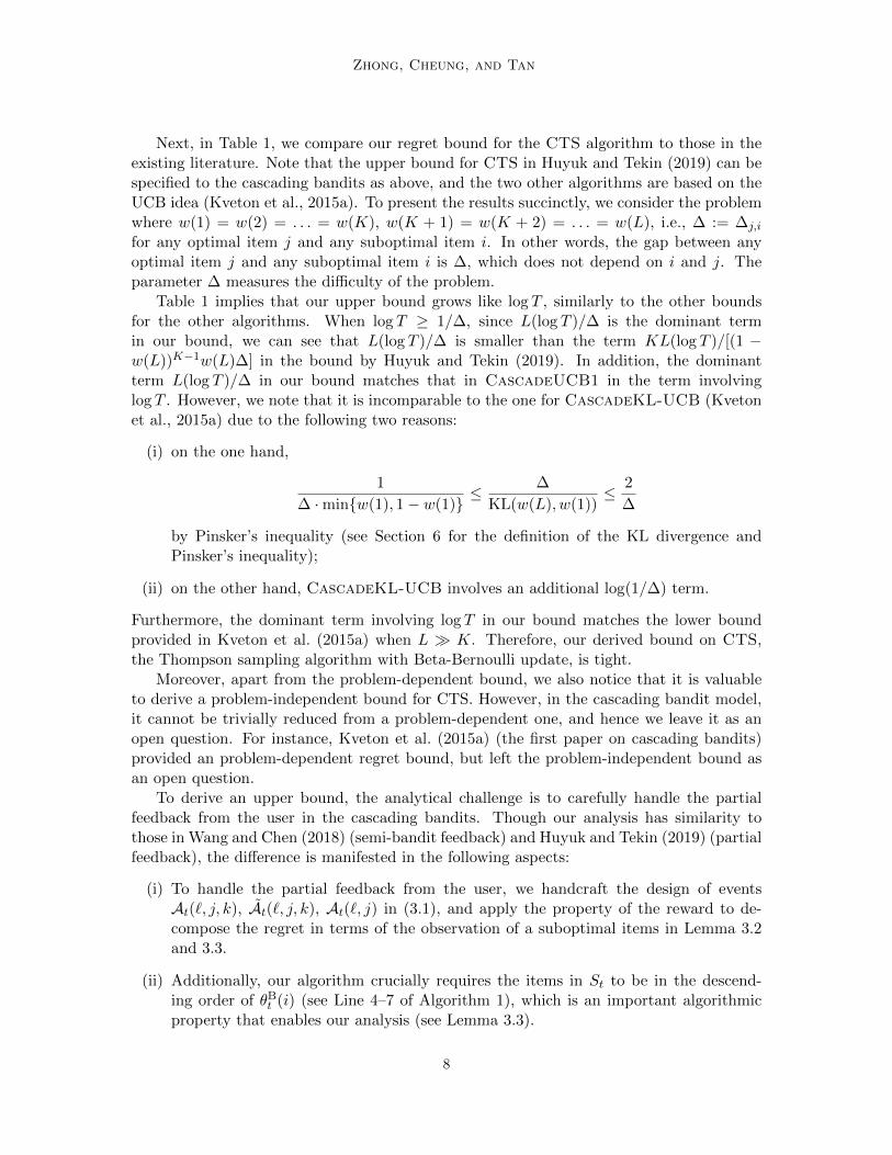
Zhong Cheung and Tan
Next in Table 1 we compare our regret bound for the CTS algorithm to those in theexisting literature Note that the upper bound for CTS in Huyuk and Tekin (2019) can bespecified to the cascading bandits as above and the two other algorithms are based on theUCB idea (Kveton et al 2015a) To present the results succinctly we consider the problemwhere w(1) = w(2) = = w(K) w(K + 1) = w(K + 2) = = w(L) ie ∆ = ∆ji
for any optimal item j and any suboptimal item i In other words the gap between anyoptimal item j and any suboptimal item i is ∆ which does not depend on i and j Theparameter ∆ measures the difficulty of the problem
Table 1 implies that our upper bound grows like log T similarly to the other boundsfor the other algorithms When log T ge 1∆ since L(log T )∆ is the dominant termin our bound we can see that L(log T )∆ is smaller than the term KL(log T )[(1 minusw(L))Kminus1w(L)∆] in the bound by Huyuk and Tekin (2019) In addition the dominantterm L(log T )∆ in our bound matches that in CascadeUCB1 in the term involvinglog T However we note that it is incomparable to the one for CascadeKL-UCB (Kvetonet al 2015a) due to the following two reasons
(i) on the one hand
1
∆ middotminw(1) 1minus w(1)le ∆
KL(w(L) w(1))le 2
∆
by Pinskerrsquos inequality (see Section 6 for the definition of the KL divergence andPinskerrsquos inequality)
(ii) on the other hand CascadeKL-UCB involves an additional log(1∆) term
Furthermore the dominant term involving log T in our bound matches the lower boundprovided in Kveton et al (2015a) when L K Therefore our derived bound on CTSthe Thompson sampling algorithm with Beta-Bernoulli update is tight
Moreover apart from the problem-dependent bound we also notice that it is valuableto derive a problem-independent bound for CTS However in the cascading bandit modelit cannot be trivially reduced from a problem-dependent one and hence we leave it as anopen question For instance Kveton et al (2015a) (the first paper on cascading bandits)provided an problem-dependent regret bound but left the problem-independent bound asan open question
To derive an upper bound the analytical challenge is to carefully handle the partialfeedback from the user in the cascading bandits Though our analysis has similarity tothose in Wang and Chen (2018) (semi-bandit feedback) and Huyuk and Tekin (2019) (partialfeedback) the difference is manifested in the following aspects
(i) To handle the partial feedback from the user we handcraft the design of eventsAt(` j k) At(` j k) At(` j) in (31) and apply the property of the reward to de-compose the regret in terms of the observation of a suboptimal items in Lemma 32and 33
(ii) Additionally our algorithm crucially requires the items in St to be in the descend-ing order of θBt (i) (see Line 4ndash7 of Algorithm 1) which is an important algorithmicproperty that enables our analysis (see Lemma 33)
8
Thompson Sampling Algorithms for Cascading Bandits
Our analytical framework which judiciously takes into the impact of partial feedback issubstantially different from Wang and Chen (2018) which assume semi-feedback and do notface the challenge of partial feedback Besides since Huyuk and Tekin (2019) consider a lessspecific problem setting they define more complicated events than in (31) to decompose theregret Moreover we carefully apply the mechanism of CTS algorithm to derive Lemma 33which leads to a tight bound on the regret Overall our concise analysis fully utilizes theproperties of cascading bandits and Algorithm 1
Now we outline the proof of Theorem 31 some details are deferred to Appendix CNote that a pull of any suboptimal item contributes to the loss of expected instantaneousreward Meanwhile we choose St according to the Thompson samples θBt (i) instead of theunknown click probability w(i) We expect that as time progresses the empirical meanwt(i) will approach w(i) and the Thompson sample θBt (i) which is drawn from Bern(θBt (i))will concentrate around w(i) with high probability In addition this probability dependsheavily on the number of observations of the item Therefore the number of observationsof each item affects the distribution of the Thompson samples and hence also affects theinstantaneous rewards Inspired by this observation we decompose the the regret in termsof the number of observations of the suboptimal items in the chain of equations including(35) to follow
We first define πt as follows For any k if the k-th item in St is optimal we placethis item at position k πt(k) = itk The remaining optimal items are positioned arbitrarilySince Slowast is optimal with respect to w w(itk) le w(πt(k)) for all k Similarly since St isoptimal with respect to θBt θBt (itk) ge θBt (πt(k)) for all k
Next for any optimal item j and suboptimal item ` index 1 le k le K time step twe say At(` j k) holds when suboptimal item ` is the k-th item to pull optimal item j isnot to be pulled and πt places j at position k We say At(` j k) holds when At(` j k)holds and item ` is observed Additionally At(` j) is the union set of events At(` j k) fork = 1 K We can also write these events as follows
At(` j k) =itk = ` πt(k) = j
At(` j k) =itk = ` πt(k) = jWt(i
t1) = = Wt(i
tkminus1) = 0
=itk = ` πt(k) = jObserve Wt(`) at t
At(` j) =K⋃k=1
At(` j k) =exist1 le k le K st itk = ` πt(k) = jObserve Wt(`) at t
(31)
Then we have
r(Slowast|w)minus r(St|w)
= r(πt(1) πt(K)|w)minus r(St|w) (32)
=
Ksumk=1
[kminus1prodm=1
[1minus w(itm))
]middot [w(πt(k))minus w(itk)] middot
[Kprod
n=k+1
(1minus w(πt(n))]
](33)
leKsumk=1
[kminus1prodm=1
(1minus w(itm))
]middot [w(πt(k))minus w(itk)]
9
Zhong Cheung and Tan
leKsumk=1
Ksumj=1
Lsum`=K+1
E
[[ kminus1prodm=1
(1minus w(itm))]middot [w(πt(k))minus w(itk)] | At(` j k)
]middot E [1 At(` j k)]
=Ksumj=1
Lsum`=K+1
Ksumk=1
∆j` middot E[1Wt(i
t1) = = Wt(i
tkminus1) = 0
|At(` j k)
]middot E [1 At(` j k)]
=
Ksumj=1
Lsum`=K+1
∆j` middotKsumk=1
E[1At(` j k)
]
=Ksumj=1
Lsum`=K+1
∆j` middot E [1 At(` j)]
Line (32) results from the fact that any permutation of 1 K maximizes the expectedreward and (πt(1) πt(K)) is one permutation of 1 K Line (33) applies theproperty of the reward (Lemma C4) The subsequent ones follow from the various eventsdefined in (31)
Let NB(i j) denote the number of time steps that At(i j) happens for optimal item jand suboptimal item i within the whole horizon then
NB(i j) =
Tsumt=1
E [1 At(i j)] (34)
Reg(T ) = T middot r(Slowast|w)minusTsumt=1
r(St|w) leKsumj=1
Lsumi=K+1
∆ji middot E[NB(i j)] (35)
We use
wt(i) =αBt (i)minus 1
αBt (i) + βBt (i)minus 2
=
sumtminus1τ=1 1item i is observed at time step τsumtminus1τ=1 1item i is pulled at time step τ
(36)
to denote the empirical mean of item i up to and including time step tminus 1 To bound theexpectation of NB(i j) we define two more events taking into account the concentration ofThompson sample θBt (i) and empirical mean wt(i)
Bt(i) = wt(i) gt w(i) + εi Ct(i j) =θBt (i) gt w(j)minus εj
1 le j le K lt i le L
with
εi =1
2middot(
∆K+1i +∆KK+1
2
) εj =
1
2middot(
∆jK +∆KK+1
2
) 1 le j le K lt i le L
Then εi ge ∆Ki4 εj ge ∆jK+14 εi + εj = ∆ji2 and we have
E[NB(i j)
]= E
[Tsumt=1
1 [At(i j)]
]
le E
[Tsumt=1
1 [At(i j) and Bt(i)]
]+ E
[Tsumt=1
1 [At(i j) and notBt(i) and Ct(i j)]
]
+ E
[Tsumt=1
1 [At(i j) and notCt(i j)]
] (37)
10
Thompson Sampling Algorithms for Cascading Bandits
Subsequently we bound the three terms in (37) separately Since we need to count thenumber of observations of items in the subsequent analysis we also use Nt(i) to denote oneplus the number of observations of item i before time t (consistent with other sections)
The first term We first derive a lemma which facilitates us to bound the probabilitythe event At(i j) and Bt(i)
Lemma 32 For any suboptimal item K lt i le L
E
[Tsumt=1
1[i isin St |wt(i)minus w(i)| gt εiObserve Wt(i) at t ]
]le 1 +
1
ε2i
Next summing over all possible pairs (i j) and then applying Lemma 32 the regretincurred by the first term can be bounded as follows
Ksumj=1
Lsumi=K+1
∆ji middot E
[Tsumt=1
1 [At(i j) and Bt(i)]
]
leLsum
i=K+1
E
Tsumt=1
Ksumj=1
1 [At(i j) and Bt(i)]
le
Lsumi=K+1
E
[Tsumt=1
1 [Bt(i)Observe Wt(i) at t]
]
leLsum
i=K+1
E
[Tsumt=1
1[i isin St |wt(i)minus w(i)| gt εiObserve Wt(i) at t ]
]
le LminusK +Lsum
i=K+1
1
ε2ile LminusK +
Lsumi=K+1
16
∆2Ki
(38)
The second term Considering the occurrence of At(i j)andnotBt(i)andCt(i j) we boundthe regret incurred by the second term as follows (see Appendix C2 for details)
Lsumi=K+1
Ksumj=1
∆ji middot E
[Tsumt=1
1 [At(i j) and notBt(i) and Ct(i j)]
]le
Lsumi=K+1
16 log T
∆Ki+
Lsumi=K+1
Ksumj=1
∆ji
(39)
The third term We use θB(minusi) to denote the vector θB without the i-th elementθB(i) For any optimal item j let Wij be the set of all possible values of θB satisfying thatAij(t) and notCt(i j) happens for some i and Wiminusj =
θB(minusj) θB isinWij
We now state
Lemma 33 whose proof depends on a delicate design of Algorithm 1 to pull items in theirdescending order of Thompson samples θBt (i)
Lemma 33 For any optimal item 1 le j le K we have
E
[Tsumt=1
Pr[existi st θBt isinWij Observe Wt(i) at t |Ftminus1
]]le c middot
(1[εj lt 116]
ε3j+
log T
ε2j
)
where c is a constant which does not depend on the problem instance
11
Zhong Cheung and Tan
Recalling the definition of Wij we bound the regret incurred by the third term
Lsumi=K+1
Ksumj=1
∆ji middot E
[Tsumt=1
1 [At(i j) and notCt(i j)]
]
leKsumj=1
∆jL middot E
[Tsumt=1
Lsumi=K+1
1 [At(i j) and notCt(i j)]
]
=Ksumj=1
∆jL middot E
[Tsumt=1
Lsumi=K+1
1[θBt isinWij Observe Wt(i) at t
]]
=
Ksumj=1
∆jL middot E
[Tsumt=1
1[existi st θBt isinWij Observe Wt(i) at t
]]
le c middotKsumj=1
∆jL middot(1[εj lt 116]
ε3j+
log T
ε2j
)le α2 middot
Ksumj=1
∆jL middot(1[∆jK+1 lt 14]
∆3jK+1
+log T
∆2jK+1
)(310)
with α2 = 64c (a constant which does not depend on the problem instance)Summation of all the terms Overall we derive an upper bound on the total regret
Reg(T ) le LminusK +Lsum
i=K+1
16
∆2Ki
+Lsum
i=K+1
16 log T
∆Ki+
Lsumi=K+1
Ksumj=1
∆ji
+ α2 middotKsumj=1
∆jL
(1[∆jK+1lt
14
]∆3jK+1
+log T
∆2jK+1
)
le LminusK + 16 middotLsum
i=K+1
(1
∆2Ki
+log T
∆Ki
)+
Lsumi=K+1
Ksumj=1
∆ji
+ α2 middotKsumj=1
∆jL
(1[∆jK+1lt
14
]∆3jK+1
+log T
∆2jK+1
)
The previous upper bound on the regret of the CTS algorithm in Theorem 31 isproblem-dependent ie it depends on the gaps ∆ijij We now present a problem-independent bound on the regret of CTS
Theorem 34 (Problem-independent bound for CTS) Assume that w(1) = w(2) = = w(K) Algorithm CTS incurs an expected regret at most
O(KT 34 + LradicT +K
radicT log T )
where the big O notation hides a constant factor that is independent of KL Tw
We remark that if all variables other than T are kept fixed the expected regret then scalesas O(KT 34) The proof of Theorem 34 can be found in Appendix C4
12
Thompson Sampling Algorithms for Cascading Bandits
Theorem 34 is established by following a case analysis on whether ∆1i le ε or ∆1i gt εfor each suboptimal item i and then tuning the parameter ε to optimize the bound Thecase analysis is in a similar vein to the reduction from problem-dependent regret bounds toproblem-independent regret bounds in the classical stochastic MAB literature (for examplesee Theorem 6 in Kveton et al (2015b)) While this reduction approach does not yield anoptimal bound in terms of T in the subsequent section we study a Thompson sampling-likealgorithm TS-Cascade which enjoys a regret bound that scales with T as
radicT In addition
TS-Cascade also naturally generalizes to a linear contextual setting
4 The TS-Cascade Algorithm
The CTS algorithm cannot be applied directly to the linear generalization setting sincethe Beta-Bernoullli update is incompatible with the linear generalization model on the clickprobabilities (see detailed discussions after Lemma 44 for an explanation) Therefore wepropose a Thompson sampling-like algorithm In the rest of the paper we call our algorithmTS-Cascade with a slight abuse of terminology as we acknowledge that it is not a bonafide Thompson sampling algorithm that is based on prior posterior updates Instead of theBeta distribution TS-Cascade designs appropriate Thompson samples that are Gaussiandistributed and uses these in the posterior sampling steps We design a variation of TS-Cascade for the linear setting in Section 5
Our algorithm TS-Cascade is presented in Algorithm 2 Intuitively to minimize theexpected cumulative regret the agent aims to learn the true weight w(i) of each itemi isin [L] by exploring the space to identify Slowast (ie exploitation) after a hopefully smallnumber of steps In our algorithm we approximate the true weight w(i) of each item iwith a Bayesian statistic θt(i) at each time step t This statistic is known as the Thompsonsample To do so first we sample a one-dimensional standard Gaussian Zt sim N (0 1) definethe empirical variance νt(i) = wt(i)(1 minus wt(i)) of each item and calculate θt(i) Secondlywe select St = (it1 i
t2 i
tK) such that θt(i
t1) ge θt(i
t2) ge ge θt(i
tK) ge maxj 6isinSt θt(j) this
is reflected in Line 10 of Algorithm 2 Finally we update the parameters for each observeditem i in a standard manner by applying Bayes rule on the mean of the Gaussian (withconjugate prior being another Gaussian) in Line 14The algorithm results in the followingtheoretical guarantee
Theorem 41 (Problem-independent) Consider the cascading bandit problem Algo-rithm TS-Cascade presented in Algorithm 2 incurs an expected regret at most
O(radicKLT log T + L log52 T )
In practical applications T L and so the regret bound is essentially O(radicKLT )
Besides we note that in problem-independent bounds for TS-based algorithms the impliedconstants in the O(middot)-notation are usually large (see Agrawal and Goyal (2013b 2017b))These large constants result from the anti-concentration bounds used in the analysis Inthis work we mainly aim to show the dependence of regret on T similarly to other paperson Thompson Sampling in which constants are not explicitly shown Hence in the spiritof those papers on Thompson Sampling we made no further attempt to optimize for thebest constants in our regret bounds Nevertheless we show via experiment that in practice
13
Zhong Cheung and Tan
Algorithm 2 TS-Cascade Thompson Sampling for Cascading Bandits with GaussianUpdate
1 Initialize w1(i) = 0 N1(i) = 0 for all i isin [L]2 for t = 1 2 do3 Sample a 1-dimensional random variable Zt sim N (0 1)4 for i isin [L] do5 Calculate the empirical variance νt(i) = wt(i)(1minus wt(i))6 Calculate standard deviation of the Thompson sample
σt(i) = max
radicνt(i) log(t+ 1)
Nt(i) + 1log(t+ 1)
Nt(i) + 1
7 Construct the Thompson sample θt(i) = wt(i) + Ztσt(i)8 end for9 for k isin [K] do
10 Extract itk isin argmaxiisin[L]it1itkminus1θt(i)
11 end for12 Pull arm St = (it1 i
t2 i
tK)
13 Observe click kt isin 1 Kinfin14 For each i isin [L] if Wt(i) is observed define wt+1(i) = Nt(i)wt(i)+Wt(i)
Nt(i)+1 and Nt+1(i) =
Nt(i) + 1 Otherwise (if Wt(i) is not observed) wt+1(i) = wt(i) Nt+1(i) = Nt(i)15 end for
TS-Cascadersquos empirical performance outperforms what the finite-time bounds (with largeconstants) suggest We elaborate on the main features of the algorithm and the guarantee
In a nutshell TS-Cascade is a Thompson sampling algorithm (Thompson 1933) basedon prior-posterior updates on Gaussian random variables with refined variances The use ofthe Gaussians is useful since it allows us to readily generalize the algorithm and analyses tothe contextual setting (Li et al 2010 2016) as well as the linear bandit setting (Zong et al2016) for handling a large L We consider the linear setting in Section 5 and plan to studythe contextual setting in the future To this end we remark that the posterior update of TScan be done in a variety of ways While the use of a Beta-Bernoulli update to maintain aBayesian estimate on w(i) is a natural option (Russo et al 2018) we use Gaussians insteadwhich is in part inspired by Zong et al (2016) this is for ease of generalization to the linearbandit setting Indeed the conjugate prior-posterior update is not the only choice for TSalgorithms for complex multi-armed bandit problems For example the posterior updatein Algorithm 2 in Agrawal et al (2017) for the multinomial logit bandit problem is notconjugate
While the use of Gaussians is useful for generalizations the analysis of Gaussian Thomp-son samples in the cascading setting comes with some difficulties as θt(i) is not in [0 1]with probability one We perform a truncation of the Gaussian Thompson sample in theproof of Lemma 45 to show that this replacement of the Beta by the Gaussian does notincur any significant loss in terms of the regret and the analysis is not affected significantly
14
Thompson Sampling Algorithms for Cascading Bandits
We elaborate on the refined variances of our Bayesian estimates Lines 5ndash7 indicatethat the Thompson sample θt(i) is constructed to be a Gaussian random variable withmean wt(i) and variance being the maximum of νt(i) log(t + 1)(Nt(i) + 1) and [log(t +1)(Nt(i) + 1)]2 Note that νt(i) is the variance of a Bernoulli distribution with mean wt(i)In Thompson sampling algorithms the choice of the variance is of crucial importance Weconsidered a naıve TS implementation initially However the theoretical and empiricalresults were unsatisfactory due in part to the large variance of the Thompson samplevariance this motivated us to improve on the algorithm leading to Algorithm 2 Thereason why we choose the variance in this manner is to (i) make the Bayesian estimatesbehave like Bernoulli random variables and to (ii) ensure that it is tuned so that the regretbound has a dependence on
radicK (see Lemma 44) and does not depend on any pre-set
parameters We utilize a key result by Audibert et al (2009) concerning the analysisof using the empirical variance in multi-arm bandit problems to achieve (i) In essence inLemma 44 the Thompson sample is shown to depend only on a single source of randomnessie the Gaussian random variable Zt (Line 3 of Algorithm 2) This shaves off a factor ofradicK vis-a-vis a more naıve analysis where the variance is pre-set in the relevant probability
in Lemma 44 depends on K independent random variables In detail if instead of Line 3ndash7in Algorithm 2 we sample independent Thompson samples as follows
θt(i) sim N(wt(i)
K log(t+ 1)
Nt(i) + 1
)foralli isin [L]
a similar analysis to our proof of Theorem 41 leads to an upper bound O(KradicLT log T )
which isradicK worse than the upper bound for TS-Cascade Hence we choose to design
our Thompson samples based on a single one-dimensional Gaussian random variable Zt
Table 2 Problem-independent upper bounds on the T -regret of CTS TS-Cascade andCUCB the problem-independent lower bound apply to all algorithms for thecascading bandit model
AlgorithmSetting Reference Bounds
CTS () Theorem 34 O(KT 34)
TS-Cascade Theorem 41 O(radicKLT log T + L log52 T )
CUCB Wang and Chen (2017) O(radic
KLT log T)
Cascading Bandits Theorem 61 Ω(radic
LTK)
(Lower Bd)
Next in Table 2 we present various problem-independent bounds on the regret forcascading bandits The () in Table 2 indicates that our bound for CTS in Theorem 34 isderived for a special instance in which all the optimal items have the same click probabilityie w(1) = w(2) = = w(K) while the remaining bounds are for any general cascadingbandit instances We observe that the bound for CTS is larger than the remaining boundsin the term involving T by a factor of approximately 4
radicT While we believe that it is
possible to establish a tighter problem-independent bound for CTS the derivation could
15
Zhong Cheung and Tan
potentially involve analysis significant from the proof of CTS in Theorems 31 and 34 Weleave the possible refinement as an interesting future direction Subsequently we focus oncomparing the remaining bounds Table 2 shows that our upper bound for TS-Cascadegrows like
radicT just like the other bounds Our bound for TS-Cascade also matches the
state-of-the-art UCB bound (up to log factors) by Wang and Chen (2017) whose algorithmwhen suitably specialized to the cascading bandit setting is the same as CascadeUCB1in Kveton et al (2015a) For the case in which T ge L our bound for TS-Cascade is aradic
log T factor worse than the problem-independent bound in Wang and Chen (2017) butwe are the first to analyze Thompson sampling for the cascading bandit problem
Moreover Table 2 shows that the major difference between the upper bound in Theo-rem 41 and the lower bound in Theorem 61 is manifested in their dependence on K (thelength of recommendation list) (i) On one hand when K is larger the agent needs tolearn more optimal items However instead of the full feedback in the semi-bandit settingthe agent only gets partial feedback in the cascading bandit setting and therefore he is notguaranteed to observe more items at each time step Therefore a larger K may lead to alarger regret (ii) On the other hand when K is smaller the maximum possible amountof observations that the agent can obtain at each time step diminishes Hence the agentmay obtain less information from the user which may also result in a larger regret Intu-itively the effect of K on the regret is not clear We leave the exact dependence of optimalalgorithms on K as an open question
Sequentially we present a proof sketch of Theorem 41 with several lemmas in orderwhen some details are postponed to Appendix C
During the iterations we update wt+1(i) such that it approaches w(i) eventually To doso we select a set St according to the order of θt(i)rsquos at each time step Hence if wt+1(i)θt(i) and w(i) are close enough then we are likely to select the optimal set This motivatesus to define two ldquonice eventsrdquo as follows
Ewt = foralli isin [L] |wt(i)minus w(i)| le gt(i) Eθt = foralli isin [L] |θt(i)minus wt(i)| le ht(i)
where νt(i) is defined in Line 5 of Algorithm 2 and
gt(i) =
radic16νt(i) log(t+ 1)
Nt(i) + 1+
24 log(t+ 1)
Nt(i) + 1 ht(i) =
radiclog(t+ 1)gt(i)
Lemma 42 For each t isin [T ] Ht isin Ewt we have
Pr [Ewt] ge 1minus 3L
(t+ 1)3 Pr [Eθt|Ht] ge 1minus 1
(t+ 1)3
Demonstrating that Ewt has high probability requires the concentration inequality inTheorem B1 this is a specialization of a result in Audibert et al (2009) to Bernoulli randomvariables Demonstrating that Eθt has high probability requires the concentration property
of Gaussian random variables (cf Theorem B2)To start our analysis define
F (S t) =Ksumk=1
kminus1prodj=1
(1minusw(ij))
(gt(ik)+ht(ik)) (41)
16
Thompson Sampling Algorithms for Cascading Bandits
and the the set
St =S = (i1 iK) isin πK(L) F (S t) ge r(Slowast|w)minus r(S|w)
Recall that w(1) ge w(2) ge ge w(L) As such St is non-empty since Slowast = (1 2 K) isinSt
Intuition behind the set St Ideally we expect the user to click an item in St for everytime step t Recall that gt(i) and ht(i) are decreasing in Nt(i) the number of time steps qrsquosin 1 tminus 1 when we get to observe Wq(i) Naively arms in St can be thought of as armsthat ldquolack observationsrdquo while arms in St can be thought of as arms that are ldquoobservedenoughrdquo and are believed to be suboptimal Note that Slowast isin St is a prime example of anarm that is under-observed
To further elaborate gt(i)+ht(i) is the ldquostatistical gaprdquo between the Thompson sampleθt(i) and the latent mean w(i) The gap shrinks with more observations of i To balanceexploration and exploitation for any suboptimal item i isin [L] [K] and any optimal itemk isin [K] we should have gt(i) + ht(i) ge w(k)minusw(i) However this is too much to hope forand it seems that hoping for St isin St to happen would be more viable (See the forthcomingLemma 43)
Further notations In addition to set St we define Ht as the collection of observationsof the agent from the beginning until the end of time t minus 1 More precisely we define
Ht = Sqtminus1q=1 cup (iqkWq(i
qk))minktinfink=1
tminus1q=1 Recall that Sq isin πK(L) is the arm pulled
during time step q and(iqkWq(i
qk))minktinfink=1
is the collection of observed items and theirrespective values during time step q At the start of time step t the agent has observedeverything in Ht and determine the arm St to pull accordingly (see Algorithm 2) Notethat event Ewt is σ(Ht)-measurable For the convenience of discussion we define Hwt =Ht Event Ewt is true in Ht The first statement in Lemma 42 is thus Pr[Ht isin Hwt] ge1minus 3L(t+ 1)3
The performance of Algorithm 2 is analyzed using the following four Lemmas To beginwith Lemma 43 quantifies a set of conditions on microt and θt so that the pulled arm St belongsto St the collection of arms that lack observations and should be explored We recall fromLemma 42 that the events Ewt and Eθt hold with high probability Subsequently we willcrucially use our definition of the Thompson sample θt to argue that inequality (42) holdswith non-vanishing probability when t is sufficiently large
Lemma 43 Consider a time step t Suppose that events Ewt Eθt and inequality
Ksumk=1
kminus1prodj=1
(1minus w(j))
θt(k) geKsumk=1
kminus1prodj=1
(1minus w(j))
w(k) (42)
hold then the event St isin St also holds
In the following we condition on Ht and show that θt is ldquotypicalrdquo wrt w in the senseof (42) Due to the conditioning on Ht the only source of the randomness of the pulledarm St is from the Thompson sample Thus by analyzing a suitably weighted version of theThompson samples in inequality (42) we disentangle the statistical dependence between
17
Zhong Cheung and Tan
partial monitoring and Thompson sampling Recall that θt is normal with σ(Ht)-measurablemean and variance (Lines 5ndash7 in Algorithm 2)
Lemma 44 There exists an absolute constant c isin (0 1) independent of wK L T suchthat for any time step t and any historical observation Ht isin Hwt the following inequalityholds
Prθt
[Eθt and (42) hold | Ht] ge cminus1
(t+ 1)3
Proof We prove the Lemma by setting the absolute constant c to be 1(192radicπe1152) gt 0
For brevity we define α(1) = 1 and α(k) =prodkminus1j=1(1 minus w(j)) for 2 le k le K By the
second part of Lemma 42 we know that Pr[Eθt|Ht] ge 1 minus 1(t + 1)3 so to complete thisproof it suffices to show that Pr[(42) holds|Ht] ge c For this purpose consider
Prθt
[Ksumk=1
α(k)θt(k) geKsumk=1
α(k)w(k)
∣∣∣∣Ht
]
= PrZt
[Ksumk=1
α(k)[wt(k)+Ztσt(k)
]ge
Ksumk=1
α(k)w(k)
∣∣∣∣ Ht
](43)
ge PrZt
[Ksumk=1
α(k) [w(k)minus gt(k)] + Zt middotKsumk=1
α(k)σt(k) geKsumk=1
α(k)w(k)
∣∣∣∣ Ht
](44)
= PrZt
[Zt middot
Ksumk=1
α(k)σt(k) geKsumk=1
α(k)gt(k)
∣∣∣∣ Ht
]
gesumK
k=1 α(k)σt(k)
4radicπ middotsumK
k=1 α(k)gt(k)middot exp
minus1
2
[Ksumk=1
α(k)gt(k)
Ksumk=1
α(k)σt(k)
]2 (45)
ge 1
192radicπe1152
= c (46)
Step (43) is by the definition of θt(i)iisinL in Line 7 in Algorithm 2 It is important tonote that these samples share the same random seed Zt Next Step (44) is by the Lemmaassumption that Ht isin Hwt which means that wt(k) ge wt(k) minus gt(k) for all k isin [K] Step(45) is an application of the anti-concentration inequality of a normal random variable inTheorem B2 as gt(k) ge σt(k) Step (46) is by applying the definition of gt(k) and σt(k)
We would like to highlight an obstacle in deriving a problem-independent bound for theCTS algorithm In the proof of Lemma 44 which is essential in deriving the bound forTS-Cascade step (44) results from the fact that the TS-Cascade algorithm generatesThompson samples with the same random seed Zt at time step t (Line 3 ndash 8 in Algorithm2) However CTS generate samples for each item individually which hinders the derivationof a similar lemma Therefore we conjecture that a problem-independent bound for CTScannot be derived using the same strategy as that for TS-Cascade
18
Thompson Sampling Algorithms for Cascading Bandits
Combining Lemmas 43 and 44 we conclude that there exists an absolute constant csuch that for any time step t and any historical observation Ht isin Hwt
Prθt
[St isin St
∣∣ Ht
]ge cminus 1
(t+ 1)3 (47)
Equipped with (47) we are able to provide an upper bound on the regret of our Thomp-son sampling algorithm at every sufficiently large time step
Lemma 45 Let c be an absolute constant such that Lemma 44 holds Consider a timestep t that satisfies c minus 2(t + 1)3 gt 0 Conditional on an arbitrary but fixed historicalobservation Ht isin Hwt we have
Eθt [r(Slowast|w)minus r(St|w)|Ht] le(
1 +2
c
)Eθt
[F (St t)
∣∣ Ht
]+
L
(t+ 1)3
The proof of Lemma 45 relies crucially on truncating the original Thompson sampleθt isin R to θt isin [0 1]L Under this truncation operation St remains optimal under θt (asit was under θt) and |θt(i) minus w(i)| le |θt(i) minus w(i)| ie the distance from the truncatedThompson sample to the ground truth is not increased
For any t satisfying cminus 2(t+ 1)3 gt 0 define
Fit = Observe Wt(i) at t G(StWt) =Ksumk=1
1(Fitkt
)middot (gt(itk) + ht(i
tk)))
we unravel the upper bound in Lemma 45 to establish the expected regret at time step t
E r(Slowast|w)minus r(St|w) le E [Eθt [r(Slowast|w)minus r(St|w) | Ht] middot 1(Ht isin Hwt)] + E [1(Ht 6isin Hwt)]
le(
1 +2
c
)E[Eθt
[F (St t)
∣∣ Ht
]1(Ht isin Hwt)
]+
1
(t+ 1)3+
3L
(t+ 1)3
le(
1 +2
c
)E [F (St t)] +
4L
(t+ 1)3(48)
=
(1 +
2
c
)E[EWt [G(StWt)
∣∣Ht St]]
+4L
(t+ 1)3
=
(1 +
2
c
)E [G(StWt)] +
4L
(t+ 1)3 (49)
where (48) follows by assuming t is sufficiently large
Lemma 46 For any realization of historical trajectory HT+1 we have
Tsumt=1
G(StWt) le 6radicKLT log T + 144L log52 T
Proof Recall that for each i isin [L] and t isin [T + 1] Nt(i) =sumtminus1
s=1 1(Fis) is the number ofrounds in [t minus 1] when we get to observe the outcome for item i Since G(StWt) involvesgt(i) + ht(i) we first bound this term The definitions of gt(i) and ht(i) yield that
gt(i) + ht(i) le12 log(t+ 1)radicNt(i) + 1
+72 log32(t+ 1)
Nt(i) + 1
19
Zhong Cheung and Tan
Subsequently we decomposesumT
t=1G(StWt) according to its definition For a fixed butarbitrary item i consider the sequence (Ut(i))
Tt=1 = (1 (Fit) middot (gt(i) + ht(i)))
Tt=1 Clearly
Ut(i) 6= 0 if and only if the decision maker observes the realization Wt(i) of item i at t Lett = τ1 lt τ2 lt lt τNT+1
be the time steps when Ut(i) 6= 0 We assert that Nτn(i) = nminus 1for each n Indeed prior to time steps τn item i is observed precisely in the time stepsτ1 τnminus1 Thus we have
Tsumt=1
1 (Fit) middot (gt(i) + ht(i)) =
NT+1(i)sumn=1
(gτn(i) + hτn(i)) leNT+1(i)sumn=1
12 log Tradicn
+72 log32 T
n
(410)
Now we complete the proof as follows
Tsumt=1
Ksumk=1
1(Fitkt
)middot (gt(itk) + ht(i
tk)) =
sumiisin[L]
Tsumt=1
1 (Fit) middot (gt(i) + ht(i))
lesumiisin[L]
NT+1(i)sumn=1
12 log Tradicn
+72 log32 T
nle 6
sumiisin[L]
radicNT+1(i) log T + 72L log32 T (log T + 1)
(411)
le 6
radicLsumiisin[L]
NT+1(i) log T + 72L log32 T (log T + 1) le 6radicKLT log T + 144L log52 T
(412)
where step (411) follows from step (410) the first inequality of step (412) follows from theCauchy-Schwarz inequalityand the second one is because the decision maker can observeat most K items at each time step hence
sumiisin[L]NT+1(i) le KT
Finally we bound the total regret from above by separating the whole horizon into twoparts with time step t0 = d 3
radic2c e We bound the regret for the time steps before t0 by 1
and the regret for time steps after t0 by (49) which holds for all t gt t0
Reg(T ) lelceil
3
radic2
c
rceil+
Tsumt=t0+1
E r(Slowast|w)minus r(St|w)
lelceil
3
radic2
c
rceil+
(1 +
2
c
)E
[Tsumt=1
G(StWt)
]+
Tsumt=t0+1
4L
(t+ 1)3
It is clear that the third term isO(L) and by Lemma 46 the second term isO(radicKLT log T+
L log52 T ) Altogether Theorem 41 is proved
5 Linear generalization
In the standard cascading bandit problem when the number of ground items L is largethe algorithm converges slowly In detail the agent learns each w(i) individually and the
20
Thompson Sampling Algorithms for Cascading Bandits
knowledge in w(i) does not help in the estimation of w(j) for j 6= i To ameliorate thisproblem we consider the linear generalization setting as described in Section 1 Recallthat w(i) = x(i)gtβ where x(i)rsquos are known feature vectors but β is an unknown universalvector Hence the problem reduces to estimating β isin Rd which when d lt L is easierthan estimating the L distinct weights w(i)rsquos in the standard cascading bandit problem
We construct a Thompson Sampling algorithm LinTS-Cascade(λ) to solve the cas-cading bandit problem and provide a theoretical guarantee for this algorithm
Algorithm 3 LinTS-Cascade(λ)
1 Input feature matrix XdtimesL = [x(1)gt x(L)gt] and parameter λ Set R = 122 Initialize b1 = 0dtimes1 M1 = Idtimesd ψ1 = Mminus11 b13 for t = 1 2 do4 Sample a d-dimensional random variable ξt sim N (0dtimes1 Idtimesd)
5 Construct the Thompson sample vt = 3Rradicd log t ρt = ψt + λvt
radicKM
minus12t ξt
6 for k isin [K] do7 Extract itk isin argmaxiisin[L]it1itkminus1
x(i)gtρt
8 end for9 Pull arm St = (it1 i
t2 i
tK)
10 Observe click kt isin 1 Kinfin11 Update Mt Bt and ψt with observed items
Mt+1 = Mt +
minktKsumk=1
x(ik)x(ik)gt bt+1 = bt +
minktKsumk=1
x(ik)Wt(ik)
ψt+1 = Mminus1t+1bt+1
12 end for
Theorem 51 ( Problem-independent bound for LinTS-Cascade) Assuming the l2norms of feature parameters are bounded by 1
radicK ie x(i) le 1
radicK for all i isin [L]1
Algorithm LinTS-Cascade(λ) presented in Algorithm 3 incurs an expected regret at most
O(
minradicdradic
logL middotKdradicT (log T )32
)
Here the big O notation depends only on λ
The upper bound in Theorem 51 grows with g(λ) = (1 + λ) middot (1 + 8radicπe7(2λ
2)) Recallthat for CascadeLinUCB Zong et al (2016) derived an upper bound in the form ofO(Kd
radicT ) and for Thompson sampling applied to linear contextual bandits Agrawal and
Goyal (2013a) proved a high probability regret bound of O(d32radicT ) Our result is a factorradic
d worse than the bound on CascadeLinUCB However our bound matches that of
1 It is realistic to assume that x(i) le 1radicK for all i isin [L] since this can always be ensured by rescaling
the feature vectors If instead we assume that x(i) le 1 as in Gai Wen et al (2015) Zong et al(2016) the result in Lemma 57 will be
radicK worse which would lead to an upper bound larger than the
bound stated in Theorem 51 by a factor ofradicK
21
Zhong Cheung and Tan
Thompson sampling for contextual bandits with K = 1 up to log factors While Zong et al(2016) proposed CascadeLinTS they did not provide accompanying performance analysisof this algorithm Our work fills this gap by analyzing a Thompson sampling algorithm forthe linear cascading bandit setting The tunable parameter σ in CascadeLinTS (Zonget al 2016) plays a role similar to that of λvt
radicK in LinTS-Cascade(λ) However the
key difference is that vt depends on the current time step t which makes it more adaptivecompared to σ which is fixed throughout the horizon As shown in Line 5 of Algorithm 3we apply λ to scale the variance of Thompson samples We see that when the given set offeature vectors are ldquowell-conditionedrdquo ie the set of feature vectors of optimal items andsuboptimal items are far away from each other in the feature space [0 1]d then the agentshould should choose a small λ to stimulate exploitation Otherwise a large λ encouragesmore exploration
Now we provide a proof sketch of Theorem 51 which is similar to that of Theorem 41More details are given in Appendix C
To begin with we observe that a certain noise random variable possesses the sub-Gaussian property (same as Appendix A1 of Filippi et al (2010)) and we assume x(i) isbounded for each i
Remark 52 (Sub-Gaussian property) Define ηt(i) = Wt(i)minusx(i)gtβ and let R = 12The fact that EWt(i) = w(i) = x(i)gtβ and Wt(i) isin [0 1] yields that Eηt(i) = EWt(i)minusw(i) =0 and ηt(i) isin [minusw(i) 1minus w(i)] Hence ηt(i) is 0-mean and R-sub-Guassian ie
E[exp(ληt)|Ftminus1] le exp(λ2R2
2
)forallλ isin R
During the iterations we update ψt+1 such that x(i)gtψt+1 approaches x(i)gtβ eventuallyTo do so we select a set St according to the order of x(i)gtρtrsquos at each time step Henceif x(i)gtψt+1 x(i)gtρt and x(i)gtβ are close enough then we are likely to select the optimalset
Following the same ideas as in the standard case this motivates us to define two ldquoniceeventsrdquo as follows
Eψt =foralli isin [L]
∣∣∣x(i)gtψt minus x(i)gtβ∣∣∣ le gt(i)
Eρt =foralli isin [L]
∣∣∣x(i)gtρt minus x(i)gtψt
∣∣∣ le ht(i) where
vt = 3Rradicd log t lt = R
radic3d log t+ 1 ut(i) =
radicx(i)gtMminus1t x(i)
gt(i) = ltut(i) ht(i) = minradicdradic
logL middotradic
4K log t middot λvtut(i)
Analogously to Lemma 42 Lemma 53 illustrates that Eψt has high probability Thisfollows from the concentration inequality in Theorem B3 and the analysis is similar tothat of Lemma 1 in Agrawal and Goyal (2013a) It also illustrates that Eρt has highprobability which is a direct consequence of the concentration bound in Theorem B2
22
Thompson Sampling Algorithms for Cascading Bandits
Lemma 53 For each t isin [T ] we have
Pr[Eψt
]ge 1minus 1
t2 Pr [Eρt|Ht] ge 1minus d+ 1
t2
Next we revise the definition of F (S t) in equation (41) for the linear generalizationsetting
F (S t) =
Ksumk=1
kminus1prodj=1
(1minusx(ij)gtβ)
(gt(ik) + ht(ik)) (51)
St =S = (i1 iK) isin πK(L) F (S t) ge r(Slowast|w)minus r(S|w)
(52)
Further following the intuition of Lemma 43 and Lemma 44 we state and prove Lemma 54and Lemma 55 respectively These lemmas are similar in spirit to Lemma 43 and Lemma 44except that θt(k) in Lemma 43 is replaced by x(k)gtρt in Lemma 54 when inequality (42)and c in Lemma 44 are replaced by inequality (53) and c(λ) in Lemma 55 respectively
Lemma 54 Consider a time step t Suppose that events Eψt Eρt and inequality
Ksumk=1
kminus1prodj=1
(1minus w(j))
x(k)gtρt geKsumk=1
kminus1prodj=1
(1minus w(j))
w(k) (53)
hold then the event St isin St also holds
Lemma 55 There exists an absolute constant c(λ) = 1(4radicπe72λ
2) isin (0 1) independent
of wKL T such that for any time step t ge 4 and any historical observation Ht isin Hψtthe following inequality holds
Prρt
[Eρt and (53) hold | Ht] ge c(λ)minus d+ 1
t2
Above yields that there exists an absolute constant c(λ) such that for any time step tand any historical observation Ht isin Hψt
Prρt
[St isin St
∣∣ Ht
]ge c(λ)minus d+ 1
t2 (54)
This allows us to upper bound the regret of LinTS-Cascade(λ) at every sufficientlylarge time step The proof of this lemma is similar to that of Lemma 45 except that θt(k)in Lemma 45 is replaced by x(k)gtθt We omit the proof for the sake of simplicity
Lemma 56 Let c(λ) be an absolute constant such that Lemma 55 holds Consider a timestep t that satisfies c(λ) gt 2(d+1)t2 t gt 4 Conditional on an arbitrary but fixed historicalobservation Ht isin Hψt we have
Eρt [r(Slowast|w)minus r(St|w)|Ht] le(
1 +4
c(λ)
)Eρt
[F (St t)
∣∣ Ht
]+d+ 1
t2
23
Zhong Cheung and Tan
For any t satisfyingc(λ) gt 2(d+ 1)t2 t gt 4 recall that
Fit = Observe Wt(i) at t G(StWt) =
Ksumk=1
1(Fitkt
)middot (gt(itk) + ht(i
tk)))
we unravel the upper bound in Lemma 56 to establish the expected regret at time step t
E r(Slowast|w)minus r(St|w) le E[Eρt [r(Slowast|w)minus r(St|w) | Ht] middot 1(Ht isin Hψt)
]+ E
[1(Ht 6isin Hψt)
]le(
1 +2
c(λ)
)E[Eρt
[F (St t)
∣∣ Ht
]1(Ht isin Hψt)
]+d+ 1
t2+
1
t2
(55)
=
(1 +
2
c(λ)
)E [G(StWt)] +
d+ 2
t2 (56)
where step (55) follows by assuming t is sufficiently large
Lemma 57 For any realization of historical trajectory HT+1 we have
Tsumt=1
G(StWt) le 40R(1 + λ) minradicdradic
logL middotKdradicT (log T )32
Note that here similarly to Lemma 46 we prove a worst case bound without needingthe expectation operatorProof Recall that for each i isin [L] and t isin [T + 1] Nt(i) =
sumtminus1s=1 1(Fis) is the number of
rounds in [t minus 1] when we get to observe the outcome for item i Since G(StWt) involvesgt(i) + ht(i) we first bound this term The definitions of gt(i) and ht(i) yield that
gt(i) + ht(i) = ut(i)[lt + minradicdradic
logL middot λradic
4K log t middot vt]
= ut(i)[Rradic
3d log t+ 1 + minradicdradic
logL middot λradic
4K log t middot 3Rradicd log t]
le 8R(1 + λ)ut(i) log tradicdK middotmin
radicdradic
logL
Further we have
Tsumt=1
G(StWt) =Tsumt=1
Ksumk=1
1(Fitkt
)middot [gt(itk) + ht(i
tk)] =
Tsumt=1
ktsumk=1
[gt(itk) + ht(i
tk)]
le 8R(1 + λ) log TradicdK middotmin
radicdradic
logLTsumt=1
ktsumk=1
ut(itk)
Let x(i) = (x1(i) x2(i) xd(i)) yt = (yt1 yt2 ytd) with
ytl =
radicradicradicradic ktsumk=1
xl(itk)
2 foralll = 1 2 d
then Mt+1 = Mt + ytygtt yt le 1
24
Thompson Sampling Algorithms for Cascading Bandits
Now we have
Tsumt=1
radicygtt M
minus1t yt le 5
radicdT log T (57)
which can be derived along the lines of Lemma 3 in Chu et al (2011) using Lemma C5 (seeAppendix C10 for details) Let M(t)minus1mn denote the (mn)th-element of M(t)minus1 Note that
ktsumk=1
ut(itk) =
ktsumk=1
radicx(itk)
gtM(t)minus1x(itk) (58)
le
radicradicradicradickt middotktsumk=1
x(itk)gtM(t)minus1x(itk) (59)
leradicK
radicradicradicradic sum1lemnled
M(t)minus1mn
[ktsumk=1
xm(itk)xn(itk)
]
leradicK
radicradicradicradicradic sum1lemnled
M(t)minus1mn
radicradicradicradic[ ktsumk=1
xm(itk)2
]middot
[ktsumk=1
xn(itk)2
](510)
=radicK
radic sum1lemnled
M(t)minus1mnytmytn =radicK
radicygtt M
minus1t yt
where step (58) follows from the definition of ut(i) (59) and (510) follow from Cauchy-Schwartz inequality
Now we complete the proof as follows
Tsumt=1
G(StWt) le 8R(1 + λ) log TradicdK middotmin
radicdradic
logLTsumt=1
ktsumk=1
ut(itk)
le 8R(1 + λ) log TradicdK middotmin
radicdradic
logL middotTsumt=1
radicK middot
radicygtt M
minus1t yt
le 40R(1 + λ) minradicdradic
logL middotKdradicT (log T )32
Finally we bound the total regret from above by separating the whole horizon into twoparts with time step t(λ) =
lceilradic8(d+ 1)c(λ)
rceil(noting c(λ) gt 2(d + 1)t2 t gt 4 when
t ge t(λ)) We bound the regret for the time steps before t(λ) by 1 and the regret for timesteps after t(λ) by (56) which holds for all t gt t(λ)
Reg(T ) lelceil
2
c(λ)
rceil+
Tsumt=t(λ)+1
E r(Slowast|w)minus r(St|w)
lelceil
2
c(λ)
rceil+
(1 +
2
c(λ)
)E
[Tsumt=1
G(StWt)
]+
Tsumt=t(λ)+1
d+ 2
t2
25
Zhong Cheung and Tan
It is clear that the first term is O(1) and the third term is O(d) and by Lemma 57 thesecond term is O
(min
radicdradic
logL middotKdradicT (log T )32
) Altogether Theorem 51 is proved
6 Lower bound on regret of the standard setting
We derive a problem-independent minimax lower bound on the regret of any algorithmπ (see definition in Section 2) in the standard cascading bandit problem following theexposition in Bubeck et al (2012 Theorem 35)
Theorem 61 (Problem-independent lower bound) The following regret lower boundholds for the cascading bandit problem
infπ
supI
Reg(T π I) = Ω(radic
LTK)
where π denotes an algorithm and I denotes a cascading bandit instance The Ω notationhides a constant factor that is independent of KL Tw
Now we outline the proof of Theorem 61 the accompanying lemmas are proved in Ap-pendix C The theorem is derived probabilistically we construct several difficult instancessuch that the difference between click probabilities of optimal and suboptimal items is sub-tle in each of them and hence the regret of any algorithm must be large when averagedover these distributions
The key difference from the analysis in Bubeck et al (2012) involves (i) the differencebetween instance 0 and instance ` (1 le ` le L) involves different distributions of k items (ii)the partial feedback from the user results in a more delicate analysis of the KL divergencebetween the probability measures of stochastic process Sπt Oπt Tt=1 under instances 0 andinstance ` (1 le ` le L) (see Lemmas 64 and 65)
Notations Before presenting the proof we remind the reader of the definition of theKL divergence (Cover and Thomas 2012) For two probability mass functions PX and PYdefined on the same discrete probability space A
KL(PX PY ) =sumxisinA
PX(x) logPX(x)
PY (x)
denotes the KL divergence between the probability mass functions PX PY (We abbreviateloge as log for simplicity) Lastly when a and b are two real numbers between 0 and 1KL(a b) = KL (Bern(a)Bern(b)) ie KL(a b) denotes the KL divergence between Bern(a)and Bern(b)
First step Construct instances
Definition of instances To begin with we define a class of L+ 1 instances indexed by` = 0 1 L as follows
bull Under instance 0 we have w(0)(i) = 1minusεK for all i isin [L]
bull Under instance ` where 1 le ` le L we have w(`)(i) = 1+εK if i isin ` `+ 1 `+K minus 1
where a = a if 1 le a le L and a = a minus L if L lt a le 2L We have w(`)(i) = 1minusεK if
i isin [L] ` `+ 1 `+K minus 1
26
Thompson Sampling Algorithms for Cascading Bandits
1 2 3 4 5 6
Slowast1
Slowast3
Slowast2
Slowast4
Slowast5
L minus 2 L minus 1 L 1 2
SlowastLminus1
SlowastLminus2
SlowastL
Figure 1 An example of instances with K = 3
where ε isin [0 1] is a small and positive number such that 0 lt (1minus ε)K lt (1 + ε)K lt 14The expected reward of a list S under instance `(0 le ` le L) is
r(S|w(`)) = 1minusprodiisinS
(1minus w(`)(i))
Under instance 0 every list S isin [L](K) is optimal while under instance ` (1 le ` le L)a list S is optimal iff S is an ordered K-set comprised of items ` `+ 1 `+K minus 1Let Slowast` = (` `+ 1 `+K minus 1) be an optimal list under instance ` for ` isin 0 LEvidently it holds that r(Slowast`|w(`)) = 1minus[1minus(1+ε)K]K if ` isin 1 L and r(Slowast0|w(0)) =1minus [1minus (1minus ε)K]K Note that Slowast1 SlowastL lsquouniformly coverrsquo the ground set 1 Lin the sense that each i isin 1 L belongs to exactly K sets among Slowast1 SlowastL InFigure 1 we give an example of Slowast1 Slowast2 SlowastL to illustrate how we construct theseinstances
Notations regarding to a generic online policy π A policy π is said to bedeterministic and non-anticipatory if the list of items Sπt recommended by policy π attime t is completely determined by the observation history Sπs Oπs tminus1s=1 That is π isrepresented as a sequence of functions πtinfint=1 where πt ([L](K)times0 1 K)tminus1 rarr [L](K)and Sπt = πt(S
π1 O
π1 S
πtminus1 O
πtminus1) We represent Oπt as a vector in 0 1 K where 0 1
represents observing no click observing a click and no observation respectively For examplewhen Sπt = (2 1 5 4) and Oπt = (0 0 1 ) items 2 1 5 4 are listed in the displayed orderitems 2 1 are not clicked item 5 is clicked and the response to item 4 is not observed Bythe definition of the cascading model the outcome Oπt = (0 0 1 ) is in general a (possiblyempty) string of 0s followed by a 1 (if the realized reward is 1) and then followed by apossibly empty string of s
Next for any instance ` we lower bound the instantaneous regret of any arm S withthe number of suboptimal items within the arm
Lemma 62 Let ε isin [0 1] integer K satisfy 0 lt (1 minus ε)K lt (1 + ε)K lt 14 Considerinstance ` where 1 le ` le L For any order K-set S we have
r(Slowast`|w(`))minus r(S|w(`)) ge2∣∣S Slowast`∣∣ εe4K
Second step Pinskerrsquos inequality
After constructing the family of instances we consider a fixed but arbitrary non-anticipatorypolicy π and analyze the stochastic process Sπt Oπt Tt=1 For instance ` isin 0 L we
27
Zhong Cheung and Tan
denote P(`)
Sπt Oπt Tt=1as the probability mass function of Sπt Oπt Tt=1 under instance ` and
we denote E(`) as the expectation operator (over random variables related to Sπt Oπt Tt=1)under instance ` Now Lemma 62 directly leads to a fundamental lower bound on theexpected cumulative regret of a policy under an instance ` isin 1 L
E(`)
[Tsumt=1
R(Slowast`|w(`))minusR(Sπt |w(`))
]ge 2ε
e4Kmiddot
sumjisin[L]Slowast`
E(`)
[Tsumt=1
1(j isin Sπt )
] (61)
To proceed we now turn to lower bounding the expectation of the number of times thatsuboptimal items appear in the chosen arms during the entire horizon We apply Pinskerrsquosinequality in this step
Lemma 63 For any non-anticipatory policy π it holds that
1
L
Lsum`=1
sumjisin[L]Slowast`
E(`)
[Tsumt=1
1(j isin Sπt )
]
ge KT
1minus K
Lminus
radicradicradicradic 1
2L
Lsum`=1
KL(P
(0)
Sπt Oπt Tt=1 P
(`)
Sπt Oπt Tt=1
)
Recall that under the null instance 0 each item has click probabilities 1minusεK and the only
difference between instance 0 and instance ` (1 le ` le L) is that the optimal items underinstance ` have click probabilities 1minusε
K under instance 0 but 1+εK under instance ` Since the
difference between optimal and suboptimal items under instance ` is small it is difficultto distinguish the optimal items from suboptimal ones Therefore the set of chosen armsand outcomes under instance ` would be similar to that under the null instance 0 Moreprecisely the distributions of the trajectory Sπt Oπt Tt=1 and that of Sπ`t Oπ`t Tt=1 wouldbe similar which implies that the KL divergence is small and hence the lower bound on theregret would be large This intuitively implies that we have constructed instances that aredifficult to discriminate and hence maximizing the expected regret
Third step chain rule
To lower bound the regret it suffices to bound the average of KL(Sπ0t Oπ0t Tt=1 S
π`t Oπ`t Tt=1
)(over `) from above Observe that the outcome Oπ`t in each time step t must be one of thefollowing K + 1 possibilities
o0 = (1 ) o1 = (0 1 ) oKminus1 = (0 0 1) and oK = (0 0)
We index each possible outcome by the number of zeros (no-clicks) which uniquely defineseach of the possible outcomes and denote O = okKk=0 The set of all possible realization
of each (Sπ`t Oπ`t ) is simply [L](K) timesOWith these notations we decompose the KL divergence according to how time pro-
gresses In detail we apply the chain rule for the KL divergence iteratively (Cover and
Thomas 2012) to decompose KL(Sπ0t Oπ0t Tt=1 S
π`t Oπ`t Tt=1
)into per-time-step KL
divergences
28
Thompson Sampling Algorithms for Cascading Bandits
Lemma 64 For any instance ` where 1 le ` le L
KL(P
(0)
Sπt Oπt Tt=1 P
(`)
Sπt Oπt Tt=1
)=
Tsumt=1
sumstisin[L](K)
P (0)[Sπt = st] middotKL(P
(0)Oπt |Sπt
(middot | st)∥∥∥P (`)
Oπt |Sπt(middot | st)
)
Fourth step conclusion
The design of instances 1 to L implies that the optimal lists cover the whole ground setuniformly and an arbitrary item in the ground set belongs to exactly K of the L op-timal lists This allows us to further upper bound the average of the KL divergence
KL
(P
(0)
Oπ0t |Sπ0t
(middot | st)∥∥∥P (`)
Oπ`t |Sπ`t
(middot | st))
as follows
Lemma 65 For any t isin [T ]
1
L
Lsum`=1
sumstisin[L](K)
P (0)[Sπt = st] middotKL(P
(0)Oπt |Sπt
(middot | st)∥∥∥P (`)
Oπt |Sπt(middot | st)
)le K
L
[(1minus ε) log
(1minus ε1 + ε
)+ (K minus 1 + ε) log
(K minus 1 + ε
K minus 1minus ε
)]
Substituting the results of Lemma 64 and Lemma 65 into inequality (C35) we have
1
L
Lsum`=1
E
[Tsumt=1
R(Slowast`|w(`))minusR(Sπ`t |w(`))
]
ge 2εT
e4
(1minus K
L
)minus
radicradicradicradicradic 1
2L
Tsumt=1
Lsum`=1
sumstisin[L](K)
P (0)[Sπt = st] middotKL(P
(0)Oπt |Sπt
(middot | st)∥∥∥P (`)
Oπt |Sπt(middot | st)
) = Ω
(εT
(1minus K
Lminus εradicTK
2L
))= Ω(
radicLTK)
The first step in the last line follows from the fact that
(1minus ε) log
(1minus ε1 + ε
)+ (K minus 1 + ε) log
(K minus 1 + ε
K minus 1minus ε
)= O(ε2)
when ε is a small positive number and the second step follows from differentiation Alto-gether Theorem 61 is proved
7 Numerical experiments
We evaluate the performance of our proposed algorithms TS-Cascade LinTS-Cascade(λ)analyzed algorithm CTS (Huyuk and Tekin 2019) as well as algorithms in some ex-isting works such as CascadeUCB1 CascadeKL-UCB in Kveton et al (2015a) and
29
Zhong Cheung and Tan
CascadeLinUCB CascadeLinTS RankedLinTS in Zong et al (2016) The pur-pose of this section is not to show that the proposed algorithms mdash which have strongtheoretical guarantees mdash are uniformly the best possible (for all choices of the param-eters) but rather to highlight some features of each algorithm and in which regime(s)which algorithm performs well We believe this empirical study will be useful for prac-titioners in the future The codes to reproduce all the experiments can be found athttpsgithubcomzixinzh2021-JMLRgit
71 Comparison of Performances of TS-Cascade and CTS to UCB-basedAlgorithms for Cascading Bandits
To demonstrate the effectiveness of the TS algorithms TS-Cascade and CTS we com-pare their expected cumulative regrets to CascadeKL-UCB and CascadeUCB1 (Kvetonet al 2015a) Since there are many numerical evaluations of these algorithms in the exist-ing literature (Cheung et al 2019 Huyuk and Tekin 2019) here we only present a briefdiscussion highlighting some salient features
For the L items we set the click probabilities of K of them to be w1 = 02 the proba-bilities of another K of them to be w2 = 01 and the probabilities of the remaining Lminus 2Kitems as w3 = 005 We vary L isin 16 32 64 256 512 1024 2048 and K isin 2 4 Weconduct 20 independent simulations with each algorithm under each setting of L K Wecalculate the averages and standard deviations of Reg(T ) and as well as the average runningtimes of each experiment
Our experiments indicate that the two TS algorithms always outperform the two UCBalgorithms in all settings considered (see Table 4 in Appendix D) and Figure 2 NextCascadeKL-UCB outperforms CascadeUCB1 when L ge 512 while CascadeUCB1 out-performs CascadeKL-UCB otherwise Similarly TS-Cascade outperforms CTS whenL ge 2048 while CTS outperforms TS-Cascade otherwise Thus for a large number ofitems TS-Cascade is preferred to CTS again demonstrating the utility of the Gaussianupdates over the seemingly more natural Bernoulli updates For simplicity we only presenta representative subset of the results in Figure 2 These observations imply that the bestchoice of algorithm depends on L the total number of items in the ground set
72 Performance of LinTS-Cascade(λ) compared to other algorithms for linearcascading bandits
In this subsection we compare Algorithm 3 (LinTS-Cascade(λ)) to other competitors us-ing numerical simulations Note that the three competitors for cascading bandits with lineargeneralization CascadeLinUCB CascadeLinTS RankedLinTS (Zong et al 2016) in-volve tuning parameters (called σ) Thus to be fair to each algorithm we also tune theparameters for each of the algorithms to ensure that the best performances are obtained sothat the comparisons are fair
We now describe how we set up these experiments In real-world applications goodfeatures that are extracted based on a large number of items are rarely obtained directlybut rather learnt from historical data of usersrsquo behaviors (Koren et al 2009) One commonlyused method to obtain the features of items is via low-rank matrix factorization In detaillet Atrain isin 0 1mtimesL be the matrix representing feedback of L items from m users The
30
Thompson Sampling Algorithms for Cascading Bandits
L = 256K = 2 L = 256K = 4
1 2 3 4 5 6 7 8 9 10
104
0
05
1
15
2
25104
1 2 3 4 5 6 7 8 9 10
104
0
05
1
15
2
25
3
35104
L = 2048K = 2 L = 2048K = 4
1 2 3 4 5 6 7 8 9 10
104
0
05
1
15
2
25
3104
1 2 3 4 5 6 7 8 9 10
104
0
05
1
15
2
25
3
35
4
45104
Figure 2 Reg(T ) of algorithms when L isin 256 2048 K isin 2 4 Each line indicates theaverage Reg(T ) (over 20 runs)
(i j)th element of feedback matrix Atrain(i j) = 1 when user i isin [m] is attracted to itemj isin [L] and Atrain(i j) = 0 when user i is not attracted to item j We apply Algorithm 4to learn the features of the items from Atrain
Algorithm 4 Generate feature matrix with historical data (Zong et al 2016)
1 Input historical data matrix Atrain isin 0 1mtimesL feature length d2 Conduct rank-d truncated SVD of Atrain Atrain asymp UmtimesdSdtimesdV gtLtimesd3 Calculate the features of items XdtimesL = SV gt to be used as an input in Algorithm 3
Our experiments reveal that somewhat unsurprisingly the amount of training data hasa noticeable impact on the performances of all algorithms assuming the linear bandit modelIn detail when the amount of training data m is small the feature matrix XdtimesL contains
31
Zhong Cheung and Tan
Table 3 The performances of CascadeUCB1 CascadeLinTS(100) CascadeKL-UCB CTS TS-Cascade RankedLinTS(001) CascadeLinUCB(01) andLinTS-Cascade(001) when L = 2048 K = 4 The first column displays themean and the standard deviation of Reg(T ) and the second column displays theaverage running time in seconds Algorithms which are analyzed in this work arehighlighted in bold
Reg(T ) Running time
CascadeUCB1 401times 104 plusmn 418times 101 557times 101
CascadeLinTS(100) 283times 104 plusmn 206times 103 236times 101
CascadeKL-UCB 300times 104 plusmn 100times 104 547times 101
CTS 167times 104 plusmn 399times 102 125times 102
TS-Cascade 150times 104 plusmn 727times 102 455times 101
RankedLinTS(001) 132times 104 plusmn 503times 103 264times 102
CascadeLinUCB(01) 771times 101 plusmn 257times 102 419times 103
LinTS-Cascade(001) 712times 101 plusmn 229times 102 508times 101
a small amount of noisy information of the latent click probabilities and thus taking intoaccount the paucity of information any algorithm assuming the linear bandit model cannotreliably identify the optimal items and hence suffers from a large (and often linear) regretConversely when m is large Atrain contains a significant amount of information about thelatent click probabilities w(i)Li=1 Thus Algorithm 4 is likely to successfully project theunknown feature vectors x(i)Li=1 sub Rd onto an informative low-dimensional subspace andto learn a linear separator in this subspace to classify the optimal and suboptimal itemsThis enables the algorithms assuming the linear bandit model with a small d to quicklycommit to the optimal set Slowast after small amount of exploration However in real-worldapplications since the historical data is limited we may not get sufficient training data butmay require the algorithm itself to explore the items Hence for this problem setting toillustrate the typical behavior of the algorithms under consideration we set m = 200 sothat the amount of information contained in Atrain is ldquoappropriaterdquo However obviouslyother choices of m will lead to other experimental outcomes but since our objective is tocompare the algorithms for the linear bandit model and not to scrutinize their performancesas functions of m we do not investigate the effect of m any further
To begin with we generate independent Bernoulli random variables with click prob-abilities w1 w2 or w3 for each item to produce the matrix Atrain isin 0 1mtimesL in whichm = 200 Next we vary the tuning parameters for each algorithm under consideration on alogarithmic scale We present the best performance of each algorithm for cascading banditswith linear generalization with tuning parameters in the finite set 001 01 1 10 100
Table 3 displays the means and the standard deviations of Reg(T ) as well as the averagerunning times The algorithms are listed in descending order of the average cumulative
32
Thompson Sampling Algorithms for Cascading Bandits
1 2 3 4 5 6 7 8 9 10
104
0
50
100
150
200
250
300
1 2 3 4 5 6 7 8 9 10
104
0
100
200
300
400
500
600
700
Figure 3 Left Reg(T ) of algorithms when L = 1024 K = 2 d = 3 Right Reg(T )of LinTS-Cascade(004) when L = 1024 K = 2 d isin 1 2 3 4 Each lineindicates the average Reg(T ) (over 20 runs) and the length of each errorbarabove and below each data point is the scaled standard deviation
regrets Note that we set d = 3 for the algorithms based on the linear bandit model Wewill explain this choice later
In the left plot of Figure 3 we present the average cumulative regrets of the algorithmsSince CascadeUCB1 CascadeKL-UCB CTS CascadeLinTS(100) incur much largerregrets compared to the remaining algorithms we omit their regrets in the plot for clarityFor the algorithms assuming the linear bandit model and for this dataset our experimentsindicate that d = 3 is the most appropriate choice For clarity we only display the regretsof the proposed LinTS-Cascade(λ) algorithm as d varies from 1 to 4 in the right plotof Figure 3 Figure 3 is a representative plot for all considered algorithms based on thelinear bandits It can be seen that d = 3 results in the best performance in terms of theexpected cumulative regret ie d = 3 minimizes the average regret among the values ofd considered here Roughly speaking this implies that the optimal and suboptimal itemscan be separated when the data is projected onto a three-dimensional subspace (comparedto subspaces of other dimensions) When d gt 3 the matrix that contains the extractedfeatures XdtimesL overfits to the historical data and due to this overfitting our algorithmmdashas well as other algorithmsmdashincurs a larger regret Hence in our comparison to otheralgorithms for linear bandits we only consider d = 3 features
Among the algorithms designed for linear bandits CascadeLinUCB requires signifi-cantly more time to run (as compared to other algorithms) as suggested by Table 3 whileRankedLinTS lacks theoretical analysis The reason why CascadeLinUCB is less com-
putationally efficient is that x(i)gtMminus12t x(i) needs to be calculated for each item i isin [L]
(the definition of Mt in Zong et al (2016) is slightly different from that in our paper see
Algorithm 2 therein) whereas we only calculate vtradicKM
minus12t ξt once for all items at each
time step t (see Line 5 of Algorithm 3) Our proposed LinTS-Cascade(λ) algorithm isthe only efficient algorithm with theoretical guarantees
33
Zhong Cheung and Tan
For LinTS-Cascade(λ) it is essential to pick an appropriate λ to balance explorationand exploitation Varying λ is equivalent to tuning the variance of the Thompson sam-ples (see Line 5 of Algorithm 3) We note that other algorithms such as CascadeLinUCBand CascadeLinTS (Zong et al 2016) also contain tuning parameters (called σ) andthus our algorithm is similar to these other competing algorithms in this aspect Howeverin Figure 3 we have displayed results in which the hyperparameters of all algorithms aretuned on a logarithmic scale to be fair
Lastly we submit that our LinTS-Cascade(λ) algorithm does not outperform otheralgorithms under all problem settings Indeed the performances of all algorithms basedon the linear bandit model are sensitive to the amount of training data Atrain isin 0 1mtimesL(ie the number of rows m) and the choice of d However it is worth emphasizing thatour proposed algorithm is computationally efficient and possesses appealing (asymptotic)theoretical guarantees cf Theorem 51 Indeed it is the only Thompson sampling algorithmfor linear cascading bandits that admits such theoretical guarantees
8 Summary and Future work
This work presents a comprehensive theoretical analysis of various Thompson samplingalgorithms for cascading bandits under the standard and linear models Firstly we providea tighter upper bound on the regret of CTS compared to Huyuk and Tekin (2019) Secondlythe upper bound on the expected regret of TS-Cascade we derived in Theorem 41 matchesthe state-of-the-art bound based on UCB by Wang and Chen (2017) (which is identical toCascadeUCB1 in Kveton et al (2015a)) Thirdly we propose LinTS-Cascade(λ) for thelinear generalization of the problem and upper bound its regret in Theorem 51 by refiningproof techniques used for TS-Cascade Finally in Theorem 61 we also derive a problem-independent lower bound on the expected cumulative regret using the information-theoretictechnique of Auer et al (2002) as well as a judicious construction of bandit instance Lastlywe also demonstrate the computational efficiency and efficacy in terms of regret of LinTS-Cascade(λ)
In Section 1 we analyze the Thompson sampling algorithm with Beta-Bernoulli updateand provide a tighter bound than Huyuk and Tekin (2019) in the cascading bandit settingOur analysis can be readily generalized to the matroid bandit setting which is also widelyconsidered in current literature as in Kveton et al (2014) Although the CTS algorithmcannot be easily generalized in a straightforward way to a linear cascading bandit setting itmay be a worthy endeavor to extend the other TS-based algorithms (such as TS-Cascade)introduced in this paper to other generalized linear bandit settings (such as logistic bandits)Next since the attractiveness of items in real life may change with time it is reasonable toconsider the cascading bandit model with unknown change points of latent click probabil-ities (Garivier and Moulines 2011) There are practical real-life implications in designingand analyzing algorithms that take into account the non-stationarity of the latent clickprobabilities eg the attractiveness of hotels in a city depending on the season Furtheranother interesting topic within the realm of multi-armed bandit problems concerns bestarm identification (Audibert and Bubeck 2010) In the cascading model since an arm isa list of items the objective here is to minimize the total number of pulls of all arms toidentify items that are ldquoclose tordquo or exactly equal to the optimal ones with high probability
34
Thompson Sampling Algorithms for Cascading Bandits
In the future we plan to design and analyze an algorithm for this purpose assuming thecascading bandit model
Acknowledgements
We thank the reviewers for their meticulous reading and insightful comments This workis partially funded by a National University of Singapore Start-Up Grant (R-266-000-136-133) a Singapore National Research Foundation (NRF) Fellowship (R-263-000-D02-281)and a Singapore Ministry of Education AcRF Tier 1 Grant (R-263-000-E80-114) Thisresearch is also supported by the National Research Foundation Singapore under its AISingapore Programme (AISG Award No AISG2-RP-2020-018) Any opinions findingsand conclusions or recommendations expressed in this material are those of the author(s)and do not reflect the views of National Research Foundation Singapore
References
Yasin Abbasi-Yadkori David Pal and Csaba Szepesvari Improved algorithms for linearstochastic bandits In Proceedings of the 24th Advances in Neural Information ProcessingSystems pages 2312ndash2320 2011
Marc Abeille and Alessandro Lazaric Linear Thompson sampling revisited In Proceedingsof the 20th International Conference on Artificial Intelligence and Statistics pages 176ndash184 2017
Milton Abramowitz and Irene A Stegun Handbook of Mathematical Functions with For-mulas Graphs and Mathematical Tables Dover New York ninth edition 1964
Shipra Agrawal and Navin Goyal Analysis of Thompson sampling for the multi-armedbandit problem In Proceedings of the 25th Annual Conference on Learning Theorypages 391ndash3926 2012
Shipra Agrawal and Navin Goyal Thompson sampling for contextual bandits with lin-ear payoffs In Proceedings of the 30th International Conference on Machine Learningvolume 28 pages 127ndash135 2013a
Shipra Agrawal and Navin Goyal Further optimal regret bounds for Thompson sampling InProceedings of the 16th International Conference on Artificial Intelligence and Statisticspages 99ndash107 2013b
Shipra Agrawal and Navin Goyal Near-optimal regret bounds for Thompson sampling JACM 64(5)301ndash3024 September 2017a
Shipra Agrawal and Navin Goyal Near-optimal regret bounds for Thompson samplingJournal of the ACM (JACM) 64(5)1ndash24 2017b
Shipra Agrawal Vashist Avadhanula Vineet Goyal and Assaf Zeevi Thompson samplingfor the MNL-bandit arXiv preprint arXiv170600977 2017
35
Zhong Cheung and Tan
Venkatachalam Anantharam Pravin Varaiya and Jean Walrand Asymptotically efficientallocation rules for the multiarmed bandit problem with multiple plays-Part I IIDrewards IEEE Transactions on Automatic Control 32(11)968ndash976 November 1987
Jean-Yves Audibert and Sebastien Bubeck Best arm identification in multi-armed banditsIn Proceedings of the 23th Conference on Learning Theory pages 41ndash53 2010
Jean-Yves Audibert Remi Munos and Csaba Szepesvari Explorationndashexploitation tradeoffusing variance estimates in multi-armed bandits Theoretical Computer Science 410(19)1876 ndash 1902 2009 Algorithmic Learning Theory
Peter Auer Nicolo Cesa-Bianchi Yoav Freund and Robert E Schapire The nonstochasticmultiarmed bandit problem SIAM Journal of Computing 32(1)48ndash77 2002
Sebastien Bubeck Nicolo Cesa-Bianchi et al Regret analysis of stochastic and nonstochas-tic multi-armed bandit problems Foundations and Trends Rcopy in Machine Learning 5(1)1ndash122 2012
Olivier Chapelle and Lihong Li An empirical evaluation of Thompson sampling In Proceed-ings of the 24th Advances in Neural Information Processing Systems pages 2249ndash22572011
Wei Chen Yajun Wang and Yang Yuan Combinatorial multi-armed bandit Generalframework and applications In Proceedings of the 30th International Conference onMachine Learning volume 28 of Proceedings of Machine Learning Research pages 151ndash159 2013
Wang Chi Cheung Vincent Tan and Zixin Zhong A Thompson sampling algorithm forcascading bandits In Proceedings of the 22nd International Conference on ArtificialIntelligence and Statistics pages 438ndash447 2019
Wei Chu Lihong Li Lev Reyzin and Robert Schapire Contextual bandits with linear payofffunctions In Proceedings of the 14th International Conference on Artificial Intelligenceand Statistics pages 208ndash214 2011
Richard Combes M Sadegh Talebi Alexandre Proutiere and Marc Lelarge Combina-torial bandits revisited In Proceedings of the 28th International Conference on NeuralInformation Processing Systems - Volume 2 pages 2116ndash2124 2015
Thomas M Cover and Joy A Thomas Elements of information theory John Wiley amp Sons2012
Nick Craswell Onno Zoeter Michael Taylor and Bill Ramsey An experimental comparisonof click position-bias models In Proceedings of the 1st ACM International Conference onWeb Search and Data Mining pages 87ndash94 2008
Sarah Filippi Olivier Cappe Aurelien Garivier and Csaba Szepesvari Parametric banditsThe generalized linear case In Proceedings of the 23rd Advances in Neural InformationProcessing Systems pages 586ndash594 2010
36
Thompson Sampling Algorithms for Cascading Bandits
Yi Gai Bhaskar Krishnamachari and Rahul Jain Learning multiuser channel allocationsin cognitive radio networks A combinatorial multi-armed bandit formulation In 2010IEEE Symposium on New Frontiers in Dynamic Spectrum (DySPAN) pages 1ndash9 2010
Aurelien Garivier and Eric Moulines On upper-confidence bound policies for switchingbandit problems In Proceedings of the 22nd International Conference on AlgorithmicLearning Theory pages 174ndash188 Springer 2011
Aditya Gopalan Shie Mannor and Yishay Mansour Thompson sampling for complex onlineproblems In Proceedings of the 31st International Conference on Machine Learning pages100ndash108 2014
Alihan Huyuk and Cem Tekin Analysis of Thompson sampling for combinatorial multi-armed bandit with probabilistically triggered arms In Proceedings of Machine LearningResearch pages 1322ndash1330 2019
Sumeet Katariya Branislav Kveton Csaba Szepesvari and Zheng Wen DCM banditsLearning to rank with multiple clicks In Proceedings of the 33rd International Conferenceon Machine Learning pages 1215ndash1224 2016
Emilie Kaufmann Nathaniel Korda and Remi Munos Thompson sampling An asymptot-ically optimal finite-time analysis In Proceedings of the 23rd International Conferenceon Algorithmic Learning Theory pages 199ndash213 2012
Junpei Komiyama Junya Honda and Hiroshi Nakagawa Optimal regret analysis of Thomp-son sampling in stochastic multi-armed bandit problem with multiple plays In Proceed-ings of The 32nd International Conference on Machine Learning pages 1152ndash1161 2015
Yehuda Koren Robert Bell and Chris Volinsky Matrix factorization techniques for recom-mender systems Computer (8)30ndash37 2009
Branislav Kveton Zheng Wen Azin Ashkan Hoda Eydgahi and Brian Eriksson Ma-troid bandits Fast combinatorial optimization with learning In Proceedings of the 30thConference on Uncertainty in Artificial Intelligence pages 420ndash429 2014
Branislav Kveton Csaba Szepesvari Zheng Wen and Azin Ashkan Cascading banditsLearning to rank in the cascade model In Proceedings of the 32nd International Confer-ence on Machine Learning pages 767ndash776 2015a
Branislav Kveton Zheng Wen Azin Ashkan and Csaba Szepesvari Tight regret boundsfor stochastic combinatorial semi-bandits In Proceedings of the 18th International Con-ference on Artificial Intelligence and Statistics pages 535ndash543 2015b
Branislav Kveton Zheng Wen Azin Ashkan and Csaba Szepesvari Combinatorial cascad-ing bandits In Proceedings of the 28th International Conference on Neural InformationProcessing Systems pages 1450ndash1458 2015c
Paul Lagree Claire Vernade and Olivier Cappe Multiple-play bandits in the position-basedmodel In Proceedings of the 29th Advances in Neural Information Processing Systemspages 1597ndash1605 Curran Associates Inc 2016
37
Zhong Cheung and Tan
Lihong Li Wei Chu John Langford and Robert E Schapire A contextual-bandit approachto personalized news article recommendation In Proceedings of the 19th InternationalConference on World Wide Web pages 661ndash670 2010
Shuai Li Baoxiang Wang Shengyu Zhang and Wei Chen Contextual combinatorial cas-cading bandits In Proceedings of the 33rd International Conference on Machine Learningpages 1245ndash1253 2016
Lijing Qin Shouyuan Chen and Xiaoyan Zhu Contextual combinatorial bandit and itsapplication on diversified online recommendation In Proceedings of the 14th SIAM In-ternational Conference on Data Mining pages 461ndash469 SIAM 2014
Daniel Russo and Benjamin Van Roy Learning to optimize via posterior sampling Math-ematics of Operations Research 39(4)1221ndash1243 2014
Daniel Russo Benjamin Van Roy Abbas Kazerouni Ian Osband and Zheng Wen Atutorial on Thompson sampling Foundations and Trends in Machine Learning 11(1)1ndash96 2018
William R Thompson On the likelihood that one unknown probability exceeds another inview of the evidence of two samples Biometrika 25(3ndash4)285ndash294 1933
Qinshi Wang and Wei Chen Improving regret bounds for combinatorial semi-bandits withprobabilistically triggered arms and its applications In Proceedings of the 30th Advancesin Neural Information Processing Systems pages 1161ndash1171 2017
Siwei Wang and Wei Chen Thompson sampling for combinatorial semi-bandits In Pro-ceedings of the 35th International Conference on Machine Learning pages 5114ndash51222018
Zheng Wen Branislav Kveton and Azin Ashkan Efficient learning in large-scale combina-torial semi-bandits In Proceedings of the 32nd International Conference on InternationalConference on Machine Learning - Volume 37 pages 1113ndash1122 2015
Masrour Zoghi Tomas Tunys Mohammad Ghavamzadeh Branislav Kveton Csaba Szepes-vari and Zheng Wen Online learning to rank in stochastic click models In Proceedingsof the 34th International Conference on Machine Learning pages 4199ndash4208 2017
Shi Zong Hao Ni Kenny Sung Nan Rosemary Ke Zheng Wen and Branislav KvetonCascading bandits for large-scale recommendation problems In Proceedings of the 32ndConference on Uncertainty in Artificial Intelligence pages 835ndash844 2016
38
Thompson Sampling Algorithms for Cascading Bandits
Appendix A Notations
[L] ground set of size L
w(i) click probability of item i isin [L]
x(i) feature vector of item i in the linear generalization
β common latent vector in the linear generalization
T time horizon
d number of features of any item in the linear generalization
K size of recommendation list
St recommendation list at time t
iti i-th recommended item at time t
[L](K) set of all K-permutations of [L]
Wt(i) reflection of the interest of the user in item t at time t
R(St|w) instantaneous reward of the agent at time t
kt feedback from the user at time t
r(St|w) expected instantaneous reward of the agent at time t
Slowast optimal ordered K-subset for maximizing the expected instan-
taneous reward
Reg(T ) expected cumulative regret
wt(i) empirical mean of item i at time t
Nt(i) number of observations of item i before time t plus 1
Zt 1-dimensional random variable drawn from the standard nor-
mal distribution at time t
νt(i) empirical variance of item i at time t
σt(i) standard deviation of Thompson sample of item i at time t in
TS-Cascade
θt(i) Thompson sample of item i at time t in TS-Cascade
αBt (i) βBt (i) statistics used in CTS
θBt (i) Thompson sample from Beta distribution at time t in CTS
39
Zhong Cheung and Tan
∆ij gap between click probabilities of optimal item i and subopti-
mal item j
∆ = ∆KK+1 minimum gap between click probabilities of optimal and sub-
optimal items
πt a permutation of optimal items used in the analysis of CTS
At(` j k) At(` j k) At(` j) events defined to help decompose the regret of CTS
NB(i j) number of time steps that At(i j) happens for optimal item j
and suboptimal item i within the whole horizon
Bt(i) Ct(i j) events that measure the concentration of θBt (i) wt(i) around
w(i) as CTS processes
θB(minusi)Wij Wiminusj variables used in the analysis of CTS
Ewt Eθt ldquonice eventsrdquo in TS-Cascade
gt(i) ht(i) functions used to define ldquonice eventsrdquo
St ldquounsaturatedrdquo set at time t
F (S t) function used to define ldquounsaturatedrdquo set
α determined by click probabilities w(i)rsquos used in the analysis
Hwt Fit G(StWt) used in the analysis of TS-Cascade
λ parameter in LinTS-Cascade(λ)
X collection of feature vector x(i)rsquos
bt Mt vt statistics used in LinTS-Cascade(λ)
ξt d-dimensional random variable drawn from standard multi-
variate normal distribution at time t in LinTS-Cascade(λ)
ψt empirical mean of latent vector β at time t
ρt Thompson sample at time t in TS-Cascade
ηt(i) random variable in the linear generalization
Eψt Eρt ldquonice eventsrdquo in LinTS-Cascade(λ)
lt ut(i) functions used to define ldquonice eventsrdquo in LinTS-Cascade(λ)
w(`)(i) click probability of item i isin [L] under instance ` (0 le ` le L)
r(St|w(`)) expected instantaneous reward of the agent at time t under
instance `
40
Thompson Sampling Algorithms for Cascading Bandits
Slowast` optimal ordered K-subset under instance `
π deterministic and non-anticipatory policy
Sπ(`)t recommendation list at time t (under instance `) by policy π
Oπ(`)t stochastic outcome by pulling S
π(`)t at time t (under instance
`) by policy π
A feedback matrix extracted from real data
yt Qt ζt σt variables used in the analysis of LinTS-Cascade(λ)
Q Jπ`t Υ`t(S) variables used in the analysis of the lower bound
Appendix B Useful theorems
Here are some basic facts from the literature that we will use
Theorem B1 (Audibert et al (2009) specialized to Bernoulli random variables)Consider N independently and identically distributed Bernoulli random variables Y1 YN isin0 1 which have the common mean m = E[Y1] In addition consider their sample meanξ and their sample variance V
ξ =1
N
Nsumi=1
Yi V =1
N
Nsumi=1
(Yi minus ξ)2 = ξ(1minus ξ)
For any δ isin (0 1) the following inequality holds
Pr
∣∣∣ξ minusm∣∣∣ leradic
2V log(1δ)
N+
3 log(1δ)
N
ge 1minus 3δ
Theorem B2 (Abramowitz and Stegun (1964) Formula 7113) Let Z sim N (micro σ2)The following inequalities hold
1
2radicπ
exp
(minus7z2
2
)le Pr (|Z minus micro| gt zσ) le exp
(minusz
2
2
)forallz gt 0
1
2radicπz
exp
(minusz
2
2
)le Pr (|Z minus micro| gt zσ) le
radic2radicπz
exp
(minusz
2
2
)forallz ge 1
Theorem B3 (Abbasi-Yadkori et al 2011 Agrawal and Goyal 2013a) Let (F primet t ge 0) bea filtration (mt t ge 1) be an Rd-valued stochastic process such that mt is (F primetminus1)-measurable(ηt t ge 1) be a real-valued martingale difference process such that ηt is (F primet)-measurable Fort ge 0 define ξt =
sumtτ=1mτητ and Mt = Id +
sumTτ=1mτm
gtτ where Id is the d-dimensional
identity matrix Assume ηt is conditionally R-sub-GaussianThen for any δprime gt 0 t ge 0 with probability at least 1minus δprime
ξtMminus1tle R
radicd log
( t+ 1
δprime)
where ξMminus1t
=radicξgtt M
minus1t ξt
41
Zhong Cheung and Tan
Appendix C Proofs of main results
In this Section we provide proofs of Lemmas 32 33 Theorem 34 Lemmas 42 43 45 63 64 65as well as derivations of inequalities (39) and (57)
C1 Proof of Lemma 32
Proof We let τ1 τ2 be the time slots such that i isin S(t) and Wt(i) is observed defineτ0 = 0 and abbreviate εi as ε for simplicity Then
E [ existt 1 le t le T i isin St |wt(i)minus w(i)| gt εObserve Wt(i) at t ]
= E
[Tsumt=1
1 [i isin St |wt(i)minus w(i)| gt εObserve Wt(i) at t]
]
le E
[Tsums=0
E
[τs+1minus1sumt=τs
1 [i isin St |wt(i)minus w(i)| gt εObserve Wt(i) at t]
]]
le E
[Tsums=0
Pr [wt(i)minus w(i)| gt εNt(i) = s]
]
le 1 +Tsums=1
Pr [|wt(i)minus w(i)| gt εNt(i) = s]
le 1 +Tsums=1
exp [minuswKL (w(i) + ε w(i))] +Tsums=1
exp [minuswKL (w(i)minus ε w(i))]
le 1 +
infinsums=1
exp [minusKL (w(i) + ε w(i))])s +
infinsumw=1
exp [minusKL (w(i)minus ε w(i))]s
le 1 +exp [minusKL (w(i) + ε w(i) )]
1minus exp [minusKL (w(i) + ε w(i))]+
exp [minusKL (w(i)minus ε w(i))]
1minus exp [minusKL (w(i)minus ε w(i))]
le 1 +1
KL (w(i) + ε w(i))+
1
KL (w(i)minus ε w(i))
le 1 +1
ε2
42
Thompson Sampling Algorithms for Cascading Bandits
C2 Upper bound on the regret incurred by the second term of (37) inSection 3
To derive the inequality (39) for any 0 lt ε lt ∆KK+12
Lsumi=K+1
Ksumj=1
∆ji middot E
[Tsumt=1
1 [At(i j) and notBt(i) and Ct(i j)]
]
le 4 log T middotLsum
i=K+1
∆Ki minus ε(∆Ki minus 2ε)2
+
Lsumi=K+1
Ksumj=1
∆ji
we use the following result
Lemma C1 (Implied by Wang and Chen (2018) Lemma 4) In Algorithm 1for anybase item i we have the following two inequalities
Pr
[θBi (t)minus wt(i) gt
radic2 log T
Nt(i)
]le 1
T Pr
[wt(i)minus θBi (t) gt
radic2 log T
Nt(i)
]le 1
T
Note that
εi =1
2middot(
∆K+1i +∆KK+1
2
)and εj =
1
2middot(
∆jK +∆KK+1
2
)implies εi + εj = ∆ji2 Let
Mij =2 log T
(∆ji minus εi minus εj)2=
8 log T
∆2ji
then when Nt(i) gt Mij ∆jiminus εiminus εj gtradic
2 log TNt(i)
Thus in expectation the time steps that
At(i j) and notBt(i) and Ct(i j) occurs can be decomposed as follows
E
[Tsumt=1
1 [At(i j) and notBt(i) and Ct(i j)]
]
= E
[Tsumt=1
1 [At(i j) and notBt(i) and Ct(i j) Nt(i) leMij ]
]
+ E
[Tsumt=1
1 [At(i j) and notBt(i) and Ct(i j) Nt(i) gt Mij ]
]
And further
E
[Tsumt=1
1 [At(i j) and notBt(i) and Ct(i j) Nt(i) gt Mij ]
]
le E
[Tsumt=1
1[wt(i) le w(i) + εi θ
Bt (i) gt w(j)minus εj Nt(i) gt Mij Observe Wt(i) at t
]]
43
Zhong Cheung and Tan
le E
[Tsumt=1
1[θBt (i) gt wt(i) + ∆ji minus εi minus εj Nt(i) gt Mij Observe Wt(i) at t
]](C1)
le E
[Tsumt=1
1
[θBt (i) gt wt(i) +
radic2 log T
Nt(i)
]](C2)
le 1
To derive line (C1) we observe that when wt(i) le w(i) + εi θBt (i) gt w(j)minus εj we have
θBt (i) gt w(j)minus εj = w(i) + ∆ji minus εj ge wt(i) + ∆ji minus εi minus εj
Besides line (C2) follows from the definition of Mij Hence
Ksumj=1
∆ji middot E
[Tsumt=1
1 [At(i j) and notBt(i) and Ct(i j)]
]
leKsumj=1
∆ji middot E
[Tsumt=1
1 [At(i j) Nt(i) leMij ]
]︸ ︷︷ ︸
(lowast)
+
Ksumj=1
∆ji
Note that (i) Nt(i) of suboptimal item i increases by one when the event Aijt happens forany optimal item j (ii) the event At(i j) happens for at most one optimal item i at anytime t and (iii) M1i le leMKi Let
Yij =
Tsumt=1
1 [ At(i j) Nt(i) leMij ]
Based on these facts it follows that Yij le Mij almost surely and moreoversumK
j=1 Yij leMKi almost surely Therefore (lowast) can be bounded from above by
max
Ksumj=1
∆jiyij 0 le yij leMij
Ksumi=1
yij leMKj
Since the gaps are decreasing ∆1i ge ∆2i ge ∆Ki the solution to the above problem isylowast1i = M1i y
lowast2i = M2i minusM1i y
lowastKi = MKi minusMKminus1i Therefore the value of (lowast) is
bounded from above by
8 log T
∆1i1
∆21i
+
Ksumj=2
∆ji
(1
∆2ji
minus 1
∆2jminus1i
) Further we use the following result
Lemma C2 (Kveton et al (2014) Lemma 3) Let ∆1 ge ge ∆K be a sequence ofK positive numbers then[
∆11
∆21
+Ksumk=2
∆k
(1
∆2k
minus 1
∆2kminus1
)]le 2
∆K
44
Thompson Sampling Algorithms for Cascading Bandits
Therefore
Ksumj=1
∆ji middot E
[Tsumt=1
1 [At(i j) and notBt(i) and Ct(i j)]
]le 16 log T
∆Ki+
Ksumj=1
∆ji
Lastly the total regret incurred by the second term in equation (37) can be boundedas follows
Lsumi=K+1
Ksumj=1
∆ji middot E
[Tsumt=1
1 [At(i j) and notBt(i) and Ct(i j)]
]le 16 log T middot
Lsumi=K+1
1
∆Ki+
Lsumi=K+1
Ksumj=1
∆ji
C3 Proof of Lemma 33
Proof We abbreviate εj as ε for simplicity By the definition of Wij and Wiminusj θBt isin Wj
yields that there exists i such that θBt (i) le w(j)minus ε θBt (minusj) isinWiminusj thus we can use
E
[Tsumt=1
Pr[existi st θBt (i) le w(j)minus ε θBt (minusj) isinWiminusj Observe Wt(i) at t | Ftminus1
]]
as an upper bound Since θBt isinWj indicates θBt (i) ge θBt (j) we have
Pr[existi st θBt (i) le w(j)minus ε θBt (minusj) isinWiminusj Observe Wt(i) at t | Ftminus1
]le Pr
[existi st θBt (j) le w(j)minus ε θBt (minusj) isinWiminusj Observe Wt(i) at t | Ftminus1
]
Denote the value pjt as Pr[θBt (j) gt w(j)minus ε|Ftminus1
] Notice that according to the cas-
cading model given Ftminus1 the value θBt (j) and the set of values θBt (minusj) are independentBesides note that notCij(t) = θBt (i) le w(j)minus ε holds when θBt (minusj) isinWiminusj If we furtherhave θBt (j) gt w(j)minus ε then j isin St
Observation of fixed i Fix θBt (minusj) isinWiminusj let
bull St = it1 it2 itK itk1 = i when θBt (j) le w(j)minus ε
bull St = it1 it2 itK itk2 = j when θBt (j) changes to θBt(j) such that θBt(j) gt w(j)minusε
Since θBt (iti) ge θBt (it2) ge θBt (it1) ge θBt (it2) ge according to Algorithm 1
θBt(j) gt w(j)minus ε ge θBt (i) = θBt (itk1) ge θBt (itk1+1) ge
Therefore k2 le k1 and itl = itl for 1 le l lt k2 Besides the observation of item i or j isdetermined by θBt (minusj)
With the observation and notation above we have
Pr[θBt (j) le w(j)minus ε θBt (minusj) isinWiminusj Observe Wt(i) at t
∣∣ Ftminus1]= (1minus pjt) middot Pr
[θBt (minusj) isinWiminusj |Ftminus1
]middot Pr
[Observe Wt(i) at t
∣∣ θBt ]= (1minus pjt) middot Pr
[θBt (minusj) isinWiminusj |Ftminus1
]middot E
[k1minus1prodl=1
(1minus w(itl))∣∣ θBt (minusj)
]
45
Zhong Cheung and Tan
and
Pr[j isin St θBt (minusj) isinWiminusj Observe Wt(j) at t|Ftminus1
]ge Pr
[θBt (j) gt w(j)minus ε θBt (minusj) isinWiminusj Observe Wt(j) at t|Ftminus1
]= pjt middot Pr
[θBt (minusj) isinWiminusj |Ftminus1
]middot Pr
[Observe Wt(j) at t
∣∣ θBt (minusj)]
= pjt middot Pr[θBt (minusj) isinWiminusj |Ftminus1
]middot E
[k2minus1prodl=1
(1minus w(itl))∣∣ θBt (minusj)
]
ge pjt middot Pr[θBt (minusj) isinWiminusj |Ftminus1
]middot E
[k1minus1prodl=1
(1minus w(itl))∣∣ θBt (minusj)
]
This leads to
Pr[θBt isinWij Observe Wt(i) at t | Ftminus1
]le (1minus pjt) middot Pr
[θBt (minusj) isinWiminusj
∣∣ Ftminus1] middot E[k1minus1prodl=1
(1minus w(itl))∣∣ θBt (minusj)
]
le 1minus pjtpjt
middot Pr[j isin St θBt (minusj) isinWiminusj Observe Wt(j) at t
∣∣ Ftminus1] Observation in the whole horizon By definition Wij are disjoint sets for different
i Hence
E
[Tsumt=1
Pr[existi st θBt isinWij Observe Wt(i) at t | Ftminus1
]]
=
Lsumi=K+1
E
[Tsumt=1
Pr[θBt isinWij Observe Wt(i) at t | Ftminus1
]]
leTsumt=1
E
[Lsum
i=K+1
E[
1minus pjtpjt
middot Pr[j isin St θBt (minusj) isinWiminusj Observe Wt(j) at t
∣∣ Ftminus1]]]
=Tsumt=1
E[
1minus pjtpjt
middot Pr[existi st j isin St θBt (minusj) isinWiminusj Observe Wt(j) at t
∣∣ Ftminus1]]
leTsumt=1
E[
1minus pjtpjt
middot Pr[j isin StObserve Wt(j) at t
∣∣ Ftminus1]]
=Tsumt=1
E[
1minus pjtpjt
middot 1 [j isin StObserve Wt(j) at t | Ftminus1]]
46
Thompson Sampling Algorithms for Cascading Bandits
Let τjq is the time step that item j is observed for the q-th time Then
E
[Tsumt=1
Pr[existi st θBt isinWij Observe Wt(i) at t | Ftminus1
]]
leTminus1sumq=0
E
1minus pjτjq+1
pjτjq+1
τjq+1sumt=τjq+1
1 [j isin StObserve Wt(j) at t | Ftminus1]
(C3)
=
Tminus1sumq=0
E[
1minus pjτjq+1
pjτjq+1
]
Line (C3) follows from the fact that the probability Pr[θBt (j) gt w(j)minus ε|Ftminus1
]only changes
when we get a feedback of item j but during time steps in [τjq + 1 τjq+1 minus 1] we do nothave any such feedback
Next we apply a variation of Lemma 29 in Agrawal and Goyal (2017b)
Lemma C3 (Implied by Agrawal and Goyal (2017b) Lemma 29) For any j pjtis Pr
[θBt (j) gt w(j)minus ε|Ftminus1
] and τjq is the time step that item j is observed for the q-th
time Then 2
E[
1
pjτjq+1minus 1
]le
3
εif q lt
8
ε
Θ
(eminusε
2q2 +1
(q + 1)ε2eminusDjq +
1
eε2q4 minus 1
)else
where Dj = KL(w(j) w(j)minus ε) = [w(j)minus ε] middot log[w(j)minusεw(j)
]+ [1minus w(j) + ε] middot log
[1minusw(j)+ε1minusw(j)
]
According to Pinskerrsquos and reverse Pinskerrsquos inequality for any two distributions P andQ defined in the same finite space X we have
δ(PQ)2 le 1
2KL(PQ) le 1
αQδ(PQ)2
where δ(PQ) = sup|P (A)minusQ(A)|∣∣A sub X and αQ = minxisinXQ(x)gt0Q(x) Therefore
Dj ge 2w(j)minus [w(j)minus ε]2 = 2ε2
Hence there exists a constant 0 lt c1 ltinfin such that
Tminus1sumq=0
E[
1minus pjτjq+1
pjτjq+1
]le
sum0leqlt8ε
3
ε+
sumTminus1geqge8ε
c1 middot[eminusε
2q2 +1
(q + 1)ε2eminus2ε
2q +1
eε2q4 minus 1
]
le 24
ε2+ c1 middot
int Tminus1
8εminus1eminusε
2x2 +1
(x+ 1)ε2eminus2ε
2x +1
eε2x4 minus 1dx
2 A (non-negative) function f(T ) = O(T ) if there exists a constant 0 lt c lt infin (dependent on w but notT ) such that f(T ) le cT for sufficiently large T Similarly f(T ) = Ω(T ) if there exists c gt 0 such thatf(T ) ge cT for sufficiently large T Finally f(T ) = Θ(T ) if f(T ) = O(T ) and f(T ) = Ω(T )
47
Zhong Cheung and Tan
Note the Taylor series of ex ex =suminfin
n=0 xnn (0 = 1) We have
(i)
int Tminus1
8εminus1eminusε
2x2 dx = minus 2
ε2eminusε
2x2
∣∣∣∣Tminus1x=8εminus1
=2
ε2eε
22 middot[eminusε
2T2 minus eminusε2(8ε)2]le 2radice
ε2
(ii)
int Tminus1
8εminus1
1
(x+ 1)ε2eminus2ε
2x dx = eε22 middot
int Tminus1
8εminus1
1
(x+ 1)ε2eminus2ε
2(x+1) dx
= eε22 middot
int T
8ε
1
xε2eminus2ε
2x dx = eε22 middot
int 2Tε2
16ε
eminusx
x2d( x
2ε2
)=eε
22
ε2middotint 2Tε2
16ε
eminusx
xdx
le eε22
ε2middotint 1
16ε
eminusx
xdx middot 1[16ε lt 1] +
eε22
ε2middotint 2Tε2
1
eminusx
xdx
le eε22
ε2middotint 1
16ε
1
16εdx middot 1[16ε lt 1] +
eε22
ε2middotint 2Tε2
1eminusx dx
le eε22
ε2middot 1
16εmiddot 1[16ε lt 1] +
eε22
ε2middot 1
e
(iii)
int Tminus1
8εminus1
1
eε2x4 minus 1dx le
int Tminus1
8εminus1
1
ε2x4dx =
4
ε2middot log x
∣∣∣Tminus18εminus1
le 4
ε2middot log T
Let c = c1 middot (2radice+ 5) + 24 then (i) if ε lt 116
Tminus1sumq=0
E[
1minus pjτjq+1
pjτjq+1
]le 24
ε2+ c1 middot
(2radice
ε2+
2radice middot ε3
+4
ε2middot log T
)le c middot
(1
ε3+
log T
ε2
)
(ii) else we have ε ge 116 and
Tminus1sumq=0
E[
1minus pjτjq+1
pjτjq+1
]le 24
ε2+ c1 middot
(2radice
ε2+
1radice middot ε2
+4
ε2middot log T
)le c log T
ε2
C4 Proof of Theorem 34
Proof We assume that w(1) = w(2) = = w(K) The problem-independent bound forCTS can be derived with a similar analysis as the problem-dependent bound in Theorem 31The key difference is to divide the items into two sets according to the gaps ∆1iLi=K+1
which were defined in the statement of Theorem 31
For any ε isin (0 1) we let S1 = i isin [L] 0 lt ∆1i le ε and S2 = i isin [L] ∆1i gt εThen S1 cap S2 = empty and S1 cup S2 = [L] Slowast According to the definition of NB(i j) in (34)sum
iisinS1
∆ji middot E[NB(i j)] le T forall1 le j le K lt i le L
48
Thompson Sampling Algorithms for Cascading Bandits
Recall from the decomposition of the expected regret in (35) that we have
Reg(T ) leKsumj=1
Lsumi=K+1
∆ji middot E[NB(i j)] =Ksumj=1
sumiisinS1
∆ji middot E[NB(i j)] +Ksumj=1
sumiisinS2
∆ji middot E[NB(i j)]
le εKT +Ksumj=1
sumiisinS2
∆ji middot E[NB(i j)]
Now we focus on the second part of the regret Similarly to before we define two moreevents taking into account the concentration of Thompson sample θBt (i) (see Line 3 ofAlgorithm 1) and empirical mean wt(i) (see (36) for definition)
Bprimet(i) =wt(i) gt w(i) + εprimei
Cprimet(i j) =
θBt (i) gt w(j)minus εprimej
j isin Slowast i isin S2
with
εprimej =ε
4forallj isin Slowast εprimei =
∆1i
2minus ε
4ge ε
4foralli isin S2
Then εprimei + εprimej = ∆ji2 Subsequently we separate the second part of the regret similarly to(37) and bound the three terms separately as follows
(i)Ksumj=1
sumiisinS2
∆ji middot E
[Tsumt=1
1[At(i j) and Bprimet(i)
]]le LminusK +
sumiisinS2
1
(εprimei)2le (LminusK) middot
(1 +
16
ε2
)
(ii)sumiisinS2
Ksumj=1
∆ji middot E
[Tsumt=1
1[At(i j) and notBprimet(i) and Cprimet(i j)
]]lesumiisinS2
16 log T
∆Ki+sumiisinS2
Ksumj=1
∆ji
le 16(LminusK) log T
ε+K(LminusK)
(iii)sumiisinS2
Ksumj=1
∆ji middot E
[Tsumt=1
1[At(i j) and notCprimet(i j)
]]
le c middotKsumj=1
∆jL middot(1[εprimej lt 116]
(εprimej)3
+log T
(εprimej)2
)le 2α2K middot
(4 middot 1[ε lt 14]
ε3+
log T
ε2
)
with α2 = 8c (a constant that does not depend on the problem instance which appeared in(310) for the first time) Similarly to (38) the first bound above results from Lemma 32The second one is derived similarly to (39) We apply Lemma 33 to derive the final boundsimilarly to (310) Overall we can derive an upper bound on the total regret as a functionof ε as follows
Reg(T ) le εKT + (LminusK) middot(
1 +16
ε2
)+
16(LminusK) log T
ε+K(LminusK)
+ 2α2K middot(
4 middot 1[ε lt 14]
ε3+
log T
ε2
)= εKT +
16(LminusK) log T
ε+
16(LminusK) + 2α2K log T
ε2+
8α2K
ε3+ (K + 1)(LminusK)
49
Zhong Cheung and Tan
If we let ε = Tminus14 we have
Reg(T ) le (1 + 8α2) middotKT 34 + 32(LminusK)(radicT +K + 1) + 2α2K
radicT log T
This bound is of order O(KT 34 + LradicT +K
radicT log T )
C5 Proof of Lemma 42
Proof Bounding probability of event Ewt We first consider a fixed non-negativeinteger N and a fixed item i Let Y1 YN be iid Bernoulli random variables with thecommon mean w(i) Denote ξN =
sumNi=1 YiN as the sample mean and VN = ξN (1 minus ξN )
as the empirical variance By applying Theorem B1 with δ = 1(t+ 1)4 we have
Pr
∣∣∣ξN minus w(i)∣∣∣ gt
radic8VN log(t+ 1)
N+
12 log(t+ 1)
N
le 3
(t+ 1)4 (C4)
By an abuse of notation let ξN = 0 if N = 0 Inequality (C4) implies the followingconcentration bound when N is non-negative
Pr
∣∣∣ξN minus w(i)∣∣∣ gt
radic16VN log(t+ 1)
N + 1+
24 log(t+ 1)
N + 1
le 3
(t+ 1)4 (C5)
Subsequently we can establish the concentration property of wt(i) by a union bound ofNt(i) over 0 1 tminus 1
Pr
(|wt(i)minus w(i)| gt
radic16νt(i) log(t+ 1)
Nt(i) + 1+
24 log(t+ 1)
Nt(i) + 1
)
le Pr
∣∣∣ξN minus w(i)∣∣∣ gt
radic16VN log(t+ 1)
N + 1+
24 log(t+ 1)
N + 1for some N isin 0 1 tminus 1
le 3
(t+ 1)3
Finally taking union bound over all items i isin L we know that event Ewt holds true withprobability at least 1minus 3L(t+ 1)3
Bounding probability of event Eθt conditioned on event Ewt Consider anobservation trajectory Ht satisfying event Ewt By the definition of the Thompson sampleθt(i) (see Line 7 in Algorithm 2) we have
Pr (|θt(i)minus wt(i)| gt ht(i) for all i isin L|Hwt)
= PrZt
(∣∣∣∣∣Zt middotmax
radicνt(i) log(t+ 1)
Nt(i) + 1log(t+ 1)
Nt(i) + 1
∣∣∣∣∣ gtradic
log(t+ 1)
[radic16νt(i) log(t+ 1)
Nt(i) + 1+
24 log(t+ 1)
Nt(i) + 1
]for all i isin [L]
∣∣∣∣ wt(i) Nt(i)
)
50
Thompson Sampling Algorithms for Cascading Bandits
le Pr
(∣∣∣∣∣Zt middotmax
radicνt(i) log(t+ 1)
Nt(i) + 1log(t+ 1)
Nt(i) + 1
∣∣∣∣∣ gtradic
16 log(t+ 1) max
radicνt(i) log(t+ 1)
Nt(i) + 1log(t+ 1)
Nt(i) + 1
for all i isin [L]
∣∣∣∣ wt(i) Nt(i)
)le exp [minus8 log(t+ 1)] le 1
(t+ 1)3 (C6)
The inequality in (C6) is by the concentration property of a Gaussian random variable seeTheorem B2 Altogether the lemma is proved
C6 Proof of Lemma 43
Proof To start we denote the shorthand θt(i)+ = maxθt(i) 0 We demonstrate that if
events Ewt Eθt and inequality (42) hold then for all S = (i1 iK) isin St we have
Ksumk=1
kminus1prodj=1
(1minus w(ij))
middotθt(ik)+ (Dagger)lt
Ksumk=1
kminus1prodj=1
(1minus w(j))
middotθt(k)+(dagger)le
Ksumk=1
kminus1prodj=1
(1minus w(itj))
middotθt(itk)+(C7)
where we recall that St = (it1 itK) in an optimal arm for θt and θt(i
t1) ge θt(it2) ge ge
θt(itK) ge maxiisin[L]it1itK θt(i) The inequalities in (C7) clearly implies that St isin St To
justifies these inequalities we proceed as followsShowing (dagger) This inequality is true even without requiring events Ewt Eθt and
inequality (42) to be true Indeed we argue the following
Ksumk=1
kminus1prodj=1
(1minus w(j))
middot θt(k)+ leKsumk=1
kminus1prodj=1
(1minus w(j))
middot θt(itk)+ (C8)
leKsumk=1
kminus1prodj=1
(1minus w(itj))
middot θt(itk)+ (C9)
To justify inequality (C8) consider function f πK(L)rarr R defined as
f((ik)
Kk=1
)=
Ksumk=1
kminus1prodj=1
(1minus w(j))
middot θt(ik)+We assert that St isin argmaxSisinπK(L)f(S) The assertion can be justified by the following twoproperties First by the choice of St we know that θt(i
t1)
+ ge θt(it2)
+ ge ge θt(itK)+ ge
maxiisin[L]St θt(i)+ Second the linear coefficients in the function f are monotonic and non-
negative in the sense that 1 ge 1minusw(1) ge (1minusw(1))(1minusw(2)) ge geprodKminus1k=1 (1minusw(k)) ge 0
Altogether we have f(St) ge f(Slowast) hence inequality (C8) is shownNext inequality (C9) clearly holds since for each k isin [K] we know that θt(i
tk)
+ ge 0
andprodkminus1j=1(1 minus w(j)) le
prodkminus1j=1(1 minus w(itj)) The latter is due to the fact that 1 ge w(1) ge
w(2) ge ge w(K) ge maxiisin[L][K]w(i) Altogether inequality (dagger) is established
51
Zhong Cheung and Tan
Showing (Dagger) The demonstration crucially hinges on events Ewt Eθt and inequality(42) being held true For any S = (i1 iK) isin St we have
Ksumk=1
kminus1prodj=1
(1minus w(ij))
θt(ik)+le
Ksumk=1
kminus1prodj=1
(1minus w(ij))
(w(ik) + gt(ik) + ht(ik)) (C10)
lt
Ksumk=1
kminus1prodj=1
(1minus w(ij))
w(ik)
+ r(Slowast|w)minus r(S|w) (C11)
= r(Slowast|w) =
Ksumk=1
kminus1prodj=1
(1minus w(j))
w(k)
leKsumk=1
kminus1prodj=1
(1minus w(j))
θt(k) leKsumk=1
kminus1prodj=1
(1minus w(j))
θt(k)+ (C12)
Inequality (C10) is by the assumption that events Ewt Eθt are true which means that forall i isin [L] we have θt(i)
+ le micro(i) + gt(i) +ht(i) Inequality (C11) is by the fact that S isin StInequality (C12) is by our assumption that inequality (42) holds
Altogether the inequalities (dagger Dagger) in (C7) are shown and the Lemma is established
C7 Proof of Lemma 45
The proof of Lemma 45 crucially uses the following lemma on the expression of the differencein expected reward between two arms
Lemma C4 (Implied by Zong et al (2016) Lemma 1) Let S = (i1 iK) Sprime =(iprime1 i
primeK) be two arbitrary ordered K-subsets of [L] For any wwprime isin RL the following
equalities holds
r(S|w)minus r(Sprime|wprime) =
Ksumk=1
kminus1prodj=1
(1minus w(ij))
middot (w(ik)minus wprime(iprimek)) middot
Kprodj=k+1
(1minus wprime(iprimej))
=
Ksumk=1
kminus1prodj=1
(1minus wprime(iprimej))
middot (w(ik)minus wprime(iprimek)) middot
Kprodj=k+1
(1minus w(ij))
While Lemma C4 is folklore in the cascading bandit literature we provide a proof in
Appendix C11 for the sake of completeness Now we proceed to the proof of Lemma 45
Proof In the proof we always condition to the historical observation Ht stated in theLemma To proceed with the analysis we define St = (it1 i
tK) isin St as an ordered
52
Thompson Sampling Algorithms for Cascading Bandits
K-subset that satisfies the following minimization criterion
Ksumk=1
kminus1prodj=1
(1minus w(ij))
(gt(ij) + ht(ij)) = minS=(i1iK)isinSt
Ksumk=1
kminus1prodj=1
(1minus w(ij))
(gt(ij) + ht(ij))
(C13)We emphasize that both St and the left hand side of (C13) are deterministic in the currentdiscussion where we condition on Ht To establish tight bounds on the regret we considerthe truncated version θt isin [0 1]L of the Thompson sample θt For each i isin L define
θt(i) = min1max0 θt(i)
The truncated version θt(i) serves as a correction of θt(i) in the sense that the Thompsonsample θt(i) which serves as a Bayesian estimate of click probability w(i) should lie in[0 1] It is important to observe the following two properties hold under the truncatedThompson sample θt
Property 1 Our pulled arm St is still optimal under the truncated estimate θt ie
St isin argmaxSisinπK(L) r(S|θt)
Indeed the truncated Thompson sample can be sorted in a descending orderin the same way as for the original Thompson sample3 ie θt(i
t1) ge θt(i
t2) ge
ge θt(itK) ge maxiisin[L]it1itK θt(i) The optimality of St thus follows
Property 2 For any t i if it holds that |θt(i)minus w(i)| le gt(i)+ht(i) then it also holds that|θt(i)minusw(i)| le gt(i)+ht(i) Indeed we know that |θt(i)minusw(i)| le |θt(i)minusw(i)|
Now we use the ordered K-subset St and the truncated Thompson sample θt to de-compose the conditionally expected round t regret as follows
r(Slowast|w)minus r(St|w) =[r(Slowast|w)minus r(St|w)
]+[r(St|w)minus r(St|w)
]le[r(Slowast|w)minus r(St|w)
]+[r(St|w)minus r(St|w)
]1(Eθt) + 1(notEθt)
le[r(Slowast|w)minus r(St|w)
]︸ ︷︷ ︸
(diams)
+[r(St|θt)minus r(St|θt)
]︸ ︷︷ ︸
(clubs)
+[r(St|θt)minus r(St|w)
]1(Eθt)︸ ︷︷ ︸
(hearts)
+[r(St|w)minus r(St|θt)
]1(Eθt)︸ ︷︷ ︸
(spades)
+1(notEθt)
(C14)
We bound (diamsclubsheartsspades) from above as followsBounding (diams) By the assumption that St = (it1 i
tK) isin St with certainty we have
(diams) leKsumk=1
kminus1prodj=1
(1minus w(itj))
(gt(itj) + ht(i
tj)) (C15)
3 Recall that that θt(it1) ge θt(it2) ge ge θt(itK) ge maxiisin[L]it
kKk=1
θt(i) for the original Thompson sample
θt
53
Zhong Cheung and Tan
Bounding (clubs) By Property 1 of the truncated Thompson sample θt we know thatr(St|θt) = maxSisinπK(L) r(S|θt) ge r(St|θt) Therefore with certainty we have
(clubs) le 0 (C16)
Bounding (hearts) We bound the term as follows
1(Eθt)[r(St|θt)minus r(St|w)
]= 1(Eθt)
Ksumk=1
kminus1prodj=1
(1minus w(itj))
middot (θt(itk)minus w(itk)) middot
Kprodj=k+1
(1minus θt(itj))
(C17)
le 1(Eθt)Ksumk=1
kminus1prodj=1
(1minus w(itj))
middot ∣∣∣θt(itk)minus w(itk)∣∣∣ middot Kprodj=k+1
∣∣∣1minus θt(itj)∣∣∣
le 1(Eθt)Ksumk=1
kminus1prodj=1
(1minus w(itj))
middot [gt(itk) + ht(itk)]
(C18)
leKsumk=1
kminus1prodj=1
(1minus w(itj))
middot [gt(itk) + ht(itk)] (C19)
Equality (C17) is by applying the second equality in Lemma C4 with S = Sprime = St as wellas wprime larr w w larr θt Inequality (C18) is by the following two facts (1) By the definition
of the truncated Thompson sample θ we know that∣∣∣1minus θt(i)∣∣∣ le 1 for all i isin [L] (2)
By assuming event Eθt and conditioning on Ht where event Ewt holds true Property 2implies that that |θt(i)minus w(i)| le gt(i) + ht(i) for all i
Bounding (spades) The analysis is similar to the analysis on (hearts)
1(Eθt)[r(St|w)minus r(St|θt)
]= 1(Eθt)
Ksumk=1
kminus1prodj=1
(1minus w(itj))
middot (w(itk)minus θt(itk)) middot
Kprodj=k+1
(1minus θt(itj))
(C20)
le 1(Eθt)Ksumk=1
kminus1prodj=1
(1minus w(itj))
middot [gt(itk) + ht(itk)]
(C21)
leKsumk=1
kminus1prodj=1
(1minus w(itj))
middot [gt(itk) + ht(itk)] (C22)
Equality (C20) is by applying the first equality in Lemma C4 with S = Sprime = St andw larr w wprime larr θt Inequality (C21) follows the same logic as inequality (C18)
54
Thompson Sampling Algorithms for Cascading Bandits
Altogether collating the bounds (C15 C16 C19 C22) for (diamsclubsheartsspades) respectivelywe bound (C14) from above (conditioned on Ht) as follows
r(Slowast|w)minus r(St|w) le 2Ksumk=1
kminus1prodj=1
(1minus w(itj))
(gt(itj) + ht(i
tj))
+Ksumk=1
kminus1prodj=1
(1minus w(itj))
middot [gt(itk) + ht(itk)]
+ 1(notEθt) (C23)
Now observe that
Eθt
Ksumk=1
kminus1prodj=1
(1minus w(itj))
(gt(itj) + ht(i
tj))∣∣∣ Ht
ge Eθt
Ksumk=1
kminus1prodj=1
(1minus w(itj))
(gt(itj) + ht(i
tj))∣∣∣ Ht St isin St
Prθt
[St isin St
∣∣∣∣ Ht
]
ge
Ksumk=1
kminus1prodj=1
(1minus w(ij))
(gt(ij) + ht(ij))
middot(cminus 1
(t+ 1)3
) (C24)
Thus taking conditional expectation Eθt [middot|Ht] on both sides in inequality (C23) gives
Eθt [R(Slowast|w)minusR(St|w)|Ht]
le
(1 +
2
cminus 1(t+1)3
)Eθt
Ksumk=1
kminus1prodj=1
(1minus w(itj))
middot [gt(itk) + ht(itk)] ∣∣∣∣ Ht
+ Eθt [1(notEθt)|Ht]
Finally the lemma is proved by the assumption that c gt 2(t + 1)3 and noting fromLemma 42 that Eθt [1(notEθt)|Ht] le 1(t+ 1)3
C8 Proof of Lemma 53
Proof Bounding probability of event Eψt We use Theorem B3 with ηt(i) = Wt(i)minusx(i)gtw F primet = Sqtminus1q=1cup
(iqkWq(i
qk))minktinfink=1
tminus1q=1cupStcup(x(i))Ki=1 (Note that effectively F primethas all the information including the items observed until time t+1 except for the clicknessof the selected items at time t+1) By the definition of F primet x(i) is (F primetminus1)-measurable and ηtis F primet-measurable Also ηt is conditionally R-sub-Gaussian due to the the problem settings(refer to Remark 52) and is a martingale difference process
E[ηt(i)|F primetminus1] = E[Wt(i)|x(i)]minus x(i)gtw = 0
55
Zhong Cheung and Tan
Also let
Qt = Id +
tsumq=1
kqsumk=1
x(iqk)x(iqk)gt
ζt =
tsumq=1
kqsumk=1
x(iqk)ηq(iqk) =
tsumq=1
kqsumk=1
x(iqk)[Wq(iqk)minus x(iqk)
gtw]
Note that Mt = Qtminus1 recall bt+1 =sumt
q=1
sumkqk=1 x(iqk)W (iqk) and ψt = Mminus1t bt
Qtminus1(ψt minus w) = Qtminus1(Mminus1t bt minus w) = bt minusQtminus1w
=tminus1sumq=1
kqsumk=1
x(iqk)W (iqk)minus
Id +
tminus1sumq=1
kqsumk=1
x(iqk)x(iqk)gt
w=
tminus1sumq=1
kqsumk=1
x(iqk)[Wq(iqk)minus x(iqk)
gtw]minus w = ζtminus1 minus w
yields that ψt minus w = Qminus1tminus1(ζtminus1 minus w) Let for any vector z isin Rdtimes1 and matrix A isin RdtimesdzA =
radicygtAy Then for all i∣∣∣x(i)gtψt minus x(i)gtw
∣∣∣ =∣∣∣x(i)gtQminus1tminus1(ζtminus1 minus w)
∣∣∣le x(i)Qminus1
tminus1ζtminus1 minus wQminus1
tminus1= x(i)Mminus1
tζtminus1 minus wQminus1
tminus1
where the inequality holds because Qminus1tminus1 is a positive definite matrix Using Theorem B3for any δprime gt 0 t ge 1 with probability at least 1minus δprime
ζtminus1Qminus1tminus1le R
radicd log
(t
δprime
)
Therefore ζtminus1minuswQminus1tminus1le ζtminus1Qminus1
tminus1+wQminus1
tminus1le R
radicd log
(tδprime
)+w le R
radicd log
(tδprime
)+1
Substituting δprime = 1t2 we get that with probability 1minus 1t2 for all i
∣∣∣x(i)gtψt minus x(i)gtw∣∣∣ le x(i)Mminus1
tmiddot
(R
radicd log
(t
δprime
)+ 1
)= x(i)Mminus1
tmiddot(Rradic
3d log t+ 1)
= ltut(i) = gt(i)
This proves the bound on the probability of EψtBounding probability of event Eρt Given any filtration Ht x(i)Mt are fixed since
ξt = (ξ1t ξ2t ξ
dt )gt is a standard multivariate normal vector (mean 0dtimes1 and covariance
Id) each ξlt (1 le l le d) is a standard univariate normal random variable (mean 0 and
56
Thompson Sampling Algorithms for Cascading Bandits
variance 1) Theorem B2 implies
Pr(|ξlt| gtradic
4 log t) le exp(minus2 log t) =1
t2forall1 le l le d
and hence Pr(ξt gtradic
4d log t) ledsuml=1
Pr(|ξlt| gtradic
4 log t) le d
t2
Further∣∣∣x(i)gtρt minus x(i)gtψt
∣∣∣ = |x(i)gt[ρt minus ψt]| = |x(i)gtMminus12t M
minus12t [ρt minus ψt]|
le λvtradicK
radicx(i)gtMminus1t x(i) middot
∥∥∥∥( 1
λvtradicKM
12t [ρt minus ψt]
)∥∥∥∥= λvt
radicKut(i)ξt le λvt
radicKut(i)
radic4d log t
with probability at least 1minus d(t2)Alternatively we can bound
∣∣∣x(i)gtρt minus x(i)gtψt
∣∣∣ for every i by considering that x(i)gtρt
is a Gaussian random variable with mean x(i)gtψ(t) and variance λ2v2tKut(i)2 Therefore
again using Theorem B2 for every i
Pr(∣∣∣x(i)gtρt minus x(i)gtψt
∣∣∣ gt λvtradicKut(i)
radic4 log(tL)
)le exp
[minus4 log(tL)
2
]=
1
t2L2
Taking union bound over i = 1 L we obtain that∣∣∣x(i)gtρt minus x(i)gtψt
∣∣∣ gt λvtradicKut(i)
radiclog(tL)
holds for all i isin [L] with probability at least 1minus 1t2Combined the two bounds give that Eρt holds with probability at least 1minus (d+ 1)(t2)Altogether the lemma is proved
C9 Proof of Lemma 55
Proof Recall α(1) = 1 and α(k) =prodkminus1j=1(1minusw(j)) =
prodkminus1j=1(1minusx(j)gtβ) for 2 le k le K By
the second part of Lemma 53 we know that Pr[Eρt|Ht] ge 1minus (d+ 1)(t2) so to completethis proof it suffices to show that Pr[(53) holds | Ht] ge c For this purpose consider
Prρt
[Ksumk=1
α(k)x(k)gtρt geKsumk=1
α(k)x(k)gtβ
∣∣∣∣ Ht
]
= Prξt
[Ksumk=1
α(k)x(k)gt(ψt+λvt
radicKM
minus12t ξt
)ge
Ksumk=1
α(k)x(k)gtβ
∣∣∣∣ Ht
](C25)
ge Prξt
[Ksumk=1
α(k)[x(k)gtβ minus gt(k)
]+ λvt
radicK
Ksumk=1
α(k)x(k)gtMminus12t ξt ge
Ksumk=1
α(k)x(k)gtβ
∣∣∣∣ Ht
](C26)
57
Zhong Cheung and Tan
= Prξt
[λvt
Ksumk=1
α(k)x(k)gtMminus12t ξt ge
Ksumk=1
α(k)gt(k)
∣∣∣∣ Ht
]
ge 1
4radicπ
exp
minus7
2
[Ksumk=1
α(k)gt(k)
σt
]2 (C27)
=1
4radicπ
exp
minus7
2
[Ksumk=1
α(k)gt(k)
]2λ2v2t
Ksumk=1
α(k)2ut(k)2
=
1
4radicπ
exp
minus 7l2t2λ2v2tK
[Ksumk=1
α(k)ut(k)
]2 Ksumk=1
α(k)2ut(k)2
(C28)
ge 1
4radicπ
exp
(minus 7
2λ2
)= c(λ) (C29)
Step (C25) is by the definition of ρt in Line 5 in Algorithm 3 Step (C26) is by theLemma assumption that Ht isin Hψt which indicates that x(k)gtψt ge x(k)gtβ minus gt(k) for all
k isin [K] Noted that λvtsumK
k=1 α(k)x(k)gtMminus1t ξt is a Normal random variable with mean 0and variance
σ2t = λ2v2tKKsumk=1
α(k)2x(k)gtMminus1t x(k) = λ2v2tKKsumk=1
α(k)2ut(k)2
step (C27) is an application of the anti-concentration inequality of a normal random vari-able in Theorem B2 Step (C28) is by applying the definition of gt(i) Step (C29) followsfrom t ge 4 which implying lt le vt and Cauchy-Schwartz inequality
C10 Derivation of Inequality (57) in Section 5
To derive the inequality (57)
Tsumt=1
radicygtt M
minus1t yt le 5
radicdT log T
we use the following result
Lemma C5 [Implied by Auer et al (2002) Lemma 11 Agrawal and Goyal (2017a)Lemma 9] Let Aprime = A + yygt where y isin Rd AAprime isin Rdtimesd and all the eigenvaluesλj j = 1 d of A are greater than or equal to 1 Then the eigenvalues λprimej j = 1 dof Aprime can be arranged so that λj le λprimej for all j and
ygtAminus1y le 10dsumj=1
λprimej minus λjλj
58
Thompson Sampling Algorithms for Cascading Bandits
Let λjt denote the eigenvalues of Mt Note that Mt+1 = Mt+ytygtt and λjt ge 1 forallj Above
implies that
ygtt Mminus1t yt le 10
dsumj=1
λjt+1 minus λjtλjt
This allows us to derive the inequality after some algebraic computations following alongthe lines of Lemma 3 in Chu et al (2011)
C11 Proof of Lemma C4
Proof Observe that
Ksumk=1
kminus1prodj=1
(1minus w(ij))
middot (w(ik)minus wprime(iprimek)) middot
Kprodj=k+1
(1minus wprime(iprimej))
=
Ksumk=1
kminus1prodj=1
(1minus w(ij))
middot Kprodj=k
(1minus wprime(iprimej))
minus kprodj=1
(1minus w(ij))
middot Kprodj=k+1
(1minus wprime(iprimej))
=
Kprodk=1
(1minus wprime(iprimek))minusKprodk=1
(1minus w(ik)) = R(S|w)minusR(Sprime|wprime)
and also that (actually we can also see this by a symmetry argument)
Ksumk=1
kminus1prodj=1
(1minus wprime(iprimej))
middot (w(ik)minus wprime(iprimek)) middot
Kprodj=k+1
(1minus w(ij))
=
Ksumk=1
kprodj=1
(1minus wprime(iprimej))
middot Kprodj=k+1
(1minus w(ij))
minuskminus1prodj=1
(1minus wprime(iprimej))
middot Kprodj=k
(1minus w(ij))
=
Kprodk=1
(1minus wprime(iprimek))minusKprodk=1
(1minus w(ik)) = R(S|w)minusR(Sprime|wprime)
This completes the proof
C12 Proof of Lemma 62
Proof Let Q =∣∣S Slowast`∣∣ It is clear that r(S|w(`)) = 1 minus
[1minus 1minusε
K
]Q [1minus 1+ε
K
]KminusQ and
then
r(Slowast`|w(`))minus r(S|w(`)) =
[1minus 1 + ε
K
]KminusQ [(1minus 1minus ε
K
)Qminus(
1minus 1 + ε
K
)Q]
=
[1minus 1 + ε
K
]KminusQ Q
K
(1minus 1minus ε
K
)Qminus1middot 2ε (C30)
59
Zhong Cheung and Tan
ge 2Q
K
(1minus 1 + ε
K
)Kminus1ε gt
2Q
K
(1minus 1 + ε
K
)Kε
ge 2Qε
Kexp [minus2(1 + ε)] ge 2Qε
e4K=
2∣∣S Slowast`∣∣ εe4K
(C31)
Step (C30) is by the application of the Mean Value Theorem on function f [minusε ε] rarr Rdefined as f(ε) =
(1minus 1minusε
K
)Q In Step (C30) ε is some number lying in [minusε ε] Step (C31)
is by the fact that 1minusδ gt exp(minus2δ) for all δ isin [0 14] and applying δ = (1+ε)K isin [0 14]to the fact
C13 Proof of Lemma 63
Proof To proceed we define a uni-variate random variable Jπ(S) for S being a K-subsetof 1 L
Jπ(S) =Tsumt=1
sumjisin[L]
1(j isin Sπt ) middot 1(j isin S)
KT
The random variable Jπ(S) isin [0 1] always and note that for any fixed S the randomvariable Jπ(S) is a deterministic function of the stochastic process Sπt Oπt Tt=1 We denote
the probability mass functions of Jπ(S) Sπt Oπt Tt=1 under instance ` as P(`)Jπ(S) P
(`)
Sπt Oπt Tt=1
respectively for each ` isin 0 1 L Now we have
1
L
Lsum`=1
sumjisin[L]Slowast`
E(`)
[Tsumt=1
1(j isin Sπt )
]
=1
L
Lsum`=1
sumjisin[L]
E(`)
[Tsumt=1
1(j isin Sπt )
]minus 1
L
Lsum`=1
sumjisinSlowast`
E(`)
[Tsumt=1
1(j isin Sπt )
]
= KT minus 1
L
Lsum`=1
E(`)
Tsumt=1
sumjisin[L]
1(j isin Sπt )1(j isin Slowast`)
= KT
1minus 1
L
Lsum`=1
E(`)[Jπ(Slowast`)]
ge KT
1minus 1
L
Lsum`=1
E(0)[Jπ(Slowast`)]minus 1
L
Lsum`=1
radic1
2KL(P
(0)
Jπ(Slowast`) P
(`)
Jπ(Slowast`)
) (C32)
= KT
1minus K
Lminus 1
L
Lsum`=1
radic1
2KL(P
(0)
Jπ(Slowast`) P
(`)
Jπ(Slowast`)
)(C33)
ge KT
1minus K
Lminus 1
L
Lsum`=1
radic1
2KL(P
(0)
Sπt Oπt Tt=1 P
(`)
Sπt Oπt Tt=1
)(C34)
60
Thompson Sampling Algorithms for Cascading Bandits
ge KT
1minus K
Lminus
radicradicradicradic 1
2L
Lsum`=1
KL(P
(0)
Sπt Oπt Tt=1 P
(`)
Sπt Oπt Tt=1
) (C35)
Step (C32) is by applying the following version of the Pinskerrsquos inequality
Theorem C6 (Pinskerrsquos Inequality) Consider two probability mass functions PX PYdefined on the same discrete probability space A sub [0 1] The following inequalities hold
|EXsimPX [X]minus EYsimPY [Y ]| le supAsubeA
sumaisinA
PX(a)minussumaisinA
PY (a)
leradic
1
2KL(PX PY )
Step (C33) is by the uniform cover property of the size-K sets Slowast`L`=1
1
L
Lsum`=1
Jπt (Slowast`) =1
LKT
Tsumt=1
Lsum`=1
sumjisin[L]
1(j isin Sπt )1(j isin Slowast`)
=1
LKT
Tsumt=1
sumjisin[L]
1(j isin Sπt ) middot
[Lsum`=1
1(j isin Slowast`)
]
=1
LT
Tsumt=1
sumjisin[L]
1(j isin Sπt ) (C36)
=K
L
Step (C36) is because each j isin [L] lies in exactly K sets in the collection Slowast`L`=1Step (C34) is by the fact that Jπt (Slowast`) is σ(Sπt Oπt Tt=1)-measurable for any ` so that
KL(P
(0)
Jπ(Slowast`) P
(`)
Jπ(Slowast`)
)le KL
(P
(0)
Sπt Oπt Tt=1 P
(`)
Sπt Oπt Tt=1
)
Finally step (C35) follows from Jensenrsquos inequality Altogether the lemma is proved
C14 Proof of Lemma 64
Proof In the following calculation the notationsumsτ oτtτ=1
meanssumsτ oτtτ=1isin([L](K)timesO)t
In addition to ease the notation we drop the subscript Sπt Oπt Tt=1 in the notation
P(`)
Sπt Oπt Tt=1 since in this section we are only works with the stochastic process Sπt Oπt
but not Jπt (S) Lastly we adopt the convention that 0 log(00) = 0 Now
KL(P
(0)
Sπt Oπt Tt=1 P
(`)
Sπt Oπt Tt=1
)=
sumstotTt=1
P (0)[Sπt Oπt Tt=1 = st otTt=1
]log
P (0)[Sπt Oπt Tt=1 = st otTt=1
]P (`)
[Sπt Oπt Tt=1 = st otTt=1
]61
Zhong Cheung and Tan
=Tsumt=1
sumsτ oτtτ=1
P (0)[Sπ0τ Oπ0τ tτ=1 = sτ oτtτ=1
]middot log
P (0)[(Sπt O
πt ) = (st ot) | Sπτ Oπτ tminus1τ=1 = sτ oτtminus1τ=1
]P (`)
[(Sπt O
πt ) = (st ot) | Sπτ Oπτ tminus1τ=1 = sτ oτtminus1τ=1
] (C37)
Step (C37) is by the Chain Rule for the KL divergence To proceed from step (C37) weinvoke the assumption that policy π is non-anticipatory and deterministic to simplify theconditional probability terms For any t ` we have
P (`)[(Sπt O
πt ) = (st ot) | Sπτ Oπτ tminus1τ=1 = sτ oτtminus1τ=1
]= P (`)
[(Sπt O
πt ) = (st ot) | Sπτ Oπτ tminus1τ=1 = sτ oτtminus1τ=1 S
πt = πt(sτ oτtminus1τ=1)
](C38)
= P (`)[(Sπt O
πt ) = (st ot) | Sπt = πt(sτ oτtminus1τ=1)
](C39)
=
P (`) [Oπt = ot | Sπt = st] if st = πt(sτ oτtminus1τ=1)
0 otherwise
Step (C38) is by our supposition on π which implies Sπt = πt(Sπ1 O
π1 S
πtminus1 O
πtminus1) for
each ` isin 0 L where πt is a deterministic function Step (C39) is by the modelassumption that conditioned on the arm Sπt pulled at time step t the outcome Oπt isindependent of the history from time 1 to tminus 1
By our adopted convention that 0 log(00) = 0 (equivalently we are removing the termswith 0 log(00) from the sum) we simplify the sum in (C37) as follows
(C37) =Tsumt=1
sumsτ oτtτ=1
P (0) [Oπt = ot | Sπt = st]P
(0)[Sπτ Oπτ tminus1τ=1 = sτ oτtminus1τ=1
]
middot 1(st = πt(sτ oτtminus1τ=1)
)middot log
P(0)Oπt |Sπt
[Oπt = ot | Sπt = st]
P(`)Oπt |Sπt
[Oπt = ot | Sπt = st]
=
Tsumt=1
sumstot
P (0)[Sπt = st]P(0) [Oπt = ot | Sπt = st] log
P(0)Oπt |Sπt
[Oπt = ot | Sπt = st]
P(`)Oπt |Sπt
[Oπt = ot | Sπt = st]
=
Tsumt=1
sumstisin[L](K)
P (0)[Sπt = st]
Ksumk=0
P(0)Oπt |Sπt
[Oπt = ok | Sπt = st
]log
P(0)Oπt |Sπt
[Oπt = ok | Sπt = st
]P
(`)Oπt |Sπt
[Oπt = ok | Sπt = st]
(C40)
=
Tsumt=1
sumstisin[L](K)
P (0)[Sπt = st] middotKL(P
(0)Oπt |Sπt
(middot | st)∥∥∥P (`)
Oπt |Sπt(middot | st)
) (C41)
Altogether the Lemma is proved
62
Thompson Sampling Algorithms for Cascading Bandits
C15 Proof of Lemma 65
Proof Consider a fixed ` isin 1 L and recall our notation a = a if 1 le a le L anda = a minus L if L lt a le 2L Recall the weigh parameters w(0)(i)iisin[L] w(`)(i)iisin[L] ofinstances 0 `
bull For i isin ` `+ 1 `+K minus 1 w(`)(i) = 1+εK while w(0)(i) = 1minusε
K
bull For i isin [L] ` `+ 1 `+K minus 1 w(`)(i) = w(0)(i) = 1minusεK
By an abuse of notation we see Slowast` S as size-K subsets (instead of order sets) when wetake the intersection Slowast` cap S More precisely for S = (i1 ik) we denote Slowast` cap S = ι ι = j for some j isin ` `+K minus 1 and ι = ij for some j isin 1 K
It is clear that for any ordered K set S isin [L](K)
KL(P
(0)Oπt |Sπt
(middot | S)∥∥∥P (`)
Oπt |Sπt(middot | S)
)=
sumiisinSlowast`capS
P (0)(i is observed) middotKL
(1minus εK
1 + ε
K
)
le |Slowast` cap S| middotKL
(1minus εK
1 + ε
K
)
For any S isin [L](K)
1
L
Lsum`=1
|Slowast` cap S| = 1
L
Lsum`=1
sumiisinS
1i isin Slowast` =sumiisinS
1
L
Lsum`=1
1i isin Slowast`
=sumiisinS
K
L= K middot K
L=K2
L
Therefore
1
L
Lsum`=1
sumstisin[L](K)
P (0)[Sπt = st] middotKL(P
(0)Oπt |Sπt
(middot | st)∥∥∥P (`)
Oπt |Sπt(middot | st)
)
=1
L
Lsum`=1
sumstisin[L](K)
P (0)[Sπ0t = st] middot |Slowast` cap st| middotKL
(1minus εK
1 + ε
K
)
= KL
(1minus εK
1 + ε
K
)middotsum
stisin[L](K)
P (0)[Sπ0t = st] middot
(1
L
Lsum`=1
|Slowast` cap st|
)
= KL
(1minus εK
1 + ε
K
)middot K
2
L=K
L
[(1minus ε) log
(1minus ε1 + ε
)+ (K minus 1 + ε) log
(K minus 1 + ε
K minus 1minus ε
)]
63
Zhong Cheung and Tan
Appendix D Additional numerical results
In this section we present a long table of extra numerical results in the standard cascadingsetting which implies the same conclusion as in Section 71
Table 4 The performances of TS-Cascade CTS CascadeUCB1 and CascadeKL-
UCB when L isin 16 32 64 256 512 1024 2048 K isin 2 4 The first column shows the
mean and the standard deviation of Reg(T ) and the second column shows the average
running time in seconds
L K Reg(T ) Running time
TS-Cascade 16 2 410times 102 plusmn 303times 101 168
CTS 16 2 161times 102 plusmn 207times 101 496
CascadeUCB1 16 2 135times 103 plusmn 577times 101 133
CascadeKL-UCB 16 2 164times 104 plusmn 649times 103 218
TS-Cascade 16 4 354times 102 plusmn 270times 101 375
CTS 16 4 120times 102 plusmn 156times 101 629
CascadeUCB1 16 4 110times 103 plusmn 460times 101 123
CascadeKL-UCB 16 4 202times 104 plusmn 606times 103 484
TS-Cascade 32 2 755times 102 plusmn 238times 101 185
CTS 32 2 330times 102 plusmn 284times 101 593
CascadeUCB1 32 2 277times 103 plusmn 972times 101 153
CascadeKL-UCB 32 2 186times 104 plusmn 704times 103 233
TS-Cascade 32 4 652times 102 plusmn 295times 101 185
CTS 32 4 284times 102 plusmn 825times 101 588
CascadeUCB1 32 4 236times 103 plusmn 553times 101 152
CascadeKL-UCB 32 4 221times 104 plusmn 713times 103 290
TS-Cascade 64 2 139times 103 plusmn 337times 101 223
CTS 64 2 667times 102 plusmn 343times 101 785
CascadeUCB1 64 2 552times 103 plusmn 111times 102 205
CascadeKL-UCB 64 2 217times 104 plusmn 803times 103 294
64
Thompson Sampling Algorithms for Cascading Bandits
TS-Cascade 64 4 122times 103 plusmn 308times 101 223
CTS 64 4 527times 102 plusmn 289times 101 783
CascadeUCB1 64 4 475times 103 plusmn 754times 101 206
CascadeKL-UCB 64 4 272times 104 plusmn 871times 103 332
TS-Cascade 128 2 246times 103 plusmn 463times 101 308
CTS 128 2 136times 103 plusmn 439times 101 117times 101
CascadeUCB1 128 2 107times 104 plusmn 170times 102 374
CascadeKL-UCB 128 2 219times 104 plusmn 811times 103 449
TS-Cascade 128 4 225times 103 plusmn 595times 101 309
CTS 128 4 106times 103 plusmn 495times 101 117times 101
CascadeUCB1 128 4 923times 103 plusmn 127times 102 358
CascadeKL-UCB 128 4 295times 104 plusmn 105times 104 471
TS-Cascade 256 2 431times 103 plusmn 227times 102 473
CTS 256 2 276times 103 plusmn 237times 102 193times 101
CascadeUCB1 256 2 192times 104 plusmn 273times 102 757
CascadeKL-UCB 256 2 219times 104 plusmn 811times 103 724
TS-Cascade 256 4 399times 103 plusmn 137times 102 479
CTS 256 4 216times 103 plusmn 827times 101 193times 101
CascadeUCB1 256 4 174times 104 plusmn 165times 102 659
CascadeKL-UCB 256 4 298times 104 plusmn 103times 104 748
TS-Cascade 512 2 683times 103 plusmn 528times 102 805
CTS 512 2 539times 103 plusmn 192times 102 349times 101
CascadeUCB1 512 2 251times 104 plusmn 147times 102 130times 101
CascadeKL-UCB 512 2 219times 104 plusmn 810times 103 131times 101
TS-Cascade 512 4 677times 103 plusmn 200times 102 820
CTS 512 4 427times 103 plusmn 173times 102 350times 101
CascadeUCB1 512 4 303times 104 plusmn 333times 102 127times 101
CascadeKL-UCB 512 4 298times 104 plusmn 103times 104 134times 101
65
Zhong Cheung and Tan
TS-Cascade 1024 2 982times 103 plusmn 682times 102 147times 101
CTS 1024 2 106times 104 plusmn 226times 102 673times 101
CascadeUCB1 1024 2 260times 104 plusmn 332times 101 101times 102
CascadeKL-UCB 1024 2 219times 104 plusmn 805times 103 257times 101
TS-Cascade 1024 4 106times 104 plusmn 623times 102 151times 101
CTS 1024 4 859times 103 plusmn 294times 102 684times 101
CascadeUCB1 1024 4 387times 104 plusmn 132times 102 256times 101
CascadeKL-UCB 1024 4 300times 104 plusmn 101times 104 407times 101
TS-Cascade 2048 2 127times 104 plusmn 172times 103 440times 101
CTS 2048 2 199times 104 plusmn 585times 102 125times 102
CascadeUCB1 2048 2 262times 104 plusmn 919 567times 101
CascadeKL-UCB 2048 2 219times 104 plusmn 805times 103 108times 102
TS-Cascade 2048 4 150times 104 plusmn 727times 102 455times 101
CTS 2048 4 167times 104 plusmn 399times 102 125times 102
CascadeUCB1 2048 4 401times 104 plusmn 418times 101 557times 101
CascadeKL-UCB 2048 4 300times 104 plusmn 100times 104 547times 101
66

Thompson Sampling Algorithms for Cascading Bandits
Our analytical framework which judiciously takes into the impact of partial feedback issubstantially different from Wang and Chen (2018) which assume semi-feedback and do notface the challenge of partial feedback Besides since Huyuk and Tekin (2019) consider a lessspecific problem setting they define more complicated events than in (31) to decompose theregret Moreover we carefully apply the mechanism of CTS algorithm to derive Lemma 33which leads to a tight bound on the regret Overall our concise analysis fully utilizes theproperties of cascading bandits and Algorithm 1
Now we outline the proof of Theorem 31 some details are deferred to Appendix CNote that a pull of any suboptimal item contributes to the loss of expected instantaneousreward Meanwhile we choose St according to the Thompson samples θBt (i) instead of theunknown click probability w(i) We expect that as time progresses the empirical meanwt(i) will approach w(i) and the Thompson sample θBt (i) which is drawn from Bern(θBt (i))will concentrate around w(i) with high probability In addition this probability dependsheavily on the number of observations of the item Therefore the number of observationsof each item affects the distribution of the Thompson samples and hence also affects theinstantaneous rewards Inspired by this observation we decompose the the regret in termsof the number of observations of the suboptimal items in the chain of equations including(35) to follow
We first define πt as follows For any k if the k-th item in St is optimal we placethis item at position k πt(k) = itk The remaining optimal items are positioned arbitrarilySince Slowast is optimal with respect to w w(itk) le w(πt(k)) for all k Similarly since St isoptimal with respect to θBt θBt (itk) ge θBt (πt(k)) for all k
Next for any optimal item j and suboptimal item ` index 1 le k le K time step twe say At(` j k) holds when suboptimal item ` is the k-th item to pull optimal item j isnot to be pulled and πt places j at position k We say At(` j k) holds when At(` j k)holds and item ` is observed Additionally At(` j) is the union set of events At(` j k) fork = 1 K We can also write these events as follows
At(` j k) =itk = ` πt(k) = j
At(` j k) =itk = ` πt(k) = jWt(i
t1) = = Wt(i
tkminus1) = 0
=itk = ` πt(k) = jObserve Wt(`) at t
At(` j) =K⋃k=1
At(` j k) =exist1 le k le K st itk = ` πt(k) = jObserve Wt(`) at t
(31)
Then we have
r(Slowast|w)minus r(St|w)
= r(πt(1) πt(K)|w)minus r(St|w) (32)
=
Ksumk=1
[kminus1prodm=1
[1minus w(itm))
]middot [w(πt(k))minus w(itk)] middot
[Kprod
n=k+1
(1minus w(πt(n))]
](33)
leKsumk=1
[kminus1prodm=1
(1minus w(itm))
]middot [w(πt(k))minus w(itk)]
9
Zhong Cheung and Tan
leKsumk=1
Ksumj=1
Lsum`=K+1
E
[[ kminus1prodm=1
(1minus w(itm))]middot [w(πt(k))minus w(itk)] | At(` j k)
]middot E [1 At(` j k)]
=Ksumj=1
Lsum`=K+1
Ksumk=1
∆j` middot E[1Wt(i
t1) = = Wt(i
tkminus1) = 0
|At(` j k)
]middot E [1 At(` j k)]
=
Ksumj=1
Lsum`=K+1
∆j` middotKsumk=1
E[1At(` j k)
]
=Ksumj=1
Lsum`=K+1
∆j` middot E [1 At(` j)]
Line (32) results from the fact that any permutation of 1 K maximizes the expectedreward and (πt(1) πt(K)) is one permutation of 1 K Line (33) applies theproperty of the reward (Lemma C4) The subsequent ones follow from the various eventsdefined in (31)
Let NB(i j) denote the number of time steps that At(i j) happens for optimal item jand suboptimal item i within the whole horizon then
NB(i j) =
Tsumt=1
E [1 At(i j)] (34)
Reg(T ) = T middot r(Slowast|w)minusTsumt=1
r(St|w) leKsumj=1
Lsumi=K+1
∆ji middot E[NB(i j)] (35)
We use
wt(i) =αBt (i)minus 1
αBt (i) + βBt (i)minus 2
=
sumtminus1τ=1 1item i is observed at time step τsumtminus1τ=1 1item i is pulled at time step τ
(36)
to denote the empirical mean of item i up to and including time step tminus 1 To bound theexpectation of NB(i j) we define two more events taking into account the concentration ofThompson sample θBt (i) and empirical mean wt(i)
Bt(i) = wt(i) gt w(i) + εi Ct(i j) =θBt (i) gt w(j)minus εj
1 le j le K lt i le L
with
εi =1
2middot(
∆K+1i +∆KK+1
2
) εj =
1
2middot(
∆jK +∆KK+1
2
) 1 le j le K lt i le L
Then εi ge ∆Ki4 εj ge ∆jK+14 εi + εj = ∆ji2 and we have
E[NB(i j)
]= E
[Tsumt=1
1 [At(i j)]
]
le E
[Tsumt=1
1 [At(i j) and Bt(i)]
]+ E
[Tsumt=1
1 [At(i j) and notBt(i) and Ct(i j)]
]
+ E
[Tsumt=1
1 [At(i j) and notCt(i j)]
] (37)
10
Thompson Sampling Algorithms for Cascading Bandits
Subsequently we bound the three terms in (37) separately Since we need to count thenumber of observations of items in the subsequent analysis we also use Nt(i) to denote oneplus the number of observations of item i before time t (consistent with other sections)
The first term We first derive a lemma which facilitates us to bound the probabilitythe event At(i j) and Bt(i)
Lemma 32 For any suboptimal item K lt i le L
E
[Tsumt=1
1[i isin St |wt(i)minus w(i)| gt εiObserve Wt(i) at t ]
]le 1 +
1
ε2i
Next summing over all possible pairs (i j) and then applying Lemma 32 the regretincurred by the first term can be bounded as follows
Ksumj=1
Lsumi=K+1
∆ji middot E
[Tsumt=1
1 [At(i j) and Bt(i)]
]
leLsum
i=K+1
E
Tsumt=1
Ksumj=1
1 [At(i j) and Bt(i)]
le
Lsumi=K+1
E
[Tsumt=1
1 [Bt(i)Observe Wt(i) at t]
]
leLsum
i=K+1
E
[Tsumt=1
1[i isin St |wt(i)minus w(i)| gt εiObserve Wt(i) at t ]
]
le LminusK +Lsum
i=K+1
1
ε2ile LminusK +
Lsumi=K+1
16
∆2Ki
(38)
The second term Considering the occurrence of At(i j)andnotBt(i)andCt(i j) we boundthe regret incurred by the second term as follows (see Appendix C2 for details)
Lsumi=K+1
Ksumj=1
∆ji middot E
[Tsumt=1
1 [At(i j) and notBt(i) and Ct(i j)]
]le
Lsumi=K+1
16 log T
∆Ki+
Lsumi=K+1
Ksumj=1
∆ji
(39)
The third term We use θB(minusi) to denote the vector θB without the i-th elementθB(i) For any optimal item j let Wij be the set of all possible values of θB satisfying thatAij(t) and notCt(i j) happens for some i and Wiminusj =
θB(minusj) θB isinWij
We now state
Lemma 33 whose proof depends on a delicate design of Algorithm 1 to pull items in theirdescending order of Thompson samples θBt (i)
Lemma 33 For any optimal item 1 le j le K we have
E
[Tsumt=1
Pr[existi st θBt isinWij Observe Wt(i) at t |Ftminus1
]]le c middot
(1[εj lt 116]
ε3j+
log T
ε2j
)
where c is a constant which does not depend on the problem instance
11
Zhong Cheung and Tan
Recalling the definition of Wij we bound the regret incurred by the third term
Lsumi=K+1
Ksumj=1
∆ji middot E
[Tsumt=1
1 [At(i j) and notCt(i j)]
]
leKsumj=1
∆jL middot E
[Tsumt=1
Lsumi=K+1
1 [At(i j) and notCt(i j)]
]
=Ksumj=1
∆jL middot E
[Tsumt=1
Lsumi=K+1
1[θBt isinWij Observe Wt(i) at t
]]
=
Ksumj=1
∆jL middot E
[Tsumt=1
1[existi st θBt isinWij Observe Wt(i) at t
]]
le c middotKsumj=1
∆jL middot(1[εj lt 116]
ε3j+
log T
ε2j
)le α2 middot
Ksumj=1
∆jL middot(1[∆jK+1 lt 14]
∆3jK+1
+log T
∆2jK+1
)(310)
with α2 = 64c (a constant which does not depend on the problem instance)Summation of all the terms Overall we derive an upper bound on the total regret
Reg(T ) le LminusK +Lsum
i=K+1
16
∆2Ki
+Lsum
i=K+1
16 log T
∆Ki+
Lsumi=K+1
Ksumj=1
∆ji
+ α2 middotKsumj=1
∆jL
(1[∆jK+1lt
14
]∆3jK+1
+log T
∆2jK+1
)
le LminusK + 16 middotLsum
i=K+1
(1
∆2Ki
+log T
∆Ki
)+
Lsumi=K+1
Ksumj=1
∆ji
+ α2 middotKsumj=1
∆jL
(1[∆jK+1lt
14
]∆3jK+1
+log T
∆2jK+1
)
The previous upper bound on the regret of the CTS algorithm in Theorem 31 isproblem-dependent ie it depends on the gaps ∆ijij We now present a problem-independent bound on the regret of CTS
Theorem 34 (Problem-independent bound for CTS) Assume that w(1) = w(2) = = w(K) Algorithm CTS incurs an expected regret at most
O(KT 34 + LradicT +K
radicT log T )
where the big O notation hides a constant factor that is independent of KL Tw
We remark that if all variables other than T are kept fixed the expected regret then scalesas O(KT 34) The proof of Theorem 34 can be found in Appendix C4
12
Thompson Sampling Algorithms for Cascading Bandits
Theorem 34 is established by following a case analysis on whether ∆1i le ε or ∆1i gt εfor each suboptimal item i and then tuning the parameter ε to optimize the bound Thecase analysis is in a similar vein to the reduction from problem-dependent regret bounds toproblem-independent regret bounds in the classical stochastic MAB literature (for examplesee Theorem 6 in Kveton et al (2015b)) While this reduction approach does not yield anoptimal bound in terms of T in the subsequent section we study a Thompson sampling-likealgorithm TS-Cascade which enjoys a regret bound that scales with T as
radicT In addition
TS-Cascade also naturally generalizes to a linear contextual setting
4 The TS-Cascade Algorithm
The CTS algorithm cannot be applied directly to the linear generalization setting sincethe Beta-Bernoullli update is incompatible with the linear generalization model on the clickprobabilities (see detailed discussions after Lemma 44 for an explanation) Therefore wepropose a Thompson sampling-like algorithm In the rest of the paper we call our algorithmTS-Cascade with a slight abuse of terminology as we acknowledge that it is not a bonafide Thompson sampling algorithm that is based on prior posterior updates Instead of theBeta distribution TS-Cascade designs appropriate Thompson samples that are Gaussiandistributed and uses these in the posterior sampling steps We design a variation of TS-Cascade for the linear setting in Section 5
Our algorithm TS-Cascade is presented in Algorithm 2 Intuitively to minimize theexpected cumulative regret the agent aims to learn the true weight w(i) of each itemi isin [L] by exploring the space to identify Slowast (ie exploitation) after a hopefully smallnumber of steps In our algorithm we approximate the true weight w(i) of each item iwith a Bayesian statistic θt(i) at each time step t This statistic is known as the Thompsonsample To do so first we sample a one-dimensional standard Gaussian Zt sim N (0 1) definethe empirical variance νt(i) = wt(i)(1 minus wt(i)) of each item and calculate θt(i) Secondlywe select St = (it1 i
t2 i
tK) such that θt(i
t1) ge θt(i
t2) ge ge θt(i
tK) ge maxj 6isinSt θt(j) this
is reflected in Line 10 of Algorithm 2 Finally we update the parameters for each observeditem i in a standard manner by applying Bayes rule on the mean of the Gaussian (withconjugate prior being another Gaussian) in Line 14The algorithm results in the followingtheoretical guarantee
Theorem 41 (Problem-independent) Consider the cascading bandit problem Algo-rithm TS-Cascade presented in Algorithm 2 incurs an expected regret at most
O(radicKLT log T + L log52 T )
In practical applications T L and so the regret bound is essentially O(radicKLT )
Besides we note that in problem-independent bounds for TS-based algorithms the impliedconstants in the O(middot)-notation are usually large (see Agrawal and Goyal (2013b 2017b))These large constants result from the anti-concentration bounds used in the analysis Inthis work we mainly aim to show the dependence of regret on T similarly to other paperson Thompson Sampling in which constants are not explicitly shown Hence in the spiritof those papers on Thompson Sampling we made no further attempt to optimize for thebest constants in our regret bounds Nevertheless we show via experiment that in practice
13
Zhong Cheung and Tan
Algorithm 2 TS-Cascade Thompson Sampling for Cascading Bandits with GaussianUpdate
1 Initialize w1(i) = 0 N1(i) = 0 for all i isin [L]2 for t = 1 2 do3 Sample a 1-dimensional random variable Zt sim N (0 1)4 for i isin [L] do5 Calculate the empirical variance νt(i) = wt(i)(1minus wt(i))6 Calculate standard deviation of the Thompson sample
σt(i) = max
radicνt(i) log(t+ 1)
Nt(i) + 1log(t+ 1)
Nt(i) + 1
7 Construct the Thompson sample θt(i) = wt(i) + Ztσt(i)8 end for9 for k isin [K] do
10 Extract itk isin argmaxiisin[L]it1itkminus1θt(i)
11 end for12 Pull arm St = (it1 i
t2 i
tK)
13 Observe click kt isin 1 Kinfin14 For each i isin [L] if Wt(i) is observed define wt+1(i) = Nt(i)wt(i)+Wt(i)
Nt(i)+1 and Nt+1(i) =
Nt(i) + 1 Otherwise (if Wt(i) is not observed) wt+1(i) = wt(i) Nt+1(i) = Nt(i)15 end for
TS-Cascadersquos empirical performance outperforms what the finite-time bounds (with largeconstants) suggest We elaborate on the main features of the algorithm and the guarantee
In a nutshell TS-Cascade is a Thompson sampling algorithm (Thompson 1933) basedon prior-posterior updates on Gaussian random variables with refined variances The use ofthe Gaussians is useful since it allows us to readily generalize the algorithm and analyses tothe contextual setting (Li et al 2010 2016) as well as the linear bandit setting (Zong et al2016) for handling a large L We consider the linear setting in Section 5 and plan to studythe contextual setting in the future To this end we remark that the posterior update of TScan be done in a variety of ways While the use of a Beta-Bernoulli update to maintain aBayesian estimate on w(i) is a natural option (Russo et al 2018) we use Gaussians insteadwhich is in part inspired by Zong et al (2016) this is for ease of generalization to the linearbandit setting Indeed the conjugate prior-posterior update is not the only choice for TSalgorithms for complex multi-armed bandit problems For example the posterior updatein Algorithm 2 in Agrawal et al (2017) for the multinomial logit bandit problem is notconjugate
While the use of Gaussians is useful for generalizations the analysis of Gaussian Thomp-son samples in the cascading setting comes with some difficulties as θt(i) is not in [0 1]with probability one We perform a truncation of the Gaussian Thompson sample in theproof of Lemma 45 to show that this replacement of the Beta by the Gaussian does notincur any significant loss in terms of the regret and the analysis is not affected significantly
14
Thompson Sampling Algorithms for Cascading Bandits
We elaborate on the refined variances of our Bayesian estimates Lines 5ndash7 indicatethat the Thompson sample θt(i) is constructed to be a Gaussian random variable withmean wt(i) and variance being the maximum of νt(i) log(t + 1)(Nt(i) + 1) and [log(t +1)(Nt(i) + 1)]2 Note that νt(i) is the variance of a Bernoulli distribution with mean wt(i)In Thompson sampling algorithms the choice of the variance is of crucial importance Weconsidered a naıve TS implementation initially However the theoretical and empiricalresults were unsatisfactory due in part to the large variance of the Thompson samplevariance this motivated us to improve on the algorithm leading to Algorithm 2 Thereason why we choose the variance in this manner is to (i) make the Bayesian estimatesbehave like Bernoulli random variables and to (ii) ensure that it is tuned so that the regretbound has a dependence on
radicK (see Lemma 44) and does not depend on any pre-set
parameters We utilize a key result by Audibert et al (2009) concerning the analysisof using the empirical variance in multi-arm bandit problems to achieve (i) In essence inLemma 44 the Thompson sample is shown to depend only on a single source of randomnessie the Gaussian random variable Zt (Line 3 of Algorithm 2) This shaves off a factor ofradicK vis-a-vis a more naıve analysis where the variance is pre-set in the relevant probability
in Lemma 44 depends on K independent random variables In detail if instead of Line 3ndash7in Algorithm 2 we sample independent Thompson samples as follows
θt(i) sim N(wt(i)
K log(t+ 1)
Nt(i) + 1
)foralli isin [L]
a similar analysis to our proof of Theorem 41 leads to an upper bound O(KradicLT log T )
which isradicK worse than the upper bound for TS-Cascade Hence we choose to design
our Thompson samples based on a single one-dimensional Gaussian random variable Zt
Table 2 Problem-independent upper bounds on the T -regret of CTS TS-Cascade andCUCB the problem-independent lower bound apply to all algorithms for thecascading bandit model
AlgorithmSetting Reference Bounds
CTS () Theorem 34 O(KT 34)
TS-Cascade Theorem 41 O(radicKLT log T + L log52 T )
CUCB Wang and Chen (2017) O(radic
KLT log T)
Cascading Bandits Theorem 61 Ω(radic
LTK)
(Lower Bd)
Next in Table 2 we present various problem-independent bounds on the regret forcascading bandits The () in Table 2 indicates that our bound for CTS in Theorem 34 isderived for a special instance in which all the optimal items have the same click probabilityie w(1) = w(2) = = w(K) while the remaining bounds are for any general cascadingbandit instances We observe that the bound for CTS is larger than the remaining boundsin the term involving T by a factor of approximately 4
radicT While we believe that it is
possible to establish a tighter problem-independent bound for CTS the derivation could
15
Zhong Cheung and Tan
potentially involve analysis significant from the proof of CTS in Theorems 31 and 34 Weleave the possible refinement as an interesting future direction Subsequently we focus oncomparing the remaining bounds Table 2 shows that our upper bound for TS-Cascadegrows like
radicT just like the other bounds Our bound for TS-Cascade also matches the
state-of-the-art UCB bound (up to log factors) by Wang and Chen (2017) whose algorithmwhen suitably specialized to the cascading bandit setting is the same as CascadeUCB1in Kveton et al (2015a) For the case in which T ge L our bound for TS-Cascade is aradic
log T factor worse than the problem-independent bound in Wang and Chen (2017) butwe are the first to analyze Thompson sampling for the cascading bandit problem
Moreover Table 2 shows that the major difference between the upper bound in Theo-rem 41 and the lower bound in Theorem 61 is manifested in their dependence on K (thelength of recommendation list) (i) On one hand when K is larger the agent needs tolearn more optimal items However instead of the full feedback in the semi-bandit settingthe agent only gets partial feedback in the cascading bandit setting and therefore he is notguaranteed to observe more items at each time step Therefore a larger K may lead to alarger regret (ii) On the other hand when K is smaller the maximum possible amountof observations that the agent can obtain at each time step diminishes Hence the agentmay obtain less information from the user which may also result in a larger regret Intu-itively the effect of K on the regret is not clear We leave the exact dependence of optimalalgorithms on K as an open question
Sequentially we present a proof sketch of Theorem 41 with several lemmas in orderwhen some details are postponed to Appendix C
During the iterations we update wt+1(i) such that it approaches w(i) eventually To doso we select a set St according to the order of θt(i)rsquos at each time step Hence if wt+1(i)θt(i) and w(i) are close enough then we are likely to select the optimal set This motivatesus to define two ldquonice eventsrdquo as follows
Ewt = foralli isin [L] |wt(i)minus w(i)| le gt(i) Eθt = foralli isin [L] |θt(i)minus wt(i)| le ht(i)
where νt(i) is defined in Line 5 of Algorithm 2 and
gt(i) =
radic16νt(i) log(t+ 1)
Nt(i) + 1+
24 log(t+ 1)
Nt(i) + 1 ht(i) =
radiclog(t+ 1)gt(i)
Lemma 42 For each t isin [T ] Ht isin Ewt we have
Pr [Ewt] ge 1minus 3L
(t+ 1)3 Pr [Eθt|Ht] ge 1minus 1
(t+ 1)3
Demonstrating that Ewt has high probability requires the concentration inequality inTheorem B1 this is a specialization of a result in Audibert et al (2009) to Bernoulli randomvariables Demonstrating that Eθt has high probability requires the concentration property
of Gaussian random variables (cf Theorem B2)To start our analysis define
F (S t) =Ksumk=1
kminus1prodj=1
(1minusw(ij))
(gt(ik)+ht(ik)) (41)
16
Thompson Sampling Algorithms for Cascading Bandits
and the the set
St =S = (i1 iK) isin πK(L) F (S t) ge r(Slowast|w)minus r(S|w)
Recall that w(1) ge w(2) ge ge w(L) As such St is non-empty since Slowast = (1 2 K) isinSt
Intuition behind the set St Ideally we expect the user to click an item in St for everytime step t Recall that gt(i) and ht(i) are decreasing in Nt(i) the number of time steps qrsquosin 1 tminus 1 when we get to observe Wq(i) Naively arms in St can be thought of as armsthat ldquolack observationsrdquo while arms in St can be thought of as arms that are ldquoobservedenoughrdquo and are believed to be suboptimal Note that Slowast isin St is a prime example of anarm that is under-observed
To further elaborate gt(i)+ht(i) is the ldquostatistical gaprdquo between the Thompson sampleθt(i) and the latent mean w(i) The gap shrinks with more observations of i To balanceexploration and exploitation for any suboptimal item i isin [L] [K] and any optimal itemk isin [K] we should have gt(i) + ht(i) ge w(k)minusw(i) However this is too much to hope forand it seems that hoping for St isin St to happen would be more viable (See the forthcomingLemma 43)
Further notations In addition to set St we define Ht as the collection of observationsof the agent from the beginning until the end of time t minus 1 More precisely we define
Ht = Sqtminus1q=1 cup (iqkWq(i
qk))minktinfink=1
tminus1q=1 Recall that Sq isin πK(L) is the arm pulled
during time step q and(iqkWq(i
qk))minktinfink=1
is the collection of observed items and theirrespective values during time step q At the start of time step t the agent has observedeverything in Ht and determine the arm St to pull accordingly (see Algorithm 2) Notethat event Ewt is σ(Ht)-measurable For the convenience of discussion we define Hwt =Ht Event Ewt is true in Ht The first statement in Lemma 42 is thus Pr[Ht isin Hwt] ge1minus 3L(t+ 1)3
The performance of Algorithm 2 is analyzed using the following four Lemmas To beginwith Lemma 43 quantifies a set of conditions on microt and θt so that the pulled arm St belongsto St the collection of arms that lack observations and should be explored We recall fromLemma 42 that the events Ewt and Eθt hold with high probability Subsequently we willcrucially use our definition of the Thompson sample θt to argue that inequality (42) holdswith non-vanishing probability when t is sufficiently large
Lemma 43 Consider a time step t Suppose that events Ewt Eθt and inequality
Ksumk=1
kminus1prodj=1
(1minus w(j))
θt(k) geKsumk=1
kminus1prodj=1
(1minus w(j))
w(k) (42)
hold then the event St isin St also holds
In the following we condition on Ht and show that θt is ldquotypicalrdquo wrt w in the senseof (42) Due to the conditioning on Ht the only source of the randomness of the pulledarm St is from the Thompson sample Thus by analyzing a suitably weighted version of theThompson samples in inequality (42) we disentangle the statistical dependence between
17
Zhong Cheung and Tan
partial monitoring and Thompson sampling Recall that θt is normal with σ(Ht)-measurablemean and variance (Lines 5ndash7 in Algorithm 2)
Lemma 44 There exists an absolute constant c isin (0 1) independent of wK L T suchthat for any time step t and any historical observation Ht isin Hwt the following inequalityholds
Prθt
[Eθt and (42) hold | Ht] ge cminus1
(t+ 1)3
Proof We prove the Lemma by setting the absolute constant c to be 1(192radicπe1152) gt 0
For brevity we define α(1) = 1 and α(k) =prodkminus1j=1(1 minus w(j)) for 2 le k le K By the
second part of Lemma 42 we know that Pr[Eθt|Ht] ge 1 minus 1(t + 1)3 so to complete thisproof it suffices to show that Pr[(42) holds|Ht] ge c For this purpose consider
Prθt
[Ksumk=1
α(k)θt(k) geKsumk=1
α(k)w(k)
∣∣∣∣Ht
]
= PrZt
[Ksumk=1
α(k)[wt(k)+Ztσt(k)
]ge
Ksumk=1
α(k)w(k)
∣∣∣∣ Ht
](43)
ge PrZt
[Ksumk=1
α(k) [w(k)minus gt(k)] + Zt middotKsumk=1
α(k)σt(k) geKsumk=1
α(k)w(k)
∣∣∣∣ Ht
](44)
= PrZt
[Zt middot
Ksumk=1
α(k)σt(k) geKsumk=1
α(k)gt(k)
∣∣∣∣ Ht
]
gesumK
k=1 α(k)σt(k)
4radicπ middotsumK
k=1 α(k)gt(k)middot exp
minus1
2
[Ksumk=1
α(k)gt(k)
Ksumk=1
α(k)σt(k)
]2 (45)
ge 1
192radicπe1152
= c (46)
Step (43) is by the definition of θt(i)iisinL in Line 7 in Algorithm 2 It is important tonote that these samples share the same random seed Zt Next Step (44) is by the Lemmaassumption that Ht isin Hwt which means that wt(k) ge wt(k) minus gt(k) for all k isin [K] Step(45) is an application of the anti-concentration inequality of a normal random variable inTheorem B2 as gt(k) ge σt(k) Step (46) is by applying the definition of gt(k) and σt(k)
We would like to highlight an obstacle in deriving a problem-independent bound for theCTS algorithm In the proof of Lemma 44 which is essential in deriving the bound forTS-Cascade step (44) results from the fact that the TS-Cascade algorithm generatesThompson samples with the same random seed Zt at time step t (Line 3 ndash 8 in Algorithm2) However CTS generate samples for each item individually which hinders the derivationof a similar lemma Therefore we conjecture that a problem-independent bound for CTScannot be derived using the same strategy as that for TS-Cascade
18
Thompson Sampling Algorithms for Cascading Bandits
Combining Lemmas 43 and 44 we conclude that there exists an absolute constant csuch that for any time step t and any historical observation Ht isin Hwt
Prθt
[St isin St
∣∣ Ht
]ge cminus 1
(t+ 1)3 (47)
Equipped with (47) we are able to provide an upper bound on the regret of our Thomp-son sampling algorithm at every sufficiently large time step
Lemma 45 Let c be an absolute constant such that Lemma 44 holds Consider a timestep t that satisfies c minus 2(t + 1)3 gt 0 Conditional on an arbitrary but fixed historicalobservation Ht isin Hwt we have
Eθt [r(Slowast|w)minus r(St|w)|Ht] le(
1 +2
c
)Eθt
[F (St t)
∣∣ Ht
]+
L
(t+ 1)3
The proof of Lemma 45 relies crucially on truncating the original Thompson sampleθt isin R to θt isin [0 1]L Under this truncation operation St remains optimal under θt (asit was under θt) and |θt(i) minus w(i)| le |θt(i) minus w(i)| ie the distance from the truncatedThompson sample to the ground truth is not increased
For any t satisfying cminus 2(t+ 1)3 gt 0 define
Fit = Observe Wt(i) at t G(StWt) =Ksumk=1
1(Fitkt
)middot (gt(itk) + ht(i
tk)))
we unravel the upper bound in Lemma 45 to establish the expected regret at time step t
E r(Slowast|w)minus r(St|w) le E [Eθt [r(Slowast|w)minus r(St|w) | Ht] middot 1(Ht isin Hwt)] + E [1(Ht 6isin Hwt)]
le(
1 +2
c
)E[Eθt
[F (St t)
∣∣ Ht
]1(Ht isin Hwt)
]+
1
(t+ 1)3+
3L
(t+ 1)3
le(
1 +2
c
)E [F (St t)] +
4L
(t+ 1)3(48)
=
(1 +
2
c
)E[EWt [G(StWt)
∣∣Ht St]]
+4L
(t+ 1)3
=
(1 +
2
c
)E [G(StWt)] +
4L
(t+ 1)3 (49)
where (48) follows by assuming t is sufficiently large
Lemma 46 For any realization of historical trajectory HT+1 we have
Tsumt=1
G(StWt) le 6radicKLT log T + 144L log52 T
Proof Recall that for each i isin [L] and t isin [T + 1] Nt(i) =sumtminus1
s=1 1(Fis) is the number ofrounds in [t minus 1] when we get to observe the outcome for item i Since G(StWt) involvesgt(i) + ht(i) we first bound this term The definitions of gt(i) and ht(i) yield that
gt(i) + ht(i) le12 log(t+ 1)radicNt(i) + 1
+72 log32(t+ 1)
Nt(i) + 1
19
Zhong Cheung and Tan
Subsequently we decomposesumT
t=1G(StWt) according to its definition For a fixed butarbitrary item i consider the sequence (Ut(i))
Tt=1 = (1 (Fit) middot (gt(i) + ht(i)))
Tt=1 Clearly
Ut(i) 6= 0 if and only if the decision maker observes the realization Wt(i) of item i at t Lett = τ1 lt τ2 lt lt τNT+1
be the time steps when Ut(i) 6= 0 We assert that Nτn(i) = nminus 1for each n Indeed prior to time steps τn item i is observed precisely in the time stepsτ1 τnminus1 Thus we have
Tsumt=1
1 (Fit) middot (gt(i) + ht(i)) =
NT+1(i)sumn=1
(gτn(i) + hτn(i)) leNT+1(i)sumn=1
12 log Tradicn
+72 log32 T
n
(410)
Now we complete the proof as follows
Tsumt=1
Ksumk=1
1(Fitkt
)middot (gt(itk) + ht(i
tk)) =
sumiisin[L]
Tsumt=1
1 (Fit) middot (gt(i) + ht(i))
lesumiisin[L]
NT+1(i)sumn=1
12 log Tradicn
+72 log32 T
nle 6
sumiisin[L]
radicNT+1(i) log T + 72L log32 T (log T + 1)
(411)
le 6
radicLsumiisin[L]
NT+1(i) log T + 72L log32 T (log T + 1) le 6radicKLT log T + 144L log52 T
(412)
where step (411) follows from step (410) the first inequality of step (412) follows from theCauchy-Schwarz inequalityand the second one is because the decision maker can observeat most K items at each time step hence
sumiisin[L]NT+1(i) le KT
Finally we bound the total regret from above by separating the whole horizon into twoparts with time step t0 = d 3
radic2c e We bound the regret for the time steps before t0 by 1
and the regret for time steps after t0 by (49) which holds for all t gt t0
Reg(T ) lelceil
3
radic2
c
rceil+
Tsumt=t0+1
E r(Slowast|w)minus r(St|w)
lelceil
3
radic2
c
rceil+
(1 +
2
c
)E
[Tsumt=1
G(StWt)
]+
Tsumt=t0+1
4L
(t+ 1)3
It is clear that the third term isO(L) and by Lemma 46 the second term isO(radicKLT log T+
L log52 T ) Altogether Theorem 41 is proved
5 Linear generalization
In the standard cascading bandit problem when the number of ground items L is largethe algorithm converges slowly In detail the agent learns each w(i) individually and the
20
Thompson Sampling Algorithms for Cascading Bandits
knowledge in w(i) does not help in the estimation of w(j) for j 6= i To ameliorate thisproblem we consider the linear generalization setting as described in Section 1 Recallthat w(i) = x(i)gtβ where x(i)rsquos are known feature vectors but β is an unknown universalvector Hence the problem reduces to estimating β isin Rd which when d lt L is easierthan estimating the L distinct weights w(i)rsquos in the standard cascading bandit problem
We construct a Thompson Sampling algorithm LinTS-Cascade(λ) to solve the cas-cading bandit problem and provide a theoretical guarantee for this algorithm
Algorithm 3 LinTS-Cascade(λ)
1 Input feature matrix XdtimesL = [x(1)gt x(L)gt] and parameter λ Set R = 122 Initialize b1 = 0dtimes1 M1 = Idtimesd ψ1 = Mminus11 b13 for t = 1 2 do4 Sample a d-dimensional random variable ξt sim N (0dtimes1 Idtimesd)
5 Construct the Thompson sample vt = 3Rradicd log t ρt = ψt + λvt
radicKM
minus12t ξt
6 for k isin [K] do7 Extract itk isin argmaxiisin[L]it1itkminus1
x(i)gtρt
8 end for9 Pull arm St = (it1 i
t2 i
tK)
10 Observe click kt isin 1 Kinfin11 Update Mt Bt and ψt with observed items
Mt+1 = Mt +
minktKsumk=1
x(ik)x(ik)gt bt+1 = bt +
minktKsumk=1
x(ik)Wt(ik)
ψt+1 = Mminus1t+1bt+1
12 end for
Theorem 51 ( Problem-independent bound for LinTS-Cascade) Assuming the l2norms of feature parameters are bounded by 1
radicK ie x(i) le 1
radicK for all i isin [L]1
Algorithm LinTS-Cascade(λ) presented in Algorithm 3 incurs an expected regret at most
O(
minradicdradic
logL middotKdradicT (log T )32
)
Here the big O notation depends only on λ
The upper bound in Theorem 51 grows with g(λ) = (1 + λ) middot (1 + 8radicπe7(2λ
2)) Recallthat for CascadeLinUCB Zong et al (2016) derived an upper bound in the form ofO(Kd
radicT ) and for Thompson sampling applied to linear contextual bandits Agrawal and
Goyal (2013a) proved a high probability regret bound of O(d32radicT ) Our result is a factorradic
d worse than the bound on CascadeLinUCB However our bound matches that of
1 It is realistic to assume that x(i) le 1radicK for all i isin [L] since this can always be ensured by rescaling
the feature vectors If instead we assume that x(i) le 1 as in Gai Wen et al (2015) Zong et al(2016) the result in Lemma 57 will be
radicK worse which would lead to an upper bound larger than the
bound stated in Theorem 51 by a factor ofradicK
21
Zhong Cheung and Tan
Thompson sampling for contextual bandits with K = 1 up to log factors While Zong et al(2016) proposed CascadeLinTS they did not provide accompanying performance analysisof this algorithm Our work fills this gap by analyzing a Thompson sampling algorithm forthe linear cascading bandit setting The tunable parameter σ in CascadeLinTS (Zonget al 2016) plays a role similar to that of λvt
radicK in LinTS-Cascade(λ) However the
key difference is that vt depends on the current time step t which makes it more adaptivecompared to σ which is fixed throughout the horizon As shown in Line 5 of Algorithm 3we apply λ to scale the variance of Thompson samples We see that when the given set offeature vectors are ldquowell-conditionedrdquo ie the set of feature vectors of optimal items andsuboptimal items are far away from each other in the feature space [0 1]d then the agentshould should choose a small λ to stimulate exploitation Otherwise a large λ encouragesmore exploration
Now we provide a proof sketch of Theorem 51 which is similar to that of Theorem 41More details are given in Appendix C
To begin with we observe that a certain noise random variable possesses the sub-Gaussian property (same as Appendix A1 of Filippi et al (2010)) and we assume x(i) isbounded for each i
Remark 52 (Sub-Gaussian property) Define ηt(i) = Wt(i)minusx(i)gtβ and let R = 12The fact that EWt(i) = w(i) = x(i)gtβ and Wt(i) isin [0 1] yields that Eηt(i) = EWt(i)minusw(i) =0 and ηt(i) isin [minusw(i) 1minus w(i)] Hence ηt(i) is 0-mean and R-sub-Guassian ie
E[exp(ληt)|Ftminus1] le exp(λ2R2
2
)forallλ isin R
During the iterations we update ψt+1 such that x(i)gtψt+1 approaches x(i)gtβ eventuallyTo do so we select a set St according to the order of x(i)gtρtrsquos at each time step Henceif x(i)gtψt+1 x(i)gtρt and x(i)gtβ are close enough then we are likely to select the optimalset
Following the same ideas as in the standard case this motivates us to define two ldquoniceeventsrdquo as follows
Eψt =foralli isin [L]
∣∣∣x(i)gtψt minus x(i)gtβ∣∣∣ le gt(i)
Eρt =foralli isin [L]
∣∣∣x(i)gtρt minus x(i)gtψt
∣∣∣ le ht(i) where
vt = 3Rradicd log t lt = R
radic3d log t+ 1 ut(i) =
radicx(i)gtMminus1t x(i)
gt(i) = ltut(i) ht(i) = minradicdradic
logL middotradic
4K log t middot λvtut(i)
Analogously to Lemma 42 Lemma 53 illustrates that Eψt has high probability Thisfollows from the concentration inequality in Theorem B3 and the analysis is similar tothat of Lemma 1 in Agrawal and Goyal (2013a) It also illustrates that Eρt has highprobability which is a direct consequence of the concentration bound in Theorem B2
22
Thompson Sampling Algorithms for Cascading Bandits
Lemma 53 For each t isin [T ] we have
Pr[Eψt
]ge 1minus 1
t2 Pr [Eρt|Ht] ge 1minus d+ 1
t2
Next we revise the definition of F (S t) in equation (41) for the linear generalizationsetting
F (S t) =
Ksumk=1
kminus1prodj=1
(1minusx(ij)gtβ)
(gt(ik) + ht(ik)) (51)
St =S = (i1 iK) isin πK(L) F (S t) ge r(Slowast|w)minus r(S|w)
(52)
Further following the intuition of Lemma 43 and Lemma 44 we state and prove Lemma 54and Lemma 55 respectively These lemmas are similar in spirit to Lemma 43 and Lemma 44except that θt(k) in Lemma 43 is replaced by x(k)gtρt in Lemma 54 when inequality (42)and c in Lemma 44 are replaced by inequality (53) and c(λ) in Lemma 55 respectively
Lemma 54 Consider a time step t Suppose that events Eψt Eρt and inequality
Ksumk=1
kminus1prodj=1
(1minus w(j))
x(k)gtρt geKsumk=1
kminus1prodj=1
(1minus w(j))
w(k) (53)
hold then the event St isin St also holds
Lemma 55 There exists an absolute constant c(λ) = 1(4radicπe72λ
2) isin (0 1) independent
of wKL T such that for any time step t ge 4 and any historical observation Ht isin Hψtthe following inequality holds
Prρt
[Eρt and (53) hold | Ht] ge c(λ)minus d+ 1
t2
Above yields that there exists an absolute constant c(λ) such that for any time step tand any historical observation Ht isin Hψt
Prρt
[St isin St
∣∣ Ht
]ge c(λ)minus d+ 1
t2 (54)
This allows us to upper bound the regret of LinTS-Cascade(λ) at every sufficientlylarge time step The proof of this lemma is similar to that of Lemma 45 except that θt(k)in Lemma 45 is replaced by x(k)gtθt We omit the proof for the sake of simplicity
Lemma 56 Let c(λ) be an absolute constant such that Lemma 55 holds Consider a timestep t that satisfies c(λ) gt 2(d+1)t2 t gt 4 Conditional on an arbitrary but fixed historicalobservation Ht isin Hψt we have
Eρt [r(Slowast|w)minus r(St|w)|Ht] le(
1 +4
c(λ)
)Eρt
[F (St t)
∣∣ Ht
]+d+ 1
t2
23
Zhong Cheung and Tan
For any t satisfyingc(λ) gt 2(d+ 1)t2 t gt 4 recall that
Fit = Observe Wt(i) at t G(StWt) =
Ksumk=1
1(Fitkt
)middot (gt(itk) + ht(i
tk)))
we unravel the upper bound in Lemma 56 to establish the expected regret at time step t
E r(Slowast|w)minus r(St|w) le E[Eρt [r(Slowast|w)minus r(St|w) | Ht] middot 1(Ht isin Hψt)
]+ E
[1(Ht 6isin Hψt)
]le(
1 +2
c(λ)
)E[Eρt
[F (St t)
∣∣ Ht
]1(Ht isin Hψt)
]+d+ 1
t2+
1
t2
(55)
=
(1 +
2
c(λ)
)E [G(StWt)] +
d+ 2
t2 (56)
where step (55) follows by assuming t is sufficiently large
Lemma 57 For any realization of historical trajectory HT+1 we have
Tsumt=1
G(StWt) le 40R(1 + λ) minradicdradic
logL middotKdradicT (log T )32
Note that here similarly to Lemma 46 we prove a worst case bound without needingthe expectation operatorProof Recall that for each i isin [L] and t isin [T + 1] Nt(i) =
sumtminus1s=1 1(Fis) is the number of
rounds in [t minus 1] when we get to observe the outcome for item i Since G(StWt) involvesgt(i) + ht(i) we first bound this term The definitions of gt(i) and ht(i) yield that
gt(i) + ht(i) = ut(i)[lt + minradicdradic
logL middot λradic
4K log t middot vt]
= ut(i)[Rradic
3d log t+ 1 + minradicdradic
logL middot λradic
4K log t middot 3Rradicd log t]
le 8R(1 + λ)ut(i) log tradicdK middotmin
radicdradic
logL
Further we have
Tsumt=1
G(StWt) =Tsumt=1
Ksumk=1
1(Fitkt
)middot [gt(itk) + ht(i
tk)] =
Tsumt=1
ktsumk=1
[gt(itk) + ht(i
tk)]
le 8R(1 + λ) log TradicdK middotmin
radicdradic
logLTsumt=1
ktsumk=1
ut(itk)
Let x(i) = (x1(i) x2(i) xd(i)) yt = (yt1 yt2 ytd) with
ytl =
radicradicradicradic ktsumk=1
xl(itk)
2 foralll = 1 2 d
then Mt+1 = Mt + ytygtt yt le 1
24
Thompson Sampling Algorithms for Cascading Bandits
Now we have
Tsumt=1
radicygtt M
minus1t yt le 5
radicdT log T (57)
which can be derived along the lines of Lemma 3 in Chu et al (2011) using Lemma C5 (seeAppendix C10 for details) Let M(t)minus1mn denote the (mn)th-element of M(t)minus1 Note that
ktsumk=1
ut(itk) =
ktsumk=1
radicx(itk)
gtM(t)minus1x(itk) (58)
le
radicradicradicradickt middotktsumk=1
x(itk)gtM(t)minus1x(itk) (59)
leradicK
radicradicradicradic sum1lemnled
M(t)minus1mn
[ktsumk=1
xm(itk)xn(itk)
]
leradicK
radicradicradicradicradic sum1lemnled
M(t)minus1mn
radicradicradicradic[ ktsumk=1
xm(itk)2
]middot
[ktsumk=1
xn(itk)2
](510)
=radicK
radic sum1lemnled
M(t)minus1mnytmytn =radicK
radicygtt M
minus1t yt
where step (58) follows from the definition of ut(i) (59) and (510) follow from Cauchy-Schwartz inequality
Now we complete the proof as follows
Tsumt=1
G(StWt) le 8R(1 + λ) log TradicdK middotmin
radicdradic
logLTsumt=1
ktsumk=1
ut(itk)
le 8R(1 + λ) log TradicdK middotmin
radicdradic
logL middotTsumt=1
radicK middot
radicygtt M
minus1t yt
le 40R(1 + λ) minradicdradic
logL middotKdradicT (log T )32
Finally we bound the total regret from above by separating the whole horizon into twoparts with time step t(λ) =
lceilradic8(d+ 1)c(λ)
rceil(noting c(λ) gt 2(d + 1)t2 t gt 4 when
t ge t(λ)) We bound the regret for the time steps before t(λ) by 1 and the regret for timesteps after t(λ) by (56) which holds for all t gt t(λ)
Reg(T ) lelceil
2
c(λ)
rceil+
Tsumt=t(λ)+1
E r(Slowast|w)minus r(St|w)
lelceil
2
c(λ)
rceil+
(1 +
2
c(λ)
)E
[Tsumt=1
G(StWt)
]+
Tsumt=t(λ)+1
d+ 2
t2
25
Zhong Cheung and Tan
It is clear that the first term is O(1) and the third term is O(d) and by Lemma 57 thesecond term is O
(min
radicdradic
logL middotKdradicT (log T )32
) Altogether Theorem 51 is proved
6 Lower bound on regret of the standard setting
We derive a problem-independent minimax lower bound on the regret of any algorithmπ (see definition in Section 2) in the standard cascading bandit problem following theexposition in Bubeck et al (2012 Theorem 35)
Theorem 61 (Problem-independent lower bound) The following regret lower boundholds for the cascading bandit problem
infπ
supI
Reg(T π I) = Ω(radic
LTK)
where π denotes an algorithm and I denotes a cascading bandit instance The Ω notationhides a constant factor that is independent of KL Tw
Now we outline the proof of Theorem 61 the accompanying lemmas are proved in Ap-pendix C The theorem is derived probabilistically we construct several difficult instancessuch that the difference between click probabilities of optimal and suboptimal items is sub-tle in each of them and hence the regret of any algorithm must be large when averagedover these distributions
The key difference from the analysis in Bubeck et al (2012) involves (i) the differencebetween instance 0 and instance ` (1 le ` le L) involves different distributions of k items (ii)the partial feedback from the user results in a more delicate analysis of the KL divergencebetween the probability measures of stochastic process Sπt Oπt Tt=1 under instances 0 andinstance ` (1 le ` le L) (see Lemmas 64 and 65)
Notations Before presenting the proof we remind the reader of the definition of theKL divergence (Cover and Thomas 2012) For two probability mass functions PX and PYdefined on the same discrete probability space A
KL(PX PY ) =sumxisinA
PX(x) logPX(x)
PY (x)
denotes the KL divergence between the probability mass functions PX PY (We abbreviateloge as log for simplicity) Lastly when a and b are two real numbers between 0 and 1KL(a b) = KL (Bern(a)Bern(b)) ie KL(a b) denotes the KL divergence between Bern(a)and Bern(b)
First step Construct instances
Definition of instances To begin with we define a class of L+ 1 instances indexed by` = 0 1 L as follows
bull Under instance 0 we have w(0)(i) = 1minusεK for all i isin [L]
bull Under instance ` where 1 le ` le L we have w(`)(i) = 1+εK if i isin ` `+ 1 `+K minus 1
where a = a if 1 le a le L and a = a minus L if L lt a le 2L We have w(`)(i) = 1minusεK if
i isin [L] ` `+ 1 `+K minus 1
26
Thompson Sampling Algorithms for Cascading Bandits
1 2 3 4 5 6
Slowast1
Slowast3
Slowast2
Slowast4
Slowast5
L minus 2 L minus 1 L 1 2
SlowastLminus1
SlowastLminus2
SlowastL
Figure 1 An example of instances with K = 3
where ε isin [0 1] is a small and positive number such that 0 lt (1minus ε)K lt (1 + ε)K lt 14The expected reward of a list S under instance `(0 le ` le L) is
r(S|w(`)) = 1minusprodiisinS
(1minus w(`)(i))
Under instance 0 every list S isin [L](K) is optimal while under instance ` (1 le ` le L)a list S is optimal iff S is an ordered K-set comprised of items ` `+ 1 `+K minus 1Let Slowast` = (` `+ 1 `+K minus 1) be an optimal list under instance ` for ` isin 0 LEvidently it holds that r(Slowast`|w(`)) = 1minus[1minus(1+ε)K]K if ` isin 1 L and r(Slowast0|w(0)) =1minus [1minus (1minus ε)K]K Note that Slowast1 SlowastL lsquouniformly coverrsquo the ground set 1 Lin the sense that each i isin 1 L belongs to exactly K sets among Slowast1 SlowastL InFigure 1 we give an example of Slowast1 Slowast2 SlowastL to illustrate how we construct theseinstances
Notations regarding to a generic online policy π A policy π is said to bedeterministic and non-anticipatory if the list of items Sπt recommended by policy π attime t is completely determined by the observation history Sπs Oπs tminus1s=1 That is π isrepresented as a sequence of functions πtinfint=1 where πt ([L](K)times0 1 K)tminus1 rarr [L](K)and Sπt = πt(S
π1 O
π1 S
πtminus1 O
πtminus1) We represent Oπt as a vector in 0 1 K where 0 1
represents observing no click observing a click and no observation respectively For examplewhen Sπt = (2 1 5 4) and Oπt = (0 0 1 ) items 2 1 5 4 are listed in the displayed orderitems 2 1 are not clicked item 5 is clicked and the response to item 4 is not observed Bythe definition of the cascading model the outcome Oπt = (0 0 1 ) is in general a (possiblyempty) string of 0s followed by a 1 (if the realized reward is 1) and then followed by apossibly empty string of s
Next for any instance ` we lower bound the instantaneous regret of any arm S withthe number of suboptimal items within the arm
Lemma 62 Let ε isin [0 1] integer K satisfy 0 lt (1 minus ε)K lt (1 + ε)K lt 14 Considerinstance ` where 1 le ` le L For any order K-set S we have
r(Slowast`|w(`))minus r(S|w(`)) ge2∣∣S Slowast`∣∣ εe4K
Second step Pinskerrsquos inequality
After constructing the family of instances we consider a fixed but arbitrary non-anticipatorypolicy π and analyze the stochastic process Sπt Oπt Tt=1 For instance ` isin 0 L we
27
Zhong Cheung and Tan
denote P(`)
Sπt Oπt Tt=1as the probability mass function of Sπt Oπt Tt=1 under instance ` and
we denote E(`) as the expectation operator (over random variables related to Sπt Oπt Tt=1)under instance ` Now Lemma 62 directly leads to a fundamental lower bound on theexpected cumulative regret of a policy under an instance ` isin 1 L
E(`)
[Tsumt=1
R(Slowast`|w(`))minusR(Sπt |w(`))
]ge 2ε
e4Kmiddot
sumjisin[L]Slowast`
E(`)
[Tsumt=1
1(j isin Sπt )
] (61)
To proceed we now turn to lower bounding the expectation of the number of times thatsuboptimal items appear in the chosen arms during the entire horizon We apply Pinskerrsquosinequality in this step
Lemma 63 For any non-anticipatory policy π it holds that
1
L
Lsum`=1
sumjisin[L]Slowast`
E(`)
[Tsumt=1
1(j isin Sπt )
]
ge KT
1minus K
Lminus
radicradicradicradic 1
2L
Lsum`=1
KL(P
(0)
Sπt Oπt Tt=1 P
(`)
Sπt Oπt Tt=1
)
Recall that under the null instance 0 each item has click probabilities 1minusεK and the only
difference between instance 0 and instance ` (1 le ` le L) is that the optimal items underinstance ` have click probabilities 1minusε
K under instance 0 but 1+εK under instance ` Since the
difference between optimal and suboptimal items under instance ` is small it is difficultto distinguish the optimal items from suboptimal ones Therefore the set of chosen armsand outcomes under instance ` would be similar to that under the null instance 0 Moreprecisely the distributions of the trajectory Sπt Oπt Tt=1 and that of Sπ`t Oπ`t Tt=1 wouldbe similar which implies that the KL divergence is small and hence the lower bound on theregret would be large This intuitively implies that we have constructed instances that aredifficult to discriminate and hence maximizing the expected regret
Third step chain rule
To lower bound the regret it suffices to bound the average of KL(Sπ0t Oπ0t Tt=1 S
π`t Oπ`t Tt=1
)(over `) from above Observe that the outcome Oπ`t in each time step t must be one of thefollowing K + 1 possibilities
o0 = (1 ) o1 = (0 1 ) oKminus1 = (0 0 1) and oK = (0 0)
We index each possible outcome by the number of zeros (no-clicks) which uniquely defineseach of the possible outcomes and denote O = okKk=0 The set of all possible realization
of each (Sπ`t Oπ`t ) is simply [L](K) timesOWith these notations we decompose the KL divergence according to how time pro-
gresses In detail we apply the chain rule for the KL divergence iteratively (Cover and
Thomas 2012) to decompose KL(Sπ0t Oπ0t Tt=1 S
π`t Oπ`t Tt=1
)into per-time-step KL
divergences
28
Thompson Sampling Algorithms for Cascading Bandits
Lemma 64 For any instance ` where 1 le ` le L
KL(P
(0)
Sπt Oπt Tt=1 P
(`)
Sπt Oπt Tt=1
)=
Tsumt=1
sumstisin[L](K)
P (0)[Sπt = st] middotKL(P
(0)Oπt |Sπt
(middot | st)∥∥∥P (`)
Oπt |Sπt(middot | st)
)
Fourth step conclusion
The design of instances 1 to L implies that the optimal lists cover the whole ground setuniformly and an arbitrary item in the ground set belongs to exactly K of the L op-timal lists This allows us to further upper bound the average of the KL divergence
KL
(P
(0)
Oπ0t |Sπ0t
(middot | st)∥∥∥P (`)
Oπ`t |Sπ`t
(middot | st))
as follows
Lemma 65 For any t isin [T ]
1
L
Lsum`=1
sumstisin[L](K)
P (0)[Sπt = st] middotKL(P
(0)Oπt |Sπt
(middot | st)∥∥∥P (`)
Oπt |Sπt(middot | st)
)le K
L
[(1minus ε) log
(1minus ε1 + ε
)+ (K minus 1 + ε) log
(K minus 1 + ε
K minus 1minus ε
)]
Substituting the results of Lemma 64 and Lemma 65 into inequality (C35) we have
1
L
Lsum`=1
E
[Tsumt=1
R(Slowast`|w(`))minusR(Sπ`t |w(`))
]
ge 2εT
e4
(1minus K
L
)minus
radicradicradicradicradic 1
2L
Tsumt=1
Lsum`=1
sumstisin[L](K)
P (0)[Sπt = st] middotKL(P
(0)Oπt |Sπt
(middot | st)∥∥∥P (`)
Oπt |Sπt(middot | st)
) = Ω
(εT
(1minus K
Lminus εradicTK
2L
))= Ω(
radicLTK)
The first step in the last line follows from the fact that
(1minus ε) log
(1minus ε1 + ε
)+ (K minus 1 + ε) log
(K minus 1 + ε
K minus 1minus ε
)= O(ε2)
when ε is a small positive number and the second step follows from differentiation Alto-gether Theorem 61 is proved
7 Numerical experiments
We evaluate the performance of our proposed algorithms TS-Cascade LinTS-Cascade(λ)analyzed algorithm CTS (Huyuk and Tekin 2019) as well as algorithms in some ex-isting works such as CascadeUCB1 CascadeKL-UCB in Kveton et al (2015a) and
29
Zhong Cheung and Tan
CascadeLinUCB CascadeLinTS RankedLinTS in Zong et al (2016) The pur-pose of this section is not to show that the proposed algorithms mdash which have strongtheoretical guarantees mdash are uniformly the best possible (for all choices of the param-eters) but rather to highlight some features of each algorithm and in which regime(s)which algorithm performs well We believe this empirical study will be useful for prac-titioners in the future The codes to reproduce all the experiments can be found athttpsgithubcomzixinzh2021-JMLRgit
71 Comparison of Performances of TS-Cascade and CTS to UCB-basedAlgorithms for Cascading Bandits
To demonstrate the effectiveness of the TS algorithms TS-Cascade and CTS we com-pare their expected cumulative regrets to CascadeKL-UCB and CascadeUCB1 (Kvetonet al 2015a) Since there are many numerical evaluations of these algorithms in the exist-ing literature (Cheung et al 2019 Huyuk and Tekin 2019) here we only present a briefdiscussion highlighting some salient features
For the L items we set the click probabilities of K of them to be w1 = 02 the proba-bilities of another K of them to be w2 = 01 and the probabilities of the remaining Lminus 2Kitems as w3 = 005 We vary L isin 16 32 64 256 512 1024 2048 and K isin 2 4 Weconduct 20 independent simulations with each algorithm under each setting of L K Wecalculate the averages and standard deviations of Reg(T ) and as well as the average runningtimes of each experiment
Our experiments indicate that the two TS algorithms always outperform the two UCBalgorithms in all settings considered (see Table 4 in Appendix D) and Figure 2 NextCascadeKL-UCB outperforms CascadeUCB1 when L ge 512 while CascadeUCB1 out-performs CascadeKL-UCB otherwise Similarly TS-Cascade outperforms CTS whenL ge 2048 while CTS outperforms TS-Cascade otherwise Thus for a large number ofitems TS-Cascade is preferred to CTS again demonstrating the utility of the Gaussianupdates over the seemingly more natural Bernoulli updates For simplicity we only presenta representative subset of the results in Figure 2 These observations imply that the bestchoice of algorithm depends on L the total number of items in the ground set
72 Performance of LinTS-Cascade(λ) compared to other algorithms for linearcascading bandits
In this subsection we compare Algorithm 3 (LinTS-Cascade(λ)) to other competitors us-ing numerical simulations Note that the three competitors for cascading bandits with lineargeneralization CascadeLinUCB CascadeLinTS RankedLinTS (Zong et al 2016) in-volve tuning parameters (called σ) Thus to be fair to each algorithm we also tune theparameters for each of the algorithms to ensure that the best performances are obtained sothat the comparisons are fair
We now describe how we set up these experiments In real-world applications goodfeatures that are extracted based on a large number of items are rarely obtained directlybut rather learnt from historical data of usersrsquo behaviors (Koren et al 2009) One commonlyused method to obtain the features of items is via low-rank matrix factorization In detaillet Atrain isin 0 1mtimesL be the matrix representing feedback of L items from m users The
30
Thompson Sampling Algorithms for Cascading Bandits
L = 256K = 2 L = 256K = 4
1 2 3 4 5 6 7 8 9 10
104
0
05
1
15
2
25104
1 2 3 4 5 6 7 8 9 10
104
0
05
1
15
2
25
3
35104
L = 2048K = 2 L = 2048K = 4
1 2 3 4 5 6 7 8 9 10
104
0
05
1
15
2
25
3104
1 2 3 4 5 6 7 8 9 10
104
0
05
1
15
2
25
3
35
4
45104
Figure 2 Reg(T ) of algorithms when L isin 256 2048 K isin 2 4 Each line indicates theaverage Reg(T ) (over 20 runs)
(i j)th element of feedback matrix Atrain(i j) = 1 when user i isin [m] is attracted to itemj isin [L] and Atrain(i j) = 0 when user i is not attracted to item j We apply Algorithm 4to learn the features of the items from Atrain
Algorithm 4 Generate feature matrix with historical data (Zong et al 2016)
1 Input historical data matrix Atrain isin 0 1mtimesL feature length d2 Conduct rank-d truncated SVD of Atrain Atrain asymp UmtimesdSdtimesdV gtLtimesd3 Calculate the features of items XdtimesL = SV gt to be used as an input in Algorithm 3
Our experiments reveal that somewhat unsurprisingly the amount of training data hasa noticeable impact on the performances of all algorithms assuming the linear bandit modelIn detail when the amount of training data m is small the feature matrix XdtimesL contains
31
Zhong Cheung and Tan
Table 3 The performances of CascadeUCB1 CascadeLinTS(100) CascadeKL-UCB CTS TS-Cascade RankedLinTS(001) CascadeLinUCB(01) andLinTS-Cascade(001) when L = 2048 K = 4 The first column displays themean and the standard deviation of Reg(T ) and the second column displays theaverage running time in seconds Algorithms which are analyzed in this work arehighlighted in bold
Reg(T ) Running time
CascadeUCB1 401times 104 plusmn 418times 101 557times 101
CascadeLinTS(100) 283times 104 plusmn 206times 103 236times 101
CascadeKL-UCB 300times 104 plusmn 100times 104 547times 101
CTS 167times 104 plusmn 399times 102 125times 102
TS-Cascade 150times 104 plusmn 727times 102 455times 101
RankedLinTS(001) 132times 104 plusmn 503times 103 264times 102
CascadeLinUCB(01) 771times 101 plusmn 257times 102 419times 103
LinTS-Cascade(001) 712times 101 plusmn 229times 102 508times 101
a small amount of noisy information of the latent click probabilities and thus taking intoaccount the paucity of information any algorithm assuming the linear bandit model cannotreliably identify the optimal items and hence suffers from a large (and often linear) regretConversely when m is large Atrain contains a significant amount of information about thelatent click probabilities w(i)Li=1 Thus Algorithm 4 is likely to successfully project theunknown feature vectors x(i)Li=1 sub Rd onto an informative low-dimensional subspace andto learn a linear separator in this subspace to classify the optimal and suboptimal itemsThis enables the algorithms assuming the linear bandit model with a small d to quicklycommit to the optimal set Slowast after small amount of exploration However in real-worldapplications since the historical data is limited we may not get sufficient training data butmay require the algorithm itself to explore the items Hence for this problem setting toillustrate the typical behavior of the algorithms under consideration we set m = 200 sothat the amount of information contained in Atrain is ldquoappropriaterdquo However obviouslyother choices of m will lead to other experimental outcomes but since our objective is tocompare the algorithms for the linear bandit model and not to scrutinize their performancesas functions of m we do not investigate the effect of m any further
To begin with we generate independent Bernoulli random variables with click prob-abilities w1 w2 or w3 for each item to produce the matrix Atrain isin 0 1mtimesL in whichm = 200 Next we vary the tuning parameters for each algorithm under consideration on alogarithmic scale We present the best performance of each algorithm for cascading banditswith linear generalization with tuning parameters in the finite set 001 01 1 10 100
Table 3 displays the means and the standard deviations of Reg(T ) as well as the averagerunning times The algorithms are listed in descending order of the average cumulative
32
Thompson Sampling Algorithms for Cascading Bandits
1 2 3 4 5 6 7 8 9 10
104
0
50
100
150
200
250
300
1 2 3 4 5 6 7 8 9 10
104
0
100
200
300
400
500
600
700
Figure 3 Left Reg(T ) of algorithms when L = 1024 K = 2 d = 3 Right Reg(T )of LinTS-Cascade(004) when L = 1024 K = 2 d isin 1 2 3 4 Each lineindicates the average Reg(T ) (over 20 runs) and the length of each errorbarabove and below each data point is the scaled standard deviation
regrets Note that we set d = 3 for the algorithms based on the linear bandit model Wewill explain this choice later
In the left plot of Figure 3 we present the average cumulative regrets of the algorithmsSince CascadeUCB1 CascadeKL-UCB CTS CascadeLinTS(100) incur much largerregrets compared to the remaining algorithms we omit their regrets in the plot for clarityFor the algorithms assuming the linear bandit model and for this dataset our experimentsindicate that d = 3 is the most appropriate choice For clarity we only display the regretsof the proposed LinTS-Cascade(λ) algorithm as d varies from 1 to 4 in the right plotof Figure 3 Figure 3 is a representative plot for all considered algorithms based on thelinear bandits It can be seen that d = 3 results in the best performance in terms of theexpected cumulative regret ie d = 3 minimizes the average regret among the values ofd considered here Roughly speaking this implies that the optimal and suboptimal itemscan be separated when the data is projected onto a three-dimensional subspace (comparedto subspaces of other dimensions) When d gt 3 the matrix that contains the extractedfeatures XdtimesL overfits to the historical data and due to this overfitting our algorithmmdashas well as other algorithmsmdashincurs a larger regret Hence in our comparison to otheralgorithms for linear bandits we only consider d = 3 features
Among the algorithms designed for linear bandits CascadeLinUCB requires signifi-cantly more time to run (as compared to other algorithms) as suggested by Table 3 whileRankedLinTS lacks theoretical analysis The reason why CascadeLinUCB is less com-
putationally efficient is that x(i)gtMminus12t x(i) needs to be calculated for each item i isin [L]
(the definition of Mt in Zong et al (2016) is slightly different from that in our paper see
Algorithm 2 therein) whereas we only calculate vtradicKM
minus12t ξt once for all items at each
time step t (see Line 5 of Algorithm 3) Our proposed LinTS-Cascade(λ) algorithm isthe only efficient algorithm with theoretical guarantees
33
Zhong Cheung and Tan
For LinTS-Cascade(λ) it is essential to pick an appropriate λ to balance explorationand exploitation Varying λ is equivalent to tuning the variance of the Thompson sam-ples (see Line 5 of Algorithm 3) We note that other algorithms such as CascadeLinUCBand CascadeLinTS (Zong et al 2016) also contain tuning parameters (called σ) andthus our algorithm is similar to these other competing algorithms in this aspect Howeverin Figure 3 we have displayed results in which the hyperparameters of all algorithms aretuned on a logarithmic scale to be fair
Lastly we submit that our LinTS-Cascade(λ) algorithm does not outperform otheralgorithms under all problem settings Indeed the performances of all algorithms basedon the linear bandit model are sensitive to the amount of training data Atrain isin 0 1mtimesL(ie the number of rows m) and the choice of d However it is worth emphasizing thatour proposed algorithm is computationally efficient and possesses appealing (asymptotic)theoretical guarantees cf Theorem 51 Indeed it is the only Thompson sampling algorithmfor linear cascading bandits that admits such theoretical guarantees
8 Summary and Future work
This work presents a comprehensive theoretical analysis of various Thompson samplingalgorithms for cascading bandits under the standard and linear models Firstly we providea tighter upper bound on the regret of CTS compared to Huyuk and Tekin (2019) Secondlythe upper bound on the expected regret of TS-Cascade we derived in Theorem 41 matchesthe state-of-the-art bound based on UCB by Wang and Chen (2017) (which is identical toCascadeUCB1 in Kveton et al (2015a)) Thirdly we propose LinTS-Cascade(λ) for thelinear generalization of the problem and upper bound its regret in Theorem 51 by refiningproof techniques used for TS-Cascade Finally in Theorem 61 we also derive a problem-independent lower bound on the expected cumulative regret using the information-theoretictechnique of Auer et al (2002) as well as a judicious construction of bandit instance Lastlywe also demonstrate the computational efficiency and efficacy in terms of regret of LinTS-Cascade(λ)
In Section 1 we analyze the Thompson sampling algorithm with Beta-Bernoulli updateand provide a tighter bound than Huyuk and Tekin (2019) in the cascading bandit settingOur analysis can be readily generalized to the matroid bandit setting which is also widelyconsidered in current literature as in Kveton et al (2014) Although the CTS algorithmcannot be easily generalized in a straightforward way to a linear cascading bandit setting itmay be a worthy endeavor to extend the other TS-based algorithms (such as TS-Cascade)introduced in this paper to other generalized linear bandit settings (such as logistic bandits)Next since the attractiveness of items in real life may change with time it is reasonable toconsider the cascading bandit model with unknown change points of latent click probabil-ities (Garivier and Moulines 2011) There are practical real-life implications in designingand analyzing algorithms that take into account the non-stationarity of the latent clickprobabilities eg the attractiveness of hotels in a city depending on the season Furtheranother interesting topic within the realm of multi-armed bandit problems concerns bestarm identification (Audibert and Bubeck 2010) In the cascading model since an arm isa list of items the objective here is to minimize the total number of pulls of all arms toidentify items that are ldquoclose tordquo or exactly equal to the optimal ones with high probability
34
Thompson Sampling Algorithms for Cascading Bandits
In the future we plan to design and analyze an algorithm for this purpose assuming thecascading bandit model
Acknowledgements
We thank the reviewers for their meticulous reading and insightful comments This workis partially funded by a National University of Singapore Start-Up Grant (R-266-000-136-133) a Singapore National Research Foundation (NRF) Fellowship (R-263-000-D02-281)and a Singapore Ministry of Education AcRF Tier 1 Grant (R-263-000-E80-114) Thisresearch is also supported by the National Research Foundation Singapore under its AISingapore Programme (AISG Award No AISG2-RP-2020-018) Any opinions findingsand conclusions or recommendations expressed in this material are those of the author(s)and do not reflect the views of National Research Foundation Singapore
References
Yasin Abbasi-Yadkori David Pal and Csaba Szepesvari Improved algorithms for linearstochastic bandits In Proceedings of the 24th Advances in Neural Information ProcessingSystems pages 2312ndash2320 2011
Marc Abeille and Alessandro Lazaric Linear Thompson sampling revisited In Proceedingsof the 20th International Conference on Artificial Intelligence and Statistics pages 176ndash184 2017
Milton Abramowitz and Irene A Stegun Handbook of Mathematical Functions with For-mulas Graphs and Mathematical Tables Dover New York ninth edition 1964
Shipra Agrawal and Navin Goyal Analysis of Thompson sampling for the multi-armedbandit problem In Proceedings of the 25th Annual Conference on Learning Theorypages 391ndash3926 2012
Shipra Agrawal and Navin Goyal Thompson sampling for contextual bandits with lin-ear payoffs In Proceedings of the 30th International Conference on Machine Learningvolume 28 pages 127ndash135 2013a
Shipra Agrawal and Navin Goyal Further optimal regret bounds for Thompson sampling InProceedings of the 16th International Conference on Artificial Intelligence and Statisticspages 99ndash107 2013b
Shipra Agrawal and Navin Goyal Near-optimal regret bounds for Thompson sampling JACM 64(5)301ndash3024 September 2017a
Shipra Agrawal and Navin Goyal Near-optimal regret bounds for Thompson samplingJournal of the ACM (JACM) 64(5)1ndash24 2017b
Shipra Agrawal Vashist Avadhanula Vineet Goyal and Assaf Zeevi Thompson samplingfor the MNL-bandit arXiv preprint arXiv170600977 2017
35
Zhong Cheung and Tan
Venkatachalam Anantharam Pravin Varaiya and Jean Walrand Asymptotically efficientallocation rules for the multiarmed bandit problem with multiple plays-Part I IIDrewards IEEE Transactions on Automatic Control 32(11)968ndash976 November 1987
Jean-Yves Audibert and Sebastien Bubeck Best arm identification in multi-armed banditsIn Proceedings of the 23th Conference on Learning Theory pages 41ndash53 2010
Jean-Yves Audibert Remi Munos and Csaba Szepesvari Explorationndashexploitation tradeoffusing variance estimates in multi-armed bandits Theoretical Computer Science 410(19)1876 ndash 1902 2009 Algorithmic Learning Theory
Peter Auer Nicolo Cesa-Bianchi Yoav Freund and Robert E Schapire The nonstochasticmultiarmed bandit problem SIAM Journal of Computing 32(1)48ndash77 2002
Sebastien Bubeck Nicolo Cesa-Bianchi et al Regret analysis of stochastic and nonstochas-tic multi-armed bandit problems Foundations and Trends Rcopy in Machine Learning 5(1)1ndash122 2012
Olivier Chapelle and Lihong Li An empirical evaluation of Thompson sampling In Proceed-ings of the 24th Advances in Neural Information Processing Systems pages 2249ndash22572011
Wei Chen Yajun Wang and Yang Yuan Combinatorial multi-armed bandit Generalframework and applications In Proceedings of the 30th International Conference onMachine Learning volume 28 of Proceedings of Machine Learning Research pages 151ndash159 2013
Wang Chi Cheung Vincent Tan and Zixin Zhong A Thompson sampling algorithm forcascading bandits In Proceedings of the 22nd International Conference on ArtificialIntelligence and Statistics pages 438ndash447 2019
Wei Chu Lihong Li Lev Reyzin and Robert Schapire Contextual bandits with linear payofffunctions In Proceedings of the 14th International Conference on Artificial Intelligenceand Statistics pages 208ndash214 2011
Richard Combes M Sadegh Talebi Alexandre Proutiere and Marc Lelarge Combina-torial bandits revisited In Proceedings of the 28th International Conference on NeuralInformation Processing Systems - Volume 2 pages 2116ndash2124 2015
Thomas M Cover and Joy A Thomas Elements of information theory John Wiley amp Sons2012
Nick Craswell Onno Zoeter Michael Taylor and Bill Ramsey An experimental comparisonof click position-bias models In Proceedings of the 1st ACM International Conference onWeb Search and Data Mining pages 87ndash94 2008
Sarah Filippi Olivier Cappe Aurelien Garivier and Csaba Szepesvari Parametric banditsThe generalized linear case In Proceedings of the 23rd Advances in Neural InformationProcessing Systems pages 586ndash594 2010
36
Thompson Sampling Algorithms for Cascading Bandits
Yi Gai Bhaskar Krishnamachari and Rahul Jain Learning multiuser channel allocationsin cognitive radio networks A combinatorial multi-armed bandit formulation In 2010IEEE Symposium on New Frontiers in Dynamic Spectrum (DySPAN) pages 1ndash9 2010
Aurelien Garivier and Eric Moulines On upper-confidence bound policies for switchingbandit problems In Proceedings of the 22nd International Conference on AlgorithmicLearning Theory pages 174ndash188 Springer 2011
Aditya Gopalan Shie Mannor and Yishay Mansour Thompson sampling for complex onlineproblems In Proceedings of the 31st International Conference on Machine Learning pages100ndash108 2014
Alihan Huyuk and Cem Tekin Analysis of Thompson sampling for combinatorial multi-armed bandit with probabilistically triggered arms In Proceedings of Machine LearningResearch pages 1322ndash1330 2019
Sumeet Katariya Branislav Kveton Csaba Szepesvari and Zheng Wen DCM banditsLearning to rank with multiple clicks In Proceedings of the 33rd International Conferenceon Machine Learning pages 1215ndash1224 2016
Emilie Kaufmann Nathaniel Korda and Remi Munos Thompson sampling An asymptot-ically optimal finite-time analysis In Proceedings of the 23rd International Conferenceon Algorithmic Learning Theory pages 199ndash213 2012
Junpei Komiyama Junya Honda and Hiroshi Nakagawa Optimal regret analysis of Thomp-son sampling in stochastic multi-armed bandit problem with multiple plays In Proceed-ings of The 32nd International Conference on Machine Learning pages 1152ndash1161 2015
Yehuda Koren Robert Bell and Chris Volinsky Matrix factorization techniques for recom-mender systems Computer (8)30ndash37 2009
Branislav Kveton Zheng Wen Azin Ashkan Hoda Eydgahi and Brian Eriksson Ma-troid bandits Fast combinatorial optimization with learning In Proceedings of the 30thConference on Uncertainty in Artificial Intelligence pages 420ndash429 2014
Branislav Kveton Csaba Szepesvari Zheng Wen and Azin Ashkan Cascading banditsLearning to rank in the cascade model In Proceedings of the 32nd International Confer-ence on Machine Learning pages 767ndash776 2015a
Branislav Kveton Zheng Wen Azin Ashkan and Csaba Szepesvari Tight regret boundsfor stochastic combinatorial semi-bandits In Proceedings of the 18th International Con-ference on Artificial Intelligence and Statistics pages 535ndash543 2015b
Branislav Kveton Zheng Wen Azin Ashkan and Csaba Szepesvari Combinatorial cascad-ing bandits In Proceedings of the 28th International Conference on Neural InformationProcessing Systems pages 1450ndash1458 2015c
Paul Lagree Claire Vernade and Olivier Cappe Multiple-play bandits in the position-basedmodel In Proceedings of the 29th Advances in Neural Information Processing Systemspages 1597ndash1605 Curran Associates Inc 2016
37
Zhong Cheung and Tan
Lihong Li Wei Chu John Langford and Robert E Schapire A contextual-bandit approachto personalized news article recommendation In Proceedings of the 19th InternationalConference on World Wide Web pages 661ndash670 2010
Shuai Li Baoxiang Wang Shengyu Zhang and Wei Chen Contextual combinatorial cas-cading bandits In Proceedings of the 33rd International Conference on Machine Learningpages 1245ndash1253 2016
Lijing Qin Shouyuan Chen and Xiaoyan Zhu Contextual combinatorial bandit and itsapplication on diversified online recommendation In Proceedings of the 14th SIAM In-ternational Conference on Data Mining pages 461ndash469 SIAM 2014
Daniel Russo and Benjamin Van Roy Learning to optimize via posterior sampling Math-ematics of Operations Research 39(4)1221ndash1243 2014
Daniel Russo Benjamin Van Roy Abbas Kazerouni Ian Osband and Zheng Wen Atutorial on Thompson sampling Foundations and Trends in Machine Learning 11(1)1ndash96 2018
William R Thompson On the likelihood that one unknown probability exceeds another inview of the evidence of two samples Biometrika 25(3ndash4)285ndash294 1933
Qinshi Wang and Wei Chen Improving regret bounds for combinatorial semi-bandits withprobabilistically triggered arms and its applications In Proceedings of the 30th Advancesin Neural Information Processing Systems pages 1161ndash1171 2017
Siwei Wang and Wei Chen Thompson sampling for combinatorial semi-bandits In Pro-ceedings of the 35th International Conference on Machine Learning pages 5114ndash51222018
Zheng Wen Branislav Kveton and Azin Ashkan Efficient learning in large-scale combina-torial semi-bandits In Proceedings of the 32nd International Conference on InternationalConference on Machine Learning - Volume 37 pages 1113ndash1122 2015
Masrour Zoghi Tomas Tunys Mohammad Ghavamzadeh Branislav Kveton Csaba Szepes-vari and Zheng Wen Online learning to rank in stochastic click models In Proceedingsof the 34th International Conference on Machine Learning pages 4199ndash4208 2017
Shi Zong Hao Ni Kenny Sung Nan Rosemary Ke Zheng Wen and Branislav KvetonCascading bandits for large-scale recommendation problems In Proceedings of the 32ndConference on Uncertainty in Artificial Intelligence pages 835ndash844 2016
38
Thompson Sampling Algorithms for Cascading Bandits
Appendix A Notations
[L] ground set of size L
w(i) click probability of item i isin [L]
x(i) feature vector of item i in the linear generalization
β common latent vector in the linear generalization
T time horizon
d number of features of any item in the linear generalization
K size of recommendation list
St recommendation list at time t
iti i-th recommended item at time t
[L](K) set of all K-permutations of [L]
Wt(i) reflection of the interest of the user in item t at time t
R(St|w) instantaneous reward of the agent at time t
kt feedback from the user at time t
r(St|w) expected instantaneous reward of the agent at time t
Slowast optimal ordered K-subset for maximizing the expected instan-
taneous reward
Reg(T ) expected cumulative regret
wt(i) empirical mean of item i at time t
Nt(i) number of observations of item i before time t plus 1
Zt 1-dimensional random variable drawn from the standard nor-
mal distribution at time t
νt(i) empirical variance of item i at time t
σt(i) standard deviation of Thompson sample of item i at time t in
TS-Cascade
θt(i) Thompson sample of item i at time t in TS-Cascade
αBt (i) βBt (i) statistics used in CTS
θBt (i) Thompson sample from Beta distribution at time t in CTS
39
Zhong Cheung and Tan
∆ij gap between click probabilities of optimal item i and subopti-
mal item j
∆ = ∆KK+1 minimum gap between click probabilities of optimal and sub-
optimal items
πt a permutation of optimal items used in the analysis of CTS
At(` j k) At(` j k) At(` j) events defined to help decompose the regret of CTS
NB(i j) number of time steps that At(i j) happens for optimal item j
and suboptimal item i within the whole horizon
Bt(i) Ct(i j) events that measure the concentration of θBt (i) wt(i) around
w(i) as CTS processes
θB(minusi)Wij Wiminusj variables used in the analysis of CTS
Ewt Eθt ldquonice eventsrdquo in TS-Cascade
gt(i) ht(i) functions used to define ldquonice eventsrdquo
St ldquounsaturatedrdquo set at time t
F (S t) function used to define ldquounsaturatedrdquo set
α determined by click probabilities w(i)rsquos used in the analysis
Hwt Fit G(StWt) used in the analysis of TS-Cascade
λ parameter in LinTS-Cascade(λ)
X collection of feature vector x(i)rsquos
bt Mt vt statistics used in LinTS-Cascade(λ)
ξt d-dimensional random variable drawn from standard multi-
variate normal distribution at time t in LinTS-Cascade(λ)
ψt empirical mean of latent vector β at time t
ρt Thompson sample at time t in TS-Cascade
ηt(i) random variable in the linear generalization
Eψt Eρt ldquonice eventsrdquo in LinTS-Cascade(λ)
lt ut(i) functions used to define ldquonice eventsrdquo in LinTS-Cascade(λ)
w(`)(i) click probability of item i isin [L] under instance ` (0 le ` le L)
r(St|w(`)) expected instantaneous reward of the agent at time t under
instance `
40
Thompson Sampling Algorithms for Cascading Bandits
Slowast` optimal ordered K-subset under instance `
π deterministic and non-anticipatory policy
Sπ(`)t recommendation list at time t (under instance `) by policy π
Oπ(`)t stochastic outcome by pulling S
π(`)t at time t (under instance
`) by policy π
A feedback matrix extracted from real data
yt Qt ζt σt variables used in the analysis of LinTS-Cascade(λ)
Q Jπ`t Υ`t(S) variables used in the analysis of the lower bound
Appendix B Useful theorems
Here are some basic facts from the literature that we will use
Theorem B1 (Audibert et al (2009) specialized to Bernoulli random variables)Consider N independently and identically distributed Bernoulli random variables Y1 YN isin0 1 which have the common mean m = E[Y1] In addition consider their sample meanξ and their sample variance V
ξ =1
N
Nsumi=1
Yi V =1
N
Nsumi=1
(Yi minus ξ)2 = ξ(1minus ξ)
For any δ isin (0 1) the following inequality holds
Pr
∣∣∣ξ minusm∣∣∣ leradic
2V log(1δ)
N+
3 log(1δ)
N
ge 1minus 3δ
Theorem B2 (Abramowitz and Stegun (1964) Formula 7113) Let Z sim N (micro σ2)The following inequalities hold
1
2radicπ
exp
(minus7z2
2
)le Pr (|Z minus micro| gt zσ) le exp
(minusz
2
2
)forallz gt 0
1
2radicπz
exp
(minusz
2
2
)le Pr (|Z minus micro| gt zσ) le
radic2radicπz
exp
(minusz
2
2
)forallz ge 1
Theorem B3 (Abbasi-Yadkori et al 2011 Agrawal and Goyal 2013a) Let (F primet t ge 0) bea filtration (mt t ge 1) be an Rd-valued stochastic process such that mt is (F primetminus1)-measurable(ηt t ge 1) be a real-valued martingale difference process such that ηt is (F primet)-measurable Fort ge 0 define ξt =
sumtτ=1mτητ and Mt = Id +
sumTτ=1mτm
gtτ where Id is the d-dimensional
identity matrix Assume ηt is conditionally R-sub-GaussianThen for any δprime gt 0 t ge 0 with probability at least 1minus δprime
ξtMminus1tle R
radicd log
( t+ 1
δprime)
where ξMminus1t
=radicξgtt M
minus1t ξt
41
Zhong Cheung and Tan
Appendix C Proofs of main results
In this Section we provide proofs of Lemmas 32 33 Theorem 34 Lemmas 42 43 45 63 64 65as well as derivations of inequalities (39) and (57)
C1 Proof of Lemma 32
Proof We let τ1 τ2 be the time slots such that i isin S(t) and Wt(i) is observed defineτ0 = 0 and abbreviate εi as ε for simplicity Then
E [ existt 1 le t le T i isin St |wt(i)minus w(i)| gt εObserve Wt(i) at t ]
= E
[Tsumt=1
1 [i isin St |wt(i)minus w(i)| gt εObserve Wt(i) at t]
]
le E
[Tsums=0
E
[τs+1minus1sumt=τs
1 [i isin St |wt(i)minus w(i)| gt εObserve Wt(i) at t]
]]
le E
[Tsums=0
Pr [wt(i)minus w(i)| gt εNt(i) = s]
]
le 1 +Tsums=1
Pr [|wt(i)minus w(i)| gt εNt(i) = s]
le 1 +Tsums=1
exp [minuswKL (w(i) + ε w(i))] +Tsums=1
exp [minuswKL (w(i)minus ε w(i))]
le 1 +
infinsums=1
exp [minusKL (w(i) + ε w(i))])s +
infinsumw=1
exp [minusKL (w(i)minus ε w(i))]s
le 1 +exp [minusKL (w(i) + ε w(i) )]
1minus exp [minusKL (w(i) + ε w(i))]+
exp [minusKL (w(i)minus ε w(i))]
1minus exp [minusKL (w(i)minus ε w(i))]
le 1 +1
KL (w(i) + ε w(i))+
1
KL (w(i)minus ε w(i))
le 1 +1
ε2
42
Thompson Sampling Algorithms for Cascading Bandits
C2 Upper bound on the regret incurred by the second term of (37) inSection 3
To derive the inequality (39) for any 0 lt ε lt ∆KK+12
Lsumi=K+1
Ksumj=1
∆ji middot E
[Tsumt=1
1 [At(i j) and notBt(i) and Ct(i j)]
]
le 4 log T middotLsum
i=K+1
∆Ki minus ε(∆Ki minus 2ε)2
+
Lsumi=K+1
Ksumj=1
∆ji
we use the following result
Lemma C1 (Implied by Wang and Chen (2018) Lemma 4) In Algorithm 1for anybase item i we have the following two inequalities
Pr
[θBi (t)minus wt(i) gt
radic2 log T
Nt(i)
]le 1
T Pr
[wt(i)minus θBi (t) gt
radic2 log T
Nt(i)
]le 1
T
Note that
εi =1
2middot(
∆K+1i +∆KK+1
2
)and εj =
1
2middot(
∆jK +∆KK+1
2
)implies εi + εj = ∆ji2 Let
Mij =2 log T
(∆ji minus εi minus εj)2=
8 log T
∆2ji
then when Nt(i) gt Mij ∆jiminus εiminus εj gtradic
2 log TNt(i)
Thus in expectation the time steps that
At(i j) and notBt(i) and Ct(i j) occurs can be decomposed as follows
E
[Tsumt=1
1 [At(i j) and notBt(i) and Ct(i j)]
]
= E
[Tsumt=1
1 [At(i j) and notBt(i) and Ct(i j) Nt(i) leMij ]
]
+ E
[Tsumt=1
1 [At(i j) and notBt(i) and Ct(i j) Nt(i) gt Mij ]
]
And further
E
[Tsumt=1
1 [At(i j) and notBt(i) and Ct(i j) Nt(i) gt Mij ]
]
le E
[Tsumt=1
1[wt(i) le w(i) + εi θ
Bt (i) gt w(j)minus εj Nt(i) gt Mij Observe Wt(i) at t
]]
43
Zhong Cheung and Tan
le E
[Tsumt=1
1[θBt (i) gt wt(i) + ∆ji minus εi minus εj Nt(i) gt Mij Observe Wt(i) at t
]](C1)
le E
[Tsumt=1
1
[θBt (i) gt wt(i) +
radic2 log T
Nt(i)
]](C2)
le 1
To derive line (C1) we observe that when wt(i) le w(i) + εi θBt (i) gt w(j)minus εj we have
θBt (i) gt w(j)minus εj = w(i) + ∆ji minus εj ge wt(i) + ∆ji minus εi minus εj
Besides line (C2) follows from the definition of Mij Hence
Ksumj=1
∆ji middot E
[Tsumt=1
1 [At(i j) and notBt(i) and Ct(i j)]
]
leKsumj=1
∆ji middot E
[Tsumt=1
1 [At(i j) Nt(i) leMij ]
]︸ ︷︷ ︸
(lowast)
+
Ksumj=1
∆ji
Note that (i) Nt(i) of suboptimal item i increases by one when the event Aijt happens forany optimal item j (ii) the event At(i j) happens for at most one optimal item i at anytime t and (iii) M1i le leMKi Let
Yij =
Tsumt=1
1 [ At(i j) Nt(i) leMij ]
Based on these facts it follows that Yij le Mij almost surely and moreoversumK
j=1 Yij leMKi almost surely Therefore (lowast) can be bounded from above by
max
Ksumj=1
∆jiyij 0 le yij leMij
Ksumi=1
yij leMKj
Since the gaps are decreasing ∆1i ge ∆2i ge ∆Ki the solution to the above problem isylowast1i = M1i y
lowast2i = M2i minusM1i y
lowastKi = MKi minusMKminus1i Therefore the value of (lowast) is
bounded from above by
8 log T
∆1i1
∆21i
+
Ksumj=2
∆ji
(1
∆2ji
minus 1
∆2jminus1i
) Further we use the following result
Lemma C2 (Kveton et al (2014) Lemma 3) Let ∆1 ge ge ∆K be a sequence ofK positive numbers then[
∆11
∆21
+Ksumk=2
∆k
(1
∆2k
minus 1
∆2kminus1
)]le 2
∆K
44
Thompson Sampling Algorithms for Cascading Bandits
Therefore
Ksumj=1
∆ji middot E
[Tsumt=1
1 [At(i j) and notBt(i) and Ct(i j)]
]le 16 log T
∆Ki+
Ksumj=1
∆ji
Lastly the total regret incurred by the second term in equation (37) can be boundedas follows
Lsumi=K+1
Ksumj=1
∆ji middot E
[Tsumt=1
1 [At(i j) and notBt(i) and Ct(i j)]
]le 16 log T middot
Lsumi=K+1
1
∆Ki+
Lsumi=K+1
Ksumj=1
∆ji
C3 Proof of Lemma 33
Proof We abbreviate εj as ε for simplicity By the definition of Wij and Wiminusj θBt isin Wj
yields that there exists i such that θBt (i) le w(j)minus ε θBt (minusj) isinWiminusj thus we can use
E
[Tsumt=1
Pr[existi st θBt (i) le w(j)minus ε θBt (minusj) isinWiminusj Observe Wt(i) at t | Ftminus1
]]
as an upper bound Since θBt isinWj indicates θBt (i) ge θBt (j) we have
Pr[existi st θBt (i) le w(j)minus ε θBt (minusj) isinWiminusj Observe Wt(i) at t | Ftminus1
]le Pr
[existi st θBt (j) le w(j)minus ε θBt (minusj) isinWiminusj Observe Wt(i) at t | Ftminus1
]
Denote the value pjt as Pr[θBt (j) gt w(j)minus ε|Ftminus1
] Notice that according to the cas-
cading model given Ftminus1 the value θBt (j) and the set of values θBt (minusj) are independentBesides note that notCij(t) = θBt (i) le w(j)minus ε holds when θBt (minusj) isinWiminusj If we furtherhave θBt (j) gt w(j)minus ε then j isin St
Observation of fixed i Fix θBt (minusj) isinWiminusj let
bull St = it1 it2 itK itk1 = i when θBt (j) le w(j)minus ε
bull St = it1 it2 itK itk2 = j when θBt (j) changes to θBt(j) such that θBt(j) gt w(j)minusε
Since θBt (iti) ge θBt (it2) ge θBt (it1) ge θBt (it2) ge according to Algorithm 1
θBt(j) gt w(j)minus ε ge θBt (i) = θBt (itk1) ge θBt (itk1+1) ge
Therefore k2 le k1 and itl = itl for 1 le l lt k2 Besides the observation of item i or j isdetermined by θBt (minusj)
With the observation and notation above we have
Pr[θBt (j) le w(j)minus ε θBt (minusj) isinWiminusj Observe Wt(i) at t
∣∣ Ftminus1]= (1minus pjt) middot Pr
[θBt (minusj) isinWiminusj |Ftminus1
]middot Pr
[Observe Wt(i) at t
∣∣ θBt ]= (1minus pjt) middot Pr
[θBt (minusj) isinWiminusj |Ftminus1
]middot E
[k1minus1prodl=1
(1minus w(itl))∣∣ θBt (minusj)
]
45
Zhong Cheung and Tan
and
Pr[j isin St θBt (minusj) isinWiminusj Observe Wt(j) at t|Ftminus1
]ge Pr
[θBt (j) gt w(j)minus ε θBt (minusj) isinWiminusj Observe Wt(j) at t|Ftminus1
]= pjt middot Pr
[θBt (minusj) isinWiminusj |Ftminus1
]middot Pr
[Observe Wt(j) at t
∣∣ θBt (minusj)]
= pjt middot Pr[θBt (minusj) isinWiminusj |Ftminus1
]middot E
[k2minus1prodl=1
(1minus w(itl))∣∣ θBt (minusj)
]
ge pjt middot Pr[θBt (minusj) isinWiminusj |Ftminus1
]middot E
[k1minus1prodl=1
(1minus w(itl))∣∣ θBt (minusj)
]
This leads to
Pr[θBt isinWij Observe Wt(i) at t | Ftminus1
]le (1minus pjt) middot Pr
[θBt (minusj) isinWiminusj
∣∣ Ftminus1] middot E[k1minus1prodl=1
(1minus w(itl))∣∣ θBt (minusj)
]
le 1minus pjtpjt
middot Pr[j isin St θBt (minusj) isinWiminusj Observe Wt(j) at t
∣∣ Ftminus1] Observation in the whole horizon By definition Wij are disjoint sets for different
i Hence
E
[Tsumt=1
Pr[existi st θBt isinWij Observe Wt(i) at t | Ftminus1
]]
=
Lsumi=K+1
E
[Tsumt=1
Pr[θBt isinWij Observe Wt(i) at t | Ftminus1
]]
leTsumt=1
E
[Lsum
i=K+1
E[
1minus pjtpjt
middot Pr[j isin St θBt (minusj) isinWiminusj Observe Wt(j) at t
∣∣ Ftminus1]]]
=Tsumt=1
E[
1minus pjtpjt
middot Pr[existi st j isin St θBt (minusj) isinWiminusj Observe Wt(j) at t
∣∣ Ftminus1]]
leTsumt=1
E[
1minus pjtpjt
middot Pr[j isin StObserve Wt(j) at t
∣∣ Ftminus1]]
=Tsumt=1
E[
1minus pjtpjt
middot 1 [j isin StObserve Wt(j) at t | Ftminus1]]
46
Thompson Sampling Algorithms for Cascading Bandits
Let τjq is the time step that item j is observed for the q-th time Then
E
[Tsumt=1
Pr[existi st θBt isinWij Observe Wt(i) at t | Ftminus1
]]
leTminus1sumq=0
E
1minus pjτjq+1
pjτjq+1
τjq+1sumt=τjq+1
1 [j isin StObserve Wt(j) at t | Ftminus1]
(C3)
=
Tminus1sumq=0
E[
1minus pjτjq+1
pjτjq+1
]
Line (C3) follows from the fact that the probability Pr[θBt (j) gt w(j)minus ε|Ftminus1
]only changes
when we get a feedback of item j but during time steps in [τjq + 1 τjq+1 minus 1] we do nothave any such feedback
Next we apply a variation of Lemma 29 in Agrawal and Goyal (2017b)
Lemma C3 (Implied by Agrawal and Goyal (2017b) Lemma 29) For any j pjtis Pr
[θBt (j) gt w(j)minus ε|Ftminus1
] and τjq is the time step that item j is observed for the q-th
time Then 2
E[
1
pjτjq+1minus 1
]le
3
εif q lt
8
ε
Θ
(eminusε
2q2 +1
(q + 1)ε2eminusDjq +
1
eε2q4 minus 1
)else
where Dj = KL(w(j) w(j)minus ε) = [w(j)minus ε] middot log[w(j)minusεw(j)
]+ [1minus w(j) + ε] middot log
[1minusw(j)+ε1minusw(j)
]
According to Pinskerrsquos and reverse Pinskerrsquos inequality for any two distributions P andQ defined in the same finite space X we have
δ(PQ)2 le 1
2KL(PQ) le 1
αQδ(PQ)2
where δ(PQ) = sup|P (A)minusQ(A)|∣∣A sub X and αQ = minxisinXQ(x)gt0Q(x) Therefore
Dj ge 2w(j)minus [w(j)minus ε]2 = 2ε2
Hence there exists a constant 0 lt c1 ltinfin such that
Tminus1sumq=0
E[
1minus pjτjq+1
pjτjq+1
]le
sum0leqlt8ε
3
ε+
sumTminus1geqge8ε
c1 middot[eminusε
2q2 +1
(q + 1)ε2eminus2ε
2q +1
eε2q4 minus 1
]
le 24
ε2+ c1 middot
int Tminus1
8εminus1eminusε
2x2 +1
(x+ 1)ε2eminus2ε
2x +1
eε2x4 minus 1dx
2 A (non-negative) function f(T ) = O(T ) if there exists a constant 0 lt c lt infin (dependent on w but notT ) such that f(T ) le cT for sufficiently large T Similarly f(T ) = Ω(T ) if there exists c gt 0 such thatf(T ) ge cT for sufficiently large T Finally f(T ) = Θ(T ) if f(T ) = O(T ) and f(T ) = Ω(T )
47
Zhong Cheung and Tan
Note the Taylor series of ex ex =suminfin
n=0 xnn (0 = 1) We have
(i)
int Tminus1
8εminus1eminusε
2x2 dx = minus 2
ε2eminusε
2x2
∣∣∣∣Tminus1x=8εminus1
=2
ε2eε
22 middot[eminusε
2T2 minus eminusε2(8ε)2]le 2radice
ε2
(ii)
int Tminus1
8εminus1
1
(x+ 1)ε2eminus2ε
2x dx = eε22 middot
int Tminus1
8εminus1
1
(x+ 1)ε2eminus2ε
2(x+1) dx
= eε22 middot
int T
8ε
1
xε2eminus2ε
2x dx = eε22 middot
int 2Tε2
16ε
eminusx
x2d( x
2ε2
)=eε
22
ε2middotint 2Tε2
16ε
eminusx
xdx
le eε22
ε2middotint 1
16ε
eminusx
xdx middot 1[16ε lt 1] +
eε22
ε2middotint 2Tε2
1
eminusx
xdx
le eε22
ε2middotint 1
16ε
1
16εdx middot 1[16ε lt 1] +
eε22
ε2middotint 2Tε2
1eminusx dx
le eε22
ε2middot 1
16εmiddot 1[16ε lt 1] +
eε22
ε2middot 1
e
(iii)
int Tminus1
8εminus1
1
eε2x4 minus 1dx le
int Tminus1
8εminus1
1
ε2x4dx =
4
ε2middot log x
∣∣∣Tminus18εminus1
le 4
ε2middot log T
Let c = c1 middot (2radice+ 5) + 24 then (i) if ε lt 116
Tminus1sumq=0
E[
1minus pjτjq+1
pjτjq+1
]le 24
ε2+ c1 middot
(2radice
ε2+
2radice middot ε3
+4
ε2middot log T
)le c middot
(1
ε3+
log T
ε2
)
(ii) else we have ε ge 116 and
Tminus1sumq=0
E[
1minus pjτjq+1
pjτjq+1
]le 24
ε2+ c1 middot
(2radice
ε2+
1radice middot ε2
+4
ε2middot log T
)le c log T
ε2
C4 Proof of Theorem 34
Proof We assume that w(1) = w(2) = = w(K) The problem-independent bound forCTS can be derived with a similar analysis as the problem-dependent bound in Theorem 31The key difference is to divide the items into two sets according to the gaps ∆1iLi=K+1
which were defined in the statement of Theorem 31
For any ε isin (0 1) we let S1 = i isin [L] 0 lt ∆1i le ε and S2 = i isin [L] ∆1i gt εThen S1 cap S2 = empty and S1 cup S2 = [L] Slowast According to the definition of NB(i j) in (34)sum
iisinS1
∆ji middot E[NB(i j)] le T forall1 le j le K lt i le L
48
Thompson Sampling Algorithms for Cascading Bandits
Recall from the decomposition of the expected regret in (35) that we have
Reg(T ) leKsumj=1
Lsumi=K+1
∆ji middot E[NB(i j)] =Ksumj=1
sumiisinS1
∆ji middot E[NB(i j)] +Ksumj=1
sumiisinS2
∆ji middot E[NB(i j)]
le εKT +Ksumj=1
sumiisinS2
∆ji middot E[NB(i j)]
Now we focus on the second part of the regret Similarly to before we define two moreevents taking into account the concentration of Thompson sample θBt (i) (see Line 3 ofAlgorithm 1) and empirical mean wt(i) (see (36) for definition)
Bprimet(i) =wt(i) gt w(i) + εprimei
Cprimet(i j) =
θBt (i) gt w(j)minus εprimej
j isin Slowast i isin S2
with
εprimej =ε
4forallj isin Slowast εprimei =
∆1i
2minus ε
4ge ε
4foralli isin S2
Then εprimei + εprimej = ∆ji2 Subsequently we separate the second part of the regret similarly to(37) and bound the three terms separately as follows
(i)Ksumj=1
sumiisinS2
∆ji middot E
[Tsumt=1
1[At(i j) and Bprimet(i)
]]le LminusK +
sumiisinS2
1
(εprimei)2le (LminusK) middot
(1 +
16
ε2
)
(ii)sumiisinS2
Ksumj=1
∆ji middot E
[Tsumt=1
1[At(i j) and notBprimet(i) and Cprimet(i j)
]]lesumiisinS2
16 log T
∆Ki+sumiisinS2
Ksumj=1
∆ji
le 16(LminusK) log T
ε+K(LminusK)
(iii)sumiisinS2
Ksumj=1
∆ji middot E
[Tsumt=1
1[At(i j) and notCprimet(i j)
]]
le c middotKsumj=1
∆jL middot(1[εprimej lt 116]
(εprimej)3
+log T
(εprimej)2
)le 2α2K middot
(4 middot 1[ε lt 14]
ε3+
log T
ε2
)
with α2 = 8c (a constant that does not depend on the problem instance which appeared in(310) for the first time) Similarly to (38) the first bound above results from Lemma 32The second one is derived similarly to (39) We apply Lemma 33 to derive the final boundsimilarly to (310) Overall we can derive an upper bound on the total regret as a functionof ε as follows
Reg(T ) le εKT + (LminusK) middot(
1 +16
ε2
)+
16(LminusK) log T
ε+K(LminusK)
+ 2α2K middot(
4 middot 1[ε lt 14]
ε3+
log T
ε2
)= εKT +
16(LminusK) log T
ε+
16(LminusK) + 2α2K log T
ε2+
8α2K
ε3+ (K + 1)(LminusK)
49
Zhong Cheung and Tan
If we let ε = Tminus14 we have
Reg(T ) le (1 + 8α2) middotKT 34 + 32(LminusK)(radicT +K + 1) + 2α2K
radicT log T
This bound is of order O(KT 34 + LradicT +K
radicT log T )
C5 Proof of Lemma 42
Proof Bounding probability of event Ewt We first consider a fixed non-negativeinteger N and a fixed item i Let Y1 YN be iid Bernoulli random variables with thecommon mean w(i) Denote ξN =
sumNi=1 YiN as the sample mean and VN = ξN (1 minus ξN )
as the empirical variance By applying Theorem B1 with δ = 1(t+ 1)4 we have
Pr
∣∣∣ξN minus w(i)∣∣∣ gt
radic8VN log(t+ 1)
N+
12 log(t+ 1)
N
le 3
(t+ 1)4 (C4)
By an abuse of notation let ξN = 0 if N = 0 Inequality (C4) implies the followingconcentration bound when N is non-negative
Pr
∣∣∣ξN minus w(i)∣∣∣ gt
radic16VN log(t+ 1)
N + 1+
24 log(t+ 1)
N + 1
le 3
(t+ 1)4 (C5)
Subsequently we can establish the concentration property of wt(i) by a union bound ofNt(i) over 0 1 tminus 1
Pr
(|wt(i)minus w(i)| gt
radic16νt(i) log(t+ 1)
Nt(i) + 1+
24 log(t+ 1)
Nt(i) + 1
)
le Pr
∣∣∣ξN minus w(i)∣∣∣ gt
radic16VN log(t+ 1)
N + 1+
24 log(t+ 1)
N + 1for some N isin 0 1 tminus 1
le 3
(t+ 1)3
Finally taking union bound over all items i isin L we know that event Ewt holds true withprobability at least 1minus 3L(t+ 1)3
Bounding probability of event Eθt conditioned on event Ewt Consider anobservation trajectory Ht satisfying event Ewt By the definition of the Thompson sampleθt(i) (see Line 7 in Algorithm 2) we have
Pr (|θt(i)minus wt(i)| gt ht(i) for all i isin L|Hwt)
= PrZt
(∣∣∣∣∣Zt middotmax
radicνt(i) log(t+ 1)
Nt(i) + 1log(t+ 1)
Nt(i) + 1
∣∣∣∣∣ gtradic
log(t+ 1)
[radic16νt(i) log(t+ 1)
Nt(i) + 1+
24 log(t+ 1)
Nt(i) + 1
]for all i isin [L]
∣∣∣∣ wt(i) Nt(i)
)
50
Thompson Sampling Algorithms for Cascading Bandits
le Pr
(∣∣∣∣∣Zt middotmax
radicνt(i) log(t+ 1)
Nt(i) + 1log(t+ 1)
Nt(i) + 1
∣∣∣∣∣ gtradic
16 log(t+ 1) max
radicνt(i) log(t+ 1)
Nt(i) + 1log(t+ 1)
Nt(i) + 1
for all i isin [L]
∣∣∣∣ wt(i) Nt(i)
)le exp [minus8 log(t+ 1)] le 1
(t+ 1)3 (C6)
The inequality in (C6) is by the concentration property of a Gaussian random variable seeTheorem B2 Altogether the lemma is proved
C6 Proof of Lemma 43
Proof To start we denote the shorthand θt(i)+ = maxθt(i) 0 We demonstrate that if
events Ewt Eθt and inequality (42) hold then for all S = (i1 iK) isin St we have
Ksumk=1
kminus1prodj=1
(1minus w(ij))
middotθt(ik)+ (Dagger)lt
Ksumk=1
kminus1prodj=1
(1minus w(j))
middotθt(k)+(dagger)le
Ksumk=1
kminus1prodj=1
(1minus w(itj))
middotθt(itk)+(C7)
where we recall that St = (it1 itK) in an optimal arm for θt and θt(i
t1) ge θt(it2) ge ge
θt(itK) ge maxiisin[L]it1itK θt(i) The inequalities in (C7) clearly implies that St isin St To
justifies these inequalities we proceed as followsShowing (dagger) This inequality is true even without requiring events Ewt Eθt and
inequality (42) to be true Indeed we argue the following
Ksumk=1
kminus1prodj=1
(1minus w(j))
middot θt(k)+ leKsumk=1
kminus1prodj=1
(1minus w(j))
middot θt(itk)+ (C8)
leKsumk=1
kminus1prodj=1
(1minus w(itj))
middot θt(itk)+ (C9)
To justify inequality (C8) consider function f πK(L)rarr R defined as
f((ik)
Kk=1
)=
Ksumk=1
kminus1prodj=1
(1minus w(j))
middot θt(ik)+We assert that St isin argmaxSisinπK(L)f(S) The assertion can be justified by the following twoproperties First by the choice of St we know that θt(i
t1)
+ ge θt(it2)
+ ge ge θt(itK)+ ge
maxiisin[L]St θt(i)+ Second the linear coefficients in the function f are monotonic and non-
negative in the sense that 1 ge 1minusw(1) ge (1minusw(1))(1minusw(2)) ge geprodKminus1k=1 (1minusw(k)) ge 0
Altogether we have f(St) ge f(Slowast) hence inequality (C8) is shownNext inequality (C9) clearly holds since for each k isin [K] we know that θt(i
tk)
+ ge 0
andprodkminus1j=1(1 minus w(j)) le
prodkminus1j=1(1 minus w(itj)) The latter is due to the fact that 1 ge w(1) ge
w(2) ge ge w(K) ge maxiisin[L][K]w(i) Altogether inequality (dagger) is established
51
Zhong Cheung and Tan
Showing (Dagger) The demonstration crucially hinges on events Ewt Eθt and inequality(42) being held true For any S = (i1 iK) isin St we have
Ksumk=1
kminus1prodj=1
(1minus w(ij))
θt(ik)+le
Ksumk=1
kminus1prodj=1
(1minus w(ij))
(w(ik) + gt(ik) + ht(ik)) (C10)
lt
Ksumk=1
kminus1prodj=1
(1minus w(ij))
w(ik)
+ r(Slowast|w)minus r(S|w) (C11)
= r(Slowast|w) =
Ksumk=1
kminus1prodj=1
(1minus w(j))
w(k)
leKsumk=1
kminus1prodj=1
(1minus w(j))
θt(k) leKsumk=1
kminus1prodj=1
(1minus w(j))
θt(k)+ (C12)
Inequality (C10) is by the assumption that events Ewt Eθt are true which means that forall i isin [L] we have θt(i)
+ le micro(i) + gt(i) +ht(i) Inequality (C11) is by the fact that S isin StInequality (C12) is by our assumption that inequality (42) holds
Altogether the inequalities (dagger Dagger) in (C7) are shown and the Lemma is established
C7 Proof of Lemma 45
The proof of Lemma 45 crucially uses the following lemma on the expression of the differencein expected reward between two arms
Lemma C4 (Implied by Zong et al (2016) Lemma 1) Let S = (i1 iK) Sprime =(iprime1 i
primeK) be two arbitrary ordered K-subsets of [L] For any wwprime isin RL the following
equalities holds
r(S|w)minus r(Sprime|wprime) =
Ksumk=1
kminus1prodj=1
(1minus w(ij))
middot (w(ik)minus wprime(iprimek)) middot
Kprodj=k+1
(1minus wprime(iprimej))
=
Ksumk=1
kminus1prodj=1
(1minus wprime(iprimej))
middot (w(ik)minus wprime(iprimek)) middot
Kprodj=k+1
(1minus w(ij))
While Lemma C4 is folklore in the cascading bandit literature we provide a proof in
Appendix C11 for the sake of completeness Now we proceed to the proof of Lemma 45
Proof In the proof we always condition to the historical observation Ht stated in theLemma To proceed with the analysis we define St = (it1 i
tK) isin St as an ordered
52
Thompson Sampling Algorithms for Cascading Bandits
K-subset that satisfies the following minimization criterion
Ksumk=1
kminus1prodj=1
(1minus w(ij))
(gt(ij) + ht(ij)) = minS=(i1iK)isinSt
Ksumk=1
kminus1prodj=1
(1minus w(ij))
(gt(ij) + ht(ij))
(C13)We emphasize that both St and the left hand side of (C13) are deterministic in the currentdiscussion where we condition on Ht To establish tight bounds on the regret we considerthe truncated version θt isin [0 1]L of the Thompson sample θt For each i isin L define
θt(i) = min1max0 θt(i)
The truncated version θt(i) serves as a correction of θt(i) in the sense that the Thompsonsample θt(i) which serves as a Bayesian estimate of click probability w(i) should lie in[0 1] It is important to observe the following two properties hold under the truncatedThompson sample θt
Property 1 Our pulled arm St is still optimal under the truncated estimate θt ie
St isin argmaxSisinπK(L) r(S|θt)
Indeed the truncated Thompson sample can be sorted in a descending orderin the same way as for the original Thompson sample3 ie θt(i
t1) ge θt(i
t2) ge
ge θt(itK) ge maxiisin[L]it1itK θt(i) The optimality of St thus follows
Property 2 For any t i if it holds that |θt(i)minus w(i)| le gt(i)+ht(i) then it also holds that|θt(i)minusw(i)| le gt(i)+ht(i) Indeed we know that |θt(i)minusw(i)| le |θt(i)minusw(i)|
Now we use the ordered K-subset St and the truncated Thompson sample θt to de-compose the conditionally expected round t regret as follows
r(Slowast|w)minus r(St|w) =[r(Slowast|w)minus r(St|w)
]+[r(St|w)minus r(St|w)
]le[r(Slowast|w)minus r(St|w)
]+[r(St|w)minus r(St|w)
]1(Eθt) + 1(notEθt)
le[r(Slowast|w)minus r(St|w)
]︸ ︷︷ ︸
(diams)
+[r(St|θt)minus r(St|θt)
]︸ ︷︷ ︸
(clubs)
+[r(St|θt)minus r(St|w)
]1(Eθt)︸ ︷︷ ︸
(hearts)
+[r(St|w)minus r(St|θt)
]1(Eθt)︸ ︷︷ ︸
(spades)
+1(notEθt)
(C14)
We bound (diamsclubsheartsspades) from above as followsBounding (diams) By the assumption that St = (it1 i
tK) isin St with certainty we have
(diams) leKsumk=1
kminus1prodj=1
(1minus w(itj))
(gt(itj) + ht(i
tj)) (C15)
3 Recall that that θt(it1) ge θt(it2) ge ge θt(itK) ge maxiisin[L]it
kKk=1
θt(i) for the original Thompson sample
θt
53
Zhong Cheung and Tan
Bounding (clubs) By Property 1 of the truncated Thompson sample θt we know thatr(St|θt) = maxSisinπK(L) r(S|θt) ge r(St|θt) Therefore with certainty we have
(clubs) le 0 (C16)
Bounding (hearts) We bound the term as follows
1(Eθt)[r(St|θt)minus r(St|w)
]= 1(Eθt)
Ksumk=1
kminus1prodj=1
(1minus w(itj))
middot (θt(itk)minus w(itk)) middot
Kprodj=k+1
(1minus θt(itj))
(C17)
le 1(Eθt)Ksumk=1
kminus1prodj=1
(1minus w(itj))
middot ∣∣∣θt(itk)minus w(itk)∣∣∣ middot Kprodj=k+1
∣∣∣1minus θt(itj)∣∣∣
le 1(Eθt)Ksumk=1
kminus1prodj=1
(1minus w(itj))
middot [gt(itk) + ht(itk)]
(C18)
leKsumk=1
kminus1prodj=1
(1minus w(itj))
middot [gt(itk) + ht(itk)] (C19)
Equality (C17) is by applying the second equality in Lemma C4 with S = Sprime = St as wellas wprime larr w w larr θt Inequality (C18) is by the following two facts (1) By the definition
of the truncated Thompson sample θ we know that∣∣∣1minus θt(i)∣∣∣ le 1 for all i isin [L] (2)
By assuming event Eθt and conditioning on Ht where event Ewt holds true Property 2implies that that |θt(i)minus w(i)| le gt(i) + ht(i) for all i
Bounding (spades) The analysis is similar to the analysis on (hearts)
1(Eθt)[r(St|w)minus r(St|θt)
]= 1(Eθt)
Ksumk=1
kminus1prodj=1
(1minus w(itj))
middot (w(itk)minus θt(itk)) middot
Kprodj=k+1
(1minus θt(itj))
(C20)
le 1(Eθt)Ksumk=1
kminus1prodj=1
(1minus w(itj))
middot [gt(itk) + ht(itk)]
(C21)
leKsumk=1
kminus1prodj=1
(1minus w(itj))
middot [gt(itk) + ht(itk)] (C22)
Equality (C20) is by applying the first equality in Lemma C4 with S = Sprime = St andw larr w wprime larr θt Inequality (C21) follows the same logic as inequality (C18)
54
Thompson Sampling Algorithms for Cascading Bandits
Altogether collating the bounds (C15 C16 C19 C22) for (diamsclubsheartsspades) respectivelywe bound (C14) from above (conditioned on Ht) as follows
r(Slowast|w)minus r(St|w) le 2Ksumk=1
kminus1prodj=1
(1minus w(itj))
(gt(itj) + ht(i
tj))
+Ksumk=1
kminus1prodj=1
(1minus w(itj))
middot [gt(itk) + ht(itk)]
+ 1(notEθt) (C23)
Now observe that
Eθt
Ksumk=1
kminus1prodj=1
(1minus w(itj))
(gt(itj) + ht(i
tj))∣∣∣ Ht
ge Eθt
Ksumk=1
kminus1prodj=1
(1minus w(itj))
(gt(itj) + ht(i
tj))∣∣∣ Ht St isin St
Prθt
[St isin St
∣∣∣∣ Ht
]
ge
Ksumk=1
kminus1prodj=1
(1minus w(ij))
(gt(ij) + ht(ij))
middot(cminus 1
(t+ 1)3
) (C24)
Thus taking conditional expectation Eθt [middot|Ht] on both sides in inequality (C23) gives
Eθt [R(Slowast|w)minusR(St|w)|Ht]
le
(1 +
2
cminus 1(t+1)3
)Eθt
Ksumk=1
kminus1prodj=1
(1minus w(itj))
middot [gt(itk) + ht(itk)] ∣∣∣∣ Ht
+ Eθt [1(notEθt)|Ht]
Finally the lemma is proved by the assumption that c gt 2(t + 1)3 and noting fromLemma 42 that Eθt [1(notEθt)|Ht] le 1(t+ 1)3
C8 Proof of Lemma 53
Proof Bounding probability of event Eψt We use Theorem B3 with ηt(i) = Wt(i)minusx(i)gtw F primet = Sqtminus1q=1cup
(iqkWq(i
qk))minktinfink=1
tminus1q=1cupStcup(x(i))Ki=1 (Note that effectively F primethas all the information including the items observed until time t+1 except for the clicknessof the selected items at time t+1) By the definition of F primet x(i) is (F primetminus1)-measurable and ηtis F primet-measurable Also ηt is conditionally R-sub-Gaussian due to the the problem settings(refer to Remark 52) and is a martingale difference process
E[ηt(i)|F primetminus1] = E[Wt(i)|x(i)]minus x(i)gtw = 0
55
Zhong Cheung and Tan
Also let
Qt = Id +
tsumq=1
kqsumk=1
x(iqk)x(iqk)gt
ζt =
tsumq=1
kqsumk=1
x(iqk)ηq(iqk) =
tsumq=1
kqsumk=1
x(iqk)[Wq(iqk)minus x(iqk)
gtw]
Note that Mt = Qtminus1 recall bt+1 =sumt
q=1
sumkqk=1 x(iqk)W (iqk) and ψt = Mminus1t bt
Qtminus1(ψt minus w) = Qtminus1(Mminus1t bt minus w) = bt minusQtminus1w
=tminus1sumq=1
kqsumk=1
x(iqk)W (iqk)minus
Id +
tminus1sumq=1
kqsumk=1
x(iqk)x(iqk)gt
w=
tminus1sumq=1
kqsumk=1
x(iqk)[Wq(iqk)minus x(iqk)
gtw]minus w = ζtminus1 minus w
yields that ψt minus w = Qminus1tminus1(ζtminus1 minus w) Let for any vector z isin Rdtimes1 and matrix A isin RdtimesdzA =
radicygtAy Then for all i∣∣∣x(i)gtψt minus x(i)gtw
∣∣∣ =∣∣∣x(i)gtQminus1tminus1(ζtminus1 minus w)
∣∣∣le x(i)Qminus1
tminus1ζtminus1 minus wQminus1
tminus1= x(i)Mminus1
tζtminus1 minus wQminus1
tminus1
where the inequality holds because Qminus1tminus1 is a positive definite matrix Using Theorem B3for any δprime gt 0 t ge 1 with probability at least 1minus δprime
ζtminus1Qminus1tminus1le R
radicd log
(t
δprime
)
Therefore ζtminus1minuswQminus1tminus1le ζtminus1Qminus1
tminus1+wQminus1
tminus1le R
radicd log
(tδprime
)+w le R
radicd log
(tδprime
)+1
Substituting δprime = 1t2 we get that with probability 1minus 1t2 for all i
∣∣∣x(i)gtψt minus x(i)gtw∣∣∣ le x(i)Mminus1
tmiddot
(R
radicd log
(t
δprime
)+ 1
)= x(i)Mminus1
tmiddot(Rradic
3d log t+ 1)
= ltut(i) = gt(i)
This proves the bound on the probability of EψtBounding probability of event Eρt Given any filtration Ht x(i)Mt are fixed since
ξt = (ξ1t ξ2t ξ
dt )gt is a standard multivariate normal vector (mean 0dtimes1 and covariance
Id) each ξlt (1 le l le d) is a standard univariate normal random variable (mean 0 and
56
Thompson Sampling Algorithms for Cascading Bandits
variance 1) Theorem B2 implies
Pr(|ξlt| gtradic
4 log t) le exp(minus2 log t) =1
t2forall1 le l le d
and hence Pr(ξt gtradic
4d log t) ledsuml=1
Pr(|ξlt| gtradic
4 log t) le d
t2
Further∣∣∣x(i)gtρt minus x(i)gtψt
∣∣∣ = |x(i)gt[ρt minus ψt]| = |x(i)gtMminus12t M
minus12t [ρt minus ψt]|
le λvtradicK
radicx(i)gtMminus1t x(i) middot
∥∥∥∥( 1
λvtradicKM
12t [ρt minus ψt]
)∥∥∥∥= λvt
radicKut(i)ξt le λvt
radicKut(i)
radic4d log t
with probability at least 1minus d(t2)Alternatively we can bound
∣∣∣x(i)gtρt minus x(i)gtψt
∣∣∣ for every i by considering that x(i)gtρt
is a Gaussian random variable with mean x(i)gtψ(t) and variance λ2v2tKut(i)2 Therefore
again using Theorem B2 for every i
Pr(∣∣∣x(i)gtρt minus x(i)gtψt
∣∣∣ gt λvtradicKut(i)
radic4 log(tL)
)le exp
[minus4 log(tL)
2
]=
1
t2L2
Taking union bound over i = 1 L we obtain that∣∣∣x(i)gtρt minus x(i)gtψt
∣∣∣ gt λvtradicKut(i)
radiclog(tL)
holds for all i isin [L] with probability at least 1minus 1t2Combined the two bounds give that Eρt holds with probability at least 1minus (d+ 1)(t2)Altogether the lemma is proved
C9 Proof of Lemma 55
Proof Recall α(1) = 1 and α(k) =prodkminus1j=1(1minusw(j)) =
prodkminus1j=1(1minusx(j)gtβ) for 2 le k le K By
the second part of Lemma 53 we know that Pr[Eρt|Ht] ge 1minus (d+ 1)(t2) so to completethis proof it suffices to show that Pr[(53) holds | Ht] ge c For this purpose consider
Prρt
[Ksumk=1
α(k)x(k)gtρt geKsumk=1
α(k)x(k)gtβ
∣∣∣∣ Ht
]
= Prξt
[Ksumk=1
α(k)x(k)gt(ψt+λvt
radicKM
minus12t ξt
)ge
Ksumk=1
α(k)x(k)gtβ
∣∣∣∣ Ht
](C25)
ge Prξt
[Ksumk=1
α(k)[x(k)gtβ minus gt(k)
]+ λvt
radicK
Ksumk=1
α(k)x(k)gtMminus12t ξt ge
Ksumk=1
α(k)x(k)gtβ
∣∣∣∣ Ht
](C26)
57
Zhong Cheung and Tan
= Prξt
[λvt
Ksumk=1
α(k)x(k)gtMminus12t ξt ge
Ksumk=1
α(k)gt(k)
∣∣∣∣ Ht
]
ge 1
4radicπ
exp
minus7
2
[Ksumk=1
α(k)gt(k)
σt
]2 (C27)
=1
4radicπ
exp
minus7
2
[Ksumk=1
α(k)gt(k)
]2λ2v2t
Ksumk=1
α(k)2ut(k)2
=
1
4radicπ
exp
minus 7l2t2λ2v2tK
[Ksumk=1
α(k)ut(k)
]2 Ksumk=1
α(k)2ut(k)2
(C28)
ge 1
4radicπ
exp
(minus 7
2λ2
)= c(λ) (C29)
Step (C25) is by the definition of ρt in Line 5 in Algorithm 3 Step (C26) is by theLemma assumption that Ht isin Hψt which indicates that x(k)gtψt ge x(k)gtβ minus gt(k) for all
k isin [K] Noted that λvtsumK
k=1 α(k)x(k)gtMminus1t ξt is a Normal random variable with mean 0and variance
σ2t = λ2v2tKKsumk=1
α(k)2x(k)gtMminus1t x(k) = λ2v2tKKsumk=1
α(k)2ut(k)2
step (C27) is an application of the anti-concentration inequality of a normal random vari-able in Theorem B2 Step (C28) is by applying the definition of gt(i) Step (C29) followsfrom t ge 4 which implying lt le vt and Cauchy-Schwartz inequality
C10 Derivation of Inequality (57) in Section 5
To derive the inequality (57)
Tsumt=1
radicygtt M
minus1t yt le 5
radicdT log T
we use the following result
Lemma C5 [Implied by Auer et al (2002) Lemma 11 Agrawal and Goyal (2017a)Lemma 9] Let Aprime = A + yygt where y isin Rd AAprime isin Rdtimesd and all the eigenvaluesλj j = 1 d of A are greater than or equal to 1 Then the eigenvalues λprimej j = 1 dof Aprime can be arranged so that λj le λprimej for all j and
ygtAminus1y le 10dsumj=1
λprimej minus λjλj
58
Thompson Sampling Algorithms for Cascading Bandits
Let λjt denote the eigenvalues of Mt Note that Mt+1 = Mt+ytygtt and λjt ge 1 forallj Above
implies that
ygtt Mminus1t yt le 10
dsumj=1
λjt+1 minus λjtλjt
This allows us to derive the inequality after some algebraic computations following alongthe lines of Lemma 3 in Chu et al (2011)
C11 Proof of Lemma C4
Proof Observe that
Ksumk=1
kminus1prodj=1
(1minus w(ij))
middot (w(ik)minus wprime(iprimek)) middot
Kprodj=k+1
(1minus wprime(iprimej))
=
Ksumk=1
kminus1prodj=1
(1minus w(ij))
middot Kprodj=k
(1minus wprime(iprimej))
minus kprodj=1
(1minus w(ij))
middot Kprodj=k+1
(1minus wprime(iprimej))
=
Kprodk=1
(1minus wprime(iprimek))minusKprodk=1
(1minus w(ik)) = R(S|w)minusR(Sprime|wprime)
and also that (actually we can also see this by a symmetry argument)
Ksumk=1
kminus1prodj=1
(1minus wprime(iprimej))
middot (w(ik)minus wprime(iprimek)) middot
Kprodj=k+1
(1minus w(ij))
=
Ksumk=1
kprodj=1
(1minus wprime(iprimej))
middot Kprodj=k+1
(1minus w(ij))
minuskminus1prodj=1
(1minus wprime(iprimej))
middot Kprodj=k
(1minus w(ij))
=
Kprodk=1
(1minus wprime(iprimek))minusKprodk=1
(1minus w(ik)) = R(S|w)minusR(Sprime|wprime)
This completes the proof
C12 Proof of Lemma 62
Proof Let Q =∣∣S Slowast`∣∣ It is clear that r(S|w(`)) = 1 minus
[1minus 1minusε
K
]Q [1minus 1+ε
K
]KminusQ and
then
r(Slowast`|w(`))minus r(S|w(`)) =
[1minus 1 + ε
K
]KminusQ [(1minus 1minus ε
K
)Qminus(
1minus 1 + ε
K
)Q]
=
[1minus 1 + ε
K
]KminusQ Q
K
(1minus 1minus ε
K
)Qminus1middot 2ε (C30)
59
Zhong Cheung and Tan
ge 2Q
K
(1minus 1 + ε
K
)Kminus1ε gt
2Q
K
(1minus 1 + ε
K
)Kε
ge 2Qε
Kexp [minus2(1 + ε)] ge 2Qε
e4K=
2∣∣S Slowast`∣∣ εe4K
(C31)
Step (C30) is by the application of the Mean Value Theorem on function f [minusε ε] rarr Rdefined as f(ε) =
(1minus 1minusε
K
)Q In Step (C30) ε is some number lying in [minusε ε] Step (C31)
is by the fact that 1minusδ gt exp(minus2δ) for all δ isin [0 14] and applying δ = (1+ε)K isin [0 14]to the fact
C13 Proof of Lemma 63
Proof To proceed we define a uni-variate random variable Jπ(S) for S being a K-subsetof 1 L
Jπ(S) =Tsumt=1
sumjisin[L]
1(j isin Sπt ) middot 1(j isin S)
KT
The random variable Jπ(S) isin [0 1] always and note that for any fixed S the randomvariable Jπ(S) is a deterministic function of the stochastic process Sπt Oπt Tt=1 We denote
the probability mass functions of Jπ(S) Sπt Oπt Tt=1 under instance ` as P(`)Jπ(S) P
(`)
Sπt Oπt Tt=1
respectively for each ` isin 0 1 L Now we have
1
L
Lsum`=1
sumjisin[L]Slowast`
E(`)
[Tsumt=1
1(j isin Sπt )
]
=1
L
Lsum`=1
sumjisin[L]
E(`)
[Tsumt=1
1(j isin Sπt )
]minus 1
L
Lsum`=1
sumjisinSlowast`
E(`)
[Tsumt=1
1(j isin Sπt )
]
= KT minus 1
L
Lsum`=1
E(`)
Tsumt=1
sumjisin[L]
1(j isin Sπt )1(j isin Slowast`)
= KT
1minus 1
L
Lsum`=1
E(`)[Jπ(Slowast`)]
ge KT
1minus 1
L
Lsum`=1
E(0)[Jπ(Slowast`)]minus 1
L
Lsum`=1
radic1
2KL(P
(0)
Jπ(Slowast`) P
(`)
Jπ(Slowast`)
) (C32)
= KT
1minus K
Lminus 1
L
Lsum`=1
radic1
2KL(P
(0)
Jπ(Slowast`) P
(`)
Jπ(Slowast`)
)(C33)
ge KT
1minus K
Lminus 1
L
Lsum`=1
radic1
2KL(P
(0)
Sπt Oπt Tt=1 P
(`)
Sπt Oπt Tt=1
)(C34)
60
Thompson Sampling Algorithms for Cascading Bandits
ge KT
1minus K
Lminus
radicradicradicradic 1
2L
Lsum`=1
KL(P
(0)
Sπt Oπt Tt=1 P
(`)
Sπt Oπt Tt=1
) (C35)
Step (C32) is by applying the following version of the Pinskerrsquos inequality
Theorem C6 (Pinskerrsquos Inequality) Consider two probability mass functions PX PYdefined on the same discrete probability space A sub [0 1] The following inequalities hold
|EXsimPX [X]minus EYsimPY [Y ]| le supAsubeA
sumaisinA
PX(a)minussumaisinA
PY (a)
leradic
1
2KL(PX PY )
Step (C33) is by the uniform cover property of the size-K sets Slowast`L`=1
1
L
Lsum`=1
Jπt (Slowast`) =1
LKT
Tsumt=1
Lsum`=1
sumjisin[L]
1(j isin Sπt )1(j isin Slowast`)
=1
LKT
Tsumt=1
sumjisin[L]
1(j isin Sπt ) middot
[Lsum`=1
1(j isin Slowast`)
]
=1
LT
Tsumt=1
sumjisin[L]
1(j isin Sπt ) (C36)
=K
L
Step (C36) is because each j isin [L] lies in exactly K sets in the collection Slowast`L`=1Step (C34) is by the fact that Jπt (Slowast`) is σ(Sπt Oπt Tt=1)-measurable for any ` so that
KL(P
(0)
Jπ(Slowast`) P
(`)
Jπ(Slowast`)
)le KL
(P
(0)
Sπt Oπt Tt=1 P
(`)
Sπt Oπt Tt=1
)
Finally step (C35) follows from Jensenrsquos inequality Altogether the lemma is proved
C14 Proof of Lemma 64
Proof In the following calculation the notationsumsτ oτtτ=1
meanssumsτ oτtτ=1isin([L](K)timesO)t
In addition to ease the notation we drop the subscript Sπt Oπt Tt=1 in the notation
P(`)
Sπt Oπt Tt=1 since in this section we are only works with the stochastic process Sπt Oπt
but not Jπt (S) Lastly we adopt the convention that 0 log(00) = 0 Now
KL(P
(0)
Sπt Oπt Tt=1 P
(`)
Sπt Oπt Tt=1
)=
sumstotTt=1
P (0)[Sπt Oπt Tt=1 = st otTt=1
]log
P (0)[Sπt Oπt Tt=1 = st otTt=1
]P (`)
[Sπt Oπt Tt=1 = st otTt=1
]61
Zhong Cheung and Tan
=Tsumt=1
sumsτ oτtτ=1
P (0)[Sπ0τ Oπ0τ tτ=1 = sτ oτtτ=1
]middot log
P (0)[(Sπt O
πt ) = (st ot) | Sπτ Oπτ tminus1τ=1 = sτ oτtminus1τ=1
]P (`)
[(Sπt O
πt ) = (st ot) | Sπτ Oπτ tminus1τ=1 = sτ oτtminus1τ=1
] (C37)
Step (C37) is by the Chain Rule for the KL divergence To proceed from step (C37) weinvoke the assumption that policy π is non-anticipatory and deterministic to simplify theconditional probability terms For any t ` we have
P (`)[(Sπt O
πt ) = (st ot) | Sπτ Oπτ tminus1τ=1 = sτ oτtminus1τ=1
]= P (`)
[(Sπt O
πt ) = (st ot) | Sπτ Oπτ tminus1τ=1 = sτ oτtminus1τ=1 S
πt = πt(sτ oτtminus1τ=1)
](C38)
= P (`)[(Sπt O
πt ) = (st ot) | Sπt = πt(sτ oτtminus1τ=1)
](C39)
=
P (`) [Oπt = ot | Sπt = st] if st = πt(sτ oτtminus1τ=1)
0 otherwise
Step (C38) is by our supposition on π which implies Sπt = πt(Sπ1 O
π1 S
πtminus1 O
πtminus1) for
each ` isin 0 L where πt is a deterministic function Step (C39) is by the modelassumption that conditioned on the arm Sπt pulled at time step t the outcome Oπt isindependent of the history from time 1 to tminus 1
By our adopted convention that 0 log(00) = 0 (equivalently we are removing the termswith 0 log(00) from the sum) we simplify the sum in (C37) as follows
(C37) =Tsumt=1
sumsτ oτtτ=1
P (0) [Oπt = ot | Sπt = st]P
(0)[Sπτ Oπτ tminus1τ=1 = sτ oτtminus1τ=1
]
middot 1(st = πt(sτ oτtminus1τ=1)
)middot log
P(0)Oπt |Sπt
[Oπt = ot | Sπt = st]
P(`)Oπt |Sπt
[Oπt = ot | Sπt = st]
=
Tsumt=1
sumstot
P (0)[Sπt = st]P(0) [Oπt = ot | Sπt = st] log
P(0)Oπt |Sπt
[Oπt = ot | Sπt = st]
P(`)Oπt |Sπt
[Oπt = ot | Sπt = st]
=
Tsumt=1
sumstisin[L](K)
P (0)[Sπt = st]
Ksumk=0
P(0)Oπt |Sπt
[Oπt = ok | Sπt = st
]log
P(0)Oπt |Sπt
[Oπt = ok | Sπt = st
]P
(`)Oπt |Sπt
[Oπt = ok | Sπt = st]
(C40)
=
Tsumt=1
sumstisin[L](K)
P (0)[Sπt = st] middotKL(P
(0)Oπt |Sπt
(middot | st)∥∥∥P (`)
Oπt |Sπt(middot | st)
) (C41)
Altogether the Lemma is proved
62
Thompson Sampling Algorithms for Cascading Bandits
C15 Proof of Lemma 65
Proof Consider a fixed ` isin 1 L and recall our notation a = a if 1 le a le L anda = a minus L if L lt a le 2L Recall the weigh parameters w(0)(i)iisin[L] w(`)(i)iisin[L] ofinstances 0 `
bull For i isin ` `+ 1 `+K minus 1 w(`)(i) = 1+εK while w(0)(i) = 1minusε
K
bull For i isin [L] ` `+ 1 `+K minus 1 w(`)(i) = w(0)(i) = 1minusεK
By an abuse of notation we see Slowast` S as size-K subsets (instead of order sets) when wetake the intersection Slowast` cap S More precisely for S = (i1 ik) we denote Slowast` cap S = ι ι = j for some j isin ` `+K minus 1 and ι = ij for some j isin 1 K
It is clear that for any ordered K set S isin [L](K)
KL(P
(0)Oπt |Sπt
(middot | S)∥∥∥P (`)
Oπt |Sπt(middot | S)
)=
sumiisinSlowast`capS
P (0)(i is observed) middotKL
(1minus εK
1 + ε
K
)
le |Slowast` cap S| middotKL
(1minus εK
1 + ε
K
)
For any S isin [L](K)
1
L
Lsum`=1
|Slowast` cap S| = 1
L
Lsum`=1
sumiisinS
1i isin Slowast` =sumiisinS
1
L
Lsum`=1
1i isin Slowast`
=sumiisinS
K
L= K middot K
L=K2
L
Therefore
1
L
Lsum`=1
sumstisin[L](K)
P (0)[Sπt = st] middotKL(P
(0)Oπt |Sπt
(middot | st)∥∥∥P (`)
Oπt |Sπt(middot | st)
)
=1
L
Lsum`=1
sumstisin[L](K)
P (0)[Sπ0t = st] middot |Slowast` cap st| middotKL
(1minus εK
1 + ε
K
)
= KL
(1minus εK
1 + ε
K
)middotsum
stisin[L](K)
P (0)[Sπ0t = st] middot
(1
L
Lsum`=1
|Slowast` cap st|
)
= KL
(1minus εK
1 + ε
K
)middot K
2
L=K
L
[(1minus ε) log
(1minus ε1 + ε
)+ (K minus 1 + ε) log
(K minus 1 + ε
K minus 1minus ε
)]
63
Zhong Cheung and Tan
Appendix D Additional numerical results
In this section we present a long table of extra numerical results in the standard cascadingsetting which implies the same conclusion as in Section 71
Table 4 The performances of TS-Cascade CTS CascadeUCB1 and CascadeKL-
UCB when L isin 16 32 64 256 512 1024 2048 K isin 2 4 The first column shows the
mean and the standard deviation of Reg(T ) and the second column shows the average
running time in seconds
L K Reg(T ) Running time
TS-Cascade 16 2 410times 102 plusmn 303times 101 168
CTS 16 2 161times 102 plusmn 207times 101 496
CascadeUCB1 16 2 135times 103 plusmn 577times 101 133
CascadeKL-UCB 16 2 164times 104 plusmn 649times 103 218
TS-Cascade 16 4 354times 102 plusmn 270times 101 375
CTS 16 4 120times 102 plusmn 156times 101 629
CascadeUCB1 16 4 110times 103 plusmn 460times 101 123
CascadeKL-UCB 16 4 202times 104 plusmn 606times 103 484
TS-Cascade 32 2 755times 102 plusmn 238times 101 185
CTS 32 2 330times 102 plusmn 284times 101 593
CascadeUCB1 32 2 277times 103 plusmn 972times 101 153
CascadeKL-UCB 32 2 186times 104 plusmn 704times 103 233
TS-Cascade 32 4 652times 102 plusmn 295times 101 185
CTS 32 4 284times 102 plusmn 825times 101 588
CascadeUCB1 32 4 236times 103 plusmn 553times 101 152
CascadeKL-UCB 32 4 221times 104 plusmn 713times 103 290
TS-Cascade 64 2 139times 103 plusmn 337times 101 223
CTS 64 2 667times 102 plusmn 343times 101 785
CascadeUCB1 64 2 552times 103 plusmn 111times 102 205
CascadeKL-UCB 64 2 217times 104 plusmn 803times 103 294
64
Thompson Sampling Algorithms for Cascading Bandits
TS-Cascade 64 4 122times 103 plusmn 308times 101 223
CTS 64 4 527times 102 plusmn 289times 101 783
CascadeUCB1 64 4 475times 103 plusmn 754times 101 206
CascadeKL-UCB 64 4 272times 104 plusmn 871times 103 332
TS-Cascade 128 2 246times 103 plusmn 463times 101 308
CTS 128 2 136times 103 plusmn 439times 101 117times 101
CascadeUCB1 128 2 107times 104 plusmn 170times 102 374
CascadeKL-UCB 128 2 219times 104 plusmn 811times 103 449
TS-Cascade 128 4 225times 103 plusmn 595times 101 309
CTS 128 4 106times 103 plusmn 495times 101 117times 101
CascadeUCB1 128 4 923times 103 plusmn 127times 102 358
CascadeKL-UCB 128 4 295times 104 plusmn 105times 104 471
TS-Cascade 256 2 431times 103 plusmn 227times 102 473
CTS 256 2 276times 103 plusmn 237times 102 193times 101
CascadeUCB1 256 2 192times 104 plusmn 273times 102 757
CascadeKL-UCB 256 2 219times 104 plusmn 811times 103 724
TS-Cascade 256 4 399times 103 plusmn 137times 102 479
CTS 256 4 216times 103 plusmn 827times 101 193times 101
CascadeUCB1 256 4 174times 104 plusmn 165times 102 659
CascadeKL-UCB 256 4 298times 104 plusmn 103times 104 748
TS-Cascade 512 2 683times 103 plusmn 528times 102 805
CTS 512 2 539times 103 plusmn 192times 102 349times 101
CascadeUCB1 512 2 251times 104 plusmn 147times 102 130times 101
CascadeKL-UCB 512 2 219times 104 plusmn 810times 103 131times 101
TS-Cascade 512 4 677times 103 plusmn 200times 102 820
CTS 512 4 427times 103 plusmn 173times 102 350times 101
CascadeUCB1 512 4 303times 104 plusmn 333times 102 127times 101
CascadeKL-UCB 512 4 298times 104 plusmn 103times 104 134times 101
65
Zhong Cheung and Tan
TS-Cascade 1024 2 982times 103 plusmn 682times 102 147times 101
CTS 1024 2 106times 104 plusmn 226times 102 673times 101
CascadeUCB1 1024 2 260times 104 plusmn 332times 101 101times 102
CascadeKL-UCB 1024 2 219times 104 plusmn 805times 103 257times 101
TS-Cascade 1024 4 106times 104 plusmn 623times 102 151times 101
CTS 1024 4 859times 103 plusmn 294times 102 684times 101
CascadeUCB1 1024 4 387times 104 plusmn 132times 102 256times 101
CascadeKL-UCB 1024 4 300times 104 plusmn 101times 104 407times 101
TS-Cascade 2048 2 127times 104 plusmn 172times 103 440times 101
CTS 2048 2 199times 104 plusmn 585times 102 125times 102
CascadeUCB1 2048 2 262times 104 plusmn 919 567times 101
CascadeKL-UCB 2048 2 219times 104 plusmn 805times 103 108times 102
TS-Cascade 2048 4 150times 104 plusmn 727times 102 455times 101
CTS 2048 4 167times 104 plusmn 399times 102 125times 102
CascadeUCB1 2048 4 401times 104 plusmn 418times 101 557times 101
CascadeKL-UCB 2048 4 300times 104 plusmn 100times 104 547times 101
66
Zhong Cheung and Tan
leKsumk=1
Ksumj=1
Lsum`=K+1
E
[[ kminus1prodm=1
(1minus w(itm))]middot [w(πt(k))minus w(itk)] | At(` j k)
]middot E [1 At(` j k)]
=Ksumj=1
Lsum`=K+1
Ksumk=1
∆j` middot E[1Wt(i
t1) = = Wt(i
tkminus1) = 0
|At(` j k)
]middot E [1 At(` j k)]
=
Ksumj=1
Lsum`=K+1
∆j` middotKsumk=1
E[1At(` j k)
]
=Ksumj=1
Lsum`=K+1
∆j` middot E [1 At(` j)]
Line (32) results from the fact that any permutation of 1 K maximizes the expectedreward and (πt(1) πt(K)) is one permutation of 1 K Line (33) applies theproperty of the reward (Lemma C4) The subsequent ones follow from the various eventsdefined in (31)
Let NB(i j) denote the number of time steps that At(i j) happens for optimal item jand suboptimal item i within the whole horizon then
NB(i j) =
Tsumt=1
E [1 At(i j)] (34)
Reg(T ) = T middot r(Slowast|w)minusTsumt=1
r(St|w) leKsumj=1
Lsumi=K+1
∆ji middot E[NB(i j)] (35)
We use
wt(i) =αBt (i)minus 1
αBt (i) + βBt (i)minus 2
=
sumtminus1τ=1 1item i is observed at time step τsumtminus1τ=1 1item i is pulled at time step τ
(36)
to denote the empirical mean of item i up to and including time step tminus 1 To bound theexpectation of NB(i j) we define two more events taking into account the concentration ofThompson sample θBt (i) and empirical mean wt(i)
Bt(i) = wt(i) gt w(i) + εi Ct(i j) =θBt (i) gt w(j)minus εj
1 le j le K lt i le L
with
εi =1
2middot(
∆K+1i +∆KK+1
2
) εj =
1
2middot(
∆jK +∆KK+1
2
) 1 le j le K lt i le L
Then εi ge ∆Ki4 εj ge ∆jK+14 εi + εj = ∆ji2 and we have
E[NB(i j)
]= E
[Tsumt=1
1 [At(i j)]
]
le E
[Tsumt=1
1 [At(i j) and Bt(i)]
]+ E
[Tsumt=1
1 [At(i j) and notBt(i) and Ct(i j)]
]
+ E
[Tsumt=1
1 [At(i j) and notCt(i j)]
] (37)
10
Thompson Sampling Algorithms for Cascading Bandits
Subsequently we bound the three terms in (37) separately Since we need to count thenumber of observations of items in the subsequent analysis we also use Nt(i) to denote oneplus the number of observations of item i before time t (consistent with other sections)
The first term We first derive a lemma which facilitates us to bound the probabilitythe event At(i j) and Bt(i)
Lemma 32 For any suboptimal item K lt i le L
E
[Tsumt=1
1[i isin St |wt(i)minus w(i)| gt εiObserve Wt(i) at t ]
]le 1 +
1
ε2i
Next summing over all possible pairs (i j) and then applying Lemma 32 the regretincurred by the first term can be bounded as follows
Ksumj=1
Lsumi=K+1
∆ji middot E
[Tsumt=1
1 [At(i j) and Bt(i)]
]
leLsum
i=K+1
E
Tsumt=1
Ksumj=1
1 [At(i j) and Bt(i)]
le
Lsumi=K+1
E
[Tsumt=1
1 [Bt(i)Observe Wt(i) at t]
]
leLsum
i=K+1
E
[Tsumt=1
1[i isin St |wt(i)minus w(i)| gt εiObserve Wt(i) at t ]
]
le LminusK +Lsum
i=K+1
1
ε2ile LminusK +
Lsumi=K+1
16
∆2Ki
(38)
The second term Considering the occurrence of At(i j)andnotBt(i)andCt(i j) we boundthe regret incurred by the second term as follows (see Appendix C2 for details)
Lsumi=K+1
Ksumj=1
∆ji middot E
[Tsumt=1
1 [At(i j) and notBt(i) and Ct(i j)]
]le
Lsumi=K+1
16 log T
∆Ki+
Lsumi=K+1
Ksumj=1
∆ji
(39)
The third term We use θB(minusi) to denote the vector θB without the i-th elementθB(i) For any optimal item j let Wij be the set of all possible values of θB satisfying thatAij(t) and notCt(i j) happens for some i and Wiminusj =
θB(minusj) θB isinWij
We now state
Lemma 33 whose proof depends on a delicate design of Algorithm 1 to pull items in theirdescending order of Thompson samples θBt (i)
Lemma 33 For any optimal item 1 le j le K we have
E
[Tsumt=1
Pr[existi st θBt isinWij Observe Wt(i) at t |Ftminus1
]]le c middot
(1[εj lt 116]
ε3j+
log T
ε2j
)
where c is a constant which does not depend on the problem instance
11
Zhong Cheung and Tan
Recalling the definition of Wij we bound the regret incurred by the third term
Lsumi=K+1
Ksumj=1
∆ji middot E
[Tsumt=1
1 [At(i j) and notCt(i j)]
]
leKsumj=1
∆jL middot E
[Tsumt=1
Lsumi=K+1
1 [At(i j) and notCt(i j)]
]
=Ksumj=1
∆jL middot E
[Tsumt=1
Lsumi=K+1
1[θBt isinWij Observe Wt(i) at t
]]
=
Ksumj=1
∆jL middot E
[Tsumt=1
1[existi st θBt isinWij Observe Wt(i) at t
]]
le c middotKsumj=1
∆jL middot(1[εj lt 116]
ε3j+
log T
ε2j
)le α2 middot
Ksumj=1
∆jL middot(1[∆jK+1 lt 14]
∆3jK+1
+log T
∆2jK+1
)(310)
with α2 = 64c (a constant which does not depend on the problem instance)Summation of all the terms Overall we derive an upper bound on the total regret
Reg(T ) le LminusK +Lsum
i=K+1
16
∆2Ki
+Lsum
i=K+1
16 log T
∆Ki+
Lsumi=K+1
Ksumj=1
∆ji
+ α2 middotKsumj=1
∆jL
(1[∆jK+1lt
14
]∆3jK+1
+log T
∆2jK+1
)
le LminusK + 16 middotLsum
i=K+1
(1
∆2Ki
+log T
∆Ki
)+
Lsumi=K+1
Ksumj=1
∆ji
+ α2 middotKsumj=1
∆jL
(1[∆jK+1lt
14
]∆3jK+1
+log T
∆2jK+1
)
The previous upper bound on the regret of the CTS algorithm in Theorem 31 isproblem-dependent ie it depends on the gaps ∆ijij We now present a problem-independent bound on the regret of CTS
Theorem 34 (Problem-independent bound for CTS) Assume that w(1) = w(2) = = w(K) Algorithm CTS incurs an expected regret at most
O(KT 34 + LradicT +K
radicT log T )
where the big O notation hides a constant factor that is independent of KL Tw
We remark that if all variables other than T are kept fixed the expected regret then scalesas O(KT 34) The proof of Theorem 34 can be found in Appendix C4
12
Thompson Sampling Algorithms for Cascading Bandits
Theorem 34 is established by following a case analysis on whether ∆1i le ε or ∆1i gt εfor each suboptimal item i and then tuning the parameter ε to optimize the bound Thecase analysis is in a similar vein to the reduction from problem-dependent regret bounds toproblem-independent regret bounds in the classical stochastic MAB literature (for examplesee Theorem 6 in Kveton et al (2015b)) While this reduction approach does not yield anoptimal bound in terms of T in the subsequent section we study a Thompson sampling-likealgorithm TS-Cascade which enjoys a regret bound that scales with T as
radicT In addition
TS-Cascade also naturally generalizes to a linear contextual setting
4 The TS-Cascade Algorithm
The CTS algorithm cannot be applied directly to the linear generalization setting sincethe Beta-Bernoullli update is incompatible with the linear generalization model on the clickprobabilities (see detailed discussions after Lemma 44 for an explanation) Therefore wepropose a Thompson sampling-like algorithm In the rest of the paper we call our algorithmTS-Cascade with a slight abuse of terminology as we acknowledge that it is not a bonafide Thompson sampling algorithm that is based on prior posterior updates Instead of theBeta distribution TS-Cascade designs appropriate Thompson samples that are Gaussiandistributed and uses these in the posterior sampling steps We design a variation of TS-Cascade for the linear setting in Section 5
Our algorithm TS-Cascade is presented in Algorithm 2 Intuitively to minimize theexpected cumulative regret the agent aims to learn the true weight w(i) of each itemi isin [L] by exploring the space to identify Slowast (ie exploitation) after a hopefully smallnumber of steps In our algorithm we approximate the true weight w(i) of each item iwith a Bayesian statistic θt(i) at each time step t This statistic is known as the Thompsonsample To do so first we sample a one-dimensional standard Gaussian Zt sim N (0 1) definethe empirical variance νt(i) = wt(i)(1 minus wt(i)) of each item and calculate θt(i) Secondlywe select St = (it1 i
t2 i
tK) such that θt(i
t1) ge θt(i
t2) ge ge θt(i
tK) ge maxj 6isinSt θt(j) this
is reflected in Line 10 of Algorithm 2 Finally we update the parameters for each observeditem i in a standard manner by applying Bayes rule on the mean of the Gaussian (withconjugate prior being another Gaussian) in Line 14The algorithm results in the followingtheoretical guarantee
Theorem 41 (Problem-independent) Consider the cascading bandit problem Algo-rithm TS-Cascade presented in Algorithm 2 incurs an expected regret at most
O(radicKLT log T + L log52 T )
In practical applications T L and so the regret bound is essentially O(radicKLT )
Besides we note that in problem-independent bounds for TS-based algorithms the impliedconstants in the O(middot)-notation are usually large (see Agrawal and Goyal (2013b 2017b))These large constants result from the anti-concentration bounds used in the analysis Inthis work we mainly aim to show the dependence of regret on T similarly to other paperson Thompson Sampling in which constants are not explicitly shown Hence in the spiritof those papers on Thompson Sampling we made no further attempt to optimize for thebest constants in our regret bounds Nevertheless we show via experiment that in practice
13
Zhong Cheung and Tan
Algorithm 2 TS-Cascade Thompson Sampling for Cascading Bandits with GaussianUpdate
1 Initialize w1(i) = 0 N1(i) = 0 for all i isin [L]2 for t = 1 2 do3 Sample a 1-dimensional random variable Zt sim N (0 1)4 for i isin [L] do5 Calculate the empirical variance νt(i) = wt(i)(1minus wt(i))6 Calculate standard deviation of the Thompson sample
σt(i) = max
radicνt(i) log(t+ 1)
Nt(i) + 1log(t+ 1)
Nt(i) + 1
7 Construct the Thompson sample θt(i) = wt(i) + Ztσt(i)8 end for9 for k isin [K] do
10 Extract itk isin argmaxiisin[L]it1itkminus1θt(i)
11 end for12 Pull arm St = (it1 i
t2 i
tK)
13 Observe click kt isin 1 Kinfin14 For each i isin [L] if Wt(i) is observed define wt+1(i) = Nt(i)wt(i)+Wt(i)
Nt(i)+1 and Nt+1(i) =
Nt(i) + 1 Otherwise (if Wt(i) is not observed) wt+1(i) = wt(i) Nt+1(i) = Nt(i)15 end for
TS-Cascadersquos empirical performance outperforms what the finite-time bounds (with largeconstants) suggest We elaborate on the main features of the algorithm and the guarantee
In a nutshell TS-Cascade is a Thompson sampling algorithm (Thompson 1933) basedon prior-posterior updates on Gaussian random variables with refined variances The use ofthe Gaussians is useful since it allows us to readily generalize the algorithm and analyses tothe contextual setting (Li et al 2010 2016) as well as the linear bandit setting (Zong et al2016) for handling a large L We consider the linear setting in Section 5 and plan to studythe contextual setting in the future To this end we remark that the posterior update of TScan be done in a variety of ways While the use of a Beta-Bernoulli update to maintain aBayesian estimate on w(i) is a natural option (Russo et al 2018) we use Gaussians insteadwhich is in part inspired by Zong et al (2016) this is for ease of generalization to the linearbandit setting Indeed the conjugate prior-posterior update is not the only choice for TSalgorithms for complex multi-armed bandit problems For example the posterior updatein Algorithm 2 in Agrawal et al (2017) for the multinomial logit bandit problem is notconjugate
While the use of Gaussians is useful for generalizations the analysis of Gaussian Thomp-son samples in the cascading setting comes with some difficulties as θt(i) is not in [0 1]with probability one We perform a truncation of the Gaussian Thompson sample in theproof of Lemma 45 to show that this replacement of the Beta by the Gaussian does notincur any significant loss in terms of the regret and the analysis is not affected significantly
14
Thompson Sampling Algorithms for Cascading Bandits
We elaborate on the refined variances of our Bayesian estimates Lines 5ndash7 indicatethat the Thompson sample θt(i) is constructed to be a Gaussian random variable withmean wt(i) and variance being the maximum of νt(i) log(t + 1)(Nt(i) + 1) and [log(t +1)(Nt(i) + 1)]2 Note that νt(i) is the variance of a Bernoulli distribution with mean wt(i)In Thompson sampling algorithms the choice of the variance is of crucial importance Weconsidered a naıve TS implementation initially However the theoretical and empiricalresults were unsatisfactory due in part to the large variance of the Thompson samplevariance this motivated us to improve on the algorithm leading to Algorithm 2 Thereason why we choose the variance in this manner is to (i) make the Bayesian estimatesbehave like Bernoulli random variables and to (ii) ensure that it is tuned so that the regretbound has a dependence on
radicK (see Lemma 44) and does not depend on any pre-set
parameters We utilize a key result by Audibert et al (2009) concerning the analysisof using the empirical variance in multi-arm bandit problems to achieve (i) In essence inLemma 44 the Thompson sample is shown to depend only on a single source of randomnessie the Gaussian random variable Zt (Line 3 of Algorithm 2) This shaves off a factor ofradicK vis-a-vis a more naıve analysis where the variance is pre-set in the relevant probability
in Lemma 44 depends on K independent random variables In detail if instead of Line 3ndash7in Algorithm 2 we sample independent Thompson samples as follows
θt(i) sim N(wt(i)
K log(t+ 1)
Nt(i) + 1
)foralli isin [L]
a similar analysis to our proof of Theorem 41 leads to an upper bound O(KradicLT log T )
which isradicK worse than the upper bound for TS-Cascade Hence we choose to design
our Thompson samples based on a single one-dimensional Gaussian random variable Zt
Table 2 Problem-independent upper bounds on the T -regret of CTS TS-Cascade andCUCB the problem-independent lower bound apply to all algorithms for thecascading bandit model
AlgorithmSetting Reference Bounds
CTS () Theorem 34 O(KT 34)
TS-Cascade Theorem 41 O(radicKLT log T + L log52 T )
CUCB Wang and Chen (2017) O(radic
KLT log T)
Cascading Bandits Theorem 61 Ω(radic
LTK)
(Lower Bd)
Next in Table 2 we present various problem-independent bounds on the regret forcascading bandits The () in Table 2 indicates that our bound for CTS in Theorem 34 isderived for a special instance in which all the optimal items have the same click probabilityie w(1) = w(2) = = w(K) while the remaining bounds are for any general cascadingbandit instances We observe that the bound for CTS is larger than the remaining boundsin the term involving T by a factor of approximately 4
radicT While we believe that it is
possible to establish a tighter problem-independent bound for CTS the derivation could
15
Zhong Cheung and Tan
potentially involve analysis significant from the proof of CTS in Theorems 31 and 34 Weleave the possible refinement as an interesting future direction Subsequently we focus oncomparing the remaining bounds Table 2 shows that our upper bound for TS-Cascadegrows like
radicT just like the other bounds Our bound for TS-Cascade also matches the
state-of-the-art UCB bound (up to log factors) by Wang and Chen (2017) whose algorithmwhen suitably specialized to the cascading bandit setting is the same as CascadeUCB1in Kveton et al (2015a) For the case in which T ge L our bound for TS-Cascade is aradic
log T factor worse than the problem-independent bound in Wang and Chen (2017) butwe are the first to analyze Thompson sampling for the cascading bandit problem
Moreover Table 2 shows that the major difference between the upper bound in Theo-rem 41 and the lower bound in Theorem 61 is manifested in their dependence on K (thelength of recommendation list) (i) On one hand when K is larger the agent needs tolearn more optimal items However instead of the full feedback in the semi-bandit settingthe agent only gets partial feedback in the cascading bandit setting and therefore he is notguaranteed to observe more items at each time step Therefore a larger K may lead to alarger regret (ii) On the other hand when K is smaller the maximum possible amountof observations that the agent can obtain at each time step diminishes Hence the agentmay obtain less information from the user which may also result in a larger regret Intu-itively the effect of K on the regret is not clear We leave the exact dependence of optimalalgorithms on K as an open question
Sequentially we present a proof sketch of Theorem 41 with several lemmas in orderwhen some details are postponed to Appendix C
During the iterations we update wt+1(i) such that it approaches w(i) eventually To doso we select a set St according to the order of θt(i)rsquos at each time step Hence if wt+1(i)θt(i) and w(i) are close enough then we are likely to select the optimal set This motivatesus to define two ldquonice eventsrdquo as follows
Ewt = foralli isin [L] |wt(i)minus w(i)| le gt(i) Eθt = foralli isin [L] |θt(i)minus wt(i)| le ht(i)
where νt(i) is defined in Line 5 of Algorithm 2 and
gt(i) =
radic16νt(i) log(t+ 1)
Nt(i) + 1+
24 log(t+ 1)
Nt(i) + 1 ht(i) =
radiclog(t+ 1)gt(i)
Lemma 42 For each t isin [T ] Ht isin Ewt we have
Pr [Ewt] ge 1minus 3L
(t+ 1)3 Pr [Eθt|Ht] ge 1minus 1
(t+ 1)3
Demonstrating that Ewt has high probability requires the concentration inequality inTheorem B1 this is a specialization of a result in Audibert et al (2009) to Bernoulli randomvariables Demonstrating that Eθt has high probability requires the concentration property
of Gaussian random variables (cf Theorem B2)To start our analysis define
F (S t) =Ksumk=1
kminus1prodj=1
(1minusw(ij))
(gt(ik)+ht(ik)) (41)
16
Thompson Sampling Algorithms for Cascading Bandits
and the the set
St =S = (i1 iK) isin πK(L) F (S t) ge r(Slowast|w)minus r(S|w)
Recall that w(1) ge w(2) ge ge w(L) As such St is non-empty since Slowast = (1 2 K) isinSt
Intuition behind the set St Ideally we expect the user to click an item in St for everytime step t Recall that gt(i) and ht(i) are decreasing in Nt(i) the number of time steps qrsquosin 1 tminus 1 when we get to observe Wq(i) Naively arms in St can be thought of as armsthat ldquolack observationsrdquo while arms in St can be thought of as arms that are ldquoobservedenoughrdquo and are believed to be suboptimal Note that Slowast isin St is a prime example of anarm that is under-observed
To further elaborate gt(i)+ht(i) is the ldquostatistical gaprdquo between the Thompson sampleθt(i) and the latent mean w(i) The gap shrinks with more observations of i To balanceexploration and exploitation for any suboptimal item i isin [L] [K] and any optimal itemk isin [K] we should have gt(i) + ht(i) ge w(k)minusw(i) However this is too much to hope forand it seems that hoping for St isin St to happen would be more viable (See the forthcomingLemma 43)
Further notations In addition to set St we define Ht as the collection of observationsof the agent from the beginning until the end of time t minus 1 More precisely we define
Ht = Sqtminus1q=1 cup (iqkWq(i
qk))minktinfink=1
tminus1q=1 Recall that Sq isin πK(L) is the arm pulled
during time step q and(iqkWq(i
qk))minktinfink=1
is the collection of observed items and theirrespective values during time step q At the start of time step t the agent has observedeverything in Ht and determine the arm St to pull accordingly (see Algorithm 2) Notethat event Ewt is σ(Ht)-measurable For the convenience of discussion we define Hwt =Ht Event Ewt is true in Ht The first statement in Lemma 42 is thus Pr[Ht isin Hwt] ge1minus 3L(t+ 1)3
The performance of Algorithm 2 is analyzed using the following four Lemmas To beginwith Lemma 43 quantifies a set of conditions on microt and θt so that the pulled arm St belongsto St the collection of arms that lack observations and should be explored We recall fromLemma 42 that the events Ewt and Eθt hold with high probability Subsequently we willcrucially use our definition of the Thompson sample θt to argue that inequality (42) holdswith non-vanishing probability when t is sufficiently large
Lemma 43 Consider a time step t Suppose that events Ewt Eθt and inequality
Ksumk=1
kminus1prodj=1
(1minus w(j))
θt(k) geKsumk=1
kminus1prodj=1
(1minus w(j))
w(k) (42)
hold then the event St isin St also holds
In the following we condition on Ht and show that θt is ldquotypicalrdquo wrt w in the senseof (42) Due to the conditioning on Ht the only source of the randomness of the pulledarm St is from the Thompson sample Thus by analyzing a suitably weighted version of theThompson samples in inequality (42) we disentangle the statistical dependence between
17
Zhong Cheung and Tan
partial monitoring and Thompson sampling Recall that θt is normal with σ(Ht)-measurablemean and variance (Lines 5ndash7 in Algorithm 2)
Lemma 44 There exists an absolute constant c isin (0 1) independent of wK L T suchthat for any time step t and any historical observation Ht isin Hwt the following inequalityholds
Prθt
[Eθt and (42) hold | Ht] ge cminus1
(t+ 1)3
Proof We prove the Lemma by setting the absolute constant c to be 1(192radicπe1152) gt 0
For brevity we define α(1) = 1 and α(k) =prodkminus1j=1(1 minus w(j)) for 2 le k le K By the
second part of Lemma 42 we know that Pr[Eθt|Ht] ge 1 minus 1(t + 1)3 so to complete thisproof it suffices to show that Pr[(42) holds|Ht] ge c For this purpose consider
Prθt
[Ksumk=1
α(k)θt(k) geKsumk=1
α(k)w(k)
∣∣∣∣Ht
]
= PrZt
[Ksumk=1
α(k)[wt(k)+Ztσt(k)
]ge
Ksumk=1
α(k)w(k)
∣∣∣∣ Ht
](43)
ge PrZt
[Ksumk=1
α(k) [w(k)minus gt(k)] + Zt middotKsumk=1
α(k)σt(k) geKsumk=1
α(k)w(k)
∣∣∣∣ Ht
](44)
= PrZt
[Zt middot
Ksumk=1
α(k)σt(k) geKsumk=1
α(k)gt(k)
∣∣∣∣ Ht
]
gesumK
k=1 α(k)σt(k)
4radicπ middotsumK
k=1 α(k)gt(k)middot exp
minus1
2
[Ksumk=1
α(k)gt(k)
Ksumk=1
α(k)σt(k)
]2 (45)
ge 1
192radicπe1152
= c (46)
Step (43) is by the definition of θt(i)iisinL in Line 7 in Algorithm 2 It is important tonote that these samples share the same random seed Zt Next Step (44) is by the Lemmaassumption that Ht isin Hwt which means that wt(k) ge wt(k) minus gt(k) for all k isin [K] Step(45) is an application of the anti-concentration inequality of a normal random variable inTheorem B2 as gt(k) ge σt(k) Step (46) is by applying the definition of gt(k) and σt(k)
We would like to highlight an obstacle in deriving a problem-independent bound for theCTS algorithm In the proof of Lemma 44 which is essential in deriving the bound forTS-Cascade step (44) results from the fact that the TS-Cascade algorithm generatesThompson samples with the same random seed Zt at time step t (Line 3 ndash 8 in Algorithm2) However CTS generate samples for each item individually which hinders the derivationof a similar lemma Therefore we conjecture that a problem-independent bound for CTScannot be derived using the same strategy as that for TS-Cascade
18
Thompson Sampling Algorithms for Cascading Bandits
Combining Lemmas 43 and 44 we conclude that there exists an absolute constant csuch that for any time step t and any historical observation Ht isin Hwt
Prθt
[St isin St
∣∣ Ht
]ge cminus 1
(t+ 1)3 (47)
Equipped with (47) we are able to provide an upper bound on the regret of our Thomp-son sampling algorithm at every sufficiently large time step
Lemma 45 Let c be an absolute constant such that Lemma 44 holds Consider a timestep t that satisfies c minus 2(t + 1)3 gt 0 Conditional on an arbitrary but fixed historicalobservation Ht isin Hwt we have
Eθt [r(Slowast|w)minus r(St|w)|Ht] le(
1 +2
c
)Eθt
[F (St t)
∣∣ Ht
]+
L
(t+ 1)3
The proof of Lemma 45 relies crucially on truncating the original Thompson sampleθt isin R to θt isin [0 1]L Under this truncation operation St remains optimal under θt (asit was under θt) and |θt(i) minus w(i)| le |θt(i) minus w(i)| ie the distance from the truncatedThompson sample to the ground truth is not increased
For any t satisfying cminus 2(t+ 1)3 gt 0 define
Fit = Observe Wt(i) at t G(StWt) =Ksumk=1
1(Fitkt
)middot (gt(itk) + ht(i
tk)))
we unravel the upper bound in Lemma 45 to establish the expected regret at time step t
E r(Slowast|w)minus r(St|w) le E [Eθt [r(Slowast|w)minus r(St|w) | Ht] middot 1(Ht isin Hwt)] + E [1(Ht 6isin Hwt)]
le(
1 +2
c
)E[Eθt
[F (St t)
∣∣ Ht
]1(Ht isin Hwt)
]+
1
(t+ 1)3+
3L
(t+ 1)3
le(
1 +2
c
)E [F (St t)] +
4L
(t+ 1)3(48)
=
(1 +
2
c
)E[EWt [G(StWt)
∣∣Ht St]]
+4L
(t+ 1)3
=
(1 +
2
c
)E [G(StWt)] +
4L
(t+ 1)3 (49)
where (48) follows by assuming t is sufficiently large
Lemma 46 For any realization of historical trajectory HT+1 we have
Tsumt=1
G(StWt) le 6radicKLT log T + 144L log52 T
Proof Recall that for each i isin [L] and t isin [T + 1] Nt(i) =sumtminus1
s=1 1(Fis) is the number ofrounds in [t minus 1] when we get to observe the outcome for item i Since G(StWt) involvesgt(i) + ht(i) we first bound this term The definitions of gt(i) and ht(i) yield that
gt(i) + ht(i) le12 log(t+ 1)radicNt(i) + 1
+72 log32(t+ 1)
Nt(i) + 1
19
Zhong Cheung and Tan
Subsequently we decomposesumT
t=1G(StWt) according to its definition For a fixed butarbitrary item i consider the sequence (Ut(i))
Tt=1 = (1 (Fit) middot (gt(i) + ht(i)))
Tt=1 Clearly
Ut(i) 6= 0 if and only if the decision maker observes the realization Wt(i) of item i at t Lett = τ1 lt τ2 lt lt τNT+1
be the time steps when Ut(i) 6= 0 We assert that Nτn(i) = nminus 1for each n Indeed prior to time steps τn item i is observed precisely in the time stepsτ1 τnminus1 Thus we have
Tsumt=1
1 (Fit) middot (gt(i) + ht(i)) =
NT+1(i)sumn=1
(gτn(i) + hτn(i)) leNT+1(i)sumn=1
12 log Tradicn
+72 log32 T
n
(410)
Now we complete the proof as follows
Tsumt=1
Ksumk=1
1(Fitkt
)middot (gt(itk) + ht(i
tk)) =
sumiisin[L]
Tsumt=1
1 (Fit) middot (gt(i) + ht(i))
lesumiisin[L]
NT+1(i)sumn=1
12 log Tradicn
+72 log32 T
nle 6
sumiisin[L]
radicNT+1(i) log T + 72L log32 T (log T + 1)
(411)
le 6
radicLsumiisin[L]
NT+1(i) log T + 72L log32 T (log T + 1) le 6radicKLT log T + 144L log52 T
(412)
where step (411) follows from step (410) the first inequality of step (412) follows from theCauchy-Schwarz inequalityand the second one is because the decision maker can observeat most K items at each time step hence
sumiisin[L]NT+1(i) le KT
Finally we bound the total regret from above by separating the whole horizon into twoparts with time step t0 = d 3
radic2c e We bound the regret for the time steps before t0 by 1
and the regret for time steps after t0 by (49) which holds for all t gt t0
Reg(T ) lelceil
3
radic2
c
rceil+
Tsumt=t0+1
E r(Slowast|w)minus r(St|w)
lelceil
3
radic2
c
rceil+
(1 +
2
c
)E
[Tsumt=1
G(StWt)
]+
Tsumt=t0+1
4L
(t+ 1)3
It is clear that the third term isO(L) and by Lemma 46 the second term isO(radicKLT log T+
L log52 T ) Altogether Theorem 41 is proved
5 Linear generalization
In the standard cascading bandit problem when the number of ground items L is largethe algorithm converges slowly In detail the agent learns each w(i) individually and the
20
Thompson Sampling Algorithms for Cascading Bandits
knowledge in w(i) does not help in the estimation of w(j) for j 6= i To ameliorate thisproblem we consider the linear generalization setting as described in Section 1 Recallthat w(i) = x(i)gtβ where x(i)rsquos are known feature vectors but β is an unknown universalvector Hence the problem reduces to estimating β isin Rd which when d lt L is easierthan estimating the L distinct weights w(i)rsquos in the standard cascading bandit problem
We construct a Thompson Sampling algorithm LinTS-Cascade(λ) to solve the cas-cading bandit problem and provide a theoretical guarantee for this algorithm
Algorithm 3 LinTS-Cascade(λ)
1 Input feature matrix XdtimesL = [x(1)gt x(L)gt] and parameter λ Set R = 122 Initialize b1 = 0dtimes1 M1 = Idtimesd ψ1 = Mminus11 b13 for t = 1 2 do4 Sample a d-dimensional random variable ξt sim N (0dtimes1 Idtimesd)
5 Construct the Thompson sample vt = 3Rradicd log t ρt = ψt + λvt
radicKM
minus12t ξt
6 for k isin [K] do7 Extract itk isin argmaxiisin[L]it1itkminus1
x(i)gtρt
8 end for9 Pull arm St = (it1 i
t2 i
tK)
10 Observe click kt isin 1 Kinfin11 Update Mt Bt and ψt with observed items
Mt+1 = Mt +
minktKsumk=1
x(ik)x(ik)gt bt+1 = bt +
minktKsumk=1
x(ik)Wt(ik)
ψt+1 = Mminus1t+1bt+1
12 end for
Theorem 51 ( Problem-independent bound for LinTS-Cascade) Assuming the l2norms of feature parameters are bounded by 1
radicK ie x(i) le 1
radicK for all i isin [L]1
Algorithm LinTS-Cascade(λ) presented in Algorithm 3 incurs an expected regret at most
O(
minradicdradic
logL middotKdradicT (log T )32
)
Here the big O notation depends only on λ
The upper bound in Theorem 51 grows with g(λ) = (1 + λ) middot (1 + 8radicπe7(2λ
2)) Recallthat for CascadeLinUCB Zong et al (2016) derived an upper bound in the form ofO(Kd
radicT ) and for Thompson sampling applied to linear contextual bandits Agrawal and
Goyal (2013a) proved a high probability regret bound of O(d32radicT ) Our result is a factorradic
d worse than the bound on CascadeLinUCB However our bound matches that of
1 It is realistic to assume that x(i) le 1radicK for all i isin [L] since this can always be ensured by rescaling
the feature vectors If instead we assume that x(i) le 1 as in Gai Wen et al (2015) Zong et al(2016) the result in Lemma 57 will be
radicK worse which would lead to an upper bound larger than the
bound stated in Theorem 51 by a factor ofradicK
21
Zhong Cheung and Tan
Thompson sampling for contextual bandits with K = 1 up to log factors While Zong et al(2016) proposed CascadeLinTS they did not provide accompanying performance analysisof this algorithm Our work fills this gap by analyzing a Thompson sampling algorithm forthe linear cascading bandit setting The tunable parameter σ in CascadeLinTS (Zonget al 2016) plays a role similar to that of λvt
radicK in LinTS-Cascade(λ) However the
key difference is that vt depends on the current time step t which makes it more adaptivecompared to σ which is fixed throughout the horizon As shown in Line 5 of Algorithm 3we apply λ to scale the variance of Thompson samples We see that when the given set offeature vectors are ldquowell-conditionedrdquo ie the set of feature vectors of optimal items andsuboptimal items are far away from each other in the feature space [0 1]d then the agentshould should choose a small λ to stimulate exploitation Otherwise a large λ encouragesmore exploration
Now we provide a proof sketch of Theorem 51 which is similar to that of Theorem 41More details are given in Appendix C
To begin with we observe that a certain noise random variable possesses the sub-Gaussian property (same as Appendix A1 of Filippi et al (2010)) and we assume x(i) isbounded for each i
Remark 52 (Sub-Gaussian property) Define ηt(i) = Wt(i)minusx(i)gtβ and let R = 12The fact that EWt(i) = w(i) = x(i)gtβ and Wt(i) isin [0 1] yields that Eηt(i) = EWt(i)minusw(i) =0 and ηt(i) isin [minusw(i) 1minus w(i)] Hence ηt(i) is 0-mean and R-sub-Guassian ie
E[exp(ληt)|Ftminus1] le exp(λ2R2
2
)forallλ isin R
During the iterations we update ψt+1 such that x(i)gtψt+1 approaches x(i)gtβ eventuallyTo do so we select a set St according to the order of x(i)gtρtrsquos at each time step Henceif x(i)gtψt+1 x(i)gtρt and x(i)gtβ are close enough then we are likely to select the optimalset
Following the same ideas as in the standard case this motivates us to define two ldquoniceeventsrdquo as follows
Eψt =foralli isin [L]
∣∣∣x(i)gtψt minus x(i)gtβ∣∣∣ le gt(i)
Eρt =foralli isin [L]
∣∣∣x(i)gtρt minus x(i)gtψt
∣∣∣ le ht(i) where
vt = 3Rradicd log t lt = R
radic3d log t+ 1 ut(i) =
radicx(i)gtMminus1t x(i)
gt(i) = ltut(i) ht(i) = minradicdradic
logL middotradic
4K log t middot λvtut(i)
Analogously to Lemma 42 Lemma 53 illustrates that Eψt has high probability Thisfollows from the concentration inequality in Theorem B3 and the analysis is similar tothat of Lemma 1 in Agrawal and Goyal (2013a) It also illustrates that Eρt has highprobability which is a direct consequence of the concentration bound in Theorem B2
22
Thompson Sampling Algorithms for Cascading Bandits
Lemma 53 For each t isin [T ] we have
Pr[Eψt
]ge 1minus 1
t2 Pr [Eρt|Ht] ge 1minus d+ 1
t2
Next we revise the definition of F (S t) in equation (41) for the linear generalizationsetting
F (S t) =
Ksumk=1
kminus1prodj=1
(1minusx(ij)gtβ)
(gt(ik) + ht(ik)) (51)
St =S = (i1 iK) isin πK(L) F (S t) ge r(Slowast|w)minus r(S|w)
(52)
Further following the intuition of Lemma 43 and Lemma 44 we state and prove Lemma 54and Lemma 55 respectively These lemmas are similar in spirit to Lemma 43 and Lemma 44except that θt(k) in Lemma 43 is replaced by x(k)gtρt in Lemma 54 when inequality (42)and c in Lemma 44 are replaced by inequality (53) and c(λ) in Lemma 55 respectively
Lemma 54 Consider a time step t Suppose that events Eψt Eρt and inequality
Ksumk=1
kminus1prodj=1
(1minus w(j))
x(k)gtρt geKsumk=1
kminus1prodj=1
(1minus w(j))
w(k) (53)
hold then the event St isin St also holds
Lemma 55 There exists an absolute constant c(λ) = 1(4radicπe72λ
2) isin (0 1) independent
of wKL T such that for any time step t ge 4 and any historical observation Ht isin Hψtthe following inequality holds
Prρt
[Eρt and (53) hold | Ht] ge c(λ)minus d+ 1
t2
Above yields that there exists an absolute constant c(λ) such that for any time step tand any historical observation Ht isin Hψt
Prρt
[St isin St
∣∣ Ht
]ge c(λ)minus d+ 1
t2 (54)
This allows us to upper bound the regret of LinTS-Cascade(λ) at every sufficientlylarge time step The proof of this lemma is similar to that of Lemma 45 except that θt(k)in Lemma 45 is replaced by x(k)gtθt We omit the proof for the sake of simplicity
Lemma 56 Let c(λ) be an absolute constant such that Lemma 55 holds Consider a timestep t that satisfies c(λ) gt 2(d+1)t2 t gt 4 Conditional on an arbitrary but fixed historicalobservation Ht isin Hψt we have
Eρt [r(Slowast|w)minus r(St|w)|Ht] le(
1 +4
c(λ)
)Eρt
[F (St t)
∣∣ Ht
]+d+ 1
t2
23
Zhong Cheung and Tan
For any t satisfyingc(λ) gt 2(d+ 1)t2 t gt 4 recall that
Fit = Observe Wt(i) at t G(StWt) =
Ksumk=1
1(Fitkt
)middot (gt(itk) + ht(i
tk)))
we unravel the upper bound in Lemma 56 to establish the expected regret at time step t
E r(Slowast|w)minus r(St|w) le E[Eρt [r(Slowast|w)minus r(St|w) | Ht] middot 1(Ht isin Hψt)
]+ E
[1(Ht 6isin Hψt)
]le(
1 +2
c(λ)
)E[Eρt
[F (St t)
∣∣ Ht
]1(Ht isin Hψt)
]+d+ 1
t2+
1
t2
(55)
=
(1 +
2
c(λ)
)E [G(StWt)] +
d+ 2
t2 (56)
where step (55) follows by assuming t is sufficiently large
Lemma 57 For any realization of historical trajectory HT+1 we have
Tsumt=1
G(StWt) le 40R(1 + λ) minradicdradic
logL middotKdradicT (log T )32
Note that here similarly to Lemma 46 we prove a worst case bound without needingthe expectation operatorProof Recall that for each i isin [L] and t isin [T + 1] Nt(i) =
sumtminus1s=1 1(Fis) is the number of
rounds in [t minus 1] when we get to observe the outcome for item i Since G(StWt) involvesgt(i) + ht(i) we first bound this term The definitions of gt(i) and ht(i) yield that
gt(i) + ht(i) = ut(i)[lt + minradicdradic
logL middot λradic
4K log t middot vt]
= ut(i)[Rradic
3d log t+ 1 + minradicdradic
logL middot λradic
4K log t middot 3Rradicd log t]
le 8R(1 + λ)ut(i) log tradicdK middotmin
radicdradic
logL
Further we have
Tsumt=1
G(StWt) =Tsumt=1
Ksumk=1
1(Fitkt
)middot [gt(itk) + ht(i
tk)] =
Tsumt=1
ktsumk=1
[gt(itk) + ht(i
tk)]
le 8R(1 + λ) log TradicdK middotmin
radicdradic
logLTsumt=1
ktsumk=1
ut(itk)
Let x(i) = (x1(i) x2(i) xd(i)) yt = (yt1 yt2 ytd) with
ytl =
radicradicradicradic ktsumk=1
xl(itk)
2 foralll = 1 2 d
then Mt+1 = Mt + ytygtt yt le 1
24
Thompson Sampling Algorithms for Cascading Bandits
Now we have
Tsumt=1
radicygtt M
minus1t yt le 5
radicdT log T (57)
which can be derived along the lines of Lemma 3 in Chu et al (2011) using Lemma C5 (seeAppendix C10 for details) Let M(t)minus1mn denote the (mn)th-element of M(t)minus1 Note that
ktsumk=1
ut(itk) =
ktsumk=1
radicx(itk)
gtM(t)minus1x(itk) (58)
le
radicradicradicradickt middotktsumk=1
x(itk)gtM(t)minus1x(itk) (59)
leradicK
radicradicradicradic sum1lemnled
M(t)minus1mn
[ktsumk=1
xm(itk)xn(itk)
]
leradicK
radicradicradicradicradic sum1lemnled
M(t)minus1mn
radicradicradicradic[ ktsumk=1
xm(itk)2
]middot
[ktsumk=1
xn(itk)2
](510)
=radicK
radic sum1lemnled
M(t)minus1mnytmytn =radicK
radicygtt M
minus1t yt
where step (58) follows from the definition of ut(i) (59) and (510) follow from Cauchy-Schwartz inequality
Now we complete the proof as follows
Tsumt=1
G(StWt) le 8R(1 + λ) log TradicdK middotmin
radicdradic
logLTsumt=1
ktsumk=1
ut(itk)
le 8R(1 + λ) log TradicdK middotmin
radicdradic
logL middotTsumt=1
radicK middot
radicygtt M
minus1t yt
le 40R(1 + λ) minradicdradic
logL middotKdradicT (log T )32
Finally we bound the total regret from above by separating the whole horizon into twoparts with time step t(λ) =
lceilradic8(d+ 1)c(λ)
rceil(noting c(λ) gt 2(d + 1)t2 t gt 4 when
t ge t(λ)) We bound the regret for the time steps before t(λ) by 1 and the regret for timesteps after t(λ) by (56) which holds for all t gt t(λ)
Reg(T ) lelceil
2
c(λ)
rceil+
Tsumt=t(λ)+1
E r(Slowast|w)minus r(St|w)
lelceil
2
c(λ)
rceil+
(1 +
2
c(λ)
)E
[Tsumt=1
G(StWt)
]+
Tsumt=t(λ)+1
d+ 2
t2
25
Zhong Cheung and Tan
It is clear that the first term is O(1) and the third term is O(d) and by Lemma 57 thesecond term is O
(min
radicdradic
logL middotKdradicT (log T )32
) Altogether Theorem 51 is proved
6 Lower bound on regret of the standard setting
We derive a problem-independent minimax lower bound on the regret of any algorithmπ (see definition in Section 2) in the standard cascading bandit problem following theexposition in Bubeck et al (2012 Theorem 35)
Theorem 61 (Problem-independent lower bound) The following regret lower boundholds for the cascading bandit problem
infπ
supI
Reg(T π I) = Ω(radic
LTK)
where π denotes an algorithm and I denotes a cascading bandit instance The Ω notationhides a constant factor that is independent of KL Tw
Now we outline the proof of Theorem 61 the accompanying lemmas are proved in Ap-pendix C The theorem is derived probabilistically we construct several difficult instancessuch that the difference between click probabilities of optimal and suboptimal items is sub-tle in each of them and hence the regret of any algorithm must be large when averagedover these distributions
The key difference from the analysis in Bubeck et al (2012) involves (i) the differencebetween instance 0 and instance ` (1 le ` le L) involves different distributions of k items (ii)the partial feedback from the user results in a more delicate analysis of the KL divergencebetween the probability measures of stochastic process Sπt Oπt Tt=1 under instances 0 andinstance ` (1 le ` le L) (see Lemmas 64 and 65)
Notations Before presenting the proof we remind the reader of the definition of theKL divergence (Cover and Thomas 2012) For two probability mass functions PX and PYdefined on the same discrete probability space A
KL(PX PY ) =sumxisinA
PX(x) logPX(x)
PY (x)
denotes the KL divergence between the probability mass functions PX PY (We abbreviateloge as log for simplicity) Lastly when a and b are two real numbers between 0 and 1KL(a b) = KL (Bern(a)Bern(b)) ie KL(a b) denotes the KL divergence between Bern(a)and Bern(b)
First step Construct instances
Definition of instances To begin with we define a class of L+ 1 instances indexed by` = 0 1 L as follows
bull Under instance 0 we have w(0)(i) = 1minusεK for all i isin [L]
bull Under instance ` where 1 le ` le L we have w(`)(i) = 1+εK if i isin ` `+ 1 `+K minus 1
where a = a if 1 le a le L and a = a minus L if L lt a le 2L We have w(`)(i) = 1minusεK if
i isin [L] ` `+ 1 `+K minus 1
26
Thompson Sampling Algorithms for Cascading Bandits
1 2 3 4 5 6
Slowast1
Slowast3
Slowast2
Slowast4
Slowast5
L minus 2 L minus 1 L 1 2
SlowastLminus1
SlowastLminus2
SlowastL
Figure 1 An example of instances with K = 3
where ε isin [0 1] is a small and positive number such that 0 lt (1minus ε)K lt (1 + ε)K lt 14The expected reward of a list S under instance `(0 le ` le L) is
r(S|w(`)) = 1minusprodiisinS
(1minus w(`)(i))
Under instance 0 every list S isin [L](K) is optimal while under instance ` (1 le ` le L)a list S is optimal iff S is an ordered K-set comprised of items ` `+ 1 `+K minus 1Let Slowast` = (` `+ 1 `+K minus 1) be an optimal list under instance ` for ` isin 0 LEvidently it holds that r(Slowast`|w(`)) = 1minus[1minus(1+ε)K]K if ` isin 1 L and r(Slowast0|w(0)) =1minus [1minus (1minus ε)K]K Note that Slowast1 SlowastL lsquouniformly coverrsquo the ground set 1 Lin the sense that each i isin 1 L belongs to exactly K sets among Slowast1 SlowastL InFigure 1 we give an example of Slowast1 Slowast2 SlowastL to illustrate how we construct theseinstances
Notations regarding to a generic online policy π A policy π is said to bedeterministic and non-anticipatory if the list of items Sπt recommended by policy π attime t is completely determined by the observation history Sπs Oπs tminus1s=1 That is π isrepresented as a sequence of functions πtinfint=1 where πt ([L](K)times0 1 K)tminus1 rarr [L](K)and Sπt = πt(S
π1 O
π1 S
πtminus1 O
πtminus1) We represent Oπt as a vector in 0 1 K where 0 1
represents observing no click observing a click and no observation respectively For examplewhen Sπt = (2 1 5 4) and Oπt = (0 0 1 ) items 2 1 5 4 are listed in the displayed orderitems 2 1 are not clicked item 5 is clicked and the response to item 4 is not observed Bythe definition of the cascading model the outcome Oπt = (0 0 1 ) is in general a (possiblyempty) string of 0s followed by a 1 (if the realized reward is 1) and then followed by apossibly empty string of s
Next for any instance ` we lower bound the instantaneous regret of any arm S withthe number of suboptimal items within the arm
Lemma 62 Let ε isin [0 1] integer K satisfy 0 lt (1 minus ε)K lt (1 + ε)K lt 14 Considerinstance ` where 1 le ` le L For any order K-set S we have
r(Slowast`|w(`))minus r(S|w(`)) ge2∣∣S Slowast`∣∣ εe4K
Second step Pinskerrsquos inequality
After constructing the family of instances we consider a fixed but arbitrary non-anticipatorypolicy π and analyze the stochastic process Sπt Oπt Tt=1 For instance ` isin 0 L we
27
Zhong Cheung and Tan
denote P(`)
Sπt Oπt Tt=1as the probability mass function of Sπt Oπt Tt=1 under instance ` and
we denote E(`) as the expectation operator (over random variables related to Sπt Oπt Tt=1)under instance ` Now Lemma 62 directly leads to a fundamental lower bound on theexpected cumulative regret of a policy under an instance ` isin 1 L
E(`)
[Tsumt=1
R(Slowast`|w(`))minusR(Sπt |w(`))
]ge 2ε
e4Kmiddot
sumjisin[L]Slowast`
E(`)
[Tsumt=1
1(j isin Sπt )
] (61)
To proceed we now turn to lower bounding the expectation of the number of times thatsuboptimal items appear in the chosen arms during the entire horizon We apply Pinskerrsquosinequality in this step
Lemma 63 For any non-anticipatory policy π it holds that
1
L
Lsum`=1
sumjisin[L]Slowast`
E(`)
[Tsumt=1
1(j isin Sπt )
]
ge KT
1minus K
Lminus
radicradicradicradic 1
2L
Lsum`=1
KL(P
(0)
Sπt Oπt Tt=1 P
(`)
Sπt Oπt Tt=1
)
Recall that under the null instance 0 each item has click probabilities 1minusεK and the only
difference between instance 0 and instance ` (1 le ` le L) is that the optimal items underinstance ` have click probabilities 1minusε
K under instance 0 but 1+εK under instance ` Since the
difference between optimal and suboptimal items under instance ` is small it is difficultto distinguish the optimal items from suboptimal ones Therefore the set of chosen armsand outcomes under instance ` would be similar to that under the null instance 0 Moreprecisely the distributions of the trajectory Sπt Oπt Tt=1 and that of Sπ`t Oπ`t Tt=1 wouldbe similar which implies that the KL divergence is small and hence the lower bound on theregret would be large This intuitively implies that we have constructed instances that aredifficult to discriminate and hence maximizing the expected regret
Third step chain rule
To lower bound the regret it suffices to bound the average of KL(Sπ0t Oπ0t Tt=1 S
π`t Oπ`t Tt=1
)(over `) from above Observe that the outcome Oπ`t in each time step t must be one of thefollowing K + 1 possibilities
o0 = (1 ) o1 = (0 1 ) oKminus1 = (0 0 1) and oK = (0 0)
We index each possible outcome by the number of zeros (no-clicks) which uniquely defineseach of the possible outcomes and denote O = okKk=0 The set of all possible realization
of each (Sπ`t Oπ`t ) is simply [L](K) timesOWith these notations we decompose the KL divergence according to how time pro-
gresses In detail we apply the chain rule for the KL divergence iteratively (Cover and
Thomas 2012) to decompose KL(Sπ0t Oπ0t Tt=1 S
π`t Oπ`t Tt=1
)into per-time-step KL
divergences
28
Thompson Sampling Algorithms for Cascading Bandits
Lemma 64 For any instance ` where 1 le ` le L
KL(P
(0)
Sπt Oπt Tt=1 P
(`)
Sπt Oπt Tt=1
)=
Tsumt=1
sumstisin[L](K)
P (0)[Sπt = st] middotKL(P
(0)Oπt |Sπt
(middot | st)∥∥∥P (`)
Oπt |Sπt(middot | st)
)
Fourth step conclusion
The design of instances 1 to L implies that the optimal lists cover the whole ground setuniformly and an arbitrary item in the ground set belongs to exactly K of the L op-timal lists This allows us to further upper bound the average of the KL divergence
KL
(P
(0)
Oπ0t |Sπ0t
(middot | st)∥∥∥P (`)
Oπ`t |Sπ`t
(middot | st))
as follows
Lemma 65 For any t isin [T ]
1
L
Lsum`=1
sumstisin[L](K)
P (0)[Sπt = st] middotKL(P
(0)Oπt |Sπt
(middot | st)∥∥∥P (`)
Oπt |Sπt(middot | st)
)le K
L
[(1minus ε) log
(1minus ε1 + ε
)+ (K minus 1 + ε) log
(K minus 1 + ε
K minus 1minus ε
)]
Substituting the results of Lemma 64 and Lemma 65 into inequality (C35) we have
1
L
Lsum`=1
E
[Tsumt=1
R(Slowast`|w(`))minusR(Sπ`t |w(`))
]
ge 2εT
e4
(1minus K
L
)minus
radicradicradicradicradic 1
2L
Tsumt=1
Lsum`=1
sumstisin[L](K)
P (0)[Sπt = st] middotKL(P
(0)Oπt |Sπt
(middot | st)∥∥∥P (`)
Oπt |Sπt(middot | st)
) = Ω
(εT
(1minus K
Lminus εradicTK
2L
))= Ω(
radicLTK)
The first step in the last line follows from the fact that
(1minus ε) log
(1minus ε1 + ε
)+ (K minus 1 + ε) log
(K minus 1 + ε
K minus 1minus ε
)= O(ε2)
when ε is a small positive number and the second step follows from differentiation Alto-gether Theorem 61 is proved
7 Numerical experiments
We evaluate the performance of our proposed algorithms TS-Cascade LinTS-Cascade(λ)analyzed algorithm CTS (Huyuk and Tekin 2019) as well as algorithms in some ex-isting works such as CascadeUCB1 CascadeKL-UCB in Kveton et al (2015a) and
29
Zhong Cheung and Tan
CascadeLinUCB CascadeLinTS RankedLinTS in Zong et al (2016) The pur-pose of this section is not to show that the proposed algorithms mdash which have strongtheoretical guarantees mdash are uniformly the best possible (for all choices of the param-eters) but rather to highlight some features of each algorithm and in which regime(s)which algorithm performs well We believe this empirical study will be useful for prac-titioners in the future The codes to reproduce all the experiments can be found athttpsgithubcomzixinzh2021-JMLRgit
71 Comparison of Performances of TS-Cascade and CTS to UCB-basedAlgorithms for Cascading Bandits
To demonstrate the effectiveness of the TS algorithms TS-Cascade and CTS we com-pare their expected cumulative regrets to CascadeKL-UCB and CascadeUCB1 (Kvetonet al 2015a) Since there are many numerical evaluations of these algorithms in the exist-ing literature (Cheung et al 2019 Huyuk and Tekin 2019) here we only present a briefdiscussion highlighting some salient features
For the L items we set the click probabilities of K of them to be w1 = 02 the proba-bilities of another K of them to be w2 = 01 and the probabilities of the remaining Lminus 2Kitems as w3 = 005 We vary L isin 16 32 64 256 512 1024 2048 and K isin 2 4 Weconduct 20 independent simulations with each algorithm under each setting of L K Wecalculate the averages and standard deviations of Reg(T ) and as well as the average runningtimes of each experiment
Our experiments indicate that the two TS algorithms always outperform the two UCBalgorithms in all settings considered (see Table 4 in Appendix D) and Figure 2 NextCascadeKL-UCB outperforms CascadeUCB1 when L ge 512 while CascadeUCB1 out-performs CascadeKL-UCB otherwise Similarly TS-Cascade outperforms CTS whenL ge 2048 while CTS outperforms TS-Cascade otherwise Thus for a large number ofitems TS-Cascade is preferred to CTS again demonstrating the utility of the Gaussianupdates over the seemingly more natural Bernoulli updates For simplicity we only presenta representative subset of the results in Figure 2 These observations imply that the bestchoice of algorithm depends on L the total number of items in the ground set
72 Performance of LinTS-Cascade(λ) compared to other algorithms for linearcascading bandits
In this subsection we compare Algorithm 3 (LinTS-Cascade(λ)) to other competitors us-ing numerical simulations Note that the three competitors for cascading bandits with lineargeneralization CascadeLinUCB CascadeLinTS RankedLinTS (Zong et al 2016) in-volve tuning parameters (called σ) Thus to be fair to each algorithm we also tune theparameters for each of the algorithms to ensure that the best performances are obtained sothat the comparisons are fair
We now describe how we set up these experiments In real-world applications goodfeatures that are extracted based on a large number of items are rarely obtained directlybut rather learnt from historical data of usersrsquo behaviors (Koren et al 2009) One commonlyused method to obtain the features of items is via low-rank matrix factorization In detaillet Atrain isin 0 1mtimesL be the matrix representing feedback of L items from m users The
30
Thompson Sampling Algorithms for Cascading Bandits
L = 256K = 2 L = 256K = 4
1 2 3 4 5 6 7 8 9 10
104
0
05
1
15
2
25104
1 2 3 4 5 6 7 8 9 10
104
0
05
1
15
2
25
3
35104
L = 2048K = 2 L = 2048K = 4
1 2 3 4 5 6 7 8 9 10
104
0
05
1
15
2
25
3104
1 2 3 4 5 6 7 8 9 10
104
0
05
1
15
2
25
3
35
4
45104
Figure 2 Reg(T ) of algorithms when L isin 256 2048 K isin 2 4 Each line indicates theaverage Reg(T ) (over 20 runs)
(i j)th element of feedback matrix Atrain(i j) = 1 when user i isin [m] is attracted to itemj isin [L] and Atrain(i j) = 0 when user i is not attracted to item j We apply Algorithm 4to learn the features of the items from Atrain
Algorithm 4 Generate feature matrix with historical data (Zong et al 2016)
1 Input historical data matrix Atrain isin 0 1mtimesL feature length d2 Conduct rank-d truncated SVD of Atrain Atrain asymp UmtimesdSdtimesdV gtLtimesd3 Calculate the features of items XdtimesL = SV gt to be used as an input in Algorithm 3
Our experiments reveal that somewhat unsurprisingly the amount of training data hasa noticeable impact on the performances of all algorithms assuming the linear bandit modelIn detail when the amount of training data m is small the feature matrix XdtimesL contains
31
Zhong Cheung and Tan
Table 3 The performances of CascadeUCB1 CascadeLinTS(100) CascadeKL-UCB CTS TS-Cascade RankedLinTS(001) CascadeLinUCB(01) andLinTS-Cascade(001) when L = 2048 K = 4 The first column displays themean and the standard deviation of Reg(T ) and the second column displays theaverage running time in seconds Algorithms which are analyzed in this work arehighlighted in bold
Reg(T ) Running time
CascadeUCB1 401times 104 plusmn 418times 101 557times 101
CascadeLinTS(100) 283times 104 plusmn 206times 103 236times 101
CascadeKL-UCB 300times 104 plusmn 100times 104 547times 101
CTS 167times 104 plusmn 399times 102 125times 102
TS-Cascade 150times 104 plusmn 727times 102 455times 101
RankedLinTS(001) 132times 104 plusmn 503times 103 264times 102
CascadeLinUCB(01) 771times 101 plusmn 257times 102 419times 103
LinTS-Cascade(001) 712times 101 plusmn 229times 102 508times 101
a small amount of noisy information of the latent click probabilities and thus taking intoaccount the paucity of information any algorithm assuming the linear bandit model cannotreliably identify the optimal items and hence suffers from a large (and often linear) regretConversely when m is large Atrain contains a significant amount of information about thelatent click probabilities w(i)Li=1 Thus Algorithm 4 is likely to successfully project theunknown feature vectors x(i)Li=1 sub Rd onto an informative low-dimensional subspace andto learn a linear separator in this subspace to classify the optimal and suboptimal itemsThis enables the algorithms assuming the linear bandit model with a small d to quicklycommit to the optimal set Slowast after small amount of exploration However in real-worldapplications since the historical data is limited we may not get sufficient training data butmay require the algorithm itself to explore the items Hence for this problem setting toillustrate the typical behavior of the algorithms under consideration we set m = 200 sothat the amount of information contained in Atrain is ldquoappropriaterdquo However obviouslyother choices of m will lead to other experimental outcomes but since our objective is tocompare the algorithms for the linear bandit model and not to scrutinize their performancesas functions of m we do not investigate the effect of m any further
To begin with we generate independent Bernoulli random variables with click prob-abilities w1 w2 or w3 for each item to produce the matrix Atrain isin 0 1mtimesL in whichm = 200 Next we vary the tuning parameters for each algorithm under consideration on alogarithmic scale We present the best performance of each algorithm for cascading banditswith linear generalization with tuning parameters in the finite set 001 01 1 10 100
Table 3 displays the means and the standard deviations of Reg(T ) as well as the averagerunning times The algorithms are listed in descending order of the average cumulative
32
Thompson Sampling Algorithms for Cascading Bandits
1 2 3 4 5 6 7 8 9 10
104
0
50
100
150
200
250
300
1 2 3 4 5 6 7 8 9 10
104
0
100
200
300
400
500
600
700
Figure 3 Left Reg(T ) of algorithms when L = 1024 K = 2 d = 3 Right Reg(T )of LinTS-Cascade(004) when L = 1024 K = 2 d isin 1 2 3 4 Each lineindicates the average Reg(T ) (over 20 runs) and the length of each errorbarabove and below each data point is the scaled standard deviation
regrets Note that we set d = 3 for the algorithms based on the linear bandit model Wewill explain this choice later
In the left plot of Figure 3 we present the average cumulative regrets of the algorithmsSince CascadeUCB1 CascadeKL-UCB CTS CascadeLinTS(100) incur much largerregrets compared to the remaining algorithms we omit their regrets in the plot for clarityFor the algorithms assuming the linear bandit model and for this dataset our experimentsindicate that d = 3 is the most appropriate choice For clarity we only display the regretsof the proposed LinTS-Cascade(λ) algorithm as d varies from 1 to 4 in the right plotof Figure 3 Figure 3 is a representative plot for all considered algorithms based on thelinear bandits It can be seen that d = 3 results in the best performance in terms of theexpected cumulative regret ie d = 3 minimizes the average regret among the values ofd considered here Roughly speaking this implies that the optimal and suboptimal itemscan be separated when the data is projected onto a three-dimensional subspace (comparedto subspaces of other dimensions) When d gt 3 the matrix that contains the extractedfeatures XdtimesL overfits to the historical data and due to this overfitting our algorithmmdashas well as other algorithmsmdashincurs a larger regret Hence in our comparison to otheralgorithms for linear bandits we only consider d = 3 features
Among the algorithms designed for linear bandits CascadeLinUCB requires signifi-cantly more time to run (as compared to other algorithms) as suggested by Table 3 whileRankedLinTS lacks theoretical analysis The reason why CascadeLinUCB is less com-
putationally efficient is that x(i)gtMminus12t x(i) needs to be calculated for each item i isin [L]
(the definition of Mt in Zong et al (2016) is slightly different from that in our paper see
Algorithm 2 therein) whereas we only calculate vtradicKM
minus12t ξt once for all items at each
time step t (see Line 5 of Algorithm 3) Our proposed LinTS-Cascade(λ) algorithm isthe only efficient algorithm with theoretical guarantees
33
Zhong Cheung and Tan
For LinTS-Cascade(λ) it is essential to pick an appropriate λ to balance explorationand exploitation Varying λ is equivalent to tuning the variance of the Thompson sam-ples (see Line 5 of Algorithm 3) We note that other algorithms such as CascadeLinUCBand CascadeLinTS (Zong et al 2016) also contain tuning parameters (called σ) andthus our algorithm is similar to these other competing algorithms in this aspect Howeverin Figure 3 we have displayed results in which the hyperparameters of all algorithms aretuned on a logarithmic scale to be fair
Lastly we submit that our LinTS-Cascade(λ) algorithm does not outperform otheralgorithms under all problem settings Indeed the performances of all algorithms basedon the linear bandit model are sensitive to the amount of training data Atrain isin 0 1mtimesL(ie the number of rows m) and the choice of d However it is worth emphasizing thatour proposed algorithm is computationally efficient and possesses appealing (asymptotic)theoretical guarantees cf Theorem 51 Indeed it is the only Thompson sampling algorithmfor linear cascading bandits that admits such theoretical guarantees
8 Summary and Future work
This work presents a comprehensive theoretical analysis of various Thompson samplingalgorithms for cascading bandits under the standard and linear models Firstly we providea tighter upper bound on the regret of CTS compared to Huyuk and Tekin (2019) Secondlythe upper bound on the expected regret of TS-Cascade we derived in Theorem 41 matchesthe state-of-the-art bound based on UCB by Wang and Chen (2017) (which is identical toCascadeUCB1 in Kveton et al (2015a)) Thirdly we propose LinTS-Cascade(λ) for thelinear generalization of the problem and upper bound its regret in Theorem 51 by refiningproof techniques used for TS-Cascade Finally in Theorem 61 we also derive a problem-independent lower bound on the expected cumulative regret using the information-theoretictechnique of Auer et al (2002) as well as a judicious construction of bandit instance Lastlywe also demonstrate the computational efficiency and efficacy in terms of regret of LinTS-Cascade(λ)
In Section 1 we analyze the Thompson sampling algorithm with Beta-Bernoulli updateand provide a tighter bound than Huyuk and Tekin (2019) in the cascading bandit settingOur analysis can be readily generalized to the matroid bandit setting which is also widelyconsidered in current literature as in Kveton et al (2014) Although the CTS algorithmcannot be easily generalized in a straightforward way to a linear cascading bandit setting itmay be a worthy endeavor to extend the other TS-based algorithms (such as TS-Cascade)introduced in this paper to other generalized linear bandit settings (such as logistic bandits)Next since the attractiveness of items in real life may change with time it is reasonable toconsider the cascading bandit model with unknown change points of latent click probabil-ities (Garivier and Moulines 2011) There are practical real-life implications in designingand analyzing algorithms that take into account the non-stationarity of the latent clickprobabilities eg the attractiveness of hotels in a city depending on the season Furtheranother interesting topic within the realm of multi-armed bandit problems concerns bestarm identification (Audibert and Bubeck 2010) In the cascading model since an arm isa list of items the objective here is to minimize the total number of pulls of all arms toidentify items that are ldquoclose tordquo or exactly equal to the optimal ones with high probability
34
Thompson Sampling Algorithms for Cascading Bandits
In the future we plan to design and analyze an algorithm for this purpose assuming thecascading bandit model
Acknowledgements
We thank the reviewers for their meticulous reading and insightful comments This workis partially funded by a National University of Singapore Start-Up Grant (R-266-000-136-133) a Singapore National Research Foundation (NRF) Fellowship (R-263-000-D02-281)and a Singapore Ministry of Education AcRF Tier 1 Grant (R-263-000-E80-114) Thisresearch is also supported by the National Research Foundation Singapore under its AISingapore Programme (AISG Award No AISG2-RP-2020-018) Any opinions findingsand conclusions or recommendations expressed in this material are those of the author(s)and do not reflect the views of National Research Foundation Singapore
References
Yasin Abbasi-Yadkori David Pal and Csaba Szepesvari Improved algorithms for linearstochastic bandits In Proceedings of the 24th Advances in Neural Information ProcessingSystems pages 2312ndash2320 2011
Marc Abeille and Alessandro Lazaric Linear Thompson sampling revisited In Proceedingsof the 20th International Conference on Artificial Intelligence and Statistics pages 176ndash184 2017
Milton Abramowitz and Irene A Stegun Handbook of Mathematical Functions with For-mulas Graphs and Mathematical Tables Dover New York ninth edition 1964
Shipra Agrawal and Navin Goyal Analysis of Thompson sampling for the multi-armedbandit problem In Proceedings of the 25th Annual Conference on Learning Theorypages 391ndash3926 2012
Shipra Agrawal and Navin Goyal Thompson sampling for contextual bandits with lin-ear payoffs In Proceedings of the 30th International Conference on Machine Learningvolume 28 pages 127ndash135 2013a
Shipra Agrawal and Navin Goyal Further optimal regret bounds for Thompson sampling InProceedings of the 16th International Conference on Artificial Intelligence and Statisticspages 99ndash107 2013b
Shipra Agrawal and Navin Goyal Near-optimal regret bounds for Thompson sampling JACM 64(5)301ndash3024 September 2017a
Shipra Agrawal and Navin Goyal Near-optimal regret bounds for Thompson samplingJournal of the ACM (JACM) 64(5)1ndash24 2017b
Shipra Agrawal Vashist Avadhanula Vineet Goyal and Assaf Zeevi Thompson samplingfor the MNL-bandit arXiv preprint arXiv170600977 2017
35
Zhong Cheung and Tan
Venkatachalam Anantharam Pravin Varaiya and Jean Walrand Asymptotically efficientallocation rules for the multiarmed bandit problem with multiple plays-Part I IIDrewards IEEE Transactions on Automatic Control 32(11)968ndash976 November 1987
Jean-Yves Audibert and Sebastien Bubeck Best arm identification in multi-armed banditsIn Proceedings of the 23th Conference on Learning Theory pages 41ndash53 2010
Jean-Yves Audibert Remi Munos and Csaba Szepesvari Explorationndashexploitation tradeoffusing variance estimates in multi-armed bandits Theoretical Computer Science 410(19)1876 ndash 1902 2009 Algorithmic Learning Theory
Peter Auer Nicolo Cesa-Bianchi Yoav Freund and Robert E Schapire The nonstochasticmultiarmed bandit problem SIAM Journal of Computing 32(1)48ndash77 2002
Sebastien Bubeck Nicolo Cesa-Bianchi et al Regret analysis of stochastic and nonstochas-tic multi-armed bandit problems Foundations and Trends Rcopy in Machine Learning 5(1)1ndash122 2012
Olivier Chapelle and Lihong Li An empirical evaluation of Thompson sampling In Proceed-ings of the 24th Advances in Neural Information Processing Systems pages 2249ndash22572011
Wei Chen Yajun Wang and Yang Yuan Combinatorial multi-armed bandit Generalframework and applications In Proceedings of the 30th International Conference onMachine Learning volume 28 of Proceedings of Machine Learning Research pages 151ndash159 2013
Wang Chi Cheung Vincent Tan and Zixin Zhong A Thompson sampling algorithm forcascading bandits In Proceedings of the 22nd International Conference on ArtificialIntelligence and Statistics pages 438ndash447 2019
Wei Chu Lihong Li Lev Reyzin and Robert Schapire Contextual bandits with linear payofffunctions In Proceedings of the 14th International Conference on Artificial Intelligenceand Statistics pages 208ndash214 2011
Richard Combes M Sadegh Talebi Alexandre Proutiere and Marc Lelarge Combina-torial bandits revisited In Proceedings of the 28th International Conference on NeuralInformation Processing Systems - Volume 2 pages 2116ndash2124 2015
Thomas M Cover and Joy A Thomas Elements of information theory John Wiley amp Sons2012
Nick Craswell Onno Zoeter Michael Taylor and Bill Ramsey An experimental comparisonof click position-bias models In Proceedings of the 1st ACM International Conference onWeb Search and Data Mining pages 87ndash94 2008
Sarah Filippi Olivier Cappe Aurelien Garivier and Csaba Szepesvari Parametric banditsThe generalized linear case In Proceedings of the 23rd Advances in Neural InformationProcessing Systems pages 586ndash594 2010
36
Thompson Sampling Algorithms for Cascading Bandits
Yi Gai Bhaskar Krishnamachari and Rahul Jain Learning multiuser channel allocationsin cognitive radio networks A combinatorial multi-armed bandit formulation In 2010IEEE Symposium on New Frontiers in Dynamic Spectrum (DySPAN) pages 1ndash9 2010
Aurelien Garivier and Eric Moulines On upper-confidence bound policies for switchingbandit problems In Proceedings of the 22nd International Conference on AlgorithmicLearning Theory pages 174ndash188 Springer 2011
Aditya Gopalan Shie Mannor and Yishay Mansour Thompson sampling for complex onlineproblems In Proceedings of the 31st International Conference on Machine Learning pages100ndash108 2014
Alihan Huyuk and Cem Tekin Analysis of Thompson sampling for combinatorial multi-armed bandit with probabilistically triggered arms In Proceedings of Machine LearningResearch pages 1322ndash1330 2019
Sumeet Katariya Branislav Kveton Csaba Szepesvari and Zheng Wen DCM banditsLearning to rank with multiple clicks In Proceedings of the 33rd International Conferenceon Machine Learning pages 1215ndash1224 2016
Emilie Kaufmann Nathaniel Korda and Remi Munos Thompson sampling An asymptot-ically optimal finite-time analysis In Proceedings of the 23rd International Conferenceon Algorithmic Learning Theory pages 199ndash213 2012
Junpei Komiyama Junya Honda and Hiroshi Nakagawa Optimal regret analysis of Thomp-son sampling in stochastic multi-armed bandit problem with multiple plays In Proceed-ings of The 32nd International Conference on Machine Learning pages 1152ndash1161 2015
Yehuda Koren Robert Bell and Chris Volinsky Matrix factorization techniques for recom-mender systems Computer (8)30ndash37 2009
Branislav Kveton Zheng Wen Azin Ashkan Hoda Eydgahi and Brian Eriksson Ma-troid bandits Fast combinatorial optimization with learning In Proceedings of the 30thConference on Uncertainty in Artificial Intelligence pages 420ndash429 2014
Branislav Kveton Csaba Szepesvari Zheng Wen and Azin Ashkan Cascading banditsLearning to rank in the cascade model In Proceedings of the 32nd International Confer-ence on Machine Learning pages 767ndash776 2015a
Branislav Kveton Zheng Wen Azin Ashkan and Csaba Szepesvari Tight regret boundsfor stochastic combinatorial semi-bandits In Proceedings of the 18th International Con-ference on Artificial Intelligence and Statistics pages 535ndash543 2015b
Branislav Kveton Zheng Wen Azin Ashkan and Csaba Szepesvari Combinatorial cascad-ing bandits In Proceedings of the 28th International Conference on Neural InformationProcessing Systems pages 1450ndash1458 2015c
Paul Lagree Claire Vernade and Olivier Cappe Multiple-play bandits in the position-basedmodel In Proceedings of the 29th Advances in Neural Information Processing Systemspages 1597ndash1605 Curran Associates Inc 2016
37
Zhong Cheung and Tan
Lihong Li Wei Chu John Langford and Robert E Schapire A contextual-bandit approachto personalized news article recommendation In Proceedings of the 19th InternationalConference on World Wide Web pages 661ndash670 2010
Shuai Li Baoxiang Wang Shengyu Zhang and Wei Chen Contextual combinatorial cas-cading bandits In Proceedings of the 33rd International Conference on Machine Learningpages 1245ndash1253 2016
Lijing Qin Shouyuan Chen and Xiaoyan Zhu Contextual combinatorial bandit and itsapplication on diversified online recommendation In Proceedings of the 14th SIAM In-ternational Conference on Data Mining pages 461ndash469 SIAM 2014
Daniel Russo and Benjamin Van Roy Learning to optimize via posterior sampling Math-ematics of Operations Research 39(4)1221ndash1243 2014
Daniel Russo Benjamin Van Roy Abbas Kazerouni Ian Osband and Zheng Wen Atutorial on Thompson sampling Foundations and Trends in Machine Learning 11(1)1ndash96 2018
William R Thompson On the likelihood that one unknown probability exceeds another inview of the evidence of two samples Biometrika 25(3ndash4)285ndash294 1933
Qinshi Wang and Wei Chen Improving regret bounds for combinatorial semi-bandits withprobabilistically triggered arms and its applications In Proceedings of the 30th Advancesin Neural Information Processing Systems pages 1161ndash1171 2017
Siwei Wang and Wei Chen Thompson sampling for combinatorial semi-bandits In Pro-ceedings of the 35th International Conference on Machine Learning pages 5114ndash51222018
Zheng Wen Branislav Kveton and Azin Ashkan Efficient learning in large-scale combina-torial semi-bandits In Proceedings of the 32nd International Conference on InternationalConference on Machine Learning - Volume 37 pages 1113ndash1122 2015
Masrour Zoghi Tomas Tunys Mohammad Ghavamzadeh Branislav Kveton Csaba Szepes-vari and Zheng Wen Online learning to rank in stochastic click models In Proceedingsof the 34th International Conference on Machine Learning pages 4199ndash4208 2017
Shi Zong Hao Ni Kenny Sung Nan Rosemary Ke Zheng Wen and Branislav KvetonCascading bandits for large-scale recommendation problems In Proceedings of the 32ndConference on Uncertainty in Artificial Intelligence pages 835ndash844 2016
38
Thompson Sampling Algorithms for Cascading Bandits
Appendix A Notations
[L] ground set of size L
w(i) click probability of item i isin [L]
x(i) feature vector of item i in the linear generalization
β common latent vector in the linear generalization
T time horizon
d number of features of any item in the linear generalization
K size of recommendation list
St recommendation list at time t
iti i-th recommended item at time t
[L](K) set of all K-permutations of [L]
Wt(i) reflection of the interest of the user in item t at time t
R(St|w) instantaneous reward of the agent at time t
kt feedback from the user at time t
r(St|w) expected instantaneous reward of the agent at time t
Slowast optimal ordered K-subset for maximizing the expected instan-
taneous reward
Reg(T ) expected cumulative regret
wt(i) empirical mean of item i at time t
Nt(i) number of observations of item i before time t plus 1
Zt 1-dimensional random variable drawn from the standard nor-
mal distribution at time t
νt(i) empirical variance of item i at time t
σt(i) standard deviation of Thompson sample of item i at time t in
TS-Cascade
θt(i) Thompson sample of item i at time t in TS-Cascade
αBt (i) βBt (i) statistics used in CTS
θBt (i) Thompson sample from Beta distribution at time t in CTS
39
Zhong Cheung and Tan
∆ij gap between click probabilities of optimal item i and subopti-
mal item j
∆ = ∆KK+1 minimum gap between click probabilities of optimal and sub-
optimal items
πt a permutation of optimal items used in the analysis of CTS
At(` j k) At(` j k) At(` j) events defined to help decompose the regret of CTS
NB(i j) number of time steps that At(i j) happens for optimal item j
and suboptimal item i within the whole horizon
Bt(i) Ct(i j) events that measure the concentration of θBt (i) wt(i) around
w(i) as CTS processes
θB(minusi)Wij Wiminusj variables used in the analysis of CTS
Ewt Eθt ldquonice eventsrdquo in TS-Cascade
gt(i) ht(i) functions used to define ldquonice eventsrdquo
St ldquounsaturatedrdquo set at time t
F (S t) function used to define ldquounsaturatedrdquo set
α determined by click probabilities w(i)rsquos used in the analysis
Hwt Fit G(StWt) used in the analysis of TS-Cascade
λ parameter in LinTS-Cascade(λ)
X collection of feature vector x(i)rsquos
bt Mt vt statistics used in LinTS-Cascade(λ)
ξt d-dimensional random variable drawn from standard multi-
variate normal distribution at time t in LinTS-Cascade(λ)
ψt empirical mean of latent vector β at time t
ρt Thompson sample at time t in TS-Cascade
ηt(i) random variable in the linear generalization
Eψt Eρt ldquonice eventsrdquo in LinTS-Cascade(λ)
lt ut(i) functions used to define ldquonice eventsrdquo in LinTS-Cascade(λ)
w(`)(i) click probability of item i isin [L] under instance ` (0 le ` le L)
r(St|w(`)) expected instantaneous reward of the agent at time t under
instance `
40
Thompson Sampling Algorithms for Cascading Bandits
Slowast` optimal ordered K-subset under instance `
π deterministic and non-anticipatory policy
Sπ(`)t recommendation list at time t (under instance `) by policy π
Oπ(`)t stochastic outcome by pulling S
π(`)t at time t (under instance
`) by policy π
A feedback matrix extracted from real data
yt Qt ζt σt variables used in the analysis of LinTS-Cascade(λ)
Q Jπ`t Υ`t(S) variables used in the analysis of the lower bound
Appendix B Useful theorems
Here are some basic facts from the literature that we will use
Theorem B1 (Audibert et al (2009) specialized to Bernoulli random variables)Consider N independently and identically distributed Bernoulli random variables Y1 YN isin0 1 which have the common mean m = E[Y1] In addition consider their sample meanξ and their sample variance V
ξ =1
N
Nsumi=1
Yi V =1
N
Nsumi=1
(Yi minus ξ)2 = ξ(1minus ξ)
For any δ isin (0 1) the following inequality holds
Pr
∣∣∣ξ minusm∣∣∣ leradic
2V log(1δ)
N+
3 log(1δ)
N
ge 1minus 3δ
Theorem B2 (Abramowitz and Stegun (1964) Formula 7113) Let Z sim N (micro σ2)The following inequalities hold
1
2radicπ
exp
(minus7z2
2
)le Pr (|Z minus micro| gt zσ) le exp
(minusz
2
2
)forallz gt 0
1
2radicπz
exp
(minusz
2
2
)le Pr (|Z minus micro| gt zσ) le
radic2radicπz
exp
(minusz
2
2
)forallz ge 1
Theorem B3 (Abbasi-Yadkori et al 2011 Agrawal and Goyal 2013a) Let (F primet t ge 0) bea filtration (mt t ge 1) be an Rd-valued stochastic process such that mt is (F primetminus1)-measurable(ηt t ge 1) be a real-valued martingale difference process such that ηt is (F primet)-measurable Fort ge 0 define ξt =
sumtτ=1mτητ and Mt = Id +
sumTτ=1mτm
gtτ where Id is the d-dimensional
identity matrix Assume ηt is conditionally R-sub-GaussianThen for any δprime gt 0 t ge 0 with probability at least 1minus δprime
ξtMminus1tle R
radicd log
( t+ 1
δprime)
where ξMminus1t
=radicξgtt M
minus1t ξt
41
Zhong Cheung and Tan
Appendix C Proofs of main results
In this Section we provide proofs of Lemmas 32 33 Theorem 34 Lemmas 42 43 45 63 64 65as well as derivations of inequalities (39) and (57)
C1 Proof of Lemma 32
Proof We let τ1 τ2 be the time slots such that i isin S(t) and Wt(i) is observed defineτ0 = 0 and abbreviate εi as ε for simplicity Then
E [ existt 1 le t le T i isin St |wt(i)minus w(i)| gt εObserve Wt(i) at t ]
= E
[Tsumt=1
1 [i isin St |wt(i)minus w(i)| gt εObserve Wt(i) at t]
]
le E
[Tsums=0
E
[τs+1minus1sumt=τs
1 [i isin St |wt(i)minus w(i)| gt εObserve Wt(i) at t]
]]
le E
[Tsums=0
Pr [wt(i)minus w(i)| gt εNt(i) = s]
]
le 1 +Tsums=1
Pr [|wt(i)minus w(i)| gt εNt(i) = s]
le 1 +Tsums=1
exp [minuswKL (w(i) + ε w(i))] +Tsums=1
exp [minuswKL (w(i)minus ε w(i))]
le 1 +
infinsums=1
exp [minusKL (w(i) + ε w(i))])s +
infinsumw=1
exp [minusKL (w(i)minus ε w(i))]s
le 1 +exp [minusKL (w(i) + ε w(i) )]
1minus exp [minusKL (w(i) + ε w(i))]+
exp [minusKL (w(i)minus ε w(i))]
1minus exp [minusKL (w(i)minus ε w(i))]
le 1 +1
KL (w(i) + ε w(i))+
1
KL (w(i)minus ε w(i))
le 1 +1
ε2
42
Thompson Sampling Algorithms for Cascading Bandits
C2 Upper bound on the regret incurred by the second term of (37) inSection 3
To derive the inequality (39) for any 0 lt ε lt ∆KK+12
Lsumi=K+1
Ksumj=1
∆ji middot E
[Tsumt=1
1 [At(i j) and notBt(i) and Ct(i j)]
]
le 4 log T middotLsum
i=K+1
∆Ki minus ε(∆Ki minus 2ε)2
+
Lsumi=K+1
Ksumj=1
∆ji
we use the following result
Lemma C1 (Implied by Wang and Chen (2018) Lemma 4) In Algorithm 1for anybase item i we have the following two inequalities
Pr
[θBi (t)minus wt(i) gt
radic2 log T
Nt(i)
]le 1
T Pr
[wt(i)minus θBi (t) gt
radic2 log T
Nt(i)
]le 1
T
Note that
εi =1
2middot(
∆K+1i +∆KK+1
2
)and εj =
1
2middot(
∆jK +∆KK+1
2
)implies εi + εj = ∆ji2 Let
Mij =2 log T
(∆ji minus εi minus εj)2=
8 log T
∆2ji
then when Nt(i) gt Mij ∆jiminus εiminus εj gtradic
2 log TNt(i)
Thus in expectation the time steps that
At(i j) and notBt(i) and Ct(i j) occurs can be decomposed as follows
E
[Tsumt=1
1 [At(i j) and notBt(i) and Ct(i j)]
]
= E
[Tsumt=1
1 [At(i j) and notBt(i) and Ct(i j) Nt(i) leMij ]
]
+ E
[Tsumt=1
1 [At(i j) and notBt(i) and Ct(i j) Nt(i) gt Mij ]
]
And further
E
[Tsumt=1
1 [At(i j) and notBt(i) and Ct(i j) Nt(i) gt Mij ]
]
le E
[Tsumt=1
1[wt(i) le w(i) + εi θ
Bt (i) gt w(j)minus εj Nt(i) gt Mij Observe Wt(i) at t
]]
43
Zhong Cheung and Tan
le E
[Tsumt=1
1[θBt (i) gt wt(i) + ∆ji minus εi minus εj Nt(i) gt Mij Observe Wt(i) at t
]](C1)
le E
[Tsumt=1
1
[θBt (i) gt wt(i) +
radic2 log T
Nt(i)
]](C2)
le 1
To derive line (C1) we observe that when wt(i) le w(i) + εi θBt (i) gt w(j)minus εj we have
θBt (i) gt w(j)minus εj = w(i) + ∆ji minus εj ge wt(i) + ∆ji minus εi minus εj
Besides line (C2) follows from the definition of Mij Hence
Ksumj=1
∆ji middot E
[Tsumt=1
1 [At(i j) and notBt(i) and Ct(i j)]
]
leKsumj=1
∆ji middot E
[Tsumt=1
1 [At(i j) Nt(i) leMij ]
]︸ ︷︷ ︸
(lowast)
+
Ksumj=1
∆ji
Note that (i) Nt(i) of suboptimal item i increases by one when the event Aijt happens forany optimal item j (ii) the event At(i j) happens for at most one optimal item i at anytime t and (iii) M1i le leMKi Let
Yij =
Tsumt=1
1 [ At(i j) Nt(i) leMij ]
Based on these facts it follows that Yij le Mij almost surely and moreoversumK
j=1 Yij leMKi almost surely Therefore (lowast) can be bounded from above by
max
Ksumj=1
∆jiyij 0 le yij leMij
Ksumi=1
yij leMKj
Since the gaps are decreasing ∆1i ge ∆2i ge ∆Ki the solution to the above problem isylowast1i = M1i y
lowast2i = M2i minusM1i y
lowastKi = MKi minusMKminus1i Therefore the value of (lowast) is
bounded from above by
8 log T
∆1i1
∆21i
+
Ksumj=2
∆ji
(1
∆2ji
minus 1
∆2jminus1i
) Further we use the following result
Lemma C2 (Kveton et al (2014) Lemma 3) Let ∆1 ge ge ∆K be a sequence ofK positive numbers then[
∆11
∆21
+Ksumk=2
∆k
(1
∆2k
minus 1
∆2kminus1
)]le 2
∆K
44
Thompson Sampling Algorithms for Cascading Bandits
Therefore
Ksumj=1
∆ji middot E
[Tsumt=1
1 [At(i j) and notBt(i) and Ct(i j)]
]le 16 log T
∆Ki+
Ksumj=1
∆ji
Lastly the total regret incurred by the second term in equation (37) can be boundedas follows
Lsumi=K+1
Ksumj=1
∆ji middot E
[Tsumt=1
1 [At(i j) and notBt(i) and Ct(i j)]
]le 16 log T middot
Lsumi=K+1
1
∆Ki+
Lsumi=K+1
Ksumj=1
∆ji
C3 Proof of Lemma 33
Proof We abbreviate εj as ε for simplicity By the definition of Wij and Wiminusj θBt isin Wj
yields that there exists i such that θBt (i) le w(j)minus ε θBt (minusj) isinWiminusj thus we can use
E
[Tsumt=1
Pr[existi st θBt (i) le w(j)minus ε θBt (minusj) isinWiminusj Observe Wt(i) at t | Ftminus1
]]
as an upper bound Since θBt isinWj indicates θBt (i) ge θBt (j) we have
Pr[existi st θBt (i) le w(j)minus ε θBt (minusj) isinWiminusj Observe Wt(i) at t | Ftminus1
]le Pr
[existi st θBt (j) le w(j)minus ε θBt (minusj) isinWiminusj Observe Wt(i) at t | Ftminus1
]
Denote the value pjt as Pr[θBt (j) gt w(j)minus ε|Ftminus1
] Notice that according to the cas-
cading model given Ftminus1 the value θBt (j) and the set of values θBt (minusj) are independentBesides note that notCij(t) = θBt (i) le w(j)minus ε holds when θBt (minusj) isinWiminusj If we furtherhave θBt (j) gt w(j)minus ε then j isin St
Observation of fixed i Fix θBt (minusj) isinWiminusj let
bull St = it1 it2 itK itk1 = i when θBt (j) le w(j)minus ε
bull St = it1 it2 itK itk2 = j when θBt (j) changes to θBt(j) such that θBt(j) gt w(j)minusε
Since θBt (iti) ge θBt (it2) ge θBt (it1) ge θBt (it2) ge according to Algorithm 1
θBt(j) gt w(j)minus ε ge θBt (i) = θBt (itk1) ge θBt (itk1+1) ge
Therefore k2 le k1 and itl = itl for 1 le l lt k2 Besides the observation of item i or j isdetermined by θBt (minusj)
With the observation and notation above we have
Pr[θBt (j) le w(j)minus ε θBt (minusj) isinWiminusj Observe Wt(i) at t
∣∣ Ftminus1]= (1minus pjt) middot Pr
[θBt (minusj) isinWiminusj |Ftminus1
]middot Pr
[Observe Wt(i) at t
∣∣ θBt ]= (1minus pjt) middot Pr
[θBt (minusj) isinWiminusj |Ftminus1
]middot E
[k1minus1prodl=1
(1minus w(itl))∣∣ θBt (minusj)
]
45
Zhong Cheung and Tan
and
Pr[j isin St θBt (minusj) isinWiminusj Observe Wt(j) at t|Ftminus1
]ge Pr
[θBt (j) gt w(j)minus ε θBt (minusj) isinWiminusj Observe Wt(j) at t|Ftminus1
]= pjt middot Pr
[θBt (minusj) isinWiminusj |Ftminus1
]middot Pr
[Observe Wt(j) at t
∣∣ θBt (minusj)]
= pjt middot Pr[θBt (minusj) isinWiminusj |Ftminus1
]middot E
[k2minus1prodl=1
(1minus w(itl))∣∣ θBt (minusj)
]
ge pjt middot Pr[θBt (minusj) isinWiminusj |Ftminus1
]middot E
[k1minus1prodl=1
(1minus w(itl))∣∣ θBt (minusj)
]
This leads to
Pr[θBt isinWij Observe Wt(i) at t | Ftminus1
]le (1minus pjt) middot Pr
[θBt (minusj) isinWiminusj
∣∣ Ftminus1] middot E[k1minus1prodl=1
(1minus w(itl))∣∣ θBt (minusj)
]
le 1minus pjtpjt
middot Pr[j isin St θBt (minusj) isinWiminusj Observe Wt(j) at t
∣∣ Ftminus1] Observation in the whole horizon By definition Wij are disjoint sets for different
i Hence
E
[Tsumt=1
Pr[existi st θBt isinWij Observe Wt(i) at t | Ftminus1
]]
=
Lsumi=K+1
E
[Tsumt=1
Pr[θBt isinWij Observe Wt(i) at t | Ftminus1
]]
leTsumt=1
E
[Lsum
i=K+1
E[
1minus pjtpjt
middot Pr[j isin St θBt (minusj) isinWiminusj Observe Wt(j) at t
∣∣ Ftminus1]]]
=Tsumt=1
E[
1minus pjtpjt
middot Pr[existi st j isin St θBt (minusj) isinWiminusj Observe Wt(j) at t
∣∣ Ftminus1]]
leTsumt=1
E[
1minus pjtpjt
middot Pr[j isin StObserve Wt(j) at t
∣∣ Ftminus1]]
=Tsumt=1
E[
1minus pjtpjt
middot 1 [j isin StObserve Wt(j) at t | Ftminus1]]
46
Thompson Sampling Algorithms for Cascading Bandits
Let τjq is the time step that item j is observed for the q-th time Then
E
[Tsumt=1
Pr[existi st θBt isinWij Observe Wt(i) at t | Ftminus1
]]
leTminus1sumq=0
E
1minus pjτjq+1
pjτjq+1
τjq+1sumt=τjq+1
1 [j isin StObserve Wt(j) at t | Ftminus1]
(C3)
=
Tminus1sumq=0
E[
1minus pjτjq+1
pjτjq+1
]
Line (C3) follows from the fact that the probability Pr[θBt (j) gt w(j)minus ε|Ftminus1
]only changes
when we get a feedback of item j but during time steps in [τjq + 1 τjq+1 minus 1] we do nothave any such feedback
Next we apply a variation of Lemma 29 in Agrawal and Goyal (2017b)
Lemma C3 (Implied by Agrawal and Goyal (2017b) Lemma 29) For any j pjtis Pr
[θBt (j) gt w(j)minus ε|Ftminus1
] and τjq is the time step that item j is observed for the q-th
time Then 2
E[
1
pjτjq+1minus 1
]le
3
εif q lt
8
ε
Θ
(eminusε
2q2 +1
(q + 1)ε2eminusDjq +
1
eε2q4 minus 1
)else
where Dj = KL(w(j) w(j)minus ε) = [w(j)minus ε] middot log[w(j)minusεw(j)
]+ [1minus w(j) + ε] middot log
[1minusw(j)+ε1minusw(j)
]
According to Pinskerrsquos and reverse Pinskerrsquos inequality for any two distributions P andQ defined in the same finite space X we have
δ(PQ)2 le 1
2KL(PQ) le 1
αQδ(PQ)2
where δ(PQ) = sup|P (A)minusQ(A)|∣∣A sub X and αQ = minxisinXQ(x)gt0Q(x) Therefore
Dj ge 2w(j)minus [w(j)minus ε]2 = 2ε2
Hence there exists a constant 0 lt c1 ltinfin such that
Tminus1sumq=0
E[
1minus pjτjq+1
pjτjq+1
]le
sum0leqlt8ε
3
ε+
sumTminus1geqge8ε
c1 middot[eminusε
2q2 +1
(q + 1)ε2eminus2ε
2q +1
eε2q4 minus 1
]
le 24
ε2+ c1 middot
int Tminus1
8εminus1eminusε
2x2 +1
(x+ 1)ε2eminus2ε
2x +1
eε2x4 minus 1dx
2 A (non-negative) function f(T ) = O(T ) if there exists a constant 0 lt c lt infin (dependent on w but notT ) such that f(T ) le cT for sufficiently large T Similarly f(T ) = Ω(T ) if there exists c gt 0 such thatf(T ) ge cT for sufficiently large T Finally f(T ) = Θ(T ) if f(T ) = O(T ) and f(T ) = Ω(T )
47
Zhong Cheung and Tan
Note the Taylor series of ex ex =suminfin
n=0 xnn (0 = 1) We have
(i)
int Tminus1
8εminus1eminusε
2x2 dx = minus 2
ε2eminusε
2x2
∣∣∣∣Tminus1x=8εminus1
=2
ε2eε
22 middot[eminusε
2T2 minus eminusε2(8ε)2]le 2radice
ε2
(ii)
int Tminus1
8εminus1
1
(x+ 1)ε2eminus2ε
2x dx = eε22 middot
int Tminus1
8εminus1
1
(x+ 1)ε2eminus2ε
2(x+1) dx
= eε22 middot
int T
8ε
1
xε2eminus2ε
2x dx = eε22 middot
int 2Tε2
16ε
eminusx
x2d( x
2ε2
)=eε
22
ε2middotint 2Tε2
16ε
eminusx
xdx
le eε22
ε2middotint 1
16ε
eminusx
xdx middot 1[16ε lt 1] +
eε22
ε2middotint 2Tε2
1
eminusx
xdx
le eε22
ε2middotint 1
16ε
1
16εdx middot 1[16ε lt 1] +
eε22
ε2middotint 2Tε2
1eminusx dx
le eε22
ε2middot 1
16εmiddot 1[16ε lt 1] +
eε22
ε2middot 1
e
(iii)
int Tminus1
8εminus1
1
eε2x4 minus 1dx le
int Tminus1
8εminus1
1
ε2x4dx =
4
ε2middot log x
∣∣∣Tminus18εminus1
le 4
ε2middot log T
Let c = c1 middot (2radice+ 5) + 24 then (i) if ε lt 116
Tminus1sumq=0
E[
1minus pjτjq+1
pjτjq+1
]le 24
ε2+ c1 middot
(2radice
ε2+
2radice middot ε3
+4
ε2middot log T
)le c middot
(1
ε3+
log T
ε2
)
(ii) else we have ε ge 116 and
Tminus1sumq=0
E[
1minus pjτjq+1
pjτjq+1
]le 24
ε2+ c1 middot
(2radice
ε2+
1radice middot ε2
+4
ε2middot log T
)le c log T
ε2
C4 Proof of Theorem 34
Proof We assume that w(1) = w(2) = = w(K) The problem-independent bound forCTS can be derived with a similar analysis as the problem-dependent bound in Theorem 31The key difference is to divide the items into two sets according to the gaps ∆1iLi=K+1
which were defined in the statement of Theorem 31
For any ε isin (0 1) we let S1 = i isin [L] 0 lt ∆1i le ε and S2 = i isin [L] ∆1i gt εThen S1 cap S2 = empty and S1 cup S2 = [L] Slowast According to the definition of NB(i j) in (34)sum
iisinS1
∆ji middot E[NB(i j)] le T forall1 le j le K lt i le L
48
Thompson Sampling Algorithms for Cascading Bandits
Recall from the decomposition of the expected regret in (35) that we have
Reg(T ) leKsumj=1
Lsumi=K+1
∆ji middot E[NB(i j)] =Ksumj=1
sumiisinS1
∆ji middot E[NB(i j)] +Ksumj=1
sumiisinS2
∆ji middot E[NB(i j)]
le εKT +Ksumj=1
sumiisinS2
∆ji middot E[NB(i j)]
Now we focus on the second part of the regret Similarly to before we define two moreevents taking into account the concentration of Thompson sample θBt (i) (see Line 3 ofAlgorithm 1) and empirical mean wt(i) (see (36) for definition)
Bprimet(i) =wt(i) gt w(i) + εprimei
Cprimet(i j) =
θBt (i) gt w(j)minus εprimej
j isin Slowast i isin S2
with
εprimej =ε
4forallj isin Slowast εprimei =
∆1i
2minus ε
4ge ε
4foralli isin S2
Then εprimei + εprimej = ∆ji2 Subsequently we separate the second part of the regret similarly to(37) and bound the three terms separately as follows
(i)Ksumj=1
sumiisinS2
∆ji middot E
[Tsumt=1
1[At(i j) and Bprimet(i)
]]le LminusK +
sumiisinS2
1
(εprimei)2le (LminusK) middot
(1 +
16
ε2
)
(ii)sumiisinS2
Ksumj=1
∆ji middot E
[Tsumt=1
1[At(i j) and notBprimet(i) and Cprimet(i j)
]]lesumiisinS2
16 log T
∆Ki+sumiisinS2
Ksumj=1
∆ji
le 16(LminusK) log T
ε+K(LminusK)
(iii)sumiisinS2
Ksumj=1
∆ji middot E
[Tsumt=1
1[At(i j) and notCprimet(i j)
]]
le c middotKsumj=1
∆jL middot(1[εprimej lt 116]
(εprimej)3
+log T
(εprimej)2
)le 2α2K middot
(4 middot 1[ε lt 14]
ε3+
log T
ε2
)
with α2 = 8c (a constant that does not depend on the problem instance which appeared in(310) for the first time) Similarly to (38) the first bound above results from Lemma 32The second one is derived similarly to (39) We apply Lemma 33 to derive the final boundsimilarly to (310) Overall we can derive an upper bound on the total regret as a functionof ε as follows
Reg(T ) le εKT + (LminusK) middot(
1 +16
ε2
)+
16(LminusK) log T
ε+K(LminusK)
+ 2α2K middot(
4 middot 1[ε lt 14]
ε3+
log T
ε2
)= εKT +
16(LminusK) log T
ε+
16(LminusK) + 2α2K log T
ε2+
8α2K
ε3+ (K + 1)(LminusK)
49
Zhong Cheung and Tan
If we let ε = Tminus14 we have
Reg(T ) le (1 + 8α2) middotKT 34 + 32(LminusK)(radicT +K + 1) + 2α2K
radicT log T
This bound is of order O(KT 34 + LradicT +K
radicT log T )
C5 Proof of Lemma 42
Proof Bounding probability of event Ewt We first consider a fixed non-negativeinteger N and a fixed item i Let Y1 YN be iid Bernoulli random variables with thecommon mean w(i) Denote ξN =
sumNi=1 YiN as the sample mean and VN = ξN (1 minus ξN )
as the empirical variance By applying Theorem B1 with δ = 1(t+ 1)4 we have
Pr
∣∣∣ξN minus w(i)∣∣∣ gt
radic8VN log(t+ 1)
N+
12 log(t+ 1)
N
le 3
(t+ 1)4 (C4)
By an abuse of notation let ξN = 0 if N = 0 Inequality (C4) implies the followingconcentration bound when N is non-negative
Pr
∣∣∣ξN minus w(i)∣∣∣ gt
radic16VN log(t+ 1)
N + 1+
24 log(t+ 1)
N + 1
le 3
(t+ 1)4 (C5)
Subsequently we can establish the concentration property of wt(i) by a union bound ofNt(i) over 0 1 tminus 1
Pr
(|wt(i)minus w(i)| gt
radic16νt(i) log(t+ 1)
Nt(i) + 1+
24 log(t+ 1)
Nt(i) + 1
)
le Pr
∣∣∣ξN minus w(i)∣∣∣ gt
radic16VN log(t+ 1)
N + 1+
24 log(t+ 1)
N + 1for some N isin 0 1 tminus 1
le 3
(t+ 1)3
Finally taking union bound over all items i isin L we know that event Ewt holds true withprobability at least 1minus 3L(t+ 1)3
Bounding probability of event Eθt conditioned on event Ewt Consider anobservation trajectory Ht satisfying event Ewt By the definition of the Thompson sampleθt(i) (see Line 7 in Algorithm 2) we have
Pr (|θt(i)minus wt(i)| gt ht(i) for all i isin L|Hwt)
= PrZt
(∣∣∣∣∣Zt middotmax
radicνt(i) log(t+ 1)
Nt(i) + 1log(t+ 1)
Nt(i) + 1
∣∣∣∣∣ gtradic
log(t+ 1)
[radic16νt(i) log(t+ 1)
Nt(i) + 1+
24 log(t+ 1)
Nt(i) + 1
]for all i isin [L]
∣∣∣∣ wt(i) Nt(i)
)
50
Thompson Sampling Algorithms for Cascading Bandits
le Pr
(∣∣∣∣∣Zt middotmax
radicνt(i) log(t+ 1)
Nt(i) + 1log(t+ 1)
Nt(i) + 1
∣∣∣∣∣ gtradic
16 log(t+ 1) max
radicνt(i) log(t+ 1)
Nt(i) + 1log(t+ 1)
Nt(i) + 1
for all i isin [L]
∣∣∣∣ wt(i) Nt(i)
)le exp [minus8 log(t+ 1)] le 1
(t+ 1)3 (C6)
The inequality in (C6) is by the concentration property of a Gaussian random variable seeTheorem B2 Altogether the lemma is proved
C6 Proof of Lemma 43
Proof To start we denote the shorthand θt(i)+ = maxθt(i) 0 We demonstrate that if
events Ewt Eθt and inequality (42) hold then for all S = (i1 iK) isin St we have
Ksumk=1
kminus1prodj=1
(1minus w(ij))
middotθt(ik)+ (Dagger)lt
Ksumk=1
kminus1prodj=1
(1minus w(j))
middotθt(k)+(dagger)le
Ksumk=1
kminus1prodj=1
(1minus w(itj))
middotθt(itk)+(C7)
where we recall that St = (it1 itK) in an optimal arm for θt and θt(i
t1) ge θt(it2) ge ge
θt(itK) ge maxiisin[L]it1itK θt(i) The inequalities in (C7) clearly implies that St isin St To
justifies these inequalities we proceed as followsShowing (dagger) This inequality is true even without requiring events Ewt Eθt and
inequality (42) to be true Indeed we argue the following
Ksumk=1
kminus1prodj=1
(1minus w(j))
middot θt(k)+ leKsumk=1
kminus1prodj=1
(1minus w(j))
middot θt(itk)+ (C8)
leKsumk=1
kminus1prodj=1
(1minus w(itj))
middot θt(itk)+ (C9)
To justify inequality (C8) consider function f πK(L)rarr R defined as
f((ik)
Kk=1
)=
Ksumk=1
kminus1prodj=1
(1minus w(j))
middot θt(ik)+We assert that St isin argmaxSisinπK(L)f(S) The assertion can be justified by the following twoproperties First by the choice of St we know that θt(i
t1)
+ ge θt(it2)
+ ge ge θt(itK)+ ge
maxiisin[L]St θt(i)+ Second the linear coefficients in the function f are monotonic and non-
negative in the sense that 1 ge 1minusw(1) ge (1minusw(1))(1minusw(2)) ge geprodKminus1k=1 (1minusw(k)) ge 0
Altogether we have f(St) ge f(Slowast) hence inequality (C8) is shownNext inequality (C9) clearly holds since for each k isin [K] we know that θt(i
tk)
+ ge 0
andprodkminus1j=1(1 minus w(j)) le
prodkminus1j=1(1 minus w(itj)) The latter is due to the fact that 1 ge w(1) ge
w(2) ge ge w(K) ge maxiisin[L][K]w(i) Altogether inequality (dagger) is established
51
Zhong Cheung and Tan
Showing (Dagger) The demonstration crucially hinges on events Ewt Eθt and inequality(42) being held true For any S = (i1 iK) isin St we have
Ksumk=1
kminus1prodj=1
(1minus w(ij))
θt(ik)+le
Ksumk=1
kminus1prodj=1
(1minus w(ij))
(w(ik) + gt(ik) + ht(ik)) (C10)
lt
Ksumk=1
kminus1prodj=1
(1minus w(ij))
w(ik)
+ r(Slowast|w)minus r(S|w) (C11)
= r(Slowast|w) =
Ksumk=1
kminus1prodj=1
(1minus w(j))
w(k)
leKsumk=1
kminus1prodj=1
(1minus w(j))
θt(k) leKsumk=1
kminus1prodj=1
(1minus w(j))
θt(k)+ (C12)
Inequality (C10) is by the assumption that events Ewt Eθt are true which means that forall i isin [L] we have θt(i)
+ le micro(i) + gt(i) +ht(i) Inequality (C11) is by the fact that S isin StInequality (C12) is by our assumption that inequality (42) holds
Altogether the inequalities (dagger Dagger) in (C7) are shown and the Lemma is established
C7 Proof of Lemma 45
The proof of Lemma 45 crucially uses the following lemma on the expression of the differencein expected reward between two arms
Lemma C4 (Implied by Zong et al (2016) Lemma 1) Let S = (i1 iK) Sprime =(iprime1 i
primeK) be two arbitrary ordered K-subsets of [L] For any wwprime isin RL the following
equalities holds
r(S|w)minus r(Sprime|wprime) =
Ksumk=1
kminus1prodj=1
(1minus w(ij))
middot (w(ik)minus wprime(iprimek)) middot
Kprodj=k+1
(1minus wprime(iprimej))
=
Ksumk=1
kminus1prodj=1
(1minus wprime(iprimej))
middot (w(ik)minus wprime(iprimek)) middot
Kprodj=k+1
(1minus w(ij))
While Lemma C4 is folklore in the cascading bandit literature we provide a proof in
Appendix C11 for the sake of completeness Now we proceed to the proof of Lemma 45
Proof In the proof we always condition to the historical observation Ht stated in theLemma To proceed with the analysis we define St = (it1 i
tK) isin St as an ordered
52
Thompson Sampling Algorithms for Cascading Bandits
K-subset that satisfies the following minimization criterion
Ksumk=1
kminus1prodj=1
(1minus w(ij))
(gt(ij) + ht(ij)) = minS=(i1iK)isinSt
Ksumk=1
kminus1prodj=1
(1minus w(ij))
(gt(ij) + ht(ij))
(C13)We emphasize that both St and the left hand side of (C13) are deterministic in the currentdiscussion where we condition on Ht To establish tight bounds on the regret we considerthe truncated version θt isin [0 1]L of the Thompson sample θt For each i isin L define
θt(i) = min1max0 θt(i)
The truncated version θt(i) serves as a correction of θt(i) in the sense that the Thompsonsample θt(i) which serves as a Bayesian estimate of click probability w(i) should lie in[0 1] It is important to observe the following two properties hold under the truncatedThompson sample θt
Property 1 Our pulled arm St is still optimal under the truncated estimate θt ie
St isin argmaxSisinπK(L) r(S|θt)
Indeed the truncated Thompson sample can be sorted in a descending orderin the same way as for the original Thompson sample3 ie θt(i
t1) ge θt(i
t2) ge
ge θt(itK) ge maxiisin[L]it1itK θt(i) The optimality of St thus follows
Property 2 For any t i if it holds that |θt(i)minus w(i)| le gt(i)+ht(i) then it also holds that|θt(i)minusw(i)| le gt(i)+ht(i) Indeed we know that |θt(i)minusw(i)| le |θt(i)minusw(i)|
Now we use the ordered K-subset St and the truncated Thompson sample θt to de-compose the conditionally expected round t regret as follows
r(Slowast|w)minus r(St|w) =[r(Slowast|w)minus r(St|w)
]+[r(St|w)minus r(St|w)
]le[r(Slowast|w)minus r(St|w)
]+[r(St|w)minus r(St|w)
]1(Eθt) + 1(notEθt)
le[r(Slowast|w)minus r(St|w)
]︸ ︷︷ ︸
(diams)
+[r(St|θt)minus r(St|θt)
]︸ ︷︷ ︸
(clubs)
+[r(St|θt)minus r(St|w)
]1(Eθt)︸ ︷︷ ︸
(hearts)
+[r(St|w)minus r(St|θt)
]1(Eθt)︸ ︷︷ ︸
(spades)
+1(notEθt)
(C14)
We bound (diamsclubsheartsspades) from above as followsBounding (diams) By the assumption that St = (it1 i
tK) isin St with certainty we have
(diams) leKsumk=1
kminus1prodj=1
(1minus w(itj))
(gt(itj) + ht(i
tj)) (C15)
3 Recall that that θt(it1) ge θt(it2) ge ge θt(itK) ge maxiisin[L]it
kKk=1
θt(i) for the original Thompson sample
θt
53
Zhong Cheung and Tan
Bounding (clubs) By Property 1 of the truncated Thompson sample θt we know thatr(St|θt) = maxSisinπK(L) r(S|θt) ge r(St|θt) Therefore with certainty we have
(clubs) le 0 (C16)
Bounding (hearts) We bound the term as follows
1(Eθt)[r(St|θt)minus r(St|w)
]= 1(Eθt)
Ksumk=1
kminus1prodj=1
(1minus w(itj))
middot (θt(itk)minus w(itk)) middot
Kprodj=k+1
(1minus θt(itj))
(C17)
le 1(Eθt)Ksumk=1
kminus1prodj=1
(1minus w(itj))
middot ∣∣∣θt(itk)minus w(itk)∣∣∣ middot Kprodj=k+1
∣∣∣1minus θt(itj)∣∣∣
le 1(Eθt)Ksumk=1
kminus1prodj=1
(1minus w(itj))
middot [gt(itk) + ht(itk)]
(C18)
leKsumk=1
kminus1prodj=1
(1minus w(itj))
middot [gt(itk) + ht(itk)] (C19)
Equality (C17) is by applying the second equality in Lemma C4 with S = Sprime = St as wellas wprime larr w w larr θt Inequality (C18) is by the following two facts (1) By the definition
of the truncated Thompson sample θ we know that∣∣∣1minus θt(i)∣∣∣ le 1 for all i isin [L] (2)
By assuming event Eθt and conditioning on Ht where event Ewt holds true Property 2implies that that |θt(i)minus w(i)| le gt(i) + ht(i) for all i
Bounding (spades) The analysis is similar to the analysis on (hearts)
1(Eθt)[r(St|w)minus r(St|θt)
]= 1(Eθt)
Ksumk=1
kminus1prodj=1
(1minus w(itj))
middot (w(itk)minus θt(itk)) middot
Kprodj=k+1
(1minus θt(itj))
(C20)
le 1(Eθt)Ksumk=1
kminus1prodj=1
(1minus w(itj))
middot [gt(itk) + ht(itk)]
(C21)
leKsumk=1
kminus1prodj=1
(1minus w(itj))
middot [gt(itk) + ht(itk)] (C22)
Equality (C20) is by applying the first equality in Lemma C4 with S = Sprime = St andw larr w wprime larr θt Inequality (C21) follows the same logic as inequality (C18)
54
Thompson Sampling Algorithms for Cascading Bandits
Altogether collating the bounds (C15 C16 C19 C22) for (diamsclubsheartsspades) respectivelywe bound (C14) from above (conditioned on Ht) as follows
r(Slowast|w)minus r(St|w) le 2Ksumk=1
kminus1prodj=1
(1minus w(itj))
(gt(itj) + ht(i
tj))
+Ksumk=1
kminus1prodj=1
(1minus w(itj))
middot [gt(itk) + ht(itk)]
+ 1(notEθt) (C23)
Now observe that
Eθt
Ksumk=1
kminus1prodj=1
(1minus w(itj))
(gt(itj) + ht(i
tj))∣∣∣ Ht
ge Eθt
Ksumk=1
kminus1prodj=1
(1minus w(itj))
(gt(itj) + ht(i
tj))∣∣∣ Ht St isin St
Prθt
[St isin St
∣∣∣∣ Ht
]
ge
Ksumk=1
kminus1prodj=1
(1minus w(ij))
(gt(ij) + ht(ij))
middot(cminus 1
(t+ 1)3
) (C24)
Thus taking conditional expectation Eθt [middot|Ht] on both sides in inequality (C23) gives
Eθt [R(Slowast|w)minusR(St|w)|Ht]
le
(1 +
2
cminus 1(t+1)3
)Eθt
Ksumk=1
kminus1prodj=1
(1minus w(itj))
middot [gt(itk) + ht(itk)] ∣∣∣∣ Ht
+ Eθt [1(notEθt)|Ht]
Finally the lemma is proved by the assumption that c gt 2(t + 1)3 and noting fromLemma 42 that Eθt [1(notEθt)|Ht] le 1(t+ 1)3
C8 Proof of Lemma 53
Proof Bounding probability of event Eψt We use Theorem B3 with ηt(i) = Wt(i)minusx(i)gtw F primet = Sqtminus1q=1cup
(iqkWq(i
qk))minktinfink=1
tminus1q=1cupStcup(x(i))Ki=1 (Note that effectively F primethas all the information including the items observed until time t+1 except for the clicknessof the selected items at time t+1) By the definition of F primet x(i) is (F primetminus1)-measurable and ηtis F primet-measurable Also ηt is conditionally R-sub-Gaussian due to the the problem settings(refer to Remark 52) and is a martingale difference process
E[ηt(i)|F primetminus1] = E[Wt(i)|x(i)]minus x(i)gtw = 0
55
Zhong Cheung and Tan
Also let
Qt = Id +
tsumq=1
kqsumk=1
x(iqk)x(iqk)gt
ζt =
tsumq=1
kqsumk=1
x(iqk)ηq(iqk) =
tsumq=1
kqsumk=1
x(iqk)[Wq(iqk)minus x(iqk)
gtw]
Note that Mt = Qtminus1 recall bt+1 =sumt
q=1
sumkqk=1 x(iqk)W (iqk) and ψt = Mminus1t bt
Qtminus1(ψt minus w) = Qtminus1(Mminus1t bt minus w) = bt minusQtminus1w
=tminus1sumq=1
kqsumk=1
x(iqk)W (iqk)minus
Id +
tminus1sumq=1
kqsumk=1
x(iqk)x(iqk)gt
w=
tminus1sumq=1
kqsumk=1
x(iqk)[Wq(iqk)minus x(iqk)
gtw]minus w = ζtminus1 minus w
yields that ψt minus w = Qminus1tminus1(ζtminus1 minus w) Let for any vector z isin Rdtimes1 and matrix A isin RdtimesdzA =
radicygtAy Then for all i∣∣∣x(i)gtψt minus x(i)gtw
∣∣∣ =∣∣∣x(i)gtQminus1tminus1(ζtminus1 minus w)
∣∣∣le x(i)Qminus1
tminus1ζtminus1 minus wQminus1
tminus1= x(i)Mminus1
tζtminus1 minus wQminus1
tminus1
where the inequality holds because Qminus1tminus1 is a positive definite matrix Using Theorem B3for any δprime gt 0 t ge 1 with probability at least 1minus δprime
ζtminus1Qminus1tminus1le R
radicd log
(t
δprime
)
Therefore ζtminus1minuswQminus1tminus1le ζtminus1Qminus1
tminus1+wQminus1
tminus1le R
radicd log
(tδprime
)+w le R
radicd log
(tδprime
)+1
Substituting δprime = 1t2 we get that with probability 1minus 1t2 for all i
∣∣∣x(i)gtψt minus x(i)gtw∣∣∣ le x(i)Mminus1
tmiddot
(R
radicd log
(t
δprime
)+ 1
)= x(i)Mminus1
tmiddot(Rradic
3d log t+ 1)
= ltut(i) = gt(i)
This proves the bound on the probability of EψtBounding probability of event Eρt Given any filtration Ht x(i)Mt are fixed since
ξt = (ξ1t ξ2t ξ
dt )gt is a standard multivariate normal vector (mean 0dtimes1 and covariance
Id) each ξlt (1 le l le d) is a standard univariate normal random variable (mean 0 and
56
Thompson Sampling Algorithms for Cascading Bandits
variance 1) Theorem B2 implies
Pr(|ξlt| gtradic
4 log t) le exp(minus2 log t) =1
t2forall1 le l le d
and hence Pr(ξt gtradic
4d log t) ledsuml=1
Pr(|ξlt| gtradic
4 log t) le d
t2
Further∣∣∣x(i)gtρt minus x(i)gtψt
∣∣∣ = |x(i)gt[ρt minus ψt]| = |x(i)gtMminus12t M
minus12t [ρt minus ψt]|
le λvtradicK
radicx(i)gtMminus1t x(i) middot
∥∥∥∥( 1
λvtradicKM
12t [ρt minus ψt]
)∥∥∥∥= λvt
radicKut(i)ξt le λvt
radicKut(i)
radic4d log t
with probability at least 1minus d(t2)Alternatively we can bound
∣∣∣x(i)gtρt minus x(i)gtψt
∣∣∣ for every i by considering that x(i)gtρt
is a Gaussian random variable with mean x(i)gtψ(t) and variance λ2v2tKut(i)2 Therefore
again using Theorem B2 for every i
Pr(∣∣∣x(i)gtρt minus x(i)gtψt
∣∣∣ gt λvtradicKut(i)
radic4 log(tL)
)le exp
[minus4 log(tL)
2
]=
1
t2L2
Taking union bound over i = 1 L we obtain that∣∣∣x(i)gtρt minus x(i)gtψt
∣∣∣ gt λvtradicKut(i)
radiclog(tL)
holds for all i isin [L] with probability at least 1minus 1t2Combined the two bounds give that Eρt holds with probability at least 1minus (d+ 1)(t2)Altogether the lemma is proved
C9 Proof of Lemma 55
Proof Recall α(1) = 1 and α(k) =prodkminus1j=1(1minusw(j)) =
prodkminus1j=1(1minusx(j)gtβ) for 2 le k le K By
the second part of Lemma 53 we know that Pr[Eρt|Ht] ge 1minus (d+ 1)(t2) so to completethis proof it suffices to show that Pr[(53) holds | Ht] ge c For this purpose consider
Prρt
[Ksumk=1
α(k)x(k)gtρt geKsumk=1
α(k)x(k)gtβ
∣∣∣∣ Ht
]
= Prξt
[Ksumk=1
α(k)x(k)gt(ψt+λvt
radicKM
minus12t ξt
)ge
Ksumk=1
α(k)x(k)gtβ
∣∣∣∣ Ht
](C25)
ge Prξt
[Ksumk=1
α(k)[x(k)gtβ minus gt(k)
]+ λvt
radicK
Ksumk=1
α(k)x(k)gtMminus12t ξt ge
Ksumk=1
α(k)x(k)gtβ
∣∣∣∣ Ht
](C26)
57
Zhong Cheung and Tan
= Prξt
[λvt
Ksumk=1
α(k)x(k)gtMminus12t ξt ge
Ksumk=1
α(k)gt(k)
∣∣∣∣ Ht
]
ge 1
4radicπ
exp
minus7
2
[Ksumk=1
α(k)gt(k)
σt
]2 (C27)
=1
4radicπ
exp
minus7
2
[Ksumk=1
α(k)gt(k)
]2λ2v2t
Ksumk=1
α(k)2ut(k)2
=
1
4radicπ
exp
minus 7l2t2λ2v2tK
[Ksumk=1
α(k)ut(k)
]2 Ksumk=1
α(k)2ut(k)2
(C28)
ge 1
4radicπ
exp
(minus 7
2λ2
)= c(λ) (C29)
Step (C25) is by the definition of ρt in Line 5 in Algorithm 3 Step (C26) is by theLemma assumption that Ht isin Hψt which indicates that x(k)gtψt ge x(k)gtβ minus gt(k) for all
k isin [K] Noted that λvtsumK
k=1 α(k)x(k)gtMminus1t ξt is a Normal random variable with mean 0and variance
σ2t = λ2v2tKKsumk=1
α(k)2x(k)gtMminus1t x(k) = λ2v2tKKsumk=1
α(k)2ut(k)2
step (C27) is an application of the anti-concentration inequality of a normal random vari-able in Theorem B2 Step (C28) is by applying the definition of gt(i) Step (C29) followsfrom t ge 4 which implying lt le vt and Cauchy-Schwartz inequality
C10 Derivation of Inequality (57) in Section 5
To derive the inequality (57)
Tsumt=1
radicygtt M
minus1t yt le 5
radicdT log T
we use the following result
Lemma C5 [Implied by Auer et al (2002) Lemma 11 Agrawal and Goyal (2017a)Lemma 9] Let Aprime = A + yygt where y isin Rd AAprime isin Rdtimesd and all the eigenvaluesλj j = 1 d of A are greater than or equal to 1 Then the eigenvalues λprimej j = 1 dof Aprime can be arranged so that λj le λprimej for all j and
ygtAminus1y le 10dsumj=1
λprimej minus λjλj
58
Thompson Sampling Algorithms for Cascading Bandits
Let λjt denote the eigenvalues of Mt Note that Mt+1 = Mt+ytygtt and λjt ge 1 forallj Above
implies that
ygtt Mminus1t yt le 10
dsumj=1
λjt+1 minus λjtλjt
This allows us to derive the inequality after some algebraic computations following alongthe lines of Lemma 3 in Chu et al (2011)
C11 Proof of Lemma C4
Proof Observe that
Ksumk=1
kminus1prodj=1
(1minus w(ij))
middot (w(ik)minus wprime(iprimek)) middot
Kprodj=k+1
(1minus wprime(iprimej))
=
Ksumk=1
kminus1prodj=1
(1minus w(ij))
middot Kprodj=k
(1minus wprime(iprimej))
minus kprodj=1
(1minus w(ij))
middot Kprodj=k+1
(1minus wprime(iprimej))
=
Kprodk=1
(1minus wprime(iprimek))minusKprodk=1
(1minus w(ik)) = R(S|w)minusR(Sprime|wprime)
and also that (actually we can also see this by a symmetry argument)
Ksumk=1
kminus1prodj=1
(1minus wprime(iprimej))
middot (w(ik)minus wprime(iprimek)) middot
Kprodj=k+1
(1minus w(ij))
=
Ksumk=1
kprodj=1
(1minus wprime(iprimej))
middot Kprodj=k+1
(1minus w(ij))
minuskminus1prodj=1
(1minus wprime(iprimej))
middot Kprodj=k
(1minus w(ij))
=
Kprodk=1
(1minus wprime(iprimek))minusKprodk=1
(1minus w(ik)) = R(S|w)minusR(Sprime|wprime)
This completes the proof
C12 Proof of Lemma 62
Proof Let Q =∣∣S Slowast`∣∣ It is clear that r(S|w(`)) = 1 minus
[1minus 1minusε
K
]Q [1minus 1+ε
K
]KminusQ and
then
r(Slowast`|w(`))minus r(S|w(`)) =
[1minus 1 + ε
K
]KminusQ [(1minus 1minus ε
K
)Qminus(
1minus 1 + ε
K
)Q]
=
[1minus 1 + ε
K
]KminusQ Q
K
(1minus 1minus ε
K
)Qminus1middot 2ε (C30)
59
Zhong Cheung and Tan
ge 2Q
K
(1minus 1 + ε
K
)Kminus1ε gt
2Q
K
(1minus 1 + ε
K
)Kε
ge 2Qε
Kexp [minus2(1 + ε)] ge 2Qε
e4K=
2∣∣S Slowast`∣∣ εe4K
(C31)
Step (C30) is by the application of the Mean Value Theorem on function f [minusε ε] rarr Rdefined as f(ε) =
(1minus 1minusε
K
)Q In Step (C30) ε is some number lying in [minusε ε] Step (C31)
is by the fact that 1minusδ gt exp(minus2δ) for all δ isin [0 14] and applying δ = (1+ε)K isin [0 14]to the fact
C13 Proof of Lemma 63
Proof To proceed we define a uni-variate random variable Jπ(S) for S being a K-subsetof 1 L
Jπ(S) =Tsumt=1
sumjisin[L]
1(j isin Sπt ) middot 1(j isin S)
KT
The random variable Jπ(S) isin [0 1] always and note that for any fixed S the randomvariable Jπ(S) is a deterministic function of the stochastic process Sπt Oπt Tt=1 We denote
the probability mass functions of Jπ(S) Sπt Oπt Tt=1 under instance ` as P(`)Jπ(S) P
(`)
Sπt Oπt Tt=1
respectively for each ` isin 0 1 L Now we have
1
L
Lsum`=1
sumjisin[L]Slowast`
E(`)
[Tsumt=1
1(j isin Sπt )
]
=1
L
Lsum`=1
sumjisin[L]
E(`)
[Tsumt=1
1(j isin Sπt )
]minus 1
L
Lsum`=1
sumjisinSlowast`
E(`)
[Tsumt=1
1(j isin Sπt )
]
= KT minus 1
L
Lsum`=1
E(`)
Tsumt=1
sumjisin[L]
1(j isin Sπt )1(j isin Slowast`)
= KT
1minus 1
L
Lsum`=1
E(`)[Jπ(Slowast`)]
ge KT
1minus 1
L
Lsum`=1
E(0)[Jπ(Slowast`)]minus 1
L
Lsum`=1
radic1
2KL(P
(0)
Jπ(Slowast`) P
(`)
Jπ(Slowast`)
) (C32)
= KT
1minus K
Lminus 1
L
Lsum`=1
radic1
2KL(P
(0)
Jπ(Slowast`) P
(`)
Jπ(Slowast`)
)(C33)
ge KT
1minus K
Lminus 1
L
Lsum`=1
radic1
2KL(P
(0)
Sπt Oπt Tt=1 P
(`)
Sπt Oπt Tt=1
)(C34)
60
Thompson Sampling Algorithms for Cascading Bandits
ge KT
1minus K
Lminus
radicradicradicradic 1
2L
Lsum`=1
KL(P
(0)
Sπt Oπt Tt=1 P
(`)
Sπt Oπt Tt=1
) (C35)
Step (C32) is by applying the following version of the Pinskerrsquos inequality
Theorem C6 (Pinskerrsquos Inequality) Consider two probability mass functions PX PYdefined on the same discrete probability space A sub [0 1] The following inequalities hold
|EXsimPX [X]minus EYsimPY [Y ]| le supAsubeA
sumaisinA
PX(a)minussumaisinA
PY (a)
leradic
1
2KL(PX PY )
Step (C33) is by the uniform cover property of the size-K sets Slowast`L`=1
1
L
Lsum`=1
Jπt (Slowast`) =1
LKT
Tsumt=1
Lsum`=1
sumjisin[L]
1(j isin Sπt )1(j isin Slowast`)
=1
LKT
Tsumt=1
sumjisin[L]
1(j isin Sπt ) middot
[Lsum`=1
1(j isin Slowast`)
]
=1
LT
Tsumt=1
sumjisin[L]
1(j isin Sπt ) (C36)
=K
L
Step (C36) is because each j isin [L] lies in exactly K sets in the collection Slowast`L`=1Step (C34) is by the fact that Jπt (Slowast`) is σ(Sπt Oπt Tt=1)-measurable for any ` so that
KL(P
(0)
Jπ(Slowast`) P
(`)
Jπ(Slowast`)
)le KL
(P
(0)
Sπt Oπt Tt=1 P
(`)
Sπt Oπt Tt=1
)
Finally step (C35) follows from Jensenrsquos inequality Altogether the lemma is proved
C14 Proof of Lemma 64
Proof In the following calculation the notationsumsτ oτtτ=1
meanssumsτ oτtτ=1isin([L](K)timesO)t
In addition to ease the notation we drop the subscript Sπt Oπt Tt=1 in the notation
P(`)
Sπt Oπt Tt=1 since in this section we are only works with the stochastic process Sπt Oπt
but not Jπt (S) Lastly we adopt the convention that 0 log(00) = 0 Now
KL(P
(0)
Sπt Oπt Tt=1 P
(`)
Sπt Oπt Tt=1
)=
sumstotTt=1
P (0)[Sπt Oπt Tt=1 = st otTt=1
]log
P (0)[Sπt Oπt Tt=1 = st otTt=1
]P (`)
[Sπt Oπt Tt=1 = st otTt=1
]61
Zhong Cheung and Tan
=Tsumt=1
sumsτ oτtτ=1
P (0)[Sπ0τ Oπ0τ tτ=1 = sτ oτtτ=1
]middot log
P (0)[(Sπt O
πt ) = (st ot) | Sπτ Oπτ tminus1τ=1 = sτ oτtminus1τ=1
]P (`)
[(Sπt O
πt ) = (st ot) | Sπτ Oπτ tminus1τ=1 = sτ oτtminus1τ=1
] (C37)
Step (C37) is by the Chain Rule for the KL divergence To proceed from step (C37) weinvoke the assumption that policy π is non-anticipatory and deterministic to simplify theconditional probability terms For any t ` we have
P (`)[(Sπt O
πt ) = (st ot) | Sπτ Oπτ tminus1τ=1 = sτ oτtminus1τ=1
]= P (`)
[(Sπt O
πt ) = (st ot) | Sπτ Oπτ tminus1τ=1 = sτ oτtminus1τ=1 S
πt = πt(sτ oτtminus1τ=1)
](C38)
= P (`)[(Sπt O
πt ) = (st ot) | Sπt = πt(sτ oτtminus1τ=1)
](C39)
=
P (`) [Oπt = ot | Sπt = st] if st = πt(sτ oτtminus1τ=1)
0 otherwise
Step (C38) is by our supposition on π which implies Sπt = πt(Sπ1 O
π1 S
πtminus1 O
πtminus1) for
each ` isin 0 L where πt is a deterministic function Step (C39) is by the modelassumption that conditioned on the arm Sπt pulled at time step t the outcome Oπt isindependent of the history from time 1 to tminus 1
By our adopted convention that 0 log(00) = 0 (equivalently we are removing the termswith 0 log(00) from the sum) we simplify the sum in (C37) as follows
(C37) =Tsumt=1
sumsτ oτtτ=1
P (0) [Oπt = ot | Sπt = st]P
(0)[Sπτ Oπτ tminus1τ=1 = sτ oτtminus1τ=1
]
middot 1(st = πt(sτ oτtminus1τ=1)
)middot log
P(0)Oπt |Sπt
[Oπt = ot | Sπt = st]
P(`)Oπt |Sπt
[Oπt = ot | Sπt = st]
=
Tsumt=1
sumstot
P (0)[Sπt = st]P(0) [Oπt = ot | Sπt = st] log
P(0)Oπt |Sπt
[Oπt = ot | Sπt = st]
P(`)Oπt |Sπt
[Oπt = ot | Sπt = st]
=
Tsumt=1
sumstisin[L](K)
P (0)[Sπt = st]
Ksumk=0
P(0)Oπt |Sπt
[Oπt = ok | Sπt = st
]log
P(0)Oπt |Sπt
[Oπt = ok | Sπt = st
]P
(`)Oπt |Sπt
[Oπt = ok | Sπt = st]
(C40)
=
Tsumt=1
sumstisin[L](K)
P (0)[Sπt = st] middotKL(P
(0)Oπt |Sπt
(middot | st)∥∥∥P (`)
Oπt |Sπt(middot | st)
) (C41)
Altogether the Lemma is proved
62
Thompson Sampling Algorithms for Cascading Bandits
C15 Proof of Lemma 65
Proof Consider a fixed ` isin 1 L and recall our notation a = a if 1 le a le L anda = a minus L if L lt a le 2L Recall the weigh parameters w(0)(i)iisin[L] w(`)(i)iisin[L] ofinstances 0 `
bull For i isin ` `+ 1 `+K minus 1 w(`)(i) = 1+εK while w(0)(i) = 1minusε
K
bull For i isin [L] ` `+ 1 `+K minus 1 w(`)(i) = w(0)(i) = 1minusεK
By an abuse of notation we see Slowast` S as size-K subsets (instead of order sets) when wetake the intersection Slowast` cap S More precisely for S = (i1 ik) we denote Slowast` cap S = ι ι = j for some j isin ` `+K minus 1 and ι = ij for some j isin 1 K
It is clear that for any ordered K set S isin [L](K)
KL(P
(0)Oπt |Sπt
(middot | S)∥∥∥P (`)
Oπt |Sπt(middot | S)
)=
sumiisinSlowast`capS
P (0)(i is observed) middotKL
(1minus εK
1 + ε
K
)
le |Slowast` cap S| middotKL
(1minus εK
1 + ε
K
)
For any S isin [L](K)
1
L
Lsum`=1
|Slowast` cap S| = 1
L
Lsum`=1
sumiisinS
1i isin Slowast` =sumiisinS
1
L
Lsum`=1
1i isin Slowast`
=sumiisinS
K
L= K middot K
L=K2
L
Therefore
1
L
Lsum`=1
sumstisin[L](K)
P (0)[Sπt = st] middotKL(P
(0)Oπt |Sπt
(middot | st)∥∥∥P (`)
Oπt |Sπt(middot | st)
)
=1
L
Lsum`=1
sumstisin[L](K)
P (0)[Sπ0t = st] middot |Slowast` cap st| middotKL
(1minus εK
1 + ε
K
)
= KL
(1minus εK
1 + ε
K
)middotsum
stisin[L](K)
P (0)[Sπ0t = st] middot
(1
L
Lsum`=1
|Slowast` cap st|
)
= KL
(1minus εK
1 + ε
K
)middot K
2
L=K
L
[(1minus ε) log
(1minus ε1 + ε
)+ (K minus 1 + ε) log
(K minus 1 + ε
K minus 1minus ε
)]
63
Zhong Cheung and Tan
Appendix D Additional numerical results
In this section we present a long table of extra numerical results in the standard cascadingsetting which implies the same conclusion as in Section 71
Table 4 The performances of TS-Cascade CTS CascadeUCB1 and CascadeKL-
UCB when L isin 16 32 64 256 512 1024 2048 K isin 2 4 The first column shows the
mean and the standard deviation of Reg(T ) and the second column shows the average
running time in seconds
L K Reg(T ) Running time
TS-Cascade 16 2 410times 102 plusmn 303times 101 168
CTS 16 2 161times 102 plusmn 207times 101 496
CascadeUCB1 16 2 135times 103 plusmn 577times 101 133
CascadeKL-UCB 16 2 164times 104 plusmn 649times 103 218
TS-Cascade 16 4 354times 102 plusmn 270times 101 375
CTS 16 4 120times 102 plusmn 156times 101 629
CascadeUCB1 16 4 110times 103 plusmn 460times 101 123
CascadeKL-UCB 16 4 202times 104 plusmn 606times 103 484
TS-Cascade 32 2 755times 102 plusmn 238times 101 185
CTS 32 2 330times 102 plusmn 284times 101 593
CascadeUCB1 32 2 277times 103 plusmn 972times 101 153
CascadeKL-UCB 32 2 186times 104 plusmn 704times 103 233
TS-Cascade 32 4 652times 102 plusmn 295times 101 185
CTS 32 4 284times 102 plusmn 825times 101 588
CascadeUCB1 32 4 236times 103 plusmn 553times 101 152
CascadeKL-UCB 32 4 221times 104 plusmn 713times 103 290
TS-Cascade 64 2 139times 103 plusmn 337times 101 223
CTS 64 2 667times 102 plusmn 343times 101 785
CascadeUCB1 64 2 552times 103 plusmn 111times 102 205
CascadeKL-UCB 64 2 217times 104 plusmn 803times 103 294
64
Thompson Sampling Algorithms for Cascading Bandits
TS-Cascade 64 4 122times 103 plusmn 308times 101 223
CTS 64 4 527times 102 plusmn 289times 101 783
CascadeUCB1 64 4 475times 103 plusmn 754times 101 206
CascadeKL-UCB 64 4 272times 104 plusmn 871times 103 332
TS-Cascade 128 2 246times 103 plusmn 463times 101 308
CTS 128 2 136times 103 plusmn 439times 101 117times 101
CascadeUCB1 128 2 107times 104 plusmn 170times 102 374
CascadeKL-UCB 128 2 219times 104 plusmn 811times 103 449
TS-Cascade 128 4 225times 103 plusmn 595times 101 309
CTS 128 4 106times 103 plusmn 495times 101 117times 101
CascadeUCB1 128 4 923times 103 plusmn 127times 102 358
CascadeKL-UCB 128 4 295times 104 plusmn 105times 104 471
TS-Cascade 256 2 431times 103 plusmn 227times 102 473
CTS 256 2 276times 103 plusmn 237times 102 193times 101
CascadeUCB1 256 2 192times 104 plusmn 273times 102 757
CascadeKL-UCB 256 2 219times 104 plusmn 811times 103 724
TS-Cascade 256 4 399times 103 plusmn 137times 102 479
CTS 256 4 216times 103 plusmn 827times 101 193times 101
CascadeUCB1 256 4 174times 104 plusmn 165times 102 659
CascadeKL-UCB 256 4 298times 104 plusmn 103times 104 748
TS-Cascade 512 2 683times 103 plusmn 528times 102 805
CTS 512 2 539times 103 plusmn 192times 102 349times 101
CascadeUCB1 512 2 251times 104 plusmn 147times 102 130times 101
CascadeKL-UCB 512 2 219times 104 plusmn 810times 103 131times 101
TS-Cascade 512 4 677times 103 plusmn 200times 102 820
CTS 512 4 427times 103 plusmn 173times 102 350times 101
CascadeUCB1 512 4 303times 104 plusmn 333times 102 127times 101
CascadeKL-UCB 512 4 298times 104 plusmn 103times 104 134times 101
65
Zhong Cheung and Tan
TS-Cascade 1024 2 982times 103 plusmn 682times 102 147times 101
CTS 1024 2 106times 104 plusmn 226times 102 673times 101
CascadeUCB1 1024 2 260times 104 plusmn 332times 101 101times 102
CascadeKL-UCB 1024 2 219times 104 plusmn 805times 103 257times 101
TS-Cascade 1024 4 106times 104 plusmn 623times 102 151times 101
CTS 1024 4 859times 103 plusmn 294times 102 684times 101
CascadeUCB1 1024 4 387times 104 plusmn 132times 102 256times 101
CascadeKL-UCB 1024 4 300times 104 plusmn 101times 104 407times 101
TS-Cascade 2048 2 127times 104 plusmn 172times 103 440times 101
CTS 2048 2 199times 104 plusmn 585times 102 125times 102
CascadeUCB1 2048 2 262times 104 plusmn 919 567times 101
CascadeKL-UCB 2048 2 219times 104 plusmn 805times 103 108times 102
TS-Cascade 2048 4 150times 104 plusmn 727times 102 455times 101
CTS 2048 4 167times 104 plusmn 399times 102 125times 102
CascadeUCB1 2048 4 401times 104 plusmn 418times 101 557times 101
CascadeKL-UCB 2048 4 300times 104 plusmn 100times 104 547times 101
66

Thompson Sampling Algorithms for Cascading Bandits
Subsequently we bound the three terms in (37) separately Since we need to count thenumber of observations of items in the subsequent analysis we also use Nt(i) to denote oneplus the number of observations of item i before time t (consistent with other sections)
The first term We first derive a lemma which facilitates us to bound the probabilitythe event At(i j) and Bt(i)
Lemma 32 For any suboptimal item K lt i le L
E
[Tsumt=1
1[i isin St |wt(i)minus w(i)| gt εiObserve Wt(i) at t ]
]le 1 +
1
ε2i
Next summing over all possible pairs (i j) and then applying Lemma 32 the regretincurred by the first term can be bounded as follows
Ksumj=1
Lsumi=K+1
∆ji middot E
[Tsumt=1
1 [At(i j) and Bt(i)]
]
leLsum
i=K+1
E
Tsumt=1
Ksumj=1
1 [At(i j) and Bt(i)]
le
Lsumi=K+1
E
[Tsumt=1
1 [Bt(i)Observe Wt(i) at t]
]
leLsum
i=K+1
E
[Tsumt=1
1[i isin St |wt(i)minus w(i)| gt εiObserve Wt(i) at t ]
]
le LminusK +Lsum
i=K+1
1
ε2ile LminusK +
Lsumi=K+1
16
∆2Ki
(38)
The second term Considering the occurrence of At(i j)andnotBt(i)andCt(i j) we boundthe regret incurred by the second term as follows (see Appendix C2 for details)
Lsumi=K+1
Ksumj=1
∆ji middot E
[Tsumt=1
1 [At(i j) and notBt(i) and Ct(i j)]
]le
Lsumi=K+1
16 log T
∆Ki+
Lsumi=K+1
Ksumj=1
∆ji
(39)
The third term We use θB(minusi) to denote the vector θB without the i-th elementθB(i) For any optimal item j let Wij be the set of all possible values of θB satisfying thatAij(t) and notCt(i j) happens for some i and Wiminusj =
θB(minusj) θB isinWij
We now state
Lemma 33 whose proof depends on a delicate design of Algorithm 1 to pull items in theirdescending order of Thompson samples θBt (i)
Lemma 33 For any optimal item 1 le j le K we have
E
[Tsumt=1
Pr[existi st θBt isinWij Observe Wt(i) at t |Ftminus1
]]le c middot
(1[εj lt 116]
ε3j+
log T
ε2j
)
where c is a constant which does not depend on the problem instance
11
Zhong Cheung and Tan
Recalling the definition of Wij we bound the regret incurred by the third term
Lsumi=K+1
Ksumj=1
∆ji middot E
[Tsumt=1
1 [At(i j) and notCt(i j)]
]
leKsumj=1
∆jL middot E
[Tsumt=1
Lsumi=K+1
1 [At(i j) and notCt(i j)]
]
=Ksumj=1
∆jL middot E
[Tsumt=1
Lsumi=K+1
1[θBt isinWij Observe Wt(i) at t
]]
=
Ksumj=1
∆jL middot E
[Tsumt=1
1[existi st θBt isinWij Observe Wt(i) at t
]]
le c middotKsumj=1
∆jL middot(1[εj lt 116]
ε3j+
log T
ε2j
)le α2 middot
Ksumj=1
∆jL middot(1[∆jK+1 lt 14]
∆3jK+1
+log T
∆2jK+1
)(310)
with α2 = 64c (a constant which does not depend on the problem instance)Summation of all the terms Overall we derive an upper bound on the total regret
Reg(T ) le LminusK +Lsum
i=K+1
16
∆2Ki
+Lsum
i=K+1
16 log T
∆Ki+
Lsumi=K+1
Ksumj=1
∆ji
+ α2 middotKsumj=1
∆jL
(1[∆jK+1lt
14
]∆3jK+1
+log T
∆2jK+1
)
le LminusK + 16 middotLsum
i=K+1
(1
∆2Ki
+log T
∆Ki
)+
Lsumi=K+1
Ksumj=1
∆ji
+ α2 middotKsumj=1
∆jL
(1[∆jK+1lt
14
]∆3jK+1
+log T
∆2jK+1
)
The previous upper bound on the regret of the CTS algorithm in Theorem 31 isproblem-dependent ie it depends on the gaps ∆ijij We now present a problem-independent bound on the regret of CTS
Theorem 34 (Problem-independent bound for CTS) Assume that w(1) = w(2) = = w(K) Algorithm CTS incurs an expected regret at most
O(KT 34 + LradicT +K
radicT log T )
where the big O notation hides a constant factor that is independent of KL Tw
We remark that if all variables other than T are kept fixed the expected regret then scalesas O(KT 34) The proof of Theorem 34 can be found in Appendix C4
12
Thompson Sampling Algorithms for Cascading Bandits
Theorem 34 is established by following a case analysis on whether ∆1i le ε or ∆1i gt εfor each suboptimal item i and then tuning the parameter ε to optimize the bound Thecase analysis is in a similar vein to the reduction from problem-dependent regret bounds toproblem-independent regret bounds in the classical stochastic MAB literature (for examplesee Theorem 6 in Kveton et al (2015b)) While this reduction approach does not yield anoptimal bound in terms of T in the subsequent section we study a Thompson sampling-likealgorithm TS-Cascade which enjoys a regret bound that scales with T as
radicT In addition
TS-Cascade also naturally generalizes to a linear contextual setting
4 The TS-Cascade Algorithm
The CTS algorithm cannot be applied directly to the linear generalization setting sincethe Beta-Bernoullli update is incompatible with the linear generalization model on the clickprobabilities (see detailed discussions after Lemma 44 for an explanation) Therefore wepropose a Thompson sampling-like algorithm In the rest of the paper we call our algorithmTS-Cascade with a slight abuse of terminology as we acknowledge that it is not a bonafide Thompson sampling algorithm that is based on prior posterior updates Instead of theBeta distribution TS-Cascade designs appropriate Thompson samples that are Gaussiandistributed and uses these in the posterior sampling steps We design a variation of TS-Cascade for the linear setting in Section 5
Our algorithm TS-Cascade is presented in Algorithm 2 Intuitively to minimize theexpected cumulative regret the agent aims to learn the true weight w(i) of each itemi isin [L] by exploring the space to identify Slowast (ie exploitation) after a hopefully smallnumber of steps In our algorithm we approximate the true weight w(i) of each item iwith a Bayesian statistic θt(i) at each time step t This statistic is known as the Thompsonsample To do so first we sample a one-dimensional standard Gaussian Zt sim N (0 1) definethe empirical variance νt(i) = wt(i)(1 minus wt(i)) of each item and calculate θt(i) Secondlywe select St = (it1 i
t2 i
tK) such that θt(i
t1) ge θt(i
t2) ge ge θt(i
tK) ge maxj 6isinSt θt(j) this
is reflected in Line 10 of Algorithm 2 Finally we update the parameters for each observeditem i in a standard manner by applying Bayes rule on the mean of the Gaussian (withconjugate prior being another Gaussian) in Line 14The algorithm results in the followingtheoretical guarantee
Theorem 41 (Problem-independent) Consider the cascading bandit problem Algo-rithm TS-Cascade presented in Algorithm 2 incurs an expected regret at most
O(radicKLT log T + L log52 T )
In practical applications T L and so the regret bound is essentially O(radicKLT )
Besides we note that in problem-independent bounds for TS-based algorithms the impliedconstants in the O(middot)-notation are usually large (see Agrawal and Goyal (2013b 2017b))These large constants result from the anti-concentration bounds used in the analysis Inthis work we mainly aim to show the dependence of regret on T similarly to other paperson Thompson Sampling in which constants are not explicitly shown Hence in the spiritof those papers on Thompson Sampling we made no further attempt to optimize for thebest constants in our regret bounds Nevertheless we show via experiment that in practice
13
Zhong Cheung and Tan
Algorithm 2 TS-Cascade Thompson Sampling for Cascading Bandits with GaussianUpdate
1 Initialize w1(i) = 0 N1(i) = 0 for all i isin [L]2 for t = 1 2 do3 Sample a 1-dimensional random variable Zt sim N (0 1)4 for i isin [L] do5 Calculate the empirical variance νt(i) = wt(i)(1minus wt(i))6 Calculate standard deviation of the Thompson sample
σt(i) = max
radicνt(i) log(t+ 1)
Nt(i) + 1log(t+ 1)
Nt(i) + 1
7 Construct the Thompson sample θt(i) = wt(i) + Ztσt(i)8 end for9 for k isin [K] do
10 Extract itk isin argmaxiisin[L]it1itkminus1θt(i)
11 end for12 Pull arm St = (it1 i
t2 i
tK)
13 Observe click kt isin 1 Kinfin14 For each i isin [L] if Wt(i) is observed define wt+1(i) = Nt(i)wt(i)+Wt(i)
Nt(i)+1 and Nt+1(i) =
Nt(i) + 1 Otherwise (if Wt(i) is not observed) wt+1(i) = wt(i) Nt+1(i) = Nt(i)15 end for
TS-Cascadersquos empirical performance outperforms what the finite-time bounds (with largeconstants) suggest We elaborate on the main features of the algorithm and the guarantee
In a nutshell TS-Cascade is a Thompson sampling algorithm (Thompson 1933) basedon prior-posterior updates on Gaussian random variables with refined variances The use ofthe Gaussians is useful since it allows us to readily generalize the algorithm and analyses tothe contextual setting (Li et al 2010 2016) as well as the linear bandit setting (Zong et al2016) for handling a large L We consider the linear setting in Section 5 and plan to studythe contextual setting in the future To this end we remark that the posterior update of TScan be done in a variety of ways While the use of a Beta-Bernoulli update to maintain aBayesian estimate on w(i) is a natural option (Russo et al 2018) we use Gaussians insteadwhich is in part inspired by Zong et al (2016) this is for ease of generalization to the linearbandit setting Indeed the conjugate prior-posterior update is not the only choice for TSalgorithms for complex multi-armed bandit problems For example the posterior updatein Algorithm 2 in Agrawal et al (2017) for the multinomial logit bandit problem is notconjugate
While the use of Gaussians is useful for generalizations the analysis of Gaussian Thomp-son samples in the cascading setting comes with some difficulties as θt(i) is not in [0 1]with probability one We perform a truncation of the Gaussian Thompson sample in theproof of Lemma 45 to show that this replacement of the Beta by the Gaussian does notincur any significant loss in terms of the regret and the analysis is not affected significantly
14
Thompson Sampling Algorithms for Cascading Bandits
We elaborate on the refined variances of our Bayesian estimates Lines 5ndash7 indicatethat the Thompson sample θt(i) is constructed to be a Gaussian random variable withmean wt(i) and variance being the maximum of νt(i) log(t + 1)(Nt(i) + 1) and [log(t +1)(Nt(i) + 1)]2 Note that νt(i) is the variance of a Bernoulli distribution with mean wt(i)In Thompson sampling algorithms the choice of the variance is of crucial importance Weconsidered a naıve TS implementation initially However the theoretical and empiricalresults were unsatisfactory due in part to the large variance of the Thompson samplevariance this motivated us to improve on the algorithm leading to Algorithm 2 Thereason why we choose the variance in this manner is to (i) make the Bayesian estimatesbehave like Bernoulli random variables and to (ii) ensure that it is tuned so that the regretbound has a dependence on
radicK (see Lemma 44) and does not depend on any pre-set
parameters We utilize a key result by Audibert et al (2009) concerning the analysisof using the empirical variance in multi-arm bandit problems to achieve (i) In essence inLemma 44 the Thompson sample is shown to depend only on a single source of randomnessie the Gaussian random variable Zt (Line 3 of Algorithm 2) This shaves off a factor ofradicK vis-a-vis a more naıve analysis where the variance is pre-set in the relevant probability
in Lemma 44 depends on K independent random variables In detail if instead of Line 3ndash7in Algorithm 2 we sample independent Thompson samples as follows
θt(i) sim N(wt(i)
K log(t+ 1)
Nt(i) + 1
)foralli isin [L]
a similar analysis to our proof of Theorem 41 leads to an upper bound O(KradicLT log T )
which isradicK worse than the upper bound for TS-Cascade Hence we choose to design
our Thompson samples based on a single one-dimensional Gaussian random variable Zt
Table 2 Problem-independent upper bounds on the T -regret of CTS TS-Cascade andCUCB the problem-independent lower bound apply to all algorithms for thecascading bandit model
AlgorithmSetting Reference Bounds
CTS () Theorem 34 O(KT 34)
TS-Cascade Theorem 41 O(radicKLT log T + L log52 T )
CUCB Wang and Chen (2017) O(radic
KLT log T)
Cascading Bandits Theorem 61 Ω(radic
LTK)
(Lower Bd)
Next in Table 2 we present various problem-independent bounds on the regret forcascading bandits The () in Table 2 indicates that our bound for CTS in Theorem 34 isderived for a special instance in which all the optimal items have the same click probabilityie w(1) = w(2) = = w(K) while the remaining bounds are for any general cascadingbandit instances We observe that the bound for CTS is larger than the remaining boundsin the term involving T by a factor of approximately 4
radicT While we believe that it is
possible to establish a tighter problem-independent bound for CTS the derivation could
15
Zhong Cheung and Tan
potentially involve analysis significant from the proof of CTS in Theorems 31 and 34 Weleave the possible refinement as an interesting future direction Subsequently we focus oncomparing the remaining bounds Table 2 shows that our upper bound for TS-Cascadegrows like
radicT just like the other bounds Our bound for TS-Cascade also matches the
state-of-the-art UCB bound (up to log factors) by Wang and Chen (2017) whose algorithmwhen suitably specialized to the cascading bandit setting is the same as CascadeUCB1in Kveton et al (2015a) For the case in which T ge L our bound for TS-Cascade is aradic
log T factor worse than the problem-independent bound in Wang and Chen (2017) butwe are the first to analyze Thompson sampling for the cascading bandit problem
Moreover Table 2 shows that the major difference between the upper bound in Theo-rem 41 and the lower bound in Theorem 61 is manifested in their dependence on K (thelength of recommendation list) (i) On one hand when K is larger the agent needs tolearn more optimal items However instead of the full feedback in the semi-bandit settingthe agent only gets partial feedback in the cascading bandit setting and therefore he is notguaranteed to observe more items at each time step Therefore a larger K may lead to alarger regret (ii) On the other hand when K is smaller the maximum possible amountof observations that the agent can obtain at each time step diminishes Hence the agentmay obtain less information from the user which may also result in a larger regret Intu-itively the effect of K on the regret is not clear We leave the exact dependence of optimalalgorithms on K as an open question
Sequentially we present a proof sketch of Theorem 41 with several lemmas in orderwhen some details are postponed to Appendix C
During the iterations we update wt+1(i) such that it approaches w(i) eventually To doso we select a set St according to the order of θt(i)rsquos at each time step Hence if wt+1(i)θt(i) and w(i) are close enough then we are likely to select the optimal set This motivatesus to define two ldquonice eventsrdquo as follows
Ewt = foralli isin [L] |wt(i)minus w(i)| le gt(i) Eθt = foralli isin [L] |θt(i)minus wt(i)| le ht(i)
where νt(i) is defined in Line 5 of Algorithm 2 and
gt(i) =
radic16νt(i) log(t+ 1)
Nt(i) + 1+
24 log(t+ 1)
Nt(i) + 1 ht(i) =
radiclog(t+ 1)gt(i)
Lemma 42 For each t isin [T ] Ht isin Ewt we have
Pr [Ewt] ge 1minus 3L
(t+ 1)3 Pr [Eθt|Ht] ge 1minus 1
(t+ 1)3
Demonstrating that Ewt has high probability requires the concentration inequality inTheorem B1 this is a specialization of a result in Audibert et al (2009) to Bernoulli randomvariables Demonstrating that Eθt has high probability requires the concentration property
of Gaussian random variables (cf Theorem B2)To start our analysis define
F (S t) =Ksumk=1
kminus1prodj=1
(1minusw(ij))
(gt(ik)+ht(ik)) (41)
16
Thompson Sampling Algorithms for Cascading Bandits
and the the set
St =S = (i1 iK) isin πK(L) F (S t) ge r(Slowast|w)minus r(S|w)
Recall that w(1) ge w(2) ge ge w(L) As such St is non-empty since Slowast = (1 2 K) isinSt
Intuition behind the set St Ideally we expect the user to click an item in St for everytime step t Recall that gt(i) and ht(i) are decreasing in Nt(i) the number of time steps qrsquosin 1 tminus 1 when we get to observe Wq(i) Naively arms in St can be thought of as armsthat ldquolack observationsrdquo while arms in St can be thought of as arms that are ldquoobservedenoughrdquo and are believed to be suboptimal Note that Slowast isin St is a prime example of anarm that is under-observed
To further elaborate gt(i)+ht(i) is the ldquostatistical gaprdquo between the Thompson sampleθt(i) and the latent mean w(i) The gap shrinks with more observations of i To balanceexploration and exploitation for any suboptimal item i isin [L] [K] and any optimal itemk isin [K] we should have gt(i) + ht(i) ge w(k)minusw(i) However this is too much to hope forand it seems that hoping for St isin St to happen would be more viable (See the forthcomingLemma 43)
Further notations In addition to set St we define Ht as the collection of observationsof the agent from the beginning until the end of time t minus 1 More precisely we define
Ht = Sqtminus1q=1 cup (iqkWq(i
qk))minktinfink=1
tminus1q=1 Recall that Sq isin πK(L) is the arm pulled
during time step q and(iqkWq(i
qk))minktinfink=1
is the collection of observed items and theirrespective values during time step q At the start of time step t the agent has observedeverything in Ht and determine the arm St to pull accordingly (see Algorithm 2) Notethat event Ewt is σ(Ht)-measurable For the convenience of discussion we define Hwt =Ht Event Ewt is true in Ht The first statement in Lemma 42 is thus Pr[Ht isin Hwt] ge1minus 3L(t+ 1)3
The performance of Algorithm 2 is analyzed using the following four Lemmas To beginwith Lemma 43 quantifies a set of conditions on microt and θt so that the pulled arm St belongsto St the collection of arms that lack observations and should be explored We recall fromLemma 42 that the events Ewt and Eθt hold with high probability Subsequently we willcrucially use our definition of the Thompson sample θt to argue that inequality (42) holdswith non-vanishing probability when t is sufficiently large
Lemma 43 Consider a time step t Suppose that events Ewt Eθt and inequality
Ksumk=1
kminus1prodj=1
(1minus w(j))
θt(k) geKsumk=1
kminus1prodj=1
(1minus w(j))
w(k) (42)
hold then the event St isin St also holds
In the following we condition on Ht and show that θt is ldquotypicalrdquo wrt w in the senseof (42) Due to the conditioning on Ht the only source of the randomness of the pulledarm St is from the Thompson sample Thus by analyzing a suitably weighted version of theThompson samples in inequality (42) we disentangle the statistical dependence between
17
Zhong Cheung and Tan
partial monitoring and Thompson sampling Recall that θt is normal with σ(Ht)-measurablemean and variance (Lines 5ndash7 in Algorithm 2)
Lemma 44 There exists an absolute constant c isin (0 1) independent of wK L T suchthat for any time step t and any historical observation Ht isin Hwt the following inequalityholds
Prθt
[Eθt and (42) hold | Ht] ge cminus1
(t+ 1)3
Proof We prove the Lemma by setting the absolute constant c to be 1(192radicπe1152) gt 0
For brevity we define α(1) = 1 and α(k) =prodkminus1j=1(1 minus w(j)) for 2 le k le K By the
second part of Lemma 42 we know that Pr[Eθt|Ht] ge 1 minus 1(t + 1)3 so to complete thisproof it suffices to show that Pr[(42) holds|Ht] ge c For this purpose consider
Prθt
[Ksumk=1
α(k)θt(k) geKsumk=1
α(k)w(k)
∣∣∣∣Ht
]
= PrZt
[Ksumk=1
α(k)[wt(k)+Ztσt(k)
]ge
Ksumk=1
α(k)w(k)
∣∣∣∣ Ht
](43)
ge PrZt
[Ksumk=1
α(k) [w(k)minus gt(k)] + Zt middotKsumk=1
α(k)σt(k) geKsumk=1
α(k)w(k)
∣∣∣∣ Ht
](44)
= PrZt
[Zt middot
Ksumk=1
α(k)σt(k) geKsumk=1
α(k)gt(k)
∣∣∣∣ Ht
]
gesumK
k=1 α(k)σt(k)
4radicπ middotsumK
k=1 α(k)gt(k)middot exp
minus1
2
[Ksumk=1
α(k)gt(k)
Ksumk=1
α(k)σt(k)
]2 (45)
ge 1
192radicπe1152
= c (46)
Step (43) is by the definition of θt(i)iisinL in Line 7 in Algorithm 2 It is important tonote that these samples share the same random seed Zt Next Step (44) is by the Lemmaassumption that Ht isin Hwt which means that wt(k) ge wt(k) minus gt(k) for all k isin [K] Step(45) is an application of the anti-concentration inequality of a normal random variable inTheorem B2 as gt(k) ge σt(k) Step (46) is by applying the definition of gt(k) and σt(k)
We would like to highlight an obstacle in deriving a problem-independent bound for theCTS algorithm In the proof of Lemma 44 which is essential in deriving the bound forTS-Cascade step (44) results from the fact that the TS-Cascade algorithm generatesThompson samples with the same random seed Zt at time step t (Line 3 ndash 8 in Algorithm2) However CTS generate samples for each item individually which hinders the derivationof a similar lemma Therefore we conjecture that a problem-independent bound for CTScannot be derived using the same strategy as that for TS-Cascade
18
Thompson Sampling Algorithms for Cascading Bandits
Combining Lemmas 43 and 44 we conclude that there exists an absolute constant csuch that for any time step t and any historical observation Ht isin Hwt
Prθt
[St isin St
∣∣ Ht
]ge cminus 1
(t+ 1)3 (47)
Equipped with (47) we are able to provide an upper bound on the regret of our Thomp-son sampling algorithm at every sufficiently large time step
Lemma 45 Let c be an absolute constant such that Lemma 44 holds Consider a timestep t that satisfies c minus 2(t + 1)3 gt 0 Conditional on an arbitrary but fixed historicalobservation Ht isin Hwt we have
Eθt [r(Slowast|w)minus r(St|w)|Ht] le(
1 +2
c
)Eθt
[F (St t)
∣∣ Ht
]+
L
(t+ 1)3
The proof of Lemma 45 relies crucially on truncating the original Thompson sampleθt isin R to θt isin [0 1]L Under this truncation operation St remains optimal under θt (asit was under θt) and |θt(i) minus w(i)| le |θt(i) minus w(i)| ie the distance from the truncatedThompson sample to the ground truth is not increased
For any t satisfying cminus 2(t+ 1)3 gt 0 define
Fit = Observe Wt(i) at t G(StWt) =Ksumk=1
1(Fitkt
)middot (gt(itk) + ht(i
tk)))
we unravel the upper bound in Lemma 45 to establish the expected regret at time step t
E r(Slowast|w)minus r(St|w) le E [Eθt [r(Slowast|w)minus r(St|w) | Ht] middot 1(Ht isin Hwt)] + E [1(Ht 6isin Hwt)]
le(
1 +2
c
)E[Eθt
[F (St t)
∣∣ Ht
]1(Ht isin Hwt)
]+
1
(t+ 1)3+
3L
(t+ 1)3
le(
1 +2
c
)E [F (St t)] +
4L
(t+ 1)3(48)
=
(1 +
2
c
)E[EWt [G(StWt)
∣∣Ht St]]
+4L
(t+ 1)3
=
(1 +
2
c
)E [G(StWt)] +
4L
(t+ 1)3 (49)
where (48) follows by assuming t is sufficiently large
Lemma 46 For any realization of historical trajectory HT+1 we have
Tsumt=1
G(StWt) le 6radicKLT log T + 144L log52 T
Proof Recall that for each i isin [L] and t isin [T + 1] Nt(i) =sumtminus1
s=1 1(Fis) is the number ofrounds in [t minus 1] when we get to observe the outcome for item i Since G(StWt) involvesgt(i) + ht(i) we first bound this term The definitions of gt(i) and ht(i) yield that
gt(i) + ht(i) le12 log(t+ 1)radicNt(i) + 1
+72 log32(t+ 1)
Nt(i) + 1
19
Zhong Cheung and Tan
Subsequently we decomposesumT
t=1G(StWt) according to its definition For a fixed butarbitrary item i consider the sequence (Ut(i))
Tt=1 = (1 (Fit) middot (gt(i) + ht(i)))
Tt=1 Clearly
Ut(i) 6= 0 if and only if the decision maker observes the realization Wt(i) of item i at t Lett = τ1 lt τ2 lt lt τNT+1
be the time steps when Ut(i) 6= 0 We assert that Nτn(i) = nminus 1for each n Indeed prior to time steps τn item i is observed precisely in the time stepsτ1 τnminus1 Thus we have
Tsumt=1
1 (Fit) middot (gt(i) + ht(i)) =
NT+1(i)sumn=1
(gτn(i) + hτn(i)) leNT+1(i)sumn=1
12 log Tradicn
+72 log32 T
n
(410)
Now we complete the proof as follows
Tsumt=1
Ksumk=1
1(Fitkt
)middot (gt(itk) + ht(i
tk)) =
sumiisin[L]
Tsumt=1
1 (Fit) middot (gt(i) + ht(i))
lesumiisin[L]
NT+1(i)sumn=1
12 log Tradicn
+72 log32 T
nle 6
sumiisin[L]
radicNT+1(i) log T + 72L log32 T (log T + 1)
(411)
le 6
radicLsumiisin[L]
NT+1(i) log T + 72L log32 T (log T + 1) le 6radicKLT log T + 144L log52 T
(412)
where step (411) follows from step (410) the first inequality of step (412) follows from theCauchy-Schwarz inequalityand the second one is because the decision maker can observeat most K items at each time step hence
sumiisin[L]NT+1(i) le KT
Finally we bound the total regret from above by separating the whole horizon into twoparts with time step t0 = d 3
radic2c e We bound the regret for the time steps before t0 by 1
and the regret for time steps after t0 by (49) which holds for all t gt t0
Reg(T ) lelceil
3
radic2
c
rceil+
Tsumt=t0+1
E r(Slowast|w)minus r(St|w)
lelceil
3
radic2
c
rceil+
(1 +
2
c
)E
[Tsumt=1
G(StWt)
]+
Tsumt=t0+1
4L
(t+ 1)3
It is clear that the third term isO(L) and by Lemma 46 the second term isO(radicKLT log T+
L log52 T ) Altogether Theorem 41 is proved
5 Linear generalization
In the standard cascading bandit problem when the number of ground items L is largethe algorithm converges slowly In detail the agent learns each w(i) individually and the
20
Thompson Sampling Algorithms for Cascading Bandits
knowledge in w(i) does not help in the estimation of w(j) for j 6= i To ameliorate thisproblem we consider the linear generalization setting as described in Section 1 Recallthat w(i) = x(i)gtβ where x(i)rsquos are known feature vectors but β is an unknown universalvector Hence the problem reduces to estimating β isin Rd which when d lt L is easierthan estimating the L distinct weights w(i)rsquos in the standard cascading bandit problem
We construct a Thompson Sampling algorithm LinTS-Cascade(λ) to solve the cas-cading bandit problem and provide a theoretical guarantee for this algorithm
Algorithm 3 LinTS-Cascade(λ)
1 Input feature matrix XdtimesL = [x(1)gt x(L)gt] and parameter λ Set R = 122 Initialize b1 = 0dtimes1 M1 = Idtimesd ψ1 = Mminus11 b13 for t = 1 2 do4 Sample a d-dimensional random variable ξt sim N (0dtimes1 Idtimesd)
5 Construct the Thompson sample vt = 3Rradicd log t ρt = ψt + λvt
radicKM
minus12t ξt
6 for k isin [K] do7 Extract itk isin argmaxiisin[L]it1itkminus1
x(i)gtρt
8 end for9 Pull arm St = (it1 i
t2 i
tK)
10 Observe click kt isin 1 Kinfin11 Update Mt Bt and ψt with observed items
Mt+1 = Mt +
minktKsumk=1
x(ik)x(ik)gt bt+1 = bt +
minktKsumk=1
x(ik)Wt(ik)
ψt+1 = Mminus1t+1bt+1
12 end for
Theorem 51 ( Problem-independent bound for LinTS-Cascade) Assuming the l2norms of feature parameters are bounded by 1
radicK ie x(i) le 1
radicK for all i isin [L]1
Algorithm LinTS-Cascade(λ) presented in Algorithm 3 incurs an expected regret at most
O(
minradicdradic
logL middotKdradicT (log T )32
)
Here the big O notation depends only on λ
The upper bound in Theorem 51 grows with g(λ) = (1 + λ) middot (1 + 8radicπe7(2λ
2)) Recallthat for CascadeLinUCB Zong et al (2016) derived an upper bound in the form ofO(Kd
radicT ) and for Thompson sampling applied to linear contextual bandits Agrawal and
Goyal (2013a) proved a high probability regret bound of O(d32radicT ) Our result is a factorradic
d worse than the bound on CascadeLinUCB However our bound matches that of
1 It is realistic to assume that x(i) le 1radicK for all i isin [L] since this can always be ensured by rescaling
the feature vectors If instead we assume that x(i) le 1 as in Gai Wen et al (2015) Zong et al(2016) the result in Lemma 57 will be
radicK worse which would lead to an upper bound larger than the
bound stated in Theorem 51 by a factor ofradicK
21
Zhong Cheung and Tan
Thompson sampling for contextual bandits with K = 1 up to log factors While Zong et al(2016) proposed CascadeLinTS they did not provide accompanying performance analysisof this algorithm Our work fills this gap by analyzing a Thompson sampling algorithm forthe linear cascading bandit setting The tunable parameter σ in CascadeLinTS (Zonget al 2016) plays a role similar to that of λvt
radicK in LinTS-Cascade(λ) However the
key difference is that vt depends on the current time step t which makes it more adaptivecompared to σ which is fixed throughout the horizon As shown in Line 5 of Algorithm 3we apply λ to scale the variance of Thompson samples We see that when the given set offeature vectors are ldquowell-conditionedrdquo ie the set of feature vectors of optimal items andsuboptimal items are far away from each other in the feature space [0 1]d then the agentshould should choose a small λ to stimulate exploitation Otherwise a large λ encouragesmore exploration
Now we provide a proof sketch of Theorem 51 which is similar to that of Theorem 41More details are given in Appendix C
To begin with we observe that a certain noise random variable possesses the sub-Gaussian property (same as Appendix A1 of Filippi et al (2010)) and we assume x(i) isbounded for each i
Remark 52 (Sub-Gaussian property) Define ηt(i) = Wt(i)minusx(i)gtβ and let R = 12The fact that EWt(i) = w(i) = x(i)gtβ and Wt(i) isin [0 1] yields that Eηt(i) = EWt(i)minusw(i) =0 and ηt(i) isin [minusw(i) 1minus w(i)] Hence ηt(i) is 0-mean and R-sub-Guassian ie
E[exp(ληt)|Ftminus1] le exp(λ2R2
2
)forallλ isin R
During the iterations we update ψt+1 such that x(i)gtψt+1 approaches x(i)gtβ eventuallyTo do so we select a set St according to the order of x(i)gtρtrsquos at each time step Henceif x(i)gtψt+1 x(i)gtρt and x(i)gtβ are close enough then we are likely to select the optimalset
Following the same ideas as in the standard case this motivates us to define two ldquoniceeventsrdquo as follows
Eψt =foralli isin [L]
∣∣∣x(i)gtψt minus x(i)gtβ∣∣∣ le gt(i)
Eρt =foralli isin [L]
∣∣∣x(i)gtρt minus x(i)gtψt
∣∣∣ le ht(i) where
vt = 3Rradicd log t lt = R
radic3d log t+ 1 ut(i) =
radicx(i)gtMminus1t x(i)
gt(i) = ltut(i) ht(i) = minradicdradic
logL middotradic
4K log t middot λvtut(i)
Analogously to Lemma 42 Lemma 53 illustrates that Eψt has high probability Thisfollows from the concentration inequality in Theorem B3 and the analysis is similar tothat of Lemma 1 in Agrawal and Goyal (2013a) It also illustrates that Eρt has highprobability which is a direct consequence of the concentration bound in Theorem B2
22
Thompson Sampling Algorithms for Cascading Bandits
Lemma 53 For each t isin [T ] we have
Pr[Eψt
]ge 1minus 1
t2 Pr [Eρt|Ht] ge 1minus d+ 1
t2
Next we revise the definition of F (S t) in equation (41) for the linear generalizationsetting
F (S t) =
Ksumk=1
kminus1prodj=1
(1minusx(ij)gtβ)
(gt(ik) + ht(ik)) (51)
St =S = (i1 iK) isin πK(L) F (S t) ge r(Slowast|w)minus r(S|w)
(52)
Further following the intuition of Lemma 43 and Lemma 44 we state and prove Lemma 54and Lemma 55 respectively These lemmas are similar in spirit to Lemma 43 and Lemma 44except that θt(k) in Lemma 43 is replaced by x(k)gtρt in Lemma 54 when inequality (42)and c in Lemma 44 are replaced by inequality (53) and c(λ) in Lemma 55 respectively
Lemma 54 Consider a time step t Suppose that events Eψt Eρt and inequality
Ksumk=1
kminus1prodj=1
(1minus w(j))
x(k)gtρt geKsumk=1
kminus1prodj=1
(1minus w(j))
w(k) (53)
hold then the event St isin St also holds
Lemma 55 There exists an absolute constant c(λ) = 1(4radicπe72λ
2) isin (0 1) independent
of wKL T such that for any time step t ge 4 and any historical observation Ht isin Hψtthe following inequality holds
Prρt
[Eρt and (53) hold | Ht] ge c(λ)minus d+ 1
t2
Above yields that there exists an absolute constant c(λ) such that for any time step tand any historical observation Ht isin Hψt
Prρt
[St isin St
∣∣ Ht
]ge c(λ)minus d+ 1
t2 (54)
This allows us to upper bound the regret of LinTS-Cascade(λ) at every sufficientlylarge time step The proof of this lemma is similar to that of Lemma 45 except that θt(k)in Lemma 45 is replaced by x(k)gtθt We omit the proof for the sake of simplicity
Lemma 56 Let c(λ) be an absolute constant such that Lemma 55 holds Consider a timestep t that satisfies c(λ) gt 2(d+1)t2 t gt 4 Conditional on an arbitrary but fixed historicalobservation Ht isin Hψt we have
Eρt [r(Slowast|w)minus r(St|w)|Ht] le(
1 +4
c(λ)
)Eρt
[F (St t)
∣∣ Ht
]+d+ 1
t2
23
Zhong Cheung and Tan
For any t satisfyingc(λ) gt 2(d+ 1)t2 t gt 4 recall that
Fit = Observe Wt(i) at t G(StWt) =
Ksumk=1
1(Fitkt
)middot (gt(itk) + ht(i
tk)))
we unravel the upper bound in Lemma 56 to establish the expected regret at time step t
E r(Slowast|w)minus r(St|w) le E[Eρt [r(Slowast|w)minus r(St|w) | Ht] middot 1(Ht isin Hψt)
]+ E
[1(Ht 6isin Hψt)
]le(
1 +2
c(λ)
)E[Eρt
[F (St t)
∣∣ Ht
]1(Ht isin Hψt)
]+d+ 1
t2+
1
t2
(55)
=
(1 +
2
c(λ)
)E [G(StWt)] +
d+ 2
t2 (56)
where step (55) follows by assuming t is sufficiently large
Lemma 57 For any realization of historical trajectory HT+1 we have
Tsumt=1
G(StWt) le 40R(1 + λ) minradicdradic
logL middotKdradicT (log T )32
Note that here similarly to Lemma 46 we prove a worst case bound without needingthe expectation operatorProof Recall that for each i isin [L] and t isin [T + 1] Nt(i) =
sumtminus1s=1 1(Fis) is the number of
rounds in [t minus 1] when we get to observe the outcome for item i Since G(StWt) involvesgt(i) + ht(i) we first bound this term The definitions of gt(i) and ht(i) yield that
gt(i) + ht(i) = ut(i)[lt + minradicdradic
logL middot λradic
4K log t middot vt]
= ut(i)[Rradic
3d log t+ 1 + minradicdradic
logL middot λradic
4K log t middot 3Rradicd log t]
le 8R(1 + λ)ut(i) log tradicdK middotmin
radicdradic
logL
Further we have
Tsumt=1
G(StWt) =Tsumt=1
Ksumk=1
1(Fitkt
)middot [gt(itk) + ht(i
tk)] =
Tsumt=1
ktsumk=1
[gt(itk) + ht(i
tk)]
le 8R(1 + λ) log TradicdK middotmin
radicdradic
logLTsumt=1
ktsumk=1
ut(itk)
Let x(i) = (x1(i) x2(i) xd(i)) yt = (yt1 yt2 ytd) with
ytl =
radicradicradicradic ktsumk=1
xl(itk)
2 foralll = 1 2 d
then Mt+1 = Mt + ytygtt yt le 1
24
Thompson Sampling Algorithms for Cascading Bandits
Now we have
Tsumt=1
radicygtt M
minus1t yt le 5
radicdT log T (57)
which can be derived along the lines of Lemma 3 in Chu et al (2011) using Lemma C5 (seeAppendix C10 for details) Let M(t)minus1mn denote the (mn)th-element of M(t)minus1 Note that
ktsumk=1
ut(itk) =
ktsumk=1
radicx(itk)
gtM(t)minus1x(itk) (58)
le
radicradicradicradickt middotktsumk=1
x(itk)gtM(t)minus1x(itk) (59)
leradicK
radicradicradicradic sum1lemnled
M(t)minus1mn
[ktsumk=1
xm(itk)xn(itk)
]
leradicK
radicradicradicradicradic sum1lemnled
M(t)minus1mn
radicradicradicradic[ ktsumk=1
xm(itk)2
]middot
[ktsumk=1
xn(itk)2
](510)
=radicK
radic sum1lemnled
M(t)minus1mnytmytn =radicK
radicygtt M
minus1t yt
where step (58) follows from the definition of ut(i) (59) and (510) follow from Cauchy-Schwartz inequality
Now we complete the proof as follows
Tsumt=1
G(StWt) le 8R(1 + λ) log TradicdK middotmin
radicdradic
logLTsumt=1
ktsumk=1
ut(itk)
le 8R(1 + λ) log TradicdK middotmin
radicdradic
logL middotTsumt=1
radicK middot
radicygtt M
minus1t yt
le 40R(1 + λ) minradicdradic
logL middotKdradicT (log T )32
Finally we bound the total regret from above by separating the whole horizon into twoparts with time step t(λ) =
lceilradic8(d+ 1)c(λ)
rceil(noting c(λ) gt 2(d + 1)t2 t gt 4 when
t ge t(λ)) We bound the regret for the time steps before t(λ) by 1 and the regret for timesteps after t(λ) by (56) which holds for all t gt t(λ)
Reg(T ) lelceil
2
c(λ)
rceil+
Tsumt=t(λ)+1
E r(Slowast|w)minus r(St|w)
lelceil
2
c(λ)
rceil+
(1 +
2
c(λ)
)E
[Tsumt=1
G(StWt)
]+
Tsumt=t(λ)+1
d+ 2
t2
25
Zhong Cheung and Tan
It is clear that the first term is O(1) and the third term is O(d) and by Lemma 57 thesecond term is O
(min
radicdradic
logL middotKdradicT (log T )32
) Altogether Theorem 51 is proved
6 Lower bound on regret of the standard setting
We derive a problem-independent minimax lower bound on the regret of any algorithmπ (see definition in Section 2) in the standard cascading bandit problem following theexposition in Bubeck et al (2012 Theorem 35)
Theorem 61 (Problem-independent lower bound) The following regret lower boundholds for the cascading bandit problem
infπ
supI
Reg(T π I) = Ω(radic
LTK)
where π denotes an algorithm and I denotes a cascading bandit instance The Ω notationhides a constant factor that is independent of KL Tw
Now we outline the proof of Theorem 61 the accompanying lemmas are proved in Ap-pendix C The theorem is derived probabilistically we construct several difficult instancessuch that the difference between click probabilities of optimal and suboptimal items is sub-tle in each of them and hence the regret of any algorithm must be large when averagedover these distributions
The key difference from the analysis in Bubeck et al (2012) involves (i) the differencebetween instance 0 and instance ` (1 le ` le L) involves different distributions of k items (ii)the partial feedback from the user results in a more delicate analysis of the KL divergencebetween the probability measures of stochastic process Sπt Oπt Tt=1 under instances 0 andinstance ` (1 le ` le L) (see Lemmas 64 and 65)
Notations Before presenting the proof we remind the reader of the definition of theKL divergence (Cover and Thomas 2012) For two probability mass functions PX and PYdefined on the same discrete probability space A
KL(PX PY ) =sumxisinA
PX(x) logPX(x)
PY (x)
denotes the KL divergence between the probability mass functions PX PY (We abbreviateloge as log for simplicity) Lastly when a and b are two real numbers between 0 and 1KL(a b) = KL (Bern(a)Bern(b)) ie KL(a b) denotes the KL divergence between Bern(a)and Bern(b)
First step Construct instances
Definition of instances To begin with we define a class of L+ 1 instances indexed by` = 0 1 L as follows
bull Under instance 0 we have w(0)(i) = 1minusεK for all i isin [L]
bull Under instance ` where 1 le ` le L we have w(`)(i) = 1+εK if i isin ` `+ 1 `+K minus 1
where a = a if 1 le a le L and a = a minus L if L lt a le 2L We have w(`)(i) = 1minusεK if
i isin [L] ` `+ 1 `+K minus 1
26
Thompson Sampling Algorithms for Cascading Bandits
1 2 3 4 5 6
Slowast1
Slowast3
Slowast2
Slowast4
Slowast5
L minus 2 L minus 1 L 1 2
SlowastLminus1
SlowastLminus2
SlowastL
Figure 1 An example of instances with K = 3
where ε isin [0 1] is a small and positive number such that 0 lt (1minus ε)K lt (1 + ε)K lt 14The expected reward of a list S under instance `(0 le ` le L) is
r(S|w(`)) = 1minusprodiisinS
(1minus w(`)(i))
Under instance 0 every list S isin [L](K) is optimal while under instance ` (1 le ` le L)a list S is optimal iff S is an ordered K-set comprised of items ` `+ 1 `+K minus 1Let Slowast` = (` `+ 1 `+K minus 1) be an optimal list under instance ` for ` isin 0 LEvidently it holds that r(Slowast`|w(`)) = 1minus[1minus(1+ε)K]K if ` isin 1 L and r(Slowast0|w(0)) =1minus [1minus (1minus ε)K]K Note that Slowast1 SlowastL lsquouniformly coverrsquo the ground set 1 Lin the sense that each i isin 1 L belongs to exactly K sets among Slowast1 SlowastL InFigure 1 we give an example of Slowast1 Slowast2 SlowastL to illustrate how we construct theseinstances
Notations regarding to a generic online policy π A policy π is said to bedeterministic and non-anticipatory if the list of items Sπt recommended by policy π attime t is completely determined by the observation history Sπs Oπs tminus1s=1 That is π isrepresented as a sequence of functions πtinfint=1 where πt ([L](K)times0 1 K)tminus1 rarr [L](K)and Sπt = πt(S
π1 O
π1 S
πtminus1 O
πtminus1) We represent Oπt as a vector in 0 1 K where 0 1
represents observing no click observing a click and no observation respectively For examplewhen Sπt = (2 1 5 4) and Oπt = (0 0 1 ) items 2 1 5 4 are listed in the displayed orderitems 2 1 are not clicked item 5 is clicked and the response to item 4 is not observed Bythe definition of the cascading model the outcome Oπt = (0 0 1 ) is in general a (possiblyempty) string of 0s followed by a 1 (if the realized reward is 1) and then followed by apossibly empty string of s
Next for any instance ` we lower bound the instantaneous regret of any arm S withthe number of suboptimal items within the arm
Lemma 62 Let ε isin [0 1] integer K satisfy 0 lt (1 minus ε)K lt (1 + ε)K lt 14 Considerinstance ` where 1 le ` le L For any order K-set S we have
r(Slowast`|w(`))minus r(S|w(`)) ge2∣∣S Slowast`∣∣ εe4K
Second step Pinskerrsquos inequality
After constructing the family of instances we consider a fixed but arbitrary non-anticipatorypolicy π and analyze the stochastic process Sπt Oπt Tt=1 For instance ` isin 0 L we
27
Zhong Cheung and Tan
denote P(`)
Sπt Oπt Tt=1as the probability mass function of Sπt Oπt Tt=1 under instance ` and
we denote E(`) as the expectation operator (over random variables related to Sπt Oπt Tt=1)under instance ` Now Lemma 62 directly leads to a fundamental lower bound on theexpected cumulative regret of a policy under an instance ` isin 1 L
E(`)
[Tsumt=1
R(Slowast`|w(`))minusR(Sπt |w(`))
]ge 2ε
e4Kmiddot
sumjisin[L]Slowast`
E(`)
[Tsumt=1
1(j isin Sπt )
] (61)
To proceed we now turn to lower bounding the expectation of the number of times thatsuboptimal items appear in the chosen arms during the entire horizon We apply Pinskerrsquosinequality in this step
Lemma 63 For any non-anticipatory policy π it holds that
1
L
Lsum`=1
sumjisin[L]Slowast`
E(`)
[Tsumt=1
1(j isin Sπt )
]
ge KT
1minus K
Lminus
radicradicradicradic 1
2L
Lsum`=1
KL(P
(0)
Sπt Oπt Tt=1 P
(`)
Sπt Oπt Tt=1
)
Recall that under the null instance 0 each item has click probabilities 1minusεK and the only
difference between instance 0 and instance ` (1 le ` le L) is that the optimal items underinstance ` have click probabilities 1minusε
K under instance 0 but 1+εK under instance ` Since the
difference between optimal and suboptimal items under instance ` is small it is difficultto distinguish the optimal items from suboptimal ones Therefore the set of chosen armsand outcomes under instance ` would be similar to that under the null instance 0 Moreprecisely the distributions of the trajectory Sπt Oπt Tt=1 and that of Sπ`t Oπ`t Tt=1 wouldbe similar which implies that the KL divergence is small and hence the lower bound on theregret would be large This intuitively implies that we have constructed instances that aredifficult to discriminate and hence maximizing the expected regret
Third step chain rule
To lower bound the regret it suffices to bound the average of KL(Sπ0t Oπ0t Tt=1 S
π`t Oπ`t Tt=1
)(over `) from above Observe that the outcome Oπ`t in each time step t must be one of thefollowing K + 1 possibilities
o0 = (1 ) o1 = (0 1 ) oKminus1 = (0 0 1) and oK = (0 0)
We index each possible outcome by the number of zeros (no-clicks) which uniquely defineseach of the possible outcomes and denote O = okKk=0 The set of all possible realization
of each (Sπ`t Oπ`t ) is simply [L](K) timesOWith these notations we decompose the KL divergence according to how time pro-
gresses In detail we apply the chain rule for the KL divergence iteratively (Cover and
Thomas 2012) to decompose KL(Sπ0t Oπ0t Tt=1 S
π`t Oπ`t Tt=1
)into per-time-step KL
divergences
28
Thompson Sampling Algorithms for Cascading Bandits
Lemma 64 For any instance ` where 1 le ` le L
KL(P
(0)
Sπt Oπt Tt=1 P
(`)
Sπt Oπt Tt=1
)=
Tsumt=1
sumstisin[L](K)
P (0)[Sπt = st] middotKL(P
(0)Oπt |Sπt
(middot | st)∥∥∥P (`)
Oπt |Sπt(middot | st)
)
Fourth step conclusion
The design of instances 1 to L implies that the optimal lists cover the whole ground setuniformly and an arbitrary item in the ground set belongs to exactly K of the L op-timal lists This allows us to further upper bound the average of the KL divergence
KL
(P
(0)
Oπ0t |Sπ0t
(middot | st)∥∥∥P (`)
Oπ`t |Sπ`t
(middot | st))
as follows
Lemma 65 For any t isin [T ]
1
L
Lsum`=1
sumstisin[L](K)
P (0)[Sπt = st] middotKL(P
(0)Oπt |Sπt
(middot | st)∥∥∥P (`)
Oπt |Sπt(middot | st)
)le K
L
[(1minus ε) log
(1minus ε1 + ε
)+ (K minus 1 + ε) log
(K minus 1 + ε
K minus 1minus ε
)]
Substituting the results of Lemma 64 and Lemma 65 into inequality (C35) we have
1
L
Lsum`=1
E
[Tsumt=1
R(Slowast`|w(`))minusR(Sπ`t |w(`))
]
ge 2εT
e4
(1minus K
L
)minus
radicradicradicradicradic 1
2L
Tsumt=1
Lsum`=1
sumstisin[L](K)
P (0)[Sπt = st] middotKL(P
(0)Oπt |Sπt
(middot | st)∥∥∥P (`)
Oπt |Sπt(middot | st)
) = Ω
(εT
(1minus K
Lminus εradicTK
2L
))= Ω(
radicLTK)
The first step in the last line follows from the fact that
(1minus ε) log
(1minus ε1 + ε
)+ (K minus 1 + ε) log
(K minus 1 + ε
K minus 1minus ε
)= O(ε2)
when ε is a small positive number and the second step follows from differentiation Alto-gether Theorem 61 is proved
7 Numerical experiments
We evaluate the performance of our proposed algorithms TS-Cascade LinTS-Cascade(λ)analyzed algorithm CTS (Huyuk and Tekin 2019) as well as algorithms in some ex-isting works such as CascadeUCB1 CascadeKL-UCB in Kveton et al (2015a) and
29
Zhong Cheung and Tan
CascadeLinUCB CascadeLinTS RankedLinTS in Zong et al (2016) The pur-pose of this section is not to show that the proposed algorithms mdash which have strongtheoretical guarantees mdash are uniformly the best possible (for all choices of the param-eters) but rather to highlight some features of each algorithm and in which regime(s)which algorithm performs well We believe this empirical study will be useful for prac-titioners in the future The codes to reproduce all the experiments can be found athttpsgithubcomzixinzh2021-JMLRgit
71 Comparison of Performances of TS-Cascade and CTS to UCB-basedAlgorithms for Cascading Bandits
To demonstrate the effectiveness of the TS algorithms TS-Cascade and CTS we com-pare their expected cumulative regrets to CascadeKL-UCB and CascadeUCB1 (Kvetonet al 2015a) Since there are many numerical evaluations of these algorithms in the exist-ing literature (Cheung et al 2019 Huyuk and Tekin 2019) here we only present a briefdiscussion highlighting some salient features
For the L items we set the click probabilities of K of them to be w1 = 02 the proba-bilities of another K of them to be w2 = 01 and the probabilities of the remaining Lminus 2Kitems as w3 = 005 We vary L isin 16 32 64 256 512 1024 2048 and K isin 2 4 Weconduct 20 independent simulations with each algorithm under each setting of L K Wecalculate the averages and standard deviations of Reg(T ) and as well as the average runningtimes of each experiment
Our experiments indicate that the two TS algorithms always outperform the two UCBalgorithms in all settings considered (see Table 4 in Appendix D) and Figure 2 NextCascadeKL-UCB outperforms CascadeUCB1 when L ge 512 while CascadeUCB1 out-performs CascadeKL-UCB otherwise Similarly TS-Cascade outperforms CTS whenL ge 2048 while CTS outperforms TS-Cascade otherwise Thus for a large number ofitems TS-Cascade is preferred to CTS again demonstrating the utility of the Gaussianupdates over the seemingly more natural Bernoulli updates For simplicity we only presenta representative subset of the results in Figure 2 These observations imply that the bestchoice of algorithm depends on L the total number of items in the ground set
72 Performance of LinTS-Cascade(λ) compared to other algorithms for linearcascading bandits
In this subsection we compare Algorithm 3 (LinTS-Cascade(λ)) to other competitors us-ing numerical simulations Note that the three competitors for cascading bandits with lineargeneralization CascadeLinUCB CascadeLinTS RankedLinTS (Zong et al 2016) in-volve tuning parameters (called σ) Thus to be fair to each algorithm we also tune theparameters for each of the algorithms to ensure that the best performances are obtained sothat the comparisons are fair
We now describe how we set up these experiments In real-world applications goodfeatures that are extracted based on a large number of items are rarely obtained directlybut rather learnt from historical data of usersrsquo behaviors (Koren et al 2009) One commonlyused method to obtain the features of items is via low-rank matrix factorization In detaillet Atrain isin 0 1mtimesL be the matrix representing feedback of L items from m users The
30
Thompson Sampling Algorithms for Cascading Bandits
L = 256K = 2 L = 256K = 4
1 2 3 4 5 6 7 8 9 10
104
0
05
1
15
2
25104
1 2 3 4 5 6 7 8 9 10
104
0
05
1
15
2
25
3
35104
L = 2048K = 2 L = 2048K = 4
1 2 3 4 5 6 7 8 9 10
104
0
05
1
15
2
25
3104
1 2 3 4 5 6 7 8 9 10
104
0
05
1
15
2
25
3
35
4
45104
Figure 2 Reg(T ) of algorithms when L isin 256 2048 K isin 2 4 Each line indicates theaverage Reg(T ) (over 20 runs)
(i j)th element of feedback matrix Atrain(i j) = 1 when user i isin [m] is attracted to itemj isin [L] and Atrain(i j) = 0 when user i is not attracted to item j We apply Algorithm 4to learn the features of the items from Atrain
Algorithm 4 Generate feature matrix with historical data (Zong et al 2016)
1 Input historical data matrix Atrain isin 0 1mtimesL feature length d2 Conduct rank-d truncated SVD of Atrain Atrain asymp UmtimesdSdtimesdV gtLtimesd3 Calculate the features of items XdtimesL = SV gt to be used as an input in Algorithm 3
Our experiments reveal that somewhat unsurprisingly the amount of training data hasa noticeable impact on the performances of all algorithms assuming the linear bandit modelIn detail when the amount of training data m is small the feature matrix XdtimesL contains
31
Zhong Cheung and Tan
Table 3 The performances of CascadeUCB1 CascadeLinTS(100) CascadeKL-UCB CTS TS-Cascade RankedLinTS(001) CascadeLinUCB(01) andLinTS-Cascade(001) when L = 2048 K = 4 The first column displays themean and the standard deviation of Reg(T ) and the second column displays theaverage running time in seconds Algorithms which are analyzed in this work arehighlighted in bold
Reg(T ) Running time
CascadeUCB1 401times 104 plusmn 418times 101 557times 101
CascadeLinTS(100) 283times 104 plusmn 206times 103 236times 101
CascadeKL-UCB 300times 104 plusmn 100times 104 547times 101
CTS 167times 104 plusmn 399times 102 125times 102
TS-Cascade 150times 104 plusmn 727times 102 455times 101
RankedLinTS(001) 132times 104 plusmn 503times 103 264times 102
CascadeLinUCB(01) 771times 101 plusmn 257times 102 419times 103
LinTS-Cascade(001) 712times 101 plusmn 229times 102 508times 101
a small amount of noisy information of the latent click probabilities and thus taking intoaccount the paucity of information any algorithm assuming the linear bandit model cannotreliably identify the optimal items and hence suffers from a large (and often linear) regretConversely when m is large Atrain contains a significant amount of information about thelatent click probabilities w(i)Li=1 Thus Algorithm 4 is likely to successfully project theunknown feature vectors x(i)Li=1 sub Rd onto an informative low-dimensional subspace andto learn a linear separator in this subspace to classify the optimal and suboptimal itemsThis enables the algorithms assuming the linear bandit model with a small d to quicklycommit to the optimal set Slowast after small amount of exploration However in real-worldapplications since the historical data is limited we may not get sufficient training data butmay require the algorithm itself to explore the items Hence for this problem setting toillustrate the typical behavior of the algorithms under consideration we set m = 200 sothat the amount of information contained in Atrain is ldquoappropriaterdquo However obviouslyother choices of m will lead to other experimental outcomes but since our objective is tocompare the algorithms for the linear bandit model and not to scrutinize their performancesas functions of m we do not investigate the effect of m any further
To begin with we generate independent Bernoulli random variables with click prob-abilities w1 w2 or w3 for each item to produce the matrix Atrain isin 0 1mtimesL in whichm = 200 Next we vary the tuning parameters for each algorithm under consideration on alogarithmic scale We present the best performance of each algorithm for cascading banditswith linear generalization with tuning parameters in the finite set 001 01 1 10 100
Table 3 displays the means and the standard deviations of Reg(T ) as well as the averagerunning times The algorithms are listed in descending order of the average cumulative
32
Thompson Sampling Algorithms for Cascading Bandits
1 2 3 4 5 6 7 8 9 10
104
0
50
100
150
200
250
300
1 2 3 4 5 6 7 8 9 10
104
0
100
200
300
400
500
600
700
Figure 3 Left Reg(T ) of algorithms when L = 1024 K = 2 d = 3 Right Reg(T )of LinTS-Cascade(004) when L = 1024 K = 2 d isin 1 2 3 4 Each lineindicates the average Reg(T ) (over 20 runs) and the length of each errorbarabove and below each data point is the scaled standard deviation
regrets Note that we set d = 3 for the algorithms based on the linear bandit model Wewill explain this choice later
In the left plot of Figure 3 we present the average cumulative regrets of the algorithmsSince CascadeUCB1 CascadeKL-UCB CTS CascadeLinTS(100) incur much largerregrets compared to the remaining algorithms we omit their regrets in the plot for clarityFor the algorithms assuming the linear bandit model and for this dataset our experimentsindicate that d = 3 is the most appropriate choice For clarity we only display the regretsof the proposed LinTS-Cascade(λ) algorithm as d varies from 1 to 4 in the right plotof Figure 3 Figure 3 is a representative plot for all considered algorithms based on thelinear bandits It can be seen that d = 3 results in the best performance in terms of theexpected cumulative regret ie d = 3 minimizes the average regret among the values ofd considered here Roughly speaking this implies that the optimal and suboptimal itemscan be separated when the data is projected onto a three-dimensional subspace (comparedto subspaces of other dimensions) When d gt 3 the matrix that contains the extractedfeatures XdtimesL overfits to the historical data and due to this overfitting our algorithmmdashas well as other algorithmsmdashincurs a larger regret Hence in our comparison to otheralgorithms for linear bandits we only consider d = 3 features
Among the algorithms designed for linear bandits CascadeLinUCB requires signifi-cantly more time to run (as compared to other algorithms) as suggested by Table 3 whileRankedLinTS lacks theoretical analysis The reason why CascadeLinUCB is less com-
putationally efficient is that x(i)gtMminus12t x(i) needs to be calculated for each item i isin [L]
(the definition of Mt in Zong et al (2016) is slightly different from that in our paper see
Algorithm 2 therein) whereas we only calculate vtradicKM
minus12t ξt once for all items at each
time step t (see Line 5 of Algorithm 3) Our proposed LinTS-Cascade(λ) algorithm isthe only efficient algorithm with theoretical guarantees
33
Zhong Cheung and Tan
For LinTS-Cascade(λ) it is essential to pick an appropriate λ to balance explorationand exploitation Varying λ is equivalent to tuning the variance of the Thompson sam-ples (see Line 5 of Algorithm 3) We note that other algorithms such as CascadeLinUCBand CascadeLinTS (Zong et al 2016) also contain tuning parameters (called σ) andthus our algorithm is similar to these other competing algorithms in this aspect Howeverin Figure 3 we have displayed results in which the hyperparameters of all algorithms aretuned on a logarithmic scale to be fair
Lastly we submit that our LinTS-Cascade(λ) algorithm does not outperform otheralgorithms under all problem settings Indeed the performances of all algorithms basedon the linear bandit model are sensitive to the amount of training data Atrain isin 0 1mtimesL(ie the number of rows m) and the choice of d However it is worth emphasizing thatour proposed algorithm is computationally efficient and possesses appealing (asymptotic)theoretical guarantees cf Theorem 51 Indeed it is the only Thompson sampling algorithmfor linear cascading bandits that admits such theoretical guarantees
8 Summary and Future work
This work presents a comprehensive theoretical analysis of various Thompson samplingalgorithms for cascading bandits under the standard and linear models Firstly we providea tighter upper bound on the regret of CTS compared to Huyuk and Tekin (2019) Secondlythe upper bound on the expected regret of TS-Cascade we derived in Theorem 41 matchesthe state-of-the-art bound based on UCB by Wang and Chen (2017) (which is identical toCascadeUCB1 in Kveton et al (2015a)) Thirdly we propose LinTS-Cascade(λ) for thelinear generalization of the problem and upper bound its regret in Theorem 51 by refiningproof techniques used for TS-Cascade Finally in Theorem 61 we also derive a problem-independent lower bound on the expected cumulative regret using the information-theoretictechnique of Auer et al (2002) as well as a judicious construction of bandit instance Lastlywe also demonstrate the computational efficiency and efficacy in terms of regret of LinTS-Cascade(λ)
In Section 1 we analyze the Thompson sampling algorithm with Beta-Bernoulli updateand provide a tighter bound than Huyuk and Tekin (2019) in the cascading bandit settingOur analysis can be readily generalized to the matroid bandit setting which is also widelyconsidered in current literature as in Kveton et al (2014) Although the CTS algorithmcannot be easily generalized in a straightforward way to a linear cascading bandit setting itmay be a worthy endeavor to extend the other TS-based algorithms (such as TS-Cascade)introduced in this paper to other generalized linear bandit settings (such as logistic bandits)Next since the attractiveness of items in real life may change with time it is reasonable toconsider the cascading bandit model with unknown change points of latent click probabil-ities (Garivier and Moulines 2011) There are practical real-life implications in designingand analyzing algorithms that take into account the non-stationarity of the latent clickprobabilities eg the attractiveness of hotels in a city depending on the season Furtheranother interesting topic within the realm of multi-armed bandit problems concerns bestarm identification (Audibert and Bubeck 2010) In the cascading model since an arm isa list of items the objective here is to minimize the total number of pulls of all arms toidentify items that are ldquoclose tordquo or exactly equal to the optimal ones with high probability
34
Thompson Sampling Algorithms for Cascading Bandits
In the future we plan to design and analyze an algorithm for this purpose assuming thecascading bandit model
Acknowledgements
We thank the reviewers for their meticulous reading and insightful comments This workis partially funded by a National University of Singapore Start-Up Grant (R-266-000-136-133) a Singapore National Research Foundation (NRF) Fellowship (R-263-000-D02-281)and a Singapore Ministry of Education AcRF Tier 1 Grant (R-263-000-E80-114) Thisresearch is also supported by the National Research Foundation Singapore under its AISingapore Programme (AISG Award No AISG2-RP-2020-018) Any opinions findingsand conclusions or recommendations expressed in this material are those of the author(s)and do not reflect the views of National Research Foundation Singapore
References
Yasin Abbasi-Yadkori David Pal and Csaba Szepesvari Improved algorithms for linearstochastic bandits In Proceedings of the 24th Advances in Neural Information ProcessingSystems pages 2312ndash2320 2011
Marc Abeille and Alessandro Lazaric Linear Thompson sampling revisited In Proceedingsof the 20th International Conference on Artificial Intelligence and Statistics pages 176ndash184 2017
Milton Abramowitz and Irene A Stegun Handbook of Mathematical Functions with For-mulas Graphs and Mathematical Tables Dover New York ninth edition 1964
Shipra Agrawal and Navin Goyal Analysis of Thompson sampling for the multi-armedbandit problem In Proceedings of the 25th Annual Conference on Learning Theorypages 391ndash3926 2012
Shipra Agrawal and Navin Goyal Thompson sampling for contextual bandits with lin-ear payoffs In Proceedings of the 30th International Conference on Machine Learningvolume 28 pages 127ndash135 2013a
Shipra Agrawal and Navin Goyal Further optimal regret bounds for Thompson sampling InProceedings of the 16th International Conference on Artificial Intelligence and Statisticspages 99ndash107 2013b
Shipra Agrawal and Navin Goyal Near-optimal regret bounds for Thompson sampling JACM 64(5)301ndash3024 September 2017a
Shipra Agrawal and Navin Goyal Near-optimal regret bounds for Thompson samplingJournal of the ACM (JACM) 64(5)1ndash24 2017b
Shipra Agrawal Vashist Avadhanula Vineet Goyal and Assaf Zeevi Thompson samplingfor the MNL-bandit arXiv preprint arXiv170600977 2017
35
Zhong Cheung and Tan
Venkatachalam Anantharam Pravin Varaiya and Jean Walrand Asymptotically efficientallocation rules for the multiarmed bandit problem with multiple plays-Part I IIDrewards IEEE Transactions on Automatic Control 32(11)968ndash976 November 1987
Jean-Yves Audibert and Sebastien Bubeck Best arm identification in multi-armed banditsIn Proceedings of the 23th Conference on Learning Theory pages 41ndash53 2010
Jean-Yves Audibert Remi Munos and Csaba Szepesvari Explorationndashexploitation tradeoffusing variance estimates in multi-armed bandits Theoretical Computer Science 410(19)1876 ndash 1902 2009 Algorithmic Learning Theory
Peter Auer Nicolo Cesa-Bianchi Yoav Freund and Robert E Schapire The nonstochasticmultiarmed bandit problem SIAM Journal of Computing 32(1)48ndash77 2002
Sebastien Bubeck Nicolo Cesa-Bianchi et al Regret analysis of stochastic and nonstochas-tic multi-armed bandit problems Foundations and Trends Rcopy in Machine Learning 5(1)1ndash122 2012
Olivier Chapelle and Lihong Li An empirical evaluation of Thompson sampling In Proceed-ings of the 24th Advances in Neural Information Processing Systems pages 2249ndash22572011
Wei Chen Yajun Wang and Yang Yuan Combinatorial multi-armed bandit Generalframework and applications In Proceedings of the 30th International Conference onMachine Learning volume 28 of Proceedings of Machine Learning Research pages 151ndash159 2013
Wang Chi Cheung Vincent Tan and Zixin Zhong A Thompson sampling algorithm forcascading bandits In Proceedings of the 22nd International Conference on ArtificialIntelligence and Statistics pages 438ndash447 2019
Wei Chu Lihong Li Lev Reyzin and Robert Schapire Contextual bandits with linear payofffunctions In Proceedings of the 14th International Conference on Artificial Intelligenceand Statistics pages 208ndash214 2011
Richard Combes M Sadegh Talebi Alexandre Proutiere and Marc Lelarge Combina-torial bandits revisited In Proceedings of the 28th International Conference on NeuralInformation Processing Systems - Volume 2 pages 2116ndash2124 2015
Thomas M Cover and Joy A Thomas Elements of information theory John Wiley amp Sons2012
Nick Craswell Onno Zoeter Michael Taylor and Bill Ramsey An experimental comparisonof click position-bias models In Proceedings of the 1st ACM International Conference onWeb Search and Data Mining pages 87ndash94 2008
Sarah Filippi Olivier Cappe Aurelien Garivier and Csaba Szepesvari Parametric banditsThe generalized linear case In Proceedings of the 23rd Advances in Neural InformationProcessing Systems pages 586ndash594 2010
36
Thompson Sampling Algorithms for Cascading Bandits
Yi Gai Bhaskar Krishnamachari and Rahul Jain Learning multiuser channel allocationsin cognitive radio networks A combinatorial multi-armed bandit formulation In 2010IEEE Symposium on New Frontiers in Dynamic Spectrum (DySPAN) pages 1ndash9 2010
Aurelien Garivier and Eric Moulines On upper-confidence bound policies for switchingbandit problems In Proceedings of the 22nd International Conference on AlgorithmicLearning Theory pages 174ndash188 Springer 2011
Aditya Gopalan Shie Mannor and Yishay Mansour Thompson sampling for complex onlineproblems In Proceedings of the 31st International Conference on Machine Learning pages100ndash108 2014
Alihan Huyuk and Cem Tekin Analysis of Thompson sampling for combinatorial multi-armed bandit with probabilistically triggered arms In Proceedings of Machine LearningResearch pages 1322ndash1330 2019
Sumeet Katariya Branislav Kveton Csaba Szepesvari and Zheng Wen DCM banditsLearning to rank with multiple clicks In Proceedings of the 33rd International Conferenceon Machine Learning pages 1215ndash1224 2016
Emilie Kaufmann Nathaniel Korda and Remi Munos Thompson sampling An asymptot-ically optimal finite-time analysis In Proceedings of the 23rd International Conferenceon Algorithmic Learning Theory pages 199ndash213 2012
Junpei Komiyama Junya Honda and Hiroshi Nakagawa Optimal regret analysis of Thomp-son sampling in stochastic multi-armed bandit problem with multiple plays In Proceed-ings of The 32nd International Conference on Machine Learning pages 1152ndash1161 2015
Yehuda Koren Robert Bell and Chris Volinsky Matrix factorization techniques for recom-mender systems Computer (8)30ndash37 2009
Branislav Kveton Zheng Wen Azin Ashkan Hoda Eydgahi and Brian Eriksson Ma-troid bandits Fast combinatorial optimization with learning In Proceedings of the 30thConference on Uncertainty in Artificial Intelligence pages 420ndash429 2014
Branislav Kveton Csaba Szepesvari Zheng Wen and Azin Ashkan Cascading banditsLearning to rank in the cascade model In Proceedings of the 32nd International Confer-ence on Machine Learning pages 767ndash776 2015a
Branislav Kveton Zheng Wen Azin Ashkan and Csaba Szepesvari Tight regret boundsfor stochastic combinatorial semi-bandits In Proceedings of the 18th International Con-ference on Artificial Intelligence and Statistics pages 535ndash543 2015b
Branislav Kveton Zheng Wen Azin Ashkan and Csaba Szepesvari Combinatorial cascad-ing bandits In Proceedings of the 28th International Conference on Neural InformationProcessing Systems pages 1450ndash1458 2015c
Paul Lagree Claire Vernade and Olivier Cappe Multiple-play bandits in the position-basedmodel In Proceedings of the 29th Advances in Neural Information Processing Systemspages 1597ndash1605 Curran Associates Inc 2016
37
Zhong Cheung and Tan
Lihong Li Wei Chu John Langford and Robert E Schapire A contextual-bandit approachto personalized news article recommendation In Proceedings of the 19th InternationalConference on World Wide Web pages 661ndash670 2010
Shuai Li Baoxiang Wang Shengyu Zhang and Wei Chen Contextual combinatorial cas-cading bandits In Proceedings of the 33rd International Conference on Machine Learningpages 1245ndash1253 2016
Lijing Qin Shouyuan Chen and Xiaoyan Zhu Contextual combinatorial bandit and itsapplication on diversified online recommendation In Proceedings of the 14th SIAM In-ternational Conference on Data Mining pages 461ndash469 SIAM 2014
Daniel Russo and Benjamin Van Roy Learning to optimize via posterior sampling Math-ematics of Operations Research 39(4)1221ndash1243 2014
Daniel Russo Benjamin Van Roy Abbas Kazerouni Ian Osband and Zheng Wen Atutorial on Thompson sampling Foundations and Trends in Machine Learning 11(1)1ndash96 2018
William R Thompson On the likelihood that one unknown probability exceeds another inview of the evidence of two samples Biometrika 25(3ndash4)285ndash294 1933
Qinshi Wang and Wei Chen Improving regret bounds for combinatorial semi-bandits withprobabilistically triggered arms and its applications In Proceedings of the 30th Advancesin Neural Information Processing Systems pages 1161ndash1171 2017
Siwei Wang and Wei Chen Thompson sampling for combinatorial semi-bandits In Pro-ceedings of the 35th International Conference on Machine Learning pages 5114ndash51222018
Zheng Wen Branislav Kveton and Azin Ashkan Efficient learning in large-scale combina-torial semi-bandits In Proceedings of the 32nd International Conference on InternationalConference on Machine Learning - Volume 37 pages 1113ndash1122 2015
Masrour Zoghi Tomas Tunys Mohammad Ghavamzadeh Branislav Kveton Csaba Szepes-vari and Zheng Wen Online learning to rank in stochastic click models In Proceedingsof the 34th International Conference on Machine Learning pages 4199ndash4208 2017
Shi Zong Hao Ni Kenny Sung Nan Rosemary Ke Zheng Wen and Branislav KvetonCascading bandits for large-scale recommendation problems In Proceedings of the 32ndConference on Uncertainty in Artificial Intelligence pages 835ndash844 2016
38
Thompson Sampling Algorithms for Cascading Bandits
Appendix A Notations
[L] ground set of size L
w(i) click probability of item i isin [L]
x(i) feature vector of item i in the linear generalization
β common latent vector in the linear generalization
T time horizon
d number of features of any item in the linear generalization
K size of recommendation list
St recommendation list at time t
iti i-th recommended item at time t
[L](K) set of all K-permutations of [L]
Wt(i) reflection of the interest of the user in item t at time t
R(St|w) instantaneous reward of the agent at time t
kt feedback from the user at time t
r(St|w) expected instantaneous reward of the agent at time t
Slowast optimal ordered K-subset for maximizing the expected instan-
taneous reward
Reg(T ) expected cumulative regret
wt(i) empirical mean of item i at time t
Nt(i) number of observations of item i before time t plus 1
Zt 1-dimensional random variable drawn from the standard nor-
mal distribution at time t
νt(i) empirical variance of item i at time t
σt(i) standard deviation of Thompson sample of item i at time t in
TS-Cascade
θt(i) Thompson sample of item i at time t in TS-Cascade
αBt (i) βBt (i) statistics used in CTS
θBt (i) Thompson sample from Beta distribution at time t in CTS
39
Zhong Cheung and Tan
∆ij gap between click probabilities of optimal item i and subopti-
mal item j
∆ = ∆KK+1 minimum gap between click probabilities of optimal and sub-
optimal items
πt a permutation of optimal items used in the analysis of CTS
At(` j k) At(` j k) At(` j) events defined to help decompose the regret of CTS
NB(i j) number of time steps that At(i j) happens for optimal item j
and suboptimal item i within the whole horizon
Bt(i) Ct(i j) events that measure the concentration of θBt (i) wt(i) around
w(i) as CTS processes
θB(minusi)Wij Wiminusj variables used in the analysis of CTS
Ewt Eθt ldquonice eventsrdquo in TS-Cascade
gt(i) ht(i) functions used to define ldquonice eventsrdquo
St ldquounsaturatedrdquo set at time t
F (S t) function used to define ldquounsaturatedrdquo set
α determined by click probabilities w(i)rsquos used in the analysis
Hwt Fit G(StWt) used in the analysis of TS-Cascade
λ parameter in LinTS-Cascade(λ)
X collection of feature vector x(i)rsquos
bt Mt vt statistics used in LinTS-Cascade(λ)
ξt d-dimensional random variable drawn from standard multi-
variate normal distribution at time t in LinTS-Cascade(λ)
ψt empirical mean of latent vector β at time t
ρt Thompson sample at time t in TS-Cascade
ηt(i) random variable in the linear generalization
Eψt Eρt ldquonice eventsrdquo in LinTS-Cascade(λ)
lt ut(i) functions used to define ldquonice eventsrdquo in LinTS-Cascade(λ)
w(`)(i) click probability of item i isin [L] under instance ` (0 le ` le L)
r(St|w(`)) expected instantaneous reward of the agent at time t under
instance `
40
Thompson Sampling Algorithms for Cascading Bandits
Slowast` optimal ordered K-subset under instance `
π deterministic and non-anticipatory policy
Sπ(`)t recommendation list at time t (under instance `) by policy π
Oπ(`)t stochastic outcome by pulling S
π(`)t at time t (under instance
`) by policy π
A feedback matrix extracted from real data
yt Qt ζt σt variables used in the analysis of LinTS-Cascade(λ)
Q Jπ`t Υ`t(S) variables used in the analysis of the lower bound
Appendix B Useful theorems
Here are some basic facts from the literature that we will use
Theorem B1 (Audibert et al (2009) specialized to Bernoulli random variables)Consider N independently and identically distributed Bernoulli random variables Y1 YN isin0 1 which have the common mean m = E[Y1] In addition consider their sample meanξ and their sample variance V
ξ =1
N
Nsumi=1
Yi V =1
N
Nsumi=1
(Yi minus ξ)2 = ξ(1minus ξ)
For any δ isin (0 1) the following inequality holds
Pr
∣∣∣ξ minusm∣∣∣ leradic
2V log(1δ)
N+
3 log(1δ)
N
ge 1minus 3δ
Theorem B2 (Abramowitz and Stegun (1964) Formula 7113) Let Z sim N (micro σ2)The following inequalities hold
1
2radicπ
exp
(minus7z2
2
)le Pr (|Z minus micro| gt zσ) le exp
(minusz
2
2
)forallz gt 0
1
2radicπz
exp
(minusz
2
2
)le Pr (|Z minus micro| gt zσ) le
radic2radicπz
exp
(minusz
2
2
)forallz ge 1
Theorem B3 (Abbasi-Yadkori et al 2011 Agrawal and Goyal 2013a) Let (F primet t ge 0) bea filtration (mt t ge 1) be an Rd-valued stochastic process such that mt is (F primetminus1)-measurable(ηt t ge 1) be a real-valued martingale difference process such that ηt is (F primet)-measurable Fort ge 0 define ξt =
sumtτ=1mτητ and Mt = Id +
sumTτ=1mτm
gtτ where Id is the d-dimensional
identity matrix Assume ηt is conditionally R-sub-GaussianThen for any δprime gt 0 t ge 0 with probability at least 1minus δprime
ξtMminus1tle R
radicd log
( t+ 1
δprime)
where ξMminus1t
=radicξgtt M
minus1t ξt
41
Zhong Cheung and Tan
Appendix C Proofs of main results
In this Section we provide proofs of Lemmas 32 33 Theorem 34 Lemmas 42 43 45 63 64 65as well as derivations of inequalities (39) and (57)
C1 Proof of Lemma 32
Proof We let τ1 τ2 be the time slots such that i isin S(t) and Wt(i) is observed defineτ0 = 0 and abbreviate εi as ε for simplicity Then
E [ existt 1 le t le T i isin St |wt(i)minus w(i)| gt εObserve Wt(i) at t ]
= E
[Tsumt=1
1 [i isin St |wt(i)minus w(i)| gt εObserve Wt(i) at t]
]
le E
[Tsums=0
E
[τs+1minus1sumt=τs
1 [i isin St |wt(i)minus w(i)| gt εObserve Wt(i) at t]
]]
le E
[Tsums=0
Pr [wt(i)minus w(i)| gt εNt(i) = s]
]
le 1 +Tsums=1
Pr [|wt(i)minus w(i)| gt εNt(i) = s]
le 1 +Tsums=1
exp [minuswKL (w(i) + ε w(i))] +Tsums=1
exp [minuswKL (w(i)minus ε w(i))]
le 1 +
infinsums=1
exp [minusKL (w(i) + ε w(i))])s +
infinsumw=1
exp [minusKL (w(i)minus ε w(i))]s
le 1 +exp [minusKL (w(i) + ε w(i) )]
1minus exp [minusKL (w(i) + ε w(i))]+
exp [minusKL (w(i)minus ε w(i))]
1minus exp [minusKL (w(i)minus ε w(i))]
le 1 +1
KL (w(i) + ε w(i))+
1
KL (w(i)minus ε w(i))
le 1 +1
ε2
42
Thompson Sampling Algorithms for Cascading Bandits
C2 Upper bound on the regret incurred by the second term of (37) inSection 3
To derive the inequality (39) for any 0 lt ε lt ∆KK+12
Lsumi=K+1
Ksumj=1
∆ji middot E
[Tsumt=1
1 [At(i j) and notBt(i) and Ct(i j)]
]
le 4 log T middotLsum
i=K+1
∆Ki minus ε(∆Ki minus 2ε)2
+
Lsumi=K+1
Ksumj=1
∆ji
we use the following result
Lemma C1 (Implied by Wang and Chen (2018) Lemma 4) In Algorithm 1for anybase item i we have the following two inequalities
Pr
[θBi (t)minus wt(i) gt
radic2 log T
Nt(i)
]le 1
T Pr
[wt(i)minus θBi (t) gt
radic2 log T
Nt(i)
]le 1
T
Note that
εi =1
2middot(
∆K+1i +∆KK+1
2
)and εj =
1
2middot(
∆jK +∆KK+1
2
)implies εi + εj = ∆ji2 Let
Mij =2 log T
(∆ji minus εi minus εj)2=
8 log T
∆2ji
then when Nt(i) gt Mij ∆jiminus εiminus εj gtradic
2 log TNt(i)
Thus in expectation the time steps that
At(i j) and notBt(i) and Ct(i j) occurs can be decomposed as follows
E
[Tsumt=1
1 [At(i j) and notBt(i) and Ct(i j)]
]
= E
[Tsumt=1
1 [At(i j) and notBt(i) and Ct(i j) Nt(i) leMij ]
]
+ E
[Tsumt=1
1 [At(i j) and notBt(i) and Ct(i j) Nt(i) gt Mij ]
]
And further
E
[Tsumt=1
1 [At(i j) and notBt(i) and Ct(i j) Nt(i) gt Mij ]
]
le E
[Tsumt=1
1[wt(i) le w(i) + εi θ
Bt (i) gt w(j)minus εj Nt(i) gt Mij Observe Wt(i) at t
]]
43
Zhong Cheung and Tan
le E
[Tsumt=1
1[θBt (i) gt wt(i) + ∆ji minus εi minus εj Nt(i) gt Mij Observe Wt(i) at t
]](C1)
le E
[Tsumt=1
1
[θBt (i) gt wt(i) +
radic2 log T
Nt(i)
]](C2)
le 1
To derive line (C1) we observe that when wt(i) le w(i) + εi θBt (i) gt w(j)minus εj we have
θBt (i) gt w(j)minus εj = w(i) + ∆ji minus εj ge wt(i) + ∆ji minus εi minus εj
Besides line (C2) follows from the definition of Mij Hence
Ksumj=1
∆ji middot E
[Tsumt=1
1 [At(i j) and notBt(i) and Ct(i j)]
]
leKsumj=1
∆ji middot E
[Tsumt=1
1 [At(i j) Nt(i) leMij ]
]︸ ︷︷ ︸
(lowast)
+
Ksumj=1
∆ji
Note that (i) Nt(i) of suboptimal item i increases by one when the event Aijt happens forany optimal item j (ii) the event At(i j) happens for at most one optimal item i at anytime t and (iii) M1i le leMKi Let
Yij =
Tsumt=1
1 [ At(i j) Nt(i) leMij ]
Based on these facts it follows that Yij le Mij almost surely and moreoversumK
j=1 Yij leMKi almost surely Therefore (lowast) can be bounded from above by
max
Ksumj=1
∆jiyij 0 le yij leMij
Ksumi=1
yij leMKj
Since the gaps are decreasing ∆1i ge ∆2i ge ∆Ki the solution to the above problem isylowast1i = M1i y
lowast2i = M2i minusM1i y
lowastKi = MKi minusMKminus1i Therefore the value of (lowast) is
bounded from above by
8 log T
∆1i1
∆21i
+
Ksumj=2
∆ji
(1
∆2ji
minus 1
∆2jminus1i
) Further we use the following result
Lemma C2 (Kveton et al (2014) Lemma 3) Let ∆1 ge ge ∆K be a sequence ofK positive numbers then[
∆11
∆21
+Ksumk=2
∆k
(1
∆2k
minus 1
∆2kminus1
)]le 2
∆K
44
Thompson Sampling Algorithms for Cascading Bandits
Therefore
Ksumj=1
∆ji middot E
[Tsumt=1
1 [At(i j) and notBt(i) and Ct(i j)]
]le 16 log T
∆Ki+
Ksumj=1
∆ji
Lastly the total regret incurred by the second term in equation (37) can be boundedas follows
Lsumi=K+1
Ksumj=1
∆ji middot E
[Tsumt=1
1 [At(i j) and notBt(i) and Ct(i j)]
]le 16 log T middot
Lsumi=K+1
1
∆Ki+
Lsumi=K+1
Ksumj=1
∆ji
C3 Proof of Lemma 33
Proof We abbreviate εj as ε for simplicity By the definition of Wij and Wiminusj θBt isin Wj
yields that there exists i such that θBt (i) le w(j)minus ε θBt (minusj) isinWiminusj thus we can use
E
[Tsumt=1
Pr[existi st θBt (i) le w(j)minus ε θBt (minusj) isinWiminusj Observe Wt(i) at t | Ftminus1
]]
as an upper bound Since θBt isinWj indicates θBt (i) ge θBt (j) we have
Pr[existi st θBt (i) le w(j)minus ε θBt (minusj) isinWiminusj Observe Wt(i) at t | Ftminus1
]le Pr
[existi st θBt (j) le w(j)minus ε θBt (minusj) isinWiminusj Observe Wt(i) at t | Ftminus1
]
Denote the value pjt as Pr[θBt (j) gt w(j)minus ε|Ftminus1
] Notice that according to the cas-
cading model given Ftminus1 the value θBt (j) and the set of values θBt (minusj) are independentBesides note that notCij(t) = θBt (i) le w(j)minus ε holds when θBt (minusj) isinWiminusj If we furtherhave θBt (j) gt w(j)minus ε then j isin St
Observation of fixed i Fix θBt (minusj) isinWiminusj let
bull St = it1 it2 itK itk1 = i when θBt (j) le w(j)minus ε
bull St = it1 it2 itK itk2 = j when θBt (j) changes to θBt(j) such that θBt(j) gt w(j)minusε
Since θBt (iti) ge θBt (it2) ge θBt (it1) ge θBt (it2) ge according to Algorithm 1
θBt(j) gt w(j)minus ε ge θBt (i) = θBt (itk1) ge θBt (itk1+1) ge
Therefore k2 le k1 and itl = itl for 1 le l lt k2 Besides the observation of item i or j isdetermined by θBt (minusj)
With the observation and notation above we have
Pr[θBt (j) le w(j)minus ε θBt (minusj) isinWiminusj Observe Wt(i) at t
∣∣ Ftminus1]= (1minus pjt) middot Pr
[θBt (minusj) isinWiminusj |Ftminus1
]middot Pr
[Observe Wt(i) at t
∣∣ θBt ]= (1minus pjt) middot Pr
[θBt (minusj) isinWiminusj |Ftminus1
]middot E
[k1minus1prodl=1
(1minus w(itl))∣∣ θBt (minusj)
]
45
Zhong Cheung and Tan
and
Pr[j isin St θBt (minusj) isinWiminusj Observe Wt(j) at t|Ftminus1
]ge Pr
[θBt (j) gt w(j)minus ε θBt (minusj) isinWiminusj Observe Wt(j) at t|Ftminus1
]= pjt middot Pr
[θBt (minusj) isinWiminusj |Ftminus1
]middot Pr
[Observe Wt(j) at t
∣∣ θBt (minusj)]
= pjt middot Pr[θBt (minusj) isinWiminusj |Ftminus1
]middot E
[k2minus1prodl=1
(1minus w(itl))∣∣ θBt (minusj)
]
ge pjt middot Pr[θBt (minusj) isinWiminusj |Ftminus1
]middot E
[k1minus1prodl=1
(1minus w(itl))∣∣ θBt (minusj)
]
This leads to
Pr[θBt isinWij Observe Wt(i) at t | Ftminus1
]le (1minus pjt) middot Pr
[θBt (minusj) isinWiminusj
∣∣ Ftminus1] middot E[k1minus1prodl=1
(1minus w(itl))∣∣ θBt (minusj)
]
le 1minus pjtpjt
middot Pr[j isin St θBt (minusj) isinWiminusj Observe Wt(j) at t
∣∣ Ftminus1] Observation in the whole horizon By definition Wij are disjoint sets for different
i Hence
E
[Tsumt=1
Pr[existi st θBt isinWij Observe Wt(i) at t | Ftminus1
]]
=
Lsumi=K+1
E
[Tsumt=1
Pr[θBt isinWij Observe Wt(i) at t | Ftminus1
]]
leTsumt=1
E
[Lsum
i=K+1
E[
1minus pjtpjt
middot Pr[j isin St θBt (minusj) isinWiminusj Observe Wt(j) at t
∣∣ Ftminus1]]]
=Tsumt=1
E[
1minus pjtpjt
middot Pr[existi st j isin St θBt (minusj) isinWiminusj Observe Wt(j) at t
∣∣ Ftminus1]]
leTsumt=1
E[
1minus pjtpjt
middot Pr[j isin StObserve Wt(j) at t
∣∣ Ftminus1]]
=Tsumt=1
E[
1minus pjtpjt
middot 1 [j isin StObserve Wt(j) at t | Ftminus1]]
46
Thompson Sampling Algorithms for Cascading Bandits
Let τjq is the time step that item j is observed for the q-th time Then
E
[Tsumt=1
Pr[existi st θBt isinWij Observe Wt(i) at t | Ftminus1
]]
leTminus1sumq=0
E
1minus pjτjq+1
pjτjq+1
τjq+1sumt=τjq+1
1 [j isin StObserve Wt(j) at t | Ftminus1]
(C3)
=
Tminus1sumq=0
E[
1minus pjτjq+1
pjτjq+1
]
Line (C3) follows from the fact that the probability Pr[θBt (j) gt w(j)minus ε|Ftminus1
]only changes
when we get a feedback of item j but during time steps in [τjq + 1 τjq+1 minus 1] we do nothave any such feedback
Next we apply a variation of Lemma 29 in Agrawal and Goyal (2017b)
Lemma C3 (Implied by Agrawal and Goyal (2017b) Lemma 29) For any j pjtis Pr
[θBt (j) gt w(j)minus ε|Ftminus1
] and τjq is the time step that item j is observed for the q-th
time Then 2
E[
1
pjτjq+1minus 1
]le
3
εif q lt
8
ε
Θ
(eminusε
2q2 +1
(q + 1)ε2eminusDjq +
1
eε2q4 minus 1
)else
where Dj = KL(w(j) w(j)minus ε) = [w(j)minus ε] middot log[w(j)minusεw(j)
]+ [1minus w(j) + ε] middot log
[1minusw(j)+ε1minusw(j)
]
According to Pinskerrsquos and reverse Pinskerrsquos inequality for any two distributions P andQ defined in the same finite space X we have
δ(PQ)2 le 1
2KL(PQ) le 1
αQδ(PQ)2
where δ(PQ) = sup|P (A)minusQ(A)|∣∣A sub X and αQ = minxisinXQ(x)gt0Q(x) Therefore
Dj ge 2w(j)minus [w(j)minus ε]2 = 2ε2
Hence there exists a constant 0 lt c1 ltinfin such that
Tminus1sumq=0
E[
1minus pjτjq+1
pjτjq+1
]le
sum0leqlt8ε
3
ε+
sumTminus1geqge8ε
c1 middot[eminusε
2q2 +1
(q + 1)ε2eminus2ε
2q +1
eε2q4 minus 1
]
le 24
ε2+ c1 middot
int Tminus1
8εminus1eminusε
2x2 +1
(x+ 1)ε2eminus2ε
2x +1
eε2x4 minus 1dx
2 A (non-negative) function f(T ) = O(T ) if there exists a constant 0 lt c lt infin (dependent on w but notT ) such that f(T ) le cT for sufficiently large T Similarly f(T ) = Ω(T ) if there exists c gt 0 such thatf(T ) ge cT for sufficiently large T Finally f(T ) = Θ(T ) if f(T ) = O(T ) and f(T ) = Ω(T )
47
Zhong Cheung and Tan
Note the Taylor series of ex ex =suminfin
n=0 xnn (0 = 1) We have
(i)
int Tminus1
8εminus1eminusε
2x2 dx = minus 2
ε2eminusε
2x2
∣∣∣∣Tminus1x=8εminus1
=2
ε2eε
22 middot[eminusε
2T2 minus eminusε2(8ε)2]le 2radice
ε2
(ii)
int Tminus1
8εminus1
1
(x+ 1)ε2eminus2ε
2x dx = eε22 middot
int Tminus1
8εminus1
1
(x+ 1)ε2eminus2ε
2(x+1) dx
= eε22 middot
int T
8ε
1
xε2eminus2ε
2x dx = eε22 middot
int 2Tε2
16ε
eminusx
x2d( x
2ε2
)=eε
22
ε2middotint 2Tε2
16ε
eminusx
xdx
le eε22
ε2middotint 1
16ε
eminusx
xdx middot 1[16ε lt 1] +
eε22
ε2middotint 2Tε2
1
eminusx
xdx
le eε22
ε2middotint 1
16ε
1
16εdx middot 1[16ε lt 1] +
eε22
ε2middotint 2Tε2
1eminusx dx
le eε22
ε2middot 1
16εmiddot 1[16ε lt 1] +
eε22
ε2middot 1
e
(iii)
int Tminus1
8εminus1
1
eε2x4 minus 1dx le
int Tminus1
8εminus1
1
ε2x4dx =
4
ε2middot log x
∣∣∣Tminus18εminus1
le 4
ε2middot log T
Let c = c1 middot (2radice+ 5) + 24 then (i) if ε lt 116
Tminus1sumq=0
E[
1minus pjτjq+1
pjτjq+1
]le 24
ε2+ c1 middot
(2radice
ε2+
2radice middot ε3
+4
ε2middot log T
)le c middot
(1
ε3+
log T
ε2
)
(ii) else we have ε ge 116 and
Tminus1sumq=0
E[
1minus pjτjq+1
pjτjq+1
]le 24
ε2+ c1 middot
(2radice
ε2+
1radice middot ε2
+4
ε2middot log T
)le c log T
ε2
C4 Proof of Theorem 34
Proof We assume that w(1) = w(2) = = w(K) The problem-independent bound forCTS can be derived with a similar analysis as the problem-dependent bound in Theorem 31The key difference is to divide the items into two sets according to the gaps ∆1iLi=K+1
which were defined in the statement of Theorem 31
For any ε isin (0 1) we let S1 = i isin [L] 0 lt ∆1i le ε and S2 = i isin [L] ∆1i gt εThen S1 cap S2 = empty and S1 cup S2 = [L] Slowast According to the definition of NB(i j) in (34)sum
iisinS1
∆ji middot E[NB(i j)] le T forall1 le j le K lt i le L
48
Thompson Sampling Algorithms for Cascading Bandits
Recall from the decomposition of the expected regret in (35) that we have
Reg(T ) leKsumj=1
Lsumi=K+1
∆ji middot E[NB(i j)] =Ksumj=1
sumiisinS1
∆ji middot E[NB(i j)] +Ksumj=1
sumiisinS2
∆ji middot E[NB(i j)]
le εKT +Ksumj=1
sumiisinS2
∆ji middot E[NB(i j)]
Now we focus on the second part of the regret Similarly to before we define two moreevents taking into account the concentration of Thompson sample θBt (i) (see Line 3 ofAlgorithm 1) and empirical mean wt(i) (see (36) for definition)
Bprimet(i) =wt(i) gt w(i) + εprimei
Cprimet(i j) =
θBt (i) gt w(j)minus εprimej
j isin Slowast i isin S2
with
εprimej =ε
4forallj isin Slowast εprimei =
∆1i
2minus ε
4ge ε
4foralli isin S2
Then εprimei + εprimej = ∆ji2 Subsequently we separate the second part of the regret similarly to(37) and bound the three terms separately as follows
(i)Ksumj=1
sumiisinS2
∆ji middot E
[Tsumt=1
1[At(i j) and Bprimet(i)
]]le LminusK +
sumiisinS2
1
(εprimei)2le (LminusK) middot
(1 +
16
ε2
)
(ii)sumiisinS2
Ksumj=1
∆ji middot E
[Tsumt=1
1[At(i j) and notBprimet(i) and Cprimet(i j)
]]lesumiisinS2
16 log T
∆Ki+sumiisinS2
Ksumj=1
∆ji
le 16(LminusK) log T
ε+K(LminusK)
(iii)sumiisinS2
Ksumj=1
∆ji middot E
[Tsumt=1
1[At(i j) and notCprimet(i j)
]]
le c middotKsumj=1
∆jL middot(1[εprimej lt 116]
(εprimej)3
+log T
(εprimej)2
)le 2α2K middot
(4 middot 1[ε lt 14]
ε3+
log T
ε2
)
with α2 = 8c (a constant that does not depend on the problem instance which appeared in(310) for the first time) Similarly to (38) the first bound above results from Lemma 32The second one is derived similarly to (39) We apply Lemma 33 to derive the final boundsimilarly to (310) Overall we can derive an upper bound on the total regret as a functionof ε as follows
Reg(T ) le εKT + (LminusK) middot(
1 +16
ε2
)+
16(LminusK) log T
ε+K(LminusK)
+ 2α2K middot(
4 middot 1[ε lt 14]
ε3+
log T
ε2
)= εKT +
16(LminusK) log T
ε+
16(LminusK) + 2α2K log T
ε2+
8α2K
ε3+ (K + 1)(LminusK)
49
Zhong Cheung and Tan
If we let ε = Tminus14 we have
Reg(T ) le (1 + 8α2) middotKT 34 + 32(LminusK)(radicT +K + 1) + 2α2K
radicT log T
This bound is of order O(KT 34 + LradicT +K
radicT log T )
C5 Proof of Lemma 42
Proof Bounding probability of event Ewt We first consider a fixed non-negativeinteger N and a fixed item i Let Y1 YN be iid Bernoulli random variables with thecommon mean w(i) Denote ξN =
sumNi=1 YiN as the sample mean and VN = ξN (1 minus ξN )
as the empirical variance By applying Theorem B1 with δ = 1(t+ 1)4 we have
Pr
∣∣∣ξN minus w(i)∣∣∣ gt
radic8VN log(t+ 1)
N+
12 log(t+ 1)
N
le 3
(t+ 1)4 (C4)
By an abuse of notation let ξN = 0 if N = 0 Inequality (C4) implies the followingconcentration bound when N is non-negative
Pr
∣∣∣ξN minus w(i)∣∣∣ gt
radic16VN log(t+ 1)
N + 1+
24 log(t+ 1)
N + 1
le 3
(t+ 1)4 (C5)
Subsequently we can establish the concentration property of wt(i) by a union bound ofNt(i) over 0 1 tminus 1
Pr
(|wt(i)minus w(i)| gt
radic16νt(i) log(t+ 1)
Nt(i) + 1+
24 log(t+ 1)
Nt(i) + 1
)
le Pr
∣∣∣ξN minus w(i)∣∣∣ gt
radic16VN log(t+ 1)
N + 1+
24 log(t+ 1)
N + 1for some N isin 0 1 tminus 1
le 3
(t+ 1)3
Finally taking union bound over all items i isin L we know that event Ewt holds true withprobability at least 1minus 3L(t+ 1)3
Bounding probability of event Eθt conditioned on event Ewt Consider anobservation trajectory Ht satisfying event Ewt By the definition of the Thompson sampleθt(i) (see Line 7 in Algorithm 2) we have
Pr (|θt(i)minus wt(i)| gt ht(i) for all i isin L|Hwt)
= PrZt
(∣∣∣∣∣Zt middotmax
radicνt(i) log(t+ 1)
Nt(i) + 1log(t+ 1)
Nt(i) + 1
∣∣∣∣∣ gtradic
log(t+ 1)
[radic16νt(i) log(t+ 1)
Nt(i) + 1+
24 log(t+ 1)
Nt(i) + 1
]for all i isin [L]
∣∣∣∣ wt(i) Nt(i)
)
50
Thompson Sampling Algorithms for Cascading Bandits
le Pr
(∣∣∣∣∣Zt middotmax
radicνt(i) log(t+ 1)
Nt(i) + 1log(t+ 1)
Nt(i) + 1
∣∣∣∣∣ gtradic
16 log(t+ 1) max
radicνt(i) log(t+ 1)
Nt(i) + 1log(t+ 1)
Nt(i) + 1
for all i isin [L]
∣∣∣∣ wt(i) Nt(i)
)le exp [minus8 log(t+ 1)] le 1
(t+ 1)3 (C6)
The inequality in (C6) is by the concentration property of a Gaussian random variable seeTheorem B2 Altogether the lemma is proved
C6 Proof of Lemma 43
Proof To start we denote the shorthand θt(i)+ = maxθt(i) 0 We demonstrate that if
events Ewt Eθt and inequality (42) hold then for all S = (i1 iK) isin St we have
Ksumk=1
kminus1prodj=1
(1minus w(ij))
middotθt(ik)+ (Dagger)lt
Ksumk=1
kminus1prodj=1
(1minus w(j))
middotθt(k)+(dagger)le
Ksumk=1
kminus1prodj=1
(1minus w(itj))
middotθt(itk)+(C7)
where we recall that St = (it1 itK) in an optimal arm for θt and θt(i
t1) ge θt(it2) ge ge
θt(itK) ge maxiisin[L]it1itK θt(i) The inequalities in (C7) clearly implies that St isin St To
justifies these inequalities we proceed as followsShowing (dagger) This inequality is true even without requiring events Ewt Eθt and
inequality (42) to be true Indeed we argue the following
Ksumk=1
kminus1prodj=1
(1minus w(j))
middot θt(k)+ leKsumk=1
kminus1prodj=1
(1minus w(j))
middot θt(itk)+ (C8)
leKsumk=1
kminus1prodj=1
(1minus w(itj))
middot θt(itk)+ (C9)
To justify inequality (C8) consider function f πK(L)rarr R defined as
f((ik)
Kk=1
)=
Ksumk=1
kminus1prodj=1
(1minus w(j))
middot θt(ik)+We assert that St isin argmaxSisinπK(L)f(S) The assertion can be justified by the following twoproperties First by the choice of St we know that θt(i
t1)
+ ge θt(it2)
+ ge ge θt(itK)+ ge
maxiisin[L]St θt(i)+ Second the linear coefficients in the function f are monotonic and non-
negative in the sense that 1 ge 1minusw(1) ge (1minusw(1))(1minusw(2)) ge geprodKminus1k=1 (1minusw(k)) ge 0
Altogether we have f(St) ge f(Slowast) hence inequality (C8) is shownNext inequality (C9) clearly holds since for each k isin [K] we know that θt(i
tk)
+ ge 0
andprodkminus1j=1(1 minus w(j)) le
prodkminus1j=1(1 minus w(itj)) The latter is due to the fact that 1 ge w(1) ge
w(2) ge ge w(K) ge maxiisin[L][K]w(i) Altogether inequality (dagger) is established
51
Zhong Cheung and Tan
Showing (Dagger) The demonstration crucially hinges on events Ewt Eθt and inequality(42) being held true For any S = (i1 iK) isin St we have
Ksumk=1
kminus1prodj=1
(1minus w(ij))
θt(ik)+le
Ksumk=1
kminus1prodj=1
(1minus w(ij))
(w(ik) + gt(ik) + ht(ik)) (C10)
lt
Ksumk=1
kminus1prodj=1
(1minus w(ij))
w(ik)
+ r(Slowast|w)minus r(S|w) (C11)
= r(Slowast|w) =
Ksumk=1
kminus1prodj=1
(1minus w(j))
w(k)
leKsumk=1
kminus1prodj=1
(1minus w(j))
θt(k) leKsumk=1
kminus1prodj=1
(1minus w(j))
θt(k)+ (C12)
Inequality (C10) is by the assumption that events Ewt Eθt are true which means that forall i isin [L] we have θt(i)
+ le micro(i) + gt(i) +ht(i) Inequality (C11) is by the fact that S isin StInequality (C12) is by our assumption that inequality (42) holds
Altogether the inequalities (dagger Dagger) in (C7) are shown and the Lemma is established
C7 Proof of Lemma 45
The proof of Lemma 45 crucially uses the following lemma on the expression of the differencein expected reward between two arms
Lemma C4 (Implied by Zong et al (2016) Lemma 1) Let S = (i1 iK) Sprime =(iprime1 i
primeK) be two arbitrary ordered K-subsets of [L] For any wwprime isin RL the following
equalities holds
r(S|w)minus r(Sprime|wprime) =
Ksumk=1
kminus1prodj=1
(1minus w(ij))
middot (w(ik)minus wprime(iprimek)) middot
Kprodj=k+1
(1minus wprime(iprimej))
=
Ksumk=1
kminus1prodj=1
(1minus wprime(iprimej))
middot (w(ik)minus wprime(iprimek)) middot
Kprodj=k+1
(1minus w(ij))
While Lemma C4 is folklore in the cascading bandit literature we provide a proof in
Appendix C11 for the sake of completeness Now we proceed to the proof of Lemma 45
Proof In the proof we always condition to the historical observation Ht stated in theLemma To proceed with the analysis we define St = (it1 i
tK) isin St as an ordered
52
Thompson Sampling Algorithms for Cascading Bandits
K-subset that satisfies the following minimization criterion
Ksumk=1
kminus1prodj=1
(1minus w(ij))
(gt(ij) + ht(ij)) = minS=(i1iK)isinSt
Ksumk=1
kminus1prodj=1
(1minus w(ij))
(gt(ij) + ht(ij))
(C13)We emphasize that both St and the left hand side of (C13) are deterministic in the currentdiscussion where we condition on Ht To establish tight bounds on the regret we considerthe truncated version θt isin [0 1]L of the Thompson sample θt For each i isin L define
θt(i) = min1max0 θt(i)
The truncated version θt(i) serves as a correction of θt(i) in the sense that the Thompsonsample θt(i) which serves as a Bayesian estimate of click probability w(i) should lie in[0 1] It is important to observe the following two properties hold under the truncatedThompson sample θt
Property 1 Our pulled arm St is still optimal under the truncated estimate θt ie
St isin argmaxSisinπK(L) r(S|θt)
Indeed the truncated Thompson sample can be sorted in a descending orderin the same way as for the original Thompson sample3 ie θt(i
t1) ge θt(i
t2) ge
ge θt(itK) ge maxiisin[L]it1itK θt(i) The optimality of St thus follows
Property 2 For any t i if it holds that |θt(i)minus w(i)| le gt(i)+ht(i) then it also holds that|θt(i)minusw(i)| le gt(i)+ht(i) Indeed we know that |θt(i)minusw(i)| le |θt(i)minusw(i)|
Now we use the ordered K-subset St and the truncated Thompson sample θt to de-compose the conditionally expected round t regret as follows
r(Slowast|w)minus r(St|w) =[r(Slowast|w)minus r(St|w)
]+[r(St|w)minus r(St|w)
]le[r(Slowast|w)minus r(St|w)
]+[r(St|w)minus r(St|w)
]1(Eθt) + 1(notEθt)
le[r(Slowast|w)minus r(St|w)
]︸ ︷︷ ︸
(diams)
+[r(St|θt)minus r(St|θt)
]︸ ︷︷ ︸
(clubs)
+[r(St|θt)minus r(St|w)
]1(Eθt)︸ ︷︷ ︸
(hearts)
+[r(St|w)minus r(St|θt)
]1(Eθt)︸ ︷︷ ︸
(spades)
+1(notEθt)
(C14)
We bound (diamsclubsheartsspades) from above as followsBounding (diams) By the assumption that St = (it1 i
tK) isin St with certainty we have
(diams) leKsumk=1
kminus1prodj=1
(1minus w(itj))
(gt(itj) + ht(i
tj)) (C15)
3 Recall that that θt(it1) ge θt(it2) ge ge θt(itK) ge maxiisin[L]it
kKk=1
θt(i) for the original Thompson sample
θt
53
Zhong Cheung and Tan
Bounding (clubs) By Property 1 of the truncated Thompson sample θt we know thatr(St|θt) = maxSisinπK(L) r(S|θt) ge r(St|θt) Therefore with certainty we have
(clubs) le 0 (C16)
Bounding (hearts) We bound the term as follows
1(Eθt)[r(St|θt)minus r(St|w)
]= 1(Eθt)
Ksumk=1
kminus1prodj=1
(1minus w(itj))
middot (θt(itk)minus w(itk)) middot
Kprodj=k+1
(1minus θt(itj))
(C17)
le 1(Eθt)Ksumk=1
kminus1prodj=1
(1minus w(itj))
middot ∣∣∣θt(itk)minus w(itk)∣∣∣ middot Kprodj=k+1
∣∣∣1minus θt(itj)∣∣∣
le 1(Eθt)Ksumk=1
kminus1prodj=1
(1minus w(itj))
middot [gt(itk) + ht(itk)]
(C18)
leKsumk=1
kminus1prodj=1
(1minus w(itj))
middot [gt(itk) + ht(itk)] (C19)
Equality (C17) is by applying the second equality in Lemma C4 with S = Sprime = St as wellas wprime larr w w larr θt Inequality (C18) is by the following two facts (1) By the definition
of the truncated Thompson sample θ we know that∣∣∣1minus θt(i)∣∣∣ le 1 for all i isin [L] (2)
By assuming event Eθt and conditioning on Ht where event Ewt holds true Property 2implies that that |θt(i)minus w(i)| le gt(i) + ht(i) for all i
Bounding (spades) The analysis is similar to the analysis on (hearts)
1(Eθt)[r(St|w)minus r(St|θt)
]= 1(Eθt)
Ksumk=1
kminus1prodj=1
(1minus w(itj))
middot (w(itk)minus θt(itk)) middot
Kprodj=k+1
(1minus θt(itj))
(C20)
le 1(Eθt)Ksumk=1
kminus1prodj=1
(1minus w(itj))
middot [gt(itk) + ht(itk)]
(C21)
leKsumk=1
kminus1prodj=1
(1minus w(itj))
middot [gt(itk) + ht(itk)] (C22)
Equality (C20) is by applying the first equality in Lemma C4 with S = Sprime = St andw larr w wprime larr θt Inequality (C21) follows the same logic as inequality (C18)
54
Thompson Sampling Algorithms for Cascading Bandits
Altogether collating the bounds (C15 C16 C19 C22) for (diamsclubsheartsspades) respectivelywe bound (C14) from above (conditioned on Ht) as follows
r(Slowast|w)minus r(St|w) le 2Ksumk=1
kminus1prodj=1
(1minus w(itj))
(gt(itj) + ht(i
tj))
+Ksumk=1
kminus1prodj=1
(1minus w(itj))
middot [gt(itk) + ht(itk)]
+ 1(notEθt) (C23)
Now observe that
Eθt
Ksumk=1
kminus1prodj=1
(1minus w(itj))
(gt(itj) + ht(i
tj))∣∣∣ Ht
ge Eθt
Ksumk=1
kminus1prodj=1
(1minus w(itj))
(gt(itj) + ht(i
tj))∣∣∣ Ht St isin St
Prθt
[St isin St
∣∣∣∣ Ht
]
ge
Ksumk=1
kminus1prodj=1
(1minus w(ij))
(gt(ij) + ht(ij))
middot(cminus 1
(t+ 1)3
) (C24)
Thus taking conditional expectation Eθt [middot|Ht] on both sides in inequality (C23) gives
Eθt [R(Slowast|w)minusR(St|w)|Ht]
le
(1 +
2
cminus 1(t+1)3
)Eθt
Ksumk=1
kminus1prodj=1
(1minus w(itj))
middot [gt(itk) + ht(itk)] ∣∣∣∣ Ht
+ Eθt [1(notEθt)|Ht]
Finally the lemma is proved by the assumption that c gt 2(t + 1)3 and noting fromLemma 42 that Eθt [1(notEθt)|Ht] le 1(t+ 1)3
C8 Proof of Lemma 53
Proof Bounding probability of event Eψt We use Theorem B3 with ηt(i) = Wt(i)minusx(i)gtw F primet = Sqtminus1q=1cup
(iqkWq(i
qk))minktinfink=1
tminus1q=1cupStcup(x(i))Ki=1 (Note that effectively F primethas all the information including the items observed until time t+1 except for the clicknessof the selected items at time t+1) By the definition of F primet x(i) is (F primetminus1)-measurable and ηtis F primet-measurable Also ηt is conditionally R-sub-Gaussian due to the the problem settings(refer to Remark 52) and is a martingale difference process
E[ηt(i)|F primetminus1] = E[Wt(i)|x(i)]minus x(i)gtw = 0
55
Zhong Cheung and Tan
Also let
Qt = Id +
tsumq=1
kqsumk=1
x(iqk)x(iqk)gt
ζt =
tsumq=1
kqsumk=1
x(iqk)ηq(iqk) =
tsumq=1
kqsumk=1
x(iqk)[Wq(iqk)minus x(iqk)
gtw]
Note that Mt = Qtminus1 recall bt+1 =sumt
q=1
sumkqk=1 x(iqk)W (iqk) and ψt = Mminus1t bt
Qtminus1(ψt minus w) = Qtminus1(Mminus1t bt minus w) = bt minusQtminus1w
=tminus1sumq=1
kqsumk=1
x(iqk)W (iqk)minus
Id +
tminus1sumq=1
kqsumk=1
x(iqk)x(iqk)gt
w=
tminus1sumq=1
kqsumk=1
x(iqk)[Wq(iqk)minus x(iqk)
gtw]minus w = ζtminus1 minus w
yields that ψt minus w = Qminus1tminus1(ζtminus1 minus w) Let for any vector z isin Rdtimes1 and matrix A isin RdtimesdzA =
radicygtAy Then for all i∣∣∣x(i)gtψt minus x(i)gtw
∣∣∣ =∣∣∣x(i)gtQminus1tminus1(ζtminus1 minus w)
∣∣∣le x(i)Qminus1
tminus1ζtminus1 minus wQminus1
tminus1= x(i)Mminus1
tζtminus1 minus wQminus1
tminus1
where the inequality holds because Qminus1tminus1 is a positive definite matrix Using Theorem B3for any δprime gt 0 t ge 1 with probability at least 1minus δprime
ζtminus1Qminus1tminus1le R
radicd log
(t
δprime
)
Therefore ζtminus1minuswQminus1tminus1le ζtminus1Qminus1
tminus1+wQminus1
tminus1le R
radicd log
(tδprime
)+w le R
radicd log
(tδprime
)+1
Substituting δprime = 1t2 we get that with probability 1minus 1t2 for all i
∣∣∣x(i)gtψt minus x(i)gtw∣∣∣ le x(i)Mminus1
tmiddot
(R
radicd log
(t
δprime
)+ 1
)= x(i)Mminus1
tmiddot(Rradic
3d log t+ 1)
= ltut(i) = gt(i)
This proves the bound on the probability of EψtBounding probability of event Eρt Given any filtration Ht x(i)Mt are fixed since
ξt = (ξ1t ξ2t ξ
dt )gt is a standard multivariate normal vector (mean 0dtimes1 and covariance
Id) each ξlt (1 le l le d) is a standard univariate normal random variable (mean 0 and
56
Thompson Sampling Algorithms for Cascading Bandits
variance 1) Theorem B2 implies
Pr(|ξlt| gtradic
4 log t) le exp(minus2 log t) =1
t2forall1 le l le d
and hence Pr(ξt gtradic
4d log t) ledsuml=1
Pr(|ξlt| gtradic
4 log t) le d
t2
Further∣∣∣x(i)gtρt minus x(i)gtψt
∣∣∣ = |x(i)gt[ρt minus ψt]| = |x(i)gtMminus12t M
minus12t [ρt minus ψt]|
le λvtradicK
radicx(i)gtMminus1t x(i) middot
∥∥∥∥( 1
λvtradicKM
12t [ρt minus ψt]
)∥∥∥∥= λvt
radicKut(i)ξt le λvt
radicKut(i)
radic4d log t
with probability at least 1minus d(t2)Alternatively we can bound
∣∣∣x(i)gtρt minus x(i)gtψt
∣∣∣ for every i by considering that x(i)gtρt
is a Gaussian random variable with mean x(i)gtψ(t) and variance λ2v2tKut(i)2 Therefore
again using Theorem B2 for every i
Pr(∣∣∣x(i)gtρt minus x(i)gtψt
∣∣∣ gt λvtradicKut(i)
radic4 log(tL)
)le exp
[minus4 log(tL)
2
]=
1
t2L2
Taking union bound over i = 1 L we obtain that∣∣∣x(i)gtρt minus x(i)gtψt
∣∣∣ gt λvtradicKut(i)
radiclog(tL)
holds for all i isin [L] with probability at least 1minus 1t2Combined the two bounds give that Eρt holds with probability at least 1minus (d+ 1)(t2)Altogether the lemma is proved
C9 Proof of Lemma 55
Proof Recall α(1) = 1 and α(k) =prodkminus1j=1(1minusw(j)) =
prodkminus1j=1(1minusx(j)gtβ) for 2 le k le K By
the second part of Lemma 53 we know that Pr[Eρt|Ht] ge 1minus (d+ 1)(t2) so to completethis proof it suffices to show that Pr[(53) holds | Ht] ge c For this purpose consider
Prρt
[Ksumk=1
α(k)x(k)gtρt geKsumk=1
α(k)x(k)gtβ
∣∣∣∣ Ht
]
= Prξt
[Ksumk=1
α(k)x(k)gt(ψt+λvt
radicKM
minus12t ξt
)ge
Ksumk=1
α(k)x(k)gtβ
∣∣∣∣ Ht
](C25)
ge Prξt
[Ksumk=1
α(k)[x(k)gtβ minus gt(k)
]+ λvt
radicK
Ksumk=1
α(k)x(k)gtMminus12t ξt ge
Ksumk=1
α(k)x(k)gtβ
∣∣∣∣ Ht
](C26)
57
Zhong Cheung and Tan
= Prξt
[λvt
Ksumk=1
α(k)x(k)gtMminus12t ξt ge
Ksumk=1
α(k)gt(k)
∣∣∣∣ Ht
]
ge 1
4radicπ
exp
minus7
2
[Ksumk=1
α(k)gt(k)
σt
]2 (C27)
=1
4radicπ
exp
minus7
2
[Ksumk=1
α(k)gt(k)
]2λ2v2t
Ksumk=1
α(k)2ut(k)2
=
1
4radicπ
exp
minus 7l2t2λ2v2tK
[Ksumk=1
α(k)ut(k)
]2 Ksumk=1
α(k)2ut(k)2
(C28)
ge 1
4radicπ
exp
(minus 7
2λ2
)= c(λ) (C29)
Step (C25) is by the definition of ρt in Line 5 in Algorithm 3 Step (C26) is by theLemma assumption that Ht isin Hψt which indicates that x(k)gtψt ge x(k)gtβ minus gt(k) for all
k isin [K] Noted that λvtsumK
k=1 α(k)x(k)gtMminus1t ξt is a Normal random variable with mean 0and variance
σ2t = λ2v2tKKsumk=1
α(k)2x(k)gtMminus1t x(k) = λ2v2tKKsumk=1
α(k)2ut(k)2
step (C27) is an application of the anti-concentration inequality of a normal random vari-able in Theorem B2 Step (C28) is by applying the definition of gt(i) Step (C29) followsfrom t ge 4 which implying lt le vt and Cauchy-Schwartz inequality
C10 Derivation of Inequality (57) in Section 5
To derive the inequality (57)
Tsumt=1
radicygtt M
minus1t yt le 5
radicdT log T
we use the following result
Lemma C5 [Implied by Auer et al (2002) Lemma 11 Agrawal and Goyal (2017a)Lemma 9] Let Aprime = A + yygt where y isin Rd AAprime isin Rdtimesd and all the eigenvaluesλj j = 1 d of A are greater than or equal to 1 Then the eigenvalues λprimej j = 1 dof Aprime can be arranged so that λj le λprimej for all j and
ygtAminus1y le 10dsumj=1
λprimej minus λjλj
58
Thompson Sampling Algorithms for Cascading Bandits
Let λjt denote the eigenvalues of Mt Note that Mt+1 = Mt+ytygtt and λjt ge 1 forallj Above
implies that
ygtt Mminus1t yt le 10
dsumj=1
λjt+1 minus λjtλjt
This allows us to derive the inequality after some algebraic computations following alongthe lines of Lemma 3 in Chu et al (2011)
C11 Proof of Lemma C4
Proof Observe that
Ksumk=1
kminus1prodj=1
(1minus w(ij))
middot (w(ik)minus wprime(iprimek)) middot
Kprodj=k+1
(1minus wprime(iprimej))
=
Ksumk=1
kminus1prodj=1
(1minus w(ij))
middot Kprodj=k
(1minus wprime(iprimej))
minus kprodj=1
(1minus w(ij))
middot Kprodj=k+1
(1minus wprime(iprimej))
=
Kprodk=1
(1minus wprime(iprimek))minusKprodk=1
(1minus w(ik)) = R(S|w)minusR(Sprime|wprime)
and also that (actually we can also see this by a symmetry argument)
Ksumk=1
kminus1prodj=1
(1minus wprime(iprimej))
middot (w(ik)minus wprime(iprimek)) middot
Kprodj=k+1
(1minus w(ij))
=
Ksumk=1
kprodj=1
(1minus wprime(iprimej))
middot Kprodj=k+1
(1minus w(ij))
minuskminus1prodj=1
(1minus wprime(iprimej))
middot Kprodj=k
(1minus w(ij))
=
Kprodk=1
(1minus wprime(iprimek))minusKprodk=1
(1minus w(ik)) = R(S|w)minusR(Sprime|wprime)
This completes the proof
C12 Proof of Lemma 62
Proof Let Q =∣∣S Slowast`∣∣ It is clear that r(S|w(`)) = 1 minus
[1minus 1minusε
K
]Q [1minus 1+ε
K
]KminusQ and
then
r(Slowast`|w(`))minus r(S|w(`)) =
[1minus 1 + ε
K
]KminusQ [(1minus 1minus ε
K
)Qminus(
1minus 1 + ε
K
)Q]
=
[1minus 1 + ε
K
]KminusQ Q
K
(1minus 1minus ε
K
)Qminus1middot 2ε (C30)
59
Zhong Cheung and Tan
ge 2Q
K
(1minus 1 + ε
K
)Kminus1ε gt
2Q
K
(1minus 1 + ε
K
)Kε
ge 2Qε
Kexp [minus2(1 + ε)] ge 2Qε
e4K=
2∣∣S Slowast`∣∣ εe4K
(C31)
Step (C30) is by the application of the Mean Value Theorem on function f [minusε ε] rarr Rdefined as f(ε) =
(1minus 1minusε
K
)Q In Step (C30) ε is some number lying in [minusε ε] Step (C31)
is by the fact that 1minusδ gt exp(minus2δ) for all δ isin [0 14] and applying δ = (1+ε)K isin [0 14]to the fact
C13 Proof of Lemma 63
Proof To proceed we define a uni-variate random variable Jπ(S) for S being a K-subsetof 1 L
Jπ(S) =Tsumt=1
sumjisin[L]
1(j isin Sπt ) middot 1(j isin S)
KT
The random variable Jπ(S) isin [0 1] always and note that for any fixed S the randomvariable Jπ(S) is a deterministic function of the stochastic process Sπt Oπt Tt=1 We denote
the probability mass functions of Jπ(S) Sπt Oπt Tt=1 under instance ` as P(`)Jπ(S) P
(`)
Sπt Oπt Tt=1
respectively for each ` isin 0 1 L Now we have
1
L
Lsum`=1
sumjisin[L]Slowast`
E(`)
[Tsumt=1
1(j isin Sπt )
]
=1
L
Lsum`=1
sumjisin[L]
E(`)
[Tsumt=1
1(j isin Sπt )
]minus 1
L
Lsum`=1
sumjisinSlowast`
E(`)
[Tsumt=1
1(j isin Sπt )
]
= KT minus 1
L
Lsum`=1
E(`)
Tsumt=1
sumjisin[L]
1(j isin Sπt )1(j isin Slowast`)
= KT
1minus 1
L
Lsum`=1
E(`)[Jπ(Slowast`)]
ge KT
1minus 1
L
Lsum`=1
E(0)[Jπ(Slowast`)]minus 1
L
Lsum`=1
radic1
2KL(P
(0)
Jπ(Slowast`) P
(`)
Jπ(Slowast`)
) (C32)
= KT
1minus K
Lminus 1
L
Lsum`=1
radic1
2KL(P
(0)
Jπ(Slowast`) P
(`)
Jπ(Slowast`)
)(C33)
ge KT
1minus K
Lminus 1
L
Lsum`=1
radic1
2KL(P
(0)
Sπt Oπt Tt=1 P
(`)
Sπt Oπt Tt=1
)(C34)
60
Thompson Sampling Algorithms for Cascading Bandits
ge KT
1minus K
Lminus
radicradicradicradic 1
2L
Lsum`=1
KL(P
(0)
Sπt Oπt Tt=1 P
(`)
Sπt Oπt Tt=1
) (C35)
Step (C32) is by applying the following version of the Pinskerrsquos inequality
Theorem C6 (Pinskerrsquos Inequality) Consider two probability mass functions PX PYdefined on the same discrete probability space A sub [0 1] The following inequalities hold
|EXsimPX [X]minus EYsimPY [Y ]| le supAsubeA
sumaisinA
PX(a)minussumaisinA
PY (a)
leradic
1
2KL(PX PY )
Step (C33) is by the uniform cover property of the size-K sets Slowast`L`=1
1
L
Lsum`=1
Jπt (Slowast`) =1
LKT
Tsumt=1
Lsum`=1
sumjisin[L]
1(j isin Sπt )1(j isin Slowast`)
=1
LKT
Tsumt=1
sumjisin[L]
1(j isin Sπt ) middot
[Lsum`=1
1(j isin Slowast`)
]
=1
LT
Tsumt=1
sumjisin[L]
1(j isin Sπt ) (C36)
=K
L
Step (C36) is because each j isin [L] lies in exactly K sets in the collection Slowast`L`=1Step (C34) is by the fact that Jπt (Slowast`) is σ(Sπt Oπt Tt=1)-measurable for any ` so that
KL(P
(0)
Jπ(Slowast`) P
(`)
Jπ(Slowast`)
)le KL
(P
(0)
Sπt Oπt Tt=1 P
(`)
Sπt Oπt Tt=1
)
Finally step (C35) follows from Jensenrsquos inequality Altogether the lemma is proved
C14 Proof of Lemma 64
Proof In the following calculation the notationsumsτ oτtτ=1
meanssumsτ oτtτ=1isin([L](K)timesO)t
In addition to ease the notation we drop the subscript Sπt Oπt Tt=1 in the notation
P(`)
Sπt Oπt Tt=1 since in this section we are only works with the stochastic process Sπt Oπt
but not Jπt (S) Lastly we adopt the convention that 0 log(00) = 0 Now
KL(P
(0)
Sπt Oπt Tt=1 P
(`)
Sπt Oπt Tt=1
)=
sumstotTt=1
P (0)[Sπt Oπt Tt=1 = st otTt=1
]log
P (0)[Sπt Oπt Tt=1 = st otTt=1
]P (`)
[Sπt Oπt Tt=1 = st otTt=1
]61
Zhong Cheung and Tan
=Tsumt=1
sumsτ oτtτ=1
P (0)[Sπ0τ Oπ0τ tτ=1 = sτ oτtτ=1
]middot log
P (0)[(Sπt O
πt ) = (st ot) | Sπτ Oπτ tminus1τ=1 = sτ oτtminus1τ=1
]P (`)
[(Sπt O
πt ) = (st ot) | Sπτ Oπτ tminus1τ=1 = sτ oτtminus1τ=1
] (C37)
Step (C37) is by the Chain Rule for the KL divergence To proceed from step (C37) weinvoke the assumption that policy π is non-anticipatory and deterministic to simplify theconditional probability terms For any t ` we have
P (`)[(Sπt O
πt ) = (st ot) | Sπτ Oπτ tminus1τ=1 = sτ oτtminus1τ=1
]= P (`)
[(Sπt O
πt ) = (st ot) | Sπτ Oπτ tminus1τ=1 = sτ oτtminus1τ=1 S
πt = πt(sτ oτtminus1τ=1)
](C38)
= P (`)[(Sπt O
πt ) = (st ot) | Sπt = πt(sτ oτtminus1τ=1)
](C39)
=
P (`) [Oπt = ot | Sπt = st] if st = πt(sτ oτtminus1τ=1)
0 otherwise
Step (C38) is by our supposition on π which implies Sπt = πt(Sπ1 O
π1 S
πtminus1 O
πtminus1) for
each ` isin 0 L where πt is a deterministic function Step (C39) is by the modelassumption that conditioned on the arm Sπt pulled at time step t the outcome Oπt isindependent of the history from time 1 to tminus 1
By our adopted convention that 0 log(00) = 0 (equivalently we are removing the termswith 0 log(00) from the sum) we simplify the sum in (C37) as follows
(C37) =Tsumt=1
sumsτ oτtτ=1
P (0) [Oπt = ot | Sπt = st]P
(0)[Sπτ Oπτ tminus1τ=1 = sτ oτtminus1τ=1
]
middot 1(st = πt(sτ oτtminus1τ=1)
)middot log
P(0)Oπt |Sπt
[Oπt = ot | Sπt = st]
P(`)Oπt |Sπt
[Oπt = ot | Sπt = st]
=
Tsumt=1
sumstot
P (0)[Sπt = st]P(0) [Oπt = ot | Sπt = st] log
P(0)Oπt |Sπt
[Oπt = ot | Sπt = st]
P(`)Oπt |Sπt
[Oπt = ot | Sπt = st]
=
Tsumt=1
sumstisin[L](K)
P (0)[Sπt = st]
Ksumk=0
P(0)Oπt |Sπt
[Oπt = ok | Sπt = st
]log
P(0)Oπt |Sπt
[Oπt = ok | Sπt = st
]P
(`)Oπt |Sπt
[Oπt = ok | Sπt = st]
(C40)
=
Tsumt=1
sumstisin[L](K)
P (0)[Sπt = st] middotKL(P
(0)Oπt |Sπt
(middot | st)∥∥∥P (`)
Oπt |Sπt(middot | st)
) (C41)
Altogether the Lemma is proved
62
Thompson Sampling Algorithms for Cascading Bandits
C15 Proof of Lemma 65
Proof Consider a fixed ` isin 1 L and recall our notation a = a if 1 le a le L anda = a minus L if L lt a le 2L Recall the weigh parameters w(0)(i)iisin[L] w(`)(i)iisin[L] ofinstances 0 `
bull For i isin ` `+ 1 `+K minus 1 w(`)(i) = 1+εK while w(0)(i) = 1minusε
K
bull For i isin [L] ` `+ 1 `+K minus 1 w(`)(i) = w(0)(i) = 1minusεK
By an abuse of notation we see Slowast` S as size-K subsets (instead of order sets) when wetake the intersection Slowast` cap S More precisely for S = (i1 ik) we denote Slowast` cap S = ι ι = j for some j isin ` `+K minus 1 and ι = ij for some j isin 1 K
It is clear that for any ordered K set S isin [L](K)
KL(P
(0)Oπt |Sπt
(middot | S)∥∥∥P (`)
Oπt |Sπt(middot | S)
)=
sumiisinSlowast`capS
P (0)(i is observed) middotKL
(1minus εK
1 + ε
K
)
le |Slowast` cap S| middotKL
(1minus εK
1 + ε
K
)
For any S isin [L](K)
1
L
Lsum`=1
|Slowast` cap S| = 1
L
Lsum`=1
sumiisinS
1i isin Slowast` =sumiisinS
1
L
Lsum`=1
1i isin Slowast`
=sumiisinS
K
L= K middot K
L=K2
L
Therefore
1
L
Lsum`=1
sumstisin[L](K)
P (0)[Sπt = st] middotKL(P
(0)Oπt |Sπt
(middot | st)∥∥∥P (`)
Oπt |Sπt(middot | st)
)
=1
L
Lsum`=1
sumstisin[L](K)
P (0)[Sπ0t = st] middot |Slowast` cap st| middotKL
(1minus εK
1 + ε
K
)
= KL
(1minus εK
1 + ε
K
)middotsum
stisin[L](K)
P (0)[Sπ0t = st] middot
(1
L
Lsum`=1
|Slowast` cap st|
)
= KL
(1minus εK
1 + ε
K
)middot K
2
L=K
L
[(1minus ε) log
(1minus ε1 + ε
)+ (K minus 1 + ε) log
(K minus 1 + ε
K minus 1minus ε
)]
63
Zhong Cheung and Tan
Appendix D Additional numerical results
In this section we present a long table of extra numerical results in the standard cascadingsetting which implies the same conclusion as in Section 71
Table 4 The performances of TS-Cascade CTS CascadeUCB1 and CascadeKL-
UCB when L isin 16 32 64 256 512 1024 2048 K isin 2 4 The first column shows the
mean and the standard deviation of Reg(T ) and the second column shows the average
running time in seconds
L K Reg(T ) Running time
TS-Cascade 16 2 410times 102 plusmn 303times 101 168
CTS 16 2 161times 102 plusmn 207times 101 496
CascadeUCB1 16 2 135times 103 plusmn 577times 101 133
CascadeKL-UCB 16 2 164times 104 plusmn 649times 103 218
TS-Cascade 16 4 354times 102 plusmn 270times 101 375
CTS 16 4 120times 102 plusmn 156times 101 629
CascadeUCB1 16 4 110times 103 plusmn 460times 101 123
CascadeKL-UCB 16 4 202times 104 plusmn 606times 103 484
TS-Cascade 32 2 755times 102 plusmn 238times 101 185
CTS 32 2 330times 102 plusmn 284times 101 593
CascadeUCB1 32 2 277times 103 plusmn 972times 101 153
CascadeKL-UCB 32 2 186times 104 plusmn 704times 103 233
TS-Cascade 32 4 652times 102 plusmn 295times 101 185
CTS 32 4 284times 102 plusmn 825times 101 588
CascadeUCB1 32 4 236times 103 plusmn 553times 101 152
CascadeKL-UCB 32 4 221times 104 plusmn 713times 103 290
TS-Cascade 64 2 139times 103 plusmn 337times 101 223
CTS 64 2 667times 102 plusmn 343times 101 785
CascadeUCB1 64 2 552times 103 plusmn 111times 102 205
CascadeKL-UCB 64 2 217times 104 plusmn 803times 103 294
64
Thompson Sampling Algorithms for Cascading Bandits
TS-Cascade 64 4 122times 103 plusmn 308times 101 223
CTS 64 4 527times 102 plusmn 289times 101 783
CascadeUCB1 64 4 475times 103 plusmn 754times 101 206
CascadeKL-UCB 64 4 272times 104 plusmn 871times 103 332
TS-Cascade 128 2 246times 103 plusmn 463times 101 308
CTS 128 2 136times 103 plusmn 439times 101 117times 101
CascadeUCB1 128 2 107times 104 plusmn 170times 102 374
CascadeKL-UCB 128 2 219times 104 plusmn 811times 103 449
TS-Cascade 128 4 225times 103 plusmn 595times 101 309
CTS 128 4 106times 103 plusmn 495times 101 117times 101
CascadeUCB1 128 4 923times 103 plusmn 127times 102 358
CascadeKL-UCB 128 4 295times 104 plusmn 105times 104 471
TS-Cascade 256 2 431times 103 plusmn 227times 102 473
CTS 256 2 276times 103 plusmn 237times 102 193times 101
CascadeUCB1 256 2 192times 104 plusmn 273times 102 757
CascadeKL-UCB 256 2 219times 104 plusmn 811times 103 724
TS-Cascade 256 4 399times 103 plusmn 137times 102 479
CTS 256 4 216times 103 plusmn 827times 101 193times 101
CascadeUCB1 256 4 174times 104 plusmn 165times 102 659
CascadeKL-UCB 256 4 298times 104 plusmn 103times 104 748
TS-Cascade 512 2 683times 103 plusmn 528times 102 805
CTS 512 2 539times 103 plusmn 192times 102 349times 101
CascadeUCB1 512 2 251times 104 plusmn 147times 102 130times 101
CascadeKL-UCB 512 2 219times 104 plusmn 810times 103 131times 101
TS-Cascade 512 4 677times 103 plusmn 200times 102 820
CTS 512 4 427times 103 plusmn 173times 102 350times 101
CascadeUCB1 512 4 303times 104 plusmn 333times 102 127times 101
CascadeKL-UCB 512 4 298times 104 plusmn 103times 104 134times 101
65
Zhong Cheung and Tan
TS-Cascade 1024 2 982times 103 plusmn 682times 102 147times 101
CTS 1024 2 106times 104 plusmn 226times 102 673times 101
CascadeUCB1 1024 2 260times 104 plusmn 332times 101 101times 102
CascadeKL-UCB 1024 2 219times 104 plusmn 805times 103 257times 101
TS-Cascade 1024 4 106times 104 plusmn 623times 102 151times 101
CTS 1024 4 859times 103 plusmn 294times 102 684times 101
CascadeUCB1 1024 4 387times 104 plusmn 132times 102 256times 101
CascadeKL-UCB 1024 4 300times 104 plusmn 101times 104 407times 101
TS-Cascade 2048 2 127times 104 plusmn 172times 103 440times 101
CTS 2048 2 199times 104 plusmn 585times 102 125times 102
CascadeUCB1 2048 2 262times 104 plusmn 919 567times 101
CascadeKL-UCB 2048 2 219times 104 plusmn 805times 103 108times 102
TS-Cascade 2048 4 150times 104 plusmn 727times 102 455times 101
CTS 2048 4 167times 104 plusmn 399times 102 125times 102
CascadeUCB1 2048 4 401times 104 plusmn 418times 101 557times 101
CascadeKL-UCB 2048 4 300times 104 plusmn 100times 104 547times 101
66
Zhong Cheung and Tan
Recalling the definition of Wij we bound the regret incurred by the third term
Lsumi=K+1
Ksumj=1
∆ji middot E
[Tsumt=1
1 [At(i j) and notCt(i j)]
]
leKsumj=1
∆jL middot E
[Tsumt=1
Lsumi=K+1
1 [At(i j) and notCt(i j)]
]
=Ksumj=1
∆jL middot E
[Tsumt=1
Lsumi=K+1
1[θBt isinWij Observe Wt(i) at t
]]
=
Ksumj=1
∆jL middot E
[Tsumt=1
1[existi st θBt isinWij Observe Wt(i) at t
]]
le c middotKsumj=1
∆jL middot(1[εj lt 116]
ε3j+
log T
ε2j
)le α2 middot
Ksumj=1
∆jL middot(1[∆jK+1 lt 14]
∆3jK+1
+log T
∆2jK+1
)(310)
with α2 = 64c (a constant which does not depend on the problem instance)Summation of all the terms Overall we derive an upper bound on the total regret
Reg(T ) le LminusK +Lsum
i=K+1
16
∆2Ki
+Lsum
i=K+1
16 log T
∆Ki+
Lsumi=K+1
Ksumj=1
∆ji
+ α2 middotKsumj=1
∆jL
(1[∆jK+1lt
14
]∆3jK+1
+log T
∆2jK+1
)
le LminusK + 16 middotLsum
i=K+1
(1
∆2Ki
+log T
∆Ki
)+
Lsumi=K+1
Ksumj=1
∆ji
+ α2 middotKsumj=1
∆jL
(1[∆jK+1lt
14
]∆3jK+1
+log T
∆2jK+1
)
The previous upper bound on the regret of the CTS algorithm in Theorem 31 isproblem-dependent ie it depends on the gaps ∆ijij We now present a problem-independent bound on the regret of CTS
Theorem 34 (Problem-independent bound for CTS) Assume that w(1) = w(2) = = w(K) Algorithm CTS incurs an expected regret at most
O(KT 34 + LradicT +K
radicT log T )
where the big O notation hides a constant factor that is independent of KL Tw
We remark that if all variables other than T are kept fixed the expected regret then scalesas O(KT 34) The proof of Theorem 34 can be found in Appendix C4
12
Thompson Sampling Algorithms for Cascading Bandits
Theorem 34 is established by following a case analysis on whether ∆1i le ε or ∆1i gt εfor each suboptimal item i and then tuning the parameter ε to optimize the bound Thecase analysis is in a similar vein to the reduction from problem-dependent regret bounds toproblem-independent regret bounds in the classical stochastic MAB literature (for examplesee Theorem 6 in Kveton et al (2015b)) While this reduction approach does not yield anoptimal bound in terms of T in the subsequent section we study a Thompson sampling-likealgorithm TS-Cascade which enjoys a regret bound that scales with T as
radicT In addition
TS-Cascade also naturally generalizes to a linear contextual setting
4 The TS-Cascade Algorithm
The CTS algorithm cannot be applied directly to the linear generalization setting sincethe Beta-Bernoullli update is incompatible with the linear generalization model on the clickprobabilities (see detailed discussions after Lemma 44 for an explanation) Therefore wepropose a Thompson sampling-like algorithm In the rest of the paper we call our algorithmTS-Cascade with a slight abuse of terminology as we acknowledge that it is not a bonafide Thompson sampling algorithm that is based on prior posterior updates Instead of theBeta distribution TS-Cascade designs appropriate Thompson samples that are Gaussiandistributed and uses these in the posterior sampling steps We design a variation of TS-Cascade for the linear setting in Section 5
Our algorithm TS-Cascade is presented in Algorithm 2 Intuitively to minimize theexpected cumulative regret the agent aims to learn the true weight w(i) of each itemi isin [L] by exploring the space to identify Slowast (ie exploitation) after a hopefully smallnumber of steps In our algorithm we approximate the true weight w(i) of each item iwith a Bayesian statistic θt(i) at each time step t This statistic is known as the Thompsonsample To do so first we sample a one-dimensional standard Gaussian Zt sim N (0 1) definethe empirical variance νt(i) = wt(i)(1 minus wt(i)) of each item and calculate θt(i) Secondlywe select St = (it1 i
t2 i
tK) such that θt(i
t1) ge θt(i
t2) ge ge θt(i
tK) ge maxj 6isinSt θt(j) this
is reflected in Line 10 of Algorithm 2 Finally we update the parameters for each observeditem i in a standard manner by applying Bayes rule on the mean of the Gaussian (withconjugate prior being another Gaussian) in Line 14The algorithm results in the followingtheoretical guarantee
Theorem 41 (Problem-independent) Consider the cascading bandit problem Algo-rithm TS-Cascade presented in Algorithm 2 incurs an expected regret at most
O(radicKLT log T + L log52 T )
In practical applications T L and so the regret bound is essentially O(radicKLT )
Besides we note that in problem-independent bounds for TS-based algorithms the impliedconstants in the O(middot)-notation are usually large (see Agrawal and Goyal (2013b 2017b))These large constants result from the anti-concentration bounds used in the analysis Inthis work we mainly aim to show the dependence of regret on T similarly to other paperson Thompson Sampling in which constants are not explicitly shown Hence in the spiritof those papers on Thompson Sampling we made no further attempt to optimize for thebest constants in our regret bounds Nevertheless we show via experiment that in practice
13
Zhong Cheung and Tan
Algorithm 2 TS-Cascade Thompson Sampling for Cascading Bandits with GaussianUpdate
1 Initialize w1(i) = 0 N1(i) = 0 for all i isin [L]2 for t = 1 2 do3 Sample a 1-dimensional random variable Zt sim N (0 1)4 for i isin [L] do5 Calculate the empirical variance νt(i) = wt(i)(1minus wt(i))6 Calculate standard deviation of the Thompson sample
σt(i) = max
radicνt(i) log(t+ 1)
Nt(i) + 1log(t+ 1)
Nt(i) + 1
7 Construct the Thompson sample θt(i) = wt(i) + Ztσt(i)8 end for9 for k isin [K] do
10 Extract itk isin argmaxiisin[L]it1itkminus1θt(i)
11 end for12 Pull arm St = (it1 i
t2 i
tK)
13 Observe click kt isin 1 Kinfin14 For each i isin [L] if Wt(i) is observed define wt+1(i) = Nt(i)wt(i)+Wt(i)
Nt(i)+1 and Nt+1(i) =
Nt(i) + 1 Otherwise (if Wt(i) is not observed) wt+1(i) = wt(i) Nt+1(i) = Nt(i)15 end for
TS-Cascadersquos empirical performance outperforms what the finite-time bounds (with largeconstants) suggest We elaborate on the main features of the algorithm and the guarantee
In a nutshell TS-Cascade is a Thompson sampling algorithm (Thompson 1933) basedon prior-posterior updates on Gaussian random variables with refined variances The use ofthe Gaussians is useful since it allows us to readily generalize the algorithm and analyses tothe contextual setting (Li et al 2010 2016) as well as the linear bandit setting (Zong et al2016) for handling a large L We consider the linear setting in Section 5 and plan to studythe contextual setting in the future To this end we remark that the posterior update of TScan be done in a variety of ways While the use of a Beta-Bernoulli update to maintain aBayesian estimate on w(i) is a natural option (Russo et al 2018) we use Gaussians insteadwhich is in part inspired by Zong et al (2016) this is for ease of generalization to the linearbandit setting Indeed the conjugate prior-posterior update is not the only choice for TSalgorithms for complex multi-armed bandit problems For example the posterior updatein Algorithm 2 in Agrawal et al (2017) for the multinomial logit bandit problem is notconjugate
While the use of Gaussians is useful for generalizations the analysis of Gaussian Thomp-son samples in the cascading setting comes with some difficulties as θt(i) is not in [0 1]with probability one We perform a truncation of the Gaussian Thompson sample in theproof of Lemma 45 to show that this replacement of the Beta by the Gaussian does notincur any significant loss in terms of the regret and the analysis is not affected significantly
14
Thompson Sampling Algorithms for Cascading Bandits
We elaborate on the refined variances of our Bayesian estimates Lines 5ndash7 indicatethat the Thompson sample θt(i) is constructed to be a Gaussian random variable withmean wt(i) and variance being the maximum of νt(i) log(t + 1)(Nt(i) + 1) and [log(t +1)(Nt(i) + 1)]2 Note that νt(i) is the variance of a Bernoulli distribution with mean wt(i)In Thompson sampling algorithms the choice of the variance is of crucial importance Weconsidered a naıve TS implementation initially However the theoretical and empiricalresults were unsatisfactory due in part to the large variance of the Thompson samplevariance this motivated us to improve on the algorithm leading to Algorithm 2 Thereason why we choose the variance in this manner is to (i) make the Bayesian estimatesbehave like Bernoulli random variables and to (ii) ensure that it is tuned so that the regretbound has a dependence on
radicK (see Lemma 44) and does not depend on any pre-set
parameters We utilize a key result by Audibert et al (2009) concerning the analysisof using the empirical variance in multi-arm bandit problems to achieve (i) In essence inLemma 44 the Thompson sample is shown to depend only on a single source of randomnessie the Gaussian random variable Zt (Line 3 of Algorithm 2) This shaves off a factor ofradicK vis-a-vis a more naıve analysis where the variance is pre-set in the relevant probability
in Lemma 44 depends on K independent random variables In detail if instead of Line 3ndash7in Algorithm 2 we sample independent Thompson samples as follows
θt(i) sim N(wt(i)
K log(t+ 1)
Nt(i) + 1
)foralli isin [L]
a similar analysis to our proof of Theorem 41 leads to an upper bound O(KradicLT log T )
which isradicK worse than the upper bound for TS-Cascade Hence we choose to design
our Thompson samples based on a single one-dimensional Gaussian random variable Zt
Table 2 Problem-independent upper bounds on the T -regret of CTS TS-Cascade andCUCB the problem-independent lower bound apply to all algorithms for thecascading bandit model
AlgorithmSetting Reference Bounds
CTS () Theorem 34 O(KT 34)
TS-Cascade Theorem 41 O(radicKLT log T + L log52 T )
CUCB Wang and Chen (2017) O(radic
KLT log T)
Cascading Bandits Theorem 61 Ω(radic
LTK)
(Lower Bd)
Next in Table 2 we present various problem-independent bounds on the regret forcascading bandits The () in Table 2 indicates that our bound for CTS in Theorem 34 isderived for a special instance in which all the optimal items have the same click probabilityie w(1) = w(2) = = w(K) while the remaining bounds are for any general cascadingbandit instances We observe that the bound for CTS is larger than the remaining boundsin the term involving T by a factor of approximately 4
radicT While we believe that it is
possible to establish a tighter problem-independent bound for CTS the derivation could
15
Zhong Cheung and Tan
potentially involve analysis significant from the proof of CTS in Theorems 31 and 34 Weleave the possible refinement as an interesting future direction Subsequently we focus oncomparing the remaining bounds Table 2 shows that our upper bound for TS-Cascadegrows like
radicT just like the other bounds Our bound for TS-Cascade also matches the
state-of-the-art UCB bound (up to log factors) by Wang and Chen (2017) whose algorithmwhen suitably specialized to the cascading bandit setting is the same as CascadeUCB1in Kveton et al (2015a) For the case in which T ge L our bound for TS-Cascade is aradic
log T factor worse than the problem-independent bound in Wang and Chen (2017) butwe are the first to analyze Thompson sampling for the cascading bandit problem
Moreover Table 2 shows that the major difference between the upper bound in Theo-rem 41 and the lower bound in Theorem 61 is manifested in their dependence on K (thelength of recommendation list) (i) On one hand when K is larger the agent needs tolearn more optimal items However instead of the full feedback in the semi-bandit settingthe agent only gets partial feedback in the cascading bandit setting and therefore he is notguaranteed to observe more items at each time step Therefore a larger K may lead to alarger regret (ii) On the other hand when K is smaller the maximum possible amountof observations that the agent can obtain at each time step diminishes Hence the agentmay obtain less information from the user which may also result in a larger regret Intu-itively the effect of K on the regret is not clear We leave the exact dependence of optimalalgorithms on K as an open question
Sequentially we present a proof sketch of Theorem 41 with several lemmas in orderwhen some details are postponed to Appendix C
During the iterations we update wt+1(i) such that it approaches w(i) eventually To doso we select a set St according to the order of θt(i)rsquos at each time step Hence if wt+1(i)θt(i) and w(i) are close enough then we are likely to select the optimal set This motivatesus to define two ldquonice eventsrdquo as follows
Ewt = foralli isin [L] |wt(i)minus w(i)| le gt(i) Eθt = foralli isin [L] |θt(i)minus wt(i)| le ht(i)
where νt(i) is defined in Line 5 of Algorithm 2 and
gt(i) =
radic16νt(i) log(t+ 1)
Nt(i) + 1+
24 log(t+ 1)
Nt(i) + 1 ht(i) =
radiclog(t+ 1)gt(i)
Lemma 42 For each t isin [T ] Ht isin Ewt we have
Pr [Ewt] ge 1minus 3L
(t+ 1)3 Pr [Eθt|Ht] ge 1minus 1
(t+ 1)3
Demonstrating that Ewt has high probability requires the concentration inequality inTheorem B1 this is a specialization of a result in Audibert et al (2009) to Bernoulli randomvariables Demonstrating that Eθt has high probability requires the concentration property
of Gaussian random variables (cf Theorem B2)To start our analysis define
F (S t) =Ksumk=1
kminus1prodj=1
(1minusw(ij))
(gt(ik)+ht(ik)) (41)
16
Thompson Sampling Algorithms for Cascading Bandits
and the the set
St =S = (i1 iK) isin πK(L) F (S t) ge r(Slowast|w)minus r(S|w)
Recall that w(1) ge w(2) ge ge w(L) As such St is non-empty since Slowast = (1 2 K) isinSt
Intuition behind the set St Ideally we expect the user to click an item in St for everytime step t Recall that gt(i) and ht(i) are decreasing in Nt(i) the number of time steps qrsquosin 1 tminus 1 when we get to observe Wq(i) Naively arms in St can be thought of as armsthat ldquolack observationsrdquo while arms in St can be thought of as arms that are ldquoobservedenoughrdquo and are believed to be suboptimal Note that Slowast isin St is a prime example of anarm that is under-observed
To further elaborate gt(i)+ht(i) is the ldquostatistical gaprdquo between the Thompson sampleθt(i) and the latent mean w(i) The gap shrinks with more observations of i To balanceexploration and exploitation for any suboptimal item i isin [L] [K] and any optimal itemk isin [K] we should have gt(i) + ht(i) ge w(k)minusw(i) However this is too much to hope forand it seems that hoping for St isin St to happen would be more viable (See the forthcomingLemma 43)
Further notations In addition to set St we define Ht as the collection of observationsof the agent from the beginning until the end of time t minus 1 More precisely we define
Ht = Sqtminus1q=1 cup (iqkWq(i
qk))minktinfink=1
tminus1q=1 Recall that Sq isin πK(L) is the arm pulled
during time step q and(iqkWq(i
qk))minktinfink=1
is the collection of observed items and theirrespective values during time step q At the start of time step t the agent has observedeverything in Ht and determine the arm St to pull accordingly (see Algorithm 2) Notethat event Ewt is σ(Ht)-measurable For the convenience of discussion we define Hwt =Ht Event Ewt is true in Ht The first statement in Lemma 42 is thus Pr[Ht isin Hwt] ge1minus 3L(t+ 1)3
The performance of Algorithm 2 is analyzed using the following four Lemmas To beginwith Lemma 43 quantifies a set of conditions on microt and θt so that the pulled arm St belongsto St the collection of arms that lack observations and should be explored We recall fromLemma 42 that the events Ewt and Eθt hold with high probability Subsequently we willcrucially use our definition of the Thompson sample θt to argue that inequality (42) holdswith non-vanishing probability when t is sufficiently large
Lemma 43 Consider a time step t Suppose that events Ewt Eθt and inequality
Ksumk=1
kminus1prodj=1
(1minus w(j))
θt(k) geKsumk=1
kminus1prodj=1
(1minus w(j))
w(k) (42)
hold then the event St isin St also holds
In the following we condition on Ht and show that θt is ldquotypicalrdquo wrt w in the senseof (42) Due to the conditioning on Ht the only source of the randomness of the pulledarm St is from the Thompson sample Thus by analyzing a suitably weighted version of theThompson samples in inequality (42) we disentangle the statistical dependence between
17
Zhong Cheung and Tan
partial monitoring and Thompson sampling Recall that θt is normal with σ(Ht)-measurablemean and variance (Lines 5ndash7 in Algorithm 2)
Lemma 44 There exists an absolute constant c isin (0 1) independent of wK L T suchthat for any time step t and any historical observation Ht isin Hwt the following inequalityholds
Prθt
[Eθt and (42) hold | Ht] ge cminus1
(t+ 1)3
Proof We prove the Lemma by setting the absolute constant c to be 1(192radicπe1152) gt 0
For brevity we define α(1) = 1 and α(k) =prodkminus1j=1(1 minus w(j)) for 2 le k le K By the
second part of Lemma 42 we know that Pr[Eθt|Ht] ge 1 minus 1(t + 1)3 so to complete thisproof it suffices to show that Pr[(42) holds|Ht] ge c For this purpose consider
Prθt
[Ksumk=1
α(k)θt(k) geKsumk=1
α(k)w(k)
∣∣∣∣Ht
]
= PrZt
[Ksumk=1
α(k)[wt(k)+Ztσt(k)
]ge
Ksumk=1
α(k)w(k)
∣∣∣∣ Ht
](43)
ge PrZt
[Ksumk=1
α(k) [w(k)minus gt(k)] + Zt middotKsumk=1
α(k)σt(k) geKsumk=1
α(k)w(k)
∣∣∣∣ Ht
](44)
= PrZt
[Zt middot
Ksumk=1
α(k)σt(k) geKsumk=1
α(k)gt(k)
∣∣∣∣ Ht
]
gesumK
k=1 α(k)σt(k)
4radicπ middotsumK
k=1 α(k)gt(k)middot exp
minus1
2
[Ksumk=1
α(k)gt(k)
Ksumk=1
α(k)σt(k)
]2 (45)
ge 1
192radicπe1152
= c (46)
Step (43) is by the definition of θt(i)iisinL in Line 7 in Algorithm 2 It is important tonote that these samples share the same random seed Zt Next Step (44) is by the Lemmaassumption that Ht isin Hwt which means that wt(k) ge wt(k) minus gt(k) for all k isin [K] Step(45) is an application of the anti-concentration inequality of a normal random variable inTheorem B2 as gt(k) ge σt(k) Step (46) is by applying the definition of gt(k) and σt(k)
We would like to highlight an obstacle in deriving a problem-independent bound for theCTS algorithm In the proof of Lemma 44 which is essential in deriving the bound forTS-Cascade step (44) results from the fact that the TS-Cascade algorithm generatesThompson samples with the same random seed Zt at time step t (Line 3 ndash 8 in Algorithm2) However CTS generate samples for each item individually which hinders the derivationof a similar lemma Therefore we conjecture that a problem-independent bound for CTScannot be derived using the same strategy as that for TS-Cascade
18
Thompson Sampling Algorithms for Cascading Bandits
Combining Lemmas 43 and 44 we conclude that there exists an absolute constant csuch that for any time step t and any historical observation Ht isin Hwt
Prθt
[St isin St
∣∣ Ht
]ge cminus 1
(t+ 1)3 (47)
Equipped with (47) we are able to provide an upper bound on the regret of our Thomp-son sampling algorithm at every sufficiently large time step
Lemma 45 Let c be an absolute constant such that Lemma 44 holds Consider a timestep t that satisfies c minus 2(t + 1)3 gt 0 Conditional on an arbitrary but fixed historicalobservation Ht isin Hwt we have
Eθt [r(Slowast|w)minus r(St|w)|Ht] le(
1 +2
c
)Eθt
[F (St t)
∣∣ Ht
]+
L
(t+ 1)3
The proof of Lemma 45 relies crucially on truncating the original Thompson sampleθt isin R to θt isin [0 1]L Under this truncation operation St remains optimal under θt (asit was under θt) and |θt(i) minus w(i)| le |θt(i) minus w(i)| ie the distance from the truncatedThompson sample to the ground truth is not increased
For any t satisfying cminus 2(t+ 1)3 gt 0 define
Fit = Observe Wt(i) at t G(StWt) =Ksumk=1
1(Fitkt
)middot (gt(itk) + ht(i
tk)))
we unravel the upper bound in Lemma 45 to establish the expected regret at time step t
E r(Slowast|w)minus r(St|w) le E [Eθt [r(Slowast|w)minus r(St|w) | Ht] middot 1(Ht isin Hwt)] + E [1(Ht 6isin Hwt)]
le(
1 +2
c
)E[Eθt
[F (St t)
∣∣ Ht
]1(Ht isin Hwt)
]+
1
(t+ 1)3+
3L
(t+ 1)3
le(
1 +2
c
)E [F (St t)] +
4L
(t+ 1)3(48)
=
(1 +
2
c
)E[EWt [G(StWt)
∣∣Ht St]]
+4L
(t+ 1)3
=
(1 +
2
c
)E [G(StWt)] +
4L
(t+ 1)3 (49)
where (48) follows by assuming t is sufficiently large
Lemma 46 For any realization of historical trajectory HT+1 we have
Tsumt=1
G(StWt) le 6radicKLT log T + 144L log52 T
Proof Recall that for each i isin [L] and t isin [T + 1] Nt(i) =sumtminus1
s=1 1(Fis) is the number ofrounds in [t minus 1] when we get to observe the outcome for item i Since G(StWt) involvesgt(i) + ht(i) we first bound this term The definitions of gt(i) and ht(i) yield that
gt(i) + ht(i) le12 log(t+ 1)radicNt(i) + 1
+72 log32(t+ 1)
Nt(i) + 1
19
Zhong Cheung and Tan
Subsequently we decomposesumT
t=1G(StWt) according to its definition For a fixed butarbitrary item i consider the sequence (Ut(i))
Tt=1 = (1 (Fit) middot (gt(i) + ht(i)))
Tt=1 Clearly
Ut(i) 6= 0 if and only if the decision maker observes the realization Wt(i) of item i at t Lett = τ1 lt τ2 lt lt τNT+1
be the time steps when Ut(i) 6= 0 We assert that Nτn(i) = nminus 1for each n Indeed prior to time steps τn item i is observed precisely in the time stepsτ1 τnminus1 Thus we have
Tsumt=1
1 (Fit) middot (gt(i) + ht(i)) =
NT+1(i)sumn=1
(gτn(i) + hτn(i)) leNT+1(i)sumn=1
12 log Tradicn
+72 log32 T
n
(410)
Now we complete the proof as follows
Tsumt=1
Ksumk=1
1(Fitkt
)middot (gt(itk) + ht(i
tk)) =
sumiisin[L]
Tsumt=1
1 (Fit) middot (gt(i) + ht(i))
lesumiisin[L]
NT+1(i)sumn=1
12 log Tradicn
+72 log32 T
nle 6
sumiisin[L]
radicNT+1(i) log T + 72L log32 T (log T + 1)
(411)
le 6
radicLsumiisin[L]
NT+1(i) log T + 72L log32 T (log T + 1) le 6radicKLT log T + 144L log52 T
(412)
where step (411) follows from step (410) the first inequality of step (412) follows from theCauchy-Schwarz inequalityand the second one is because the decision maker can observeat most K items at each time step hence
sumiisin[L]NT+1(i) le KT
Finally we bound the total regret from above by separating the whole horizon into twoparts with time step t0 = d 3
radic2c e We bound the regret for the time steps before t0 by 1
and the regret for time steps after t0 by (49) which holds for all t gt t0
Reg(T ) lelceil
3
radic2
c
rceil+
Tsumt=t0+1
E r(Slowast|w)minus r(St|w)
lelceil
3
radic2
c
rceil+
(1 +
2
c
)E
[Tsumt=1
G(StWt)
]+
Tsumt=t0+1
4L
(t+ 1)3
It is clear that the third term isO(L) and by Lemma 46 the second term isO(radicKLT log T+
L log52 T ) Altogether Theorem 41 is proved
5 Linear generalization
In the standard cascading bandit problem when the number of ground items L is largethe algorithm converges slowly In detail the agent learns each w(i) individually and the
20
Thompson Sampling Algorithms for Cascading Bandits
knowledge in w(i) does not help in the estimation of w(j) for j 6= i To ameliorate thisproblem we consider the linear generalization setting as described in Section 1 Recallthat w(i) = x(i)gtβ where x(i)rsquos are known feature vectors but β is an unknown universalvector Hence the problem reduces to estimating β isin Rd which when d lt L is easierthan estimating the L distinct weights w(i)rsquos in the standard cascading bandit problem
We construct a Thompson Sampling algorithm LinTS-Cascade(λ) to solve the cas-cading bandit problem and provide a theoretical guarantee for this algorithm
Algorithm 3 LinTS-Cascade(λ)
1 Input feature matrix XdtimesL = [x(1)gt x(L)gt] and parameter λ Set R = 122 Initialize b1 = 0dtimes1 M1 = Idtimesd ψ1 = Mminus11 b13 for t = 1 2 do4 Sample a d-dimensional random variable ξt sim N (0dtimes1 Idtimesd)
5 Construct the Thompson sample vt = 3Rradicd log t ρt = ψt + λvt
radicKM
minus12t ξt
6 for k isin [K] do7 Extract itk isin argmaxiisin[L]it1itkminus1
x(i)gtρt
8 end for9 Pull arm St = (it1 i
t2 i
tK)
10 Observe click kt isin 1 Kinfin11 Update Mt Bt and ψt with observed items
Mt+1 = Mt +
minktKsumk=1
x(ik)x(ik)gt bt+1 = bt +
minktKsumk=1
x(ik)Wt(ik)
ψt+1 = Mminus1t+1bt+1
12 end for
Theorem 51 ( Problem-independent bound for LinTS-Cascade) Assuming the l2norms of feature parameters are bounded by 1
radicK ie x(i) le 1
radicK for all i isin [L]1
Algorithm LinTS-Cascade(λ) presented in Algorithm 3 incurs an expected regret at most
O(
minradicdradic
logL middotKdradicT (log T )32
)
Here the big O notation depends only on λ
The upper bound in Theorem 51 grows with g(λ) = (1 + λ) middot (1 + 8radicπe7(2λ
2)) Recallthat for CascadeLinUCB Zong et al (2016) derived an upper bound in the form ofO(Kd
radicT ) and for Thompson sampling applied to linear contextual bandits Agrawal and
Goyal (2013a) proved a high probability regret bound of O(d32radicT ) Our result is a factorradic
d worse than the bound on CascadeLinUCB However our bound matches that of
1 It is realistic to assume that x(i) le 1radicK for all i isin [L] since this can always be ensured by rescaling
the feature vectors If instead we assume that x(i) le 1 as in Gai Wen et al (2015) Zong et al(2016) the result in Lemma 57 will be
radicK worse which would lead to an upper bound larger than the
bound stated in Theorem 51 by a factor ofradicK
21
Zhong Cheung and Tan
Thompson sampling for contextual bandits with K = 1 up to log factors While Zong et al(2016) proposed CascadeLinTS they did not provide accompanying performance analysisof this algorithm Our work fills this gap by analyzing a Thompson sampling algorithm forthe linear cascading bandit setting The tunable parameter σ in CascadeLinTS (Zonget al 2016) plays a role similar to that of λvt
radicK in LinTS-Cascade(λ) However the
key difference is that vt depends on the current time step t which makes it more adaptivecompared to σ which is fixed throughout the horizon As shown in Line 5 of Algorithm 3we apply λ to scale the variance of Thompson samples We see that when the given set offeature vectors are ldquowell-conditionedrdquo ie the set of feature vectors of optimal items andsuboptimal items are far away from each other in the feature space [0 1]d then the agentshould should choose a small λ to stimulate exploitation Otherwise a large λ encouragesmore exploration
Now we provide a proof sketch of Theorem 51 which is similar to that of Theorem 41More details are given in Appendix C
To begin with we observe that a certain noise random variable possesses the sub-Gaussian property (same as Appendix A1 of Filippi et al (2010)) and we assume x(i) isbounded for each i
Remark 52 (Sub-Gaussian property) Define ηt(i) = Wt(i)minusx(i)gtβ and let R = 12The fact that EWt(i) = w(i) = x(i)gtβ and Wt(i) isin [0 1] yields that Eηt(i) = EWt(i)minusw(i) =0 and ηt(i) isin [minusw(i) 1minus w(i)] Hence ηt(i) is 0-mean and R-sub-Guassian ie
E[exp(ληt)|Ftminus1] le exp(λ2R2
2
)forallλ isin R
During the iterations we update ψt+1 such that x(i)gtψt+1 approaches x(i)gtβ eventuallyTo do so we select a set St according to the order of x(i)gtρtrsquos at each time step Henceif x(i)gtψt+1 x(i)gtρt and x(i)gtβ are close enough then we are likely to select the optimalset
Following the same ideas as in the standard case this motivates us to define two ldquoniceeventsrdquo as follows
Eψt =foralli isin [L]
∣∣∣x(i)gtψt minus x(i)gtβ∣∣∣ le gt(i)
Eρt =foralli isin [L]
∣∣∣x(i)gtρt minus x(i)gtψt
∣∣∣ le ht(i) where
vt = 3Rradicd log t lt = R
radic3d log t+ 1 ut(i) =
radicx(i)gtMminus1t x(i)
gt(i) = ltut(i) ht(i) = minradicdradic
logL middotradic
4K log t middot λvtut(i)
Analogously to Lemma 42 Lemma 53 illustrates that Eψt has high probability Thisfollows from the concentration inequality in Theorem B3 and the analysis is similar tothat of Lemma 1 in Agrawal and Goyal (2013a) It also illustrates that Eρt has highprobability which is a direct consequence of the concentration bound in Theorem B2
22
Thompson Sampling Algorithms for Cascading Bandits
Lemma 53 For each t isin [T ] we have
Pr[Eψt
]ge 1minus 1
t2 Pr [Eρt|Ht] ge 1minus d+ 1
t2
Next we revise the definition of F (S t) in equation (41) for the linear generalizationsetting
F (S t) =
Ksumk=1
kminus1prodj=1
(1minusx(ij)gtβ)
(gt(ik) + ht(ik)) (51)
St =S = (i1 iK) isin πK(L) F (S t) ge r(Slowast|w)minus r(S|w)
(52)
Further following the intuition of Lemma 43 and Lemma 44 we state and prove Lemma 54and Lemma 55 respectively These lemmas are similar in spirit to Lemma 43 and Lemma 44except that θt(k) in Lemma 43 is replaced by x(k)gtρt in Lemma 54 when inequality (42)and c in Lemma 44 are replaced by inequality (53) and c(λ) in Lemma 55 respectively
Lemma 54 Consider a time step t Suppose that events Eψt Eρt and inequality
Ksumk=1
kminus1prodj=1
(1minus w(j))
x(k)gtρt geKsumk=1
kminus1prodj=1
(1minus w(j))
w(k) (53)
hold then the event St isin St also holds
Lemma 55 There exists an absolute constant c(λ) = 1(4radicπe72λ
2) isin (0 1) independent
of wKL T such that for any time step t ge 4 and any historical observation Ht isin Hψtthe following inequality holds
Prρt
[Eρt and (53) hold | Ht] ge c(λ)minus d+ 1
t2
Above yields that there exists an absolute constant c(λ) such that for any time step tand any historical observation Ht isin Hψt
Prρt
[St isin St
∣∣ Ht
]ge c(λ)minus d+ 1
t2 (54)
This allows us to upper bound the regret of LinTS-Cascade(λ) at every sufficientlylarge time step The proof of this lemma is similar to that of Lemma 45 except that θt(k)in Lemma 45 is replaced by x(k)gtθt We omit the proof for the sake of simplicity
Lemma 56 Let c(λ) be an absolute constant such that Lemma 55 holds Consider a timestep t that satisfies c(λ) gt 2(d+1)t2 t gt 4 Conditional on an arbitrary but fixed historicalobservation Ht isin Hψt we have
Eρt [r(Slowast|w)minus r(St|w)|Ht] le(
1 +4
c(λ)
)Eρt
[F (St t)
∣∣ Ht
]+d+ 1
t2
23
Zhong Cheung and Tan
For any t satisfyingc(λ) gt 2(d+ 1)t2 t gt 4 recall that
Fit = Observe Wt(i) at t G(StWt) =
Ksumk=1
1(Fitkt
)middot (gt(itk) + ht(i
tk)))
we unravel the upper bound in Lemma 56 to establish the expected regret at time step t
E r(Slowast|w)minus r(St|w) le E[Eρt [r(Slowast|w)minus r(St|w) | Ht] middot 1(Ht isin Hψt)
]+ E
[1(Ht 6isin Hψt)
]le(
1 +2
c(λ)
)E[Eρt
[F (St t)
∣∣ Ht
]1(Ht isin Hψt)
]+d+ 1
t2+
1
t2
(55)
=
(1 +
2
c(λ)
)E [G(StWt)] +
d+ 2
t2 (56)
where step (55) follows by assuming t is sufficiently large
Lemma 57 For any realization of historical trajectory HT+1 we have
Tsumt=1
G(StWt) le 40R(1 + λ) minradicdradic
logL middotKdradicT (log T )32
Note that here similarly to Lemma 46 we prove a worst case bound without needingthe expectation operatorProof Recall that for each i isin [L] and t isin [T + 1] Nt(i) =
sumtminus1s=1 1(Fis) is the number of
rounds in [t minus 1] when we get to observe the outcome for item i Since G(StWt) involvesgt(i) + ht(i) we first bound this term The definitions of gt(i) and ht(i) yield that
gt(i) + ht(i) = ut(i)[lt + minradicdradic
logL middot λradic
4K log t middot vt]
= ut(i)[Rradic
3d log t+ 1 + minradicdradic
logL middot λradic
4K log t middot 3Rradicd log t]
le 8R(1 + λ)ut(i) log tradicdK middotmin
radicdradic
logL
Further we have
Tsumt=1
G(StWt) =Tsumt=1
Ksumk=1
1(Fitkt
)middot [gt(itk) + ht(i
tk)] =
Tsumt=1
ktsumk=1
[gt(itk) + ht(i
tk)]
le 8R(1 + λ) log TradicdK middotmin
radicdradic
logLTsumt=1
ktsumk=1
ut(itk)
Let x(i) = (x1(i) x2(i) xd(i)) yt = (yt1 yt2 ytd) with
ytl =
radicradicradicradic ktsumk=1
xl(itk)
2 foralll = 1 2 d
then Mt+1 = Mt + ytygtt yt le 1
24
Thompson Sampling Algorithms for Cascading Bandits
Now we have
Tsumt=1
radicygtt M
minus1t yt le 5
radicdT log T (57)
which can be derived along the lines of Lemma 3 in Chu et al (2011) using Lemma C5 (seeAppendix C10 for details) Let M(t)minus1mn denote the (mn)th-element of M(t)minus1 Note that
ktsumk=1
ut(itk) =
ktsumk=1
radicx(itk)
gtM(t)minus1x(itk) (58)
le
radicradicradicradickt middotktsumk=1
x(itk)gtM(t)minus1x(itk) (59)
leradicK
radicradicradicradic sum1lemnled
M(t)minus1mn
[ktsumk=1
xm(itk)xn(itk)
]
leradicK
radicradicradicradicradic sum1lemnled
M(t)minus1mn
radicradicradicradic[ ktsumk=1
xm(itk)2
]middot
[ktsumk=1
xn(itk)2
](510)
=radicK
radic sum1lemnled
M(t)minus1mnytmytn =radicK
radicygtt M
minus1t yt
where step (58) follows from the definition of ut(i) (59) and (510) follow from Cauchy-Schwartz inequality
Now we complete the proof as follows
Tsumt=1
G(StWt) le 8R(1 + λ) log TradicdK middotmin
radicdradic
logLTsumt=1
ktsumk=1
ut(itk)
le 8R(1 + λ) log TradicdK middotmin
radicdradic
logL middotTsumt=1
radicK middot
radicygtt M
minus1t yt
le 40R(1 + λ) minradicdradic
logL middotKdradicT (log T )32
Finally we bound the total regret from above by separating the whole horizon into twoparts with time step t(λ) =
lceilradic8(d+ 1)c(λ)
rceil(noting c(λ) gt 2(d + 1)t2 t gt 4 when
t ge t(λ)) We bound the regret for the time steps before t(λ) by 1 and the regret for timesteps after t(λ) by (56) which holds for all t gt t(λ)
Reg(T ) lelceil
2
c(λ)
rceil+
Tsumt=t(λ)+1
E r(Slowast|w)minus r(St|w)
lelceil
2
c(λ)
rceil+
(1 +
2
c(λ)
)E
[Tsumt=1
G(StWt)
]+
Tsumt=t(λ)+1
d+ 2
t2
25
Zhong Cheung and Tan
It is clear that the first term is O(1) and the third term is O(d) and by Lemma 57 thesecond term is O
(min
radicdradic
logL middotKdradicT (log T )32
) Altogether Theorem 51 is proved
6 Lower bound on regret of the standard setting
We derive a problem-independent minimax lower bound on the regret of any algorithmπ (see definition in Section 2) in the standard cascading bandit problem following theexposition in Bubeck et al (2012 Theorem 35)
Theorem 61 (Problem-independent lower bound) The following regret lower boundholds for the cascading bandit problem
infπ
supI
Reg(T π I) = Ω(radic
LTK)
where π denotes an algorithm and I denotes a cascading bandit instance The Ω notationhides a constant factor that is independent of KL Tw
Now we outline the proof of Theorem 61 the accompanying lemmas are proved in Ap-pendix C The theorem is derived probabilistically we construct several difficult instancessuch that the difference between click probabilities of optimal and suboptimal items is sub-tle in each of them and hence the regret of any algorithm must be large when averagedover these distributions
The key difference from the analysis in Bubeck et al (2012) involves (i) the differencebetween instance 0 and instance ` (1 le ` le L) involves different distributions of k items (ii)the partial feedback from the user results in a more delicate analysis of the KL divergencebetween the probability measures of stochastic process Sπt Oπt Tt=1 under instances 0 andinstance ` (1 le ` le L) (see Lemmas 64 and 65)
Notations Before presenting the proof we remind the reader of the definition of theKL divergence (Cover and Thomas 2012) For two probability mass functions PX and PYdefined on the same discrete probability space A
KL(PX PY ) =sumxisinA
PX(x) logPX(x)
PY (x)
denotes the KL divergence between the probability mass functions PX PY (We abbreviateloge as log for simplicity) Lastly when a and b are two real numbers between 0 and 1KL(a b) = KL (Bern(a)Bern(b)) ie KL(a b) denotes the KL divergence between Bern(a)and Bern(b)
First step Construct instances
Definition of instances To begin with we define a class of L+ 1 instances indexed by` = 0 1 L as follows
bull Under instance 0 we have w(0)(i) = 1minusεK for all i isin [L]
bull Under instance ` where 1 le ` le L we have w(`)(i) = 1+εK if i isin ` `+ 1 `+K minus 1
where a = a if 1 le a le L and a = a minus L if L lt a le 2L We have w(`)(i) = 1minusεK if
i isin [L] ` `+ 1 `+K minus 1
26
Thompson Sampling Algorithms for Cascading Bandits
1 2 3 4 5 6
Slowast1
Slowast3
Slowast2
Slowast4
Slowast5
L minus 2 L minus 1 L 1 2
SlowastLminus1
SlowastLminus2
SlowastL
Figure 1 An example of instances with K = 3
where ε isin [0 1] is a small and positive number such that 0 lt (1minus ε)K lt (1 + ε)K lt 14The expected reward of a list S under instance `(0 le ` le L) is
r(S|w(`)) = 1minusprodiisinS
(1minus w(`)(i))
Under instance 0 every list S isin [L](K) is optimal while under instance ` (1 le ` le L)a list S is optimal iff S is an ordered K-set comprised of items ` `+ 1 `+K minus 1Let Slowast` = (` `+ 1 `+K minus 1) be an optimal list under instance ` for ` isin 0 LEvidently it holds that r(Slowast`|w(`)) = 1minus[1minus(1+ε)K]K if ` isin 1 L and r(Slowast0|w(0)) =1minus [1minus (1minus ε)K]K Note that Slowast1 SlowastL lsquouniformly coverrsquo the ground set 1 Lin the sense that each i isin 1 L belongs to exactly K sets among Slowast1 SlowastL InFigure 1 we give an example of Slowast1 Slowast2 SlowastL to illustrate how we construct theseinstances
Notations regarding to a generic online policy π A policy π is said to bedeterministic and non-anticipatory if the list of items Sπt recommended by policy π attime t is completely determined by the observation history Sπs Oπs tminus1s=1 That is π isrepresented as a sequence of functions πtinfint=1 where πt ([L](K)times0 1 K)tminus1 rarr [L](K)and Sπt = πt(S
π1 O
π1 S
πtminus1 O
πtminus1) We represent Oπt as a vector in 0 1 K where 0 1
represents observing no click observing a click and no observation respectively For examplewhen Sπt = (2 1 5 4) and Oπt = (0 0 1 ) items 2 1 5 4 are listed in the displayed orderitems 2 1 are not clicked item 5 is clicked and the response to item 4 is not observed Bythe definition of the cascading model the outcome Oπt = (0 0 1 ) is in general a (possiblyempty) string of 0s followed by a 1 (if the realized reward is 1) and then followed by apossibly empty string of s
Next for any instance ` we lower bound the instantaneous regret of any arm S withthe number of suboptimal items within the arm
Lemma 62 Let ε isin [0 1] integer K satisfy 0 lt (1 minus ε)K lt (1 + ε)K lt 14 Considerinstance ` where 1 le ` le L For any order K-set S we have
r(Slowast`|w(`))minus r(S|w(`)) ge2∣∣S Slowast`∣∣ εe4K
Second step Pinskerrsquos inequality
After constructing the family of instances we consider a fixed but arbitrary non-anticipatorypolicy π and analyze the stochastic process Sπt Oπt Tt=1 For instance ` isin 0 L we
27
Zhong Cheung and Tan
denote P(`)
Sπt Oπt Tt=1as the probability mass function of Sπt Oπt Tt=1 under instance ` and
we denote E(`) as the expectation operator (over random variables related to Sπt Oπt Tt=1)under instance ` Now Lemma 62 directly leads to a fundamental lower bound on theexpected cumulative regret of a policy under an instance ` isin 1 L
E(`)
[Tsumt=1
R(Slowast`|w(`))minusR(Sπt |w(`))
]ge 2ε
e4Kmiddot
sumjisin[L]Slowast`
E(`)
[Tsumt=1
1(j isin Sπt )
] (61)
To proceed we now turn to lower bounding the expectation of the number of times thatsuboptimal items appear in the chosen arms during the entire horizon We apply Pinskerrsquosinequality in this step
Lemma 63 For any non-anticipatory policy π it holds that
1
L
Lsum`=1
sumjisin[L]Slowast`
E(`)
[Tsumt=1
1(j isin Sπt )
]
ge KT
1minus K
Lminus
radicradicradicradic 1
2L
Lsum`=1
KL(P
(0)
Sπt Oπt Tt=1 P
(`)
Sπt Oπt Tt=1
)
Recall that under the null instance 0 each item has click probabilities 1minusεK and the only
difference between instance 0 and instance ` (1 le ` le L) is that the optimal items underinstance ` have click probabilities 1minusε
K under instance 0 but 1+εK under instance ` Since the
difference between optimal and suboptimal items under instance ` is small it is difficultto distinguish the optimal items from suboptimal ones Therefore the set of chosen armsand outcomes under instance ` would be similar to that under the null instance 0 Moreprecisely the distributions of the trajectory Sπt Oπt Tt=1 and that of Sπ`t Oπ`t Tt=1 wouldbe similar which implies that the KL divergence is small and hence the lower bound on theregret would be large This intuitively implies that we have constructed instances that aredifficult to discriminate and hence maximizing the expected regret
Third step chain rule
To lower bound the regret it suffices to bound the average of KL(Sπ0t Oπ0t Tt=1 S
π`t Oπ`t Tt=1
)(over `) from above Observe that the outcome Oπ`t in each time step t must be one of thefollowing K + 1 possibilities
o0 = (1 ) o1 = (0 1 ) oKminus1 = (0 0 1) and oK = (0 0)
We index each possible outcome by the number of zeros (no-clicks) which uniquely defineseach of the possible outcomes and denote O = okKk=0 The set of all possible realization
of each (Sπ`t Oπ`t ) is simply [L](K) timesOWith these notations we decompose the KL divergence according to how time pro-
gresses In detail we apply the chain rule for the KL divergence iteratively (Cover and
Thomas 2012) to decompose KL(Sπ0t Oπ0t Tt=1 S
π`t Oπ`t Tt=1
)into per-time-step KL
divergences
28
Thompson Sampling Algorithms for Cascading Bandits
Lemma 64 For any instance ` where 1 le ` le L
KL(P
(0)
Sπt Oπt Tt=1 P
(`)
Sπt Oπt Tt=1
)=
Tsumt=1
sumstisin[L](K)
P (0)[Sπt = st] middotKL(P
(0)Oπt |Sπt
(middot | st)∥∥∥P (`)
Oπt |Sπt(middot | st)
)
Fourth step conclusion
The design of instances 1 to L implies that the optimal lists cover the whole ground setuniformly and an arbitrary item in the ground set belongs to exactly K of the L op-timal lists This allows us to further upper bound the average of the KL divergence
KL
(P
(0)
Oπ0t |Sπ0t
(middot | st)∥∥∥P (`)
Oπ`t |Sπ`t
(middot | st))
as follows
Lemma 65 For any t isin [T ]
1
L
Lsum`=1
sumstisin[L](K)
P (0)[Sπt = st] middotKL(P
(0)Oπt |Sπt
(middot | st)∥∥∥P (`)
Oπt |Sπt(middot | st)
)le K
L
[(1minus ε) log
(1minus ε1 + ε
)+ (K minus 1 + ε) log
(K minus 1 + ε
K minus 1minus ε
)]
Substituting the results of Lemma 64 and Lemma 65 into inequality (C35) we have
1
L
Lsum`=1
E
[Tsumt=1
R(Slowast`|w(`))minusR(Sπ`t |w(`))
]
ge 2εT
e4
(1minus K
L
)minus
radicradicradicradicradic 1
2L
Tsumt=1
Lsum`=1
sumstisin[L](K)
P (0)[Sπt = st] middotKL(P
(0)Oπt |Sπt
(middot | st)∥∥∥P (`)
Oπt |Sπt(middot | st)
) = Ω
(εT
(1minus K
Lminus εradicTK
2L
))= Ω(
radicLTK)
The first step in the last line follows from the fact that
(1minus ε) log
(1minus ε1 + ε
)+ (K minus 1 + ε) log
(K minus 1 + ε
K minus 1minus ε
)= O(ε2)
when ε is a small positive number and the second step follows from differentiation Alto-gether Theorem 61 is proved
7 Numerical experiments
We evaluate the performance of our proposed algorithms TS-Cascade LinTS-Cascade(λ)analyzed algorithm CTS (Huyuk and Tekin 2019) as well as algorithms in some ex-isting works such as CascadeUCB1 CascadeKL-UCB in Kveton et al (2015a) and
29
Zhong Cheung and Tan
CascadeLinUCB CascadeLinTS RankedLinTS in Zong et al (2016) The pur-pose of this section is not to show that the proposed algorithms mdash which have strongtheoretical guarantees mdash are uniformly the best possible (for all choices of the param-eters) but rather to highlight some features of each algorithm and in which regime(s)which algorithm performs well We believe this empirical study will be useful for prac-titioners in the future The codes to reproduce all the experiments can be found athttpsgithubcomzixinzh2021-JMLRgit
71 Comparison of Performances of TS-Cascade and CTS to UCB-basedAlgorithms for Cascading Bandits
To demonstrate the effectiveness of the TS algorithms TS-Cascade and CTS we com-pare their expected cumulative regrets to CascadeKL-UCB and CascadeUCB1 (Kvetonet al 2015a) Since there are many numerical evaluations of these algorithms in the exist-ing literature (Cheung et al 2019 Huyuk and Tekin 2019) here we only present a briefdiscussion highlighting some salient features
For the L items we set the click probabilities of K of them to be w1 = 02 the proba-bilities of another K of them to be w2 = 01 and the probabilities of the remaining Lminus 2Kitems as w3 = 005 We vary L isin 16 32 64 256 512 1024 2048 and K isin 2 4 Weconduct 20 independent simulations with each algorithm under each setting of L K Wecalculate the averages and standard deviations of Reg(T ) and as well as the average runningtimes of each experiment
Our experiments indicate that the two TS algorithms always outperform the two UCBalgorithms in all settings considered (see Table 4 in Appendix D) and Figure 2 NextCascadeKL-UCB outperforms CascadeUCB1 when L ge 512 while CascadeUCB1 out-performs CascadeKL-UCB otherwise Similarly TS-Cascade outperforms CTS whenL ge 2048 while CTS outperforms TS-Cascade otherwise Thus for a large number ofitems TS-Cascade is preferred to CTS again demonstrating the utility of the Gaussianupdates over the seemingly more natural Bernoulli updates For simplicity we only presenta representative subset of the results in Figure 2 These observations imply that the bestchoice of algorithm depends on L the total number of items in the ground set
72 Performance of LinTS-Cascade(λ) compared to other algorithms for linearcascading bandits
In this subsection we compare Algorithm 3 (LinTS-Cascade(λ)) to other competitors us-ing numerical simulations Note that the three competitors for cascading bandits with lineargeneralization CascadeLinUCB CascadeLinTS RankedLinTS (Zong et al 2016) in-volve tuning parameters (called σ) Thus to be fair to each algorithm we also tune theparameters for each of the algorithms to ensure that the best performances are obtained sothat the comparisons are fair
We now describe how we set up these experiments In real-world applications goodfeatures that are extracted based on a large number of items are rarely obtained directlybut rather learnt from historical data of usersrsquo behaviors (Koren et al 2009) One commonlyused method to obtain the features of items is via low-rank matrix factorization In detaillet Atrain isin 0 1mtimesL be the matrix representing feedback of L items from m users The
30
Thompson Sampling Algorithms for Cascading Bandits
L = 256K = 2 L = 256K = 4
1 2 3 4 5 6 7 8 9 10
104
0
05
1
15
2
25104
1 2 3 4 5 6 7 8 9 10
104
0
05
1
15
2
25
3
35104
L = 2048K = 2 L = 2048K = 4
1 2 3 4 5 6 7 8 9 10
104
0
05
1
15
2
25
3104
1 2 3 4 5 6 7 8 9 10
104
0
05
1
15
2
25
3
35
4
45104
Figure 2 Reg(T ) of algorithms when L isin 256 2048 K isin 2 4 Each line indicates theaverage Reg(T ) (over 20 runs)
(i j)th element of feedback matrix Atrain(i j) = 1 when user i isin [m] is attracted to itemj isin [L] and Atrain(i j) = 0 when user i is not attracted to item j We apply Algorithm 4to learn the features of the items from Atrain
Algorithm 4 Generate feature matrix with historical data (Zong et al 2016)
1 Input historical data matrix Atrain isin 0 1mtimesL feature length d2 Conduct rank-d truncated SVD of Atrain Atrain asymp UmtimesdSdtimesdV gtLtimesd3 Calculate the features of items XdtimesL = SV gt to be used as an input in Algorithm 3
Our experiments reveal that somewhat unsurprisingly the amount of training data hasa noticeable impact on the performances of all algorithms assuming the linear bandit modelIn detail when the amount of training data m is small the feature matrix XdtimesL contains
31
Zhong Cheung and Tan
Table 3 The performances of CascadeUCB1 CascadeLinTS(100) CascadeKL-UCB CTS TS-Cascade RankedLinTS(001) CascadeLinUCB(01) andLinTS-Cascade(001) when L = 2048 K = 4 The first column displays themean and the standard deviation of Reg(T ) and the second column displays theaverage running time in seconds Algorithms which are analyzed in this work arehighlighted in bold
Reg(T ) Running time
CascadeUCB1 401times 104 plusmn 418times 101 557times 101
CascadeLinTS(100) 283times 104 plusmn 206times 103 236times 101
CascadeKL-UCB 300times 104 plusmn 100times 104 547times 101
CTS 167times 104 plusmn 399times 102 125times 102
TS-Cascade 150times 104 plusmn 727times 102 455times 101
RankedLinTS(001) 132times 104 plusmn 503times 103 264times 102
CascadeLinUCB(01) 771times 101 plusmn 257times 102 419times 103
LinTS-Cascade(001) 712times 101 plusmn 229times 102 508times 101
a small amount of noisy information of the latent click probabilities and thus taking intoaccount the paucity of information any algorithm assuming the linear bandit model cannotreliably identify the optimal items and hence suffers from a large (and often linear) regretConversely when m is large Atrain contains a significant amount of information about thelatent click probabilities w(i)Li=1 Thus Algorithm 4 is likely to successfully project theunknown feature vectors x(i)Li=1 sub Rd onto an informative low-dimensional subspace andto learn a linear separator in this subspace to classify the optimal and suboptimal itemsThis enables the algorithms assuming the linear bandit model with a small d to quicklycommit to the optimal set Slowast after small amount of exploration However in real-worldapplications since the historical data is limited we may not get sufficient training data butmay require the algorithm itself to explore the items Hence for this problem setting toillustrate the typical behavior of the algorithms under consideration we set m = 200 sothat the amount of information contained in Atrain is ldquoappropriaterdquo However obviouslyother choices of m will lead to other experimental outcomes but since our objective is tocompare the algorithms for the linear bandit model and not to scrutinize their performancesas functions of m we do not investigate the effect of m any further
To begin with we generate independent Bernoulli random variables with click prob-abilities w1 w2 or w3 for each item to produce the matrix Atrain isin 0 1mtimesL in whichm = 200 Next we vary the tuning parameters for each algorithm under consideration on alogarithmic scale We present the best performance of each algorithm for cascading banditswith linear generalization with tuning parameters in the finite set 001 01 1 10 100
Table 3 displays the means and the standard deviations of Reg(T ) as well as the averagerunning times The algorithms are listed in descending order of the average cumulative
32
Thompson Sampling Algorithms for Cascading Bandits
1 2 3 4 5 6 7 8 9 10
104
0
50
100
150
200
250
300
1 2 3 4 5 6 7 8 9 10
104
0
100
200
300
400
500
600
700
Figure 3 Left Reg(T ) of algorithms when L = 1024 K = 2 d = 3 Right Reg(T )of LinTS-Cascade(004) when L = 1024 K = 2 d isin 1 2 3 4 Each lineindicates the average Reg(T ) (over 20 runs) and the length of each errorbarabove and below each data point is the scaled standard deviation
regrets Note that we set d = 3 for the algorithms based on the linear bandit model Wewill explain this choice later
In the left plot of Figure 3 we present the average cumulative regrets of the algorithmsSince CascadeUCB1 CascadeKL-UCB CTS CascadeLinTS(100) incur much largerregrets compared to the remaining algorithms we omit their regrets in the plot for clarityFor the algorithms assuming the linear bandit model and for this dataset our experimentsindicate that d = 3 is the most appropriate choice For clarity we only display the regretsof the proposed LinTS-Cascade(λ) algorithm as d varies from 1 to 4 in the right plotof Figure 3 Figure 3 is a representative plot for all considered algorithms based on thelinear bandits It can be seen that d = 3 results in the best performance in terms of theexpected cumulative regret ie d = 3 minimizes the average regret among the values ofd considered here Roughly speaking this implies that the optimal and suboptimal itemscan be separated when the data is projected onto a three-dimensional subspace (comparedto subspaces of other dimensions) When d gt 3 the matrix that contains the extractedfeatures XdtimesL overfits to the historical data and due to this overfitting our algorithmmdashas well as other algorithmsmdashincurs a larger regret Hence in our comparison to otheralgorithms for linear bandits we only consider d = 3 features
Among the algorithms designed for linear bandits CascadeLinUCB requires signifi-cantly more time to run (as compared to other algorithms) as suggested by Table 3 whileRankedLinTS lacks theoretical analysis The reason why CascadeLinUCB is less com-
putationally efficient is that x(i)gtMminus12t x(i) needs to be calculated for each item i isin [L]
(the definition of Mt in Zong et al (2016) is slightly different from that in our paper see
Algorithm 2 therein) whereas we only calculate vtradicKM
minus12t ξt once for all items at each
time step t (see Line 5 of Algorithm 3) Our proposed LinTS-Cascade(λ) algorithm isthe only efficient algorithm with theoretical guarantees
33
Zhong Cheung and Tan
For LinTS-Cascade(λ) it is essential to pick an appropriate λ to balance explorationand exploitation Varying λ is equivalent to tuning the variance of the Thompson sam-ples (see Line 5 of Algorithm 3) We note that other algorithms such as CascadeLinUCBand CascadeLinTS (Zong et al 2016) also contain tuning parameters (called σ) andthus our algorithm is similar to these other competing algorithms in this aspect Howeverin Figure 3 we have displayed results in which the hyperparameters of all algorithms aretuned on a logarithmic scale to be fair
Lastly we submit that our LinTS-Cascade(λ) algorithm does not outperform otheralgorithms under all problem settings Indeed the performances of all algorithms basedon the linear bandit model are sensitive to the amount of training data Atrain isin 0 1mtimesL(ie the number of rows m) and the choice of d However it is worth emphasizing thatour proposed algorithm is computationally efficient and possesses appealing (asymptotic)theoretical guarantees cf Theorem 51 Indeed it is the only Thompson sampling algorithmfor linear cascading bandits that admits such theoretical guarantees
8 Summary and Future work
This work presents a comprehensive theoretical analysis of various Thompson samplingalgorithms for cascading bandits under the standard and linear models Firstly we providea tighter upper bound on the regret of CTS compared to Huyuk and Tekin (2019) Secondlythe upper bound on the expected regret of TS-Cascade we derived in Theorem 41 matchesthe state-of-the-art bound based on UCB by Wang and Chen (2017) (which is identical toCascadeUCB1 in Kveton et al (2015a)) Thirdly we propose LinTS-Cascade(λ) for thelinear generalization of the problem and upper bound its regret in Theorem 51 by refiningproof techniques used for TS-Cascade Finally in Theorem 61 we also derive a problem-independent lower bound on the expected cumulative regret using the information-theoretictechnique of Auer et al (2002) as well as a judicious construction of bandit instance Lastlywe also demonstrate the computational efficiency and efficacy in terms of regret of LinTS-Cascade(λ)
In Section 1 we analyze the Thompson sampling algorithm with Beta-Bernoulli updateand provide a tighter bound than Huyuk and Tekin (2019) in the cascading bandit settingOur analysis can be readily generalized to the matroid bandit setting which is also widelyconsidered in current literature as in Kveton et al (2014) Although the CTS algorithmcannot be easily generalized in a straightforward way to a linear cascading bandit setting itmay be a worthy endeavor to extend the other TS-based algorithms (such as TS-Cascade)introduced in this paper to other generalized linear bandit settings (such as logistic bandits)Next since the attractiveness of items in real life may change with time it is reasonable toconsider the cascading bandit model with unknown change points of latent click probabil-ities (Garivier and Moulines 2011) There are practical real-life implications in designingand analyzing algorithms that take into account the non-stationarity of the latent clickprobabilities eg the attractiveness of hotels in a city depending on the season Furtheranother interesting topic within the realm of multi-armed bandit problems concerns bestarm identification (Audibert and Bubeck 2010) In the cascading model since an arm isa list of items the objective here is to minimize the total number of pulls of all arms toidentify items that are ldquoclose tordquo or exactly equal to the optimal ones with high probability
34
Thompson Sampling Algorithms for Cascading Bandits
In the future we plan to design and analyze an algorithm for this purpose assuming thecascading bandit model
Acknowledgements
We thank the reviewers for their meticulous reading and insightful comments This workis partially funded by a National University of Singapore Start-Up Grant (R-266-000-136-133) a Singapore National Research Foundation (NRF) Fellowship (R-263-000-D02-281)and a Singapore Ministry of Education AcRF Tier 1 Grant (R-263-000-E80-114) Thisresearch is also supported by the National Research Foundation Singapore under its AISingapore Programme (AISG Award No AISG2-RP-2020-018) Any opinions findingsand conclusions or recommendations expressed in this material are those of the author(s)and do not reflect the views of National Research Foundation Singapore
References
Yasin Abbasi-Yadkori David Pal and Csaba Szepesvari Improved algorithms for linearstochastic bandits In Proceedings of the 24th Advances in Neural Information ProcessingSystems pages 2312ndash2320 2011
Marc Abeille and Alessandro Lazaric Linear Thompson sampling revisited In Proceedingsof the 20th International Conference on Artificial Intelligence and Statistics pages 176ndash184 2017
Milton Abramowitz and Irene A Stegun Handbook of Mathematical Functions with For-mulas Graphs and Mathematical Tables Dover New York ninth edition 1964
Shipra Agrawal and Navin Goyal Analysis of Thompson sampling for the multi-armedbandit problem In Proceedings of the 25th Annual Conference on Learning Theorypages 391ndash3926 2012
Shipra Agrawal and Navin Goyal Thompson sampling for contextual bandits with lin-ear payoffs In Proceedings of the 30th International Conference on Machine Learningvolume 28 pages 127ndash135 2013a
Shipra Agrawal and Navin Goyal Further optimal regret bounds for Thompson sampling InProceedings of the 16th International Conference on Artificial Intelligence and Statisticspages 99ndash107 2013b
Shipra Agrawal and Navin Goyal Near-optimal regret bounds for Thompson sampling JACM 64(5)301ndash3024 September 2017a
Shipra Agrawal and Navin Goyal Near-optimal regret bounds for Thompson samplingJournal of the ACM (JACM) 64(5)1ndash24 2017b
Shipra Agrawal Vashist Avadhanula Vineet Goyal and Assaf Zeevi Thompson samplingfor the MNL-bandit arXiv preprint arXiv170600977 2017
35
Zhong Cheung and Tan
Venkatachalam Anantharam Pravin Varaiya and Jean Walrand Asymptotically efficientallocation rules for the multiarmed bandit problem with multiple plays-Part I IIDrewards IEEE Transactions on Automatic Control 32(11)968ndash976 November 1987
Jean-Yves Audibert and Sebastien Bubeck Best arm identification in multi-armed banditsIn Proceedings of the 23th Conference on Learning Theory pages 41ndash53 2010
Jean-Yves Audibert Remi Munos and Csaba Szepesvari Explorationndashexploitation tradeoffusing variance estimates in multi-armed bandits Theoretical Computer Science 410(19)1876 ndash 1902 2009 Algorithmic Learning Theory
Peter Auer Nicolo Cesa-Bianchi Yoav Freund and Robert E Schapire The nonstochasticmultiarmed bandit problem SIAM Journal of Computing 32(1)48ndash77 2002
Sebastien Bubeck Nicolo Cesa-Bianchi et al Regret analysis of stochastic and nonstochas-tic multi-armed bandit problems Foundations and Trends Rcopy in Machine Learning 5(1)1ndash122 2012
Olivier Chapelle and Lihong Li An empirical evaluation of Thompson sampling In Proceed-ings of the 24th Advances in Neural Information Processing Systems pages 2249ndash22572011
Wei Chen Yajun Wang and Yang Yuan Combinatorial multi-armed bandit Generalframework and applications In Proceedings of the 30th International Conference onMachine Learning volume 28 of Proceedings of Machine Learning Research pages 151ndash159 2013
Wang Chi Cheung Vincent Tan and Zixin Zhong A Thompson sampling algorithm forcascading bandits In Proceedings of the 22nd International Conference on ArtificialIntelligence and Statistics pages 438ndash447 2019
Wei Chu Lihong Li Lev Reyzin and Robert Schapire Contextual bandits with linear payofffunctions In Proceedings of the 14th International Conference on Artificial Intelligenceand Statistics pages 208ndash214 2011
Richard Combes M Sadegh Talebi Alexandre Proutiere and Marc Lelarge Combina-torial bandits revisited In Proceedings of the 28th International Conference on NeuralInformation Processing Systems - Volume 2 pages 2116ndash2124 2015
Thomas M Cover and Joy A Thomas Elements of information theory John Wiley amp Sons2012
Nick Craswell Onno Zoeter Michael Taylor and Bill Ramsey An experimental comparisonof click position-bias models In Proceedings of the 1st ACM International Conference onWeb Search and Data Mining pages 87ndash94 2008
Sarah Filippi Olivier Cappe Aurelien Garivier and Csaba Szepesvari Parametric banditsThe generalized linear case In Proceedings of the 23rd Advances in Neural InformationProcessing Systems pages 586ndash594 2010
36
Thompson Sampling Algorithms for Cascading Bandits
Yi Gai Bhaskar Krishnamachari and Rahul Jain Learning multiuser channel allocationsin cognitive radio networks A combinatorial multi-armed bandit formulation In 2010IEEE Symposium on New Frontiers in Dynamic Spectrum (DySPAN) pages 1ndash9 2010
Aurelien Garivier and Eric Moulines On upper-confidence bound policies for switchingbandit problems In Proceedings of the 22nd International Conference on AlgorithmicLearning Theory pages 174ndash188 Springer 2011
Aditya Gopalan Shie Mannor and Yishay Mansour Thompson sampling for complex onlineproblems In Proceedings of the 31st International Conference on Machine Learning pages100ndash108 2014
Alihan Huyuk and Cem Tekin Analysis of Thompson sampling for combinatorial multi-armed bandit with probabilistically triggered arms In Proceedings of Machine LearningResearch pages 1322ndash1330 2019
Sumeet Katariya Branislav Kveton Csaba Szepesvari and Zheng Wen DCM banditsLearning to rank with multiple clicks In Proceedings of the 33rd International Conferenceon Machine Learning pages 1215ndash1224 2016
Emilie Kaufmann Nathaniel Korda and Remi Munos Thompson sampling An asymptot-ically optimal finite-time analysis In Proceedings of the 23rd International Conferenceon Algorithmic Learning Theory pages 199ndash213 2012
Junpei Komiyama Junya Honda and Hiroshi Nakagawa Optimal regret analysis of Thomp-son sampling in stochastic multi-armed bandit problem with multiple plays In Proceed-ings of The 32nd International Conference on Machine Learning pages 1152ndash1161 2015
Yehuda Koren Robert Bell and Chris Volinsky Matrix factorization techniques for recom-mender systems Computer (8)30ndash37 2009
Branislav Kveton Zheng Wen Azin Ashkan Hoda Eydgahi and Brian Eriksson Ma-troid bandits Fast combinatorial optimization with learning In Proceedings of the 30thConference on Uncertainty in Artificial Intelligence pages 420ndash429 2014
Branislav Kveton Csaba Szepesvari Zheng Wen and Azin Ashkan Cascading banditsLearning to rank in the cascade model In Proceedings of the 32nd International Confer-ence on Machine Learning pages 767ndash776 2015a
Branislav Kveton Zheng Wen Azin Ashkan and Csaba Szepesvari Tight regret boundsfor stochastic combinatorial semi-bandits In Proceedings of the 18th International Con-ference on Artificial Intelligence and Statistics pages 535ndash543 2015b
Branislav Kveton Zheng Wen Azin Ashkan and Csaba Szepesvari Combinatorial cascad-ing bandits In Proceedings of the 28th International Conference on Neural InformationProcessing Systems pages 1450ndash1458 2015c
Paul Lagree Claire Vernade and Olivier Cappe Multiple-play bandits in the position-basedmodel In Proceedings of the 29th Advances in Neural Information Processing Systemspages 1597ndash1605 Curran Associates Inc 2016
37
Zhong Cheung and Tan
Lihong Li Wei Chu John Langford and Robert E Schapire A contextual-bandit approachto personalized news article recommendation In Proceedings of the 19th InternationalConference on World Wide Web pages 661ndash670 2010
Shuai Li Baoxiang Wang Shengyu Zhang and Wei Chen Contextual combinatorial cas-cading bandits In Proceedings of the 33rd International Conference on Machine Learningpages 1245ndash1253 2016
Lijing Qin Shouyuan Chen and Xiaoyan Zhu Contextual combinatorial bandit and itsapplication on diversified online recommendation In Proceedings of the 14th SIAM In-ternational Conference on Data Mining pages 461ndash469 SIAM 2014
Daniel Russo and Benjamin Van Roy Learning to optimize via posterior sampling Math-ematics of Operations Research 39(4)1221ndash1243 2014
Daniel Russo Benjamin Van Roy Abbas Kazerouni Ian Osband and Zheng Wen Atutorial on Thompson sampling Foundations and Trends in Machine Learning 11(1)1ndash96 2018
William R Thompson On the likelihood that one unknown probability exceeds another inview of the evidence of two samples Biometrika 25(3ndash4)285ndash294 1933
Qinshi Wang and Wei Chen Improving regret bounds for combinatorial semi-bandits withprobabilistically triggered arms and its applications In Proceedings of the 30th Advancesin Neural Information Processing Systems pages 1161ndash1171 2017
Siwei Wang and Wei Chen Thompson sampling for combinatorial semi-bandits In Pro-ceedings of the 35th International Conference on Machine Learning pages 5114ndash51222018
Zheng Wen Branislav Kveton and Azin Ashkan Efficient learning in large-scale combina-torial semi-bandits In Proceedings of the 32nd International Conference on InternationalConference on Machine Learning - Volume 37 pages 1113ndash1122 2015
Masrour Zoghi Tomas Tunys Mohammad Ghavamzadeh Branislav Kveton Csaba Szepes-vari and Zheng Wen Online learning to rank in stochastic click models In Proceedingsof the 34th International Conference on Machine Learning pages 4199ndash4208 2017
Shi Zong Hao Ni Kenny Sung Nan Rosemary Ke Zheng Wen and Branislav KvetonCascading bandits for large-scale recommendation problems In Proceedings of the 32ndConference on Uncertainty in Artificial Intelligence pages 835ndash844 2016
38
Thompson Sampling Algorithms for Cascading Bandits
Appendix A Notations
[L] ground set of size L
w(i) click probability of item i isin [L]
x(i) feature vector of item i in the linear generalization
β common latent vector in the linear generalization
T time horizon
d number of features of any item in the linear generalization
K size of recommendation list
St recommendation list at time t
iti i-th recommended item at time t
[L](K) set of all K-permutations of [L]
Wt(i) reflection of the interest of the user in item t at time t
R(St|w) instantaneous reward of the agent at time t
kt feedback from the user at time t
r(St|w) expected instantaneous reward of the agent at time t
Slowast optimal ordered K-subset for maximizing the expected instan-
taneous reward
Reg(T ) expected cumulative regret
wt(i) empirical mean of item i at time t
Nt(i) number of observations of item i before time t plus 1
Zt 1-dimensional random variable drawn from the standard nor-
mal distribution at time t
νt(i) empirical variance of item i at time t
σt(i) standard deviation of Thompson sample of item i at time t in
TS-Cascade
θt(i) Thompson sample of item i at time t in TS-Cascade
αBt (i) βBt (i) statistics used in CTS
θBt (i) Thompson sample from Beta distribution at time t in CTS
39
Zhong Cheung and Tan
∆ij gap between click probabilities of optimal item i and subopti-
mal item j
∆ = ∆KK+1 minimum gap between click probabilities of optimal and sub-
optimal items
πt a permutation of optimal items used in the analysis of CTS
At(` j k) At(` j k) At(` j) events defined to help decompose the regret of CTS
NB(i j) number of time steps that At(i j) happens for optimal item j
and suboptimal item i within the whole horizon
Bt(i) Ct(i j) events that measure the concentration of θBt (i) wt(i) around
w(i) as CTS processes
θB(minusi)Wij Wiminusj variables used in the analysis of CTS
Ewt Eθt ldquonice eventsrdquo in TS-Cascade
gt(i) ht(i) functions used to define ldquonice eventsrdquo
St ldquounsaturatedrdquo set at time t
F (S t) function used to define ldquounsaturatedrdquo set
α determined by click probabilities w(i)rsquos used in the analysis
Hwt Fit G(StWt) used in the analysis of TS-Cascade
λ parameter in LinTS-Cascade(λ)
X collection of feature vector x(i)rsquos
bt Mt vt statistics used in LinTS-Cascade(λ)
ξt d-dimensional random variable drawn from standard multi-
variate normal distribution at time t in LinTS-Cascade(λ)
ψt empirical mean of latent vector β at time t
ρt Thompson sample at time t in TS-Cascade
ηt(i) random variable in the linear generalization
Eψt Eρt ldquonice eventsrdquo in LinTS-Cascade(λ)
lt ut(i) functions used to define ldquonice eventsrdquo in LinTS-Cascade(λ)
w(`)(i) click probability of item i isin [L] under instance ` (0 le ` le L)
r(St|w(`)) expected instantaneous reward of the agent at time t under
instance `
40
Thompson Sampling Algorithms for Cascading Bandits
Slowast` optimal ordered K-subset under instance `
π deterministic and non-anticipatory policy
Sπ(`)t recommendation list at time t (under instance `) by policy π
Oπ(`)t stochastic outcome by pulling S
π(`)t at time t (under instance
`) by policy π
A feedback matrix extracted from real data
yt Qt ζt σt variables used in the analysis of LinTS-Cascade(λ)
Q Jπ`t Υ`t(S) variables used in the analysis of the lower bound
Appendix B Useful theorems
Here are some basic facts from the literature that we will use
Theorem B1 (Audibert et al (2009) specialized to Bernoulli random variables)Consider N independently and identically distributed Bernoulli random variables Y1 YN isin0 1 which have the common mean m = E[Y1] In addition consider their sample meanξ and their sample variance V
ξ =1
N
Nsumi=1
Yi V =1
N
Nsumi=1
(Yi minus ξ)2 = ξ(1minus ξ)
For any δ isin (0 1) the following inequality holds
Pr
∣∣∣ξ minusm∣∣∣ leradic
2V log(1δ)
N+
3 log(1δ)
N
ge 1minus 3δ
Theorem B2 (Abramowitz and Stegun (1964) Formula 7113) Let Z sim N (micro σ2)The following inequalities hold
1
2radicπ
exp
(minus7z2
2
)le Pr (|Z minus micro| gt zσ) le exp
(minusz
2
2
)forallz gt 0
1
2radicπz
exp
(minusz
2
2
)le Pr (|Z minus micro| gt zσ) le
radic2radicπz
exp
(minusz
2
2
)forallz ge 1
Theorem B3 (Abbasi-Yadkori et al 2011 Agrawal and Goyal 2013a) Let (F primet t ge 0) bea filtration (mt t ge 1) be an Rd-valued stochastic process such that mt is (F primetminus1)-measurable(ηt t ge 1) be a real-valued martingale difference process such that ηt is (F primet)-measurable Fort ge 0 define ξt =
sumtτ=1mτητ and Mt = Id +
sumTτ=1mτm
gtτ where Id is the d-dimensional
identity matrix Assume ηt is conditionally R-sub-GaussianThen for any δprime gt 0 t ge 0 with probability at least 1minus δprime
ξtMminus1tle R
radicd log
( t+ 1
δprime)
where ξMminus1t
=radicξgtt M
minus1t ξt
41
Zhong Cheung and Tan
Appendix C Proofs of main results
In this Section we provide proofs of Lemmas 32 33 Theorem 34 Lemmas 42 43 45 63 64 65as well as derivations of inequalities (39) and (57)
C1 Proof of Lemma 32
Proof We let τ1 τ2 be the time slots such that i isin S(t) and Wt(i) is observed defineτ0 = 0 and abbreviate εi as ε for simplicity Then
E [ existt 1 le t le T i isin St |wt(i)minus w(i)| gt εObserve Wt(i) at t ]
= E
[Tsumt=1
1 [i isin St |wt(i)minus w(i)| gt εObserve Wt(i) at t]
]
le E
[Tsums=0
E
[τs+1minus1sumt=τs
1 [i isin St |wt(i)minus w(i)| gt εObserve Wt(i) at t]
]]
le E
[Tsums=0
Pr [wt(i)minus w(i)| gt εNt(i) = s]
]
le 1 +Tsums=1
Pr [|wt(i)minus w(i)| gt εNt(i) = s]
le 1 +Tsums=1
exp [minuswKL (w(i) + ε w(i))] +Tsums=1
exp [minuswKL (w(i)minus ε w(i))]
le 1 +
infinsums=1
exp [minusKL (w(i) + ε w(i))])s +
infinsumw=1
exp [minusKL (w(i)minus ε w(i))]s
le 1 +exp [minusKL (w(i) + ε w(i) )]
1minus exp [minusKL (w(i) + ε w(i))]+
exp [minusKL (w(i)minus ε w(i))]
1minus exp [minusKL (w(i)minus ε w(i))]
le 1 +1
KL (w(i) + ε w(i))+
1
KL (w(i)minus ε w(i))
le 1 +1
ε2
42
Thompson Sampling Algorithms for Cascading Bandits
C2 Upper bound on the regret incurred by the second term of (37) inSection 3
To derive the inequality (39) for any 0 lt ε lt ∆KK+12
Lsumi=K+1
Ksumj=1
∆ji middot E
[Tsumt=1
1 [At(i j) and notBt(i) and Ct(i j)]
]
le 4 log T middotLsum
i=K+1
∆Ki minus ε(∆Ki minus 2ε)2
+
Lsumi=K+1
Ksumj=1
∆ji
we use the following result
Lemma C1 (Implied by Wang and Chen (2018) Lemma 4) In Algorithm 1for anybase item i we have the following two inequalities
Pr
[θBi (t)minus wt(i) gt
radic2 log T
Nt(i)
]le 1
T Pr
[wt(i)minus θBi (t) gt
radic2 log T
Nt(i)
]le 1
T
Note that
εi =1
2middot(
∆K+1i +∆KK+1
2
)and εj =
1
2middot(
∆jK +∆KK+1
2
)implies εi + εj = ∆ji2 Let
Mij =2 log T
(∆ji minus εi minus εj)2=
8 log T
∆2ji
then when Nt(i) gt Mij ∆jiminus εiminus εj gtradic
2 log TNt(i)
Thus in expectation the time steps that
At(i j) and notBt(i) and Ct(i j) occurs can be decomposed as follows
E
[Tsumt=1
1 [At(i j) and notBt(i) and Ct(i j)]
]
= E
[Tsumt=1
1 [At(i j) and notBt(i) and Ct(i j) Nt(i) leMij ]
]
+ E
[Tsumt=1
1 [At(i j) and notBt(i) and Ct(i j) Nt(i) gt Mij ]
]
And further
E
[Tsumt=1
1 [At(i j) and notBt(i) and Ct(i j) Nt(i) gt Mij ]
]
le E
[Tsumt=1
1[wt(i) le w(i) + εi θ
Bt (i) gt w(j)minus εj Nt(i) gt Mij Observe Wt(i) at t
]]
43
Zhong Cheung and Tan
le E
[Tsumt=1
1[θBt (i) gt wt(i) + ∆ji minus εi minus εj Nt(i) gt Mij Observe Wt(i) at t
]](C1)
le E
[Tsumt=1
1
[θBt (i) gt wt(i) +
radic2 log T
Nt(i)
]](C2)
le 1
To derive line (C1) we observe that when wt(i) le w(i) + εi θBt (i) gt w(j)minus εj we have
θBt (i) gt w(j)minus εj = w(i) + ∆ji minus εj ge wt(i) + ∆ji minus εi minus εj
Besides line (C2) follows from the definition of Mij Hence
Ksumj=1
∆ji middot E
[Tsumt=1
1 [At(i j) and notBt(i) and Ct(i j)]
]
leKsumj=1
∆ji middot E
[Tsumt=1
1 [At(i j) Nt(i) leMij ]
]︸ ︷︷ ︸
(lowast)
+
Ksumj=1
∆ji
Note that (i) Nt(i) of suboptimal item i increases by one when the event Aijt happens forany optimal item j (ii) the event At(i j) happens for at most one optimal item i at anytime t and (iii) M1i le leMKi Let
Yij =
Tsumt=1
1 [ At(i j) Nt(i) leMij ]
Based on these facts it follows that Yij le Mij almost surely and moreoversumK
j=1 Yij leMKi almost surely Therefore (lowast) can be bounded from above by
max
Ksumj=1
∆jiyij 0 le yij leMij
Ksumi=1
yij leMKj
Since the gaps are decreasing ∆1i ge ∆2i ge ∆Ki the solution to the above problem isylowast1i = M1i y
lowast2i = M2i minusM1i y
lowastKi = MKi minusMKminus1i Therefore the value of (lowast) is
bounded from above by
8 log T
∆1i1
∆21i
+
Ksumj=2
∆ji
(1
∆2ji
minus 1
∆2jminus1i
) Further we use the following result
Lemma C2 (Kveton et al (2014) Lemma 3) Let ∆1 ge ge ∆K be a sequence ofK positive numbers then[
∆11
∆21
+Ksumk=2
∆k
(1
∆2k
minus 1
∆2kminus1
)]le 2
∆K
44
Thompson Sampling Algorithms for Cascading Bandits
Therefore
Ksumj=1
∆ji middot E
[Tsumt=1
1 [At(i j) and notBt(i) and Ct(i j)]
]le 16 log T
∆Ki+
Ksumj=1
∆ji
Lastly the total regret incurred by the second term in equation (37) can be boundedas follows
Lsumi=K+1
Ksumj=1
∆ji middot E
[Tsumt=1
1 [At(i j) and notBt(i) and Ct(i j)]
]le 16 log T middot
Lsumi=K+1
1
∆Ki+
Lsumi=K+1
Ksumj=1
∆ji
C3 Proof of Lemma 33
Proof We abbreviate εj as ε for simplicity By the definition of Wij and Wiminusj θBt isin Wj
yields that there exists i such that θBt (i) le w(j)minus ε θBt (minusj) isinWiminusj thus we can use
E
[Tsumt=1
Pr[existi st θBt (i) le w(j)minus ε θBt (minusj) isinWiminusj Observe Wt(i) at t | Ftminus1
]]
as an upper bound Since θBt isinWj indicates θBt (i) ge θBt (j) we have
Pr[existi st θBt (i) le w(j)minus ε θBt (minusj) isinWiminusj Observe Wt(i) at t | Ftminus1
]le Pr
[existi st θBt (j) le w(j)minus ε θBt (minusj) isinWiminusj Observe Wt(i) at t | Ftminus1
]
Denote the value pjt as Pr[θBt (j) gt w(j)minus ε|Ftminus1
] Notice that according to the cas-
cading model given Ftminus1 the value θBt (j) and the set of values θBt (minusj) are independentBesides note that notCij(t) = θBt (i) le w(j)minus ε holds when θBt (minusj) isinWiminusj If we furtherhave θBt (j) gt w(j)minus ε then j isin St
Observation of fixed i Fix θBt (minusj) isinWiminusj let
bull St = it1 it2 itK itk1 = i when θBt (j) le w(j)minus ε
bull St = it1 it2 itK itk2 = j when θBt (j) changes to θBt(j) such that θBt(j) gt w(j)minusε
Since θBt (iti) ge θBt (it2) ge θBt (it1) ge θBt (it2) ge according to Algorithm 1
θBt(j) gt w(j)minus ε ge θBt (i) = θBt (itk1) ge θBt (itk1+1) ge
Therefore k2 le k1 and itl = itl for 1 le l lt k2 Besides the observation of item i or j isdetermined by θBt (minusj)
With the observation and notation above we have
Pr[θBt (j) le w(j)minus ε θBt (minusj) isinWiminusj Observe Wt(i) at t
∣∣ Ftminus1]= (1minus pjt) middot Pr
[θBt (minusj) isinWiminusj |Ftminus1
]middot Pr
[Observe Wt(i) at t
∣∣ θBt ]= (1minus pjt) middot Pr
[θBt (minusj) isinWiminusj |Ftminus1
]middot E
[k1minus1prodl=1
(1minus w(itl))∣∣ θBt (minusj)
]
45
Zhong Cheung and Tan
and
Pr[j isin St θBt (minusj) isinWiminusj Observe Wt(j) at t|Ftminus1
]ge Pr
[θBt (j) gt w(j)minus ε θBt (minusj) isinWiminusj Observe Wt(j) at t|Ftminus1
]= pjt middot Pr
[θBt (minusj) isinWiminusj |Ftminus1
]middot Pr
[Observe Wt(j) at t
∣∣ θBt (minusj)]
= pjt middot Pr[θBt (minusj) isinWiminusj |Ftminus1
]middot E
[k2minus1prodl=1
(1minus w(itl))∣∣ θBt (minusj)
]
ge pjt middot Pr[θBt (minusj) isinWiminusj |Ftminus1
]middot E
[k1minus1prodl=1
(1minus w(itl))∣∣ θBt (minusj)
]
This leads to
Pr[θBt isinWij Observe Wt(i) at t | Ftminus1
]le (1minus pjt) middot Pr
[θBt (minusj) isinWiminusj
∣∣ Ftminus1] middot E[k1minus1prodl=1
(1minus w(itl))∣∣ θBt (minusj)
]
le 1minus pjtpjt
middot Pr[j isin St θBt (minusj) isinWiminusj Observe Wt(j) at t
∣∣ Ftminus1] Observation in the whole horizon By definition Wij are disjoint sets for different
i Hence
E
[Tsumt=1
Pr[existi st θBt isinWij Observe Wt(i) at t | Ftminus1
]]
=
Lsumi=K+1
E
[Tsumt=1
Pr[θBt isinWij Observe Wt(i) at t | Ftminus1
]]
leTsumt=1
E
[Lsum
i=K+1
E[
1minus pjtpjt
middot Pr[j isin St θBt (minusj) isinWiminusj Observe Wt(j) at t
∣∣ Ftminus1]]]
=Tsumt=1
E[
1minus pjtpjt
middot Pr[existi st j isin St θBt (minusj) isinWiminusj Observe Wt(j) at t
∣∣ Ftminus1]]
leTsumt=1
E[
1minus pjtpjt
middot Pr[j isin StObserve Wt(j) at t
∣∣ Ftminus1]]
=Tsumt=1
E[
1minus pjtpjt
middot 1 [j isin StObserve Wt(j) at t | Ftminus1]]
46
Thompson Sampling Algorithms for Cascading Bandits
Let τjq is the time step that item j is observed for the q-th time Then
E
[Tsumt=1
Pr[existi st θBt isinWij Observe Wt(i) at t | Ftminus1
]]
leTminus1sumq=0
E
1minus pjτjq+1
pjτjq+1
τjq+1sumt=τjq+1
1 [j isin StObserve Wt(j) at t | Ftminus1]
(C3)
=
Tminus1sumq=0
E[
1minus pjτjq+1
pjτjq+1
]
Line (C3) follows from the fact that the probability Pr[θBt (j) gt w(j)minus ε|Ftminus1
]only changes
when we get a feedback of item j but during time steps in [τjq + 1 τjq+1 minus 1] we do nothave any such feedback
Next we apply a variation of Lemma 29 in Agrawal and Goyal (2017b)
Lemma C3 (Implied by Agrawal and Goyal (2017b) Lemma 29) For any j pjtis Pr
[θBt (j) gt w(j)minus ε|Ftminus1
] and τjq is the time step that item j is observed for the q-th
time Then 2
E[
1
pjτjq+1minus 1
]le
3
εif q lt
8
ε
Θ
(eminusε
2q2 +1
(q + 1)ε2eminusDjq +
1
eε2q4 minus 1
)else
where Dj = KL(w(j) w(j)minus ε) = [w(j)minus ε] middot log[w(j)minusεw(j)
]+ [1minus w(j) + ε] middot log
[1minusw(j)+ε1minusw(j)
]
According to Pinskerrsquos and reverse Pinskerrsquos inequality for any two distributions P andQ defined in the same finite space X we have
δ(PQ)2 le 1
2KL(PQ) le 1
αQδ(PQ)2
where δ(PQ) = sup|P (A)minusQ(A)|∣∣A sub X and αQ = minxisinXQ(x)gt0Q(x) Therefore
Dj ge 2w(j)minus [w(j)minus ε]2 = 2ε2
Hence there exists a constant 0 lt c1 ltinfin such that
Tminus1sumq=0
E[
1minus pjτjq+1
pjτjq+1
]le
sum0leqlt8ε
3
ε+
sumTminus1geqge8ε
c1 middot[eminusε
2q2 +1
(q + 1)ε2eminus2ε
2q +1
eε2q4 minus 1
]
le 24
ε2+ c1 middot
int Tminus1
8εminus1eminusε
2x2 +1
(x+ 1)ε2eminus2ε
2x +1
eε2x4 minus 1dx
2 A (non-negative) function f(T ) = O(T ) if there exists a constant 0 lt c lt infin (dependent on w but notT ) such that f(T ) le cT for sufficiently large T Similarly f(T ) = Ω(T ) if there exists c gt 0 such thatf(T ) ge cT for sufficiently large T Finally f(T ) = Θ(T ) if f(T ) = O(T ) and f(T ) = Ω(T )
47
Zhong Cheung and Tan
Note the Taylor series of ex ex =suminfin
n=0 xnn (0 = 1) We have
(i)
int Tminus1
8εminus1eminusε
2x2 dx = minus 2
ε2eminusε
2x2
∣∣∣∣Tminus1x=8εminus1
=2
ε2eε
22 middot[eminusε
2T2 minus eminusε2(8ε)2]le 2radice
ε2
(ii)
int Tminus1
8εminus1
1
(x+ 1)ε2eminus2ε
2x dx = eε22 middot
int Tminus1
8εminus1
1
(x+ 1)ε2eminus2ε
2(x+1) dx
= eε22 middot
int T
8ε
1
xε2eminus2ε
2x dx = eε22 middot
int 2Tε2
16ε
eminusx
x2d( x
2ε2
)=eε
22
ε2middotint 2Tε2
16ε
eminusx
xdx
le eε22
ε2middotint 1
16ε
eminusx
xdx middot 1[16ε lt 1] +
eε22
ε2middotint 2Tε2
1
eminusx
xdx
le eε22
ε2middotint 1
16ε
1
16εdx middot 1[16ε lt 1] +
eε22
ε2middotint 2Tε2
1eminusx dx
le eε22
ε2middot 1
16εmiddot 1[16ε lt 1] +
eε22
ε2middot 1
e
(iii)
int Tminus1
8εminus1
1
eε2x4 minus 1dx le
int Tminus1
8εminus1
1
ε2x4dx =
4
ε2middot log x
∣∣∣Tminus18εminus1
le 4
ε2middot log T
Let c = c1 middot (2radice+ 5) + 24 then (i) if ε lt 116
Tminus1sumq=0
E[
1minus pjτjq+1
pjτjq+1
]le 24
ε2+ c1 middot
(2radice
ε2+
2radice middot ε3
+4
ε2middot log T
)le c middot
(1
ε3+
log T
ε2
)
(ii) else we have ε ge 116 and
Tminus1sumq=0
E[
1minus pjτjq+1
pjτjq+1
]le 24
ε2+ c1 middot
(2radice
ε2+
1radice middot ε2
+4
ε2middot log T
)le c log T
ε2
C4 Proof of Theorem 34
Proof We assume that w(1) = w(2) = = w(K) The problem-independent bound forCTS can be derived with a similar analysis as the problem-dependent bound in Theorem 31The key difference is to divide the items into two sets according to the gaps ∆1iLi=K+1
which were defined in the statement of Theorem 31
For any ε isin (0 1) we let S1 = i isin [L] 0 lt ∆1i le ε and S2 = i isin [L] ∆1i gt εThen S1 cap S2 = empty and S1 cup S2 = [L] Slowast According to the definition of NB(i j) in (34)sum
iisinS1
∆ji middot E[NB(i j)] le T forall1 le j le K lt i le L
48
Thompson Sampling Algorithms for Cascading Bandits
Recall from the decomposition of the expected regret in (35) that we have
Reg(T ) leKsumj=1
Lsumi=K+1
∆ji middot E[NB(i j)] =Ksumj=1
sumiisinS1
∆ji middot E[NB(i j)] +Ksumj=1
sumiisinS2
∆ji middot E[NB(i j)]
le εKT +Ksumj=1
sumiisinS2
∆ji middot E[NB(i j)]
Now we focus on the second part of the regret Similarly to before we define two moreevents taking into account the concentration of Thompson sample θBt (i) (see Line 3 ofAlgorithm 1) and empirical mean wt(i) (see (36) for definition)
Bprimet(i) =wt(i) gt w(i) + εprimei
Cprimet(i j) =
θBt (i) gt w(j)minus εprimej
j isin Slowast i isin S2
with
εprimej =ε
4forallj isin Slowast εprimei =
∆1i
2minus ε
4ge ε
4foralli isin S2
Then εprimei + εprimej = ∆ji2 Subsequently we separate the second part of the regret similarly to(37) and bound the three terms separately as follows
(i)Ksumj=1
sumiisinS2
∆ji middot E
[Tsumt=1
1[At(i j) and Bprimet(i)
]]le LminusK +
sumiisinS2
1
(εprimei)2le (LminusK) middot
(1 +
16
ε2
)
(ii)sumiisinS2
Ksumj=1
∆ji middot E
[Tsumt=1
1[At(i j) and notBprimet(i) and Cprimet(i j)
]]lesumiisinS2
16 log T
∆Ki+sumiisinS2
Ksumj=1
∆ji
le 16(LminusK) log T
ε+K(LminusK)
(iii)sumiisinS2
Ksumj=1
∆ji middot E
[Tsumt=1
1[At(i j) and notCprimet(i j)
]]
le c middotKsumj=1
∆jL middot(1[εprimej lt 116]
(εprimej)3
+log T
(εprimej)2
)le 2α2K middot
(4 middot 1[ε lt 14]
ε3+
log T
ε2
)
with α2 = 8c (a constant that does not depend on the problem instance which appeared in(310) for the first time) Similarly to (38) the first bound above results from Lemma 32The second one is derived similarly to (39) We apply Lemma 33 to derive the final boundsimilarly to (310) Overall we can derive an upper bound on the total regret as a functionof ε as follows
Reg(T ) le εKT + (LminusK) middot(
1 +16
ε2
)+
16(LminusK) log T
ε+K(LminusK)
+ 2α2K middot(
4 middot 1[ε lt 14]
ε3+
log T
ε2
)= εKT +
16(LminusK) log T
ε+
16(LminusK) + 2α2K log T
ε2+
8α2K
ε3+ (K + 1)(LminusK)
49
Zhong Cheung and Tan
If we let ε = Tminus14 we have
Reg(T ) le (1 + 8α2) middotKT 34 + 32(LminusK)(radicT +K + 1) + 2α2K
radicT log T
This bound is of order O(KT 34 + LradicT +K
radicT log T )
C5 Proof of Lemma 42
Proof Bounding probability of event Ewt We first consider a fixed non-negativeinteger N and a fixed item i Let Y1 YN be iid Bernoulli random variables with thecommon mean w(i) Denote ξN =
sumNi=1 YiN as the sample mean and VN = ξN (1 minus ξN )
as the empirical variance By applying Theorem B1 with δ = 1(t+ 1)4 we have
Pr
∣∣∣ξN minus w(i)∣∣∣ gt
radic8VN log(t+ 1)
N+
12 log(t+ 1)
N
le 3
(t+ 1)4 (C4)
By an abuse of notation let ξN = 0 if N = 0 Inequality (C4) implies the followingconcentration bound when N is non-negative
Pr
∣∣∣ξN minus w(i)∣∣∣ gt
radic16VN log(t+ 1)
N + 1+
24 log(t+ 1)
N + 1
le 3
(t+ 1)4 (C5)
Subsequently we can establish the concentration property of wt(i) by a union bound ofNt(i) over 0 1 tminus 1
Pr
(|wt(i)minus w(i)| gt
radic16νt(i) log(t+ 1)
Nt(i) + 1+
24 log(t+ 1)
Nt(i) + 1
)
le Pr
∣∣∣ξN minus w(i)∣∣∣ gt
radic16VN log(t+ 1)
N + 1+
24 log(t+ 1)
N + 1for some N isin 0 1 tminus 1
le 3
(t+ 1)3
Finally taking union bound over all items i isin L we know that event Ewt holds true withprobability at least 1minus 3L(t+ 1)3
Bounding probability of event Eθt conditioned on event Ewt Consider anobservation trajectory Ht satisfying event Ewt By the definition of the Thompson sampleθt(i) (see Line 7 in Algorithm 2) we have
Pr (|θt(i)minus wt(i)| gt ht(i) for all i isin L|Hwt)
= PrZt
(∣∣∣∣∣Zt middotmax
radicνt(i) log(t+ 1)
Nt(i) + 1log(t+ 1)
Nt(i) + 1
∣∣∣∣∣ gtradic
log(t+ 1)
[radic16νt(i) log(t+ 1)
Nt(i) + 1+
24 log(t+ 1)
Nt(i) + 1
]for all i isin [L]
∣∣∣∣ wt(i) Nt(i)
)
50
Thompson Sampling Algorithms for Cascading Bandits
le Pr
(∣∣∣∣∣Zt middotmax
radicνt(i) log(t+ 1)
Nt(i) + 1log(t+ 1)
Nt(i) + 1
∣∣∣∣∣ gtradic
16 log(t+ 1) max
radicνt(i) log(t+ 1)
Nt(i) + 1log(t+ 1)
Nt(i) + 1
for all i isin [L]
∣∣∣∣ wt(i) Nt(i)
)le exp [minus8 log(t+ 1)] le 1
(t+ 1)3 (C6)
The inequality in (C6) is by the concentration property of a Gaussian random variable seeTheorem B2 Altogether the lemma is proved
C6 Proof of Lemma 43
Proof To start we denote the shorthand θt(i)+ = maxθt(i) 0 We demonstrate that if
events Ewt Eθt and inequality (42) hold then for all S = (i1 iK) isin St we have
Ksumk=1
kminus1prodj=1
(1minus w(ij))
middotθt(ik)+ (Dagger)lt
Ksumk=1
kminus1prodj=1
(1minus w(j))
middotθt(k)+(dagger)le
Ksumk=1
kminus1prodj=1
(1minus w(itj))
middotθt(itk)+(C7)
where we recall that St = (it1 itK) in an optimal arm for θt and θt(i
t1) ge θt(it2) ge ge
θt(itK) ge maxiisin[L]it1itK θt(i) The inequalities in (C7) clearly implies that St isin St To
justifies these inequalities we proceed as followsShowing (dagger) This inequality is true even without requiring events Ewt Eθt and
inequality (42) to be true Indeed we argue the following
Ksumk=1
kminus1prodj=1
(1minus w(j))
middot θt(k)+ leKsumk=1
kminus1prodj=1
(1minus w(j))
middot θt(itk)+ (C8)
leKsumk=1
kminus1prodj=1
(1minus w(itj))
middot θt(itk)+ (C9)
To justify inequality (C8) consider function f πK(L)rarr R defined as
f((ik)
Kk=1
)=
Ksumk=1
kminus1prodj=1
(1minus w(j))
middot θt(ik)+We assert that St isin argmaxSisinπK(L)f(S) The assertion can be justified by the following twoproperties First by the choice of St we know that θt(i
t1)
+ ge θt(it2)
+ ge ge θt(itK)+ ge
maxiisin[L]St θt(i)+ Second the linear coefficients in the function f are monotonic and non-
negative in the sense that 1 ge 1minusw(1) ge (1minusw(1))(1minusw(2)) ge geprodKminus1k=1 (1minusw(k)) ge 0
Altogether we have f(St) ge f(Slowast) hence inequality (C8) is shownNext inequality (C9) clearly holds since for each k isin [K] we know that θt(i
tk)
+ ge 0
andprodkminus1j=1(1 minus w(j)) le
prodkminus1j=1(1 minus w(itj)) The latter is due to the fact that 1 ge w(1) ge
w(2) ge ge w(K) ge maxiisin[L][K]w(i) Altogether inequality (dagger) is established
51
Zhong Cheung and Tan
Showing (Dagger) The demonstration crucially hinges on events Ewt Eθt and inequality(42) being held true For any S = (i1 iK) isin St we have
Ksumk=1
kminus1prodj=1
(1minus w(ij))
θt(ik)+le
Ksumk=1
kminus1prodj=1
(1minus w(ij))
(w(ik) + gt(ik) + ht(ik)) (C10)
lt
Ksumk=1
kminus1prodj=1
(1minus w(ij))
w(ik)
+ r(Slowast|w)minus r(S|w) (C11)
= r(Slowast|w) =
Ksumk=1
kminus1prodj=1
(1minus w(j))
w(k)
leKsumk=1
kminus1prodj=1
(1minus w(j))
θt(k) leKsumk=1
kminus1prodj=1
(1minus w(j))
θt(k)+ (C12)
Inequality (C10) is by the assumption that events Ewt Eθt are true which means that forall i isin [L] we have θt(i)
+ le micro(i) + gt(i) +ht(i) Inequality (C11) is by the fact that S isin StInequality (C12) is by our assumption that inequality (42) holds
Altogether the inequalities (dagger Dagger) in (C7) are shown and the Lemma is established
C7 Proof of Lemma 45
The proof of Lemma 45 crucially uses the following lemma on the expression of the differencein expected reward between two arms
Lemma C4 (Implied by Zong et al (2016) Lemma 1) Let S = (i1 iK) Sprime =(iprime1 i
primeK) be two arbitrary ordered K-subsets of [L] For any wwprime isin RL the following
equalities holds
r(S|w)minus r(Sprime|wprime) =
Ksumk=1
kminus1prodj=1
(1minus w(ij))
middot (w(ik)minus wprime(iprimek)) middot
Kprodj=k+1
(1minus wprime(iprimej))
=
Ksumk=1
kminus1prodj=1
(1minus wprime(iprimej))
middot (w(ik)minus wprime(iprimek)) middot
Kprodj=k+1
(1minus w(ij))
While Lemma C4 is folklore in the cascading bandit literature we provide a proof in
Appendix C11 for the sake of completeness Now we proceed to the proof of Lemma 45
Proof In the proof we always condition to the historical observation Ht stated in theLemma To proceed with the analysis we define St = (it1 i
tK) isin St as an ordered
52
Thompson Sampling Algorithms for Cascading Bandits
K-subset that satisfies the following minimization criterion
Ksumk=1
kminus1prodj=1
(1minus w(ij))
(gt(ij) + ht(ij)) = minS=(i1iK)isinSt
Ksumk=1
kminus1prodj=1
(1minus w(ij))
(gt(ij) + ht(ij))
(C13)We emphasize that both St and the left hand side of (C13) are deterministic in the currentdiscussion where we condition on Ht To establish tight bounds on the regret we considerthe truncated version θt isin [0 1]L of the Thompson sample θt For each i isin L define
θt(i) = min1max0 θt(i)
The truncated version θt(i) serves as a correction of θt(i) in the sense that the Thompsonsample θt(i) which serves as a Bayesian estimate of click probability w(i) should lie in[0 1] It is important to observe the following two properties hold under the truncatedThompson sample θt
Property 1 Our pulled arm St is still optimal under the truncated estimate θt ie
St isin argmaxSisinπK(L) r(S|θt)
Indeed the truncated Thompson sample can be sorted in a descending orderin the same way as for the original Thompson sample3 ie θt(i
t1) ge θt(i
t2) ge
ge θt(itK) ge maxiisin[L]it1itK θt(i) The optimality of St thus follows
Property 2 For any t i if it holds that |θt(i)minus w(i)| le gt(i)+ht(i) then it also holds that|θt(i)minusw(i)| le gt(i)+ht(i) Indeed we know that |θt(i)minusw(i)| le |θt(i)minusw(i)|
Now we use the ordered K-subset St and the truncated Thompson sample θt to de-compose the conditionally expected round t regret as follows
r(Slowast|w)minus r(St|w) =[r(Slowast|w)minus r(St|w)
]+[r(St|w)minus r(St|w)
]le[r(Slowast|w)minus r(St|w)
]+[r(St|w)minus r(St|w)
]1(Eθt) + 1(notEθt)
le[r(Slowast|w)minus r(St|w)
]︸ ︷︷ ︸
(diams)
+[r(St|θt)minus r(St|θt)
]︸ ︷︷ ︸
(clubs)
+[r(St|θt)minus r(St|w)
]1(Eθt)︸ ︷︷ ︸
(hearts)
+[r(St|w)minus r(St|θt)
]1(Eθt)︸ ︷︷ ︸
(spades)
+1(notEθt)
(C14)
We bound (diamsclubsheartsspades) from above as followsBounding (diams) By the assumption that St = (it1 i
tK) isin St with certainty we have
(diams) leKsumk=1
kminus1prodj=1
(1minus w(itj))
(gt(itj) + ht(i
tj)) (C15)
3 Recall that that θt(it1) ge θt(it2) ge ge θt(itK) ge maxiisin[L]it
kKk=1
θt(i) for the original Thompson sample
θt
53
Zhong Cheung and Tan
Bounding (clubs) By Property 1 of the truncated Thompson sample θt we know thatr(St|θt) = maxSisinπK(L) r(S|θt) ge r(St|θt) Therefore with certainty we have
(clubs) le 0 (C16)
Bounding (hearts) We bound the term as follows
1(Eθt)[r(St|θt)minus r(St|w)
]= 1(Eθt)
Ksumk=1
kminus1prodj=1
(1minus w(itj))
middot (θt(itk)minus w(itk)) middot
Kprodj=k+1
(1minus θt(itj))
(C17)
le 1(Eθt)Ksumk=1
kminus1prodj=1
(1minus w(itj))
middot ∣∣∣θt(itk)minus w(itk)∣∣∣ middot Kprodj=k+1
∣∣∣1minus θt(itj)∣∣∣
le 1(Eθt)Ksumk=1
kminus1prodj=1
(1minus w(itj))
middot [gt(itk) + ht(itk)]
(C18)
leKsumk=1
kminus1prodj=1
(1minus w(itj))
middot [gt(itk) + ht(itk)] (C19)
Equality (C17) is by applying the second equality in Lemma C4 with S = Sprime = St as wellas wprime larr w w larr θt Inequality (C18) is by the following two facts (1) By the definition
of the truncated Thompson sample θ we know that∣∣∣1minus θt(i)∣∣∣ le 1 for all i isin [L] (2)
By assuming event Eθt and conditioning on Ht where event Ewt holds true Property 2implies that that |θt(i)minus w(i)| le gt(i) + ht(i) for all i
Bounding (spades) The analysis is similar to the analysis on (hearts)
1(Eθt)[r(St|w)minus r(St|θt)
]= 1(Eθt)
Ksumk=1
kminus1prodj=1
(1minus w(itj))
middot (w(itk)minus θt(itk)) middot
Kprodj=k+1
(1minus θt(itj))
(C20)
le 1(Eθt)Ksumk=1
kminus1prodj=1
(1minus w(itj))
middot [gt(itk) + ht(itk)]
(C21)
leKsumk=1
kminus1prodj=1
(1minus w(itj))
middot [gt(itk) + ht(itk)] (C22)
Equality (C20) is by applying the first equality in Lemma C4 with S = Sprime = St andw larr w wprime larr θt Inequality (C21) follows the same logic as inequality (C18)
54
Thompson Sampling Algorithms for Cascading Bandits
Altogether collating the bounds (C15 C16 C19 C22) for (diamsclubsheartsspades) respectivelywe bound (C14) from above (conditioned on Ht) as follows
r(Slowast|w)minus r(St|w) le 2Ksumk=1
kminus1prodj=1
(1minus w(itj))
(gt(itj) + ht(i
tj))
+Ksumk=1
kminus1prodj=1
(1minus w(itj))
middot [gt(itk) + ht(itk)]
+ 1(notEθt) (C23)
Now observe that
Eθt
Ksumk=1
kminus1prodj=1
(1minus w(itj))
(gt(itj) + ht(i
tj))∣∣∣ Ht
ge Eθt
Ksumk=1
kminus1prodj=1
(1minus w(itj))
(gt(itj) + ht(i
tj))∣∣∣ Ht St isin St
Prθt
[St isin St
∣∣∣∣ Ht
]
ge
Ksumk=1
kminus1prodj=1
(1minus w(ij))
(gt(ij) + ht(ij))
middot(cminus 1
(t+ 1)3
) (C24)
Thus taking conditional expectation Eθt [middot|Ht] on both sides in inequality (C23) gives
Eθt [R(Slowast|w)minusR(St|w)|Ht]
le
(1 +
2
cminus 1(t+1)3
)Eθt
Ksumk=1
kminus1prodj=1
(1minus w(itj))
middot [gt(itk) + ht(itk)] ∣∣∣∣ Ht
+ Eθt [1(notEθt)|Ht]
Finally the lemma is proved by the assumption that c gt 2(t + 1)3 and noting fromLemma 42 that Eθt [1(notEθt)|Ht] le 1(t+ 1)3
C8 Proof of Lemma 53
Proof Bounding probability of event Eψt We use Theorem B3 with ηt(i) = Wt(i)minusx(i)gtw F primet = Sqtminus1q=1cup
(iqkWq(i
qk))minktinfink=1
tminus1q=1cupStcup(x(i))Ki=1 (Note that effectively F primethas all the information including the items observed until time t+1 except for the clicknessof the selected items at time t+1) By the definition of F primet x(i) is (F primetminus1)-measurable and ηtis F primet-measurable Also ηt is conditionally R-sub-Gaussian due to the the problem settings(refer to Remark 52) and is a martingale difference process
E[ηt(i)|F primetminus1] = E[Wt(i)|x(i)]minus x(i)gtw = 0
55
Zhong Cheung and Tan
Also let
Qt = Id +
tsumq=1
kqsumk=1
x(iqk)x(iqk)gt
ζt =
tsumq=1
kqsumk=1
x(iqk)ηq(iqk) =
tsumq=1
kqsumk=1
x(iqk)[Wq(iqk)minus x(iqk)
gtw]
Note that Mt = Qtminus1 recall bt+1 =sumt
q=1
sumkqk=1 x(iqk)W (iqk) and ψt = Mminus1t bt
Qtminus1(ψt minus w) = Qtminus1(Mminus1t bt minus w) = bt minusQtminus1w
=tminus1sumq=1
kqsumk=1
x(iqk)W (iqk)minus
Id +
tminus1sumq=1
kqsumk=1
x(iqk)x(iqk)gt
w=
tminus1sumq=1
kqsumk=1
x(iqk)[Wq(iqk)minus x(iqk)
gtw]minus w = ζtminus1 minus w
yields that ψt minus w = Qminus1tminus1(ζtminus1 minus w) Let for any vector z isin Rdtimes1 and matrix A isin RdtimesdzA =
radicygtAy Then for all i∣∣∣x(i)gtψt minus x(i)gtw
∣∣∣ =∣∣∣x(i)gtQminus1tminus1(ζtminus1 minus w)
∣∣∣le x(i)Qminus1
tminus1ζtminus1 minus wQminus1
tminus1= x(i)Mminus1
tζtminus1 minus wQminus1
tminus1
where the inequality holds because Qminus1tminus1 is a positive definite matrix Using Theorem B3for any δprime gt 0 t ge 1 with probability at least 1minus δprime
ζtminus1Qminus1tminus1le R
radicd log
(t
δprime
)
Therefore ζtminus1minuswQminus1tminus1le ζtminus1Qminus1
tminus1+wQminus1
tminus1le R
radicd log
(tδprime
)+w le R
radicd log
(tδprime
)+1
Substituting δprime = 1t2 we get that with probability 1minus 1t2 for all i
∣∣∣x(i)gtψt minus x(i)gtw∣∣∣ le x(i)Mminus1
tmiddot
(R
radicd log
(t
δprime
)+ 1
)= x(i)Mminus1
tmiddot(Rradic
3d log t+ 1)
= ltut(i) = gt(i)
This proves the bound on the probability of EψtBounding probability of event Eρt Given any filtration Ht x(i)Mt are fixed since
ξt = (ξ1t ξ2t ξ
dt )gt is a standard multivariate normal vector (mean 0dtimes1 and covariance
Id) each ξlt (1 le l le d) is a standard univariate normal random variable (mean 0 and
56
Thompson Sampling Algorithms for Cascading Bandits
variance 1) Theorem B2 implies
Pr(|ξlt| gtradic
4 log t) le exp(minus2 log t) =1
t2forall1 le l le d
and hence Pr(ξt gtradic
4d log t) ledsuml=1
Pr(|ξlt| gtradic
4 log t) le d
t2
Further∣∣∣x(i)gtρt minus x(i)gtψt
∣∣∣ = |x(i)gt[ρt minus ψt]| = |x(i)gtMminus12t M
minus12t [ρt minus ψt]|
le λvtradicK
radicx(i)gtMminus1t x(i) middot
∥∥∥∥( 1
λvtradicKM
12t [ρt minus ψt]
)∥∥∥∥= λvt
radicKut(i)ξt le λvt
radicKut(i)
radic4d log t
with probability at least 1minus d(t2)Alternatively we can bound
∣∣∣x(i)gtρt minus x(i)gtψt
∣∣∣ for every i by considering that x(i)gtρt
is a Gaussian random variable with mean x(i)gtψ(t) and variance λ2v2tKut(i)2 Therefore
again using Theorem B2 for every i
Pr(∣∣∣x(i)gtρt minus x(i)gtψt
∣∣∣ gt λvtradicKut(i)
radic4 log(tL)
)le exp
[minus4 log(tL)
2
]=
1
t2L2
Taking union bound over i = 1 L we obtain that∣∣∣x(i)gtρt minus x(i)gtψt
∣∣∣ gt λvtradicKut(i)
radiclog(tL)
holds for all i isin [L] with probability at least 1minus 1t2Combined the two bounds give that Eρt holds with probability at least 1minus (d+ 1)(t2)Altogether the lemma is proved
C9 Proof of Lemma 55
Proof Recall α(1) = 1 and α(k) =prodkminus1j=1(1minusw(j)) =
prodkminus1j=1(1minusx(j)gtβ) for 2 le k le K By
the second part of Lemma 53 we know that Pr[Eρt|Ht] ge 1minus (d+ 1)(t2) so to completethis proof it suffices to show that Pr[(53) holds | Ht] ge c For this purpose consider
Prρt
[Ksumk=1
α(k)x(k)gtρt geKsumk=1
α(k)x(k)gtβ
∣∣∣∣ Ht
]
= Prξt
[Ksumk=1
α(k)x(k)gt(ψt+λvt
radicKM
minus12t ξt
)ge
Ksumk=1
α(k)x(k)gtβ
∣∣∣∣ Ht
](C25)
ge Prξt
[Ksumk=1
α(k)[x(k)gtβ minus gt(k)
]+ λvt
radicK
Ksumk=1
α(k)x(k)gtMminus12t ξt ge
Ksumk=1
α(k)x(k)gtβ
∣∣∣∣ Ht
](C26)
57
Zhong Cheung and Tan
= Prξt
[λvt
Ksumk=1
α(k)x(k)gtMminus12t ξt ge
Ksumk=1
α(k)gt(k)
∣∣∣∣ Ht
]
ge 1
4radicπ
exp
minus7
2
[Ksumk=1
α(k)gt(k)
σt
]2 (C27)
=1
4radicπ
exp
minus7
2
[Ksumk=1
α(k)gt(k)
]2λ2v2t
Ksumk=1
α(k)2ut(k)2
=
1
4radicπ
exp
minus 7l2t2λ2v2tK
[Ksumk=1
α(k)ut(k)
]2 Ksumk=1
α(k)2ut(k)2
(C28)
ge 1
4radicπ
exp
(minus 7
2λ2
)= c(λ) (C29)
Step (C25) is by the definition of ρt in Line 5 in Algorithm 3 Step (C26) is by theLemma assumption that Ht isin Hψt which indicates that x(k)gtψt ge x(k)gtβ minus gt(k) for all
k isin [K] Noted that λvtsumK
k=1 α(k)x(k)gtMminus1t ξt is a Normal random variable with mean 0and variance
σ2t = λ2v2tKKsumk=1
α(k)2x(k)gtMminus1t x(k) = λ2v2tKKsumk=1
α(k)2ut(k)2
step (C27) is an application of the anti-concentration inequality of a normal random vari-able in Theorem B2 Step (C28) is by applying the definition of gt(i) Step (C29) followsfrom t ge 4 which implying lt le vt and Cauchy-Schwartz inequality
C10 Derivation of Inequality (57) in Section 5
To derive the inequality (57)
Tsumt=1
radicygtt M
minus1t yt le 5
radicdT log T
we use the following result
Lemma C5 [Implied by Auer et al (2002) Lemma 11 Agrawal and Goyal (2017a)Lemma 9] Let Aprime = A + yygt where y isin Rd AAprime isin Rdtimesd and all the eigenvaluesλj j = 1 d of A are greater than or equal to 1 Then the eigenvalues λprimej j = 1 dof Aprime can be arranged so that λj le λprimej for all j and
ygtAminus1y le 10dsumj=1
λprimej minus λjλj
58
Thompson Sampling Algorithms for Cascading Bandits
Let λjt denote the eigenvalues of Mt Note that Mt+1 = Mt+ytygtt and λjt ge 1 forallj Above
implies that
ygtt Mminus1t yt le 10
dsumj=1
λjt+1 minus λjtλjt
This allows us to derive the inequality after some algebraic computations following alongthe lines of Lemma 3 in Chu et al (2011)
C11 Proof of Lemma C4
Proof Observe that
Ksumk=1
kminus1prodj=1
(1minus w(ij))
middot (w(ik)minus wprime(iprimek)) middot
Kprodj=k+1
(1minus wprime(iprimej))
=
Ksumk=1
kminus1prodj=1
(1minus w(ij))
middot Kprodj=k
(1minus wprime(iprimej))
minus kprodj=1
(1minus w(ij))
middot Kprodj=k+1
(1minus wprime(iprimej))
=
Kprodk=1
(1minus wprime(iprimek))minusKprodk=1
(1minus w(ik)) = R(S|w)minusR(Sprime|wprime)
and also that (actually we can also see this by a symmetry argument)
Ksumk=1
kminus1prodj=1
(1minus wprime(iprimej))
middot (w(ik)minus wprime(iprimek)) middot
Kprodj=k+1
(1minus w(ij))
=
Ksumk=1
kprodj=1
(1minus wprime(iprimej))
middot Kprodj=k+1
(1minus w(ij))
minuskminus1prodj=1
(1minus wprime(iprimej))
middot Kprodj=k
(1minus w(ij))
=
Kprodk=1
(1minus wprime(iprimek))minusKprodk=1
(1minus w(ik)) = R(S|w)minusR(Sprime|wprime)
This completes the proof
C12 Proof of Lemma 62
Proof Let Q =∣∣S Slowast`∣∣ It is clear that r(S|w(`)) = 1 minus
[1minus 1minusε
K
]Q [1minus 1+ε
K
]KminusQ and
then
r(Slowast`|w(`))minus r(S|w(`)) =
[1minus 1 + ε
K
]KminusQ [(1minus 1minus ε
K
)Qminus(
1minus 1 + ε
K
)Q]
=
[1minus 1 + ε
K
]KminusQ Q
K
(1minus 1minus ε
K
)Qminus1middot 2ε (C30)
59
Zhong Cheung and Tan
ge 2Q
K
(1minus 1 + ε
K
)Kminus1ε gt
2Q
K
(1minus 1 + ε
K
)Kε
ge 2Qε
Kexp [minus2(1 + ε)] ge 2Qε
e4K=
2∣∣S Slowast`∣∣ εe4K
(C31)
Step (C30) is by the application of the Mean Value Theorem on function f [minusε ε] rarr Rdefined as f(ε) =
(1minus 1minusε
K
)Q In Step (C30) ε is some number lying in [minusε ε] Step (C31)
is by the fact that 1minusδ gt exp(minus2δ) for all δ isin [0 14] and applying δ = (1+ε)K isin [0 14]to the fact
C13 Proof of Lemma 63
Proof To proceed we define a uni-variate random variable Jπ(S) for S being a K-subsetof 1 L
Jπ(S) =Tsumt=1
sumjisin[L]
1(j isin Sπt ) middot 1(j isin S)
KT
The random variable Jπ(S) isin [0 1] always and note that for any fixed S the randomvariable Jπ(S) is a deterministic function of the stochastic process Sπt Oπt Tt=1 We denote
the probability mass functions of Jπ(S) Sπt Oπt Tt=1 under instance ` as P(`)Jπ(S) P
(`)
Sπt Oπt Tt=1
respectively for each ` isin 0 1 L Now we have
1
L
Lsum`=1
sumjisin[L]Slowast`
E(`)
[Tsumt=1
1(j isin Sπt )
]
=1
L
Lsum`=1
sumjisin[L]
E(`)
[Tsumt=1
1(j isin Sπt )
]minus 1
L
Lsum`=1
sumjisinSlowast`
E(`)
[Tsumt=1
1(j isin Sπt )
]
= KT minus 1
L
Lsum`=1
E(`)
Tsumt=1
sumjisin[L]
1(j isin Sπt )1(j isin Slowast`)
= KT
1minus 1
L
Lsum`=1
E(`)[Jπ(Slowast`)]
ge KT
1minus 1
L
Lsum`=1
E(0)[Jπ(Slowast`)]minus 1
L
Lsum`=1
radic1
2KL(P
(0)
Jπ(Slowast`) P
(`)
Jπ(Slowast`)
) (C32)
= KT
1minus K
Lminus 1
L
Lsum`=1
radic1
2KL(P
(0)
Jπ(Slowast`) P
(`)
Jπ(Slowast`)
)(C33)
ge KT
1minus K
Lminus 1
L
Lsum`=1
radic1
2KL(P
(0)
Sπt Oπt Tt=1 P
(`)
Sπt Oπt Tt=1
)(C34)
60
Thompson Sampling Algorithms for Cascading Bandits
ge KT
1minus K
Lminus
radicradicradicradic 1
2L
Lsum`=1
KL(P
(0)
Sπt Oπt Tt=1 P
(`)
Sπt Oπt Tt=1
) (C35)
Step (C32) is by applying the following version of the Pinskerrsquos inequality
Theorem C6 (Pinskerrsquos Inequality) Consider two probability mass functions PX PYdefined on the same discrete probability space A sub [0 1] The following inequalities hold
|EXsimPX [X]minus EYsimPY [Y ]| le supAsubeA
sumaisinA
PX(a)minussumaisinA
PY (a)
leradic
1
2KL(PX PY )
Step (C33) is by the uniform cover property of the size-K sets Slowast`L`=1
1
L
Lsum`=1
Jπt (Slowast`) =1
LKT
Tsumt=1
Lsum`=1
sumjisin[L]
1(j isin Sπt )1(j isin Slowast`)
=1
LKT
Tsumt=1
sumjisin[L]
1(j isin Sπt ) middot
[Lsum`=1
1(j isin Slowast`)
]
=1
LT
Tsumt=1
sumjisin[L]
1(j isin Sπt ) (C36)
=K
L
Step (C36) is because each j isin [L] lies in exactly K sets in the collection Slowast`L`=1Step (C34) is by the fact that Jπt (Slowast`) is σ(Sπt Oπt Tt=1)-measurable for any ` so that
KL(P
(0)
Jπ(Slowast`) P
(`)
Jπ(Slowast`)
)le KL
(P
(0)
Sπt Oπt Tt=1 P
(`)
Sπt Oπt Tt=1
)
Finally step (C35) follows from Jensenrsquos inequality Altogether the lemma is proved
C14 Proof of Lemma 64
Proof In the following calculation the notationsumsτ oτtτ=1
meanssumsτ oτtτ=1isin([L](K)timesO)t
In addition to ease the notation we drop the subscript Sπt Oπt Tt=1 in the notation
P(`)
Sπt Oπt Tt=1 since in this section we are only works with the stochastic process Sπt Oπt
but not Jπt (S) Lastly we adopt the convention that 0 log(00) = 0 Now
KL(P
(0)
Sπt Oπt Tt=1 P
(`)
Sπt Oπt Tt=1
)=
sumstotTt=1
P (0)[Sπt Oπt Tt=1 = st otTt=1
]log
P (0)[Sπt Oπt Tt=1 = st otTt=1
]P (`)
[Sπt Oπt Tt=1 = st otTt=1
]61
Zhong Cheung and Tan
=Tsumt=1
sumsτ oτtτ=1
P (0)[Sπ0τ Oπ0τ tτ=1 = sτ oτtτ=1
]middot log
P (0)[(Sπt O
πt ) = (st ot) | Sπτ Oπτ tminus1τ=1 = sτ oτtminus1τ=1
]P (`)
[(Sπt O
πt ) = (st ot) | Sπτ Oπτ tminus1τ=1 = sτ oτtminus1τ=1
] (C37)
Step (C37) is by the Chain Rule for the KL divergence To proceed from step (C37) weinvoke the assumption that policy π is non-anticipatory and deterministic to simplify theconditional probability terms For any t ` we have
P (`)[(Sπt O
πt ) = (st ot) | Sπτ Oπτ tminus1τ=1 = sτ oτtminus1τ=1
]= P (`)
[(Sπt O
πt ) = (st ot) | Sπτ Oπτ tminus1τ=1 = sτ oτtminus1τ=1 S
πt = πt(sτ oτtminus1τ=1)
](C38)
= P (`)[(Sπt O
πt ) = (st ot) | Sπt = πt(sτ oτtminus1τ=1)
](C39)
=
P (`) [Oπt = ot | Sπt = st] if st = πt(sτ oτtminus1τ=1)
0 otherwise
Step (C38) is by our supposition on π which implies Sπt = πt(Sπ1 O
π1 S
πtminus1 O
πtminus1) for
each ` isin 0 L where πt is a deterministic function Step (C39) is by the modelassumption that conditioned on the arm Sπt pulled at time step t the outcome Oπt isindependent of the history from time 1 to tminus 1
By our adopted convention that 0 log(00) = 0 (equivalently we are removing the termswith 0 log(00) from the sum) we simplify the sum in (C37) as follows
(C37) =Tsumt=1
sumsτ oτtτ=1
P (0) [Oπt = ot | Sπt = st]P
(0)[Sπτ Oπτ tminus1τ=1 = sτ oτtminus1τ=1
]
middot 1(st = πt(sτ oτtminus1τ=1)
)middot log
P(0)Oπt |Sπt
[Oπt = ot | Sπt = st]
P(`)Oπt |Sπt
[Oπt = ot | Sπt = st]
=
Tsumt=1
sumstot
P (0)[Sπt = st]P(0) [Oπt = ot | Sπt = st] log
P(0)Oπt |Sπt
[Oπt = ot | Sπt = st]
P(`)Oπt |Sπt
[Oπt = ot | Sπt = st]
=
Tsumt=1
sumstisin[L](K)
P (0)[Sπt = st]
Ksumk=0
P(0)Oπt |Sπt
[Oπt = ok | Sπt = st
]log
P(0)Oπt |Sπt
[Oπt = ok | Sπt = st
]P
(`)Oπt |Sπt
[Oπt = ok | Sπt = st]
(C40)
=
Tsumt=1
sumstisin[L](K)
P (0)[Sπt = st] middotKL(P
(0)Oπt |Sπt
(middot | st)∥∥∥P (`)
Oπt |Sπt(middot | st)
) (C41)
Altogether the Lemma is proved
62
Thompson Sampling Algorithms for Cascading Bandits
C15 Proof of Lemma 65
Proof Consider a fixed ` isin 1 L and recall our notation a = a if 1 le a le L anda = a minus L if L lt a le 2L Recall the weigh parameters w(0)(i)iisin[L] w(`)(i)iisin[L] ofinstances 0 `
bull For i isin ` `+ 1 `+K minus 1 w(`)(i) = 1+εK while w(0)(i) = 1minusε
K
bull For i isin [L] ` `+ 1 `+K minus 1 w(`)(i) = w(0)(i) = 1minusεK
By an abuse of notation we see Slowast` S as size-K subsets (instead of order sets) when wetake the intersection Slowast` cap S More precisely for S = (i1 ik) we denote Slowast` cap S = ι ι = j for some j isin ` `+K minus 1 and ι = ij for some j isin 1 K
It is clear that for any ordered K set S isin [L](K)
KL(P
(0)Oπt |Sπt
(middot | S)∥∥∥P (`)
Oπt |Sπt(middot | S)
)=
sumiisinSlowast`capS
P (0)(i is observed) middotKL
(1minus εK
1 + ε
K
)
le |Slowast` cap S| middotKL
(1minus εK
1 + ε
K
)
For any S isin [L](K)
1
L
Lsum`=1
|Slowast` cap S| = 1
L
Lsum`=1
sumiisinS
1i isin Slowast` =sumiisinS
1
L
Lsum`=1
1i isin Slowast`
=sumiisinS
K
L= K middot K
L=K2
L
Therefore
1
L
Lsum`=1
sumstisin[L](K)
P (0)[Sπt = st] middotKL(P
(0)Oπt |Sπt
(middot | st)∥∥∥P (`)
Oπt |Sπt(middot | st)
)
=1
L
Lsum`=1
sumstisin[L](K)
P (0)[Sπ0t = st] middot |Slowast` cap st| middotKL
(1minus εK
1 + ε
K
)
= KL
(1minus εK
1 + ε
K
)middotsum
stisin[L](K)
P (0)[Sπ0t = st] middot
(1
L
Lsum`=1
|Slowast` cap st|
)
= KL
(1minus εK
1 + ε
K
)middot K
2
L=K
L
[(1minus ε) log
(1minus ε1 + ε
)+ (K minus 1 + ε) log
(K minus 1 + ε
K minus 1minus ε
)]
63
Zhong Cheung and Tan
Appendix D Additional numerical results
In this section we present a long table of extra numerical results in the standard cascadingsetting which implies the same conclusion as in Section 71
Table 4 The performances of TS-Cascade CTS CascadeUCB1 and CascadeKL-
UCB when L isin 16 32 64 256 512 1024 2048 K isin 2 4 The first column shows the
mean and the standard deviation of Reg(T ) and the second column shows the average
running time in seconds
L K Reg(T ) Running time
TS-Cascade 16 2 410times 102 plusmn 303times 101 168
CTS 16 2 161times 102 plusmn 207times 101 496
CascadeUCB1 16 2 135times 103 plusmn 577times 101 133
CascadeKL-UCB 16 2 164times 104 plusmn 649times 103 218
TS-Cascade 16 4 354times 102 plusmn 270times 101 375
CTS 16 4 120times 102 plusmn 156times 101 629
CascadeUCB1 16 4 110times 103 plusmn 460times 101 123
CascadeKL-UCB 16 4 202times 104 plusmn 606times 103 484
TS-Cascade 32 2 755times 102 plusmn 238times 101 185
CTS 32 2 330times 102 plusmn 284times 101 593
CascadeUCB1 32 2 277times 103 plusmn 972times 101 153
CascadeKL-UCB 32 2 186times 104 plusmn 704times 103 233
TS-Cascade 32 4 652times 102 plusmn 295times 101 185
CTS 32 4 284times 102 plusmn 825times 101 588
CascadeUCB1 32 4 236times 103 plusmn 553times 101 152
CascadeKL-UCB 32 4 221times 104 plusmn 713times 103 290
TS-Cascade 64 2 139times 103 plusmn 337times 101 223
CTS 64 2 667times 102 plusmn 343times 101 785
CascadeUCB1 64 2 552times 103 plusmn 111times 102 205
CascadeKL-UCB 64 2 217times 104 plusmn 803times 103 294
64
Thompson Sampling Algorithms for Cascading Bandits
TS-Cascade 64 4 122times 103 plusmn 308times 101 223
CTS 64 4 527times 102 plusmn 289times 101 783
CascadeUCB1 64 4 475times 103 plusmn 754times 101 206
CascadeKL-UCB 64 4 272times 104 plusmn 871times 103 332
TS-Cascade 128 2 246times 103 plusmn 463times 101 308
CTS 128 2 136times 103 plusmn 439times 101 117times 101
CascadeUCB1 128 2 107times 104 plusmn 170times 102 374
CascadeKL-UCB 128 2 219times 104 plusmn 811times 103 449
TS-Cascade 128 4 225times 103 plusmn 595times 101 309
CTS 128 4 106times 103 plusmn 495times 101 117times 101
CascadeUCB1 128 4 923times 103 plusmn 127times 102 358
CascadeKL-UCB 128 4 295times 104 plusmn 105times 104 471
TS-Cascade 256 2 431times 103 plusmn 227times 102 473
CTS 256 2 276times 103 plusmn 237times 102 193times 101
CascadeUCB1 256 2 192times 104 plusmn 273times 102 757
CascadeKL-UCB 256 2 219times 104 plusmn 811times 103 724
TS-Cascade 256 4 399times 103 plusmn 137times 102 479
CTS 256 4 216times 103 plusmn 827times 101 193times 101
CascadeUCB1 256 4 174times 104 plusmn 165times 102 659
CascadeKL-UCB 256 4 298times 104 plusmn 103times 104 748
TS-Cascade 512 2 683times 103 plusmn 528times 102 805
CTS 512 2 539times 103 plusmn 192times 102 349times 101
CascadeUCB1 512 2 251times 104 plusmn 147times 102 130times 101
CascadeKL-UCB 512 2 219times 104 plusmn 810times 103 131times 101
TS-Cascade 512 4 677times 103 plusmn 200times 102 820
CTS 512 4 427times 103 plusmn 173times 102 350times 101
CascadeUCB1 512 4 303times 104 plusmn 333times 102 127times 101
CascadeKL-UCB 512 4 298times 104 plusmn 103times 104 134times 101
65
Zhong Cheung and Tan
TS-Cascade 1024 2 982times 103 plusmn 682times 102 147times 101
CTS 1024 2 106times 104 plusmn 226times 102 673times 101
CascadeUCB1 1024 2 260times 104 plusmn 332times 101 101times 102
CascadeKL-UCB 1024 2 219times 104 plusmn 805times 103 257times 101
TS-Cascade 1024 4 106times 104 plusmn 623times 102 151times 101
CTS 1024 4 859times 103 plusmn 294times 102 684times 101
CascadeUCB1 1024 4 387times 104 plusmn 132times 102 256times 101
CascadeKL-UCB 1024 4 300times 104 plusmn 101times 104 407times 101
TS-Cascade 2048 2 127times 104 plusmn 172times 103 440times 101
CTS 2048 2 199times 104 plusmn 585times 102 125times 102
CascadeUCB1 2048 2 262times 104 plusmn 919 567times 101
CascadeKL-UCB 2048 2 219times 104 plusmn 805times 103 108times 102
TS-Cascade 2048 4 150times 104 plusmn 727times 102 455times 101
CTS 2048 4 167times 104 plusmn 399times 102 125times 102
CascadeUCB1 2048 4 401times 104 plusmn 418times 101 557times 101
CascadeKL-UCB 2048 4 300times 104 plusmn 100times 104 547times 101
66

Thompson Sampling Algorithms for Cascading Bandits
Theorem 34 is established by following a case analysis on whether ∆1i le ε or ∆1i gt εfor each suboptimal item i and then tuning the parameter ε to optimize the bound Thecase analysis is in a similar vein to the reduction from problem-dependent regret bounds toproblem-independent regret bounds in the classical stochastic MAB literature (for examplesee Theorem 6 in Kveton et al (2015b)) While this reduction approach does not yield anoptimal bound in terms of T in the subsequent section we study a Thompson sampling-likealgorithm TS-Cascade which enjoys a regret bound that scales with T as
radicT In addition
TS-Cascade also naturally generalizes to a linear contextual setting
4 The TS-Cascade Algorithm
The CTS algorithm cannot be applied directly to the linear generalization setting sincethe Beta-Bernoullli update is incompatible with the linear generalization model on the clickprobabilities (see detailed discussions after Lemma 44 for an explanation) Therefore wepropose a Thompson sampling-like algorithm In the rest of the paper we call our algorithmTS-Cascade with a slight abuse of terminology as we acknowledge that it is not a bonafide Thompson sampling algorithm that is based on prior posterior updates Instead of theBeta distribution TS-Cascade designs appropriate Thompson samples that are Gaussiandistributed and uses these in the posterior sampling steps We design a variation of TS-Cascade for the linear setting in Section 5
Our algorithm TS-Cascade is presented in Algorithm 2 Intuitively to minimize theexpected cumulative regret the agent aims to learn the true weight w(i) of each itemi isin [L] by exploring the space to identify Slowast (ie exploitation) after a hopefully smallnumber of steps In our algorithm we approximate the true weight w(i) of each item iwith a Bayesian statistic θt(i) at each time step t This statistic is known as the Thompsonsample To do so first we sample a one-dimensional standard Gaussian Zt sim N (0 1) definethe empirical variance νt(i) = wt(i)(1 minus wt(i)) of each item and calculate θt(i) Secondlywe select St = (it1 i
t2 i
tK) such that θt(i
t1) ge θt(i
t2) ge ge θt(i
tK) ge maxj 6isinSt θt(j) this
is reflected in Line 10 of Algorithm 2 Finally we update the parameters for each observeditem i in a standard manner by applying Bayes rule on the mean of the Gaussian (withconjugate prior being another Gaussian) in Line 14The algorithm results in the followingtheoretical guarantee
Theorem 41 (Problem-independent) Consider the cascading bandit problem Algo-rithm TS-Cascade presented in Algorithm 2 incurs an expected regret at most
O(radicKLT log T + L log52 T )
In practical applications T L and so the regret bound is essentially O(radicKLT )
Besides we note that in problem-independent bounds for TS-based algorithms the impliedconstants in the O(middot)-notation are usually large (see Agrawal and Goyal (2013b 2017b))These large constants result from the anti-concentration bounds used in the analysis Inthis work we mainly aim to show the dependence of regret on T similarly to other paperson Thompson Sampling in which constants are not explicitly shown Hence in the spiritof those papers on Thompson Sampling we made no further attempt to optimize for thebest constants in our regret bounds Nevertheless we show via experiment that in practice
13
Zhong Cheung and Tan
Algorithm 2 TS-Cascade Thompson Sampling for Cascading Bandits with GaussianUpdate
1 Initialize w1(i) = 0 N1(i) = 0 for all i isin [L]2 for t = 1 2 do3 Sample a 1-dimensional random variable Zt sim N (0 1)4 for i isin [L] do5 Calculate the empirical variance νt(i) = wt(i)(1minus wt(i))6 Calculate standard deviation of the Thompson sample
σt(i) = max
radicνt(i) log(t+ 1)
Nt(i) + 1log(t+ 1)
Nt(i) + 1
7 Construct the Thompson sample θt(i) = wt(i) + Ztσt(i)8 end for9 for k isin [K] do
10 Extract itk isin argmaxiisin[L]it1itkminus1θt(i)
11 end for12 Pull arm St = (it1 i
t2 i
tK)
13 Observe click kt isin 1 Kinfin14 For each i isin [L] if Wt(i) is observed define wt+1(i) = Nt(i)wt(i)+Wt(i)
Nt(i)+1 and Nt+1(i) =
Nt(i) + 1 Otherwise (if Wt(i) is not observed) wt+1(i) = wt(i) Nt+1(i) = Nt(i)15 end for
TS-Cascadersquos empirical performance outperforms what the finite-time bounds (with largeconstants) suggest We elaborate on the main features of the algorithm and the guarantee
In a nutshell TS-Cascade is a Thompson sampling algorithm (Thompson 1933) basedon prior-posterior updates on Gaussian random variables with refined variances The use ofthe Gaussians is useful since it allows us to readily generalize the algorithm and analyses tothe contextual setting (Li et al 2010 2016) as well as the linear bandit setting (Zong et al2016) for handling a large L We consider the linear setting in Section 5 and plan to studythe contextual setting in the future To this end we remark that the posterior update of TScan be done in a variety of ways While the use of a Beta-Bernoulli update to maintain aBayesian estimate on w(i) is a natural option (Russo et al 2018) we use Gaussians insteadwhich is in part inspired by Zong et al (2016) this is for ease of generalization to the linearbandit setting Indeed the conjugate prior-posterior update is not the only choice for TSalgorithms for complex multi-armed bandit problems For example the posterior updatein Algorithm 2 in Agrawal et al (2017) for the multinomial logit bandit problem is notconjugate
While the use of Gaussians is useful for generalizations the analysis of Gaussian Thomp-son samples in the cascading setting comes with some difficulties as θt(i) is not in [0 1]with probability one We perform a truncation of the Gaussian Thompson sample in theproof of Lemma 45 to show that this replacement of the Beta by the Gaussian does notincur any significant loss in terms of the regret and the analysis is not affected significantly
14
Thompson Sampling Algorithms for Cascading Bandits
We elaborate on the refined variances of our Bayesian estimates Lines 5ndash7 indicatethat the Thompson sample θt(i) is constructed to be a Gaussian random variable withmean wt(i) and variance being the maximum of νt(i) log(t + 1)(Nt(i) + 1) and [log(t +1)(Nt(i) + 1)]2 Note that νt(i) is the variance of a Bernoulli distribution with mean wt(i)In Thompson sampling algorithms the choice of the variance is of crucial importance Weconsidered a naıve TS implementation initially However the theoretical and empiricalresults were unsatisfactory due in part to the large variance of the Thompson samplevariance this motivated us to improve on the algorithm leading to Algorithm 2 Thereason why we choose the variance in this manner is to (i) make the Bayesian estimatesbehave like Bernoulli random variables and to (ii) ensure that it is tuned so that the regretbound has a dependence on
radicK (see Lemma 44) and does not depend on any pre-set
parameters We utilize a key result by Audibert et al (2009) concerning the analysisof using the empirical variance in multi-arm bandit problems to achieve (i) In essence inLemma 44 the Thompson sample is shown to depend only on a single source of randomnessie the Gaussian random variable Zt (Line 3 of Algorithm 2) This shaves off a factor ofradicK vis-a-vis a more naıve analysis where the variance is pre-set in the relevant probability
in Lemma 44 depends on K independent random variables In detail if instead of Line 3ndash7in Algorithm 2 we sample independent Thompson samples as follows
θt(i) sim N(wt(i)
K log(t+ 1)
Nt(i) + 1
)foralli isin [L]
a similar analysis to our proof of Theorem 41 leads to an upper bound O(KradicLT log T )
which isradicK worse than the upper bound for TS-Cascade Hence we choose to design
our Thompson samples based on a single one-dimensional Gaussian random variable Zt
Table 2 Problem-independent upper bounds on the T -regret of CTS TS-Cascade andCUCB the problem-independent lower bound apply to all algorithms for thecascading bandit model
AlgorithmSetting Reference Bounds
CTS () Theorem 34 O(KT 34)
TS-Cascade Theorem 41 O(radicKLT log T + L log52 T )
CUCB Wang and Chen (2017) O(radic
KLT log T)
Cascading Bandits Theorem 61 Ω(radic
LTK)
(Lower Bd)
Next in Table 2 we present various problem-independent bounds on the regret forcascading bandits The () in Table 2 indicates that our bound for CTS in Theorem 34 isderived for a special instance in which all the optimal items have the same click probabilityie w(1) = w(2) = = w(K) while the remaining bounds are for any general cascadingbandit instances We observe that the bound for CTS is larger than the remaining boundsin the term involving T by a factor of approximately 4
radicT While we believe that it is
possible to establish a tighter problem-independent bound for CTS the derivation could
15
Zhong Cheung and Tan
potentially involve analysis significant from the proof of CTS in Theorems 31 and 34 Weleave the possible refinement as an interesting future direction Subsequently we focus oncomparing the remaining bounds Table 2 shows that our upper bound for TS-Cascadegrows like
radicT just like the other bounds Our bound for TS-Cascade also matches the
state-of-the-art UCB bound (up to log factors) by Wang and Chen (2017) whose algorithmwhen suitably specialized to the cascading bandit setting is the same as CascadeUCB1in Kveton et al (2015a) For the case in which T ge L our bound for TS-Cascade is aradic
log T factor worse than the problem-independent bound in Wang and Chen (2017) butwe are the first to analyze Thompson sampling for the cascading bandit problem
Moreover Table 2 shows that the major difference between the upper bound in Theo-rem 41 and the lower bound in Theorem 61 is manifested in their dependence on K (thelength of recommendation list) (i) On one hand when K is larger the agent needs tolearn more optimal items However instead of the full feedback in the semi-bandit settingthe agent only gets partial feedback in the cascading bandit setting and therefore he is notguaranteed to observe more items at each time step Therefore a larger K may lead to alarger regret (ii) On the other hand when K is smaller the maximum possible amountof observations that the agent can obtain at each time step diminishes Hence the agentmay obtain less information from the user which may also result in a larger regret Intu-itively the effect of K on the regret is not clear We leave the exact dependence of optimalalgorithms on K as an open question
Sequentially we present a proof sketch of Theorem 41 with several lemmas in orderwhen some details are postponed to Appendix C
During the iterations we update wt+1(i) such that it approaches w(i) eventually To doso we select a set St according to the order of θt(i)rsquos at each time step Hence if wt+1(i)θt(i) and w(i) are close enough then we are likely to select the optimal set This motivatesus to define two ldquonice eventsrdquo as follows
Ewt = foralli isin [L] |wt(i)minus w(i)| le gt(i) Eθt = foralli isin [L] |θt(i)minus wt(i)| le ht(i)
where νt(i) is defined in Line 5 of Algorithm 2 and
gt(i) =
radic16νt(i) log(t+ 1)
Nt(i) + 1+
24 log(t+ 1)
Nt(i) + 1 ht(i) =
radiclog(t+ 1)gt(i)
Lemma 42 For each t isin [T ] Ht isin Ewt we have
Pr [Ewt] ge 1minus 3L
(t+ 1)3 Pr [Eθt|Ht] ge 1minus 1
(t+ 1)3
Demonstrating that Ewt has high probability requires the concentration inequality inTheorem B1 this is a specialization of a result in Audibert et al (2009) to Bernoulli randomvariables Demonstrating that Eθt has high probability requires the concentration property
of Gaussian random variables (cf Theorem B2)To start our analysis define
F (S t) =Ksumk=1
kminus1prodj=1
(1minusw(ij))
(gt(ik)+ht(ik)) (41)
16
Thompson Sampling Algorithms for Cascading Bandits
and the the set
St =S = (i1 iK) isin πK(L) F (S t) ge r(Slowast|w)minus r(S|w)
Recall that w(1) ge w(2) ge ge w(L) As such St is non-empty since Slowast = (1 2 K) isinSt
Intuition behind the set St Ideally we expect the user to click an item in St for everytime step t Recall that gt(i) and ht(i) are decreasing in Nt(i) the number of time steps qrsquosin 1 tminus 1 when we get to observe Wq(i) Naively arms in St can be thought of as armsthat ldquolack observationsrdquo while arms in St can be thought of as arms that are ldquoobservedenoughrdquo and are believed to be suboptimal Note that Slowast isin St is a prime example of anarm that is under-observed
To further elaborate gt(i)+ht(i) is the ldquostatistical gaprdquo between the Thompson sampleθt(i) and the latent mean w(i) The gap shrinks with more observations of i To balanceexploration and exploitation for any suboptimal item i isin [L] [K] and any optimal itemk isin [K] we should have gt(i) + ht(i) ge w(k)minusw(i) However this is too much to hope forand it seems that hoping for St isin St to happen would be more viable (See the forthcomingLemma 43)
Further notations In addition to set St we define Ht as the collection of observationsof the agent from the beginning until the end of time t minus 1 More precisely we define
Ht = Sqtminus1q=1 cup (iqkWq(i
qk))minktinfink=1
tminus1q=1 Recall that Sq isin πK(L) is the arm pulled
during time step q and(iqkWq(i
qk))minktinfink=1
is the collection of observed items and theirrespective values during time step q At the start of time step t the agent has observedeverything in Ht and determine the arm St to pull accordingly (see Algorithm 2) Notethat event Ewt is σ(Ht)-measurable For the convenience of discussion we define Hwt =Ht Event Ewt is true in Ht The first statement in Lemma 42 is thus Pr[Ht isin Hwt] ge1minus 3L(t+ 1)3
The performance of Algorithm 2 is analyzed using the following four Lemmas To beginwith Lemma 43 quantifies a set of conditions on microt and θt so that the pulled arm St belongsto St the collection of arms that lack observations and should be explored We recall fromLemma 42 that the events Ewt and Eθt hold with high probability Subsequently we willcrucially use our definition of the Thompson sample θt to argue that inequality (42) holdswith non-vanishing probability when t is sufficiently large
Lemma 43 Consider a time step t Suppose that events Ewt Eθt and inequality
Ksumk=1
kminus1prodj=1
(1minus w(j))
θt(k) geKsumk=1
kminus1prodj=1
(1minus w(j))
w(k) (42)
hold then the event St isin St also holds
In the following we condition on Ht and show that θt is ldquotypicalrdquo wrt w in the senseof (42) Due to the conditioning on Ht the only source of the randomness of the pulledarm St is from the Thompson sample Thus by analyzing a suitably weighted version of theThompson samples in inequality (42) we disentangle the statistical dependence between
17
Zhong Cheung and Tan
partial monitoring and Thompson sampling Recall that θt is normal with σ(Ht)-measurablemean and variance (Lines 5ndash7 in Algorithm 2)
Lemma 44 There exists an absolute constant c isin (0 1) independent of wK L T suchthat for any time step t and any historical observation Ht isin Hwt the following inequalityholds
Prθt
[Eθt and (42) hold | Ht] ge cminus1
(t+ 1)3
Proof We prove the Lemma by setting the absolute constant c to be 1(192radicπe1152) gt 0
For brevity we define α(1) = 1 and α(k) =prodkminus1j=1(1 minus w(j)) for 2 le k le K By the
second part of Lemma 42 we know that Pr[Eθt|Ht] ge 1 minus 1(t + 1)3 so to complete thisproof it suffices to show that Pr[(42) holds|Ht] ge c For this purpose consider
Prθt
[Ksumk=1
α(k)θt(k) geKsumk=1
α(k)w(k)
∣∣∣∣Ht
]
= PrZt
[Ksumk=1
α(k)[wt(k)+Ztσt(k)
]ge
Ksumk=1
α(k)w(k)
∣∣∣∣ Ht
](43)
ge PrZt
[Ksumk=1
α(k) [w(k)minus gt(k)] + Zt middotKsumk=1
α(k)σt(k) geKsumk=1
α(k)w(k)
∣∣∣∣ Ht
](44)
= PrZt
[Zt middot
Ksumk=1
α(k)σt(k) geKsumk=1
α(k)gt(k)
∣∣∣∣ Ht
]
gesumK
k=1 α(k)σt(k)
4radicπ middotsumK
k=1 α(k)gt(k)middot exp
minus1
2
[Ksumk=1
α(k)gt(k)
Ksumk=1
α(k)σt(k)
]2 (45)
ge 1
192radicπe1152
= c (46)
Step (43) is by the definition of θt(i)iisinL in Line 7 in Algorithm 2 It is important tonote that these samples share the same random seed Zt Next Step (44) is by the Lemmaassumption that Ht isin Hwt which means that wt(k) ge wt(k) minus gt(k) for all k isin [K] Step(45) is an application of the anti-concentration inequality of a normal random variable inTheorem B2 as gt(k) ge σt(k) Step (46) is by applying the definition of gt(k) and σt(k)
We would like to highlight an obstacle in deriving a problem-independent bound for theCTS algorithm In the proof of Lemma 44 which is essential in deriving the bound forTS-Cascade step (44) results from the fact that the TS-Cascade algorithm generatesThompson samples with the same random seed Zt at time step t (Line 3 ndash 8 in Algorithm2) However CTS generate samples for each item individually which hinders the derivationof a similar lemma Therefore we conjecture that a problem-independent bound for CTScannot be derived using the same strategy as that for TS-Cascade
18
Thompson Sampling Algorithms for Cascading Bandits
Combining Lemmas 43 and 44 we conclude that there exists an absolute constant csuch that for any time step t and any historical observation Ht isin Hwt
Prθt
[St isin St
∣∣ Ht
]ge cminus 1
(t+ 1)3 (47)
Equipped with (47) we are able to provide an upper bound on the regret of our Thomp-son sampling algorithm at every sufficiently large time step
Lemma 45 Let c be an absolute constant such that Lemma 44 holds Consider a timestep t that satisfies c minus 2(t + 1)3 gt 0 Conditional on an arbitrary but fixed historicalobservation Ht isin Hwt we have
Eθt [r(Slowast|w)minus r(St|w)|Ht] le(
1 +2
c
)Eθt
[F (St t)
∣∣ Ht
]+
L
(t+ 1)3
The proof of Lemma 45 relies crucially on truncating the original Thompson sampleθt isin R to θt isin [0 1]L Under this truncation operation St remains optimal under θt (asit was under θt) and |θt(i) minus w(i)| le |θt(i) minus w(i)| ie the distance from the truncatedThompson sample to the ground truth is not increased
For any t satisfying cminus 2(t+ 1)3 gt 0 define
Fit = Observe Wt(i) at t G(StWt) =Ksumk=1
1(Fitkt
)middot (gt(itk) + ht(i
tk)))
we unravel the upper bound in Lemma 45 to establish the expected regret at time step t
E r(Slowast|w)minus r(St|w) le E [Eθt [r(Slowast|w)minus r(St|w) | Ht] middot 1(Ht isin Hwt)] + E [1(Ht 6isin Hwt)]
le(
1 +2
c
)E[Eθt
[F (St t)
∣∣ Ht
]1(Ht isin Hwt)
]+
1
(t+ 1)3+
3L
(t+ 1)3
le(
1 +2
c
)E [F (St t)] +
4L
(t+ 1)3(48)
=
(1 +
2
c
)E[EWt [G(StWt)
∣∣Ht St]]
+4L
(t+ 1)3
=
(1 +
2
c
)E [G(StWt)] +
4L
(t+ 1)3 (49)
where (48) follows by assuming t is sufficiently large
Lemma 46 For any realization of historical trajectory HT+1 we have
Tsumt=1
G(StWt) le 6radicKLT log T + 144L log52 T
Proof Recall that for each i isin [L] and t isin [T + 1] Nt(i) =sumtminus1
s=1 1(Fis) is the number ofrounds in [t minus 1] when we get to observe the outcome for item i Since G(StWt) involvesgt(i) + ht(i) we first bound this term The definitions of gt(i) and ht(i) yield that
gt(i) + ht(i) le12 log(t+ 1)radicNt(i) + 1
+72 log32(t+ 1)
Nt(i) + 1
19
Zhong Cheung and Tan
Subsequently we decomposesumT
t=1G(StWt) according to its definition For a fixed butarbitrary item i consider the sequence (Ut(i))
Tt=1 = (1 (Fit) middot (gt(i) + ht(i)))
Tt=1 Clearly
Ut(i) 6= 0 if and only if the decision maker observes the realization Wt(i) of item i at t Lett = τ1 lt τ2 lt lt τNT+1
be the time steps when Ut(i) 6= 0 We assert that Nτn(i) = nminus 1for each n Indeed prior to time steps τn item i is observed precisely in the time stepsτ1 τnminus1 Thus we have
Tsumt=1
1 (Fit) middot (gt(i) + ht(i)) =
NT+1(i)sumn=1
(gτn(i) + hτn(i)) leNT+1(i)sumn=1
12 log Tradicn
+72 log32 T
n
(410)
Now we complete the proof as follows
Tsumt=1
Ksumk=1
1(Fitkt
)middot (gt(itk) + ht(i
tk)) =
sumiisin[L]
Tsumt=1
1 (Fit) middot (gt(i) + ht(i))
lesumiisin[L]
NT+1(i)sumn=1
12 log Tradicn
+72 log32 T
nle 6
sumiisin[L]
radicNT+1(i) log T + 72L log32 T (log T + 1)
(411)
le 6
radicLsumiisin[L]
NT+1(i) log T + 72L log32 T (log T + 1) le 6radicKLT log T + 144L log52 T
(412)
where step (411) follows from step (410) the first inequality of step (412) follows from theCauchy-Schwarz inequalityand the second one is because the decision maker can observeat most K items at each time step hence
sumiisin[L]NT+1(i) le KT
Finally we bound the total regret from above by separating the whole horizon into twoparts with time step t0 = d 3
radic2c e We bound the regret for the time steps before t0 by 1
and the regret for time steps after t0 by (49) which holds for all t gt t0
Reg(T ) lelceil
3
radic2
c
rceil+
Tsumt=t0+1
E r(Slowast|w)minus r(St|w)
lelceil
3
radic2
c
rceil+
(1 +
2
c
)E
[Tsumt=1
G(StWt)
]+
Tsumt=t0+1
4L
(t+ 1)3
It is clear that the third term isO(L) and by Lemma 46 the second term isO(radicKLT log T+
L log52 T ) Altogether Theorem 41 is proved
5 Linear generalization
In the standard cascading bandit problem when the number of ground items L is largethe algorithm converges slowly In detail the agent learns each w(i) individually and the
20
Thompson Sampling Algorithms for Cascading Bandits
knowledge in w(i) does not help in the estimation of w(j) for j 6= i To ameliorate thisproblem we consider the linear generalization setting as described in Section 1 Recallthat w(i) = x(i)gtβ where x(i)rsquos are known feature vectors but β is an unknown universalvector Hence the problem reduces to estimating β isin Rd which when d lt L is easierthan estimating the L distinct weights w(i)rsquos in the standard cascading bandit problem
We construct a Thompson Sampling algorithm LinTS-Cascade(λ) to solve the cas-cading bandit problem and provide a theoretical guarantee for this algorithm
Algorithm 3 LinTS-Cascade(λ)
1 Input feature matrix XdtimesL = [x(1)gt x(L)gt] and parameter λ Set R = 122 Initialize b1 = 0dtimes1 M1 = Idtimesd ψ1 = Mminus11 b13 for t = 1 2 do4 Sample a d-dimensional random variable ξt sim N (0dtimes1 Idtimesd)
5 Construct the Thompson sample vt = 3Rradicd log t ρt = ψt + λvt
radicKM
minus12t ξt
6 for k isin [K] do7 Extract itk isin argmaxiisin[L]it1itkminus1
x(i)gtρt
8 end for9 Pull arm St = (it1 i
t2 i
tK)
10 Observe click kt isin 1 Kinfin11 Update Mt Bt and ψt with observed items
Mt+1 = Mt +
minktKsumk=1
x(ik)x(ik)gt bt+1 = bt +
minktKsumk=1
x(ik)Wt(ik)
ψt+1 = Mminus1t+1bt+1
12 end for
Theorem 51 ( Problem-independent bound for LinTS-Cascade) Assuming the l2norms of feature parameters are bounded by 1
radicK ie x(i) le 1
radicK for all i isin [L]1
Algorithm LinTS-Cascade(λ) presented in Algorithm 3 incurs an expected regret at most
O(
minradicdradic
logL middotKdradicT (log T )32
)
Here the big O notation depends only on λ
The upper bound in Theorem 51 grows with g(λ) = (1 + λ) middot (1 + 8radicπe7(2λ
2)) Recallthat for CascadeLinUCB Zong et al (2016) derived an upper bound in the form ofO(Kd
radicT ) and for Thompson sampling applied to linear contextual bandits Agrawal and
Goyal (2013a) proved a high probability regret bound of O(d32radicT ) Our result is a factorradic
d worse than the bound on CascadeLinUCB However our bound matches that of
1 It is realistic to assume that x(i) le 1radicK for all i isin [L] since this can always be ensured by rescaling
the feature vectors If instead we assume that x(i) le 1 as in Gai Wen et al (2015) Zong et al(2016) the result in Lemma 57 will be
radicK worse which would lead to an upper bound larger than the
bound stated in Theorem 51 by a factor ofradicK
21
Zhong Cheung and Tan
Thompson sampling for contextual bandits with K = 1 up to log factors While Zong et al(2016) proposed CascadeLinTS they did not provide accompanying performance analysisof this algorithm Our work fills this gap by analyzing a Thompson sampling algorithm forthe linear cascading bandit setting The tunable parameter σ in CascadeLinTS (Zonget al 2016) plays a role similar to that of λvt
radicK in LinTS-Cascade(λ) However the
key difference is that vt depends on the current time step t which makes it more adaptivecompared to σ which is fixed throughout the horizon As shown in Line 5 of Algorithm 3we apply λ to scale the variance of Thompson samples We see that when the given set offeature vectors are ldquowell-conditionedrdquo ie the set of feature vectors of optimal items andsuboptimal items are far away from each other in the feature space [0 1]d then the agentshould should choose a small λ to stimulate exploitation Otherwise a large λ encouragesmore exploration
Now we provide a proof sketch of Theorem 51 which is similar to that of Theorem 41More details are given in Appendix C
To begin with we observe that a certain noise random variable possesses the sub-Gaussian property (same as Appendix A1 of Filippi et al (2010)) and we assume x(i) isbounded for each i
Remark 52 (Sub-Gaussian property) Define ηt(i) = Wt(i)minusx(i)gtβ and let R = 12The fact that EWt(i) = w(i) = x(i)gtβ and Wt(i) isin [0 1] yields that Eηt(i) = EWt(i)minusw(i) =0 and ηt(i) isin [minusw(i) 1minus w(i)] Hence ηt(i) is 0-mean and R-sub-Guassian ie
E[exp(ληt)|Ftminus1] le exp(λ2R2
2
)forallλ isin R
During the iterations we update ψt+1 such that x(i)gtψt+1 approaches x(i)gtβ eventuallyTo do so we select a set St according to the order of x(i)gtρtrsquos at each time step Henceif x(i)gtψt+1 x(i)gtρt and x(i)gtβ are close enough then we are likely to select the optimalset
Following the same ideas as in the standard case this motivates us to define two ldquoniceeventsrdquo as follows
Eψt =foralli isin [L]
∣∣∣x(i)gtψt minus x(i)gtβ∣∣∣ le gt(i)
Eρt =foralli isin [L]
∣∣∣x(i)gtρt minus x(i)gtψt
∣∣∣ le ht(i) where
vt = 3Rradicd log t lt = R
radic3d log t+ 1 ut(i) =
radicx(i)gtMminus1t x(i)
gt(i) = ltut(i) ht(i) = minradicdradic
logL middotradic
4K log t middot λvtut(i)
Analogously to Lemma 42 Lemma 53 illustrates that Eψt has high probability Thisfollows from the concentration inequality in Theorem B3 and the analysis is similar tothat of Lemma 1 in Agrawal and Goyal (2013a) It also illustrates that Eρt has highprobability which is a direct consequence of the concentration bound in Theorem B2
22
Thompson Sampling Algorithms for Cascading Bandits
Lemma 53 For each t isin [T ] we have
Pr[Eψt
]ge 1minus 1
t2 Pr [Eρt|Ht] ge 1minus d+ 1
t2
Next we revise the definition of F (S t) in equation (41) for the linear generalizationsetting
F (S t) =
Ksumk=1
kminus1prodj=1
(1minusx(ij)gtβ)
(gt(ik) + ht(ik)) (51)
St =S = (i1 iK) isin πK(L) F (S t) ge r(Slowast|w)minus r(S|w)
(52)
Further following the intuition of Lemma 43 and Lemma 44 we state and prove Lemma 54and Lemma 55 respectively These lemmas are similar in spirit to Lemma 43 and Lemma 44except that θt(k) in Lemma 43 is replaced by x(k)gtρt in Lemma 54 when inequality (42)and c in Lemma 44 are replaced by inequality (53) and c(λ) in Lemma 55 respectively
Lemma 54 Consider a time step t Suppose that events Eψt Eρt and inequality
Ksumk=1
kminus1prodj=1
(1minus w(j))
x(k)gtρt geKsumk=1
kminus1prodj=1
(1minus w(j))
w(k) (53)
hold then the event St isin St also holds
Lemma 55 There exists an absolute constant c(λ) = 1(4radicπe72λ
2) isin (0 1) independent
of wKL T such that for any time step t ge 4 and any historical observation Ht isin Hψtthe following inequality holds
Prρt
[Eρt and (53) hold | Ht] ge c(λ)minus d+ 1
t2
Above yields that there exists an absolute constant c(λ) such that for any time step tand any historical observation Ht isin Hψt
Prρt
[St isin St
∣∣ Ht
]ge c(λ)minus d+ 1
t2 (54)
This allows us to upper bound the regret of LinTS-Cascade(λ) at every sufficientlylarge time step The proof of this lemma is similar to that of Lemma 45 except that θt(k)in Lemma 45 is replaced by x(k)gtθt We omit the proof for the sake of simplicity
Lemma 56 Let c(λ) be an absolute constant such that Lemma 55 holds Consider a timestep t that satisfies c(λ) gt 2(d+1)t2 t gt 4 Conditional on an arbitrary but fixed historicalobservation Ht isin Hψt we have
Eρt [r(Slowast|w)minus r(St|w)|Ht] le(
1 +4
c(λ)
)Eρt
[F (St t)
∣∣ Ht
]+d+ 1
t2
23
Zhong Cheung and Tan
For any t satisfyingc(λ) gt 2(d+ 1)t2 t gt 4 recall that
Fit = Observe Wt(i) at t G(StWt) =
Ksumk=1
1(Fitkt
)middot (gt(itk) + ht(i
tk)))
we unravel the upper bound in Lemma 56 to establish the expected regret at time step t
E r(Slowast|w)minus r(St|w) le E[Eρt [r(Slowast|w)minus r(St|w) | Ht] middot 1(Ht isin Hψt)
]+ E
[1(Ht 6isin Hψt)
]le(
1 +2
c(λ)
)E[Eρt
[F (St t)
∣∣ Ht
]1(Ht isin Hψt)
]+d+ 1
t2+
1
t2
(55)
=
(1 +
2
c(λ)
)E [G(StWt)] +
d+ 2
t2 (56)
where step (55) follows by assuming t is sufficiently large
Lemma 57 For any realization of historical trajectory HT+1 we have
Tsumt=1
G(StWt) le 40R(1 + λ) minradicdradic
logL middotKdradicT (log T )32
Note that here similarly to Lemma 46 we prove a worst case bound without needingthe expectation operatorProof Recall that for each i isin [L] and t isin [T + 1] Nt(i) =
sumtminus1s=1 1(Fis) is the number of
rounds in [t minus 1] when we get to observe the outcome for item i Since G(StWt) involvesgt(i) + ht(i) we first bound this term The definitions of gt(i) and ht(i) yield that
gt(i) + ht(i) = ut(i)[lt + minradicdradic
logL middot λradic
4K log t middot vt]
= ut(i)[Rradic
3d log t+ 1 + minradicdradic
logL middot λradic
4K log t middot 3Rradicd log t]
le 8R(1 + λ)ut(i) log tradicdK middotmin
radicdradic
logL
Further we have
Tsumt=1
G(StWt) =Tsumt=1
Ksumk=1
1(Fitkt
)middot [gt(itk) + ht(i
tk)] =
Tsumt=1
ktsumk=1
[gt(itk) + ht(i
tk)]
le 8R(1 + λ) log TradicdK middotmin
radicdradic
logLTsumt=1
ktsumk=1
ut(itk)
Let x(i) = (x1(i) x2(i) xd(i)) yt = (yt1 yt2 ytd) with
ytl =
radicradicradicradic ktsumk=1
xl(itk)
2 foralll = 1 2 d
then Mt+1 = Mt + ytygtt yt le 1
24
Thompson Sampling Algorithms for Cascading Bandits
Now we have
Tsumt=1
radicygtt M
minus1t yt le 5
radicdT log T (57)
which can be derived along the lines of Lemma 3 in Chu et al (2011) using Lemma C5 (seeAppendix C10 for details) Let M(t)minus1mn denote the (mn)th-element of M(t)minus1 Note that
ktsumk=1
ut(itk) =
ktsumk=1
radicx(itk)
gtM(t)minus1x(itk) (58)
le
radicradicradicradickt middotktsumk=1
x(itk)gtM(t)minus1x(itk) (59)
leradicK
radicradicradicradic sum1lemnled
M(t)minus1mn
[ktsumk=1
xm(itk)xn(itk)
]
leradicK
radicradicradicradicradic sum1lemnled
M(t)minus1mn
radicradicradicradic[ ktsumk=1
xm(itk)2
]middot
[ktsumk=1
xn(itk)2
](510)
=radicK
radic sum1lemnled
M(t)minus1mnytmytn =radicK
radicygtt M
minus1t yt
where step (58) follows from the definition of ut(i) (59) and (510) follow from Cauchy-Schwartz inequality
Now we complete the proof as follows
Tsumt=1
G(StWt) le 8R(1 + λ) log TradicdK middotmin
radicdradic
logLTsumt=1
ktsumk=1
ut(itk)
le 8R(1 + λ) log TradicdK middotmin
radicdradic
logL middotTsumt=1
radicK middot
radicygtt M
minus1t yt
le 40R(1 + λ) minradicdradic
logL middotKdradicT (log T )32
Finally we bound the total regret from above by separating the whole horizon into twoparts with time step t(λ) =
lceilradic8(d+ 1)c(λ)
rceil(noting c(λ) gt 2(d + 1)t2 t gt 4 when
t ge t(λ)) We bound the regret for the time steps before t(λ) by 1 and the regret for timesteps after t(λ) by (56) which holds for all t gt t(λ)
Reg(T ) lelceil
2
c(λ)
rceil+
Tsumt=t(λ)+1
E r(Slowast|w)minus r(St|w)
lelceil
2
c(λ)
rceil+
(1 +
2
c(λ)
)E
[Tsumt=1
G(StWt)
]+
Tsumt=t(λ)+1
d+ 2
t2
25
Zhong Cheung and Tan
It is clear that the first term is O(1) and the third term is O(d) and by Lemma 57 thesecond term is O
(min
radicdradic
logL middotKdradicT (log T )32
) Altogether Theorem 51 is proved
6 Lower bound on regret of the standard setting
We derive a problem-independent minimax lower bound on the regret of any algorithmπ (see definition in Section 2) in the standard cascading bandit problem following theexposition in Bubeck et al (2012 Theorem 35)
Theorem 61 (Problem-independent lower bound) The following regret lower boundholds for the cascading bandit problem
infπ
supI
Reg(T π I) = Ω(radic
LTK)
where π denotes an algorithm and I denotes a cascading bandit instance The Ω notationhides a constant factor that is independent of KL Tw
Now we outline the proof of Theorem 61 the accompanying lemmas are proved in Ap-pendix C The theorem is derived probabilistically we construct several difficult instancessuch that the difference between click probabilities of optimal and suboptimal items is sub-tle in each of them and hence the regret of any algorithm must be large when averagedover these distributions
The key difference from the analysis in Bubeck et al (2012) involves (i) the differencebetween instance 0 and instance ` (1 le ` le L) involves different distributions of k items (ii)the partial feedback from the user results in a more delicate analysis of the KL divergencebetween the probability measures of stochastic process Sπt Oπt Tt=1 under instances 0 andinstance ` (1 le ` le L) (see Lemmas 64 and 65)
Notations Before presenting the proof we remind the reader of the definition of theKL divergence (Cover and Thomas 2012) For two probability mass functions PX and PYdefined on the same discrete probability space A
KL(PX PY ) =sumxisinA
PX(x) logPX(x)
PY (x)
denotes the KL divergence between the probability mass functions PX PY (We abbreviateloge as log for simplicity) Lastly when a and b are two real numbers between 0 and 1KL(a b) = KL (Bern(a)Bern(b)) ie KL(a b) denotes the KL divergence between Bern(a)and Bern(b)
First step Construct instances
Definition of instances To begin with we define a class of L+ 1 instances indexed by` = 0 1 L as follows
bull Under instance 0 we have w(0)(i) = 1minusεK for all i isin [L]
bull Under instance ` where 1 le ` le L we have w(`)(i) = 1+εK if i isin ` `+ 1 `+K minus 1
where a = a if 1 le a le L and a = a minus L if L lt a le 2L We have w(`)(i) = 1minusεK if
i isin [L] ` `+ 1 `+K minus 1
26
Thompson Sampling Algorithms for Cascading Bandits
1 2 3 4 5 6
Slowast1
Slowast3
Slowast2
Slowast4
Slowast5
L minus 2 L minus 1 L 1 2
SlowastLminus1
SlowastLminus2
SlowastL
Figure 1 An example of instances with K = 3
where ε isin [0 1] is a small and positive number such that 0 lt (1minus ε)K lt (1 + ε)K lt 14The expected reward of a list S under instance `(0 le ` le L) is
r(S|w(`)) = 1minusprodiisinS
(1minus w(`)(i))
Under instance 0 every list S isin [L](K) is optimal while under instance ` (1 le ` le L)a list S is optimal iff S is an ordered K-set comprised of items ` `+ 1 `+K minus 1Let Slowast` = (` `+ 1 `+K minus 1) be an optimal list under instance ` for ` isin 0 LEvidently it holds that r(Slowast`|w(`)) = 1minus[1minus(1+ε)K]K if ` isin 1 L and r(Slowast0|w(0)) =1minus [1minus (1minus ε)K]K Note that Slowast1 SlowastL lsquouniformly coverrsquo the ground set 1 Lin the sense that each i isin 1 L belongs to exactly K sets among Slowast1 SlowastL InFigure 1 we give an example of Slowast1 Slowast2 SlowastL to illustrate how we construct theseinstances
Notations regarding to a generic online policy π A policy π is said to bedeterministic and non-anticipatory if the list of items Sπt recommended by policy π attime t is completely determined by the observation history Sπs Oπs tminus1s=1 That is π isrepresented as a sequence of functions πtinfint=1 where πt ([L](K)times0 1 K)tminus1 rarr [L](K)and Sπt = πt(S
π1 O
π1 S
πtminus1 O
πtminus1) We represent Oπt as a vector in 0 1 K where 0 1
represents observing no click observing a click and no observation respectively For examplewhen Sπt = (2 1 5 4) and Oπt = (0 0 1 ) items 2 1 5 4 are listed in the displayed orderitems 2 1 are not clicked item 5 is clicked and the response to item 4 is not observed Bythe definition of the cascading model the outcome Oπt = (0 0 1 ) is in general a (possiblyempty) string of 0s followed by a 1 (if the realized reward is 1) and then followed by apossibly empty string of s
Next for any instance ` we lower bound the instantaneous regret of any arm S withthe number of suboptimal items within the arm
Lemma 62 Let ε isin [0 1] integer K satisfy 0 lt (1 minus ε)K lt (1 + ε)K lt 14 Considerinstance ` where 1 le ` le L For any order K-set S we have
r(Slowast`|w(`))minus r(S|w(`)) ge2∣∣S Slowast`∣∣ εe4K
Second step Pinskerrsquos inequality
After constructing the family of instances we consider a fixed but arbitrary non-anticipatorypolicy π and analyze the stochastic process Sπt Oπt Tt=1 For instance ` isin 0 L we
27
Zhong Cheung and Tan
denote P(`)
Sπt Oπt Tt=1as the probability mass function of Sπt Oπt Tt=1 under instance ` and
we denote E(`) as the expectation operator (over random variables related to Sπt Oπt Tt=1)under instance ` Now Lemma 62 directly leads to a fundamental lower bound on theexpected cumulative regret of a policy under an instance ` isin 1 L
E(`)
[Tsumt=1
R(Slowast`|w(`))minusR(Sπt |w(`))
]ge 2ε
e4Kmiddot
sumjisin[L]Slowast`
E(`)
[Tsumt=1
1(j isin Sπt )
] (61)
To proceed we now turn to lower bounding the expectation of the number of times thatsuboptimal items appear in the chosen arms during the entire horizon We apply Pinskerrsquosinequality in this step
Lemma 63 For any non-anticipatory policy π it holds that
1
L
Lsum`=1
sumjisin[L]Slowast`
E(`)
[Tsumt=1
1(j isin Sπt )
]
ge KT
1minus K
Lminus
radicradicradicradic 1
2L
Lsum`=1
KL(P
(0)
Sπt Oπt Tt=1 P
(`)
Sπt Oπt Tt=1
)
Recall that under the null instance 0 each item has click probabilities 1minusεK and the only
difference between instance 0 and instance ` (1 le ` le L) is that the optimal items underinstance ` have click probabilities 1minusε
K under instance 0 but 1+εK under instance ` Since the
difference between optimal and suboptimal items under instance ` is small it is difficultto distinguish the optimal items from suboptimal ones Therefore the set of chosen armsand outcomes under instance ` would be similar to that under the null instance 0 Moreprecisely the distributions of the trajectory Sπt Oπt Tt=1 and that of Sπ`t Oπ`t Tt=1 wouldbe similar which implies that the KL divergence is small and hence the lower bound on theregret would be large This intuitively implies that we have constructed instances that aredifficult to discriminate and hence maximizing the expected regret
Third step chain rule
To lower bound the regret it suffices to bound the average of KL(Sπ0t Oπ0t Tt=1 S
π`t Oπ`t Tt=1
)(over `) from above Observe that the outcome Oπ`t in each time step t must be one of thefollowing K + 1 possibilities
o0 = (1 ) o1 = (0 1 ) oKminus1 = (0 0 1) and oK = (0 0)
We index each possible outcome by the number of zeros (no-clicks) which uniquely defineseach of the possible outcomes and denote O = okKk=0 The set of all possible realization
of each (Sπ`t Oπ`t ) is simply [L](K) timesOWith these notations we decompose the KL divergence according to how time pro-
gresses In detail we apply the chain rule for the KL divergence iteratively (Cover and
Thomas 2012) to decompose KL(Sπ0t Oπ0t Tt=1 S
π`t Oπ`t Tt=1
)into per-time-step KL
divergences
28
Thompson Sampling Algorithms for Cascading Bandits
Lemma 64 For any instance ` where 1 le ` le L
KL(P
(0)
Sπt Oπt Tt=1 P
(`)
Sπt Oπt Tt=1
)=
Tsumt=1
sumstisin[L](K)
P (0)[Sπt = st] middotKL(P
(0)Oπt |Sπt
(middot | st)∥∥∥P (`)
Oπt |Sπt(middot | st)
)
Fourth step conclusion
The design of instances 1 to L implies that the optimal lists cover the whole ground setuniformly and an arbitrary item in the ground set belongs to exactly K of the L op-timal lists This allows us to further upper bound the average of the KL divergence
KL
(P
(0)
Oπ0t |Sπ0t
(middot | st)∥∥∥P (`)
Oπ`t |Sπ`t
(middot | st))
as follows
Lemma 65 For any t isin [T ]
1
L
Lsum`=1
sumstisin[L](K)
P (0)[Sπt = st] middotKL(P
(0)Oπt |Sπt
(middot | st)∥∥∥P (`)
Oπt |Sπt(middot | st)
)le K
L
[(1minus ε) log
(1minus ε1 + ε
)+ (K minus 1 + ε) log
(K minus 1 + ε
K minus 1minus ε
)]
Substituting the results of Lemma 64 and Lemma 65 into inequality (C35) we have
1
L
Lsum`=1
E
[Tsumt=1
R(Slowast`|w(`))minusR(Sπ`t |w(`))
]
ge 2εT
e4
(1minus K
L
)minus
radicradicradicradicradic 1
2L
Tsumt=1
Lsum`=1
sumstisin[L](K)
P (0)[Sπt = st] middotKL(P
(0)Oπt |Sπt
(middot | st)∥∥∥P (`)
Oπt |Sπt(middot | st)
) = Ω
(εT
(1minus K
Lminus εradicTK
2L
))= Ω(
radicLTK)
The first step in the last line follows from the fact that
(1minus ε) log
(1minus ε1 + ε
)+ (K minus 1 + ε) log
(K minus 1 + ε
K minus 1minus ε
)= O(ε2)
when ε is a small positive number and the second step follows from differentiation Alto-gether Theorem 61 is proved
7 Numerical experiments
We evaluate the performance of our proposed algorithms TS-Cascade LinTS-Cascade(λ)analyzed algorithm CTS (Huyuk and Tekin 2019) as well as algorithms in some ex-isting works such as CascadeUCB1 CascadeKL-UCB in Kveton et al (2015a) and
29
Zhong Cheung and Tan
CascadeLinUCB CascadeLinTS RankedLinTS in Zong et al (2016) The pur-pose of this section is not to show that the proposed algorithms mdash which have strongtheoretical guarantees mdash are uniformly the best possible (for all choices of the param-eters) but rather to highlight some features of each algorithm and in which regime(s)which algorithm performs well We believe this empirical study will be useful for prac-titioners in the future The codes to reproduce all the experiments can be found athttpsgithubcomzixinzh2021-JMLRgit
71 Comparison of Performances of TS-Cascade and CTS to UCB-basedAlgorithms for Cascading Bandits
To demonstrate the effectiveness of the TS algorithms TS-Cascade and CTS we com-pare their expected cumulative regrets to CascadeKL-UCB and CascadeUCB1 (Kvetonet al 2015a) Since there are many numerical evaluations of these algorithms in the exist-ing literature (Cheung et al 2019 Huyuk and Tekin 2019) here we only present a briefdiscussion highlighting some salient features
For the L items we set the click probabilities of K of them to be w1 = 02 the proba-bilities of another K of them to be w2 = 01 and the probabilities of the remaining Lminus 2Kitems as w3 = 005 We vary L isin 16 32 64 256 512 1024 2048 and K isin 2 4 Weconduct 20 independent simulations with each algorithm under each setting of L K Wecalculate the averages and standard deviations of Reg(T ) and as well as the average runningtimes of each experiment
Our experiments indicate that the two TS algorithms always outperform the two UCBalgorithms in all settings considered (see Table 4 in Appendix D) and Figure 2 NextCascadeKL-UCB outperforms CascadeUCB1 when L ge 512 while CascadeUCB1 out-performs CascadeKL-UCB otherwise Similarly TS-Cascade outperforms CTS whenL ge 2048 while CTS outperforms TS-Cascade otherwise Thus for a large number ofitems TS-Cascade is preferred to CTS again demonstrating the utility of the Gaussianupdates over the seemingly more natural Bernoulli updates For simplicity we only presenta representative subset of the results in Figure 2 These observations imply that the bestchoice of algorithm depends on L the total number of items in the ground set
72 Performance of LinTS-Cascade(λ) compared to other algorithms for linearcascading bandits
In this subsection we compare Algorithm 3 (LinTS-Cascade(λ)) to other competitors us-ing numerical simulations Note that the three competitors for cascading bandits with lineargeneralization CascadeLinUCB CascadeLinTS RankedLinTS (Zong et al 2016) in-volve tuning parameters (called σ) Thus to be fair to each algorithm we also tune theparameters for each of the algorithms to ensure that the best performances are obtained sothat the comparisons are fair
We now describe how we set up these experiments In real-world applications goodfeatures that are extracted based on a large number of items are rarely obtained directlybut rather learnt from historical data of usersrsquo behaviors (Koren et al 2009) One commonlyused method to obtain the features of items is via low-rank matrix factorization In detaillet Atrain isin 0 1mtimesL be the matrix representing feedback of L items from m users The
30
Thompson Sampling Algorithms for Cascading Bandits
L = 256K = 2 L = 256K = 4
1 2 3 4 5 6 7 8 9 10
104
0
05
1
15
2
25104
1 2 3 4 5 6 7 8 9 10
104
0
05
1
15
2
25
3
35104
L = 2048K = 2 L = 2048K = 4
1 2 3 4 5 6 7 8 9 10
104
0
05
1
15
2
25
3104
1 2 3 4 5 6 7 8 9 10
104
0
05
1
15
2
25
3
35
4
45104
Figure 2 Reg(T ) of algorithms when L isin 256 2048 K isin 2 4 Each line indicates theaverage Reg(T ) (over 20 runs)
(i j)th element of feedback matrix Atrain(i j) = 1 when user i isin [m] is attracted to itemj isin [L] and Atrain(i j) = 0 when user i is not attracted to item j We apply Algorithm 4to learn the features of the items from Atrain
Algorithm 4 Generate feature matrix with historical data (Zong et al 2016)
1 Input historical data matrix Atrain isin 0 1mtimesL feature length d2 Conduct rank-d truncated SVD of Atrain Atrain asymp UmtimesdSdtimesdV gtLtimesd3 Calculate the features of items XdtimesL = SV gt to be used as an input in Algorithm 3
Our experiments reveal that somewhat unsurprisingly the amount of training data hasa noticeable impact on the performances of all algorithms assuming the linear bandit modelIn detail when the amount of training data m is small the feature matrix XdtimesL contains
31
Zhong Cheung and Tan
Table 3 The performances of CascadeUCB1 CascadeLinTS(100) CascadeKL-UCB CTS TS-Cascade RankedLinTS(001) CascadeLinUCB(01) andLinTS-Cascade(001) when L = 2048 K = 4 The first column displays themean and the standard deviation of Reg(T ) and the second column displays theaverage running time in seconds Algorithms which are analyzed in this work arehighlighted in bold
Reg(T ) Running time
CascadeUCB1 401times 104 plusmn 418times 101 557times 101
CascadeLinTS(100) 283times 104 plusmn 206times 103 236times 101
CascadeKL-UCB 300times 104 plusmn 100times 104 547times 101
CTS 167times 104 plusmn 399times 102 125times 102
TS-Cascade 150times 104 plusmn 727times 102 455times 101
RankedLinTS(001) 132times 104 plusmn 503times 103 264times 102
CascadeLinUCB(01) 771times 101 plusmn 257times 102 419times 103
LinTS-Cascade(001) 712times 101 plusmn 229times 102 508times 101
a small amount of noisy information of the latent click probabilities and thus taking intoaccount the paucity of information any algorithm assuming the linear bandit model cannotreliably identify the optimal items and hence suffers from a large (and often linear) regretConversely when m is large Atrain contains a significant amount of information about thelatent click probabilities w(i)Li=1 Thus Algorithm 4 is likely to successfully project theunknown feature vectors x(i)Li=1 sub Rd onto an informative low-dimensional subspace andto learn a linear separator in this subspace to classify the optimal and suboptimal itemsThis enables the algorithms assuming the linear bandit model with a small d to quicklycommit to the optimal set Slowast after small amount of exploration However in real-worldapplications since the historical data is limited we may not get sufficient training data butmay require the algorithm itself to explore the items Hence for this problem setting toillustrate the typical behavior of the algorithms under consideration we set m = 200 sothat the amount of information contained in Atrain is ldquoappropriaterdquo However obviouslyother choices of m will lead to other experimental outcomes but since our objective is tocompare the algorithms for the linear bandit model and not to scrutinize their performancesas functions of m we do not investigate the effect of m any further
To begin with we generate independent Bernoulli random variables with click prob-abilities w1 w2 or w3 for each item to produce the matrix Atrain isin 0 1mtimesL in whichm = 200 Next we vary the tuning parameters for each algorithm under consideration on alogarithmic scale We present the best performance of each algorithm for cascading banditswith linear generalization with tuning parameters in the finite set 001 01 1 10 100
Table 3 displays the means and the standard deviations of Reg(T ) as well as the averagerunning times The algorithms are listed in descending order of the average cumulative
32
Thompson Sampling Algorithms for Cascading Bandits
1 2 3 4 5 6 7 8 9 10
104
0
50
100
150
200
250
300
1 2 3 4 5 6 7 8 9 10
104
0
100
200
300
400
500
600
700
Figure 3 Left Reg(T ) of algorithms when L = 1024 K = 2 d = 3 Right Reg(T )of LinTS-Cascade(004) when L = 1024 K = 2 d isin 1 2 3 4 Each lineindicates the average Reg(T ) (over 20 runs) and the length of each errorbarabove and below each data point is the scaled standard deviation
regrets Note that we set d = 3 for the algorithms based on the linear bandit model Wewill explain this choice later
In the left plot of Figure 3 we present the average cumulative regrets of the algorithmsSince CascadeUCB1 CascadeKL-UCB CTS CascadeLinTS(100) incur much largerregrets compared to the remaining algorithms we omit their regrets in the plot for clarityFor the algorithms assuming the linear bandit model and for this dataset our experimentsindicate that d = 3 is the most appropriate choice For clarity we only display the regretsof the proposed LinTS-Cascade(λ) algorithm as d varies from 1 to 4 in the right plotof Figure 3 Figure 3 is a representative plot for all considered algorithms based on thelinear bandits It can be seen that d = 3 results in the best performance in terms of theexpected cumulative regret ie d = 3 minimizes the average regret among the values ofd considered here Roughly speaking this implies that the optimal and suboptimal itemscan be separated when the data is projected onto a three-dimensional subspace (comparedto subspaces of other dimensions) When d gt 3 the matrix that contains the extractedfeatures XdtimesL overfits to the historical data and due to this overfitting our algorithmmdashas well as other algorithmsmdashincurs a larger regret Hence in our comparison to otheralgorithms for linear bandits we only consider d = 3 features
Among the algorithms designed for linear bandits CascadeLinUCB requires signifi-cantly more time to run (as compared to other algorithms) as suggested by Table 3 whileRankedLinTS lacks theoretical analysis The reason why CascadeLinUCB is less com-
putationally efficient is that x(i)gtMminus12t x(i) needs to be calculated for each item i isin [L]
(the definition of Mt in Zong et al (2016) is slightly different from that in our paper see
Algorithm 2 therein) whereas we only calculate vtradicKM
minus12t ξt once for all items at each
time step t (see Line 5 of Algorithm 3) Our proposed LinTS-Cascade(λ) algorithm isthe only efficient algorithm with theoretical guarantees
33
Zhong Cheung and Tan
For LinTS-Cascade(λ) it is essential to pick an appropriate λ to balance explorationand exploitation Varying λ is equivalent to tuning the variance of the Thompson sam-ples (see Line 5 of Algorithm 3) We note that other algorithms such as CascadeLinUCBand CascadeLinTS (Zong et al 2016) also contain tuning parameters (called σ) andthus our algorithm is similar to these other competing algorithms in this aspect Howeverin Figure 3 we have displayed results in which the hyperparameters of all algorithms aretuned on a logarithmic scale to be fair
Lastly we submit that our LinTS-Cascade(λ) algorithm does not outperform otheralgorithms under all problem settings Indeed the performances of all algorithms basedon the linear bandit model are sensitive to the amount of training data Atrain isin 0 1mtimesL(ie the number of rows m) and the choice of d However it is worth emphasizing thatour proposed algorithm is computationally efficient and possesses appealing (asymptotic)theoretical guarantees cf Theorem 51 Indeed it is the only Thompson sampling algorithmfor linear cascading bandits that admits such theoretical guarantees
8 Summary and Future work
This work presents a comprehensive theoretical analysis of various Thompson samplingalgorithms for cascading bandits under the standard and linear models Firstly we providea tighter upper bound on the regret of CTS compared to Huyuk and Tekin (2019) Secondlythe upper bound on the expected regret of TS-Cascade we derived in Theorem 41 matchesthe state-of-the-art bound based on UCB by Wang and Chen (2017) (which is identical toCascadeUCB1 in Kveton et al (2015a)) Thirdly we propose LinTS-Cascade(λ) for thelinear generalization of the problem and upper bound its regret in Theorem 51 by refiningproof techniques used for TS-Cascade Finally in Theorem 61 we also derive a problem-independent lower bound on the expected cumulative regret using the information-theoretictechnique of Auer et al (2002) as well as a judicious construction of bandit instance Lastlywe also demonstrate the computational efficiency and efficacy in terms of regret of LinTS-Cascade(λ)
In Section 1 we analyze the Thompson sampling algorithm with Beta-Bernoulli updateand provide a tighter bound than Huyuk and Tekin (2019) in the cascading bandit settingOur analysis can be readily generalized to the matroid bandit setting which is also widelyconsidered in current literature as in Kveton et al (2014) Although the CTS algorithmcannot be easily generalized in a straightforward way to a linear cascading bandit setting itmay be a worthy endeavor to extend the other TS-based algorithms (such as TS-Cascade)introduced in this paper to other generalized linear bandit settings (such as logistic bandits)Next since the attractiveness of items in real life may change with time it is reasonable toconsider the cascading bandit model with unknown change points of latent click probabil-ities (Garivier and Moulines 2011) There are practical real-life implications in designingand analyzing algorithms that take into account the non-stationarity of the latent clickprobabilities eg the attractiveness of hotels in a city depending on the season Furtheranother interesting topic within the realm of multi-armed bandit problems concerns bestarm identification (Audibert and Bubeck 2010) In the cascading model since an arm isa list of items the objective here is to minimize the total number of pulls of all arms toidentify items that are ldquoclose tordquo or exactly equal to the optimal ones with high probability
34
Thompson Sampling Algorithms for Cascading Bandits
In the future we plan to design and analyze an algorithm for this purpose assuming thecascading bandit model
Acknowledgements
We thank the reviewers for their meticulous reading and insightful comments This workis partially funded by a National University of Singapore Start-Up Grant (R-266-000-136-133) a Singapore National Research Foundation (NRF) Fellowship (R-263-000-D02-281)and a Singapore Ministry of Education AcRF Tier 1 Grant (R-263-000-E80-114) Thisresearch is also supported by the National Research Foundation Singapore under its AISingapore Programme (AISG Award No AISG2-RP-2020-018) Any opinions findingsand conclusions or recommendations expressed in this material are those of the author(s)and do not reflect the views of National Research Foundation Singapore
References
Yasin Abbasi-Yadkori David Pal and Csaba Szepesvari Improved algorithms for linearstochastic bandits In Proceedings of the 24th Advances in Neural Information ProcessingSystems pages 2312ndash2320 2011
Marc Abeille and Alessandro Lazaric Linear Thompson sampling revisited In Proceedingsof the 20th International Conference on Artificial Intelligence and Statistics pages 176ndash184 2017
Milton Abramowitz and Irene A Stegun Handbook of Mathematical Functions with For-mulas Graphs and Mathematical Tables Dover New York ninth edition 1964
Shipra Agrawal and Navin Goyal Analysis of Thompson sampling for the multi-armedbandit problem In Proceedings of the 25th Annual Conference on Learning Theorypages 391ndash3926 2012
Shipra Agrawal and Navin Goyal Thompson sampling for contextual bandits with lin-ear payoffs In Proceedings of the 30th International Conference on Machine Learningvolume 28 pages 127ndash135 2013a
Shipra Agrawal and Navin Goyal Further optimal regret bounds for Thompson sampling InProceedings of the 16th International Conference on Artificial Intelligence and Statisticspages 99ndash107 2013b
Shipra Agrawal and Navin Goyal Near-optimal regret bounds for Thompson sampling JACM 64(5)301ndash3024 September 2017a
Shipra Agrawal and Navin Goyal Near-optimal regret bounds for Thompson samplingJournal of the ACM (JACM) 64(5)1ndash24 2017b
Shipra Agrawal Vashist Avadhanula Vineet Goyal and Assaf Zeevi Thompson samplingfor the MNL-bandit arXiv preprint arXiv170600977 2017
35
Zhong Cheung and Tan
Venkatachalam Anantharam Pravin Varaiya and Jean Walrand Asymptotically efficientallocation rules for the multiarmed bandit problem with multiple plays-Part I IIDrewards IEEE Transactions on Automatic Control 32(11)968ndash976 November 1987
Jean-Yves Audibert and Sebastien Bubeck Best arm identification in multi-armed banditsIn Proceedings of the 23th Conference on Learning Theory pages 41ndash53 2010
Jean-Yves Audibert Remi Munos and Csaba Szepesvari Explorationndashexploitation tradeoffusing variance estimates in multi-armed bandits Theoretical Computer Science 410(19)1876 ndash 1902 2009 Algorithmic Learning Theory
Peter Auer Nicolo Cesa-Bianchi Yoav Freund and Robert E Schapire The nonstochasticmultiarmed bandit problem SIAM Journal of Computing 32(1)48ndash77 2002
Sebastien Bubeck Nicolo Cesa-Bianchi et al Regret analysis of stochastic and nonstochas-tic multi-armed bandit problems Foundations and Trends Rcopy in Machine Learning 5(1)1ndash122 2012
Olivier Chapelle and Lihong Li An empirical evaluation of Thompson sampling In Proceed-ings of the 24th Advances in Neural Information Processing Systems pages 2249ndash22572011
Wei Chen Yajun Wang and Yang Yuan Combinatorial multi-armed bandit Generalframework and applications In Proceedings of the 30th International Conference onMachine Learning volume 28 of Proceedings of Machine Learning Research pages 151ndash159 2013
Wang Chi Cheung Vincent Tan and Zixin Zhong A Thompson sampling algorithm forcascading bandits In Proceedings of the 22nd International Conference on ArtificialIntelligence and Statistics pages 438ndash447 2019
Wei Chu Lihong Li Lev Reyzin and Robert Schapire Contextual bandits with linear payofffunctions In Proceedings of the 14th International Conference on Artificial Intelligenceand Statistics pages 208ndash214 2011
Richard Combes M Sadegh Talebi Alexandre Proutiere and Marc Lelarge Combina-torial bandits revisited In Proceedings of the 28th International Conference on NeuralInformation Processing Systems - Volume 2 pages 2116ndash2124 2015
Thomas M Cover and Joy A Thomas Elements of information theory John Wiley amp Sons2012
Nick Craswell Onno Zoeter Michael Taylor and Bill Ramsey An experimental comparisonof click position-bias models In Proceedings of the 1st ACM International Conference onWeb Search and Data Mining pages 87ndash94 2008
Sarah Filippi Olivier Cappe Aurelien Garivier and Csaba Szepesvari Parametric banditsThe generalized linear case In Proceedings of the 23rd Advances in Neural InformationProcessing Systems pages 586ndash594 2010
36
Thompson Sampling Algorithms for Cascading Bandits
Yi Gai Bhaskar Krishnamachari and Rahul Jain Learning multiuser channel allocationsin cognitive radio networks A combinatorial multi-armed bandit formulation In 2010IEEE Symposium on New Frontiers in Dynamic Spectrum (DySPAN) pages 1ndash9 2010
Aurelien Garivier and Eric Moulines On upper-confidence bound policies for switchingbandit problems In Proceedings of the 22nd International Conference on AlgorithmicLearning Theory pages 174ndash188 Springer 2011
Aditya Gopalan Shie Mannor and Yishay Mansour Thompson sampling for complex onlineproblems In Proceedings of the 31st International Conference on Machine Learning pages100ndash108 2014
Alihan Huyuk and Cem Tekin Analysis of Thompson sampling for combinatorial multi-armed bandit with probabilistically triggered arms In Proceedings of Machine LearningResearch pages 1322ndash1330 2019
Sumeet Katariya Branislav Kveton Csaba Szepesvari and Zheng Wen DCM banditsLearning to rank with multiple clicks In Proceedings of the 33rd International Conferenceon Machine Learning pages 1215ndash1224 2016
Emilie Kaufmann Nathaniel Korda and Remi Munos Thompson sampling An asymptot-ically optimal finite-time analysis In Proceedings of the 23rd International Conferenceon Algorithmic Learning Theory pages 199ndash213 2012
Junpei Komiyama Junya Honda and Hiroshi Nakagawa Optimal regret analysis of Thomp-son sampling in stochastic multi-armed bandit problem with multiple plays In Proceed-ings of The 32nd International Conference on Machine Learning pages 1152ndash1161 2015
Yehuda Koren Robert Bell and Chris Volinsky Matrix factorization techniques for recom-mender systems Computer (8)30ndash37 2009
Branislav Kveton Zheng Wen Azin Ashkan Hoda Eydgahi and Brian Eriksson Ma-troid bandits Fast combinatorial optimization with learning In Proceedings of the 30thConference on Uncertainty in Artificial Intelligence pages 420ndash429 2014
Branislav Kveton Csaba Szepesvari Zheng Wen and Azin Ashkan Cascading banditsLearning to rank in the cascade model In Proceedings of the 32nd International Confer-ence on Machine Learning pages 767ndash776 2015a
Branislav Kveton Zheng Wen Azin Ashkan and Csaba Szepesvari Tight regret boundsfor stochastic combinatorial semi-bandits In Proceedings of the 18th International Con-ference on Artificial Intelligence and Statistics pages 535ndash543 2015b
Branislav Kveton Zheng Wen Azin Ashkan and Csaba Szepesvari Combinatorial cascad-ing bandits In Proceedings of the 28th International Conference on Neural InformationProcessing Systems pages 1450ndash1458 2015c
Paul Lagree Claire Vernade and Olivier Cappe Multiple-play bandits in the position-basedmodel In Proceedings of the 29th Advances in Neural Information Processing Systemspages 1597ndash1605 Curran Associates Inc 2016
37
Zhong Cheung and Tan
Lihong Li Wei Chu John Langford and Robert E Schapire A contextual-bandit approachto personalized news article recommendation In Proceedings of the 19th InternationalConference on World Wide Web pages 661ndash670 2010
Shuai Li Baoxiang Wang Shengyu Zhang and Wei Chen Contextual combinatorial cas-cading bandits In Proceedings of the 33rd International Conference on Machine Learningpages 1245ndash1253 2016
Lijing Qin Shouyuan Chen and Xiaoyan Zhu Contextual combinatorial bandit and itsapplication on diversified online recommendation In Proceedings of the 14th SIAM In-ternational Conference on Data Mining pages 461ndash469 SIAM 2014
Daniel Russo and Benjamin Van Roy Learning to optimize via posterior sampling Math-ematics of Operations Research 39(4)1221ndash1243 2014
Daniel Russo Benjamin Van Roy Abbas Kazerouni Ian Osband and Zheng Wen Atutorial on Thompson sampling Foundations and Trends in Machine Learning 11(1)1ndash96 2018
William R Thompson On the likelihood that one unknown probability exceeds another inview of the evidence of two samples Biometrika 25(3ndash4)285ndash294 1933
Qinshi Wang and Wei Chen Improving regret bounds for combinatorial semi-bandits withprobabilistically triggered arms and its applications In Proceedings of the 30th Advancesin Neural Information Processing Systems pages 1161ndash1171 2017
Siwei Wang and Wei Chen Thompson sampling for combinatorial semi-bandits In Pro-ceedings of the 35th International Conference on Machine Learning pages 5114ndash51222018
Zheng Wen Branislav Kveton and Azin Ashkan Efficient learning in large-scale combina-torial semi-bandits In Proceedings of the 32nd International Conference on InternationalConference on Machine Learning - Volume 37 pages 1113ndash1122 2015
Masrour Zoghi Tomas Tunys Mohammad Ghavamzadeh Branislav Kveton Csaba Szepes-vari and Zheng Wen Online learning to rank in stochastic click models In Proceedingsof the 34th International Conference on Machine Learning pages 4199ndash4208 2017
Shi Zong Hao Ni Kenny Sung Nan Rosemary Ke Zheng Wen and Branislav KvetonCascading bandits for large-scale recommendation problems In Proceedings of the 32ndConference on Uncertainty in Artificial Intelligence pages 835ndash844 2016
38
Thompson Sampling Algorithms for Cascading Bandits
Appendix A Notations
[L] ground set of size L
w(i) click probability of item i isin [L]
x(i) feature vector of item i in the linear generalization
β common latent vector in the linear generalization
T time horizon
d number of features of any item in the linear generalization
K size of recommendation list
St recommendation list at time t
iti i-th recommended item at time t
[L](K) set of all K-permutations of [L]
Wt(i) reflection of the interest of the user in item t at time t
R(St|w) instantaneous reward of the agent at time t
kt feedback from the user at time t
r(St|w) expected instantaneous reward of the agent at time t
Slowast optimal ordered K-subset for maximizing the expected instan-
taneous reward
Reg(T ) expected cumulative regret
wt(i) empirical mean of item i at time t
Nt(i) number of observations of item i before time t plus 1
Zt 1-dimensional random variable drawn from the standard nor-
mal distribution at time t
νt(i) empirical variance of item i at time t
σt(i) standard deviation of Thompson sample of item i at time t in
TS-Cascade
θt(i) Thompson sample of item i at time t in TS-Cascade
αBt (i) βBt (i) statistics used in CTS
θBt (i) Thompson sample from Beta distribution at time t in CTS
39
Zhong Cheung and Tan
∆ij gap between click probabilities of optimal item i and subopti-
mal item j
∆ = ∆KK+1 minimum gap between click probabilities of optimal and sub-
optimal items
πt a permutation of optimal items used in the analysis of CTS
At(` j k) At(` j k) At(` j) events defined to help decompose the regret of CTS
NB(i j) number of time steps that At(i j) happens for optimal item j
and suboptimal item i within the whole horizon
Bt(i) Ct(i j) events that measure the concentration of θBt (i) wt(i) around
w(i) as CTS processes
θB(minusi)Wij Wiminusj variables used in the analysis of CTS
Ewt Eθt ldquonice eventsrdquo in TS-Cascade
gt(i) ht(i) functions used to define ldquonice eventsrdquo
St ldquounsaturatedrdquo set at time t
F (S t) function used to define ldquounsaturatedrdquo set
α determined by click probabilities w(i)rsquos used in the analysis
Hwt Fit G(StWt) used in the analysis of TS-Cascade
λ parameter in LinTS-Cascade(λ)
X collection of feature vector x(i)rsquos
bt Mt vt statistics used in LinTS-Cascade(λ)
ξt d-dimensional random variable drawn from standard multi-
variate normal distribution at time t in LinTS-Cascade(λ)
ψt empirical mean of latent vector β at time t
ρt Thompson sample at time t in TS-Cascade
ηt(i) random variable in the linear generalization
Eψt Eρt ldquonice eventsrdquo in LinTS-Cascade(λ)
lt ut(i) functions used to define ldquonice eventsrdquo in LinTS-Cascade(λ)
w(`)(i) click probability of item i isin [L] under instance ` (0 le ` le L)
r(St|w(`)) expected instantaneous reward of the agent at time t under
instance `
40
Thompson Sampling Algorithms for Cascading Bandits
Slowast` optimal ordered K-subset under instance `
π deterministic and non-anticipatory policy
Sπ(`)t recommendation list at time t (under instance `) by policy π
Oπ(`)t stochastic outcome by pulling S
π(`)t at time t (under instance
`) by policy π
A feedback matrix extracted from real data
yt Qt ζt σt variables used in the analysis of LinTS-Cascade(λ)
Q Jπ`t Υ`t(S) variables used in the analysis of the lower bound
Appendix B Useful theorems
Here are some basic facts from the literature that we will use
Theorem B1 (Audibert et al (2009) specialized to Bernoulli random variables)Consider N independently and identically distributed Bernoulli random variables Y1 YN isin0 1 which have the common mean m = E[Y1] In addition consider their sample meanξ and their sample variance V
ξ =1
N
Nsumi=1
Yi V =1
N
Nsumi=1
(Yi minus ξ)2 = ξ(1minus ξ)
For any δ isin (0 1) the following inequality holds
Pr
∣∣∣ξ minusm∣∣∣ leradic
2V log(1δ)
N+
3 log(1δ)
N
ge 1minus 3δ
Theorem B2 (Abramowitz and Stegun (1964) Formula 7113) Let Z sim N (micro σ2)The following inequalities hold
1
2radicπ
exp
(minus7z2
2
)le Pr (|Z minus micro| gt zσ) le exp
(minusz
2
2
)forallz gt 0
1
2radicπz
exp
(minusz
2
2
)le Pr (|Z minus micro| gt zσ) le
radic2radicπz
exp
(minusz
2
2
)forallz ge 1
Theorem B3 (Abbasi-Yadkori et al 2011 Agrawal and Goyal 2013a) Let (F primet t ge 0) bea filtration (mt t ge 1) be an Rd-valued stochastic process such that mt is (F primetminus1)-measurable(ηt t ge 1) be a real-valued martingale difference process such that ηt is (F primet)-measurable Fort ge 0 define ξt =
sumtτ=1mτητ and Mt = Id +
sumTτ=1mτm
gtτ where Id is the d-dimensional
identity matrix Assume ηt is conditionally R-sub-GaussianThen for any δprime gt 0 t ge 0 with probability at least 1minus δprime
ξtMminus1tle R
radicd log
( t+ 1
δprime)
where ξMminus1t
=radicξgtt M
minus1t ξt
41
Zhong Cheung and Tan
Appendix C Proofs of main results
In this Section we provide proofs of Lemmas 32 33 Theorem 34 Lemmas 42 43 45 63 64 65as well as derivations of inequalities (39) and (57)
C1 Proof of Lemma 32
Proof We let τ1 τ2 be the time slots such that i isin S(t) and Wt(i) is observed defineτ0 = 0 and abbreviate εi as ε for simplicity Then
E [ existt 1 le t le T i isin St |wt(i)minus w(i)| gt εObserve Wt(i) at t ]
= E
[Tsumt=1
1 [i isin St |wt(i)minus w(i)| gt εObserve Wt(i) at t]
]
le E
[Tsums=0
E
[τs+1minus1sumt=τs
1 [i isin St |wt(i)minus w(i)| gt εObserve Wt(i) at t]
]]
le E
[Tsums=0
Pr [wt(i)minus w(i)| gt εNt(i) = s]
]
le 1 +Tsums=1
Pr [|wt(i)minus w(i)| gt εNt(i) = s]
le 1 +Tsums=1
exp [minuswKL (w(i) + ε w(i))] +Tsums=1
exp [minuswKL (w(i)minus ε w(i))]
le 1 +
infinsums=1
exp [minusKL (w(i) + ε w(i))])s +
infinsumw=1
exp [minusKL (w(i)minus ε w(i))]s
le 1 +exp [minusKL (w(i) + ε w(i) )]
1minus exp [minusKL (w(i) + ε w(i))]+
exp [minusKL (w(i)minus ε w(i))]
1minus exp [minusKL (w(i)minus ε w(i))]
le 1 +1
KL (w(i) + ε w(i))+
1
KL (w(i)minus ε w(i))
le 1 +1
ε2
42
Thompson Sampling Algorithms for Cascading Bandits
C2 Upper bound on the regret incurred by the second term of (37) inSection 3
To derive the inequality (39) for any 0 lt ε lt ∆KK+12
Lsumi=K+1
Ksumj=1
∆ji middot E
[Tsumt=1
1 [At(i j) and notBt(i) and Ct(i j)]
]
le 4 log T middotLsum
i=K+1
∆Ki minus ε(∆Ki minus 2ε)2
+
Lsumi=K+1
Ksumj=1
∆ji
we use the following result
Lemma C1 (Implied by Wang and Chen (2018) Lemma 4) In Algorithm 1for anybase item i we have the following two inequalities
Pr
[θBi (t)minus wt(i) gt
radic2 log T
Nt(i)
]le 1
T Pr
[wt(i)minus θBi (t) gt
radic2 log T
Nt(i)
]le 1
T
Note that
εi =1
2middot(
∆K+1i +∆KK+1
2
)and εj =
1
2middot(
∆jK +∆KK+1
2
)implies εi + εj = ∆ji2 Let
Mij =2 log T
(∆ji minus εi minus εj)2=
8 log T
∆2ji
then when Nt(i) gt Mij ∆jiminus εiminus εj gtradic
2 log TNt(i)
Thus in expectation the time steps that
At(i j) and notBt(i) and Ct(i j) occurs can be decomposed as follows
E
[Tsumt=1
1 [At(i j) and notBt(i) and Ct(i j)]
]
= E
[Tsumt=1
1 [At(i j) and notBt(i) and Ct(i j) Nt(i) leMij ]
]
+ E
[Tsumt=1
1 [At(i j) and notBt(i) and Ct(i j) Nt(i) gt Mij ]
]
And further
E
[Tsumt=1
1 [At(i j) and notBt(i) and Ct(i j) Nt(i) gt Mij ]
]
le E
[Tsumt=1
1[wt(i) le w(i) + εi θ
Bt (i) gt w(j)minus εj Nt(i) gt Mij Observe Wt(i) at t
]]
43
Zhong Cheung and Tan
le E
[Tsumt=1
1[θBt (i) gt wt(i) + ∆ji minus εi minus εj Nt(i) gt Mij Observe Wt(i) at t
]](C1)
le E
[Tsumt=1
1
[θBt (i) gt wt(i) +
radic2 log T
Nt(i)
]](C2)
le 1
To derive line (C1) we observe that when wt(i) le w(i) + εi θBt (i) gt w(j)minus εj we have
θBt (i) gt w(j)minus εj = w(i) + ∆ji minus εj ge wt(i) + ∆ji minus εi minus εj
Besides line (C2) follows from the definition of Mij Hence
Ksumj=1
∆ji middot E
[Tsumt=1
1 [At(i j) and notBt(i) and Ct(i j)]
]
leKsumj=1
∆ji middot E
[Tsumt=1
1 [At(i j) Nt(i) leMij ]
]︸ ︷︷ ︸
(lowast)
+
Ksumj=1
∆ji
Note that (i) Nt(i) of suboptimal item i increases by one when the event Aijt happens forany optimal item j (ii) the event At(i j) happens for at most one optimal item i at anytime t and (iii) M1i le leMKi Let
Yij =
Tsumt=1
1 [ At(i j) Nt(i) leMij ]
Based on these facts it follows that Yij le Mij almost surely and moreoversumK
j=1 Yij leMKi almost surely Therefore (lowast) can be bounded from above by
max
Ksumj=1
∆jiyij 0 le yij leMij
Ksumi=1
yij leMKj
Since the gaps are decreasing ∆1i ge ∆2i ge ∆Ki the solution to the above problem isylowast1i = M1i y
lowast2i = M2i minusM1i y
lowastKi = MKi minusMKminus1i Therefore the value of (lowast) is
bounded from above by
8 log T
∆1i1
∆21i
+
Ksumj=2
∆ji
(1
∆2ji
minus 1
∆2jminus1i
) Further we use the following result
Lemma C2 (Kveton et al (2014) Lemma 3) Let ∆1 ge ge ∆K be a sequence ofK positive numbers then[
∆11
∆21
+Ksumk=2
∆k
(1
∆2k
minus 1
∆2kminus1
)]le 2
∆K
44
Thompson Sampling Algorithms for Cascading Bandits
Therefore
Ksumj=1
∆ji middot E
[Tsumt=1
1 [At(i j) and notBt(i) and Ct(i j)]
]le 16 log T
∆Ki+
Ksumj=1
∆ji
Lastly the total regret incurred by the second term in equation (37) can be boundedas follows
Lsumi=K+1
Ksumj=1
∆ji middot E
[Tsumt=1
1 [At(i j) and notBt(i) and Ct(i j)]
]le 16 log T middot
Lsumi=K+1
1
∆Ki+
Lsumi=K+1
Ksumj=1
∆ji
C3 Proof of Lemma 33
Proof We abbreviate εj as ε for simplicity By the definition of Wij and Wiminusj θBt isin Wj
yields that there exists i such that θBt (i) le w(j)minus ε θBt (minusj) isinWiminusj thus we can use
E
[Tsumt=1
Pr[existi st θBt (i) le w(j)minus ε θBt (minusj) isinWiminusj Observe Wt(i) at t | Ftminus1
]]
as an upper bound Since θBt isinWj indicates θBt (i) ge θBt (j) we have
Pr[existi st θBt (i) le w(j)minus ε θBt (minusj) isinWiminusj Observe Wt(i) at t | Ftminus1
]le Pr
[existi st θBt (j) le w(j)minus ε θBt (minusj) isinWiminusj Observe Wt(i) at t | Ftminus1
]
Denote the value pjt as Pr[θBt (j) gt w(j)minus ε|Ftminus1
] Notice that according to the cas-
cading model given Ftminus1 the value θBt (j) and the set of values θBt (minusj) are independentBesides note that notCij(t) = θBt (i) le w(j)minus ε holds when θBt (minusj) isinWiminusj If we furtherhave θBt (j) gt w(j)minus ε then j isin St
Observation of fixed i Fix θBt (minusj) isinWiminusj let
bull St = it1 it2 itK itk1 = i when θBt (j) le w(j)minus ε
bull St = it1 it2 itK itk2 = j when θBt (j) changes to θBt(j) such that θBt(j) gt w(j)minusε
Since θBt (iti) ge θBt (it2) ge θBt (it1) ge θBt (it2) ge according to Algorithm 1
θBt(j) gt w(j)minus ε ge θBt (i) = θBt (itk1) ge θBt (itk1+1) ge
Therefore k2 le k1 and itl = itl for 1 le l lt k2 Besides the observation of item i or j isdetermined by θBt (minusj)
With the observation and notation above we have
Pr[θBt (j) le w(j)minus ε θBt (minusj) isinWiminusj Observe Wt(i) at t
∣∣ Ftminus1]= (1minus pjt) middot Pr
[θBt (minusj) isinWiminusj |Ftminus1
]middot Pr
[Observe Wt(i) at t
∣∣ θBt ]= (1minus pjt) middot Pr
[θBt (minusj) isinWiminusj |Ftminus1
]middot E
[k1minus1prodl=1
(1minus w(itl))∣∣ θBt (minusj)
]
45
Zhong Cheung and Tan
and
Pr[j isin St θBt (minusj) isinWiminusj Observe Wt(j) at t|Ftminus1
]ge Pr
[θBt (j) gt w(j)minus ε θBt (minusj) isinWiminusj Observe Wt(j) at t|Ftminus1
]= pjt middot Pr
[θBt (minusj) isinWiminusj |Ftminus1
]middot Pr
[Observe Wt(j) at t
∣∣ θBt (minusj)]
= pjt middot Pr[θBt (minusj) isinWiminusj |Ftminus1
]middot E
[k2minus1prodl=1
(1minus w(itl))∣∣ θBt (minusj)
]
ge pjt middot Pr[θBt (minusj) isinWiminusj |Ftminus1
]middot E
[k1minus1prodl=1
(1minus w(itl))∣∣ θBt (minusj)
]
This leads to
Pr[θBt isinWij Observe Wt(i) at t | Ftminus1
]le (1minus pjt) middot Pr
[θBt (minusj) isinWiminusj
∣∣ Ftminus1] middot E[k1minus1prodl=1
(1minus w(itl))∣∣ θBt (minusj)
]
le 1minus pjtpjt
middot Pr[j isin St θBt (minusj) isinWiminusj Observe Wt(j) at t
∣∣ Ftminus1] Observation in the whole horizon By definition Wij are disjoint sets for different
i Hence
E
[Tsumt=1
Pr[existi st θBt isinWij Observe Wt(i) at t | Ftminus1
]]
=
Lsumi=K+1
E
[Tsumt=1
Pr[θBt isinWij Observe Wt(i) at t | Ftminus1
]]
leTsumt=1
E
[Lsum
i=K+1
E[
1minus pjtpjt
middot Pr[j isin St θBt (minusj) isinWiminusj Observe Wt(j) at t
∣∣ Ftminus1]]]
=Tsumt=1
E[
1minus pjtpjt
middot Pr[existi st j isin St θBt (minusj) isinWiminusj Observe Wt(j) at t
∣∣ Ftminus1]]
leTsumt=1
E[
1minus pjtpjt
middot Pr[j isin StObserve Wt(j) at t
∣∣ Ftminus1]]
=Tsumt=1
E[
1minus pjtpjt
middot 1 [j isin StObserve Wt(j) at t | Ftminus1]]
46
Thompson Sampling Algorithms for Cascading Bandits
Let τjq is the time step that item j is observed for the q-th time Then
E
[Tsumt=1
Pr[existi st θBt isinWij Observe Wt(i) at t | Ftminus1
]]
leTminus1sumq=0
E
1minus pjτjq+1
pjτjq+1
τjq+1sumt=τjq+1
1 [j isin StObserve Wt(j) at t | Ftminus1]
(C3)
=
Tminus1sumq=0
E[
1minus pjτjq+1
pjτjq+1
]
Line (C3) follows from the fact that the probability Pr[θBt (j) gt w(j)minus ε|Ftminus1
]only changes
when we get a feedback of item j but during time steps in [τjq + 1 τjq+1 minus 1] we do nothave any such feedback
Next we apply a variation of Lemma 29 in Agrawal and Goyal (2017b)
Lemma C3 (Implied by Agrawal and Goyal (2017b) Lemma 29) For any j pjtis Pr
[θBt (j) gt w(j)minus ε|Ftminus1
] and τjq is the time step that item j is observed for the q-th
time Then 2
E[
1
pjτjq+1minus 1
]le
3
εif q lt
8
ε
Θ
(eminusε
2q2 +1
(q + 1)ε2eminusDjq +
1
eε2q4 minus 1
)else
where Dj = KL(w(j) w(j)minus ε) = [w(j)minus ε] middot log[w(j)minusεw(j)
]+ [1minus w(j) + ε] middot log
[1minusw(j)+ε1minusw(j)
]
According to Pinskerrsquos and reverse Pinskerrsquos inequality for any two distributions P andQ defined in the same finite space X we have
δ(PQ)2 le 1
2KL(PQ) le 1
αQδ(PQ)2
where δ(PQ) = sup|P (A)minusQ(A)|∣∣A sub X and αQ = minxisinXQ(x)gt0Q(x) Therefore
Dj ge 2w(j)minus [w(j)minus ε]2 = 2ε2
Hence there exists a constant 0 lt c1 ltinfin such that
Tminus1sumq=0
E[
1minus pjτjq+1
pjτjq+1
]le
sum0leqlt8ε
3
ε+
sumTminus1geqge8ε
c1 middot[eminusε
2q2 +1
(q + 1)ε2eminus2ε
2q +1
eε2q4 minus 1
]
le 24
ε2+ c1 middot
int Tminus1
8εminus1eminusε
2x2 +1
(x+ 1)ε2eminus2ε
2x +1
eε2x4 minus 1dx
2 A (non-negative) function f(T ) = O(T ) if there exists a constant 0 lt c lt infin (dependent on w but notT ) such that f(T ) le cT for sufficiently large T Similarly f(T ) = Ω(T ) if there exists c gt 0 such thatf(T ) ge cT for sufficiently large T Finally f(T ) = Θ(T ) if f(T ) = O(T ) and f(T ) = Ω(T )
47
Zhong Cheung and Tan
Note the Taylor series of ex ex =suminfin
n=0 xnn (0 = 1) We have
(i)
int Tminus1
8εminus1eminusε
2x2 dx = minus 2
ε2eminusε
2x2
∣∣∣∣Tminus1x=8εminus1
=2
ε2eε
22 middot[eminusε
2T2 minus eminusε2(8ε)2]le 2radice
ε2
(ii)
int Tminus1
8εminus1
1
(x+ 1)ε2eminus2ε
2x dx = eε22 middot
int Tminus1
8εminus1
1
(x+ 1)ε2eminus2ε
2(x+1) dx
= eε22 middot
int T
8ε
1
xε2eminus2ε
2x dx = eε22 middot
int 2Tε2
16ε
eminusx
x2d( x
2ε2
)=eε
22
ε2middotint 2Tε2
16ε
eminusx
xdx
le eε22
ε2middotint 1
16ε
eminusx
xdx middot 1[16ε lt 1] +
eε22
ε2middotint 2Tε2
1
eminusx
xdx
le eε22
ε2middotint 1
16ε
1
16εdx middot 1[16ε lt 1] +
eε22
ε2middotint 2Tε2
1eminusx dx
le eε22
ε2middot 1
16εmiddot 1[16ε lt 1] +
eε22
ε2middot 1
e
(iii)
int Tminus1
8εminus1
1
eε2x4 minus 1dx le
int Tminus1
8εminus1
1
ε2x4dx =
4
ε2middot log x
∣∣∣Tminus18εminus1
le 4
ε2middot log T
Let c = c1 middot (2radice+ 5) + 24 then (i) if ε lt 116
Tminus1sumq=0
E[
1minus pjτjq+1
pjτjq+1
]le 24
ε2+ c1 middot
(2radice
ε2+
2radice middot ε3
+4
ε2middot log T
)le c middot
(1
ε3+
log T
ε2
)
(ii) else we have ε ge 116 and
Tminus1sumq=0
E[
1minus pjτjq+1
pjτjq+1
]le 24
ε2+ c1 middot
(2radice
ε2+
1radice middot ε2
+4
ε2middot log T
)le c log T
ε2
C4 Proof of Theorem 34
Proof We assume that w(1) = w(2) = = w(K) The problem-independent bound forCTS can be derived with a similar analysis as the problem-dependent bound in Theorem 31The key difference is to divide the items into two sets according to the gaps ∆1iLi=K+1
which were defined in the statement of Theorem 31
For any ε isin (0 1) we let S1 = i isin [L] 0 lt ∆1i le ε and S2 = i isin [L] ∆1i gt εThen S1 cap S2 = empty and S1 cup S2 = [L] Slowast According to the definition of NB(i j) in (34)sum
iisinS1
∆ji middot E[NB(i j)] le T forall1 le j le K lt i le L
48
Thompson Sampling Algorithms for Cascading Bandits
Recall from the decomposition of the expected regret in (35) that we have
Reg(T ) leKsumj=1
Lsumi=K+1
∆ji middot E[NB(i j)] =Ksumj=1
sumiisinS1
∆ji middot E[NB(i j)] +Ksumj=1
sumiisinS2
∆ji middot E[NB(i j)]
le εKT +Ksumj=1
sumiisinS2
∆ji middot E[NB(i j)]
Now we focus on the second part of the regret Similarly to before we define two moreevents taking into account the concentration of Thompson sample θBt (i) (see Line 3 ofAlgorithm 1) and empirical mean wt(i) (see (36) for definition)
Bprimet(i) =wt(i) gt w(i) + εprimei
Cprimet(i j) =
θBt (i) gt w(j)minus εprimej
j isin Slowast i isin S2
with
εprimej =ε
4forallj isin Slowast εprimei =
∆1i
2minus ε
4ge ε
4foralli isin S2
Then εprimei + εprimej = ∆ji2 Subsequently we separate the second part of the regret similarly to(37) and bound the three terms separately as follows
(i)Ksumj=1
sumiisinS2
∆ji middot E
[Tsumt=1
1[At(i j) and Bprimet(i)
]]le LminusK +
sumiisinS2
1
(εprimei)2le (LminusK) middot
(1 +
16
ε2
)
(ii)sumiisinS2
Ksumj=1
∆ji middot E
[Tsumt=1
1[At(i j) and notBprimet(i) and Cprimet(i j)
]]lesumiisinS2
16 log T
∆Ki+sumiisinS2
Ksumj=1
∆ji
le 16(LminusK) log T
ε+K(LminusK)
(iii)sumiisinS2
Ksumj=1
∆ji middot E
[Tsumt=1
1[At(i j) and notCprimet(i j)
]]
le c middotKsumj=1
∆jL middot(1[εprimej lt 116]
(εprimej)3
+log T
(εprimej)2
)le 2α2K middot
(4 middot 1[ε lt 14]
ε3+
log T
ε2
)
with α2 = 8c (a constant that does not depend on the problem instance which appeared in(310) for the first time) Similarly to (38) the first bound above results from Lemma 32The second one is derived similarly to (39) We apply Lemma 33 to derive the final boundsimilarly to (310) Overall we can derive an upper bound on the total regret as a functionof ε as follows
Reg(T ) le εKT + (LminusK) middot(
1 +16
ε2
)+
16(LminusK) log T
ε+K(LminusK)
+ 2α2K middot(
4 middot 1[ε lt 14]
ε3+
log T
ε2
)= εKT +
16(LminusK) log T
ε+
16(LminusK) + 2α2K log T
ε2+
8α2K
ε3+ (K + 1)(LminusK)
49
Zhong Cheung and Tan
If we let ε = Tminus14 we have
Reg(T ) le (1 + 8α2) middotKT 34 + 32(LminusK)(radicT +K + 1) + 2α2K
radicT log T
This bound is of order O(KT 34 + LradicT +K
radicT log T )
C5 Proof of Lemma 42
Proof Bounding probability of event Ewt We first consider a fixed non-negativeinteger N and a fixed item i Let Y1 YN be iid Bernoulli random variables with thecommon mean w(i) Denote ξN =
sumNi=1 YiN as the sample mean and VN = ξN (1 minus ξN )
as the empirical variance By applying Theorem B1 with δ = 1(t+ 1)4 we have
Pr
∣∣∣ξN minus w(i)∣∣∣ gt
radic8VN log(t+ 1)
N+
12 log(t+ 1)
N
le 3
(t+ 1)4 (C4)
By an abuse of notation let ξN = 0 if N = 0 Inequality (C4) implies the followingconcentration bound when N is non-negative
Pr
∣∣∣ξN minus w(i)∣∣∣ gt
radic16VN log(t+ 1)
N + 1+
24 log(t+ 1)
N + 1
le 3
(t+ 1)4 (C5)
Subsequently we can establish the concentration property of wt(i) by a union bound ofNt(i) over 0 1 tminus 1
Pr
(|wt(i)minus w(i)| gt
radic16νt(i) log(t+ 1)
Nt(i) + 1+
24 log(t+ 1)
Nt(i) + 1
)
le Pr
∣∣∣ξN minus w(i)∣∣∣ gt
radic16VN log(t+ 1)
N + 1+
24 log(t+ 1)
N + 1for some N isin 0 1 tminus 1
le 3
(t+ 1)3
Finally taking union bound over all items i isin L we know that event Ewt holds true withprobability at least 1minus 3L(t+ 1)3
Bounding probability of event Eθt conditioned on event Ewt Consider anobservation trajectory Ht satisfying event Ewt By the definition of the Thompson sampleθt(i) (see Line 7 in Algorithm 2) we have
Pr (|θt(i)minus wt(i)| gt ht(i) for all i isin L|Hwt)
= PrZt
(∣∣∣∣∣Zt middotmax
radicνt(i) log(t+ 1)
Nt(i) + 1log(t+ 1)
Nt(i) + 1
∣∣∣∣∣ gtradic
log(t+ 1)
[radic16νt(i) log(t+ 1)
Nt(i) + 1+
24 log(t+ 1)
Nt(i) + 1
]for all i isin [L]
∣∣∣∣ wt(i) Nt(i)
)
50
Thompson Sampling Algorithms for Cascading Bandits
le Pr
(∣∣∣∣∣Zt middotmax
radicνt(i) log(t+ 1)
Nt(i) + 1log(t+ 1)
Nt(i) + 1
∣∣∣∣∣ gtradic
16 log(t+ 1) max
radicνt(i) log(t+ 1)
Nt(i) + 1log(t+ 1)
Nt(i) + 1
for all i isin [L]
∣∣∣∣ wt(i) Nt(i)
)le exp [minus8 log(t+ 1)] le 1
(t+ 1)3 (C6)
The inequality in (C6) is by the concentration property of a Gaussian random variable seeTheorem B2 Altogether the lemma is proved
C6 Proof of Lemma 43
Proof To start we denote the shorthand θt(i)+ = maxθt(i) 0 We demonstrate that if
events Ewt Eθt and inequality (42) hold then for all S = (i1 iK) isin St we have
Ksumk=1
kminus1prodj=1
(1minus w(ij))
middotθt(ik)+ (Dagger)lt
Ksumk=1
kminus1prodj=1
(1minus w(j))
middotθt(k)+(dagger)le
Ksumk=1
kminus1prodj=1
(1minus w(itj))
middotθt(itk)+(C7)
where we recall that St = (it1 itK) in an optimal arm for θt and θt(i
t1) ge θt(it2) ge ge
θt(itK) ge maxiisin[L]it1itK θt(i) The inequalities in (C7) clearly implies that St isin St To
justifies these inequalities we proceed as followsShowing (dagger) This inequality is true even without requiring events Ewt Eθt and
inequality (42) to be true Indeed we argue the following
Ksumk=1
kminus1prodj=1
(1minus w(j))
middot θt(k)+ leKsumk=1
kminus1prodj=1
(1minus w(j))
middot θt(itk)+ (C8)
leKsumk=1
kminus1prodj=1
(1minus w(itj))
middot θt(itk)+ (C9)
To justify inequality (C8) consider function f πK(L)rarr R defined as
f((ik)
Kk=1
)=
Ksumk=1
kminus1prodj=1
(1minus w(j))
middot θt(ik)+We assert that St isin argmaxSisinπK(L)f(S) The assertion can be justified by the following twoproperties First by the choice of St we know that θt(i
t1)
+ ge θt(it2)
+ ge ge θt(itK)+ ge
maxiisin[L]St θt(i)+ Second the linear coefficients in the function f are monotonic and non-
negative in the sense that 1 ge 1minusw(1) ge (1minusw(1))(1minusw(2)) ge geprodKminus1k=1 (1minusw(k)) ge 0
Altogether we have f(St) ge f(Slowast) hence inequality (C8) is shownNext inequality (C9) clearly holds since for each k isin [K] we know that θt(i
tk)
+ ge 0
andprodkminus1j=1(1 minus w(j)) le
prodkminus1j=1(1 minus w(itj)) The latter is due to the fact that 1 ge w(1) ge
w(2) ge ge w(K) ge maxiisin[L][K]w(i) Altogether inequality (dagger) is established
51
Zhong Cheung and Tan
Showing (Dagger) The demonstration crucially hinges on events Ewt Eθt and inequality(42) being held true For any S = (i1 iK) isin St we have
Ksumk=1
kminus1prodj=1
(1minus w(ij))
θt(ik)+le
Ksumk=1
kminus1prodj=1
(1minus w(ij))
(w(ik) + gt(ik) + ht(ik)) (C10)
lt
Ksumk=1
kminus1prodj=1
(1minus w(ij))
w(ik)
+ r(Slowast|w)minus r(S|w) (C11)
= r(Slowast|w) =
Ksumk=1
kminus1prodj=1
(1minus w(j))
w(k)
leKsumk=1
kminus1prodj=1
(1minus w(j))
θt(k) leKsumk=1
kminus1prodj=1
(1minus w(j))
θt(k)+ (C12)
Inequality (C10) is by the assumption that events Ewt Eθt are true which means that forall i isin [L] we have θt(i)
+ le micro(i) + gt(i) +ht(i) Inequality (C11) is by the fact that S isin StInequality (C12) is by our assumption that inequality (42) holds
Altogether the inequalities (dagger Dagger) in (C7) are shown and the Lemma is established
C7 Proof of Lemma 45
The proof of Lemma 45 crucially uses the following lemma on the expression of the differencein expected reward between two arms
Lemma C4 (Implied by Zong et al (2016) Lemma 1) Let S = (i1 iK) Sprime =(iprime1 i
primeK) be two arbitrary ordered K-subsets of [L] For any wwprime isin RL the following
equalities holds
r(S|w)minus r(Sprime|wprime) =
Ksumk=1
kminus1prodj=1
(1minus w(ij))
middot (w(ik)minus wprime(iprimek)) middot
Kprodj=k+1
(1minus wprime(iprimej))
=
Ksumk=1
kminus1prodj=1
(1minus wprime(iprimej))
middot (w(ik)minus wprime(iprimek)) middot
Kprodj=k+1
(1minus w(ij))
While Lemma C4 is folklore in the cascading bandit literature we provide a proof in
Appendix C11 for the sake of completeness Now we proceed to the proof of Lemma 45
Proof In the proof we always condition to the historical observation Ht stated in theLemma To proceed with the analysis we define St = (it1 i
tK) isin St as an ordered
52
Thompson Sampling Algorithms for Cascading Bandits
K-subset that satisfies the following minimization criterion
Ksumk=1
kminus1prodj=1
(1minus w(ij))
(gt(ij) + ht(ij)) = minS=(i1iK)isinSt
Ksumk=1
kminus1prodj=1
(1minus w(ij))
(gt(ij) + ht(ij))
(C13)We emphasize that both St and the left hand side of (C13) are deterministic in the currentdiscussion where we condition on Ht To establish tight bounds on the regret we considerthe truncated version θt isin [0 1]L of the Thompson sample θt For each i isin L define
θt(i) = min1max0 θt(i)
The truncated version θt(i) serves as a correction of θt(i) in the sense that the Thompsonsample θt(i) which serves as a Bayesian estimate of click probability w(i) should lie in[0 1] It is important to observe the following two properties hold under the truncatedThompson sample θt
Property 1 Our pulled arm St is still optimal under the truncated estimate θt ie
St isin argmaxSisinπK(L) r(S|θt)
Indeed the truncated Thompson sample can be sorted in a descending orderin the same way as for the original Thompson sample3 ie θt(i
t1) ge θt(i
t2) ge
ge θt(itK) ge maxiisin[L]it1itK θt(i) The optimality of St thus follows
Property 2 For any t i if it holds that |θt(i)minus w(i)| le gt(i)+ht(i) then it also holds that|θt(i)minusw(i)| le gt(i)+ht(i) Indeed we know that |θt(i)minusw(i)| le |θt(i)minusw(i)|
Now we use the ordered K-subset St and the truncated Thompson sample θt to de-compose the conditionally expected round t regret as follows
r(Slowast|w)minus r(St|w) =[r(Slowast|w)minus r(St|w)
]+[r(St|w)minus r(St|w)
]le[r(Slowast|w)minus r(St|w)
]+[r(St|w)minus r(St|w)
]1(Eθt) + 1(notEθt)
le[r(Slowast|w)minus r(St|w)
]︸ ︷︷ ︸
(diams)
+[r(St|θt)minus r(St|θt)
]︸ ︷︷ ︸
(clubs)
+[r(St|θt)minus r(St|w)
]1(Eθt)︸ ︷︷ ︸
(hearts)
+[r(St|w)minus r(St|θt)
]1(Eθt)︸ ︷︷ ︸
(spades)
+1(notEθt)
(C14)
We bound (diamsclubsheartsspades) from above as followsBounding (diams) By the assumption that St = (it1 i
tK) isin St with certainty we have
(diams) leKsumk=1
kminus1prodj=1
(1minus w(itj))
(gt(itj) + ht(i
tj)) (C15)
3 Recall that that θt(it1) ge θt(it2) ge ge θt(itK) ge maxiisin[L]it
kKk=1
θt(i) for the original Thompson sample
θt
53
Zhong Cheung and Tan
Bounding (clubs) By Property 1 of the truncated Thompson sample θt we know thatr(St|θt) = maxSisinπK(L) r(S|θt) ge r(St|θt) Therefore with certainty we have
(clubs) le 0 (C16)
Bounding (hearts) We bound the term as follows
1(Eθt)[r(St|θt)minus r(St|w)
]= 1(Eθt)
Ksumk=1
kminus1prodj=1
(1minus w(itj))
middot (θt(itk)minus w(itk)) middot
Kprodj=k+1
(1minus θt(itj))
(C17)
le 1(Eθt)Ksumk=1
kminus1prodj=1
(1minus w(itj))
middot ∣∣∣θt(itk)minus w(itk)∣∣∣ middot Kprodj=k+1
∣∣∣1minus θt(itj)∣∣∣
le 1(Eθt)Ksumk=1
kminus1prodj=1
(1minus w(itj))
middot [gt(itk) + ht(itk)]
(C18)
leKsumk=1
kminus1prodj=1
(1minus w(itj))
middot [gt(itk) + ht(itk)] (C19)
Equality (C17) is by applying the second equality in Lemma C4 with S = Sprime = St as wellas wprime larr w w larr θt Inequality (C18) is by the following two facts (1) By the definition
of the truncated Thompson sample θ we know that∣∣∣1minus θt(i)∣∣∣ le 1 for all i isin [L] (2)
By assuming event Eθt and conditioning on Ht where event Ewt holds true Property 2implies that that |θt(i)minus w(i)| le gt(i) + ht(i) for all i
Bounding (spades) The analysis is similar to the analysis on (hearts)
1(Eθt)[r(St|w)minus r(St|θt)
]= 1(Eθt)
Ksumk=1
kminus1prodj=1
(1minus w(itj))
middot (w(itk)minus θt(itk)) middot
Kprodj=k+1
(1minus θt(itj))
(C20)
le 1(Eθt)Ksumk=1
kminus1prodj=1
(1minus w(itj))
middot [gt(itk) + ht(itk)]
(C21)
leKsumk=1
kminus1prodj=1
(1minus w(itj))
middot [gt(itk) + ht(itk)] (C22)
Equality (C20) is by applying the first equality in Lemma C4 with S = Sprime = St andw larr w wprime larr θt Inequality (C21) follows the same logic as inequality (C18)
54
Thompson Sampling Algorithms for Cascading Bandits
Altogether collating the bounds (C15 C16 C19 C22) for (diamsclubsheartsspades) respectivelywe bound (C14) from above (conditioned on Ht) as follows
r(Slowast|w)minus r(St|w) le 2Ksumk=1
kminus1prodj=1
(1minus w(itj))
(gt(itj) + ht(i
tj))
+Ksumk=1
kminus1prodj=1
(1minus w(itj))
middot [gt(itk) + ht(itk)]
+ 1(notEθt) (C23)
Now observe that
Eθt
Ksumk=1
kminus1prodj=1
(1minus w(itj))
(gt(itj) + ht(i
tj))∣∣∣ Ht
ge Eθt
Ksumk=1
kminus1prodj=1
(1minus w(itj))
(gt(itj) + ht(i
tj))∣∣∣ Ht St isin St
Prθt
[St isin St
∣∣∣∣ Ht
]
ge
Ksumk=1
kminus1prodj=1
(1minus w(ij))
(gt(ij) + ht(ij))
middot(cminus 1
(t+ 1)3
) (C24)
Thus taking conditional expectation Eθt [middot|Ht] on both sides in inequality (C23) gives
Eθt [R(Slowast|w)minusR(St|w)|Ht]
le
(1 +
2
cminus 1(t+1)3
)Eθt
Ksumk=1
kminus1prodj=1
(1minus w(itj))
middot [gt(itk) + ht(itk)] ∣∣∣∣ Ht
+ Eθt [1(notEθt)|Ht]
Finally the lemma is proved by the assumption that c gt 2(t + 1)3 and noting fromLemma 42 that Eθt [1(notEθt)|Ht] le 1(t+ 1)3
C8 Proof of Lemma 53
Proof Bounding probability of event Eψt We use Theorem B3 with ηt(i) = Wt(i)minusx(i)gtw F primet = Sqtminus1q=1cup
(iqkWq(i
qk))minktinfink=1
tminus1q=1cupStcup(x(i))Ki=1 (Note that effectively F primethas all the information including the items observed until time t+1 except for the clicknessof the selected items at time t+1) By the definition of F primet x(i) is (F primetminus1)-measurable and ηtis F primet-measurable Also ηt is conditionally R-sub-Gaussian due to the the problem settings(refer to Remark 52) and is a martingale difference process
E[ηt(i)|F primetminus1] = E[Wt(i)|x(i)]minus x(i)gtw = 0
55
Zhong Cheung and Tan
Also let
Qt = Id +
tsumq=1
kqsumk=1
x(iqk)x(iqk)gt
ζt =
tsumq=1
kqsumk=1
x(iqk)ηq(iqk) =
tsumq=1
kqsumk=1
x(iqk)[Wq(iqk)minus x(iqk)
gtw]
Note that Mt = Qtminus1 recall bt+1 =sumt
q=1
sumkqk=1 x(iqk)W (iqk) and ψt = Mminus1t bt
Qtminus1(ψt minus w) = Qtminus1(Mminus1t bt minus w) = bt minusQtminus1w
=tminus1sumq=1
kqsumk=1
x(iqk)W (iqk)minus
Id +
tminus1sumq=1
kqsumk=1
x(iqk)x(iqk)gt
w=
tminus1sumq=1
kqsumk=1
x(iqk)[Wq(iqk)minus x(iqk)
gtw]minus w = ζtminus1 minus w
yields that ψt minus w = Qminus1tminus1(ζtminus1 minus w) Let for any vector z isin Rdtimes1 and matrix A isin RdtimesdzA =
radicygtAy Then for all i∣∣∣x(i)gtψt minus x(i)gtw
∣∣∣ =∣∣∣x(i)gtQminus1tminus1(ζtminus1 minus w)
∣∣∣le x(i)Qminus1
tminus1ζtminus1 minus wQminus1
tminus1= x(i)Mminus1
tζtminus1 minus wQminus1
tminus1
where the inequality holds because Qminus1tminus1 is a positive definite matrix Using Theorem B3for any δprime gt 0 t ge 1 with probability at least 1minus δprime
ζtminus1Qminus1tminus1le R
radicd log
(t
δprime
)
Therefore ζtminus1minuswQminus1tminus1le ζtminus1Qminus1
tminus1+wQminus1
tminus1le R
radicd log
(tδprime
)+w le R
radicd log
(tδprime
)+1
Substituting δprime = 1t2 we get that with probability 1minus 1t2 for all i
∣∣∣x(i)gtψt minus x(i)gtw∣∣∣ le x(i)Mminus1
tmiddot
(R
radicd log
(t
δprime
)+ 1
)= x(i)Mminus1
tmiddot(Rradic
3d log t+ 1)
= ltut(i) = gt(i)
This proves the bound on the probability of EψtBounding probability of event Eρt Given any filtration Ht x(i)Mt are fixed since
ξt = (ξ1t ξ2t ξ
dt )gt is a standard multivariate normal vector (mean 0dtimes1 and covariance
Id) each ξlt (1 le l le d) is a standard univariate normal random variable (mean 0 and
56
Thompson Sampling Algorithms for Cascading Bandits
variance 1) Theorem B2 implies
Pr(|ξlt| gtradic
4 log t) le exp(minus2 log t) =1
t2forall1 le l le d
and hence Pr(ξt gtradic
4d log t) ledsuml=1
Pr(|ξlt| gtradic
4 log t) le d
t2
Further∣∣∣x(i)gtρt minus x(i)gtψt
∣∣∣ = |x(i)gt[ρt minus ψt]| = |x(i)gtMminus12t M
minus12t [ρt minus ψt]|
le λvtradicK
radicx(i)gtMminus1t x(i) middot
∥∥∥∥( 1
λvtradicKM
12t [ρt minus ψt]
)∥∥∥∥= λvt
radicKut(i)ξt le λvt
radicKut(i)
radic4d log t
with probability at least 1minus d(t2)Alternatively we can bound
∣∣∣x(i)gtρt minus x(i)gtψt
∣∣∣ for every i by considering that x(i)gtρt
is a Gaussian random variable with mean x(i)gtψ(t) and variance λ2v2tKut(i)2 Therefore
again using Theorem B2 for every i
Pr(∣∣∣x(i)gtρt minus x(i)gtψt
∣∣∣ gt λvtradicKut(i)
radic4 log(tL)
)le exp
[minus4 log(tL)
2
]=
1
t2L2
Taking union bound over i = 1 L we obtain that∣∣∣x(i)gtρt minus x(i)gtψt
∣∣∣ gt λvtradicKut(i)
radiclog(tL)
holds for all i isin [L] with probability at least 1minus 1t2Combined the two bounds give that Eρt holds with probability at least 1minus (d+ 1)(t2)Altogether the lemma is proved
C9 Proof of Lemma 55
Proof Recall α(1) = 1 and α(k) =prodkminus1j=1(1minusw(j)) =
prodkminus1j=1(1minusx(j)gtβ) for 2 le k le K By
the second part of Lemma 53 we know that Pr[Eρt|Ht] ge 1minus (d+ 1)(t2) so to completethis proof it suffices to show that Pr[(53) holds | Ht] ge c For this purpose consider
Prρt
[Ksumk=1
α(k)x(k)gtρt geKsumk=1
α(k)x(k)gtβ
∣∣∣∣ Ht
]
= Prξt
[Ksumk=1
α(k)x(k)gt(ψt+λvt
radicKM
minus12t ξt
)ge
Ksumk=1
α(k)x(k)gtβ
∣∣∣∣ Ht
](C25)
ge Prξt
[Ksumk=1
α(k)[x(k)gtβ minus gt(k)
]+ λvt
radicK
Ksumk=1
α(k)x(k)gtMminus12t ξt ge
Ksumk=1
α(k)x(k)gtβ
∣∣∣∣ Ht
](C26)
57
Zhong Cheung and Tan
= Prξt
[λvt
Ksumk=1
α(k)x(k)gtMminus12t ξt ge
Ksumk=1
α(k)gt(k)
∣∣∣∣ Ht
]
ge 1
4radicπ
exp
minus7
2
[Ksumk=1
α(k)gt(k)
σt
]2 (C27)
=1
4radicπ
exp
minus7
2
[Ksumk=1
α(k)gt(k)
]2λ2v2t
Ksumk=1
α(k)2ut(k)2
=
1
4radicπ
exp
minus 7l2t2λ2v2tK
[Ksumk=1
α(k)ut(k)
]2 Ksumk=1
α(k)2ut(k)2
(C28)
ge 1
4radicπ
exp
(minus 7
2λ2
)= c(λ) (C29)
Step (C25) is by the definition of ρt in Line 5 in Algorithm 3 Step (C26) is by theLemma assumption that Ht isin Hψt which indicates that x(k)gtψt ge x(k)gtβ minus gt(k) for all
k isin [K] Noted that λvtsumK
k=1 α(k)x(k)gtMminus1t ξt is a Normal random variable with mean 0and variance
σ2t = λ2v2tKKsumk=1
α(k)2x(k)gtMminus1t x(k) = λ2v2tKKsumk=1
α(k)2ut(k)2
step (C27) is an application of the anti-concentration inequality of a normal random vari-able in Theorem B2 Step (C28) is by applying the definition of gt(i) Step (C29) followsfrom t ge 4 which implying lt le vt and Cauchy-Schwartz inequality
C10 Derivation of Inequality (57) in Section 5
To derive the inequality (57)
Tsumt=1
radicygtt M
minus1t yt le 5
radicdT log T
we use the following result
Lemma C5 [Implied by Auer et al (2002) Lemma 11 Agrawal and Goyal (2017a)Lemma 9] Let Aprime = A + yygt where y isin Rd AAprime isin Rdtimesd and all the eigenvaluesλj j = 1 d of A are greater than or equal to 1 Then the eigenvalues λprimej j = 1 dof Aprime can be arranged so that λj le λprimej for all j and
ygtAminus1y le 10dsumj=1
λprimej minus λjλj
58
Thompson Sampling Algorithms for Cascading Bandits
Let λjt denote the eigenvalues of Mt Note that Mt+1 = Mt+ytygtt and λjt ge 1 forallj Above
implies that
ygtt Mminus1t yt le 10
dsumj=1
λjt+1 minus λjtλjt
This allows us to derive the inequality after some algebraic computations following alongthe lines of Lemma 3 in Chu et al (2011)
C11 Proof of Lemma C4
Proof Observe that
Ksumk=1
kminus1prodj=1
(1minus w(ij))
middot (w(ik)minus wprime(iprimek)) middot
Kprodj=k+1
(1minus wprime(iprimej))
=
Ksumk=1
kminus1prodj=1
(1minus w(ij))
middot Kprodj=k
(1minus wprime(iprimej))
minus kprodj=1
(1minus w(ij))
middot Kprodj=k+1
(1minus wprime(iprimej))
=
Kprodk=1
(1minus wprime(iprimek))minusKprodk=1
(1minus w(ik)) = R(S|w)minusR(Sprime|wprime)
and also that (actually we can also see this by a symmetry argument)
Ksumk=1
kminus1prodj=1
(1minus wprime(iprimej))
middot (w(ik)minus wprime(iprimek)) middot
Kprodj=k+1
(1minus w(ij))
=
Ksumk=1
kprodj=1
(1minus wprime(iprimej))
middot Kprodj=k+1
(1minus w(ij))
minuskminus1prodj=1
(1minus wprime(iprimej))
middot Kprodj=k
(1minus w(ij))
=
Kprodk=1
(1minus wprime(iprimek))minusKprodk=1
(1minus w(ik)) = R(S|w)minusR(Sprime|wprime)
This completes the proof
C12 Proof of Lemma 62
Proof Let Q =∣∣S Slowast`∣∣ It is clear that r(S|w(`)) = 1 minus
[1minus 1minusε
K
]Q [1minus 1+ε
K
]KminusQ and
then
r(Slowast`|w(`))minus r(S|w(`)) =
[1minus 1 + ε
K
]KminusQ [(1minus 1minus ε
K
)Qminus(
1minus 1 + ε
K
)Q]
=
[1minus 1 + ε
K
]KminusQ Q
K
(1minus 1minus ε
K
)Qminus1middot 2ε (C30)
59
Zhong Cheung and Tan
ge 2Q
K
(1minus 1 + ε
K
)Kminus1ε gt
2Q
K
(1minus 1 + ε
K
)Kε
ge 2Qε
Kexp [minus2(1 + ε)] ge 2Qε
e4K=
2∣∣S Slowast`∣∣ εe4K
(C31)
Step (C30) is by the application of the Mean Value Theorem on function f [minusε ε] rarr Rdefined as f(ε) =
(1minus 1minusε
K
)Q In Step (C30) ε is some number lying in [minusε ε] Step (C31)
is by the fact that 1minusδ gt exp(minus2δ) for all δ isin [0 14] and applying δ = (1+ε)K isin [0 14]to the fact
C13 Proof of Lemma 63
Proof To proceed we define a uni-variate random variable Jπ(S) for S being a K-subsetof 1 L
Jπ(S) =Tsumt=1
sumjisin[L]
1(j isin Sπt ) middot 1(j isin S)
KT
The random variable Jπ(S) isin [0 1] always and note that for any fixed S the randomvariable Jπ(S) is a deterministic function of the stochastic process Sπt Oπt Tt=1 We denote
the probability mass functions of Jπ(S) Sπt Oπt Tt=1 under instance ` as P(`)Jπ(S) P
(`)
Sπt Oπt Tt=1
respectively for each ` isin 0 1 L Now we have
1
L
Lsum`=1
sumjisin[L]Slowast`
E(`)
[Tsumt=1
1(j isin Sπt )
]
=1
L
Lsum`=1
sumjisin[L]
E(`)
[Tsumt=1
1(j isin Sπt )
]minus 1
L
Lsum`=1
sumjisinSlowast`
E(`)
[Tsumt=1
1(j isin Sπt )
]
= KT minus 1
L
Lsum`=1
E(`)
Tsumt=1
sumjisin[L]
1(j isin Sπt )1(j isin Slowast`)
= KT
1minus 1
L
Lsum`=1
E(`)[Jπ(Slowast`)]
ge KT
1minus 1
L
Lsum`=1
E(0)[Jπ(Slowast`)]minus 1
L
Lsum`=1
radic1
2KL(P
(0)
Jπ(Slowast`) P
(`)
Jπ(Slowast`)
) (C32)
= KT
1minus K
Lminus 1
L
Lsum`=1
radic1
2KL(P
(0)
Jπ(Slowast`) P
(`)
Jπ(Slowast`)
)(C33)
ge KT
1minus K
Lminus 1
L
Lsum`=1
radic1
2KL(P
(0)
Sπt Oπt Tt=1 P
(`)
Sπt Oπt Tt=1
)(C34)
60
Thompson Sampling Algorithms for Cascading Bandits
ge KT
1minus K
Lminus
radicradicradicradic 1
2L
Lsum`=1
KL(P
(0)
Sπt Oπt Tt=1 P
(`)
Sπt Oπt Tt=1
) (C35)
Step (C32) is by applying the following version of the Pinskerrsquos inequality
Theorem C6 (Pinskerrsquos Inequality) Consider two probability mass functions PX PYdefined on the same discrete probability space A sub [0 1] The following inequalities hold
|EXsimPX [X]minus EYsimPY [Y ]| le supAsubeA
sumaisinA
PX(a)minussumaisinA
PY (a)
leradic
1
2KL(PX PY )
Step (C33) is by the uniform cover property of the size-K sets Slowast`L`=1
1
L
Lsum`=1
Jπt (Slowast`) =1
LKT
Tsumt=1
Lsum`=1
sumjisin[L]
1(j isin Sπt )1(j isin Slowast`)
=1
LKT
Tsumt=1
sumjisin[L]
1(j isin Sπt ) middot
[Lsum`=1
1(j isin Slowast`)
]
=1
LT
Tsumt=1
sumjisin[L]
1(j isin Sπt ) (C36)
=K
L
Step (C36) is because each j isin [L] lies in exactly K sets in the collection Slowast`L`=1Step (C34) is by the fact that Jπt (Slowast`) is σ(Sπt Oπt Tt=1)-measurable for any ` so that
KL(P
(0)
Jπ(Slowast`) P
(`)
Jπ(Slowast`)
)le KL
(P
(0)
Sπt Oπt Tt=1 P
(`)
Sπt Oπt Tt=1
)
Finally step (C35) follows from Jensenrsquos inequality Altogether the lemma is proved
C14 Proof of Lemma 64
Proof In the following calculation the notationsumsτ oτtτ=1
meanssumsτ oτtτ=1isin([L](K)timesO)t
In addition to ease the notation we drop the subscript Sπt Oπt Tt=1 in the notation
P(`)
Sπt Oπt Tt=1 since in this section we are only works with the stochastic process Sπt Oπt
but not Jπt (S) Lastly we adopt the convention that 0 log(00) = 0 Now
KL(P
(0)
Sπt Oπt Tt=1 P
(`)
Sπt Oπt Tt=1
)=
sumstotTt=1
P (0)[Sπt Oπt Tt=1 = st otTt=1
]log
P (0)[Sπt Oπt Tt=1 = st otTt=1
]P (`)
[Sπt Oπt Tt=1 = st otTt=1
]61
Zhong Cheung and Tan
=Tsumt=1
sumsτ oτtτ=1
P (0)[Sπ0τ Oπ0τ tτ=1 = sτ oτtτ=1
]middot log
P (0)[(Sπt O
πt ) = (st ot) | Sπτ Oπτ tminus1τ=1 = sτ oτtminus1τ=1
]P (`)
[(Sπt O
πt ) = (st ot) | Sπτ Oπτ tminus1τ=1 = sτ oτtminus1τ=1
] (C37)
Step (C37) is by the Chain Rule for the KL divergence To proceed from step (C37) weinvoke the assumption that policy π is non-anticipatory and deterministic to simplify theconditional probability terms For any t ` we have
P (`)[(Sπt O
πt ) = (st ot) | Sπτ Oπτ tminus1τ=1 = sτ oτtminus1τ=1
]= P (`)
[(Sπt O
πt ) = (st ot) | Sπτ Oπτ tminus1τ=1 = sτ oτtminus1τ=1 S
πt = πt(sτ oτtminus1τ=1)
](C38)
= P (`)[(Sπt O
πt ) = (st ot) | Sπt = πt(sτ oτtminus1τ=1)
](C39)
=
P (`) [Oπt = ot | Sπt = st] if st = πt(sτ oτtminus1τ=1)
0 otherwise
Step (C38) is by our supposition on π which implies Sπt = πt(Sπ1 O
π1 S
πtminus1 O
πtminus1) for
each ` isin 0 L where πt is a deterministic function Step (C39) is by the modelassumption that conditioned on the arm Sπt pulled at time step t the outcome Oπt isindependent of the history from time 1 to tminus 1
By our adopted convention that 0 log(00) = 0 (equivalently we are removing the termswith 0 log(00) from the sum) we simplify the sum in (C37) as follows
(C37) =Tsumt=1
sumsτ oτtτ=1
P (0) [Oπt = ot | Sπt = st]P
(0)[Sπτ Oπτ tminus1τ=1 = sτ oτtminus1τ=1
]
middot 1(st = πt(sτ oτtminus1τ=1)
)middot log
P(0)Oπt |Sπt
[Oπt = ot | Sπt = st]
P(`)Oπt |Sπt
[Oπt = ot | Sπt = st]
=
Tsumt=1
sumstot
P (0)[Sπt = st]P(0) [Oπt = ot | Sπt = st] log
P(0)Oπt |Sπt
[Oπt = ot | Sπt = st]
P(`)Oπt |Sπt
[Oπt = ot | Sπt = st]
=
Tsumt=1
sumstisin[L](K)
P (0)[Sπt = st]
Ksumk=0
P(0)Oπt |Sπt
[Oπt = ok | Sπt = st
]log
P(0)Oπt |Sπt
[Oπt = ok | Sπt = st
]P
(`)Oπt |Sπt
[Oπt = ok | Sπt = st]
(C40)
=
Tsumt=1
sumstisin[L](K)
P (0)[Sπt = st] middotKL(P
(0)Oπt |Sπt
(middot | st)∥∥∥P (`)
Oπt |Sπt(middot | st)
) (C41)
Altogether the Lemma is proved
62
Thompson Sampling Algorithms for Cascading Bandits
C15 Proof of Lemma 65
Proof Consider a fixed ` isin 1 L and recall our notation a = a if 1 le a le L anda = a minus L if L lt a le 2L Recall the weigh parameters w(0)(i)iisin[L] w(`)(i)iisin[L] ofinstances 0 `
bull For i isin ` `+ 1 `+K minus 1 w(`)(i) = 1+εK while w(0)(i) = 1minusε
K
bull For i isin [L] ` `+ 1 `+K minus 1 w(`)(i) = w(0)(i) = 1minusεK
By an abuse of notation we see Slowast` S as size-K subsets (instead of order sets) when wetake the intersection Slowast` cap S More precisely for S = (i1 ik) we denote Slowast` cap S = ι ι = j for some j isin ` `+K minus 1 and ι = ij for some j isin 1 K
It is clear that for any ordered K set S isin [L](K)
KL(P
(0)Oπt |Sπt
(middot | S)∥∥∥P (`)
Oπt |Sπt(middot | S)
)=
sumiisinSlowast`capS
P (0)(i is observed) middotKL
(1minus εK
1 + ε
K
)
le |Slowast` cap S| middotKL
(1minus εK
1 + ε
K
)
For any S isin [L](K)
1
L
Lsum`=1
|Slowast` cap S| = 1
L
Lsum`=1
sumiisinS
1i isin Slowast` =sumiisinS
1
L
Lsum`=1
1i isin Slowast`
=sumiisinS
K
L= K middot K
L=K2
L
Therefore
1
L
Lsum`=1
sumstisin[L](K)
P (0)[Sπt = st] middotKL(P
(0)Oπt |Sπt
(middot | st)∥∥∥P (`)
Oπt |Sπt(middot | st)
)
=1
L
Lsum`=1
sumstisin[L](K)
P (0)[Sπ0t = st] middot |Slowast` cap st| middotKL
(1minus εK
1 + ε
K
)
= KL
(1minus εK
1 + ε
K
)middotsum
stisin[L](K)
P (0)[Sπ0t = st] middot
(1
L
Lsum`=1
|Slowast` cap st|
)
= KL
(1minus εK
1 + ε
K
)middot K
2
L=K
L
[(1minus ε) log
(1minus ε1 + ε
)+ (K minus 1 + ε) log
(K minus 1 + ε
K minus 1minus ε
)]
63
Zhong Cheung and Tan
Appendix D Additional numerical results
In this section we present a long table of extra numerical results in the standard cascadingsetting which implies the same conclusion as in Section 71
Table 4 The performances of TS-Cascade CTS CascadeUCB1 and CascadeKL-
UCB when L isin 16 32 64 256 512 1024 2048 K isin 2 4 The first column shows the
mean and the standard deviation of Reg(T ) and the second column shows the average
running time in seconds
L K Reg(T ) Running time
TS-Cascade 16 2 410times 102 plusmn 303times 101 168
CTS 16 2 161times 102 plusmn 207times 101 496
CascadeUCB1 16 2 135times 103 plusmn 577times 101 133
CascadeKL-UCB 16 2 164times 104 plusmn 649times 103 218
TS-Cascade 16 4 354times 102 plusmn 270times 101 375
CTS 16 4 120times 102 plusmn 156times 101 629
CascadeUCB1 16 4 110times 103 plusmn 460times 101 123
CascadeKL-UCB 16 4 202times 104 plusmn 606times 103 484
TS-Cascade 32 2 755times 102 plusmn 238times 101 185
CTS 32 2 330times 102 plusmn 284times 101 593
CascadeUCB1 32 2 277times 103 plusmn 972times 101 153
CascadeKL-UCB 32 2 186times 104 plusmn 704times 103 233
TS-Cascade 32 4 652times 102 plusmn 295times 101 185
CTS 32 4 284times 102 plusmn 825times 101 588
CascadeUCB1 32 4 236times 103 plusmn 553times 101 152
CascadeKL-UCB 32 4 221times 104 plusmn 713times 103 290
TS-Cascade 64 2 139times 103 plusmn 337times 101 223
CTS 64 2 667times 102 plusmn 343times 101 785
CascadeUCB1 64 2 552times 103 plusmn 111times 102 205
CascadeKL-UCB 64 2 217times 104 plusmn 803times 103 294
64
Thompson Sampling Algorithms for Cascading Bandits
TS-Cascade 64 4 122times 103 plusmn 308times 101 223
CTS 64 4 527times 102 plusmn 289times 101 783
CascadeUCB1 64 4 475times 103 plusmn 754times 101 206
CascadeKL-UCB 64 4 272times 104 plusmn 871times 103 332
TS-Cascade 128 2 246times 103 plusmn 463times 101 308
CTS 128 2 136times 103 plusmn 439times 101 117times 101
CascadeUCB1 128 2 107times 104 plusmn 170times 102 374
CascadeKL-UCB 128 2 219times 104 plusmn 811times 103 449
TS-Cascade 128 4 225times 103 plusmn 595times 101 309
CTS 128 4 106times 103 plusmn 495times 101 117times 101
CascadeUCB1 128 4 923times 103 plusmn 127times 102 358
CascadeKL-UCB 128 4 295times 104 plusmn 105times 104 471
TS-Cascade 256 2 431times 103 plusmn 227times 102 473
CTS 256 2 276times 103 plusmn 237times 102 193times 101
CascadeUCB1 256 2 192times 104 plusmn 273times 102 757
CascadeKL-UCB 256 2 219times 104 plusmn 811times 103 724
TS-Cascade 256 4 399times 103 plusmn 137times 102 479
CTS 256 4 216times 103 plusmn 827times 101 193times 101
CascadeUCB1 256 4 174times 104 plusmn 165times 102 659
CascadeKL-UCB 256 4 298times 104 plusmn 103times 104 748
TS-Cascade 512 2 683times 103 plusmn 528times 102 805
CTS 512 2 539times 103 plusmn 192times 102 349times 101
CascadeUCB1 512 2 251times 104 plusmn 147times 102 130times 101
CascadeKL-UCB 512 2 219times 104 plusmn 810times 103 131times 101
TS-Cascade 512 4 677times 103 plusmn 200times 102 820
CTS 512 4 427times 103 plusmn 173times 102 350times 101
CascadeUCB1 512 4 303times 104 plusmn 333times 102 127times 101
CascadeKL-UCB 512 4 298times 104 plusmn 103times 104 134times 101
65
Zhong Cheung and Tan
TS-Cascade 1024 2 982times 103 plusmn 682times 102 147times 101
CTS 1024 2 106times 104 plusmn 226times 102 673times 101
CascadeUCB1 1024 2 260times 104 plusmn 332times 101 101times 102
CascadeKL-UCB 1024 2 219times 104 plusmn 805times 103 257times 101
TS-Cascade 1024 4 106times 104 plusmn 623times 102 151times 101
CTS 1024 4 859times 103 plusmn 294times 102 684times 101
CascadeUCB1 1024 4 387times 104 plusmn 132times 102 256times 101
CascadeKL-UCB 1024 4 300times 104 plusmn 101times 104 407times 101
TS-Cascade 2048 2 127times 104 plusmn 172times 103 440times 101
CTS 2048 2 199times 104 plusmn 585times 102 125times 102
CascadeUCB1 2048 2 262times 104 plusmn 919 567times 101
CascadeKL-UCB 2048 2 219times 104 plusmn 805times 103 108times 102
TS-Cascade 2048 4 150times 104 plusmn 727times 102 455times 101
CTS 2048 4 167times 104 plusmn 399times 102 125times 102
CascadeUCB1 2048 4 401times 104 plusmn 418times 101 557times 101
CascadeKL-UCB 2048 4 300times 104 plusmn 100times 104 547times 101
66

Zhong Cheung and Tan
Algorithm 2 TS-Cascade Thompson Sampling for Cascading Bandits with GaussianUpdate
1 Initialize w1(i) = 0 N1(i) = 0 for all i isin [L]2 for t = 1 2 do3 Sample a 1-dimensional random variable Zt sim N (0 1)4 for i isin [L] do5 Calculate the empirical variance νt(i) = wt(i)(1minus wt(i))6 Calculate standard deviation of the Thompson sample
σt(i) = max
radicνt(i) log(t+ 1)
Nt(i) + 1log(t+ 1)
Nt(i) + 1
7 Construct the Thompson sample θt(i) = wt(i) + Ztσt(i)8 end for9 for k isin [K] do
10 Extract itk isin argmaxiisin[L]it1itkminus1θt(i)
11 end for12 Pull arm St = (it1 i
t2 i
tK)
13 Observe click kt isin 1 Kinfin14 For each i isin [L] if Wt(i) is observed define wt+1(i) = Nt(i)wt(i)+Wt(i)
Nt(i)+1 and Nt+1(i) =
Nt(i) + 1 Otherwise (if Wt(i) is not observed) wt+1(i) = wt(i) Nt+1(i) = Nt(i)15 end for
TS-Cascadersquos empirical performance outperforms what the finite-time bounds (with largeconstants) suggest We elaborate on the main features of the algorithm and the guarantee
In a nutshell TS-Cascade is a Thompson sampling algorithm (Thompson 1933) basedon prior-posterior updates on Gaussian random variables with refined variances The use ofthe Gaussians is useful since it allows us to readily generalize the algorithm and analyses tothe contextual setting (Li et al 2010 2016) as well as the linear bandit setting (Zong et al2016) for handling a large L We consider the linear setting in Section 5 and plan to studythe contextual setting in the future To this end we remark that the posterior update of TScan be done in a variety of ways While the use of a Beta-Bernoulli update to maintain aBayesian estimate on w(i) is a natural option (Russo et al 2018) we use Gaussians insteadwhich is in part inspired by Zong et al (2016) this is for ease of generalization to the linearbandit setting Indeed the conjugate prior-posterior update is not the only choice for TSalgorithms for complex multi-armed bandit problems For example the posterior updatein Algorithm 2 in Agrawal et al (2017) for the multinomial logit bandit problem is notconjugate
While the use of Gaussians is useful for generalizations the analysis of Gaussian Thomp-son samples in the cascading setting comes with some difficulties as θt(i) is not in [0 1]with probability one We perform a truncation of the Gaussian Thompson sample in theproof of Lemma 45 to show that this replacement of the Beta by the Gaussian does notincur any significant loss in terms of the regret and the analysis is not affected significantly
14
Thompson Sampling Algorithms for Cascading Bandits
We elaborate on the refined variances of our Bayesian estimates Lines 5ndash7 indicatethat the Thompson sample θt(i) is constructed to be a Gaussian random variable withmean wt(i) and variance being the maximum of νt(i) log(t + 1)(Nt(i) + 1) and [log(t +1)(Nt(i) + 1)]2 Note that νt(i) is the variance of a Bernoulli distribution with mean wt(i)In Thompson sampling algorithms the choice of the variance is of crucial importance Weconsidered a naıve TS implementation initially However the theoretical and empiricalresults were unsatisfactory due in part to the large variance of the Thompson samplevariance this motivated us to improve on the algorithm leading to Algorithm 2 Thereason why we choose the variance in this manner is to (i) make the Bayesian estimatesbehave like Bernoulli random variables and to (ii) ensure that it is tuned so that the regretbound has a dependence on
radicK (see Lemma 44) and does not depend on any pre-set
parameters We utilize a key result by Audibert et al (2009) concerning the analysisof using the empirical variance in multi-arm bandit problems to achieve (i) In essence inLemma 44 the Thompson sample is shown to depend only on a single source of randomnessie the Gaussian random variable Zt (Line 3 of Algorithm 2) This shaves off a factor ofradicK vis-a-vis a more naıve analysis where the variance is pre-set in the relevant probability
in Lemma 44 depends on K independent random variables In detail if instead of Line 3ndash7in Algorithm 2 we sample independent Thompson samples as follows
θt(i) sim N(wt(i)
K log(t+ 1)
Nt(i) + 1
)foralli isin [L]
a similar analysis to our proof of Theorem 41 leads to an upper bound O(KradicLT log T )
which isradicK worse than the upper bound for TS-Cascade Hence we choose to design
our Thompson samples based on a single one-dimensional Gaussian random variable Zt
Table 2 Problem-independent upper bounds on the T -regret of CTS TS-Cascade andCUCB the problem-independent lower bound apply to all algorithms for thecascading bandit model
AlgorithmSetting Reference Bounds
CTS () Theorem 34 O(KT 34)
TS-Cascade Theorem 41 O(radicKLT log T + L log52 T )
CUCB Wang and Chen (2017) O(radic
KLT log T)
Cascading Bandits Theorem 61 Ω(radic
LTK)
(Lower Bd)
Next in Table 2 we present various problem-independent bounds on the regret forcascading bandits The () in Table 2 indicates that our bound for CTS in Theorem 34 isderived for a special instance in which all the optimal items have the same click probabilityie w(1) = w(2) = = w(K) while the remaining bounds are for any general cascadingbandit instances We observe that the bound for CTS is larger than the remaining boundsin the term involving T by a factor of approximately 4
radicT While we believe that it is
possible to establish a tighter problem-independent bound for CTS the derivation could
15
Zhong Cheung and Tan
potentially involve analysis significant from the proof of CTS in Theorems 31 and 34 Weleave the possible refinement as an interesting future direction Subsequently we focus oncomparing the remaining bounds Table 2 shows that our upper bound for TS-Cascadegrows like
radicT just like the other bounds Our bound for TS-Cascade also matches the
state-of-the-art UCB bound (up to log factors) by Wang and Chen (2017) whose algorithmwhen suitably specialized to the cascading bandit setting is the same as CascadeUCB1in Kveton et al (2015a) For the case in which T ge L our bound for TS-Cascade is aradic
log T factor worse than the problem-independent bound in Wang and Chen (2017) butwe are the first to analyze Thompson sampling for the cascading bandit problem
Moreover Table 2 shows that the major difference between the upper bound in Theo-rem 41 and the lower bound in Theorem 61 is manifested in their dependence on K (thelength of recommendation list) (i) On one hand when K is larger the agent needs tolearn more optimal items However instead of the full feedback in the semi-bandit settingthe agent only gets partial feedback in the cascading bandit setting and therefore he is notguaranteed to observe more items at each time step Therefore a larger K may lead to alarger regret (ii) On the other hand when K is smaller the maximum possible amountof observations that the agent can obtain at each time step diminishes Hence the agentmay obtain less information from the user which may also result in a larger regret Intu-itively the effect of K on the regret is not clear We leave the exact dependence of optimalalgorithms on K as an open question
Sequentially we present a proof sketch of Theorem 41 with several lemmas in orderwhen some details are postponed to Appendix C
During the iterations we update wt+1(i) such that it approaches w(i) eventually To doso we select a set St according to the order of θt(i)rsquos at each time step Hence if wt+1(i)θt(i) and w(i) are close enough then we are likely to select the optimal set This motivatesus to define two ldquonice eventsrdquo as follows
Ewt = foralli isin [L] |wt(i)minus w(i)| le gt(i) Eθt = foralli isin [L] |θt(i)minus wt(i)| le ht(i)
where νt(i) is defined in Line 5 of Algorithm 2 and
gt(i) =
radic16νt(i) log(t+ 1)
Nt(i) + 1+
24 log(t+ 1)
Nt(i) + 1 ht(i) =
radiclog(t+ 1)gt(i)
Lemma 42 For each t isin [T ] Ht isin Ewt we have
Pr [Ewt] ge 1minus 3L
(t+ 1)3 Pr [Eθt|Ht] ge 1minus 1
(t+ 1)3
Demonstrating that Ewt has high probability requires the concentration inequality inTheorem B1 this is a specialization of a result in Audibert et al (2009) to Bernoulli randomvariables Demonstrating that Eθt has high probability requires the concentration property
of Gaussian random variables (cf Theorem B2)To start our analysis define
F (S t) =Ksumk=1
kminus1prodj=1
(1minusw(ij))
(gt(ik)+ht(ik)) (41)
16
Thompson Sampling Algorithms for Cascading Bandits
and the the set
St =S = (i1 iK) isin πK(L) F (S t) ge r(Slowast|w)minus r(S|w)
Recall that w(1) ge w(2) ge ge w(L) As such St is non-empty since Slowast = (1 2 K) isinSt
Intuition behind the set St Ideally we expect the user to click an item in St for everytime step t Recall that gt(i) and ht(i) are decreasing in Nt(i) the number of time steps qrsquosin 1 tminus 1 when we get to observe Wq(i) Naively arms in St can be thought of as armsthat ldquolack observationsrdquo while arms in St can be thought of as arms that are ldquoobservedenoughrdquo and are believed to be suboptimal Note that Slowast isin St is a prime example of anarm that is under-observed
To further elaborate gt(i)+ht(i) is the ldquostatistical gaprdquo between the Thompson sampleθt(i) and the latent mean w(i) The gap shrinks with more observations of i To balanceexploration and exploitation for any suboptimal item i isin [L] [K] and any optimal itemk isin [K] we should have gt(i) + ht(i) ge w(k)minusw(i) However this is too much to hope forand it seems that hoping for St isin St to happen would be more viable (See the forthcomingLemma 43)
Further notations In addition to set St we define Ht as the collection of observationsof the agent from the beginning until the end of time t minus 1 More precisely we define
Ht = Sqtminus1q=1 cup (iqkWq(i
qk))minktinfink=1
tminus1q=1 Recall that Sq isin πK(L) is the arm pulled
during time step q and(iqkWq(i
qk))minktinfink=1
is the collection of observed items and theirrespective values during time step q At the start of time step t the agent has observedeverything in Ht and determine the arm St to pull accordingly (see Algorithm 2) Notethat event Ewt is σ(Ht)-measurable For the convenience of discussion we define Hwt =Ht Event Ewt is true in Ht The first statement in Lemma 42 is thus Pr[Ht isin Hwt] ge1minus 3L(t+ 1)3
The performance of Algorithm 2 is analyzed using the following four Lemmas To beginwith Lemma 43 quantifies a set of conditions on microt and θt so that the pulled arm St belongsto St the collection of arms that lack observations and should be explored We recall fromLemma 42 that the events Ewt and Eθt hold with high probability Subsequently we willcrucially use our definition of the Thompson sample θt to argue that inequality (42) holdswith non-vanishing probability when t is sufficiently large
Lemma 43 Consider a time step t Suppose that events Ewt Eθt and inequality
Ksumk=1
kminus1prodj=1
(1minus w(j))
θt(k) geKsumk=1
kminus1prodj=1
(1minus w(j))
w(k) (42)
hold then the event St isin St also holds
In the following we condition on Ht and show that θt is ldquotypicalrdquo wrt w in the senseof (42) Due to the conditioning on Ht the only source of the randomness of the pulledarm St is from the Thompson sample Thus by analyzing a suitably weighted version of theThompson samples in inequality (42) we disentangle the statistical dependence between
17
Zhong Cheung and Tan
partial monitoring and Thompson sampling Recall that θt is normal with σ(Ht)-measurablemean and variance (Lines 5ndash7 in Algorithm 2)
Lemma 44 There exists an absolute constant c isin (0 1) independent of wK L T suchthat for any time step t and any historical observation Ht isin Hwt the following inequalityholds
Prθt
[Eθt and (42) hold | Ht] ge cminus1
(t+ 1)3
Proof We prove the Lemma by setting the absolute constant c to be 1(192radicπe1152) gt 0
For brevity we define α(1) = 1 and α(k) =prodkminus1j=1(1 minus w(j)) for 2 le k le K By the
second part of Lemma 42 we know that Pr[Eθt|Ht] ge 1 minus 1(t + 1)3 so to complete thisproof it suffices to show that Pr[(42) holds|Ht] ge c For this purpose consider
Prθt
[Ksumk=1
α(k)θt(k) geKsumk=1
α(k)w(k)
∣∣∣∣Ht
]
= PrZt
[Ksumk=1
α(k)[wt(k)+Ztσt(k)
]ge
Ksumk=1
α(k)w(k)
∣∣∣∣ Ht
](43)
ge PrZt
[Ksumk=1
α(k) [w(k)minus gt(k)] + Zt middotKsumk=1
α(k)σt(k) geKsumk=1
α(k)w(k)
∣∣∣∣ Ht
](44)
= PrZt
[Zt middot
Ksumk=1
α(k)σt(k) geKsumk=1
α(k)gt(k)
∣∣∣∣ Ht
]
gesumK
k=1 α(k)σt(k)
4radicπ middotsumK
k=1 α(k)gt(k)middot exp
minus1
2
[Ksumk=1
α(k)gt(k)
Ksumk=1
α(k)σt(k)
]2 (45)
ge 1
192radicπe1152
= c (46)
Step (43) is by the definition of θt(i)iisinL in Line 7 in Algorithm 2 It is important tonote that these samples share the same random seed Zt Next Step (44) is by the Lemmaassumption that Ht isin Hwt which means that wt(k) ge wt(k) minus gt(k) for all k isin [K] Step(45) is an application of the anti-concentration inequality of a normal random variable inTheorem B2 as gt(k) ge σt(k) Step (46) is by applying the definition of gt(k) and σt(k)
We would like to highlight an obstacle in deriving a problem-independent bound for theCTS algorithm In the proof of Lemma 44 which is essential in deriving the bound forTS-Cascade step (44) results from the fact that the TS-Cascade algorithm generatesThompson samples with the same random seed Zt at time step t (Line 3 ndash 8 in Algorithm2) However CTS generate samples for each item individually which hinders the derivationof a similar lemma Therefore we conjecture that a problem-independent bound for CTScannot be derived using the same strategy as that for TS-Cascade
18
Thompson Sampling Algorithms for Cascading Bandits
Combining Lemmas 43 and 44 we conclude that there exists an absolute constant csuch that for any time step t and any historical observation Ht isin Hwt
Prθt
[St isin St
∣∣ Ht
]ge cminus 1
(t+ 1)3 (47)
Equipped with (47) we are able to provide an upper bound on the regret of our Thomp-son sampling algorithm at every sufficiently large time step
Lemma 45 Let c be an absolute constant such that Lemma 44 holds Consider a timestep t that satisfies c minus 2(t + 1)3 gt 0 Conditional on an arbitrary but fixed historicalobservation Ht isin Hwt we have
Eθt [r(Slowast|w)minus r(St|w)|Ht] le(
1 +2
c
)Eθt
[F (St t)
∣∣ Ht
]+
L
(t+ 1)3
The proof of Lemma 45 relies crucially on truncating the original Thompson sampleθt isin R to θt isin [0 1]L Under this truncation operation St remains optimal under θt (asit was under θt) and |θt(i) minus w(i)| le |θt(i) minus w(i)| ie the distance from the truncatedThompson sample to the ground truth is not increased
For any t satisfying cminus 2(t+ 1)3 gt 0 define
Fit = Observe Wt(i) at t G(StWt) =Ksumk=1
1(Fitkt
)middot (gt(itk) + ht(i
tk)))
we unravel the upper bound in Lemma 45 to establish the expected regret at time step t
E r(Slowast|w)minus r(St|w) le E [Eθt [r(Slowast|w)minus r(St|w) | Ht] middot 1(Ht isin Hwt)] + E [1(Ht 6isin Hwt)]
le(
1 +2
c
)E[Eθt
[F (St t)
∣∣ Ht
]1(Ht isin Hwt)
]+
1
(t+ 1)3+
3L
(t+ 1)3
le(
1 +2
c
)E [F (St t)] +
4L
(t+ 1)3(48)
=
(1 +
2
c
)E[EWt [G(StWt)
∣∣Ht St]]
+4L
(t+ 1)3
=
(1 +
2
c
)E [G(StWt)] +
4L
(t+ 1)3 (49)
where (48) follows by assuming t is sufficiently large
Lemma 46 For any realization of historical trajectory HT+1 we have
Tsumt=1
G(StWt) le 6radicKLT log T + 144L log52 T
Proof Recall that for each i isin [L] and t isin [T + 1] Nt(i) =sumtminus1
s=1 1(Fis) is the number ofrounds in [t minus 1] when we get to observe the outcome for item i Since G(StWt) involvesgt(i) + ht(i) we first bound this term The definitions of gt(i) and ht(i) yield that
gt(i) + ht(i) le12 log(t+ 1)radicNt(i) + 1
+72 log32(t+ 1)
Nt(i) + 1
19
Zhong Cheung and Tan
Subsequently we decomposesumT
t=1G(StWt) according to its definition For a fixed butarbitrary item i consider the sequence (Ut(i))
Tt=1 = (1 (Fit) middot (gt(i) + ht(i)))
Tt=1 Clearly
Ut(i) 6= 0 if and only if the decision maker observes the realization Wt(i) of item i at t Lett = τ1 lt τ2 lt lt τNT+1
be the time steps when Ut(i) 6= 0 We assert that Nτn(i) = nminus 1for each n Indeed prior to time steps τn item i is observed precisely in the time stepsτ1 τnminus1 Thus we have
Tsumt=1
1 (Fit) middot (gt(i) + ht(i)) =
NT+1(i)sumn=1
(gτn(i) + hτn(i)) leNT+1(i)sumn=1
12 log Tradicn
+72 log32 T
n
(410)
Now we complete the proof as follows
Tsumt=1
Ksumk=1
1(Fitkt
)middot (gt(itk) + ht(i
tk)) =
sumiisin[L]
Tsumt=1
1 (Fit) middot (gt(i) + ht(i))
lesumiisin[L]
NT+1(i)sumn=1
12 log Tradicn
+72 log32 T
nle 6
sumiisin[L]
radicNT+1(i) log T + 72L log32 T (log T + 1)
(411)
le 6
radicLsumiisin[L]
NT+1(i) log T + 72L log32 T (log T + 1) le 6radicKLT log T + 144L log52 T
(412)
where step (411) follows from step (410) the first inequality of step (412) follows from theCauchy-Schwarz inequalityand the second one is because the decision maker can observeat most K items at each time step hence
sumiisin[L]NT+1(i) le KT
Finally we bound the total regret from above by separating the whole horizon into twoparts with time step t0 = d 3
radic2c e We bound the regret for the time steps before t0 by 1
and the regret for time steps after t0 by (49) which holds for all t gt t0
Reg(T ) lelceil
3
radic2
c
rceil+
Tsumt=t0+1
E r(Slowast|w)minus r(St|w)
lelceil
3
radic2
c
rceil+
(1 +
2
c
)E
[Tsumt=1
G(StWt)
]+
Tsumt=t0+1
4L
(t+ 1)3
It is clear that the third term isO(L) and by Lemma 46 the second term isO(radicKLT log T+
L log52 T ) Altogether Theorem 41 is proved
5 Linear generalization
In the standard cascading bandit problem when the number of ground items L is largethe algorithm converges slowly In detail the agent learns each w(i) individually and the
20
Thompson Sampling Algorithms for Cascading Bandits
knowledge in w(i) does not help in the estimation of w(j) for j 6= i To ameliorate thisproblem we consider the linear generalization setting as described in Section 1 Recallthat w(i) = x(i)gtβ where x(i)rsquos are known feature vectors but β is an unknown universalvector Hence the problem reduces to estimating β isin Rd which when d lt L is easierthan estimating the L distinct weights w(i)rsquos in the standard cascading bandit problem
We construct a Thompson Sampling algorithm LinTS-Cascade(λ) to solve the cas-cading bandit problem and provide a theoretical guarantee for this algorithm
Algorithm 3 LinTS-Cascade(λ)
1 Input feature matrix XdtimesL = [x(1)gt x(L)gt] and parameter λ Set R = 122 Initialize b1 = 0dtimes1 M1 = Idtimesd ψ1 = Mminus11 b13 for t = 1 2 do4 Sample a d-dimensional random variable ξt sim N (0dtimes1 Idtimesd)
5 Construct the Thompson sample vt = 3Rradicd log t ρt = ψt + λvt
radicKM
minus12t ξt
6 for k isin [K] do7 Extract itk isin argmaxiisin[L]it1itkminus1
x(i)gtρt
8 end for9 Pull arm St = (it1 i
t2 i
tK)
10 Observe click kt isin 1 Kinfin11 Update Mt Bt and ψt with observed items
Mt+1 = Mt +
minktKsumk=1
x(ik)x(ik)gt bt+1 = bt +
minktKsumk=1
x(ik)Wt(ik)
ψt+1 = Mminus1t+1bt+1
12 end for
Theorem 51 ( Problem-independent bound for LinTS-Cascade) Assuming the l2norms of feature parameters are bounded by 1
radicK ie x(i) le 1
radicK for all i isin [L]1
Algorithm LinTS-Cascade(λ) presented in Algorithm 3 incurs an expected regret at most
O(
minradicdradic
logL middotKdradicT (log T )32
)
Here the big O notation depends only on λ
The upper bound in Theorem 51 grows with g(λ) = (1 + λ) middot (1 + 8radicπe7(2λ
2)) Recallthat for CascadeLinUCB Zong et al (2016) derived an upper bound in the form ofO(Kd
radicT ) and for Thompson sampling applied to linear contextual bandits Agrawal and
Goyal (2013a) proved a high probability regret bound of O(d32radicT ) Our result is a factorradic
d worse than the bound on CascadeLinUCB However our bound matches that of
1 It is realistic to assume that x(i) le 1radicK for all i isin [L] since this can always be ensured by rescaling
the feature vectors If instead we assume that x(i) le 1 as in Gai Wen et al (2015) Zong et al(2016) the result in Lemma 57 will be
radicK worse which would lead to an upper bound larger than the
bound stated in Theorem 51 by a factor ofradicK
21
Zhong Cheung and Tan
Thompson sampling for contextual bandits with K = 1 up to log factors While Zong et al(2016) proposed CascadeLinTS they did not provide accompanying performance analysisof this algorithm Our work fills this gap by analyzing a Thompson sampling algorithm forthe linear cascading bandit setting The tunable parameter σ in CascadeLinTS (Zonget al 2016) plays a role similar to that of λvt
radicK in LinTS-Cascade(λ) However the
key difference is that vt depends on the current time step t which makes it more adaptivecompared to σ which is fixed throughout the horizon As shown in Line 5 of Algorithm 3we apply λ to scale the variance of Thompson samples We see that when the given set offeature vectors are ldquowell-conditionedrdquo ie the set of feature vectors of optimal items andsuboptimal items are far away from each other in the feature space [0 1]d then the agentshould should choose a small λ to stimulate exploitation Otherwise a large λ encouragesmore exploration
Now we provide a proof sketch of Theorem 51 which is similar to that of Theorem 41More details are given in Appendix C
To begin with we observe that a certain noise random variable possesses the sub-Gaussian property (same as Appendix A1 of Filippi et al (2010)) and we assume x(i) isbounded for each i
Remark 52 (Sub-Gaussian property) Define ηt(i) = Wt(i)minusx(i)gtβ and let R = 12The fact that EWt(i) = w(i) = x(i)gtβ and Wt(i) isin [0 1] yields that Eηt(i) = EWt(i)minusw(i) =0 and ηt(i) isin [minusw(i) 1minus w(i)] Hence ηt(i) is 0-mean and R-sub-Guassian ie
E[exp(ληt)|Ftminus1] le exp(λ2R2
2
)forallλ isin R
During the iterations we update ψt+1 such that x(i)gtψt+1 approaches x(i)gtβ eventuallyTo do so we select a set St according to the order of x(i)gtρtrsquos at each time step Henceif x(i)gtψt+1 x(i)gtρt and x(i)gtβ are close enough then we are likely to select the optimalset
Following the same ideas as in the standard case this motivates us to define two ldquoniceeventsrdquo as follows
Eψt =foralli isin [L]
∣∣∣x(i)gtψt minus x(i)gtβ∣∣∣ le gt(i)
Eρt =foralli isin [L]
∣∣∣x(i)gtρt minus x(i)gtψt
∣∣∣ le ht(i) where
vt = 3Rradicd log t lt = R
radic3d log t+ 1 ut(i) =
radicx(i)gtMminus1t x(i)
gt(i) = ltut(i) ht(i) = minradicdradic
logL middotradic
4K log t middot λvtut(i)
Analogously to Lemma 42 Lemma 53 illustrates that Eψt has high probability Thisfollows from the concentration inequality in Theorem B3 and the analysis is similar tothat of Lemma 1 in Agrawal and Goyal (2013a) It also illustrates that Eρt has highprobability which is a direct consequence of the concentration bound in Theorem B2
22
Thompson Sampling Algorithms for Cascading Bandits
Lemma 53 For each t isin [T ] we have
Pr[Eψt
]ge 1minus 1
t2 Pr [Eρt|Ht] ge 1minus d+ 1
t2
Next we revise the definition of F (S t) in equation (41) for the linear generalizationsetting
F (S t) =
Ksumk=1
kminus1prodj=1
(1minusx(ij)gtβ)
(gt(ik) + ht(ik)) (51)
St =S = (i1 iK) isin πK(L) F (S t) ge r(Slowast|w)minus r(S|w)
(52)
Further following the intuition of Lemma 43 and Lemma 44 we state and prove Lemma 54and Lemma 55 respectively These lemmas are similar in spirit to Lemma 43 and Lemma 44except that θt(k) in Lemma 43 is replaced by x(k)gtρt in Lemma 54 when inequality (42)and c in Lemma 44 are replaced by inequality (53) and c(λ) in Lemma 55 respectively
Lemma 54 Consider a time step t Suppose that events Eψt Eρt and inequality
Ksumk=1
kminus1prodj=1
(1minus w(j))
x(k)gtρt geKsumk=1
kminus1prodj=1
(1minus w(j))
w(k) (53)
hold then the event St isin St also holds
Lemma 55 There exists an absolute constant c(λ) = 1(4radicπe72λ
2) isin (0 1) independent
of wKL T such that for any time step t ge 4 and any historical observation Ht isin Hψtthe following inequality holds
Prρt
[Eρt and (53) hold | Ht] ge c(λ)minus d+ 1
t2
Above yields that there exists an absolute constant c(λ) such that for any time step tand any historical observation Ht isin Hψt
Prρt
[St isin St
∣∣ Ht
]ge c(λ)minus d+ 1
t2 (54)
This allows us to upper bound the regret of LinTS-Cascade(λ) at every sufficientlylarge time step The proof of this lemma is similar to that of Lemma 45 except that θt(k)in Lemma 45 is replaced by x(k)gtθt We omit the proof for the sake of simplicity
Lemma 56 Let c(λ) be an absolute constant such that Lemma 55 holds Consider a timestep t that satisfies c(λ) gt 2(d+1)t2 t gt 4 Conditional on an arbitrary but fixed historicalobservation Ht isin Hψt we have
Eρt [r(Slowast|w)minus r(St|w)|Ht] le(
1 +4
c(λ)
)Eρt
[F (St t)
∣∣ Ht
]+d+ 1
t2
23
Zhong Cheung and Tan
For any t satisfyingc(λ) gt 2(d+ 1)t2 t gt 4 recall that
Fit = Observe Wt(i) at t G(StWt) =
Ksumk=1
1(Fitkt
)middot (gt(itk) + ht(i
tk)))
we unravel the upper bound in Lemma 56 to establish the expected regret at time step t
E r(Slowast|w)minus r(St|w) le E[Eρt [r(Slowast|w)minus r(St|w) | Ht] middot 1(Ht isin Hψt)
]+ E
[1(Ht 6isin Hψt)
]le(
1 +2
c(λ)
)E[Eρt
[F (St t)
∣∣ Ht
]1(Ht isin Hψt)
]+d+ 1
t2+
1
t2
(55)
=
(1 +
2
c(λ)
)E [G(StWt)] +
d+ 2
t2 (56)
where step (55) follows by assuming t is sufficiently large
Lemma 57 For any realization of historical trajectory HT+1 we have
Tsumt=1
G(StWt) le 40R(1 + λ) minradicdradic
logL middotKdradicT (log T )32
Note that here similarly to Lemma 46 we prove a worst case bound without needingthe expectation operatorProof Recall that for each i isin [L] and t isin [T + 1] Nt(i) =
sumtminus1s=1 1(Fis) is the number of
rounds in [t minus 1] when we get to observe the outcome for item i Since G(StWt) involvesgt(i) + ht(i) we first bound this term The definitions of gt(i) and ht(i) yield that
gt(i) + ht(i) = ut(i)[lt + minradicdradic
logL middot λradic
4K log t middot vt]
= ut(i)[Rradic
3d log t+ 1 + minradicdradic
logL middot λradic
4K log t middot 3Rradicd log t]
le 8R(1 + λ)ut(i) log tradicdK middotmin
radicdradic
logL
Further we have
Tsumt=1
G(StWt) =Tsumt=1
Ksumk=1
1(Fitkt
)middot [gt(itk) + ht(i
tk)] =
Tsumt=1
ktsumk=1
[gt(itk) + ht(i
tk)]
le 8R(1 + λ) log TradicdK middotmin
radicdradic
logLTsumt=1
ktsumk=1
ut(itk)
Let x(i) = (x1(i) x2(i) xd(i)) yt = (yt1 yt2 ytd) with
ytl =
radicradicradicradic ktsumk=1
xl(itk)
2 foralll = 1 2 d
then Mt+1 = Mt + ytygtt yt le 1
24
Thompson Sampling Algorithms for Cascading Bandits
Now we have
Tsumt=1
radicygtt M
minus1t yt le 5
radicdT log T (57)
which can be derived along the lines of Lemma 3 in Chu et al (2011) using Lemma C5 (seeAppendix C10 for details) Let M(t)minus1mn denote the (mn)th-element of M(t)minus1 Note that
ktsumk=1
ut(itk) =
ktsumk=1
radicx(itk)
gtM(t)minus1x(itk) (58)
le
radicradicradicradickt middotktsumk=1
x(itk)gtM(t)minus1x(itk) (59)
leradicK
radicradicradicradic sum1lemnled
M(t)minus1mn
[ktsumk=1
xm(itk)xn(itk)
]
leradicK
radicradicradicradicradic sum1lemnled
M(t)minus1mn
radicradicradicradic[ ktsumk=1
xm(itk)2
]middot
[ktsumk=1
xn(itk)2
](510)
=radicK
radic sum1lemnled
M(t)minus1mnytmytn =radicK
radicygtt M
minus1t yt
where step (58) follows from the definition of ut(i) (59) and (510) follow from Cauchy-Schwartz inequality
Now we complete the proof as follows
Tsumt=1
G(StWt) le 8R(1 + λ) log TradicdK middotmin
radicdradic
logLTsumt=1
ktsumk=1
ut(itk)
le 8R(1 + λ) log TradicdK middotmin
radicdradic
logL middotTsumt=1
radicK middot
radicygtt M
minus1t yt
le 40R(1 + λ) minradicdradic
logL middotKdradicT (log T )32
Finally we bound the total regret from above by separating the whole horizon into twoparts with time step t(λ) =
lceilradic8(d+ 1)c(λ)
rceil(noting c(λ) gt 2(d + 1)t2 t gt 4 when
t ge t(λ)) We bound the regret for the time steps before t(λ) by 1 and the regret for timesteps after t(λ) by (56) which holds for all t gt t(λ)
Reg(T ) lelceil
2
c(λ)
rceil+
Tsumt=t(λ)+1
E r(Slowast|w)minus r(St|w)
lelceil
2
c(λ)
rceil+
(1 +
2
c(λ)
)E
[Tsumt=1
G(StWt)
]+
Tsumt=t(λ)+1
d+ 2
t2
25
Zhong Cheung and Tan
It is clear that the first term is O(1) and the third term is O(d) and by Lemma 57 thesecond term is O
(min
radicdradic
logL middotKdradicT (log T )32
) Altogether Theorem 51 is proved
6 Lower bound on regret of the standard setting
We derive a problem-independent minimax lower bound on the regret of any algorithmπ (see definition in Section 2) in the standard cascading bandit problem following theexposition in Bubeck et al (2012 Theorem 35)
Theorem 61 (Problem-independent lower bound) The following regret lower boundholds for the cascading bandit problem
infπ
supI
Reg(T π I) = Ω(radic
LTK)
where π denotes an algorithm and I denotes a cascading bandit instance The Ω notationhides a constant factor that is independent of KL Tw
Now we outline the proof of Theorem 61 the accompanying lemmas are proved in Ap-pendix C The theorem is derived probabilistically we construct several difficult instancessuch that the difference between click probabilities of optimal and suboptimal items is sub-tle in each of them and hence the regret of any algorithm must be large when averagedover these distributions
The key difference from the analysis in Bubeck et al (2012) involves (i) the differencebetween instance 0 and instance ` (1 le ` le L) involves different distributions of k items (ii)the partial feedback from the user results in a more delicate analysis of the KL divergencebetween the probability measures of stochastic process Sπt Oπt Tt=1 under instances 0 andinstance ` (1 le ` le L) (see Lemmas 64 and 65)
Notations Before presenting the proof we remind the reader of the definition of theKL divergence (Cover and Thomas 2012) For two probability mass functions PX and PYdefined on the same discrete probability space A
KL(PX PY ) =sumxisinA
PX(x) logPX(x)
PY (x)
denotes the KL divergence between the probability mass functions PX PY (We abbreviateloge as log for simplicity) Lastly when a and b are two real numbers between 0 and 1KL(a b) = KL (Bern(a)Bern(b)) ie KL(a b) denotes the KL divergence between Bern(a)and Bern(b)
First step Construct instances
Definition of instances To begin with we define a class of L+ 1 instances indexed by` = 0 1 L as follows
bull Under instance 0 we have w(0)(i) = 1minusεK for all i isin [L]
bull Under instance ` where 1 le ` le L we have w(`)(i) = 1+εK if i isin ` `+ 1 `+K minus 1
where a = a if 1 le a le L and a = a minus L if L lt a le 2L We have w(`)(i) = 1minusεK if
i isin [L] ` `+ 1 `+K minus 1
26
Thompson Sampling Algorithms for Cascading Bandits
1 2 3 4 5 6
Slowast1
Slowast3
Slowast2
Slowast4
Slowast5
L minus 2 L minus 1 L 1 2
SlowastLminus1
SlowastLminus2
SlowastL
Figure 1 An example of instances with K = 3
where ε isin [0 1] is a small and positive number such that 0 lt (1minus ε)K lt (1 + ε)K lt 14The expected reward of a list S under instance `(0 le ` le L) is
r(S|w(`)) = 1minusprodiisinS
(1minus w(`)(i))
Under instance 0 every list S isin [L](K) is optimal while under instance ` (1 le ` le L)a list S is optimal iff S is an ordered K-set comprised of items ` `+ 1 `+K minus 1Let Slowast` = (` `+ 1 `+K minus 1) be an optimal list under instance ` for ` isin 0 LEvidently it holds that r(Slowast`|w(`)) = 1minus[1minus(1+ε)K]K if ` isin 1 L and r(Slowast0|w(0)) =1minus [1minus (1minus ε)K]K Note that Slowast1 SlowastL lsquouniformly coverrsquo the ground set 1 Lin the sense that each i isin 1 L belongs to exactly K sets among Slowast1 SlowastL InFigure 1 we give an example of Slowast1 Slowast2 SlowastL to illustrate how we construct theseinstances
Notations regarding to a generic online policy π A policy π is said to bedeterministic and non-anticipatory if the list of items Sπt recommended by policy π attime t is completely determined by the observation history Sπs Oπs tminus1s=1 That is π isrepresented as a sequence of functions πtinfint=1 where πt ([L](K)times0 1 K)tminus1 rarr [L](K)and Sπt = πt(S
π1 O
π1 S
πtminus1 O
πtminus1) We represent Oπt as a vector in 0 1 K where 0 1
represents observing no click observing a click and no observation respectively For examplewhen Sπt = (2 1 5 4) and Oπt = (0 0 1 ) items 2 1 5 4 are listed in the displayed orderitems 2 1 are not clicked item 5 is clicked and the response to item 4 is not observed Bythe definition of the cascading model the outcome Oπt = (0 0 1 ) is in general a (possiblyempty) string of 0s followed by a 1 (if the realized reward is 1) and then followed by apossibly empty string of s
Next for any instance ` we lower bound the instantaneous regret of any arm S withthe number of suboptimal items within the arm
Lemma 62 Let ε isin [0 1] integer K satisfy 0 lt (1 minus ε)K lt (1 + ε)K lt 14 Considerinstance ` where 1 le ` le L For any order K-set S we have
r(Slowast`|w(`))minus r(S|w(`)) ge2∣∣S Slowast`∣∣ εe4K
Second step Pinskerrsquos inequality
After constructing the family of instances we consider a fixed but arbitrary non-anticipatorypolicy π and analyze the stochastic process Sπt Oπt Tt=1 For instance ` isin 0 L we
27
Zhong Cheung and Tan
denote P(`)
Sπt Oπt Tt=1as the probability mass function of Sπt Oπt Tt=1 under instance ` and
we denote E(`) as the expectation operator (over random variables related to Sπt Oπt Tt=1)under instance ` Now Lemma 62 directly leads to a fundamental lower bound on theexpected cumulative regret of a policy under an instance ` isin 1 L
E(`)
[Tsumt=1
R(Slowast`|w(`))minusR(Sπt |w(`))
]ge 2ε
e4Kmiddot
sumjisin[L]Slowast`
E(`)
[Tsumt=1
1(j isin Sπt )
] (61)
To proceed we now turn to lower bounding the expectation of the number of times thatsuboptimal items appear in the chosen arms during the entire horizon We apply Pinskerrsquosinequality in this step
Lemma 63 For any non-anticipatory policy π it holds that
1
L
Lsum`=1
sumjisin[L]Slowast`
E(`)
[Tsumt=1
1(j isin Sπt )
]
ge KT
1minus K
Lminus
radicradicradicradic 1
2L
Lsum`=1
KL(P
(0)
Sπt Oπt Tt=1 P
(`)
Sπt Oπt Tt=1
)
Recall that under the null instance 0 each item has click probabilities 1minusεK and the only
difference between instance 0 and instance ` (1 le ` le L) is that the optimal items underinstance ` have click probabilities 1minusε
K under instance 0 but 1+εK under instance ` Since the
difference between optimal and suboptimal items under instance ` is small it is difficultto distinguish the optimal items from suboptimal ones Therefore the set of chosen armsand outcomes under instance ` would be similar to that under the null instance 0 Moreprecisely the distributions of the trajectory Sπt Oπt Tt=1 and that of Sπ`t Oπ`t Tt=1 wouldbe similar which implies that the KL divergence is small and hence the lower bound on theregret would be large This intuitively implies that we have constructed instances that aredifficult to discriminate and hence maximizing the expected regret
Third step chain rule
To lower bound the regret it suffices to bound the average of KL(Sπ0t Oπ0t Tt=1 S
π`t Oπ`t Tt=1
)(over `) from above Observe that the outcome Oπ`t in each time step t must be one of thefollowing K + 1 possibilities
o0 = (1 ) o1 = (0 1 ) oKminus1 = (0 0 1) and oK = (0 0)
We index each possible outcome by the number of zeros (no-clicks) which uniquely defineseach of the possible outcomes and denote O = okKk=0 The set of all possible realization
of each (Sπ`t Oπ`t ) is simply [L](K) timesOWith these notations we decompose the KL divergence according to how time pro-
gresses In detail we apply the chain rule for the KL divergence iteratively (Cover and
Thomas 2012) to decompose KL(Sπ0t Oπ0t Tt=1 S
π`t Oπ`t Tt=1
)into per-time-step KL
divergences
28
Thompson Sampling Algorithms for Cascading Bandits
Lemma 64 For any instance ` where 1 le ` le L
KL(P
(0)
Sπt Oπt Tt=1 P
(`)
Sπt Oπt Tt=1
)=
Tsumt=1
sumstisin[L](K)
P (0)[Sπt = st] middotKL(P
(0)Oπt |Sπt
(middot | st)∥∥∥P (`)
Oπt |Sπt(middot | st)
)
Fourth step conclusion
The design of instances 1 to L implies that the optimal lists cover the whole ground setuniformly and an arbitrary item in the ground set belongs to exactly K of the L op-timal lists This allows us to further upper bound the average of the KL divergence
KL
(P
(0)
Oπ0t |Sπ0t
(middot | st)∥∥∥P (`)
Oπ`t |Sπ`t
(middot | st))
as follows
Lemma 65 For any t isin [T ]
1
L
Lsum`=1
sumstisin[L](K)
P (0)[Sπt = st] middotKL(P
(0)Oπt |Sπt
(middot | st)∥∥∥P (`)
Oπt |Sπt(middot | st)
)le K
L
[(1minus ε) log
(1minus ε1 + ε
)+ (K minus 1 + ε) log
(K minus 1 + ε
K minus 1minus ε
)]
Substituting the results of Lemma 64 and Lemma 65 into inequality (C35) we have
1
L
Lsum`=1
E
[Tsumt=1
R(Slowast`|w(`))minusR(Sπ`t |w(`))
]
ge 2εT
e4
(1minus K
L
)minus
radicradicradicradicradic 1
2L
Tsumt=1
Lsum`=1
sumstisin[L](K)
P (0)[Sπt = st] middotKL(P
(0)Oπt |Sπt
(middot | st)∥∥∥P (`)
Oπt |Sπt(middot | st)
) = Ω
(εT
(1minus K
Lminus εradicTK
2L
))= Ω(
radicLTK)
The first step in the last line follows from the fact that
(1minus ε) log
(1minus ε1 + ε
)+ (K minus 1 + ε) log
(K minus 1 + ε
K minus 1minus ε
)= O(ε2)
when ε is a small positive number and the second step follows from differentiation Alto-gether Theorem 61 is proved
7 Numerical experiments
We evaluate the performance of our proposed algorithms TS-Cascade LinTS-Cascade(λ)analyzed algorithm CTS (Huyuk and Tekin 2019) as well as algorithms in some ex-isting works such as CascadeUCB1 CascadeKL-UCB in Kveton et al (2015a) and
29
Zhong Cheung and Tan
CascadeLinUCB CascadeLinTS RankedLinTS in Zong et al (2016) The pur-pose of this section is not to show that the proposed algorithms mdash which have strongtheoretical guarantees mdash are uniformly the best possible (for all choices of the param-eters) but rather to highlight some features of each algorithm and in which regime(s)which algorithm performs well We believe this empirical study will be useful for prac-titioners in the future The codes to reproduce all the experiments can be found athttpsgithubcomzixinzh2021-JMLRgit
71 Comparison of Performances of TS-Cascade and CTS to UCB-basedAlgorithms for Cascading Bandits
To demonstrate the effectiveness of the TS algorithms TS-Cascade and CTS we com-pare their expected cumulative regrets to CascadeKL-UCB and CascadeUCB1 (Kvetonet al 2015a) Since there are many numerical evaluations of these algorithms in the exist-ing literature (Cheung et al 2019 Huyuk and Tekin 2019) here we only present a briefdiscussion highlighting some salient features
For the L items we set the click probabilities of K of them to be w1 = 02 the proba-bilities of another K of them to be w2 = 01 and the probabilities of the remaining Lminus 2Kitems as w3 = 005 We vary L isin 16 32 64 256 512 1024 2048 and K isin 2 4 Weconduct 20 independent simulations with each algorithm under each setting of L K Wecalculate the averages and standard deviations of Reg(T ) and as well as the average runningtimes of each experiment
Our experiments indicate that the two TS algorithms always outperform the two UCBalgorithms in all settings considered (see Table 4 in Appendix D) and Figure 2 NextCascadeKL-UCB outperforms CascadeUCB1 when L ge 512 while CascadeUCB1 out-performs CascadeKL-UCB otherwise Similarly TS-Cascade outperforms CTS whenL ge 2048 while CTS outperforms TS-Cascade otherwise Thus for a large number ofitems TS-Cascade is preferred to CTS again demonstrating the utility of the Gaussianupdates over the seemingly more natural Bernoulli updates For simplicity we only presenta representative subset of the results in Figure 2 These observations imply that the bestchoice of algorithm depends on L the total number of items in the ground set
72 Performance of LinTS-Cascade(λ) compared to other algorithms for linearcascading bandits
In this subsection we compare Algorithm 3 (LinTS-Cascade(λ)) to other competitors us-ing numerical simulations Note that the three competitors for cascading bandits with lineargeneralization CascadeLinUCB CascadeLinTS RankedLinTS (Zong et al 2016) in-volve tuning parameters (called σ) Thus to be fair to each algorithm we also tune theparameters for each of the algorithms to ensure that the best performances are obtained sothat the comparisons are fair
We now describe how we set up these experiments In real-world applications goodfeatures that are extracted based on a large number of items are rarely obtained directlybut rather learnt from historical data of usersrsquo behaviors (Koren et al 2009) One commonlyused method to obtain the features of items is via low-rank matrix factorization In detaillet Atrain isin 0 1mtimesL be the matrix representing feedback of L items from m users The
30
Thompson Sampling Algorithms for Cascading Bandits
L = 256K = 2 L = 256K = 4
1 2 3 4 5 6 7 8 9 10
104
0
05
1
15
2
25104
1 2 3 4 5 6 7 8 9 10
104
0
05
1
15
2
25
3
35104
L = 2048K = 2 L = 2048K = 4
1 2 3 4 5 6 7 8 9 10
104
0
05
1
15
2
25
3104
1 2 3 4 5 6 7 8 9 10
104
0
05
1
15
2
25
3
35
4
45104
Figure 2 Reg(T ) of algorithms when L isin 256 2048 K isin 2 4 Each line indicates theaverage Reg(T ) (over 20 runs)
(i j)th element of feedback matrix Atrain(i j) = 1 when user i isin [m] is attracted to itemj isin [L] and Atrain(i j) = 0 when user i is not attracted to item j We apply Algorithm 4to learn the features of the items from Atrain
Algorithm 4 Generate feature matrix with historical data (Zong et al 2016)
1 Input historical data matrix Atrain isin 0 1mtimesL feature length d2 Conduct rank-d truncated SVD of Atrain Atrain asymp UmtimesdSdtimesdV gtLtimesd3 Calculate the features of items XdtimesL = SV gt to be used as an input in Algorithm 3
Our experiments reveal that somewhat unsurprisingly the amount of training data hasa noticeable impact on the performances of all algorithms assuming the linear bandit modelIn detail when the amount of training data m is small the feature matrix XdtimesL contains
31
Zhong Cheung and Tan
Table 3 The performances of CascadeUCB1 CascadeLinTS(100) CascadeKL-UCB CTS TS-Cascade RankedLinTS(001) CascadeLinUCB(01) andLinTS-Cascade(001) when L = 2048 K = 4 The first column displays themean and the standard deviation of Reg(T ) and the second column displays theaverage running time in seconds Algorithms which are analyzed in this work arehighlighted in bold
Reg(T ) Running time
CascadeUCB1 401times 104 plusmn 418times 101 557times 101
CascadeLinTS(100) 283times 104 plusmn 206times 103 236times 101
CascadeKL-UCB 300times 104 plusmn 100times 104 547times 101
CTS 167times 104 plusmn 399times 102 125times 102
TS-Cascade 150times 104 plusmn 727times 102 455times 101
RankedLinTS(001) 132times 104 plusmn 503times 103 264times 102
CascadeLinUCB(01) 771times 101 plusmn 257times 102 419times 103
LinTS-Cascade(001) 712times 101 plusmn 229times 102 508times 101
a small amount of noisy information of the latent click probabilities and thus taking intoaccount the paucity of information any algorithm assuming the linear bandit model cannotreliably identify the optimal items and hence suffers from a large (and often linear) regretConversely when m is large Atrain contains a significant amount of information about thelatent click probabilities w(i)Li=1 Thus Algorithm 4 is likely to successfully project theunknown feature vectors x(i)Li=1 sub Rd onto an informative low-dimensional subspace andto learn a linear separator in this subspace to classify the optimal and suboptimal itemsThis enables the algorithms assuming the linear bandit model with a small d to quicklycommit to the optimal set Slowast after small amount of exploration However in real-worldapplications since the historical data is limited we may not get sufficient training data butmay require the algorithm itself to explore the items Hence for this problem setting toillustrate the typical behavior of the algorithms under consideration we set m = 200 sothat the amount of information contained in Atrain is ldquoappropriaterdquo However obviouslyother choices of m will lead to other experimental outcomes but since our objective is tocompare the algorithms for the linear bandit model and not to scrutinize their performancesas functions of m we do not investigate the effect of m any further
To begin with we generate independent Bernoulli random variables with click prob-abilities w1 w2 or w3 for each item to produce the matrix Atrain isin 0 1mtimesL in whichm = 200 Next we vary the tuning parameters for each algorithm under consideration on alogarithmic scale We present the best performance of each algorithm for cascading banditswith linear generalization with tuning parameters in the finite set 001 01 1 10 100
Table 3 displays the means and the standard deviations of Reg(T ) as well as the averagerunning times The algorithms are listed in descending order of the average cumulative
32
Thompson Sampling Algorithms for Cascading Bandits
1 2 3 4 5 6 7 8 9 10
104
0
50
100
150
200
250
300
1 2 3 4 5 6 7 8 9 10
104
0
100
200
300
400
500
600
700
Figure 3 Left Reg(T ) of algorithms when L = 1024 K = 2 d = 3 Right Reg(T )of LinTS-Cascade(004) when L = 1024 K = 2 d isin 1 2 3 4 Each lineindicates the average Reg(T ) (over 20 runs) and the length of each errorbarabove and below each data point is the scaled standard deviation
regrets Note that we set d = 3 for the algorithms based on the linear bandit model Wewill explain this choice later
In the left plot of Figure 3 we present the average cumulative regrets of the algorithmsSince CascadeUCB1 CascadeKL-UCB CTS CascadeLinTS(100) incur much largerregrets compared to the remaining algorithms we omit their regrets in the plot for clarityFor the algorithms assuming the linear bandit model and for this dataset our experimentsindicate that d = 3 is the most appropriate choice For clarity we only display the regretsof the proposed LinTS-Cascade(λ) algorithm as d varies from 1 to 4 in the right plotof Figure 3 Figure 3 is a representative plot for all considered algorithms based on thelinear bandits It can be seen that d = 3 results in the best performance in terms of theexpected cumulative regret ie d = 3 minimizes the average regret among the values ofd considered here Roughly speaking this implies that the optimal and suboptimal itemscan be separated when the data is projected onto a three-dimensional subspace (comparedto subspaces of other dimensions) When d gt 3 the matrix that contains the extractedfeatures XdtimesL overfits to the historical data and due to this overfitting our algorithmmdashas well as other algorithmsmdashincurs a larger regret Hence in our comparison to otheralgorithms for linear bandits we only consider d = 3 features
Among the algorithms designed for linear bandits CascadeLinUCB requires signifi-cantly more time to run (as compared to other algorithms) as suggested by Table 3 whileRankedLinTS lacks theoretical analysis The reason why CascadeLinUCB is less com-
putationally efficient is that x(i)gtMminus12t x(i) needs to be calculated for each item i isin [L]
(the definition of Mt in Zong et al (2016) is slightly different from that in our paper see
Algorithm 2 therein) whereas we only calculate vtradicKM
minus12t ξt once for all items at each
time step t (see Line 5 of Algorithm 3) Our proposed LinTS-Cascade(λ) algorithm isthe only efficient algorithm with theoretical guarantees
33
Zhong Cheung and Tan
For LinTS-Cascade(λ) it is essential to pick an appropriate λ to balance explorationand exploitation Varying λ is equivalent to tuning the variance of the Thompson sam-ples (see Line 5 of Algorithm 3) We note that other algorithms such as CascadeLinUCBand CascadeLinTS (Zong et al 2016) also contain tuning parameters (called σ) andthus our algorithm is similar to these other competing algorithms in this aspect Howeverin Figure 3 we have displayed results in which the hyperparameters of all algorithms aretuned on a logarithmic scale to be fair
Lastly we submit that our LinTS-Cascade(λ) algorithm does not outperform otheralgorithms under all problem settings Indeed the performances of all algorithms basedon the linear bandit model are sensitive to the amount of training data Atrain isin 0 1mtimesL(ie the number of rows m) and the choice of d However it is worth emphasizing thatour proposed algorithm is computationally efficient and possesses appealing (asymptotic)theoretical guarantees cf Theorem 51 Indeed it is the only Thompson sampling algorithmfor linear cascading bandits that admits such theoretical guarantees
8 Summary and Future work
This work presents a comprehensive theoretical analysis of various Thompson samplingalgorithms for cascading bandits under the standard and linear models Firstly we providea tighter upper bound on the regret of CTS compared to Huyuk and Tekin (2019) Secondlythe upper bound on the expected regret of TS-Cascade we derived in Theorem 41 matchesthe state-of-the-art bound based on UCB by Wang and Chen (2017) (which is identical toCascadeUCB1 in Kveton et al (2015a)) Thirdly we propose LinTS-Cascade(λ) for thelinear generalization of the problem and upper bound its regret in Theorem 51 by refiningproof techniques used for TS-Cascade Finally in Theorem 61 we also derive a problem-independent lower bound on the expected cumulative regret using the information-theoretictechnique of Auer et al (2002) as well as a judicious construction of bandit instance Lastlywe also demonstrate the computational efficiency and efficacy in terms of regret of LinTS-Cascade(λ)
In Section 1 we analyze the Thompson sampling algorithm with Beta-Bernoulli updateand provide a tighter bound than Huyuk and Tekin (2019) in the cascading bandit settingOur analysis can be readily generalized to the matroid bandit setting which is also widelyconsidered in current literature as in Kveton et al (2014) Although the CTS algorithmcannot be easily generalized in a straightforward way to a linear cascading bandit setting itmay be a worthy endeavor to extend the other TS-based algorithms (such as TS-Cascade)introduced in this paper to other generalized linear bandit settings (such as logistic bandits)Next since the attractiveness of items in real life may change with time it is reasonable toconsider the cascading bandit model with unknown change points of latent click probabil-ities (Garivier and Moulines 2011) There are practical real-life implications in designingand analyzing algorithms that take into account the non-stationarity of the latent clickprobabilities eg the attractiveness of hotels in a city depending on the season Furtheranother interesting topic within the realm of multi-armed bandit problems concerns bestarm identification (Audibert and Bubeck 2010) In the cascading model since an arm isa list of items the objective here is to minimize the total number of pulls of all arms toidentify items that are ldquoclose tordquo or exactly equal to the optimal ones with high probability
34
Thompson Sampling Algorithms for Cascading Bandits
In the future we plan to design and analyze an algorithm for this purpose assuming thecascading bandit model
Acknowledgements
We thank the reviewers for their meticulous reading and insightful comments This workis partially funded by a National University of Singapore Start-Up Grant (R-266-000-136-133) a Singapore National Research Foundation (NRF) Fellowship (R-263-000-D02-281)and a Singapore Ministry of Education AcRF Tier 1 Grant (R-263-000-E80-114) Thisresearch is also supported by the National Research Foundation Singapore under its AISingapore Programme (AISG Award No AISG2-RP-2020-018) Any opinions findingsand conclusions or recommendations expressed in this material are those of the author(s)and do not reflect the views of National Research Foundation Singapore
References
Yasin Abbasi-Yadkori David Pal and Csaba Szepesvari Improved algorithms for linearstochastic bandits In Proceedings of the 24th Advances in Neural Information ProcessingSystems pages 2312ndash2320 2011
Marc Abeille and Alessandro Lazaric Linear Thompson sampling revisited In Proceedingsof the 20th International Conference on Artificial Intelligence and Statistics pages 176ndash184 2017
Milton Abramowitz and Irene A Stegun Handbook of Mathematical Functions with For-mulas Graphs and Mathematical Tables Dover New York ninth edition 1964
Shipra Agrawal and Navin Goyal Analysis of Thompson sampling for the multi-armedbandit problem In Proceedings of the 25th Annual Conference on Learning Theorypages 391ndash3926 2012
Shipra Agrawal and Navin Goyal Thompson sampling for contextual bandits with lin-ear payoffs In Proceedings of the 30th International Conference on Machine Learningvolume 28 pages 127ndash135 2013a
Shipra Agrawal and Navin Goyal Further optimal regret bounds for Thompson sampling InProceedings of the 16th International Conference on Artificial Intelligence and Statisticspages 99ndash107 2013b
Shipra Agrawal and Navin Goyal Near-optimal regret bounds for Thompson sampling JACM 64(5)301ndash3024 September 2017a
Shipra Agrawal and Navin Goyal Near-optimal regret bounds for Thompson samplingJournal of the ACM (JACM) 64(5)1ndash24 2017b
Shipra Agrawal Vashist Avadhanula Vineet Goyal and Assaf Zeevi Thompson samplingfor the MNL-bandit arXiv preprint arXiv170600977 2017
35
Zhong Cheung and Tan
Venkatachalam Anantharam Pravin Varaiya and Jean Walrand Asymptotically efficientallocation rules for the multiarmed bandit problem with multiple plays-Part I IIDrewards IEEE Transactions on Automatic Control 32(11)968ndash976 November 1987
Jean-Yves Audibert and Sebastien Bubeck Best arm identification in multi-armed banditsIn Proceedings of the 23th Conference on Learning Theory pages 41ndash53 2010
Jean-Yves Audibert Remi Munos and Csaba Szepesvari Explorationndashexploitation tradeoffusing variance estimates in multi-armed bandits Theoretical Computer Science 410(19)1876 ndash 1902 2009 Algorithmic Learning Theory
Peter Auer Nicolo Cesa-Bianchi Yoav Freund and Robert E Schapire The nonstochasticmultiarmed bandit problem SIAM Journal of Computing 32(1)48ndash77 2002
Sebastien Bubeck Nicolo Cesa-Bianchi et al Regret analysis of stochastic and nonstochas-tic multi-armed bandit problems Foundations and Trends Rcopy in Machine Learning 5(1)1ndash122 2012
Olivier Chapelle and Lihong Li An empirical evaluation of Thompson sampling In Proceed-ings of the 24th Advances in Neural Information Processing Systems pages 2249ndash22572011
Wei Chen Yajun Wang and Yang Yuan Combinatorial multi-armed bandit Generalframework and applications In Proceedings of the 30th International Conference onMachine Learning volume 28 of Proceedings of Machine Learning Research pages 151ndash159 2013
Wang Chi Cheung Vincent Tan and Zixin Zhong A Thompson sampling algorithm forcascading bandits In Proceedings of the 22nd International Conference on ArtificialIntelligence and Statistics pages 438ndash447 2019
Wei Chu Lihong Li Lev Reyzin and Robert Schapire Contextual bandits with linear payofffunctions In Proceedings of the 14th International Conference on Artificial Intelligenceand Statistics pages 208ndash214 2011
Richard Combes M Sadegh Talebi Alexandre Proutiere and Marc Lelarge Combina-torial bandits revisited In Proceedings of the 28th International Conference on NeuralInformation Processing Systems - Volume 2 pages 2116ndash2124 2015
Thomas M Cover and Joy A Thomas Elements of information theory John Wiley amp Sons2012
Nick Craswell Onno Zoeter Michael Taylor and Bill Ramsey An experimental comparisonof click position-bias models In Proceedings of the 1st ACM International Conference onWeb Search and Data Mining pages 87ndash94 2008
Sarah Filippi Olivier Cappe Aurelien Garivier and Csaba Szepesvari Parametric banditsThe generalized linear case In Proceedings of the 23rd Advances in Neural InformationProcessing Systems pages 586ndash594 2010
36
Thompson Sampling Algorithms for Cascading Bandits
Yi Gai Bhaskar Krishnamachari and Rahul Jain Learning multiuser channel allocationsin cognitive radio networks A combinatorial multi-armed bandit formulation In 2010IEEE Symposium on New Frontiers in Dynamic Spectrum (DySPAN) pages 1ndash9 2010
Aurelien Garivier and Eric Moulines On upper-confidence bound policies for switchingbandit problems In Proceedings of the 22nd International Conference on AlgorithmicLearning Theory pages 174ndash188 Springer 2011
Aditya Gopalan Shie Mannor and Yishay Mansour Thompson sampling for complex onlineproblems In Proceedings of the 31st International Conference on Machine Learning pages100ndash108 2014
Alihan Huyuk and Cem Tekin Analysis of Thompson sampling for combinatorial multi-armed bandit with probabilistically triggered arms In Proceedings of Machine LearningResearch pages 1322ndash1330 2019
Sumeet Katariya Branislav Kveton Csaba Szepesvari and Zheng Wen DCM banditsLearning to rank with multiple clicks In Proceedings of the 33rd International Conferenceon Machine Learning pages 1215ndash1224 2016
Emilie Kaufmann Nathaniel Korda and Remi Munos Thompson sampling An asymptot-ically optimal finite-time analysis In Proceedings of the 23rd International Conferenceon Algorithmic Learning Theory pages 199ndash213 2012
Junpei Komiyama Junya Honda and Hiroshi Nakagawa Optimal regret analysis of Thomp-son sampling in stochastic multi-armed bandit problem with multiple plays In Proceed-ings of The 32nd International Conference on Machine Learning pages 1152ndash1161 2015
Yehuda Koren Robert Bell and Chris Volinsky Matrix factorization techniques for recom-mender systems Computer (8)30ndash37 2009
Branislav Kveton Zheng Wen Azin Ashkan Hoda Eydgahi and Brian Eriksson Ma-troid bandits Fast combinatorial optimization with learning In Proceedings of the 30thConference on Uncertainty in Artificial Intelligence pages 420ndash429 2014
Branislav Kveton Csaba Szepesvari Zheng Wen and Azin Ashkan Cascading banditsLearning to rank in the cascade model In Proceedings of the 32nd International Confer-ence on Machine Learning pages 767ndash776 2015a
Branislav Kveton Zheng Wen Azin Ashkan and Csaba Szepesvari Tight regret boundsfor stochastic combinatorial semi-bandits In Proceedings of the 18th International Con-ference on Artificial Intelligence and Statistics pages 535ndash543 2015b
Branislav Kveton Zheng Wen Azin Ashkan and Csaba Szepesvari Combinatorial cascad-ing bandits In Proceedings of the 28th International Conference on Neural InformationProcessing Systems pages 1450ndash1458 2015c
Paul Lagree Claire Vernade and Olivier Cappe Multiple-play bandits in the position-basedmodel In Proceedings of the 29th Advances in Neural Information Processing Systemspages 1597ndash1605 Curran Associates Inc 2016
37
Zhong Cheung and Tan
Lihong Li Wei Chu John Langford and Robert E Schapire A contextual-bandit approachto personalized news article recommendation In Proceedings of the 19th InternationalConference on World Wide Web pages 661ndash670 2010
Shuai Li Baoxiang Wang Shengyu Zhang and Wei Chen Contextual combinatorial cas-cading bandits In Proceedings of the 33rd International Conference on Machine Learningpages 1245ndash1253 2016
Lijing Qin Shouyuan Chen and Xiaoyan Zhu Contextual combinatorial bandit and itsapplication on diversified online recommendation In Proceedings of the 14th SIAM In-ternational Conference on Data Mining pages 461ndash469 SIAM 2014
Daniel Russo and Benjamin Van Roy Learning to optimize via posterior sampling Math-ematics of Operations Research 39(4)1221ndash1243 2014
Daniel Russo Benjamin Van Roy Abbas Kazerouni Ian Osband and Zheng Wen Atutorial on Thompson sampling Foundations and Trends in Machine Learning 11(1)1ndash96 2018
William R Thompson On the likelihood that one unknown probability exceeds another inview of the evidence of two samples Biometrika 25(3ndash4)285ndash294 1933
Qinshi Wang and Wei Chen Improving regret bounds for combinatorial semi-bandits withprobabilistically triggered arms and its applications In Proceedings of the 30th Advancesin Neural Information Processing Systems pages 1161ndash1171 2017
Siwei Wang and Wei Chen Thompson sampling for combinatorial semi-bandits In Pro-ceedings of the 35th International Conference on Machine Learning pages 5114ndash51222018
Zheng Wen Branislav Kveton and Azin Ashkan Efficient learning in large-scale combina-torial semi-bandits In Proceedings of the 32nd International Conference on InternationalConference on Machine Learning - Volume 37 pages 1113ndash1122 2015
Masrour Zoghi Tomas Tunys Mohammad Ghavamzadeh Branislav Kveton Csaba Szepes-vari and Zheng Wen Online learning to rank in stochastic click models In Proceedingsof the 34th International Conference on Machine Learning pages 4199ndash4208 2017
Shi Zong Hao Ni Kenny Sung Nan Rosemary Ke Zheng Wen and Branislav KvetonCascading bandits for large-scale recommendation problems In Proceedings of the 32ndConference on Uncertainty in Artificial Intelligence pages 835ndash844 2016
38
Thompson Sampling Algorithms for Cascading Bandits
Appendix A Notations
[L] ground set of size L
w(i) click probability of item i isin [L]
x(i) feature vector of item i in the linear generalization
β common latent vector in the linear generalization
T time horizon
d number of features of any item in the linear generalization
K size of recommendation list
St recommendation list at time t
iti i-th recommended item at time t
[L](K) set of all K-permutations of [L]
Wt(i) reflection of the interest of the user in item t at time t
R(St|w) instantaneous reward of the agent at time t
kt feedback from the user at time t
r(St|w) expected instantaneous reward of the agent at time t
Slowast optimal ordered K-subset for maximizing the expected instan-
taneous reward
Reg(T ) expected cumulative regret
wt(i) empirical mean of item i at time t
Nt(i) number of observations of item i before time t plus 1
Zt 1-dimensional random variable drawn from the standard nor-
mal distribution at time t
νt(i) empirical variance of item i at time t
σt(i) standard deviation of Thompson sample of item i at time t in
TS-Cascade
θt(i) Thompson sample of item i at time t in TS-Cascade
αBt (i) βBt (i) statistics used in CTS
θBt (i) Thompson sample from Beta distribution at time t in CTS
39
Zhong Cheung and Tan
∆ij gap between click probabilities of optimal item i and subopti-
mal item j
∆ = ∆KK+1 minimum gap between click probabilities of optimal and sub-
optimal items
πt a permutation of optimal items used in the analysis of CTS
At(` j k) At(` j k) At(` j) events defined to help decompose the regret of CTS
NB(i j) number of time steps that At(i j) happens for optimal item j
and suboptimal item i within the whole horizon
Bt(i) Ct(i j) events that measure the concentration of θBt (i) wt(i) around
w(i) as CTS processes
θB(minusi)Wij Wiminusj variables used in the analysis of CTS
Ewt Eθt ldquonice eventsrdquo in TS-Cascade
gt(i) ht(i) functions used to define ldquonice eventsrdquo
St ldquounsaturatedrdquo set at time t
F (S t) function used to define ldquounsaturatedrdquo set
α determined by click probabilities w(i)rsquos used in the analysis
Hwt Fit G(StWt) used in the analysis of TS-Cascade
λ parameter in LinTS-Cascade(λ)
X collection of feature vector x(i)rsquos
bt Mt vt statistics used in LinTS-Cascade(λ)
ξt d-dimensional random variable drawn from standard multi-
variate normal distribution at time t in LinTS-Cascade(λ)
ψt empirical mean of latent vector β at time t
ρt Thompson sample at time t in TS-Cascade
ηt(i) random variable in the linear generalization
Eψt Eρt ldquonice eventsrdquo in LinTS-Cascade(λ)
lt ut(i) functions used to define ldquonice eventsrdquo in LinTS-Cascade(λ)
w(`)(i) click probability of item i isin [L] under instance ` (0 le ` le L)
r(St|w(`)) expected instantaneous reward of the agent at time t under
instance `
40
Thompson Sampling Algorithms for Cascading Bandits
Slowast` optimal ordered K-subset under instance `
π deterministic and non-anticipatory policy
Sπ(`)t recommendation list at time t (under instance `) by policy π
Oπ(`)t stochastic outcome by pulling S
π(`)t at time t (under instance
`) by policy π
A feedback matrix extracted from real data
yt Qt ζt σt variables used in the analysis of LinTS-Cascade(λ)
Q Jπ`t Υ`t(S) variables used in the analysis of the lower bound
Appendix B Useful theorems
Here are some basic facts from the literature that we will use
Theorem B1 (Audibert et al (2009) specialized to Bernoulli random variables)Consider N independently and identically distributed Bernoulli random variables Y1 YN isin0 1 which have the common mean m = E[Y1] In addition consider their sample meanξ and their sample variance V
ξ =1
N
Nsumi=1
Yi V =1
N
Nsumi=1
(Yi minus ξ)2 = ξ(1minus ξ)
For any δ isin (0 1) the following inequality holds
Pr
∣∣∣ξ minusm∣∣∣ leradic
2V log(1δ)
N+
3 log(1δ)
N
ge 1minus 3δ
Theorem B2 (Abramowitz and Stegun (1964) Formula 7113) Let Z sim N (micro σ2)The following inequalities hold
1
2radicπ
exp
(minus7z2
2
)le Pr (|Z minus micro| gt zσ) le exp
(minusz
2
2
)forallz gt 0
1
2radicπz
exp
(minusz
2
2
)le Pr (|Z minus micro| gt zσ) le
radic2radicπz
exp
(minusz
2
2
)forallz ge 1
Theorem B3 (Abbasi-Yadkori et al 2011 Agrawal and Goyal 2013a) Let (F primet t ge 0) bea filtration (mt t ge 1) be an Rd-valued stochastic process such that mt is (F primetminus1)-measurable(ηt t ge 1) be a real-valued martingale difference process such that ηt is (F primet)-measurable Fort ge 0 define ξt =
sumtτ=1mτητ and Mt = Id +
sumTτ=1mτm
gtτ where Id is the d-dimensional
identity matrix Assume ηt is conditionally R-sub-GaussianThen for any δprime gt 0 t ge 0 with probability at least 1minus δprime
ξtMminus1tle R
radicd log
( t+ 1
δprime)
where ξMminus1t
=radicξgtt M
minus1t ξt
41
Zhong Cheung and Tan
Appendix C Proofs of main results
In this Section we provide proofs of Lemmas 32 33 Theorem 34 Lemmas 42 43 45 63 64 65as well as derivations of inequalities (39) and (57)
C1 Proof of Lemma 32
Proof We let τ1 τ2 be the time slots such that i isin S(t) and Wt(i) is observed defineτ0 = 0 and abbreviate εi as ε for simplicity Then
E [ existt 1 le t le T i isin St |wt(i)minus w(i)| gt εObserve Wt(i) at t ]
= E
[Tsumt=1
1 [i isin St |wt(i)minus w(i)| gt εObserve Wt(i) at t]
]
le E
[Tsums=0
E
[τs+1minus1sumt=τs
1 [i isin St |wt(i)minus w(i)| gt εObserve Wt(i) at t]
]]
le E
[Tsums=0
Pr [wt(i)minus w(i)| gt εNt(i) = s]
]
le 1 +Tsums=1
Pr [|wt(i)minus w(i)| gt εNt(i) = s]
le 1 +Tsums=1
exp [minuswKL (w(i) + ε w(i))] +Tsums=1
exp [minuswKL (w(i)minus ε w(i))]
le 1 +
infinsums=1
exp [minusKL (w(i) + ε w(i))])s +
infinsumw=1
exp [minusKL (w(i)minus ε w(i))]s
le 1 +exp [minusKL (w(i) + ε w(i) )]
1minus exp [minusKL (w(i) + ε w(i))]+
exp [minusKL (w(i)minus ε w(i))]
1minus exp [minusKL (w(i)minus ε w(i))]
le 1 +1
KL (w(i) + ε w(i))+
1
KL (w(i)minus ε w(i))
le 1 +1
ε2
42
Thompson Sampling Algorithms for Cascading Bandits
C2 Upper bound on the regret incurred by the second term of (37) inSection 3
To derive the inequality (39) for any 0 lt ε lt ∆KK+12
Lsumi=K+1
Ksumj=1
∆ji middot E
[Tsumt=1
1 [At(i j) and notBt(i) and Ct(i j)]
]
le 4 log T middotLsum
i=K+1
∆Ki minus ε(∆Ki minus 2ε)2
+
Lsumi=K+1
Ksumj=1
∆ji
we use the following result
Lemma C1 (Implied by Wang and Chen (2018) Lemma 4) In Algorithm 1for anybase item i we have the following two inequalities
Pr
[θBi (t)minus wt(i) gt
radic2 log T
Nt(i)
]le 1
T Pr
[wt(i)minus θBi (t) gt
radic2 log T
Nt(i)
]le 1
T
Note that
εi =1
2middot(
∆K+1i +∆KK+1
2
)and εj =
1
2middot(
∆jK +∆KK+1
2
)implies εi + εj = ∆ji2 Let
Mij =2 log T
(∆ji minus εi minus εj)2=
8 log T
∆2ji
then when Nt(i) gt Mij ∆jiminus εiminus εj gtradic
2 log TNt(i)
Thus in expectation the time steps that
At(i j) and notBt(i) and Ct(i j) occurs can be decomposed as follows
E
[Tsumt=1
1 [At(i j) and notBt(i) and Ct(i j)]
]
= E
[Tsumt=1
1 [At(i j) and notBt(i) and Ct(i j) Nt(i) leMij ]
]
+ E
[Tsumt=1
1 [At(i j) and notBt(i) and Ct(i j) Nt(i) gt Mij ]
]
And further
E
[Tsumt=1
1 [At(i j) and notBt(i) and Ct(i j) Nt(i) gt Mij ]
]
le E
[Tsumt=1
1[wt(i) le w(i) + εi θ
Bt (i) gt w(j)minus εj Nt(i) gt Mij Observe Wt(i) at t
]]
43
Zhong Cheung and Tan
le E
[Tsumt=1
1[θBt (i) gt wt(i) + ∆ji minus εi minus εj Nt(i) gt Mij Observe Wt(i) at t
]](C1)
le E
[Tsumt=1
1
[θBt (i) gt wt(i) +
radic2 log T
Nt(i)
]](C2)
le 1
To derive line (C1) we observe that when wt(i) le w(i) + εi θBt (i) gt w(j)minus εj we have
θBt (i) gt w(j)minus εj = w(i) + ∆ji minus εj ge wt(i) + ∆ji minus εi minus εj
Besides line (C2) follows from the definition of Mij Hence
Ksumj=1
∆ji middot E
[Tsumt=1
1 [At(i j) and notBt(i) and Ct(i j)]
]
leKsumj=1
∆ji middot E
[Tsumt=1
1 [At(i j) Nt(i) leMij ]
]︸ ︷︷ ︸
(lowast)
+
Ksumj=1
∆ji
Note that (i) Nt(i) of suboptimal item i increases by one when the event Aijt happens forany optimal item j (ii) the event At(i j) happens for at most one optimal item i at anytime t and (iii) M1i le leMKi Let
Yij =
Tsumt=1
1 [ At(i j) Nt(i) leMij ]
Based on these facts it follows that Yij le Mij almost surely and moreoversumK
j=1 Yij leMKi almost surely Therefore (lowast) can be bounded from above by
max
Ksumj=1
∆jiyij 0 le yij leMij
Ksumi=1
yij leMKj
Since the gaps are decreasing ∆1i ge ∆2i ge ∆Ki the solution to the above problem isylowast1i = M1i y
lowast2i = M2i minusM1i y
lowastKi = MKi minusMKminus1i Therefore the value of (lowast) is
bounded from above by
8 log T
∆1i1
∆21i
+
Ksumj=2
∆ji
(1
∆2ji
minus 1
∆2jminus1i
) Further we use the following result
Lemma C2 (Kveton et al (2014) Lemma 3) Let ∆1 ge ge ∆K be a sequence ofK positive numbers then[
∆11
∆21
+Ksumk=2
∆k
(1
∆2k
minus 1
∆2kminus1
)]le 2
∆K
44
Thompson Sampling Algorithms for Cascading Bandits
Therefore
Ksumj=1
∆ji middot E
[Tsumt=1
1 [At(i j) and notBt(i) and Ct(i j)]
]le 16 log T
∆Ki+
Ksumj=1
∆ji
Lastly the total regret incurred by the second term in equation (37) can be boundedas follows
Lsumi=K+1
Ksumj=1
∆ji middot E
[Tsumt=1
1 [At(i j) and notBt(i) and Ct(i j)]
]le 16 log T middot
Lsumi=K+1
1
∆Ki+
Lsumi=K+1
Ksumj=1
∆ji
C3 Proof of Lemma 33
Proof We abbreviate εj as ε for simplicity By the definition of Wij and Wiminusj θBt isin Wj
yields that there exists i such that θBt (i) le w(j)minus ε θBt (minusj) isinWiminusj thus we can use
E
[Tsumt=1
Pr[existi st θBt (i) le w(j)minus ε θBt (minusj) isinWiminusj Observe Wt(i) at t | Ftminus1
]]
as an upper bound Since θBt isinWj indicates θBt (i) ge θBt (j) we have
Pr[existi st θBt (i) le w(j)minus ε θBt (minusj) isinWiminusj Observe Wt(i) at t | Ftminus1
]le Pr
[existi st θBt (j) le w(j)minus ε θBt (minusj) isinWiminusj Observe Wt(i) at t | Ftminus1
]
Denote the value pjt as Pr[θBt (j) gt w(j)minus ε|Ftminus1
] Notice that according to the cas-
cading model given Ftminus1 the value θBt (j) and the set of values θBt (minusj) are independentBesides note that notCij(t) = θBt (i) le w(j)minus ε holds when θBt (minusj) isinWiminusj If we furtherhave θBt (j) gt w(j)minus ε then j isin St
Observation of fixed i Fix θBt (minusj) isinWiminusj let
bull St = it1 it2 itK itk1 = i when θBt (j) le w(j)minus ε
bull St = it1 it2 itK itk2 = j when θBt (j) changes to θBt(j) such that θBt(j) gt w(j)minusε
Since θBt (iti) ge θBt (it2) ge θBt (it1) ge θBt (it2) ge according to Algorithm 1
θBt(j) gt w(j)minus ε ge θBt (i) = θBt (itk1) ge θBt (itk1+1) ge
Therefore k2 le k1 and itl = itl for 1 le l lt k2 Besides the observation of item i or j isdetermined by θBt (minusj)
With the observation and notation above we have
Pr[θBt (j) le w(j)minus ε θBt (minusj) isinWiminusj Observe Wt(i) at t
∣∣ Ftminus1]= (1minus pjt) middot Pr
[θBt (minusj) isinWiminusj |Ftminus1
]middot Pr
[Observe Wt(i) at t
∣∣ θBt ]= (1minus pjt) middot Pr
[θBt (minusj) isinWiminusj |Ftminus1
]middot E
[k1minus1prodl=1
(1minus w(itl))∣∣ θBt (minusj)
]
45
Zhong Cheung and Tan
and
Pr[j isin St θBt (minusj) isinWiminusj Observe Wt(j) at t|Ftminus1
]ge Pr
[θBt (j) gt w(j)minus ε θBt (minusj) isinWiminusj Observe Wt(j) at t|Ftminus1
]= pjt middot Pr
[θBt (minusj) isinWiminusj |Ftminus1
]middot Pr
[Observe Wt(j) at t
∣∣ θBt (minusj)]
= pjt middot Pr[θBt (minusj) isinWiminusj |Ftminus1
]middot E
[k2minus1prodl=1
(1minus w(itl))∣∣ θBt (minusj)
]
ge pjt middot Pr[θBt (minusj) isinWiminusj |Ftminus1
]middot E
[k1minus1prodl=1
(1minus w(itl))∣∣ θBt (minusj)
]
This leads to
Pr[θBt isinWij Observe Wt(i) at t | Ftminus1
]le (1minus pjt) middot Pr
[θBt (minusj) isinWiminusj
∣∣ Ftminus1] middot E[k1minus1prodl=1
(1minus w(itl))∣∣ θBt (minusj)
]
le 1minus pjtpjt
middot Pr[j isin St θBt (minusj) isinWiminusj Observe Wt(j) at t
∣∣ Ftminus1] Observation in the whole horizon By definition Wij are disjoint sets for different
i Hence
E
[Tsumt=1
Pr[existi st θBt isinWij Observe Wt(i) at t | Ftminus1
]]
=
Lsumi=K+1
E
[Tsumt=1
Pr[θBt isinWij Observe Wt(i) at t | Ftminus1
]]
leTsumt=1
E
[Lsum
i=K+1
E[
1minus pjtpjt
middot Pr[j isin St θBt (minusj) isinWiminusj Observe Wt(j) at t
∣∣ Ftminus1]]]
=Tsumt=1
E[
1minus pjtpjt
middot Pr[existi st j isin St θBt (minusj) isinWiminusj Observe Wt(j) at t
∣∣ Ftminus1]]
leTsumt=1
E[
1minus pjtpjt
middot Pr[j isin StObserve Wt(j) at t
∣∣ Ftminus1]]
=Tsumt=1
E[
1minus pjtpjt
middot 1 [j isin StObserve Wt(j) at t | Ftminus1]]
46
Thompson Sampling Algorithms for Cascading Bandits
Let τjq is the time step that item j is observed for the q-th time Then
E
[Tsumt=1
Pr[existi st θBt isinWij Observe Wt(i) at t | Ftminus1
]]
leTminus1sumq=0
E
1minus pjτjq+1
pjτjq+1
τjq+1sumt=τjq+1
1 [j isin StObserve Wt(j) at t | Ftminus1]
(C3)
=
Tminus1sumq=0
E[
1minus pjτjq+1
pjτjq+1
]
Line (C3) follows from the fact that the probability Pr[θBt (j) gt w(j)minus ε|Ftminus1
]only changes
when we get a feedback of item j but during time steps in [τjq + 1 τjq+1 minus 1] we do nothave any such feedback
Next we apply a variation of Lemma 29 in Agrawal and Goyal (2017b)
Lemma C3 (Implied by Agrawal and Goyal (2017b) Lemma 29) For any j pjtis Pr
[θBt (j) gt w(j)minus ε|Ftminus1
] and τjq is the time step that item j is observed for the q-th
time Then 2
E[
1
pjτjq+1minus 1
]le
3
εif q lt
8
ε
Θ
(eminusε
2q2 +1
(q + 1)ε2eminusDjq +
1
eε2q4 minus 1
)else
where Dj = KL(w(j) w(j)minus ε) = [w(j)minus ε] middot log[w(j)minusεw(j)
]+ [1minus w(j) + ε] middot log
[1minusw(j)+ε1minusw(j)
]
According to Pinskerrsquos and reverse Pinskerrsquos inequality for any two distributions P andQ defined in the same finite space X we have
δ(PQ)2 le 1
2KL(PQ) le 1
αQδ(PQ)2
where δ(PQ) = sup|P (A)minusQ(A)|∣∣A sub X and αQ = minxisinXQ(x)gt0Q(x) Therefore
Dj ge 2w(j)minus [w(j)minus ε]2 = 2ε2
Hence there exists a constant 0 lt c1 ltinfin such that
Tminus1sumq=0
E[
1minus pjτjq+1
pjτjq+1
]le
sum0leqlt8ε
3
ε+
sumTminus1geqge8ε
c1 middot[eminusε
2q2 +1
(q + 1)ε2eminus2ε
2q +1
eε2q4 minus 1
]
le 24
ε2+ c1 middot
int Tminus1
8εminus1eminusε
2x2 +1
(x+ 1)ε2eminus2ε
2x +1
eε2x4 minus 1dx
2 A (non-negative) function f(T ) = O(T ) if there exists a constant 0 lt c lt infin (dependent on w but notT ) such that f(T ) le cT for sufficiently large T Similarly f(T ) = Ω(T ) if there exists c gt 0 such thatf(T ) ge cT for sufficiently large T Finally f(T ) = Θ(T ) if f(T ) = O(T ) and f(T ) = Ω(T )
47
Zhong Cheung and Tan
Note the Taylor series of ex ex =suminfin
n=0 xnn (0 = 1) We have
(i)
int Tminus1
8εminus1eminusε
2x2 dx = minus 2
ε2eminusε
2x2
∣∣∣∣Tminus1x=8εminus1
=2
ε2eε
22 middot[eminusε
2T2 minus eminusε2(8ε)2]le 2radice
ε2
(ii)
int Tminus1
8εminus1
1
(x+ 1)ε2eminus2ε
2x dx = eε22 middot
int Tminus1
8εminus1
1
(x+ 1)ε2eminus2ε
2(x+1) dx
= eε22 middot
int T
8ε
1
xε2eminus2ε
2x dx = eε22 middot
int 2Tε2
16ε
eminusx
x2d( x
2ε2
)=eε
22
ε2middotint 2Tε2
16ε
eminusx
xdx
le eε22
ε2middotint 1
16ε
eminusx
xdx middot 1[16ε lt 1] +
eε22
ε2middotint 2Tε2
1
eminusx
xdx
le eε22
ε2middotint 1
16ε
1
16εdx middot 1[16ε lt 1] +
eε22
ε2middotint 2Tε2
1eminusx dx
le eε22
ε2middot 1
16εmiddot 1[16ε lt 1] +
eε22
ε2middot 1
e
(iii)
int Tminus1
8εminus1
1
eε2x4 minus 1dx le
int Tminus1
8εminus1
1
ε2x4dx =
4
ε2middot log x
∣∣∣Tminus18εminus1
le 4
ε2middot log T
Let c = c1 middot (2radice+ 5) + 24 then (i) if ε lt 116
Tminus1sumq=0
E[
1minus pjτjq+1
pjτjq+1
]le 24
ε2+ c1 middot
(2radice
ε2+
2radice middot ε3
+4
ε2middot log T
)le c middot
(1
ε3+
log T
ε2
)
(ii) else we have ε ge 116 and
Tminus1sumq=0
E[
1minus pjτjq+1
pjτjq+1
]le 24
ε2+ c1 middot
(2radice
ε2+
1radice middot ε2
+4
ε2middot log T
)le c log T
ε2
C4 Proof of Theorem 34
Proof We assume that w(1) = w(2) = = w(K) The problem-independent bound forCTS can be derived with a similar analysis as the problem-dependent bound in Theorem 31The key difference is to divide the items into two sets according to the gaps ∆1iLi=K+1
which were defined in the statement of Theorem 31
For any ε isin (0 1) we let S1 = i isin [L] 0 lt ∆1i le ε and S2 = i isin [L] ∆1i gt εThen S1 cap S2 = empty and S1 cup S2 = [L] Slowast According to the definition of NB(i j) in (34)sum
iisinS1
∆ji middot E[NB(i j)] le T forall1 le j le K lt i le L
48
Thompson Sampling Algorithms for Cascading Bandits
Recall from the decomposition of the expected regret in (35) that we have
Reg(T ) leKsumj=1
Lsumi=K+1
∆ji middot E[NB(i j)] =Ksumj=1
sumiisinS1
∆ji middot E[NB(i j)] +Ksumj=1
sumiisinS2
∆ji middot E[NB(i j)]
le εKT +Ksumj=1
sumiisinS2
∆ji middot E[NB(i j)]
Now we focus on the second part of the regret Similarly to before we define two moreevents taking into account the concentration of Thompson sample θBt (i) (see Line 3 ofAlgorithm 1) and empirical mean wt(i) (see (36) for definition)
Bprimet(i) =wt(i) gt w(i) + εprimei
Cprimet(i j) =
θBt (i) gt w(j)minus εprimej
j isin Slowast i isin S2
with
εprimej =ε
4forallj isin Slowast εprimei =
∆1i
2minus ε
4ge ε
4foralli isin S2
Then εprimei + εprimej = ∆ji2 Subsequently we separate the second part of the regret similarly to(37) and bound the three terms separately as follows
(i)Ksumj=1
sumiisinS2
∆ji middot E
[Tsumt=1
1[At(i j) and Bprimet(i)
]]le LminusK +
sumiisinS2
1
(εprimei)2le (LminusK) middot
(1 +
16
ε2
)
(ii)sumiisinS2
Ksumj=1
∆ji middot E
[Tsumt=1
1[At(i j) and notBprimet(i) and Cprimet(i j)
]]lesumiisinS2
16 log T
∆Ki+sumiisinS2
Ksumj=1
∆ji
le 16(LminusK) log T
ε+K(LminusK)
(iii)sumiisinS2
Ksumj=1
∆ji middot E
[Tsumt=1
1[At(i j) and notCprimet(i j)
]]
le c middotKsumj=1
∆jL middot(1[εprimej lt 116]
(εprimej)3
+log T
(εprimej)2
)le 2α2K middot
(4 middot 1[ε lt 14]
ε3+
log T
ε2
)
with α2 = 8c (a constant that does not depend on the problem instance which appeared in(310) for the first time) Similarly to (38) the first bound above results from Lemma 32The second one is derived similarly to (39) We apply Lemma 33 to derive the final boundsimilarly to (310) Overall we can derive an upper bound on the total regret as a functionof ε as follows
Reg(T ) le εKT + (LminusK) middot(
1 +16
ε2
)+
16(LminusK) log T
ε+K(LminusK)
+ 2α2K middot(
4 middot 1[ε lt 14]
ε3+
log T
ε2
)= εKT +
16(LminusK) log T
ε+
16(LminusK) + 2α2K log T
ε2+
8α2K
ε3+ (K + 1)(LminusK)
49
Zhong Cheung and Tan
If we let ε = Tminus14 we have
Reg(T ) le (1 + 8α2) middotKT 34 + 32(LminusK)(radicT +K + 1) + 2α2K
radicT log T
This bound is of order O(KT 34 + LradicT +K
radicT log T )
C5 Proof of Lemma 42
Proof Bounding probability of event Ewt We first consider a fixed non-negativeinteger N and a fixed item i Let Y1 YN be iid Bernoulli random variables with thecommon mean w(i) Denote ξN =
sumNi=1 YiN as the sample mean and VN = ξN (1 minus ξN )
as the empirical variance By applying Theorem B1 with δ = 1(t+ 1)4 we have
Pr
∣∣∣ξN minus w(i)∣∣∣ gt
radic8VN log(t+ 1)
N+
12 log(t+ 1)
N
le 3
(t+ 1)4 (C4)
By an abuse of notation let ξN = 0 if N = 0 Inequality (C4) implies the followingconcentration bound when N is non-negative
Pr
∣∣∣ξN minus w(i)∣∣∣ gt
radic16VN log(t+ 1)
N + 1+
24 log(t+ 1)
N + 1
le 3
(t+ 1)4 (C5)
Subsequently we can establish the concentration property of wt(i) by a union bound ofNt(i) over 0 1 tminus 1
Pr
(|wt(i)minus w(i)| gt
radic16νt(i) log(t+ 1)
Nt(i) + 1+
24 log(t+ 1)
Nt(i) + 1
)
le Pr
∣∣∣ξN minus w(i)∣∣∣ gt
radic16VN log(t+ 1)
N + 1+
24 log(t+ 1)
N + 1for some N isin 0 1 tminus 1
le 3
(t+ 1)3
Finally taking union bound over all items i isin L we know that event Ewt holds true withprobability at least 1minus 3L(t+ 1)3
Bounding probability of event Eθt conditioned on event Ewt Consider anobservation trajectory Ht satisfying event Ewt By the definition of the Thompson sampleθt(i) (see Line 7 in Algorithm 2) we have
Pr (|θt(i)minus wt(i)| gt ht(i) for all i isin L|Hwt)
= PrZt
(∣∣∣∣∣Zt middotmax
radicνt(i) log(t+ 1)
Nt(i) + 1log(t+ 1)
Nt(i) + 1
∣∣∣∣∣ gtradic
log(t+ 1)
[radic16νt(i) log(t+ 1)
Nt(i) + 1+
24 log(t+ 1)
Nt(i) + 1
]for all i isin [L]
∣∣∣∣ wt(i) Nt(i)
)
50
Thompson Sampling Algorithms for Cascading Bandits
le Pr
(∣∣∣∣∣Zt middotmax
radicνt(i) log(t+ 1)
Nt(i) + 1log(t+ 1)
Nt(i) + 1
∣∣∣∣∣ gtradic
16 log(t+ 1) max
radicνt(i) log(t+ 1)
Nt(i) + 1log(t+ 1)
Nt(i) + 1
for all i isin [L]
∣∣∣∣ wt(i) Nt(i)
)le exp [minus8 log(t+ 1)] le 1
(t+ 1)3 (C6)
The inequality in (C6) is by the concentration property of a Gaussian random variable seeTheorem B2 Altogether the lemma is proved
C6 Proof of Lemma 43
Proof To start we denote the shorthand θt(i)+ = maxθt(i) 0 We demonstrate that if
events Ewt Eθt and inequality (42) hold then for all S = (i1 iK) isin St we have
Ksumk=1
kminus1prodj=1
(1minus w(ij))
middotθt(ik)+ (Dagger)lt
Ksumk=1
kminus1prodj=1
(1minus w(j))
middotθt(k)+(dagger)le
Ksumk=1
kminus1prodj=1
(1minus w(itj))
middotθt(itk)+(C7)
where we recall that St = (it1 itK) in an optimal arm for θt and θt(i
t1) ge θt(it2) ge ge
θt(itK) ge maxiisin[L]it1itK θt(i) The inequalities in (C7) clearly implies that St isin St To
justifies these inequalities we proceed as followsShowing (dagger) This inequality is true even without requiring events Ewt Eθt and
inequality (42) to be true Indeed we argue the following
Ksumk=1
kminus1prodj=1
(1minus w(j))
middot θt(k)+ leKsumk=1
kminus1prodj=1
(1minus w(j))
middot θt(itk)+ (C8)
leKsumk=1
kminus1prodj=1
(1minus w(itj))
middot θt(itk)+ (C9)
To justify inequality (C8) consider function f πK(L)rarr R defined as
f((ik)
Kk=1
)=
Ksumk=1
kminus1prodj=1
(1minus w(j))
middot θt(ik)+We assert that St isin argmaxSisinπK(L)f(S) The assertion can be justified by the following twoproperties First by the choice of St we know that θt(i
t1)
+ ge θt(it2)
+ ge ge θt(itK)+ ge
maxiisin[L]St θt(i)+ Second the linear coefficients in the function f are monotonic and non-
negative in the sense that 1 ge 1minusw(1) ge (1minusw(1))(1minusw(2)) ge geprodKminus1k=1 (1minusw(k)) ge 0
Altogether we have f(St) ge f(Slowast) hence inequality (C8) is shownNext inequality (C9) clearly holds since for each k isin [K] we know that θt(i
tk)
+ ge 0
andprodkminus1j=1(1 minus w(j)) le
prodkminus1j=1(1 minus w(itj)) The latter is due to the fact that 1 ge w(1) ge
w(2) ge ge w(K) ge maxiisin[L][K]w(i) Altogether inequality (dagger) is established
51
Zhong Cheung and Tan
Showing (Dagger) The demonstration crucially hinges on events Ewt Eθt and inequality(42) being held true For any S = (i1 iK) isin St we have
Ksumk=1
kminus1prodj=1
(1minus w(ij))
θt(ik)+le
Ksumk=1
kminus1prodj=1
(1minus w(ij))
(w(ik) + gt(ik) + ht(ik)) (C10)
lt
Ksumk=1
kminus1prodj=1
(1minus w(ij))
w(ik)
+ r(Slowast|w)minus r(S|w) (C11)
= r(Slowast|w) =
Ksumk=1
kminus1prodj=1
(1minus w(j))
w(k)
leKsumk=1
kminus1prodj=1
(1minus w(j))
θt(k) leKsumk=1
kminus1prodj=1
(1minus w(j))
θt(k)+ (C12)
Inequality (C10) is by the assumption that events Ewt Eθt are true which means that forall i isin [L] we have θt(i)
+ le micro(i) + gt(i) +ht(i) Inequality (C11) is by the fact that S isin StInequality (C12) is by our assumption that inequality (42) holds
Altogether the inequalities (dagger Dagger) in (C7) are shown and the Lemma is established
C7 Proof of Lemma 45
The proof of Lemma 45 crucially uses the following lemma on the expression of the differencein expected reward between two arms
Lemma C4 (Implied by Zong et al (2016) Lemma 1) Let S = (i1 iK) Sprime =(iprime1 i
primeK) be two arbitrary ordered K-subsets of [L] For any wwprime isin RL the following
equalities holds
r(S|w)minus r(Sprime|wprime) =
Ksumk=1
kminus1prodj=1
(1minus w(ij))
middot (w(ik)minus wprime(iprimek)) middot
Kprodj=k+1
(1minus wprime(iprimej))
=
Ksumk=1
kminus1prodj=1
(1minus wprime(iprimej))
middot (w(ik)minus wprime(iprimek)) middot
Kprodj=k+1
(1minus w(ij))
While Lemma C4 is folklore in the cascading bandit literature we provide a proof in
Appendix C11 for the sake of completeness Now we proceed to the proof of Lemma 45
Proof In the proof we always condition to the historical observation Ht stated in theLemma To proceed with the analysis we define St = (it1 i
tK) isin St as an ordered
52
Thompson Sampling Algorithms for Cascading Bandits
K-subset that satisfies the following minimization criterion
Ksumk=1
kminus1prodj=1
(1minus w(ij))
(gt(ij) + ht(ij)) = minS=(i1iK)isinSt
Ksumk=1
kminus1prodj=1
(1minus w(ij))
(gt(ij) + ht(ij))
(C13)We emphasize that both St and the left hand side of (C13) are deterministic in the currentdiscussion where we condition on Ht To establish tight bounds on the regret we considerthe truncated version θt isin [0 1]L of the Thompson sample θt For each i isin L define
θt(i) = min1max0 θt(i)
The truncated version θt(i) serves as a correction of θt(i) in the sense that the Thompsonsample θt(i) which serves as a Bayesian estimate of click probability w(i) should lie in[0 1] It is important to observe the following two properties hold under the truncatedThompson sample θt
Property 1 Our pulled arm St is still optimal under the truncated estimate θt ie
St isin argmaxSisinπK(L) r(S|θt)
Indeed the truncated Thompson sample can be sorted in a descending orderin the same way as for the original Thompson sample3 ie θt(i
t1) ge θt(i
t2) ge
ge θt(itK) ge maxiisin[L]it1itK θt(i) The optimality of St thus follows
Property 2 For any t i if it holds that |θt(i)minus w(i)| le gt(i)+ht(i) then it also holds that|θt(i)minusw(i)| le gt(i)+ht(i) Indeed we know that |θt(i)minusw(i)| le |θt(i)minusw(i)|
Now we use the ordered K-subset St and the truncated Thompson sample θt to de-compose the conditionally expected round t regret as follows
r(Slowast|w)minus r(St|w) =[r(Slowast|w)minus r(St|w)
]+[r(St|w)minus r(St|w)
]le[r(Slowast|w)minus r(St|w)
]+[r(St|w)minus r(St|w)
]1(Eθt) + 1(notEθt)
le[r(Slowast|w)minus r(St|w)
]︸ ︷︷ ︸
(diams)
+[r(St|θt)minus r(St|θt)
]︸ ︷︷ ︸
(clubs)
+[r(St|θt)minus r(St|w)
]1(Eθt)︸ ︷︷ ︸
(hearts)
+[r(St|w)minus r(St|θt)
]1(Eθt)︸ ︷︷ ︸
(spades)
+1(notEθt)
(C14)
We bound (diamsclubsheartsspades) from above as followsBounding (diams) By the assumption that St = (it1 i
tK) isin St with certainty we have
(diams) leKsumk=1
kminus1prodj=1
(1minus w(itj))
(gt(itj) + ht(i
tj)) (C15)
3 Recall that that θt(it1) ge θt(it2) ge ge θt(itK) ge maxiisin[L]it
kKk=1
θt(i) for the original Thompson sample
θt
53
Zhong Cheung and Tan
Bounding (clubs) By Property 1 of the truncated Thompson sample θt we know thatr(St|θt) = maxSisinπK(L) r(S|θt) ge r(St|θt) Therefore with certainty we have
(clubs) le 0 (C16)
Bounding (hearts) We bound the term as follows
1(Eθt)[r(St|θt)minus r(St|w)
]= 1(Eθt)
Ksumk=1
kminus1prodj=1
(1minus w(itj))
middot (θt(itk)minus w(itk)) middot
Kprodj=k+1
(1minus θt(itj))
(C17)
le 1(Eθt)Ksumk=1
kminus1prodj=1
(1minus w(itj))
middot ∣∣∣θt(itk)minus w(itk)∣∣∣ middot Kprodj=k+1
∣∣∣1minus θt(itj)∣∣∣
le 1(Eθt)Ksumk=1
kminus1prodj=1
(1minus w(itj))
middot [gt(itk) + ht(itk)]
(C18)
leKsumk=1
kminus1prodj=1
(1minus w(itj))
middot [gt(itk) + ht(itk)] (C19)
Equality (C17) is by applying the second equality in Lemma C4 with S = Sprime = St as wellas wprime larr w w larr θt Inequality (C18) is by the following two facts (1) By the definition
of the truncated Thompson sample θ we know that∣∣∣1minus θt(i)∣∣∣ le 1 for all i isin [L] (2)
By assuming event Eθt and conditioning on Ht where event Ewt holds true Property 2implies that that |θt(i)minus w(i)| le gt(i) + ht(i) for all i
Bounding (spades) The analysis is similar to the analysis on (hearts)
1(Eθt)[r(St|w)minus r(St|θt)
]= 1(Eθt)
Ksumk=1
kminus1prodj=1
(1minus w(itj))
middot (w(itk)minus θt(itk)) middot
Kprodj=k+1
(1minus θt(itj))
(C20)
le 1(Eθt)Ksumk=1
kminus1prodj=1
(1minus w(itj))
middot [gt(itk) + ht(itk)]
(C21)
leKsumk=1
kminus1prodj=1
(1minus w(itj))
middot [gt(itk) + ht(itk)] (C22)
Equality (C20) is by applying the first equality in Lemma C4 with S = Sprime = St andw larr w wprime larr θt Inequality (C21) follows the same logic as inequality (C18)
54
Thompson Sampling Algorithms for Cascading Bandits
Altogether collating the bounds (C15 C16 C19 C22) for (diamsclubsheartsspades) respectivelywe bound (C14) from above (conditioned on Ht) as follows
r(Slowast|w)minus r(St|w) le 2Ksumk=1
kminus1prodj=1
(1minus w(itj))
(gt(itj) + ht(i
tj))
+Ksumk=1
kminus1prodj=1
(1minus w(itj))
middot [gt(itk) + ht(itk)]
+ 1(notEθt) (C23)
Now observe that
Eθt
Ksumk=1
kminus1prodj=1
(1minus w(itj))
(gt(itj) + ht(i
tj))∣∣∣ Ht
ge Eθt
Ksumk=1
kminus1prodj=1
(1minus w(itj))
(gt(itj) + ht(i
tj))∣∣∣ Ht St isin St
Prθt
[St isin St
∣∣∣∣ Ht
]
ge
Ksumk=1
kminus1prodj=1
(1minus w(ij))
(gt(ij) + ht(ij))
middot(cminus 1
(t+ 1)3
) (C24)
Thus taking conditional expectation Eθt [middot|Ht] on both sides in inequality (C23) gives
Eθt [R(Slowast|w)minusR(St|w)|Ht]
le
(1 +
2
cminus 1(t+1)3
)Eθt
Ksumk=1
kminus1prodj=1
(1minus w(itj))
middot [gt(itk) + ht(itk)] ∣∣∣∣ Ht
+ Eθt [1(notEθt)|Ht]
Finally the lemma is proved by the assumption that c gt 2(t + 1)3 and noting fromLemma 42 that Eθt [1(notEθt)|Ht] le 1(t+ 1)3
C8 Proof of Lemma 53
Proof Bounding probability of event Eψt We use Theorem B3 with ηt(i) = Wt(i)minusx(i)gtw F primet = Sqtminus1q=1cup
(iqkWq(i
qk))minktinfink=1
tminus1q=1cupStcup(x(i))Ki=1 (Note that effectively F primethas all the information including the items observed until time t+1 except for the clicknessof the selected items at time t+1) By the definition of F primet x(i) is (F primetminus1)-measurable and ηtis F primet-measurable Also ηt is conditionally R-sub-Gaussian due to the the problem settings(refer to Remark 52) and is a martingale difference process
E[ηt(i)|F primetminus1] = E[Wt(i)|x(i)]minus x(i)gtw = 0
55
Zhong Cheung and Tan
Also let
Qt = Id +
tsumq=1
kqsumk=1
x(iqk)x(iqk)gt
ζt =
tsumq=1
kqsumk=1
x(iqk)ηq(iqk) =
tsumq=1
kqsumk=1
x(iqk)[Wq(iqk)minus x(iqk)
gtw]
Note that Mt = Qtminus1 recall bt+1 =sumt
q=1
sumkqk=1 x(iqk)W (iqk) and ψt = Mminus1t bt
Qtminus1(ψt minus w) = Qtminus1(Mminus1t bt minus w) = bt minusQtminus1w
=tminus1sumq=1
kqsumk=1
x(iqk)W (iqk)minus
Id +
tminus1sumq=1
kqsumk=1
x(iqk)x(iqk)gt
w=
tminus1sumq=1
kqsumk=1
x(iqk)[Wq(iqk)minus x(iqk)
gtw]minus w = ζtminus1 minus w
yields that ψt minus w = Qminus1tminus1(ζtminus1 minus w) Let for any vector z isin Rdtimes1 and matrix A isin RdtimesdzA =
radicygtAy Then for all i∣∣∣x(i)gtψt minus x(i)gtw
∣∣∣ =∣∣∣x(i)gtQminus1tminus1(ζtminus1 minus w)
∣∣∣le x(i)Qminus1
tminus1ζtminus1 minus wQminus1
tminus1= x(i)Mminus1
tζtminus1 minus wQminus1
tminus1
where the inequality holds because Qminus1tminus1 is a positive definite matrix Using Theorem B3for any δprime gt 0 t ge 1 with probability at least 1minus δprime
ζtminus1Qminus1tminus1le R
radicd log
(t
δprime
)
Therefore ζtminus1minuswQminus1tminus1le ζtminus1Qminus1
tminus1+wQminus1
tminus1le R
radicd log
(tδprime
)+w le R
radicd log
(tδprime
)+1
Substituting δprime = 1t2 we get that with probability 1minus 1t2 for all i
∣∣∣x(i)gtψt minus x(i)gtw∣∣∣ le x(i)Mminus1
tmiddot
(R
radicd log
(t
δprime
)+ 1
)= x(i)Mminus1
tmiddot(Rradic
3d log t+ 1)
= ltut(i) = gt(i)
This proves the bound on the probability of EψtBounding probability of event Eρt Given any filtration Ht x(i)Mt are fixed since
ξt = (ξ1t ξ2t ξ
dt )gt is a standard multivariate normal vector (mean 0dtimes1 and covariance
Id) each ξlt (1 le l le d) is a standard univariate normal random variable (mean 0 and
56
Thompson Sampling Algorithms for Cascading Bandits
variance 1) Theorem B2 implies
Pr(|ξlt| gtradic
4 log t) le exp(minus2 log t) =1
t2forall1 le l le d
and hence Pr(ξt gtradic
4d log t) ledsuml=1
Pr(|ξlt| gtradic
4 log t) le d
t2
Further∣∣∣x(i)gtρt minus x(i)gtψt
∣∣∣ = |x(i)gt[ρt minus ψt]| = |x(i)gtMminus12t M
minus12t [ρt minus ψt]|
le λvtradicK
radicx(i)gtMminus1t x(i) middot
∥∥∥∥( 1
λvtradicKM
12t [ρt minus ψt]
)∥∥∥∥= λvt
radicKut(i)ξt le λvt
radicKut(i)
radic4d log t
with probability at least 1minus d(t2)Alternatively we can bound
∣∣∣x(i)gtρt minus x(i)gtψt
∣∣∣ for every i by considering that x(i)gtρt
is a Gaussian random variable with mean x(i)gtψ(t) and variance λ2v2tKut(i)2 Therefore
again using Theorem B2 for every i
Pr(∣∣∣x(i)gtρt minus x(i)gtψt
∣∣∣ gt λvtradicKut(i)
radic4 log(tL)
)le exp
[minus4 log(tL)
2
]=
1
t2L2
Taking union bound over i = 1 L we obtain that∣∣∣x(i)gtρt minus x(i)gtψt
∣∣∣ gt λvtradicKut(i)
radiclog(tL)
holds for all i isin [L] with probability at least 1minus 1t2Combined the two bounds give that Eρt holds with probability at least 1minus (d+ 1)(t2)Altogether the lemma is proved
C9 Proof of Lemma 55
Proof Recall α(1) = 1 and α(k) =prodkminus1j=1(1minusw(j)) =
prodkminus1j=1(1minusx(j)gtβ) for 2 le k le K By
the second part of Lemma 53 we know that Pr[Eρt|Ht] ge 1minus (d+ 1)(t2) so to completethis proof it suffices to show that Pr[(53) holds | Ht] ge c For this purpose consider
Prρt
[Ksumk=1
α(k)x(k)gtρt geKsumk=1
α(k)x(k)gtβ
∣∣∣∣ Ht
]
= Prξt
[Ksumk=1
α(k)x(k)gt(ψt+λvt
radicKM
minus12t ξt
)ge
Ksumk=1
α(k)x(k)gtβ
∣∣∣∣ Ht
](C25)
ge Prξt
[Ksumk=1
α(k)[x(k)gtβ minus gt(k)
]+ λvt
radicK
Ksumk=1
α(k)x(k)gtMminus12t ξt ge
Ksumk=1
α(k)x(k)gtβ
∣∣∣∣ Ht
](C26)
57
Zhong Cheung and Tan
= Prξt
[λvt
Ksumk=1
α(k)x(k)gtMminus12t ξt ge
Ksumk=1
α(k)gt(k)
∣∣∣∣ Ht
]
ge 1
4radicπ
exp
minus7
2
[Ksumk=1
α(k)gt(k)
σt
]2 (C27)
=1
4radicπ
exp
minus7
2
[Ksumk=1
α(k)gt(k)
]2λ2v2t
Ksumk=1
α(k)2ut(k)2
=
1
4radicπ
exp
minus 7l2t2λ2v2tK
[Ksumk=1
α(k)ut(k)
]2 Ksumk=1
α(k)2ut(k)2
(C28)
ge 1
4radicπ
exp
(minus 7
2λ2
)= c(λ) (C29)
Step (C25) is by the definition of ρt in Line 5 in Algorithm 3 Step (C26) is by theLemma assumption that Ht isin Hψt which indicates that x(k)gtψt ge x(k)gtβ minus gt(k) for all
k isin [K] Noted that λvtsumK
k=1 α(k)x(k)gtMminus1t ξt is a Normal random variable with mean 0and variance
σ2t = λ2v2tKKsumk=1
α(k)2x(k)gtMminus1t x(k) = λ2v2tKKsumk=1
α(k)2ut(k)2
step (C27) is an application of the anti-concentration inequality of a normal random vari-able in Theorem B2 Step (C28) is by applying the definition of gt(i) Step (C29) followsfrom t ge 4 which implying lt le vt and Cauchy-Schwartz inequality
C10 Derivation of Inequality (57) in Section 5
To derive the inequality (57)
Tsumt=1
radicygtt M
minus1t yt le 5
radicdT log T
we use the following result
Lemma C5 [Implied by Auer et al (2002) Lemma 11 Agrawal and Goyal (2017a)Lemma 9] Let Aprime = A + yygt where y isin Rd AAprime isin Rdtimesd and all the eigenvaluesλj j = 1 d of A are greater than or equal to 1 Then the eigenvalues λprimej j = 1 dof Aprime can be arranged so that λj le λprimej for all j and
ygtAminus1y le 10dsumj=1
λprimej minus λjλj
58
Thompson Sampling Algorithms for Cascading Bandits
Let λjt denote the eigenvalues of Mt Note that Mt+1 = Mt+ytygtt and λjt ge 1 forallj Above
implies that
ygtt Mminus1t yt le 10
dsumj=1
λjt+1 minus λjtλjt
This allows us to derive the inequality after some algebraic computations following alongthe lines of Lemma 3 in Chu et al (2011)
C11 Proof of Lemma C4
Proof Observe that
Ksumk=1
kminus1prodj=1
(1minus w(ij))
middot (w(ik)minus wprime(iprimek)) middot
Kprodj=k+1
(1minus wprime(iprimej))
=
Ksumk=1
kminus1prodj=1
(1minus w(ij))
middot Kprodj=k
(1minus wprime(iprimej))
minus kprodj=1
(1minus w(ij))
middot Kprodj=k+1
(1minus wprime(iprimej))
=
Kprodk=1
(1minus wprime(iprimek))minusKprodk=1
(1minus w(ik)) = R(S|w)minusR(Sprime|wprime)
and also that (actually we can also see this by a symmetry argument)
Ksumk=1
kminus1prodj=1
(1minus wprime(iprimej))
middot (w(ik)minus wprime(iprimek)) middot
Kprodj=k+1
(1minus w(ij))
=
Ksumk=1
kprodj=1
(1minus wprime(iprimej))
middot Kprodj=k+1
(1minus w(ij))
minuskminus1prodj=1
(1minus wprime(iprimej))
middot Kprodj=k
(1minus w(ij))
=
Kprodk=1
(1minus wprime(iprimek))minusKprodk=1
(1minus w(ik)) = R(S|w)minusR(Sprime|wprime)
This completes the proof
C12 Proof of Lemma 62
Proof Let Q =∣∣S Slowast`∣∣ It is clear that r(S|w(`)) = 1 minus
[1minus 1minusε
K
]Q [1minus 1+ε
K
]KminusQ and
then
r(Slowast`|w(`))minus r(S|w(`)) =
[1minus 1 + ε
K
]KminusQ [(1minus 1minus ε
K
)Qminus(
1minus 1 + ε
K
)Q]
=
[1minus 1 + ε
K
]KminusQ Q
K
(1minus 1minus ε
K
)Qminus1middot 2ε (C30)
59
Zhong Cheung and Tan
ge 2Q
K
(1minus 1 + ε
K
)Kminus1ε gt
2Q
K
(1minus 1 + ε
K
)Kε
ge 2Qε
Kexp [minus2(1 + ε)] ge 2Qε
e4K=
2∣∣S Slowast`∣∣ εe4K
(C31)
Step (C30) is by the application of the Mean Value Theorem on function f [minusε ε] rarr Rdefined as f(ε) =
(1minus 1minusε
K
)Q In Step (C30) ε is some number lying in [minusε ε] Step (C31)
is by the fact that 1minusδ gt exp(minus2δ) for all δ isin [0 14] and applying δ = (1+ε)K isin [0 14]to the fact
C13 Proof of Lemma 63
Proof To proceed we define a uni-variate random variable Jπ(S) for S being a K-subsetof 1 L
Jπ(S) =Tsumt=1
sumjisin[L]
1(j isin Sπt ) middot 1(j isin S)
KT
The random variable Jπ(S) isin [0 1] always and note that for any fixed S the randomvariable Jπ(S) is a deterministic function of the stochastic process Sπt Oπt Tt=1 We denote
the probability mass functions of Jπ(S) Sπt Oπt Tt=1 under instance ` as P(`)Jπ(S) P
(`)
Sπt Oπt Tt=1
respectively for each ` isin 0 1 L Now we have
1
L
Lsum`=1
sumjisin[L]Slowast`
E(`)
[Tsumt=1
1(j isin Sπt )
]
=1
L
Lsum`=1
sumjisin[L]
E(`)
[Tsumt=1
1(j isin Sπt )
]minus 1
L
Lsum`=1
sumjisinSlowast`
E(`)
[Tsumt=1
1(j isin Sπt )
]
= KT minus 1
L
Lsum`=1
E(`)
Tsumt=1
sumjisin[L]
1(j isin Sπt )1(j isin Slowast`)
= KT
1minus 1
L
Lsum`=1
E(`)[Jπ(Slowast`)]
ge KT
1minus 1
L
Lsum`=1
E(0)[Jπ(Slowast`)]minus 1
L
Lsum`=1
radic1
2KL(P
(0)
Jπ(Slowast`) P
(`)
Jπ(Slowast`)
) (C32)
= KT
1minus K
Lminus 1
L
Lsum`=1
radic1
2KL(P
(0)
Jπ(Slowast`) P
(`)
Jπ(Slowast`)
)(C33)
ge KT
1minus K
Lminus 1
L
Lsum`=1
radic1
2KL(P
(0)
Sπt Oπt Tt=1 P
(`)
Sπt Oπt Tt=1
)(C34)
60
Thompson Sampling Algorithms for Cascading Bandits
ge KT
1minus K
Lminus
radicradicradicradic 1
2L
Lsum`=1
KL(P
(0)
Sπt Oπt Tt=1 P
(`)
Sπt Oπt Tt=1
) (C35)
Step (C32) is by applying the following version of the Pinskerrsquos inequality
Theorem C6 (Pinskerrsquos Inequality) Consider two probability mass functions PX PYdefined on the same discrete probability space A sub [0 1] The following inequalities hold
|EXsimPX [X]minus EYsimPY [Y ]| le supAsubeA
sumaisinA
PX(a)minussumaisinA
PY (a)
leradic
1
2KL(PX PY )
Step (C33) is by the uniform cover property of the size-K sets Slowast`L`=1
1
L
Lsum`=1
Jπt (Slowast`) =1
LKT
Tsumt=1
Lsum`=1
sumjisin[L]
1(j isin Sπt )1(j isin Slowast`)
=1
LKT
Tsumt=1
sumjisin[L]
1(j isin Sπt ) middot
[Lsum`=1
1(j isin Slowast`)
]
=1
LT
Tsumt=1
sumjisin[L]
1(j isin Sπt ) (C36)
=K
L
Step (C36) is because each j isin [L] lies in exactly K sets in the collection Slowast`L`=1Step (C34) is by the fact that Jπt (Slowast`) is σ(Sπt Oπt Tt=1)-measurable for any ` so that
KL(P
(0)
Jπ(Slowast`) P
(`)
Jπ(Slowast`)
)le KL
(P
(0)
Sπt Oπt Tt=1 P
(`)
Sπt Oπt Tt=1
)
Finally step (C35) follows from Jensenrsquos inequality Altogether the lemma is proved
C14 Proof of Lemma 64
Proof In the following calculation the notationsumsτ oτtτ=1
meanssumsτ oτtτ=1isin([L](K)timesO)t
In addition to ease the notation we drop the subscript Sπt Oπt Tt=1 in the notation
P(`)
Sπt Oπt Tt=1 since in this section we are only works with the stochastic process Sπt Oπt
but not Jπt (S) Lastly we adopt the convention that 0 log(00) = 0 Now
KL(P
(0)
Sπt Oπt Tt=1 P
(`)
Sπt Oπt Tt=1
)=
sumstotTt=1
P (0)[Sπt Oπt Tt=1 = st otTt=1
]log
P (0)[Sπt Oπt Tt=1 = st otTt=1
]P (`)
[Sπt Oπt Tt=1 = st otTt=1
]61
Zhong Cheung and Tan
=Tsumt=1
sumsτ oτtτ=1
P (0)[Sπ0τ Oπ0τ tτ=1 = sτ oτtτ=1
]middot log
P (0)[(Sπt O
πt ) = (st ot) | Sπτ Oπτ tminus1τ=1 = sτ oτtminus1τ=1
]P (`)
[(Sπt O
πt ) = (st ot) | Sπτ Oπτ tminus1τ=1 = sτ oτtminus1τ=1
] (C37)
Step (C37) is by the Chain Rule for the KL divergence To proceed from step (C37) weinvoke the assumption that policy π is non-anticipatory and deterministic to simplify theconditional probability terms For any t ` we have
P (`)[(Sπt O
πt ) = (st ot) | Sπτ Oπτ tminus1τ=1 = sτ oτtminus1τ=1
]= P (`)
[(Sπt O
πt ) = (st ot) | Sπτ Oπτ tminus1τ=1 = sτ oτtminus1τ=1 S
πt = πt(sτ oτtminus1τ=1)
](C38)
= P (`)[(Sπt O
πt ) = (st ot) | Sπt = πt(sτ oτtminus1τ=1)
](C39)
=
P (`) [Oπt = ot | Sπt = st] if st = πt(sτ oτtminus1τ=1)
0 otherwise
Step (C38) is by our supposition on π which implies Sπt = πt(Sπ1 O
π1 S
πtminus1 O
πtminus1) for
each ` isin 0 L where πt is a deterministic function Step (C39) is by the modelassumption that conditioned on the arm Sπt pulled at time step t the outcome Oπt isindependent of the history from time 1 to tminus 1
By our adopted convention that 0 log(00) = 0 (equivalently we are removing the termswith 0 log(00) from the sum) we simplify the sum in (C37) as follows
(C37) =Tsumt=1
sumsτ oτtτ=1
P (0) [Oπt = ot | Sπt = st]P
(0)[Sπτ Oπτ tminus1τ=1 = sτ oτtminus1τ=1
]
middot 1(st = πt(sτ oτtminus1τ=1)
)middot log
P(0)Oπt |Sπt
[Oπt = ot | Sπt = st]
P(`)Oπt |Sπt
[Oπt = ot | Sπt = st]
=
Tsumt=1
sumstot
P (0)[Sπt = st]P(0) [Oπt = ot | Sπt = st] log
P(0)Oπt |Sπt
[Oπt = ot | Sπt = st]
P(`)Oπt |Sπt
[Oπt = ot | Sπt = st]
=
Tsumt=1
sumstisin[L](K)
P (0)[Sπt = st]
Ksumk=0
P(0)Oπt |Sπt
[Oπt = ok | Sπt = st
]log
P(0)Oπt |Sπt
[Oπt = ok | Sπt = st
]P
(`)Oπt |Sπt
[Oπt = ok | Sπt = st]
(C40)
=
Tsumt=1
sumstisin[L](K)
P (0)[Sπt = st] middotKL(P
(0)Oπt |Sπt
(middot | st)∥∥∥P (`)
Oπt |Sπt(middot | st)
) (C41)
Altogether the Lemma is proved
62
Thompson Sampling Algorithms for Cascading Bandits
C15 Proof of Lemma 65
Proof Consider a fixed ` isin 1 L and recall our notation a = a if 1 le a le L anda = a minus L if L lt a le 2L Recall the weigh parameters w(0)(i)iisin[L] w(`)(i)iisin[L] ofinstances 0 `
bull For i isin ` `+ 1 `+K minus 1 w(`)(i) = 1+εK while w(0)(i) = 1minusε
K
bull For i isin [L] ` `+ 1 `+K minus 1 w(`)(i) = w(0)(i) = 1minusεK
By an abuse of notation we see Slowast` S as size-K subsets (instead of order sets) when wetake the intersection Slowast` cap S More precisely for S = (i1 ik) we denote Slowast` cap S = ι ι = j for some j isin ` `+K minus 1 and ι = ij for some j isin 1 K
It is clear that for any ordered K set S isin [L](K)
KL(P
(0)Oπt |Sπt
(middot | S)∥∥∥P (`)
Oπt |Sπt(middot | S)
)=
sumiisinSlowast`capS
P (0)(i is observed) middotKL
(1minus εK
1 + ε
K
)
le |Slowast` cap S| middotKL
(1minus εK
1 + ε
K
)
For any S isin [L](K)
1
L
Lsum`=1
|Slowast` cap S| = 1
L
Lsum`=1
sumiisinS
1i isin Slowast` =sumiisinS
1
L
Lsum`=1
1i isin Slowast`
=sumiisinS
K
L= K middot K
L=K2
L
Therefore
1
L
Lsum`=1
sumstisin[L](K)
P (0)[Sπt = st] middotKL(P
(0)Oπt |Sπt
(middot | st)∥∥∥P (`)
Oπt |Sπt(middot | st)
)
=1
L
Lsum`=1
sumstisin[L](K)
P (0)[Sπ0t = st] middot |Slowast` cap st| middotKL
(1minus εK
1 + ε
K
)
= KL
(1minus εK
1 + ε
K
)middotsum
stisin[L](K)
P (0)[Sπ0t = st] middot
(1
L
Lsum`=1
|Slowast` cap st|
)
= KL
(1minus εK
1 + ε
K
)middot K
2
L=K
L
[(1minus ε) log
(1minus ε1 + ε
)+ (K minus 1 + ε) log
(K minus 1 + ε
K minus 1minus ε
)]
63
Zhong Cheung and Tan
Appendix D Additional numerical results
In this section we present a long table of extra numerical results in the standard cascadingsetting which implies the same conclusion as in Section 71
Table 4 The performances of TS-Cascade CTS CascadeUCB1 and CascadeKL-
UCB when L isin 16 32 64 256 512 1024 2048 K isin 2 4 The first column shows the
mean and the standard deviation of Reg(T ) and the second column shows the average
running time in seconds
L K Reg(T ) Running time
TS-Cascade 16 2 410times 102 plusmn 303times 101 168
CTS 16 2 161times 102 plusmn 207times 101 496
CascadeUCB1 16 2 135times 103 plusmn 577times 101 133
CascadeKL-UCB 16 2 164times 104 plusmn 649times 103 218
TS-Cascade 16 4 354times 102 plusmn 270times 101 375
CTS 16 4 120times 102 plusmn 156times 101 629
CascadeUCB1 16 4 110times 103 plusmn 460times 101 123
CascadeKL-UCB 16 4 202times 104 plusmn 606times 103 484
TS-Cascade 32 2 755times 102 plusmn 238times 101 185
CTS 32 2 330times 102 plusmn 284times 101 593
CascadeUCB1 32 2 277times 103 plusmn 972times 101 153
CascadeKL-UCB 32 2 186times 104 plusmn 704times 103 233
TS-Cascade 32 4 652times 102 plusmn 295times 101 185
CTS 32 4 284times 102 plusmn 825times 101 588
CascadeUCB1 32 4 236times 103 plusmn 553times 101 152
CascadeKL-UCB 32 4 221times 104 plusmn 713times 103 290
TS-Cascade 64 2 139times 103 plusmn 337times 101 223
CTS 64 2 667times 102 plusmn 343times 101 785
CascadeUCB1 64 2 552times 103 plusmn 111times 102 205
CascadeKL-UCB 64 2 217times 104 plusmn 803times 103 294
64
Thompson Sampling Algorithms for Cascading Bandits
TS-Cascade 64 4 122times 103 plusmn 308times 101 223
CTS 64 4 527times 102 plusmn 289times 101 783
CascadeUCB1 64 4 475times 103 plusmn 754times 101 206
CascadeKL-UCB 64 4 272times 104 plusmn 871times 103 332
TS-Cascade 128 2 246times 103 plusmn 463times 101 308
CTS 128 2 136times 103 plusmn 439times 101 117times 101
CascadeUCB1 128 2 107times 104 plusmn 170times 102 374
CascadeKL-UCB 128 2 219times 104 plusmn 811times 103 449
TS-Cascade 128 4 225times 103 plusmn 595times 101 309
CTS 128 4 106times 103 plusmn 495times 101 117times 101
CascadeUCB1 128 4 923times 103 plusmn 127times 102 358
CascadeKL-UCB 128 4 295times 104 plusmn 105times 104 471
TS-Cascade 256 2 431times 103 plusmn 227times 102 473
CTS 256 2 276times 103 plusmn 237times 102 193times 101
CascadeUCB1 256 2 192times 104 plusmn 273times 102 757
CascadeKL-UCB 256 2 219times 104 plusmn 811times 103 724
TS-Cascade 256 4 399times 103 plusmn 137times 102 479
CTS 256 4 216times 103 plusmn 827times 101 193times 101
CascadeUCB1 256 4 174times 104 plusmn 165times 102 659
CascadeKL-UCB 256 4 298times 104 plusmn 103times 104 748
TS-Cascade 512 2 683times 103 plusmn 528times 102 805
CTS 512 2 539times 103 plusmn 192times 102 349times 101
CascadeUCB1 512 2 251times 104 plusmn 147times 102 130times 101
CascadeKL-UCB 512 2 219times 104 plusmn 810times 103 131times 101
TS-Cascade 512 4 677times 103 plusmn 200times 102 820
CTS 512 4 427times 103 plusmn 173times 102 350times 101
CascadeUCB1 512 4 303times 104 plusmn 333times 102 127times 101
CascadeKL-UCB 512 4 298times 104 plusmn 103times 104 134times 101
65
Zhong Cheung and Tan
TS-Cascade 1024 2 982times 103 plusmn 682times 102 147times 101
CTS 1024 2 106times 104 plusmn 226times 102 673times 101
CascadeUCB1 1024 2 260times 104 plusmn 332times 101 101times 102
CascadeKL-UCB 1024 2 219times 104 plusmn 805times 103 257times 101
TS-Cascade 1024 4 106times 104 plusmn 623times 102 151times 101
CTS 1024 4 859times 103 plusmn 294times 102 684times 101
CascadeUCB1 1024 4 387times 104 plusmn 132times 102 256times 101
CascadeKL-UCB 1024 4 300times 104 plusmn 101times 104 407times 101
TS-Cascade 2048 2 127times 104 plusmn 172times 103 440times 101
CTS 2048 2 199times 104 plusmn 585times 102 125times 102
CascadeUCB1 2048 2 262times 104 plusmn 919 567times 101
CascadeKL-UCB 2048 2 219times 104 plusmn 805times 103 108times 102
TS-Cascade 2048 4 150times 104 plusmn 727times 102 455times 101
CTS 2048 4 167times 104 plusmn 399times 102 125times 102
CascadeUCB1 2048 4 401times 104 plusmn 418times 101 557times 101
CascadeKL-UCB 2048 4 300times 104 plusmn 100times 104 547times 101
66