Embed Size (px)
Citation preview

This page intentionally left blank

CANONICAL GRAVITY AND APPLICATIONS
Canonical methods are a powerful mathematical tool within the field of gravitationalresearch, both theoretical and observational, and have contributed to a number of recentdevelopments in physics. Providing mathematical foundations as well as physical appli-cations, this is the first systematic explanation of canonical methods in gravity. The bookdiscusses the mathematical and geometrical notions underlying canonical tools, highlight-ing their applications in all aspects of gravitational research, from advanced mathematicalfoundations to modern applications in cosmology and black-hole physics. The main canon-ical formulations, including the Arnowitt–Deser–Misner (ADM) formalism and Ashtekarvariables, are derived and discussed.
Ideal for both graduate students and researchers, this book provides a link betweenstandard introductions to general relativity and advanced expositions of black hole physics,theoretical cosmology, or quantum gravity.
Martin Bojowald is an Associate Professor at the Institute for Gravitation and the Cosmos,Pennsylvania State University. He pioneered loop quantum cosmology, a field in which hisresearch continues to focus.


CANONICAL GRAVITY ANDAPPLICATIONS
Cosmology, black holes, quantum gravity
MARTIN BOJOWALDInstitute for Gravitation and the Cosmos
The Pennsylvania State University

cambridge university pressCambridge, New York, Melbourne, Madrid, Cape Town, Singapore,
Sao Paulo, Delhi, Dubai, Tokyo, Mexico City
Cambridge University PressThe Edinburgh Building, Cambridge CB2 8RU, UK
Published in the United States of America by Cambridge University Press, New York
www.cambridge.orgInformation on this title: www.cambridge.org/9780521195751
C© M. Bojowald 2011
This publication is in copyright. Subject to statutory exceptionand to the provisions of relevant collective licensing agreements,no reproduction of any part may take place without the written
permission of Cambridge University Press.
First published 2011
Printed in the United Kingdom at the University Press, Cambridge
A catalogue record for this publication is available from the British Library
Library of Congress Cataloguing in Publication dataBojowald, Martin.
Canonical gravity and applications : cosmology, black holes, and quantum gravity / Martin Bojowald.p. cm.
Includes bibliographical references and index.ISBN 978-0-521-19575-1 (hardback)
1. Quantum gravity. 2. General relativity (Physics) 3. Cosmology. I. Title.QC178.B625 2010
530.14′3 – dc22 2010038771
ISBN 978-0-521-19575-1 Hardback
Cambridge University Press has no responsibility for the persistence oraccuracy of URLs for external or third-party internet websites referred to
in this publication, and does not guarantee that any content on suchwebsites is, or will remain, accurate or appropriate.

Contents
1 Introduction page 12 Isotropic cosmology: a prelude 4
2.1 Equations of motion 52.2 Matter parameters 82.3 Energy conditions 102.4 Singularities 112.5 Linear perturbations 12
3 Hamiltonian formulation of general relativity 173.1 Constrained systems 183.2 Geometry of hypersurfaces 403.3 ADM formulation of general relativity 503.4 Initial-value problem 723.5 First-order formulations and Ashtekar variables 823.6 Canonical matter systems 98
4 Model systems and perturbations 1134.1 Bianchi models 1134.2 Symmetry 1294.3 Spherical symmetry 1474.4 Linearized gravity 163
5 Global and asymptotic properties 1845.1 Geodesic congruences 1855.2 Trapped surfaces 1985.3 Asymptotic infinity 2035.4 Matching of solutions 2175.5 Horizons 235
6 Quantum gravity 2486.1 Constrained quantization and background
independence 2496.2 Quantum cosmology 258
v

vi Contents
6.3 Quantum black holes 2716.4 The status of canonical quantum gravity 273
Appendix A: Some mathematical methods 274References 289Index 300

1
Introduction
Einstein’s equation
Gab = 8πGTab (1.1)
presents a complicated system of non-linear partial differential equations of up tosecond order for the space-time metric gab. As a tensorial equation, it determines thestructure of space-time in a covariant and coordinate-independent way. Nevertheless, coor-dinates are often chosen to arrive at specific solutions, and the Einstein tensor is split intoits components in the process. In component form, one then notices that some of theequations are of first order only; they do not appear as evolution equations but rather asconstraints on the initial values that can be posed for the second-order part of Einstein’sequation. Moreover, some components of the metric do not appear as second-order deriva-tives at all.
Physically, all these properties taken together capture the self-interacting nature of thegravitational field and its intimate relationship with the structure of space-time. Einstein’sequation is not to be solved on a given background space-time, its solutions rather determinehow space-time itself evolves starting with the structure of an initial spatial manifold.General covariance allows one to express solutions in any coordinate system and to relatesolutions based only on different choices of coordinates in consistent ways. Consistency isensured by properties of the first-order part of the equation, and coordinate redundancy bythe different behaviors of metric components. All these properties are thus crucial, but theymake the theory rather difficult to analyze and to understand.
Instead of solving Einstein’s equation just as one set of coupled partial differentialequations, the use of geometry provides important additional insights by which muchinformation can be gained in an elegant and systematic way. There is, first, space-timeitself which is equipped with a Riemannian structure and thus encodes the gravitationalfield in a geometrical way. Geometry allows many identifications of observable space-time quantities, and it provides means to understand space-time globally and to arrive atgeneral theorems, for instance regarding singularities. These structures can be analyzedwith differential geometry, which is provided in most introductory textbooks on generalrelativity and will be assumed at least as basic knowledge in this book. (More advanced
1

2 Introduction
geometrical topics are provided in the Appendix.) We will be assuming familiarity with thefirst part of the book by Wald (1984), and use similar notations.
In addition to space-time, also the solution space to Einstein’s equation, just like thesolution space of any field theory, is equipped with a special kind of geometry: symplecticor Poisson geometry as the basis of canonical methods. General properties of solutionspaces regarding gauge freedom, as originally analyzed by Dirac, are best seen in sucha setting. In this book, the traditional treatment of systems with constraints followingDirac’s classification will be accompanied by a mathematical discussion of geometricalproperties of the solution spaces involved. With this combination, a more penetrating viewcan be developed, showing how natural several of the distinctions made by Dirac are froma mathematical perspective. In gravity, these techniques become especially important forunderstanding the solutions of Einstein’s equation and their relationships to each otherand to observables. They provide exactly the systematic tools required to understand theevolution problem and consistency of Einstein’s equation and the meaning of the wayin which space-time structure is described, but they are certainly not confined to thispurpose. Canonical techniques are relevant for many applications, including cosmologyof homogeneous models and perturbations around them, and collapse models of matterdistributions into black holes. Regarding observational aspects of cosmology, for instance,canonical methods provide systematic tools to derive gauge-invariant observables and theirevolution. Finally, canonical methods are important when the theory is to be quantized toobtain quantum gravity.
We will first illustrate the appearance and application of canonical techniques in gravityby the example of isotropic cosmology. What we learn in this context will be applied togeneral relativity in Chapter 3, in which the main versions of canonical formulations — thosedue to Arnowitt, Deser and Misner (ADM) (2008) and a reformulation in terms of Ashtekarvariables — are derived. At the same time, mathematical techniques of symplectic andPoisson geometry will be developed. Applications at this general level include a discussionof the initial-value problem as well as an exhibition of canonical methods and their resultsin numerical relativity. Canonical matter systems will also be discussed in this chapter.
Just as one often solves Einstein’s equation in a symmetric context, symmetry-reducedmodels provide interesting applications of the canonical equations. Classes of these models,general issues of symmetry reduction, and perturbations around symmetric models are thetopic of Chapter 4. The main cosmological implications of general relativity will be touchedupon in the process. From the mathematical side, the general theory of connections andfiber bundles will be developed in this chapter. Spherically symmetric models, then, do notonly provide insights about black holes, but also illustrate the symmetry structures behindthe canonical formulation of general relativity (in terms of Lie algebroids).
Chapter 5 does not introduce new canonical techniques, but rather, shows how theyare interlinked with other, differential geometric methods often used to analyze globalproperties of solutions of general relativity. These include geodesic congruences, singularitytheorems, the structure of horizons, and matching techniques to construct complicatedsolutions from simpler ones. The class of physical applications in this chapter will mainly
Introduction 3
be black holes, regarding properties of their horizons as well as models for their formationin gravitational collapse.
Chaper 6 then provides concluding discussions with a brief, non-exhaustive outlook onthe application to canonical quantum gravity. This topic would require an entire book fora detailed discussion, and so here we only use the final chapter to provide a self-containedlink from the methods developed in the main body of this book to the advanced topic ofquantum gravity. Several books exist by now dedicated to the topic of canonical quantumgravity, to which we refer for further studies.
This book grew out of a graduate course on “Advanced Topics in General Relativity”held at Penn State, taking place with the prerequisite of a one-semester introduction togeneral relativity that normally covers the usual topics up to the Schwarzschild space-time.In addition to extending the understanding of Einstein’s equation, this course has the aimto provide the basis for research careers in the diverse direction of gravitational physics,such as numerical relativity, cosmology and quantum gravity. The material contained inthis book is much more than could be covered in a single semester, but it has been includedto provide a wider perspective and some extra background material. If the book is used forteaching, choices of preferred topics will have to be made. The extra material is sometimesused for independent studies projects, as happened during the preparation of this book.
I am grateful to a large number of colleagues and students for collaborations and explo-rations over several years, in particular to Rupam Das, Xihao Deng, Golam Hossain,Mikhail Kagan, George Paily, Juan Reyes, Aureliano Skirzewski, Thomas Strobl, RakeshTibrewala and Artur Tsobanjan, with whom I have worked on issues related to the mater-ial in this book. Finally, I thank Hans Kastrup for having instilled in me a deep respectfor Hamiltonian methods. One of the clearest memories from my days as a student is ahomework problem of a classical-mechanics class taught by Hans Kastrup. It was aboutHamilton–Jacobi methods, epigraphed with the quote “Put off thy shoes from off thy feet,for the place whereon thou standest is holy ground.”
2
Isotropic cosmology: a prelude
Cosmology presents the simplest dynamical models of space-time by assuming space to behomogeneous and isotropic on large scales. This reduces the line element to Friedmann–Lemaıtre–Robertson–Walker (FLRW) form:
ds2 = −N (t)2dt2 + a(t)2dσ 2k (2.1)
with the spatial line element
dσ 2k = dr2
1 − kr2+ r2(dϑ2 + sin2 ϑdϕ2) (2.2)
of a 3-space of constant curvature. Only this form is compatible with the assumption ofspatial isotropy — the existence of a 6-dimensional isometry group acting transitively onspatial slices t = const and on tangent spaces — as we will derive in detail in Chapter 4.2.1.The only free functions are the lapse function N (t) and the scale factor a(t), while theconstant curvature parameter k can take the values zero (spatial flatness), plus one (positivespatial curvature; 3-sphere) or minus one (negative spatial curvature; hyperbolic space).
Both the lapse function and the scale factor must be non-zero, and can be assumedpositive without loss of generality. The lapse function determines the clock-rate by which thecoordinate t measures time. It can be absorbed by using cosmological proper time1 τ definedvia dτ = N (t)dt , a differential equation for τ (t). With a positive N (t), τ (t) = ∫
N (t)dt isa monotonic function and can thus be inverted to obtain t(τ ) to be inserted in a(t) in themetric if we want to transform from t to τ .
The scale factor measures the expansion or contraction of space in time. For a spatially flatmodel, it can be rescaled by a constant which would simply change the spatial coordinates.(For models with non-vanishing spatial curvature, the rescaling freedom of coordinatesis conventionally fixed by normalizing k to be ±1.) However, unlike N (t) it cannot becompletely absorbed in coordinates while preserving the isotropic form of the line element.Its relative change such as the Hubble parameter a/a or relative acceleration parametersthus do have physical meaning. They are subject to the dynamical equations of isotropiccosmological models.
1 The notion of proper time refers to observers, in the present case to co-moving ones staying at a fixed point in space andpassively following the expansion or contraction of the universe.
4
2.1 Equations of motion 5
2.1 Equations of motion
The dynamics of gravity is determined by the Einstein–Hilbert action
SEH[g] =∫
d4x
(1
16πG
√− det gR + Lmatter
)(2.3)
where gab is the space-time metric, Lmatter a Lagrangian density for matter and R =gabRab = gabRacb
c the Ricci scalar. We will later verify that this action indeed producesEinstein’s equation; see Example 3.7.
2.1.1 Reduced Lagrangian
For an isotropic metric (2.1) it is easy to derive the Ricci scalar:
R = 6
(a
N2a+ a2
N2a2− aN
aN3+ k
a2
). (2.4)
With det g = −r4 sin2(ϑ)N (t)2a(t)6/(1 − kr2) we then have the reduced gravitationalaction
S isograv[a,N ] = 3V0
8πG
∫dtNa3
(a
N2a+ a2
N2a2− aN
aN3+ k
a2
)(2.5)
= − 3V0
8πG
∫dt
(aa2
N− kaN
)(2.6)
integrating by parts in the second step. Note that we do not need to integrate over all ofspace (and in fact cannot always do so in a well-defined way if space is non-compact)because the geometry of our isotropic space-time is the same everywhere for constant t . Anarbitrary constant V0 := ∫
drdϑdϕr2 sinϑ/√
1 − kr2 thus arises after picking a compactintegration region. From now on we will be assuming that V0 equals one, which can alwaysbe achieved by picking a suitable region to integrate over. This identifies the reducedgravitational Lagrangian as
Lisograv = − 3
8πG
(aa2
N− kaN
). (2.7)
Note that it does not depend on the time derivative of the lapse function.In this derivation, we are commuting the two steps involved in the derivation of reduced
equations of motion: we do not use the full equations of motion that are obtained fromvarying the action (as done explicitly in Example 3.7) and then insert a special symmetricform of solutions, but insert this symmetric form, (2.1), into the action and then deriveequations of motion from variations. There is no guarantee in general that this is in factallowed: equations of motion correspond to extrema of the action functional; if the action isrestricted before variation, some extrema might be missed. The reduced action may, in somecases, not produce the correct equations of motion. In the case of interest here, however,it is true that one can proceed in this way and we do so because it is simpler. We will
6 Isotropic cosmology: a prelude
come back to this problem (called symmetric criticality) from a more general perspectivein Chapter 4.2.2.
2.1.2 Canonical analysis
In the reduced action, our free functions of time are a(t) and N (t), which lead to thecanonical variables (a, pa;N,pN ). Momenta are derived in the usual way as
pa = ∂Lisograv
∂a= − 3
4πG
aa
N, pN = ∂Liso
grav
∂N= 0 . (2.8)
Because the Lagrangian does not depend on N , the momentum pN vanishes identicallyand is not a degree of freedom. Its vanishing rather presents a primary constraint on thecanonical variables and their dynamics. Constraints of this form are associated with gaugefreedom of the action, and pN = 0 corresponds to the freedom of redefining time: as seenfrom the line element, N (t) can be absorbed in the choice of the coordinate t . It thus cannotbe a physical degree of freedom, and is not granted a non-trivial momentum.
Proceeding with the canonical analysis, we derive the gravitational Hamiltonian
H isograv = apa + NpN − Liso
grav = −2πG
3
Np2a
a− 3
8πGkaN . (2.9)
Or, keeping a general matter contribution with Hamiltonian Hmatter and our primary con-straint, which can be added since it vanishes, we have the total Hamiltonian
H isototal = H iso
grav + H isomatter + λpN (2.10)
where λ(t) is an arbitrary function. This Hamiltonian determines evolution by Hamiltonianequations of motion
N = ∂H isototal
∂pN
= λ (2.11)
pN = −∂H isototal
∂N= 2πG
3
p2a
a+ 3
8πGka − ∂H iso
matter
∂N(2.12)
a = ∂H isototal
∂pa
= −4πG
3
Npa
a(2.13)
pa = −∂H isototal
∂a= −2πG
3
Np2a
a2+ 3
8πGNk − ∂H iso
matter
∂a. (2.14)
The first equation, (2.11), tells us again that N (t) is completely arbitary as a function oftime, for λ(t) remained free when we added the primary constraint to the Hamiltonian. Thesecond equation, (2.12), implies a secondary constraint because pN = 0 must be valid atall times, and thus pN = 0, or
− 2πG
3
p2a
a− 3
8πGka + ∂H iso
matter
∂N= 0 . (2.15)

2.1 Equations of motion 7
The third equation, (2.13), reproduces the definition (2.8) of the momentum pa , whoseequation of motion (2.14) then provides a second-order evolution equation for a.2
2.1.3 Scalar field
This set of equations for the gravitational variables is accompanied by equations for matterdegrees of freedom, if present, which can be derived analogously from an explicit matterHamiltonian. In isotropic cosmology, the only matter source compatible with the exactsymmetries is a scalar field ϕ, which in minimally coupled form has an action
Sscalar[ϕ] = −∫
d4x√
− det g
(1
2gµν∂µϕ∂νϕ + V (ϕ)
). (2.16)
(More generally, there can be non-minimal coupling terms to gravity of the form 12ξRϕ2 with
the Ricci scalar R. Any other curvature couplings would require a parameter of dimensionlength, which is not available at the classical level; only quantum corrections could provideextra terms making use of the Planck length P = √
Gh.) For isotropic metrics and spatiallyhomogeneous ϕ, this reduces to the Lagrangian
Lisoscalar = a3
2Nϕ2 − Na3V (ϕ) (2.17)
which we now analyze canonically.The scalar has a momentum
pϕ = ∂Lisoscalar
∂ϕ= a3ϕ
N(2.18)
and the Hamiltonian is
H isoscalar(ϕ, pϕ) = ϕpϕ − Liso
scalar(ϕ, pϕ) = Np2ϕ
2a3+ Na3V (ϕ) . (2.19)
Hamiltonian equations of motion are ϕ = ∂H isoscalar/∂pϕ = Npϕ/a
3 which reproduces (2.18)and
pϕ = −∂H isoscalar
∂ϕ= −Na3V ′(ϕ) . (2.20)
2.1.4 Friedmann equations
In order to bring the equations in more conventional form, we use (2.13) to eliminate pa in(2.15) and (2.14). In this way we obtain the Friedmann equation(
a
aN
)2
+ k
a2= 8πG
3
1
a3
∂H isomatter
∂N(2.21)
2 Had we not chosen to set V0 = 1, the Lagrangian, the momenta, and the Hamiltonian would have remained multiplied withV0. In all equations of motion, both sides scale in the same way when V0 is changed; the dynamics is thus independent of thechoice of V0.
8 Isotropic cosmology: a prelude
and the Raychaudhuri equation
(a/N ).
aN= −4πG
3
(1
a3
∂H isomatter
∂N− 1
Na2
∂H isomatter
∂a
). (2.22)
For the scalar field,3
1
a3
∂H isoscalar
∂N= p2
ϕ
2a6+ V (ϕ) (2.23)
and
− 1
Na2
∂H isoscalar
∂a= 3
(p2ϕ
2a6− V (ϕ)
).
The first-order Hamiltonian equations of motion for ϕ and pϕ can be combined to a second-order equation for ϕ, the Klein–Gordon equation
(ϕ/N).
N− 3
a
Na
ϕ
N+ V ′(ϕ) = 0 . (2.24)
2.2 Matter parameters
In a matter Hamiltonian, formulated in canonical variables, any N -dependence arises onlyfrom the measure factor
√− det g, and thus the Hamiltonian must be proportional to N .For a homogeneous space-time, we then have
∂Hmatter
∂N= 1
NHmatter = E (2.25)
as the matter Hamiltonian measured in proper time, or the energy. (Energy is frame-dependent, in the case of isotropic cosmology amounting to a reference to N . We willexhibit the general frame dependence in the full expressions in Chapter 3.6.) Furthermore,we use the spatial volume V = a3 to define the energy density4
ρ := E
V= Hmatter
Na3(2.26)
and pressure
P := −∂E
∂V= − 1
3Na2
∂Hmatter
∂a. (2.27)
These quantities, unlike E, are independent under rescaling a or changing the time coordi-nate. (In an isotropic universe, these two quantities completely determine the stress-energytensor
Tab = ρuaub + P (gab + uaub) (2.28)
3 All partial derivatives require the other canonical variables to be held fixed while taking them since these are the independentvariables in Hamiltonian equations of motion. Thus, ∂pϕ/∂a = 0 even though pϕ , according to (2.18), appears to depend on a.However, ∂ϕ/∂a �= 0 because ϕ is not a canonical variable held fixed for ∂/∂a.
4 With our choice of V0 = 1, this is the energy in our integration region divided by the volume of the region. Thanks tohomogeneity, this ratio must be the energy density everywhere.
2.2 Matter parameters 9
in perfect-fluid form, such that ρ = Tabuaub and P = Tabv
ava where ua = (∂/∂τ )a withuau
a = −1 is the fluid 4-velocity and va is a unit spatial vector satisfying vaua = 0 andvav
a = 1.)Thus, we rewrite the Friedmann and Raychaudhuri equations (2.21) and (2.22) as(
a
aN
)2
+ k
a2= 8πG
3ρ (2.29)
(a/N).
aN= −4πG
3(ρ + 3P ) . (2.30)
This set of one first- and one second-order differential equation implies, as a consistencycondition, the continuity equation
ρ
N+ 3
a
Na(ρ + P ) = 0 . (2.31)
One can also derive this equation from the conservation equation of a perfect-fluid stress-energy tensor.
Notice that these equations only refer to observable quantities, which are the scaling-independent matter parameters ρ and P as well as the Hubble parameter
H = a
aN(2.32)
and the deceleration parameter
q = −a(a/N) · Na2
. (2.33)
There is no dependence on the rescaling of the scale factor in these parameters, nor is therea dependence on the choice of time coordinate. In fact, all time derivatives appear in theinvariant proper-time form d/dτ = N−1d/dt .
Example 2.1 (de Sitter expansion)If pressure equals the negative energy density, P = −ρ, the energy density and thus theHubble parameter H must be constant in time by virtue of (2.31). This behavior is realizedwhen matter contributions are dominated by a positive cosmological constant �. In propertime, we then have the Friedmann equation a = Ha, solved by a = a0 exp(Hτ ).
Next to proper time, a parameter often used is conformal time with N = a, making (2.1)with k = 0 conformally equivalent to flat space-time. In this example, the transformation toconformal time is obtained as η(τ ) = ∫
e−Hτdτ = −(Ha(τ ))−1. Thus, the scale factor asa function of conformal time behaves as a(η) = −(Hη)−1. While proper time can take thewhole range of real values, conformal time must be negative. (None of these coordinatescovers all of de Sitter space with a flat spatial slicing.) A finite conformal-time intervalapproachingη → 0 corresponds to an infinite amount of proper time. The divergence of a(η)for η → 0 is thus only a coordinate effect but with no physical singularity since no observer,who must experience proper time in the rest frame, can live to experience the divergence.For later use we note the relationships a′′/a = 2/η2 = 2a2 = 2H2
conf for conformal-time
10 Isotropic cosmology: a prelude
derivatives (denoted by primes) and the conformal Hubble parameter Hconf = a′/a = a �=H.
In order to solve the equations of isotropic cosmology, an equation of state P (ρ) mustbe known, or matter degrees of freedom subject to additional equations of motion mustbe specified. In the preceding example, this was the simple relationship P = −ρ. Moregenerally, one may assume a linear relationship P = wρ with a constant equation-of-stateparameter w.
Example 2.2 (Perfect fluid)A perfect fluid satisfies the equation of state P = wρ with a constant w. For w = 0, thefluid is called dust, and for w = 1/3 we have radiation (see Chapter 3.6.3). Solving thecontinuity equation (2.31) implies that
ρ ∝ a−3(w+1) . (2.34)
For dust, energy density ρ ∝ a−3 is thus just being diluted as the universe expands, whileradiation with ρ ∝ a−4 has an additional red-shift factor. In proper time, N = 1, and for aspatially flat universe, k = 0, the Friedmann equation (a/a)2 ∝ a−3(w+1) shows that a(τ ) ∝(τ − τ0)2/(3+3w) for w �= −1 and a(τ ) ∝ exp(
√8πG�/3 τ ) for w = −1, where the matter
contribution is only from a cosmological constant� = ρ = −P . In conformal time,N = a,the Friedmann equation reads (a′/a2)2 ∝ a−3(w+1) and gives a(η) ∝ (η − η0)2/(1+3w) forw �= −1/3.
In the example, we can see the following properties:
1. Deceleration, q > 0, is realized for w > − 13 , which includes all normal forms of matter.
2. Solutions are in general singular:
(i) a can diverge at finite proper time for w < −1.(ii) a can vanish at finite proper time for w > −1, which includes in particular dust and radiation.
In both cases, the Ricci scalar diverges and the Friedmann equation ceases to provide a well-posed initial-value problem. (For the limiting value of w = −1, we have the maximallysymmetric, and thus non-singular, de Sitter space-time of Example 2.1.)
2.3 Energy conditions
In order to distinguish classes of general matter sources, those not necessarily characterizedby a single parameter such as w, with physically and causally reasonable properties onedefines energy conditions which a stress-energy tensor should satisfy:
Weak energy condition, WEC Tabvavb ≥ 0 must be satisfied for all timelike va (which by conti-
nuity implies that it is also satisfied for null vector fields). If this is true, the local energy densitywill be non-negative for any observer.
In an isotropic space-time the stress-energy tensor Tab = ρuaub + P (gab + uaub) mustbe of perfect-fluid form, for which the WEC directly implies that ρ = Tabu
aub ≥ 0, and
2.4 Singularities 11
Tabvavb = (ρ + P )(uav
a)2 + Pvava ≥ 0 gives ρ + P ≥ 0, since va can be arbitrarily close to
a null vector.The WEC requires that w ≥ −1, which still allows singularities.
Dominant energy condition Tabvavb ≥ 0 and T abva must be non-spacelike for all timelike va .
Then, the local energy flow is never spacelike and energy dominates other components of thestress-energy tensor: T 00 ≥ |T ab| for all a, b. With ρ ≥ P , the speed of sound dP/dρ ≤ 1 is nolarger than the speed of light for small ρ and P .
Strong energy condition, SEC Tabvavb ≥ 1
2Tbb v
ava for all timelike va implies timelike conver-gence: via Einstein’s equation, we then have Rabv
avb ≥ 0 and the expansion of a family oftimelike geodesics never increases. (More details of geodesic families are provided in Chapter 5.)For va = ua the 4-velocity of a perfect fluid, we have ρ ≥ − 1
2 (−ρ + 3P ) and thus ρ + 3P ≥ 0which is satisfied for w ≥ − 1
3 . The strong energy condition thus rules out accelerated expansion.
For the gravitational force governing an isotropic universe, the energy conditions implythat gravity is always attractive because the sign of ρ + 3P restricts the sign of a or of q
via the Raychaudhuri equation (2.22).
2.4 Singularities
Assuming that the SEC is satisfied, acceleration of an isotropic universe is ruled out, andsingularities are guaranteed. We have seen this in Example 2.2 for specific perfect fluidsolutions, but it can also be shown more generally: we use the Raychaudhuri equation inproper time in the form
H =(a
a
).
= a
a−
(a
a
)2
= −4πG
3(ρ + 3P ) − H2 ≤ −H2 (2.35)
applying also the Friedmann equation; the last inequality follows from the SEC. Thus, theHubble parameter satisfies
d
dτ
1
H ≥ 1 (2.36)
which for solutions implies that
1
H − 1
H0≥ τ − τ0 . (2.37)
If we assume initial values to be such that the universe is contracting at τ = τ0 and thusH0 = H(τ0) < 0,
1
H ≥ 1
H0+ τ − τ0
is positive for τ > τ0 + 1/|H0|. Since 1/H was initially negative and is growing at leastas fast as 1/H0 + τ − τ0, it must reach zero before the time τ1 = τ0 + 1/|H0|; H divergeswithin the finite proper time interval [τ0, τ1], and then ρ diverges as per the Friedmannequation.

12 Isotropic cosmology: a prelude
Any isotropic space-time containing matter that satisfies the SEC is thus valid only fora finite amount of proper time to the future if it is contracting at one time. By the samearguments, one concludes that an isotropic space-time which is expanding once had a validpast for only a finite amount of proper time.
One may want specific matter ingredients to avoid the formation of a singularity, whichin an isotropic space-time can only be achieved by a turn-around in a(t), satisfying botha = 0 and a > 0 to guarantee a minimum of a at some time. The first condition can berealized for positive spatial curvature, k = 1, and positive energy density ρ ≥ 0. However,the SEC does not allow the solution a = √
3/8πGρ to be a minimum; such a point can onlybe the maximum of a recollapsing universe. One has to violate positive-energy conditionsfor a minimum, but even this may not be sufficient.
The arguments in this section only apply to isotropic space-times, and initially therewere hopes that non-symmetric matter perturbations may prevent the singularity from acollapse into a single point. However, these hopes were not realized as general singularitytheorems showed. We will come back to these questions in Chapter 5. But first we willdiscuss the structure of equations of motion and the Hamiltonian formulation of generalrelativity without assuming any space-time symmetries. This analysis will provide generalproperties of the dynamical systems in gravitational physics, which are useful for manyfurther applications.
2.5 Linear perturbations
In order to test the stability of isotropic models as well as to investigate how inhomogeneouscosmological structures can evolve in an expanding universe, perturbations of Einstein’sequation around FLRW models are essential. Linear perturbations gab = 0gab + δgab ofthe space-time metric and ϕ = 0ϕ + δϕ of matter fields are the first step. In a sim-ple manner, linear perturbations can be introduced by changing the line element (2.1)to
ds2 = −N (t)2(1 + φ(x, t))2dt2 + a(t)2(1 − ψ(x, t))2dσ 2k . (2.38)
To linear order in the inhomogeneity functions φ(x, t) and ψ(x, t), which are consideredsmall, the time part of the line element is thus multiplied with (1 + φ(x, t))2 and the spacepart with (1 − ψ)2, rescaling the lapse function and the scale factor in a position-dependentway. These rescalings cannot be absorbed in a redefinition of the coordinates and thuscapture physical effects in the metric. Nevertheless, the precise form of position-dependentterms does depend on coordinate choices, and the functions φ and ψ introduced in thisway are not coordinate independent or scalar; they do not directly correspond to physicalobservables.
Specializing to a spatially flat background model with a scalar field ϕ as matter source,and expanding Einstein’s equation in the perturbations φ and ψ in a line element of the
2.5 Linear perturbations 13
form (2.38) results in the following equations:
D2ψ − 3Hconf(ψ ′ + Hconfφ
)= 4πG
(0ϕ′δϕ′ − ( 0ϕ′)2φ + a2 dV
dϕ
∣∣∣∣0ϕ
δϕ
)(2.39)
from the time-time components of the Einstein and stress-energy tensor,
∂a(ψ ′ + Hconfφ
) = 4πG 0ϕ′∂aδϕ (2.40)
from the time-space components,
ψ ′′ + Hconf(2ψ ′ + φ′) + (
2H′conf + H2
conf
)φ
= 4πG
(0ϕ′δϕ′ − a2 dV
dϕ
∣∣∣∣0ϕ
δϕ
)(2.41)
from diagonal spatial components, and
D2(φ − ψ) = 0 (2.42)
from the off-diagonal spatial ones. All indices are raised and lowered using the flat Euclideanmetric δab on spatial slices, with indices a, b indicating spatial directions. The equations arewritten in conformal time, which is useful in combination with the simultaneous applicationof the flat derivative operator ∂a with Laplacian D2 = δab∂a∂b. Coefficients in the equationsdepend on the conformal Hubble parameter Hconf of the background.
The scalar field, now also inhomogeneous and perturbed as ϕ(x, t) = 0ϕ + δϕ(x, t),must satisfy
δϕ′′ + 2Hconfδϕ′ − D2δϕ + a2 d2V
dϕ2
∣∣∣∣0ϕ
δϕ + 2a2 dV
dϕ
∣∣∣∣0ϕ
φ − 0ϕ′ (φ′ + 3ψ ′) = 0 (2.43)
as the linearized Klein–Gordon equation. More details about the derivation and someapplications of these equations will be given in Chapter 4.4; here, only their structure shallconcern us.
Example 2.3 (Poisson equation)Evaluating Eq. (2.39) on a slowly expanding background, thus ignoring terms includingthe Hubble parameter, we have the equation
a−2D2φ = 4πG
( 0ϕ′
a
δϕ′
a− ( 0ϕ′)2
a2φ + dV
dϕδϕ
).
All conformal-time derivatives are divided by the lapse function (the scale factor in confor-mal time). Using δN/N = φ, the first two terms can be identified as the linear perturbationof 1
2N−2(dϕ/dt)2, which is the kinetic energy density of the scalar field (see (2.23)), while
14 Isotropic cosmology: a prelude
the last term is the linear perturbation of the potential. Thus, the equation
a−2D2φ = 4πGδρ
is the Poisson equation for the Newtonian potential φ of a linearized metric.
As we already saw for the exactly homogeneous FLRW models, the set of dynamicalequations is overdetermined: there are more equations than unknowns; five equations forthree free functions φ(x, t), ψ(x, t) and δϕ(x, t). Nevertheless, the system is consistent.For instance, using the background equations for the isotropic variables, one can derive thelinearized Klein–Gordon equation by taking a time derivative of (2.39) and combining itin a suitable way with the other components of the linearized Einstein equation. Moreover,integrating (2.40) spatially (both sides are gradients and boundary terms can be droppedsince the homogeneous modes have been split off) and taking a time derivative producesexactly Eq. (2.41) upon using the background Klein–Gordon equation. Thus, two of thefive equations are redundant and we are left with three equations for three functions. (Oneof them, (2.42), is easily solved by φ = ψ whenever, as in the scalar-field case, there is nooff-diagonal spatial term in the stress-energy tensor. Such matter is called free of anisotropicstress.)
In addition to the consistency, there is the issue of coordinate dependence as alreadyalluded to. Changing coordinates does not leave the form (2.38) for a perturbed metricinvariant, even if we change our coordinates by xµ → xµ + ξµ with a vector field ξµ
whose components are considered of the same order as the inhomogeneities so as to keepthe linear approximation. Under such a transformation, our line element, for perturbationsof a spatially flat model, will still describe perturbations of an isotropic geometry of thesame order as before, but in general now takes the form
ds2 = − (N (t)(1 + φ(x, t)))2 dt2 + N (t)∂aB(x, t)dtdxa
+ ((a(t)(1 − ψ(x, t)))2 δab + ∂a∂bE(x, t)
)dxadxb (2.44)
with two new perturbations E(x, t) and B(x, t). (This is in fact the most general linearperturbation of (2.1) by spatial scalars; vectorial and tensorial perturbations will be intro-duced in Chapter 4.4.) As long as the coordinate change is linear in perturbations, any suchsystem of coordinates would be equally good.
As discussed in detail in Chapter 4, if one looks at the transformation properties of allcomponents in (2.44), one can see that the combinations
� = ψ − Hconf(B − E′) (2.45)
and
� = φ + (B − E′)′ + Hconf(B − E′) (2.46)
(called Bardeen variables after Bardeen (1980)) are left invariant. Similarly, there is acoordinate-independent combination of perturbations involving the scalar field. Equationsof motion derived for the perturbed line element (2.44) involve all components φ, ψ , E

Exercises 15
and B, but the terms combine in such a way that only � and � appear, together with theinvariant matter perturbation. In fact, they are merely obtained by replacing φ, ψ and δϕ in(2.40)–(2.42) by their coordinate-independent counterparts.
All this, of course, is as it should be. Equations of motion must form a consistent set,and they must not depend on what space-time coordinates are used to formulate them. Butmathematically, these properties are certainly not obvious for an arbitrary set of equations.The equations of general relativity ensure that consistency and coordinate independence arerealized by the fact that the Einstein tensor is conserved and is indeed a tensor transformingappropriately under coordinate changes. These two crucial properties appear somewhatunrelated at the level of equations of motion, or of Lagrangians. But as we will see inthe detailed analysis of canonical gravity to follow, they are closely interrelated. Theconservation law implies the existence of constraints, such as those seen in the beginning ofthis chapter, and the constraints are the generators of space-time symmetries. By fulfillingcertain algebraic properties, they guarantee consistency. In addition to revealing theseinsights, a Hamiltonian formulation has many extra advantages in an analysis of the structureand implications of dynamical equations.
Exercises
2.1 Consider the line element
ds2 = gµνdxµdxν = −N (t)2dt2 + a(t)2(dx2 + dy2 + dz2)
with arbitrary positive functions N (t) and a(t).
(i) Show that the Ricci scalar is given by
R = 6
(a
aN2+ a2
a2N2− N
N3
a
a
).
(ii) Derive Einstein’s equation for an isotropic perfect fluid.
2.2 Compute the Ricci tensor and scalar for the 3-dimensional line element
ds2 = habdxadxb = a2
(dr2
1 − kr2+ r2(dϑ2 + sin2 ϑdϕ2)
)with constant k and a �= 0, and verify that Rab = 2khab/a
2 and R = 6k/a2.2.3 Show that there is a solution (the so-called Einstein static universe) to the Friedmann
equation in the presence of a positive cosmological constant for which the space-timeline element ds2 = −dτ 2 + a2dσ 2
1 has a spatial part given by the 3-sphere line elementa2σ 2
1 with constant radius a. Relate the 3-sphere line element to the spatial part of anisotropic model with positive spatial curvature, and find conditions for the scale factorto be constant.
16 Isotropic cosmology: a prelude
2.4 (i) Use the Friedmann and Raychaudhuri equations to show that any matter systemwith energy density ρ and pressure P satisfies the continuity equation ρ + 3H(ρ +P ) = 0.
(ii) If P = wρ with constant w, show that ρa3(w+1) is constant in time.2.5 Let matter be given by a scalar field ϕ satisfying the Klein–Gordon equation
gµν∇µ∇νϕ − dV (ϕ)
dϕ= 0
with potential V (ϕ). Show that a homogeneous field ϕ in an isotropic space-time withline element ds2 = −N (t)2dt2 + a(t)2(dx2 + dy2 + dz2) satisfies
(ϕ/N )
N− 3
aϕ
aN2+ dV (ϕ)
dϕ= 0
by all three following methods:
(i) specializing the Klein–Gordon equation to an isotropic metric,(ii) using the Lagrangian
Lscalar = −∫
d3x√
− det g( 12g
µν∇µϕ∇νϕ + V (ϕ))
and deriving its equations of motion for homogeneous ϕ and isotropic gµν , and(iii) transforming from Lscalar to the Hamiltonian Hscalar = ∫
d3x(ϕpϕ − Lscalar) andcomputing its isotropic Hamiltonian equations of motion.
2.6 Verify explicitly that the scalar of the preceding problem satisfies the continuity equa-tion by computing its energy density and pressure from the Hamiltonian.
2.7 (i) Start with a flat isotropic line element
ds2 = −N (t)2dt2 + a(t)2(dx2 + dy2 + dz2)
and compute its change, given by Lξ gµν , under an infinitesimal coordinate trans-formation generated by a vector field ξµ(t, x, y, z)∇µ.
(ii) Specialize the change δds2 = Lξ gµνdxµdxν from (i) to a purely temporal vectorfield
ξµ∇µ = ξ t (t, x, y, z)∇t
and compare with the change obtained by replacing t with t + ξ t (t, x, y, z) in a(t)and N (t)dt and expanding to first order in ξ t .
(iii) Show that the Bardeen variables � and � are invariant under the coordinatetransformation of part (ii).
3
Hamiltonian formulation of general relativity
As we will see throughout this book, Hamiltonian formulations provide important insights,especially for gauge theories such as general relativity with its underlying symmetry prin-ciple of general covariance. Canonical structures play a role for a general analysis of thesystems of dynamical equations encountered in this setting, for the issue of observables,for the specific types of equation as they occur in cosmology or the physics of black holes,for a numerical investigation of solutions, and, last but not least, for diverse sets of issuesforming the basis of quantum gravity.
Several different Hamiltonian formulations of general relativity exist. In his compre-hensive analysis, Dirac (1969), based on Dirac (1958a) and Dirac (1958b) and in paral-lel with Anderson and Bergmann (1951), developed much of the general framework ofconstrained systems as they are realized for gauge theories. (Earlier versions of Hamilto-nian equations for gravity were developed by Pirani and Schild (1950) and Pirani et al.(1953). In many of these papers, the canonical analysis is presented as a mere preludeto canonical quantization. It is now clear that quantum gravity entails much more, asindicated in Chapter 6, but also that a Hamiltonian formulation of gravity has its ownmerits for classical purposes.) The most widely used canonical formulation in metric vari-ables is named after Arnowitt, Deser and Misner (Arnowitt et al. (1962)) who first under-took the lengthy derivations in coordinate-independent form. To date, there are severalother canonical formulations, such as one based on connections introduced by Ashtekar(1987), which serve different purposes in cosmology, numerical relativity or quantumgravity.
In all cases, to set up a canonical formulation one introduces momenta for time derivativesof the fields. Any such procedure must be a departure from obvious manifest covariancebecause one initially refers to a choice of time, and then replaces only time derivatives bymomenta in the Hamiltonian, leaving spatial derivatives unchanged. Accordingly, canonicalequations of motion are formulated for spatial tensors rather than space-time tensors.Introducing momenta after performing a space-time coordinate transformation would ingeneral result in a different set of canonical variables, and so the setting does not have adirect action of space-time diffeomorphisms on all its configurations.
Although the space-time symmetry is no longer manifest and not obvious from theequations, it must still be present; after all, one is just reformulating the classical theory.
17

18 Hamiltonian formulation of general relativity
Symmetries in such a context can usefully be analyzed by Hamiltonian methods, whichthen provides crucial insights for the full framework irrespective of whether it is formulatedcanonically. The mathematical basis of Hamiltonian methods is provided by symplecticand Poisson geometry.
A thorough presentation requires prerequisites of the general theory of constrained sys-tems and of geometrical concepts for hypersurfaces, related to space-time curvature decom-positions. This will be developed first in this chapter. More on the mathematical backgroundmaterial of Poisson geometry and tensor densities, which will become important in laterstages, is collected in the Appendix.
3.1 Constrained systems
For the linearized cosmological perturbation equations (2.39)–(2.42), we can already noticethat there are variables and types of equation of different forms. Only the perturbationψ(x, t), appearing in the spatial part of the metric (as well as E(x, t) in the fully perturbedsetting (2.44)) enters with second-order derivatives in time. For the perturbation φ(x, t) ofthe lapse function (or B(x, t) in (2.44)), only up to first-order derivatives in time are to betaken. Moreover, we can see that, concerning time derivatives, there are first- as well assecond-order differential equations.
A closer look at the components of the Einstein tensor reveals that these are generalproperties realized not just for perturbations: Einstein’s tensorial equation Gab = 8πGTab,when split into components, contains equations of different types. As a whole, the systemof partial differential equations is of second order, and thus an initial-value formulation(whose details can be found later in this chapter) would have to pose the values of fieldsand their first-order time derivatives. But the time components1 G0
0 and G0a of the Einstein
tensor, unlike purely spatial components, do not contain second-order time derivatives.There is a simple argument for this using the contracted Bianchi identity ∇aG
ab = 0.
(When matter is present, the same identity holds for Gab − 8πGT a
b .) If we write this outand solve for the time derivative, we obtain
∂0G0µ = −∂aG
aµ − �ν
νκGκµ + �κ
νµGνκ . (3.1)
The right-hand side clearly contains time derivatives of, at most, second order since ∂a
is only spatial, which means that G0µ on the left-hand side can, at most, be of first order
in time derivatives. Those components of the Einstein tensor play the role of constraintson the initial values of second-order equations; the equations G0
µ = 8πGT 0µ relate initial
values of fields instead of determining how fields evolve. Another important property thenfollows from (3.1): the constraints are preserved in time; their time derivative automaticallyvanishes if the spatial part of Einstein’s equation is satisfied and if the constraints hold atone time, making the right-hand side of (3.1) zero.
1 From now on, we will use a, b, . . . as abstract tangent-space indices irrespective of the dimension. Whenever it seems advisableto distinguish between space-time and spatial tensors in order to avoid confusion, we will use Greek letters µ, ν, . . . forspace-time tensors, and reserve Latin ones for spatial tensors.
3.1 Constrained systems 19
Checking the orders of derivatives directly in components of the Einstein tensor willreveal a second property; the calculation is thus useful despite being somewhat cumbersome.We start with the Ricci tensor
Rµν = ∂κ�κµν − ∂µ�
κκν + �κ
µν�λκλ − �κ
λν�λκµ . (3.2)
Second-order time derivatives can come only from the first two terms, since the Christoffelsymbols
�κµν = 1
2gκλ
(∂µgλν + ∂νgµλ − ∂λgµν
)are of first order in derivatives of the metric. The second term in (3.2) is easier to deal with,since �κ
κν = 12g
κλ∂νgκλ has only one term. Thus, ∂µ�κκν clearly can acquire second-order
time derivatives only for µ = 0 = ν. In this case, up to terms of lower derivatives in timeindicated by the dots, we have
∂0�κκ0 = 1
2gκλ∂2
0gκλ + · · ·
Extracting terms of highest time-derivative order in ∂κ�κµν requires that κ = 0 and leads
to
∂κ�κµν = 1
2g0λ∂0
(∂µgλν + ∂νgµλ
) − 1
2g00∂2
0gµν + · · ·
where we split off the second term, since it appears in the same form for all µ and ν. Forthe different options of µ and ν, we read off
∂κ�κ00 = g0λ∂2
0g0λ − 1
2g00∂2
0g00 + · · ·
for µ = 0 = ν,
∂κ�κ0a = 1
2g0λ∂2
0gλa − 1
2g00∂2
0g0a + · · · = 1
2g0b∂2
0gab + · · ·
for µ = 0 and a spatial ν = a. When both µ and ν are spatial, only the last term
∂κ�κab = −1
2g00∂2
0gab + · · ·
contributes a second-order time derivative.For the Ricci tensor, this implies that
R00 = g0λ∂20g0λ − 1
2g00∂2
0g00 − 1
2gκλ∂2
0gκλ + · · · = −1
2gab∂2
0gab + · · ·
R0a = 1
2g0b∂2
0gab + · · ·
Rab = −1
2g00∂2
0gab + · · ·

20 Hamiltonian formulation of general relativity
At this stage, we can already confirm that a crucial property seen in cosmological modelsis realized in general: only spatial components gab of the metric appear with their second-order time derivatives. The other components, g00 which plays the role of the lapse functionseen earlier, and g0a appear only with lower-order time derivatives; they do not play thesame dynamical role as gab does.
From the Ricci tensor, we obtain the second-order time derivative part of the Ricci scalar,
R = (g0ag0b − g00gab)∂20gab + · · ·
and, combined, the Einstein tensor Gµν = Rµν − 12gµνR with components
G00 = −1
2
(gab + g00(g0ag0b − g00gab)
)∂2
0gab + · · ·
G0a = 1
2g0b∂2
0gab − 1
2g0a(g0cg0d − g00gcd )∂2
0gcd + · · ·
Gab = −1
2g00∂2
0gab − 1
2gab(g0cg0d − g00gcd )∂2
0gcd + · · ·
If we finally compute the components G0ν of the Einstein tensor with mixed index positions
as they feature in the contracted Bianchi identity, we have the combinations
G00 = g00G00 + g0aG0a
= −1
2(g00gab − g0ag0b)(1 − g00g00 − g0cg0c)∂
20gab + · · ·
G0a = g00G0a + g0bGab
= 1
2(g00gcd − g0cg0d )(g00g0a + g0bgab)∂2
0gcd + · · ·
Writing down the identity gµνgνλ = δµλ in components, one easily sees that 1 − g00g00 −
g0cg0c and g00g0a + g0bgab vanish; thus, G00 and G0
a do not contain any second-order timederivatives at all (while the spatial Ga
b do). The corresponding parts of Einstein’s equationare of lower order, as we have already observed for cosmological perturbation equationsas well as by the general arguments involving the Bianchi identity. These equations, beingof lower order in time derivatives than the whole system, provide constraints on the initialvalues while the spatial components determine the evolution.
This splitting of the equations is important for several reasons. The presence of constraintsshows not only that initial values cannot be chosen arbitrarily, but also that there areunderlying symmetries. Constraints of a certain type called first class, as they are realizedin general relativity, generate gauge transformations, quite analogously to time translationsgenerated by energy in classical mechanics. Classically, the gauge transformations ofgeneral relativity are equivalent to coordinate changes. Gauge invariance thus implies thegeneral covariance under coordinate changes.
Constrained systems, sometimes called singular systems, appear whenever a theory hasgauge symmetries. General relativity is one example of a more special class of generally

3.1 Constrained systems 21
initial conditions
change coordinates/metric
t=const
Fig. 3.1 The hole argument: initial values are specified on a spacelike surface in a way that must leadto complete solutions in a deterministic theory. However, one can change coordinates arbitrarily inany region not intersecting the initial data surface, such that a formally different solution is obtainedfor the same initial values. Physical observables in a deterministic theory must uniquely follow fromthe initial values. When coordinate changes lead to different representations of solutions evolvingfrom the same initial values, determinism is ensured only if observables are independent of the choiceof coordinates.
covariant theories in which the local symmetries are given by coordinate transformations.Since time plays an important role in canonical systems, with a Hamiltonian that generatestranslations in time — or evolution — but is now, in a covariant setting, subject to gaugetransformations, several subtleties arise. This feature lies at the heart of the geometricalunderstanding of general relativity, and it is the origin of several characteristic and hardproblems to be addressed in numerical relativity and quantum gravity.
In practice, the presence of constraints means that the formulation of a theory in termsof fields on a space-time has redundancy. Even though only the geometry is physicallyrelevant, specific, coordinate-dependent values of fields such as the space-time metric atsingle points are used in any field theoretic setup. Coordinate transformations exist that relatesolutions that formally appear different when represented as fields, but that evolve from thesame initial values, for instance when the coordinate transformation only affects a regionnot intersecting the initial data surface, as represented in Fig. 3.1. A deterministic theory,however, cannot allow different solutions to evolve out of the same initial values. Solutionswith the same initial values but different field values in a future region must be identifiedand considered as two different representations of the same physical configuration.
The number of distinguishable physical solutions is thus smaller than one would expectjust from the number of initial values required for a set of second-order partial differentialequations for a given number of physical fields. Additional restrictions on the initial condi-tions must exist, which do not take the form of equations of motion but of constraints. Thisis why the constraints must enter: functionals on the phase space that do not provide equa-tions for time derivatives of canonical variables but rather, non-trivial relations between
22 Hamiltonian formulation of general relativity
them. They imply conditions to be satisfied by suitable initial values, but also show howdifferent representations of the same physical solution must be identified.
While the invariance under coordinate transformations is well known and present alreadyin the Lagrangian formulation of general relativity, the canonical formulation involvingconstraints has several advantages. In this way, the structure of space-time can be analyzedin terms of the algebra of constraints undertaking Poisson brackets, without reference tocoordinates. This algebraic viewpoint is important, for instance, in approaches to quantumgravity, where a continuum manifold with coordinates may not be available but insteadbe replaced by new structures. In terms of quantized constraints, one would still be ableto analyze the underlying quantum geometry of space-time. But already, at the classicallevel, a canonical formulation has several important features, such as the implementationof gauge choices which is easier and more physical to discuss in terms of space-time fieldsrather than in terms of coordinates.
3.1.1 Lagrangian formulation
Formally, constraints arise from variations of the action just as equations of motion do. Atthis level, both types of equation are at the same footing, the only difference being thatequations of motion are of higher order in time derivatives compared with constraints. Onecan see how constraints arise directly by following the usual procedure of determiningthe dynamics from an action principle. On the correct dynamical solutions, the action mustbe stationary. By the usual variational techniques, applied to a generic first-order action ofthe form
S[qi(t)] =∫
L(qi, qi)dt (3.3)
for a system of n configuration degrees of freedom qi , i = 1, . . . , n, one derives the Euler–Lagrange equations
− d
dt
∂L
∂qi+ ∂L
∂qi= − ∂2L
∂qi∂qjqj − ∂2L
∂qi∂qjqj + ∂L
∂qi= 0 . (3.4)
Clearly, the equations of motion in this case of an action depending on configurationvariables and their first-order time derivatives are of second order. But we have a completeset of second-order equations of motion, in general coupled for all the n variables qi , onlyif the matrix
Wij := ∂2L
∂qi∂qj(3.5)
which multiplies the second-order derivatives of qi in (3.4) is non-degenerate. If this is so,one can invert Wij and obtain explicit equations of motion
qi = (W−1)ij(
− ∂2L
∂qj ∂qkqk + ∂L
∂qj
)
3.1 Constrained systems 23
instead of implicit ones. If Wij is degenerate, on the other hand, the Euler–Lagrangeequations (3.4) tell us that qi and qi must always be such that the vector
Vi(qj , qk) := − ∂2L
∂qi∂qjqj + ∂L
∂qi, (3.6)
required by the variational equations to equal Wij qj , is in the image of Wij : Rn → Rn,
seen as a linear mapping between vector spaces. If Wij is not invertible, the image underthis mapping has a non-vanishing co-dimension of the same size as the kernel, and cannotbe the full space. The Vi in (3.6) must then lie in a subspace of dimension less than n andcannot be linearly independent, imposing non-trivial restrictions on the fields and the initialvalues one is allowed to choose for them.
As a symmetric matrix, Wij has m = n − rankW null-eigenvectors Y is , s = 1, . . . , m,
for which Y isWij = 0. Multiplying the Euler–Lagrange equations with the matrix Y i
s fromthe left implies that
φs(qi, qi) := Y i
s
(− ∂2L
∂qi∂qjqj + ∂L
∂qi
)= Y i
sWij qj = 0 . (3.7)
These functionals are constraints to be imposed on qi and qi , and, in particular, on theirinitial values to be evolved by the second-order part of the equations. As this generaldiscussion shows, equations of motion as well as the constraints are contained in the set ofEuler–Lagrange equations.
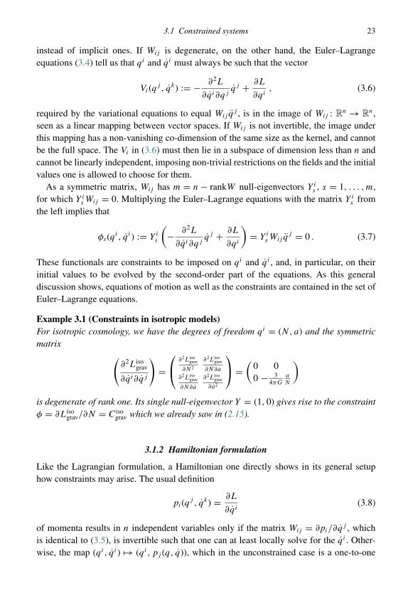
Example 3.1 (Constraints in isotropic models)For isotropic cosmology, we have the degrees of freedom qi = (N, a) and the symmetricmatrix (
∂2Lisograv
∂qi∂qj
)=
∂2Lisograv
∂N2
∂2Lisograv
∂N∂a
∂2Lisograv
∂N∂a
∂2Lisograv
∂a2
=(
0 00 − 3
4πGaN
)is degenerate of rank one. Its single null-eigenvector Y = (1, 0) gives rise to the constraintφ = ∂Liso
grav/∂N = C isograv which we already saw in (2.15).
3.1.2 Hamiltonian formulation
Like the Lagrangian formulation, a Hamiltonian one directly shows in its general setuphow constraints may arise. The usual definition
pi(qj , qk) = ∂L
∂qi(3.8)
of momenta results in n independent variables only if the matrix Wij = ∂pi/∂qj , which
is identical to (3.5), is invertible such that one can at least locally solve for the qi . Other-wise, the map (qi, qi) → (qi, pj (q, q)), which in the unconstrained case is a one-to-one
24 Hamiltonian formulation of general relativity
rP
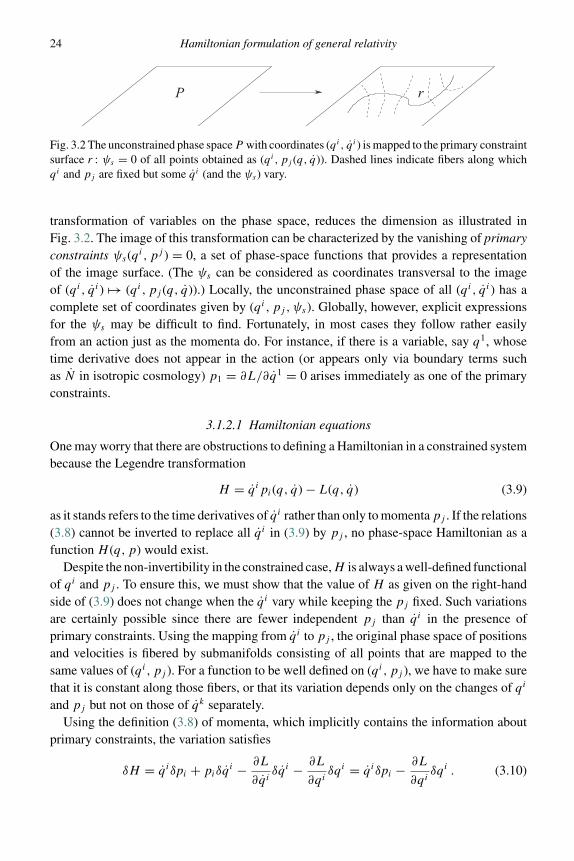
Fig. 3.2 The unconstrained phase spaceP with coordinates (qi, qi) is mapped to the primary constraintsurface r : ψs = 0 of all points obtained as (qi, pj (q, q)). Dashed lines indicate fibers along whichqi and pj are fixed but some q i (and the ψs) vary.
transformation of variables on the phase space, reduces the dimension as illustrated inFig. 3.2. The image of this transformation can be characterized by the vanishing of primaryconstraints ψs(qi, pj ) = 0, a set of phase-space functions that provides a representationof the image surface. (The ψs can be considered as coordinates transversal to the imageof (qi, qi) → (qi, pj (q, q)).) Locally, the unconstrained phase space of all (qi, qi) has acomplete set of coordinates given by (qi, pj , ψs). Globally, however, explicit expressionsfor the ψs may be difficult to find. Fortunately, in most cases they follow rather easilyfrom an action just as the momenta do. For instance, if there is a variable, say q1, whosetime derivative does not appear in the action (or appears only via boundary terms suchas N in isotropic cosmology) p1 = ∂L/∂q1 = 0 arises immediately as one of the primaryconstraints.
3.1.2.1 Hamiltonian equations
One may worry that there are obstructions to defining a Hamiltonian in a constrained systembecause the Legendre transformation
H = qipi(q, q) − L(q, q) (3.9)
as it stands refers to the time derivatives of qi rather than only to momenta pj . If the relations(3.8) cannot be inverted to replace all q i in (3.9) by pj , no phase-space Hamiltonian as afunction H (q, p) would exist.
Despite the non-invertibility in the constrained case,H is always a well-defined functionalof qi and pj . To ensure this, we must show that the value of H as given on the right-handside of (3.9) does not change when the qi vary while keeping the pj fixed. Such variationsare certainly possible since there are fewer independent pj than qi in the presence ofprimary constraints. Using the mapping from qi to pj , the original phase space of positionsand velocities is fibered by submanifolds consisting of all points that are mapped to thesame values of (qi, pj ). For a function to be well defined on (qi, pj ), we have to make surethat it is constant along those fibers, or that its variation depends only on the changes of qi
and pj but not on those of qk separately.Using the definition (3.8) of momenta, which implicitly contains the information about
primary constraints, the variation satisfies
δH = qiδpi + piδqi − ∂L
∂qiδqi − ∂L
∂qiδqi = qiδpi − ∂L
∂qiδqi . (3.10)

3.1 Constrained systems 25
Since the final expression, just as the general variation
δH = ∂H
∂qiδqi + ∂H
∂pi
δpi (3.11)
of a function on the momentum phase space, depends only on variations of qi and pj , whileall other qi-variations cancel once the definition of momenta is used, H is guaranteed tobe a well-defined function on the primary constraint surface. (As an example of a functionthat is not well defined on the primary constraint surface, consider q i . Its value is notdetermined for all i by just specifying a point (qi, pj ) on the primary constraint surface.Accordingly, the variation along qi can be expressed in terms of those along qi and pj onlyif qi happens to be one of the velocities that can be expressed in terms of momenta, i.e. oneof the velocities not primarily constrained.)
Returning to the Hamiltonian, the definition gives rise to a function H (qi, pj ) on theprimary constraint surface whose variation, combining (3.10) and (3.11), satisfies theequation (
∂H
∂qi+ ∂L
∂qi
)δqi +
(∂H
∂pi
− qi
)δpi = 0 (3.12)
for any variation (δqi, δpi) tangent to the primary constraint surface. Writing this equationas (
∂H
∂qi+ ∂L
∂qi,∂H
∂pj
− qj
)(δqi
δpj
)= 0
shows that the vector
δ :=(∂H
∂qi+ ∂L
∂qi,∂H
∂pj
− qj
)must be normal to the constraint surface. Since the surface is represented as ψs = 0,s = 1, . . . , m, a basis of its normal space is given by the gradients
νs :=(∂ψs
∂qi,∂ψs
∂pj
)of all the primary constraint functions. Thus, δ = ∑
s λsνs for some coefficients λs (which
might be functions on phase space), or
∂H
∂qi+ ∂L
∂qi= λs ∂ψs
∂qi(3.13)
∂H
∂pi
− qi = λs ∂ψs
∂pi
. (3.14)
26 Hamiltonian formulation of general relativity
In this way, we have derived Hamiltonian equations of motion
qi = ∂H
∂pi
− λs ∂ψs
∂pi
(3.15)
pi = ∂L
∂qi= −∂H
∂qi+ λs ∂ψs
∂qi. (3.16)
Compared to the form of Hamiltonian equations of motion in unconstrained systems,there are new terms arising from the constraints. However, writing
qi = ∂(H − λsψs)
∂pi
+ ∂λs
∂pi
ψs (3.17)
pi = −∂(H − λsψs)
∂qi− ∂λs
∂qi
ψs (3.18)
shows that, up to terms that vanish on the primary constraint surface, defined by ψs = 0,they can be seen as the usual Hamiltonian equations for the total Hamiltonian
Htotal = H − λsψs . (3.19)
In this case, one also writes
qi ≈ ∂Htotal
∂pi
, pi ≈ −∂Htotal
∂qi
where the “weak equality” sign ≈ denotes an identity up to terms that vanish on theconstraint surface.
While the value of the total Hamiltonian does not change by adding primary constraintsand is independent of the λs , the evolution it generates depends on derivatives of the ψs .Unlike the ψs , the derivatives may not vanish, and evolution can thus depend on the (so farundetermined) λs . To see the role of the λs and how well-defined evolution can result, themathematical theory of constraints, best described in terms of Poisson structures, is useful.
3.1.2.2 Poisson brackets
To discuss the general behavior of constrained systems, as well as those specific onesrealized in general relativity, the concept of Poisson brackets and symplectic structures isthe appropriate tool. As in classical mechanics, we have the general definition of Poissonbrackets
{f (q, p), g(q, p)} :=n∑
i=1
(∂f
∂qi
∂g
∂pi
− ∂f
∂pi
∂g
∂qi
)(3.20)
for a system with finitely many degrees of freedom. (The generalization to infinite-dimensional cases will be done in Chapter 3.1.3.) As one can verify by direct calculations,Poisson brackets satisfy the following defining properties:
• linearity in both entries;• antisymmetry when the two entries are commuted;
3.1 Constrained systems 27
• the Leibniz rule {f, gh} = {f, g}h + g{f, h};• the Jacobi identity
{{f, g}, h} + {{g, h}, f } + {{h, f }, g} = 0 . (3.21)
With this definition, we can write the equations of motion in the compact form
qi ≈ {qi,Htotal} , pi ≈ {pi,Htotal} (3.22)
or F ≈ {F,Htotal} for an arbitrary phase-space function F (qi, pj ). Whenever a change ofphase-space variables is obtained in this way by taking Poisson brackets with a specificphase-space function H , H is said to generate the corresponding change. Viewing thevariations (qi , pj ) as a vector field, the Hamiltonian vector field with components {·,H }is associated with any phase-space function H . In particular, (3.22) expresses the fact thatthe total Hamiltonian generates the dynamical flow of the phase-space variables in time.
Poisson tensor Poisson brackets present a geometrical notion of spaces that in severalrespects is quite similar to the notion of Riemannian geometry as it arises from a metrictensor; in others it is markedly different. If we express the Poisson bracket as
{f, g} = P ij (∂if )(∂jg) , (3.23)
which is always possible thanks to the linearity of Poisson brackets and the Leibniz rule,it becomes clear that the bracket structure is captured by a contravariant 2-tensor, or abivector P ij , the Poisson tensor. Unlike a metric, this tensor is antisymmetric. Moreover,as a consequence of the Jacobi identity, it must satisfy
εiklP ij ∂jPkl = 0 . (3.24)
Conversely, any antisymmetric 2-tensor satisfying (3.24) defines a Poisson bracket via(3.23). Since such tensors may depend non-trivially on the phase space coordinates, unlikethe basic example of (3.20), a more general notion is obtained. The expression (3.20)represents the local form of a Poisson bracket as it can be achieved in suitably chosenphase-space coordinates qi and pj (so-called Darboux coordinates), and it is preserved bycanonical transformations. But in general phase-space coordinates, the Poisson tensor neednot be constant and may have components different from zero or ±1.
Example 3.2 (Poisson tensor)
(P ij ) := 0 z −y
−z 0 x
y −x 0
on R3, i.e. P ij = εijkxk , defines a Poisson tensor; see Exercise 3.1.
The example of (3.20) leads to a Poisson tensor with an additional property: the matrixP ij is invertible, with an inverse
�ij := (P−1)ij . (3.25)

28 Hamiltonian formulation of general relativity
Invertibility is not a general requirement for Poisson tensors, as we will discuss in moredetail below. But the non-degenerate case with an existing inverse occurs often and leadsto several special properties. If the inverse �ij of P ij exists, providing an antisymmetriccovariant 2-tensor, it is called a symplectic form.
As usual with metric tensors, we might be tempted to use the same symbol for aninvertible Poisson tensor and its inverse 2-form, distinguished from each other only bythe position of indices. However, this is normally not done for the following reason: anon-degenerate Poisson tensor defines a bijection P� : T ∗M → TM, αi → P ij αj fromthe co-tangent space to the tangent space of a manifold M , raising indices by contractionwithP ij .2 This is similar to the use of an inverse metric tensor, except that the Poisson tensoris antisymmetric. The inverse P�−1 of this bijection defines a map �� = P�−1 : TM →T ∗M, vi → (P)−1
ij vj = �ijvj lowering indices. By tensor products, indices of tensors of
arbitrary degree can be lowered and raised. In particular, we can lower the indices of P ij
using P�−1:
(P�−1)ik(P�−1)j lPkl = δli (P�−1)j l = −(P−1)ij
which is not �ij but its negative. The antisymmetry of tensors in Poisson geometry intro-duces an ambiguity which does not exist for Riemannian geometry. In Riemannian geom-etry, taking the inverse metric agrees with raising the indices of the metric by its inverse.In Poisson geometry, agreement is realized only up to a sign. For this reason, we do notfollow the convention of using the same letter for the tensor and its inverse, as we woulddo for a metric, but rather, keep separate symbols P and �.
Symplectic form If we contract the Jacobi identity (3.24), written as
P ij ∂jPkl + Pkj ∂jP li + P lj ∂jP ik = 0 ,
with �mi and �nk , then use �ij∂kPj l = −Pj l∂k�ij due to the inverse relationship of thetwo tensors, we obtain3
P lk(∂m�nk − ∂n�mk + ∂k�mn) = P lk(d�)mnk = 0 .
Thus, the inverse of an invertible Poisson tensor is always a closed 2-form. It is also non-degenerate thanks to the invertibility, and any 2-form satisfying these properties is called asymplectic form. A Poisson structure (M,P) on a manifold M with an invertible Poissontensor is equivalent to a symplectic structure (M,�).
Hamiltonian vector fields Given a Poisson tensor, we associate the Hamiltonian vectorfield Xf to any function f on the Poisson manifold by
Xf := P�df = −P ij (∂if )∂j . (3.26)
2 This so-called “musical isomorphism” is sometimes denoted simply as � : T ∗M → TM , with inverse � : TM → T ∗M . Weprefer to indicate the object used to define the mapping, here the Poisson tensor, since general relativity employs also analogousbut quite different mappings defined with a metric.
3 Differential forms, whose tangent-space indices are suppressed, will be denoted here and throughout this book by bold-faceletters.
3.1 Constrained systems 29
(In Riemannian geometry, an analogous construction provides the normal vector to thesurface given by f = const.) In terms of the Poisson bracket, one can write Xf = {·, f } asthe action of the vector field on functions, to be inserted for the dot. The Poisson bracketitself can be written in terms of Hamiltonian vector fields and the symplectic form:
�(Xf ,Xg) = �ijP ikPj l∂kf ∂lg = −Pki∂kf ∂ig = −{f, g} .One can interpret the Hamiltonian vector field as the phase-space direction of change
corresponding to the function f ; for f = p, we have Xp = ∂/∂q. When f is one of thecanonical coordinates, its Hamiltonian vector field is along its canonical momentum. Inthis sense, the Hamiltonian vector field generalizes the notion of momentum to arbitraryphase-space functions. Integrating the Hamiltonian vector field Xf to a 1-parameter familyof diffeomorphisms, we obtain the Hamiltonian flow �
(f )t generated by f . The dynamical
flow of a canonical system is generated by the Hamiltonian function on phase space.
Poisson and presymplectic geometry If the requirement of invertibility is dropped, twounequal siblings spring from the pair of Poisson and symplectic geometry. A non-invertiblePoisson tensor is still said to provide a Poisson geometry, but it does not have an equivalentsymplectic formulation. A closed 2-form not required to be invertible is called a presym-plectic form, providing the manifold on which it is defined with presymplectic geometry.
A presymplectic form �ij has a kernel C ⊂ TM of vector fields vi satisfying �ijvj = 0.
These vector fields define a flow on phase space, which can be factored out by identifyingall points on orbits of the flow. The resulting factor space is symplectic: every vector fieldin the kernel of �ij is factored out. In this way, a reduced symplectic geometry can beassociated with any presymplectic geometry.
A degenerate Poisson tensor P ij provides so-called Casimir functions CI satisfying{CI , f } = 0 with any other function f . Thus, the 1-forms dCI are in the kernel of P ij ,P ij ∂jC
I = 0. In this situation, we naturally define a distribution T ⊂ TM of subspacessuch that dCI (v) = vi∂iC
I = 0 for any vi ∈ T . Any vi in this distribution is annihilated bythe kernel of P ij and is thus in the image, expressed as vi = P ij αj for some co-vector αi ;conversely, any P ij αj satisfies P ij αj ∂iC
I = 0 and is thus in T . Thus, T = ImP�. Thanksto the Jacobi identity (3.24), this distribution is integrable: for two vectors vi = P ij αj andwi = P ij βj in the distribution, the Lie bracket [v,w]i is also in the distribution. Indeed, aquick calculation using the Jacobi identity shows that
[v,w]i = Pjkαk∂j (P ilβl) − Pjkβk∂j (P ilαl)
= P il(Pjk(αk∂jβl − βk∂jαl) + αkβj∂lPjk
) =: P ilγl
is an element of the distribution. Thanks to the integrability, a Poisson manifold is foliated4
into submanifolds spanned by the distribution, with tangent spaces annihilated by allCasimir functions. Integral surfaces of the distribution, leaves of this foliation, are called
4 In general, the foliation may be singular: leaves are not guaranteed to have the same dimension.

30 Hamiltonian formulation of general relativity
symplectic leaves. The leaves are indeed symplectic: the Poisson tensor restricted to thespace co-tangent to the leaves is invertible.
Example 3.3 (Symplectic leaves)Define P ij = εijkxk on R3, as in Example 3.2. The conditions P ij ∂jC = 0 for a Casimirfunction C impose the equations εijk∂kC = 0, which is solved by any function depending onx, y and z only via x2 + y2 + z2. We can thus choose our Casimir function as C(x, y, z) =x2 + y2 + z2. Surfaces of constant C = r2 are spheres of radius r , on which it is usefulto choose polar coordinates ϕ and ϑ . With the relationship between polar and Cartesiancoordinates, one finds that P(dϕ, sinϑdϑ) = sinϑP ij ∂iϕ∂jϑ = r−1 is non-vanishing forr �= 0, and thus the Poisson tensor is non-degenerate on the co-tangent space of a sphere.Spheres are symplectic leaves of the Poisson manifold considered here.
Constraints on symplectic manifolds If we constrain a symplectic manifold M with sym-plectic form �ij and Poisson tensor P ij to a subset C defined by the vanishing of constraintfunctions CI , C : CI = 0, there are different possibilities for symplectic properties of thesubset. These properties are mainly determined by the Hamiltonian vector fields of the con-straints:5 We call a constraint CI first class with respect to all constraints if its Hamiltonianvector field is everywhere tangent to the constraint surface C. We call it second class if itsHamiltonian vector field is nowhere tangent to the constraint surface. By the definition ofHamiltonian vector fields, this is equivalent to saying that {CI , CJ } vanishes on the con-straint surface for all CJ if CI is first class; it vanishes nowhere on the constraint surfaceif CI is second class. (No condition is posed for the behavior of these Poisson brackets offthe constraint surface.) The surface is called a first-class constraint surface if all constraintsdefining it are first class, and a second-class constraint surface if all constraints are secondclass. (The terminology of first- and second-class constraints was introduced by Andersonand Bergmann (1951), developed further by Dirac (1958a) and especially for gravity byDirac (1958b), then summarized by Dirac (1969).)
We can equip the constraint surface with a presymplectic form � by pulling back thesymplectic form to it. If ι : C → M is the embedding of the constraint surface in M , wewrite � = ι∗�. In components, if ι : yα → xi describes the embedding in local coordinates,�αβ = �ij (∂xi/∂yα)(∂xj/∂yβ ). (We cannot directly equip it with a Poisson structure, sincethe Poisson tensor, being contravariant, cannot be pulled back.) If one of the constraintsis first class, say C, the presymplectic form is degenerate: its Hamiltonian vector fieldXi
C is tangent to the constraint surface and thus defines a vector field Xα on it by simplerestriction. For this, we have �αβX
β = ι∗(�ijXj
C) = ι∗(∂iC) = 0 using the definition ofHamiltonian vector fields.
Only if all constraints are second class does a symplectic structure result on the constraintsurface. In this case, it can directly be used as the phase space of the reduced system where
5 For all constraints considered here, we assume the Hamiltonian vector field to be non-vanishing in a neighborhood of theconstraint surface. Such constraints, called regular, provide good local coordinates transversal to the constraint surface.

3.1 Constrained systems 31
the constraints are solved. If there are first-class constraints, their Hamiltonian flow mustbe factored out to obtain the reduced phase space as the factor space of the presymplecticconstraint surface by the Hamiltonian flow. In physical terms, this flow is the gauge flowgenerated by the constraints as discussed in more detail below.
Dirac bracket If one does not explicitly solve all the constraints, which can often becomplicated, one may work with the constrained system implicitly by using the constraintswithout solving them. In this case, if Hamiltonian flows of phase-space functions are used,most importantly the dynamical flow generated by the Hamiltonian, one must be carefulthat they do not leave the constraint surface. This would be guaranteed if all constraintsare solved explicitly — every flow would automatically be restricted to the reduced phasespace — but not if some of them cannot be solved. If all constraints are first class, theirHamiltonian flow is tangent to the constraint surface; they do not cause a problem in thiscontext. But second-class constraints generate a flow transversal to the constraint surface.If second-class constraints are left unsolved, they may contribute terms to a Hamiltonianmaking the flow move off the constraint surface.
Rather than solving all second-class constraints, one may modify the Poisson brackets soas to ensure that the Hamiltonian flow generated by the old constraints with respect to thenew Poisson structure is tangent to the constraint surface. This is possible by introducingthe Dirac bracket
{f, g}D := {f, g} −∑I,J
{f,CI }({CI , CJ })−1{CJ , g} . (3.27)
Here, the double sum is taken for all second-class constraints, for which the matrix inverseof {CI , CJ } is guaranteed to exist. With this new Poisson bracket, the flow generated bythe second-class constraints does indeed not leave the constraint surface; it even vanishes:
{f,CK}D = {f,CK} −∑I,J
{f,CI }({CI , CJ })−1{CJ ,CK} = 0 .
The new Poisson tensor defined by the Dirac bracket is degenerate, with the second-class constraints as its Casimir functions. Moreover, for any phase-space function f whoseHamiltonian vector field is already tangent to the second-class constraint surface with theoriginal Poisson structure, i.e. XfC
I = 0 for all second-class constraints CI , we have{f,CI } = P ij ∂if ∂jC
I = −Xj
f ∂jCI = −XfC
I = 0, and thus {f, g}D = {f, g} with anyother phase-space function g. In summary, the Dirac bracket leaves the Poisson structure forfunctions generating a flow tangent to the constraint surface unchanged, while removing anyflow off the constraint surface generated by functions of the second-class constraints. Evenif not all second-class constraints can be solved, the Dirac bracket, which is often easierto compute, makes sure that they do not lead to spurious flows off the constraint surface.(Further mathematical properties of the Dirac bracket are discussed in the Appendix.)
Using the Dirac bracket, only the flow of first-class constraints need be considered. Itcannot be removed in a similar way, since the matric {CI , CJ } is not invertible if first-class constraints are present. To obtain a phase space with symplectic structure, the flows

32 Hamiltonian formulation of general relativity
generated by first-class constraints must be factored out, as already stated. We will soonsee why this factoring-out is necessary from a physical perspective.
3.1.2.3 Constraint algebras
With information about Poisson geometry and the mathematical theory of constraint sur-faces in symplectic spaces, we now return to the physical analysis of constrained systemsand their dynamics. We had arrived at the total Hamiltonian, Htotal in (3.19), as the sumof the Hamiltonian and all primary constraints ψs multiplied with parameters λs . The λs
play the role of Lagrange multipliers which add the primary constraints to the originalHamiltonian, making sure that these constraints are implemented. They may or may not bedetermined by solving the equations of motion or other equations, depending on the formof the constraints. Here, the mathematical classification of constraints becomes relevant.
Secondary constraints In addition to the primary constraints, there are further equationsto be satisfied by initial values: Consistency conditions are required because the timederivatives of the primary constraints, like the constraints themselves, must vanish at alltimes,
0 = ψs ≈ {ψs,H } − λt {ψs,ψt } =: {ψs,H } − λtCst . (3.28)
(In the weak equality we are again free to move the λt past the derivatives contained in thePoisson bracket because only terms constrained to be zero result in this way.)
The (phase-space dependent) matrix Cst := {ψs,ψt } introduced here determines thestructure of the constrained system. If det(Cst ) �= 0, no further constraints result and wecan fulfill the consistency conditions (3.28) by solving them for all λt . In this way, thetotal Hamiltonian and the flow it generates will be completely specified. If det(Cst ) = 0,however, not all λt can be determined to solve the consistency conditions completely. Inthis case, (3.28) implies secondary constraints which follow from the equations of motion,rather than from the basic definition of momenta as the primary constraints. Secondaryconstraints in general take the form Zs
r {ψs,H } = 0 for any zero-eigenvector Zsr of the
primary constraint matrix: ZsrCst = 0. If a non-trivial zero-eigenvactor Zs
r exists, ψs = 0is preserved in time only if Zs
r {ψs,H } = 0.Also, the secondary constraints imply consistency conditions of the form (3.28), which
may generate further constraints. This process must be continued until all consistencyconditions for all the constraints are satisfied, making sure that constraints can hold at alltimes. Once this is realized, one has determined the complete constrained system. At thisstage, the distinction between primary and other constraints becomes irrelevant, and sowe call all constraints derived in this way Cs , including the primary constraints ψs . (Forsimplicity, we reuse the label s, even though it may now run through a larger range.) Ifdet({Cs, Ct }) does not vanish on the constraint surface, the constraints are second class;more generally, the number of second-class constraints is given by rank({Cs, Ct }). If allconstraints are second class, we can solve for all the multipliers λt and the dynamics isdetermined uniquely.
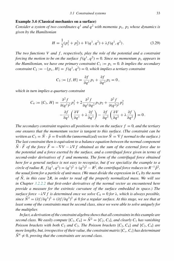
3.1 Constrained systems 33
Example 3.4 (Classical mechanics on a surface)Consider a system of two coordinates q1 and q2 with momenta p1, p2 whose dynamics isgiven by the Hamiltonian
H = 1
2(p2
1 + p22) + V (q1, q2) + λf (q1, q2) . (3.29)
The two functions V and f , respectively, play the role of the potential and a constraintforcing the motion to be on the surface f (q1, q2) = 0. Since no momentum pλ appears inthe Hamiltonian, we have one primary constraint C1 := pλ = 0. It implies the secondaryconstraint C2 := −{pλ,H } = f (q1, q2) = 0, which implies a tertiary constraint
C3 := {f,H } = ∂f
∂q1p1 + ∂f
∂q2p2 = 0 ,
which in turn implies a quartary constraint
C4 := {C3,H } = ∂2f
∂(q1)2p2
1 + 2∂2f
∂q1∂q2p1p2 + ∂2f
∂(q2)2p2
2
− ∂f
∂q1
(∂V
∂q1+ λ
∂f
∂q1
)− ∂f
∂q2
(∂V
∂q2+ λ
∂f
∂q2
)= 0 .
The secondary constraint requires all positions to be on the surface f = 0, and the tertiaryone ensures that the momentum vector is tangent to this surface. (The constraint can bewritten as C3 = �N · �p = 0 with the (unnormalized) vector �N = ∇f normal to the surface.)The last constraint then is equivalent to a balance equation between the normal component�N · �F of the force �F = −∇V − λ∇f obtained as the sum of the external force due to
the potential and a force exerted by the surface, and a centrifugal force given in terms ofsecond-order derivatives of f and momenta. The form of the centrifugal force obtainedhere for a general surface is not easy to recognize, but if we specialize the example to acircle of radius R, f (q1, q2) = (q1)2 + (q2)2 − R2, the centrifugal force reduces to R−1 �p2,the usual form for a particle of unit mass. (We must divide the expression in C4 by the normof �N , in this case 2R, in order to read off the properly normalized mass. We will seein Chapter 3.2.2.2 that first-order derivatives of the normal vector as encountered hereprovide a measure for the extrinsic curvature of the surface embedded in space.) Thesurface force −λ∇f is determined once we solve C4 = 0 for λ, which is always possible,since �N2 = (∂f/∂q1)2 + (∂f/∂q2)2 �= 0 for a regular surface. At this stage, we see that atleast some of the constraints must be second class, since we were able to solve uniquely forthe multiplier.
In fact, a derivation of the constraint algebra shows that all constraints in this example aresecond class. We easily compute {C1, C4} = �N2 = {C2, C3}, and clearly C1 has vanishingPoisson brackets with both C2 and C3. The Poisson brackets {C2, C4} and {C3, C4} aremore lengthy, but, irrespective of their value, the constraint matrix {Cs, Ct } has determinant�N4 �= 0, proving that the constraints are second class.

34 Hamiltonian formulation of general relativity
If the constraints satisfy {Cs, Ct } ≈ 0 on the constraint surface Ct = 0, they are first-class constraints. (In the presence of a Hamiltonian generating evolution, one usuallyincludes {Cs,H } = 0 as a condition for first-class constraints combined with a first-classHamiltonian. One may interpret this as including the condition of energy conservation withthe constraints Cs .) Not all the Lagrange multipliers can be solved for, and the dynamics isnot unique. Gauge transformations arise.
Gauge transformations As seen in the general analysis of Poisson geometry, first-classconstraints play a special role because their constraint surface is not symplectic: theygenerate a Hamiltonian flow tangent to the constraint surface, along which the presym-plectic form, obtained by pulling the symplectic form back to the constraint surface,is degenerate. In the physical interpretation, this means that first-class constraints notonly restrict initial values but also generate gauge transformations. The infinitesimalmapping
F (q, p) → F (q, p) + δ(s)ε F (q, p) := F (q, p) + {F, εCs} (3.30)
of a phase-space function F , defined for any first-class constraint Cs , maps solutions to theconstraints and equations of motion into other solutions: under this mapping, δ(s)
ε Ct ≈ 0 ≈δ(s)ε H .
Interpreting these transformations as gauge means that we do not consider solutionsmapped to each other by the Hamiltonian flow of first-class constraints as physicallydistinct. We are not merely applying a symmetry transformation to map a known solutioninto a new one, like rotating an orbit in a spherically symmetric potential which gives rise toa new allowed solution. Gauge transformations map different mathematical solutions intoeach other, but they are interpreted merely as different representations of the same physicalsolution.
This stronger interpretation is required when we consider the dynamical flow gener-ated by the total Hamiltonian Htotal = H1 − λsψs , which explicitly contains the primaryconstraints ψs , but also implicitly secondary or other ones in H1. (We now use the sym-bol H1 to indicate that second-class constraints should already have been solved at thisstage, fixing their multipliers. Alternatively, we could use the Dirac bracket in the fol-lowing argument.) Every phase-space function f changes in time by f = {f,Htotal}. Ingeneral, the change in time of a function f then depends on the undetermined parametersλs corresponding to the first-class constraints unless {f,Cs} = 0 for all first-class con-straints. If f has a vanishing Poisson bracket with all first-class constraints, it is calleda complete (or Dirac) observable. For phase-space functions with non-vanishing Poissonbrackets with the first class constraints, however, a dependence of their change in timeon some of the λs cannot be avoided. To have a well-defined theory with unambiguousphysical predictions, the only viable conclusion is that the infinitesimal flow {f,Cs} onlychanges the mathematical representation but does not change the physics of the observableinformation. The change of f is just a gauge transformation without affecting the physicalstate.

3.1 Constrained systems 35
Example 3.5 (Gauge in isotropic models)In Chapter 2.1 we saw an example of a system with two constraints, the primary constraintpN = 0 and the secondary constraint C = 0. Since C is independent of N , we immediatelyhave {pN,C} = 0 such that the system of constraints is first class. The total Hamiltonianis NC − λpN where N arises automatically as a multiplier of the secondary constraint C.
The gauge transformations generated by the constraints correspond to time reparam-eterizations, as one can see explicitly: we have
δεa = {a, εNC} = −4πG
3εpa
aN = εa
and δλN = {N, λpN } = λ, δεpa = {pa, εNC} = εpa and finally δεpN = C ≈ 0. Thegauge transformation a → a + δεa = a + εa = a(t + ε) + O(ε2) thus agrees to linearorder in ε with a change of the time coordinate while N can be changed arbitrarily. Onemay view this as evolution along the time parameter, or as a reparameterization of the oldtime parameter t to a new one making coordinate time gauge-dependent.
In totally constrained systems such as the preceding example, constraints play severalroles: they constrain allowed field values to reside on the constraint surface, they generategauge transformations as identifications of physically equivalent field configurations onthe constraint surface and they provide the total Hamiltonian. The last property meansthat a particular combination of the constraints, such as H = NC in the example with asingle constraint, generates Hamiltonian equations of motion in a time coordinate. Whichcombination we choose for the total Hamiltonian, i.e. which multiplier function N weuse in the example, will have an influence on the form of equations of motion. For first-class constraints, this function remains undetermined by the constraints. Any choice isallowed, and there is no unique, absolute notion of evolution — a further reflection of thegauge structure of the theory. Any particular choice for the total Hamiltonian will result inequations of motion written in a specific gauge. But since the theory is invariant under gaugetransformations generated by the constraints, the choice of a total Hamiltonian does notmatter, and all sets of equations of motion obtained for different gauges are equivalent. Wewill see in this chapter that general relativity, also in the absence of space-time symmetries,has first-class constraints and a fully constrained Hamiltonian. We will also encounterformulations that have additional second-class constraints.
3.1.3 Field theories
Lagrangian or Hamiltonian formulations of field theories follow the same lines as discussedso far for finite-dimensional systems. One may view such theories as having independentvariables ϕ(x) labelled not by a discrete parameter i taking a finite number of values, butby a continuous parameter x. Most constructions still go through with this understanding,but it hides several subtleties. Especially, derivatives by the fields, as they are required forvariational equations or Poisson brackets, require mathematical care. For instance, insteadof having the relationship ∂qi/∂qj = δij for independent variables, a basic functional
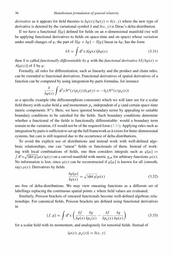
36 Hamiltonian formulation of general relativity
derivative as it appears for field theories is δϕ(x)/δϕ(y) = δ(x, y) where the new type ofderivative is denoted by the variational symbol δ and δ(x, y) is Dirac’s delta-distribution.
If we have a functional S[ϕ] defined for fields on an n-dimensional manifold (we willbe applying functional derivatives to fields on space-time and on space) whose variationunder small changes of ϕ, the part of S[ϕ + δϕ] − S[ϕ] linear in δϕ, has the form
δS =∫
dnxA[ϕ(x)]δϕ(x) (3.31)
then S is called functionally differentiable by ϕ with the functional derivative δS/δϕ(x) =A[ϕ(x)] of S by ϕ.
Formally, all rules for differentiation, such as linearity and the product and chain rules,can be extended to functional derivatives. Functional derivatives of spatial derivatives of afunction can be computed by using integration-by-parts formulas, for instance
δ
δϕ(x)
∫d3yNa(y)pϕ(y)∂aϕ(y) = −∂a(Na(x)pϕ(x))
as a specific example (the diffeomorphism constraint) which we will later see for a scalarfield theory with scalar field ϕ and momentum pϕ independent of ϕ (and certain space-timemetric components Na). Here, we have ignored boundary terms by appealing to suitableboundary conditions to be satisfied for the fields. Such boundary conditions determinewhether a functional of the fields is functionally differentiable: would a boundary termremain in the variation, δS would not be of the required form (3.31). Applying rules such asintegration by parts is sufficient to set up the full framework as it exists for finite-dimensionalsystems, but care is still required due to the occurrence of delta-distributions.
To avoid the explicit use of distributions and instead work with well-defined alge-braic relationships, one can “smear” fields or functionals of them. Instead of work-ing with local combinations of fields, one then considers integrals such as ϕ[µ] :=∫
dnx√|det g|µ(x)ϕ(x) on a curved manifold with metric gab for arbitrary functions µ(x).
No information is lost, since ϕ(x) can be reconstructed if ϕ[µ] is known for all (smooth,say) µ(x). Derivatives by fields
δϕ[µ]
δϕ(x)=
√|det g|µ(x) (3.32)
are free of delta-distributions. We may view smearing functions as a different set oflabellings replacing the continuous spatial points x where field values are evaluated.
Similarly, Poisson brackets of smeared functionals become well-defined algebraic rela-tionships. For canonical fields, Poisson brackets are defined using functional derivativesin
{f, g} =∫
dnx
(δf
δϕ(x)
δg
δpϕ(x)− δf
δpϕ(x)
δg
δϕ(x)
)(3.33)
for a scalar field with its momentum, and analogously for tensorial fields. Instead of
{ϕ(x), pϕ(y)} = δ(x, y)
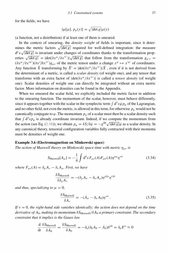
3.1 Constrained systems 37
for the fields, we have
{ϕ[µ], pϕ(y)} =√
|det g|µ(y)
(a function, not a distribution) if at least one of them is smeared.In the context of smearing, the density weight of fields is important, since it deter-
mines the metric factors√|det g| required for well-defined integration: the measure
dnx√|det g| is invariant under changes of coordinates thanks to the transformation prop-
erties√|det g|′ = |det(∂xµ/∂x ′ν ′
)|√|det g| that follow from the transformation gµ′ν ′ =(∂xµ/∂x ′µ′
)(∂xν/∂x ′ν ′)gµν of the metric tensor under a change xµ → x ′µ′
of coordinates.Any function X transforming by X′ = |det(∂xµ/∂x ′ν ′
)|X , even if it is not derived fromthe determinant of a metric, is called a scalar density (of weight one), and any tensor thattransforms with an extra factor of |det(∂xµ/∂x ′ν ′
)| is called a tensor density (of weightone). Scalar densities of weight one can directly be integrated without an extra metricfactor. More information on densities can be found in the Appendix.
When we smeared the scalar field, we explicitly included the metric factor in additionto the smearing function. The momentum of the scalar, however, must behave differently,since it appears together with the scalar in the symplectic term
∫d3xϕpϕ of the Lagrangian,
and no other field, not even the metric, is allowed in this term, for otherwise pϕ would not becanonically conjugate to ϕ. The momentum pϕ of a scalar must then be a scalar density suchthat
∫d3xpϕ is already coordinate invariant. Indeed, if we compute the momentum from
the action (see Eq. (2.16)), we obtain pϕ = δS/δϕ = −g00√|det g|ϕ as a scalar density. Inany canonical theory, tensorial configuration variables fully contracted with their momentamust be densities of weight one.
Example 3.6 (Electromagnetism on Minkowski space)The action of Maxwell theory on Minkowski space-time with metric ηµν is
SMaxwell[Aµ] = −1
4
∫d4xFµν(A)Fρσ (A)ηµρηνσ (3.34)
where Fµν(A) = ∂µAν − ∂νAµ. First, we have
δSMaxwell
δ∂µAν
= −(∂ρAσ − ∂σAρ)ηρ[µην]σ
and thus, specializing to µ = 0,
δSMaxwell
δAν
= −(Aσ − ∂σA0)ηνσ . (3.35)
If ν = 0, the right-hand side vanishes identically; the action does not depend on the timederivative of A0, making its momentum δSMaxwell/δA0 a primary constraint. The secondaryconstraint that it implies is the Gauss law
d
dt
δSMaxwell
δA0= δSMaxwell
δA0= −∂a(∂bA0 − Ab)δab = ∂aE
a ≈ 0
38 Hamiltonian formulation of general relativity
with the electric fieldEa = δab(Ab − ∂bA0) whose components, as seen from (3.35), providethe momenta of Aa: {Aa(x), Eb(y)} = δbaδ(x, y). (Only spatial indices contribute at thisstage. Note that the fixed background metric prevents all density weights from being seen.)
The Gauss constraint does not generate further constraints, and so the system is complete:on our phase space we can directly eliminate the simple primary constraint function, leavingas canonical variables Aa with momenta Eb, subject to the Gauss constraint ∂aEa = 0.The Gauss constraint does not depend on Aa , and is thus first class. If we smear it toG[�] = ∫
d3x�(x)∂aEa , we have the Abelian algebra {G[�1],G[�2]} = 0. The smearedconstraint generates gauge transformations leaving Ea fixed and changing Aa by thegradient {Aa,G[�]} = −∂a� of �.
If we introduce a gauge-fixing condition, for instance the Coulomb gauge C :=δab∂aAb = 0 smeared to C[K] = ∫
d3xK(x)C(x), the system of constraints ceases to befirst class. We have
{G[�], C[K]} =∫
d3xd3y(∂a�)(x)(−δab∂bK(y))δ(x, y) =∫
d3xKδab∂a∂b�
which clearly does not vanish everywhere on the constraint surface. The system providedby the Gauss constraint together with the Coulomb gauge condition is second class for allsmearing functions satisfying δab∂a∂b� �= 0. For harmonic functions satisfying δab∂a∂b� =0, the gauge fixing is not complete and does not provide a second-class system of constraints.This is the well-known fact that the Coulomb gauge fixes the gauge freedom of changingAa to Aa − ∂a� only up to gauge transformations generated by harmonic functions:if δab∂aAb = 0 satisfies the gauge, also δab∂a(Ab − ∂b�) = 0 satisfies it if and only ifδab∂a∂b� = 0.
In general, completely fixing the gauge requires a restriction to a subspace intersectingeach gauge orbit exactly once. If this can be achieved, which is often difficult to do inexplicit form, no gauge freedom is left. Since all gauge flows are then transversal to thegauge-fixing surface, the set of constraints plus gauge-fixing conditions is second class bydefinition.
Example 3.7 (Einstein–Hilbert action)For gravity, the action to start with is the Einstein–Hilbert action
SEH[g] =∫
d4x
(√− det gR
16πG+ Lmatter
)(3.36)
whose stationary points are given by solutions to Einstein’s equation. The proof is lengthybut makes use of several identities which will also appear in the canonical formulation.Before continuing with the machinery of Hamiltonian formulations, we will thus firstdemonstrate explicitly that (3.36) is indeed the correct starting point to derive momentaand equations of motion.
We compute the variation δ(√− det gRabg
ab) by a background-field expansion, settinggab = gab + δgab for an arbitrary gab and expanding to linear order in δgab. Functional
3.1 Constrained systems 39
derivatives can then be read off using (3.31). We will show that gab satisfies Einstein’sequation if and only if δSEH = 0.
1. Connection components. We call ∇a the derivative operator compatible with gab, and ∇a theoperator compatible with gab. All indices will be lowered or raised with gab and its inverse. Thisgives
0 = ∇agbc = ∇agbc − Cdabgdc − Cd
acgbd
for a partially symmetric tensor Cabc = Ca
(bc). Thus, Ccab + Cbac = ∇agbc for Cabc := gadCdbc and,
using the symmetry of Cabc,
Ccab = gcdCdab = 1
2gcd ((Cdab + Cbad ) + (Cdba + Cabd ) − (Cbda + Cadb))
= 1
2gcd
(∇agbd + ∇bgad − ∇dgab
)= 1
2(gcd + δgcd )
(∇aδgbd + ∇bδgad − ∇dδgab
).
Due to Ccab|δgab=0 = 0, this is at least of linear order in δgab. Its linear term is
δCcab = 1
2gcd
(∇aδgbd + ∇bδgad − ∇dδgab
). (3.37)
2. Curvature. Using ∇a∇bωc − ∇b∇aωc = Rabcdωd for any 1-form ωa and
∇a∇bωc = ∇a∇bωc − ∇a(Cdbcωd ) − Ce
ab(∇eωc − Cdecωd ) − Ce
ac(∇bωe − Cdbeωd )
we have
(∇a∇b − ∇b∇a)ωc = (∇a∇b − ∇b∇a)ωc − (∇aCdbc − ∇bC
dac)ωd + (Ce
caCdbe − Ce
cbCdae)ωd
and thus
Rabcd = Rabc
d − 2∇[aCdb]c + 2Ce
c[aCdb]e .
For the Ricci tensor, this implies that
Rac = Rac − 2∇[aCbb]c + 2Ce
c[aCbb]e
which has as linear variation
δRac = −∇aδCbbc + ∇bδC
bac . (3.38)
In particular, gacδRac =: ∇ava is a total divergence.
3. Determinant. We make use of the identity
εabcdgacgbf gcggdh = εefgh det g (3.39)
where εabcd and εabcd both denote the totally antisymmetric tensor taking values zero or ±1. (Weuse the bar to indicate that εabcd is not obtained by lowering indices of εabcd . In fact, as tensorfields they are quite different, εabcd having density weight one and εabcd density weight minus one;
40 Hamiltonian formulation of general relativity
see the Appendix.) Thus,
δ det g = 1
4!δ(εabcdεefghgaegbf gcggdh
) = 1
6εabcdεefghgbf gcggdhδgae
= 1
6εefgh(gal εlfgh det g)δgae = det ggaeδgae
= − det g gaeδgae (3.40)
where we used 0 = δ(gaegae) = gaeδgae + gaeδgae in the last step. We conclude that
δ√
−det g = − δ det g
2√−det g
= −1
2
√−det ggaeδg
ae . (3.41)
With these variations, we finally have
δ(√
−det gRabgab) = −1
2
√−det g gcdRabg
abδgcd +√
−det gRabδgab
+√
−det g gabδRab
=√
−det g((Rab − 1
2Rgab)δgab + gabδRab
). (3.42)
Here,√−det ggabδRab = √−det g∇av
a = ∂a(√−det gva) integrates to a boundary term
by Stoke’s theorem. Provided that there is no boundary or that boundary terms vanishby fall-off conditions, SEH[g] is functionally differentiable, and its variation produces theEinstein tensor. We will discuss the issue of boundary terms in Chapter 3.3.2, once additionalmethods for dealing with hypersurfaces have been provided.
3.2 Geometry of hypersurfaces
We now turn to the canonical formulation of gravity and apply the systematic proceduresfor an analysis of constrained systems. There will be several constraints with a non-trivialand very interesting algebra, and their expressions are rather involved, more so at leastthan the Gauss constraint of electromagnetism. It is thus helpful to perform the requiredcalculations not by brute force, although a certain amount of force will be necessary, butby using geometrical techniques to split a space-time tensor into spatial parts.
3.2.1 Foliation
As SEH in (3.36) is the correct action for Einstein’s equation, it can be used as starting pointfor a canonical decomposition. A canonical formulation then requires a space-time splitting,since only time derivatives are transformed to momenta but not space derivatives. For fieldtheories on Minkowski space, there are natural choices of time, and global Lorentziansymmetries exist to change one’s choice of time. But we now face a situation in whichno background symmetries or preferred (inertial) observers exist. The notion of time hasbecome much more general. We thus only assume space-time M to be foliated by spatial
3.2 Geometry of hypersurfaces 41
surfaces � ≈ �t : t = const of some time function t . Space-time is assumed to be globallyhyperbolic: topologically, M = � × R.
3.2.1.1 Normal and spatial structures
A surface �t0 in space-time can be considered as a constraint surface characterized by theconstraint Ct0 = t − t0 = 0 with a constant t0. The difference from our previous constraintson phase space is, however, that we do not have a Poisson or symplectic geometry onspace-time, but a Riemannian one given by the metric gab and its inverse gab. In lieu of aHamiltonian vector field generated by the constraint, we have the vector gab∂bCt0 = gab∂bt
obtained by raising the index of the 1-form dt . (In analogy to the previous notation, wecould write it as g�dt .) In contrast to Poisson geometry, where the Hamiltonian vectorfield of a single, necessarily first-class constraint must be tangent to the constraint surface,Riemannian geometry ensures that Xa = gab∂bt is normal to the surface: for any vectorfield sa tangent to t = const, we have gabs
aXb = sa∂at = 0. (It is the antisymmetry of thePoisson tensor that makes the Hamiltonian vector field of a single constraint C tangent tothe constraint surface: XCC = P ij ∂jC∂iC = 0.) The non-degeneracy of the metric alsogives us a means to normalize the (timelike) normal vector to na := Xa/
√−gbcXbXc
such that gabnanb = −1. (Obviously, Hamiltonian vector fields cannot be normalized
in the context of Poisson geometry.) We finally identify a unique normal by requiringit to be future-pointing: na∂at > 0. For globally hyperbolic space-times, this is alwayspossible.
With this structure, the tangent space in TM at each point of �t is naturally decomposedinto a spatial tangent space spanned by vectors tangent to �t and a normal space spannedby the unique unit future-pointing vector field na normal to �t . Each spatial slice �t isequipped with its own Riemannian structure: we have the induced metric hab = gab + nanb
which is uniquely determined by the two conditions that habnb = 0 (it is insensitive to the
normal direction) and habsa = gabs
a for any vector sa tangent to �t (when applied totangent vectors intrinsic to �t , it gives the same geometry as gab). (Comparing again toPoisson geometry, the induced metric is analogous to the Dirac bracket, which subtractsfrom off the Poisson structure any contribution from the flow of constraints transversalto the constraint surface.) In the sense of its action on different vector fields, only spatialcomponents are non-zero in hab, and they agree with those of gab. We can thus considerhab as the spatial part of gab, defining a positive definite metric on each spatial slice �t .Similarly, we define hab = gab + nanb. It reduces to the inverse of hab when applied tospatial vectors tangent to �t , but is not the inverse of hab as a space-time tensor. In fact,neither hab nor hab is invertible on space-time.
3.2.1.2 Time derivatives
The field hab will play a crucial role as the configuration variable of canonical gravity.In order to define it, we had to make use of a time function, or of the foliation �t itgenerates. Accordingly, we cannot view hab as a space-time tensor field, but rather, as a
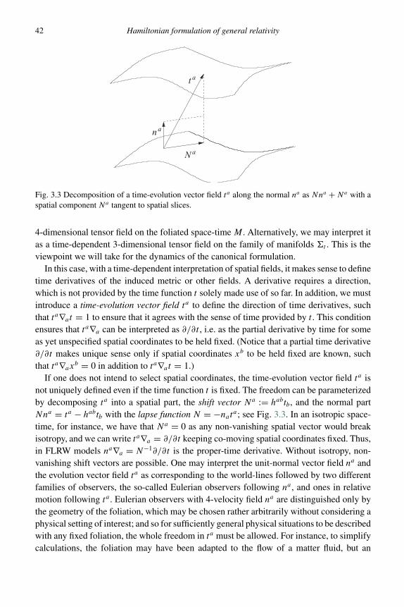
42 Hamiltonian formulation of general relativity
na
N a
t a
Fig. 3.3 Decomposition of a time-evolution vector field ta along the normal na as Nna + Na with aspatial component Na tangent to spatial slices.
4-dimensional tensor field on the foliated space-time M . Alternatively, we may interpret itas a time-dependent 3-dimensional tensor field on the family of manifolds �t . This is theviewpoint we will take for the dynamics of the canonical formulation.
In this case, with a time-dependent interpretation of spatial fields, it makes sense to definetime derivatives of the induced metric or other fields. A derivative requires a direction,which is not provided by the time function t solely made use of so far. In addition, we mustintroduce a time-evolution vector field ta to define the direction of time derivatives, suchthat ta∇at = 1 to ensure that it agrees with the sense of time provided by t . This conditionensures that ta∇a can be interpreted as ∂/∂t , i.e. as the partial derivative by time for someas yet unspecified spatial coordinates to be held fixed. (Notice that a partial time derivative∂/∂t makes unique sense only if spatial coordinates xb to be held fixed are known, suchthat ta∇ax
b = 0 in addition to ta∇at = 1.)If one does not intend to select spatial coordinates, the time-evolution vector field ta is
not uniquely defined even if the time function t is fixed. The freedom can be parameterizedby decomposing ta into a spatial part, the shift vector Na := habtb, and the normal partNna = ta − habtb with the lapse function N = −nat
a; see Fig. 3.3. In an isotropic space-time, for instance, we have that Na = 0 as any non-vanishing spatial vector would breakisotropy, and we can write ta∇a = ∂/∂t keeping co-moving spatial coordinates fixed. Thus,in FLRW models na∇a = N−1∂/∂t is the proper-time derivative. Without isotropy, non-vanishing shift vectors are possible. One may interpret the unit-normal vector field na andthe evolution vector field ta as corresponding to the world-lines followed by two differentfamilies of observers, the so-called Eulerian observers following na , and ones in relativemotion following ta . Eulerian observers with 4-velocity field na are distinguished only bythe geometry of the foliation, which may be chosen rather arbitrarily without considering aphysical setting of interest; and so for sufficiently general physical situations to be describedwith any fixed foliation, the whole freedom in ta must be allowed. For instance, to simplifycalculations, the foliation may have been adapted to the flow of a matter fluid, but an
3.2 Geometry of hypersurfaces 43
observer should not be required to follow the same flow; ta then describes the observer’smotion with respect to the fluid.
As defined, ta is not normalized and thus cannot directly be the 4-velocity of observers.If we normalize it, using the normalization of na and naNa = 0, we obtain
ta√−||t ||2
= na + Na/N√1 − ( �N/N )2
as the relativistic 4-velocity (γ �V , γ �V �V ) expressed in the frame of Eulerian observers, withγ �V = (1 − �V 2)−1/2 corresponding to the 3-velocity �V = �N/N . The shift vector thus pro-vides the velocity field relative to Eulerian observers.
Given a time-evolution vector field, we complete the interpretation of tensor fields ona foliated space-time as time-dependent tensor fields on space. To speak of the time-dependence of a field, we must be able to identify points at which we read off the timedependence. If we just have two different slices in the foliation, it is impossible to say howa field defined on them changes unless we can uniquely associate a point on one slice with apoint on the other slice. Once this is available, evaluating the fields at the associated pointsshows their change when going from one slice to the next, that is their time dependence.A time-evolution vector field provides such an association: taking any one of its integralcurves, we identify its intersections with all surfaces in �t as corresponding to the samespatial point at different times. Thanks to the condition ta∇at = 1, integral curves intersecteach �t exactly once, making the identification well defined. We can then meaningfullydefine a time derivative as the Lie derivative (as discussed in the Appendix) along thetime-evolution vector field ta:
T a1···anb1···bm := ha1
c1· · ·han
cnhd1b1
· · · hdmbmLt T
c1···cnd1···dm (3.43)
including spatial projections to ensure that T a1···anb1···bm is spatial. (Without projections,
Lt Ta1···an
b1···bm is guaranteed to be spatial according to the foliation normal to na only if[t, n]a = 0.)
3.2.1.3 Metric decomposition
Using the preceding definitions, we decompose the inverse space-time metric as
gab = hab − nanb = hab − 1
N2(ta − Na)(tb − Nb) . (3.44)
Writing this as a matrix in a coordinate basis and inverting it, we obtain the line element
ds2 = −N2dt2 + hab(dxa + Nadt)(dxb + Nbdt) (3.45)
in coordinates xa such that ta∇a = ∂/∂t . Space-time geometry is thus described not by asingle metric but by the spatial geometry of slices, encoded in hab, together with deforma-tions of neighboring slices with respect to each other as described by N and Na .
For integration measures or other purposes, it is often important to know the determinantof the metric. For the space-time metric, its decomposition in spatial terms has a simple
44 Hamiltonian formulation of general relativity
expression: from (3.44) we read off the inverse time-time component g00 = −1/N2, whileits purely spatial part is hab. The shift vector only contributes to the mixed time-spacecomponents. By a general formula for inverse matrices, the (i, j )-component of the inversematrix of A is given by the co-factor Cji (defined as (−1)i+j times the determinant ofthe submatrix obtained by striking out row j and column i) divided by the determinantof A: (A−1)ij = Cji/ detA. Here, for the (0, 0)-component of the inverse metric, we havethe co-factor given by the determinant of hab, C00 = det hab, and we already know thatg00 = −1/N2 = C00/ det(gcd ). Thus,
det(gcd ) = −N2 det(hab) . (3.46)
3.2.2 Intrinsic and extrinsic geometry
For a given foliation �t of space-time, we define spatial tensors as those that vanishwhen contracted with the normal na on any index. Examples seen so far are the spatialmetric hab and the shift vector Na . Among spatial tensors, one can distinguish intrinsicand extrinsic geometrical notions, depending on whether only the spatial metric hab is usedin the definition or also na separately, which refers to the slicing of space-time. Finally,there are tensors that depend even on the choice of time evolution vector field, such asNa . Such tensors are not purely geometrical but require choices about the representation ofdynamics.
3.2.2.1 Intrinsic geometry
The spatial metric itself is an intrinsic quantity, and as a metric it allows one to define aunique covariant derivative operatorDa on� such thatDahbc = 0. This covariant derivativecan be written in terms of the space-time covariant derivative ∇a as
DcTa1...ak
b1...bl = ha1d1 · · ·hak
dkhb1e1 · · ·hbl
el hcf ∇f T
d1...dke1...el . (3.47)
For a proof, it suffices to note that (3.47) satisfies all requirements of the unique covariantderivative: it immediately follows from the definition that it is linear, satisfies the Leibnizrule and preserves the spatial metric. Indeed,
hadhb
ehcf ∇f hde = ha
dhbehc
f ∇f (gde + ndne) = 0
since gde is covariantly constant for ∇f and in the second term at least one na will becontracted with hab after using the product rule. Even though the right-hand side of (3.47)does make use of space-time constructs, when applied to spatial tensors it is an intrinsicnotion, since it is equivalent to the spatial covariant derivative defined solely by referenceto hab.
Given the covariant derivative Da , one defines intrinsic-curvature tensors as with anycovariant derivative. For instance, we have the 3-dimensional Riemann tensor defined by
(3)Rabcdωd = DaDbωc − DbDaωc (3.48)
3.2 Geometry of hypersurfaces 45
for all spatial ωc, ωana = 0. Since we make use only of the spatial derivative Da , applied
to spatial 1-forms, (3)Rabcd is intrinsically defined. From the intrinsic Riemann curvature
tensor, we obtain the Ricci tensor and scalar by the usual contractions.
3.2.2.2 Extrinsic curvature
The route to extrinsic geometrical notions is opened up by the observation that (3.47) ismore general than the compatible covariant derivative of the spatial metric hab: it can beapplied to any space-time tensor, not just spatial ones. After applying Da , the result isalways a spatial tensor according to (3.47), even if it is applied to a general space-timetensor. We thus obtain spatial tensors, but refer to space-time objects; the resulting notionsof spatial geometry will be extrinsic.
Before introducing examples, we should be warned that (3.47) is not just an identity,but a definition of a more general derivative operator when T a1...ak
b1...bl is not spatial. Thegeneralization sometimes provides pitfalls if one is not careful enough. In particular, whenthe covariant derivative is applied to a space-time tensor, one cannot use its compatibilitywith the spatial metric which, by construction, only applies when the derivative is takenof a purely spatial tensor. For instance, below in (3.49) we will consider the spatial tensorDanb, with the unit normal na to spatial slices. Erroneously using compatibility, one wouldconclude that the trace habDanb of this tensor must vanish because hab could be commutedwith Da , and habnb = 0. However, one cannot commute hab with Da in this case becausena is not a spatial tensor, and the general definition of Da must be used; only the right-handside of (3.47) can then be used as a definition of Da , where hab and ∇f do not commute.
In contrast to the intrinsic geometry, which applies to a single (�, hab) no matter how itis embedded in a space-time manifold, the extrinsic geometry of � in � × R refers to thebending of � in its neighborhood, which in general implies a changing normal vector fieldna along �. This notion is captured in the definition of the extrinsic-curvature tensor
Kab := Danb = hcah
db∇cnd . (3.49)
It is a spatial tensor on � by definition of Da , but is not intrinsically defined because werefer to na and thus to the embedding of � in space-time. Several properties of Kab illustratethis tensor’s meaning and will play a role later on:
1. Kab = hac∇cnb = ∇anb + nan
c∇cnb: we can drop one spatial metric from the general definitionof Da which would be contracted over the index b. This follows from
Kab = hbdha
c∇cnd = (gbd + nbn
d )hac∇cnd = ha
c∇cnb + nbndha
c∇cnd
noting that nd∇cnd = 12 (nd∇cnd + nd∇cn
d ) = 12 ∇c(ndn
d ) = 0 (na is normalized). Here, we haveseveral times commuted the space-time metric and its covariant derivative, which, in contrast tocommuting hab with Dc, is always allowed.
2. Kab = Kba : the extrinsic curvature tensor is symmetric. To prove this, we take two arbitrary spatialtangent vector fields Y a∇a = f α∂/∂xα and Za∇a = gα∂/∂xα and compute their commutator
[Y,Z]a∇a :=(f α ∂g
β
∂xα− gα ∂f
β
∂xα
)∂
∂xβ.

46 Hamiltonian formulation of general relativity
By definition, the commutator is also spatial. Thus, we have
0 = na[Y,Z]a = na(Y b∇bZa − Zb∇bY
a)
= −ZaY b∇bna + Y aZb∇bna = Y aZb(∇bna − ∇anb)
where we used naZa = 0 = naY
a before the last step. As a result, all spatial projections of ∇anb
are symmetric, which constitute Kab. (This is a special case of the Frobenius theorem.)3. Extrinsic curvature is (half) the Lie derivative of the intrinsic metric along the unit normal:
Kab = 1
2Lnhab (3.50)
To prove this, we compute
Lnhab = nc∇chab + hcb∇anc + hac∇bn
c
= nc∇c(nanb) + ∇anb + ∇bna
= (gac + nan
c)∇cnb + (gbc + nbn
c)∇cna = 2Kab
using the symmetry of Kab in the last step.4. Finally, we have
Kab = 1
2N(hab − DaNb − DbNa) (3.51)
where we use the time derivative hab = hachb
dLt hcd defined by evolution along ta-trajectories asin (3.43). This follows from the last property:
Kab = 1
2Lnhab = 1
2N(Nnc∇chab + hac∇b(Nnc) + hcb∇a(Nnc))
= 1
2Nha
chbdLt−Nhcd = 1
2Nha
chbd (Lt hcd − LNhcd )
where we substituted Nna = ta − Na and smuggled in projections hcah
db , since we know that
Kab is spatial. The claimed identity then follows from the last step noting that LNhcd , with thespatial shift vector Na , can be computed purely spatially and equals DaNb + DbNa , since Da
is compatible with hab. (Notice that, according to our definitions, hab is not an object of eitherintrinsic or extrinsic geometry, since its definition requires not just knowledge of na or the foliation�t , but also of the selection of a time-evolution vector field ta . So do the lapse function N andthe shift vector Na . The dependence on properties of ta not given solely by na cancels out in thecombination with N and Na on the right-hand side of (3.51).)
Example 3.8 (A 2-sphere in Euclidean 3-space)Our definitions and calculations in this section were mostly insensitive to the signature ofspace-time, and so we can apply them in Euclidean space as well. A 2-sphere in Euclidean 3-space is most easily described in polar coordinates (r, ϑ, ϕ). We have the line element ds2 =dr2 + r2(dϑ2 + sin2 ϑdϕ2). A surface at constant r has unit co-normal na = (dr)a , and car-ries the induced line element habdxadxb = (gab − nanb)dxadxb = r2(dϑ2 + sin2 ϑdϕ2).(Only one of the signs in this equation must be adapted to the signature, or more preciselythe spacelike nature of the co-normal.) With constant components of the co-normal in the
3.2 Geometry of hypersurfaces 47
coordinates used, ∇anb = −�rab provides a diagonal matrix with components (0, r, r sin2 ϑ)
along the diagonal. Multiplying with hba , which simply projects to the angular components,
Kab as a tensor on the sphere is represented by a diagonal matrix with components(r, r sin2 θ ) along the diagonal. This clearly agrees with the normal derivative of the met-ric according to (3.50), in this case Kab = 1
2∂hab/∂r . The trace of extrinsic curvature isK = 2/r .
3.2.3 Curvature relations
Intrinsic and extrinsic curvature (3.48) and (3.49) together describe the space-time curva-ture, analogously to the splitting of the space-time metric gab into hab and na in (3.44). Inthe case of curvature, however, the correspondence is not complete as a simple countingof independent components shows: taking into account all its symmetries, the Riemanntensor in n dimensions has n2(n2 − 1)/12 independent components which results in 20components of the space-time tensor and 6 for the spatial Riemann tensor. The extrinsiccurvature tensor, which is symmetric, provides only 6 components more, which adds up to12 rather than 20 independent quantities.
Nevertheless, what we have introduced so far captures all curvature components neces-sary for a canonical decomposition. The precise relation between curvature components issummarized in relations between the different tensors.
1. The Gauss equation
haehb
f hcghh
dRefgh = (3)Rabc
d + KacKbd − KbcKa
d (3.52)
follows from
DaDbωc = Da(hbdhc
e∇dωe) = haf hb
ghch∇f (hg
dhhe∇dωe)
= haf hb
dhce∇f ∇dωe + hc
e(haf hb
g∇f hgd )∇dωe + hb
d (haf hc
h∇f hhe)∇dωe
where we have haf hb
g∇f hgd = ha
f hbg∇f (gg
d + ngnd ) = ndhb
g∇ang = Kabnd in the second
term and
hbd (ha
f hch∇f hh
e)∇dωe = hbdKacn
e∇dωe = −Kachbdωe∇dn
e
= −KacKebωe
in the last term for spatial ωe with ωana = 0. Thus,
(3)Rabceωe = DaDbωc − DbDaωc
= haf hb
dhce(∇f ∇dωe − ∇d∇f ωe) − KacK
ebωe + KbcK
eaωe
which proves the identity.2. Codazzi equation:
haeh
bf h
cgRabcdn
d = DeKfg − DfKeg (3.53)
48 Hamiltonian formulation of general relativity
because the last term in
haeh
bf h
cgRabcdn
d = haeh
bf h
cg(∇a∇b − ∇b∇a)nc
= haeh
bf h
cg(∇a(gb
d∇dnc) − ∇b(gad∇dnc))
= DeKfg − haeh
bf h
cg∇a(nbn
d∇dnc) − haeh
bf h
cg∇a(nbn
d∇dnc)
−DfKeg + haeh
bf h
cg∇b(nan
d∇dnc)
= DeKfg − DfKeg − haeh
bf h
cg(nd∇dnc)(∇anb − ∇bna)
vanishes, using the symmetries of the spatial projection of ∇anb.3. Ricci equation:
Racbdncnd = −LnKab + KacK
cb + D(aab) + aaab (3.54)
with the Lie derivative Ln along the unit normal na , and the normal acceleration aa := nc∇cna
(satisfying aana = 0). This equation is slightly more tedious to derive than the others; we thus
proceed in steps, sketching the main ingredients: first, we have
LnKab = nc∇cKab + Kac∇bnc + Kbc∇an
c .
Using Kab = hca∇cnb = ∇anb + nan
c∇cnb, the first term becomes
nc∇cKab = nc∇c∇anb + (nc∇cna)(nd∇dnb) + nanc∇c(n
d∇dnb)
= nc∇c∇anb + aaab − (∇and )(∇dnb) − nd∇a∇dnb + hc
a∇c(nd∇dnb) .
In the last term, obtained after using nanc = −gc
a + hca , we write
hca(he
b − nbne)∇cae = Daab − hc
anbne∇cae
= Daab + nbae∇ane + nan
cnbae∇cne .
Thus,
nc∇cKab = nc(∇c∇a − ∇a∇c)nb + aaab + Daab − (∇and )(∇dnb)
+ nb(∇ane)(nc∇cne) + nanb(nc∇cn
e)(nd∇dne) .
The remaining terms in LnKab can be written as
Kac∇bnc + Kbc∇an
c = (∇anc)(∇bnc) + nbn
c(∇cnd )(∇and ) + Kac(K
cb − nbn
d∇dnc)
= (∇anc)(∇bnc) + KacK
cb − nan
d (∇dnc)nbne∇en
c .
Several of the terms contributing to LnKab then cancel once we note that
(∇anc)(∇bnc) − (∇an
d )(∇dnb) + nb(∇ane)(nc∇cne)
= (∇anc)(∇bnc − ∇cnb + nbn
d∇dnc
)= (∇an
c)(hdb (∇dnc − ∇cnd ) + nbn
d∇cnd
) = 0 (3.55)

3.2 Geometry of hypersurfaces 49
whose last term vanishes, since na is normalized, and the rest, since
hdb (∇dnc − ∇cnd ) = hd
bhec(∇dne − ∇end ) − hd
bncne(∇dne − ∇end )
= −ncne∇enb
is proportional to nc, and vanishes when contracted with ∇anc in (3.55). (The first terms in the last
line vanish, since spatial projections of ∇dne must form a symmetric tensor as seen in the contextof extrinsic curvature.)
The Ricci equation then follows, since Racbdncnd = nc(∇a∇c − ∇c∇a)nb.
4. It is useful to note a particular case of the Ricci equation that will directly be used below: there isa vector field va such that
Rabnanb = (Ka
a )2 − KabKb
a + ∇ava . (3.56)
This follows as a contraction of (3.54), or directly from
Rabnanb = Racb
cnanb = −na(∇a∇c − ∇c∇a)nc
= (∇ana)(∇cn
c) − (∇cna)(∇an
c) − ∇a(na∇cnc) + ∇c(n
a∇anc)
using
(∇cna)(∇an
c) = gadgc
e(∇cnd )(∇dn
c)
= (hec∇cn
a)(had∇dn
e) − hadncne(∇cn
a)(∇dnc)
− nandhe
c(∇cna)(∇dn
e) + nandncne(∇cn
a)(∇dnc)
= KaeK
ea
and an analogous calculation for (∇ana)(∇cn
c). Thus, va = −na∇cnc + nc∇cn
a .
All other possible contractions of Rabcd with na or hab vanish due to symmetries of the
Riemann tensor.
Example 3.9 (Foliated 1 + 1-dimensional space-time)In two space-time dimensions, the symmetries of the Riemann tensor require that it is fullydetermined by the Ricci scalarR such thatRabcd = 1
2Rεabεcd (with the totally antisymmetricεab = √|det g|εab without density weight). A 1-dimensional spatial slice � has, up toorientation, a unique unit tangent vector sa in addition to the usual future-pointing unitnormal. We fix the orientation by choosing sa = εabn
b (as opposed to −εabnb) which
is guaranteed to be normalized and orthogonal to na . Only symmetric spatial tensorsexist, and for degree n are proportional to sa1 · · · san . The spatial metric, for instance, ishab = sasb with a unit prefactor following from the normalization; habhab = (sasa)2 = 1as required for a projector to a 1-dimensional space. Similarly, there is a scalar K suchthat Kab = Khab.
The Gauss and Codazzi equations are trivially satisfied in this situation, since theywould require non-zero spatial antisymmetric 2-tensors which do not exist here. (Forinstance, εcdhc
ahdb = 0.) The Ricci equation is more interesting: first, we have Racbdn
cnd =12Rεacn
cεbdnd = 1
2Rhab using εabnb = sa . On the right-hand side of the Ricci equation,

50 Hamiltonian formulation of general relativity
LnKab = Ln(Khab) = habLnK + 2K2hab. The acceleration vector satisfies aa = asa witha scalar a. Here, Daab = sas
csbsd∇c(asd ) = sasb
(ascsd∇csd + sc∇ca
) = habLsa. For thescalars multiplying hab, the Ricci equation then becomes
1
2R = −K2 − LnK + a2 + Lsa . (3.57)
3.3 ADM formulation of general relativity
Extrinsic curvature, as shown by (3.51), plays the role of a “velocity” of the spatial metricand is thus a candidate for its momentum. It indeed appears in the Einstein–Hilbert actiondue to the Gauss–Codazzi relations: using symmetries of the Riemann tensor, we have
R = (hab − nanb)(hcd − ncnd )Rabcd = habhcdRabcd − 2Rabnanb
= hef hghheahf
bhgchh
dRabcd − 2Rabnanb
= (3)R + KabKab − (Ka
a)2 − 2∇ava .
Up to the divergence ∇ava , we can thus decompose the Ricci scalar into a “kinetic” term
quadratic in extrinsic curvature and a “potential” term (3)R which only depends on thespatial metric and its spatial derivatives.
The Lagrangian, with det g = −N2 det h from (3.46), becomes
Lgrav = 1
16πG
∫d3x
√−det g R
= 1
16πG
∫d3xN
√det h((3)R + KabK
ab − (Kaa)2) (3.58)
up to boundary terms which do not affect local field equations. (Boundary terms will bediscussed shortly.)
3.3.1 Constraints
From (3.58) we immediately see that the action depends on hab via Kab but, as expectedfrom the considerations at the beginning of this chapter, is independent of time deriva-tives of the remaining space-time metric components N and Na . We thus have primaryconstraints,
pN (x) = δLgrav
δN (x)= 0 , pa(x) = δLgrav
δNa(x)= 0 . (3.59)
These are all the primary constraints because the relation
pab(x) = δLgrav
δhab(x)= 1
2N
δLgrav
δKab
=√
det h
16πG(Kab − Kc
chab) (3.60)
3.3 ADM formulation of general relativity 51
can be inverted for
hab = 16πGN√det h
(2pab − pcchab) + 2D(aNb) . (3.61)
We have the total gravitational Hamiltonian
Hgrav =∫
d3x(habp
ab − Lgrav + λpN + µapa
)=
∫d3x
(16πGN√
det h
(pabp
ab − 1
2(pc
c)2
)+ 2pabDaNb−N
√det h
16πG
(3)R
)
+∫
d3x(λpN + µapa) . (3.62)
The primary constraints imply secondary constraints
0 = pN = {pN,Hgrav} = − 16πG√det h
(pabp
ab−1
2(pa
a )2
)+
√det h
16πG
(3)R =: −Cgrav (3.63)
called the Hamiltonian constraint, and
0 = pNa = {pNa ,Hgrav} = 2√
det hDb((det h)−1/2pab
) = 2Dbpba =: −Cgrav
a (3.64)
called the diffeomorphism constraint. To derive Cgrava , we have integrated by parts, using
2∫
d3x√
det hDa(pabNb/√
det h) as a boundary term for any vector field Na . Also, thisboundary term is ignored for now, but will play an important role later.
With these definitions, we see that the total Hamiltonian (3.62) is a linear combinationof constraints (times multipliers):
Hgrav =∫
d3x(NCgrav + NaCgrava + λpN + µapNa ) + H∂� (3.65)
up to boundary terms H∂� whose form we will determine in the next section. The lapsefunction N and shift vector Na now play the role of Lagrange multipliers of secondaryconstraints. There is no proper Hamiltonian which would be non-trivial on the constraintsurface. This is in agreement with the fact that there is no absolute time in general relativity,since a non-vanishing Hamiltonian would generate time evolution in an external timeparameter. (Only non-vanishing boundary terms based on fixed boundary values for themetric could lead to unconstrained evolution with respect to a preferred boundary time.)Instead, dynamics is determined by the constraints, such that evolution as a gauge flowcan be parameterized arbitrarily. In this way, we see the reparameterization invariance ofcoordinates in a generally covariant theory. In fact, explicit calculations (to be discussed inmore detail in Chapter 3.3.4) confirm that the constraints are first class and thus generategauge transformations which do not change the physical information in solutions. TheHamiltonian constraint does this for time, and the diffeomorphism constraint for spatialcoordinates. Once these constraints are satisfied, we make sure that the formulation is

52 Hamiltonian formulation of general relativity
space-time covariant even though we started the canonical formulation with the slicing ofspace-time determined by a time function t .
3.3.2 Boundary terms
We have so far ignored boundary terms, in the variation of the Einstein–Hilbert action inExample 3.7 as well as in variations done so far for the canonical formulation. If spaceis without boundaries, boundary terms clearly play no role, and in other cases they cansometimes vanish by boundary conditions. However, not all situations in general relativityallow sufficiently strong fall-off conditions to make all boundary terms vanish, since themetric must remain non-degenerate; not all its components can drop off to zero.
A discussion of boundary terms is required to ensure that the Lagrangian varied is indeedfunctionally differentiable by the fields. Functional differentiability means that we can writethe variation of the Lagrangian Lgrav as
δLgrav =∫
d3x(Aabδhab + BabδKab
)(3.66)
with two functionalsAab andBab which we then identify with δLgrav/δhab and δLgrav/δKab,respectively. If there is a boundary and boundary terms do not vanish by virtue of fall-offconditions for the fields or restrictions on the variations, the varied Lagrangian is not ofthe form (3.66) with only a bulk contribution, and functional derivatives are undefined. Toensure functional differentiability, boundary terms must be added to the original action, inorder to cancel those terms arising from integrating the variation by parts. The values ofboundary terms will also play an important physical role in Chapters 4.2.2 and 5.3.6.
3.3.2.1 Gibbons–Hawking term
In Example 3.7 we ignored the term gabδRab when verifying that the Einstein–Hilbertaction has extrema given by solutions to Einstein’s equation. Thanks to Eq. (3.38), thisterm is the total divergence
gabδRab = −∇a(gabδCccb − gbcδCa
bc)
which does not contribute to the local field equations if the action is functionally differen-tiable. To ensure that all boundary terms cancel, we now compute the value of the resultingcontribution.
As always, in order to fully specify the variational principle used, we must determinehow the fields are allowed to be varied at the boundary. In classical mechanics, for instance,Euler–Lagrange equations for a particle’s motion are found by varying the trajectory q(t),keeping its endpoints fixed. While δq is unrestricted at all times between the initial time tinitial
and the final one, tfinal, δq(tinitial) and δq(tfinal) are held constant. (After having determinedthe equations of motion, it is sometimes useful to allow more general variations, for instanceto find conserved quantities.) Similarly, variations of fields on manifolds with boundariesof space, amounting to timelike boundaries in space-time, cannot be completely free atthe boundaries. In what follows, we will require the induced metric to be fixed at the
3.3 ADM formulation of general relativity 53
boundary, while the space-time metric in a neighborhood, and thus extrinsic curvature ofthe boundary, may vary. To be specific, we will assume the boundary to be timelike; afixed boundary metric can then be interpreted as an asymptotic reference frame carriedby a family of observers moving along the boundary. To avoid convergence issues, weassume the boundary to be at a finite location in space; truly asymptotic properties will beintroduced and used for boundary observables in Chapter 5.3.6.
Using the formula (3.37) for the varied connection, we obtain gabδCccb = 1
2gcd∇aδgcd and
gbcδCabc = gbcgad∇bδgcd − 1
2gbc∇aδgbc, easily combined to provide the total-divergence
term gabδRab = ∇a(∇bδgac − ∇aδgbc)gbc. Thus, if space-time M has a boundary ∂M , aboundary term∫
M
d4x√
−det g gabδRab =∫∂M
d3y√
−det q ragbc(∇bδgac − ∇aδgbc)
=∫∂M
d3y√
−det q raqbc(∇bδgac − ∇aδgbc)
arises. Here, we denote coordinates on the boundary by y. For a timelike boundary, asassumed, the induced metric qab has negative determinant. The spacelike unit normal to theboundary is the vector field ra . Thus, qab = gab − rarb by a change of signature comparedto our induced metrics for spacelike slices. We have made use of this relationship as wellas of antisymmetry properties in the last step.
Let us now restrict the metric variations to those leaving the boundary metric and thenormal vector field unchanged: δgab|∂M = 0. This eliminates the first term of the previousresult, since qbc∇b is a derivative tangent to the boundary, along which δgac is constant.We are left with∫
M
d4x√
−det g gabδRab = −∫∂M
d3y√
−det q raqbc∇aδgbc . (3.67)
In this expression, a normal derivative ra∇a of the metric features, which looks similarto Eq. (3.50) obtained for spacelike surfaces. Indeed, it is easy to relate the remainingvariation to one of extrinsic curvature of the boundary, more precisely the trace of extrinsiccurvature K = qab∇bra . Since the induced metric and the normal are held fixed, the onlyterm contributing to δK is the connection �c
ab, from which we have
δK = −qabδCcabrc = 1
2qabrc∇cδgab .
(The other terms in δCcab have only derivatives of δgab tangent to the boundary.) The result
is exactly what we have in (3.67), and we write∫M
d4x√
−det g gabδRab = −2∫∂M
d3y√
−det q δK . (3.68)
The boundary term vanishes only if δK vanishes. However, we have already decided thatthe induced boundary metric remains unchanged under variations; also to fix the extrinsiccurvature would usually be too restrictive. There may thus be a non-vanishing boundary term— unless we amend the original action, SEH, by a boundary term to cancel the one produced

54 Hamiltonian formulation of general relativity
r
n
a
a
Fig. 3.4 A spatial slice with normal na , intersecting the timelike space-time boundary with outward-pointing normal ra .
here. This is indeed possible, since (3.68) is the total variation −2δ(∫
∂Md3y
√−det qK).
If we use the action
S = SEH + 1
8πG
∫∂M
d3y√
−det qK (3.69)
amended by the Gibbons–Hawking boundary term (as proposed by Gibbons and Hawking(1977)), all boundary terms in variations cancel and the action is functionally differentiablein the presence of boundaries with fixed induced metric. A detailed account of boundaryterms in variations of the Einstein–Hilbert action has been given by York (1986).
3.3.2.2 Boundary contribution to constraints
With the Gibbons–Hawking term, the action is functionally differentiable by metric varia-tions fixed at the boundary. The boundary term must then also be included in the canonicaldecomposition, where it will provide extra terms. Returning now to the canonical analysis,we notice that another boundary term was ignored when writing the Einstein–Hilbert actionin the form (3.58), producing a combination of different boundary terms. We already knowthe form of the Gibbons–Hawking term; now we can compute the remaining one to seehow it all combines.
In the situation of constraints in the presence of boundaries, we are led to consider twodifferent 3-dimensional submanifolds of space-time: the boundary, which we still assumeto be timelike, and a spatial slice; see Fig. 3.4. The boundary has unit normal ra , andthe induced metric qab = gab − rarb as before. The spatial slice � with its unit normalna carries the canonical induced metric hab = gab + nanb. At the boundary ∂� of thespatial slice these two submanifolds intersect in a 2-dimensional surface. On that surfacewe can induce a metric σab in two ways: from the spatial slice or from the boundary. Weobtain σab = hab − rarb = qab + nanb. Here and in what follows we make the simplifying

3.3 ADM formulation of general relativity 55
assumption that nara = 0. Thus, ra is tangent to � and provides the normal to ∂� within�; similarly, na is tangent to ∂M and provides the normal to ∂� within ∂M .
When expressing the 4-dimensional Ricci scalar in terms of the 3-dimensional one andextrinsic curvature by
R = (3)R + KabKab − K2 − 2∇a(nb∇bna − na∇bn
b)
we had so far ignored the total divergence. If the spatial slice � has a boundary ∂�, theLagrangian (3.58) will receive a boundary term from this divergence, in addition to theGibbons–Hawking term restricted to ∂�. Since the total divergence is obtained for a space-time vector field, we have to start from the space-time action and work our way down tothe 2-surface ∂�. Using the normal ra to the boundary ∂M and the induced metric qab, wehave
−2∫M
d4x√
−det g ∇ava = −2
∫∂M
d3y√
−det q ra(nb∇bna − na∇bn
b)
= −2∫∂M
d3y√
−det q ranb∇bn
a
thanks to the assumption rana = 0.
On the boundary, the cross-section ∂� plays the role of a spatial slice in the 3-dimensionalboundary space-time ∂M; its metric determinant satisfies N
√det σ = √−det q with the
lapse function N at the boundary. Moreover, we denote coordinates on ∂� by z, whichcombines with the time coordinate t to the coordinates y on ∂M; in particular, d3y =d2zdt . Then, the purely spatial boundary contribution to the constraints, splitting off thet-integration, is
−2∫∂�
d2zN√
det σ ranb∇bn
a = 2∫∂�
d2zN√
det σ nanb∇bra
using again our simplifying assumption nara = 0.This term is to be combined with the restriction of the Gibbons–Hawking term to ∂�,
resulting in
2∫∂�
d2zN√
det σ (K + nanb∇bra) = 2∫∂�
d2zN√
det σ (qab + nanb)∇bra
= 2∫∂�
d2zN√
det σ σab∇bra
= 2∫∂�
d2zN√
det σ k
as the boundary term of the canonical Lagrangian (3.58). All terms combine to the trace ofextrinsic curvature k, now corresponding to the spatial boundary ∂� as a surface in � withunit normal ra .
Finally, there is a boundary term 2∫
d2z√
det σ ra(pabNb/√
det h) that arose when wecomputed the diffeomorphism constraint by varying the shift vector. The total Hamiltonian
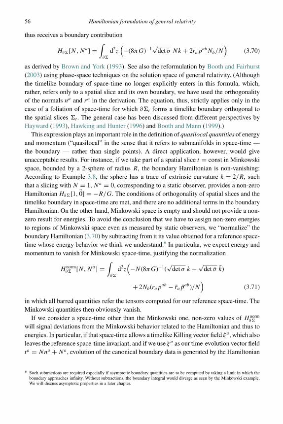
56 Hamiltonian formulation of general relativity
thus receives a boundary contribution
H∂�[N,Na] =∫∂�
d2z(−(8πG)−1
√det σ Nk + 2rap
abNb/N)
(3.70)
as derived by Brown and York (1993). See also the reformulation by Booth and Fairhurst(2003) using phase-space techniques on the solution space of general relativity. (Althoughthe timelike boundary of space-time no longer explicitly enters in this formula, which,rather, refers only to a spatial slice and its own boundary, we have used the orthogonalityof the normals na and ra in the derivation. The equation, thus, strictly applies only in thecase of a foliation of space-time for which ∂�t forms a timelike boundary orthogonal tothe spatial slices �t . The general case has been discussed from different perspectives byHayward (1993), Hawking and Hunter (1996) and Booth and Mann (1999).)
This expression plays an important role in the definition of quasilocal quantities of energyand momentum (“quasilocal” in the sense that it refers to submanifolds in space-time —the boundary — rather than single points). A direct application, however, would giveunacceptable results. For instance, if we take part of a spatial slice t = const in Minkowskispace, bounded by a 2-sphere of radius R, the boundary Hamiltonian is non-vanishing:According to Example 3.8, the sphere has a trace of extrinsic curvature k = 2/R, suchthat a slicing with N = 1, Na = 0, corresponding to a static observer, provides a non-zeroHamiltonian H∂�[1, �0] = −R/G. The conditions of orthogonality of spatial slices and thetimelike boundary in space-time are met, and there are no additional terms in the boundaryHamiltonian. On the other hand, Minkowski space is empty and should not provide a non-zero result for energies. To avoid the conclusion that we have to assign non-zero energiesto regions of Minkowski space even as measured by static observers, we “normalize” theboundary Hamiltonian (3.70) by subtracting from it its value obtained for a reference space-time whose energy behavior we think we understand.6 In particular, we expect energy andmomentum to vanish for Minkowski space-time, justifying the normalization
H norm∂� [N,Na] =
∫∂�
d2z(−N (8πG)−1(
√det σ k −
√det σ k)
+ 2Nb(rapab − rap
ab)/N)
(3.71)
in which all barred quantities refer the tensors computed for our reference space-time. TheMinkowski quantities then obviously vanish.
If we consider a space-time other than the Minkowski one, non-zero values of H norm∂�
will signal deviations from the Minkowski behavior related to the Hamiltonian and thus toenergies. In particular, if that space-time allows a timelike Killing vector field ξa , which alsoleaves the reference space-time invariant, and if we use ξa as our time-evolution vector fieldta = Nna + Na , evolution of the canonical boundary data is generated by the Hamiltonian
6 Such subtractions are required especially if asymptotic boundary quantities are to be computed by taking a limit in which theboundary approaches infinity. Without subtractions, the boundary integral would diverge as seen by the Minkowski example.We will discuss asymptotic properties in a later chapter.
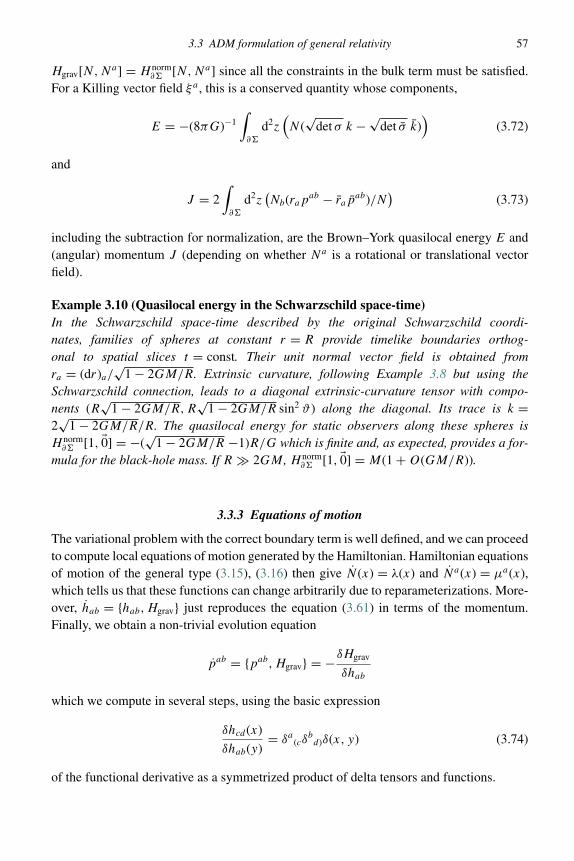
3.3 ADM formulation of general relativity 57
Hgrav[N,Na] = H norm∂� [N,Na] since all the constraints in the bulk term must be satisfied.
For a Killing vector field ξa , this is a conserved quantity whose components,
E = −(8πG)−1∫∂�
d2z(N (
√det σ k −
√det σ k)
)(3.72)
and
J = 2∫∂�
d2z(Nb(rap
ab − rapab)/N
)(3.73)
including the subtraction for normalization, are the Brown–York quasilocal energy E and(angular) momentum J (depending on whether Na is a rotational or translational vectorfield).
Example 3.10 (Quasilocal energy in the Schwarzschild space-time)In the Schwarzschild space-time described by the original Schwarzschild coordi-nates, families of spheres at constant r = R provide timelike boundaries orthog-onal to spatial slices t = const. Their unit normal vector field is obtained fromra = (dr)a/
√1 − 2GM/R. Extrinsic curvature, following Example 3.8 but using the
Schwarzschild connection, leads to a diagonal extrinsic-curvature tensor with compo-nents (R
√1 − 2GM/R,R
√1 − 2GM/R sin2 ϑ) along the diagonal. Its trace is k =
2√
1 − 2GM/R/R. The quasilocal energy for static observers along these spheres isH norm
∂� [1, �0] = −(√
1 − 2GM/R −1)R/G which is finite and, as expected, provides a for-mula for the black-hole mass. If R � 2GM , H norm
∂� [1, �0] = M(1 + O(GM/R)).
3.3.3 Equations of motion
The variational problem with the correct boundary term is well defined, and we can proceedto compute local equations of motion generated by the Hamiltonian. Hamiltonian equationsof motion of the general type (3.15), (3.16) then give N (x) = λ(x) and Na(x) = µa(x),which tells us that these functions can change arbitrarily due to reparameterizations. More-over, hab = {hab,Hgrav} just reproduces the equation (3.61) in terms of the momentum.Finally, we obtain a non-trivial evolution equation
pab = {pab,Hgrav} = −δHgrav
δhab
which we compute in several steps, using the basic expression
δhcd (x)
δhab(y)= δa (cδ
bd)δ(x, y) (3.74)
of the functional derivative as a symmetrized product of delta tensors and functions.

58 Hamiltonian formulation of general relativity
We denote the different hab-dependent terms in Hgrav as
H1 :=∫
d3x16πGN√
det h
(pabpcdhachbd − 1
2pabpcdhabhcd
)(3.75)
H2 := 2∫
d3xpabDaNb = 2∫
d3xpabhbc(∂aNc + Gc
abNd ) (3.76)
H3 := −∫
d3xN
√det h
16πGhab (3)Rab (3.77)
where Gcab are connection coefficients for the spatial covariant derivative Da . In these
expressions, it is important to use indices in positions as they appear in the basic definitions,for instance pab with upper indices. (This tensor density is canonically conjugate to hab andthus to be held fixed in functional derivatives by hab.) Otherwise, one could overlook factorsof the spatial metric which contribute to the functional derivatives. Similarly, covariantderivatives are metric-dependent via the connection coefficients and provide non-vanishingfunctional derivatives.
In the variations of H1, H2 and H3 we will make use of of the formulas (3.37) and (3.41)already computed in Example 3.7:
δ det h = det h habδhab (3.78)
δGabc = 1
2had (Dbδhcd + Dcδhbd − Ddδhbc) . (3.79)
These relations also hold in the three spatial dimensions used here, not just in four space-time dimensions for which they were derived explicitly. We then have
δH1
δhab
= 32πGN√det h
(pacpbdhcd − 1
2pabpc
c
)− 8πGN√
det hhab
(pcdpcd − 1
2(pc
c)2
)from the explicit metric factors as well as the determinant,
δH2
δhab
= 2p(a|c|DcNb) + 2
∫d3xpcdhde
δGecf
δhab
Nf
= 2pc(aDcNb) +
∫d3x
(pcdNf
(Dc
(δa (f δ
bd)δ(x, y)
)+Df
(δa (cδ
bd)δ(x, y)
) − Dd
(δa (cδ
bf )δ(x, y)
)))= 2pc(aDcN
b) −√
det h(Dc
(pc(bNa)/
√det h
)+Df
(pabNf /
√det h
)− Dd
(p(a|d|Nb)/
√det h
))= 2pc(aDcN
b) −√
det hDc
(pabNc/
√det h
)

3.3 ADM formulation of general relativity 59
with several terms from the derivative of connection coefficients, and finally
δH3
δhab
= N√
det h
16πG
(3)Rab − N√
det h
32πGhab(3)R +
∫d3x
N√
det h
16πG
(Dc δG
ddc
δhab
− Dd
δGdcc
δhab
)
= N√
det h
16πG
(3)Rab − N√
det h
32πGhab(3)R +
√det h
(habDcD
cN − DaDbN).
In the last calculation, we have used
∫d3x
N√
det h
16πG
(Dc δG
ddc
δhab
− Dd
δGdcc
δhab
)= 1
2
∫d3xN
√det h
(Dc
(hde
(Dd
(δa(cδ
be)δ(x, y)
) + Dc
(δa(dδ
be)δ(x, y)
)−De
(δa(dδ
bc)δ(x, y)
))) + Dd
(hdehcf
(Dc
(δa(f δ
be)δ(x, y)
)+Df
(δa(cδ
be)δ(x, y)
) − De
(δa(cδ
bf )δ(x, y)
))))= 1
2
∫d3x
√det h
(−(DcN )(D(b
(δa)c δ(x, y)
) + habDcδ(x, y)
−D(a(δb)c δ(x, y)
)) + (DeN )(D(a
(δb)e δ(x, y)
) +D(a(δb)e δ(x, y)
) − habDeδ(x, y)))
= 1
2
√det h(habDcD
cN − 2DaDbN + habDeDeN )
=√
det h(habDcDcN − DaDbN ) .
Combining all variations, we obtain the final equation of motion
pab = −N√
det h
16πG
((3)Rab − 1
2(3)Rhab
)+ 8πGN√
det hhab
(pcdpcd − 1
2(pc
c)2
)
− 32πGN√det h
(pacpc
b − 1
2pabpc
c
)+
√det h
16πG(DaDbN − habDcD
cN )
+√
det hDc(pabNc/
√det h) − 2pc(aDcN
b) . (3.80)
So far, we have used only the gravitational part of the action given by SEH. If mattersources are present, they, too, contribute to the action and thus to the canonical constraints.

60 Hamiltonian formulation of general relativity
In particular, the matter Hamiltonian will be added to the Hamiltonian constraint Cgrav, andenergy flows of matter to the diffeomorphism constraint C
grava . The canonical derivation
presents these contributions in terms of functional derivatives of the matter energy, whichallows one to relate the terms to physical components of the stress-energy tensor. We willdiscuss examples in more detail in Chapter 3.6.
Alternative gravity theories Along similar lines, canonical formulations are performed foralternative theories of gravity, such as higher-curvature actions where curvature invariantsobtained from contractions of the Riemann tensor are added to the Einstein–Hilbert action,or theories in higher dimensions. With higher-curvature terms, new degrees of freedomnormally arise and the phase space is enlarged. In the space-time picture, this results fromhigher-derivative terms in the action, with field equations no longer of second order. Then,some of the first-order time derivatives are to be treated as independent variables ratherthan momenta, and they have momenta of their own. One can see this from the variationalequations, which for a Lagrangian L(q, q, . . . , q (m)) depending on derivatives up to orderm are
m∑k=0
(−1)kdk
dtk∂L
∂q(k)= 0 . (3.81)
By the Ostrogradsky procedure, one reformulates this higher-order equation as a first-order system by introducing the variables pm−1 := ∂L/∂q(m) and recursively pk−1 :=∂L/∂q(k) − pk for 1 ≤ k ≤ m − 1. The equation (3.81), when combined with the definingequations for all the pi , then takes the Hamiltonian form p0 = ∂L/∂q. A discussion of Leg-endre transformation shows that pk plays the role of the momentum of q(k). This procedurehas been reviewed for instance by Govaerts and Rashid (1994) who have also provided a sys-tematic formulation in the spirit of constrained systems. The higher-derivative Lagrangianis extended by auxiliary degrees of freedom qk and µk , 1 ≤ k ≤ m − 1, appearing in theextended Lagrangian
L(q, q, qk, qk, µk) := L(q, qk, qm−1) +m∑
k=1
µk(qk − qk−1) (3.82)
where L is the original higher-order Lagrangian with higher derivatives reduced to first-order ones using the auxiliary variables subject to the relations qk = qk−1 imposed viaconstraints. (We identify q0 := q.)
Example 3.11 (Auxiliary variables)A canonical analysis of (3.82) leads to momenta p0 := p = ∂L/∂q, pk = ∂L/∂qk of qk
and πk = ∂L/∂µk of µk , the latter constrained to vanish as primary constraints. Anotherset of primary constraints follows from the definition of pk: ψk := pk−1 − µk = 0 for1 ≤ k ≤ m − 1. (Although qk appears in the action, for k ≤ m − 2 this happens only
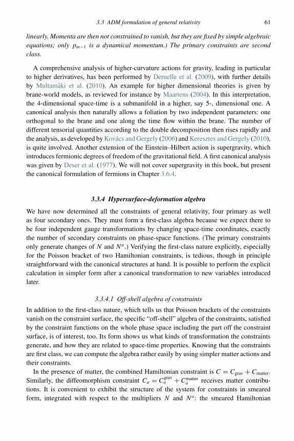
3.3 ADM formulation of general relativity 61
linearly. Momenta are then not constrained to vanish, but they are fixed by simple algebraicequations; only pm−1 is a dynamical momentum.) The primary constraints are secondclass.
A comprehensive analysis of higher-curvature actions for gravity, leading in particularto higher derivatives, has been performed by Deruelle et al. (2009), with further detailsby Multamaki et al. (2010). An example for higher dimensional theories is given bybrane-world models, as reviewed for instance by Maartens (2004). In this interpretation,the 4-dimensional space-time is a submanifold in a higher, say 5-, dimensional one. Acanonical analysis then naturally allows a foliation by two independent parameters: oneorthogonal to the brane and one along the time flow within the brane. The number ofdifferent tensorial quantities according to the double decomposition then rises rapidly andthe analysis, as developed by Kovacs and Gergely (2006) and Keresztes and Gergely (2010),is quite involved. Another extension of the Einstein–Hilbert action is supergravity, whichintroduces fermionic degrees of freedom of the gravitational field. A first canonical analysiswas given by Deser et al. (1977). We will not cover supergravity in this book, but presentthe canonical formulation of fermions in Chapter 3.6.4.
3.3.4 Hypersurface-deformation algebra
We have now determined all the constraints of general relativity, four primary as wellas four secondary ones. They must form a first-class algebra because we expect there tobe four independent gauge transformations by changing space-time coordinates, exactlythe number of secondary constraints on phase-space functions. (The primary constraintsonly generate changes of N and Na .) Verifying the first-class nature explicitly, especiallyfor the Poisson bracket of two Hamiltonian constraints, is tedious, though in principlestraightforward with the canonical structures at hand. It is possible to perform the explicitcalculation in simpler form after a canonical transformation to new variables introducedlater.
3.3.4.1 Off-shell algebra of constraints
In addition to the first-class nature, which tells us that Poisson brackets of the constraintsvanish on the constraint surface, the specific “off-shell” algebra of the constraints, satisfiedby the constraint functions on the whole phase space including the part off the constraintsurface, is of interest, too. Its form shows us what kinds of transformation the constraintsgenerate, and how they are related to space-time properties. Knowing that the constraintsare first class, we can compute the algebra rather easily by using simpler matter actions andtheir constraints.
In the presence of matter, the combined Hamiltonian constraint is C = Cgrav + Cmatter.Similarly, the diffeomorphism constraint Ca = C
grava + Cmatter
a receives matter contribu-tions. It is convenient to exhibit the structure of the system for constraints in smearedform, integrated with respect to the multipliers N and Na: the smeared Hamiltonian

62 Hamiltonian formulation of general relativity
constraint H [N ] = ∫d3xN (x)C(x) and the smeared diffeomorphism constraint D[Na] =∫
d3xNa(x)Ca(x). For two Hamiltonian constraints, we then have
{H [N ],H [M]} = {Hgrav[N ] + Hmatter[N ],Hgrav[M] + Hmatter[M]}= {Hgrav[N ],Hgrav[M]} + {Hgrav[N ],Hmatter[M]}
+ {Hmatter[N ],Hgrav[M]} + {Hmatter[N ],Hmatter[M]} .Now we use the fact that the gravitational Hamiltonian constraint does not contain terms withspatial derivatives of the momenta. If we choose a matter contribution that does not coupleto extrinsic curvature but only to the spatial metric, as it is realized for a (minimally coupled)scalar field or the Maxwell Hamiltonian, no integrations by parts have to be performed incomputing the mixed bracket {Hgrav[N ],Hmatter[M]}. Thus, no derivatives of lapse func-tions occur, and the combination {Hgrav[N ],Hmatter[M]} + {Hmatter[N ],Hgrav[M]} of mixedbrackets is proportional to NM − MN = 0. For matter without curvature couplings, wehave
{H [N ],H [M]} = {Hgrav[N ],Hgrav[M]} + {Hmatter[N ],Hmatter[M]} . (3.83)
Minimally coupled scalar field Here, the second term can be computed easily if we choosea simple scalar field ϕ with momentum pϕ , subject to the Hamiltonian constraint
Hscalar[N ] =∫
d3xN
(1
2
p2ϕ√
det h− 1
2
√det hhab(∂aϕ)(∂bϕ) +
√det hV (ϕ)
)(3.84)
and the diffeomorphism constraint
Dscalar[Na] =
∫d3xNa(∂aϕ)pϕ . (3.85)
Functional derivatives of Hscalar[N ] are easy to compute:
δHscalar[N ]
δϕ(x)=
√det hhab(∂aN )(∂bϕ) + N∂a
(√det hhab∂bϕ
)+ N
√det h
dV
dϕ
δHscalar[N ]
δpϕ(x)= N
pϕ√det h
which gives
δHscalar[N ]
δϕ
δHscalar[M]
δpϕ
− δHscalar[M]
δϕ
δHscalar[N ]
δpϕ
= hab(∂bϕ)pϕ(M∂aN − N∂aM)
and upon integration
{Hscalar[N ],Hscalar[M]} = Dscalar[hab(M∂bN − N∂bM)] . (3.86)

3.3 ADM formulation of general relativity 63
The constraint contributions for a scalar field form a linear algebra, with two Hamiltonianconstraints with lapse function N and M having a Poisson bracket equal to the diffeomor-phism constraint with shift vector hab(M∂bN − N∂bM).
Similarly, we compute δDscalar[Na]/δϕ = −∂a(Napϕ), δDscalar[Na]/δpϕ = Na∂ϕ, andthus
{Dscalar[Na],Dscalar[M
a]} =∫
d3x(−∂a(Napϕ)Mb∂bϕ + Na∂aϕ∂b(Mbpϕ)
)= Dscalar[N
a∂aMb − Ma∂aN
b] . (3.87)
Since the diffeomorphism constraint of matter is independent of the metric and its momen-tum, the matter part of the Poisson bracket (3.87) already shows the diffeomorphism con-straint algebra. The Poisson bracket of a Hamiltonian constraint with the diffeomorphismconstraint, on the other hand, requires the gravitational part of the diffeomorphism con-straint to be taken into account due to the metric dependence of the Hamiltonian constraint;see Exercise 3.6.
General algebra Matter contributions do not form individual constraints; they rather con-tribute to the total constraints together with the gravitational parts. Poisson brackets betweenmatter contributions nevertheless tell us what the full constraint algebra must look like,using the fact that we expect it to be first class: according to (3.83), for matter withoutcurvature couplings the gravitational and matter Poisson brackets must add up to a com-bination of full constraints. From (3.86), we know that the matter contributions providea Poisson bracket given by the matter contribution to the diffeomorphism constraint witha specific shift vector. The full algebra can be first class only if the Poisson bracket oftwo gravitational contributions to the Hamiltonian constraint provides the gravitational partof the diffeomorphism constraint with exactly the same shift vector. Thus, we must have{H [N ],H [M]} = −D[hab(N∂bM − M∂bN )].
Explicit calculations for the Poisson brackets involving the diffeomorphism constraint,such as (3.87), complete the full constraint algebra
{D[Nb],D[Ma]} = D[LNbMa] (3.88)
{D[Na],H [N ]} = H [LNaN ] (3.89)
{H [N ],H [M]} = −D[hab(N∂bM − M∂bN )] . (3.90)
In the first two lines, we simply have the expected action of infinitesimal spatial diffeomor-phisms, with multipliers on the right-hand side given by Lie derivatives LNbMa = [N,M]a
and LNaN = Na∂aN . The last line, however, does not have a direct geometrical interpreta-tion and differs from the first two by the appearance of the field hab, a phase-space functionrather than just multipliers. This part of the algebra shows that we are dealing here with
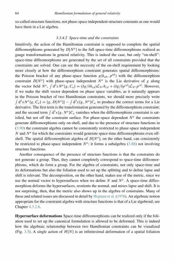
64 Hamiltonian formulation of general relativity
so-called structure functions, not phase-space independent structure constants as one wouldhave them in a Lie algebra.
3.3.4.2 Space-time and the constraints
Intuitively, the action of the Hamiltonian constraint is supposed to complete the spatialdiffeomorphisms generated by D[Na] to the full space-time diffeomorphisms realized asgauge transformations in general relativity. This is indeed the case, but only “on-shell”:space-time diffeomorphisms are generated by the set of all constraints provided that theconstraints are solved. One can see the necessity of the on-shell requirement by lookingmore closely at how the diffeomorphism constraint generates spatial diffeomorphisms:the Poisson bracket of any phase-space function g(hab, p
ab) with the diffeomorphismconstraint D[Na] with phase-space independent Na is the Lie derivative of g alongthe vector field Na ,
∫d3xNa{g,Ca} = (δg/δhcd )LNahcd + (δg/δpcd )LNapcd . However,
if we make the shift vector dependent on phase space variables, as it naturally appearsin the Poisson bracket of two Hamiltonian constraints, we should more precisely write∫
d3xNa{g,Ca} = {g,D[Na]} − ∫d3x{g,Na}Ca to produce the correct terms for a Lie
derivative. The first term is the transformation generated by the diffeomorphism constraint;and the second term
∫d3x{g,Na}Ca vanishes when the diffeomorphism constraint is sat-
isfied, but not off the constraint surface. For phase-space dependent Na the constraintsgenerate diffeomorphisms only on-shell, and due to the presence of structure functions in(3.90) the constraint algebra cannot be consistently restricted to phase-space independentN and Na for which the constraints would generate space-time diffeomorphisms even off-shell. The spatial diffeomorphism algebra of D[Na], on the other hand, can consistentlybe restricted to phase-space independent Na: it forms a subalgebra (3.88) not involvingstructure functions.
Another consequence of the presence of structure functions is that the constraints donot generate a group. Thus, they cannot completely correspond to space-time diffeomor-phisms, which do form a group. For the algebra of constraints, not only space-time andits deformations but also the foliation used to set up the splitting and to define lapse andshift is relevant. The decomposition, on the other hand, makes use of the metric, since weuse the normal vector to hypersurfaces when we define N and Na . A space-time diffeo-morphism deforms the hypersurfaces, reorients the normal, and mixes lapse and shift. It isnot surprising, then, that the metric also shows up in the algebra of constraints. Many ofthese and related issues are discussed in detail by Hojman et al. (1976). An algebraic notionappropriate for the constraint algebra with structure functions is that of a Lie algebroid; seeChapter 4.3.2.6.
Hypersurface deformations Space-time diffeomorphisms can be realized only if the foli-ation used to set up the canonical formulation is allowed to be deformed. This is indeedhow the algebraic relationship between two Hamiltonian constraints can be visualized(Fig. 3.5). A single action of H [N ] is an infinitesimal deformation of a spatial foliation

3.3 ADM formulation of general relativity 65
N
N
NN
N
22
1
1
a
Fig. 3.5 Illustration of the hypersurface deformation algebra. The thin solid line is obtained from theinitial one (bottom) by deforming with N1(x) along the initial normal, the dashed one by deformationwith N2(x). Secondary deformations are then done with respect to the normals of these intermediatesurfaces.
along the normal vector field by a position-dependent amount N (x). The Poisson bracket(3.90) corresponds to the difference in doing two such deformations associated with N (x)and M(x) in a row, but in the two different orderings. Since the second deformation isthen performed with respect to two different intermediate slicings with their normal vectorfields, the result depends on the ordering (unless N and M are constants, in which case thespatial slices are just moved parallel along their normals). Infinitesimally, the differenceis a deformation along the final slice as generated by the spatial diffeomorphism on theright-hand side of (3.90).
The hypersurface-deformation algebra illustrates the underlying covariance of the theory.Such an algebraic property of constraints is more complicated to check than covariance ofan action formulated in terms of space-time tensors, but it has the same content. (It is evenmore general, since it can apply to modified space-time structures as well, as they oftenoccur in quantum descriptions of gravity; see Chapter 6.) Just as the gravitational action isdetermined by the requirements that field equations be covariant and of a certain order inderivatives of the metric as analyzed in detail by Lovelock (1970), the canonical constraintscan be reconstructed from the constraint algebra together with an assumption about thederivative order, as shown by Hojman et al. (1976) and Kuchar (1974).
Poincare algebra For Minkowski space-time, we can use the usual global Cartesian co-ordinates to define spatial slices t = const., on which we have coordinates xa . A Poincaretransformation maps these coordinates to new ones t ′ and x ′a′
, and the new spatial slicest ′ = const. represent a hypersurface deformation of the old ones (or in this specific situation,a hypersurface tilt as defined by Kuchar (1976b)). For a pure rotation, only the shift vectoris non-vanishing and of the form Na = εabcγbxc. A spatial translation has a constant shiftvector Na = δa . For a pure boost, a spatial slice is tilted, represented by a linear lapsefunction N = αax
a vanishing on one plane through the slice with rapidity artanh|α|; seeFig. 3.6. A time translation, finally, has a constant lapse N = β.
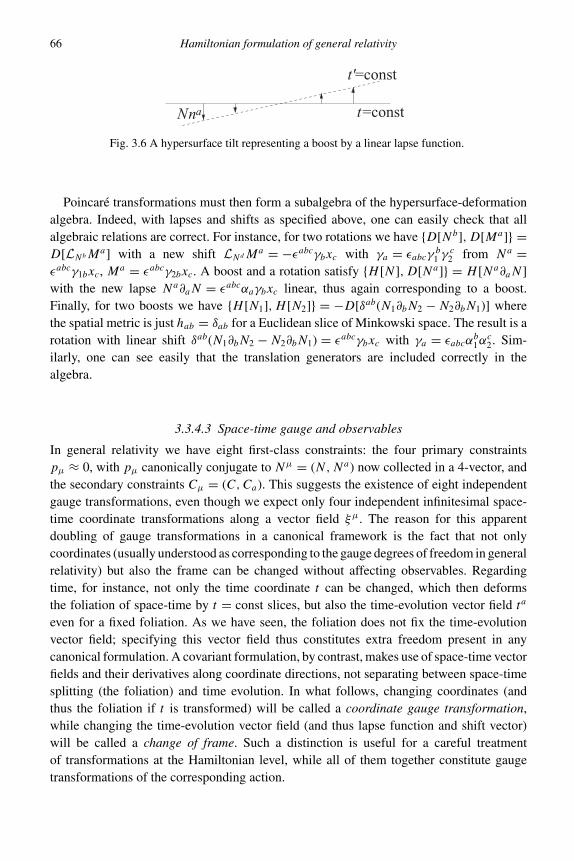
66 Hamiltonian formulation of general relativity
naN t=const
t'=const
Fig. 3.6 A hypersurface tilt representing a boost by a linear lapse function.
Poincare transformations must then form a subalgebra of the hypersurface-deformationalgebra. Indeed, with lapses and shifts as specified above, one can easily check that allalgebraic relations are correct. For instance, for two rotations we have {D[Nb],D[Ma]} =D[LNbMa] with a new shift LNdMa = −εabcγbxc with γa = εabcγ
b1 γ
c2 from Na =
εabcγ1bxc, Ma = εabcγ2bxc. A boost and a rotation satisfy {H [N ],D[Na]} = H [Na∂aN ]with the new lapse Na∂aN = εabcαaγbxc linear, thus again corresponding to a boost.Finally, for two boosts we have {H [N1],H [N2]} = −D[δab(N1∂bN2 − N2∂bN1)] wherethe spatial metric is just hab = δab for a Euclidean slice of Minkowski space. The result is arotation with linear shift δab(N1∂bN2 − N2∂bN1) = εabcγbxc with γa = εabcα
b1α
c2. Sim-
ilarly, one can see easily that the translation generators are included correctly in thealgebra.
3.3.4.3 Space-time gauge and observables
In general relativity we have eight first-class constraints: the four primary constraintspµ ≈ 0, with pµ canonically conjugate to Nµ = (N,Na) now collected in a 4-vector, andthe secondary constraints Cµ = (C,Ca). This suggests the existence of eight independentgauge transformations, even though we expect only four independent infinitesimal space-time coordinate transformations along a vector field ξµ. The reason for this apparentdoubling of gauge transformations in a canonical framework is the fact that not onlycoordinates (usually understood as corresponding to the gauge degrees of freedom in generalrelativity) but also the frame can be changed without affecting observables. Regardingtime, for instance, not only the time coordinate t can be changed, which then deformsthe foliation of space-time by t = const slices, but also the time-evolution vector field ta
even for a fixed foliation. As we have seen, the foliation does not fix the time-evolutionvector field; specifying this vector field thus constitutes extra freedom present in anycanonical formulation. A covariant formulation, by contrast, makes use of space-time vectorfields and their derivatives along coordinate directions, not separating between space-timesplitting (the foliation) and time evolution. In what follows, changing coordinates (andthus the foliation if t is transformed) will be called a coordinate gauge transformation,while changing the time-evolution vector field (and thus lapse function and shift vector)will be called a change of frame. Such a distinction is useful for a careful treatmentof transformations at the Hamiltonian level, while all of them together constitute gaugetransformations of the corresponding action.

3.3 ADM formulation of general relativity 67
Space-time gauge For a full discussion of the space-time gauge in canonical gravity, itis useful to employ the extended phase space, where not only hab and pab are canonicalvariables but also Nµ and pµ. This framework, including its application to gauge transfor-mations and observables, has been developed in particular by Pons et al. (1997). From theperspective of canonical variables, we can see another reason why covariant formulationsmix the roles of gauge and frame, distinguished more clearly in canonical versions. If wewere to take only the four secondary constraints, they generate the correct transformationsof the spatial metric under changes of coordinates. However, the full space-time metric mustchange, but its time-time and time-space components depend only on lapse and shift andthus have vanishing Poisson brackets with the secondary constraints. In order to generatethe correct coordinate transformations of all space-time metric components, the primaryconstraints are also required. But which combination of primary and secondary constraintsgenerates space-time gauge transformations?
The values of the lapse function and shift vector used in a particular space-time gaugemust change when a coordinate transformation is applied. From the canonical perspective,this follows from the fact that lapse and shift enter the equations of motion for the dynamicalvariables via the constraints. If we consider a generic situation of a fully constrainedsystem with a certain number of constraints denoted collectively as C[NA] with severalindependent Lagrange multipliers NA, any phase-space variable q changes in time byq = {q, C[NA]} with respect to the frame specified by a fixed set of NA. (For generalrelativity, NA = (N (x), Na(x)) would be a 4-vector defined on a spatial slice. Counting thespatial dependence, these are infinitely many multipliers.) A coordinate transformation isgenerated by the same constraints: q ′ = q + δεAq with δεAq = {q, C[εA]}. In general, thetransformed q can satisfy the same form of equations of motion,
(q ′). = {q ′, C[N ′A]} , (3.91)
only if there is a non-trivial transformation from NA to N ′A = NA + δεBNA. The equations
written here, together with the constraint algebra, are sufficient to derive the δεBNA and
their generator.We do so by computing both sides of (3.91) separately. On the left, we have
(q ′). = q + (δεAq). = q + δεA q + δεAq
= q + {q, C[εA]} + {q, C[εA]} = q + {{q, C[NB ]}, C[εA]} + {q, C[εA]}= q + {q, {C[NB], C[εA]}} + {q, C[εA]} + {{q, C[εA]}, C[NB]}
using the Jacobi identity in the last step. On the right-hand side of (3.91), we have
{q ′, C[NB ′]} = {q + δεAq, C[NB + δεCNB]}
= q + {q, C[δεANB]} + {δεAq, C[NB ]} + O(ε2)
= q + {q, C[δεANB]} + {{q, C[εA]}, C[NB]}
68 Hamiltonian formulation of general relativity
up to terms of second order in the infinitesimal generator εA. Comparison shows that
C[δεANB] = C[εB] + {C[NB], C[εA]} = C[εB] + C[〈N, ε〉B ] (3.92)
defining the bracket 〈N, ε〉C := NAεBFCAB with the structure constants (or functions)
FCAB of the constraint algebra {C[NA], C[MB]} = C[FC
ABNAMB]. For field theories with
smeared constraints C[Nµ(x)] = ∫d3xNµ(x)Cµ(x), the definition of the structure con-
stants/functions involves integrations:
{C[Nµ(x)], C[Mν(y)]} =∫
d3xd3yd3zNµ(x)Nν(y)Fρµν(x, y; z)Cρ(z) .
From (3.92) we read off the change δεANB = εB + 〈N, ε〉B required for gauge transfor-
mations consistent with the equations of motion. Combined with the gauge transformationsδεAq for dynamical fields, a compact expression for the generator of all gauge transforma-tions is G[εA, εB] = C[εA] + p[εB + 〈N, ε〉B ] where pA are again the momenta of NA,providing the primary constraints now smeared with εB + 〈N, ε〉B . A general gauge trans-formation, including the Lagrange multipliers, thus depends on εA as well as εA. These twofields must be considered as independent, since all fields in the canonical formulation aredefined only on space, while coordinate time is simply a parameter along the gauge flow.The justification for denoting εA in this suggestive way comes from a comparison withequations of motion as in the derivation above, or with space-time gauge transformations,for instance as Lie derivatives, in general relativity.
In fact, as one can verify by explicit calculations, the combination
G[εµ, εµ] = C[εµ] + p[εµ + ∫ d3xd3yNν(x)ελ(y)Fµ
νλ(x, y; z)], (3.93)
smeared with two independent vector fields εµ and εµ and computed with the secondaryconstraints and structure functions F
µνλ(x, y; z) of general relativity, is the generator of
coordinate changes for all the space-time metric components. The structure functionsF
µνλ(x, y; z) can be read off by comparing
{C[λµ], C[κν]} =: C[∫ d3xd3yλµ(x)κν(y)Fρµν(x, y; z)] (3.94)
with (3.88), (3.89) and (3.90). For instance, F 0a0(x, y; z) = δ(x, z)∂ya δ(x, y).
In general relativity, the vector field εµ is defined only on spatial slices, and gives rise to aspatial scalar ε0 parameterizing deformations along the normal of spatial slices, and a spatialvector field εa parameterizing deformations within spatial slices. For a given foliation withunit normal vector field na and spatial vectors sai , i = 1, 2, 3, spanning a basis of vectorfields tangent to the spatial slices, the components of εµ provide a space-time vectorfield
εa = ε0na + εisai . (3.95)
The functional (3.93) generates space-time deformations along this vector field. To comparethis with a coordinate transformation, we must relate the vector field εa decomposed incomponents εµ normal and tangential to spatial slices, to a vector field with components ξµ
3.3 ADM formulation of general relativity 69
along the coordinate lines. Spatial coordinates are not that important in this context, and sowe can assume them to change along the directions sai (or assume that we have chosen thesai along spatial coordinate lines in the first place). The time direction, by contrast, matters:in general, it is not along the unit normal vector field na but along the time-evolutionvector field ta = Nna + Na . Inverting for na and inserting in (3.95) provides the newdecomposition
εa = ε0
Nta +
(εi − Ni
Nε0
)sai =: ξ 0ta + ξ isai . (3.96)
Gauge transformations generated by (3.93) along εa agree with coordinate transformationsxµ → xµ + ξµ, using the relationship (3.96).
Gauge fixing In order to fix the full gauge, gauge-fixing conditions for the primary aswell as secondary constraints must be specified. According to our distinction, this requiresconditions to fix the frame (the choice of lapse and shift entering the time-evolution vectorfield) and the coordinate gauge. It is much easier to discuss frame-fixing, thanks to thesimple form of primary constraints.
The primary constraints appear in the total Hamiltonian Htotal = H + λµpµ with unspec-ified multipliers λµ. Fixing the primary constraints means that we choose four additionalconstraints ψµ = 0 such that the combination of primary constraints and the gauge-fixingconditions ψµ becomes second class. Second-class constraints can directly be solved with-out considering any gauge transformation, which in our context means that the primaryconstraints, and the undetermined multipliers λµ with them, will simply drop out of thetotal Hamiltonian.
With the choice ψµ := Nµ − f µ with certain functions f µ depending only on hab
and pab but not on pµ or Nµ, the primary constraints will clearly be part of a second-class constrained system (pµ,ψ
ν): det{pµ,ψν} �= 0. Solving the second-class constraints
provides the frame-fixed Hamiltonian H = ∫d3xNµCµ = ∫
d3xf µCµ in which lapse andshift have been specified by f µ. After frame-fixing, there is a unique generator of thedynamics.
After solving the second-class part of the frame-fixed system, there still remain thesecondary constraints Cµ generating the coordinate gauge. They, too, may be fixed bygauge-fixing conditions χµ = 0 such that det{χµ,Cν} �= 0, but doing so explicitly in aglobally valid form is much more complicated than for the primary constraints. Moreover,we would want the gauge-fixing conditions to be preserved by the evolution generated byH , imposing the further requirement that
{χµ,H } + ∂χµ
∂t≈
∫d3xf ν{χµ,Cν} + ∂χµ
∂t= 0 .
The matrix {χµ,Cν} here is required to be invertible for good gauge-fixing conditions,and f µ cannot vanish identically for a non-trivial dynamics from H = ∫
d3xf µCµ. Allthese conditions can be reconciled only if ∂χµ/∂t �= 0 for at least one component µ. Inother words, some of the gauge-fixing functions χµ of the secondary constraints must be

70 Hamiltonian formulation of general relativity
explicitly time-dependent, and thus time in this context must be a combination of phase-space variables: we can solve the gauge-fixing conditions for t (at least locally) to obtaina relationship between t and phase-space variables. Such a time variable is called internaltime, rather than an external time parameter as used in coordinate representations. Noticethat this conclusion, which can be found in Pons et al. (1997), of a required internal-timepicture results directly from the fully constrained nature of the system discussed here: onlyin this case are the matrix {χµ,Cν} appearing in the conditions for second-class constraintsafter gauge-fixing and the one appearing in the dynamical preservation of gauge-fixingconditions identical to each other.
Internal time Coordinate time in general relativity appears as a gauge parameter, andthe dynamics is fully constrained. There is no non-trivial Hamiltonian which would takenon-zero values on solutions to the constraints and generate any noticeable change withrespect to some absolute time. If we decide to forgo gauge parameters and gauge-dependentquantities, time in general relativistic systems must be relational: we can notice changenot by the motion of objects with respect to an external time parameter, but by the relativechange of one object or degree of freedom with respect to another one. This viewpoint hasbeen and is still being developed by Bergmann (1961); Rovelli (1991) and Dittrich (2006,2007).
The choice of the object whose change is to be described usually depends on the physicalquestions asked, for instance the growth of the scale factor a in cosmology. Its change, in agauge-independent manner, must be described with respect to another degree of freedom,such as a matter field ϕ. The choice of this reference degree of freedom, then called internaltime, is rather arbitrary. Ideally, one would like a quantity that has a monotonic relationshipwith coordinate time t in a gauge-dependent formulation. Any event characterized by afixed value of ϕ would then correspond to a unique time slice t = const. However, findingsuch a variable is very difficult, except for some simple models; this constitutes the problemof time, reviewed by Kuchar (1992).
The relationship between coordinate-time and internal-time formulations can explicitlybe demonstrated for so-called deparameterizable systems. They exist in two types: “non-relativistic” and “relativistic”. In each case, a system is deparameterizable if its Hamiltonianconstraint can be brought to the form
C = −f (q, p) + g(q, p)h(pϕ) = 0 (3.97)
with a function h depending only on the momentum pϕ conjugate to the choice of internaltimeϕ, and two other functions f and g which depend only on canonical variables other thanϕ and pϕ . For h(pϕ) = pϕ (or some other linear function), the system is “non-relativistic,”for h(pϕ) = p2
ϕ (or some other quadratic polynomial) the system is “relativistic.” Thedistinction here refers to the usual energy dependence of dispersion relations in non-relativistic and relativistic systems, respectively, with pϕ as the momentum of time playingthe role of energy. This is a property of the deparameterization, not of the physical model
3.3 ADM formulation of general relativity 71
considered. There are “relativistic” as well as “non-relativistic” deparameterizations ofmodels in general relativity, as we will see.
We now describe the “relativistic” version in more detail, but the “non-relativistic” oneis very analogous (and slightly simpler). There are then two possible procedures: we cantreat the constraint (3.97) as a generator of gauge transformations with coordinate time asthe gauge parameter, or we can solve the constraint for pϕ and treat pϕ as a Hamiltoniangenerating evolution with respect to internal timeϕ. The latter procedure is reasonable, sincethe evolution generated for ϕ, dϕ/dϕ = {ϕ, pϕ} = 1 makes sure that ϕ proceeds uniformly.In order to show that pϕ is indeed the Hamiltonian for evolution with respect to ϕ, we willnow evaluate both procedures and verify that they are equivalent.
Let us focus on a phase-space function x(q, p) independent of ϕ and pϕ . In coordinatetime, it changes by
dx
dt= {x, C} = −{x, f } + {x, g}p2
ϕ
The variable ϕ changes by
dϕ
dt= {ϕ,C} = 2gpϕ .
The Hamiltonian pϕ(q, p) = ±√f/g generates evolution with respect to internal time:
dx
dϕ= {x, pϕ(q, p)} = ±g−1{x, f } − fg−2{x, g}
2√f/g
= − dx/dt
dϕ/dt.
Except for the minus sign, all these equations of motion are consistent with each otheraccording to the chain rule.
Evolving observables The equation of motion dx/dϕ = {x, pϕ(q, p)} is a differentialequation for x(ϕ), possibly coupled to other equations for the remaining canonical variables.If we can find the general solution x(ϕ; q0, p0) parameterized by labels q0,p0 which one mayinterpret as the initial values of q and p at some fixed time ϕ0, we obtain a gauge-invariantDirac observable: Gauge transformations
{x(ϕ; q0, p0), C(q0, p0, pϕ)} = −{x, f } + {x, g}p2ϕ + 2gpϕ
dx
dϕ= 0
of x(ϕ; q0, p0), interpreted as a phase-space function via (q0, p0) and parameterized by ϕ,vanish.
Example 3.12 (Free, massless relativistic particle in one dimension)The energy relation for a free, massless relativistic particle amounts to the constraintC = −p2 + p2
ϕ = 0, where pϕ is the energy conjugate to an internal time ϕ. Solving theconstraint implies pϕ = |p| as the Hamiltonian in internal time (assuming the “energy”pϕ to be positive). Internal-time equations of motion are dq/dϕ = sgnp and dp/dϕ = 0.While p is constant and already a Dirac observable, for q(ϕ) we obtain the solutions
72 Hamiltonian formulation of general relativity
q(ϕ; q0, p0) = q0 + ϕ sgnp0. A direct calculation verifies that {q(ϕ; q0, p0),−p20 + p2
ϕ} =−2p0 + 2pϕ sgnp0 = 0.
Equations of motion in coordinate time are dq/dt = −2p, dp/dt = 0, dϕ/dt = 2pϕ anddpϕ/dt = 0. Clearly, dq/dϕ = sgnp = 2p/2|p| = −(dq/dt)/(dϕ/dt).
3.4 Initial-value problem
For testable predictions, any theory must provide unique solutions in terms of suitable initialdata. This corresponds to the practical situation in which one sets up an experiment, thatis, specifies an initial configuration and boundary conditions, and then makes observationsto be eventually compared with theoretical predictions. A basic mathematical requirementfor the equations underlying a theoretical framework is thus that they form a well-posedinitial-value problem: for any allowed set of initial values a unique solution must existsuch that it depends on the initial data in a continuous manner. The first condition ensurespredictivity, the latter is added in order to ensure stability in situations in which initialvalues cannot be arranged to arbitrary precision. For general relativity, analyzing theserather practical questions is closely related to the issue of space-time gauge; see also thereview by Friedrich and Rendall (2000).
3.4.1 Hyperbolic systems
Well-posedness is often realized if the underlying differential equations are hyperbolic. Weassume a quasi-linear system of k differential equations of order m in n variables, of thegeneral form ∑
∑i αi=m
A(α1,...,αn)[u](x)∂α1
x1 · · · ∂αn
xn u = L[u] (3.98)
where u(x) ∈ Rk collects the unknown functions, L[·] is an arbitrary (possibly non-linear)derivative operator of order m − 1 and A(α1,...,αn)[u](x) are coefficients forming a k × k-matrix depending on x and derivatives ∂
α1
x1 · · · ∂αn
xn u of lower order∑
i αi < m. Only thehighest-order derivative with
∑i αi = m, explicitly written in (3.98), thus appears in linear
form, but not lower order ones.For a quasi-linear system, we define the principal symbol
σ (x, u, ξa) :=∑α
A(α1,...,αn)[u](x)ξα11 · · · ξαn
n (3.99)
evaluated in an arbitrary covector ξa , whose components are taken to the powers αi . Theprincipal symbol is thus a k × k-matrix which depends on x, u and the inserted covector.A characteristic is a co-vector ξa satisfying the characteristic equation
det σ (x, u, ξa) = 0 . (3.100)
3.4 Initial-value problem 73
A characteristic surface is a constant-level surface � = const for which the differential d�is a characteristic. In particular, a characteristic surface requires a real-valued characteristic.
Example 3.13 (Wave equation)For the 2-dimensional Klein–Gordon wave equation φ − φ′′ + V (φ) = 0 we have the prin-cipal symbol σ (ξ ) = ξ 2
t − ξ 2x , which is independent of t , x and φ. Characteristic surfaces
are obtained from functions � satisfying �2 − �′2 = 0, solved by �(t, x) = f (t ± x) withan arbitrary function f . The surfaces � = const are given by the 2-dimensional light conest ± x = const.
In general, characteristic surfaces correspond to wave fronts and determine the localform of linearized plane wave solutions. They are thus relevant for the propagation ofinitial values.
A quasi-linear system is called hyperbolic if km real characteristics exist, counting theirmultiplicity as solutions of the characteristic equation (3.100). It is called strictly hyperbolicif km distinct real characteristics exist. Strictly hyperbolic systems are important becausethey can be shown to define well-posed initial value problems. For instance, by the precedingexample, we know that a single wave equation is strictly hyperbolic. But two coupled waveequations of the same type are only hyperbolic and not strictly hyperbolic because themultiplicity of characteristics is increased. Strictly hyperbolic systems are rather specialand do not encompass all types of wave equation found even in simple examples.
A more general version of hyperbolicity, which is implied by strict hyperbolicity, issymmetric hyperbolicity. A symmetric hyperbolic system is a set of first-order equations
A0(t, x, u)∂tu + Ai(t, x, u)∂iu + B(t, x, u) = 0 (3.101)
such that A0 and Ai are symmetric matrices and A0 is positive definite. Symmetric hyper-bolicity is defined only for first-order equations, but this is not a strong restriction, sincehigher-order equations can be reformulated as first-order ones by introducing auxiliaryfields. However, hyperbolicity properties of the resulting system may depend on how thereformulation is performed.
Example 3.14 (Wave equation in symmetric hyperbolic form)In the wave equation φ − φ′′ + V (φ) = 0 we introduce ψ := φ and σ := φ′ so as totransform it to a set of first-order differential equations. As our independent functions weuse φ, σ and ψ and impose the additional condition σ = φ′ = ψ ′ as it follows from thedefinitions. Then, an equivalent formulation of the wave equation is
∂t
φ
σ
ψ
=0 0 0
0 0 10 1 0
∂x
φ
σ
ψ
+ ψ
0−V (φ)
which is of symmetric hyperbolic form.
Had we chosen to use φ′ = σ as one of the differential equations instead of σ = ψ ′, theresulting system would not have been symmetric hyperbolic, although it would certainly
74 Hamiltonian formulation of general relativity
have been equivalent to the same second-order wave equation. This demonstrates how thechoice of independent fields matters in the formulation as a symmetric hyperbolic system.In more complicated cases, such as Einstein’s equations, exploring the possibilities ofbringing a system to symmetric hyperbolic form can be quite involved.
The example also illustrates the importance of the signature for hyperbolicity: for the dif-
ferential operator φ + φ′′ the same procedure would result in a matrixAx =0 0 0
0 0 10 −1 0
which is not symmetric. This cannot be repaired by a different choice of independent fieldbecause the equation is elliptic, not hyperbolic.
Symmetric hyperbolic systems are more general than strictly hyperbolic ones; forinstance, coupling two wave equations would leave the system symmetric hyperbolic butnot strictly hyperbolic. Even the more general symmetric hyperbolic systems are wellposed, the proof of which we sketch here for the case of A0 = 1.7 We will also assume ∂iA
i
and B to be bounded. The key tool in the proof is the energy functional
E =∫�
||u||2dn−1x (3.102)
over surfaces t = const. It will allow us to use ordinary differential-equation techniques toanalyze partial differential equations.
We assume u to be of compact support and provide an energy estimate, i.e. an upperbound for
dE
dt= 2
∫�
〈u, u〉dn−1x = −2∫�
〈u,Ai∂iu + B〉dn−1x . (3.103)
Using the symmetry of Ai , we have∫�
〈u,Ai∂iu〉dn−1x =∫�
〈Aiu, ∂iu〉dn−1x
=∫�
∂i〈Aiu, u〉dn−1x −∫�
〈∂i(Aiu), u〉dn−1x
= −∫�
〈(∂iAi)u, u〉dn−1x −∫�
〈Ai∂iu, u〉dn−1x
and thus
−2∫�
〈u,Ai∂iu〉dn−1x =∫�
〈(∂iAi)u, u〉dn−1x .
7 This is a restriction and cannot always be achieved by diagonalization while preserving the symmetric hyperbolic form. Onecan certainly write A0 = R−1DR with an orthogonal matrix R and a diagonal one D, since A0 is symmetric in the symmetrichyperbolic case. Moreover, D cannot have vanishing entries for A0 to be positive definite; they could thus be transformed toone by rescalings. However, the components of R and D will in general depend on the coordinates and, more importantly in thiscontext, on u, preventing us from absorbing the rotations and rescalings in a redefined dependent vector u without introducingextra terms from derivatives. More general proofs exist to show well-posedness of any strictly hyperbolic system.

3.4 Initial-value problem 75
Applying the Cauchy–Schwarz inequality to (3.103)∣∣∣∣dE
dt
∣∣∣∣ =∣∣∣∣∫
�
〈(∂iAi)u, u〉dn−1x − 2∫�
〈u,B〉dn−1x
∣∣∣∣≤
(∫�
||(∂iAi)u − 2B||2dn−1x
)1/2 (∫�
||u||2dn−1x
)1/2
≤ ||∂iAi ||sup
∫�
||u||2dn−1x + 2
(∫�
||B||2dn−1x
)1/2 (∫�
||u||2dn−1x
)1/2
≤ C1E + C2
√E (3.104)
for some constants C1 and C2 obtained as the supremum of ∂iAi and the L2-norm of B,
respectively.This energy estimate can now be used to conclude uniqueness of solutions: assume
that we have two solutions u1 and u2 for the same initial data and consider E :=∫�
||u1 − u2||2dn−1x. Since both solutions have the same initial data, we have thatEt=0 = 0. Moreover, the energy estimate implies that 0 ≤ |dE/dt | ≤ C1E + C2
√E and
thus (dE/dt)t=0 = 0. Taking time derivatives8 of (3.104) and applying the same reasoningthen shows that all time derivatives of E vanish at E = 0, and E(t) = 0 must be identicallysatisfied (using analyticity). Thus, u1 = u2 and any two solutions with the same initialvalues must be identical. (At this point the positive definiteness of A0 would be used in ageneral derivation.)
Similarly, we can derive stability because the energy estimate implies that dE/dt mustbe small if E is small, i.e. nearby solutions deviate from each other only slowly. Todemonstrate the existence of solutions for given initial data, we can choose a functionbasis, approximate it by a finite set and thus map the partial differential equation to a largesystem of ordinary differential equations. For the latter, there are general results which implythe existence of solutions, and we can use continuity to take the limit back to the infinitebasis.
3.4.2 Hyperbolic reductions
In its canonical formulation, Einstein’s equation is formulated as a set of first-order equa-tions. The ADM form, however, does not make this system symmetric hyperbolic. Forinstance, the corresponding A0 is degenerate: from the point of view of differential equa-tions, N and Na are independent functions but do not appear with time derivatives inequations of motion. Instead, they can be freely chosen and determine the space-time
8 An inequality f1(x) ≤ f2(x) for two differentiable functions does not imply that f ′1(x) ≤ f ′
2(x) as one can easily see fromexamples. But if f1(0) = f2(0), the inequality does imply that f ′
1(x) ≤ f ′2(x) in a neighborhood of zero. This is the situation
we have here.

76 Hamiltonian formulation of general relativity
frame, that is, the direction of the flow of time used in the differential equations themselves.In the presence of arbitrary functions in the equations, the solution for hab and pab start-ing from given initial data cannot be unique, which would be one of the requirements ofwell-posedness.
3.4.2.1 Space-time gauge
Especially for numerical relativity — the development of computational codes to solve andevaluate the equations — this constitutes a problem that may be dealt with by includingadditional equations, such as gauge-fixing conditions. To motivate common choices, it isuseful to discuss the relation of N and Na , or the frame, to the space-time gauge determinedby choosing coordinates such that the time evolution vector field is ∂/∂t .
Let us start with an arbitrary coordinate system t ′, x ′a′, in which the metric tensor has
components g′µ′ν ′. Metric components in canonical form (3.44) are determined by
− 1
N (t, xa)2= g′µ′ν ′
(x ′)∂µ′ t∂ν ′ t (3.105)
1
N (t, xc)2Na(t, xc) = g′µ′ν ′
(x ′)∂µ′ t∂ν ′xa (3.106)
as they follow from the general tensor transformation law. For a given, specified choice oflapse and shift, these equations may initially not be satisfied, but one may view them aspartial differential equations for new coordinates t(x ′), xa(x ′) such that the metric becomesone written in the desired frame: g00 = −1/N2 and g0a = Na/N2 according to (3.44). Forinstance, (3.105) has the form of a wave equation for t coupled to the remaining equationsthrough xa . In this way, prescribing N and Na can be seen as determining coordinatesystems, and thus the space-time manifold via the atlas they form.
Solutions to canonical equations depend on initial values for hab and pab, but also on N
and Na as gauge conditions (on all of space-time). For given N and Na , coordinates canbe determined in the way described, which implies that the manifold is part of the solution.This is the distinguishing feature of general relativity as a generally covariant framework,in contrast to other field theories such as Maxwell theory whose solutions are functions ona given manifold.
In this sense, general relativity provides dynamical equations not for fields on a givenspace-time, but for space-time itself. This property is one of immense implications forthe fundamental understanding of nature, but it complicates the issue of well-posednessof the field equations. Having to specify certain functions, lapse and shift, on the wholespace-time, not just their initial values, is unsuitable for an initial-value problem. Alsopractically, there is too much freedom in choosing N and Na to achieve desired propertiesfor space-time representations in numerical codes. For a more tractable set of equations,one has to reformulate the system of equations further by introducing new equations forlapse and shift which determine them through initial values. This can only be achieved byparameterizing the gauge freedom more conveniently, for instance by coupling lapse and

3.4 Initial-value problem 77
shift to gauge-source functions: source terms appearing in differential equations for lapseand shift or for coordinates. If a hyperbolic system results in this way, the reformulation iscalled a hyperbolic reduction, discussed by Friedrich (1996).
3.4.2.2 Gauge-source functions and the ADM system
A gauge-source function cannot be formulated in terms of tensors, which would be insen-sitive to the gauge. Any equation fixing the gauge must be non-covariant so that it canbe satisfied only in one coordinate system. A natural choice is to use the non-tensorialChristoffel symbols for this purpose. In particular, we may take the contracted coefficients�µ := gνλ�µ
νλ and require that they equal a fixed set of functions,�µ = Fµ. This conditionprovides differential equations for new coordinates x ′ν ′
, since
∇µ′∇µ′x ′ν ′ = gµ′λ′∇µ′δν
′λ′ = −gµ′λ′
�ρ ′µ′λ′δ
ν ′ρ ′ = −�ν ′ = −Fν ′
. (3.107)
(Note that we have to treat x ′ν ′as functions rather than a tensor in the first covariant
derivative. The second covariant derivative then acts on a tensor provided by the firstcovariant derivative, which results in the connection coefficients.) Since (3.107) providesstandard wave equations known to be well-posed, solutions determine coordinates onspace-time from given initial values.
A common choice is Fµ = 0, in which case one obtains harmonic coordinates satisfying∇µ∇µx ′ν ′ = 0. These coordinates have several analytical but also numerical advantagesas pointed out by Bona and Masso (1988, 1992). The first numerical results obtainedby Pretorius (2005) for the form of gravitational waves from merging black holes wereextracted using generalized harmonic coordinates introduced by Garfinkle (2002), obeying(3.107) with functions Fν ′
that are evolved numerically, starting with the harmonic initialcondition Fν ′ = 0. The equations they obey specify the gauge, or the evolution of theframe.
Alternatively, one obtains evolution equations for lapse and shift by prescribing theFν on all of space-time. From the equation for the Christoffel coefficients in terms ofpartial derivatives of metric components, applied to the canonical metric, one obtains (seeExercise 3.12)
∂tN − Na∂aN = N2(Kaa − na�a) (3.108)
∂tNa − Nb∂bN
a = N2(Ga − Da logN − hab�
b) (3.109)
where Ga := hbcGabc, Ga
bc being the spatial connection components as used before. Withthese equations we have first-order differential equations for lapse and shift in terms of thegauge-source functions �a , which complement the equations of motion (and constraints)we already have for hab and Kab from the ADM formulation.
In order to see their hyperbolicity, we reformulate all equations as second-order differ-ential equations for N , Na and hab for a given �a . The leading differential order in the
78 Hamiltonian formulation of general relativity
equation of motion for N is then
1
N2(∂t − Na∂a)2N = (∂t − Na∂a)Ka
a + lower-order terms
= DaDaN + lower-order terms
= hab∂a∂bN + lower-order terms
where we have used the first-order equation of motion for Kaa and the Hamiltonian
constraint to express (3)R in terms of lower-order derivatives. Similarly, we obtain
1
N2(∂t − Na∂a)2Nb − hcd∂c∂dN
a = lower-order terms
1
N2(∂t − Na∂a)2hbc − hde∂d∂ehbc = lower-order terms
with the same differential operators at the highest (second) order. Since lower-order deriva-tives, even non-linear ones, do not matter for hyperbolicity, they need not be consideredhere. Then, all fields are subject to the same hyperbolic type of differential equationgab∂a∂bf = lower-order terms with the canonical metric gab from (3.44), coupled to eachother only via the lower-order terms.
We have seen that coupling different wave equations of the same type, as now realizedby the second-order equations for N , Na and hab, does not lead to a strictly hyperbolicsystem. However, we can formulate all the second-order wave equations as first-ordersymmetric hyperbolic systems as in Example 3.14. The property of symmetric hyperbolicityis preserved under coupling different equations, which proves that the whole system of ourequations is symmetric hyperbolic and thus well-posed. For any given set of gauge-sourcefunctions �µ, we obtain a unique solution in terms of initial data. The �µ must be specifiedon all of space-time, not just on the initial slice. Changing the gauge-source functionsimplies that we choose different coordinates determined by them as source terms via(3.107). For given initial values, solutions to general relativity are unique up to coordinatechanges. The evolution of space-time geometry is uniquely determined.
3.4.2.3 BSSN equations
The ADM system has been used for some time in numerical relativity; see, e.g., some ofthe results reported by Bona et al. (1995) and Brady et al. (1998). However, it transpiresthat there are several difficulties regarding a consistent numerical implementation, see,e.g., the discussion by Choptuik (1991) and Frittelli (1997). A useful reformulation of theADM system was introduced by Baumgarte and Shapiro (1998) and Shibata and Nakamura(1995) by splitting a conformal factor off the spatial metric, and the trace off the extrinsiccurvature. That is, instead of hab andKab, the variables h := det hab, hab := h−1/3hab,K :=habKab and Kab := h−1/3(Kab − 1
3Khab) are used in the evolution equations. For instance,
3.4 Initial-value problem 79
we have
K − NcDcK = −N (h2/3KabKab + 1
3K2) + DaDaN (3.110)
using (3.80) and the Hamiltonian constraint. (Variables of fractional density weights occurin some of the equations, which is to be taken into account when computing Lie derivativesalong the time-evolution vector field.)
So far, only the original ADM system has been reformulated, and the same problemsregarding gauge exist. By accompanying the evolution equations for log h, hab, K and Kab
with evolution equations for the new gauge-source functions �a := hbc�abc, computed for
the conformal metric hab, a new symmetric hyperbolic system results. Evolution equationsfor �a = −∂bh
ab (using det(hab) = 1) are obtained from (3.61) via ∂t �a = −∂b(∂t hab). In
the numerical BSSN codes which have successfully produced black-hole mergers and theresulting gravitational wave-forms, the evolution equations for logh, hab, K , Kab and �a
are accompanied by modified evolution equations for lapse and shift, rather than (3.108) and(3.109). Campanelli et al. (2006) use a relation similar to (3.108) for ∂tN and ∂tN
a = Ba
with a new function Ba satisfying ∂tBa = − 3
4∂t �a − ηBa for some parameter η. In this
way, the lapse function can be evolved regularly for a long time. Baker et al. (2006) modifythese equations further. At this stage, it is mainly numerical advantages that motivate thechoices. For reviews of numerical relativity, see, e.g., Lehner (2001) and Baumgarte andShapiro (2010).
3.4.3 Slicing conditions
Gauge-source functions such as �µ allow us to prove well-posedness, but they do notalways lead easily to intuitive choices that may improve the stability of numerical evolution.Also, directly specifying lapse and shift is often inconvenient. With the simplest choice,N = 1 and Na = 0, for instance, one cannot rule out that singularities are approachedtoo quickly. In order to have a good numerical evolution of black holes, valid for longtimes in regions far away from singularities, one must ensure that the evolved geometriesstay away from singularities long enough everywhere on the spatial slices. If we indeedmake the choice N = 1, Na = 0 in a black-hole space-time of mass M , this would onlyallow a small amount of proper time of about τ = 2M for evolution even far away fromthe horizon. From Eq. (3.110), this choice of frame leads to the equation ∂K/∂t ≥ 1
3K2,
whose solutions, by the same arguments as used for cosmological models in Chapter 2.4,lead to a coordinate singularity with diverging K after a finite amount of time t . See, also,the detailed analysis by Eardley and Smarr (1979).
In order to find good conditions for lapse and shift, one rather refers to geometricalslicing conditions which are formulated more intuitively and can be solved for N and Na .Several of these concepts have been introduced by Smarr and York (1978) and Garfinkle

80 Hamiltonian formulation of general relativity
and Gundlach (1999). The best-known such condition is maximal slicing, defined by
K = − 8πG√det h
paa = 0 , (3.111)
the right-hand side in terms of the canonical momentum evolving according to (3.80). Since(3.111) is to hold at all times, the equation
0 = Lt (pcc) = habp
ab + pabhab
= −√
det h
8πGDaD
aN + LNbpaa + 32πGN√
det h
(pabpab − 1
2(pc
c)2
)(3.112)
follows. With the Hamiltonian constraint and (3.111), this provides an elliptic equation
DaDaN = N (3)R (3.113)
for the lapse function which one can use to determine N at fixed times. Thanks to thecurvature term, this condition tends to suppress N if (3)R becomes large: for such a gaugechoice, evolution slows down when singularities are approached. (See also Exercise 3.13.)
The drawback is that slices are stretched and deformed if their evolution is nearly halted atsome places but continues unhindered elsewhere. This unwelcome feature can be counteredby adapting the shift vector which was free so far. Following Smarr and York (1978), wedefine the distortion
�ab := 1
2(det h)1/3Lt
hab
(det h)1/3(3.114)
= N
(Kab − 1
3habK
cc
)+ D(aNb) − 1
3habDcN
c (3.115)
whose first contribution is the geometric shear, while the rest can be viewed as coordinateshear. Minimizing distortion by varying the functional D := ∫
d3x√
det h�ab�ab with
respect to Nc implies Da�ab = 0, and thus
DaDaNb + 1
3DbDaN
a + (3)RabNa = 2Da
(N
(Kab − 1
3habKcc
)). (3.116)
Also here, we have an elliptic equation for the shift vector, whose solution is called minimal-distortion shift.
While maximal slicings and minimal distortion shifts are desirable, the elliptic equationsthey obey are difficult to solve numerically. One often replaces them by driver conditions,as, e.g., by Balakrishna et al. (1996), which are parabolic equations. For maximal slicing,for instance, one can use
∂tN = ε(DaDaN − N (3)R) (3.117)
for some parameter ε. Solutions to this equation are driven toward the fixed point wherethe right-hand side vanishes. This also ensures stability of the maximal slicing conditionbecause deviations due to numerical errors cannot grow when the solution is driven backto the fixed point.

3.4 Initial-value problem 81
3.4.4 Constraints on initial values
By the preceding schemes, evolution from given initial values is formulated in a way usefulfor numerical procedures. However, evolution equations are not the only equations to besolved: initial values cannot be arbitrary but must obey the constraints. Constraints onspatial fields are not hyperbolic equations but elliptic ones, of the form
DaKab = 0
(3)R + (Kaa)2 − KabK
ab = 0
(in vacuum) and thus numerically difficult to deal with. The complexity can, however, bereduced by analytical manipulations.
If we assume maximal slicing, one term already drops out of the Hamiltonian constraintdue to Ka
a = 0. As in the BSSN scheme, we then apply a conformal transformationdefining hab = φ−4hab, such that hab = φ4hab. Similarly, we rescale the now tracelessKab by Kab = φ−sKab for some s to be determined. Here, however, we do not imposeconditions on hab or hab to fix φ; rather, we introduce φ as a new degree of freedomobeying an equation to be solved for later on. Starting with any pair (hab,Kab) with Kab
traceless and solving the diffeomorphism constraint, a suitable φ can then be found suchthat the rescaled quantities satisfy the Hamiltonian constraint, as well.
To derive the required equations, we must apply the conformal transformation by φ to thecurvature components. First, the transformation of the Christoffel symbols can be obtainedthrough the tensor Cc
ab in Daωb = Daωb − Ccabωc such that
Ccab = 1
2hcd
(Dahbd + Dbhad − Ddhab
)= 2
(hcbDa logφ + hc
aDb logφ − habDc logφ
). (3.118)
Then, we have
DaKab = φ−4hac(Dc(φ
sKab) − Cdcaφ
sKdb − Cdcbφ
sKad
)= φ−4+s
(DaKab + (s + 2)KabD
a logφ − 2KaaDb logφ
)= φ−4+sDaKab (3.119)
simplified using maximal slicing and setting s = −2 at this stage. Finally, transforming thespatial Ricci scalar, the Hamiltonian constraint with maximal slicing (and keeping s = −2)becomes
(3)R − KabKab = −8φ−5
(DaD
aφ − 1
8(3)Rφ + 1
8φ−7KabK
ab
). (3.120)
To find initial values obeying the constraints, we then solve the diffeomorphism constraintDaKab = 0 for a traceless Kab and some hab freely specified. According to (3.119), thisconstraint remains satisfied after the conformal rescaling with s = −2. The Hamiltonian
82 Hamiltonian formulation of general relativity
constraint, using (3.120) is equivalent to the Lichnerowicz equation
DaDaφ − 1
8(3)Rφ + 1
8φ−7KabK
ab = 0 (3.121)
for φ, using the solution for Kab of the diffeomorphism constraint and the chosen hab.This equation was introduced by Lichnerowicz (1944) and discussed further, e.g. by York(1971). Then, Kab = φ2Kab and hab = φ4hab solve the constraints for maximal slicing.
Example 3.15 (Brill–Lindquist initial data)Brill and Lindquist (1963) have introduced initial data by starting with a time-symmetricinitial surface Kab = 0, which obviously solves the vacuum diffeomorphism constraint.Furthermore, hab is chosen flat such that it only remains to solve the equation DaD
aφ = 0,the linear Laplace equation. The well-known solution φ(r, ϑ, ϕ) = 1 + M/2r in polarcoordinates produces the Schwarzschild metric in its conformally flat form.
With a linear equation for φ, different solutions, and, in particular, different black holes,can be superposed. The solution
φ(xa) = 1 +N∑i=1
αi
2√
(xa − xai )(xb − xb
i )hab
. (3.122)
represents N black holes at initial positions xai . When the distance to all xa
i is large, the con-formal factor behaves as 1 + M/2r with the total mass M = ∑N
i=1 αi . By expanding in thevicinity of a single xa
i , one obtains the individual masses Mi = αi + ∑j �=i αiαj /rij with the
distance raij =√
(xa − xai )(xb − xb
i )hab between two centers. Brandt and Brugmann (1997)have extended this method for an application in numerical relativity. Further constructionsof general N -body initial data have been provided by Chrusciel et al. (2010).
3.5 First-order formulations and Ashtekar variables
The usual formulation of general relativity is of second order: the Einstein–Hilbert action,upon variation by gµν , provides second-order field equations. Alternatively, one can viewthe system as first order if one initially interprets the connection �a
bc as arbitrary, as givenby an additional field independent of gab. In this so-called Palatini formulation,
S[g, �] =∫
d4x√
− det gR[�] (3.123)
is linear in first-order derivatives of the fields, in particular of �, and provides first-ordervariational equations relating gab and �a
bc.With �a
bc an independent field, new variational equations δS/δ�abc = 0 arise and must
be satisfied. To compute this variation, assuming for now no �abc-dependence in the matter
terms, we can make use of the earlier result (3.38) and conclude that δRac = −∇aδ�bbc +
∇bδ�bac. Inserting this in the variation of (3.123) and integrating by parts shows that the
�abc-variation implies the equation of motion ∇agbc = 0.

3.5 First-order formulations and Ashtekar variables 83
Example 3.16 (First-order action)More explicitly, we write
Rab[�] = ∂c�cab − ∂b�
cac + �c
ab�dcd − �c
ad�dbc
and vary the action by �cab. We obtain
−∂c(√
− det ggab) + gbc ∂d (
√− det ggad ) +
√− det ggab�d
cd (3.124)
+√
− det ggdegbc�
ade −
√− det ggad�b
dc −√
− det ggdb�adc = 0
after inserting metric tensors to make all occurrences of �cab appear with the same indices.
If we take a trace of this equation by equating and summing over c and b, it impliesthat ∂d (
√− det ggad ) = −√− det ggde�ade, making the second and fourth terms in (3.124)
cancel each other. The remaining terms on the left-hand side of (3.124) combine to thecovariant derivative ∇c(
√− det ggab) of the tensor density√− det ggab. Thus,
√− det ggab
is covariantly constant, and so is its determinant det(√− det ggab) = det g. Combining
these results, gab and its inverse gab are covariantly constant.
Solving this equation means that �abc must be the Christoffel symbol, as the unique one
compatible with the metric. In terms of the metric, the connection can thus be solved for,irrespective of initial or boundary conditions. Using the metric-compatible connection in theequations of motion following from varying the metric, which is just Rab[�] − 1
2gabR[�] =0, then shows that the same equations of motion result as in the second-order formulation.
The result changes if the connection �abc does appear in the matter action. Then, matter
contributes a source term to the metric compatibility equation and the resulting connectionis no longer Christoffel and typically acquires torsion. Such a situation is usually realizedwhen fermionic matter is coupled to gravity, for which the connection must appear in anon-trivial way. (For minimally coupled scalar or Yang–Mills theories, derivative terms areeither just partial or exterior derivatives and do not require a connection.) We will comeback to this in more detail when discussing matter terms in Chapter 3.6.4.
3.5.1 Tetrad formulation and Holst action
First-order formulations have become particularly important in the Ashtekar framework,which is a canonical formulation of general relativity based on canonical fields given by atriad, instead of the spatial metric, and an independent connection, the Ashtekar connection.From the general viewpoint of constrained systems, this example provides an interestingset of combined first- and second-class constraints.
3.5.1.1 Tetrads and connections
A tetrad provides a way to specify geometries alternative but equivalent to metrics or lineelements. Parallel transport or covariant derivatives are then formulated by connectionswhich generalize the Christoffel symbols of the metric formulation. All curvature tensors
84 Hamiltonian formulation of general relativity
can be computed in a tetrad formulation as well as in a metric formulation, sometimeseven more conveniently so, thanks to the easy use of differential-form notation in tetradlanguage.
Tetrads We define a space-time tetrad as a set of four vector fields eaI , labeled by anadditional index I taking the values 0, 1, 2, 3, such that they provide an orthonormal basisof the tangent space at each point:
gabeaI e
bJ = ηIJ (3.125)
with the Minkowski metric ηIJ . Thus, ea0 is timelike while ea1 , ea2 and ea3 are spacelike.We may view the label I simply as an index to distinguish the vector fields, but a morepowerful interpretation is to think of eaI as a double-vector field: a vector field on the tangentbundle of space-time taking values in Minkowski space. With a 1-form ωa , eaI ωa assigns toevery point in space-time a covector in Minkowski space. In this context, one often thinksof space-time as equipped with two independent vectorial structures: its tangent space aswell as an independent set of Minkowski spaces, one attached to each point. Minkowskispace in this context is called an internal vector space, and eaI ωa of the above examplean internal vector field. A manifold with a copy of the same vector space attached toeach point is called a vector bundle. (For a precise definition, see the Appendix.) Otherexamples of vector bundles are used in particle physics, where internal spaces correspondto representation spaces of the gauge groups of fundamental interactions.
Using the Minkowski metric, we can contract the internal indices of a tetrad:
ηIJ eaI ebJ = δab (3.126)
(with ebJ := gbcecJ ) which can easily be verified as a consequence of (3.125) after contrac-
tion with the invertible ebK . Raising the index b, we have
ηIJ eaI ebJ = gab . (3.127)
There are thus orthogonality relationships for both of the possible contractions of a productof tetrad components. So far, we have only lowered the tangent-space index a of a tetrad,using the space-time metric. With the internal Minkowski metric, we may raise the internalindex I , too. Doing both operations at once, we have
eIa = ηIJ ebJ gab . (3.128)
The orthogonality relations then show that eIa is the inverse of eaI , just as gab is the inverseof gab. We call eIa the co-tetrad.
In terms of vector spaces — the tangent space Vp = TpM and the internal Minkowskispace Mp at each point p — the tetrad at each point is an isometry eaI (p) : Mp → Vp, v
I →eaI (p)vI with inverse map eIa(p) : Vp → Mp. Without changing the geometry, we can thusreplace all tangent-space indices with internal indices, and vice versa, by contractionswith the tetrad or co-tetrad: for any tensor field T a1···an
b1···bm we define T I1···InJ1···Jm
=eI1a1
· · · eInaneb1J1
· · · ebmJmT a1···an
b1···bm .

3.5 First-order formulations and Ashtekar variables 85
Equation (3.127) provides another interpretation of the tetrad: it contains all the infor-mation found in the metric, since the latter can be reconstructed from it. The tetrad can thusbe taken as a fundamental description of geometry, with the metric as a derived concept.However, the tetrad (a tensor without symmetry conditions) has more independent compo-nents than the metric. The difference is explained by the fact that we can apply a Lorentztransformation eaI → �I
J eaJ to the tetrad without changing the corresponding gab: by defini-tion of Lorentz transformations, ηIJ�I
K�JLeaKebL = (�T η�)KLeaKebL = ηKLeaKebL = gab.
Lorentz transformations of the tetrad provide new gauge freedom, which we will call inter-nal gauge to distinguish it from the space-time gauge that arises in any theory of space-timegeometry.
Connections For vector fields on a curved manifold, parallel transport is not uniquelydefined unless a connection is specified. General relativity usually employs the Christoffelconnection �a
bc, providing the covariant derivative ∇avb = ∂av
b + �bacv
c for vector fields.On a vector bundle, a new type of vector field vI arises whose parallel transport or covariantderivative must be defined independently of that for space-time vector fields va . In order tospecify a covariant derivative for internal vector fields, we need connection 1-forms ωa
IJ ,
analogous to �bac, and then define the covariant derivative
DavI = ∇av
I + ωaIJ v
J (3.129)
of a vector field vI . For internal tensors, each index requires the addition (or subtraction)of a connection term in order to ensure the Leibniz rule. If we have a mixed tangent-space and internal tensor, such as the tetrad, we apply ∇a using the Christoffel connectionfor which internal indices do not matter, and a term containing ±ωa
IJ for every internal
index.Transformation properties of the connection 1-forms can be derived from the behav-
ior of covariant derivatives under local Lorentz transformations by a position-dependentmatrix �I
J (x) changing internal vector fields vI to �IJ v
J . The space-time covari-ant derivative does not transform covariantly under local Lorentz transformations, since∇a(�I
J vJ ) = �I
J∇avJ + (∇a�
IJ )vJ cannot be written as the Lorentz transformation of
an internal vector field. The covariant derivative Da , on the other hand, has an extra termcontaining the connection 1-form, which should transform as well if the Lorentz frame ischanged. For Da to be a covariant derivative, mapping internal tensors to internal tensors,we must have D′
av′I ′ = �I ′
JDavJ if v′I ′ = �I ′
J vJ and D′
av′I ′ = ∇av
′I ′ + ω′aI ′J ′vJ ′
usingthe transformed connection 1-forms ω′
aI ′J ′ . Thus,
D′a(�I ′
J vJ ) = �I ′
J∇avJ + (ω′
aI ′J ′�J ′
K + ∇a�I ′K )vK
= �I ′J
(∇av
J+((�−1)J L′ω′aL′
M ′�M ′K + (�−1)J L′∇a�
L′K )vK
)= �I ′
JDavJ
86 Hamiltonian formulation of general relativity
provided that the connection 1-forms transform as
ωaJK = (�−1)J L′ω′
aL′
M ′�M ′K + (�−1)J L′∇a�
L′K . (3.130)
Connections 1-forms, just like the Christoffel coefficients, are thus not tensorial but havean inhomogeneous term in their transformation, depending on derivatives of �L′
K .
Example 3.17 (Minkowski metric)The Minkowski metric ηIJ is a scalar from the viewpoint of the tangent-space derivative ∇a ,since there are no tangent-space indices. Moreover, it takes the same values everywhere, isspatially constant and thus satisfies ∇aηIJ = 0. But it varies under the covariant derivativeDa , unless the connection 1-forms are such that
0 = DaηIJ = ∇aηIJ − ωaK
IηKJ − ωaK
J ηIK = −ωaJI − ωaIJ .
Connection 1-forms leaving the Minkowski metric invariant must be antisymmetric in theirinternal indices. We will require this from now on.
With this condition, parallel transport along a curve is a mapping leaving Minkowskispace invariant, and amounts to a Lorentz transformation. When contracted with a vectorfield va , the connection 1-forms provide an infinitesimal parallel transport vaωa
IJ along
the direction va . With the required symmetry properties, vaωaIJ ∈ so(1, 3) indeed takes
values in the Lie algebra of SO(1, 3).
We then have a covariant derivative Da which preserves the internal metric ηIJ as wellas, thanks to the same property of ∇a , the space-time metric gab. In a tetrad formulation,however, we describe the space-time geometry not by any one of these tensors, but by thetetrad or its inverse, the co-tetrad eIa . A reasonable requirement then is that also the co-tetradmust be covariantly constant. This is achieved with the definition
ωaIJ := ebI∇aebJ (3.131)
of the connection 1-forms (which can easily be verified to satisfy the transformation property(3.130).
Example 3.18 (Co-tetrad)Taking a covariant derivative of the co-tetrad, we have Dae
Ib = ∇ae
Ib + ωa
IJ e
Jb . The con-
nection 1-forms as defined in (3.131) as well as orthogonality of the co-tetrad make thesecond term equal ωa
IJ e
Jb = ecI∇a(ecJ )eJb = −ecI ecJ∇ae
Jb = −∇ae
Ib . Thus, Dae
Ib = 0.
The covariant derivative defined with the connection 1-forms (3.131) preserves thetetrad as well as the space-time metric. It must then also preserve the Minkowski metricηIJ = gabeIae
Jb and its inverse ηIJ , and so the ωaIJ defined in (3.131) are antisymmetric in
I and J , as can easily be verified.
When all indices are made internal, the connection 1-forms ωIJK = eaI ωaJK =eaI e
bJ∇aebK are called Ricci rotation coefficients.

3.5 First-order formulations and Ashtekar variables 87
Curvature Starting with the Riemann tensor Rabcd , we obtain the internal tensorRIJKL = Rabcde
aI e
bJ e
cKedL = eaI e
bJ e
cK (∇a∇b − ∇b∇a)ecL by contraction with the tetrad.
Using
ecK∇a∇becL = ∇a(ecK∇becL) − (∇aecK )(∇becL) = ∇aωbKL − ηMNωaNKωbML
we can write the Riemann tensor as
RIJKL = eaI ebJ
(∇aωbKL − ∇bωaKL − ηMN (ωaNKωbML − ωbNKωaML))
= eaI ∇aωJKL − eaJ∇aωIKL − ηMN (ωINKωJML − ωJNKωIML
+ωINJωMKL − ωJNIωMKL) . (3.132)
(Here, we used that ebJ , while covariantly constant with respect to Da , is not covariantlyconstant with respect to ∇a unless the connection 1-forms all vanish. This provides theextra terms in the last line.) In the last equation, only the Ricci rotation coefficients enter,which are purely internal tensors without space-time indices. They are scalars from thetangent-space point of view, and their space-time covariant derivatives by ∇a can be simplycomputed with partial derivatives.
The Riemann tensor then provides the Ricci tensor RIJ = ηKLRIKJL by con-traction. This can easily be seen to agree with the contraction of Rab with tetradcoefficients.
A great advantage of the tetrad formulation is that it lends itself easily to differential-form notation. This often allows faster computations of curvature components or morecompact forms of equations of motion. First, the relation for the connection 1-forms,upon antisymmetrization, can be written as ηIJ eI [aωb]KJ = ∇[aeb]K = (deK )ab in termsof the exterior derivative of the 1-form eK taking values in the internal vector space. Theexterior derivative, obtained after antisymmetrization, requires only partial derivatives forits computation, and thus, no knowledge of the Christoffel coefficients is required. Solelyin differential forms, we write
deI = eJ ∧ ωIJ . (3.133)
Thanks to the antisymmetry of the connection 1-forms, they can be determined completelyfrom (3.133). (If deI does not equal eJ ∧ ωI
J , space-time is said to have torsion, with thetorsion tensor defined as the difference between these two terms.)
If we introduce the mixed tangent-space/internal-space Riemann tensor RabIJ , we mayview it as a 2-form RIJ thanks to the symmetries of the tensor. Equation (3.132) for theRiemann tensor in terms of connection 1-forms then takes the compact form
RIJ = dωI
J + ωIK ∧ ωK
J . (3.134)
Equations (3.133) and (3.134) are called the first and second structure equations. Analo-gously, we define the curvature 2-form FabI
J = 2∂[aωb]IJ + 2ω[a|I |Kωb]K
J of a generalconnection 1-form ωaI
J not required to obey the first structure equation.

88 Hamiltonian formulation of general relativity
Example 3.19 (Riemann curvature of isotropic models)A space-time line element of FLRW form, given by (2.1) with (2.2), can be described witha tetrad basis
eaτ = −(
∂
∂τ
)a
, ear =√
1 − kr2
a(τ )
(∂
∂r
)a
eaϑ = 1
ra(τ )
(∂
∂ϑ
)a
, eaϕ = 1
r sinϑa(τ )
(∂
∂ϕ
)a
.
We have chosen the sign of eaτ such that the τ -component of the co-tetrad, 1-forms obtainedas eI = gabe
bI dxa = eIadxa , is the differential of the time function τ : eτ = dτ , together
with
er = a(τ )√1 − kr2
dr , eϑ = a(τ )rdϑ , eϕ = a(τ )r sinϑdϕ .
The first structure equation provides four conditions from the differentials
deτ = 0 (3.135)
der = a√1 − kr2
dτ ∧ dr (3.136)
deϑ = ardτ ∧ dϑ + adr ∧ dϑ (3.137)
deϕ = ar sinϑdτ ∧ dϕ + a sinϑdr ∧ dϕ + ar cosϑdϑ ∧ dϕ (3.138)
from which we are able to read off the Ricci rotation 1-forms ωIJ uniquely: First, (3.138)
can be consistent with (3.133) only if
ωϕτ = ar sinϑdϕ + · · · dτ
ωϕr =
√1 − kr2 sinϑdϕ + · · · dr
ωϕϑ = cosϑdϕ + · · · dϑ
with coefficients . . . as yet undetermined. Equation (3.137) then requires that
ωϑτ = ardϑ + · · · dτ
ωϑr =
√1 − kr2dϑ + · · · dr
and Eq. (3.136)
ωrτ = a√
1 − kr2dr + · · · dτ .
The first equation (3.135), now solved last, does not provide new 1-forms, but it shows thatall unspecified terms “· · · ” must vanish. As promised, the Ricci rotation 1-forms have beenfound uniquely from the first structure equation.

3.5 First-order formulations and Ashtekar variables 89
The second structure equation (3.134) allows us to compute the Riemann tensor fromthe Ricci rotation 1-forms. We have
Rrτ = dωr
τ + ωrϑ ∧ ωϑ
τ + ωrϕ ∧ ωϕ
τ
= a√1 − kr2
dτ ∧ dr = a
aeτ ∧ er
Rϑτ = dωϑ
τ + ωϑr ∧ ωr
τ + ωϑϕ ∧ ωϕ
τ
= ardτ ∧ dϑ + adr ∧ dϑ + adϑ ∧ dr = a
aeτ ∧ eϑ
Rϕτ = dωϕ
τ + ωϕr ∧ ωr
τ + ωϕϑ ∧ ωϑ
τ
= ar sinϑdτ ∧ dϕ = a
aeτ ∧ eϕ
Rϑr = dωϑ
r + ωϑτ ∧ ωτ
r + ωϑϕ ∧ ωϕ
r
= − kr√1 − kr2
dr ∧ dϑ + ra2
√1 − kr2
dϑ ∧ dr = a2 + k
a2eϑ ∧ er
Rϑϕ = dωϑ
ϕ + ωϑτ ∧ ωτ
ϕ + ωϑr ∧ ωr
ϕ
= sinϑdϑ ∧ dϕ + a2r2 sinϑdϑ ∧ dϕ − (1 − kr2) sinϑdϑ ∧ dϕ
= a2 + k
a2eϑ ∧ eϕ
Rϕr = dωϕ
r + ωϕτ ∧ ωτ
r + ωϕϑ ∧ ωϑ
r
= − kr√1 − kr2
sinϑdr ∧ dϕ +√
1 − kr2 cosϑdϑ ∧ dϕ
+ a2r√1 − kr2
sinϑdϕ ∧ dr+√
1 − kr2 cosϑdϕ ∧ dϑ = a2 + k
a2eϑ ∧ er
Projecting with the tetrad basis, so as to obtain the components RIJKL = eaI e
bJRabK
L
whose indices we will adorn with a bar to indicate the reference to the tetrad rather thancoordinate basis, we have the non-vanishing Riemann-tensor components
Rrτ rτ = Rϑτ ϑ
τ = Rϕτ ϕτ = a
a
Rϑrϑr = Rϑϕϑ
ϕ = Rϕrϕr = a2 + k
a2,
the non-vanishing Ricci tensor components
Rrr = Rϑϑ = Rϕϕ = a
a+ 2
a2 + k
a2, Rτ τ = −3
a
a
90 Hamiltonian formulation of general relativity
and the Ricci scalar
R = −Rττ + Rrr + Rϑϑ + Rϕϕ = 6
(a
a+ a2 + k
a2
).
3.5.1.2 General relativity in tetrad form
In terms of tetrads, a first-order action for general relativity is
S[e, ω] = 1
16πG
∫M
d4x |e|eaI ebJF IJab (ω) . (3.139)
with the space-time tetrad eaI , with determinant e−1, and the curvature F IJab (ω) = 2∂[aω
IJb] +
2ωIK[a ωLJ
b] ηKL of the so(1,3)-connection 1-forms ωaIJ . The independent fields are eaI and
ωaIJ . Since ωa
IJ is unrestricted at the level of the action, we distinguish notationally
between the Riemann curvature RIJab and the curvature F IJ
ab of ωaIJ .
Example 3.20 (Einstein’s equation from the tetrad formulation)Before we compute equations of motion, it is useful to rewrite the action using 2ee[a
I eb]J =
εabcdεIJKLeKc eLd (which can be derived by contracting εIJKLe
Iae
Jb e
Kc eLd = eεabcd twice with
the tetrad). As an aside, this identity also allows us to write the action in differential-formnotation: S[e, ω] = (64πG)−1
∫M
εIJKLeK ∧ eL ∧ FIJ (ω).The curvature variation is δF IJ
ab = 2D[aδωIJb] , or δFIJ = DδωIJ . (Only the space-time
connection drops out of the antisymmetrized covariant derivative, not the Lorentz connec-tion.) Varying the action (3.139) by ωa
IJ and integrating by parts provides
εabcdεIJKLDa(eKc eLd ) = 0 (3.140)
which is equivalent to the compatibility condition
D[aeIb] = ∂[ae
Ib] + ω[a
I |J |eJb] = 0 . (3.141)
Varying by eIa , we have
εabcdεIJKLeIaF
JKbc = 0 . (3.142)
Equation (3.141) implies that the tetrad is covariantly constant with respect to the covariantderivative defined by ωIJ
a . This equation is identical to the first structure equation (3.133),and solved for a given tetrad by the compatible connection 1-forms (3.131).
Computed with the 1-forms preserving the tetrad, F IJab = RIJ
ab equals the Riemann tensor.The second equation of motion is then related to the mixed-indices Ricci tensor, RI
a =RIJ
ab ebJ , with Ricci scalar R = RI
aeaI . Using eIaε
abcdεIJKL = εIbcdεIJKL = 3!eeb[J ecKedL]
allows us to write (3.142) as RKb − 1
2ReKb = 0. This is Einstein’s equation in vacuum.As this example shows, the vacuum action (3.139) depends on the connection via the
Riemann tensor when it is computed on-shell, that is, evaluated on solutions to the equationsof motion. As we will see in Chapter 3.6.4, however, certain matter couplings may changethe form of the connection, and F IJ
ab no longer equals the usual Riemann tensor. For thisreason, we will continue to refer to the curvature tensor as F IJ
ab .

3.5 First-order formulations and Ashtekar variables 91
We will be led to our next reformulation of the gravitational action by exploring whatwould have happened if εIJ KLF
KLab had been used in the action instead of just F IJ
ab . Theconnection variation then provides εabcdDa(eIc e
Jd ) = 0 instead of (3.140), also equivalent to
the compatibility condition. We are thus still dealing with the connection 1-forms preservingthe tetrad, and can write the second equation of motion in terms of the Riemann tensor RIJ
ab .That equation now reads
0 = εIabcεIJKLεJK
MNRMNab = −2εIabcRabIL
and is identically satisfied by virtue of symmetries of the Riemann tensor. With the extra fac-tor of εIJ KL, the solution space is extremely enlarged and contains all pairs of connectionsand tetrads compatible with each other.
Such an action is not of much physical interest, but it allows us to generalize the Palatiniaction used so far. We now do not replace the Palatini term with eeaI e
bJF
KLab (ω)εIJ KL, but
change it by adding this term (with a free, conventionally chosen pre-factor −1/2γ ):
S[e, ω] = 1
16πG
∫M
d4x |e|eaI ebJP IJKLF
KLab (ω) (3.143)
with
P IJKL = δ
[IK δ
J ]L − 1
2γεIJ KL . (3.144)
The connection variation then provides the equation
εabcdεIJKLPKL
MNDa(eMc eNd ) = 0 (3.145)
and still results in the compatibility condition. This equivalence to the previous conditionsis most easily seen by noting that the matrix P IJ
KL, interpreted as a mapping from thetensor product of two Minkowski spaces into itself, is invertible, with inverse
(P−1)IJKL = γ 2
γ 2 + 1
(δ
[KI δ
L]J + 1
2γεIJ
KL
). (3.146)
Varying by the tetrad provides an equation with εIabcRabIL added to Einstein’s equation.Again, this extra term vanishes by symmetries of the Riemann tensor. Thus, irrespective ofthe value of γ , we produce the same equations of motion. The action used here is called theHolst action, introduced by Holst (1996), and γ the Barbero–Immirzi parameter whose rolewas recognized by Barbero G. (1995) and Immirzi (1997). As may be expected from thefact that equations of motion remain unchanged, the extra term in the action can be related toa topological invariant, the Nieh–Yan invariant analyzed in this context by Mercuri (2006)and Date et al. (2009).
In the presence of boundaries, the term (8πG)−1∫∂M
d3y |e| rae[aI e
b]J ωIJ
b with the co-normal ra to the boundary makes the action functionally differentiable when the tetrad isheld fixed at the boundary. Boundary terms and quasilocal energies in the spirit of Brownand York were analyzed in this context of connection and first-order formulations by Lau(1996), for the Palatini action by Ashtekar et al. (2008) and for the Holst action by Corichiand Wilson-Ewing (2010).
92 Hamiltonian formulation of general relativity
3.5.2 Ashtekar–Barbero variables
For a canonical formulation, we foliate space-time. Analogously to introducing the spatialcanonical metric hab, we now consider the new space-time tensor field Ea
I = eaI + nanI withthe unit normal na to spatial slices and nI := eaI na . This field satisfies Ea
I na = EaI n
I = 0and thus can be considered a spatial triad. In addition to the usual decomposition of space-time tensors in normal and spatial parts, an extra condition arises to split the internaldirections of the tetrad in Minkowski time and space components. The simplest way todo this is by employing a partial gauge fixing of the internal SO(3,1)-transformations,the so-called time gauge. Choosing a timelike internal vector field nI = δI0 , we fix theboost part of internal Lorentz transformations by requiring that ea0 = nI eaI = na is the unitnormal to the foliation. The tetrad eaI then becomes the local inertial frame of Eulerianobservers; the partial gauge fixing is thus natural from the perspective of observablesin a canonical formulation arising as those with respect to Eulerian observers. With thepartial gauge fixing, internal Minkowski transformations are reduced to spatial rotationsby requiring them to fix the chosen nI . When directly referring only to the spatial rota-tion part of the group, we will use lower-case internal indices such as Ea
i for the spatialtriad.
In terms of components of the unit normal na = N−1(ta − Na), we now decompose theaction as
S [e, ω] = 1
16πG
∫M
d4x√
det hP IJKLF
KLab (ω)
(NEa
I − 2nI ta + 2NanI
)EbJ
(3.147)
noting the antisymmetry of P IJKL. (We have used the determinant |e| = N
√det h of the
co-tetrad.)Given our experience with the ADM action, it is clear that the factor NEa
I − 2nI ta +
2NanI in (3.147) provides the Hamiltonian constraint by its first term, the diffeomorphismconstraint by its last one and the symplectic structure with a derivative along ta by themiddle term. We start with an analysis of the symplectic term to find the new canonicalvariables: we first introduce the purely spatial tensor
P ai :=
√det h
8πγGEai (3.148)
and then write
−γ
∫d4xnI t
aP bJ P
IJKLFab
KL = γ
∫d4xtaP b
j
(Fab
0j − 1
2γε0j
KLFabKL
)= γ
∫d4xtaP b
j
(∂aω
0jb −∂bω
0ja +2ω[a
0kωb]kj
+ 1
γεj kl(∂[aω
klb] + ω[a
kKωb]Kl))
3.5 First-order formulations and Ashtekar variables 93
where most internal indices have become spatial. (For the signs, notice that nI = ηIJ nJ =
ηI0 = −δ0I and that we define ε0123 = 1. The latter choice is irrelevant, since changing the
sign can be absorbed by replacing γ with −γ .) If we integrate by parts the second term, weproduce the time derivative Ltωb
0j = ta∂aωb0j + ωa
0j ∂bta in combination with the first
one. Similarly, the second line produces the Lie derivative of 12γ ε
jklω
klb . Since these are the
only time derivatives appearing in the action, and since both of them are multiplied withγP b
j , the variable canonically conjugate to P bj is
Aia := 1
2εiklω
kla + γω0i
a . (3.149)
We can interpret the different space-time connection components entering this variable asfollows: �i
a := 12ε
iklω
kla appears in spatial covariant derivatives
Davi = ∇av
i + hbaωb
ij v
j = ∇avi − εijk�
jav
k (3.150)
and is called the spin connection. The second term, Kia := ω0i
a , can directly be computedfrom the compatible connection 1-forms (3.131),
EciKia = −hb
aEciωi0b = −hb
aEciedi∇be
0d = hb
ahdc∇bnd = Kac ,
(using e0d = η0I gdce
cI = −gdce
c0 = −nd ) and is then realized as extrinsic curvature con-
tracted with the spatial triad. Thus, our canonical variable is
Aia = �i
a + γKia , (3.151)
the Ashtekar–Barbero connection originally defined by Ashtekar (1987) and Barbero G.(1995).
Example 3.21 (ADM triad variables)The canonical variables of the ADM formulation using triad rather than metric vari-ables can be obtained from the preceding calculations by the limit γ → ∞, which at thelevel of the action produces the Palatini form. Our canonical variables (Ai
a, Pbj ) found
here cannot be directly taken in this limit, but the limit is well defined after the canoni-cal transformation (Ai
a, Pbj ) → (γ−1Ai
a, γP bj ). For γ → ∞, we obtain the canonical pair
(Kia, (8πG)−1Eb
j ) with the densitized triad Eai = √
det hEai and the extrinsic curvature ten-
sorKj
b = EajKab. In terms of triads, canonical variables do not have to distinguish betweenextrinsic curvature and momenta, as was required for the pab of the ADM formulation.This slight simplification is due to the density weight now appearing in metric variables.(Variables of slightly different form had been introduced by Schwinger (1962).) Demon-strating that (Ki
a, (8πG)−1Ebj ) → (hab, p
cd ) preserves Poisson brackets is the subject ofExercise 3.17.

94 Hamiltonian formulation of general relativity
Continuing with the decomposition of the action, we write the remaining terms in thecontribution containing ta as∫
d4xta(γω0j
a
(∂bP
bj + ωbj
kP bk − 1
γεkjlωb0
lP bk
)+ 1
2εj klωa
kl
(∂bP
bj − 1
2εj
nmεnqpωbqpP b
m + γ εnjmωb
0nP bm
))=
∫d4x
(�jD(A)
b P bj + (1 + γ 2)εjm
nωt0jωb
0mP bn
)with the covariant derivative D(A)
b using the Ashtekar–Barbero connection, and intro-ducing �j := 1
2εjklω
klt + γωt
0j . (We have used 12εkj
nεj qpωaqpP b
n = −ωakjP b
j andεl
nj εlkmεnqpωakmωnqpP b
j = 3! εlnj δl[nδkqδ
mp]ωakmωb
qpP bj = 4εlkj ωak
mωbmlP b
j . Notice that�j looks like the t-component of Ai
a , but due to the combination of different ωaij -
components in Aia , there is no space-time connection whose pull back is Ai
a .)The components �j and ωt
0j do not appear with time derivatives in the action; theirmomenta are thus constrained to vanish, and they provide Lagrange multipliers of secondaryconstraints. These secondary constraints are the Gauss constraint
Gj := D(A)b P b
j = 0 (3.152)
and the constraint
Sj := εjmnωb
0mP bn = εjm
nKmb P b
n = 0 (3.153)
which ensures that Kab := KiaEbi satisfies
0 = εijkKibP
bj = Kabε
ijkEai P
bj = 1
8πγGKabε
abcEkc . (3.154)
With the antisymmetric part K[ab] required to vanish, Kab must be a symmetric tensor,compatible with the interpretation as extrinsic curvature. The two constraints (3.152) and(3.153) combined imply also that DbP
bj = 0 holds, using only the spin connection. This is
consistent with a spin connection compatible with the triad, but the Gauss constraint alonedoes not uniquely fix the connection. After discussing the remaining constraints, we willbe able to determine �i
a uniquely in terms of the triad.The diffeomorphism and Hamiltonian constraints follow from terms in the action propor-
tional to Na and N , respectively. These constraints are obtained in terms of purely spatialcurvature components Fab
ij , which can be written as
F lab := 1
2εl ijFab
ij = 2∂[a�lb] + εl ij ε
ikmε
kjn�
m[a�
nb] = 2∂[a�
lb] − εljk�
j
[a�kb] (3.155)
using the spin connection. Since the canonical connection is the Asthekar–Barbero one,rather than the spin connection, it is useful to rewrite the curvature using Ai
a , which we
3.5 First-order formulations and Ashtekar variables 95
denote as
F lab = 2∂[a(�l
b] + γKlb]) − εljk(�j
a + γKja )(�k
b + γKkb )
= F lab + 2γD[aK
lb] − γ 2εljkK
jaK
kb . (3.156)
Our contribution to the diffeomorphism constraint then is
NaCgrava = −γ nIN
aP bj P
IJKLFab
KL
= γNaP bj
(Fab
0j − 1
2γε0j
klFabkl
)= 2γNaP b
j
(∂[aωb]
0j+ω[a0kωb]k
j+ 1
2γ
(2∂[a�
j
b]+εj klω[akLωb]L
l))
= NaP bj
(2∂[aA
j
b] − γ εjmk�m[aK
kb] − 1
2εj kl
(�k
[a�lb] − Kk
[aKlb]
))= NaP b
j
(F j
ab + (1 + γ 2)εj klKkaK
lb
)(3.157)
and to the Hamiltonian constraint
Cgrav = −4πGγ 2P a
i Pbj√
det hP ij
KLFabKL
= −4πGγ 2P a
i Pbj√
det h
(Fab
ij − 1
2γεijKLFab
KL
)
= −4πGγ 2P a
i Pbj√
det h
(2∂[aωb]
ij + 2ω[aiKωb]
LjηKL
+ 2
γεij k
(∂[aωb]
k0 + ω[aklωb]l
0))
= −4πGγ 2P a
i Pbj√
det h
(F
ij
ab + 2Ki[aK
j
b] − 2
γεij kD[aK
kb]
)
= −4πGγ 2P a
i Pbj√
det hεij k
(F k
ab + (1 + γ 2)εkmnKma Kn
b
− 21 + γ 2
γεij kEa
i Pbj D[aK
kb]
). (3.158)
We have now realized the Hamiltonian as a sum of constraints,
Hgrav[Aia, P
bj ] =
∫d3x
(−�iGi − (1 + γ 2)ω0j
t Sj + NCgrav + NaCgrava
). (3.159)
This expression shows which secondary constraints arise from the non-dynamical variables N , Na and the connection components �i and ω
0jt . However, there
are even more constraints, since we have only the dynamical connection components Aia , a
96 Hamiltonian formulation of general relativity
fixed combination of ωija and ω0i
a , while ωija and ω0i
a must be allowed to vary independently.A further set of constraints thus comes from the variation by �i
a = 12ε
ijkω
jka , keeping the
dynamical connection Aia fixed. In particular, we will have to view Ki
a in the previous termsas the combination Ki
a = γ−1(Aia − �i
a), which is not independent of �ia . Collecting all
terms depending on �ia in this way, we have another secondary constraint
0 = δHgrav
δ�ia
= −(1 + γ 2)εiklω0k
t P al − 2
1 + γ 2
γ 2N [aP
b]j εj il(A
lb − �l
b)
−8πG(1 + γ 2)√det h
(εjki
√det h∂b
(P a
j Pbk N/
√det h
)− 2N�
j
bPa[i P
bj ]
).
This equation is most useful to analyze after multiplying it with eal :
ealδHgrav
δ�ia
= (1 + γ 2)
( √det h
8πGγ 2ωt
0j εjil − γ−1ealNaSi + γ−2Nbεlik(Ak
b − �kb)
− 1
8πG
(εil
kebk∂bN + Nεabceal∂beci√
det h− N (δil�
j
bEbj − �blEb
i )
)).
The part symmetric in l and i does not depend on Na or ω0jt and is linear in N . Since it
must vanish separately, it provides us with the condition
εabc√det h
(eal∂beci + eai∂becl) − 2δil�j
bEbj + �blEb
i + �biEbl = 0 .
The trace of this equation gives Ebj �
j
b = 12 (det h)−1/2εabceal∂be
lc, and the symmetric part of
the condition reduces to an equation for �b(lEbi). From the Gauss constraint together with
Si = 0, on the other hand, we have an equation for �b[lEbi]. The combination allows us
to determine �ia uniquely in terms of the triad, and it turns out to be the compatible spin
connection.As a consequence, we see that 0 = δHgrav/δ�
ia must at least partially be second class
because we are able to solve for some of the non-dynamical variables. Also, the antisym-metric part of the equation can be solved, in this case for the multipliers ω0k
t of Sk; thus,Sk must also be second class. After solving the second-class constraints completely for �i
a ,ω0k
t and noting that Sk = 0 is implied by the Gauss constraint once the spin connection isknown to be compatible with the triad, we are left with
H 1grav[Ai
a, Pbj ] =
∫d3x
(−�iGi + NCgrav + NaCgrava
)(3.160)
containing only the Gauss, diffeomorphism and Hamiltonian constraints. Moreover, usingcompatibility of the triad with the spin connection obtained after solving the second-class

3.5 First-order formulations and Ashtekar variables 97
constraints, we can write
Cgrava = P b
j Fj
ab + (1 + γ 2)KkaSk , (3.161)
Cgrav = −4πGγ 2εij kP a
i Pbj√
det h
(F k
ab + (1 + γ 2)εkmnKma Kn
b
) − 8πGγ (1 + γ 2)P a
i DaSi
√det h
.
(3.162)
Since Si = 0 once second-class constraints are solved, the diffeomorphism and Hamiltonianconstraints can be slightly simplified by dropping their last terms.
The remaining constraints are first class, generating the expected gauge freedom oftriad rotations and space-time diffeomorphisms. Since we were able to solve the second-class constraints, H 1
grav generates evolution and gauge transformations on the second-classconstraint surface; we do not need to compute Dirac brackets.
Example 3.22 (Second-order formulation)In a second-order formulation, we could use the same action of Holst type but wouldfix the connection ωIJ
a to be compatible with the triad from the outset. The second-classconstraints obtained here by varying the action with respect to connection components donot then arise. Instead of deriving the symmetry of Kab from second-class constraints, itwould follow directly from the Gauss constraint.
The results obtained so far can be used to match the number of degrees of freedom usedto set up triad and metric formulations. In a triad formulation, the canonical pair (Kj
b ,Eai )
has more degrees of freedom compared to what is realized in a metric formulation with thesymmetric tensors (hab, p
cd ). The three extra components of the triad as opposed to thespatial metric are removed by the three independent gauge transformations generated bythe Gauss constraint. Once the freedom of rotating the triad is removed as gauge, it containsthe same information as the spatial metric. Solving the Gauss constraint implies that thetensor Kab constructed from the non-symmetric Ki
a is symmetric. In this way, the degreesof freedom in the different formulations match.
If we allow complex values of the Barbero–Immirzi parameter, complexifying the theory,we notice that the value γ = ±i plays a special role. The constraint algebra in this casechanges considerably, since the former second-class constraints, all containing a factor(1 + γ 2), become identically satisfied. Then, the spin connection remains unrestricted byconstraints and can be chosen arbitrarily at least on an initial surface; one would thennormally take a second-order viewpoint fixing the spin connection as the compatible onefrom the outset. (In the covariant analysis of the theory, the freedom of choosing thespin connection follows from the fact that P IJ
KL is not invertible for γ = ±i, as seen from(3.146).) Furthermore, since Ki
a appear in the first-class constraints only in the combinationAi
a but not separately, the constraints simplify. (This simplification making the constraintspolynomial up to a factor of 1/
√det h in the Hamiltonian constraint, which could be
absorbed using a lapse function of density weight minus one, was the initial motivation

98 Hamiltonian formulation of general relativity
for the introduction of complex Ashtekar variables by Ashtekar (1987).) One can solvecomparatively simple constraints, and then implement reality conditions. Reality conditionshave to require that the densitized triad be real and that the real part of the Ashtekarconnection equals the compatible spin connection as determined by the densitized triad.Now, the rather complicated expression for �i
a reappears, not in constraints but in realityconditions. Complications in solving equations cannot be avoided altogether. (If the space-time signature were Euclidean, simplifications would occur for γ = ±1 without the needfor reality conditions; see Exercise 3.19.)
3.6 Canonical matter systems
In manifestly covariant formulations of general relativity, the stress-energy tensor is thesource of the gravitational field. In a canonical formulation, this space-time tensor appearsin a form split up into its components, with energy density as the time-time component,energy flux and momentum density as the time-space components, and the spatial stresstensor (including pressure as one third of its trace) as the purely spatial part. For a givenmatter field, all these terms can be derived from the matter contributions to the constraints,just as the stress-energy tensor
Tab = − 2√− det g
δSmatter
δgab(3.163)
can be derived by varying the matter action with respect to the metric.
3.6.1 Stress-energy components
A space-time foliation used for the canonical formulation provides a unit normal vectorfield na to the spatial slices, which is the 4-velocity field of Eulerian observers. For mattersource terms entering the constraint equations, this is the only vector field that could appearcontracted with the stress-energy tensor; the time-evolution vector field only appears whenlapse and shift are specified, which is relevant for equations of motion generated by theconstraints but not for the constraint equations themselves. Matter contributions to theconstraints thus correspond to stress-energy components Tabn
anb, Tabnahb
c and Tabhach
bd
projected normally with respect to the slices. These are the components of energy density,energy flux and spatial stress as measured by Eulerian observers.
We will now derive these quantities from a purely canonical perspective. Physically,energy density is the amount of energy in a region divided by the size of the region.The energy as seen by a Eulerian observer is the matter contribution to the Hamiltonianconstraint, which generates hypersurface deformations along the normal, and the volumeis given locally by
√det h. Thus, Eulerian observers measure the energy density
ρE = Hmatter[N ]
N√
det h. (3.164)
We have divided by N to ensure that energy is determined with respect to proper time.
3.6 Canonical matter systems 99
Energy current arises when matter is moving with respect to the Eulerian observers. Therest-frame of matter then has a 4-velocity field ta/
√−||tb||2 with a non-vanishing shift
with respect to Eulerian observers. The shift vector enters the diffeomorphism constraint,whose matter contribution gives the energy current
J Ea = 1√
det h
δDmatter[Na]
δNa. (3.165)
From thermodynamics we have pressure defined as the negative change of energy byvolume. For a Eulerian observer, the proper energy is obtained as the Hamiltonian by thelapse function, and with volume following from the determinant of the spatial metric, wecan write
PE = − 1
N
δHmatter[N ]
δ√
det h. (3.166)
In order to rewrite the derivative, we change our variables such that det h is included asan independent one: (det h, hab) with det h = 1, thus hab = (det h)1/3hab. (This is similarto the treatment of metric components in the BSSN equations. An explicit example toparameterize hab will be seen in the next chapter in a homogeneous context, given by theMisner variables of Bianchi models.) Keeping hab fixed in the partial derivative, we havethat ∂hab/∂ det h = 1
3 (det h)−1hab. Then,
δ
δ√
det h= 2
√det h
δ
δ det h= 2
√det h
∂hab
∂ det h
δ
δhab
= 2
3√
det hhab
δ
δhab
and thus
PE = − 2
3N√
det hhab
δHmatter[N ]
δhab
. (3.167)
In terms of the spatial stress tensor SabE , pressure is defined as PE = 1
3habSabE . Removing
the trace from (3.167) thus shows that
SabE = − 2
N√
det h
δHmatter[N ]
δhab
(3.168)
is an appropriate formula. Of course, the trace does not fix the tensor, but physically it isreasonable that stress components are given by variations of energy by distortions alongdifferent directions, as realized by varying metric components.
Example 3.23 (Scalar field)In the general definitions of canonical stress-energy components, we have used a label “E”to indicate the reference to a special, Eulerian observer. That observer would interpret ρE asthe energy density of matter, and PE as its pressure. These notions are distinct from energydensity and pressure of matter as a fluid, which are defined as scalars and without referenceto an observer. If the stress-energy tensor of matter has the form Tab = (ρ + P )uaub + Pgab
for a unit timelike vector field ua , ρ is its energy density and P the pressure. Energy density,for instance, is then defined as T00 as measured in the rest-frame of the fluid moving

100 Hamiltonian formulation of general relativity
along ua , a definition that makes ρ invariant. For the constraints of canonical gravity, onthe other hand, motion along the unit normal to spatial hypersurfaces is relevant, whichcannot always be chosen along matter flows. (An exception is given by isotropic models,in which no non-zero spatial vector can exist. Matter flow in isotropic models thus alwayshas ua = na , and Eulerian energy density and pressure agree with the invariantly definedones. For this reason, we did not include such labels in Chapter 2.)
For a minimally coupled scalar field, the action
Sscalar = −∫M
d4x√
− det g(
12g
ab(∇aϕ)(∇bϕ) + V (ϕ))
(3.169)
results in the stress-energy tensor
Tab = (∇aϕ)(∇bϕ) − gab
(12g
cd (∇cϕ)(∇dϕ) + V (ϕ)). (3.170)
Provided that ∇aϕ is timelike, we can define ua := ∇aφ/√
−||∇bϕ||2 and bring the stress-energy tensor in perfect-fluid form with energy density ρ = − 1
2gab(∇aϕ)(∇bϕ) + V (ϕ) and
pressure P = − 12g
ab(∇aϕ)(∇bϕ) − V (ϕ). For a vanishing potential, the scalar obeys thesimple equation of state P = ρ of a stiff fluid. This relationship between P and ρ is notsatisfied for the quantities measured by general Eulerian observers. (Non-minimal couplinghas been analyzed by Madsen (1988).)
We have defined all stress-energy components purely canonically, using the constraints.One can directly verify that ρE = Tabn
anb, J Ea = −Tbcn
bhca and SE
ab = Tcdhcah
db have the
correct relationships with projected stress-energy components. To do so, one may startfrom (3.163), write δSmatter = − 1
2
∫d4xN
√det hTabδg
ab and compute the components ofδgab in terms of δN , δNa and δhab using the canonical metric components introduced by(3.44). For instance, δg00 = 2N−3δN with an index “0” referring to contraction with ta .Collecting all terms in δSmatter multiplied by δN , δNa and δhcd then relates δSmatter/δN ,δSmatter/δN
a and δSmatter/δhcd , respectively, to the stress-energy components T00, Ta0 and
Tab:
T00 = − N√det h
(N
δSmatter
δN+ 2Na δSmatter
δNa+ 2
NaNb
N2
δSmatter
δhab
)T0a = − N√
det h
(δSmatter
δNa+ 2
Nb
N2
δSmatter
δhab
)Tab = − 2
N√
det h
δSmatter
δhab.
Since only metric but no matter variations are involved, we can use δSmatter/δgab =
−δHmatter/δgab. Finally, because the components with indices 0 refer to the time-evolution
vector field ta used in (3.44), we must transform to Eulerian observers by expanding the(0, a)-components with na = N−1(ta − Na). In this way we reproduce (3.164), (3.165) and(3.168).
3.6 Canonical matter systems 101
Example 3.24 (Eulerian energy density)Contracting twice with the normal,
Tabnanb = 1
N2(T00 − 2T0aN
a + TabNaNb) = ρE (3.171)
equals the Eulerian energy density (3.164).
Further discussion is given by Kuchar (1976a).
3.6.2 Dust
Dust is a perfect fluid with vanishing pressure. These conditions are idealized, and so dustcannot be considered a fundamental field. Nevertheless, it often provides an interestingmatter source for model systems; developing its canonical formulation is thus worthwhile.
As introduced by Brown and Kuchar (1995) (and in a null version by Bicak and Kuchar(1997)), the dynamics of dust can be described using the co-moving coordinates Zk of itsparticle constituents as well as proper time T along the flow lines as fields. At an initial timeslice, we use spatial coordinates Zk to provide unique labels for dust-particle world-linescrossing the slice. Proper time T along the world-lines then allows us to complete the initialspatial coordinates to a space-time coordinate system. For a well-defined description,we require det(∂aZk) �= 0, excluding intersections of the flow lines (or caustics). Thematrix ∂aZ
k transforms tensor components from arbitrary spatial coordinates to the dustcoordinates; it may be viewed as a triad mapping the spatial tangent space to an internalspace R3 equipped with the metric Hij := hab(∂aZi)(∂bZj ).
In the dust-coordinate frame, we write the 4-velocity field as ua = −∂aT + Wi∂aZi
with 3-velocity components Wi . The 4-velocity cannot be arbitrary but must satisfy theusual relativistic normalization condition. For this, the fields introduced so far must beconstrained by adding a term
Ldust := −1
2
√− det gρ(gabuaub + 1) (3.172)
to the matter Lagrange density, with a multiplier ρ. It turns out that (3.172) is already thecomplete dust Lagrangian, producing all the required field equations:
• ua∂aZi = 0 from varying Wi ; thus the 4-velocity is indeed along the flow lines of constant Zi ;
• ∂a(√− det gρua) = √− det g∇a(ρua) = 0 from varying T , thus the current J a := ρua is con-
served;• ∂a(
√− det gρWiua) = 0 from varying Zi , thus also the current J a
i := WiJa is conserved.
A suitable interpretation for ρ is therefore as the energy density, which makes J a theenergy current and J a
i the momentum current. This interpretation is also consistent withthe stress-energy tensor
Tab = − 2√− det g
δS
δgab= ρuaub
102 Hamiltonian formulation of general relativity
upon using the condition gabuaub = −1 which follows from varying by ρ. We indeed havethe stress-energy tensor of a perfect fluid with energy density ρ and vanishing pressure.
With the usual canonical definitions, we decompose the Lagrangian density as
Ldust = 1
2
√det hρ
(N−1(u0 − Naua)2 − N (habuaub + 1)
)= 1
2
√det hρ
(N−1(−T + WiZ
i − uaNa)2 − N (habuaub + 1)
). (3.173)
Momentum variables are
P = δLdust
δT=
√det h
ρ
N(T − WiZ
i + uaNa) = −
√det hJ ana (3.174)
(the Eulerian energy) conjugate to T , and Pi = δLdust/δZi = −PWi conjugate to Zi .
A Legendre transformation leads to the Hamiltonian
Hdust =∫
d3x(P T + PiZ
i − Ldust) =
∫d3x
(NCdust + NaCdust
a
)with the contribution
Cdusta = −Pua = P∂aT + Pi∂aZ
i (3.175)
to the diffeomorphism constraint and
Cdust = 1
2
P 2
ρ√
det h+ 1
2ρ√
det hP 2 + habCdust
a Cdustb
P 2
to the Hamiltonian constraint. Since 0 = δLdust/δρ = −NδCdust/δρ, we have
√det hρ = P 2√
P 2 + habCdusta Cdust
b
.
This can be used to simplify Cdust as written so far, resulting in
Cdust =√P 2 + habCdust
a Cdustb . (3.176)
Example 3.25 (Canonical stress-energy of dust)From the dust contributions to the constraints, we obtain the dust energy density
ρEdust = P√
det h
√1 + habuaub = −γρuana
using (3.175), (3.174) and the relativistic factor γ =√
1 + habuaub = (1 − habVaV b)−1/2
with the 3-velocity V a = γ−1habub. Similarly,
J Ea dust = Pua√
det h= −J bnbua = ρubnbua .
In the dust frame with ua = na , these expressions reduce to ρdust = ρ and J dusta = −ρua .
3.6 Canonical matter systems 103
In particular for isotropic models, in which the spatial vector Cdusta = 0 must vanish just
by the symmetry, we have the simple dust Hamiltonian Cdust = P linear in momenta. In thiscase, the full Hamiltonian constraint C = Cgrav + P = 0 is automatically deparameterized(“non-relativistically”) with respect to dust proper time T .
3.6.3 Electromagnetic field
For the electromagnetic field we start with the Maxwell action
SMaxwell = −1
4
∫d4x
√− det gFabF
ab
= −1
4
∫d4x
√− det gFabFcdg
acgbd (3.177)
where Fab = ∇aAb − ∇bAa is the field strength of the vector potential Aa . In the lastexpression in (3.177) it has already been made explicit that the metric is used to raiseindices. This is important for the derivation of stress-energy terms, since its componentsare obtained from derivatives by metric components.
We first transform to the Hamiltonian description. Writing the inverse metric as gab =hab − nanb with the spatial metric hab and the unit normal na , we obtain terms such as
hbcFabn
a = 1
N
(Ab − hb
c∂b(Aat
a) − Nahb
cFab
). (3.178)
As earlier, the time derivative Aa = hbaLtAb = hb
a(t c∂cAb + Ac∂btc) is defined as the Lie
derivative along the time-evolution vector field ta , projected spatially. The momentumconjugate to the spatial Aa , multiplying Aa in (3.177), is the densitized vector field
Ec = δSMaxwell
δAc
=√
det hhcdFdbnb . (3.179)
One can interpret it as the densitized electric field measured by a Eulerian observer. The timecomponent taAa does not appear as a time derivative and will be a Langrange multiplierfor a constraint.
Writing the action as
SMaxwell = −1
4
∫d4xN
√det h
(hachbdFabFcd − 2hbdnaFabn
cFcd
)(3.180)
and integrating by parts, we obtain
SMaxwell[Aa,Ea] =
∫dt
∫�t
d3x(EaAa + Adt
d∂aEa − NcpaFca
−N
(1
2√
det hEaEbhab +
√det h
4FabFcdh
achbd
))(3.181)
which exhibits all contributions to the constraints. The last two terms, multiplied by Nc
and N , respectively, can be recognized as the energy current Sa = EbFab = εabcEbBc and
104 Hamiltonian formulation of general relativity
the energy density ρ = 12 (det h)−1/2(EaEa + BaBa) of the electromagnetic field. Here, the
densitized magnetic field is Ba = 12ε
abcFbc. The contributions add to the diffeomorphismand Hamiltonian constraints when coupled to gravity. The second term in (3.181) is alsoa constraint, since the time component Aat
a does not have a non-vanishing momentum.Instead, Aat
a appears as the multiplier of the Gauss constraint ∂aEa = ∇aEa = 0 which
is just the usual Gauss law of electromagnetism. In smeared form, it generates the gaugetransformations of a U(1)-connection: {Aa,
∫d3x�(x)∇aE
a} = −∇a�.The total Maxwell Hamiltonian
HMaxwell =∫�t
d3x
(−Adt
d∂aEa + NcEaFca
+N
(1
2√
det hEaEbhab +
√det h
4FabFcdh
achbd
))(3.182)
can be used to derive stress-energy components. We obtain the energy density
ρE = 1
2 det hEaEbhab + 1
4FabFcdh
achbd (3.183)
and pressure
PE = 1
3
(EaEbhab
2 det h+ 1
4FabF
ab
). (3.184)
(For a short derivation, one may use the variables (det h, hab) and take the derivative in(3.167) only by det h.)
The results can be combined to the simple equation of state
w = PE
ρE= 1
3(3.185)
which is always realized for a conformally invariant theory such as electromagnetism. (Sucha theory has a vanishing trace of the stress-energy tensor, which requires that −ρ + 3P = 0.Since the equation of state in this case follows from the trace of Tab, it is frame-independent.)
3.6.4 Fermions
We have now seen examples for the canonical formulation of matter systems representedby phenomenological fields such as dust, of scalars, and of gauge fields in the simplest caseof the U(1)-theory underlying Maxwell’s electromagnetism. Non-Abelian gauge theoriesfollow similar lines, as indicated also by the SU(2)-gauge formulation underlying theconnection variables for gravity. The remaining class of important matter theories is thatof fermions, presented here for the example of Dirac fields.
Dirac fermions are covariantly formulated in terms of 4-component bi-spinors � =(ψ, η)T , where ψ and η are 2-spinors transforming in the fundamental representation ofSL(2,C), the complexification of SU(2). In the covariant formulation, we use Dirac’s

3.6 Canonical matter systems 105
gamma matrices γI , defined as satisfying the Clifford algebra relations
γIγJ + γJ γI = 2ηIJ I (3.186)
with the Minkowski metric ηIJ . For the space-time signature used here, this implies that
γ 20 = −I , γ 2
j = I , γI γJ = −γJ γI for I �= J . (3.187)
An explicit representation satisfying the relations is
γ 0 =(
0 i
i 0
), γ j =
(0 −iσ j
iσ j 0
)(3.188)
with the Pauli matrices σ j .From the four gamma matrices, we construct further useful ones, such as the gen-
erators of Lorentz symmetries. Infinitesimal Lorentz transformations λIK , acting on
Minkowski vectors vK , satisfy the relation λIKηKJ + ηILλJ
L = 0, such that λIJ is anti-symmetric. A complete set of antisymmetric matrices is thus sufficient to write arbi-trary infinitesimal Lorentz transformations. Using the gamma matrices, one easily findsthe antisymmetric combinations σIJ := 1
4 [γI , γJ ], and the general rule [[A,B], C] ={A, {B,C}} − {B, {A,C}} together with the anticommutation relations for gamma matriceseasily show [γI , λ
JKσJK ] = λIKγK as required for an infinitesimal Lorentz transforma-
tion of a Minkowski vector. The matrices σJK thus provide representation matrices forinfinitesimal Lorentz transformations. Moreover, they satisfy σ
†ij = −σij and σ
†0j = σ0j .
On a spinor �, we define the action of the Lorentz group by � ′(x) = S(�)�(�−1x) whereS(�) = exp(λIJ σIJ ) for �I
J = exp(λ)I J . The matrices S(�) satisfy the useful relations
− γ 0S†γ 0 = S−1 , S−1γ IS = �IJ γ
J . (3.189)
The last one follows directly from the Lorentz representation properties of σIJ , the firstone from the fact that Hermitian conjugation in combination with commuting it with γ 0
changes the sign of all σIJ .Hermitian conjugation combined with multiplication with γ 0 is an often used operation,
denoted as � = i�†γ 0 = i (�∗)T γ 0 for spinors and A = −γ 0A†γ 0 for matrices. (Extrafactors of i compared with the notation often used in particle physics appear here due tothe signature.) This form of conjugation ensures that AB = BA and A� = �A. For thematrices encountered so far, we have that γ I = −γ I and σIJ = −σIJ .
While the matrices γI do not form a vector, they appear in vector currents con-structed from spinor fields: the real-valued field i�γ I� transforms as a Lorentz vector,while �� is scalar. To see this, note, for instance, that i�
′γ I� ′ = −�†S†γ 0γ IS� =
−�†γ 0S−1γ IS� = i�IJ�γ J�. Another useful matrix constructed from the γI is
γ 5 := iγ 0γ 1γ 2γ 3, in the representation used here given by γ 5 =(−1 0
0 1
)(seen eas-
ily using −iσ1σ2σ3 = I). This matrix is Hermitian, satisfies γ 5 = −γ 5 and anticommuteswith all the initial gamma matrices. In particular, it anticommutes with γ 0, which imple-ments a parity transformation on spinors by � ′ = iγ 0� (so that the Dirac equation

106 Hamiltonian formulation of general relativity
(γ I ∂I + m)� = 0 on Minkowski space is invariant under xi → −xi , x0 → x0, � →iγ 0�). Inserting an additional γ 5 in the expression for the fermion density �� or thefermion current i�γ I� thus results in a pseudoscalar �γ 5� or a pseudovector i�γ 5γ I�,called the axial current.
On a curved space-time, we obtain tensorial fields from spinors by using a tetrad eaI tomap internal Minkowski-space quantities to tangent-space objects. The vectorial fermioncurrent, for instance, is ieaI�γ I�. The Lorentz generators σIJ are used to define a covariantSO(3,1)-derivative on spinor fields by
Da� = ∂a� + 1
2ωIJ
a σIJ� = ∂a� + 1
4ωIJ
a γ[I γJ ]� (3.190)
with a Lorentz connection ωIJa as introduced in Chapter 3.5.1.1.
The covariant derivative, finally, allows us to define a generally covariant fermion action,whose kinetic term is
SDirac = 1
2
∫M
d4x |e| (�γ IeaIDa� − Da�γ I eaI�). (3.191)
This action provides minimal coupling to gravity when added to the first-order Palatini action (corresponding to the Holst action for an infiniteBarbero–Immirzi parameter). For the general Holst action with Barbero–Immirzi parameterγ , minimal coupling of fermions to gravity is achieved by the action
Sγ
Dirac = 1
2
∫M
d4x |e|(�γ IeaI
(1 − i
γγ 5
)Da� − Da�
(1 − i
γγ 5
)γ I eaI�
).
(3.192)This action, as explicitly shown by Mercuri (2006), is equivalent to fermions minimallycoupled to the Palatini action. (If the value of γ used here differs from that used in the Holstaction for gravity, fermions are coupled non-minimally. Although pseudo-vectors appearin the action, parity is not violated at the level of equations of motion.)
3.6.4.1 Torsion
In contrast to the electromagnetic or scalar fields, fermionic matter couples directly to thespace-time connection via the covariant derivative. This has interesting consequences in afirst-order formulation of gravity coupled to fermions, since variations by the connectioncomponents, as used in part of the field equations, now receive contributions from matterterms. (A second-order formulation, by contrast, works always with the tetrad-compatibleconnection, and so its equations differ from the first-order ones when fermions are present.)The connection-dependent terms in the Dirac action are obtained in terms of fermioncurrents as
1
4eaI ω
JKa
(�γ I
(1 − i
γγ 5
)σJK� + �σJK
(1 − i
γγ 5γ I
)�
)whose combinations of gamma matrices can be written as
γ IσJK + σJKγ I = γ IγJ γK = iεI JKLγ5γ L
3.6 Canonical matter systems 107
derived using the fact that the original expression is antisymmetric in all indices, not justin J and K , and
−iγ I γ 5σJK − iσJKγ 5γ I = iγ 5(γ IσJK − σJKγ I ) = 2iγ 5γLδI[J δ
LK]
in which the middle expression is non-vanishing only if I = J or I = K . (This observationallows us to write γ IσJK − σJKγ I = XδI[J δ
LK]γL with a numberX which can be determined
to equal X = 2 after contracting the equation with δJI .) Combined with the gravitationaltetrad action, which in vacuum provided (3.145), we obtain a connection variation
Da
(ee
[aI e
b]J
)= 2πG|e|(P−1)IJ
KL
(ebI ε
IKLJ J
J + 2
γebKJL
)= 2πG|e|ebKεKIJ
LJL (3.193)
(independent of γ ) with the axial fermion current JL = i�γ 5γ L�. In particular, theconnection is no longer compatible with the tetrad. There will be a torsion contribution tothe Lorentz connection, which we can write as ωIJ
a = ω[e]IJa + CIJa with the torsion-free
connection ωIJa determined by the tetrad. Equation (3.193) can then be solved to yield
CaJK = 2πGeIaεIJKLJL . (3.194)
Canonical decomposition In a canonical analysis, the connection coupling implies thatthe second-class constraints, which followed from variations of the action by connectioncomponents, change in the presence of fermions. Looking first at terms containing timederivatives of the fermions, we write
− i
2
∫�t
d3x√
det h(
(1 + i/γ )ψ†ψ − (1 − i/γ )ψ†ψ)
=∫�t
d3x(pψψ − 2πiG(1 − i/γ )γψ†ψeicP
ci
) −∫�t
d3x1 − i/γ
2Lt (pψψ) . (3.195)
with pψ = −i√
det hψ†. We will discuss the additional term containing P ci a little later, and
for now note that the canonical structure of fermions is given by the pairs (ψ,−i√
det hψ†)and similarly (η,−i
√det hη†) via 2-spinors. The axial 4-current J I splits into its spatial
components J i = ψ†σ iψ + η†σ iη and the time component J 0 = ψ†ψ − η†η.Performing the canonical analysis of the Holst–Dirac system along the lines of the
vacuum case shows that the Ashtekar–Barbero connection Aia = �i
a + γKia receives torsion
contributions to both its terms, coming from the spin connection and extrinsic curvature.(Thus, Ki
a will no longer be purely extrinsic curvature contracted with the triad.) Solvingthe second-class constraints as before shows that the spin-connection part changes to
�kb = �k
b − 2πGekbJ0 , (3.196)
with the torsion-free spin connection �kb obtained earlier. The torsion contribution is indeed
the same one as expected from spatially projecting the space-time contribution CIJµ to
108 Hamiltonian formulation of general relativity
torsion:
Cja = 1
2hbaε
IJKLnIC
KLb = −2πGejaJ
0
from (3.194).While the torsion contribution to the spin connection follows directly from the second-
class constraints, for the complete torsion contribution to extrinsic curvature the equationsof motion for the triad must be used; the second-class constraints only tell us what additionalcontributions to the antisymmetric part of Kab arise. The Gauss constraint now reads
D(A)b P b
i = 1
2
√det hJi (3.197)
(including the torsion contributions in D(A)a ), and in lieu of Si = 0 we have
γ εkmnKmb P b
n = −√
det hJk (3.198)
and Kibeai can no longer be a symmetric tensor. These equations taken together imply that
DbPbj = 0 even in the presence of torsion generated by the fermions, which is consistent
with a spin connection (3.196) whose torsion contribution is proportional to the co-triad:εij k�
kbP
bj = εij k�
kbP
bj . We write the Ashtekar–Barbero connection as
Aia = �i
a + γKia − 2πGeiaJ
0 . (3.199)
3.6.4.2 Half-densities
Fermions also provide an interesting example for the use of fractional density weights,in this case weight 1/2. If we couple fermions to gravity in a Holst formulation, thesymplectic terms arise from (3.195). The last term is a total time derivative and can bedropped in the action, and the first one is the usual one providing us with the expressionfor the momentum pψ = −i
√det hψ† of ψ . But from the second term of the first integral,
involving P ai , we are led to conclude that the connection Ai
a in the combined system ofgravity with fermions acquires a complex correction term 2πiG(1 − i/γ )γψ†ψeia . Onecan complexify the theory and work with SL(2,C) rather than SU(2)-connections. Alreadyin the vacuum case, this may even be used to simplify the constraints. However, realityconditions will have to be imposed to ensure that the imaginary part of Ai
a is not arbitrarybut of the required form depending on ψ and eia , and those conditions are often difficult toimplement.9
9 The problem becomes especially pressing when one tries to quantize the theory where non-compact structure groups suchas SL(2,C) (as opposed to SU(2)) make current background-independent techniques inapplicable; see the last chapter. Thereis, in fact, a second problem when it comes to quantizing the fermion fields: so far, our canonical pair is (ψ,pψ ) withpψ = −i
√det hψ†. Quantization requires us to find operators on a Hilbert space such that the canonical Poisson brackets
between the pair become a non-vanishing anticommutator — see the end of this section — equaling ih, and that theycommute with all other basic operators. One must also implement the reality condition p
†ψ = i
√det hψ in an operator form
p†ψ = i
√det hψ . But then, for an arbitrary function f (A) of the connection conjugate to the spatial metric, we have
0 = ([pψ , f (A)])† = i[√
det h, f (A)]ψ �= 0 (3.200)
which is inconsistent.

3.6 Canonical matter systems 109
This problem, as well as difficulties with possible quantum theories, was recognized andelegantly solved by Thiemann (1998a), proposing to use half-densitized spinor fields, i.e.work with ξ := 4
√det hψ instead of ψ (and χ := 4
√det hη instead of η) as the fermionic
configuration variables with momentum pξ = −iξ †. (For unrelated reasons, half-densitizedspinor fields were also introduced in the canonical formulation of supergravity by Deser et al.(1977).) The inconsistency in (3.200) is eliminated, since the reality condition p
†ξ = −iξ
for half-densities does not involve the metric. Moreover, the symplectic term becomes
− i
2
∫�t
d3x√
det h(
(1 + i/γ )(ψ†ψ − η†η) − (1 − i/γ )(ψ†ψ − η†η))
= −i
∫�t
d3x(ξ †ξ + χ†χ
) + 2πG
∫�t
d3xP ai Lt (e
iaJ
0) (3.201)
(ignoring total time derivatives). Combining the last term here with the gravitational sym-plectic term, there is still a contribution 2πGeiaJ
0 to be added to the Ashtekar-Barberoconnection Ai
a , but it is real-valued. The new connection
Aia := Ai
a + 2πGeiaJ0 = �i
a + (Ci
a + 2πGeiaJ0) + γKi
a := �ia + γKi
a
can easily be employed without new reality conditions. Using half-densities has the inter-esting effect that the new canonical connection Ai
a contains only the torsion-free spinconnection, even in the presence of fermions (while there is still a torsion contribu-tion to the extrinsic-curvature part). This feature, however, is realized only for minimalcoupling.
The canonical structure of gravity with Dirac fermions is thus given by the pair (Aia, P
bj )
for the gravitational variables and two pairs (ξ, pξ ) and (χ, pχ ) of half-densitized 2-spinors. For the fermionic Poisson brackets, the canonical transformations are generatedprovided that one treats the spinors as Grassmann variables, i.e. their components (aswell as derivatives of field-dependent functions by their components as they feature inthe Poisson bracket) anticommute: κλ = −λκ if both κ and λ are Grassmannian vari-ables such as the components of ξ , while a fermionic component commutes with anynon-fermionic field. The full motivation is due to quantum field theory, but a classicalformulation of anticommuting fermions is possible. For functions f and g of the fermioncomponents,
{f, g} =∑α
(∂f
∂ξα
∂g
∂pαξ
+ ∂f
∂pαξ
∂g
∂ξα
)(3.202)
with a symmetric Poisson tensor (satisfying a graded Jacobi identity). Thus, {f, g} =−{g, f } if f and g are Grassmann-even functions of the spinor components (functions com-muting with the spinor components, for instance ξ†ξ ). For Grassmann-odd functions κ andλ anticommuting with the spinor components (such as the spinor components themselves),{κ, λ} = {λ, κ}. Martin (1959) provides more details about the mathematical formulationof classical mechanics with fermionic degrees of freedom.
110 Hamiltonian formulation of general relativity
Example 3.26 (Gauge transformation of 2-spinors)Using the Gauss constraint (3.197), SU(2)-gauge transformations of the half-densitizedfermions are generated by the current 1
2
√det hJj = 1
2 i(pξσj ξ + pχσjχ ). Infinitesimalgauge transformations of the first 2-spinor are {ξ, Jj } = 1
2 iσj ξ and {pξ , Jj } = − 12 ipξσj .
The minus sign in the latter expression arises from anticommuting the pξ (or the derivativeby ξ in the Poisson bracket) past the pξ in Jj . The signs of these two transformations areconsistent with the relationship pξ = −iξ †.
Exercises
3.1 Verify that the tensor P ij defined in Example 3.3 is a Poisson tensor.3.2 Verify the formula
εi1...inMj1i1
· · ·Mjnin
= εj1...jn detM
for an n × n matrix Mj
i using induction, where εi1...in is antisymmetric in all indiceswith ε1...n = 1.
3.3 Compute the determinant det g of a space-time metric gab with line element
ds2 = −N2dt2 + hab(dxa + Nadt)(dxb + Nbdt)
using the formula from the preceding exercise.3.4 Show that the Lie derivative Lnhab of the spatial metric hab along the unit normal
na∇a of a spatial slice is spatial, i.e. naLnhab = 0. Use only the definition of a Liederivative but not the relation to Kab.
3.5 Show that Lt Ta is spatial for a spatial tensor Ta if the time-evolution vector field ta
has a vanishing Lie bracket with the normal to hypersurfaces.3.6 Let F [hab, p
ab] be a functional of the spatial metric and its momentum. Show thatthe diffeomorphism constraint C
grava = −2hacDbp
cb generates diffeomorphisms inthe sense that {
F,
∫d3xNa(x)Cgrav
a
}=
∫d3x
(δF
δhab(x)LNhab(x) + δF
δpab(x)LNpab(x)
)provided that hab and pab satisfy the constraint. Ignore boundary terms whenever youintegrate by parts. It helps to consider first functionals G[hab] and H [pab] only of thespatial metric or its momentum, respectively, and then combine the results.
3.7 Use curvature relations to show that the vacuum constraints of canonical general rel-ativity are proportional to the normal projections Gabn
anb and Gbchban
c, respectively,of the Einstein tensor.
Then show that the gravitational constraints (divided by√
det h) are linear com-binations of the Einstein-tensor components G0
a which were found to depend only

Exercises 111
on first-order time derivatives of gab. Here, an index 0 refers to projection along thetime-evolution vector field.
3.8 Show that the normal-projected stess-energy components Tabnanb and Tabn
ahbc equal
the matter contributions to the constraints C and Cc (divided by√
det h).3.9 Complete the canonical analysis of higher-derivative Lagrangians as begun in
Example 3.11.3.10 Derive the Poincare algebra from the hypersurface-deformation algebra.3.11 Compute the Lie derivative of gab along a vector field ξa , and read off the coordinate
transformations of the lapse function N and the shift vector Na under xµ → xµ + ξµ.Verify that the gauge transformation (3.93) generates the same transformation,
observing the relationship (3.96).3.12 Compute �a = gbc(∂cgab − 1
2∂agbc) for the canonical form of the space-time metricin terms of N , Na and hab and verify that
N2na�a = N (�0 − Na�a) = ∂0N − Na∂aN − N2Kaa
hab�b = −Da logN − 1
N2∂0N
a + 1
N2Nb∂bN
a + Ga
where Ga = hbcGabc is obtained by contracting the spatial connection components.
3.13 (i) Use the canonical equations to show that the maximal-slicing condition Kaa = 0
implies that the elliptic equation DaDaN = N (3)R for N .(ii) As a simple model for a strong curvature region, assume that the spatial metric
is flat while the curvature scalar is given by (3)R(r) = R0θ (r0 − r) with constantR0, r0 and the step function θ (x) which is zero for x < 0. Solve the ellipticequation for N with these fields and show that N decreases in regions of positivescalar curvature.
Verify that the model is self-consistent for R0r20 � 1 by solving the elliptic
equation with the same scalar curvature but a spherically symmetric metric ds2 =(1 + δL(r))2dr2 + r2d�2 perturbatively in δL to first order, such that (3)R(r)corresponds to this metric.
3.14 (i) Verify that the distortion tensor defined by
�ab = 1
2(det h)1/3 d
dt
hab
(det h)1/3
is related to shear by
�ab = N (Kab − 13habK
cc) + D(aNb) − 1
3habDcNc .
(ii) Show that the integrated distortion∫�
d3x√
det h�ab�ab is minimized by a shift
vector satisfying Da�ab = 0 and express this equation as an elliptic equation
DaDaNb + 1
3DbDaNa + (3)RabN
a = −2Da(N (Kab − 13habK
cc))
for Na .

112 Hamiltonian formulation of general relativity
3.15 Use the tetrad method to compute the Ricci scalar (2.4) for an isotropic space-timewith general lapse function N .
3.16 Use the tetrad method to compute the curvature invariant RabcdRabcd for theSchwarzschild space-time.
[Hint: Eq. (5.74).]3.17 Starting with {Ki
a(x), Ebj (y)} = 8πGδbaδ
ij δ(x, y) and the relationships between Ki
a
and pcd and Ebj and hab, respectively, show that the correct Poisson brackets
{hab(x), pcd (y)} = δc(aδdb)δ(x, y) for the ADM variables are produced.
3.18 Compute the constraint algebra {D[Na1 ],D[Na
2 ]}, {H [N ],D[Na]}, {H [N1],H [N2]}in complex Ashtekar variables.
3.19 Analyze the Holst action in Euclidean signature, replacing theMinkowski metric ηIJ with δIJ .
3.20 Derive the Eulerian energy current J Ea and the Eulerian stress tensor Sab
E in terms ofcomponents of Tab as in Example 3.24.
3.21 Derive all Eulerian stress-energy components for the minimally coupled scalar field,and compare with the perfect-fluid form of stress-energy tensors.
3.22 Verify that the diffeomorphism constraint for half-densitized fermions generates Liederivatives of the fermions.
3.23 Compute the canonical stress-energy components for Dirac fermions.
4
Model systems and perturbations
Many of the new phenomena predicted by general relativity are best illustrated and ana-lyzed not by strenuous applications of the general equations but by physically motivatedreductions to more special and simpler situations. One of the main tools is symmetry reduc-tion, the investigation of solutions exhibiting certain space-time symmetry properties. Themost well-known examples are spatially homogeneous geometries for cosmological models(implementing the Copernican principle) and spherically symmetric ones for non-rotatingblack holes. Deviations from these exactly symmetric situations are described by pertur-bation theory, which is heavily used, for instance, in scenarios of cosmological structureformation.
4.1 Bianchi models
The vacuum Hamiltonian constraint (3.63) can be written as
Cgrav = 16πGGabcdpabpcd −
√det h
16πG
(3)R (4.1)
with the DeWitt supermetric
Gabcd = 1√det h
(ha(chd)b − 12habhcd ) . (4.2)
It takes the form of a Hamiltonian with a kinetic term quadratic in momenta and a potentialterm −√
det h (3)R/16πG. In fact, for the choice Na = 0, N = 1 (Eulerian observers) onecan easily verify that this Hamiltonian Cgrav generates the equations of motion previouslyderived, such that in this case evolution can be interpreted as motion on the space of metricsgoverned by the curvature potential. (Without specifying lapse and shift, this motion isgoverned by NCgrav + NaC
grava . Also in an inhomogeneous neighborhood of isotropic
models, the Hamiltonian constraint equation takes the form of a hyperbolic evolutionequation as shown by Giulini (1995).)
The space of metrics in general is an infinite-dimensional space, but is finite-dimensionalwhen spatial homogeneity is imposed. Gravitational dynamics then provides interesting andtractable dynamical systems representing cosmological evolution.
113

114 Model systems and perturbations
4.1.1 Bianchi classification
Spatial homogeneity implies that there is a symmetry group S acting on space-time togetherwith a time function t such that S acts transitively on each spatial slice �t : for any pair(x, y) of points in �t , there is a group element s ∈ S such that s(x) = y. Moreover, on �t
the group action is an isometry: s∗hab = hab and s∗Kab = Kab for the action of S restrictedto �t such that the induced metric and extrinsic curvature, specifying the hypersurfacegeometry of �t in space-time, are preserved.
The symmetry group must be continuous, forming a Lie group if its action is also requiredto be differentiable. The action of each element s in the connected component of the identitycan be written as s(x) = �
ξt (x) with a vector field ξa and some t ∈ R, i.e. as the action of
the flow generated by ξa . All other values of t provide group elements as well, in particular,small ones for which we can expand �
ξt (x)µ = xµ + tξµ. Since �
ξt preserves the metric,
ξa must be a Killing vector field.
Example 4.1 (Expansion of �ξt )
To second order in t , we write �ξt (x)µ = xµ + tξµ + t2Yµ + O(t3) with an object Yµ to be
determined. Since the flow is obtained by integrating along ξa , the identity �ξt ◦ �
ξt = �
ξ
2t
must be satisfied: the left-hand side just splits the integration region of the right-hand sidein two. (More generally, �ξ
t for a fixed ξa is a group homomorphism from the real numbersto a 1-parameter subgroup of S.) Computing both sides with our second-order ansatz, weobtain
�ξt (�ξ
t (x))µ = �ξt (xµ + tξµ(xν) + t2Yµ(xν) + O(t3))
= (xµ + tξµ + t2Yµ) + tξµ(xν + tξ ν) + t2Yµ + O(t3)
= xµ + 2tξµ + t2(2Yµ + ξν∂νξµ) + O(t3)
taking into account the position-dependence of the vector field ξµ, and
�ξ
2t (x)µ = xµ + 2tξµ + 4t2Yµ + O(t3) .
Comparison results in Yµ = 12ξ
ν∂νξµ, and thus
�ξt (x)µ = xµ + tξµ + 1
2ξν∂νξ
µ + O(t3) . (4.3)
Proceeding in this way for higher orders, the series expansion
�ξt (x)µ =
∞∑n=0
1
n!tn(ξν∂ν)nxµ =: (exp(tξ )x)µ (4.4)
results.A Lie group can thus be interpreted as obtained by exponentiating the action of vector
fields. The dimension of the space spanned by the set {ξaI } of vector fields used determines
the dimension of the group. For the exponentials to form a group, certain identities must berealized between the vector fields ξa
I . The most important one can be seen by considering

4.1 Bianchi models 115
the product commutator �ξ1t �
ξ2r �
ξ1−t�
ξ2−r for two different vector fields ξa
1 and ξa2 . Inserting
all expansions to second order in the parameters t and r , one obtains
�ξ1t �ξ2
r �ξ1−t�
ξ2−r (x)µ = xµ + rt[ξ1, ξ2]µ + · · · (4.5)
with the vector-field commutator [ξ1, ξ2]a = ξb1 ∂bξ
a2 − ξb
2 ∂bξa1 . Given the group property,
we know that there must be a vector field ξa3 and a real number q such that�ξ1
t �ξ2r �
ξ1−t�
ξ2−r =
�ξ3q . Comparing the expansions of both sides then shows that for any pair of vector fields
ξa1 and ξa
2 , there must be another vector field ξa3 such that [ξ1, ξ2]a ∝ ξa
3 and ξa3 gives rise
to a group element when exponentiated.
A Lie group is obtained by exponentiating a set of vector fields that form a closed algebraundertaking Lie brackets. Such a set forms a Lie algebra defined by relations of the form
[ξI , ξJ ] = −CKIJ ξK (4.6)
with structure constants CKIJ ∈ R antisymmetric in I and J . A Lie group that acts as
the transitive symmetry group of a 3-space �, as considered in the present context, hasa 3-dimensional Lie algebra of spatial Killing vector fields with basis (ξa
I )I=1,...,3. Due totransitivity, at each point x the triple ξa
I (x) of vector fields forms a basis of the tangent spaceTx�. As in this example, the bracket operation has arisen as the Lie bracket of vector fields;it may now be abstracted to denote the Lie bracket for composition of Lie algebra elements.By definition, it must have the properties of linearity in both entries, antisymmetry, and theJacobi identity εIJK [ξI , [ξJ , ξK ]] = 0. All this is automatically satisfied for a Lie bracketarising from Lie commutators of vector fields.
A Lie algebra is characterized by its structure constants CKIJ , and it contains much
information about the Lie group obtained from it by exponentiation. Moreover, a linearalgebra is easier to analyze than a non-linear group; the algebraic viewpoint is thus ofadvantage, focusing on properties of the structure constants. These constants cannot bechosen arbitrarily, for the relations (4.6) must obey the properties of a Lie algebra. We havealready pointed out the antisymmetry of the structure constants in their two lower indices.Another relation follows from the Jacobi identity, as we will use it below for a classificationof 3-dimensional Lie algebras.
Given a set of vector fields forming the Lie algebra of a transitively acting symmetrygroup, the Killing equation allows us to test whether a given spatial metric (or extrinsiccurvature) tensor is left invariant. But it does not provide us with means to construct invarianttensors systematically, which would be required for a general analysis of homogeneousgeometries and their dynamics. To that end, we will now construct invariant tensorialobjects, starting with invariant vector fields which by dualization and tensorization allowus to construct invariant tensors of any type.
Invariant vector fields We assume that a Lie algebra of vector fields, together with itsstructure constants, has been chosen. From this, we would like to determine a tangent-space basis of invariant spatial vector fields Xa
I .
116 Model systems and perturbations
Example 4.2 (Push-forward)So far, we have formulated the action of the Lie group on space, with coordinates xµ. Theaction on vector fields or tensors is obtained by considering �
ξt as a diffeomorphism acting
on the space on which the vector field is defined. For a diffeomorphism � : � → �, theusual tensor transformation law, viewing xµ → �−1(xµ)ν as a change of coordinates,1
then provides the push-forward action
�∗Xλ(xµ) = ∂�−1(x)λ
∂xνXν(�(xµ)) (4.7)
of an arbitrary vector field Xa on �.For a diffeomorphism �
ξt generated by a vector field ξa , we use the linear expansion
�ξt (x)µ = xµ + tξµ + O(t2) in t to derive
�ξt∗X
λ(xµ) = (δλν − t∂νξλ)Xν(xµ + tξµ) + O(t2)
= Xλ(xµ) − t(Xν∂νξλ − ξµ∂µX
λ) + O(t2)
= Xλ(xµ) + t[ξ,X]λ + O(t2) .
Infinitesimally, the Lie bracket determines how a diffeomorphism acts on vector fields. Asdiscussed in more detail in the Appendix, the Lie bracket here is realized as a special caseof the Lie derivative
LξXλ = lim
t→0
(�ξt∗ − I)Xλ
t= [ξ,X]λ (4.8)
applied to a vector field.
Invariant vector fields XaJ must have vanishing Lie brackets with all symmetry generators
ξaI , LξI X
aJ = 0, so that the symmetry flow leaves them invariant. The original vector fields
ξaI are themselves invariant only if CI
JK = 0, realized only for an Abelian symmetry group.For a general symmetry type, we must construct a new set of vector fields Xa
I invariantunder the flow generated by the ξa
I .For a transitive group action, a basis of invariant vector fields can always be constructed,
as follows by expanding XaI = XJ
I ξaJ (the ξa
I forming a tangent-space basis) and integratingthe relations
0 = [ξI , XJ ]a = (ξbI ∂bX
KJ )ξa
K − XKJ CL
IKξaL (4.9)
for the functions XJI . According to the preceding example, this ensures that all infinitesimal
actions of the Lie algebra leave the vector fields XaI invariant. While global integrations
may be non-trivial, we can at least see the existence of local vector fields by starting at apoint p where XJ
I = (X0)JI of some fixed choice, and then integrating the equations to awhole neighborhood in some order, e.g. first along a trajectory of ξa
1 through p, followed
1 If � transports objects such as vector fields on � (the active picture), their coordinate descriptions are related by �−1 (thepassive picture).

4.1 Bianchi models 117
ξa1
ξa
2
p
Fig. 4.1 Integration scheme for the coefficients of invariant vector fields: start at a point p, integratealong the ξa
1 -trajectory through p, then from each point of the trajectory along ξa2 , and finally along
ξa3 .
by ξa2 -trajectories with initial values along the ξa
1 -trajectory, and finally for ξa3 (illustrated
in Fig. 4.1).Like the symmetry generators ξa
I , the invariant vector fields XaI also form a closed algebra
under Lie brackets:
[XI ,XJ ]a = [XI ,XKJ ξK ]a = (Xb
I ∂bXKJ )ξa
K
= XLI (ξb
L∂bXKJ )ξa
K = XLI X
KJ CM
LKξaM
= CNIJX
aN (4.10)
using (4.9) and introducing
CNIJ := XL
I XKJ CM
LK (X−1)NM . (4.11)
The new structure constants CNIJ are equivalent to the original ones because XJ
I isinvertible. They are invariant under the action of the symmetry group:
(ξaL∂aC
KIJ )Xb
K = [ξL, CK
IJXK ]b = [ξL, [XI ,XJ ]]b
= −[XJ , [ξL,XI ]]b − [XI , [XJ , ξL]]b = 0
implies ξaL∂aC
KIJ = 0 for all L since {Xb
K} is a basis.In terms of Lie groups (see Appendix for more information), the two sets of com-
muting vector fields ξaI and Xa
J generate diffeomorphisms corresponding to left- and right-translation Lg : h → gh and Rg : h → hg on the group manifold S ∼ �t . This observationdemonstrates the existence of global commuting sets of vector fields because left and rightmultiplication commute: Rg2Lg1h = (g1h)g2 = g1(hg2) = Lg1Rg2h.
Invariant tensors For a basis of invariant vector fields XaI as we have determined it, there
is a unique dual basis of the cotangent space given by 1-forms ωIa satisfying Xa
JωIa = δIJ .
This relation together with the product rule and the invertibility of XaI already implies that
the dual basis vectors are also invariant: LξJ ωIa = 0.

118 Model systems and perturbations
As the analog of a closed Lie algebra of invariant vector fields, invariant 1-forms satisfythe Maurer–Cartan relations
D[aωIb] = −1
2CI
JKωJa ω
Kb (4.12)
or, in differential-form notation, dωI = − 12C
IJKωJ ∧ ωK . To prove this, we note that in
the XI -basis
2(D[aωIb])X
aJX
bK = Xa
J (DaωIb)Xb
K − XaJ (Dbω
Ia)Xb
K
= XaJDa(ωI
bXbK ) − Xa
JωIbDaX
bK − Xa
KDa(ωIbX
bJ ) + Xa
KωIbDaX
bJ
= −ωIb[XJ ,XK ]b = −ωI
bCLJKXb
L = −CIJK
using Da(ωIbX
bK ) = 0.
With invariant vector fields and a dual basis of invariant 1-forms, we define invarianttensors, of arbitrary degree, which have vanishing Lie derivatives along the ξa
I :
T a1...akb1...bl = T I1...Ik
J1...JlX
a1I1
· · ·XakIKω
J1b1
· · ·ωJl
bl(4.13)
is invariant for spatial constants T I1...IkJ1...Jl
. Invariant tensor densities of weight n areprovided with an extra factor of | det(ωI
a)|n. In particular, we define a class of homogeneousspatial metrics
hab = hIJωIaω
Jb (4.14)
with a symmetric matrix hIJ whose coefficients depend on time only. Any such metrichab is invariant under the given group action of S, and is thus homogeneous with Killingvector fields ξa
I , I = 1, 2, 3. As can be seen for instance in Hawking (1969), the structureconstants determine the curvature of any such metric by the Ricci scalar
(3)R = −1
2CI
JKCKLIh
JL − 1
4CI
JKCLMNhJMhILh
KN − CIIJC
KKLh
JL (4.15)
as it enters the dynamics via the curvature potential in the Hamiltonian constraint.
Example 4.3 (Homogeneous metric)For an Abelian Lie algebra R3, the structure constants vanish and the Maurer–Cartanrelations are easily solved by differentials ωI
a = (dxI )a of the Cartesian coordinates xI
in R3 = �. A dual basis of invariant vector fields is given by coordinate derivativesXa
I = (∂/∂xI )a . Any invariant spatial metric obeying an R3-symmetry is of the form hab =hIJ (dxI )a(dxJ )b with spatially constant (but possibly time-dependent) coefficients hIJ . Ifsome structure constants are non-vanishing, no invariant coordinate basis of the tangentspace exists.
4.1 Bianchi models 119
Structure constants So far, we have assumed a given symmetry group with its Lie algebraand determined its invariant tensors. Via invariant vector fields and 1-forms used to constructthem, the form of invariant tensors depends on the structure constants. The structureconstants themselves cannot be chosen arbitrarily because the axioms satisfied by thesymmetry group imply relations between them.
More precisely, the symmetry generators ξaI and the invariant vector fields Xa
I form aLie algebra, which must obey antisymmetry of the Lie bracket and the Jacobi identity.Moreover, we do not want to distinguish between different versions of CI
JK just obtainedby redefining the basis of symmetry generators by linear transformations. This reduces thepossible choices for CI
JK to nine types, as they have been classified by Bianchi.It is useful to parameterize the options in the following form: first, using antisymmetry,
CIJK = CI
[JK], all the information in the structure constants can equivalently be expressedby a matrix
1
2CI
JKεJKL =: n(IL) + A[IL] = nIL + εILKaK .
In the first step, we have decomposed this matrix into its symmetric and antisymmetricparts, and then expressed the antisymmetric part AIL by its three non-trivial componentsgathered in the vector aK . With this decomposition we express the structure constants as
CIJK = 1
2(CI
JK − CIKJ ) = 1
2CI
LMεLMNεNJK = εNJKnIN + δIKaJ − δIJ aK . (4.16)
Finally, the symmetric matrix can be diagonalized by a constant change of the basis XaI
as nIJ = n(I )δIJ (where we are not summing over I on the right-hand side, as indicatedby the brackets). We are left with six independent parameters nI and aJ in the structureconstants.
The vector aI plays an important role in the classification of Bianchi models by theirstructure constants because it allows one to split them in two classes, the so-called Bianchiclass A models which have aI = 1
2CJIJ = 0, and Bianchi class B models for which aI �= 0.
With the Jacobi identity
[XI , [XJ ,XK ]] + cyclic = 0 ,
which we have not used so far in the classification, an identity for the structure constantsfollows, implying nIJ aJ = 0 (Exercise 4.1). Thus, the vector aI is an eigenvector of thesymmetric matrix nIJ and, without loss of generality, can be chosen to be (a, 0, 0) in theeigenbasis that makes nIJ diagonal. Now, only four independent parameters are left in theclassification.
Redefinitions of the Lie algebra basis allow further simplifications by rescaling andreflecting basis vectors. In this way, all components can be made either zero or ±1, andonly relative signs between the parameters are relevant. The matrix nIJ and the vector aI
can be interpreted as tensors on R3 transforming under linear transformations. Withoutraising or lowering indices and noting that nIJ aJ = 0 vanishes automatically, this allows
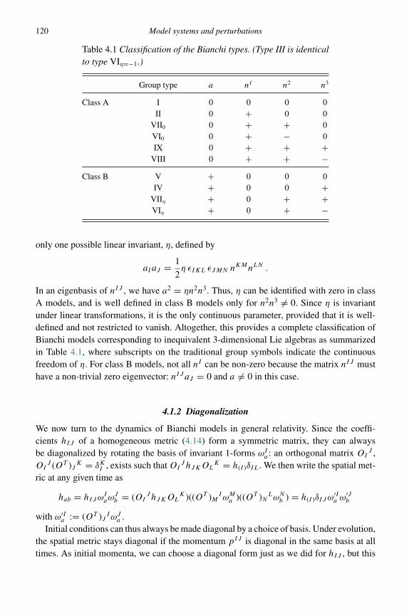
120 Model systems and perturbations
Table 4.1 Classification of the Bianchi types. (Type III is identicalto type VIη=−1.)
Group type a nI n2 n3
Class A I 0 0 0 0II 0 + 0 0
VII0 0 + + 0VI0 0 + − 0IX 0 + + +
VIII 0 + + −Class B V + 0 0 0
IV + 0 0 +VIIη + 0 + +VIη + 0 + −
only one possible linear invariant, η, defined by
aI aJ = 1
2η εIKL εJMN nKMnLN .
In an eigenbasis of nIJ , we have a2 = ηn2n3. Thus, η can be identified with zero in classA models, and is well defined in class B models only for n2n3 �= 0. Since η is invariantunder linear transformations, it is the only continuous parameter, provided that it is well-defined and not restricted to vanish. Altogether, this provides a complete classification ofBianchi models corresponding to inequivalent 3-dimensional Lie algebras as summarizedin Table 4.1, where subscripts on the traditional group symbols indicate the continuousfreedom of η. For class B models, not all nI can be non-zero because the matrix nIJ musthave a non-trivial zero eigenvector: nIJ aJ = 0 and a �= 0 in this case.
4.1.2 Diagonalization
We now turn to the dynamics of Bianchi models in general relativity. Since the coeffi-cients hIJ of a homogeneous metric (4.14) form a symmetric matrix, they can alwaysbe diagonalized by rotating the basis of invariant 1-forms ωI
a : an orthogonal matrix OIJ ,
OIJ (OT )J K = δKI , exists such that OI
JhJKOLK = h(I )δIL. We then write the spatial met-
ric at any given time as
hab = hIJωIaω
Jb = (OI
JhJKOLK )((OT )M
IωMa )((OT )N
LωNb ) = h(I )δIJω
′Ia ω′J
b
with ω′Ia := (OT )J IωJ
a .Initial conditions can thus always be made diagonal by a choice of basis. Under evolution,
the spatial metric stays diagonal if the momentum pIJ is diagonal in the same basis at alltimes. As initial momenta, we can choose a diagonal form just as we did for hIJ , but this
4.1 Bianchi models 121
will be preserved in time only if pIJ , or the spatial Ricci tensor related to it by the evolutionequations (3.80), is diagonal. In general, this is only the case for class A models. In whatfollows we will restrict attention to diagonalizable models which already exhibit the mostinteresting features of homogeneous models, and thus assume that aI = 0 together with adiagonal metric hIJ (t) = h(I )(t)δIJ valid at all times.
The dynamics of diagonal models is most easily formulated for a vanishing shift vectorNa = 0 and a lapse “function”
N =√
det h
16πG(4.17)
(which for this choice is actually a scalar density). Since we assume class A, we have struc-ture constants CI
JK = εIJKn(I ). For a diagonal spatial metric hIJ = h(I )δIJ and vanishingshift vector, one easily computes the extrinsic curvature KIJ = 1
2N h(I )δIJ from (3.51), andthus also the momentum pIJ = p(I )δIJ (derived from a density-weighted homogeneouspab = | det(ωK
a )|pIJXaI X
bJ ) is diagonal. For its components and those of hIJ , we have
the Poisson bracket {hI , pJ } = δJI , as it follows from the pull-back of the homogeneous
symplectic term to the subspace of diagonal configurations:∫d3xhabp
ab =∫
d3x| det(ωKa )|hIJ p
IJ =∫
d3x| det(ωKa )|hIp
I = hIpI .
(As in Chapter 2, we set the coordinate volume V0 = ∫d3x| det(ωK
a )| = 1.)These reductions can now be inserted into the Hamiltonian constraint
NCgrav = pabpab − 1
2(pa
a)2 − det h
(16πG)2(3)R = 0 (4.18)
whose curvature potential is given by (4.15). The kinetic term quadratic in momenta is
pabpab − 1
2
(pa
a
)2 = hachbdpcdpab − 1
2(habp
ab)2
= hIKhJLpKLpIJ − 1
2
(hIJp
IJ)2
=3∑
I=1
h2I
(pI
)2 − 1
2
(3∑
I=1
hIpI
)2
= 1
2
(h2
1(p1)2 + h22(p2)2 + h2
3(p3)2) − h1h2p
1p2
−h1h3p1p3 − h2h3p
2p3 .
Misner variables Even with diagonal metrics, the kinetic term is not of diagonal form in thesense that there are cross products of different momentum components. For convenience,one can change this by a canonical transformation, following Misner (1969), that we splitinto two steps:

122 Model systems and perturbations
1. In the first step, we do not yet diagonalize but absorb the metric components of the kinetic terminto new momenta
αI := 1
2loghI , ρI := 2h(I )p
I such that {αI , ρJ } = δJI . (4.19)
The kinetic term then depends only on ρI .2. Now we define the Misner variables (α, β+, β−) and their momenta (pα, p+, p−) via
α1 =: α + β+ +√
3β− , ρ1 =:1
3pα + 1
6p+ + 1
2√
3p− (4.20)
α2 =: α + β+ −√
3β− , ρ2 =:1
3pα + 1
6p+ − 1
2√
3p− (4.21)
α3 =: α − 2β+ , ρ3 =:1
3pα − 1
3p+ . (4.22)
It can easily be verified that this transformation makes the kinetic term diagonal in momenta:
pabpab − 1
2(pa
a )2 = 1
8
((ρ1)2 + (ρ2)2 + (ρ3)2
) − 1
4(ρ1ρ2 + ρ1ρ3 + ρ2ρ3)
= 1
24(−p2
α + p2+ + p2
−) . (4.23)
In Misner variables, the geometry is not described by the usual metric components but bythe total spatial volume
α = 1
3(α1 + α2 + α3) = log(det hIJ )1/6 (4.24)
and the anisotropy parameters β± which vanish for isotropic metrics where α1 = α2 = α3.
Anisotropy potential The kinetic term is to be combined with the curvature potential(4.15) which we write as
(3)R = −1
2
(n1h1
h2h3+ n2h2
h1h3+ n3h3
h1h2− 2
n1n2
h3− 2
n1n3
h2− 2
n2n3
h1
)(4.25)
= −1
2e−2α
(n1e4(β++√
3β−) + n2e4(β+−√3β−) + n3e−8β+
− 2n1n2e4β+ − 2n1n3e−2(β+−√3β−) − 2n2n3e−2(β++√
3β−))
(4.26)
for diagonal metrics and then in Misner variables. This gives a curvature potential−e6α (3)R/(16πG)2 in (4.18).
Equations of motion for the metric components and with our choice (4.17) of the lapsefunction are simply
α = {α,NCgrav} = − 1
12pα , β+ = 1
12p+ , β− = 1
12p− (4.27)
which allows us to write the Hamiltonian constraint as
−6α2 + 6β2+ + 6β2
− − e6α (3)R
(16πG)2= 0 .
4.1 Bianchi models 123
4.1.3 Kasner solutions and BKL scenario
Anisotropic geometries, even if they are homogeneous, allow more general kinds of cur-vature than the isotropic FLRW models. They are thus especially important for an under-standing of the behavior of universe models near a singularity, when curvature is large. Infact, specific solutions as well as general properties of anisotropic models show that theisotropic approach to a singularity is very special. The anisotropic approach, on the otherhand, seems generic, as indicated by several arguments to be discussed now.
Bianchi I and Kasner solutions The simplest Bianchi model is obtained for type I, inwhich case the symmetry group is Abelian: R3 or a compactification. All structure constantsvanish, CI
JK = 0, and invariant 1-forms can simply be chosen as differentials of Cartesiancoordinates: ωI
adxa = dxI ; see also Example 4.3.As a further consequence, the curvature potential vanishes identically. The system with
Hamiltonian constraint
NCgrav = 1
24(−p2
α + p2+ + p2
−) (4.28)
becomes deparameterizable in internal time α, providing solutions β±(α) with preservedmomenta. With a constant potential in the anisotropy plane, solutions for β±(α) are straightlines. In fact, we can easily solve equations of motion also in coordinate time: for thevariables (4.19),
ρI = {ρI ,NCgrav} = 0
implies that all ρI are constant in time, and thus also
αI = {αI ,NCgrav} = 1
4(2ρI − ρ1 − ρ2 − ρ3) =: vI
are constant. Solutions are αI (t) = vI t + α(0)I in a time coordinate t corresponding to our
choice of lapse. The constants are not arbitrary because initial values must satisfy theHamiltonian constraint
0 = NCgrav = 1
8
∑I
(ρI )2 − 1
4(ρ1ρ2 + ρ1ρ3 + ρ2ρ3) =
∑I
α2I −
(∑I
αI
)2
which requires
∑I
(vI )2 =(∑
I
vI
)2
. (4.29)
For any such solution, we transform back to the original metric components
hI = e2αI = h(0)I e2vI t ,
compute the lapse function N ∝ √det h ∝ exp((v1 + v2 + v3)t), and obtain proper time
τ = ∫ τN (t)dt ∝ exp((v1 + v2 + v3)t). In this time coordinate, the line element takes the

124 Model systems and perturbations
form
ds2 = −dτ 2 + τ 2v1(dx1)2 + τ 2v2
(dx2)2 + τ 2v3(dx3)2 (4.30)
of the Kasner metric , where we absorbed the constants h(0)I in the spatial coordinates and
defined the Kasner exponents
vI = vI∑J vJ
.
They must satisfy ∑I
vI = 1 =∑I
(vI )2 , (4.31)
the first part by definition, the second due to the Hamiltonian constraint (4.29).Kasner solutions have several characteristic properties. The volume as a function of
proper time is proportional to τ v1+v2+v3 = τ , which vanishes at τ = 0 independently of theKasner exponents. The conditions (4.31) allow only solutions for which −1 < vI ≤ 1 insuch a way that one of the exponents is negative while the other two are positive. Thus, it isnot possible that all directions are expanding or contracting at the same time, which showsthe difference to isotropic solutions. Moreover, extrinsic curvature, whose components aregiven by time derivatives of hI and thus expressions proportional to τ 2vI−1, does not remainfinite at τ = 0, while the spatial Ricci scalar vanishes. By the Gauss equation, the space-time Ricci scalar diverges at τ = 0, presenting a singularity at a finite proper time: relaxingthe assumption of isotropy does not eliminate singularities. (See also Exercise 4.3.)
Bianchi IX and mixmaster behavior For the Bianchi IX model, we have structure con-stants CI
JK = εI JK of the Lie algebra su(2), and a non-trivial curvature potential
− e6α
(16πG)2(3)R = 1
2
e4α
(16πG)2
(e−8β+ − 4e−2β+ cosh(2
√3β−)
+ 2e4β+ (cosh(4√
3β−) − 1))
(4.32)
with the following properties:
1. From the deparameterized perspective used initially for Kasner solutions, e6α (3)R presents a time(α) dependent potential in the anisotropy plane (β+, β−). The system is no longer deparameteriz-able by α.
2. The potential is symmetric under rotations of (β+, β−) by 2π/3.3. Along radial directions away from the isotropy point β+ = 0 = β−, the potential generically has
exponentially increasing walls, except for the direction β− = 0, β+ → ∞ and its two rotations by±2π/3.
4. The shape of the typical wall can be determined from β− = 0, β+ → −∞: its dominant increaseis by e8|β+|.
Some of these features can be seen in Fig. 4.2. (See also the cover image.)

4.1 Bianchi models 125
−1
−0.8
−0.6
−0.4
−0.2
0
0.2
0.4
0.6
0.8
1
β−
−1 −0.8 −0.6 −0.4 −0.2 0 0.2 0.4 0.6 0.8 1β+
Fig. 4.2 Logarithm of the norm of the curvature potential for a Bianchi IX model in the anisotropyplane at fixed volume. Solid lines of this contour plot correspond to positive values of the potential,dashed lines to negative values.
Even though the system is not globally deparameterizable by α, we can visualize anddescribe the evolution by the picture of a point particle moving in the anisotropy potential.When the potential is small near the isotropy point, we have almost free Kasner motionas in the Bianchi I model, a so-called Kasner epoch. However, the particle, following astraight line, moves away from isotropy and generically approaches one of the exponentialwalls. Because of their steepness, reflections at the walls can be approximated as almostinstantaneous. The Kasner exponents vI change during such a reflection in a way whichcan be determined from the equations of motion. After a reflection, we enter a differentKasner epoch in such a way that the previously negative exponent becomes positive andone of the positive ones becomes negative. The directions change roles at each reflectionregarding their expansion/contraction behavior. There are infinitely many reflections beforetime t = 0 is reached, earning the dynamics the moniker mixmaster behavior. At any time,the volume is decreasing in the evolution toward smaller t , and hits a singularity after a finiteamount of proper time. Because reflections happen in the triangular shape of the potentialwhich encloses a finite volume in the anisotropy plane, general results of billiard systemsimply that the dynamics is chaotic; see, for instance, the review by Damour et al. (2003).
126 Model systems and perturbations
BKL scenario As first undertaken by Belinskii et al. (1982), one may look for genericasymptotic line elements close to a spacelike singularity at τ = 0 by making an ansatz ofthe form
ds2 = −dτ 2 + τ 2v1(x)(ω1)2 + τ 2v2(x)(ω2)2 + τ 2v3(x)(ω3)2 (4.33)
with homogeneous 1-forms ωI of some Bianchi type and “Kasner exponents” vI (x) whichare now space-dependent. The equations of motion for a homogeneous model correspondingto the invariant 1-forms ωI are then modified by terms containing spatial derivatives ∂avI (x).
The spatial curvature tensor then acquires two contributions, one from the invariant 1-forms which may have non-vanishing derivatives, and one from the spatially dependentvI (x). The first contribution simply agrees with the curvature tensor of a homogeneousmodel as used before. The second contribution captures properties of the inhomogeneityand is thus more interesting in the present context. By the product rule, the spatial connectioncoefficients
Gcab = 1
2hcd (∂ahbd + ∂bhad − ∂dhab)
with hab = δabτ2v(b)
from (4.33) acquire a contribution
δGcab = log τ (δcb∂av
(b) + δca∂bv(a) − δcdδab∂dv
(a))
from the inhomogeneity, which diverges as log τ at the singularity. Spatial Riemann orRicci curvature tensors, quadratic in the connection coefficients, diverge as (log τ )2, andthe Ricci scalar has diverging contributions of the order τ−2vI
(log τ )2 with an additionalfactor from the inverse metric.
There are also curvature terms not containing derivatives of vI , which are the same asin the homogeneous case. The strongest divergence in the Ricci scalar (4.25) comes fromterms of the form
h1
h2h3∝ τ 2v1−2v2−2v3
.
This particular term is dominant if v1 < 0 is the negative one of the exponents. Becauseof 2v1 − 2v2 − 2v3 < −2vI for all vI if v1 < 0, the homogeneous contribution to spatialcurvature always diverges more strongly than the inhomogeneous contributions from spatialderivative terms of vI . Thus, spatial derivatives are subdominant for asymptotic solutionsnear a space-like singularity if the metric takes the form (4.33). The local behavior isthen that of a homogeneous model, and in general resembles the Mixmaster behaviorof the Bianchi IX (or VIII) model since the strongest divergences arise when all nI arenon-vanishing.
BKL’s conclusion is encouraging, for it suggests that the approach to generic spacelikesingularities can be understood solely in terms of homogeneous models. There are, however,several caveats and the BKL conjecture, stating that the homogeneous behavior character-izes even inhomogeneous singularities, is not completely proven. (Growing numericalevidence exists, for instance by Garfinkle (2004) and reviewed by Berger (2002), as well aspartial analytical support by Uggla et al. (2003), Rendall (2005) and Andersson and Rendall
4.1 Bianchi models 127
(2001). Black-hole singularities have been analyzed in this spirit as well, by the numericalstudies of Saotome et al. (2010).) First, one should notice that the conjecture does not at allstate that space-like singularities must be homogeneous. It is just the local behavior at eachpoint that agrees with the dynamics of a Bianchi model; the exponents vI remain spatiallydependent even though their spatial derivatives do not strongly affect the dynamics.
Moreover, the chaos of the mixmaster behavior is relevant, since it implies furtherfragmentation and in fact a very inhomogeneous general appearance of singularities: farfrom the singularity, one may start with an approximation of spatial geometries by acollection of homogeneous patches, and then evolve backwards. Nearby patches whichinitially were similar in their metrics differ rapidly from each other as time goes on becausethe chaotic dynamics makes evolution highly sensitive to initial data. To maintain theapproximation by homogeneous patches, one must subdivide them. Spatial slices becomemore and more structured and inhomogeneous. Spatial gradients then seem to be growing,which might challenge the BKL picture.
Example 4.4 (Gowdy models)Gowdy (1974) introduced a class of inhomogeneous models which by now serve severalinteresting purposes in the analysis of cosmological situations, for instance in the contextof the BKL behavior. In one type of model, the metric takes the form
ds2 = e(λ+t)/2(−e−2tdt2 + dx2) + e−t(eP (dy + Qdz)2 + e−P dz2
)(4.34)
with three functions λ(t, x), P (t, x), Q(t, x) of t and x only. A singularity is approachedfor t → ∞, which amounts to finite proper time. When (4.34) is inserted into Einstein’sequation, it produces the equations
∂2t P − e2P (∂tQ)2 − e−2t ∂2
xP + e2(P−t)(∂xQ)2 = 0 (4.35)
∂2t Q + 2∂tP ∂tQ − e−2t (∂2
xQ + 2∂xP ∂xQ) = 0
for its coefficients. Once solutions for P and Q are known, λ can be determined from
∂tλ = − ((∂tP )2 + e2P (∂tQ)2
) − e−2t((∂xP )2 + e2P (∂xQ)2
)∂xλ = −2(∂tP ∂xP + e2P ∂tQ∂tP ) .
As the singularity is approached, spatial derivatives are suppressed by factors exp(−2t)while time derivatives remain.
The BKL scenario is thus supported by Gowdy models, provided that P stays bounded asthe singularity is approached for t → ∞. IfP diverges as well, not all the spatial derivativesare necessarily suppressed, since e2(P−t) appears in one coefficient in (4.35). Indeed, so-called spikes, isolated points where P grows large and gradients become steep, have beenfound in numerical as well as analytical solutions. Spikes seem to remain isolated and donot challenge the general BKL ideas; they do, however, illustrate some of the difficulties infinding a rigorous proof of the conjecture.
Analytical results related to the BKL picture have been reviewed by Rendall (2005), andnumerical progress is described by Berger (2002), Garfinkle (2004) and Lim et al. (2009).

128 Model systems and perturbations
Spikes have been constructed explicitly and compared with numerical results by Rendalland Weaver (2001).
In the fragmentation argument, there was no obvious violation of time reversal symmetry,and thus one may even expect fragmentation to the future. Such a behavior would be inconflict with observations of structures in the universe. The contradiction is resolved bynoting that fragmentation relied on the chaotic behavior of the Bianchi IX dynamics,which may be used reliably near a spacelike singularity. Evolving to the future, away fromthe singularity, leads to a different form of dynamics to which the asymptotic solutiondiscussed here does not apply. To understand homogenization and isotropization in anexpanding universe, one must use different approximations valid at later times.
For homogenization, inflation is often used as an argument, stating that a small patchof an early geometry is enlarged rapidly to all that we can see now. If the early patch, byvirtue of being tiny, was very nearly homogeneous, our currently visible universe shouldstill be nearly homogeneous. However, this argument is incomplete: given the precedingdiscussion, we expect chaotic behavior to play a large role in the dynamics of the very earlyuniverse. With chaos, one often sees fractal structures which should arise in the spatialgeometries, for instance by the fragmentation process sketched above. But if a self-similarfractal is enlarged by some factor of whatever size, its structure will not change. Thus, aspointed out by Penrose (1990), inflation by itself cannot explain the homogeneity of thecurrent universe (and may not even get started if the initial geometry is too inhomogeneous).Isotropization, once a nearly homogeneous space-time is assumed, can be explained moreeasily based on the behavior of Bianchi models containing perfect-fluid matter sources asfirst studied by Misner (1968). A simple heuristic argument uses the fact that anisotropiescontribute a shear term to the Friedmann equation of an average isotropic universe, which asa contribution to energy density depends on β± and behaves as a−6: a much faster drop-offbehavior than that of standard matter. Anisotropies thus do not play a dominant role for thedynamics of a large universe.
Example 4.5 (Anisotropic shear)A universe of Bianchi type I containing matter obeys the Hamiltonian constraint
NC = 1
24(−p2
α + p2+ + p2
−) + e6α
16πGρ = 0
with the anisotropic variables used before for the vacuum model, and the energy density ρ ofmatter (−16πGρ taking the place of the spatial Ricci scalar in the Hamiltonian constraintof general Bianchi models). The gravitational part of this constraint was obtained in (4.28)with a lapse function N = √
det h/16πG = e3α/16πG. The derivative of α by proper timeis thus dα/dτ = {α,C} = − 4
3πGe−3αpα . Combining this equation with the constraint andrecalling that α = log a, we can write the dynamics in Friedmann form:(
a
a
)2
=(
dα
dτ
)2
= 16π2G2
9
p2α
e6α= 8πG
3ρ + 16
9π2G2 p
2+ + p2
−a6
. (4.36)
4.2 Symmetry 129
During a Kasner epoch, the momenta p+ and p− are nearly constant provided that, in thepresence of matter, ρ is isotropic and does not depend strongly on the anisotropy parametersβ±. The shear term provided by an anisotropic geometry then behaves as a−6, and in anexpanding universe drops off faster than the usual matter ingredients. (Anisotropies showthe dilution behavior of a stiff fluid.)
4.2 Symmetry
As demonstrated by Bianchi models, Einstein’s equation, also in canonical form, can oftenbe analyzed rather easily in models exhibiting continuous space-time symmetries. Variousimportant phenomena are illustrated in this way, and in many cases have been uncoveredonly thanks to sufficiently general symmetric models. A framework for the formulation andderivation of symmetry-reduced dynamical equations thus constitutes an important tool toanalyze canonical gravity.
4.2.1 Symmetry reduction
We will first describe the basic constructions of symmetric models in terms of their equationsof motion. In the following parts of this subsection, general classification schemes andadditional ingredients as well as subtleties for the reduction of canonical models will bediscussed. Throughout this section, we will use the example of symmetry reduction todevelop techniques of principal fiber bundles and connections. This can only be a briefintroduction; for details, we suggest reading Gockeler and Schucker (1989).
4.2.1.1 Symmetric space-times
For symmetric models, we are looking for space-time metrics gab invariant under thetransformations of a certain symmetry group S : M → M , i.e. s∗gab = gab for all s ∈ S.The orbits of S in M are generated by Killing vector fields of invariant metrics.
The symmetry group always acts on space-time M . To be left with a non-stationaryand thus dynamical reduced theory, however, we require that all Killing vector fields arespacelike. Derived as infinitesimal generators of a group action, they form a closed algebraunder the Lie bracket, they are in involution and thus span the tangent spaces to spatialsubmanifolds, the spatial orbits of the symmetry groups along which invariant tensors donot change. If the orbits are 3-dimensional, homogeneity is realized with a transitive actionof the symmetry group on a distinguished class of spatial 3-manifolds given by its orbits.These models, called mini-superspaces, are those of the Bianchi classification, or (with afurther generator of an isotropy) the Kantowski–Sachs model.2 If the orbits are less than 3-dimensional, we obtain a midi-superspace model. Their orbit spaces obtained by identifyingevery orbit to a single point in the reduced manifold, form the spaces of inhomogeneous
2 The Kantowski–Sachs model is realized inside the horizon of the Schwarzschild solution. It is the only homogeneous modelthat cannot be obtained by imposing an extra isotropic symmetry on a Bianchi model.
130 Model systems and perturbations
models. For spherically symmetric space-times, for instance, orbits are 2-spheres and theirorbit space on spatial slices, also called the reduced manifold, is the radial line.
To identify the fields of a reduced model for a given symmetry group, we need acomplete basis for all invariant tensors involved. For the gravitational field in its canonicalform, we decompose the spatial metric and the co-normal by using invariant 2-tensors andvectors on the symmetry orbits. Invariance conditions such as s∗hab = hab are linear inthe fields, and there are only finitely many independent equations if the symmetry grouphas a finite number of generators. In principle, the equations are not difficult to solve, butthe amount of freedom left for solutions is not always easy to oversee and to order. Wewill discuss systematic classification methods in the context of connections, and for nowassume that the invariance conditions have been solved and a basis of invariant tensor fieldsis known.
If, for certain label sets with indices I ∈ I and K ∈ K, a basis of invariant 2-tensorsis given by {hI
ab}I∈I and a basis of invariant co-vectors by {NKa }K∈K, then any invariant
spatial metric can be written as hab = φIhIab with fields φI on the reduced manifold, and
the choice of frame, characterized by lapse and shift, gives rise to further fields N and NI
on the reduced manifold such that Na = NINIa . While N is always a spatial scalar, the
tensorial properties of the fields φI and NI depend on the specific symmetry type. Fromthe spatial metric and the co-normal, the general form gab = −nanb + hab of an invariantspace-time metric is constructed.
Example 4.6 (Invariant metrics)For homogeneity, the reduced manifold is a single point. All components φI are scalarsand functions of time only, while NI = 0.
For spherical symmetry, there is only one invariant vector field ∂/∂r , and thus Na =M(∂/∂r)a . The spatial metric must be of the form hab = φ1(dr)a(dr)b + φ2(d�2)ab. Thus,a spherically symmetric space-time line element is of the general form
ds2 = −N2dt2 + φ1(dr + Mdt)2 + φ2d�2 . (4.37)
All fields N , M , φ1 and φ2 depend only on r and t .
Once the general invariant form of the metric has been found, such as (4.37), inserting itinto the full field equations provides the equations of motion for the reduced model. Theyform a set of second-order differential equations for the φI , depending on the frame via thelapse and shift components N and NI .
4.2.1.2 Invariant connections
So far, except for examples, we have not specified the form of invariant tensors such as hIab,
or described any systematic scheme to derive a complete basis. Indeed, oftentimes the formof invariant metrics may appear rather obvious, as in the cases of homogeneous models, inwhich Lie theory helps us to classify all possible geometries, or for the familiar sphericallysymmetric space-times. It is nevertheless important to have a general classification schemeat hand, one that works for midi-superspace models, too, and which can show that, indeed,

4.2 Symmetry 131
all possible invariant forms are covered for a given type of symmetry. Mathematically, thisclassification is much better developed for connections rather than metrics. The apparatus,based on principal fiber bundles, is quite involved, but it is an important tool in modernphysics and thus is also useful for other purposes. From invariant connections, as we willsee, one can find the form of invariant metrics. But the classification of invariant connectionsis already of interest for canonical gravity, since several of its most useful formulations arebased on connection variables.
So far, we have encountered several examples of connections, primarily the Lorentzconnection ωa
IJ . Since the parallel transport it generates leaves invariant the Minkowski
metric ηIJ , the infinitesimal transport vaωaIJ ∈ so(3, 1) along an arbitrary vector field va
takes values in the Lie algebra of the Lorentz group. In general, a connection behaveslike a 1-form taking values in the Lie algebra of a so-called structure group G, but it issubject to non-tensorial transformation properties as seen for the Lorentz connection inEq. (3.130). Choosing a basis (τi)AB , we also denote a connection by its coefficients Ai
a
in a decomposition ωaAB = Ai
a(τi)AB , as used for the Ashtekar–Barbero connection: ansu(2)-connection Ai
a which, using su(2)-generators τj = 12 iσj in terms of Pauli matrices
σj , provides su(2)-connection 1-forms.
Example 4.7 (Homogeneous fields)For an invariant connection, in addition to the structure group G we have a second groupS, the symmetry group acting on spatial slices � whose elements are supposed to leaveAi
a invariant when applied to it by pull-back. If the whole � is a Lie group, it carriesan obvious symmetry action by its own (left) multiplication; in this case we can identifythe spatial manifold � with the symmetry group S as a manifold. The symmetry actionis transitive, and we obtain the set of homogeneous Bianchi models. There is already ageneral sense of invariance: the left-invariant 1-forms ωI collected in the Maurer–Cartanform θMC = ωI TI with generators TI of the Lie algebra of S (see also the Appendix). Fora matrix group, θMC = s−1ds can be computed directly from a parameterization of groupelements s. From this expression, it is clear that θMC is invariant under left multiplicationLr : s → rs by a constant r ∈ S transforming the whole group manifold. The representations−1(ds)a = ωI
aTI provides useful means for computing the left-invariant 1-forms ωIa of a
matrix Lie group. Every ωI obtained in this way is a 1-form on S such that s∗ωI = ωI forall s ∈ S acting on S by left multiplication, providing systematic means for the computationof invariant structures.
As a whole, the 1-form θMC takes values in the Lie algebra of S. An invariant connectionwith structure group G obeys just the same invariance condition as θMC, but it must takevalues in the Lie algebra of G, not S. A linear map is required, to be applied to the valuesof θMC. There is no natural linear map φ : LS → LG (not required to be an algebrahomomorphism) between two arbitrary Lie algebras, LS and LG. Any one of them givesrise to an invariant connection Ai
aτidxa = φ ◦ θMC = φi
I τiωI , with components obtained
from φ(TI ) =: φiI τi . This determines the set of all connections invariant under a transitive
and freely acting symmetry group.
132 Model systems and perturbations
If the symmetry group still acts transitively but not freely, additional isotropies occur. Ateach point x ∈ �, there is a non-trivial isotropy subgroup Fx < S whose elements leavex fixed. For different points, thanks to transitivity, the Fx only differ by conjugation (iff (x) = x and s(x) = y, all transformations leaving y invariant are obtained as sf s−1(y) =y), and we are allowed to pick one of them as a representative F . Now, we can identify thespatial manifold � (an orbit of the symmetry action) with the factor space S/F .
Example 4.8 (Euclidean group)A group that combines translations and rotations in its action on R3 is the Euclidean groupS = R3 � SO(3), defined as the manifold R3 × SO(3) of pairs t ∈ R3 and R ∈ SO(3) withthe semidirect product rule
(t1, R1)(t2, R2) = (t1 + R1t2, R1R2) . (4.38)
The Euclidean group acts on R3 by (t, R)(x) = Rx + t . For any x ∈ R3, the isotropysubgroup is given by Fx = {(I − R)x,R) : R ∈ SO(3)} ∼= SO(3). Symmetry orbits areS/F ∼= R3 = �.
In general, a factor space such as S/F is not a group, and so there is no Maurer–Cartan form defined on S/F to be used for invariant connections. Nevertheless, we canobtain invariant 1-forms if we choose an embedding ι : S/F → S and take the pull-backι∗θMC of the Maurer–Cartan form defined on S. Normally, there is no unique embeddingof this form, but different choices will simply amount to choosing coordinates on thehomogeneous space. Using linear maps as before, invariant connections are then of theform φ ◦ ι∗θMC.
The pull back of the Maurer–Cartan form takes values in LS. The map φ thus still mapsfrom LS to LG, even though the dimension of LS is now larger than that of �. Thereseem to be more components to an invariant connection, even though we are imposingstronger symmetries. The contradiction is resolved by considering the action of the isotropysubgroup F , which leaves points x in � fixed. It thus acts on the tangent space of x,linearly transforming the space on which φ is defined. No such transformation occurredin the free case, in which arbitrary φ gave rise to invariant connections. Now, there is anisotropy condition also for the map φ, and the symmetry has not been imposed completelysimply by using the left-invariant 1-forms. To handle isotropy conditions, additional toolsto understand the gauge transformations, in particular principal fiber bundles, are useful.This will also allow us to derive the general form of invariant connections for groups notacting transitively, corresponding to midi-superspace models.
Connections We first have to extend the formal notion of a connection from a point-wisemapping Tx� → LG, as used for homogeneous configurations, to a global construct. Thisextension makes use of bundles, which like the tangent bundle T� or the internal vectorbundles attach a vector space of a given type, such as LG, to each point of a manifold. Aconnection 1-form on a manifold M is then a map Ai
a : T� → E, va → Aiav
a from thetangent bundle T� of � to a vector bundle E over the base manifold �. We thus handle the
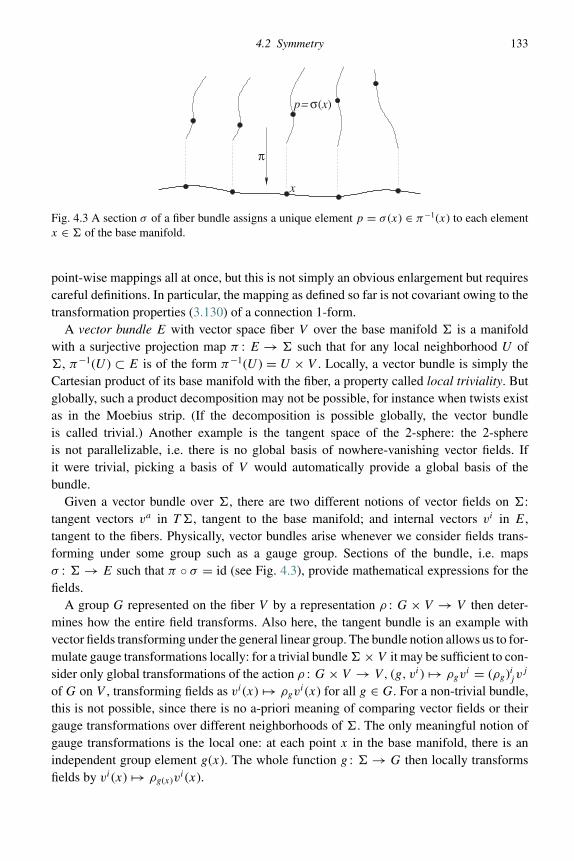
4.2 Symmetry 133
x
p= (x)σ
π
Fig. 4.3 A section σ of a fiber bundle assigns a unique element p = σ (x) ∈ π−1(x) to each elementx ∈ � of the base manifold.
point-wise mappings all at once, but this is not simply an obvious enlargement but requirescareful definitions. In particular, the mapping as defined so far is not covariant owing to thetransformation properties (3.130) of a connection 1-form.
A vector bundle E with vector space fiber V over the base manifold � is a manifoldwith a surjective projection map π : E → � such that for any local neighborhood U of�, π−1(U ) ⊂ E is of the form π−1(U ) = U × V . Locally, a vector bundle is simply theCartesian product of its base manifold with the fiber, a property called local triviality. Butglobally, such a product decomposition may not be possible, for instance when twists existas in the Moebius strip. (If the decomposition is possible globally, the vector bundleis called trivial.) Another example is the tangent space of the 2-sphere: the 2-sphereis not parallelizable, i.e. there is no global basis of nowhere-vanishing vector fields. Ifit were trivial, picking a basis of V would automatically provide a global basis of thebundle.
Given a vector bundle over �, there are two different notions of vector fields on �:tangent vectors va in T�, tangent to the base manifold; and internal vectors vi in E,tangent to the fibers. Physically, vector bundles arise whenever we consider fields trans-forming under some group such as a gauge group. Sections of the bundle, i.e. mapsσ : � → E such that π ◦ σ = id (see Fig. 4.3), provide mathematical expressions for thefields.
A group G represented on the fiber V by a representation ρ : G × V → V then deter-mines how the entire field transforms. Also here, the tangent bundle is an example withvector fields transforming under the general linear group. The bundle notion allows us to for-mulate gauge transformations locally: for a trivial bundle � × V it may be sufficient to con-sider only global transformations of the action ρ : G × V → V, (g, vi) → ρgv
i = (ρg)ij vj
of G on V , transforming fields as vi(x) → ρgvi(x) for all g ∈ G. For a non-trivial bundle,
this is not possible, since there is no a-priori meaning of comparing vector fields or theirgauge transformations over different neighborhoods of �. The only meaningful notion ofgauge transformations is the local one: at each point x in the base manifold, there is anindependent group element g(x). The whole function g : � → G then locally transformsfields by vi(x) → ρg(x)v
i(x).
134 Model systems and perturbations
Just as we need to specify a covariant derivative for an unambiguous notion of differenti-ation on a curved manifold, we need a covariant derivative to determine how to differentiatefields in a vector bundle. Covariance requires that the transformation of every object agreeswith the transformations of all the terms from which it is constructed: Dav
i must be a con-travariant internal vector (and a spatial covector), which requires a suitable transformationproperty for the covariant derivative operator (and the connection 1-forms it contains) asper
ρg(Davi) = (ρg)i jDav
j = (ρgDa)(ρgvi) . (4.39)
Simple partial derivatives are not covariant under local gauge transformations,
∂a((ρg)i j vj ) = (ρg)i j (∂av
j ) + (∂a(ρg)i j )vj �= ρg(∂avi) . (4.40)
A covariant derivative must have an additional contribution to cancel the second term,which is done by means of a connection 1-form Ai
a . It provides the covariant derivativeDav
i := ∂avi + A
jaτ
ijkv
k where τ ijk is the representation matrix of the generator τj of the
structure group G. (For instance for the adjoint action of G on its Lie algebra V , τ ijk = Ci
jk
are the structure constants of the group.) Taking the derivative along a vector field ta , we seethat there is an extra term τ i
j = taAkaτ
ikj which acts on internal vectors by the representation
of the structure group. For Davi to be covariant under local gauge transformations, the
connection 1-form must transform as
ρg(Akaτ
ikj ) = (ρg)il (A
kaτ
lkm)(ρg−1 )mj − ∂a(ρg)im(ρg−1 )mj (4.41)
ensuring that (ρgDa)(ρgvi) = (ρg)il (∂av
l + Akaτ
lkmv
m) = ρg(Davi) in combination with
(4.40). Or, dropping the indices (i, j ) and viewing Akaτ
ikj =: (A)ai j as a 1-form taking
values in the transformation space of V ,
ρgA = ρgAρg−1 − (dρg)ρg−1 . (4.42)
This defines the transformation properties of a connection 1-form, generalizing the trans-formation of a Lorentz connection in Eq. (3.130) (which was written for the inverse
ρg−1 A = ρg−1 Aρg + ρg−1 (dρg) (4.43)
of the transformation considered here).
Principal fiber bundles Just as it is useful to view vector fields as global sections v : � →E of a vector bundle, rather than a collection of local assignments of vectors in the fiberV to all points in the base manifold �, there is a global notion for a connection locallyrepresented by the connection 1-forms Ai
a on �. The required bundle notion is not a vectorbundle but a principal fiber bundle over the same base manifold, �, with fibers not givenby a vector space but by the structure group G itself. Locally, a principal fiber bundle P
over the base manifold � with bundle projection π : P → � is thus of the form � × G,but globally a decomposition is not possible in general. A principal fiber bundle carries an
4.2 Symmetry 135
action of the group G by multiplication on its fibers (the right action of G on P ), which istransitive. These can be taken as the defining properties of a principal fiber bundle.
A principal fiber bundle subsumes all possible gauges of a theory of connections. Choos-ing a gauge means that a unique point is specified on each fiber of the principal fiber bundleP , preferably in a smooth way. A gauge is thus described by a local section σ : U → P
such that π (σ (x)) = x for all x ∈ U ⊂ � in an open neighborhood U . Similarly, changingthe gauge is accomplished by a section h : � → G acting on P by right multiplication, andchanging the original section σ to σh (fiberwise product).
In a local trivialization, P can be written as the union of all U × G where U runs throughall neighborhoods in an open covering of �. Locally, we can thus map P |U := π−1(U) ⊂ P
to {(π (p), g(p))}p∈π−1(U ) with a map g : P |U → G. The functions g(p) can be used as localcoordinates on the bundle, together with coordinates of �.
With these structures, we are able to reformulate the non-covariant term g−1(dg)a in thetransformation of a connection as a covariant tensor on the bundle (rather than the basemanifold). We use coordinates yµ on P , xi on �, and choose a section σ : U → P, xi →yµ(x) in coordinate form. In the non-covariant term, we write
g−1 ∂g
∂xidxi = g−1 ∂g
∂yµ
∂yµ
∂xidxi = σ ∗(g−1dg) = σ ∗θ (P )
MC
with the Maurer–Cartan form θ(P )MC := g−1dg : T P → LG. This form, defined on P , only
varies along the fibers. On a single fiber, it is the Maurer–Cartan form θMC : TG → LG onthe structure group, taking values in the Lie algebra.
Generalizing the Maurer–Cartan form of Lie groups, we define a connection on theprincipal G-fiber bundle P to be a 1-form θ : T P → LG on P taking values in the Liealgebra LG of the structure group, such that θ |TG = θMC is fixed along the fibers. Thevalues along directions not tangent to fibers are not fixed, and correspond to the freedomcontained in a local connection 1-form A. With a local section σ : U → P to specify agauge, we have A(σ ) := σ ∗θ = σ−1A(I)σ + σ−1dσ where the local connection 1-form A(σ )
in the gauge σ is defined by this equation for a given θ , and σ−1dσ arises from the pull-backof the fiber contribution to θ . The 1-form A(I), used here for reference, is obtained for the“flat” gauge in which the section maps to the identity element everywhere. For a non-trivialprincipal fiber bundle, a gauge depends on the local trivialization chosen via the section,and does not exist globally.3 (Accordingly, the gauge-dependent local connection 1-formscannot always form a global object; only the P -connection θ can.)
We change the gauge by right multiplication of sections h : σ → σh, and a new localconnection 1-form A(σh) is obtained from
A(σh) = (σh)∗θ = (σh)−1A(I)σh + (σh−1)d(σh)
= h−1(σ−1A(I)σ + σ−1dσ )h + h−1dh = h−1A(σ )h + h−1dh .
3 Assume that there is a global section σ : � → P . At each x ∈ �, there is for all p ∈ π−1(x) a unique hσ (p) such thatp = σ (x) · hσ (p) by right action. The map P → � × G,p → (π (p), hσ (p)) gives a globally defined trivialization of P . Thus,a principal fiber bundle with a global section is trivial.

136 Model systems and perturbations
Thus, while θ is simply a 1-form defined on the whole bundle, gauge transformations arisefor its pull-backs along sections. In this way, principal fiber bundles allow a covariant,global formulation of the notion of connections by means of θ .
Classification of symmetric principal fiber bundles We now turn to the question of howto construct and classify all possible forms of connections on a space �, invariant under theaction of a given symmetry group. Again, the invariance condition is given via the pull-backby elements of the symmetry group. However, if we work with a local connection 1-form,it can reasonably be required to be invariant only up to a gauge transformation: applyinga symmetry transformation to the connection will produce the same physics even if theconnection is not exactly invariant but only invariant up to gauge. The conditions to solveare now
s∗A = ρg(s)A = g(s)−1Ag(s) + g(s)−1dg(s) (4.44)
for a certain assignment of local gauge transformations g(s) to the symmetry group ele-ments. This complicates the situation: while the equations are still linear in Ai
a , one mustknow suitable g(s) to solve them. In g(s), however, the equations are not linear. Moreover,while applying a symmetry transformation twice leads to certain conditions for g(s1s2) interms of g(s1) and g(s2), they do not distinguish g : S → G as a group homomorphism.
Example 4.9 (Spherically symmetric connections)As derived by Cordero (1977), a general spherically symmetric SU(2)-connection in polarcoordinates, has the form
A(x, ϑ, ϕ) = A1(x)τ3dx + (A2(x)τ1 + A3(x)τ2)dϑ
+ (A2(x)τ2 − A3(x)τ1) sinϑdϕ + cosϑ dϕ τ3 (4.45)
with three independent fields AI (x) depending only on the radial coordinate x, and withsu(2)-generators τi . (The gauge here is different from the one chosen by Cordero (1977).)An exactly invariant connection would only have the radial term A1(x)τ3dx, as expected fora spherically symmetric co-vector field which can only point radially. The extra terms dochange when a rotation is applied, but this can be compensated for by a gauge transforma-tion as shown by a direct calculation. Compared to the radial contribution, it is much morecomplicated to guess the general form of the angular ones. Here, a systematic classificationscheme is most useful.
The mathematical classification of invariant connections was developed by Kobayashiand Nomizu (1963, 1969); Brodbeck (1996) splits the problem of finding suitable g(s)and solving for Ai
a into two steps, making use of principal fiber bundles. Then using theglobal notion of connections, an invariant connection α on P is defined simply by thepull-back condition s∗α = α, while gauge transformations are implemented by evaluatingα at different points along the fibers. Gauge transformations and symmetry actions do notmix as they did in (4.44). However, to evaluate the condition of symmetry, we now need anaction of the symmetry group on P , the space on which α is defined, while we are initially
4.2 Symmetry 137
given an action on the base manifold � only. Lifting the action to P amounts to findingsuitable g(s), and so we are not completely freed from that task. The great advantage nowis that an extension to P can be analyzed without using connections or the invariancecondition.
Let us start with a given action of the symmetry group S on �. In general, for a pointx ∈ � there may be an isotropy subgroup Fx < S with f (x) = x for all f ∈ Fx . Liftingthe action to automorphisms on a principal fiber bundle π : P → � over � with structuregroup G must produce an action Fx : π−1(x) → π−1(x) on the fiber over x, commutingwith the right action of G on the bundle. The action from fiber to fiber is determined by theaction of S on �. But while Fx acts trivially on �, its action on π−1(x) may be non-trivial.Here, the different lifts to P are realized. If we can determine all possible actions of F alongthe fibers compatible with the action of S on a principal fiber bundle, the classification ofsymmetric principal fiber bundles is complete.
Let us assume that an action of F on the fibers is given. Since the right action of thebundle is transitive, to each point p ∈ π−1(x) on the fiber is uniquely assigned a grouphomomorphism λp : F → G by f (p) =: p · λp(f ) for all f ∈ F . To verify that λp isindeed a group homomorphism, we first derive its behavior under gauge transformations,changing the point p along the fiber to p′ = p · g with g ∈ G:
p′ · λp′ (f ) = f (p′) = f (p · g) = f (p) · g = (p · λp(f )) · g = p′ · Adg−1λp(f )
with the adjoint action Adgh = ghg−1 of G on itself. (By the automorphism conditionabove, the action of f commutes with right multiplication by g.) Thus, λp·g = Adg−1 ◦ λp.Then, we have
(f1 ◦ f2)(p) = f1(p · λp(f2)) = (p · λp(f2)) · Adλp(f2)−1λp(f1) = p · (λp(f1) · λp(f2))
and the homomorphism property follows. To summarize, the action on fibers is characterizedby a map λ : P × F → G, (p, f ) → λp(f ) which obeys the relation λp·g = Adg−1 ◦ λp.An important element of the classification of symmetric principal fiber bundles is thus anequivalence class [λ] of group homomorphisms λ : F → G up to conjugation. Changing λ
within a conjugacy class simply amounts to a change of gauge.The remaining elements of the classification amount to the structure of a reduced bundle.
We expect that the base manifold, which is � for P , can be reduced to the orbit space �/S,since the structure of a symmetric bundle is not supposed to change when applying S. Thereduced bundle is indeed a subbundle of the restricted bundle P |�/S . It turns out that thestructure group must also be reduced. For an explicit construction of the bundle (or later oninvariant connections on it) we will be working with a specific homomorphism λ, not witha conjugacy class. Gauge transformations on P then split into two different classes: thosethat fix the conjugacy class (and thus the image λ(F ) in G) and which will be representedas gauge transformations of the reduced bundle, and those that would change the conjugacyclass and thus the reduced bundle. Reduced gauge transformations in the former class formthe centralizer ZG(λ(F )) of λ(F ) in G, i.e. the set of all G-elements commuting with all

138 Model systems and perturbations
elements of λ(F ). This determines the structure of the reduced bundle
Qλ(B,ZG(λ(G)), πQ) := {p ∈ P|B : λp = λ} (4.46)
for a given homomorphism λ : F → G. Conjugation by G on λ(F ) implies a correspondingaction on the set of reduced bundles. In summary, following Brodbeck (1996), we have
Theorem 4.1 An S-symmetric principal fiber bundle P (�,G, π) with isotropy subgroupF ≤ S of the action of S on � is uniquely characterized by a conjugacy class [(λ,Qλ)] ofhomomorphisms λ : F → G together with a reduced bundle Qλ(�/S,ZG(λ(F )), πQ).
The action of a symmetry group often has different types of isotropy subgroup dependingon the point x ∈ �. For spherical symmetry, for instance, S = SO(3) and F = SO(2)outside the center while F = SO(3) at the center. In those cases, the bundle must be splitby patching regions of different isotropy types.
In order to determine all conjugacy classes of homomorphisms λ : F → G we can makeuse of the relation
Hom(F,G)/Ad ∼= Hom(F, T (G))/W (G) (4.47)
where T (G) is a maximal torus and W (G) the Weyl group of G.4 Physically, differentconjugacy classes correspond to different sectors of the gauge theory, or different valuesof a topological charge. In spherically symmetric electromagnetism, this is the well-knownmagnetic charge; see Example 4.10. Equation (4.47) will also be applied in Example 4.13.
Classification of invariant connections Given a symmetric principal fiber bundle P clas-sified by [(λ,Qλ)], the invariant connections it allows must satisfy s∗α = α for all s ∈ S.Since Q is a subbundle of P , we can restrict the connection to obtain a connection α
on the reduced bundle Q. This is not completely obvious, since a connection on Q musttake values in the Lie algebra of the reduced structure group, while the restriction ofa connection on P is initially expected to take values in the Lie algebra of G. An S-invariant connection on P , on the other hand, automatically takes values in the Lie algebraof the reduced structure group ZG(λ(F )): at an arbitrary point p ∈ P we choose a vec-tor v in TpP such that π∗v ∈ σ∗Tπ (p)(�/S) where σ is the embedding of �/S into �.The condition means that v does not have components along symmetry orbits, and isthus fixed by the action of the isotropy group: df (v) = v. (Any such vector v is along∂/∂r in spherical symmetry.) By definition, the pull-back of α by f ∈ F , applied tov, is f "αp(v) = αf (p)(df (v)) which now equals αf (p)(v). On the other hand, as usedin the classification of symmetric bundles, f acts as a gauge transformation by λp(f ),under which α transforms as αf (p)(v) = Adλp(f )−1αp(v). We have assumed the connec-tion α to be S-invariant, thus f "αp(v) = Adλp(f )−1αp(v) = αp(v) for all f ∈ F such that
4 The maximal torus T of a compact Lie group G is a maximal compact, connected, Abelian subgroup. It can be shown that itnon-trivially intersects every conjugacy class in the group, but sometimes conjugacy classes are intersected more than once.The Weyl group W (defined as the normalizer of T modulo its centralizer in G) then acts transitively on T ∩ [g] for an arbitraryg ∈ G.

4.2 Symmetry 139
αp(v) ∈ LZG(λp(F )). An invariant connection α on P can thus be restricted to a connectionon the bundle Qλ with structure group Zλ. Such a connection on the reduced bundle is thefirst part of the classification of invariant connections.
The reduced connection is not the complete information contained in an invariant one onP . (In the example of spherical symmetry, this connection would just be the radial part.)From α we further construct a linear map �p : LS → LG,X → αp(X) for any p ∈ P ,evaluating α on the vector field X on P , given by Xψ := d(exp(tX)"ψ)/dt |t=0 for X ∈ LS
and ψ a differentiable function on P . If X ∈ LF , X is vertical; we have �p(X) = dλp(X)in terms of λp already defined for the symmetric bundle, irrespective of the connection. Bygauge choice, λ can be held constant along �/S and so �p evaluated on the Lie algebra ofthe isotropy subgroup does not provide free fields. But the remaining components, �p|LF⊥making use of a decomposition LS = LF ⊕ LF⊥, for instance with respect to the Killingmetric for a semisimple Lie algebra, do yield independent information about the invariantconnection α, subject only to the condition
�p(Adf (X)) = Adλp(f )(�p(X)) for f ∈ F,X ∈ LS . (4.48)
This equation, following from the transformation of α under the adjoint representation,provides a set of equations to determine the form of the components �, and thus ofinvariant connections.
In addition to the reduced connection α, we have the components of a field φ : Q →LG ⊗ LF"
⊥ determined by �p|LF⊥ . This field can be regarded as having dimLF⊥ compo-nents of LG-valued scalar fields. We have now completed the characterization of invariantconnections, and conclude with Brodbeck (1996):
Theorem 4.2 (Generalized Wang theorem) Let P (�,G) be an S-symmetric principalfiber bundle classified by [(λ,Qλ)] according to Theorem 4.1, and let α be an S-invariantconnection on P .
Then, in a gauge given by (λ,Qλ) the connection α is uniquely determined by a reducedconnection α on Qλ and a scalar field φ : Qλ × LF⊥ → LG obeying Eq. (4.48).
As components of an invariant P -connection, φ transforms under G. However, if wesolve Eq. (4.48), we must use a specific selection for the isotropy subgroup F (and thus fixits conjugacy class in G). Not all G-elements will leave this choice and thus the solutionspace of (4.48) for a given F invariant. Again, it is only elements of ZG(λ(F )), the reducedstructure group, that do so; they form the group under which the scalar fields transform.
From a reduced connection α on Qλ and scalars φ solving (4.48) an invariant connectionα on P can be reconstructed, completing the classification. With the (local) decomposition� ∼= �/S × S/F , we have
α = α + αS/F (4.49)
where αS/F is given by the scalars, or rather, the whole �, via � ◦ ι"θMC. Here, θMC is theMaurer–Cartan form on S taking values in LS, and ι : S/F ↪→ S is a (local) embedding.Choosing ι contributes to the gauge of the reconstructed connection.
140 Model systems and perturbations
Example 4.10 (Spherically symmetric electromagnetism)With S = SU(2), F = U(1) (which we realize as a subgroup of SU(2) by F = exp〈τ3〉),and G = U(1) we have conjugacy classes of homomorphism represented by λn : U(1) →U(1), exp(ϕτ3) → exp(inϕ) for integer n. For an Abelian structure group, Adλn(f ) = id andthe condition (4.48) reads �p(AdfX) = �p(X). The adjoint action of F on LS leaves onlythe subalgebra LF invariant, and so (4.48) implies that �|LF⊥ = 0, while �|LF = dλn is,as always, fully determined by the homomorphism λn. For Abelian structure groups, nofree scalar fields arise in the classification of invariant connections.
The only free part in a spherically symmetric U(1)-connection is thus the reduced con-nection A = A(r)dr . But there is an extra contribution from �|LF , whose form follows fromAS/F for the homogeneous space of a sphere. Together with results of Example 4.14 andExercise 4.8, the map � realized here implies that AS/F = dλn(τ3) cosϑdϕ = in cosϑdϕ.If we remove the generator i of LU(1), a connection of the form AS/F corresponds to a fieldstrength FS/F = −n sinϑdϑ ∧ dϕ, and a (dedensitized) radial magnetic field of magnitudeBr = −n(r2 sinϑ)−1 sinϑ = −n/r2. This is the magnetic field of a magnetic monopole ofcharge n, providing a physical example for the topological-charge parameter n classifyinginequivalent symmetric bundles via λn. (Notice that the language of principal fiber bundleshas allowed us to express the field of a magnetic monopole in a well-defined way, avoidingthe string-like singularities in distributional realizations related to Dirac monopoles.)
Additional examples for applications of this general procedure will be provided after adiscussion of how invariant connections can be used to derive invariant metrics.
4.2.1.3 Canonical reduction
In many formulations of gravity, connections appear as one half of a set of canonicalvariables. Their classification is now available, but we also have to know how their momentacan be reduced to symmetric forms. A reduction must obviously occur, for the symmetryhas diminished the number of independent components of connections. A symplectic phasespace then requires the same number of conditions for their conjugate momenta.
Tensorial objects other than connections do not have the same degree of theoretical clas-sification for their invariant forms. Fortunately, if the reduction is known for one canonicalhalf, that of the other can be read off much more simply, using duality. If we know a basisof all invariant connections AI
a (for instance, the left-invariant 1-forms for homogeneousmodels) for a given symmetry type, their momenta must be built from dual invariant fieldsXa
I satisfying AIaX
aJ = δIJ . This condition ensures that the same number of independent
fields arises for configuration variables and momenta. Moreover, expansion coefficientsby the invariant basis are automatically canonically conjugate: general invariant fieldsAi
a = φiIA
Ia and Ea
i = XpIi X
aI , expanded in suitable invariant bases and with an invariant
density X (for instance, X = | detXaI |−1) to provide the density weight on symmetry orbits,
satisfy∫
d3xAiaE
ai = ∫
d3xX ˙φiI p
Ii . Once trivial integrations over symmetric orbits are per-
formed, φiI and pI
i appear as canonically conjugate fields; see also the examples in the nextsection.
4.2 Symmetry 141
Example 4.11 (Reduced densities)Homogeneity is realized with respect to left-invariant 1-forms ωI
a and dual vector fieldsXa
I , providing an invariant density X = | detXaI |−1 = | detωI
a |. The symplectic structure
follows from∫
d3xX ˙φiI p
Ii = V0
˙φiI p
Ii with V0 = ∫
d3xX integrated over some finite region.The homogeneous variables φi
I and pIi have lost the density weight of the original fields.
In spherical symmetry, some variables remain as 1-dimensional densities on the radialline. Factors of X = sinϑ provide the density weight on spherical orbits.
In particular, the classification of invariant connections can be used to tell us what thegeneral invariant form of metric tensors is. As we have seen, in the canonical formulationsof gravity in terms of connection variables, conjugate momentum variables Ea
i can begiven the geometrical interpretation of densitized triads. They, in turn, directly lead tothe spatial metric hab = Ea
i Ebi/| det(Ec
j )| whose invariant form then follows from that ofthe densitized triad. Momentum variables conjugate to the metric in ADM formulations,finally, are obtained by duality as in the case of connection variables. At this stage, we havea systematic procedure to determine the complete form of all invariant tensor fields as theyoccur in canonical theories of gravity.
The relation to metric variables provides one further condition on the allowed forms:non-degeneracy of the metric. If we start with a class of invariant connections, we are led toinvariant densitized triads, and then to metrics. Not all of the possible sectors of invariantconnections, classified by topological charges, may allow non-degenerate metrics. Thus,not all values for the charge, which might be allowed for a non-gravitational gauge theory,will be possible. We will see such an example in spherical symmetry.
4.2.1.4 Examples
We can now complete the examples already introduced in the course of this section.
Example 4.12 (Homogeneous models, once more)In Bianchi models the transitive symmetry group acts freely on �, which we locally identifywith the group manifold S. We have three generators TI , 1 ≤ I ≤ 3, of LS, with relations[TI , TJ ] = CK
IJ TK . By definition, the structure constants CKIJ of LS fulfill CJ
IJ = 0 forclass A models. From the Maurer–Cartan form θMC = s−1ds = ωI TI on S we obtainleft-invariant 1-forms ωI on S, fulfilling the Maurer–Cartan equations
dωI = − 12C
IJKωJ ∧ ωK . (4.50)
The reduced manifold �/S is a single point for homogeneous models, and any reducedbundle is trivial. Due to F = {1} for a freely acting group, there is only one homomor-phism λ : F → G, 1 → 1. Only one type of symmetric bundle exists, with structure groupZG(λ(F )) = G.
With the reduced manifold a single point, there is no reduced connection α contributingto an invariant one. Only the scalar fields φ : LS → LG,TI → φ(TI ) =: φi
I τi appear,unrestricted by (4.48) which is empty in this case. To reconstruct an invariant connection,

142 Model systems and perturbations
we use the obvious embedding ι = id : S/F ≡ S ↪→ S. Invariant connection 1-forms thentake the form A = φ ◦ θMC = φi
I τiωI = Ai
aτidxa with matrices τi generating LG.
Left-invariant vector fields XaI on the Lie algebra, obeying ωI (XJ ) = δIJ , provide the
dual form of invariant vector fields. Analogously to the Maurer–Cartan relations for left-invariant 1-forms, they satisfy the Lie brackets [XI ,XJ ] = CK
IJXK . Momenta canonicallyconjugate to Ai
a = φiIω
Ia can be written as Ea
i = √h0 p
Ii X
aI with independent components
pIi . In addition to Xa
I , we use h0 = det(ωIa)2 as the determinant of the left-invariant metric
h0 ab := ∑I ω
Iaω
Ib on �, providing the density weight of Ea
i . To verify that the pIi are
canonically conjugate to the φiI , we compute
1
8πγG
∫d3x Ai
aEai = 1
8πγG
∫d3x
√h0
˙φiI p
Ji ω
IaX
aJ = V0
8πγG˙φiI p
Ii ,
and obtain
{φiI , p
Jj } = 8πγGV0δ
ij δ
JI (4.51)
with the volume V0 := ∫d3x
√h0 of � measured with the invariant metric h0. (If � is non-
compact, we choose a finite region which we over integrate. Thanks to the homogeneity,results from the model will be insensitive to the choice.)
This completes the invariant structure of canonical fields for homogeneous models with-out a non-trivial isotropy subgroup, and verifies what we already saw in Example 4.7 beforethe systematic classification. The general discussion will be most important when isotropysubgroups enter the game.
Example 4.13 (Isotropic models)For a Bianchi model with additional isotropies, including FLRW models, the symmetrygroup is a semidirect product S = N �ρ F of the isotropy subgroup F and the translationalsubgroup N , one of the Bianchi groups. (See Example 4.8 for the specific case of theEuclidean group.) The isotropy subgroup may be SO(3) for fully isotropic models, or U(1)for models with a single isotropic axis (called locally rotationally symmetric, LRS, asintroduced by Ellis and MacCallum (1969)).
Composition in this group of semidirect-product form is defined by
(n1, f1)(n2, f2) := (n1ρ(f1)(n2), f1f2) (4.52)
with a group homomorphism ρ : F → AutN into the automorphism group of N (thatis, ρ(f ) : N → N is an isomorphism for all f ∈ F ). Inverse elements are (n, f )−1 =(ρ(f −1)(n−1), f −1). To determine the form of invariant connections, we compute theMaurer–Cartan form on S
θ(S)MC(n, f ) = (n, f )−1d(n, f ) = (ρ(f −1)(n−1), f −1)(dn, df )
= (ρ(f −1)(n−1)ρ(f −1)(dn), f −1df ) = (ρ(f −1)(n−1dn), f −1df )
=(ρ(f −1)(θ (N)
MC(n)), θ (F )MC(f )
). (4.53)

4.2 Symmetry 143
in terms of θ(N)MC on N and θ
(F )MC on F . If we choose the embedding ι : S/F = N ↪→ S
as ι : n → (n, 1), we have ι∗θ (S)MC = θ
(N)MC. A reconstructed connection takes the same form
φ ◦ ι∗θ (S)MC = φi
IωI τi as seen for anisotropic models before. (Now, ωI are left-invariant
1-forms on the translation group N , which earlier was the full symmetry group.) However,here φ is constrained by Eq. (4.48), and only a subset of linear maps φ from LN , generatedby TI , to LG provides isotropic connections.
Solving Eq. (4.48) requires us to treat LRS and isotropic models separately. To bespecific, we specialize the structure group G to SU(2) as realized for the Ashtekar–Barberoconnection. In the first case (LRS) we choose LF = 〈τ3〉, whereas in the second case(isotropy) we have LF = 〈τ1, τ2, τ3〉 (denoting by 〈·〉 the linear span). Equation (4.48) canbe written infinitesimally as
φ(adτi (TI )) = addλ(τi )φ(TI ) = [dλ(τi), φ(TI )]
(i = 3 for LRS, 1 ≤ i ≤ 3 for isotropy). On LN = LF⊥ the isotropy subgroup F actsby rotation, adτi (TI ) = εiIKTK . This is expected for an additional rotational symmetry,but it also follows automatically from the derivative of the representation ρ definingthe semidirect product S: conjugation on the left-hand side of (4.48) is Ad(1,f )(n, 1) =(1, f )(n, 1)(1, f −1) = (ρ(f )(n), 1) according to the composition in S.
To evaluate (4.48) further, we determine the possible conjugacy classes of homomorphismλ : F = U(1) → G = SU(2). Applying Eq. (4.47), we use the standard maximal torus
T (SU(2)) = {diag(z, z−1) : z ∈ U(1)} ∼= U(1)
of SU(2), with the Weyl group of SU(2) given by the permutation group of two elements,W (SU(2)) ∼= S2, its generator acting on T (SU(2)) by diag(z, z−1) → diag(z−1, z). Up toconjugation, all homomorphisms in Hom(U(1), T (SU(2))) are given by
λk : z → diag(zk, z−k) (4.54)
for k ∈ Z, factored out by the action of the Weyl group to leave only the maps λk , k ∈ N0,as representatives of all conjugacy classes of homomorphism.
For LRS models, we choose representatives
λk : U(1) → SU(2), exp tτ3 → exp ktτ3
for k ∈ N0 = {0, 1, . . .}. For the components φiI , Eq. (4.48) takes the form ε3IKφ
j
K =kε3lj φ
lI . There is a non-trivial solution only if k = 1, in which case φ can be written
as φ1 = aτ1 + bτ2, φ2 = −bτ1 + aτ2, φ3 = cτ3 with arbitrary numbers a, b, c. Theirconjugate momenta take the form p1 = 1
2 (paτ1 + pbτ2), p2 = 12 (−pbτ1 + paτ2), p3 =
pcτ3, with non-vanishing Poisson brackets {a, pa} = {b, pb} = {c, pc} = 8πγGV0. Thereis remaining gauge freedom from the reduced structure group Zλ
∼= U(1) which rotatesthe pairs (a, b) and (pa, pb). The gauge invariant combinations are only
√a2 + b2 and its
momentum (apa + bpb)/√a2 + b2.
In the case of isotropic models with S = SU(2), we have only two homomorphismsup to conjugation: λ0 : SU(2) → SU(2), f → 1 and λ1 = id. For λ0, (4.48) in the form
144 Model systems and perturbations
εiIKφj
K = 0 lacks non-trivial solutions. For λ1, we solve εiIKφj
K = εilj φlI as we did for LRS
models with k = 1, resulting in φiI = cδiI with an arbitrary c. In this case the conjugate
momenta can be written as pIi = pδIi , and from V0(8πγG)−1 ˙φi
I pIi = 3V0(8πγG)−1 ˙cp we
have the Poisson bracket {c, p} = 8π3 GγV0. Obviously, p must be related to the scale factor
of an isotropic metric. Indeed, computing the isotropic reduction of a Bianchi IX metricfollowing from the left-invariant 1-forms of SU(2), one obtains a closed FLRW metric withscale factor a = 2a = 2
√|p|; see Exercise 4.4. (The Bianchi I model does not allow fixingthe numerical relationship, since the scale factor of its isotropic reduction can be rescaledarbitrarily.)
In both classes of isotropic submodel, there is a unique non-trivial sector and no topo-logical charge appears.
For an example with non-trivial reduced connections in a midi-superspace model, wenow consider spherical symmetry.
Example 4.14 (Spherical symmetry)Outside a symmetry center of spherically symmetric spaces, we have S = SU(2) withF ∼= U(1), which we realize as F = exp〈τ3〉. An invariant connection 1-form can be gaugedto be A = A + AS/F with a reduced connection 1-form A on �/S and
AS/F = (�(τ2) sinϑ + �(τ3) cosϑ)dϕ + �(τ1)dϑ (4.55)
(see Exercise 4.8). Here, (ϑ, ϕ) are (local) coordinates on S/F ∼= S2 and as usual we usethe basis elements τi of LS. The LF -component �(τ3) is given by dλ, whereas �(τ1,2) arethe scalar field components φ = �|LF⊥ .
The fields � are not arbitrary. As in the previous example, we need to know all homomor-phisms in Hom(U(1), T (SU(2))) up to conjugation, given by (4.54) with k ∈ N0. We usethe homomorphisms λk : exp tτ3 → exp ktτ3 out of each conjugacy class. This leads to areduced structure group ZG(λk(F )) = exp〈τ3〉 ∼= U(1) for k �= 0 and ZG(λ0(F )) = SU(2)for k = 0. The map �|LF is given by dλk : 〈τ3〉 → LG, τ3 → kτ3, and the remainingcomponents of � are subject to Eq. (4.48), or � ◦ adτ3 = addλ(τ3) ◦ �. Specifically,
�(a0τ2 − b0τ1) = k(a0[τ3,�(τ1)] + b0[τ3,�(τ2)])
where a0τ1 + b0τ2, a0, b0 ∈ R is an element of LF⊥. Since a0 and b0 are arbitrary, weobtain two equations: k[τ3,�(τ1)] = �(τ2) and k[τ3,�(τ2)] = −�(τ1). A general ansatz�(τI ) = aI τ1 + bI τ2 + cI τ3 for I = 1, 2 with arbitrary parameters aI , bI , cI ∈ R yields
k(a1τ2 − b1τ1) = a2τ1 + b2τ2 + c2τ3 , k(−a2τ2 + b2τ1) = a1τ1 + b1τ2 + c1τ3
with non-trivial solutions only for k = 1: b2 = a1, a2 = −b1, c1 = c2 = 0.Now, with a non-trivial reduced manifold �/S given by the radial line, all free
parameters are fields a, b, c : �/S → R. They provide the U(1)-connection 1-formA = c(x) τ3 dx of the reduced connection and two scalar field components �|〈τ1〉 : �/S →LSU(2), x → a(x)τ1 + b(x)τ2. (The general solution for � shows that it is sufficient to
4.2 Symmetry 145
consider �|〈τ1〉 only.) If we introduce the complex-valued field w(x) := 12 (b(x) − ia(x)),
we have �(τ1) =(
0 −w(x)w(x) 0
). Under a local U(1)-gauge transformation z(x) =
exp(t(x)τ3) these fields transform as c → c + dt/dx and w(x) → exp(−it)w, which canbe read off from
A → z−1Az + z−1dz = A + τ3dt ,
�(τ1) → z−1�(τ1)z =(
0 − exp(it)wexp(−it)w 0
).
A general invariant connection has the form (4.45), with a dual form
E = E1 sinϑ τ3∂
∂x+ 1
2 sinϑ(E2τ1 + E3τ2)∂
∂ϑ+ 1
2 (E2τ2 − E3τ1)∂
∂ϕ(4.56)
for an invariant densitized triad field, with coefficients EI canonically conjugate to AI .Under local U(1)-gauge transformations, the radial component Ex := E1 is invariant,while (E2, E3) transforms as a 2-vector under SO(2) ∼= U(1). In addition to Ex , Eϕ :=√
(E1)2 + (E2)2 is thus invariant. Such an invariant densitized triad produces a spatialmetric corresponding to (4.37) with Ex and Eϕ related to φ1 and φ2; see Exercise 4.10.The symplectic structure
{AI (x), EJ (y)} = 2γGδJI δ(x, y) (4.57)
can be derived by inserting the invariant expressions into (8πγG)−1∫�
d3xAia Ea
i . SinceE2 and E3 are non-vanishing only for k = 1, this is the unique sector providing non-degenerate triads. The topological charge which initially arises for a general sphericallysymmetric gauge theory (for instance, of Yang–Mills monopoles) is fixed by the requirementof a non-degenerate metric.
After our analysis of how to classify and construct symmetric models, we now return toaspects of their dynamics.
4.2.2 Symmetric criticality
In our discussion of Bianchi class A models, we have used the Hamiltonian constraint spe-cialized to homogeneous variables, then applied the reduced constraint to generate equa-tions of motion. Similarly, a general reduced model is obtained by inserting the previouslyclassified forms of invariant fields in the constraints and equations of motion. Computingequations of motion directly from the reduced constraints means that one is taking varia-tions of a restricted expression, rather than of the full action: homogeneous configurationsare only a small subspace of the infinite-dimensional space of all metrics. Since stationarypoints of a restricted functional supported only on a subset of all possible configurationsmay not agree with those of the functional on the full space, it is not guaranteed that varyinga restricted action produces the correct equations of motion for the restricted configurations.
146 Model systems and perturbations
For class A models, it turns out, as shown by MacCallum and Taub (1972), that one doesobtain the correct equations of motion if one first specializes the action or Hamiltonian tohomogeneous variables. But there are cases where this commutation property of reductionand variation does not hold true, notably class B models.
The property that varying an action specialized to symmetric fields of some kind givesthe same result as specializing the full equations of motion to this symmetry is calledsymmetric criticality. In general, there is no guarantee that this property is satisfied for areduced model. One of the main obstructions is the presence of boundary terms. For generalfields, we have treated boundaries in Chapter 3.3.2 by keeping the metric at the boundaryfixed, δgab|∂� = 0. However, if the fields obey a symmetry of some form, whose orbitsalong which fields must remain constant intersect the boundary, variations of the boundaryvalues are no longer independent of variations in the interior. Then, boundary terms cannotalways be canceled by a surface term and differences between reduced equations of motionand equations of motion from a reduced action or Hamiltonian may arise.
Looking back at the derivation of canonical equations of motion for general relativity inADM variables, boundary terms arose
• in the variation by δNa : varying H2 in (3.76), produces a boundary term from∫d3x
√det hDa
pabδNb√det h
= 1
16πG
∫d3x
√det hDa
((Kab − Kc
c hab)δNb
);
• in the variation by δhab: varying H2 produces a boundary term from∫d3x
√det hDf
pcgNf δhcg√det h
= 1
16πG
∫d3x
√det hDf
((Kcg − Ka
a hcg)Nf δhcg
)from one term in δGa
bc (while the other terms cancel), and varying H3 in (3.77) produces a boundaryterm from ∫
d3x√
det hDc(NhdeDcδhde − Nhe
chdfDdδhf e
)=
∫d3x
√det hDa
(N (hachde − haehcd )Dcδhde
)and one from ∫
d3x√
det hDc
((DcN )hdeδhde − hcf (DeN )δhf e
)=
∫d3x
√det hDc
((DaN )(hachde − haehcd )δhde
)due to integration by parts twice.
These terms must now specifically be checked in homogeneous models, where we cannotrely on vanishing boundary variations of the metric to make them automatically zero.However, they may vanish from the homogeneity assumption alone. This can easily beseen to be the case for the last boundary term listed because DaN = 0 in any homogeneousmodel. To assess the other boundary terms, we make use of a reformulation of the total

4.3 Spherical symmetry 147
divergences Dava for vector fields as they appear in the boundary terms for different
versions of va . In a homogeneous space, we expand va in the basis XaI of invariant vector
fields, va = vIXaI with constant vI ; thus Dav
a = vIDaXaI . With
DaXaI = 1
2habLXI
hab = −1
2habLXI
hab = −1
2hJKωJ
a ωKb LXI
(XaLX
bM )hLM
= −hJKhLMωJa ω
Kb Xa
LLXIXb
M = −ωKb [XI ,XK ]b = −CK
IK = −2aI
we have
Dava = −2vI aI . (4.58)
The boundary terms are divergences with specific expressions for va . From the δNa-variation, the boundary term becomes aI (KIJ − KK
KhIJ )δNJ . From the hab variation weobtain aI (KJK − KL
LhJK )δhJKNI from H2 and aIω
IaDc
((hachde − haehcd )δhde
)from
the first term arising from H3. They all vanish in class A models, but not in class B modelsin which aI �= 0. While class A models are thus safe to use as we did — they satisfythe property of symmetric criticality — for class B models there is no straightforwardreduced Hamiltonian formulation. Simply reducing the constraints of general relativitydoes not produce the correct reduced equations of motion in this case. (It may be possibleto construct other Hamiltonian formulations not directly obtained by reducing the fullaction, which then do produce the correct equations of motion. But there is no systematicprocedure to do so.)
There are various general results for conditions under which symmetric criticality isrealized, described by Torre (1999) and Anderson et al. (2000). The main example isthe compactness of the symmetry group, a criterion which applies to Bianchi IX andalso to spherical symmetry. From the discussion of boundary terms, this conclusion isunderstandable because symmetry orbits have to extend to the boundary to have a chanceof violating symmetric criticality, and then cannot be compact. Requiring staticity is anexample that does not necessarily result in a correct reduced formulation: time translationscorrespond to non-compact symmetry orbits.
4.3 Spherical symmetry
Spherically symmetric models are the simplest inhomogeneous ones and thus provideinteresting arenas in which to apply methods of general relativity. In vacuum, a uniquefamily of solutions is given by the Schwarzschild space-time for different mass parameters.A larger class of models is provided by 2-dimensional dilaton gravity, a generalizationof the spherical reduction of general relativity. Here, elegant mathematical reformulationsshed light on the constraint algebra, such as the occurrence of structure functions. In2-dimensional models, the constraint algebra can be interpreted as originating from anunderlying symmetry given not by a Lie algebra as in usual gauge theories but by a Liealgebroid.
148 Model systems and perturbations
4.3.1 Schwarzschild solution
With spherical symmetry we can further illustrate the solution procedure of Einstein’sequation in canonical form. As stated in the preceding section, spherical symmetry obeyssymmetric criticality; we are allowed to insert the symmetric forms of variables, such as(4.45) and (4.56) in a connection formulation, into the constraints, and then determine theequations of motion that they generate.
4.3.1.1 Static solutions
We work with a spherically symmetric spatial line element. From (4.56) we see that it canonly be of the form
ds2 = L(x)2dx2 + S(x)2(dϑ2 + sin2 ϑdϕ2) (4.59)
with L = Eϕ/√|Ex | and S = Ex ; see Exercise 4.10. In addition, we use a lapse function
N (x) and a radial shift vector with a single component Nx(x) depending only on theradial coordinate5 (as well, certainly, as on time which is suppressed in the notation).Non-vanishing connection coefficients for the spatial metric are:
Gxxx = L′
L, Gx
ϑϑ = −SS ′
L2, Gx
ϕϕ = − sin2 ϑSS ′
L2
Gϑxϑ = Gϕ
xϕ = S ′
S, G
ϕϑϕ = cosϑ
sinϑ, Gϑ
ϕϕ = − sinϑ cosϑ .
Primes here denote derivatives by x. This implies the Ricci curvature components
(3)Rxx = −2S ′′
S+ 2
S ′
S
L′
L(4.60)
(3)Rϑϑ = 1 + SS ′L′
L3− (SS ′)′
L2= 1
sin2 ϑ
(3)Rϕϕ (4.61)
and the Ricci scalar
(3)R = 2
S2− 2
(S ′)2
L2S2+ 4
S ′
S
L′
L3− 4
S ′′
L2S. (4.62)
Before going through a general canonical analysis, we will first be looking for staticsolutions, requiring vanishing momenta (as well as conditions on the frame as discussedshortly). Moreover, we choose our radial coordinate x = r such that S(r) = r . This is agauge-fixing condition: for spherically symmetric variables, we have the diffeomorphismconstraint D[Nx] = ∫
dxNx(pSS′ − Lp′
L) with momenta pS and pL canonically conju-gate to S and L, respectively; see the following subsection for more details. Togetherwith χ := S(x) − x, we render the diffeomorphism contribution to the constraint algebrasecond class: {D[Nx], S − x} = − ∫
dxNxS ′. The diffeomorphism constraint is not just
5 We reserve the symbol r in the context of spherical symmetry for the areal radius, which is realized if S(r) = r in the metric, aspecific gauge choice used below.

4.3 Spherical symmetry 149
gauge-fixed but also, with vanishing momenta, identically satisfied; only the Hamiltonianremains to be studied.
At this stage, we implement the second condition for staticity, namely a vanishing shiftvector Nx = 0. With this condition and vanishing momenta, the Hamiltonian constraintreads
0 = (3)R = 2
r2− 2
r2L2+ 4
L′
rL3.
Introducing a new function � := L2, this is a differential equation
�′ − �
r+ �2
r= 0
whose solutions satisfy �/(1 − �) = cr with a constant c, or
L =√� = 1
1 + (cr)−1. (4.63)
With this result, we have arrived at the correct form for all components S and L of thespatial Schwarzschild metric, but for the full space-time metric we must still determine N .
All constraints have been solved, but additional consistency conditions arise becausemomenta and their derivatives are assumed to vanish in this static case. Thus, with thecanonical equations of motion for momenta, we must ensure that
16πG√det h
pab = −N (3)Rab + DaDbN − habDcDcN = 0 (4.64)
making use of the vanishing shift vector and the Hamiltonian constraint in the form (3)R = 0.Equation (4.64) is indeed an equation for the lapse function.
One might wonder why such an equation arises, given that N supposedly can be chosenfreely as part of the choice of frame. In general, this is true, but in the present treatmentwe have already made a choice for the space-time gauge by requiring the momenta tovanish. In the phase-space language, this looks like gauge-fixing conditions provided thatthe flow generated by the Hamiltonian constraint does not leave the condition invariant;the surface of vanishing momenta provides a cross-section of the gauge orbits generatedby H [N ] on the constraint surface. However, we have not been so careful as to ensureproper cross-sections of the putative gauge-fixing surface (by vanishing momenta) withgauge orbits of the Hamiltonian constraint, requiring exactly one intersection per orbit.We have also imposed too many conditions: two functions, the momenta of L and S, arerequired to take a prescribed value even though we are now dealing with a single constraintfunction. An interpretation of staticity as gauge fixing is thus incorrect; instead, we viewit as an ansatz: we impose staticity and look for a frame (eventually determined by the asyet unspecified lapse function) respecting this condition. By changing N , we change theHamiltonian vector field of H [N ], a feature which we can exploit in trying to turn theHamiltonian vector field parallel to the staticity surface pS = 0 = pL in phase space. If itis not possible to turn the vector field parallel to the surface, staticity conditions cannot be

150 Model systems and perturbations
preserved by the gauge flow; those conditions would have been a bad choice. If turningthe vector field parallel is possible, on the other hand, staticity does provide consistentsolutions, and the lapse function N realizing the parallel vector field is the consistent staticframe.
The flow of the Hamiltonian constraint along its Hamiltonian vector field is exactlywhat we have used to derive (4.64): this equation results from the equation of motion formomenta, whose time derivatives are required to vanish. Solving this equation provides,via N and the vanishing Na , the frame realizing this gauge choice.
In (4.64), we have6
hcdDcDdN = hrrDrDrN + 2hϑϑDϑDϑN
= hrr (∂r − Grrr )∂rN − 2hϑϑGr
ϑϑ∂rN
= 1
L2N ′′ − L′
L3N + 2
S ′
SL2N ′
and thus
(hrchrd − hrrhcd )DcDdN = −2S ′
SL4N ′
(hϑchϑd − hϑϑhcd )DcDdN = − N ′′
S2L2+ L′N ′
S2L3− S ′N ′
S3L2.
From the equations of motion for momenta, we obtain conditions for a = b = r:
N ′ −(S ′′
S− L′
L
)N = 0
and for a = b = ϑ :
−N ′
S4
(1 + SS ′L′
L3− (SS ′)′
L2
)− N ′′
S2L2+ L′N ′
S2L3− S ′N ′
S3L2= 0 .
If the last two equations are satisfied, the Hamiltonian vector field of H [N ] respects bothconditions pS = 0 and pL = 0. For S(r) = r , the first condition implies N ′/N = −L′/Lwhich is solved by N ∝ 1/L in agreement, combined with (4.63), with what we know fromthe Schwarzschild solution. At this stage, we have reproduced the full Schwarzschild lineelement by a canonical description, the free constant c = −(2GM)−1 being related to themass.
The second condition then reads
N ′′ +(
1
r− L′
L
)N ′ + L2
r2
(1 + rL′
L3− 1
L2
)N = 0
which is consistent with the solutions already obtained for L and N ; the equation need notbe solved separately. While this equation does not impose further restrictions, it illustrates
6 Note that DϑDϑN does not necessarily vanish even though N depends only on r and the derivatives look deceptively angular.The abstract index notation, which may be somewhat confusing at this place, implies that DϑDϑN is the ϑ-ϑ component of thetensor DaDbN . While DϑN = 0 as the ϑ-component of the co-vector DaN , components of the tensor DaDbN where b = ϑ
do not necessarily vanish because DbN as a co-vector is non-zero.

4.3 Spherical symmetry 151
the non-triviality of the existence of a static space-time. The staticity assumption impliesthat we are solving three equations for two functions, L and N . In general relativity, staticsolutions turn out to exist in a spherically symmetric vacuum, but this may not be the casein alternative theories of gravity in which equations of motion are changed (for instance,due to quantum effects, as discussed in the last chapter).
4.3.1.2 Reduced phase space
We have reproduced the Schwarzschild space-time in canonical form by choosing a gauge,making explicit use of the expected staticity. Illustrative is also a solution of all the canoni-cal equations without gauge fixing, but by solving all the constraints and factoring out theirgauge flows. For spherically symmetric vacuum space-times, this can be performed explic-itly, as found independently by Kuchar (1994) in metric variables and by Thiemann andKastrup (1993); Kastrup and Thiemann (1994) in complex Ashtekar variables. Bicak andHajıcek (2003) and Horvath et al. (2006) have analyzed the canonical theory of sphericallysymmetric space-times in the presence of null dust.
Canonical transformation Without any gauge choices, spherically symmetric generalrelativity in metric variables has the phase-space variables L with momentum pL and S
with momentumpS , all depending on the radial coordinatex but not on angles. The momentapL and pS can be written in terms of extrinsic-curvature components only after makinguse of the equations of motion for L and S, and so we view them as independent variablesat this stage. From the 3-dimensional spatial perspective, they are simply components of asymmetric contravariant and spherically symmetric tensor of density weight one,
p = 1
8πLpL sinϑ
∂
∂x⊗ ∂
∂x+ 1
16πSpS
(sinϑ
∂
∂ϑ⊗ ∂
∂ϑ+ 1
sinϑ
∂
∂ϕ⊗ ∂
∂ϕ
)independent of the metric or its time derivatives. Choosing the tensor p of this form ensuresits duality with the spatial metric (4.59) as dicussed in Chapter 4.2.1.3, and correct Poissonrelationships between (L, S) and (pL, pS): we insert the spherically symmetric forms intothe full 3-dimensional term
∫d3xhabp
ab from which we read off the symplectic term∫d3xhabp
ab =∫
dx(LpL + SpS) .
As promised in Example 4.11, a 1-dimensional density weight must remain in the reducedvariables. The density weight on spherical orbits has been removed by integrating sinϑ
over the 2-spheres.Inserting the spherically symmetric line element and momentum tensor into the general
expressions for the Hamiltonian and diffeomorphism constraints provides their reducedforms:
Cgrav = −pSpL
S+ Lp2
L
2S2+ SS ′′
L− SS ′L′
L2+ (S ′)2
2L− L
2(4.65)
Cgravx = pSS
′ − Lp′L (4.66)
152 Model systems and perturbations
with only the radial component of the diffeomorphism constraint as a non-trivial one. (Theform of the diffeomorphism constraint shows that L, not pL, carries the density weight inthe canonical pair (L,pL); see Exercise 4.11.
Solving the constraints and factoring out the flow — providing a complete reduction tothe physical, gauge-invariant degrees of freedom — requires good knowledge of the gaugeflow and of observables. In spherical symmetry, we know that the mass is an observable,and as determined by Kuchar (1994) it can be expressed in canonical variables as
GM = p2L
2S− S(S ′)2
2L2+ S
2. (4.67)
Indeed, on the constraint surface this phase-space function has vanishing Poisson bracketswith both constraints and is thus a Dirac observable. For the Schwarzschild solution,the momenta vanish and L−2 = 1 − 2GM/x, S = x shows that M is indeed the mass.Equation (4.67), however, is valid, irrespective of the chosen gauge.
For now, we have to view GM as a phase-space function defined by (4.67), and thus asone of the fields depending on x just as L, pL and S in its definition do. If we use it as oneof the canonical variables, the further analysis should simplify, since it is left invariant bythe gauge flows. We thus perform a canonical transformation to a new pair of configurationvariables: the new M and the old S. This is accomplished by transforming the momentumvariables to
pM := LpL
SF
with F := 1 − 2GM/S, and
πS := pS − LpL
2S− LpL
2SF− (LpL)′SS ′ − LpL(SS ′)′
SL2F.
Although we did not change the configuration variable S, it acquires a new momentum πS
to ensure that {GM,πS} = 0.The new momentum πS turns out to be a linear combination of the constraints:
πS = 1
F
(pLCgrav
S+ S ′Cgrav
x
L2
).
The same property holds true for the radial derivative
GM ′ = −S ′Cgrav + pLCgravx /S
L.
Instead of the original constraints, we can now use πS together with M ′, which, at leastgenerically, determine the same constraint surface and gauge flows thanks to the linearityof the transformation. (Some of the coefficients vanish or diverge at special subsets of thephase space, for instance one corresponding on-shell to the Schwarzschild horizon whereF = 0. At those places, a more careful analysis is required.) A canonical action describing

4.3 Spherical symmetry 153
the system in simpler form is
S =∫
dt∫
dx(pMGM + πSS − NMGM ′ − NSπS) (4.68)
with new multipliers NM and NS .With constraints identical to one phase-space coordinate and the derivative of another
one, the reduced-phase-space analysis is indeed much simpler than for the complicatedoriginal constraints. On the constraint surface, we have πS = 0 with gauge flow δεS = ε.The gauge parameter ε can be an arbitrary function of x, allowing us to change S(x) at will.The degree of freedom (S, πS) is completely removed by implementing the constraint.
By the second constraint, G∫
dxεM ′ in smeared form, M is restricted but only requiredto be spatially constant. A single real number is left as phase-space degree of freedom,out of an initial functional freedom. Its momentum PM can be changed by δεPM = ε′. Ifwe ignore boundaries for now, the integral τ := ∫
dxPM (x) is gauge invariant and formsa second observable. We have now implemented all the constraints by solving them andfactoring out their flows. Starting with the initial field theory on the radial line, with twofunctional degrees of freedom, a single canonical pair (M, τ ) is left. This pair forms thereduced phase space of physical observables.
Boundary term We have so far ignored boundaries, which in the case of interest are asymp-totic. A more detailed treatment will be given later in Chapter 5.3.6, but spherical symmetryalready provides a glimpse on their importance. There is no finite spatial boundary in theSchwarzschild space-time, but the behavior at spatial infinity, x → ∞, is of a particularform which, for the equations used here, amounts to specifying boundary conditions. Morespecifically, the class of space-times considered is asymptotically flat: for large valuesr � GM of the areal radius on any given black-hole solution, the metric approaches theMinkowski form. Moreover, the asymptotic fall-off of metric components as functions of ris of a particular form in the Schwarzschild solution as a characteristic example: the lapsefunction and the radial metric component approach the Minkowski values as 1 + O(r−1),and all other components are exactly Minkowskian. For general solutions required to beasymptotically flat (though not necessarily Schwarzschild) this fall-off behavior is retained:N (r) ∼ 1 + O(r−1) and hab = δab + O(r−1). To ensure that the symplectic form can beintegrated, we then require momenta to fall off at least as pab = O(r−2).
Boundary conditions have an influence on what we consider as gauge transformations.The lapse function is the multiplier of the Hamiltonian constraint; if its boundary behavioris restricted, the gauge freedom is reduced. In the present context, canonical variables arerequired to approach a prescribed form for r → ∞. Gauge transformations are frozen asthe asymptotic boundary is approached, which shows that
∫drPM is indeed gauge invariant
even if there is a boundary on the r-axis.Boundary conditions also play a role for the dynamics on the reduced phase space. The
theory is fully constrained: there is no bulk Hamiltonian after solving all the constraints.However, the frozen gauge freedom at the asymptotic boundary implies that boundary
154 Model systems and perturbations
degrees of freedom are present, as they are realized by the non-trivial reduced phase space.They are subject to dynamics, which follows from a complete action functional. So far, wehave been working with (4.68) for the constraint reduction. In the presence of boundaries,however, we must be careful especially with functional derivatives by the phase-spacevariable M , for instance when computing gauge transformations of PM . An integration byparts is required, leaving a boundary term −NM in the variation of S by M . The bulk termof this variation provides us with a simple equation of motion PM = (NM )′, but the wholevariation must vanish as an Euler–Lagrange equation. With a non-vanishing boundary term,this can only be achieved by adding a surface term
∫dtNMGM evaluated at the boundary
to the original action, just as we did with the Gibbons–Hawking term for the full action. Inmathematical terms, the action is functionally differentiable only when this surface term isadded to it.
Physically, the consequence is that the Hamiltonian acquires the same boundary term(with a minus sign) and no longer vanishes on the constraint surface. The reduced Hamil-tonian is −NMGM , and thus proportional to the mass as expected for a measure of energy.Indeed, the correct equations of motion are generated on the reduced phase space: M is aconstant of motion, while τ = {τ,−NMGM} = NM proceeds with lapse NM .
At this stage, we have completed the reduction, showing the crucial steps of determininga reduced phase space. When this is possible, the constrained system is under full control:all observables and their reduced dynamics are known, and one may attempt a canonicalquantization of the reduced canonical system if so desired. However, the present example,which from the point of view of space-time solutions — the Schwarzschild family — isnot at all over complicated, also demonstrates that such complete treatments cannot beexpected to be feasible in many cases. Much has to be known about the system in detailedform, and many calculational simplifications must conspire to allow solutions in closedform. Although such solvable examples are very useful as model systems (for another one,see cylindrical gravitational waves as analyzed by Kouletsis et al. (2003)), a more practicaltreatment of constrained systems as they arise in general relativity is given by fixing asuitable gauge.
4.3.2 2-dimensional dilaton gravity
A large class of models is obtained by formulating gravity in two space-time dimensions.Without extra fields, this does not give rise to non-trivial dynamics because the actionintegral
∫d2x
√− det gR, according to the Gauss–Bonnet theorem, is a topological invariantand thus, despite appearances, does not depend on the metric at all. Variational equationsby gab are identically satisfied and no space-time dynamics ensues.
Coupling a scalar field to gravity in two dimensions, introducing the dilaton φ in theform
S = 1
4G
∫�
d2x√
− det g(φR − V (φ)) (4.69)

4.3 Spherical symmetry 155
not only results in non-trivial dynamics but also corresponds to several cases of physicalinterest depending on the choice of the dilaton potential V (φ) (as reviewed by Grumilleret al. (2002)). Forφ = S2,V (φ) = −2
√φ, for instance, one obtains the action of spherically
reduced gravity with S as it appears in the line element (4.59). The 2-dimensional metric andRicci scalar then refer to the (t, r)-part of the line element, rescaled by a conformal factorS. (Reducing D-dimensional gravity to spherically symmetric form results in a potentialV (φ) = −(D − 2)(D − 3)φ1/(D−2) in D > 3 space-time dimensions, with φ = SD−2. Theconformal transformation is then done with SD−3.) Finally, 2-dimensional dilaton gravitymodels are included in the more general class of Poisson sigma models, introduced byIkeda and Izawa (1993); Ikeda (1994) and Schaller and Strobl (1994), which show a richamount of interesting symmetries and mathematical structures.
4.3.2.1 Poisson sigma model
To reformulate (4.69) and introduce Poisson sigma models, we express the action in first-order form using co-dyads eαa and connection 1-forms ωa
αβ . Indices α, β, . . . refer to
the internal 2-dimensional Minkowski spaces on which the 1-dimensional structure groupSO(1, 1) ∼= R is acting. We will mainly be using light-cone indices ±, corresponding tothe coordinates x± := x ± t . Co-dyad components with respect to this coordinate basis aree±a = 2−1/2(e0
a ± e1a).
In two dimensions, the curvature scalar can be realized in a simple way. Starting withthe Riemann tensor, tensorial symmetries show that it must be characterized completely bya single function X such that Rabα
β = √− det gXεabεαβ . Here, εab is the tensor density
of density weight −1, which we remove by multiplying with the determinant of the 2-dimensional metric.
Example 4.15 (2-dimensional curvature tensors)For a Riemann tensor Rabα
β = √− det gXεabεαβ on a 2-dimensional space-time we have
the Ricci tensor
Rab = eαb ecβRacα
β =√
− det gXeαb ecβεacεα
β
=√
− det gXεacgbdεdc(det e)−1 = −Xgab
using the determinant identity εαβedαecβ = (det e)−1εdc with the determinant det e of the
co-dyad eαa . The Ricci scalar is then obtained as R = −2X; thus, Rab = 12Rgab. In two
space-time dimensions, the Einstein tensor Gab = Rab − 12Rgab vanishes identically. 2-
dimensional gravity becomes non-trivial only by coupling the dilaton field, or other matterfields.
Like the curvature tensor, the Ricci rotation coefficients ωaαβ can also be reduced to a
single 1-form ωa such that ωaαβ = ωaε
αβ . Again, this reduction follows from the tensorial
symmetries, or from the fact that we have a 1-dimensional Lie algebra so(1, 1) with asingle generator εαβ . Also owing to the 1-dimensionality of the structure group, the secondstructure equation (3.134) simplifies: Rα
β = dωαβ . Together with our expression for the
156 Model systems and perturbations
Riemann tensor in terms of X = − 12R, this implies that − 1
2R√− det gεabεαβ = (dω)abεαβ ,
or Rε = −2dω with the volume form εab = √− det gεab.We can thus write the action as
S = 1
4G
∫�
d2x√
− det g(φR − V (φ)) = − 1
2G
∫�
(φdω + 1
2V (φ)ε
)(4.70)
where ωa is understood as the connection 1-form compatible with the dyad, satisfyingDeα = deα + ωεαβ ∧ eβ = 0 according to the first structure equation (3.133). We are goingto use this action also in first-order form, but unlike in the 4-dimensional case the firststructure equation in two dimensions is not implied by the equations of motion: by variationsof the action (4.70), ωa is restricted only by the second structure equation. In order to ensurethe correct connection 1-form in a first-order form, we add the first structure equationDeα = 0 as a constraint, with Lagrange multipliers Xα:
S = − 1
2G
∫�
(φdω + 1
2V (φ)ε + XαDeα
). (4.71)
This is the first-order action for dilaton gravity. (If the dilaton potential is allowed to dependon the Lorentz invariant XαXα in addition to φ, a theory with torsion results.) Integratingby parts (discarding boundary terms), we arrive at the action
S = − 1
2G
∫�
(eα ∧ dXα + ω ∧ dφ + Xαε
αβω ∧ eβ + 1
2V (φ)ε
).
Renaming the various variables as
(Xi)i=1,2,3 := (Xα, φ) = (X+, X−, φ) (4.72)
for the scalars, and
(Ai)i=1,2,3 := (eα,ω) = (e+, e−,ω) (4.73)
for the 1-forms, and introducing the matrix
(P ij ) = 0 − 1
2V (φ) −X−12V (φ) 0 X+X− −X+ 0
(4.74)
the action becomes
S = − 1
2G
∫�
(Ai ∧ dXi + 1
2P ijAi ∧ Aj
). (4.75)
We now have a connection formulation with 3-dimensional internal spaces, coordinatizedby Xi : compared with space-time, the dimension is enlarged since the dilaton and the con-nection have been included as additional internal directions by the definitions (4.72), (4.73).No new symmetries on the internal space arise from this extension, but the internal spacedoes acquire a new structure: it has become a Poisson manifold, since the matrix (4.74),interpreted as a bivector, satisfies all conditions for a Poisson tensor; see Exercise 4.14.

4.3 Spherical symmetry 157
The action thus describes a sigma model of fields Xi : � → (M,P), xα → Xi(xα) whoseworld-sheet � is 2-dimensional and whose target space M is a 3-dimensional Poissonmanifold: a Poisson sigma model. Later on, we will be able to interpret the connectionfields Ai as a related mapping of algebraic structures.
Field equations are easily obtained by variation:
− 2GδS
δAi
= dXi + P ij (X)Aj = 0 (4.76)
−2GδS
δXi= dAi + 1
2
(∂iPkl(X)
)Ak ∧ Al = 0 . (4.77)
Moreover, the action is invariant under the local transformations
Xi → Xi + εjPji(X) , Ai → Ai + dεi + ∂iPkl(X)Akεl (4.78)
for arbitrary functions εi . (This symmetry relies on P ij being a Poisson tensor, satisfyingthe Jacobi identity. The Poisson property is thus crucial for Poisson sigma models.)
Poisson sigma models are more general than dilaton gravity. Other examples are:
Example 4.16 (Gauge theories as Poisson sigma models)1. BF -theory: If P ij is the Poisson tensor defined on the dual of a Lie algebra LG by the Kirillov–
Kostant structure, P ij = CijkX
k with the structure constants Cijk , the action of the resulting
Poisson sigma model can be written compactly as
S(X,A) =∫�
X · F (A)
with the LG-valued curvature 2-form F (A) = dA + 12C
ijkAi ∧ Aj T
k = dA + [A,A]. (The formof the Lagrangian density, the field X often called B, gives rise to the name BF -theory.) WhileF (A) takes values in LG, X takes values in the dual (LG)∗. Applying a dual element to onein LG is indicated by the ‘·’. The field equations are DAX = dX + [A, X] = 0 and F (A) = 0.Symmetries (4.78) of the action integrate to the standard gauge transformations X → g−1Xg andA → g−1Ag + g−1dg with g = exp(εiT i) ∈ G in the Lie group.
2. Yang–Mills theory is obtained in a similar way after adding C(X)w to the action with C thequadratic Casimir function of the Lie algebra and w a volume form on the world-sheet. Incontrast to BF -theory, the field equations of Yang–Mills theory in two dimensions thus partiallydepend on a background geometry via the volume form.
In general, Poisson sigma models allow arbitrary dimensions for the target space involved.For dilaton gravity, the target space is 3-dimensional, but coupling BF -theory or Yang–Mills theory to gravity increases the dimension. From now on, we will work with generaltarget spaces required only to carry a Poisson structure.
4.3.2.2 Solutions
Solutions of a Poisson sigma model in general terms can be characterized entirely by thetarget manifold’s Poisson geometry. Most importantly, the structure of symplectic leaveswhich foliate the Poisson manifold is important. (See the Appendix or Chapter 3.1.2.2.)

158 Model systems and perturbations
For a symplectic manifold, there is only one symplectic leaf, the whole manifold. For adegenerate Poisson tensor, however, symplectic leaves are of lower dimensions than the fullmanifold and defined in such a way that they carry a symplectic structure compatible with thePoisson tensor. One can construct the leaves using the subbundle P�(T ∗M) ⊂ TM , whichdefines an integrable distribution owing to the Jacobi identity. Integrating the distributionresults in a foliation by the symplectic leaves.
Since tangent spaces to the leaves are in the image of P�, they carry a non-degeneratesymplectic structure. The co-normal space to the leaves is kerP�, and can locally be givenin terms of Casimir functions CI such that P�(dCI ) = P ij ∂iC
I ∂j = 0 as a vector field.Still locally, one can always introduce Casimir–Darboux coordinates7 (xα, CI ) such thatthe Poisson tensor takes the standard form (A.13) given in the Appendix, introducing theleaf-symplectic structure �αβ .
Writing the field equations of a Poisson sigma model in Casimir–Darboux coordinatesfor the target space, they reduce to
dXI = 0 , dXα = PαβAβ , dAI = 0 .
The equation for dAα is solved automatically by inverting dXα = PαβAβ to Aα = �αβdXβ .Gauge transformations (4.78) take the form
δεXI = 0 , δεX
α = εβPβα , δεAI = dεI , δεAα = dεα .
We first solve the equations for Xi : its components must satisfy XI = constI , whichmeans that the image of � under X must entirely lie in one symplectic leaf of (M,P) givenby the Casimir values CI = XI . The other components Xα are undetermined and in factcan be changed arbitrarily by choosing a gauge: on the leaf, Pαβ is invertible such thatδεX
α = εβPβα includes all vector fields tangent to the leaf. The image of � under Xi canthus be deformed within the leaf without restrictions; gauge invariant is only the homotopyclass of the mapping.
The connection components Aα are determined from Xα while the gauge transforma-tion for AI tells us that gauge-invariant solutions are given by elements αI of the firstcohomology group of �: the space of closed 1-forms on �, dAI = 0, modulo exact ones,identifying AI with AI + dεI . If the leaf allows a compatible presymplectic form �ij , onecan, following Bojowald and Strobl (2003a), write a complete solution for Ai as
Ai = −X∗(�ijdXj ) + αIX∗(∂iC
I ) .
4.3.2.3 Canonical formulation
The action (4.75) is already in first-order form and can easily be decomposed in a space-timesplitting:
S = − 1
2G
∫dt
∫dx
(AiX
i − �i((Xi)′ + P ijAj )
)(4.79)
7 We are recycling the letters α, β, . . . for indices; internal 2-dimensional Minkowski indices will no longer be used from nowon.
4.3 Spherical symmetry 159
with
Ai := Axi and �i := At i . (4.80)
We immediately read off the canonical variables with their field-space Poisson brackets
{Aj (x), Xi(y)} = 2Gδij δ(x, y)
(to be distinguished from the Poisson structure given by P ij on the finite-dimensionaltarget space). Since �i does not appear with time derivatives, its momenta vanish asprimary constraints, implying the secondary constraint G[�i] = ∫
dx �iGi ≈ 0 with
Gi := − 1
2G((Xi)′ + P ijAj ) .
With infinitesimal parameters εj , the constraints G[εj ] generate gauge transformations
δεXi = εjPji(X) (4.81)
δεAi = dεi + 1
2(∂iPkl(X))Akεl (4.82)
in agreement with (4.78).The constraints can easily be seen to form the first-class algebra
{G[�i], G[Kj ]} = − 2
GG[�iKl∂kP il] . (4.83)
For the Poisson sigma model corresponding to dilaton gravity, the constraints include gen-erators of spatial diffeomorphisms, seen by noting that the combination D := −AiG
i =Ai(Xi)′ has the correct form for a diffeomorphism constraint in one spatial dimension; andindeed, the transformations generated by D are Lie derivatives of the fields. The constraintG3 generates local so(1, 1)-gauge transformations, and the remaining independent combi-nation of Gi amounts to a Hamiltonian constraint. In Poisson sigma models, all constraints,including the dynamical ones, can be described by a single algebra in terms of the Poissontensor. We will exploit this convenient feature in the next subsection.
Example 4.17 (Linear Poisson tensor)For a linear Poisson tensor P ij = C
ij
k Xk , the constraint algebra (4.83) has structureconstants ∂kP ij = C
ij
k , rather than structure functions that would depend on Xi . Theconstraints are equivalent to the usual Gauss constraint of a gauge theory whose structuregroup has the same structure constants. Indeed, as already seen in the context of BF -theoryin Example 4.16, the gauge transformations (4.78) in this case are of the well-known form
δεXi = C
ji
k εjXk = [ε,X]i (4.84)
δεAi = dεi + Ckli Akεl = dεi − [ε,A]i (4.85)
with the Lie bracket [X, Y ]k = Cij
k XiXj .

160 Model systems and perturbations
For non-linear Poisson tensors as realized, for instance, by spherically symmetric gravity,on the other hand, the system has structure functions. With this property, non-linear Poissonsigma models provide interesting systems exhibiting one of the key aspects of full generalrelativity. Even in the case of structure functions, the gauge structure of Poisson sigmamodels can still be understood algebraically. However, they no longer come from a Liealgebra but from the more general notion of a Lie algebroid.
4.3.2.4 Lie algebroids
As already seen, for a linear Poisson tensor the fields Xi take values in the dual of a Liealgebra, and Ai maps vector fields on the world-sheet to co-vectors on the dual Lie algebraor, using double duality, to elements of the Lie algebra itself. In the non-linear case, aPoisson manifold (M,P) does not have an interpretation as the dual of a Lie algebra, butit forms a Lie algebroid as defined in the Appendix: a vector bundle E = T ∗M over thePoisson manifold M with an anchor map ρ : T ∗M → TM, αi → P ij αj and a Lie bracket[dXi, dXj ] = ∂kP ijdXk on coordinate differentials on M , extended to all sections of T ∗Mby linearity and the Leibniz rule. Compatibility conditions between the anchor map andthe Lie bracket are satisfied, making the co-tangent bundle of a Poisson manifold a Liealgebroid. A Lie algebra is a Lie algebroid over a single point, and so Lie algebroidsnaturally generalize Lie algebras.
The tangent space of a manifold is also a Lie algebroid, with the anchor being the identitymap and the usual Lie bracket of vector fields. The fields of a Poisson sigma model canbe interpreted as maps between these two Lie algebroids: the first one given by the tangentbundle of the world-sheet � with the usual Lie bracket of vector fields, the second oneas the co-tangent bundle of the target manifold M with its Lie bracket defined via thePoisson tensor. Any section of E1 := T�, i.e. a vector field va , is mapped to a sectionof E2 := T ∗M with co-vector Aiav
a(x) at X(x). When the fields satisfy the equations ofmotion of a Poisson sigma model, these maps are Lie algebroid morphisms mapping thestructures of the Lie algebroids, anchor and Lie bracket, into each other. The specific lawsto be satisfied by a Lie algebroid morphism are collected in the Appendix.
This statement can be proved by direct calculations. We start by showing the first propertyof a Lie algebroid morphism φ : E1 → E2, namely ρ2 ◦ φ = (φ0)∗ ◦ ρ1. Here, ρT� = id,ρT ∗M = P�, φ0 = X and φ(v) = Aiav
adXi ∈ T ∗X(x)M for any v ∈ Tx�. Thus,
(ρT ∗M ◦ φ)(v) = PjiAjava∂i
and
((φ0)∗ ◦ ρT�)(v) = X∗v = dX(v) = ∂aXiva∂i
by the chain rule. Both expressions are equal if and only if dXi = PjiAj , which is the firstfield equation (4.76).
The second property of a Lie algebroid morphism then ensures that, in addition to theanchors, the algebraic operations are also respected: for sections s1/2 and s ′
1/2 of E1/2, theconditions φ ◦ s1 = s2 ◦ φ0 and φ ◦ s ′
1 = s ′2 ◦ φ0 must ensure φ ◦ [s1, s
′1]1 = [s2, s
′2]2 ◦ φ0.

4.3 Spherical symmetry 161
In our case, the assumption means that for all vector fields va and wa on �, there are sectionsαi and βi of T ∗M such that Aiav
a = X∗αi and Aiawa = X∗βi as sections of X∗(T ∗M),
i.e. as fields on � taking values in T ∗M . For φ ◦ [s1, s′1]1, we compute Aia[v,w]a , which
can easily be done using Cartan’s formula (see Exercise A.3 in the Appendix):
Aia[v,w]a = (dAi)abwavb + va∂a(Aibw
b) − wa∂a(Aibvb) .
For the terms on the right-hand side, we have
(dAi)abwavb = −1
2∂iPklAkaAlbw
avb = −X∗(∂iPklβkαl)
= X∗ (([dXk, dXl]T ∗M )iαkβl
)using the second field equation (4.77) and the definitions. Then,
va∂a(Aibwb) = X∗ ((X∗v)βi) = X∗ ((P�α)βi
)where we have used
P�(X∗α) = P ij (X∗αi)∂j = P ijAiava∂j = (dXj )av
a∂j = ∂aXjva∂j = X∗v
with the first field equation. Fully analogously,
wa∂a(Aibvb) = X∗ ((P�β)αi
).
Combining these equations gives
Aia[v,w]a = X∗ (([dXk, dXl]T ∗M )iαkβl + ρ(α)βi − ρ(β)αi
) = X∗([α, β]i)
according to the Leibniz rule. Since Aia represents φ, and Xi provides φ0, preservation ofthe brackets follows from the field equations, and vice versa.
4.3.2.5 Symmetries
Solutions (Xi,Ai) of the field equations for a Poisson sigma model are in one-to-onecorrespondence with Lie algebroid morphisms from the tangent space of the world-sheetto the tangent space of the target Poisson manifold. Symmetries, with structure functionsin the non-linear case, act on the fields and should be interpreted as relationships betweenLie algebroid morphisms. In the linear case, symmetries can be realized just on the targetspace, by the usual pointwise gauge transformations from the Lie algebra. In the non-linearcase, world-sheet and target manifold can no longer be split.
We will denote the anchor map components as ρiI , as they arise from applying the anchor
map to basis sections bI of E: ρ(bI ) =: ρiI ∂i . For the structure functions, we write CI
JK ,obtained from [bJ , bK ] = CI
JKbI . All these components are determined by the Poissontensor in the case of a Poisson sigma model, but it is useful to denote them by their algebraicmeaning. At the same time, a generalization to Lie algebroid morphisms not related toPoisson manifolds opens up in this way, as introduced by Strobl (2004). Our symmetriesthen read δεX
i = ρiI ε
I and δεAI = dεI + CIJKAJ εK with a section εI of E2. The pair
(Xi,AI ) provides a Lie algebroid morphism; our field space is thus M = {φ : E1 → E2},

162 Model systems and perturbations
while Xi alone provides maps in M0 = {φ0 : � → M}. From δεXi we obtain a vector
field on M0, but including δεAI does not automatically result in a vector field on M. Thedefinition of δεAI is not frame-covariant: if we change our basis for sections of E, suchthat the components of the gauge generator εI and of AI itself transform according toεI = BI
J (X)εJ , the symmetry transformation dεI + CIJKAJ εK of AI does not transform
as AI does. By the Leibniz rule, we should have
δε(BIJ AJ ) = BI
J δεAJ + AJ (∂iBIJ )δεX
i
but what we find for the symmetry transformation is
dεI + CIJKAJ εK = BI
J (dεI + CIJKAJ εK )
+ (∂iBIJ )dXiεJ + (∂iB
IJ )ρi
KAJ εK − (∂iBIJ )ρi
KAKεJ
with BMK ρi
M =: ρiK . This equation is obtained using
CILMBL
J BMK = CN
JKBIN + ρi
K∂iBIJ − ρi
J ∂iBIK
which in turn follows from the definitions [bJ , bK ] = CIJKbI and [BL
J bL, BMK bM ] =
CNJKBI
NbI and the Leibniz rule [s, f s ′] = f [s, s ′] + (ρ(s)f )s ′ of a Lie algebroid. Thedifference of all terms in the frame-transformed symmetries is (∂iBI
J )(dXi − ρiIAI ) =:
(∂iBIJ )Fi εJ which is not identically zero, but vanishes on-shell. We thus expect that
the field equations must be used to interpret the symmetries as relationships betweenLie algebroid morphisms. We will sketch this proof for on-shell symmetries followingBojowald et al. (2005b), who also have provided a more complicated extension to off-shellsymmetries.
Definition 4.1 Two Lie algebroid morphisms φ, φ′ : E1 → E2 are homotopic if and onlyif there is a morphism φ from the direct sum E := E1 ⊕ T I over M1 × I with the intervalI = [0, 1] to the Lie algebroid E2 such that φ restricted to M1 × {0} equals φ1, and φ
restricted to M1 × {1} equals φ′.
Lie algebroid morphisms resulting from solutions to a Poisson sigma model over theworld-sheet� can naturally be extended to the tangent bundle over� × I : With a coordinatet ∈ I , fields Xi(x, t) and AI = AI + AI
t dt provide a general extension φ. We will denotethe differential operator on � × I as d = d + dt ∧ ∂t . The structure functions CI
JK andanchor map components ρi
I remain unchanged and t-independent, since they refer onlyto E2.
For φ to be a morphism, the field equations of a Poisson sigma model must be satisfiedfor the components Xi and AI defining the extended morphism. Thus, we must have
0 = Fi := dXi − ρiI AI = Fi(t) + dt ∧ (∂tX
i − ρiIA
It )
using the non-extended Fi at each t , and
0 = FI := dAI + 1
2CI
JKAJ ∧ AK = FI (t) + dt ∧ (∂tAI − dAIt + CI
JKAJt AK ) .
4.4 Linearized gravity 163
Identifying εI := AIt shows that the field equations are satisfied for φ if and only if they are
satisfied for all fixed t and ∂tXi = δεX
i , ∂tAI = δεAI . Thus, we have a homotopy of Liealgebroid morphisms, represented by two different solutions of a Poisson sigma model, ifand only if the solutions are related by the symmetries of a Poisson sigma model.
4.3.2.6 The gauge groupoid of canonical gravity
Poisson sigma models allow one to formulate the gauge transformations (with structurefunctions) underlying spherically symmetric gravity as the action of a Lie algebroid. Asshown by Cattaneo and Felder (2000), the class of Lie algebroids encountered here can beintegrated to Lie groupoids. Also, the full gauge algebra (3.88), (3.89) and (3.90) can beinterpreted as a Lie algebroid, derived from a Lie groupoid, but the realization is much lessdirect than in the case of spherical symmetry.
Blohmann et al. (2010) show that pairs (N,Na) of a function and a vector field on aspatial manifold � form a Lie algebroid over the base manifold M of metrics hab on �
with the bracket
[(N,Na), (M,Ma)] = (Na∂aM − Ma∂aN, [N,M]a − hab(N∂bM − M∂bN ))
and anchor map
ρ(N,Na)hab= Lt(N,Na )hab
with a vector field ta(N,Nb) = Nna + Na for an embedding of � in space-time such thatit acquires the normal na and the space-time metric becomes Gaussian. The constructionthus requires a choice of gauge, amounting to a local trivialization of the Lie algebroidconstructed. Globally, however, the Lie algebroid exists without requiring gauge choices.
The Lie algebroid is the infinitesimal version of a Lie groupoid which can be describedin simple terms. Consider as objects all space-time evolutions M1→2 from one spatial slice�1 to another one �2 according to Einstein’s equation. We identify s(M1→2) := �1 as thesource and t(M1→2) := �2 as the target of M . These objects can be composed by adjoiningthe space-time regions, provided that the target of the first one equals the source of thesecond one, in this way defining a groupoid. As Blohmann et al. (2010) demonstrate, thisis the Lie groupoid integrating the Lie algebroid underlying the constraint algebra.
4.4 Linearized gravity
When the gravitational field is not too strong, Einstein’s equation can be linearized. Thisis often used to discuss gravitational waves, cosmological structure formation or physicsnear the Newtonian limit. Also, the stability of properties found in symmetric modelscan be analyzed by introducing perturbations around them. In those cases, one startswith a background metric 0gab around which the metric is defined as a perturbationgab = 0gab + δgab. To linear order, the inverse metric is then gab = 0gab − δgab where

164 Model systems and perturbations
δgab = 0gac 0gbdδgcd . Here and in what follows, indices are raised and lowered using thebackground metric.
4.4.1 Linearized Einstein equation
A perturbed metric provides the perturbed connection �cab = 0�c
ab + Ccab with the tensor
Ccab = 1
20gcd
( 0∇aδgbd + 0∇bδgad − 0∇dδgab
).
It determines the Ricci tensor by
Rab = 0Rab + ∂cCcab − ∂aC
ccb + 0�c
abCdcd + Cc
ab0�d
cd
− 0�cdbC
dca − Cc
ab0�d
ca + O(δg2) = 0Rab + 0∇cCcab − 0∇aC
ccb + O(δg2)
= 0Rab + 0∇c 0∇(bδga)c − 1
20∇c 0∇cδgab − 1
20∇a
0∇bδgcd0gcd + O(δg)2 (4.86)
and the Ricci scalar by
R = 0R − δgab 0Rab + 0∇a 0∇bδgab − 0∇c 0∇cδgab0gab + O(δg2) .
Taken together, this gives the Einstein tensor
Gab = Rab − 1
2Rgab = 0Gab + 0∇c 0∇(bδga)c − 1
20∇c 0∇cδgab
− 1
20∇c 0∇dδgcd
0gab − 1
20Rδgab + 1
20gab
0Rcdδgcd
= 8πG( 0Tab + δTab) (4.87)
where we introduce δgab := δgab − 12
0gab0gcdδgcd . Since the background solves the unper-
turbed equation 0Gab = 8πG 0Tab, for instance by a model of homogeneous cosmology,δgab is subject to the partial differential equations
0∇c 0∇cδgab + 0gab0∇c 0∇dδgcd − 2 0∇c 0∇(bδga)c
= 0gab0Rcdδg
cd − 0Rδgab − 16πGδTab . (4.88)
If matter is provided by a field such as a scalar ϕ, 0Tab and δTab can be obtained byperturbing e.g. ϕ = 0ϕ + δϕ and expanding Tab in δϕ.
The linearized equations are a system of hyperbolic equations that couple δgab to matterand the background curvature. For instance, on Minkowski space as the background 0gab =ηab, we can gauge δN and Na to zero and impose other gauge conditions such that onlygravitational waves given by the transverse-traceless part of the spatial metric hab remain.In a cosmological situation, other modes are of interest as well.

4.4 Linearized gravity 165
4.4.1.1 Mode decomposition
In order to perform the mode decomposition of δgµν on a general background 0gµν , we usethe canonical form
dxµdxνδgµν = −2 0NδNdt2 + δhab(dxa + 0Nadt)(dxb + 0Nbdt) + 2 0habδNadtdxb
for the metric perturbation, where we have perturbed N = 0N + δN , Na = 0Na + δNa
and hab = 0hab + δhab. The coefficients provide metric perturbations of different (spatial)tensorial types. In these perturbations, δN =: 0Nφ is a spatial scalar and 0habδN
a is a spatialcovector which we decompose further as 0habδN
a = wTb + 0Dbσ1 such that 0DbwT
b = 0(wT
a is transverse). Thus,
0Db 0Dbσ1 = 0Db( 0habδNa) . (4.89)
Decompositions of this form allow us to split perturbations into different parts, one comingfrom a scalar mode, σ1, another from a vectorial one, wT
b . Although they both contributeto the spatial vector δNa , these scalar and vector perturbations obey separate evolutionequations at the linear level, and are subject to different sources. The split is thus useful toorganize and analyze linear perturbation equations.
In addition to scalar and vector modes of different types, tensor modes arise in a similarway. The spatial tensor δhab can be decomposed as δhab = −2ψ 0hab + kab where kab istraceless and ψ = − 1
6δhab0hab is a further scalar mode. Moreover, we decompose kab as
kab = hT Tab + 2 0D(aub) − 2
30hab
0Dcuc
= hT Tab + 2 0D(au
Tb) + 2( 0Da
0Db − 13
0hab0Dc 0Dc)σ2 . (4.90)
Here, we are first adding ub-terms to make hT Tab transverse-traceless, i.e. hT T
ab0hab = 0 and
0DahT Tab = 0. This requires that 0Dakab = 2 0Da 0D(aub) − 2
30Db
0Dcuc, or
0Da 0Daub + 1
30Db
0Daua + 0(3)Rdbud = 0Dakab (4.91)
using the spatial background Ricci tensor 0(3)Rab. In the second step of (4.90), we havetreated the co-vector field ua as we treated wa before, decomposing it as ub = uT
b + 0Dbσ2
with transverse uTb , i.e. 0DbuT
b = 0. For a given ub solving (4.91), σ2 is determined asa solution of 0Db 0Dbσ2 = 0Dbub. The transverse parts are then found as the differencesuTb = ub − 0Dbσ2 and hT T
ab = kab − 2 0D(aub) + 23
0hab0Dcuc.
For suitable boundary or asymptotic conditions to make the elliptic equations appearinghere well-posed, as discussed by Stewart (1990), the original metric perturbations havebeen split uniquely into the components (φ,ψ, σ1, σ2; uT
a , wTb ;hT T
ab ): four scalars, twovectors and one tensor which constitute ten independent fields. (A transverse vector fieldhas two independent components, since it is subject to one linear transversality condition,while a transverse-traceless symmetric tensor has two independent components.) Thisparameterizes the ten components of the symmetric space-time metric perturbations.
166 Model systems and perturbations
So far, we have not reduced the amount of information in the variables, but this canbe done by gauge conditions which correspond to fixing some of the freedom of makingchanges of coordinates. These changes are generated by the Lie derivative along arbitraryspace-time vector fields ξµ such that xµ → xµ + ξµ. For an FLRW background, which weassume from now on, a coordinate change thus implies a change of the background metricto 0gµν + δξgµν where
dxµdxνδξgµν = −2 0N ( 0Nξt ).dt2 + 2(a2(a−2ξa). + 0Daξt
)dxadt
+ (2aaξ t 0hab + 2 0D(aξb)
)dxadxb . (4.92)
This can be computed from the Lie derivative δξgµν = Lξ0gµν of the background metric
ds2 = − 0N2dt2 + a2 0habdxadxb along ξµ, or simply by replacing coordinates xµ by xµ +ξµ in the differentials as well as the arguments of N (t) and a(t). By changing coordinates,we thus transform our original metric perturbation δgµν to δgµν + δξgµν and, by suitablechoices of ξ , eliminate some of the components of the perturbation.
For instance, starting with a perturbed metric decomposed as above, we may choose thespatial components of the vector field to be ξa = −ua and the time component ξt such that
0Da 0Daξt + a2 0Da(ξa/a2). = − 0Da 0Daσ1 . (4.93)
Observing that by (4.93) the coordinate change implies a shift change δξNa = a2(a−2ξa). +0Daξt in (4.92) satisfying 0DaδξNa = − 0Da 0Daσ1, we have 0Da(δξNa + δNa) = 0 accord-ing to the condition (4.89) for σ1. We thus cancel any contribution σ1 to the perturbed metric,and similarly eliminate the three other metric components σ2 and uT
a because we have cho-sen ξa = −ua . These components are pure gauge: they can be eliminated completely bychoosing particular coordinates. Having eliminated four independent fields, all the freedomprovided by coordinate transformations has been used. The remaining modes must corre-spond to physical degrees of freedom, their dynamics determined by evolution equations.
4.4.1.2 Propagation
In order to discuss hyperbolicity issues and the physical significance of the modes φ, ψ , wTa
and hT Tab regarding their propagation behavior, we look in more detail at the principal parts
of the linearized equations of motion. These are given entirely by the gravitational parts ofthe equations, and thus independent of the form of matter stress-energy. We read off termsfrom (4.88) and split them into the perturbed metric components, also using transversalityof some modes.
We will use the barred metric perturbation
dxµdxνδgµν = − 0N2(φ + 3ψ)dt2 + 2wTa dxadt + (
(ψ − φ) 0hab + hT Tab
)dxadxb (4.94)
as it follows using δgµν0gµν = 2(φ − 3ψ). Thanks to transversality of the modes with
superscript “T ”, we have
0∇µ 0∇νδgµν = 0∇ t 0∇ t δgtt + 1
30hbc 0Da 0Daδgbc . (4.95)

4.4 Linearized gravity 167
For the (t, t)-component of Einstein’s equation (4.88), we obtain the principal part
0∇µ 0∇µδgtt + 0gtt0∇µ 0∇νδgµν − 2 0∇µ 0∇t δgtµ
= 0Da 0Daδgtt + 0gtt0Da 0Dbδgab = 0Da 0Da
(δgtt + 1
30gtt
0hbcδgbc
)(4.96)
using (4.95), transversality of wTa in δgab and 0gtt
0∇ t = 0∇t for a diagonal 0gab. Withδgtt + 1
30gtt
0hbcδgbc = −4 0Nψ , (4.96) amounts to an elliptic operator acting on ψ .For the (a, t)-component with spatial a, we have the principal part
0∇µ 0∇µδgtν − 0∇µ 0∇t δgµν − 0∇µ 0∇νδgtµ = 0Db 0Dbδgta − 0∇ t 0Daδgtt
− 0Db 0∇t δgab . (4.97)
The transverse part of this differential operator provides an elliptic equation for wTa , the
rest a first-order (in time) equation for 0Daψ .Finally, from the spatial (a, b)-components we have
0∇µ 0∇µδgab + 0hab0∇µ 0∇νδgµν − 2 0∇µ 0∇(aδgb)µ =: δGab . (4.98)
The tensor δGab has a traceless part
δGab − 1
30hcdδGcd
0hab = 0∇µ 0∇µhT Tab − 2 0∇µ 0D(aδgb)µ + 2
30hab
0∇µ 0Ddδgµd
whose last two terms can be split into its transverse-vector and scalar parts by
2 0∇µ 0D(aδgb)µ = 2 0∇ t 0D(awTb) + 2
(0Dc 0D(aδgb)c − 1
30hab
0Dc 0Dcδgcd
).
Here, the only off-diagonal scalar contribution is 0Dc 0D(aδgb)c = 0Da0Db(ψ − φ), pro-
viding an elliptic equation for ψ − φ. (If there is no off-diagonal matter source term —called anisotropic stress — this equation is simply solved by φ = ψ .)
The transverse-vector contribution to the trace-free part results in a first-order evolutionequation for 0Daw
Tb , and the transverse-traceless part of 0∇c 0∇cδgab is a hyperbolic
operator for hT Tab . Then, the trace-part of δGab provides −4 0N2 0∇ t 0∇ tψ , which results
in a second-order evolution equation for ψ without spatial derivatives. (As expected, wehave six equations from the spatial part of Einstein’s equation: one for a scalar ψ , one forthe difference ψ − φ, two for a transverse vector wT
a and two for a transverse-tracelesssymmetric tensor hT T
ab .)
4.4.1.3 Equations of motion
From the analysis of principal parts, we expect only hT Tab to be propagating, subject to a wave
equation. The other modes are subject only to equations that are either constraints (of lessthan second order in time derivatives) or purely time derivatives in their principal parts. Suchmodes evolve, but merely in reaction to sources, not as propagating degrees of freedom.Explicitly, the equations in the presence of a scalar field source ϕ (whose stress-energytensor is free of off-diagonal spatial components) as already seen in Chapter 2 are indeed a
168 Model systems and perturbations
constraint (2.40) from the (t, a)-equation (corresponding to the diffeomorphism constraint),another constraint (2.39) from the (t, t)-component (corresponding to the Hamiltonianconstraint) and an evolution equation (2.41) for the scalar mode. For the vector mode, wehave the constraint
0Db 0DbwTa = 0 (4.99)
and an evolution equation
∂
∂t
0D(awTb) = 0 (4.100)
(source-free for a scalar matter source), and the wave equation for the tensor mode.This demonstrates the following properties of the modes:
1. At the linear level, all the modes φ, ψ , wTa and hT T
ab decouple from each other and satisfy separatedifferential equations.
2. There are no wave equations for the scalar modes φ and ψ or the vector mode wTa but only (elliptic)
constraint equations and evolution equations. Thus, these modes do not propagate but only changein time in reaction to matter sources.
3. For the tensor mode hT Tab we have a wave equation, and thus the transverse-traceless components
of the spatial metric, in the gauge chosen here, constitute two propagating degrees of freedomwhich can be excited even in vacuum: these are gravitational waves.
4.4.2 Gauge-invariant perturbations
In the previous section, we fixed the coordinate gauge by eliminating four of the met-ric perturbations. Alternatively, one can derive combinations of the general perturbationsinvariant under changing coordinates by arranging the quantities such that coordinate-dependent terms cancel. These gauge-invariant perturbations are useful because they allowone to do calculations in a coordinate and gauge-independent manner.
4.4.2.1 Space-time treatment
The tensor mode is already gauge invariant because the Lie derivative of the metric alongany vector field does not have a transverse-traceless part. Scalar and vector perturbations,however, change under coordinate transformations. A space-time vector field can be decom-posed into one transverse vector component and two scalars: the time component and thegradient part of the spatial vector. These contributions provide independent gauge trans-formations, two scalar and one 2-component transverse vector, corresponding to the fourindependent coordinate choices.
For vector modes, only coordinate changes are relevant that are generated by a vectorfield with spatial components satisfying transversality, 0Daξ
a = 0. Using the previousdecompositions and (4.92), this implies the transformation wTa → wTa + a2ξ a and uT a →uT a + ξa . Thus, in the combination V a := wTa − a2uT a the transformation terms cancel,
4.4 Linearized gravity 169
andV a is gauge invariant (as well as transverse). This is the coordinate independent measureof the vector mode.
Similarly, one obtains gauge-invariant combinations for scalar modes introduced byBardeen (1980), the so-called Bardeen variables. (See the articles by Stewart (1990) andGoode (1989) for further properties.) There are four scalar perturbations in a space-timemetric: φ, ψ , σ1 and σ2. It turns out to be useful to redefine some of them by introducingB via σ1 =: 0NB, and we also rename σ2 =: E. If we then choose conformal time η, suchthat 0N = a, the scalar contribution to the line element becomes
ds2 = a2(−(1 + 2φ)dη2 + 2∂aBdηdxa
+ ((1 − 2ψ)δab + 2(∂a∂b − 1
3δab∂c∂c)E
)dxadxb
)(4.101)
with ordinary partial derivatives ∂a on the spatially flat background (which differ from 0Da
by a factor of a). Conformal-time derivatives will be denoted by primes.A gauge transformation, given by the Lie derivative along a space-time vector field ξµ,
now gives rise to two scalar parameters ξ 0 and the gradient part ξ such that ξa = ∂aξ . Twoindependent gauge transformations for scalar modes arise:
• If only ξ0 is non-zero, we change η to η + ξ 0, thus dη2 becomes, to first order in ξ 0,
dη2 + 2ξ 0′dη2 + 2∂aξ0dηdxa
and a(η)2 changes to a(η)2(1 + 2a′ξ 0/a). From this, we read off the transformation formulas
φ → φ + ξ 0′ + a′
aξ 0 , ψ → ψ − a′
aξ 0 , B → B − ξ 0 , E → E . (4.102)
• If only ξ is non-zero, δabdxadxb changes to
δabdxadxb + 2∂aξ′dηdxa + 2∂a∂bξdxadxb
from which we read off
φ → φ , ψ → ψ , B → B + ξ ′ , E → E + ξ . (4.103)
We deduce that B − E′ is invariant under ξ -transformations and changes to B − E′ − ξ 0
under ξ 0-transformations. Thus,
� := φ + a′
a(B − E′) + (B − E′)′ and � := ψ − a′
a(B − E′) (4.104)
are gauge invariant.When there is an additional field due to matter, it also changes under coordinate trans-
formations. This can be used to eliminate the two scalar perturbations B and E from theexpressions of gauge-invariant perturbations. A scalar field ϕ only changes under ξ 0 byδϕ + 0ϕ′ξ 0 where δϕ is the linear perturbation of the field around its homogeneous value0ϕ. Thus,
δϕ + 0ϕ′(B − E′) (4.105)

170 Model systems and perturbations
is gauge invariant. This allows us to eliminateB − E′ in (4.104) and obtain the perturbations
R1 = ψ + a′
a 0ϕ′ δϕ
R2 = φ − 1
2
( a
a′)′
ψ − 10ϕ′
(a′
a−
0ϕ′′0ϕ′
)δϕ + 1
2
a
a′ ψ′ − 1
2 0ϕ′ δϕ′ (4.106)
as gauge invariant quantities independent of B and E. The so-called curvature perturbationR1 will be used later in the context of inflationary structure formation.
4.4.2.2 Canonical treatment
It is instructive to derive the gauge-invariant perturbations from a canonical perspective,done without reference to the space-time manifold or coordinates. One interesting issueis how the gauge transformations for time-time and time-space components of the metricarise. (A Hamiltonian formulation of cosmological perturbations has been provided byLanglois (1994), but using some information about gauge-invariant variables known fromthe covariant treatment.)
Scalar modes To start with, we have to specify the change of gauge by the form of lapseand shift, which corresponds to the form of the initial metric in a covariant treatment. Wedo so by introducing the gauge parameters
ε0 = δN = 0Nξ 0, εa = δNa = ξa = ∂aξ,
according to (3.96), with a free background value 0N , which would be 0N = 1 for propertime and 0N = a for conformal time. (Since we are perturbing around FLRW models, thereis no background shift vector: 0Na = 0.)
Since some of the metric perturbations are those of lapse and shift, we have to use thegeneral gauge generator (3.93) on the extended phase space introduced in Chapter 3.3.4.3:
G[εµ, εµ] = C[εµ] + p[εµ + 〈N, ε〉µ]
with
〈N, ε〉µ = ∫ d3xd3yNν(x)ελ(y)Fµνλ(x, y; z)
in terms of the structure functions Fµνλ(x, y; z) of gravity.
We first look at the transformations of lapse and shift perturbations in N = 0N (1 + φ)and Na = 0N∂aB, generated by the p[·]-part of the gauge generator G[εµ, εµ]. Thesetransformations depend only on the constraint algebra via the structure constants, but noton the explicit form of the constraints. For the transformation of φ we need the 0-componentof 〈N, ε〉µ, which is the contribution producing a Hamiltonian constraint in the constraintalgebra. Such a term can only come from the Poisson bracket of a Hamiltonian with a dif-feomorphism constraint, for which the general hypersurface deformation algebra provides〈N, ε〉0 = LNa ε0 − LεaN
0. Here, εµ only has first-order terms while Na has a vanishingbackground value and 0N is spatially constant. There are thus no zeroth or first-order terms in
4.4 Linearized gravity 171
〈N, ε〉0, and it does not contribute to gauge transformations of linear perturbations. The onlylinear gauge transformation of δN comes from ε0 in G[εµ, εµ]: δ[ε0,ε](δN ) = ε0 = ( 0Nξ 0)..By definition of φ, this equals 0Nδ[ε0,ε]φ = 0N (ξ 0 + 0Nξ 0/ 0N ). (In conformal time, thismeans that δ[ε0,ε]φ = ξ 0′ + a′ξ 0/a in agreement with the result (4.102) obtained from aLie derivative.) By analogy, we obtain the spatial part of 〈N, ε〉a from the Poisson bracketsof two diffeomorphism or two Hamiltonian constraints. From two diffeomorphism con-straints we do not produce a non-zero linear result, while two Hamiltonian constraints giveus 〈N, ε〉a = − 0habN∂bε
0 = − 0N∂aε0. Together with the term from εa and the definitionof the metric perturbation B according to δNa = 0N∂aB, we have δ[ε0,ε]B = −ξ 0 + ξ
independently of the choice of background lapse.Gauge transformations of perturbed dynamical fields are generated by the secondary
constraints, whose form now plays a larger role. For gauge transformations of linearvariables, we need gauge generators expanded to second order (counting also the orderof the Lagrange multipliers lapse and shift):
δ[ε0,ε]X ≡ {X,H (2)[ 0Nξ 0]} + {X,D(2)[∂aξ ]} .Poisson brackets of linear perturbations with second-order constraints will then producelinear results. Since our multipliers 0Nξ 0 and ∂aξ used to generate gauge transformationsare already of first order, the phase-space expressions of the constraints need be expandedonly linearly. Following Bojowald et al. (2009b), we will do the explicit calculations incanonical variables of Example 3.21 given by a densitized triad Ea
i and extrinsic curvatureKi
a , which is somewhat in between the ADM and Ashtekar–Barbero variables.We thus perturb the densitized triad Ea
i = 0Eai + δEa
i with
0Eai = pδai , δEa
i = −2pψδai + p(δai $ − ∂a∂i)E (4.107)
for scalar modes and with the background triad parameter |p| = a2. Similarly, Kia = kδia +
δKia with expressions for k and δKi
a in terms of time derivatives of the triad componentsderived later from the equations of motion. For the constraints expanded to second order,one may use the linear expression
δ�ia = 1
pεijeδac∂eδE
cj (4.108)
for the spin connection (whose background value vanishes in the case of a spatially flatmodel considered here), and we find the Hamiltonian constraint
H (2)[δN ] = 1
16πG
∫d3x δN
(−4k
√|p|δcj δKj
c − k2
√|p|δjc δE
cj+
2√|p|∂c∂j δEc
j
).
(4.109)Matter fields can be included similarly by expansions. The diffeomorphism constraint hasthe second-order term
D(2)[δNa] = 1
8πG
∫�
d3x δNa(p∂a(δdk δK
kd ) − p(∂kδK
ka ) − kδka(∂dδE
dk )). (4.110)
172 Model systems and perturbations
Gauge transformations of some variables will depend on k, which we express in termsof a using the background constraints. Only the background Hamiltonian constraint isnon-vanishing, and its gravitational part, which is sufficient for now, reads
H (0)grav[ 0N ] = − 3V0
8πG
0N√
|p|k2 . (4.111)
One of the equations of motion, ˙p = {p, H (0)grav[ 0N ]} = 2 0N
√|p|k, thus tells us that k =˙p/(2 0N
√|p|) (which in conformal time specializes to the conformal Hubble parameterk = p′/2p = a′/a = Hconf).
With the expanded constraints, the spatial part of the metric, encoded in the densitizedtriad, transforms as
δ[ε0,ε]δEai = 2k
√|p|ε0δai + p(δai $ε − ∂a∂iε) (4.112)
under gauge transformations. By comparing this with the general expansion (4.107) of thedensitized triad, we see
δ[ε0,ε]ψ = − k√|p|ε0 = − a
aξ 0 , δ[ε0,ε]E = ε = ξ . (4.113)
To summarize, we have the gauge transformations (4.113) together with
δ[ε0,ε]φ = ξ 0 +0N
0Nξ 0 , δ[ε0,ε]B = −ξ 0 + ξ (4.114)
in an arbitrary background gauge specified by 0N . The two gauge-invariant scalar combi-nations are
� := φ +0N
0N(B − E) + (B − E)• and � := ψ − a
a(B − E) . (4.115)
Vector modes The only other gauge transformation is generated by the transverse part ofεa , acting on the vector mode. Among the non-dynamical fields, only the shift vector isinvolved in vector modes, and since linear-order terms in 〈N, ε〉a are all gradients but nottransverse, the vector mode in δNa =: Sa receives gauge transformations only from theεa-part in (3.93): δ[0,εT a ]S
a = εT a .The spatial part of the metric contains a vector mode via uT
b in kab of (4.90). DefininguTb =: a2Fb, it produces a linearly perturbed densitized triad
Eai = pδai − ∂auT
i = p(δai − ∂iFa) .
Computing the corresponding metric (noting that the determinant of the perturbed metricdoes not have linear terms thanks to the transversality of Fa), we indeed produce the correctform hab = a2(δab + ∂aFb + ∂bFa).
For gauge transformations of the spatial-metric perturbations, we again use the second-order constraints. The Hamiltonian constraint (4.109) does not contribute to gauge trans-formations of δEa
i , since only the non-transverse momentum δak δKka appears in it. From the
4.4 Linearized gravity 173
diffeomorphism constraint, we generate δ[0,εT a ](δEai ) = −p∂iε
T a , or
δ[0,εT a ]Fa = εT a , δ[0,εT a ]S
a = εT a . (4.116)
The gauge-invariant combination of vector modes is σa := Sa − F a .
4.4.3 Gauge-invariant equations of motion
Covariantly, cosmological perturbation equations are obtained by linearizing the Einsteinand stress-energy tensors around an FLRW solution. Although the equations are over-determined, they are fully consistent and can be expressed purely in terms of the gauge-invariant perturbations. Canonically, all the required equations follow from the constraints,and consistency as well as gauge independence is ensured by the first-class nature ofthe constraints: first-class constraint equations CI = 0 are automatically preserved by theevolution equations they generate, CI = {CI ,
∑J NJCJ } ≈ 0 in a choice of frame specified
by the multipliers NI . One can demonstrate these aspects by examples for the canonicalperturbation equations of general relativity.
As before, we need the constraints expanded to second order to generate equations ofmotion for linear modes. However, unlike in the case of gauge transformations, the multi-pliers inserted in the constraints now have zeroth-order terms when we generate evolution:the background frame is specified by a non-vanishing lapse 0N (while the background shiftstill vanishes for perturbations around an isotropic model). We can use the second-orderdiffeomorphism constraint as obtained before, but the second-order Hamiltonian constraintacquires new terms quadratic in δEa
i and δKia , and multiplied with 0N . We will not present
this more lengthy constraint here and end the discussion of equations of motion with twoexamples.
Example 4.18 (Diffeomorphism constraint)The second-order diffeomorphism constraint implies a linear equation by variation withrespect to δNa . Including the matter part for a scalar field ϕ, which is
∫�
d3xδNc 0pϕ∂cδϕ,the equation for linear metric perturbations is
p(∂c(δK
iaδ
ai ) − ∂k(δKk
c )) − k∂dδE
dk δ
kc + 8πG 0pϕ∂cδϕ = 0 .
From the equation of motion for δEai we obtain an equation expressing δKi
a in terms of themetric perturbations and their time derivatives. Using the Bardeen variables, this is
δKia = −δia
(� ′+Hconf (� + �)
)−δiaH′conf(B − E′)+∂a∂
i(HconfE−(B − E′)
).
Inserting this expression in the diffeomorphism constraint results in
∂c(� ′ + Hconf� − 4πG 0ϕ′δϕGI) = 0 , (4.117)
producing Eq. (2.40).

174 Model systems and perturbations
In a similar way, the Hamiltonian constraint equation and the evolution equations can beexpressed solely in terms of gauge-invariant quantities, owing to the first-class nature ofthe constraints.
Example 4.19 (Tensor mode)For tensor modes, we perturb the densitized triad as
Eai = p
(δai − 1
2hai
)(4.118)
with the tracelessness condition δiaδEai = 0 as well as transversality. Computing the spatial
metric, this can easily be seen to result in a metric perturbation hT Tab = δi(bh
ia). If we
combine δEai = − 1
2 (phai + ˙pha
i ) with the canonical equation of motion for Eai , we obtain
(hia)′′ + 2Hconf(hi
a)′ − 0D2hia = 0 in conformal time.
For some purposes in modern cosmology, higher-order perturbations starting with thesecond order must be used. Techniques to organize these calculations have been developed,e.g., by Malik and Wands (2004) and Brizuela et al. (2007). Gauge-invariant quantitiesdefined at all orders (and even frame-independent) have been introduced by Ellis and Bruni(1989); Bruni et al. (1992) and used by Langlois and Vernizzi (2005). One of the results isa general statement about the evolution of large-scale modes, which we will discuss usingcanonical methods in the next section.
4.4.4 Basics of inflationary structure formation
According to the inflationary scenario, all the large-scale structures one sees in the universe,such as anisotropies of the cosmic microwave radiation or the galaxy distribution, can bephenomenologically described as arising from vacuum fluctuations of a single scalar fieldϕ, blown out of proportion by an early accelerating phase of the universe.
During inflation, we have a > 0 for a universe nearly isotropic on large scales. TheHubble radius 1/aH = 1/a is decreasing, and if one waits for a sufficiently long time, anyinhomogeneity mode (of metric perturbations or the scalar field) of wave number k will atsome point “exit the Hubble radius”, i.e. the Hubble radius will become less than the mode’swavelength. As we will see in detail, the dynamical behavior of modes outside the Hubbleradius is quite special and, when put into the right form, follows simple evolution equationsgoverned by conservation laws. Irrespective of the precise expansion of the background,which very early on in the universe would depend on largely unknown equations of stateof exotic matter forms, large-scale modes can easily be followed from the very early timewhen they leave the Hubble radius to a much later time, long after inflation has ended, whenthe decelerated radiation or matter-dominated expansion has grown the Hubble radius backto a size larger than the wavelength of the mode considered. We are thus able to bridge along time-span from suitable initial conditions at the onset of inflation all the way to theseeds of structure in a universe filled with ordinary matter or radiation.

4.4 Linearized gravity 175
4.4.4.1 Conservation of power on large scales
Linear perturbations are sufficient to discuss most of these basic aspects quantitatively. Butthe behavior of modes outside the Hubble radius can be seen in a more general, non-linearway using the so-called separate-universe approach of Salopek and Bond (1990); Wandset al. (2000) and Bertschinger (2006). Here, one employs the full canonical equations forthe spatial metric and extrinsic curvature, but drops all second-order spatial derivatives(which are subdominant for modes of long wavelength compared to time derivatives orfactors of aH), and sets Na = 0. Although non-linear inhomogeneities are present, theresulting equations will look much like those of an isotropic universe.
Equations of motion First, in a way very similar to the BSSN scheme in Chapter 3.4.2.3, wesplit the extrinsic-curvature tensor Kab into its trace part, the expansion θ := habKab whichcan be used as a measure for the local Hubble parameter H = θ/3, and the trace-free shearterm σab := Kab − 1
3θhab. A conformal decomposition hab =: h1/3hab with h := det hab
then results in
θ = 1
2Nh
∂h
∂t, σab = 1
2Nh1/3 ∂hab
∂t(4.119)
computed using (3.40) to arrive at θ , then using (3.51) with a vanishing shift vector.Dropping all terms containing second-order spatial derivatives as well as those containing
the shift vector results in simplified constraints
σabσab − 2
3θ2 + 16πGρE = 0 (4.120)
−Dbσba + 2
3Daθ − 8πGJ E
a = 0 (4.121)
from (3.63) and (3.64) using pab = (16πG)−1√h(σab − 2
3θhab). Matter terms provide theenergy density ρE = N−2T00 (Eq. (3.171) with Na = 0) and the energy current J E
a =−N−1T0a . Equations of motion for Kab from (3.80) are
1
N
∂θ
∂t= −1
3θ2 − σabσ
ab − 4πGN(ρE + 3PE) (4.122)
1
N
∂σab
∂t= −θσ a
b − 8πGSaEb (4.123)
wherePE = 13h
abSEab is pressure and the trace-free SEab = SEab − PEhab anisotropic stress.(See also Exercise 4.2.)
In the absence of anisotropic stress, the shear, combining (4.119) and (4.123), mustsatisfy the equation
∂σ ab
∂t= −σa
b
2h
∂h
∂t
which implies that σab = (h/h0)−1/2(σ0)ab in terms of an initial shear (σ0)ab decays as the
universe expands. Terms containing σab can thus be dropped, simplifying the equations
176 Model systems and perturbations
further. We are left with the Hamiltonian constraint 13θ
2 = 8πGρE, the diffeomorphismconstraint
Daθ = 12πGJ Ea (4.124)
and the evolution equation
1
3N
∂θ
∂t= −4πG(ρE + PE) (4.125)
from (4.122), using the Hamiltonian constraint. The first one of these equations is equivalentto the Friedmann equation of an isotropic, spatially flat universe with Hubble parameterH = 1
3θ , and the third one amounts to the Raychaudhuri equation. At this stage, large-scalemodes of inhomogeneities are seen to follow the FLRW dynamics. Different spatial regionsfollow this dynamics independently, except that initial conditions must obey the constraintequation (4.124).
Consistency We have obtained a simplified system of equations by assuming spatial deriva-tives to be small. As zeroth-order quantities in this kind of derivative expansion, we haveθ , N and the matter parameters ρE and PE. Of first order are the energy current J E
a (whichfor matter fields depends on spatial derivatives of the field) and explicit spatial derivativessuch as ∂aθ . Although we have started with a consistent set of constraint and evolutionequations, consistency after the truncation at first-derivative order is not automatically guar-anteed, but it can be demonstrated explicitly in this case based on the conservation equationof matter.
The Hamiltonian constraint together with the evolution equation, although now formu-lated for spatially varying fields θ , ρE and PE, just provides us with the system of equationsrealized in isotropic cosmology, which is known to be consistent. The crucial new equationin the separate-universe approximation is the diffeomorphism constraint (4.124), restrictingthe spatial dependence of the fields. Taking a time derivative of (4.124) and a spatial deriva-tive of (4.125) produces two equations for ∂t∂aθ which must agree for consistency. From thematter terms, this requires a relationship between the time derivative of the energy currentand spatial derivatives of energy density and pressure as it is provided by stress-energyconservation.
Example 4.20 (Consistency)We compute the conservation equation 0 = ∇µT
µa = ∂µT
µa + �µ
µνTνa − �ν
µaTµν for a spatial
index a, assuming a vanishing shift vector and vanishing anisotropic stress SEab. Stress-energy components can then be identified as T 0
0 = g00T00 = −ρE, T 0a = g00T0a = N−1J E
a
and T ba = gbcTca = Sb
Ea = PEhba .
4.4 Linearized gravity 177
Partial derivatives of T 0a in the conservation equation then are ∂µT
µa = N−1∂tJ
Ea +
∂aPE − NN−2J Ea . The Christoffel terms, making use of the vanishing shift, are
�µµνT
νa = 1
2
(g00∂tg00 + h/h
)T 0a + 1
2
(g00∂bg00 + ∂bh
h
)T ba
= N
N2J Ea + θJ E
a +(∂aN
N+ ∂ah
h
)PE
�νµaT
µν = 1
2g00∂ag00T
00 − 1
2g00∂tgbaT
b0 + 1
2gbc∂tgacT
0b + 1
2
∂b
hT ba
= −∂aN
NρE + 1
2
∂ah
hPE .
In the last step, two terms have cancelled thanks to gbcT 0c = T 0b = gc0T b
c = g00T b0 when
the shift vector vanishes.Combining all the terms results in ∂tJ
Ea = −NθJ E
a − N∂aPE − (ρE + PE)∂aN as part ofthe conservation equation of the stress-energy tensor. With this equation (4.124) is preservedby the equation of motion (4.125): from the Friedmann equation and (4.124), we first obtain23θ∂aθ = 8πG∂aρE = 8πGθJ E
a , and thus ∂aρE = J Ea θ . Then, the time derivative ∂tCa =
∂a∂tθ − 12πG∂tJEa = −12πG(∂a(N (ρE + PE)) + ∂tJ
Ea ) of the diffeomorphism constraint
Ca = ∂aθ − 12πGJ Ea automatically vanishes; the large-scale approximation is consistent.
For a specific form of matter, consistency of the equations implies a conservation lawfor a certain combination of metric components and matter fields. We derive this formatter provided by a scalar ϕ, such that ∂aH = −4πG%∂aϕ and ∂tH = −4πGN%2 with% := ϕ/N (which is not the scalar momentum, since it lacks a factor of a3). The Friedmannequation will not be used for the present argument. Taking a time derivative of the constraintequation and a spatial derivative of the evolution equation, we have
∂t∂aH = −4πG(%∂aϕ + %∂aϕ)
= ∂a∂tH = −8πGN%∂a% − 4πG%2∂aN = −8πG%∂aϕ + 4πG%2∂aN
and thus %∂aϕ = %∂aϕ + %2∂aN . If we now take a time derivative of the curvatureperturbation
Ra := 1
6
∂ah
h− H
%∂aϕ (4.126)
with the local Hubble parameter H = 16 h/Nh, we have
1
N∂tRa = ∂aH + H∂aN
N− H
N%∂aϕ + H%
N%2∂aϕ − H
N%∂aϕ = 0 (4.127)
and Ra is conserved on a large scale. (Note that ∂a(h/h) = ∂t (∂ah/h).) For linear pertur-bations, Ra = ∂aR1 in terms of the curvature perturbation defined earlier, Eq. (4.106).

178 Model systems and perturbations
4.4.4.2 Initial conditions
The curvature perturbation that becomes conserved on super-Hubble scales obeys a simpleevolution equation in a space-time gauge in which linear metric perturbations vanish. Forits behavior, the Klein–Gordon equation controlling δϕ is sufficient. If we are able topose reasonable initial conditions in the asymptotic past, the values obtained at Hubbleexit can then be computed by integrating the evolution. According to the inflationaryscenario, a suitable asymptotic initial condition is given by quantum fluctuations in thevacuum state, as developed by Lyth (1985) and Guth and Pi (1985) as well as, with specialemphasis on the classical–quantum transition, by Polarski and Starobinsky (1996); Kieferet al. (1998). Reviews are available from Lidsey et al. (1997), Bassett et al. (2006) andBaumann (2007).
Before a Fourier-mode δϕk of wave number k leaves the Hubble radius, i.e. before k
becomes smaller than aH, it follows inflationary dynamics. In this potential-dominatedregime of the scalar one assumes that the potential is flat enough for the kinetic energy ofthe background scalar to remain small. Derivatives of the potential must be small, whichcan systematically be formulated in the slow-roll approximation, an expansion in terms ofnormalized derivatives of the potential.
Evolution of Fourier modes For the Fourier modes δϕk , this means that we can ignore thepotential term d2V/dϕ2δϕk compared to the others in the Klein–Gordon equation. Beforea mode leaves the Hubble radius, its dynamics is thus determined by
δϕ′′k + 2Hδϕ′
k + k2δϕk = 0
or, removing the first-order term by substituting vk := aδϕk ,
v′′k + (k2 − a′′/a)vk = 0 . (4.128)
For near-de Sitter expansion, a′′/a = 2/η2 in terms of conformal time η (see Example 2.1),which makes the equation solvable:
vk(η) = Ae−ikη(1 − i/kη) + Beikη(1 + i/kη) (4.129)
with two constants A and B determined via the initial values.Equation (4.128), derived independently by Mukhanov and Sasaki, has the form of
a single harmonic-oscillator equation for each mode, with a time-dependent frequency√k2 − 2/η2. In the asymptotic past, the time dependence vanishes and the frequency is
just the wave number k. With this observation, we can perform a heuristic quantizationthat provides initial values for vk as they would be realized by a single harmonic oscillatorstarting its evolution in the ground state. Expectation values of position, representing vk
here, and momentum vanish in the ground state, not giving rise to non-trivial evolution.But fluctuations cannot vanish, and so one may take the quantum fluctuation $vk as areasonable measure for the initial size of the perturbation.
4.4 Linearized gravity 179
Quantum fluctuations The correct size of quantum fluctuations can only be computedfrom an action or Hamiltonian, since a classical equation of motion, even if it could bequantized sidestepping actions or Hamiltonians, does not provide a normalization for thevk . An analysis of the canonical structure underlying the equation of motion provides aunique normalization of quantum fluctuations, provided that the state the modes are in isspecified.
We have obtained the equation of motion for vk in a space-time gauge with vanishingmetric perturbations; thus, only the scalar field is inhomogeneous. With an isotropic metricbackground, the action Sscalar[ϕ] = − 1
2
∫d4x
√− det ggµν(∂µϕ)(∂νϕ) (in the absence of apotential) reduces to 1
2
∫dη
((aϕ′)2 − δab(∂aϕ)(∂bϕ)
)in conformal time η. Using v = aϕ
as before, we can write this action as
1
2
∫dη
((v′)2 − 2Hconfvv
′ + H2confv
2 − hab(∂av)(∂bv)).
Integrating by parts in the second term allows us to identify∫
dηHconfvv′ =
− 12
∫dηH′
confv2 such that the Lagrangian density becomes
L = 1
2(v′)2 + 1
2
a′′
av2 − 1
2hab(∂av)(∂bv)
and the Hamiltonian for conformal-time evolution is
H = 1
2
∫d3x
(p2v − a′′
av2 + hab(∂av)(∂bv)
).
Also, here, we recognize the time-dependent frequency for the modes of v. Moreover, thecanonical form allows us to quantize the modes individually and determine their fluctuationsin a ground state. According to properties of the harmonic-oscillator ground state, withvalues of m = 1 for the mass and frequency ω = k at η → −∞ by the analogy usedhere, $vk = √
h/2k. The usual time dependence e−iωt of the asymptotic quantum state isthen e−ikη, associated with the parameter A in the general solution (4.129). We have anasymptotic vacuum state if we choose B = 0 and A = √
h/2k.Transforming back to ϕ-perturbations, we obtain values of all the modes δϕk = vk/a
at later times, in particular at the time when a mode leaves the Hubble radius. From thenon, its value will be frozen owing to the conservation of curvature perturbations, until itre-enters the Hubble radius long after inflation has ended. Values of the modes at Hubbleexit thus provide the primordial spectrum of perturbations used for subsequent evolution.The distribution is usually expressed in terms of the power spectrum
Pδϕ(k) = k3
2π2|δϕk|2Hubble exit = k3
2π2|vk/a|2k=aH . (4.130)
From (4.129) with B = 0, we see that k3|vk/a|2 = a−2k3A2(1 + (kη)−2
) =12ha
−2k2(1 + a2H2/k2
)from the de Sitter relationship 1/η = −aH seen in Example 2.1.
At horizon exit of the mode k, implying that k = aH, we have Pδϕ(k) ∝ H2 which is

180 Model systems and perturbations
nearly independent of k as long as H is almost constant, as assumed for the near-de Sitterderivation. The power spectrum is thus nearly scale-free.
Exercises
4.1 Consider a Lie algebra with generators XI and structure constants CIJK such that
[XJ ,XK ] = CIJKXI . Prove that the Jacobi identity
[XI , [XJ ,XK ]] + [XK, [XI ,XJ ]] + [XJ , [XK,XI ]] = 0
implies that CL[IJC
MK]L = 0.
For structure constants
CIJK = εNJKn(IN) + δIKaJ − δIJ aK ,
rewrite the Jacobi identity as nIJ aJ = 0.4.2 Let na be the unit timelike normal to a family of homogeneous spatial slices with
spatial tangent spaces spanned by three linearly independent Killing vector fields ξaI .
(i) Define the tensor Kab := ∇anb and show that all its non-spatial components van-ish, i.e. nanbKab = naξb
I Kab = nbξaI Kab = 0. It thus agrees with the extrinsic-
curvature tensor of the homogeneous spatial slices and is symmetric.(ii) Decompose Kab into its trace-free part σab (the shear tensor) and its trace θ
(expansion):
Kab = σab + 1
3θhab .
Show that
H := 1
3θ = 1
6N
d
dtlog det h
which agrees with the Hubble parameter if the spatial metric hab is isotropic.Time derivatives are taken with respect to a time-evolution vector field ta = Nna ,i.e. we choose a vanishing shift vector (or one given by a Killing vector field) topreserve spatial homogeneity.
(iii) Express the momentum pab of hab in terms of σab and θ and show that
θ = −8πGd
dt
(pabhab√
det h
).
(iv) Use the canonical equations of motion, in the presence of a matter HamiltonianHmatter, to derive
HN
= −H2 − 1
3σabσab − 4πG
3(ρE + 3PE) . (E4.1)
Verify also that for hbc = a2δbc the average pressure agrees with the pressure(2.27) defined for an isotropic metric.

Exercises 181
4.3 Generalize the isotropic singularity theorem (Chapter 2.4) to anisotropic models byusing equation (E4.1) to show, assuming the strong energy condition to be satisfied,that H must diverge after some finite amount of proper time if H < 0 initially. Theaverage scale a := (det h)1/6 then becomes zero. Use the continuity equation ρ =−3H(ρ + P ), which still holds in this form in the anisotropic case, to show thatρ mustdiverge after a finite amount of proper time if the strong energy condition holds.
[Hint: show that d(ρa2)/dt is positive under the above assumptions.]4.4 (i) Find the minimum of the curvature potential for the Bianchi IX model and show
that it is obtained for isotropic metrics.(ii) Verify that the spatial Ricci scalar of the Bianchi IX model for an isotropic metric
hIJ = hδIJ agrees with the result (3)R = 6a−2 obtained from the direct isotropiccalculation (Exercise 2.2 in Chapter 2).
In polar coordinates (ϑ, ϕ) and with 0 ≤ ρ < 2π , explicit invariant 1-formsfor a Bianchi IX model are
ω1 = 2 sinϑ cosϕdρ + [sin 2ρ cosϑ cosϕ − (cos 2ρ − 1) sinϕ]dϑ
+ [− sin 2ρ sinϕ − (cos 2ρ − 1) cosϑ cosϕ] sinϑdϕ
ω2 = 2 sinϑ sinϕdρ + [sin 2ρ cosϑ sinϕ + (cos 2ρ − 1) cosϕ]dϑ
+ [sin 2ρ cosϕ − (cos 2ρ − 1) cosϑ sinϕ] sinϑdϕ
ω3 = 2 cosϑdρ − sin 2ρ sinϑdϑ + (cos 2ρ − 1) sin2 ϑdϕ
(see Exercise 4.7 below). Use this to compute the isotropic metric ds2 =∑I ω
Iaω
Ibdxadxb and relate h to the scale factor a.
4.5 (i) Determine all non-vanishing structure constants for the Bianchi type V model.(ii) Compute the spatial Ricci scalar for a diagonal type V metric which is isotropic,
hIJ = hδIJ , using the general expression for (3)R in terms of arbitrary structureconstants.
(iii) Assume that the momentum is also isotropic,pIJ = PδIJ , and relate the momen-tum ph of h to P . (The momentum of h can be read off from hIJ p
IJ = hph
using the fact that hIJ and pIJ are conjugate.)(iv) Specialize the homogeneous Hamiltonian constraint to isotropic type V models
and verify that it coincides with the Hamiltonian constraint for an isotropicmodel of negative spatial curvature (k = −1).
(v) Show that all boundary terms arising in the derivation of equations of motionfor the Bianchi type V model vanish when the metric is specialized to isotropicform. The isotropic reduction of the type V model (which is of class B) thereforedoes have a valid Hamiltonian formulation corresponding to that of the isotropicmodel of negative spatial curvature.
4.6 Show that the volume of any diagonal Bianchi class A model decreases monotonicallyif it is decreasing initially.
[Hint: derive and use ddt (pαe
−2α) ≥ 0.]

182 Model systems and perturbations
4.7 Derive the left-invariant 1-forms quoted in Exercise 4.4 from the Maurer–Cartan form (θMC)a = ωI
aTI = s−1(ds)a . Parameterize group elements s ∈ SO(3) byEuler angles: s(ρ, ϑ, ϕ) = R3(ρ)R1(ϑ)R3 (ϕ) with rotation matricesR3 andR1 aroundthe z- and x-axes, respectively.
4.8 Show that the invariant connection AS/F on S/F = SO(3)/U(1) can be gauged to beof the form (4.55). To do so, use the embedding ι : S/F → S described by ρ = ϕ/2in terms of Euler angles and the Maurer–Cartan form from the preceding exercise. Inorder to change the gauge to the form (4.55), show and make use of
gτ1g−1 = −sinϕni
ϕτi + cosϕniϑτi
gτ2g−1 = cosϕni
ϕτi + sinϕniϑτi
gτ3g−1 = ni
xτi
with g := exp(ϑniϕτi) ∈ SU(2) and the unit vectors ni
x , niϑ and ni
ϕ along polar-coordinate lines.
4.9 Show that the action of the Euclidean group on R3 defined in Example 4.8 is indeeda group action.
Verify that inverse elements in the Euclidean group are given as in Example 4.13.4.10 Show that a spherically symmetric densitized triad (4.56) is equivalent to a spherically
symmetric spatial metric (4.59), and relate Ex and Eϕ to L and S.4.11 Compute the gauge transformations generated by the spherically symmetric diffeo-
morphism constraint (4.66), compare with Lie derivatives along a 1-dimensionalvector field with component Nx , and conclude that pS and L are densities, while S
and pL are scalar.4.12 Show that a 1-form on a 1-dimensional space transforms like a scalar density under
orientation-preserving coordinate changes.Compute the reduced diffeomorphism constraint in spherically symmetric
Ashtekar–Barbero variables and determine the density weights of all U(1)-gaugeinvariant components Ax , Aϕ , Ex and Eϕ .
4.13 Solve the canonical equations for a spherically symmetric metric such that spatialslices are flat (ds2 = dr2 + r2(dϑ2 + sin2 ϑdφ2) on slices T = const) and the lapsefunction is N (T , r) = 1. (This choice of gauge results in the Painleve–Gullstrandspace-time.)
Show that this agrees with the Schwarzschild form in coordinates (t, r, ϑ, ϕ) whereT (t, r) = t + f (r), and use this to relate integration constants to the mass.
4.14 Show that the bivector (4.74) appearing in the action of 2-dimensional dilaton gravitydefines a Poisson tensor.
[Hint: the vector 12εijkPkl might be useful for compactness of the calculations.]
4.15 Show that the action (4.75) is left invariant by the transformations (4.78) if and onlyif P ij is a Poisson tensor.
Exercises 183
4.16 Compute L�ξ0ϕ and L�ξ δϕ for a scalar field ϕ(x) = 0ϕ + δϕ(x) and compare with
gauge transformations generated by the diffeomorphism constraint.Repeat for a scalar density p(x) = 0p + δp(x).
4.17 Compute the canonical form of gauge transformations for a scalar field ϕ, as well asthe background and linear equations of motion in conformal time.
4.18 Show that the linear perturbation equations (2.39)–(2.42) together with the linearKlein–Gordon equation (2.43) form a consistent set.

5
Global and asymptotic properties
Hyperbolicity, as verified for general relativity in Chapter 3.4.2, guarantees the existenceof local solutions in terms of initial data, but not the existence of global ones at all times.When evolving for long time intervals, singularities can develop in the solution and preventit from being extendable further. We have already seen examples in homogeneous solutionsof Bianchi models and the simpler isotropic solutions of FLRW models. In these cases,for matter satisfying the strong energy condition, there were always reasonable initialvalues which led to solutions with a diverging Hubble parameter and expansion rate atsome time in the future or the past. The Hubble parameter corresponds to the expansionof the family of timelike geodesics followed by comoving Eulerian observers, a conceptwhich presents a useful perspective in the context of singularities. When this expansionparameter diverges, the geodesic family no longer defines a smooth submanifold of space-time but develops a caustic or focal point where, in a homogeneous geometry, all geodesicsintersect. For every spatial point on a non-singular slice, there is exactly one such geodesicintersecting it; when all these geodesics simultaneously intersect at the singular slice, itmeans that the whole space collapses into a single point after a finite amount of propertime. At this time, the initial value problem breaks down and space-time cannot be extendedfurther.
In general inhomogeneous space-times, similar conclusions about geodesics can bederived. However, the route from a caustic of geodesic families, which could simplybe a harmless focusing event of matter or radiation without major implications for thesurrounding space-time, to a space-time singularity is not as direct. In this chapter wewill start with a general discussion of timelike geodesic congruences and then proceedto the extra input required for singularity theorems that can be derived from geodesicproperties. A complete understanding of the structure of singularities, as of space-timeitself, requires global and asymptotic aspects, which make up the second part of this chapter.Concrete models for the formation of singularities by matter collapse will be discussed inthe context of black holes. Several notions introduced in this chapter have a relation tothe constructions made for canonical gravity; the general viewpoint here will be wider,however.
184
5.1 Geodesic congruences 185
5.1 Geodesic congruences
A geodesic congruence is a family of geodesics, defining a surface in space-time which canbe 2-, 3- or 4-dimensional depending on whether the geodesics are emanating transversallyfrom a curve, a 2-dimensional surface or a spatial region as the cross-section with a spatialslice. The entire surface defined by the family may be mathematically singular, i.e. haveself-intersections. At any point of each geodesic the tangent vector is defined as usual,extended to a tangent vector field ξa on the surface defined by the congruence. If thetangent vector field is everywhere timelike, which we then normalize to ξaξa = −1, wehave a timelike geodesic congruence. The null case with ξaξa = 0 is also of interest.
5.1.1 Timelike geodesic congruences
On the geodesic congruence, we define the tensor field Bab := ∇bξa such that ξaBab =0 = ξbBab using the normalization condition and the geodesic property of the tangentvector field. If ξa were the unit normal vector field to a spatial surface, Bab would beits extrinsic-curvature tensor (3.49). In general, however, the tangent vector field ξa of atimelike geodesic congruence may not be hypersurface orthogonal, i.e. there may be noslicing into spatial surfaces such that ξa is normal to the slices at each cross-section with thecongruence. Thus, unlike in the case of extrinsic curvature the Frobenius theorem used inChapter 3.2.2.2 to show the symmetry of Kab is not applicable and we may have a non-zeroantisymmetric part B[ab] =: ωab, called the rotation of the geodesic congruence.
For further decomposition of Bab, we introduce the symmetric tensor hab = gab + ξaξb
(which would be the induced spatial metric if ξa were hypersurface orthogonal to afamily of spatial slices). The symmetric part of Bab can then be decomposed into itstrace, the expansion θ := Babhab = Babgab, and its symmetric trace-free part, the shearσab := B(ab) − 1
3θhab. Thus, the whole field
Bab = 1
3θhab + σab + ωab (5.1)
is uniquely decomposed into a scalar, a symmetric and an antisymmetric tensor.The tensor Bab changes along the geodesic family in a characteristic way. Its rate of
change obeys the general equation
ξ c∇cBab = ξ c∇c∇bξa = ∇b(ξ c∇cξa) − (∇bξc)(∇cξa) + Rcba
dξ cξd
= −BcbBac + Rcba
dξ cξd . (5.2)
Taking the trace, we obtain the rate of change of expansion, which satisfies the Raychaudhuriequation
d
dτθ = ξc∇cθ = −1
3θ2 − σabσ
ab + ωabωab − Rcdξ
cξd (5.3)
where τ is proper time along the geodesics. For the timelike geodesic congruence of co-moving observers in an isotropic space-time, or for the evolution of large-scale modes in

186 Global and asymptotic properties
the separate-universe approach, this is the Raychaudhuri Eq. (2.22) for the Hubble rateH = 1
3θ .If the geodesic congruence is hypersurface orthogonal, i.e.ωab = 0, and the strong energy
condition is satisfied, i.e. Rabξaξb ≥ 0, having an initially negative expansion θ = θ0 < 0
at one time τ0 implies that θ diverges after a finite amount of proper time bounded byτ ≤ 3/|θ0|. This follows in exactly the same way as the isotropic singularity theorem forthe Hubble rate of an isotropic universe. However, the diverging expansion of a geodesiccongruence does not immediately imply a space-time singularity as it did in Chapter 2.4. Itmerely means that all geodesics in the congruence converge to a single point, but space-timecould remain regular. (For a homogeneous space-time we used the unit-normal congruence.If it converges, this implies a singularity because space then collapses to a single point.)
5.1.1.1 Maximization of proper time
In order to use the focusing of geodesics for conclusions about space-time singularities,the focal point must somehow be related to an emerging boundary of space-time, or someother cataclysmic event. The main tool is to demonstrate that, under additional conditions,geodesics cannot be extended further beyond the focal point of their congruence. If thisis the case, test masses which follow geodesics in the congruence can serve as probes totest space-time only for a limited range beyond which no space-time to be probed canexist. Space-time itself must develop a boundary when there are geodesics that stop at acertain point and cannot be extended further. If this is an insurmountable boundary reachedin a finite amount of proper time by test particles or observers, it presents a space-timesingularity.
To analyze extendability, it is useful to consider timelike curves of maximum arc-length(or proper time) from a given initial surface � to a point p. Such curves tell us how far wecan at best go in space-time. To identify curves of maximal length, we take a 1-parameterfamily of curves all emanating from � and intersecting in p as in Fig. 5.1. This provides acongruence of timelike curves γσ (t) labelled by σ ∈ R such that γσ (0) ∈ � and γσ (1) = p
for all σ . By a variational principle, we now determine which conditions a curve of maximallength must satisfy.
Along the family of curves, we define the tangent vector fields
ξa :=(
∂
∂t
)a
and ηa :=(
∂
∂σ
)a
(5.4)
such that ηa|t=0 is tangent to � and ηa|t=1 = 0. Moreover, because these are coordinatevector fields, we have [ξ, η]a = 0. (At this point we do not require normalization, whichmight not be compatible with commutation of the vector fields.)
First variation Each curve in the family has a length (σ ) = ∫ 10
√−ξaξadt , and we haveto find the curve labeled by σ0 such that (σ0) is maximal. At this value of σ in the family,the first variation must vanish and the second variation be negative. For the first variation
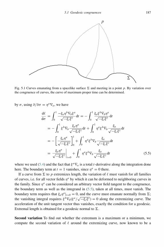
5.1 Geodesic congruences 187
Σ
p
Fig. 5.1 Curves emanating from a spacelike surface � and meeting in a point p. By variation overthe congruence of curves, the curve of maximum proper time can be determined.
by σ , using ∂/∂σ = ηa∇a , we have
d
dσ=
∫ 1
0
−ξaηb∇bξ
a
√−ξcξ cdt = −
∫ 1
0
ξaξb∇bη
a
√−ξcξ cdt
= −∫ 1
0ξb∇b
ξaηa
√−ξcξ cdt +
∫ 1
0ηaξb∇b
ξa√−ξcξ cdt
= −[
ξaηa
√−ξcξ c
]1
0
+∫ 1
0ηaξb∇b
ξa√−ξcξ cdt
= ξaηa
√−ξcξ c
∣∣∣∣t=0
+∫ 1
0ηaξb∇b
ξa√−ξcξ cdt (5.5)
where we used (5.4) and the fact that ξa∇a is a total t-derivative along the integration donehere. The boundary term at t = 1 vanishes, since ηa = 0 there.
If a curve from � to p extremizes length, the variation of must vanish for all familiesof curves, i.e. for all vector fields ηa by which it can be deformed to neighboring curves inthe family. Since ηa can be considered an arbitrary vector field tangent to the congruence,the boundary term as well as the integrand in (5.5), taken at all times, must vanish. Theboundary term requires that ξaηa|t=0 = 0, and the curve must emanate normally from �;the vanishing integral requires ξb∇b(ξa/
√−ξcξ c) = 0 along the extremizing curve. Theacceleration of the unit tangent vector thus vanishes, exactly the condition for a geodesic.Extremal length is obtained for a geodesic normal to �.
Second variation To find out whether the extremum is a maximum or a minimum, wecompute the second variation of around the extremizing curve, now known to be a

188 Global and asymptotic properties
geodesic normal to �. Starting from (5.5), the second variation is
d2
dσ 2=
∫ 1
0ηc∇c
(ηaξb∇b
ξa√−ξdξd
)dt + ηc∇c
ξaηa√
−ξdξd
∣∣∣∣∣t=0
=: I (η) + B(η) .
Note that it is meaningful to take the derivative of the boundary term along ηc because ηc
is tangent to � at t = 0.We will discuss the integral term I (η) and the boundary term B(η) separately. (The
integral I (η) is not zero in general because ξb∇bξa√−ξcξ c is required to vanish at one σ only,
corresponding to the extremizing geodesic; its σ -derivative may be non-vanishing.)For the integral term we have, using that γσ0 is the extremizing geodesic and that
[ξ, η]a = 0,
I (η)|σ=σ0 =∫ 1
0ηcηa(∇cξ
b)∇b
ξa√−ξdξd
dt +∫ 1
0ηcηaξb∇c∇b
ξa√−ξdξd
dt
=∫ 1
0ηa(ξ c∇cη
b)∇b
ξa√−ξdξd
dt +∫ 1
0ηcηaξb∇b∇c
ξa√−ξdξd
dt
+∫ 1
0ηcηaξbRcba
d ξd√−ξeξ edt
=∫ 1
0ηaξc∇c
(ηb∇b
ξa√−ξdξd
)dt +
∫ 1
0ηcηaξbRcba
d ξd√−ξeξ edt
=∫ 1
0
(ηaξc∇c
(ξb√
−ξdξd∇bηa + ξaξ
bξd
(−ξeξ e)3/2∇bη
d
)
+ ηcηaξbRcbad ξd√−ξeξ e
)dt
=∫ 1
0ηa
(ξc∇c
ξ b√−ξdξd
∇b
(ηa + ξdη
d ξa
−ξeξ e
)
+ Rcbadηcξb ξd√−ξeξ e
)dt
=∫ 1
0η⊥a
(ξc∇c
ξ b√−ξdξd
∇bη⊥a + Rcba
dη⊥cξ b ξd√−ξeξ e
)dt (5.6)
having in the final steps again used the fact that ξa at the extremum is the tangent vector toa geodesic. We also defined the component
η⊥a = ηa − ηdξd
ξeξ eξa
of ηa orthogonal to ξa .

5.1 Geodesic congruences 189
For the boundary term we have, using ξaηa = 0 at t = 0,
B(η)|σ=σ0 = ηc∇c
ξaηa√
−ξbξb
∣∣∣∣∣t=0
= ξa√−ξbξb
ηc∇cηa
∣∣∣∣∣t=0
+ ξaηa
(−ξdξd )3/2ξbη
c∇cξb
∣∣∣∣t=0
+ ηa√−ξbξb
ηc∇cξa
∣∣∣∣∣t=0
= ξa√−ξbξb
ηc∇cηa
∣∣∣∣∣t=0
+ ηa ξc√−ξbξb
∇cηa
∣∣∣∣∣t=0
= ξa√−ξbξb
η⊥c∇cη⊥a
∣∣∣∣∣t=0
+ η⊥a ξ c√−ξbξb
∇cη⊥a
∣∣∣∣∣t=0
= −η⊥cη⊥a∇c
ξa√−ξbξb
∣∣∣∣∣t=0
+ η⊥a ξ c√−ξbξb
∇cη⊥a
∣∣∣∣∣t=0
= −Kabη⊥aη⊥b
∣∣t=0 + η⊥a d
dτη⊥a
∣∣∣∣t=0
(5.7)
with the extrinsic curvature Kab, defined as in (3.49), of � as the surface at t = 0, whoseunit normal is ξa/
√−ξbξb. Thus, η⊥a projects ∇c(ξa/
√−ξbξb) tangentially to �.
So far, we have assumed the curves to be differentiable. If there are finitely many kinksat points pi where γσ (ti) is not differentiable and derivatives are discontinuous, we split thewhole t-integration into a sum of integrals over smooth parts of curves. In particular, wewill use the case of a kink in ηa while assuming that ξa remains smooth. Boundary termsof t-integrals from kink to kink then contribute via the second term in (5.7) the terms
$i
(η⊥a ξb
√−ξcξ c∇bη
⊥a
)(5.8)
where we defined
$if := limε→0
(f (ti + ε) − f (ti − ε))
for a function f . Thus, combining (5.6), (5.7) and (5.8) the second variation of arc lengtharound the extremum given by a geodesic is
d2
dσ 2
∣∣∣∣extremum
(η) =∫ 1
0dτη⊥a
(d2
dτ 2η⊥a + Rcba
dη⊥c ξ bξd
−ξeξ e
)+ η⊥a d
dτη⊥a
∣∣∣∣t=0
− Kabη⊥aη⊥b
∣∣t=0
+∑i
$i
(η⊥a d
dτη⊥a
). (5.9)
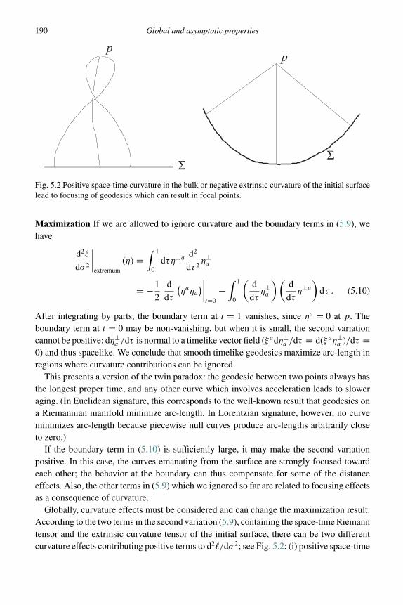
190 Global and asymptotic properties
ΣΣ
Fig. 5.2 Positive space-time curvature in the bulk or negative extrinsic curvature of the initial surfacelead to focusing of geodesics which can result in focal points.
Maximization If we are allowed to ignore curvature and the boundary terms in (5.9), wehave
d2
dσ 2
∣∣∣∣extremum
(η) =∫ 1
0dτη⊥a d2
dτ 2η⊥a
= −1
2
d
dτ
(ηaηa
)∣∣∣∣t=0
−∫ 1
0
(d
dτη⊥a
)(d
dτη⊥a
)dτ . (5.10)
After integrating by parts, the boundary term at t = 1 vanishes, since ηa = 0 at p. Theboundary term at t = 0 may be non-vanishing, but when it is small, the second variationcannot be positive: dη⊥
a /dτ is normal to a timelike vector field (ξadη⊥a /dτ = d(ξaη⊥
a )/dτ =0) and thus spacelike. We conclude that smooth timelike geodesics maximize arc-length inregions where curvature contributions can be ignored.
This presents a version of the twin paradox: the geodesic between two points always hasthe longest proper time, and any other curve which involves acceleration leads to sloweraging. (In Euclidean signature, this corresponds to the well-known result that geodesics ona Riemannian manifold minimize arc-length. In Lorentzian signature, however, no curveminimizes arc-length because piecewise null curves produce arc-lengths arbitrarily closeto zero.)
If the boundary term in (5.10) is sufficiently large, it may make the second variationpositive. In this case, the curves emanating from the surface are strongly focused towardeach other; the behavior at the boundary can thus compensate for some of the distanceeffects. Also, the other terms in (5.9) which we ignored so far are related to focusing effectsas a consequence of curvature.
Globally, curvature effects must be considered and can change the maximization result.According to the two terms in the second variation (5.9), containing the space-time Riemanntensor and the extrinsic curvature tensor of the initial surface, there can be two differentcurvature effects contributing positive terms to d2/dσ 2; see Fig. 5.2: (i) positive space-time

5.1 Geodesic congruences 191
curvature in the form Rcbadη⊥cξ bη⊥aξd > 0 leads to bending and focusing of geodesics
which then evolve into focal points, and (ii) negative extrinsic curvature of the initial surfacewould aim the geodesics toward each other, also implying a focal point even in the absenceof space-time curvature. Beyond the focal point, timelike geodesics no longer maximizearc-length, which we now demonstrate using the notion of Jacobi vector fields.
5.1.1.2 Jacobi vector fields
A Jacobi vector field κa along a geodesic γ is a non-vanishing vector field which iseverywhere orthogonal to the tangent vector ξa , i.e. ξaκa = 0, and is a solution of thegeodesic deviation equation
d2
dτ 2κa + Rcba
dκc ξbξd
−ξeξ e= 0 . (5.11)
This being a second-order differential equation for a 4-vector restricted by ξaχa = 0, itprovides six independent solutions for Jacobi vector fields. To recall, the geodesic deviationequation is satisfied by a deviation vector (∂/∂σ )a in a congruence γσ (t) whose curves forfixed σ are all geodesic. One can thus interpret the family of Jacobi vector fields as aparameterization of all possible embeddings of the given geodesic γ in a congruence, aninterpretation that illustrates our interest in Jacobi vector fields for the questions consideredhere.
Geodesic congruences For a congruence of geodesics emanating from a surface and cul-minating in a focal point, there must be a Jacobi vector field satisfying κa(1) = 0 if thefocal point is reached at t = 1, as well as
dκadτ
∣∣∣∣t=0
= Kabκb|t=0 (5.12)
at the initial surface � : t = 0. We show this in the following calculation.
Example 5.1 (Geodesic congruences and extrinsic curvature)For the proper-time derivative of a Jacobi vector field along a geodesic congruence, wehave
d
dτκa = ξb
√−ξcξc∇bκa = κb∇bξa√−ξcξc
.
We did not normalize the tangent vector ξa to keep our coordinate vector fields (5.4)commuting, a property used in the second step of the preceding equation.
At the initial surface � : t = 0 of the congruence, the normalized tangent vector togeodesics provides the unit normal, since the deviation vector χa must be tangent to thesurface and is normal to the geodesic tangent vectors in the case of a Jacobi vector field.The vector field ξa , once normalized, can thus be used to compute the extrinsic curvature
Kab = hca∇c
ξb√−ξdξd
192 Global and asymptotic properties
of �. We compare the two formulas using also
κb∇b
√−ξcξc = −ξcκb∇bξc√
−ξdξd= −ξcξb∇bκc√
−ξdξd= κcξ
b∇bξc√−ξdξd
= 0
at t = 0 because κa and ξa are orthogonal and since ξa is tangent to a geodesic. Thus,
dκadτ
= κb∇b
ξa√−ξcξc= κbKab ,
proving (5.12), since κa is tangent to � at t = 0, providing a projection of the derivativeof the unit tangent.
If a Jacobi vector field κa with the boundary conditions κa(1) = 0 and (5.12) exists alongthe geodesic γ from � to q = γ (1), the point q = γ (1) is called conjugate to �.
We assume now that we have a geodesic γ from � to a point p, and that it lies in acongruence with a conjugate point q to � before p is reached along γ . Thus, between� and q we have a Jacobi vector field with the above boundary conditions; in particular,κa = 0 at q. We continuously extend κa as a vector field beyond q by saying that itvanishes between q and p. Moreover, we choose another vector field λa with ξaλa = 0such that λadκa/dτ = −1 at q. Using ηa := ελa + ε−1κa for some ε ∈ R\{0}, we definethe deviation vector field of a new congruence (not necessarily geodesic, and one with akink at q where ηa is not smooth). It implies a second variation of arc-length
d2
ds2
∣∣∣∣extremum
(η) = ε2 d2
ds2
∣∣∣∣extremum
(λ) + 2$q(λadκa/dτ )
= ε2 d2
ds2
∣∣∣∣extremum
(λ) + 2
using the fact that κa is piecewise Jacobi (or identically zero beyond q) with the givenboundary condition (5.12) at �, and taking one new contribution in (5.9) from the point qwhere the congruence has its kink. This variation becomes positive for sufficiently small ε,which proves that the timelike geodesic γ no longer provides a curve of maximum lengthbeyond a focal point (see Fig. 5.3).
Diverging expansion Jacobi fields can also be used to demonstrate that the expansion of acongruence diverges at a focal point. We pick three independent Jacobi fields κa
i , i = 1, 2, 3,satisfying the boundary condition (5.12) at �. They give us the deviation vectors of threeindependent congruences. The components of κa
i can be viewed as forming a matrix, whichmust be invertible at places of the congruence that are not conjugate points to �. Then, from(ξb/
√−ξcξc)∇bκai = κb
i ∇b(ξa/√−ξcξc) = κb
i Bba (by a calculation as in Example 5.1) we
obtain the expansion
θ = Baa = (κ−1)ia
ξ b
√−ξcξc∇bκ
ai = ξb
√−ξcξc∇b log | det(κa
i )| . (5.13)
At a conjugate point, the matrix κai becomes degenerate, and the expansion diverges.

5.1 Geodesic congruences 193
qp
γ
Σ
Fig. 5.3 Beyond a focal point, non-geodesic curves of proper time larger than that of any geodesic exist(dashed). (The Euclidean representation here makes the dashed extension look shorter, not longer.)
Just as in the case of isotropic and homogeneous singularity theorems, the Raychaudhuriequation guarantees the existence of conjugate points in congruences emanating from asurface whose extrinsic curvature has a trace bounded from above by a negative constant,Ka
a ≤ C < 0, provided that the strong energy condition holds. The tangent vector field ξa
on the congruence is normal to the initial surface, where we haveKaa = ∇a(ξa/
√−ξbξb) =
θ ≤ C < 0. Moreover, ξa is hypersurface orthogonal at � by assumption, and thus hasinitially vanishing rotation. It then follows from the rate of change (5.2) of Bab that ωab = 0on the whole congruence as long as θ is regular, i.e. at least until a conjugate point isreached. Thus, the Raychaudhuri equation (5.3) can be estimated and solved just as in thehomogeneous case in Chapter 2.4, with the conclusion that θ diverges after a proper timeof at most τ ≤ 3/|C|; there must be a conjugate point before that time.
We are now able to formulate the first general singularity theorem (for details, seeHawking and Ellis (1973)):
Theorem 5.1 (Singularity theorem) Assume that the strong energy condition is satisfiedand that space-time is globally hyperbolic. If there is a spacelike Cauchy surface � ofextrinsic curvature Ka
a ≤ C < 0, then no timelike curve from � can have a proper lengthlarger than 3/|C|.Proof (Sketch) The proof is indirect: assume that there is a timelike curve λ with properlength larger than 3/|C| and take a point p on λ of a distance more than 3/|C| away from�. Global hyperbolicity can be shown to imply the existence of a curve γ of maximumlength from � to p, which by assumption must have a length larger than 3/|C|. From theprevious results, this can only be a geodesic without a conjugate point between � and p,in contradiction to what follows from the Raychaudhuri equation. �
The theorem demonstrates that under the given conditions space-time is incomplete. Thereare timelike curves of finite proper time that cannot be extended further. Test massesfollowing these curves only exist for a finite amount of proper time.
194 Global and asymptotic properties
5.1.2 Null geodesic congruences
Null congruences, whose tangent vector field is everywhere null, require a decomposition ofBab different from (5.1). If we again define hab = gab + kakb, now calling the null tangentvector field ka , it is degenerate on vectors orthogonal to ka , including ka itself. Formally,one can still define the decomposition as in (5.1), since no inverse of hab is required.However, this will not capture the correct number of degrees of freedom describing a nullcongruence.
5.1.2.1 Decomposition
There are two equivalent ways to deal with the degeneracy. For the first one, as followedby Wald (1984), we consider the 2-dimensional factor space of all vectors orthogonal toka modulo the vector space K generated by ka: any element in this factor space can berepresented by κa + λka where κaka = 0 and λ ∈ R is arbitrary. The degenerate directionis here simply factored out. Any tensor T a1...an
b1...bmthat vanishes on K , i.e. when contracted with
ka on any of its indices, yields a well-defined projection to the factor space, then denotedby a hat: T a1...an
b1...bm. Due to T
a1...anb1...bm
kai = 0 = Ta1...anb1...bm
kbj
for all 1 ≤ i ≤ n and 1 ≤ j ≤ m byassumption, a contraction of the tensor with κa + λka on any one of its indices will notdepend on λ, and thus will yield the same result for the whole equivalence class of vectors.The projected tensor T a1...an
b1...bmis in this way defined on the factor space. One example is hab
obtained from hab (or gab, since the projection of kakb vanishes) as the non-degenerateinduced metric on the 2-dimensional factor space.
For the second procedure, we note that the null property of the tangent vector fieldimplies the existence of a second independent null vector field a , aa = 0, which wecan cross-normalize with ka such that aka = −1. Then, hab := gab + 2(akb) satisfiesahab = 0 = kahab and is thus the 2-metric on a 2-dimensional subspace normal to both ka
and a . Defining hab as the evaluation of hab on the 2-dimensional subspace of the tangentspace normal to both ka and a , we obtain a specific representative of the factor-spacemetric defined by the first procedure.
Another example for a projectable tensor is Bab = ∇bka: it satisfies Babka = 0 = Babk
b
as already seen in the timelike case. (Here, we have to use the affine parameterization fornull geodesics, i.e. kc∇ck
a = 0.) The projection is then decomposed as
Bab = 1
2θhab + σab + ωab (5.14)
with
θ = gabBab , σab = Bab − 1
2θhab , ωab = B[ab] . (5.15)
(Notice that we have the trace gabhab = gab(gab + 2akb) = δaa + 2aka = 2.) Since theaffine parameterization is fixed only up to a multiplicative constant of ka , also θ , σab andωab are defined only up to a multiplicative constant in the null case.
5.1 Geodesic congruences 195
As before, we derive
kc∇cBab + BcbBac = Rcbadkckd
which implies that
kc∇cθ = −1
2θ2 − σabσ
ab + ωabωab − Rcdk
ckd . (5.16)
The last term is again non-positive if the strong energy condition holds, but now even forthe weak energy condition, since kc is null. We conclude that there must be a focal pointin any hypersurface-orthogonal null congruence whose expansion θ0 is negative at somevalue of the affine parameter, and this focal point is reached within an affine length of atmost 2/|θ0|. (This statement is invariant under rescaling the affine parameter λ defined bykc∇c = d/dλ: λ and 1/θ0 scale in the same way if the affine parameter is changed. Suitablecombinations such as λθ0 are scaling invariant.)
5.1.2.2 Trapped surfaces and singularities
As in the timelike case, a singularity theorem requires us to connect the appearance of a focalpoint in geodesic congruences with inextendability. While timelike congruences capturethe intuitive notion of co-moving observers experiencing the whole expansion or collapseof space in a cosmological situation, null congruences describe the motion of light. Forcosmological singularities, having a time when the expansion is everywhere bounded awayfrom zero was seen to guarantee a singularity in the past or the future. Null congruences arerelated to a different concept that provides an initial condition to guarantee singularities.Focal points of null geodesic congruences lead to singularities if a trapped surface T exists:a compact, 2-dimensional smooth spacelike submanifold T such that the expansion of bothsets of future-directed null geodesics orthogonal to T is everywhere negative on T .
In Minkowski space, any compact 2-dimensional spacelike surface has one expanding(“outgoing”) and one contracting (“ingoing”) family of future-directed normal null con-gruences. But even light rays shining “out of” a trapped surface are contracted towardsmaller cross-sections of the beam. A geometry allowing trapped surfaces must thus berather different from the one known for Minkowski space. After showing in the rest ofthis subsection the importance of trapped surfaces for singularities, recognized by Penrose(1965), we will provide examples and interpretations for them in what follows.
Theorem 5.2 (Singularity theorem: trapped-surface version) Assume that the weakor strong energy condition holds and that space-time M is globally hyperbolic with anon-compact connected Cauchy surface �. If a trapped surface T exists with expansionsθ ≤ θ0 < 0 for both normal null congruences, then there is an inextendible null geodesicof affine distance no larger than 2/|θ0| from T .
Proof (Sketch) We first introduce the future I+(T ) of T as the set of all points in M
connected to T by future-directed timelike curves. Its boundary I+(T ) is closed (theboundary of a boundary is empty) and is a 3-dimensional (but not necessarily differentiable;

196 Global and asymptotic properties
tr
S
Fig. 5.4 The future (hashed) of a spherical surface has a non-smooth part where it intersects thecenter. Here, we show a 2-dimensional space-time diagram in which points represent 2-surfacesin space-time and light rays travel along ±450 lines. (More on this technique of causal diagramswill be discussed in Chapter 5.2.2.) To the future of the kink, light signals appear to originate fromthe reflection of the initial sphere S at the r = 0 world-line (dashed). The first reflection point is aconjugate point of S, and lies at a kink of I+(S). Except for this point, r = 0 is not part of I+(S);the future of the kink is in the interior of I+(S). The boundary of the future is non-differentiable:points in the diagram are spheres for r �= 0 but points also in 4-dimensional space-time for r = 0.Including the dashed mirror-reflection in the diagram illustrates the non-smooth behavior of I+(S) inspace-time.
see Fig. 5.4) manifold locally generated by null geodesics. In general, I+(T ) does notcontain complete null geodesics: any point on a null geodesic beyond a conjugate pointcan be connected to T by a timelike curve and thus lies in the interior rather than theboundary of I+(T ). (This can be shown by constructing a deformation similar to that used inChapter 5.1.1.2 to show that timelike geodesics fail to maximize on arc-length beyondconjugate points.)
In the context of the theorem, the expansion of null geodesics emanating from a trappedsurface T is initially bounded from above by a negative value. Using the Raychaudhuriequation, all null geodesics have a conjugate point after some finite affine length. Providedthat all null geodesics are extendible arbitrarily, I+(T ) must then be compact. (It is closedas the boundary of the future and bounded because the affine distance between any twopoints in the set is bounded. Note that it does not have a boundary, but like a 2-sphere inspace is bounded in the sense that its complement in space-time is open.) To bring this to acontradiction, we use an arbitrary time-evolution vector field whose trajectories define a mapψ : I+(T ) → S ⊂ � which is a homeomorphism; see Fig. 5.5. The image S of a compactset must then be closed and bounded but cannot have a boundary, as these topologicalproperties are transferred from I+(T ): no homeomorphism can map a compact to a non-compact set. This contradicts the non-compactness of the Cauchy surface � assumed in

5.1 Geodesic congruences 197
Σ
T
Fig. 5.5 Mapping the future of T to a spatial surface � along trajectories of a time-evolution vectorfield.
the theorem. The only consistent conclusion is that our assumption of extendability of allnull geodesics must be violated, and we again derive geodesic incompleteness. �
Many assumptions in the singularity theorems can be weakened if more refined tech-niques are used. For instance, global hyperbolicity is not necessary. Four essential conditionsthen remain, as reviewed, e.g., by Senovilla (1998):
• an energy condition;• a genericity assumption (such as the one stating that each timelike geodesic contains a point where
Rabcdξaξ d �= 0);
• there is no closed timelike curve; and• at least one additional property specifying an initial condition:
(i) a closed universe (a compact spatial submanifold without boundary exists),(ii) a trapped surface exists, or
(iii) there is a point p such that the expansion of future-directed null geodesics from p becomesnegative along each geodesic.
Under these conditions, space-time must be singular in the sense that at least one inex-tendible timelike or null geodesic exists. (In general, however, it is not guaranteed thatall such geodesics are inextendible, nor are conclusions about curvature divergencesdrawn.)
At such a general level, the actual conclusions of singularity theorems may appear ratherweak, predicting properties much tamer than what is known from explicit examples in cos-mology or the physics of black holes. Moreover, the conclusions can be evaded by violatingsome of the more peculiar assumptions even without introducing exotic matter forms, asfirst constructed by Senovilla (1990); see also the detailed description by Chinea et al.(1992). Extensions of the traditional assumptions and theorems have thus been attempted,for instance by Clarke (1998), Vickers and Wilson (2000, 2001) and Senovilla (2007), butthe level of generality of the theorems based on geodesic incompleteness remains unsur-passed. Nevertheless, singularity theorems are of utmost conceptual importance: they showthat there is no mechanism in classical general relativity that could guarantee unlimitedevolution of generic initial values. The theorems highlight major roadblocks to completeevolution within the theory, and they show the stability of singularities: they refer only to
198 Global and asymptotic properties
inequalities in their assumptions, such that perturbations around explicitly known singular-ities cannot eliminate singular behavior.
5.2 Trapped surfaces
We have seen two versions of singularity theorems, one of which is suitable for cosmologicalsolutions, and one for black holes:
1. Extrinsic curvature on a Cauchy slice which is bounded from above by a negative constantmeans that the universe is globally contracting at one time. The singularity Theorem 5.1 impliesgeodesic incompleteness which one can interpret as a consequence of the universe collapsing intoa singularity.
2. The existence of a trapped surface means that there is a bounded region of space-time where thegravitational field is strong enough to contain even light emanating from the trapped surface. (Inthis case light is contained at least locally, as the negative value of expansion of the outgoingnull normal congruence on the trapped surface may grow and become positive away from thesurface.) According to singularity Theorem 5.2, this region collapses into a singularity which onecan associate with a black hole.
In both cases, the fact that gravity is purely attractive under most circumstances (unlesspressure becomes very negative) removes any means to stop the collapse of matter andspace once it has progressed sufficiently far.
5.2.1 Black-hole solutions
We have seen the cosmological situation of collapse in several examples of homogeneousmodels. The trapped-surface version of the singularity theorem is realized in the simplestcase for the Schwarzschild solution
ds2 = −(
1 − 2M
r
)dt2 +
(1 − 2M
r
)−1
dr2 + r2d�2 . (5.17)
This line element is ill-defined at r = 2M owing to a failure of the coordinate system used.The two separate regions r > 2M and r < 2M can, however, be discussed appropriatelyin Schwarzschild coordinates. Their behavior is quite different:
r > 2M: A timelike Killing vector field ∂/∂t exists in addition to the spherical Killing vector fields.The metric in this region is stationary (and, in fact, static).
r < 2M: Because 1 − 2M/r < 0 in this region, the Killing vector field ∂/∂t is now spacelike. Themetric is no longer stationary but rather dynamical. Instead of stationarity, the Killing vector fieldtogether with spherical symmetry implies homogeneity: there are three independent spacelikeKilling vectors at each point.1
1 The submanifolds defined by r = const are spacelike and have the topology R × S2 with t as the coordinate of R and thepolar coordinates on the 2-spheres. Since there are three independent rotational Killing vector fields (only two of which arelinearly independent at each point), in addition to homogeneity, there is a rotational symmetry around one axis transverse tothe 2-spheres. The geometry is of Kantowski–Sachs type, a homogeneous model not contained as a special case in the Bianchiclassification: its symmetry group is 4-dimensional without allowing a 3-dimensional Bianchi subgroup.

5.2 Trapped surfaces 199
r0<rr0
r0>r
r0<r
r0
Fig. 5.6 If r = r0 = const defines timelike surfaces, the two future-pointing null normal congruencesto spheres at r0 either increase or decrease the cross-section area; the spheres are thus untrapped (left).If r = r0 = const is spacelike, however, both normal congruences change cross-section areas in thesame way — the region is trapped (right).
In particular, surfaces r = const are timelike for r > 2M but spacelike for r < 2M . Thisproperty has immediate consequences for the existence of trapped surfaces, as visualizedin the causal diagram Fig. 5.6 where null lines run at ±450: in any situation in which r isthe area radius coordinate such that the angular part of the metric is r2d�2 as in (5.17),a spacelike surface r = const implies that 2-dimensional spherical cross-sections definedby r = const, t = const are trapped. If r = const is timelike, future-pointing null normalsreach smaller r for the “ingoing” family and larger r for the “outgoing” family. The firstcongruence has negative expansion and the second one positive expansion because thecross-section area proportional to r2 increases for the latter. A surface at constant t is thusnot trapped. But if r = const is spacelike, both future pointing null normals can only reacheither smaller or larger r . It is then only possible that both expansions are negative or bothare positive. Spheres at constant t and r are trapped (future trapped if smaller r is to thefuture, and past trapped if larger r is to the future).
Example 5.2 (Spherical trapped surfaces)In order to see more concretely that the nature of r = const surfaces in a sphericallysymmetric space-time provides a criterion for spherical trapped surfaces, we compute thegeneral form of radial null vector fields in a 2-dimensional space-time with general lineelement ds2 = gttdt2 + 2grtdtdr + grrdr2. We assume that grt > 0 and that t is a goodtime coordinate in the whole region considered; if there is a flip of t and r as happenswhen the horizon in Schwarzschild coordinates is traversed, the following arguments mustbe adapted. A radial null vector ξa satisfies grr (ξ r )2 + 2grt ξ
rξ t + gtt (ξ t )2 = 0, which weinterpret as a quadratic polynomial for ξ r . Null vector fields thus satisfy one of the tworelationships
ξ r± = −grt
grr
(1 ∓
√1 − gtt
grrg2rt
)ξ t± (5.18)

200 Global and asymptotic properties
between their components. For a future-pointing null vector, we assume that ξ t± > 0, but
for the following argument we do not need to restrict ξ t± further. (For a null geodesic family
in affine parameterization, for instance, the geodesic equation would provide anothercondition for ξ t
±(t, r) to satisfy.)A null normal congruence emanating from a sphere at constant r = r0 is expanding if its
tangent vector field ξa satisfies ξa∂ar > 0, and is contracting if ξa∂ar < 0. By this condition,the vector field ξa
− in (5.18) is always contracting while ξa+ may be expanding or contracting
depending on the geometry. It is expanding if gtt /grr < 0, and contracting if gtt /grr > 0.The intermediate case belongs to a spherical marginally trapped surface. Inverting the lineelement, the condition can equally be formulated in terms of grr/gtt = gtt /grr whose signin regions where the lapse function does not vanish, and thus gtt = −1/N2 < 0, is solelydetermined by grr = gab(dr)a(dr)b = |na|2 with the co-normalna = (dr)a to spheres. Thus,if the normal na to r = r0 is spacelike (such that the surface r = r0 is timelike), grr > 0 andthe outgoing null normal congruence is expanding. The surface r = r0 is not trapped. Inthe opposite case, for a timelike normal na both normal null congruences are contractingand r = r0 is trapped.
Horizon properties from different perspectives especially in the spherical context areexhibited by Nielsen and Visser (2006) and Nielsen (2009).
Example 5.3 (Trapped surfaces in Painleve–Gullstrand coordinates)Both regions of the Schwarzschild space-time can be described simultaneously in a coor-dinate system of Painleve–Gullstrand form where (5.17) becomes:
ds2 = −dT 2 +(
dr +√
2M/r dT)2
+ r2d�2 (5.19)
with a suitable new coordinate T (t, r). (As an aside, notice that spatial slices of constantT are flat.) Also here, for r < 2M surfaces r = const are spacelike because they have theinduced metric ds2 = −(1 − 2M/r)dT 2 + r2d�2. We can explicitly compute null congru-ences with tangents ξa
± normal to spheres from the conditions gabξa±ξ
b± = 0 together with
ξa±∇aT > 0 to pick the future-pointing ones. This yields
ξa± =
(∂
∂T
)a
−(√
2M
r∓ 1
)(∂
∂r
)a
.
With ξa−∇ar = −(1 + √
2M/r) < 0, ξa− is always the ingoing null normal of negative
expansion. For the outgoing null normal ξa+, we have ξa
+∇ar = 1 − √2M/r which is
negative for r < 2M . Thus, in this region both future-pointing null normal congruenceshave negative expansion because the area radius decreases along both of them. Here,spheres of constant r and T are trapped.
For the sherically symmetric Schwarzschild solution, one can of course construct thewhole space-time solution and directly verify the existence of a curvature singularity tothe future of the trapped region r < 2M: r plays the role of a time coordinate for r < 2M
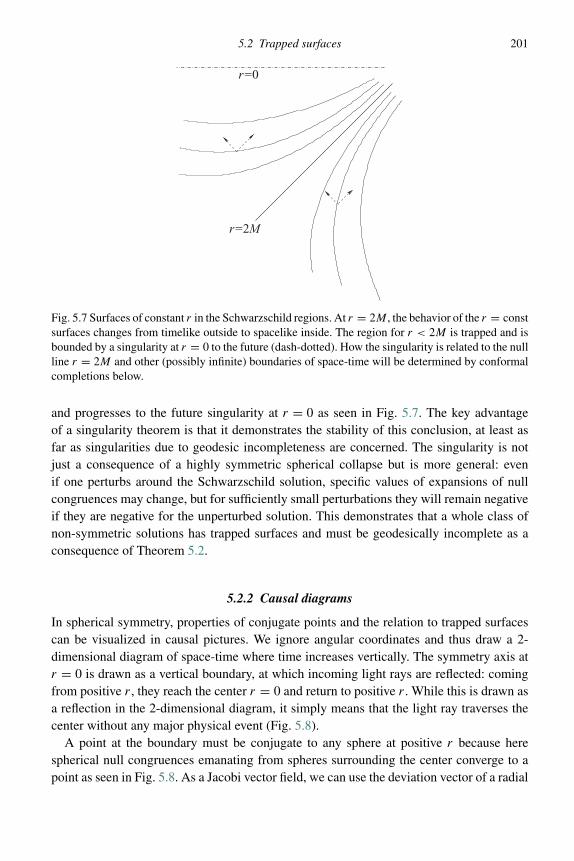
5.2 Trapped surfaces 201
r=2M
r=0
Fig. 5.7 Surfaces of constant r in the Schwarzschild regions. At r = 2M , the behavior of the r = constsurfaces changes from timelike outside to spacelike inside. The region for r < 2M is trapped and isbounded by a singularity at r = 0 to the future (dash-dotted). How the singularity is related to the nullline r = 2M and other (possibly infinite) boundaries of space-time will be determined by conformalcompletions below.
and progresses to the future singularity at r = 0 as seen in Fig. 5.7. The key advantageof a singularity theorem is that it demonstrates the stability of this conclusion, at least asfar as singularities due to geodesic incompleteness are concerned. The singularity is notjust a consequence of a highly symmetric spherical collapse but is more general: evenif one perturbs around the Schwarzschild solution, specific values of expansions of nullcongruences may change, but for sufficiently small perturbations they will remain negativeif they are negative for the unperturbed solution. This demonstrates that a whole class ofnon-symmetric solutions has trapped surfaces and must be geodesically incomplete as aconsequence of Theorem 5.2.
5.2.2 Causal diagrams
In spherical symmetry, properties of conjugate points and the relation to trapped surfacescan be visualized in causal pictures. We ignore angular coordinates and thus draw a 2-dimensional diagram of space-time where time increases vertically. The symmetry axis atr = 0 is drawn as a vertical boundary, at which incoming light rays are reflected: comingfrom positive r , they reach the center r = 0 and return to positive r . While this is drawn asa reflection in the 2-dimensional diagram, it simply means that the light ray traverses thecenter without any major physical event (Fig. 5.8).
A point at the boundary must be conjugate to any sphere at positive r because herespherical null congruences emanating from spheres surrounding the center converge to apoint as seen in Fig. 5.8. As a Jacobi vector field, we can use the deviation vector of a radial
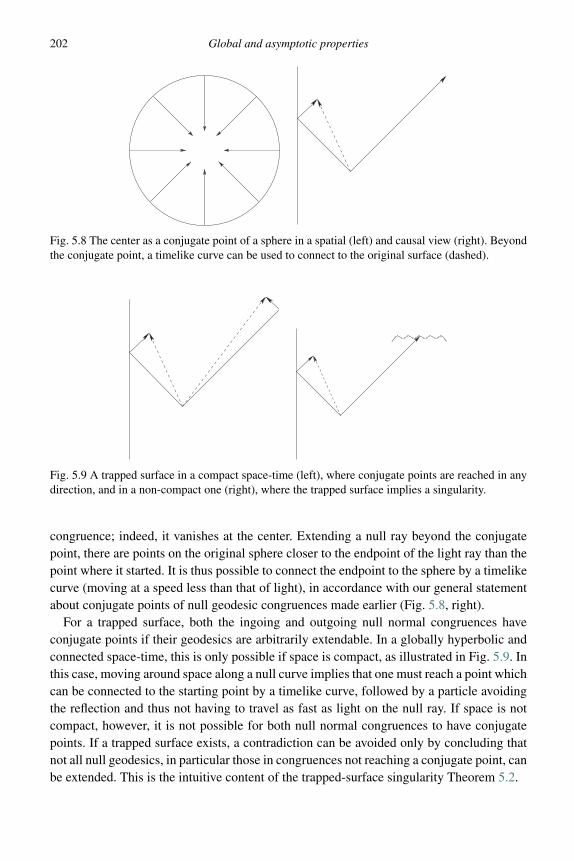
202 Global and asymptotic properties
Fig. 5.8 The center as a conjugate point of a sphere in a spatial (left) and causal view (right). Beyondthe conjugate point, a timelike curve can be used to connect to the original surface (dashed).
Fig. 5.9 A trapped surface in a compact space-time (left), where conjugate points are reached in anydirection, and in a non-compact one (right), where the trapped surface implies a singularity.
congruence; indeed, it vanishes at the center. Extending a null ray beyond the conjugatepoint, there are points on the original sphere closer to the endpoint of the light ray than thepoint where it started. It is thus possible to connect the endpoint to the sphere by a timelikecurve (moving at a speed less than that of light), in accordance with our general statementabout conjugate points of null geodesic congruences made earlier (Fig. 5.8, right).
For a trapped surface, both the ingoing and outgoing null normal congruences haveconjugate points if their geodesics are arbitrarily extendable. In a globally hyperbolic andconnected space-time, this is only possible if space is compact, as illustrated in Fig. 5.9. Inthis case, moving around space along a null curve implies that one must reach a point whichcan be connected to the starting point by a timelike curve, followed by a particle avoidingthe reflection and thus not having to travel as fast as light on the null ray. If space is notcompact, however, it is not possible for both null normal congruences to have conjugatepoints. If a trapped surface exists, a contradiction can be avoided only by concluding thatnot all null geodesics, in particular those in congruences not reaching a conjugate point, canbe extended. This is the intuitive content of the trapped-surface singularity Theorem 5.2.

5.3 Asymptotic infinity 203
u= constv=const
rt
Fig. 5.10 Double-null coordinates u and v in Minkowski space and their coordinate lines. At thecenter (dashed), a v = const line is “reflected” into a u = const line, and vice versa.
5.3 Asymptotic infinity
For a full view on space-time, the behavior at infinity is also important. There is a rich struc-ture, owing to the fact that the behavior depends on the direction in which one approachesinfinity, for instance along null curves compared to spacelike curves. Structures at infinityalso provide useful tools to extract physical and observable information: light from non-trapped regions can leave strong-curvature regimes and provide signals to distant observers.How one can extract observables from geodesic congruences or space-time geometries isan important problem for relativistic astrophysics. The situation here is much more com-plicated than in early-universe cosmology, where simple gauge-invariant combinations oflinear metric and matter perturbations provide the main observable quantities.
To start with describing structures at infinity, in particular the space-time metric nearinfinity, the infinite boundary can first be mapped to a finite one via a coordinate transfor-mation. For example, for Minkowski space with line element ds2 = −dt2 + dr2 + r2d�2
we may introduce the null coordinates v := t + r and u := t − r restricted to the rangev ≥ u because r ≥ 0 (see Fig. 5.10). In these coordinates, the metric is
ds2 = −dudv + 1
4(v − u)2d�2 . (5.20)
We are interested in the limits v → ∞, u = const (outgoing null rays) and u → −∞,v = const (incoming null rays). These are the only null lines due to v ≥ u; v → −∞ atconstant u and u → ∞ at constant v are not possible.
The asymptotic limiting points are mapped to finite values by using a new set of coor-dinates, T = arctan v + arctan u, R = arctan v − arctan u, such that dT = dv/(1 + v2) +du/(1 + u2) and dR = dv/(1 + v2) − du/(1 + u2), or
−dT 2 + dR2 = − 4
(1 + u2)(1 + v2)dudv .

204 Global and asymptotic properties
This is not the radial part of Minkowski space (5.20), but it suggests a conformal transfor-mation to gab = �2gab with
�2 = 4
(1 + u2)(1 + v2). (5.21)
As the new metric conformal to Minkowski space, we thus obtain
ds2 = �2ds2 = −dT 2 + dR2 + sin2 Rd�2 (5.22)
where we used
sinR = sin(arctan v) cos(arctan u) − cos(arctan v) sin(arctan u)
= 1√(1 + v−2)(1 + u2)
− 1√(1 + v2)(1 + u−2)
= v − u√(1 + u2)(1 + v2)
.
The metric (5.22) is that of an FLRW model with positive spatial curvature and aconstant scale factor. Such a solution, called Einstein static universe, exists in the presenceof a cosmological constant; see Exercise 2.3 in Chapter 2. The construction shows that thewhole Minkowski space is conformally equivalent to a finite region of the Einstein staticuniverse with metric (5.22), where T and R are bounded. Infinity of Minkowski space canbe studied by a neighborhood of the boundary of the region it defines in the Einstein staticuniverse. This finite region is characterized by the conditions (i) R ≥ 0 due to v ≥ u and(ii) −π < T ± R < π due to properties of the arctan used in the definitions of T and R.Moreover, R < π . When the finite region representing the original space-time is combinedwith its boundary in a conformal embedding, the closed region thus obtained is calledconformal completion or a Carter–Penrose diagram.
The boundary of the region in the Einstein static universe conformally equivalent toMinkowski space is of triangular shape (not smooth but with three corners). One candistinguish several characteristic components; see Fig. 5.11:
R = 0, −π ≤ T ≤ π : this is a timelike line representing the center of polar coordinates. It has twoendpoints, one called i+ at T = π and one called i− at T = −π .
R = π , T = 0: a single point called i0.T + R = π : a null curve at constant v, called J + (and pronounced “scri-plus”).T − R = −π : a null curve at constant u, called J −.
The meaning of these boundary regions can be seen from the behavior of radial geodesicsapproaching them. In Minkowski space, these are straight lines represented by linearrelationships between t and r:
Timelike geodesics Radial, future-pointing timelike geodesics satisfy t = ar + b with some |a| > 1near t → ∞. Thus, t ± r = (1 ± a−1)t ∓ b/a → ∞, and both u and v approach infinity at thefuture endpoint in Minkowski space. In the conformally embedded region, this leads to T → π
and R → 0, which is i+, or future timelike infinity.Similarly, past-pointing timelike geodesics have the above form for t → −∞, where u and v
approach −∞. Here, T → −π and R → 0 approaches i−, or past timelike infinity.

5.3 Asymptotic infinity 205
π
−π
π
J
J
−
+
−
+
0 R
T
0
i
i
i0
Fig. 5.11 Conformal completion of Minkowski space with its boundary components, embedded inthe Einstein Static Universe.
Radially outgoing spacelike geodesics Here, we have the form t = ar + b with |a| < 1 near r →∞. Thus, t ± r = (a ± 1)r + b → ±∞ and v → ∞, u → −∞. In this way, we reach T → 0,R → π and thus i0, or spacelike infinity.
Radially outgoing null geodesics The form t = r + b near t → ∞ implies v → ∞ while u = b
remains constant. Thus, T + R → π , |T − R| < π and we reach J +, or future null infinity.Radially incoming null geodesics In this case, t = −r + b near t → −∞. Now, v = b remains
constant while u → −∞, implying T − R → −π , |T + R| < π . All these geodesics come fromJ −, or past null infinity.
Cataclysmic events such as black holes lead to conformal completions very different fromthe global structure of Minkowski space, impressively showing the difference in geometries.
5.3.1 Asymptotic flatness
Although we have explicitly constructed the conformally completed space-time region onlyfor Minkowski space, the form of asymptotic infinity obtained is general for a large class ofspace-times, or at least certain parts of them. Let us take an arbitrary space-time (M,gab) andassume that it can be conformally embedded in (M, gab = �2gab) as a finite region whoseboundary is given by the set where � = 0, in such a way that ∇a� �= 0 is non-vanishingand finite wherever the boundary is differentiable. The original space-time is said to beasymptotically empty if its energy momentum tensor behaves as Tab = O(�3) near � = 0.These and other asymptotic definitions, together with techniques for the construction ofgeneral conformal diagrams, go back to Penrose (1963).
In order to show that all such space-times have the same structure at infinity as Minkowskispace, we will use a more general version to allow for the presence of a cosmological

206 Global and asymptotic properties
J−
J+ J+
J−
J
Fig. 5.12 Conformal diagrams of an asymptotically flat, asymptotically de Sitter and asymptoticallyanti de Sitter space. Dashed lines indicate symmetry centers or periodic identifications.
constant. In this case, Tab will not approach zero near the boundary and the asymptoticstructure will change, but we can use the same calculations to determine its properties.More generally, we assume that there is a constant � such that Tab + �gab/8πG = O(�3)near � = 0. Einstein’s equation, satisfied on M , then implies a Ricci scalar of the form
R = −8πGgabTab = −8πG�−2gabTab
= 4� + O(�) (5.23)
where we used the fact that the components of gab are finite at � = 0. Moreover, theconformal transformation provides a relation between the Ricci scalars of gab and gab,derived directly from the expression of R in terms of the metric based on equations suchas (3.118):
R = �−2(R − 6gab∇a∇b log� − 6gab(∇a log�)(∇b log�)
)(5.24)
or, inversely,
R = �2R + 6�gab∇a∇b� − 12gab(∇a�)(∇b�) . (5.25)
Because all individual factors on the right-hand side remain finite for � → 0, only the lastterm is non-zero at � = 0. We see that
sgn((∇a�)(∇a�)
) |�=0 = −sgnR|�=0 = −sgn� . (5.26)
The gradient ∇a� = na is the co-normal to the boundary � = 0, and so the boundaryis
• null if � = 0, in which case the space-time (M,gab) is called asymptotically Minkowski,• spacelike if � > 0, in which case the space-time (M,gab) is called asymptotically de Sitter, and• timelike if � < 0, in which case the space-time (M,gab) is called asymptotically anti de Sitter.
The conformal diagrams look like the examples in Fig. 5.12.To eliminate possible pathologies, one often defines geometries more specific than those
corresponding asymptotically to any one of the maximally symmetric ones.
Definition 5.1 A space-time (M,gab) is asymptotically simple if a subset N ⊂ M and aspace-time (M, gab) exist such that
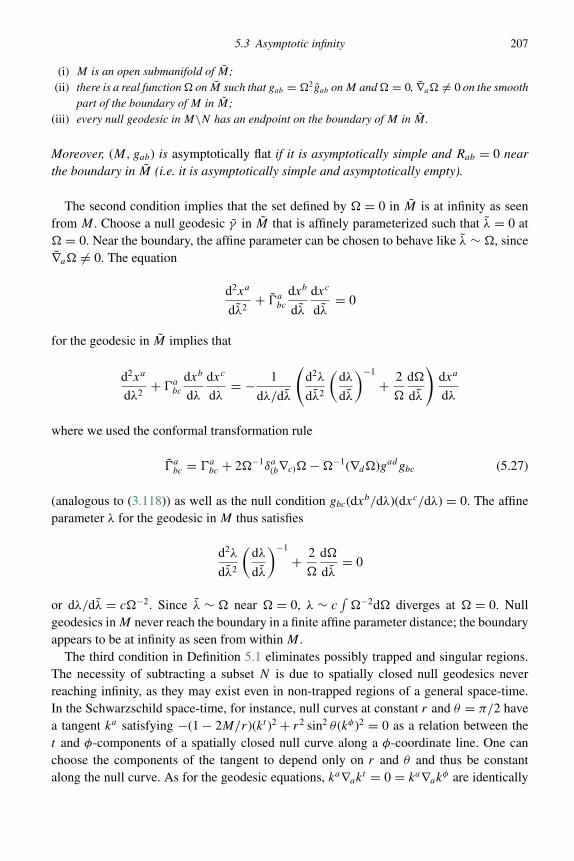
5.3 Asymptotic infinity 207
(i) M is an open submanifold of M;(ii) there is a real function � on M such that gab = �2gab on M and � = 0, ∇a� �= 0 on the smooth
part of the boundary of M in M;(iii) every null geodesic in M\N has an endpoint on the boundary of M in M .
Moreover, (M,gab) is asymptotically flat if it is asymptotically simple and Rab = 0 nearthe boundary in M (i.e. it is asymptotically simple and asymptotically empty).
The second condition implies that the set defined by � = 0 in M is at infinity as seenfrom M . Choose a null geodesic γ in M that is affinely parameterized such that λ = 0 at� = 0. Near the boundary, the affine parameter can be chosen to behave like λ ∼ �, since∇a� �= 0. The equation
d2xa
dλ2+ �a
bc
dxb
dλ
dxc
dλ= 0
for the geodesic in M implies that
d2xa
dλ2+ �a
bc
dxb
dλ
dxc
dλ= − 1
dλ/dλ
(d2λ
dλ2
(dλ
dλ
)−1
+ 2
�
d�
dλ
)dxa
dλ
where we used the conformal transformation rule
�abc = �a
bc + 2�−1δa(b∇c)� − �−1(∇d�)gadgbc (5.27)
(analogous to (3.118)) as well as the null condition gbc(dxb/dλ)(dxc/dλ) = 0. The affineparameter λ for the geodesic in M thus satisfies
d2λ
dλ2
(dλ
dλ
)−1
+ 2
�
d�
dλ= 0
or dλ/dλ = c�−2. Since λ ∼ � near � = 0, λ ∼ c∫�−2d� diverges at � = 0. Null
geodesics in M never reach the boundary in a finite affine parameter distance; the boundaryappears to be at infinity as seen from within M .
The third condition in Definition 5.1 eliminates possibly trapped and singular regions.The necessity of subtracting a subset N is due to spatially closed null geodesics neverreaching infinity, as they may exist even in non-trapped regions of a general space-time.In the Schwarzschild space-time, for instance, null curves at constant r and θ = π/2 havea tangent ka satisfying −(1 − 2M/r)(kt )2 + r2 sin2 θ (kφ)2 = 0 as a relation between thet and φ-components of a spatially closed null curve along a φ-coordinate line. One canchoose the components of the tangent to depend only on r and θ and thus be constantalong the null curve. As for the geodesic equations, ka∇ak
t = 0 = ka∇akφ are identically

208 Global and asymptotic properties
satisfied, and ka∇akθ = −sin θ cos θ (kφ)2 vanishes at θ = π/2. Finally,
ka∇akr = �r
tt (kt )2 + �r
φφ(kφ)2
= M
r2
(1 − 2M
r
)(kt )2 − r
(1 − 2M
r
)sin2 θ (kφ)2
= −(r − 3M)r2 sin2 θ (kφ)2
vanishes for r = 3M as the radius of a spatially closed null geodesic (indeed lying outsidethe trapped region r < 2M).
5.3.2 Examples
In general, finding suitable transformations to conformally embed a given space-time asa finite region of some other space-time can be challenging. Should this be the case fora space-time of interest, one can make use of a procedure patching together the wholespace-time out of parts that can each be conformally embedded. Alternatively, the behaviorof null-lines can be used to determine the structure of a conformal diagram, as applied byWinitzki (2005). The general construction is illustrated by the usual examples of explicitlyknown solutions.
5.3.2.1 Schwarzschild exterior
With
u := t −(r + 2M log
( r
2M− 1
))and := 1
r(5.28)
the Schwarzschild metric becomes
ds2 = 1
2
(−2(1 − 2M)du2 + 2dud + d�2).
(An analogously defined v instead of u, adding instead of subtracting the r-dependentterm, would bring the metric to Eddington–Finkelstein form when expressed in coordinates(v, r, θ, φ).) In the exterior, we have 0 < < 1/2M , and → 0 at r → ∞. A conformalfactor � = thus satisfies the required conditions for a conformal completion, including∇a� �= 0 at � = 0. Moreover, since Rab = 0 near = 0, we have an asymptotically emptyspace-time as shown in Fig. 5.13.
In contrast to Minkowski space, the past of J + constructed in this way is not the wholespace-time. Instead, the past has a boundary given by the event horizon at r = 2M . (Bydefinition, the event horizon in a given space-time is the boundary of the past of J +.)Furthermore, not all timelike geodesics reach i+ in the future; those crossing the horizonenter the trapped region and stop at the singularity, the place of their inextendability.

5.3 Asymptotic infinity 209
J −
J+
i −
i +
i 0
Fig. 5.13 Conformal diagram of the Schwarzschild space-time. In Eddington–Finkelstein coordinates,only the region spanned by the solid lines and the future singularity is covered. The future fate ofobjects differs from that in Minkowski space: depending on the initial radial velocity, a massive objectmay fall into the singularity or reach future timelike infinity. Similarly, a massless particle travelingalong null curves either escapes to J + or falls into the singularity.
5.3.2.2 Spatially closed FLRW model
In conformal time η, an FLRW line element with spatial slices of positive curvature is
ds2 = a(η)2(−dη2 + dR2 + sin2 Rd�2
). (5.29)
This is already conformally equivalent in an obvious way to the Einstein static universe. Inthe absence of a cosmological constant, η has a bounded range because there is a past aswell as a future singularity at finite η where a(η) vanishes. The radial coordinate R is notrestricted by singularities, but is periodically identified due to the spatially closed topology.The conformal diagram is shown in Fig. 5.14.
A recollapsing, spatially closed model is not asymptotically flat as a consequence of thehomogeneous matter distribution, never diluting down arbitrarily much. For this reason, itdoes not have the structure of null, timelike and spacelike infinities.
5.3.2.3 Open FLRW model
An open model in conformal time does not directly provide a conformal embedding intothe Einstein static universe, but rather, in Minkowski or hyperbolic space. Qualitatively, inthe case of a vanishing cosmological constant, we now expect a regular part of the boundarygiven by future null and timelike infinity, the asymptotic region where matter has dilutedcompletely, but also a past singularity. These ingredients, together with the coordinatecenter as a timelike finite boundary, already provide the conformal diagram in Fig. 5.14.

210 Global and asymptotic properties
J+
Fig. 5.14 Conformal diagrams of closed (left) and open (right) FLRW models.
5.3.3 Conformal gauge
For a conformal completion, one must choose a conformal embedding such that the space-time investigated becomes a bounded region in the conformally equivalent space-time. Thechoice of conformal embedding is not unique: every g′
ab = ω2gab with ω(x) �= 0 on M
provides the same asymptotic structure for M . This freedom is called conformal gauge.For the structures at infinity, the normal to the boundary of M in M has played an
important role by telling us whether boundary components are null, spacelike or timelike.At J ±, changing the conformal gauge by a function ω as above transforms the co-normalna = ∇a� on the boundary to n′
a = ω∇a� + �∇aω = ωna (since � = 0 at the boundary),and ∇anb becomes
∇′an
′b = ∇an
′b − 2ω−1δc(a(∇b)ω)n′
c + ω−1(∇dω)gcd gabn′c
= ω∇anb + nb∇aω + (∇a�)(∇bω) + �∇a∇bω − 2n(a∇b)ω + gabnc∇cω
= ω∇anb + gabnc∇cω
where the last equality holds on J ±. (In the first line, we have conformally transformedthe connection using (5.27).)
While there was no restriction on ∇anb so far, this transformation of the conformal gaugecan be used to set ∇′
an′b to equal any particular function on the boundary, for instance making
the simple choice ∇′an
′b = 0 called the Bondi gauge. By this extra condition, the conformal
gauge will be restricted, requiring ω to satisfy the equation gabnc∇cω = −ω∇anb.
In the case of null infinity, in which na is both normal and tangent to the boundary, thisequation becomes a differential equation along J ±. To rewrite ∇anb as it appears in thedifferential equation, we make use of (5.25) and
Rab = Rab + 2�−1∇a∇b� + gabgcd
(�−1∇c∇d� − 3�−2(∇c�)(∇d�)
). (5.30)
Given a sufficiently strong fall-off of Tab and using Einstein’s equation, (5.25) implies that
�−1gcd (∇c�)(∇d�) = 1
2gcd∇c∇d�
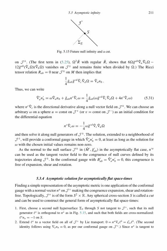
5.3 Asymptotic infinity 211
Σ
J +
S
S
Fig. 5.15 Future null infinity and a cut.
on J ±. (The first term in (5.25), �2R with regular R, shows that 6�gab∇a∇b� −12gab(∇a�)(∇b�) vanishes on J ± and remains finite when divided by �.) The Riccitensor relation Rab = 0 near J ± on M then implies that
1
4gabg
cd∇c∇d� = ∇anb .
Thus, we can write
∇′an
′b = ω∇anb + gabn
c∇cω = 1
4gab(ωgcd∇c∇d� + 4nc∇cω) (5.31)
where nc∇c is the directional derivative along a null vector field on J ±. We can choose anarbitrary ω on a sphere u = const on J + (or v = const on J −) as an initial condition forthe differential equation
nc∇cω = −1
4ωgcd∇c∇d�
and then solve it along null generators of J ±. The solution, extended to a neighborhood ofJ ±, will provide a conformal gauge in which ∇′
an′b = 0, at least as long as the solution for
ω with the chosen initial values remains non-zero.As the normal to the null surface J ± in (M ′, g′
ab) in the asymptotically flat case, n′a
can be used as the tangent vector field to the congruence of null curves defined by itstrajectories along J ±. In the conformal gauge with B ′
ab = ∇′an
′b = 0, this congruence is
free of expansion, shear and rotation.
5.3.4 Asymptotic solution for asymptotically flat space-times
Finding a simple representation of the asymptotic metric is one application of the conformalgauge with a normal vector na onJ + making the congruence expansion, shear and rotation-free. Topologically, J + is of the form S2 × R. Any spherical cross-section S is called a cutand can be used to construct the general form of asymptotically flat space-times:
1. First, choose a second null hypersurface �S through S not tangent to J +, such that its nullgenerator a is orthogonal to na as in Fig. 5.15, and such that both fields are cross-normalized:ana = −1 on S.
2. Extend a to a vector field on all of J + by Lie transport: 0 = na∇ab = Ln
b. (The secondidentity follows using ∇anb = 0, as per our conformal gauge on J +.) Since na is tangent to

212 Global and asymptotic properties
affinely parameterized null geodesics (again using ∇anb = 0, in particular na∇anb = 0), thecross-normalization condition ana = −1 chosen on S is preserved by this extension and holdson all of J +.
3. On every cut we write the induced metric in the form hab = gab + 2(anb) such that ahab = 0 =habn
a . This induced metric is constant along J +: in addition to Lnna = 0 (which is obvious) and
Lnb = 0 used above, we have Lngab = ∇(anb) = 0 and thus Lnhab = 0.
4. The condition ∇anb = 0 does not fix the conformal gauge completely. We can still change ourconformal factor by � → ω� with ω �= 0 on J + such that nc∇cω = 0. This freedom correspondsto the choice of initial values for the differential equation satisfied by ω. Thus, ω must be constantalong the null direction of J +, but it can be freely specified, as long as it is non-zero, on an initialcut. In particular, on S the 2-dimensional Ricci scalar associated with hab will map to
(2)R = ω2 (2)R + 2ω∇a∇aω − 2(∇aω)∇aω (5.32)
by the new conformal transformation. On a 2-dimensional manifold, there is always a conformaltransformation bringing the space to constant-curvature form. In particular, we can choose ω so asto make the 2-metric equal habdxadxb = dϑ2 + sin2 ϑdϕ2. This finally fixes the conformal gaugeand makes every cut a round 2-sphere of unit radius.
5. The round 2-sphere contributions already give us the angular part of the metric; what remains to bedone is to determine the form of the directions transversal to the cuts. For an explicit representationof the asymptotic space-time metric, we choose as the remaining coordinates the new conformalfactor � in a neighborhood of J +, where the condition ∇a� �= 0 near � = 0 indeed guaranteesthat � is a good coordinate, together with an affine parameter u along na , normalized such thatna∇au = 1. Initially, ϑ and ϕ of the round 2-sphere cuts as well as u are only defined on J +, butwe can transport them as functions into a neighborhood of the boundary by requiring that they haveconstant values along the null generators of �S . The line element resulting in the neighborhoodwill depend on the choice made for �S , but its asymptotic form will not. With all conditionsimposed, the space-time metric near J + in these coordinates is
ds2 ∼ −2d�du + dϑ2 + sin2 ϑdϕ2 . (5.33)
As one can directly verify, this indeed makes ∇a� and ∇au null, as well as gab(∇a�)(∇bu) = −1for the cross-normalization.
5.3.5 Asymptotic symmetries
The preceding construction has provided an asymptotic metric in a fixed conformal gauge,but not all the ingredients were free of choices. In particular, while there is no intrinsicrestriction on the conformal factor other than that it be non-zero everywhere, the metric onan initial cut was conveniently but rather arbitrarily chosen to be the round 2-sphere metricof radius one. Moreover, the embedding of the round sphere as a cut of J ± depends on thecoordinate u along J ± and on what one considers as its constant-level surfaces. This free-dom gives rise to a specific form of coordinates combined with conformal transformationsas asymptotic symmetries. These transformations are required only to leave the structure
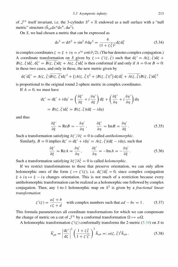
5.3 Asymptotic infinity 213
of J ± itself invariant, i.e. the 3-cylinder S2 × R endowed as a null surface with a “nullmetric” structure (habdxadxb, du2).
On S, we had chosen a metric that can be expressed as
ds2 = dϑ2 + sin2 ϑdϕ2 = 4
(1 + ζ ζ )2dζdζ (5.34)
in complex coordinates ζ = ξ + iη = eiϕ cot(ϑ/2). (The bar denotes complex conjugation.)A coordinate transformation on S given by ζ → ζ ′(ζ, ζ ) such that dζ ′ = A(ζ, ζ )dζ +B(ζ, ζ )dζ , dζ ′ = B(ζ, ζ )dζ + A(ζ, ζ )dζ is then conformal if and only if A = 0 or B = 0:in these two cases, and only in these, the new metric given by
dζ ′dζ ′ = A(ζ, ζ )B(ζ, ζ )dζ 2 + (|A(ζ, ζ )|2 + |B(ζ, ζ )|2) dζdζ + A(ζ, ζ )B(ζ, ζ )dζ 2
is proportional to the original round 2-sphere metric in complex coordinates.If A = 0, we must have
dζ ′ = dξ ′ + idη′ =(∂ξ ′
∂ξ+ i
∂η′
∂ξ
)dξ +
(∂ξ ′
∂η+ i
∂η′
∂η
)dη
= B(ζ, ζ )dζ = B(ζ, ζ )(dξ − idη)
and thus
∂ξ ′
∂ξ= ReB = −∂η′
∂η,
∂ξ ′
∂η= ImB = ∂η′
∂ξ. (5.35)
Such a transformation satisfying ∂ζ ′/∂ζ = 0 is called antiholomorphic.Similarly, B = 0 implies dζ ′ = dξ ′ + idη′ = A(ζ, ζ )(dξ − idη), such that
∂ξ ′
∂ξ= ReA = ∂η′
∂η,
∂ξ ′
∂η= −ImA = −∂η′
∂ξ. (5.36)
Such a transformation satisfying ∂ζ ′/∂ζ = 0 is called holomorphic.If we restrict transformations to those that preserve orientation, we can only allow
holomorphic ones of the form ζ → ζ ′(ζ ), i.e. dζ ′/dζ = 0, since complex conjugationξ + iη → ξ − iη changes orientation. This is not much of a restriction because everyantiholomorphic transformation can be realized as a holomorphic one followed by complexconjugation. Then, any 1-to-1 holomorphic map on S2 is given by a fractional lineartransformation
ζ ′(ζ ) = aζ + b
cζ + dwith complex numbers such that ad − bc = 1 . (5.37)
This formula parameterizes all coordinate transformations for which we can compensatethe change of metric on a cut of J ± by a conformal transformation � → ω�.
A holomorphic transformation ζ ′(ζ ) conformally transforms the 2-metric (5.34) on S to
h′ab =
∣∣∣∣dζ ′
dζ
∣∣∣∣2 ( 1 + ζ ζ
1 + ζ ′ζ ′
)2
hab =: ω(ζ, ζ )2hab . (5.38)
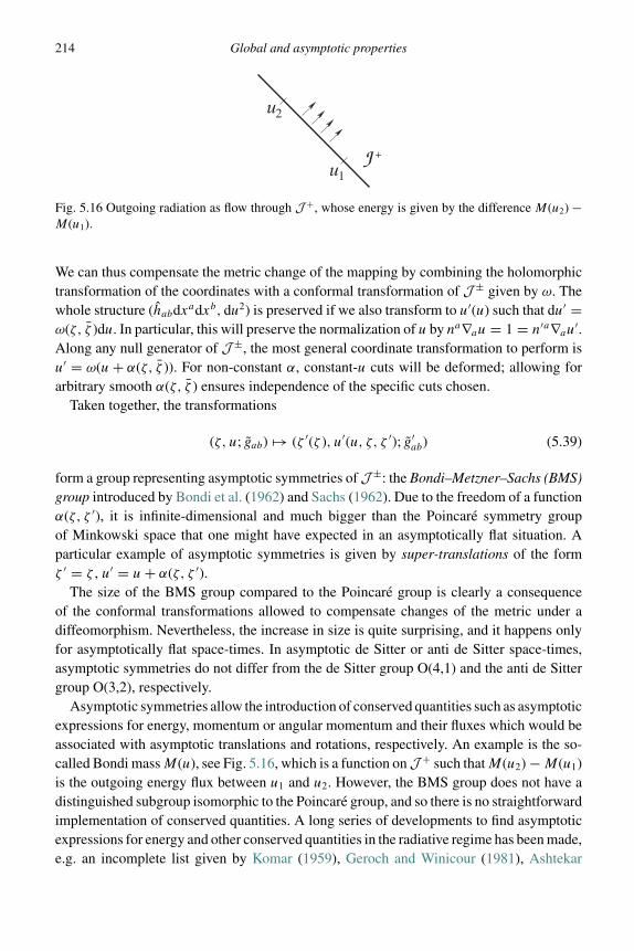
214 Global and asymptotic properties
J +
u2
u1
Fig. 5.16 Outgoing radiation as flow through J +, whose energy is given by the difference M(u2) −M(u1).
We can thus compensate the metric change of the mapping by combining the holomorphictransformation of the coordinates with a conformal transformation of J ± given by ω. Thewhole structure (habdxadxb, du2) is preserved if we also transform to u′(u) such that du′ =ω(ζ, ζ )du. In particular, this will preserve the normalization of u by na∇au = 1 = n′a∇au
′.Along any null generator of J ±, the most general coordinate transformation to perform isu′ = ω(u + α(ζ, ζ )). For non-constant α, constant-u cuts will be deformed; allowing forarbitrary smooth α(ζ, ζ ) ensures independence of the specific cuts chosen.
Taken together, the transformations
(ζ, u; gab) → (ζ ′(ζ ), u′(u, ζ, ζ ′); g′ab) (5.39)
form a group representing asymptotic symmetries of J ±: the Bondi–Metzner–Sachs (BMS)group introduced by Bondi et al. (1962) and Sachs (1962). Due to the freedom of a functionα(ζ, ζ ′), it is infinite-dimensional and much bigger than the Poincare symmetry groupof Minkowski space that one might have expected in an asymptotically flat situation. Aparticular example of asymptotic symmetries is given by super-translations of the formζ ′ = ζ , u′ = u + α(ζ, ζ ′).
The size of the BMS group compared to the Poincare group is clearly a consequenceof the conformal transformations allowed to compensate changes of the metric under adiffeomorphism. Nevertheless, the increase in size is quite surprising, and it happens onlyfor asymptotically flat space-times. In asymptotic de Sitter or anti de Sitter space-times,asymptotic symmetries do not differ from the de Sitter group O(4,1) and the anti de Sittergroup O(3,2), respectively.
Asymptotic symmetries allow the introduction of conserved quantities such as asymptoticexpressions for energy, momentum or angular momentum and their fluxes which would beassociated with asymptotic translations and rotations, respectively. An example is the so-called Bondi mass M(u), see Fig. 5.16, which is a function onJ + such that M(u2) − M(u1)is the outgoing energy flux between u1 and u2. However, the BMS group does not have adistinguished subgroup isomorphic to the Poincare group, and so there is no straightforwardimplementation of conserved quantities. A long series of developments to find asymptoticexpressions for energy and other conserved quantities in the radiative regime has been made,e.g. an incomplete list given by Komar (1959), Geroch and Winicour (1981), Ashtekar

5.3 Asymptotic infinity 215
(1981), and based on canonical methods especially by Ashtekar and Streubel (1981), Iyerand Wald (1994) and Wald and Zoupas (2000).
5.3.6 Spatial infinity
Before radiation can carry away energy through J +, the original mass contained inspace-time is computationally accessible at spatial infinity i0. In stationary situations, thisdescribes the mass of compact objects. The space-time metric near i0 in an asymptoticallyflat space-time cannot be arbitrary but must allow asymptotically Cartesian coordinates xµ
such that it takes the form
gµν ∼ δµν + O(r−1) , ∂ρgµν ∼ O(r−2) (5.40)
where r is the radius as a function of the spatial Cartesian coordinates. Energy should thenequal the Hamiltonian of the canonical formulation, but as we have seen, its bulk part is theHamiltonian constraint and vanishes for every solution. Non-zero energy can result only ifthere is a remaining boundary term that does not vanish for the given fall-off conditions,as already seen in Chapter 3.3.2 for quasilocal quantities associated with finite boundaries.In the asymptotic context, energy and other conserved quantities based on boundary termshave been derived by Regge and Teitelboim (1974).
In terms of the canonical variables, the fall-off conditions follow from the relation withthe space-time metric:
hab ∼ δab + O(r−1) , pab ∼ O(r−2) (5.41)
N ∼ 1 + O(r−1) , ∂aN ∼ O(r−2) (5.42)
Na ∼ O(r−1) , ∂bNa ∼ O(r−2) . (5.43)
From the variations of the action as in Chapter 4.2.2, we obtain several boundary terms ata fixed 2-sphere Sr : r = const with spatial normal ra = (dr)a:
2∫Sr
d2yrapabδNb ∼ r2O(r−3) = 0
2∫Sr
d2yrapcgNaδhcg ∼ r2O(r−4) = 0
1
16πG
∫Sr
d2yraN (hachde − haehcd )Dcδhde ∼ r2O(r−2) �= 0
1
16πG
∫Sr
d2yrc(DaN )(hachde − haehcd )δhde ∼ r2O(r−3) = 0 .

216 Global and asymptotic properties
This gives rise to only one non-vanishing asymptotic boundary term in the variation
δ
∫�
d3xNCgrav = limr→∞
∫Sr
d2yraN (hachde − haehcd )Dcδhde
∼ limr→∞
∫Sr
d2yraδabδcd (Dbδhcd − Dcδhbd )
∼ limr→∞ δ
(∫Sr
d2yraδabδcd (Dbhcd − Dchbd )
)=: −16πGδEADM[hab] (5.44)
where Da denotes the asymptotically Cartesian spatial derivative operator which is inde-pendent of hab. Indices are explicitly raised or lowered with the asymptotically Cartesianmetric δab.
The total Hamiltonian must have vanishing variation once field equations are satisfied,which can be the case only if EADM[hab] is added as a boundary term to cancel the variation(5.44) of the bulk term. Thus,
H =∫�
d3x(NCgrav + NaCgrava ) + EADM[hab] (5.45)
is the total Hamiltonian. When field equations are satisfied, the constraints Cgrav = 0 =C
grava vanish such that the Hamiltonian on the space of solutions takes the value of the ADM
energy
EADM = − 1
16πGlimr→∞
∫Sr
d2yraδabδcd (Dbhcd − Dchbd ) . (5.46)
Hawking and Horowitz (1996) have shown that EADM agrees with the asymptotic limit ofthe Brown–York quasilocal energy on spheres.
Momentum and angular momentum can be derived from the Nother theorem, accordingto which the change of the action under a symmetry provides a conserved charge. Here,we consider coordinate changes xµ → xµ + ξµ(x) under which fields change by their Liederivative along ξa . The ADM energy then remains invariant because we have Lξhab =2D(aξb) asymptotically, and DbDaξ
b − DaDbξb = 0 for the asymptotically flat metric.
The remaining terms in the Lagrangian required to be invariant are thosein
∫d3x(pabhab − NCgrav − NaC
grava ), which change by an integrated divergence∫
d3xDc
((pabhab − NCgrav − NaC
grava )ξ c
)(duly taking into account the Lie derivative of a
scalar density). If the constraints are satisfied, only the boundary term∫
d3xDc(pabhabξc) =
limr→∞∫Sr
d2yrcξcpabhab must be required to vanish for an asymptotic symmetry. This
provides some restrictions on vector fields ξa that can be asymptotic symmetries of theaction. For any vector field for which the boundary term vanishes, Nother’s theorem pro-vides us with a conserved quantity because we have
0 = δS =∫
d3xpabδhab|t2t1 (5.47)
5.4 Matching of solutions 217
for the boundary term resulting from integrating by parts in time. The conserved charge isthus ∫
d3xpabδξhab = 2∫
d3xpabD(aξb) = 2∫
d3x(Da(pabξb) − ξbDap
ab)
= 2 limr→∞
∫Sr
d2yrapabξb (5.48)
for any ξa such that raξa = O(1) on Sr with its co-normal ra = (dr)a . This formula agreeswith the asymptotic limit of the Brown–York momentum in (3.71) for translations alongthe shift ξb = Nb/N , using the fact that the reference momentum pab drops off to zero fastenough.
Examples for vector fields satisfying this condition are asymptotic translations andasymptotic rotations, providing momentum and angular momentum as conserved quantities.For an asymptotic translation, ξa = −εa is constant and the ADM momentum
P a = −2 limr→∞
∫Sr
d2yrbpab (5.49)
results. For an asymptotic rotation ξa = −εabcφbxc with a constant rotation vector φa
(whose length gives the rotation angle) we have the angular momentum
Lb = −2 limr→∞
∫Sr
d2yraεbcdpacxd . (5.50)
Note, however, that there is arbitrariness in this definition, since angular momentum refersto an origin of rotations in Cartesian coordinates which may lie outside the asymptoticCartesian region. Different choices of coordinates (different asymptotic observers and theirsynchronizations) can give rise to different values of angular momentum.
For other notions of energy and angular momentum in general relativity, see the reviewby Jaramillo and Gourgoulhon (2010).
5.4 Matching of solutions
Matching techniques of different space-time regions to result in one global solution providethe means to construct conformal diagrams of complicated space-times from those ofsimpler ones.
The Schwarzschild space-time, for instance, is an explicit solution illustrating severalgeneral properties of black holes such as trapped regions, horizons and singularities. Butit describes neither the formation of the black hole in a collapse process nor dynamicalproperties after the black hole has formed. It is thus of interest to construct models ofcollapsing matter that display the general behavior of trapped surfaces and the consequencesof horizons and singularities.
To model a collapsing star, we require a distribution of matter in its interior with vacuumspace-time outside the star’s surface. The whole space-time has to obey Einstein’s equation,

218 Global and asymptotic properties
Σ
−M M
na
M
M
−
+
+
naa
Σ
Fig. 5.17 The matching surface � splits space-time into components M±, with the normal vector na
of � (or the cross-normalized vector a in the null case) pointing toward M+.
for whose solutions several examples are easily available separately in the presence ofmatter as well as in vacuum. However, we must also ensure that the equation is satisfied forfields residing on the star surface, separating the well-known regions. This can be done bymatching interior and vacuum solutions at this boundary, imposing conditions for limitingvalues of the fields when the surface is approached from both sides as part of a completesolution.
Idealizing the surface as a sharp transition from matter to vacuum requires some carein discussing the fields. At the surface, the energy-momentum tensor Tab is discontinuous.On the other hand, not all geometric quantities can be discontinuous if the Einstein tensorGab and the derivatives it contains are to be regular. This observation provides matchingconditions for suitable space-time metrics in the two bordering regions. If these conditionscan be satisfied for given choices of inside and outside metrics, a valid model of a star isobtained. General discussions of matching in different situations have been provided byClarke and Dray (1987) and Mars and Senovilla (1993), based on seminal work by Israel(1966).
In this setting, as sketched in Fig. 5.17, we have the matching surface � boundingtwo different space-time regions (M±, g±
ab). Since both regions overlap at �, there mustbe a map ∂M− → ∂M+ linking the boundaries of M+ and M−, which then providesan identification of the two tangent spaces induced on � by viewing the surface as theboundary of M+ and M−, respectively, identified as one surface by the mapping. In orderto complete the identification of the full tangent spaces of M± at �, we also identify thenormals na
± =: na of �. (We choose na+ to be inward-pointing and na
− outward-pointing tobe specific.) If the matching surface is null, a case we will discuss separately, na is tangentto the surface, and we choose a normal a cross-normalized with na , ana = −1, pointinginto M+.
5.4 Matching of solutions 219
Example 5.4 (Null surfaces)Null surfaces and their normals have already been used several times. At this stage, someof the differences to non-null surfaces will become important. Consider the example ofthe null surface � : x − t = const in Minkowski space. We directly obtain the co-normalna = (d(x − t))a = (dx)a − (dt)a , and one can easily verify that it is co-normal to thesurface: nav
a = 0 for all va tangent to the surface. Raising the index, we have na =(∂/∂x)a + (∂/∂t)a , a tangent vector to the surface, since nan
a = 0 with na null. Indeed,na∇a(x − t) = 0 such that displacements along na stay on the surface �. A transversalvector to the null surface is obtained not by raising the index of the co-normal, but bydetermining the null vector cross-normalized with na . Here, a = 1
2 (−(∂/∂x)a + (∂/∂t)a)is null, transversal to � (a∇a(x − t) �= 0), and satisfies ana = −1. Both na and a arefuture-pointing, which is ensured by the cross-normalization to a negative number.
Both regions, (M+, g+ab) and (M−, g−
ab), induce metrics h±ab on �, which must be identical
for a valid matching; otherwise, the extrinsic curvature Kab = 12Lnhab of � in the resulting
space-time would be singular on �, and, with the curvature relations from Chapter 3.2.3,the Ricci tensor Rab would have a singularity. Since the metric is regular, even thoughdiscontinuous, the Ricci scalar gabRab would diverge, implying a curvature singularity.
If the induced metrics agree, on the other hand, all tangential derivatives of the space-timemetric are continuous: for any vc with vcnc = 0 we have vc$(∂cgab) = 0 where we use thenotation
$f (x) = limM+�y→x
f (y) − limM−�y→x
f (y) (5.51)
for the discontinuity of a function f . The space co-normal to � is spanned by n+a , and so
derivatives of the metric must have a discontinuity of the general form $(∂cgab) = ncγab
with a symmetric (non-tensorial) object γab that measures the discontinuity of ∂cgab. Fromthis, a discontinuity
$�abc = 1
2$
(gad (∂bgdc + ∂cgbd − ∂dgbc)
) = 1
2(nbγ
ac + ncγ
ab − naγbc) (5.52)
of the connection coefficients follows: �abc is the sum of a continuous distribution and
θ�$�abc with the surface step function θ� taking the values ± 1
2 in M±.
Example 5.5 (Surface step and delta functions)We use the step function θ� with values ± 1
2 in the manifolds M± with common boundary �
in order to describe discontinuities across �. Its derivatives along directions not tangent to� result in Dirac-type delta distributions δ� , vanishing inM±\� and satisfying
∫δ�dn = 1
when integrated along a curve n(t) from M− to M+, normal to � at the intersection point.The tangent vector of the curve where it intersects � is thus na if � is non-null, and a if itis null.
While tangential derivatives of θ� vanish, vc∇cθ� = 0 for all va tangent to �, normalderivatives result in delta distributions. Again using the fact that the co-normal space to� is spanned by na , we can write ∇cθ� ∝ ncδ� . To determine the coefficient, we integrate
220 Global and asymptotic properties∫na∇aθ�dn = θ+
� − θ−� = 1 and compare with
∫nanaδ�dn = −1 for a timelike surface
and∫nanaδ�dn = 1 for a spacelike one. For a null surface, a is used instead of na as
the tangent to the normal curve (while the co-normal na remains in ∇cθ� ∝ ncδ�), alsoresulting in
∫anaδ�dn = −1 with cross-normalization. Comparison then fixes ∇cθ� =
−ncδ� for timelike and null surfaces, with a plus sign instead of the minus for a spacelikesurface.
Then, also Rab will be discontinuous or could even be singular of δ-function form:Rab = R
non-singab + R
singab δ� . The coefficient of the δ-function arises from normal derivatives
in the general expression
Rab = ∇c�cab − ∇b�
cca + �d
ab�cdc − �d
cb�cda
of the Christoffel coefficients and takes the form
Rsingab = nc$�c
ab − nb$�cac
= 1
2(nancγ
cb + ncnbγ
ca − ncn
cγab − nbnaγcc − nbncγ
ca + nbn
cγac)
= ncn(bγa)c − 1
2ncncγab − 1
2nanbγ
cc .
The Ricci scalar thus has a δ-function coefficient
Rsing = nanbγab − nanaγbb (5.53)
and the Einstein tensor one of the form
Gsingab = R
singab − 1
2Rsinggab
= ncn(bγa)c − 1
2ncncγab − 1
2nanbγ
cc − 1
2gab(ncndγcd − ncncγ
dd ) . (5.54)
These equations are valid for any value of ncnc, including the null case in which some termsdrop out. Further considerations and the precise matching conditions, however, depend onwhether the normal is null.
5.4.1 Non-null matching surface
If the surface is not null, we can normalize the normal to nana = ±1 and explicitly writethe induced metric on the matching surface � as hab = gab ± nanb. The induced metric iscontinuous, producing the same value, irrespective of whether we induce it from M+ or
5.4 Matching of solutions 221
M−. Extrinsic curvature is regular but discontinuous:
$Kab = $(hca∇cnb) = −$(�d
cbndhca)
= −1
2(ncndγ
db + nbndγ
dc ± γcb)(gc
a ± ncna)
= −1
2(2ndn(aγ
db) ± γab − ndnaγ
db ± nanbn
cndγcd + ncnaγcb)
= −ndn(aγdb) ∓ 1
2γab ∓ 1
2nanbn
cndγcd (5.55)
and
$Kaa = −1
2(nanbγab ± γ a
a ) . (5.56)
If we compare this with (5.54), we see that
Gsingab = −$Kab + hab$Kc
c (5.57)
which shows that the Einstein tensor is non-singular if and only if Kab is continuous.For a regular stress-energy tensor, the Einstein tensor must be regular, which provides
the junction conditions K+ab = K−
ab in addition to h+ab = h−
ab. If the energy-momentumtensor has a δ-function singularity, which would mean that there is a surface layer ofenergy-momentum on �, the Einstein tensor is allowed to have a singular part, requiredto agree with that of the energy-momentum tensor: G
singab = 8πGT
singab . Via the resulting
discontinuity in Kab, fixed in terms of T singab , the matching is again determined.
Practically, to see whether one can consistently match two space-times along a surface,one makes a choice of how to embed the matching surface in each of them, and thencomputes the induced metrics and extrinsic curvatures as seen from both space-times.Finally, one checks whether they can be made to agree. This is most interesting in thecase of a timelike rather than spacelike matching surface, for the spacelike matching isnothing but a rederivation of the initial value problem of Chapter 3.4: junction conditionsfor spacelike � can be interpreted as saying that on � we must have initial conditions forM+ in agreement with the final geometry as seen from M− (if na is future pointing to M+).The timelike case is, however, new and provides interesting possibilities for constructingnew solutions. A detailed example is provided after the discussion of null matching surfaces.
5.4.2 Null matching surface
If nana = 0, we have a second null vector a and cross-normalized with na: ana = −1.Instead of a spatial metric on all of �, we induce a spatial metric qab on cross-sectionsof � normal to both na and a by gab = qab − 2(anb). In this case, instead of extrinsiccurvature, various derivatives of both null normals appear. The singular part of the Einstein
222 Global and asymptotic properties
tensor becomes
Gsingab = ncn(bγa)c − 1
2nanbγ
cc − 1
2gabn
cndqcd
= ncn(bγa)c − 1
2nanbγcd (qcd − 2(cnd)) − 1
2qabn
cndγcd + (anb)ncndγcd
= −1
2nanbγcdq
cd + nanbcndγcd + ncn(bγa)c + (anb)n
cndγcd − 1
2qabn
cndγcd
= nanb$θ − 2$η(anb) − $ωqab (5.58)
where we used nanbcndγcd + ncn(bγa)c + (anb)n
cndγcd = ndγcdqc(anb) and introduced
θ := qcd∇cd (the expansion of the null congruence defined by a), ηa := qcan
d∇cd andω := an
c∇cna . They have discontinuities
$θ = −qcd$�ecde = −1
2qcdγcd
$ηa = −qcan
d$�ecde = −1
2qcan
dγcd
$ω = anc$�a
cbnb = 1
2nbncγbc
which justifies our use of these quantities in Gsingab . Thus, for continuous θ, ηa and ω the
Einstein tensor is non-singular on the matching surface. There are only four conditionsrather than six for the symmetric Kab in the non-null case; null-junction conditions are thusweaker. In particular, the full Riemann tensor Rabc
d can be singular on a null matchingsurface even if the Einstein tensor is non-singular, i.e. without a matter source of a surfacelayer. Physically, this singular situation corresponds to a gravitational shock wave.
5.4.3 Oppenheimer–Snyder model
Oppenheimer and Snyder (1939) model a collapsing homogeneous star surrounded byvacuum by matching an FLRW solution as the interior to a Schwarzschild exterior. Asthe collection of world-lines for all particles on the star’s surface, the matching surface �
should be timelike.Our interior metric is now given by
ds2− = −dτ 2 + X(τ, r)2dr2 + Y (τ, r)2d�2 (5.59)
where
X(τ, r) = a(τ )√1 − kr2
, Y (τ, r) = a(τ )r . (5.60)
In contrast to a cosmological model, we do not use this line element for all of space-time,but, as in Fig. 5.18, cut off the manifold at a value r = R to define the matching surface �
as a boundary of M−. Its unit normal vector is na− = X−1(∂/∂r)a and it inherits an induced
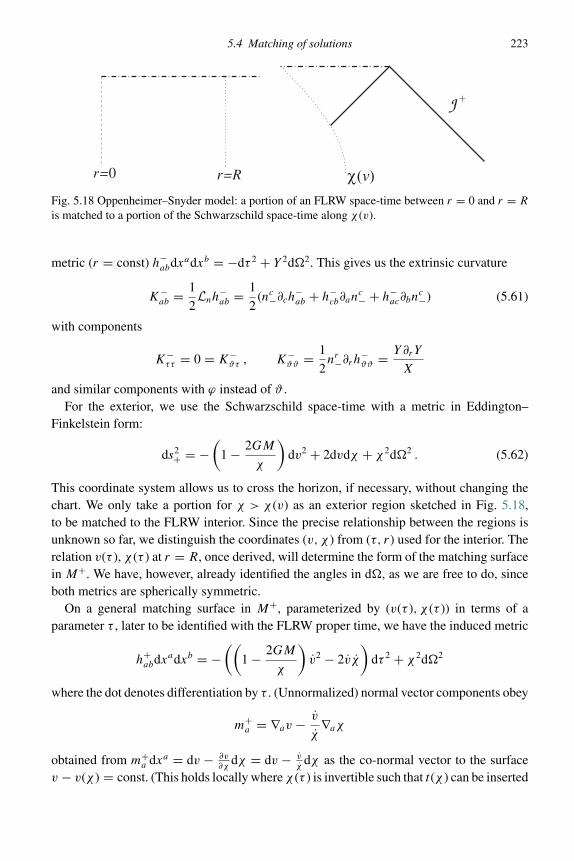
5.4 Matching of solutions 223
r=0 r=R
J
χ
+
(v)
Fig. 5.18 Oppenheimer–Snyder model: a portion of an FLRW space-time between r = 0 and r = R
is matched to a portion of the Schwarzschild space-time along χ (v).
metric (r = const) h−abdxadxb = −dτ 2 + Y 2d�2. This gives us the extrinsic curvature
K−ab = 1
2Lnh
−ab = 1
2(nc
−∂ch−ab + h−
cb∂anc− + h−
ac∂bnc−) (5.61)
with components
K−ττ = 0 = K−
ϑτ , K−ϑϑ = 1
2nr
−∂rh−ϑϑ = Y∂rY
X
and similar components with ϕ instead of ϑ .For the exterior, we use the Schwarzschild space-time with a metric in Eddington–
Finkelstein form:
ds2+ = −
(1 − 2GM
χ
)dv2 + 2dvdχ + χ2d�2 . (5.62)
This coordinate system allows us to cross the horizon, if necessary, without changing thechart. We only take a portion for χ > χ (v) as an exterior region sketched in Fig. 5.18,to be matched to the FLRW interior. Since the precise relationship between the regions isunknown so far, we distinguish the coordinates (v, χ ) from (τ, r) used for the interior. Therelation v(τ ), χ (τ ) at r = R, once derived, will determine the form of the matching surfacein M+. We have, however, already identified the angles in d�, as we are free to do, sinceboth metrics are spherically symmetric.
On a general matching surface in M+, parameterized by (v(τ ), χ (τ )) in terms of aparameter τ , later to be identified with the FLRW proper time, we have the induced metric
h+abdxadxb = −
((1 − 2GM
χ
)v2 − 2vχ
)dτ 2 + χ2d�2
where the dot denotes differentiation by τ . (Unnormalized) normal vector components obey
m+a = ∇av − v
χ∇aχ
obtained from m+a dxa = dv − ∂v
∂χdχ = dv − v
χdχ as the co-normal vector to the surface
v − v(χ ) = const. (This holds locally where χ (τ ) is invertible such that t(χ ) can be inserted
224 Global and asymptotic properties
in v(τ ) to obtain v(χ ).) With the norm
g+abm
a+m
b+ = 1 − 2GM
χ− 2
χ
v
the unit normal vector components are
nv+ = 1√
1 − 2GM/χ − 2χ/v, n
χ+ = 1 − 2GM/χ − χ/v√
1 − 2GM/χ − 2χ/v.
This gives us the relevant components of extrinsic curvature in(K+
vv + 2K+vχ
dχ
dv+ K+
χχ
(dχ
dv
)2)
dv2
which we are not going to need explicitly, and
K+ϑϑ = 1
2nχ+∂χh
+ϑϑ = χ
1 − 2GM/χ − χ/v√1 − 2GM/χ − 2χ/v
.
With these preparations, we formulate the junction conditions:
h+ϑϑ = h−
ϑϑ : we obtain χ (τ ) = Y (τ, r) = a(τ )R which for a given interior a(τ ) determines χ on theexterior matching surface up to the free parameter R.
h+ττ = h−
ττ : the equation (1 − 2GM/χ ) v2 − 2vχ = 1 provides a differential equation
(dχ
dv
)2
= χ 2
v2= a2R2
(1 − 2GM
χ− 2
dχ
dv
)(5.63)
for χ (v). The relation between the exterior coordinates is now determined (up to the value of R),fixing the matching surface in M+.
K+ττ = K−
ττ : another differential equation
K+vv + 2K+
vχ
dχ
dv+ K+
χχ
(dχ
dv
)2
= 0
results for χ (v), which turns out to be automatically satisfied given the other junction conditions.Together with the hττ -matching, we have fixed χ (τ ) and v(τ ) consistently. After this matching ofthe boundaries of M− and M+ as a single matching surface �, no free function is left and the onlyremaining parameter is R.
K+ϑϑ = K−
ϑϑ : a final equation
χ1 − 2GM/χ − dχ/dv√1 − 2GM/χ − 2dχ/dv
= YY ′
X(5.64)

5.4 Matching of solutions 225
remains to be satisfied on the whole matching surface. Using χ = Y from the hϑϑ -matching, thiscan be written as (
Y ′
X
)2 (1 − 2GM
χ− 2
dχ
dv
)
=(
1 − 2GM
χ− dχ
dv
)2
=(
1 − 2GM
Y
)2
− 2dχ
dv
(1 − 2GM
Y
)+
(dχ
dv
)2
=(
1 − 2GM
Y
)2
− 2dχ
dv
(1 − 2GM
Y
)+ Y 2
(1 − 2GM
χ− 2
dχ
dv
)=
(1 − 2GM
χ− 2
dχ
dv
)(1 − 2GM
Y+ Y 2
)where we used the hττ -matching in the next-to-last step. This equation can then be solved for themass
GM = 1
2Y
(1 + Y 2 −
(Y ′
X
)2)
= 1
2aR
(1 + r2a2 − (1 − kR2)
)= 1
2R3a(a2 + k)
using that X = a/√
1 − kR2 and Y = aR at the matching surface. This expression, as the massparameter of the Schwarzschild solution, must be time independent, a condition which restrictsthe allowed matter content of the FLRW interior. The equation can be reformulated as(
a
a
)2
+ k
a2= 2GM
a3R3= 8πG
3ρ . (5.65)
By comparison with the Friedmann equation, pressure is required to vanish in the star in order forthe energy density to behave like a−3. For zero pressure, we then have
M = 4π
3R3a3ρ = Vρ (5.66)
which relates the star’s mass to its volume and energy density ρ.
Now, all junction conditions are satisfied and we have a combined space-time solvingEinstein’s equation everywhere. The derivation shows that the existence of a consistentmatching is non-trivial: there were several junction equations which made use of detailedproperties of the interior and exterior metrics. In particular, an FLRW model with non-zeropressure cannot be matched to a Schwarzschild exterior. Physically, the non-zero pressure atthe surface would cause matter to be ejected, in conflict with a vacuum exterior. (To modelthis situation, one could, for instance, use a Vaidya space-time or a generalized version ofit, where the coordinate dependence M(v) or M(v, χ ) allows more freedom to satisfy thematching equations; see Exercise 5.12. The Vaidya space-time itself will be discussed inthe next section.)
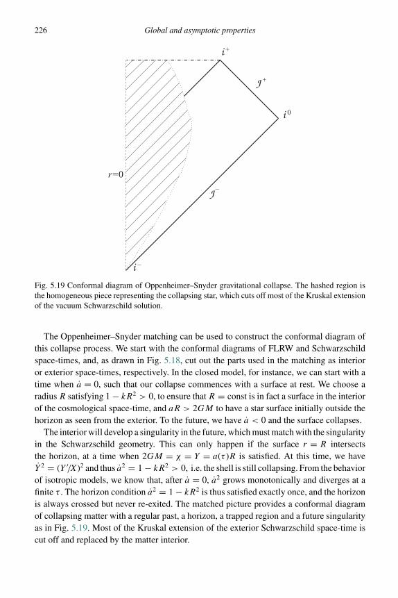
226 Global and asymptotic properties
J +
J
i
i
i
−
−
0
+
r=0
Fig. 5.19 Conformal diagram of Oppenheimer–Snyder gravitational collapse. The hashed region isthe homogeneous piece representing the collapsing star, which cuts off most of the Kruskal extensionof the vacuum Schwarzschild solution.
The Oppenheimer–Snyder matching can be used to construct the conformal diagram ofthis collapse process. We start with the conformal diagrams of FLRW and Schwarzschildspace-times, and, as drawn in Fig. 5.18, cut out the parts used in the matching as interioror exterior space-times, respectively. In the closed model, for instance, we can start with atime when a = 0, such that our collapse commences with a surface at rest. We choose aradius R satisfying 1 − kR2 > 0, to ensure that R = const is in fact a surface in the interiorof the cosmological space-time, and aR > 2GM to have a star surface initially outside thehorizon as seen from the exterior. To the future, we have a < 0 and the surface collapses.
The interior will develop a singularity in the future, which must match with the singularityin the Schwarzschild geometry. This can only happen if the surface r = R intersectsthe horizon, at a time when 2GM = χ = Y = a(τ )R is satisfied. At this time, we haveY 2 = (Y ′/X)2 and thus a2 = 1 − kR2 > 0, i.e. the shell is still collapsing. From the behaviorof isotropic models, we know that, after a = 0, a2 grows monotonically and diverges at afinite τ . The horizon condition a2 = 1 − kR2 is thus satisfied exactly once, and the horizonis always crossed but never re-exited. The matched picture provides a conformal diagramof collapsing matter with a regular past, a horizon, a trapped region and a future singularityas in Fig. 5.19. Most of the Kruskal extension of the exterior Schwarzschild space-time iscut off and replaced by the matter interior.
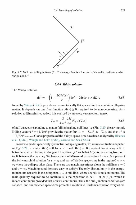
5.4 Matching of solutions 227
J
J
i
+
0
−
v
Fig. 5.20 Null dust falling in from J −. The energy flow is a function of the null coordinate v whichvaries along J −.
5.4.4 Vaidya solution
The Vaidya solution
ds2 = −(
1 − 2GM(v)
r
)dv2 + 2dvdr + r2d�2 , (5.67)
found by Vaidya (1953), provides an asymptotically flat space-time that contains collapsingmatter. It depends on one free function M(v) ≥ 0, required to be non-decreasing. As asolution to Einstein’s equation, it is sourced by an energy-momentum tensor
Tab = G
4πr2
dM
dv(∇av)(∇bv) (5.68)
of null dust, corresponding to matter falling in along null lines; see Fig. 5.20: the asymptoticKilling vector ξa = (∂/∂v)a provides the matter flux ja = −Tabξ
b ∝ −∇av, and thus ja ∝−(∂/∂r)a|v=const. Global properties of the Vaidya space-time have been analyzed by Hiscocket al. (1982), Waugh and Lake (1986), Girotto and Saa (2004).
In order to model spherically symmetric collapsing matter, we assume a situation depictedin Fig. 5.21 in which M(v) = 0 for v < 0 and M(v) = M constant for v > v0 > 0. Inbetween, matter is falling in along null lines fromJ − such that M(v) is increasing from zeroto M between 0 < v < v0. We have a piece of Minkowski space-time for v < 0, a piece ofthe Schwarzschild solution for v > v0 and part of Vaidya space-time in the region 0 < v <
v0 where the collapse takes place. There are two matching surfaces along the null lines v = 0and v = v0. Matching conditions are easy to satisfy: The only discontinuity in the energy-momentum tensor is in the component Tvv at null lines where dM/dv is not continuous. Themain quantity required to be continuous is the expansion θ ∝ 1 − 2GM(v)/r , which isindeed continuous provided that M(v) is continuous. Thus, the null-junction conditions aresatisfied, and our matched space-time presents a solution to Einstein’s equation everywhere.
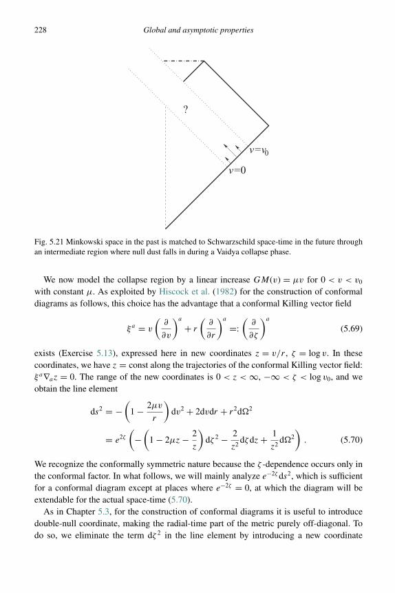
228 Global and asymptotic properties
?
v=0
v=v0
Fig. 5.21 Minkowski space in the past is matched to Schwarzschild space-time in the future throughan intermediate region where null dust falls in during a Vaidya collapse phase.
We now model the collapse region by a linear increase GM(v) = µv for 0 < v < v0
with constant µ. As exploited by Hiscock et al. (1982) for the construction of conformaldiagrams as follows, this choice has the advantage that a conformal Killing vector field
ξa = v
(∂
∂v
)a
+ r
(∂
∂r
)a
=:
(∂
∂ζ
)a
(5.69)
exists (Exercise 5.13), expressed here in new coordinates z = v/r , ζ = log v. In thesecoordinates, we have z = const along the trajectories of the conformal Killing vector field:ξa∇az = 0. The range of the new coordinates is 0 < z < ∞, −∞ < ζ < log v0, and weobtain the line element
ds2 = −(
1 − 2µv
r
)dv2 + 2dvdr + r2d�2
= e2ζ
(−
(1 − 2µz − 2
z
)dζ 2 − 2
z2dζdz + 1
z2d�2
). (5.70)
We recognize the conformally symmetric nature because the ζ -dependence occurs only inthe conformal factor. In what follows, we will mainly analyze e−2ζ ds2, which is sufficientfor a conformal diagram except at places where e−2ζ = 0, at which the diagram will beextendable for the actual space-time (5.70).
As in Chapter 5.3, for the construction of conformal diagrams it is useful to introducedouble-null coordinate, making the radial-time part of the metric purely off-diagonal. Todo so, we eliminate the term dζ 2 in the line element by introducing a new coordinate

5.4 Matching of solutions 229
η := ζ + f (z) such that (1 − 2µz − 2
z
)f ′(z) = 2
z2. (5.71)
We then have
−(
1 − 2µz − 2
z
)dζdη = −
(1 − 2µz − 2
z
)dζ 2 − 2
z2dζdz
as a representation of the line element in double-null form:
ds2 = e2ζ
(−
(1 − 2µz − 2
z
)dζdη + 1
z2d�2
).
The differential equation (5.71) is solved by the integral
f (z) = −2∫ z dx
x(2µx2 − x + 2)(5.72)
of a function with poles at z = 0 and z± = 14µ
−1(1 ± √1 − 16µ). As a consequence, the
new coordinate η is not always globally defined, since f (z) may diverge at finite values ofz, and we have to discuss different cases, depending on the behavior of the poles.
5.4.4.1 Spacelike singularity
For µ > 1/16, there is only one real pole at z = 0 and we always have 2µz2 − z + 2 > 0.The function (5.72) is integrated to
f (z) = −log z + 1
2log(2µz2 − z + 2) − 1√
16µ − 1arctan
4µz − 1√16µ − 1
(5.73)
providing a coordinate η = ζ + f (z) that is well defined for all allowed values of z. Inparticular, we have η = ζ − log z + g(z) with a function g(z) bounded at z = 0.
The collapse region is described by a global double-null pair (ζ, η), in which we havethe following limiting behaviors:
• η → ∞ is reached for any finite ζ if z → 0. For z → ∞, η → ±∞ diverges (the sign dependingon the value of µ in the allowed range).
• ζ → −∞ for finite η if z → 0 in such a way that ze−ζ remains finite, and ζ → ∞ for finite η ifz → ∞.
This asymptotic behavior of null coordinates determines the boundaries in the sense of J ±,but there is also a singular part of the boundary: for the Vaidya metric, we have a curvatureinvariant of the form
RabcdRabcd = 48GM(v)2
r6= 48µ2z6e−4ζ (5.74)
which diverges for z → ∞ when ζ remains finite.In order to disentangle the different parts of the boundary, we first look at the case where
v0 → ∞, i.e. the mass function M(v) increases linearly from zero at v = 0 to infinity
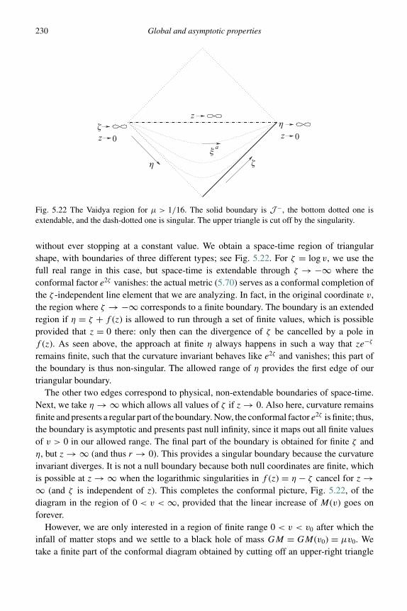
230 Global and asymptotic properties
ζ ηz
η ζξ
z 0 z 0a
Fig. 5.22 The Vaidya region for µ > 1/16. The solid boundary is J −, the bottom dotted one isextendable, and the dash-dotted one is singular. The upper triangle is cut off by the singularity.
without ever stopping at a constant value. We obtain a space-time region of triangularshape, with boundaries of three different types; see Fig. 5.22. For ζ = log v, we use thefull real range in this case, but space-time is extendable through ζ → −∞ where theconformal factor e2ζ vanishes: the actual metric (5.70) serves as a conformal completion ofthe ζ -independent line element that we are analyzing. In fact, in the original coordinate v,the region where ζ → −∞ corresponds to a finite boundary. The boundary is an extendedregion if η = ζ + f (z) is allowed to run through a set of finite values, which is possibleprovided that z = 0 there: only then can the divergence of ζ be cancelled by a pole inf (z). As seen above, the approach at finite η always happens in such a way that ze−ζ
remains finite, such that the curvature invariant behaves like e2ζ and vanishes; this part ofthe boundary is thus non-singular. The allowed range of η provides the first edge of ourtriangular boundary.
The other two edges correspond to physical, non-extendable boundaries of space-time.Next, we take η → ∞ which allows all values of ζ if z → 0. Also here, curvature remainsfinite and presents a regular part of the boundary. Now, the conformal factor e2ζ is finite; thus,the boundary is asymptotic and presents past null infinity, since it maps out all finite valuesof v > 0 in our allowed range. The final part of the boundary is obtained for finite ζ andη, but z → ∞ (and thus r → 0). This provides a singular boundary because the curvatureinvariant diverges. It is not a null boundary because both null coordinates are finite, whichis possible at z → ∞ when the logarithmic singularities in f (z) = η − ζ cancel for z →∞ (and ζ is independent of z). This completes the conformal picture, Fig. 5.22, of thediagram in the region of 0 < v < ∞, provided that the linear increase of M(v) goes onforever.
However, we are only interested in a region of finite range 0 < v < v0 after which theinfall of matter stops and we settle to a black hole of mass GM = GM(v0) = µv0. Wetake a finite part of the conformal diagram obtained by cutting off an upper-right triangle
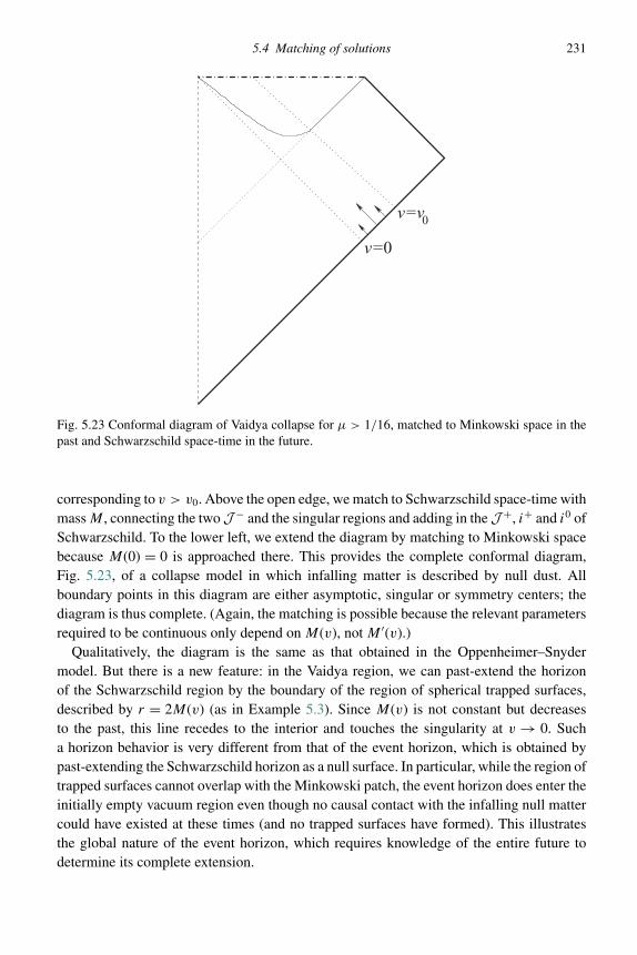
5.4 Matching of solutions 231
v=0
v=v0
Fig. 5.23 Conformal diagram of Vaidya collapse for µ > 1/16, matched to Minkowski space in thepast and Schwarzschild space-time in the future.
corresponding to v > v0. Above the open edge, we match to Schwarzschild space-time withmass M , connecting the two J − and the singular regions and adding in the J +, i+ and i0 ofSchwarzschild. To the lower left, we extend the diagram by matching to Minkowski spacebecause M(0) = 0 is approached there. This provides the complete conformal diagram,Fig. 5.23, of a collapse model in which infalling matter is described by null dust. Allboundary points in this diagram are either asymptotic, singular or symmetry centers; thediagram is thus complete. (Again, the matching is possible because the relevant parametersrequired to be continuous only depend on M(v), not M ′(v).)
Qualitatively, the diagram is the same as that obtained in the Oppenheimer–Snydermodel. But there is a new feature: in the Vaidya region, we can past-extend the horizonof the Schwarzschild region by the boundary of the region of spherical trapped surfaces,described by r = 2M(v) (as in Example 5.3). Since M(v) is not constant but decreasesto the past, this line recedes to the interior and touches the singularity at v → 0. Sucha horizon behavior is very different from that of the event horizon, which is obtained bypast-extending the Schwarzschild horizon as a null surface. In particular, while the region oftrapped surfaces cannot overlap with the Minkowski patch, the event horizon does enter theinitially empty vacuum region even though no causal contact with the infalling null mattercould have existed at these times (and no trapped surfaces have formed). This illustratesthe global nature of the event horizon, which requires knowledge of the entire future todetermine its complete extension.
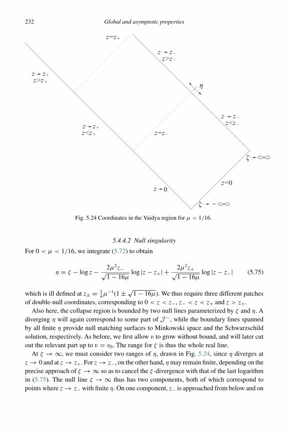
232 Global and asymptotic properties
ζ
ζ −
η
++
+
−
−
z z
+
−
−
+
z>z
zz<z
zz=z
z 0
z=z
z>zz z
−
z<zz z
z=0
Fig. 5.24 Coordinates in the Vaidya region for µ < 1/16.
5.4.4.2 Null singularity
For 0 < µ < 1/16, we integrate (5.72) to obtain
η = ζ − log z − 2µ2z−√1 − 16µ
log |z − z+| + 2µ2z+√1 − 16µ
log |z − z−| (5.75)
which is ill defined at z± = 14µ
−1(1 ± √1 − 16µ). We thus require three different patches
of double-null coordinates, corresponding to 0 < z < z−, z− < z < z+ and z > z+.Also here, the collapse region is bounded by two null lines parameterized by ζ and η. A
diverging η will again correspond to some part of J −, while the boundary lines spannedby all finite η provide null matching surfaces to Minkowski space and the Schwarzschildsolution, respectively. As before, we first allow v to grow without bound, and will later cutout the relevant part up to v = v0. The range for ζ is thus the whole real line.
At ζ → ∞, we must consider two ranges of η, drawn in Fig. 5.24, since η diverges atz → 0 and at z → z+. For z → z−, on the other hand, η may remain finite, depending on theprecise approach of ζ → ∞ so as to cancel the ζ -divergence with that of the last logarithmin (5.75). The null line ζ → ∞ thus has two components, both of which correspond topoints where z → z− with finite η. On one component, z− is approached from below and on

5.4 Matching of solutions 233
+
z
z z
Fig. 5.25 Conformal diagram of a Vaidya region for µ < 1/16 with unbounded linear increase of themass. Coordinate lines of constant z are dotted. Dash-dotted lines are singularities.
the other from above. Also, z → 0 and z → z+ lie on the boundary part with ζ → ∞, butsince they require η → ∞, too, they only present single points in the conformal diagram.
For ζ → −∞, on the other hand, there are three components: we necessarily haveη → −∞ for z → z−, giving a single point on the boundary, but η can be finite if z → 0 orz → z+. There are now three boundary contributions, corresponding to z → 0 and z → z+from below as well as from above.
Not all the boundary contributions are regular (see Fig. 5.25): curvature diverges when-ever z → ∞ and ζ remains finite, or when ζ → −∞ and z �= 0. The first possibilityprovides a space-like singularity, as in the previous case, but the second possibility is anull singularity because it lies at constant values of the null coordinate ζ → −∞. It isan extended region rather than a single point because it encompasses the whole boundarywhere z → z+. On the remaining ζ → −∞ part, where z → 0, on the other hand, curva-ture is finite but the conformal factor e2ζ of the metric (5.70) becomes zero. Space-timeis extendable across this boundary part where v = 0, and here we can match to a pastMinkowski region.
To match to Schwarzschild in the future, we take the collapse region only up to a finitevalue of ζ corresponding to v = v0. Here, the mass has grown to GM = µv0, which we
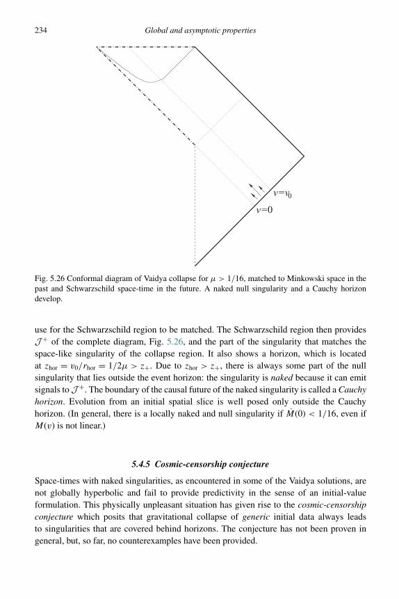
234 Global and asymptotic properties
v=0
v=v0
Fig. 5.26 Conformal diagram of Vaidya collapse for µ > 1/16, matched to Minkowski space in thepast and Schwarzschild space-time in the future. A naked null singularity and a Cauchy horizondevelop.
use for the Schwarzschild region to be matched. The Schwarzschild region then providesJ + of the complete diagram, Fig. 5.26, and the part of the singularity that matches thespace-like singularity of the collapse region. It also shows a horizon, which is locatedat zhor = v0/rhor = 1/2µ > z+. Due to zhor > z+, there is always some part of the nullsingularity that lies outside the event horizon: the singularity is naked because it can emitsignals to J +. The boundary of the causal future of the naked singularity is called a Cauchyhorizon. Evolution from an initial spatial slice is well posed only outside the Cauchyhorizon. (In general, there is a locally naked and null singularity if M(0) < 1/16, even ifM(v) is not linear.)
5.4.5 Cosmic-censorship conjecture
Space-times with naked singularities, as encountered in some of the Vaidya solutions, arenot globally hyperbolic and fail to provide predictivity in the sense of an initial-valueformulation. This physically unpleasant situation has given rise to the cosmic-censorshipconjecture which posits that gravitational collapse of generic initial data always leadsto singularities that are covered behind horizons. The conjecture has not been proven ingeneral, but, so far, no counterexamples have been provided.
5.5 Horizons 235
Here, it is important to keep in mind the requirement of generic initial data. As we haveseen in the discussion of Vaidya solutions, large classes of models do exist in which nakedsingularities form in gravitational collapse. However, due to their symmetry, these solutionsdo not provide generic initial conditions. As analyzed by Podolsky and Svıtek (2005), onecan perturb around the Vaidya solutions, for instance in the form of Robinson–Trautmanmetrics
ds2 = −(K + 2r∂v log f − 2
M
r
)dv2 + 2dvdr + r2
f 2d�2
with the mass function M(v), as in Vaidya space-times, but also including an arbitraryperturbation by a non-spherical f (v, ϑ, ϕ). The perturbation f , for this class of models,then defines K = f 2(1 + $2 log f ) where $2 is the Laplacian on the unit 2-sphere withline element d�2.
With the stress-energy tensor of Vaidya, this is a solution to Einstein’s equation if
∂f
∂v= f$K
12M(v).
A collapse region perturbed in this way can be matched to past Minkowski and futureSchwarzschild as before, but now it turns out that solutions for f diverge for v → ∞.Thus, the complete Vaidya solution is not stable against perturbations, and the nakedsingularities they show are not generic. This instability of a physical phenomenon, in thiscase the formation of naked singularities, means that the phenomenon can have only limitedmeaning. (An example of a stable phenomenon is the general occurrence of singularities ofthe general type in terms of geodesic incompleteness, which is a generic feature accordingto the singularity theorems.)
Incidentally, Robinson–Trautman metrics also exhibit an interesting behavior regardingtheir differentiability. Just like Vaidya solutions, they can be matched to Minkowski spaceat v = 0, where f cannot be smooth. Instead, for M(v) = µv we have the following twocases:
1. If 2/µ is an integer, f is 30/µ − 1 times differentiable at the matching surface. Since µ ≤ 2 for2/µ to be integer, this means that f is at least 14 times differentiable. In the limiting case ofµ = 1/16, it is 479 times differentiable, but not more.
2. Otherwise, f is {2/µ} times differentiable, which designates the largest integer smaller than 2/µ.If µ > 2, f is not differentiable but continuous.
5.5 Horizons
A horizon, in contrast to a sharp surface such as the boundary of a star, captures the notionof the border of a black hole. We have already seen several examples in explicit solutions,as well as the importance of horizons to characterize the occurrence of strong gravitationalforces able to capture even light. While the physical picture as a region trapping light isintuitive, the general mathematical situation is not so clear. There are different definitions

236 Global and asymptotic properties
of horizons, which in many cases lead to different pictures of the behavior. A precisedefinition, however, would be important, for instance to discuss the merger process of twoblack holes; if we are not able to locate their horizons precisely, we cannot tell when a singlehorizon has formed, indicating that the black holes have merged. Some of the propertiesassociated with different notions of horizons are discussed in this section.
5.5.1 Notions of horizons
The event horizon, defined as the boundary of the past of J +, is a global concept. Thepast is the set of all points that can be connected to J + by future-pointing timelike or nullcurves. Thus, the event horizon is always a null submanifold. It requires global knowledgeof space-time due to the use of J + in its definition.
A more local definition of horizons uses future-trapped surfaces which can be analyzedwithout reference to asymptotic regions: as defined in Chapter 5.1.2, these are closed spatial2-surfaces S such that both future-pointing null normal congruences emanating from themhave negative expansion. A marginal future-trapped surface is the limiting case of a closedspatial 2-surface such that the expansion of one future-pointing null normal congruencevanishes and the other one is negative. Future-trapped surfaces can only lie within an eventhorizon in asymptotically flat situations, because the necessary presence of conjugate pointsalong both null congruences prevents null curves from reaching J +; thus, they cannot bein the past of J +. The motivation for the following definitions is that the limiting case ofmarginal trapped surfaces may provide a good local definition of a horizon, which in factin some cases agrees with the event horizon.
The definition of an apparent horizon is based on a foliation of an asymptotically flatspace-time into spatial slices�. On each slice, the set of outermost marginal trapped surfaceslying in � defines the place where the apparent horizon intersects the slice. (Outermostsurfaces are here defined as those closest to the asymptotic region along the slice.) Stackingup all slices of the foliation and the outermost marginal trapped surfaces within them thenprovides the 3-dimensional manifold of the apparent horizon in space-time. While thisnotion is more local than that of an event horizon, it has the disadvantage of being foliation-dependent. Moreover, for a given foliation, only trapped surfaces within an entire � areconsidered, a procedure that may overlook other trapped surfaces (as discussed explicitlyby Wald and Iyer (1991)). It turns out that the apparent horizon may be discontinuous,for instance in the collapse of two black holes. This concept of a horizon, as describedby Thornburg (1996, 2007) is used mostly in numerical simulations, which are alreadybased on the evolution of data on spatial slices and provide an underlying foliation bytheir setup.
A trapping horizon as defined by Hayward (1994) is a 3-dimensional surface H inspace-time which allows a foliation by marginal future-trapped surfaces. This conceptrequires neither asymptotic structures nor a foliation of space-time and thus eliminatesthe disadvantages of event and apparent horizons. (The notion of a trapping horizon has
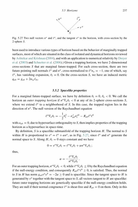
5.5 Horizons 237
na l a
v a
S
Fig. 5.27 Two null vectors na and a , and the tangent va to the horizon, with cross-section by the2-sphere S.
been used to introduce various types of horizon based on the behavior of marginally trappedsurfaces, most of which are situated in the class of isolated and dynamical horizons reviewedby Ashtekar and Krishnan (2004), and with an application to numerical relativity by Dreyeret al. (2003) and Schnetter et al. (2006).) Given a trapping horizon, we have 2-dimensionalcross-sections S that are marginal future-trapped. For each cross-section, there are twofuture pointing null normals a and na , cross-normalized to ana = −1, one of which, saya , has vanishing expansion, θ = 0. On the cross-section S, we have an induced metricqab = gab + 2n(ab).
5.5.2 Spacelike properties
For a marginal future-trapped surface, we have by definition θ = 0, θn < 0. We call thehorizon an outer trapping horizon if na∇aθ < 0 at any of its 2-sphere cross-sections S,where we extend a to a neighborhood of S. In this case, the trapped region lies in thedirection of na . The null version of the Raychaudhuri equation
a∇aθ = −1
2θ2 − σ
abσab − Rab
ab
with ωab = 0, due to hypersurface orthogonality to S, then implies properties of the trappinghorizon as a hypersurface in space-time.
By definition, S is a spacelike submanifold of the trapping horizon H . The normal to S
within H is proportional to va = a + αna , as in Fig. 5.27, since a and na generate thenormal space to S. Along H , θ = 0 stays constant and we have
0 = va∇aθ = a∇aθ + αna∇aθ ;
thus,
α = −a∇aθ
nb∇bθ.
For an outer trapping horizon, na∇aθ < 0, while a∇aθ ≤ 0 by the Raychaudhuri equationif the null-energy condition, and consequently Rab
ab ≥ 0, is satisfied. Thus, the normalto S in H has norm gabv
avb = −2α ≥ 0 and is spacelike. Since the tangent space to H isgenerated by va together with the tangent space to S, all vectors tangent to H are spacelike:future outer trapping horizons are generically spacelike if the null-energy condition holds.They are null if their normal congruence a is shear-free and Rab = 0 on them. Only in this
238 Global and asymptotic properties
case, which can be interpreted as the absence of gravitational radiation and matter at thehorizon, can the trapping horizon agree with the event horizon.
Example 5.6 (Trapping horizon in the Vaidya space-time)The Vaidya space-time is spherically symmetric, making it easy to find spherical marginallytrapped surfaces. Using only spherical surfaces, however, is a restriction of the generalset of trapped surfaces to be considered according to the definition of a trapping horizon;we will only obtain a lower bound for the radius of the trapping horizon in this way:there may well be non-spherical trapped surfaces outside the region of spherical trappedsurfaces. Such trapped surfaces have indeed been found numerically by Krishnan andSchnetter (2006) as well as analytically by Ben-Dov (2007) in the Vaidya space-time;Eardley (1998) has conjectured that every point within the event horizon allows a trappedsurface through it, and Bengtsson and Senovilla (2009) have constructed trapped surfaces inthe matched Vaidya space-time as constructed here even through points in the flat Minkowskiregion. The region of spherical marginal trapped surfaces satisfies r = 2GM(v), a surfacewhich has the co-normal na = ∇ar − 2G(∇av)dM/dv. For collapsing matter, we havenana = −4GdM/dv < 0 as the timelike normal, and thus the surface r = 2GM(v) isindeed spacelike as expected for a trapping horizon.
Even though spherical trapped surfaces may not give the exact horizon position, thetrapping horizon cannot agree exactly with the event horizon. The event horizon is alwaysnull, while the trapping horizon is null only if the shear of a as well asRab
ab vanish alongit. For the Vaidya space-time, we have a stress-energy tensor Tab = (4πr2)−1(dM/dv)nanb
where na = ∇av is the ingoing null normal to the marginal trapped surfaces slicing thehorizon. Using cross-normalization with the outgoing null normal a , we have Rab
ab =8πGTab
ab = 2Gr−2dM/dv > 0, which does not vanish in the collapse region. Thus,in any region where the mass function strictly increases, the trapping horizon of a Vaidyaspace-time is spacelike and cannot agree with the event horizon. If there are different phasesof matter infall, as in Fig. 5.28, even a null part of a trapping horizon can be distinct froma part of the event horizon.
Properties of spacelike horizons can often be derived from the constraint equations,which must hold on any spacelike surface. In particular, according to Ashtekar and Krishnan(2003), balance laws follow from integrations of the constraints over regions of the horizon.
Example 5.7 (Balance of quasilocal angular momentum)If we denote the unit normal to a spacelike horizon by Na (to distinguish it from thecross-normalized null normal na used conventionally in the context of horizons), the dif-feomorphism constraint (3.64) with a matter contribution is
Ca = −2∇bpab +
√det hNbT
ab =√
det h
(− 1
8πGDb(Kab − Kc
chab) + NbT
ab
).
(5.76)
We now pick a foliation of the horizon into spherical cross-sections, choose a vector fieldφa tangent to the cross-sections, and integrate the φaCa over a finite part H of the horizon
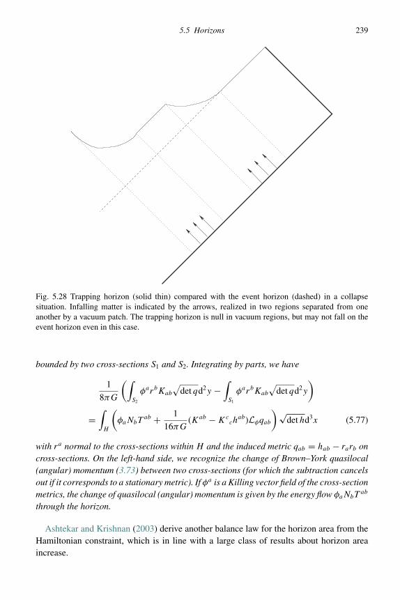
5.5 Horizons 239
Fig. 5.28 Trapping horizon (solid thin) compared with the event horizon (dashed) in a collapsesituation. Infalling matter is indicated by the arrows, realized in two regions separated from oneanother by a vacuum patch. The trapping horizon is null in vacuum regions, but may not fall on theevent horizon even in this case.
bounded by two cross-sections S1 and S2. Integrating by parts, we have
1
8πG
(∫S2
φarbKab
√det qd2y −
∫S1
φarbKab
√det qd2y
)=
∫H
(φaNbT
ab + 1
16πG(Kab − Kc
chab)Lφqab
)√det hd3x (5.77)
with ra normal to the cross-sections within H and the induced metric qab = hab − rarb oncross-sections. On the left-hand side, we recognize the change of Brown–York quasilocal(angular) momentum (3.73) between two cross-sections (for which the subtraction cancelsout if it corresponds to a stationary metric). If φa is a Killing vector field of the cross-sectionmetrics, the change of quasilocal (angular) momentum is given by the energy flow φaNbT
ab
through the horizon.
Ashtekar and Krishnan (2003) derive another balance law for the horizon area from theHamiltonian constraint, which is in line with a large class of results about horizon areaincrease.
240 Global and asymptotic properties
5.5.3 Area increase
There are several general properties, provable by different methods for trapping as wellas event horizons, even though these concepts in general do not agree in terms of thesubmanifold they define. One of the main results states that the cross-section area ofa horizon cannot decrease if energy conditions are satisfied. The area of cross-sectionsof a trapping horizon is determined by the induced metric qab = gab + 2n(ab), as A =∫S2 dy2√det q. Its change along the horizon, derived by Hayward (1994), is given by its
Lie derivative along the tangent vector va = a + αna:
Lv det q = det q qabLvqab = det q qab(Lqab + αLnqab)
= det q (θ + αθn) (5.78)
where we used
qabLqab = qab∇ab + qab(aLnb + naLb) = θ .
On the trapping horizon, θ = 0 and θn < 0. Moreover, we have seen that α < 0 fora spacelike horizon, α = 0 for a null horizon, and α > 0 for a timelike horizon if thatwere allowed. Thus, the area must increase along a spacelike horizon, remains constantalong a null horizon and decreases along a timelike horizon. This is consistent with theunderstanding that the black hole grows if stress-energy is falling through its horizon, whichcould either come from matter as Tab
ab or from gravitational radiation as σ abσ
ab . Any
contribution of these types, both positive provided that the null energy condition holds,results in a spacelike trapping horizon whose area grows. Again using the Vaidya space-time as an example, we can directly confirm this general observation at the boundary ofspherical trapped surfaces whose radius is r = 2M(v). The cross-sections at constant v
thus have areas A(v) = 4πr(v)2 = 16πM(v)2, a function which increases if matter fallsthrough.
A similar result holds for the event horizon as derived by Hawking (1972), although itis slightly different: the event horizon is always null, but still the cross-section area maydecrease if matter is falling through. On the other hand, the area can never decrease ifenergy conditions hold.
5.5.4 Stationary horizons and black-hole thermodynamics
A special class of black holes is given by stationary ones, in which we have a null trappinghorizon (non-growing in a stationary situation) such that there is a Killing vector field χa ina neighborhood that agrees with χa = a on the horizon. For instance, the Schwarzschildhorizon is stationary with χa = (∂/∂t)a . In this case, the Killing vector field agreeing witha on the horizon is the stationary Killing vector field of space-time. But this need not bethe case in general, especially for rotating black holes. In the latter case, we have insteadχa = ξa + �ψa where ψa is a spacelike Killing vector field (for a rotational symmetry)and � the angular velocity.

5.5 Horizons 241
In the case of a stationary horizon, the congruence defined by a has special properties: bydefinition, it is expansion free (outward normal to marginal trapped surfaces) and rotationfree (hypersurface orthogonal). Moreover, it is shear free because only this allows thetrapping horizon to be null. In fact, a defines a null geodesic congruence.
Using the horizon as a null surface in a space-time solution without a surface layer ofenergy-momentum, the matching analysis of Chapter 5.4.2 shows that ω = na
c∇ca is
continuous across the horizon. (Note that the roles of a and na , using conventional nota-tions, are exchanged compared to our notation in the discussion of null-junction conditions.)If ω were discontinuous, spatial components of the stress-energy tensor were singular at thesurface, with a singular part with coefficient 8πGT
singab ∼ G
singab = −$ωqab. If we wanted
to place the interior of the stationary horizon in empty flat space, rather than the black-holeexterior, the matching could be consistent only if a surface pressure P given by the singularpart of Tab stabilized the horizon. This surface pressure, 8πGP = $ω, implies that wehave to exert a force on the whole surface to replace the pull of gravity normally activewhen the interior belongs to a black hole rather than a surface layer of sress-energy inMinkowski space. We identify the required counteracting pressure κ = − 1
2$πGP = −4ωas the surface gravity acting on the boundary of the interior region:
κ := −1
2nab∇ba . (5.79)
Since only derivatives along the stationary horizon are involved in κ , we can replace a
with the Killing vector χa , and use the Killing-vector property to write
κ = −1
2naχb∇bχa|Hor = 1
2naχb∇aχb|Hor = 1
4na∇a(χbχb)|Hor .
(Notice that the last derivative is not along the horizon where χbχb = bb = 0 would beconstant.) From this equation, we can see that κ is constant along a: using ∇a(χbχb) =−4κχa from the definition of κ and with cross-normalization ana = −1 (which on thehorizon holds for χa instead of a , too), we have on the horizon
−4aLκ = L(−4κχa) = Lχ∇a(χbχb) = χc∇c(∇a(χbχb)) − ∇c(χbχb)∇cχa
= ∇a(χc∇c(χbχb)) − (∇aχc)∇c(χ
bχb) − (∇cχa)∇c(χbχb) = 0
where the first term vanishes because it is a derivative of χbχb along the horizon where itis constant, and the last terms cancel each other because χa is a Killing vector field. Forstationary black holes, the gravitational force thus remains constant.
Moreover, if the dominant energy condition holds, surface gravity is constant all over thespatial cross-sections of the horizon, even in situations that are not spherically symmetric. Infact, one can show thatχ[d∇c]κ = −χ[dR
f
c]χf = 0 which vanishes becauseT cf χf , given thedominant energy condition, must be future-directed timelike or null. Due to Tabχ
aχb = 0along the stationary horizon, this is possible only if T cf χf ∝ χc, and thus Rcf χf ∝ χc,making χ[d∇c]κ = −χ[dχc] = 0. Contraction with spatial tangent vectors orthogonal to χa
then shows that the surface gravity is the same everywhere on the stationary horizon.
242 Global and asymptotic properties
Surface gravity plays a role in parameter changes between different black holes, whichone may think of as adiabatic processes slowly changing the stationary horizon. In suchprocesses, one can show that mass, surface area and angular momentum can change onlyin ways respecting the relation
δM = 1
8πGκδA + �δJ . (5.80)
This relationship is very similar to thermodynamics. In fact, by analogy Bardeen et al.(1973) formulate several laws of black-hole thermodynamics:
0th law: Surface gravity κ is constant on stationary horizons and plays a role analogous totemperature.
1st law: In adiabatic processes, the mass changes by (5.80) where κδA/8πG is analogous to T δS,in agreement with an identification of surface gravity as temperature. This suggests that the surfacearea is to be considered as a measure analogous to entropy.
2nd law: The surface area does not decrease provided that positive energy holds (which correspondsto stability). This is again consistent because we have interpreted the area as being analogous toentropy.
This set of analogies suggests that surface gravity κ can be interpreted as a measure forthe temperature of the black hole, and A as its entropy. Then, the term κδA in (5.80) playsthe role of T δS in thermodynamics. These laws are formal analogies,2 but they can, quitesurprisingly, be substantiated: no-hair theorems show that stationary black-hole solutionsare determined only by three parameters, their mass together with angular momentum andelectric charge. (Black-hole uniqueness theorems are reviewed by Heusler (1998).) Thus,only a few macroscopic parameters determine the whole black hole as a large system.Moreover, detailed calculations started by Bekenstein (1973) show that the black-hole areaincreases if matter is dropped in adiabatically by precisely the amount required to makeStotal = Smatter + SBH non-decreasing. If the black-hole area would be ignored, on the otherhand, entropy would decrease if matter is dropped into the black hole where it disappearsfrom outside view.
There is, however, a problem with this picture: black holes would have negative heatcapacity, defined as the derivative ∂E/∂T keeping the other intensive variables constant.For the Schwarzschild solution, for instance, we have κ = 1/4M , and thus E ∝ 1/T with∂E/∂T < 0. A system with negative heat capacity should radiate thermally, but no radiationcan escape from a black hole. There is also a dimensional problem: entropy is dimensionless,while area has the dimension length squared. From the fundamental constants involved inclassical general relativity, one cannot form a quantity of dimension length to match thedimensions of entropy and area.
One indication for a resolution comes from the fact that black holes could radiate if stress-energy components were to become negative. This is usually not allowed for classical matter,
2 Moreover, they can be derived in this form for the different versions of horizons that have been discussed, which in generaldo not correspond to the same physical surface. Thus, it seems difficult to attribute too much physical meaning to the laws ofblack-hole thermodynamics. Nevertheless, they still stimulate many questions about classical and quantum gravity.
5.5 Horizons 243
but positive energy conditions can be violated by quantum fields. For instance, uncertaintyrelations can provide negative energy for brief times due to fluctuations. More precisely,there are general quantum inequalities for quantum fields on curved space-times as derived,for instance, by Pfennig and Ford (1998), which take the form∫
ρ(t)g(t)dt ≥ − c
$T 4(5.81)
where g(t) is a sampling function of width $T and c is a constant. This inequality doesprovide a lower bound on the energy contained in a space-time region, but this lower boundis negative. That quantum physics can provide negative energies can also be seen based onsuperpositions: given a system with a ground state |0〉 of vanishing energy, 〈0|E|0〉 = 0,and an excited state |1〉, the energy in the superposition
|ψ〉 := 1√1 + ε2
(|0〉 + ε|1〉)
is
〈ψ |E|ψ〉 = 1
1 + ε2(2εRe〈0|E|1〉 + ε2〈1|E|1〉) . (5.82)
This value can be negative for small ε if Re〈0|E|1〉 < 0 which can easily be obtained by aparticular choice of the phases.
Negative energy of this form is not sufficient to prevent singularities in general, but it doesaffect horizon properties. Black holes then become unstable and Hawking-radiate, whichis just what one expects from the thermodynamical analogy. To make this quantitative, onehas to compute the spectrum of the radiation and see whether it is thermal and at whattemperature. This calculation requires quantum field theory on a curved spacetime. Asoriginally used by Hawking (1971), on flat space one can define the usual notion of a vacuumstate as the unique Poincare-invariant state, based on the underlying symmetries of thebackground. If the background is different, however, there is no unique Fock representationof particle states. In fact, the concept of particles and antiparticles depends on the availabilityof a time translation symmetry to split waves into positive and negative frequency modes.This is not available on general curved spacetimes such as that of a black hole. Instead, onecan only introduce asymptotic notions of incoming and outgoing particle states if spacetimeis asymptotically flat.
One has the usual particle pictures on J − and J +, but in general they do not match:what appears as the vacuum state on J − looks, when evolved to J +, like an excited state.In a flat space, the field operator has a decomposition
ψ(t, x) =∫
d3k√2ωk
(e−i(ωkt−kx)ak + ei(ωkt+kx)a†k ) (5.83)
in field modes, where the annihilation operators ak define the vacuum by the conditionsak|0〉 = 0 for all k, and ωk(k) is the dispersion relation of the field. If this is obtainedin an asymptotically flat regime on a curved space-time, the asymptotic mode functions

244 Global and asymptotic properties
+
J
J
−
Fig. 5.29 A tentative conformal diagram describing the evoparation of a black hole by Hawkingradiation. When the horizon disappears, a regular center may be left, but the part of space-timecorresponding to the black-hole interior remains incomplete.
define the corresponding particle concept. But in different asymptotic regimes of a singlespace-time, such as J − and J +, asymptotic expressions for the mode functions usuallydiffer, mixing terms of ak and a
†k when transforming from one regime to another one. In
this formal sense, a past vacuum state can evolve into a future multi-particle state such asa thermal one.
If one uses an expectation value 〈Tab〉 for a quantum field instead of a classical energy-momentum tensor, one can obtain a negative Rab
ab along horizons. Then, the horizonbecomes timelike and its area decreases. In this way, the thermodynamics of black holesbecomes consistent when quantum effects are taken into account. Moreover, through thecalculation of the temperature of Hawking radiation, all free constants are fixed unambigu-ously in terms of Planck’s constant:
TBH = hκ
2π, SBH = A
4hG. (5.84)
The combination hG determining the relation between area and entropy is the square of thePlanck length.
Despite the consistency of this picture, black-hole evaporation is not completely under-stood. What is lacking is a common solution for radiating quantum fields together withtheir back-reaction on the underlying space-time geometry. Only such a solution, or at leasta good approximation, can provide insights into the endstate of black-hole evaporation andshow what conformal picture, possibly of the form shown in Fig. 5.29, is obtained. In thisfinal stage of a black hole where the horizon falls into the strong curvature regime near thecentral singularity, moreover, it is no longer consistent to consider only quantized matter

Exercises 245
on a classical geometry. Here, a complete quantization including the gravitational field isrequired, giving rise to quantum gravity.
Exercises
5.1 (i) Derive an equation for the rate of change ξc∇cωab of the rotation of a timelikegeodesic congruence with tangent vector field ξa .
(ii) Show that a timelike geodesic congruence which is initially hypersurface orthog-onal remains so as long as its expansion and shear are finite.
5.2 Define a timelike geodesic congruence in Minkowski space by the straight linesgenerating the double cone x2 + y2 + z2 = 1
4 t2. Compute its expansion and verify
that it diverges at the tip of the double cone.5.3 Verify that also the expansion of the null geodesic congruence defined by generators
of the double cone x2 + y2 + z2 = t2 in Minkowski space diverges at the tip.5.4 Find the coordinate transformation (t, r) → (T , r) that maps the Schwarzschild line
element to Painleve–Gullstrand form.5.5 In a spherically symmetric region of space-time where the lapse function does not
vanish, marginally trapped surfaces are given by solutions to grr = 0.
(i) Show that this condition can equivalently be written as
1
grr
− (Nr )2
N2= 0 . (E5.1)
(ii) Evaluate (E5.1) for the Schwarzschild space-time in Painleve–Gullstrandcoordinates.
5.6 The Vaidya solution describing gravitational collapse is given by the line element
ds2 = −(
1 − 2M(v)
r
)dv2 + 2dvdr + r2d�2
with a bounded, non-decreasing function M(v) ≥ 0.
(i) Find the ingoing and outgoing null normal vector fields ka± to a spherical surface
defined by constant values of r and v. Check under which conditions they givetangent vectors of affinely parameterized geodesics, i.e. ka
±∇akb± = 0. If they
do not, rescale the normal vectors such that they give affinely parameterizedfuture-pointing tangent vectors.
(ii) For a spherically symmetric null congruence, the normal tangent space up tomultiples of ka
± is spanned by the angular vector fields (∂/∂ϑ)a and (∂/∂ϕ)a .Thus, hab is just the angular part of the inverse metric and the expansion of aspherical null congruence is given by
θ = hab∇akb = gϑϑ∇ϑkϑ + gϕϕ∇ϕkϕ .
246 Global and asymptotic properties
Compute this for the two normal congruences derived in part (i) and find thespace-time region of the Vaidya solution which contains spherically symmetrictrapped surfaces.
5.7 Use the Friedmann equation for positive spatial curvature to show that de Sitter spacecan be expressed as
ds2 = −dτ 2 + α2 cosh2(τ/α)(dr2 + sin2 rd�2)
(0 ≤ r < π ) and find the relation between α and the cosmological constant.In order to find the conformal diagram of de Sitter space, introduce a new coordinate
t(τ ) (leaving r unchanged) such that the metric is conformal to the Einstein staticuniverse. Derive and draw the resulting conformal diagram.
5.8 (i) Show that in complex coordinates ζ (ϑ, ϕ) = eiϕ cot ϑ2 one has
dζdζ = 1
4(1 + ζ ζ )2(dϑ2 + sin2 ϑdϕ2) .
(ii) For Cartesian coordinates x, y, z verify
x = rζ + ζ
1 + ζ ζ, y = −ir
ζ − ζ
1 + ζ ζ, z = r
ζ ζ − 1
1 + ζ ζ
with r2 = x2 + y2 + z2 and polar angles ϑ , ϕ. Use this to show that ζ does notchange up to order r−1 under a translation x ′ = x + b, y ′ = y + c, z′ = z + d:ζ ′ = ζ + O(r−1).
(iii) Consider now Minkowski space-time in Cartesian coordinates t , x, y, z andintroduce the null coordinate u = t − r where r is as before. Show that a trans-lation t ′ = t + a combined with the spatial translation of part (ii) correspondsto an asymptotic supertranslation of the form
u′ = u + A + Bζ + Bζ + Cζ ζ
1 + ζ ζ+ O(r−1)
with real A and C. Relate A, B and C to the translation parameters a, b, c, d.5.9 Compute the ADM energy of a Schwarzschild black hole.
5.10 Compute the angular momentum of a Kerr black hole.5.11 Show that the ADM mass equals the quasilocal expression for energy associated with
a 2-sphere boundary of spatial slices, approaching the sphere at infinity.5.12 (i) Perform the matching for an arbitrary isotropic interior region described by an
FLRW model with scale factor a(t) and an exterior region of generalized Vaidyaform,
ds2 = −(
1 − 2M(v, χ )
χ
)dv2 + 2dvdχ + χ2d�2 .
Derive M(v(t), χ (t)), dχ/dv and v along the matching surface in terms of thescale factor and its derivative, making sure that v is positive for a collapsinginterior (a < 0).

Exercises 247
(ii) Matching vv-components of extrinsic curvature implies that
3(1 − 2∂χM)dχ
dv= 2
(∂vM + χ
d2χ
dv2
).
Use this to write ∂vM in terms of total derivatives of M and χ with respect to v
along the matching surface χ (v).(iii) Compute ∂vM at the place where the matching surface intersects the boundary
2M(v, χ ) = χ of the region of spherical trapped surfaces. Total derivatives alongthe matching surface can be written in terms of time derivatives of the interiorscale factor. Show that this boundary given by 2M(v, χ ) = χ is always nullwhere it intersects the matching surface.
5.13 Show that ξa = v(
∂∂v
)a + χ(
∂∂χ
)a
is a conformal Killing vector field of the Vaidyaspace-time
ds2 = −(
1 − 2M(v)
χ
)dv2 + 2dvdχ + χ2d�2 ,
i.e. ∇(aξb) ∝ gab, if and only if the mass function is of the form M(v) = µv with aconstant µ.
6
Quantum gravity
In general relativity, the space-time metric provides the physical field of gravity and is sub-ject to dynamical laws. For a complete and uniform fundamental description of nature,the gravitational force, and thus space-time, is to be quantized by implementing theusual features of quantum states, endowing it with quantum fluctuations and imposingthe superposition principle. Only then do we obtain a fully consistent description of nature,since matter as well as the non-gravitational forces are quantum, described by quantumstress-energy which can couple to gravity only via some quantum version of the Einsteintensor.
An implementation of this program requires a clear distinction of the different conceptsused in general relativity. One normally works with the line element for metric purposes,but this is a combination of metric tensor components and coordinate differentials (sepa-rating events from each other). Only the geometry is dynamical, not the coordinates. Afterquantization, we may have a representation for geometrical observables such as the sizes ofphysically characterized regions, but not for coordinates or distances between mathematicalpoints as mere auxiliary ingredients. Metrics or other tensors may arise in an effective formfrom quantum gravity, but they are not the basic object. One has to dig deeper, similarly tohydrodynamics where the continuous fluid flow is not suitable for a fundamental quantumtheory, which must, rather, be based on an atomic picture.
For quantum gravity, we do not know yet what fundamental structures are required, andwe certainly do not have any observational hints. In such a situation, canonical methodscome in handy, since they allow us to tell what the observable ingredients of a theory arein the sense of gauge invariance. For gravity, this means that we learn about the possiblyobservable signatures of space-time without having to refer to coordinates. We can expressinformation contained in the geometry in a gauge-invariant way, at least in principle. Explicitconstructions of gauge-invariant observables in general terms are certainly very difficult,constituting one of the major problems for quantum gravity. Nevertheless, many steps ofconstructing a canonical quantum theory of gravity can be followed, and they indicate keyfeatures for such formulations, as well as possible physical implications in cosmology andblack-hole physics. In this chapter, only the basic outline of canonical quantum gravitywill be given, with a focus on the canonical methods involved (rather than, for instance,issues of Hilbert space representations). The aim is to see how the gravitational dynamics is
248
6.1 Constrained quantization and background independence 249
expected to change from quantum effects, and what implications it might have on globalspace-time issues. For more details of constructive canonical quantum gravity, we refer tothe books by Kiefer (2004), Rovelli (2004) and Thiemann (2007). Different approaches toquantum gravity are described in the books by Oriti (2009) and Ellis et al. (2011).
6.1 Constrained quantization and background independence
As a constrained theory, general relativity requires several different constructions to beperformed for a quantum formulation. For quantization in general terms, phase-spacevariables are to be turned into operators, which is a guideline with a clear aim even thoughno universal procedures exist to do that in practice. But in constrained theories, there aredifferent kinds of phase space: the unrestricted (also called kinematical) one, on whichconstraint functions are defined, and the reduced phase space on which constraints havebeen solved and on which the flow of the first-class part has been factored out. If only asubset of the constraints is solved, there are other, in-between versions of phase spaces ofdifferent dimensions.
6.1.1 Reduced phase-space quantization
One can rightfully argue that the reduced phase space should be the most important one,since it contains only observable information without gauge freedom. All variables arerestricted to the values allowed by the constraints, and by factoring out the gauge flow allconfigurations related by gauge have been identified as one single observable. One wouldsolve the constraints before quantization, using just the classical calculations, and find acomplete set of observables parameterizing the reduced phase space. The reduced phasespace would then form the basis for constructing a quantum theory.
Example 6.1 (Quantized circle)The constraint C = (q1)2 + (q2)2 − R2 on a 4-dimensional phase space R4 with canonicalcoordinates (q1, q2, p1, p2) constrains the two configuration variables to be on a circleof radius R. A local coordinate on the constraint surface is given by the angle ϕ =arctan(q2/q1), and it is easy to verify that a second independent observable is given bypϕ = q1p2 − q2p1, obeying {pϕ,C} = 0, which is conjugate to ϕ: {ϕ, pϕ} = 1. However,the expression for ϕ is only local and not suitable for a quantization; the reduced phasespace is not R2 but the co-tangent space of the circle. A global parameterization cannot begiven in terms of a single angle variable but rather, requires at least two coordinate charts.
Instead of trying to implement coordinate transformations in quantum physics, a moresuccessful strategy is to enlarge the number of observables considered. Not all of themwill be independent, but they can all be globally defined. Specifically, we replace thesingle local function ϕ by the globally defined sinϕ = q2/
√(q1)2 + (q2)2 and cosϕ =
q1/√
(q1)2 + (q2)2. For the global variables, we obtain a new algebra under Poisson

250 Quantum gravity
brackets:
{sinϕ, pϕ} = cosϕ , {cosϕ, pϕ} = − sinϕ , {sinϕ, cos ϕ} = 0 (6.1)
which is not canonical but corresponds to the Lie algebra of the Euclidean group R2 �
SO(2) of 2-space. Appropriate quantizations of the reduced phase space can be foundfrom the representation theory of the Euclidean group (or its universal covering), usinggroup theoretical methods as developed by Isham (1983) in general terms. No uniquerepresentation is picked out, and so a parameter due to quantization ambiguities ariseseven in the action of basic phase-space operators.
The origin of the ambiguity parameter is easy to see in the angle representation of wavefunctions and basic operators. We choose states to be wave functionsψ(ϕ), providing a well-defined probability density if |ψ(ϕ)|2 is periodic in ϕ. Representing the circle by the range0 ≤ ϕ < 2π , the wave function must obey boundary conditions ψ(2π ) = ψ(0) exp(2πiθ)for some parameter θ ∈ [0, 1). Our Hilbert space is going to be the space of square-integrable functions on [0, 2π ] obeying the boundary conditions as specified with referenceto θ . No boundary condition of this form is respected by ϕ as a multiplication operator, andso it cannot be represented. The global functions sinϕ and cosϕ, on the other hand, havewell-defined representations by multiplication. Together with pϕ = −ihd/dϕ, the correctcommutator representation of the classical Poisson relations (6.1) follows. For any givenθ , we can choose an orthonormal basis of states ψ (θ)
n (ϕ) = exp(i(n + θ )ϕ)/√
2π , n ∈ Z.These states are eigenstates of the momentum operator pϕ with eigenvalues n + θ . Thediscrete spectrum of the momentum on the circle is clearly affected by the ambiguity θ .Representations with different θ cannot be related by unitary transformations.
This so-called reduced phase-space quantization is appealing due to its emphasis ongauge-invariant notions, but too often it turns out to be impractical. Solution spaces tothe constraints may have complicated forms and topologies, difficult to be equipped withsufficiently simple phase-space variables to be turned into operators, with Poisson bracketrelations (multiplied with ih) becoming commutators. Even finite-dimensional systems ofnon-trivial topologies can be difficult to quantize; and if quantum representations can befound, they tend to be non-unique in those cases. Especially for general relativity, forwhich a complete set of observables to form the reduced phase space looks too difficult tobe constructed explicitly, reduced phase-space quantization seems to be a limited option.(Still, model systems can sometimes be analyzed in this way, providing useful information.)
One may also worry that possibly crucial “off-shell” information would be overlooked:for quantum theories, configurations not solving the classical equations do contribute tothe quantum theory, as can most intuitively be seen from a path-integral perspective.Constrained systems do not just have equations of motion but also their constraints, whichfollow from the action just as the evolution equations do. If one solves the constraintsbefore quantization, one does not consider the full space of classical configurations andloses access to some of the off-shell part.
6.1 Constrained quantization and background independence 251
6.1.2 Dirac quantization
Several of the problems associated with reduced phase-space quantizations are avoided inthe Dirac quantization procedure for constraints. Here, one turns the kinematical phasespace, that on which the constraint functions are defined, into an operator algebra acting onthe kinematical Hilbert space. With this algebra, one quantizes the constraints just as onewould quantize the Hamiltonian of an unconstrained theory: one tries to find an operatorwith the classical expression as the correspondence. Once all the constraint operators CI
have been determined, they are solved by requiring physical states to be annihilated by allof them: CI |ψ〉 = 0. Physical states thus solve the constraints, and they are automaticallygauge-invariant, since the unitary flow exp(itC) generated by a self-adjoint constraintoperator C acts as the identity on states annihilated by C.
Example 6.2 (Circle)Continuing with the preceding example, we easily represent the constraint as an operatorin the standard position representation of the phase space R4. The solution space requiresphysical states ψ(q1, q2) = ψ(ϕ)δC=0 to be supported only on the circle defined by theclassical constraint, making solutions distributional and non-normalizable. The physicalHilbert space of states satisfying the Dirac constraints will be spanned by the functionsψ arising as coefficients of the delta function, but those states do not automatically comeequipped with an inner product (as it were the case if solutions to constraints were normal-izable, i.e. if zero were in the discrete spectrum of the constraint).
Methods for inducing a physical inner product on the solution space exist, such as groupaveraging as described by Marolf (1995) and Giulini and Marolf (1999). One writes allphysical states as ψ := ∫
dt exp(−itC)ψ in terms of kinematical states ψ . In the presentexample, the integrated operator amounts to multiplication with a delta function on thecircle. Instead of using the kinematical inner product for expectation values in ψ or overlapswith other states, which may not be well defined, a new physical inner product can be writtenas
(ψ1, ψ2) = ψ1[ψ2] :=∫
dt〈ψ1, exp(itC)ψ2〉
using the evaluation of the distribution ψ1 on the kinematical state ψ2 that gives rise to ψ2
when group averaged. The evaluation is independent of the choice of ψ2 as a kinematicalrepresentative of ψ2 because we are integrating over the full range of t .
For the circle, we reproduce the sector θ = 0 in this way. The ambiguity is realizedhere by the fact that we could have chosen a different kinematical Hilbert space. If wehad chosen to represent kinematical states not on the full plane but on the plane minusits origin, states periodic in the polar angle only up to a phase would be possible. Groupaveraging of those states leads to all the θ -sectors. These representations can be obtainedonly after removing the origin from the plane, and so one may prefer the θ = 0 sectorfor which this removal is not required. However, the origin is an unphysical point of the

252 Quantum gravity
constrained system, and so kinematical properties relying on its presence should not beused to distinguish representations.
Also, this procedure is typically subject to quantization ambiguities, such as differentchoices to order the factors of a constraint operator. And although the kinematical phasespace is often simple enough to be quantized by standard means, many mathematicalsubtleties can arise in determining physical states and the Hilbert space they form. If allphysical states correspond to an eigenvalue of zero in the discrete part of the spectrum ofall constraint operators, the physical Hilbert space is simply a subspace of the kinematicalone, spanned by all the zero-eigenstates. But if this is not the case, not all physical statesare kinematically normalizable; one will have to define a new, physical inner product onthe solution space. Procedures for this exist, but that part is usually the most difficult oneof a Dirac quantization in specific cases.
To extract information such as expectation values, one needs operators that are gauge-invariant in the sense that they commute with the constraint operators. Such operators O willmap a physical state |ψ〉 to another one, |ψ ′〉 = O|ψ〉: if C|ψ〉 = 0, C|ψ ′〉 = CO|ψ〉 =OC|ψ〉 = 0 if CO = OC. At this stage, we are led back to the problem of observables. It isless severe than in the reduced phase-space quantization in some respects, since we do notrequire a complete set. If we are interested in a specific question, for instance regarding theevolution of a certain matter field in cosmology, one observable capturing this informationwould suffice. On the other hand, the problem of finding a single observable becomes moredifficult than in a classical setting, since we must have two commuting operators O and C
rather than a pair of phase-space functions with vanishing Poisson bracket. This is usuallya more complicated problem because even the ordering of factors in the definition of theoperator will matter.
A further crucial issue in Dirac quantizations is that of anomalies. As we have seen inseveral examples, the first-class nature of the Hamiltonian and diffeomorphism constraintsof general relativity is not just important for the underlying gauge freedom but also for theconsistency of all the equations involved. The same is true at the quantum level. Here, com-mutators [CI , CJ ] of constraint operators vanish on states annihilated by the constraints,just as Poisson brackets {CI , CJ } must vanish on a first-class constraint surface.1 The dan-ger in quantizations, then, is that [CI , CJ ] may not exactly equal the constraint introducedas the quantization {CI , CJ }; there may be quantum corrections. In gravity, for instance,the commutator [H [N1], H [N2]] would have to equal the quantized diffeomorphism con-straint, including the quantized metric in its structure function. Only quantum correctionsproportional to the constraints can be allowed in the commutator, so that they will vanishon-shell and do not destroy the first-class nature. If this is not the case, we would have twoconditions, namely that [CI , CJ ] as well as {CI , CJ } annihilate physical states, which caneasily become inconsistent with each other and leave too small a solution space. In general
1 Second-class constraints must be implemented differently: at the quantum level they cannot be solved sharply due to uncertaintyrelations. As non-commuting operators they would not have a common eigenspace of zero-eigenstates. Normally one solvessecond-class constraints classically before quantization, but other methods exist as discussed by Klauder (2001).
6.1 Constrained quantization and background independence 253
situations, specifying suitable classes of semiclassical states sufficiently explicitly can be afurther challenge.
Example 6.3 (Anomalies)The constraints C1 := q1 and C2 := q2 + q1p2
1 form a first-class set. When we quantize thesystem, factor-ordering choices arise in C2, for which we may choose C
(1)2 = q2 + q1p2
1 ,C
(2)2 = q2 + p2
1 q1 or (perhaps preferably) the symmetric C
(3)2 = q2 + p1q
1p1. Combina-tions of these versions are also possible, such as another symmetric option 1
2 (C(1)2 + C
(2)2 ).
For these choices, the algebra of constraint operators will be
[C1, C(1)2 ] = 2q1p1 , [C1, C
(2)2 ] = 2p1q
1 , [C1, C(3)2 ] = p1q
1 + q1p1
using C1 = q1. Only C(2)2 provides an anomaly-free quantization, since [C1, C
(2)2 ] anni-
hilates all states annihilated by C1. Moreover, the anomalous terms q1p1 in the othercommutators are not even defined on states annihilated by C1. We can order q1 to the right,q1p1 = p1q
1 + ih, in order to have it act on states first, and annihilate physical ones. Butthis will give rise to non-zero (and imaginary) reordering terms. Due to the anomaly, thequantum system in those cases is overconstrained and leaves no physical solutions at all.
In particular, no symmetric ordering of C2 produces an anomaly-free system. UsingC
(2)1 , there is an anomaly-free quantization with a non-symmetric constraint operator.
Expectation values of the constraint are then not guaranteed to be real, even thoughthe classical constraint is real. But this is acceptable given that the constraint is not anobservable, and that the reality statement at this level refers to the kinematical innerproduct, which is anyway going to change on the physical Hilbert space. Making sure thatbasic observables become self-adjoint operators can be used as a guiding principle todetermine a physical inner product. For gravity, the necessity of non-Hermitian constraintshas been argued for by Komar (1979).
If an anomaly-free quantization can be found and interesting quantum observables areavailable, the last issue is the selection of a suitable class of states to be studied. For acomparison with the classical behavior, these states should be semiclassical: they shouldprovide expectation values near to what we would expect from the classical observables,but still show deviations as they may arise from quantum fluctuations.
6.1.3 Effective space-times
At least the problem of observables can be evaded by using effective constraints. Foran anomaly-free algebra of constraint operators and a class of kinematical semiclassicalstates (not annihilated by the constraints), effective constraints are defined as expectationvalues of the constraint operators in these states, as well as of products of other operatorswith a constraint as the rightmost factor. For information about observables, the effectiveconstraints then still have to be solved, which requires extra constructions as we will providethem below. But even before doing so, the effective constraint functionals themselves,

254 Quantum gravity
and the algebra they obey under Poisson brackets, provide interesting insights. Effectiveconstraints also make many of the classical canonical techniques of Chapter 3 available forquantum systems.
Example 6.4 (Expectation values of constraints)In the preceding example, all physical states must have vanishing expectation values〈q1〉 = 0, 〈q2 + p2
1 q1〉 = 0 with the constraints. Moreover, the expectation value 〈p2
1 q1〉
contained in the expectation value of C(2)2 automatically vanishes if C1 is already imposed.
Thus, in the anomaly-free quantization restrictions on expectation values of the basicoperators 〈q1〉 and 〈q2〉 are consistent.
With the anomalous quantization C(3)2 , by contrast, the expectation value
0 = 〈C(3)2 〉 = 〈q2〉 + 〈p1q
1p1〉 = 〈q2〉 + 〈p21 q
1〉 + ih〈p1〉 ,
if it can consistently vanish in an implementation of the quantum constraint, requires〈q2〉 = −ih〈p1〉. This relation, following from the anomaly, is problematic for two reasons:we expect 〈q2〉 to be a physical observable (its classical analog has vanishing Poissonbrackets with all constraints), and so it should be real. This can be realized only forimaginary values of 〈p1〉. Moreover, the physical variable 〈q2〉 refers to the non-physical〈p1〉 which is subject to gauge transformations generated by C1.
For an anomaly-free quantization, the effective constraints are first class. But theirphase-space functionals as well as the algebra they form typically differ from the classicalconstraints by quantum corrections, providing what is called a consistent deformation ofthe classical theory: the equations of the classical theory are modified — “deformed” —but in a consistent way without breaking the number of gauge transformations. The form ofgauge transformations and the observables they imply may change, but the transformationalgebra after deformation is as large as the classical one. No gauge transformation is brokenor violated, and no first-class constraint becomes second class.
In some cases, deformed constraints may still satisfy the classical algebra. As computedin detail by Deruelle et al. (2009), this happens, for instance, if quantum effects implythe addition of higher-curvature terms to the Einstein–Hilbert action. While the dynamicschanges in this case, the hypersurface-deformation algebra remains of the classical form.This robustness of the algebra is not surprising, for the algebra contains very basic infor-mation about the deformation of hypersurfaces in a space-time manifold, which is stillexpected to be realized for higher-curvature theories.
But examples also exist in which even the constraint algebra is deformed, and struc-ture functions are quantum corrected. In such a case, transformations generated by theconstraints can no longer be interpreted as space-time diffeomorphisms. We can still trans-form the full space-time metric using the quantum-corrected effective constraints and theiralgebra, as discussed in general terms in Chapter 3.3.4.3 and used explicitly for classicalcosmological perturbations in Chapter 4.4.2.2. While observables can still be computedand interpreted consistently in this way, metric information cannot be expressed in the

6.1 Constrained quantization and background independence 255
form of an “effective” line element: if gauge transformations of metric components areno longer of the form of space-time diffeomorphisms as indicated by a deformed algebra,they differ from the transformations of coordinate differentials. Line elements constructedin the usual way, multiplying dynamical solutions for metric components with coordinatedifferentials, would not be gauge invariant under the corrected transformations. Such lineelements, making use of the ordinary notion of coordinates, do not correspond to observ-able information, and results would depend on the space-time gauge chosen. In fact, if theunderlying gauge transformations are not space-time diffeomorphisms, we cannot use theusual space-time manifold structure to interpret our observables geometrically. Generalizedversions are, for instance, provided by non-commutative spaces and their geometries, onwhich the deformed diffeomorphisms would act.
Explicit instances of such consequences can usually be found in simplified settings suchas symmetry reduced models or phenomenologically motivated effective equations. Wewill show examples in the following sections on quantum cosmology and black holes, butfirst finish the discussion of general constructions with further specifics about the basicoperators of candidate quantum theories of gravity.
6.1.4 Kinematical operators
Following the Dirac procedure, even before constraints are quantized and imposed, thekinematical setting of quantum gravity provides subtleties. Kinematical quantization meansthat the basic canonical phase-space variables, such as hab and pab in the ADM formulationof general relativity, are to be turned into operators such that their classical Poisson algebrais represented by the commutator algebra. In other words, the procedure of quantummechanics, turning position q and momentum p into operators q and p such that [q, p] =ih{q, p} = ih, is to be extended to general relativity.
6.1.4.1 Scalar field
This extension is challenging. First, the classical Poisson algebra of field theories is notstrictly an algebra: we have {hab(x), pcd (y)} = δc(aδ
db)δ(x, y) as a distribution, not a function.
The normal procedure to arrive at a well-defined algebra free of infinite coefficients issmearing. For a scalar field, for instance, the ill-defined algebra {ϕ(x), pϕ(y)} = δ(x, y)can be made well defined by using the integrated fields ϕ[N ] := ∫
d3xN (x)√
det hϕ(x)and pϕ[M] := ∫
d3xM(x)pϕ(x) with {ϕ[N ], pϕ[M]} = ∫d3x
√det hN (x)M(x). (With pϕ
being a scalar density, no metric factor is required to make its integration well defined.)Here, a new problem arises: integrating the fields with scalar multiplier functions requires
a background metric at least for some of them, ϕ in the case considered so far. Otherwise,the integration would not be well defined in all cases. Making use of a background metricis acceptable if a field theory is to be quantized on a given space-time manifold, such aselectromagnetism on a possibly curved space-time. A metric would readily be available,and not be quantized itself.

256 Quantum gravity
If we quantize gravity, however, the metric is one of the objects to be turned into anoperator. As a field, it must be smeared, requiring an integration measure. We could usean auxiliary metric to define the measure for smearing the actual physical metric, but thisbackground structure would remain in the theory and is likely to lead to spurious results. Or,we could use the physical metric to define the integration measure for its own smearing. Butthen, the smeared metric would be highly non-linear and not even polynomial, preventingthe existence of a simple Poisson algebra of basic objects to be turned into an operatoralgebra.
To resolve this situation, one must look for alternative smearings. For the scalar fieldthis is easy. Instead of using an ordinary scalar smearing function N (x), we could use ascalar density. With this understanding, ϕ[N ] = ∫
d3xN(x)ϕ(x) is well defined withoutany metric factor, and so is {ϕ[N ], pϕ[M]} = ∫
d3xN(x)M(x). Or, we could simply dropthe smearing of ϕ while using the previous one for pϕ , resulting in the well-defined{ϕ(x), pϕ[M]} = M(x).
6.1.4.2 Gravity
A similar route can also be taken for gravity, although the choices are more involveddue to the tensorial nature of fields. Historically, the first quantization, due to Wheelerand DeWitt, turned the classical fields into formal operators acting on wave functionalsψ[hab] by multiplication with hab and functional derivatives of pab = −ihδ/δhab, withoutworrying about the smearing. Accordingly, this quantization has remained purely formalexcept for homogeneous models of quantum cosmology in which only finitely many degreesof freedom remain, as introduced by DeWitt (1967). Another difficulty is that the space ofall metrics, on which wave functions are defined, is hard to control or to equip with a goodmeasure to be used for normalizing wave functions.
Loop quantum gravity has taken the smearing issue more seriously, and found a solu-tion, first proposed by Rovelli and Smolin (1990) for gravity (but preceded by Gambiniand Trias (1980) for non-gravitational interactions). It turns out that connection variablesare much better to control than metric variables, which helps in finding a measure tonormalize states defined as wave functions of connections rather than metrics. Moreover,a natural background-independent smearing is available. Now we are dealing with fieldsgiven by a connection Ai
a (the Ashtekar–Barbero2 connection) and a densitized triad Ebj ,
such that {Aia(x), Eb
j (y)} = 8πγGδbaδij δ(x, y). The connection can easily be integrated
1-dimensionally along curves e in space, by defining holonomies
he(A) = P exp
(∫e
dsaAiaτi
). (6.2)
Here, τj = − 12 iσj , with Pauli matrices σj , are generators of the Lie algebra su(2), such
that holonomies take values in SU(2). The symbol P indicates that the ordering of factors
2 Initially, complex connections were used which simplify the constraints. But these variables come with two major difficulties:complicated reality conditions would have to be imposed after quantization, and the non-compact structure group obtained bycomplexifying SU(2) makes defining inner products of states challenging.

6.1 Constrained quantization and background independence 257
in the matrix exponential, defined by its power series expansion, must be specified suitablyalong the path. Holonomies then satisfy the parallel-transport equation
dhe(λ)
dλ= Ai
aeaτihe(λ) (6.3)
for the family he(λ) of holonomies along pieces of the path e between parameter values 0and λ.
Similarly, a densitized triad can be naturally integrated 2-dimensionally over surfaces S,resulting in fluxes
F(f )S (E) =
∫S
d2yEai naf
i (6.4)
with an su(2)-valued smearing function f i . Here, the co-normal na to the surface does notrequire an auxiliary metric, unlike the normal. (If the surface is specified as a constant-levelsurface g(x) = const, for instance, na = ∂ag.)
Holonomies and fluxes are suitable phase-space variables, since Aia and Eb
j can berecovered from them when computed for all curves and surfaces, as shown explicitly forholonomies by Giles (1981). Curves and surfaces (and matrix indices) have thus replacedthe labels a, i and x of the initial fields. Most importantly, the Poisson algebra betweenholonomies and fluxes is well defined, as explicitly computed by Lewandowski et al. (1993):the integrations combine to a 3-dimensional one, integrating out the delta-function of thefield algebra and resulting in the intersection number of a curve and a surface used.
To quantize these objects, one may work in a connection representation and viewholonomies as the analog of creation and annihilation operators. Starting from a simplestate ψ[Ai
a] = 1, we construct more complicated ones by multiplying with matrix elementsof holonomies along collections of curves eI :
ψ{eI ,AI ,BI }[Aia] =
∏I
(heI (A
ia))AI
BI. (6.5)
Although for any finite collection of edges states depend on the connection only along1-dimensional graphs g = {eI } defined by the curves used, it turns out that the set of allstates is large enough to represent all connections. Moreover, taking all finite graphs, weobtain an orthonormal basis of a Hilbert space which endows holonomies with the rightadjointness properties. As defined by Ashtekar and Lewandowski (1995), the inner productcan be written as
〈ψ, φ〉 =∫
SU(2)n
n∏I=1
dµHaar(hI )ψ(h1, . . . , hn)∗φ(h1, . . . , hn) (6.6)
for two states based on the same graph with edges eI , I = 1, . . . , n (and a vanishing innerproduct for states based on different graphs). Here, dµHaar is the normalized Haar measureon SU(2), endowing the group with unit volume. At this place the compactness of the groupmatters: the inner product is required for states on an infinite-dimensional field space, and sofor general states we have to integrate over all possible curves in space. For states depending
258 Quantum gravity
only on a finite number of holonomies, almost all the integrations reduce to unit factors. Ifthe structure group were non-compact, for instance as a consequence of complexification,it would not support a normalizable invariant measure and reductions to finite dimensionswould be impossible.
Flux operators in the connection representation act as functional derivative operators
F(f )S = 8πγGh
i
∫S
d2ynafi δ
δAia(y)
.
The product Gh = 2P is the square of the Planck length. Acting on a state of the form (6.5),
we have
F(f )S ψ{eI ,AI ,BI } = −8iπγ 2
P
∑I
∫S
d2y
∫eI
dλna(y)eaδ(y, e(λ))f i(τi)AI
BI· ψ{eI ,AI ,BI } (6.7)
showing that the graph states are eigenstates of fluxes. The eigenvalues depend on the inter-section numbers Int(S, e) = ∫
Sd2y
∫eI
dλna(y)eaδ(y, e(λ)) between the surface throughwhich we compute the flux and the curves in the graph, which takes integer values. Also,the remaining coefficients are discrete, and so flux operators have discrete spectra.
Since fluxes quantize the densitized triad, related to the spatial metric, a discreteversion of quantum geometry is indicated. In fact, from the fluxes one can, follow-ing Rovelli and Smolin (1995) and Ashtekar and Lewandowski (1997, 1998), construct
area operators by quantizing AS = ∫S
d2y
√naE
ai nbE
bi or volume operators by quantizing
VR = ∫R
d3x
√| det(Eb
j )|. And also, these operators have discrete spectra, so that spatial
geometry is indeed realized in a quantized way. This does not yet tell us what space-timelooks like on small scales, for we still have to implement the constraints. But spatial dis-creteness is one important geometrical property that can be expected to have dynamicalimplications. It is also one of the key features by which loop quantum gravity deviates froma Wheeler–DeWitt quantization even in its basic representation. All this is a rather directconsequence of background independence which has forced us to consider objects such asholonomies and fluxes, and to construct their representations.
6.2 Quantum cosmology
If one considers isotropic space-times or the homogeneous ones of Bianchi type, just a finitenumber of phase-space parameters suffices to characterize the metric. In such a reducedsetting, there is a finite number of degrees of freedom; we are no longer dealing with afield theory and no smearing is required to represent the basic variables. One might expectthat the key differences between Wheeler–DeWitt quantum gravity and loop quantumgravity, caused mainly by a different viewpoint toward the smearings involved, woulddisappear. This, however, turns out not to be the case, and so quantum cosmology providesan interesting setting to explore and test these frameworks.
6.2 Quantum cosmology 259
6.2.1 Representation
A Wheeler–DeWitt quantization of isotropic cosmological models initially looks just likequantum mechanics. As seen in Chapter 2, we have a single pair of gravitational phase-space variables, a and pa , plus possible matter variables. For quantization, in this contextone usually chooses the metric representation, with wave functions ψ(a) depending on thescale factor, normalized by
∫da|ψ(a)|2 = 1. Accordingly, a is a multiplication operator
and pa = −ih∂/∂a. Clearly, a has a continuous spectrum and there is no sign of discretespatial geometry.
6.2.1.1 Physical Hilbert spaces
A subtlety concerns the self-adjointness of the basic operators, especially the momentum.If a > 0 as required classically, we are quantizing a system with a coordinate restrictedto the positive half-line. While a is self-adjoint, pa is not. This can be seen by severalmeans: first, pa generates a translation in a by the operator exp(iεpa); shifting ψ(a) outof its domain of definition when a = 0 is crossed means that exp(iεpa) cannot be unitary.Second, pa has an eigenstate ψ(a) = c exp(−a), normalizable on the half-line, belongingto a non-real eigenvalue. One can deal with this issue by using more suitable operatoralgebras as developed under the name affine quantum gravity by Klauder (2003, 2006).Alternatively, one may take the viewpoint that only self-adjointness relations of physicaloperators, those quantizing observables defined on the physical phase space solving theconstraints, are relevant.
In any case, the next step is to raise the classical constraints to conditions for states inthe Hilbert space of quantum cosmology. As in quantum mechanics, this is possible byreplacing any a by a and any pa by pa in the classical constraint (2.15) (as well, possibly,as matter components by their quantizations). Thus, one obtains a constraint operator
C = −2πG
3
p2a
a− 3
8πGka + Hmatter
N. (6.8)
Due to products of the non-commuting a and pa , there is no unique definition for C.Physical states are those annihilated by the constraint: C|ψ〉 = 0. If zero is contained in
the discrete spectrum of C, there are solutions in the original, kinematical Hilbert spacewhose inner product we can use for the solution space. For zero in the continuous part ofthe spectrum, on the other hand, physical states are not normalizable by the kinematicalinner product; a new physical Hilbert space must be determined in this case. As mentionedin the general discussion of the preceding section, several procedures exist, such as groupaveraging, guided by the requirement that observables must become self-adjoint operatorson the physical Hilbert space. For most of these procedures, C must be self-adjoint.
The condition for physical states solves the constraint. Its classical analog is first class,which means that a complete solution requires not just finding the constraint surface but alsofactoring out the gauge. For the quantization of a first-class constraint, no gauge need befactored out. In fact, the transformation generated by the constraint via the unitary operator
260 Quantum gravity
exp(iεC) (replacing the Poisson flow generated by a classical constraint) is already reducedto the identity for physical states annihilated by C. The condition of physical states is thusthe only one implementing a first-class constraint, making the imposition of first-classquantum constraints rather natural.
Example 6.5 (Physical Hilbert space of deparameterizable systems)In this example we consider systems with two degrees of freedom t and q with momenta pt
and p, subject to one deparameterizable constraint. Before implementing the constraint,we use the kinematical representation of wave functions ψ(t, q).
For a non-relativistically deparameterizable constraint with quantization C = pt +H (q, p), the constraint equation C|ψ〉 = 0 requires that ψ(t, q) satisfy the Schrodingerequation with Hamiltonian H . Physical states are uniquely characterized by their “initial”values ψ(t0, q) at some fixed t0. An inner product on physical states is easily defined as〈ψ1, ψ2〉 = ∫
dqψ∗1 (t0, q)ψ2(t0, q), making q and p self-adjoint operators. The physical
inner product is independent of the choice of t0 for a self-adjoint Hamiltonian H , generatingunitary evolution.
For a relativistic deparameterization, the constraint equation (p2t − H 2)|ψ〉 = 0 implies
the Klein–Gordon-type equation (−h2∂2t ψ − H 2)ψ = 0 for physical states. Solutions to
this equation can be obtained from solutions to the Schrodinger equation ih∂tψ = ±|H |ψ ,so-called positive and negative frequency solutions, or superpositions thereof. A conservedbilinear form now is of the form
(ψ1, ψ2) = i
∫dq(ψ∗
1 ∂tψ2 − ψ2∂tψ∗1 ) (6.9)
but it is not positive definite: it produces positive norms of positive-frequency solutionsand negative norms of negative-frequency solutions. Since positive and negative-frequencysolutions of the same absolute value of the frequency are automatically orthogonal, aslight modification of the conserved bilinear form to 〈ψ1, ψ2〉 := (ψ1, ψ2) if both statesare positive frequency, 〈ψ1, ψ2〉 := −(ψ1, ψ2) if they are both negative frequency, and〈ψ1, ψ2〉 := 0 in the mixed case produces a valid inner product. The relationship of thisinner product with group averaging has been explored by Hartle and Marolf (1997).
If a complete eigenbasis of |H | with eigenstates ϕn and eigenvalues hωn is known,positive-frequency and negative-frequency physical states can be expanded as
ψ±(t, q) =∑n
cnϕn(q) exp(∓iωnt)
if |H | has a discrete spectrum (and replacing the sum by an integration otherwise). For afree, massless relativistic particle, for instance, H = p with eigenstates ϕk(q) = exp(ikq),k real. And |H |, by definition of the operator absolute value, has the same eigenstates ϕk
with eigenvalues h|k|.

6.2 Quantum cosmology 261
6.2.1.2 Loop representation
Loop quantum cosmology, reviewed by Bojowald (2008, 2011), implements the same stepsas loop quantum gravity, but in a reduced setting. Its results can rather easily be comparedwith those of a Wheeler–DeWitt quantization, showing key differences between the strate-gies. For isotropic models, only holonomies evaluated in isotropic connections Ai
a = cδiaappear; see Example 4.13. Along straight lines in the direction of translation symmetriesXa
I = (∂/∂xI )a , holonomies exp(∫Xa
IAiaτi) in the fundamental representation of SU(2)
have matrix elements of the form exp(iµc) where µ depends on the length of the curveused. Here, it turns out to be useful to introduce c := V
1/30 c in terms of the coordinate size
V0 of the region used to define the isotropic phase space as in Example 4.13, and so µ fora given curve also depends on V0. As in the general situation of loop quantum gravity, westart with a simple state in the connection representation, ψ(c) = 1, and create more com-plicated ones by multiplying with holonomies. This setup of the construction is thus verydifferent from Wheeler–DeWitt quantum cosmology. While Wheeler–DeWitt quantizationuses quantum mechanical intuition to define basic operators and the kinematical Hilbertspace, loop quantum cosmology uses tools developed for full quantum gravity based on theprinciple of background independence. Several ingredients of the kinematical constructioncan be induced from those in the full theory. In the full theory, uniqueness theorems forthe holonomy-flux representation have been proved by Lewandowski et al. (2006) andFleischhack (2009), which by the induction distinguishes the analogous properties of themodels.
All states obtained in this way can be written as
ψ{µI ,fI }(c) =∑I
fI exp(iµI c) ,
with an inner product
〈ψ1, ψ2〉 = limT→∞
∫ T
−T
dcψ∗1 ψ2 . (6.10)
For general graph states (6.5) without homogeneity, we obtained orthogonal ones whendifferent graphs were used. Here similarly, we obtain orthogonal states when different{µI } are used. Thus, the set {exp(iµI c) : µI ∈ R} is a basis of our resulting Hilbert space.Moreover, unlike plane waves in quantum mechanics, the states ψµI
(c) := exp(iµI c) arenormalized.
What is constructed in this way is a representation inequivalent to the one used byWheeler and DeWitt. There is no unitary transformation connecting the two representations,seen by the fact that they differ in properties which would be preserved by any unitarytransformation. For instance, holonomy operators quantizing exp(iµc) by the constructionsketched above are not continuous in µ: they have matrix elements
(ψµ1 , exp(iµc)ψµ2 ) = δµ1,µ+µ2 ={
1 if µ = µ1 − µ2
0 otherwise.
262 Quantum gravity
Thus, while the exponentials are well-defined operators, no operator for c can be derivedby taking a derivative of exp(iµc) by µ. In a Wheeler–DeWitt quantization, by contrast, anoperator c could easily (though not uniquely, owing to factor ordering choices) be obtainedfrom a and pa using c = γ a ∝ pa/a for the example of spatially flat models.
In order to extract geometrical information, we use triad operators. An isotropic den-sitized triad has the form Ea
i = pδai , where |p| = a2 can be read off from the relationto the spatial metric. Analogously to c, we define p := V
2/30 p. (Since the triad can have
two different orientations, p can take either sign. This information is not contained in themetric. Based on triad variables, loop quantum cosmology thus easily avoids the questionof how to quantize a system on the positive half-line, were we to use a metric represen-tation. With the metrical variable p allowed to take all real values, we quantize on thefull real line.) As seen in Example 4.13, it turns out that p is canonically conjugate to c,{c, p} = 8πγG/3, and so p becomes a derivative operator p = − 8
3 iπγ 2P∂/∂c. On the
basis states ψµ(c) = exp(iµc), it acts by
pψµ = 8πγ
32
Pµψµ
clearly showing the triad spectrum. (Now we can see why the redefinitions from (c, p)to (c, p) were useful: the Poisson bracket and quantum representations do not explicitlydepend on V0. The specific powers of V0 are motivated by the dimensionality of smearingsto holonomies and fluxes.)
Eigenvalues of p can take any real numbers, suggesting a continuous spectrum. How-ever, the eigenstates are normalizable, which is normally a characteristic of states in thediscrete spectrum of an operator. The apparent contradiction is resolved if we observe thatthe Hilbert space with which we are dealing here is not separable: it has an uncountablebasis {exp(iµc) : µ ∈ R}. In this situation, normalizability of eigenstates turns out to bethe more crucial requirement for a discrete spectrum, and so fluxes are discrete in loopquantum cosmology. (The real line can be equipped with continuous or discrete topologies,and so the set of eigenvalues forming the real line does not tell us much about discretenessunless we know the relevant topology. Using the normalizability of states as a criterion isfree of this limitation.) Similarly, the spatial volume V = |p|3/2 of the integration regionof coordinate size V0 has a discrete spectrum.
Discreteness and continuity properties, or the lack thereof, clearly show the differencesin representations. Also, dynamics notices these features. In Wheeler–DeWitt quantumcosmology one can directly quantize the Hamiltonian constraint, resulting in a second-orderdifferential operator. In loop quantum cosmology, by contrast, there is no operator directlyfor c; only exponentials exp(iδc) are represented. Since these are non-linear expressions inc, higher powers of c, or of curvature components, must necessarily be included in such aquantization. Additional choices are now required, such as the value (or evenp-dependence;see Chapter 6.2.3) of δ used and the precise form of a function agreeing with c2 at small

6.2 Quantum cosmology 263
curvature. For instance,
Cloop = − 3
8πG
sin(δc)2
γ 2δ2
√|p| + Hmatter (6.11)
has a well-defined representation while the original classical constraint containing a termwith c2 has not. This kind of regularization is not unique, but in any case the resultingconstraint equation for a state ψµ in the triad representation is a difference rather thandifferential operator, since exp(iδc) acts on states by a finite shift of the triad eigenvalue. Atsmall volume and large curvature, the discreteness matters and leads to different behaviorsof wave functions.
6.2.2 Effective treatment and implications
Implications of mathematical differences in the dynamics are best shown by effectiveequations, which implement the key quantum effects but do not require us to deal directlywith wave functions. Such formulations can be done rather similarly to classical canonicalones, except that quantum degrees of freedom appear together with the classical ones.The material briefly reviewed in this section presents another application of Hamiltonianconcepts.
6.2.2.1 Quantum phase space
The commutator of operators on a Hilbert space satisfies almost all the relations requiredfor a Poisson bracket — antisymmetry, linearity and the Jacobi identity — but it is notdefined on a function space and thus lacks an analog of the Leibniz rule. A complete linkbetween commutator algebras and Poisson structures can easily be established by defining
{〈A〉, 〈B〉} := 〈[A, B]〉ih
(6.12)
where 〈A〉, for an arbitrary fixed operator, is interpreted as a (densely defined) function onthe space of states used to compute the expectation value: 〈A〉(ψ) = 〈ψ |A|ψ〉 for a purestate or more generally 〈A〉(ρ) = tr(Aρ). By linearity and the Leibniz rule, the definition(6.12) can easily be extended to arbitrary combinations of the expectation values. The statespace thus becomes a phase space with a Poisson bracket for functions defined on it.
Given a canonical pair a and pa of basic operators, the newly defined Poisson bracketmimicks the classical bracket: {〈a〉, 〈pa〉} = 1. Nevertheless, the quantum Poisson algebrais a major extension of the classical one, for it applies to infinitely many more degrees offreedom. Not only expectation values amount to independent information about a state, butwith 〈a2〉 �= 〈a〉2 in general, quantum fluctuations such as ($a)2 = 〈(a − 〈a〉)2〉 provideindependent variables. In fact, there are infinitely many new variables, since any productof arbitrarily many factors of a − 〈a〉 and pa − 〈pa〉 results in independent moments
G
a···a︸︷︷︸k
pa ···pa︸ ︷︷ ︸l = 〈(a − 〈a〉)k(pa − 〈pa〉)l〉Weyl (6.13)

264 Quantum gravity
with totally symmetric ordering (indicated by the subscript “Weyl”). The quantum statespace is infinite-dimensional, and so clearly requires infinitely many independent parame-ters.
Moments are linear combinations of integer powers of expectation values taken forproducts of operators, functions to which our Poisson bracket can be applied. It thenfollows that
{〈a〉,Ga···a︸︷︷︸
k
pa ···pa︸ ︷︷ ︸l } = 0 = {〈pa〉,G
a···a︸︷︷︸k
pa ···pa︸ ︷︷ ︸l }
for all moments, and so the quantum variables supply a subspace symplectically orthogonalto the classical one.
Example 6.6 (Second-order moments)At second order, we have three independent moments: two fluctuations Gaa = 〈(a −〈a〉)2〉 = ($a)2 and Gpapa = 〈(pa − 〈pa〉)2〉 = ($pa)2 as well as the covariance Gapa =12 〈apa + paa〉 − 〈a〉〈pa〉. Poisson brackets are
{Gaa,Gpapa } = {〈a2〉 − 〈a〉2,Gpapa } = 1
ih〈[a2, p2
a]〉 − 2{〈a2〉, 〈pa〉} = 4Gapa
{Gaa,Gapa } = 2Gaa
{Gapa ,Gpapa } = 2Gpapa .
On the quantum phase space of expectation values and all moments, the expectationvalue of the Hamiltonian operator defines a Hamiltonian flow equivalent to what one wouldobtain from solutions of the Schrodinger equation. For most systems, this flow couples allinfinitely many moments to each other and to the expectation values. This is, in fact, howquantum corrections arise: moments such as fluctuations couple to expectation values, andso the changing shape of a wave function influences its mean position. Exact solutions ofsuch infinitely coupled systems are difficult to find, but there are approximation schemes,for instance an adiabaticity assumption exploited by Bojowald and Skirzewski (2006)for anharmonic systems, as well as rare, exactly solvable models in which the equationsdecouple. We will first illustrate the application to constrained systems, developed byBojowald et al. (2009a) and Bojowald and Tsobanjan (2009), and then discuss a solvablemodel for quantum cosmology.
Example 6.7 (Effective constraints for the free, massless particle)The constraint operator C = p2
t − p2 implies the effective constraint
C := 〈C〉 = 〈pt 〉2 − 〈p〉2 + ($pt )2 − ($p)2 = 0 ,
which must vanish when evaluated in a physical state, but also requires expectation valuessuch as
Cpt:= 〈(pt − 〈pt 〉)C〉 = 2〈pt 〉($pt )
2 − 2〈p〉Gptp = 0
Cp := 〈(p − 〈p〉)C〉 = 2〈pt 〉Gptp − 2〈p〉($p)2 = 0
6.2 Quantum cosmology 265
(computed up to moments of third order) to vanish since C is acting on the state to theright. In a semiclassical state, moments of third (or higher) order are suppressed comparedto those of second order by an additional power of h, and so solving constraints forsecond-order moments and expectation values can provide a good approximation to thefull quantum behavior. A finite-dimensional constrained system results that can be analyzedby standard means; there is, however, one difference compared to usual canonical systemsin classical physics because the phase-space of second-order moments is 3-dimensional:it cannot be a symplectic manifold but is outright Poisson. This feature sometimes requirescare in the discussion of gauge flows and the classification of first-class versus second-classconstrained surfaces (see the Appendix).
In the present example, we solve Cp = 0 to obtain Gptp = ($p)2〈p〉/〈pt 〉, and with thissolve Cpt
= 0 for ($pt )2 = Gptp〈p〉/〈pt 〉 = ($p)2〈p〉2/〈pt 〉2. The first constraint C = 0then leads to a fourth-order equation
〈pt 〉4 − (〈p〉2 − ($p)2)〈pt 〉2 − 〈p〉2($p)2 = 0
for the expectation value of pt , solved by 〈pt 〉 = ±〈p〉 just as classically. Had we includeda non-trivial potential, additional moments would have appeared in the solution, implyingdeviations from the classical behavior.
For observables, the gauge flow of effective constraints on the quantum phase spaceis to be considered. If the system is deparameterizable with t as time, the structure ofthe constraints shows that all moments involving t can be fixed as part of the gaugechoice, while moments involving pt are determined by solving the constraints. Onlymoments not involving t or pt remain dynamical and free to choose as initial val-ues. Solving the constraints for the expectation value of pt , an expression of the form〈pt 〉 = Heff(〈q〉, 〈p〉, ($q)2, ($p)2,Gqp, . . .) results correcting the classical deparameter-ized Hamiltonian by moment terms. This is the same form as expected for a quantizationperformed after deparameterization.
6.2.2.2 Solvable models
A free, massless scalar field in isotropic cosmology can serve well for deparameterization,since the only term its energy density contributes is kinetic and does not contain ϕ. For aspatially flat isotropic model in connection variables, we have the Hamiltonian constraint
− 3
8πG
c2
γ 2
√|p| + 1
2
p2ϕ
|p|3/2= 0
which can be reformulated in deparameterized form as
pϕ ±√
3
4πG
|cp|γ
= 0 .
For a Hamiltonian of the form H = ± 12
√3/4πγ 2G (cp + pc) we can easily compute
the expectation value HQ = 〈H 〉 = ±√
3/4πγ 2G(〈c〉〈p〉 + Gcp). (We have dropped the

266 Quantum gravity
norm, which seems dangerous but is justified for states supported only on the positivepart of the spectrum of cp + pc.) The quantum Hamiltonian generates the flow d〈c〉/dϕ =±2
√4πG/3 〈c〉 and d〈p〉/dϕ = ∓2
√4πG/3 〈p〉 (independent of any moments for this
solvable model) which is easily solved by exponentials. The densitized-triad expectationvalue 〈p〉 reaches zero asymptotically, where the energy density and curvature diverge.Although it takes an infinite amount of ϕ to evolve there, it is a finite amount of propertime. To see this, we just need to relate proper time τ to ϕ by solving dϕ/dτ = |p|−3/2pϕ ,using the fact that pϕ is a constant of motion. The model thus remains singular after aWheeler–DeWitt quantization.
In loop quantum cosmology, the Hamiltonian must change, since holonomy operators,exponentials of c, are represented but not c itself. This automatically introduces higher-order terms in c, and the system is no longer solvable as before. A Hamiltonian constraintthat can be represented is, for instance,
− 3
8πG
sin2(δc)
γ 2δ2
√|p| + 1
2
1
|p|3/2p2ϕ = 0 (6.14)
obtained from (6.11) with the Hamiltonian of a free, massless scalar. This expressionshows the higher-order terms when Taylor expanded in c, as a consequence of holonomycorrections. Also present is a second type of correction from the discrete nature of quan-tum geometry: flux operators, just as p in the isotropic reduction, have discrete spectracontaining the eigenvalue zero, and so they cannot have densely defined inverse operators.On the other hand, an operator whose classical limit is |p|−3/2 is needed to quantize thematter Hamiltonian and analyze the quantum constraint. Such operators exist despite thenon-existence of a precise inverse operator: if we write
1
|p|3/2=
∣∣∣∣ 3
4πγG{c,
√|p|}
∣∣∣∣3 =∣∣∣∣ 3i
4πγ δGeiδc{e−iδc,
√|p|}
∣∣∣∣3following a general procedure of loop quantum gravity developed by Thiemann (1998b,c)and then quantize the right-hand side using holonomy operators, the flux operator for thepositive power
√|p|, and then turning the Poisson bracket into a commutator by ih, weobtain a well-defined operator
1
|p|3/2=
∣∣∣∣ 3
8πγ δ2P
(eiδc
[e−iδc
√|p|
]− e−iδc
[eiδc,
√|p|
])∣∣∣∣3 .
Its eigenvalues (3
8πγ 2P
)δ−3
∣∣∣√µ + δ −√µ − δ
∣∣∣3 ∼(
8πγ 2P|µ|
3
)3
,
obtained in the triad eigenstates, agree with the expected result for |p|−3/2 for µ � δ butshow strong deviations for small µ. In particular, they are regular for all µ, automaticallycutting off the classical divergence at p = 0.

6.2 Quantum cosmology 267
Both corrections — from holonomies and from the inverse triad — have been analyzed inseveral models. Holonomy corrections are more interesting in the present context becausethey allow us to keep the model of solvable form even in the presence of quantum effects.Even with the higher-order terms implied by non-polynomial expressions in c, it turns outthat, in a certain ordering of the factors, the quantized model displays the same kind ofsolvability in new variables. (Moreover, as first seen qualitatively by Date and Hossain(2005) and then numerically by Ashtekar et al. (2006), this type of correction in the givenmodel provides an interesting example of bouncing solutions in cosmology. The relevanceand different types of bouncing cosmology have been reviewed by Novello and Bergliaffa(2008).)
If, following Bojowald (2007), we introduce the variables (p, J ) with J := p exp(iδc)instead of the canonical ones (c, p), we can realize the ϕ-Hamiltonian corresponding to(6.14) in linear form,
pϕ = H = ±√
3
4πG
|ImJ |γ δ
. (6.15)
By itself a linear Hamiltonian in some variables does not guarantee solvability, but here itdoes because the basic variables (p, J ) form a linear algebra:
{p, J } = 8πγG
3iδJ , {p, J } = −8πγG
3iδJ , {J, J } = −16πγG
3iδp .
We include J as an independent variable in addition to the complex J . The variables willeventually have to be cut back to two real ones by imposing the reality condition J J = p2,or its quantized analog.
6.2.2.3 Cosmological bounces
For a linear Hamiltonian (6.15), the effective Hamiltonian HQ = 〈H 〉 equals the classicalone. Thus, quantum equations for expectation values of p and J are identical to the classicalones,
d〈p〉dϕ
= 2
√4πG
3Re〈J 〉 , d〈J 〉
dϕ= 2
√4πG
3〈p〉 .
Solving these equations gives
〈p〉(ϕ) = A exp(2√
4πG/3ϕ) + B exp(−2√
4πG/3ϕ)
(〈J 〉ϕ) = A exp(2√
4πG/3ϕ) − B exp(−2√
4πG/3ϕ) + i
√4πG
3γ δpϕ
where the imaginary part of 〈J 〉 is determined by the ϕ-Hamiltonian in terms of pϕ .We see that 〈p〉(ϕ), compared to the Wheeler–DeWitt solutions, has a different mixture
of exponentials. At this stage there might still be a singularity of 〈p〉(ϕ) being zero, whichwill happen at some ϕ when the integration constants A and B have opposite signs, butwe have not yet imposed the reality condition. At the quantum level, requiring J J † = p2,

268 Quantum gravity
this is done by imposing 〈J 〉〈J 〉 − 〈p〉2 = O(h) which need not be sharply zero, sincefluctuation terms would add to the expectation value of the quadratic condition. But as onecan verify by analyzing the evolution of moments, the extra terms are constants of motion.They are thus small for a state required to be semiclassical at just one value of ϕ whichcould be at large volume — a reasonable assumption. Then, we have
−4AB + 4πG
3γ 2δ2p2
ϕ = O(h)
and AB > 0. With A and B required to have the same sign by the reality condition, 〈p〉(ϕ)never reaches zero, not even asymptotically, and the singularity is resolved. In this model,the classical singularity is replaced by a bounce: a non-zero minimum of the volume.Although the high symmetry and the specific matter content make this model very special,it illustrates how the general results of singularity theorems can be avoided by quantumeffects. Even though we did not change the classical matter contribution, thus not violatingenergy conditions, the gravitational dynamics changes. In particular, the Raychaudhuriequation no longer applies in the classical form, which was used to relate caustics ofgeodesics to incompleteness. How this can be realized at the level of sufficiently generalspace-times remains an open problem.
Other systems will be more complicated, since quantum back-reaction effects —the coupling of fluctuations, correlations or higher moments of a state to its expecta-tion values — does arise and can in general not be ignored. The structure and fate of thesingularity might then be more complicated to discuss at least in a long-term picture, butthe approach to a quantum singularity can be analyzed in terms of the higher-dimensionaldynamical systems provided by expectation values with a certain number of moments. Atthis stage, the analysis proceeds in a way close to canonical gravity, just with more variablesand possibly extra contributions such as reality conditions of partially complex variablesor uncertainty relations for some of the moments.
6.2.3 Lattice refinement
Another issue to be taken into account for more realistic modelling is lattice refinement.We have seen that loop quantum cosmology replaces the continuous geometry of clas-sical gravity and of the Wheeler–DeWitt quantization by a discrete structure. States in asymmetry-reduced model are supposed to model behavior of a full state when averaged overlarge distances. Classically, only the scale factor and its momentum (plus matter variables)remain for an isotropic model. But in a discrete version of quantum gravity one wouldexpect that the local change of the discreteness size, which is not fixed by the Planck lengthbut can vary according to the excitation level of states, provides an independent evolvingvariable. It is not easy to implement such changing lattices in the context of quantum fieldtheory, as discussed in several different contexts, e.g. by Weiss (1985), Unruh (1997) andJacobson (2000).

6.2 Quantum cosmology 269
Indeed, several models of loop quantum cosmology have shown that dynamical refine-ment must happen for consistency with semiclassical behavior at large volume: when auniverse expands, its underlying discrete structure of space must be refined so as to avoidexpanding the elementary scales to macroscopic sizes. Ensuring this by a dynamical mech-anism is one of the key consistency requirements on discrete versions of quantum gravity. Infull generality, no such mechanism has been formulated. But in homogeneous constructionsone can at least model different refinement behaviors and see if and how consistent picturescan arise. Stability considerations have been discussed in this context by Bojowald et al.(2007), and phenomenological constraints found by Nelson and Sakellariadou (2007a,b)and Grain et al. (2010).
At the basic level of loop quantum cosmology, lattice refinement affects the spacing ofthe dynamical difference equation. Difference operators arose from the action of isotropicholonomies exp(iδc) so that δ determines the step size of the equation. Geometrically, δencodes the length of a (straight) curve used to compute the holonomy for an isotropicconnection. If lattice refinement happens, curves in a graph underlying a state will have tochange when parameterized in a fixed coordinate system; to embed more curves in a regionof constant coordinate size V0, coordinate lengths of all curves must shrink. While theclassical expansion is described by an increasing scale factor a(ϕ) with respect to internaltime ϕ, lattice refinement shrinks the curves and thus requires an a-dependent parameterδ(a).
When used in a Hamiltonian constraint operator, the step size of the difference equationbecomes non-uniform: it depends on the step. In isotropic models, one can change variablesso as to make the equation uniform again, at least up to factor-ordering terms. But this will nolonger be possible in anisotropic models where more complicated versions of the equationsoccur.
Lattice refinement also has an influence on the exactly solvable model where exp(iδ(p)c)must be used in the new variable J if we still want to produce a linear Hamiltonian. Butthis will change the algebra between J and J , making it in general non-linear (and not evenperiodic in c). For power-law behaviors δ(p) = δ0p
x with some parameter x, however,we can perform a canonical transformation p′ := p1−x/(1 − x), c′ := pxc and use (p′, J ′)with J ′ := p′ exp(iδ0c
′) in the same way as before. None of the follow-up equations willchange, and the dynamics of the solvable model is insensitive to the refinement schemeas long as it is power-law. Non-solvable models, however, depend more sensitively on therefinement.
6.2.4 Quantum-cosmological perturbations
Homogeneous models often show possible implications of quantum effects in direct ways,but they may be too special for general conclusions. Reliable statements can be made onlyif results have been shown to have the potential of remaining intact when at least linearperturbations by inhomogeneities are included. For quantum cosmology, this also providesaccess to cosmological structure formation.

270 Quantum gravity
Once inhomogeneity is included, the constraint algebra becomes a major point to discuss.In a homogeneous model, there is just one constraint, the Hamiltonian constraint for constantlapse, which by necessity has a vanishing Poisson bracket with itself. At this level, quantumcorrections can be included nearly at will, with possible restrictions only from consistencyconsiderations of the quantum representations used. The main examples we have seen arethe modification of a2 ∝ c2 in the isotropic constraint by periodic functions representable onthe Hilbert space of loop quantum cosmology, and the behavior of inverse-triad expressions.
For inhomogeneous constraints, even if they are formulated for linearized equations,the situation changes drastically. The anomaly problem immediately rises to full strength,requiring all quantum corrections to be such that constraints remain first class even in theirmodified form. If this is not realized, evolution equations will not be of purely gauge-invariant form, coupling gauge artefacts to gauge-invariant perturbations. Corrections inperturbation equations must be tightly related to corrections in background equations forgauge-dependent terms to decouple from the physical dynamics. The equations may alsobe inconsistent if anomalies are present; for instance, from the gravitational equations formetric perturbations one would derive a second-order evolution equation for the mattersource in conflict with the matter evolution equation. In covariant terms, this would corre-spond to mismatched corrections in the Einstein and stress-energy tensors such that theyno longer fulfill the same form of conservation equations.
One may avoid discussing the constraint algebra by fixing the gauge before quantumcorrections are computed, or by adopting a reduced phase-space approach where only thegauge-invariant variables would be quantized, as advocated for cosmology, e.g., by Gieselet al. (2007). But none of these procedures appears generic enough to be applicable in allnecessary situations, and to show all quantum effects.
In loop quantum cosmology, consistent cosmological perturbation equations arisingfrom an anomaly-free system of constraints have been found. But there is as yet no generalformulation including all the expected quantum corrections. In particular with holonomycorrections, crucial to produce bouncing solutions in solvable models, consistent deforma-tions turn out to be challenging to find explicitly.
Another correction, resulting from changes in the behavior of inverses of densitized-triad components, has a simpler form and has been included in consistent deformationsfound by Bojowald et al. (2008). Its analysis shows key implications of possible quantum-gravitational effects in cosmological structure formation, and also for the fundamentalstructure of quantum space-time. In particular, the constraint algebra is indeed deformed:it remains first class but has quantum corrections in its structure functions.
This result may be surprising, for quantum gravity corrections are often expected to beof higher-curvature type, but all higher-curvature actions give rise to the same form ofthe constraint algebra. The algebra, after all, describes the deformation of hypersurfaces inspace-time, as they are used for any canonical formulation. If the hypersurface-deformationalgebra changes, one can only conclude that the elementary structure of space-time, evenas a manifold, is replaced by a different object in quantum gravity. And even semiclassicalgravity will have a remnant of this new structure in the corrected algebra of its effective
6.3 Quantum black holes 271
constraints. What this new manifold structure is, perhaps of non-commutative form, remainsan open question. Changes to space-time structures are also of potential significance forcosmological observations, for they may affect the general classical results about conser-vation of power on large scales seen in Chapter 4.4.4.1. If power is not exactly preserved,even if only by a small amount, corrections may add up during long evolution times fromHubble exit to re-entrance. In this way, the potential for quantum-gravity corrections islarger than expected: higher-curvature corrections in cosmology would give rise to extraterms about the size of the tiny PH, but additional magnification effects can occur duringlong-term evolution if the form of conservation laws changes.
6.3 Quantum black holes
Black holes provide another class of examples for solutions of general relativity in whichsingularities occur; they thus present additional tests of quantum gravity. But by necessitythey are less symmetric than isotropic space-times, and thus more challenging.
As seen in Chapter 5.2.1, the region inside the horizon of a Schwarzschild black holeis homogeneous because the Killing vector field which is timelike outside the horizonturns spacelike and combines with the rotational symmetries to a transitive group action.The interior resembles a homogeneous cosmological model and its singularity may beeliminated by the same mechanisms, as discussed by Ashtekar and Bojowald (2006) andModesto (2006). Results are so far less specific, since a homogeneous model can be usedonly for vacuum black holes, lacking any matter that could provide high densities at whicha bounce of the geometrical variables could occur. A possible way out may be providedby matching techniques applied to non-singular matter models as collapsing isotropic starinteriors. But in order to analyze black-hole singularities in general, including the vacuumcase, one has to enter much more into a discussion of strong quantum regimes.
Qualitatively at least, one can speculate what a non-singular quantum extension ofa classical black-hole space-time might look like. Especially the horizon behavior canchange dramatically because quantum effects (even those of matter alone) easily violateenergy conditions; there is no reason to assume horizons to be strictly spacelike or nullin strong quantum regimes. Horizons may shrink from Hawking radiation, or possiblydisappear completely owing to stronger quantum-gravity effects. If this were to happen, theblack-hole interior would be opened up, no longer covered by a horizon. Light would havebeen trapped only for a possibly long but finite duration, but not forever. Trapping horizonswould still form, and with them the usual black-hole properties. But if they disappear lateron, the total space-time would be complete; no event horizon would exist. With horizonsallowed to become timelike by quantum effects, smooth effective geometries can becomepossible in which an inner and outer horizon in a low-curvature regime close up at strongcurvature to form a joint horizon enclosing the black-hole region from all sides. Basedon negative-energy results, such behaviors have been proposed by Frolov and Vilkovisky(1981), Roman and Bergmann (1983) and Hayward (2006).

272 Quantum gravity
J
−
i 0
H
I
+
J
Fig. 6.1 A non-singular diagram of black-hole evaporation. A trapping horizon H forms as it wouldclassically, but then dissolves in the strong quantum-gravity regime (hashed).
With quantum-gravity effects describing the collapse of an isotropic matter configu-ration, as realized for isotropic models of quantum cosmology, matching techniques canshow what implications this might have for an effective space-time surrounding a star.Constructions follow the classical case of Oppenheimer–Snyder, except that the modifiedinterior dynamics can no longer be matched to a static exterior; quantum-gravity correctionslead to effective pressures. Instead, a more general matching to Vaidya-type space-timescan be constructed, showing the geometry at least in a neighborhood of the matching sur-face. (Only in a neighborhood because the matching to a general class of solutions doesnot determine functions such as M(χ, v) everywhere in a generalized-Vaidya space-time.)Following Bojowald et al. (2005a), one concludes that the initial collapse proceeds as itdoes classically, with a trapping horizon forming and enclosing the collapsing matter atsome time. Differences to the classical case arise at high densitities, where the cosmologicalmodel used for the interior may show a bounce. The radius of the matter region as a functionof time is no longer monotonic, and a second intersection of the surface with a trappinghorizon can arise. Looking at the detailed equations, one finds that the matching breaksdown beyond that point; physically, the collapsed interior would reappear from within thehorizon, not describable by a simple matching. No complete constructions of non-singularcollapse models exist yet, but this picture of horizons is consistent with the expectation ofa closed one, extending the two intersections at the matching surface as well as the innerhorizon formed within the matter region. As discussed by Ashtekar and Bojowald (2005)
6.4 The status of canonical quantum gravity 273
and illustrated in Fig. 6.1, several features of the endpoint of black-hole evaporation changein this context.
Further properties of black holes whose potential corrections in canonical quantumgravity are being studied are critical phenomena in the collapse process, found classicallyby Choptuik (1993) and analyzed with quantum-geometry effects by Husain (2009), anddeviations from the thermality of Hawking radiation, e.g. by Vachaspati and Stojkovic(2008). Finally, by providing further specific examples for consistent deformations of theclassical constrained system of general relativity, black-hole space-times with sphericalsymmetry, such as the constraints analyzed by Bojowald et al. (2009c), are providingmeans to probe the quantum structure of space-time.
6.4 The status of canonical quantum gravity
Here, we have only provided a sketch of the basic principles, methods and some applicationsof quantum gravity related to the canonical formulation. As indicated, promising effectshave been found which can solve conceptual problems or may show the way to observa-tional tests, but many open problems remain. Within this setting, canonical methods areindispensable owing to the tight control they give over observables, gauge properties andspace-time structure.
Appendix A
Some mathematical methods
AA.1 Lie derivatives
Given a vector field v on a manifold M , one can take derivatives of tensor fields on Malong its direction. Unlike the covariant derivative, the definition does not require any extrastructures such as a connection or a metric. For a scalar α, the Lie derivative is equivalent tothe definition of a vector field as a derivation: Lvα = vα = va∂aα. Once the Lie derivativeof a vector field along another vector field is defined, the definition can be extended to alltensor fields using the Leibniz rule.
It turns out that the vector field commutator Lvw = [v,w] with [v,w]a = vb∂bwa −
wb∂bva satisfies the requirements for a derivation acting on w and can thus be used as a
suitable definition for the Lie derivative: Lv(fwa) = fLvwa + (vf )wa for a function f .
For 1-forms ωa , for instance, we use the Leibniz rule and the scalar nature of ωawa with
an arbitrary vector field wa . Thus,
Lv(ωawa) = (Lvωa)wa + ωa[v,w]a = (Lvωa)wa + ωav
b∂bwa − ωaw
b∂bva
on the one hand and
Lv(ωawa) = va∂a(ωbw
b) = va(∂aωb)wb + ωbva∂aw
b
on the other implies
Lvωa = vb∂bωa + ωb∂avb
since wa was arbitrary.The concept of the Lie derivative does in fact follow from a general viewpoint, applying
to all tensor fields. We start with the vector field va along which the derivative is to bedefined, and consider the 1-parameter family of diffeomorphisms �
(v)t : M → M it defines
by integration. (This is, in fact, a 1-parameter group satisfying �(v)t ◦ �(v)
s = �(v)t+s .) Thus,
�(v)0 is the identity and d�(v)
t /dt |p at each point p is identical to the vector field v(p) at thispoint. Here, the t-derivative is interpreted as the vector field acting on functions α by
d�(v)t
dt
∣∣∣∣∣p
α = dα(�(v)t (p))
dt
∣∣∣∣∣t=0
. (A.1)
The 1-parameter family of diffeomorphisms can be found by integrating ordinary first-orderdifferential equations in coordinates.
274
AA.2 Tensor densities 275
The 1-parameter family of diffeomorphisms �t , by its action on M , defines a pull-backaction on functions and covariant tensors as well as a push-forward on contravariant tensors.The pull-back on functions is simply defined by �∗
t α(p) = α(�t (p)). On vector fields w,the push-forward �t∗w is defined by mapping the integral curves of the vector field withthe diffeomorphism and then computing the vector field along the new integral curves. Acovariant tensor field ωa is pulled back by (�∗
t ωa)wa = ωa(�t∗wa) for any wa . Extensionsto higher tensor fields then follow from usual tensorization. (The distinction between push-forward and pull-back becomes clearer if one considers the more general case of maps fromone manifold M to another one, N . Then, the push-forward of a contravariant tensor on Mis a tensor of the same type on N , while the pull-back of a covariant tensor on N is a tensorof the same type on M . Unless the mapping from M to N considered is invertible, it doesnot give rise to a mapping of covariant tensors from M to N , or of contravariant ones fromN to M .)
By push-forward with �t or pull-back with �−1t = �−t , the 1-parameter family of
diffeomorphisms can be used to define the general Lie derivative along the vector field vwhose integration gives �t . On an arbitrary tensor T of some type, �t defines a t-dependentmapping which we simply denote by �tT . Then, we have
LvT = d�(v)t T
dt. (A.2)
As one can verify by direct calculation, this provides the formulas for Lie derivatives alreadygiven for scalars and vector fields. For scalars, this is (A.1). For vector fields, we work ina small neighborhood around some point p and use local expressions v = ∑
i vi∂/∂xi and
w = ∑i w
i∂/∂xi . Applied to a coordinate function xi in the neighborhood,
(�(v)t∗ w(�(v)
t (p)))xi = w(�(v)t (p))(xi ◦ �
(v)−t ) =
∑j
wj (�(v)t (p))
(δij − t
∂gi(v)
∂xj
)
where gi(v)(t, q) is defined such that the flow for small t is described by xi(�(v)
−t (q)) −xi(q) = −tgi
(v)(t, q). (Thus, gi(v)(0, q) = vi(q).) For the Lie derivative, we need
1
t
((�(v)
t∗ w)xi − wxi)
= wi(�(v)t (p)) − wi(p)
t−
∑j
wj (�(v)t (p))
∂gi(v)(t, �
(v)t (p))
∂xj
which for t → 0 becomes
∂wi
∂xkvk − wj ∂v
i
∂xj= [v,w]xi .
Definition (A.2) also provides formulas for tensors of other types, but given the Liederivative on scalars and vector fields, such formulas can more easily be derived by theLeibniz rule.
AA.2 Tensor densities
For a spatial metric hab, its determinant is a function but not a scalar because its valueschange under coordinate transformations. The combination
√det hd3x behaves tensorially,

276 Some mathematical methods
but not√
det h alone. This is captured by introducing a new type of covariant object, densi-ties πa1...ak
b1...bl , which can be thought of as being obtained from tensors by multiplying witha power of the determinant of the metric. This definition is independent of the dimensionand signature of the Riemannian manifold, i.e. it can be used for objects on space or onspace-time, or on any manifold of dimension D ∈ N and any signature.
A tensor density πa1...akb1...bl of weight n ∈ R is an object defined on a differentiable
manifold by a collection of components transforming under changes of coordinates xa →x ′a′
by
π ′a′1...a
′kb′
1...b′l=
∣∣∣∣det
(∂xc
∂x ′c′
)∣∣∣∣n πa1...akb1...bl
∂x ′a′1
∂xa1· · · ∂x
′a′k
∂xak
∂xb1
∂x ′b′1· · · ∂xbl
∂x ′b′l
.
In particular, a tensor density of weight zero is a tensor, and√|det g| a scalar density
of weight one. It follows immediately that the density weight is additive under tensormultiplication. Any tensor density of weight n can be dedensitized by multiplying it with|det g|−n/2.
Further examples of tensor densities are the objects εa1...aD , defined such that they areantisymmetric in all indices and ε1...D = 1 in any coordinate system, and εa1...aD , definedsuch that it is antisymmetric in all indices and ε1...D = 1 in any coordinate system.(This appears to be the same definition in both cases, except that indices take differentpositions.) As shown in Exercise A.4, εa1...aD has density weight one, and εa1...aD densityweight −1; they are thus two different tensor densities. In particular, εa1...aD cannot beobtained by lowering the indices of εa1...aD , as this operation would not change the densityweight.
The tensor densities εa1...aD and εa1...aD take the same constant values in any coordi-nate system and can thus reasonably be defined to have vanishing covariant derivative:∇aε
a1...aD = 0 = ∇aεa1...aD . Observing (3.39), this implies that ∇a det g = 0, since the met-ric gab is also covariantly constant.
For a tensor density πa1...akb1...bl of weight n, |det g|−n/2 πa1...ak
b1...bl is a tensor withoutdensity weight, for which we can use the standard formula for its covariant derivative.Using the Leibniz rule, this implies that
∇aπa1...ak
b1...bl = |det g|n/2 ∇a
(|det g|−n/2 πa1...akb1...bl
)= ∂aπ
a1...akb1...bl + �a1
acπca2...ak
b1...bl + · · · + �akacπ
a1...ak−1cb1...bl
−�cab1
πa1...akcb2...bl − · · · − �c
ablπa1...ak
b1...bl−1c − n�bbaπ
a1...akb1...bl
for a tensor density πa1...akb1...bl of weight n. Notice the last term, which arises from the
partial derivative ∂a log det g = 2�bba .
Also, the Lie derivatives of εa1...aD and εa1...aD are zero, but Lvgab is in general non-zero.With
Lv det g = 2 det g∇ava
(using again (3.39) and (3.40) implied by it) the Lie derivative of a tensor density πa1...akb1...bl
of weight n is
Lvπa1...ak
b1...bl = |det g|n/2 Lv
(|det g|−n/2 πa1...akb1...bl
) + nπa1...akb1...bl∇av
a (A.3)

AA.3 Geometry of Lie groups and Lie algebras 277
where the right-hand side requires only the Lie derivative of a tensor without densityweight.
Tensor densities arise naturally in canonical formulations of field theories where thespace-time metric is considered one of the physical fields. In a Liouville term of the form∫
d3xϕpϕ as it is required for a Legendre transformation, one cannot insert the squareroot of the determinant of the metric as a measure factor, since this would make ϕ andpϕ non-canonical. For scalars ϕ and pϕ , on the other hand, the simple coordinate measured3x would not be appropriate for coordinate-independent integrations. However, if pφ
has density weight one, the product d3xpϕ transforms invariantly. Similarly, the variableconjugate to a 1-form Aa must be a vector field Ea of density weight one.
Density weights of canonical variables influence the appearance of the diffeomorphismconstraint. It must generate Lie derivatives of the canonical variables, and those expressionsdepend on the density weight; the variables in a canonical pair thus appear in differentforms in the constraint. For a scalar ϕ with its momentum pϕ , the constraint is D[Na] =∫
d3xNapϕ∂aϕ, generating different transformations for ϕ and pϕ according to their densityweights.
AA.3 Geometry of Lie groups and Lie algebras
A Lie groupG is a smooth manifold whose elements form a group with smooth composition.There are thus diffeomorphisms ·−1 : h → h−1, Lg : h → gh and Rg : h → hg for allg ∈ G. Left-translation Lg and right-translation Rg define actions of the group on itself.These actions are transitive: for any pair (h1, h2) ∈ G × G there is a g ∈ G such thath2 = Lgh1; and free: g is unique, g = h−1
2 h1. (The free, transitive group action has beenused in Chapter 4.1 to construct and classify homogeneous cosmological models withoutisotropies.)
Differential geometry can be performed on a Lie group, introducing various kinds ofvector and tensor field. Of particular importance are left-invariant vector fields X satisfyingLg∗X = X. The Lie commutator of a pair of left-invariant vector fields is again left-invariant, using �∗[X, Y ] = [�∗X,�∗Y ] for a diffeomorphism �. Left-invariant vectorfields thus form a Lie algebra, a linear space equipped with a bracket operation [·, ·]defined on it. When a Lie algebra is defined as the set of invariant vector fields of a Liegroup G, we call it LG. Choosing a basis XI of the Lie algebra, we define the structureconstants via [XJ,XK ] = CI
JKXI .Transitivity of Lg means that a left-invariant vector field X is completely determined
by the value it takes at one point, conveniently chosen as the identity element h = I ofthe Lie group. In particular, we can identify the Lie algebra LG with the tangent space ofG at the identity, and thus dimLG = dimG. A basis of the tangent space at the identityprovides a set of generators TI of the Lie algebra. As another consequence, every Lie grouppossesses a global tangent-space basis obtained by left-translating the tangent basis at I;every Lie group is parallelizable. A 2-sphere cannot be the manifold of a Lie group, whilethe 3-sphere is realized as the group manifold of SU(2).
For a matrix group, a Lie group realized as a subgroup of the general linear group GL(n) ofinvertible n × n-matrices, we can use matrix elements xα
β as global coordinates (transportedfrom a neighborhood of the identity to all of G by left translation). In these coordinates, weexpand a vector in the tangent space at unity as X|I = Xα
β (∂/∂xαβ )|I. Transporting it to all
278 Some mathematical methods
of G, we obtain the corresponding left-invariant vector field
X|g = (Lg∗X)|g =(∂(Lg∗(I))αβ
∂xγ
δ
Xγ
δ
)∂
∂xαβ
∣∣∣∣∣g
= ∂(x(g)αε xεβ)
∂xγ
δ
Xγ
δ
∂
∂xαβ
∣∣∣∣∣g
= x(g)αγXγ
β
∂
∂xαβ
∣∣∣∣∣g
= tr
((gX)T
∂
∂g
)
evaluated at a fixed but arbitrary g ∈ G represented by coordinates x(g)αβ .Integration is used to invert the transition from a Lie group to its Lie algebra. From an
element X of the Lie algebra, we obtain a left-invariant vector field X(g) on G, whoseintegral curves h(t) ⊂ G are found by integrating (dh/dt)|g = X(g). For a fixed X, thisdefines a flow on G. Starting at the unit element and computing the flows of all X ∈ LGup to t = 1 produces a Lie group, which can be shown to be the universal covering ofthe Lie group from which LG was obtained. (By the integration procedure, a simply-connected manifold is obtained.) Since X is constant along its integral curves, obtainedby left translation, the flow equations for a matrix group can be solved by the matrixexponential
exp(tX) =∞∑n=0
1
n!(tX)n . (A.4)
The exponential map exp: LG → G thus provides a mapping from the Lie algebra to aLie group, inverting the descent from a Lie group to its Lie algebra as the tangent space atthe unit element.
By duality with invariant vector fields, we obtain invariant 1-forms ωI such that ωI (XJ ) =δIJ and L∗
gωI = ωI for all g ∈ G. By the same calculation as used in Chapter 4.1, the
structure constants in the Lie algebra of left-invariant vector fields appear in the Maurer–Cartan relations dω = − 1
2 [ω,ω], or
dωI = −1
2CI
JKωJ ∧ ωK . (A.5)
With a basis of left-invariant 1-forms ωI dual to left-invariant vector fields associatedwith generators TI of the Lie algebra, we define the Maurer–Cartan form θMC := ωI TI ,a left-invariant 1-form on G taking values in LG. It follows that θMC(vJXJ ) = vJ TJ forarbitrary coefficients vJ (a vector at the tangent space of unity). Thus, the Maurer–Cartanform restricted to left-invariant vector fields representing the Lie algebra, θMC|LG = id,acts as the identity map. While it is invariant under left translations, it satisfies R∗
gθMC =Adg−1θMC under right translations. Both properties also follow from the formula derivednext.
In coordinates for a matrix group, the dual-basis relationships
dxαβ
(∂
∂xγ
δ
)= δαγ δ
δβ = idαδ
γβ
AA.4 Fiber bundles, connections and n-beins 279
show that the Maurer–Cartan form at the unit element of G is simply (θMC|I)αβ = dxαβ . With
ωI |g = L∗g−1ω
I |I for left-invariant 1-forms, we thus obtain the expression
(θMC|g)αβ = L∗g−1 dxα
β = d(x(g−1))αβ = ∂(x(g−1)αγ xγ
β )
∂xδε
dxδε |g
= x(g−1)αδ dxδβ |g = (g−1dg)αβ .
This provides a simple way to compute the Maurer–Cartan form, or a basis of left-invariant1-forms, for matrix groups.
AA.4 Fiber bundles, connections and n-beins
Several first-order formulations of general relativity exist whose basic fields are not themetric tensor but rather, connections and tetrads (on space-time) or triads (on space). Suchformulations are often related to additional geometrical structures that do not necessarilyarise in metric formulations.
AA.4.1 Fiber bundles
Many field theories are described by space-time dependent objects taking values in a vectorspace V . The basic mathematical structure behind this notion is that of vector bundles,which can be understood as a base manifold M (such as space-time) with a copy of avector space V attached to each point x. In this way, a generalization of the tangent spacearises with internal spaces Vx , called fibers of the vector bundle, not associated with anydirections in the base manifold M . Like the tangent bundle, a vector bundle in general is nottrivial, i.e. not of the form M × V . A physical field is then a section of the vector bundle,which assigns to each point x ∈ M a vector vA ∈ Vx . Examples are the gauge theories ofparticle physics, whose fibers are representation spaces of the gauge groups, and gravitywhich can be formulated for tangent-space tensor fields or for internal vector spaces inn-bein formulations.
A fiber bundle (B,M,π) over M with fiber F is a differentiable manifold B togetherwith a smooth surjective map π : B → M with pre-image π−1(x) ∼= F for all x ∈ M , suchthat the fibration is locally trivial: for an open covering M = ⋃
λ Uλ of the base manifoldM , π−1(Uλ) ∼= Uλ × F for all λ. There is thus a family of diffeomorphisms fλ such thatevery p ∈ π−1(Uλ) is smoothly identified with (π (p), fλ(p)). Restricting the map to π−1(x)provides an identification fλ|x : π−1(x) → F of all fibers with the general F . However, theidentification in general depends on the neighborhood used, and thus different overlappingneighborhoods can give rise to different identifications of fiber elements. An illustration isgiven in Fig. 4.3 on page 133.
To take this into account, we consider the transition functions gλµ(x) := fλ|x ◦(fµ|x)−1 : F → F defined for x in the overlap region Uλ ∩ Uµ. These maps show howthe identification of points on a fiber changes when a different local trivialization is used.All transition functions are invertible, with g−1
λµ = gµλ, and can be composed with eachother should at least three neighborhoods overlap at x, in which case gλµ ◦ gµν = gλν .The transition functions form a groupoid: a set of invertible elements gµν with two mapss(gµν) := Uµ and t(gµν) := Uν in which composition of two elements g(1) and g(2) is not

280 Some mathematical methods
always defined but is so if t(g(1)) = s(g(2)). In most cases, one is interested in G-bundlesfor which the transition functions take values in a representation of some structure groupG acting on F , for instance the general linear group acting on a vector space F .
A principal fiber bundle (P,G,M,π ) is a G-bundle (P,M,π ) with fibers F = G andG acting on itself by the left translation Lg : G → G,h → g · h. An important property ofa principal fiber bundle is that it carries a natural right action of the structure group G onall of P , defined by Rgp = fλ|−1
π(p)(fλ|π(p) · g). In the definition, we refer to neighborhoodsand the fiber identifications they provide by local trivializations, but the right action of Gis independent of that extra choice. Indeed,
fλ|π(p) · g = (gλµ(π (p))fµ|π(p)
) · g = gλµ(π (p))(fµ|π(p) · g)
= fλ|π(p) ◦ fµ|−1π(p)
(fµ|π(p) · g) .
Applying fλ|−1π(p) to both ends of this equation shows that Rg is independent of the choice
of local trivialization.The right action allows the identification of left-invariant vertical vector fields, vector
fields va on P satisfying π∗va = 0, with the Lie algebra of the structure group. For everyX ∈ LG there is a vertical vector field X on P for which X|p = dRexp(tX)p/dt .
Physically, the right action by the structure group of a principal fiber bundle encodesgauge transformations, with gauge fields realized by connections as described in the nextsection. Other fields subject to gauge transformations are formulated by means of asso-ciated vector bundles over M with the same structure group and a vector space F asfiber. One can define an associated vector bundle with fiber F as one having the sametransition functions gλµ as the principal fiber bundle it is associated with. More com-pactly, the associated fiber bundle is the manifold P ×ρ F := (P × F )/ ∼, defined asthe Cartesian product of P and F , factored out by the equivalence relation (Rgp, f ) ∼(p, ρ(g)f ) where ρ introduces the action of the structure group on the fiber. Or, one canrealize the associated fiber bundle as (P × F )/G, the Cartesian product modulo the groupaction G : (p, f ) → (Rg−1p, ρ(g)f ) of G.
The fact that G acts transitively on the fibers of P means that (P × F )/G is locallyM × F (while P × F is locally M × G × F ). Thus, the associated bundle is a G-bundleover M with fiber F . In an overlap region Uλ ∩ Uµ of M , a point p ∈ P is decomposed as(π (p), hλ(p)) = (π (p), gλµ(π (p))hµ(p)) with the transition functions gλµ of P . Thus, on(P × F )/ ∼ we have
(π (p), hλ(p), f ) ∼ (π (p), I, ρ(hλ(p))f ) = (π (p), I, fλ(p))
∼ (π (p), I, ρ(gλµ(π (p))hµ(p))f ) = (π (p), I, ρ(gλ,µ(π (p)))fµ(p))
confirming that the transition functions are the same for P and the associated bundle.
AA.4.2 Connections
To define derivatives of vector-bundle fields, one needs a prescription to compare vectorsat different points. As on the tangent space, this is done by introducing a connection1-form �B
a C , an object such that ta�BaC evaluated at a point x is a linear map vB →
ta�BaCv
C on the vector space Vx for every vector ta tangent to M . For a curve in M , thisallows us to define
δvB = −ta�BaCv
Cδt (A.6)
AA.4 Fiber bundles, connections and n-beins 281
as the infinitesimal displacement of an initial vector vC at a point x along the curve withtangent vector ta at x. If the vector spaces Vx are representation spaces of a Lie group,allowed values of va�B
a C are usually restricted to be in the Lie algebra of the group. Inthis case, the connection components are often written as �i
a such that �BaC = �i
a(Ti)BC forgenerators Ti of the Lie algebra. For the theory of weak interactions, for instance, the groupis SU(2) with three generators given by the Pauli matrices. The connection componentscorrespond to the gauge fields �i
a , i = 1, 2, 3, given by the three vector bosons Z and W±.Integrating the infinitesimal displacements (A.6) along the curve then provides an expres-
sion in the Lie group, which is the parallel transport or holonomy from one vector spaceto another one. Using the form in terms of the generators provides compact expressionsas matrix exponentials, where, however, the non-Abelian case requires care with the factorordering. In this form, integrations of the infinitesimal transport equation are usually writtenas
he(�) = P exp(∫eta�i
aTidλ) (A.7)
where e(λ) is the curve involved with tangent vector ta . This expression represents a solutionto the parallel-transport equation
dhe(�)
dλ= �i
ataTihe(�) (A.8)
with a λ-dependence of he(�) by the endpoint of the curve e(λ) taken from 0 to λ.Vector fields in gauge theories are sections of associated bundles. Instead of working
with these sections, a connection can equivalently be introduced as a covariant derivative onthe whole bundle, or on the principal fiber bundle with which it is associated. A connectionon the principal fiber bundle P is defined as a 1-form θ on P taking values in the Liealgebra of the structure group, such that R∗
gθ = Adg−1θ for all g ∈ G and θ (X) = X for allX ∈ LG (X being the vertical vector field introduced before). These two properties showthat a connection generalizes the notion of the Maurer–Cartan form from a Lie group G toa principal fiber bundle with structure group G.
Unlike the Maurer–Cartan form, a connection is not uniquely defined by the requirementsin its definition. It is determined when evaluated on vertical vector fields by the relationshipto the Lie algebra of G, but free on the part transversal to the fibers. Indeed, a connectionamounts to specifying what the horizontal direction at every point p ∈ P should mean,which, unlike the vertical direction along the fibers, is not determined by the structure ofa principal fiber bundle. With a connection θ , the horizontal space H ⊂ T P is defined asthe kernel of θ : θ (H ) = 0. (The kernel cannot have a vertical component, owing to thetransitivity of the right action of G on P .)
With a notion of horizontality given by a connection θ , we can lift tangent vectorsv ∈ TM to horizontal vectors v ∈ T P such that θ (v) = 0 and π∗v = v. Through any pointin the fiber over x, there is a unique lift of a given vector at x. Given a starting point in thefiber, we can even lift a whole curve e from a point in π−1(e(0)) to one in π−1(e(1)) suchthat it is everywhere horizontal. Parallel transport is defined as the map from π−1(e(0)) toπ−1(e(1)) obtained by lifting the curve e to all starting points in the fiber over e(0).
The relationship between connections as 1-forms on a principal fiber bundle and ascoefficients in a covariant derivative of sections can be seen using local connection 1-forms. Given a local trivialization of P , we split elements (x, h) of P into base points xand fiber points h, and a vector field (vM, vG) into its base and fiber components. Since the

282 Some mathematical methods
evaluation of a connection on vertical vector fields vG is fixed, we decompose it as
θ (x,h)(vM, vG) = Adh−1 Ax(vM ) + θMC|h(vG) . (A.9)
The local connection 1-forms A are defined only with respect to a local trivialization; theychange by gauge transformations
A(µ) = Adg−1λµ
A(λ) + Adg−1λµ
θMC (A.10)
when the local trivialization is changed by hλ → gλµhµ.
AA.4.3 n-beins
On a vector bundle, we have two different kinds of vector and tensor fields, those takingvalues in the fibers and those taking values in the tangent space to the base manifold.Relating these objects requires an additional structure, which is usually introduced in thecontext of fibers equipped with a metric ηAB .
An n-bein eaA, A = 1, . . . , n in an n-dimensional Riemannian manifold (a tetrad in fourdimensions, a triad in three dimensions, a dyad in two dimensions) is an orthonormal basisof vector fields, such that eaAeBa = ηAB . One can view the label A simply as an index toenumerate the independent vector fields in the orthonormal basis of TM , or more usefullytake the whole object eaA as a section of a fiber bundle obtained as the tensor product of thetangent bundle and another vector bundle over M . The symbol ηAB in the normalizationcondition of n-beins is then indeed the metric on the fibers.
We can also contract tetrads on the internal indices, for which we obtain ηABeaAeBb = δabfrom the line
ηABeaAeBbebC = ηABeaAηBC = eaC = δabe
bC
and the fact the ebC as a matrix must be invertible for {eaA}A=1,...,n to form an orthonormalbasis. The inverse matrix of eaA differs notationally only by index positions, since fromthe previous equations it follows that it is given by eAa = ηABebBgab. This shows anotherrelationship between an n-bein and the space-time metric: eAa ebA = gab. Thus, an n-beincan replace the space-time metric, which then becomes a derived concept.
We are now dealing with a vector bundle over space-time M equipped with two normedvector spaces attached to each point x. There is the usual tangent space TxM with metricgab(x), but also the copy Vx of the internal vector space with the constant metric ηAB .(From the point of view of transformations on space-time, this internal metric is a scalar,in agreement with the fact that it does not have space-time indices.) An n-bein providespointwise isometries between these spaces: the map eaA(x) : Vx → TpM, vA → eaAv
A andthe inverse eAa (x) : TxM → Vx . In more methodological terms, n-beins can be used toreplace all space-time indices a, . . . by internal indices A, . . . and vice versa.
Just as a metric defines a unique compatible connection, the Christoffel connection on thetangent bundle, an n-bein defines a unique compatible connection. Its connection 1-formscan be computed by ωaAB = ebA∇aeBb, where ∇a is the derivative operator compatiblewith the metric defined by the tetrad. With the connection 1-forms ωaAB , a covariantderivative and associated parallel transport is defined for internal vector and tensor fields,such as Dav
A = ∇avA + ωa
ABv
B . Applying a covariant derivative to the internal metricηAB , which is constant, implies that
DaηAB = ∇aηAB − ωaCAηCB − ωa
CBηAC = −ωaBA − ωaAB = 0 .

AA.5 Poisson geometry 283
Thus, the connection 1-forms must be antisymmetric in the internal indices, in agreementwith the fact that taωa
AB , according to the general concepts for connections, must take
values in the Lie algebra of the group preserving ηAB (for instance, the Lorentz group foran internal Minkowski space). In terms of a basis Ti generating the Lie algebra, we definethe spin connection coefficients ωi
a via ωaAB = ωi
a(Ti)AB .Any n-bein determines a unique spin connection for which it is covariantly con-
stant: DaeAb = 0. Writing out the covariant derivative with connection components, we
have ∂aeBb − �c
abeBc + �B
aAeAb = 0 with the Christoffel connection �c
ab, and thus �BaA =
−ebA(∂aeBb − �cabe
Bc ). Using the general expression of the Christoffel connection in terms
of the metric, which in turn is related to the n-bein, we write
ηFG�GaE = ebEecF�
cab − ebE∂aebF = 2(∂[bea][F )ebE] + eBa e
b[Ee
cF ]∂be
Bc . (A.11)
In special dimensions, this can be written in alternative ways; see Exercise A.8.
AA.5 Poisson geometry
In contrast to the geometry of space-time — which is determined by a symmetric covariant2-tensor, the metric gab — the geometry of phase space is determined by an antisymmetriccontravariant 2-tensor, the Poisson tensor P ij . In addition to the antisymmetry, it mustsatisfy the Jacobi identity
Pk[i∂kPj l] = 0 (A.12)
This tensor provides the Poisson bracket {f, g} := P ij (∂if )(∂jg) for any pair of phase-spacefunctions f and g. A Poisson tensor also provides a unique association of a Hamiltonianvector field generated by a phase-space function H : the vector field P ij (∂jH )∂i in acoordinate basis, coordinate independently also denoted as P�dH where P� : T ∗M → TMis the map obtained by lifting co-tangent space indices using the Poisson tensor.
If P ij is invertible, the phase space is a symplectic manifold with symplectic form�ij = (P ij )−1. The Jacobi identity then implies that �ij is indeed a closed 2-form, asrequired for a symplectic form. In this case, the phase space is also endowed with symplecticgeometry.
AA.5.1 Local structure of Poisson manifolds
A Poisson manifold can be thought of as built from symplectic leaves, which provide a(possibly singular) foliation of the manifold. Symplectic leaves are defined as the integralsurfaces of the distribution P�
x(T ∗x M) ⊂ TxM , which is guaranteed to be integrable by the
Jacobi identity. The co-normal space to the foliation, given by ker P�, is locally givenby Casimir functions CI such that P�(dCI ) = (P ij ∂iC
I )∂j = 0 is the zero vector field.Factoring out the co-normal directions removes the kernel from the Poisson tensor. On theleaves a symplectic structure is induced.
Indeed, locally one can always choose Casimir–Darboux coordinates (xα, CI ) such thatthe Poisson tensor is
(P ij ) =(%αβ 0
0 0
)(A.13)
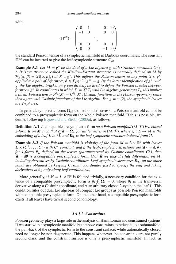
284 Some mathematical methods
with
(%αβ) =
0 1 0 0
−1 0 0 0. . .
0 0 0 10 0 −1 0
the standard Poisson tensor of a symplectic manifold in Darboux coordinates. The constant%αβ can be inverted to give the leaf-symplectic structure �αβ .
Example A.1 Let M = g∗ be the dual of a Lie algebra g with structure constants Cijk .
A Poisson structure, called the Kirillov–Kostant structure, is naturally defined on M byPX(α, β) = X([α, β]g) at X ∈ g∗. This defines the Poisson tensor at any point X ∈ g∗,applied to a pair of 1-forms α, β ∈ T ∗
Xg∗ ∼= g∗∗ = g. By the latter identification of g∗∗ with
g, the Lie algebra bracket on g can directly be used to define the Poisson bracket betweenforms on g∗. In coordinates in which X = XkTk with Lie algebra generators Tk , this impliesa linear Poisson tensor P ij (X) = Cij
kXk . Casimir functions in the Poisson-geometry sense
then agree with Casimir functions of the Lie algebra. For g = su(2), the symplectic leavesare 2-spheres.
In general, symplectic forms �αβ defined on the leaves of a Poisson manifold cannot becombined to a presymplectic form on the whole Poisson manifold. If this is possible, wedefine, following Bojowald and Strobl (2003a), as follows:
Definition A.1 A compatible presymplectic form on a Poisson manifold (M,P) is a closed2-form � on M such that ι∗L� = �L for all leaves L in (M,P), where ιL : L → M is theembedding of a leaf L in M , and �L is the leaf symplectic structure induced from P .
Example A.2 If the Poisson manifold is globally of the form M = L × Rk with leavesL × (C1, . . . , Ck) with CI constant, and if the leaf-symplectic structures are �L = dLθL
for 1-forms θL defined on the leaves (parameterized by Casimir coordinates CI ), then� = dθ is a compatible presymplectic form. (For � we take the full differential on M ,including derivatives by Casimir coordinates. Leaf-symplectic structures �L, on the otherhand, are obtained by keeping Casimir coordinates fixed to specify the leaf and takingderivatives in dL only along leaf coordinates.)
More generally, if M = L × Rk is foliated trivially, a necessary condition for the exis-tence of a compatible presymplectic form is ∂I
∮σ
�L = 0, where ∂I is the transversalderivative along a Casimir coordinate, and σ an arbitrary closed 2-cycle in the leaf L. Thiscondition rules out dual Lie algebras of compact Lie groups as possible Poisson manifoldswith compatible presymplectic form. On the other hand, a compatible presymplectic formexists if all leaves have trivial second cohomology.
AA.5.2 Constraints
Poisson geometry plays a large role in the analysis of Hamiltonian and constrained systems.If we start with a symplectic manifold but impose constraints to reduce it to a submanifold,the pull-back of the symplectic form to the constraint surface, while automatically closed,need no longer be non-degenerate. This happens whenever the constraints are not purelysecond class, and the constraint surface is only a presymplectic manifold. In fact, as
AA.5 Poisson geometry 285
suggested by Bojowald and Strobl (2003b), one can take these considerations to arrive at ageneral definition of first- and second-class surfaces.
Definition A.2 Let (M,P) be a Poisson manifold, and ι : C → M be an embedded sub-manifold such that ι∗T C ⊂ P�(T ∗M). (The submanifold C is thus contained in a symplecticleaf of (M,P).) We call C
(i) first class if {0} �= P�(T ∗⊥x C) ⊂ TxC for all x ∈ C, and
(ii) second class if P�(T ∗⊥x C) ∩ TxC = {0}.
In both cases, we use the co-normal space T ∗⊥x C := {α ∈ T ∗
x M : α(v) = 0 for allv ∈ T Cx}.If the surface is locally described by vanishing constraints CI = 0 (including Casimirfunctions), such that the co-normal space is spanned by dCI , all Hamiltonian vector fieldsXCI generated by the constraints are tangent to C if C is first class, while none of them istangent to C for a second-class surface. The requirement that P�(T ∗⊥
x C) not vanish for afirst-class surface ensures that the constraints are not just Casimir functions of the Poissonmanifold, and that C is indeed a proper subset of a symplectic leaf. (Otherwise, a symplecticleaf would be both first and second class.)
If P = �−1 is invertible, first- and second-class constraint surfaces in a symplecticmanifold (M,�) are first- and second-class surfaces, respectively, in the sense defined inthe context of the Dirac classification of constraints. The definition given here is moregeneral and applies to any Poisson manifold.
For second-class constraints in a symplectic manifold (M,�), we can define the Diracbracket via the Poisson bivector
PD = P +∑I,J
({CI , CJ })−1XCI ∧ XCJ (A.14)
with P = �−1. Its interpretation in the context of Poisson geometry is that (M,PD) is aPoisson manifold in which the second-class surface is a symplectic leaf (with the constraintfunctions CI as Casimir functions) such that � provides a compatible (pre)symplectic form:the leaf-symplectic structure is �L = ι∗L� for all symplectic leaves of (M,PD), embeddedby ιL. In terms of the Casimir functions, we realize each leaf L by the equation CI = CI
(L)
assigning fixed values to the CI .
Proof We take two functions f, g ∈ C∞(L) on L and compare {f, g}L = Xgf (computedusing the leaf-symplectic structure) with {F,G}D evaluated as the Dirac bracket for twoarbitrary extensions F and G of f and g, respectively: F,G ∈ C∞(M) such that ι∗F = fand ι∗G = g. Around a fixed L, two different extensions F and F ′ of f are related byF ′ = F + xI (CI − CI
(L)) for some functions xI . With {CI , ·}D = 0 by construction, thevalue of {F,G}D does not depend on the extension we choose. For simplicity, we thenchoose F and G such that ι∗L(XCI F ) = 0 and ι∗L(XCIG) = 0 for all CI (and thus F andG are extremized on L along transversal directions). Since no XCI is tangent to L for asecond-class surface as assumed, the values of ι∗LF and ι∗LG are not restricted by theseconditions.
Then,
ι∗L{F,G}D = ι∗L(P ij (∂iF )(∂jG) + ({CI , CJ })−1(XCI F )(XCJ G)
)= ι∗L
(P ij (∂iF )(∂jG)
) = ι∗L(XGF ) .

286 Some mathematical methods
Since ι∗L(XGCI ) = −ι∗L(XCIG) = 0, XG is tangent to L on L, so that its restriction XG|L ∈
�(T L) defines a vector field on L. Moreover, the existence of an expansion � = �L +ρI ∧ dCI + σIJ dCI ∧ dCJ in a neighborhood of L with 1-forms ρI and functions σIJ ,combined with ι∗LdCI = 0, implies that(
P�−1L XG|L
)β
= (�L)αβXG|αL = ι∗L(�αβXαG)
= (ι∗L(��XG)
)β
= (ι∗LdG)β = (dg)β
and thus ι∗L(XGF ) = (XG|LF )|L = (P�
Ldg)f = Xgf = {f, g}, completing the proof. �
AA.6 Lie algebroids
Lie algebroids are generalizations of Lie algebras, obtained by making the structure func-tions depend on positions in some space. Accordingly, they can be used to interpret the sym-metries behind constraint algebras with structure functions. As shown in Chapter 4.3.2.4,this has been established especially for Poisson sigma models, which contain 2-dimensionaldilaton gravity models as special cases. Sophisticated algebraic structures then facilitate adeeper understanding of the solution spaces of these systems. While no comparably explicitconstruction is available for full gravity in 3 + 1 dimensions, the hypersurface-deformationalgebra is another example for Lie algebroids; see Chapter 4.3.2.6. Lie algebroids thusprovide several important insights about the nature of gauge transformations.
Position dependence can be formulated elegantly in the fiber-bundle language, withthe base manifold M as the space of dependence. Structure functions are then elementsof C∞(M), and symmetry generators are elements of a fiber basis equipped with a Liebracket. The appropriate notion on which algebraic relations are to be defined is thus thatof sections in the fiber bundle, on which smooth functions act by multiplication. For theLie bracket to be a derivation, we must require a Leibniz rule to be satisfied, which in turnrequires a map from the fibers of the bundle to vector fields on M . These are the crucialingredients of the following Definition
Definition A.3 A Lie algebroid is a vector bundle E over a base manifold M together witha bundle map ρ : E → TM (the anchor) and a Lie algebra structure (�(E), [·, ·]) on itssections such that the Leibniz rule
[s1, f s2] = f [s1, s2] + (ρ(s1)f ) s2 (A.15)
is satisfied for all s1, s2 ∈ �(E) and f ∈ C∞(M).
From the Leibniz rule, it follows that the kernel of ρ defines a Lie algebra over everypoint in M , called the transversal Lie algebra.
Example A.3 Several well-known bundles with algebraic operations defined on them canbe interpreted as Lie algebroids:
(i) A Lie algebra g seen as a vector bundle over a single point with anchor map ρ = 0 is a Liealgebroid. So is a bundle of Lie algebras over a base manifold, with anchor map ρ = 0.
(ii) The tangent bundle TM over any manifold M with ρ = id is a Lie algebroid.(iii) Consider the co-tangent space T ∗M of a Poisson manifold (M,P). The Poisson tensor defines a
map P� : T ∗M → TM via P�(α) = P(α, ·). (In components, the 1-form α = αidXi is mapped

AA.6 Lie algebroids 287
to the vector field αiP ij ∂j .) The map ρ = P� provides the anchor map on E = T ∗M . Tointroduce the Lie bracket on sections, one defines [df, dg] = d{f, g} on exact 1-forms andextends this to all 1-forms using linearity and the Leibniz rule. (In components, [dXi, dXj ] =∂kP ijdXk .)
To compare and relate different Lie algebroids, the notion of morphisms is used. SinceLie algebroids are vector bundles, we start with vector bundle morphisms between twobundles E1 → M1 and E2 → M2. To preserve the vector-bundle structure, a morphismmust map the first base manifold to the second one, and be fiberwise linear, i.e. relatethe fibers over M1 and their images in a linear way. Thus, a vector bundle morphism φis obtained from a base map φ0 : M1 → M2 together with a section of E∗
1 ⊗ φ∗0E2. The
latter bundle is obtained as the tensor product of the dual bundle of E1 (having the duals offiber spaces of E1 as its fibers over the same base manifold M1) and the pull-back bundleφ∗
0E2, a vector bundle over M1 whose fiber over x ∈ M1 is the E2-fiber over φ0(x). (Here,just fibers are being pulled back, not sections. Such a pull-back bundle is independent ofpull-backs of differential forms, which are sections of the co-tangent bundle. The pull-backbundle exists for any vector bundle, such as the tangent bundle even though sections in thetangent bundle cannot be pulled back.) The dual action of E∗
1 on E1, mapping a section onE1 to a function over M1, then makes sections of E∗
1 ⊗ φ∗0E2 identical to maps from �(E1)
to �(φ∗0E2).
To take into account also the algebraic structure of Lie algebroids, we use the followingDefinition
Definition A.4 A Lie algebroid morphism between Lie algebroids (Ei,Mi, ρi, [·, ·]i), i =1, 2, is a vector-bundle morphism φ : E1 → E2 such that
ρ2 ◦ φ = (φ0)∗ ◦ ρ1 (A.16)
(the morphisms φ : E1 → E2 and (φ0)∗ : TM1 → TM2 commute with the anchor maps ρ1and ρ2) and
φ ◦ s1 = s2 ◦ φ0 and φ ◦ s ′1 = s ′
2 ◦ φ0 implies φ ◦ [s1, s′1]1 = [s2, s
′2]2 ◦ φ0 (A.17)
for all si, s ′i ∈ �(Ei).
It follows directly that Lie algebra morphisms provide Lie algebroid morphisms in the caseof vanishing anchor maps. If the anchor map is the identity, diffeomorphisms on the basemanifold provide Lie algebroid morphisms for the tangent bundle. A non-trivial exampleof Lie algebroid morphisms is given by solutions of Poisson sigma models, which, asshown in Chapter 4.3.2.4, provide Lie algebroid morphisms from the tangent bundle of theworldsheet to the Poisson target manifold.
Some Lie algebroids can be realized as certain tangent spaces in Lie groupoids, gen-eralizing the relationship between Lie algebras and Lie groups. However, not every Liealgebroid can be integrated to a Lie group; a complete classification of the integrablecases has been given by Crainic and Fernandes (2003). A Lie groupoid is a differentiablemanifold G together with two maps s : G → M (“source”) and t : G → M (“target”)to a manifold M , such that an associative product g1g2 is defined for any pair(g1, g2) ∈ G with t(g2) = s(g1). Moreover, there is an identity section I : M → G suchthat I(t(g))g = g = gI(s(g)), and groupoid elements are invertible in the sense that for allg, g−1g = I(s(g)) and gg−1 = I(s(g)).
A Lie groupoid does not act transitively on itself by multiplication, but there is a leftaction defined by multiplication of g ∈ G on t−1(s(g)) ⊂ G. A left-invariant vector field
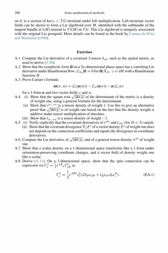
288 Some mathematical methods
on G is a section of ker t∗ ⊂ TG invariant under left multiplication. Left-invariant vectorfields can be shown to form a Lie algebroid over M , identified with the subbundle of thetangent bundle at I(M) normal to T I(M) in TG. This Lie algebroid is uniquely associatedwith the original Lie groupoid. More details can be found in the book by Cannas da Silvaand Weinstein (1999).
Exercises
A.1 Compute the Lie derivative of a covariant 2-tensor hab, such as the spatial metric, asused to derive (3.50).
A.2 Show that the symplectic form � on a 2n-dimensional phase space has a vanishing Liederivative under Hamiltonian flow:LXH
� = 0 for �(XH, ·) = dH with a Hamiltonianfunction H .
A.3 Prove Cartan’s formula
dα(v,w) = Lv(α(w)) − Lw(α(v)) − α(Lvw)
for a 1-form α and two vector fields v and w.A.4 (i) Show that the square root
√|det g| of the determinant of the metric is a densityof weight one, using a general formula for the determinant.
(ii) Show that εa1...aD is a tensor density of weight 1. Use this to give an alternativeproof that
√|det g| is of weight one based on the fact that the density weight isadditive under tensor multiplication of densities.
(iii) Show that εa1...aD is a tensor density of weight −1.A.5 (i) Verify explicitly that the covariant derivatives of εabc and εabc (for D = 3) vanish.
(ii) Show that the covariant divergence ∇aEa of a vector densityEa of weight one does
not depend on the connection coefficients and equals the divergence in coordinatederivatives.
A.6 Compute the Lie derivative of√|det g|, and of a general tensor density πab of weight
one.A.7 Show that a scalar density on a 1-dimensional space transforms like a 1-form under
orientation-preserving coordinate changes, and a vector field of density weight onelike a scalar.
A.8 Derive (A.11). On a 3-dimensional space, show that the spin connection can beexpressed via �A
a = 12ε
ABC�
CaB as
�Aa = 1
2εABCebC(2∂[bea]B + ecBeaD∂be
Dc ) . (EA.1)
References
Anderson, I. Fels, M. and Torre, C. (2000). Group invariant solutions withouttransversality and the principle of symmetric criticality. Commun. Math. Phys., 212,653–686.
Anderson, J. L. and Bergmann, P. G. (1951). Constraints in covariant field theories. Phys.Rev., 83, 1018–1025.
Andersson, L. and Rendall, A. D. (2001). Quiescent cosmological singularities. Commun.Math. Phys., 218, 479–511.
Arnowitt, R. Deser, S. and Misner, C. W. (1962). The Dynamics of General Relativity.New York: Wiley. Reprinted in Arnowitt et al. (2008).
Arnowitt, R. Deser, S. and Misner, C. W. (2008). The dynamics of general relativity. Gen.Rel. Grav., 40, 1997–2027.
Ashtekar, A. (1981). Radiative degrees of freedom of the gravitational field in exactgeneral relativity. J. Math. Phys., 22, 2885–2895.
Ashtekar, A. (1987). New Hamiltonian formulation of general relativity. Phys. Rev. D,36(6), 1587–1602.
Ashtekar, A. and Bojowald, M. (2005). Black hole evaporation: A paradigm. Class.Quantum Grav., 22, 3349–3362.
Ashtekar, A. and Bojowald, M. (2006). Quantum geometry and the Schwarzschildsingularity. Class. Quantum Grav., 23, 391–411.
Ashtekar, A. and Krishnan, B. (2003). Dynamical horizons and their properties. Phys.Rev. D, 68, 104030.
Ashtekar, A. and Krishnan, B. (2004). Isolated and dynamical horizons and theirapplications. Living Rev. Rel., 7, 1–77.
Ashtekar, A. and Lewandowski, J. (1995). Projective techniques and functionalintegration for gauge theories. J. Math. Phys., 36(5), 2170–2191.
Ashtekar, A. and Lewandowski, J. (1997). Quantum theory of geometry I: Area operators.Class. Quantum Grav., 14, A55–A82.
Ashtekar, A. and Lewandowski, J. (1998). Quantum theory of geometry II: Volumeoperators. Adv. Theor. Math. Phys., 1, 388–429.
Ashtekar, A. and Streubel, M. (1981). Symplectic geometry of radiative modes andconserved quantities at null infinity. Proc. Roy. Soc. Lond. A, 376, 585–607.
Ashtekar, A. Pawlowski, T. and Singh, P. (2006). Quantum nature of the Big Bang: Ananalytical and numerical investigation. Phys. Rev. D, 73, 124038.
Ashtekar, A. Engle, J. and Sloan, D. (2008). Asymptotics and Hamiltonians in a firstorder formalism. Class. Quantum Grav., 25, 095020.
289
290 References
Baker, J. G. Centrella, J. Choi, D. I. Koppitz, M. and van Meter, J. (2006).Gravitational-wave extraction from an inspiraling configuration of merging blackholes. Phys. Rev. Lett., 96, 111102.
Balakrishna, J. Daues, G. Seidel, E. Suen, W.-M. Tobias, M. and Wang, E. (1996).Coordinate conditions in three-dimensional numerical relativity. Class. QuantumGrav., 13, L135–L142.
Barbero G., J. F. (1995). Real Ashtekar variables for Lorentzian signature space-times.Phys. Rev. D, 51(10), 5507–5510.
Bardeen, J. M. (1980). Gauge-invariant cosmological perturbations. Phys. Rev. D, 22,1882–1905.
Bardeen, J. M. Carter, B. and Hawking, S. W. (1973). The four laws of black holemechanics. Commun. Math. Phys., 31, 161–170.
Bassett, B. A. Tsujikawa, S. and Wands, D. (2006). Inflation dynamics and reheating.Rev. Mod. Phys., 78, 537–589.
Baumann, D. (2007). On the quantum origin of structure in the inflationary universe.arXiv:0710.3187.
Baumgarte, T. W. and Shapiro, S. L. (1998). Numerical integration of Einstein’s fieldequations. Phys. Rev. D, 59, 024007.
Baumgarte, T. W. and Shapiro, S. L. (2010). Numerical Relativity: Solving Einstein’sEquations on the Computer. Cambridge University Press.
Bekenstein, J. D. (1973). Black holes and entropy. Phys. Rev. D, 1, 2333–2346.Belinskii, V. A. Khalatnikov, I. M. and Lifschitz, E. M. (1982). A general solution of the
Einstein equations with a time singularity. Adv. Phys., 13, 639–667.Ben-Dov, I. (2007). Outer trapped surfaces in Vaidya spacetimes. Phys. Rev. D, 75,
064007.Bengtsson, I. and Senovilla, J. M. M. (2009). A note on trapped surfaces in the Vaidya
solution. Phys. Rev. D, 79, 024027.Berger, B. (2002). Numerical approaches to spacetime singularities. Living Rev.
Relativity, 5, 1. http://www.livingreviews.org/lrr-2002-1.Bergmann, P. G. (1961). Observables in general relativity. Rev. Mod. Phys., 33,
510–514.Bertschinger, E. (2006). On the growth of perturbations as a test of dark energy.
Astrophys. J., 648, 797.Bicak, J. and Hajıcek, P. (2003). Canonical theory of spherically symmetric spacetimes
with cross-streaming null dusts. Phys. Rev. D, 68, 104016.Bicak, J. and Kuchar, K. V. (1997). Null dust in canonical gravity. Phys. Rev. D, 56,
4878–4895.Blohmann, C. Barbosa Fernandes, M. C. and Weinstein, A. (2010). Groupoid symmetry
and constraints in general relativity. 1: Kinematics. arXiv:1003.2857.Bojowald, M. (2007). Large scale effective theory for cosmological bounces. Phys. Rev.
D, 75, 081301(R).Bojowald, M. (2008). Loop quantum cosmology. Living Rev. Relativity, 11, 4.
http://www.livingreviews.org/lrr-2008-4.Bojowald, M. (2011). Quantum Cosmology: A Fundamental Theory of the Universe. New
York: Springer.Bojowald, M. and Skirzewski, A. (2006). Effective equations of motion for quantum
systems. Rev. Math. Phys., 18, 713–745.Bojowald, M. and Strobl, T. (2003a). Classical solutions for Poisson sigma models on a
Riemann surface. JHEP, 0307, 002.

References 291
Bojowald, M. and Strobl, T. (2003b). Poisson geometry in constrained systems. Rev.Math. Phys., 15, 663–703.
Bojowald, M. and Tsobanjan, A. (2009). Effective constraints for relativistic quantumsystems. Phys. Rev. D, 80, 125008.
Bojowald, M. Goswami, R. Maartens, R. and Singh, P. (2005a). A black hole massthreshold from non-singular quantum gravitational collapse. Phys. Rev. Lett., 95,091302.
Bojowald, M. Kotov, A. and Strobl, T. (2005b). Lie algebroid morphisms, Poisson sigmamodels, and off-shell closed gauge symmetries. J. Geom. Phys., 54, 400–426.
Bojowald, M. Cartin, D. and Khanna, G. (2007). Lattice refining loop quantumcosmology, anisotropic models and stability. Phys. Rev. D, 76, 064018.
Bojowald, M. Hossain, G. Kagan, M. and Shankaranarayanan, S. (2008). Anomalyfreedom in perturbative loop quantum gravity. Phys. Rev. D, 78, 063547.
Bojowald, M. Sandhofer, B. Skirzewski, A. and Tsobanjan, A. (2009a). Effectiveconstraints for quantum systems. Rev. Math. Phys., 21, 111–154.
Bojowald, M. Hossain, G. Kagan, M. and Shankaranarayanan, S. (2009b). Gaugeinvariant cosmological perturbation equations with corrections from loop quantumgravity. Phys. Rev. D, 79, 043505.
Bojowald, M. Reyes, J. D. and Tibrewala, R. (2009c). Non-marginal LTB-like modelswith inverse triad corrections from loop quantum gravity. Phys. Rev. D, 80, 084002.
Bona, C. and Masso, J. (1988). Harmonic synchronizations of spacetime. Phys. Rev. D,38, 2419–2422.
Bona, C. and Masso, J. (1992). Hyperbolic evolution system for numerical relativity.Phys. Rev. Lett., 68, 1097–1099.
Bona, C. Masso, J. Seidel, E. and Stela, J. (1995). New formalism for numericalrelativity. Phys. Rev. Lett., 75, 600–603.
Bondi, H. van der Burg, M. G. J. and Metzner, A. W. K. (1962). Gravitational waves ingeneral relativity. VII. Waves from axi-symmetric isolated systems. Proc. Roy. Soc.A, 269, 21–52.
Booth, I. and Fairhurst, S. (2003). Canonical phase space formulation of quasilocalgeneral relativity. Class. Quantum Grav., 20, 4507–4532.
Booth, I. and Mann, R. (1999). Moving observers, nonorthogonal boundaries, andquasilocal energy. Phys. Rev. D, 59, 064021.
Brady, P. R. Creighton, J. D. E. and Thorne, K. S. (1998). Computing the merger ofblack-hole binaries: The IBBH problem. Phys. Rev. D, 58, 061501.
Brandt, S. and Brugmann, B. (1997). A simple construction of initial data for multipleblack holes. Phys. Rev. Lett., 78, 3606–3609.
Brill, D. R. and Lindquist, R. W. (1963). Interaction energy in geometrostatics. Phys.Rev., 131, 471–476.
Brizuela, D. Martın-Garcıa, J. M. and Mena Marugan, G. A. (2007). Higher-ordergauge-invariant perturbations of a spherical spacetime. Phys. Rev. D, 76, 024004.
Brodbeck, O. (1996). On symmetric gauge fields for arbitrary gauge and symmetrygroups. Helv. Phys. Acta, 69, 321–324.
Brown, J. D. and Kuchar, K. V. (1995). Dust as a standard of space and time in canonicalquantum gravity. Phys. Rev. D, 51, 5600–5629.
Brown, J. D. and York, J. W. (1993). Quasilocal energy and conserved charges derivedfrom the gravitational action. Phys. Rev. D, 47, 1407–1419.
Bruni, M. Dunsby, P. K. S. and Ellis, G. F. R. (1992). Cosmological perturbations and thephysical meaning of gauge invariant variables. Astrophys. J., 395, 34–53.

292 References
Campanelli, M. Lousto, C. O. Marronetti, P. and Zlochower, Y. (2006). Accurateevolutions of orbiting black-hole binaries without excision. Phys. Rev. Lett., 96,111101.
Cannas da Silva, A. and Weinstein, A. (1999). Geometric models for noncommutativealgebras. Berkeley Mathematics Lectures, vol. 10. Providence: Am. Math. Soc.
Cattaneo, A. S. and Felder, G. (2000). Poisson sigma models and symplectic groupoids.math/0003023.
Chinea, F. J. Fernandez-Jambrina, L. and Senovilla, J. M. M. (1992). A singularity-freespace-time. Phys. Rev. D, 45, 481–486.
Choptuik, M. W. (1991). Consistency of finite-difference solutions of Einstein’sequations. Phys. Rev. D, 44, 3124–3135.
Choptuik, M. W. (1993). Universality and scaling in gravitational collapse of a masslessscalar field. Phys. Rev. Lett., 2, 9–12.
Chrusciel, P. T. Corvino, J. and Isenberg, J. (2010). Construction of N -body initial datasets in general relativity. arXiv:1004.1355.
Clarke, C. J. S. (1998). Generalised hyperbolicity in singular space-times. Class. Quant.Grav., 15, 975–984.
Clarke, C. J. S. and Dray, T. (1987). Junction conditions for null hypersurfaces. Class.Quantum Grav., 4, 265–275.
Cordero, P. (1977). Canonical formulation of the spherically symmetricEinstein–Yang–Mills–Higgs system for a general gauge group. Ann. Phys., 108,79–98.
Corichi, A. and Wilson-Ewing, E. (2010). Surface terms, asymptotics andthermodynamics of the Holst action. arXiv:1005.3298.
Crainic, M. and Fernandes, R. L. (2003). Integrability of Lie brackets. Ann. Math., 157,575–620.
Damour, T. Henneaux, M. and Nicolai, H. (2003). Cosmological billiards. Class.Quantum Grav., 20, R145–R200.
Date, G. and Hossain, G. M. (2005). Genericity of big bounce in isotropic loop quantumcosmology. Phys. Rev. Lett., 94, 011302.
Date, G. Kaul, R. K. and Sengupta, S. (2009). Topological interpretation ofBarbero–Immirzi parameter. Phys. Rev. D, 79, 044008.
Deruelle, N. Sasaki, M. Sendouda, Y. and Yamauchi, D. (2009). Hamiltonianformulation of f (Riemann) theories of gravity. Prog. Theor. Phys., 123, 169–185.
Deser, S. Kay, J. H. and Stelle, K. S. (1977). Hamiltonian formulation of supergravity.Phys. Rev. D, 16, 2448–2455.
DeWitt, B. S. (1967). Quantum theory of gravity. I. The canonical theory. Phys. Rev., 160,1113–1148.
Dirac, P. A. M. (1958a). Generalized Hamiltonian dynamics. Proc. Roy. Soc. A, 246,326–332.
Dirac, P. A. M. (1958b). The theory of gravitation in Hamiltonian form. Proc. Roy. Soc. A,246, 333–343.
Dirac, P. A. M. (1969). Lectures on Quantum Mechanics. New York: Yeshiva UniversityPress.
Dittrich, B. (2006). Partial and complete observables for canonical general relativity.Class. Quant. Grav., 23, 6155–6184.
Dittrich, B. (2007). Partial and complete observables for Hamiltonian constrainedsystems. Gen. Rel. Grav., 39, 1891–1927.

References 293
Dreyer, O. Krishnan, B. Shoemaker, D. and Schnetter, E. (2003). Introduction to isolatedhorizons in numerical relativity. Phys. Rev. D, 67, 024018.
Eardley, D. M. (1998). Black hole boundary conditions and coordinate conditions. Phys.Rev. D, 57, 2299–2304.
Eardley, D. M. and Smarr, L. (1979). Time functions in numerical relativity: Marginallybound dust collapse. Phys. Rev. D, 19, 2239–2259.
Ellis, G. F. R. and Bruni, M. (1989). Covariant and gauge invariant approach tocosmological density fluctuations. Phys. Rev. D, 40, 1804–1818.
Ellis, G. F. R. and MacCallum, M. A. H. (1969). A class of homogeneous cosmologicalmodels. Commun. Math. Phys., 12, 108–141.
Ellis, G. F. R. Murugan, J. and Weltman, A. (2011). Foundations of Space and Time.Cambridge University Press.
Fleischhack, C. (2009). Representations of the Weyl algebra in quantum geometry.Commun. Math. Phys., 285, 67–140.
Friedrich, H. (1996). Hyperbolic reductions for Einstein’s equations. Class. QuantumGrav., 13, 1451–1469.
Friedrich, H. and Rendall, A. D. (2000). The Cauchy problem for the Einstein equations.Lect. Notes Phys., 540, 127–224.
Frittelli, S. (1997). Note on the propagation of the ocnstraints in standard 3 + 1 generalrelativity. Phys. Rev. D, 55, 5992–5995.
Frolov, V. P. and Vilkovisky, G. A. (1981). Spherically symmetric collapse in quantumgravity. Phys. Lett. B, 106, 307–313.
Gambini, R. and Trias, A. (1980). Second quantization of the free electromagnetic field asquantum mechanics in the loop space. Phys. Rev. D, 22, 1380–1384.
Garfinkle, D. (2002). Harmonic coordinate method for simulating generic singularities.Phys. Rev. D, 65, 044029.
Garfinkle, D. (2004). Numerical simulations of generic singuarities. Phys. Rev. Lett., 93,161101.
Garfinkle, D. and Gundlach, C. (1999). Symmetry-seeking spacetime coordinates. Class.Quantum Grav., 16, 4111–4123.
Geroch, R. and Winicour, J. (1981). Linkages in general relativity. J. Math. Phys., 22,803–812.
Gibbons, G. W. and Hawking, S. W. (1977). Action integrals and partition functions inquantum gravity. Phys. Rev. D, 15, 2752–2756.
Giesel, K. Hofmann, S. Thiemann, T. and Winkler, O. (2007). Manifestly gauge-invariantgeneral relativistic perturbation theory: I. Foundations. arXiv:0711.0115.
Giles, R. (1981). The reconstruction of gauge potentials from Wilson loops. Phys. Rev. D,24, 2160–2168.
Girotto, F. and Saa, A. (2004). Semianalytical approach for the Vaidya metric indouble-null coordinates. Phys. Rev. D, 70, 084014.
Giulini, D. (1995). What is the geometry of superspace? Phys. Rev. D, 51(10), 5630–5635.
Giulini, D. and Marolf, D. (1999). On the generality of refined algebraic quantization.Class. Quantum Grav., 16, 2479–2488.
Gockeler, M. and Schucker, T. (1989). Differential Geometry, Gauge Theories, adGravity. Cambridge University Press.
Goode, S. W. (1989). Analysis of spatially inhomogeneous perturbations of the FRWcosmologies. Phys. Rev. D, 39, 2882–2892.

294 References
Govaerts, J. and Rashid, M. S. (1994). The Hamiltonian formulation of higher orderdynamical systems. hep-th/9403009.
Gowdy, R. H. (1974). Vacuum spacetimes with two-parameter spacelike isometry groupsand compact invariant hypersurfaces: Topologies and boundary conditions. Ann.Phys., 83, 203–241.
Grain, J. Cailleteau, T. Barrau, A. and Gorecki, A. (2010). Fully LQC-correctedpropagation of gravitational waves during slow-roll inflation. Phys. Rev. D, 81,024040.
Grumiller, D. Kummer, W. and Vassilevich, D. V. (2002). Dilaton gravity in twodimensions. Phys. Rept., 369, 327–430.
Guth, A. H. and Pi, S. Y. (1985). Quantum mechanics of the scalar field in the newinflationary universe. Phys. Rev. D, 32, 1899–1920.
Hartle, J. B. and Marolf, D. (1997). Comparing formulations of generalized quantummechanics for reparametrization-invariant systems. Phys. Rev. D, 56, 6247–6257.
Hawking, S. W. (1969). On the rotation of the universe. MNRAS, 142, 129–141.Hawking, S. W. (1971). Gravitational radiation from colliding black holes. Phys. Rev.
Lett., 36, 1344–1346.Hawking, S. W. (1972). Black holes in general relativity. Commun. Math. Phys., 25,
152–166.Hawking, S. W. and Ellis, G. F. R. (1973). The Large Scale Structure of Space-time.
Cambridge University Press.Hawking, S. W. and Horowitz, G. T. (1996). The gravitational Hamiltonian, action,
entropy and surface terms. Class. Quantum Grav., 13, 1487–1498.Hawking, S. W. and Hunter, C. J. (1996). The gravitational Hamiltonian in the presence
of non-orthogonal boundaries. Class. Quantum Grav., 13, 2735–2752.Hayward, G. (1993). Gravitational action for spacetimes with nonsmooth boundaries.
Phys. Rev. D, 47, 3275–3280.Hayward, S. A. (1994). General laws of black-hole dynamics. Phys. Rev. D, 49,
6467–6474.Hayward, S. A. (2006). Formation and evaporation of non-singular black holes. Phys. Rev.
Lett., 96, 031103.Heusler, M. (1998). Stationary black holes: Uniqueness and beyond. Living Rev. Rel.,
1, 6.Hiscock, W. A. Williams, L. G. and Eardley, D. M. (1982). Creation of particles by
shell-focusing singularities. Phys. Rev. D, 26, 751–760.Hojman, S. A. Kuchar, K. and Teitelboim, C. (1976). Geometrodynamics regained. Ann.
Phys. (New York), 96, 88–135.Holst, S. (1996). Barbero’s Hamiltonian derived from a generalized Hilbert–Palatini
action. Phys. Rev. D, 53, 5966–5969.Horvath, Z. Kovacs, Z. and Gergely, L. A. (2006). Geometrodynamics in a spherically
symmetric, static crossflow of null dust. Phys. Rev. D, 74, 084034.Husain, V. (2009). Critical behaviour in quantum gravitational collapse. Adv. Sci. Lett., 2,
214.Ikeda, N. (1994). Two-dimensional gravity and nonlinear gauge theory. Ann. Phys., 235,
435–464.Ikeda, N. and Izawa, K. I. (1993). General form of dilaton gravity and nonlinear gauge
theory. Prog. Theor. Phys., 90, 237.Immirzi, G. (1997). Real and complex connections for canonical gravity. Class. Quantum
Grav., 14, L177–L181.
References 295
Isham, C. J. (1983). Topological and global aspects of quantum theory. In: DeWitt, B. S.and Stora, R. (eds), Relativity, Groups and Topology II. Lectures given at the 1983Les Houches Summer School on Relativity, Groups and Topology.
Israel, W. (1966). Singular hypersurfaces and thin shells in general relativity. NuovoCimento B, 44, 1.
Iyer, V. and Wald, R. M. (1994). Some properties of the Noether charge and a proposalfor dynamical black hole entropy. Phys. Rev. D, 50, 846–864.
Jacobson, T. (2000). Trans-Planckian redshifts and the substance of the space-time river.Jaramillo, J. L. and Gourgoulhon, E. (2010). Mass and angular momentum in general
relativity. arXiv:1001.5429.Kastrup, H. A. and Thiemann, T. (1994). Spherically symmetric gravity as a completely
integrable system. Nucl. Phys. B, 425, 665–686.Keresztes, Z. and Gergely, L. A. (2010). Covariant gravitational dynamics in 3 + 1 + 1
dimensions. Class. Quantum Grav., 27, 105009.Kiefer, C. (2004). Quantum Gravity. Oxford University Press.Kiefer, C. Polarski, D. and Starobinsky, A. A. (1998). Quantum-to-classical transition for
fluctuations in the early Universe. Int. J. Mod. Phys. D, 7, 455–462.Klauder, J. (2001). Quantization of constrained systems. Lect. Notes Phys., 572, 143–182.Klauder, J. (2003). Affine quantum gravity. Int. J. Mod. Phys. D, 12, 1769–1774.Klauder, J. (2006). Overview of affine quantum gravity. Int. J. Geom. Meth. Mod. Phys., 3,
81–94.Kobayashi, S. and Nomizu, K. (1963). Foundations of Differential Geometry. Vol. 1.
New York: John Wiley.Kobayashi, S. and Nomizu, K. (1969). Foundations of Differential Geometry. Vol. 2.
New York: John Wiley.Komar, A. (1959). Covariant conservation laws in general relativity. Phys. Rev., 113,
934–936.Komar, A. (1979). Consistent factor ordering of general relativistic constraints. Phys. Rev.
D, 20, 830–833.Kouletsis, I. Hajıcek, P. and Bicak, J. (2003). Gauge-invariant Hamiltonian dynamics of
cylindrical gravitational waves. Phys. Rev. D, 68, 104013.Kovacs, Z. and Gergely, L. A. (2006). New variables for brane-world gravity. AIP Conf.
Proc., 861, 897–902.Krishnan, B. and Schnetter, E. (2006). Non-symmetric trapped surfaces in the
Schwarzschild and Vaidya spacetimes. Phys. Rev. D, 73, 021502(R).Kuchar, K. V. (1974). Geometrodynamics regained: A Lagrangian approach. J. Math.
Phys., 15, 708–715.Kuchar, K. V. (1976a). Dynamics of tensor fields in hyperspace. III. J. Math. Phys., 17,
801–820.Kuchar, K. V. (1976b). Geometry of hypersurfaces. I. J. Math. Phys., 17, 777–
791.Kuchar, K. V. (1992). Time and interpretations of quantum gravity. In: Kunstatter, G.
Vincent, D. E. and Williams, J. G. (eds), Proceedings of the 4th CanadianConference on General Relativity and Relativistic Astrophysics. Singapore: WorldScientific.
Kuchar, K. V. (1994). Geometrodynamics of Schwarzschild black holes. Phys. Rev. D,50(6), 3961–3981.
Langlois, D. (1994). Hamiltonian formalism and gauge invariance for linear perturbationsin inflation. Class. Quantum Grav., 11, 389–407.
296 References
Langlois, D. and Vernizzi, F. (2005). Evolution of non-linear cosmological perturbations.Phys. Rev. Lett., 95, 091303.
Lau, S. R. (1996). New variables, the gravitational action and boosted quasilocalstress-energy-momentum. Class. Quantum Grav., 13, 1509–1540.
Lehner, L. (2001). Numerical relativity: A review. Class. Quantum Grav., 18, R25–R86.Lewandowski, J. Newman, E. T. and Rovelli, C. (1993). Variations of the parallel
propagator and holonomy operator and the gauss law constraint. J. Math. Phys., 34,4646–4654.
Lewandowski, J. Okołow, A. Sahlmann, H. and Thiemann, T. (2006). Uniqueness ofdiffeomorphism invariant states on holonomy-flux algebras. Commun. Math. Phys.,267, 703–733.
Lichnerowicz, A. (1944). J. Math. Pure Appl., 23, 37.Lidsey, J. E. Liddle, A. R. Kolb, E. W. Copeland, E. J. Barreiro, T. and Abney, M.
(1997). Reconstructing the inflaton potential — an overview. Rev. Mod. Phys., 69,373–410.
Lim, W. C. Andersson, L. Garfinkle, D. and Pretorius, F. (2009). Spikes in theMixmaster regime of G2 cosmologies. Phys. Rev. D, 79, 123526.
Lovelock, D. (1970). The Einstein tensor and its generalizations. J. Math. Phys., 12,498–501.
Lyth, D. H. (1985). Large scale energy density perturbations and inflation. Phys. Rev. D,31, 1792.
Maartens, R. (2004). Brane-world gravity. Living Rev. Rel., 7, 7.http://www.livingreviews.org/lrr-2004-7.
MacCallum, M. A. H. and Taub, A. H. (1972). Variational principles and spatially-homogeneous universes, including rotation. Commun. Math. Phys., 25, 173–189.
Madsen, M. S. (1988). Scalar fields in curved spacetimes. Class. Quantum Grav., 5,627–639.
Malik, K. and Wands, D. (2004). Evolution of second-order cosmological perturbations.Class. Quantum Grav., 21, L65–L71.
Marolf, D. (1995). Refined algebraic quantization: Systems with a single constraint.gr-qc/9508015.
Mars, M. and Senovilla, J. (1993). Geometry of general hypersurfaces in spacetime:junction conditions. Class. Quantum Grav., 10, 1865–1897.
Martin, J. L. (1959). Generalized classical dynamics, and the ‘classical analogue’ of aFermi oscillator. Proc. Roy. Soc. A, 251, 536–542.
Mercuri, S. (2006). Fermions in Ashtekar-Barbero connections formalism for arbitraryvalues of the Immirzi parameter. Phys. Rev. D, 73, 084016.
Misner, C. W. (1968). The isotropy of the Universe. Astrophys. J., 151, 431–457.Misner, C. W. (1969). Mixmaster universe. Phys. Rev. Lett., 22, 1071–1074.Modesto, L. (2006). Loop quantum black hole. Class. Quantum Grav., 23, 5587–5601.Multamaki, T. Vainio, J. and Vilja, I. (2010). Hamiltonian perturbation theory in f (R)
gravity. Phys. Rev. D, 81, 064025.Nelson, W. and Sakellariadou, M. (2007a). Lattice refining loop quantum cosmology and
inflation. Phys. Rev. D, 76, 044015.Nelson, W. and Sakellariadou, M. (2007b). Lattice refining LQC and the matter
Hamiltonian. Phys. Rev. D, 76, 104003.Nielsen, A. B. (2009). Black holes and black hole thermodynamics without event
horizons. Gen. Rel. Grav., 41, 1539–1584.

References 297
Nielsen, A. B. and Visser, M. (2006). Production and decay of evolving horizons. Class.Quantum Grav., 23, 4637–4658.
Novello, M. and Bergliaffa, S. E. P. (2008). Bouncing cosmologies. Phys. Rep., 463,127–213.
Oppenheimer, J. R. and Snyder, H. (1939). On continued gravitational contraction. Phys.Rev., 56, 455–459.
Oriti, D. (2009). Approaches to Quantum Gravity: Toward a New Understanding ofSpace, Time and Matter. Cambridge University Press.
Penrose, R. (1963). Asymptotic properties of fields and space-times. Phys. Rev. Lett., 10,66–68.
Penrose, R. (1965). Gravitational collapse and space-time singularities. Phys. Rev. Lett.,14, 57–59.
Penrose, R. (1990). Difficulties with inflationary cosmology. In: Fenves, E. (ed.),Proceedings of the 14th Texas Symposium on Relativistic Astrophysics. New York:N.Y. Acad. Sci.
Pfennig, M. J. and Ford, L. H. (1998). Scalar field quantum inequalities in staticspace-times. Phys. Rev. D, 57, 3489–3502.
Pirani, F. A. E. and Schild, A. (1950). On the quantization of Einstein’s gravitational fieldequations. Phys. Rev., 79, 986–991.
Pirani, F. A. E. Schild, A. and Skinner, R. (1953). Quantization of Einstein’s gravitationalfield equations. II. Phys. Rev., 87, 452–454.
Podolsky, J. and Svıtek, O. (2005). Radiative spacetimes approaching the Vaidya metric.Phys. Rev. D, 71, 124001.
Polarski, D. and Starobinsky, A. A. (1996). Semiclassicality and decoherence ofcosmological perturbations. Class. Quantum Grav., 13, 377–392.
Pons, J. M. Salisbury, D. C. and Shepley, L. C. (1997). Gauge transformations in theLagrangian and Hamiltonian formalisms of generally covariant theories. Phys. Rev.D, 55, 658–668.
Pretorius, F. (2005). Evolution of binary black-hole spacetimes. Phys. Rev. Lett., 95,121101.
Regge, T. and Teitelboim, C. (1974). Role of surface integrals in the Hamiltonianformulation of general relativity. Ann. Phys., 88, 286–318.
Rendall, A. D. (2005). The Nature of Spacetime Singularities. Singapore: World Scientific.Rendall, A. D. and Weaver, M. (2001). Manufacture of Gowdy spacetimes with spikes.
Class. Quantum Grav., 18, 2959–2975.Roman, T. A. and Bergmann, P. G. (1983). Stellar collapse without singularities? Phys.
Rev. D, 28, 1265–1277.Rovelli, C. (1991). What is observable in classical and quantum gravity? Class. Quantum
Grav., 8, 297–316.Rovelli, C. (2004). Quantum Gravity. Cambridge University Press.Rovelli, C. and Smolin, L. (1990). Loop space representation of quantum general
relativity. Nucl. Phys. B, 331, 80–152.Rovelli, C. and Smolin, L. (1995). Discreteness of area and volume in quantum gravity.
Nucl. Phys. B, 442, 593–619. Erratum: Nucl. Phys. B 456 (1995) 753.Sachs, R. (1962). Asymptotic symmetries in gravitational theory. Phys. Rev., 128,
2851–2864.Salopek, D. S. and Bond, J. R. (1990). Nonlinear evolution of long wavelength metric
fluctuations in inflationary models. Phys. Rev. D, 42, 3936–3962.
298 References
Saotome, R. Akhoury, R. and Garfinkle, D. (2010). Examining gravitational collapsewith test scalar fields. arXiv:1004.3569.
Schaller, P. and Strobl, T. (1994). Poisson structure induced (topological) field theories.Mod. Phys. Lett. A, 9, 3129–3136.
Schnetter, E. Krishnan, B. and Beyer, F. (2006). Introduction to dynamical horizons innumerical relativity. Phys. Rev. D, 74, 024028.
Schwinger, J. (1962). Quantized gravitational field. Phys. Rev., 130, 1253–1258.Senovilla, J. M. M. (1990). New class of inhomogeneous cosmological perfect-fluid
solutions without Big-Bang Singularity. Phys. Rev. Lett., 64, 2219–2221.Senovilla, J. M. M. (1998). Singularity theorems and their consequences. Gen. Rel. Grav.,
30, 701–848.Senovilla, J. M. M. (2007). A singularity theorem based on spatial averages. Pramana, 69,
31–48.Shibata, M. and Nakamura, T. (1995). Evolution of three-dimensional gravitational
waves: Harmonic slicing case. Phys. Rev. D, 52, 5428–5444.Smarr, L. and York, J. W. (1978). Kinematical conditions in the construction of
spacetime. Phys. Rev. D, 17, 2529–2551.Stewart, J. M. (1990). Perturbations of Friedmann–Robertson–Walker cosmological
models. Class. Quantum Grav., 7, 1169–1180.Strobl, T. (2004). Algebroid Yang–Mills theories. Phys. Rev. Lett., 93, 211601.Thiemann, T. (1998a). Kinematical Hilbert spaces for fermionic and Higgs quantum field
theories. Class. Quantum Grav., 15, 1487–1512.Thiemann, T. (1998b). Quantum spin dynamics (QSD). Class. Quantum Grav., 15,
839–873.Thiemann, T. (1998c). QSD V: Quantum gravity as the natural regulator of matter
quantum field theories. Class. Quantum Grav., 15, 1281–1314.Thiemann, T. (2007). Introduction to Modern Canonical Quantum General Relativity.
Cambridge University Press.Thiemann, T. and Kastrup, H. A. (1993). Canonical quantization of spherically symmetric
gravity in Ashtekar’s self-dual representation. Nucl. Phys. B, 399, 211–258.Thornburg, J. (1996). Finding apparent horizons in numerical relativity. Phys. Rev. D, 54,
4899–4918.Thornburg, J. (2007). Event and apparent horizon finders for 3 + 1 numerical relativity.
Living Rev. Rel., 10, 3.Torre, C. G. (1999). Midi-superspace models of canonical quantum gravity. Int. J. Theor.
Phys., 38, 1081–1102.Uggla, C. van Elst, H. Wainwright, J. and Ellis, G. F. R. (2003). The past attractor in
inhomogeneous cosmology. Phys. Rev. D, 68, 103502.Unruh, W. (1997). Time, gravity, and quantum mechanics. In: Savitt, S. F. (ed.) Time’s
Arrows Today. Cambridge University Press, 23–94.Vachaspati, T. and Stojkovic, D. (2008). Quantum radiation from quantum gravitational
collapse. Phys. Lett. B, 663, 107–110.Vaidya, P. C. (1953). ‘Newtonian’ Time in General Relativity. Nature, 171, 260.Vickers, J. A. and Wilson, J. P. (2001). Generalised hyperbolicity: Hypersurface
singularities. gr-qc/0101018.Vickers, J. A. and Wilson, J. P. (2000). Generalised hyperbolicity in conical space-times.
Class. Quantum Grav., 17, 1333–1360.Wald, R. M. (1984). General Relativity. University of Chicago Press.
References 299
Wald, R. M. and Iyer, V. (1991). Trapped surfaces in the Schwarzschild geometry andcosmic censorship. Phys. Rev. D, 44, 3719–3722.
Wald, R. M. and Zoupas, A. (2000). General definition of “conserved quantities” ingeneral relativity and other theories of gravity. Phys. Rev. D, 61, 084027.
Wands, D. Malik, K. A. Lyth, D. H. and Liddle, A. R. (2000). A new approach to theevolution of cosmological perturbations on large scales. Phys. Rev. D, 62, 043527.
Waugh, B. and Lake, K. (1986). Double-null coordinates for the Vaidya metric. Phys.Rev. D, 34, 2978–2984.
Weiss, N. (1985). Constraints on Hamiltonian lattice formulations of field theories in anexpanding universe. Phys. Rev. D, 32, 3228–3232.
Winitzki, S. (2005). Drawing conformal diagrams for a fractal landscape. Phys. Rev. D,71, 123523.
York, J. W. (1971). Gravitational degrees of freedom and the initial-value problem. Phys.Rev. Lett., 26, 1656–1658.
York, J. W. (1986). Boundary terms in the action principles of general relativity. Found.Phys., 16, 249–257.

Index
BF -theory, 157
G-bundle, 280
n-bein, 282
2-dimensional gravity, 155
action principle, 22
adjoint action, 137
ADM momentum, 217
affine quantum gravity, 259
anchor map, 160, 286
angular momentum, 217
anisotropic shear, 128
stress, 14, 167, 175
anisotropy parameter, 122
plane, 125
potential, 122
anomaly, 252, 253, 270
anti-commutation, 109
apparent horizon, 236
areal radius, 148
area increase, 240
Arnowitt–Deser–Misner (ADM) energy, 216
Ashtekar–Barbero connection, 93, 107, 108, 109, 256
Ashtekar variables, 98
associated vector bundle, 280
asymptotically anti de Sitter space-time, 206
de Sitter space-time, 206
empty space-time, 205
flat space-time, 153, 205, 207, 211, 216
Minkowski space-time, 206
simple space-time, 206
asymptotic infinity, 203
asymptotic solution, 211
axial current, 106, 107
back-reaction, 244
background-field expansion, 38
background independence, 261
metric, 255
Barbero–Immirzi parameter, 91, 106
Bardeen variables, 14, 169, 173
Belinskii–Khalatnokov–Lifschitz (BKL) conjecture,
126
Bianchi classification, 114, 119, 120, 129, 198
class A, 119, 141, 145, 147
class B, 119, 146, 147, 181
identity, 18
models, 131, 141, 277
type I, 123, 128
type IX, 124, 126, 128, 181
type V, 181
black-hole entropy, 242
evaporation, 244
thermodynamics, 242
black hole, 82, 127, 198, 230, 235, 242, 271
Bondi–Metzner–Sachs (BMS) group, 214
boundary degree of freedom, 154
term, 52, 53, 91, 146, 153, 181, 215
Brill–Lindquist initial data, 82
Brown–York quasilocal energy, 57, 216
BSSN equations, 78
canonical line element, 43, 165
Cartan’s formula, 161
Carter–Penrose diagram, 204
Casimir–Darboux coordinates, 158, 283
Casimir function, 29, 31, 157, 158, 283
Cauchy horizon, 234
causal diagram, 201
caustic, 101, 191
centralizer, 137
chaos, 125, 127, 128
characteristic, 72
Christoffel symbols, 19, 39, 77, 83
Clifford algebra, 105
co-tetrad, 84
Codazzi equation, 47, 50
cohomology, 158
compatible presymplectic form, 158, 284, 285
complex connection, 108, 256
300

Index 301
conformal completion, 204, 205, 208
diagram, 226, 228, 230, 233, 234, 244
gauge, 210
Hubble parameter, 10, 172
time, 9
transformation, 81, 175
conjugate point, 101, 192, 202
conjugation, 132, 137, 143
connection, 132, 134, 135, 256, 281
connection 1-form, 85, 86, 134, 135, 155, 280, 282
conservation equation, 176
of power, 177, 179, 271
consistency, 14, 15, 173, 176
consistent deformation, 254, 270
constraints, 18, 20, 22, 23, 167, 284
constraint algebra, 63, 170, 270
continuity equation, 9, 181
coordinate independence, 15
transformation, 14, 21, 66, 116, 166
cosmic censorship, 234
covariance, 52, 65
covariant derivative, 44, 85, 134, 276, 282
cross-normalization, 194, 211, 219
curvature, 87, 155
curvature 2-form, 87
curvature perturbation, 170, 177
potential, 124, 125, 181
Darboux coordinates, 27
deceleration, 10, 11
parameter, 9
densitized triad, 93, 171, 172
density weight, 37, 93, 141, 151, 276
deparameterization, 70, 103, 123, 260, 265
derivative expansion, 176
determinant, 39, 43
DeWitt supermetric, 113
de Sitter space, 9, 10
diagonal Bianchi model, 121
diffeomorphism, 63, 64
constraint, 51, 61, 81, 95, 96, 99, 102, 104, 110, 148, 151,
159, 171, 173, 176, 277
dilaton, 154
gravity, 154, 156
potential, 155
Dirac action, 106
bracket, 31, 97, 285
classification, 285
equation, 106
observable, 34, 71, 152
quantization, 251
discrete spectrum, 258, 262, 266
distortion, 80
driver, 80
dust, 10, 101
Hamiltonian, 103
dyad, 155, 282
Eddington–Finkelstein coordinates, 208, 223
effective constraint, 253, 271
equation, 263
Hamiltonian, 265, 267
Einstein–Hilbert action, 5, 38, 50, 54
Einstein static universe, 15, 204
tensor, 20, 155, 164
electric field, 103
electromagnetism, 37, 103
energy condition, 10, 181, 237, 241, 268, 271
current, 99, 103, 175
density, 8, 98, 101, 104, 175
epsilon tensor density, 276
equation of state, 10, 104
Euclidean group, 132, 250
Euler–Lagrange equations, 22
Eulerian observer, 42, 92, 98, 99, 113
Euler angles, 182
event horizon, 208, 231, 234, 236, 238, 271
evolving observable, 71
expansion, 11, 180, 185, 192
exponential map, 114, 278
extended phase space, 67, 170
extrinsic-curvature tensor, 33, 45, 50, 53, 57, 93, 94, 108, 171,
180, 185, 191, 193
extrinsic geometry, 45
factor ordering, 253
space, 132, 194
fermion, 83, 104, 106, 107, 109
fiber bundle, 279
field strength, 103, 140
field theory, 35, 255, 277
first-class Hamiltonian, 34
constraint, 20, 30, 34, 51, 61, 66, 97, 173, 249, 252, 259,
270, 285
constraint surface, 30
formulation, 82, 106, 155
first-class constraint, 159
first structure equation, 87, 90, 156
flux, 257
focal point, 191, 192, 195
foliation, 29, 40, 64, 92, 98
frame, 8, 66, 69, 130, 149, 173
frame independence, 174
free group action, 277
Friedmann–Lemaıtre–Robertson–Walker (FLRW) models, 4,
42, 88, 123, 142, 144, 166, 209, 222
Friedmann equation, 7, 9, 128, 176
functionally differentiable, 154

302 Index
functional derivative, 36, 154
differentiability, 36, 52
future null infinity, 205
timelike infinity, 204
gamma matrices, 105
gauge, 135
gauge-invariant perturbation, 168, 172
variable, 174
vector mode, 173
gauge-source function, 77
gauge conditions, 166
fixing, 38, 69, 76, 148, 149
freedom, 6
invariance, 252
transformation, 31, 34, 51, 66, 133, 136, 153, 157, 161,
168, 172, 280, 282, 286
Gauss constraint, 94, 96, 104, 108, 110, 159
equation, 47, 50
law, 37
generalized harmonic coordinates, 77
general covariance, 20
generator of gauge transformations, 68
geodesic congruence, 11, 185
deviation equation, 191
Gibbons–Hawking term, 54, 154
global section, 135
Gowdy models, 127
Grassmann variable, 109
gravitational collapse, 226, 227, 234, 238
gravitational waves, 168
ground state, 179
groupoid, 279
group averaging, 251
half-densitized spinor, 109
Hamiltonian, 24
Hamiltonian constraint, 51, 61, 81, 95, 96, 98, 102, 104, 121,
122, 151, 171, 176
equations of motion, 6, 7, 26
vector field, 27, 28, 283
harmonic coordinates, 77
Hawking radiation, 244, 271
higher-curvature action, 61, 254, 270
higher-derivative Lagrangian, 60
higher-dimensional theory, 61
hole argument, 21
holonomy, 256, 281
correction, 266
Holst–Dirac action, 107
Holst action, 91, 106
homogeneity, 4, 118, 129, 130, 131, 141, 142, 146, 198
homotopic, 162
horizon, 226, 234, 235
horizontal space, 281
Hubble exit, 271
parameter, 4, 9, 175, 180
radius, 174, 178
hyperbolic, 73, 77, 166
reduction, 77
hypersurface-deformation algebra, 65, 163, 254, 270, 286
hypersurface tilt, 65
induced metric, 41
inflation, 128, 174, 178
inhomogeneity, 126, 174
inhomogeneous model, 130
initial-value problem, 10, 18, 20, 72, 234
initial data, 234
internal time, 70, 71, 265
vector, 84
intrinsic-curvature tensor, 44
invariance up to gauge, 136
invariant 1-forms, 118
connection, 131, 136, 139, 142, 144, 182
densitized triad, 145
metric, 129, 130, 141
tensor, 118, 130, 141
vector field, 115, 116
inverse-triad correction, 267
isolated horizon, 237
isotropic connection, 143
isotropization, 128
isotropy, 4, 132
isotropy subgroup, 132, 137, 138, 142
Jacobi identity, 27, 115, 119, 157, 180, 283
vector field, 191
junction conditions, 221, 224
Kantowski–Sachs model, 129, 198
Kasner epoch, 125
exponent, 124
metric, 124
solution, 124
kinematical Hilbert space, 251, 255
phase space, 249
Kirillov–Kostant structure, 157, 284
Klein–Gordon equation, 8, 13, 16, 73, 178, 260
lapse function, 4, 42, 51, 67, 76, 170
large-scale mode, 176
lattice refinement, 268
leaf-symplectic structure, 158
left-invariant vector field, 277
left-translation, 117, 277
Legendre transformation, 24, 60, 102, 277
Leibniz rule, 27, 85, 160

Index 303
Lichnerowicz equation, 82
Lie algebra, 115, 131, 277
algebroid, 64, 160, 163, 286
algebroid morphism, 161, 287
derivative, 63, 64, 93, 103, 116, 166, 169, 274, 276,
277
group, 114, 277
groupoid, 163, 287
linearized equations, 166
perturbations, 163
linear perturbation, 12, 14
perturbation equation, 173
locally rotationally symmetric (LRS) models, 142
trivial, 133, 279
local gauge transformation, 134
section, 135
trivialization, 135
loop quantum cosmology, 261, 266
gravity, 256
Lorentz connection, 106, 107
transformation, 86, 105
magnetic charge, 138
field, 104, 140
monopole, 140
marginal trapped surface, 236
mass, 152
matching, 217, 227, 241, 271
matrix exponential, 278
group, 277
Maurer–Cartan form, 131, 135, 139, 141, 142, 182,
278
relations, 118, 278
maximal slicing, 80, 111
torus, 138, 143
maximum arc-length, 186, 190
metric perturbation, 165
midi-superspace model, 129, 144
mini-superspace, 129
minimal-distortion shift, 80
Minkowski space, 37, 56, 65, 84, 203, 219
Misner variables, 122
mixmaster behavior, 125
mode decomposition, 165
moments, 263
Mukhanov–Sasaki equation, 178
musical isomorphism, 28
naked singularity, 234
non-linear inhomogeneity, 175
non-minimal coupling, 7, 100, 106, 109
normal, 41
null-junction conditions, 222, 227
null coordinates, 203
dust, 101, 227, 231
infinity, 230
normal, 219
singularity, 233
surfaces, 219
vector, 194
numerical relativity, 76, 77, 78, 237
observable, 152, 249, 252
off-shell, 61
on-shell, 64
Oppenheimer–Snyder model, 222, 231
orbit, 129, 132
Ostrogradsky procedure, 60
Painleve–Gullstrand metric, 182, 200
Palatini action, 93, 106
formulation, 82
parallelizable, 277
parallel transport, 85, 281
parity, 105
past null infinity, 205
timelike infinity, 204
perfect fluid, 9, 10, 100, 102
perturbed line element, 169
physical Hilbert space, 259
inner product, 251, 260
state, 251, 259
Planck length, 7, 244, 258, 268
Poincare group, 214
transformation, 66
Poisson bracket, 26, 36, 63, 108, 109, 121, 263,
283
equation, 14
manifold, 156, 157, 265
sigma model, 157, 287
structure, 28, 159
tensor, 27, 109, 156, 160, 283
positive/negative frequency, 260
pressure, 8, 99
presymplectic form, 29, 284
manifold, 285
primary constraint, 6, 24, 50, 60, 159
constraints, 67
primordial spectrum, 179
principal fiber bundle, 135, 280
part, 166
symbol, 72
problem of time, 70
proper time, 4, 123
pseudoscalar, 106
pull back, 30, 275
bundle, 287
push-forward, 116, 275

304 Index
quantization, 108, 178, 179, 250, 255, 259
quantum back-reaction, 268
correction, 264
cosmology, 258
field theory, 109, 243
fluctuation, 174, 178, 179, 263
geometry, 258
gravity, 245
phase space, 264
quasi-linear, 72
quasilocal, 56
radiation, 10
Raychaudhuri equation, 8, 9, 176, 185, 193, 237,
268
reality condition, 98, 108, 267
reduced bundle, 137
Hamiltonian, 154
manifold, 130
phase space, 31, 153, 249
structure group, 139, 143, 144
symplectic structure, 29
relational, 70
relativistic particle, 71, 260
Ricci equation, 48
rotation 1-forms, 88
coefficients, 155
scalar, 5, 118
tensor, 19, 39, 155, 164
Riemann tensor, 87, 89, 90, 91, 155
right-translation, 117, 277
right action, 135, 280
Robinson–Trautman metric, 235
rotation, 185
scalar density, 37, 276
field, 7, 13, 62, 99, 255
mode, 14, 165, 168, 169
scale-free, 180
scale factor, 4, 144, 181
Schrodinger equation, 260, 264
Schwarzschild space-time, 57, 150, 198, 208, 223, 271
second-class constraint, 30, 31, 32, 38, 61, 69, 96, 97, 107,
148, 285
surface, 30
second-order formulation, 97, 106
secondary constraint, 6, 32, 51, 67, 94, 96, 159, 171
second structure equation, 87, 155
section, 133, 279
semiclassical state, 253, 268
semidirect product, 132, 142
separate-universe approach, 175, 186
shear, 80, 128, 180, 185
shift vector, 42, 51, 67, 76, 170
sigma model, 157
singularity, 9, 10, 11, 79, 123, 124, 126, 186, 198, 226, 230,
233, 244, 268, 271
theorem, 12, 181, 193, 195, 197, 202, 235, 268
slicing conditions, 79
smearing, 36, 61, 255
space-time gauge, 67, 76
manifold, 76
spacelike infinity, 205
spatial tensor, 44
infinity, 215
stress tensor, 99
spherically symmetric connection, 136
electromagnetism, 140
spherical symmetry, 130, 141, 144, 147, 151, 155
trapped surface, 199, 200, 231
spikes, 127
spinor, 104
spin connection, 93, 107, 283
sructure function, 64
state, 179
stationary horizon, 240
stiff fluid, 100, 129
stress-energy, 104
tensor, 8, 98, 99, 101, 177
strictly hyperbolic, 73
structure constants, 115, 117, 119, 141, 159, 180,
277
formation, 269
functions, 160, 170, 286
group, 131, 134, 280
super-translation, 214
supergravity, 61, 109
surface delta function, 219
gravity, 241
step function, 219
symmetric criticality, 6, 146
hyperbolic, 73
principal fiber bundle, 137, 141
symmetry group, 114, 129, 131, 138
reduction, 129
symplectic form, 28, 283
leaf, 30, 157, 283
structure, 28, 284
target space, 157
tensor density, 37, 118, 276
mode, 165, 168, 174
tetrad, 84, 106, 282
formulation, 90
time, 35, 40, 51, 66, 70
time-evolution vector field, 42, 66, 69, 100
time derivative, 43
gauge, 92

Index 305
topological charge, 138, 140, 144, 145
torsion, 83, 87, 107, 156
total Hamiltonian, 6, 26, 32, 34, 51, 56, 69
transition functions, 279
transitive group action, 114, 129, 131, 135, 277
transversal Lie algebra, 286
transverse-traceless tensor, 165
transverse vector, 165
trapped region, 226
surface, 195, 198, 236
trapping horizon, 236, 238, 271
triad, 92, 93, 282
formulation, 97
trivial bundle, 133
uncertainty relation, 243
Vaidya solution, 227
variation, 36, 52, 60, 82, 90, 145
vector bundle, 84, 133, 279
current, 105
mode, 165, 168
potential, 103
vertical vector field, 280
wave equation, 73, 76, 78, 167, 168
weak equality, 26
Weyl group, 138, 143
Wheeler–DeWitt quantization, 256
world-sheet, 157
Yang–Mills monopole, 145
theory, 157


![Rational Canonical Formbuzzard.ups.edu/...spring...canonical-form-present.pdfIntroductionk[x]-modulesMatrix Representation of Cyclic SubmodulesThe Decomposition TheoremRational Canonical](https://img.dokumen.tips/doc/110x75/6021fbf8c9c62f5c255e87f1/rational-canonical-introductionkx-modulesmatrix-representation-of-cyclic-submodulesthe.jpg)