N O T I C E

THIS DOCUMENT HAS BEEN REPRODUCED FROM MICROFICHE. ALTHOUGH IT IS RECOGNIZED THAT

CERTAIN PORTIONS ARE ILLEGIBLE, IT IS BEING RELEASED IN THE INTEREST OF MAKING AVAILABLE AS MUCH

INFORMATION AS POSSIBLE

https://ntrs.nasa.gov/search.jsp?R=19920005434 2018-08-29T15:52:35+00:00Z

r ;r.

77

re4 'yzsq

E2AUG

INPUT

Preliminary basic performance analysis

of the cedar multiprocessormemory system

K. Gallivan, W. alby, S. Turner, A. Veidenhaum

H. Wijshoff

RUU-CS-91-15June 1991

fl

^OS. Soc

Q ^

Utrecht UniversityDepartment of Computer Science

Padualsan 14, P.O. Box 80.089,3508 TB Utrecht, The Netherlands,Tel, t ... + 31 - 30 - 531454

,. A

Preliminary basic performance analysis

of the cedar multiprocessormemory system

K. Gallivan, W. Jalby, S. Turner, A. Veidenbaum

H. Wijshoff

Technical Report RUU-CS-91-15June 1991

Department of Computer ScienceUtrecht University

RO.Box 80.0893508 TB UtrechtThe Netherlands

Preliminary Basic Performance Analysis of the CedarMultiprocessor Memory System*

K. Gallivant W. Jalbytt S. Turnert A. VeidenbaumtH. Wijshoff$

t Center for Supercomputing Research and Development,University of Illinois at Urbana-Champaign, USA

tt IRISA, University of Rennes, FranceDepartment of Computer Science, Utrecht University,

the Netherlands

Abstract

In this paper we present some preliminary basic results on the performance of theCedar multiprocessor memory system. Empiricai results are presented and used tocalibrate a memory system simulator which is then used to discuss the scalability ofthe system.

1 Introduction

The Cedar system is a multivector processor comprising 4 clusters of 8 vector computa-tional elements (CE's) and a global memory system. Each cluster is a modified AlliantFX/8 in which the 8 CE's share a data cache and a cluster memory system. The 32 CE'sare connected to 32 global memory banks by a two-stage Q-network whose basic compo-nent is an 8-by-8 crossbar and whose interconnection topology is shown in Figure 2. Notethe 32-to-16 fan-in followed by a 16-to-32 fan-out connection scheme. The details of thesystem are given in a companion paper [4], but we recapitulate some of the aspects ofinterest in this paper.

One of the most striking aspects of the architecture is the memory system. Each clusterhas a private hierarchy consisting of vector registers private to each CE, a shared datacache and a shared cluster memory. Intercluster communication is accomplished via thelarge shared global memory accessible by all of the CE's. Each CE communicates with theglobal network via a private global interface board (GIB) which contains a vector prefetchunit that can be used to access elements independently of CE processing and therebymitigate the cost of global memory latency. The prefetch unit is capable of issuing a blockof addresses given a base address, a stride and a length. The prefetch block size can beup to 512 64-bit words. When elements of the prefetch block return to the GIB they are

'This work was supported by the Department of Energy under Grant No. DE-FG02-85ER25001, theNational Science Foundation under Grant No. NSF 89-208!c1, the NASA Ames Research Center underGrant No. NASA NCC 2-559, Cray Research Inc. and Alliant Computer Systems.

placed in the prefetch buffer which is essentially a direct map cache with some restrictions.As is seen below, the exploitation of the cache nature of the prefetch buffer can improveglobal memory performance significantly.

Clearly, exploiting this memory system efficiently is crucial if a reasonable fraction ofthe peak performance of Cedar is to be achieved in practice. This paper presents some ofthe results of a global memory periormance characterization effort presently underway. Itincludes the use of a simulator, which has been calibrated based on empirical observationsof Cedar memory performance, to investigate the scalability of the approach.

2 Memory system experiments

2.1 Description of experiments

2.1.1 The LOAD/STORE kernels

The memory system has been explored by a generalization to the Cedar architecture ofearlier work done within a cluster for 'the purposes of characterization and performanceprediction, (1, 2j. This approach makes use of a set of parameterized memory access kernelsinformally referred to as the LOAD/STORE kernels. In order to predict performance onCedar these memory system kernels must be augmented with a similar set of kernels whichisolate the effect of the control constructs available on Cedar. In this paper, however, wewill only give a brief summary of some of the h,asic results for the LOAD/STORE kernels.A more complete description of the LOAD/STORE characterization of Cedar and theassociated performance prediction will be discussed in a forthcoming paper.

The kernels were built in order to investigate the behavior of the memory systemstressed by various memory request streams. They were parameterized in a manner whichrespects the following constraints:

• It must be possible to adjust the set of parameters in such a way to emulate memoryrequests sequences arising from real codes.

The parameters have to be chosen so they can be varied independently in c.rder toanalyze precisely the behavior of the memory system and its interaction with thememory request stream.

Our study is restricted to a steady state analysis, i.e., each CE loops around thesame piece of code (which by construction will have exactly the same pattern of memoryrequests) a large number of times. The main reasons for concentrating on steady stateanalysis were to limit the number of possible parameters affecting the behavior and toreduce the number of cases which are pathologically difficult to analyze. There are waysto approximate the effect of transient behavior on Cedar for performance prediction butthey are beyond the scope of thispaper.

The main parameters that were varied during the experiments are:

1. Number of CE's and Clusters

2. Mode of request on each CE: scalar, vector without prefetch, vector block prefetch(implicit and explicit)

2

3. Type and pattern of requests: various LOAD, STORE combinations such as, LOAD,STORE, LOAD-STORE, LOAD-LOAD-STORE, etc.

4. Temporal distribution of requests

5. Spatial distribution cif requests: stride and offset

6. Scheduling

Let us examine in turn each of these parameters and their potential effect on the memorysystem behavior.

The number of CE's and Clusters issuing requests is the most obvious parameter tovary the workload imposed on the memory. However, it should be noted, that a priori fora same number of CE's requesting, the partitioning of the active CE's across the clustersmay have a nonnegligible impact. For example given 8 CE's active, the behavior maybedifferent if the 8 CE's belong to the same cluster or if they are evenly distributed acrossthe cluCers.

The mode of request obviously affects the issue rate of the requests but it also alters theway they are handled. In scalar mode and vector mode without prefetch, the processor canhave at most 2 outstanding requests to global memory pending at any time. Since vectormode implies that a series of independent fetches are required 2 outstanding requestsare maintained for the duration of the vector instruction. In scalar mode, however, thenumber of outstanding requests maintained over a series of instructions depends uponresource dependences. Each request may have to pay the full cost of latency.

When prefetch is used the prefetch unit can issue and handle several outstandingrequests to global mem,jry. The number of outstanding requests allowed by the prefetchunit is controlled by length of the prefetch block, bpl, which can range from 1 byte to 51264-bit words. The prefetch unit can be used in two modes: implicit and explicit. In both,modes, a burst of bpl requests is emitted by the prefetch unit at a rate of one request percycle. In implicit mode for a LOAD, the CE then attempts to transfer elements, in order,from the prefetch buffer into vector registers. If the next data element in order has notarrived in the prefetch buffer the CE stalls until the data is available. (Data returningfrom global memory, however, is loaded into the prefetch buffer any order by the prefetchunit.) The implicit mode, therefore, is effectively an accelerated global memory vectorload instruction.

In explicit mode, the CE is allowed to continue executing any instructions following theprefetch start which does not involve the prefetch unit, e.g., operations involving registersor cluster memory. At some point, however, the CE will attempt to access the data thatwas prefetched and it will then behave in a manner identical to the implicit prefetch.

The type of request, LOAD or STORE, affects the significance of the mode of request.In the case of loads, the discussion above applies. On the other hand, requests for writesare emitted as fast as the processing of the particular instruction allows, e.g., every cyclefor a vector write. The CE does not wait for an acknowledgment of a write completion.The GIB/CE pair has an explicit instruction, that is used for synchronization purposes,which stalls the CE until all outstanding write requests for the CE have completed. Inthis paper, we will will concentrate LOAD requests.

The pattern of memory request is intended to study the effect of interleaving vectorLOADS and STORES. The reason for studying the mixing the types of requests is that

3

they result in different traffic patterns on the forward and reverse networks. In the caseof a LOAD (STORE) request, a packet of one word (two words) traverses the forwardnetwork and a packet of two words (one word) travels back from memory across thereverse network. This asymmetry may generate a difference in performance between along sequence of LOADS followed by a sequence of STORES and a sequence interleavingLOADS and STORES. The first sequence heavily loads the reverse network initially, duringthe LOAD sequence, then the forward network, during the STORE sequence. The secondsequence achieves a better tempwal balance on broth networks.

The temporal distribution mainly refers to the variation in issue request rate. Thisis achieved in two ways. Inside a block prefetch request (implicit or explicit), the useof different vector mask values allows us to emulate various distributions. For example,a mask set to the value 010101 will in be in fact equivalent to issuing a request everyother cycle. More complex patterns allow the generation small bursts of requests.suchas 11110000 The insertion of a variable number of null operations, Nors, between thepi pfetch blocks allows us to vary the distribution at a higher level. (This level is moreuseful from a performance prediction point of view).

The spatial distribution essentially covers the way the banks are addressed. The sim-plest parameter is the stride. It affects the order in which the memory banks are accessedas well as the number of distinct memory banks accessed. For example, assuming thatevery processor starts in the same bank (0), striding by 2 will concentrate all the requeststo the even numbered banks. Another parameter used to affect the spatial distribution isthe offset. This parameter selects the bank in which each processor starts its requests andis typically a function of the processor number, i.e., it depends upon which cluster a CEis ii. and its local CE number 0 < p < 7. As is seen below, the careful selection of theseparameters can significantly affect the bandwi&h from global memory.

Since our experimental templates use loops as the basic control construct, the iterationscheduling also plays a key role. Two types of scheduling have been studied: self schedulingin which the iterations o: the loop are dynamically allocated to each processor, and staticscheduling where the iterations assigned to a given processor are determined a priori. Inthis last scheme, the number of iterations is equally distributed among the processors.Therefore any load imbalance with that scheme will allow to detect asymmetries in thebehavior of each processor. This is particularly significant in networks where conflictarbitration is based on processor numbers. The results below are all from tests which usedself-scheduling.

2.1.2 Description of a basic LOAD/STORE kernel

The code which implements the vector-concurrent prefetch version of the LOAD kernel istypical. The other forms are simple modifications. (The crucial portions of the kernelsare implemented in assembler but are given below in a high-level language.)

The code comprises several nested loops. The outermost loop distribute _*Ae workamong the clusters: each cluster will run exactly the same code. (This loop has beenimplemented to minimize as much as possible the associated overhead.) Inside each cluster,a loop over Ni iterations is executed where each iteration consists of a CE performing Simemory accesses as a series of prefetches with block size Sbf . The temporal distributionof access is controlled by the insertion of Noes at key points in the iteration. The valuesof the parameters used in the experiments is given in Table 1.

4

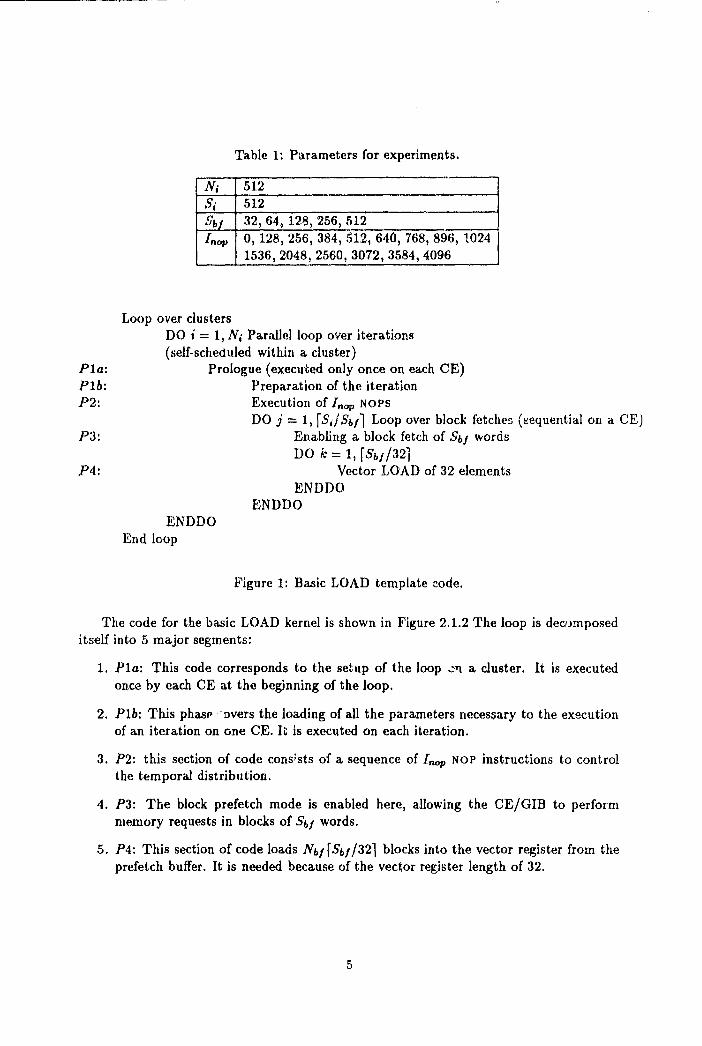
Table 1: Parameters for experiments.

Ni 512Si 512_Sb 32, 64, 128, 256, 5 12I„W 0, 128, 256, 384, 512, 640, 768, 896, 1024

1536, 2048, 2560, 3072, 3584, 4096

Loop over clustersDO i = 1, Ni Parallel loop over iterations(self-scheduled within a cluster)

Pla: Prologue (executed only once on each CE)Plb: Preparation of the iterationP2: Execution of I„oP NOPs

DO j = 1, (S; f Sb f I Loop over block fetches (sequential on a CE)P3: Enabling a block fetch of Sb f words

DO k = 1, [Sb f /32 j

P4: Vector LOAD of 32 elementsENDDO

ENDDOENDDO

End loop

Figure 1: Basic LOAD template cede.

The code for the basic LOAD kernel is shown in Figure 2.1.2 The loop is decomposeditself into 5 major segments:

1. Pla: This code corresponds to the setup of the loop :n a cluster. It is executedonce by each CE at the beginning of the loop.

2. Plb: This phase -overs the loading of all the parameters necessary , to the executionof an iteration on one CE. It is executed on each iteration.

3. P2: this section of code cons ; sts of a sequence of I„, )p NOP instructions to controlthe temporal distribution.

4. P3: The block prefetch mode is enabled here, allowing the CE/GIB to performmemory requests in blocks of Sb f words.

5. P4: This section of code loads Nb f (Sb f /321 blocks into the vector register from theprefetch buffer. It is needed because of the vector register length of 32.

5

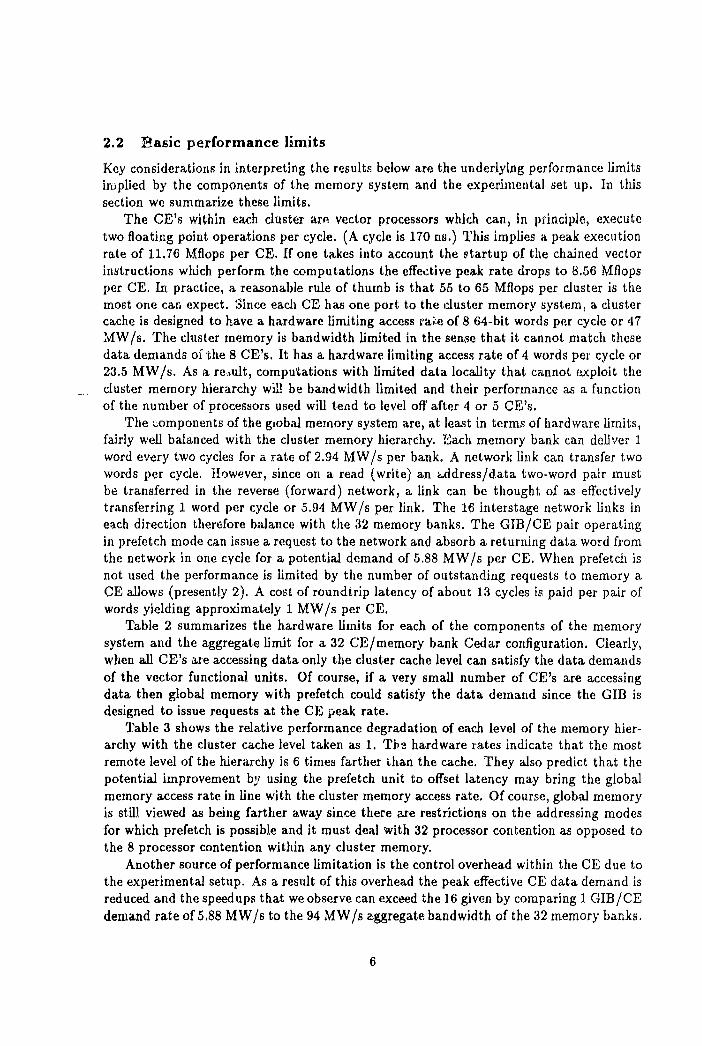
2.2 Rasic performance limits

Key considerations in interpreting the results below are the underlying performance limitsimplied by the components of the memory system and the experimental set up. In thissection we summarize these limits.

The CE's within each cluster ar p. vector processors which can, in principle, executetwo floating point operations per cycle. (A cycle is 170 no.) This implies a peak executionrate of 11.76 Mflops per CE, if one takes into account the startup of the chained vectorinstructions wldch perform the computations the effective peak rate drops to 8.56 Mflopsper CE. In practice, a reasonable rule of thumb is that 55 to 65 Mflops per cluster is themost one can expect. Since each CE has one port to the cluster memory system, a clustercache is designed to have a hardware limiting access care of 8 64 -bit words per cycle or 47MW/s. The cluster memory is bandwidth limited in the sense that it cannot match thesedata demands of the 8 CE's. It has a hardware limiting access rate of 4 words per cycle or23.5 MW/s. As a re:.,ult, computations with limited data locality that cannot exploit the

__. cluster memory hierarchy will be bandwidth limited and their performance as a functionof the number of processors used will tend to level off after 4 or 5 CE's.

The components of the g,obal memory system are, at least in terms of hardware limits,fairly well balanced with the cluster memory hierarchy. 10'ach memory bank can deliver 1word every two cycles for a rate of 2.94 MW/s per bank, A network link can transfer twowords per cycle. However, since on a read (write) an address/data two-word pair mustbe transferred in the reverse (forward) network, a link can be thought, of as effectivelytransferring 1 word per cycle or 5.94 MW/s per link. The 16 interstage network links ineach direction therefore balance with the 32 memory banks. The GIB/CE pair operatingin prefetch mode can issue a request to the network and absorb a returning data word fromthe network in one cycle for a potential demand of 5.88 MW/s per CE. When prefetch isnot used the performance is limited by the number of outstanding requests to memory aCE allows (presently 2). A cost of roundtrip latency of about 13 cycles is paid per pair ofwords yielding approximately 1 MW/s per CE.

Table 2 summarizes the hardware limits for each of the components of the memorysystem and the aggregate limit for a 32 CE/memory bank Cedar configuration. Clearly,when all CE's are accessing data only the cluster cache level can satisfy the data demandsof the vector functional units. Of course, if a very small number of CE's are accessingdata then global memory with prefetch could satisfy the data demand since the GIB isdesigned to issue requests at the CE peak rate.

Table 3 shows the relative performance degradation of each level of the memory hier-archy with the cluster cache level taken as 1. Tbe hardware rates indicate that the mostremote level of the hierarchy is 6 times farther than the cache. They also predict that thepotential improvement by using the prefetch unit to offset latency may bring the globalmemory access rate in line with the cluster memory access rate. Of course, global memoryis still viewed as being farther away since there are restrictions on the addressing; modesfor which prefetch is possible and it must deal with 32 processor contention as opposed tothe 8 processor contention within any cluster memory.

Another source of performance limitation is the control overhead within the CE due tothe experimental setup. As a result of this overhead the peak effective CE data demand isreduced and the speedups that we observe can exceed the 16 given by comparing 1 GIB/CEdemand rate of 5.88 MW/s to the 94 MW/s aggregate bandwidth of the 32 memory banks.

Component Brat rate Aggregate rateCluster cache 7 138

Cluster memory 23.5 94Network link 519 94Memory bank 2,94 94

GIB/CEw/o prefetch ^ 1 32w/ prefetch 5,88 188

Table 2: Hardware limiting access rates in MW/s.

Component SlowdownCluster cache x

Cluster memory 2Global memory

w/ prefetch 2w/o prefetch ;^- G

Table 3: Relative performance degradation of memory hierarchy based on hardware rates.

In our experiments the multicluster control overhead has been reduced to negligible levelsdue to our steady state assumptions. However, the control overhead due to the dynamicscheduling of the iterations within cluster and the looping within a CE represent overheadthat is real in the sense that it is unavoidable any time the memory system is used inpractice. We have kept this as small as possible so that any further overhead incurred ina particular practica situation may be modeled by the Note parameter.

This overhead has been estimated in two ways. The first - a static cycle count ofthe code generated for the experiments - results in a prediction of 3.4 MW/s per CE fora prefetch block of size 32 and 4.7 MW/s per CE for a prefetch block of size 512 whenusing prefetch in global memory. (The prediction assumes a very simple assignment ofiteration blocks to processors.) This yields aggregate CE-induced limits of 108 MW/sand 150 MW/s respectively. These are still over the limiting bandwidths of the globalhardware but are more reasonable peaks to compare agzinst when discussing the balanceof the system. (The cycle counts above apply to the code which can use multiple CE's percluster. When only 1 CE per cluster is used the overhead is slightly lower.)

These limits can also be tested empirically with a simple modification of the templateof Figure 2.1.2. The innermost loop iteration, P4, is altered to operate on register datarather than global memory. This simulates a global memory that does not suffer anybandwidth degradation due to multiple processor accesses. Latency is modeled by issuing• single scalar read from global memory at the beginning of the loop which processes• prefetch block, i.e., after P2. Table 4 shows the empirically determined CE overheadlimits to achievable bandwidths. It is these bandwidths that should be used to determinehow well the global memory is doing when it is not saturated,. The values show that, as

expected, the cyc":^ o5 arit predictions are somewhat optimistic. Note .hat for a prefetchblock of size 32 the bandwidth for 32 CE's is very close to the hardware limit of global.memory.

Tetal CE's Clusters pf=32 pf=.5121 1 3.3 11162 2 6,5 9.23 3 9.8 13.74816

412

13,026.051.0

18,235.070.0

24 3 75,4 105,032 4 90.1 140,0

Table 4; Basic global memory vector read overhead bandwidths in MW/s.

2.3 Results

In this section, we present so,,ne of the results of the basic performance of the memorysystem, We concentrate on the LOAD kernel from the various locations in the memorysystem,

2,3.1 Basic memory perforrance

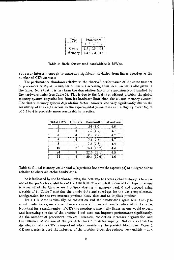
The performance of the cluster memory hierarchy has been characterized in detail andan attendant performance prediction strategy developed elsewhere, (1, 2), and will not berepeated in detail here. As expected, the performance varies considerably for each of theparameters listed above. For comparison purposes, Table 5 contains the basic performanceof a single cluster memory system for a stride 1 access using an iteration block of 512 (asis used for the global memory experiments) and 0 Noes. The cache bandwidths are muchmore sensitive to the variation of the experimental paramct.^rs than the cluster memorybandwidths and therefore the value of 34 MW/s is somewhat optimistic in practice. Ratesin the high 20's are more typical. Note that, not surprisingly, the observed performance issignificantly lower than the cluster hardware limits in Table 2; a factor of 2 for the memoryand between IA and 2 for the cache. The relative degradation of observed performancefor cluster cache to that of cluster memory, roughly 2 - 3, is about the same as the factorof dictated by the hardware limits (see Table 3). The bandwidth limitation of the clustermemory as the number of CE's increases is also apparent from the observed performance.

The most basic way to access global memory on Cedar is in vector mode withoutprefetch. Since the memory system is designed to handle requests issued at a much.higher rate there is no real difficulty with degradation due to network and memory bankcontention. Table 6 contains the performance for various cases of the basic experimentalconfiguration, i.e., iteration block size of 512 and 0 Noes, The speedup relative to a singleprocessor accessing global memory without prefetch is included. Clearly, contention does

8

Type Processors

Cache

1 4 84,5 18 34

Memory 2.3 9.3 12

Table 5; Basic cluster read bandwidths in MW/s,

not occur intensely enough to cause any significant deviation from linear speedup as thenumber of CE's increases.

Tile performance slowdown relative to the observed performance of the same numberof processors in the same number of clusters accessing their local caches is also given iil.the table. Note: that it is less than the degradation factor of approximately 6 implied bythe hardware limits (see Table 3). This is due tcl the fact that without prefetch the globalmemory system degrades less from its hardware limit than the cluster memory system.The cluster memory system degradation factor, however, can vary significantly clue to thesensitivity of the cache access to the experimental parameters and a filightly Iower figureof 3.5 to 4 is probably more reasonable in practice.

Total CE's Clusters Bandwidth Slowdown1 1 '98(1.0) 4.62 2 1,9 (1.9) 4.7

3 3 2.9 (2.9) 4.7

4 4 3,8 (3.'y ) 4.7^8 1 7.7 (7.8) 4.4

16 2 15.4 ( 1 5.7) 4.424 3 22,6 (23,1) 4.5

32 4 29.4 (30.0) 4.6

Table 6 , Global memory vector read w/o prefetch bandwidths (speedups) and degradationsrelative to observed cache bandwidths.

As is indicated by the hardware limits, the best way to access global memory is to makeuse of the prefetch capabilities of the GIB/CE. The simplest moue of this type of accessis when all of the CE's access locations starting in memory bank 0 and proceed usinga stride of 1. Table 7 contains the bandwidths and speedups for the basic experimentalconfiguration for the two extreme prefetch block sizes and an implicit prefetch.

For 1 CE there is virtually no contention and the bandwidths agree with the cyclecount predictions given above. There are several important results indicated in the table,Note that for a small number of CE's the speedup is essentially linear, as one would expect,and increasing the size of the prefetch block used can improve performance significantly.As the number of processors involved increases, contention increases degradation andthe influence of the size of the prefetch block diminishes rapidly. Notice also that thedistribution of the CE's is important when considering the prefetch block size. When 1CE per cluster is used the influence of the prefetch block size reduces very quickly — at 4

9

Total CE's Clusters pf-32 pf;:=5121 1 3,2 (1.0) 4.4 (1.4)2 2 6,3 (1,9) 8.8 (2.8)3 3 9.4 (2,9) 11.0 (3,4)4 4 12.0 (3.8) 13.0 (4,1)8 1 21.5 (6,7) 30.9 (9,7)16 2 37.2 (11.6) 46,2 (14A)24 3 48,3 (15.0) 52.1 (16.3)32 4 54.7 (17,1) 54,4 (17.0)

Table 7: Basic global memory vector rear] bandwidths in MW/s (speedups),

CE's the difference between 32 and 512 is negligible. But, when 8 CE's are used within asingle cluster, the difference in performance between 32 and 51.2 is still significant. Thisis due to the initial shuffle which is present in the network between the CE's and the firststage crossbars, As a result, if we assume that CE 0 is used in each cluster for the 4 CE4 cluster data point all 4 CE's are competing for the 4 output ports of the same crossbar.Therefore, contention dominates over the effect of the prefetch block size. When 8 CE's in1 cluster are used, the CE's are distributed in pairs across all 4 first stage crossbars. Eachpair then has 4 output ports available for use resulting in significantly less contention inthe first stage of the network. It is also clear that contention levels off the performance ofthe memory system once the number of CE's exceeds 16,

Table 8 shows the slowdown of observed global memory bandwidth relative to theobserved cache bandwidth with the same CE/cluster configuration. It is clear that for asmall number of CE's when the network is not a problem the global memory can approachthe rate of the cluster cache, Data in the prefetch buffer on each GIB can be accessedin essentially the same amount of time as a cluster cache, So after paying the roundtrip latency cost for the first element of the prefetch block the rest are accessed at cacherates. (For a. small number of CE's stalls due to elements returning to the prefetch bufferout of order are few.) As the number of CE's contention begins to play a role and theperformance falls between that of cluster cache and cluster memory, For some points itis still significantly better than cluster memory, e.g., 8, 16 and 24 CE's have slowdownsrelative to cache of 1.1, 1.5, and 1.9 respectively. As the number of CE's approach 32 theperformance is only slightly better than cluster memory.

The surprisingly good performance of the global network compared to cluster memorycan be attributed to two facts. First, the global network is more robust in the face ofcontention since it is an O-network as opposed to the bandwidth limited bus used tocommunicate between cluster memory and cluster cache. Second, transactions betweenthe CE and the cluster memory are processed with only 2 outstanding memory requests,.per CE possible. The number of outstanding requests per CE in the global network isdetermined by the prefetch block size and can be as large as 512, The transfer betweenthe prefetch buffer and the CE is done with 2 outstanding requests, but as noted above,the cost of a prefetch buffer access is about the same as a cluster cache access, So untilcontention slows down the rate at which the prefetch buffer is loaded from global memory

10

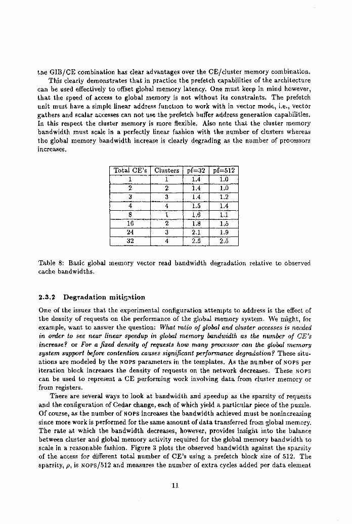
the 0113/CE combination has clear advantages over the CE/cluster memory combination.This clearly demonstrates that in practice the prefetch capabilities of the architecture

can be used effectively to offset global memory latency. One must keep in mind however,that the speed of access to global memory is not without its constraints. The prefetchunit must have a simple linear address function to work with in vector mode, i.e., vectorgathers and scalar accesses can not use the prefetch buffer address generation capabilities.In this respect the cluster memory is more flexible. Also note that the cluster memorybandwidth must scale in a perfectly linear ,fashion with the dumber of clusters whereasthe global memory bandwidth increase is clearly degrading as the number of processorsincreases.

Total CE's Clusters pf=32 pf=5121 1 1.4 1102 2 1.4 1.03 3 1.4 1.24 4 1.5 1.48 1: 1 1 1:.116

2is 15

24 3 2.1 1.932 4 2,5 2,5

Table 8: Basic global memory vector read bandwidth degradation relative to observedcache bandwidths.

2.3.2 Degradation mitigation

One of the issues that the experimental configuration attempts to address is the effect ofthe density of requests on the performance of the global meriory system. We might, forexample, want to answer the question: What ratio of global and cluster accesses is neededin order to see near linear speedup in global memory bandwidth as the number of C .'sincrease? or For a fixed density of requests how many pnx;essor can the global memorysystem support before contention causes significant performance degradation? These situ-ations are modeled by the NODS parameters in the templates. As the number of NOPS periteration block increases the density of requests on the network decreases. These NoPS

can be used to represent a CE performing work involving data from cluster memory orfrom registers.

There are several ways to look at bandwidth and speedup as the sparsity of requestsand the configuration of Cedar change, each of which yield a particular piece of the puzzle.Of course, as the number of NAPS increases the bandwidth achieved must be nonincreasingsince more work is performed for the same amount of data transferred frost global memory.The rate at which the bandwidth decreases, however, provides insight into the balancebetween cluster and global memory activity required for the global memory bandwidth toscale in a reasonable fashion. Figure 3 plots the observed bandwidth against the sparsityof the access for different total number of CE's using a prefetch block size of 512. Thesparsity, p, is Noes/512 and measures the number of extra cycles added per data element

11

fetch .in the block of 612 elements that a CE fetches on a single iteration using variousprefetch block sizes. If p = 0 th(,,J^ there are no added dead cycles, i.e., the access isas dense as possible, As p increases the sparsity of the access increases and the amountof contention is decreased. (Of course, the value of p only reflects the sparsity withinan iteration block. The other cycles due to loop control arid other CE overhead alsocontribute dead cycles to increase sparsity but those are fixed for all of the experiments.)

If contention is not a significant factor the observed bandwidth should be a hyper-bolically decreasing function of p as is seen for p = 1 to p = 8. When contention is aproblem, however, increasing the sparsity may reduce contention and the general shape ofthe! bandwidth curve is decreasing but concave. This is due to the fact that the reductionin contention improves the effective bandwidth more than the additional cluster work,represented by NoPS, decreases the effective bandwidth. The more intense the contentionfor the configurr.,tion the longer the concave region persists along the sparsity axis. Thevariation in concavity is clearly seen by comparing the p = 16, 24, and 32 curves. Theincreasing number of CE's entailQ an increased amount of contention and a larger concaveregion.

Figure 4 presents another view of the effect of sparsity. It plots bandwidth againstCE,'s for various sparsity values p. To answer the first question above one would look forthe value of p beyond which the bandwidth increased nearly linearly. The more linear thecurve the less degradation due to contention. Clearly, as p approaches 2 the curves havean essentially linear profile against the number of CE's. The second question is answeredby noting the number of processors on each curve, P ij, where the bandwidth begins tolevel off thereby degrading the desired near linear behavior. The expected trend of P,,.;rincreasing as p increases is evident in the figure.

As the sparsity of requests increases, the importance of the behavior of global memoryin determining speedup over 1 CE decreases. This is clear, for example, when the NoPSare used to represent the amount of work performed by the CE's that involves only clustermemory and registers. In the limit, for very large values of NoPS the speedup observedfor these templates rhould be equal to the number of CE's in use, p. Figures 5 and 6 plotspeedup over 1 CE as a function of p for a given number of CE's for prefetch block sizesof 32 and 512 respectively, If contention is not significant the curve should be horizontalat the value of p. Deviation from horizontal indicates the magnitude of the degradationdue to contention. The near horizontal behavior of the curves for small p shows that thereis not enough activity to cause serious contention even with very dense global memorytraffic. As p increases, the degradation from horizontal becomes more extreme. Also notethe difference in trends caused by the change in the preft'6ch block size. Prefetching 512elements places more of a strain on the network since there is relatively less sparsity causedby CE overhead. As a result, degradation of performance occurs with fewer CE's thanwhen prefetching 32 elements. Also, the rate at which the curve moves to horj7,ontal for agiver, increase in p is greater when prefetching 512 elements.

The results above address the issue of balance between global and cluster memoryactivity. However, for a given code running a particular problem thin is a fixed ratio. Wenext address the issue of manipulating contention in this case. We will take the worstcase sparsity from above, i.e., p = 0 and attempt to improve performance of the steadystate global memory bandwidth. Of course, we must still access the same locations, butwe do have degrees of freedom concerning what elements each CE will fetch. This canbe controlled via the offset from bank 0 of the initial element accessed by a CE and the

12

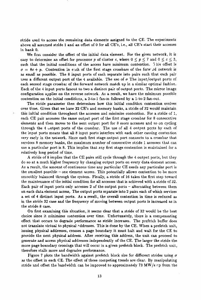
stride used to access the remaining data elements assigned to the CE. The experimentsabove all assumed stride 1 and an offset of 0 for all CE's, i.e,, all CE's start their accessesin bank 0.

We first consider the offset of the initial data element. For the given network, it iseasy to determine an offset for processor p of cluster c, where 0 < p < 7 and 0 < c < 3,such that the initial conditions of the access have minimum contention. 'i his offset isa = 8c + P. Contention in a ich of the first stage crossbars of the forw ,rd network isas small as possible. The 8 input ports of each separate into pairs such that each pairuses a different output port of the 4 available. The use of o The input/output ports ofeach second stage crossbar of the forward network match up in a similar optimal fashion.Each of the 4 input ports fanout to two a distinct pa;r of output ports. The mirror imageconfiguration applies on the reverse network. As a result, we have the minimum possiblecontention on the initial conditions, a 2-to-1 fan-in followed by a 1-to -2 fan-out.

The stride parameter then determines how this initial condition contention evolvesover time. Given that we have 32 CE's and memory banks, a stride of 32 would maintainthis initial condition throughout the accesses and minimize contention. For a stride of 1,each CE pair accesses the same output port of the first stage crossbar for 8 consecutiveelements and then moves to the next output port for 3 more accesses and so on cyclingthrough the 4 output ports of the crossbar. The use of all 4 output ports by each ofthe input ports means that all 8 input ports interfere with each other causing contentionvery early in the nei,work. Since each first stage output port connects to a crossbar thatservices 8 memory banks, the maximum number of consecutive stride 1 accesses that canuse a particular port is 8. This implies that any first stage contention is maintained for arelatively long period of time.

A stride of 8 implies that the CE pairs still cycle through the 4 output ports, but theydo so at a much higher frequency by changing output ports on every data element access.As a result, the amount of continuous time any particular CE needs any particular port isthe smallest possible — one element access. This potentially allows contention to be moresmoothly balanced through the system. Finally, a stride of 16 takes the first step towardthe maintenance of the initial condition for all accesses that is achieved with a stride of 32.Each pair of input ports only accesses 2 of the output ports — alternating between themon each data element access. The output parts separate into 2 pairs each of which servicesa set of 4 distinct input ports. As a result, the overall contention in time is reduced asin the stride 32 case and the frequency of moving between output ports is increased as inthe stride 8 case.

On first examining this situation, it seems clear that a stride of 32 would be the bestchoice since it minimizes contention over time. Unfortunately, there is a compensatingeffect that occurs to degrade performance as stride increases. The prefetch buffer doesnot translate virtual to physical Mdresses. This is done by the CE. When a prefetch unit,issuing physical addresses, crosses a page boundary it must halt and wait for the CE toprovide the next physical address. After receiving this address, the unit can proceed togenerate and access physical addresses independently of the CE. The larger the stride themore page boundary crossings that will occur in a given prefetch block. The prefetch unit,therefore stalls more and degrades performance.

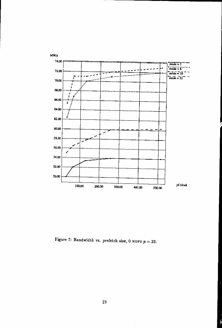
Figure 7 plots the bandwidth against prefetch block size for different strides using aas the offset in each CE. The effect of these competing trends are clear. By manipulatingstride and offset the bandwidth can be improved to approximately 73 MW /s r,p from the

13

55 MW/s seen above for the no offset stride 1 accesses. Note the superiority of the stridesof 8 and 16 which strike a reasonable compromise between contention and page boundarycrossing. The stride 1 access does not improve performance by altering the offset from 0to a. Similar experiments with random offsets have shown a similar lack of sensitivity —or more precisely, they have shown that p and the prefetch block size are the importantparameters for a 0 NOP stride 1 access.

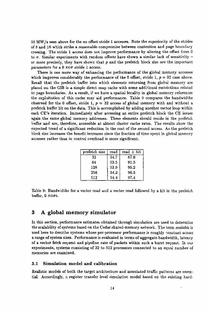
There is one more way of enhancing the performance of the global memory accesseswhich improves considerably the performance of the 0 offset, stride 1, p = 32 case above.Recall that the prefetch buffer into which elements returning from global memory areplaced on the GIB is a simple direct map cache with some additional restrictions relatedto page boundaries. As a result, if we have a spatial locality in global memory referencesthe exploitation of this cache may aid performance. Table 9 compares the bandwidthsobserved for the 0 offset, stride 1, p = 32 access of global memory with and without aprefetch buffer hit on the data. This is accomplished by adding another vector loop withineach CE's iteration. Immediately after accessing an entire prefetch block the CE issuesagain the same global memory addresses. These elements should reside in the prefetchbuffer and are, therefore, accessible at almost cluster cache rates. The results show theexpected trend of a significant reduction in the cost of the second access. As the prefetchblock size increases the benefit increases since the fraction of time spent in global memoryaccesses rather than in control overhead is more significant.

prefetch size read read + hit32 54.7 87.064 53.5 91.5128 53.9 95.2256 54.2 96.5512 54.4 97.4

Table 9: Bandwidths for a vector read and a vector read followed by a hit in the prefetchbuffer, 0 NODS.

3 A global memory simulator

In this section, performance estimates obtained through simulation are used to determinethe scalability of systems based on the Cedar shared-memory network. The term scalable isused here to describe systems whose per-processor performance is roughly ^onstant acrossa range of system sizes. Performance is evaluated in terms of aggregate bandwidth, latencyof a vector fetch request and pipeline rate of packets within such a burst request. In ourexperiments, systems consisting of 32 to 512 processors connected to an equal number ofmemories are examined.

3.1 Simulation model and calibration

Realistic models of both the target architecture and associated traffic patterns are essen-tial. Accordingly, a register transfer level simulation model ba.,ed on the existing hard-

14

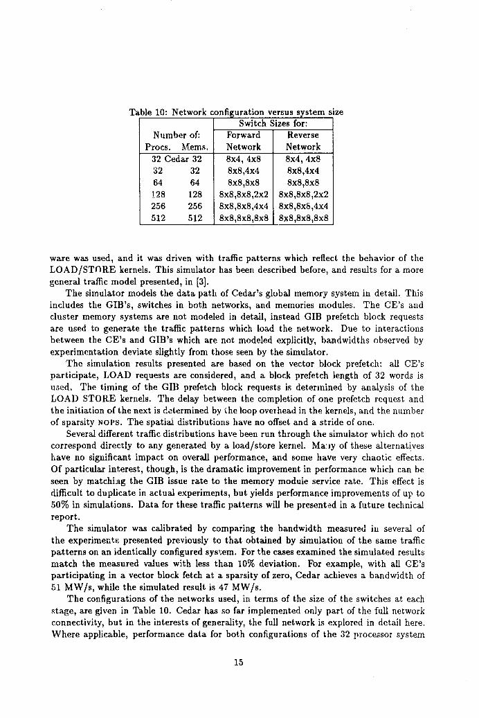
Table 10: Network configuration versus system size

Number of:Switch Sizes for:

Forward ReverseProcs. Mems. Network Network

32 Cedar 32 8x4, 4x8 8x4, 4x832 32 8x8,4x4 8x8,4x464 64 8x8,8x8 8x8,8x8128 128 8x8,8x8,2x2 8x8,8x8,2x2256 256 8x8,8x8,4x4 8x8,8xS,4x4512 512 8x8,8x8,8x8 8x8,8x8,8x8

ware was used, and it was driven with traffic patterns which reflect the behavior of theLOAD/STORE kernels. This simulator has been described before, and results for a moregeneral traffic model presented, in (3].

The simulator models the data path of Cedar's global memory system in detail. Thisincludes the GIB's, switches in both networks, and memories modules. The CE's andcluster memory systems are not modeled in detail, instead GIB prefetch block requestsare used to generate the traffic patterns which load the network. Due to interactionsbetween the CE's and GIB's which are not modeled explicitly, bandwidths observed byexperimentation deviate slightly from those seen by the simulator.

The simulation results presented are based on the vector block prefetch: all CE'sparticipate, LOAD requests are considered, and a block prefetch length of 32 words isused. The tinning of the GIB prefetch block requests is determined by analysis of theLOAD STORE kernels. The delay between the completion of one prefetch request andthe initiation of the next is determined by the loop overhead in the kernels, and the numberof sparsity Noes. The spatial distributions have no offset and a, stride of one.

Several different traffic distributions have been run through the simulator which do notcorrespond directly to any generated by a load/store kernel. Ma:.iy of these alternativeshave no significant impact on overall performance, and some have very chaotic effects.Of particular interest, though, is the dramatic improvement in performance which can beseen by matchiaig the GIB issue rate to the memory module service rate. This effect isdifficult to duplicate in actual experiments, but yields performance improvements of up to50% in simulations. Data for these traffic patterns will be presented in a future technicalreport.

The simulator was calibrated by comparing the bandwidth measured in several ofthe experiment., presented previously to that obtained by simulation of the same trafficpatterns on an identically configured system. For the cases examined the simulated resultsmatch the measured values with less than 10% deviation. For example, with all CE'sparticipating in a vector block fetch at a sparsity of zero, Cedar achieves a bandwidth of51 MW/s, while the simulated result is 47 MW/s.

The configurations of the networks used, in terms of the size of the switches at eachstage, are given in Table 10. Cedar has so far implemented only part of the full networkconnectivity, but in the interests of generality, the full network is explored in detail here.Where applicable, performance data for both configurations of the 32 processor system

15

Table 11: Performance results for sparsity= 0System

SizeBandwidth

(MVO'/s)Block

LatencyInterarrival

TimeCedar 47 25.2 5.4

32 78 15.5 2.864 107 18.3 4.0128 178 24.1 4.8256 305 32.4 5.4512 527 31.7 6.7

are given.

3.2 Metrics

Within the simulations three metrics are used. A3 before, aggregate bandwidth andspeedups are used to evaluate overall. performance. In addition, block latency and mes-sage interarrival time are used to describe the behavior of individual block fetches. Theselatter metrics are determined for each individual message and the arithmetic mean overall elements is then calculated.

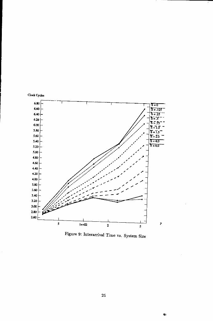
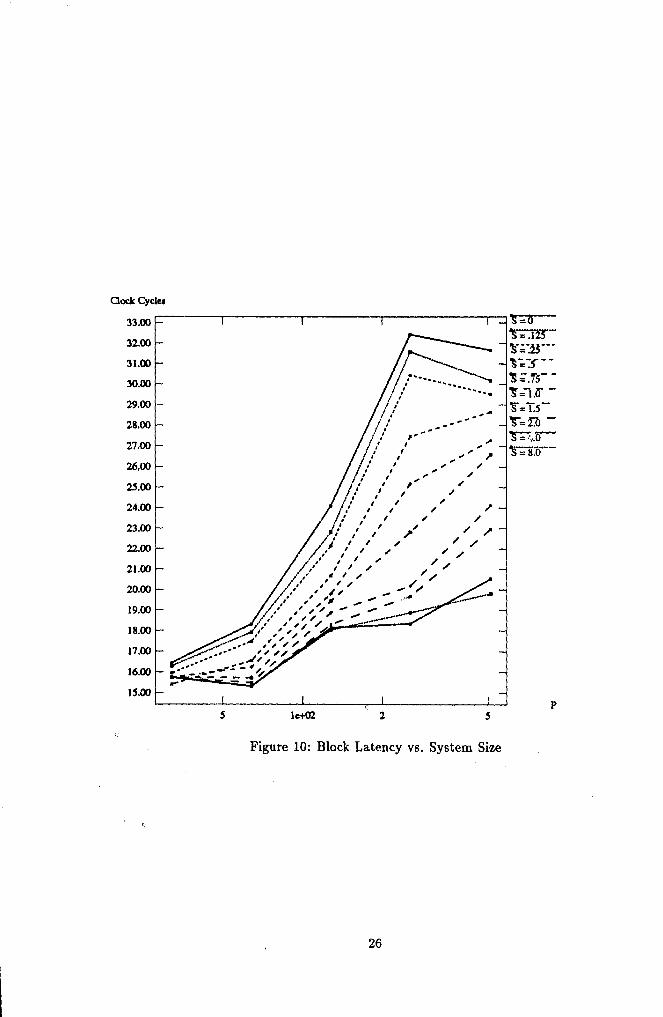
Block latency is defined as the number of clock cycles that elapses between the time aprocessor begins issuing a block fetch and the time that the first message in the block isreceived by the processor. Interarrival time is the delay between the return of successivepackets in a block to the processor that issued them.

3.3 Results

The performance results for various systems performing a vector block prefetch with asparsity of zero are shown in Table 11. In theory, the 32 to 16 fan-in, and 16 to 32 fan-outshould not limit the performance of the network, because the memories can only servicerequests at half the rate at which GIB's generate them. In practice, this can be seen to beuntrue. By doubling the number of connections in the middle of the forward and backwardnetworks, achieved bandwidth increases by over 50%. Only the "full" network case willbe considered further.

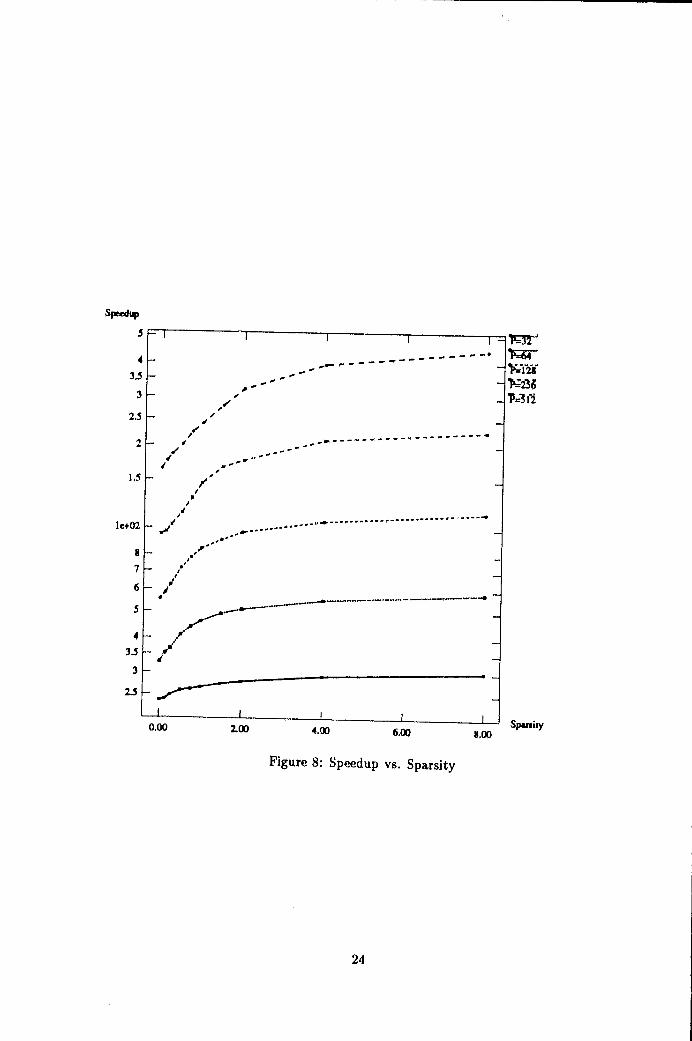
We now consider traffic with more sparsity. In Figure 8, curves are shown whichcorrespond to those shown previously for the Cedar system. Because of the large range ofvalues shown, the y-axis is scaled logarithmically, All the systems achieve a good fractionof the ideal speedup for some value of sparsity, but the larger systems require largeramounts of sparsity (which is in a sense equivalent to locality of reference within a Cedarcluster) in order to offset their increased contention.

In Figures 9 and 10 a similar trend can be seen in the interarrival time and latencyvalues. Here the x-axis shows the size of the system on a logarithmic scale to emphasizethe fact that for low sparsity performance degrades as the log of system size. As sparsity(S) increases, the system scales better: for very moderate sparsity (2-}-), per-processorperformance is almost constant across system sizes. The jump in latency seen as the size

16

increases from 64 to 128 processors is due to the extra network stage needed to constructthe larger systems (see Table 10).

It is important to remember that the number of buffers used in the Cedar networkis quite low, only 3 or 4 words of buffering per stage. In previous experiments (see [3])moderate buffering has been shown to allow much more intense traffic to perform as wellon large systems as on the 32 processor Cedar machine. By increasing buffering to 16words per stage performance scales well for high loads, and the limiting factor becomesthe memory access time, which is four 85ns network cycles for the Cedar system.

References

[1] K. GALLIVAN, D. GANNON, W. JALBY, A. MALONY, AND H. WIJSHOFF, Behavioralcharacterization of multiprocessor memory systems, in Proc. 1989 ACM SIGMETRICSConf. on Measuring and Modeling Computer Systems, New York, 1989, ACM Press,PP . 79-89.

[2] K. GALLIVAN, W. JALBY, A. MALONY, AND H. WIJSHOFF, Performance predictionof loop constructs on multiprocessor hierarchical memory systems, in Proc. 1989 Intl.Conf. Supercomputing, New York, 1989, ACM Press, pp. 433-442.

[3] E. D. GRANSTON, S. W. TURNER, AND A. V. VEIDENBAUM, Design and analysisof a scalable shared-memory system with support for burst tragic, in Proceedings ofthe 2nd Annual Workshop on Shared-memory Multiprocessors, ISCA -90, Kluwer andAssocs., 1991.

[4] J. KONICEK, T. TILTON, ET AL., The organization of the cedar system, in Proc. 1991International Conference on Parallel Processing, Penn State UNiversity Press, 1991.

17

LO

ro30

IR

00Nd0n.

Figure 2: The Cedar interconnection network

18

MW/I

55.0

50.0

45.0

40.01

35.01

30.0(

25,0(

20.0c

15.00

10.00

5.00

0.00

P=P Y...

P -3--a _P= 4

P = 16 --P = 24p _ 32

f41 ^

- -.- ------

sparsityv.w L.W 4.00 6.00 8.00

Figure 3: Implicit prefetch vector read bandwidth vs. sparsity, p f = 512.

19

MW/s

55,00 spar. _

50.00spar =-0.50 =-

YWG=-.75••'•''^

'

// + spar, = 1.0045,00 ' .. .......i:23'

spar. 1.50 — —40.00 I / / i' / spar'= 1.'13T

spar. = 2.00

35.00 i / / ' i 'ipar. = 3.00•/' / / •' / «spar. = 4.00

30.00 _t—L '' spar. =1.00/ spar. = 8.00

25.00 : • / /'

•

20.00 / / ^/ '•

15.00

10.00

5.00

•i'0.00

0.00 5.00 10.00 15.00 20.00 25.00 30.00procs.

Figure 4: Implicit prefetch vector read bandwidth vs. CE's, pf = 512.

20

sp-dup

JzlUU

p 230.00 P-

P 423,00 — --

P = 8

26,00 — P --, 16

P- 24--24.00 — 72 p

22,00 — .... ...... ....... ...... — ------

10.00 —

Igloo

6,00 —

4,00 —

2.00 —

oloo — -

8.00

6.00 — -

4,00— — ------ — ------ ------

2.00 —..................

z1vu 4.00 6.00 8.00......

Figure 5: Speedup vs. sparsity, p = 32.

21

I

i

... -----------

... •------

r;

I'

w ^.. -. w.. -. ...... ------- ._...-------- ...... ^.-•__...

sp-dup

92.0

30.0

28,01

26.01

240

22.0(

20.0(

18.0(

16.0C

14.00

12.00

10.00

8.00

6 ?0

4.00

2.00

P= 2—

pp= 4

p ^ 8—p= 16p 24

p— 32

sparsityv.w ;L.uu 4.00 6.00 8.00

Figure 6: Speedup vs. sparsity, pJ = 512.

22

Mw/I

1,,W

72.00

,70,00

68.00

I /

66.00

64,00

62.00

60.00 ^.

58.00

56,09

54.00

52,00

50.00

1 e7

•suide.- ^

7,itnde ^ 1a ^"

oUide a;-327

pf-block100.00 200.00 300,00 400,00 500.00

Figure 7: Bandwidth vs. prefetch size, 0 NOPS p = 32.

23

Sp-dup

i----- -- --------------i

r

d!f f' ^^.... ...............

.....

r',r ter_,..._-,»......,_,.,^._...... .. .».......,_..».._. ..._..^

^r1

v.w 2UO 4.00 6.00 8100

Figure 8: Speedup vs, Sparsity

4

3,3

3

2.5

2

1.5

Ie+02

B

7

6

5

4

3.5

3

2.5

X12!p=23b

Spaniry

24

aock Cycles

6,8O ._-_-

6.60_'F-'

j' -6.406.2U-'^--

• Is T5- -6,0o

•'^

s _5,80

5.60 3'" 2 b _

5.40 "o IS 4.0 -5.205.00 i

4.80 ,• ' ri^,'4.60 ^f' .• ^' ^' i

4.40 / ,•• r4.20 lop'.

•ol

4.003.80 ! .'^+ r ^ i3.603.40

3.20 %^' + r •^ ^ ^^^"3.002.802.60

5 1e402 2 5P

Figure 9: Interarrival Time vs. System Size

25

-J' -r:

i

i .0

ri

s ^ ^

970—

= .T5" -^=1s

Clock Cycla

33.00

32.00

31.00

30.00

29.00

28.00

27.00

26.00

25.00

24.00

23.00

22.00

21.00

20.00

19.00

18.00

17.00

16.00

15.00

1e+02

Figure 10: Block Latency vs. System Size

26