1

Introduction

Dynamic changes resulting from a variety of causes (e.g. structural damage or

nonlinearity onset) may disturb or threaten the normal working conditions of a system. The

capacity to estimate the mechanical health condition of a structure using remote non-

destructive techniques constitutes a substantial plan which allows to reduce maintenance costs

and to ensure safety. Hence, questions such as the detection of those events have attracted the

attention of countless researchers in recent times.

A well-known classification for damage detection, presented in Rytter (1993)[109],

defines four levels in increasing order of complexity:

- Level 1: Damage detection: inspection of the presence of damage in the structure

- Level 2: Damage localization: determination of geometrical location of the damage

- Level 3: Assessment of the severity of the damage

- Level 4: Prediction of the remaining lifetime of the structure

Damage detection can be implemented by visual inspection or by using localized methods

such as acoustic and ultrasonic techniques, magnet field methods, radiography, penetrant

liquids, eddy-current methods and thermal field methods. However, such methods require the

accessibility of the zone where damage is located.

“Smart structure” is a popular expression in modern engineering that relates to vibration

monitoring. It consists in a structure instrumented by sensors measuring vibration responses

of the structures in real time, for the purpose of structural health monitoring (SHM).

Nowadays, this kind of approach is widely used because vibration monitoring systems is well

developed. Efficient and reliable vibration analysis tools allow to detect the occurrence of

damage, to assess its severity and to predict the residual life of the structure. By acting before

the apparition of a serious fault, the cost of maintenance and reparation may be considerably

reduced and at the same time, the security may be improved. Vibration analysis is based on

the assumption that the dynamical behavior of a structure, observed by measured responses,

relates directly to system features as stiffness, mass and damping distribution. A fault in a

dynamic system may be shown by changes in the dynamic properties of the structure, namely

the eigenfrequencies, the mode shapes/deformation shapes, the modal damping ratios and/or

the transfer functions. So, identification of those quantities is also of primary importance for

the diagnosis problem.

Nowadays identification methods of linear systems are rather powerful, but they are based

on stationarity and linearity assumptions, which is not always the case in real-life

applications. For example, nonlinearity may be induced by environmental factors such as

temperature, humidity, wind or comes from physical factors related to geometric effects or to

material behavior, etc. Furthermore, as reported in Farrar et al. (2007)[25], there are many

types of damage that make an initially linear structural system respond in a nonlinear manner.

For example, cracks subsequently open and close under operational condition. Other common

2

damages that produce nonlinear system responses come from loose connections, delamination

in bonded, layered materials under dynamic loading or material nonlinearities. The new

response characteristics induced by the nonlinearity can be considered as indicators of

damage. However, accurate determination of these quantities should be assured so that they

can be utilized for indicators of damage. And so, the detection problem necessitates methods

that are able to study nonlinear systems.

The objective of this thesis is to identify changes in the dynamical behaviour of a

mechanical system through the development of identification, detection and model updating

techniques. Damage or nonlinearity onset is considered responsible for the changes.

According to the classification of damage identification presented above, the diagnosis

problem in the present work is addressed for the first three levels, i.e. detection, localization

and assessment. The identification of damages and nonlinearity onset is always based on the

comparison between a current and the reference (normal) states.

The layout of the dissertation is as follows:

Chapter 1 presents a literature review on modal identification and detection methods. This

part describes some main features of nonlinear systems and also the challenges that the

nonlinearity presents. Localization and evaluation problems are next discussed separately.

Chapters 2, 3 and 4 focus on the detection of fault, namely nonlinearity onset or damage

occurrence by three methods respectively: the Wavelet Transform (WT), the Second Order

Blind Identification (SOBI) method and the Kernel Principal Component Analysis (KPCA)

method. Output-only measurements are used for signal processing. The first two methods

achieve health monitoring through a process of modal identification while the last method

works directly in the characteristic spaces determined by a chosen kernel function. The

detection can be performed by means of the concept of subspace angle or be based on

statistics.

The robustness of the methods is illustrated on a clamped beam structure with a

geometrical nonlinearity at the end; this benchmark was studied in the framework of the

European COST Action F3. Other examples are considered such as an aircraft mock-up with

different levels of damage and two industrial applications with the aim of performing quality

control on a set of electro-mechanical devices and on welded joints.

Chapter 5 aims at damage localization based on sensitivity analysis of Principal

Component Analysis (PCA) results in the frequency domain. The localization is performed

through comparison of the principal component sensitivities between the reference (healthy)

and the damaged states. Only measured responses, e.g. frequency response functions (FRFs)

are needed for this purpose.

Following the sensitivity analysis in Chapter 5, Chapter 6 addresses the evaluation of

parameters, namely assessment of damages. For this purpose, a model updating procedure is

performed. This procedure requires to build an analytical model of the structure.

The sensitivity analysis for damage detection is illustrated by both numerical and

experimental data in mass-spring systems and in beam structures. A real-life structure i.e. the

I-40 bridge in New Mexico that was destroyed in 1993 is also examined.

Finally, conclusions are withdrawn based on the realized work and some perspectives are

given for the continuation of this research.

3

Chapter 1

Literature review

1.1 Introduction

The detection problem is often achieved by comparing dynamic properties of a system

between its initial state and a current state. The dynamic properties, namely the natural

frequencies, the mode shapes and the damping ratios, can be determined by modal

identification methods so that modal identification can be seen as an important tool for the

purpose of detection. This chapter gives a brief overview on common methods used for modal

identification, detection, localization and parameter evaluation, respectively.

As noted previously, nonlinear features give rise to many challenges when inspecting

mechanical systems owing to the main following reasons:

o The superposition principle that forms the basis of modal analysis in linear

systems is no longer valid. The resolution of nonlinear equations requires more

advanced mathematical techniques.

o The Maxwell‟s reciprocity theorem is not verified for a nonlinear system.

o The nonlinearity can originate from different sources: nonlinear material behavior,

frictional contact, geometrical nonlinearity, energy loss mechanism, open-close

crack ...

o In nonlinear dynamics, the responses are much more complex and sometimes, may

not be forecasted. Even with a deterministic input, the output dynamics can

become rich or even chaotic. In a system with nonlinear stiffness, resonant

frequencies do not keep constant but show time varying features. Other

phenomena that are not observed in linear systems may also occur, namely:

bifurcations, harmonics, limit cycles, modal interactions (internal resonances, inter

modulation)… The presence of the above phenomena depends on the type of

excitation, as well as on the initial conditions. So, the number of nonlinear normal

modes (NNMs) may be greater than the number of degrees of freedom of the

system. NNMs can be stable or unstable.

Such nonlinear behaviors render inadequate identification and detection methods, as well

as updating techniques developed for linear models. Since there is not a single method to

model and identify all types of nonlinearities, the elaboration of a nonlinear identification and

damage detection toolbox raises a lot of challenges.

In the following, linear systems are first studied. Then nonlinear systems are considered

with the aim of detecting the onset of nonlinearity in the dynamic behaviour.

4

1.2 Modal identification methods

To evaluate modal parameters of a structure, two paths can be followed: a theoretical

approach and an experimental approach as presented in Figure 1.1. Because a mathematical

model of an existing structure is not always available, the experimental modal analysis

approach is particularly interesting. It is based on the exploitation of system responses and

requires identification techniques to extract modal parameters.

Figure 1.1: Classification of modal analysis methods

Modal identification methods may be classified into two categories depending on whether

they are carried out in the frequency domain (e.g. using frequency response functions - FRFs)

or in the time domain (e.g. using time signals). Several well established techniques are

reported in the literature e.g. Maia et al. (1997)[75]. As the goal of this work is not to describe

all the methods in details, we have limited the presentation to some typical time-domain

methods proposed in the last decade and that are the most relevant for our work.

Stochastic Subspace Identification - SSI

The main advantage of the SSI method is that it does not need the measurement of the

excitation as long as it can be assumed as a combination of uncorrelated random signals. The

discretized state-space model at sampling step k can be written as:

rk+1 = A rk + wk (1.1)

5

yk = B rk + vk (1.2)

where matrices A and B are the state space and output matrices, respectively.

rkm represents the state vector and yk

m the time series. wk and vk represent the process

and measurement noises, respectively. Those last vectors are assumed to be zero-mean white

Gaussian noise processes.

Based on the definition of the block Hankel matrix, either in the covariance-driven form

or in the data-driven form, the SSI method aims at determining the state space and output

matrices A and B. Then the modal features may be deduced in a straightforward manner from

those matrices.

For linear systems, SSI has proven to be efficient for modal identification and damage

detection (Peeters and De Roeck (2001)[98], Yan et al. (2004)[132]). The method has also

been used by several authors for other purposes. For example, to handle a multi-patch

measurements setup with uncontrolled and non-stationary excitation, the covariance

normalization is proposed in Mevel et al. (2002)[81] in order to neglect the influence of

excitation. For the identification of nonlinear vibrating structures, the perspective of

nonlinearities is adopted as internal feedback forces in Marchesiello and Garibaldi (2008)[78].

Blind Source Separation – BSS

The multidimensional observations can be represented in the following form:

)()()()()( ttttt σAsσyx (1.3)

where x(t) is considered as an instantaneous linear mixture of source signals and noise.

T

1( ) ( ),..., ( )mt s t s ts contains the signals issued from m sources of narrow frequency

range.

T

1( ) ( ),..., ( )mt y t y ty contains the assembly of sources at a time t.

A is the transfer matrix or the mixing matrix between sensors.

)(tσ represents the noise vector.

Blind source separation consists in retrieving the source signals s(t) from their observed

mixtures x(t). BSS attempts to separate a set of signals, without the knowledge (or with very

little information) about the source signals or the mixing process. In most cases, vectors found

in the mixing matrix A can describe vibration modes of the system and the sources in s(t)

allows determining natural frequencies and damping.

Among the methods in the BSS family, one can cite for example Principal Component

Analysis (PCA) or Proper Orthogonal Decomposition (POD), Smooth Orthogonal

Decomposition (SOD), Independent Component Analysis (ICA) and Second-Order Blind

Identification (SOBI). All of them have been exploited in many engineering applications

owing to their versatility and their simplicity of practical use. Each method presents some

advantages and drawbacks. For instance, natural frequencies can be estimated through the

investigation of smooth orthogonal coordinates (in SOD) and sources (in ICA and SOBI).

PCA involves a knowledge of the system‟s mass matrix for modal identification while SOD is

able to overcome this drawback (Chelidze and Zhou (2006)[13]). In the PCA and SOD

methods, the modes are orthogonal while in the ICA method, they are linearly independent.

PCA may show some limitations when the data is not Gaussian or multi-modal Gaussian,

6

because in those cases, PCA simply gives uncorrelated variables which are not guaranteed

statically independent. On the contrary, ICA consists in separating non-Gaussian source

signals that are mutually statistically independent. The ICA method requires that at most one

of the sources is Gaussian. Regarding to the SOBI method, the statistical independence is not

required, but some degree of unrelatedness among the sources is required for source

separation (Tang et al. (2005)[120]). SOBI considers the temporal relationship between

components at multiple time delays by second-order statistics and makes it still possible to

separate temporally correlated sources (Belouchrani et al. (1993)[8], (1997)[9]). Hazra and

Narasimhan (2009)[39] remarked that SOBI-based methods show significant improvement

over ICA methods in systems with high levels of damping because SOBI utilizes the inherent

time structures of the sources.

The two families of methods cited above are based on the assumption of stationarity of the

signals and lead to the identification of a unique set of „modal‟ features. Time-frequency

decompositions are helpful to capture transient dynamic features that appear during operation.

Non-stationary signals can be more adequately inspected by time-frequency analysis using for

instance Short-Time Fourier Transform (STFT), Wigner-Ville distribution, Wavelet

Transform (WT), Hilbert-Huang Tranform (HHT)… For the sake of conciseness, we will

focus on the last two methods, which allow extracting instantaneous features and have

interested countless of researchers in recent time.

Wavelet Transform - WT

A wavelet is a wave-like oscillation that is very useful for signal processing. Through the

convolution operation on portions of an unknown signal, wavelets allow us to get information

about the signal. Such process where the wavelets are scaled and translated is called the

Wavelet transform. The WT shows advantages over the Fourier transform (FT) and the short-

term Fourier transform (STFT) for analyzing signals that have discontinuities and sharp peaks

and/or for analyzing non-periodic and non-stationary signals. The FT is localized in frequency

and is unable to describe time-shifting frequency components. The STFT allows localization

in both time and frequency but induces a frequency-time resolution trade-off (Mallat

(1999)[76]) because the signal is observed by a window of constant size. Restrictions of the

FT and STFT can be overcome by the WT thanks to the balanced resolution at any time and

frequency with scaled and translated windows.

The WT in its discrete or continuous form has been used in many applications in various

domains. The wavelet family comprises a lot of analyzing functions. Using Morlet wavelet,

Kijewski and Kareem (2003)[56] dealt with system identification in civil engineering and

Staszewski (1998)[118] with identification of systems with cubic stiffness nonlinearity.

Argoul, Le and Erlicher [2, 68 and 21] used the continuous Cauchy wavelet transform as a

tool for modal identification in linear and nonlinear systems. By combining with the

capabilities of the bootstrap distribution in statistical estimation, the WT was used to consider

the uncertainty effect on modal parameters of output-only system in Yan et al. (2006)[138]. In

Lilien et al. (2006) [70], the WT was used to filter noisy data and then to identify frequency

contents for the purpose of real time monitoring of electric line ampacity. Recently, Hazra and

Narasimhan (2009)[39] proposed to use the WT for pre-processing in a SOBI-based

technique. The technique was illustrated with civil structures under wind and earthquake

excitations.

7

The use of the WT to detect nonlinearity onset in a dynamical system is described in

details in Chapter 2.

Hilbert-Huang Transform - HHT

The Hilbert-Huang Transform is basically an Empirical Mode Decomposition (EMD)

technique. Huang et al. (1998)[44] proposed the EMD for decomposing a measured response

x(t) in m intrinsic mode functions (IMFs).

1

( ) ( ) ( )m

i m

i

x t c t r t

(1.4)

in which ( )ic t (i = 1, 2, …, m) are IMFs of x(t) and ( )mr t is a residue that can be the mean

trend of the signal or a constant.

An IMF is a mono-component which admits well-behaved Hilbert transforms. The EMD

is applicable to nonstationary signals. The method achieves a sifting procedure consisting in

subtracting the signal from the average of the upper and lower envelopes of the signal until

the resulting signal becomes mono-component (IMF). The original signal is then subtracted

from the IMF and the sifting procedure is repeated to the remaining signal to acquire another

IMF. The IMFs c1, c2, …, cm are frequency components arranged in decreasing order.

In the EMD, the envelopes are constructed by spline-fitting technique and the method is

intuitive. Problems of smoothing can appear at the extremities of the signal, which requires

several techniques to smooth the edges.

Let us consider a general signal noted x(t). The Hilbert transform of x(t) allows to

determine a single set of value for amplitude, phase and frequency at any time t. For a

meaningful composition of a signal in the frequency-time domain, Huang et al. (1998)[44]

proposed to process the Hilbert transform to each IMF in order to obtain different frequency

components at any time t. So we can acquire m spectral components from m IMFs resulting

from the EMD procedure. The determination of damping ratios was described in [44]. Mode

shapes can be deducted from the HHT achievement in the ensemble of DOFs of the system.

However, it is important to mention the following particularities of the method:

- each IMF contains intrinsic characteristics of the signal x(t);

- neighbouring components may contain oscillations of the same frequency, but they

never occur at the same time in two different IMF components. An IMF has not the

same frequency as the previous IMF at the same moment t;

- the HHT is applicable for non-stationary signals and for nonlinear dynamic

behaviours;

- if one considers a linear combination of two sinusoidal oscillations of close

frequencies, the EMD method can extract the two components and their instantaneous

frequencies overlap. The key problem of the HHT is the use of splines as it seems to

be the main factor of limitation of the method;

- problems of smoothing at signal extremities produce unexpected large oscillations.

This boundary effect is due to the spline smoothing and to the Hilbert transform.

The HHT has been used successfully in the last decade for the analysis of non-stationary

and/or nonlinear signals. The method has been recently improved by countless researchers so

that its application becomes more friendly and accurate. For example, Flandrin et al.

8

(2005)[28] used added noise to overcome one of the difficulties of the original EMD method.

Wu and Huang (2009)[131] proposed a new Ensemble Empirical Mode Decomposition that

sifts an ensemble of white noise-added signal and treats the mean as the final true result.

Huang et al. (2009)[45] proposed two new methods to overcome the difficulties of computing

instantaneous frequency: the direct quadrature and the normalized Hilbert transform.

Nowadays, as mentioned previously, identification of nonlinear systems presents many

challenges with respect to linear systems. There is a big interest in the identification of

nonlinear structures both in the frequency and time domains. The NARMAX (Nonlinear Auto

Regressive Moving Average with eXogenous outputs) model is an example; it was fitted

using modal coordinates in Thouverez and Jezequel (1996)[122] to identify nonlinear

systems. Adams and Allemang (2000)[1] proposed a method in the frequency domain called

Nonlinear Identification through Feedback of the Output. Artificial neural networks have

received lot of attention in identifying nonlinear systems (Le Riche et al. (2001)[66], Pei et al.

(2004)[100]). In the period of 1997-2001, in the framework of the European Cooperation in

the field of Scientific and Technical Research - COST Action F3 Structural Dynamics, the

identification of nonlinear systems was addressed by a specific working group (Golinval et al.

(2003)[34]). Two main benchmarks were studied using different methods: for example, the

condition reserve path method in the frequency domain, the restoring force surface method in

the time domain, some modal methods based on the definition of nonlinear normal modes

(NNMs), the proper orthogonal decomposition (POD), the wavelet transform (WT) and model

updating techniques. More recently, Arquier et al. (2006)[3] presented the time integration

periodic orbit method and the modal representation method for undamped nonlinear

mechanical systems. Marchesiello and Garibaldi (2008)[78] identified nonlinear vibrating

structures by subspace methods. Peeters et al. (2009)[99] developed a technique for

determining the NNMs of nonlinear mechanical systems based on a shooting procedure and a

method for the continuation of NNM motions. They also proposed a phase resonance

appropriation technique to identify NNMs experimentally. Da Silva et al. (2010)[15]

proposed a method to identify localized nonlinear parameters based on the identification of

Wiener kernels through model updating. Rainieri and Fabbrocino (2010)[105] discussed the

identification from non-stationary signals by comparing the results of the automated output-

only modal identification algorithm LEONIDA and some other methods. Their applications

are achieved through data recorded in operational conditions and during ground motions

induced by the recent L‟Aquila earthquake.

All these methods of identification provide us better comprehension of mechanical

systems. Furthermore, they can provide useful tools for detection problem, as presented in the

next section.

1.3 Methods of detection

Detection of changes in the dynamic state of structures is an important issue in the field of

Structural Health Monitoring (SHM). It may be caused by the occurrence of damage but also

by the onset of a nonlinear behaviour.

Detection methods that use mathematical models include parametric and non-parametric

techniques. Parametric methods require the construction of a structural model and are based

on model updating techniques (Friswell et al. (2001)[31], Titurus et al. (2003)[124, 125]). A

precise model is of primary importance in this case; it offers the advantage to allow damage

location and possibly remaining lifetime calculation but it generally needs a lot of modelling

and computation time. Non-parametric methods do not require a structural model. Based on

9

vibration measurements only, those methods attempt to extract features, which are sensitive to

changes in the current dynamic state of the monitored structure. They may be based on the

direct use of modal parameters (eigenfrequencies and mode shapes), or stiffness and

flexibility matrices. There exists a large amount of damage detection methods using

eigenfrequency changes (Messina et al. (1998)[82], Yang et al. (2004)[140]). The techniques

using only eigenfrequencies are simple; however it is necessary to distinguish damage from

the influence of environmental and operational conditions (Yan et al. (2005)[134, 135],

Deraemaeker et al. (2008)[19]). The main drawbacks of those techniques are that sometimes

unrealistic damage patterns are found, and the number of measured eigenfrequencies is

generally lower than the number of unknown model parameters, resulting in a non-unique

solution (Maeck (2003)[74]). Alternatively, the monitoring of mode-shape changes is a useful

approach for detection. A common measure used to evaluate the correlation between two

families of modes {A} and {B}

is the Modal Assurance Criterion - MAC:

T 2

MAC ,

A B

i jA B

i j A B

i j

(1.5)

where A

i , B

j denote modes i and j of two different states A and B respectively (e.g. normal

and faulty states). The MAC value between two modes can vary from 0 to 1; the value of 0

means no correlation and 1 means perfect correlation. The deviation from unity can reflect a

faulty state.

Damage detection can also be based on the dynamically measured flexibility matrix,

which is just the inverse of the stiffness matrix. The measured flexibility matrix F is estimated

from the mass-normalized mode shapes and frequencies as:

1

21

1m

i i

i i

F ΦΩ Φ

(1.6)

where the mode-shape vectors have been mass-normalized such that T Φ MΦ I ,

2diag iΩ (i = 1,…, m) is the spectral matrix containing the m eigen-frequencies. In Yan

and Golinval (2005)[133], the flexibility matrix was assembled from mode shapes identified

by the stochastic subspace method (SSI), which permits to deduce the corresponding stiffness

matrix by a pseudo-inversion. Koo et al. (2009)[61] proposed a damage detection method

based on the damage-induced chord-wise deflections which were estimated using the modal

flexibility matrices.

Furthermore, several other methods exist. They perform the detection based on the

ensemble of extracted modal features, e.g. a subspace built by mode shapes. Other indexes are

used to indicate detection. For example, some damage detection techniques are based on

principal component analysis (PCA) of vibration measurements (De Boe and Golinval

(2003)[16], Yan et al. (2005)[134]) where damage indexes are based on the concept of

subspace angle and/or on statistics using the Novelty Index analysis. In Zang et al.

(2004)[141], independent component analysis (ICA) was combined with neural networks for

structural damage detection. Without modal identification, null subspace analysis (NSA)

based on the definition of Hankel matrices (Yan and Golinval (2006)[137]) allows detecting

damages efficiently. Several other BSS methods are attractive for fault detection, namely: the

mean field independent component analysis (Pontoppidan et al. (2005)[102]); the fourth-order

cumulant-based decorrelation method (Jianping and Guang (2009)[49]).

10

PCA is known as an efficient method to compress a set of random variables and to extract

the most important features of a dynamical system. However, this method is based on the

assumption of linearity. To some extent, many systems show a certain degree of nonlinearity

and/or non-stationarity, and PCA may then overlook useful information on the nonlinear

behavior of the system. Therefore, detection problem may necessitate methods which are able

to study nonlinear systems.

Efforts have been made to develop nonlinear damage detection methods based on PCA.

For example, the nonlinear PCA method proposed in Kramer (1999)[62], Sohn et al.

(2001)[117] used artificial neural network training procedures which are able to generate

nonlinear features. In Reference Yan et al. (2005)[135], local PCA is used to perform

piecewise linearization in the cluster of nonlinear data in order to split it into several regions,

and then to carry out PCA in each sub-region.

Alternatively, Kernel Principal Component Analysis (KPCA) is a nonlinear extension of

PCA built to authorize features such that the relation between variables is nonlinear. Lee et al.

(2004)[69] used KPCA to detect fault in the biological wastewater treatment process by

means of statistics charts. Sun et al. (2007)[119] achieved fault diagnosis in a large-scale

rotating machine through classification techniques. Widodo and Yang (2007)[130] extracted

nonlinear feature in support vector machines (SVM) to classify the faults of induction motor.

He et al. (2007)[40] monitored gearbox conditions by extracting the nonlinear features with

low computational complexity based on subspace methods. Cui et al. (2008)[14] reduced the

computational complexity of KPCA in the fault detection by a feature vector selection

scheme. At the same time, they improved the KPCA detection by adopting a KPCA plus

Fisher discriminant analysis. Chang and Sohn (2009)[12] detected damage in the presence of

environment and operational variations by basing on unsupervised support vector machines.

Ge et al. (2009)[32] improved the KPCA monitoring in nonlinear processes when the

Gaussian assumption is violated by proposing a new joint local approach-KPCA.

On the other hand, time-frequency decompositions prove to be effective for studying

systems in which responses are non-stationary or/and nonlinear. The Hilbert-Huang transform

(HHT) has been exploited to evaluate damage in Yang et al. (2002)[139] and to determine the

time of occurrence of damage in Yang et al. (2004)[140]. The detection and identification of

nonlinearities were performed on the basis of HHT and perturbation analysis by Pai and

Palazotto (2008)[95]. One of the main drawbacks of the HHT method relies in its empirical

formulation. Conversely, the theoretical basis of the Wavelet Transform (WT) makes it more

appropriate for non-stationary data analysis. Gurley and Kareem (1999)[37] used both the

continuous and discrete WT for identification and characterization of transient random

processes involving earthquakes, wind and ocean engineering. Messina (2004)[83] discussed

and compared the continuous WT with differentiator filters for detecting damage in

transversally vibrating beam. Yan and Gao (2005)[136] proposed an approach based on the

Discrete Harmonic Wavelet packet transform to machine health diagnosis. The WT was also

combined with auto-associative neural network in Sanz et al. (2007)[114] for monitoring the

condition of rotating machinery; with outlier analysis in Rizzo et al. (2007)[108] for structural

damage detection. In Argoul and Le (2003)[2], four WT instantaneous indicators are proposed

to facilitate the characterization of the nonlinear behaviour of a structure.

To detect the onset of nonlinearity, other nonlinear indicator functions can be used as

reported in Farrar et al. (2007)[25]. Basic signal statistics are commonly adopted; they are

cited in Table 1.1. In He et al. (2007)[40], statistics in time and frequency domains were

exploited for detecting nonlinear damage; these statistics allow to avoid the use of raw time

series data. Nonlinearity can also be observed by checking linearity and reciprocity.

11

Nonlinearity onset was detected by comparing the FRF and coherence functions or PCA

subspaces (Thouverez (2002)[123], Kerschen (2003)[52], Hot et al. (2010)[41]). Harmonic or

waveform distortion is also one of the clearest indicators of the nonlinearity onset (Qiao and

Cao (2008)[104], Nguyen et al., (2010)[87], Da Silva et al. (2010)[15]). Furthermore,

NARMAX model represents an efficient tool in analysing nonlinear responses [72, 129]. Liu

et al. (2001) [72] proposed a tool for interpreting and analysing nonlinear system with

significant nonlinear effects, then it was applied for fault detection in the civil engineering

domain. Wei et al. (2005)[129] assessed internal delamination in multi-layer composite plates

by basing on the NARMAX model.

Table 1.1: Basic signal statistics

Mean ( x ) Peak

amplitude (xp)

Root mean square

(RMS)

Square root value

(R)

Standard deviation

( )

1

1 N

i

i

x xN

p max ix x 2

1

1RMS

N

i

i

xN

2

1

1R

N

i

i

xN

2

1

1 N

i

i

x xN

Crest factor

(C)

Shape factor

(S)

Kurtosis ( ) Skewness (Sk)

C= xp/RMS S= RMS/ x

4

1

4

1 N

i

i

x xN

3

1

3

1 N

i

ik

x xN

S

1.4 Methods for localization and evaluation

The methods cited above provide effective tools to detect the presence of faults.

Furthermore, the problem of damage localization and assessment has been approached from

many directions in the last decade. Often based on the monitoring of modal features, these

processes can be achieved by using an analytical model and/or promptly by measurements.

The methods may be used for one or both purposes: localization/ assessment.

Damage can cause change in structural parameters, involving the mass, damping and

stiffness matrices of the structure. Thus many methods deal directly with these system

matrices. The Finite Element Method is an efficient tool in this process (Huynh et al.

(2005)[46], Michels et al. (2008)[85]). The problem of detection and localization may be

resolved by this method through model updating or sensitivity analysis (Pascual (1999)[97]).

For damage localization and evaluation, model updating is utilized to reconstruct the stiffness

perturbation matrix (Koh and Ray (2003)[59]); to handle changes in the system matrices of

nonlinear systems (D‟Souza and Epureanu (2008)[20]). This may be combined with a genetic

algorithm (Gomes and Silva (2008)[36]) or based on modal parameter sensitivity (Bakir et al.

(2007)[4]). In model updating, an optimization procedure is established in order to minimize

the differences between experimental and numerical modal data by adjusting uncertain model

parameters (Maia et al. (1997)[75]).

Among sensitivity analyses, natural frequency sensitivity has been used considerably in

localization problem. Messina et al. (1998)[82] estimated the size of defects in a structure

12

based on the sensitivity of frequencies with respect to damage locations where all the

structural elements were considered as potentially damaged sites. Ray and Tian (1999)[106]

discussed sensitivity of natural frequencies with respect to the location of local damage. In

that study, damage localization involved the considering of mode shape change. Teughels and

De Roeck (2004)[121] identified damage in a highway bridge by updating both Young‟s

modulus and shear modulus using an iterative sensitivity based finite element model updating

method. Other authors (Koh and Ray (2004)[60], Jiang (2007)[47]) have located damage by

measuring natural frequency changes before and after the occurrence of damage. However,

such methods require a well fitted numerical model to compare with the actual system. Jiang

and Wang (2009)[48] removed that requirement by utilizing a mathematical model identified

from experimental measurement data, where a closed-loop control is designed to enhance the

frequency sensitivity for the sake of structural damage localization and assessment.

Methods based on measurements are also widely used because of their availability in

practice. Yang et al. (2002)[139] estimated damage severity by computing the current

stiffness of each element. They used Hilbert-Huang spectral analysis based only on

acceleration measurements using a known mass matrix assumption. Yan and Golinval

(2005)[133] achieved damage localization by analyzing flexibility and stiffness without

system matrices, using time data measurements. Koo et al. (2009)[61] detected and localized

low-level damage in beam-like structures using deflections obtained by modal flexibility

matrices. Following localization, Kim and Stubbs (2002)[57] estimated damage severity based

on the mode shape of a beam structure. Rucka and Wilde (2006)[111] decomposed measured

frequency response functions (FRFs) by continuous wavelet transform (CWT) in order to

achieve damage localization. Based also on CWT, Bayissa et al. (2008)[6] analyzed measured

time responses to extract the principal structural response features. Then the combination with

the zeroth-order moment allows detecting and localizing damage in a plate model and a full-

scale bridge structure. For crack identification in beam-type structures, Hadjileontiadis et al.

(2005)[38] used fractal dimension analysis; Qiao and Cao (2008)[104] explored waveform

fractal dimension and applied it to mode shape without a requirement of a numerical or

measured baseline mode shape. The damage in a 50-year old bridge (Reynders et al.

(2007)[107]) was identified using model updating based on eigen-frequencies, mode-shape

vectors and modal curvature vectors. In References Bakir et al. (2008)[5] and Fang et al.

(2008)[22], damage localization and quantification were achieved in reinforced concrete

frames by comparing eigen-frequencies and mode-shapes with different optimization

techniques. Using static load tests and non-linear vibration characteristic, Waltering et al.

(2008)[128] assessed damage in a gradually damaged prestressed concrete bridge.

Deraemaeker and Preumont (2006)[18] suggested a way to distinguish global from local

damage through modal filters and frequency deviation. Cao and Qiao (2009)[10] recently

used a novel Laplacian scheme for damage localization. Other authors have located damage

by comparing identified mode shapes (Ray and Tian (1999)[106]) or their second-order

derivatives (Pandey et al. (1991)[96]) in varying levels of damage. Sampaio et al. (1999)[113]

extended the method proposed in [96] through the use of measured FRFs. Considering only

the FRFs in the low-frequency range, Liu et al. (2009)[73] use the imaginary parts of FRF

shapes and normalizing FRF shapes for damage localization. Their method was illustrated by

a numerical example of cantilever beam.

Beside the performance of damage assessment, methods for parameter estimation are also

very helpful for characterizing nonlinear systems. For example, the condition reserve path

method (Marchesiello et al. (2001)[77], Kerschen (2003)[52]) consists in separating the linear

and nonlinear part of the system response and in constructing uncorrelated response

components in the frequency domain. The restoring force surface method (Kerschen et al.

13

(2001)[51]) allows a direct identification for single-degree-of-freedom nonlinear systems and

can be extended to multi-degree-of-freedom systems. The second order differential equations

expressed in terms of linear modal co-ordinates was employed in Bellizi and Defilippi

(2001)[7] to determine the linear stiffness and modal damping parameter as well as nonlinear

parameters. The second order differential equations expressed in terms of physical co-

ordinates allowed identifying physical parameters of an initial nonlinear model (Meyer et al.

(2001)[84]). Besides, the NIFO method (Nonlinear Identification through Feedback of the

Outputs) (Adams and Allemang (2000)[1]) provides a simple method to estimate the linear

and nonlinear coefficients. In Lenaerts (2002)[64], the Proper Orthogonal Decomposition was

combined with the Wavelet transform to estimate nonlinear parameters. More recently, the

subspace methods in the time domain (Marchesiello and Garibaldi (2008)[78]) were proposed

to estimate the coefficients of nonlinearities. Assessment of localized nonlinear parameters

was achieved by identifying the first and second-order Wiener kernels through modal

updating in Da Silva et al. (2010)[15].

1.5 Concluding remarks

In this chapter, a brief overview of the state of the art on modal identification and

detection methods in linear and nonlinear mechanical systems was presented.

Based on this overview, some methods which appear to us to be very promising are

considered in the development of our research and are studied in details in the next chapters.

Among time-frequency decompositions, the Wavelet transform is a mathematically

rigorous method which, combined with other tools, turns out to be a very promising tool for

the purpose of treating nonlinear and non-stationary signals.

Output-only-based methods are very attractive for identification and detection since no

structural analytical model is needed. Several methods as PCA, ICA… are well known and

have been widely used in detection problems. The SOBI method has been introduced recently

for modal identification purposes in the literature but its use for damage detection in

mechanical systems has not been yet well studied. As a nonlinear feature extractor, KPCA

appears also as an interesting alternative to PCA in the processing of nonlinear signals.

Localization and evaluation questions are more problematic than detection. For this

purpose, sensitivity analysis is an appropriate approach and has been considered by many

authors. In this dissertation, the sensitivity of mode shapes is used to locate and evaluate

damage in structures. It consists in a PCA-based sensitivity analysis developed in the

frequency domain.

14

Chapter 2

Nonlinearity Detection Method Based on

the Wavelet Transform

2.1 Introduction

As mentioned in the previous chapter, the Wavelet transform is well-appreciated for both

identification and detection purposes. The aim of this chapter is to propose a method to detect

nonlinearity using the Wavelet Transform and the concept of subspace angle. Morlet wavelet

is considered here as the mother wavelet to extract instantaneous frequencies and amplitudes

from time measurements at different locations on the structure. Deformation modes associated

to instantaneous frequencies may then be extracted from the whole data set and assembled to

build instantaneous observation matrices. Singular value decomposition of these matrices

allows to determine the dimensionality of the system. Next, the retained deformation shapes

are compared with reference mode-shapes using the concept of subspace angle. The objective

pursued here is to provide an index able to detect the onset of the nonlinear behaviour of the

structure. The proposed technique is illustrated on the example of a clamped beam which

exhibits a geometric nonlinearity at one end. It shows a good sensitivity to small changes in

the dynamic behaviour of the structure and thus may also be used for damage detection.

2.2 Preliminary bases

Fourier Transform

The Fourier Transform (FT) analyses the "frequency content" of a signal. The FT ˆ ( )f

of ( )f t is defined by:

ˆ( ) ( ) j tf f t e dt

with 1j (2.1)

The signal ( )f t may be reconstructed by considering the inverse Fourier Transform:

1 ˆ( ) ( )2

j tf t f e d

(2.2)

Equation (2.1) shows that the FT ˆ ( )f is a global representation of the signal in the sense

that it necessitates the knowledge of the signal in the whole time domain and the information

15

is mixed due to infinite support of the basic function j te . That means the use of the FT is

appropriate when the considered signal is stationary.

The main limitation of the FT is due to the fact that it ignores the time evolution of the

signal frequency content. So the FT does not allow to analyze local frequency behavior of the

signal, nor its local regularity. In this case, it is necessary to use local transforms, i.e. which

permit to decompose the signal on a basis generated by functions localized in time and

frequency.

Analytic signal

In order to analyze the time evolution of frequency content of a signal, it is necessary to

use the notion of analytic signal that allows to separate the phase and amplitude information

of signals.

A signal ( )af t is called an analytic signal if it has no negative-frequency components. The

analytic part ( )af t of a signal ( )f t is necessarily complex and is given by its FT (Mallat

(1999)[76]).

ˆ2 ( ) if 0ˆ ( )0 if 0

a

ff

(2.3)

Instantaneous frequency

A real signal ( )f t may be decomposed in an amplitude a(t) modulated by a time-varying

phase ( )t :

( ) ( )cos ( )f t a t t ( ) 0a t (2.4)

The instantaneous frequency ( )t is the non-negative derivative of the phase:

( ) '( )t t '( ) 0t (2.5)

However it exists many possible choices for a(t) and ( )t . A particular decomposition

may be performed by means of the analytic part fa(t) of ( )f t of which the FT is defined in

(2.3), this complex signal consists of the module and the complex phase:

( ) ( )

j t

af t a t e

(2.6)

Since Real af f , one has: ( ) ( )cos ( )f t a t t .

a(t) is called the analytic amplitude of ( )f t and '( )t is its instantaneous frequency, these

quantities are uniquely defined.

Analytic amplitude and instantaneous frequency are of great importance in the synthesis

of signals which have non-stationary frequency contents.

Time - frequency localization and Uncertainty Principle

The FT may be seen as a representation of sine curve basis. These sine curves are very

well localized in frequency, but not in time, as their support is infinite. It is a consequence of

their periodicity.

If one wants to represent the frequency properties of a signal locally in time, they should

be analyzed by signals localized in time and frequency. For example, we can use (if possible)

16

a basis consisting of functions with compact support in time and frequency, called time-

frequency atoms. One associates them with a unitary norm function ( )t in which may be

multi-index parameter characterizing an atom.

It is proven that inner products are conserved by the FT up to a factor of 2 , i.e.

1 ˆ ˆ( ) ( ) ( ) ( )2

f t g t dt f g d

(2.7)

Eq. (2.7) is called the Parseval formula, which allows to perform the signal transform

T in this set of time-frequency atoms:

1 ˆ ˆ( ) ( ) ( ) ( )

2T f t t dt f d

(2.8)

where ˆ ( ) is the FT of the atom ( )t .

The “time-frequency localization” of a basic atom is represented as a “Heisenberg box”

(Figure 2.1), placed in the time - frequency plan, that is a rectangle of dimensions t and ,

centered in the coordinates (u, ).

Figure 2.1: Heisenberg box of a time-frequency atom (Mallat (1999)[76])

The uncertainty principle proves that the area of this rectangle satisfies:

1

2t (2.9)

This area is minimum when ( )t is a Gaussian, i.e. if it exists 2 2, , ,u a b C

such as

2

( )j t b t u

t ae

. In this case, the maximum resolution in time and frequency is

achieved. For a Gaussian of type

2

221/ 4

2

1( )

t

t e

which is presented in terms of

parameter , the spreads in time and frequency are / 2 and 1/ 2 , respectively.

Short-term Fourier Transform

The short-term Fourier Transform (STFT), or alternatively short-time Fourier Transform

of a signal ( )f t introduces a notion of time locality by multiplying the signal by a suitably

17

chosen window ( )g t (having good properties of localization) and by calculating the resulted

product FT (Figure 2.2):

,, , ( ) ( ) j t

uSf u f g f t g t u e dt

(2.10)

Figure 2.2: Time localization by the STFT

Considering a real, symmetric window with a unitary norm ( ) ( )g t g t of finite energy,

it is translated by u and modulated by the frequency :

, ( ) ( )j t

ug t e g t u

(2.11)

Its FT ,

ˆ ( )ug is given by:

( )

,ˆ ˆ( ) ( ) ju

ug g e

(2.12)

The Parseval formula (2.7) permits to write:

1 ˆ ˆ, ( ) ( )

2

j uSf u f g e d

(2.13)

Expressions (2.10) and (2.13) show that the window , ( )ug t allows the observation of the

signal ( )f t around the time t = u and the frequency window ,

ˆ ( )ug allows the observation

of the signal frequency spectrum ˆ ( )f around the frequency . The STFT provides thus

information on the content of ( )f t in the neighborhood of point t = u and .

It is easy to prove that the spreads in time ,, ut g

and in frequency ,, ug are independent

of the translation u and of the modulation . Those resolutions are then equal to the spreads

,t g and ,g of the mother window ( )g t . It means that if the standard deviation in time is

constant; the one in frequency is also constant. The family is thus obtained by translation in

time and frequency of a single window with constant size (Figure 2.3a).

However, paving dimensions in the time-frequency plan depend on the chosen mother

window. The choice of an adequate window is then of primary importance.

2.3 Wavelet transform

The Wavelet transform attempts to soften the main drawback of the STFT: a window of

constant size does not allow to obtain an optimal time or frequency resolution. In fact, a small

temporal window is adequate to localize a high frequency phenomenon whereas a larger

window is necessary for a lower frequency phenomenon. The advantage of using wavelets is

18

to adapt the resolution to different components of the signal by its own nature. It results that

the resolutions in time and frequency are variable in the time-frequency plan.

Definition

In the same manner as the Fourier Transform may be defined as a projection on the

complex exponential basis, the Wavelet Transform is introduced as the projection on the basis

of wavelet functions (Mallat (1999)[76]):

1( , ) ( )

t uWf u s f t dt

ss

with u,s (2.14)

A wavelet is a zero mean function 2( ) ( )t L , with unitary norm (and so with finite

energy) and centered in the neighborhood of t = 0. The functions , ( )u s t are obtained by

dilating the mother wavelet by a scale factor s and translating it by u:

,

1( )u s

t ut

ss

(2.15)

The last function is centered in the neighborhood of u, as the STFT atom. If the center

frequency of ( )t is , then the center frequency of a dilated function is / s . The wavelet

coefficients ( , )Wf u s designate the similitude between the dilated (compressed)/ translated

mother wavelet and the signal at the time t and at the scale (frequency) s.

Admissibility condition

The function 2( )t L must satisfy the condition:

2

0

ˆ ( )C d

(2.16)

This condition allows to analyze the signal and then to reconstruct it without loss of

information according to the formula:

, 2

0

2( ) Real , u s

dsf t Wf u s du

C s

Moreover, the admissibility condition implicates that the FT of the wavelet must be zero

at the frequency 0 :

0ˆ( ) 0 (2.17)

It implies two important consequences: 1) the wavelets must have a band-pass spectrum;

2) the equivalence of the last equation under the form:

( ) 0t dt

(2.18)

shows ( )t must be zero mean. ( )t is thus a function of finite larger in time (time window)

possessing an oscillation characteristic. One has then a small wave: a wavelet.

The time spread is proportional to s while the frequency spread is proportional to the

inverse of s.

19

tt s ; s

(2.19)

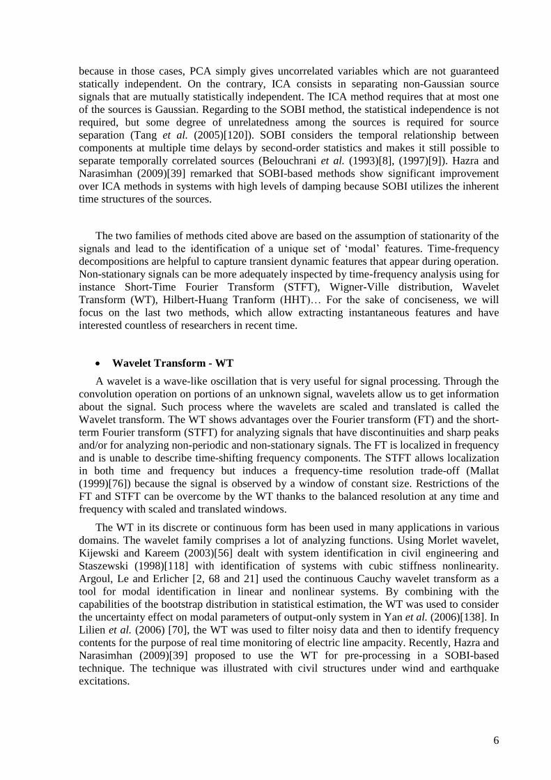
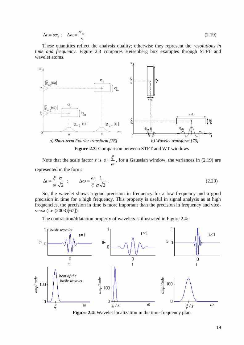
These quantities reflect the analysis quality; otherwise they represent the resolutions in

time and frequency. Figure 2.3 compares Heisenberg box examples through STFT and

wavelet atoms.

a) Short-term Fourier transform [76] b) Wavelet transform [76]

Figure 2.3: Comparison between STFT and WT windows

Note that the scale factor s is s

, for a Gaussian window, the variances in (2.19) are

represented in the form:

2t

;

1

2

. (2.20)

So, the wavelet shows a good precision in frequency for a low frequency and a good

precision in time for a high frequency. This property is useful in signal analysis as at high

frequencies, the precision in time is more important than the precision in frequency and vice-

versa (Le (2003)[67]).

The contraction/dilatation property of wavelets is illustrated in Figure 2.4:

Figure 2.4: Wavelet localization in the time-frequency plan

/ s / s

basic wavelet

beat of the

basic wavelet

am

pli

tud

e

am

pli

tud

e

am

pli

tud

e

20

In frequency analysis, the WT may be considered as a filter with the quality factor Q

defined by the ratio between the center frequency / s and the frequency band / s [67]:

/

2 / 2

sQ

s

(2.21)

This factor is independent of s and it depends only on characteristic parameters of the

mother wavelet ( )t .

Using the Parseval formula (Eq. 2.7), the WT can be computed by the FT:

ˆ ˆ( , ) ( ) ( )2

j usWf u s f s e d

(2.22)

For each scale s, one computes the inverse transform of the product of signal ( )f t and the

dilated versions ˆ ( )s of the mother wavelet ( )t . In numerical applications, the WT

computation is completed practically through the fast Fourier transform (FFT) algorithm.

Scalogram

A bi-dimensional energy density is defined, the scalogram ,WP f u which measures the

energy of ( )f t in the Heisenberg box of each wavelet ,u s centered at , /u s :

2

2

,, ( , ) ( ) ( )W u sP f u Wf u s f t t dt

(2.23)

Or the normalized scalogram ,W

normP f u :

21 1

, , ,norm

W WP f u P f u Wf u ss s

So, thanks to its ability to consider time and frequency resolutions at the same time, the

WT is particularly well adapted to detect discontinuity or sharp signal transitions.

To separate amplitude and phase information of signals, one uses analytic complex

wavelets, which have the property of progressiveness, i.e. ˆ( ) 0 for 0 . The

progressiveness ensures the WT does not produce any interference between the past and

future in the time domain. The energy of ˆ ( ) is then localized around a center frequency

0 .

Choice of wavelet

Many analytic wavelets are studied in the literature. The choice of mother wavelet

depends on several analysis properties. The Morlet wavelet is very popular in the literature

because its analogues to the FT are useful for harmonic analysis. It is the reason why it is

chosen in this work. The Morlet wavelet is defined by the complete formula:

22 20

20 22( )

t

j tt c e e e

,

2 20

2 20

1

3 2

4

24

11 2c e e

(2.24)

where 0 and c are respectively the center frequency of and the adequate normalization

factor.

21

The term 2 2

0e is known as the correction term, as it verifies the admissibility condition

and the zero-mean condition of the Morlet wavelet. In practice, for enough large value of

product 0 , it is negligible. In this case, the Morlet wavelet becomes:

0( ) ( )j t

M t g t e with

2

22

24

1( )

t

g t e

(2.25)

This simplified Morlet wavelet is well-known in the literature and called the Morlet

wavelet or the standard Morlet wavelet. The FT of the window ( )g t is

2 21/ 4

2 / 2ˆ( ) 4g e . If 2 2

0 1 , so ˆ( ) 0g for 0 , the wavelet is considered

as approximately analytical and admissible.

The analogues to FT of the Morlet wavelet are clear in the basic Morlet function:

0 0( ) ( )[cos( ) sin( )]M t g t t i t . Essentially, this wavelet is a FT of Gaussian window, with

oscillating sine and cosine at the center frequency 0 . Dilatations of this temporally localized

mother wavelet permit to discover harmonic components within the signal.

In the frequency domain, it is written:

22

0

12 24ˆ ( ) /M e

(2.26)

The relation between scale and frequency may be given prominence by considering the

frequency formulation of the dilated Morlet wavelet:

22

0

12 24ˆ ( ) /

s

M s e

(2.27)

The function reaches the maximum at 0s . As

0 is a fixed parameter that defines

the wavelet, at a given scale s, the function is maximal at:

0

s

(2.28)

The last equation explains the relation between the instantaneous frequency and scale. It

represents also the single relation between the dilatation parameter s and the frequency .

The standard Morlet wavelet does not verify exactly the zero mean in the admissibility

condition. However, the simplified wavelet average is very small for high values of the

product 0 ( 0 5 in practice) and the admissibility condition is nearly verified. For

example, for 0 5 , 1 , one has 6

0ˆ ( ) 10M

; for 0 10 , 22

0ˆ ( ) 10M

.

The center frequencies of the complete and standard Morlet wavelets are deduced from

their frequency spectrum expressions. The relation between those values is described with the

correction term:

2 2

0

, 1c c M e

.

Then, the term 2 2

0e

is the relative difference, if 0 5 , 1 , so 2 2

0 1110e

(as

described in Figure 2.5a), the standard Morlet wavelet may be considered like the complete

one.

22

a) with

0 5, 1

b) with

0 2, 1

Figure 2.5: Morlet wavelet in the time and frequency domains

For too small values of the product 0 , the admissibility condition is not verified as

0ˆ( ) 0 as illustrated in Figure 2.5b. One uses often a Gaussian envelop of unitary

variance and the condition of enough high values for 0 (which represents properly the

factor Q in equation 2.21) comes down to enough high values for 0 .

However, a wavelet employed in the WT must be a wave that is not lengthened, i.e. a

really small wave. It implicates a wave of which the support is compact (the effective larger

of the support is the smallest) or the decay is enough fast, to obtain the localization in time.

Practically, by choosing enough high values for 0 , one can use the standard Morlet

wavelet even if the admissibility condition is not strictly verified. It is very adequate for the

research of instantaneous frequencies and amplitudes of a signal. Moreover, the Gaussian

window used in the Morlet wavelet is optimal, i.e. it shows the same resolution in both the

time and frequency domains. It shows itself as a wavelet for which the time-frequency

localization is very good.

2.3.1 Wavelet ridges

Different methods exist to define and to extract ridges (Staszewski (1998)[118], Carmona

et al. (1999)[11] and Mallat (1999)[76]). The scalogram ,WP f u (expression 2.23)

measures the energy of ( )f t in the time-frequency neighborhood of ,u . The ridge

algorithm computes instantaneous frequencies of the signal from local maxima of the

scalogram (Figure 2.6).

23

Figure 2.6: Instantaneous frequency identification in aid of wavelet ridge, WT of a signal of

pure frequency ( ) j tf t e

The ridge algorithm relies on the analytic wavelet transform. An analytic wavelet may be

constructed by the product of a real and symmetric window g(t) and an exponential complex:

0( ) ( )j t

t g t e (2.29)

The wavelet under the form of (2.29), called Gabor wavelet, may be determined from a

normalized Gaussian window g(t) as in Eq. (2.25). For enough high values of the product

0 so that 2 2

0 1 , one has ˆ( ) 0g for 0 . Since the center frequency is

0 , the

value ˆ 0 is nearly zero, and such wavelet may be considered approximately analytic.

If a(u) and ( )u are respectively instantaneous amplitude and phase, the WT is given in

[76]:

ˆ( , ) ( ) '( ) ,2

j usWf u s a u e g s u u

(2.30)

where ,u is a corrective term. If this term is negligible, it is clear that (2.30) enables the

measurement of a(u) and '( )u from ( , )Wf u s . The corrective term is negligible if a(u) and

'( )u have small variations over the support of ,u s and '( ) /u s , that is

bandwidth of g .

The scalogram reaches its maximum at 0( ) '( )( )

u us u

and the points

, ( )u u constitute the ridge. If ,W u is the complex phase of ( , )Wf u s , at ridge points,

the instantaneous frequency '( )u and the analytic amplitude a(u) are given respectively by:

,'( )

W uu

u

(2.31)

22 ( , ) /

( )ˆ 0

Wf u s sa u

g (2.32)

24

When '( )u , the corrective term ,u is dominated by the second order, they are

negligible if [76]:

2

0

2

''( )1

( )'( )

a u

a uu

and

2

0 2

''( )1

'( )

u

u

(2.33)

The presence of ' in the denominator shows that 'a and ' may vary slowly if ' is

small but may vary much faster for larger instantaneous frequencies.

2.3.2 End effect

The spreads in time and frequency in the WT are non-zero; they depend on the mother

wavelet characteristics and on the analysis scale. Despite the wavelet localization in time and

frequency, the time window of localization spreads toward the past and future at a given time

(Figure 2.7). As the signal has finite length and is sampled with a non-zero sample period, it

exists an anomaly at the ends.

A simple solution for this problem is to extend the signal at the start and at the end and to

leave the perturbed values due to the end effect outside the interest zone. The use of a zero-

padding is simple but it introduces discontinuity at ends. A more adequate method is obtained

by expanding the signal by reflection at its ends (Figure 2.8); in this way, the signal always

keeps locally its frequency characteristics (Kijewski and Kareem (2002)[55]).

Figure 2.7: Wavelet spreads outside the finite signal

Figure 2.8: The generated signal by the reflection

NNNinitial xxxxxx 12321 x (2.34)

2 1 1 2 2 1 1 2generated N N N N Nx x x x x x x x x x (2.35)

T

T

25

The time length of the dilated window it for a frequency (scale) i is given by (2.20):

0

2i

i

t

.

The effectiveness of the end effect reduction is illustrated in Figure 2.9.

a) from the original signal b) from the generated signal

Figure 2.9: WT for ( ) sin(2 )f t ft (measured in the time interval of [t0; tf])

An extension of the signal constructed by reflection is quite simple and adapts naturally to

a signal with stable amplitude (e.g. responses to harmonic or random excitation). However,

when the frequency varies depending on the amplitude size, such extension still induces

discontinuity at the ends. It is illustrated in Figure 2.10a in the case of a nonlinear stiffness

system when the free response has to be extended to the left. Another approach is proposed

here to better adapt to the WT continuity.

Fitting padding

The principal idea is: added part must have a form according to the global appearance of

the original signal. A simple technique for signal generating is proposed below. It is described

with the left extension as presented in Figure 2.10b.

a- Find the maximal absolute value of the signal xmax, for free response; it stays

usually at the start of the signal.

b- Determine a superior or inferior envelope at end. For simplicity, this envelope may

be approximately shaped by finding a quadratic parabola passing three points early

determined. For the inferior (superior) envelope, those three points are all minima

(maxima) of which values are lowest (highest). Consider that the parabola passing

those three points can describe tendency of the signal at the left end. Suppose that

the signal will be extended until moment –t0, then one can compute ordinate x0

corresponding to abscissa –t0 of the envelop.

c- The generated part is just a period staying in the interval [0, t0] of the signal,

amplified following the formula:

0

00,

max

padding t

xX X

x (2.36)

is a fitting coefficient which ensures an entire harmonic appearance of the

generated signal.

26

a) b)

Figure 2.10: A signal and its extension

The treatment for the right end may be carried out with similar way.

Figure 2.11 shows end effects when the WT is performed respectively with the initial

signal, the signal prolonged by reflection and by fitting padding, respectively.

a) WT of the original signal

b) WT of the signal generated by reflection

c) WT of the signal generated by fitting padding

Figure 2.11: WT of a signal and its prolongation versions

initial signal

reflection paddingX 00, tX

t0

inferior enveloppe

x0

xmax

-t0 -t0

27

The results in Figure 2.11 show that the fitting padding improves the curves at boundaries.

Instantaneous frequencies at ends accord better with the central part. Regarding instantaneous

amplitudes, the end effect is effectively reduced.

2.3.3 Multiple frequencies

An important key in the multi-component signal analysis is the choice of the mother

wavelet parameters in order to discriminate each component.

Let 1 '( )u and

2 '( )u be instantaneous frequencies of two different components, the ridges

do not interfere if the dilated window gets sufficient frequency resolution at the ridge scales:

1 2ˆ '( ) '( ) 1g s u u (2.37)

Define as bandwidth of ˆ ( )g by:

ˆ 1g for (2.38)

Expression (2.37) means that the wavelet needs an enough small value for 0

in order to

isolate those spectral components:

1 2

1 0

'( ) '( )

'( )

u u

u

and 1 2

2 0

'( ) '( )

'( )

u u

u

(2.39)

Parameter 0 of the mother wavelet must be chosen in an adequate manner to satisfy

simultaneously the conditions (2.33) and (2.39). If two spectral lines are too close, they

interfere so that the ridge pattern is destroyed.

The spectral line number is generally unknown. Ridges corresponding to a low amplitude

are often carried off because they may be due to noise, or correspond to “shadows” of other

instantaneous frequencies created by the side-lobes of ˆ ( )g .

Figures 2.12 and 2.13 illustrate the interference phenomenon between the components of a

signal ( )f t including two spectral lines:

( ) sin 2 .5 sin 2 .12f t t t

A Morlet wavelet with 0 5, 1 yields evidently ridge interference, as shown in

Figure 2.12.

It can be observed that the instantaneous amplitude associated with the frequency of 12Hz

oscillates around a mean which is equal to the amplitude of the other component. If the

product 0 is chosen to be larger, this unwanted phenomenon is reduced.

Figure 2.13 shows that a larger product of 0 improves significantly the interference

between ridges but the end effect perturbs seriously the time-amplitude plan. Thus, if is too

large, the wavelet is thus too extended, which affects the precision in time because if 0 is

too large, the condition (2.33) is not ensured.

28

Figure 2.12: WT with 0 5, 1

Figure 2.13: WT with 0 5, 1.7

2.3.4 The WT as a band-pass filter

In the WT of a multi-component signal, one can isolate a single frequency component of

interest by choosing appropriately the scale interval as well as the characteristic factor 0 of

the mother wavelet. In this case, the WT plays the role of a band-pass filter.

29

2.4 Detection based on the concept of subspace angle

For a given excitation, the WT allows to identify the instantaneous frequencies (or ridges)

for a set of different measurement coordinates on the structure. Accordingly, it provides the

amplitude ratios between coordinates associated to an identified ridge line. Using these ratios,

one can assess time-varying deformation („mode‟) shapes of the system. The modes with the

strongest energies may be regarded as active modes and used to construct active subspaces

(which reflect states of the system) at different time instants. A change in the dynamic

behaviour modifies consequently the state of the system, i.e. the instantaneous frequencies

and deformation shapes. This change may be estimated using the concept of subspace angle

introduced by Golub and Van Loan (1996)[35]. This concept was used in De Boe and

Golinval (2003)[16] as a tool to quantify existing spatial coherence between two data sets

resulting from observation of a vibration system.

Given two subspaces (each with linear independent columns) Sm p and

Dm q (p>q), the procedure is as follows. Carry out the QR factorizations:

S = QSRS QSm p

D = QDRD QDm q (2.40)

The columns of QS and QD define the orthonormal bases for S and D respectively. The

angles i between the subspaces S and D are computed from singular values associated with

the product Q T

SQ D :

Q T

SQ D = U SDSDΣ V T

SD

cos , 1,...,SD idiag i q Σ (2.41)

The largest singular value is thus related with the largest angle characterizing the

geometric difference between two subspaces.

Figure 2.14: Angle formed by active subspaces (hyperplanes) according to the

reference and current states, due to a dynamic change

The change in a structure (e.g. the onset of nonlinearity or damage) may be detected by

monitoring the angular coherence between subspaces estimated from the reference

observation set and from the observation set of a current state respectively. A state is

considered as a reference state if the system operates in normal conditions (i.e. nonlinearity is

not activated or damage does not exist). Figure 2.14 shows a 2D example in which an active

subspace (or hyperplane) is built from two principal deformation shapes.

30

2.5 WT application to detect nonlinearity

The example consists in identifying the modal features and in detecting the level of

nonlinearity in a cubic stiffness system by means of the WT. The analysis is conducted both

numerically and experimentally. The studied structure is a beam clamped at one end and

exhibiting a cubic stiffness at the other end (Figure 2.15). The cubic stiffness is realised by

means of a very thin beam. For weak excitation, the system behaviour may be considered as

linear. When the excitation level increases, the thin beam exhibits large displacements and a

nonlinear geometric effect is activated resulting in a stiffening effect at the end of the main

beam. The structure was used as a benchmark for nonlinear system identification during the

European action COST F3 (Argoul and Le (2003)[2], Lenaerts et al. (2003)[65]).

a)

b)

Figure 2.15: The beam with a nonlinear stiffness (a) and its finite element model (b)

2.5.1 Numerical analysis

The main beam is modelled with seven beam finite elements (Figure 2.15b). The thin

beam is represented by two equivalent grounded springs: one in translation (kl + knl) and one

in rotation (kr). The nonlinear stiffening effect of the thin beam is modelled by a nonlinear

function in displacement of the form: ( ) sign( )nlf x A x x

, where A is a nonlinear

coefficient, 9 36.1 10 /A N m and is a nonlinear exponent, 3 . These parameters were

determined experimentally in Reference [65].

Nonlinear normal modes

The nonlinear normal modes (NNMs) of this structure were calculated in some companion

studies (Peeters et al. (2009)[99], Nguyen et al. (2010)[87]). These modal features depend on

the total energy in the system as illustrated in Figure 2.16 by the frequency-energy plot of the

first and the second NNMs.

a) First NNM b) Second NNM

Figure 2.16: Frequency-energy plot of the first (a) and second (b) NNMs

31

The first and second NNM motions are plotted in Figure 2.17 at low and high energy level

respectively. The low energy level (actually the linear normal modes) corresponds to

1 32.60 Hzf and 2 144.79 Hzf while the high energy level (the nonlinear case)

corresponds to 1 38.46 Hzf and 2 147.67 Hzf .

Figure 2.17: Analytical deformation shapes of the 1st, 2

nd modes respectively

For the purpose of this study, the beam is supposed to be submitted to an impact force at

its right end. The free response of the structure is measured in the vertical direction at the

seven coordinates indicated in Figure 2.15b and the WT is applied to the measured data.

Starting at a „low‟ excitation level (impact of 70 N), the behaviour of the beam appears as

linear (the largest displacement is lower than 0.15 mm). The WT of the displacement at

coordinate n° 7 is given in Figure 2.18 in terms of instantaneous frequencies and amplitudes.

Two frequency lines (called „ridges‟) are observed respectively at 32.6 Hz and 144.7 Hz,

which is in agreement with the frequencies occurring at low energy in the frequency-energy

plot (Figure 2.16).

Figure 2.18: Instantaneous frequencies and amplitudes at low energy (linear case)

Let us consider next a high level of excitation (impact of 1500 N) corresponding to a

maximum displacement at the right end of about 2.4 mm. Figure 2.19 presents the

corresponding WT results. It clearly shows a drop-off of the frequencies down to the linear

system values as the nonlinear effect vanishes progressively and the amplitude goes down.

Figure 2.19 also reveals the presence of a third order super harmonic of the first frequency

(curve n° 3).

Figure 2.19: Instantaneous frequencies and amplitudes at high energy (nonlinear case)

32

Identification of deformation shapes and detection of nonlinear behaviour

Figure 2.20 presents the first two modes of the beam identified with the „low‟ impact

excitation when the dynamic behaviour of the structure may be considered as linear.

Figure 2.20: WT modes 1 and 2 in the linear case

Figure 2.21 gives the deformation shapes at higher excitation levels. When the

displacement at the right end starts to be significant, both the first two deformation shapes

associated to ridges n° 1 and n° 2 become influenced by the magnitude of the nonlinearity of

the structure (the reference shape corresponds to the linear normal modes shown in Figure

2.20). It is interesting to note that one can find an intermediate deformation shape from ridge

line n° 3; the last plot of Figure 2.21 gives the corresponding deformation shapes for different

amplitudes of the displacement at the right end of the beam.

Figure 2.21: Deformation shapes associated to the 1st, 2

nd and super harmonic modes

33

The instantaneous deformation shapes M1, M2 and M3 corresponding to the three ridges

allow defining an instantaneous deformation matrix A = [M1 M2 M3]. Performing the

singular-value decomposition of matrix A, it can be shown that the third deformation shape

(M3) (super harmonic) is actually a linear combination of the two other „modes‟. Figure 2.22

shows the instantaneous singular values of the decomposition in terms of energy percentage.

It reveals that the third singular value is negligible compared to the two others.

Figure 2.22: Instantaneous singular values of the deformation „mode‟ matrix

The comparisons may be equally carried out by means of the MAC (Modal Assurance

Criterion). In Figure 2.23, deformation shapes obtained through the WT are compared with

the linear normal modes identified by the SSI (Stochastic Subspace Identification) method for

different values of the displacement at the end of the beam. When the displacement is low

(Figure 2.23a), the MAC indicates a perfect correlation. At this level of excitation, the

deformation shapes are identical to the linear normal modes. On the other hand, when the

displacement amplitude is high (Figure 2.23c), the nonlinearity is well excited which results

in a frequency increase and a slight loss of correlation with the linear normal modes

(identified by SSI). Figure 2.23 shows however that the MAC is not a deciding criterion for

the detection of nonlinearity.

a) Displacement amplitude d ≈ 0.6 mm b) d ≈ 1.25 mm c) d ≈ 2.3 mm

Figure 2.23: MAC between WT „modes‟ and SSI modes

Detection based on the concept of subspace angle

For the purpose of detection of nonlinearity, the structure is now supposed to be excited at

increasing levels of impact force (amplitudes ranging from 100 N to 1500 N). The

corresponding instantaneous frequencies obtained through the WT of the response signals at

coordinate n° 7 are shown in Figure 2.24.

As explained in Section 2.4, the instantaneous deformation shapes associated to these two

frequencies may be considered as instantaneous active modes to define a subspace which

34

characterises the dynamic state of the structure. The comparison of subspace angles between

the reference state (defined by the linear normal modes) and current states at different

excitation levels reveals the range of activation of the nonlinearity as illustrated in Figure

2.25. Larger is the excitation level, more significant is the angle. As responses are damped,

the angles reach their largest values at the beginning and then decrease gradually to converge

to zero as the dynamic behaviour of the beam becomes linear.

a) from the 1st ridges

b) from the 2nd

ridges

Figure 2.24: Instantaneous frequencies corresponding to different excitation levels

As the activation of the nonlinearity depends on the amplitude level of the displacement,

the display of subspace angles according to the evolution of the instantaneous displacement

amplitude measured at the end of the beam is informative. Figure 2.26 shows the evolution of

subspace angles in function of the displacement amplitude measured at the end of the beam at

time t = 0.1 s. It can be observed that the subspace angle criterion for the 2nd

mode is more

sensitive to the nonlinearity in comparison to the 1st mode (which is confirmed by the MAC in

Figure 2.23). In terms of frequency changes however, the 1st mode appears as more affected

than the 2nd

mode (Figure 2.24).

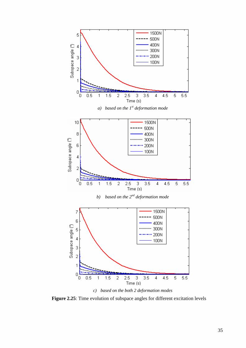
35

a) based on the 1st deformation mode

b) based on the 2nd

deformation mode

c) based on the both 2 deformation modes

Figure 2.25: Time evolution of subspace angles for different excitation levels

36

Figure 2.26: Relation angle - displacement amplitude at the end of the beam at t = 0.1 s

In summary, the onset of nonlinearity may be detected by observing the evolution of

instantaneous frequencies as illustrated in Figure 2.24 but a high frequency resolution is

needed to distinguish between close levels of excitation (e.g. impacts of 100 N to 500 N). In

this respect, subspace angle curves look more promising as they look less affected by the

frequency resolution. Another advantage is that the concept of subspace angle allows to

handle several modes simultaneously in a unique detection index. Furthermore, even without

processing, the end effect has less influence on the detection by subspace angle because the

use of amplitude ratios in the method may weaken or even eliminate this unwanted effect.

2.5.2 Experimental results

Impact excitation

Experimental results were collected using 7 accelerometers (Figure 2.27) evenly

distributed along the main beam as presented in Figure 2.15. The data are recorded during 6.4

seconds with a time-step of 0.00078125 s.

Figure 2.27: Experimental set up

An impact of very low amplitude was first applied at the end of the beam to obtain the

reference state. The first two natural frequencies are observed at 31.3 Hz and 143.5 Hz

respectively as shown in Figure 2.28 which gives the WT of the response measured at the end

of the beam (coordinate n° 7). These values are slightly lower than the frequencies predicted

by the numerical model, which is mainly due to the influence of the mass of the sensors.

An impact of higher amplitude was then applied to activate the nonlinearity. The results

are shown in Figure 2.29. It is observed that three instantaneous frequencies (ridges) are

detected and that they are decreasing over time.

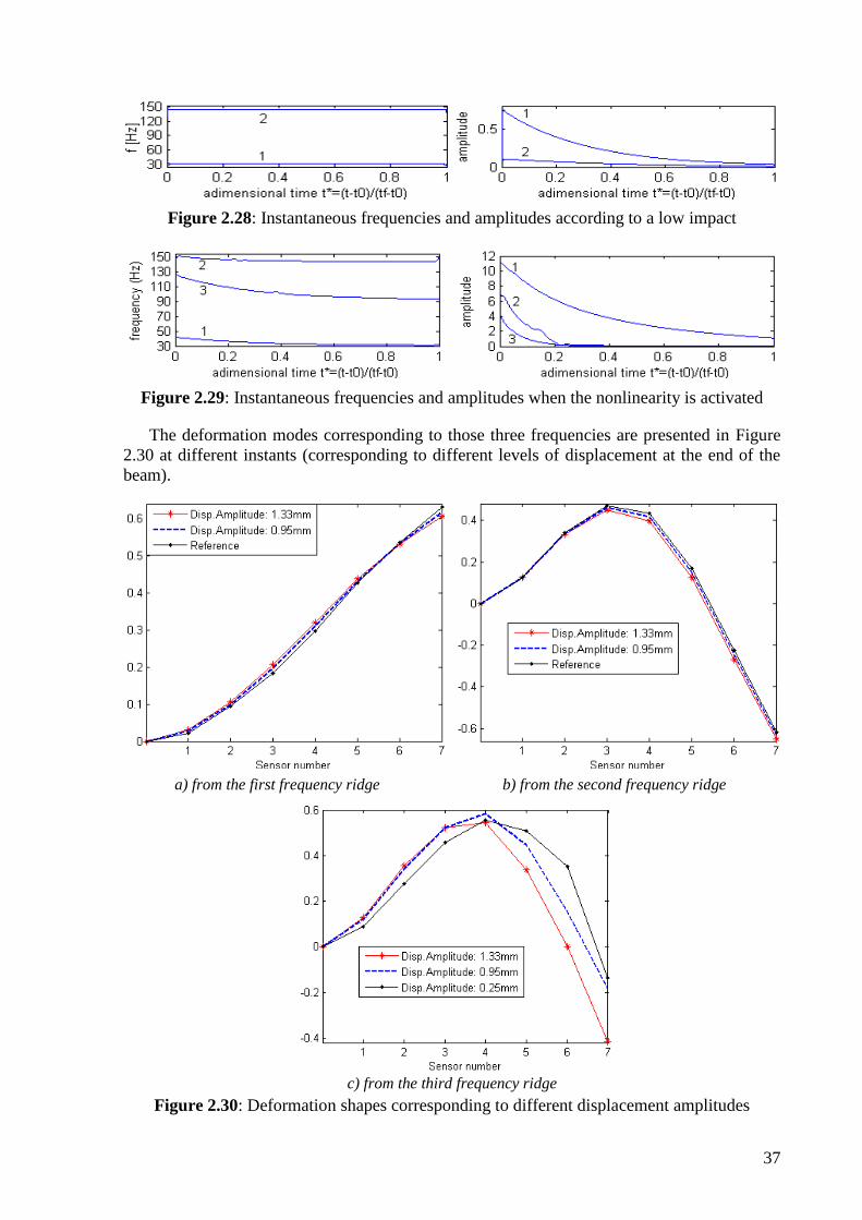
37

Figure 2.28: Instantaneous frequencies and amplitudes according to a low impact

Figure 2.29: Instantaneous frequencies and amplitudes when the nonlinearity is activated

The deformation modes corresponding to those three frequencies are presented in Figure

2.30 at different instants (corresponding to different levels of displacement at the end of the

beam).

a) from the first frequency ridge b) from the second frequency ridge

c) from the third frequency ridge

Figure 2.30: Deformation shapes corresponding to different displacement amplitudes

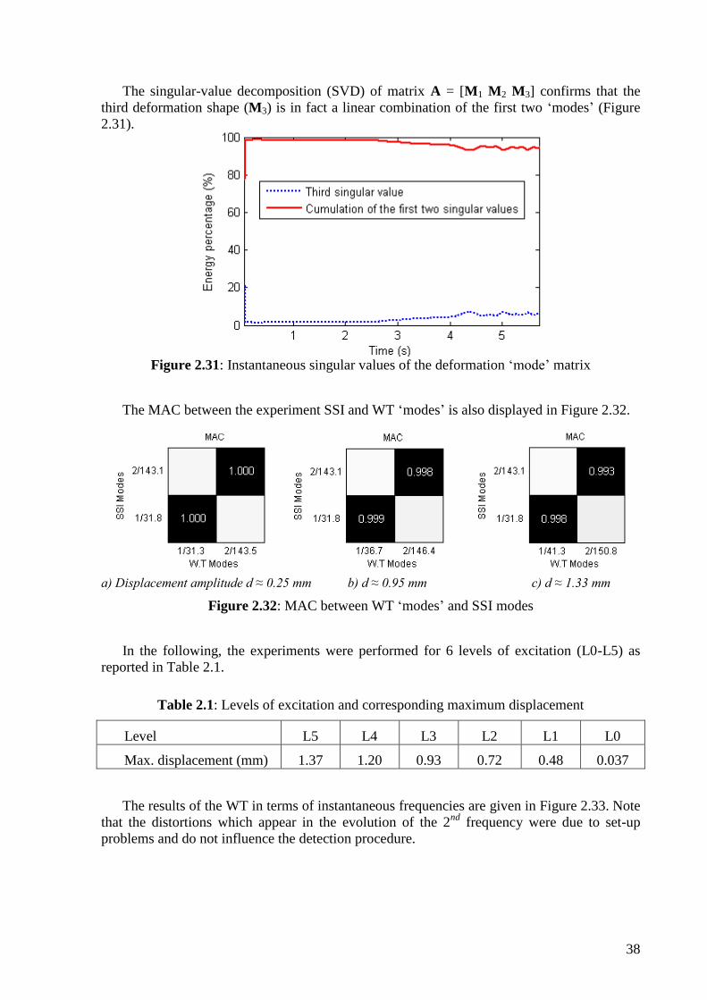
38

The singular-value decomposition (SVD) of matrix A = [M1 M2 M3] confirms that the

third deformation shape (M3) is in fact a linear combination of the first two „modes‟ (Figure

2.31).

Figure 2.31: Instantaneous singular values of the deformation „mode‟ matrix

The MAC between the experiment SSI and WT „modes‟ is also displayed in Figure 2.32.

a) Displacement amplitude d ≈ 0.25 mm b) d ≈ 0.95 mm c) d ≈ 1.33 mm

Figure 2.32: MAC between WT „modes‟ and SSI modes

In the following, the experiments were performed for 6 levels of excitation (L0-L5) as

reported in Table 2.1.

Table 2.1: Levels of excitation and corresponding maximum displacement

Level L5 L4 L3 L2 L1 L0

Max. displacement (mm) 1.37 1.20 0.93 0.72 0.48 0.037

The results of the WT in terms of instantaneous frequencies are given in Figure 2.33. Note

that the distortions which appear in the evolution of the 2nd

frequency were due to set-up

problems and do not influence the detection procedure.

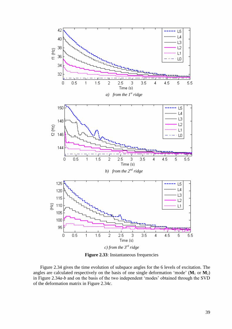
39

a) from the 1st ridge

b) from the 2nd

ridge

c) from the 3rd

ridge

Figure 2.33: Instantaneous frequencies

Figure 2.34 gives the time evolution of subspace angles for the 6 levels of excitation. The

angles are calculated respectively on the basis of one single deformation „mode‟ (M1 or M2)

in Figure 2.34a-b and on the basis of the two independent „modes‟ obtained through the SVD

of the deformation matrix in Figure 2.34c.

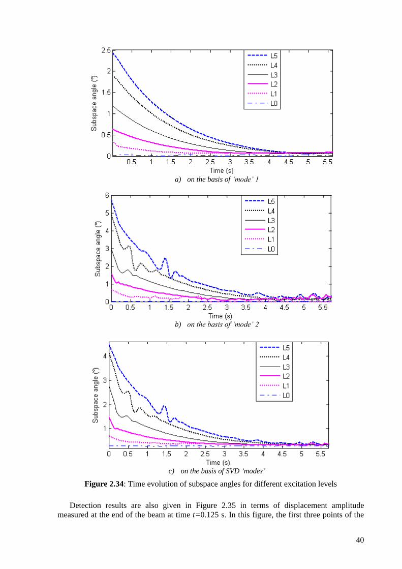
40

a) on the basis of ‘mode’ 1

b) on the basis of ‘mode’ 2

c) on the basis of SVD ‘modes’

Figure 2.34: Time evolution of subspace angles for different excitation levels

Detection results are also given in Figure 2.35 in terms of displacement amplitude

measured at the end of the beam at time t=0.125 s. In this figure, the first three points of the

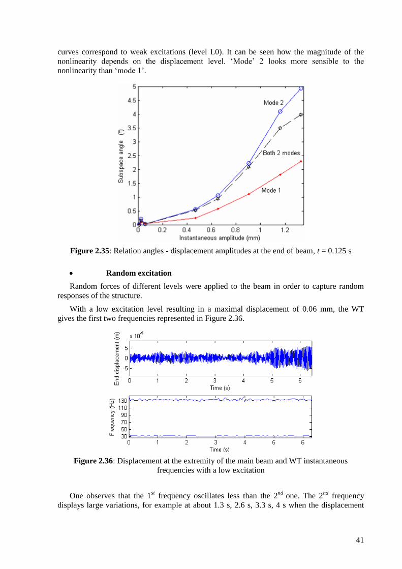
41

curves correspond to weak excitations (level L0). It can be seen how the magnitude of the

nonlinearity depends on the displacement level. „Mode‟ 2 looks more sensible to the

nonlinearity than „mode 1‟.

Figure 2.35: Relation angles - displacement amplitudes at the end of beam, t = 0.125 s

Random excitation

Random forces of different levels were applied to the beam in order to capture random

responses of the structure.

With a low excitation level resulting in a maximal displacement of 0.06 mm, the WT

gives the first two frequencies represented in Figure 2.36.

Figure 2.36: Displacement at the extremity of the main beam and WT instantaneous

frequencies with a low excitation

One observes that the 1st frequency oscillates less than the 2

nd one. The 2

nd frequency

displays large variations, for example at about 1.3 s, 2.6 s, 3.3 s, 4 s when the displacement

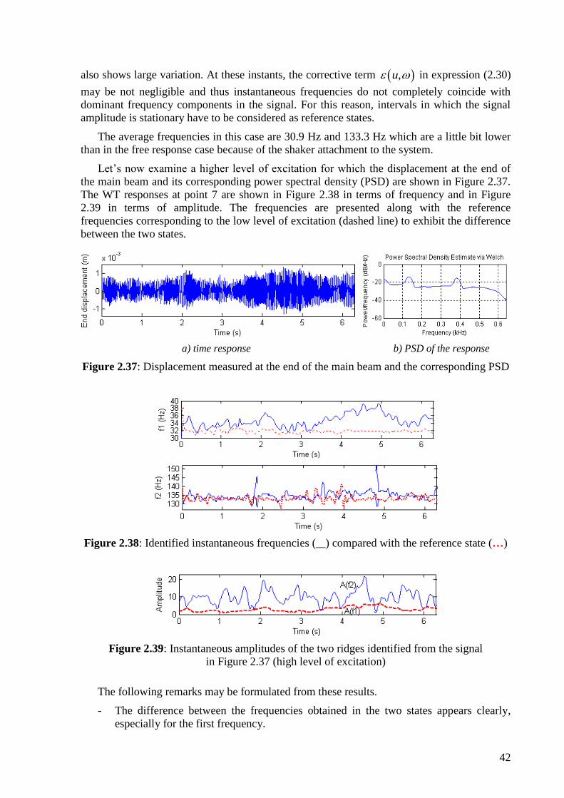
42

also shows large variation. At these instants, the corrective term ,u in expression (2.30)

may be not negligible and thus instantaneous frequencies do not completely coincide with

dominant frequency components in the signal. For this reason, intervals in which the signal

amplitude is stationary have to be considered as reference states.

The average frequencies in this case are 30.9 Hz and 133.3 Hz which are a little bit lower

than in the free response case because of the shaker attachment to the system.

Let‟s now examine a higher level of excitation for which the displacement at the end of

the main beam and its corresponding power spectral density (PSD) are shown in Figure 2.37.

The WT responses at point 7 are shown in Figure 2.38 in terms of frequency and in Figure

2.39 in terms of amplitude. The frequencies are presented along with the reference

frequencies corresponding to the low level of excitation (dashed line) to exhibit the difference

between the two states.

a) time response b) PSD of the response

Figure 2.37: Displacement measured at the end of the main beam and the corresponding PSD

Figure 2.38: Identified instantaneous frequencies (__) compared with the reference state (…)

Figure 2.39: Instantaneous amplitudes of the two ridges identified from the signal

in Figure 2.37 (high level of excitation)

The following remarks may be formulated from these results.

- The difference between the frequencies obtained in the two states appears clearly,

especially for the first frequency.

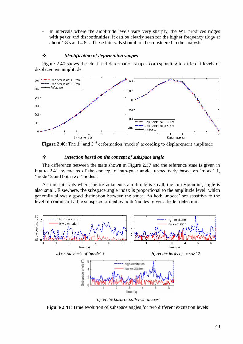
43

- In intervals where the amplitude levels vary very sharply, the WT produces ridges

with peaks and discontinuities; it can be clearly seen for the higher frequency ridge at

about 1.8 s and 4.8 s. These intervals should not be considered in the analysis.

Identification of deformation shapes

Figure 2.40 shows the identified deformation shapes corresponding to different levels of

displacement amplitude.

Figure 2.40: The 1st and 2

nd deformation „modes‟ according to displacement amplitude

Detection based on the concept of subspace angle

The difference between the state shown in Figure 2.37 and the reference state is given in

Figure 2.41 by means of the concept of subspace angle, respectively based on „mode‟ 1,

„mode‟ 2 and both two „modes‟.

At time intervals where the instantaneous amplitude is small, the corresponding angle is

also small. Elsewhere, the subspace angle index is proportional to the amplitude level, which

generally allows a good distinction between the states. As both „modes‟ are sensitive to the

level of nonlinearity, the subspace formed by both „modes‟ gives a better detection.

a) on the basis of ‘mode’ 1 b) on the basis of ‘mode’ 2

c) on the basis of both two ‘modes’

Figure 2.41: Time evolution of subspace angles for two different excitation levels

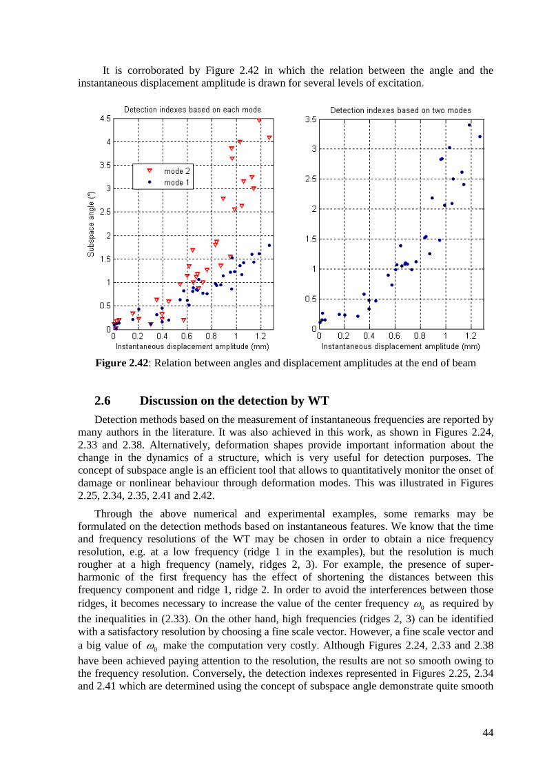
44

It is corroborated by Figure 2.42 in which the relation between the angle and the

instantaneous displacement amplitude is drawn for several levels of excitation.

Figure 2.42: Relation between angles and displacement amplitudes at the end of beam

2.6 Discussion on the detection by WT

Detection methods based on the measurement of instantaneous frequencies are reported by

many authors in the literature. It was also achieved in this work, as shown in Figures 2.24,

2.33 and 2.38. Alternatively, deformation shapes provide important information about the

change in the dynamics of a structure, which is very useful for detection purposes. The

concept of subspace angle is an efficient tool that allows to quantitatively monitor the onset of

damage or nonlinear behaviour through deformation modes. This was illustrated in Figures

2.25, 2.34, 2.35, 2.41 and 2.42.

Through the above numerical and experimental examples, some remarks may be

formulated on the detection methods based on instantaneous features. We know that the time

and frequency resolutions of the WT may be chosen in order to obtain a nice frequency

resolution, e.g. at a low frequency (ridge 1 in the examples), but the resolution is much

rougher at a high frequency (namely, ridges 2, 3). For example, the presence of super-

harmonic of the first frequency has the effect of shortening the distances between this

frequency component and ridge 1, ridge 2. In order to avoid the interferences between those

ridges, it becomes necessary to increase the value of the center frequency 0 as required by

the inequalities in (2.33). On the other hand, high frequencies (ridges 2, 3) can be identified

with a satisfactory resolution by choosing a fine scale vector. However, a fine scale vector and

a big value of 0 make the computation very costly. Although Figures 2.24, 2.33 and 2.38

have been achieved paying attention to the resolution, the results are not so smooth owing to

the frequency resolution. Conversely, the detection indexes represented in Figures 2.25, 2.34

and 2.41 which are determined using the concept of subspace angle demonstrate quite smooth

45

curves. It indicates the advantage of using instantaneous amplitudes: providing that an 0

high enough to well separate the ridges, the resolution is not a delicate problem for the

instantaneous amplitude. It is illustrated in Appendix A by comparing the resolution in

frequency and amplitude through a raw scale vector and a much finer one. In conclusion, the

WT instantaneous amplitudes provide a good means of detection without the need to consider

a sophisticated scale vector and the detection is advantageously performed through the use of

the concept of subspace angle.

2.7 Concluding remarks

The Wavelet Transform is known for its ability to analyze non-stationary signals and to

detect nonlinear behaviour in a structure. As reported in Argoul and Le (2003)[2], it can be

used to identify several instantaneous indicators, namely instantaneous frequency, positive

„modal‟ shape.

In this study, detection of nonlinearity in a dynamic system was performed further using

the concept of subspace angle between instantaneous deformation „modes‟. These

deformation „modes‟ are associated to instantaneous frequencies obtained from the WT of

vibration signals measured at different coordinates of the system. Instantaneous bases of

independent modes may be generated using the singular value decomposition of deformation

„mode‟ matrices, which determines the dimensionality of the system. The procedure was

illustrated numerically and experimentally on the example of a nonlinear cantilever beam

submitted to impact and random excitations.

The concept of subspace angle allows to define a global detection index. When used in

combination with instantaneous „modes‟ extracted from the WT, this index was found to be

sensitive to small dynamic changes and robust with regards to frequency resolution of the

transform.

46

Chapter 3

Second-Order Blind Identification

Method Applied to Damage Detection

3.1 Introduction

Blind source separation (BSS) techniques are applied in many domains, since they allow

separating a set of signals from their observed mixture, without the knowledge (or with very

little knowledge) of the sources signals or the mixing process. In structural dynamics, BSS

techniques showed useful for modal identification from numerical and experimental data

(Kerschen et al. (2007)[54], Poncelet et al. (2007)[101], Zhou and Chelidze (2007)[142],

Farooq and Feeny (2008)[23]), for separating sources from traffic-induced building vibrations

(Popescu and Manolescu (2007)[103]) and for damage detection and condition monitoring

(Zang et al. (2004)[141], Pontoppidan et al. (2005)[102], Jianping and Guang (2009)[49]). A

particular BSS technique called second-order blind identification is considered in this chapter

for the purpose of condition monitoring as well as damage detection. The beam with

geometric nonlinearity presented in Chapter 2 and an airplane mock-up are used as illustrative

examples.

3.2 Second-order blind identification

Second-order blind identification (SOBI) was introduced by Belouchrani et al. (1999)[9].

Like other BSS approaches, SOBI considers observed signals as a noisy instantaneous linear

mixture of source signals. In many situations, multidimensional observations are represented

as:

( ) ( ) ( ) ( ) ( )t t t t t x y σ As σ (3.1)

where, T

1( ) ( ),..., ( )mt x t x tx is a linear instantaneous mixture of source signals and of noise.

T

1( ) ( ),..., ( )pt s t s t s contains the signals issued from p narrow band sources, p < m.

T

1( ) ( ),..., ( )mt y t y ty contains the sources assembly at a time t.

The transfer matrix A between the sources and the sensors is called the mixing matrix.

( )tσ is the noise vector, modelled as a stationary white noise of zero mean and is assumed to

be independent of the sources.

47

The method attempts to extract the sources s(t) and the mixing matrix A from the

observed data x(t). The term “blind” implies that the mixing matrix A is not known a priori,

so that only the output signals are exploited. Additionally, some assumptions on the source

signals are introduced (Belouchrani et al. (1997)[9]). SOBI relies on the second order

statistics and is based on the diagonalization of time-lagged covariance matrices.

The sources are assumed stationary, uncorrelated and of unitary variance; their covariance

matrix is written:

0 [ ]s E t t R s s I (3.2)

where superscript * denotes the conjugate transpose of a vector and I is the identity matrix.

The added noise is modeled as a stationary white, zero-mean random process independent

of the source signals. For simplicity, )(tσ is assumed spatially white, i.e.

2[ ]E t t σ σ I (3.3)

The method may be extended to the case of an unknown noise variance matrix.

The matrix A is assumed to have full column rank but is otherwise unknown. The

covariance matrix of the array output can be written under the form:

H 20 0[ ]x sE t t R x x AR A I (3.4)

H[ ]x sE t t R x x AR A 0 (3.5)

where superscript H denotes the complex conjugate transpose of a matrix.

As the sources are independent, one has:

IR 0s , and so H0 [ ]y E t t R y y AA (3.6)

The SOBI procedure comprises two steps: whitening and determination of the unitary

matrix.

3.2.1 Whitening

The first step relates to the whitening of the signal y(t) such that the whitened data are

uncorrelated and of unit variance. It consists in applying to y(t) a whitening matrix W, i.e., a

p×m matrix that verifies:

H H H H0[ ] yE t t Wy y W WR W WAA W I (3.7)

Expression (3.7) shows that if W is a whitening matrix, then WA is a p×p unitary matrix.

Thus, for any whitening matrix W, there exists a p×p unitary matrix U such that WA U .

Consequently, matrix A can be deduced by the relation:

UWA (3.8)

where superscript denotes the Moore-Penrose pseudo-inverse. This whitening procedure

reduces the determination of the m×p mixing matrix A to that of a unitary p×p unitary matrix

U. The whitened process z(t) = Wx(t) still follows a linear model where the signal of the

whitened process is now a “unitary mixture” of the source signals:

tttttt WσUsσAsWWxz (3.9)

48

The effect of the whitening procedure is to “exhaust” all information contained in the

covariance matrix in the sense that changing U in (3.8) by any other unitary matrix keeps the

covariance of z(t) unchanged. Moreover, the signal of observations z(t) reduces the array

output to a p-dimensional vector.

As IR 0s (ex. (3.6)), from (3.4), one has:

H 20x AA R I (3.10)

Expressions (3.7) and (3.10) show that a whitening matrix W can be determined through

the covariance matrix Rx(0) [9]. This determination is still possible even if the noise variance

matrix is unknown.

3.2.2 Determination of the unitary matrix

Starting with the spatially whitened covariance matrices wR :

H H[ ] [ ]wx E t t E t t R WR W W x x W z z 0 (3.11)

Those matrices correspond to the covariance matrices of the process z(t). From (3.5) and

(3.8), the following important relation is presented:

H H Hw

s s R WAR A W UR U 0 (3.12)

where [ ]s E t t R s s is the covariance matrix of the sources for some time lag .

Since U is unitary and sR is diagonal, (3.12) shows that the whitened covariance matrix

wR is diagonal. So, matrix U can be determined by an eigenvalue decomposition of the

time-lagged whitened covariance matrix. This procedure can be achieved through the

technique of joint diagonalization described in Belouchrani et al. (1997)[9]; it consists in a

generalization of the Jacobi technique. Some materials for joint diagonalization presented by

Cardoso can be found in [43].

The computation of the mixing matrix A and sources is straightforward, according to

formulas (3.8) and (3.13), once U is determined.

Ht t t s U Wx Vx (3.13)

where HV U W which is called the de-mixing matrix is the generalized inverse of the

mixing matrix A.

The method necessitates that the diagonal elements of sR must be different, so that the

eigenvalues of wR are distinct. This condition is not always checked a priori for any time

lag . However, the choice of is significantly facilitated when several time lags are

considered, as explained in [9]. Alternatively, the use of a few time lags makes less the

probability of an unfortunate choice for , and matrix U is deduced in a more accurate way

from a larger set of statistics.

3.3 Modal identification using SOBI

Consider the equations of motion of a mechanical system without damping:

ttt fKxxM (3.14)

49

The system responses can be expressed by modal superposition:

1

p

i i

i

t t t

x Φη (3.15)

where the matrix Φ is the modal matrix comprising the normal modes and η is the vector of

normal coordinates which describes the amplitude modulations of Φ . As noted in Kerschen

et al. (2007)[54], equation (3.15) shows that “when expanding the system response in terms of

the vibration modes, the normal coordinates may, under certain assumptions, act as virtual

sources regardless of the number and type of the physical excitation forces”. On the other

hand, time responses can be represented by a static mixture of those virtual sources.

If the natural frequencies are distinct, the normal coordinates are harmonic functions

(Géradin and Rixen (1994)[33]) and can be considered as sources with different spectral

contents, under certain assumptions [54]. Relating to SOBI, it is noticeable that the mixing

matrix matches the matrix of vibration modes, and the identified sources correspond to the

normal coordinates, i.e.

ΦA and t ts η (3.16)

In presence of damping, mode-shapes are generally complex and appear in conjugate

pairs. If CM-1

K is symmetric, where C is the damping matrix, 2p complex modes turn out

into p real modes. For damped systems, Poncelet et al. (2007)[101] pointed out that BSS

methods are able to identify normal coordinates as identified sources if damping ratios are

low enough.

Equation (3.16) shows that the mode shapes can be found in the mixing matrix A. The

identification of natural frequencies and damping ratios is straightforward from the identified

sources, e.g. using 1 DOF fitting techniques (Maia (1997)[75]).

SOBI characterizes the dynamical features of a structure by way of the mixing matrix A

and the sources. Thus, when the structure is perturbed or damaged, the fault may be reflected

through the identified sources and the matrix A. In the following, damage detection is

achieved by monitoring the variation of modal features (e.g. resonant frequencies, mode

shapes) and the angular coherence between subspaces built from the columns of the mixing

matrices.

3.4 SOBI and the Hankel matrices - ESOBI

The so-called Block Hankel matrices play an important role in subspace identification of

linear systems (Overschee and De Moor (1997)[94]). It is also commonly used for damage

detection (Yan et al. (2004)[132], Yan and Golinval (2006)[137]), damage localization (Yan

and Golinval (2005)[133]) or even identification of nonlinear structures (Marchesiello and

Garibaldi (2008)[78]). The data-driven block Hankel matrix is defined as:

50

1 2

2 3 1

1 1

1,2

1 2

2 3 1

2 2 1 2 1

... ...

... ...

... ... ... ... ...

... ...

... ...

... ...

... ... ... ... ...

... ...

j

j

i i i j p

i

i i i j f

i i i j

i i i j

x x x

x x x

x x x X

H

x x x X

x x x

x x x

" "

" "

past

future (3.17)

where 2i is a user-defined number of row blocks, each block contains m rows (number of

measurement sensors), j is the number of columns (practically j = N-2i+1, N is the number of

sampling points). The Hankel matrix 1,2iH is split into two equal parts of i block rows: past

and future data. Thus, the algorithm considers vibration signals at different instants and not

only instantaneous representations of responses. This allows to take into account temporal

correlations between measurements when current data depends on past data. The principal

idea in modal analysis is to retain all past information to predict the future. Although the past

and future inputs have many elements in common, they are always distinct because the

corresponding columns of Xp and Xf have no elements in common (Overschee and De Moor

(1997)[94]). Therefore, the objective pursued here in using the block Hankel matrix rather

than the observation matrix is to improve the sensitivity of the detection method. The

combined method will be called enhanced SOBI - ESOBI in the following.

We know that in the SOBI method, the size of a column vector in the mixing matrix A

depends on the number of sensors m; moreover, the number p of sources successfully

identified cannot exceed m. It results that, if the number of sensors is very small, a perfect

identification of all the resonance frequencies is impossible by means of SOBI. However, in

the same situation, ESOBI, as it exploits more of the signals through the Hankel matrix, is

able to provide better information about the dynamics of the system. Moreover, the detection

based on the concept of subspace angle can still be achieved, even with a single sensor as

illustrated later.

3.5 An extension of SOBI called Blind Modal Identification

A BSS method like SOBI for which the mixing matrix is real-valued is not always

suitable for identifying generally damped systems. Recently a novel approach called Blind

Modal Identification (BMID) has been proposed by McNeil and Zimmerman (2008)[79]. It

uses BSS techniques to yield modal responses and complex mode shape estimates (McNeil

and Zimmerman (2010)[80]). The principle of the BMID method is to apply SOBI on an

augmented and pre-treated dataset.

From the measured data, denoted as 0 ( )tx , the Hilbert transform pairs,

90( )tx are

introduced. Note that the Hilbert transform of a sinusoid results in a 90° phase shift of the

sinusoid. This results in the double sized mixing problem:

51

(2 1) (2 2 ) (2 1)m m p p x A s , (2 1) (2 2 ) (2 1)p p m m s V x ,

( 1) ( 1)

0 0(2 2 )

( 1) ( 1)

90 90

m p

m p

m p

x sA

x s,

( 1) ( 1)

0 0(2 2 )

( 1) ( 1)

90 90

p m

p m

p m

s xV

s x (3.18)

where 90 ( )ts are the Hilbert transform pairs of the source components

0( )ts .

Because 0 ( )tx and

90( )tx are respectively the real and imaginary parts of the analytic

signal 0 90( ) ( ) ( )a t t j t x x x , (with 1j ) the partition of the augmented dataset in

equation (3.18) shows similarity with the familiar concept of the analytic signal.

The matrix A in (3.18) can be partitioned into two block columns corresponding to 0( )ts

and 90 ( )ts :

0 90A A A (3.19)

The ith column of 0A gives the contribution of

0 ( )is t to each measurement and the

corresponding phase shifted measurement. Likewise, the ith column of 90A and

90 ( )is t

presents a similar relation. Complex modes, cΦ , can be formed by taking the first or last

block of m rows in:

0 90'c j Φ A A (3.20)

It is important to note that the Hilbert transform presents end effects, i.e. errors are

introduced at the end of 90( )tx . End effects can be lessened by e.g. zero padding or reflection

padding as mentioned in Chapter 2.

McNeil and Zimmerman proposed also a Modal Contribution Indicator (MCI) to measure

modal strength in a simple manner. If the sources are scaled to unit variance, the mode shapes

are scaled by the modal amplitude. An indicator may be put forward for a relative measure of

the modal contribution of mode k to the overall response:

1

MCTm

k ik

i

(3.21)

where m is the number of measured DOFs. This measure can be normalized by the Modal

Contribution Indicator (MCI):

1

MCTMCI

MCT

kk p

k

k

(3.22)

where p is the number of modes. MCIk may roughly represent the fractional contribution of

the kth mode to the overall response. In our work, MCI is employed in order to select physical

modes that have an essential impact on the system responses.

52

3.6 Examples of application

3.6.1 Experiments in an aircraft model in different conditions

Let us consider an aircraft model made of steel and suspended freely by means of three

springs, as illustrated in Figure 3.1.

a) Aircraft model b) removing of 1-3 connecting bolts

Figure 3.1: An aircraft model (a) and the simulated damages (b)

A straight beam of rectangular section with a length of 1.2 m represents the fuselage.

Plate-type beams connected to the fuselage form the wing (1.5 m) and tails (0.2 m). Their

dimensions are detailed in Figure 3.2. The structure is randomly excited on the top of the left

wing with an electro-dynamic shaker in the frequency range of 0-130 Hz. Eleven

accelerometers are installed for capturing the dynamic responses of the structure in

accordance with the set-up description given in Figure 3.2. Three levels of damage are

simulated by removing, respectively, one, two and three connecting bolts on one side of the

wing (Figure 3.1b). The data of this experiment was formerly used for illustrating damage

detection methods based on Principal Component Analysis, on Kalman model and on Null

subspace analysis (Yan et al. (2004)[132], Yan and Golinval (2006)[137]); it was also used

for damage localization (Yan and Golinval (2005)[133]). Some results of modal identification

were also described in [132].

Figure 3.2: Dimensions (in millimeters) and location of the 11 sensors

Modal identification using SOBI

For the sake of illustrating the sensitivity of SOBI to damage occurrence, we start first to

identify modal features, namely the resonance frequencies and mode shapes. Figure 3.3a

53

represents the first eight resonance frequencies obtained through the FFT of the identified

sources in the healthy (undamaged) state. Some resonance frequencies are found to be

relatively close, e.g. f3 (83.29 Hz) and f4 (85.44 Hz); f6 (102.13 Hz) and f7 (103.35 Hz). Those

results are in perfect agreement with the identification performed in Reference [132] using the

Kalman model based on SSI.

a) Healthy state b) Damaged state

Figure 3.3: SOBI identification of resonance frequencies by FFT of the sources

The SOBI mode-shapes, contained in the columns of the mixing matrix A, are represented

in Figure 3.4, where sensors n° 1-8 represent the motion in the wing and sensors n° 9-11 show

the responses in the tails.

54

Figure 3.4: Mode shapes identified by SOBI in the healthy and damaged (dashed line) states

Let us now examine a damaged case when all the three connecting bolts are removed

(Figure 3.1b). The FFT of the identified sources are juxtaposed to the ones corresponding to

the healthy (reference) state in Figure 3.3b. The largest frequency variation is observed on the

first frequency with 8.4% of decrease. Another very noticeable change is the disappearance of

sources n° 4 and 7 when the structure is damaged. We note also that the MCI of modes n° 4

and 7 in Figure 3.3a is quite small in comparison to the previous components - modes n° 3

and 6. Instead of 8 sources/ modes, we can identify only 6 sources/modes in the damaged

case. The obtained mode-shapes are superposed in Figure 3.4.

Modal identification using BMID

In the same way, FFT of sources and mode shapes identified by BMID are presented in

Figures 3.5 and 3.6, respectively. It is observed in Figure 3.5 that compared to SOBI sources,

BMID spectral components are slightly less noisy (e.g. sources n° 1-3). Thereto, the disparity

between the healthy and damaged states is better shown by BMID mode shapes n° 2, 5 and 8.

55

a) Healthy state b) Damaged state

Figure 3.5: BMID identification of resonance frequencies by FFT of the sources

56

Figure 3.6: Mode shapes identified by BMID in the healthy and damaged (dashed line) states

Modal identification using Enhanced SOBI - ESOBI

To enrich the information in the data matrix, several block rows are assembled to build the

data-driven Hankel matrix as in expression (3.17). In this application, the number of block

rows has been fixed to 10. First, the enhancement provided by ESOBI can be noticed through

the quality of the sources identified in Figure 3.7. The sources are now much clearer, i.e.

noisy spectral components in each source are minimized with respect to Figure 3.3. It follows

that the separation of the sources is considerably improved by the use of the data-driven

Hankel matrix. Note also that in identification methods using the Hankel matrices (e.g. SSI

(Peeters and De Roeck (2001)[98]), NSA (Yan and Golinval (2006)[137]), one mode may be

represented by two components. In this case, the sum of the MCI of these two components is

approximately equal to the MCI of the corresponding source in the SOBI analysis.

ESOBI mode-shapes are also presented in Figure 3.8.

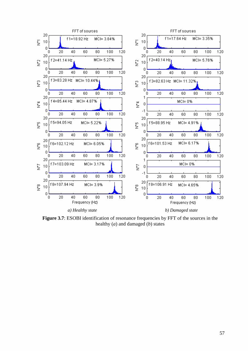
57

a) Healthy state b) Damaged state

Figure 3.7: ESOBI identification of resonance frequencies by FFT of the sources in the

healthy (a) and damaged (b) states

58

Figure 3.8: Mode shapes identified by ESOBI in two states: healthy and damaged states

Damage detection based on subspace angles

Several tests were achieved with the aircraft model in different conditions; they are

summarized in Table 3.1. Tests n° 1-3 compare various healthy states consisting of different

amplitude levels of excitation. The next tests correspond to three levels of damage with

increasing degrees, according to the removing of one, two and three connecting bolts

respectively.

Table 3.1: Condition of tests

Test n° 1 2 3 4 5 6

Condition Exc. 1.5:0.5 Exc. 1:0.5 Exc. 1:1.5 Dam. 1 Dam. 2 Dam. 3

Since sources n° 4 and 7 are not identified in the damaged states, only six mode-shapes

according to sources n° 1-3, 5, 6, 8 are considered in the subspace.

59

a) SOBI, BMID and PCA methods b) ESOBI, EBMID and NSA methods

Figure 3.9: Damage detection based on the subspace angles

Damage detection results based on the concept of subspace angle are presented in Figure

3.9. The results of the proposed methods (SOBI, BMID and ESOBI) are compared to those of

Principal Component Analysis (PCA) and Null Subspace Analysis (NSA) obtained in

Reference [137]. Like ESOBI and NSA, BMID may also be performed by assembling the

Hankel matrix, which is denoted here by EBMID. In Figure 3.9a, SOBI, BMID and PCA

detections are displayed together. Their indexes are quite similar; however, in the PCA-based

method, the first level of damage (Dam. 1) is not detected and the index corresponding to the

highest level (Dam. 3) is not the biggest. Conversely, in the SOBI and BMID-based methods,

the smallest damage can be detected and the levels of damage are logically revealed. It

appears in Figure 3.9a that the BMID-based method is the most sensitive to the presence of

damage.

Detection results obtained by the use the Hankel matrix (named ESOBI, EBMID and

NSA) are presented in Figure 3.9b.

To facilitate the comparison between the different methods, a common reference threshold

is used in Figure 3.10, i.e. the indexes are normalized such that the maximal indexes

according to the reference states (tests n° 1-3) are set to unity. According to Figure 3.10, the

normalized indexes show that damage detection by SOBI and BMID is better than by PCA;

ESOBI is more sensitive than NSA for damage levels 1 and 3 but EBMID is by far the most

sensitive method.

60

Figure 3.10: Normalized detection indexes by SOBI, PCA, BMID, ESOBI, NSA and EBMID

It is worth noting that when the Hankel matrix is combined with BMID, the number of

block rows might be less than in ESOBI and NSA. Actually, as the measured data is first

expanded using the Hilbert transform, BMID leads to double the size of the dataset. For an

equivalent size of the generated data matrix, the Hankel matrix applied to BMID requires only

half of the number of block rows which is used for ESOBI or NSA. Consequently the number

of block rows of the Hankel matrix in EBMID should be kept moderate to accommodate the

data generation. In Figures 3.9 and 3.10, the results were generated with a Hankel matrix

containing 10 block rows in the case of ESOBI and NSA and 5 block rows in the case of

EBMID.

In conclusion, damage detection based on the concept of subspace angle using SOBI or its

alternatives like ESOBI, BMID and EBMID looks very useful as illustrated in the above

example. The methods are sensitive to damage even if it is small. In the modal identification

step, we can detect damage occurrence, not only by looking at resonance frequency shifts but

also looking at disappearance of some sources. This helps to determine the dimensionality of

the problem and to construct an adequate subspace containing only compatible modes in

different states of the structure.

Damage detection using one single sensor

The construction of the Hankel matrix to apply SOBI allows to improve the identification

and furthermore to detect damage even if the number of sensors is small. While SOBI cannot

separate sources of narrow spectral band from only one sensor, ESOBI is able to handle this

task. It is illustrated in Figure 3.11a when only one sensor located at point 7 and 20 block

rows are used for the Hankel matrix. Similarly, the identification using EBMID is presented

in Figure 3.11b.

61

a) by ESOBI b) by EBMID

Figure 3.11: Identification of resonance frequencies, using only one sensor

Damage detection results based on the subspace angles are shown in Figure 3.12. In the

case of ESOBI, 20 block rows are used for the Hankel matrix and the best result is obtained

by considering the first two column vectors of the mixing matrix A in the feature subspaces.

In this case, damage of level 1 can be distinguished from the false-positive tests (Figure

3.12a). However, this damage is ignored if more vectors are taken into account, as shown in

Figure 3.12b. In the case of EBMID, the best detection is displayed in Figure 3.12c when 8

block rows are used and all the first three column vectors in matrix A are taken into account.

If fewer vectors are considered in the subspace, damage detection is similar to ESOBI result

in Figure 3.12a. Thus, EBMID still looks as more appealing when the number of sensor is

small.

a) ESOBI, by the first 2 vectors in A b) ESOBI, by more vectors c) EBMID

Figure 3.12: Damage detection by ESOBI and EBMID, only one sensor is used

62

3.6.2 Experiments on a nonlinear structure (impact excitation)

Let us consider the beam with a cubic stiffness at the end presented in Section 2.5. Since

the response of this structure submitted to impact excitation is non-stationary, the behavior of

SOBI depends on the excitation amplitude.

As shown in Poncelet et al., (2007)[101], SOBI identification is accurate for linear

systems with weak damping and distinct frequencies. So, at low impact level, the beam

behaves as a linear structure and the identification using SOBI gives good results. Figure 3.13

presents all the sources identified and their FFT respectively. Thanks to the MCI indicator, it

is easy to select three actual sources s1, s4 and s7. Each of these sources shows a monochrome

appearance with a pure dominant frequency.

a) b)

Figure 3.13: Sources (a) and their FFT (b) identified by SOBI for the linear state

Let us now examine an impact level at which nonlinearity is excited – (level L5 in §2.5.2).

As illustrated in Figure 3.14, the modal contribution indicator (MCI) allows the selection of

three sources s1, s3 and s6 for which the dominant frequencies correspond to the three actual

sources in the linear case. However, the perfect separation of the sources fails. Only the

source corresponding to the highest frequency (s6) appears to be not affected by the

nonlinearity. Sources s1 and s3, according to modes 1 and 2, show peaks respectively at 39.84

and 149.37 Hz which are clearly higher than in the linear case, but multiple frequency

components are also observed. A new frequency at 122.1 Hz appearing in those sources

corresponds to the third harmonic of the first frequency. As noted in the WT analysis, the

☼

☼

☼

amp

litu

de

63

„mode‟ associated to this harmonic is a combination of the first two „modes‟. This is the

reason why it prevents separating the first and the second „modes‟: the assumption of SOBI

that the sources are uncorrelated is no longer guaranteed in the nonlinear case.

a) b)

Figure 3.14: Sources (a) and their FFT (b) identified by SOBI for a nonlinear state

ESOBI

Figure 3.15 shows that ESOBI is successful in providing „monochrome‟ sources in the

interested frequency range. In this example, 35 block rows were used to construct the Hankel

matrix. The sources are sorted in ascending order of frequencies so that the harmonic of f1

corresponds to source s2; the remaining components correspond to f1, f2 and f3 respectively.

The corresponding columns in the mixing matrix A give deformation shapes of the

structure. Modes 1 and 2 are shown in Figure 3.16 for the linear state (maximum

displacement of 0.1 mm) and for the nonlinear state (maximum displacement of 1.4 mm)

respectively. The distinction between those two states is less clear in Figure 2.30 based on the

Wavelet Transform. The third mode at about 400 Hz is not influenced by the nonlinearity and

thus is not presented. The deformation shape corresponding to the 3rd

harmonic of the 1st

frequency is plotted in Figure 3.17. It is worth noting that this shape looks like the 2nd

mode,

which explains why this harmonic merges considerably with the second frequency in the

SOBI source s3 (Figure 3.14).

☼

☼

☼

amp

litu

de

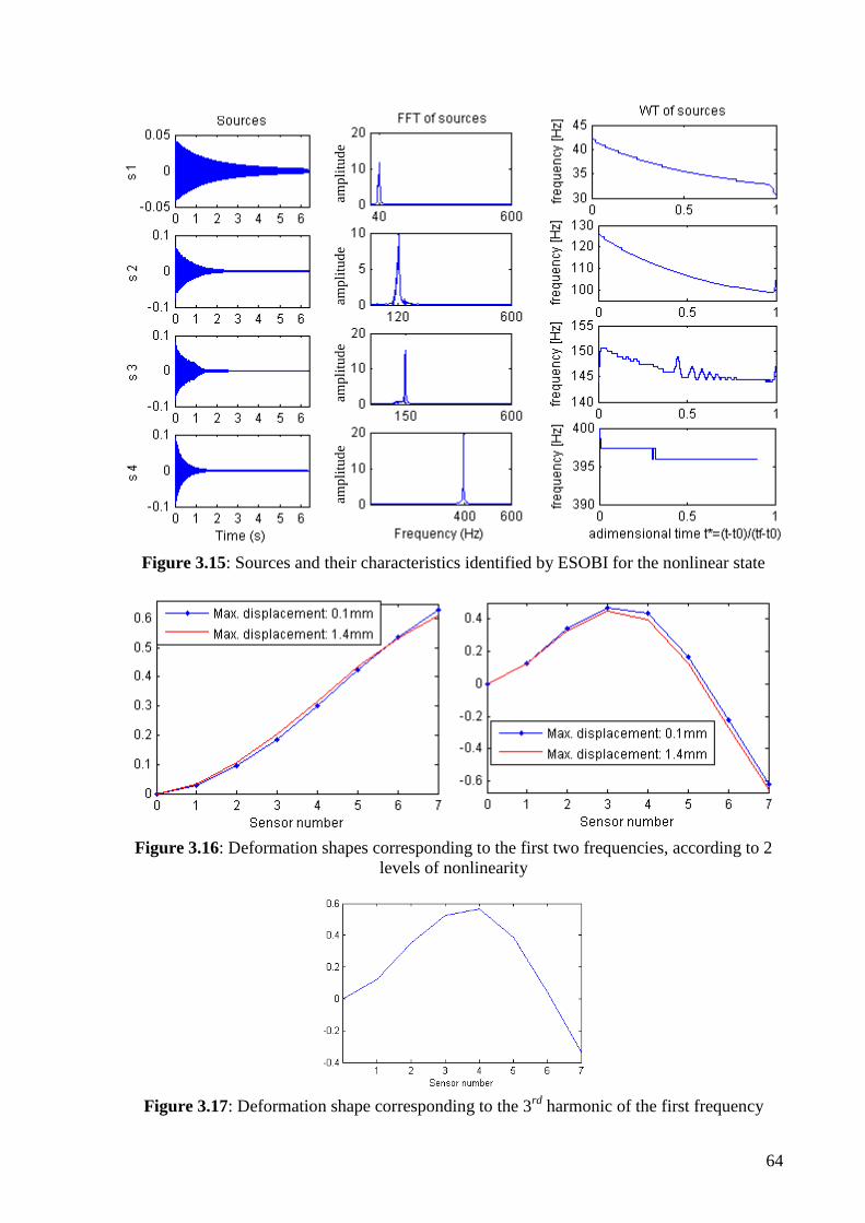
64

Figure 3.15: Sources and their characteristics identified by ESOBI for the nonlinear state

Figure 3.16: Deformation shapes corresponding to the first two frequencies, according to 2

levels of nonlinearity

Figure 3.17: Deformation shape corresponding to the 3rd

harmonic of the first frequency

amp

litu

de

amp

litu

de

amp

litu

de

amp

litu

de

65

Nonlinearity detection based on the concept of subspace angle

As the identification by SOBI fails when the behavior of the structure becomes nonlinear,

only ESOBI is considered in this section. As determined previously, the reference subspace

for the linear state contains three basic modes corresponding to the frequencies 31.8; 143.1

and 394.8 Hz. In Figure 3.18, the angles are represented in terms of the maximal displacement

measured at the end of the beam. The first tests correspond to the linear state of the structure

for which the maximal displacements is less than 0.1 mm. The last five tests correspond to

levels L1-L5 reported in § 2.5.2.

In Figure 3.18a, all the sensors are considered to determine the subspace angle index. In

Figure 3.18b, only one sensor (sensor n° 7) is used. These results show that ESOBI is able to

detect the onset of nonlinearity.

a) with full range of sensors b) with only one sensor

Figure 3.18: Detection by ESOBI

ESOBI with time-lag calibration

When SOBI and ESOBI are applied on the whole history of the data, they provide a single

set of modal characteristics. It is then necessary to resort to the Wavelet transform to

determine the instantaneous frequencies of the identified sources. However, it is also possible

to observe the non-stationary behavior of the structure thanks to the following technique

proposed for the ESOBI process. It consists in adjusting the time-lag between successive

block rows to construct the data-driven Hankel matrix. In equation (3.17), block rows are

shifted by one time sample. The time-shift can be extended to several intervals, i.e. the data

matrix is assembled in the following way:

66

1 2

1 2

1 ( 1) 2 ( 1) ( 1)

1,2

1 2

1 ( 1) 2 ( 1) ( 1)

1 (2 1) 2 (2 1) (2 1)

... ...

... ...

... ... ... ... ...

... ...

... ...

... ...

... ... ... ... ...

... ...

j

j

i i j i

i

i i j i

i i j i

i i j i

x x x

x x x

x x xH

x x x

x x x

x x x

(3.23)

where 1 and (2 1)j N i .

By choosing an adequate number of time-lags to represent the time distinction between

the block rows (so that the modulation of the dynamic responses is better exhibited), the data

matrix in (3.23) facilitates the analysis of signals involving time-varied dynamic states. In this

way, ESOBI becomes able to treat non-stationary data.

Figure 3.19: Sources of nonlinear behavior and their FFT according to the 1st linear mode, by

ESOBI with 40

amp

litu

de

67

Figure 3.19 presents identified sources and their FFTs corresponding to the first mode. In

this case, the blocks rows are shifted by 40 time samples, i.e. 0.0313 second. It can be

observed that each source appears at different instants: sources of higher frequency are active

at earlier times and vice-versa. The deformation shapes corresponding to some identified

sources are presented in Figure 3.20, which can also indicate varied levels of nonlinearity

during the measured period. Similar results are presented for the second mode in Figures 3.21

and 3.22.

Figure 3.20: Deformation shapes according to some sources in Figure 3.19

Figure 3.21: Sources according to the 2nd

linear mode and their FFT, by ESOBI with 40

amp

litu

de

68

Figure 3.22: Deformation shapes according to some sources in Figure 3.21

3.6.3 Experiments on a nonlinear structure (random excitation)

We first consider the nonlinear beam submitted to a low excitation level (as reported in

Figure 2.36). The application of SOBI gives the results shown in Figure 3.23. Even if the

sources are quite separated, some other components of very weak energy are present. The

application of ESOBI allows to improve the results as shown in Figure 3.24.

Figure 3.23: Sources and their FFTs identified by SOBI for low excitation

amp

litu

de

69

Figure 3.24: Sources and their FFTs identified by ESOBI for low excitation

Results obtained with a higher level of excitation (as reported in Figure 2.37) are shown in

Figures 3.25 and 3.26 for SOBI and ESOBI respectively. It can be observed that the problem

of mixing is more serious for SOBI. Fortunately, ESOBI appears to be still robust in this case

because it cleans up noisy components around the main frequency. As the vibration amplitude

of the beam varies in a quite large band, the first and second sources obtained do not show a

single spectral component. For example, f1 presents some peaks in the frequency range from

32.5 to 38 Hz; f2 from 133.5 to 136 Hz and f3 appears as unchanged. For the sake of

completeness, the WT of sources s1 and s2 is given in Figure 3.27.

Figure 3.25: Sources and their FFTs identified by SOBI for high excitation

amp

litu

de

amp

litu

de

70

Figure 3.26: Sources and their FFTs identified by ESOBI for high excitation

Figure 3.27: WT of sources s1 and s2 respectively

Figure 3.28 gives ESOBI deformation shapes according to the first two frequencies for

two levels of excitation.

a) the 1st deformation shape b) the 2

nd deformation shape

Figure 3.28: ESOBI deformation shapes corresponding to the first two sources, according

to 2 levels of nonlinearity

amp

litu

de

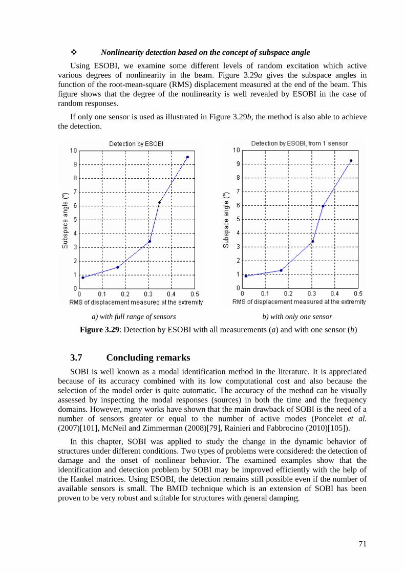
71

Nonlinearity detection based on the concept of subspace angle

Using ESOBI, we examine some different levels of random excitation which active

various degrees of nonlinearity in the beam. Figure 3.29a gives the subspace angles in

function of the root-mean-square (RMS) displacement measured at the end of the beam. This

figure shows that the degree of the nonlinearity is well revealed by ESOBI in the case of

random responses.

If only one sensor is used as illustrated in Figure 3.29b, the method is also able to achieve

the detection.

a) with full range of sensors b) with only one sensor

Figure 3.29: Detection by ESOBI with all measurements (a) and with one sensor (b)

3.7 Concluding remarks

SOBI is well known as a modal identification method in the literature. It is appreciated

because of its accuracy combined with its low computational cost and also because the

selection of the model order is quite automatic. The accuracy of the method can be visually

assessed by inspecting the modal responses (sources) in both the time and the frequency

domains. However, many works have shown that the main drawback of SOBI is the need of a

number of sensors greater or equal to the number of active modes (Poncelet et al.

(2007)[101], McNeil and Zimmerman (2008)[79], Rainieri and Fabbrocino (2010)[105]).

In this chapter, SOBI was applied to study the change in the dynamic behavior of

structures under different conditions. Two types of problems were considered: the detection of

damage and the onset of nonlinear behavior. The examined examples show that the

identification and detection problem by SOBI may be improved efficiently with the help of

the Hankel matrices. Using ESOBI, the detection remains still possible even if the number of

available sensors is small. The BMID technique which is an extension of SOBI has been

proven to be very robust and suitable for structures with general damping.

72

When time signals are non-stationary, the Wavelet Transform provides a better

mathematical framework for the analysis. However, ESOBI can also give helpful information

at a low computational cost as the time transformation of the dynamic responses can be

observed by enlarging the time-lag between block rows of the data matrix or by the

application of WT on the sources.

73

Chapter 4

Fault Detection Based on

Kernel Principal Component Analysis

4.1 Introduction

Principal Component Analysis (PCA) is a linear multivariable statistical method that can

be used for damage detection of structures or fault diagnosis in mechanical systems. In

Section 1.3, the advantages and limitations of PCA have been discussed along with its

derivations for nonlinear contexts. This chapter focuses on a nonlinear extension of PCA

named Kernel Principal Component Analysis (KPCA) which authorizes features such that the

relation between variables is nonlinear.

The KPCA method is “flexible” in the sense that different kernel functions may be used to

better fit the testing data. KPCA shows a remarkable advantage with respect to other

nonlinear PCA approaches because the method does not require nonlinear optimization. In the

beginning, KPCA has interested many scientists in the domain of image processing

(Schölkopf et al. (1998)[115], (1999)[116] and Kim et al. (2005)[58]). These researchers

showed that KPCA may reveal more advantageous than other techniques such as PCA or

Wavelet transform etc. in encoding image structure. In the last five years, KPCA has been

introduced in other fields of research as reported in Chapter 1 (chemical domain, industrial

machine or mechanical system) and has shown its ability in the monitoring of nonlinear

process.

We deal here with the detection problem in mechanical structures where nonlinearity

appears implicitly in the responses. The content of the chapter is as follows. First the PCA

method is described briefly as it constitutes the background of the proposed method. Next, the

kernel PCA method is introduced to deal with nonlinear systems and the definition of the

covariance-driven block Hankel matrix is recalled. The method is illustrated on experimental

examples and applications. The first example is the detection of the nonlinearity onset in the

beam with geometric nonlinearity. The next examples consist in detecting damage in a

rotating device and in controlling quality of welded joints. Two types of index are used for the

detection: (1)-the subspace angle and (2)-the Hotelling‟s T2 statistics and the Q-statistics.

4.2 Principal Component Analysis

Let us suppose that a dynamical system characterized by a set of vibration features

identified at time tk is represented by the m-dimensional vector kx ( 1,..., )k N , where N is

74

the number of samplings. All the samples are collected in the observation matrix X m N . In

general, PCA involves a data normalization procedure, which leads to a set of variables with

zero-mean and unitary standard deviation (Yan et al. (2005)[134]), i.e.

norm k

k

x

x xx

(4.1)

where x and x are the mean and standard deviation of each dataset, respectively:

1

1 N

k

kN

x x ; 2

1

1 N

x k

kN

x x

PCA, known as Karhunen-Loève transform or Proper Orthogonal Decomposition (POD)

(Krzanowski (2000)[63]), provides a linear mapping of data from the original dimension m to

a lower dimension p using the transformation:

Y = TX (4.2)

where p NY is called the score matrix and p mT the loading matrix. The dimension p

represents the physical order of the system or the number of principal components which

affect the vibration features. The loading matrix may be found from the main p eigenvectors

of the covariance matrix of X. In practice, PCA is often computed by Singular Value

Decomposition of the covariance matrix, i.e.

T TXX UΣU (4.3)

where U is an orthonormal matrix whose columns define the principal components (PCs) and

form a subspace spanning the data. The energy of those PCs is represented by the

corresponding singular values on the diagonal of matrix Σ . The singular values are written in

decreasing order:

1 2 1diag( ) , , ..., , , ...,p p mΣ with 1 2 1... ... 0p p m (4.4)

The order p of the system is determined by selecting the first p singular values in Σ

which have a significant magnitude („energy‟) as described in De Boe (2003)[17]. However,

the remaining singular values do not entirely equal zero due to noise or to nonlinear effects.

It is worth noting that, under some assumptions, PCs in matrix U may represent the

vibration modes of the system (Feeny and Kappagantu (1998)[26], Feeny and Liang

(2002)[27]).

Selection of active principal components

The quality of the representation of the observation space through PCs can by quantified

by inspection of the values j . The percentage of energy associated to a PC is defined by De

Boe (2003)[17]:

1

Energyj

j m

i

i

(4.5)

One can fix a threshold in terms of cumulated energies: 1

Energyj

i

i

(j = 1,…, m) which

allows to select the effective number of PCs that is required for a good representation of the

75

observation matrix X. In practice, a cumulated energy of 75% to 95% is generally adequate

for the selection of the active PCs.

4.3 Kernel Principal Component Analysis

The definitions and formulation presented here follow closely the ones described in

Schölkopf et al. (1999)[116] and He et al. (2007)[40].

The key idea of KPCA is first to define a nonlinear map k kx x with

, ( 1,..., )m

k k N x which represents a high dimensional feature space F, and then to apply

PCA to the data in space F.

Suppose that the mapped data are centered, i.e. 1

( ) 0N

i

i

x , then the covariance matrix

in the space F is:

T

1

1( ) ( )

N

i i

iN

C x x (4.6)

Principal components may be next extracted by solving the eigenvalue equation:

V CV (4.7)

All the eigensolutions V with 0 must lie in the subspace spanned by

1( ),..., ( )N x x , which means that coefficients i , ( 1,..., )i N exist such that:

1

( )N

i i

i

V x (4.8)

Pre-multiplication of equation (4.7) by T( )k x gives:

T T( ) ( )k k x V x CV ( 1,...,k N ) (4.9)

Let us define the kernel matrix K of dimension N N such that:

T( , ) ( ) ( )i j ij i jK K x x x x (4.10)

Mercer‟s theorem of functional analysis implies that the kernel function is a continuous

kernel of a positive integral operator. For instance, the following kernel functions proposed by

Vapnik (1995)[127], may be used:

polynomial kernel,

T( , ) ( 1)di j i jK x x x x , where d is a positive integer (4.11)

radial basis function (RBF),

2

2( , ) exp

2

i j

i jK

x xx x (4.12)

where 22 w is the width of the Gaussian kernel

sigmoid kernel,

76

T( , ) tanh ( )i j i jK b x x x x (4.13)

It is worth noting that in general, the above kernel functions give similar results if

appropriate parameters are chosen. The sigmoid kernel does not always satisfy Mercer‟s

theorem. The RBF can present advantages owing to its flexibility in choosing the associated

parameter. For example, the width of the Gaussian kernel can be very small (<1) or quite

large. Contrarily the polynomial kernel requires a positive integer for the exponent. In the

present work, we use the polynomial and RBF kernels.

The combination of equations (4.6) to (4.10) yields:

N α Kα (4.14)

where α is the column vector collecting the coefficients 1,..., N . Similarly to PCA, KPCA

requires the data points ( )i x , ( 1,..., )i N to be centered in the feature space F, so that the

centered kernel matrix is defined:

1 1 1 1ij N N N N ijK K K K K (4.15)

where 1N is a matrix of dimension N N of which 1 1/N ijN . Further details may be found

in Reference Schölkopf et al. (1998)[115].

Replacing K in equation (4.14) by K , the eigenvalue equation may be rewritten by:

N α Kα (4.16)

The eigenvalues associated to the eigenvectors of K : 1 2, ,..., Nα α α , are ordered in

descending order 1 2 1... ... 0p p N where

1,...,p N are negligible with

respect to the first p eigenvalues (suppose that 0 ). Normalization of 1,..., pα α results

from the normalization of the corresponding vectors in F, i.e.

T 1k k V V (k =1,…, p) (4.17)

According to equations (4.8), (4.10) and (4.16), it follows that:

T 1k k k α α (4.18)

The eigenvectors identified in the feature space F can be considered as kernel principal

components (KPCs), which characterize the dynamical system in each working state.

Note that, since the number of eigenvectors (i.e. nonlinear PCs) is the same as the number

of samples, it is higher than the number of (linear) PCs given by PCA. The KPCA method is

termed “nonlinear” since the feature mapping in the space F is achieved by a nonlinear

function (Eqs. 4.11-4.13). Thanks to that property, extracted KPCs should be able to reflect

nonlinear or high order features which allow the representation and classification of varied

states. For example, Figure 4.1 represents the PCA and KPCA features and the corresponding

principal eigenvector V in the bi-dimensional input space. According to Schölkopf et al.

(1999)[116], KPCA has the capability to use more nonlinear PCs than PCA, which allows to

collect more structural features rather than noise.

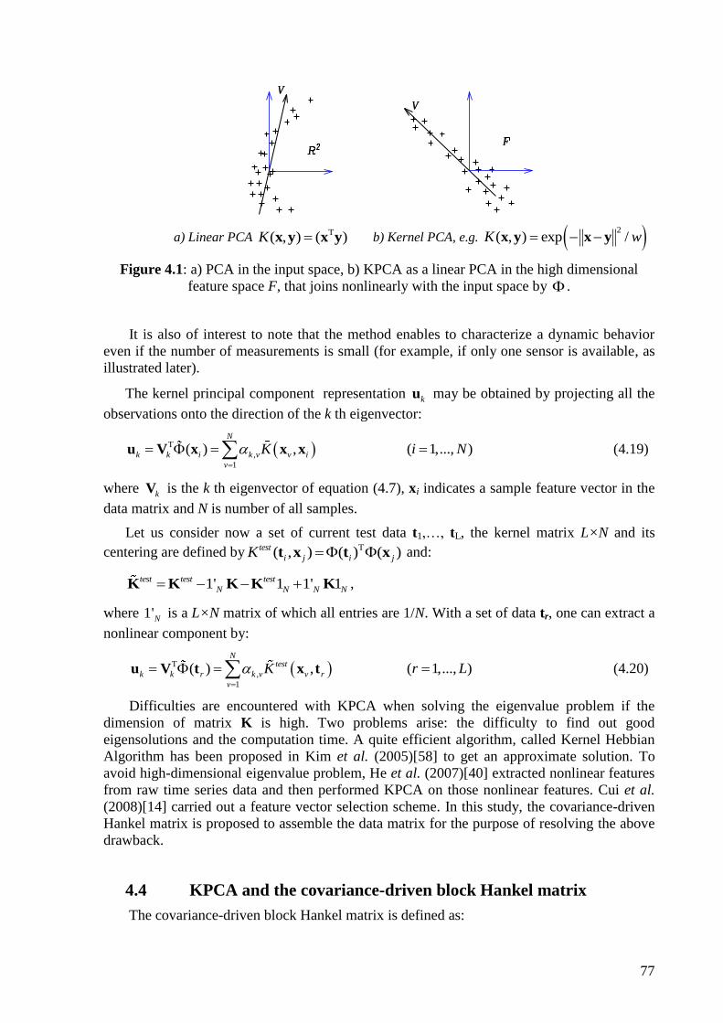
77

a) Linear PCA T( , ) ( )K x y x y b) Kernel PCA, e.g. 2

( , ) exp /K w x y x y

Figure 4.1: a) PCA in the input space, b) KPCA as a linear PCA in the high dimensional

feature space F, that joins nonlinearly with the input space by .

It is also of interest to note that the method enables to characterize a dynamic behavior

even if the number of measurements is small (for example, if only one sensor is available, as

illustrated later).

The kernel principal component representation ku may be obtained by projecting all the

observations onto the direction of the k th eigenvector:

T

,

1

( ) ,N

k k i k v v i

v

K

u V x x x ( 1,..., )i N (4.19)

where kV is the k th eigenvector of equation (4.7), xi indicates a sample feature vector in the

data matrix and N is number of all samples.

Let us consider now a set of current test data t1,…, tL, the kernel matrix L×N and its

centering are defined by T( , ) ( ) ( )test

i j i jK t x t x and:

1' 1 1' 1test test test

N N N N K K K K K ,

where 1'N is a L×N matrix of which all entries are 1/N. With a set of data tr, one can extract a

nonlinear component by:

T

,

1

( ) ,N

test

k k r k v v r

v

K

u V t x t ( 1,..., )r L (4.20)

Difficulties are encountered with KPCA when solving the eigenvalue problem if the

dimension of matrix K is high. Two problems arise: the difficulty to find out good

eigensolutions and the computation time. A quite efficient algorithm, called Kernel Hebbian

Algorithm has been proposed in Kim et al. (2005)[58] to get an approximate solution. To

avoid high-dimensional eigenvalue problem, He et al. (2007)[40] extracted nonlinear features

from raw time series data and then performed KPCA on those nonlinear features. Cui et al.

(2008)[14] carried out a feature vector selection scheme. In this study, the covariance-driven

Hankel matrix is proposed to assemble the data matrix for the purpose of resolving the above

drawback.

4.4 KPCA and the covariance-driven block Hankel matrix

The covariance-driven block Hankel matrix is defined as:

78

1 2

2 3 1

1 1

... ...

... ...

... ... ... ... ...

... ...

c

c

r r r c

Δ Δ Δ

Δ Δ ΔX

Δ Δ Δ

( c r ) (4.21)

where r, c are user-defined parameters (r = c in this study) and iΔ represents the output

covariance matrix defined by:

T

1

1 N i

i k i k

kN i

Δ x x ( 0 1i N ) (4.22)

where kx is the measurement vector at time step k and N is the number of sampling points.

The covariance-driven Hankel matrix characterizes the dynamics of the analyzed signals

and has been used for modal identification and damage detection. If the covariance-driven

Hankel matrix is considered as the input data matrix for the KPCA procedure and the number

of block rows r is equal to the number of block columns c, so X is a square matrix. Its size is

determined by the product of the number of blocks and the dimension m of vector xk.

4.5 KPCA monitoring using the concept of subspace angle and

statistics

In the previous chapters, the detection problem has been achieved using the concept of

subspace angle between subspaces constructed by mode-shape vectors (in WT, SOBI) or by

principal component vectors (in PCA). In KPCA, the same procedure may be applied by

constructing the subspace with the kernel principal components (KPCs) which characterize

the feature space F. This section presents other detection indexes based on statistics.

A popular method for dynamical monitoring is the chart of Hotelling‟s T2 statistics and the

Q-statistics, also known as the squared prediction error (SPE) which are depicted in Figure

4.2. T2 measures the distance in the principal subspace (spanned by the first p PCs), whereas

SPE characterizes the distance in the residual subspace (spanned by the remaining PCs, which

is orthogonal to the principal subspace). In general, the use of T2 and SPE distances in

detection methods based on linear PCs (PCA method) is expressed in terms of Mahalanobis

and Euclidian distances, respectively. The only difference here is that those indexes are built

in the feature subspace in order to exploit the results of KPCA. The following formulation

proposed by Lee et al. (2004)[69] shows interesting because of its simplicity.

Figure 4.2: Graphical description of the two monitoring statistics T2 and SPE

T2 measures the variation within the model subspace, which is the sum of the normalized

squared scores defined as:

79

T2 1

1 1,..., ,...,p pT u u Λ u u (4.23)

where ku is obtained by (4.19) or (4.20) and 1

Λ is the diagonal matrix of the inverse of the

eigenvalues associated with p retained PCs. Assuming that the scores have a multivariate

normal distribution, the confidence limit for T2 is calculated using the Snedecor's F

distribution (F-distribution) as:

2

, , , ,

( 1)p N p N p

p NT F

N p

(4.24)

where N is the number of samples in the model or the size of the covariance-driven block

Hankel matrix if this matrix is used. , ,p N pF is a F-distribution with degrees of freedom p and

N-p with level of significance [69].

Figure 4.3: Conceptual diagram of KPCA

In the KPCA method, the observations are not analyzed in the input space, but in the

feature space F. The measure of goodness of fit of a sample to the PCA model was suggested

through a simple calculation of SPE in the feature space F. The conceptual framework of the

KPCA method is shown schematically in Figure 4.3 (Romdhani et al. (1999)[110]). First, an

input vector x is projected using a nonlinear mapping Φ in a high-dimensional feature space

F. Then linear PCA is performed in this feature space and gives score values uk in a lower p-

dimensional KPCA space (eq. (4.19) or (4.20)). A feature vector ( ) x may be reconstructed

from uk by projecting uk into the feature space via kV and it results in a reconstruction with p

PCs in the feature space: 1

ˆ ( )p

p k kk x u V . The SPE statistics in the feature space is

defined by: 2

ˆSPE ( ) ( )p x x . ( ) x is just identical to 1

ˆ ( )h

h k kk x u V where h is

the number of nonzero eigenvalues generated from (4.14) among all the N eigenvalues. The

SPE can be deduced from the expression: 2 2

T T Tˆ ˆ ˆ ˆ ˆ ˆ ˆ ˆ ˆSPE ( ) ( ) ( ) ( ) ( ) ( ) 2 ( ) ( ) ( ) ( )p h p h h h p p p x x x x x x x x x x

T T T

1 1 1 1 1 12

h h h p p p

k k i i k k i i k k i ik i k i k i u V u V u V u V u V u V

2 2 2 2 2

1 1 1 1 12

h p p h p

k k k k kk k k k k u u u u u (4.25)

T

,

1

( ) ,N

k k i k v v i

v

K

u V x x x

80

as T 1k i V V when k=i, otherwise T 0k i V V .

Assuming that the prediction errors are normally distributed, the confidence limit for the

SPE is calculated by fitting a weighted 2 -distribution and is given by:

2

2

2 / ,SPE

2 e v

v

e

(4.26)

where e and v are the estimated mean and variance of the SPE, respectively (Nomikos and

MacGregor (1995)[93]). This approximating distribution works well even in cases for which

the errors do not follow a Gaussian distribution.

Given the T2 and SPE statistics as well as their control limits, we can compute outlier

statistics to count how many prediction errors (represented in percentage) overpass the control

limits for each state. In normal condition, i.e. without damage, the outlier statistics of the

current data should be similar to the statistics of the reference state. Conversely, the feature

subspace associated with a damage state should present significant changes from the reference

state. Thus, the outlier statistics in this case should increase clearly. In order to compare the

statistics related to two different sets of data, the ratio Sd /Sr is also computed, where d and r

denote the damage and the reference states respectively, S describes the average SPE or T2 in

according statistic measurements. While Sd /Sr → 1 indicates a normal state, a higher value of

this ratio can indicates the occurrence of a possible damage.

In the following, the KPCA-based detection method is illustrated on some examples in

which the different indexes (based on the concept of subspace angle and on the T2 and SPE

statistics) are considered.

4.6 Detection of nonlinearity onset

Let us consider again the beam with the geometric nonlinearity presented in Chapters 2

and 3. Now KPCA is used on the experimental data corresponding to the two types of

excitation (impact and random).

In this example, KPCA is used with the aim of detecting the onset of nonlinear behavior

when the load level is increasing. The detection is first based on the concept of subspace angle

and KPCA is compared to the classical PCA. A zero-mean normalization of the measured

responses is first performed in order to obtain centered data sets. A mean-variance

normalization procedure can be also realized to take into account different working conditions

of the system and the variety of sensors. Results based on the T2 and SPE statistics are

presented later.

4.6.1 Impact excitation

Twelve impact tests were performed as reported in Table 4.1. Tests n° 1-7 correspond to

the linear behavior of the structure and play the role of false-positive. In tests n° 8-12, the

nonlinear behavior of the structure is activated with increasing levels.

For this type of excitation, the nonlinear behavior is the strongest at early stages and

vanishes progressively due to the presence of damping. For this reason, we consider responses

in the first time interval of [0; 0.5 s]. Accelerations measured at the seven locations in Figure

2.27 are used for constructing the observation matrix X.

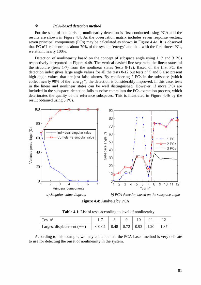
81

PCA-based detection method

For the sake of comparison, nonlinearity detection is first conducted using PCA and the

results are shown in Figure 4.4. As the observation matrix includes seven response vectors,

seven principal components (PCs) may be calculated as shown in Figure 4.4a. It is observed

that PC n°1 concentrates about 70% of the system „energy‟ and that, with the first threes PCs,

we attaint nearly 100%.

Detection of nonlinearity based on the concept of subspace angle using 1, 2 and 3 PCs

respectively is reported in Figure 4.4b. The vertical dashed line separates the linear states of

the structure (tests 1-7) from the nonlinear states (tests 8-12). Based on the first PC, the

detection index gives large angle values for all the tests 8-12 but tests n° 5 and 6 also present

high angle values that are just false alarms. By considering 2 PCs in the subspace (which

collect nearly 90% of the „energy‟), the detection is considerably improved. In this case, tests

in the linear and nonlinear states can be well distinguished. However, if more PCs are

included in the subspace, detection fails as noise enters into the PCs extraction process, which

deteriorates the quality of the reference subspaces. This is illustrated in Figure 4.4b by the

result obtained using 3 PCs.

a) Singular-value diagram b) PCA detection based on the subspace angle

Figure 4.4: Analysis by PCA

Table 4.1: List of tests according to level of nonlinearity

Test n° 1-7 8 9 10 11 12

Largest displacement (mm) < 0.04 0.48 0.72 0.93 1.20 1.37

According to this example, we may conclude that the PCA-based method is very delicate

to use for detecting the onset of nonlinearity in the system.

82

KPCA-based detection method

KPCA differs from PCA, notably in the number of kernel principal components (KPCs)

which is equal to the number N (e.g. of time samples) whereas the number of PCs in the PCA

method is equal to the number m of measurement responses. In the KPCA method, the energy

distribution of KPCs depends on the parameter chosen in the kernel function. The results

shown in Figure 4.5 were achieved with KPCA using the polynomial kernel function with the

exponent d = 2. The eigenvalue diagram shows that the first seven KPCs capture most of the

system energy.

a) Eigenvalue diagram b) KPCA detection based on the subspace angle

Figure 4.5: Analysis by KPCA

Note that KPCs do not have any specific physical meanings, as reported in He et al.

(2007)[40], contrary to PCs in PCA which may represent modal features (e.g. mode-shapes)

under certain circumstances [26]. However, KPCs are useful for classifying different dynamic

behaviors of the system. To assemble enough effective information, the KPCA method needs

to add up a sufficiently large number of KPCs in the subspace. Regarding PCA, as discussed

earlier, the quality of the detection may be deteriorated by the use of more and more PCs in

the analysis as noise energy is then taken into account and perturbs the procedure. On the

other hand, KPCA offers a possibility to redistribute the energy of KPCs, i.e. to regulate the

main energy on the first but also on secondary KPCs (as discussed in the next paragraph). In

other words, KPCA helps to extract several first representative KPCs and to decline noise

which is related mainly to last components. As shown in Figure 4.5b, the use of 5 KPCs

allows a good detection as the index given by false-positives tests remains low. It is

interesting to note that by taking into account more KPCs, the detection is actually performed

in a stable manner. In this example, it is optimal with 6 or 7 KPCs. In conclusion, the KPCA-

based method looks more effective than the PCA-based method for the detection of the onset

of the nonlinear behavior of a system.

83

Discussion on the choice of the kernel parameter

Kernel parameters (e.g the exponent in the polynomial kernel or the width of the Gaussian

kernel) are user-defined quantities and different values of these parameters may produce

unequal effects. For illustration, let us consider further two examples by varying the kernel

parameters, as shown in Figures 4.6 and 4.7. The comparison between pictures (a) of these

figures and Figure 4.5a reveals clear differences.

a) Eigenvalue diagram b) KPCA detection based on the subspace angle

Figure 4.6: KPCA detection with the width of the Gaussian kernel w = 4

a) Eigenvalue diagram b) KPCA detection based on the subspace angle

Figure 4.7: KPCA detection with the width of the Gaussian kernel w = 35

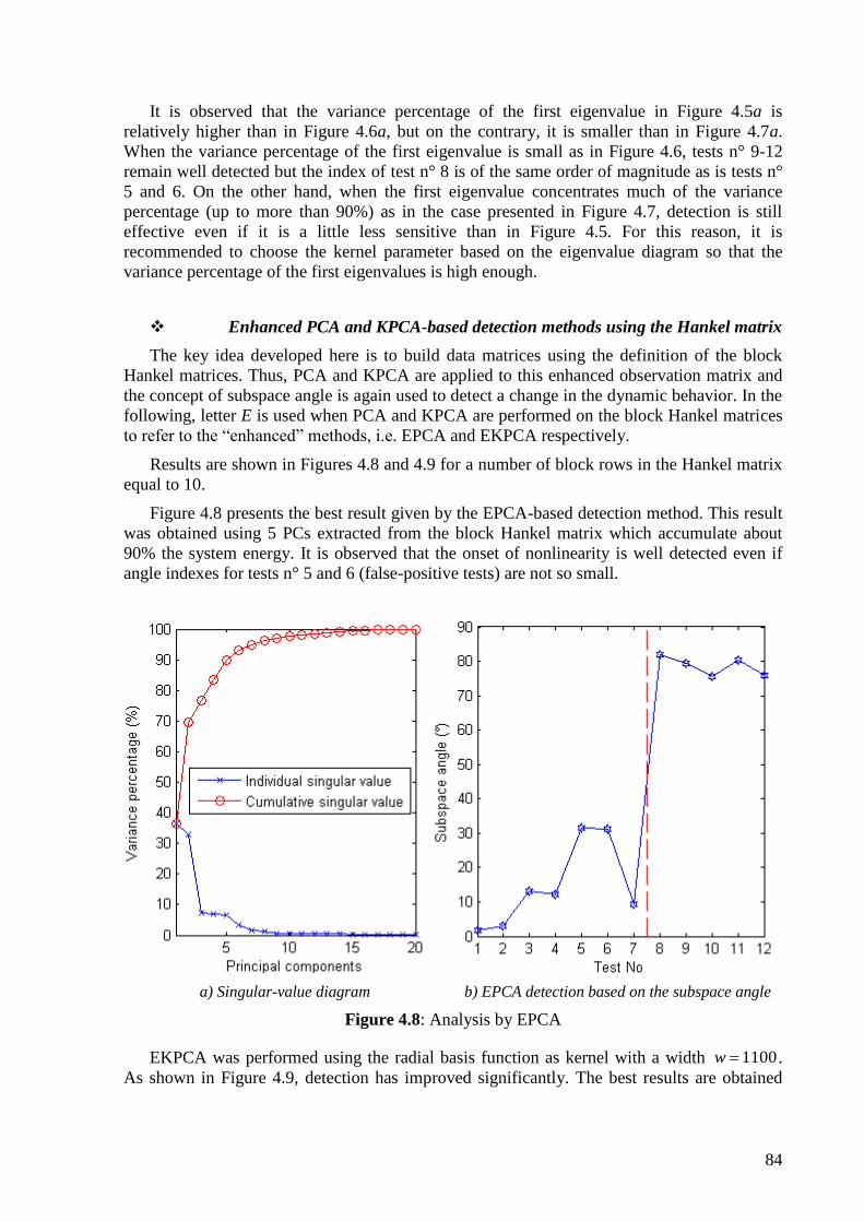
84

It is observed that the variance percentage of the first eigenvalue in Figure 4.5a is

relatively higher than in Figure 4.6a, but on the contrary, it is smaller than in Figure 4.7a.

When the variance percentage of the first eigenvalue is small as in Figure 4.6, tests n° 9-12

remain well detected but the index of test n° 8 is of the same order of magnitude as is tests n°

5 and 6. On the other hand, when the first eigenvalue concentrates much of the variance

percentage (up to more than 90%) as in the case presented in Figure 4.7, detection is still

effective even if it is a little less sensitive than in Figure 4.5. For this reason, it is

recommended to choose the kernel parameter based on the eigenvalue diagram so that the

variance percentage of the first eigenvalues is high enough.

Enhanced PCA and KPCA-based detection methods using the Hankel matrix

The key idea developed here is to build data matrices using the definition of the block

Hankel matrices. Thus, PCA and KPCA are applied to this enhanced observation matrix and

the concept of subspace angle is again used to detect a change in the dynamic behavior. In the

following, letter E is used when PCA and KPCA are performed on the block Hankel matrices

to refer to the “enhanced” methods, i.e. EPCA and EKPCA respectively.

Results are shown in Figures 4.8 and 4.9 for a number of block rows in the Hankel matrix

equal to 10.

Figure 4.8 presents the best result given by the EPCA-based detection method. This result

was obtained using 5 PCs extracted from the block Hankel matrix which accumulate about

90% the system energy. It is observed that the onset of nonlinearity is well detected even if

angle indexes for tests n° 5 and 6 (false-positive tests) are not so small.

a) Singular-value diagram b) EPCA detection based on the subspace angle

Figure 4.8: Analysis by EPCA

EKPCA was performed using the radial basis function as kernel with a width 1100w .

As shown in Figure 4.9, detection has improved significantly. The best results are obtained

85

with 7 or 8 KPCs (up to 95% of the system energy). According to this example, EKPCA

enables a clear classification between linear and nonlinear behaviors.

a) Eigenvalue diagram b) EKPCA detection based on the subspace angle

Figure 4.9: Analysis by EKPCA

Figure 4.10: KPCA and EKPCA detections by only one sensor

As mentioned earlier, the number of KPCs in KPCA is directly related to the number N of

time samples and thus, is not conditioned by the number of measured responses. For this

86

reason, it is always possible to construct a subspace even if only one response signal is

available. (Note that it is also the case with PCA if the block Hankel matrix is exploited). For

example, the detection results using KPCA and EKPCA based on the single response of

sensor 7 are given in Figure 4.10. It can be seen that, using one sensor only, KPCA suffers

the same problem as PCA: tests n° 5 and 6 (which differs from the other linear states by the

testing conditions) are falsely detected positive. On the other hand, EKPCA shows its

capability to make a clear distinction between the linear and the nonlinear states of the

structure.

Let us now examine the problem through the T2 and SPE statistics. Since the detection

indexes are statistics measured according to various excitation levels, the data is normalized

to have zero mean and a unitary standard deviation. For example, two tests representing two

different states (test n° 1 and 8) are examined and the results are shown in Figures 4.11 and

4.12 respectively when all sensors are used. The monitoring diagram is split into two parts:

the left part trains the reference data and the right part analyzes the current data. The

difference between the two tests can be revealed by the SPE statistics, especially by the ratios

Sd /Sr. For test n° 1, Sd /Sr is equal to about 6 but it rises up to more than 2000 for test n° 8.

Nevertheless, the T2 charts do not reveal any change. The SPE result is summarily reported in

Figure 4.13 for all tests. The SPE monitoring, presenting outlier statistics, is 100% for all

nonlinear states but also for tests n° 5 and 6. Fortunately, linear and nonlinear behaviours can

be perfectly distinguished through the ratio Sd /Sr. All tests n° 8-12 show predominant SPE

ratios with respect to the previous tests. Those results reveal also that the nonlinearity onset is

clearly detected by the SPE ratios even if the level of nonlinearity is not well identified. For

instance, tests n° 11 and 12 which correspond to the highest levels of nonlinearity present

smaller indexes than tests n° 8-10. Consequently, in this problem, the detection of nonlinear

behaviour based on the concept of subspace angle seems more attractive because the angles

reflect well the level of nonlinearity.

Figure 4.11: SPE and T2 statistics - test n° 1 (linear behavior)

87

Figure 4.12: SPE and T2 statistics - test n° 8 (nonlinear behavior)

Figure 4.13: EKPCA detection based on the SPE statistics

4.6.2 Random excitation

Time samples of 0.5s were analyzed and classified according to the root-mean-square

(RMS) value of the measured displacement amplitude at the end of the beam.

Twenty tests were studied as shown in Figure 4.14: seven training samples corresponding

to tests n° 1-7 play the role of false-positive and thirteen testing samples corresponding to

tests n° 8-20 present nonlinear behaviors.

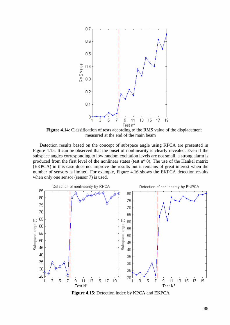
88

Figure 4.14: Classification of tests according to the RMS value of the displacement

measured at the end of the main beam

Detection results based on the concept of subspace angle using KPCA are presented in

Figure 4.15. It can be observed that the onset of nonlinearity is clearly revealed. Even if the

subspace angles corresponding to low random excitation levels are not small, a strong alarm is

produced from the first level of the nonlinear states (test n° 8). The use of the Hankel matrix

(EKPCA) in this case does not improve the results but it remains of great interest when the

number of sensors is limited. For example, Figure 4.16 shows the EKPCA detection results

when only one sensor (sensor 7) is used.

Figure 4.15: Detection index by KPCA and EKPCA

89

Figure 4.16: Detection using only one sensor

4.7 Fault detection in industrial applications

4.7.1 Damage detection in electro-mechanical devices

This industrial application concerns the case of electro-mechanical devices for which the

overall quality at the end of the assembly line has to be assessed.

A set of five good (healthy) devices and four damaged devices was considered. Dynamic

responses were collected by one mono-axial accelerometer on the top and one tri-axial

accelerometer on the flank of the device as illustrated in Figure 4.17. Only data measured in

one direction on the flank (X, Y, Z in Figure 4.17) or on the top of the device is used for the

detection.

Figure 4.17: Location of the accelerometers on the electro-mechanical device: one mono-

axial accelerometer on the top and one tri-axial accelerometer on the flank of the device

It is worth recalling that with only one sensor response, detection cannot be performed by

a subspace method like PCA. For this reason, fault detection was realized by Rutten et al.

(2009)[112] through Null subspace analysis (NSA), using the Novelty Index (NI) based on the

Mahalanobis norm. In this work, the authors based their detection on outlier statistics

X Z

Y

Top monoaxial

accelerometer

Flank triaxial

accelerometer

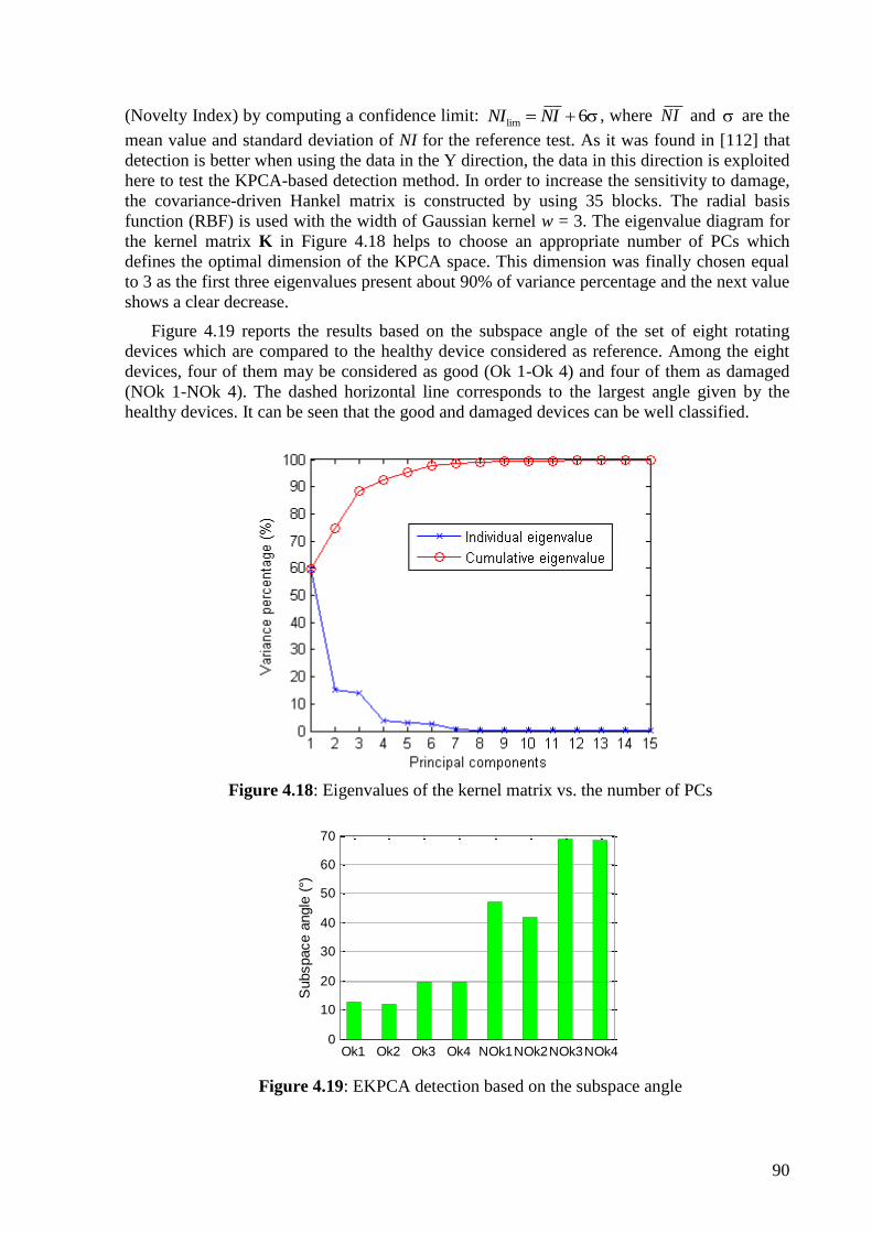
90

(Novelty Index) by computing a confidence limit: lim 6NI NI , where NI and are the

mean value and standard deviation of NI for the reference test. As it was found in [112] that

detection is better when using the data in the Y direction, the data in this direction is exploited

here to test the KPCA-based detection method. In order to increase the sensitivity to damage,

the covariance-driven Hankel matrix is constructed by using 35 blocks. The radial basis

function (RBF) is used with the width of Gaussian kernel w = 3. The eigenvalue diagram for

the kernel matrix K in Figure 4.18 helps to choose an appropriate number of PCs which

defines the optimal dimension of the KPCA space. This dimension was finally chosen equal

to 3 as the first three eigenvalues present about 90% of variance percentage and the next value

shows a clear decrease.

Figure 4.19 reports the results based on the subspace angle of the set of eight rotating

devices which are compared to the healthy device considered as reference. Among the eight

devices, four of them may be considered as good (Ok 1-Ok 4) and four of them as damaged

(NOk 1-NOk 4). The dashed horizontal line corresponds to the largest angle given by the

healthy devices. It can be seen that the good and damaged devices can be well classified.

Figure 4.18: Eigenvalues of the kernel matrix vs. the number of PCs

Ok1 Ok2 Ok3 Ok4 NOk1NOk2NOk3NOk40

10

20

30

40

50

60

70

Subspace a

ngle

(°)

Figure 4.19: EKPCA detection based on the subspace angle

91

On the other hand, the devices are also controlled by means of the statistics. First, a

healthy device is examined and the results are shown in Figure 4.20. As expected, Figure 4.20

does not reveal any fault because the outlier statistics of the current data is not relevant and

the ratios Sd /Sr remain close to unity for both SPE and T2. The confidence limit for T

2 is much

bigger than all T2 values and is not shown in the figure.

Figure 4.20: SPE and T

2 statistics - no damage

In Figure 4.21, one damaged device is considered. In this case, the SPE outlier statistics

goes to 100%; the ratios Sd /Sr reach 13.75 for the SPE and 2.49 for the T2 index.

Figure 4.21: SPE and T

2 statistics - with damage

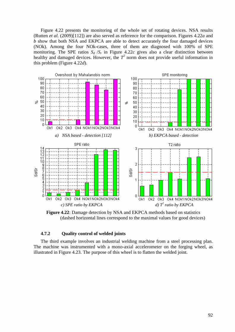
92

Figure 4.22 presents the monitoring of the whole set of rotating devices. NSA results

(Rutten et al. (2009)[112]) are also served as reference for the comparison. Figures 4.22a and

b show that both NSA and EKPCA are able to detect accurately the four damaged devices

(NOk). Among the four NOk-cases, three of them are diagnosed with 100% of SPE

monitoring. The SPE ratios Sd /Sr in Figure 4.22c gives also a clear distinction between

healthy and damaged devices. However, the T2 norm does not provide useful information in

this problem (Figure 4.22d).

a) NSA based - detection [112] b) EKPCA based - detection

c) SPE ratio by EKPCA d) T

2 ratio by EKPCA

Figure 4.22: Damage detection by NSA and EKPCA methods based on statistics

(dashed horizontal lines correspond to the maximal values for good devices)

4.7.2 Quality control of welded joints

The third example involves an industrial welding machine from a steel processing plan.

The machine was instrumented with a mono-axial accelerometer on the forging wheel, as

illustrated in Figure 4.23. The purpose of this wheel is to flatten the welded joint.

93

Figure 4.23: Location of the accelerometer on the forging wheel of the welding machine

The quality of the weld depends on several parameters. In Rutten et al. (2009)[112], six

welded joints with nominal welding parameters (OK 1-OK 6) and 27 joints with out-of-range

parameters were studied. Some welding parameters were altered, namely covering,

compensation, current and forging pressure, as reported in Table 4.2. From a microscope

quality control, welded joints C and G were diagnosed good, welded joints A, D, E, H were

diagnosed acceptable and welded joints named B, F, I were diagnosed bad.

Table 4.2: Welds realized with altered parameters (with respect to the nominal parameters)

Name Modified parameter Weld quality

Welding A -33% covering Acceptable

Welding B -66% covering Bad

Welding C -33% compensation Good

Welding D -66% compensation Acceptable

Welding E -10% current Acceptable

Welding F -20% current Bad

Welding G -10% forging pressure Good

Welding H +5% forging pressure Acceptable

Welding I -66% covering and compensation Bad

The parameter modifications were clearly identified using the NSA-based detection

method as presented in Figure 4.24. It is observed that all OK welded joints do not present

non-zero outlier statistic, and so do welded joints C and G.

94

0 20 40 60 80

OK-1OK-2OK-3OK-4OK-5OK-6

A-1A-2A-3B-1B-2B-3C-1C-2C-3D-1D-2D-3E-1E-2E-3F-1F-2F-3G-1G-2G-3H-1H-2H-3I-1I-2I-3

%

Overshoot for each welding (6 lim.)

Figure 4.24: NSA-based detection (from [112], lim 6NI NI )

The welded joints are now examined by means of the EKPCA method. From only one

response vector, the covariance-driven Hankel matrix is built using 30 blocks. The width of

Gaussian kernel w = 150 was chosen for the RBF kernel. The eigenvalue diagram is presented

in Figure 4.25. It reveals that the first three PCs concentrate 70% of the accumulated variance

percentage. It is interesting to note that, as long as the number of principal components is

higher than 3, detection results lead to the same conclusion. The best results are obtained

within the range of 5-7 PCs which accumulate 80-90% of the variance percentage. They are

presented in Figures 4.26 and 4.27 on the basis of the concept of subspace angle and on

statistics, respectively.

Figure 4.25: Eigenvalues of the kernel matrix vs. the number of PCs

95

Figure 4.26: EKPCA detection based on the subspace angle (the dash-dot line

corresponds to the maximal value for healthy welded joints)

Figure 4.27: EKPCA detection based on statistics

96

In general, the subspace angles given in Figure 4.26 and the SPE-based indexes in Figure

4.27 allow to identify the alterations reported in Table 4.2. The SPE statistics appears fairly

better in this example. For instance, the indexes of welded joints C1-C3, G1, G3 are in the

same range as for healthy welded joints OK1-OK6 (i.e. with nominal parameters). This is in

good agreement with microscopic quality control inspections. Weld G2 gives an index close

to the one of welds A, D, E, H which are diagnosed as acceptable. Finally, welds B, F and I

are characterized by significant overshoots and high ratios Sd /Sr. Their diagnosis as bad joints

is corroborated by the quality control inspection. It should be noted also that index T2 does not

lead to significant detection results in this problem. Furthermore, the detection indicators used

in the EKPCA method as well as in the NSA method are not proportional to the severity of

the defects.

4.8 Concluding remarks

KPCA is useful for the processing of nonlinear systems. The robustness of the method for

the detection of dynamic changes (due to nonlinear behavior or damage) has been illustrated

on several experimental examples and applications in comparison with other methods. Two

types of indicators (subspace angle and statistics) were used for detection and were compared

regarding to their performance.

Combined with the Hankel matrix, the EKPCA method provides a very appropriate tool

for monitoring a structure. Especially, the covariance-data Hankel matrix allows to lessen

considerably the computation load by reducing the size of the eigenvalue problem to solve.

The method works well even if only one sensor is available.

97

Chapter 5

Damage Localization using Sensitivities of

Principal Component Analysis Results

5.1 Introduction

Let us now deal with another aspect of the detection problem which is the localization. As

presented in Section 1.4, damage localization can be performed using output-only

measurements or be based on a mathematical model. To solve the problem of localization in

beam-like structure, this chapter focuses on the use of sensitivity analysis of measurements.

Natural frequency sensitivity has been also used extensively for the purpose of damage

localization. However, most of the methods based on frequency sensitivity with respect to

damage variables require an accurate analytical model. Jiang and Wang (2009)[48] extended

the frequency sensitivity approach by eliminating that requirement. However, an optimization

scheme is still needed to estimate the unknown system matrices through an identified model

using input-output measurement data.

Natural frequencies are known to be successful in characterizing dynamical systems.

Mode shapes are used in model updating because they give information regarding the spatial

distribution of damage whereas it is difficult to locate the damage by using the frequencies

only in the objective function constructed for minimization. Hence, we use not only

sensitivity of frequencies, but also of mode shapes in this work. Modal identification and

construction of an analytical model are not necessary for the localization procedure. Damage

localization may be carried out by monitoring the distortion of a sensitivity vector.

Illustrations are performed through several examples as mass-spring systems, a cantilever

beam and a real bridge structure.

5.2 Methodology: Some approaches for Sensitivity Analysis

The behavior of a dynamical system depends on many parameters related to material,

geometry and dimensions. The sensitivity of a quantity to a parameter is described by the first

and higher orders of its partial derivatives with respect to the parameter. Sensitivity analysis

of modal parameters may be a useful tool for uncovering and locating damaged or changed

components of a structure. On one hand, we know that the dynamic behavior of a system is

fully characterized by its modal parameters which result from the resolution of an eigenvalue

problem based on the system matrices (when a model is available). On the other hand,

Principal Component Analysis (PCA) of the response matrix of the system is also a way to

extract modal features (i.e. principal directions) which span the same subspace as the

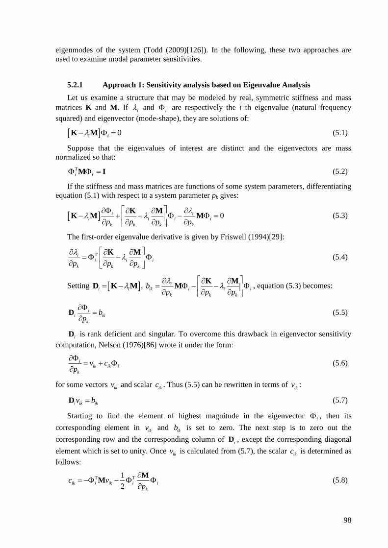
98

eigenmodes of the system (Todd (2009)[126]). In the following, these two approaches are

used to examine modal parameter sensitivities.

5.2.1 Approach 1: Sensitivity analysis based on Eigenvalue Analysis

Let us examine a structure that may be modeled by real, symmetric stiffness and mass

matrices K and M. If i and i

are respectively the i th eigenvalue (natural frequency

squared) and eigenvector (mode-shape), they are solutions of:

0 K Mi i (5.1)

Suppose that the eigenvalues of interest are distinct and the eigenvectors are mass

normalized so that:

T

i i M I (5.2)

If the stiffness and mass matrices are functions of some system parameters, differentiating

equation (5.1) with respect to a system parameter pk gives:

0

K MK M Mi i

i i i i

k k k kp p p p (5.3)

The first-order eigenvalue derivative is given by Friswell (1994)[29]:

Tii i i

k k kp p p

K M (5.4)

Setting D K Mi i,

K MMi

ik i i i

k k k

bp p p

, equation (5.3) becomes:

D i

i ik

k

bp

(5.5)

Di is rank deficient and singular. To overcome this drawback in eigenvector sensitivity

computation, Nelson (1976)[86] wrote it under the form:

iik ik i

k

v cp

(5.6)

for some vectors ikv and scalar

ikc . Thus (5.5) can be rewritten in terms of ikv :

Di ik ikv b (5.7)

Starting to find the element of highest magnitude in the eigenvector i , then its

corresponding element in ikv and ikb is set to zero. The next step is to zero out the

corresponding row and the corresponding column of Di , except the corresponding diagonal

element which is set to unity. Once ikv is calculated from (5.7), the scalar ikc is determined as

follows:

T T1

2ik i ik i i

k

c vp

MM (5.8)

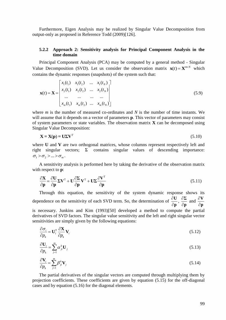
99

Furthermore, Eigen Analysis may be realized by Singular Value Decomposition from

output-only as proposed in Reference Todd (2009)[126].

5.2.2 Approach 2: Sensitivity analysis for Principal Component Analysis in the

time domain

Principal Component Analysis (PCA) may be computed by a general method - Singular

Value Decomposition (SVD). Let us consider the observation matrix ( ) m Ntx X which

contains the dynamic responses (snapshots) of the system such that:

1 1 1 2 1

2 1 2 2 2

1 2

( ) ( ) ... ( )

( ) ( ) ... ( )( )

... ... ... ...

( ) ( ) ... ( )

N

N

m m m N

x t x t x t

x t x t x tt

x t x t x t

x X (5.9)

where m is the number of measured co-ordinates and N is the number of time instants. We

will assume that it depends on a vector of parameters p. This vector of parameters may consist

of system parameters or state variables. The observation matrix X can be decomposed using

Singular Value Decomposition:

T( )X = X p = UΣV (5.10)

where U and V are two orthogonal matrices, whose columns represent respectively left and

right singular vectors; Σ contains singular values of descending importance:

1 2 ... m .

A sensitivity analysis is performed here by taking the derivative of the observation matrix

with respect to p:

TT T

X U Σ VΣV U V UΣ

p p p p (5.11)

Through this equation, the sensitivity of the system dynamic response shows its

dependence on the sensitivity of each SVD term. So, the determination of

U

p,

Σ

p and

V

p

is necessary. Junkins and Kim (1993)[50] developed a method to compute the partial

derivatives of SVD factors. The singular value sensitivity and the left and right singular vector

sensitivities are simply given by the following equations:

T

ii i

k kp p

XU V (5.12)

1

mkiji j

jkp

UU (5.13)

1

mkiji j

jkp

VV (5.14)

The partial derivatives of the singular vectors are computed through multiplying them by

projection coefficients. These coefficients are given by equation (5.15) for the off-diagonal

cases and by equation (5.16) for the diagonal elements.

100

T

T T

2 2

T

T T

2 2

1

1

k

ji i j i j i j

i j k k

k

ji j j i i i j

i j k k

p p

p p

X XU V U V

X XU V U V

, j i (5.15)

T

TT

1

1

k k iii ii i i

i k k

k k iii ii i i

i k k

p p

p p

XU V

XV U

, j i (5.16)

Junkins and Kim (1993)[50] showed also that the diagonal coefficients keep only their

imaginary part (their real parts are empty).

5.2.3 PCA-based methodology developed in the frequency domain

Sensitivity analysis for PCA may be developed in the frequency domain, e.g. by

considering frequency response functions (FRFs) (Todd (2009)[126]).

As the dynamical system matrices depend on a vector of parameters p, the FRF matrix

takes the form:

1

2, ( ) ( ) ( )

iH p M p C p K p (5.17)

where represents the circular frequency. With regard to sensitivity analysis, the partial

derivative of equation (5.17) with respect to one parameter pk may be written [126]:

2

2

, ,

, ,

k k

k k k

i

p p

ip p p

M C KHH p H p

M C KH p H p

(5.18)

Equation (5.18) provides a way of determining the derivative of the FRF matrix needed

for the sensitivity analysis by means of the partial derivative of the system matrices.

Let us consider the FRFs for a single input at location s, and build a subset of the FRF

matrix (5.17):

1 1 1 2 1

2 1 2 2 2

1 2

...

...( )

... ... ... ...

...

N

Ns

m m m N

h h h

h h h

h h h

H

(5.19)

where m is the number of measured co-ordinates and N is the number of frequency lines.

This matrix is the frequency domain analog of the observation matrix (5.9). The rows in

(5.19) represent the response at the measured degrees of freedom (DOFs), while the columns

101

are “snapshots” of the FRFs at different frequencies. We consider that this matrix depends on

a given set of parameters. We can assess its principal components through SVD by (5.10):

T( , )s

f f fH p U Σ V (5.20)

where the left singular vectors fU give spatial information, the diagonal matrix of singular

values fΣ shows scaling parameters and the right singular vectors

fV represents modulation

functions depending on frequency. In other words, this SVD separates information depending

on space and on frequency.

The sensitivity of the ith principal component in (5.20) can be computed by (5.12-5.16).

First, we compute the SVD of the FRF matrix in (5.19) for the set of responses and the chosen

input location. Then, the partial derivatives of (5.19) are determined using equation (5.18).

For a particular input, only a subset of the derivatives in (5.18) is needed.

5.3 Damage localization based on sensitivity analysis of FRF matrix

In the following, sensitivity analysis is used to resolve the problem of damage

localization. According to Eigen Analysis, sensitivity of eigensolution is straightforward if the

system matrices are available. Regarding FRF analysis, we present now some simplifications

that may be carried out in experimental practice.

Giving the FRF matrix sH for a single input at location s of the system and its SVD, the

sensitivity computation of the principal components (PCs) requires the partial derivatives

/ s

kpH which are a subset of / kpH . This quantity may be assessed by (5.18) requiring

the partial derivative of the system matrices with respect to system parameters. If the

parameter concerned is a coefficient ke of the stiffness matrix K, the partial derivatives of the

system matrices are selected such that / kp M and / kp C equal zero and

/ /k ep k K K .

Although only a subset of / kpH is needed for a particular input s, i.e. / s

kpH which

corresponds to the s th column of / kpH , the calculation of (5.18) demands the whole

matrix H , which turns out to be costly. However, we can compute / s

kpH by measuring

only some columns of H , as explained below.

We recall that our parameter of interest is some coefficient ke of the stiffness matrix K.

Equation (5.17) shows that FRF matrices are symmetric if system matrices are symmetric. In

experiment, the number of degrees of freedom (DOF) equals the number of response sensors.

So, the FRF matrix has the same size as the number of sensors. Let us consider for instance a

structure instrumented with four sensors. The FRF matrix takes the symmetrical form:

a b c d

b e f g

c f h i

d g i k

H (5.21)

Assuming that ke accords to the element between DOFs 2 and 3, we have: / 0kp M ;

/ 0kp C and:

102

0 0 0 0

0 1 1 0/ /

0 1 1 0

0 0 0 0

k ep k

K K (5.22)

Equation (5.18) allows us to deduce the partial derivative of the FRF matrix:

( ) ( ) ( ) ( ) ( )

( ) ( ) ( ) ( ) ( ), ,

( ) ( ) ( ) ( ) ( )

( ) ( ) ( ) ( ) ( )

k k

b c e f f h g i b c

b c e f f h g i e f

p p b c e f f h g i f h

b c e f f h g i g i

H KH p H p (5.23)

To compute the sensitivity of sH , only the s th column of / kpH is needed, which is

written in (5.25) in setting:

T

( ) ( ) ( ) ( )ek b c e f f h g i H (5.24)

This relies entirely upon the columns corresponding to ke in the FRF matrix in equation

(5.21).

,.

e e

s

k k s

kp

HH H (5.25)

where ,ek sH is the s th element of the vector ekH . Thus, the sensitivity of s

H with respect to

ke does not involve the entire matrix H ; only the columns relating to ke is needed.

It is worth noting that the choice of system parameter in the derivative process is not

unique. The parameter can consist in a DOF only, i.e. it relates to a coefficient ke of the

stiffness matrix. For example, assuming that ke accords to the second DOF only, we have:

0 0 0 0

0 1 0 0/ /

0 0 0 0

0 0 0 0

k ep k

K K ,

k

b e f g b

b e f g e

p b e f g f

b e f g g

H (5.26)

Setting T

ek b e f gH (5.27)

this is just the column corresponding to ke in the FRF matrix in equation (5.21). Finally, the

same equation in (5.25) may be found for / s

kpH . This time again, only the column related

to ke is needed for the sensitivity of sH with respect to ke.

5.4 Localization indicators

Once / s

kpH has been computed, the sensitivity of principal components can be

determined using equations (5.12-5.16). The sensitivities of the left singular vectors or

eigenvectors are good candidates for resolving localization problems of linear-form structures,

e.g. chain-like or beam-like structures. In each working condition of the system, we can

103

compute the sensitivity /i kp U . The reference state is denoted by R

i

kp

U, and the deviation

of the current condition may be assessed as follows:

R

i i i

k k kp p p

U U U (5.28)

For structure that has several spans, a normalized deviation norm can be used to count on

the influence of different magnitudes of the sensitivity vector in the spans. It is computed in

accordance with the span:

norm

norm /

tt

tR

i kp

U

(5.29)

where t contains the elements according to span t of vector , /t

Ri kp U describes the

sensitivity elements in span t in the reference state and norm( ) is an operator giving the

maximal singular value of a vector.

Other indicators may be utilized to better locate dynamic change, such as:

I

1

1j j jd

r (5.30)

II

1 12

12j j j jd

r (5.31)

where r is average distance between measurement points and j denotes the j

th element of .

Figure 5.1: Geometrical illustration for position of elements in the indicators

Id in eq. (5.30) represents the relative difference between adjacent elements of and has

one element less than . For a Id vector containing all the m elements (as the number of

DOFs), one more element in may be generated, e.g. element m+1, as illustrated in Figure

5.1. Of course, this generated element must not affect the remaining elements; a technique

that may be applied is the cubic spline extrapolation. We can proceed similarly for the IId

vector. The indicators Id and IId are effectively comparable with the first and second

derivatives of vector i

kp

U and allow the maximization of useful information for damage

localization.

104

The indicator IId is widely used in the literature of damage localization, e.g. in Pandey et

al. (1991)[96], Sampaio et al. (1999)[113]. However, the methods proposed in the literature

compare mode shape vectors or FRF data. In this study, the sensitivity of singular vectors is

the subject under examination.

It should be noted that a zero-mean normalization is generally applied to the data in the

classical PCA technique. However, such normalization can be avoided in the present case

because the localization indicators are characterized by the principal components vectors and

their derivatives. This is illustrated in Figure 5.2 in a two-dimensional case where two

features y1 and y2 are considered. The features in data set S1 are distributed around their

geometric centre - point O1 and if a zero-mean normalization is achieved, they are represented

by data set S0. The application of PCA to S1 gives two principal components PC 1 and PC 2,

which are just the principal components of set S0. In our application, a health state of the

dynamic structure is shown by the vectors of principal components and their sensitivities; and

the localization is achieved by comparing the last vectors of two different health states. To

this purpose, a zero-mean normalization is not necessary for the data preprocessing. However,

in order to facilitate the comparison between two states, the unit-norm normalization is

implemented to the sensitivity vectors, i.e.

/

/norm( / )

i ki k

i k

pp

p

UU

U (5.32)

This normalization step provides more meaningful and accurate comparison between

different conditions.

Figure 5.2: Geometric interpretation of PCA

5.5 Applications to damage localization

5.5.1 Numerical example of a spring-mass-damper system

Let us examine the system studied in Todd (2009)[126] which consists in a linear system

of 20 degrees of freedom as presented in Figure 5.3.

The damping matrix is set to C = 0.01M. Input is introduced at point 18. The frequency

range is selected from 0 to 2 rad/sec at intervals of 0.005 rad/sec. Some results of principal

component sensitivities with respect to a spring constant are presented in [126].

105

Figure 5.3: Spring-mass-damper system

In this study, sensitivity analysis is applied with the aim of damage localization. For this

purpose, damage is simulated in the system by a stiffness reduction of spring n° 8. Both

approaches based on Eigen analysis and PCA are considered. Figure 5.4 compares the

sensitivities of the first eigenvector and of the first left singular vector with respect to the

stiffness of the second spring (k2). As can be observed, both techniques lead to similar results;

in the following, we present the development of damage localization based on PCA analysis.

Figure 5.4: Analytical sensitivities of the first eigenvector and of the first left singular vector

Let us consider now the structure in three states: the reference state (no damage), level 1

and level 2 induced by a stiffness reduction of 20% and 50% of the 8th

spring. Figure 5.5

shows the sensitivity of the first left singular vector with respect to several system parameters

for all the states.

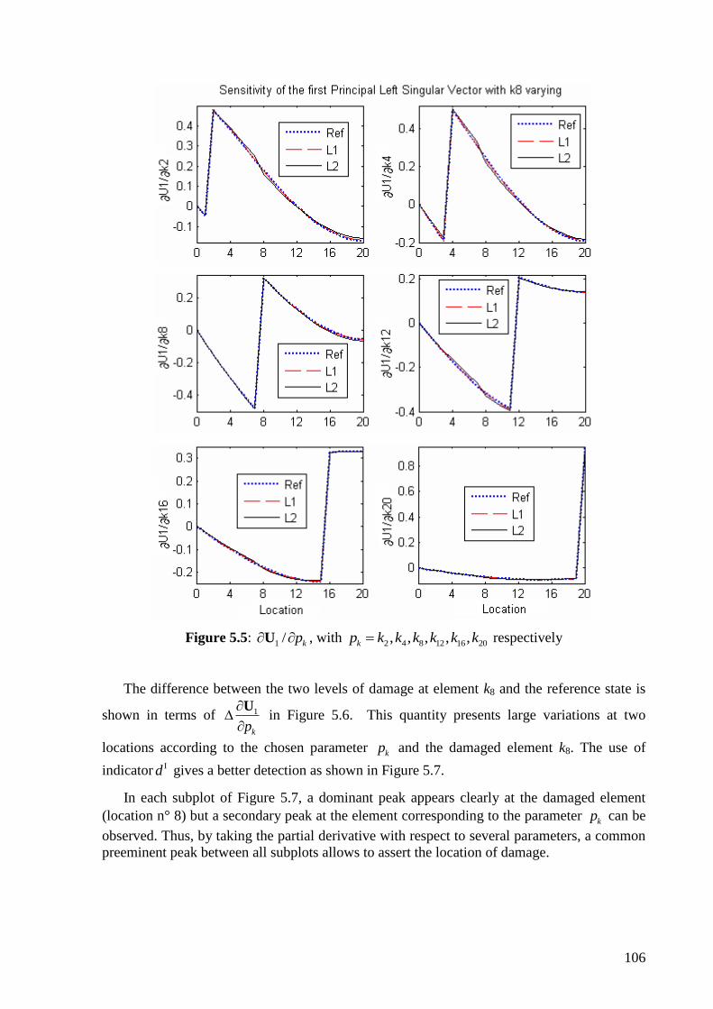
106

Figure 5.5: 1 / kp U , with

2 4 8 12 16 20, , , , ,kp k k k k k k respectively

The difference between the two levels of damage at element k8 and the reference state is

shown in terms of 1

kp

U in Figure 5.6. This quantity presents large variations at two

locations according to the chosen parameter kp and the damaged element k8. The use of

indicator Id gives a better detection as shown in Figure 5.7.

In each subplot of Figure 5.7, a dominant peak appears clearly at the damaged element

(location n° 8) but a secondary peak at the element corresponding to the parameter kp can be

observed. Thus, by taking the partial derivative with respect to several parameters, a common

preeminent peak between all subplots allows to assert the location of damage.

107

Figure 5.6: 1

kp

U for levels 1 and 2 with

2 4 8 12 16 20, , , , ,kp k k k k k k respectively

Figure 5.7: Id for levels 1 and 2 with 2 4 8 12 16 20, , , , ,kp k k k k k k respectively

108

The damage is also exactly located even if it occurs far from the clamping. In Figure 5.8,

the damaged element (stiffness reduction of the 20th

spring) is well detected.

Figure 5.8: Id with damage in k20

5.5.2 Numerical example of a cantilever beam

Let us examine a steel cantilever beam with a length of 700 mm and a square section of

dimension 214 14(mm ) . The beam is modeled by twenty finite elements as illustrated in

Figure 5.9. The input location is chosen at node 7 and the snapshot matrix is assembled from

FRFs corresponding to the vertical displacements at nodes 1 to 20.

Figure 5.9: Discretization of cantilever beam

We model the damage by a stiffness reduction of a beam element. Four states are

examined: the reference (healthy) state, and three levels of damage (L1, L2, L3) induced by a

reduction of stiffness of respectively 10%, 20% and 40%. The damage is assumed to occur in

element 12. Note that the maximum deviations on the first three frequencies from the

reference state are 0.70%, 1.41% and 2.81% for the three levels respectively.

For illustration, sensitivity analysis results are shown in Figures 5.10 and 5.11 according

to the parameter pk=k15. Note that similar results were obtained for other stiffness parameter

in various positions. The FRFs were considered in the frequency range from 0 Hz to 165 Hz

at intervals of 1 Hz.

109

Figure 5.10 shows the sensitivity difference 1

15k

U of the first left singular vector

with respect to the coefficient associated to the 15th

DOF in the stiffness matrix and its

derivatives Id , II d are presented in Figure 5.11. It is observed that the curves are

discontinuous at DOFs 11 and 12, index Id shows a discontinuity with large variations

around element 12 and finally, index II d allows us to discover explicitly the position of the

damaged element.

Figure 5.10: 1

15

U

k for 3 levels with pk=k15

Figure 5.11: Id and II d indexes for 3 levels with pk=k15

Even though damage occurs at a delicate location, it can be indicated. For example, Figure

5.12 detects damage taking place at the first or at the last element respectively.

Figure 5.12: II d for 3 levels with damage at element 1 and 20 respectively

The method reveals itself robust when damage develops simultaneously in several

elements. Localization results are shown in Figure 5.13 for two different cases of damage. We

note that index II d does not indicate the same level of damage in the damaged elements.

However, the damage locations are accurately indicated. The difference in magnitude is due

110

to unequal sensitivities for various damage locations, as discussed in Ray and Tian (1999)

[106].

a) damage at elements 12, 13, 14 b) damage at elements 7 and 16

Figure 5.13: II d for three levels of damages

Furthermore, the following remarks may be formulated regarding to the sensitivity of the

damage localization method to different factors.

Influence of noise

In order to examine the robustness of the proposed method to noise, the time responses

(vertical displacements) are perturbed by adding 5% of noise. Indicators Id and IId , which are

the most sensitive to damage in this cantilever beam, are considered. Figure 5.14 corresponds

to a damage localized in element 12 and Figure 5.15 to a damage localized in element 15. It

appears from these examples that levels L2 and L3 are well detected, however, due to noise,

the lowest damage-level L1 is not identified.

Figure 5.14: Three damage levels in element 12: reduction of stiffness of 10%, 20% and

40%; 5% of noise

Figure 5.15: Three damage levels in element 15: reduction of stiffness of 10%, 20% and

40%; 5% of noise

111

Influence of the number of sensors

Let us assume that the full range of sensors is not available and that the measurements are

implemented at fewer locations, which is very common in practical applications. As an

example, we consider again the case in which damage is located at element 12 (element

between DOFs 11 and 12 of the initial model in Figure 5.9); however, we suppose that only

seven sensors are available and distributed as shown in Figure 5.16a. In this new situation, the

damaged element lays between sensors n° 4 and 5, which is perfectly indicated in Figure

5.16b, c.

a) Damaged element and sensor instrumentation

b) d I index c) d

II index

Figure 5.16: Localization of damage in element 12 using 7 sensors only

For a more detailed localization, a deductive technique may be proposed as follows. Based

on the real measurements, indexes at other positions between the available sensors can be

deducted. For example, the vector of sensitivity computed from the real measurements can be

generated by interpolation; the results of this interpolation are illustrated in Figure 5.17a in

which 19 points (including the 7 points instrumented by sensors) are examined. According to

those 19 points, the damaged element is correctly located at points 10 and 11 as illustrated in

Figure 5.17b and c.

112

a) Position of points measured (n° 1, 4, 7, 10, 13, 16, 19 - few sensors) and points deducted

b) d I index c) d

II index

Figure 5.17: Localization of damage in element 12, represented according to 19 points in

the generated sensitivity vector

Other results are also presented in Figures 5.18 and 5.19, when damage occurs in element

14. Figure 5.18 shows localization results based on 7 sensors only and Figure 5.19 gives

localization results with a better resolution based on interpolation.

a) Damaged element and sensor instrumentation

b) d

I index c) d

II index

Figure 5.18: Localization of damage in element 14 using 7 sensors only

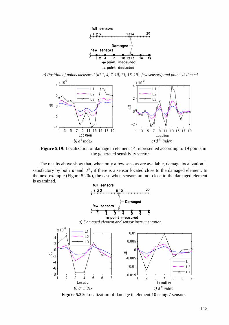
113

a) Position of points measured (n° 1, 4, 7, 10, 13, 16, 19 - few sensors) and points deducted

b) d

I index c) d

II index

Figure 5.19: Localization of damage in element 14, represented according to 19 points in

the generated sensitivity vector

The results above show that, when only a few sensors are available, damage localization is

satisfactory by both Id and IId , if there is a sensor located close to the damaged element. In

the next example (Figure 5.20a), the case when sensors are not close to the damaged element

is examined.

a) Damaged element and sensor instrumentation

b) d

I index c) d

II index

Figure 5.20: Localization of damage in element 10 using 7 sensors

114

In Figure 5.20b, c, the highest index values are found at locations 3 and 4 for index Id

and at locations 2 and 4 for index IId . This is a reasonable result because these locations are

close to the damage which is located actually between sensors 3 and 4. Regarding the

deductive technique, the results are given in Figure 5.21. As shown in Figure 5.21a, the

damaged element corresponds to points 8 and 9 in the generated vector. Indicators Id and IId

are able to find these locations but they also point out other locations, e.g. points 2-4.

a) Position of points measured (n° 1, 4, 7, 10, 13, 16, 19 - few sensors) and points deducted

b) d I index c) d

II index

Figure 5.21: Localization of damage in element 10, represented according to 19 points in

the generated sensitivity vector

The examples above show that damage can still be localized when the number of sensors

is limited. The deductive technique allows to refine localization if sensors are instrumented

close to the damage.

5.5.3 Experiments involving a mass-spring system

The next example involves the system of eight DOFs (Figure 5.22) constructed by Los

Alamos National Laboratory - LANL and for which data are available in [42]. The system

comprises eight translating masses connected by springs. In the undamaged configuration, all

the springs have the same constant: 56.7 kN/m. Each mass weighs 419.5 grams; the weight is

559.3 grams for the mass located at the end which is attached to the shaker.

The acceleration response and also the FRFs of all the masses are measured with the

excitation force applied to mass 1 - the first mass at the right-hand end (Figure 5.22). The

FRFs are assembled so as to localize the damage by the proposed method. Frequency lines are

selected from 0 to 55 Hz at intervals of 0.1562 Hz.

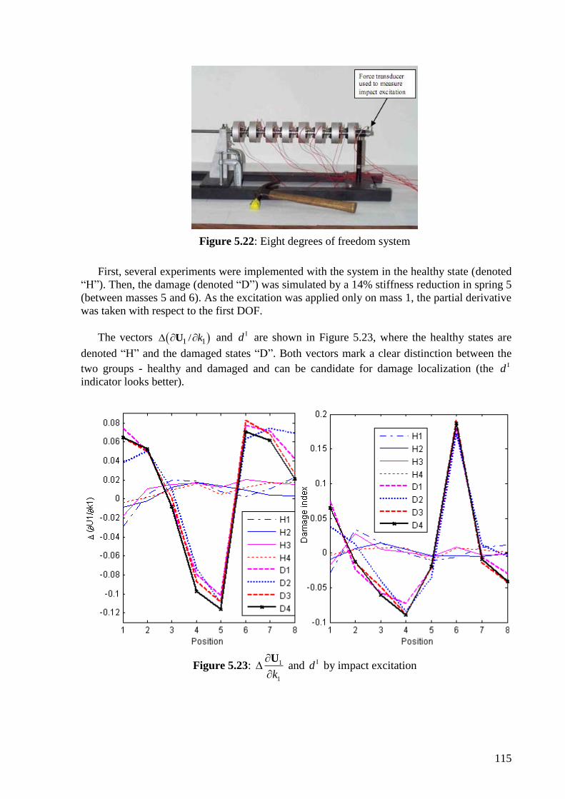
115

Figure 5.22: Eight degrees of freedom system

First, several experiments were implemented with the system in the healthy state (denoted

“H”). Then, the damage (denoted “D”) was simulated by a 14% stiffness reduction in spring 5

(between masses 5 and 6). As the excitation was applied only on mass 1, the partial derivative

was taken with respect to the first DOF.

The vectors 1 1/ k U and Id are shown in Figure 5.23, where the healthy states are

denoted “H” and the damaged states “D”. Both vectors mark a clear distinction between the

two groups - healthy and damaged and can be candidate for damage localization (the Id

indicator looks better).

Figure 5.23: 1

1

k

U and Id by impact excitation

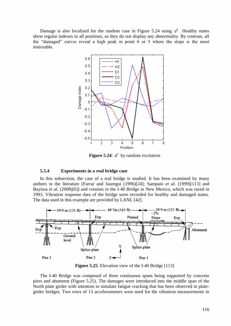
116

Damage is also localized for the random case in Figure 5.24 using Id . Healthy states

show regular indexes in all positions, so they do not display any abnormality. By contrast, all

the “damaged” curves reveal a high peak in point 6 or 5 where the slope is the most

noticeable.

Figure 5.24: Id by random excitation

5.5.4 Experiments in a real bridge case

In this subsection, the case of a real bridge is studied. It has been examined by many

authors in the literature (Farrar and Jauregui (1996)[24]; Sampaio et al. (1999)[113] and

Bayissa et al. (2008)[6]) and consists in the I-40 Bridge in New Mexico, which was razed in

1993. Vibration response data of the bridge were recorded for healthy and damaged states.

The data used in this example are provided by LANL [42].

Figure 5.25: Elevation view of the I-40 Bridge [113]

The I-40 Bridge was composed of three continuous spans being supported by concrete

piers and abutment (Figure 5.25). The damages were introduced into the middle span of the

North plate girder with intention to simulate fatigue cracking that has been observed in plate-

girder bridges. Two rows of 13 accelerometers were used for the vibration measurements in

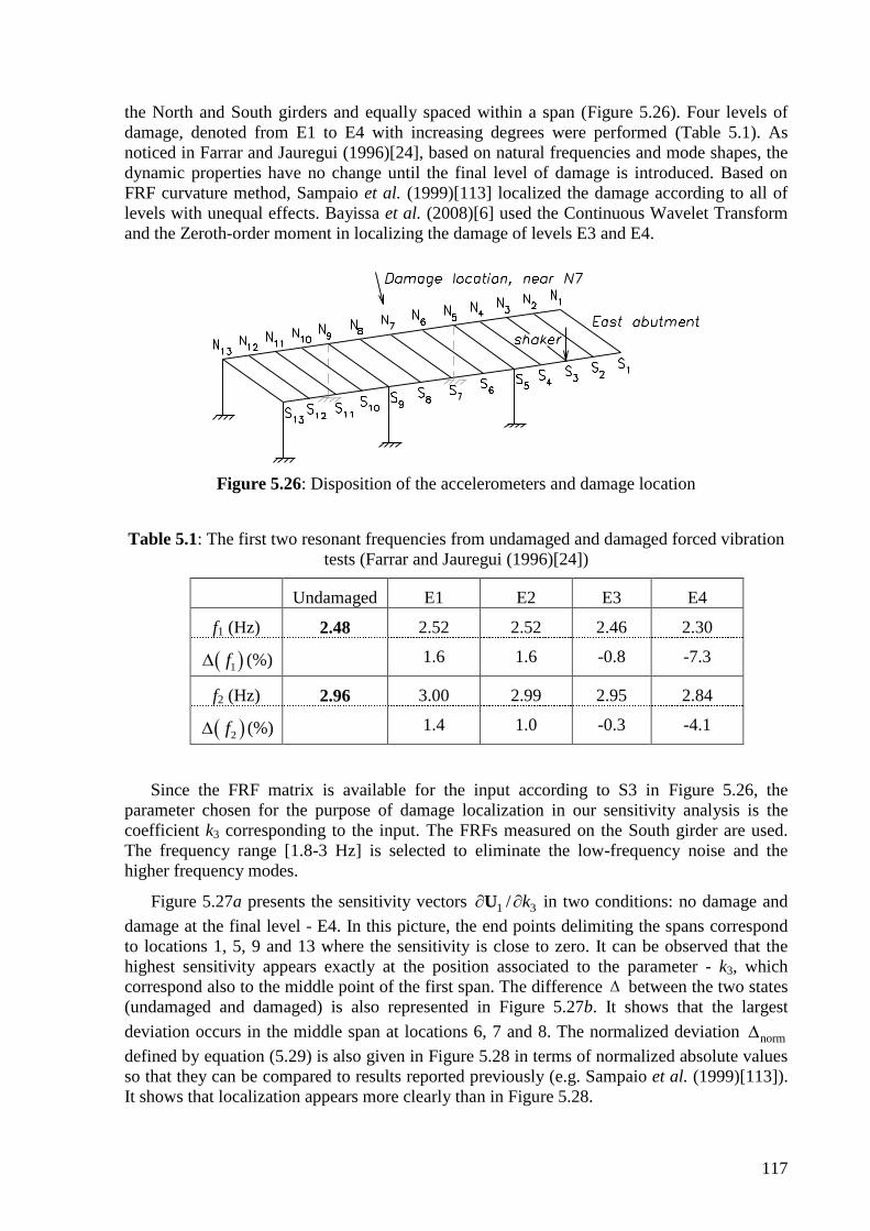
117

the North and South girders and equally spaced within a span (Figure 5.26). Four levels of

damage, denoted from E1 to E4 with increasing degrees were performed (Table 5.1). As

noticed in Farrar and Jauregui (1996)[24], based on natural frequencies and mode shapes, the

dynamic properties have no change until the final level of damage is introduced. Based on

FRF curvature method, Sampaio et al. (1999)[113] localized the damage according to all of

levels with unequal effects. Bayissa et al. (2008)[6] used the Continuous Wavelet Transform

and the Zeroth-order moment in localizing the damage of levels E3 and E4.

Figure 5.26: Disposition of the accelerometers and damage location

Table 5.1: The first two resonant frequencies from undamaged and damaged forced vibration

tests (Farrar and Jauregui (1996)[24])

Undamaged E1 E2 E3 E4

f1 (Hz) 2.48 2.52 2.52 2.46 2.30

1f (%) 1.6 1.6 -0.8 -7.3

f2 (Hz) 2.96 3.00 2.99 2.95 2.84

2f (%) 1.4 1.0 -0.3 -4.1

Since the FRF matrix is available for the input according to S3 in Figure 5.26, the

parameter chosen for the purpose of damage localization in our sensitivity analysis is the

coefficient k3 corresponding to the input. The FRFs measured on the South girder are used.

The frequency range [1.8-3 Hz] is selected to eliminate the low-frequency noise and the

higher frequency modes.

Figure 5.27a presents the sensitivity vectors 1 3/ k U in two conditions: no damage and

damage at the final level - E4. In this picture, the end points delimiting the spans correspond

to locations 1, 5, 9 and 13 where the sensitivity is close to zero. It can be observed that the

highest sensitivity appears exactly at the position associated to the parameter - k3, which

correspond also to the middle point of the first span. The difference between the two states

(undamaged and damaged) is also represented in Figure 5.27b. It shows that the largest

deviation occurs in the middle span at locations 6, 7 and 8. The normalized deviation norm

defined by equation (5.29) is also given in Figure 5.28 in terms of normalized absolute values

so that they can be compared to results reported previously (e.g. Sampaio et al. (1999)[113]).

It shows that localization appears more clearly than in Figure 5.28.

118

a) sensitivity vectors 1 3/ k U b) difference

Figure 5.27: 1 3/ k U in the healthy and damage (E4) states and their difference

Figure 5.28: Normalized norm , damage E4

Next, the lower levels of damage E3, E2 and E1 are examined successively and the results

are presented in Figure 5.29a, b and c respectively. The better localization result is attained

for damage state E2. Regarding to damage state E3, the index is higher at locations 8 and 7 as

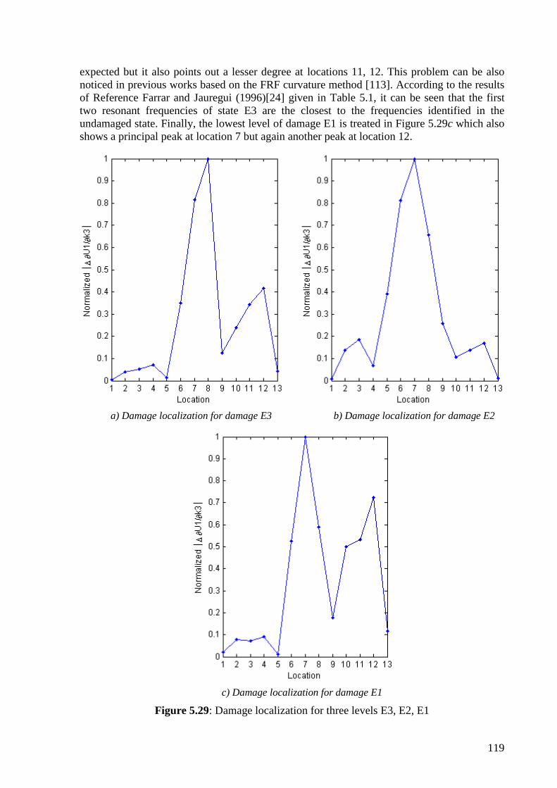
119

expected but it also points out a lesser degree at locations 11, 12. This problem can be also

noticed in previous works based on the FRF curvature method [113]. According to the results

of Reference Farrar and Jauregui (1996)[24] given in Table 5.1, it can be seen that the first

two resonant frequencies of state E3 are the closest to the frequencies identified in the

undamaged state. Finally, the lowest level of damage E1 is treated in Figure 5.29c which also

shows a principal peak at location 7 but again another peak at location 12.

a) Damage localization for damage E3 b) Damage localization for damage E2

c) Damage localization for damage E1

Figure 5.29: Damage localization for three levels E3, E2, E1

120

So, through this example, the proposed method shows also robust in localization of

damage, particularly the damages are not well remarked by resonant frequency monitoring.

The damage location is determined in all conditions; however the effectiveness of the

detection is affected by the damage degree.

5.6 Concluding remarks

The sensitivity computation of principal components by analytical methods has been

presented in Todd (2009)[126] in both the time domain and the frequency domain. The

contribution of the present study is the application of sensitivity analysis in the frequency

domain to the problem of damage localization. Damage localization is achieved here as a

result of the difference in principal component /eigenvector sensitivity between the reference

and the damaged states.

The method relies on the measurement of frequency response functions. However, as

demonstrated, it is not necessary to measure the complete FRF matrix in (5.17). If the system

matrices are symmetrical, only responses according to parameter pk are necessary to compute

sensitivity with respect to this parameter.

As sensitivity computation from FRFs is easy and does not need an analytical model, the

technique should be suitable for online monitoring.

121

Chapter 6

Parameter Assessment using Sensitivities

of Principal Component Analysis

6.1 Introduction

For the sake of efficiency and safety, it is important to well understand the dynamics of

structures in operation. To this purpose, it is necessary to have a good knowledge on the

structural parameters (namely the geometric and material properties), the applied loads, the

nonlinear characteristics, etc. If damage occurs in operation, its knowledge in terms of

localization and magnitude is of primary importance for the evaluation of the remaining

lifetime of the system. The objective of this chapter is to focus on parameter evaluation with

the aim of qualifying the severity of damage.

During the last years, the assessment of parameters has increasingly attracted the interest

of researchers (see Ray and Tian (1999)[106], Kim and Stubbs (2002)[57], Koh and Ray

(2003)[59], Jiang (2007)[47], Gomes and Silva (2008)[36], Jiang and Wang (2009)[48] for

the purpose of damage estimation). Parameter identification has also been used to characterize

the nonlinearity of structures (Adams and Allemang (2000)[1], Kerschen et al. (2006)[53],

Marchesiello and Garibaldi (2008)[78] and Da Silva et al. (2010)[15], etc.).

A popular way for evaluating parameters is to resort to model updating, which reduces the

discrepancy between the actual responses of the real-life structure and the corresponding

analytical responses (often predicted using a finite element model). In this chapter, model

updating based on analytical sensitivities of Principal Component Analysis results is utilized

for the assessment of parameters, e.g. the severity of damage.

6.2 Model parameter estimation technique

We first assemble the modal features of a system coming from the singular value

decomposition (SVD) of the FRF matrix (5.19) into a vector v called the model vector.

Principal components (PCs) in U or their energies in Σ (5.20) may be considered to construct

the model vector. In the literature, PC vectors have been often considered as more convenient

for damage detection so they will be used here.

The model vector v of a system is usually a nonlinear function of the parameters T

1[ ... ]pnp pp where np is the number of parameters. The Taylor series expansion (limited to

the first two terms) of this vector in terms of the parameter is given by:

1

( )pn

a k a

k k

pp

vv p v v S p (6.1)

122

where aa p pv v represents the model vector evaluated at the linearization point

ap p . S is

the sensitivity matrix of which the columns are the sensitivity vectors. The changes in

parameters are represented by a p p p .

The residual vector measures the difference between analytical and measured structural

behaviors (Link (1999)[71]):

( )w m v vr W r W v v p (6.2)

where mv represents measured quantities. The weighting matrix

vW (according to a weighted

least squares approach) takes care of the relative importance of each term in the residual

vector r. Substituting (6.1) into (6.2) and setting a m a r v v leads to the linearized residual

vector:

( ) ( )w m a a v v vr W r W v v S p W r S p (6.3)

Let us define the penalty (objective) function to be minimized as the weighted squared

sum of the residual vector:

T Tmin minw w J r r r Wr , T v vW W W (6.4)

Equation (6.3) may be solved from the objective function derivative / 0 J p , which

produces the linear equation:

a v vW S p W r (6.5)

for which the solution is:

T 1 T( ) a

p S WS S Wr (6.6)

In our approach, we will assume that the number of measurements is larger than the

number of updating parameters, which yields an overdetermined system of equations. Note

that the conditioning of the sensitivity matrix S plays an important role in the accuracy and

the uniqueness of the solution. The solution may be implemented using QR decomposition or

SVD, which allows to check the conditioning of S [71].

The updating process is shown in Figure 6.1 where the i th PC is considered as the model

vector. The two separated branches correspond to: 1) the analytical model which will be

updated; 2) experimental responses of the damaged structure, input position and correction

parameters. The choice of correction parameters may be based on the damage localization

results. A minimum number of correction parameters facilitates an accurate and efficient

estimation.

123

Figure 6.1: Updating diagram

Choice of weighting matrix

The positive definite weighting matrix is usually a diagonal matrix whose elements are

given by the reciprocals of the variance of the corresponding measurements (Friswell and

Mottershead (1995)[30]):

1 2diag( , ,..., ,..., )i mw w w wW (6.7)

Analytic

model

, ,K M C

Experiment : s

H

input s, parameters p

1

2 i

H M C K

2

k k k k

ip p p p

H M C KH H

ss ,

kp

HH

s[ , , ] svd( )U Σ V H

ii

kp

US

W

sˆ ˆ ˆ ˆ[ , , ] svd( )U Σ V H

T 1 T

ˆ

( )

a i i

a

r U U

p S WS S Wr

1n n p p p

1n np p

(min J)

p

+

1n n K K p

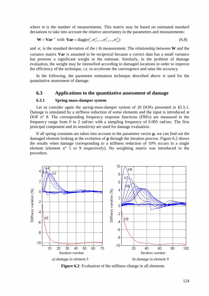
124

where m is the number of measurements. This matrix may be based on estimated standard

deviations to take into account the relative uncertainty in the parameters and measurements:

1W Var with 2 2 2 2

1 2diag( , ,..., ,..., )i m Var (6.8)

and i is the standard deviation of the i th measurement. The relationship between W and the

variance matrix Var is assumed to be reciprocal because a correct data has a small variance

but presents a significant weight in the estimate. Similarly, in the problem of damage

evaluation, the weight may be intensified according to damaged locations in order to improve

the efficiency of the technique, i.e. to accelerate the convergence and raise the accuracy.

In the following, the parameter estimation technique described above is used for the

quantitative assessment of damage.

6.3 Applications to the quantitative assessment of damage

6.3.1 Spring-mass-damper system

Let us consider again the spring-mass-damper system of 20 DOFs presented in §5.5.1.

Damage is simulated by a stiffness reduction of some elements and the input is introduced at

DOF n° 8. The corresponding frequency response functions (FRFs) are measured in the

frequency range from 0 to 2 rad/sec with a sampling frequency of 0.005 rad/sec. The first

principal component and its sensitivity are used for damage evaluation.

If all spring constants are taken into account in the parameter vector p, we can find out the

damaged element looking at the evolution of p through the iteration process. Figure 6.2 shows

the results when damage corresponding to a stiffness reduction of 10% occurs in a single

element (element n° 5 or 9 respectively). No weighting matrix was introduced in the

procedure.

a) damage in element 5 b) damage in element 9

Figure 6.2: Evaluation of the stiffness change in all elements

125

The number of iterations to converge to the solution is very high in this case. However, if

only the damaged element is considered in the parameter vector (based on the damage

localization results previously performed in Chapter 5), the convergence rate and the accuracy

are largely improved.

For illustration, only spring n° 9 (corresponding to the damaged element) is considered

now in the parameter vector. Different levels of damage (stiffness reduction of 5%, 10%,

20%, 25% and 30%) are considered and the results are shown in Figure 6.3a.

a) with updated a /i kp U b) without updated

a /i kp U

Figure 6.3: Damage evaluation

Let us discuss the use of the sensitivity vector at each iteration step. The question is if we

can use the initial sensitivity during the whole iteration process, i.e. is it necessary to update

/i kp U at each iteration step? This short cut which is illustrated in Figure 6.1 by the arrow

in dashed line, is proposed to save the computation of sensitivities at each iteration step,

which may be sometimes costly.

The results of damage evaluation without updating of the sensitivity vector /i kp U are

presented in Figure 6.3b. Compared to Figure 6.3a, it can be observed that results are quite

similar in the case of small damages for both ways of calculation. However, for higher

damages, the difference between /i kp U before and after an iteration step may be high and

more iterations are necessary to converge.

If several elements are damaged, the procedure also works. Two examples are presented

in Figure 6.4 for which the parameter vector contains many damaged elements (as well as

undamaged elements).

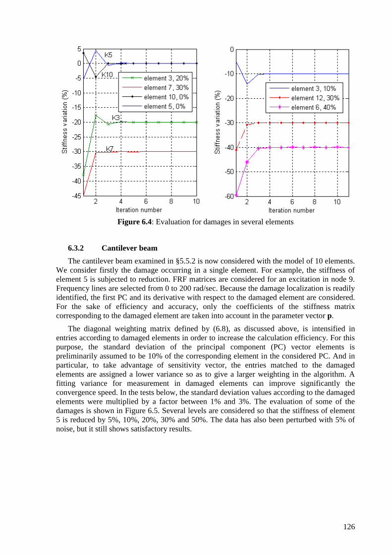
126

Figure 6.4: Evaluation for damages in several elements

6.3.2 Cantilever beam

The cantilever beam examined in §5.5.2 is now considered with the model of 10 elements.

We consider firstly the damage occurring in a single element. For example, the stiffness of

element 5 is subjected to reduction. FRF matrices are considered for an excitation in node 9.

Frequency lines are selected from 0 to 200 rad/sec. Because the damage localization is readily

identified, the first PC and its derivative with respect to the damaged element are considered.

For the sake of efficiency and accuracy, only the coefficients of the stiffness matrix

corresponding to the damaged element are taken into account in the parameter vector p.

The diagonal weighting matrix defined by (6.8), as discussed above, is intensified in

entries according to damaged elements in order to increase the calculation efficiency. For this

purpose, the standard deviation of the principal component (PC) vector elements is

preliminarily assumed to be 10% of the corresponding element in the considered PC. And in

particular, to take advantage of sensitivity vector, the entries matched to the damaged

elements are assigned a lower variance so as to give a larger weighting in the algorithm. A

fitting variance for measurement in damaged elements can improve significantly the

convergence speed. In the tests below, the standard deviation values according to the damaged

elements were multiplied by a factor between 1% and 3%. The evaluation of some of the

damages is shown in Figure 6.5. Several levels are considered so that the stiffness of element

5 is reduced by 5%, 10%, 20%, 30% and 50%. The data has also been perturbed with 5% of

noise, but it still shows satisfactory results.

127

a) with updated /i kp U b) without updated /i kp U

Figure 6.5: Evaluation damage, noise free ( ____ ) and noise 5% ( __ __ __)

In this particular problem, we note that the convergence rate to the correct answer is not

accelerated when the sensitivity is updated. Moreover, without sensitivity updating, the

parameter evolution looks more stable and smoother. It can be explains as follows. Since we

have only one term in the parameter vector (pk is the coefficient corresponding to DOF n° 5 in

the stiffness matrix), the matrix S contains one column and equation (6.6) can be expressed

as:

T

T

a S Wr

pS WS

(6.9)

If the sensitivity is updated at each step, the variation of the denominator in (6.9) affects

clearly the evolution rate of the parameter. On the contrary, when the initial sensitivity is used

at each iteration step, only the numerator of (6.9) is updated, which assures a smooth

convergence to the good solution, as illustrated in Figure 6.5b.

So in this example, the use of the initial sensitivity appears advantageous since it ensures a

more stable evolution of the computation when estimating the damage. Moreover, the CPU

time is efficiently reduced for two reasons: the convergence to the good solution is faster and

the calculation of sensitivities is avoided at each step.

Let us now examine the problem of many elements being simultaneously damaged; these

elements may be close or distant from each other. The results of various occurrences of

damage are given in Figures 6.6 and 6.7 for the same or for different levels, respectively. In

this example, about 5% of noise was taken into account.

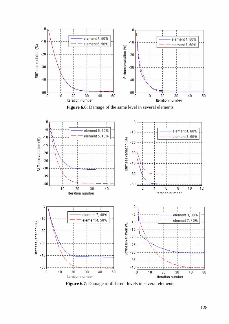
128

Figure 6.6: Damage of the same level in several elements

Figure 6.7: Damage of different levels in several elements

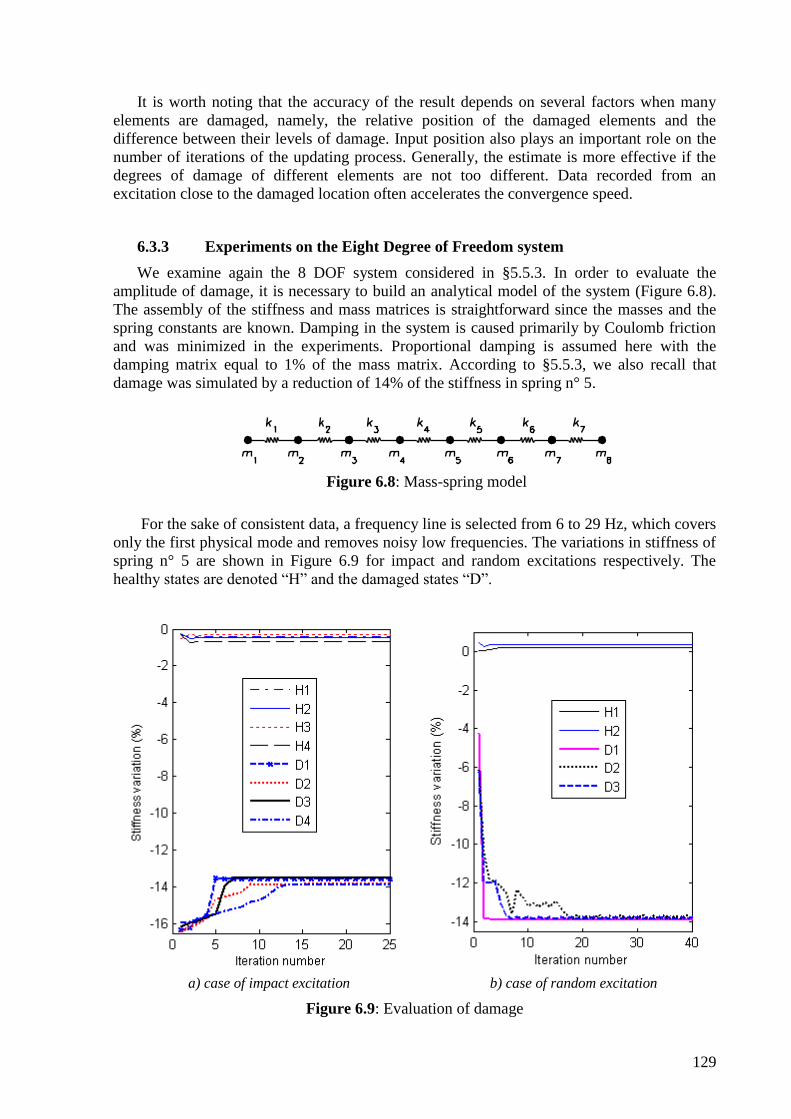
129

It is worth noting that the accuracy of the result depends on several factors when many

elements are damaged, namely, the relative position of the damaged elements and the

difference between their levels of damage. Input position also plays an important role on the

number of iterations of the updating process. Generally, the estimate is more effective if the

degrees of damage of different elements are not too different. Data recorded from an

excitation close to the damaged location often accelerates the convergence speed.

6.3.3 Experiments on the Eight Degree of Freedom system

We examine again the 8 DOF system considered in §5.5.3. In order to evaluate the

amplitude of damage, it is necessary to build an analytical model of the system (Figure 6.8).

The assembly of the stiffness and mass matrices is straightforward since the masses and the

spring constants are known. Damping in the system is caused primarily by Coulomb friction

and was minimized in the experiments. Proportional damping is assumed here with the

damping matrix equal to 1% of the mass matrix. According to §5.5.3, we also recall that

damage was simulated by a reduction of 14% of the stiffness in spring n° 5.

Figure 6.8: Mass-spring model

For the sake of consistent data, a frequency line is selected from 6 to 29 Hz, which covers

only the first physical mode and removes noisy low frequencies. The variations in stiffness of

spring n° 5 are shown in Figure 6.9 for impact and random excitations respectively. The

healthy states are denoted “H” and the damaged states “D”.

a) case of impact excitation b) case of random excitation

Figure 6.9: Evaluation of damage

130

For both two types of excitation, the results are very satisfactory. All false-positives

indicate small stiffness variations in the element concerned, and they show any detection of

damage. Conversely, all damaged states give an evaluation very close to the exact damage – a

stiffness reduction of 14%.

6.4 Concluding remarks

The results obtained in this chapter on numerical and experimental examples show that the

method presented here is efficient for assessing the severity of damages even if data is

perturbed by noise. The use of the weighting matrix in the computation of residuals may not

only enhance the convergence speed, but also enable and facilitate the evaluation of damage

when it occurs at several locations. Furthermore, an appropriate input position is important for

the convergence to the solution.

Damage evaluation is based on the correlation of a principal component between

experimental (current) and analytical data. So it is necessary to verify that the considered PC

describes the same “mode” in both the experimental and the analytical model. Otherwise, the

problem may lead to divergence.

131

Conclusions

Several monitoring methods of dynamical systems were studied in this work. The

objective of these methods (WT, SOBI and KPCA) is to diagnose the presence of structural

damage or the onset of a nonlinear behaviour from output-only measurements. Along with

these detection methods, sensitivity analysis of PCA was developed to localize and quantify

the detected damage. The robustness of the methods was studied using numerical and

experimental examples (e.g. beam with nonlinearity, aeroplane model, mass-spring and beam

systems) and illustrated on data obtained from industrial and civil engineering applications

(electro-mechanical devices, quality control of welded joints and I-40 bridge).

The WT is very convenient when analysing non-stationary signals and is well adapted to

observe nonlinear behaviours of dynamical systems. For example, the WT is able to put in

evidence phenomena such as the occurrence of sub- or super-harmonics, the combination of

fundamental „modes‟, etc. By combining the results of the WT on an ensemble of signals (at

different DOFs) in terms of amplitude, it is possible to inspect the time evolution of

deformation modes associated to the ridges of the transform. Calculation of the angles

between the subspaces spanned by those deformation modes provides a detection index that

allows indicating the onset of nonlinearity in the system. This index is able to associate

several modes simultaneously and appears fine with regard to the frequency resolution of the

transform. However, the WT shows some drawbacks when the natural frequencies of the

system are close or when noise contaminating the signals causes intermittences in the WT

responses.

SOBI, as other BSS techniques based on the assumption of system linearity is attractive

because of its rapidity and easiness of implementation. Some of the WT drawbacks cited

above are relieved with SOBI which reveals quite adequate for identification and damage

detection. However, the use of SOBI is more restrictive when processing nonlinear/non-

stationary signals and systems with high damping. In this case, the combination of SOBI with

the Hankel matrix (ESOBI) enhances considerably the identification and detection processes.

ESOBI can also provide more useful information for non-stationary signals by adjusting the

time-lag in the Hankel matrix. Moreover, ESOBI may be applied even using one sensor only.

The BMID technique which is an extension of SOBI looks really promising because it is

able to examine structures of general damping. BMID was found to be more efficient than

SOBI for modal identification as well as for damage detection.

The KPCA method reveals quite appealing in processing nonlinear data. Contrary to the

WT and SOBI, KPCA achieves the detection problem without modal identification. In KPCA,

the vibration data is first projected into a high dimensional feature space using a nonlinear

mapping, and PCA is then performed in this space for the purpose of detection. As in SOBI,

the use of the Hankel matrix improves the robustness of KPCA in all aspects.

According to our personal judgment, the main performances/characteristics of the

detection methods considered in the present work are listed in Table 7.1.

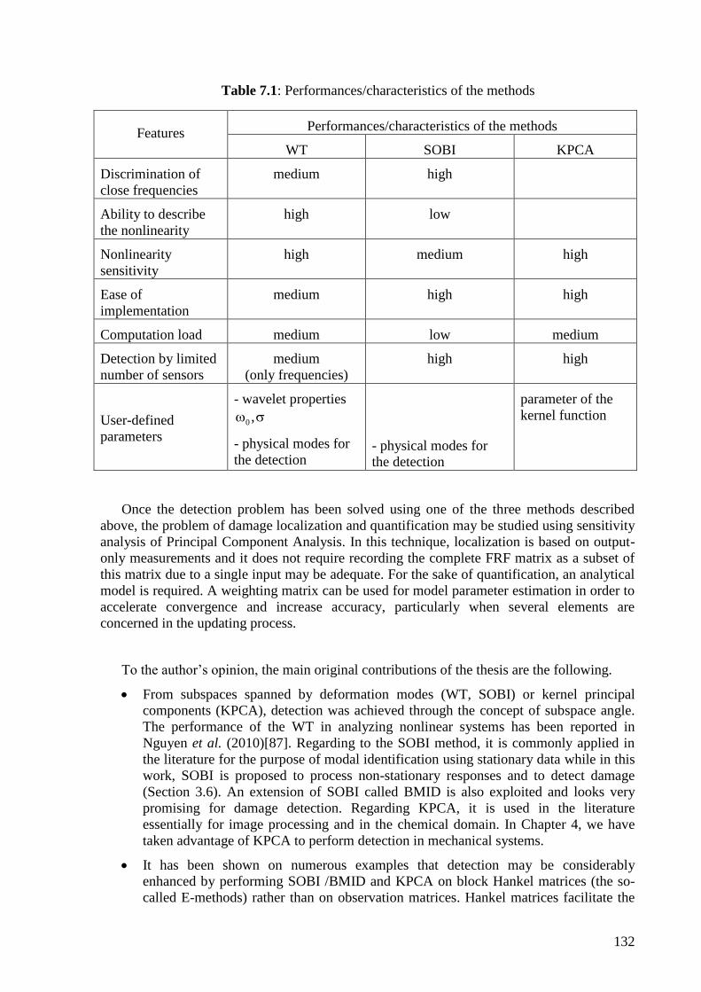
132

Table 7.1: Performances/characteristics of the methods

Features Performances/characteristics of the methods

WT SOBI KPCA

Discrimination of

close frequencies

medium high

Ability to describe

the nonlinearity

high low

Nonlinearity

sensitivity

high medium high

Ease of

implementation

medium high high

Computation load medium low medium

Detection by limited

number of sensors

medium

(only frequencies)

high high

User-defined

parameters

- wavelet properties

0 ,

- physical modes for

the detection

- physical modes for

the detection

parameter of the

kernel function

Once the detection problem has been solved using one of the three methods described

above, the problem of damage localization and quantification may be studied using sensitivity

analysis of Principal Component Analysis. In this technique, localization is based on output-

only measurements and it does not require recording the complete FRF matrix as a subset of

this matrix due to a single input may be adequate. For the sake of quantification, an analytical

model is required. A weighting matrix can be used for model parameter estimation in order to

accelerate convergence and increase accuracy, particularly when several elements are

concerned in the updating process.

To the author‟s opinion, the main original contributions of the thesis are the following.

From subspaces spanned by deformation modes (WT, SOBI) or kernel principal

components (KPCA), detection was achieved through the concept of subspace angle.

The performance of the WT in analyzing nonlinear systems has been reported in

Nguyen et al. (2010)[87]. Regarding to the SOBI method, it is commonly applied in

the literature for the purpose of modal identification using stationary data while in this

work, SOBI is proposed to process non-stationary responses and to detect damage

(Section 3.6). An extension of SOBI called BMID is also exploited and looks very

promising for damage detection. Regarding KPCA, it is used in the literature

essentially for image processing and in the chemical domain. In Chapter 4, we have

taken advantage of KPCA to perform detection in mechanical systems.

It has been shown on numerous examples that detection may be considerably

enhanced by performing SOBI /BMID and KPCA on block Hankel matrices (the so-

called E-methods) rather than on observation matrices. Hankel matrices facilitate the

133

detection of slight changes in dynamical systems thanks to the increase of sensitivity

obtained by exploiting temporal correlations of measurements. Furthermore, the

proposed E-methods give the possibility to solve detection problems using one sensor

only (Nguyen and Golinval (2010)[91]). Additionally, in the KPCA method, the

difficulty related to the large size of the eigenvalue problem when using directly the

raw time responses can be avoided by processing the covariance-driven Hankel matrix

(Nguyen et al. (2010)[92]).

Sensitivity computation of principal components in the frequency domain has been

proposed to solve damage localization and evaluation [Nguyen and Golinval

(2010)[88-90]. If experimental FRFs are used, input may be introduced at some or

even at only one position; excitation applied to every DOF is not necessary.

Localization can be based on several proposed detection indexes. The analytical model

is not required for the purpose of localization but it is the basis of the parameter

evaluation procedure through model updating. One feature which appears as very

important in the model updating procedure is the choice of the weighting matrix.

Among the possible perspectives of the work, let us suggest the following ideas.

As illustrated in the corresponding chapters, Blind Modal Identification and Kernel

Principal Component Analysis show a very good potential to detect damage

effectively and more particularly if they are combined with Hankel matrices. The

methods could be further applied to more complex systems and the influence of

environmental and/or operational factors should be investigated.

Damage localization has been achieved on the basis of FRF measurements in the

present work. The development of a localization method using directly time domain

data could be also an interesting alternative.

In the model updating procedure presented in Chapter 6, the weighting matrix plays an

important role in the optimal evaluation of the updating parameters, particularly if the

number of parameters is high. A deeper study on the choice of the weighting matrix

could be an interesting subject to develop.

It would be useful to build a wavelet toolbox which makes the choice of ridges more

automatically. A step for de-noising signals would be to consider.

134

Appendix A

Examples on the resolution of WT

instantaneous frequency and amplitudes

Figure A1 shows identification results of ridge 2 using the WT of the signal measured at

DOF 4 of the beam. In order to improve the resolution of the instantaneous frequency shown

in Figure A1a, the scale vector was divided by five times to obtain the results presented in

Figure A1b. It is observed that, although the instantaneous frequency is now better modulated,

the instantaneous amplitude remains the same.

a) by a raw scale vector b) by a fine scale vector

Figure A1: Instantaneous frequency and amplitude using a raw scale vector (a) and a much

finer scale vector (b)

135

Bibliography

[1] Adams D.E., Allemang R.J., “A frequency domain method for estimating the

parameters of a nonlinear structural dynamic model through feedback”,

Mechanical System and Signal Processing 14, 2000, pp. 637-656.

[2] Argoul P. and Le T. P., “Instantaneous indicators of structural behaviour based

on the continuous Cauchy wavelet analysis”, Mechanical Systems and Signal

Processing, 17(1), 2003, pp. 243-250.

[3] Arquier R, Bellizzi S., Bouc R., Cochellin B., “Two methods for the

computation of nonlinear modes of vibrating systems at large amplitudes”,

Computers and Structures, 84, 2006, pp. 1565-1576.

[4] Bakir P. G., Reynders E., De Roeck G., “Sensitivity-based finite element model

updating using constrained optimization with a trust region algorithm”, Journal

of Sound and Vibration 305, 2007, pp. 211-225.

[5] Bakir P. G., Reynders E., De Roeck G., “An improved finite element model

updating method by the global optimization technique „Coupled Local

Minimizers‟”, Computers and Structures, 2008, pp. 1339-1352.

[6] Bayissa W.L., Haritos N., Thelandersson S., “Vibration-based structural damage

identification using wavelet transform”, Mechanical System and Signal

Processing 22, 2008, pp. 1194-1215.

[7] Bellizi S. and Defilippi M., “Nonlinear mechanical system identification using

linear system with random parameters”, Proceedings of the International

Conference on Structural System Identification, Kassel, Germany 2001, pp. 377-

386.

[8] Belouchrani A., Meraim K.A., Cardoso J.-F. and Moulines E., “Second-order

blind separation of correlated sources”, Proceedings International Conference on

Digital Signal Processing, Cyprus, 1993, pp. 346–351.

[9] Belouchrani A., Meraim K.A., Cardoso J.F., Moulines E., “A blind source

separation technique using Second - order statistics”, IEEE transactions on signal

Processing 45, 1997, pp. 434-444.

[10] Cao M., Qiao P., “Novel Laplacian scheme and multiresolution modal

curvatures for structural damage identification”, Mechanical System and Signal

Processing 23, 2009, pp. 1223-1242.

[11] Carmona R. A., Hwang W. L., Torrésani B., “Multiridge detection and time-

frequency reconstruction”, IEEE transactions on Signal processing, vol. 47, n° 2,

February 1999, pp. 480-492.

[12] Chang K. O., Sohn H., “Damage diagnosis under environmental and operational

variations using unsupervised support vector machine”, Journal of Sound and

Vibration 325, 2009, pp. 224-239.

136

[13] Chelidze D., Zhou W., “Smooth orthogonal decomposition-based vibration

mode identification”, Journal of Sound and Vibration, 292, 2006, pp. 461-473.

[14] Cui P., Li J., Wang G., “Improved kernel principal component analysis for fault

detection”, Expert Systems with Applications 34, 2008, pp. 1210-1219.

[15] Da Silva S., Cogan S., Foltête E., “Nonlinear identification in structural

dynamics based on Wiener series and Kautz filters”, Mechanical Systems and

Signal Processing 24, 2010, pp. 52-58.

[16] De Boe P., Golinval J.-C., “Principal component analysis of a piezosensor array

for damage localization”, Structural Health Monitoring, 2003, pp.137-144.

[17] De Boe P., “Les éléments piézo-laminés appliqués à la dynamique des

structures”, PhD dissertation, University of Liège, 2003.

[18] Deraemaeker A., Preumont A., “Vibration based damage detection using large

array sensors and spatial filters”, Mechanical Systems and Signal Processing 20,

2006, p. 1615-1630.

[19] Deraemaeker A., Reynders E., De Roeck G., Kullaa J., “Vibration-based

structural health monitoring using output-only measurements under changing

environment”, Mechanical Systems and Signal Processing 22, 2008, pp. 34-56.

[20] D‟Souza K., Epureanu B. I., “Multiple augmentation of nonlinear systems and

generalized minimum rank perturbations for damage detection”, Journal of

Sound and Vibration 316, 2008, pp. 101-121.

[21] Erlicher S., Argoul P., “Modal identification of linear non-proportionally

damped systems by wavelet transform”, Mechanical Systems and Signal

Processing 21, 2007, pp. 1386-1421.

[22] Fang S.E., Perera R., De Roeck G., “Damage identification of a reinforced

concrete frame by finite element model updating using damage

parameterization”, Journal of Sound and Vibration, 313, 2008, pp. 544-559.

[23] Farooq U., Feeny B. F., “Smooth orthogonal decomposition for modal analysis

of randomly excited systems”, Journal of Sound and Vibration, 316, 2008, pp.

137-146.

[24] Farrar C., Jauregui D., “Damage Detection Algorithms Applied to Experimental

and Numerical Modal Data from the I-40 Bridge”, Los Alamos National

Laboratory, 1996.

[25] Farrar C. R., Worden K., Todd M. D., Park G., Nochols J., Adams D. E., Bement

M. T., Farinholt K., 2007, “Nonlinear System Identification for Damage

Detection”, Los Alamost National Laboratory 11, 2007.

[26] Feeny B. F., Kappagantu R., “On the physical interpretation of proper

orthogonal modes in vibrations”, Journal of Sound and Vibration, 211(4), 1998,

pp. 607-616.

[27] Feeny B. F., Liang Y., “Interpreting proper orthogonal modes of randomly

excited vibration systems”, Journal of Sound and Vibration, 265, 2003, pp. 953-

966.

[28] Flandrin P., Gonçalvès P., Rilling G., “EMD equivalent filter banks, from

interpretation to applications”, in Hibert-Huang Transform: Introduction and

137

Application, eds. N.E.Huang and S.S.P. Shen (World Scientific, Singapore),

2005, pp. 67-87.

[29] Friswell M., “Calculation of Second and higher order eigenvector derivatives”,

Journal of Guidance, Control and Dynamics, Volume 18, No 4, 1994, pp. 919-

921.

[30] Friswell M.I. and Mottershead J.E., “Finite Element Model Updating in

Structural Dynamics”, Kluwer Academic Publishers, 1995.

[31] Friswell M.I., Mottershead J.E., Ahmadian H., “Finite-element model updating

using experimental test data: parametrization and regularization”, Transactions

of the Royal Society of London, Series A, Special Issue on Experimental Modal

Analysis, 359(1778), 2001, pp. 169-186.

[32] Ge Z., Yang C., Song Z., “Improved kernel PCA-based monitoring approach for

nonlinear process”, Chemical Engineering Science 74, 2009, pp. 2245-2255.

[33] Géradin M., Rixen D., Mechanical Vibrations, “Theory and Application to

structural dynamics”, Masson, Paris, 1994.

[34] Golinval J.-C., Kerschen G., Lenaerts V., Thouverez F. and Argoul P.,

“European COST action F3 on structural dynamics. Working group 3:

identification of non-linear systems. Introduction and Conclusions”, Mechanical

System and Signal Processing 17, 2003, pp. 177-178; pp. 251-254.

[35] Golub G.H., Van Loan C.F., “Matrix computations” (3rd ed.), Baltimore, The

Johns Hopkins University Press, 1996.

[36] Gomes H. M., Silva N. R. S., “Some comparisons for damage detection on

structures using genetic algorithms and modal sensitivity method”, Applied

Mathematical Modelling, 2008, pp. 2216-2232.

[37] Gurley K., Kareem A., “Applications of wavelet transforms in Earthquake, Wind

and Ocean Engineering”, Engineering Structures 21, 1999, pp. 149-167.

[38] Hadjileontiadis L.J., Douka E., Trochidis A., “Fractal dimension analysis for

crack identification in beam structures”, Mechanical System and Signal

Processing 19, 2005, pp. 659-674.

[39] Hazra B., Narasimhan S., “Wavelet-based Second-order Blind Identification of

Structures”, Joint ASCE-ASME-SES Conference on Mechanics and Materials,

2009.

[40] He Q., Kong F., Yan R., “Subspace-based gearbox condition monitoring by

kernel principal component analysis”, Mechanical Systems and Signal

Processing 21, 2007, pp. 1755-1772.

[41] Hot A., Kerschen G., Foltête E., Cogan S., Buffe F., Buffe J., Behar S.,

“Detection and Quantification of nonlinear dynamic behaviours in space

structures”, Proceedings of the IMAC-XXVIII, Florida USA, 2010.

[42] http://institute.lanl.gov/ei/software-and-data/data

[43] http://perso.telecom-paristech.fr/~cardoso/jointdiag.html

[44] Huang N. E., Shen Z., Long S. R., Wu M. C., Shih H. H., Zheng Q., Yen N.-C.,

Tung C. C., and Liu H. H., “The empirical mode decomposition and Hilbert

138

spectrum for nonlinear and nonstationary time series analysis”, Proceedings of

the Royal Society of London, 1998, Series A, vol. 454, pp. 903-995.

[45] Huang N., Wu Z., Long S.R., Arnold K.C., Chen X., Blank K., “On

instantaneous frequency”, Advances in Adaptive Data Analysis, Vol. 1, No. 2,

2009, pp. 177-229.

[46] Huynh D., He J., Tran D., “Damage location vector: A non-destructive structural

damage detection technique”, Computers and Structures 83, 2005, pp. 2353-

2367.

[47] Jiang L. J., “An optimal sensitivity-enhancing feedback control approach via

eigenstructure assignment for structural damage identification”, Journal of

Vibration and Acoustics, 129(6), 2007, pp. 771-783.

[48] Jiang L. J. and Wang K. W., “An experiment-based frequency sensitivity

enhancing control approach for structural damage detection”, Smart Materials

and Structures 18, 2009, online at stacks.iop.org/SMS/18/065005.

[49] Jianping J., Guang M., “A novel method for multi-fault diagnosis of rotor

system”, Mechanism and machine theory, 2009, vol. 4, n° 4, pp. 697-709.

[50] Junkins J.L. and Kim Y., “Introduction to Dynamics and Control of Flexible

Structures”, AIAA Education Series, Reston, VA, 1993.

[51] Kerschen G., Golinval J.-C., Worden K., “Theoretical and experimental

identification of a non-linear beam”, Journal of Sound and Vibration 244, 2001,

pp. 597-613.

[52] Kerschen G., “On the Model Validation in Nonlinear Structural Dynamics”,

Ph.D. Thesis, University of Liège, 2003.

[53] Kerschen G., Worden K., Vakakis A. F., Golinval J.-C., “Past, present and future

of nonlinear system identification in structural dynamics”, Mechanical Systems

and Signal Processing 20, 2006, pp. 505-592.

[54] Kerschen G., Poncelet F., Golinval J.-C., “Physical interpretation of independent

component analysis in structural dynamics”, Mechanical Systems and Signal

Processing, 2007, pp. 1561-1575.

[55] Kijewski T. and Kareem A., “On the presence of end effects and their

melioration in wavelet-based analysis”, Journal of Sound and Vibration, 256(5),

2002, pp. 980-988.

[56] Kijewski T., Kareem A., “Wavelet transforms for system identification in civil

engineering”, Computer-aided civil and Infrastructure Engineering 18, 2003, pp.

339-355.

[57] Kim J.-T. and Stubbs N., “Improved damage identification method based on

modal information”, Journal of Sound and Vibration, 252(2), 2002, pp. 223-238.

[58] Kim K. I., Franz M. O. and Schölkopf B., “Iterative Kernel Principal Component

Analysis for Image Modeling”, IEEE Transactions on Pattern Analysis and

Machine Intelligence 27(9), 2005, pp. 1351-1366.

[59] Koh B. H. and Ray L. R., “Localisation of damage in smart structures through

sensitivity enhancing feedback control”, Mechanical Systems and Signal

Processing, 17(4), 2003, pp. 837-855.

139

[60] Koh B. H. and Ray L. R., “Feedback controller design for sensitivity-based

damage localization”, Journal of Sound and Vibration 273, 2004, pp. 317-335.

[61] Koo K.Y, Lee J.J, Yun C.B and Brownjohn J.MW, “Damage detection in beam-

like structures using deflections obtained by modal flexibility matrices”,

Proceedings of the IMAC-XXVII, Orlando, Florida, USA, February 9-12, 2009.

[62] Kramer M.A., “Nonlinear principal component analysis using autoassociative

neural networks”, A.I.Ch.E. Journal 37 (2), 1999, pp. 233-243.

[63] Krzanowski W.J., “Principles of Multivariate Analysis – A User‟s Perspective”,

Revised ed., Oxford University Press, Oxford, 2000.

[64] Lenaerts V., “Identification de modèles structuraux en dynamique non linéaire”,

PhD dissertation, University of Liège, 2002.

[65] Lenaerts V., Kerschen G., Golinval J.-C., “Identification of a continuous

structure with a geometrical non-linearity, part II: proper orthogonal

decomposition”, Journal of Sound and Vibration 262, 2003, pp. 907-919.

[66] Le Riche R., Gualandris D., Thomas J.J., Hemez F.M., “Neural identification of

nonlinear dynamic structures”, Journal of Sound and Vibration 248, 2001, pp.

247-265.

[67] Le T. P., “Auscultation dynamique des structures à l‟aide de l‟analyse continue

en ondelettes”, PhD dissertation, Ecole nationale des ponts et chaussées, Paris,

2003.

[68] Le T. P., Argoul P., “Continuous wavelet transform for modal identification

using free decay response”, Journal of Sound and Vibration 277, Issues 1-2, 6,

2004, pp. 73-100.

[69] Lee J. M., Yoo C.K., Choi S. W., Vanrolleghem P. A., Lee I.-B., “Nonlinear

process monitoring using kernel principal component analysis”, Chemical

Engineering Sciences 59, 2004, pp. 223-234.

[70] Lilien J.- L., Guérard S., Godard B., Feiereisen J.- M., Destiné J., “Power lines

real time monitoring”, Proceedings of the 11th ICPVT conference, Vancouver,

BC, Canada, 2006.

[71] Link M., “Updating of analytical models-basic procedures and extensions”, in:

J.M.M. Silva, N.M.M. Maia (Eds.), Modal Analysis and Testing, Kluwer

Academic Publishers, London 1999, pp. 281-304.

[72] Liu J.J., Cheng S.J., Kung I C., Chang H.C., Billings S.A., “Nonlinear system

identification and fault diagnosis using a new GUI interpretation tool”,

Mathematics and Computers in Simulation 54, 2001, pp. 425-449.

[73] Liu X., Lieven N.A.J., Escamilla-Ambrosio P.J., “Frequency response function

shape-based methods for structural damage localization”, Mechanical System

and Signal Processing 23, 2009, pp. 1243-1259.

[74] Maeck J., “Damage Assessment of Civil Engineering Structures by Vibration

Monitoring”, Ph.D. dissertation, Katholieke Universiteit Leuven, 2003.

[75] Maia, Silva, He, Lieven, Lin, Skingle, To, Urgueira, “Theoretical and

Experimental Modal Analysis”, Research Studies Press, Taunton, Somerset, UK,

1997.

140

[76] Mallat, “A wavelet tour of signal processing”, Academic press, 1999.

[77] Marchesiello S., Garibaldi L. and Fasana A., “CRP application to the non-linear

beam benchmark of the COST F3 action”, Proceedings of the International

Conference on Structural System Identification, Kassel, Germany 2001, pp. 139-

150.

[78] Marchesiello S., Garibaldi L., “A time domain approach for identifying

nonlinear vibrating structures by subspace methods”, Mechanical Systems and

Signal Processing 22, 2008, pp. 81-101.

[79] McNeil S.I., Zimmerman D.C., “A framework for blind modal identification

using joint approximate diagonalization”, Mechanical Systems and Signal

Processing 22, 2008, pp. 1526-1548.

[80] McNeil S.I., Zimmerman D.C., “Blind modal identification applied to output-

only building vibration”, Proceedings of the IMAC-XXVIII, Florida, USA,

February 2010.

[81] Mevel L., Basseville M., Benveniste A. and Goursat M., “Merging sensor data

from multiple measurement setups for nonstationary subspace-based modal

analysis”, Journal of Sound and Vibration 249, 2002, pp. 719–741.

[82] Messina A., Williams E. J. and Contursi T., “Structural damage detection by a

sensitivity and statistical-based method”, Journal of Sound and Vibration, 216

(5), 1998, pp. 791-808.

[83] Messina A., “Detecting damage in beams through digital differentiators filters

and continuous wavelet transforms”, Journal of Sound and Vibration, 271, 2004,

pp. 385-412.

[84] Meyer S., Weiland M. and Link M. “Modelling and updating of local

nonlinearities using frequency response residuals”, Proceedings of the

International Conference on Structural System Identification, Kassel, Germany

2001, pp. 151-160.

[85] Michels J., Waldmann D., Maas S., Zürbes A., “Bearing capacity of SFRC flat

slabs with opening in the column area: experimental and numerical

investigation”, Proceedings of the 7th

RILEM-Symposium on Fibre Reinforced

Concrete: Design and Applications, 2008, pp. 921-930.

[86] Nelson R. B., “Simplified calculation of eigenvector derivatives”, AIAA Journal,

Vol. 14, No. 9, September 1976, pp. 1201-1205.

[87] Nguyen V. H., Peeters M., Golinval J.-C., “Detection of nonlinearity in a

dynamic system using deformation modes obtained from the Wavelet transform

of measured responses”, Shock and Vibration 17, number 4-5, 2010, pp. 491-

506.

[88] Nguyen V. H., Golinval J.-C., “Damage diagnosis of Beam-like Structures based

on Sensitivities of Principal Component Analysis Results”, Proceedings of the

IMAC-XXVIII, Jacksonville, Florida, USA, February 1-4, 2010.

[89] Nguyen V. H., Golinval J.-C., “Damage localization and quantification for

Beam-like Structures using Sensitivities of Principal Component Analysis

Results”, Mechanical Systems and Signal Processing 24, 2010, pp. 1831-1843.

141

[90] Nguyen V. H., Golinval J.-C., “Damage localization in Linear-Form Structures

Based on Sensitivity Investigation for Principal Component Analysis”, Journal

of Sound and Vibration 329, 2010, pp. 4550-4566.

[91] Nguyen V. H., Golinval J.-C., “Detection of nonlinearity onset based on Kernel

Principal Component Analysis”, Engineering Structures 32, 2010, pp. 3683-

3691.

[92] Nguyen V. H., Rutten C., Golinval J.-C., “Fault detection in mechanical systems

based on subspace features”, to be presented at ISMA 2010 International

Conference on Noise and Vibration Engineering, September, 2010.

[93] Nomikos P., MacGregor J.F., “Multivariate SPC charts for monitoring batch

processes”, Technometrics 37, 1995, pp. 41-59.

[94] Overschee P. V., De Moor B., “Subspace identification for linear systems-

Theory-Implementation-Applications”, Kluwer Academic Publishers, 1997.

[95] Pai P. F., Palazotto A. N., “Detection and identification of nonlinearities by

amplitude and frequency modulation analysis”, Mechanical System and Signal

Processing 22, 2008, pp. 1107-1132.

[96] Pandey A. K., Biswas M. and Samman M. M., “Damage detection from changes

in curvature mode shape”, Journal of Sound and Vibration, 142, 1991, pp. 321-

332.

[97] Pascual Jimenez R., “Model Based Structural Damage Assessment Using

Vibration Measurements”, PhD Thesis, University of Liège, 1999.

[98] Peeters B., De Roeck G., “Stochastic System Identification for Operational

Modal Analysis: A Review”, Journal of Dynamic Systems, Measurement and

Control, Transaction of the ASME, vol 123, December 2001, pp. 659-667.

[99] Peeters M., Viguié R., Sérandour G., Kerschen G., Golinval J.C., “Nonlinear

Normal Modes, Part II: Toward a practical computation using numerical

continuation techniques”, Mechanical Systems and Signal Processing, 23, 2009,

pp. 195-216.

[100] Pei J.S., Smyth A.W., Kosmatopoulos E.B., “Analysis and modification of

Volterra/Wiener neural networks for the adaptive identification of nonlinear

hysteretic dynamic systems”, Journal of Sound and Vibration 275, 2004, pp.

693-718.

[101] Poncelet F., Kerschen G., Golinval J.-C., Verhelst D., “Output-only modal

analysis using blind source separation techniques”, Mechanical Systems and

Signal Processing 21, 2007, pp. 2335-2358.

[102] Pontoppidan N. H., Sigurdsson S. and Larsen J., “Condition monitoring with

mean field independent components analysis”, Mechanical Systems and Signal

Processing 19, 2005, pp. 1337-1347.

[103] Popescu T.D., Manolescu M., “Blind Source Separation of Traffic-Induced

Vibrations in Building Monitoring”, IEEE International Conference on Control

and Automation, ICCA 2007, pp. 2101-2106.

[104] Qiao P., Cao M., “Waveform fractal dimension for mode shape-based damage

identification of beam-type structures”, International Journal of Solids and

Structures 45, 2008, pp. 5946-5961.

142

[105] Rainieri C., Fabbrocino G., “Automated output-only dynamic identification of

civil engineering structures”, Mechanical Systems and Signal Processing 24,

2010, pp. 678-695.

[106] Ray L. R. and Tian L., “Damage detection in smart structures through sensitivity

enhancing feedback control”, Journal of Sound and Vibration, 227(5), 1999, pp.

987-1002.

[107] Reynders E., De Roeck Guido, Bakir P.G. and Sauvage C., “Damage

Identification on the Tilff bridge by Vibration Monitoring Using Optical Fiber

Strain Sensors”, Journal of Engineering mechanics – ASCE, Volume 133, Issue

2, 2007, pp. 185-193.

[108] Rizzo P., Sorrivi E., Lanza di Scalea F., Viola E., “Wavelet-based outlier

analysis for guided wave structural monitoring: Application to multi-wire

strands”, Journal of Sound and Vibration, 307, 2007, pp. 52-68.

[109] Rytter A., “Vibration based inspection of civil engineering structures”, PhD

dissertation, Aalborg University, Denmark, 1993.

[110] Romdhani S., Gong S. and Psarrou A., “A multi-view nonlinear active shape

model using kernel PCA”, Proceedings of BMVC, Nottingham, UK, 1999, pp.

483-492.

[111] Rucka M., Wilde K., “Application of continuous wavelet transform in vibration

based damage detection method for beam and plates”, Journal of Sound and

Vibration, 2006, pp. 536-550.

[112] Rutten C., Loffet C., Golinval J.-C., “Damage detection of mechanical

components using null subspace analysis”, 2th International Symposium

ETE‟2009 – Brussels, Belgium.

[113] Sampaio R. P. C, Maia N. M. M. and Silva J. M. M., “Damage detection using

the frequency – response – function curvature method”, Journal of Sound and

Vibration, 226(5), 1999, pp. 1029-1042.

[114] Sanz J., Perera R., Huerta C., “Fault diagnosis of rotating machinery based on

auto-associative neural networks and wavelet transforms”, Journal of Sound and

Vibration, 302, 2007, pp. 981-999.

[115] Schölkopf B., Smola A., Müller K.-R., “Nonlinear component analysis as a

kernel eigenvalue problem”, Neural Computation 10, 1998, pp. 1299-1319.

[116] Schölkopf B., Mika S., Burges C.J.C., Knirsch P., Müller K.-R., Smola A.,

“Input space vs feature space in kernel-based methods”, IEEE Transaction on

Neural Networks 5, 1999, pp. 1000-1017.

[117] Sohn H., Worden K., Farrar C.F, “Novelty detection under changing

environmental conditions”, SPIE‟s Eight Annual International Symposium on

Smart Structures and Materials, Newport Beach, CA (LA-UR-01-1894), 2001.

[118] Staszewski W. J., “Identification of non-linear systems using multi-scale ridges

and skeletons of the Wavelet transform”, Journal of Sound and Vibration, 214

(4), 1998, pp. 639-658.

[119] Sun R., Tsung F., Qu L., “Evolving kernel principal component analysis for fault

diagnosis”, Computers & Industrial Engineering 53, 2007, pp. 361-371.

143

[120] Tang A. C., Sutherland M. T. and J.McKinney C., “Validation of SOBI

components from high-density EEG”, NeuroImage, volume 25, issue 2, 2005,

pp. 539-553.

[121] Teughels A. and De Roeck G., “Structural damage identification of the highway

bridge Z24 by FE model updating”, Journal of Sound and Vibration 278, 2004,

pp. 589-610.

[122] Thouverez F., Jezequel L., “Identification of NARMAX models on a modal

base”, Journal of Sound and Vibration, 189 (2), 1996, pp. 193-213.

[123] Thouverez F., “Presentation of the ECL benchmark”, Mechanical Systems and

Signal Processings, 17(1), 2003, pp. 195-202.

[124] Titurus B., Friswell M. I., Starek L., “Damage detection using generic elements.

Part I. Model updating”, Computers and Structures 81, 2003, pp. 2273-2286.

[125] Titurus B., Friswell M.I., Starek L., “Damage detection using generic elements.

Part II. Damage detection”, Computers and Structures 81, 2003, pp. 2287-2299.

[126] Todd Griffith D., “Analytical sensitivities for Principal Components Analysis of

Dynamical systems”, Proceedings of the IMAC-XXVII, Orlando, Florida, USA,

February 9-12, 2009.

[127] Vapnik V., “The nature of statistical learning theory”, New York: Springer

Verlag, 1995.

[128] Waltering M., Bungard V., Maas S., Zuerbes A., Waldmann D., De Roeck G.,

“Damage assessment of a gradually damaged prestressed concrete bridge using

static load tests and non-linear vibration characteristic”, International Conference

on Noise and Vibration Engineering, ISMA 2008.

[129] Wei Z., Yam L.H., Cheng L., “NARMAX model representation and its

application to damage detection for multi-layer composites”, Computers

Structures 68, 2005, pp. 109-117.

[130] Widodo A., Yang B.-S., “Application of nonlinear feature extraction and support

vector machines for fault diagnosis of induction motor”, Expert Systems with

Applications 33, 2007, pp. 241-250.

[131] Wu Z., Huang N., “Ensemble empirical mode decomposition: a noise-assisted

data analysis method”, Advances in Adaptive Data Analysis, Vol. 1, No. 1,

2009, pp. 1-41.

[132] Yan A.-M., De Boe P. and Golinval J.-C., “Structural Damage Diagnosis by

Kalman Model Based on Stochastic Subspace Identification”, Structural Health

Monitoring, 3, 103, 2004, pp. 103-119.

[133] Yan A.-M. and Golinval J.-C., “Structural damage localization by combining

flexibility and stiffness methods”, Engineering Structures 27, 2005, pp. 1752-

1761.

[134] Yan A.-M., Kerschen G., De Boe P., Golinval J.-C., “Structural damage

diagnosis under varying environmental conditions – Part I: A linear analysis”,

Mechanical Systems and Signal Processing 19, 2005, pp. 847-864.

[135] Yan A.-M., Kerschen G., De Boe P., Golinval J.-C., “Structural damage

diagnosis under changing environmental conditions – Part II: local PCA for

144

nonlinear analysis”, Mechanical System and Signal Processing 19(4), 2005, pp.

865-880.

[136] Yan R., Gao R. X., “An efficient approach to machine health diagnosis based on

harmonic wavelet packet transform”, Robotics and Computers-Integrated

Manufacturing 21, 2005, pp. 291-301.

[137] Yan A.-M., Golinval J.-C., “Null subspace-based damage detection of structures

using vibration measurements”, Mechanical Systems and Signal Processing 20,

2006, pp. 611-626.

[138] Yan B.F., Miyamoto A., Brühwiler E., “Wavelet transform-based modal

parameter identification considering uncertainty”, Journal of Sound and

Vibration 291, 2006, pp. 285-301.

[139] Yang J. N., Lin S. and Pan S., “Damage identification of structures using

Hilbert-Huang spectral analysis”, Proc. 15th ASCE Engineering Mechanics

Conference, New York, 2002.

[140] Yang J.N., Lei Y., Lin S., Huang N., “Hilbert-Huang based approach for

structural damage detection”, Journal of Engineering Mechanics, No. 1, January

2004.

[141] Zang C., Friswell M.I., Imregun M., “Structural damage detection using

independent component analysis”, Structural Health Monitoring 3, 2004, pp. 69-

83.

[142] Zhou W., Chelidze D., “Blind source separation based vibration mode

identification”, Mechanical System and Signal Processing 21, 2007, pp. 3072-

3087.