Embed Size (px)
Citation preview

Third Edition
DECEMBER 1999
Collaborating institutes:
QARAD, BE
LUCK, BE
ARCADES, FR
LRCB, NL
EMIFMA, BE
NCCPM, UK
Contributors:
M. Fitzgerald, London, UK
P. Heid, Marseille, FR
R. van Loon, Brussels, BE
H. Mol, Brussels, BE
D. Dierckx, Brussels, BE
F. Verdun, Lausanne, CH
M. Säbel, Erlangen, DE
D. Dance, London, UK
A. Ferro de Carvalho, Lisbon, PT
A. Flioni Vyza, Athens, GR
M. Gambaccini, Ferrara, IT
C. Maccia, Cachan, FR
W. Leitz, Stockholm, SE
E. Vaño, Madrid, ES

J. Shekdhar, London, UK
T. Deprez, Leuven, BE
H. Bosmans, Leuven, BE
A. Carton, Leuven, BE
N. Gerardy, Brussels, BE
J. Lindeijer, Nijmegen, NL
R. Bijkerk, Nijmegen, NL
B. Moores, Liverpool, UK
H. Schibilla, Brussels, EC
F. Stieve, Neuherberg, DE
D. Teunen, Luxembourg, EC
J. Pages, Brussels, BE
J. Zoetelief, Rijswijk, NL
A. Watt, Edinburgh, UK
E. van der Kop, Nijmegen, NL
II - D- THE EUROPEAN PROTOCOL FOR THE QUALITY CONTROL OF THE PHYSICAL AND TECHNICAL ASPECTS OF MAMMOGRAPHY SCREENING
Executive summary II - D - 1
1. Introduction to the measurements II - D - 3
2. Description of the measurements II - D - 5
2.1 X-ray generation and control II - D - 5
2.1.1 X-ray source II - D - 5
Focal spot size II - D - 5
Focal spot size: star pattern method II - D - 5
Focal spot size, slit camera method II - D - 6
Focal spot size, pinhole method II - D - 6

Source-to-image distance II - D - 7
Alignment of X-ray field/image receptor II - D - 7
Radiation leakage II - D - 7
Tube output II - D - 7
2.1.2 Tube voltage II - D - 8
Reproducibility and accuracy II - D - 8
Half Value Layer II - D - 8
2.1.3 AEC-system II - D - 9
Optical density control setting: central value and difference per step II - D - 9
Guard timer II - D - 9
Short term reproducibility II - D - 10
Long term reproducibility II - D - 10
Object thickness and tube voltage II - D - 10
2.1.4 Compression II - D - 10
Compression force II - D - 11
Compression plate alignment II - D - 11
2.2 Bucky and image receptor II - D - 12
2.2.1 Anti scatter grid II - D - 12
Grid system factor II - D - 12
Grid imaging II - D - 12
2.2.2 Screen-film II - D - 12
Inter cassette sensitivity and attenuation variation II - D - 12
Screen-film contact II - D - 12
2.3 Film processing II - D - 14
2.3.1 Baseline performance processor II - D - 14
Temperature II - D - 14
Processing time II - D - 14

2.3.2 Film and processor II - D - 14
Sensitometry II - D - 14
Daily performance II - D - 15
Artefacts II - D - 15
2.3.3 Darkroom II - D - 15
Light leakage II - D - 15
Safelights II - D - 16
Film hopper II - D - 16
Cassettes II - D - 16
2.4 Viewing conditions II - D - 17
2.4.1 Viewing box II - D - 17
Luminance II - D - 17
Homogeneity II - D - 17
2.4.2 Ambient light II - D - 18
Level II - D - 18
2.5 System properties II - D - 19
2.5.1 Dosimetry II - D - 19
Entrance surface air kerma II - D - 19
2.5.2 Image Quality II - D - 19
Spatial resolution II - D - 19
Image contrast II - D - 20
Threshold contrast visibility II - D - 20
Exposure time II - D – 20
3. Daily and weekly QC tests. II - D – 21
4. Definition of terms II - D - 22
5. Tables II - D - 26
6. Bibliography II - D - 29

Appendix 1: Film-parameters II - D - 33
Appendix 2: A method to correct for the film curve II - D - 34
Appendix 3: Typical values for other spectra and densities II - D – 35
Appendix 4: Contrast visibility
Appendix 5: Digital Mammography
Appendix 6: Completion forms for QC reporting II - D - 37
II - D- THE EUROPEAN PROTOCOL FOR THE QUALITY CONTROL OF THE
PHYSICAL AND TECHNICAL ASPECTS OF MAMMOGRAPHY SCREENING
Executive summary
A prerequisite for a successful screening project is that the mammograms contain sufficient diagnostic information to be able to detect breast cancer, using as low a radiation dose as is reasonablyachievable (ALARA). This quality demand holds for every single mammogram. Quality Control (QC) therefore must ascertain that the equipment performs at a constant high quality level.
In the framework of "Europe Against Cancer" (EAC), a European approach for mammography screening is chosen to achieve comparable high quality results for all centres participating in themammography screening programme. Within this programme, Quality Assurance (QA) takes into account the medical, organisational and technical aspects. This section is specifically concerned withthe quality control of physical and technical aspects and the dosimetry.
The intention of this part of the guidelines is to indicate the basic test procedures, dose measurements and their frequencies. The use of these tests and procedures is essential for ensuring high qualitymammography and comparison between centres. This Document is intended as a minimum standard for implementation throughout the EC Member States and does not reduce more comprehensiveand refined requirements for QC that are specified in local or national QA Programmes. Therefore some screening programmes may implement additional procedures.
Quality Control (QC)
Mammography screening should only be performed using modern dedicated X-ray equipment and appropriate image receptors.
QC of the physical and technical aspects in mammography screening starts with specification and purchase of the appropriate equipment, meeting accepted standards of performance. Before thesystem is put into clinical use, it must undergo acceptance testing to ensure that the performance meets these standards. This holds for the mammography X-ray equipment, image receptor, filmprocessor and QC test equipment. After acceptance, the performance of all equipment must be maintained above the minimum level and at the highest level possible.
The QC of the physical and technical aspects must guarantee that the following objectives are met:
1. The radiologist is provided with images that have the best possible diagnostic information obtainable when the appropriate radiographic technique is employed. The images should at least contain thedefined acceptable level of information, necessary to detect the smaller lesions (see CEC Document EUR 16260).
2. The image quality is stable with respect to information content and optical density and consistent with that obtained by other participating screening centres.
3. The breast dose is As Low As Reasonably Achievable (ALARA) for the diagnostic information required.
QC Measurements and Frequencies
To attain these objectives, QC measurements should be carried out. Each measurement should follow a written QC protocol that is adapted to the specific requirements of local or national QAprogrammes. The European Protocol for the Quality Control of the Physical and Technical Aspects of Mammography Screening gives guidance on individual physical, technical and dose
measurements, and their frequencies, that should be performed as part of mammography screening programmes.
Several measurements can be performed by the local staff. The more elaborate measurements should be undertaken by medical physicists who are trained and experienced in diagnostic radiology andspecifically trained in mammography QC. Comparability and consistency of the results from different centres is best achieved if data from all measurements, including those performed by localtechnicians or radiographers are collected and analysed centrally.
Image quality and breast dose depend on the equipment used and the radiographic technique employed. QC should be carried out by monitoring the physical and technical parameters of themammographic system and its components. The following components and system parameters should be monitored:
• X-ray generator and control system;
• Bucky and image receptor;
• Film processing;
• System properties (including dose);
• Viewing conditions
The probability of change and the impact of a change on image quality and on breast dose determine the frequencies at which the parameters should be measured. These frequencies are indicated foreach test. The protocol gives also the acceptable and desirable limiting values for some QC parameters. The acceptable values indicate the minimal performance limits. The desirable values indicatethe limits that are achievable. Limiting values are only indicated when consensus on the measurement method and parameter values has been obtained. The equipment required for conducting QCtests is listed together with the appropriate tolerances in Table II.
Diagnostic reference levels for mammography screening should be established according to the methods proposed in the "European Protocol on Dosimetry in Mammography" (EUR16263). Itprovides accepted indicators for breast dose, from both measurements on a group of women and on test objects.
The first (1992) version of this document (REF: EUR 14821) was produced by a Study Group, selected from the contractors of the CEC Radiation Protection Actions. The revised (1996) version isbased on a critical review of recent QA and QC literature and includes the experience gained by users of the document and comments from manufacturers of equipment and film-screen systems (seeliterature and reference list, Chapter 6, bibliography). This 1999 revision is based on further practical experience with the protocol, comments from manufacturers and the need to adapt to newdevelopments in equipment and in the literature. Communication on this protocol can be directed to the
EUREF Co-ordinating Office,
National Expert and Training Centre for Breast Cancer Screening,
PO-box 9101,
NL-6500 HB Nijmegen,
The Netherlands,
Tel: +31-(0)24-3617606
Fax: +31-(0)24- 3540527
E-mail: [email protected]
Web: WWW.EUREF.ORG or WWW.EUREF.COM
This protocol describes the basic techniques for the quality control (QC) of the physical and technical aspects of mammography screening. It has been developed from existing protocols (see chapter 6,bibliography) and the experience of groups performing QC of mammography equipment. Since the technique of mammographic imaging and the equipment used are constantly improving, the protocolis subject to regular updates. In the near future digital mammography can be expected to replace film screen mammography. Some considerations on the implications for Technical Quality Control aregiven in appendix 5.
Many measurements are performed using an exposure of a test object. All measurements are performed under normal working conditions: no special adjustments of the equipment are necessary.
Two standard types of exposures are specified:
- The reference exposure- which is intended to provide information on the system under defined conditions, independent of the clinical settings.
The routine exposure- which is intended to provide information on the system under clinical settings.
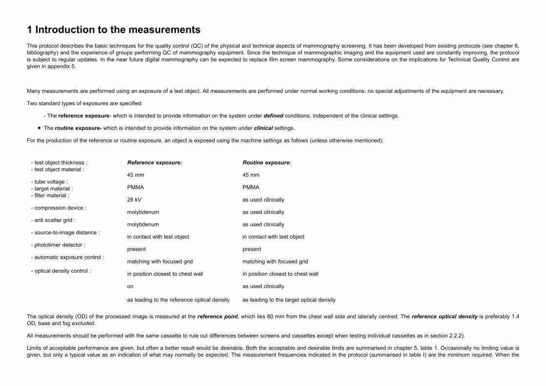
For the production of the reference or routine exposure, an object is exposed using the machine settings as follows (unless otherwise mentioned):
- test object thickness :- test object material :
- tube voltage :- target material :- filter material :
- compression device :
- anti scatter grid :
- source-to-image distance :
- phototimer detector :
- automatic exposure control :
- optical density control :
Reference exposure:
45 mm
PMMA
28 kV
molybdenum
molybdenum
in contact with test object
present
matching with focused grid
in position closest to chest wall
on
as leading to the reference optical density
Routine exposure:
45 mm
PMMA
as used clinically
as used clinically
as used clinically
in contact with test object
present
matching with focused grid
in position closest to chest wall
as used clinically
as leading to the target optical density
The optical density (OD) of the processed image is measured at the reference point, which lies 60 mm from the chest wall side and laterally centred. The reference optical density is preferably 1.4OD, base and fog excluded.
All measurements should be performed with the same cassette to rule out differences between screens and cassettes except when testing individual cassettes as in section 2.2.2).
Limits of acceptable performance are given, but often a better result would be desirable. Both the acceptable and desirable limits are summarised in chapter 5, table 1. Occasionally no limiting value isgiven, but only a typical value as an indication of what may normally be expected. The measurement frequencies indicated in the protocol (summarised in table I) are the minimum required. When the

acceptable limiting value is exceeded the measurement should be repeated. If necessary, additional measurements should be performed to determine the origin of the observed problem andappropriate actions should be taken to solve the problem.
For guidance on the specific design and operating criteria of suitable test objects; see the Proceedings of the CEC Workshop on Test Phantoms (see chapter 6, Bibliography). Definition of terms, suchas the ‘reference point’ and the ‘reference density’ are given in chapter 4. The evaluation of the results of the QC measurements can be simplified by using the forms for QC reporting provided inappendix 6.
Staff and equipment
Several measurements can be performed by the local staff. The more elaborate measurements should be undertaken by medical physicists who are trained and experienced in diagnostic radiology andspecifically trained in mammography QC. Comparability and consistency of the results from different centres is best achieved if data from all measurements, including those performed by localtechnicians or radiographers are collected and analysed centrally.
The staff conducting the daily/weekly QC-tests will need the following equipment at the screening site:
- Sensitometer - Standard test block (45 mm PMMA)
- Densitometer - QC test object
- Thermometer - Reference cassette
- PMMA plates
The medical physics staff conducting the other QC-tests will need the following additional equipment and may need duplicates of many of the above1:
- Dosemeter
- kVp-meter
- Exposure time meter
- Light meter
- QC test objects
- Aluminium sheets
- Focal spot test device + stand
- Stopwatch
- Film/screen contact test device
- Tape measure
- Compression force test device
- Rubber foam
- Lead sheet

- Aluminium stepwedge
Generally when absolute measurements of dose are performed, make sure that the proper corrections for temperature and air pressure are applied to the raw values. Use one and the same box of(fresh) film throughout the tests described in this protocol.
2.1 X-ray generation
2.1.1 X-ray source
The measurements to determine the focal spot size, source-to-image distance, alignment of X-ray field and image receptor, radiation leakage and tube output, are described in this section.
Focal spot size
The measurement of the focal spot size is intended to determine its physical dimensions at installation or when resolution has markedly decreased. The focal spot size must be determined for allavailable targets of the mammography unit. For routine quality control the evaluation of spatial resolution is considered adequate.
The focal spot dimensions can be obtained by using one of the following methods.
• star pattern method; a convenient method (routine testing);
• slit camera; a complex, but accurate method for exact dimensions (acceptance testing)
• pinhole camera; a complex, but accurate method to determine the shape (acceptance testing)• multi-pinhole test tool, a simple method to determine the size across the field (routine/acceptance
testing)
A magnified X-ray image of the test device is produced using a non-screen cassette. This can be achieved by placing a black film (OD ³ 3) between screen and film. Select the focal spot size required,28 kV tube voltage and a focal spot charge (mAs) to obtain an optical density between 0.8 and 1.4 OD base and fog excluded (measured in the central area of the image). The device should be imagedat the reference point of the image plane, which is located at 60 mm from the chest wall side and laterally centred. Remove the compression device and use the test stand to support the test device.Select about the same focal spot charge (mAs) that is used to produce the standard image of 45 mm PMMA, which will result in an optical density of the star pattern image in the range 0.8 to 1.4.
According the IEC/NEMA norm, an 0.3 nominal focal spot is limited to a width of 0.45 mm and a length of 0.65 mm. An 0.4 nominal focal spot is limited to 0.60 and 0.85 mm respectively. No specificlimiting value is given here, since the measurement of imaging performance of the focal spot is incorporated in the limits for spatial resolution at high contrast. (see 2.5.2)
Focal spot size: star pattern method
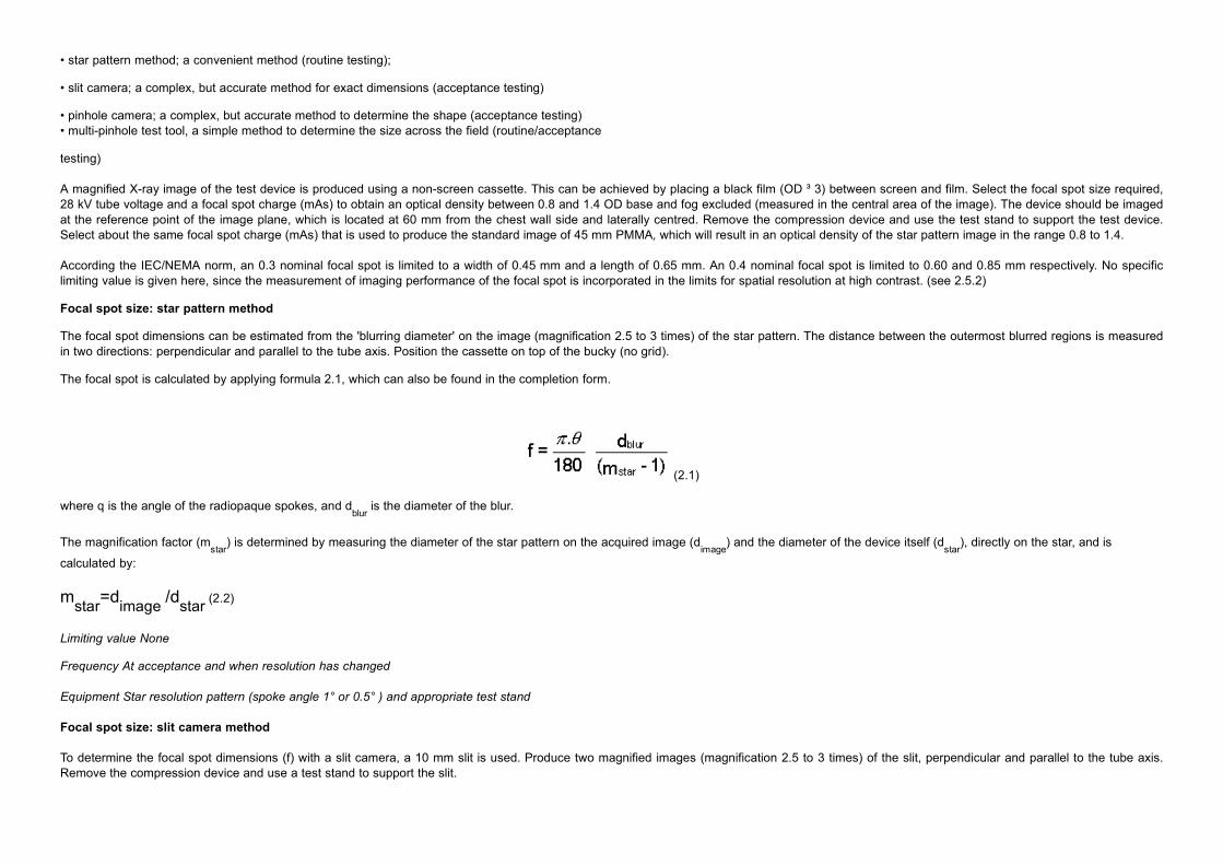
The focal spot dimensions can be estimated from the 'blurring diameter' on the image (magnification 2.5 to 3 times) of the star pattern. The distance between the outermost blurred regions is measuredin two directions: perpendicular and parallel to the tube axis. Position the cassette on top of the bucky (no grid).
The focal spot is calculated by applying formula 2.1, which can also be found in the completion form.
(2.1)
where q is the angle of the radiopaque spokes, and dblur
is the diameter of the blur.
The magnification factor (mstar
) is determined by measuring the diameter of the star pattern on the acquired image (dimage
) and the diameter of the device itself (dstar
), directly on the star, and is
calculated by:
mstar=dimage /dstar (2.2)
Limiting value None
Frequency At acceptance and when resolution has changed
Equipment Star resolution pattern (spoke angle 1° or 0.5° ) and appropriate test stand
Focal spot size: slit camera method
To determine the focal spot dimensions (f) with a slit camera, a 10 mm slit is used. Produce two magnified images (magnification 2.5 to 3 times) of the slit, perpendicular and parallel to the tube axis.Remove the compression device and use a test stand to support the slit.
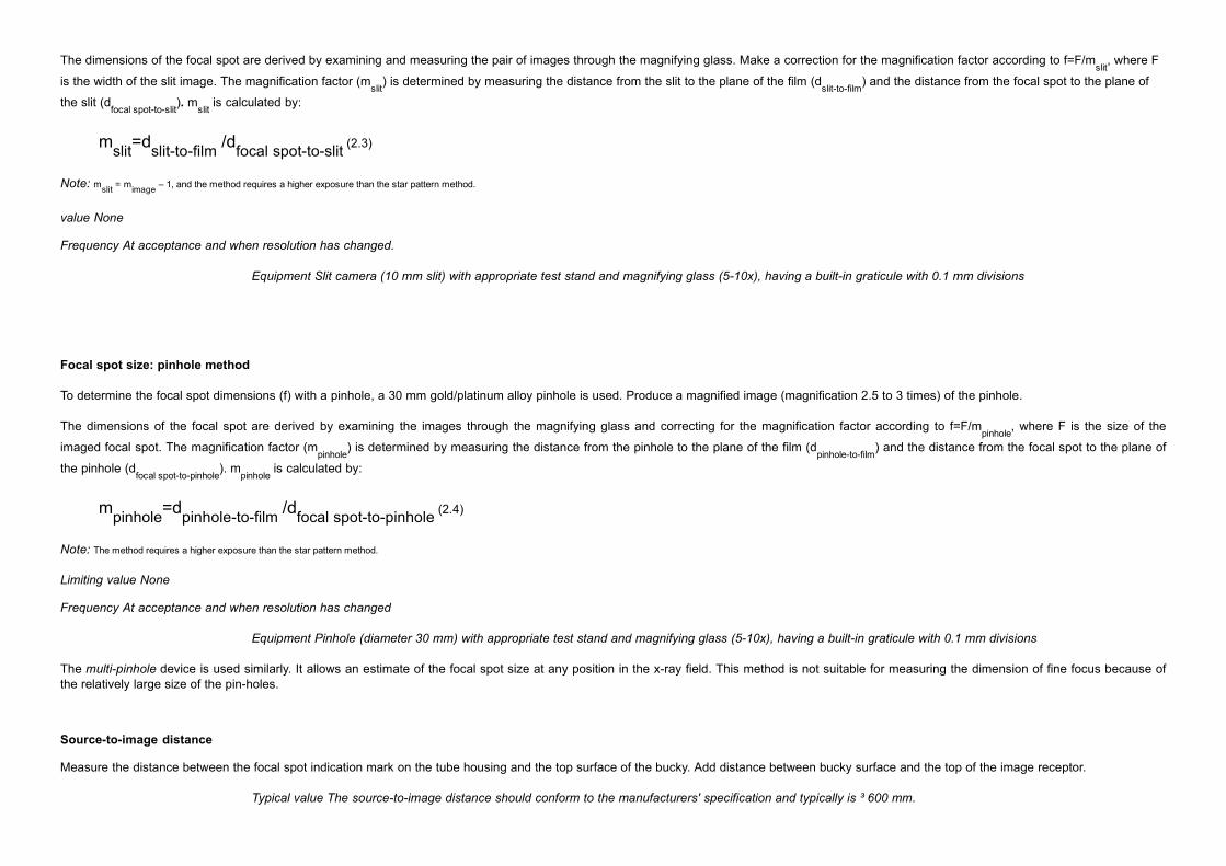
The dimensions of the focal spot are derived by examining and measuring the pair of images through the magnifying glass. Make a correction for the magnification factor according to f=F/mslit
, where F
is the width of the slit image. The magnification factor (mslit
) is determined by measuring the distance from the slit to the plane of the film (dslit-to-film
) and the distance from the focal spot to the plane of
the slit (dfocal spot-to-slit
). mslit
is calculated by:
mslit=dslit-to-film /dfocal spot-to-slit (2.3)
Note: mslit = mimage – 1, and the method requires a higher exposure than the star pattern method.
value None
Frequency At acceptance and when resolution has changed.
Equipment Slit camera (10 mm slit) with appropriate test stand and magnifying glass (5-10x), having a built-in graticule with 0.1 mm divisions
Focal spot size: pinhole method
To determine the focal spot dimensions (f) with a pinhole, a 30 mm gold/platinum alloy pinhole is used. Produce a magnified image (magnification 2.5 to 3 times) of the pinhole.
The dimensions of the focal spot are derived by examining the images through the magnifying glass and correcting for the magnification factor according to f=F/mpinhole
, where F is the size of the
imaged focal spot. The magnification factor (mpinhole
) is determined by measuring the distance from the pinhole to the plane of the film (dpinhole-to-film
) and the distance from the focal spot to the plane of
the pinhole (dfocal spot-to-pinhole
). mpinhole
is calculated by:
mpinhole=dpinhole-to-film /dfocal spot-to-pinhole (2.4)
Note: The method requires a higher exposure than the star pattern method.
Limiting value None
Frequency At acceptance and when resolution has changed
Equipment Pinhole (diameter 30 mm) with appropriate test stand and magnifying glass (5-10x), having a built-in graticule with 0.1 mm divisions
The multi-pinhole device is used similarly. It allows an estimate of the focal spot size at any position in the x-ray field. This method is not suitable for measuring the dimension of fine focus because ofthe relatively large size of the pin-holes.
Source-to-image distance
Measure the distance between the focal spot indication mark on the tube housing and the top surface of the bucky. Add distance between bucky surface and the top of the image receptor.
Typical value The source-to-image distance should conform to the manufacturers' specification and typically is ³ 600 mm.
Frequency At acceptance only.
When distance is adjustable: every six months.
Equipment Tape measure.
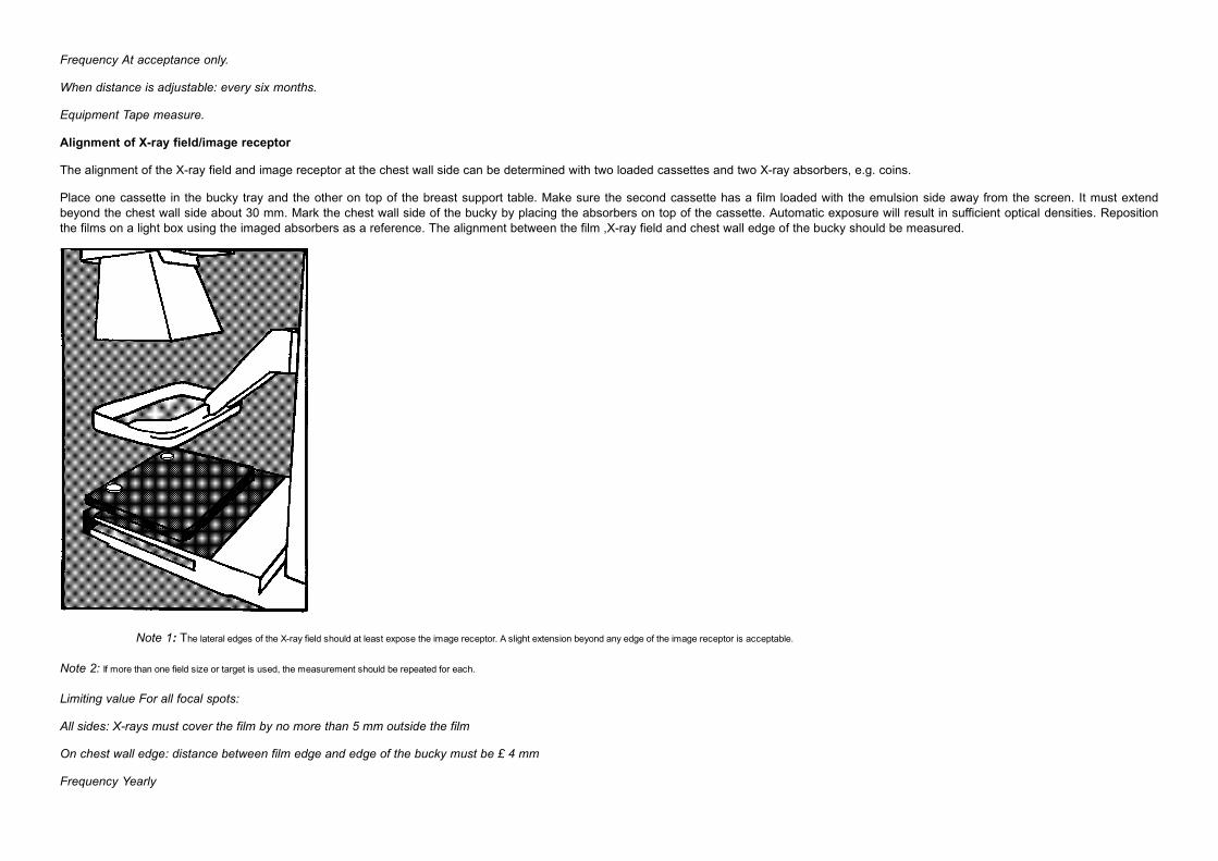
Alignment of X-ray field/image receptor
The alignment of the X-ray field and image receptor at the chest wall side can be determined with two loaded cassettes and two X-ray absorbers, e.g. coins.
Place one cassette in the bucky tray and the other on top of the breast support table. Make sure the second cassette has a film loaded with the emulsion side away from the screen. It must extendbeyond the chest wall side about 30 mm. Mark the chest wall side of the bucky by placing the absorbers on top of the cassette. Automatic exposure will result in sufficient optical densities. Repositionthe films on a light box using the imaged absorbers as a reference. The alignment between the film ,X-ray field and chest wall edge of the bucky should be measured.
Note 1: The lateral edges of the X-ray field should at least expose the image receptor. A slight extension beyond any edge of the image receptor is acceptable.
Note 2: If more than one field size or target is used, the measurement should be repeated for each.
Limiting value For all focal spots:
All sides: X-rays must cover the film by no more than 5 mm outside the film
On chest wall edge: distance between film edge and edge of the bucky must be £ 4 mm
Frequency Yearly

Equipment X-ray absorbers -e.g. coins, rulers, iron balls, tape measure
Radiation leakage
The measurement of leakage radiation comprises two parts; firstly the location of leakage and secondly, the measurement of its intensity.
Position a beam stopper (e.g. lead sheet) over the end of the diaphragm assembly such that no primary radiation is emitted. Enclose the tube housing with loaded cassettes and expose to themaximum tube voltage and a high tube current (several exposures). Process the films and pin-point any excessive leakage. Next, quantify the amount of radiation at the "hot-spots" at a distance of 50mm of the tube with a suitable detector. Correct the readings to air kerma rate in mGy/h (free in air) at the distance of 1 m from the focal spot at the maximum rating of the tube.
Limiting value Not more than 1 mGy in 1 hour at 1 m from the focus at the maximum rating of the tube
averaged over an area not exceeding 100 cm², and according to local regulations
Frequency At acceptance and after intervention on the tube housing
Equipment Dose meter and appropriate detector
Tube output
The specific tube output (mGy/mAs) and the output rate (mGy/s) should both be measured at 28 kVp on a line passing through the focal spot and the reference point, in the absence of scatter materialand attenuation (e.g. due to the compression plate). A tube load (mAs) similar to that required for the reference exposure should be used for the measurement. Correct for the distance from the focalspot to the detector and calculate the specific output at 1 metre and the output rate at a distance equal to the focus-to-film distance (FFD).
Typical values 40-75 mGy/mAs at 1 metre
10-30 mGy/s at a distance equal to the FFD
Frequency Every six months and when problems occur
Equipment Dose-meter, exposure timer
Note: A high output is desirable for a number of reasons e.g. it results in shorter exposure times, minimising the effects of patient movement and ensures adequate penetration of large/dense breasts within the setting ofthe guard timer. In addition any marked changes in output require investigation.
2.1.2 Tube voltage
The radiation quality of the emitted X-ray beam is determined by tube voltage, anode material and filtration. Tube voltage and Half Value Layer (i.e. beam quality assessment) can be assessed by themeasurements described below.
Reproducibility and accuracy
A tube voltage check over the range 25 - 31 kVp at 1 kV intervals should be performed. If other tube voltages are used clinically then these must be measured also. The reproducibility is measured byrepeated exposures at one fixed tube voltage that is normally used clinically (e.g. 28 kVp).
Note: Consult the instruction manual of the kVp-meter for the correct positioning.
Limiting value Accuracy for 25-31 kV: < ± 1 kV, reproducibility < ± 0.5 kV
Frequency Every six months

Equipment kVp-meter
Half Value Layer
The Half Value Layer (HVL) can be assessed by adding thin aluminium (Al) filters to the X-ray beam and measuring the attenuation.
Position the exposure detector at the reference point (since the HVL is position dependent) on top of the bucky. Place the compression device halfway between focal spot and detector. Select 28 kVtube voltage and an adequate focal spot charge (mAs-setting), and expose the detector directly. The filters can be positioned on the compression device and must intercept the whole radiation field.Use the same tube load (mAs) setting and expose the detector through each filter. For higher accuracy (about 2%) a diaphragm, positioned on the compression paddle, limiting the exposure to the areaof the detector may be used (see European Protocol on Dosimetry in Mammography, ISBN 92-827-7289-6). The HVL is calculated by applying formula 2.5.
The direct exposure reading is denoted as Y0; Y
1 and Y
2 are the exposure readings with added aluminium thickness of X
1 and X
2 respectively.
Note 1: The purity of the aluminium ³ 99.9% is required. The thickness of the aluminium sheets should be measured with an accuracy of 1%.
Note 2: For this measurement the output of the X-ray machine needs to be stable.
Note 3: The HVL for other (clinical) tube voltages and other target materials and filters may also be measured for assessment of the mean glandular dose (see appendix 3 and the European Protocol on Dosimetry in Mammography, ISBN92-827-7289-6).
Note 4: Alternatively a digital HVL-meter can be used, but correct these readings under extra filtration following the manufacturers’ manual.
Limiting value For 28 kV Mo/Mo the HVL must be over 0.30 mm Al equivalent, and is
typically < 0.40 mm Al. Typical values for other tube voltages, targets and filters, are shown in appendix 3
Frequency Yearly
Equipment Dosemeter, aluminium sheets 0.30 and 0.40 mm
2.1.3 AEC-system
The performance of the Automatic Exposure Control (AEC) system can be described by the reproducibility and accuracy of the automatic optical density control under varying conditions, like differentobject thickness and tube voltages. Essential prerequisites for these measurements are a stable operating film-processor and the use of the reference cassette. If more than one breast support table,with a different AEC detector attached, is used then each system must be assessed separately.
Optical density control setting: central value and difference per step
To compensate for the long term variations in mean density due to system variations the central optical density setting and the difference per step of the selector are assessed. To verify the adjustmentof the optical density control, produce exposures with a 45 mm PMMA test object with varying settings of the optical density control selector. Typical routine exposure factors should be used.
A target value for the mean optical density at the reference point should be established according to local preference, in the range: 1.3 – 1.8 OD, base and fog included.
Limiting value The optical density (base and fog included) at the reference point should remain within
± 0.15 OD of the target value
The change produced by each step in the optical density control should be about 0.10
OD; step-sizes within the range 0.05 to 0.20 OD are acceptable
The acceptable value for the range covered by full adjustment of the density control
is > 1.0 OD
Frequency Step-size and adjustable range: every six months
Density and mAs-value for clinically used AEC setting: daily
Equipment Standard test block, densitometer
Guard timer
The AEC system should also be equipped with a guard timer which will terminate the exposure in case of malfunctioning of the AEC system. Measure the tube load (mAs) at which the systemterminates the exposure e.g. when using increasing thickness of PMMA plates.
Warning: an incorrect functioning of the guard timer could damage the tube. To avoid excessive tube load consult the manual for maximum permitted exposure time.
Limiting value None
Frequency Yearly
Equipment Sheet of lead
Short term reproducibility
Position the dosemeter in the x-ray beam but without covering the AEC-detector. The short term reproducibility of the AEC system is calculated by the deviation of the exposure meter reading of tenroutine exposures (45 mm PMMA).
Limiting value The deviations from the mean value of exposures must be < ± 5%. Desirable would be
< ± 2%
Frequency Every six months
Equipment Standard test block, dosemeter
Note: For the assessment of the reproducibility, also compare these results from the short term reproducibility with the results from the thickness and tube voltage compensation and from the optical density control settingat 45 mm PMMA at identical settings. Any problem will be indicated by a mismatch between those figures.
Long term reproducibility
The long term reproducibility can be assessed from the measurement of optical density and tube load (mAs) resulting from the exposures of a PMMA-block or the QC test object in the daily qualitycontrol. Causes of deviations can be found by comparison of the daily sensitometry data and tube load (mAs) recordings (see 2.3.2)
Limiting value The variation from the target value must be within < ± 0.20 OD; < ± 0.15 OD desirable Frequency Daily
Equipment Standard test block or QC test object, densitometer

Object thickness and tube voltage compensation
Compensation for object thickness should be measured by exposures of PMMA plates in the thickness range 20 to 70 mm, using a range of clinical settings (tube voltage, target, filter, modes) for theAEC corresponding to clinical practice. These settings include: full-automatic, semi-automatic as well as manual modes. In full-automatic mode all pre-programmed combinations of tube voltage, anodeand filter should be chosen automatically when going through the range of PMMA thicknesses. When a combination is not chosen automatically then this combination must be selected manually, withthe simulated breast thickness closest to the proper thickness (i.e. the PMMA thickness where this technique is appropriate). See appendix 5 for samples of such settings in the report forms.
Limiting value All optical density variations must be within ± 0.15 OD, with respect of the target optical
density. Desirable: ± 0.10 OD
Frequency Every six months: full test
Weekly: 20, 45, 65 mm PMMA exposed as for clinical settings
Equipment PMMA: plates 10x180x240 mm3, densitometer
.
2.1.4 Compression
The compression of the breast tissue should be firm but tolerable. There is no optimal value known for the force, but attention should be given to the applied compression and the accuracy of theindication. All units must have motorised compression. See also chapter I-2, paragraph on compression.
Compression force
The compression force can be adequately measured with a compression force test device or a bathroom scale (use compressible material e.g. a tennis ball to protect the bucky and compressiondevice).
When compression force is indicated on the console, it should be verified whether the figure corresponds with the measured value. It should also be verified whether the applied compression force ismaintained over a period of 1 minute. A loss of force over this time may be explained, for example, by a leakage in the pneumatic system.

Limiting value Maximum automatically applied force: 130 - 200 N. (~ 13-20 kg), and must be maintained
unchanged for at least 1 minute
Frequency Yearly
Equipment Compression force test device
Compression plate alignment
The alignment of the compression device at maximum force can be visualised and measured when a piece of foam-rubber is compressed. Measure the distance between bucky surface andcompression device on each corner. Normally, those four distances are equal. Misalignment normal to the chest wall side is less disturbing than in the parallel direction, as it compensates for the heeleffect. The upright edge of the device must be projected outside the receptor area and optimally within the chest wall side of the bucky.
Limiting value Minimal misalignment is allowed, £ 15 mm is acceptable for asymmetrical load and in the
direction towards the nipple, £ 5 mm for symmetrical load
Frequency Yearly
Equipment Foam rubber (specific mass: about 30 mg/cm3), tape measure
2.2 Bucky and image receptor
If more than one bucky and image receptor system is attached to the imaging chain than each system must be assessed separately.
2.2.1 Anti scatter grid
The anti scatter grid is composed of strips of lead and low density interspace material and is designed to absorb scattered photons. The grid system is composed of the grid, a cassette holder, a breastsupport table and a mechanism for moving the grid.
Grid system factor
The grid system factor can be determined by dose measurements. Produce two images, one with and one without the grid system. Use manual exposure control to obtain images of about referenceoptical density. The first image is made with the cassette in the bucky tray (imaged using the grid system) and PMMA on top of the bucky. The second with the cassette on top of the bucky (imaging not
using the grid system) and PMMA on top of the cassette. The grid system factor is calculated by dividing the dose meter readings, corrected for the inverse square law and optical density differences.
Note: Not correcting the doses for the inverse square law will result in an over estimation of 5%.
Typical value < 3.
Frequency At acceptance and when dose or exposure time increases suddenly.
Equipment Dosemeter, standard test block and densitometer.
Grid imaging
To assess the homogeneity of the grid in case of suspected damage or looking for the origin of artefacts, the grid may be imaged by automatic exposure of the bucky at the lowest position of theAEC-selector, without any added PMMA. This in general gives a good image of the gridlines.
Limiting value No significant non uniformity
Frequency Yearly
Equipment None
2.2.2 Screen-film
The current image receptor in screen-film mammography consists of a cassette with one intensifying screen in close contact with a single emulsion film. The performance of the stock of cassettes isdescribed by the inter cassette sensitivity variation and screen-film contact.
Inter cassette sensitivity and attenuation variation and optical density range
The differences between cassettes can be assessed with the reference exposure (chapter 1). Select an AEC setting (should be the normal position and using a fixed tube voltage, target and filter) toproduce an image having about the clinically used mean optical density on the processed film. Repeat for each cassette using films from the same box or batch. Make sure the cassettes are identifiedproperly. Measure the exposure (in terms of mGy or mAs) and the corresponding optical densities on each film at the reference point. To ensure that the cassette tests are valid the AEC system in themammography unit needs to be sufficiently stable. It will be sufficient if the variation in repeated exposures selected by the AEC for a single cassette is (in terms of mGy and mAs) <± 2%.
Limiting value The exposure, in terms of mGy (or mAs), must be within ±5% of the mean for all
cassettes
The maximum difference in optical density between all cassettes: ± 0.10 OD is
Acceptable: ± 0.08 OD is desirable
Frequency Yearly, and after introducing new screens
Equipment Standard test object, dosemeter, densitometer
Screen-film contact
Clean the inside of the cassette and the screen. Wait for at least 5 minutes to allow air between the screen and film to escape. Place the mammography contact test device (about 40 metal wires/inch,1.5 wires/mm) on top of the cassette and make a non grid exposure to produce a film with an average optical density of about 2 OD at the reference point. Regions of poor contact will be blurred and

appear as dark spots in the image. Reject cassettes only when they show the same spots when the test is repeated after cleaning. View at a distance of 1 meter. Additionally the screen resolution maybe measured by imaging a resolution pattern placed directly on top of a cassette.
Limiting value No significant areas (i.e. > 1 cm2 ) of poor contact are allowed in the diagnostically
relevant part of the film
Frequency Every six months and after introducing new screens
Equipment Mammography screen-film contact test device, densitometer and viewbox
2.3 Film processing
The performance of the film processing greatly affects image quality. The best way to measure the performance is by sensitometry. Measurements of temperature and processing time are performed toestablish the baseline performance.
2.3.1 Baseline performance of the processor
Temperature verification and baseline
To establish a baseline performance of the automatic processor, the temperature of developer and fixer are measured. Take care that the temperature is measured at a fixed point, as recommended bythe manufacturers. The measured values can be used as background information when malfunction is suspected. Do not use a glass thermometer because of the contamination risk in the event ofbreakage.
Limiting value Compliance with the manufacturer’s recommendations
Frequency Every six months
Equipment Electronic thermometer
Processing time
The total processing time can be measured with a stopwatch. Insert the film into the processor and start the timer when the signal is given by the processor. When the processed film is available, stopthe timer. When malfunction of the processor is suspected, measure this processing time exactly the same way again and check to see if there is any difference.
Limiting value Compliance with the manufacturer’s recommendations
Frequency At acceptance and when problems occur
Equipment Stopwatch
2.3.2 Film and processor
The films used in mammography should be specially designed for that purpose. Light sensitometry is a suitable method to measure the performance of the processor. Disturbing processor artefactsshould not be present on the processed image.
Sensitometry
Use a sensitometer to expose a film with light and insert the exposed side into the processor first. Before measuring the optical densities of the step-wedge, a visual comparison can be made with areference strip to rule out a procedure fault, like exposure with a different colour of light or exposure of the base instead of the emulsion side.
From the characteristic curve (the graph of measured optical density against the logarithm of exposure by light) the values of base and fog, maximum density, speed and film gradients can be derived.These parameters characterise the processing performance. A detailed description of these ANSI-parameters and their clinical relevance can be found in appendix 1, film parameters.

Typical values: base and fog: 0.15 – 0.25 OD
contrast: MGrad: 3.0 - 4.0
Grad 1-2
: 3.5 – 5.0
Frequency Daily
Equipment Sensitometer, densitometer
Note: There is no clear evidence for the optimal value of film gradient; the ranges quoted are based on what is typical of current practice. At the top end of these ranges the high film gradient may lead to under- and over exposure of parts ofthe image for some types of breast, thereby reducing the information content. A further complication of using a very high film contrast is that stable conditions with very low variability of the parameters are required to achieve any benefit interms of overall image quality (See appendix 1).
Daily performance
The daily performance of the processor is assessed by sensitometry. After the processor has been used for about one hour each morning, perform the sensitometry as described above. The variabilityof the parameters can be calculated over a period of time e.g. one month (see calculation of film parameters in appendix 1).
Limiting value See table below
Frequency Daily and more often when problems occur
Equipment Sensitometer, densitometer
The assessment of variations can be found in the use of the following table, where the values are expressed as a range (Max value - Min value). Acceptable and desirable ranges are quoted in thetable below for speed and contrast indices for centres where computer facilities for calculating speed and film gradient (Mgrad and Grad1,2) are not available. However this approach is less satisfactoryas these indices are not pure measures of speed and contrast.
Assessment of variations
acceptable desirable
base and fog < 0.03 < 0.02 OD
max. density < 0.30 < 0.20 OD
speed < 0.05 < 0.03
mean gradient (Mgrad) < 0.30 < 0.15
mid gradient (Grad1,2) <0.40 <0.20
speed index < 0.30 < 0.20 OD
contrast index < 0.30 < 0.20 OD
temperature displayed < 2 < 1 °C
Table to 2.3.2.
Artefacts

An image of the standard test block obtained daily, using a routine exposure should be inspected. This should show a homogeneous density, without significant scratches, shades or other marksindicating artefacts.
Limiting value No artefacts
Frequency Daily
Equipment Standard test block or PMMA plates 40-60 mm and area 18X24cm, viewing box
2.3.3 Darkroom
Light tightness of the darkroom should be verified. It is reported, that about half of darkrooms are found to be unacceptable. Cassettes and film hopper should also be light tight. Extra fogging by thesafelights must be within given limits.
Light leakage
Remain in the darkroom for a minimum of five minutes with all the lights, including the safelights, turned off. Ensure that adjacent rooms are fully illuminated. Inspect all those areas likely to be a sourceof light leakage. To measure the extra fog as a result of any light leakage or other light sources, a pre-exposed film of about 1.2 OD is needed. This film can be obtained by a reference exposure of auniform PMMA block. Always measure the optical density differences in a line perpendicular to the tube axis to avoid influence of the heel effect.
Open the cassette with pre-exposed film and position the film (emulsion up) on the (appropriate part of the) workbench. Cover half the film and expose for two minutes. Position the cover parallel to thetube axis to avoid the influence of the heel effect in the measurements. Measure the optical density difference of the background (D
bg) and the fogged area (D
fogged). The extra fog (DD) equals:
DD = Dfogged - Dbg (2.6)
Limiting value Extra fog: DD£ 0.02 OD in 2 minutes
Frequency Every six months and when light leakage is suspected
Equipment Film cover, densitometer
Safelights
Perform a visual check that all safelights are in good working order (filters not cracked). To measure the extra fog as a result of the safelights, repeat the procedure for light leakage but with thesafelights on. Make sure that the safelights were on for more than 5 minutes to avoid start-up effects.

Limiting value Extra fog: DD£ 0.05 OD in 2 minutes
Frequency At acceptance, every six months and every time the darkroom environment has changed
Equipment Film cover, densitometer
Film hopper
Fogged edges on unexposed (clear) films may indicate that the film hopper is no longer light tight. Place one fresh sheet of film in the hopper. Leave it there for several hours with full white lightillumination in the darkroom. Inspect the processed film for light leakage of the hopper.
Limiting value Extra fog: < 0.02
Frequency When light leakage is suspected
Equipment None
Cassettes
Dark edges on radiographs indicate a need to perform light leakage tests on individual cassettes. Reload the suspect cassette with a fresh sheet of film and place it in front of a viewing box for severalhours. Making
sure that each side of the cassette is exposed to bright light by turning it over. Inspect the processed film for dark edges due to light leakage of the cassette.
Limiting value No extra fogging
Frequency This test should be performed at acceptance and when light leakage is suspected
2.4 Viewing conditions
Since good viewing conditions are important for the correct interpretation of the diagnostic images, they must be optimised. Although the need for relatively bright light boxes is generally appreciated,the level of ambient lighting is also very important and should be kept low. In addition it is imperative that glare is minimised by masking the film.
As regards light levels the procedures for photometric measurements and the values required for optimum mammographic viewing are not well established. However there is general agreement on theparameters that are important. The two main measurements in photometry are luminance and illuminance. The luminance of viewing boxes is the amount of light emitted from a surface measured incandela/m2. Illuminance is the amount of light falling on a surface and is measured in lux (lumen/m2). The illuminance that is of concern here is the light falling on the viewing box, i.e. the ambient lightlevel. (An alternative approach is to measure the light falling on the film readers eye by pointing the light detector at the viewing box from a suitable distance with the viewing box off.) Whether one ismeasuring luminance or illuminance one requires a detector and a photometric filter. This combination is designed to provide a spectral sensitivity similar to the human eye. The collection geometry andcalibration of the instrument is different for luminance and illuminance. To measure luminance a lens or fibre-optic probe is used, whereas a cosine diffuser is fitted when measuring illuminance. Wherethe only instrument available is an illuminance meter calibrated in lux it is common practice to measure luminance by placing the light detector in contact facing the surface of the viewing box andconverting from lux to cd/m2 by dividing by p. Since this approach makes assumptions about the collection geometry, a correctly calibrated luminance detector is preferred.
There is no clear consensus on what luminance is required for viewing boxes. It is generally thought that viewing boxes for mammography need to be higher than for general radiography. In a review of20 viewing boxes used in mammographic screening in the UK, luminance averaged 4500 cd/m2 and ranged from 2300 to 6700 cd/m2. In the USA the ACR recommend a minimum of 3500 cd/m2 formammography. However some experts have suggested that the viewing box luminance need not be very high provided the ambient light is sufficiently low and that the level of ambient light is the mostcritical factor. The limiting values suggested here represent a compromise position until clearer evidence is available.

2.4.1. Viewing box
Luminance
The tendency to use a high optical density for mammography means that one must ensure that the luminance of the viewbox is adequate. Measure the luminance close to the centre of the illuminatedarea of each panel using a luminance meter calibrated in cd/m2. An upper limit is included to minimise glare where films are imperfectly masked.
Limiting value Luminance should be in the range 3000-6000 cd/m2
Frequency Yearly
Equipment Luminance meter
Homogeneity
The homogeneity of a single viewing box is measured by multiple readings of luminance over the surface of the illuminator, compared with the mean value of readings in the middle of the viewing area.Readings very near the edges (e.g. within 5 cm) of the viewing box should be avoided. Gross mismatch between viewing boxes or between viewing conditions used by the radiologist and those used bythe radiographer should be avoided. If a colour mismatch exists, check to see that all lamps are of the same brand, type and age. Change all tubes at the same time. To avoid inhomogeneities as aresult of dust, clean the light boxes regularly inside and out.
Limiting value The uniformity of luminance across a single light box should be within ± 30% in the area 5 cm in from the edge of the pane. The intensity of different lightboxes at one department should be within 15% of the average (measured in the middle of the viewing area)
Frequency Yearly
Equipment Luminance meter
2.4.2. Ambient light
Level
When measuring the ambient light level (illuminance), the viewing box should be switched off. Place the detector against the viewing area and rotate away from the surface to obtain a maximal reading.This value is denoted as the ambient light level.
Limiting value Ambient light level < 50 lux
Frequency Yearly
Equipment Illuminance meter
2.5 System properties
The success of a screening programme is dependent on the proper information transfer and therefore on the image quality of the mammogram. Decreasing the dose per image for reasons of radiationprotection is only justified when the information content of the image remains sufficient to achieve the aim.
2.5.1 Dosimetry
The measurement of exposure and the calculation of the mean glandular dose in mammography are described in detail in the European Protocol on Dosimetry in Mammography. (See chapter 6,Bibliography.) Only the measurement of entrance surface air kerma is described here for convenience.
Entrance surface air kerma
This measurement is performed under reference conditions (28 kV, Mo target material, 30m m Mo filter) either with AEC or manual exposure.
Produce two exposures of the standard test block with an optical density under and over 1.4 OD (excluding base and fog). The corresponding entrance surface dose should be measured as close to thereference point as possible. The value for the entrance surface air kerma at the reference density should be interpolated linearly from these data. From this value the average glandular dose can becalculated (see: page 29, European Protocol On Dosimetry). The average glandular dose for a 4.5 cm thick breast is typically less than 2.0 mGy.
Limiting value £15 mGy (for other OD’s and thicknesses: see appendix 3)
Frequency Yearly
Equipment Dose meter, standard test block, densitometer
2.5.2 Image Quality
The information content of an image may best be defined in terms of just visible contrasts and details, characterised by its contrast-detail curve. The basic conditions for good performance and theconstancy of a system can be assessed by measurement of the following: resolution, contrast visibility, threshold contrast and exposure time.
Spatial resolution
One of the parameters which determine image quality is the system spatial resolution. It can be adequately measured by imaging two resolution lead bar patterns, up to 20 line pairs per mm (lp/mm)each. They should be placed on top of PMMA plates with a total thickness of 45 mm. Image the patterns at the reference point both parallel and perpendicular to the tube axis, and determine theseresolutions.
Note: If the resolution is measured at different heights between 25 and 50 mm from the tabletop it can differ by as much as 4 lp/mm. The distance from the chest wall edge is critical, but the position parallel to the thorax side is not critical within ± 5cm from the reference point. Resolution is generally worse parallel to the tube axis due to the asymmetrical shape of the focal spot.
Limiting value > 10 lp/mm acceptable, > 13 lp/mm desirable at the reference point in both directions
Frequency Weekly
Equipment PMMA plates 180x240 mm, resolution pattern(s) up to 20 lp/mm, densitometer
Image contrast
Since image contrast is affected by various parameters (like tube voltage, film contrast etc.) this measurement is an effective method to detect a range of system faults. Make a reference exposure of analuminium or PMMA stepwedge and measure the optical density of each step in the stepwedge. Draw a graph of the readings at each step against the stepnumber. The graph gives an impression ofthe image contrast. Since this graph includes the processing conditions, the film curve has to be excluded to find the radiation contrast, see Appendix 2.
Remarks: The value for image contrast is dependent on the whole imaging chain, therefore no absolute limits are given. Ideally the object is part of, or placed on top of, the daily quality control testobject.
Limiting value ±10% acceptable, ±5% desirable
Frequency Weekly, and when problems occur
Equipment PMMA or aluminium stepwedge, densitometer
Threshold contrast visibility
This measurement should give an indication of the lowest detectable contrast of "large" objects (diameter > 5 mm). Therefore a selection of low contrast objects have to be embedded in a PMMA testobject to mimic clinical exposures. There should be at least two visible and two non-visible objects. Note, that the result is dependent on the mean OD of the image and on noise.

Produce a routine exposure and let two or three observers examine the low contrast objects. The number of visible objects is recorded. Ideally the object is part of, or placed on top of, the daily qualitycontrol test object.
Limiting value minimum detectable contrast for a < 6 mm detail < 1.5% (see appendix 4)
Frequency Weekly
Equipment Test object with low contrast details plus PMMA plates, to a thickness of 45 mm,
densitometer
Exposure time
Long exposure times can give rise to motion unsharpness. Exposure time may be measured by some designs of kVp- and output meters. Otherwise a dedicated exposure timer has to be used. Thetime for a routine exposure is measured.
Limiting value Acceptable: < 2 sec.; desirable: <1.5 sec
Frequency Yearly and when problems occur
Equipment Exposure time meter, standard test block
To ascertain that the performance of the equipment is likely to be unchanged with respect to former measurements a number of tests should be conducted daily. For this purpose, a dedicated QC-testobject or set of test objects are convenient. The actual frequencies recommended for each measurement are specified in Section 2 and summarised in Table 5. The procedure must facilitate themeasurement of some essential physical quantities, and it should be designed to evaluate:
- AEC reproducibility
- tube output
- reference optical density
- spatial resolution
- image contrast
- threshold contrast visibility
- homogeneity, artefacts
- sensitometry (speed, contrast, gross fog)
Practical considerations:
- Ideally the sensitometric stepwedge should be on the same film as the image of the test object, to be able to correct optimally for the processing conditions.

- To improve the accuracy of the daily measurement, the test object should be designed in such a way that it can be positioned reproducibly on the bucky.
- The shape of the test object does not have to be breast-like. To be able to perform a good homogeneity check, the test object should cover the normally imaged area on the image receptor (180x240mm).
- For testing the AEC reproducibility, the PMMA test object may comprise several layers of PMMA, 10- or 20-mm thick. It is important to use the same PMMA blocks since variations in thickness of thePMMA plates will influence the tube load (mAs) read-out. Sufficient blocks are required to make up a thickness in the range 20-70 mm to adequately simulate the range of breast thickness foundclinically.
The definitions given here specify the meaning of the terms used in this document.
Accuracy: This is the closeness of an observed value of a quantity to the true value. It is calculated here as the difference between measured value (m) and true value (t) according: (m/t -1). Whenexpressed as an percentage use (m/t -1) X 100%.
Air kerma: The quotient of dEtr
by dm, measured in Gray, where dEtr is the sum of initial kinetic energies of all the charged ionising particles liberated by uncharged ionising particles in a mass of air dm
(adapted from ICRU 1980)
Automatic exposure control (AEC): A mode of operation of an X-ray machine by which the tube loading is automatically controlled and terminated when a pre-set radiation exposure to the imagereceptor is reached. The tube potential (kV), target- and filter material may also be automatically selected.
Average glandular dose: Reference term (ICRP 1987) for radiation dose estimation from X-ray mammography i.e. the average absorbed dose in the glandular tissue (excluding skin) in a uniformlycompressed breast of, e.g., 50% adipose, 50% glandular tissue composition. The reference breast thickness and composition should be specified.
Baseline value: The observed value of a parameter that is typical for a system.
Breast compression: The application of pressure to the breast during mammography so as to immobilise the breast and to present a lower and more uniform breast thickness to the X-ray beam.
Compression paddle: An approximately rectangular plate, positioned parallel to and above the breast table of a mammography X-ray machine, which is used to compress the breast.
Deviation (± %): The percentage of difference between measured value (m) and prescribed value (p) according: (m/p -1) x 100% .
Dmin: Minimum density achievable with an exposed film; usually the density of the first step of a sensitometric strip.
Dmax: Maximum density achievable with an exposed film; usually the density of the highest step of a sensitometric strip.
Entrance surface air kerma (ESAK): The air kerma measured free-in-air (without backscatter) at a point in a plane corresponding to the entrance surface of a specified object e.g., a patient’s breast ora standard test object.
Film gradient: The film gradient provides a measure of the film contrast.
Mgrad Mean Gradient; the property which expresses the film contrast in the diagnostic range. MGrad is calculated as the slope of the line through the points D1=Dmin+0.25 OD and
D2=Dmin+2.00 OD. Since the film curve is constructed from a limited number of points, D
1 and D
2 must be interpolated. Linear interpolation of the construction points of the film curve will
result in sufficient accuracy.
Grad1,2 Middle Gradient; the property which expresses the film contrast in the middle of the diagnostic range. Grad1,2
is calculated as the slope of the line through the points
D1=Dmin+1.00 OD and D
2=Dmin+2.00 OD. Since the film curve is constructed from a limited number of points, D
1 and D
2 must be interpolated. Linear interpolation of the construction

points of the film curve will result in sufficient accuracy.
Grad: see: film gradient.
Grid: A device which is positioned close to the entrance surface of an image receptor to reduce the quantity of scattered radiation reaching the receptor.
Half-value layer (HVL): The thickness of absorber which attenuates the air kerma of a collimated X-ray beam by half. The absorber used normally is high purity aluminium.
Heel effect: The non-uniform distribution of air kerma rate in an X-ray beam in a direction parallel to the cathode-anode axis.
Inverse square law: The physical law which states that the X-ray beam intensity reduces in inverse proportion to the square of the distance from the point of measurement to the X-ray tube focus.
Image Quality: Information content of the image in terms of just visible contrasts and details.
Laterally centred: Centred on a line perpendicular to the cathode-anode axis, not necessarily in the middle of the image.
Limiting value: A value of a parameter which, if exceeded, indicates that corrective action is required, although the equipment may continue to be used clinically. Limiting values for dose or air kermaare derived differently from reference values, i.e., reference ESD is based on third quartile values derived during surveys whereas limiting values of other parameters are derived from standard goodpractice.
Mammography: The X-ray examination of the female breast. This may be undertaken for health screening of a population (mammography screening) or to investigate symptoms of breast disease(symptomatic diagnosis).
Net optical density: Optical density excluding base and fog.
Optical density (OD): The logarithm of the ratio of the intensity of perpendicularly incident light (Io) on a film to the light intensity (I) transmitted by the film: OD=log10(Io/I). Optical density differencesshould be measured in a line perpendicular to the tube axis to avoid influences by the heel-effect.
Patient: Any woman attending a facility for mammography whether for screening or for symptomatic diagnosis.
Patient dose: A generic term for a variety of radiation dose quantities applied to a (group of) patient(s).
PMMA: The synthetic material polymethylmethacrylate. Trade names include Lucite, Perspex and Plexiglas.
Precision: The variation (usually relative standard deviation) in observed values. A synonym is repeatability.
QC test object: Object made of tissue simulating material (usually PMMA) with embedded measuring devices (e.g. resolution pattern, stepwedge) .
Quality Assurance as defined by the WHO (1982): "All those planned and systematic actions necessary to provide adequate confidence that a structure, system or component will perform satisfactorilyin service (ISO 6215-1980). Satisfactory performance in service implies the optimum quality of the entire diagnostic process-i.e., the consistent production of adequate diagnostic information withminimum exposure of both patients and personnel."
Quality Control as defined by the WHO (1982): "The set of operations (programming, co-ordinating, carrying out) intended to maintain or to improve [ . . . ] (ISO 3534-1977). As applied to a diagnosticprocedure, it covers monitoring, evaluation, and maintenance at optimum levels of all characteristics of performance that can be defined, measured, and controlled."
Radiation detector: An instrument indicating the presence and amount of radiation.
Radiation dose: A generic term for a variety of radiation quantities.
Radiation dosemeter: A radiation detector, connected to a measuring and display unit, which has a geometry, size, energy response and sensitivity suitable for measurements of the radiationgenerated by an X-ray machine.

Radiation output: The air kerma measured free-in-air (without backscatter) per unit of tube loading at a specified distance from the X-ray tube focus and at stated radiographic exposure factors.
Radiation quality: A measure of the penetrating power of an X-ray beam, usually characterised by a statement of the tube potential and the half-value layer (HVL).
Range: The absolute difference of minimum and maximum values of measured quantities.
Reference cassette: The identified cassette that is used for the QC tests.
Reference exposure: The exposure of the test object to provide an image at the reference optical density.
Reference optical density: The optical density of 1.4 OD, base and fog excluded, measured in the reference point.
Reference point: A measurement position in the plane occupied by the entrance surface of a 45 mm thick test object, 60 mm perpendicular to the chest wall edge of the table and centred laterally.
Reference value (for dose): The value of a quantity obtained for patients which may be used as a guide to the acceptability of a result. In the 1996 version of the "European Guidelines on QualityCriteria for Diagnostic Radiographic Images" it is stated that the reference value can be taken as a ceiling from which progress should be pursued to lower dose values in line with the ALARA principle.This objective is also in line with the recommendations of ICRP Publication 60 (1991) that consideration be given to the use of "dose constraints and reference or investigation levels" for application insome common diagnostic procedures.
Reproducibility indicates the reliability of a measuring method or tested equipment. The results under identical conditions should be constant.
Resolution (at high or low contrast) describes the smallest detectable detail at a defined high or low contrast to a given background.
Routine exposure: The exposure of the standard test object under the conditions that would normally be used to produce a mammogram. It is used to determine image quality and dose under clinicalconditions.
Speed: see appendix 1: "Film-parameters"
Standard breast: A model used for calculations of glandular dose consisting of a 40 mm thick central region comprising a 50% : 50% mixture by weight of adipose tissue and glandular tissuesurrounded by a 5 mm thick superficial layer of adipose tissue. The standard breast is semicircular with a radius ³80 mm and has a total thickness of 50 mm. (Note that other definitions of a standardbreast have been used in other protocols e.g. in the U.K. the standard breast has a total thickness of 45 mm with a 35 mm thick central region.)
Standard test block: A PMMA test object to represent approximately the average breast (although not an exact tissue-substitute) so that the X-ray machine operates correctly under automaticexposure control and the dosemeter readings may be converted into dose to glandular tissue. The thickness is 45 ± 0.5 mm and the remaining dimensions are either rectangular ³ 150 mm x 100 mm orsemi-circular with a radius of ³ 100 mm.
Target OD: The optical density (OD) at the reference point of a routine exposure, chosen by the local staff as the optimal value for their imaging system. The target OD chosen should be in the range1.3 - 1.8 OD, base and fog included.
Test object: See QC test object.
Threshold contrast: The contrast that produces a just visible difference between an object and the background.
Tube-current exposure-time product (mAs): The product of the X-ray tube current (milliampere, mA) and the radiographic exposure time (second, s)
Tube loading: The tube-current exposure-time product (mAs) that applies during a particular exposure.
Tube potential: The potential difference (kilovolt, kV) applied across the anode and cathode of the X-ray tube during a radiographic exposure.
Typical value: The value of a parameter that is found in most facilities in comparable measurements. The statement of such a value is an indication of what to expect, without any limits attached to that.

X-ray spectrum: The distribution of photon energies in an X-ray beam.
TABLE 1. Radiographic technique parameters, frequency of Quality Control, measured and limiting values.
2.1 X-ray generation and control frequency typical
value
limiting value unit
acceptable desirable
X-ray source - focal spot size
- source-to-image distance
- alignment of x- ray field/image receptor
- film/bucky edge
- radiation leakage
* output
* output rate
i
i
12
12
i
6
6
0.3
³600
-
-
-
40 – 75
10 – 30
IEC/NEMA
-
< 5
< 4
< 1
> 30
> 7.5
-
-
< 5
< 4
< 1
> 40
> 10
-
mm
mm
mm
mGy/hr
mGy/mAs
mGy/s
tube voltage - reproducibility
- accuracy (25 – 31 kV)
- HVL (Mo/Mo)
6
6
12
-
-
0.3-0.4
< ± 0.5
< ± 1.0
> 0.3
< ± 0.5
< ± 1.0
> 0.3.
kV
kV
mm Al
AEC * central opt. dens control setting (1)
- opt. dens. control step
- adjustable range
* short term reproducibility
* long term reproducibility
- object thickness compensation and
6
6
6
6
d
w
-
-
-
-
-
-
< ± 0.15
< 0.20, > 0.05
> 1.0
< ± 5 %
< ± 0.20
< ± 0.15
< ± 0.15
< 0.10, > 0.05
> 1.0
< ± 2 %
< ± 0.15
< ± 0.10
OD
OD
OD
OD
OD
OD

tube voltage compensation 6 < ± 0.15 <± 0.10 OD
compression - compression force
- maintain force for
- compression plate alignment, asymmetric to nipple
- compression plate alignment, laterally symmetric
12
12
12
12
130-200
-
-
-
-
1
< 15
< 5
-
1
< 15
< 5
N
min
mm
mm
2.2 Bucky and image receptor
anti scatter grid * grid system factor i < 3 - - -
screen-film * inter cassette sensitivity variation (mAs)
* inter cassette sensitivity variation (OD range)
- screen-film contact
12
12
12
-
-
-
< ±5%
< ± 0.10
-
< ±5%
< ± 0.08
-
mGy
OD
-
i = At acceptance; d = daily; w = weekly; 6 = every 6 months; 12 = every 12 months
* standard measurement conditions
(1) total optical density is indicated, base and fog are included, relative to the target density (1.3-1.8)
=> This table is continued on next page.
TABLE 1, continued. Radiographic technique parameters, frequency and limiting values.
2.3 film processing frequency typical
value
limiting value unit
acceptable desirable
processor - temperature
- processing time
i
i
34-36
90
-
-
-
-
°C
s
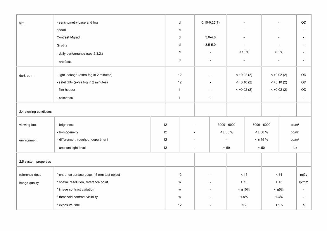
film - sensitometry:base and fog
speed
Contrast Mgrad:
Grad12
- daily performance (see 2.3.2.)
- artefacts
d
d
d
d
d
d
0.15-0.25(1)
-
3.0-4.0
3.5-5.0
-
-
-
-
-
-
< 10 %
-
-
-
-
-
< 5 %
-
OD
-
-
-
-
-
darkroom - light leakage (extra fog in 2 minutes)
- safelights (extra fog in 2 minutes)
- film hopper
- cassettes
12
12
i
i
-
-
-
-
< +0.02 (2)
< +0.10 (2)
< +0.02 (2)
-
< +0.02 (2)
< +0.10 (2)
< +0.02 (2)
-
OD
OD
OD
-
2.4 viewing conditions
viewing box
environment
- brightness
- homogeneity
- difference throughout department
- ambient light level
12
12
12
12
-
-
-
-
3000 - 6000
< ± 30 %
-
< 50
3000 - 6000
< ± 30 %
< ± 15 %
< 50
cd/m²
cd/m²
cd/m²
lux
2.5 system properties
reference dose
image quality
* entrance surface dose; 45 mm test object
* spatial resolution, reference point
* image contrast variation
* threshold contrast visibility
* exposure time
12
w
w
w
12
-
-
-
-
-
< 15
> 10
< ±10%
1.5%
< 2
< 14
> 13
< ±5%
1.3%
< 1.5
mGy
lp/mm
-
-
s

i = At acceptance; d = daily; w = weekly; 6 = every 6 months; 12 = every 12 months
* standard measurement conditions(1) for standard blue based films only
(2) at net optical density 1.00 OD
=> End of table 1.
TABLE 2. QC equipment and calibration requirements
QC equipmentaccuracy reproducibility unit
sensitometer
densitometer
dosemeter
thermometer
kVp-meter for mammographic use
exposure time meter
luminance meter
illuminance meter
test objects, PMMA
compression force test device
-
±0.02 at 1.00 OD
± 5%
± 0.3
± 2%
± 5%
± 10%
± 10%
± 2%
± 10%
± 2%
± 1%
± 1%
± 0.1
± 1%
± 1%
± 5%
± 5%
-
± 5%
OD
OD
mGy
C
kV
s
Cd.m-2
klux
mm
N
aluminium filters (purity ³ 99,9%)aluminium stepwedgeresolution pattern (> 15 lp/mm)
focal spot test device
stopwatch
film/screen contact test tool
tape measure

rubber foam for compression plate alignment
lead sheet
CEC-Reports
1 Technical and Physical Parameters for Quality Assurance in Medical Diagnostic Radiology; Tolerances, Limiting Values and Appropriate Measuring Methods
1989: British Institute of Radiology; BIR-Report 18, CEC-Report EUR 11620.
2 Optimisation of Image Quality and Patient Exposure in Diagnostic Radiology
1989: British Institute of Radiology; BIR-Report 20, CEC-Report EUR 11842.
3 Dosimetry in Diagnostic Radiology
Proceedings of a Seminar held in Luxembourg, March 19-21, 1991.
1992: Rad. Prot. Dosimetry vol 43, nr 1-4, CEC-Report EUR 14180.
Test Objects and Optimisation in Diagnostic Radiology and Nuclear Medicine4.
Proceedings of a Discussion Workshop held in Würtzburg (FRG), June 15-17, 1992
1993: Rad. Prot. Dosimetry vol 49, nr 1-3; CEC-Report EUR 14767.
5 Quality Control and Radiation Protection of the Patient in Diagnostic Radiology and Nuclear Medicine
1995: Rad. Prot. Dosimetry vol 57, nr 1-4, CEC-Report EUR 15257.
6 European Guidelines on Quality Criteria for Diagnostic Radiographic Images
1996: CEC-Report EUR 16260.
Protocols
1 The European Protocol for the Quality Control of the Technical Aspects of Mammography Screening.
1993: CEC-Report EUR 14821
2 European Protocol on Dosimetry in Mammography.
1996: CEC-Report EUR 16263.
3 Protocol acceptance inspection of screening units for breast cancer screening, version 1993.
National Expert and Training Centre for Breast Cancer Screening, University Hospital Nijmegen (NL)

1996 (translated in English).
4 LNETI/DPSR: Protocol of quality control in mammography (in English) 1991.
5 ISS: Controllo di Qualità in Mammografia: aspetti technici e clinici.
Instituto superiore de sanità (in Italian),
1995: ISTASAN 95/12
6 IPSM: Commissioning and Routine testing of Mammographic X-Ray Systems - second edition
The Institute of Physical Sciences in Medicine, York
1994: Report no. 59/2.
7 American College of Radiology (ACR), Committee on Quality Assurance in Mammography: Mammography quality control.
1994, revised edition
8 American Association of Physicists in Medicine (AAPM): Equipment requirements and quality control for mammography
1990: report No. 29
9 Quality Control in Mammography,
1995: Physics consulting group Ontario Breast Screening Programme
10 QARAD/LUCK: Belgisch Protocol voor de kwaliteitszorg van de fysische en technishe aspecten bijmammografische screening (in Dutch)
1999
Publications
1 Chakraborty D.P.: Quantitative versus subjective evaluation of mammography accreditation test object images.
1995: Med. Phys. 22(2):133-143
2 Wagner A.J.: Quantitative mammography contrast threshold test tool.
1995: Med. Phys. 22(2):127-132
3 Widmer J.H.: Identifying and correcting processing artefacts.
Technical and scientific monograph
Health Sciences Division
Eastman Kodak Company, Rochester, New York, 1994
4 Caldwell C.B.: Evaluation of mammographic image quality: pilot study comparing five methods.
1992: AJR 159:295-301
5 Wu X.: Spectral dependence of glandular tissue dose in screen-film mammography.
1991: Radiology 179:143-148
6 Hendrick R.E.: Standardization of image quality and radiation dose in mammography.
1990: Radiology 174(3):648-654
Baines C.J.: Canadian national breast screening study: assessment of technical quality by external7.
review.
1990: AJR 155:743-747
8 Jacobson D.R.: Simple devices for the determination of mammography dose or radiographic exposure.
1994: Z. Med. Phys. 4:91-93
9 Conway B.J.: National survey of mammographic facilities in 1985, 1988 and 1992.
1994: Radiology 191:323-330
10 Farria D.M.: Mammography quality assurance from A to Z.
1994: Radiographics 14: 371-385
11 Sickles E.A.: Latent image fading in screen-film mammography: lack of clinical relevance for batch-processed films.
1995: Radiology 194:389-392
12 Sullivan D.C.: Measurement of force applied during mammography.
1991: Radiology 181:355-357
Russell D.G.: Pressures in a simulated breast subjected to compression forces comparable to those of mammography.13.
1995: Radiology 194:383-387
Faulkner K.: Technical note: perspex blocks for estimation of dose to a standard breast - effect of14.
variation in block thickness.
1995: Br. J. Radiol. 68:194-196
Faulkner K.: An investigation into variations in the estimation of mean glandular dose in15.
mammography.
1995: Radiat. Prot. Dosimet. 57:405-407
16 K.C. Young, M.G. Wallis, M. L. Ramsdale: Mammographic Film Density and Detection of Small Breast
cancers, 1994 Clin. Radiol (49) 461-465

17 Tang S.: Slit camera focal spot measurement errors in mammography.
1995: Med. Phys. 22:1803-1814
18 Hartmann E.: Quality control of radiographic illuminators and associated viewing equipment.
Retrieval and viewing conditions.
1989: BIR report 18:135-137
19 Haus A.G.: Technologic improvements in screen-film mammography.
1990: Radiology 174(3):628-637
L.K. Wagner, B.R. Archer, F. Cerra; On the measurement of half-value layer in film-screen20.
mammography.
1990: Med. Phys. (17):989-997.
J.D. Everson, J.E. Gray: Focal-Spot Measurement: Comparison of Slit, Pinhole, and Star Resolution Pattern Techniques.21.
1987: Radiology (165):261-264.
22 J. Law: The measurement and routine checking of mammography X-ray tube kV.
1991: Phys.Med.Biol. (36):1133-1139.
23 J. Law: Measurements of focal spot size in mammography X-ray tubes.
1993: Brit. J. Of Radiology (66):44-50
24 M. Thijssen et al: A definition of image quality: the image quality figure.
1989: Brit. Inst. Radiology, BIR-report 20: 29-34
25 R.L. Tanner: Simple test pattern for mammographic screen-film contact measurement.
1991: Radiology (178):883-884.
K.C. Young, M.L. Ramsdale, A. Rust: Mammographic dose and image quality in the UK breast26.
screening programme. 1998, NHSBSP report 35
27 J. Zaers, S. van Woudenberg, G. Brix: Qualitätssicherung in der Röntgenmammographie
1997: Der Radiologe (37):617-620
28 J. Law: Checking the consistency of sensitometers and film processors in a mammographic screening
ptogramme. 1996 Brit. J. Of Radiology (69) 143-147
K. J. Robson, C.J. Kotre, K. Faulkner : The use of a contrast-detail test object in the optimization of29.
optical density in mammography, 1995 Brit. J. Of Radiology (68) 277-282
J.A. Terry, R.G. Waggener, M.A. Miller Blough: Half-value layer and intensity variations as a function of position in the radiation field for film screen mammography 1999 Med. Phys. 26 259-26630.
S. Tang, G.T. Barnes, R.L. Tanner: Slit camera focal spot measurement errors in mammography31.
1995 Med. Phys. (22) 1803-1814
J. Coletti et al.: Comparison of exposure standards in the mammography x-ray region,32.
1997 Med. Phys (8) 1263-1267
C. Kimme Smith et al. Mammography film processor replenishment rate: Bromide level monitoring,33.
1997 Med. Phys. (3) 369-372
35 M. Goodsitt, H. Chan, B. Liu: Investigation of the line-pair method for evaluating mammographic focal spot performance, 1997 Med. Phys. (1) 11-15
A. Krol et al. Scatter reduction in mammography with air gap34.
1996 Med. Phys. (7) 1263-1270
D. McLean, J. Gray: K-characteristic photon absorption from intensifying screens and other materials:35.
Theoretical calculations and measurements,
1996 Med. Phys. (7) 1253-1261
P. Rezentes, A de Almeida, G. Barnes: Mammographic Grid Performance36.
1999 Radiology 210:227-232
J. Hogge et al. Quality assurance in Mammography: Artifact Analysis37.
1999 Radiographics 19:503-522
J. Byng et al.: Analysis of Mammographic Density and Breast Cancer Risk from Digitized Mammograms38.
1998 Radiographics 18:1587-1598
Other reports
International Electrotechnical Commission (IEC), Geneva, Switzerland: Characteristics of focal spots1.
in diagnostic X-ray tube assemblies for medical use
1982: IEC-Publication 336.
2 Quality assurance in mammography - quality control of performance and constancy

1990: Series of Nordic Reports on radiation Safety No. 1, Denmark, Finland, Iceland, Norway and
Sweden.
3 Société française des physiciens d'hôpital, Nancy: Contrôle de qualité et mesure de dose en mammographie - aspects théoriques et pratiques (in French)
1991.
4 Department Health & Social Security, Supplies Technology Division (DHSS): Guidance notes for health
authorities on mammographic equipment requirements for breast cancer screening
1987: STD
5 :87:34
Department of Radiodiagnostic Radiology, University of Lund, Sweden: Quality Assurance in
Mammography
1989.
6 Sicherung der Bildqualität in röntgendiagnostischen Betrieben - Filmverarbeitung (in German)
1985: DIN 6868 teil 2: Beuth Verlag GmbH, Berlin.
7 American Association of Physicists in Medicine (AAPM): Basic quality control in diagnostic radiology
1978: report No. 4
8 ECRI: Special issue: Mammography Units;
1989: Health Devices:Vol.18:No.1:Plymouth Meeting (PA)
9 ECRI: Double issue: Mammography Units;
1990: Health Devices:Vol.19:No.5-6:Plymouth Meeting (PA)
10 Siemens Medical Systems Inc., New Jersey: Mammography QA - Doc.# 54780/up
1990
11 ANSI: Determination of ISO speed and average gradient.
American National Standards Institute (ANSI).
1983: Nr. PH2.50.
Sicherung der Bildqualität in röntgendiagnostischen Betrieben - Konstantzprüfung für die Mammographie (in German)12.
1989: DIN-1:6868 teil 7:Beuth Verlag GmbH, Berlin.
Sicherung der Bildqualität in röntgendiagnostischen Betrieben - Abnahmeprüfung an13.
Mammographie-Einrichtungen (in German)
1989: DIN-2:6868 teil 52: Beuth Verlag GmbH, Berlin.
14 ICRP Publication 52, including the Statement from the Como Meeting of the ICRP.
1987: Annals of the ICRP 17 (4), i-v, Pergamon Press, Oxford, UK.
15 ICRP Publication 60, 1990 Recommendations of the ICRP.
(Adopted by the Commission in November 1990);
1991: Annals of the ICRP 21 (1-3), Pergamon Press, Oxford, UK.
The film curve can be characterised by a few parameters. Most important items are contrast, sensitivity and base and fog. There are different methods to calculate the film parameters. Existingnormalisation’s differ so much that the following method is suggested, derived from the Dutch protocol (1991), which is based on the ANSI (1983) norm.
Very high contrast can be a problem because of an associated reduction in dynamic range which may result in dense breast tissue being imaged in relatively low film densities where the filmperformance is relatively poor. To some extent this can be compensated for by setting relatively high average film densities, but even then a lower film contrast may better image local areas of densetissue. Conversely a very low overall film contrast may indicate an inadequately processed film and subtle details may be missed by the radiologist.
Research has shown that film gradient measured by light sensitometry correlates well with film gradient measured by x-ray sensitometry using a fixed kV and target filter combination. One must bear inmind that film emulsions may respond slightly differently to the light from a sensitometer as opposed to the light from the screen used for imaging.
Dmin
Base and fog; the optical density of a non exposed film after developing. The minimum optical density can be visualised by fixation only of an unexposed film. The extra fog is a result ofdeveloping the (unexposed) emulsion.
Dmax
The maximum density achievable with an exposed film; i.e. the highest density step.
Mgrad
Mean Gradient; the property which expresses the filmcontrast in the diagnostic range. MGrad is calculated as the slope of the line through the points D1=Dmin+0.25 OD and
D2=Dmin+2.00 OD. Since the film curve is constructed from a limited number of points, D
1 and D
2 must be interpolated. Linear interpolation of the construction points of the film curve will
result in sufficient accuracy.
Grad1,2
Middle Gradient; the property which expresses the filmcontrast in the diagnostic range. Grad1,2
is calculated as the slope of the line through the points D1=Dmin+1.00 OD and
D2=Dmin+2.00 OD. Since the film curve is constructed from a limited number of points, D
1 and D
2 must be interpolated. Linear interpolation of the construction points of the film curve will
result in sufficient accuracy.

Gradgland
The glandular tissue gradient can be defined as an alternatively. This is the gradient at glandular
densities 0.8 – 1.5 OD. This gradient is used in combination with the Gradfat.
Gradfat
The alternative fat tissue gradient is defined between densities of 1.8 and 2.5 OD. This gradient is used in combination with the Gradgland.
Speed
Sensitivity; the property of the film emulsion directly related to the dose. The Speed is calculated as the x-axis cut-off at optical density 1.00+Dmin, also called 'Speedpoint'. The higher thefigure for Speed, the more dose is needed to obtain the right optical density. Since the film curve is constructed from a limited number of points, the Speed must be interpolated. Linearinterpolation will result in sufficient accuracy.
Since these parameters are derived from the characteristic curve by interpolation they are not very practical if a computer is not available. A simpler procedure is to use the parameters below which arebased on density measurements of particular sensitometric steps.
Speed Index
The density of the step near to the speedpoint density 1.0 OD, base and fog excluded. Usually this is the density of step 11 of the sensitometric stepwedge.
Contrast Index 1
The difference in density found between the step nearest to the speedpoint density (1.0 OD, base and fog excluded) and the one with a 0.6 log E (factor 4) higher light exposure (normally4 density steps) (ACR).
Contrast Index 2
The difference in density steps found between the step nearest to the speedpoint and the step nearest to a density at 2.0 OD, base and fog excluded (IPSM, see bibliography).
The optical density of a film is the result of X-ray exposure and processing. The film is mainly exposed by light emitted by the intensifying screen. The light-emission of the screen is proportional with theincident X-ray exposure. Primary X-rays only contribute up to 5% of the total exposure. The developing process determines the optical density of the exposed area.
When an optical density in any given film is measured, the corresponding exposure is unknown. However, the film curve (measured with light-sensitometry) describes the relation between light-exposure and optical density. Any measured optical density can be converted into a relative log(light-exposure) or log(I') by interpolation of the film curve. This figure log(I') is a relative value andstrongly depends on the sensitometer used. But still it is a useful value, closely related with the radiation dose applied and is therefore suitable to calculate the mass attenuation coefficient of anarbitrary X-ray step wedge.
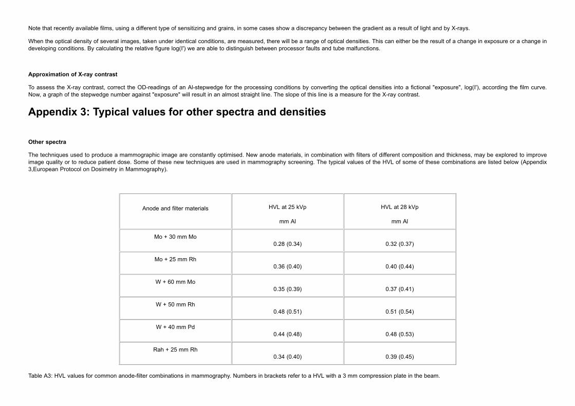
Note that recently available films, using a different type of sensitizing and grains, in some cases show a discrepancy between the gradient as a result of light and by X-rays.
When the optical density of several images, taken under identical conditions, are measured, there will be a range of optical densities. This can either be the result of a change in exposure or a change indeveloping conditions. By calculating the relative figure log(I') we are able to distinguish between processor faults and tube malfunctions.
Approximation of X-ray contrast
To assess the X-ray contrast, correct the OD-readings of an Al-stepwedge for the processing conditions by converting the optical densities into a fictional "exposure", log(I'), according the film curve.Now, a graph of the stepwedge number against "exposure" will result in an almost straight line. The slope of this line is a measure for the X-ray contrast.
Other spectra
The techniques used to produce a mammographic image are constantly optimised. New anode materials, in combination with filters of different composition and thickness, may be explored to improveimage quality or to reduce patient dose. Some of these new techniques are used in mammography screening. The typical values of the HVL of some of these combinations are listed below (Appendix3,European Protocol on Dosimetry in Mammography).
Anode and filter materials HVL at 25 kVp
mm Al
HVL at 28 kVp
mm Al
Mo + 30 mm Mo0.28 (0.34) 0.32 (0.37)
Mo + 25 mm Rh0.36 (0.40) 0.40 (0.44)
W + 60 mm Mo0.35 (0.39) 0.37 (0.41)
W + 50 mm Rh0.48 (0.51) 0.51 (0.54)
W + 40 mm Pd0.44 (0.48) 0.48 (0.53)
Rah + 25 mm Rh0.34 (0.40) 0.39 (0.45)
Table A3: HVL values for common anode-filter combinations in mammography. Numbers in brackets refer to a HVL with a 3 mm compression plate in the beam.
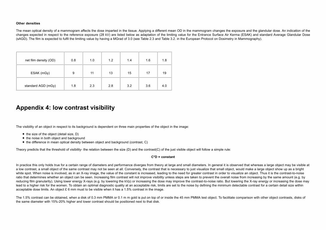
Other densities
The mean optical density of a mammogram affects the dose imparted in the tissue. Applying a different mean OD in the mammogram changes the exposure and the glandular dose. An indication of thechanges expected in respect to the reference exposure (28 kV) are listed below as adaptation of the limiting value for the Entrance Surface Air Kerma (ESAK) and standard Average Glandular Dose(sAGD). The film is expected to fulfil the limiting value by having a MGrad of 3.0 (see Table 2.3 and Table 3.2. in the European Protocol on Dosimetry in Mammography).
net film density (OD) 0.8 1.0 1.2 1.4 1.6 1.8
ESAK (mGy) 9 11 13 15 17 19
standard AGD (mGy) 1.8 2.3 2.8 3.2 3.6 4.0
The visibility of an object in respect to its background is dependent on three main properties of the object in the image:
the size of the object (detail size, D)the noise in both object and backgroundthe difference in mean optical density between object and background (contrast, C)
Theory predicts that the threshold of visibility- the relation between the size (D) and the contrast(C) of the just visible object will follow a simple rule:
C*D = constant
In practice this only holds true for a certain range of diameters and performance diverges from theory at large and small diameters. In general it is observed that whereas a large object may be visible ata low contrast, a small object of the same contrast may not be seen at all. Conversely, the contrast that is necessary to just visualize that small object, would make a large object show up as a brightwhite spot. When noise is involved, as in an X-ray image, the value of the constant is increased, leading to the need for greater contrast in order to visualize an object. Thus it is the contrast-to-noiseratio that determines whether an object can be seen. Increasing film contrast will not improve visibility unless steps are taken to prevent the overall noise from increasing by the same amount (e.g. byreducing film granularity). Using lower energy X-rays (e.g. by lowering the kVp) or increasing the dose may improve the contrast-to-noise ratio. But lowering the X-ray energy or increasing the dose maylead to a higher risk for the women. To obtain an optimal diagnostic quality at an acceptable risk, limits are set to the noise by defining the minimum detectable contrast for a certain detail size withinacceptable dose limits. An object £ 6 mm must to be visible when it has a 1.5% contrast in the image.
The 1.5% contrast can be obtained, when a disk of 0.3 mm PMMA or 0.1 m m gold is put on top of or inside the 45 mm PMMA test object. To facilitate comparison with other object contrasts, disks ofthe same diameter with 15%-20% higher and lower contrast should be positioned next to that disk.
The introduction of mammography systems that do not use the screen-film combination as detector and storage medium but that produces a digital image, allows the visualization of contrasts beyondthe limitations of the film. That gives rise to a different approach of the quality demands that are stated in this document. A separate part will have to deal with these aspects in future editions.
Some considerations on the subject are given here:
Spatial resolution
In film-screen systems it is sufficient to characterize the information transfer at lower frequencies by its spatial resolution at higher frequencies: a maximal resolution of 12 lp/mm ensures sufficientcontrast at frequencies about 2-5 lp/mm, where the human eye is most sensitive.
In digital systems the resolution is limited by the properties of the detecting medium, the pixel size used in the detector and by the imaging system. As a result, the resolution that is given by the pixelsize of the imaging system is not the right measure to characterize the imaging capabilities of the digital system.
Since the detection of an object is dependent on its contrast to the background, the contrast-detail (CD) curve or other contrast based transfer functions of the system might be a more appropriatemeasure than the currently used Modulation Transfer Function (MTF). Adequate test devices are readily available but need a more complicated evaluation than resolution patterns.
The use of digital systems allows the adjustment of very low contrasts to the sensitivity of the human eye. This will make the demand of a resolution better than 10 lp/mm obsolete for digital systems(2.5.2).
X-ray generation
The information needed to produce images of sufficient diagnostic quality is produced by the X-ray part of the system. This can lead to the conclusion, that no reduction in the demands on geometryand focal spot size are allowed. The influence of the stability in X-ray production, the reproducibility of the automatic exposure system and kVp-thickness compensations may however become lessimportant.
Threshold contrast visibility
Since most of the digital systems make use of detectors with a higher detective quantum efficiency (DQE) than the film-screen systems, this will set new standards for the threshold contrast visibility of"large" objects (2.5.2). Also the computing power of these systems might give detecting results beyond the capabilities of the human eye, by using image improvement algorithms and computer aideddiagnosis (CAD).
Grid
The contrast in film-screen systems is strongly affected by scatter, since this adds to an offset optical density of both the object and its background. This leads to the strong benefit of the use of ananti-scatter grid. In digital systems these relations change due to the properties of the detector and the ability to adjust for this offset. This might allow the use of a grid with reduced selectivity forprimary radiation or no grid at all, which has a great benefit to the dose per image.
Dose
Since the threshold contrast visibility improves by allowing a higher dose per image to the detector due to the better signal-to-noise ratio, and since the digital systems are able to process a wide rangeof intensities, there will be a tendency to increase the exposure per image. This leads to a higher absorbed dose in the glandular tissue, which increases the risk for the women. Great care should betaken in the techniques chosen to make the exposures, since they can be chosen freely, where in screen-film systems the mean optical density and the risk of under- or overexposure of the film limit thedose to the women. The dose constraint (2.5.1) also holds for digital systems. Exposure parameters or system sensitivity therefore should be included in the image and in the file information.
Summary
The introduction of digital mammography will lead to different measures and limitations in the quality control for these systems in respect to screen-film systems. Since many aspects are still developingor not yet fully understood, research has to be done on the aspects of quality control of digital mammography systems. The dose per image must be monitored carefully.

Appendix 6: Completion forms for QC reporting
based on
Third edition
DECEMBER 1999
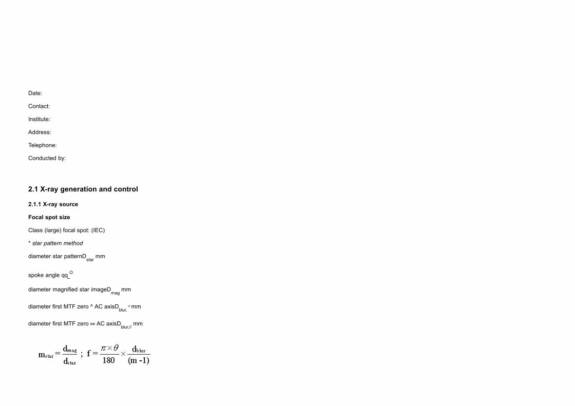
Date:
Contact:
Institute:
Address:
Telephone:
Conducted by:
2.1 X-ray generation and control
2.1.1 X-ray source
Focal spot size
Class (large) focal spot: (IEC)
* star pattern method
diameter star patternDstar
mm
spoke angle qq O
diameter magnified star imageDmag
mm
diameter first MTF zero ^ AC axisDblur,
mm
diameter first MTF zero ¤¤ AC axisDblur,//
mm

* slit camera method
width slit mm
distance slit-to-filmdslit-film
mm
distance focus-to-slitdfocus-slit
mm
width slit image ^ AC axisF mm
width slit image ¤¤ AC axisF// mm
* pinhole method
diameter pinhole mm
distance pinhole-to-filmdpinhole-film
mm
distance focus-to-pinholedfocus-pinhole
mm
diameter pinhole ^ AC axisf^ mm
diameter pinhole ¤¤ AC axisf// mm
Focal spot size f^ = mm
f// = mm Accepted: yes / no
Source-to-image distance

Nominal value : mm
Measured value :
- Focus indication to bucky : mm
- Bucky to cassette : mm
Source-to-image distance : mm
Alignment of X-ray field / image receptor
Distance at chest wall side film:
position inside/outside image receptor:
left : mm, in / out
nipple: mm, in / out
right : mm, in / out
chest : mm, in / out
Distance between film edge and bucky edge mm
Accepted: yes / no
Radiation leakage
Description of position of ‘hot spots’
1
2
3
detector surface area : mm2
measured:calculated for
distance from tube: 50 mm 1000 mm,
surface area:____ mm2 100 cm²:
nr:

1. mGy/hr
2. mGy/hr
3. mGy/hr
Accepted: yes / no
Tube output
focus to detector distance: mm
surface air kerma: mGy
focal spot charge: mAs
specific tube output at 1 m mGy/mAs
output rate at FFD mGy/s
Accepted: yes / no
2.1.2 Tube voltage
Reproducibility and accuracy
Pre-set tube load: ____ mAs
Clinically most relevant kV: ____ kV
Accuracy
Setting 25 26 27 28 29 30 31 kV
Measured kV
Deviation kV
Accepted: yes / no
Accuracy at other clinical values
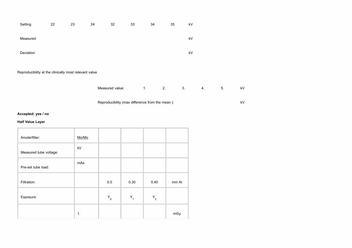
Setting 22 23 24 32 33 34 35 kV
Measured kV
Deviation kV
Reproducibility at the clinically most relevant value
Measured value: 1. 2. 3. 4. 5. kV
Reproducibility (max difference from the mean ): kV
Accepted: yes / no
Half Value Layer
Anode/filter: Mo/Mo
Measured tube voltage:kV
Pre-set tube load:mAs
Filtration:
0.0 0.30 0.40 mm Al
Exposure:
Y0
Y1
Y2
1. mGy
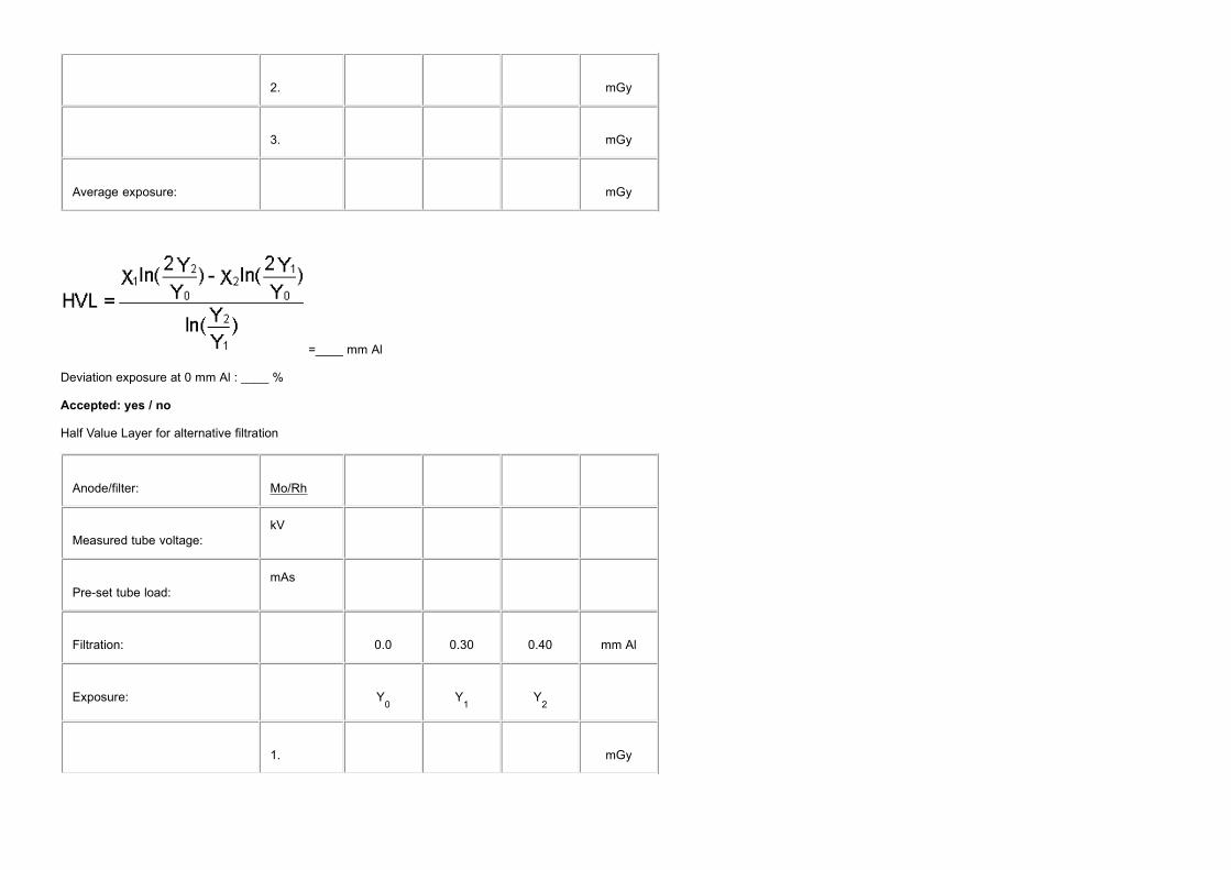
2. mGy
3. mGy
Average exposure:
mGy
=____ mm Al
Deviation exposure at 0 mm Al : ____ %
Accepted: yes / no
Half Value Layer for alternative filtration
Anode/filter: Mo/Rh
Measured tube voltage:kV
Pre-set tube load:mAs
Filtration:
0.0 0.30 0.40 mm Al
Exposure:
Y0
Y1
Y2
1. mGy

2. mGy
3. mGy
Average exposure:
mGy
HVL:____ mm Al
Deviation exposure at 0 mm Al : ____ %
Accepted: yes / no
2.1.3 AEC-system
Optical density control setting: central value and difference per step
Target density value: ____ OD
Setting Exposure Tube load Density Density incr.
mGy mAs OD OD
-3 ____ ____ ____
-2 ____ ____ ____ ____
-1 ____ ____ ____ ____
0 ____ ____ ____ ____
1 ____ ____ ____ ____

2 ____ ____ ____ ____
3 ____ ____ ____ ____
Accepted: yes / no
Adjustable range: ____ OD
Accepted: yes / no
Optical density control setting for reference density:____
Optical density control setting for target density:____
Guard timer
Exposure terminates by exposure limit :yes/no
Alarm or error code :yes/no
Exposure :____ mGy
Tube load :____ mAs
Short term reproducibility
Optical density control setting: ____
Exp. # Exposure (mGy) Tube load (mAs)
1 ____ ____
2 ____ ____

3 ____ ____
4 ____ ____
5 ____ ____
6 ____ ____
7 ____ ____
8 ____ ____
9 ____ ____
10 ____ ____
Deviation in tube load: ____ % (= 100 x (max-min)/mean )
Accepted: yes / no
Long term reproducibility: forms should be made to suit the local preferences
Object thickness and tube voltage compensation
Optical density control setting: ____
If there is an automatic kV/anode/filter mode find out for each mode where the switchpoints are:
Switchpoint from thickness [cm] to thickness [cm] kV anode filter
A:
B:
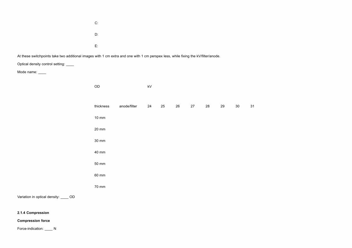
C:
D:
E:
At these switchpoints take two additional images with 1 cm extra and one with 1 cm perspex less, while fixing the kV/filter/anode.
Optical density control setting: ____
Mode name: ____
OD
kV
thickness anode/filter 24 25 26 27 28 29 30 31
10 mm
20 mm
30 mm
40 mm
50 mm
60 mm
70 mm
Variation in optical density: ____ OD
2.1.4 Compression
Compression force
Force-indication: ____ N

Measured compression force: ____ N
Compression force after 5 min: ____ N
Compression plate alignment
attachment compression plate : in order / out of order
Symmetric load
Thickness indication : ___ cm
Height of compression plate above the bucky at full compression:
left right difference(l/r)
Rear : ___ ___ ___ cm
Front : ___ ___ ___ cm
Difference(r/f) ___ ___ cm
Accepted: yes / no
A-symmetric load left-right
Height of compression plate above the bucky at full compression:
left right difference(l/r)
Rear : ___ ___ ___ cm
Front : ___ ___ ___ cm
Difference(r/f) ___ ___ cm
Accepted: yes / no
A-symmetric load front-rear
Height of compression plate above the bucky at full compression:
left right difference(l/r)
Rear : ___ ___ ___ cm
Front : ___ ___ ___ cm
Difference(r/f) ___ ___ cm
Accepted: yes / no

2.2 Bucky and image receptor
2.2.1. Anti scatter grid
Grid system factor
exposure tube load density
[mGy] [mAs] [OD]
Present: ____ ____ ____
Absent: ____ ____ ____
Grid system factor: ____
Accepted: yes / no
Grid imaging
Additional grid images made:
# added PMMA description of artefacts
1. yes/no
yes/no2.
yes/no3.
Accepted: yes / no
2.2.2. Screen-film
Inter cassette sensitivity and attenuation variation and optical density range
AEC setting: __
Cassette id exposure tube load density
[mGy] [mAs] [OD]
1 ____ ____ ____
2 ____ ____ ____
3 ____ ____ ____
4 ____ ____ ____
5 ____ ____ ____
6 ____ ____ ____

7 ____ ____ ____
8 ____ ____ ____
9 ____ ____ ____
10 ____ ____ ____
11 ____ ____ ____
12 ____ ____ ____
Average values: ____ mAs ____ OD
Max. deviation: ____ %____mAs ____ OD
Reference cassette : __
Accepted: yes / no
Screen-film contact
Cassette id: Description of artefacts:
__ _______________________________
__ _______________________________
__ _______________________________
__ _______________________________
__ _______________________________
__ _______________________________
__ _______________________________
__ _______________________________
__ _______________________________
__ _______________________________
__ _______________________________
__ _______________________________
Accepted: yes / no
2.3 Film processing
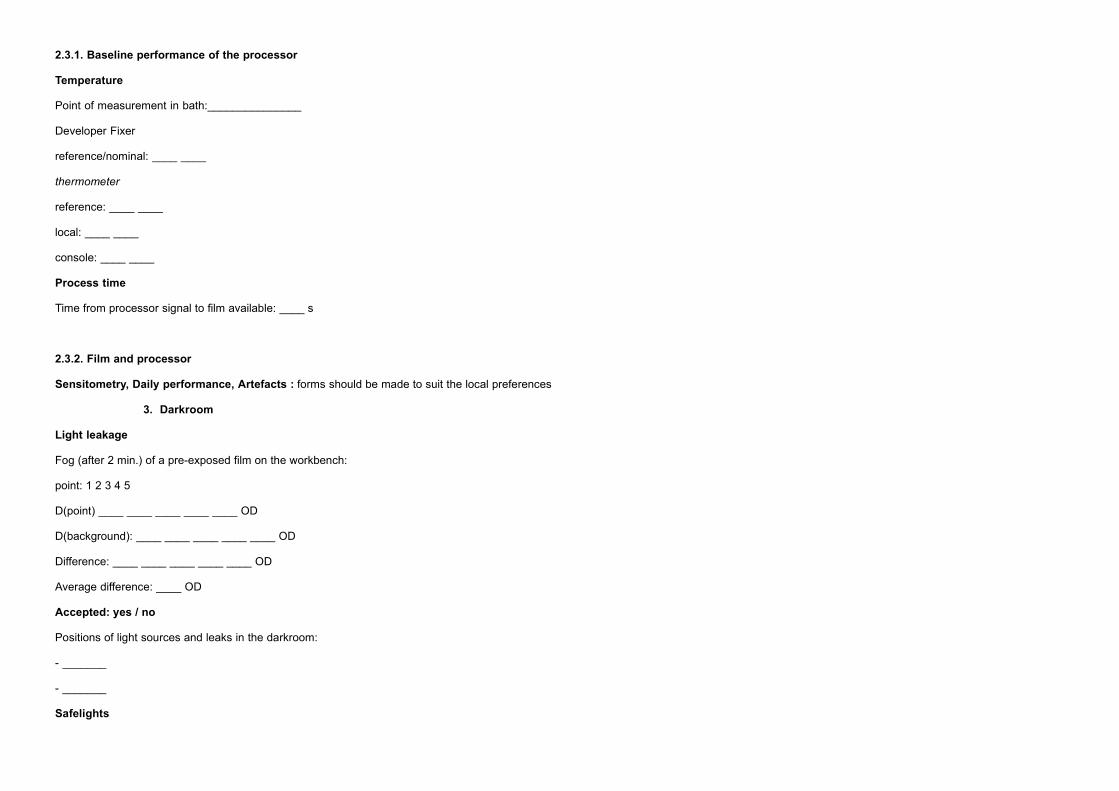
2.3.1. Baseline performance of the processor
Temperature
Point of measurement in bath:_______________
Developer Fixer
reference/nominal: ____ ____
thermometer
reference: ____ ____
local: ____ ____
console: ____ ____
Process time
Time from processor signal to film available: ____ s
2.3.2. Film and processor
Sensitometry, Daily performance, Artefacts : forms should be made to suit the local preferences
Darkroom3.
Light leakage
Fog (after 2 min.) of a pre-exposed film on the workbench:
point: 1 2 3 4 5
D(point) ____ ____ ____ ____ ____ OD
D(background): ____ ____ ____ ____ ____ OD
Difference: ____ ____ ____ ____ ____ OD
Average difference: ____ OD
Accepted: yes / no
Positions of light sources and leaks in the darkroom:
- _______
- _______
Safelights

Type of lighting: direct/indirect
Height : ca. ___ meter above workbench
Setting: ___
Filter condition : good/ insufficient / absent / not checked
Fog (after 2 min.) of a pre-exposed film on the workbench:
point: 1 2 3 4 5
D(point) ____ ____ ____ ____ ____ OD
D(background): ____ ____ ____ ____ ____ OD
Difference: ____ ____ ____ ____ ____ OD
Average difference: ____ OD
Accepted: yes / no
Film hopper
Fogging due to lightleakage in film hopper is absent: yes/no
Accepted: yes / no
Cassettes
The following cassettes show lightleakage:
Cassette id: leaking position
__ _______________________________
__ _______________________________
__ _______________________________
Accepted: yes / no
2.4 Viewing conditions
2.4.1. Viewing box
Viewing box luminance
Reading from the luminance meter (detector at the centre of the image plane) : ____ Cd/m²
Homogeneity

Cover the view box pane with mammography films, measure the luminance (remove films first) at
all centre positions of these films.
Position 1 2 3 4 5
Top ____ ____ ____ ____ ____
Bottom ____ ____ ____. ____ ____
Homogeneity: ____ % ( = 100% .(Lmax
- Lmin
) / Lcentre
)
Accepted: yes / no
2.4.2. Ambient light level
Reading from the illuminance meter (detector at the image plane, box is off) : ____ lux
Accepted: yes / no
2.5 System properties
2.5.1 Dosimetry
Entrance surface air kerma for D = 1.4 OD(excl. base + fog)
exposure tube load density
[mGy] [mAs] [OD]
____ ____ ____
____ ____ ____
Exposure for D = 1.4 OD (excl. b+s ): ____ mGy
Accepted: yes / no
2.5.2 Image Quality
Spatial resolution
Position of the centre of the pattern:
Height above the bucky surface: ____ mm
Distance from thorax side of the bucky: ____ mm
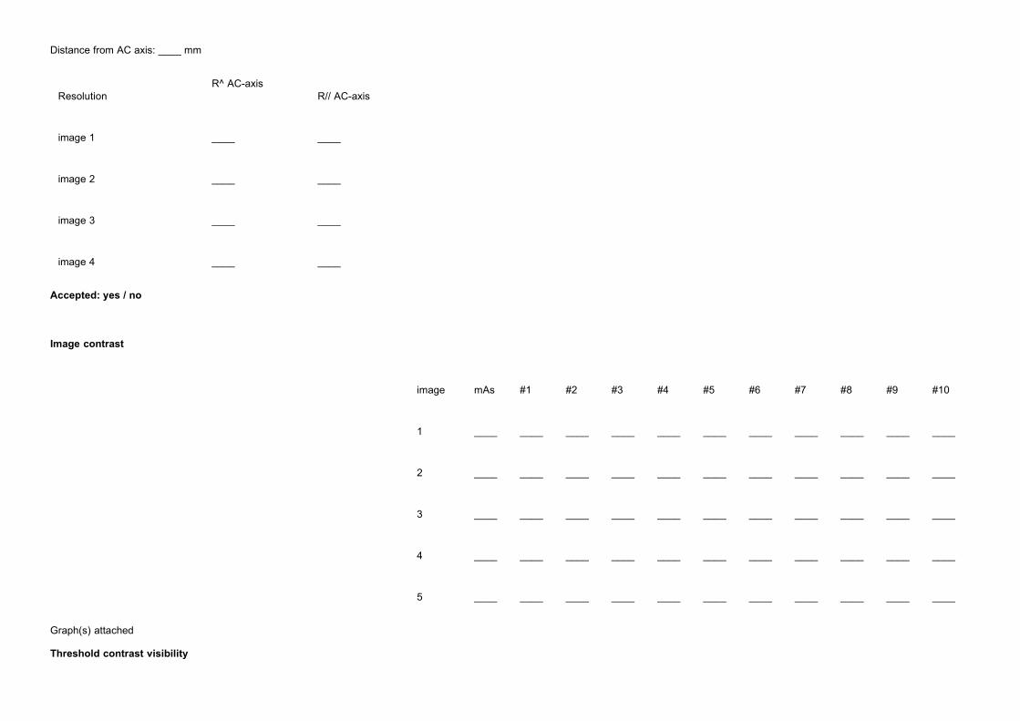
Distance from AC axis: ____ mm
ResolutionR^ AC-axis
R// AC-axis
image 1 ____ ____
image 2 ____ ____
image 3 ____ ____
image 4 ____ ____
Accepted: yes / no
Image contrast
image mAs #1 #2 #3 #4 #5 #6 #7 #8 #9 #10
1 ____ ____ ____ ____ ____ ____ ____ ____ ____ ____ ____
2 ____ ____ ____ ____ ____ ____ ____ ____ ____ ____ ____
3 ____ ____ ____ ____ ____ ____ ____ ____ ____ ____ ____
4 ____ ____ ____ ____ ____ ____ ____ ____ ____ ____ ____
5 ____ ____ ____ ____ ____ ____ ____ ____ ____ ____ ____
Graph(s) attached
Threshold contrast visibility

Observer # objects identified
1 ____
2 ____
3 ____
Accepted: yes / no
Exposure time
AEC setting for a routine image:____
tube load obtained:____ mAs
exposure time:____ s
Accepted: yes / no