Thiosemicarbazone Metal Complexes: From Structure to Activity

www.elsevier.com/locate/sna

Multiple Criteria for Evaluating MachineLearning Algorithms for Land CoverClassification from Satellite Data

R. S. DeFries* and Jonathan Cheung-Wai Chan†

Operational monitoring of land cover from satellite of criteria in addition to the traditional accuracy mea-sures and that there are likely to be trade-offs betweendata will require automated procedures for analyzingalgorithm performance and required computational re-large volumes of data. We propose multiple criteria forsources. Elsevier Science Inc., 2000assessing algorithms for this task. In addition to standard

classification accuracy measures, we propose criteria toaccount for computational resources required by the al-

INTRODUCTIONgorithms, stability of the algorithms, and robustness tonoise in the training data. We also propose that classifi- Over the past few decades, satellite data have becomecation accuracy take account, through estimation of mis- one of the primary sources for obtaining informationclassification costs, of unequal consequences to the user about the vegetation on the Earth’s land surface. At thedepending on which cover types are confused. In this ar- global scale, land cover data sets have been derived forticle, we apply these criteria to three variants of decision application in a range of earth system models primarilytree classifiers, a standard decision tree implemented in from data acquired by the Advanced Very High Resolu-C5.0 and two techniques recently proposed in the mation Radiometer (AVHRR) onboard NOAA meteorologi-chine learning literature known as “bagging” and “boost- cal satellites (DeFries et al., 1998; Hansen et al., 2000;ing.” Each of these algorithms are applied to two data Loveland and Belward, 1997). At regional and localsets, a global land cover classification from 8 km AVHRR scales, data acquired by higher resolution sensors such asdata and a Landsat Thematic Mapper scene in Peru. Re- Landsat and SPOT have been used extensively to extractsults indicate comparable accuracy of the three variants detailed information about the land surface in specific lo-of the decision tree algorithms on the two data sets, with cations (e.g., Skole and Tucker, 1993).boosting providing marginally higher accuracies. The A wide variety of techniques has been used to clas-bagging and boosting algorithms, however, are both sub- sify land cover over large areas from satellite data. Tech-stantially more stable and more robust to noise in the niques range from unsupervised clustering algorithmstraining data compared with the standard C5.0 decision (e.g., Loveland and Belward, 1997; Loveland et al., 1991)tree. The bagging algorithm is most costly in terms of to parametric supervised algorithms such as maximumcomputational resources while the standard decision tree likelihood (e.g., DeFries and Townshend, 1994; Tuckeris least costly. The results illustrate that the choice of the et al., 1985) to machine learning algorithms such as deci-most suitable algorithm requires consideration of a suite sion trees (e.g., Friedl et al., 1999) and neural networks

(e.g., Gopal et al., 1996). For a general review of thesetechniques, see Jensen (1996), Richards (1993), and

* Earth System Science Interdisciplinary Center and Department Quinlan (1993). While some comparisons of algorithmof Geography, University of Maryland, College Parkperformance have been published (Friedl et al., 1999),† Department of Geography, University of Maryland, College

Park there are not generally accepted criteria for selection ofAddress correspondence to R. DeFries, Dept. of Geography, 2181 the most appropriate classification algorithm for a given

Lefrak Hall, Univ. of Maryland, College Park, MD 20742. E-mail: set of [email protected] 6 December 1999; revised 14 April 2000. With recent and upcoming launches of a large num-

REMOTE SENS. ENVIRON. 74:503–515 (2000)Elsevier Science Inc., 2000 0034-4257/00/$–see front matter655 Avenue of the Americas, New York, NY 10010 PII S0034-4257(00)00142-5

504 DeFries and Chan

Table 1. Cover Types and Number of Pixels in Training andber of satellites, notably NASA’s Earth Observing Sys-Test Data for 8 km AVHRR Data Used in This Studytem, the volume of data available for analysis of land

cover will increase many fold (Kalluri et al., 2000). Tech- No. ofTraining No. of Testniques for extracting land cover information need to be

Cover Type Pixels Pixelsautomated to the degree possible to process these largeEvergreen needleleaf forest 667 859volumes of data. In addition, the techniques need to beEvergreen broadleaf forest 1302 1089objective, reproducible, and feasible to implement withinDeciduous needleleaf forest 48 164available resources. For example, the international effort Deciduous broadleaf forest 473 313

on Global Observations of Forest Cover (Ahern et al., Mixed forest 575 3581998; Janetos and Ahern, 1997) aims to characterize the Woodlands 686 1174

Wooded grasslands/shrublands 374 704extent of forest cover globally from satellite data at re-Closed bushlands or shrublands 293 356peated intervals over time. This task can only realisticallyOpen shrublands 617 894

be achieved through techniques that minimize time-con- Grasses 1309 1119suming human interpretation and maximize automated Croplands 1520 1049

Bare 1204 1313procedures for data analysis.Mosses and Lichens 202 652Comparisons of algorithm performance for landTotal 9306 10,044cover classification have generally been based on the sin-

gle criterion of classification accuracy (Friedl et al., 1999;Hansen and Reed, 2000). In an operational context formonitoring land cover from satellite data, there are mul- formance of the machine learning algorithms. The datatiple criteria for assessing the suitability of algorithms in sets are described below.addition to accuracy. Is the algorithm efficient in termsof speed? Does it produce stable results or is it unac- 8 km Global Land Cover Classificationceptably sensitive to minor variations in the input data? DeFries et al. (1998) derived a global land cover classifi-How robust is the algorithm to noisy data? Are there cation of 13 cover types based on the AVHRR Pathfindertradeoffs between speed and accuracy, for example, that Land data (Agbu and James, 1994) for 1984. The classifi-should be considered? cation was based on 24 metrics describing the temporal

This article sets out a number of criteria for evaluat- dynamics of vegetation over an annual cycle. These met-ing algorithms for classifying land cover from satellite rics are: maximum annual, minimum annual, mean an-data. The criteria are intended to highlight the tradeoffs nual, and amplitude (maximum minus minimum) forthat would be faced in selecting algorithms for opera- each of the AVHRR channels including the normalizedtional monitoring of land cover from satellite data. We difference vegetation index (NDVI defined as [(Channelillustrate methods for quantifying these criteria using two 22Channel 1)/(Channel 21Channel 1)] and Channels 1data sets, one derived from AVHRR and one derived (visible reflectance, 0.58–0.69 lm), 2 (near-infrared re-from Landsat Thematic Mapper data. For this article, we flectance, 0.725–1.1 lm), 3 (thermal infrared, 3.55–3.93demonstrate the use of these criteria with various types lm), 4 (thermal, 10.3–11.3 lm), and 5 (thermal, 11.5–of univariate decision tree algorithms. The criteria, how- 12.5 lm). A decision tree algorithm was used for theever, could also be applied to other classification algo- classification but not in a completely automated mode.rithms. The decision tree was modified based on human knowl-

edge of global vegetation to obtain the final global landcover map (DeFries et al., 1998).

DATA Training data for the classifier used to generate the8 km global land cover classification were obtained fromTo explore criteria for assessing algorithms for land cover

classification, we use two data sets: multitemporal a global network of 156 Landsat scenes. As described inDeFries et al. (1998), these scenes were visually inter-AVHRR Pathfinder Land data for 1984 and a Landsat

Thematic Mapper scene (path/row 006/066 centered on preted through consultation with ancillary maps and re-gional experts to identify locations for which the land8.6848S, 74.1678W) around Pucallpa, Peru acquired 16

October 1996. These data sets were selected because re- cover type is known with a high degree of confidence.The scenes were coregistered with the 8 km AVHRRliable land cover classifications have been derived from

them using field knowledge, expert consultation, and hu- data. Those 8 km pixels containing over 90% of the covertype identified from the Landsat scene were labeled asman interpretation. We consequently have a high degree

of confidence in these land cover classifications. In the training data. Approximately 9000 AVHRR pixels oftraining data were obtained.absence of true validation data from ground-based mea-

surements, these land cover classifications serve as a ba- For the study described in this article, both data totrain the classifiers and data to test the classification re-sis for test data against which we can compare the per-

Evaluating Machine Learning Algorithms for Land Cover Classification 505

sults are required (Table 1). For training, we use the 24 chine learning technique particularly suited to applica-tions where it is important for a human to understandmetrics from the 9000 pixels identified by overlaying

Landsat scenes on the 8 km AVHRR data. Each training the classification structure, have successfully been ap-plied to multidimensional satellite data for extraction ofpixel is labeled as a cover type based on interpretation

of the Landsat scene. For the test data, we obtain a ran- land cover categories (DeFries et al., 1998; Friedl et al.,1999; Hansen et al., 2000).dom sample of 10,000 pixels (distributed in proportion

to the area occupied by each cover type in the final clas- The multiple criteria for assessing algorithm perfor-mance are illustrated in this article with several variantssification) from the final classification results derived by

DeFries et al. (1998). Because this final classification re- of a basic decision tree algorithm. As no single machinelearning algorithm has been demonstrated to be superiorsult was examined and modified through human knowl-

edge of global vegetation distributions, we believe that for all applications (Kohavi et al., 1996), it is necessaryto test a number of algorithms for the specific applica-the test data have a high degree of confidence, although

it is possible that errors do occur. tion, in this case repeatable and objective classificationof satellite data into land cover types. While this articleillustrates the criteria through various decision tree algo-Landsat Thematic Mapper Datarithms, the same criteria could be applied to other typesIn contrast to the coarse resolution 8 km AVHRR dataof algorithms such as neural networks, maximum likeli-based on multitemporal information, we also test the cri-hood, and even unsupervised classification techniques.teria described in this article using data from the Landsat

Thematic Mapper scene around Pucallpa, Peru. ThisDecision Tree Algorithmsscene was classified by the Landsat Pathfinder project

mapping deforestation in the humid tropics (Townshend Decision tree theory (Breiman et al., 1984) has pre-et al., 1995) for the purpose of determining the extent viously been applied to land cover classification from sat-of deforestation between the 1970s, 1980s, and 1990s. ellite data (DeFries et al., 1998; Friedl and Brodley,The TM scene includes five bands at 30 m resolution 1997; Friedl et al., 1999; Hansen et al., 2000; 1996;(.45–.53 lm, .52–.60 lm, .63–.69 lm, .76–.90 lm, and Swain and Hauska, 1977). Decision trees predict class1.55–1.75 lm). The scene was classified into six classes membership by recursively partitioning a data set into(Table 2). The classification approach was a combination more homogeneous subsets. Different variables andof unsupervised and supervised classification techniques splits are then used to split the subsets into further sub-using a high degree of human interpretation and expert sets. In univariate decision trees as used for this study,knowledge about the location (A. Desch, personal com- each node is formed from a binary split of one variable.munication). As such, we have a high degree of confi- The grown tree can be pruned based on decision rulesdence in the classification result. to produce more stable predictions of class membership.

Training data for this study were selected by sam- The decision tree has a number of advantages overpling the classification result in proportion to the area traditional classification algorithms (Hansen et al., 1996).covered by each class; 5958 pixels were randomly se- First, the univariate decision tree is not based on any as-lected. For testing, we randomly selected an additional sumptions of normality within training statistics and is12,084 pixels (Table 2). Because both the training and well suited to situations where a single cover type is rep-test data were derived from the same classification result resented by more than one cluster in the spectral space.and were not independently derived, we expect the accu- Second, the decision tree can reveal nonlinear and hier-racies derived in this study to overestimate those that archical relationships between input variables and usewould be obtained in a realistic situation where a classifi- these to predict class membership. Third, the decisioncation result is not available. However, we believe that tree yields a set of rules which are easy to interpret andthese data sets can nevertheless be used to illustrate the suitable for deriving a physical understanding of the clas-criteria for evaluating the machine learning algorithms. sification process.

In this study, we use the C5.0 decision tree estima-tion algorithm, a univariate decision tree algorithm that

METHODS AND RESULTS is the commercial successor of C4.5 (Quinlan, 1993). Ina decision tree estimation algorithm, the most importantData mining techniques have been developing over the

past few decades for a large number of applications rang- component is the method used to estimate splits at eachinternal node of the tree. It is this method that deter-ing from computer security to medical diagnosis to de-

tection of volcanoes on Venus (Brodley et al., 1999). Ma- mines which features are selected to form the classifier.C5.0 uses the “information gain ratio” to estimate splitschine learning, one means of data mining, refers to

algorithms that analyze the information, recognize pat- at each internal node of the tree. The information gainmeasures the reduction in entropy in the data producedterns, and improve prediction accuracy through repeated

learning from training instances. Decision trees, a ma- by a split. Using this metric, the test at each node within


Table 3. Misclassification Costs Used in This Study toTable 2. Cover Types and Number of Pixels in Trainingand Test Data for Landsat Thematic Mapper Data Used Adjust Accuracy Measure for Global Land Cover

Classification from 8 km AVHRR Dataain This Study

No. of Training No. of Test Category Group 1b Group 2c Group 3d Group 4e

Cover Type Pixels PixelsGroup 1 0 0.3 0.6 1Group 2 0.3 0 0.3 0.6Forest 1164 2328

Water 963 1959 Group 3 0.6 0.3 0 0.3Group 4 1 0.6 0.3 0Cloud 958 1939

Shadow 980 1990 a Actual misclassification costs would vary with specific applications ofDegraded forest 937 1912 the land cover classification.Nonforest vegetation 956 1956 b Group 1: evergreen needleleaf forest; evergreen broadleaf forest; de-Total 5958 12,084 ciduous broadleaf forest; mixed forest; woodlands.

c Group 2: wooded grasslands/shrubs; closed bushlands or shrublands.d Group 3: grasses; croplands; mosses and lichens.e Group 4: open shrubland; bare.

a tree is selected based on that subdivision of the datathat maximizes the reduction in entropy of the descen-

outside of the training set are to be classified. C5.0 usesdant nodes. Given a training data set T composed of ob-error-based pruning to remove features from the classi-servations belonging to one of kclasses {C1,C2, . . ., Ck},fier that are spurious and not supported by the data. Forthe amount of information required to identify the classmore detail, see Quinlan (1993).for an observation in T is

Bagging and Boostinginfo(T)52o

k

j51

freq(Cj,T)|T| 3log2

freq(Cj,T)|T| , (1) A number of refinements of this basic decision tree algo-

rithm have recently been developed in the machinewhere freq(Cj,T) is equal to the number of cases in T be- learning community, including “boosting” and “bagging.”longing to class Cj, and |T| is the total number of obser- Boosting and bagging techniques construct ensembles ofvations in T. Given a test, X, that partitions T into n out- individual classifiers and obtain classification decisions bycomes of a test X, the total information content after voting from the individual classifiers (Quinlan, 1996).applying X is These techniques can be applied to any supervised classi-

fication algorithm. In this article we refer only to the ap-infox(T)5o

n

i51

|Ti||T|3info(Ti). (2) plication of boosting and bagging for decision trees.

Bagging, proposed by Breiman (1996), generates anThe information gained by splitting T using X is ensemble of individual decision trees by bootstrap sam-

pling of the training data set. Multiple samples from thegain(X)5info(T)2infox(T). (3)training set are generated by sampling with replacement

The “gain criteria”’ selects the test for which gain(X) is from the training data. A decision tree classifier is gener-maximum. To compensate for favoring tests with large ated for each sample. The final classification result is ob-numbers of splits, gain(X) is normalized by tained by plurality vote of the individual classifiers. Bag-

ging has been shown to improve the performance on testsplit info(X)52o

n

i51

|Ti||T|3log21|Ti|

|T|2 . (4) data sets in domains other than remote sensing in caseswhere small changes in the training set cause largechanges in the classifier (Breiman, 1996; Quinlan, 1996).The splitting metric isExperiments indicate that performance gain reaches a

gain ratio(X)5gain(X)/split info(X). (5) plateau at no more than 100 individual trees (Indurkhyaand Weiss, 1998).T is recursively split such that the gain ratio is max-

imized at each node of the tree. This procedure contin- Boosting, proposed by Freund and Shapiro (1996),is also an ensemble technique where multiple iterationsues until each leaf node contains only observations from

a single class or no gain in information is yielded by fur- of decision tree classifiers are generated. In this case, theentire training set is used to generate the decision tree.ther splitting. For a univariate decision tree using contin-

uous attributes as is the case for this study, data is parti- For each iteration of the decision tree, a weight is as-signed to each training observation. Observations mis-tioned into 2 outcomes (n52) at each node based on a

threshold value for a single attribute. The threshold classified in the previous iteration are assigned a heavierweight. The decision tree is forced to concentrate onvalue with the greatest gain ratio value is selected at each

node in the decision tree. those observations that were misclassified in the previousiteration. Each iteration generates a decision tree thatThe decision tree resulting from this procedure may

be overfit to noise in the training data so that the tree aims to correct errors in the previous iteration. The finalclassifier is generated by voting from the classificationsmust be pruned to reduce classification errors when data


Table 4. Misclassification Costs Used in This Study to Adjust AccuracyMeasure for Classification from Landsat TM Scene

Degraded NonforestForest Water Cloud Shadow Forest Vegetation

Forest 0 0.6 1 1 0.3 0.3Water 0.6 0 0.3 0.3 0.6 0.6Cloud 1 0.3 0 0.3 1 1Shadow 1 0.3 0.3 0 1 1Degraded

forest 0.3 0.6 1 1 0 0.3Nonforest

vegetation 0.3 0.6 1 1 0.3 0.6

generated from the individual classifiers. In the Ada- cations in a quasiautomated fashion but required exten-sive and time consuming collection of a global trainingBoost.M1 algorithm implemented in C5.0 (Quinlan,

1996), voting from the individual decision tree classifiers data set. For future efforts such as the Global Observa-tions of Forest Cover, it will be necessary to evaluate ais weighted by the accuracy of the classifier [see Freund

and Shapiro (1996) and Friedl et al. (1999) for explana- number of approaches for obtaining land cover infor-mation.tion of how the weightings are calculated in Ada-

Boost.M1]. Here we present a number of criteria-and methodsto quantify these criteria-relevant to the consideration ofBoosting has been shown to reduce misclassificationthe most appropriate algorithm for land cover classifica-rates of land cover based on monthly NDVI values ob-tion. These criteria are: classification accuracy, computa-tained from AVHRR data by 20–50% with most of thetional resources, stability of the algorithm, and ro-benefit achieved after seven boosting iterations (Friedl etbustness to noise in the training data.al., 1999). On data sets other than in the remote sensing

domain, boosting substantially improved classification ac- Classification Accuracycuracy on most data sets but severely reduced accuracy Classification accuracy is the primary criterion for algo-on others (Quinlan, 1996). Dietterich (1998) shows that rithm comparisons in the literature. Accuracy is com-boosting is generally more accurate than bagging for 33 monly measured as the percentage of pixels correctlydomains in the repository of machine learning data bases classified in the test set. It is necessary to consider bothmaintained at the University of California Irvine (Merz overall accuracy (percentage of all test pixels correctlyand Murphy, 1996). However, in the presence of noise classified) and mean class accuracy (mean accuracy of allin the training set, bagging proved more accurate than classes computed individually) to avoid domination of theboosting. accuracy measure by those classes with disproportionate

numbers of test pixels. Other measures such as produc-Multiple Criteria for Evaluating Land Cover er’s and user’s accuracy can also be computed from anClassification Algorithms error matrix (Congalton, 1991; Congalton and Green,Selection of the most appropriate algorithm for land 1999), though these are less commonly reported in thecover classification from satellite data in an operational remote sensing literature.setting will depend on specific circumstances and avail- In addition to the overall and mean class accuracies,able resources. Most certainly, the decision involves misclassification between certain classes may be more ortradeoffs between a number of important criteria includ- less important depending on the application of the landing accuracy, computational speed, and ability to auto- cover classification (DeFries and Los, 1999). For exam-mate the process. One of the important criteria is the ple, misclassification between a needleleaf evergreen anddegree to which human interpretation and involvement a mixed forest may be inconsequential in a modeling ap-in the process are feasible and desirable. For example, plication that does not distinguish between these forestthe unsupervised classification approach used to generate types. In this case, the misclassification cost is zero. Cal-the IGBP DISCover global land cover classification from culation of overall accuracy assumes that all misclassifica-1km AVHRR data (Loveland and Belward, 1997), in tion costs are equal.which each cluster was interpreted and labeled based on In machine learning, Receiver Operating Character-ancillary information, involved many person-years but istic (ROC) analysis has been proposed to describe theeliminated the need for cumbersome collection of train- predictive behavior of a classifier independent of classing data. On the other hand, the global land cover classi- distributions or misclassification costs for two class prob-fications using a decision tree approach (DeFries et al., lems (Provost and Fawcett, 1997; Provost et al., 1998).

In ROC analysis of a true-false classification problem,1998; Hansen et al., 2000) were able to generate classifi-


Fig

ure

1.A

ccur

acy

ofst

anda

rdC

5.0

deci

sion

tree

and

boos

ting

and

bagg

ing

with

the

deci

sion

tree

onth

e8

kmda

tafo

rov

eral

l,m

ean

clas

s,an

dad

just

edac

cura

cy(a

,b,

and

c,re

spec

tivel

y)an

dL

ands

atda

ta(d

,e,

and

f).

Lin

esin

the

box

plot

sin

dica

tem

edia

nva

lue

ofth

ete

ntr

ials

and

shad

edbo

xes

give

valu

esfo

r50

thpe

rcen

tile

s.


Table 5. Number of Operations Required for Decision Tree Algorithms toClassify Data Sets Used in This Study

Algorithm 8 km AVHRR Data Landsat TM Data

C5.0 decision tree 80926 97818C5.0 decision tree with bagging 100 times 100 timesC5.0 decision tree with boosting 10 times 10 times

the true positive rate (positives correctly classified/total In the absence of a framework to evaluate algorithmpositives) is plotted against the false positive rate (nega- performance independent of misclassification cost, wetives incorrectly classified/total negatives). If one algo- use a “loss matrix” (Margineantu and Dietterich, 1999)rithm dominates the ROC space, meaning that ROC to account for unequal misclassification costs (Tables 3curves for all other algorithms are beneath it, it can be and 4). These loss matrices were constructed rather arbi-concluded that the algorithm is better than all others for trarily based on a presumption that there is a greater costall possible costs and class distributions. It is, however, to confusion of forest types with nonforest types thanpossible that a particular algorithm may dominate in only confusion within forest types. The actual misclassificationa portion of the curve. If this is the case, selection of costs depend on the specific application of the land coverthe “best” algorithm needs to be done by considering the classification. In the use of a land cover classificationdesired rate of false positive outcomes. For example, within a land surface model, for example, the misclassifi-false positive outcomes may be less acceptable than false cation costs vary even within the model depending onnegative outcomes in the case of medical diagnosis. A the scheme for aggregating land cover types for estimat-false positive will precipitate unnecessary medical treat- ing each parameter (DeFries and Los, 1999).ment, but a false negative would lead to neglect when For this study, we test accuracy against the test datatreatment is needed. These techniques in machine learn- by using a bootstrap sample of 90% of the training dataing have only been applied to problems with two classes (with replacement) 10 times. Accuracy measures are cal-and extension to multiclass problems is an active re- culated as the mean value of the 10 bootstrap trainingsearch area (Provost et al., 1998).

Figure 3. j-error diagrams for a) 8 km data and b) LandsatFigure 2. Overall accuracy with number of iterations used data using 10 classifiers with 10% of training data. Bluewith bagging for a) 8 km data and b) Landsat data. These indicates results from the standard C5.0 decision tree, redruns were done using the intentionally mislabeled training from the results using boosting, and green from thedata as described in the text. results using bagging.


Figure 4. Location of training data in the 8 km data. Open squares are sites of Landsat scenes used to derive training data.Closed squares are locaitons of training data intentionally mislabeled for this study.

samples. This procedure was carried out to ensure that cation costs than in those classes with high costs. Judgingfrom this accuracy criterion alone, there is only marginalthe accuracy reported is representative of multiple ratheradvantage in choosing boosting over the standard C5.0than a single test.decision tree and even less advantage in choosing bag-We report accuracy in three ways (Fig. 1): 1) overallging of the C5.0 decision tree for these data sets.accuracy, 2) mean class accuracy, and 3) adjusted accu-

racy taking into account misclassification costs indicated Computational Resourcesin the loss matrices (Tables 3 and 4). The weightings in The computational resources required for the classifica-these loss matrices are intended to illustrate the concept tion are likely to be a key consideration in choosing anbased on what the costs might be for a typical application algorithm. In the case of decision tree algorithms, mini-rather than to quantify the misclassification costs for all mal resources are required to grow the tree on the train-applications. These misclassification costs will vary with ing data set while vast resources might be required tothe application and need to be developed with respect classify unseen cases according to the decision rules.to the specific application of the land cover classification. To compare algorithms, it is necessary to have a

Another active area of research in machine learning measure independent of the computer, programmingis incorporation of misclassification costs in the genera- language, programmer, and implementation details suchtion of the decision tree itself (Margineantu and Dietter- as counting array indexes or setting pointers in dataich, 1999; Schiffers, 1997). The splitting criteria are structures. For example, it would not be reasonable tobased on the misclassification costs. A feature is available establish a criterion based on execution time because itin the C5.0 algorithm to assign misclassification costs varies with the computer. A count of all statements exe-through a loss matrix. However, we did not experience cuted by a program would likewise depend on the pro-improved performance when using this feature, probably gramming. In machine learning, algorithms are comparedbecause it is a complex problem to identify optimum based on the “amount of work done” or “complexityweights from the loss matrix when the number of classes measure” (Baase, 1988). This measure simply counts theis greater than two (Margineantu and Dietterich, 1999). number of basic operations performed.

Results indicate that the decision tree, bagging, and In the case of decision trees, the number of basicboosting provide fairly similar accuracies by all three operations is the number of decision points in the treemeasures on both data sets (Fig. 1). In all cases, boosting (or ensemble of trees in the case of bagging and boost-provides the highest accuracies, but the differences are ing). When using the same input data, we can compareonly small. Acccuracies are generally within 5% for the the algorithms based on the total number of decisionthree algorithms by all measures. Differences between points traversed to classify all pixels. For the standardaccuracies are even smaller when they are adjusted for C5.0 decision tree, 80,926 and 97,818 operations are per-misclassification costs, indicating that error is occurring formed to classify the test data based on a tree generated

from the training data for the 8km and Landsat TM datain higher proportion in those classes with low misclassifi-


Figure 5. Classified Landsat scene used for this study. Thebox indicates the location of training data intentionallymislabeled for this study.

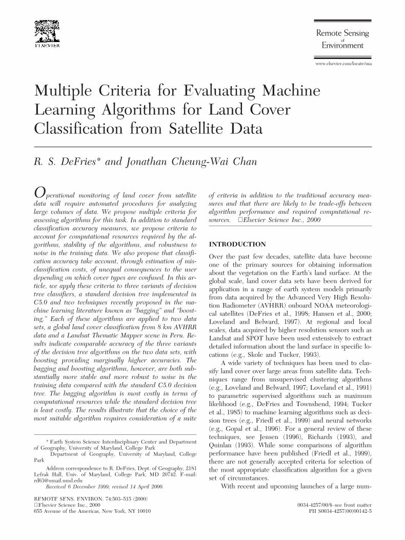
respectively (Table 5). With bagging, this number of Figure 6. j-error diagrams for 8 km data with randomnoise in the training data at a) 10%, b) 30%, and c) 50%.operations increases in proportion to the number ofBlue indicates results from the standard C5.0 decision tree,bootstrap samples used to generate the ensemble of indi-red from the results using boosting, and green from thevidual decision trees. The number of samples is conven- results using bagging.

tionally 100 (Breiman, 1996). Our investigation shows,however, that accuracy does not increase substantiallybeyond approximately 50 iterations for the 8 km data and decision tree requires less resources than boosting and20 iterations for the Landsat data (Fig. 2). Therefore, the substantially less than bagging. While this conclusion isnumber of basic operations required to achieve the ben- obvious in the case of the univariate decision trees usedefits of bagging is somewhat less for these data sets than for this study, the “amount of work done” provides athe convention would indicate. framework for assessing computational resources re-

For boosting, the number of operations is in propor- quired for other types of classifiers where such a com-tion to the number of iterations used. In this study, we parison is not as straightforward.used 10 iterations because previous studies with nonre-

Stability of the Algorithmmote sensing data suggest that this number provides maxi-It is desirable that an algorithm produce stable resultsmum improvement in classification accuracy (Freund andwhen faced with minor variability in the input data. InSchapire, 1997). With application of boosting to remotethe use of satellite data for monitoring land cover, algo-sensing data, Friedl et al. (1999) report that little accuracyrithm instability could erroneously indicate changes inis gained beyond seven iterations.land cover when none actually occurred. If training dataThe comparison of the algorithms according to the

“amount of work done” indicates that the standard C5.0 are used from the same locations at repeated intervals,


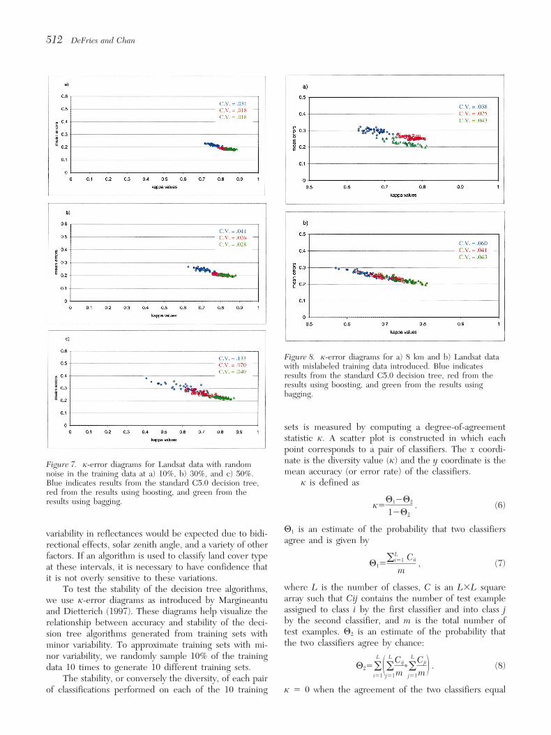
Figure 8. j-error diagrams for a) 8 km and b) Landsat datawith mislabeled training data introduced. Blue indicatesresults from the standard C5.0 decision tree, red from theresults using boosting, and green from the results usingbagging.

sets is measured by computing a degree-of-agreementstatistic j. A scatter plot is constructed in which eachpoint corresponds to a pair of classifiers. The x coordi-nate is the diversity value (j) and the y coordinate is theFigure 7. j-error diagrams for Landsat data with randommean accuracy (or error rate) of the classifiers.noise in the training data at a) 10%, b) 30%, and c) 50%.

j is defined asBlue indicates results from the standard C5.0 decision tree,red from the results using boosting, and green from theresults using bagging. j5

Q12Q2

12Q2. (6)

H1 is an estimate of the probability that two classifiersvariability in reflectances would be expected due to bidi-agree and is given byrectional effects, solar zenith angle, and a variety of other

factors. If an algorithm is used to classify land cover typeQ15

oLi51 Cii

m, (7)at these intervals, it is necessary to have confidence that

it is not overly sensitive to these variations.where L is the number of classes, C is an L3L squareTo test the stability of the decision tree algorithms,array such that Cij contains the number of test examplewe use j-error diagrams as introduced by Margineantuassigned to class i by the first classifier and into class jand Dietterich (1997). These diagrams help visualize theby the second classifier, and m is the total number ofrelationship between accuracy and stability of the deci-test examples. Q2 is an estimate of the probability thatsion tree algorithms generated from training sets withthe two classifiers agree by chance:minor variability. To approximate training sets with mi-

nor variability, we randomly sample 10% of the trainingH25o

L

i511o

L

j51

Cij

m*oL

j51

Cji

m 2 . (8)data 10 times to generate 10 different training sets.The stability, or conversely the diversity, of each pair

of classifications performed on each of the 10 training j 5 0 when the agreement of the two classifiers equal


that expected by chance and 1 when the two classifiers rates and lower stability as seen in the larger coefficientsof variation than the bagging and boosting results foragree on every example. Negative values occur whenboth the 8 km and Landsat data (Figs. 6 and 7). Baggingagreement is less than that expected by chance in the caseand boosting perform comparably for the 8 km dataof systematic bias.while bagging appears slightly more stable with higherIf an algorithm produces stable results, the j-errorinternal agreement than the boosting result for thediagram produces a compact cloud of points with j val-Landsat data. In general, the 8 km data has higher errorues close to 1. A spread of j values indicates that therates than the Landsat data, possibly because the 8 kmalgorithm is producing results that vary when using thedata contains several classes with relatively few trainingdifferent training sets.pixels or because the Landsat training data is derivedFor both the 8 km and Landsat data, the standardfrom the classification result itself. For nonremote sens-C5.0 decision tree produces a cloud of points with sub-ing data, Weiss (1995) illustrates that noise in the train-stantially larger spread than the boosting and bagging re-ing set leads to a disproportionate number of errors insults (Fig. 3). For the 8 km data, boosting produced theclasses with a small number of training samples.most compact cloud of points. Coefficients of variation

Mislabeling of training data causes more severeof the j values were .016 for boosting, compared withproblems in terms of stability for the decision tree algo-.022 for bagging, and .027 for the standard C5.0 decisionrithms than random noise (Fig. 8). While, overall, the er-tree. For the Landsat data, both bagging and boostingror rates are lower with mislabeled noise than with ran-produce compact clouds (coefficients of variation .013dom noise, the spread of points is much larger. Theand .012, respectively) with bagging showing higher jstandard C5.0 decision tree is least stable and has thevalues for the same mean error value, indicating greaterhighest error of all the algorithms for both the 8 km andagreement between samples. When input data can be ex-Landsat data. Bagging produces slightly lower error ratespected to show variability, as is the case with remotelyfor comparable stability compared with the boosting result.sensed data, these results suggest that bagging and boost-

In sum, bagging and boosting appear substantiallying provide a more stable classification result than a stan-more robust to random noise in the training data thandard decision tree.the standard C5.0 decision tree. For the Landsat data

Robustness to Noise in Training Data set, bagging appears more robust than boosting, while,Remotely sensed training data is likely to be noisy due in the 8 km data set, bagging and boosting appear com-to many factors including saturation of the signal, missing parable. For noise caused by mislabeled training data, allscans, mislabeling, problems with the sensor, and viewing the algorithms produce less stable results than with ran-geometry. Ideally, an algorithm would not be overly sen- dom noise. However, as with the random noise, baggingsitive to the presence of noise in the training data. This and boosting have lower error rates and greater stabilitycriterion is related to the stability of the algorithm, but than the standard C5.0 decision tree.even a stable algorithm will not necessarily perform wellin the presence of noise.

SUMMARY AND CONCLUSIONSFor this study, we investigate two types of noise thatcould realistically occur in the training data: random In this article, we propose several criteria for evaluatingnoise in the input data (input data are metrics in the case machine learning algorithms for operational monitoringof the 8 km AVHRR data and reflectance values in the of land cover with satellite data. In addition to the stan-case of the Landsat TM data) and mislabeling of the dard criterion of classification accuracy, we compare thecover type in the training data. For random noise, we computational resources required by the algorithmsintroduce zero values randomly (10%, 30%, and 50%) through quantifying the number of operations that needinto the training input data for both the 8 km and Land- to be performed. Through the use of j-error diagrams,sat data to simulate missing data. For mislabeling of the we also compare the stability of the algorithms when8 km data, we assigned class 13 to the class label in the faced with variability in the training data set and the ro-training data for all training pixels derived from three bustness of the algorithms to noise in the training data.Landsat scenes distributed around the world (Fig. 4). With respect to the classification accuracy, we also pro-This type of mislabeling is likely to occur in the case of pose that misclassification costs be taken into accounterroneous ancillary data or misinterpretation of the Land- because not all confusions between cover types havesat scene from which the training data were derived. For equal consequences for the user.the Landsat data from Peru, we mislabeled approximately To illustrate these criteria, we apply them to three10% of the training data as class 6 in a spatially heteroge- variants of decision tree algorithms used in machineneous portion of the scene (Fig. 5). learning: the standard decision tree from C5.0; the C5.0

The j-error diagrams help understand the effect of decision tree with “bagging”; and the C5.0 decision treenoise on the algorithms. For the case of random noise, with “boosting.” Each of these algorithms are applied to

two data sets, a global land cover classification from 8the standard C5.0 decision tree clearly has higher error


Table 6. Relative Ranking (Low, Medium, and High) of Multiple Criteria to Assess Algorithm Performance on 8 km andLandsat Data

Computational Robustness toAccuracy Resources Stability Noise

8 km data

Standard C5.0 decision tree Slightly lower Low Low LowDecision tree with boosting Slightly higher Medium High HighDecision tree with bagging Medium High High High

Landsat data

Standard C5.0 decision tree Slightly lower Low Low LowDecision tree with boosting Slightly higher Medium Medium MediumDecision tree with bagging Medium High High High

the 27th International Symposium on Remote Sensing of En-km AVHRR data and a Landsat Thematic Mapper scenevironment, Tromso, Norway.from Pucallpa, Peru. These data sets have each been

Baase, S. (1988), Computer Algorithms: Introduction to Designclassified with extensive human interpretation and expertand Analysis, Addison-Wesley, Reading, MA.knowledge that provide reliable test data for assessing

Breiman, L. (1996), Bagging predictors. Mach. Learn. 24:the classification results.123–140.Results indicate comparable accuracy of the three Breiman, L., Friedman, J. H., Olshend, R. A., and Stone, C.

variants of the decision tree algorithms on the two data J. (1984), Classification and Regression Trees, Wadsworth,sets for all the three accuracy measures investigated here Monterey, CA.(overall accuracy, mean class accuracy, and adjusted ac- Brodley, C., Lane, T., and Stough, T. (1999), Knowledge dis-curacy to account for hypothetical misclassification covery and data mining. Am. Sci. (Jan./Feb.):54–61.costs). Accuracies are highest for boosting, but only by Congalton, R. G. (1991), A review of assessing the accuracy of

classifications of remotely sensed data. Remote Sens. Envi-a few percentages. However, the bagging and boostingron. 37:35–46.algorithms are both more stable and more robust to

Congalton, R. G., and Green, K. (1999), Assessing the Accu-noise in the training data compared with the standardracy of Remotely Sensed Data: Principles and Practices,C5.0 decision tree. These advantages are associated withLewis Publishers, New York.a cost of increased requirements for computation re-

DeFries, R. S., and Los, S. O. (1999), Implications of landsources. The bagging algorithm is most costly in termscover misclassification for parameter estimates in global“amount of work done” while the standard decision treeland surface models: an example from the Simple Biosphere

is least costly (Table 6). The results presented here illus- Model (SiB2). Photogramm. Eng. Remote Sens. 65:trate that multiple criteria need to be evaluated in as- 1083–1088.sessing the most suitable algorithms for land cover classi- DeFries, R. S., and Townshend, J. R. G. (1994), NDVI-derivedfication. The choice of the most suitable algorithm land cover classification at global scales. Int. J. Remoterequires consideration of a number of criteria in addition Sens. 15:3567–3586.to the traditional accuracy measures. DeFries, R., Hansen, M., Townshend, J. R. G., and Sohlberg,

R. (1998), Global land cover classifications at 8 km spatialresolution: the use of training data derived from LandsatThis research was supported by NASA Grants NAG56970 andimagery in decision tree classifiers. Int. J. Remote Sens. 19:NAG56004. The Landsat Pathfinder project for Deforestation3141–3168.in the Humid Tropics supplied the TM data. We thank Carla

Dietterich, T. G. (in press), An experimental comparison ofBrodley, Purdue University; Mark Friedl, Boston University;Arthur Desch, University of Maryland; and Matt Hansen, Uni- three methods for constructing ensembles of decision trees:versity of Maryland for helpful comments and suggestions. bagging, boosting, and randomization. Mach. Learn.

Freund, Y., and Shapiro, R. E. (1996), Experiments with a newboosting algorithm, In Machine Learning Proceedings of the

REFERENCES Thirteenth International Conference, Morgan-Kaufman, SanFrancisco, CA, pp. 148–156.

Friedl, M. A., and Brodley, C.E. (1997), Decision tree classifi-Agbu, P. A., and James, M. E. (1994), The NOAA/NASA Path-finder AVHRR Land Data Set User’s Manual, Goddard Dis- cation of land cover form remotely sensed data. Remote

Sens. Environ. 61:399–409.tributed Active Archive Center Publications, GCDG, Green-belt, MD. Friedl, M. A., Brodley, C. E., and Strahler, A. (1999), Maximiz-

ing land cover classification accuracies produced by decisionAhern, F., Janetos, A., and Langham, E. (1998), Global Obser-vations of Forest Cover: one component of CEOS’ inte- trees at continental to global scales. IEEE Trans. Geosci.

Remote Sens. 37:969–977.grated global observing system strategy. In Proceedings of


Freund, Y., and Schapire, R. E. (1997), A decision-theoretic Conference on Artificial Intelligence, Morgan Kaufmann,San Francisco.generalization of on-line learning and an application to

Margineantu, D. D., and Dietterich, T. G. (1999), Learning de-boosting. Journal of Computer and System Sciencescision trees for loss minimization in multi-class problems,55(1):119–139.Oregon State University, Corvallis.Gopal, S., Woodcock, C., and Strahler, A. H. (1996), Fuzzy

Merz, C. J., and Murphy, P. M. (1996), UCI repository of ma-ARTMAP classification of global land cover fom AVHRRchine learning databases. University of California Irvine,data set. In Proceedings of the 1996 International Geosci-Morgan Kaufmann, CA.ence and Remote Sensing Symposium, Lincoln, NE, 27–31

Provost, F., and Fawcett, T. (1997), Analysis and visulaizationMay, pp. 538–540.of classifier performance: comparison under imprecise classHansen, M., and Reed, B. (2000), Comparison of IGBP DIS-and cost distribution. In Proceedings of the Third Interna-Cover and University of Maryland 1km global land covertional Conference on Knowledge Discovery and Data Min-classifications. Int. J. Remote Sens. 21:1365–1374.ing (KDD-97), American Association for Artificial Intelli-Hansen, M., DeFries, R., Townshend, J. R. G., and Sohlberg,gence, Huntington Beach, CA (www.aaai.org).R. (2000), Global land cover classification at 1km spatial res-

Provost, F., Fawcett, T., and Kohavi, R. (1998), Building theolution using a classification tree approach. Int. J. Remotecase against accuracy estimation for comparing induction al-Sens. 21:1331–1364.gorithms. Proceedings of the Fifteenth International Con-Hansen, M., Dubayah, R., and DeFries, R. (1996), Classifica-ference on Machine Learning (IMLC-98), Madison, WI.tion trees: an alternative to traditional land cover classifiers.

Quinlan, R. J. (1993), C4.5: Programs for Machine Learning,Int. J. Remote Sens. 17:1075–1081.Morgan Kaufmann, San Mateo, CA.Indurkhya, N., and Weiss, S. M. (1998), Estimating perfor-

Quinlan, J. R. (1996), Bagging, boosting and C4.5. In Proceed-mance gains for voted decision trees. Intell. Data Anal. 2(4):ings of the Thirteenth National Conference on Artificial In-1–10.telligence, AAAI Press, Portland, OR, pp. 725–730.Janetos, A. C., and Ahern, F. (1997), CEOS Pilot Project:

Richards, J. A. (1993), Remote Sensing Digital Image Analysis:Global Observations of Forest Cover (GOFC), Report fromAn Introduction, Springer-Verlag, New York.meeting, Ottawa, Ontario, Canada.

Schiffers, J. (1997), A classification approach incorporating mis-Jensen, J. R. (1996), Introductory Digital Image Processing: Aclassification costs. Intell. Data Anal. 1(1):1–10.Remote Sensing Perspective, Prentice Hall, Upper Saddle

Skole, D., and Tucker, C. (1993), Tropical deforestation andRiver, NJ.habitat fragmentation in the Amazon: satellite data from

Kalluri, S. N. V., Jaja, J., Bader, P. A. (2000), High perfor- 1978 to 1988. Science 260:1905–1910.mance computing algorithms for land cover dynamics using Swain, P. H., and Hauska, H. (1977), The decision tree classi-remote sensing data. Int. J. Remote Sens. 21(6):1513–1536. fier: design and potential. IEEE Trans. Geosci. Electron.

Kohavi, R., Sommerfield, D., and Dougherty, J. (1996), Data GE-15:142–147.mining using MLC11: a machine learning library in C11. Townshend, J. R. G., Bell, V., Desch, A. (1995), The NASAInt. J. Artif. Intell. Tools 6:537–566. Landsat Pathfinder Humid Tropical Deforestation Project,

Loveland, T. R., and Belward, A. S. (1997), The IGBP-DIS Land satellite information in the next decade, ASPRS Con-global 1 km land cover data set, DISCover: first results. Int. ference, Vienna, VA, 25–28 September, pp. IV-76-IV-87.J. Remote Sens. 18:3289–3295. Tucker, C. J., Townshend, J. R. G., and Goff, T. E. (1985),

Loveland, T. R., Merchant, J. W., Ohlen, D. O., and Brown, African land-cover classification using satellite data. Sci-J. F. (1991), Development of a land-cover characteristics da- ence 227:369–375.tabase for the conterminous U.S. Photogramm. Eng. Remote Weiss, G. M. (1995), Learning with rare cases and small dis-Sens. 57:1453–1463. juncts. In Machine Learning: Proceedings of the Twelfth In-

Margineantu, D., and Dietterich, T. (1997), Pruning adaptive ternational Conference, Morgan Kaufmann, San Fancisco,pp. 558–565.boosting. In Proceedings of the Fourteenth International

Documents

Thiosemicarbazone Metal Complexes: From Structure to Activity