Embed Size (px)
Citation preview

Thiago de Barros Lacerda
SUPPORTING REAL-TIME MOBILITY SERVICES WITH
SCALABLE FLOCK PATTERN MINING
M.Sc. Dissertation
Federal University of [email protected]
<www.cin.ufpe.br/~posgraduacao>
RECIFE2016
Thiago de Barros Lacerda
SUPPORTING REAL-TIME MOBILITY SERVICES WITHSCALABLE FLOCK PATTERN MINING
A M.Sc. Dissertation presented to the Informatics Center
of Federal University of Pernambuco in partial fulfillment
of the requirements for the degree of Master of Science in
Computer Science.
Advisor: Stênio Flávio de Lacerda Fernandes
RECIFE2016

Catalogação na fonte
Bibliotecária Monick Raquel Silvestre da S. Portes, CRB4-1217
L131s Lacerda, Thiago de Barros
Supporting real-time mobility services with scalable flock pattern mining / Thiago de Barros Lacerda. – 2016.
67 f.: il., fig., tab. Orientador: Stênio Flávio de Lacerda Fernandes. Dissertação (Mestrado) – Universidade Federal de Pernambuco. CIn,
Ciência da Computação, Recife, 2016. Inclui referências.
1. Mineração de dados. 2. Dados espaço-temporais. I. Fernandes, Stênio Flávio de Lacerda (orientador). II. Título. 006.312 CDD (23. ed.) UFPE- MEI 2016-116

Thiago de Barros Lacerda
SUPPORTING REAL-TIME MOBILITY SERVICES WITHSCALABLE FLOCK PATTERN MINING
Dissertação de Mestrado apresentada ao programa dePós-Graduação em Ciência da Computação da UniversidadeFederal de Pernambuco, como requisito parcial paraobtenção do título de Mestre em Ciência da Computação.
Aprovado em: 29/07/2016
BANCA EXAMINADORA
———————————————————————–Prof. Rostand Edson Oliveira Costa
Laboratório de Aplicações de Vídeo Digital - LAVID/UFPB
———————————————————————–Prof. Kiev Santos da Gama
Centro de Informática/UFPE
———————————————————————–Prof. Stênio Flávio de Lacerda Fernandes
Centro de Informática/UFPE
RECIFE2016

To my wife, my son and my parents!

Acknowledgements
To be honest, I thought that would not finish this. I was already seeing myself giving upthis masters due to a lot of things: new country, new city, new job, huge load of work in my newjob, baby coming... etc.. It was not easy to work on double journey for lots of months, sleepingonly 3 to 4 hours a day. But yes! It is over! Some people helped me to no give up and keep upwith that "stressful journey" and here they deserve my "Thank you!".
I would like to thank my advisor Stênio, by having me as his student, for the second time,and lending me some time of his busy agenda, helping me out to finish this work.
Many thanks to my beloved wife Thaís, who was always supporting me during the yearsof this masters, telling me to never give up and giving up time with me in favor of me workingon this dissertation. Also, thanks to my baby boy Daniel, who isn’t even born yet, but helped meto finish this dissertation as fast as possible so I can enjoy some free time before I lose them allafter he is born :). Thanks to my mother Catari and my father Cândido for their support duringthis time too.
Thanks to Andre, who was always telling me that we were going to end this and wasalso always warning me about the important deadline dates of the University. I also would liketo thank my friends here in Seattle: PP and Fabio, for lending me some VMs on their Azureaccounts, so I could run my benchmarks; Fernando, for good academic advices and motivationalspeechs :).

...there are two paths you can go by, but in the long run there’s still time to
change the road you’re on...
—LED ZEPPELIN, STAIRWAY TO HEAVEN

Resumo
Detecção de padrões em dados espaço-temporais tem se mostrado um tema de muita relevâncianos dias atuais, tanto na academia quanto na indústria, devido a sua vasta aplicabilidade emauxiliar a solucionar problemas enfrentados na sociedade. Muitos desses problemas podemser classificados no conexto de Cidades Inteligentes (Smart Cities), como Gerenciamento deTráfego, Segurança e Planejamento de Cidades. Dentre os vários padrões espaço-temporaisque podem ser extraídos de uma base de dados, o padrão de flock é um que vem atraindomuita atenção, devido a sua relação intrínseca com os problemas mencionados anteriormente.Muitas pesquisas vêm sendo feitas na academia, visando desenvolver algoritmos capazes deidentificar esse padrão de movimentação. Porém, nenhum deles foi capaz de executar tal tarefaeficientemente, nem conseguiu escalar de maneira aceitável quando uma base de dados degrande tamanho foi analisada. Além disso, não foi encontrado nos trabalhos relacionados umaarquitetura de software que conseguisse ser simples e modular o suficiente para ser usada noproblema de detecção de padrões de flock em dados espaço-temporais. Com isso em mente, essadissertação propõe uma arquitetura de software modular, direcionada para solucionar problemasde detecção desse padrão e possivelmente ser utilizada para outros experimentos envolvendomineração de padrões em dados espaço-temporais. Tal arquitetura foi então usada como base naimplementação de um algoritmo de detecção de flock, focando em alcançar grandes ganhos emtempo de processamento, sem comprometer a precisão, visando então cenários de aplicações detempo real em Cidades Inteligentes. No fim, nós propomos uma remodelagem no nosso algoritmopara poder utilizar ao máximo o poder de processamento oferecido pelas arquiteturas multi-core
dos processadores modernos. Nossos resultados mostraram que nossa solução conseguiu superarpropostas do estado da arte, alcançando 99% de redução no tempo de processamento total. Alémdisso, nossa remodelagem multi-thread conseguiu melhorar os resultados da nossa solução ematé 96% em alguns casos. A eficiência e performance da nossa proposta foi comprovada comavaliações feitas com bases de dados geradas sinteticamente e coletadas em experimentos reais.
Palavras-chave: Cidades Inteligentes. Mineração de Padrões. Dados Espaço-temporais. Padrãode Flock

Abstract
Pattern mining in spatio-temporal datasets is a really relevant subject in the academia and theindustry nowadays, due to its wide applicability in helping to solve real-world problems. Manyof them can be found in the context of Smart Cities, like Traffic Management, Surveillanceand Security and City Planning, to name a few. Among the various spatio-temporal patternsthat one can extract from a spatio-temporal dataset, the flock pattern is one that has gained alot of attention, because of its intrinsic relation with the aforementioned problems. A lot ofwork has been done in the academia, in order to provide algorithms able to identify the flockpattern. However, none of them could perform that task efficiently nor be able to scale wellwhen a large dataset was the analysis target. Additionally, we found that there was no systemarchitecture proposal that could be simple and modular enough to be used in that spatio-temporalpattern detection problem. Given that context, this dissertation proposes a modular systemarchicture designed to help solving flock pattern mining problems and possibly be reused toother spatio-temporal mining experiments. We then use such architecture as the infrastructureto implement an efficient flock detection algorithm, aiming at achieving considerable gainsin execution time without compromising accuracy, thus targeting real-time deployment andon-line processing in Smart Cities. Last, but not least, we remodel our algorithm in order to takeadvantage of multi-core architectures present in modern computers. Our results indicate thatour proposal outperforms the current state-of-the-art techniques, by achieving 99% CPU timeimprovement. Moreover, with our multi-thread model, we were able to reduce the processingtime of our proposed algorithm by 96% in some cases. We prove the efficiency of our solutionby performing evaluation with both real and synthetic large datasets.
Keywords: Smart Cities. Pattern Mining. Spatio-temporal data. Flock Pattern

List of Figures
1.1 Orange, green and blue trajectories form a flock of size 3 with minimum lengthof 3 time steps, with a disk enclosing all trajectories at each time step ti . . . . 15
2.1 A moving cluster composed by clusters S0, S1 and S2 and θ = 0.5 . . . . . . . 192.2 A Convoy pattern . . . . . . . . . . . . . . . . . . . . . . . . . . . . . . . . . 20
3.1 T1, T2 and T3 form a flock of size µ = 3 with minimum length of δ = 3 timeslots and with a disk diameter of size ε = d . . . . . . . . . . . . . . . . . . . 28
3.2 Two disks with radius ε/2 that are found based on points p1 and p2. c1 and c2
stand for the disks centers and m represents the midpoint between p1 and p2. . 303.3 Cell grid for time slot ti. The dark grey is the cell that is currently being processed
and the light gray cells around are the grids that will be in the search space ofthe dark cell. Each small circle inside the grid, represents a Global PositioningSystem (GPS) point that was collected in time slot ti . . . . . . . . . . . . . . . 31
4.1 Modular system architecture overview . . . . . . . . . . . . . . . . . . . . . . 334.2 Percentage of time spent between disk and flock processing tasks against other
tasks in the algorithm . . . . . . . . . . . . . . . . . . . . . . . . . . . . . . . 354.3 Sequence of disks in 4 consecutive time slots and the points that were clustered
to them . . . . . . . . . . . . . . . . . . . . . . . . . . . . . . . . . . . . . . 364.4 Interaction between GPS Stream Buffer (GSB) (red) and Flock Processor (FP)
(gray) in 5 consecutive time slots, showing how the presence bitmaps areconstructed. In the example we have µ = 3 and δ = 3 . . . . . . . . . . . . . . 40
4.5 Modeling the FP in a Producer-Multiple Consumers architecture . . . . . . . . 43
5.1 System design implemented for the experiments . . . . . . . . . . . . . . . . . 455.2 FlockProcessor class composition . . . . . . . . . . . . . . . . . . . . . . . . 465.3 Results varying δ and ε for Trucks dataset . . . . . . . . . . . . . . . . . . . . 475.4 Results varying µ and number of disks generated over time for Trucks dataset . 475.5 Results varying δ and ε for BerlinMOD dataset . . . . . . . . . . . . . . . . . 485.6 Results varying µ and number of disks generated over time for BerlinMOD dataset 495.7 Results varying δ and ε for TDrive dataset . . . . . . . . . . . . . . . . . . . . 495.8 Results varying µ and number of disks generated over time for TDrive dataset . 505.9 Results varying δ and ε for Brinkhoff dataset . . . . . . . . . . . . . . . . . . 515.10 Results varying µ and number of disks generated over time for Brinkhoff dataset 515.11 Execution time reduction by number of threads for the Trucks dataset . . . . . 535.12 Results varying δ and ε for Trucks dataset . . . . . . . . . . . . . . . . . . . . 545.13 Results having δ = 20, ε = 1.5 and µ varying for the Trucks dataset . . . . . . 54

5.14 Execution time reduction by number of threads for the BerlinMOD dataset . . . 555.15 Results varying δ and ε for BerlinMOD dataset . . . . . . . . . . . . . . . . . 555.16 Results having δ = 8, ε = 100 and µ varying for the BerlinMOD dataset . . . . 565.17 Execution time reduction by number of threads for the TDrive dataset . . . . . 565.18 Results varying δ and ε for TDrive dataset . . . . . . . . . . . . . . . . . . . . 575.19 Results having δ = 8, ε = 100 and µ varying for the TDrive dataset . . . . . . 585.20 Execution time reduction by number of threads for the Brinkhof dataset . . . . 585.21 Sum of disks generated by the disk threads (red) and number of disks that were
inserted in the global disk set after subset/superset check (blue), by time slot . . 595.22 Results varying δ and ε for Brinkhoff dataset . . . . . . . . . . . . . . . . . . 605.23 Results having δ = 8, ε = 100 and µ varying for the Brinkhoff dataset . . . . . 60

List of Tables
3.1 Conversion from World Geodetic System 1984 (WGS84) to R2 . . . . . . . . . 253.2 Ideal dataset sample rate . . . . . . . . . . . . . . . . . . . . . . . . . . . . . 263.3 Real-world dataset sample rate . . . . . . . . . . . . . . . . . . . . . . . . . . 263.4 Mapping points from Table 3.3 to its correspondent time slot, using σ = 3 . . . 26
4.1 Bitmaps in GSB after buffering four time slots . . . . . . . . . . . . . . . . . . 36

List of Acronyms
AO Analysis Outcome. . . . . . . . . . . . . . . . . . . . . . . . . . . . . . . . . . . . . . . . . . . . . . . . . . . . . .46
AWS Amazon Web Services . . . . . . . . . . . . . . . . . . . . . . . . . . . . . . . . . . . . . . . . . . . . . . . . . . 32
BFE Basic Flock Evaluation . . . . . . . . . . . . . . . . . . . . . . . . . . . . . . . . . . . . . . . . . . . . . . . . . 16
BitDF Bitmaps for Disk Filtering . . . . . . . . . . . . . . . . . . . . . . . . . . . . . . . . . . . . . . . . . . . . . . 36
CPU Central Processing Unit . . . . . . . . . . . . . . . . . . . . . . . . . . . . . . . . . . . . . . . . . . . . . . . . . 16
DC Dynamic Convoy . . . . . . . . . . . . . . . . . . . . . . . . . . . . . . . . . . . . . . . . . . . . . . . . . . . . . . 20
DD Data Decoder . . . . . . . . . . . . . . . . . . . . . . . . . . . . . . . . . . . . . . . . . . . . . . . . . . . . . . . . . . 32
DL Data Listener . . . . . . . . . . . . . . . . . . . . . . . . . . . . . . . . . . . . . . . . . . . . . . . . . . . . . . . . . . 32
DP Data Processor . . . . . . . . . . . . . . . . . . . . . . . . . . . . . . . . . . . . . . . . . . . . . . . . . . . . . . . . . 32
DSC Data Source Connector . . . . . . . . . . . . . . . . . . . . . . . . . . . . . . . . . . . . . . . . . . . . . . . . . 32
EC Evolving Convoy. . . . . . . . . . . . . . . . . . . . . . . . . . . . . . . . . . . . . . . . . . . . . . . . . . . . . . .20
EGC Extended Grid Cell . . . . . . . . . . . . . . . . . . . . . . . . . . . . . . . . . . . . . . . . . . . . . . . . . . . . . 41
FP Flock Processor . . . . . . . . . . . . . . . . . . . . . . . . . . . . . . . . . . . . . . . . . . . . . . . . . . . . . . . . 36
GPS Global Positioning System . . . . . . . . . . . . . . . . . . . . . . . . . . . . . . . . . . . . . . . . . . . . . . 20
GSB GPS Stream Buffer . . . . . . . . . . . . . . . . . . . . . . . . . . . . . . . . . . . . . . . . . . . . . . . . . . . . . 36
IBMC Influence-based Moving Cluster . . . . . . . . . . . . . . . . . . . . . . . . . . . . . . . . . . . . . . . . . 19
IoT Internet of Things . . . . . . . . . . . . . . . . . . . . . . . . . . . . . . . . . . . . . . . . . . . . . . . . . . . . . . 16
LTS Long Term Support . . . . . . . . . . . . . . . . . . . . . . . . . . . . . . . . . . . . . . . . . . . . . . . . . . . . .46
MFP Maximal-duration Flock Pattern . . . . . . . . . . . . . . . . . . . . . . . . . . . . . . . . . . . . . . . . . 22
MO Moving Object . . . . . . . . . . . . . . . . . . . . . . . . . . . . . . . . . . . . . . . . . . . . . . . . . . . . . . . . . 17
MT Multi-thread . . . . . . . . . . . . . . . . . . . . . . . . . . . . . . . . . . . . . . . . . . . . . . . . . . . . . . . . . . . 17
PFP Parallel Flock Processor . . . . . . . . . . . . . . . . . . . . . . . . . . . . . . . . . . . . . . . . . . . . . . . . 52
REMO RElative MOtion . . . . . . . . . . . . . . . . . . . . . . . . . . . . . . . . . . . . . . . . . . . . . . . . . . . . . . . 18
DBSCAN Density-based Spatial Clustering of Applications with Noise . . . . . . . . . . . . . . . 19
WGS84 World Geodetic System 1984 . . . . . . . . . . . . . . . . . . . . . . . . . . . . . . . . . . . . . . . . . . . . 11
WHOI Woods Hole Oceanographic Institution . . . . . . . . . . . . . . . . . . . . . . . . . . . . . . . . . . . 25

Contents
1 Introduction 14
2 Related Work 182.1 General trajectory data and pattern mining . . . . . . . . . . . . . . . . . . . . 182.2 Flock pattern mining . . . . . . . . . . . . . . . . . . . . . . . . . . . . . . . 212.3 Academic Contribution . . . . . . . . . . . . . . . . . . . . . . . . . . . . . . 23
3 Technical Background 253.1 Trajectory and data information . . . . . . . . . . . . . . . . . . . . . . . . . 253.2 Flock pattern . . . . . . . . . . . . . . . . . . . . . . . . . . . . . . . . . . . 27
3.2.1 Disk discovery . . . . . . . . . . . . . . . . . . . . . . . . . . . . . . 28
4 Modular and Efficient Flock Pattern Identification 324.1 Modular System Architecture . . . . . . . . . . . . . . . . . . . . . . . . . . . 324.2 Aggregation and data processing efficiency . . . . . . . . . . . . . . . . . . . 344.3 BitDF . . . . . . . . . . . . . . . . . . . . . . . . . . . . . . . . . . . . . . . 364.4 Taking Advantage of Multi-core Architectures . . . . . . . . . . . . . . . . . . 41
4.4.1 Multi-threaded Design . . . . . . . . . . . . . . . . . . . . . . . . . . 42
5 Experimental Results 445.1 Trucks Dataset . . . . . . . . . . . . . . . . . . . . . . . . . . . . . . . . . . 465.2 BerlinMOD Dataset . . . . . . . . . . . . . . . . . . . . . . . . . . . . . . . . 485.3 TDrive Dataset . . . . . . . . . . . . . . . . . . . . . . . . . . . . . . . . . . 485.4 Brinkhoff Dataset . . . . . . . . . . . . . . . . . . . . . . . . . . . . . . . . . 505.5 Multi-threaded evaluation . . . . . . . . . . . . . . . . . . . . . . . . . . . . . 52
6 Conclusion 616.1 Future Work . . . . . . . . . . . . . . . . . . . . . . . . . . . . . . . . . . . . 62
6.1.1 Deployment Challenges in Real World Scenarios . . . . . . . . . . . . 63
References 64

141414
1Introduction
The advances of positioning technologies are enabling lot of different objects present inour daily usage (e.g. vehicles, smartphones and wearable devices) to be shipped with locationtracking systems. Those devices are able to collect and report mobility information of people,animals and natural phenomena (e.g. hurricanes), to name a few. That technological advance isenabling the generation of massive volumes of spatio-temporal data that can contain informationranging from the daily routine of residents of a city (FARRAHI; GATICA-PEREZ, 2008) to thebehavior of wild animals in a specific region (LEE; HAN; WHANG, 2007; LI et al., 2010a). It isnotorious the interest of both industry and academia in such subject, specially with the rising ofSmart Cities, in which spatio-temporal datasets can provide important insights in the context ofproblems like traffic management and urban planning (JENSEN; GUTIERREZ; PEDERSEN,2015; DING et al., 2016). Those datasets can be used to help solving a variety of issues andanswer some questions, such as:
1. What are the busiest times and locations (such as traffic jams locations) in acity? (WANG et al., 2013)
2. What are the movement patterns of the citizens of a city during work hours?
3. What is the migration pattern of inhabitants of a specific area?
4. What is the movement behavior of wild animals in their habitat? (LI et al., 2011)
5. Is there any suspicious movement of groups of objects during some specific timewindow?
That list can grow indefinitely, as the scenarios and applications of spatio-temporal dataanalyses are vast. Some of the questions listed above are in the context of Smart Cities, which cantake advantage of spatio-temporal data analysis as an aid to a broad set of applications, like urbanplanning, public security, and public health and commerce (PAN et al., 2013). Additionally,understanding the data in question and being able to take actions fast according to the conclusionsextracted from such data is crucial to create and evolve a Smart City. However, due to the hugevolume of data that is produced on a daily basis and the need analyze them to in order to help

15
those applications and answer those questions, the main problem is still the same: how to be ableto analyze massive data volumes fast and efficiently so we can empower decision takers to actquickly?
In the aforementioned questions and applications, some of the queries are intrinsicallyrelated to collaborative or group patterns, such as flock (GUDMUNDSSON; KREVELD;SPECKMANN, 2004), convoy (JEUNG; SHEN; ZHOU, 2008), swarm (LI et al., 2010b),and the like. Those patterns contain moving objects that have a strong relationship by being closeto each other, within a certain distance range and during some minimum time interval. Becausewe extract information about groups of people interacting, instead of just dealing with trackingof individuals alone, such patterns can be applied to a wide range of scenarios of Smart Cities(e.g. city roads planning, intelligent transportation, public security, etc.), causing the mining ofthose patterns to gain great importance within the research community. There are a number ofresearch challenges in this topic, specially regarding the development of accurate algorithms todetect those patterns. In addition of being precise, it is of paramount importance to design fastalgorithms so that they can keep up with real-time data. Hence, reiterating what as mentioned inthe previous paragraph, efficiently extraction of data patterns empowering real-time analyses andon the fly decision-making is still an open challenge.
Figure 1.1: Orange, green and blue trajectories form a flock of size 3 with minimum length of 3time steps, with a disk enclosing all trajectories at each time step ti
Source: Made by the author.
Among those collaborative patterns, the flock pattern is one that has gained a lot ofattention in the research community, since it can address all the scenarios and questions thatwere mentioned in this chapter and represents a very familiar behavior that is frequently seen in
16
our daily routines. A seminal formal definition of that pattern was proposed by Laube, Kreveldand Imfeld (2005) and Gudmundsson, Kreveld and Speckmann (2004) and since then, a lot ofother studies has follow suit (we refer the reader to Chapter 2 for some of them), mainly dueto the interests in developing mechanisms to solve real-world problems in the scope of Internetof Things (IoT) (TSAI et al., 2014) and Smart Cities (DJAHEL et al., 2015). According toGudmundsson, Kreveld and Speckmann (2004), a flock pattern consists of a minimum number ofentities that are within a disk of radius r at a given time. However, this definition only applies toone single time step and does not help on extracting some useful collective behavior information.Such initial definition was then extended by Benkert et al. (2008), introducing the minimumtime interval δ that the entities should stay together in order to characterize a flock pattern, asdepicted in Figure 1.1. That figure shows a flock pattern that lasts three time steps and is formedby the orange, green and blue trajectories. It is worth mentioning that the remaining trajectories(yellow and pink) are not part of a flock pattern because there are no disks enclosing them in allthree time steps.
When it comes to flock pattern detection efficiency and speed, one major problem ondoing that is to find the disks that enclose the trajectories in each time step. Since the diskscenters do not need to match any point in the dataset, there can be infinite possible disks. Vieira,Bakalov and Tsotras (2009) proposed a way to limit the number of disks to generate and analyze,so a finite number of disks are in place to cluster the trajectories into them. They also proposedan algorithm to find the flock pattern, namely Basic Flock Evaluation (BFE). Even though BFEcan find flock patterns in spatio-temporal datasets, it does suffer from some severe performancelimitations, meaning that it is not able to scale properly when the dataset is really large. Themain reason that we identified that makes it perform so inefficiently is that BFE is not smartenough to predict what portions of the data can really generate flock patterns, then it ends upwasting Central Processing Unit (CPU) cycles by processing data that is not relevant.
Despite the considerable number of research studies regarding flock pattern detection,there is still something that nobody ever got to it, based on the systematic literature revisionfield that we did, but it would be of great value if defined and formalized: A framework/systemarchitecture that can be modular and simple, to serve as the building blocks for flock detectionalgorithms. By creating such architecture, researchers can take advantage of that as a startingpoint to develop their algorithms and can also have a common ground to compare and reusework of others.
In our related work research, we noticed that the state of the art algorithms for flockpattern detection are not ready to aid the development and evolution of Smart Cities, sincethey are not able to efficiently process the huge volumes of data that are generated by them.With that in mind, this dissertation proposes an efficient flock detection algorithm aiming atachieving considerable gains in execution time, without compromising accuracy, thus targetingreal-time deployment and on-line processing. With that algorithm, we could address SmartCities scenarios, where decisions need to be made on the fly and rapidly enough in order to

17
keep up with their development pace (PAN et al., 2013; BATTY et al., 2012). Such gains weremade possible by creating a filtering heuristic, based on bitmaps, in order to save processingtime. Our proposal focuses on identifying Moving Objects (MOs) that can actually form a flock,resulting in a huge reduction in the number of disks generated and thus resulting in less datato be processed. Our results indicate that our proposal outperforms the current state-of-the-arttechniques, by achieving 99% CPU time improvement and 96% disks generation reduction insome relevant scenarios. Going even further, we also remodeled our proposed algorithm to takeadvantage of multi-core architectures, having some components executing in parallel resultingin impressive speed gains. With our Multi-thread (MT) model, we were able to reduce theprocessing time of our proposed algorithm by 96% in some cases. It is worth mentioning thatthe gains achieved with the MT model are over the gains that we had already obtained over thestate-of-the-art techniques.
Last, but not least, we also propose a modular system architecture, aiming at helping tofind flock patterns in spatio-temporal datasets. We validate our architecture by implementing ouralgorithm and our MT model using it as the building blocks. To summarize, the contribution ofthis dissertation is threefold:
1. An efficient flock pattern detection algorithm
2. A remodeled algorithm able to take advantage of multi-core architectures andrapidly find flock patterns
3. A simple and modular system architecture to aid solving spatio-temporal flockpattern detection problems
The remainder of this dissertation is organized as follows. Chapter 2 highlights therelated work in both flock detection and trajectory data mining and explain in more details theacademic contribution of our work. Chapter 3 presents the technical background necessary tounderstand this dissertation, like the formal flock pattern definition and how an algorithm to finda flock pattern works. Our contribution is detailed in Chapter 4, whereas in Chapter 5 we showthe results of our experimental evaluations, on the datasets that we picked, based on the chosenmetrics. Lastly, in Chapter 6 we draw some concluding remarks and provide directions for futurework.
181818
2Related Work
This is a research field that has had a lot of attention in both academia and industry inpast and present years. Hence, the related work in this area and related fields is quite extensiveand broad. With that in mind, we will split this section in (1) General trajectory data and patternmining and (2) Flock pattern mining
It is worth noting that the only set of research studies that are pertinent to this work, arethose in Section 2.2. Hence, those will be the only research studies that we will point out someflaws that are addressed by this dissertation.
2.1 General trajectory data and pattern mining
Here we present the broader scope of trajectory data and pattern mining that were usefulto gather some understanding in the field and insightful ideas for this dissertation.
Laube, Kreveld and Imfeld (2005) proposed the RElative MOtion (REMO) concept,which analyzes motion attributes (speed, azimuth and location) of entities and relate to themotion of other entities that are close to them. They also introduced some moving patterns, suchas flock, convergence, encounter, and leadership. In the end the authors went through some datastructures and algorithms that could be used in order to detect those patterns. However, only highlevel abstract algorithms were presented, but neither concrete implementation nor evaluationwere shown.
An interesting approach for finding patterns that are frequently repeated by MOs waspresented by Cao, Mamoulis and Cheung (2005). The authors presented an algorithm thatfocused on approximating the spatio-temporal series of a MO to a line, where the distance ofeach trajectory point of that MO to the line would be no greater than a pre-defined threshold.After that, bounding boxes were created based on those approximated lines and then lines thatbelong to the same box were declared as similar sequential patterns.
Algorithms aiming at finding moving clusters, with MOs coming in and out of the cluster,were presented by Kalnis, Mamoulis and Bakiras (2005). In that research paper, the authorsconsider a moving cluster as a moving region despite the identity of the objects that are part ofit, but for each timestamp the intersection of points between subsequent clusters needs to be

2.1. GENERAL TRAJECTORY DATA AND PATTERN MINING 19
Figure 2.1: A moving cluster composed by clusters S0, S1 and S2 and θ = 0.5
Source: (KALNIS; MAMOULIS; BAKIRAS, 2005).
above a certain threshold θ . In Figure 2.1 one can see a moving cluster composed by clusters
S0, S1 and S2, having θ = 0.5, meaning that|ci∩ ci+1||ci∪ ci+1|
≥ 0.5. They presented three different
approaches to find moving clusters (with one of them being an approximation method), beingsupported by a density function. They claim that their proposal is applicable for large-temporaldatasets, but that large dataset that they analyzed had only 50K entries. Yet on clusters, Jensen,Lin and Ooi (2007) added velocity as a parameter in order to help finding moving clusters (usingdissimilarity functions), achieving some improvements in processing time. An approach usinga trajectory similarity measure based on the Hausdorff distance was proposed by Atev, Millerand Papanikolopoulos (2010), where the sequential order of trajectories was preserved over time.The authors also presented a method aiming at clustering trajectories, taking advantage of somespectral clustering methods. A more recent research by Patel (2015) proposed a novel type ofcluster classification: Influence-based Moving Cluster (IBMC). The author stated that an IBMCconsists in a set of moving clusters where each MO, in each cluster, influences at least anotherMO in the next immediate cluster. It was shown that the space for discovering IBMC was veryextensive and an algorithm for finding the maximal answer was proposed.
Jeung et al. (2008), Jeung, Shen and Zhou (2008) proposed the convoy pattern. Theyfirst pointed out the key difference between flock and convoy patterns: flock pattern relies on alltrajectories being present in a disk of pre-defined radius, while convoy does not rely on any kindof shape to cluster its trajectories. That difference is depicted in Figure 2.2, where the seconddisk is of different size of the other disks and not all trajectories are present in the consecutiveclusters (another difference from the flock pattern). The authors proposed three density basedalgorithms to find convoy patterns using line simplification techniques. Their work was inspiredby the algorithms already proposed by Kalnis, Mamoulis and Bakiras (2005) and Density-based
Spatial Clustering of Applications with Noise (DBSCAN) (ESTER et al., 1996). More work on

2.1. GENERAL TRAJECTORY DATA AND PATTERN MINING 20
Figure 2.2: A Convoy pattern
Source: (JEUNG et al., 2008).
convoy patterns can be found with Aung and Tan (2010), where they divided convoy patterns intwo different groups, namely Dynamic Convoys (DCs) and Evolving Convoys (ECs). To this end,they presented three algorithms to identify EC patterns.
Gathering is another moving pattern that was analyzed by the academia. Zheng et al.(2013) stated that a gathering pattern consists in various grouped incidents such as celebrations,parades, protests, traffic jams, etc. They first formalized and modeled the gathering pattern andthen proposed algorithms to find the such pattern. Effectiveness and efficiency evaluations werepresented, showing an overall good result, however only one dataset was analyzed. Instead oflooking for patterns that happen exactly at the same time (e.g. clusters and flocks), Li et al.(2010b) proposed the swarm pattern. Such pattern tries to group MOs that may actually divergetemporarily and congregate at certain timestamps, it is not required also that a trajectory stays allthe time with the same swarm cluster. The authors in that work formalized the swarm conceptand presented algorithms to find the pattern. The effectiveness of the algorithms was comparedagainst convoy pattern algorithms and it was shown that, for some datasets, the swarm patternwas better suited.
An algorithm to find patterns in Origin-Destination databases, meaning that only theorigin and destination points of a trajectory are recorded in the analyzed dataset, was presentedby Guo et al. (2012). They proposed a way to model points of interest, since MOs going tothe same place (e.g. airport) will report different Global Positioning System (GPS) coordinates.The proposed algorithm has a preprocessing phase that makes a Delaunay Triangulation of thepoints and then clusters those points based on two parameters: (k) the number of points to builda cluster and (θ ) the minimum number of points (or weight) of a cluster. After building theclusters, they derive some mobility measures, in order to extract spatial and temporal mobilitypatterns, presenting an useful way of understanding traffic loads in a city.
Baratchi, Meratnia and Havinga (2013) proposed a way to find frequently visited pathsbetween two points of interests. The authors presented an algorithm that deals with trajectory

2.2. FLOCK PATTERN MINING 21
uncertainty and uses cluster based techniques to map uncertain trajectories to actual paths ina map that were most likely to be followed by the MO. First they gathered points of interests(those where the MO stayed for at least 30 minutes with its speed close to 0) and groupedall subtrajectories that had the same start and end points of interest. They then applied theiralgorithm, which consists in dividing the space in grids and assigning each point to a grid, andpartitioned those subtrajectories in even small subtrajectories based on breakpoints. After thatpartition step they used a score mechanism to decide which set of subtrajctories are more likelyto be a frequent path. Their algorithm was mainly targeted to offline analyses and used a mapmatching algorithm in order to match GPS points to actual map segments. They did not presentthe dataset used for evaluation nor the numbers of such dataset. Their evaluation was somewhatshallow and did not present any take away results.
A comprehensive state-of-the-art review in trajectory data mining was presented byZheng (2015). He covered relevant research topics, such as trajectory data preprocessing,trajectory data management, uncertainty of trajectories, trajectory pattern mining, and trajectoryclassification. He pointed out some public trajectory datasets that can be used to evaluate patterndetection algorithms, like the dataset TDrive (ZHENG, 2011) used in this dissertation.
2.2 Flock pattern mining
Gudmundsson, Kreveld and Speckmann (2004), Gudmundsson and Kreveld (2006)extended and formalized the flock concept proposed by the REMO Framework (LAUBE;KREVELD; IMFELD, 2005). They also introduced the concept that the flock pattern mustcontain a disk of radius R, enclosing all trajectories, in each time step. They proposedapproximation and exact algorithms for flock pattern detection, but no performance evaluationswere made and only theoretical analyses were presented, which does not show if the algorithmsare efficient or not. Later on, the same authors (GUDMUNDSSON; KREVELD, 2006) extendedthe flock pattern definition by adding the temporal length variable: the entities must staytogether during some time interval δ to be claimed as a flock. To this end, they presented someapproximation algorithms that work on approximating the radius R of the disk used to clusterthe flock, based on a defined ε . The evaluations performed (GUDMUNDSSON; KREVELD,2006) varied only the δ parameter leaving all other parameters variation out of the experiments.Additionally, the performance results were not good, having scenarios where the algorithms tookmore than 1500 seconds to analyze a dataset containing 1 million of entries. It is important tosay that all algorithms did waste time by analyzing disks that would not form a flock pattern,thus having a degradation in performance.
Vieira, Bakalov and Tsotras (2009) proposed a polynomial algorithm to find flock patternsof fixed duration, based in three parameters: minimum number of trajectories µ , the disk radiusε and a minimum time length δ . In order to discover the centers of the cluster disks for eachtime step, they paired the points that had distance less or equal to 2∗ ε , created two disks based

2.2. FLOCK PATTERN MINING 22
on that pair and tried to cluster other points into those disks. Their algorithm assumed that eachpoint is sampled in a fixed time interval, assumption that does not reflect real-world datasets.Additionally, their algorithm suffered from wasting CPU cycles by processing disk candidatesthat were not real potential flock candidates. The authors also proposed some filtering heuristicsto optimize the processing time, but the optimizations did not present good results, and our localtests showed that the optimizations affected the final number of flocks found by the algorithm.
An algorithm that mixed together BFE (VIEIRA; BAKALOV; TSOTRAS, 2009) with a"Frequent Pattern Mining" heuristic was proposed by Turdukulov et al. (2014). They made someperformance comparison against BFE and were able to show some improvement in the processingtime when varying the radius R of the disk. However, despite the improvements, their resultsdid not propose a fair comparison: (1) BFE is an on-line algorithm and their implementationimposed an offline implementation; (2) they filtered out some trajectories based on randomassumptions, e.g. trajectories with less than 10 minutes or 20 minutes, which might benefit theiralgorithm and cut out possible flocks of that length; (3) they only showed results varying thedisk radius and not the other parameters used by BFE.
The problem of Maximal-duration Flock Pattern (MFP) was addressed by the work ofGeng et al. (2014), which proposed algorithms to enumerate all MFP in a trajectory dataset.MFP, in other words, means that the flock cannot be extended without increasing the diskradius R. They proposed a set of algorithms for finding MFP and proved that they could indeedenumerate all MFP from a trajectory dataset. They also compared their algorithms with BFEfrom Vieira, Bakalov and Tsotras (2009) and showed that their implementations outperformedthe later in some scenarios. However, they still wasted CPU cycles by analyzing disks that wouldbe discarded later, by not being potential flock candidates.
Wachowicz et al. (2011) and Wirz et al. (2011) presented algorithms for finding flocksusing pedestrian spatio-temporal data. The former performed a lot pre- and post-processing inthe dataset (which makes not possible to be used in real-time analysis) and neither performancenor accuracy evaluations were presented. The latter, did not provide any performance evaluationeither, only showing accuracy experiments with a tiny dataset of only 13 entities in a time spanof 32 minutes.
Wang et al. (2013) proposed a framework for detecting traffic jams in trajectory data,which can be considered as a flock pattern, since MOs stay together in a road during an intervalof time. They listed the requirements for both a data model and a visual interface for theirsystem, in order to be able to expose useful information for users and extract conclusions fromthe analysis. Their algorithm was bound to a map network, which means that one part of datapreprocessing would be to map the data points to the respective roads in a map. They claimed tobe able to detect traffic jams with high accuracy, however they did not have any ground truth datato validate the assumptions. It is also worth noting that only one dataset was used to evaluate theproposed system, which did not show that the solution was ready for varied data scenarios.
There were also some studies focusing on indoor flock detection using mobile phone

2.3. ACADEMIC CONTRIBUTION 23
sensors, in which Wi-Fi signal strengths were mapped into coordinates (KJÆRGAARD et al.,2012b), or a variety of mobile phone sensors (e.g. accelerometer, magnetometer and Wi-Fi)were used to detect flock patterns (KJÆRGAARD et al., 2012a). However, those studies onlyaddressed flock detection in indoor environments, not using GPS coordinates, which are not inthe scope of the problem addressed by this dissertation.
2.3 Academic Contribution
It is notorious, from the related work presented in Section 2.1 and Section 2.2, that thereis a lot to cover in order to provide efficient flock pattern detection as well as a lack of elegantand modular system architecture to address the flock pattern detection problem (which was notseen in any of the presented works). All of that is a subject to care about due to the extensivenumber of scenarios that data pattern mining, as well as flock patterns, can help and be applied to.We can have flock pattern detection helping the following, to name a few (GUDMUNDSSON;LAUBE; WOLLE, 2008):
1. Traffic Management: Unusual grouping of vehicles, or abnormal traffic volume incertain regions can be detected with the help of flock pattern detection algorithms.That information can help the accountable entities to better plan cities or trafficspaces.
2. Surveillance and Security: Suspicious movements of groups of people or vehiclescan indicate a security threat and automatic pattern detection systems can aid thedetection of abnormal behavior in a group of MOs.
3. Human Movement: Governmental organizations can study how people are movingfrom one part of the city/country/state to another with the help of flock patterndetection. They can also acquire information about the habits of the population andprovide resources to enhance life quality of those involved.
In Section 4.1 we will propose an elegant, modular and simple system architecture thatwill be able to address flock pattern detection problems. Such architecture will be divided inlogic modules and components, each one with a very specific and self-contained goal, makingthen reusable and good candidates to address other data analysis problems. We will also showthat by modifying a single component in that architecture will enable the usage of a differentsoftware paradigm, thus proving its modularity, extensibility and ease of use.
We could notice that the presented algorithms suffer from CPU cycles waste by processingdata that will not generate any pattern, like the flock disks that contain points that are not presentin subsequent time steps. Avoiding such unnecessary processing can boost the running time of aflock pattern detection algorithm and then provide information in a real-time fashion for decisiontakers. With that in mind, we will present an efficient algorithm, based on bitmaps, that will only

2.3. ACADEMIC CONTRIBUTION 24
be concerned with data that can really generate flock patterns, saving a considerable amountof time in processing. Moreover, our algorithm will be able to provide information, about thedatasets being analyzed, way faster than other algorithms. We will prove such efficiency byshowing benchmarks comparing the running time of our solution against the state-of-the-artalgorithm and also show how that our implementation generates way less unimportant data thanthe compared target algorithm, which dramatically affects the running time of the latter. Last, butnot least, we will provide a multi-core aware implementation of our algorithm, taking advantageof the proposed system architecture mentioned in the previous paragraph, which will achieveeven more savings in running time, without affecting the number of flocks that are found. Aimingat showing that our solution is ready for multiple types of data, we will perform experimentswith 4 different datasets, being them real and synthetic generated and with a large amount ofdata entries, with some of them having more than 50 million records.

252525
3Technical Background
We now present some technical background that will be required to understand theremaining of this dissertation.
3.1 Trajectory and data information
Spatio-temporal datasets usually come in the form of a set of tuples {Oid,φ ,λ , t}. Where:Oid uniquely identifies a MO; t corresponds to the timestamp that the GPS position was extracted;φ and λ correspond to the latitude and longitude of the MO respectively, at the given timestamp t.Each MO represented by an Oid has a trajectory Tid associated with it, being a trajectory definedas follows.
Definition 3.1. Given an Oid , a trajectory Tid consists of a sequence of 3-D points, belonging toOid in the form of < (φ0,λ0, t0),(φ1,λ1, t1), ...,(φn,λn, tn)>, with n ∈ N and t0 < t1 < ... < tn.
Table 3.1: Conversion from WGS84 to R2
WGS84 R2
φ λ x y
0◦ 0◦ 0 038.018470◦ 23.845089◦ 2654452.0 4203597.239.9048◦ 116.368◦ 12954167.2 4412163.540.0623◦ 116.582◦ 12977989.8 4429577.940.0114◦ 116.551◦ 12974538.9 4423950.052.5863◦ 13.2363◦ 1473474.2 5814321.9
GPS coordinates are often represented using the WGS84 (NIMA, 1997), which canmake some mathematical operations needed by the algorithm proposed in this dissertation (e.g.vectorial operations) harder to be performed. Given that limitation, once the coordinates areread from a dataset, transformations from WGS84 to the R2 system are made. We use 0◦ asboth latitude and longitude coordinates for our equivalent origin point in the R2 system andexecute the algorithm used by the Woods Hole Oceanographic Institution (WHOI) to perform

3.1. TRAJECTORY AND DATA INFORMATION 26
the conversion from WGS84 to R2 on the fly (WHOI, 2015). Please refer to Table 3.1 for someexamples of WGS84 coordinates being translated to R2, using the algorithm provided by WHOI.
Table 3.2: Ideal dataset sample rate
Oid φ λ t
0 38.018470 23.845089 01 38.018069 23.845179 02 38.018241 23.845530 03 38.017440 23.845499 04 38.015609 23.844780 00 38.015609 23.844780 11 38.014018 23.844780 12 38.012569 23.844869 13 38.011600 23.845360 14 38.010650 23.845550 10 38.010478 23.845100 21 38.010478 23.845100 22 38.010508 23.844640 23 38.010520 23.844530 24 38.010520 23.844530 2
Table 3.3: Real-world dataset sample rate
Oid φ λ t
0 38.018470 23.845089 41 38.018069 23.845179 02 38.018241 23.845530 13 38.017440 23.845499 104 38.015609 23.844780 80 38.015609 23.844780 61 38.014018 23.844780 52 38.012569 23.844869 23 38.011600 23.845360 164 38.010650 23.845550 120 38.010478 23.845100 141 38.010478 23.845100 62 38.010508 23.844640 33 38.010520 23.844530 254 38.010520 23.844530 30
Table 3.4: Mapping points from Table 3.3 to its correspondent time slot, using σ = 3
Oid φ λ t Time slot0 38.018470 23.845089 4 11 38.018069 23.845179 0 02 38.018241 23.845530 1 03 38.017440 23.845499 10 34 38.015609 23.844780 8 20 38.015609 23.844780 6 21 38.014018 23.844780 5 12 38.012569 23.844869 2 03 38.011600 23.845360 16 54 38.010650 23.845550 12 40 38.010478 23.845100 14 41 38.010478 23.845100 6 22 38.010508 23.844640 3 13 38.010520 23.844530 25 84 38.010520 23.844530 30 10
It is worth noting that real-world datasets do not guarantee that all points of all trajectoriesare sampled at the same rate. In a ideal world, a perfect spatio-temporal dataset would haveits entries as described in Table 3.2, where one can see that each Oid has its position sampledin intervals of a consistent t unit (1 in that example). However, Table 3.3 presents how MOs

3.2. FLOCK PATTERN 27
in real-world datasets have their position sampled over time: no fixed rate interval due totransmission noises, precision issues and other problems that can make the sample rate varying alot from one Oid to another. Therefore, we need to have a way to be able to compare and grouppoints belonging to the same logical time interval. With that in mind, we divided the time extentin buckets of size σ , where σ should be chosen accordingly to the dataset being analyzed, basedon the sampling rate of points. Hence, from this point forward, every time when we refer to anytimestamp ti we are actually talking about the ith time bucket (or time slot) of size σ .
After dividing the time extent of the dataset presented by Table 3.3 using σ = 3, Table 3.4shows in which time slot each Oid entry will end up at. The assignment of the time slot is madeby dividing the timestamp value by the bucket size σ and then performing a floor operation, asshown in equation
� �3.1 .
s =⌊ t
σ
⌋ � �3.1
3.2 Flock pattern
We use the same definition of flock from Vieira, Bakalov and Tsotras (2009):
Definition 3.2. Given a set of trajectories T , a minimum number of trajectories µ > 1 (µ ∈N), amaximum distance ε > 0 defined over the distance function d, and a minimum time duration δ > 1(δ ∈ N). A flock pattern Flock(µ,ε,δ ) reports all maximal size collections F of trajectorieswhere: for each fk in F , the number of trajectories in fk is greater or equal than µ (| fk| ≥ µ)and there exist δ consecutive timestamps such that for every ti ∈ [ f t1
k ... f t1+δ
k ], there is a disk withcenter cti
k and radius ε/2 covering all points in f tik . That is: ∀ fk ∈F ,∀ti ∈ [ f t1
k ... f t1+δ
k ],∀Tj ∈ fk :| fk| ≥ µ,d(pti
j ,ctik)≤ ε/2.
In other words, what Definition 3.2 states is that a flock pattern basically consists in a setof at least µ trajectories (where each trajectory Tid belongs to the MO represented by Oid) thatstay together for a minimum time extent δ . Additionally, in order to be considered a flock, theremust exist a disk, with radius ε/2, that encloses all points of all trajectories for each time slot.Hence, we have a flock pattern relying on three key parameters:
1. µ: the minimum number of trajectories, in order to be considered a flock
2. ε: diameter of the disk that needs to enclose the trajectories for each time slot
3. δ : the minimum number of time slot units that the trajectories need to stay together
That definition is well depicted in Figure 3.1, where you can see that for each time slot tithere is a disk of diameter ε = d enclosing the points of trajectories T1, T2 and T3. Thus, if wehave set our flock parameters to µ = 3, ε = d and δ = 3, we would have found the flock patternf = {T1,T2,T3} shown in Figure 3.1. It is worth noting that trajectory T4 could not be part of the

3.2. FLOCK PATTERN 28
Figure 3.1: T1, T2 and T3 form a flock of size µ = 3 with minimum length of δ = 3 time slotsand with a disk diameter of size ε = d
Source: Made by the author.
flock pattern because it was not possible to find a disk of diameter d that would enclose 2 moretrajectories along with T4 in each time slot ti.
3.2.1 Disk discovery
One of the most important part, that enables the flock pattern identification, is how toefficiently discover the disks that can enclose potential flock patterns. Since the disk does notneed to have its center matching any of the points in the dataset, there can be infinite places tolook for them in the dataset space. Vieira, Bakalov and Tsotras (2009) proposed a way to reducethat search space to a finite number of locations, which we will explain in the remaining of thissection and will be used in the algorithm proposed by this dissertation.
Algorithm 1 shows how we can find two circles that intersect two points, using somevectorial operations. Given two GPS points p1 and p2, we get the values of x1 and y1, which willcorrespond to the longitude and latitude in meters (such conversion is mentioned in Section 3.1)of p1, and x2 and y2 being the equivalent of p2 (lines 1 to 4). We know that the centers of thetwo disks c1 and c2 (that can be generated by those two points), lie in the line that is orthogonalto points p1 and p2 and passes through the midpoint pm of those same points. After calculatingpm (lines 6 and 7) we convert those same points into a vector v (lines 9 and 10) and calculate itslength (line 12), which will be used later to normalize v. Line 13 calculates the distance cd fromthe centers tom pm whereas lines 15 and 16 calculate the orthogonal vector o of v, which willguide the direction for the disks centers. The algorithm ends by finding the center c1 by addingpm to the product of o and cd , and c2 by subtracting pm from the product of o and cd . The disksthat we could find are depicted in Figure 3.2.
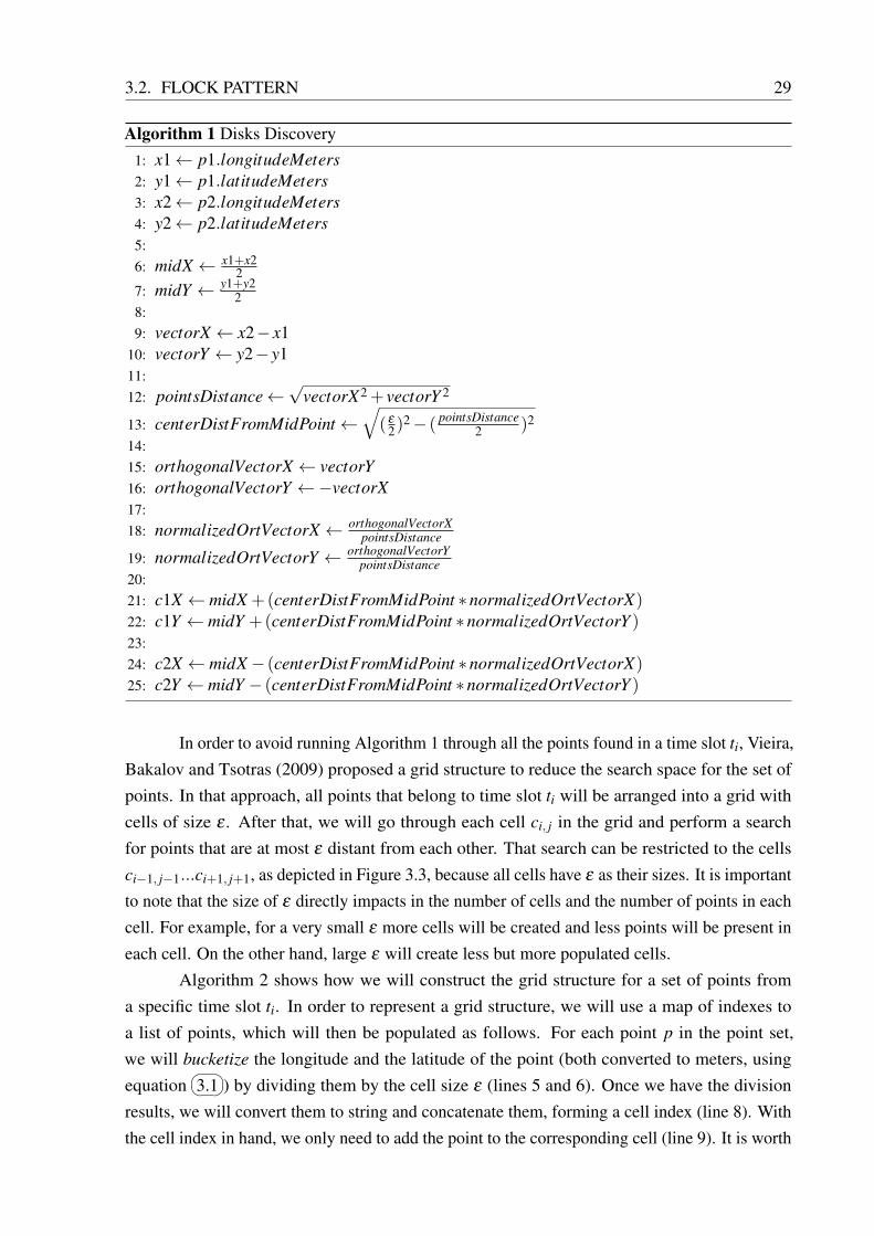
3.2. FLOCK PATTERN 29
Algorithm 1 Disks Discovery1: x1← p1.longitudeMeters2: y1← p1.latitudeMeters3: x2← p2.longitudeMeters4: y2← p2.latitudeMeters5:6: midX ← x1+x2
27: midY ← y1+y2
28:9: vectorX ← x2− x1
10: vectorY ← y2− y111:12: pointsDistance←
√vectorX2 + vectorY 2
13: centerDistFromMidPoint←√( ε
2)2− ( pointsDistance
2 )2
14:15: orthogonalVectorX ← vectorY16: orthogonalVectorY ←−vectorX17:18: normalizedOrtVectorX ← orthogonalVectorX
pointsDistance
19: normalizedOrtVectorY ← orthogonalVectorYpointsDistance
20:21: c1X ← midX +(centerDistFromMidPoint ∗normalizedOrtVectorX)22: c1Y ← midY +(centerDistFromMidPoint ∗normalizedOrtVectorY )23:24: c2X ← midX− (centerDistFromMidPoint ∗normalizedOrtVectorX)25: c2Y ← midY − (centerDistFromMidPoint ∗normalizedOrtVectorY )
In order to avoid running Algorithm 1 through all the points found in a time slot ti, Vieira,Bakalov and Tsotras (2009) proposed a grid structure to reduce the search space for the set ofpoints. In that approach, all points that belong to time slot ti will be arranged into a grid withcells of size ε . After that, we will go through each cell ci, j in the grid and perform a searchfor points that are at most ε distant from each other. That search can be restricted to the cellsci−1, j−1...ci+1, j+1, as depicted in Figure 3.3, because all cells have ε as their sizes. It is importantto note that the size of ε directly impacts in the number of cells and the number of points in eachcell. For example, for a very small ε more cells will be created and less points will be present ineach cell. On the other hand, large ε will create less but more populated cells.
Algorithm 2 shows how we will construct the grid structure for a set of points froma specific time slot ti. In order to represent a grid structure, we will use a map of indexes toa list of points, which will then be populated as follows. For each point p in the point set,we will bucketize the longitude and the latitude of the point (both converted to meters, usingequation
� �3.1 ) by dividing them by the cell size ε (lines 5 and 6). Once we have the divisionresults, we will convert them to string and concatenate them, forming a cell index (line 8). Withthe cell index in hand, we only need to add the point to the corresponding cell (line 9). It is worth

3.2. FLOCK PATTERN 30
noting that this proposed approach will not create empty cells, saving memory and unnecessarycell traversing time.
Figure 3.2: Two disks with radius ε/2 that are found based on points p1 and p2. c1 and c2 standfor the disks centers and m represents the midpoint between p1 and p2.
Source: Made by the author.
Algorithm 2 Construct Grid
1: grid← map{index, [...]} . map of cell index to list of points that belong to that cell2: points← GETPOINTSOFTIMESLOT(ti)3:4: for each point p in points do5: xIndex←
⌊p.longitudeMeters
ε
⌋6: yIndex←
⌊p.latitudeMeters
ε
⌋7:8: index← TOSTRING(xIndex)+ ”_”+TOSTRING(yIndex)9: grid[index].add(p)
10: end for
Another important concept to keep in mind is that we are only interested in the maximumdisks. Once we have found the disks with the points that belong to them, we will check if anydisk di is a subset of another disk d j. By saying that di is a subset of d j we mean that d j has allthe points that di has. This was identified as being a tremendous processing bottleneck for analgorithm that aims at finding flock patterns.

Figure 3.3: Cell grid for time slot ti. The dark grey is the cell that is currently being processedand the light gray cells around are the grids that will be in the search space of the dark cell. Each
small circle inside the grid, represents a GPS point that was collected in time slot ti
Source: Made by the author.

323232
4Modular and Efficient Flock Pattern Identification
4.1 Modular System Architecture
After the related work research that was performed, we noticed a lack of systemarchitecture in order to solve the flock pattern detection problem in spatio-temporal datasets. Sofar, no previous work has provided such system architecture that could be modular and simple inorder to help address the issues related to flock pattern detection.
We first tried to approach this problem in a more generic fashion, since the flock patternmining (and also a lot of other moving pattern mining problems) has the same workflow:
1. Connect to a spatio-temporal data source
2. Retrieve and aggregate spatio-temporal data
3. Process and mine that data in order to find the desired pattern (flock, in this case)
With that in mind, we designed a modular and simple system architecture that wasbuilt towards the flock pattern detection problem in spatio-temporal datasets, which is depictedby Figure 4.1. One can notice that we focus on 4 key building blocks, that can be easilyregistered/unregistered according to the targeting problem: (1) Data Source Connectors (DSCs);(2) Data Decoders (DDs); (3) Data Listeners (DLs) (Data aggregators); (4) Data Processors(DPs).
In layer (1) we are concerned on how to retrieve the data, meaning how to communicateproperly to the data source in order to be able to extract each spatio-temporal record from it.Thus, each DSC depicted in the Data Connectors’ Module in Figure 4.1 represents a logicalpiece that knows how to connect to and extract data from a specific data source. We can havea DSC that knows how to connect to a MySQL database, or another one that can connect to acloud based storage system like Amazon Web Services (AWS) DynamoDB, or even a DSC thatsimply connects to an online data stream and listen for incoming data.
After connecting and retrieving data from a data source, we need to clean, decode andtranslate the incoming raw data to a format that is simple and understandable to our system.Aiming at achieving that, we will have a DD component, which knows how to interpret the

4.1. MODULAR SYSTEM ARCHITECTURE 33
Figure 4.1: Modular system architecture overview
Source: Made by the author.
raw data format that comes from a DSC and translate it to a format that layer (3) onwards canunderstand. We can see in Figure 4.1 that a DD can register itself to a DSC in order to receive

4.2. AGGREGATION AND DATA PROCESSING EFFICIENCY 34
each data record that such DSC gathers from a data source. It is important to note that a DD canregister to only one DSC, but a DSC can have multiple DDs registered to it.
In any problem of data mining, aggregation is one of the most important phases, sinceit is there that the data gathering happens and necessary arrangements are made in order to getthe data ready for processing. In our system, that phase happens in layer (4), which we callthe Data Listeners’ Module. We can have multiple types of DLs in that module, and each ofthem can perform different types of aggregation and pre-processing depending on the final goal.For example, we could have an aggregator (or listener) that bucketize the GPS points by theirtimestamp and filter out outliers, before sending to processing, or another one that performspoint interpolation in order to reduce trajectory uncertainty. Similarly to the DD module, a DLcan only register itself to one DD, but a DD can have multiple DLs registered to it. Later on wewill see a DL implementation as one of the contributions of this dissertation, which will performa bufferized aggregation of points.
The last, but not least, remaining piece is the Data Processors’ Module, in layer (5).It is there that we will have the intelligence to perform a data mining task that will generateinsights for decision making, detect moving patterns and the forth. We can have a DP thatdetects flock patterns, another one that detects convergence patterns and even another DP thatprovides traffic information in real-time, to name a few. Also, following the pattern of theaforementioned modules, each DP can only register itself to a single DL, but a DL can havemultiple DPs registered to it. Fitting in the scope of this dissertation, we will implement andshow a novel DP that can detect flock patterns, based on the BFE algorithm proposed by Vieira,Bakalov and Tsotras (2009).
Researchers and data analysts, working with flock pattern detection, can leverage fromthe proposed architecture in order to have some infrastructure to help on their spartio-temporalproblems.
4.2 Aggregation and data processing efficiency
By analyzing some of the algorithms proposed in Section 2.2 and their respective runningtimes, we noticed that most of the CPU cycles were spent in analyzing disks that will not generateflock patterns, due to the points not being present in δ consecutive time slots. In all algorithms,disks generated in time slot ti+1 are compared with the potential flocks found in ti in order tocheck if an extension to a potential flock pattern is found. This operation has O(nm) complexity,with n being the number of disks and m the number of potential flocks from previous time slots.Additionally, for each comparison between a disk and a potential flock, an intersection operationbetween them needs to be made.
Things get even worse in algorithms like BFE, where a new created disk d j is checked if itis either subset or a duplicate of a previously found disk di (as already mentioned in Section 3.2.1).The running time of this step can result in a O(n2) time complexity in the worst case (with

4.2. AGGREGATION AND DATA PROCESSING EFFICIENCY 35
n being the number of disks generated by that time slot) requiring an intersection operationbetween each pair of disks that are being compared. We can reduce significantly that number ofdisks by only creating disks with points that can potentially form a flock pattern, i.e. with pointsthat appears in the dataset for δ consecutive time slots. In order to show how expensive thosedisk operations can be, we measured the time spent in such operations using the datasets that wewill use in our experiments and present the results in Figure 4.2. The analysis shows that thedisk and flock related operations can reach 99% of the overall processing time of the algorithm.
Figure 4.2: Percentage of time spent between disk and flock processing tasks against other tasksin the algorithm
Trucks BerlinMOD TDrive Brinkhoff
Non disk related processing
Disk processing
Dataset
% o
f tim
e
020
40
60
80
100
Source: Made by the author.
Consider the BFE algorithm running example depicted in Figure 4.3, where we arelooking for flock patterns having µ = 4 and δ = 4 as its parameter values. As we can see, intime slot t0 our dataset reported points p1, p2, p3 and p4 and, due to the proximity between them,disk d0 was created enclosing all four points. In the subsequent time slot t1 the same points werereported and again the BFE algorithm was able to create another disk d1. However, in time slot t2,p3 was not present and the disk d2 only contained three points, which is not enough to represent aflock pattern because of the number of trajectories being less than µ = 4. With the disk d2 beinginvalid in t2, we will need to discard disks d0 and d1 created in the previous time slots, since theycannot generate a flock pattern starting from t0. Hence, we could avoid the creation of disksd0 and d1 if we would know in advance that p3 was missing in t2, saving CPU cycles of disk

4.3. BITDF 36
comparisons in t0 and t1. We argue that when scaled to a dataset with millions of records, doingreal-time analyses, such processing for checking disks subsets and flock extension, performedby regular algorithms (like BFE), will lead to a severe degradation in performance. With thatin mind, we can say with high confidence that reducing the volume of data that is processed bythose flock and disk comparison tasks (by filtering out disks that will not generate flock patterns),can dramatically reduce the overall processing time of a flock detection algorithm.
Figure 4.3: Sequence of disks in 4 consecutive time slots and the points that were clustered tothem
Source: Made by the author.
4.3 BitDF
Our solution consists on using Bitmaps for Disk Filtering (BitDF), based on the BFEalgorithm. BitDF is basically a DL and a DP components, as those in the architecture presentedin Section 4.1. We call them GPS Stream Buffer (GSB) and Flock Processor (FP) the DL andDP respectively, and will have each of them keeping track of the history of every Oid in time.
Table 4.1: Bitmaps in GSB after buffering four time slots
Oid Bitmap
1 1111
2 0111
3 1011
4 1111
Algorithm 3 shows a big picture of how GSB will work once it receives spatio-temporaldata records from a DD. It will listen to the incoming GPS point stream in the procedureRECEIVEPOINTS, add each point to the pointBuffer structure (which is a hash map of pointsby time slot) and record the presence in time of that Oid in its bitmap structure (presencemap) by calling ADDPOINTPRESENCE. When GSB has buffered δ time slots (line 23) it will

4.3. BITDF 37
then send the points of timeSlot − δ , along with the bitmaps, to FP. After FP is done withprocessing the points, GSB will discard the first bit of the bitmaps (which corresponds to thepoints of timeSlot−δ sent to FP), by calling SHIFTPRESENCEMAPS, and also discard the pointscollected in timeSlot−δ , which were already processed by FP. The flow continues indefinitelyby buffering the points from the next time slot ti and send the points from ti−δ and the bitmaps toFP for processing. It is worth noting that timeSlotSize, referred in line 21, represents the timeslot σ introduced in Section 3.1.
Algorithm 3 GPS Stream Buffer
1: pointBu f f er← map{index,{id, point[...]}}2: presenceMap← map{id,bitmap}3: lastTimeslot←−14:5: procedure ADDPOINTPRESENCE(id)6: mask← SHIFTLEFT(1, pointBu f f er.size−1)7: presence← BITOR(presenceMap[id],mask)8: presenceMap[id]← presence9: end procedure
10:11: procedure SHIFTPRESENCEMAPS
12: for all id ∈ KEYS(presenceMap) do13: shi f ted← SHIFTRIGHT(presenceMap[id],1)14: presenceMap[id]← shi f ted15: end for16: end procedure17:18: procedure RECEIVEPOINTS
19: loop20: point← gpsPointStream.dequeue21: timeSlot← point.timestamp/timeSlotSize22: if timeSlot > lastTimeslot then23: if pointBu f f er.size≥ δ then24: FP.PROCESS(pointBuffer.first)25: delete pointBu f f er. f irst26: SHIFTPRESENCEMAPS
27: end if28: lastTimeslot← timeSlot29: end if30: pointBu f f er[timeSlot][point.id].append(point)31: ADDPOINTPRESENCE(point.id)32: end loop33: end procedure
Using Figure 4.3 as an example, we can see in Table 4.1 the state of the GSB bitmaps foreach Oid after receiving the points in t3. With those bitmaps, we can easily look up for a specificpoint occurrence in time and check whether that point in that specific time slot can potentially

4.3. BITDF 38
form a flock pattern or not. We do that by checking if that Oid appears for δ consecutive timeslots in the dataset, i.e. it has δ consecutive bits set to 1. The bitmaps in GSB will always referto the future of a specific Oid .
Algorithm 4 Flock Processor Helper Procedures
1: bu f f ered← 0 . max time span of the current flocks, max value is δ
2: f lockMap← map{id,bitmap}3:4: procedure ISPOINTELIGIBLE(id)5: presence← CONCAT(presenceMap[id], f lockMap[id])6: eligibleMask← SHIFTLEFT(1,δ )−17: range← pointBu f f er.size+bu f f ered8: checks←MAX(1,range−δ +1)9: while checks > 0 do
10: tmp← BITAND(presence,eligibleMask)11: if BITXOR(tmp,eligibleMask) then12: return true13: end if14: checks← checks−115: eligibleMask← SHIFTLEFT(eligibleMask,1)16: end while17: return false18: end procedure19:20: procedure MAPPOINTFLOCK(id)21: mask← SHIFTLEFT(1,bu f f ered)22: f lockMap[id]← BITOR( f lockMap[id,mask)23: end procedure24:25: procedure SHIFTFLOCKMAPS
26: for all id ∈ KEYS( f lockMap) do27: f lockMap[id]← SHIFTRIGHT( f lockMap[id],1)28: end for29: end procedure30:31: procedure STOREDISKIFELIGIBLE(diskSet,d)32: if COUNT(d)≥ µ and not SUBSET(d) then33: ADDDISK(diskSet,d)34: else35: delete d36: end if37: end procedure
Our DP is explained in more detail by Algorithm 4 and Algorithm 5 as follows. InAlgorithm 4 we start by first listing the procedures that will help the core procedure of FP (thePROCESS procedure, in Algorithm 5). It is also in Algorithm 4 that we list the most importantpiece of this DP that allows us to achieve such good optimizations, in both CPU cycles and

4.3. BITDF 39
Algorithm 5 Flock Processor Process Procedure
1: procedure PROCESS(pointMap{id, point[...]}, timeslot)2: D← /03: cells← BUILDGRID(pointMap)4: if bu f f ered ≥ δ then5: SHIFTFLOCKMAPS
6: bu f f ered← bu f f ered−17: end if8: for all cx,y ∈ cells do9: cellRange← [cx−1,y−1...cx+1,y+1]
10: for all p1 ∈ cx,y do11: for all p2 ∈ cellRange do12: if d(p1, p2)≤ ε then13: d1,d2← CREATEDISKS(p1, p2)14: for all p ∈ cellRange do15: added← false16: if INDISK(d1, p) and ISPOINTELIGIBLE(p) then17: ADD(D1, P)()18: added← true19: end if20: if INDISK(d2, p) and ISPOINTELIGIBLE(p) then21: ADD(D2, P)()22: added← true23: end if24: if added = true then25: MAPPOINTFLOCK(p.id)26: end if27: end for28: STOREDISKIFELIGIBLE(D,d1)29: STOREDISKIFELIGIBLE(D,d2)30: end if31: end for32: end for33: end for34: bu f f ered← bu f f ered +135: end procedure
number of disks generated, which is the ISPOINTELIGIBLE procedure. Such procedure isresponsible to put together what happened in the past and what is going to happen in the future
for a given point p, in order to decide whether p can be part of a potential flock pattern or not. Itdoes that by concatenating, for a given Oid , the bitmap from FP with the bitmap from GSB (line5 of Algorithm 4) and searching for a sequence of δ bits set to 1 (lines 6 to 15 of Algorithm 4).That search is performed by combining AND and XOR bitwise operations against the presencebitmap assembled in line 5 of Algorithm 4. If a sequence of δ bits set to 1 is found, we canstate with confidence that such point p can potentially be part of a flock pattern. Later on, if a

4.3. BITDF 40
potential flock is found in a time slot ti and p is part of it, we need to update the FP’s bitmap ofthat point so when we process points of time slot ti+1 we have the correct bitmap representationof p and that is where MAPPOINTFLOCK (line 20) comes to play. MAPPOINTFLOCK does thatby prepending 1 to p’s bitmap in FP module by performing an OR bitwise operation.
Figure 4.4 shows how GSB (red) and FP (gray) will interact in a scenario where µ = 3and δ = 3. In the first column we can see GSB receiving points p1, p2, p3, p4 and p5 at timeslot t0 and then updating the bitmap for each of the points (red grid). Later on, at time slot t1,GSB receives points p2, p3, p4, p5 and p6 and again updates the presence bitmaps for eachpoint. After the bitmap updates, one can notice that now p1 has 01 as its presence bitmap value,meaning that p1 was present at time slot t0 but not at t1, and GSB now has a buffer of points fortime slot t0 (red dashed box). When the points from time slot t2 are received, and the presencebitmaps are updated, GSB sends the points buffered from time slot t0 to FP for processing. Atthis time, FP has not received any set of points for processing, so its bitmaps are clean (rightmostgray grid) and the concatenation of the bitmaps from GSB and FP will end up being the samevalue as in GSB. After processing the buffered points from time slot t0, FP will generate a diskd1 with points p2, p4 and p5, leaving p1 and p6 out because their bitmaps say that they will notappear in the next 2 consecutive time slots.
Figure 4.4: Interaction between GSB (red) and FP (gray) in 5 consecutive time slots, showinghow the presence bitmaps are constructed. In the example we have µ = 3 and δ = 3
Source: Made by the author.

4.4. TAKING ADVANTAGE OF MULTI-CORE ARCHITECTURES 41
The same flow continues for time slot t3, with GSB sending the buffered points fromtime slot t1 to FP for processing. We can now notice that the points that formed disk d1 in thetime slot t0 now have a bit set to 1 in their presence bitmaps in FP. Moreover, it is worth notinghow we perform the bitmap concatenation in FP (when it receives points from t1), in which thepast time (FP bitmaps) goes at the right and the future (GSB bitmaps) goes at the left side ofthe concatenated bitmap. We then perform a search for µ = 3 bits set to 1 in that concatenatedbitmaps to figure out which points can potentially form a flock pattern and can be placed in adisk. Late in time slot t4, when FP receives the points from time slot t2, a flock pattern will befound, since we could find 3 consecutive disks containing at least µ = 3 unique Oid .
4.4 Taking Advantage of Multi-core Architectures
It’s well known that multi-core architectures are the current trend in technology. There isa myriad of multi-core processors in the market and many chipset companies taking advantagesof those processor architectures too (even small devices, like smartphones, are being shippedwith multi-core processors). Given that current scenario, there is no sense in not taking advantageof those multi-core processors and still executing our solution in a serial fashion. Thus, wewill remodel our proposed architecture in a multi-threaded structure and parallelize some of theexpensive tasks that our algorithm is doing, in order to make it more responsive and fast so it canempower decision makers to act in real-time.
One can see that the FP component, that we described in the previous section, is doing alot of work in order to discover the flock patterns. Whenever the FP receives the set of pointsfrom GSB it performs the following actions:
1. Build the whole point grid
2. For each grid cell:
(a) Get the Extended Grid Cell (EGC) (e.g. for cell cx,y it will get cellscx−1,y−1...cx+1,y+1)
(b) Process the EGC, trying to cluster the points into disks
3. Get the resulting disks and assure that there are neither duplicates nor subsets of otherdisks
4. Try to merge the disks with potential flocks from previous time slots
5. Report new found flocks
It can be easily perceived that the EGC processing (steps (a) and (b)) can be donein parallel for the multiple cells that will be processed, since there is no dependency andno concurrent writing operations between cells. Another step that is very CPU heavy is the
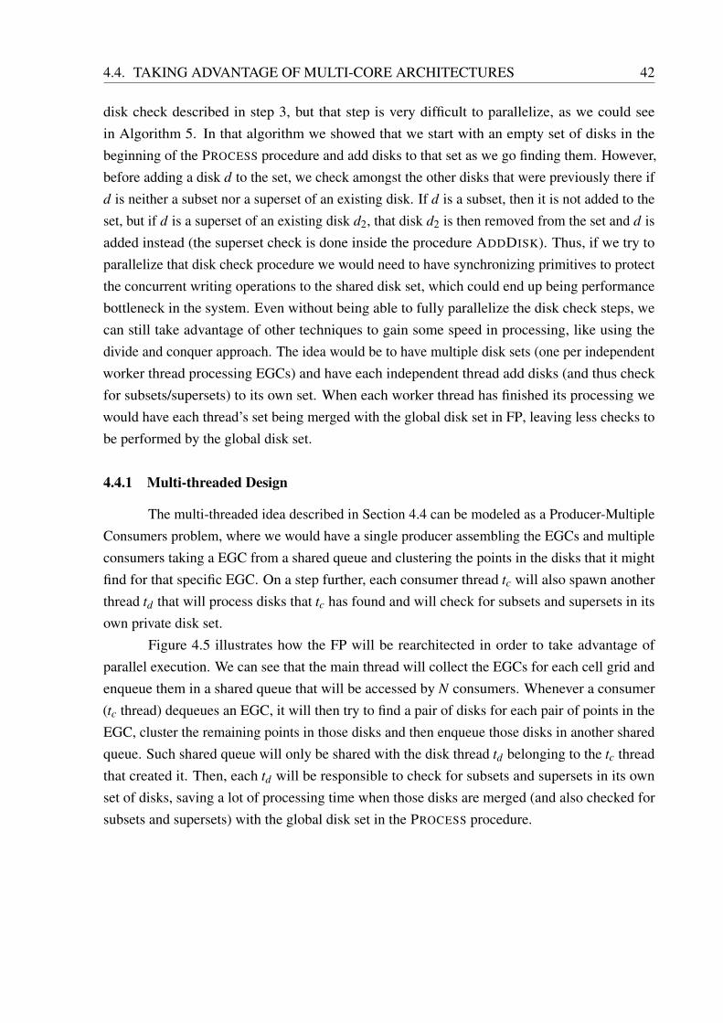
4.4. TAKING ADVANTAGE OF MULTI-CORE ARCHITECTURES 42
disk check described in step 3, but that step is very difficult to parallelize, as we could seein Algorithm 5. In that algorithm we showed that we start with an empty set of disks in thebeginning of the PROCESS procedure and add disks to that set as we go finding them. However,before adding a disk d to the set, we check amongst the other disks that were previously there ifd is neither a subset nor a superset of an existing disk. If d is a subset, then it is not added to theset, but if d is a superset of an existing disk d2, that disk d2 is then removed from the set and d isadded instead (the superset check is done inside the procedure ADDDISK). Thus, if we try toparallelize that disk check procedure we would need to have synchronizing primitives to protectthe concurrent writing operations to the shared disk set, which could end up being performancebottleneck in the system. Even without being able to fully parallelize the disk check steps, wecan still take advantage of other techniques to gain some speed in processing, like using thedivide and conquer approach. The idea would be to have multiple disk sets (one per independentworker thread processing EGCs) and have each independent thread add disks (and thus checkfor subsets/supersets) to its own set. When each worker thread has finished its processing wewould have each thread’s set being merged with the global disk set in FP, leaving less checks tobe performed by the global disk set.
4.4.1 Multi-threaded Design
The multi-threaded idea described in Section 4.4 can be modeled as a Producer-MultipleConsumers problem, where we would have a single producer assembling the EGCs and multipleconsumers taking a EGC from a shared queue and clustering the points in the disks that it mightfind for that specific EGC. On a step further, each consumer thread tc will also spawn anotherthread td that will process disks that tc has found and will check for subsets and supersets in itsown private disk set.
Figure 4.5 illustrates how the FP will be rearchitected in order to take advantage ofparallel execution. We can see that the main thread will collect the EGCs for each cell grid andenqueue them in a shared queue that will be accessed by N consumers. Whenever a consumer(tc thread) dequeues an EGC, it will then try to find a pair of disks for each pair of points in theEGC, cluster the remaining points in those disks and then enqueue those disks in another sharedqueue. Such shared queue will only be shared with the disk thread td belonging to the tc threadthat created it. Then, each td will be responsible to check for subsets and supersets in its ownset of disks, saving a lot of processing time when those disks are merged (and also checked forsubsets and supersets) with the global disk set in the PROCESS procedure.

Figure 4.5: Modeling the FP in a Producer-Multiple Consumers architecture
Source: Made by the author.

444444
5Experimental Results
As explained in Chapter 3, the flock pattern detection relies mainly in 3 parameters,namely number of trajectories (µ), flock extension (or length) (δ ) and disk radius (ε/2). Thoseparameters impact significantly in the number of patterns found as well as the time taken to findthose patterns, depending on the dataset being analyzed. To validate the efficiency of BitDF, wechose 4 datasets referred by Zheng (2015), that are being widely used in trajectory data miningresearches in the academia. Of those 4 datasets, 2 were collected from real-world experimentsand 2 were synthetic generated.
Before evaluating the performance of BitDF using those datasets, we first gathered somemetadata information about them, in order to choose wisely the value for the aforementionedparameters, so we could indeed find a good number of flocks patterns. Such metadata werecollected by running BitDF multiple times with various values for those parameters. Thus,based on the dataset description, we picked some starting values for them and then increased ordecreased the values according to the number of flock patterns that we were able to find. Afterfinding at least 100 flock patterns, we then settled on a range of values for those parameters andused them to evaluate each dataset.
Figure 5.1 shows the components (using the architecture proposed in Section 4.1) thatwill be part of our experiments and how our experiments are going to be performed. For eachdataset (which will be presented individually in the subsections to come) that we used, wesimulated an online stream of GPS data arriving at the ONLINECONNECTOR DSC in our system.Then, that incoming GPS data would be forwarded to a DD that knows how to translate eachentry in that specific dataset to a structure that can be understood by the GSB DL. When theGSB DL gets the data, the Algorithm 3 will take care of it, buffering it and building the necessarypresence bitmap for that Oid . After we have buffered δ time slots of points in GSB, the nextdestination of the GPS data is the FP DP, which is composed by three different components, asdepicted in Figure 5.2:
1. Grid Manager: Will get the GPS data and build the grid depicted in Figure 3.3 andprovide the EGC for each grid cell.
2. Disk Manager: Gets each disk generated by FP and will check for duplicates/superset

45
disks and add it to the global disk set, if that disk is unique.
3. Flock Manager: Stores the potential flock patterns from previous time slots andmerges the disks generated by the current time slot in order to find new flock patterns.
Figure 5.1: System design implemented for the experiments
Source: Made by the author.
The metrics that we chose to measure the efficiency of BitDF were (1) Running Time and(2) Number of Disks Generated. For (1) we went through each individual parameter (µ , δ and ε),fixed it in a specific value and varied the remaining others based on the range that we settled fromour metadata gathering. We picked (2) as an evaluation metric because it will show with numbersthe reason why BitDF can run way faster than the comparison baseline algorihtm. Finally, inorder to have a baseline to compare against BitDF, we implemented the BFE algorihtm proposedby Vieira, Bakalov and Tsotras (2009) and ran our benchmarks with it as well.
We implemented the system architecture proposed in Figure 5.1 in C++, using g++ 4.8.4and the C++11 (ISO, 2012) features. Our test machine used to run our performance experiments

5.1. TRUCKS DATASET 46
Figure 5.2: FlockProcessor class composition
Source: Made by the author.
was a Linux box with Intel Xeon Quad processor and 14GB of main memory running UbuntuServer 14.04 Long Term Support (LTS). As already mentioned, we used four datasets (real andsynthetic) in our experiments, with some of them having more than 50M entries and 2K uniqueOid .
Before showing the results, there are some Analysis Outcome (AO) that will hold forany dataset being analyzed here:
1. δ variation: The longer the flock patterns we try to find (long δ ), the more diskswill stay cached being analyzed and trying to be merged with new disks from timeslots to come. This can have a big impact in running time.
2. ε variation: As the disk radius (ε/2) gets bigger, more points will be clustered insidea disk and thus more intersections and duplicates of those disks as more likely tobe found. This will impact the time spent in analyzing disks from one time slot toanother.
3. µ variation: By increasing µ , it gets more and more difficult to find disks that areflock candidates (|d| ≥ µ), so less disks are generated. This scenario is where BitDFwill achieve less improvements.
5.1 Trucks Dataset
This was one of the datasets that Vieira, Bakalov and Tsotras (2009) used in theexperiments of BFE, but the authors modified such dataset (CHOROCHRONOS, 2012), resultingin a dataset which is way far from those found in real-world analyses. In their modification, everytime interval is of one second, the GPS coordinates were mapped to a R2 coordinate system(ranging from 0 to 1000) and most of the points are present in each time interval. The modifieddataset resulted in 112,203 entries and 276 unique Oid (instead of 50 in the original dataset).
By looking at Figure 5.3 and Figure 5.4, we can see that BitDF had some gains inexecution time. However, they were not too significant due to the fact that the number of

5.1. TRUCKS DATASET 47
Figure 5.3: Results varying δ and ε for Trucks dataset
(a) µ = 4, ε = 1.5 and δ varying150
200
250
Tim
e (
secs)
4 6 8 10 12 14 16 18 20
BFE
BitDF
(b) µ = 4, δ = 20 and ε varying
50
100
150
200
250
Tim
e (
secs)
0.8 0.9 1.0 1.1 1.2 1.3 1.4 1.5
BFE
BitDF
Source: Made by the author.
Figure 5.4: Results varying µ and number of disks generated over time for Trucks dataset
(a) δ = 20, ε = 1.5 and µ varying
50
100
150
200
250
Tim
e (
secs)
4 6 8 10 12 14 16 18 20
BFE
BitDF
(b) Cumulative disks by time
0 200 400 600 800
010
20
30
40
Time slot
Dis
ks g
enera
ted x
10
3
BFE
BitDF
Source: Made by the author.
disks generated by each time slot does not differ too much between BFE and BitDF, as we cansee in Figure 5.4b. This happens because almost all points appear in every single time slot,then buffering and mapping the Oid presence in time does not make a big impact, since wewill not be able to filter out disks created with points not being present in δ consecutive timeslots. Figure 5.3a and Figure 5.3b show some running time improvements against BFE, which

5.2. BERLINMOD DATASET 48
are backed up by the explanations given at AO 1 and AO 2. A different behavior is observedin Figure 5.4a, in which BitDF starts better but ends up almost tied with BFE, which can beexplained by AO 3, but is also very influenced by the dataset modifications.
5.2 BerlinMOD Dataset
BerlinMOD consists in a traffic generation model (DüNTGEN; BEHR; GüTING, 2009b)used to create sythentic datasets of MOs. This particular dataset that we are analysing was thebiggest one that we could find in the set of synthetic datasets that are available in their website(DüNTGEN; BEHR; GüTING, 2009a) and consists of 56,127,943 entries and 2,000 unique Oid .
Figure 5.5: Results varying δ and ε for BerlinMOD dataset
(a) µ = 4, ε = 100 and δ varying
400
500
600
700
Tim
e (
secs)
4 8 20 30
BFE
BitDF
(b) µ = 4, δ = 8 and ε varying
500
1000
1500
2000
Tim
e (
secs)
80 100 120 140 200
BFE
BitDF
Source: Made by the author.
As we can see by the results presented in Figure 5.5 and Figure 5.6, BitDF was able toachieve great performance gains over BFE, in some cases being 57% faster (Figure 5.5a). InFigure 5.6b it is shown that BitDF reduces the cumulative number of disks created over timein 94%, by only creating disks that can indeed form flock patterns, which justifies the greatimprovements that BitDF was able to get in this dataset. Differently from the results presentedin Section 5.1, BitDF was able to get great improvements over BFE, ranging from 20% to 48%,even when increasing the value of µ as depicted in Figure 5.6a. Lastly, as depicted in Figure 5.5b,BitDF was able to outperform BFE in almost 50% when varying the parameter ε .
5.3 TDrive Dataset
This is a real dataset, having spatio-temporal data describing one week of trajectoriesof taxis in Beijing, China, available in (ZHENG, 2011). It has 17,762,489 entries with 10,336

5.3. TDRIVE DATASET 49
Figure 5.6: Results varying µ and number of disks generated over time for BerlinMOD dataset
(a) δ = 8, ε = 100 and µ varying400
500
600
700
Tim
e (
secs)
4 6 8 10 20
BFE
BitDF
(b) Cumulative disks by time
0 2000 6000 100000
20
40
60
80
Time slot
Dis
ks g
enera
ted x
10
3
BFE
BitDF
Source: Made by the author.
unique Oid .
Figure 5.7: Results varying δ and ε for TDrive dataset
(a) µ = 4, ε = 100 and δ varying
200
400
600
800
1000
Tim
e (
secs)
4 8 20 30
BFE
BitDF
(b) µ = 4, δ = 8 and ε varying
200
400
600
800
1000
Tim
e (
secs)
10 30 50 80 100
BFE
BitDF
Source: Made by the author.
One can see by the results presented in Figure 5.7 and Figure 5.8, that BitDF wasable to dramatically reduce the execution time, when compared to BFE. When varying the δ
parameter, the running time improvement was of almost 90%, droping from 1,265 seconds toonly 125 seconds of processing time, as shown in Figure 5.7a. Continuing the improvements,

5.4. BRINKHOFF DATASET 50
in Figure 5.7b we can see that BitDF reduced the execution time up to 74% when varyingε . Additionally, despite seeing some similar behavior with the other analyzed datasets (likepresented in Section 5.1) when varying µ , Figure 5.8a shows that BitDF was able to improve theexecution time by 74% in some cases. It is also worth noting that the results achieved are a reflexof the huge decrease of disks that were generated by time, as depicted in Figure 5.8b, reachingalmost 96% of reduction.
Figure 5.8: Results varying µ and number of disks generated over time for TDrive dataset
(a) δ = 8, ε = 100 and µ varying
200
400
600
800
1000
Tim
e (
secs)
4 6 8 10 20
BFE
BitDF
(b) Cumulative disks by time
0 500 1000 1500
050
100
150
200
250
300
Time slot
Dis
ks g
enera
ted x
10
3
BFE
BitDF
Source: Made by the author.
5.4 Brinkhoff Dataset
Likewise BerlinMOD, Brinkhoff is also a city traffic generation model (BRINKHOFF,2002). We generated a synthetic dataset using the Minnesota Web-based Traffic Generator(MINNESOTA, 2013), having 2,000 as the "Starting Vehicles" and 100 as the "Simulation Time"parameters, which are the largest allowed numbers by the generator. The result dataset has314,523 entries and 7,000 unique Oid .
The results achieved with this dataset were the best that BitDF was able to get amongstthe other datasets analyzed in this dissertation, as one can notice by looking to Figure 5.9 andFigure 5.10. There were huge drops in execution time, as depicted in Figure 5.9a, where BitDFanalyzed the whole dataset in only 69 seconds, while BFE took 12,732 seconds, representingan improvement of 99.5%. Another great running time improvement of 99% can be seen whenwe varied the ε parameter, as shown in Figure 5.9b, droping from 13,141 seconds to only 125seconds. We can see in Figure 5.10a that even with the variation of µ , BitDF was able to showhuge improvement, with results ranging from 98% to 99% of CPU time reduction. Additionally,

5.4. BRINKHOFF DATASET 51
Figure 5.9: Results varying δ and ε for Brinkhoff dataset
(a) µ = 4, ε = 200 and δ varying0
2000
6000
10000
Tim
e (
secs)
4 8 20 30
BFE
BitDF
(b) µ = 4, δ = 8 and ε varying
02000
6000
10000
Tim
e (
secs)
80 100 120 140 200
BFE
BitDF
Source: Made by the author.
Figure 5.10: Results varying µ and number of disks generated over time for Brinkhoff dataset
(a) δ = 8, ε = 200 and µ varying
02000
6000
10000
Tim
e (
secs)
4 6 8 10 20
BFE
BitDF
(b) Cumulative disks by time
0 20 40 60 80 100
05
10
15
Time slot
Dis
ks g
enera
ted x
10
3
BFE
BitDF
Source: Made by the author.
we can see in Figure 5.10b that we were able to reduce the number of disks by 95%, which is adramatic improvement and is reflecting directly in the running time improvements that we couldsee with this dataset.

5.5. MULTI-THREADED EVALUATION 52
5.5 Multi-threaded evaluation
After implementing the architecture proposed in Section 4.1, evaluating it in Chapter 5and seeing great improvements in the running time when compared with other algorithms, wedecided to test how our system would perform by taking advantage of the multi-core paradigmthat is been widely used nowadays. We then took a step further and implement a new DP, thatwe called Parallel Flock Processor (PFP). PFP was implemented having in mind the MT modeldescribed in Section 4.4.1, which we call BitDF MT.
In order to see how BitDF MT would perform, we took from Chapter 5 the worstperformances of BitDF for each dataset and compared such performance against BitDF MTrunning with a varied number of worker threads executing in parallel.
Our benchmarks were executed in a different machine from that one mentioned in thebeginning of Chapter 5, in a way that we opted to get a better multi-core processor setup. Hence,we ran our experiments in a Linux box, running Ubuntu 16.04 LTS, having an Intel Xeon CPU,with 2.3 GHz and 4 physical cores, using Intel Hyper-Threading technology (MARR et al., 2012)meaning that we would theoretically have 8 different processing units.
Below we will present the benchmarks that were executed for each dataset already seenin Chapter 5, namely Trucks, TDrive, BerlinMOD and Brinkhoff. For each of the aforementioneddatasets, we ran BitDF MT with the same parameters as the longest BitDF execution presentedin Chapter 5, varying the worker threads from 1 (pure BitDF) to 30. With variations of 1 workerthread from 1 to 10, 2 worker threads from 10 to 20 and 5 worker threads from 20 to 30. Itis important to notice that when we say that we are running with x worker threads, we areactually running with 2∗x threads: having x tc threads processing different EGCs plus 1 td thread(attached to its tc thread) processing the disks generated by its parent tc. We set the result ofpure BitDF as being 100% of the total execution time and highlighted it with red color and allBitDF MT runs are in blue, always being a percentage of the red highlighted result. It is worthmentioning here that the only metric that we are evaluating in these experiments is the runningtime of BitDF MT, because the number of generated disks will be the same that we have seenin the previous results shown for BitDF in Chapter 5, since we are still using the same bitmapfiltering heuristic proposed by BitDF. Moreover, in order to have a better idea on how BitDF MToutperforms BitDF and BFE, we show some graphs depicting the running time of them together,for each dataset. For such comparion, we picked 5 and 7 as the number of worker threads forBitDF MT, since those are the values that show the best peformance overall.
First we present the results for the Trucks dataset, which we ran with the followingparameters (based on previous results from Section 5.1): µ = 4, δ = 20 and ε = 1.5. Thatdataset would be the most difficult one to show running time improvements due to its smallsize and running times being already fast (with the longest one being around 200 seconds forBitDF). Despite that, we can see in Figure 5.11 that we were able to reduce as much as 51%when running with 5 tc threads, which totalizes 10 threads. After that we can see that we could

5.5. MULTI-THREADED EVALUATION 53
stay almost stable, not gaining any performance but also not deteriorating it too much. Suchperformance stabilization is an expected result, as the processor would start to schedule and pausethe execution of threads, because of having all its resources busy, as the number of executingthreads exceeds too much the number of available processing units.
Figure 5.11: Execution time reduction by number of threads for the Trucks dataset
Trucks dataset
Threads
% o
f to
tal tim
e
02
04
06
08
01
00
1 2 3 4 5 6 7 8 9 10 12 14 16 18 20 25 30
Source: Made by the author.
Figure 5.12 and Figure 5.13 show that we were able to achieve more meaningful resultswith BitDF MT, than those presented in Section 5.1 and that the improvements obtained withBitDF MT runing with both 5 and 7 worker threads were almost the same. We could reduce therunning time of BitDF by 18% when varying µ (Figure 5.13) and ε (Figure 5.12b) and by 30%when varying δ (Figure 5.12a).
In Figure 5.14, we show the graph with the results for the BerlinMOD dataset. Due toits large size and somewhat long execution times (as previously presented in Section 5.2) weexpected to obtain good results in running BitDF with independent worker threads. We have setour parameters to have the following values: µ = 4, δ = 8 and ε = 200, as we had those resultingin the longest running time (around 1,000 seconds) in our first experiments with this dataset. It isnoticed by Figure 5.14 that the results also tend to stabilize when we reach 5 worker threads (10in total), but we reach our best running time with 8 worker threads, with an improvement of 62%.It is also seen that the running time starts to get worse as we exceed the number of processingunits available (shown when BitDF MT is executing with 30 worker threads, being 60 in total).

5.5. MULTI-THREADED EVALUATION 54
Figure 5.12: Results varying δ and ε for Trucks dataset
(a) µ = 4, ε = 1.5 and δ varying1
00
15
02
00
25
0
Tim
e (
se
cs)
4 6 8 10 12 14 16 18 20
BFE
BitDF
BitDF 5 Threads
BitDF 7 Threads
(b) µ = 4, δ = 20 and ε varying
50
10
01
50
20
02
50
Tim
e (
se
cs)
0.8 0.9 1.0 1.1 1.2 1.3 1.4 1.5
BFE
BitDF
BitDF 5 Threads
BitDF 7 Threads
Source: Made by the author.
Figure 5.13: Results having δ = 20, ε = 1.5 and µ varying for the Trucks dataset
05
01
00
15
02
00
25
0
Tim
e (
se
cs)
4 6 8 10 12 14 16 18 20
BFE
BitDF
BitDF 5 Threads
BitDF 7 Threads
Source: Made by the author.
By looking at Figure 5.15 and Figure 5.16, one can see that even where BitDF had theworst results, BitDF MT was able to achieve important reductions in running time, showinghow a good multi-threaded remodeling is important in order to get the most out of a multi-corearchitecture. BitDF MT improved the running time of BitDF by 50% when running with both 5and 7 worker threads, as shown in Figure 5.15a. BitDF MT also achieved good results when wevaried the µ parameter, having 45% of running time decrease as it is depicted in Figure 5.16.
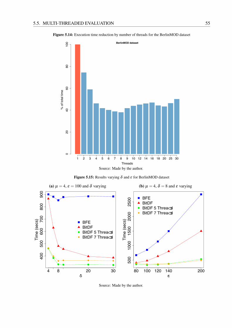
5.5. MULTI-THREADED EVALUATION 55
Figure 5.14: Execution time reduction by number of threads for the BerlinMOD dataset
BerlinMOD dataset
Threads
% o
f to
tal tim
e
02
04
06
08
01
00
1 2 3 4 5 6 7 8 9 10 12 14 16 18 20 25 30
Source: Made by the author.
Figure 5.15: Results varying δ and ε for BerlinMOD dataset
(a) µ = 4, ε = 100 and δ varying
40
05
00
60
07
00
80
09
00
Tim
e (
se
cs)
4 8 20 30
BFE
BitDF
BitDF 5 Threads
BitDF 7 Threads
(b) µ = 4, δ = 8 and ε varying
50
01
00
01
50
02
00
02
50
0
Tim
e (
se
cs)
80 100 120 140 200
BFE
BitDF
BitDF 5 Threads
BitDF 7 Threads
Source: Made by the author.

5.5. MULTI-THREADED EVALUATION 56
Figure 5.16: Results having δ = 8, ε = 100 and µ varying for the BerlinMOD dataset
30
04
00
50
06
00
70
08
00
Tim
e (
se
cs)
4 6 8 10 20
BFE
BitDF
BitDF 5 Threads
BitDF 7 Threads
Source: Made by the author.
Last, but definitely not least, we can se in Figure 5.15b that BitDF MT improved the runningtime of BitDF by 70%, with both 5 and 7 worker threads.
Figure 5.17: Execution time reduction by number of threads for the TDrive dataset
TDrive dataset
Threads
% o
f to
tal tim
e
02
04
06
08
01
00
1 2 3 4 5 6 7 8 9 10 12 14 16 18 20 25 30
Source: Made by the author.

5.5. MULTI-THREADED EVALUATION 57
Another large dataset that we evaluate was the TDrive dataset, in which BitDF showedgreat results when analzing it. Based on the results presented in Section 5.3, we chose theparameter values that led to the longest execution time (around 600 seconds): µ = 4, δ = 4 andε = 100. Figure 5.17 shows that the results follow the same pattern that we have been seeing inthe previous analyses: great improvements in the beginning, but stabilizing as we exceed thenumber of processing units in the machine. We can also see some slight improvements evenwhen we evaluate with more than 5 worker threads. It is also depicted in Figure 5.17 that wewere able to reduce the running time as much as 70%, when compared to the single threadedmodel, which is a huge improvement added to those already achieved in Section 5.3
Figure 5.18: Results varying δ and ε for TDrive dataset
(a) µ = 4, ε = 100 and δ varying
50
01
00
01
50
0
Tim
e (
se
cs)
4 8 20 30
(b) µ = 4, δ = 8 and ε varying
50
01
00
01
50
0
Tim
e (
se
cs)
10 30 50 80 100
BFE
BitDF
BitDF 5 Threads
BitDF 7 Threads
Source: Made by the author.
When it comes to comparing the running time of BitDF MT against BitDF and BFE, wecan see that BitDF MT was able to improve the running time even more than we have seen inSection 5.3. When varying the parameter µ we could reduce the execution time by 60%, as onecan see in Figure 5.19. Figure 5.18b also shows improvements of 60%, when compared againstBitDF, when varying the parameter ε . The best result though is when we varied the parameterδ , in which we could improve the BitDF running time by 70% when executing BitDF MT withboth 5 and 7 worker threads, as depicted in Figure 5.18a.
Our last dataset to evaluate is the Brinkhoff synthetic dataset. We were already able toachieve huge running time improvements with BitDF, but we could achieve even more withBitDF MT. Based on the dataset results (Section 5.4), we chose the running parameters asfollows: µ = 4, δ = 4 and ε = 1200. Figure 5.20 shows that we were always able to reduce theBitDF running time even with the number of worker threads being way higher than the numberof available processing units in the machine. That is a result that is completely different from

5.5. MULTI-THREADED EVALUATION 58
Figure 5.19: Results having δ = 8, ε = 100 and µ varying for the TDrive dataset
50
01
00
01
50
0
Tim
e (
se
cs)
4 6 8 10 20
BFE
BitDF
BitDF 5 Threads
BitDF 7 Threads
Source: Made by the author.
Figure 5.20: Execution time reduction by number of threads for the Brinkhof dataset
Brinkhoff dataset
Threads
% o
f to
tal tim
e
02
04
06
08
01
00
1 2 3 4 5 6 7 8 9 10 12 14 16 18 20 25 30
Source: Made by the author.
those that we saw with the previous datasets. Compared with the BitDF run, we could reduce therunning time by 96%, being that highest cutback achieved with 30 worker threads (60 in total).Given that different behavior from the other datasets, we took a closer look on it when running

5.5. MULTI-THREADED EVALUATION 59
with a high number of threads, in order to try to find out the reason that BitDF MT runs betteras the number of worker threads grow. As one can see in Figure 5.21, the number of disks thatare being generated by the disk threads (td) are very close to the final number of disks that arebeing inserted in the global disk set. That means that the each disk thread is able to eliminate alot of repeated and superset disks before returning them to be merged in the global set. Anotherthing that is important to note is that the number of disks being generated is really small as timeadvances, meaning that the points are more scattered over time, causing less disks to be generatedand then less synchronization between shared queues for each executing thread. Because of that,threads could spend less time blocked waiting for shared data to become available.
Figure 5.21: Sum of disks generated by the disk threads (red) and number of disks that wereinserted in the global disk set after subset/superset check (blue), by time slot
0 20 40 60 80 100
0100
200
300
400
Time slot
Num
ber
of D
isks
Disks from Threads
Disks after Merge
Source: Made by the author.
Despite the reduction in running time of more than 90% that BitDF was able to achieve,as seen in Section 5.4, we could reduce that number even more with BitDF MT. It is difficult tosee the actual difference between the running time of BitDF and BitDF MT, due to the slownessof BFE in that dataset, which is causing the y axis range to be very wide. However, BitDFMT with 5 and 7 worker threads could reduce the time of BitDF by 82% when varying the µ
parameters, as shown in Figure 5.23. When varying the ε parameter, BitDF MT with 5 and 7worker threads could also decrease the BitDF running time by 82% (Figure 5.22b). Finally, byvarying the δ parameter and running with 5 worker threads, BitDF MT could outperform BitDF
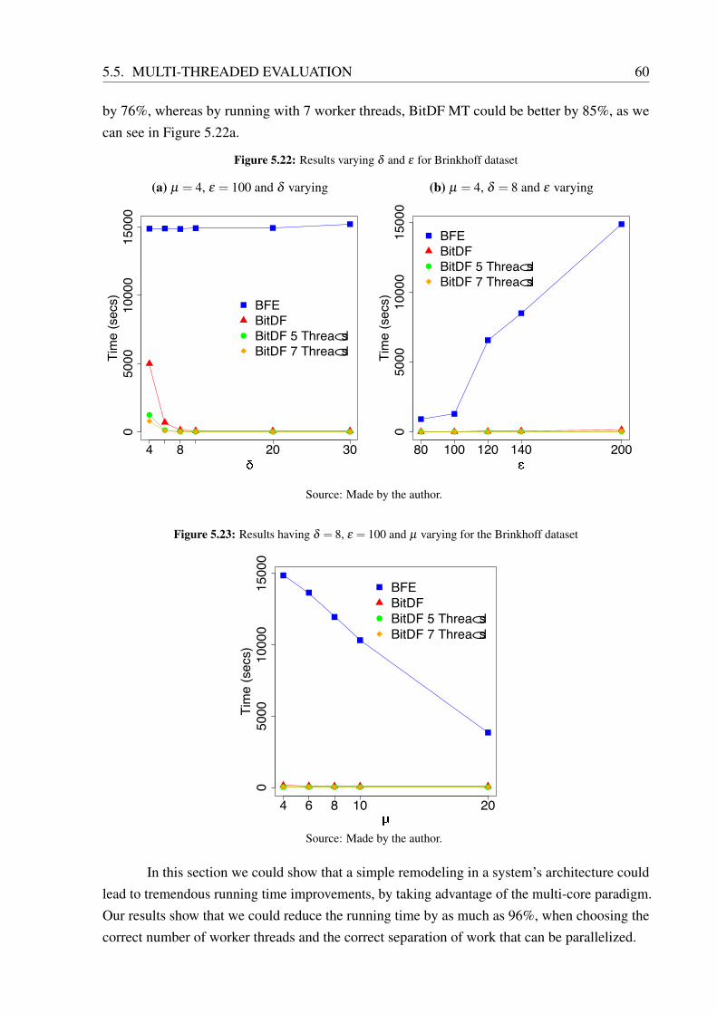
5.5. MULTI-THREADED EVALUATION 60
by 76%, whereas by running with 7 worker threads, BitDF MT could be better by 85%, as wecan see in Figure 5.22a.
Figure 5.22: Results varying δ and ε for Brinkhoff dataset
(a) µ = 4, ε = 100 and δ varying
05
00
01
00
00
15
00
0
Tim
e (
se
cs)
4 8 20 30
BFE
BitDF
BitDF 5 Threads
BitDF 7 Threads
(b) µ = 4, δ = 8 and ε varying
05
00
01
00
00
15
00
0
Tim
e (
se
cs)
80 100 120 140 200
BFE
BitDF
BitDF 5 Threads
BitDF 7 Threads
Source: Made by the author.
Figure 5.23: Results having δ = 8, ε = 100 and µ varying for the Brinkhoff dataset
05
00
01
00
00
15
00
0
Tim
e (
se
cs)
4 6 8 10 20
BFE
BitDF
BitDF 5 Threads
BitDF 7 Threads
Source: Made by the author.
In this section we could show that a simple remodeling in a system’s architecture couldlead to tremendous running time improvements, by taking advantage of the multi-core paradigm.Our results show that we could reduce the running time by as much as 96%, when choosing thecorrect number of worker threads and the correct separation of work that can be parallelized.

616161
6Conclusion
Pattern mining in spatio-temporal datasets is a really relevant subject in the academiaand the industry nowadays, due to its wide applicability in helping to solve real-world problems.Many of them can be found in the context of Smart Cities, like Traffic Management, Surveillanceand Security and City Planning, to name a few. Among the various spatio-temporal patternsthat one can extract from a spatio-temporal dataset, the flock pattern is one that has gained alot of attention. The reason for such attention it is because of its collective behavior properties,which are very applicable and are intrinsically related to the type of problems that we have justmentioned.
Throughout this dissertation, we could show that a lot of work has been done in theacademia, in order to provide algorithms able to identify the flock pattern. However, none ofthem could perform that task efficiently nor be able to scale well when a large dataset wasthe analysis target. Additionally, we found that there was no system architecture proposalthat could be simple and modular in order to address the problem of flock pattern detection inspatio-temporal datasets. Hence, since we are witnessing the rising of Smart Cities, helping tosolve those aforementioned issues would be of tremendous importance and the flock pattern canbe a valueable ally on that matter.
Given the importance of efficiently discovering flock patterns, in order to enable decisionmakers to act fast, we proposed a simple, and modular system architecture that can fit in the flockpattern detection problem and possibly be used in other pattern mining scenarios as well. Wethen used that architecture to implement a novel flock pattern detection algorithm that was able tooutperform the state-of-the-art solutions in more than 99%, with absolutely no impact in accuracy.Such impressive results were possible due to the filtering heuristic based on bitmaps that weproposed, which was able to reduce the generation of cluster disks in more than 96%, directlyreducing the amount of data that needed to be processed by the algorithm. Despite the greatresults achieved with our solution, we realized that there was still more room for improvements,given the large availability of multi-core processors in today’s computers. With that in mind, weremodeled our proposed solution to perform some critical and time consuming tasks in parallel,taking full advantage of the multi-core paradigm. Our performance benchmarks showed that wecould outperform our own single threaded solution by 96% in some cases. Moreover, if we were

6.1. FUTURE WORK 62
to show our performance gains in numbers of seconds spent to analyze a large dataset, we wereable to reduce a running time of 15,000 seconds (state-of-the-art techniques) to only 13 seconds(BitDF MT). It is also important to mention that our experiments were performed using variousdatasets, both synthetic generated and collected from real-world experiments and all of themhaving a considerable number of entries.
6.1 Future Work
Even though we were able to present great contributions in this field, there are still somegaps that can be filled and points that need more work and can lead to important results as well.Here is a list with some of them:
1. The disk superset and duplicate check is very expensive and would need furtherinvestigation in order to make our proposed architecture even more efficient. Additionally,because it modifies the same disk set, it is really hard to parallelize it without causingperformance degradation.
2. When investigating a grid cell, its extended grid might have cells that were previouslyprocessed by other extended grids. Thus, we could avoid paring the same points andgenerating the same disks again if we could keep some sort of disk cache and reusethose disks.
3. There is no study to see how different flocks relate to each other, like some MO thatstarts in one flock and later moves to a different one.
4. Make each module of the proposed architecture run in its own thread/process andthen make them independent of the time spent in other modules.
In this dissertation we showed how BitDF and BitDF MT behaves when applied todatasets collected from vehicle mobility in road networks, or datasets that simulate that samescenario. There are still other mobility scenarios that can also take advantage of flock patterndetection:
1. See how BitDF performs in indoor flock detection.
2. Use BitDF in pedestrian mobility datasets.
3. Evaluate BitDF in animal mobility datasets, such as those from Movebank Database(MOVEBANK, 2015).
Finally, some other data handling techniques can be used to help in the clustering processof points, such as Voronoi Diagrams used in conjuntion with Delaunay Triangulation and datastructures like K-D-Tress.

6.1. FUTURE WORK 63
6.1.1 Deployment Challenges in Real World Scenarios
In order to be ready to be deployed and used as a data mining solution, some work is stillneeded. In our experiments, we noticed that, due to the nature of real-world datasets, one bigchallenge is still the time synchronization of the data stream, i.e. the discovery of the correct timeslot size. As we said in Chapter 3, we cannot assume that the data entries in a spatio-temporaldataset are sampled in a fixed time rate, so there is still an effort needed in order to synchronizeand group the entries in buckets of a pre-defined size, as we did with our σ parameter. Therefore,for online analysis, there is a need for an automatic process to detect the best value of that σ
parameter according to the dataset being analyzed and also being able recalibrate it if the databehavior changes. Additionally, such automatic process should be smart enough to deal withabnormalities, such as outliers.
Another scenario that needs to be evaluated is when we have a high speed online stream ofdata. With high speed incoming data, we can face some data drop, because of a DSC componentbeing busy processing the data or forwarding the data to other components and that taking toolong. Some evaluation would need to be done in that scenario and mitigation solutions wouldneed to be proposed. Some possible solutions to avoid data drop could be: implement somebuffering mechanism of incoming data, data sampling, data hashing, etc.
GPS data is known to be very noisy and thus generate a lot of outliers. That said, it isvery important to know how to deal with such problematic data without excluding good dataentries. More importantly, when filtering bad data entries, such pre-processing should be done ina way that does not compromise the accuracy nor the efficiency of the solution proposed in thisdissertation.

646464References
ATEV, S.; MILLER, G.; PAPANIKOLOPOULOS, N. P. Clustering of vehicle trajectories. IEEETransactions on Intelligent Transportation Systems, v. 11, n. 3, p. 647–657, sep 2010. ISSN1524-9050.
AUNG, H. H.; TAN, K.-L. Discovery of evolving convoys. In: . Scientific and StatisticalDatabase Management: 22nd international conference, ssdbm 2010, heidelberg, germany, june30–july 2, 2010. proceedings. Berlin, Heidelberg: Springer Berlin Heidelberg, 2010. p. 196–213.ISBN 978-3-642-13818-8.
BARATCHI, M.; MERATNIA, N.; HAVINGA, P. J. M. Finding frequently visited paths:Dealing with the uncertainty of spatio-temporal mobility data. In: IEEE INTERNATIONALCONFERENCE ON INTELLIGENT SENSORS, SENSOR NETWORKS ANDINFORMATION PROCESSING, Melbourne, Australia. Proceedings... [S.l.], 2013. p. 479–484.
BATTY, M. et al. Smart cities of the future. The European Physical Journal Special Topics,v. 214, n. 1, p. 481–518, 2012. ISSN 1951-6355.
BENKERT, M. et al. Reporting flock patterns. Comput. Geom. Theory Appl., Elsevier SciencePublishers B. V., Amsterdam, The Netherlands, The Netherlands, v. 41, n. 3, p. 111–125, nov2008. ISSN 0925-7721.
BRINKHOFF, T. A framework for generating network-based moving objects. Geoinformatica,Kluwer Academic Publishers, Hingham, MA, USA, v. 6, n. 2, p. 153–180, jun 2002. ISSN1384-6175.
CAO, H.; MAMOULIS, N.; CHEUNG, D. W. Mining frequent spatio-temporal sequentialpatterns. In: IEEE INTERNATIONAL CONFERENCE ON DATA MINING (ICDM ’05),Houston, TX, USA. Proceedings... Washington, DC, USA: IEEE Computer Society, 2005. p.82–89. ISBN 0-7695-2278-5.
CHOROCHRONOS. Trucks dataset. 2012. Available In: <http://chorochronos.datastories.org>.Accessed on: 8 may 2016.
DING, Z. et al. Enabling smart transportation systems: A parallel spatio-temporal databaseapproach. IEEE Transactions on Computers, v. 65, n. 5, p. 1377–1391, may 2016. ISSN0018-9340.
DJAHEL, S. et al. A communications-oriented perspective on traffic management systemsfor smart cities: Challenges and innovative approaches. IEEE Communications SurveysTutorials, v. 17, n. 1, p. 125–151, first quarter 2015. ISSN 1553-877X.
DüNTGEN, C.; BEHR, T.; GüTING, R. H. BerlinMOD. 2009. Available In: <http://dna.fernuni-hagen.de/secondo/BerlinMOD/BerlinMOD.html>. Accessed on: 6 may 2016.
DüNTGEN, C.; BEHR, T.; GüTING, R. H. Berlinmod: A benchmark for moving objectdatabases. The VLDB Journal, Springer-Verlag New York, Inc., Secaucus, NJ, USA, v. 18,n. 6, p. 1335–1368, dec 2009. ISSN 1066-8888.
ESTER, M. et al. A density-based algorithm for discovering clusters in large spatial databaseswith noise. In: INTERNATIONAL CONFERENCE ON KNOWLEDGE DISCOVERY ANDDATA MINING, Portland, OR, USA. Proceedings... [S.l.], 1996. p. 226–231.

REFERENCES 65
FARRAHI, K.; GATICA-PEREZ, D. What did you do today?: Discovering daily routines fromlarge-scale mobile data. In: ACM INTERNATIONAL CONFERENCE ON MULTIMEDIA(MM ’08), Vancouver, BC, Canada. Proceedings... New York, NY, USA: ACM, 2008. p.849–852. ISBN 978-1-60558-303-7.
GENG, X. et al. Enumeration of complete set of flock patterns in trajectories. In: ACMSIGSPATIAL INTERNATIONAL WORKSHOP ON GEOSTREAMING (IWGS ’14),Dallas, TX, USA. Proceedings... New York, NY, USA: ACM, 2014. p. 53–61. ISBN978-1-4503-3139-5.
GUDMUNDSSON, J.; KREVELD, M. van. Computing longest duration flocks in trajectorydata. In: ACM INTERNATIONAL SYMPOSIUM ON ADVANCES IN GEOGRAPHICINFORMATION SYSTEMS (GIS ’06), Arlington, VA, USA. Proceedings... New York, NY,USA: ACM, 2006. p. 35–42. ISBN 1-59593-529-0.
GUDMUNDSSON, J.; KREVELD, M. van; SPECKMANN, B. Efficient detection of motionpatterns in spatio-temporal data sets. In: ACM INTERNATIONAL WORKSHOP ONGEOGRAPHIC INFORMATION SYSTEMS (GIS ’04), Washington, DC, USA. Proceedings...New York, NY, USA: ACM, 2004. p. 250–257. ISBN 1-58113-979-9.
GUDMUNDSSON, J.; LAUBE, P.; WOLLE, T. Movement patterns in spatio-temporaldata. In: . Encyclopedia of GIS. Boston, MA: Springer US, 2008. p. 726–732. ISBN978-0-387-35973-1.
GUO, D. et al. Discovering spatial patterns in origin-destination mobility data. Transactions inGIS, Blackwell Publishing Ltd, v. 16, n. 3, p. 411–429, 2012. ISSN 1467-9671.
ISO. INCITS/ISO/IEC 14882-2012: Information technology - programming languages - c++.[S.l.], 2012.
JENSEN, C. S.; LIN, D.; OOI, B. C. Continuous clustering of moving objects. IEEETransactions on Knowledge and Data Engineering, v. 19, n. 9, p. 1161–1174, sep 2007.ISSN 1041-4347.
JENSEN, M.; GUTIERREZ, J. M.; PEDERSEN, J. M. Vehicle data activity quantification usingspatio-temporal gis on modelling smart cities. In: INTERNATIONAL CONFERENCE ONCOMPUTING, NETWORKING AND COMMUNICATIONS (ICNC), Anaheim, CA, USA.Proceedings... [S.l.], 2015. p. 303–307.
JEUNG, H.; SHEN, H. T.; ZHOU, X. Convoy queries in spatio-temporal databases. In: IEEEINTERNATIONAL CONFERENCE ON DATA ENGINEERING (ICDE ’08), Cancun, Mexico.Proceedings... Washington, DC, USA: IEEE Computer Society, 2008. p. 1457–1459. ISBN978-1-4244-1836-7.
JEUNG, H. et al. Discovery of convoys in trajectory databases. Proc. VLDB Endow., VLDBEndowment, v. 1, n. 1, p. 1068–1080, aug 2008. ISSN 2150-8097.
KALNIS, P.; MAMOULIS, N.; BAKIRAS, S. On discovering moving clusters in spatio-temporaldata. In: INTERNATIONAL CONFERENCE ON ADVANCES IN SPATIAL AND TEMPORALDATABASES (SSTD ’05), Angra dos Reis, Brazil. Proceedings... Berlin, Heidelberg:Springer-Verlag, 2005. p. 364–381. ISBN 3-540-28127-4, 978-3-540-28127-6.

REFERENCES 66
KJÆRGAARD, M. B. et al. Detecting pedestrian flocks by fusion of multi-modal sensors inmobile phones. In: ACM CONFERENCE ON UBIQUITOUS COMPUTING (UBICOMP ’12),Pittsburgh, PA, USA. Proceedings... New York, NY, USA: ACM, 2012. p. 240–249. ISBN978-1-4503-1224-0.
KJÆRGAARD, M. B. et al. Mobile sensing of pedestrian flocks in indoor environments usingwifi signals. In: IEEE INTERNATIONAL CONFERENCE ON PERVASIVE COMPUTINGAND COMMUNICATIONS (PERCOM), Lugano, Switzerland. Proceedings... [S.l.], 2012. p.95–102.
LAUBE, P.; KREVELD, M.; IMFELD, S. Finding remo — detecting relative motion patternsin geospatial lifelines. In: . Developments in Spatial Data Handling: 11th internationalsymposium on spatial data handling. Berlin, Heidelberg: Springer Berlin Heidelberg, 2005. p.201–215. ISBN 978-3-540-26772-0.
LEE, J.-G.; HAN, J.; WHANG, K.-Y. Trajectory clustering: A partition-and-group framework.In: ACM SIGMOD INTERNATIONAL CONFERENCE ON MANAGEMENT OF DATA(SIGMOD ’07), Beijing, China. Proceedings... New York, NY, USA: ACM, 2007. p. 593–604.ISBN 978-1-59593-686-8.
LI, Z. et al. Mining periodic behaviors for moving objects. In: ACM SIGKDDINTERNATIONAL CONFERENCE ON KNOWLEDGE DISCOVERY AND DATA MINING(KDD ’10), Washington, DC, USA. Proceedings... New York, NY, USA: ACM, 2010. p.1099–1108. ISBN 978-1-4503-0055-1.
LI, Z. et al. Swarm: Mining relaxed temporal moving object clusters. Proc. VLDB Endow.,VLDB Endowment, v. 3, n. 1-2, p. 723–734, sep 2010. ISSN 2150-8097.
LI, Z. et al. Movemine: Mining moving object data for discovery of animal movement patterns.ACM Trans. Intell. Syst. Technol., ACM, New York, NY, USA, v. 2, n. 4, p. 37:1–37:32, jul2011. ISSN 2157-6904.
MARR, D. et al. Hyper-threading technology microarchitecture and architecture. IntelTechnology Journal, v. 6, 2012.
MINNESOTA, U. of. MNTG Traffic Generator. 2013. Available In: <http://mntg.cs.umn.edu/tg/index.php>. Accessed on: 6 may 2016.
MOVEBANK. Movebank data. 2015. Available In: <hhttps://www.movebank.org://www.movebank.org>. Accessed on: 15 may 2016.
NIMA. Department of Defense World Geodetic System 1984: Its definition and relationshipswith local geodetic systems. [S.l.], 1997. Available In: <http://earth-info.nga.mil/GandG/publications/tr8350.2/wgs84fin.pdf>. Accessed on: 30 apr. 2016.
PAN, G. et al. Trace analysis and mining for smart cities: issues, methods, and applications.IEEE Communications Magazine, v. 51, n. 6, p. 120–126, jun 2013. ISSN 0163-6804.
PATEL, D. On discovery of spatiotemporal influence-based moving clusters. ACM Trans.Intell. Syst. Technol., ACM, New York, NY, USA, v. 6, n. 1, p. 4:1–4:23, mar 2015. ISSN2157-6904.

REFERENCES 67
TSAI, C.-W. et al. Data mining for internet of things: A survey. IEEE CommunicationsSurveys Tutorials, v. 16, n. 1, p. 77–97, first quarter 2014. ISSN 1553-877X.
TURDUKULOV, U. et al. Visual mining of moving flock patterns in large spatio-temporal datasets using a frequent pattern approach. Int. J. Geogr. Inf. Sci., Taylor & Francis, Inc., Bristol,PA, USA, v. 28, n. 10, p. 2013–2029, oct 2014. ISSN 1365-8816.
VIEIRA, M. R.; BAKALOV, P.; TSOTRAS, V. J. On-line discovery of flock patterns inspatio-temporal data. In: ACM SIGSPATIAL INTERNATIONAL CONFERENCE ONADVANCES IN GEOGRAPHIC INFORMATION SYSTEMS (GIS ’09), Seattle, WA, USA.Proceedings... New York, NY, USA: ACM, 2009. p. 286–295. ISBN 978-1-60558-649-6.
WACHOWICZ, M. et al. Finding moving flock patterns among pedestrians through collectivecoherence. International Journal of Geographical Information Science, v. 25, n. 11, p.1849–1864, 2011.
WANG, Z. et al. Visual traffic jam analysis based on trajectory data. IEEE Transactionson Visualization and Computer Graphics, v. 19, n. 12, p. 2159–2168, dec 2013. ISSN1077-2626.
WIRZ, M. et al. Towards an online detection of pedestrian flocks in urban canyons by smoothedspatio-temporal clustering of gps trajectories. In: ACM SIGSPATIAL INTERNATIONALWORKSHOP ON LOCATION-BASED SOCIAL NETWORKS (LSBN ’11), Chicago, IL, USA.Proceedings... New York, NY, USA: ACM, 2011. p. 17–24. ISBN 978-1-4503-1033-8.
WOODS HOLE OCEANOGRAPHIC INSTITUTE. NDSF Utility: LatLong to XY. 2015.Available In: <http://www.whoi.edu/marine/ndsf/cgi-bin/NDSFutility.cgi?form=0&from=LatLon&to=XY>. Accessed on: 30 apr. 2016.
ZHENG, Y. T-Drive dataset. 2011. Available In: <http://research.microsoft.com/apps/pubs/?id=152883>. Accessed on: 6 may 2016.
ZHENG, Y. Trajectory data mining: An overview. ACM Trans. Intell. Syst. Technol., ACM,New York, NY, USA, v. 6, n. 3, p. 29:1–29:41, may 2015. ISSN 2157-6904.
ZHENG, Y. et al. On discovery of gathering patterns from trajectories. In: IEEEINTERNATIONAL CONFERENCE ON DATA ENGINEERING (ICDE ’13), Brisbane,Australia. Proceedings... Washington, DC, USA: IEEE Computer Society, 2013. p. 242–253.ISBN 978-1-4673-4909-3.