Embed Size (px)
Citation preview

Learning Dependency-Based Compositional Semantics
by
Percy Shuo Liang
A dissertation submitted in partial satisfaction of the
requirements for the degree of
Doctor of Philosophy
in
Electrical Engineering and Computer Sciences
and the Designated Emphasis
in
Communication, Computation, and Statistics
in the
Graduate Division
of the
University of California, Berkeley
Committee in charge:
Professor Dan Klein, ChairProfessor Michael I. Jordan
Professor Tom Griffiths
Fall 2011
Learning Dependency-Based Compositional Semantics
Copyright 2011by
Percy Shuo Liang

1
Abstract
Learning Dependency-Based Compositional Semantics
by
Percy Shuo Liang
Doctor of Philosophy in Electrical Engineering and Computer Sciences
and the Designated Emphasis
in
Communication, Computation, and Statistics
University of California, Berkeley
Professor Dan Klein, Chair
Suppose we want to build a system that answers a natural language question by representingits semantics as a logical form and computing the answer given a structured database of facts.The core part of such a system is the semantic parser that maps questions to logical forms.Semantic parsers are typically trained from examples of questions annotated with their targetlogical forms, but this type of annotation is expensive.
Our goal is to learn a semantic parser from question-answer pairs instead, where the logi-cal form is modeled as a latent variable. Motivated by this challenging learning problem, wedevelop a new semantic formalism, dependency-based compositional semantics (DCS), whichhas favorable linguistic, statistical, and computational properties. We define a log-linear dis-tribution over DCS logical forms and estimate the parameters using a simple procedure thatalternates between beam search and numerical optimization. On two standard semanticparsing benchmarks, our system outperforms all existing state-of-the-art systems, despiteusing no annotated logical forms.

i
To my parents...
and
to Ashley.

ii
Contents
1 Introduction 1
2 Representation 52.1 Notation . . . . . . . . . . . . . . . . . . . . . . . . . . . . . . . . . . . . . . 52.2 Syntax of DCS Trees . . . . . . . . . . . . . . . . . . . . . . . . . . . . . . . 62.3 Worlds . . . . . . . . . . . . . . . . . . . . . . . . . . . . . . . . . . . . . . . 6
2.3.1 Types and Values . . . . . . . . . . . . . . . . . . . . . . . . . . . . . 72.3.2 Examples . . . . . . . . . . . . . . . . . . . . . . . . . . . . . . . . . 9
2.4 Semantics of DCS Trees: Basic Version . . . . . . . . . . . . . . . . . . . . . 102.4.1 DCS Trees as Constraint Satisfaction Problems . . . . . . . . . . . . 102.4.2 Computation . . . . . . . . . . . . . . . . . . . . . . . . . . . . . . . 122.4.3 Aggregate Relation . . . . . . . . . . . . . . . . . . . . . . . . . . . . 13
2.5 Semantics of DCS Trees: Full Version . . . . . . . . . . . . . . . . . . . . . . 152.5.1 Denotations . . . . . . . . . . . . . . . . . . . . . . . . . . . . . . . . 162.5.2 Join Relations . . . . . . . . . . . . . . . . . . . . . . . . . . . . . . . 202.5.3 Aggregate Relations . . . . . . . . . . . . . . . . . . . . . . . . . . . 212.5.4 Mark Relations . . . . . . . . . . . . . . . . . . . . . . . . . . . . . . 222.5.5 Execute Relations . . . . . . . . . . . . . . . . . . . . . . . . . . . . . 23
2.6 Construction Mechanism . . . . . . . . . . . . . . . . . . . . . . . . . . . . . 302.6.1 Lexical Triggers . . . . . . . . . . . . . . . . . . . . . . . . . . . . . . 312.6.2 Recursive Construction of DCS Trees . . . . . . . . . . . . . . . . . . 312.6.3 Filtering using Abstract Interpretation . . . . . . . . . . . . . . . . . 332.6.4 Comparison with CCG . . . . . . . . . . . . . . . . . . . . . . . . . . 35
3 Learning 373.1 Semantic Parsing Model . . . . . . . . . . . . . . . . . . . . . . . . . . . . . 37
3.1.1 Features . . . . . . . . . . . . . . . . . . . . . . . . . . . . . . . . . . 373.2 Parameter Estimation . . . . . . . . . . . . . . . . . . . . . . . . . . . . . . 40
3.2.1 Objective Function . . . . . . . . . . . . . . . . . . . . . . . . . . . . 403.2.2 Algorithm . . . . . . . . . . . . . . . . . . . . . . . . . . . . . . . . . 41

iii
4 Experiments 434.1 Experimental Setup . . . . . . . . . . . . . . . . . . . . . . . . . . . . . . . . 43
4.1.1 Datasets . . . . . . . . . . . . . . . . . . . . . . . . . . . . . . . . . . 434.1.2 Settings . . . . . . . . . . . . . . . . . . . . . . . . . . . . . . . . . . 454.1.3 Lexical Triggers . . . . . . . . . . . . . . . . . . . . . . . . . . . . . . 46
4.2 Comparison with Other Systems . . . . . . . . . . . . . . . . . . . . . . . . . 484.2.1 Systems that Learn from Question-Answer Pairs . . . . . . . . . . . . 484.2.2 State-of-the-Art Systems . . . . . . . . . . . . . . . . . . . . . . . . . 49
4.3 Empirical Properties . . . . . . . . . . . . . . . . . . . . . . . . . . . . . . . 514.3.1 Error Analysis . . . . . . . . . . . . . . . . . . . . . . . . . . . . . . . 524.3.2 Visualization of Features . . . . . . . . . . . . . . . . . . . . . . . . . 534.3.3 Learning, Search, Bootstrapping . . . . . . . . . . . . . . . . . . . . . 544.3.4 Effect of Various Settings . . . . . . . . . . . . . . . . . . . . . . . . 55
5 Discussion 585.1 Semantic Representation . . . . . . . . . . . . . . . . . . . . . . . . . . . . . 585.2 Program Induction . . . . . . . . . . . . . . . . . . . . . . . . . . . . . . . . 605.3 Grounded Language . . . . . . . . . . . . . . . . . . . . . . . . . . . . . . . 605.4 Conclusions . . . . . . . . . . . . . . . . . . . . . . . . . . . . . . . . . . . . 61
A Details 68A.1 Denotation Computation . . . . . . . . . . . . . . . . . . . . . . . . . . . . . 68
A.1.1 Set-expressions . . . . . . . . . . . . . . . . . . . . . . . . . . . . . . 69A.1.2 Join and Project on Set-Expressions . . . . . . . . . . . . . . . . . . 70

iv
Acknowledgments
My last six years at Berkeley have been an incredible journey—one where I have growntremendously, both academically and personally. None of this would have been possiblewithout the support of the many people I have interacted with over the years.
First, I am extremely grateful to have been under the guidance of not one great adviser,but two. Michael Jordan and Dan Klein didn’t just teach me new things—they truly shapedthe way I think in a fundamental way and gave me invaluable perspective on research. FromMike, I learned how to really make sense of mathematical details and see the big importantideas; Dan taught me how to make sense of data and read the mind of a statistical model.The two influences complemented each other wonderfully, and I cannot think of a betterenvironment for me.
Having two advisers also meant having the fortune of interacting with two vibrant re-search groups. I remember having many inspiring conversations in meeting rooms, hall-ways, and at Jupiter—thanks to all the members of the SAIL and NLP groups, as well asPeter Bartlett’s group. I also had the pleasure of collaborating on projects with Alexan-dre Bouchard-Cote, Ben Taskar, Slav Petrov, Tom Griffiths, Aria Haghighi, Taylor Berg-Kirkpatrick, Ben Blum, Jake Abernethy, Alex Simma, and Ariel Kleiner. I especially wantto thank Dave Golland and Gabor Angeli, whom I really enjoyed mentoring.
Many people outside of Berkeley also had a lasting impact on me. Nati Srebro introducedme to research when I was an undergraduate at MIT, and first got me excited about machinelearning. During my masters at MIT, Michael Collins showed me the rich world of statisticalNLP. I also learned a great deal from working with Paul Viola, Martin Szummer, FrancisBach, Guillaume Bouchard, and Hal Daume through various collaborations. In a fortuitousturn of events, I ended up working on program analysis with Mayur Naik, Omer Tripp,and Mooly Sagiv. Mayur Naik taught me almost everything I know about the field ofprogramming languages.
There are several additional people I’d like to thank: John Duchi, who gave me an excuseto bike long distances for my dinner; Mike Long, with whom I first explored the beauty ofthe Berkeley hills; Rodolphe Jenatton, avec qui j’ai appris a parler francais et courir enmeme temps; John Blitzer, with whom I seemed to get better research done in the hills thanin the office; Kurt Miller, with whom I shared exciting adventures in St. Petersburg, to becontinued in New York; Blaine Nelson, who introduced me to great biking in the Bay Area;my Ashby housemates (Dave Golland, Fabian Wauthier, Garvesh Raskutti, Lester Mackey),with whom I had many whole wheat conversations not about whole wheat; Haggai Niv andRay Lifchez, pillars of my musical life; Simon Lacoste-Julien and Sasha Skorokhod, whoexpanded my views on life; and Alex Bouchard-Cote, with whom I shared so many vividmemories during our years at Berkeley.

v
My parents, Frank Liang and Ling Zhang, invested in me more than I can probablyimagine, and they have provided their unwavering support throughout my life—words simplyfail to express my appreciation for them. Finally, Ashley, thank you for your patience duringmy long journey, for always providing a fresh perspective, for your honesty, and for alwaysbeing there for me.
1
Chapter 1
Introduction
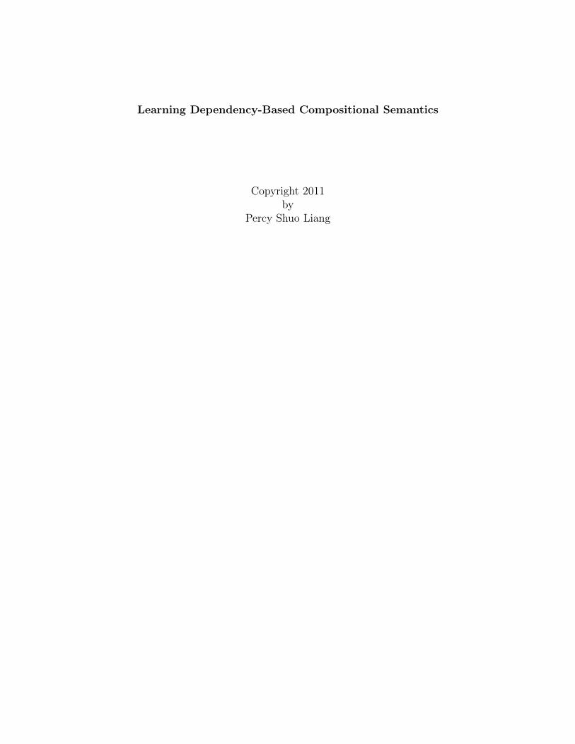
We are interested in building a system that can answer natural language questions givena structured database of facts. As a running example, consider the domain of US geography(Figure 1.1).
What is the total population of theten largest cities in California?
city
San FranciscoChicagoBoston· · ·
loc
Mount Shasta CaliforniaSan Francisco CaliforniaBoston Massachusetts· · · · · ·
>
7 35 018 2· · · · · ·
state
AlabamaAlaskaArizona· · ·
population
Los Angeles 3.8 millionSan Francisco 805,000Boston 617,000· · · · · ·
count
{} 0
{1,4} 2
{2,5,6} 3· · · · · ·
System
?
Figure 1.1: The goal: a system that answers natural language questions given a structureddatabase of facts. An example is shown in the domain of US geography.
The problem of building these natural language interfaces to databases (NLIDBs) has along history in NLP, starting from the early days of AI with systems such as Lunar (Woodset al., 1972), Chat-80 (Warren and Pereira, 1982), and many others (see Androutsopouloset al. (1995) for an overview). While quite successful in their respective limited domains,because these systems were constructed from manually-built rules, they became difficult toscale up, both to other domains and to more complex utterances. In response, against thebackdrop of a statistical revolution in NLP during the 1990s, researchers began to buildsystems that could learn from examples, with the hope of overcoming the limitations ofrule-based methods. One of the earliest statistical efforts was the Chill system (Zelle andMooney, 1996), which learned a shift-reduce semantic parser. Since then, there has beena healthy line of work yielding increasingly more accurate semantic parsers by using newsemantic representations and machine learning techniques (Zelle and Mooney, 1996; Miller

CHAPTER 1. INTRODUCTION 2
et al., 1996; Tang and Mooney, 2001; Ge and Mooney, 2005; Kate et al., 2005; Zettlemoyerand Collins, 2005; Kate and Mooney, 2006; Wong and Mooney, 2006; Kate and Mooney,2007; Zettlemoyer and Collins, 2007; Wong and Mooney, 2007; Kwiatkowski et al., 2010,2011).
However, while statistical methods provided advantages such as robustness and porta-bility, their application in semantic parsing achieved only limited success. One of the mainobstacles was that these methods depended crucially on having examples of utterances pairedwith logical forms, and this requires substantial human effort to obtain. Furthermore, theannotators must be proficient in some formal language, which drastically reduces the sizeof the annotator pool, dampening any hope of acquiring enough data to fulfill the vision oflearning highly accurate systems.
In response to these concerns, researchers have recently begun to explore the possibilityof learning a semantic parser without any annotated logical forms (Clarke et al., 2010; Lianget al., 2011; Goldwasser et al., 2011; Artzi and Zettlemoyer, 2011). It is in this vein thatwe develop our present work. Specifically, given a set of (x, y) example pairs, where x is anutterance (e.g., a question) and y is the corresponding answer, we wish to learn a mappingfrom x to y. What makes this mapping particularly interesting is it passes through a latentlogical form z, which is necessary to capture the semantic complexities of natural language.Also note that while the logical form z was the end goal in past work on semantic parsing,for us, it is just an intermediate variable—a means towards an end. Figure 1.2 shows thegraphical model which captures the learning setting we just described: The question x,answer y, and world/database w are all observed. We want to infer the logical forms z andthe parameters θ of the semantic parser, which are unknown quantities.
While liberating ourselves from annotated logical forms reduces cost, it does increase thedifficulty of the learning problem. The core challenge here is program induction: on eachexample (x, y), we need to efficiently search over the exponential space of possible logicalforms z and find ones that produces the target answer y, a computationally daunting task.There is also a statistical challenge: how do we parametrize the mapping from utterance xto logical form z so that it can be learned from only the indirect signal y? To address thesetwo challenges, we must first discuss the issue of semantic representation. There are twobasic questions here: (i) what should the formal language for the logical forms z be, and (ii)what are the compositional mechanisms for constructing those logical forms?
The semantic parsing literature is quite multilingual with respect to the formal languageused for the logical form: Researchers have used SQL (Giordani and Moschitti, 2009), Pro-log (Zelle and Mooney, 1996; Tang and Mooney, 2001), a simple functional query languagecalled FunQL (Kate et al., 2005), and lambda calculus (Zettlemoyer and Collins, 2005), justto name a few. The construction mechanisms are equally diverse, including synchronousgrammars (Wong and Mooney, 2007), hybrid trees (Lu et al., 2008), Combinatorial Catego-rial Grammars (CCG) (Zettlemoyer and Collins, 2005), and shift-reduce derivations (Zelleand Mooney, 1996). It is worth pointing out that the choice of formal language and theconstruction mechanism are decisions which are really more orthogonal than it is often

CHAPTER 1. INTRODUCTION 3
[0.3,−0.7, 4.5, 1.2, . . . ]
city
San FranciscoChicagoBoston· · ·
loc
Mount Shasta CaliforniaSan Francisco CaliforniaBoston Massachusetts· · · · · ·
>
7 35 018 2· · · · · ·
state
AlabamaAlaskaArizona· · ·
population
Los Angeles 3.8 millionSan Francisco 805,000Boston 617,000· · · · · ·
count
{} 0
{1,4} 2
{2,5,6} 3· · · · · ·
(parameters) (world)
θ w
x z y
(utterance) (logical form) (answer)
state with thelargest area x1x1
1
1
cc
argmax
area
state
∗∗ Alaska
Semantic Parsingz ∼ p(z | x; θ)
Semantic Evaluationy = JzKw
Figure 1.2: Our probabilistic model consists of two steps: (i) semantic parsing: an utterancex is mapped to a logical form z by drawing from a log-linear distribution parametrized bya vector θ; and (ii) evaluation: the logical form z is evaluated with respect to the world w(database of facts) to deterministically produce an answer y = JzKw. The figure also showsan example configuration of the variables around the graphical model. Logical forms z asrepresented as labeled trees. During learning, we are given w and (x, y) pairs (shaded nodes)and try to infer the latent logical forms z and parameters θ.
assumed—the former is concerned with what the logical forms look like; the latter, how togenerate a set of possible logical forms in a compositional way given an utterance. (How toscore these logical forms is yet another dimension.)
The formal languages and construction mechanisms in past work were chosen somewhatout of the convenience of conforming to existing standards. For example, Prolog and SQLwere existing standard declarative languages built for querying a deductive or relationaldatabase, which was convenient for the end application, but they were not designed for rep-resenting the semantics of natural language. As a result, the construction mechanism thatbridges the gap between natural language and formal language is quite complicated anddifficult to learn. CCG (Steedman, 2000) and more generally, categorial grammar, is the defacto standard in linguistics. In CCG, logical forms are constructed compositionally using asmall handful of combinators (function application, function composition, and type raising).For a wide range of canonical examples, CCG produces elegant, streamlined analyses, butits success really depends on having a good, clean lexicon. During learning, there is often

CHAPTER 1. INTRODUCTION 4
large amounts of uncertainty over the lexical entries, which makes CCG more cumbersome.Furthermore, in real-world applications, we would like to handle disfluent utterances, andthis further strains CCG by demanding either extra type-raising rules and disharmonic com-binators (Zettlemoyer and Collins, 2007) or a proliferation of redundant lexical entries foreach word (Kwiatkowski et al., 2010).
To cope with the challenging demands of program induction, we break away from tradi-tion in favor of a new formal language and construction mechanism, which we call dependency-based compositional semantics (DCS). The guiding principle behind DCS is to make a simpleand intuitive framework for constructing and representing logical forms. Logical forms inDCS are tree structures called DCS trees. The motivation is two-fold: (i) DCS trees aremeant to parallel syntactic dependency trees, which facilitates parsing; and (ii) a DCS treeessentially encodes a constraint satisfaction problem, which can be solved efficiently useddynamic programming. In addition, DCS provides a mark-execute construct, which providesa uniform way of dealing with scope variation, a major source of trouble in any semanticformalism. The construction mechanism in DCS is a generalization of labeled dependencyparsing, which leads to simple and natural algorithms. To a linguist, DCS might appearunorthodox, but it is important to keep in mind that our primary goal is effective programinduction, not necessarily to model new linguistic phenomena in the tradition of formalsemantics.
Armed with our new semantic formalism, DCS, we then define a discriminative proba-bilistic model, which is depicted in Figure 1.2. The semantic parser is a log-linear distributionover DCS trees z given an utterance x. Notably, z is unobserved, and we instead observeonly the answer y, which is z evaluated on a world/database w. There are an exponentialnumber of possible trees z, and usually dynamic programming is employed for efficientlysearching over the space of these combinatorial objects. However, in our case, we mustenforce the global constraint that the tree generates the correct answer y, which makes dy-namic programming infeasible. Therefore, we resort to beam search and learn our modelwith a simple procedure which alternates between beam search and optimizing a likelihoodobjective restricted to those beams. This yields a natural bootstrapping procedure in whichlearning and search are integrated.
We evaluated our DCS-based approach on two standard benchmarks, Geo, a US geogra-phy domain (Zelle and Mooney, 1996) and Jobs, a job queries domain (Tang and Mooney,2001). On Geo, we found that our system significantly outperforms previous work that alsolearns from answers instead of logical forms (Clarke et al., 2010). What is perhaps a moresignificant result is that our system even outperforms state-of-the-art systems that do rely onannotated logical forms. This demonstrates that the viability of training accurate systemswith much less supervision than before.
The rest of this thesis is organized as follows: Chapter 2 introduces dependency-basedcompositional semantics (DCS), our new semantic formalism. Chapter 3 presents our prob-abilistic model and learning algorithm. Chapter 4 provides an empirical evaluation of ourmethods. Finally, Chapter 5 situates this work in a broader context.
5
Chapter 2
Representation
In this chapter, we present the main conceptual contribution of this work, dependency-based compositional semantics (DCS), using the US geography domain (Zelle and Mooney,1996) as a running example. To do this, we need to define the syntax and semantics ofthe formal language. The syntax is defined in Section 2.2 and is quite straightforward: Thelogical forms in the formal language are simply trees, which we call DCS trees. In Section 2.3,we give a type-theoretic definition of worlds (also known as databases or models) with respectto which we can define the semantics of DCS trees.
The semantics, which is the heart of this thesis, contains two main ideas: (i) usingtrees to represent logical forms as constraint satisfaction problems or extensions thereof,and (ii) dealing with cases when syntactic and semantic scope diverge (e.g., for generalizedquantification and superlative constructions) using a new construct which we call mark-execute. We start in Section 2.4 by introducing the semantics of a basic version of DCSwhich focuses only on (i) and then extend it to the full version (Section 2.5) to account for(ii).
Finally, having fully specified the formal language, we describe a construction mechanismfor mapping a natural language utterance to a set of candidate DCS trees (Section 2.6).
2.1 Notation
Operations on tuples will play a prominent role in this thesis. For a sequence1 v = (v1, . . . , vk),we use |v| = k to denote the length of the sequence. For two sequences u and v, we useu+ v = (u1, . . . , u|u|, v1, . . . , v|v|) to denote their concatenation.
For a sequence of positive indices i = (i1, . . . , im), let vi = (vi1 , . . . , vim) consist of thecomponents of v specified by i; we call vi the projection of v onto i. We use negative indices
1We use the sequence to include both tuples (v1, . . . , vk) and arrays [v1, . . . , vk]. For our purposes, thereis no functional difference between tuples and arrays; the distinction is convenient when we start to talkabout arrays of tuples.

CHAPTER 2. REPRESENTATION 6
to exclude components: v−i = (v(1,...,|v|)\i). We can also combine sequences of indices byconcatenation: vi,j = vi + vj. Some examples: if v = (a, b, c, d), then v2 = b, v3,1 = (c, a),v−3 = (a, b, d), v3,−3 = (c, a, b, d).
2.2 Syntax of DCS Trees
The syntax of the DCS formal language is built from two ingredients, predicates and relations:
• Let P be a set of predicates. We assume that P always contains a special null predicateø and several domain-independent predicates (e.g., count, <, >, and =). In addition,P contains domain-specific predicates. For example, for the US geography domain, Pwould include state, river, border, etc. Right now, think of predicates as just labels,which have yet to receive formal semantics.
• Let R be the set of relations. The full set of relations are shown in Table 2.1; notethat unlike the predicates P , the relations R are fixed.
The logical forms in DCS are called DCS trees. A DCS tree is a directed rooted tree inwhich nodes are labeled with predicates and edges are labeled with relations; each node alsomaintains an ordering over its children. Formally:
Definition 1 (DCS trees) Let Z be the set of DCS trees, where each z ∈ Z consists of (i)a predicate z.p ∈ P and (ii) a sequence of edges z.e = (z.e1, . . . , z.em). Each edge e consistsof a relation e.r ∈ R (see Table 2.1) and a child tree e.c ∈ Z.
We will either draw a DCS tree graphically or write it compactly as 〈p; r1 : c1; . . . ; rm : cm〉where p is the predicate at the root node and c1, . . . , cm are its m children connected viaedges labeled with relations r1, . . . , rm, respectively. Figure 2.2(a) shows an example of aDCS tree expressed using both graphical and compact formats.
A DCS tree is a logical form, but it is designed to look like a syntactic dependency tree,only with predicates in place of words. As we’ll see over the course of this chapter, it is thistransparency between syntax and semantics provided by DCS which leads to a simple andstreamlined compositional semantics suitable for program induction.
2.3 Worlds
In the context of question answering, the DCS tree is a formal specification of the question.To obtain an answer, we still need to evaluate the DCS tree with respect to a database of facts(see Figure 2.1 for an example). We will use the term world to refer to this database (it issometimes also called model, but we avoid this term to avoid confusion with the probabilisticmodel that we will present in Section 3.1).

CHAPTER 2. REPRESENTATION 7
Relations RName Relation Description
join jj′ for j, j′ ∈ {1, 2, . . . } j-th component of parent = j′-th component of child
aggregate Σ parent = set of feasible values of childextract e mark node for extractionquantify q mark node for quantification, negationcompare c mark node for superlatives, comparativesexecute xi for i ∈ {1, 2 . . . }∗ process marked nodes specified by i
Table 2.1: Possible relations that appear on edges of DCS trees. Basic DCS uses only thejoin and aggregate relations; the full version uses all of them.
w:city
San FranciscoChicagoBoston· · ·
loc
Mount Shasta CaliforniaSan Francisco CaliforniaBoston Massachusetts· · · · · ·
>
7 35 018 2· · · · · ·
state
AlabamaAlaskaArizona· · ·
population
Los Angeles 3.8 millionSan Francisco 805,000Boston 617,000· · · · · ·
count
{} 0
{1,4} 2
{2,5,6} 3· · · · · ·
Figure 2.1: An example of a world w (database) in the US geography domain. A worldmaps each predicate (relation) to a set of tuples. Here, the world w maps the predicate loc
to the set of pairs of places and their containers. Note that functions (e.g., population)are also represented as predicates for uniformity. Some predicates (e.g., count) map to aninfinite number of tuples and would be represented implicitly.
2.3.1 Types and Values
To define a world, we start by constructing a set of values V . The exact set of valuesdepend on the domain (we will continue to use US geography as a running example).Briefly, V contains numbers (e.g., 3 ∈ V), strings (e.g., Washington ∈ V), tuples (e.g.,(3,Washington) ∈ V), sets (e.g., {3,Washington} ∈ V), and other higher-order entities.
To be more precise, we construct V recursively. First, define a set of primitive values V?,which includes the following:
• Numeric values: each value has the form x : t ∈ V?, where x ∈ R is a real number andt ∈ {number, ordinal, percent, length, . . . } is a tag. The tag allows us to differentiate

CHAPTER 2. REPRESENTATION 8
3, 3rd, 3%, and 3 miles—this will be important in Section 2.6.3. We simply write xfor the value x :number.
• Symbolic values: each value has the form x : t ∈ V?, where x is a string (e.g.,Washington) and t ∈ {string, city, state, river, . . . } is a tag. Again, the tag allowsus to differentiate, for example, the entities Washington :city and Washington :state.
Now we build the full set of values V from the primitive values V?. To define V , weneed a bit more machinery: To avoid logical paradoxes, we construct V in increasing order ofcomplexity using types (see Carpenter (1998) for a similar construction). The casual readercan skip this construction without losing any intuition.
Define the set of types T to be the smallest set that satisfies the following properties:
1. The primitive type ? ∈ T ;
2. The tuple type (t1, . . . , tk) ∈ T for each k ≥ 0 and each non-tuple type ti ∈ T fori = 1, . . . , k; and
3. The set type {t} ∈ T for each tuple type t ∈ T .
Note that {?}, {{?}}, and ((?)) are not valid types.For each type t ∈ T , we construct a corresponding set of values Vt:
1. For the primitive type t = ?, the primitive values V? have already been specified. Notethat these types are rather coarse: Primitive values with different tags are consideredto have the same type ?.
2. For a tuple type t = (t1, . . . , tk), Vt is the cross product of the values of its componenttypes:
Vt = {(v1, . . . , vk) : ∀i, vi ∈ Vti}. (2.1)
3. For a set type t = {t′}, Vt contains all subsets of its element type t′:
Vt = {s : s ⊂ Vt′}. (2.2)
Note that all elements of the set must have the same type.
Let V = ∪t∈T Vt be the set of all possible values.A world maps each predicate to its semantics, which is a set of tuples (see Figure 2.1
for an example). First, let Ttuple ⊂ T be the tuple types, which are the ones of the form(t1, . . . , tk). Let V{tuple} denote all the sets of tuples (with the same type):
V{tuple}def=
⋃t∈Ttuple
V{t}. (2.3)
Now we define a world formally:

CHAPTER 2. REPRESENTATION 9
Definition 2 (World) A world w : P 7→ V{tuple} ∪ {V} is a function that maps each non-null predicate p ∈ P\{ø} to a set of tuples w(p) ∈ V{tuple} and maps the null predicate ø tothe set of all values (w(ø) = V).
For a set of tuples A with the same arity, let Arity(A) = |x|, where x ∈ A is arbitrary;if A is empty, then Arity(A) is undefined. Now for a predicate p ∈ P and world w, defineArityw(p), the arity of predicate p with respect to w, as follows:
Arityw(p) =
{1 if p = ø,
Arity(w(p)) if p 6= ø.(2.4)
The null predicate has arity 1 by fiat; the arity of a non-null predicate p is inherited fromthe tuples in w(p).
Remarks In higher-order logic and lambda calculus, we construct function types and val-ues, whereas in DCS, we construct tuple types and values. The two are equivalent in repre-sentational power, but this discrepancy does point at the fact that lambda calculus is basedon function application, whereas DCS, as we will see, is based on declarative constraints.The set type {(?, ?)} in DCS corresponds to the function type ? → (? → bool). In DCS,there is no explicit bool type—it is implicitly represented by using sets.
2.3.2 Examples
The world w maps each domain-specific predicate to a finite set of tuples. For the USgeography domain, w has a predicate that maps to the set of US states (state), anotherpredicate that maps to set of pairs of entities and where they are located (loc), and so on:
w(state) = {(California :state), (Oregon :state), . . . }, (2.5)
w(loc) = {(San Francisco :city,California :state), . . . } (2.6)
. . . (2.7)
To shorten notation, we use state abbreviations (e.g., CA = California :state).The world w also specifies the semantics of several domain-independent predicates (think
of these as helper functions), which usually correspond to an infinite set of tuples. Functionsare represented in DCS by a set of input-output pairs. For example, the semantics of thecountt predicate (for each type t ∈ T ) contains pairs of sets S and their cardinalities |S|:
w(countt) = {(S, |S|) : S ∈ V{(t)}} ∈ V{({(t)},?)}. (2.8)
As another example, consider the predicate averaget (for each t ∈ T ), which takes aset of key-value pairs (with keys of type t) and returns the average value. For notationalconvenience, we treat an arbitrary set of pairs S as a set-valued function: We let S1 = {x :

CHAPTER 2. REPRESENTATION 10
(x, y) ∈ S} denote the domain of the function, and abusing notation slightly, we define thefunction S(x) = {y : (x, y) ∈ S} to be the set of values y that co-occur with the given x.The semantics of averaget contains pairs of sets and their averages:
w(averaget) =
(S, z) : S ∈ V{(t,?)}, z = |S1|−1∑x∈S1
|S(x)|−1∑y∈S(x)
y
∈ V{({(t,?)},?)}.(2.9)
Similarly, we can define the semantics of argmint and argmaxt, which each takes a set ofkey-value pairs and returns the keys that attain the smallest (largest) value:
w(argmint) =
{(S, z) : S ∈ V{(t,?)}, z ∈ argmin
x∈S1
minS(x)
}∈ V{({(t,?)},t)}, (2.10)
w(argmaxt) =
{(S, z) : S ∈ V{(t,?)}, z ∈ argmax
x∈S1
maxS(x)
}∈ V{({(t,?)},t)}. (2.11)
These helper functions are monomorphic: For example, countt only computes cardinal-ities of sets of type {(t)}. In practice, we mostly operate on sets of primitives (t = ?). Toreduce notation, we simply omit t to refer to this version: count = count?, average =average?, etc.
2.4 Semantics of DCS Trees: Basic Version
The semantics or denotation of a DCS tree z with respect to a world w is denoted JzKw. First,we define the semantics of DCS trees with only join relations (Section 2.4.1). In this case,a DCS tree encodes a constraint satisfaction problem (CSP); this is important because ithighlights the constraint-based nature of DCS and also naturally leads to a computationallyefficient way of computing denotations (Section 2.4.2). We then allow DCS trees to haveaggregate relations (Section 2.4.3). The fragment of DCS which has only join and aggregaterelations is called basic DCS.
2.4.1 DCS Trees as Constraint Satisfaction Problems
Let z be a DCS tree with only join relations on its edges. In this case, z encodes a constraintsatisfaction problem (CSP) as follows: For each node x in z, the CSP has a variable a(x); thecollection of these variables is referred to as an assignment a. The predicates and relationsof z introduce constraints:
1. a(x) ∈ w(p) for each node x labeled with predicate p ∈ P ; and

CHAPTER 2. REPRESENTATION 11
Example: major city in California
z = 〈city; 11 :〈major〉 ; 11 :〈loc; 21 :〈CA〉〉〉
1
1
1
1
major2
1
CA
loc
city
λc∃m∃`∃s .city(c) ∧ major(m) ∧ loc(`) ∧ CA(s)∧c1 = m1 ∧ c1 = `1 ∧ `2 = s1
(a) DCS tree (b) Lambda calculus formula
(c) Denotation: JzKw = {SF, LA, . . . }
Figure 2.2: (a) An example of a DCS tree (written in both the mathematical and graphicalnotation). Each node is labeled with a predicate, and each edge is labeled with a relation.(b) A DCS tree z with only join relations encodes a constraint satisfaction problem. (c) Thedenotation of z is the set of feasible values for the root node.
2. a(x)j = a(y)j′ for each edge (x, y) labeled with jj′ ∈ R, which says that the j-th
component of a(x) must equal the j′-th component of a(y).
We say that an assignment a is feasible if it satisfies all the above constraints. Next, fora node x, define V (x) = {a(x) : assignment a is feasible} as the set of feasible values forx—these are the ones which are consistent with at least one feasible assignment. Finally, wedefine the denotation of the DCS tree z with respect to the world w to be JzKw = V (x0),where x0 is the root node of z.
Figure 2.2(a) shows an example of a DCS tree. The corresponding CSP has four variablesc,m, `, s.2 In Figure 2.2(b), we have written the equivalent lambda calculus formula. Thenon-root nodes are existentially quantified, the root node c is λ-abstracted, and all constraintsintroduced by predicates and relations are conjoined. The λ-abstraction of c represents thefact that the denotation is the set of feasible values for c (note the equivalence between theboolean function λc.p(c) and the set {c : p(c)}).
Remarks Note that CSPs only allow existential quantification and conjunction. Why didwe choose this particular logical subset as a starting point, rather than allowing universalquantification, negation, or disjunction? There seems to be something fundamental aboutthis subset, which also appears in Discourse Representation Theory (DRT) (Kamp and Reyle,1993; Kamp et al., 2005). Briefly, logical forms in DRT are called Discourse RepresentationStructures (DRSes), each of which contains (i) a set of existentially-quantified discourse
2Technically, the node is c and the variable is a(c), but we use c to denote the variable to simplify notation.

CHAPTER 2. REPRESENTATION 12
referents (variables), (ii) a set of conjoined discourse conditions (constraints), and (iii) nestedDRSes. If we exclude nested DRSes, a DRS is exactly a CSP.3 The default existentialquantification and conjunction are quite natural for modeling cross-sentential anaphora: Newvariables can be added to a DRS and connected to other variables. Indeed, DRT wasoriginally motivated by these phenomena (see Kamp and Reyle (1993) for more details).
Tree-structured CSPs can capture unboundedly complex recursive structures—such ascities in states that border states that have rivers that. . . . However, one limitation whichwill stay with us even with the full version of DCS, is the inability to capture long dis-tance dependencies arising from anaphora (ironically, given our connection to DRT). Forexample, consider the phrase a state with a river that traverses its capital. Here, its bindsto state, but this dependence cannot be captured in a tree structure. However, given thehighly graphical context in which we’ve been developing DCS, a solution leaps out at usimmediately: Simply introduce an edge between the its node and the state node. This edgeintroduces a CSP constraint that the two nodes must be equal. The resulting structure is agraph rather than a tree, but still a CSP. In this thesis, we will not pursue these non-treestructures, but it should be noted that such an extension is possible and quite natural.
2.4.2 Computation
So far, we have given a declarative definition of the denotation JzKw of a DCS tree z with onlyjoin relations. Now we will show how to compute JzKw efficiently. Recall that the denotationis the set of feasible values for the root node. In general, finding the solution to a CSP isNP-hard, but for trees, we can exploit dynamic programming (Dechter, 2003). The key isthat the denotation of a tree depends on its subtrees only through their denotations:
J⟨p; j1j′1 :c1; · · · ; jmj′m :cm
⟩Kw
= w(p) ∩m⋂i=1
{v : vji = tj′i , t ∈ JciKw}. (2.12)
On the right-hand side of (2.12), the first term w(p) is the set of values that satisfy the nodeconstraint, and the second term consists of an intersection across all m edges of {v : vji =tj′i , t ∈ JciKw}, which is the set of values v which satisfy the edge constraint with respect tosome value t for the child ci.
To further flesh out this computation, we express (2.12) in terms of two operations: joinand project. Join takes a cross product of two sets of tuples and keeps the resulting tuplesthat match the join constraint:
A ./j,j′ B = {u+ v : u ∈ A, v ∈ B, uj = v′j}. (2.13)
Project takes a set of tuples and keeps a fixed subset of the components:
A[i] = {vi : v ∈ A}. (2.14)
3DRSes are not necessarily tree-structured, though economical DRT (Bos, 2009) imposes a tree-likerestriction on DRSes for computational reasons.

CHAPTER 2. REPRESENTATION 13
The denotation in (2.12) can now be expressed in terms of these join and project operations:
J⟨p; j1j′1 :c1; · · · ; jmj′m :cm
⟩Kw
= ((w(p) ./j1,j′1 Jc1Kw)[i] · · · ./jm,j′m JcmKw)[i], (2.15)
where i = (1, . . . ,Arityw(p)). Projecting onto i keeps only components corresponding to p.The time complexity for computing the denotation of a DCS tree JzKw scales linearly
with the number of nodes, but there is also a dependence on the cost of performing the joinand project operations. For details on how we optimize these operations and handle infinitesets of tuples, see Appendix A.1.
The denotation of DCS trees is defined in terms of the feasible values of a CSP, andthe recurrence in (2.12) is only one way of computing this denotation. However, in light ofthe extensions to come, we now consider (2.12) as the actual definition rather than just acomputational mechanism. It will still be useful to refer to the CSP in order to access theintuition of using declarative constraints.
Remarks The fact that trees enable efficient computation is a general theme which appearsin many algorithmic contexts, notably, in probabilistic inference in graphical models. Indeed,a CSP can be viewed as a deterministic version of a graphical model where we maintain onlysupports of distributions (sets of feasible values) rather than the full distribution. Recallthat trees—dependency trees, in particular—also naturally capture the syntactic locality ofnatural language utterances. This is not a coincidence for the two are intimately connected,and DCS trees highlight their connection.4
2.4.3 Aggregate Relation
Thus far, we have focused on DCS trees that only use join relations, which are insuffi-cient for capturing higher-order phenomena in language. For example, consider the phrasenumber of major cities. Suppose that number corresponds to the count predicate, and thatmajor cities maps to the DCS tree 〈city; 1
1 :〈major〉〉. We cannot simply join count withthe root of this DCS tree because count needs to be joined with the set of major cities (thedenotation of 〈city; 1
1 :〈major〉〉) not just a single city.We therefore introduce the aggregate relation (Σ) that takes a DCS subtree and reifies its
denotation so that it can be accessed by other nodes in its entirety. Consider a tree 〈Σ:c〉,where the root is connected to a child c via Σ. The denotation of the root is simply thesingleton set containing the denotation of c:
J〈Σ:c〉Kw = {(JcKw)}. (2.16)
4 As a side note, if we introduce k non-tree edges, we obtain a graph with tree-width at most k. We couldthen modify our recurrences to compute the denotation of those graphs, akin to the junction tree algorithmin graphical models.

CHAPTER 2. REPRESENTATION 14
number of major cities
1
2
1
1
ΣΣ
1
1
major
city
∗∗
count
∗∗average population of major cities
1
2
1
1
ΣΣ
1
1
1
1
major
city
population
∗∗
average
∗∗city in Oregon or a state bordering Oregon
1
1
2
2
1
3
2
1
1
1
ΣΣ
OR
∗∗ΣΣ
1
1
2
1
OR
border
state
∗∗
union
contains
loc
city
(a) Counting (b) Averaging (c) Disjunction
Figure 2.3: Examples of DCS trees that use the aggregate relation (Σ) to (a) computethe cardinality of a set, (b) take the average over a set, (c) represent a disjunction over twoconditions. The aggregate relation sets the parent node deterministically to the denotationof the child node.
Figure 2.3(a) shows the DCS tree for our running example. The denotation of the middlenode is {(s)}, where s is all major cities. Everything above this node is an ordinary CSP:s constrains the count node, which in turns constrains the root node to |s|. Figure 2.3(b)shows another example of using the aggregate relation Σ. Here, the node right above Σ isconstrained to be a set of pairs of major cities and their populations. The average predicatethen computes the desired answer.
To represent logical disjunction in natural language, we use the aggregate relation andtwo predicates, union and contains, which are defined in the expected way:
w(union) = {(S,B,C) : C = A ∪B}, (2.17)
w(contains) = {(A, x) : x ∈ A}. (2.18)
Figure 2.3(c) shows an example of a disjunctive construction: We use the aggregate relationsto construct two sets, one containing Oregon, an the other containing states bordering Ore-gon. We take the union of these two sets; contains takes the set and reads out an element,which then constrains the city node.
Remarks A DCS tree that contains only join and aggregate relations can be viewed as acollection of tree-structured CSPs connected via aggregate relations. The tree structure stillenables us to compute denotations efficiently based on the recurrences in (2.15) and (2.16).

CHAPTER 2. REPRESENTATION 15
Example: most populous city
most
populous
city1
2
1
1
ΣΣ
1
1
city
population
∗∗
argmax
∗∗x12x12
1
1ee
∗∗
cc
argmax
population
city
∗∗
(a) Syntax (b) Using only join and aggregate (c) Using mark-execute
Figure 2.4: Two semantically-equivalent DCS trees are shown in (b) and (c). The DCS treein (b), which uses the join and aggregate relations in the basic DCS, does not correspondwell with the syntactic structure of most populous city (a), and thus is undesirable. TheDCS tree in (c), by using the mark-execute construct, corresponds much better, with city
rightfully dominating its modifiers. The full version of DCS allows us to construct (c), whichis preferable to (b).
Recall that a DCS tree with only join relations is a DRS without nested DRSes. Theaggregate relation corresponds to the abstraction operator in DRT and is one way of makingnested DRSes. It turns the abstraction operator is sufficient to obtain the full representa-tional power of DRT, and subsumes generalized quantification and disjunction constructs inDRT. By analogy, we use the aggregate relation to handle disjunction (Figure 2.3(c)) andgeneralized quantification (Section 2.5.5).
DCS restricted to join relations is less expressive than first-order logic because it does nothave universal quantification, negation, and disjunction. The aggregate relation is analogousto lambda abstraction, which we can use to implement those basic constructs using higher-order predicates (e.g., not,every,union). We can also express logical statements such asgeneralized quantification, which go beyond first-order logic.
2.5 Semantics of DCS Trees: Full Version
Basic DCS allows only join and aggregate relations, but is already quite expressive. However,it is not enough to simply express a denotation using an arbitrary logical form; one logicalform can be better than another even if the two are semantically-equivalent. For example,consider the superlative construction most populous city, which has a basic syntactic depen-dency structure shown in Figure 2.4(a). Figure 2.4(b) shows a DCS tree with only join and

CHAPTER 2. REPRESENTATION 16
aggregate relations that expresses the correct semantics. However, the two structures arequite divergent—the syntactic head is city and the semantic head is argmax. This divergenceruns counter to the principal motivation of DCS, which is to create a transparent interfacebetween syntax and semantics.
In this section, we resolve this dilemma by introducing mark and execute relations, whichwill allow us to use the DCS tree in Figure 2.4(c) to represent the same semantics. Impor-tantly, the structure of the semantic structure in Figure 2.4(c) matches the syntactic structurein Figure 2.4(a). The focus of this section is on this mark-execute construct—using markand execute relations to give proper semantically-scoped denotations to syntactically-scopedtree structures.
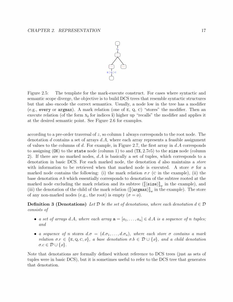
The basic intuition of the mark-execute construct is as follows: We mark a node low inthe tree with a mark relation; then higher up in the tree, we invoke it with a correspondingexecute relation (Figure 2.5). For our example in Figure 2.4(c), we mark the population
node, which puts the child argmax in a temporary store; when we execute the city node,we fetch the superlative predicate argmax from the store and invoke it.
This divergence between syntactic and semantic scope arises in other linguistic contextsbesides superlatives such as quantification and negation. In each of these cases, the generaltemplate is the same: a syntactic modifier low in the tree needs to have semantic forcehigher in the tree. A particularly compelling case of this divergence happens with quantifierscope ambiguity (e.g., Some river traverses every city.), where the quantifiers appear in fixedsyntactic positions, but the wide or narrow reading correspond to different semantically-scoped denotations. Analogously, a single syntactic structure involving superlatives can alsoyield two different semantically-scoped denotations—the absolute and relative readings (e.g.,state bordering the largest state). The mark-execute construct provides a unified frameworkfor dealing all these forms of divergence between syntactic and semantic scope. See Figure 2.6for more concrete examples.
2.5.1 Denotations
We now formalize our intuitions about the mark-execute construct by defining the deno-tations of DCS trees that use mark and execute relations. We saw that the mark-executeconstruct appears to act non-locally, putting things in a store and retrieving them out later.This means that if we want the denotation of a DCS tree to only depend on the denotationsof its subtrees, the denotations need to contain more than the set of feasible values for theroot node, as was the case for basic DCS. We need to augment denotations to include infor-mation about all marked nodes, since these are the ones that can be accessed by an executerelation higher up in the tree.
More specifically, let z be a DCS tree and d = JzKw be its denotation. The denotationd consists of n columns, where each column is either the root node of z or a non-executedmarked node in z. In the example in Figure 2.7, there are two columns, one for the rootstate node and the other for size node, which is marked by c. The columns are ordered
CHAPTER 2. REPRESENTATION 17
xixi
e | q | ce | q | c
∗∗
· · · · · ·
· · ·
∗∗
Figure 2.5: The template for the mark-execute construct. For cases where syntactic andsemantic scope diverge, the objective is to build DCS trees that resemble syntactic structuresbut that also encode the correct semantics. Usually, a node low in the tree has a modifier(e.g., every or argmax). A mark relation (one of e, q, c) “stores” the modifier. Then anexecute relation (of the form xi for indices i) higher up “recalls” the modifier and applies itat the desired semantic point. See Figure 2.6 for examples.
according to a pre-order traversal of z, so column 1 always corresponds to the root node. Thedenotation d contains a set of arrays d.A, where each array represents a feasible assignmentof values to the columns of d. For example, in Figure 2.7, the first array in d.A correspondsto assigning (OK) to the state node (column 1) to and (TX, 2.7e5) to the size node (column2). If there are no marked nodes, d.A is basically a set of tuples, which corresponds to adenotation in basic DCS. For each marked node, the denotation d also maintains a storewith information to be retrieved when that marked node is executed. A store σ for amarked node contains the following: (i) the mark relation σ.r (c in the example), (ii) thebase denotation σ.b which essentially corresponds to denotation of the subtree rooted at themarked node excluding the mark relation and its subtree (J〈size〉Kw in the example), and(iii) the denotation of the child of the mark relation (J〈argmax〉Kw in the example). The storeof any non-marked nodes (e.g., the root) is empty (σ = ø).
Definition 3 (Denotations) Let D be the set of denotations, where each denotation d ∈ Dconsists of
• a set of arrays d.A, where each array a = [a1, . . . , an] ∈ d.A is a sequence of n tuples;and
• a sequence of n stores d.σ = (d.σ1, . . . , d.σn), where each store σ contains a markrelation σ.r ∈ {e,q,c, ø}, a base denotation σ.b ∈ D ∪ {ø}, and a child denotationσ.c ∈ D ∪ {ø}.
Note that denotations are formally defined without reference to DCS trees (just as sets oftuples were in basic DCS), but it is sometimes useful to refer to the DCS tree that generatesthat denotation.

CHAPTER 2. REPRESENTATION 18
California borders which states?
x1x1
2
1
1
1
CA
ee
∗∗
state
border
∗∗Alaska borders no states.
x1x1
2
1
1
1
AK
no
state
border
∗∗Some river traverses every city.
x12x12
2
1
1
1
some
river
every
city
traverse
∗∗x21x21
2
1
1
1
some
river
every
city
traverse
∗∗
(narrow) (wide)
(a) Extraction (e) (b) Quantification (q) (c) Quantifier scope ambiguity (q,q)
city traversed by no rivers
x12x12
1
2ee
∗∗1
1
no
river
traverse
city
∗∗state bordering the most states
x12x12
1
1ee
∗∗2
1
cc
argmax
state
border
state
∗∗most populous city
x12x12
1
1ee
∗∗
cc
argmax
population
city
∗∗
(d) Quantification (q,e) (e) Superlative (c) (f) Superlative (c)
state bordering more states than Texas
x12x12
1
1ee
∗∗2
1
cc
3
1
TX
more
state
border
state
∗∗state bordering the largest state
1
1
2
1
x12x12
1
1ee
∗∗cc
argmax
size
state
∗∗
border
state
x12x12
1
1ee
∗∗2
1
1
1
cc
argmax
size
state
border
state
∗∗
(absolute) (relative)
Most states’ largest city is major.
x1x1
x2x2
1
1
1
1
2
1
most
state
loc
cc
argmax
size
city
major
∗∗
(g) Comparative (c) (h) Superlative scope ambiguity (c) (i) Quantification+Superlative (q,c)
Figure 2.6: Examples of DCS trees that use the mark-execute construct. (a) The headverb borders has a direct object states modified by which and needs to be returned. (b)The quantifier no is syntactically dominated by state but needs to take wider scope. (c)Two quantifiers yield two possible readings; we build the same basic structure, markingboth quantifiers; the choice the execute relation (x12 versus x21) determines the reading. (d)We employ two mark relations, q on river for the negation, and e on city to force thequantifier to be computed for each value of city. (e,f,g) Analogous construction but withthe c relation (for comparatives and superlatives). (h) Analog of quantifier scope ambiguityfor superlatives: the placement of the execute relation determines an absolute versus relativereading. (i) Interaction between a quantifier and a superlative.

CHAPTER 2. REPRESENTATION 19
1
1
2
1
1
1
cc
argmax
size
state
border
state
J·Kw
column 1 column 2
A:
[(OK)
[(NM)
[(NV)· · ·
(TX,2.7e5)]
(TX,2.7e5)]
(CA,1.6e5)]· · ·
r: ø c
b: ø J〈size〉Kwc: ø J〈argmax〉Kw
DCS tree Denotation
Figure 2.7: Example of the denotation for a DCS tree with a compare relation c. Thisdenotation has two columns, one for each active node—the root node state and the markednode size.
For notational convenience, we write d as 〈〈A; (r1, b1, c1); . . . ; (rn, bn, cn)〉〉. Also let d.ri =d.σi.r, d.bi = d.σi.b, and d.ci = d.σi.c. Let d{σi = x} be the denotation which is identical tod, except with d.σi = x; d{ri = x}, d{bi = x}, and d{ci = x} are defined analogously. We
also define a project operation for denotations: 〈〈A;σ〉〉[i] def= 〈〈{ai : a ∈ A};σi〉〉. Extending
this notation further, we use ø to denote the indices of the non-initial columns with emptystores (i > 1 such that d.σi = ø). We can then use d[−ø] to represent projecting away thenon-initial columns with empty stores. For the denotation d in Figure 2.7, d[1] keeps column1, d[−ø] keeps both columns, and d[2,−2] swaps the two columns.
In basic DCS, denotations are sets of tuples, which works quite well for representing thesemantics of wh-questions such as What states border Texas? But what about polar questionssuch as Does Louisiana border Texas? The denotation should be a simple boolean value,which basic DCS does not represent explicitly. Using our new denotations, we can representboolean values explicitly using zero-column structures: true corresponds to a singleton setcontaining just the empty array (dt = 〈〈{[ ]}〉〉) and false is the empty set (df = 〈〈∅〉〉).
Having described denotations as n-column structures, we now give the formal mappingfrom DCS tree to these structures. As in basic DCS, this mapping is defined recursively overthe structure of the tree. We have a recurrence for each case (the first line is the base case,

CHAPTER 2. REPRESENTATION 20
and each of the others handles a different edge relation):
J〈p〉Kw = 〈〈{[v] : v ∈ w(p)}; ø〉〉, [base case] (2.19)
J⟨p; e; jj′ :c
⟩Kw
= J〈p; e〉Kw ./−øj,j′ JcKw, [join] (2.20)
J〈p; e; Σ:c〉Kw = J〈p; e〉Kw ./−ø∗,∗ Σ (JcKw) , [aggregate] (2.21)
J〈p; e;xi :c〉Kw = J〈p; e〉Kw ./−ø∗,∗ Xi(JcKw), [execute] (2.22)
J〈p; e;e :c〉Kw = M(J〈p; e〉Kw,e, JcKw), [extract] (2.23)
J〈p; e;c :c〉Kw = M(J〈p; e〉Kw,c, JcKw), [compare] (2.24)
J〈p;q :c; e〉Kw = M(J〈p; e〉Kw,q, JcKw). [quantify] (2.25)
Note that these definitions depend on several operations (./−øj,j′ ,Σ,Xi,M), which we have not
defined yet. We will do so lazily as we walk through each of the cases.
Base Case (2.19) defines the denotation for a DCS tree z with a single node with predicatep. The denotation of z has one column whose arrays correspond to the tuples w(p); the storefor that column is empty.
2.5.2 Join Relations
(2.20) defines the recurrence for join relations. On the left-hand side,⟨p; e; jj′ :c
⟩is a DCS
tree with p at the root, a sequence of edges e followed by a final edge with relation jj′ connect
to a child DCS tree c. On the right-hand side, we take the recursively computed denotationof 〈p; e〉, the DCS tree without the final edge, and perform a join-project-inactive operation(notated ./−ø
j,j′) with the denotation of the child DCS tree c.The join-project-inactive operation joins the arrays of the two denotations (this is the
core of the join operation in basic DCS—see (2.13)), and then projects away the non-initialempty columns:
〈〈A;σ〉〉 ./−øj,j′ 〈〈A
′;σ′〉〉 = 〈〈A′′;σ + σ′〉〉[−ø],where (2.26)
A′′ = {a + a′ : a ∈ A, a′ ∈ A′, a1j = a′1j′}.
We concatenate all arrays a ∈ A with all arrays a′ ∈ A′ that satisfy the join conditiona1j = a′1j′ . The sequences of stores are simply concatenated (σ+ σ′). Finally, any non-initialcolumns with empty stores are projected away by applying ·[−ø].
Note that the join works on column 1, the other columns are carried along for the ride.As another piece of convenient notation, we use ∗ to represent all components, so that ./−ø
∗,∗would impose the join condition that the entire tuple has to agree (a1 = a′1).

CHAPTER 2. REPRESENTATION 21
1
1
2
1
ee
∗∗
state
border
state
J·Kw
column 1 column 2
A:[(FL)
[(GA)· · ·
(AL)]
(AL)]· · ·
r: ø eb: ø 〈〈{[(AL)], [(AK)], . . . }; ø〉〉c: ø ø
Σ (·)
ΣΣ
1
1
2
1
ee
∗∗
state
border
state
∗∗
J·Kw
column 1 column 2
A:[({(FL), (GA), (MS), (TN)})
[({})· · ·
(AL)]
(AK)]· · ·
r: ø eb: ø 〈〈{[(AL)], [(AK)], . . . }; ø〉〉c: ø ø
DCS tree Denotation
Figure 2.8: An example of applying the aggregate operation, which takes a denotationand aggregates the values in column 1 for every setting of the other columns. The basedenotations (b) are used to put in {} for values that do not appear in A. (in this example,AK, corresponding to the fact that Alaska does not border any states).
2.5.3 Aggregate Relations
(2.21) defines the recurrence for aggregate relations. Recall that in basic DCS, aggregate(2.16) simply takes the denotation (a set of tuples) and puts it into a set. Now, the denotationis not just a set, so we need to generalize this operation. Specifically, the aggregate operationapplied to a denotation forms a set out of the tuples in the first column for each setting ofthe rest of the columns:
Σ (〈〈A;σ〉〉) = 〈〈A′ ∪ A′′;σ〉〉, (2.27)
A′ = {[S(a), a2, . . . , an] : a ∈ A},S(a) = {a′1 : [a′1, a2, . . . , an] ∈ A},A′′ = {[∅, a2, . . . , an] : ∀i ∈ {2, . . . , n}, [ai] ∈ σi.b.A[1],¬∃a1, a ∈ A}.
The aggregate operation takes the set of arrays A and produces two sets of arrays, A′ andA′′, which are unioned (note that the stores do not change). The set A′ is the one that firstcomes to mind: For every setting of a2, . . . , an, we construct S(a), the set of tuples a′1 in thefirst column which co-occur with a2, . . . , an in A.
However, there is another case: what happens to settings of a2, . . . , an that do not co-occur with any value of a′1 in A? Then, S(a) = ∅, but note that A′ by construction will not
CHAPTER 2. REPRESENTATION 22
state J·Kw
column 1
A:[(AL)]
[(AK)]· · ·
r: øb: øc: ø
M(·,q, J〈every〉Kw)
every
state
J·Kw
column 1
A:[(AL)]
[(AK)]· · ·
r: qb: 〈〈{[(AL)], [(AK)], . . . }; ø〉〉c: J〈every〉Kw
DCS tree Denotation
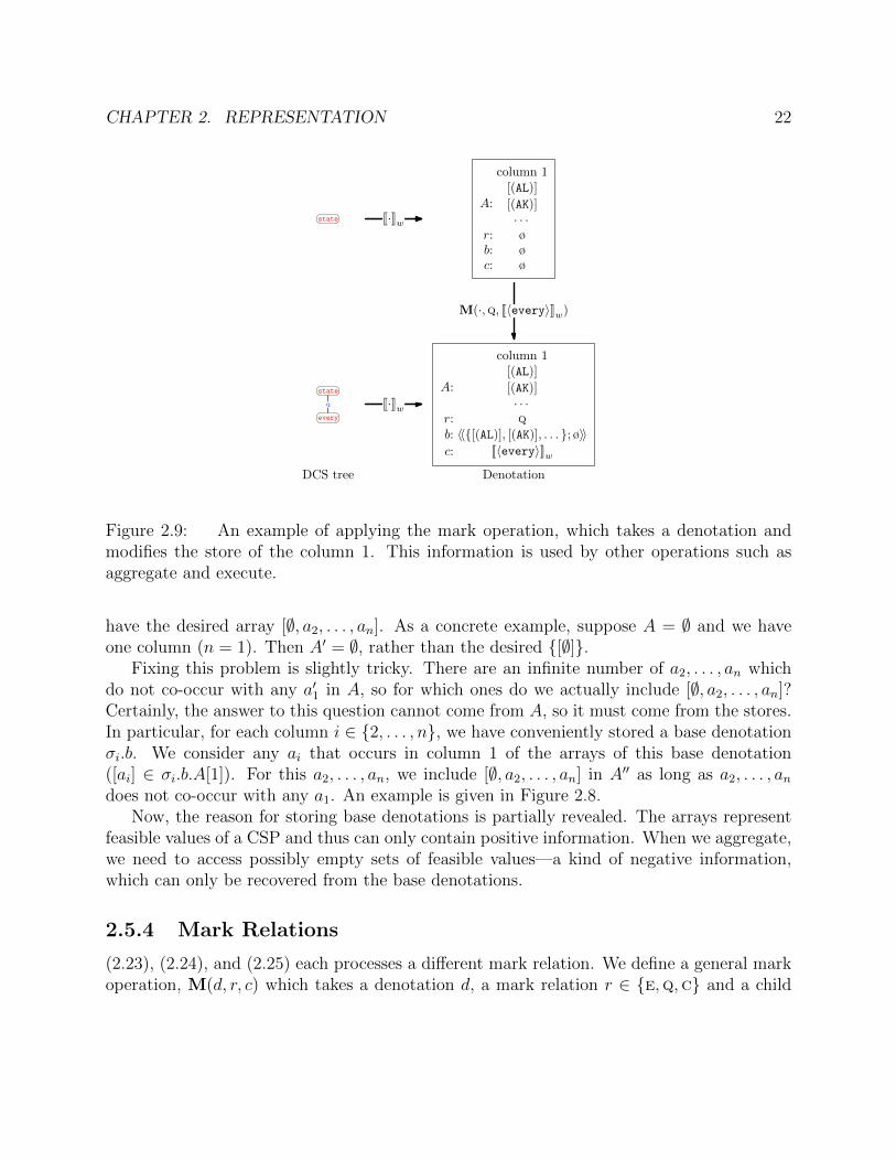
Figure 2.9: An example of applying the mark operation, which takes a denotation andmodifies the store of the column 1. This information is used by other operations such asaggregate and execute.
have the desired array [∅, a2, . . . , an]. As a concrete example, suppose A = ∅ and we haveone column (n = 1). Then A′ = ∅, rather than the desired {[∅]}.
Fixing this problem is slightly tricky. There are an infinite number of a2, . . . , an whichdo not co-occur with any a′1 in A, so for which ones do we actually include [∅, a2, . . . , an]?Certainly, the answer to this question cannot come from A, so it must come from the stores.In particular, for each column i ∈ {2, . . . , n}, we have conveniently stored a base denotationσi.b. We consider any ai that occurs in column 1 of the arrays of this base denotation([ai] ∈ σi.b.A[1]). For this a2, . . . , an, we include [∅, a2, . . . , an] in A′′ as long as a2, . . . , andoes not co-occur with any a1. An example is given in Figure 2.8.
Now, the reason for storing base denotations is partially revealed. The arrays representfeasible values of a CSP and thus can only contain positive information. When we aggregate,we need to access possibly empty sets of feasible values—a kind of negative information,which can only be recovered from the base denotations.
2.5.4 Mark Relations
(2.23), (2.24), and (2.25) each processes a different mark relation. We define a general markoperation, M(d, r, c) which takes a denotation d, a mark relation r ∈ {e,q,c} and a child

CHAPTER 2. REPRESENTATION 23
denotation c, and sets the store of d in column 1 to be (r, d, c):
M(d, r, c) = d{r1 = r, b1 = d, c1 = c}. (2.28)
The base denotation of the first column b1 is set to the current denotation d. This, in somesense, creates a snapshot of the current denotation. Figure 2.9 shows an example of themark operation.
2.5.5 Execute Relations
(2.22) defines the denotation of a DCS tree where the last edge of the root is an executerelation. Similar to the aggregate case (2.21), we recurse on the DCS tree without thelast edge (〈p; e〉) and then join it to the result of applying the execute operation Xi to thedenotation of the child (JcKw).
The execute operation Xi is the most intricate part of DCS and is what does the heavylifting. The operation is parametrized by a sequence of distinct indices i which specifies theorder in which the columns should be processed. Specifically, i indexes into the subsequenceof columns with non-empty stores. We then process this subsequence of columns in reverseorder, where processing a column means performing some operations depending on the storedrelation in that column. For example, suppose that columns 2 and 3 are the only non-emptycolumns. Then X12 processes column 3 before column 2. On the other hand, X21 processescolumn 2 before column 3. For the double quantifier example, If each column stores aquantifier example (Figure 2.6(c)), these lead to the narrow and wide readings, respectively.We will define the execute operation Xi for a single column i. There are three distinct cases,depending on the relation stored in column i:
Extraction
For a denotation d with the extract relation e in column i, executing Xi(d) involves threesteps: (i) moving column i to before column 1 (·[i,−i]), (ii) projecting away non-initial emptycolumns (·[−ø]), and (iii) removing the store (·{σ1 = ø}):
Xi(d) = d[i,−i][−ø]{σ1 = ø} if d.ri = e. (2.29)
An example is given in Figure 2.10. There are two main uses of extraction:
1. By default, the denotation of a DCS tree is the set of feasible values of the root node(which occupies column 1). To return the set of feasible values of another node, wemark that node with e. Upon execution, the feasible values of that node move intocolumn 1. See Figure 2.6(a) for an example.
2. Unmarked nodes are existentially quantified and have narrower scope than all markednodes. Therefore, we can make a node x have wider scope than another node y by

CHAPTER 2. REPRESENTATION 24
2
1
1
1
CA
ee
∗∗
state
border
J·Kw
column 1 column 2
A:
[(CA,AZ)
[(CA,NV)
[(CA,OR)
(AZ)]
(NV)]
(OR)]r: ø e
b: ø J〈state〉Kwc: ø ø
X1(·)
x1x1
2
1
1
1
CA
ee
∗∗
state
border
∗∗
J·Kw
column 1
A:
(AZ)
(NV)
(OR)r: øb: øc: ø
DCS tree Denotation
Figure 2.10: An example of applying the execute operation on column i with the extractrelation e.
marking x (with e) and executing y before x (see Figure 2.6(d,e) for examples). Theextract relation e (in fact, any mark relation) signifies that we want to control thescope of a node, and the execute relation allows us to set that scope.
Generalized Quantification
Generalized quantifiers (including negation) are predicates on two sets, a restrictor A and anuclear scope B. For example,
w(some) = {(A,B) : A ∩B > 0}, (2.30)
w(every) = {(A,B) : A ⊂ B}, (2.31)
w(no) = {(A,B) : A ∩B = ∅}, (2.32)
w(most) = {(A,B) : |A ∩B| > 1
2|A|}. (2.33)
We think of the quantifier as a modifier which always appears as the child of a q relation;the restrictor is the parent. For example, in Figure 2.6(b), no corresponds to the quantifierand state corresponds to the restrictor. The nuclear scope should be the set of all states thatAlaska borders. More generally, the nuclear scope is the set of feasible values of the restrictornode with respect to the CSP that includes all nodes between the mark and execute relations.

CHAPTER 2. REPRESENTATION 25
2
1
1
1
AK
no
state
border
J·Kw
column 1 column 2A:r: ø q
b: ø J〈state〉Kwc: ø J〈no〉Kw
X1(·)
x1x1
2
1
1
1
AK
no
state
border
∗∗
J·Kw
A: [ ]r:b:c:
DCS tree Denotation
x1x1
2
1
1
1
AK
no
state
border
∗∗
“ ”
[−1][−1]
2
1
1
1
ΣΣ
state
∗∗ΣΣ
x1x1
2
1
1
1
AK
ee
∗∗
state
border
∗∗
∗∗
no
∗∗
(a) Execute a quantify relation q (b) Execute “expands the DCS tree”
Figure 2.11: (a) An example of applying the execute operation on column i with thequantify relation q. Before executing, note that A = {} (because Alaska does not borderany states). The restrictor (A) is the set of all states, and the nuclear scope (B) is empty.Since the pair (A,B) does exists in w(no), the final denotation, is 〈〈{[ ]}〉〉 (which representstrue). (b) Although the execute operation actually works on the denotation, think of it interms of expanding the DCS tree. We introduce an extra projection relation [−1], whichprojects away the first column of the child subtree’s denotation.
The restrictor is also the set of feasible values of the restrictor node, but with respect to theCSP corresponding to the subtree rooted at that node.5
We implement generalized quantifiers as follows: Let d be a denotation and supposewe are executing column i. We first construct a denotation for the restrictor dA and adenotation for the nuclear scope dB. For the restrictor, we take the base denotation incolumn i (d.bi)—remember that the base denotation represents a snapshot of the restrictornode before the nuclear scope constraints are added. For the nuclear scope, we take thecomplete denotation d (which includes the nuclear scope constraints) and extract column i(d[i,−i][−ø]{σ1 = ø}—see (2.29)). We then construct dA and dB by applying the aggregate
5 Defined this way, we can only handle conservative quantifiers, since the nuclear scope will always be asubset of the restrictor. This design decision is inspired by DRT, where it provides a way of modeling donkeyanaphora. We are not treating anaphora in this work, but we can handle it by allowing pronouns in thenuclear scope to create anaphoric edges into nodes in the restrictor. These constraints naturally propagatethrough the nuclear scope’s CSP without affecting the restrictor.

CHAPTER 2. REPRESENTATION 26
operation to each. Finally, we join these sets with the quantifier denotation, stored in d.ci:
Xi(d) =((d.ci ./
−ø1,1 dA
)./−ø
2,1 dB)
[−1] if d.ri = q,where (2.34)
dA = Σ (d.bi) , (2.35)
dB = Σ (d[i,−i][−ø]{σ1 = ø}) . (2.36)
When there is one quantifier, think of the execute relation as performing a syntactic rewritingoperation, as shown in Figure 2.11(b). For more complex cases, we must defer to (2.34).
Figure 2.6(c) shows an example with two interacting quantifiers. The denotation of theDCS tree before execution is the same in both readings, as shown in Figure 2.12. Thequantifier scope ambiguity is resolved by the choice of execute relation: x12 gives the narrowreading, x21 gives the wide reading.
2
1
1
1
some
river
every
city
traverse
J·Kw
column 1 column 2 column 3
A:[(Hudson,NY)
[(Columbia,OR)· · ·
(Hudson)
(Columbia)· · ·
(NY)]
(OR)]· · ·
r: ø q q
b: ø J〈river〉Kw J〈state〉Kwc: ø J〈some〉Kw J〈every〉Kw
DCS tree Denotation
Figure 2.12: Denotation of Figure 2.6(c) before the execute relation is applied.
Figure 2.6(d) shows how extraction and quantification work together. First, the no
quantifier is processed for each city, which is an unprocessed marked node. Here, theextract relation is a technical trick to give city wider scope.
Comparatives and Superlatives
Comparative and superlative constructions involve comparing entities, and for this, we relyon a set S of entity-degree pairs (x, y), where x is an entity and y is a numeric degree.Recall that we can treat S as a function, which maps an entity x to the set of degrees S(x)associated with x. Note that this set can contain multiple degrees. For example, in therelative reading of state bordering the largest state, we would have a degree for the size ofeach neighboring state.
Superlatives use the argmax and argmin predicates, which are defined in Section 2.3.Comparatives use the more and less predicates: w(more) contains triples (S, x, y), where xis “more than” y as measured by S; w(less) is defined analogously:
w(more) = {(S, x, y) : maxS(x) > maxS(y)}, (2.37)
w(less) = {(S, x, y) : minS(x) < minS(y)}. (2.38)

CHAPTER 2. REPRESENTATION 27
1
1ee
∗∗2
1
1
1
cc
argmax
size
state
border
state
J·Kw
column 1 column 2
A:
[(AR)
[(LA)
[(NM)
[(OK)
[(NV)· · ·
(TX,267K)]
(TX,267K)]
(TX,267K)]
(TX,267K)]
(CA,158K)]· · ·
r: ø c
b: ø J〈size〉Kwc: ø J〈argmax〉Kw
X12(·)
x12x12
1
1ee
∗∗2
1
1
1
cc
argmax
size
state
border
state
∗∗
J·Kw
column 1
A:
[(AR)]
[(LA)]
[(NM)]
[(OK)]r: øb: øc: ø
DCS tree Denotation
x12x12
1
1ee
∗∗2
1
1
1
cc
argmax
size
state
border
state
∗∗
“ ”
1
2
1
1
ΣΣ
+2,1+2,1
2
1
x2x2
1
1ee
∗∗2
1
1
1
ee
∗∗
size
state
border
state
∗∗
∗∗
∗∗
∗∗
argmax
∗∗
(a) Execute a compare relation c (b) Execute “expands the DCS tree”
Figure 2.13: (a) Executing a compare relation c for an example superlative construction(relative reading of state bordering the largest state from Figure 2.6(h)). Before executing,column 1 contains the entity to compare, and column 2 contains the degree information,of which only the second component is relevant. After executing, the resulting denotationcontains a single column with only the entities that obtain the highest degree (in this case, thestates that border Texas) (b) For this example, think of the execute operation as expandingthe original DCS tree, although the execute operation actually works on the denotation, notthe DCS tree. The expanded DCS tree has the same denotation as the original DCS tree,and syntactically captures the essence of the execute-compare operation. Going through therelations of the expanded DCS tree from bottom to top: The x2 relation swaps columns1 and 2; the join relation keeps only the second component ((TX, 267K) becomes (267K));+2,1 concatenates columns 2 and 1 ([(267K), (AR)] becomes [(AR, 267K)]); Σ aggregates thesetuples into a set; argmax operates on this set and returns the elements.
We use the same mark relation c for both comparative and superlative constructions. Interms of the DCS tree, there are three key parts: (i) the root x, which corresponds to the

CHAPTER 2. REPRESENTATION 28
entity to be compared, (ii) the child c of a c relation, which corresponds to the comparative orsuperlative predicate, and (iii) c’s parent p, which contains the “degree information” (whichwill be described later) used for comparison. We assume that the root is marked (usuallywith a relation e). This forces us to compute a comparison degree for each value of the rootnode. In terms of the denotation d corresponding to the DCS tree prior to execution, theentity to be compared occurs in column 1 of the arrays d.A, the degree information occurs incolumn i of the arrays d.A, and the denotation of the comparative or superlative predicateitself is the child denotation at column i (d.ci).
First, we define a concatenating function +i (d), which combines the columns i of d byconcatenating the corresponding tuples of each array in d.A:
+i (〈〈A;σ〉〉) = 〈〈A′;σ′〉〉,where (2.39)
A′ = {a(1...i1)\i + [ai1 + · · ·+ ai|i| ] + a(i1...n)\i : a ∈ A}σ′ = σ(1...i1)\i + [σi1 ] + σ(i1...n)\i.
Note that the store of column i1 is kept and the others are discarded. As an example:
+2,1 (〈〈{[(1), (2), (3)], [(4), (5), (6)]};σ1, σ2, σ3〉〉) = 〈〈{[(2, 1), (3)], [(5, 4), (6)]};σ2, σ3〉〉.(2.40)
We first create a denotation d′ where column i, which contains the degree information, isextracted to column 1 (and thus column 2 corresponds to the entity to be compared). Next,we create a denotation dS whose column 1 contains a set of entity-degree pairs. There aretwo types of degree information:
1. Suppose the degree information has arity 2 (Arity(d.A[i]) = 2). This occurs, forexample, in most populous city (see Figure 2.6(f)), where column i is the population
node. In this case, we simply set the degree to the second component of populationby projection (J〈ø〉Kw ./
−ø1,2 d
′). Now columns 1 and 2 contain the degrees and entities,respectively. We concatenate columns 2 and 1 (+2,1 (·)) and aggregate to produce adenotation dS which contains the set of entity-degree pairs in column 1.
2. Suppose the degree information has arity 1 (Arity(d.A[i]) = 1). This occurs, forexample, in state bordering the most states (see Figure 2.6(e)), where column i is thelower marked state node. In this case, the degree of an entity from column 2 is thenumber of different values that column 1 can take. To compute this, aggregate the setof values (Σ (d′)) and apply the count predicate. Now with the degrees and entitiesin columns 1 and 2, respectively, we concatenate the columns and aggregate again toobtain dS.
Having constructed dS, we simply apply the comparative/superlative predicate which hasbeen patiently waiting in d.ci. Finally, the store of d’s column 1 was destroyed by the

CHAPTER 2. REPRESENTATION 29
concatenation operation +2,1 (() ·), so we must restore it with ·{σ1 = d.σ1}. The completeoperation is as follows:
Xi(d) =(J〈ø〉Kw ./
−ø1,2
(d.ci ./
−ø1,1 dS
)){σ1 = d.σ1} if d.σi = c, d.σ1 6= ø, where (2.41)
dS =
{Σ(+2,1
(J〈ø〉Kw ./
−ø1,2 d
′)) if Arity(d.A[i]) = 2
Σ(+2,1
(J〈ø〉Kw ./
−ø1,2
(J〈count〉Kw ./
−ø1,1 Σ (d′)
)))if Arity(d.A[i]) = 1,
(2.42)
d′ = d[i,−i][−ø]{σ1 = ø}. (2.43)
An example of executing the c relation is shown in Figure 2.13(a). As with executing a qrelation, for simple cases, we can think of executing a c relation as expanding a DCS tree,as shown in Figure 2.13(b).
Figure 2.6(e) and Figure 2.6(f) show examples of superlative constructions with the arity1 and arity 2 types of degree information, respectively. Figure 2.6(g) shows an example ofan comparative construction. Comparatives and superlatives both use the exact same ma-chinery, differing only in the predicate: argmax versus 〈more; 3
1 :TX〉 (more than Texas). Butboth predicates have the same template behavior: Each takes a set of entity-degree pairsand returns any entity satisfying some property. For argmax, the property is obtaining thehighest degree; for more, it is having a degree higher than a threshold. We can handle gener-alized superlatives (the five largest or the fifth largest or the 5% largest) as well by swappingin a different predicate; the execution mechanisms defined in (2.41) remain the same.
We saw that the mark-execute machinery allowed decisions regarding quantifier scope tomade in a clean and modular fashion. Superlatives also have scope ambiguities in the formof absolute versus relative readings. Consider the example in Figure 2.6(g). In the absolutereading, we first compute the superlative in a narrow scope (the largest state is Alaska),and then connect it with the rest of the phrase, resulting in the empty set (since no statesborder Alaska). In the relative reading, we consider the first state as the entity we want tocompare, and its degree is the size of a neighboring state. In this case, the lower state nodecannot be set to Alaska because there are no states bordering it. The result is therefore anystate that borders Texas (the largest state that does have neighbors). The two DCS treesin Figure 2.6(g) show that we can naturally account for this form of superlative ambiguitybased on where the scope-determining execute relation is placed without drastically changingthe underlying tree structure.
Remarks All these issues are not specific to DCS; every serious semantic formalism mustaddress them as well. Not surprisingly then, the mark-execute construct bears some resem-blance to other mechanisms that operate on categorial grammar and lambda calculus, suchas quantifier raising, Montague’s quantifying in, Cooper storage, and Carpenter’s scopingconstructor (Carpenter, 1998). Very broadly speaking, these mechanisms delay applicationof the divergent element (usually a quantifier), “marking” its spot with a dummy pronoun(as in Montague’s quantifying in) or in a store (as in Cooper storage), and then “executing”

CHAPTER 2. REPRESENTATION 30
the quantifier at a later point in the derivation. One subtle but important difference betweenmark-execute in DCS and the others is that a DCS tree (which contains the mark and exe-cute relations) is the final logical form, and all the action happens in the computing of thedenotation of this logical form. In more traditional approaches, the action happens in theconstruction mechanism for building the logical form; the actually logical form produced atthe end of the day is quite simple. In other words, we have pushed the inevitable complexityfrom the construction mechanism into the semantics of the logical from. This refactoringis important because we want our construction mechanism to focus not on linguistic issues,but on purely computational and statistical ones, which ultimately determine the success ofour system.
2.6 Construction Mechanism
We have thus far defined the syntax (Section 2.2) and semantics (Section 2.5) of DCS trees,but we have only vaguely hinted at how these DCS trees might be connected to naturallanguage utterances by appealing to idealized examples. In this section, we formally definethe construction mechanism for DCS, which takes an utterance x and produces a set of DCStrees ZL(x).
Since we motivated DCS trees based on dependency syntax, it might be tempting to takea dependency parse tree of the utterance, replace the words with predicates, and attach somerelations on the edges to produce a DCS tree. To a first-order approximation, this is whatwe will do, but we need to be a bit more flexible for several reasons: (i) some nodes in theDCS tree do not have predicates (e.g., children of a e relation or parent of an xi relation);(ii) nodes have predicates that do not correspond to words (e.g., in California cities, thereis a implicit loc predicate that bridges CA and city); (iii) some words might not correspondto any predicates in our world (e.g., please); and (iv) the DCS tree might not always bealigned with the syntactic structure depending on which syntactic formalism one ascribesto. While syntax was the inspiration for the DCS formalism, we will not actually use it inconstruction.
It is also worth stressing the purpose of the construction mechanism. In linguistics, thepurpose of the construction mechanism is to try to generate the exact set of valid logicalforms for a sentence. We view the construction mechanism instead as simply a way ofcreating a set of candidate logical forms. A separate step defines a distribution over thisset to favor certain logical forms over others. The construction mechanism should thereforeoverapproximate the set of logical forms. Settling for an overapproximation allows us tosimplify the construction mechanism.
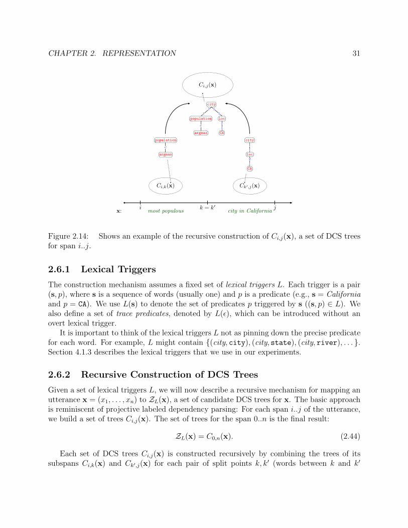
CHAPTER 2. REPRESENTATION 31
x: most populous city in Californiai jk = k′
Ci,k(x) Ck′,j(x)
cc
argmax
population1
1
2
1
CA
loc
city
1
1
1
1
cc
argmax
population2
1
CA
loc
city
Ci,j(x)
Figure 2.14: Shows an example of the recursive construction of Ci,j(x), a set of DCS treesfor span i..j.
2.6.1 Lexical Triggers
The construction mechanism assumes a fixed set of lexical triggers L. Each trigger is a pair(s, p), where s is a sequence of words (usually one) and p is a predicate (e.g., s = Californiaand p = CA). We use L(s) to denote the set of predicates p triggered by s ((s, p) ∈ L). Wealso define a set of trace predicates, denoted by L(ε), which can be introduced without anovert lexical trigger.
It is important to think of the lexical triggers L not as pinning down the precise predicatefor each word. For example, L might contain {(city, city), (city, state), (city, river), . . . }.Section 4.1.3 describes the lexical triggers that we use in our experiments.
2.6.2 Recursive Construction of DCS Trees
Given a set of lexical triggers L, we will now describe a recursive mechanism for mapping anutterance x = (x1, . . . , xn) to ZL(x), a set of candidate DCS trees for x. The basic approachis reminiscent of projective labeled dependency parsing: For each span i..j of the utterance,we build a set of trees Ci,j(x). The set of trees for the span 0..n is the final result:
ZL(x) = C0,n(x). (2.44)
Each set of DCS trees Ci,j(x) is constructed recursively by combining the trees of itssubspans Ci,k(x) and Ck′,j(x) for each pair of split points k, k′ (words between k and k′

CHAPTER 2. REPRESENTATION 32
are ignored). These combinations are then augmented via a function A and filtered via afunction F ; these functions will be specified later. Formally, Ci,j(x) is defined recursively asfollows:
Ci,j(x) = F(A({〈p〉i..j : p ∈ L(xi+1..j)} ∪
⋃i≤k≤k′<ja∈Ci,k(x)b∈Ck′,j(x)
T2(a, b)))). (2.45)
This recurrence has two parts:
• The base case: we take the phrase (sequence of words) over span i..j and look up theset of predicates p in the set of lexical triggers. For each predicate, we construct aone-node DCS tree. We also extend the definition of DCS trees in Section 2.2 to alloweach node to store the indices of the span i..j that triggered the predicate at that node;this is denoted by 〈p〉i..j. This span information will be useful in Section 3.1.1, wherewe will need to talk about how an utterance x is aligned with a DCS tree z.
• The recursive case: T1(a, b), which we will define shortly, that takes two DCS trees, aand b, and returns a set of new DCS trees formed by combining a and b. Figure 2.14shows this recurrence graphically.
We now focus on how to combine two DCS trees. Define Td(a, b) as the set of resultingDCS trees by making either a or b the root and connecting the other via a chain of relationsand at most d− 1 trace predicates:
Td(a, b) = T↘d (a, b) ∪ T↙d (b, a), (2.46)
Here, T↘d (a, b) is the set of DCS trees where a is the root; for T↙d (a, b), b is the root. Theformer is defined recursively as follows:
T↘0 (a, b) = ∅, (2.47)
T↘d (a, b) =⋃r∈Rp∈L(ε)
{〈a; r :b〉 , 〈a; r :〈Σ:b〉〉} ∪ T↘d−1(a, 〈p; r :b〉).
First, we consider all possible relations r ∈ R and try putting r between a and b (〈a; r :b〉),possibly with an additional aggregate relation (〈a; r :〈Σ:b〉〉). Of course, R contains an infi-nite number of join and execute relations, but only a small finite number of them make sense:we consider join relations j
j′ only for j ∈ {1, . . . ,Arity(a.p)} and j′ ∈ {1, . . . ,Arity(b.p)},and execute relations xi for which i does not contain indices larger than the number ofcolumns of JbKw. Next, we further consider all possible trace predicates p ∈ L(ε), and re-cursively try to connect a with the intermediate 〈p; r :b〉, now allowing d − 1 additionalpredicates. See Figure 2.15 for an example. In the other direction, T↙d is defined similarly:

CHAPTER 2. REPRESENTATION 33
a = city
b = state
T↘1 (a, b)
1
1
state
city1
1
ΣΣ
state
∗∗
city
state
city1
1
2
1
state
loc
city1
2
1
1
state
loc
city1
1
2
1
state
border
city · · ·
T↙1 (a, b)
1
1
city
state1
1
ΣΣ
city
∗∗
state
city
state1
1
2
1
city
loc
state1
2
1
1
city
loc
state1
1
2
1
city
border
state · · ·
Figure 2.15: Given two DCS trees, a and b, T↘1 (a, b) and T↙1 (a, b) are the two sets of DCStrees formed by combining a and b with a at the root and b at the root, respectively; onetrace predicate can be inserted in between. In this example, the DCS trees which survivefiltering (Section 2.6.3) are shown.
T↙0 (a, b) = ∅, (2.48)
T↙d (a, b) =⋃r∈Rp∈L(ε)
{〈b.p; r :a; b.e〉 , 〈b.p; r :〈Σ:a〉 ; b.e〉} ∪ T↘d−1(a, 〈p; r :b〉).
Inserting trace predicates allows us to build logical forms with more predicates than whatis explicitly triggered by the words. This ability is useful for several reasons. Sometimes,there actually is a predicate not overtly expressed, especially in noun compounds (e.g.,California cities). For semantically light words such as prepositions (e.g., for) it is difficultto enumerate all the possible predicates that it might trigger; it is computationally simplerto try to insert trace predicates. We can even omit lexical triggers for transitive verbs suchas border because the corresponding predicate border can be just inserted as trace predicate.
The function T1(a, b) connects two DCS trees via a path of relations and trace predicates.The augmentation function A adds additional relations (specifically, e and/or xi) on a singleDCS tree:
A(Z) =⋃z∈Zxi∈R
{z, 〈z;e :〈ø〉〉 , 〈xi :z〉 , 〈xi :〈z;e :〈ø〉〉〉}, (2.49)
2.6.3 Filtering using Abstract Interpretation
The current construction procedure is extremely permissive and generates many DCS treeswhich are obviously wrong—for example, 〈state; 1
1 :〈>; 21 〈3〉〉〉, which tries to compare a state
with the number 3. There is nothing syntactically wrong this expression: its denotation willsimply be empty (with respect to the world). But semantically, this DCS tree is anomalous.

CHAPTER 2. REPRESENTATION 34
We cannot simply just discard DCS trees with empty denotations, because we wouldincorrectly rule out 〈state; 1
1 :〈border; 21 〈AK〉〉〉. The difference here is that even though the
denotation is empty in this world, it is possible that it might not be empty in a different worldwhere history and geology took another turn, whereas it is simply impossible to comparecities and numbers.
Now let us quickly flesh out this intuition before falling into a philosophical discussionabout possible worlds. Given a world w, we define an abstract world α(w), to be describedshortly. We compute the denotation of a DCS tree z with respect to this abstract world. Ifat any point in the computation we create an empty denotation, we judge z to be impossibleand throw it away. The filtering function F is defined as follows:6
F (Z) = {z ∈ Z : ∀z′ subtree of z , Jz′Kα(w).A 6= ∅}. (2.50)
Now we need to define the abstract world α(w). The intuition is to map concrete valuesto abstract values: 3 : length becomes length, Oregon : state becomes ∗ : state, and ingeneral, primitive value x : t becomes ∗ : t. We perform abstraction on tuples componentwise,so that (Oregon : state, 3 : length) becomes (∗ : state, ∗ : length). Our abstraction of setsis slightly more complex: the empty set maps to the empty set, a set containing values allwith the same abstract value a maps to {a}, and a set containing values with more thanone abstract value maps to a {mixed}. Finally, a world maps each predicate onto a setof (concrete) tuples; the corresponding abstract world maps each predicate onto the set ofabstract tuples. Formally, the abstraction function is defined as follows:
α(x : t) = ∗ : t, [primitive values] (2.51)
α((v1, . . . , vn)) = (α(v1), . . . , α(vn)), [tuples] (2.52)
α(A) =
∅ if A = ∅,{α(x) : x ∈ A} if |{α(x) : x ∈ A}| = 1,
{mixed} otherwise.
[sets] (2.53)
α(w) = λp.{α(x) : x ∈ w(p)}. [worlds] (2.54)
As an example, the abstract world might look like this:
α(w)(>) = {(∗ :number, ∗ :number, ∗ :number), (∗ :length, ∗ :length, ∗ :length), . . . },(2.55)
α(w)(state) = {(∗ :state)}, (2.56)
α(w)(AK) = {(∗ :state)}, (2.57)
α(w)(border) = {(∗ :state, ∗ :state)}. (2.58)
6 To further reduce the search space, F imposes a few additional constraints, e.g., limiting the numberof columns to 2, and only allowing trace predicates between arity 1 predicates.

CHAPTER 2. REPRESENTATION 35
Example: states that border Texas
λx.state(x) ∧ border(x, TX)
λx.state(x)
states
λf.λx.f(x) ∧ border(x, TX)
λg.λf.λx.f(x) ∧ g(x)
that
λx.border(x, TX)
λy.λx.border(x, y)
border
TX
Texas
>
>
<
state
states that border
TX
Texas
border
1
1
2
1
(a) CCG construction (b) DCS construction
Figure 2.16: Comparison between the construction mechanisms of CCG and DCS. Thereare three principal differences: First, in CCG, words are mapped onto a lambda calculus ex-pression; in DCS, words are just mapped onto a predicate. Second, in CCG, lambda calculusexpressions are built by combining (e.g., via function application) two smaller expressions;in DCS, trees are combined by inserting relations (and possibly other predicates betweenthem). Third, in CCG, all words map to a logical expression; in DCS, only a small subset ofwords (e.g., state and Texas) map to predicates; the rest participate in features for scoringDCS trees.
Now returning our motivating example at the beginning of this section, we see that the badDCS tree has an empty abstract denotation J〈state; 1
1 :〈>; 21 〈3〉〉〉Kα(w) = 〈〈∅; ø〉〉. The good
DCS tree has an non-empty abstract denotation: J〈state; 11 :〈border; 2
1 〈AK〉〉〉Kα(w) = 〈〈{(∗ :state)}; ø〉〉, as desired.
Remarks Computing denotations on an abstract world is called abstract interpretation(Cousot and Cousot, 1977) and is very powerful framework commonly used in the program-ming languages community. The idea is to obtain information about a program (in our case,a DCS tree) without running it concretely, but rather just by running it abstractly. It isclosely related to type systems, but the type of abstractions one uses is often much richerthan standard type systems.
2.6.4 Comparison with CCG
We now compare our construction mechanism with CCG (see Figure 2.16 for an example).The main difference is that our lexical triggers contain less information than a lexicon in aCCG. In CCG, the lexicon would have an entry such as
major ` n/n : λf.λx.major(x) ∧ f(x), (2.59)

CHAPTER 2. REPRESENTATION 36
which gives detailed information about how this word should interact with its context. How-ever, in DCS construction, each lexical trigger only has the minimal amount of information:
major ` major. (2.60)
A lexical trigger specifies a pre-theoretic “meaning” of a word which does not commit to anyformalisms. One advantage of this minimality is that lexical triggers could be easily obtainedfrom non-expert supervision: One would only have to associate words with database tablenames (predicates).
In some sense, the DCS construction mechanism pushes the complexity out of the lex-icon. In linguistics, this complexity usually would end up in the grammar, which wouldbe undesirable. However, we do not have to fight this tradeoff, because the constructionmechanism only produces an overapproximation, which means it is possible to have both asimple “lexicon” and a simple “grammar.”
There is an important but subtle rationale for this design decision. During learning, wenever just have one clean lexical entry per word (as is typically assumed in formal linguistics).Rather, there are often many possible lexical entries (and to handle disfluent utterances orutterances in free word-order languages, we might actually need many of them (Kwiatkowskiet al., 2010, 2011)):
major ` n : λx.major(x) (2.61)
major ` n/n : λf.λx.major(x) ∧ f(x) (2.62)
major ` n\n : λf.λx.major(x) ∧ f(x) (2.63)
. . . (2.64)
Now think of a DCS lexical trigger major ` major as simply a compact representation for aset of CCG lexical entries. Furthermore, the choice of the lexical entry is made not at theinitial lexical base case, but rather during the recursive construction by inserting relationsbetween DCS subtrees. It is exactly at this point that the choice can be made, becauseafter all, the choice is one that depends on context. The general principle is to compactlyrepresent the indeterminacy until one can resolve it.
Type raising is a combinator in CCG that turns one logical form into another. It canbe used to turn one entity into related entity (a kind of generalized metonymy). For example,Zettlemoyer and Collins (2007) used it to allow conversion from Boston to λx.from(x, Boston).Type raising in CCG is analogous to inserting trace predicates in DCS, but there is an im-portant distinction: Type raising is a unary operation and thus is somewhat unconstrainedbecause it changes logical forms into new ones without regard for how they will interact withthe context. Inserting trace predicates is a binary operation which is constrained by the twopredicates that it is mediating. In the example, from would only be inserted to combineBoston with flight. This is another instance of the general principle of delaying uncertaindecisions until there is more information.

37
Chapter 3
Learning
In Chapter 2, we defined DCS trees and a construction mechanism for producing a set ofcandidate DCS trees given an utterance. We now define a probability distribution over thatset (Section 3.1) and an algorithm for estimating the parameters (Section 3.2). The numberof candidate DCS trees grows exponentially, so we use beam search to control this growth.The final learning algorithm alternates between beam search and optimizing the parameters,leading to a natural bootstrapping procedure which integrates learning and search.
3.1 Semantic Parsing Model
The semantic parsing model specifies a conditional distribution over a set of candidate DCStrees C(x) given an utterance x. This distribution depends on a function φ(x, z) ∈ Rd,which takes a (x, z) pair and extracts a set of local features (see Section 3.1.1 for a fullspecification). Associated with this feature vector is a parameter vector θ ∈ Rd. Theinner product between the two vectors φ(x, z)>θ yields a numerical score, which intuitivelymeasures the compatibility of the utterance x with the DCS tree z. We exponentiate thescore and normalize over C(x) to obtain a proper probability distribution:
p(z | x;C, θ) = exp{φ(x, z)>θ − A(θ; x, C)}, (3.1)
A(θ; x, C) = log∑z∈C(x)
exp{φ(x, z)>θ}. (3.2)
Here, A(θ; x, C) is the log-partition function with respect to the candidate set function C(x).
3.1.1 Features
We now define the feature vector φ(x, z) ∈ Rd, the core part of the semantic parsing model.Each component j = 1, . . . , d of this vector is a feature, and φ(x, z)j is the number oftimes that feature occurs in (x, z). Rather than working with indices, we treat features as

CHAPTER 3. LEARNING 38
symbols (e.g., TriggerPred[states, state]). Each feature captures some property about(x, z) which abstracts away from the details of the specific instance and allow us to generalizeto new instances that share common features.
The features are organized into feature templates, where each feature template instan-tiates a set of features. Figure 3.1 shows all the feature templates for a concrete example.The feature templates are as follows:
• PredHit contains the single feature PredHit, which fires for each predicate in z.
• Pred contains features {Pred[α(p)] : p ∈ P}, each of which fires on α(p), the ab-straction of predicate p, where
α(p) =
{∗ : t if p = x : t
p otherwise.(3.3)
The purpose of the abstraction is to abstract away the details of concrete values suchas TX = Texas :state.
• PredRel contains features {PredRel[α(p),q] : p ∈ P ,q ∈ ({↙,↘} × R)∗}. Afeature fires when a node x has predicate p and is connected via some path q =(d1, r1), . . . , (dm, rm) to the lowest descendant node y with the property that each nodebetween x and y has a null predicate. Each (d, r) on the path represents an edgelabeled with relation r connecting to a left (d =↙) or right (d =↘) child. If x has nochildren, then m = 0. The most common case is when m = 1, but m = 2 also occurswith the aggregate and execute relations (e.g., PredRel[count,↘ 1
1 ↘ Σ] fires forFigure 2.3(a)).
• PredRelPred contains features {PredRelPred[α(p),q, α(p′)] : p, p′ ∈ P ,q ∈ ({↙,↘}×R)∗}, which are the same as PredRel, except that we include both the pred-icate p of x and the predicate p′ of the descendant node y. These features do not fireif m = 0.
• TriggerPred contains features {TriggerPred[s, p] : s ∈ W ∗, p ∈ P}, where W ={it,Texas, . . . } is the set of words. Each of these features fires when a span of theutterance with words s triggers the predicate p—more precisely, when a subtree 〈p; e〉i..jexists with s = xi+1..j. Note that these lexicalized features use the predicate p ratherthan the abstracted version α(p).
• TracePred contains features {TracePred[s, p, d] : s ∈ W ∗, p ∈ P , d ∈ {↙,↘}},each of which fires when a trace predicate p has been inserted over a word s. Thesituation is the following: Suppose we have a subtree a that ends at position k (thereis a predicate in a that is triggered by a phrase with right endpoint k) and anothersubtree b that begins at k′. Recall that in the construction mechanism (2.46), we
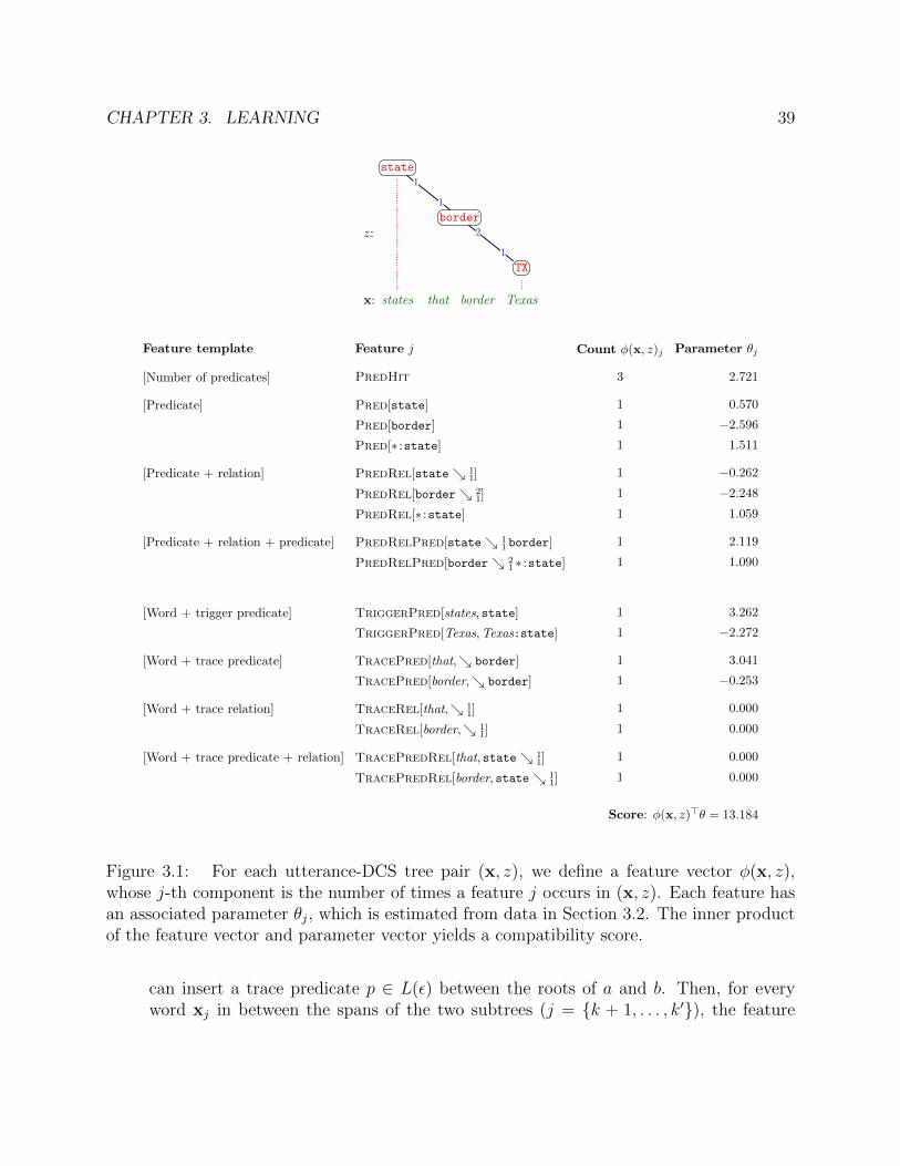
CHAPTER 3. LEARNING 39
z:
x:
state
states that border
TX
Texas
border
1
1
2
1
Feature template Feature j Count φ(x, z)j Parameter θj
[Number of predicates] PredHit 3 2.721
[Predicate] Pred[state] 1 0.570
Pred[border] 1 −2.596Pred[∗ :state] 1 1.511
[Predicate + relation] PredRel[state↘ 11] 1 −0.262
PredRel[border↘ 21] 1 −2.248
PredRel[∗ :state] 1 1.059
[Predicate + relation + predicate] PredRelPred[state↘ 11 border] 1 2.119
PredRelPred[border↘ 21 ∗ :state] 1 1.090
[Word + trigger predicate] TriggerPred[states, state] 1 3.262
TriggerPred[Texas,Texas:state] 1 −2.272
[Word + trace predicate] TracePred[that,↘ border] 1 3.041
TracePred[border,↘ border] 1 −0.253
[Word + trace relation] TraceRel[that,↘ 11] 1 0.000
TraceRel[border,↘ 11] 1 0.000
[Word + trace predicate + relation] TracePredRel[that, state↘ 11] 1 0.000
TracePredRel[border, state↘ 11] 1 0.000
Score: φ(x, z)>θ = 13.184
Figure 3.1: For each utterance-DCS tree pair (x, z), we define a feature vector φ(x, z),whose j-th component is the number of times a feature j occurs in (x, z). Each feature hasan associated parameter θj, which is estimated from data in Section 3.2. The inner productof the feature vector and parameter vector yields a compatibility score.
can insert a trace predicate p ∈ L(ε) between the roots of a and b. Then, for everyword xj in between the spans of the two subtrees (j = {k + 1, . . . , k′}), the feature

CHAPTER 3. LEARNING 40
TracePred[xj, p, d] fires (d =↙ if b dominates a and d =↘ if a dominates b).
• TraceRel contains features {TraceRel[s, d, r] : s ∈ W ∗, d ∈ {↙,↘}, r ∈ R}, eachof which fires when some trace predicate with parent relation r has been inserted overa word s.
• TracePredRel contains features {TracePredRel[s, p, d, r] : s ∈ W ∗, p ∈ P , d ∈{↙,↘}, r ∈ R}, each of which fires when a predicate p is connected via child relationr to some trace predicate over a word s.
These features are simple generic patterns which can be applied for modeling essentiallyany distribution over sequences and labeled trees—there is nothing specific to DCS at all.The first half of the feature templates (PredHit, Pred, PredRel, PredRelPred) cap-ture properties of the tree independent of the utterance, and are similar to ones used forsyntactic dependency parsing. The other feature templates (TriggerPred, TracePred,TraceRel, TracePredRel) connect predicates in the DCS tree with words in the utter-ance, similar to those in a model of machine translation.
3.2 Parameter Estimation
We have now fully specified the details of the graphical model in Figure 1.2: Section 3.1described semantic parsing and Chapter 2 described semantic evaluation. Next, we focus onestimating the parameters θ of the model from data.
3.2.1 Objective Function
We assume that our learning algorithm is given a training dataset D containing question-answer pairs (x, y). Because the logical forms are unobserved, we work with log p(y | x;C, θ),the marginal log-likelihood of obtaining the correct answer y given an utterance x. Thismarginal log-likelihood sums over all z ∈ C(x) that evaluate to y:
log p(y | x;C, θ) = log p(z ∈ Cy(x) | x;C, θ) (3.4)
= A(θ; x, Cy)− A(θ,x, C), where (3.5)
Cy(x)def= {z ∈ C(x) : JzKw = y}. (3.6)
Here, Cy(x) is the set of DCS trees z with denotation y.We call an example (x, y) ∈ D feasible if the candidate set of x contains a DCS tree that
evaluates to y (Cy(x) 6= ∅). Define an objective function O(θ, C) containing two terms: Thefirst term is the sum of the marginal log-likelihood over all feasible training examples. The
CHAPTER 3. LEARNING 41
second term is a quadratic penalty on the parameters θ with regularization parameter λ.Formally:
O(θ, C)def=
∑(x,y)∈DCy(x)6=∅
log p(y | x;C, θ)− λ
2‖θ‖2
2 (3.7)
=∑
(x,y)∈DCy(x)6=∅
(A(θ; x, Cy)− A(θ; x, C))− λ
2‖θ‖2
2.
We would like to maximize O(θ, C). The log-partition function A(θ; ·, ·) is convex, butO(θ, C) is the difference of two log-partition functions and hence is not concave (nor con-vex). Our plan is to use gradient-based optimization to hill climb the objective anyway. Astandard result is that the derivative of the log-partition function is the expected featurevector (Wainwright and Jordan, 2008). Using this, we obtain the gradient of our objectivefunction:
∂O(θ, C)
∂θ=
∑(x,y)∈DCy(x)6=∅
(Ep(z|x;Cy ,θ)[φ(x, z)]− Ep(z|x;C,θ)[φ(x, z)]
)− λθ. (3.8)
Updating the parameters in the direction of the gradient would move the parameters towardsthe DCS trees that yield the correct answer (Cy) and away from over all candidate DCS trees(C). We can use any standard numerical optimization algorithm that requires only black-box access to a gradient. Section 4.3.4 will discuss the empirical ramifications the choice ofoptimization algorithm.
3.2.2 Algorithm
Given a candidate set function C(x), we can optimize (3.7) to obtain parameters θ. Ideally,we would use C(x) = ZL(x), the candidate sets from our construction mechanism in Sec-tion 2.6, but we quickly run into the problem of computing (3.8) efficiently. Note that ZL(x)(defined in (2.44)) grows exponentially with the length of x. This by itself is not a show stop-per. Our features (Section 3.1.1) actually decompose along the edges of the DCS tree, so it ispossible to use dynamic programming1 to compute the second expectation Ep(z|x;ZL,θ)[φ(x, z)]of (3.8). The problem is computing the first expectation Ep(z|x;ZyL,θ)[φ(x, z)], which sums overthe subset of candidate DCS trees z satisfying the constraint JzKw = y. Though this is asmaller set, there is no efficient dynamic program for this set since the constraint does notdecompose along the structure of the DCS tree. Therefore, we need to approximate ZyL, andin fact, we will approximate ZL as well so that the two expectations in (3.8) are coherent.
1 The state of the dynamic program would be the span i..j and the head predicate over that span.

CHAPTER 3. LEARNING 42
Learning Algorithm
Initialize: θ(0) ← (0, . . . , 0)For each iteration t = 1, . . . , T :−Update candidate sets: C(t)(x)← ZL,θ(t−1)(x)
−Update parameters: θ(t) ← argmaxθO(θ, C(t))Return θ(T )
Figure 3.2: The learning algorithm alternates between updating the candidate sets basedon beam search and updating the parameters using standard numerical optimization.
Recall that ZL(x) was built by recursively constructing a set of DCS trees Ci,j(x) for eachspan i..j. In our approximation, we simply use beam search, which truncates each Ci,j(x)to include the (at most) K DCS trees with the highest score φ(x, z)>θ. We let Ci,j,θ(x)denote this approximation and define the set of candidate DCS trees with respect to thebeam search:
ZL,θ(x) = C0,n,θ(x). (3.9)
We now have a chicken-and-egg problem: If we had good parameters θ, we could generategood candidate sets C(x) using beam search ZL,θ(x). If we had good candidate sets C(x),we could generate good parameters by optimizing our objective O(θ, C) in (3.7). Thisproblem leads to a natural solution: simply alternate between the two steps (Figure 3.2).This procedure is not theoretically guaranteed to converge due to the heuristic nature of thebeam search, but we found it to be effective in practice.
Lastly, we use the trained model with parameters θ to answer new questions x by choosingthe most likely answer y, summing out the latent logical form z:
Fθ(x)def= argmax
yp(y | x; θ, ZL,θ) (3.10)
= argmaxy
∑z∈ZL,θ(x)
JzKw=y
p(z | x; θ, ZL,θ). (3.11)
43
Chapter 4
Experiments
We have now completed the conceptual part of this thesis—using DCS trees to representlogical forms (Chapter 2), and learning a probabilistic model over them (Chapter 3). In thissection, we evaluate and study our approach empirically. Our main result is that our systemobtains higher accuracies than existing systems, despite requiring no annotated logical forms.
4.1 Experimental Setup
We first describe the datasets (Section 4.1.1) that we use to train and evaluate our system.We then mention various choices in the model and learning algorithm (Section 4.1.2). Oneof these choices is the lexical triggers, which is further discussed in Section 4.1.3.
4.1.1 Datasets
We tested our methods on two standard datasets, referred to in this thesis as Geo and Jobs.These datasets were created by Ray Mooney’s group during the 1990s and have been usedto evaluate semantic parsers for over a decade.
US Geography The Geo dataset, originally created by Zelle and Mooney (1996), contains880 questions about US Geography and a database of facts encoded in Prolog. The questionsin Geo ask about general properties (e.g., area, elevation, population) of geographical entities(e.g., cities, states, rivers, mountains). Across all the questions, there are 280 word types,and the length of an utterance ranges from 4 to 19 words, with an average of 8.5 words. Thequestions involve conjunctions, superlatives, negation, but no generalized quantification.Each question is annotated with a logical form in Prolog, for example:
Utterance: What is the highest point in Florida?Logical form: answer(A,highest(A,(place(A),loc(A,B),const(B,stateid(florida)))))

CHAPTER 4. EXPERIMENTS 44
Since our approach learns from answers, not logical forms, we evaluated the annotatedlogical forms on the provided database to obtain the correct answers.
Recall that a world/database w maps each predicate p ∈ P to a set of tuples w(p). Somepredicates contain the set of tuples explicitly (e.g., mountain); others can be derived (e.g.,higher takes two entities x and y and returns true if elevation(x) > elevation(y)). Otherpredicates are higher-order (e.g., sum, highest) in that they take other predicates as argu-ments. We do not use the provided domain-specific higher-order predicates (e.g., highest),but rather provide domain-independent higher-order predicates (e.g., argmax) and the ordi-nary domain-specific predicates (e.g., elevation). This provides more compositionality andtherefore better generalization. Similarly, we use more and elevation instead of higher.Altogether, P contains 43 predicates plus one predicate for each value (e.g., CA).
Job Queries The Jobs dataset (Tang and Mooney, 2001) contains 640 natural languagequeries about job postings. Most of the questions ask for jobs matching various criteria: jobtitle, company, recruiter, location, salary, languages and platforms used, areas of expertise,required/desired degrees, and required/desired years of experience. Across all utterances,there are 388 word types, and the length of an utterance ranges from 2 to 23 words, withan average of 9.8 words. The utterances are mostly based on conjunctions of criteria, witha sprinkling of negation and disjunction. Here is an example:
Utterance: Are there any jobs using Java that are not with IBM?Logical form: answer(A,(job(A),language(A,’java’),¬company(A,’IBM’)))
The Jobs dataset comes with a database, which we can use as the world w. However,when the logical forms are evaluated on this database, close to half of the answers are empty(no jobs match the requested criteria). Therefore, there is a large discrepancy betweenobtaining the correct logical form (which has been the focus of most work on semanticparsing) and obtaining the correct answer (our focus).
To bring these two into better alignment, we generated a random database as follows: Wecreated m = 100 jobs. For each job j, we go through each predicate p (e.g., company) thattakes two arguments, a job and a target value. For each of the possible target values v, weadd (j, v) to w(p) independently with probability α = 0.8. For example, for p = company,j = job37, we might add (job37, IBM) to w(company). The result is a database with atotal of 23 predicates (which includes the domain-independent ones) in addition to the valuepredicates (e.g., IBM).
The goal of using randomness is to ensure that two different logical forms will most likelyyield different answers. For example, consider two logical forms:
z1 = λj.job(j) ∧ company(j, IBM), (4.1)
z2 = λj.job(j) ∧ language(j, Java). (4.2)
Under the random construction, The denotation of z1 is S1, an random subset of the jobs,where each job is included in S1 independently with probability α, and the denotation

CHAPTER 4. EXPERIMENTS 45
of z2 is S2, which has the same distribution as S1 but importantly is independent of S1.Therefore, the probability that S1 = S2 is [α2 + (1− α)2]m, which is exponentially small inm. This construction yields a world that is not entirely “realistic” (a job might have multipleemployers), but it ensures that if we get the correct answer, we probably also obtain thecorrect logical form.
4.1.2 Settings
There are a number of settings which control the tradeoffs between computation, expres-siveness, and generalization power of our model, shown below. For now, we will use genericsettings chosen rather crudely; Section 4.3.4 will explore the effect of changing these settings.
Lexical Triggers The lexical triggers L (Section 2.6.1) define the set of candidate DCStrees for each utterance. There is a tradeoff between expressiveness and computationalcomplexity: The more triggers we have, the more DCS trees we can consider for a givenutterance, but then either the candidate sets become too large or beam search startsdropping the good DCS trees. Choosing lexical triggers is important and requiresadditional supervision (Section 4.1.3).
Features Our probabilistic semantic parsing model is defined in terms of feature templates(Section 3.1.1). Richer features increase expressiveness but also might lead to overfit-ting. By default, we include all the feature templates.
Number of training examples (n) An important property of any learning algorithm isits sample complexity—how many training examples are required to obtain a certainlevel of accuracy? By default, all training examples are used.
Number of training iterations (T ) Our learning algorithm (Figure 3.2) alternates be-tween updating candidate sets and update parameters for T iterations. We use T = 5as the default value.
Beam size (K) The computation of the candidate sets in Figure 3.2 is based on beamsearch where each intermediate state keeps at most K DCS trees. The default value isK = 100.
Optimization algorithm Updating the parameters in Figure 3.2 involves optimizing anthe objective function O(θ, C). The optimization algorithm determines both the speedof convergence and the quality of the converged solution. By default, we use the stan-dard L-BFGS algorithm (Nocedal, 1980) with a backtracking line search for choosingthe step size.
Regularization (λ) The regularization parameter λ > 0 in the objective function O(θ, C)is another knob for controlling the tradeoff between fitting and overfitting. The defaultis λ = 0.01.

CHAPTER 4. EXPERIMENTS 46
4.1.3 Lexical Triggers
The lexical triggers L (Section 2.6.1) is a set of entries (s, p), where s is a sequence of wordsand p is a predicate. We will run experiments on two sets of lexical triggers: base triggersLb and augmented triggers Lb+p.
Base Triggers The base triggers Lb include three types of entries:
• Domain-independent triggers: For each domain-independent predicate (e.g., argmax),we manually specify a few words associated with that predicate (e.g., most). The fulllist is shown at the top of Figure 4.1.
• Values: For each value x that appears in the world (specifically, x ∈ vj ∈ w(p) for sometuple v, index j, and predicate p), Lb contains an entry (x, x) (e.g., (Boston,Boston :city)). Note that this rule implicitly specifies an infinite number of triggers.
Regarding predicate names, we do not add entries such as (city, city), because wewant our system to be language-independent. In Turkish, for instance, we would nothave the luxury of lexicographical cues that associate city with sehir. So we shouldthink of the predicates as just symbols predicate1, predicate2, etc. On the otherhand, values in the database are generally proper nouns (e.g., city names) for whichthere are generally strong cross-linguistic lexicographic similarities.
• Part-of-speech (POS) triggers:1 For each domain-specific predicate p, we specify a setof part-of-speech tags T . Implicitly, Lb contains all pairs (x, p) where the word x hasa POS tag t ∈ T . For example, for city, we would specify nn and nns, which meansthat any word which is a singular or plural common noun triggers the predicate city.Note that city triggers city as desired, but state also triggers city.
The POS triggers for Geo and Jobs domains are shown in the left side of Figure 4.1.Note that that some predicates such as traverse and loc are not associated withany POS tags. Predicates corresponding to verbs and prepositions are not includedas overt lexical triggers, but rather included as trace predicates L(ε). In constructingthe logical forms, nouns and adjectives serve as anchor points. Trace predicates can beinserted in between these anchors. This strategy is more flexible than requiring eachpredicate to spring from some word.
Augmented Triggers We now define the augmented triggers Lb+p, which contains moredomain-specific information than Lb. Specifically, for each domain-specific predicate (e.g.,city), we manually specify a single prototype word (e.g., city) associated with that predicate.
1 To perform POS tagging, we used the Berkeley Parser (Petrov et al., 2006), trained on the WSJ Treebank(Marcus et al., 1993) and the Question Treebank (Judge et al., 2006)—thanks to Slav Petrov for providingthe trained grammar.

CHAPTER 4. EXPERIMENTS 47
Domain-independent triggers
no |not | dont | doesnt | outside | exclude ` not
each | every ` every
most ` argmax
least | fewest ` argmin
count |number |many ` count
large | high | great ` affirm
small | low ` negate
sum | combined | total ` sum
less | at most ` less
more | at least ` more
called |named ` nameObj
Geo POS triggers
nn |nns ` city | state | country | lake |mountain | river | place | person |capital | population
nn |nns | jj ` len | negLen | size | negSize |elevation | negElevation | density |negDensity | area | negArea
nn |nns ` usa:country
jj ` major
wrb ` loc
ε ` loc | next to | traverse |hasInhabitant
Geo prototypes
city ` city
state ` state
country ` country
lake ` lake
mountain ` mountain
river ` river
point ` place
where ` loc
major ` major
capital ` capital
high point ` high point
person ` person
population ` population
long ` len
short ` negLen
large ` size
small ` negSize
high ` elevation
low ` negElevation
dense ` density
sparse ` negDensity
area ` area
Jobs POS triggers
nn |nns ` job | deg | exp | language | locε ` salary greater than | require | desire |
title | company | recruiter | area |platform | application | language | loc
Jobs prototypes
(beginning of utterance) ` job
degree ` deg
experience ` exp
language ` language
location ` loc
Figure 4.1: Lexical triggers used in our experiments.
Under Lb+p, city would trigger only city because city is a prototype word, but town wouldtrigger all the nn predicates (city, state, country, etc.) because it is not a prototypeword.
Prototype triggers require only a modest amount of domain-specific supervision (see theright side of Figure 4.1 for the entire list for Geo and Jobs). In fact, as we’ll see inSection 4.2, prototype triggers are not absolutely required to obtain good accuracies, butthey give an extra boost and also improve computational efficiency by reducing the set ofcandidate DCS trees.
Finally, we use a small set of rules that expand morphology (e.g., largest is mapped to
CHAPTER 4. EXPERIMENTS 48
most large). To determine triggering, we stem all words using the Porter stemmer Porter(1980), so that mountains triggers the same predicates as mountain.
4.2 Comparison with Other Systems
We now compare our approach with existing methods (Section 4.2). We used the sametraining-test splits as Zettlemoyer and Collins (2005) (600 training and 280 test examplesfor Geo, 500 training and 140 test examples for Jobs). For development, we created fiverandom splits of the training data. For each split, we put 70% of the examples into adevelopment training set and the remaining 30% into a development test set. The actual testset was only used for obtaining final numbers.
4.2.1 Systems that Learn from Question-Answer Pairs
We first compare our system (henceforth, LJK11) with Clarke et al. (2010) (henceforth,CGCR10), which is most similar to in our work in that it also learns from question-answerpairs without using annotated logical forms. CGCR10 works with the FunQL language andcasts semantic parsing as integer linear programming (ILP). In each iteration, the learningalgorithm solves the ILP to predict the logical form for each training example. The exampleswith correct predictions are fed to a structural SVM and the model parameters are updated.
Though similar in spirit, there are some important differences between CGCR10 and ourapproach. They use ILP instead of beam search and structural SVM instead of log-linearmodels, but the main difference is which examples are used for learning. Our approachlearns on any feasible example (Section 3.2.1), one where the candidate set contains a logicalform that evaluates to the correct answer. CGCR10 uses a much more stringent criteria:the highest scoring logical form must evaluate to the correct answer. Therefore, for theiralgorithm to progress, the model already must be non-trivially good before learning evenstarts. This is reflected in the amount of prior knowledge and initialization that CGCR10employs before learning starts: WordNet features, and syntactic parse trees, and a set oflexical triggers with 1.42 words per non-value predicate. Our system with base triggersrequires only simple indicator features, POS tags, and 0.5 words per non-value predicate.
CGCR10 created a version of Geo which contains 250 training and 250 test examples.Table 4.1 compares the empirical results on this split. We see that our system (LJK11) withbase triggers significantly outperforms CGCR10 (84% over 73.2%), and it even outperformsthe version of CGCR10 that is trained using logical forms (84.0% over 80.4%). If we useaugmented triggers, we widen the gap by another 3.6%.2
2Note that the numbers for LJK11 differ from those presented in Liang et al. (2011), which reports resultsbased on 10 different splits rather than the one used by CGCR10.

CHAPTER 4. EXPERIMENTS 49
System AccuracyCGCR10 w/answers (Clarke et al., 2010) 73.2CGCR10 w/logical forms (Clarke et al., 2010) 80.4LJK11 w/base triggers (Liang et al., 2011) 84.0LJK11 w/augmented triggers (Liang et al., 2011) 87.6
Table 4.1: Results on Geo with 250 training and 250 test examples. Our system (LJK11with base triggers and no logical forms) obtains higher test accuracy than CGCR10, evenwhen CGCR10 is trained using logical forms.
4.2.2 State-of-the-Art Systems
We now compare our system (LJK11) with state-of-the-art systems, which all require anno-tated logical forms (except Precise). Here is a brief overview of the systems:
• Cocktail (Tang and Mooney, 2001) uses inductive logic programming to learn rulesfor driving the decisions of a shift-reduce semantic parser. It assumes that a lexicon(mapping from words to predicates) is provided.
• Precise (Popescu et al., 2003) does not use learning, but instead relies on matchingwords to strings in the database using various heuristics based on WordNet and theCharniak parser. Like our work, it also uses database type constraints to rule outspurious logical forms. One of the unique features of Precise is that it has 100%precision—it refuses to parse an utterance which it deems semantically intractable.
• Scissor (Ge and Mooney, 2005) learns a generative probabilistic model that extendsthe Collins models (Collins, 1999) with semantic labels, so that syntactic and semanticparsing can be done jointly.
• Silt (Kate et al., 2005) learns a set of transformation rules for mapping utterances tological forms.
• Krisp (Kate and Mooney, 2006) uses SVMs with string kernels to drive the localdecisions of a chart-based semantic parser.
• Wasp (Wong and Mooney, 2006) uses log-linear synchronous grammars to transformutterances into logical forms, starting with word alignments obtained from the IBMmodels.
• λ-Wasp (Wong and Mooney, 2007) extends Wasp to work with logical forms thatcontain bound variables (lambda abstraction).

CHAPTER 4. EXPERIMENTS 50
• LNLZ08 (Lu et al., 2008) learns a generative model over hybrid trees, which are logicalforms augmented with natural language words. IBM model 1 is used to initialize theparameters, and a discriminative reranking step works on top of the generative model.
• ZC05 (Zettlemoyer and Collins, 2005) learns a discriminative log-linear model overCCG derivations. Starting with a manually-constructed domain-independent lexicon,the training procedure grows the lexicon by adding lexical entries derived from associ-ating parts of an utterance with parts of the annotated logical form.
• ZC07 (Zettlemoyer and Collins, 2007) extends ZC05 with extra (disharmonic) combi-nators to increase the expressive power of the model.
• KZGS10 (Kwiatkowski et al., 2010) uses a restricted higher-order unification procedure,which iteratively breaks up a logical form into smaller pieces. This approach graduallyadds lexical entries of increasing generality, thus obviating the need for the manually-specified templates used by ZC05 and ZC07 for growing the lexicon. IBM model 1 isused to initialize the parameters.
• KZGS11 (Kwiatkowski et al., 2011) extends KZGS10 by factoring lexical entries intoa template plus a sequence of predicates which fill the slots of the template. Thisfactorization improves generalization.
With the exception of Precise, all other systems require annotated logical forms, whereasour system learns from annotated answers. On the other hand, many of the later systemsrequire essentially no manually-crafted lexicon and instead rely on unsupervised word align-ment (e.g., Wong and Mooney (2006, 2007); Kwiatkowski et al. (2010, 2011)) and/or lexiconlearning (e.g., Zettlemoyer and Collins (2005, 2007); Kwiatkowski et al. (2010, 2011)). Wecannot use these automatic techniques because they require annotated logical forms. Oursystem instead relies on lexical triggers, which does require some manual effort. These lexicaltriggers play a crucial role in the initial stages of learning, because they constrain the set ofcandidate DCS trees, barring a hopelessly intractable search problem.
Table 4.2 shows the results for Geo. Semantic parsers are typically evaluated on theaccuracy of the logical forms: precision (the accuracy on utterances which are successfullyparsed) and recall (the accuracy on all utterances). We only focus on recall (a lower boundon precision) and simply use the word accuracy to refer to recall.3 Our system is evaluatedonly on answer accuracy because our model marginalizes out the latent logical form. Allother systems are evaluated on the accuracy of logical forms. To calibrate, we also evaluatedKZGS10 on answer accuracy and found that it was quite similar to its logical form accuracy(88.9% versus 88.2%).4 This does not imply that our system would necessarily have a high
3 Our system produces a logical form for every utterance, and thus our precision is the same as our recall.4The 88.2% corresponds to 87.9% in Kwiatkowski et al. (2010). The difference is due to using a slightly
newer version of the code.

CHAPTER 4. EXPERIMENTS 51
System LF AnswerCocktail (Tang and Mooney, 2001) 79.4 –Precise (Popescu et al., 2003) 77.5 77.5Scissor (Ge and Mooney, 2005) 72.3 –Silt (Kate et al., 2005) 54.1 –Krisp (Kate and Mooney, 2006) 71.7 –Wasp (Wong and Mooney, 2006) 74.8 –λ-Wasp (Wong and Mooney, 2007) 86.6 –LNLZ08 (Lu et al., 2008) 81.8 –ZC05 (Zettlemoyer and Collins, 2005) 79.3 –ZC07 (Zettlemoyer and Collins, 2007) 86.1 –KZGS10 (Kwiatkowski et al., 2010) 88.2 88.9KZGS11 (Kwiatkowski et al., 2010) 88.6 –LJK11 w/base triggers (Liang et al., 2011) – 87.9LJK11 w/augmented triggers (Liang et al., 2011) – 91.4
Table 4.2: Results on Geo. Logical form accuracy (LF) and answer accuracy (Answer) ofthe various systems. The first group of systems are evaluated using 10-fold cross-validationon all 880 examples; the second are evaluated on the 680 + 200 split of Zettlemoyer andCollins (2005). Our system (LJK11) with base triggers obtains comparable accuracy to pastwork, while with augmented triggers, our system obtains the highest overall accuracy.
logical form accuracy because multiple logical forms can produce the same answer, and oursystem does not receive a training signal to tease them apart. Even with only base triggers,our system (LJK11) outperforms all but two of the systems, falling short of KZGS10 byonly one point (87.9% versus 88.9%).5 With augmented triggers, our system takes the lead(91.4% over 88.9%).
Table 4.3 shows the results for Jobs. The two learning-based systems (Cocktail andZC05) are actually outperformed by Precise, which is able to use strong database typeconstraints. By exploiting this information and doing learning, we obtain the best results.
4.3 Empirical Properties
In this section, we try to gain more intuition about the properties of our approach. Allexperiments in this section are performed on random development splits. Throughout thissection, “accuracy” means development test accuracy.
5The 87.9% and 91.4% correspond to 88.6% and 91.1% in Liang et al. (2011). These differences are dueto minor differences in the code.
CHAPTER 4. EXPERIMENTS 52
System LF AnswerCocktail (Tang and Mooney, 2001) 79.4 –Precise (Popescu et al., 2003) 88.0 88.0ZC05 (Zettlemoyer and Collins, 2005) 79.3 –LJK11 w/base triggers (Liang et al., 2011) – 90.7LJK11 w/augmented triggers (Liang et al., 2011) – 95.0
Table 4.3: Results on Jobs. Both Precise and our system use database type constraints,which results in a decisive advantage over the other systems. In addition, LJK11 incorporateslearning and therefore obtains the highest accuracies.
4.3.1 Error Analysis
To understand the type of errors our system makes, we examined one of the developmentruns, which had 34 errors on the test set. We classified these errors into the followingcategories (the number of errors in each category is shown in parentheses):
• Incorrect POS tags (8): Geo is out-of-domain for our POS tagger, so the tagger makessome basic errors which adversely affect the predicates that can be lexically triggered.For example, the question What states border states . . . is tagged as wp vbz nn nns. . . , which means that the first states cannot trigger state. In another example,major river is tagged as nnp nnp, so these cannot trigger the appropriate predicateseither, and thus the desired DCS tree cannot even be constructed.
• Non-projectivity (3): The candidate DCS trees are defined by a projective constructionmechanism (Section 2.6) that prohibits edges in the DCS tree from crossing. Thismeans we cannot handle utterances such as largest city by area, since the desired DCStree would have city dominating area dominating argmax. To construct this DCStree, we could allow local reordering of the words.
• Unseen words (2): We never saw at least or sea level at training time. The former hasthe correct lexical trigger, but not a sufficiently large feature weight (0) to encourageits use. For the latter, the problem is more structural: We have no lexical triggers for0 :length, and only adding more lexical triggers can solve this problem.
• Wrong lexical triggers (7): Sometimes the error is localized to a single lexical trigger.For example, the model incorrectly thinks Mississippi is the state rather than the river,and that Rochester is the city in New York rather than the name, even though thereare contextual cues to disambiguate in these cases.
• Extra words (5): Sometimes, words trigger predicates that should be ignored. Forexample, for population density, the first word triggers population, which is used

CHAPTER 4. EXPERIMENTS 53
TriggerPred[city, ·]city 1.00
river 0.00
capital 0.00
· · · · · ·
TriggerPred[peak, ·]mountain 0.92
place 0.08
city 0.00
· · · · · ·
TriggerPred[sparse, ·]elevation 1.00
density 0.00
size 0.00
· · · · · ·
TracePred[in, ·, ·]loc ↘ 0.99
traverse ↘ 0.01
border ↘ 0.00
· · · · · ·
TracePred[have, ·, ·]loc ↘ 0.68
border ↘ 0.20
traverse ↘ 0.12
· · · · · ·
TracePred[flow, ·, ·]traverse ↘ 0.71
border ↘ 0.18
loc ↘ 0.11
· · · · · ·
PredRelPred[·, ·, city]ø x1,2 0.38
ø Σ 0.19
count ↘ 11 ø Σ 0.19
· · · · · ·
PredRelPred[·, ·, loc]
city ↘ 11 0.25
state ↘ 12 0.25
place ↘ 11 0.17
· · · · · ·
PredRelPred[·, ·, elevation]
place ↙ 11 0.65
mountain ↙ 11 0.27
ø 12 0.08
· · · · · ·
Figure 4.2: Learned feature distributions. In a feature group (e.g., TriggerPred[city, ·]),each feature is associated with the marginal probability that the feature fires according to(4.3). Note that we have successfully learned that city means city, but incorrectly learnedthat sparse means elevation (due to the confounding fact that Alaska is the most sparsestate and has the highest elevation).
rather than density.
• Over-smoothing of DCS tree (9): The first half of our features (Figure 3.1) are definedon the DCS tree alone; these produce a form of smoothing that encourages DCS trees tolook alike regardless of the words. We found several instances where this essential toolfor generalization went too far. For example, in state of Nevada, the trace predicateborder is inserted between the two nouns, because it creates a structure more similarto that of the common question what states border Nevada?
4.3.2 Visualization of Features
Having analyzed the behavior of our system for individual utterances, let us move fromthe token-level to the type-level and analyze the learned parameters of our model. We donot look at raw feature weights, because there are complex interactions between them notrepresented by examining individual weights. Instead, we look at expected feature counts,which we think are more interpretable.

CHAPTER 4. EXPERIMENTS 54
1 2 3 4 5 6
iteration
20
40
60
80
100
Fra
ction
feasible
Random 1
Random 2
Random 3
Random 4
Random 5
Figure 4.3: The fraction of feasible training examples increases steadily as the parame-ters, and thus, the beam search, improves. Each curve corresponds to a run on a differentdevelopment split.
Consider a group of “competing” features J , for example J = {TriggerPred[city, p] :p ∈ P}. We define a distribution q(·) over J as follows:
q(j) =Nj∑j′∈J Nj′
, where (4.3)
Nj =∑
(x,y)∈D
Ep(z|x,ZL,θ,θ)[φ(x, z)].
Think of q(j) as a marginal distribution (since all our features are positive) which representsthe relative frequencies with which the features j ∈ J fire with respect to our trainingdataset D and trained model p(z | x, ZL,θ, θ). To appreciate the difference between whatthis distribution and raw feature weights each capture, suppose we had two features, j1
and j2, which are identical (φ(x, z)j1 ≡ φ(x, z)j2). The weights would be split across thetwo features, but the features would have the same marginal distribution (q(j1) = q(j2)).Figure 4.2 shows some of the feature distributions learned.
4.3.3 Learning, Search, Bootstrapping
Recall from Section 3.2.1 that a training example is feasible (with respect to our beamsearch) if the resulting candidate set contains a DCS tree with the correct answer. Infeasibleexamples are skipped, but an example may become feasible in a later iteration. A naturalquestion is how many training examples are feasible in each iteration. Figure 4.3 shows theanswer: Initially, only around 30% of the training examples are feasible; this is not surprising
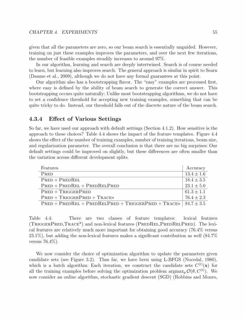
CHAPTER 4. EXPERIMENTS 55
given that all the parameters are zero, so our beam search is essentially unguided. However,training on just these examples improves the parameters, and over the next few iterations,the number of feasible examples steadily increases to around 97%.
In our algorithm, learning and search are deeply intertwined. Search is of course neededto learn, but learning also improves search. The general approach is similar in spirit to Searn(Daume et al., 2009), although we do not have any formal guarantees at this point.
Our algorithm also has a bootstrapping flavor. The “easy” examples are processed first,where easy is defined by the ability of beam search to generate the correct answer. Thisbootstrapping occurs quite naturally: Unlike most bootstrapping algorithms, we do not haveto set a confidence threshold for accepting new training examples, something that can bequite tricky to do. Instead, our threshold falls out of the discrete nature of the beam search.
4.3.4 Effect of Various Settings
So far, we have used our approach with default settings (Section 4.1.2). How sensitive is theapproach to these choices? Table 4.4 shows the impact of the feature templates. Figure 4.4shows the effect of the number of training examples, number of training iterations, beam size,and regularization parameter. The overall conclusion is that there are no big surprises: Ourdefault settings could be improved on slightly, but these differences are often smaller thanthe variation across different development splits.
Features AccuracyPred 13.4± 1.6Pred + PredRel 18.4± 3.5Pred + PredRel + PredRelPred 23.1± 5.0Pred + TriggerPred 61.3± 1.1Pred + TriggerPred + Trace∗ 76.4± 2.3Pred + PredRel + PredRelPred + TriggerPred + Trace∗ 84.7± 3.5
Table 4.4: There are two classes of feature templates: lexical features(TriggerPred,Trace*) and non-lexical features (PredRel,PredRelPred). The lexi-cal features are relatively much more important for obtaining good accuracy (76.4% versus23.1%), but adding the non-lexical features makes a significant contribution as well (84.7%versus 76.4%).
We now consider the choice of optimization algorithm to update the parameters givencandidate sets (see Figure 3.2). Thus far, we have been using L-BFGS (Nocedal, 1980),which is a batch algorithm: Each iteration, we construct the candidate sets C(t)(x) forall the training examples before solving the optimization problem argmaxθO(θ, C(t)). Wenow consider an online algorithm, stochastic gradient descent (SGD) (Robbins and Monro,

CHAPTER 4. EXPERIMENTS 56
100 200 300 400
iteration
20
40
60
80
100Accura
cy
Random 1
Random 2
Random 3
Random 4
Random 5
5 10 15 20 25 30
iteration
20
40
60
80
100
Accura
cy
Random 1
Random 2
Random 3
Random 4
Random 5
(a) Effect of # training examples (b) Effect of # training iterations
1 3 10 30 100 300
Beam size (K)
20
40
60
80
100
Accura
cy
0 0.001 0.003 0.01 0.03 0.1 0.3
Regularization (λ)
60
70
80
90
100Accura
cy
(c) Effect of beam size (d) Effect of regularization
Figure 4.4: (a) The learning curve shows test accuracy as the number of training examplesincreases; about 300 examples suffices to get around 80% accuracy. (b) Although our algo-rithm is not guaranteed to converge, the test accuracy is fairly stable (with one exception)with more training iterations—hardly any overfitting occurs. (c) As the beam size increases,the accuracy increases monotonically, although the computational burden also increases.There is a small gain from our default setting of K = 100 to the more expensive K = 300.(d) The accuracy is relatively insensitive to the choice of the regularization parameter for awide range of values. In fact, no regularization is also acceptable. This is probably becausethe features are simple, and the lexical triggers and beam search already provide some helpfulbiases.
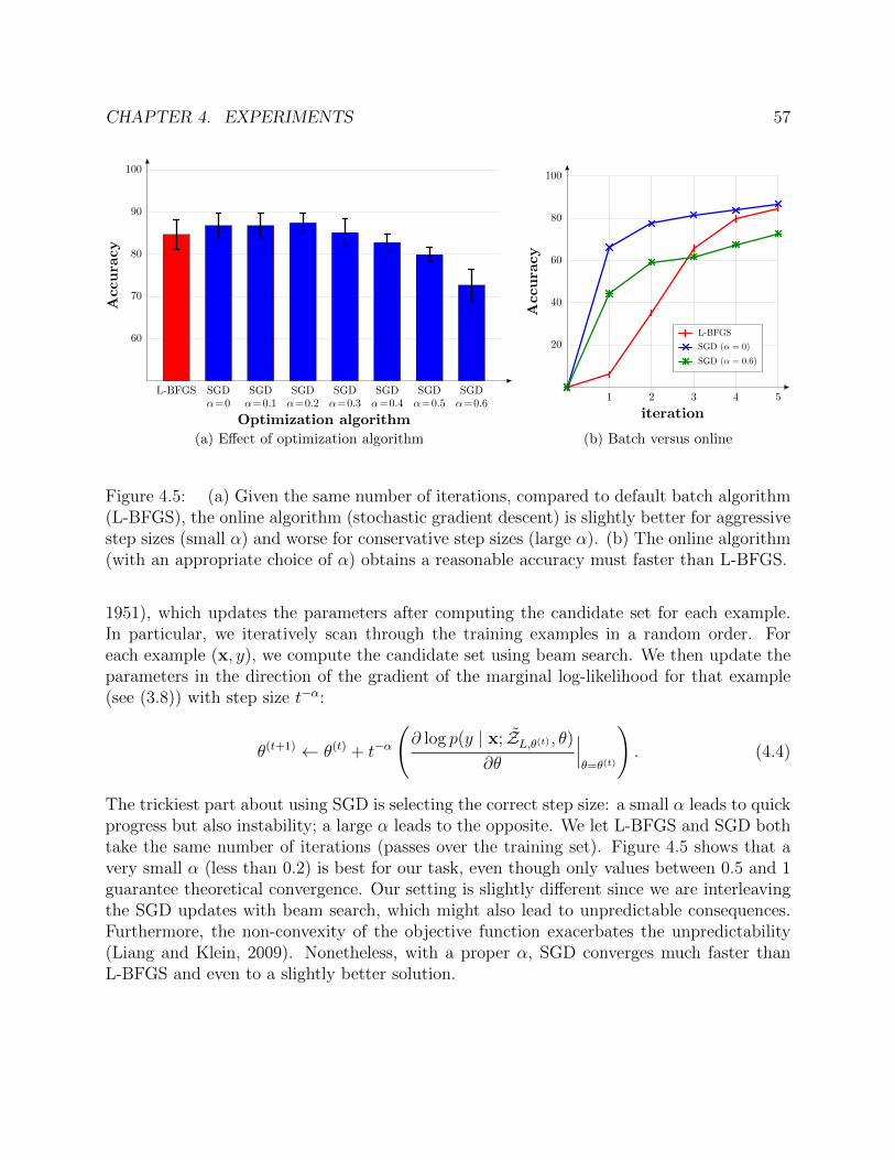
CHAPTER 4. EXPERIMENTS 57
L-BFGS SGDα=0
SGDα=0.1
SGDα=0.2
SGDα=0.3
SGDα=0.4
SGDα=0.5
SGDα=0.6
Optimization algorithm
60
70
80
90
100
Accura
cy
1 2 3 4 5
iteration
20
40
60
80
100
Accura
cy
L-BFGS
SGD (α = 0)
SGD (α = 0.6)
(a) Effect of optimization algorithm (b) Batch versus online
Figure 4.5: (a) Given the same number of iterations, compared to default batch algorithm(L-BFGS), the online algorithm (stochastic gradient descent) is slightly better for aggressivestep sizes (small α) and worse for conservative step sizes (large α). (b) The online algorithm(with an appropriate choice of α) obtains a reasonable accuracy must faster than L-BFGS.
1951), which updates the parameters after computing the candidate set for each example.In particular, we iteratively scan through the training examples in a random order. Foreach example (x, y), we compute the candidate set using beam search. We then update theparameters in the direction of the gradient of the marginal log-likelihood for that example(see (3.8)) with step size t−α:
θ(t+1) ← θ(t) + t−α
(∂ log p(y | x; ZL,θ(t) , θ)
∂θ
∣∣∣θ=θ(t)
). (4.4)
The trickiest part about using SGD is selecting the correct step size: a small α leads to quickprogress but also instability; a large α leads to the opposite. We let L-BFGS and SGD bothtake the same number of iterations (passes over the training set). Figure 4.5 shows that avery small α (less than 0.2) is best for our task, even though only values between 0.5 and 1guarantee theoretical convergence. Our setting is slightly different since we are interleavingthe SGD updates with beam search, which might also lead to unpredictable consequences.Furthermore, the non-convexity of the objective function exacerbates the unpredictability(Liang and Klein, 2009). Nonetheless, with a proper α, SGD converges much faster thanL-BFGS and even to a slightly better solution.
58
Chapter 5
Discussion
The work we have presented in this thesis contains three important themes. The firsttheme is semantic representation (Section 5.1): How do we parametrize the mapping fromutterances to their meanings? The second theme is program induction (Section 5.2): Howdo we efficiently search through the space of logical structures given a weak feedback signal?Finally, the last theme is grounded language (Section 5.3): How do we use constraints fromthe world to guide learning of language and conversely use language to interact with theworld?
5.1 Semantic Representation
Since the late nineteenth century, philosophers and linguists have worked on elucidating therelationship between an utterance and its meaning. One of the pillars of formal semantics isFrege’s principle of compositionality, that the meaning of an utterance is built by composingthe meaning of its parts. What these parts are and how they are composed is the mainquestion. The dominant paradigm, which stems from the seminal work of Richard Montaguein the early 1970s (Montague, 1973), states that parts are lambda calculus expressions thatcorrespond to syntactic constituents, and composition is function application.
Consider the compositionality principle from a statistical point of view, where we liberallyconstrue compositionality as factorization. Factorization, the way a statistical model breaksinto features, is necessary for generalization: It enables us to learn from previously seenexamples and interpret new utterances. Projecting back to Frege’s original principle, theparts are the features (Section 3.1.1), and composition is the DCS construction mechanism(Section 2.6) driven by parameters learned from training examples.
Taking the statistical view of compositionality, finding a good semantic representationbecomes designing a good statistical model. But statistical modeling must also deal with theadditional issue of language acquisition or learning, which presents complications: In absorb-ing training examples, our learning algorithm must inevitably traverse through intermediate

CHAPTER 5. DISCUSSION 59
models that are wrong or incomplete. The algorithms must therefore tolerate this degra-dation, and do so in a computationally efficient way. For example, in the line of work onlearning probabilistic CCGs (Zettlemoyer and Collins, 2005, 2007; Kwiatkowski et al., 2010),many candidate lexical entries must be entertained for each word even when polysemy doesnot actually exist (Section 2.6.4).
To improve generalization, the lexicon can be further factorized (Kwiatkowski et al.,2011), but this is all done within the constraints of CCG. DCS represents a departurefrom this tradition, which replaces a heavily-lexicalized constituency-based formalism with alightly-lexicalized dependency-based formalism. We can think of DCS as a shift in linguisticcoordinate systems, which makes certain factorizations or features more accessible. Forexample, we can define features on paths between predicates in a DCS tree which capturecertain lexical patterns much more easily than on a lambda calculus expression or a CCGderivation.
The benefits of working with dependency-based logical forms also led to the independentdevelopment of a semantic representation called natural logic form (Alshawi et al., 2011), butthe details of the two semantic formalisms and the goals are both different. Alshawi et al.(2011) focuses on parsing much complex sentences in an open-domain where a structureddatabase or world does not exist. While they do equip their logical forms with a full model-theoretic semantics, the logical forms are actually closer to dependency trees: quantifierscope is left unspecified, and the predicates are simply the words.
Perhaps not immediately apparent is the fact that DCS draws an important idea fromDiscourse Representation Theory (DRT) (Kamp and Reyle, 1993)—not from its treatmentof anaphora and presupposition which it is known for, but something closer to its core.This is the idea of having a logical form where all variables are existentially quantified andconstraints are combined via conjunction—a Discourse Representation Structure (DRS) inDRT, or a basic DCS tree with only join relations. Computationally, such these logicalstructures conveniently encode CSPs. Linguistically, it appears that existential quantifiersplay an important role and should be treated specially (Kamp and Reyle, 1993). DCStakes this core and focuses more on semantic compositionality and computation, while DRTfocuses more on discourse and pragmatics.
In addition to the statistical view of DCS as a semantic representation, it is useful tothink about DCS from the perspective of programming language design. Two programminglanguages can be equally expressive, but what matters is how simple it is to express adesired type of computation with in a given language. In some sense, we designed the DCSformal language to make it easy to represent computations expressed by natural language.An important part of DCS is the mark-execute construct, a uniform framework for dealingwith the divergence between syntactic and semantic scope. This construct allows us tobuild simple DCS tree structures and still handle the complexities of phenomena such asquantifier scope variation. Compared to lambda calculus, think of DCS as a higher-levelprogramming language tailored to natural language, which results in simpler programs (DCStrees). Simpler programs are easier for us to work with and easier for an algorithm to learn.

CHAPTER 5. DISCUSSION 60
5.2 Program Induction
Searching over the space of programs is hard though. This is the central computationalchallenge of program induction, that of inferring programs (logical forms) from their behavior(denotations). This problem has been tackled by difference communities in various forms:program induction in AI, programming by demonstration in HCI, and program synthesis inprogramming languages. The core computational difficulty is that the supervision signal—the behavior—is a complex function of the program which cannot be easily inverted. Whatprogram generated the output Arizona, Nevada, and Oregon?
Perhaps somewhat counterintuitively, program induction is easier if we infer programs fornot a single task but for multiple tasks. The intuition is that when the tasks are related, thesolution to one task can help another task, both computationally in navigating the programspace but statistically in choosing the appropriate program if there are multiple feasiblepossibilities (Liang et al., 2010). In our semantic parsing work, we want to infer a logicalform for each utterance (task). Clearly the tasks are related because they use the samevocabulary to talk about the same domain.
Natural language also makes program induction easier by providing side information(words) which can be used to guide the search. There has been several papers that induceprograms in this setting: Eisenstein et al. (2009) induces conjunctive formulae from naturallanguage instructions, Piantadosi et al. (2008) induces first-order logic formulae using CCGin a small domain assuming observed lexical semantics, and Clarke et al. (2010) induceslogical forms in semantic parsing. In the ideal case, the words would determine the programpredicates, and the utterance would determine the entire program compositionally. But ofcourse, this mapping is not given and must be learned.
5.3 Grounded Language
In recent years, there has been an increased interest in connecting language with the world.1
One of the primary issues in grounded language is alignment—figuring out what fragments ofutterances refer to what aspects of the world. In fact, semantic parsers trained on examplesof utterances and annotated logical form (those discussed in Section 4.2.2) need to solve thetask of aligning words to predicates. Some can learn from utterances paired with a set oflogical forms, one of which is correct (Kate and Mooney, 2007; Chen and Mooney, 2008).Liang et al. (2009) tackles the even more difficult alignment problem of segmenting andaligning a discourse to a database of facts, where many parts of either side are irrelevant(Liang et al., 2009).
If we know how the world relates to language, we can leverage structure in the worldto guide the learning and interpretation of language. We saw that type constraints from
1Here, world need not refer to the physical world, but could be any virtual world. The point is that theworld has non-trivial structure and exists extra-linguistically.

CHAPTER 5. DISCUSSION 61
the database/world reduces the set of candidate logical forms and leads to more accuratesystems (Popescu et al., 2003; Liang et al., 2011). Even for syntactic parsing, informationfrom the denotation of an utterance can be helpful (Schuler, 2003).
One of the exciting aspects about using the world for learning language is that it opensthe door to many new types of supervision. We can obtain answers given a world, which arecheaper to obtain than logical forms (Clarke et al., 2010; Liang et al., 2011). Goldwasseret al. (2011) learns a semantic parser based on bootstrapping and estimating the confidenceof its own predictions. Artzi and Zettlemoyer (2011) learns a semantic parser not fromannotated logical forms, but from user interactions with a dialog system. Branavan et al.(2009, 2010, 2011) use reinforcement learning learn to follow natural language instructionsfrom a reward signal. In general, supervision from the world is more indirectly related tothe learning task, but it is often much more plentiful and natural to obtain.
The benefits can also flow from language to the world. For example, previous work learnedto interpret language to troubleshoot a Windows machine (Branavan et al., 2009, 2010), wina game of Civilization (Branavan et al., 2011), play a legal game of solitaire (Eisenstein et al.,2009; Goldwasser and Roth, 2011), and navigate a map by following directions (Vogel andJurafsky, 2010; Chen and Mooney, 2011). Even when the objective in the world is definedindependently of language (e.g., in Civilization), language can provide a useful bias towardsthe non-linguistic end goal.
5.4 Conclusions
The main conceptual contribution of this thesis is a new semantic formalism, dependency-based compositional semantics (DCS), which has favorable linguistic, statistical, and compu-tational properties. This enabled us to learn a semantic parser from question-answer pairswhere the intermediate logical form (a DCS tree) is induced in an unsupervised manner.Our final question answering system was able to outperform current state-of-the-art systemsdespite requiring no annotated logical forms.
However, there is currently a large divide between our question answering system (whichare natural language interfaces to databases) and open-domain question answering systems.The former focuses on understanding a question compositionally and computing the answercompositionally, while the latter focuses on retrieving and ranking answers from a largeunstructured textual corpus. The former has depth; the latter has breadth. Developingmethods that can both model the semantic richness of language and scale up to an open-domain setting remains an open challenge.
We believe that it is possible to push our approach in that direction. Neither DCS northe learning algorithm is tied to having a clean rigid database, which could instead be adatabase generated from a noisy information extraction process. The key is to drive thelearning with the desired behavior, the question-answer pairs. The latent variable is thelogical form or program, which just tries to compute the desired answer by piecing together

CHAPTER 5. DISCUSSION 62
whatever information is available. Of course, there are many open challenges ahead, butwith the proper combination of linguistic, statistical, and computational insight, we hope toeventually build systems with both breadth and depth.

63
Bibliography
H. Alshawi, P. Chang, and M. Ringgaard. Deterministic statistical mapping of sentencesto underspecified semantics. In International Conference on Compositional Semantics(IWCS), pages 15–24, 2011.
I. Androutsopoulos, G. D. Ritchie, and P. Thanisch. Natural language interfaces to databases– an introduction. Journal of Natural Language Engineering, 1:29–81, 1995.
Y. Artzi and L. Zettlemoyer. Bootstrapping semantic parsers from conversations. In Empir-ical Methods in Natural Language Processing (EMNLP), pages 421–432, 2011.
J. Bos. A controlled fragment of DRT. In Workshop on Controlled Natural Language, pages1–5, 2009.
S. Branavan, H. Chen, L. S. Zettlemoyer, and R. Barzilay. Reinforcement learning formapping instructions to actions. In Association for Computational Linguistics and Inter-national Joint Conference on Natural Language Processing (ACL-IJCNLP), pages 82–90,Singapore, 2009. Association for Computational Linguistics.
S. Branavan, L. Zettlemoyer, and R. Barzilay. Reading between the lines: Learning to maphigh-level instructions to commands. In Association for Computational Linguistics (ACL),pages 1268–1277. Association for Computational Linguistics, 2010.
S. Branavan, D. Silver, and R. Barzilay. Learning to win by reading manuals in a Monte-Carlo framework. In Association for Computational Linguistics (ACL), pages 268–277.Association for Computational Linguistics, 2011.
B. Carpenter. Type-Logical Semantics. MIT Press, 1998.
D. L. Chen and R. J. Mooney. Learning to sportscast: A test of grounded language acqui-sition. In International Conference on Machine Learning (ICML), pages 128–135. Omni-press, 2008.
D. L. Chen and R. J. Mooney. Learning to interpret natural language navigation instructionsfrom observations. In Association for the Advancement of Artificial Intelligence (AAAI),Cambridge, MA, 2011. MIT Press.

BIBLIOGRAPHY 64
J. Clarke, D. Goldwasser, M. Chang, and D. Roth. Driving semantic parsing from the world’sresponse. In Computational Natural Language Learning (CoNLL), pages 18–27, 2010.
M. Collins. Head-Driven Statistical Models for Natural Language Parsing. PhD thesis,University of Pennsylvania, 1999.
P. Cousot and R. Cousot. Abstract interpretation: a unified lattice model for static analysisof programs by construction or approximation of fixpoints. In Principles of ProgrammingLanguages (POPL), pages 238–252, 1977.
H. Daume, J. Langford, and D. Marcu. Search-based structured prediction. Machine Learn-ing Journal (MLJ), 75:297–325, 2009.
R. Dechter. Constraint Processing. Morgan Kaufmann, 2003.
J. Eisenstein, J. Clarke, D. Goldwasser, and D. Roth. Reading to learn: Constructingfeatures from semantic abstracts. In Empirical Methods in Natural Language Processing(EMNLP), pages 958–967, Singapore, 2009.
R. Ge and R. J. Mooney. A statistical semantic parser that integrates syntax and semantics.In Computational Natural Language Learning (CoNLL), pages 9–16, Ann Arbor, Michigan,2005.
A. Giordani and A. Moschitti. Semantic mapping between natural language questions andSQL queries via syntactic pairing. In International Conference on Applications of NaturalLanguage to Information Systems, pages 207–221, 2009.
D. Goldwasser and D. Roth. Learning from natural instructions. In International JointConference on Artificial Intelligence (IJCAI), pages 1794–1800, 2011.
D. Goldwasser, R. Reichart, J. Clarke, and D. Roth. Confidence driven unsupervised se-mantic parsing. In Association for Computational Linguistics (ACL), pages 1486–1495.Association for Computational Linguistics, 2011.
J. Judge, A. Cahill, and J. v. Genabith. Question-bank: creating a corpus of parse-annotatedquestions. In International Conference on Computational Linguistics and Associationfor Computational Linguistics (COLING/ACL), pages 497–504, Sydney, Australia, 2006.Association for Computational Linguistics.
H. Kamp and U. Reyle. From Discourse to Logic: An Introduction to the Model-theoretic Se-mantics of Natural Language, Formal Logic and Discourse Representation Theory. Kluwer,Dordrecht, 1993.
H. Kamp, J. v. Genabith, and U. Reyle. Discourse representation theory. In Handbook ofPhilosophical Logic. 2005.

BIBLIOGRAPHY 65
R. J. Kate and R. J. Mooney. Using string-kernels for learning semantic parsers. In Interna-tional Conference on Computational Linguistics and Association for Computational Lin-guistics (COLING/ACL), pages 913–920, Sydney, Australia, 2006. Association for Com-putational Linguistics.
R. J. Kate and R. J. Mooney. Learning language semantics from ambiguous supervision. InAssociation for the Advancement of Artificial Intelligence (AAAI), pages 895–900, Cam-bridge, MA, 2007. MIT Press.
R. J. Kate, Y. W. Wong, and R. J. Mooney. Learning to transform natural to formallanguages. In Association for the Advancement of Artificial Intelligence (AAAI), pages1062–1068, Cambridge, MA, 2005. MIT Press.
T. Kwiatkowski, L. Zettlemoyer, S. Goldwater, and M. Steedman. Inducing probabilisticCCG grammars from logical form with higher-order unification. In Empirical Methods inNatural Language Processing (EMNLP), 2010.
T. Kwiatkowski, L. Zettlemoyer, S. Goldwater, and M. Steedman. Lexical generalization inCCG grammar induction for semantic parsing. In Empirical Methods in Natural LanguageProcessing (EMNLP), pages 1512–1523, 2011.
P. Liang and D. Klein. Online EM for unsupervised models. In North American Associationfor Computational Linguistics (NAACL). Association for Computational Linguistics, 2009.
P. Liang, M. I. Jordan, and D. Klein. Learning semantic correspondences with less super-vision. In Association for Computational Linguistics and International Joint Conferenceon Natural Language Processing (ACL-IJCNLP), Singapore, 2009. Association for Com-putational Linguistics.
P. Liang, M. I. Jordan, and D. Klein. Learning programs: A hierarchical Bayesian approach.In International Conference on Machine Learning (ICML). Omnipress, 2010.
P. Liang, M. I. Jordan, and D. Klein. Learning dependency-based compositional seman-tics. In Association for Computational Linguistics (ACL), pages 590–599. Association forComputational Linguistics, 2011.
W. Lu, H. T. Ng, W. S. Lee, and L. S. Zettlemoyer. A generative model for parsing nat-ural language to meaning representations. In Empirical Methods in Natural LanguageProcessing (EMNLP), pages 783–792, 2008.
M. P. Marcus, M. A. Marcinkiewicz, and B. Santorini. Building a large annotated corpus ofEnglish: the Penn Treebank. Computational Linguistics, 19:313–330, 1993.

BIBLIOGRAPHY 66
S. Miller, D. Stallard, R. Bobrow, and R. Schwartz. A fully statistical approach to naturallanguage interfaces. In Association for Computational Linguistics (ACL), pages 55–61.Association for Computational Linguistics, 1996.
R. Montague. The proper treatment of quantification in ordinary English. In Approaches toNatural Language, pages 221–242, 1973.
J. Nocedal. Updating quasi-newton matrices with limited storage. Mathematics of Compu-tation, 35:773–782, 1980.
S. Petrov, L. Barrett, R. Thibaux, and D. Klein. Learning accurate, compact, and inter-pretable tree annotation. In International Conference on Computational Linguistics andAssociation for Computational Linguistics (COLING/ACL), pages 433–440. Associationfor Computational Linguistics, 2006.
S. T. Piantadosi, N. D. Goodman, B. A. Ellis, and J. B. Tenenbaum. A Bayesian model of theacquisition of compositional semantics. In Proceedings of the Thirtieth Annual Conferenceof the Cognitive Science Society, 2008.
A. Popescu, O. Etzioni, and H. Kautz. Towards a theory of natural language interfaces todatabases. In International Conference on Intelligent User Interfaces (IUI), pages 149–157, 2003.
M. F. Porter. An algorithm for suffix stripping. Program, 14:130–137, 1980.
H. Robbins and S. Monro. A stochastic approximation method. Annals of MathematicalStatistics, 22(3):400–407, 1951.
W. Schuler. Using model-theoretic semantic interpretation to guide statistical parsing andword recognition in a spoken language interface. In Association for Computational Lin-guistics (ACL), pages 529–536. Association for Computational Linguistics, 2003.
M. Steedman. The Syntactic Process. MIT Press, 2000.
L. R. Tang and R. J. Mooney. Using multiple clause constructors in inductive logic program-ming for semantic parsing. In European Conference on Machine Learning, pages 466–477,2001.
A. Vogel and D. Jurafsky. Learning to follow navigational directions. In Association for Com-putational Linguistics (ACL), pages 806–814. Association for Computational Linguistics,2010.
M. Wainwright and M. I. Jordan. Graphical models, exponential families, and variationalinference. Foundations and Trends in Machine Learning, 1:1–307, 2008.

BIBLIOGRAPHY 67
D. Warren and F. Pereira. An efficient easily adaptable system for interpreting naturallanguage queries. Computational Linguistics, 8:110–122, 1982.
Y. W. Wong and R. J. Mooney. Learning for semantic parsing with statistical machinetranslation. In North American Association for Computational Linguistics (NAACL),pages 439–446, New York City, 2006. Association for Computational Linguistics.
Y. W. Wong and R. J. Mooney. Learning synchronous grammars for semantic parsing withlambda calculus. In Association for Computational Linguistics (ACL), pages 960–967,Prague, Czech Republic, 2007. Association for Computational Linguistics.
W. A. Woods, R. M. Kaplan, and B. N. Webber. The lunar sciences natural languageinformation system: Final report. Technical report, BBN Report 2378, Bolt Beranek andNewman Inc., 1972.
M. Zelle and R. J. Mooney. Learning to parse database queries using inductive logic pro-ramming. In Association for the Advancement of Artificial Intelligence (AAAI), pages1050–1055, Cambridge, MA, 1996. MIT Press.
L. S. Zettlemoyer and M. Collins. Learning to map sentences to logical form: Structured clas-sification with probabilistic categorial grammars. In Uncertainty in Artificial Intelligence(UAI), pages 658–666, 2005.
L. S. Zettlemoyer and M. Collins. Online learning of relaxed CCG grammars for parsing tological form. In Empirical Methods in Natural Language Processing and ComputationalNatural Language Learning (EMNLP/CoNLL), pages 678–687, 2007.

68
Appendix A
Details
A.1 Denotation Computation
This section describes the details of how we compute the denotations of basic DCS treesaccording to (2.15). We could simply convert DCS trees into SQL or relational algebraand use an off-the-shelf database management system (DBMS). After all, our bottom-upapproach to computing the denotation of a DCS tree is not necessarily optimal. For example,if the predicate at the root contains only one tuple, then a top-down approach would mostlikely be preferable, and a global query optimizer might choose that query execution plan.While this might have been a viable route, we use a custom implementation for severalreasons:
1. We wanted to present a simple algorithm with a transparent computational complexity;
2. DCS trees can be built from custom predicates (e.g., for generalized quantification andsuperlatives), which are more cumbersome to incorporate into standard engines;
3. We need to compute denotations not of one DCS tree but of a forest of DCS trees whichshare many subtrees. Exploiting this structure requires a particular form of multiplequery optimization which is readily incorporated into our construction mechanism.
In (2.15), we have reduced the computation of denotations to two operations, join andproject, but there is still much to be said regarding how these operations are implemented.For example, for two finite sets of tuples, A and B, their join, A ./j,j′ B can either becomputed by enumerating the elements of A and querying B for each one, or by enumeratingB and querying A. We can estimate the costs of these operations and choose the cheaperoption. We also build various indices to make these operations more efficient. Many of theseideas are based on standard database query optimization techniques.
Recall that our worlds are only conceptually databases, for they contain infinite sets oftuples, which arise due to predicates such as >. Performing join and project operations on

APPENDIX A. DETAILS 69
1
1
2
1
2
1
1million
>
population
city
Set-expression Denotation
explicit-predicate1 {(x) : city(x) ∧ ∃y.population(x, y) ∧ y > 106}
explicit-predicate2 {(x, y) : population(x, y) ∧ y > 106}
>{·2 = 106} {(x, 106) : x > 106}
1million {(106)}
Figure A.1: Shows the computation and representation of the denotations for the DCS treecorresponding to city with population greater than 1 million. For each node, we compute thedenotation for the subtree rooted at that node, which is represented by set-expressions.
these infinite sets can produce other infinite sets. To handle these manipulations, we need away of representing these infinite sets symbolically.
A.1.1 Set-expressions
We define a language for representing sets of tuples and show how to perform join and projectoperations on expressions in that language (set-expressions). As a running example, considercomputing the denotation for the DCS tree corresponding to city with population greater than 1 million,shown in Figure A.1.
Our language for representing sets is given by the following grammar:
set ::= predicate [base case] (A.1)
| set{·i = v} [select] (A.2)
| set[i] [project] (A.3)
| set× set [product] (A.4)
| set ∪ set [union] (A.5)
Perhaps not surprisingly, set-expressions bear a striking similarity to relational algebra. Eachset-expression e denotes the set JeKw specified below for each case:
• Predicate (e.g., population): a predicate p ∈ P represents its semantics JpKw = w(p).
• Filter (e.g., >{·2 = 106}): Je{·i = v}Kw = {x ∈ JeKw : x[i] = v}.
• Project (e.g., population[2]): Je[i]Kw = {xi : x ∈ JeKw}.
• Product (e.g., population× area): Je1 × e2Kw = {x+ y : x ∈ Je1Kw, y ∈ Je2Kw}.

APPENDIX A. DETAILS 70
• Union (e.g., city ∪ river): Je1 ∪ e2Kw = Je1Kw ∪ Je2Kw.
At this point, it is worth stressing the difference between three kinds of objects: DCStrees, set-expressions, and the actual sets of tuples in the world. DCS trees have denotationsgiven by (2.15), which are sets of tuples. These denotations are computed by manipulatingset-expressions, which themselves denote the same sets of tuples in the world.
A.1.2 Join and Project on Set-Expressions
We now define join and project operations that operate on set-expressions rather than setsof tuples. To distinguish these operations, we use J(e1, j, j
′, e2) and P(i, e) for the operationsthat work on set-expressions, reserving A ./j,j′ B and A[i] for the operations that work onsets of tuples.
For convenience, define a caching function Cw(A), which takes a set of tuples A andreturns a fresh new predicate p with denotation A (think of Cw as a technical trick whichimplements the inverse of J·Kw):
Cw(A)def= p such that w(p) = A. (A.6)
We also define a reduction function R(e), which takes a set-expression e and caches theresult if e denotes a finite set:
R(e)def=
{Cw(JeKw) if |JeKw| <∞e otherwise.
(A.7)
The idea is that we want to reduce set-expressions to predicates whenever possible.We implement the join operation J using two operations: (i) enumerate E(e), which
returns the set of tuples denoted by e; and (ii) select S(i,v, e), which returns a set-expressiondenoting the subset JeKw which matches the select condition. Using enumerate and select,we implement the join of two set-expressions e1 and e2 by enumerating the tuples in e1 andusing each one to select e2 or vice-versa:
J(e1, j, j′, e2)
def=
⋃x∈E(e1)
Cw({x})× S(j′, e1j, e2) or⋃
x∈E(e2)
S(j, e2j′ , e1)×Cw({x}). (A.8)
Now, it suffices to define enumerate (E), select (S), and project (P) for each type ofset-expression. First, the enumerate operation E simply computes the semantics of set-expressions, with the added caveat that the set of tuples must be finite:
E(e)def= JeKw if |JeKw| <∞. (A.9)
The select operation S is defined for each type of set-expression as follows:
APPENDIX A. DETAILS 71
• Predicate: S(i,v, p) = R(p{·i = v}). If we know that the resulting set of tuples is finite,then we simply return a predicate corresponding to those tuples. For finite predicatessuch as p = city, the result is always finite. For infinite predicates where the selectcondition is restrictive enough, such as p = count with i = (1) and v = ({(1), (2), (3)}),then the resulting set is still finite—in this case, {({(1), (2), (3)}, 3)}. Otherwise, werepresent the computation symbolically and return p{·i = v}.
• Select: S(i,v, e{·j = t}) = R(p{·i+j = v + t}) (simply concatenate the select condi-tions).
• Project: S(i,v, e[j]) = R(e{·ji = v}[j]) (push the select operation inside the project).
• Product: S(i,v, e1 × e2) = R(S(ij,vj, e1) ∩ S(i−j,v−j, e2)), where j = {j : ij <Arity(Je1Kw)} are the indices corresponding to the e1 part.
• Union: S(i,v, e1 ∪ e2) = R(S(i,v, e1) ∪ S(i,v, e2)).
The project operation P is defined for each type of set-expression as follows:
• Predicate: P(i, p) = R(p[i]).
• Select: P(i, e{·j = v}) = e{·j = v}[i] (leave the project outside the select).
• Project: P(i, e[j]) = R(e[ji]) (accumulate the two project operations).
• Product: P(i, e1 × e2) = R(P(ij, e1) × P(i−j, e2)), where j = {j : ij < Arity(Je1Kw)}are the indices corresponding to the e1 part.
• Union: P(i, e1 ∪ e2) = R(P(i, e1) ∪P(i, e2)).
The basic strategy when operating on set-expressions is to try to push the select op-erations as far in as possible, followed by project operations. Whenever we detect that aset-expression denotes a finite set, we evaluate the set-expression to get a concrete set oftuples and assign a new predicate to it. Note that it is not necessarily optimal to alwaysconstruct a new predicate when possible. However, note that this does result in caching theresults of the computation, which can be reused later.
At the root of the DCS tree, we obtain a set-expression. If the set-expression is a singlepredicate, we happily return the corresponding set of tuples as the final answer. Otherwise,we say that we have failed to compute the denotation, because the set is probably infinite.This happens mostly in strange cases, such as with the DCS tree 〈ø; 1
1 :〈count; 21 :〈3〉〉〉, whose
denotation is all sets (of primitive values) with cardinality 3. Though this denotation issemantically meaningful, it never arises in our intended applications. Thus, the failure tocompute a denotation serves as a pragmatic filter on the set of DCS trees (see Section 2.6.3).
Let us walk through the example in Figure A.1. At the bottom of the DCS tree, westart with the set-expression corresponding to the constant predicate 1million. We then

APPENDIX A. DETAILS 72
join > with 1million, which results in the set-expression >{·2 = 106}. Note that we cannotreduce this set-expression to a predicate because it has an infinite denotation. Next, wejoin >{·2 = 106} with population, which does produce a finite set, which is cached asexplicit-predicate2. Finally, explicit-predicate2 is joined with city, which yieldsthe answer, which can be stored in explicit-predicate1.
Local Query Optimization The computation of the denotation is driven by the joinoperation (A.8). There are two points worth making. First, the core computation is intaking a set-expression (usually a predicate p) and performing a select operation (S(j, x, p)).To avoid naıvely enumerating the tuples in E(p) and checking the select condition on eachtuple, we perform some indexing to improve efficiency. Specifically, let A = w(p) be theset of tuples. For each component j = 1, . . . ,Arity(A), we maintain a map IA from eachcomponent j and value v to the set of matching tuples in A; formally,
IA(j, x) = {t ∈ A : tj = x}. (A.10)
Now, each S(j, x, p) operation simply returns Iw(p)(j, x) using a single lookup.Second, when joining two set-expressions e1 and e2 (A.8), there is the choice of whether
to enumerate e1 or e2. We first estimate the costs of each option and choose the cheaperone. Specifically, let NA(j) be the average size of IA(j, x), where v is drawn from a uniformdistribution over A[j]:
NA(j) =1
|A[j]|∑x∈A[j]
|IA(j, x)|. (A.11)
More sophisticated query optimization techniques can be used to improve this estimate,but we do not pursue them here. For example, suppose we would like to join A and B,which both have arity 1. Then the only possible join relation is 1
1, which corresponds toset intersection. The cost for the enumerate-A-query-B option is |A| and the cost form theenumerate-B-query-A option is |B| (recall that querying is constant time). We would choosethe former option if |A| < |B| and the latter otherwise.
The other common case is when A has arity 2 and B has arity 1; assume the join relationis j
1 with j ∈ {1, 2}. The enumerate-A-query-B option is the same as before, with a costof |A|. The enumerate-B-query-A option is a bit different, because querying A is no longerjust a simple set-containment check. Instead, each query to A returns a set of arity 2 tuples.We take the union of these results: ∪x∈BIA(j, x); this operation has an estimated cost of|B|NA(j).