Thesis Public version - Universiteit Twenteessay.utwente.nl/61905/1/master_B._Maarse.pdf · Backtesting Framework for PD, EAD and LGD ... Improving the current backtesting methodology

Master Thesis Backtesting Framework for PD, EAD and LGD

Rabobank International

Quantitative Risk Analytics

Coöperatieve Centrale Raiffeisen-Boerenleenbank BA Registered at the Chamber of Commerce, Utrecht no. 30.046.259

Author: Bauke Maarse

Date: July 16, 2012

Exam committee Berend Roorda

Reinoud Joosten

Danesh Nathoeni

Viktor Tchistiakov

Public Version

ii

iii

Colophon

Title Backtesting Framework for PD, EAD and LGD

Date July 16, 2012

On behalf of Rabobank International – Quantitative Risk Analytics & University of Twente

Author Bauke Maarse

Project Backtesting framework for retail modelling

First Rabobank

Supervisor

D. Nathoeni

Second Rabobank

Supervisor

V. Tchistiakov

First Supervisor B. Roorda

Second Supervisor R.A.M.G. Joosten

Contact address [email protected] / [email protected]

Rabobank, 2012

iv

Management Summary

The objective of this thesis is to develop a backtesting framework

Currently a general framework is available. However, this framework has been

developed several years ago and risk management of Rabobank International believes

that there is room for improvement. This leads to the main goal of this thesis: improving

the current backtesting methodology for

(LGD) and exposure at default (EAD) and develop a framework for Rabobank

International.

Backtesting is the use of statistical methods to compare the estimates with the reali

outcomes. Performing a backtest consists out of three stages: stability, discriminatory

power and predictive power. Stability testing concerns the stability of the portfolio to

ensure that the model is able to perform well. Discriminatory power refers to the ability

to differentiate between default

power focuses on the comparison of the estimates with the reali

shows an overview of the

Figure 0.1: Overview of the proposed backtesting framework

The current framework did not contain stabi

proposed, one for continuous and one for discrete samples.

For PD the current tests used for discriminatory power are suitable

improvements are the rejection areas, these were based on

thresholds do not take

improved by the use of confidence bounds.

The tests for predictive power

should be performed with two adjustments. First

the influence of the correlation with the economic cycle. Second

intervals should be based on Type

Management Summary

The objective of this thesis is to develop a backtesting framework for retail models.


l years ago and risk management of Rabobank International believes


the current backtesting methodology for probability of default (PD), loss given default

xposure at default (EAD) and develop a framework for Rabobank

Backtesting is the use of statistical methods to compare the estimates with the reali




to differentiate between defaults and non defaults, or high and low losses. P

the comparison of the estimates with the realized values.

an overview of the proposed backtesting framework.

Figure 0.1: Overview of the proposed backtesting framework

The current framework did not contain stability testing. Therefore two tests are

proposed, one for continuous and one for discrete samples.

For PD the current tests used for discriminatory power are suitable. The only

rejection areas, these were based on fixed thresholds

the variance and number of observations into account

of confidence bounds.

The tests for predictive power can be improved on several aspects. The binomial test

with two adjustments. First, a point-in-time adjustment to reduce

correlation with the economic cycle. Second, the confidence

should be based on Type-I and Type-II errors, instead of Type

v

for retail models.


l years ago and risk management of Rabobank International believes


robability of default (PD), loss given default

xposure at default (EAD) and develop a framework for Rabobank

Backtesting is the use of statistical methods to compare the estimates with the realized




, or high and low losses. Predictive

ed values. Figure 0.1

Therefore two tests are

. The only

fixed thresholds. These

into account, this can be

on several aspects. The binomial test

time adjustment to reduce

the confidence

, instead of Type-I errors only.

vi

The composed model test, used to test whether the rejection of part of the portfolio

(bucket) should lead to a rejection of the whole model, is considered to be too strict for

small samples. Therefore, for small samples this test should be replaced by a Chi-

squared test.

The current backtesting framework for LGD was less developed and several

improvements are proposed. To test the discriminatory power for two comparable

samples the powerstat should be used. This is improved by using the LGDs instead of

the loss at default, because this gives more information. For samples that have different

distributions, two tests are proposed. On bucket level the cumulative LGD accuracy

ratio (CLAR) can still be used but with improved rejection areas. On model level the

Spearman’s rank correlation is proposed.

For predictive power the loss shortfall and mean absolute deviation were used to

compare the predicted with the observed loss at default (LGD times EAD). For both

tests improved rejection areas are proposed which are based on the sample size and

variance instead of fixed thresholds. Additionally a t-test is used to compare the

observed with the predicted LGDs

The current backtesting framework for EAD is still adequate and therefore will be used

in the proposed framework.

1

MANAGEMENT SUMMARY ................................................................................................... V

1 INTRODUCTION ............................................................................................................... 5

1.1 Background .................................................................................................... 5

1.2 Research objective and approach ................................................................... 6

1.3 Outline ........................................................................................................... 8

2 CURRENT SITUATION: MODELS, GUIDELINES AND BACKTESTING

METHODOLOGY ....................................................................................................................... 9

2.1 Models ........................................................................................................... 9

2.1.1 Probability of Default model ........................................................................... 9

2.1.2 Loss Given Default model .............................................................................. 9

2.1.3 Exposure at Default model ........................................................................... 10

2.1.4 Introduction to the backtesting procedure ................................................. 11

2.2 Regulatory and internal guidelines................................................................ 13

2.2.1 Regulatory guidelines .................................................................................... 13

2.2.2 Internal guidelines ........................................................................................ 14

2.3 Current Backtesting Framework .................................................................... 15

2.3.1 Traffic light approach .................................................................................... 15

2.3.2 Stability testing ............................................................................................. 15

2.3.3 PD backtesting............................................................................................... 16

2.3.4 LGD Backtesting ............................................................................................ 18

2.3.5 EAD Backtesting ............................................................................................ 22

2.4 Conclusion Current situation ......................................................................... 22

3 PROPOSALS FOR IMPROVED STABILITY TESTING ........................................... 25

3.1 System Stability Index .................................................................................. 25

3.2 Kolmogorov-Smirnov test ............................................................................ 25

3.3 Chi-squared test ........................................................................................... 27

3.4 Comparison .................................................................................................. 27

3.5 Conclusion .................................................................................................... 27

2

4 PROPOSALS FOR IMPROVEMENT OF BACKTESTING PD ................................ 29

4.1 Discriminatory power ................................................................................... 29

4.1.1 Confidence interval ROC curve ..................................................................... 29

4.1.2 Area under curve confidence interval .......................................................... 32

4.2 Predictive power .......................................................................................... 34

4.2.1 Incorporating correlation .............................................................................. 34

4.2.2 Methodology for Type-II errors ................................................................... 38

4.2.3 Composed model test ................................................................................... 41

4.3 Overview PD framework ............................................................................... 45

4.4 Conclusion PD framework ............................................................................. 46

5 PROPOSALS FOR IMPROVEMENT OF BACKTESTING LGD ............................ 47

5.1 Discriminatory power ................................................................................... 47

5.1.1 Powercurve ................................................................................................... 48

5.1.2 Comparison of Curves ................................................................................... 49

5.1.3 CLAR curve compared to powercurve .......................................................... 51

5.1.4 CLAR rejection area ....................................................................................... 52

5.1.5 Spearman’s rank correlation ......................................................................... 53

5.2 Predictive Power .......................................................................................... 55

5.2.1 Loss Shortfall ................................................................................................. 55

5.2.2 Mean Absolute Deviation ............................................................................. 56

5.2.3 LGD model and bucket test ........................................................................... 58

5.2.4 Transition matrix test .................................................................................... 60

5.3 Overview proposed LGD backtesting framework ........................................... 61

5.4 Conclusion LGD Framework .......................................................................... 62

6 PROPOSALS FOR IMPROVEMENT OF BACKTESTING EAD ............................. 65

6.1 Predictive power: Student t-test ................................................................... 65

6.2 Conclusion .................................................................................................... 65

7 CONCLUSION .................................................................................................................. 67

8 BIBLIOGRAPHY ............................................................................................................. 69

3

Appendix 1: Regulatory guidelines .......................................................................... 72

Appendix 2: CLAR curve .......................................................................................... 73

Appendix 3: Granularity adjustment approximation ................................................ 74

Appendix 4: ROC curve confidence interval ............................................................. 74

Appendix 5: Hosmer-Lemeshow test versus composed model test .......................... 75

Appendix 6: CLAR rejection area ............................................................................. 76

Appendix 7: Loss Shortfall confidence interval ........................................................ 78

Appendix 8: MAD rejection area ............................................................................. 78

Appendix 9: Normal assumption of average CCF...................................................... 79

4

5

1 Introduction

Since the introduction of Basel II banks are allowed to use internally developed models

to estimate the key drivers of credit risk: probability of default (PD), loss given default

(LGD) and exposure at default (EAD). These risk components determine the capital

requirement for banks.

Over the past years Rabobank International has developed models to estimate these risk

components for several retail portfolios. To test whether these models are still adequate,

their performance has to be validated. Part of this validation is backtesting, according to

BIS (2005) backtesting is defined as: “The use of statistical methods to compare

estimates of the three risk drivers to realised outcomes”. The goal of this thesis is to

develop a framework to backtest the retail models within Rabobank International.

We start with a short background on capital requirements and validation of models.

Then we describe the research objectives and give the further outline of this thesis.

1.1 Background

To determine the capital requirements of a bank the expected loss plays a crucial role.

The expected loss is the product of the three risk components:

�� = � ∗ �� ∗ �� (1.1)

Probability of default is the probability that a counterparty will default within one year.

Exposure at default is the maximum amount that could be lost when a default occurs,

assuming that there will be no recovery. Loss given default is the percentage of the EAD

that is lost when a counterparty defaults, it is the part of the EAD that is not recovered

(Hull, 2007).

Figure 1.1: Calculation of economic capital

6

The expected loss is used to calculate the economic capital. The economic capital is

needed to cover unexpected losses. The unexpected loss is the difference between

expected loss and the worst case loss. The worst case loss is set according to a

confidence level. Figure 1.1 illustrates the calculation of the economic capital (Hull,

2007).

One of the requirements by Basel II is to prove the soundness and appropriateness of the

models used to estimate the economic capital. This validation process is performed

periodically (commonly once a year) and consists out of monitoring, backtesting and

benchmarking. Monitoring has a more qualitative nature and focuses on portfolio

dynamics, quality of the data and use of the model. Backtesting and benchmarking

concentrate on the quantitative performance of the model components. These parts test

whether the discriminatory and predictive power are still adequate. Discriminatory

power refers to the ability of a model to differentiate between defaults and non defaults

and between high and low losses. The predictive power compares the predicted with the

realized rates.

Backtesting uses statistical methods to test the performance, it compares the realized

values of the three risk components with the predicted values. To make sure that the

model is able to perform well the stability of the portfolio is tested. A change in the

portfolio can influence the performance of the model.

Benchmarking refers to comparing the internal predictions with the predictions of other

banks. The validation process is concluded with the performance of the different model

components and possible actions that can be performed after backtesting, so called

follow-up actions.

1.2 Research objective and approach

The objective of this thesis is to develop a backtesting framework for retail models.

Currently a general backtesting framework is available. However, this framework has

been developed several years ago and risk management of Rabobank International

believes that there is some room for improvement regarding different aspects. This

thesis will focus on weaknesses of the current framework and will use this framework as

a starting point to develop a framework for Rabobank International. The weaknesses

will be identified by analysing the statistical methods used in the current framework. To

resolve the weaknesses of the current framework, methodologies described in literature

and recent developments within the Rabobank will be examined. The research goal of

this thesis is:

Improving the current backtesting methodology for PD, LGD and EAD and to develop a

framework for Rabobank International. The PD framework is well developed and will

be improved on specific aspects. For LGD the framework is less developed and

therefore almost the complete methodology has to be improved. The EAD framework is

developed well and will only be validated on its correctness.

7

To reach this goal the estimation models and the backtesting procedure have to be

understood in depth. As a result the models used for PD, LGD and EAD estimation have

been investigated and a full description of the model components and the aspects that

require backtesting are included in this thesis. Taking these objectives into account the

first sub question is:

Which models are used for estimating PD, LGD and EAD and on what aspects should

they be backtested?

When the models and their backtesting aspects are known the current backtesting

methodology will be examined. The methodology for each model will be described and

examined using literature research, quantitative analysis and expert views. This will

answer the second sub question:

Which backtesting methods are currently used and what are the points of improvement

for these methods?

The points of improvement of the current methodology are the start of a more in-depth

research on improving the current methodology. We will start with examining the first

stage in backtesting, the portfolio stability. Then for each component the discriminatory

and predictive tests will be further examined. Therefore the third sub question is:

Which tests should be used to test the stability of the portfolio?

For PD the current methodology can be improved on three specific aspects. First the

current methodology assumes independence between defaults which is incorrect

because the default frequency depends on the economic situation and therefore defaults

are correlated. Second the rejection areas, used to define the result of the test, are not

always based on statistics. Third the current methodology incorporates a test that

verifies whether the whole model should be rejected if one or more parts of the model

are rejected, which is called the composed model test. This test is hard to compute and

strict, therefore replacement by another test will be examined. The fourth sub question

therefore is:

How can the current PD backtesting methodology be improved on the aspects: default

correlation, rejection areas and the composed model test?

The backtesting methodology for LGD and EAD is less developed compared to PD.

Therefore this research will be much broader and will contain more pioneering work.

Currently not all aspects are tested and it is unclear which tests to use for each aspect of

the model. One of the research aspects is to determine the rejection areas for the

different tests. Therefore the fifth sub question is:

Which tests should be used to backtest LGD and EAD and how should the rejection

areas be set?

8

Besides literature research and expert views, quantitative analysis will be done. This

analysis will be based on a portfolio from Bank BGZ, which is a subsidiary of

Rabobank in Poland. This portfolio is chosen because Rabobank International recently

developed a PD, LGD and EAD model for this portfolio and it has not been backtested

yet.

1.3 Outline

In Chapter two we will describe the current situation. It starts with a description of the

models used to predict PD, LGD and EAD. Next, we summarize the regulatory and

internal Rabobank guidelines for backtesting. We end the Chapter with a description of

the current backtesting methodologies per risk component and their drawbacks. The first

two research questions will be answered in this Chapter.

In Chapter three we focus at stability testing. Several methods to test the stability of a

portfolio are examined and a final choice is made. We will conclude this Chapter with

answering the third research question.

In Chapter four we focus on the improvements of the backtesting methodology for PD.

We start this Chapter with the improvements for discriminatory power, which focuses at

improving the rejection areas. Next the improvements for predictive power will be

examined, which concern the correlation between defaults, the rejection areas and a

substitute for the composed model test. We will conclude this Chapter with an overview

of the proposed backtesting framework for PD and the answer on the fourth sub

question.

In Chapter five we focus on the development of a framework for backtesting LGD. This

Chapter is split up in discriminatory and predictive power. For both aspects the current

tests will be improved and additional tests are examined. This results in a framework for

LGD backtesting and will therefore answer the fifth sub question.

In Chapter six we examine the test used to backtest EAD. This results in a test used to

backtest EAD and answers the fifth sub question.

9

2 Current Situation: Models, Guidelines and Backtesting Methodology

We start this Chapter with a description of the models used to predict PD, EAD and

LGD. Subsequently, the regulatory and internal Rabobank guidelines for backtesting

will be described. Finally, we describe the current backtesting methodologies for PD,

EAD and LGD and their drawbacks.

2.1 Models

To be able to select an appropriate backtesting procedure, the three different models

have to be understood in more detail. For each model the methodology of assigning a

value to the particular risk component (PD, LGD or EAD) will be described. Depending

on the methods used to predict a backtesting procedures is selected. This section ends

with an overview of the backtesting process for the three risk components.

2.1.1 Probability of Default model

A PD model estimates the probability that a counterparty will default within one year.

According to BIS II (BIS, 2006) a default has occurred if at least one of the following

two statements hold:

• The bank considers that the obligor is unlikely to pay its credit obligations to

the bank in full.

• The obligor is past due more than 90 days on any material obligation to the

banking group.

The objective of PD modelling is to predict the default rate. To be able to make

adequate predictions the model has to differentiate between good and bad facilities,

which is defined as discriminatory power. A good facility is a credit that did not go into

default, whereas a bad facility did.

To differentiate between good and bad clients, a scorecard approach is used. A

scorecard consists out of several factors qualitative (e.g. education) and quantitative

(e.g. total income), which are selected based on their discriminatory and predictive

power. The different factors result in a total score, this score indicates the

creditworthiness of a facility (loan of a client) for the coming year. The score is the

main input to either accept or reject clients and is used to assign facilities to their

buckets. Besides the score an additional dimension can be used to bucket the facilities.

A bucket is a pool with facilities with similar characteristics (scorecard scores). To each

bucket a PD is assigned. This calibration is preferably done by counting the number of

historical defaults within a bucket, the use of a transition matrix is also possible, the

transition matrix will be further explained for the LGD model (Kurcz et al., 2011).

2.1.2 Loss Given Default model

A LGD model estimates the percentage of the exposure that is lost when the obligor

defaults. According to BIS II loss is defined as economic loss. When economic loss is

measured all relevant factors should be taken into account. Therefore the discount

10

effects and the direct and indirect costs made for collecting the exposure should be

incorporated. Figure 2.1 illustrates the LGD model whereas the LGD can

be calculated with the following formula:

�� = 1 − 1�� ∗ ��ℎ �� − �� − �� (2.1)

As for PD, the facilities are assigned to buckets according to their risk characteristics.

This bucketing can be based on different dimensions, e.g. collateral score or product

type, which differentiates between high and low recoveries. According to these

dimensions a facility is assigned to a bucket. Next, the LGD values are estimated for

each bucket. This can be done by the counting or the transition matrix approach. The

counting approach is based on the observed LGDs of facilities that have completed the

recovery cycle. Since a full cycle can be lengthy this can be seen as a drawback

(Kozlowski, 2011).

The transition matrix approach does not need a full recovery cycle of data because it

concerns monthly transitions. A transition indicates the probability that a defaulted

facility pays-off or is written-off every month it is in default. These probabilities are

combined in a matrix that indicates how a facility repays the loss over several years. The

main advantage is that the matrix can be derived from a relative short time period

(Kozlowski, 2011).

2.1.3 Exposure at Default model

An EAD model estimates the maximum amount that could be lost (assuming no

recovery) if a default occurs. There are two different cases in estimating the EAD,

depending on the permission of an off-balance sheet exposure. In the first case there is

only an on-balance sheet exposure, which means that the obligor is not allowed to

increase the exposure. In this case the EAD is equal to the on-balance sheet amount. In

the second case the obligor can increase its exposure with the off-balance sheet amount.

Figure 2.1: LGD model

The proportion of the off

the credit conversion factor (CCF)

has an off-balance of €2000 and an on

the off-balance is used and the

To calculate the exposure at default the following formula is used:

�� = ��

To estimate the CCF a model is needed. As for PD and LGD, facilities can be bucketed

on different dimensions, for instance on product type (Hanoeman, 2010a)

each bucket a specific CCF is estimated. The CCF buckets are calibrated by a counting

method, two approaches are used. O

while the other approach uses a simple average of the observed CCFs. Th

taken into account when backtesting the factor.

The CCF is commonly smaller than one,

the maximum possible amount at default. The CCF is th

EAD model that needs to be

EAD will be of minor importance.

2.1.4 Introduction to the backtesting procedure

Figure 2.3 summarizes which aspect

components.

The backtesting process

1. Stability: the goal of backtesting stability is to find out if changes have occurred

between the population used to develop the model and the population during the

backtesting period. Examples of aspects that are compared

the facilities in

or LGD scores. If these aspects have significantly changed they can impact the

model, which makes

2. Discriminatory power

whether the model can distinguishes between good and bad facilities

and low LGDs (Castermans et al., 20

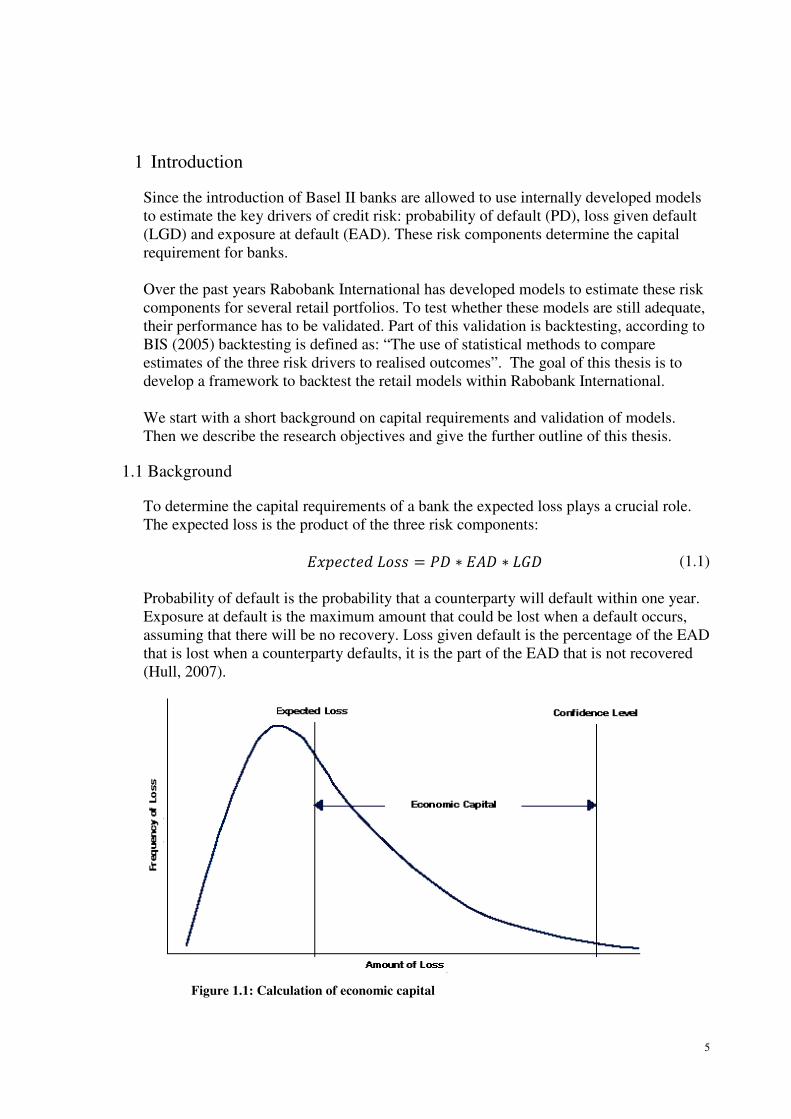
Figure 2.2: EAD estimation

The proportion of the off-balance sheet amount that is drawn in case of default

the credit conversion factor (CCF) (OeNB, 2004). Figure 2.2. illustrates a facility that

€2000 and an on-balance of €3000. If the EAD

balance is used and the credit conversion factor is 500/2000=1/4.

To calculate the exposure at default the following formula is used:

�� ! ∗ �� " #��ℎ� �To estimate the CCF a model is needed. As for PD and LGD, facilities can be bucketed

on different dimensions, for instance on product type (Hanoeman, 2010a)


, two approaches are used. One approach weighs the factors with the off

while the other approach uses a simple average of the observed CCFs. Th

taken into account when backtesting the factor.

The CCF is commonly smaller than one, for these portfolios the facilities do not draw

the maximum possible amount at default. The CCF is the only parameter within the

model that needs to be backtested. Our investigation will focus

EAD will be of minor importance.

backtesting procedure

2.3 summarizes which aspects have to be backtested for each of the three risk

The backtesting process can be divided into three stages;

he goal of backtesting stability is to find out if changes have occurred


backtesting period. Examples of aspects that are compared are the frequencies of

the facilities in PD or LGD buckets and if applicable the distribution of the PD


model, which makes it no longer appropriate to use (Castermans et al., 2

Discriminatory power: the goal of backtesting discriminatory power is to verify

whether the model can distinguishes between good and bad facilities

and low LGDs (Castermans et al., 2010). A good PD model is capable

11

in case of default is called

2.2. illustrates a facility that

EAD is €3500, €500 of

is 500/2000=1/4.

� �� (2.2)

To estimate the CCF a model is needed. As for PD and LGD, facilities can be bucketed

on different dimensions, for instance on product type (Hanoeman, 2010a). Hence, for


s the factors with the off-balance

while the other approach uses a simple average of the observed CCFs. This should be

the facilities do not draw

e only parameter within the

will focus on PD and LGD,

to be backtested for each of the three risk

he goal of backtesting stability is to find out if changes have occurred


are the frequencies of

the distribution of the PD


(Castermans et al., 2010).

he goal of backtesting discriminatory power is to verify

whether the model can distinguishes between good and bad facilities, or high

A good PD model is capable of

ranking the facilities in such a way that most defaults occur in the buckets with

the highest PDs and

similar for an LGD model, which is good if high

highest LGD buckets an

3. Predictive power

calibrated well. It compares the

predicted PD/LGD/CCF of the model (ex ante).

Stability is tested before

portfolio can influence the backtest

development population

predict adequately.

Figure 2.3: Overview of backtesting process

Since PD and LGD are divided into buckets according to a combination of factors that

differentiate between high and low values

For EAD the discriminatory p

power will be tested for all three components. It is tested on different levels, for PD and

LGD the predictions for the buckets and the whole model have to be tested, for EAD

there is only a CCF on product level which has to be tested. The main focus of

backtesting will be on the predictive power because the

the capital requirements.

In the case that a transition matrix is used to estimate PD

done. The matrix has to be tested

status to another.

In Figure 2.3 we give a general outline of the aspects that should be backteste

backtesting framework. We use this

current backtesting methodology.


the highest PDs and less defaults occur in the buckets with low PDs. This is

LGD model, which is good if high losses are observed in the

highest LGD buckets and low losses in the lowest LGD buckets.

Predictive power: backtesting the predictive power tests if the model is

librated well. It compares the observed PD/LGD/CCF (ex post) with the

predicted PD/LGD/CCF of the model (ex ante).

re the other two stages are tested, because the stability

luence the backtest. Hence, if the portfolio differs significantly

population it could be that the model is no longer able to differentiate and

Figure 2.3: Overview of backtesting process


differentiate between high and low values, the discriminatory power

For EAD the discriminatory power is not relevant and will not be tested

will be tested for all three components. It is tested on different levels, for PD and


n product level which has to be tested. The main focus of

backtesting will be on the predictive power because the predictions are use as a

the capital requirements.

In the case that a transition matrix is used to estimate PD or LGD an e

has to be tested on the probabilities to migrate from

a general outline of the aspects that should be backteste

backtesting framework. We use this outline in the rest of this thesis

current backtesting methodology.

12


defaults occur in the buckets with low PDs. This is

are observed in the

in the lowest LGD buckets.

acktesting the predictive power tests if the model is

observed PD/LGD/CCF (ex post) with the

because the stability of the

significantly from the

it could be that the model is no longer able to differentiate and


the discriminatory power has to be tested.

tested. The predictive

will be tested for all three components. It is tested on different levels, for PD and


n product level which has to be tested. The main focus of

predictions are use as a input for

LGD an extra test can be

from one repayment

a general outline of the aspects that should be backtested in the

thesis to improve the

13

2.2 Regulatory and internal guidelines

This section describes the guidelines set by regulators and the internal guidelines as they

are set within Rabobank.

2.2.1 Regulatory guidelines

The regulatory guidelines for the validation of internal rating systems and their risk

estimation are part of the Basel II framework (BIS, 2006), the Guidelines on the

implementation, validation and assessment of Advanced Measurement (AMA) and

Internal Ratings Based (IRB) Approaches by the Committee of European Banking

Supervisors (CEBS, 2006).

In short1 BIS has the following guidelines:

- (500) Banks must have a robust system to validate the accuracy and

consistency of the internal rating systems.

- (501) Banks must compare the estimates for PD, LGD and EAD by the use

of historical data. This should be documented and yearly updated.

- (502)The dataset for backtesting should cover a range of economic

conditions.

- (503) Banks must demonstrate that quantitative testing methods do not vary

systematically with the economic cycle. Changes in methods and data must

be clearly documented.

- (504) Banks must have well-articulated internal standards when the realized

PDs, LGDs and EADs deviate significantly from expectations.

Basel III does not change the guidelines for backtesting. Basel III does increase the

capital requirement for banks (BIS, 2011). Since the internal models are used as an input

for the capital calculations, it is important that these models predict adequately. This

indicates that a proper backtesting procedure will be even more important.

CEBS has overlap with the BIS guidelines, the additional guidelines are:

- (392) Institutions are expected to provide sound, robust and accurate predictive

and forward-looking estimates of the risk parameters.

- (393, 394 & 395) Banks should use backtesting. Backtesting generally involves

comparing realized with estimated parameters for a comparable and

homogeneous data set for PD, LGD and EAD models by statistical methods.

- (396) At a minimum backtesting should focus on the following issues:

• The underlying rating philosophy used in developing rating systems (e.g.

point-in-time or through-the-cycle forecasting in PD models. This will be

discussed in more detail in subsection 4.2.1.).

• Institutions should have a policy with remedial actions when a

backtesting result breaches the tolerance thresholds for validation.

• If backtesting is hindered by lack of data or quantitative information,

institutions have to rely more on additional qualitative information.

1 Appendix 1 contains a longer version

14

• The identification of specific reasons for discrepancies between predicted

values and observed outcomes.

At a minimum institutions should adopt and document policies that explain the objective

and logic in their backtesting procedure.

These guidelines stress the importance of backtesting. They indicate that the rating

philosophy should be taken into account. In subsection 4.2.1, two rating philosophies,

point-in-time and through-the-cycle, will be further analyzed. This will explain the

influence these rating philosophies have on backtesting.

The guidelines focus on statistical tests and emphasize that the deviations should be

tested on statistical significance. In the current framework not all tests are clear and the

rejection areas are often based on percentages which may not be appropriate to test

significant deviations. These points will be further investigated.

2.2.2 Internal guidelines

Probability of Default

For each of the three stages certain general tests have to be performed. Additional

optional tests can be performed. Table 2.1 gives an overview of the general tests. In the

next Chapters, the tests and their assumptions will be explained in more detail and their

problems will be identified (RMVM, 2010). Description Test

Predictive power

Model test Tests PD with observed defaults on model-level. Binomial test

Rating bucket test Tests PD with observed defaults on bucket level. Binomial test

Composed model test Extend to the rating bucket test. Test if the

number of rejected buckets is not to high.

Multinomial test

Discriminative power

Power statistic Measures discriminatory power. Powerstat

Receiver operating

characteristic

Compares discriminatory power of model with a

random model.

ROC curve

Stability testing

Model coverage Compares the model coverage during

development with the current coverage.

-

Table 2.1: General tests

Exposure at Default and Loss Given Default

The internal guidelines for EAD and LGD models are less strict. It is not necessary to

use certain mathematical tools but the guidelines advise to review the models in three

stages: stability, discriminatory and predictive power. It is also recommended to validate

the transition matrix.

How to analyze these three stages depends on the model and the data availability. For

EAD the bucketing is performed according to one dimension, which determines the

CCF. Because there is only one dimension that differentiates the CCFs the

discriminatory power will not be tested (Risk Dynamics, 2006). The three stages will be

used as a starting point for developing the framewor

deciding which tests will be used to backtest.

2.3 Current Backtesting

In this section on the current

backtesting procedures f

disadvantages.

2.3.1 Traffic light approach

To present the outcomes of a backtest the traffic light approach is used. In general the

traffic light approach has three zones: green, yellow and red. Green means that the

model is accepted in the backtest.

null hypothesis is not rejected

model has to be monitored or further tests have to be done. Using a confi

a yellow zone refers to a rejection of the null hypothesis

Red means rejection of the

that either redevelopment, recalibration

approach is a commonly

Rabobank and will be u

2.3.2 Stability testing

Stability testing is the first step in backtesting. It compares the backtesting portfolio w

the portfolio during development.

models not enough attention is paid to

part of a much broader monitoring process

range of tests. Based on

Figure 2.4 Overview current PD backtesting. Dotted lines are optional paths.

used as a starting point for developing the framework and there is much freedom in

will be used to backtest.

Current Backtesting Framework

current backtesting framework we will describe the current

backtesting procedures for each of the risk categories and their advantages and

Traffic light approach

present the outcomes of a backtest the traffic light approach is used. In general the


in the backtest. When a confidence interval is used this means that the

null hypothesis is not rejected for a 95 percent significance level. Yellow means that the

model has to be monitored or further tests have to be done. Using a confi

a yellow zone refers to a rejection of the null hypothesis with 95 percent

Red means rejection of the null hypothesis with 99 percent significance

redevelopment, recalibration or further tests have to be perform

ly known presentation method of the backtesting

Rabobank and will be used in the rest of this thesis.

testing is the first step in backtesting. It compares the backtesting portfolio w

the portfolio during development. In the current backtesting methodology for retail

not enough attention is paid to stability tests. Stability testing is considered to be

part of a much broader monitoring process. The monitoring process covers a

range of tests. Based on a literature study tests will be selected for backtesting.


15

is much freedom in

describe the current

advantages and

present the outcomes of a backtest the traffic light approach is used. In general the


is used this means that the

Yellow means that the

model has to be monitored or further tests have to be done. Using a confidence interval,

95 percent significance.

significance, which indicates

performed. This

backtesting results within

testing is the first step in backtesting. It compares the backtesting portfolio with

In the current backtesting methodology for retail

Stability testing is considered to be

. The monitoring process covers a broad

tests will be selected for backtesting.


16

2.3.3 PD backtesting

Figure 2.4 gives an overview of the current backtesting framework. The framework is

split up in two parts, discriminatory and predictive power. Each of these tests will be

explained in more detail below. For the discriminatory power a Receiver Operation

Curve is constructed which results in a powerstat. The conclusion of the discriminatory

power is based on the powerstat. For predictive power a binomial test is performed on

model and bucket level. If at least one of the buckets is rejected the composed model

test will be performed. It is optional to perform a binomial test with Type-II error

adjustment. The conclusion is based on a combination of the performed tests.

Discriminatory power

To test the discriminatory power of the scorecard the powerstat is used. To calculate the

powerstat a receiver operating characteristic (ROC) curve is drawn.

Default Non Default

Rating

score

Below C In concordance with

prediction (hit)

Wrong prediction

(false alarm)

Above C Wrong prediction

(miss)

In concordance

with prediction

Table 2.2: Different scenarios for score C

To draw the ROC curve all facilities are ordered based on their scorecard scores, from a

high PD (low score) to a low PD (high score). Then for each score C the hit rate and

false alarm rate are calculated (see Table 2.2).

$�� %�� &�' = ( )�#�� *+*,-./&0'1�� )�#�� (2.3)

!�� # %�� &�' = ( )�#�� )� ��*+*,-./&0'1�� )�#�� )� �� (2.4)

When C equals the minimum score the hit rate and false alarm rate both are zero.

Figure 2.5: ROC curve

The ROC curve depicts a rating curve which

for each score. Two additional curves are drawn.

(0,0) through (0,1) to (1,1)

observed. A random curve, the diagonal,

as non defaults and therefore does not differentiate

A ROC curve is used to test

score. To summarize the ROC curve

is the area under the rating curve. The AUC

2.5 the powerstat is B/(A+B), the quotient of the area between the rating curve and the

diagonal (B), and the area between the

Engelmann et al. (2003) show that:

According to the Rabobank guidelines, an increase

compared to the powerstat

power (Hanoeman, 2010c)

Predictive power

To test the predictive power of a PD model test

composed model level.

level.

Figure

To test on bucket and model level, the binomial distribution is approximated with the

normal distribution. Based on this normal distribution a

interval is created and it is tested

intervals.

These test are based on minimizing the

rejecting a correct model.

which is the probability of

overcome this problem a

confidence bounds based on both errors

the possible improvements and will be

ROC curve depicts a rating curve which is the hit rate against the false alarm rate

Two additional curves are drawn. The perfect model curve

rough (0,1) to (1,1), which captures all defaults before one non defaults is

observed. A random curve, the diagonal, which captures the same percentage of defaults

herefore does not differentiate (OeNB, 2004).

curve is used to test whether a lower score leads to more defaults

To summarize the ROC curve the Area Under Curve (AUC) is calculated.

is the area under the rating curve. The AUC is used to calculate the

owerstat is B/(A+B), the quotient of the area between the rating curve and the

area between the perfect model and the diagonal (A+B)

(2003) show that:

�� = 2 ∗ &�3� − 456'

According to the Rabobank guidelines, an increase or decreases of more than 20 percent

owerstat during the development indicates insufficient

(Hanoeman, 2010c).

predictive power of a PD model tests are performed on bucket,

composed model level. Figure 2.6 illustrates the difference between

Figure 2.6: Model and bucket level


normal distribution. Based on this normal distribution a 95 and 99 percent

d it is tested whether the observed default rate falls within these

on minimizing the Type-I error, which is the probability of

model. If the Type-I error decreases, the Type-II error increases,

the probability of accepting an incorrect model (Hanoeman, 2010c)

overcome this problem an adjusted backtesting methodology was proposed

based on both errors. The implementation of this method is one

possible improvements and will be further examined in subsection

17

is the hit rate against the false alarm rate

perfect model curve, a line from

which captures all defaults before one non defaults is

which captures the same percentage of defaults

a lower score leads to more defaults than a higher

ve (AUC) is calculated. Which

he powerstat. In Figure

owerstat is B/(A+B), the quotient of the area between the rating curve and the

diagonal (A+B).

(2.5)

more than 20 percent

indicates insufficient discriminatory

s are performed on bucket, model and

difference between model and bucket


percent confidence

efault rate falls within these

probability of

II error increases,

(Hanoeman, 2010c). To

backtesting methodology was proposed to set the

e implementation of this method is one of

section 4.2.2.

18

The composed model test, tests whether the number of rejected buckets is acceptable for

an adequate model. For example if a model has 20 buckets it is expected that one will

result in yellow. This test is preferred over the normal test at model level, because the

test on model level compensates optimistic buckets with conservative buckets (RMVM,

2010).

Advantages, disadvantages and points of improvement

Table 2.3 gives an overview of the advantages, disadvantages and improvements for

each test.

Advantages Disadvantages Improvements


ROC curve/

Powerstat

- Intuitive method

- Easy to use.

- Confidence interval

possible.

- Shape of curve is not used, where it

does give information about the

discriminatory power (OeNB, 2004).

- Dependent on underlying portfolio,

only similar portfolios should be

compared (Blochwitz, 2005).

- Rejection is based on a percentage and

not on a confidence interval.

- Use the shape of the

curve.

-Confidence intervals for

powerstat and ROC

curve .

Predictive power

Binomial

test

- Commonly known

method.

- Easy to calculate.

- Assumes independence between

defaults. Independence of defaults might

be assumed for a point-in-time PD, but a

through-the-cycle PD is used. This will

be further explained in subsection 4.2.1.

-Take the correlation

between defaults into

account.

- Examine the new

adjusted backtesting

methodology for Type-II

errors and whether it can

be implemented.

Composed

model test

-Takes into account the

chance a bucket is

rejected in a adequate

model.

- Does not cancel out too

optimistic against too

conservative buckets.

- Hard to compute (Hanoeman, 2010c).

- Not intuitive.

- Replace this test by

another test on model

level.

Table 2.3: Overview advantages, disadvantages and points of improvement

Figure 2.4 indicates the possible improvements, the tests with blue borders can be

improved on the confidence bounds, the red borders can be improved on the aspects

mentioned above. These improvements will be examined in Chapter 4.

2.3.4 LGD Backtesting

Figure 2.7 shows the backtesting framework for LGD. All tests will be explained in

more detail below. For discriminatory power there is a split between tests on model and

bucket level. On model level a powercurve is constructed which results in a powerstat.

On bucket level the CLAR is calculated. Based on the powerstat and the CLAR a

Figure 2.7: Overview

conclusion is drawn. Predictive power is split up in loss at default (LGD times EAD)

and LGD. Based on the results of all three tests the predictive power is derived.


Testing discriminatory power is split up in a powercurve on model

Cumulative LGD Accuracy Ratio (CLAR)

powercurve is constructed by ranking all predicted losses at default (LGD times EAD)

from high till low. On the x

on the y-axis the cumulative percentage of observed

similar to the ROC-curve used in backtesting PD, the difference is the x

depicts all observations instead of only the non default

calculated by B/(A+B), which

Rabobank guidelines the result is green if the powerstat is above 40 percent, yellow

between 0 and 40 percent and red below zero percent.

Figure 2.7: Overview current LGD backtesting methodology




Testing discriminatory power is split up in a powercurve on model level and a

Cumulative LGD Accuracy Ratio (CLAR) on bucket level. For the powerstat a

Figure 2.8: Powercurve


till low. On the x-axis the cumulative percentage of observations is stated and

cumulative percentage of observed losses at default. This curve is

curve used in backtesting PD, the difference is the x

vations instead of only the non defaults. Then the powerstat is

calculated by B/(A+B), which is equal to the powerstat used for PD. According to the

the result is green if the powerstat is above 40 percent, yellow

between 0 and 40 percent and red below zero percent.

19



level and a

on bucket level. For the powerstat a


of observations is stated and

losses at default. This curve is

curve used in backtesting PD, the difference is the x-axis which

Then the powerstat is

to the powerstat used for PD. According to the

the result is green if the powerstat is above 40 percent, yellow

To test the discriminatory power on

CLAR. In Figure 2.9 the CLAR

curve, observed LGDs are ordered from high till

X observations are selected, where

bucket. From these X observations the number of observations out of the highest LGD

bucket is counted. This number divided by the

percentage of correctly assigned observations. This is repeated on a cumulative

each LGD bucket. Figure

of 75 percent2. The red li

correct.

According to the Rabobank guidelines the

yellow between 25 and 50 p

data used to construct Figure

powerstat, therefore the adequateness

further examined.

Predictive power

Testing the predictive power is split up in loss at default and LGD. Testing the loss at

default means that the

only the percentages.

The loss shortfall (LS)

predicted.

��OLGD = Observed LGD

2 The calculation of this CLAR curve is shown in Appendix

Figure 2.9 CLAR curve

To test the discriminatory power on bucket level a different measure is used, called the

he CLAR is twice the area under the curve (A)

observed LGDs are ordered from high till low. From these ordered LGDs

observations are selected, where X is the number of observations in the highest LGD

observations the number of observations out of the highest LGD

bucket is counted. This number divided by the total number of observations

percentage of correctly assigned observations. This is repeated on a cumulative

Figure 2.9 illustrates a CLAR curve for three buckets with a CLAR

. The red line indicates the perfect model, where each observation is

According to the Rabobank guidelines the CLAR results in green above

yellow between 25 and 50 percent and red below 25 percent (Hanoeman, 2010b)

Figure 2.9 had low discriminatory power according to the

the adequateness of the rejection areas is suspicious and will be


actual losses are tested (LGD times EAD), testing LGD

indicates how much the loss at default is lower than the

�� 7ℎ�� = 1 − ( &��*� ��*'8*,9( &��*� ��*'8*,9

LGD

is CLAR curve is shown in Appendix 2.

20

a different measure is used, called the

(A). To construct the

low. From these ordered LGDs the first

is the number of observations in the highest LGD

observations the number of observations out of the highest LGD

total number of observations is the

percentage of correctly assigned observations. This is repeated on a cumulative basis for

buckets with a CLAR

ect model, where each observation is

results in green above 50 percent,

(Hanoeman, 2010b). The

according to the

is suspicious and will be


losses are tested (LGD times EAD), testing LGD concerns

is lower than the

'' (2.6)

21

LGD = Predicted LGD

The model is red above zero and below -0.20, yellow between -0.20 and -0.10 and green

between -0.10 and zero. The model tests conservatism because the model is only

accepted if the observed loss is lower than the predicted loss.

The Mean Absolute Deviation (MAD) concerns the absolute difference between the

observed and predicted loss, which is calculated by:

:�� = ( ;��* − ��*; � ��*8 *,9 ( ��*8*,9 (2.7)

The model is green below 10 percent, yellow between 10 and 20 and red above 20

percent. The LS compares the total loss levels while the MAD measures the average

difference per facility. As for PD the LGD predictions on model and bucket level are

tested by constructing a confidence interval around the predictions (Hanoeman, 2010b).

In the current framework it is not described how to perform these tests.

Advantages, disadvantages and points of improvement

Table 2.4 gives an overview of the advantages, disadvantages and improvements for

each test.

Advantages Disadvantages Improvements

Discriminatory Power

Powercurve/

Powerstat

-Easy to compute

- Intuitive.

- Can be based on

loss at default or

LGD.

- Shape of curve is not used, where it does give

information about the discriminatory power

(OeNB, 2004).

- Dependent on underlying portfolio, only

similar portfolios should be compared

(Blochwitz et al., 2005).

- No statistical confidence interval possible,

because these are based on binary variables.

- Analyze the shape of the

curve.

- Determine which version of

the curve (based on loss at

default or LGDs) gives the

most information.

CLAR - Tests on bucket

level.

- High computational effort.

- Less intuitive than powercurve.

- Further analyze the CLAR to

see whether it has advantages

over the powerstat.

-Validate the rejection areas.

Predictive Power

Loss shortfall - Easy to

compute.

- intuitive.

- Cancels out too high LGDs against too low

LGDs.

- Rejection based on percentage and not on a

confidence interval.

- Redefine the rejection area

such that it incorporates the

variance and number of

observations.

Mean

Absolute

Deviation

- Easy to

compute.

- intuitive.

- Highly influenced by variance which should

be taken into account in the rejection areas.

- Redefine the rejection area

such that it incorporates the

variance and number of

observations.

Model/Bucket

test

- Not clear which distribution is used and how

the confidence bounds are set.

- Develop test to backtest

LGD percentages.

Transition

matrix

- Currently not tested. - Incorporate a test to backtest

the transition matrix.

Table 2.4: Overview advantages, disadvantages and points of improvement

22

Figure 2.7 indicates the improvements, the tests with blue borders can be improved on

the confidence bounds, the red borders can be improved on the aspects mentioned

above. These improvements will be examined in Chapter 5.

2.3.5 EAD Backtesting

Predictive power

To test the predictive power of an EAD model a student t-test is used to create a

confidence interval around the observed CCF (Hanoeman, 2010a).

Advantages, disadvantages and points of improvement Because the only factor that has to be backtested is the prediction of the CCF, which is

done by the student t-test. This test is well-known, but does make some assumptions.

The test will be examined for EAD, but is expected to be suitable.

2.4 Conclusion Current situation

In this Chapter we focused at answering the first two research questions:

- Which models are used for estimating PD, LGD and EAD and on what aspects

should they be backtested?

- Which backtesting methods are currently used and what are the points of

improvement for these methods?

Stability is the first aspect that has to be tested. In the current reviewing process stability

testing is part of monitoring and is only slightly touched upon. The monitoring process

covers a broad range of tests. Based on literature study, appropriate tests will be selected

for the backtesting framework.

To predict the PD a scorecard is used as main input. According to the score and possible

additional dimensions a facility is assigned to a bucket, with a certain PD. The PD

models have to be tested on all three stages. For the predictive and discriminatory power

there are strict internal guidelines. For discriminatory power a ROC curve has to be

plotted and a powerstat calculated. For predictive power the binomial test has to be used

on model and bucket level and a composed model test has to be used to test the number

of rejected buckets. The points of improvement are: confidence bounds for the

powerstat and curve, implementing the Type-II error adjustment, replacing the

composed model test and incorporating correlation between defaults in the binomial

test.

LGD is predicted according to multiple dimensions, which are used to bucket the LGDs.

For the prediction of the repayments a transition matrix or the counting approach can be

used. LGD has to be backtested on all three stages. Discriminatory power is tested by

the powercurve and the CLAR. The predictive power is tested by loss shortfall, mean

absolute deviation and a test on model and buckets level that compares the observed and

23

predicted LGDs. The points of improvement are: the rejection areas, the different

options for the powercurve and two additional test that have to be added. First, a test to

compare the observed with the predicted LGDs on model and bucket level, currently

this test is not developed. Second, a test to backtest the transition matrix, which is not

incorporated in the current framework.

For EAD only the CCF is estimated. Therefore the stability of the portfolio and the

predictive power have to be tested. The internal guidelines are less strict, no specific test

is required. For EAD a student t-test is used to compare the predicted and observed

CCF, this test will be examined.

24

25

3 Proposals for improved stability testing

In the current backtesting methodology for retail models stability tests are not included.

Stability testing is considered to be part of a much broader monitoring process. The tests

used in the monitoring process are compared with tests mentioned in literature.

Castermans et al. (2010) compare several methods and based on this comparison it can

be concluded that the system stability index (SSI) and the Chi-squared test are preferred

to test ordinal data. The SSI is easy to use and intuitive while the Chi-squared test is

statistically well founded. Poëta (2009) uses the Kolmogorov-Smirnov test for

continuous data and a test similar to the SSI for ordinal data. The Kolmogorov-Smirnov

and the SSI are used in the current monitoring process (RMVM, 2010). These three tests

are described in more detail and compared in this Chapter.

3.1 System Stability Index

The purpose of the system stability index is to test whether two discrete samples have a

similar distribution. An advantage of this test is that it does not assume a specific

distribution. A disadvantage is that it can only be used to compare discrete samples. If a

sample is continuously distributed, cut-off values have to be determined to split the

population up in segments, these cut-off values can be hard to determine (Castermans et

al., 2010). Another advantage is that it uses the relative size of the shift by multiplying

with �� <=>?>@.

The SSI is defined as:

77A = B&C* − �*' ∗ �� DC*�*E* (3.1) �* , C* are the percentages of the datasets A (backtesting) and B (reference) that belong

to segment i.

According to the Rabobank guidelines the conclusion can be drawn subject to a Rule of

Thumb (RMVM, 2010):

• SSI < 0.10: No shift

• SSI in [0.10, 0.25]: Minor shift

• SSI > 0.25 Major shift

3.2 Kolmogorov-Smirnov test

The Kolmogorov-Smirnov test (KS-test) is used to determine whether two samples are

drawn from the same continuous distribution. The following hypotheses are formulated:

H0: The distributions are the same.

H1: The distributions are not the same.

The KS-test does not assume a specific distribution of the data. The test is based on the

maximum distance between two cumulative distributions. A requirement of the test is

that it must be able to rank the observations to determine two comparable cumulative

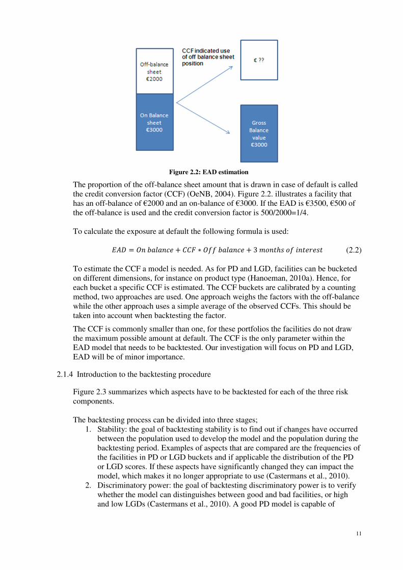
distributions. Figure 3.1 illustrates the maximum distance between two distributions.

26

To calculate the maximum distance two cumulative distributions are constructed:

!GH&�' = 1) B AIH>JKL8

*,9 (3.2)

!GM&�' = 1: B AIM>JKLN

*,9

(3.3)

Where Xi as the observation from sample X, with i=1,..,N and Yj as the observations

from sample Y, with j=1,...,M. I is an indicator function.

The maximum distance is defined as:

�N8 = maxK R!GH&�' − !GM&�'R (3.4)

Then the test statistic is calculated by (RMVM, 2010):

1 = S ):) : ∗ �N8 (3.5)

When the sample size goes to infinity, T is Kolmogorov-Smirnov (KS) distributed. The

sample size is sufficiently large enough to use this distribution when there are more than

40 observations (Higgins, 2004).

The test is based on three assumptions:

• Xi and Yi are independent random samples, which have cumulative distributions

FX and FY.

• For the test to be exact FX and FY must be continuous.

• The measurement scale is at least ordinal (Higgins, 2004).

0

0,2

0,4

0,6

0,8

1

1 2 3 4 5 6 7 8

Cu

mu

lati

ve

dis

trib

uti

on

Segments x

Development sample

Review sample

Figure 3.1: KS-test, maximum difference between two cumulative distributions

27

3.3 Chi-squared test

The Chi-squared test compares discrete distributions as the SSI. It compares the

observed frequencies with predicted frequencies within a segment i. The chi-squared

test assumes independence between segments. The test statistic is chi-squared

distributed, therefore conclusion can be drawn based on this distribution:

T NU9V ~ B &��X�� Y��Z* − �� Y��Z*'V�� Y��Z*N

*,9 (3.6)

Where M is the number of observations and M-1 the degrees of freedom (Castermans et

al., 2010).

3.4 Comparison

The Chi-squared and the SSI both test discrete distributions. The main advantage of the

SSI over the Chi-squared test is that the SSI incorporates the relative importance. A shift

in a segment with a low number of observations is less important than a shift in a

segment with a high number of observations. For the Chi-squared test each segment is

equally important and a shift in a small bucket can reject the whole portfolio. Therefore

the Chi-squared test is too strict to test the stability of a portfolio and the SSI will be

used.

The Kolmogorov-Smirnov test gives adequate results if ranking is possible. If ranking is

not possible or difficult, the test is strongly influenced by the ordering of observations.

If ranking is not possible the sample has to be split up in segments and the SSI will be

used.

3.5 Conclusion

This Chapter answers the third sub question:

Which tests should be used to test the stability of the portfolio?

Based on tests described in literature and in the monitoring guidelines, the stability

should be tested by the Kolmogorov-Smirnov test for continuous samples and by the

system stability index for discrete samples. The Chi-squared test is not selected because

it rejects portfolios in many cases, mainly because every segment has equal importance

which results in rejection when a segment with low frequencies has a significant shift.

28

29

4 Proposals for improvement of Backtesting PD

We start this Chapter with an analysis of the points of improvement that resulted from

the assessment of the current backtesting methodology. This Chapter is split up in two

parts, a part on discriminatory and a part on predictive power.

The discriminatory power of the current framework can be improved by adding

confidence intervals to the ROC curve and Powerstat.

For predictive power three improvements of the current framework will be investigated:

- Correlation between defaults and their effect on the binomial test.

- Implementing the adjusted backtesting methodology for Type-II errors.

- Replacement of the composed model test by another test on model level.

This Chapter ends with an overview of the proposed backtesting framework for PD.

4.1 Discriminatory power

The discriminatory power part of the current backtesting framework can be improved by

creating a confidence interval around the ROC curve and powerstat. In the current

situation the ROC curve itself is not used, only its summary statistic, the powerstat is

used. The curve itself gives valuable information by its steepness and curvature. To

indicate if the observed curve deviates significantly from the curve during development

a confidence interval is needed. Several options will be given in this section.

In the current framework the rejection areas for the powerstat are based on percentages

which means that it does not take the number of observations into account and therefore

is not statistically underpinned. A rejection area relative to the performance of the model

during development based on variance is more desirable. As mentioned in subsection

2.3.3 the powerstat is linearly dependent on the Area Under Curve (AUC):

�� = 2 ∗ &�3� − 456' (4.1)

For the AUC it is possible to construct a confidence interval, this we will examine

further.

4.1.1 Confidence interval ROC curve

To test whether two datasets with the same underlying distribution have similar

discriminatory power a confidence interval is constructed. Macskassy and Provost

(2005) compared in their paper several confidence bounds for ROC curves. They

described several methods and validated them with data. This research resulted in two

relatively robust methods that should give accurate confidence intervals. These methods,

the simultaneous joint confidence region method (SJR) and the fixed-width confidence

bound (FWB) will be examined further and eventually compared for the use in

backtesting. Both methods shift the ROC curve to create confidence bounds, this results

in bounds that do not start in (0,0) and end in (1,1). This is counter intuitive because the

curve will never deviate from these points in practice. Because for the backtested curve

the start and end points are fixed the major deviations will be in the middle where the

30

bounds do resemble the true deviation. Besides these two methods a bootstrapped

confidence interval will be analyzed, this interval will have the intuitive start and end

point, but is time consuming to construct.

Fixed Width confidence Bound method

For the FWB method the original ROC curve is shifted along a slope b, b < 0 over a

distance d. The distance d is defined by bootstrapping, such that (1-α) percent of the

bootstrapped samples fall within the bounds, where α is (1-confidence level). The slope

b is defined as � = – \:/), where M is the number of true positives (defaults) and N

the number true negatives (non defaults) (Macskassy & Provost, 2005). This is

illustrated in Figure 4.1. A drawback of this method is the computational effort needed

to calculate the distance d.

Simultaneous Joint confidence Region method

The SJR method uses the Kolmogorov-Smirnov (KS) test statistic. The KS statistic is

used to test whether two samples come from the same underlying distribution, by

analyzing the maximum vertical distance between two cumulative distributions. In the

case of a ROC curve the KS statistic is used twice, once to determine the maximum

horizontal distance from the hit rate and once for the maximum vertical distance from

the false alarm rate (Macskassy & Provost, 2005).

Figure 4.2: Simultaneous Joint Confidence Regions (Macskassy & Provost, 2005)

Figure 4.1: Fixed-Width confidence bounds (Macskassy, 2004)

31

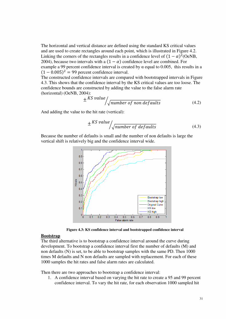
The horizontal and vertical distance are defined using the standard KS critical values

and are used to create rectangles around each point, which is illustrated in Figure 4.2.

Linking the corners of the rectangles results in a confidence level of &1 − ^'V(OeNB,

2004), because two intervals with a &1 − ^' confidence level are combined. For

example a 99 percent confidence interval is created by α equal to 0.005, this results in a &1 − 45446'V = 99 percent confidence interval.

The constructed confidence intervals are compared with bootstrapped intervals in Figure

4.3. This shows that the confidence interval by the KS critical values are too loose. The

confidence bounds are constructed by adding the value to the false alarm rate

(horizontal) (OeNB, 2004):

± a7 X�� \��#�� b (4.2)

And adding the value to the hit rate (vertical):

± a7 X�� \��#�� b (4.3)

Because the number of defaults is small and the number of non defaults is large the

vertical shift is relatively big and the confidence interval wide.

Bootstrap

The third alternative is to bootstrap a confidence interval around the curve during

development. To bootstrap a confidence interval first the number of defaults (M) and

non defaults (N) is set, to be able to bootstrap samples with the same PD. Then 1000

times M defaults and N non defaults are sampled with replacement. For each of these

1000 samples the hit rates and false alarm rates are calculated.

Then there are two approaches to bootstrap a confidence interval:

1. A confidence interval based on varying the hit rate to create a 95 and 99 percent

confidence interval. To vary the hit rate, for each observation 1000 sampled hit

Figure 4.3: KS confidence interval and bootstrapped confidence interval

32

rates are ranked and the lower and upper quantiles are selected. For the selected

hit rates the corresponding false alarm rate is calculated and these combinations

are plotted.

2. A confidence interval based on varying the hit rate and the false alarm rate, to

create a 95 and 99 percent confidence interval around both variables. For these

confidence intervals the upper and lower quantiles of the ranked hit and false

alarm rate are selected. As for the SJR approach these quantiles can be used to

create rectangles around each point which are linked to create the confidence

intervals. This results in a slightly broader confidence interval, because two

confidence intervals are combined.

Both methods result in very similar bounds (see Appendix 4 for illustration). The second

method does not take into account that the hit rate and false alarm rate are related for

each observation. Combining both confidence levels independently results into points

that do not exist. For example after 20 observations the upper quantile of the hit rate has

2 hits and the upper quantile of the false alarm rate has 20 false alarms, which cannot be

observed after 20 observations. The first method is preferred because the confidence

level is known and the points are feasible. Appendix 4 shows that the bounds are

appropriate because most of the 100 bootstrapped samples are within the bounds.

Conclusion

The FWB method will not be used because it is hard to define distance d. The SJR

method results in a very broad confidence intervals which are deemed unrealistic and

therefore will not be used. The third alternative is to use a bootstrapped confidence

interval. This is more time consuming than the SJR but does result in intuitive and

adequate confidence bounds. Therefore the confidence intervals will be based on

bootstrapping.

4.1.2 Area under curve confidence interval

The statistic used to reject or accept the discriminatory power of a model is the AUC.

Therefore a confidence interval is needed to indicate whether the observed AUC is

different from the AUC during development. The AUC and the confidence interval can

be constructed using the distributions of defaulters and non defaulters. The AUC is

constructed according to the scores S of the defaulters SD,1, ..., SD,N and the non

defaulters SND,1,…,SND,M. The AUC is then given by:

�3� = ( ( 1cde,>fce,g8h,*N*,9 :) (4.4)

M = Number of non defaulters

N = Number of defaulters

This is equal to the value of the Wilcoxon-Mann-Whitney statistic, which compares the

ranking of two samples. The AUC is equal because it estimates the probability PND,D

that a randomly chosen non-defaulter is ranked higher than a randomly chosen defaulter

(Cortes & Mohri, 2005).

33

For large samples a confidence interval can be constructed using the normal distribution

(BIS, 2005), therefore the variance must be calculated. Two approaches to estimate the

variance are defined. These variances are based on the assumption that the model is

capable of differentiating, which means that the AUC is greater than a half. If this is the

case the variance is dependent on the distribution of defaulters and non defaulters. The

first approach assumes that the ratings are on a continuous scale. The second approach

does not make this assumption (Hanley & McNeil, 1982).

The hypotheses to compare the Area Under Curves are:

H0: The observed proportion of non defaulters that is ranked higher than

defaulters is equal to the AUC during development.

H1: These proportions are unequal.

No ties

The first approach assumes that the ratings are sufficiently continuous, continuous

means that it does not produce ‘ties’(Cortes & Mohri, 2005; Hanley & McNeil, 1982).

i?jkV = �3�&1 − �3�' &: − 1'l 8m,8m,m − �3�Vn &) − 1'l 8m,m,m − �3�Vn:)

(4.5)

If �8m,H and �8m,M are two independent randomly chosen non defaulter from 78m and �m,H and �m,M are two independent random chosen defaulter from 7m then 8m,m,mand 8m,8m,m are defined as:

8m,8m,m = l�8m,H , �8m,M > �m,Hn (4.6)

8m,m,m = l�m,H , �m,M < �8m,Hn (4.7)

Including ties The second approach as mentioned in BIS (2005) and Bamber (1975) does not assume

continuity of the rating scores and therefore may include ties:

iq?jkV = &7m ≠ 78m' &) − 1' 8m,m,m &: − 1' m,8m,8m − 4&) : − 1' <�3� − 12@V4&: − 1'&) − 1'

(4.8)

In BIS (2005) &7m ≠ 78m' is set at 1, which would mean no ties.

8m,m,m = l�m,H, �m,H < �8mn l�8m,H <, �m,H , �m,Mn− l�m,H < �8m,H < �m,Mn − l�m,M < �8m,H < �m,Mn (4.9)

m,8m,8m = l�8m,H , �8m,M < �m,Hn l�m,H < �8m,H , �8m,Mn− l�8m,H < �m,H < �8m,Mn − l�8m,M < �m,H < �8m,Mn

(4.10)

For large sample sizes (more than 50 defaults) the confidence interval α (95 or 99

percent) can be calculated using the normal distribution (BIS, 2005).

�� X�� = t�3� − i?jkV uU9 D1 ^2 E , �3� i?jkV uU9 D1 ^2 Ev

(4.11)

34

Based on the data of Bank BGZ the standard deviation and confidence intervals are

calculated. These theoretical confidence intervals and a confidence intervals based on a

bootstrap are shown in Table 4.1.

Method Sigma (%) 95% Bound (%) 99% Bound (%)

No ties 1.72 [74.77; 81.51][Confidential] 1.73

[74.76; 81.52]

[73.71; 82.57]

Ties [73.68; 82.60]

Bootstrap [74.78; 81.38] [73.61;82.46]

Table 4.1: Confidence interval for area under curve

Both methods give similar results because the BGZ data has only a few ties in its

observations. It can therefore be considered to be sufficiently continuous. Both

confidence intervals are in accordance with the bootstrapped confidence interval. The

first method is chosen, because the data is continuous and the more intuitive calculation.

If the ranking method is not continuous the second approach should be used.

4.2 Predictive power

For predictive power the binomial test can be improved on two aspects. First the impact

of correlation will be explained and then two methods to incorporate it will be

examined. The second aspect is the incorporation of Type-II errors when setting the

confidence bounds. Another point of improvement is the composed model test, this test

is hard to compute and not transparent, therefore two alternatives are examined that can

replace this test.

4.2.1 Incorporating correlation

There are two drivers for correlation between defaults. There is correlation between

defaults that arises due to the fact that companies operate in the same sector or region

and there is a more general correlation between defaults and the macroeconomic

situation. During economic downturn there are many defaults, while during economic

expansion there are less defaults. The correlation with the macroeconomic situation can

be incorporated in the rating philosophy, which is called a point-in-time rating. The

incorporation of the macroeconomic factors results in a lower correlation than when

macroeconomic factors are not included (through-the-cycle PD) (Miu & Ozdemir,

2005). Since the forecasted PDs for retail are not based on macroeconomic factors, an

adjustment can be made to reduce the influence of correlation. First the two different

rating philosophies will be discussed. Then two approaches to incorporate correlation

will be discussed.

4.2.1.1 Point-in-time and trough-the-cycle

There are two rating philosophies: point-in-time (PIT) and through-the-cycle (TTC).

PIT PDs reflect the probability of default over a future period, mostly a year. The PIT

PD is based on the current situation and can change rapidly if the macroeconomic

situation changes. PIT PDs tend to rise during economic downturns and fall during

economic expansion. The TTC PD is based mainly on obligor information and tends to

be constant over time. A TTC PD i

conditions and estimates the ave

Most rating systems within Rabobank are a combination between TTC and PIT. The PD

predictions are mainly based on a TTC philosophy to k

constant. But there is also a PIT aspect. PD buckets have fixed default rates, which

predict the PD through

output of the scorecard, but during

higher because the bucketing is influenced by manual overr

PDs (Mijnen, 2012). During economic expansion the opposite effect is observed. In the

case of retail modeling the rating system also has a PIT a

allowed, but in the scorecard there are factors which are influenced by the state of the

economy. In an economic downturn this results in migrations of facilities to

with higher PDs.

Most of the time backtesting incorporates a relatively short time period, commonly

backtesting is done over one year. Backtesting tests whether the observed number of

defaults during that year is in accordance with the predicted number of defaults in that

year. Because of the short time period, backtesting

rate with the predicted TTC PD.

The main difference between a PIT PD and a TTC PD is the influence of

macroeconomic factors. A PIT system predicts “conditional” on corr

macroeconomic factors while a TTC system predicts “unconditional”. The effect of

correlation between defaults is lower in a PIT rating philosophy because the systematic

movements of the macroeconomi

Figure 4.4 shows a stylized example of the difference betwe


be constant over time. A TTC PD is not adjusted explicitly to macroeconomic

and estimates the average PD over an economic cycle (BIS, 2005)


predictions are mainly based on a TTC philosophy to keep the capital requirements


predict the PD through-the-cycle. A facility is normally bucketed according to the

output of the scorecard, but during economic downturn the average PD predictions are

higher because the bucketing is influenced by manual overrides to buckets with higher

During economic expansion the opposite effect is observed. In the

case of retail modeling the rating system also has a PIT aspect. Manual overrides are not


economy. In an economic downturn this results in migrations of facilities to




year. Because of the short time period, backtesting compares the observed

with the predicted TTC PD.


macroeconomic factors. A PIT system predicts “conditional” on corr



movements of the macroeconomic factors are already included (Miu & Ozdemir

shows a stylized example of the difference between the observed default rate,

Figure 4.4: PIT and TTC PD

35


s not adjusted explicitly to macroeconomic

(BIS, 2005).


eep the capital requirements


cycle. A facility is normally bucketed according to the

verage PD predictions are

ides to buckets with higher

During economic expansion the opposite effect is observed. In the

spect. Manual overrides are not


economy. In an economic downturn this results in migrations of facilities to buckets




the observed PIT default


macroeconomic factors. A PIT system predicts “conditional” on correlation with



Miu & Ozdemir, 2005).

en the observed default rate,

36

the predicted TTC PD and PIT PD. It can be seen that for most years a comparison of

the observed default rate (PIT) and the TTC PD will lead to a rejection of the model,

because the observed default rate is either much lower or much higher than the TTC PD.

A PIT PD is more in concordance with the observed default rate over a short time

period.

To reduce this effect, correlation with macroeconomic factors is used to transform the

TTC PD into a PIT PD. By this transformation it is possible to backtest an estimation

for several years with one year of data. The transformation can be done by the use of the

one factor Vasicek model, which models the dependence on one common factor, in this

case a combination of macroeconomic factors. Vasicek’s one factor model (Hull, 2007):

w* = \x ∙ z* \1 − x ∙ {* (4.12) w* = Asset value z* = Common systematic factor, macroeconomic factors. {* = Independent factor x = Correlation, calculated according to Basel II guidelines

Two approaches based on this model will be discussed.

4.2.1.2 Basel approach

This approach is used in the Basel working paper about validation of internal rating

systems. It is used to analyze the influence of default correlation on the critical value k,

which is the upper confidence bound based on the binomial distribution. To calculate

the critical value k the following approach is used:

The number of defaults is defined as:

�8 = B 1l\|∙H>}\9U|∙~>��n8

*,9 , �ℎ�� = ФU9& �' (4.13)

N is the number of observations.

The default rate is defined as:

%8 = �8) (4.14)

If N becomes very large the default rate is:

% = lim8→� %8 = Ф �� − \xz\1 − x � (4.15)

The distribution of �8, to determine the critical value k, then becomes:

&�8 ≤ �' = � B <)�@��,�

�U� %�&1 − %'8U��&�'�� (4.16)

37

This can be approximated by a second order Taylor expansion. See the Appendix 3 for

this approximation (Tasche, 2003; BIS, 2005).

[Confidential]

Table 4.2: Comparison Binomial model and the Basel adjustment. Left side has fixed correlation of

5% while right side uses the Basel correlation.

The effect of the incorporation of default correlation on the critical value k is shown in

Table 4.2. The incorporation of correlation increases the upper confidence bound

significantly. Therefore this adjustment results in a broader confidence interval. If the

Basel correlation is used none of the buckets is rejected while without correlation all

these buckets were rejected on both a 95 and 99 percent significance level.

The main disadvantage is that this method results in a very high Type-II error (accepting

an incorrect model), because the critical values are bigger, which results in a lower

chance of rejection.

4.2.1.3 Rabobank internal approach

This approach is used within Rabobank to backtest a portfolio during economic

downturn or expansion and is based on correlation with macroeconomic factors. A

combination of macroeconomic factors is used to estimate the systematic factor.

According to the historical development of the macro-economic factors the actual

quantile of the economy over the backtesting period is estimated. If for example the

economy is in a downturn situation, which for example happens once every five years,

the actual quantile of the economy is 80 percent. So, there is a chance of 80 percent that

the economy performs better than the observed situation.

In order to transform the estimated TTC PD into a PIT PD, which corresponds to this

period in the economic cycle the Basel retail correlation is used. In formula form the

PIT PD is estimated by:

� A1 = ) �)−1& �11�' \x)−1&�� Y��'\1 − x � (4.17)

N= Cumulative normal distribution.

This adjusted PD is used as an input for backtesting. A confidence interval is created

around this adjusted PD (Herel, 2011; Hull, 2007).

A disadvantage is that the actual quantile of the economy has to be modeled and this

introduces an extra source of uncertainty. Therefore if an observed PD is rejected it

could be caused by an erroneous PD estimation or an erroneous estimation of the actual

quantile.

The advantages over the Basel approach is that the confidence interval does not widen

and the improved methodology which incorporates both Type-I and Type-II errors can

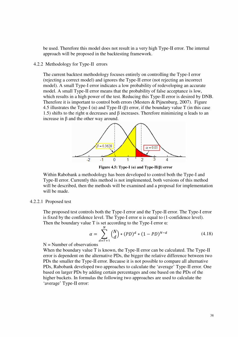
38

be used. Therefore this model does not result in a very high Type-II error. The internal

approach will be proposed in the backtesting framework.

4.2.2 Methodology for Type-II errors

The current backtest methodology focuses entirely on controlling the Type-I error

(rejecting a correct model) and ignores the Type-II error (not rejecting an incorrect

model). A small Type-I error indicates a low probability of redeveloping an accurate

model. A small Type-II error means that the probability of false acceptance is low,

which results in a high power of the test. Reducing this Type-II error is desired by DNB.

Therefore it is important to control both errors (Mesters & Pijnenburg, 2007). Figure

4.5 illustrates the Type-I (α) and Type-II (β) error, if the boundary value T (in this case

1.5) shifts to the right α decreases and β increases. Therefore minimizing α leads to an

increase in β and the other way around.

Figure 4.5: Type-I (α) and Type-II(β) error

Within Rabobank a methodology has been developed to control both the Type-I and

Type-II error. Currently this method is not implemented, both versions of this method

will be described, then the methods will be examined and a proposal for implementation

will be made.

4.2.2.1 Proposed test

The proposed test controls both the Type-I error and the Type-II error. The Type-I error

is fixed by the confidence level. The Type-I error α is equal to (1-confidence level).

Then the boundary value T is set according to the Type-I error α:

^ = B <)�@ ∗ & �'� ∗ &1 − �'8U�8�,�}9 (4.18)

N = Number of observations

When the boundary value T is known, the Type-II error can be calculated. The Type-II

error is dependent on the alternative PDs, the bigger the relative difference between two

PDs the smaller the Type-II error. Because it is not possible to compare all alternative

PDs, Rabobank developed two approaches to calculate the ‘average’ Type-II error. One

based on larger PDs by adding certain percentages and one based on the PDs of the

higher buckets. In formulas the following two approaches are used to calculate the

‘average’ Type-II error:

39

1. Based on all PDs larger than the predicted PD (RMVM, 2010).

The alternative PDs are defined as:

��* = �% � ∈ I � 1, � 2, … ,99L (4.19)

Then the Type-II error for each alternative PD is:

��* = B <)� @ �& ��*'��&1 − ��*'8U��,� (4.20)

Then the weighted average Type-II error for a certain T is :

� = ( & ��* − �'��*��*,�m}9( & ��* − �'��*,�m}9 (4.21)

2. Based on the PDs of higher buckets (Mesters & Pijnenburg, 2007).

� �� %* = ( l �h − �*n1*h8}9h,*}9( l �h − �*n8}9h,*}9 (4.22) 1*h = Probability of accepting H0 (rating Ri) when H1(rating Rj) is correct. 1*h is

calculated as ��* with PDai is PDj. �*= Predicted PD of rating bucket Ri. For the highest PD bucket an additional bucket

has to be added and is defined by PDN+1 > PDN.

N= Number of buckets.

Both methods use the same optimization criteria to find the optimal T value. When the

first optimization criterion is not feasible the second is used, etc.

1. Maximize Type-I, while both Type-I and Type-II are below 5 percent.

2. Minimize Type-I, while Type-II is below 5 percent.

3. Minimize Type-I, with no constraint on Type-II error (Mesters & Pijnenburg,

2007).

4.2.2.2 Comparison and improvements

There are two aspects that influence the average Type-II error, illustrated in Figure 4.6.

Based on all higher PDs

The first aspect is the difference of impact of a one percent increase in PD for different

PD values. A one percent increase has a different effect on a bucket with a low PD than

on a bucket a high PD. For the low PD an increase of one percent results in a much

lower Type-II error than for a high PD.

The second aspect is the maximum shift that has an impact. For low PDs only an

increase till a few percent influences the Type-II error while for high PDs a much bigger

increase still influences the Type-II error. In calculating the average Type-II error all

higher alternative PDs are taken into account. This sometimes results in a Type-II error

equaling zero, because there is a big difference between the two PDs. When taking βais

equal to zero into account the average Type-II error will be smaller than expected. This

because if the βai is zero the sum in the numerator stays equal while the denominator

grows with & ��* − �'.

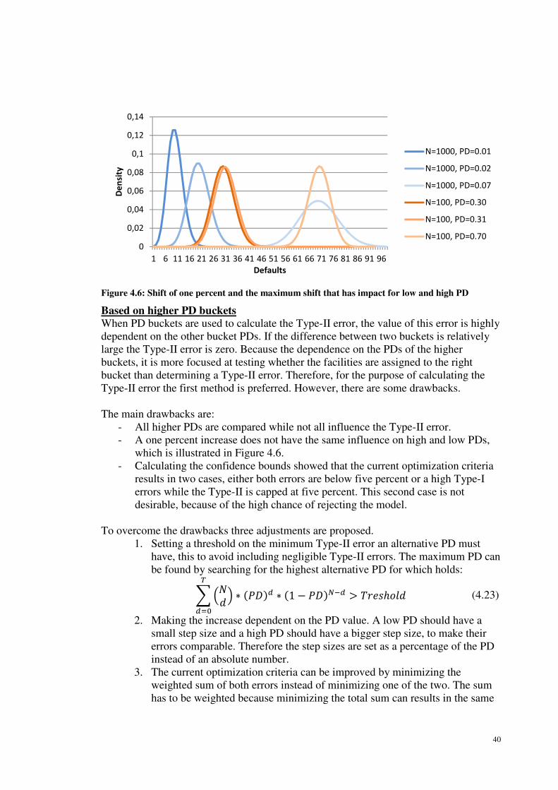
40

Figure 4.6: Shift of one percent and the maximum shift that has impact for low and high PD

Based on higher PD buckets

When PD buckets are used to calculate the Type-II error, the value of this error is highly

dependent on the other bucket PDs. If the difference between two buckets is relatively

large the Type-II error is zero. Because the dependence on the PDs of the higher

buckets, it is more focused at testing whether the facilities are assigned to the right

bucket than determining a Type-II error. Therefore, for the purpose of calculating the

Type-II error the first method is preferred. However, there are some drawbacks.

The main drawbacks are:

- All higher PDs are compared while not all influence the Type-II error.

- A one percent increase does not have the same influence on high and low PDs,

which is illustrated in Figure 4.6.

- Calculating the confidence bounds showed that the current optimization criteria

results in two cases, either both errors are below five percent or a high Type-I

errors while the Type-II is capped at five percent. This second case is not

desirable, because of the high chance of rejecting the model.

To overcome the drawbacks three adjustments are proposed.

1. Setting a threshold on the minimum Type-II error an alternative PD must

have, this to avoid including negligible Type-II errors. The maximum PD can

be found by searching for the highest alternative PD for which holds:

B <)� @ ∗ & �'� ∗ &1 − �'8U��,� > 1��ℎ�� (4.23)

2. Making the increase dependent on the PD value. A low PD should have a

small step size and a high PD should have a bigger step size, to make their

errors comparable. Therefore the step sizes are set as a percentage of the PD

instead of an absolute number.

3. The current optimization criteria can be improved by minimizing the

weighted sum of both errors instead of minimizing one of the two. The sum

has to be weighted because minimizing the total sum can results in the same

0

0,02

0,04

0,06

0,08

0,1

0,12

0,14

1 6 11 16 21 26 31 36 41 46 51 56 61 66 71 76 81 86 91 96

De

nsi

ty

Defaults

N=1000, PD=0.01

N=1000, PD=0.02

N=1000, PD=0.07

N=100, PD=0.30

N=100, PD=0.31

N=100, PD=0.70

41

boundaries for different confidence levels. By weighting the errors this can

be avoided. Different weights were tested, of which the weight for the Type-I

error is higher because this is used in the original test and will result in a

lower number of rejections. From Table 4.3 it can be seen that if the weights

are 60/40 both confidence levels give similar bounds which does not solve

the problem. For the weight 80/20 the boundary T does not differ from the

normal boundary values without the error adjustment. The weight 65/35 and

70/30 give the same results. Therefore 65/35 is chosen because this gives the

highest weight to the Type-II error which should be included.

Confidence level

Boundary value T Weights (Type-

I/Type-II) Bucket 1 Bucket 2 Bucket 3 Bucket 4

95% boundary values of

normal binomial test

11 30 44 42

95% 11 30 44 41 80/20

11 29 43 41 70/30

11 29 43 41 65/35

10 28 42 40 60/40

99% 12 30 44 41 80/20

11 29 43 41 70/30

11 29 43 41 65/35

11 28 42 40 60/40

Table 4.3: Comparison boundary values with different weights

4.2.3 Composed model test

The test on model level tests whether the average observed default rate falls within

certain confidence bounds. The model test is based on the average observed default rate.

However, it can be the case that one bucket has a too high estimated PD and another

bucket has a too low estimated PD but the result on average is still adequate. This is the

first reason to have an additional test where this effect does not play a role. The second

reason is to have a test which combines the results from the bucket tests. Each bucket is

tested separately, but how many buckets have to be rejected in order to reject the whole

model? Currently the composed model test is used to test these two aspects, but there

are some drawbacks. These drawbacks will be discussed first, then two alternative tests

are introduced.

4.2.3.1 Technical description of the composed model test

The composed model test verifies whether the number of observed yellow-zones and

red-zones is likely to be in line with an accurate model. The test consists out of six

subtests, four one sided tests on too optimistic or conservative buckets, both for yellow

and red zones and two two-sided tests on yellow and red zones.

42

The test is based on the parameter βi, which is the Type-I error per rating bucket i. βi

should be smaller than the confidence level.

C = B z*8

*,9 (4.24)

B is the number of buckets in a specific zone. Xi is one if bucket i falls in the zone, zero

otherwise. The chances of rejecting B buckets is calculated as follows:

&C = 4' = �&1 − �*'8*,9 (4.25)

&C = 1' = B ��1 − ��8

��,9 �&1 − �*'8*,9 (4.26)

&C = �' = B B ⋯8U&�UV'��f��

B ��1 − �� ⋯ �� 1 − �� 1 − ��

8��f��

�&1 − �*'8*,9

8U&�U9'��,9

(4.27)

&C = )' = �&�*'8*,9

(4.28)

The probability distribution for B is then defined as:

&C ≤ �' = B &C = �'�*,� (4.29)

The critical values determine the boundaries by:

B1:( &C ≤ �' < 96% ≤ ( &C ≤ �'=��,¡=�U9�,¡ (4.30)

B2:( &C ≤ �' < 99% ≤ ( &C ≤ �'=��,¡=�U9�,¡ (4.31)

These boundaries are determined for all six subtests and then compared with the

observed number of rejected buckets.

This method has some disadvantages. First, the computational effort to determine the

critical values is considerable, especially when there are many buckets. Second, the test

is very strict when there is a limited number of buckets. In this case the test will always

reject the model if only one bucket is in a red zone. Third, the composed model test

bases the predictive performance on rejected buckets only. The deviations of non

rejected buckets are not taken into account, while these do give information about

predictive power. Two alternative tests are described and analyzed to see whether they

could replace the composed model test.

4.2.3.2 Alternative Tests

To test multiple buckets at once there are two commonly known tests. The Hosmer-

Lemeshow Chi-squared test and the Spiegelhalter test. Both tests will be introduced and

compared in this section.

43

Hosmer-Lemeshow-Chi-squared test

The Hosmer-Lemeshow test measures the squared difference between forecasted and

observed defaults on bucket level. Under the null hypothesis two assumptions are made:

The forecasted default probabilities and the observed default rates are identically

distributed and the defaults are independent.

The hypotheses are:

H0: The observed number of defaults is equal to the predicted number of

Defaults.

H1:The number of predicted and observed defaults are unequal.

T=UVV ~ B &)* ∙ �* − �*'V)* ∙ �*&1 − �*'=

�,9 (4.31)

�*= Predicted PD for bucket i )* = Number of observations in bucket i �*= Number of observed defaults in bucket i (Tasche, 2006)

Under the assumptions the test statistic converges to a chi-squared distribution with B-2

degrees of freedom, if N goes to infinity (Blochwitz et al., 2006).

This test has some drawbacks. First, there might be bad approximations for buckets with

low3 number of facilities. Second, independence between facilities is assumed, which

can be justified by using a point-in-time approach (Tasche, 2006). Third, the model does

not distinguish between conservative and optimistic deviations which do have a

different impact. The composed model test also assumes independence, but does take

into account the difference between conservative and optimistic deviations.

Spiegelhalter Test

The Spiegelhalter test has the mean square error (MSE) as starting point.

:7� = 1) B&Z* − ¢£¤ 'V8*,9 (4.32)

The hypotheses are:

H0: The observed default rate is equal to the predicted PD (¢* = ¢£¤ '.

H1:The predicted PD and observed default rate are unequal (¢* ≠ ¢£¤ '.

If facility i defaults Z* = 1 and otherwise Z* = 4. ¢£¤ is the predicted default rate for

facility i. N is the total number of facilities.

Spiegelhalter derived a statistical test to determine whether the MSE is significantly

different from its expected value. If the predicted default rate is equal to the observed

rate, the expectation and variance are:

�l:7�¥>,¥¦§n = 1) B ¢*&1 − ¢*'8*,* (4.33)

3 The number of observation is large enough if �� ≥ 14 and ��&1 − �' ≥ 14 which is the minimum number of observations

used to approximate a binomial distribution with the normal distribution.

44

w��l:7�¥>,¥¦§n = 1)V B&1 − 2¢*'V8*,9 ∙ ¢* ∙ &1 − ¢*' (4.34)

In general a lower MSE indicates a better performance. From the formula of the

expected MSE it can be seen that this does not equal zero, therefore comparing absolute

MSEs is not meaningful. Using the central limit theorem, it can be shown that under the

null hypothesis the test statistic follows a standard normal distribution (Rauhmeier,

2006):

©ª = :7� − �l:7�¥>,¥¦§n «w��l:7�¥>,¥¦§n

(4.35)

This test has two drawbacks. First, the test assumes independence between defaults,

which can be incorporated in the PD by the use of a point-in-time correction. Second,

the test cancels out buckets with a too high estimated PD against buckets with a too low

estimated PD. This is the main reason to perform the composed model test, therefore the

Spiegelhalter test is not an appropriate alternative. The following comparison will

therefore not include the Spiegelhalter test.

Comparison

The comparison of the composed model test and the Hosmer-Lemeshow test is based on

qualitative aspects and the results of these tests for the BGZ portfolio and a range of

stylized portfolios. These results are shown in Appendix 5.

Table 4.4: Comparison composed model test and Hosmer-Lemeshow test.

For the BGZ portfolio, both tests give similar results. There is one year where the

composed model test is stricter. This strictness is also observed for the stylized

portfolios. It is mainly caused by the fact that the composed model test always rejects

when there is one red bucket in a portfolio with a limited number of buckets. Table 4.4

gives an overview of the advantages and disadvantages of both tests.

Advantages Disadvantages

Composed model test - Takes into account the difference

between optimistic and conservative

buckets.

- Very strict, especially for a low

number of buckets. Always rejects if

one bucket is red.

- Hard to compute


defaults.

Hosmer-Lemeshow test - Takes into account the deviations

for buckets that are not rejected.

- Can reject the model when the

average predicted PD is different but

no buckets are rejected.

- Easy to compute.

- Does not make a distinction

between conservative and optimistic

buckets.

- Approximation can be bad for low

number of observations.


defaults.

To conclude, the composed model test is

when there are 154 or less buckets

Hosmer-Lemeshow test over the composed model test is that it is easier to compute and

takes into account deviations of non

framework the Hosmer

be used if there are more than 15 buckets.

4.3 Overview PD framework

Figure 4.7 illustrates the proposed backtesting framework. The blue borders indicate

that the rejection area is adjusted and the red borders indicate new or adjusted tests.

Figure 4.7: Proposed f

For discriminatory power the following test

• ROC curve: This curve will be compared with

confidence intervals based on bootstrapping.

• Powerstat: Summary statistic of

Wilcoxon-Mann

For predictive power the following tests are proposed:

• Binomial test: If this test is rejected (yellow or red) a binomial test with

PIT/TTC adjustment will be performed. It is optional to use the

adjustment.

• The Hosmer-Lemeshow test is

buckets.

4 See appendix 8.6 for calculation of this boundary.

, the composed model test is very strict. It will always reject the model

or less buckets and one bucket is red. The main advantages of the

Lemeshow test over the composed model test is that it is easier to compute and

takes into account deviations of non rejected buckets. Therefore in the proposed

framework the Hosmer-Lemeshow will be preferred and the composed model test can

f there are more than 15 buckets.

Overview PD framework

illustrates the proposed backtesting framework. The blue borders indicate


Figure 4.7: Proposed framework. Dotted lines are optional paths.

For discriminatory power the following tests are proposed:

his curve will be compared with the curve during development

confidence intervals based on bootstrapping.

ummary statistic of the ROC curve with rejection areas based on the

Mann-Whitney statistic.

the following tests are proposed:

Binomial test: If this test is rejected (yellow or red) a binomial test with

PIT/TTC adjustment will be performed. It is optional to use the

Lemeshow test is preferably performed if the binomial test rejects

See appendix 8.6 for calculation of this boundary.

45

very strict. It will always reject the model

. The main advantages of the

Lemeshow test over the composed model test is that it is easier to compute and

. Therefore in the proposed

Lemeshow will be preferred and the composed model test can

illustrates the proposed backtesting framework. The blue borders indicate


the curve during development by

the ROC curve with rejection areas based on the

Binomial test: If this test is rejected (yellow or red) a binomial test with

PIT/TTC adjustment will be performed. It is optional to use the Type-II error

if the binomial test rejects

46

• The composed model test can be used if there are more than fifteen rejected

buckets.

4.4 Conclusion PD framework

For the PD framework the following question was formulated:

How can the current PD backtesting methodology be improved on the aspects:

default correlation, rejection areas and the composed model test?

Discriminatory power could be improved by constructing a confidence interval around

the ROC curve and powerstat. For the ROC curve three methods, the simultaneous joint

confidence region method (SJR), the fixed-width confidence bound (FWB) and

bootstrapping were examined. The SJR method based on the Kolmogorov-Smirnov

statistic is easy to compute, but leads to a too broad confidence interval. The FWB is

hard to construct, therefore both methods will not be used and the confidence interval

will be constructed by bootstrapping.

The confidence interval for the powerstat can be defined using the Wilcoxon-Mann-

Whitney statistic. Two approaches were analyzed, one with ties and one without. Both

resulted in correct intervals. Therefore, the more intuitive method without ties is

proposed to define the rejection areas for the Area Under Curve and powerstat.

For predictive power the binomial test could be improved on two aspects: the

correlation between defaults and the incorporation of the Type-II error adjustment.

To incorporate correlation the internal approach of the Rabobank will be used. This

approach estimates an actual quantile of the economy based on macroeconomic factors

which results in an adjusted PD. This PD can be used to backtest the observed default

rate.

For the adjustment of Type-II errors there were multiple options. In the proposed

framework the Type-II error will be estimated by comparing a limited number of higher

alternative PDs. These alternative PDs are set according to a step size based on a

percentage of the backtested PD. To determine the confidence bounds the Type-II error

should be weighted with the Type-I error to take both errors into account.

The composed model level turned out to be too strict when the number of buckets is

limited. This can be improved by replacing this test by the Hosmer-Lemshow test which

is based on the Chi-squared test.

47

5 Proposals for improvement of backtesting LGD

We start this Chapter with an analysis on the points of improvement that resulted from

the assessment of the current backtest framework. This Chapter is split up in two parts,

the first part is about tests regarding the discriminatory power and the second part is

about tests concerning the predictive power.

For discriminatory power two points are investigated further:

- The powercurve can be constructed based on losses (Loss at Default) and LGDs,

it has to be analyzed which curve provides most information about the

discriminatory power.

- The CLAR is similar to the powercurve in some aspects, but not in all. The

differences are therefore analyzed. The CLAR rejection areas are also validated

and are brought in line with the rejection areas of the powercurve.

For predictive power several points have been investigated further:

- The loss shortfall (LS) has to be improved on the rejection areas which should

incorporate the number of observations and variance.

- The mean absolute deviation (MAD) should also be improved on the rejections

areas.

- A test on model/bucket level has to be developed, this test should compare the

observed with the predicted LGD on bucket and model level.

- A test to backtest the transition matrix should be incorporated.

Bear in mind that the LGD framework is less well developed than the PD framework.

Therefore this Chapter will focus on the points of improvement and will also describe

and analyze an additional method to test discriminatory power of LGD models. This

Chapter ends with the proposed backtesting framework for LGD.

5.1 Discriminatory power

Both the powercurve and the CLAR are analyzed further in this section.

A powercurve is based on the ranking of the predicted values. For these ranked

observations the realized values are used to construct the powercurve. There are three

options to construct the curve:

1. Ranking based on predicted losses and curve based on observed losses.

2. Ranking based on predicted LGDs and curve based on observed losses.

3. Ranking based on predicted LGDs and curve based on observed LGDs.

These three options will be analyzed and the curve that provides most information about

discriminatory power will be proposed in the framework.

The CLAR curve is also able to test the discriminatory power of LGD models and is

comparable to the powercurve. Both tests analyze the discriminatory power by ranking

observations on their predicted LGDs. The realized LGDs are then used to determine the

discriminatory power of the model. In subsection 5.1.2 the differences between the

curves will be analyzed further. When determining the CLAR and powerstat for one

sample their output (red/yellow/green zone) can be different. Therefore the rejection

area of the CLAR is analyzed further. One of the objectives is to align the rejections

areas of these tests.

48

For discriminatory power an additional test will be analyzed. This test is based on the

correlation between observed and predicted LGD ranking and is used in various

literature studies to test the discriminatory power.

5.1.1 Powercurve

The powercurve shows for a cumulative portion of predicted observations which part of

the total realized losses/LGDs is captured. A curve that captures a large part of the total

realized losses/LGDs for a small number of observations ranked on prediction is

preferred. This shows that the model can differentiate well between high and low losses.

The powercurve can be constructed in three different ways based on either percentages

(LGD) or losses at default (LAD), three options: (Li et al. 2009; Hanoeman 2010b)

1. Ranking based on predicted LAD and curve based on observed LAD.

2. Ranking based on predicted LGD and curve based on observed LAD.

3. Ranking based on predicted LGD and curve based on observed LGD. Since the

LGDs are percentages they are multiplied with one to transform them to absolute

numbers. Implicitly this means that the exposure of each observation is set at 1

such that the true exposure does not play a role in the ranking.

All tests are all constructed in the same way. To determine the powerstat three curves

are plotted:

- Perfect curve: Rank the observations according to the observed LAD/ LGD and

plot the cumulative LGD/ LAD. This results in a curve that captures a big part of

the losses/LGDs for only a small part of the observations.

- Model curve: Rank the observations according to the predicted LAD/ LGD an

plot the cumulative LGD/ LAD. This indicates the models ability to differentiate

between high and low LGDs/ losses.

- Random curve: The diagonal. This curves captures for each part of the

observations an equal part of the losses and therefore does not differentiate.

Figure 5.1 illustrates these curves for each of the three options.

Figure 5.1: Powercurves

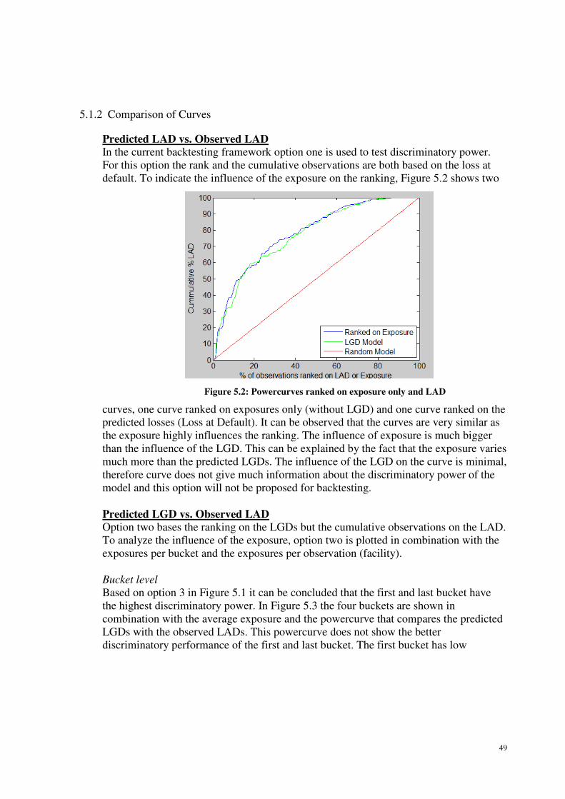
49

5.1.2 Comparison of Curves

Predicted LAD vs. Observed LAD

In the current backtesting framework option one is used to test discriminatory power.

For this option the rank and the cumulative observations are both based on the loss at

default. To indicate the influence of the exposure on the ranking, Figure 5.2 shows two

curves, one curve ranked on exposures only (without LGD) and one curve ranked on the

predicted losses (Loss at Default). It can be observed that the curves are very similar as

the exposure highly influences the ranking. The influence of exposure is much bigger

than the influence of the LGD. This can be explained by the fact that the exposure varies

much more than the predicted LGDs. The influence of the LGD on the curve is minimal,

therefore curve does not give much information about the discriminatory power of the

model and this option will not be proposed for backtesting.

Predicted LGD vs. Observed LAD

Option two bases the ranking on the LGDs but the cumulative observations on the LAD.

To analyze the influence of the exposure, option two is plotted in combination with the

exposures per bucket and the exposures per observation (facility).

Bucket level

Based on option 3 in Figure 5.1 it can be concluded that the first and last bucket have

the highest discriminatory power. In Figure 5.3 the four buckets are shown in

combination with the average exposure and the powercurve that compares the predicted

LGDs with the observed LADs. This powercurve does not show the better

discriminatory performance of the first and last bucket. The first bucket has low

Figure 5.2: Powercurves ranked on exposure only and LAD

50

[Confidential]

Figure 5.3: Predicted LGD vs. observed LAD and exposure per bucket

discriminatory power because of its low exposure. The last two buckets have the best

discriminatory power mainly caused by their high exposure. Therefore the exposure

influences the discriminatory power of the buckets. This powercurve does give some

information about whether high exposures perform better than low exposures, but in

general the curve is distorted by exposures and therefore hard to interpret.

Facility level

On facility level it can be seen that high exposures often lead to an increase in the LGD

model curve. Figure 5.4 shows that peaks in the exposure often result in steeper parts of

the curve. The exposures influence the shape of the curve and therefore make the curve

hard to interpret. Option two will not be used because the information it gives about the

discriminatory power is limited and the curve is hard to interpret.

[Confidential]

Figure 5.4: Predicted LGD vs. observed LAD and exposure per facility

Predicted LGD vs. Observed LGD

Both the ranking and the cumulative observed percentage of losses are based on the

LGDs. This gives a clear overview of the ranking ability of the model and it is not

distorted by exposures. Therefore this option will be proposed in the backtesting

framework.

51

Remarks

Two remarks have to be made when using the powerstat for LGD. First the

discriminatory power for LGD is low compared to PD. This is caused by the perfect

curve used as reference. The perfect curve is constructed in such a way that all observed

LGDs are ranked from high till low and the cumulative observed LGDs are plotted

based on this ranking. The model curve is constructed by ranking on the predicted

LGDs and this results in a perfect curve and model curve that are different. LGD

buckets contain mainly observations around 100 and 0 percent, therefore each LGD

bucket contains high and low observed LGDs. For the perfect curve all high LGD

observations are automatically located at the beginning of the curve, whereas for the

model curve the high LGD observations will be distributed over all available buckets. It

is possible to construct a perfect curve that is in accordance with the best ranking

possible according to the predicted LGDs. This curve could use the predicted LGDs per

bucket to plot a curve that shows high LGDs at the start and low LGDs at the end of

each bucket. A drawback of this curve is that it can be outperformed by the observed

LGDs when these are higher than predicted. Therefore this curve is not always the best

possible curve and will not be used as a reference.

Second it is preferred to rank the facilities based on the dimensions used to bucket them.

This results in a ranking on facility level, which differentiates between facilities within a

bucket. If this is not possible the ranking will be performed on the predicted LGDs,

which results in the discriminatory power per bucket which is less detailed than on

facility level.

5.1.3 CLAR curve compared to powercurve

On first sight the CLAR curve and the powercurve give similar results, but there is a

difference. The CLAR curve is only dependent on the ranking of the observed LGDs.

The frequency of correctly ranked facilities is determined by comparing the observed

LGDs on one side and the predicted LGDs on the other. The powercurve dependents on

the predicted LGD values and on the observed LGD values because it depicts the

cumulative percentage of observed LGDs. Hence, in the power curve there is more

stress on the LGD values and for the CLAR the focus is even more on the ranking

characteristics. To show the difference, two portfolios were created, both with the same

ranking, but with different LGD values:

- Uniform: ten observations uniformly distributed between 0 and 1.

- Non Uniform: five observations around 0 and five observations around 1.

Figures 5.5 and 5.6 show the curves for both distributions. The CLAR curve is the same

for both, while the powercurves differ. The uniformly distributed has a powerstat of

0.88 while the not uniform distributed has a powerstat of 0.95 (higher is better). The

difference occurs because the powerstat compares the LGD percentages, these differ and

therefore result in different proportions of loss for the same number of observations. The

CLAR only compares the ranking which is the same for both distributions.

52

Figure 5.5: CLAR curve for both distributions

Figure 5.6: Powercurve for both distributions

For similar distributions the powercurve is preferred over the CLAR for two reasons:

- The CLAR can only be constructed on bucket level while the powercurve can be

constructed based on individual facilities.

- The shape of the powercurve gives more information than the CLAR. It indicate

which part performs better (worse) than other parts. The CLAR always has a

similar shape (convex) and therefore does not clearly show this information.

5.1.4 CLAR rejection area

In the current situation a CLAR above 50 percent gives a green result and a CLAR

between 25 and 50 percent a yellow result and below 25 percent means rejection. The

CLAR and powerstat are similar measures and therefore should result in similar

conclusions. For the BGZ portfolio the powerstat and CLAR result in different

conclusions, this indicates that the rejection area could be incorrect.

To further analyze the rejection area first the minimum value is defined. The CLAR

indicates the models ability to rank losses. The minimum value is obtained when the

observed ranking is completely opposite from the predicted ranking. Figure 5.7 shows

the CLAR for the worst possible ranking and the best possible ranking. In the worst case

0%

20%

40%

60%

80%

100%

0% 20% 40% 60% 80% 100%

Cu

mu

lati

ve

co

rre

ctly

ass

ign

ed

ob

serv

ati

on

s

Cumulative percentage of observations

Uniform distributed

Not uniform distributed

Perfect model

0%

10%

20%

30%

40%

50%

60%

70%

80%

90%

100%

0% 20% 40% 60% 80% 100%

Cu

mu

lati

ve

lo

ss

Cumulative percentage of observations

Uniform distributed

Not uniform distributed

Perfect Model

53

the first correct observations is observed after 50 percent of the observations, and the

minimum CLAR, twice the area under curve, is 0.5 . In Appendix 6 the minimum value

is shown for different portfolios.

Figure 5.7: Perfect and worst case CLAR curve

To set the green, yellow and red zones, boundaries have to be determined. From the

BGZ portfolio a stylized example was created with an opposite ranking. The high LGD

predictions were combined with the low observed LGDs, the CLAR of this portfolio

was 55.8 percent, which should indicate low discriminatory power. To define the border

for good discriminatory power a stylized portfolio was created out of the BGZ data with

a powerstat of 0.305. From this stylized portfolio 100 datasets were created by sampling

100 observations. For the samples with a powerstat above 0.3 the majority (65 percent)

of the CLAR values was above 75 percent. For samples with a powerstat below 0.3 the

majority (85 percent) was below 75 percent.

Therefore the following boundaries are proposed. A CLAR above 75 percent means that

the bucketing is good and the result is green, a CLAR between 75 and 60 percent means

monitoring and the result is yellow and below 60 percent means a rejection of the model

and a red result.

5.1.5 Spearman’s rank correlation

On bucket level the CLAR curve is independent of the distribution of the LGDs. To

remove this dependency on model level the Spearman’s rank correlation can be used as

an alternative for the powerstat. This is a non parametric test, that tests the correlation

between two rankings. The null and alternative hypotheses of this test are:

H0: There is no positive correlation between the predicted LGD and the observed

LGD.

H1: There is positive correlation between the predicted LGD and the observed

LGD.

Discriminatory power tests whether there is correlation between the predicted and

observed LGDs. Therefore the null hypothesis has to be rejected. First the test statistic

will be described and then the rejections areas based on the normal distribution.

5 In the current guidelines this threshold is set at 0.4, but according to experts this is too high. Therefore this is adjusted to

0.3.

0%

20%

40%

60%

80%

100%

0% 20% 40% 60% 80% 100%

cum

ula

tiv

e %

co

rre

clty

ass

ign

ed

LG

Ds

Cumulative % of observations

Worst case model

Perfect Model

54

The test statistic is defined by ranking the facilities twice, once based on the predicted

LGDs and once based on the realised LGDs. The correlation is defined as:

�ª = 1 − 6)&)V − 1' B&�* − X*'V8*,9 (5.1)

�*= Rank of facility i based on LGD score (predicted LGD) X*= Rank of facility i based on observed LGD

N = Number of facilities

rs = 1 is the optimal score, this means that both rankings are the same

rs= 0 means that the ranking is random.

rs= -1 means that the ranking is opposite.

(Poëta, 2009)

Rejection area

A confidence interval can be set using the student t-distribution. If there are more than

40 observations �ª) − 1 is approximately normal distributed (MEI, 2007).

Therefore the null hypothesis can be rejected with 95 percent significance if �ª) − 1 > ®�5�¯, were z is the cumulative normal distribution. This indicates that there

is significant correlation. However, it does not always indicate that the model

discriminates well. The value of the correlation is important as well. In the case of a

large number of observations a relative low correlation can be statistically significant

but this does not mean that the model discriminates better than a model with the same

correlation and a low number of observations. Therefore minimum bounds have to be

set.

The bounds will be based on a comparison with the powercurve. For the powercurve

fixed rejection areas are set. The powercurve results in red if it is below random, which

corresponds to a negative rs. The powercurve results in a yellow zone if the powercurve

is above the random curve. This is in accordance with a rs statistic above zero but and

within the 95 percent confidence interval. If the rs statistic is greater than the 95 percent

confidence level, there is significant correlation. As reasoned above this is not enough to

conclude that the discriminatory power is good. This will be based on an additional

minimum threshold.

This minimum threshold is set according to sampling with replacement from a stylized

data set. This dataset had a powerstat of 0.3 which indicates good discriminatory power.

From this dataset 100 sets were sampled. For each of these sets the powerstat and

Spearman rank correlating were calculated. For powerstats above 0.3 the Spearman’s

rank correlation was most of the times (65 percent) above 0.15 and for powerstats

below 0.3 Spearman’s rank correlation was most of the times (85 percent) below 0.15.

Therefore the threshold is set at 0.15. This value is in accordance with values used in

literature, these values between 0.2 and 0.4 were used to compare different regression

models for LGD (Jie & Lyn, 2012).

55

5.2 Predictive Power

In the current situation the rejection areas for the loss shortfall and the mean absolute

deviation are set as percentages, which do not take into account the number of

observations and the distribution of the observed losses. This results in high chance of

rejection for portfolios with high variance. New confidence bounds for both measures

will be proposed.

Currently the predicted and observed LGD percentages are not compared. This test will

be proposed in the new framework. Currently there is also no test incorporated to

backtest the transition matrix used to predict LGDs, this will be added.

5.2.1 Loss Shortfall

The loss shortfall (LS) is defined as:

�� 7ℎ�� = 1 − ( &�� *� ��*'8*,9( &��X�� *� ��*'8*,9 (5.2)


The current rejection areas are set as a percentage. These do not take into account that

the LGD has a variance. If the variance of the observed loss is high the loss shortfall is

expected to deviate more than with a low variance, because the distribution of the loss at

default is broader. Bootstrapping with replacement confirmed this reasoning. Two

portfolios were used with the same loss shortfall, for low variance the 95 percent

bootstrapped confidence interval was [-0.05, -0.01] and for the high variance [-0.30,

0.14]6. This shows that the variance influence the LS and should be used when setting

the rejection area.

The variance of the LS is dependent on the variance of the observed losses. There is no

linear relation, therefore distribution of predicted LS is unknown. To take the variance

into account a distribution will be bootstrapped around the observed LS. This is done by

sampling with replacement N observations and calculate an observed LS. This is

repeated 1000 times to generate a distribution around the observed LS. The distribution

will be used to test whether the expected LS of zero is within a 95/99 percent confidence

interval of the observed LS.

The main advantage of bootstrapping is that no assumption has to be made on the

underlying distribution, therefore it is applicable in many cases. The main drawback is

the computation effort needed. Another drawback is that it tends to be optimistic about

the standard error, which results in a somewhat smaller confidence interval (Wehrens et

al., 2000). For backtesting this means that the confidence interval might be somewhat

conservative.

6 For the complete calculation see Appendix 7

56

5.2.2 Mean Absolute Deviation

The exposure weighted MAD is calculated by:

:�� = ( ;��* − ��*; ∗ ��*8 *,9 ( ��*8*,9 (5.3) ��*= observed LGD of observation i ��*= LGD of observation i


Currently the rejection areas are set by percentages, smaller than 10 percent results in

green, between 10 and 20 percent results in yellow and greater than 20 percent results in

red. These areas are independent of the variance of the observed loss. The influence of

the variance on the expected outcome is even bigger than for the LS because the MAD

does not cancel out a positive against a negative deviation. A portfolio with high

variance will have a high MAD because observed LGDs deviate much from the

predicted LGD.

There are two options to incorporate the variance in the rejection areas. Option one is

based on an expected MAD which uses the variance. Option two is based on a

bootstrapped MAD using the observed LGDs only.

Rejection area based on variance

The MAD is related to the variance. This approach will show how to estimate an

expected MAD based on the variance.

The non exposure weighted mean absolute deviation is defined as:

:�� = 1) B;�* − �°;8*,9 (5.4)

N= Number of observations

This MAD is related to the underlying distribution. In the case of normal distributed

underlying variables the relation to the standard deviation is (Herrey, 1965):

:�� = S2¢ i (5.5)

For an LGD model each bucket has its own variance, and therefore its own MAD. To

show how to determine the MAD for the model the following setting is used:

A model with two buckets:

- Bucket 1 with LGD1 and M observations.

- Bucket 2 with LGD2 and K observations.

N is the total number of observations is N, M+K=N

The MAD for the model can then be written as:

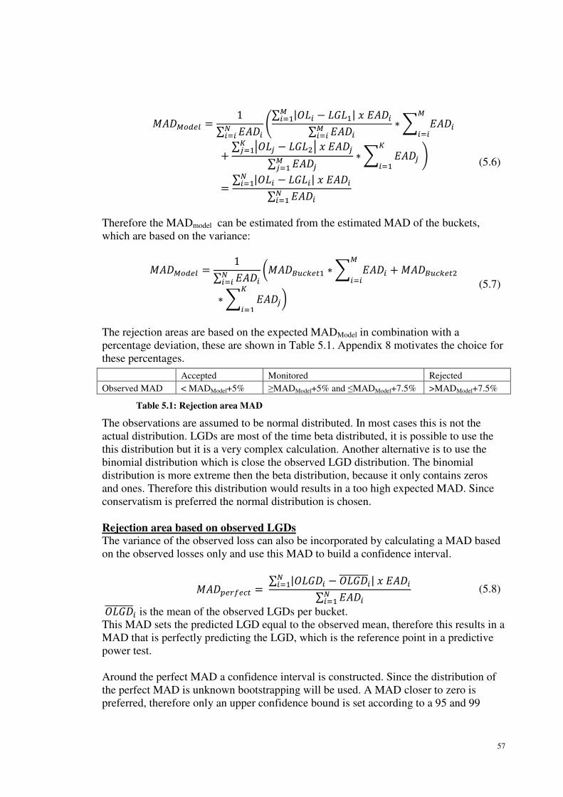
57

:��N¡�±² = 1( ��*8*,* �( ;�* − �9; � ��*N *,9 ( ��*N*,* ∗ B ��*N*,* ( R�h − �VR � ��h³h,9 ( ��hNh,9 ∗ B ��h³

*,9 �= ( ;�* − �*; � ��*8 *,9 ( ��*8*,9

(5.6)

Therefore the MADmodel can be estimated from the estimated MAD of the buckets,

which are based on the variance:

:��N¡�±² = 1( ��*8*,* D:��=´0�±�9 ∗ B ��*N*,* :��=´0�±�V

∗ B ��h³*,9 E

(5.7)

The rejection areas are based on the expected MADModel in combination with a

percentage deviation, these are shown in Table 5.1. Appendix 8 motivates the choice for

these percentages.

Table 5.1: Rejection area MAD

The observations are assumed to be normal distributed. In most cases this is not the

actual distribution. LGDs are most of the time beta distributed, it is possible to use the

this distribution but it is a very complex calculation. Another alternative is to use the

binomial distribution which is close the observed LGD distribution. The binomial

distribution is more extreme then the beta distribution, because it only contains zeros

and ones. Therefore this distribution would results in a too high expected MAD. Since

conservatism is preferred the normal distribution is chosen.

Rejection area based on observed LGDs

The variance of the observed loss can also be incorporated by calculating a MAD based

on the observed losses only and use this MAD to build a confidence interval.

:��µ±¶·±0� = ( ;��* − ��¸̧ ¸̧ ¸̧ ¸̧ *; � ��*8 *,9 ( ��*8*,9 (5.8)

��¸̧ ¸̧ ¸̧ ¸̧ * is the mean of the observed LGDs per bucket.

This MAD sets the predicted LGD equal to the observed mean, therefore this results in a

MAD that is perfectly predicting the LGD, which is the reference point in a predictive

power test.

Around the perfect MAD a confidence interval is constructed. Since the distribution of

the perfect MAD is unknown bootstrapping will be used. A MAD closer to zero is

preferred, therefore only an upper confidence bound is set according to a 95 and 99

Accepted Monitored Rejected

Observed MAD < MADModel+5% ≥MADModel+5% and ≤MADModel+7.5% >MADModel+7.5%

58

percent confidence level. If the observed MAD is below the confidence bound the

model is accepted, otherwise rejected.

Conclusion

The first method has two disadvantages. First it assumes that the underlying variables

are normally distributed, which is not the actual distribution. Second it bases the

rejection areas on percentages which fit the tested portfolios but could be less suitable

for other portfolios.

The second method does not make an assumption about the distribution, but uses the

actual observed distribution. Therefore the confidence interval will always be suitable to

the portfolio. Because of these advantages the rejection area based on the observed LGD

will be proposed in the backtesting framework.

5.2.3 LGD model and bucket test

In the current framework there is no clear method to compare the observed LGDs with

the predicted LGDs on model and bucket level. The hypotheses of this test would be:

H0: The observed LGD percentage is equal to the predicted.

H1: The observed LGD percentage is unequal to the predicted.

There are two options to test this. The first option is to use bootstrapping, either

parametric or nonparametric, to construct a distribution around the observed LGD and

to set the confidence interval. The second option is to perform a t-test which compares

two means based on the student t-distribution.

Parametric bootstrapping

By parametric bootstrapping samples are drawn from a known distribution, therefore the

distribution of LGDs has to be estimated. Figure 5.8 shows the distribution of the LGDs

on model level which is similar to the distribution per bucket. The characteristic of this

distribution is that there are many losses around zero percent and many losses around

100 percent and almost no losses in-between.

[Confidential]

Figure 5.8: Distribution of LGD

59

The losses can be modelled as random variables between 0 percent and 100 percent. A

distribution often used to model this is the beta distribution. This distribution is used

because it can be bounded between two points [0, 1] and has a wide range of possible

shapes. The shape is defined by two shape parameters α and β.

^ = ¹º»¼mV � 1 − º»¼mi»¼mV ½ − º»¼m (5.9)

� = ^ � D 1º»¼m − 1E (5.10)

º»¼m = Average LGD for each bucket. i»¼mV = Is the variance of the LGD in the bucket (Stoyanov, 2009).

Figure 5.9 shows two estimations of the Beta distribution, one based on the parameters

above and one fitted using the betafit function in Matlab. This function uses maximum

likelihood to estimate alfa and beta.

The calculated distribution shows a better fit because it better incorporates the peak

around zero. The calculated parameters have a mean equal to the observed mean while

the Matlab fit has much higher mean. Therefore the calculated parameters will be used.

To generate a confidence interval the number of observation N, is bootstrapped 1000

times from the beta distribution. For each sample the mean is calculated and these

means are ranked to define the lower and upper confidence bounds for the observed

LGD. This procedure can also be performed on bucket level.

Nonparametric bootstrapping

This bootstrap approach is similar to the construction of confidence intervals for the loss

shortfall and the mean absolute deviation. From the observed LGDs, 1000 times a

sample of size N is drawn with replacement. For each sample the mean is calculated and

the from these means the upper and lower bounds are determined.

[Confidential]

Figure 5.9 Fitted and calculated Beta distribution

60

Both bootstrapping methods result in a similar confidence interval. The nonparametric

interval is somewhat broader which is in accordance with Figure 5.9 where the actual

distribution has a higher density around 0 and 1 than the estimated distribution. Because

both approaches give similar results no preference is made.

T-test

A one sample t-test compares the sample mean with a known mean. For the LGD model

and bucket test the observed LGD (sample mean) has to be compared with the predicted

LGD, therefore the one sample t-test can be used. In section 6.1 the test is further

explained for backtesting the credit conversion factor for EAD. The only difference is

the weights used to calculate the mean and test statistic, for LGD these weights will be

the exposure.

The t-test is based on three assumptions: independence between observations, normal

distribution of the observed LGD and equal variance of the observed and predicted

LGD. The first assumption is a common known drawback of many statistical tests. The

second assumption, normal distribution of the observed LGDs is valid if the sample is

large enough. For large samples the central limit theory states that the sample means is

approximately normal distributed. A sample is considered to be large enough if the

number of observations is greater of equal to 30. The third assumption cannot be

validated since the variance of the predicted LGD is unknown.

The advantage of the t-test over the two bootstrapping methods mentioned above is that

it is easy to compute, because it does not need sampling to create a confidence interval.

Since the t-test can only be used for large enough samples the two methods mentioned

above will be used for small sample and the t-test for large samples.

5.2.4 Transition matrix test

The goal of backtesting the transition matrix is to verify whether the transition

probabilities are still as predicted. For backtesting the transition matrix a simplified

approach is taken. The matrix is divided into individual transitions which are assumed to

be uncorrelated. Then a binomial approach is taken to test whether “The transition of

LGD bucket x leads to bucket y (Event A)” or “The transition of LGD bucket x does not

lead to bucket y (Event B)” the probability of the transition from x to y is pforecast

.

The hypotheses are:

H0: The observed probability of the transition from x to y is equal to pforecast

.

H1: The observed probability of the transition from x to y is unequal to pforecast

.

To compare the observed transition probability with the predicted the binomial

distribution is used:

If the predicted transition probability is too low (OenB, 2004):

B <)? )=� @ lp¿ÀÁÂ+ÃÄÅnÆl1 − p¿ÀÁÂ+ÃÄÅn8Ç}8ÈUÆ > z8ÇÆ,�

(5.11)

If the predicted transition probability is too high

B <)? 8ÇÆ,�)?= Observed number of event A)== Observed number of event B

X = Confidence level

This approach is very simplistic, because the individual transitions are considered to be

independent, which is not the case. All transition events are correlated, but the

magnitude of the correlation

would result in too complex equations

5.3 Overview proposed LGD backtesting framework

Figure 5.10 illustrates the proposed backtesting framework. The tests with blue orders

have improved rejection areas. The tests with red borders are added to the framework or

are changed.

Figure 5.10: Overview proposed LGD framework. Dotted lines indicate optio

based on test outcomes and ranking ability

For discriminatory power the choice of the test is dependent on the outcome of the

stability tests. If the distribution of the LGD is s

otherwise the CLAR or Spearman’s

are proposed to test discriminatory power:

If the predicted transition probability is too high (OenB, 2004):

< )=� @ lp¿ÀÁÂ+ÃÄÅnÆl1 − p¿ÀÁÂ+ÃÄÅn8Ç}8ÈUÆ <= Observed number of event A

= Observed number of event B



magnitude of the correlations is not known. The incorporation of actual correlation

uld result in too complex equations (OenB, 2004).

Overview proposed LGD backtesting framework

5.10 illustrates the proposed backtesting framework. The tests with blue orders


Figure 5.10: Overview proposed LGD framework. Dotted lines indicate optio

based on test outcomes and ranking ability


stability tests. If the distribution of the LGD is stable the powercurve will be used

otherwise the CLAR or Spearman’s rank correlation will be used. The following tests

are proposed to test discriminatory power:

61

< 1 − z (5.12)



. The incorporation of actual correlation

5.10 illustrates the proposed backtesting framework. The tests with blue orders


Figure 5.10: Overview proposed LGD framework. Dotted lines indicate optional paths


the powercurve will be used

rank correlation will be used. The following tests

62

• Powercurve: The powercurve will be based on LGD percentages and not on

losses because this provides more information. The test is performed either on

model or bucket level. The shape of the curve will be used to indicate

discriminatory power.

• Powerstat: Summary statistic of the powercurve.

• CLAR curve: Only used when different LGD distributions are compared. The

CLAR tests on bucket level the discriminatory power and has improved rejection

areas.

• Spearman’s Rank Correlation: Only used when different LGD distributions are

compared. Tests discriminatory power on model level.

Predictive power is divided into testing the loss at default and the LGD.

For the loss at default two tests are performed:

• Loss shortfall: With a statistical confidence interval.

• Mean absolute deviation: With a statistical confidence interval.

For the LGD the following tests are performed:

• Model and bucket test: For small samples bootstrapping will be used. For large

samples a one sample t-test will be used.

• Transition matrix test: Optional test if the model or bucket test is rejected, to

backtest the transition matrix.

5.4 Conclusion LGD Framework

To define a backtesting framework for LGD the following sub question is partly

answered:

Which tests should be used to backtest LGD and EAD and how should the

rejection areas be set?

To test discriminatory power the powercurve is used. This curve can be constructed

based on the LGD percentages only or weighted with exposure. Analysis showed that

the incorporation of the exposures highly influences the outcomes of the curve.

Therefore a curve based on percentages is chosen to test discriminatory power. A

downside of this method is that the powercurve is dependent on the underlying

distribution, therefore only similar distributions should be compared. Comparison of

two different LGD distributions should be based on the CLAR or Spearman’s Rank

Correlation.

The CLAR curve shows on bucket level a curve similar to the powercurve, but is purely

based on the ranking of the LGDs. The rejection areas for the CLAR were redefined

such that they are in line with the powerstat. The alternative for the CLAR on model

level is Spearman’s Rank Correlation. This calculates the correlation between two

rankings, observed and predicted. The rejection areas were defined such that they are in

line with the powerstat.

63

To test predictive power the loss shortfall and the mean absolute deviation will still be

used. The rejection areas for these measures are improved and are based on variance and

number of observation instead of fixed thresholds.

Another test for predictive power is a comparison of the observed and predicted LGDs

on model and bucket level. For small samples the rejection areas are set by

bootstrapping the observed LGDs. For large enough samples the one sample t-test will

be used.

If the test on model or bucket level is rejected the transition matrix has to be backtested.

To backtest the performance of the transition matrix a binomial test is used which tests

each transition separately.

64

65

6 Proposals for improvement of backtesting EAD

The current backtesting methodology includes a method to backtest EAD, this method

will be analyzed to see whether it is appropriate to use.

6.1 Predictive power: Student t-test

In the current backtesting methodology the observed CCF factor is compared by a

(weighted) student t-test. The test should include weights (the off-balance value)

because in the EAD calculation the CCF factor is multiplied by the off-balance value:

�� = B&��* " #��ℎ� ��*' ��! ∗ B&��'8*,9

8*,9 (6.1)

The following is tested:

H0: The predicted CCF (CCFmodel) is equal to the observed CCF (CCFBacktest).

H1: The predicted CCF (CCFmodel) is unequal to the observed CCF (CCFBacktest).

The confidence interval is constructed around the observed CCF for different

confidence levels by:

�A&CCFËÃ+ÌÅÂÄÅ' = CCFËÃ+ÌÅÂÄÅ ± tÎU9 SÐÃ+ÌÅÂÄÅN (6.2) tÎU9= Student t distribution with N-1 degrees of freedom


Wi = Weight of facility i, this weight is the off balance value.

(Hanoeman, 2010a)

This t-test is based on three assumptions: independence between observations, normal

distribution of the average CCF and equal variance of the observed and predicted CCF.

The first assumption is a drawback of many tests and is hard to verify. The second

assumption can be tested by for example plotting a Q-Q plot, in Appendix 9 this plot is

shown for the BGZ portfolio. It shows that the average CCF is approximately normal

distributed. The third assumption should be verified before testing.

This backtesing method is appropriate to use, it has clear confidence intervals, takes into

account the weights and the assumptions can be verified.

6.2 Conclusion

To finalize the backtesting framework the following sub question is (partly) answered:

Which tests should be used to backtest LGD and EAD and how should the

rejection areas be set?

EAD will be backtested in the same way as in the current backtesting framework, by a

weighted student t-test. This method is appropriate to use because it has proper

confidence bounds and the assumptions are valid.

66

67

7 Conclusion

The goal of this thesis was to improve the current backtesting methodology for PD,

LGD and EAD and to develop a retail backtesting framework. Since the PD framework

was already well developed this could only be improved on specific aspects. LGD was

less developed and therefore the full methodology was examined and improved. For

EAD the current methodology was concluded to be valid.

The first stage of backtesting is stability testing. The current backtesting methodology

did not contain stability testing. Therefore two tests are proposed: the Kolmogorov-

Smirnov test for continuous samples and the system stability index for discrete samples.

Predictive and discriminatory power for PD

In the current methodology discriminatory power for PD was tested using the

powercurve and powerstat. These are suitable methods, only the confidence interval had

to be improved. The proposed framework contains bootstrapped confidence bounds

around the powercurve and uses the Wilcoxon-Mann-Whitney statistic to set confidence

bounds for the powerstat.

The predictive power for PD was tested by a binomial test and the composed model test.

The binomial test is extended with two adjustments. First, a binomial test should be

performed with a point-in-time adjustment to reduce the influence of correlation with

the economic cycle. Second, the confidence interval for the binomial test should be

based on a combination of the Type-I and Type-II errors. The last point to improve is

the complex and strict composed model test, which should be replaced for small

samples by a Hosmer-Lemeshow test based on the chi-squared test.

Predictive and discriminatory power for LGD

The discriminatory power for LGD was tested by a powercurve based on the loss at

default and a CLAR curve. Proposed is to use a powercurve when similar distributions

are compared, the curve should be based on the LGDs instead of the loss at default

because this provides more information. To compare distributions that differ the CLAR

can be used on bucket level and Spearman’s rank correlation on model level, both tests

are based on ranking characteristics only.

For the predictive power the mean absolute deviation and the loss shortfall were used to

test the loss at default. For both tests new rejection areas are proposed which are based

on the sample size and variance. These intervals are created by bootstrapping with

replacement. The proposed framework contains two additional tests. A test to compare

the observed and predicted LGDs, which will be done by a t-test for large samples and a

bootstrapped distribution for smaller samples. A test to backtest the transition matrix

which is used to predict bucket LGDs.

This proposed framework tests the models on the required aspects and uses statistical

methods and confidence intervals as much as possible to reject or accept the

performance of the models. The field of backtesting these capital models has a broad

68

scope and is still developing, therefore there are several aspects that could be further

investigated.

Further research

Some aspects that are suggested that could be further investigated to improve the

framework:

1. Multiple period backtesting for PD. Besides backtesting the PD for one year, one

could backtest the PD over multiple years. If multiple years are tested the point-

in-time effect is reduced and a PIT/TTC adjustment is not needed. Currently a

multi period backtesting approach is tested within Rabobank. It should be

analyzed whether this method could be included in a future framework.

2. Currently there is limited research available on LGD backtesting. Aspects that

could be improved are the discriminatory power of LGD, which is low and

therefore difficult to backtest. The comparison between observed and predicted

LGDs. This is currently mainly based on bootstrapping the observed LGDs,

where it is desirable to base the rejection areas on the predicted LGDs. These

aspects could be improved when more research is available about backtesting

LGD.

3. A point-in-time correction for LGD. For PD there is a point-in-time correction to

include cyclical effects. For LGD cyclical effects are also expected but for retail

loans no clear effect is proven. For example Asarnow and Edwards (1995)

concluded that the LGD variation is not cyclical and Bellotti and Crook (2009)

expected cyclical effects in LGDs for credit cards but could not proof this

because there was no severe downturn in their data period. To perform an

adequate backtest, it has to be known if there is a cyclical effect and how to

include this.

69

8 Bibliography

Asarnow, E. & Edwards, E. (1995). Measuring Loss on Defaulted Bank Loans: A 24-

Year Study. The journal of commercial lending, 7, 11-23

Bamber, D. (1975). The Area above the Ordinal Dominance Graph and the Area below

the Receiver Operating Characteristic Graph. Journal of Math. Psychology, 12, 387-415

Bellotti, T. & Crook, J. (2009). LGD models for UK retail credit cards. CRC working

paper 09/1, 1-28

Castermans, G., Martens, D., van Gestel, T., Hamers, B. & Baesens, B. (2010). An

overview and Framework for PD Backtesting and Benchmarking. Journal of the

Operational Research Society, 61,359–373

BIS (2005). Studies on the Validation of Internal Rating Systems. Working Paper No

14. Retrieved from http://www.bis.org/publ/bcbs_wp14.htm

BIS (2006). International Convergence of Capital Measurement and Capital Standards,

A revised Framework. Retrieved from http://www.bis.org/publ/bcbs128.pdf

BIS (2011). Basel III: A global regulatory framework for more resilient banks and

banking system. Retrieved from http://www.bis.org/publ/bcbs189.pdf

Blochwitz, S., Hamerle, A., Hohl, S., Rauhmeir, R. & Rösch, D. (2005). Myth and

Reality of Discriminatory Power for Rating Systems. Wilmott Magazine, 2-6

Blochwitz. S., Martin, M.R.W. & Wehn, C.S. (2006). Statistical Approaches to PD

Validation. The Basel II Risk Parameters: Estimation, Validation, and Stress Testing,

289-306

CEBS (2006). Guidelines on the implementation, validation and assessment of

Advanced Measurement (AMA) and Internal Ratings Based (IRB) Approaches.

Retrieved from http://www.eba.europa.eu/getdoc/5b3ff026-4232-4644-b593-

d652fa6ed1ec/GL10.aspx

Cortes, C. & Mohri, M. (2005). Confidence Intervals for the Area under the ROC curve.

Neural Information Processing Systems 17, 305-312

Engelmann, B., Hayden, E.& Tasche, D. (2003). Testing rating accuracy. Risk, 82-86

Hanley, J.A. & McNeil, B.J. (1982). The Meaning and Use of the Area under a Receiver

Operating Characteristic (ROC) Curve. Radiology, 29-36

Hanoeman, S. (2010a). Review methodologie EaD, Particulier & Zakelijk (Retail &

Corporate). Utrecht: Rabobank Nederland

70

Hanoeman, S. (2010b). Review methodologie LGD Retail/Corporate. Utrecht:

Rabobank Nederland

Hanoeman, S. (2010c). Review methodologie PD Retail. Utrecht: Rabobank Nederland

Herel, M. (2011). Backtesting ACC & Portfolio Analysis. Utrecht: Rabobank

International

Herrey, E.M.J. (1965). Confidence intervals based on the mean absolute deviation of a

normal sample. Journal of the American Statistical Association, 60 (309), 257-270

Higgins, J.J. (2004). Introduction to Modern Nonparamteric Statistics, Kansas State

University, 29-34

Hull, J.C. (2007). Risk Management and Financial Institutions. Prentice Hall

International

Kozlowski, L. (2011). PD, LGD & EAD calibration framework. BGŻ Risk Modeling

Bureau, Working Document

Kurcz, M., Nathoeni, D., Opzeeland van, J. (2011). Micro companies scorecard, BGZ

Micro companies. Utrecht: Rabobank International

Jie,Z. & Lyn,C.T. (2012). Comparison of linear regression and survival analysis using

single and mixture distributions approaches in LGD modelling. International Journal of

Forecasting, 28, 204-215

Li, D., Bhariok, R., Keenan, S. & Santilli, S. (2009). Validation techniques and

performance metrics for loss given default models. The Journal of Risk Model

Validation, 3, 3-26

Macskassy, S. & Provost, F. (2005). Confidence bands for ROC curves: Methods and an

empirical study. Proceeding of the 22nd

international conference on Machine learning,

537-544

MEI (2007). MEI paper on Spearman’s rank correlation coefficient. Retrieved from

http://www.mei.org.uk/files/pdf/Spearmanrcc.pdf

Mesters, M. & Pijnenburg, M. (2007). Memorandum: “New Backtest”. Utrecht:

Rabobank Nederland

Mijnen, B. (2012). Multi Period Binomial Distribution. Working document. Utrecht:

Rabobank Nederland

Mui, P. & Ozdemir, B. (2005). Practical and Theoretical Challenges in Validating Basel

Parameters: Key Learnings from the Experience of a Canadian Bank. Journal of Credit

Risk, 4, 89-136

71

OeNB (2004). Guidelines on Credit Risk Management, Rating Models and Validation.

Vienna: Oesterreichische Nationalbank

Poëta, S. (2009). LGD Backtesting Methodology. Presentation Eurobanking 2009.

Retrieved from http://www.eurobankingonline.net/Duesseldorf%202009/19-eb09-d-

SylvainPoeta-LGDBacktestingMethodology.pdf

Rauhmeier, R. (2006). PD-Validation – Experience from Banking Practice. The Basel II

Risk Parameters: Estimation, Validation and Stress Testing, 307-345

Risk Dynamics (2006). Exposure at Default and Loss Given Default Review

Guidelines. Utrecht: Rabobank Nederland

RMVM (2010). Model Review, Technical Description for Probability of Default

models. Utrecht: Rabobank Nederland

Stoyanov, S. (2009). Application LGD Model Development, A case Study for a leading

CEE Bank. Credit Scoring and Credit Control XI Conference, Edinburgh

Tasche, D. (2003). A traffic lights approach to PD validation, Working Paper

Tasche, D. (2006). Validation of internal rating systems and PD estimates, Working

Paper

Wehrens, R., Putter, H., Buydens, L. M. C. (2000) The bootstrap: a tutorial.

Chemometrics and Intelligent Laboratory Systems, 54, 35-52

72

Appendix 1: Regulatory guidelines

BIS guidelines:

- (500) Banks must have a robust system to validate the accuracy and

consistency of rating systems. A bank must demonstrate that the internal

validation process enables it to assess the performance of the internal rating

system and risk estimation system.

- (501) Banks that use the advance IRB approach must regularly compare

realized rates with estimated rates for PD, LGD and EAD. To compare they

must use historical data over as long a period as possible. The method and

data must be clearly documented. This must be updated at least annually.

- (502) The internal assessment of performance must be based on a data set

covering a range of economic conditions, and ideally one or more complete

business cycles.

- (503) Banks must demonstrate that quantitative testing methods do not vary

systematically with the economic cycle. Changes in methods and data must

be clearly documented.

- (504) Banks must have well-articulated internal standards for situations

where deviations in realized PDs, LGDs and EADs from expectations

become significant enough to call the validity of the estimates into question.

These standards must take business cycles and systematic variability into

account. If realized values continue to be higher, banks must revise their

estimates upward to reflect their default and loss experience.

CEBS has overlap with the BIS guidelines, the additional guidelines:

- (392) Institutions are expected to provide sound, robust and accurate predictive

and forward-looking estimates of the risk parameters.

- (393) Banks should use backtesting and benchmarking. Backtesting consists of

checking the performance of the risk rating systems estimates by comparing

realized risk parameter with the estimated.

- (394 & 395) Backtesting generally involves comparing realized with estimated

parameters for a comparable and homogeneous data set for PD, LGD and EAD

models. This can be done by using statistical methods to implement statistical

tests for defining acceptable levels of potential discrepancy between the

prediction and realization.

- (396) At a minimum backtesting should focus on the following issues:

• The underlying rating philosophy used in developing rating systems (e.g.

PIT vs TTC PD). Institutions that use different rating systems will need

to take into account any differences in their rating philosophies when

backtesting the estimates.

• Institutions should have a policy with remedial actions when a

backtesting result breaches the tolerance thresholds for validation.

• If backtesting is hindered by lack of data or quantitative information.

institutions have to rely more on additional qualitative information.

• The identification of specific reasons for discrepancies between predicted

values and observed outcomes.

73

At a minimum institutions should adopt and document policies that explain the objective

and logic in their backtesting procedure.

Appendix 2: CLAR curve

For this CLAR curve a rating model is used with ten observations in three buckets:

1. Bucket 1 with LGD of 60 percent and 3 observations.



Table 1 shows the observations ranked on the observed losses (high till low). For the

first three losses only one observation is out of bucket 1, so the part that is correctly

assigned is 1/10. The same is done for the other two buckets, which results in 3/10 and

10/10 . This results in a CLAR of 75 percent which is much higher than the current

threshold for good discriminatory power, 50 percent. The powerstat for this data is 0.38,

which results in a yellow zone. This indicates that the current rejection areas for the

powerstat and CLAR are not in line and should be further investigated.

Figure 1: CLAR curve example

Table 1: Example CLAR

74

Appendix 3: Granularity adjustment approximation

As given in 4.2.1.2: %8 = �8)

% = lim8→� %8 = Ф �� − \xz\1 − x �

Then the quantile Y&^, %' is: Y&^, %' = u �\xФU9&^' �\1 − x �

The common factor is normal distributed: z~)&4,1'

Therefore the quantile Y&1 − ^, z' is: Y&1 − ^, z' = ФU9&1 − ^' After using the second order Taylor expansion, one arrives at:

Y&^, �8' ≈ )Y&^, %' 9V Ó2Y&^, %' − 1 Ô&Õ,Ö'l9UÔ&Õ,Ö'n×�\ØÙ&� Ú,Û' Ü\� Ø � DÔ&9UÕ,H'U�\9U| E − «9U|| Y&1 − ^, z'Ý

(Tasche, 2003)

Appendix 4: ROC curve confidence interval

Figure 2: Comparison of two bootstrapping methods

75

[Confidential]

Figure 3:Chosen bootstrap method with 100 random samples

Appendix 5: Hosmer-Lemeshow test versus composed model test

To compare the performance of the composed model test and the Hosmer-Lemeshow

test, the tests are performed for the four years of data available for BGZ.

[ Confidential]

Table 2: Comparison Hosmer-Lemshow test and Composed model test. The values in brackets

indicate the boundaries of the yellow and red zone. For example [1;2] means that the result is yellow

if one or more bucket is rejected and red if two or more are rejected. The red color indicates that

the model is rejected with a 99% significance level. yellow indicates 95% significance.

Table 2 shows that the composed model test and the Hosmer-Lemeshow test give

similar results. Only in the case of 2007, the Hosmer-Lemeshow test statistic does not

reject for a 99 percent significance level, but does for 95 percent.

Tables 3 and 4 show the results of the composed model test and the Hosmer-Lemeshow

test for stylized portfolios. Out of these results it can be concluded that the composed

model test is more strict than the Hosmer-Lemeshow test when a red bucket is observed.

This causes most of the times the difference between the two tests.

Scenario description

Composed

Model Test

Hosmer

Lemeshow Test

Model Test Difference

5(1) Buckets optimistic Red Red Red NO

3(1) Buckets optimistic Red Red Red NO

2 Buckets optimistic Yellow Green Yellow YES

2 optimistic and 2 conservative Red Red Green NO

2(1) optimistic Red Yellow Red YES

High PD for all buckets, but no buckets rejected Green Yellow Red YES

1(1) bucket optimistic Red Green Yellow YES

2(0) optimistic Red Green Yellow YES

1(1) optimistic and 1 conservative Red Red Yellow NO

2 Conservative Red Red Green NO

Table 3: Comparison Composed Model Test and Hosmer Lemeshow test based on 8 buckets. 5(1)

Optimistic means that there are five buckets in the yellow zone of which one is also in the red zone.

76

Scenario description

(Normal scenario has 8 buckets)

Composed

Model Test

Hosmer

Lemeshow Test

Model Test Difference

2 optimistic + 3 extra buckets Red Red Red NO

1 optimistic and 1 conservative + 5 extra buckets Green Yellow Yellow YES

2(1) optimistic + 5 extra buckets Red Yellow Red YES

1(1) Optimistic + 5 extra buckets Red Green Green YES

2 Conservative + 5 extra buckets Red Green Red YES

Table 4 Comparison Composed Model Test and Hosmer Lemeshow test based on 8 buckets plus

extra buckets. 5(1) Optimistic means that there are five buckets in the yellow zone of which one is

also in the red zone.

Minimum number of buckets

The border value of 15 buckets is set according to a calculation of the amount of

rejected buckets that is needed to reject the model. Rejection based on one red bucket is

not desired therefore the number of buckets is calculated that would need two rejected

red buckets. This minimum number is 16 according to the following calculation. P is set

at 0.01. &C ≤ 1' = &1 − 4541'9Þ 16 45411 − 4541 ∗ &1 − 4541'9Þ = 45989

&C ≤ 2' = &1 − 4541'9Þ ∗ �1 16 ∗ 45411 − 4541 16V ∗ 45411 − 4541V� = 45992

So red if two or more buckets are rejected.

Appendix 6: CLAR rejection area

To determine the new critical values, first the upper and lower boundary had to be set.

The upper boundary is still valid, which is a CLAR value of one and indicates perfect

discriminatory power. The minimum value of the CLAR curve occurs when the ranking

is opposite, high predicted LGDs result in low observed LGDs and the other way

around. In this case there is still a minimum CLAR value of 0.5, because in the worst

case the first correct observation will be after 50 percent of the observations. This is

illustrated with the example in Table 5. Table 5 shows an opposite ranking, which result

in a CLAR of 0.5. Figure 4 shows this CLAR curve and for three alternative portfolios.

77

Observed

LGD

Predicted LGD If observed correctly on cumulative basis 1, else 0.

0.6 0.1 0 0 0 1

0.6 0.1 0 0 0 1

0.6 0.1 0 0 0 1

0.4 0.2 0 1 1

0.4 0.2 0 1 1

0.4 0.2 0 1 1

0.2 0.4 1 1

0.2 0.4 1 1

0.2 0.4 1 1

0.1 0.6 1

0.1 0.6 1

0.1 0.6 1

Y coordinate 0 0 0 0.5 0.75

X coordinate 0 0.25 0.5 0.75 1

Table 5: Worst case CLAR data Table

Table 5 shows an optimal portfolio, with four equal sized buckets, but this minimum

value is the minimum for all portfolios. By three portfolios with different bucket sizes it

will be shown that their CLAR is at least 0.5. Three portfolios with different bucket

sizes:

- Portfolio 1: has a CLAR of 0.5417. First two buckets contain more than half of

the observations. The difference is that 0.6 has one observation more and 0.2 one

less. Therefore after two buckets (7 observations) there are two correct, the rest

is the same as for the original portfolio.

- Portfolio 2: has a CLAR of 0.5417. First two buckets contain less than half of

the observations. The difference is that 0.4 has one observation less and 0.2 one

more. After two buckets (5 observations) still no correct observation. After these

5 observations the curve increases but is less steep than in the original portfolio,

because it starts earlier.

- Portfolio 3: has a CLAR of 0.5833. The last bucket 0.1 has 7 observations.

Therefore after observing the first 3 buckets (5 observations) none is correct.

Then the last bucket is observed and all observations are correct. Therefore this

results in one straight line after 3 buckets.

78

Figure 4:CLAR curve for different portfolios

Appendix 7: Loss Shortfall confidence interval

Confidence bounds for high and low variance

To see whether the loss shortfall is dependent on the variance, two portfolios were

created. One with a high variance and one with a low variance. The high variance is ten

times higher than the low variance. These two portfolios were compared by sampling

1000 times 30 facilities out of 100 to compute an LS percentage, with and without

exposure. The expected losses from the two portfolios are: -0.03298 and -0.03414 for

high and low variance, which are both accepted. The resulting confidence intervals are

shown in Table 6. The differences between the intervals for high and low variance are

significant, with and without the use of exposure. Therefore the confidence interval

should not be based on a percentage.

Low 95% bound High 95% bound

Low Variance -0,0489 -0,0061

High Variance -0.2790 0.1387

Low Variance Exposure -0,0625 -0,0098

High Variance Exposure -0,2956 0,1413

Table 6: Loss shortfall with different variances.

Appendix 8: MAD rejection area

For each bucket the variance can be calculated and therefore an expected MADBucket and

expected MADModel can be calculated. To create the rejection area three portfolios were

tested one with high variance, one with low variance and the BGZ portfolio. From each

of the portfolios 1000 times a sample of N (portfolio size) was drawn to determine the

number of rejections. This has been done for different percentages added to the expected

MADModel. Table 7 shows the results.

0%

10%

20%

30%

40%

50%

60%

70%

80%

90%

100%

0% 20% 40% 60% 80% 100%

Cu

mu

lati

ve

% c

orr

ect

ly a

ssin

ge

d

LGD

s

Cumulative % of observations

Portfolio 1

Portfolio 2

Portfolio 3

Perfect model

Original portfolio

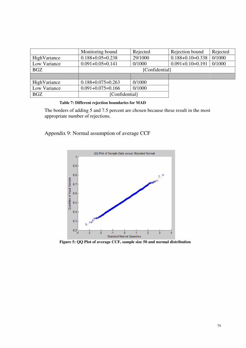
79

Table 7: Different rejection boundaries for MAD

The borders of adding 5 and 7.5 percent are chosen because these result in the most

appropriate number of rejections.

Appendix 9: Normal assumption of average CCF

Figure 5: QQ Plot of average CCF, sample size 50 and normal distribution

Monitoring bound Rejected Rejection bound Rejected

HighVariance 0.188+0.05=0.238 29/1000 0.188+0.10=0.338 0/1000

Low Variance 0.091+0.05=0.141 0/1000 0.091+0.10=0.191 0/1000

BGZ [Confidential]

HighVariance 0.188+0.075=0.263 0/1000

Low Variance 0.091+0.075=0.166 0/1000

BGZ [Confidential]

Documents

Thesis Public version - Universiteit Twenteessay.utwente.nl/61905/1/master_B._Maarse.pdf · Backtesting Framework for PD, EAD and LGD ... Improving the current backtesting methodology