Embed Size (px)
Citation preview
NAVAL POSTGRADUATE SCHOOL Monterey, California
THESIS DESIGN OF DIGITAL CONTROL ALGORITHMS FOR
UNMANNED AIR VEHICLES
by
Steven J. Froncillo
March 1998
Thesis Advisor: Isaac. I. Kaminer
Approved for public release; distribution is unlimited.
•i'Jii ̂ m&v,
REPORT DOCUMENTATION PAGE Form Approved OMB No. 0704-0188
Public reporting burden for this collection of information is estimated to average 1 hour per response, including the time for reviewing instruction, searching existing data sources, gathering and maintaining the data needed, and completing and reviewing the collection of information. Send comments regarding this burden estimate or any other aspect of this collection of information, including suggestions for reducing this burden, to Washington headquarters Services, Directorate for Information Operations and Reports, 1215 Jefferson Davis Highway, Suite 1204, Arlington, VA 22202-4302, and to the Office of Management and Budget, Paperwork Reduction Project (0704-0188) Washington DC 20503.
1. AGENCY USE ONLY (Leave blank) 2. REPORT DATE
March 1998 3. REPORT TYPE AND DATES COVERED
Master's Thesis
4. TITLE AND SUBTITLE
DESIGN OF DIGITAL CONTROL ALGORITHMS FOR UNMANNED AIR VEHICLES
6. AUTHOR(S)
Froncillo, Steven J.
7. PERFORMING ORGANIZATION NAME(S) AND ADDRESS(ES)
Naval Postgraduate School Monterey, CA 93943-5000
9. SPONSORING / MONITORING AGENCY NAME(S) AND ADDRESS(ES)
5. FUNDING NUMBERS
8. PERFORMING ORGANIZATION REPORT NUMBER
10. SPONSORING/ MONITORING
AGENCY REPORT NUMBER
11. SUPPLEMENTARY NOTES ~~
The views expressed in this thesis are those of the author and do not reflect the official policy or position of the Department of Defense or the U.S. Government. 12a. DISTRIBUTION / AVAILABILITY STATEMENT
Approved for public release; distribution is unlimited. 12b. DISTRIBUTION CODE
13. ABSTRACT (maximum 200 words)
Recent advances in the design of high performance aircraft, such as fly-by-wire controls, complex autopilot systems, and unstable platforms for greater maneuverability, are all possible due to the use of digital control systems. With the aid of modern control tools and techniques based on state-space methods, the aerospace engineer has the ability to design a dynamic aircraft model, verify its accuracy, and design and implement the controller within a matter of a few months. This work examines the digital control design process utilizing a Rapid Prototyping System developed at the Naval Postgraduate School. The entire design process is presented, from design of the controller to implementation and flight test on an Unmanned Air Vehicle (UAV).
14. SUBJECT TERMS ~ ~
Unmanned Aerial Vehicles, Rapid Prototyping Systems, Hardware-In-The-Loop Simulation, AROD, FROG, MATRIXx, SystemBuild
17. SECURITY CLASSIFICATION OF REPORT
Unclassified
18. SECURITY CLASSIFICATION OF THIS PAGE
Unclassified 19. SECURITY CLASSIFI-CATION OF ABSTRACT
Unclassified
15. NUMBER OF PAGES
100
16. PRICE CODE
20. LIMITATION OF ABSTRACT
UL

11
Approved for public release; distribution is unlimited
DESIGN OF DIGITAL CONTROL ALGORITHMS FOR UNMANNED AIR VEHICLES
Steven J. Froncillo Lieutenant Commander, United States Navy
B.S., University of Rhode Island, 1983
Submitted in partial fulfillment of the requirements for the degree of
MASTER OF SCIENCE IN AERONAUTICAL ENGINEERING
from the
NAVAL POSTGRADUATE SCHOOL March 1998
Author: Steven J. Froncillo
Approved by:
Isaac I. Kaminer, Thesis Advisor
•7?,^#V^ Russell W. Duren, Second Reader
Gerald H. Lindsey, Chairman Department of Aeronautics and Astronautics
111

IV
ABSTRACT
Recent advances in the design of high performance aircraft, such as fly-by-wire
controls, complex autopilot systems, and unstable platforms for greater maneuverability,
are all possible due to the use of digital control systems. With the aid of modern control
tools and techniques based on state-space methods, the aerospace engineer has the ability
to design a dynamic aircraft model, verify its accuracy, and design and implement the
controller within a matter of a few months. This work examines the digital control
design process utilizing a Rapid Prototyping System developed at the Naval Postgraduate
School. The entire design process is presented, from design of the controller to
implementation and flight test on an Unmanned Air Vehicle (UAV).

VI
TABLE OF CONTENTS
I. INTRODUCTION 1
II. SAMPLED-DATA SYSTEMS 5
A DISCRETE MODELS OF SAMPLED-DATA SYSTEMS 5 B. THE Z-TRANSFORM 9 C. ANALYSIS OF DISCRTE-TIME SYSTEMS 11 D. SIGNAL ANALYSIS AND DYNAMIC RESPONSE 18 E. SAMPLED-DATA SYSTEMS ANALYSIS 20 F. DISCRETE EQUIVALENTS BY NUMERICAL INTEGRATION 26
III. INTRODUCTION TO RAPID PROTOTYPING 29
A. RAPID PROTOTYPING SYSTEM ARCHITECTURE 30 B. XMATH/SYSTEM BUILD 31 C. REALSIM SERIES RAPID PROTOTYPING 36
IV. HARDWARE-IN-THE-LOOP (HITL) 45
A. HARDWARE DESCRIPTION FOR AROD 45 B. CONVERSION SUPERBLOCKS 46 C. SENSOR CALIBRATION 49 D. INPUT/OUTPUT CONNECTIONS 50
V. DIGITAL CONTROL DESIGN 53
A. MODELING ACTUATORS AND SENSORS 53 B. FEEDBACK CONTROLLER DESIGN 57 C. HARDWARE-IN-THE-LOOP TESTING 59
VI. ALTITUDE CONTROLLER DESIGN PROJECT 63
A. DESIGN REQUIREMENTS 63 B. FROG AND AUTOPILOT MODELS 63 C. FEEDBACK CONTROLLER DESIGN 65 D. HARDWARE-IN-THE-LOOP TEST 72 E. IMPLEMENTATION AND FLIGHT TEST 72
VII. CONCLUSIONS AND RECOMMENDATIONS 81
A. CONCLUSIONS 81 B. RECOMMENDATIONS 81
APPENDIX A. HCE SCREENS FOR HITL PROJECT 83
APPENDIX B. ADITIONAL SUPERBLOCKS DIAGRAMS 85
LIST OF REFERENCES 89
Vll

INITIAL DISTRIBUTION LIST 91
Vlll

I. INTRODUCTION
The use of digital computers in the real-time control of aircraft has paved the way
to new aircraft designs that are faster, more maneuverable and safer than ever before.
With this growing emphasis on digital control design, new tools and techniques have
been developed to aid in the design and implementation of complex control systems.
Traditionally, control systems are developed using classical control design methods that
are costly and time consuming. Newer technologies, like rapid prototyping based on
modern control methods, integrate the design process and shorten the time required to
complete a control design from a few years to a few months.
The purpose of this thesis is twofold: develop the background material for an
Advanced Control of Aerospace Vehicles course, and design and flight test an altitude
hold controller for a UAV.
At the Naval Postgraduate School, students in the Aeronautical and Avionics
Engineering curriculum receive a full sequence of controls courses with the final course
being Advanced Control of Aerospace Vehicles, for which this thesis is written. This
course will introduce the students to the critical aspects of the design, implementation and
flight testing of the basic controllers for fixed-wing aircraft. The course examines both
classical (transform) and modern (state-space) control methods for designing complex
digital control systems.
The main focus is on the study of sampled-data systems, systems that have both
discrete and continuous-time components. Devices used for the interface between the
continuous and discrete components, the analog-to-digital converter and the digital-to-
analog converter, are covered in detail. This thesis will derive mathematical models for
each of these operations, and develop tools for analysis and synthesis.
The class is largely project oriented. Much of the class is concentrated in the
Avionics/Controls laboratory and the Unmanned Air Vehicle (UAV) laboratory. The
projects are centered on a Rapid Prototyping System (RPS) developed by the aeronautical
engineering department for flight testing control algorithms for unmanned air vehicles.
The system affords a small team the ability to test new concepts in guidance, navigation,
and digital control. The RPS consists of commercially available rapid prototyping
software with an open architecture design to allow for a wide range of applications. The
application software developed by Integrated Systems Incorporated (ISI), called RealSim,
allows students to participate in design projects from the initial concept stage to the flight
testing phase of the design process. This software has two main advantages:
• The ability to automatically generate higher-language code such as C for the
designed controller.
• The system utilizes industry standard I/O devices including digital-to-analog,
analog-to-digital, pulse width modulation, and serial capability, permitting easy
connections to hardware.
The test bed aircraft used is a UAV called FROG , shown in Figure 1.1. This UAV is
equipped with a complete avionics suite necessary for autonomous flight.
The accomplishment of this endeavor has led to a number of successful projects,
including voice controlled flight and an airspeed controller, and is paving the way for
more complex projects such as autonomous landing. This thesis will describe in detail
one such design project, the development of an altitude hold controller implemented in
the FROG using the RPS tools. The automation of the design process is completed in
three developmental phases:
• Feedback controller design. In this phase a model of the plant is created. The
controller is then designed through various methods of classical input/output
control techniques and/or modern state-space control techniques. The process
typically involves many iterations to satisfy specific design requirements.
• Hardware-In-the-Loop Testing. The feedback system is tested with some or
all of the actual hardware which will be used to control the aircraft. This is the
final validation of the controller prior to an actual flight.
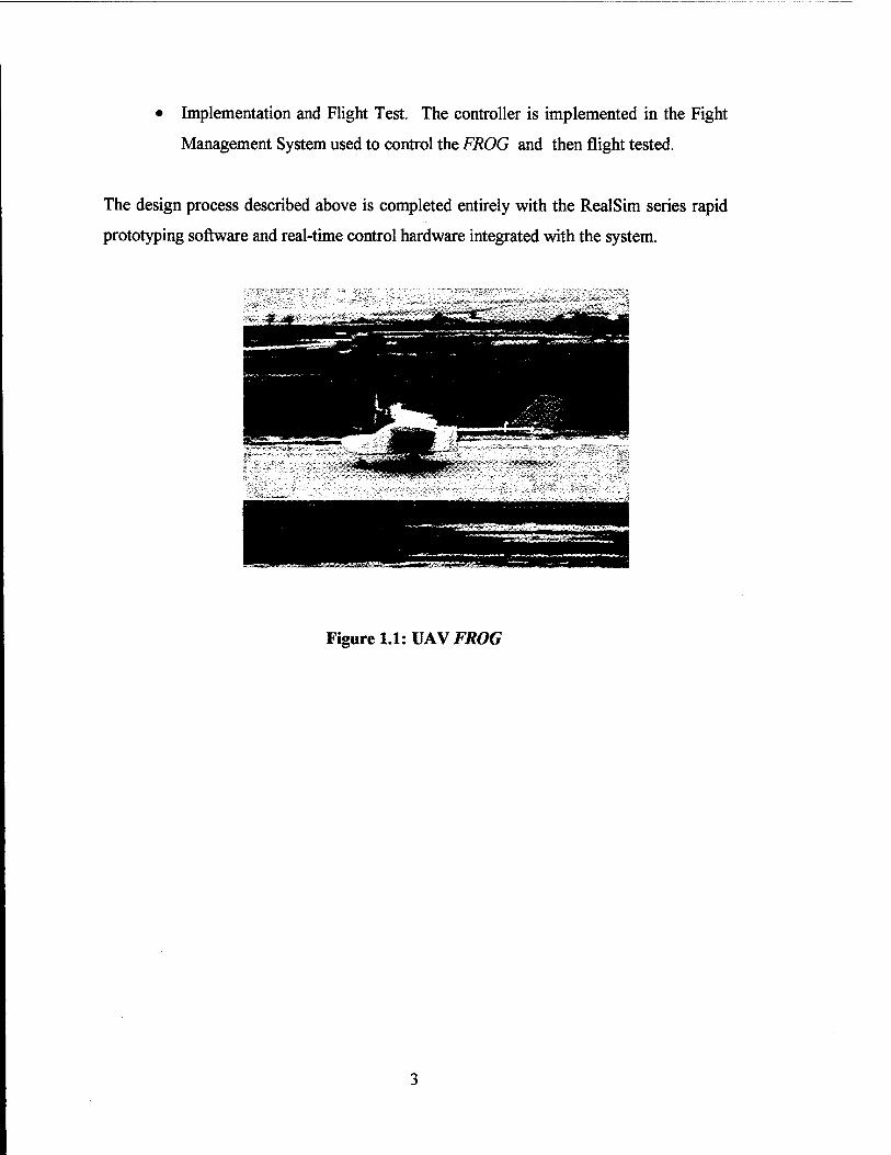
• Implementation and Flight Test. The controller is implemented in the Fight
Management System used to control the FROG and then flight tested.
The design process described above is completed entirely with the RealSim series rapid
prototyping software and real-time control hardware integrated with the system.
Figure 1.1: VAW FROG

II. SAMPLED-DATA SYSTEMS
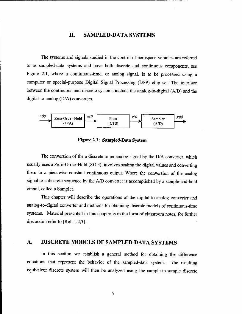
The systems and signals studied in the control of aerospace vehicles are referred
to as sampled-data systems and have both discrete and continuous components, see
Figure 2.1, where a continuous-time, or analog signal, is to be processed using a
computer or special-purpose Digital Signal Processing (DSP) chip set. The interface
between the continuous and discrete systems include the analog-to-digital (A/D) and the
digital-to-analog (D/A) converters.
u(k) Zero-Order-Hold
(D/A)
u(t) Plant (CTS)
y(t) Sampler (A/D)
y(k)
Figure 2.1: Sampled-Data System
The conversion of the a discrete to an analog signal by the D/A converter, which
usually uses a Zero-Order-Hold (ZOH), involves scaling the digital values and converting
them to a piecewise-constant continuous output. Where the conversion of the analog
signal to a discrete sequence by the A/D converter is accomplished by a sample-and-hold
circuit, called a Sampler.
This chapter will describe the operations of the digital-to-analog converter and
analog-to-digital converter and methods for obtaining discrete models of continuous-time
systems. Material presented in this chapter is in the form of classroom notes, for further
discussion refer to [Ref. 1,2,3].
A. DISCRETE MODELS OF SAMPLED-DATA SYSTEMS
In this section we establish a general method for obtaining the difference
equations that represent the behavior of the sampled-data system. The resulting
equivalent discrete system will then be analyzed using the sample-to-sample discrete
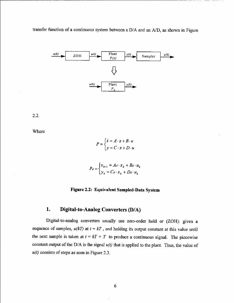
transfer function of a continuous system between a D/A and an A/D, as shown in Figure
u(k) ZOH u(0, Plant P(s)
0
y(t). Sampler y(k),
u(k) Plant P.,
y(k).
2.2.
Where
P = \x = A-x + B-u
[y = C-x + D-u
Pd-- \xk+} =Ad-xk+Bd-uk
\yk=Cd-xk+Dd-uk
Figure 2.2: Equivalent Sampled-Data System
1. Digital-to-Analog Converters (D/A)
Digital-to-analog converters usually use zero-order hold or (ZOH): given a
sequence of samples, u(kT) at t = kT, and holding its output constant at this value until
the next sample is taken at / = kT + T to produce a continuous signal. The piecewise
constant output of the D/A is the signal u(t) that is applied to the plant. Thus, the value of
u(t) consists of steps as seen in Figure 2.3.
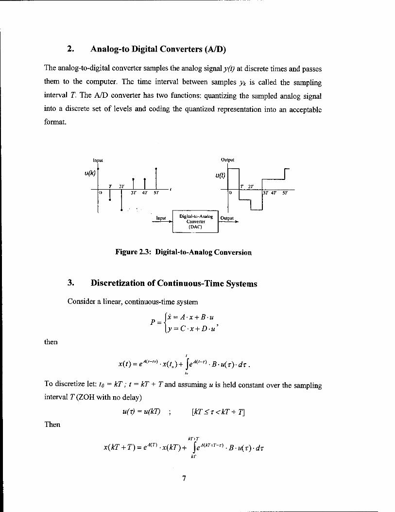
2. Analog-to Digital Converters (A/D)
The analog-to-digital converter samples the analog signal y(t) at discrete times and passes
them to the computer. The time interval between samples yk is called the sampling
interval T. The A/D converter has two functions: quantizing the sampled analog signal
into a discrete set of levels and coding the quantized representation into an acceptable
format.
In nil
i ■ i
k)
T 2r | |
"1 37' 47' 57
i i * ■
Output
u(t)
Input Digilal-lo-Analog Converter (DAC)
T IT
r 37" 47* 57"
Output
Figure 2.3: Digital-to-Analog Conversion
then
3. Discretization of Continuous-Time Systems
Consider a linear, continuous-time system
jx = A-x + B-u
\y = C-x + D-u'
x(t) = eA("U)) ■ x(t„) + jeA{"T) -B-u(T)-dT. i„
To discretize let: t0 = kT; t = kT+ T and assuming u is held constant over the sampling
interval T (ZOH with no delay)
U(T) = u(kT) ; [kT < r < kT + T\
Then
kT+T
x(kT + T) = eA{T) ■ x(kT) + \eA{kr+r-T) .B-u{r)-dr kT

Let
Z = (kT + T)-T
d{ = -dr,
then
r = kt=>4=T
Let x(kT+T)= x4+,,then
**+i = ßAr ■ Xu + \eH -B-uk-d$ (Eq. 2.1) 0
Define
AT 0 = e T
o
The discrete equivalent of P
jxk+]=®-xk+r-uk
P<=\yk=C.Xk+D.uk <*•">
Note the equivalent discrete system is shift-invariant, since O and T are not functions of
k. Commands to discretize: Matlab--c2d, Xmath-discretize
EXAMPLE 2.1: Discretize the following CTS
x = -a-x + a-u a P(s) =
y=x s+a
From equation 2.2
<$> = e
r
-a-T
r= \e~H ■{a)-d^ = {\-e-aT) o
xk+.=e-aT-xk+(l-e-aT)-uk
yk=xk
8

B. THE Z-TRANSFORM
1. Definition
Given a sequence {xk}, k- - oo,... <x> , let
00
X(z) = ^xk-z~k, r<> < \z\ < Ro, (Eq. 2.3) A=-oo
where we assume we can find values of r0 and for which the series converges.
As in the case of the Laplace transform, Eq. (2.3) is considered an operator that
transforms a sequence xk into a function X(z), symbolically represented by
X(z) = Z{xk}
The Xk and X(z) are said to form a z-transform pair denoted as
X(z) <-> Z{xk)
EXAMPLE 2.2 Consider the sequence given in example problem 2.1
P(s) = -^- => xk = eakT ; k=0,l,2,... s + a
By Eq. (2.3) the z-transform of Xk is
Z{xk} = X(z) = ±e-"kTz-k =±(e-aT ■ z'1) *=o k=0
Note: a infinite geometric sum is given by
„,=o l —a
Letting a = (e'aT -z_1)
l-(e-fl'7-z-) X(z)=, ,_-a.T -K i Yar-z-'\<\ ■ \z\>e'
2. Some Properties of the z-Transform
Listed below are some properties of the z-transform useful to the material
presented in this section. For reference, a more complete list is found in [Ref. 1].
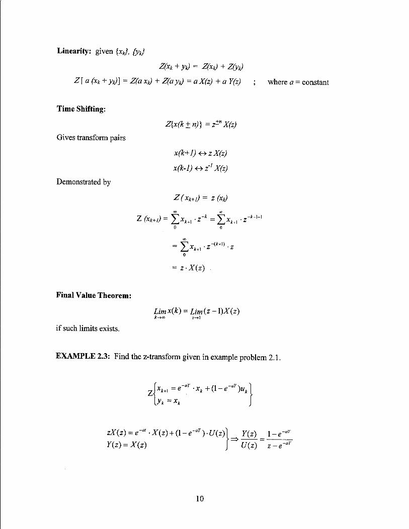
Linearity: given {xkj, {yk}
Z(xk+yk) = Z(x0+Z(yk)
Z[a(xk+y!i)]= Z(a x0 + Z(ay0 = aX(z) + a Y(z) ; where a = constant
Time Shifting:
Z{x(k±n)} = z-nX(z)
Gives transform pairs
x(k+l)+>zX(z)
x(k-l) <-> z1 X(z)
Demonstrated by
Z(xk+i) = Z (X0
00 00
Z(xk+1)= Xx*+rz_* =Sx*+i-
z" 0 0
= ±xk+rz-^.z 0
= z-X(z)
■A-l+1
Final Value Theorem:
if such limits exists.
Limx(k) = Lim(z-\)X(z)
EXAMPLE 2.3: Find the z-transform given in example problem 2.1.
[yk = **
z*(z) = e- • X(z) + (1 - e-a7') • U(z)\ Y(z) \-e~aT
Y(z) = X(z) U(z) z-e-aT
10

C. ANALYSIS OF DISCRETE-TIME SYSTEMS
1. The Discrete Transfer Function
Consider the continuous-time and discrete-time systems shown in Figure 2.4.
u(t) y(t) —►
u(k) y(k)
Figure 2.4: System Transfer Functions
The transfer function for the continuous-time system is
Y(s) = {C(sl - A)~x -B + D}- U(S)
For the discrete-time system compute
\yk=C-xk+D-uk J
z(xk+1) = z(®-xk+r-u)
z-X(z) = 0-X(z) + T-U(z)
x(z) = (zi-®y]-r-u(z)
Z(yk) = Z(C-xk+D-uk)
Y(z) = C-X(z) + D-U(z)
Y(z) = {C■ (zl - <D)-' • T + D\ ■ U(z)
Discrete transfer function
U(z) c(zi-®y'r+D (Eq.2.4)
EXAMPLE 2.4: Find the discrete transfer function from example problem 2.1
11

Given:
P(s) = a
s + a
Continuous-Time
a
Discrete-Time
Y(s) = [C • (si - AT -B + D]- U(s) => Y(s) = -?— ■ U(s) s + a
0> = e~aT T = \e-ai ■ (a)d£ = (1 -e~aT)
From Eq. (2.4)
Y(z) = (l)[zI-e-a,r-(\-e-"1) = \-e-aT
a-T U(z) z-e
Now consider the sampled-data system in Figure 2.5.
D/A «fiV P(s) y(% A/D yk
Let
Figure 2.5: Prototype Sampled-Data System
fl;* = 0 u(kT) = '
|0;£ * 0
Then u(k) is the unit impulse. The response to a unit impulse determines the impulse
response of the D/A converter:
u(t) = \(t)-\(t-T)
Then
1 e~xT 1 U(s) = ^e—^(l-e-«)
s s s
and
y(t)=u G(s) •(l-e-))
V s
y(kT) = y(t), (k-\)T<t<kT
12

Finally,
G(z) = Z(y(kT))
rG(s) = ZU"
V s (j-«-)
-K ry\ T-\ (1-O-Z \L '<?(^
(l-z-)-Z
I V s J
rG(s)\
V s J
Where the "L'1" is dropped for convenience.
EXAMPLE 2.5: Compute the discrete transfer function for
a G(s) =
s + a
Then
The corresponding time function
G(s) 1 1
s s s + a
r«-i(,)-«-(o
(Eq. 2.5)
y(kT) = l(kT)-e-ak7 -l(kT)
The z transform
1 s J ^V z-1 z-e-' (z-l)(z-e-aT)
From equation 2.5
G(z) = (l-z-') Kl z(l-e-°r) ,(z-l)(z-0
1-e -aT
z-e -aT
13
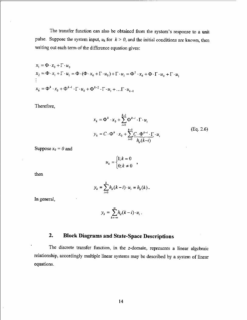
The transfer function can also be obtained from the system's response to a unit
pulse. Suppose the system input, uk for k > 0, and the initial conditions are known, then
writing out each term of the difference equation gives:
x, = O • x0 + T • u0
x2=<&-xl+r-ux =o-(o-x0+r-«0)+r-w1 =o2-x0 + o-r-w0+r-«1
xk =o* -x0 +a>*-1 -r-w0 +o*-2 -r-u, +...r-w,_,
Therefore,
1=0
A-i (Eq. 2.6) ^=c-Q*-x0+yc-P*-'-r-t/;
'=° A,(*-i)
Suppose xo = 0 and
then
In general,
u =rk=0
;=0
2. Block Diagrams and State-Space Descriptions
The discrete transfer function, in the z-domain, represents a linear algebraic
relationship, accordingly multiple linear systems may be described by a system of linear
equations.
14

Parallel Connections: The system response of a parallel combination of two LTI
systems is the sum of the single-path transfer function, Figure 2.6.
» H,(z)
Or2* H2(2) 1
Figure 2. 6: Parallel blocks
7(z) = [#, (z) + #2 (z)] • l/(z) = //(z) • U(z)
W)
Cascade Connections: The system response of two LTI systems in series is related by
the product, Figure 2.7.
u H,(z) H2(z) y
Figure 2.7: Cascade blocks
Yx(z)=Hx{z)-U{z)\ Y(z)=H2(z).Yl(z)\Y^H^H^-U^
Feedback Connections: The transfer function of a single loop, Figure 2.8, is given by:
■>0 ►! H,(z) A"
y
H2(z)
Figure 2.8: Feedback transfer function
15

y = Hx-e y = Hx-(u-H2-y)=>Y(z) =
Hx(z) U(z) e = u-H2-y\ ' ' * ' " - --' \ + Hx(z)-H2(z)
These transfer function relationships can be used in combination to describe
complex multi-path systems.
In general
H(z) =
Example of 3rd order system
a0+ax •z~'+...am-z-m
1 + 6, -z~x +b2-z~2+...bn-z- £(£) b(z)
H(z) = ax-z ' + a2-z~2 + a3-z
3
l + b,-z-] +b, -z-'+L-z-'
State-space realization (control canonical form), Figure 2.9.
Figure 2.9: State-Space Realization
By inspection
xl(k + \) = x2(k)
x2(k + l) = x3(k)
x3(k + l) = -bx-x3(k)-b2-x2(k)-b3-xx(k) + u
y = a1 -x3(k) + a2-x2(k) + a3-xx(k)
16
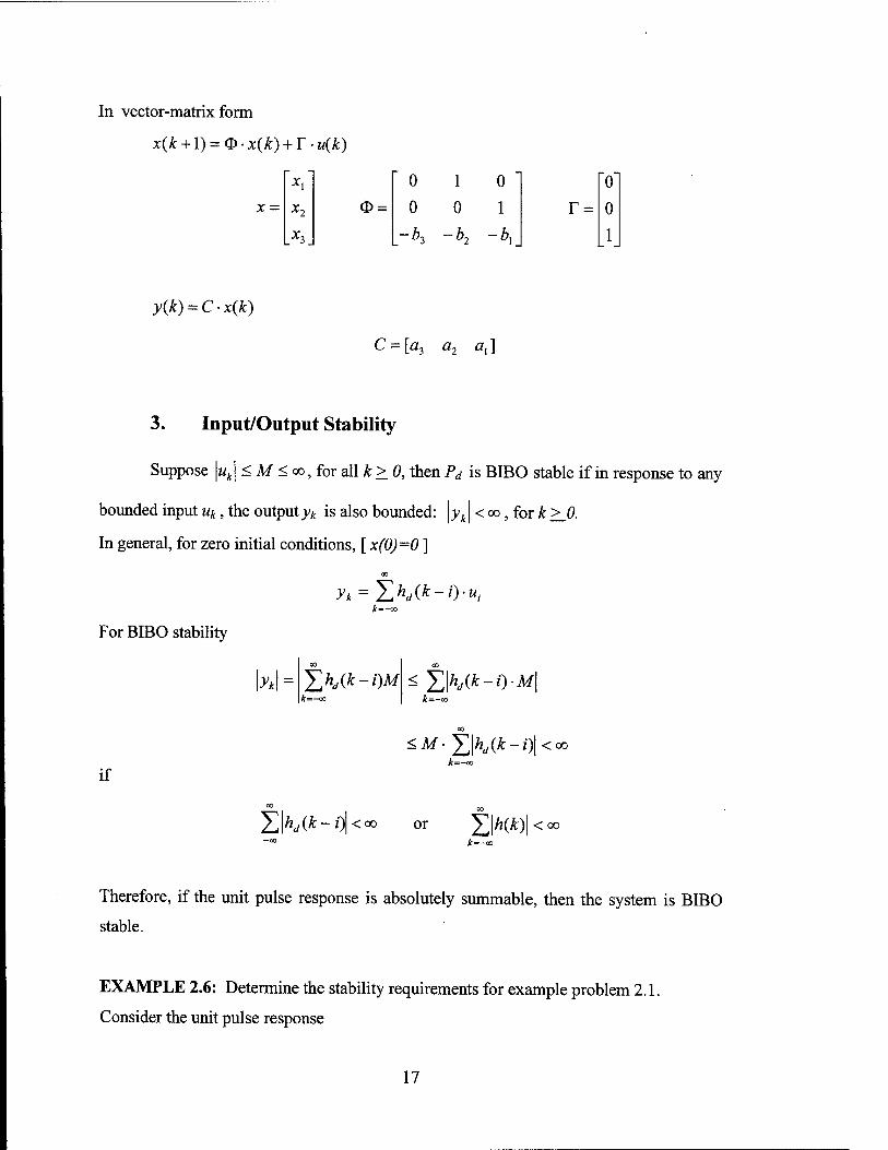
In vector-matrix form
x(k + i) = o-x(k)+r-u(k)
x = o = 0 1 0 0 0 0 1 r = 0
*3 ~b2 -&. l
y(k) = C-x(k)
C = [a3 a2 a,]
3. Input/Output Stability
Suppose \uk\ < M < oo, for all k > 0, then Pd is BIBO stable if in response to any
bounded input Uk, the output yk is also bounded: \yk \ < oo, for k >_0.
In general, for zero initial conditions, [ x(0)=0 ]
CO
yk = IXC*-*)-«/ A=-oo
For BIBO stability
\yk t^Kik-iW k=-°°
if
<Y\hd{k-i)-M\ k=-ao
^M-|;|Ärf(Ä:-i)|<oo
X|^(Ä:-O|<oo or S|ä(*)|<«> -°° k=-oo
Therefore, if the unit pulse response is absolutely summable, then the system is BIBO
stable.
EXAMPLE 2.6: Determine the stability requirements for example problem 2.1.
Consider the unit pulse response
17

yk =hd{k) = ak k=0,1,2,3...oo
and
00 1
5V=-T7 *=o 1 - \a\
is BIBO stable if |a| < 1, and unstable otherwise.
D. SIGNAL ANALYSIS AND DYNAMIC RESPONSE
1. Signal Transforms
The unit pulse:
U(z)=fjuk-z-k=z°=\ ; k=-x
The unit step:
U(z)=±uk.z-> = ±z-*=-±zr = -?-
"* = fl,* = 0
f1;>t > 0 0;£<0
General sinusoid:
uk =r*-cos(Ä;ö)-l(Ä:) = r/ re/^+e-./*o ■i(*)
Z[rk -cos(k0)-l(k)] = z z —— + z-re'e z-re~'e
U(z) = ^-r-cosfl) z2-2r(cos0)z + r2
2. Frequency Response of DTS
Consider a sinusoid at frequency co0 applied to a continuous-time system
u(t) = A ■ cos(ö)0 • t)
The continuous-time response is
18
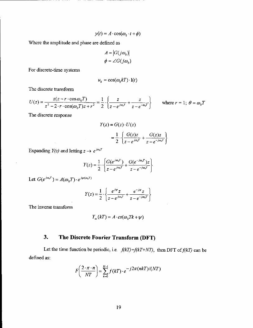
y{t) = A■ cos(o)0 -t + f)
Where the amplitude and phase are defined as
A = \G(jco0)\
<f> = ZG(jo)0)
For discrete-time systems
uk = cos(co0kT) ■ 1(0
The discrete transform
TT. . z(z-r-cosco0T) \ [ z z ] U(z) = ^-± ° —T = --\ 7T7 + 7TT\ where r = 1; 0 = <T
z2 -2-r-cos(co0T)z + r2 2 {z-em>' z-e'*"' J °
The discrete response
Y(z) = G(z)-U(z)
_ I \ G(z)z G(z)z } 2 [z-eM'T z-e~M'T.
Expanding Y(z) and letting z -» ejwJ
{)~2[z-e^T z-e-'^]
Let G(eM'T) = A(co0T)-em6)»T)
1 f eJvz e~ivz 1 2 [z-e/<B"r z-e-J°°T\
The inverse transform
Yxs(kT) = A-cs(o)0Tk + y/)
3. The Discrete Fourier Transform (DFT)
Let the time function be periodic, i.e. f(kT)=f(kT+NT), then DFT offflcT) can be
defined as:
J2W| = ^f{kT). -j2x{nkT)l{NT)
19
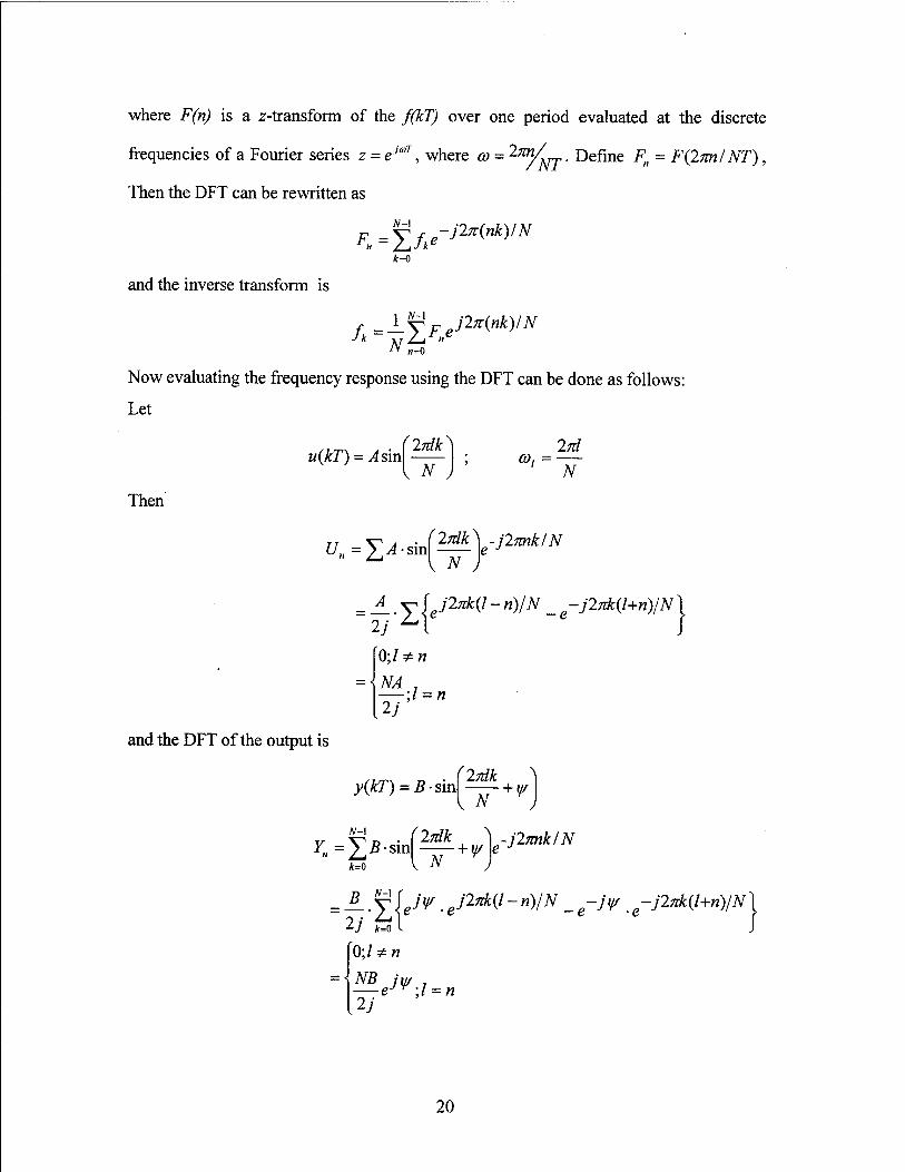
where F(n) is a z-transform of the ffiT) over one period evaluated at the discrete
frequencies of a Fourier series z = eJmT, where a> = 2im/fsrr • Define F„ = F(2m/NT),
Then the DFT can be rewritten as
AM
F„=Yfk rj27i{nk)IN
*=0
and the inverse transform is
N ,,=o
Now evaluating the frequency response using the DFT can be done as follows:
Let
u(kT) = A sin V N ,
0),= 2jd_
N
Then
= A. V U27*« ~ n)lN _ e-J2nk(l+n)/N 1 V
= - NA
{V ;l = n
and the DFT of the output is
y(kT) = B-sin 2nlk
■ + y/
*=0 V N )
..JL. v/,-/> .J2*k(I-n)/N _-iw ,e-j2nk(l+n)IN 2jfrT-^ 0;/ * n
= \NB jy, . —eJT ;l = n
20
lid Therefore the transfer function for co, is defined by ' NT J
where 7/ = FFT(y0 and U, = FFT(uO, evaluated at n=l.
JcmiN\_Y, _Be» \ ) U, A
E. SAMPLED-DATA SYSTEMS ANALYSIS
For the purpose of studying the sampled-data systems, each operation involved
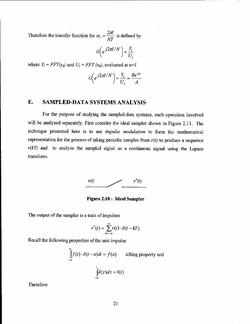
will be analyzed separately. First consider the ideal sampler shown in Figure 2.11. The
technique presented here is to use impulse modulation to form the mathematical
representation for the process of taking periodic samples from r(t) to produce a sequence
r(kT) and to analyze the sampled signal as a continuous signal using the Lapace
transform.
r(t) ^ r*(t)
Figure 2.10 : Ideal Sampler
The output of the sampler is a train of impulses
'*(')= Y,r{t)-S(t-kT) k=-oo
Recall the following properties of the unit impulse
j/(0 • <>(t ~ a)dt = f(a) sifting property and —oo
/
\ö{r)dr = 1(0 -co
Therefore
21
00
Lf*(0}= yO)-e-"dT — 00
* oo
= \^Lr{r)ö{t-kT)-e-STdz -00*=-"»
00 °°
= YJ \r(r)S(t-kT)-e-ST -dx *=-«>.
= Yjr(kT)-e-xkT = R'(s)
where we used the sifting property of 8.
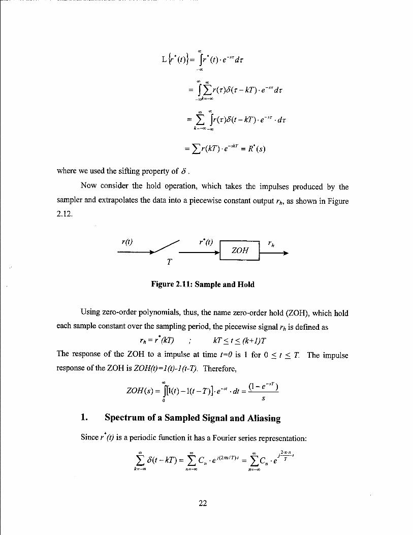
Now consider the hold operation, which takes the impulses produced by the
sampler and extrapolates the data into a piecewise constant output rh, as shown in Figure
2.12.
r(t) r*(t) ZOH
Figure 2.11: Sample and Hold
Using zero-order polynomials, thus, the name zero-order hold (ZOH), which hold
each sample constant over the sampling period, the piecewise signal rh is defined as
rh = r(kT) ; kT<t<(k+l)T
The response of the ZOH to a impulse at time t=0 is 1 for 0 < / < T. The impulse
response of the ZOH is ZOH(t)=l(t)-l(t-T). Therefore,
ZOH{s) = J[l(/)-1(7-T)\e~sl ■ dt = (1~e * )
0 s
1. Spectrum of a Sampled Signal and Aliasing
Since r (t) is a periodic function it has a Fourier series representation:
A=-oo
22

where
7/2 C«=i j is(t-kT).e-'"^'r>'dt
■* —7"/ 21=—"»
~r Therefore,
jr«y(r-^) = ify(2*,/7'>' A=-00 * «=-00
Let o, = — , be the sampling frequency and take the Laplace transform of the sampler
output:
L{r\t))= J Yr(t)-S(t-kT) e~sldt -oo\n=-«>
-00 1-* »=-00 J
^^■e >"*>'■ e-«dt T H=-co _„
Let s =ja)
1 °° ~ Y,R(<s-Jncos)
i °° R\jo) ) = -YJ
RUa>-jno)s) ■*- M=—on
Notice, that sampling produces an infinite train of sidebands at ncos, n = -oo... oo.
EXAMPLE 2.7: Let ö>5 = 1, m = 1/8
Ä*0-l/8) = ... + JRO-ö)1) + Ä[y(ffl1-ö)J] + JRL/(ö2,-ö)JI)] + ...
= ... + i?01/8) + i?[;(-7/8)] + i?[y(-14/8)] + ...
If R(jco) has components above the Nyquist frequency cos/2 or nIT, then after sampling
overlap or aliasing will occur and the original signal can not be reconstructed. This leads
23
to the sampling theorem: the original signal can be recovered from its samples if the
sampling frequency (cos = 27i/T) is at least twice the highest frequency in the signal. To
avoid aliasing a low-pass anti-alias filter is usually inserted preceding the sampling
operation.
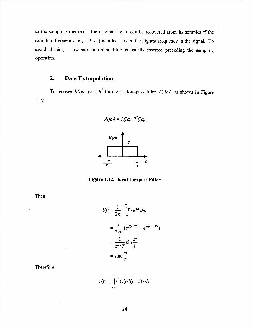
2. Data Extrapolation
To recover RQco) pass R* through a low-pass filter L(jco) as shown in Figure
2.12.
R0a>)=L(ja))R(jco)
it (O
T
Figure 2.12: Ideal Lowpass Filter
Then
/(/) = — [T-eialdco OTT J In -nIT
2njt (e >(*"''"> _e-'<*'/7">\
l . m -sin —
MIT T
sine —
Therefore,
r(t)= jr*(T)-!(t-T)-dT
24
. 7t(t - Z) J £ r (r) • S(T - kT) ■ sine H T) dr
_ooi=-oo T
Ä rirT. . 7C(t-kT) = 2_, r(kT)smc— -
Note, the ideal extrapolator is noncausal, since l(t) is nonzero for t < 0. Suppose Z(/vt^ is
replaced by ZOH.
Recall,
l-e-Jar
ZOH(ja>) = j®
Expressing the transfer function in magnitude and phase form
ZOH (ju)) = T-e-,eoJ,z sine V ^ J
Therefore,
\ZOH(jco)\ = T sinc- coT
ZZOH(jco) = -^ +180 • ö(ü) - n2n)
The resulting signal contains unwanted harmonics or impostors. By frequency analysis
oir(t) the principal harmonic can be identified.
Consider the sinusoid signal v(t) = ej0>"'+M
V(jco)=)eU^t+J^).e-Joytdt
—oo
00
This integral is not defined, however notice Z(S(t)) = \e~'m ■ S(t) -dt = \,
S(t) = — \eia,dco. In
25
Now replace t with co to get
S(co) = — \eia"dt
Therefore,
-CO
= 2m '*8(co-co0)
Since 8 is a even function, the spectrum of r(t) can be written in terms of impulse
functions
To recover the signal Rh , multiply the spectrum of R* by the transfer function of the
ZOH.
F. DISCRETE EQUIVALENTS BY NUMERICAL INTEGRATION
Concept: Represent a given continuous transfer function H(s) as a differential
equation and derive a difference equation whose solution is an approximation to that of
the differential equation.
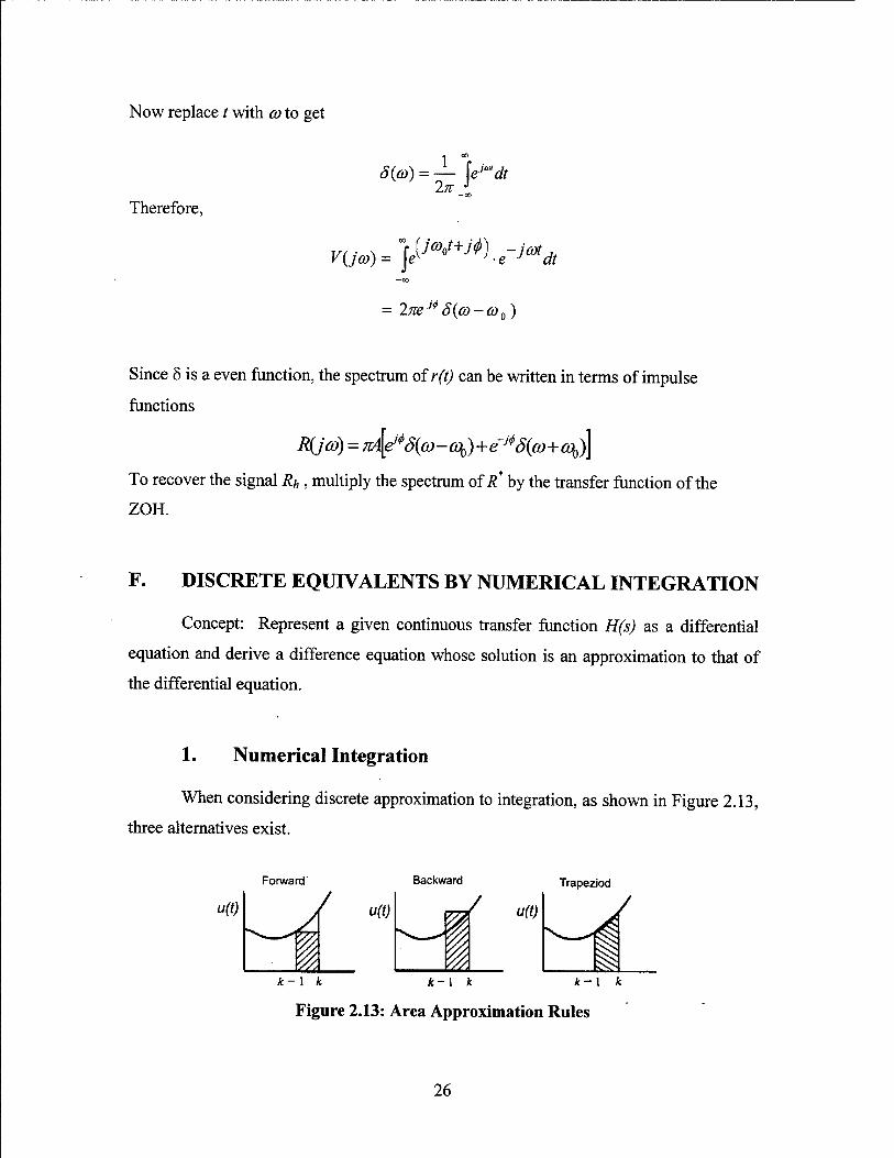
1. Numerical Integration
When considering discrete approximation to integration, as shown in Figure 2.13,
three alternatives exist.
Forward Backward Trapeziod
U(t) V2 /
i k-l k k-\ k k-\ k
Figure 2.13: Area Approximation Rules
26
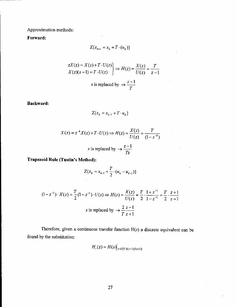
Approximation methods:
Forward:
zK+i =xk+T-(uk)}
zX(z) = X(z) + T-U(z)\ X(z) T 1 — H(z) = X(z)(z-l) = T-U(z) J U(z) z-\
s is replaced by ->
Backward:
zixk =xk.i+T-uk]
-Iw^.-r rr,_^ rrs.s X{z) T X(z) = z"X(z) + T ■ U(z) => H(z) =
s is replaced by ->
U(z) (1-z-1)
2-1
Tz
Trapezoid Rule (Tustin's Method):
T zixk=xkA+--(uk-uk_l)}
(l-z-1).X(z) = ^(l-z-').f/(z)^//(z) = ^^ = ^.i±^ = ^.£±l 2V W U(z) 2 1-z-' 2 z-1
5 is replaced by -» Jz + 1
Therefore, given a continuous transfer function H(s) a discrete equivalent can be
found by the substitution:
H,(z) = H(S)\s__ :(2/7-)[(2-I)/(Z + l)]
27
2. Zero-Pole Mapping Equivalents
This technique consists of a set of rules for locating the zeros and poles and
setting the gain of a z-transform that will describe a discrete, equivalent transfer function
that approximates the given H(s).
Rule #1: All poles of H(s) are mapped by z = esT. Replace s with esT for the poles of
H(s). HH(s) has a pole at s = a, then H(z) has a pole at z = eaT. If H(s) has a complex
pole at s = -a +jb, then H(z) has a pole at z = re±je.
Rule #2: All finite zeros are mapped by z = esT.
Rule #3: All infinite zeros of H(s) are mapped by z = -1.
a) Only one zero of H(s) at s - oo is mapped into z = oo.
Rule #4: The gain of the digital filter is selected to match the gain of H(s) at the band
center.
3. Zero-Order Hold Equivalent
If the approximating hold is the ZOH, then the equivalent to H(s) is
//(z) = (l-z-')ZpM} This is the same relationship that was derived earlier in section C of this chapter.
28
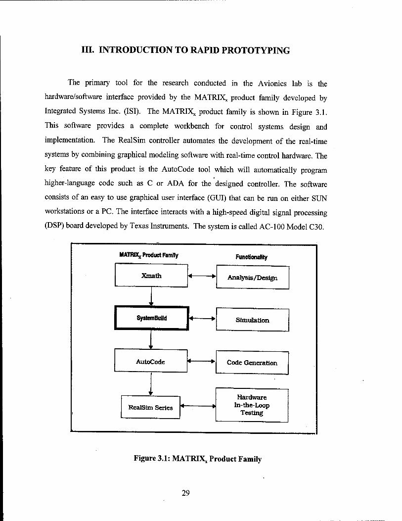
III. INTRODUCTION TO RAPID PROTOTYPING
The primary tool for the research conducted in the Avionics lab is the
hardware/software interface provided by the MATRIXX product family developed by
Integrated Systems Inc. (ISI). The MATRIXX product family is shown in Figure 3.1.
This software provides a complete workbench for control systems design and
implementation. The RealSim controller automates the development of the real-time
systems by combining graphical modeling software with real-time control hardware. The
key feature of this product is the AutoCode tool which will automatically program
higher-language code such as C or ADA for the designed controller. The software
consists of an easy to use graphical user interface (GUI) that can be run on either SUN
workstations or a PC. The interface interacts with a high-speed digital signal processing
(DSP) board developed by Texas Instruments. The system is called AC-100 Model C30.
MATRIXX Product Family Functionality
Xmath ■*
Analysis/Design w
i '
L SystemBuild Simulation 1 * r
AutoCode ^ Code Generation w
^ ' Hardware
In-the-Loop Testing 1
RealSim Series •
Figure 3.1: MATRIX, Product Family
29

A. RAPID PROTOTYPING SYSTEM ARCHITECTURE
The rapid prototyping system architecture consists of a UNIX workstation and a
windows based PC host computer which is equipped with two ISA bus adapter boards
(Figure 3.2). The workstation and PC are connected through Ethernet, using the standard
TCP/IP protocol suite. The two hardware boards in the PC consist of a board which acts
as the motherboard for the C30 DSP, and a "DSPFLEX" carrier board which holds four
input/output, or "IP", modules. The I/O boards connect the model to the real hardware
via the Hardware Connection Editor (HCE), which will be discussed in later sections. The
complete system is referred to as the AC-100 Model C30 real-time controller.
The avionics lab currently has two PC's configured as described above: a Pentium
tower PC called America and a luggable PC called AC 100. The luggable PC is normally
Workstation RealSim User Interface and Data Collection
1 r
Host Computer DSP C30 Processor
Generate AutoCode C I/O Management
IP 1
Hardware
IP 2
IP 3
IP 4
Figure 3. 2 : RealSim Architecture
30

connected to a stand alone Sparc II workstation, used for field fight testing with the
school's Unmanned Air Vehicle (UAV) called FROG.
There are a number of different types of I/O cards available depending on the
application. Currently both PC's have 4 IP modules consisting of a serial communication
(IPSerial) module, digital-to-analog (IP_DAC) module, analog-to-digital (IP_HiADC)
module, and a pulse width modulation (IP68332) module. A description of each IP
module and procedures for connecting hardware to the model is covered in detail in the
Hardware-In-The-Loop Testing section of this thesis.
B. XMATH/SYSTEMBUILD
Xmath/SystemBuild is a software program similar to the Matlab/Simulink
software programs. Xmath is the parent process and will launch the SystemBuild editor
when the build command is given or when a file is loaded that contains SystemBuild
data. It was designed to include an extensive set of design and analysis functions for both
the classical input/output control techniques and the modern state-space control
techniques. The SystemBuild program uses a hierarchical method of organization, based
on the SuperBlock concept. SuperBlocks provide a way of organizing a group of blocks
that define a function into a compact form for display. Through the use of this hierarchy,
variable names can be passed up and down the hierarchical structure allowing the
engineer to easily track and understand what variables are and where they interact with
the model. This section will cover the basic functions of Xmath/SystemBuild, for
detailed information refer to [Ref. 4].
1. Xmath Basics
Xmath can be run from either the SUN or SGI workstations located in the
avionics and aeronautics labs. Prior to using the MATRIXX software, the user must
configure his UNIX account to source the 'aclOOsetup' file which defines the editor used
by the system. This command should be set up as a marcro in the user's .cshrc file so it
31
will automatically run each time the user logs on to the workstation. Adding the
following command line to the .cshrc file: 'source$ISI/AC100/bin/acl00setup.sh', will
accomplish this.
Before invoking Xmath, a separate directory for each project should be created to
avoid using project files from one project with the standard files of another project.
Therefore, start by first creating a project directory and then move to that new directory
using the following UNIX commands: mkdir projectname, cd project_name. To start
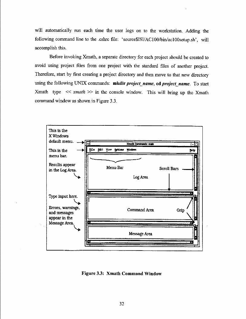
Xmath type « xmath » in the console window. This will bring up the Xmath
command window as shown in Figure 3.3.
This is the X Windows default menu.
This is the menu bar.
Results appear in the Log Area.
V
Type input here.
Errors, warnings, and messages appear in the
Xmath Commands: matt m File Edit Vie» gptirns ■utdsn »tip
Menu Bar Scroll Bars f
Log Area
Command Area
Message Area
Grip 7\
0
Figure 3.3: Xmath Command Window
32
2. SystemBuild Modeling
This section is a tutorial that covers the basics of the SystemBuild editor and
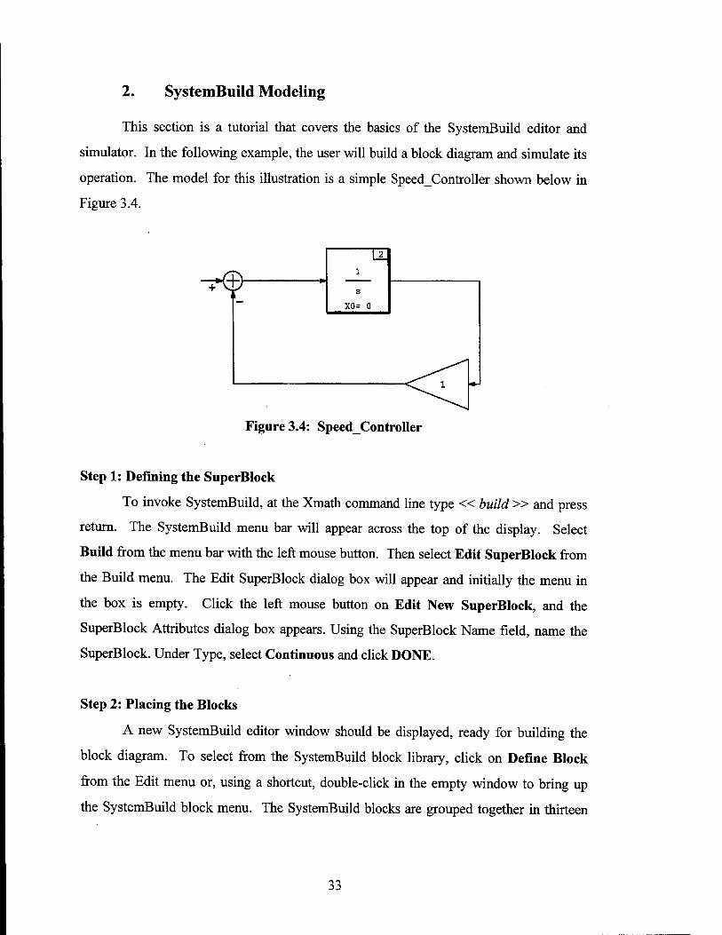
simulator. In the following example, the user will build a block diagram and simulate its
operation. The model for this illustration is a simple SpeedController shown below in
Figure 3.4.
T*©
Figure 3.4: Speed_Controller
Step 1: Defining the SuperBlock
To invoke SystemBuild, at the Xmath command line type « build » and press
return. The SystemBuild menu bar will appear across the top of the display. Select
Build from the menu bar with the left mouse button. Then select Edit SuperBlock from
the Build menu. The Edit SuperBlock dialog box will appear and initially the menu in
the box is empty. Click the left mouse button on Edit New SuperBlock, and the
SuperBlock Attributes dialog box appears. Using the SuperBlock Name field, name the
SuperBlock. Under Type, select Continuous and click DONE.
Step 2: Placing the Blocks
A new SystemBuild editor window should be displayed, ready for building the
block diagram. To select from the SystemBuild block library, click on Define Block
from the Edit menu or, using a shortcut, double-click in the empty window to bring up
the SystemBuild block menu. The SystemBuild blocks are grouped together in thirteen
33
palettes. To select a palette, click on one of the three-letter combinations at the top of the
menu.
To begin building the Speed_Controller, first select the Gain Block from the
algebraic block palette (ALG). Click and hold the left mouse button on this block, drag it
into the screen, and release the mouse button when the Gain block dialog box appears,
name the block, if desired, and click DONE. Next, select the Summer block from the
AGL palette and the Inegrator block from the DYN palette using the same procedures.
Step 3: Connecting the Blocks
The next step is to connect the blocks. Note the middle mouse button will be used
to make connections. Start by connecting the Summer block with the Integrator block.
Click in the Summer block, with the middle mouse button, then click on the Integrator
block. A line should connect the two blocks. Using the same procedure, connect the
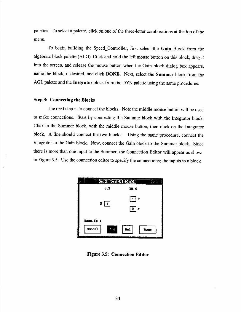
Integrator to the Gain block. Now, connect the Gain block to the Summer block. Since
there is more than one input to the Summer, the Connection Editor will appear as shown
in Figure 3.5. Use the connection editor to specify the connections; the inputs to a block
flail ■CONNECTION EDITOR! ■Bffl
FrcM,To :
c.3
f0
TO.4
Cancel B3 Del Done
Figure 3.5: Connection Editor
34
are in numerical order from top to bottom. The output from the Gain block should go to
the second input of the Summer. Then with the left mouse button' connect to Gain block
with the number 2 Summer input, highlight Add and click Done.
Note that the blocks can be resized by clicking on the block id number and
moving the mouse, or flipped by double-clicking on the block's body.
Step 4: Connecting External Inputs and Outputs
Input connections: click the middle mouse button in the open space, then in the
Summer block. The connection editor dialog box appears. With the left mouse button,
click the number 1 port of the Summer block then click Done. To label the external
input, click and hold the left mouse button in the SuperBlock ID bar, just above the
SystemBuild window. Select SuperBlock Attributes. In the dialog box, select the Labels
tab and under Input Naming select Enter Local Label Names. Now select the Input
tab and beside Input Label type the desired name. Click Done.
Output connections: With the middle mouse button click in the integrator block,
then click in an open space. Connect the two boxes, then click Done.
Simulating the Model
The SpeedControl model can now be simulated. There are a number of different
methods to simulate model, two of which are described here;
Method 1: First define a time-vector in Xmath by specifing a name, range, and
an increment. In the Xmath command window type: « t=[0 : .1 : 20]' »;. Next,
specify an input vector of magnitude one: « u=ones(t) »;. Enter the simulation
command. Type: «y=sim("Name of SuperBlock", t, u) »;. Note in this example the
name of the SuperBlock is Speed Contt-oiler. This command invokes the simulator,
specifies that the Speed_Controller model SuperBlock is to be processed, and sets the
output equal to y. After the simulation is complete, plot the output by typing: <<plot(y)
». Note, more details on using the sim command are available by typing « help sim »
in the Xmath command window.
35
Method 2: From the menu bar under analysis select Simulation. This will bring
up the simulation parameter dialog box. Define a time vector and input vector as above
and run.
Analyzing the Model
The Xmath/SystemBuild software contains an extensive set of functions for
system analysis. Specifics for analyzing the model can be found in the Xmath and
SystemBuild Core Manuals located in the avionics lab or by using the help command.
To linearize the model, the Xmath command is « sys=lin(" SuperBlock
name", {keywords}) », where sys is the name of the Xmath system object in state-space
form. Other useful commands include: poles (sys), eig(a),bode (sys).
Saving the Model
To save the model select File from the menu bar, highlight the SuperBlock name
and click on Save.
C. REALSIM SERIES RAPID PROTOTYPING
This section will continue with the design of the speed controller presented in the
last section. The tutorial will demonstrate the basic procedures for using the GUI and
testing on a real-time controller. Later sections will describe how the hardware is
connected to the model and the procedures for hardware-in-the-loop testing.
1. RealSim Graphical User Interface (GUI)
Each RealSim project is placed in a unique RealSim project directory. A number
of standard files are associated with each RealSim project. Therefore it is recommended
to create a separate project directory for each project. The project name and the directory
name should be the same.
36
To invoke the RealSim GUI type « realsim » in the UNIX command window.
When the RealSim GUI is invoked in a new directory a dialog box will appear along with
the GUI. Pressing return or clicking yes in the dialog box will enable the makeproject
command which creates the first of the required standard files called animation
configuration file (animation.cfg). Once all the default settings have been accepted, the
project name in the bottom left-hand corner of the GUI should be listed.
Next the user must create a target configuration file (target_config.cfg) file. This
file contains information such as the settings that the AutoCode needs to generate the
appropriate C code, which controller the model is to run, how many processors are in the
controller. This file will be used later to compile, link, download and run the design. To
create this file, click on show utilities in the GUI and select Retarget. The target is the
node name of the controller. In the UNIX command window the user will be asked for
the 'controller host name[ ]:' which in the avionics lab is 'america.' All of the remaining
default settings should be accepted. After retargeting the system to 'americcC the GUI
should indicate this in the middle of the bottom line in the GUI, see Figure 3.6.
These files are only created once for each project, as long as there are no changes
to the system configuration. Once these standard files have been set up for a specific
project, and the user is in the project directory for that project, typing « realsim » in
the UNIX command window will start the GUI targeted accordingly.
Through the use of the GUI the designer can now follow the flow diagram that
steps the user through the design process. As the user performs each step of the process,
the GUI paths are filled in, indicating the current stage in the design process. If certain
RealSim files are older than their logical predecessors, the Needs Up dating indicator will
be displayed.
2. Building the Model
The first step in the process is building the model using Xmath/SystemBuild, as
described in the previous section. To continue with the speed controller model, click on
the Xmath/SystemBuild block in the GUI. This will bring up the Xmath command
37

window. From this window, select file and load from the menu bar. Highlight the file
name and click OK. Select the SuperBlock from the build menu to display the model of
the Speed_Controller.
ra KCIISIM GUI S
■: Needs Updating XaAtli/
Sjatu tuild IMl
Utilities
Makeeroiect
Rewre« Convert D A Data
^^^^ Data AM. Editor
lAOtent
<Mit«C>da
■ Animtioit View Autocode
VjewComecÖons
EdittareetconfiR
I 1 Spa^on
8Ä3Debug«er
tHpUl art
m link
lurduKr* Csnaectien
B Miter
Ecutaiimation.dE HideUoh&ei
iHDlMt ud Ha
bit
|
The Project is The Target is Al is the target the name of the the node name of configuration of project you are the controller. application currently running. processor # 1.
Figure 3.6: RealSim Graphical User Interface
The SuperBlock design, for this example, is presently a continuous type and needs
to be transformed to a discrete controller (z-domain). Selecting Transform SuperBlock
under Build from the menu bar will display the transform dialog box. Highlight the
SuperBlock name and under type select Discrete, then click Transform. When
transforming from continuous-time to discrete-time a time delay block must be added to
the block diagram, as shown in Figure 3.7. From the DYN palette select the time delay
block.
38
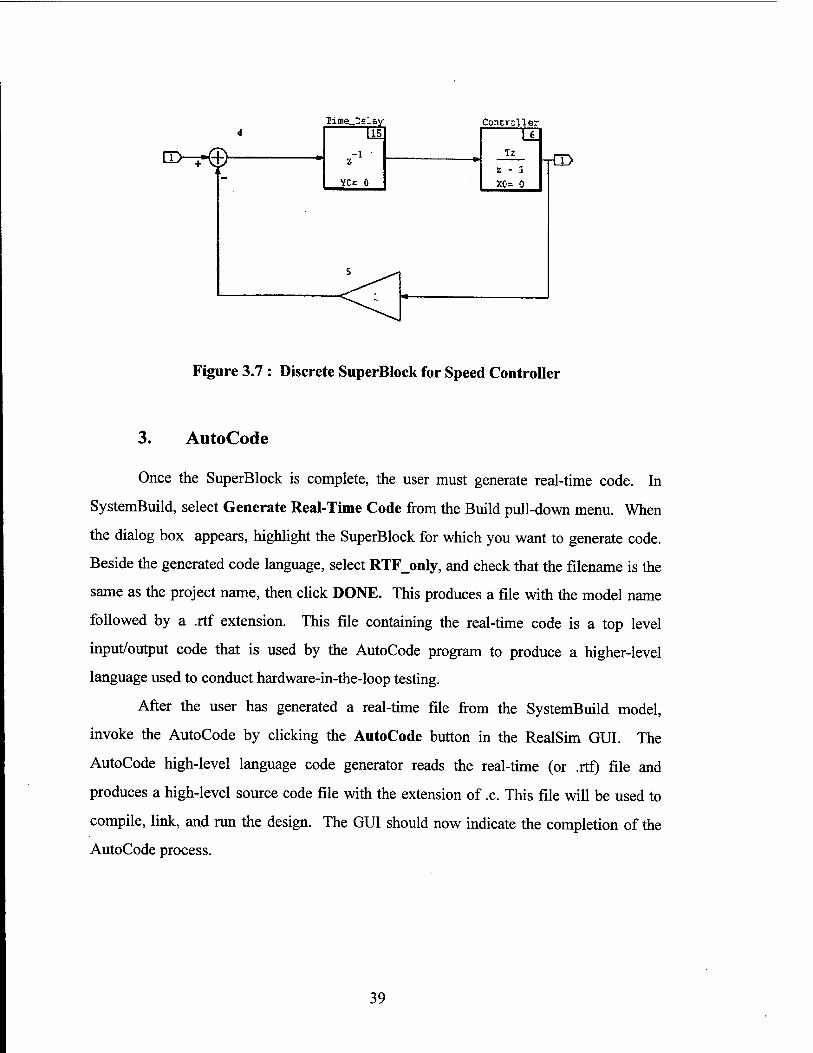
Q>-r©
Iime_^slay Controller
TCD
Figure 3.7 : Discrete SuperBlock for Speed Controller
3. AutoCode
Once the SuperBlock is complete, the user must generate real-time code. In
SystemBuild, select Generate Real-Time Code from the Build pull-down menu. When
the dialog box appears, highlight the SuperBlock for which you want to generate code.
Beside the generated code language, select RTF_only, and check that the filename is the
same as the project name, then click DONE. This produces a file with the model name
followed by a .rtf extension. This file containing the real-time code is a top level
input/output code that is used by the AutoCode program to produce a higher-level
language used to conduct hardware-in-the-loop testing.
After the user has generated a real-time file from the SystemBuild model,
invoke the AutoCode by clicking the AutoCode button in the RealSim GUI. The
AutoCode high-level language code generator reads the real-time (or .rtf) file and
produces a high-level source code file with the extension of .c. This file will be used to
compile, link, and run the design. The GUI should now indicate the completion of the
AutoCode process.
39
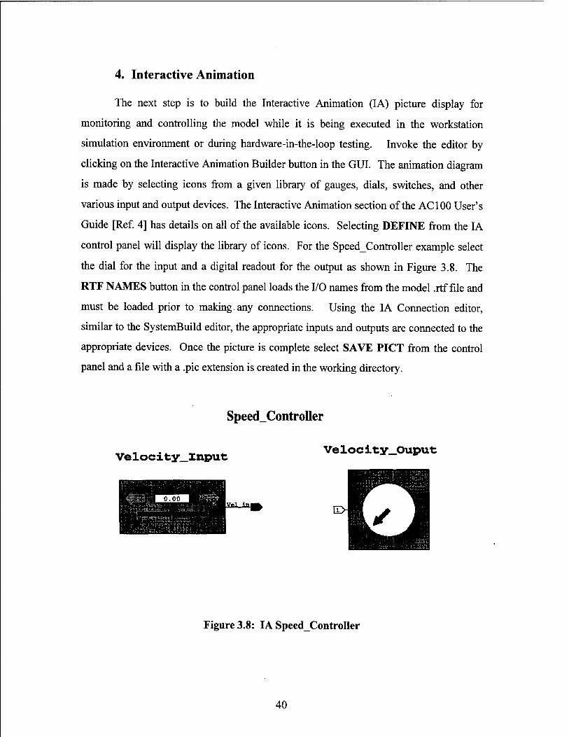
4. Interactive Animation
The next step is to build the Interactive Animation (IA) picture display for
monitoring and controlling the model while it is being executed in the workstation
simulation environment or during hardware-in-the-loop testing. Invoke the editor by
clicking on the Interactive Animation Builder button in the GUI. The animation diagram
is made by selecting icons from a given library of gauges, dials, switches, and other
various input and output devices. The Interactive Animation section of the AC 100 User's
Guide [Ref. 4] has details on all of the available icons. Selecting DEFINE from the IA
control panel will display the library of icons. For the SpeedController example select
the dial for the input and a digital readout for the output as shown in Figure 3.8. The
RTF NAMES button in the control panel loads the I/O names from the model .rtf file and
must be loaded prior to making any connections. Using the IA Connection editor,
similar to the SystemBuild editor, the appropriate inputs and outputs are connected to the
appropriate devices. Once the picture is complete select SAVE PICT from the control
panel and a file with a .pic extension is created in the working directory.
Speed_Controller
Ve locity_lnpufc Velocity_Ouput
Figure 3.8: IA SpeedController
40
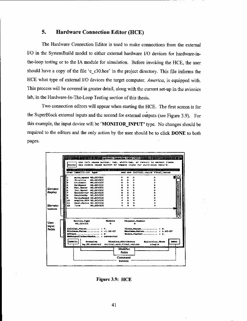
5. Hardware Connection Editor (HCE)
The Hardware Connection Editor is used to make connections from the external
I/O in the SystemBuild model to either external hardware I/O devices for hardware-in-
the-loop testing or to the IA module for simulation. Before invoking the HCE, the user
should have a copy of the file 'c_c30.hce' in the project directory. This file informs the
HCE what type of external I/O devices the target computer, America, is equipped with.
This process will be covered in greater detail, along with the current set-up in the avionics
lab, in the Hardware-In-The-Loop Testing section of this thesis.
Two connection editors will appear when starting the HCE. The first screen is for
the SuperBlock external inputs and the second for external outputs (see Figure 3.9). For
this example, the input device will be 'MONITORJNPUT' type. No changes should be
required to the editors and the only action by the user should be to click DONE to both
pages.
Elevator display
Elevator buttons
User input fields
IMCUOH Bator tHCEiH
uae left mouse button, tab. shift-tab» or return to »elect items. Hlnte Use middle mouse button on toggle items for pull—doun menu'e.
chan labeltl:10) tupe BELOKBBBBI nod Che initial—value f inal-value
1 auto-speed 2 Throttle 3 CruiseOn 4 SetSpeed 5 Dec-Speed 6 Xne_Speed 7 SpeedError 6 DeelredSp 9 Nolsuspeed 10 engine-RPM 11 Dear-Ratio 12 Tims
NO-DEVICE NO-DEVICE NO-DEVICE NO-DEVICE NO-DEVICE NO-DEVICE NO-DEVICE NO-DEVICE NO-DEVICE NO-OEVICE NO-DEVICE NO-OEVICE
<r
m
O Device-Type
NO-OEVICE
Mitial-Ualue Ifinlnuej-Ualue......... Offset BbOutputTsUssrHoake...
Itodule o
connscted
Chaanel-Mwafeer 0
Final-Value ntucitem-Ualue Scale-Factor........
CANCEL groupie« elOMino-ettrlbutee by-SB.ehannel initial-and-flnal_valuoa
Selection—Mode single
Modifier fields
Command " buttons '
Figure 3.9: HCE
41
6. Compile and Link
Once the AutoCode is complete the C source files need to be compiled and linked
to the C30. Selecting the Compile and Link button in the RealSim GUI will cause the
UNIX systems to connect via ftp with the AC 100 target computer (America). For this to
happen the host computer, America, must be in the ftp mode. Typing 'aclOOsvr' at the
DOS prompt on America will enable the computer for ftp transfer. The compiler
generates object code from the .c file and the link creates a C30 DSP executable from the
object code.
7. Download and Run
When all the above steps are completed, the model is ready to be tested. The
testing for this illustration will be a simulation only, since no hardware is connected.
Selecting Download and Run on the GUI will connect the RealSim software to the target
AC 100 computer through ftp. Once the connection is made, it will automatically load the
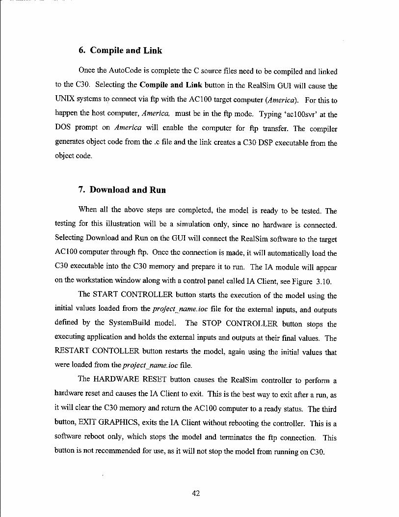
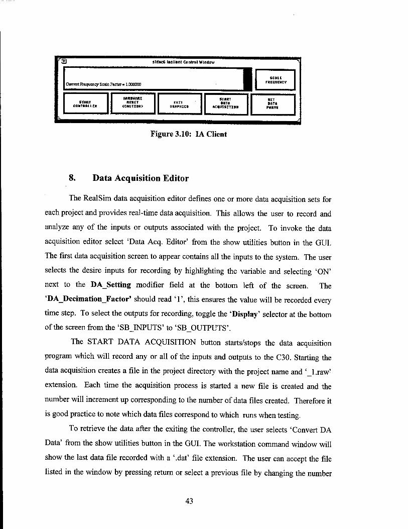
C30 executable into the C30 memory and prepare it to run. The IA module will appear
on the workstation window along with a control panel called IA Client, see Figure 3.10.
The START CONTROLLER button starts the execution of the model using the
initial values loaded from the project name, ioc file for the external inputs, and outputs
defined by the SystemBuild model. The STOP CONTROLLER button stops the
executing application and holds the external inputs and outputs at their final values. The
RESTART CONTOLLER button restarts the model, again using the initial values that
were loaded from the project name.ioc file.
The HARDWARE RESET button causes the RealSim controller to perform a
hardware reset and causes the IA Client to exit. This is the best way to exit after a run, as
it will clear the C30 memory and return the AC 100 computer to a ready status. The third
button, EXIT GRAPHICS, exits the IA Client without rebooting the controller. This is a
software reboot only, which stops the model and terminates the ftp connection. This
button is not recommended for use, as it will not stop the model from running on C30.
42
a Sldac6 lacllent Control Window
Currant Frequency Scöe Factor »1.000000 HJ
SCALE FREIIUEKCr
START CONTROLLER
HARDWARE RESET
<CAUTIOH> EXIT
BRHPHICS
START OATA
ACQUISITION
StT DATA
PARrlS
J Figure 3.10: IA Client
8. Data Acquisition Editor
The RealSim data acquisition editor defines one or more data acquisition sets for
each project and provides real-time data acquisition. This allows the user to record and
analyze any of the inputs or outputs associated with the project. To invoke the data
acquisition editor select 'Data Acq. Editor' from the show utilities button in the GUI.
The first data acquisition screen to appear contains all the inputs to the system. The user
selects the desire inputs for recording by highlighting the variable and selecting 'ON'
next to the DA_Setting modifier field at the bottom left of the screen. The
'DA_Decimation_Factor' should read T, this ensures the value will be recorded every
time step. To select the outputs for recording, toggle the 'Display' selector at the bottom
of the screen from the 'SB_INPUTS' to 'SB_OUTPUTS'.
The START DATA ACQUISITION button starts/stops the data acquisition
program which will record any or all of the inputs and outputs to the C30. Starting the
data acquisition creates a file in the project directory with the project name and '_l.raw'
extension. Each time the acquisition process is started a new file is created and the
number will increment up corresponding to the number of data files created. Therefore it
is good practice to note which data files correspond to which runs when testing.
To retrieve the data after the exiting the controller, the user selects 'Convert DA
Data' from the show utilities button in the GUI. The workstation command window will
show the last data file recorded with a '.dat' file extension. The user can accept the file
listed in the window by pressing return or select a previous file by changing the number
43

of the file. This process creates a file with the same name as the corresponding raw file
that can now be loaded directly into Xmath for analysis. The variable names will be the
same as those used as the input or output names in the SystemBuild model. These
variables will be vectors with lengths depending on the amount of time that data was
recorded. A reference file is also created when converting the data that contains specific
information on that data file, such as the amount of time recorded or the number of
elements in the file. This will help identify data files if numerous runs are made during
testing.
44

IV. HARDWARE-IN-THE-LOOP (HITL)
This section outlines the process of connecting hardware to a digital controller.
By using the standard input/output devices integrated with the RealSim software, the
SystemBuild diagram is connected to the desired hardware. A critical part of connecting
hardware to the controller is the calibration of the sensors. The controller uses an
algebraic conversion of the measured sensor output signal from the hardware. This
algebraic conversion requires calibration by determining the correct conversion constants.
To demonstrate this step of the design process in the avionics lab, a device called
the Airborne Remotely Operated Device, AROD, will be used. The lab currently has two
AROD devices which the students will use for calibration and HITL testing. A complete
description of the AROD is given in [Ref. 5].
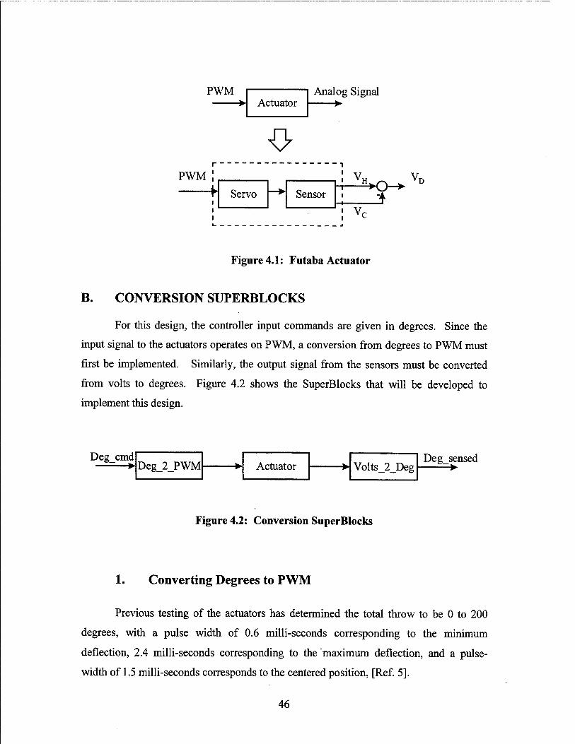
A. HARDWARE DESCRIPTION FOR AROD
The control surfaces of the AROD are actuated by Futaba FP S34 servo motors.
To control these actuators, a Pulse Width Modulation (PWM) input signal is used. The
width of the pulse determines how far the servo will turn. The internal control circuit of
the Futaba motor includes a small potentiometer in a feedback loop to sense the servo
position. The output signal from this sensor is noisy due to the varying current draw
during motor operation. Therefore, the actuators installed on the AROD in the lab have
been modified to reduce sensor noise. An additional wire has been added so that the
positive voltage on the potentiometer could be measured at the same time as the center
voltage [Ref. 5]. Taking the difference between the measured high voltage VH and the
centered voltage Vc , give a delta voltage VD and results in a significant reduction in
sensor noise. This set up is shown in Figure 4.1.
45
PWM Actuator
Analog Signal ►
o r
pwM; i v„ Servo —► Sensor
L 1 *V- f : ■*
i : vc
vr
Figure 4.1: Futaba Actuator
B. CONVERSION SUPERBLOCKS
For this design, the controller input commands are given in degrees. Since the
input signal to the actuators operates on PWM, a conversion from degrees to PWM must
first be implemented. Similarly, the output signal from the sensors must be converted
from volts to degrees. Figure 4.2 shows the SuperBlocks that will be developed to
implement this design.
Degcmd Deg_2_PWM Actuator Volts_2_Deg
Degsensed
Figure 4.2: Conversion SuperBlocks
1. Converting Degrees to PWM
Previous testing of the actuators has determined the total throw to be 0 to 200
degrees, with a pulse width of 0.6 milli-seconds corresponding to the minimum
deflection, 2.4 milli-seconds corresponding to the "maximum deflection, and a pulse-
width of 1.5 milli-seconds corresponds to the centered position, [Ref. 5].
46

The refresh frequency for the AROD HITL test was chosen to equal the controller
frequency of 25 Hertz, giving a period T of 40 milli-seconds. Figure 4.3 depicts the
relevant quantities for a PWM signal.
+5V.
h*pH
Figure 4.3: PWM
Duty cycle is calculated as:
Duty Cycle = -£-
A minimum pulse width of 0.6 milli-seconds, corresponding to -100 degrees, results in a
duty cycle of:
Min. Duty Cycle (-100 deg.) = — = 0.015
The maximum pulse width of 2.4 milli-seconds, corresponding to +100 degrees, results in
a duty cycle of:
2.4 Max. Duty Cycle (+100 deg.) = — = 0.06
Assuming a linear relationship from minimum to maximum values, the following
function is used to determine the required duty cycle for a given input in degrees.
Duty Cycle = 0.0002 * (Desired deflection in degrees) + 0.03 75 (Eq. 4.1)
The algebraic block iDeg_2_PWM' shown in Figure 4.4 implements this equation.
47
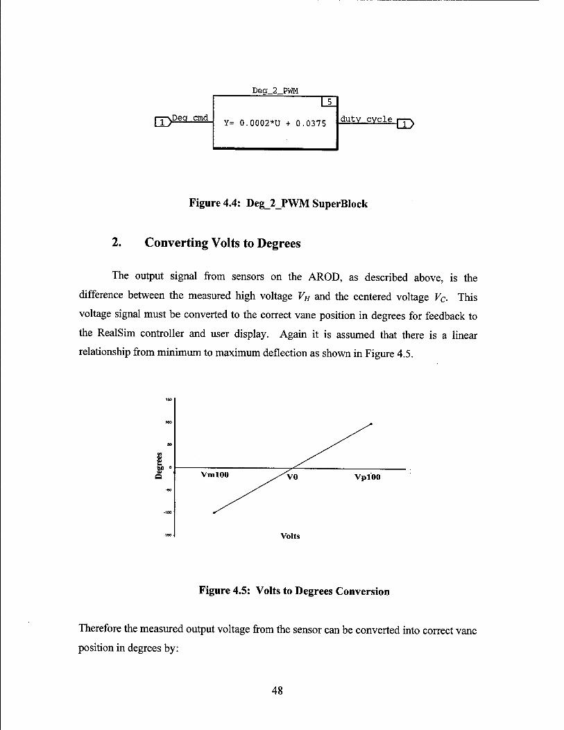
Deg_2_PWM
Q^Deg.
Figure 4.4: Deg_2_PWM SuperBlock
2. Converting Volts to Degrees
The output signal from sensors on the AROD, as described above, is the
difference between the measured high voltage VH and the centered voltage Vc. This
voltage signal must be converted to the correct vane position in degrees for feedback to
the RealSim controller and user display. Again it is assumed that there is a linear
relationship from minimum to maximum deflection as shown in Figure 4.5.
VmlOO VpiOO
Volts
Figure 4.5: Volts to Degrees Conversion
Therefore the measured output voltage from the sensor can be converted into correct vane
position in degrees by:
48
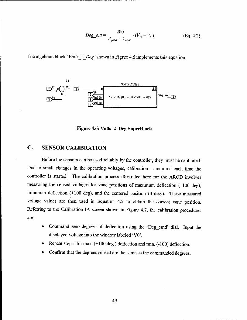
Degout ■■ 200
V -V v pi 00 y ml 00
(VD-V0) (Eq. 4.2)
The algebraic block ' Volts 2 Deg' shown in Figure 4.6 implements this equation.
Volts_2_Deg
Figure 4.6: Volts_2_Deg SuperBlock
C. SENSOR CALIBRATION
Before the sensors can be used reliably by the controller, they must be calibrated.
Due to small changes in the operating voltages, calibration is required each time the
controller is started. The calibration process illustrated here for the AROD involves
measuring the sensed voltages for vane positions of maximum deflection (-100 deg),
minimum deflection (+100 deg), and the centered position (0 deg.). These measured
voltage values are then used in Equation 4.2 to obtain the correct vane position.
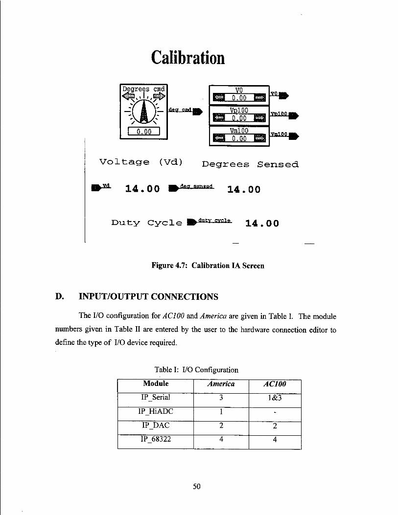
Referring to the Calibration IA screen shown in Figure 4.7, the calibration procedures
are:
• Command zero degrees of deflection using the 'Degcmd' dial. Input the
displayed voltage into the window labeled 'V0\
• Repeat step 1 for max. (+100 deg.) deflection and min. (-100) deflection.
• Confirm that the degrees sensed are the same as the commanded degrees.
49
Calibration
Degrees and
0.00
aeq...cnai
vo 0.00
VplOO 0.00
VmlOO 0.00
Til Mi
aiflfij
3ttlMM>
Voltage (Vd) Degrees Sensed
fg>*L 14,oo m*™-«™*«« i4.oo
Duty Cycle .duty..cycle.. 14.00
Figure 4.7: Calibration IA Screen
D. INPUT/OUTPUT CONNECTIONS
The I/O configuration for AC100 and America are given in Table I. The module
numbers given in Table II are entered by the user to the hardware connection editor to
define the type of I/O device required.
Table I: I/O Configuration
Module America AC100
IP_Serial 3 1&3
IP_HiADC 1 -
IP_DAC 2 2
IP_68322 4 4
50
As an example, the HITL design project requires an IP_68322 I/O module for the
PWM connection from the C30 to the AROD. The voltage signal from the AROD to the
C30 uses the IPHiADC module. Appendix A includes the HCE input and output
screens for this project.
A brief description is given below for the I/O modules used in the avionics lab.
References are also provided which contain more specific details on each module and
procedures for making the required connections.
1. Serial Connections/ IP_Serial Module
The IPSerial module provides two channels of high performance multi-mode
serial communication, [Ref. 6] section 5 page 69. Both RS-232-C and RS-422 are fully
supported. The module can be programmed to baud rates of 2 Mbit/sec and
asynchronous or synchronous protocols.
2. Analog-to-Digital Connections/IPHiADC
The HiADC provides 16 input analog channels with 12-bit resolution and
synchronous sampling of all inputs, [Ref. 6 ] section 5 page 61. The module can convert
one analog channel in 1.2 jusec or approximately 800 K samples/second. Each channel
has a fixed voltage range of + 5 V. No anti-aliasing filtering is provided for by the
module so inputs should be band-limited to V2 the sampling frequency of the system.
3. Digital-to-Analog Connections/IPDAC
The DAC module provides six channels of 12-bit digital-to-analog conversion.
Each channel can be configured to either + 5V or 0-10V output ranges, [Ref. 6] section 5
page 34.
51

4. Pulse Width Modulation Connections/IP_68332
The IP68332 module is a time processing unit (TPU) that can perform one or
more hardware I/O functions, [Ref. 6] section 5 page 52. It can be programmed to
generate various digital I/O signals, the current set-up in the avionics lab will use Pulse
Width Modulation (PWM) signals. In the PWM mode, the user specifies the duty cycle
as the output from the SystemBuild diagram.
52
V. DIGITAL CONTROL DESIGN
The RealSim rapid prototyping series allows for control system to be tested in
real-time with hardware-in-the-loop while recording any or all the state variables to
verify performance. This section will step through the design process using a simple
controller to control the control surfaces of the FROG.
A. MODELING ACTUATORS AND SENSORS
Before the controller can be designed, a mathematical model of the plant which is
to be controlled must first be created. The techniques involved to develop the model
depend on the characteristics of the plant. This section details the technique used to
model the actuators used on the FROG. Since both the FROG and AROD's control
surfaces are actuated by Futaba FP S34 servo motors, the AROD is used in the lab.
To develop an accurate representation of the Futaba actuators, the system is
modeled as a second-order transfer function.
H(s) ~ a" s + 2 ■ C, ■ con • s + <on
The system response is obtained by applying a step function to the actuators and
recording the response using the data acquisition editor feature of the RealSim software.
To calculate the transfer function, the rise time tr and maximum overshot Mp values are
measured from the system response. From these values the natural frequency (on and the
damping ratio C, are calculated using the following formulae:
ln(MD) C= , ; 2 (Eq.5.1)
53
-tan '^c s
<°n = Vw1 (Eq. 5.2)
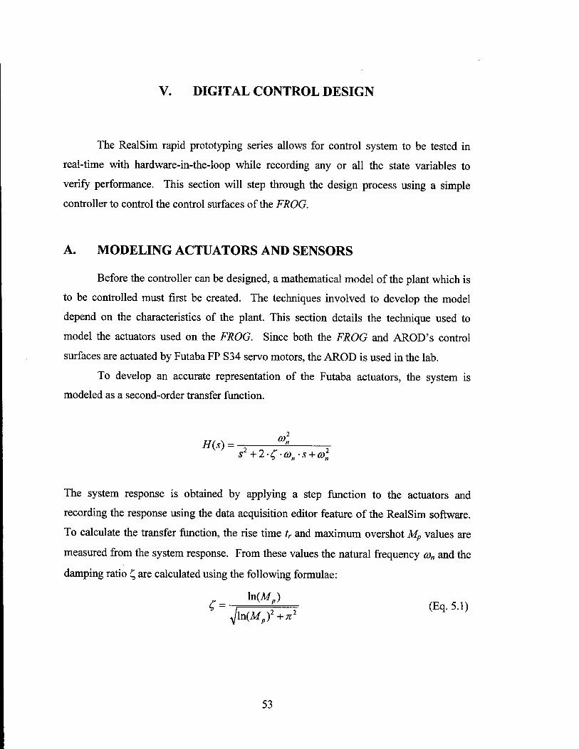
It is assumed the actuators have a rate-limiter therefore a small step response of
10 degrees is used so the effect of the rate-limiter on the rise time would be minimized.
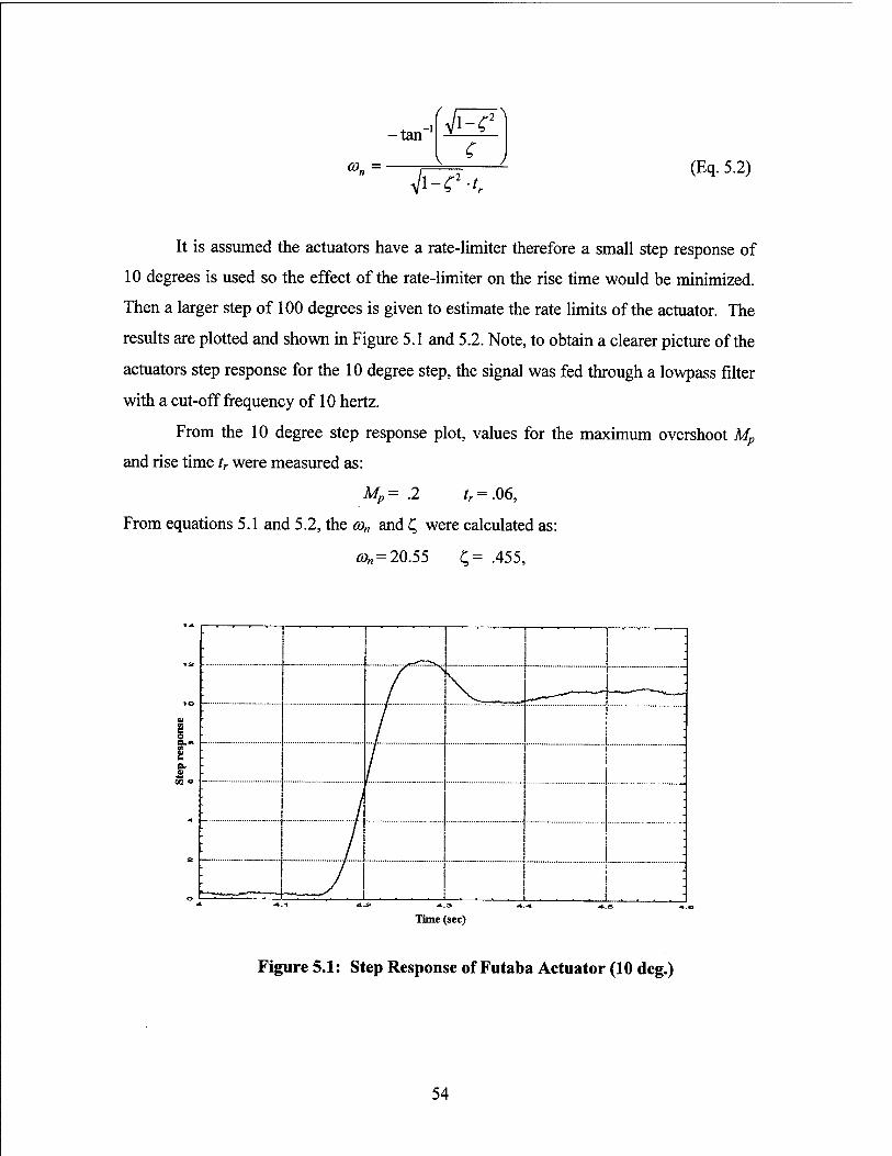
Then a larger step of 100 degrees is given to estimate the rate limits of the actuator. The
results are plotted and shown in Figure 5.1 and 5.2. Note, to obtain a clearer picture of the
actuators step response for the 10 degree step, the signal was fed through a lowpass filter
with a cut-off frequency of 10 hertz.
From the 10 degree step response plot, values for the maximum overshoot Mp
and rise time tr were measured as:
Mp = .2 tr=.06,
From equations 5.1 and 5.2, the co„ and C, were calculated as:
con= 20.55 £= .455,
a. 03 c
Time (sec)
Figure 5.1: Step Response of Futaba Actuator (10 deg.)
54
s
,111!
■
• •
- •
■ :
■
Time (sec)
Figure 5.2: Step Response of Futaba Actuator (100 deg.)
The slope of the 100 degree step response is measured and used to calculate the
rate-limiter, which was found to be approximately +325 deg./sec.
The 2n order transfer function can be given in general form by:
-2
H(s) = axs + a2s
where
a, =0
a2 = o)„
bx=2-£-cön
b2 = a,,
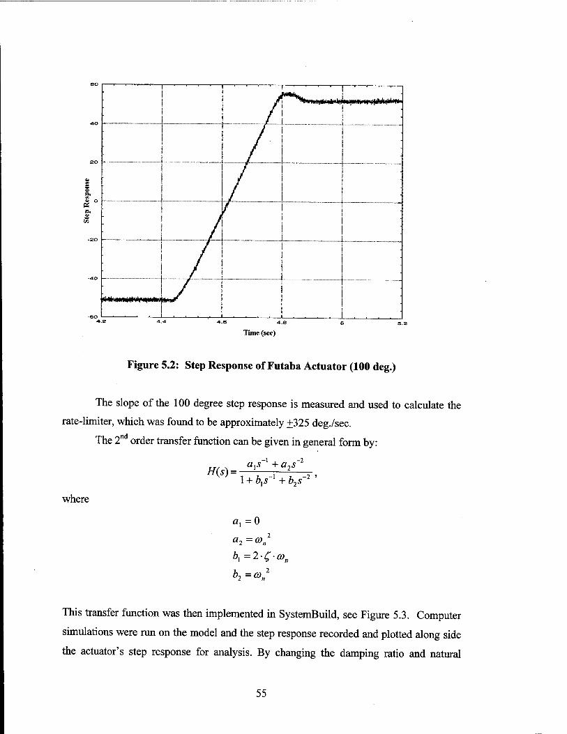
This transfer function was then implemented in SystemBuild, see Figure 5.3. Computer
simulations were run on the model and the step response recorded and plotted along side
the actuator's step response for analysis. By changing the damping ratio and natural
55
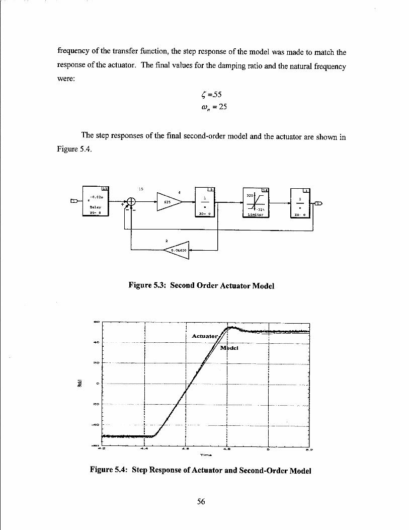
frequency of the transfer function, the step response of the model was made to match the
response of the actuator. The final values for the damping ratio and the natural frequency
were:
^=.55 con = 25
The step responses of the final second-order model and the actuator are shown in
Figure 5.4.
o- * — -rd>
Figure 5.3: Second Order Actuator Model
Figure 5.4: Step Response of Actuator and Second-Order Model
56

B. FEEDBACK CONTROLLER DESIGN
The next step is to design a feedback controller that satisfies specific
requirements. The requirements are normally specified in terms of response time,
overshoot, stability and robustness. The controller design process is outlined below:
•
•
Create a nonlinear model. A block diagram is formed that includes the plant
model and nonlinear controller.
Linearize the model and adjust controller gains. The linear model is
linearized and then analyzed using frequency response and/or root-locus
methods.
Analyze closed-loop system. Computer simulations are run with the feedback
system, the controller gains are adjusted to create the desired control.
Applying classical control techniques, the controller model is generally first
designed in continuous-time. After a satisfactory response is achieved the system is
transform to discrete-time and tested again for satisfactory response.
For this example the SpeedController developed in Chapter III is implemented
with the actuator model. To analysis the system the loop between the controller and plant
is broken as shown in Figure 5.5. The system is linearized using the Xmath command
sys=lin(" Super Block name"). The linearized model can be used to analyze the system
using root-locus methods and Bode frequency response methods. The root-locus and
Bode plots, shown in Figure 5.6, are generated using the Xmath commands: rlocus(sys)
and bode(sys). After a satisfactory response is obtained, the system is transformed to
discrete-time and tested again.
57

Controller Model 98 199
1
-CD CD-
In
~r\ C SUPER
BLOCK 0 1 +
s
X0= 0 Continuous
Figure 5.5: Broken-Loop Block Diagram
Output 1
-120
200
-i<^- i --I 1- i -i-t-i-i- -»- ' ~ r - t - t -i- » IT r r — -i- -r-r"k-i-i-t-
. • -» —«—•_ a -;-;-;-; 1 L.J. J.I.IüI i. -^Xl- -■__•. J _L L L
i... _ i _«.
Fraquency [Hz]
Figure 5.6: Bode Plot
58

C. HARDWARE-IN-THE-LOOP TESTING
Hardware-in-the-loop testing is where the feedback system is tested with some or
all of the actual hardware. In this case, the design will include the actuator, the actuator
model and the Speed_Controller, as shown in Figure 5.7. This design allows the
controller to be simulated with the actuator model or conduct HITL testing. If the
actuator model is accurate and the controller design is correct, there should be no
apparent difference in the performance of the controller. If the actuators are not modeled
well, the test of the controller may indicate that the controller works as designed while
the HITL test may show that the feedback system is unstable.
ny .Vh _/T\ Vd
CD* !f
CD01-0- „i US Q>2
Cal_gwitch
r« u3 — *
err1 ■*' +»(?}
o
XSP-—
Vol tS_i_poq
Y- JOO/ira - VO'IDl - U2i
aw_2_pu» TE
Y« 0.00041*11 * 0.053 autv..evcU ^
SUPER BIOCX >J
H»
Qy Ltl «
Jl — -«
Variable G&ic
Eä^ar-saia.
198
T= U1-U2
Controllar
2-1
X0= 0
Figure 5.7: HITL Test SystemBuild Block Diagram
The simulation includes two switches for controlling the desired simulation state.
The three simulation states are:
• Sensor calibration
• Actuator model
• HITL
The calibration switch controls which input command will be used by the
actuators. With the calibration switch On, the command input Degcmd is used. When
59

the switch is Off, the commanded input is from the error signal of the Vel_cmd in the
loop. The HITL switch will control which test is desired: the computer actuator model or
the actual hardware. Table II summarizes these switch functions. The interactive
animation page used to monitor and control the model is shown in Figure 5.8.
Calibration Switch
On
Off
Off
Table II: Simulation States
HITL Switch
X
Off
On
Simulation
Sensor Calibration
Actuator Model
HITL
Cal_sw
On
Off1
Calibration
VD 0,00
VPIOO
O.QQ
v»aoo 0,00
Voltage (v<3) Degrees Sensed
W°- 14.00 »"*" """*■ 14.00
HITL sw
On
Off
Speed Controller Speed_cnd (input)
a i o.oo i ■ +
i ■ i ■ i ■ i ■ | • i ■ i ■ i ■-[
Speed (output)
14.00
Variable Gain
1,00
+ pri'l'iT
Figure 5.8: IA Screen for HITL Test
The HITL design includes a variable gain block, which permits the user to adjust
the gain during the testing. The gain margin can be found experimentally by running the
HITL test and slowly increasing the gain until the system goes unstable. The results are
60
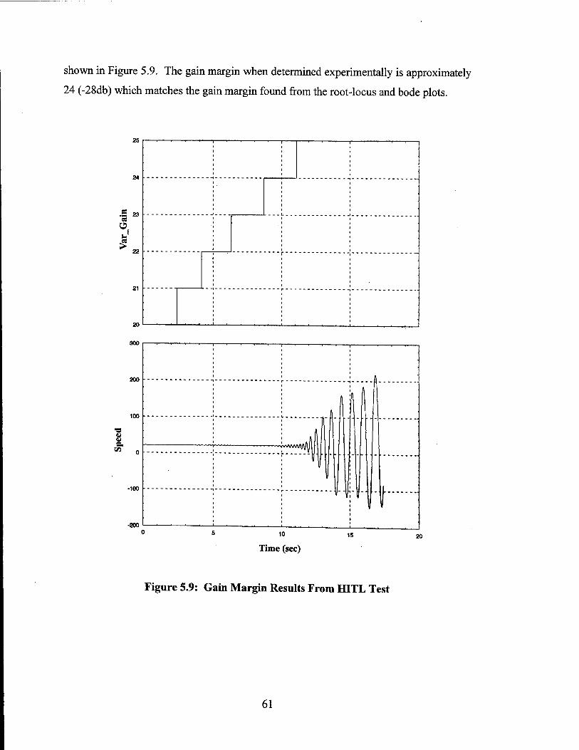
shown in Figure 5.9. The gain margin when determined experimentally is approximately
24 (-28db) which matches the gain margin found from the root-locus and bode plots.
25
24
.3 23 58 o J
22
21
20
300
. '___ .. 1 L__ _.____!_... _-..»
Time (sec)
Figure 5.9: Gain Margin Results From HITL Test
61

62
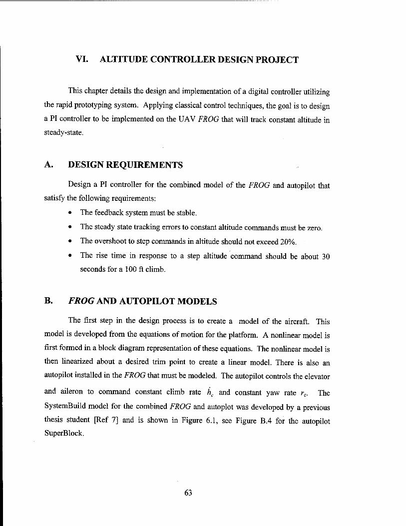
VI. ALTITUDE CONTROLLER DESIGN PROJECT
This chapter details the design and implementation of a digital controller utilizing
the rapid prototyping system. Applying classical control techniques, the goal is to design
a PI controller to be implemented on the UAV FROG that will track constant altitude in
steady-state.
A. DESIGN REQUIREMENTS
Design a PI controller for the combined model of the FROG and autopilot that
satisfy the following requirements:
• The feedback system must be stable.
• The steady state tracking errors to constant altitude commands must be zero.
• The overshoot to step commands in altitude should not exceed 20%.
• The rise time in response to a step altitude command should be about 30
seconds for a 100 ft climb.
B. FROG AND AUTOPILOT MODELS
The first step in the design process is to create a model of the aircraft. This
model is developed from the equations of motion for the platform. A nonlinear model is
first formed in a block diagram representation of these equations. The nonlinear model is
then linearized about a desired trim point to create a linear model. There is also an
autopilot installed in the FROG that must be modeled. The autopilot controls the elevator
and aileron to command constant climb rate hc and constant yaw rate rc. The
SystemBuild model for the combined FROG and autoplot was developed by a previous
thesis student [Ref 7] and is shown in Figure 6.1, see Figure B.4 for the autopilot
SuperBlock.
63
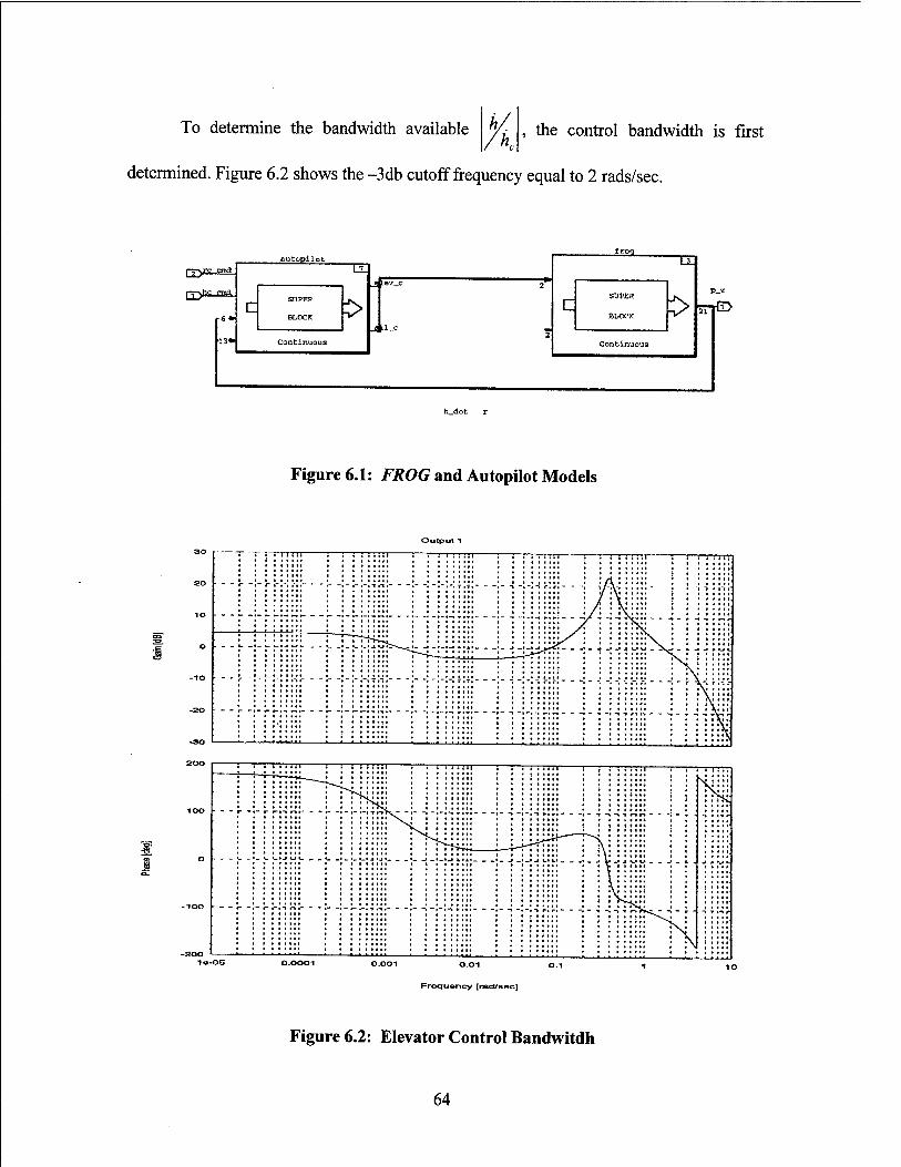
To determine the bandwidth available , the control bandwidth is first
determined. Figure 6.2 shows the -3db cutoff frequency equal to 2 rads/sec.
Qys-ssä.
rr>hc CT*3
autopilot
SUPER
BLOCK 5> Continuous
Ircxi
c Lev_c
Ll c
2 SUPER
BLOCK
Continuous
Figure 6.1: FROG and Autopilot Models
30 r -* .-
-SO
20O
T ; i ;::::! i TTTTim ! TTTTT771 :—: : :::::1 ?—* * = »TTH •—t ; ;: n:
Figure 6.2: Elevator Control Bandwitdh
64
C. FEEDBACK CONTROLLER DESIGN
The next step is to design a PI controller that satisfies the requirements outlined in
section A. This is an iterative process employing various methods with the controller
gains being the design knobs used to meet requirements of response time, overshoot, and
command and control loop bandwidths.
Applying classical control techniques, the initial controller gains are generally
first obtained for continuous-time model. After a satisfactory response is achieved the
system is transformed to discrete-time and tested again for satisfactory response.
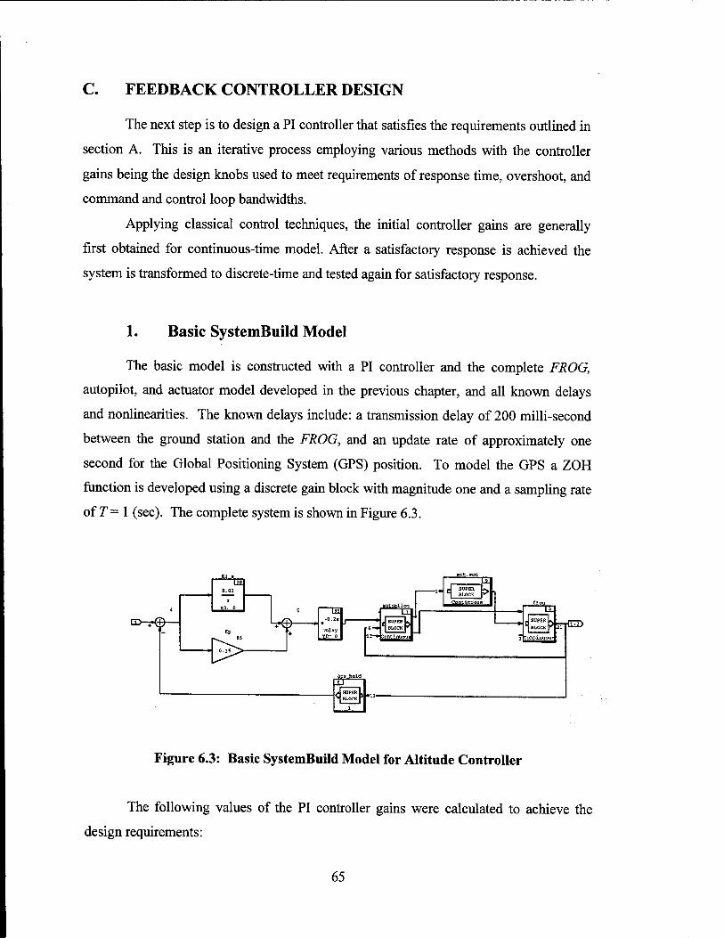
1. Basic SystemBuild Model
The basic model is constructed with a PI controller and the complete FROG,
autopilot, and actuator model developed in the previous chapter, and all known delays
and nonlinearities. The known delays include: a transmission delay of 200 milli-second
between the ground station and the FROG, and an update rate of approximately one
second for the Global Positioning System (GPS) position. To model the GPS a ZOH
function is developed using a discrete gain block with magnitude one and a sampling rate
of T= 1 (sec). The complete system is shown in Figure 6.3.
Figure 6.3: Basic SystemBuild Model for Altitude Controller
The following values of the PI controller gains were calculated to achieve the
design requirements:
65
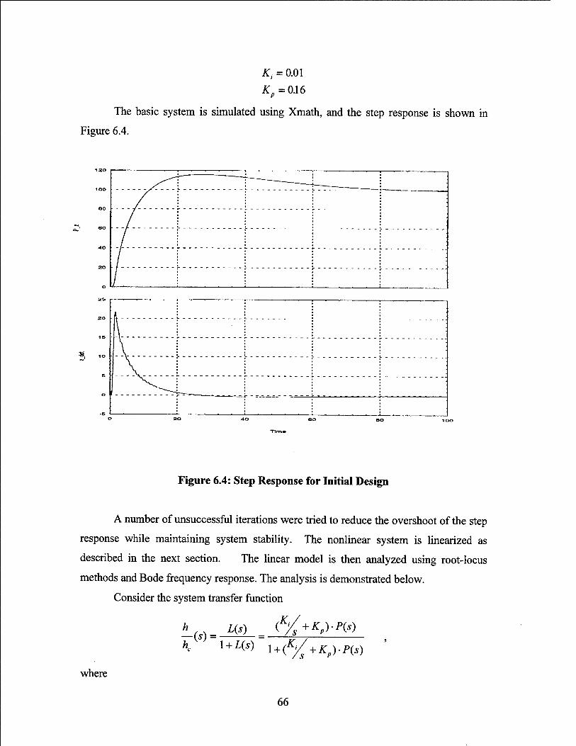
Figure
£, = 0.01 £,=0.16
The basic system is simulated using Xmath, and the step response is 5
6.4.
shown in
100
00
-•O
20
_»---r ~ ———_.
20
15
0
. i
\ *
V = \ •
^-L_ » 20 40 eo so 100
Figure 6.4: Step Response for Initial Design
A number of unsuccessful iterations were tried to reduce the overshoot of the step
response while maintaining system stability. The nonlinear system is linearized as
described in the next section. The linear model is then analyzed using root-locus
methods and Bode frequency response. The analysis is demonstrated below.
Consider the system transfer function
\.y m _ iK/s+Kp).Pis) K l + L(s) ! + (% + *,)■/»(,)
where
66
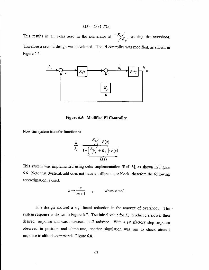
L(s)=C(s)-P(s)
This results in an extra zero in the numerator at ~ yK , causing the overshoot.
Therefore a second design was developed. The PI controller was modified, as shown in
Figure 6.5.
K ■o
A K/s -o
A-
K„
P(s)
Figure 6.5: Modified PI Controller
Now the system transfer function is
h_
k.
K, P(s)
1 + K, s P
P(s)
L{s)
This system was implemented using delta implementation [Ref. 8], as shown in Figure
6.6. Note that SystemBuild does not have a differentiator block, therefore the following
approximation is used:
5-> es + \
where s «1
This design showed a significant reduction in the amount of overshoot. The
system response is shown in Figure 6.7. The initial value for Kt produced a slower then
desired response and was increased to .2 rads/sec. With a satisfactory step response
observed in position and climb-rate, another simulation was run to check aircraft
response to altitude commands, Figure 6.8.
67

O^G^
Figure 6.6: CTS Altitude Controller
0 . i - .VL j_ j \_ m ; ■
ti \t— ____; _ .... ; ; ...__*.-____„... _.„j
& *■ • ■ ■ ■ 1 • . . «_—. . . . i__ _ : *IO GO
Tim«
Figure 6.7: Step Response for PI Controller
68

Figure 6.8: Dynamic Response of Model
69
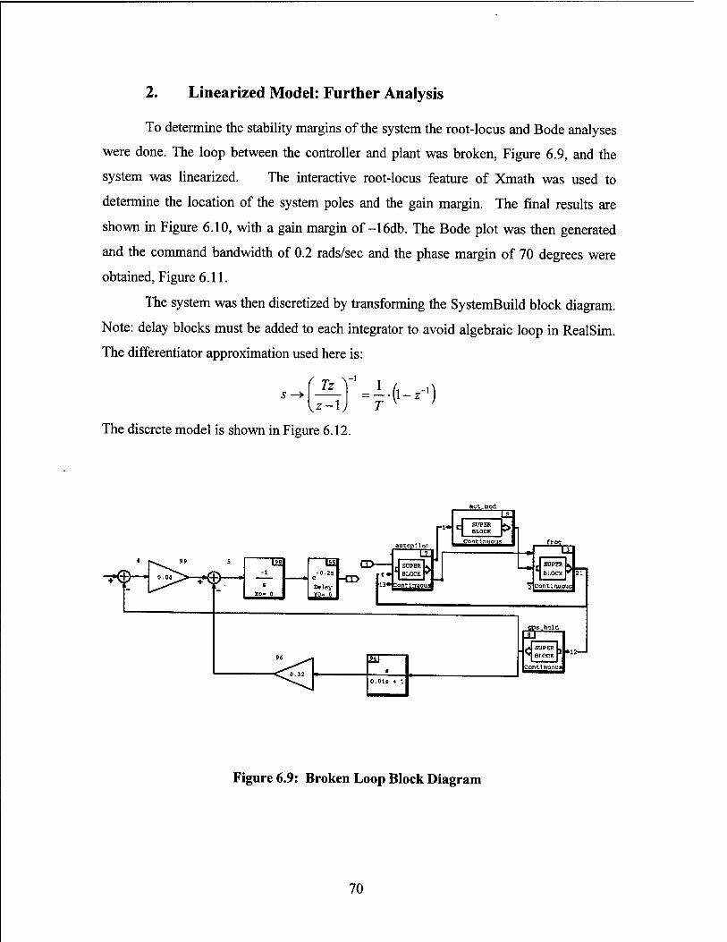
2. Linearized Model: Further Analysis
To determine the stability margins of the system the root-locus and Bode analyses
were done. The loop between the controller and plant was broken, Figure 6.9, and the
system was linearized. The interactive root-locus feature of Xmath was used to
determine the location of the system poles and the gain margin. The final results are
shown in Figure 6.10, with a gain margin of-16db. The Bode plot was then generated
and the command bandwidth of 0.2 rads/sec and the phase margin of 70 degrees were
obtained, Figure 6.11.
The system was then discretized by transforming the SystemBuild block diagram.
Note: delay blocks must be added to each integrator to avoid algebraic loop in RealSim.
The differentiator approximation used here is:
f TV V1
s -> Tz z-\ 4-(i-^')
The discrete model is shown in Figure 6.12.
Figure 6.9: Broken Loop Block Diagram
70
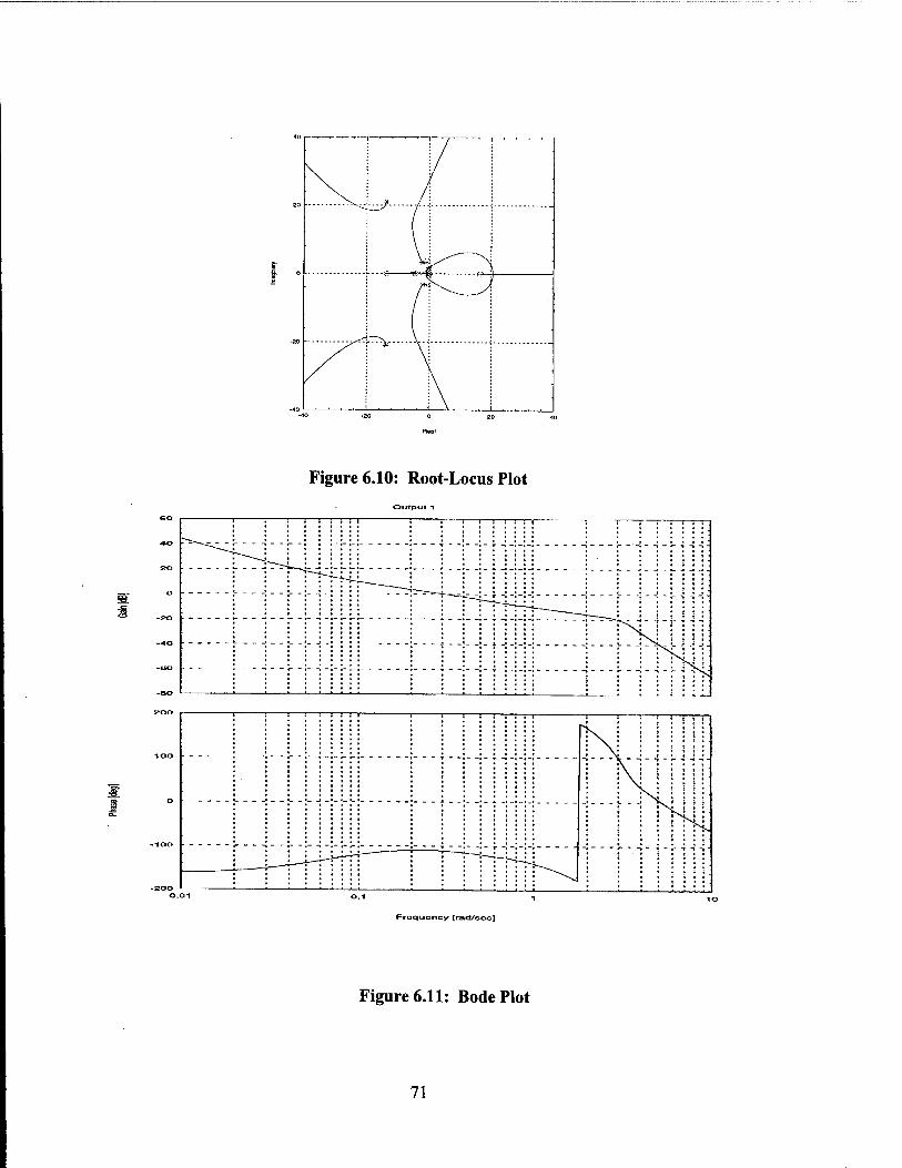
Figure 6.10: Root-Locus Plot
a.
. . ;...... | . ;::;:; r —
u -100
fTffi i • ■
o
u| too . ; _;_ _;— ;—;_;_;_;_; ; ^ ; ;_ j. _'_;_•_■
_J 4_-i-4-r-rrtT'" ! i iTTTH-L^^ ; ? \
zoo : : : 1 : : ! :: ! : ! ! ■ ! ! ■ • "^
Froquoncy [rad/soc]
Figure 6.11: Bode Plot
71
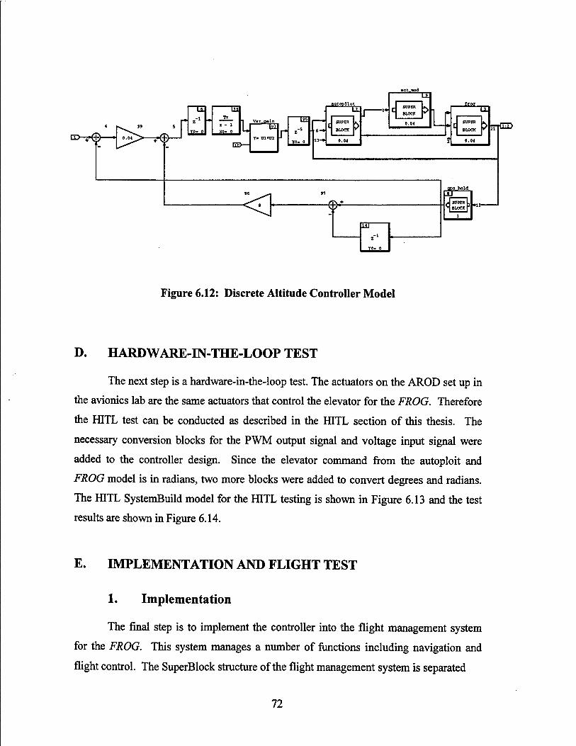
o-r©—• ■r®
z
YO- 0
I2ä Tz
z - 0
Es>—
Var..qaln
r -OH
z-5 U«-l YO- 0
autopilot
SUPER
BLOCK
e^-
SUPER
BLOCK
nr i
TO" 0
SUPER
BLOCK mCiD
AT pps_hold
SUPER BLOCK
Figure 6.12: Discrete Altitude Controller Model
D. HARDWARE-IN-THE-LOOP TEST
The next step is a hardware-in-the-loop test. The actuators on the AROD set up in
the avionics lab are the same actuators that control the elevator for the FROG. Therefore
the HITL test can be conducted as described in the HITL section of this thesis. The
necessary conversion blocks for the PWM output signal and voltage input signal were
added to the controller design. Since the elevator command from the autoploit and
FROG model is in radians, two more blocks were added to convert degrees and radians.
The HITL SystemBuild model for the HITL testing is shown in Figure 6.13 and the test
results are shown in Figure 6.14.
E. IMPLEMENTATION AM) FLIGHT TEST
1. Implementation
The final step is to implement the controller into the flight management system
for the FROG. This system manages a number of functions including navigation and
flight control. The SuperBlock structure of the flight management system is separated
72
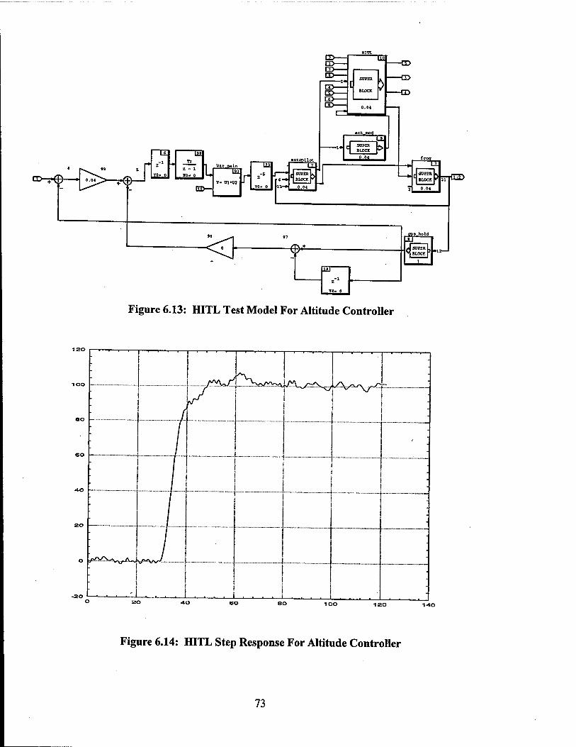
E> 4 f>"*s^ "
Figure 6.13: HITL Test Model For Altitude Controller
Figure 6.14: HITL Step Response For Altitude Controller
73

into five lower level SuperBlocks according to their function. The altitude controller is
inserted into the control SuperBlock as shown in Figure 6.15. Appendix B contains the
hierarchy for the SuperBlocks that make up the complete flight management system.
The UAV can be controlled by either the computer or RC pilot with a standard
RC Futaba transmitter. A complete description of the FROG and its components is given
in [Ref. 9]. To prevent large control inputs during transitions from RC pilot to computer
control, the altitude controller is implemented using a delta altitude as the input
command. As an example, if the user desired to maintain level altitude at hand off, a
command of zero should be given. A script block is used to freeze the GPS altitude
position at hand-over. The delta commanded altitude is then summed with the frozen
altitude position and is used as the entered altitude command for the controller. The
controller outputs a climb-rate command to the autopilot. The feedback loop uses the
GPS altitude position referenced with respect to the local tangent plane (LTP) at the field.
The orientation of the frame is specified as North-East-Down (NED), therefore a
conversion gain is added to the feedback loop to reverse the sign. A conversion gain is
also added to the controller's output. The FROG autopilot model differs from the actual
autopilot in the units used for the entered climb-rate command. The model uses (ft/sec)
where the actual autopilot uses (ft/min). The two switches are part of the wind down
loop. If either or both switches are in the "OFF" position, the integrator is forced back to
its initial value. This is done to prevent initiation of the controller at a previous state.
Once the controller is added to the flight management system, the user interface is
added in the Interactive Animation screen used to monitor and control the FROG. The
necessary input/output devices are added to the existing throttle control IA page, shown
in Figure 6.16. For the initial flight testing, the screen is designed to display a number of
performance variables not normally used for an operational flight display. These displays
help evaluate whether the controller is working properly. The two digital output displays
show the commanded altitude and the actual GPS altitude in feet. When the altitude
controller is operating and working properly, the altitude readouts should match. An
open loop input for the climb-rate is also added. With this feature the climb-rate
command can be given directly to the autopilot by the user. The input slide gage is added
74
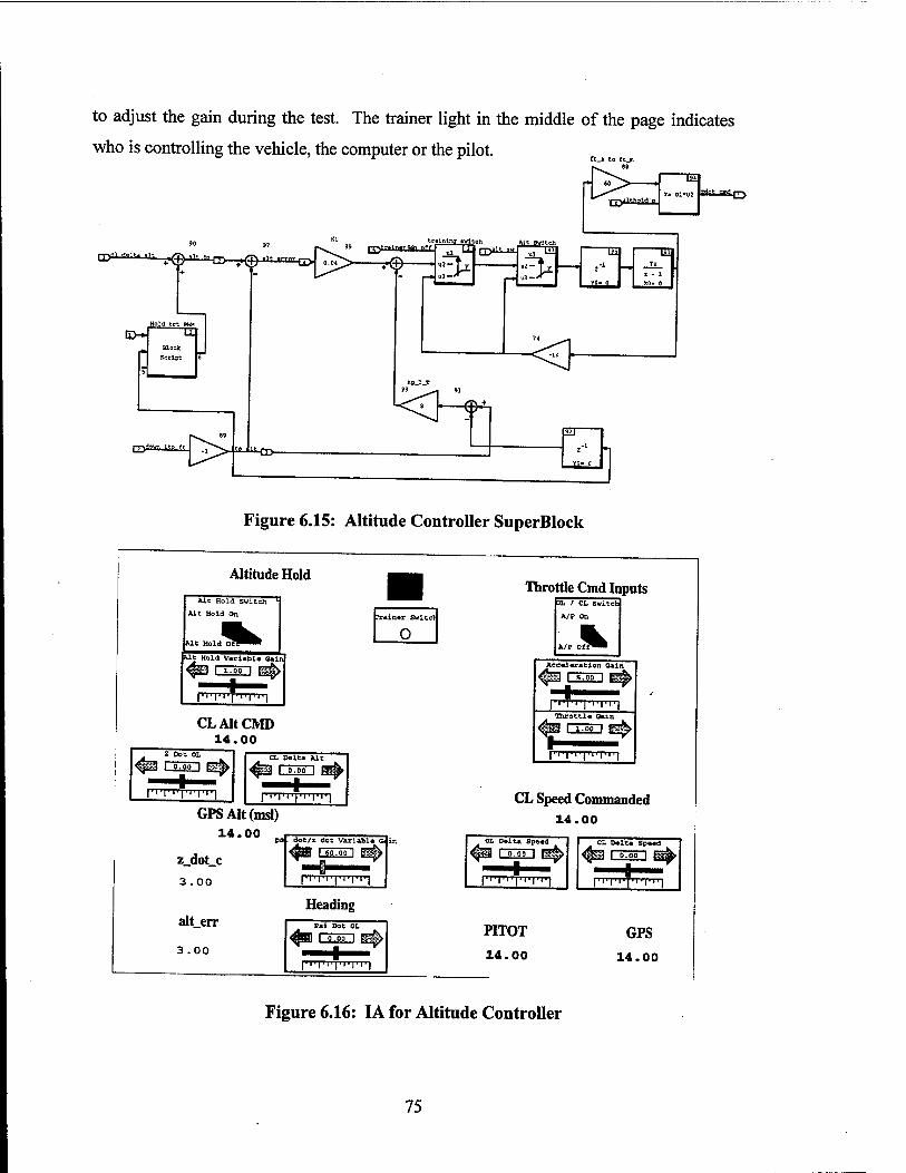
to adjust the gain during the test. The trainer light in the middle of the page indicates
who is controlling the vehicle, the computer or the pilot.
Hold trt PWj
E>-> Block
Script
E3ääSGLl£2-£t_ £> üO-
■pfylthold'w
E3 5aS£-S&05
tr«lnlng awl ch MC switch " Dtr»""rM' ""I ul Lil p»'t ■»[ S. " tptntnTMi off M U. Tsq
<] ©^
Ear
Figure 6.15: Altitude Controller SuperBlock
Altitude Hold
Alt Hold swicch '
U[ Hold On
Me Hold Variable sain
I l.oo I üf
r> -I ■ i ■«■ i ■ ■ ■ i ■' ■ i
CLAltCMD 14.00
Z Dot OL
I 000 I H§
I ■ I • 1 ■»■ I ■ f I ■»• I
CL Dolt» Alt
pU I 0.00 I
I GPSAIt(msl)
14.00
Prainer Switcl
O
z_dot_c
3.00
alt_err
3 .00
. dot/z dot Variabla c^ir. rso.oo
r',i,|T',r|,l
Heading Psi Dot OL
i o.oo} mn
+ I'I'I'I'I'ITM
Throttle Cmd Inputs 3L / CL Switch
A/P On
Acceleration Oain pi I 5,00 I ßip
I'lV'T'Tl'l throttle Gain
HU I 1.00 I ■ rl'l"'l'''l,''l
CL Speed Commanded 14.00
OL Delta Speed
I o.oin
r'-i'i'i'i-i'i-i
PITOT
14.00
CL Dalta Spaad
GPS
14.00
Figure 6.16: IA for Altitude Controller
75
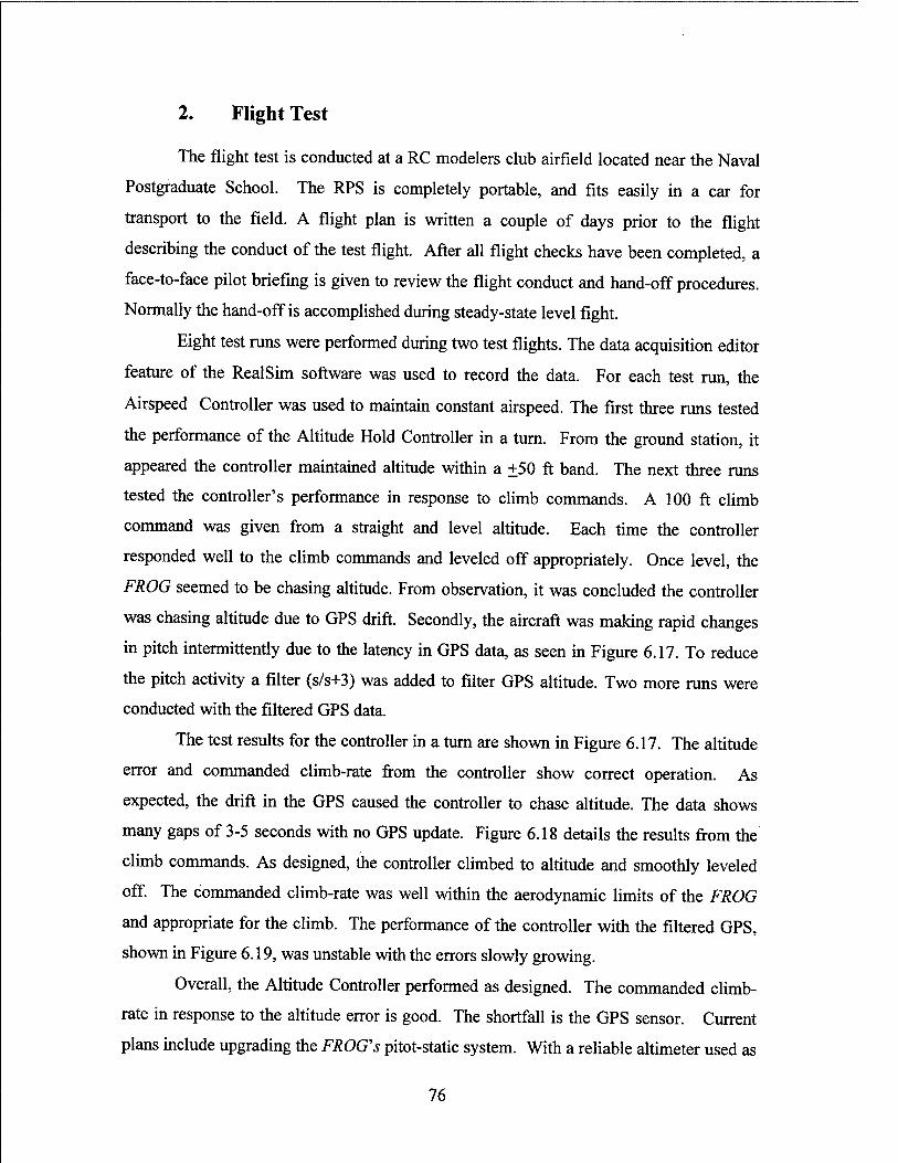
2. Flight Test
The flight test is conducted at a RC modelers club airfield located near the Naval
Postgraduate School. The RPS is completely portable, and fits easily in a car for
transport to the field. A flight plan is written a couple of days prior to the flight
describing the conduct of the test flight. After all flight checks have been completed, a
face-to-face pilot briefing is given to review the flight conduct and hand-off procedures.
Normally the hand-off is accomplished during steady-state level fight.
Eight test runs were performed during two test flights. The data acquisition editor
feature of the RealSim software was used to record the data. For each test run, the
Airspeed Controller was used to maintain constant airspeed. The first three runs tested
the performance of the Altitude Hold Controller in a turn. From the ground station, it
appeared the controller maintained altitude within a +50 ft band. The next three runs
tested the controller's performance in response to climb commands. A 100 ft climb
command was given from a straight and level altitude. Each time the controller
responded well to the climb commands and leveled off appropriately. Once level, the
FROG seemed to be chasing altitude. From observation, it was concluded the controller
was chasing altitude due to GPS drift. Secondly, the aircraft was making rapid changes
in pitch intermittently due to the latency in GPS data, as seen in Figure 6.17. To reduce
the pitch activity a filter (s/s+3) was added to filter GPS altitude. Two more runs were
conducted with the filtered GPS data.
The test results for the controller in a turn are shown in Figure 6.17. The altitude
error and commanded climb-rate from the controller show correct operation. As
expected, the drift in the GPS caused the controller to chase altitude. The data shows
many gaps of 3-5 seconds with no GPS update. Figure 6.18 details the results from the
climb commands. As designed, the controller climbed to altitude and smoothly leveled
off. The commanded climb-rate was well within the aerodynamic limits of the FROG
and appropriate for the climb. The performance of the controller with the filtered GPS,
shown in Figure 6.19, was unstable with the errors slowly growing.
Overall, the Altitude Controller performed as designed. The commanded climb-
rate in response to the altitude error is good. The shortfall is the GPS sensor. Current
plans include upgrading the FROG's pitot-static system. With a reliable altimeter used as
76
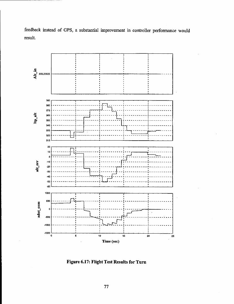
feedback instead of GPS, a substantial improvement in controller performance would
result.
2
la U
E e :- © •9 N
370
360
350
340
330
320
310
20
10
0
-10
-20
-30
-40
-SO
-60
1000
, 4771 LUii ...
x^pi::::: l-r
-500
-1000
b^Jfe::::::.:^ \ : : ...JJ : : h
L ■.■.1......J77-..: , : :Lrd i
= i :
10 15
Time (sec) 20 25
Figure 6.17: Flight Test Results for Turn
77
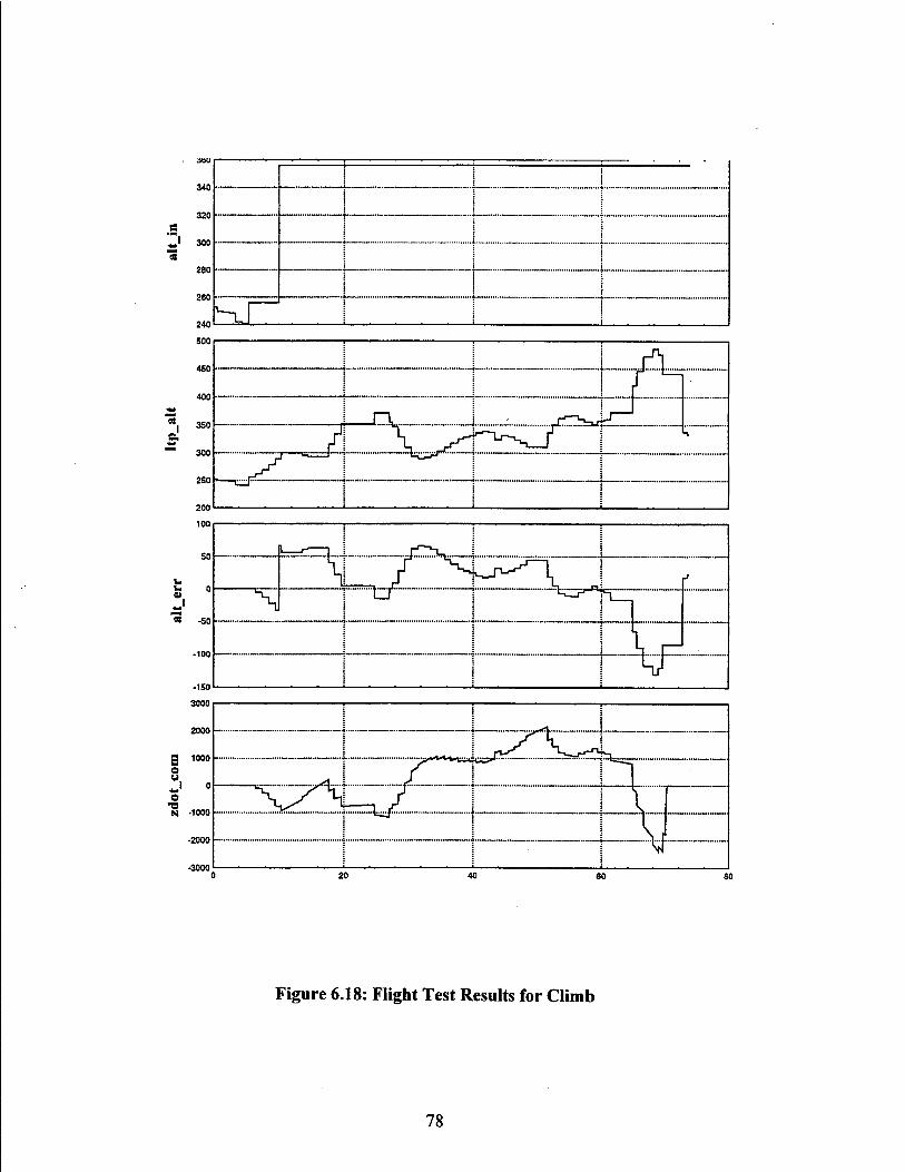
a
340
320
• I i : j i
280
260 !
240
a!
200
100
50
U
t=r=l......
\ J ^4^^n |
J
N ^^jT ^ ^P*M
1 1 I P
2000
g iooo o u J e
■a (4 -1000
■2000
•3000
±=SF 20 60
Figure 6.18: Flight Test Results for Climb
78

SÜU
500
480
7' 460
et 440
420
400
380
650
600
550
500
450
400 ■•
350
200
150
100
50
0
-SO
-100
-ISO
2000
ÖEEEEEEEEE
^isggM
Figure 6.19: Flight Test Results for Filtered GPS
79

80

VII. CONCLUSIONS AND RECOMMENATIONS
A. CONCLUSIONS
The Advanced Controls of Aerospace Vehicles course, offered at the Naval
Postgraduate School, provides an excellent opportunity for students to apply classical and
modern control methods to the design of basic controllers. A strong foundation is
presented on the operations and analysis of sampled-data systems. The rapid prototyping
system, developed by the department, is an excellent design tool and allows the student
valuable hands-on experience in the design, implementation and flight testing of control
algorithms for unmanned air vehicles. The ability of the application software, RealSim,
to automatically generate higher-language code and eliminate the time consuming task of
programming the code for a working model, enables design projects ample time to be
completed in the twelve weeks allotted for the course.
Even though the RPS is still in its initial stages of development, it has generated a
number of thesis opportunities, with many more foreseen in the future. Utilizing mostly
off-the shelf technology, the cost of this educational tool will be minimal.
B. RECOMMENDATIONS
Considering the conclusions stated above and the knowledge gained in the course
of instruction given in the Advanced Controls of Aerospace Vehicles, the following
recommendations are forwarded:
• Investigate scheduling this course, and its prerequisites, earlier in the avionics
curriculum. The UAV program developed by the department produces many
excellent opportunities for thesis work. To allow ample time for students to
complete their thesis work, this class should be scheduled prior to the last
quarter of instruction.
• Presently there are no elective courses offered by the aeronautical engineering
department in the area of digital control. Investigate the establishment of an
81

elective course that would introduce to the student system identification
methods and advanced multivariable and optimal control procedures.
Devote more classroom time to Design of Digital Control Systems Using
Transform Techniques presented in Chapter V of [Ref. 1], and Design of
Digital Control Systems Using State-Space Methods presented in Chapter VI
of [Ref. 1]. Less time should be given to Chapter II of [Ref. 1], Linear,
Discrete, Dynamic-Systems Analysis: The z-Transform. Material covered in
chapter 2, discrete Fourier transform (DFT), z-transform, and block diagram
descriptions, should be introduced during the prerequisite course, EO 2402,
Introduction to Linear Systems.
Establish a library within the avionics lab containing all previous thesis work
and material related to the UAV FROG. Many of the design projects and
future thesis work will build on the work from past projects. Good
documentation is required to keep track of modifications, input/output
variables, and improvements made to the system.
Purchase a second target computer to supplement America. Currently the
computer lab has only one computer with the AC 100 model set-up and often
two or three students end up waiting for access to America to compile and link
their programs or to run the hardware setup.
82
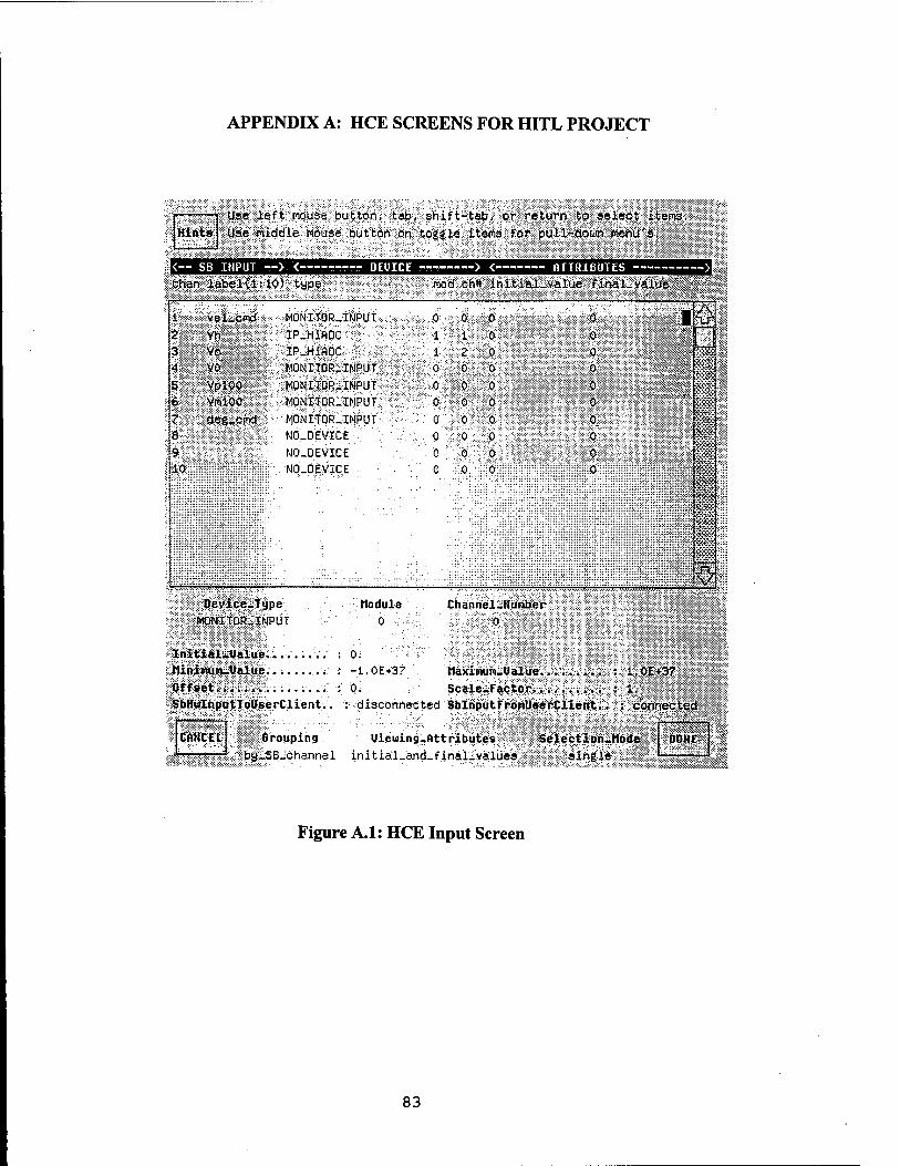
APPENDIX A: HCE SCREENS FOR HITL PROJECT
Hints Use left mouse button, tab, shift-tab, or return, to select items,! Use middle mouse button on toggle item3 for pull-rdown menu's;
<-- SB INPUT —> < '---- OEUICE — > < ATTRIBUTES > mod ehttlinitiai_-value f inal_ value V\x- >\s 'Chan iabel(4:10) type
4;a? vetternd> MONITOR-INPUT 2 - Vh" IP_riiflDC 3 Vc. IP_HiADC ;;.: 4 vo -. MONITOR-INPUT 5'-/ VplOO MONITORwINPUT & VmlOO MONITOR-INPUT
7 deg_cmd MONITOR-INPUT 8 NO_DEVICE
9 NO-DEVICE 10 NO-DEVICE
0
J'O"
0
0
:^;:
i-O'i
; -0';
<> :;0hi
0
"Pi
o
o
Device-Type «ONITORIINPUT
Module Channel-Hutaber
InitialiValue......... Minimum-Value. Offset...; SbHuInputToUserClient..
CiflMCEt
-1.0E+3? Maximun-Ualue :. l.OE+37 0. Scale-Factor : 1.
: disconnected SblnpütFronUser : cohnect^dJ
' Grouping Uieuing-Attributes Nby_SB_channel initiäl_and_final.values
SelectiqniMode! single
iäffp
Figure A.1: HCE Input Screen
83

Hints Uae lBFt mouse button, tat), ahift-tab, or return to select iteraa, Use middle mouse button an toggle itetrs for puil-douin menu's.
>- *>u ouipur -> < utuxcfc > c ftfiKiburts 1 chan label(i: 10 > type
t veL-aut ND-DEVICE 2 duty-cycle IP_68332_PUM 3 deg_aen ND-DEVICE 4 Vd NO-DEVICE B ND-DEVICE 6 -NO-DEVICE 7 NQ-DEVICE ß ND_DEVrCE 9 NO-DEVICE tO NO-DEVICE
nod ch* initial-value final_value
0 4 O 0 o 0 0 0 0 o
o l 0 0 0 0 0 ö 0 0
0 o o o 0 o o o o o
O e wiee_Type NO-DEVICE
I &
\i v'lw
JJJij;
V tfadule Chonnel-Hunber
0 ■'■■■"-:■'■ . '0 "■..
Initial-Value. ........ ; 0. nlninum-Value. ........: -1.OEK37 Offset ....... :0. SbOutputToUeerCliant..". : connected
CANCEL
Fiiml-Ualue........... : 0, riaxinun-Value. ........ : l.QE*37 Scale-Factor..........: l.
Grouping Uieuinn-flttributes Selection-Mode by_SB_channBl initial-end-final-values single
DOHE
Figure A.2: HCE Output Screen
84

APPENDIX B: ADDITIONAL SUPERBLOCK DIAGRAMS
Figure B.1: Flight Test SuperBlock
85

, ü n
F
o o *b
SU
PE
R
BL
OC
K
o i I
E J
I
Figure B.2: Flight Management SuperBlock
86
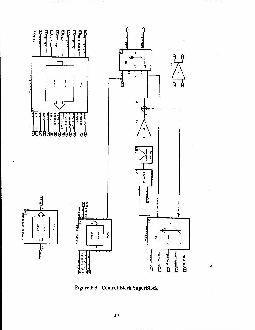
> f ö f »I r ft X! 4:
r- JJ
*i > c ■o a a
a a 3
c 1
08886il@ÖÖÖÖ @
iiii 1 £ ö ä
Figure B.3: Control Block SuperBlock
87
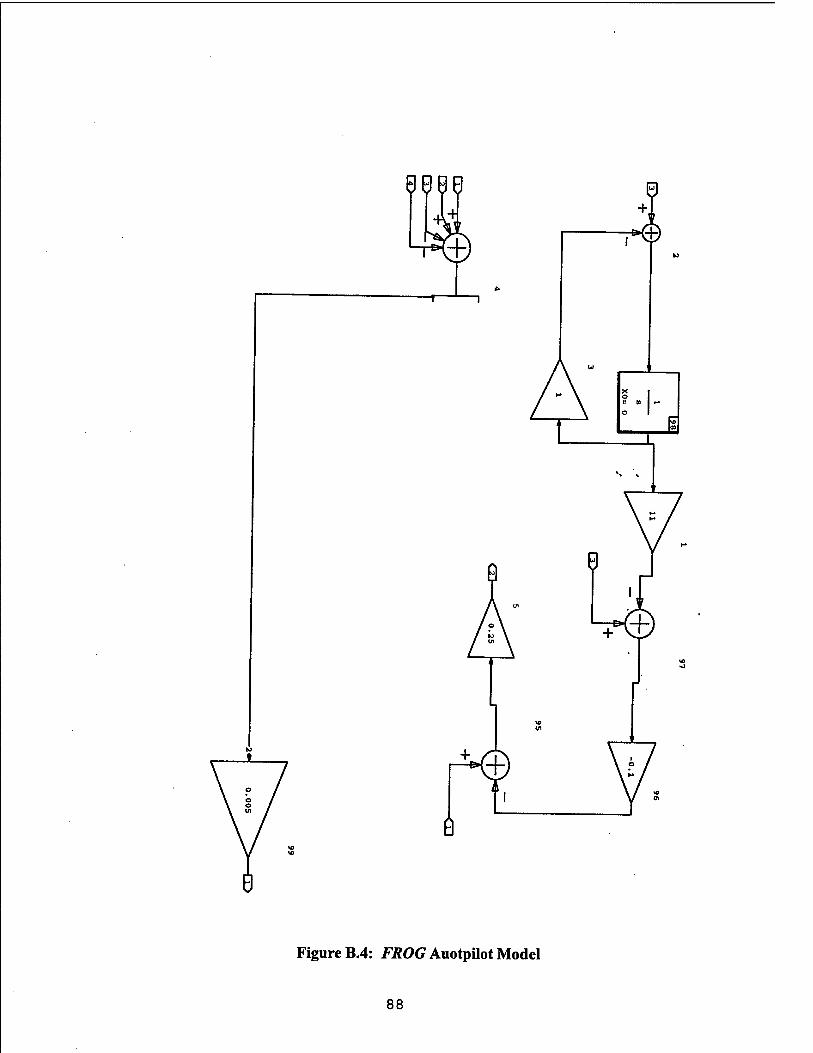
BEIRR 0
i
+. -en 4>
"
x t ii n 1 H o 1
P
Figure B.4: FROG Auotpilot Model
88

LIST OF REFERENCES
1. Franklin, G. F., Powell, J. D., Workman, M. L., Digital Control of Dynamic Systems, Addison-Wesley, 1990.
2. Strum, R. D., Kirk, D. E., Contemporary Linear Systems, PWS Publishing Company, 1996.
3. Kaminer, 1.1., Class Notes for AA4342, Naval Postgraduate School, Monterey, CA, 1997.
4. Integrated Systems Inc., MATRLXX Product Family System Manuals, SystemBuild, Version 5.0, 1996.
5. Moats, M. L., Automation of Hardware-in-the-Loop Testing of Control Systems for Unmanned Air Vehicles, Master's Thesis, Naval Postgraduate School, Monterey, CA, 1994.
6. Integrated Systems Inc., MATRLXX Product Family System Manuals, RealSim, Version 5.0, 1996.
7. Papageorgiou, E. C, Development of a Dynamic Model for aUAV, Master's Thesis, Naval Postgraduate School, Monterey, CA, March 1997.
8. Pascoal, A., Class Notes for AA 3341, Naval Postgraduate School, Monterey, CA, 1997.
9. Komlosy III, J. A., Applications of Rapid Prototyping to the Design and Testing of UAVFight Control Systems, Master's Thesis. Naval Postgraduate School, Monterey, CA, March 1998.
89

90
INITIAL DISTRIBUTION LIST
Defense Technical Information Center. 8725 John J. Kingman Rd., STE 0944 Ft. Belvoir, Virginia 22060-6218
Dudley Knox Library Naval Postgraduate School 411 Dyer Rd. Monterey, California 93943-5101
Doctor Isaac I. Kaminer, Code AA/KA Department of Aeronautics and Astronautics Naval Postgraduate School Monterey, California 93943-5121
Doctor Rüssel W. Duren, Code AA/DR Department of Aeronautics and Astronautics Naval Postgraduate School Monterey, California 93943-5121
Department of Aeronautics and Astronautics. CodeAA Naval Postgraduate School 699 Dyer Rd. Rm. 137 Monterey, California 93943-5106
LCDR Steven J. Froncillo.... 712 Country Club BLVD. Chesapeake, Virginia 23460
91