Embed Size (px)
DESCRIPTION
Microphones
Citation preview
Design of an Electret based Measurement
Microphone
Brian Dwyer
Directed by Dr. Gareth Bennett
Department of Mechanical & Manufacturing Engineering
Parsons Building
Trinity College
Dublin 2
Ireland
March 2010

Declaration
I declare that I am the author of this thesis and that all work described herein is my
own, unless otherwise referenced. Furthermore, this work has not been submitted in
whole or part, to any other university or college for any degree or qualification.
I authorise the library of Trinity College Dublin to lend this thesis.
________________________
Brian Dwyer, Date

Abstract
Measurement microphones are a high quality microphone used by engineers for
tests which require high accuracy. Typically measurement microphones are
extremely expensive. With the likes of Bruel and Kjaer, with a typical single channel
Bruel and Kjaer Measurement microphone, consisting of microphone, cables and
amplification signal conditioning equal to €750. Recent interest in multimedia
applications have resulted in a prolificacy of microphones in consumer electrical
appliances such as smart phones, computers, mobile phones, PDAs, etc. This has
resulted in the availability of an electret based microphone at an extremely affordable
price which is due to the huge volumes of these devices being generated. This
project develops from a previous project where the evaluation or proof of concept of
an electret capsule showed feasibility of developing an affordable high quality
microphone. This project will further develop the electronic instrumentation of the
previous microphone and in particular will focus on repackaging the components in a
more production friendly, compact, user friendly, aesthetic product.
The project presents an improved product at the total manufacturing and materials
cost of €28.58 per unit. The new design is benchmarked against a high quality
G.R.A.S. (BF40) microphone and is tested for its sensitivity, dynamic range and
linearity as a function of frequency as well as a function of amplitude and is shown to
perform extremely well with a noise floor of approximately 7dB and an upper
threshold in excess of 119dB and linear response when compared. In addition the
project completed its objectives of packaging all electronic instrumentation including
power supply, amplifier, LED and Electret capsule within a single small compact
stainless steel 8mm diameter casing.

Acknowledgement
I would like to express my deeply gratitude to everyone who helped me with this
project.
I express my gratitude to Dr. Gareth Bennett for his motivation and guidance through
out this project. I am truly grateful for being given such an opportunity to work on this
project.
I express my gratitude to Mr. Shane Hunt for his time and assistance over the course
of the project.
My thanks are also due to Mr. Sean O‟Callaghan, Mr. Mick Reilly and Mr Gabriel
Nicholson for their guidance in this project.

Contents
Chapter 1 Introduction .................................................................................................................... 1
Chapter 2 Background and Literature Review ............................................................................. 2
2.1 Microphones ......................................................................................................................... 2
2.2 Microphone arrays ................................................................................................................ 2
2.3 Previous Electret based Measurement Microphone Design ...................................................... 4
2.4 Current Research Rig .......................................................................................................... 5
2.5 Existing Microphone Competitors ....................................................................................... 7
Brüel & Kjær ............................................................................................................................ 7
GRAS ....................................................................................................................................... 9
Chapter 3 Theory .......................................................................................................................... 11
3.1 Sound .................................................................................................................................. 11
3.2 Duct Acoustics .................................................................................................................... 12
Mechanics of component materials ......................................................................................... 22
Electronics ................................................................................................................................. 27
Automated Manufacture and its Benefits ................................................................................ 31
Chapter 4 Concept development................................................................................................. 32
Design Specifications ............................................................................................................... 32
Engineering considerations .................................................................................................. 32
Ethical Issues ........................................................................................................................ 33
Manufacturing and product maintenance............................................................................ 34
Concept structure...................................................................................................................... 34
Concept models ........................................................................................................................ 36
Chapter 5 Embodiment ................................................................................................................ 38
Power Supply ........................................................................................................................ 38
Outer Casing ......................................................................................................................... 43
Battery Compartment............................................................................................................ 44
Output Connection ................................................................................................................ 52
Positive Contact .................................................................................................................... 54
Negative Contact ..................................................................................................................... 55
Switch ........................................................................................................................................ 56
Slide switches ........................................................................................................................ 56
Push Button switch ............................................................................................................... 57

Toggle switch......................................................................................................................... 57
Amplifier and Electret capsule ................................................................................................. 57
Other components .................................................................................................................... 58
Flag System ........................................................................................................................... 58
Battery Insulation .................................................................................................................. 58
Chapter 6 Final Design ................................................................................................................ 59
Bill of Materials .......................................................................................................................... 62
Manufacturing and Assembly process .................................................................................... 64
Chapter 7 Testing ......................................................................................................................... 67
Sensitivity at 1kHz..................................................................................................................... 67
Frequency response ................................................................................................................. 67
Noise floor Test ..................................................................................................................... 69
White Noise Test ................................................................................................................... 69
Chapter 8 Results and Discussion .............................................................................................. 70
Chapter 9 Future Work ................................................................................................................. 76
Further Testing .......................................................................................................................... 76
Initial Batch ................................................................................................................................ 76
Application into other research projects .................................................................................. 76
Testing within other applications ............................................................................................. 77
Large scale batch production ................................................................................................... 77
Chapter 10 Project Management ................................................................................................ 79
Project Costs ............................................................................................................................. 80
Chapter 11 Conclusion ................................................................................................................. 82
Chapter 12 Bibliography................................................................................................................. 83
Chapter 13 Appendices ................................................................................................................ 86

Table of Figures
Figure 1 : Photograph of the two previously designed electret based measurement
microphones. .............................................................................................................. 4
Figure 2 : Microphone array rig in the fluids lab in Trinity College Dublin. .................. 5
Figure 3 : Amplification units with external AC power supply .................................... 6
Figure 4 : Bruel & Kjaer Precision Array Microphone, Type 4958 .............................. 7
Figure 5 : GRAS model type 40PH............................................................................. 9
Figure 6 : Duct closed at one end and open at the other of length L and diameter a 12
Figure 7 : Microphone array with an incoming wave ................................................ 17
Figure 8:The theoretical directivity pattern of a linear array of 4 microphones at a
frequency level of 700Hz .......................................................................................... 18
Figure 9 : The theoretical directivity patern of a linear array of 4 microphones at a
frequency level of 1000Hz ........................................................................................ 19
Figure 10 : The theoretical directivity pattern of a linear array of 4 microphones at a
frequency level of 3000Hz ........................................................................................ 19
Figure 11: The theoretical directivity pattern of a linear array of 4 of the previous
electret based microphones closely packed next to one another at a frequency of
8000Hz ..................................................................................................................... 20
Figure 12 : The theoretical directivity pattern of a linear array of 4 of the new electret
based microphones closely packed next to one another at a frequency of 8000Hz . 21
Figure 13 : curved surface split into a number of equal width elements for analysis 25
Figure 14 : Schematic of beams side profile when a force P is applied to its end .... 26
Figure 15 : A simple circuit consisting of 3 resistors in parallel ................................ 29
Figure 16 : Concept model A with push fit cap ......................................................... 36
Figure 17 : Concept model B with polymer battery shield ........................................ 36
Figure 18 : Concept model C with twist fit cap ......................................................... 36
Figure 19 : Concept model C with sliding battery cover ........................................... 36
Figure 20 : The batteries‟ capacity in MAh and corresponding calculated battery life
when used in the microphone assembly .................................................................. 40
Figure 21 : Cost per microphone for the required number of battery cells ................ 40
Figure 22 : The measured diameter of each battery cell. ......................................... 41
Figure 23 : Oscilloscope Screen shot. Channel 1 (yellow): Oscilloscope electrical
noise, Channel 2(blue): ZA10 electrical noise, Channel 3(pink): AC with voltage
regulator. .................................................................................................................. 42
Figure 24 : slider system with labelled components ................................................. 45
Figure 25 : slider system in action ............................................................................ 45
Figure 26 : Twist top design with section removed to allow for wires to pass. .......... 46
Figure 27 : 2D outline of tube A after being tapped. ................................................. 46
Figure 28 : Push fit design (tube A left, tube B right) ................................................ 48
Figure 29 : Tube A and B connected ........................................................................ 48
Figure 30 : Newton meter with a human hand exerting forces on the hook .............. 49
Figure 31 : Annotated model with an overview of the mechanism in action ............. 51
Figure 32 : Polymer cover with flexible clip mechanism highlighted ......................... 51
Figure 33 : SMB bulkhead male Jack, SMB straight male jack, SMB straight female
and Female Straight Plug shown from left to right .................................................... 53
Figure 34 : Tube drawing with a rounded end .......................................................... 53
Figure 35 : Grounding mechanism for the power supply .......................................... 56
Figure 36 : The final prototype (8mm outer diameter, 90mm length)........................ 59
Figure 37 : 3D model of internal layout of components within the final prototype ..... 60
Figure 38 : Power supply, amplifier, flag system and electret wiring diagram .......... 61
Figure 39 : Printed Circuit board Design (Shane Hunt,2010) ................................... 62
Figure 40 : Schematic of test rig used for the frequency response function test, noise
floor test and auto-spectra plot. ................................................................................ 68
Figure 41 : Noise floor for electret based measurement microphone and G.R.A.S
microphone within an impedance tube ..................................................................... 70
Figure 42 : Auto-spectra for electret based measurement microphone and G.R.A.S –
white noise in impedance tube ................................................................................. 71
Figure 43 : Frequency response function electret / reference assembly – Magnitude
................................................................................................................................. 72
Figure 44 : Frequency response function electret / reference assembly - Phase ..... 73
Figure 45 : Input/ Output relationship for both assemblies ....................................... 74
Figure 46 : Electret based Measurement microphone with incorporated polymer
battery cover ............................................................................................................ 77

1
Chapter 1 Introduction
Microphones are sensors which provide high level information and have been used
successfully to date in power management projects (C. Harris and V. Cahill, 2007).
Microphones convert acoustical energy into electrical energy and can be divided into
two categories, active and passive. Active microphones require a supply voltage,
passive on the other hand do not. Each category contains numerous microphone
types and designs. The more common designs are Carbon Microphones, Externally
Polarized Condenser Microphones, Prepolarized Electret Condenser Microphones,
Magnetic Microphones, and Piezoelectric Microphones (Valentino, 2008).
Electret Microphones are an example of an active microphone which is commonly
found in multi-media devices and because of the high level mass production they are
very affordable. This project employs this fact and develops an Electret based
measurement microphone. The size and obtrusiveness of the microphone design are
very important and reasons for this are explained in the following chapter.
Arrays of microphones can provide more complex information which can be used to
optimise energy saving procedures or in other areas of engineering, such as
aeroacoustics, to perform noise source identification techniques to reduce
environmental noise (Bennett, 2008). Microphone array techniques require large
numbers of microphones to optimise spatial and frequency resolution.
Most transducers require some form of amplification and in the case of microphones
it is usually an external AC powered unit. This project sets out to develop an all in
one analogue microphone assembly which includes all the necessary analog
components of a measurement microphone channel. In doing so reducing the size
and parts required in microphone array rigs.
2
Chapter 2 Background and Literature Review
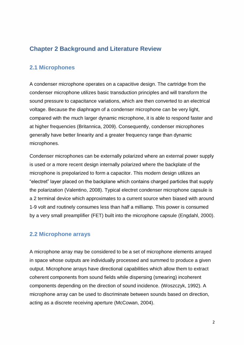
2.1 Microphones
A condenser microphone operates on a capacitive design. The cartridge from the
condenser microphone utilizes basic transduction principles and will transform the
sound pressure to capacitance variations, which are then converted to an electrical
voltage. Because the diaphragm of a condenser microphone can be very light,
compared with the much larger dynamic microphone, it is able to respond faster and
at higher frequencies (Britannica, 2009). Consequently, condenser microphones
generally have better linearity and a greater frequency range than dynamic
microphones.
Condenser microphones can be externally polarized where an external power supply
is used or a more recent design internally polarized where the backplate of the
microphone is prepolarized to form a capacitor. This modern design utilizes an
“electret” layer placed on the backplane which contains charged particles that supply
the polarization (Valentino, 2008). Typical electret condenser microphone capsule is
a 2 terminal device which approximates to a current source when biased with around
1-9 volt and routinely consumes less than half a milliamp. This power is consumed
by a very small preamplifier (FET) built into the microphone capsule (Engdahl, 2000).
2.2 Microphone arrays
A microphone array may be considered to be a set of microphone elements arrayed
in space whose outputs are individually processed and summed to produce a given
output. Microphone arrays have directional capabilities which allow them to extract
coherent components from sound fields while dispersing (smearing) incoherent
components depending on the direction of sound incidence. (Woszczyk, 1992). A
microphone array can be used to discriminate between sounds based on direction,
acting as a discrete receiving aperture (McCowan, 2004).

3
Noise and reverberation can seriously degrade both microphone reception and
loudspeaker transmission of audio signals in telecommunication systems.
Microphone arrays can be effective in combating these problems. The application of
microphone arrays may be useful for teleconferencing and speech pickup in noisy
and reverberant environments (Elko, 2004).
Microphone arrays are also effectively used in noise sourcing techniques.
Beamforming is an array-based measurement technique for sound-source location
from medium to long measurement distances. Beamforming is used extensively in
underwater acoustic imaging (Papazoglou, 1996), airborne targeting (Benson, 2006)
as well as underground imaging (C Frazier, 2000). A specific example of this is the
acoustic camera used to monitor source position images of airborne sounds and is
used in military and law enforcement applications.
Planar Near-field Acoustical Holography (NAH) is another established technique for
efficient and accurate noise source location. The measurement grid must
capture the major part of the sound radiation into a half space and therefore
completely cover the noise source plus approximately a 45º solid angle and the grid
spacing must be less than half a wavelength at the highest frequency of interest (JD
Maynard, 1985). For both techniques the resolution is dependent on the number of
microphones in the array and the spacing between them. This dependency is
explained further in chapter 3. Both the size and the cost of each individual
microphone can determine the effectiveness and success of noise sourcing
techniques.

4
2.3 Previous Electret based Measurement Microphone Design
The previous electret based measurement microphone design shown in figure 1
incorporates low cost, off the shelf electret capsules. The assembly includes an
amplifier mounted on a Printed Circuit Board (PCB) which is positioned at the end of
the tube. The power supply is in the form of a 9 volt battery which contributes hugely
to the size of the assembly. This 9 volt battery requires a voltage regulator in order to
reduce the input voltage to 5.5 volts, required to power the assembly. Comparative
tests with a high specification production microphone show that the magnitude and
phase response of the assemblies are frequency dependent, and that this variation
changes from one assembly to another (Gareth J. Bennett, 2009). The comparative
test results and circuitry diagram are attached in the appendix 1.
Figure 1 : Photograph of the two previously designed electret based measurement microphones.
5
2.4 Current Research Rig
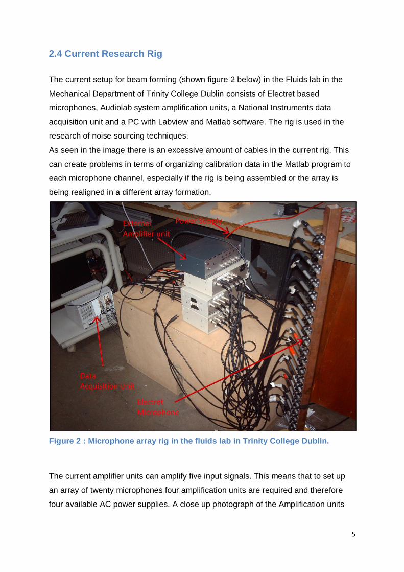
The current setup for beam forming (shown figure 2 below) in the Fluids lab in the
Mechanical Department of Trinity College Dublin consists of Electret based
microphones, Audiolab system amplification units, a National Instruments data
acquisition unit and a PC with Labview and Matlab software. The rig is used in the
research of noise sourcing techniques.
As seen in the image there is an excessive amount of cables in the current rig. This
can create problems in terms of organizing calibration data in the Matlab program to
each microphone channel, especially if the rig is being assembled or the array is
being realigned in a different array formation.
Figure 2 : Microphone array rig in the fluids lab in Trinity College Dublin.
The current amplifier units can amplify five input signals. This means that to set up
an array of twenty microphones four amplification units are required and therefore
four available AC power supplies. A close up photograph of the Amplification units

6
from above is shown in figure 3. As one can conclude from these photos alone the
rig is not very versatile or portable in its construction.
Figure 3 : Amplification units with external AC power supply

7
2.5 Existing Microphone Competitors
There are numerous brands on the market that produce measurement microphones,
ranging from high quality, expensive measurement microphones to low spec cheap
alternatives. Although a number of measurement microphones were researched for
this section of the project three models will be focused on for comparative purposes
as these three microphones displayed features considered beneficial to the
discussed applications. Two of the leading brands of measurement microphones are
G.R.A.S. and Brüel & Kjær. Due to the cost of each microphone manufactured by
these brands it is inherently expensive to use them in microphone arrays as well as
other microphone applications.
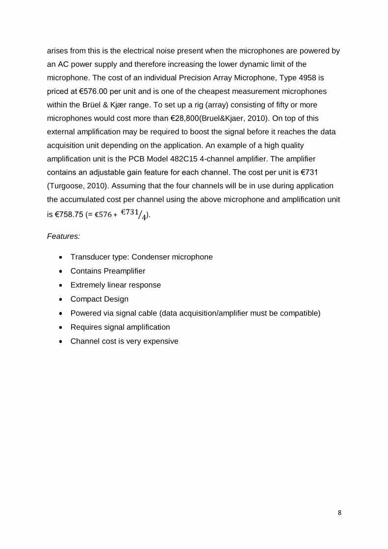
Brüel & Kjær
The Brüel & Kjær Precision Array Microphone,
Type 4958 (shown to the right) is marketed as
an array microphone and therefore to be
purchased in multiples. The instrument uses a
high quality condenser microphone as the
transducer and provides good amplitude and
phase response which is important for accuracy
in array techniques. It contains an SMB (Sub
Miniature version B) coaxial connection; it is very small in diameter (1/4 inch);
contains a small preamplifier and has an integrated TEDS (transducer electronic
data sheet1).
The power supply, signal and TED are transferred via one cable attached to the back
of the instrument. This is advantageous in terms of significantly reducing number of
cables in an experimental rig. A disadvantage with the powering methods of this
microphone is that the instruments are not compatible with all data acquisition
systems as not all systems can supply power via the signal cable. Another issue that
1 A Transducer Electronic Data Sheet is a device that is used to store the calibration data of a transducer so
that when used with compatible software the transducer’s data can be automatically calibrated. The transducers are calibrated pre shipping of the product and must be recalibrated by the user after periods of use.
Figure 4 : Bruel & Kjaer Precision Array Microphone, Type 4958
8
arises from this is the electrical noise present when the microphones are powered by
an AC power supply and therefore increasing the lower dynamic limit of the
microphone. The cost of an individual Precision Array Microphone, Type 4958 is
priced at €576.00 per unit and is one of the cheapest measurement microphones
within the Brüel & Kjær range. To set up a rig (array) consisting of fifty or more
microphones would cost more than €28,800(Bruel&Kjaer, 2010). On top of this
external amplification may be required to boost the signal before it reaches the data
acquisition unit depending on the application. An example of a high quality
amplification unit is the PCB Model 482C15 4-channel amplifier. The amplifier
contains an adjustable gain feature for each channel. The cost per unit is €731
(Turgoose, 2010). Assuming that the four channels will be in use during application
the accumulated cost per channel using the above microphone and amplification unit
is €758.75 (= € + ).
Features:
Transducer type: Condenser microphone
Contains Preamplifier
Extremely linear response
Compact Design
Powered via signal cable (data acquisition/amplifier must be compatible)
Requires signal amplification
Channel cost is very expensive

9
GRAS
The G.R.A.S model type 40PH (figure 5) and type 40PL are recently developed
versions of the G.R.A.S predecessor model, BF40.
They are ¼ inch in diameter and have an integrated TEDS for the purpose of
calibration. The phase and amplitude response of the microphones are specified to
be extremely linear (G.R.A.S, 2009). Similarly to the Brüel & Kjær model type 4958
the microphones are powered by an external AC source that is supplied via the
signal cable.
Figure 5 : GRAS model type 40PH
The cost per G.R.A.S microphone is €400. Adding this to the cost per amplifier
channel described in the previous section, the cost per channel is estimated to be
€582.75.
Features:
Transducer type: Condenser microphone
Contains Preamplifier
Extremely linear response
Compact Design
Powered via signal cable (data acquisition/amplifier must be compatible)
Requires signal amplification
Channel cost is expensive
10
There is quite a selection of cheaper alternatives available on the market. An
example of a cheaper measurement microphone is the MM01 manufactured by
Samson. The cost per microphone is €60. It comprises of an Electret microphone, a
plastic casing, an XLR2 connection and a voltage regulator. The Electret capsule
contains a preamplifier which requires an external power supply. This power supply
is supplied via the signal cable. The overall design is simple. The total estimated
channel cost per microphone for a Samson, MM01 and required external amplifier
(PCB Model 482C15) is €242.75.
Features:
Transducer type: Electret microphone
Contains Preamplifier
Powered via signal cable (data acquisition/amplifier must be compatible)
Requires signal amplification
Relatively low cost
Similar microphones to the Samson MM01 that were researched included brands
such as Apex(€70, (directproaudio, 2010)), Behringer (€55, (zzsounds, 2010)) and
Beyerdynamic (€220, (Pro-audio, 2010)), all of which use electret condenser
microphone transducers and require external amplification.
All of the above models are externally powered by an AC power supply via the signal
cable and require a “plug-in-power” or “phantom power” compatible external amplifier
or data acquisition unit.
2 An XLR connector is an electrical connector design commonly found in audio and video electronic hardware.
XLR connectors are twice the size of the standard RCA plugs and sockets found on consumer equipment and are more prone to electrical noise than SMB coaxial connectors.

11
Chapter 3 Theory
In this chapter important definitions and basic acoustic theories will be demonstrated
which contribute in defining design parameters.
Basic microphone and microphone array theory as well as duct acoustics are
investigated to further understand the background and results of this project.
Finally Mechanical and Electronic principals used in the design process are
discussed.
3.1 Sound
Sound pressure (P) is the pressure induced by the disturbance of sound waves. The
SI unit for sound pressure is the Pascal (Pa). The sound pressure deviation formula
is:
3-1
Where F is force and A is the area in which it is acting.
Sound pressure is most commonly converted into Decibel units in acoustics as the
unit scale is more adaptable to the user and it becomes more apparent of how loud a
signal is using the decibel scale. To convert sound pressure into decibels:
3-2
Where is the sound pressure and is the reference pressure, usually taken as
0.0002.
Impedance, Z is the complex ratio of the sound pressure on a given surface to the
sound flux through that surface. It is expressed in acoustic ohms and can be found
using the basic equation:

12
3-3
Where F is force and u is the particle velocity.
Particle velocity is the speed of a particle in a medium as it transmits a wave. From
the momentum equation3 it is found that:
3-4
Where is the medium density and is the sound pressure.
3.2 Duct Acoustics
For the purpose of being able to analyze a microphone‟s functionality the
microphone must be tested using plane waves. For this reason tests are carried out
within a tube or duct. The characteristic property of a plane wave is that each
acoustic variable has constant amplitude and phase on any plane perpendicular to
the direction of propagation. This is very advantageous when comparing
microphones. Solving for the general acoustics of a 2D duct, shown in figure 6 is as
follows:
Figure 6 : Duct closed at one end and open at the other of length L and diameter a
3

13
Using Helmholtz equation:
3-5
Where the boundary conditions at y = a and y = 0 is
By using the separation of variables approach, let p(x,y) = p(x)f(y):
3-6
From further manipulation we can separate the above equation into its x and y
components to get:
and
The general solution is
3-7
Incorporating the boundary conditions we know that . Substituting this in
to the above equation taking the point y = 0 we get:
Now again apply , the above equation, assuming A and C are both not
equal to zero we find that to satisfy this condition,
Where n = 0, 1, 2 …
where
The solution for P is:
3-8
Therefore

14
Where
Letting n = 0 we get the equation
3-9
This equation satisfies plane waves within the and there is no variation across the
duct. Now letting n = 1 we get the equation:
3-10
The condition for the waves to propagate down the duct is that must
remain real where . From this we can derive what is known as the duct‟s cut
off frequency.
The equation for calculating the cut-off frequency of a circular duct is:
3-11
Where a is the radius of the duct and c is the speed of sound.
Under this frequency only plane waves propagate and above this frequency
evanescent waves are present.
During analysis of results when testing the electret based measurement microphone
acoustic characteristics of the testing environment play a huge role in the results
achieved. A key example of this is the presence of standing waves when radiating
white noise down a duct. Standing waves are a result of the phase interference
between the transmitted and reflected waves in a terminated pipe (Fundamentals of
Acoustics, 4th edition, Lawrence E. Kinsler, Austin R.Frey, Alan B. Coppens, James
V. Sanders). The frequencies at which the standing waves are present appear at
greater amplitudes when plotting in the frequency domain and these frequencies can
be predicted for verification purposes. The amplitude at a pressure antinode is the
combined amplitude of the transmitted and reflected wave at that frequency and the
amplitude at a node is the transmitted wave‟s amplitude minus the reflected wave‟s
15
amplitude. The ratio of these amplitudes is known as the standing wave ratio and
can be used to find the load impedance of the tube termination/tube mouth.
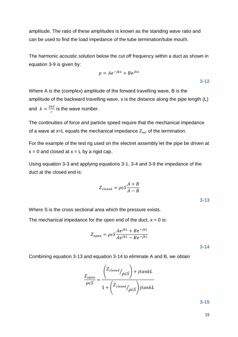
The harmonic acoustic solution below the cut off frequency within a duct as shown in
equation 3-9 is given by:
3-12
Where A is the (complex) amplitude of the forward travelling wave, B is the
amplitude of the backward travelling wave, x is the distance along the pipe length (L)
and is the wave number.
The continuities of force and particle speed require that the mechanical impedance
of a wave at x=L equals the mechanical impedance of the termination.
For the example of the test rig used on the electret assembly let the pipe be driven at
x = 0 and closed at x = L by a rigid cap.
Using equation 3-3 and applying equations 3-1, 3-4 and 3-9 the impedance of the
duct at the closed end is:
3-13
Where S is the cross sectional area which the pressure exists.
The mechanical impedance for the open end of the duct, x = 0 is:
3-14
Combining equation 3-13 and equation 3-14 to eliminate A and B, we obtain
3-15

16
As the closed end of the duct is closed by a rigid cap we can let .
Applying this to equation 3-15 yields:
The reactance is zero and resonance occurs when ,
This equation rearranged gives:
3-16
Where is the duct‟s natural frequency for modes n=1,2,3…, c is the speed of
sound and L is the duct length.

17
Basic Microphone Array Acoustics
As defined in chapter 2 a microphone array may be considered to be a set of
microphone elements arrayed in space whose outputs are individually processed
and summed to produce a given output. A simple line array as shown in the figure
below (similar to rig shown in chapter 2, figure 2) consists of a group of equally
spaced omnidirectional microphones whose outputs are summed directly.
Figure 7 : Microphone array with an incoming wave
The microphones represented in the above figure are all subject to the same
incoming wave where is the wavelength, ( ); is the angle at which the wave
is to the normal plane and d is the spacing distance between the microphones.
The far–field directivity function R(ф) (Eagle, 2004) is given by the following
equation:
3-17
18
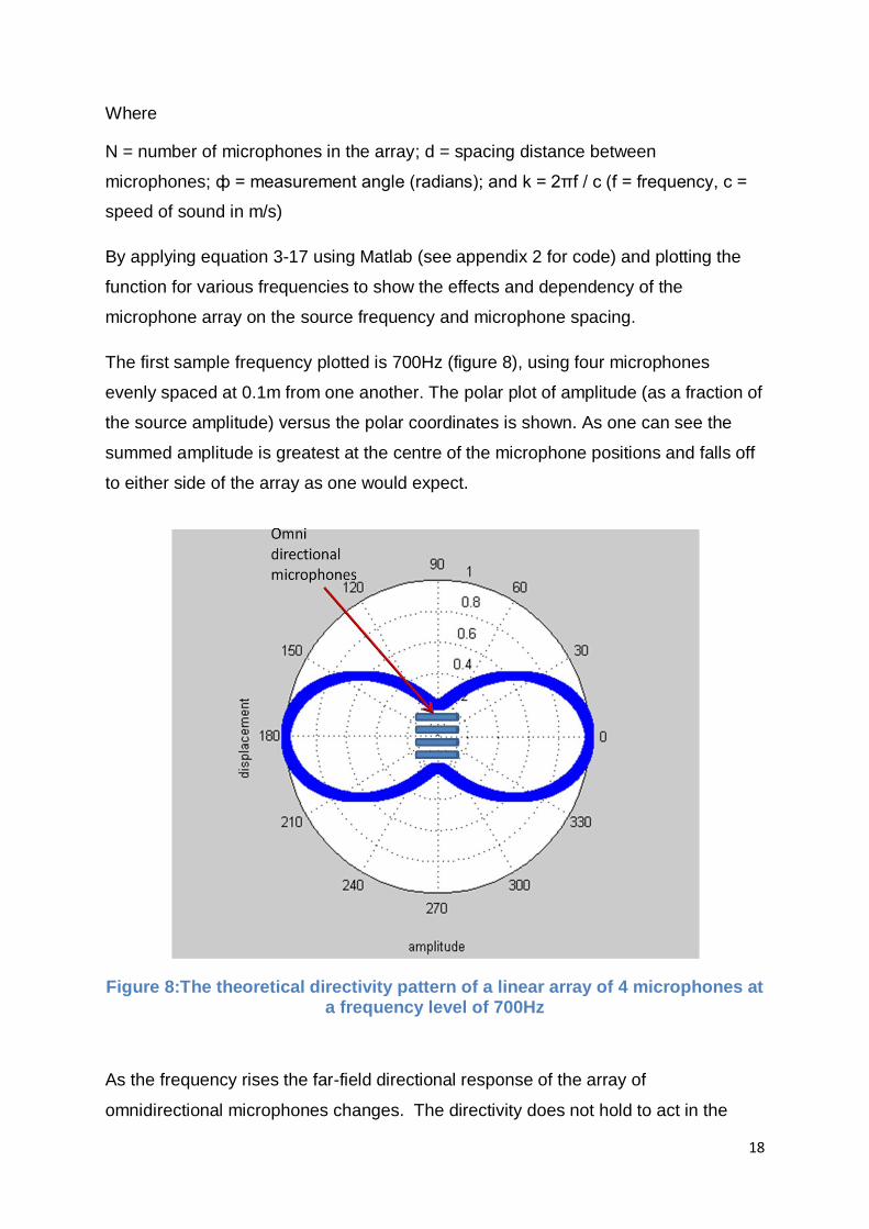
Where
N = number of microphones in the array; d = spacing distance between
microphones; ф = measurement angle (radians); and k = 2πf / c (f = frequency, c =
speed of sound in m/s)
By applying equation 3-17 using Matlab (see appendix 2 for code) and plotting the
function for various frequencies to show the effects and dependency of the
microphone array on the source frequency and microphone spacing.
The first sample frequency plotted is 700Hz (figure 8), using four microphones
evenly spaced at 0.1m from one another. The polar plot of amplitude (as a fraction of
the source amplitude) versus the polar coordinates is shown. As one can see the
summed amplitude is greatest at the centre of the microphone positions and falls off
to either side of the array as one would expect.
Figure 8:The theoretical directivity pattern of a linear array of 4 microphones at a frequency level of 700Hz
As the frequency rises the far-field directional response of the array of
omnidirectional microphones changes. The directivity does not hold to act in the

19
same direction as shown above. Instead unwanted off-axis lobes present themselves
as the frequency increases for microphone arrays as shown in figure 9 and figure
10Figure 10 : The theoretical directivity pattern of a linear array of 4 microphones at
a frequency level of 3000Hz.
Figure 9 : The theoretical directivity patern of a linear array of 4 microphones at a frequency level of 1000Hz

20
Figure 10 : The theoretical directivity pattern of a linear array of 4 microphones at a frequency level of 3000Hz
From the three plots shown above it is observed that the increasing amplitude levels
to the sides of the microphone array rig and a reduction in the desired plane of
measurement are highly dependent on the frequency of the source. This directivity
pattern is also dependent on the spacing between the microphones in the array. By
reducing the distance between the points of measure we can use microphone arrays
at higher frequency levels without the presence of off-axis lobes seen in figure 10.
For demonstration we will take the example of the previous electret based
measurement microphone design, using a sample frequency of 8000Hz and packing
four microphones next to one another (distance of 35mm) the following theoretical
results are shown:

21
Figure 11: The theoretical directivity pattern of a linear array of 4 of the previous electret based microphones closely packed next to one another at a frequency of 8000Hz
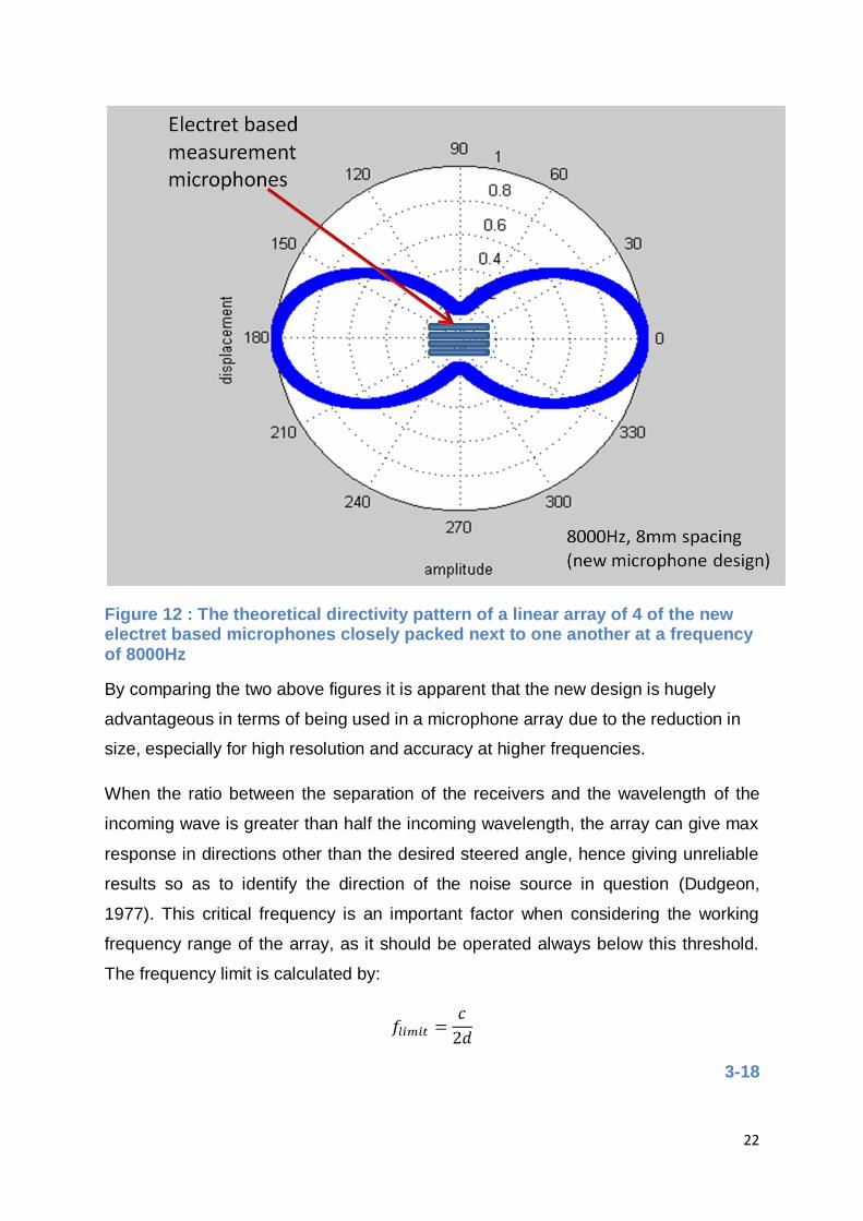
In the new design the microphones are capable of being packed as close as 8mm
from one another. Taking the same sample frequency of 8000Hz the theoretical
results achieved are shown in figure 12 below.
22
Figure 12 : The theoretical directivity pattern of a linear array of 4 of the new electret based microphones closely packed next to one another at a frequency of 8000Hz
By comparing the two above figures it is apparent that the new design is hugely
advantageous in terms of being used in a microphone array due to the reduction in
size, especially for high resolution and accuracy at higher frequencies.
When the ratio between the separation of the receivers and the wavelength of the
incoming wave is greater than half the incoming wavelength, the array can give max
response in directions other than the desired steered angle, hence giving unreliable
results so as to identify the direction of the noise source in question (Dudgeon,
1977). This critical frequency is an important factor when considering the working
frequency range of the array, as it should be operated always below this threshold.
The frequency limit is calculated by:
3-18

23
Where d is the microphone spacing.
Applying equation 3-18 to the minimum spacing between the new electret based
design (8mm) it is calculated that the maximum working frequency is 21250Hz.
Mechanics of component materials
Calculations were carried out in the selection and design process of mechanical
components. An example of a crucial component which required investigation before
purchasing was the helical compression spring.
Compression springs, like extension springs are stressed in torsion. In effect, these
springs can be considered similar to a torsion bar wound helically to reduce space.
Compression springs are generally designed so that the minimum working position
is, at most 85% of the total deflection available (Lyons, 2008). The choice of spring
type can be dictated by a number of factors: the choice of spring‟s anticipated
working requirements; its fittings; the wire diameter; the spring diameter and the cost
of the end product. The working environment must be taken into account when
selecting/designing a spring, any environmental factors that may affect the spring‟s
performance and more importantly in this case the performance of the product or
assembly in which the spring is being designed for. An example is the ability for the
spring to conduct electricity.
When integrating a component into a design amongst other components the
dimensions are always an important issue. As springs change in there length when
forces are acting on them it is important as an engineer to understand how they are
changing and the factors that affect these changes. The deflection in helical
compression can be found by the equation:
3-19
Where F is the force acting on the spring, x is the displacement and k is the spring
constant.
This k value can be determined from a number of parameters which will now be
investigated using analysis of an equivalent simple bar.

24
The strain energy stored due to torsion in a simple bar is:
3-20
Where J is the second moment of area ( for a round bar), G is the torsional
modulus of rigidity, T is the stress and l is the length of the equivalent simple bar
The strain energy stored in a bar due to shear is:
3-21
Where P is the load and A is the cross sectional area of the bar (or the wire in the
case of a spring).
By simply adding equation 3-20 and equation 3-21 the total strain energy for a helical
spring is found.
3-22
By letting , where D is the Spring diameter,
is the number of coils and d is the wire diameter.
3-23
Using Castigliano‟s Therom:
3-24
(Units in equation 3-24 are in mm)
As we can write

25
3-25
By substituting equation 3-25 into equation 3-19Error! Reference source not
found. where the deflection is equivalent to the displacement we get the following
solution:
3-26
This k value is the spring constant and is usually displayed along with a spring‟s
model number. Using this equation can help to determine the spring‟s dimensions
and characteristics in the design process.
Finite Element Analysis
For the deflection of parts in the assembly a finite element bending analysis is
carried out on the component‟s deflection when a force is acting against it. The
purpose of carrying out finite element analysis was to get a better insight into the
design parameters with accurate figures.
The analysis works on the concept that the curved surface is split up into a number
of cantilever beams and analysed individually and summed up. Due to the
complexity of the shape certain parameters are constantly changing across the
element. As seen in figure 13 the cross section of each beam is changing across the
tube in the plane which the force is acting.

26
Figure 13 : curved surface split into a number of equal width elements for analysis
The Bending equation for a beam (Fenner, 1988):
3-27
Where: P = normal force, l = beam length, w= beam width, t= beam thickness and
y=deflection at point of load.
The finite element analysis was compared to a simple analysis to ensure accuracy.
The simple analysis for verification method is as follows:

27
P
L
A B
Vax
Figure 14 : Schematic of beams side profile when a force P is applied to its end
Where M is the moments, P is the force acting at the distance x.
Applying equations for Slope and Elastic Curve:
3-28
Where E = young‟s modulus of the material, I = moment of inertia, v = displacement.
After integrating twice yields:
3-29
3-30
Applying boundary conditions of dv/dx = 0 at x = L and v=0 at x=L (making the
assumption that the piece is fixed at this point), Equation 3-29 becomes
Therefore, and . Substituting these results back into
equation 3-30, we get

28
3-31
The maximum displacement occurs at A (x=0), for which
This equation rearranged to calculate the force P required to deflect the stainless
steel tube so that a tension fit can be achieved between two parts. (Note: the
negative sign can be ignored as it is merely as function of direction)
3-32
This equation is applied to the stainless steel tube with a curved surface.
The max allowable stress in a beam is found using the following equation (Hibbeler,
2007):
3-33
Where d is the deflection, E is the flexural modulus, t is the thickness and l is the
length of the beam.
Electronics
In order to design an electric circuit compiled of premanufactured componentry an
understanding of the fundamentals of electric circuits must be attained. In this
section some basic principles are explained which were used in the process of
design. The first of these principle‟s is Kirchhoff‟s current law. This law must be
addressed when changing circuit layout and also adding or removing components
from the previous design.

29
3-34
The law states that the sum of the currents ( ) at a junction of two or more
conductors must equal zero. When analysing a circuit this law enables us to express
currents in a circuit in terms of each other. Combining Kirchhoff‟s law with Ohm‟s law
(equation 3-35) one can analyse and grasp an understanding of basic electronic
circuitry.
3-35
Where V is the voltage (volts), I is the current (amperes) and R is the resistance
(ohms).
As the three parameters are all dependent on one another it is possible to
manipulate a circuit by adding basic electrical components such as resistors of
determined values knowing the required voltage of all components and the current
draw of the components. With these parameters defined the next step in designing a
circuit is choosing ideal source4.
Applying Kirchhoff‟s current law to the example circuit shown below,
about the circled node.
4 An ideal voltage source provides a prescribed voltage across its terminals irrespective of the current flowing
through it. The amount of current supplied by the source is determined by the circuit connected to it (Rizzoni, 2000)

30
Figure 15 : A simple circuit consisting of 3 resistors in parallel
By applying Ohm‟s law, equation 3-35 the current can be expressed as follows:
Letting where
3-36
Using the ratio, as the voltage is same throughout the example circuit we
can express the following:
From this we can derive the general expression for the current divider for a circuit
with N parallel resistors:
31
3-37
Where n is the element in question.
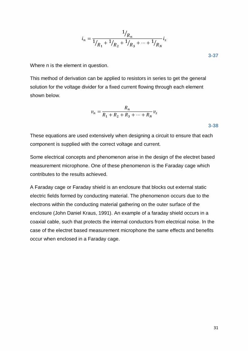
This method of derivation can be applied to resistors in series to get the general
solution for the voltage divider for a fixed current flowing through each element
shown below.
3-38
These equations are used extensively when designing a circuit to ensure that each
component is supplied with the correct voltage and current.
Some electrical concepts and phenomenon arise in the design of the electret based
measurement microphone. One of these phenomenon is the Faraday cage which
contributes to the results achieved.
A Faraday cage or Faraday shield is an enclosure that blocks out external static
electric fields formed by conducting material. The phenomenon occurs due to the
electrons within the conducting material gathering on the outer surface of the
enclosure (John Daniel Kraus, 1991). An example of a faraday shield occurs in a
coaxial cable, such that protects the internal conductors from electrical noise. In the
case of the electret based measurement microphone the same effects and benefits
occur when enclosed in a Faraday cage.

32
Automated Manufacture and its Benefits
When using automated methods of manufacturing you reduce the risk of
inaccuracies, increase productivity greatly and reduce the cost of manufacture.
Along with production costs constantly on the rise is the necessity for manufacturing
to remain as competitive as possible by utilizing these benefits of automation in the
manufacturing industry. Using automated methods of manufacture can in some
processes reduce the production cycle to as low as 5% of the equivalent manual
operation time (A Tiwari, 2008). In the design process concepts that could facilitate
automated manufacturing processes were developed more so than those requiring
manually assisted manufacturing processes for the purpose of low cost, efficient
future production.

33
Chapter 4 Concept development
Design Specifications
In this section the aims in the design process are outlined under categorized
headings.
Engineering considerations
Environment
Temperature: The microphones are for the purpose of laboratory application
so the temperature in which they are subjected to can be assumed to be room
temperature averaging around 23°C (IEC61094-2, 1992).
Pressure: The static pressure in which a measurement microphone can be
assumed to be subjected to is 101,325 kPa (BSEN61094-2, 1994).
The humidity in which a measurement microphone is expected to function at
is relative humidity of 50% (BSEN61094-2, 1994). The microphone assembly
must be able to withstand the corrosion at this level of humidity.
Dimensions, Geometry and Weight
Due to the applications and advantages discussed in chapters 1 and 2 the
dimensions of the microphone assembly must remain as small as possible.
This is especially true for the plane of measurement when being applied to an
array of microphones.
In reducing the size of the microphone assembly it is extremely important that
its functionality is not sacrificed.
Reducing the number of components including the required number of cables
required during operation is very important as this increases ease of set up
and portability.
Linked into portability is the weight of the microphone assembly. As the
microphones are portable and potentially used in high numbers it is highly
advantageous to keep the weight of the instrument as low as possible.
Life
The product as a whole should have an indefinite lifetime

34
The replacing of components such as power supply should be carried out as
necessary and are taken into account as a design parameter to reduce the
number of power cell changes over the lifetime of the product.
Quantity
The product is intended for multiple microphone applications as well as
independent operation.
For the purpose of this project the microphone is designed with an initial batch
size of 75 units in mind.
Product Cost
As the market for measurement microphones is very competitive the cost of
the microphone can determine the products success or failure.
For research purposes when using microphones in applications as discussed
in chapters 1 and 2 it is notably important to keep the cost of individual
instruments low.
Ethical Issues
Safety
The device must not expose the user to excessive temperatures, injury by
mechanical components or cause hazardous currents to pass through the
human body (IEC60065, 2001).
The apparatus shall be so constructed that there is no risk of an electric shock
from accessible parts or from those parts rendered accessible following the
removal by hand of a cover (IEC60065, 2001).
Aesthetic Considerations
As with all products on the market aesthetics of a product can be the
determining factor on whether a customer will choose this product as opposed
to another brand‟s product.
Good aesthetics in a product can display the product‟s standard and
performance to a customer who has not yet used the product.

35
Manufacturing and product maintenance
Manufacturing considerations
Due to the low cost of mass manufactured components the approach of
sourcing pre-manufactured components when possible will be applied.
The machining and alteration of components will be limited as much as
possible so that costs and production time remain low. Also the use of
automated manufacture will be an available option when manufacturing
multiple amounts post project and shall be taken into account during the
design process.
Material selection is heavily influenced by their required manufacturing
processes and therefore impacting on the instrument design.
Maintenance
The microphone assembly should entail easy maintenance if parts fail. In
doing so all internal components should be accessible to a certain degree
without interfering with other design specifications discussed in this section.
Another consideration that affects ease of maintenance is the use of stock
components which makes parts easily replaceable at low lead times.
Concept structure
To formalise the design process for efficiency and effectiveness the design of the
product was split into subsections, as listed below in table 1. The table displays the
corresponding concept solutions (in no specific order) that were developed during
the design process.

36
Table 1 : Design subsections and Corresponding concept solutions
1 2 3 4
Power supply
ZA10
BR435
CR927
Plug-in-power
Outer casing
Stainless steel tube with Push fit cap
Stainless steel tube with Sliding battery cover
Stainless steel tube with polymer battery shield
Stainless steel tube with Twist top fit
Power supply contacts
Polymer cap to allow direct contact
Compression spring
Rigid Steel cap
Conical Spring
Transducer
WM-61 electret
WM-64 electret
Signal Output
SMB bulkhead jack
SMB bulkhead female
SMB straight female plug
SMB male solder connection
Switch Slide Switch Push Button Switch
Toggle switch
Amplifier Low voltage amplifier
High voltage amplifier
Other Components
Flag system Power supply insulation
Wires

37
Concept models
From the above concept table‟s contents concept models were developed, four of
which are displayed in the table below.
Table 2 : 4 Concept models that were developed
Figure 16 : Concept model A with push fit cap
Concept
Figure 17 : Concept model B with polymer battery shield
Figure 18 : Concept model C with twist fit cap
Figure 19 : Concept model C with sliding battery cover
In order for the concepts to develop into a prototype an „adapt to specification‟
method was used. A visual outline of this development process can be found in
appendix 3. The idea behind this approach is that all previous subsection concepts

38
were verified and reworked when required if the current subsection and one of the
previous subsections were not compatible with one another.

39
Chapter 5 Embodiment
For the purpose of embodiment, concepts from the concept table were developed
and investigated further. In this chapter each sub section concept is elaborated
further and the variants in the subsection are compared with one another. Each
section is concluded with the concept that was pursued in prototyping.
Power Supply
The options for the power supply were narrowed down to four options for the design.
These included Lithium button cells, Lithium Pin-type cells, Zinc Air button cells and
plug-in-power (“phantom power”).
Instrument requirements Units
Voltage 5.5 (volts)
Current Draw 0.5 (milliAmpere)
Table 3 : The overall voltage and current requirements calculated for the microphone assembly
Lithium Button Cell
The lithium button cell model CR927 Button Cell Type Lithium Battery. These
batteries are composed of lithium ion technology which is renowned to have a very
high capacity and are a very “clean” source of power (low noise). CR927 cells are
commonly found in watches. Each 3 volt cell has a capacity of 100 MilliAmpere
hours (MAh). The dimensions of each cell are: height: 2.7 mm, diameter: 9.5 mm
and depth: 2.85 mm. As each cell produces 3 volts for the purpose of the electret
based measurement microphone only two cells would be required per assembly.
The main disadvantage to the CR927 button cell is that the diameter of each cell
spans largely outside of the diameter of the electret microphone by comparison to
that of the other power source options. This therefore as previously explained before
reduces the capabilities of the measurement microphone. The CR927 are the
smallest lithium button cells currently available on the market.

40
Lithium Pin-type cell
Lithium Pin-type cells (BR435) are power supplies commonly found in fishing rod
assemblies. Pin-type cells are very narrow in their construction. Each 3 volt cell has
a capacity of 25 MAh and the dimensions are: diameter: 4.2mm and length: 25.9mm.
The cost of each cell ranges between 2 and 4 euro depending on the supplier. As
mentioned above the lithium ion cells are a very clean source of power. The main
disadvantage to this power source is the cost per unit and also that the small
capacity of each cell compared to that of alternative power supplies.
Zinc Air Button cell
Zinc-Air button cells, ZA10 are power supplies commonly found in hearing aid
appliances. They are small in nature, are a low noise power supply and have a very
high capacity for their size. The dimensions for each cell are: 5.8mm diameter and
3.6mm height. The diameter, similar to that of the Lithium Pin-type cells (BR435) is
within the dimensions of the electret microphone and therefore does not affect the
measurement plane or impact on microphone spacing when used in an array. The
cost per pack of 6 units is 3 euro and due to the mass manufacturing of this cell type
it is easily available. The capacity of each 1.4 volt battery is 105MAh. As the voltage
of each cell is 1.4 volts and the requirement for the microphone is 5.5volts using four
cells as a power supply is ideal as it eliminated the previous necessity of a voltage
regulator.
Comparison of Cell Types
Comparative charts are shown below of the three selected power supply options in
the design, comparing the capacity of each power supply and the related battery life,
the cost and diameters of each unit. These parameters are considered the most
important in terms of designing a successful instrument. From the charts (figures 20,
21 and 22) it is apparent that the ZA10 button cell is the strongest contender is in
terms of design.

41
Figure 20 : The batteries’ capacity in MAh and corresponding calculated battery life when used in the microphone assembly
Figure 21 : Cost per microphone for the required number of battery cells
0
50
100
150
200
250
Lithium pin-type (BR435)
Lithium Button cell
(CR927)
Zinc-Air Button cell
(ZA10)
Capacity (MAh)
Battery life (hours)
0
1
2
3
4
5
6
Lithium pin-type
(BR435)
Lithium Button cell
(CR927)
Zinc-Air Button cell
(ZA10)
Cost (per microphone, €)
Cost (per microphone, €)

42
Figure 22 : The measured diameter of each battery cell.
Plug In Power
Plug in power (commonly referred to as phantom power) is a phenomenon by where
the power supply to an active microphone is supplied via the same cable as that of
the signal. Advantages to this method of powering a microphone is that there is no
need to change batteries and although it is an external AC power supply powering
the instruments there are no extra cables attached to the instrument. Disadvantages
to “phantom power” supply are that the data acquisition unit must be capable of
supplying power via the input terminal as well as the inevitable risk of electrical noise
in the signal generated by AC power and causing inaccuracies in results.
To demonstrate the presence of electrical noise in AC power supplies a test was
carried out comparing the electrical noise produced by the ZA10 button cells to the
electrical noise produced by an AC power supply with a voltage regulator. By doing
so it helped to conclude which power supply to include in the prototype. The results
from the test are shown below:
0
2
4
6
8
10
Lithium pin-type (BR435)
Lithium Button cell (CR927)
Zinc-Air Button cell (ZA10)
Diameter (mm)
Diameter (mm)
43
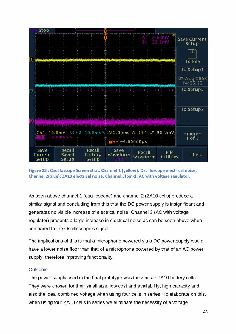
Figure 23 : Oscilloscope Screen shot. Channel 1 (yellow): Oscilloscope electrical noise, Channel 2(blue): ZA10 electrical noise, Channel 3(pink): AC with voltage regulator.
As seen above channel 1 (oscilloscope) and channel 2 (ZA10 cells) produce a
similar signal and concluding from this that the DC power supply is insignificant and
generates no visible increase of electrical noise. Channel 3 (AC with voltage
regulator) presents a large increase in electrical noise as can be seen above when
compared to the Oscilloscope‟s signal.
The implications of this is that a microphone powered via a DC power supply would
have a lower noise floor than that of a microphone powered by that of an AC power
supply, therefore improving functionality.
Outcome
The power supply used in the final prototype was the zinc air ZA10 battery cells.
They were chosen for their small size, low cost and availability, high capacity and
also the ideal combined voltage when using four cells in series. To elaborate on this,
when using four ZA10 cells in series we eliminate the necessity of a voltage
44
regulator as required in the previous design to reduce the voltage to required level.
As stated in table 3 the required voltage is 5.5volts and of the power supply selection
presented on this section the combined voltage of the ZA10 cells was the closest to
the required voltage. This allows a reduction in parts within the circuitry and further
lowering cost and size of the overall product.
Outer Casing
Stainless steel tubing was chosen as the outer casing for the microphone instrument.
The previous design used stainless steel tubing to hold the electret microphone and
also acted as a structural element for applications and the mounting of the 9volt
battery. This part of the previous design was developed further for the new design.
As the material selected for the casing is a conductive one the casing can be utilized
as a grounding mechanism for the instrument. This allowed for the reduction of
internal components, therefore reducing the cost and increasing compactibility. By
enclosing all the electrical components within the stainless steel tube and using the
tube as a ground for the circuit a Faraday cage is formed around the instrument.
The selection of tubes with suitable dimensions was very important in the design as
the tube needed to encapsulate all the electronic components, the power supply and
the electret capsule as well as remaining as small as possible making the electret
based microphone as effective in its design as possible.
Note: as the casing is a conductive material it is required that the power supply‟s
positive element is insulated from contacting the casing wall.
Suitable tubes were sourced that were considered suitable candidates to enclose
both the power supply and electret capsule. The selection of tubes considered are
shown in the table below:

45
Table 4 : Tube specifications for the corresponding power supplies
Power supply Outer Diameter
(mm)
Inner diameter
(mm)
Material
ZA10 (Za button
cell)
8 6.8 Stainless Steel 316
BR435 (Li pin-type) 8 6 Stainless Steel 316
Plug-in-power (AC) 8 6 Stainless Steel 316
CR927 (Li button
cell)
12 10 Stainless Steel 316
Outcome
The outer casing used in the final prototype was the first tube listed on table 4. This
tube is a conductive material so can be used as a ground for the circuitry; it has a
very small outer diameter and an inner diameter allowing 1mm for battery insulation
and a signal wire to pass by.
Battery Compartment
A number of concepts were developed to accommodate the different power supplies
and enable the changing of batteries if required.
Slider system
A slider system was designed to act as a
cover for the batteries when placed within
the outer casing. The system is compiled of
a number of components. These include a
10mm diameter compression spring, 2 pins,
an o-ring and an outer tube.

46
Figure 24 : slider system with labelled components
Figure 25 : slider system in action
The concept works on the basis that when the user requires changing the battery
cells they can slide back this mechanism and when finished the cover will
automatically return to its original position as shown in figure 25.
Although this concept is considered to be very user friendly the integration of the
mechanism into the microphone assembly increases in number of components and
also increases its size.
Threaded top
The twist top mechanism works on the basis that the instrument as a whole is
divided into two sections, one containing the power supply, circuitry and output
connection (tube A) and the other containing the electret capsule (tube B). The
concept is designed on the basis that tube A is of a thinner wall thickness than tube
B. Assuming that both tube A and tube B start out with the same outer diameter
material can be removed from the outside of tube B as shown in Figure 26 so that
the inner diameter of tube A is slightly smaller than the outer diameter of tube B at
the point of contact. This way a threading can be applied to tube B and a tube A can
be tapped for a twist fit between the two tubes.

47
Figure 26 : Twist top design with section removed to allow for wires to pass.
The tapping tool available to machine the inside of tube A is of specification M07,0.5.
This tool will remove material to a diameter of 7mm in intervals of 0.5mm as shown
in figure 27.
Figure 27 : 2D outline of tube A after being tapped.
For tube B to fit effectively with tube A the piece must have material removed so that
the new outer diameter is 7mm and a 0.1mm threading applied to the same section
of the tube.

48
As the amount of material being removed is very small tolerances must be extremely
low for this design to work. There is the high risk of cross threading5 when removing
and attaching tube A and tube B to one another.
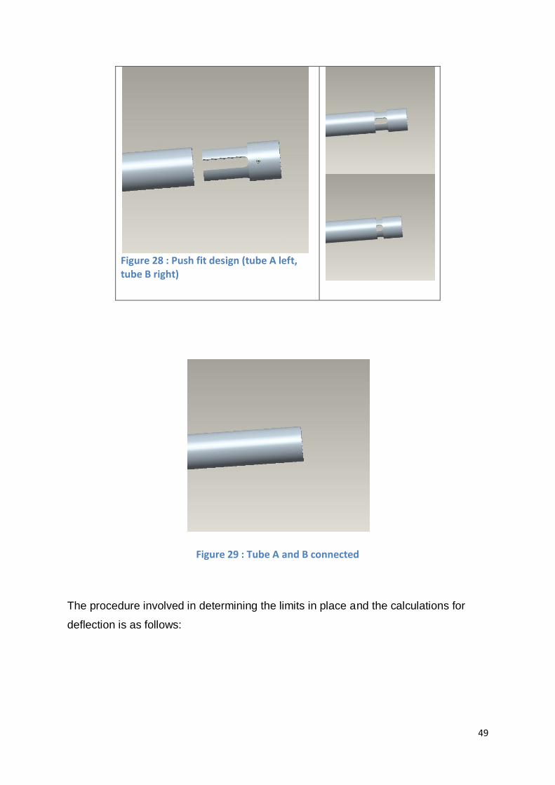
Push fit
Similar to the above concept the instrument is divided into two sections. For the
purpose of this description each tube will be referred to in the same manner as
previous (Tube A and tube B, containing the power supply, circuitry and output
connection and the electret capsule respectively). As in the twist fit design material is
removed from the outer diameter of tube B as shown in figure 28. When the piece is
being machined a slight gradient is left on the section closest to that of tube A. This
way its diameter is slightly outside of the dimensions of tube A‟s inner diameter
causing the section of tube B to deflect. This deflection causes normal forces
between the two surfaces when the tubes are connected (figure 29) as tube B is
trying to return to its original position. The theoretical values for these forces were
calculated to ensure that this design was a viable option before being prototyped.
The deflection forces needed to be within two limits. The first so that the forces when
multiplied by the friction coefficient of the steel tube were greater than that exerted
on the top cap by the battery contact or spring and the second is that the deflection
forces are lower than that exerted by the user when being inserted into tube A.
5 A condition that occurs when a rotating fastener is misaligned with a tapped hole (cross threading, 2010).
49
Figure 28 : Push fit design (tube A left, tube B right)
Figure 29 : Tube A and B connected
The procedure involved in determining the limits in place and the calculations for
deflection is as follows:
50
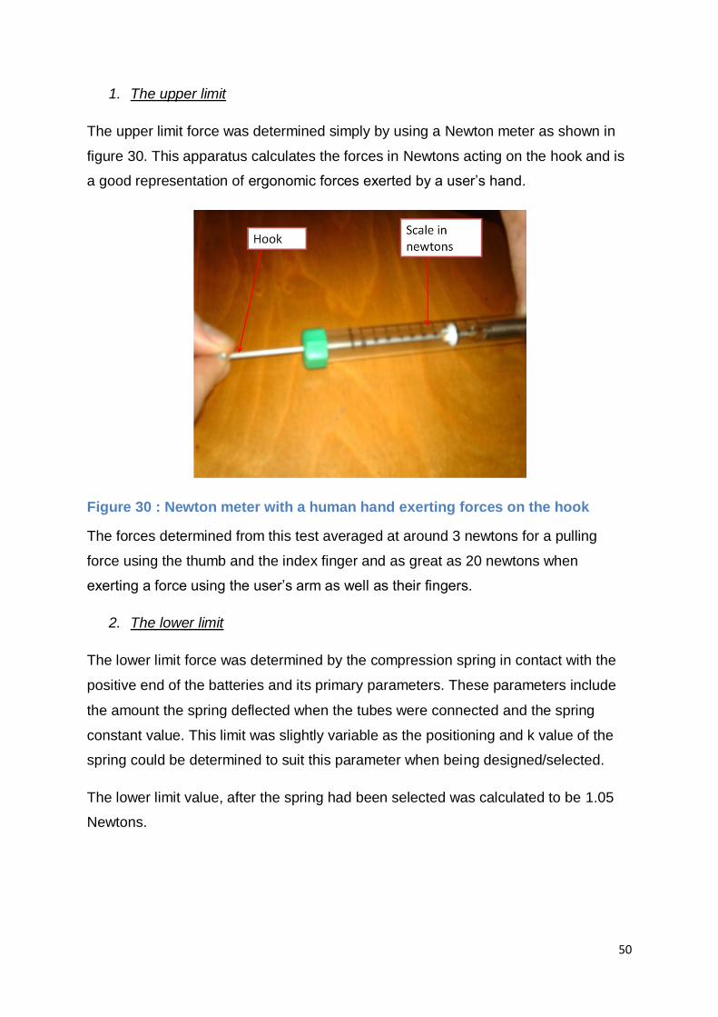
1. The upper limit
The upper limit force was determined simply by using a Newton meter as shown in
figure 30. This apparatus calculates the forces in Newtons acting on the hook and is
a good representation of ergonomic forces exerted by a user‟s hand.
Figure 30 : Newton meter with a human hand exerting forces on the hook
The forces determined from this test averaged at around 3 newtons for a pulling
force using the thumb and the index finger and as great as 20 newtons when
exerting a force using the user‟s arm as well as their fingers.
2. The lower limit
The lower limit force was determined by the compression spring in contact with the
positive end of the batteries and its primary parameters. These parameters include
the amount the spring deflected when the tubes were connected and the spring
constant value. This limit was slightly variable as the positioning and k value of the
spring could be determined to suit this parameter when being designed/selected.
The lower limit value, after the spring had been selected was calculated to be 1.05
Newtons.

51
3. The deflection forces
The method for calculating the deflection forces was a finite element analysis which
is discussed in chapter 3 and verified by a simple model to ensure accuracy. Matlab
was used to compute the calculations for the finite element analysis so that a higher
number of elements could be calculated for and therefore achieve greater accuracy
in results. The code can be found in the attached appendix 4. Recalling equation 3-
27 to calculate the bending forces:
The parameters that are fixed due to design constraints for the Finite element
analysis are inputted into the program by the user. These include the Young‟s
modulus of the material ( ), the length of the section of analysis ( and the required
deflection (y) and width of each element (w).
The variable in the equation is the thickness of each element across the structure.
The force required to deflect wall of the tube by 0.5mm is calculated to be 19.9
Newtons for the finite element analysis. The simple model calculated a similar force
of 22.3 Newtons.
Taking the average of the two methods of calculation and multiplying it by the friction
coefficient of stainless steel 316 to calculate the forces restricting motion between
the two surfaces was identified.
The calculated normal force between the surfaces of tube B and tube A was
calculated to be 21.16 Newtons. By multiplying this by the friction coefficient of 0.15
for stainless steel 316 (Finishing, 2010) by the calculated forces a value of 3.16
Newtons was found.
The calculated value for the friction forces falls within the upper and lower limits from
section 1 and 2 above.
52
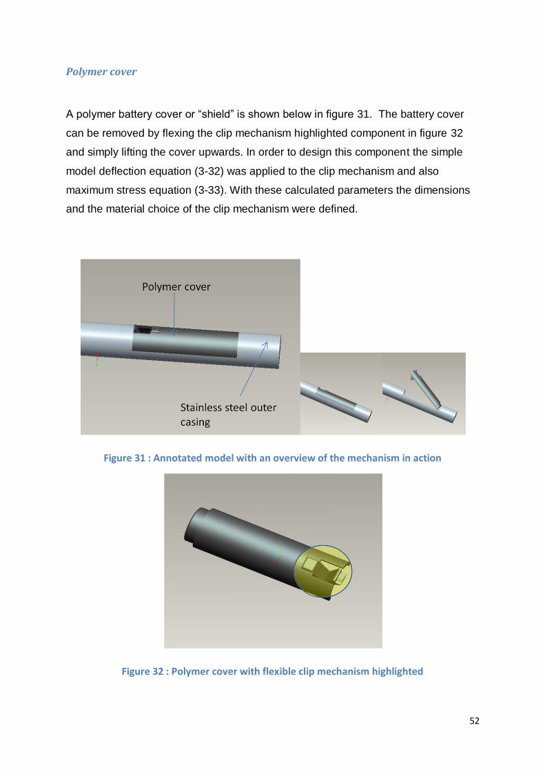
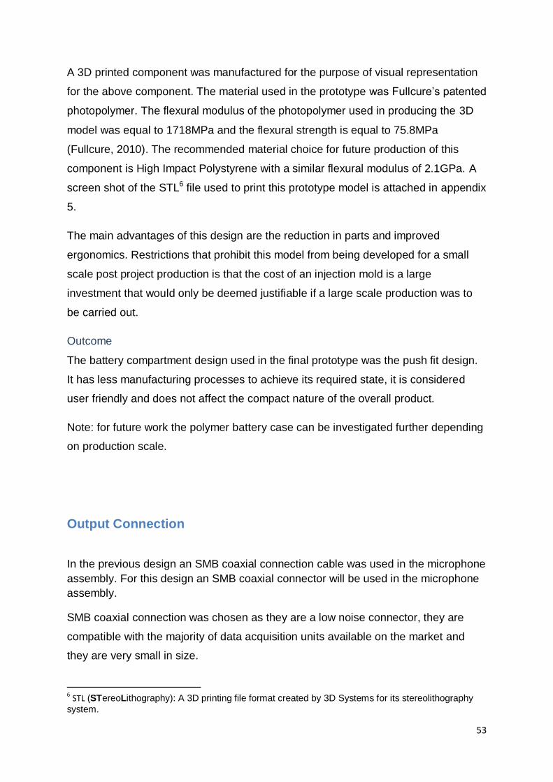
Polymer cover
A polymer battery cover or “shield” is shown below in figure 31. The battery cover
can be removed by flexing the clip mechanism highlighted component in figure 32
and simply lifting the cover upwards. In order to design this component the simple
model deflection equation (3-32) was applied to the clip mechanism and also
maximum stress equation (3-33). With these calculated parameters the dimensions
and the material choice of the clip mechanism were defined.
Figure 31 : Annotated model with an overview of the mechanism in action
Figure 32 : Polymer cover with flexible clip mechanism highlighted
53
A 3D printed component was manufactured for the purpose of visual representation
for the above component. The material used in the prototype was Fullcure‟s patented
photopolymer. The flexural modulus of the photopolymer used in producing the 3D
model was equal to 1718MPa and the flexural strength is equal to 75.8MPa
(Fullcure, 2010). The recommended material choice for future production of this
component is High Impact Polystyrene with a similar flexural modulus of 2.1GPa. A
screen shot of the STL6 file used to print this prototype model is attached in appendix
5.
The main advantages of this design are the reduction in parts and improved
ergonomics. Restrictions that prohibit this model from being developed for a small
scale post project production is that the cost of an injection mold is a large
investment that would only be deemed justifiable if a large scale production was to
be carried out.
Outcome
The battery compartment design used in the final prototype was the push fit design.
It has less manufacturing processes to achieve its required state, it is considered
user friendly and does not affect the compact nature of the overall product.
Note: for future work the polymer battery case can be investigated further depending
on production scale.
Output Connection
In the previous design an SMB coaxial connection cable was used in the microphone
assembly. For this design an SMB coaxial connector will be used in the microphone
assembly.
SMB coaxial connection was chosen as they are a low noise connector, they are
compatible with the majority of data acquisition units available on the market and
they are very small in size.
6 STL (STereoLithography): A 3D printing file format created by 3D Systems for its stereolithography
system.

54
Many SMB connections were researched and a number were purchased during
prototyping stages to investigate the selection further and the SMB chosen was
based on ease of assembly and price. Some of the SMB connections investigated
further include SMB Female Straight Plug, clamped SMB straight male jack, SMB
straight female and SMB bulkhead Jack shown below. Methods for assembly for
each connection were investigated and the SMB with the least number of required
assembly operations, required parts and for the best price was integrated into the
design.
Figure 33 : SMB bulkhead male Jack, SMB straight male jack, SMB straight female and Female Straight Plug shown from left to right
The two SMB connectors that were investigated the most of the four connectors
were the male jack type connectors (the first and second from left shown above).
The prime reason for pursuing these models further was that the design enabled the
circuit boards to be fixed to the back of the SMB connector by a push/twisting action.
For both SMB connectors a different assembly method would be required. The first
SMB connector required to be turned and therefore reducing the outer diameter
slightly to achieve a push fit with the outer
casing. The second SMB connector
required that the end of the tube was
rounded like shown in figure 34 and the
SMB connector is inserted into the tube
via the opposite end. This rounding
operation involves customized
manufacturing tools and is not cost beneficial for the purpose of a prototype.
Outcome
The SMB connection chosen for the final prototype was an SMB bulkhead jack. This
component as mentioned above acts as a fixture for the circuit board increasing the
Figure 34 : Tube drawing with a rounded end

55
product‟s durability and reducing the number of components. The SMB coaxial
connector was altered slightly so that a push fit connection could be made between
the SMB and the outer casing and consequently creating a direct path for the ground
of the circuit.
Positive Contact
Compression spring
When choosing a compression spring there are a number of parameters that need to
be defined. Some of these parameters are fixed or constrained by other components
within the assembly while others are variable and interdependent with one another.
The fixed or constrained parameters include the width of the spring, the material and
the stiffness of the spring. The variable parameters are the length of the spring and
the wire diameter. The stiffness of the suitable spring is determined using equation
3-36. The suitable spring stiffness was calculated to be between 0.3 and 0.5
depending on the positioning of the spring within the assembly (see appendix 6).
The positioning of the spring so that it would exert a given force on the ZA10 cells
and battery push fit cap was determined using equation 3-19. This way the spring is
expected to deflect between 3 and 4 mm and exert a force of 1.05 Newtons on the
push fit battery cap.
Conical spring
Similarly the concept for a conical spring was researched but was found that the
smallest conical springs on the market were too large (Raymonddistribution, 2010)
and would inhibit the compactibility of the product. This concept was discarded after
contacting numerous suppliers.
Direct contact
A concept of a direct contact was developed in which the power supply was in direct
contact with a section of the circuit board thus creating a positive connection to the

56
circuit. The main purpose of doing this is to reduce the number of parts and hence
reducing costs and size.
The restriction of this concept is that tolerances would no longer be allowed for in
this section of the assembly. By confining tolerances to such a small scale the cost
of production then inherently increases and the initial purpose of reducing the
number of parts is lost.
Outcome
The small compression spring was used in the final prototype. Reasons for this choice
included the available sizes and the accommodation of inaccurate tolerances.
Negative Contact
Spring contact
Similar to above a spring contact was considered for the negative battery contact.
Direct Contact
As the positive end of the power supply was facilitated by a compression a direct contact
could be designed for the negative contact of the power supply without effecting
tolerances. Using a direct contact reduces the number of parts, therefore reducing cost and
size of the overall design. The direct contact is made between tube B and the batteries as
shown in figure 35. The ground from tube B is transferred through tube A to the earth of the
SMB connection.
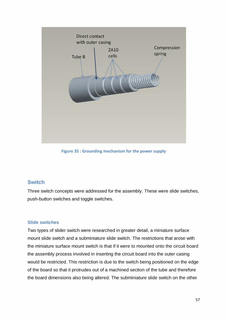
57
Figure 35 : Grounding mechanism for the power supply
Switch
Three switch concepts were addressed for the assembly. These were slide switches,
push-button switches and toggle switches.
Slide switches
Two types of slider switch were researched in greater detail, a miniature surface
mount slide switch and a subminiature slide switch. The restrictions that arose with
the miniature surface mount switch is that if it were to mounted onto the circuit board
the assembly process involved in inserting the circuit board into the outer casing
would be restricted. This restriction is due to the switch being positioned on the edge
of the board so that it protrudes out of a machined section of the tube and therefore
the board dimensions also being altered. The subminiature slide switch on the other
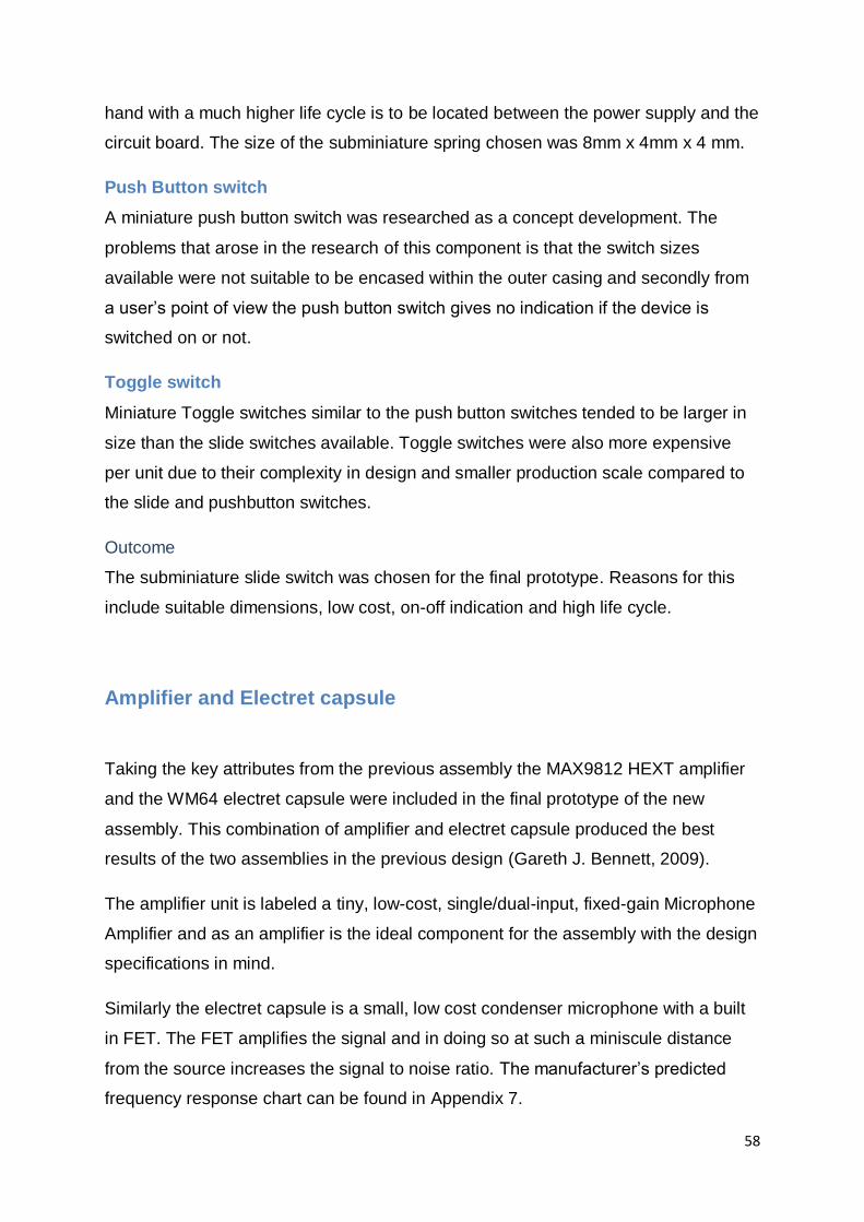
58
hand with a much higher life cycle is to be located between the power supply and the
circuit board. The size of the subminiature spring chosen was 8mm x 4mm x 4 mm.
Push Button switch
A miniature push button switch was researched as a concept development. The
problems that arose in the research of this component is that the switch sizes
available were not suitable to be encased within the outer casing and secondly from
a user‟s point of view the push button switch gives no indication if the device is
switched on or not.
Toggle switch
Miniature Toggle switches similar to the push button switches tended to be larger in
size than the slide switches available. Toggle switches were also more expensive
per unit due to their complexity in design and smaller production scale compared to
the slide and pushbutton switches.
Outcome
The subminiature slide switch was chosen for the final prototype. Reasons for this
include suitable dimensions, low cost, on-off indication and high life cycle.
Amplifier and Electret capsule
Taking the key attributes from the previous assembly the MAX9812 HEXT amplifier
and the WM64 electret capsule were included in the final prototype of the new
assembly. This combination of amplifier and electret capsule produced the best
results of the two assemblies in the previous design (Gareth J. Bennett, 2009).
The amplifier unit is labeled a tiny, low-cost, single/dual-input, fixed-gain Microphone
Amplifier and as an amplifier is the ideal component for the assembly with the design
specifications in mind.
Similarly the electret capsule is a small, low cost condenser microphone with a built
in FET. The FET amplifies the signal and in doing so at such a miniscule distance
from the source increases the signal to noise ratio. The manufacturer‟s predicted
frequency response chart can be found in Appendix 7.

59
Other components
Flag System
The integration of a flag system so that the user could be warned when the power
supply has dropped below a certain voltage was considered. Initially the concept of
an LED to be included in the circuit so that when the circuit is complete that the LED
would light up. This concept was quickly replaced with an alternative solution of
using a comparator within the circuit. By using a comparator the LED will light up
once the voltage has fallen below a determined voltage using resistors within the
circuit. The voltage chosen was 4.5 volts and was determined in the design by
positions resistors within the circuitry, values of which were calculated using
equation 3-34 and 3 -35 (Kirchhoff‟s and ohm‟s law). Due to the small size of the
circuit board and the small scope for expanding its dimensions a nanopower
comparator was decided upon. The nanopower comparator chosen was one which
displayed an extremely low current draw of 600nA current. For this reason the
comparator would have negligible effect on the battery life.
Battery Insulation
Selections of battery insulation were trialled in order to find the best fit and material
to insulate the batteries from the outer casing which is a conductive material. A
number of thin walled heat shrink insulations were tested and also a number of
plastic drinking straws.
The plastic drinking straws were less flexible than the majority of the heat shrink
insulation selection and therefore more advantageous in terms of supporting the
batteries inside the outer casing.
The main determining factor in this situation as it is such a small component is the
dimensions as they need to be within the limits specified. These were less than
6.6mm for the outer diameter and greater 5.8mm for the inner diameter. Being within
these limits allows for the insulation to fit within the outer casing and enclose the
batteries chosen.

60
Chapter 6 Final Design
In this chapter the outcomes from each subsection of the assembly discussed in the
previous chapter are elaborated on in terms of the overall product, interconnections
with other subsections and the relevant manufacturing or assembly stages involved.
A bill of materials is presented with costing for an initial batch of 75 units included
and finally an overview of the final prototype is included with all the relevant
documentation included in the chapter or in the referenced appendices.
The final prototype is shown in figure 36 (for further images see Appendix 8)
Figure 36 : The final prototype (8mm outer diameter, 90mm length)
Tube A is connected to tube B via the push fit design discussed in chapter 6. The
LED and slide switch are positioned near the centre of the design as shown and the
electret capsule and SMB fixed with a push fit at
opposite ends of the design.
The final prototype is compact and lightweight.
Dimensions: 8mm outer diameter and 90mm in
length
Weight: 15g

61
The internal layout of components within the assembly is as shown in figure 37.
Figure 37 : 3D model of internal layout of components within the final prototype
From figure 37 it can be seen that the amount of space within tube A is utilized as
much as possible. A schematic of the internal layout can be found in appendix 9. The
amplifier and comparator are mounted on the circuit board along with the LED and
the required resistors and capacitors. A full wiring diagram and circuit board design
are shown in figure 38 and figure 39 respectively.

62
R2
Op Amp
+
-
20dB
max9812h
refR1
mic
SMB
3
2
4
1
5
6
R4
1
1.25
4
3
2
5
R3
C2
max9118
C1
C3
Figure 38 : Power supply, amplifier, flag system and electret wiring diagram
Part Detail
R1 2.2K,Chip resistor
R2 390K,Chip resistor
R3 1M,Chip resistor
R4 1K,Chip resistor
C1 0.1uF, capacitor
C2 0.1uF, capacitor
C3 0.1uF, capacitor Table 5 : Resistor and capacitor values for the above wiring diagram
5.6V
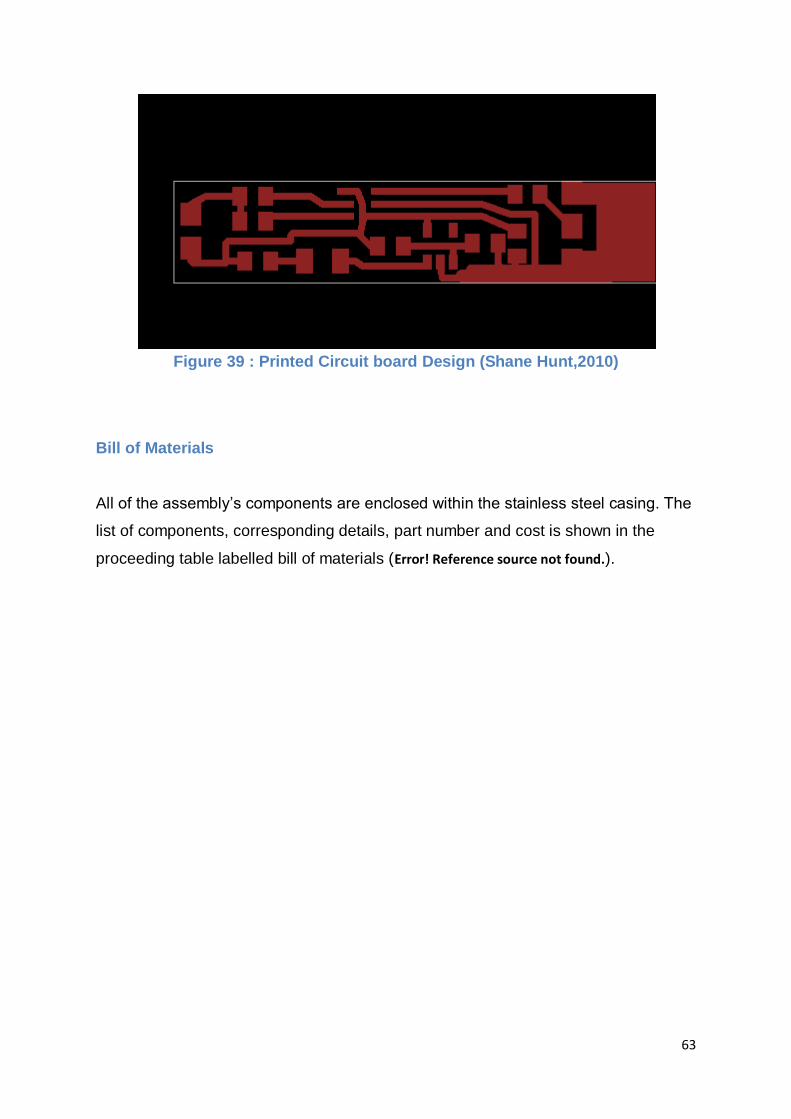
63
Figure 39 : Printed Circuit board Design (Shane Hunt,2010)
Bill of Materials
All of the assembly‟s components are enclosed within the stainless steel casing. The
list of components, corresponding details, part number and cost is shown in the
proceeding table labelled bill of materials (Error! Reference source not found.).
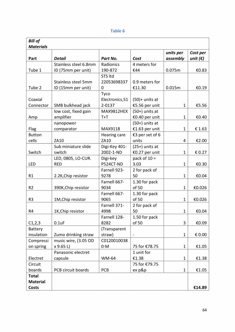
64
Table 6
Bill of Materials
Part Detail Part No. Cost units per assembly
Cost per unit (€)
Tube 1 Stainless steel 6.8mm ID (75mm per unit)
Radionics 190-872
4 meters for €44 0.075m €0.83
Tube 2 Stainless steel 5mm ID (15mm per unit)
STS ltd 220536983370
0.9 meters for €11.30 0.015m €0.19
Coaxial Connector SMB bulkhead jack
Tyco Electronics,512-0137
(50)+ units at €5.56 per unit 1 €5.56
Amp low cost, fixed gain amplifier
MAX9812HEXT+T
(50+) units at €0.40 per unit 1 €0.40
Flag nanopower comparator MAX9118
(50+) units at €1.63 per unit 1 € 1.63
Button cells ZA10
Hearing care ZA10
€3 per set of 6 units 4 €2.00
Switch Sub miniature slide switch
Digi-Key 401-2002-1-ND
(25+) units at €0.27 per unit 1 € 0.27
LED LED, 0805, LO-CUR. RED
Digi-key P524CT-ND
pack of 10 = 3.03 1 €0.30
R1 2.2K,Chip resistor Farnell 923-9278
2 for pack of 50 1 €0.04
R2 390K,Chip resistor Farnell 667-9034
1.30 for pack of 50 1 €0.026
R3 1M,Chip resistor Farnell 667-9065
1.30 for pack of 50 1 €0.026
R4 1K,Chip resistor Farnell 371-4998
2 for pack of 50 1 €0.04
C1,2,3 0.1uF Farnell 128-8282
1.50 for pack of 50 3 €0.09
Battery insulation Zumo drinking straw
(Transparent straw) - 1 € 0.00
Compression spring
music wire, (3.05 OD x 9.65 L)
C01200100380-M 75 for €78.75 1 €1.05
Electret Panasonic electret capsule WM-64
1 unit for €1.38 1 €1.38
Circuit boards PCB circuit boards PCB
75 for €79.75 ex p&p 1 €1.05
Total Material Costs €14.89

65
Manufacturing and Assembly process
1. For the purpose of a prototype the surface mounted components were
soldered by hand using a fine tip soldering iron and a macroscope. In future
the circuit boards are to be populated using a reflow oven, one of which is
available for use in Trinity College‟s electronics department.
2. The two tubes used for the outer casing were machined to specification (see
drawings appendix 10 and 11) using a lathe and a milling machine. In future
automated processes available in Trinity‟s mechanical department can be
used for batch quantities. This will keep manufacturing costs low. The quoted
price for each tube to be machined to specification using the Okuma LT15M
CNC machine is estimated to be €2.50 per tube for each unit and this figure
includes set-up time (estimated 2 hours total) costs (Reilly, 2010). The CNC
machine is capable of machining up to 240 components per hour at extremely
high precision when coupled with the available bar feeder, the LNS Quickload.
3. The SMB requires to be turned on a lathe to reduce the outer diameter so that
a push fit can be achieved with the outer casing.
4. The circuit board is fixed to the SMB connection with a push/twist fit. To do
this the edges of the board are filed slightly so that the board can simply
twisted into the tapped section of SMB. A direct solder connection is then
made between the SMB earth and the circuit board‟s earth.
5. The slide switch is firstly connected via wire to the compression spring and
placed within the outer casing. So that the slide switch is firmly held in place
within the assembly glue is injected using a glue-gun through a hole in the
outer casing at the back of the switch‟s position. The hole is purely for this
purpose and is set at the same diameter as the hole for the LED light and the
section removed for the switch to protrude out of. This way the same
machining tool can be used for all three operations. Only a small amount of
glue is required to fix the switch in place. NOTE: ensure that the signal wire
connecting the electret capsule and the circuit board is placed inside the tube
so that it is bypassing the switch before adding glue.

66
6. A 20mm length of the battery insulation (Zumo straw) is placed in the tube so
that the spring and batteries are insulated from the outer casing but leaving
the signal cable travel along the outside of the insulation.
7. The signal wire is soldered to the electret capsule at one end and the circuit
board at the other. This can be done after the electret capsule has been
placed in the push fit cap or before once the signal is passed through the
push fit cap.
8. Finally the wire attaching the slide switch to the circuit board terminal is
soldered and the SMB is pushed into the tube end.
9. When this is complete four ZA10 batteries can be inserted and the
microphone is ready for testing.
Costing
Manufacturing Costs
Part Detail Machinery/equipment personnel
cost per unit
Cost per batch of 75
Tube A
switch section and two holes machined
Okuma CNC machine
Automated* € 2.50 € 187.50
Tube B
External and internal diameter machined with 4 slits machined
Okuma CNC machine
Automated* € 2.50 € 187.50
Circuit Board
Board mounted components soldered in specified position
Reflow oven
Automated* € 3.00 € 225.00
SMB Outer diameter machined to 6mm Lathe
Mechanical technician € 0.50 € 37.50
wiring Required soldering of components
Soldering iron
Electric Technician € 3.00 € 225.00
Switch Adding adhesive to fix the switch in place Glue gun
Electric Technician € 0.50 € 37.50
Assembly
Fitting components into specified position within casing Technician € 1.50 € 112.50
Total €
13.50 € 1,012.50 * = Automated process that requires a manual set up operation which has
been incorporated in the cost per unit.

67
Batch Material Costs
Part Cost per unit (€) Cost for batch of 75 units
Tube 1 €0.83 €62.25 Tube 2 €0.19 €14.25
Coaxial Connector €5.56 €417.00 Amp €0.59 €44.25
Flag €1.63 €122.25 Button cells €2.00 €150.00
Switch €0.27 €20.25 LED €0.30 €22.50
R1 0.04 €3.00 R2 0.026 €1.95
R3 0.026 €1.95 R4 0.04 €3.00
C1,2,3 0.09 €6.75 Compression spring €1.05 €78.75
Electret €1.38 €103.50 Circuit boards €1.05 €79.00
Total Material Costs €15.08 €1,130.65 Note: the above costs do not take into account the service costs to date. These can
be found in chapter 10, Project Management.

68
Chapter 7 Testing
The final prototype of the electrets based measurement microphone was tested
against a reference microphone. The reference microphone was a high quality
measurement microphone, manufactured by G.R.A.S, model BF40. The tests carried
out were to analyse for the electret microphone‟s sensitivity, noise floor, frequency
response and upper dynamic limits. These results were compared to that of the
G.R.A.S assembly for analysis purposes. Tests were carried out at room
temperature in a laboratory environment.
Sensitivity at 1kHz
An initial test was carried out on the two microphone assemblies using a Bruel &
Kjaer Sound Level Calibrator Type 4231. This apparatus exposes the microphone to
94dB or 1 Pa at 1kHz by positioning the microphone against the calibrator‟s signal
source.
The results were 0.0623 V/Pa and 0.00358496 V/Pa for the electret assembly and
the G.R.A.S assembly respectively. As a 20dB gain of the MAX9812H op amp is
equivalent to an order of magnitude increase, these results and the result from the
reference assembly are consistent with the supplier‟s documentation.
As these results are calculated at 1kHz only, multiplication by this number assumes
a flat frequency response. As this is usually not the case, when analysing the results
this assumption must be taken onboard and addressed if any large deviations arise
at much higher or lower frequencies than 1kHz.
Frequency response
In this stage of testing the two microphone assemblies are flush mounted at the
sealed end of a cylindrical duct. This is so that both microphone assemblies are
exposed to the same acoustic field. As discussed in the theory section of this report,
below the cut-off frequency of the duct, only plane waves will propagate down the
duct and only these wave forms can used for analysis. Therefore, the microphones
that are flush mounted parallel to one another are exposed to the same sound field
radiated by the loudspeaker located at the open end of the duct.

69
Rig and Apparatus:
A schematic of the test rig is shown below in
Figure 40 : Schematic of test rig used for the frequency response function test, noise floor test and auto-spectra plot.
An impedance tube of internal diameter 50mm was used during testing of the
microphone against the reference microphone. By using an impedance tube of this
diameter the cut off frequency is calculated to be 3701Hz using equation 3-11.
The data was acquired from the microphone assemblies using a National
Instruments analog to digital (A/D) convertor. The A/D convertor can sample each
channel simultaneously with 24-bit resolution. Labview software was used to control
the acquisition system during testing and to save the data to the hard disc of the
laptop (to view program set-up see appendix 12). Matlab was used post testing to
process the data into a visual format for analysis purposes. The Matlab code is
attached in appendix 13. To calculate the frequency response function equation 7-1
was used and the spectral estimate parameters are shown in table 7.
The frequency response function (Piersol, 1986) is calculated by:
7-1

70
Where the single sided average cross-spectrum is defined by
7-2
And similarly the auto spectrum is calculated using equation 7-3 shown below.
7-3
Parameter Value
Segment Length (data points per segment, N) 1024
Sample rate (fsamp, Hz) 8192 Segment length (Td = N/fsamp, s) 0.125
Sampling interval (∆t = 1/fsamp, s) 1.22E-
04
Frequency step (∆f = 1/Td, Hz) 8 Upper frequency limit (fc = fsamp/2, Hz) 4096
No. of frequencies, Ly = N/2 512 No. of independent averages (nd) 80
Overlap 0 Sample length (s) 10
Table 7 : Spectral estimate parameters
Noise floor Test
The test to see the lower dynamic range of the microphone was carried out and is
referred to as the noise floor test. It is carried out in a relatively quiet environment.
The results and proceeding discussion of results can be seen in chapter 8, figure 41.
White Noise Test
The white noise test consisted of the apparatus in the schematic diagram shown in
figure 40. The speaker radiated white noise down the impedance tube. Both
microphones were calibrated according to the measured sensitivities. The plot for the
auto-spectrum for both assemblies is shown in chapter 8, figure 42

71
Chapter 8 Results and Discussion
The results from the noise floor test are shown below in figure 41. From this plot we
can see that the electret based measurement microphone has a much lower noise
floor than the GRAS microphone. Reasons for this include the thermal movement of
the diaphragm in the GRAS assembly‟s transducer and also electrical noise from the
circuitry. As discussed in chapter 5 an AC power supply contributes greater levels of
electric noise and as the electret assembly uses a DC power supply it is not
subjected to this electrical noise. Another point to note is that the electret assembly‟s
signal is amplified at a much closer proximity to the source of the signal (within the
assembly casing) so that the signal is amplified before any electrical noise is
generated and therefore the signal to noise ratio is much greater than that of
microphones externally amplified.
Figure 41 : Noise floor for electret based measurement microphone and
G.R.A.S microphone within an impedance tube

72
The peaks occurring in the electret assembly‟s response are due the standing waves
present at these frequencies within the impedance tube. As can be seen these
frequencies are picked by the GRAS assembly at the very low end of the frequency
spectrum but due to its higher „lower limit‟ for its dynamic range it can no longer pick
up these resonant frequencies. The electret assembly on the other hand can pick up
these frequencies due to the reasons explained above. These frequencies are
present due to air flow within the room and external sources of vibration causing the
air inside the impedance tube to resonate.
The noise floor for the GRAS assembly is showing to be around 30dB while the
noise floor of the electret based assembly is levelling off at around 7dB. To put into
perspective how low an amplitude level this is, a person breathing produces a 10dB
noise level (Industry, 2005).
Figure 42 : Auto-spectra for electret based measurement microphone and
G.R.A.S – white noise in impedance tube

73
The auto-spectra plot shows the results of the white noise test for the two
microphone assemblies. The peaks in both of the assemblies‟ results are due to the
modes of the duct as explained in the discussion of the noise floor test results. The
Matlab program used to calculate the resonant frequencies of the duct is attached in
appendix 14 and 15 along with the results. The first four modes are 103Hz, 309Hz,
516Hz and 722Hz respectively which correspond to that of the plot shown above.
The results are shown for a bandwidth of 0 to 4000Hz. The reason for this is that the
frequency cut off for the duct is calculated to be 3701Hz from equation 3-31 and
above this frequency plane waves no longer propagate down the duct and
evanescent waves are present which cannot be used in analysis.
From the plot we can see that there is a very small increase in magnitude between
the range of 1500Hz and 3500Hz in the electret assembly‟s auto-spectrum plot
compared to that of the GRAS assembly. This can be understood and compensated
for by calculating the frequency response function between the two assemblies.
Figure 43 : Frequency response function electret / reference assembly – Magnitude
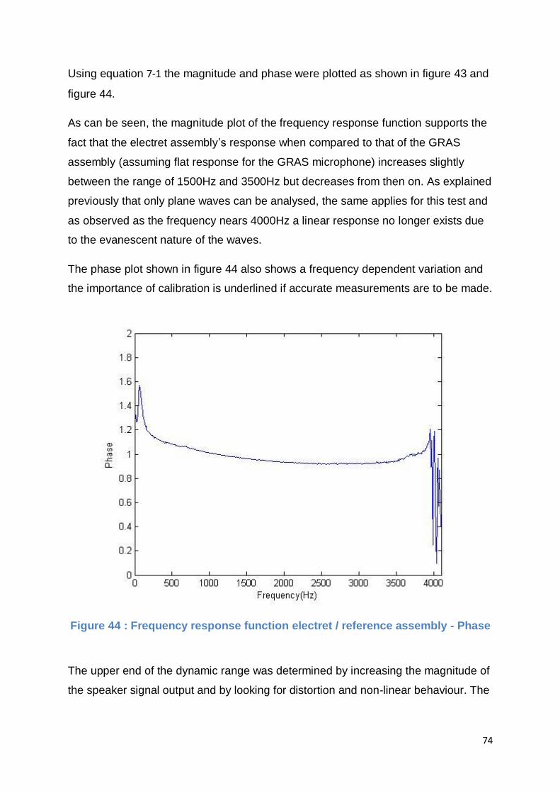
74
Using equation 7-1 the magnitude and phase were plotted as shown in figure 43 and
figure 44.
As can be seen, the magnitude plot of the frequency response function supports the
fact that the electret assembly‟s response when compared to that of the GRAS
assembly (assuming flat response for the GRAS microphone) increases slightly
between the range of 1500Hz and 3500Hz but decreases from then on. As explained
previously that only plane waves can be analysed, the same applies for this test and
as observed as the frequency nears 4000Hz a linear response no longer exists due
to the evanescent nature of the waves.
The phase plot shown in figure 44 also shows a frequency dependent variation and
the importance of calibration is underlined if accurate measurements are to be made.
Figure 44 : Frequency response function electret / reference assembly - Phase
The upper end of the dynamic range was determined by increasing the magnitude of
the speaker signal output and by looking for distortion and non-linear behaviour. The

75
plot shown figure 45 displays the RMS7 voltage to the loud speaker against the RMS
voltage measured by the acquisition system. The output voltage from the
microphones has been converted to Pascals to allow SPL (Sound pressure level) in
dB to be determined.
From the plot it can be seen that both responses are very similar. The assemblies
have slope values of 259 and 279 for the Electret and GRAS assembly respectively.
These slope values are very similar illustrating that the response of both
microphones‟ upper dynamic range are very similar. In this test the GRAS assembly
was capable of displaying amplitude levels of 120dB while the electret assembly was
capable of displaying amplitude levels of 119dB.
Figure 45 : Input/ Output relationship for both assemblies
The previous electret based measurement microphone design, discussed in chapter
1, showed a non linear response when the input/output relationship was plotted. This
can be seen in appendix 1. Potential reasons for differences in results include a 7 Root mean square

76
different testing environment; testing was previously carried out in a narrow
impedance tube and therefore exposed to a wider bandwidth of plane waves and the
differences in the electret capsules sensitivity. To elaborate further, the previous
WM-64 electret capsule assembly displayed 0.0793V/Pa for its tested sensitivity,
while the new assembly was less sensitive displaying a value of 0.0623V/Pa.

77
Chapter 9 Future Work
This work produces a low cost, high functionality measurement microphone in the
form of a compact assembly. The next stage in developing this product would entail
further performance testing, an initial batch production and the application of the
microphone into a number of scenarios.
Further Testing
Further investigation using a small diameter impedance tube would be
recommended to test the characteristics and responses of the microphone in greater
depth. Incorporating statistics such as t-distributions to ensure that the results from
each test are accurate would be highly beneficial.
Initial Batch
Costing has been carried out for an initial batch with the methods of manufacture
briefly described in chapter 6. Automated methods of manufacture that are available
at Trinity College Dublin should be availed of where possible to reduce costs and to
increase manufacturing precision and efficiency. Statistical quality control methods
such as 6sigma can be applied in manufacturing this initial batch to ensure high
quality products and that all specifications fall within the quality control limits.
Before commencing the initial batch production some of the more expensive
microphone components should be investigated further in order to find lower cost
alternatives. Although procurement was a key factor in selecting components and a
vast amount of time was dedicated to this, time restriction of the thesis completion
meant that for one or two components, a cheaper supplier may possibly be sourced
once time constraints are removed.
Application into other research projects
As measurement microphones are currently being used in the fluids labs as well as
other departments within Trinity (Media Technology Department), the new electret
assembly could be applied in multiples to those already undergoing research

78
projects to help improve accuracy levels. The microphone could also be used for
acoustic consultancy services within the college.
Testing within other applications
Tests can be performed using the microphones outside of laboratory settings such
as free field recordings in external environments, studio recording and venue
acoustics. These examples stem from large markets where measurement
microphones are already being used and can be considered a potential commercial
exploitation of the product.
Large scale batch production
There is market potential for a large scale production of the measurement
microphone presented in this project. A polymer casing, as discussed in chapter 6,
has been designed for the purpose of a large scale batch production model. This
model can be considered slightly more user friendly as no wires are exposed when
changing batteries and is ideal for out of laboratory settings. A 3D model of this
design is shown below.
Figure 46 : Electret based Measurement microphone with incorporated polymer battery cover

79
The large scale production of the measurement microphone will allow for the use of
manufacturing processes which are not considered investible options for a low scale
production of the microphones. An example is injection molding where the initial cost
of a mould can be great, however the piece part cost is low when mass produced, so
with greater quantities the overall price decreases. Along with this is the generic
reduction in component part‟s prices when larger batches are ordered.

80
Chapter 10 Project Management
Project management plays an essential role in the running, control and organization
of any project, no matter how big or small the tasks involved. The primary challenge
of project management is said to involve achieving all of the project goals and
objectives while honouring the project constraints (Lewis, 2006). The secondary
challenge of project management involves optimising the allocation and integration
of inputs necessary to meet all the pre-defined objectives (Stevens, 2002).
The project management plan was drawn up at the beginning with the help of the
project supervisor. The plan included identification and specification of individual
tasks that needed to be carried out. These tasks combined to form work packages
that contained important milestones which needed to be met as this would enable
the project objectives to be achieved.
Microsoft Project was used to keep an electronic record of project progress (see
appendix 16 for Gantt chart), to ensure efficiency and for task organisation. Regular
meetings were held with the project supervisor Dr Gareth Bennett to identify action
points and to review previous and undergoing work. Meetings with other college
personnel were regularly organized. The decimation of information was an ongoing
task over the course of the project as the project was an interdepartmental project
that involved electronic staff as well as mechanical and manufacturing staff.
The project work is originally broken down into smaller work packages to facilitate
organization of tasks and efficient project management. The main work packages
are as follows:
Topic research Background Information: Weeks 1-4 Literature/Publication Review: Weeks 2-6 Preliminary Project Report & Presentation: Weeks 5-7 Conceptual Design Weeks 8-13 Mid Term Report work: Weeks 14-16 Prototyping Weeks 17-20 Final Results and Conclusions: Weeks 22-24 Write-Up and Presentation: Weeks 22-26 Final Report: Weeks 27-28 Project Management: Weeks 1-28
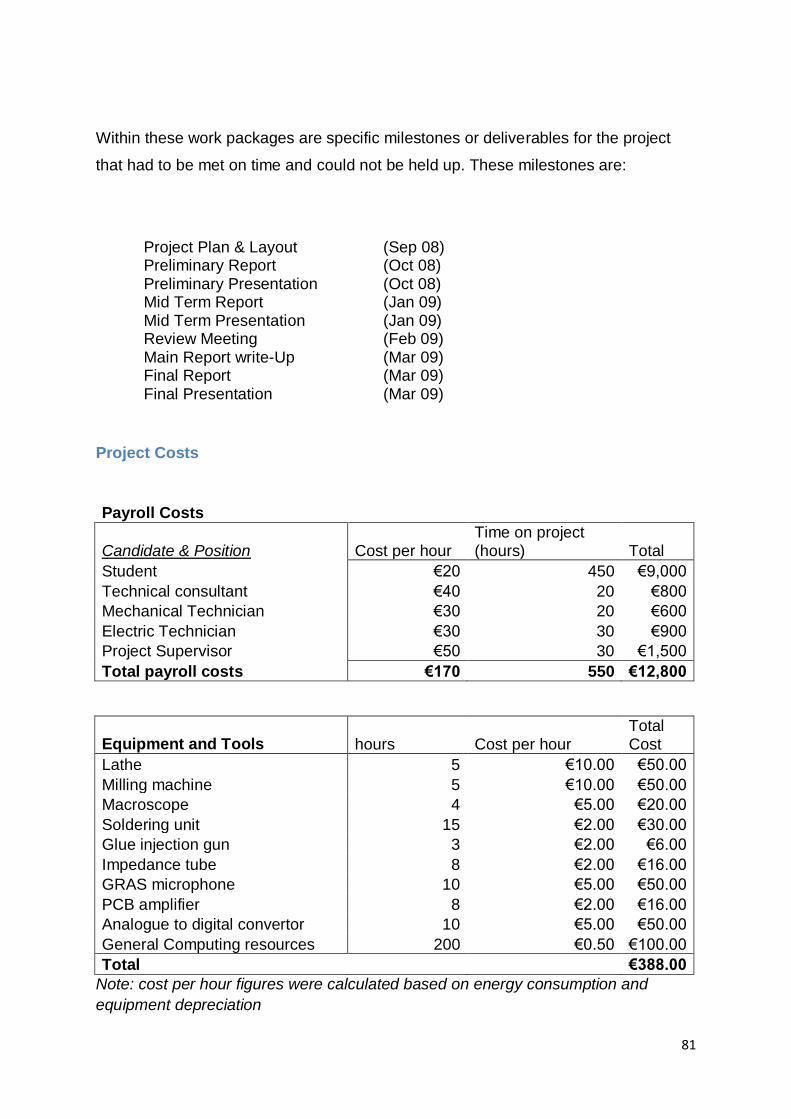
81
Within these work packages are specific milestones or deliverables for the project
that had to be met on time and could not be held up. These milestones are:
Project Plan & Layout (Sep 08) Preliminary Report (Oct 08) Preliminary Presentation (Oct 08) Mid Term Report (Jan 09) Mid Term Presentation (Jan 09) Review Meeting (Feb 09) Main Report write-Up (Mar 09) Final Report (Mar 09) Final Presentation (Mar 09)
Project Costs
Payroll Costs
Candidate & Position Cost per hour Time on project (hours) Total
Student €20 450 €9,000
Technical consultant €40 20 €800
Mechanical Technician €30 20 €600
Electric Technician €30 30 €900
Project Supervisor €50 30 €1,500
Total payroll costs €170 550 €12,800
Equipment and Tools hours Cost per hour Total Cost
Lathe 5 €10.00 €50.00
Milling machine 5 €10.00 €50.00
Macroscope 4 €5.00 €20.00
Soldering unit 15 €2.00 €30.00
Glue injection gun 3 €2.00 €6.00
Impedance tube 8 €2.00 €16.00
GRAS microphone 10 €5.00 €50.00
PCB amplifier 8 €2.00 €16.00
Analogue to digital convertor 10 €5.00 €50.00
General Computing resources 200 €0.50 €100.00
Total €388.00
Note: cost per hour figures were calculated based on energy consumption and
equipment depreciation
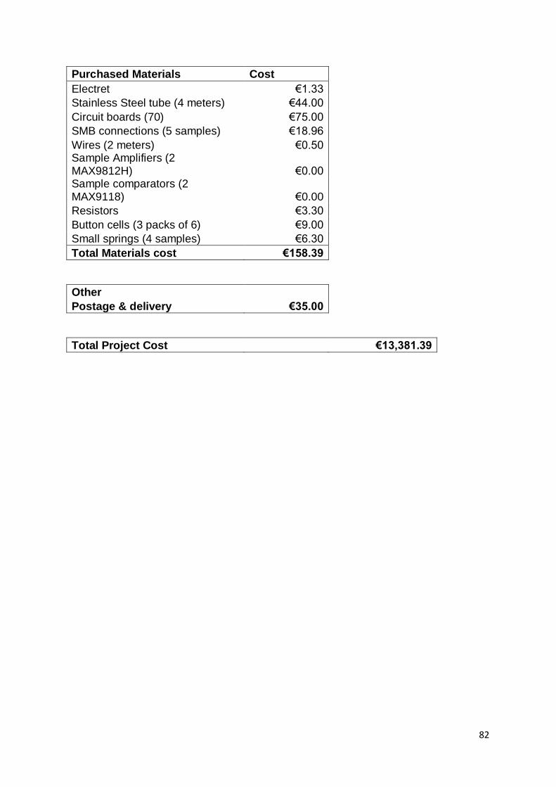
82
Purchased Materials Cost
Electret €1.33
Stainless Steel tube (4 meters) €44.00
Circuit boards (70) €75.00
SMB connections (5 samples) €18.96
Wires (2 meters) €0.50 Sample Amplifiers (2 MAX9812H) €0.00 Sample comparators (2 MAX9118) €0.00
Resistors €3.30
Button cells (3 packs of 6) €9.00
Small springs (4 samples) €6.30
Total Materials cost €158.39
Other
Postage & delivery €35.00
Total Project Cost €13,381.39

83
Chapter 11 Conclusion
The result of this project is a low cost, high functionality electret based measurement
microphone with improved aesthetics, ergonomics, size and versatility compared to
the previous electret based measurement microphone design.
Due to the high level of time and attention given to the design and component
selection process the final design encapsulates the entire required analog
components to perform acoustic testing within an 8mm diameter, 90mm length user-
friendly product.
Test results show that the microphone displays very good functionality compared to
that of a high quality reference microphone. The electret based microphone has a
very low noise floor (7dB), relatively linear response and an overall wide dynamic
range.
The product cost remains low as intended at a material cost of €14.89 per unit.
Machining and assembly costs for a batch of 75 units are estimated to be €15.08 per
unit, bringing the total unit cost to € 29.97 (NOTE: this cost does not entail fixed
overhead such as premises costing and bank rates). The total cost for an initial batch
of 75 units is calculated to be € 2,247.41.
84
Chapter 12 Bibliography A Tiwari, K. V. (2008). Automated inspection using database technology within the
aerospace industry.
Bennett, J. F. (2008). Noise Source Identification for Ducted Fan Systems. American
Institue of Aeronautics and Astronautics Journal , 1663-1674.
Benson, S. T. (2006). Sound source imaging of low flying airborne targets with an
acoustic array.
Britannica. (2009). Electromechanical-transducer. Retrieved from Britannica:
www.britannica.com/EBchecked/topic/183345/electromechanical-
transducer/64020/Microhpnes
Bruel&Kjaer. (2010).
www.bksv.com/products/transducersconditioning/acoustictransducers/microphones/
4957.aspx. Retrieved from www.bksv.com.
BSEN61094-2. (1994). Specification for Measurement Microphones.
C Frazier, D. O. (2000). Acoustic imaging of objects buried in soil. Acoustic Soc Am.
C. Harris and V. Cahill. (2007). An empirical Study of the Potential for Context-Aware
Power. InnsBruck, Austria: UbiComp.
cross threading. (2010). Retrieved from toolingu: http://www.toolingu.com/definition-
700215-22852-cross-threading.html
directproaudio. (2010). Apex220. Retrieved from directproaudio:
http://www.directproaudio.com/product.cfm?directid=55871
Dudgeon, D. E. (1977). Fundamentals of digital array processing. IEEE.
Eagle, J. (2004). The Microphone Handbook. Focal Press.
Elko, G. W. (2004). Audio Signal Processing for Next Generation Multimedia
Communication Systems. Avaya: Avaya Labs.
Engdahl, T. (2000). Microphone Powering. Retrieved from Epanorama:
http://www.epanorama.net/circuits/microphone_powering.html
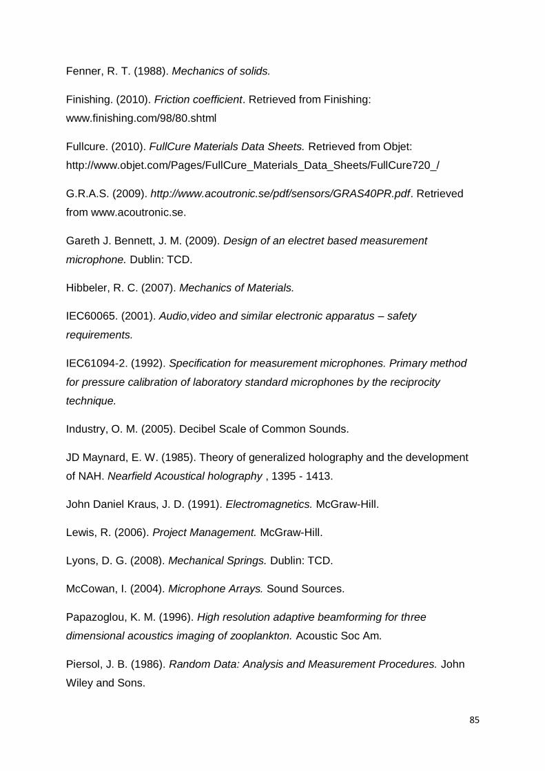
85
Fenner, R. T. (1988). Mechanics of solids.
Finishing. (2010). Friction coefficient. Retrieved from Finishing:
www.finishing.com/98/80.shtml
Fullcure. (2010). FullCure Materials Data Sheets. Retrieved from Objet:
http://www.objet.com/Pages/FullCure_Materials_Data_Sheets/FullCure720_/
G.R.A.S. (2009). http://www.acoutronic.se/pdf/sensors/GRAS40PR.pdf. Retrieved
from www.acoutronic.se.
Gareth J. Bennett, J. M. (2009). Design of an electret based measurement
microphone. Dublin: TCD.
Hibbeler, R. C. (2007). Mechanics of Materials.
IEC60065. (2001). Audio,video and similar electronic apparatus – safety
requirements.
IEC61094-2. (1992). Specification for measurement microphones. Primary method
for pressure calibration of laboratory standard microphones by the reciprocity
technique.
Industry, O. M. (2005). Decibel Scale of Common Sounds.
JD Maynard, E. W. (1985). Theory of generalized holography and the development
of NAH. Nearfield Acoustical holography , 1395 - 1413.
John Daniel Kraus, J. D. (1991). Electromagnetics. McGraw-Hill.
Lewis, R. (2006). Project Management. McGraw-Hill.
Lyons, D. G. (2008). Mechanical Springs. Dublin: TCD.
McCowan, I. (2004). Microphone Arrays. Sound Sources.
Papazoglou, K. M. (1996). High resolution adaptive beamforming for three
dimensional acoustics imaging of zooplankton. Acoustic Soc Am.
Piersol, J. B. (1986). Random Data: Analysis and Measurement Procedures. John
Wiley and Sons.

86
Pro-audio. (2010). MM1 Measurement Microphone. Retrieved from pro-
audio.musiciansfriend: http://pro-audio.musiciansfriend.com/product/-MM-1-
Measurement-Microphone?sku=272045
Raymonddistribution. (2010). Retrieved from www.raymonddistribution.ie
Reilly, M. (2010). Price Quotation.
Rizzoni, G. (2000). Principles and Applications of electrical engineering. Thomas
Casson.
Stevens, M. (2002). Project Management Pathways - Association for Project
Management . APM PUblishing Limited.
Turgoose, G. (2010). PCB Piezotronics Limited. United Kingdom.
Valentino, M. (2008). Microphone Handbook.
Woszczyk, W. R. (1992). Microphone Arrays Optimized for Music Recording.
Montreal: Audio Engineering Society.
zzsounds. (2010). Behringer ECM8000. Retrieved from www.zzounds.com/:
http://www.zzounds.com/item--BEHECM8000

87
Chapter 13 Appendices
Appendix 1 (a)
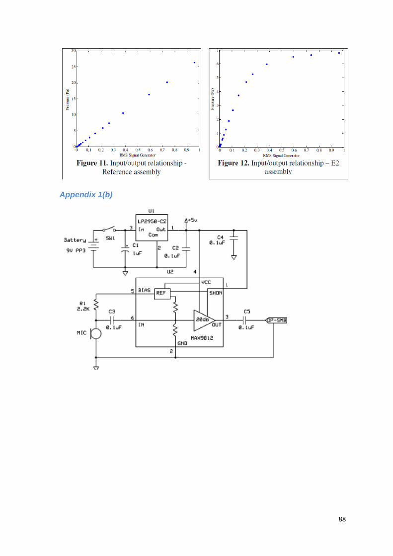
88
Appendix 1(b)
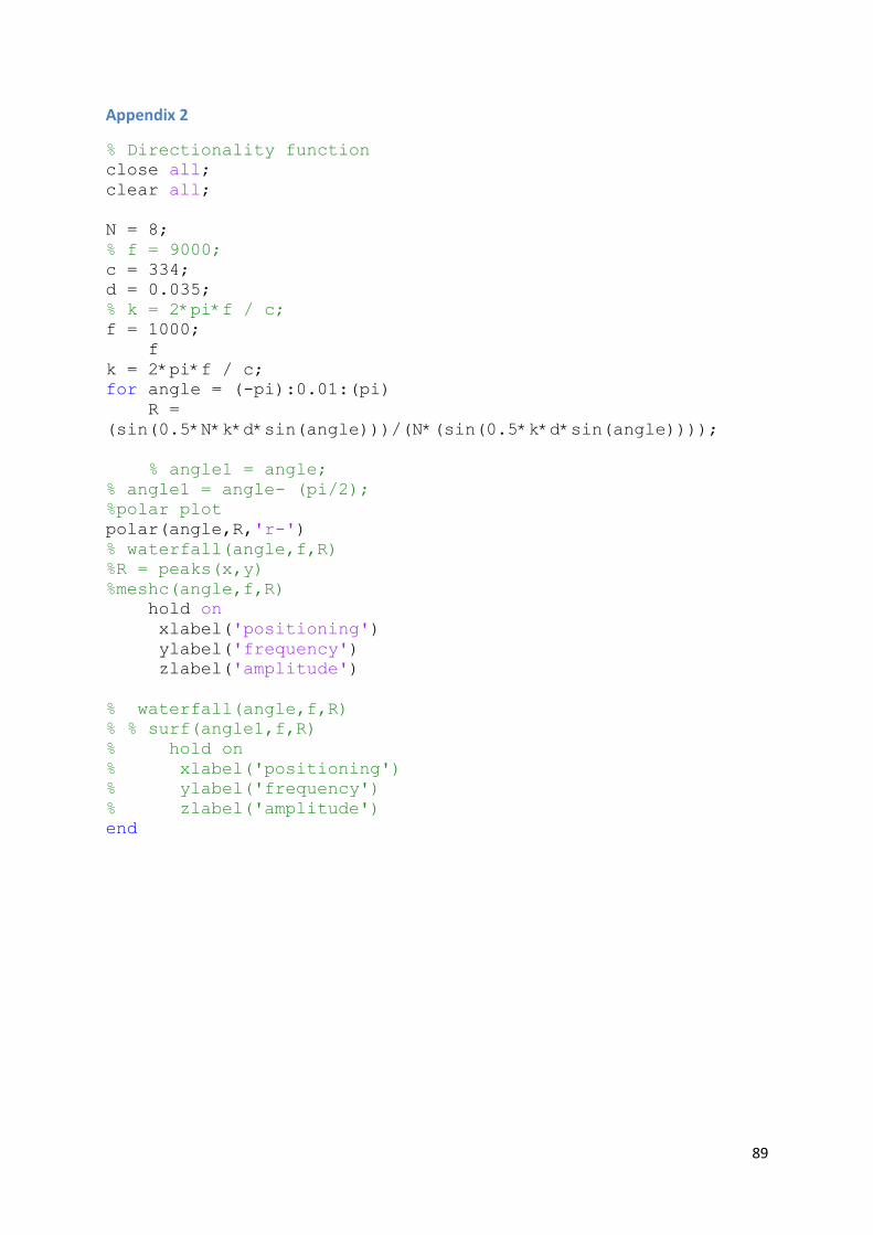
89
Appendix 2
% Directionality function
close all;
clear all;
N = 8;
% f = 9000;
c = 334;
d = 0.035;
% k = 2*pi*f / c;
f = 1000;
f
k = 2*pi*f / c;
for angle = (-pi):0.01:(pi)
R =
(sin(0.5*N*k*d*sin(angle)))/(N*(sin(0.5*k*d*sin(angle))));
% angle1 = angle;
% angle1 = angle- (pi/2);
%polar plot
polar(angle,R,'r-')
% waterfall(angle,f,R)
%R = peaks(x,y)
%meshc(angle,f,R)
hold on
xlabel('positioning')
ylabel('frequency')
zlabel('amplitude')
% waterfall(angle,f,R)
% % surf(angle1,f,R)
% hold on
% xlabel('positioning')
% ylabel('frequency')
% zlabel('amplitude')
end
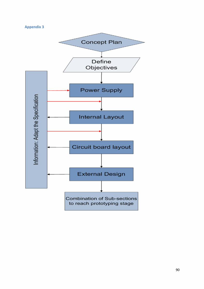
90
Appendix 3

91
Appendix 4
% top cap deflection calculation
% grade 316 young's modulus 193 GPa
E = 193000000000;
% circle equation (x-a)^2 + (y-b)^2 = r^2
%Pressure equation; P = E*4*w*(t^3)*y/(L^3)
%outer_d;
%outer diameter = 7mm as material is removed from 8mm.
r1 = 0.007/2;
a1 = 0.0035;
b1 = 0;
%inner diameter = 5mm....a point is same for both circles
r2 = 0.005/2;
a2 = a1;
b1 = 0;
%wall thickness of tube B
t = 0.001
n = input('please input the number of nodes for calculation');
w = r1 / n;
%w2 = 2*r2 / n;
condition = 0;
y3=0;
x2 = 0.006;
i = 0;
P=0;
while condition == 0
i = i+1
x1 = ((2*r1) - ((i-1)*w))
y1 = b1 + (sqrt((r1^2) - ((x1 - a1)^2)))
%x2 = x1
%x2 = 0.01((2*r1) - (i*w2))
if x1>x2 %let this section be represented as a single
part, calculated in terms of an equivalent square (as it is
similar to a triangle)
y2 = 0;
else
y2 = b1 + (sqrt((r2^2) - ((x1 - a2)^2)))
end
%after circle peaks

92
if x1>0.005
y2=y1;
end
% if y1 < y3
if x1 < r1
condition = 1
% else
% y3 = y1
end
% plot(y1,n)
% hold on
% plot(y2,n)
t = y1 - y2
def = 0.00005;
P1 = E*4*w*(t^3)*(def)/0.015^3;
P = (P + P1);
end
%P3 = 2*P
P3=10;
deflection = def
FEA_force_required = P
%I for semi circle tube
%It = pi*(r1^4)/8 - pi*(r2^4)/8;
%circle with part milled out
circ_o = 2*pi*r1;
circ_i = 2*pi*r2;
%material removed
removed = 0.002;
circ_o_wall = (circ_o/4) - (removed);
circ_i_wall = (circ_i/4) - (removed);
angle1 = circ_o_wall/r1;
angle2 = circ_i_wall/r2;
%moment of inertia for circle wall of an angle i =
%(angle-sin(angle))(r^4)/8
Io = (angle1 - sin(angle1))*(r1^4)/8;
Ii = (angle2 - sin(angle2))*(r2^4)/8;
It = Io -Ii;
deflection_from_ten_newtons_force = (P3)*0.015^3/3*E*It
P2 = (def*3*E*It)/(0.015^3); %
Simple_analysis_force_ = P2
v2 = (P2)*(0.015^3)/(3*E*It); %deflection = P L^3 / 3EI

93
Average = (FEA_force_required+Simple_analysis_force_)/2
friction_coef1 = 0.35;
friction_coef2 = 0.15;
larger = Average*friction_coef1
smaller = Average*friction_coef2

94
Appendix 5

95
Appendix 6
close all;
clear all;
% spring selection program
% F was calculated to be 2 newtons when using an index finger
and a newton
% meter
F = input('please enter the pushing force against the
spring');
% displacement of 4mm
x1 = 4;
% force acting against cap top
x2 = 3;
k = F/x1;
k
F_cap = k*x2;
F_cap
%3.180 12.700 0.500 0.360 6.350 12.000
%k2 = spring constant, d = wire diameter, G = torsional
modulus of
%rigidity, Do = outer diameter, Na = number of coils
k2 = 0.58
d=0.53;
Do=3.76;
Na=10;
F2 = k2*x1
%k2 = ((d^4)*(G))/(8*(Do^3)*Na)
G = (k2*(8*(Do^3)*Na)) / (d^4)
Appendix 7

96
Appendix 8
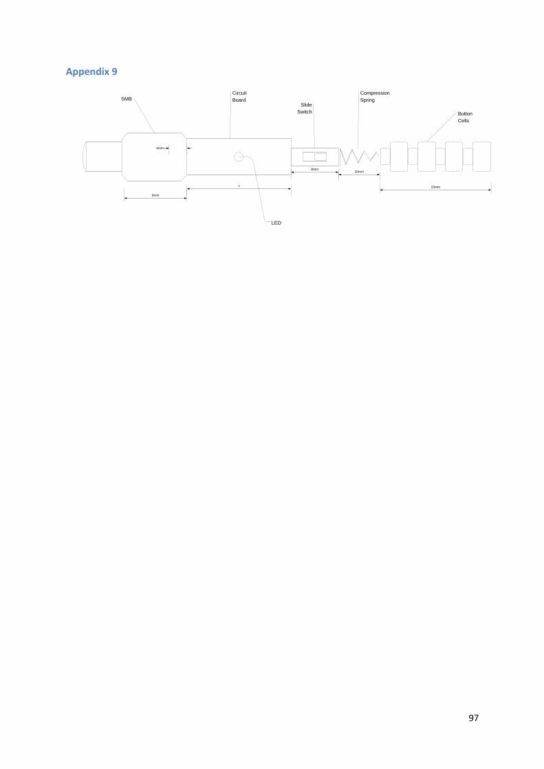
97
Appendix 9
SMB
Circuit
BoardSlide
Switch
Compression
Spring
Button
Cells
9mm
x
4mm
8mm10mm
15mm
LED

98
Appendix 10

99

100
Appendix 11

101

102
Appendix 12
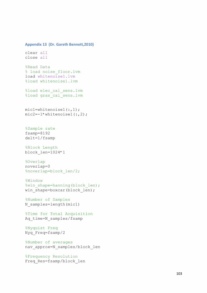
103
Appendix 13 (Dr. Gareth Bennett,2010)
clear all
close all
%Read Data
% load noise_floor.lvm
load whitenoise1.lvm
%load whitenoise1.lvm
%load elec_cal_sens.lvm
%load gras_cal_sens.lvm
mic1=whitenoise1(:,1);
mic2=-1*whitenoise1(:,2);
%Sample rate
fsamp=8192
delt=1/fsamp
%Block Length
block_len=1024*1
%Overlap
noverlap=0
%noverlap=block_len/2;
%Window
%win_shape=hanning(block_len);
win_shape=boxcar(block_len);
%Number of Samples
N_samples=length(mic1)
%Time for Total Acquisition
Aq_time=N_samples/fsamp
%Nyquist Freq
Nyq_Freq=fsamp/2
%Number of averages
nav_approx=N_samples/block_len
%Frequency Resolution
Freq_Res=fsamp/block_len

104
%Taxis
taxis=[0:N_samples-1]*delt;
%Subtract Mean and Determine Calibration Constant (std)
mic1=mic1-mean(mic1);
mic2=mic2-mean(mic2);
%calib_const=std(detrend(mic))
%gras_const=std(mic2)
elec_const=0.0623;
gras_const=0.00358496;
%Divide by Calibration Constant (Signal therefore has std = 1)
mic1_calib=mic1./elec_const;
mic2_calib=mic2./gras_const;
%mic2_calib=mic2;
dB_mic1=10.*log10( ( (std(mic1_calib))./2E-5 ).^2)
dB_mic2=10.*log10( ( (std(mic2_calib))./2E-5 ).^2)
% %Mic 1
figure,
subplot(2,1,1), plot(taxis,mic1_calib,'-x')
subplot(2,1,2), plot(taxis,mic2_calib,'-x')
%Calculate calibrated data
[P_mic1_calib,F_calib] =
cpsd(mic1_calib,mic1_calib,win_shape,noverlap,block_len,fsamp)
;
mag=sqrt(P_mic1_calib*Freq_Res);
db_P_mic1_calib=20*log10(mag/2E-5);
[P_mic2_calib,F_calib] =
cpsd(mic2_calib,mic2_calib,win_shape,noverlap,block_len,fsamp)
;
mag=sqrt(P_mic2_calib*Freq_Res);
db_P_mic2_calib=20*log10(mag/2E-5);
figure,
subplot(1,2,1), plot(F_calib,db_P_mic1_calib)
subplot(1,2,2), plot(F_calib,db_P_mic2_calib)
figure,
subplot(1,2,1), plot(F_calib,db_P_mic1_calib)
axis([0 60 0 90])

105
subplot(1,2,2), plot(F_calib,db_P_mic2_calib)
axis([0 6000 40 90])
figure,
plot(F_calib,db_P_mic2_calib,'r',F_calib,db_P_mic1_calib,'b')
axis([0 Nyq_Freq 0 150])
title('hhh')
legend('Gras','Electret')
xlabel('Frequency (Hz)')
ylabel('SPL (db)')
[Txy,F] =
tfestimate(mic1_calib,mic2_calib,win_shape,noverlap,block_len,
fsamp);
%amplitude ploted to scale of e and phase plotted to pi
figure,
subplot(2,1,1), semilogy(F,abs(Txy))
axis([0 6000 1e-2 1e2])
xlabel('Frequency')
Ylabel('magnitude')
subplot(2,1,2), plot(F,angle(Txy))
axis([0 6000 -pi pi])
xlabel('Frequency')
ylabel('Phase angle')
%unitless plots
figure,
% subplot(2,1,1), plot(F,abs(Txy))
plot(F,abs(Txy))
axis([0 Nyq_Freq 0 2])
xlabel('Frequency(Hz)')
ylabel('Phase')
% subplot(2,1,2), plot(F,angle(Txy))
figure,%
plot(F,angle(Txy))%
axis([0 Nyq_Freq -1 1])
xlabel('Frequency(Hz)')
Ylabel('magnitude')

106
Appendix 14
close all; clear all; %natural resonance frequencies of duct %speed of sound c_s=344; %tube length in meters L=1.2; for n = 0:15 f_n= ((c_s)*((2*n)+1))/4*L end Appendix 15
Longitudinal duct modes
103.2000
309.6000
516
722.4000
928.8000
1.1352e+003
1.3416e+003
1548
1.7544e+003
1.9608e+003
2.1672e+003
2.3736e+003
2580
2.7864e+003
2.9928e+003
3.1992e+003
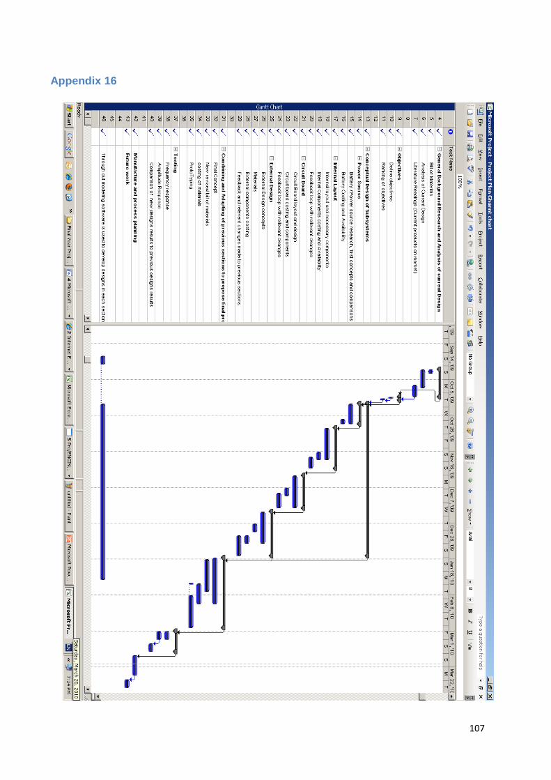
107
Appendix 16