Embed Size (px)
Citation preview
THESIS
ANALYSIS OF THE GROUNDWATER/SURFACE WATER
INTERACTIONS IN THE ARIKAREE RIVER BASIN OF
EASTERN COLORADO
Submitted By:
Ryan Oliver Bailey Banning
Department of Civil and Environmental Engineering
In partial fulfillment of the requirements
For the Degree of Master of Science
Colorado State University
Fort Collins, Colorado
Summer 2010

ii
COLORADO STATE UNIVERSITY
May 12, 2010
WE HEREBY RECOMMEND THAT THE THESIS PREPARED UNDER OUR
SUPERVISION BY RYAN OLIVER BAILEY BANNING ENTITLED ANALYSIS OF
THE GROUNDWATER/SURFACE WATER INTERACTIONS IN THE ARIKAREE
RIVER BASIN OF EASTERN COLORADO, BE ACCEPTED AS FULFILLING IN
PART THE REQUIREMENTS FOR THE DEGREE OF MASTER OF SCIENCE.
Committee on Graduate Work
Kurt D. Fausch
Ramchand Oad
Advisor: Deanna Durnford
Department Head: Luis Garcia

iii
ABSTRACT OF THESIS
ANALYSIS OF THE GROUNDWATER/SURFACE WATER
INTERACTIONS IN THE ARIKAREE RIVER BASIN OF EASTERN
COLORADO
The decline of stream baseflows along Colorado’s high plains streams is
degrading aquatic and riparian habitat. Historic strongholds for many plains fish species
no longer exist. In Eastern Colorado, center-pivot irrigation is common and clearly
contributing to the decline of baseflow in some stream basins. The purpose of this study
is to develop a defensible conceptualization of the stream-aquifer system in the Arikaree
River basin of eastern Colorado, in part using the results of a preliminary groundwater
model developed to predict groundwater levels, analyze stream depletion and examine
the effects of irrigation well retirements on groundwater and stream levels.
The groundwater conceptualization and model represent the Arikaree River
groundwater system of Southern Yuma County where there is significant hydro-
geological connection between the Ogallala and alluvial aquifers. Analytical and
numerical models presented in this thesis calculate seasonal stream-depletion of the
Arikaree River due to nearby wells and similar potential effects of riparian vegetation.

iv
Finally, the author examines the river basin water budget in Southern Yuma County to
determine possible pumping effects on the amount of available water for streamflow and
habitat.
Ryan Oliver Bailey Banning Civil and Environmental Engineering Department
Colorado State University Fort Collins, Colorado 80523
Summer 2010

v
To my loving and patient wife for all of your support. To my family for all of your encouragement throughout my college career.
I love you and thank you.

vi
ACKNOWLEDGEMENTS
I would like to express my sincere gratitude to Colorado State University, Dr.
Deanna Durnford and the Agricultural Experiment Station for providing me with this
graduate research assistantship. This study would have been impossible without this
opportunity. I would also like to express my appreciation to the committee for
encouragement, time and support provided throughout this study. The committee
members are Dr. Deanna Durnford, Committee Chairman, Professor of Civil and
Environmental Engineering, Dr. Ramchand Oad, Professor of Civil and Environmental
Engineering, and Dr. Kurt Fausch, Professor of Fish, Wildlife and Conservation Biology.
I appreciate the guidance that all of the Civil Engineering Department faculty and
staff have provided me during my studies. I thank Dr. Deanna Durnford for introducing
me to groundwater engineering and for her patience during the writing of this thesis.
Thank you to Dr. James Warner for introducing me to groundwater modeling using
Visual Modflow and Calvin Miller for providing me with his library of research articles.
Thanks are extended to Eric Wachob for the guidance and help during the first
few months of the study. His thesis work was invaluable as it helped to determine many
of the parameters used in the groundwater model. I would like to acknowledge Steve
Griffin and Lisa Fardal for their work around the study site. Their work was helpful for
determine model parameters.
I also thank the Nature Conservancy for allowing me access to their Fox Ranch
property and stock wells during data collection. The Fox Ranch is a wonderfully

vii
enchanting place and I appreciate the work the Nature Conservancy is doing to try to
preserve it.
Thanks are also in order for my office mates Linda Riley, Rose Rotter and
Kristoph Kinzli. We have shared a lot of fun times and frustrations though the last few
years. My time at Colorado State University has been wonderful and a great adventure
and I appreciate the university, student body and the Fort Collins community for that.
Last but certainly not least, I thank my wife, family and friends. Without their
network of support, it would have been much more difficult to continue throughout the
graduate studies process.

viii
TABLE OF CONTENTS
CHAPTER 1 INTRODUCTION ........................................................................................ 1
1.1 Study Background............................................................................................... 1 1.2 Site Location & Geological Background............................................................ 4 1.3 Research Objectives............................................................................................ 9 1.4 Conceptualization ............................................................................................... 9
CHAPTER 2 Literature Review ....................................................................................... 12 2.1 Introduction....................................................................................................... 12 2.2 Study Background............................................................................................. 12 2.3 Regional Groundwater Basin............................................................................ 15
CHAPTER 3 Data Collection and Observed Groundwater Trends.................................. 18 3.1 Stock wells Measurements................................................................................ 18
CHAPTER 4 Arikaree River Numerical Groundwater Model ......................................... 25 4.1 Numerical Model .............................................................................................. 25 4.2 Numerical Modeling Techniques...................................................................... 25 4.3 Processing Information for Model Input........................................................... 26
4.3.1 Surface Creation........................................................................................ 27 4.3.2 Comparison of Surfaces............................................................................ 28 4.3.3 Importation of Surfaces............................................................................. 29 4.3.4 Resolving Surface Importation Errors ...................................................... 32 4.3.5 Well Data .................................................................................................. 33
4.4 Model Assumptions, Development and Parameter Values............................... 35 4.4.1 Evapotranspiration Assumptions .............................................................. 36 4.4.2 Recharge Assumptions.............................................................................. 42 4.4.3 Hydraulic Conductivity............................................................................. 46 4.4.4 Specific Yield............................................................................................ 48 4.4.5 Model Boundary Conditions..................................................................... 49 4.4.6 Well Pumping Rates ................................................................................. 51
4.5 Stream Package................................................................................................. 52 4.6 Calibration......................................................................................................... 53 4.7 Transient State Model ....................................................................................... 56
4.7.1 Development of the Transient Model ....................................................... 57 4.8 Numerical Model Summary.............................................................................. 60
CHAPTER 5 Well Analysis.............................................................................................. 62 5.1 Drawdown Analysis.......................................................................................... 63
5.1.1 Theis Equation Drawdown ....................................................................... 63 5.1.2 Numerical Model Drawdown ................................................................... 66
5.2 Stream Depletion Analysis ............................................................................... 68 5.2.1 Numerical Model Stream Depletion Analysis .......................................... 69
5.2.1.1 Additive Method ................................................................................... 71

ix
5.2.1.2 Subtractive Method............................................................................... 73 5.2.2 Analytical Glover Equation Analysis ....................................................... 74
5.2.2.1 Glover Parameter Estimation................................................................ 77 5.3 Stream Depletion Analysis Results................................................................... 78
5.3.1 Numerical Model Stream Depletion Analysis Results ............................. 78 5.3.2 Glover Equation Results ........................................................................... 83 5.3.3 Well Distance Implications....................................................................... 88
5.4 Analysis, Observations & Conclusions............................................................. 88 CHAPTER 6 Arikaree Basin Water Balance.................................................................... 91
6.1.1 Atmospheric Effects.................................................................................. 92 6.1.2 Streamflow................................................................................................ 96 6.1.3 Groundwater ............................................................................................. 96 6.1.4 Irrigation ................................................................................................... 98 6.1.5 Total Water balance .................................................................................. 99
CHAPTER 7 Conceptualization ..................................................................................... 102 7.1 General Arikaree River conceptualization...................................................... 102 7.2 Upstream Conceptualization........................................................................... 110 7.3 Fox Ranch Conceptualization ......................................................................... 111 7.4 Transitional Conceptualization ....................................................................... 116 7.5 Downstream Conceptualization ...................................................................... 117
CHAPTER 8 Summary and Conclusions ....................................................................... 120 8.1 Summary ......................................................................................................... 120 8.2 Conclusions..................................................................................................... 121 8.3 Well Details .................................................................................................... 123 8.4 Recommendations for Future Research .......................................................... 124
References....................................................................................................................... 125 Appendix A Public Land Survey Coordinate System..................................................131 Appendix B Fox Ranch Windmill and Well Survey Data...........................................134 Appendix C Public Gauge Data...................................................................................136 Appendix D 123-Day Drawdown Comparison and Calculations................................139 Appendix E Glover Equation Analysis........................................................................142 Appendix F Numerical Model Well Ranks Grouped By Analysis Method................145 Appendix G Top 15 Additive & Subtractive Analysis Output Sheet Printouts...........150

x
TABLE OF FIGURES
Figure 1-1: Location of the Arikaree River ........................................................................ 3 Figure 1-2: Southern Yuma and the Arikaree River with Major Tributaries ..................... 4 Figure 1-3: Geology of Arikaree River Basin (Sharps 1980) ............................................. 5 Figure 1-4: Surface Geology of Southern Yuma County (Weist 1964) ............................. 6 Figure 1-5: 1958 Arikaree River Groundwater Basin & Water Table Contours (Weist
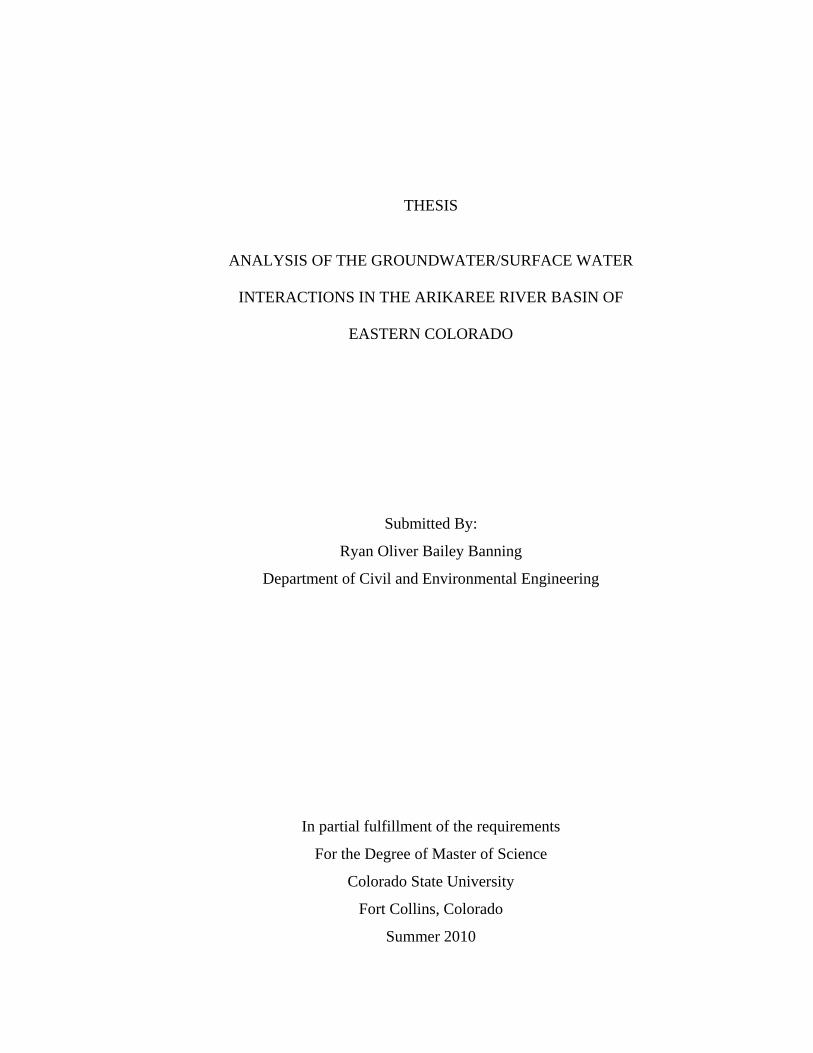
1964) ........................................................................................................................... 7 Figure 1-6: Bedrock Contours (Johnson et al. 2002).......................................................... 8 Figure 2-1: Griffin SDF Area (Griffin 2004 data depicted in ArcGIS)............................ 14 Figure 3-1: Fox Ranch and Stock Wells (Modified Unknown USGS Quad Map) .......... 19 Figure 3-2: Water Table Contours on the Fox Ranch in Southern Yuma County............ 20 Figure 3-3: Stock Well Level Deviation........................................................................... 22 Figure 3-4: Southern Yuma County Irrigation Well Locations (USDA 2005; CDWR
2005; CDOT 2006) ................................................................................................... 24 Figure 4-1: Grid Elevation Importation and Resulting Yuma County Surfaces (Visual
Modflow v. 4.0 2003) ............................................................................................... 30 Figure 4-2: Scanned Image of Weist (1964) - 1958 Water Table Contours, Southern
Yuma County ............................................................................................................ 31 Figure 4-3: Modflow Initial Head Contours After Importation (m) ................................. 31 Figure 4-4: Initial Model Domain w/ Initial Head Contours (m) and Interpolation Error
Band (Visual Modflow v. 4.0 2003) ......................................................................... 32 Figure 4-5: Grid Editor for Cell Error Correction (Visual Modflow v. 4.0 2003) ........... 33 Figure 4-6: Wells Included in Arikaree River Model (Visual Modflow v. 4.0 2003)...... 35 Figure 4-7: NLT LandSat 7 Visible Spectrum Satellite Photo of Southern Yuma County
(NASA World Wind 2006)....................................................................................... 39 Figure 4-8: Arikaree River Model ET Zones (Visual Modflow v. 4.0 2003)................... 40 Figure 4-9: Generalized Model Recharge Zones (Visual Modflow v. 4.0 2003) ............. 45 Figure 4-10: Specific Yield Zones (Visual Modflow v. 4.0 2003)................................... 48 Figure 4-11: Final Model Boundary Conditions w/ Well Locations, Groundwater Basin
and Bedrock Contours (Visual Modflow v. 4.0 2003).............................................. 51 Figure 4-12: Observation Points used for Calibration (Visual Modflow v. 4.0 2003) ..... 54 Figure 4-13: Comparison of Calibration Output Head Contours and the Initial Head
Contours (Visual Modflow v. 4.0 2003)................................................................... 55 Figure 4-14: Steady-State Model Calibration Correlation Graph (Visual Modflow v. 4.0
2003) ......................................................................................................................... 56 Figure 4-15: 10-year May 15th Pre-development Transient State Model Output Contours
vs. Weist (1964) Input data (Visual Modflow v. 4.0 2003)...................................... 58 Figure 4-16: Transient State Model Calibration Correlation Graph (Visual
Modflow v. 4.0 2003) ............................................................................................... 59 Figure 5-1: Theis Equation Riparian Bands and Centroid Locations ............................... 65 Figure 5-2: Growing Season Well Drawdown w/o ET (Visual Modflow v. 4.0, 2003)... 66

xi
Figure 5-3: Growing Season Drawdown from ET (Visual Modflow v. 4.0 2003)........... 67 Figure 5-4: Cumulative Seasonal Drawdown, Irrigation and ET at the end of the growing
season (day 257) (Visual Modflow v. 4.0 2003) ...................................................... 68 Figure 5-5: Sample Mass Balance Output Sheet (Visual Modflow v. 4.0 2003) ............. 69 Figure 5-6: Explanation Diagram of Sample Mass Balance Output Sheet (Figure 5-5) .. 70 Figure 5-7: Locations of Wells Included in Table 5-2 with Glover Analysis Ranks ....... 87 Figure 6-1: Water Budget Explanation ............................................................................. 91 Figure 6-2: Predevelopment Water Balance ..................................................................... 99 Figure 6-3: Developed Water Balance............................................................................ 100 Figure 7-1: Initial and 10-year Water Table Contours (Start of Pumping)..................... 104 Figure 7-2: Satellite Photo of the Arikaree River through Southwestern Yuma County
(USDA 2005) .......................................................................................................... 105 Figure 7-3: Diurnal Alluvial Groundwater Fluctuations on the Fox Ranch (Wachob 2005)
................................................................................................................................. 108 Figure 7-4: Gauge Recorded Streamflow at Haigler, NE (USGS Gauge Data) ............. 109 Figure 7-5: Precipitation Data, Akron Colorado Weather Station (Vigil, M. F. (2004)) 109 Figure 7-6: Conceptual Regions of the Arikaree River through Southern Yuma County
(Background by Weist 1964) .................................................................................. 110 Figure 7-7: Fox Ranch Property Location (Base Aerial Photo by USDA 2002)............ 112 Figure 7-8: N/S Cross-Section of Adjacent Well Effect on Fox Ranch Alluvium......... 113 Figure 7-9: N/S Cross Section of Alluvial Deposit Water Table Fluctuations at the Fox
Ranch ...................................................................................................................... 114 Figure 7-10: Plan View of Fox Ranch Flow Concept..................................................... 114 Figure 7-11: W/E Profile along the Streambed of Alluvial Well Effect on Fox Ranch
Stream Stage ........................................................................................................... 115 Figure 7-12: Transitional Region.................................................................................... 117 Figure 7-13: Connectivity diagrams of the downstream stretch (from Scheurer et al.
2003) ....................................................................................................................... 118 Figure 7-14: Diagram of the Downstream Arikaree River Conceptualization ............... 119
TABLE OF TABLES
Table 3-1: Stock Well Depth to Water ............................................................................. 21 Table 4-1: Stream Model Characteristics ......................................................................... 53 Table 4-2: Wells Requiring Additional Pumping Rate Reductions to Prevent Drying in
the Transient Model (See Figure 5-7)....................................................................... 60 Table 5-1: Top 15 Wells According to Additive and Subtractive Streamflow Change
Results for day 257 (All Shown at End of Pumping) ............................................... 80 Table 5-2: Glover Equation Analysis Results Compared to Numerical Analyses ........... 85

xii
PREFACE PLS Notes
Many figures and well descriptions presented in this text were developed using
the Public Land Survey (PLS) coordinate system. Boundaries of townships with section
line divisions are shown in these figures to indicate scale. The PLS coordinate system is
explained in appendix A.
Evapotranspiration (ET) Notes
According to the USGS, the definition of evapotranspiration (ET) varies
depending upon the needs of an author of a study using the term (USGS 2010). The word
is composed of and derived from “evaporation”, the process of water vaporizing into the
atmosphere, and “transpiration”, the process by which water is expelled into the
atmosphere by physiological functions of the plant. Evaporation includes water lost to the
atmosphere from the ground surface, from the capillary fringe of the groundwater table
and from surface-water bodies. Transpiration can occur from any part of the root zone,
including from the aquifer or the capillary fringe.
Unless otherwise noted, ET is from all possible water sources at a given location.
The initial abstraction is generally not included when ET is referenced except as
explained in chapter 6 to determine probable infiltration at the ground level, using
precipitation. In chapter 4, model input ET rates are always the maximum possible,
occurring when the calculated water table is at the ground surface. This rate is reduced
linearly with the extinction depth, to zero as described in the chapter.

1
CHAPTER 1 INTRODUCTION
1.1 STUDY BACKGROUND
Much of the western United States is semi-arid, requiring significant irrigation to
grow common crops. Improvements in pump technology during the 1960s made
groundwater wells an easy solution for satisfying crop requirements. However, by 1989
significant groundwater level reductions of up to 30.5-m (100-ft) were observed in parts
of the High Plains aquifer (also referred to as the Ogallala aquifer for its geologic
formation) underlying the states from South Dakota to Texas (Dugan et al. 1990).
Reductions in streamflow have had negative impacts on aquatic habitat resulting,
in some cases, in the extirpation of fish species from western rivers (Labbe & Fausch
2000). In Colorado, the disappearance of habitat is threatening the Brass Minnow
(Hybognathus hankinsoni), throughout the Arikaree River which is a stronghold for this
species (Scheurer et al. 2003; Falke 2009) particularly along The Nature Conservancy’s
Fox Ranch property (Figure 1-1, Figure 1-2) along the Arikaree River.
Groundwater models often are used to investigate water rights or to estimate
habitat recovery. The assumptions made during the modeling process are very different
depending on which of these goals the modeler is trying to achieve. Modeling for habitat
recovery projections requires the modeler to assume conservative estimates of flow

2
recovery (underestimation) because over estimation could mean habitat is actually not
available where projected. If a given species were to require the area of habitat recovery
projected in the model for survival and it were not available, there may not be enough
time to remedy the situation. Conversely, underestimation of stream depletion causes
legal problems when modeling to establish water rights because a user may be imposing
on a senior right held by another user. The distinction is important and the purpose of a
model must be established before it is used for any work.
It was determined that a study of the groundwater basin was required to
understand the Arikaree River system. This thesis is part of the preliminary study in what
is a collaborative effort between the Civil and Environmental Engineering and the Fish,
Wildlife and Conservation Biology Departments at Colorado State University. By better
understanding the river system through modeling and conceptualization it is hoped that
future research will aid in the preservation of the Arikaree River basin habitat.

3
Figure 1-1: Location of the Arikaree River
(CDOT 2006)
N

4
Figure 1-2: Southern Yuma and the Arikaree River with Major Tributaries
(CDOT 2006, Base Map by Mapquest 2006)
1.2 SITE LOCATION & GEOLOGICAL BACKGROUND
The Arikaree River is groundwater dependent and originates at roughly the edge
of the Ogallala formation near Limon, Colorado in Lincoln County (Figure 1-1). The
river flows northeast through Southern Yuma County into Kansas and toward the north
fork of the Republican River. The ground surface geologic formation at the headwaters of
the Arikaree is the Grand Island Formation (Figure 1-3). The sandy material cuts into the

5
Peoria Loess, which is underlain by the Ogallala Formation (Sharps 1980). Low
hydraulic conductivity of the Peoria Loess creates a region of high runoff and consequent
low infiltration at the mouth of the Arikaree River. Runoff has left deposits of the alluvial
Grand Island formation in the low-lying river channel area created over a long period by
erosion.
Figure 1-3: Geology of Arikaree River Basin (Sharps 1980)
As the Arikaree River flows northeast through Washington County (Figure 1-2),
the Peoria Loess top soil disappears revealing the Ogallala formation below. The Ogallala
formation is highly porous and is comprised of various soils from clay to gravel. Reddell
(1967) describes the formation as “homogeneous in its heterogeneity” inferring that the
soils are consistently mixed throughout the formation. The higher infiltration rate of the
Ogallala formation augments groundwater storage. The Ogallala formation is the major

6
geological formation of the High Plains aquifer and the names are used synonymously.
The High Plains aquifer is unconfined in eastern Colorado.
In southern Yuma County, deposits of wind-blown dune sand overlay the Ogallala
formation north of the Arikaree River. Yuma County surface geology maps by Sharps
(1980) (Figure 1-3) and Weist (1964) (Figure 1-4) are concurring descriptions of the
superficial soils.
Figure 1-4: Surface Geology of Southern Yuma County (Weist 1964)
The Arikaree River groundwater basin through Southern Yuma County was
delineated using data from Weist (1964) as shown in Figure 1-5. Groundwater contours
were connected at the point where they are perpendicular to the river to define the basin.

7
Figure 1-5: 1958 Arikaree River Groundwater Basin & Water Table Contours (Weist 1964)
The elevation of the Pierre Shale Bedrock is higher toward the north edge of the
basin as shown in Figure 1-6. Paleo-channels exist on both sides of the river. South of the
river, the prominent channel runs west to east. North of the river, the channels proceed to
the north from the Arikaree basin toward the north fork of the Republican River. The
Pierre Shale bedrock elevation descends to the east at a rate less than that of the ground
surface elevation creating intermittent bedrock outcroppings. Outcroppings appear
starting around the mouth of Copper Kettle Creek (Figure 1-2) in South Central Yuma
County and north of Idalia. At the Kansas border, the U.S. Geological Survey has
accepted the Arikaree as the lowest point in Colorado at 1,010 m (3,315 ft) above sea
level.

8
Figure 1-6: Bedrock Contours (Johnson et al. 2002)
The Arikaree River flows through Kansas for roughly three-miles before reaching
Nebraska to the north. It continues for ten miles from the Nebraska-Kansas border before
reaching the confluence with the north fork of the Republican River. At one time, the
flow rate of the Arikaree River was large enough for the river was perennially connected
through Yuma County into Nebraska (Wachob 2006). The river is now intermittent and
disconnected during summer months.

9
1.3 RESEARCH OBJECTIVES
The objectives of this study are to improve current understanding of the Arikaree
river groundwater system and to develop a defensible conceptualization of the river
basin.
The research tasks completed as part of this thesis are:
1) Collect and organize data describing the hydrogeological structure of the
Arikaree groundwater basin.
2) Conceptualize the groundwater basin and flow regime based on collected data.
3) Numerically model the groundwater basin in Southern Yuma County
associated with the Arikaree River.
4) Apply the model to identify wells causing the most stream depletion, compare
the results to analytical solutions and determine potential streamflow
recovery.
5) Develop a regional Southern Yuma County water budget.
6) Refine the conceptualization based on the analysis results.
1.4 CONCEPTUALIZATION
One of the main contributions of this thesis was to derive a conceptualization of
the Arikaree River water cycle and groundwater system. The final conceptualization is
described in depth, in chapter 7 and is supported by the research throughout this text. The
final conceptualization has the following major components:
1) The Ogallala Aquifer reduces in thickness from west to east because the slope
of the bedrock is less than the slope of the ground surface. This creates

10
outcroppings of bedrock toward the eastern half of Southern Yuma County
and modifies the behavior of the river.
2) There is an overall water balance deficit, due to irrigation wells, that lowers
the watertable and the resulting baseflow to the stream over time.
3) The boundary of the groundwater basin is stable and will remain independent
in the future, regardless of watertable levels.
4) Although all irrigation wells contribute to the decline of the water table over
time and ultimately the survival of the river, wells farther than around 3,000-
m from the river do not have a seasonal effect on the river stage. Instead,
alluvial wells and riparian ET cause intermittent disconnection of the stream
and affect the seasonal dynamics of the river.
5) The alluvium and groundwater flow through the “alluvial river” is taking the
place of channel flow as less water is available for streamflow.
6) The Arikaree River through Southern Yuma County must broken up into 4
distinct regions for conceptualization including: Upstream, Fox Ranch,
Transitional and Downstream regions. This is because the river and its
behavior due to the surrounding hydrogeology, irrigation and riparian
vegetation is very different depending upon the location.
7) The channel in the Upstream region is typically dry due to irrigation and
lower water table depth.
8) The Fox Ranch region is wet, although streamflow is disconnected throughout
the summer. This is because of nearby recharge areas and the lack of nearby

11
irrigation wells. The amount of water available at the surface will continue to
decline as water table levels decline.
9) Streamflow in the Transitional region continues to decline compared to the
Fox Ranch region. The aquifer is disconnected from the river in many
locations due to bedrock outcroppings. The alluvium is very dynamic because
of reduced base flow.
10) The Downstream region is mostly dry except for near the confluences of the
river with tributaries. This is because of riparian ET and alluvial wells. The
Ogallala aquifer is cut off from the alluvium by bedrock outcroppings. The
tributaries intercept east to west groundwater flow. This allows them to stay
wet but this water infiltrates into the alluvium at the confluence points.

12
CHAPTER 2 LITERATURE REVIEW
2.1 INTRODUCTION
Existing information concerning the Arikaree River in Southern Yuma County
includes the effects of artificial recharge on groundwater levels, brassy minnow habitat
persistence and agricultural studies including irrigation practices. Other pertinent studies
include estimated evapotranspiration (ET) rates, recharge rates and stream depletion rates
caused by pumping groundwater wells. Data collected from various sources included
water table levels, bedrock surface elevations, ground surface elevations, geology, land
use, well locations and pump capacities.
2.2 STUDY BACKGROUND
Fardal (2003), Griffin (2004) and Wachob (2006) completed history and
background reviews of literature for the Arikaree River near the Fox Ranch property. The
reviews detail the development of Southern Yuma County’s agricultural economy.
Fardal and Griffin also conducted studies of stream conditions, possible effects of
irrigation and agricultural trends for the area surrounding the Fox Ranch. Fardal’s study
included a preliminary discussion of groundwater pumping and its correspondence to the
Arikaree River stream stage. Later, data collected by Griffin improved the understanding

13
of relationship between stream stage and regional pumping indicating that her conclusion
of an inverse relationship between stream stage and regional pumping might be more of
an indirect relationship. However, seasonal groundwater use was determined using
farmer surveys and power consumption records. The average pump efficiency was
estimated for regional groundwater wells to be 61 %.
Griffin’s study included stream-depletion factor calculations along with an
examination of the correlation of shallow alluvial well levels and nearby stream stage. A
large area near the Fox Ranch portion of the Arikaree River was included in the analysis.
Effects of pumping from all of the wells in the eight townships highlighted in Figure 2-1
were included in the computation of the total stream depletion from a common point on
the river. A portion of the included wells, as indicated on the provided map (Figure 2-1)
is not within the 1958 Arikaree River groundwater basin shown shadowed from bottom
left to top right on the map provided as.
Griffin (2004) assumed a regional average hydraulic-transmissivity of 2,483-
m2/day (26,736-ft2/day) in his study. He found, using simplified analytical stream-
depletion models, that groundwater irrigation wells could be causing complete seasonal
depletion of all Arikaree River streamflow through the Fox Ranch. There was no
noticeable change however, found to the timing of the stream-stage decline between two
consecutive years, despite a delay in the pumping start date of two weeks during the
second year. The pumping start date delay without equal delay in stream-stage decline
schedule indicates that there are sources of stream depletion other than irrigation wells.

14
Figure 2-1: Griffin SDF Area (Griffin 2004 data depicted in ArcGIS)
Wachob (2006) documented alluvial water table levels over the 2005 growing
season to examine evapotranspiration from riparian areas containing cottonwood stands.
Comparisons were made between methods of calculating ET using specific yield (White
1932) and the FAO Penman-Monteith Equation (Allen el al. 1998), used in agricultural
calculations. Seasonal riparian ET from cottonwoods was calculated to be approximately
127-cm (50-in) from the alluvium using the White method. The White method evaluates
ET using groundwater levels and does not directly account for the initial abstraction or
evaporation from open water. Because of this, the ET calculated using the White method
analysis is probably not the maximum.
Scheurer (2003) studied brassy minnow persistence at three locations in
southeastern Yuma County. The study documented the existence of adult and juvenile
±

15
fish associated with spawning for the years 2000 and 2001. The species persisted despite
drying of large portions of the river. Scheurer documented stream connectivity and its
reestablishment from changing stream conditions. Repopulation of areas where fish had
been extirpated was observed after periods of stream connectivity.
Solek (1998) suggested that the Fox Ranch would be the best available land along
the Arikaree River to be purchased by The Nature Conservancy for a wildlife preserve.
Her conclusions were based on geology and the absence of nearby irrigation wells. Solek
cited the vast deposits of dune sand, north of the ranch with thin underlying Ogallala
formation as benefits to habitat on the property because the geologic configuration allows
high rates of aquifer recharge. Farming is less than ideal in the dune sand, thus
discouraging high capacity well installation near the property.
Katz (2001) studied the invasion of plant species into western riparian regions
including the Arikaree River valley along with the geomorphology of the alluvium. Flood
terracing was found to exist in many stages including from the major flood recorded in
1935 among others. Flooding has influenced plant variety, plant population and ET rates.
Large stands of cottonwoods have developed where they did not exist before the 1935
flood.
2.3 REGIONAL GROUNDWATER BASIN
Weist (1964) studied the geology and groundwater resources of Southern Yuma
County. Surface geology was mapped and a fence diagram of subsurface geology was
created. Contour maps were included showing the elevation of the bedrock surface, water

16
table surface, ground surface and relationship between each surfaces. Weist approximated
the alluvial water table depth between 6 and 15 meters, which varies by location.
Borman et al. (1980) looked at the hydraulic characteristics of the High Plains
Aquifer in Colorado. Saturated thicknesses and changes in storage were mapped along
with aquifer characteristics including hydraulic conductivity and specific yield. Aquifer
properties ranges from Borman were used in the model, detailed in chapter 4.
Surface geology data was compiled by Sharps (1980) for eastern Colorado. The
resulting map (Figure 1-3) shows dune sand, Ogallala formation outcropping, Peoria
Loess deposit and bedrock outcropping locations throughout Yuma County. The surface
geology at the headwaters of the Arikaree River was included.
Reddell (1967) studied natural High Plains Aquifer recharge in Colorado.
Recharge in subdivided regions of the aquifer was calculated using a numerical model.
The model cell size was six square miles. Reddell suggested that the composite average
high plains aquifer recharge for Yuma County is 1.45 in/yr (3.56-cm). Reddell also
attempted to quantify regional water budget inputs.
Longenbaugh (1966) studied artificial recharge near the Arikaree River. He
concluded that artificial recharge was possible at a study site near Cope, Colorado.
Observations wells were used to measure the increases in water table level induced by
recharge ponds created using excess surface water.
Dugan et al. (1990) completed a study of The High Plains Aquifer water levels
changes. The study included the entire aquifer from South Dakota to Texas. From 1980
and 1988, water table level changes were observed ranging between 3 to 15 meters in
portions of the High Plains Aquifer of Colorado. Changes of over 30-m were observed in

17
other regions during the same time interval. A related study by Luckey (1988) examined
the effects of pumping in the aquifer as determined by regional models. Changes in water
level were similar for these studies.
Gutentag et al. (1984) showed that groundwater-irrigated agriculture in the High
Plains Aquifer of Eastern Colorado increased from between 0 and 10% up to between 25
and 50% during a fourteen-year period from 1964 and 1978. This is a regional estimate
from the maps presented in the study. The increase is due to vast well installations during
the late 1960’s. Expectation of groundwater regulation in the late 1960’s and new pump
technology were catalysts to development of groundwater wells.

18
CHAPTER 3 DATA COLLECTION AND OBSERVED GROUNDWATER TRENDS
3.1 STOCK WELLS MEASUREMENTS
Nineteen wind-powered stock wells are located on the Fox Ranch as shown in
Figure 3-1. The location of these wells varies substantially in elevation and proximity to
the Arikaree River. Differential GPS was used to survey the location and elevation of the
stock wells. A site-specific GPS reference point was established for the project and was
utilized as the base station for all surveys completed during 2004-2005 including
measurements in the survey for Wachob (2006). The base station is a permanent mark
etched into a large rock outcropping, located in the horse trap in Figure 3-1. The datum
elevation and coordinates for all windmills are provided in Appendix B. Wells 5 and 9,
shown to the north of the ranch house and river were not measureable.
The wells were monitored starting in the spring of 2005. All well survey and
groundwater measurement points of reference were the center of the well casing cap.
Monitoring occurred on various dates throughout the year as access to the wells was
obtained. Most wells were visited three times (Table 3-1). The depth to water was
measured from the top of the well casing.

19
Figure 3-1: Fox Ranch and Stock Wells (Modified Unknown USGS Quad Map)
±
0 1 20.5 Kilometers

20
Figure 3-2 shows the resulting groundwater contour map from the stockwell
measurement data (Table 3-1), collected on 8/16/2005 (10/15/2005 for wells 16 & 17).
The data set was plotted along with measurements from the shallow alluvial well survey
for Wachob (2006), new measurements of wells from the Griffin (2004) study and an
ongoing Fish, Wildlife and Conservation Biology study measurements of the stream
water-surface elevation at various locations along the river. The water-surface elevation
was calculated by adding the stream-stage to riverbed elevations surveyed with
differential GPS starting at the river just south of well seven (Figure 3-1) and proceeding
east. The riverbed west of well seven was approximated using the data from a DEM
(National Elevation Dataset 1999) and GIS. These points are referred to as “hypothetical”
in the figure. Appendix B shows the collected data used in the plot.
Figure 3-2: Water Table Contours on the Fox Ranch in Southern Yuma County
(Coordinates in UTM NAD 1983 zone 13 N) Note: Contour lines to the bottom left of the figure, above elevation 1,190 m, are not
relevant because no measurable wells were located in that region.

21
The groundwater gradient was determined using the contour map in Figure 3-2.
On the date of these measurements, the gradient is approximately 0.014 to 0.021-m/m
toward the river from the north and 0.009 to 0.014-m/m from the south. The contour map
shows that the river is gaining through the Fox Ranch.
Table 3-1 shows the measurements taken at each of the wells over the period from
3/15/2005 to 3/16/2006. The maximum change in water level over that time for each well
was calculated when multiple observation data were available.
Table 3-1: Stock Well Depth to Water (Measured from the top of the well casing)
Depth to Water Table (m) Max LevelWindmill 3/15/2005 5/19/2005 6/26/2005 8/16/2005 10/6/2005 10/15/2005 3/16/2006 Change (m)
1 16.49 16.52 -0.032 18.10 0.003 6.35 6.08 6.46 -0.384 25.63 25.72 -0.096 18.47 0.007 18.26 18.23 18.47 18.44 18.41 -0.248 25.08 25.45 25.33 -0.37
10 27.37 28.31 27.52 -0.9411 36.30 36.06 36.06 0.2412 30.55 30.75 30.66 -0.2013 23.16 23.26 23.16 -0.0914 49.77 50.11 49.95 50.02 -0.3415 45.21 45.21 45.38 -0.1716 44.47 44.44 44.56 -0.12
16 Off Site 53.64 53.73 53.64 -0.0917 32.89 32.89 32.92 -0.0318 9.74 9.72 9.72 0.0219 41.60 41.68 41.79 0.1920 21.57 21.61 21.67 -0.1021 24.29 0.00
Because of nearly a one-meter groundwater level reduction followed by close to
complete recovery at the August 16th reading, it appears there was an error in the June
26th reading for well 10. Well level reductions of more than 0.3-m occurred in wells 3, 8
and 14. Well 15 is located approximately 2-km east of an irrigation well and Well 14 is
located approximately 1.2-km north and 1.6-km northeast of two irrigation wells.

22
Additional irrigation wells are located approximately 1.6-km west, 0.8-km south and 2.4-
km west, 0.8-km south of stock well 14. Wells 14 and 15 are the closest of all measured
stock wells to irrigation wells.
No clear downward trend in water levels was observed throughout the year
(Figure 3-3). The overall groundwater levels at the end of the growing season were not
noticeably lower than in the early season (Table 3-1). The average change in stock well
water level was a reduction of 0.21-m. Seasonal changes in the groundwater level at the
stock wells appeared affected more by atmospheric conditions and localized river
conditions than by irrigation well pumping. This was concluded because water level
declines in some stock wells located near the river were within 0.1-m of the decline seen
in well 14, located near irrigation wells. Well 7 is an example, of a well far away from
the irrigation wells that measured similar declines to well 14 (0.24-m vs. 0.34-m).
Well Level Deviation (in meters)(Base Well Number)
0
5
10
15
20
2/17/2005
4/8/2005
5/28/2005
7/17/2005
9/5/2005
10/25/2005
12/14/2005
2/2/2006
3/24/2006
5/13/2006Date of Observation
Wel
l Num
ber -
Lev
el D
evia
tion
from
Hig
hest
Rea
ding
(m)
Figure 3-3: Stock Well Level Deviation

23
Although additional years of data should be collected, it was concluded from the
measured data that irrigation pumping was not the primary, but a secondary cause of
seasonal water table fluctuations for the Fox Ranch stock wells in Table 3-1. For
irrigation pumping on the Fox Ranch to be the primary cause of seasonal water table
level decline, it would be expected that the water table elevation be highest on 5/19/2005.
It would also be expected that the water table levels decline throughout the growing
season to the 10/15/2005 level and that seasonal recovery would increase the water table
elevation such that measurements in the beginning of spring on 3/16/2006 would be
higher than those measured after irrigation season on 8/16/2005 and 10/15/2005. None of
these trends was clear from analysis of this data set.
It was indicated from this data set that irrigation pumping in the aquifer to the
north and south of the Fox Ranch was not causing seasonal depletion of the river. If this
were the case, stock well water table levels would be expected to recover with similar
timing to the observed seasonal streamflow recovery. This data set does not provide
enough information about upstream alluvial wells to determine where depletion is
coming from.
Wells 14 through 17 (Figure 3-1) are located on the south side of the ranch and
are the closest stock wells to the irrigation wells (Figure 3-4). A gradual regional decline
for these wells was indicated from the measurements on 3/16/2006. The measurements
on that date trended lower than the majority of the previous measurements. Further
monitoring should be completed to determine long-term groundwater trends.
24
Figure 3-4: Southern Yuma County Irrigation Well Locations (USDA 2005; CDWR 2005; CDOT 2006)
±
25
CHAPTER 4 ARIKAREE RIVER NUMERICAL GROUNDWATER MODEL
4.1 NUMERICAL MODEL
To achieve a better understanding of the groundwater system contributing
baseflow to the Arikaree River, a numerical groundwater model was created representing
southern Yuma County. This model was the first attempt for this project and is the
foundation for further groundwater modeling and exploration of the factors contributing
to the decline of Arikaree River streamflow. This model was used in the
conceptualization of the stream basin and was useful in determining where additional
research was needed to refine the understanding of the system. Many of the parameters,
such as ET and recharge were approximated using previous studies of the river basin and
other areas similar to the basin. The most reliable data were used wherever possible.
4.2 NUMERICAL MODELING TECHNIQUES
Typical numerical groundwater modeling strategies implement either a variety of
simple models representing various conceptual models of the same system or a single
complex and realistic model. Modelers use statistical analysis with the simple model
technique, to create a confidence interval of model results. The more complex, realistic
models are used for approximating large-scale flow regimes and estimating water-
quantity solutions. For this reason, the realistic technique was used for this study.
Significant raw data were available for the area because of advances in satellite
technology and studies by the USGS, such as Weist (1964). Visual MODFLOW

26
(Waterloo Hydrogeologic, distributed by Scientific Software Group, Washington D.C.)
was the numerical model interface used to create the model. The software contains
computer code allowing importation of data in various formats including tabulated data
and ESRI shapefiles.
4.3 PROCESSING INFORMATION FOR MODEL INPUT
Geographical information systems (GIS) technology was used extensively for
processing raw data into Visual Modflow model data sets. The ArcGIS 9.1 software
(ESRI Inc. 2005) was used exclusively for GIS data manipulation and processing. The
reader is urged to reference an ESRI ArcGIS manual for file type definitions and
explanation of data manipulation techniques.
A water table contour map from Weist (1964) was scanned and converted to a
polyline GIS data file. This file and the Johnson et al. (2002), bedrock contours were
interpolated into raster data and processed for importation and interpretation by the
Visual MODFLOW software. The surface geology map from Weist (Figure 1-4), was
digitized and used to identify soil type zones while designating regional
evapotranspiration and recharge trends in the model. A USGS digital elevation model
(National Elevation Dataset 1999) of the area, containing ground-surface elevation data
set was also processed for model importation. Well locations and pump capacity data
from the Colorado Division of Water Resources (CDWR 2005) was used in the model.
In order to organize model data effectively, a common spatial referencing system
was used. The North American Datum (NAD) 1983 Universal Trans-Mercator (UTM)
zone 13N was chosen because it is the current standard for government data in Eastern

27
Colorado (CDWR 2005). Utilizing ArcGIS, digital-aerial photos and scanned images
were aligned or “geo-referenced” to spatial and elevation data sets in NAD 1983 UTM
zone 13N. Most historic well and property location data for Yuma County was recorded
using the United States Public Land Survey (PLS) system for identifying spatial
locations. The PLS coordinates were converted to NAD 1983, UTM zone 13N for
alignment to other GIS data.
The complete process used for importing surfaces shown on hardcopy maps into
modflow is as follows:
1. Digitize the contour map image by converting it to raster image file
2. Convert the raster file to a digital contour file of polylines
3. Interpolate a Digital Elevation Map (DEM) from a digital contour file
4. Verify the Digital Data
5. Convert a DEM to digital point file
6. Export the point file to a table of values
7. Import the table into modflow to create the model surface.
8. Make appropriate corrections to the imported data set.
The following is a description of the steps involved in the process.
4.3.1 Surface Creation
The ArcGIS toolbox was used to digitize the Weist (1964) water table contour
map. The map was scanned to create bit-map image file. The representative image file,
based upon a two-dimensional document, was geo-referenced to intersections of PLS

28
section lines or other common locations and aligned with the spatial reference system.
This was a required image distortion process used to match the UTM projection.
The image file was touched up manually to remove any flawed image data
resulting from the digitization process. Once the file was cleaned, the image conversion
tool was used to convert the image files into poly-line vector shape files. Contours were
manually connected where required to create a comprehensive and continuous data set for
the entire model area. The now geo-referenced, poly-line contours entities were manually
assigned elevation values shown by the Weist (1964) map.
The Weist (1964) contour data set and the Johnson et al. (2002) bedrock surface
contour set were converted to raster-value, DEM-type surfaces by interpolating cell
elevation values from the contours. The new surface files were created to have a cell sizes
of 4.05-ha (10-acres).
4.3.2 Comparison of Surfaces
Arithmetic operations of raster files are possible using the spatial analyst tool in
ArcGIS. The tool creates a new raster surfaces that are a data set of cells with associated
horizontal location, size and some relevant data. The data are the result of the some
specified operation chosen at the creation of the output-surface from the overlapping
input-surface cells. A raster file was created showing the proximity of the National
Elevation Dataset (1999) ground elevation surface to the Johnson et al. (2002) bedrock
elevation surface by subtracting the elevation value of the cells in the bedrock elevation
surface from the ground elevation surface. Exposed bedrock locations were defined in the
resulting surface at locations where the cells contained negative or zero values. The

29
locations were verified by comparing the resulting exposed bedrock cells to exposed
bedrock regions shown in Figure 1-4.
4.3.3 Importation of Surfaces
ASCII files (basic text files) containing tables of data were used to import surface
data. Tables of elevation data and their associated x-y coordinates (interpolation tables)
were created from the “parent” DEM files using an ArcGIS data export.
To create the tables, the DEMs were converted to vector point entities centered
over the 10-acre raster square. The points were used to extract elevation and coordinate
data associated with parent raster cells. The process was used for the ground-elevation
surface, bedrock-elevation surface and the 1958 water-table surface (Weist 1964) files.
One point was created for every cell in each raster surface. Elevation and UTM
coordinate data associated with the points were then exported to ASCII file tables. Visual
Modflow used kriging interpolation (Oliver 1990) to create a model surfaces from each
table.
The raster surface files and Visual Modflow model were created having
equivalent, 4.05-ha (10-acre) cell sizes. Each model cell corresponded to a matching
point created from the DEMs so interpolation resulted in very accurate model surfaces.
The cell size was chosen because it was the smallest parcel area described in the PLS
coordinate system. An image of the uploading screen and resulting cell top and cell
bottom surfaces (ground and bedrock surfaces) are shown in Figure 4-1.

30
Figure 4-1: Grid Elevation Importation and Resulting Yuma County Surfaces (Visual Modflow v. 4.0 2003)
The initial head surface was uploaded similarly to the ground and bedrock
surfaces. However, the initial head interpolation tool does not have the visual output
capability used to display the surface as shown in Figure 4-1. Instead, the interpolated
initial-head surface was compared visually to the digital image of the Weist (1964)
contour map (Figure 4-2). By visual inspection, contours only deviate from the original
contours along the boundaries of the image. The initial head surface, shown using the
Visual Modflow contouring tools is shown as Figure 4-3.

31
Figure 4-2: Scanned Image of Weist (1964) - 1958 Water Table Contours, Southern Yuma County
(Visual Modflow v. 4.0 2003)
Figure 4-3: Modflow Initial Head Contours After Importation (m)
(Area matches Figure 4-2 -Visual Modflow v. 4.0 2003)

32
4.3.4 Resolving Surface Importation Errors
Some obvious model-surface errors occurred during importation of the surfaces,
mostly around the outer edge of the model. The interpolation algorithm for those areas
was constrained to using only elevations from input data on the inner side of the
interpolated point. Figure 4-4 shows the original error band around the outer edge of the
model.
Figure 4-4: Initial Model Domain w/ Initial Head Contours (m) and Interpolation Error Band (Visual Modflow v. 4.0 2003)
Excluding the error band around the outer edge of the model was necessary to
avoid erroneous results. Limits of the band were set by inspection of the individual cross
sections. Errors could have been avoided by including data points from a larger region
ERROR BAND (TYP.)

33
than was encompassed by the model. This was realized after the model was complete but
was insignificant to modeling results because the error band was excluded from the
model to alleviate the problems.
Localized cell errors occurred in three internal model locations where the
interpolated points did not coincide exactly with cell geometry. Local errors were
corrected manually by smoothing the surface between the four surrounding cells. Visual
Modflow contains an elevation adjustment tool as shown in Figure 4-5. The tool allows
the user to edit numerical elevation data manually or adjusting elevation by visually
smoothing the cross section line.
Figure 4-5: Grid Editor for Cell Error Correction (Visual Modflow v. 4.0 2003)
4.3.5 Well Data
The Colorado Division of Water Resources (CDWR 2005) provided well data in
data base format. Well coordinates in UTM, rated pump capacities and well identification

34
numbers were tabulated separately for use in the GIS. Colorado usually requires the
owner of a well to provide PLS coordinates indicating the proposed well location upon
applying for an installation permit. It was discovered that the owners do not necessarily
provide updated well location information after the installation of the well is completed.
At times, duplicate well coordinates were provided for multiple wells owned by one
party, or the owner provided the coordinates of their dwelling instead of the well
installation location.
Well locations were verified using satellite photos (Figure 7-2, USDA 2005).
Satellite photos were aligned to the NAD 1983 UTM coordinate system and vector point
files created from the well table. Fine resolution (< 3-m) satellite photos served as a
method of determining the well location “ground truth”. The location of wells not
coincident with an irrigated field but within the groundwater basin and model borders
were moved to fields assumed to be irrigated by the wells.
Wells were added manually to the model because each had distinct pumping rates
and screening elevations. The screening used for all wells in the model was 100-pecent of
the well depth, under the assumption that the entire depth of the Ogallala Aquifer is
potentially water bearing. Pumping schedules were set based on the Wachob (2005)
pumping season length of 123 days, starting on the 135th day of the year (May 15). The
Wachob schedule was an average of growing season length from farmer interviews by
Fardal (2003). The 95 wells used in the model are shown in Figure 4-6.

35
Figure 4-6: Wells Included in Arikaree River Model (Visual Modflow v. 4.0 2003)
4.4 MODEL ASSUMPTIONS, DEVELOPMENT AND PARAMETER VALUES
Important parameters and boundary conditions that affected model results include
evapotranspiration rates, recharge rates, pump efficiency, soil hydraulic conductivity,
saturated thickness, specific yield and model boundary conditions. The selection of inputs
as described in this section improved the initial calibration. These parameters can all be
improved with further study of the area. For this first model attempt, it was only possible
to find reasonable ranges with supporting literature.
ET rates that have been input into the model are always the maximum possible
rate. Calculated ET reduces linearly from the maximum ET rate when the water table is at
the ground surface, to zero when the water table is at or below the extinction depth.

36
4.4.1 Evapotranspiration Assumptions
Riparian evapotranspiration (ET) has recently been a topic of significant debate.
There is currently no “correct” technique used to determine riparian ET. Because of the
ambiguity of this model input, an attempt was made to use ET data from recent studies in
the modeled area, but true riparian ET, both rate and volume, is still unknown. Modeled
ET is an educated guess, the parameter was varied, attempting to simulate growing
season trends and transpiration.
A study of riparian ET along the Arikaree River at the Fox Ranch has been
ongoing starting with the work by Fardal (2003), Griffin (2004) and continued by
Wachob (2006). Monitoring of shallow alluvial wells along the river has been part of this
study in an attempt to quantify riparian ET, including cottonwood stands. Monitoring was
conducted manually on a semi-monthly basis as well as using pressure transducers,
recording data at 1-hr intervals. A review of literature concerning riparian ET was
included in the study by Wachob (2006).
Lou (1994) found that ET from riparian cottonwoods in New Mexico is around
145-cm per growing season. Pataki (2005) found that riparian ET from Populus
vegetation is around 114-cm per growing season in the Colorado River Basin of Utah.
Robinson (1968) studied a stand of cottonwoods in California and found that ET is
approximately 164-cm per year.
Crop ET has been studied for years resulting in the wide use of the FAO Penman-
Monteith Equation (Allen et al. 1998) but the equation is not easily applied to riparian
vegetation because the method calls for a consistent crop in aerial extent, starting
annually from seed with similar age and attributes. Consistency is not characteristic of

37
natural riparian areas. The riparian area is also very distinct from that of the plains shelf,
located a few hundred yards away.
Using the White Method (White 1932) analysis for one growing season worth of
observed well data, Wachob (2005) calculated a total growing season ET of 135-cm from
cottonwood trees on the Fox Ranch. Specific yield was assumed to be 0.2 for this
analysis, which is consistent with the very sandy material found in the alluvium (Fetter
2001). More recently, Squires (2007) and Riley (2009) completed a more in depth study
of ET along the riparian areas near the Arikaree in an attempt to improve future models.
Their work estimates a lower specific yield of 0.175 and corresponding seasonal riparian
ET of about 90-cm.
To model ET using Modflow, a maximum ET rate and an assumed extinction
depth are input. The extinction depth parameter is the depth below ground surface that
the calculated water table must be for the ET to be assumed negligible. The model
assumes a linear reduction in the rate of ET from the maximum input ET to zero as the
calculated water table elevation reduces from the ground surface to the extinction depth.
Because of this, the ET rate calculated by the model is only the input maximum when the
water table reaches the ground surface. The modeled ET is lower than the maximum ET
input or zero for the majority of the model because the water table is not normally at or
near the ground surface.
The riparian extinction depth used in the model was 5-m to simulate the
phreatophytic cottonwoods in the area and the maximum ET rate was 127-cm/year.
Extinction depth of phreatophytes such as cottonwood trees can be rather large, upwards
of 4.5-m (15-ft) accounting for their root structure (Katz 2001). The surrounding river

38
basin was assumed to have a 2-m extinction depth because of a mixture of plant types in
the area with fewer to no trees.
The extinction depth was set to 0.5-m for the majority of the model with only the
riparian and surrounding river basin areas assumed deeper. Doing this reduces the ET rate
to zero anywhere that the water table is below 0.5-m from the ground surface. In essence,
ET was not used in the model anywhere except in the river basin and riparian areas as
shown in Figure 4-7 and Figure 4-8.
The ET parameter was applied to the riparian areas of the model with a maximum
rate equal to a cumulative seasonal ET of 127-cm (50-in) distributed only over the 123-
day growing season (~1-cm/day). The maximum riparian ET was reduced to a rate equal
to 89-cm (35-in) per year (~0.2-cm/day) on day 258 to simulate the transition of the
vegetation during autumn and set to zero on day 288 to simulate the winter months. For
multi-year runs, the cycle was repeated. Using these inputs, the cumulative maximum
possible ET is 133-cm (52.4-in) per season, in situations where the groundwater is at the
ground surface and less as the groundwater subsides. This maximum is slightly less than
the 135-cm calculated by Wachob (2005).
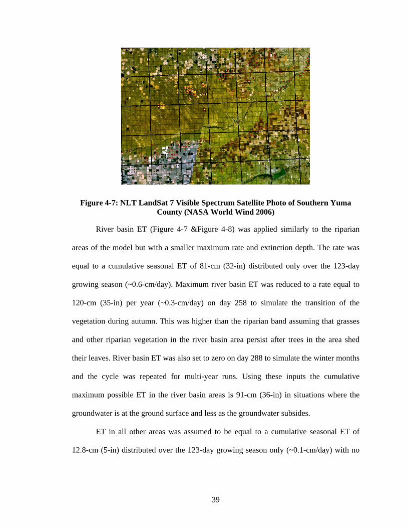
Areas of high vegetative cover around the river valley were apparent from aerial
photos. These are referred to in this study as river basin areas (Figure 4-7). Green
spectrums from the photos indicate possible higher moisture levels available for
photosynthetic use. These areas were located near the river at lower elevations, and along
known and apparent drainage ways.
39
Figure 4-7: NLT LandSat 7 Visible Spectrum Satellite Photo of Southern Yuma County (NASA World Wind 2006)
River basin ET (Figure 4-7 &Figure 4-8) was applied similarly to the riparian
areas of the model but with a smaller maximum rate and extinction depth. The rate was
equal to a cumulative seasonal ET of 81-cm (32-in) distributed only over the 123-day
growing season (~0.6-cm/day). Maximum river basin ET was reduced to a rate equal to
120-cm (35-in) per year (~0.3-cm/day) on day 258 to simulate the transition of the
vegetation during autumn. This was higher than the riparian band assuming that grasses
and other riparian vegetation in the river basin area persist after trees in the area shed
their leaves. River basin ET was also set to zero on day 288 to simulate the winter months
and the cycle was repeated for multi-year runs. Using these inputs the cumulative
maximum possible ET in the river basin areas is 91-cm (36-in) in situations where the
groundwater is at the ground surface and less as the groundwater subsides.
ET in all other areas was assumed to be equal to a cumulative seasonal ET of
12.8-cm (5-in) distributed over the 123-day growing season only (~0.1-cm/day) with no

40
reduction for autumn months. This only applies to a handful of cells with high, calculated
water table because of the 0.5-m extinction depth set for the remainder of the model.
Figure 4-8 shows the ET zones used in the model where red, white, teal, green
and blue were used to designate land usage with the assumed usages being
plains/farmland, plains/dune sands, irrigated area, river basin and riparian areas
respectively.
Figure 4-8: Arikaree River Model ET Zones (Visual Modflow v. 4.0 2003)
The cumulative ET distributed over the entire 80,900-ha (200,000-acre) model
was calculated to approximately 365-ha-m/yr (2,950-acre-ft/yr). The cumulative ET
distributed evenly over the model is therefore 0.45-cm/yr (0.18-in/yr) from groundwater.
The total area designated as riparian area is approximately 3,180-ha (7,900-acres) and the
river basin area is approximately 11,200-ha (27,700-acres). The cumulative ET, if
distributed evenly over the total riparian and river basin area of 14,400-ha (35,600-acres)

41
roughly is 2.5-cm/yr (1.0-in/yr). If the ET is distributed over the riparian area only, the
total ET is 11.5-cm/yr (4.5-in/yr).
The modeled ET is significantly below the literature values of ET for
cottonwoods. From these results, it appears the majority of the ET in the model is
occurring in the riparian area. Also, the modeled ET may be too low given modeled
stream outflow is too high as discussed in later sections and that there is a large
discrepancy between the Wachob (2005) riparian ET of 135-cm per growing season and
the ET computed by the model. Adjustments to the extinction depths throughout the
model and possibly the addition of small values for ET during the winter period may
improve the model. These adjustments are hard to justify without improved studies of the
parameters.
Even though the calculated ET was far less than the maximum input ET rate, the
seasonal riparian ET of 127-cm (50-in) or ~1-cm/growing season day, used for the
maximum ET was analyzed to see if it is reasonable for cottonwood trees (Populus
fremonti), the assumed rate was compared to measured growing-season ET rates. The
Northern Colorado region average historical reference ET (13-cm stand of cool weather
grass) is 89-cm (35.12-in) for the growing season (April to October) or 0.42-cm/growing
season day (Mecham 2004). The total reference ET for the month of June 2006 in Fort
Morgan, CO was 27-cm (10.67-in) or 0.90 cm/growing season day for a total of 110.7-cm
(43.6-in) per 123-day growing season. The modeled ET rate of ~1-cm/growing season
day was considered high but reasonable because of the additional foliage of trees when
compared to 13-cm of grass (Lou 1994; Pataki 2005). The model growing season also

42
started on day 135 (May 15th) and ended on day 258 (September 16th) including July and
August, historically the hottest months of the year in Colorado (City Rating.com 2007).
The ET variable was generally not useful for calibration outside of the alluvium
and major drainage ways because of the low water table levels with respect to the ground
surface. Implications of high ET rates due to riparian vegetation were evident in model
results. The model calculated drawdown of more than 0.5-m (chapter 5) along the river
due solely to ET.
4.4.2 Recharge Assumptions
Since measurement of groundwater recharge is difficult, the recharge parameter
was not well known. Recharge was used partially as a calibration variable within a
reasonable range from published data. This variable was ambiguous however, because
there were no studies of natural recharge found for the area.
Recharge was assumed to be very high for sandy regions within the model.
Ponding on the dunes was limited during a high intensity rainstorm observed by the
author on August 16, 2005 (0.8 to 1.2-in/hr, storm depth 0.2-in) (COAgMet 2006) even
in local depressions. No ponding remained two minutes after the end of the storm.
Average precipitation for Idalia, CO is 45-cm (17.7-in) per year (High Plains Regional
Climate Center 2006) of which a high percentage would be expected to infiltrate.
Vegetative cover in the dunes is sporadic at best, which also increases infiltration and
potential recharge.
Gaye and Edmunds (1996) determined using chloride concentrations that recharge
was approximately 30-mm per year in the sands of Northwestern Senegal. This is similar

43
to the approximation for Yuma County by Reddell (1957) of 36.8-mm per year using a
numerical model.
A study by Jackson and Rushton (1987) determined that there is a very large
range of possible recharge values for differing ground cover conditions. Recharge values
in many cases, were indicated to be much higher than standard approximations.
Calibration of a model for their study concluded that recharge input must be around 2.4-
cm per year for portions of their study site with clay surface soils. A modeled run for
April of 1981 required a much higher recharge rate to calibrate for a sandy soil region.
2.14-million liters per day was used for the 1-km2 area, equivalent to a rate of 78.1-cm
per year of recharge for that month.
Scanlon et al. (2002) reviewed methods of approximating recharge. Cited studies
report ranges of recharge values from 0.01-cm /day to as high as 300-cm/day. Ranges
varied by method of recharge computation and site characteristics. Sophocleous and
Perry (1985) found a recharge range of 0.25 to 15.4-cm for a five-month span where the
primary surface geological formation was dune sand at the study site in south-central
Kansas.
Due to the wide range of published recharge rates, the model recharge zones were
first delineated using maps of surface geology so they could be varied with calibration.
Five basic surface geology zones exist within Southern Yuma County (Figure 1-4, Weist
1964). Dune sand is located northwest of the ranch. The Ogallala formation is exposed at
the surface to the southwest of the river. Peoria Loess is the surface material to the east.
Alluvial material underlies the Arikaree River channel. Exposed Pierre Shale bedrock is

44
prevalent to the east of the ranch separating the alluvium and the Ogallala or Peoria Loess
top soils.
Well-sorted coarse sands have higher hydraulic conductivities and infiltrative
capacity than do other materials (Fetter 2001). Of the five surface formations mentioned
above, the sandy alluvial material and dune sand would tend to have the highest
infiltrative capacity. Peoria Loess has a lower hydraulic conductivity than the other
surface materials. The Ogallala formation is a water bearing and yielding material but
cannot be classified as well sorted soil (Reddell 1967). Recharge was assigned to the
model based upon mapped surface material locations (Figure 1-3, Figure 1-4).
A high infiltration rate was assumed for the alluvial material. 38-cm (15-in) per
year was used for the recharge rate assuming that the majority of the precipitation
reaching the ground will find open water or the shallow alluvial water table. The water
table through the alluvium is very high and the water table responds very quickly to
infiltration events (Wachob 2005). ET also occurs at a high rate and the net recharge is
the difference between ET and infiltration. Results from monitoring well observations
show rises in the water table level of up to 0.5-m, less than an hour after the start of
precipitation (Wachob 2005).
The other modeled areas were assigned recharge based on the surface geology.
Recharge input into the model was 12-cm/year for Peoria loess, 15-cm/year for the
Ogallala and 20-cm-year for the north dune sands. These are all high and could be
improved with more accurate modeled vadose zone calculations and specific yield.
During calibration, recharge values were adjusted if regional water table levels
were too high or too low. An additional zone was implemented in the northern dune area

45
with lower recharge value than southern dune sand (both north of the river) (Figure 4-9).
Less recharge and slightly lower sand content was assumed for the soils to the north
because of increased farming seen in aerial photos.
No significant changes from initial recharge estimations were required for the
Peoria Loess or the Ogallala Formation. Changes made to the rate of recharge from the
assumed rate were quite high for dune sand and alluvial material. Final rates were
changed from 15-cm (6-in) per year to 33-cm (13-in) per year for the south dune sand,
15-cm (6-in) per year to 20-cm (8-in) per year for the north dune sand and 25-cm (10-in)
per year to 38-cm (15-in) per year for the alluvium. Recharge zones assigned in the
model are shown in Figure 4-9.
Figure 4-9: Generalized Model Recharge Zones (Visual Modflow v. 4.0 2003)

46
Stream outflow from the model was expected to be high because of the increased
recharge used to maintain high water table elevations. As described later in chapter 5, the
model results show that the stream outflow from the model is 356,549-m3/day (145-cfs)
too high. Assuming this is due solely to high recharge values, recharge would need to be
reduced throughout the model by 16-cm (6.3-in). Obviously, the distribution of the
reduction would need to be representative of the proximity of the water table to the
ground surface, the ground cover and surface soils. Further study of this parameter is
needed to determine that distribution.
Using these inputs, the total recharge calculated by the model was 17,900-ha-m/yr
(144,800-acre-ft/yr). Distributed across the 200,000-acre model, this is roughly 22-cm/yr
(8.7-in/yr). This is high. Further calibration by recharge and Sya over multiple year runs
would help to improve the internal water balance.
4.4.3 Hydraulic Conductivity
Approximate hydraulic conductivity ranges from the USGS (Borman 1983) were
used for the Ogallala formation in Southern Yuma County. Borman (1983) suggested that
the hydraulic conductivity of the aquifer around the Arikaree River ranges from 15-m/day
(50-ft/day) to 61-m/day (200-ft/day). Well driller logs were used in the development of
the Borman data. It is clear that this data is very generalized by the rough character of the
map. Zones of high hydraulic conductivity are seen within zones of low hydraulic
conductivity and vice versa. No obvious deposition method corresponds to this
characteristic. Ogallala hydraulic conductivity values between 7.6-m/day (25-ft/day) and
99-m/day (325-ft/day) were used in the model. 152-m/day (500-ft/day) was used for

47
alluvial hydraulic conductivity, which is very high and could be improved with more
research.
Hydraulic conductivity was one of the more important parameters used in model
calibration. Water table contour shape was sensitive to hydraulic conductivity.
Assignment of cell hydraulic conductivity was an iterative process, attempting to match
the shape of the Weist (1964) water table contours with the model-calculated water table
contours. Bedrock surface elevation was used to influence trends. High hydraulic
conductivity was assigned in bedrock lows, assumed to be paleo-channels.
Hydraulic conductivity was assumed lowest upstream of paleo-channels and was
increased incrementally proceeding downstream as dictated by calibration output
contours. Hydraulic conductivity was decreased moving away from the river and the
paleo-channels. Calibration of the model was simplified by taking into account paleo-
channel assumptions. The model was calibrated to the 1958 USGS water table data
(Weist 1964) (Figure 1-5). Calibration by recharge was concurrent to calibration by
hydraulic conductivity but limited by precipitation and was used to increase or decrease
heads regionally. Calibration statistics are provided in section 4.6.
During the calibration, there was found to be no correlation between the surface
soils and changes in aquifer hydraulic conductivity. The lack of correspondence between
hydraulic conductivity and surface soil type was assumed reasonable because the
Ogallala Formation underlies the entire modeled region (excluding bedrock
outcroppings).

48
4.4.4 Specific Yield
Specific yield values between 0.175 and 0.225 were used in the model. Values
were taken directly from Borman (1983). Islands of high or low specific yield were
apparent in the specific yield map as they were in the map of hydraulic conductivity. This
was assumed to be a problem with specific yield data as well, although other studies were
not available for comparison. Figure 4-10 shows specific yield zone location used in the
model.
Figure 4-10: Specific Yield Zones (Visual Modflow v. 4.0 2003)
(Green Sy =0.22, White Sy = 0.175, Blue Sy = 0.155) (Adapted from Borman 1983)

49
Again, more research is needed to determine the actual specific yield of the soils
in the area but published values were used in the model. According to the results of the
model, recharge is too high. Because of the high recharge input, specific yield is also
probably too high in order to offset recharge. Lower specific yield would reduce the
recharge required to calibrate the model and would in-turn, lower stream outflow closer
to what was measured in the field.
4.4.5 Model Boundary Conditions
Modeling the Arikaree River basin was first attempted including all of Southern
Yuma County. With this configuration, the model was unstable due to some areas of very
small saturated thickness. The instabilities occurred when the algorithm could not solve
for water level in any particular cell including in areas of bedrock outcropping. These
areas were located in the catch basin and downstream of the mouth of Copperkettle Creek
(Figure 1-2, Figure 3-4). After examination of the necessary boundary conditions and the
location of the cells creating model instabilities, the model was reduced in size as shown
in Figure 4-11. Ultimately, the limits of the model were set just outside of the 1958 water
table divides of the Arikaree groundwater basin. Upstream and downstream limits were
set at Copper Kettle Creek to the east and the western border of range 47, about six miles
(9.7-km) west of the Fox Ranch.
Constant head values were assigned to the boundaries calculated by interpolating
between initial head values at the section lines. Initial head values from the 1958 data
were used (Weist 1964). Constant head boundaries were changed to general heads after
initial calibration. General heads were used because water levels in cells specified with a
general head boundary can respond to given perturbations such as nearby wells and

50
recharge. Reference points outside of the model boundaries are required for use of
general head boundaries. The points were chosen having a known head, distance from
and conductivity to the desired general head boundary.
Annotated lines were drawn as shown in Figure 4-11, on the model interface
1,000-meters away to the north and south and 2,000-meters to the east and west from
desired general head boundary location. Input head values were those originally assigned
as initial head to the cells at the annotated lines. The harmonic mean of the initially
calibrated conductivity from the general head to the target cell was used.
The hydraulic head values were less for reference cells than for boundary cells
since the boundaries of the model were set at, or outside of, the water table divide. It was
assumed that the boundary was not interfering with cells inside the model when the
model maintained initial head values inside the boundary. As such, the water table divide
location was maintained.
Cell height was very limited along Copperkettle Creek (Figure 1-2). The model
and surface geology maps both show outcropping of bedrock along the creek. Head
values were assumed not to change much in the alluvium at the up and downstream edges
of the model. Constant head boundaries were therefore used to maintain initial heads in
those locations as shown in Figure 4-11. Green cells in the figure signify general head
boundaries. The general head boundary condition was used at the north and south
boundaries of the model. Red cells in the figure signify constant head boundaries.

51
Figure 4-11: Final Model Boundary Conditions w/ Well Locations, Groundwater Basin and Bedrock Contours (Visual Modflow v. 4.0 2003)
4.4.6 Well Pumping Rates
Pump discharge capacities were reduced from rated capacities because of pump
age. Most of the wells in the model were installed in the 1950’s or 1960’s, resulting in an
approximate pump age of 40-years. According to a limited number of farmer surveys
(Fardal 2003), it was found that pump rates in Southern Yuma County average around
61% of rated capacity. All well pumping rates were reduced to 61% of rated capacity for
runs after calibration. Full rated well capacities were used during calibration for wells
existing in 1958 according to Weist (1964). All wells used in the model are shown in
Figure 4-11 as diamonds.

52
4.5 STREAM PACKAGE
Initially, constant head cells were used as the stream cell boundary for model
calibration. The Weist (1960) water-table contour map and onsite stock well
measurements (chapter 3) show that the stream is gaining, justifying the use of a constant
head boundary condition as a rough representation of the stream. The stream has a natural
maximum stage (head) at flood level, just above where the stream becomes bank full. A
minimum head is expected, not far below streambed because the stream is currently
gaining according to the groundwater gradient.
After initial calibration, the constant head stream boundary was replaced by a
stream package boundary to simulate the dynamics of a flowing stream. The stream
package uses the elevations of the top of the designated cells to determine channel slope.
The data set used to import the top of cell elevations was not refined enough to show
streambed elevation because the stream channel is only a few meters wide. Streambed
cells had to be assigned manually. The cells representing the streambed in the model of
the Arikaree River were smoothed to ensure stream connectivity. The streambed was
defined in the stream boundary cells at a slope obtained using a differential GPS survey
of the streambed (Appendix B) along with an aerial photo of the stream. The top-of-cell
elevations set at 0.5-m above the streambed to create a 0.5-m deep channel at the
measured streambed elevations. The stream package boundary condition was used to
create a continuous stream model. Streamflow is transferred from one cell to the next
along the stream while simulating gains and losses in flow rate as required by the model
due to aquifer conditions. The stream characteristics used as stream package input values

53
are shown in Table 4-1 and were derived from the October 2005 streamflow
measurements.
Table 4-1: Stream Model Characteristics
Parameter ValueManning's Roughness 0.75 (s/m1/3)Channel Width 1 (m)Channel Depth 0.5 (m)Streambed Hydraulic Conductivity 76.2 (m/day)Headwater Inflow 4,893 (m3/day)
STREAM PARAMETERS
4.6 CALIBRATION
Hydraulic conductivity, as previously discussed was the primary calibration
parameter for the Arikaree River model. Recharge and ET were secondary calibration
parameters. Hydraulic conductivity was used first because calibration was completed by
comparing the steady state head results to the 1958 initial heads from Weist (1964).
Matching the shape of these contours was only possible using hydraulic conductivity
because unreasonable recharge values and zones would have had to be assigned to match
the heads. Wells shown in the 1958 data set were pumped during calibration at 100
percent capacity rating. The stream was represented using a constant head boundary
during calibration with the stream stage elevation in a given location as the input head
value for each cell.
Calibration of the model using the pertinent data from all of Southern Yuma
County was completed first to approximate regional groundwater trends. Limits of the
Southern Yuma County model were the east and west borders of the county along with
the north and south forks of the Republican River within the county as shown in Figure
4-4. Alluvial hydraulic conductivity of 152-m/day was used for the Arikaree and both

54
forks of the Republican River. Recharge was varied as previously discussed. ET was used
to decrease water-table elevation only in areas of local high water tables because the ET
model does not extract water when the water table is below the extinction depth.
The model size was later reduced by moving the boundaries to those shown in
Figure 4-11. Calibration was then refined for the smaller model. The correlation of the
calibrated heads to the 1958 water table was examined by creating observation points
throughout the model containing the initial head values from the input data based on the
1958 water table contour map by Weist (1964). 173 points were created, approximately
one every square mile as shown in Figure 4-12.
Figure 4-12: Observation Points used for Calibration (Visual Modflow v. 4.0 2003)

55
Initial head was compared to the model output values for the cells at each of the
173 observation points. At the 95% confidence interval, the standard error of the
estimates was 0.242-m with an absolute residual mean of 2.337-m, a maximum residual
of 10.07-m and a minimum residual of 0.012-m. The correlation coefficient of the
calibration was 0.996. Figure 4-13 is the output head contours overlaid upon the 1958
initial head contours. Figure 4-14 is a graph of the calculated heads versus the observed
heads at the calibration points.
Figure 4-13: Comparison of Calibration Output Head Contours and the Initial Head Contours (Visual Modflow v. 4.0 2003)

56
Figure 4-14: Steady-State Model Calibration Correlation Graph (Visual Modflow v. 4.0 2003)
4.7 TRANSIENT STATE MODEL
The last step in modeling the Arikaree River groundwater system was developing
a transient model, rather than a steady-state model, and evaluating the calibration.
Evaluation of the seasonal stream-depletion and drawdown from pumping was required
to identify which wells around the Fox Ranch would be the best forbearance candidates
in terms of quick response time and maximum streamflow recovery.
The recharge was more realistically modeled by omitting pumping from the
model during the winter season. The typical Colorado growing season is about 123 days
per year (Fardal 2003). By modeling pumping for only the 123 days per year included in
the growing season, water-table level recovery was modeled during the non-irrigation
season.

57
Flow in the Arikaree River is typically lowest at the end of the summer, after
water has been removed from the area by ET and well pumping. At the end of the
growing season, fish habitat is generally lowest because of reduced streamflow. Well
analysis was completed using the late-season period.
4.7.1 Development of the Transient Model
Steady state was assumed for initial model calibration. The transient model used
the base steady-state data, but time intervals were added to represent the change of
seasons. As time intervals were added to the model, the output heads were compared to
the 1958 water-table data to check for significant changes in the quality of the calibration
relative to steady state. Wells known to exist in 1958 according to Weist (1964) were
pumped during the first 135 days (Jan. 1st to May 15th) of the first model year to represent
residual effects of previous pumping seasons. This helped to maintain the steady state
calibration, before the first growing season.
Water levels for the pre-development (no pumping) transient state model were
assumed to recover to the pre-growing season levels each year. The pre-development
water levels were assumed to be equal on the same day of each year (e.g. Jan. 1st 1957
compared to Jan. 1st 1958). For this to be true, the assumption was made that there was no
yearly water-storage change in the model (the water budget was balanced before
development). Ten years of seasonal changes to ET and recharge were added and the
initial water table levels were compared to the model output heads at each calibration
observation point, for the day representing day 3,785 (May 15th of the eleventh year). At
the 95 % confidence interval, the standard error of the estimates was 0.429-m with an

58
absolute residual mean of 5.537-m, a maximum residual of 17.7-m, and a minimum
residual of 0.021-m. The correlation coefficient of the calibration was 0.988. Figure 4-15
is the output head contours for May 15th of the eleventh year overlaid upon the 1958
initial head contours (Weist 1964). Figure 4-16 is a graph of the calculated heads versus
the observed heads at the calibration points. After comparing the ten-year model output to
the initial heads, all developed wells were pumped to represent the developed model.
Figure 4-15: 10-year May 15th Pre-development Transient State Model Output Contours vs. Weist (1964) Input data (Visual Modflow v. 4.0 2003)

59
Figure 4-16: Transient State Model Calibration Correlation Graph (Visual Modflow v. 4.0 2003)
For the post-development model, wells were pumped during the growing season
from day 135 to day 258 (May 15th to Sept. 15th). Cells containing seven of the 90 wells
included in the model (Table 4-2) dried after pumping for multiple seasons. By changing
the specific yield to a constant 0.22 throughout the model, from the specific yield shown
in Figure 4-10, drying of wells was avoided. This indicated that the ten-year water table
projection could be improved using more accurate estimates of specific yield. The model
however, was not recalibrated using specific yield to prevent well drying. Instead, well
pumping rates for those wells that dried were reduced yearly as the model progressed.
Table 4-2 shows the coordinates of the wells with reduced pumping rates, the elevation
data for the wells, the rated capacity of each well, the maximum and the minimum
pumping rate used for each of the seven wells.
One implication of reducing capacity instead of calibration by Sya was that the
water table level at each of these well locations was maintained in close proximity to the

60
bedrock elevation throughout the transient model runs. Small saturated-thickness (< 6-m)
occurred at three of the well locations. The primary cause of well drying is unknown but
it is suspected that there is a cumulative effect from incorrect specific yield, uncertainties
in the well pumping schedules and pump capacity along with superimposed effects from
other wells.
Table 4-2: Wells Requiring Additional Pumping Rate Reductions to Prevent Drying in the Transient Model (See Figure 5-7)
Well D J K O V W Y
PLS Coordinate SC00404714AB SC00404618BA SC00404713AC SC00404618AA SC00304703BC SC00304704AC SC00304705DA UTM Easting (m) 705571.4 708387.6 707415.3 709628.1 702719.5 701976.6 701076.9UTM Northing (m) 4398855.0 4398889.0 4398319.0 4398922.0 4411269.0 4411253.0 4410782.0
Ground Elevation (m) 1269.8 1250.6 1264.1 1257.4 1280.6 1281.3 1284.0Initial Water Level (m) 1242.0 1232.9 1237.5 1228.7 1244.7 1246.3 1251.5Bedrock Elevation (m) 1213.5 1196.1 1198.2 1191.7 1239.3 1242.2 1247.1
Rated Capacity (m3/d) 5451 8722 6541 5451 8722 7596 5451Max Modeled Rate (m3/d) 3325 5320 3990 3325 5320 4633 3325Min. Modeled Rate (m3/d) 2317 3134 3543 2862 3407 2998 2862
Int. Sat. Thick. (m) 28.5 36.8 39.3 37.0 5.4 4.0 4.4Final Reduction % 43% 36% 54% 53% 39% 39% 53%
4.8 NUMERICAL MODEL SUMMARY
A numerical model was created using Visual Modflow v. 4.0 2003, for the
Arikaree River groundwater basin in Yuma County. The model was created to be as
realistic as possible using input data from published sources. Weist (1964) was the most
important and relevant data source used in model because it provided initial head and
surface geology data for the model. The format of digital bedrock and ground surfaces
developed by the U.S.G.S. was modified and use in the model. Existing wells located
within the model boundaries were included based on well data from the Colorado
Division or Water Resources (CDWR).
The steady state model was calibrated to match the pre-1958 water table levels
using primarily the hydraulic conductivity within a range based on Weist (1964). The

61
hydraulic conductivity was varied, based on observed trends in bedrock surface and
proximity to existing stream channels. The model was developed for transient state
analysis of stream depletion caused by wells in close proximity to the Arikaree River near
the Fox Ranch, located in south-central Yuma County.
The least-known model inputs were evapotranspiration, recharge and specific
yield. Specific yield estimates need to be improved for better multiple-year projections
from transient modeling. Evapotranspiration and recharge are active areas of research for
this area. Preliminary estimates of these values were used in the model but need to be
improved to accurately calculate the water budget for the area.

62
CHAPTER 5 WELL ANALYSIS
An analysis of stream depletion and drawdown was conducted to determine the
effects of irrigation wells located within the model. The analysis compares the results of
the numerical model and analytical models. Despite the fact that the model is preliminary
and many of the input parameters need to be refined or revised, the well analysis should
be valid because the calibration was effective and the analysis is based upon
superposition. By superposition, a model will calculate the same results for well analyses
regardless of the background conditions, provided the transmissivity and specific yield
are appropriate. Superposition is valid for modflow models because the basic differential
equation used in the model is linear.
Stream depletion and drawdown, as a result of specific wells pumping, were
estimated using the numerical model, the Theis equation and the Glover equation. The
drawdowns at the river from ET and irrigation well pumping were calculated using the
numerical model and compared to the drawdown calculated using the Theis equation.
The numerical model stream depletion was compared to the stream depletion calculated
using Glover equation analysis. The numerical model was used to determine which wells
have the most impact on streamflow, based on the calculated change in streamflow from

63
the modeled wells. Results were used to rank wells in order of their importance in
hypothetical forbearance considerations.
5.1 DRAWDOWN ANALYSIS
5.1.1 Theis Equation Drawdown
Drawdown from irrigation wells was initially thought to be large along the
Arikaree River. An investigation was completed to compare the amount of drawdown
from wells versus drawdown from water use by riparian vegetation. The Theis equation
(Equation 5-1) was used to calculate drawdown from ET and irrigation wells located
closest to the Fox Ranch, 123 days after the start of the growing season. Detailed
descriptions of the Theis and related equations are found in McWhorter & Sunada (1977).
Equation 5-1 is the drawdown response to pumping of a single isolated well in an infinite,
homogeneous, isotropic aquifer:
Equation 5-1
)(4
uWT
Qsπ
=
Where: s = drawdown (L)
Q = well pumping rate (L3/T)
T = Transmissivity (L2/T)

64
W(u) is the exponential integral, referred to as the Theis well function. The Boltzman
variable ‘u’ is:
truα4
2
=
Where: α = T / Sya
r = radial distance away from the well (L)
t = time (T)
Sya = Specific Yield
Using 1.09-cm/day, equivalent to 53-in per 123-day growing season (Wachob
2006), for riparian ET and a riparian band of 243-m width, total seasonal riparian ET is
2,660-m3/day per linear kilometer of river. The assumption was made that riparian ET
can be represented as a series of pumping wells in the alluvium. Drawdown was
calculated for incremental bands, upstream and downstream of a hypothetical point. The
bands had lengths in fractions of kilometers starting with 1/64, 1/32, 1/16 and1/8-km,
then increasing by 1/8 km increments to one-kilometer and finally including two and
three km bands. Pumping was assumed to occur from the centroid of each band.
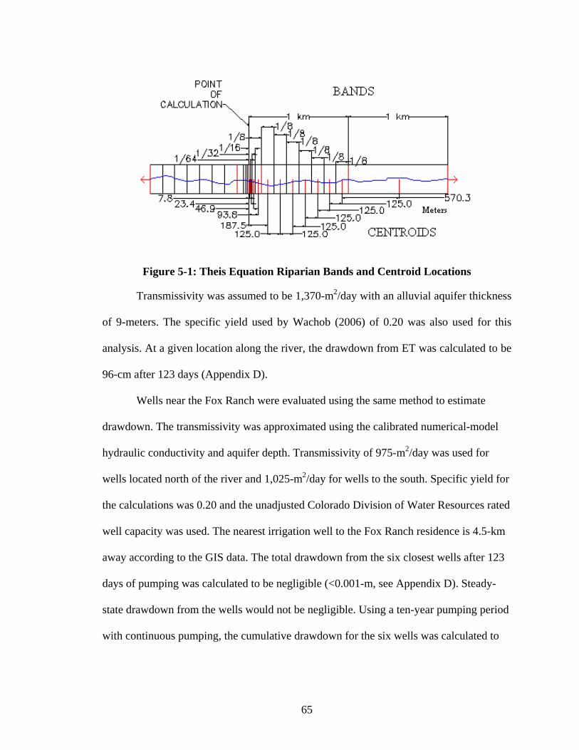
65
Figure 5-1: Theis Equation Riparian Bands and Centroid Locations
Transmissivity was assumed to be 1,370-m2/day with an alluvial aquifer thickness
of 9-meters. The specific yield used by Wachob (2006) of 0.20 was also used for this
analysis. At a given location along the river, the drawdown from ET was calculated to be
96-cm after 123 days (Appendix D).
Wells near the Fox Ranch were evaluated using the same method to estimate
drawdown. The transmissivity was approximated using the calibrated numerical-model
hydraulic conductivity and aquifer depth. Transmissivity of 975-m2/day was used for
wells located north of the river and 1,025-m2/day for wells to the south. Specific yield for
the calculations was 0.20 and the unadjusted Colorado Division of Water Resources rated
well capacity was used. The nearest irrigation well to the Fox Ranch residence is 4.5-km
away according to the GIS data. The total drawdown from the six closest wells after 123
days of pumping was calculated to be negligible (<0.001-m, see Appendix D). Steady-
state drawdown from the wells would not be negligible. Using a ten-year pumping period
with continuous pumping, the cumulative drawdown for the six wells was calculated to

66
be 2.1-meters. It is concluded that irrigation wells are too far away to produce drawdown
at the ranch within a single growing season.
5.1.2 Numerical Model Drawdown
The seasonal well drawdown calculated by the numerical model was negligible at
the river using the stream package boundary condition along the Fox Ranch as shown in
Figure 5-2. The model indicates that drawdown occurs at the river adjacent to the well
field located to the east of the Fox Ranch (contour intervals starting away from the wells:
outer to inner contours are 0.05-m, 0.13-m, 0.25-m, 0.5-m, 0.75-m, 1-m, 2-m and 3-m).
Figure 5-2: Growing Season Well Drawdown w/o ET (Visual Modflow v. 4.0, 2003)

67
The model calculated extensive seasonal drawdown along the river due to ET.
Figure 5-3 shows drawdown contours, the largest of which is 2-meters at the end of the
growing season, from ET. By inspection of the model output contours, the total
drawdown from ET increases progressing from left (upstream) to right (downstream).
This is partly because a constant inflow was specified at the river headwaters with the
stream package. Inflow is not decreased as would be required to accurately represent ET
upstream of the model. The contour intervals are the same as above for drawdown by
irrigation only.
Figure 5-3: Growing Season Drawdown from ET (Visual Modflow v. 4.0 2003)

68
Figure 5-4 shows the cumulative seasonal drawdown from both irrigation and ET.
The cones of depression and drawdowns are larger than in previous figures along the
river. The contour intervals are the same as stated for drawdown by irrigation only.
Figure 5-4: Cumulative Seasonal Drawdown, Irrigation and ET at the end of the growing season (day 257) (Visual Modflow v. 4.0 2003)
5.2 STREAM DEPLETION ANALYSIS
Southern Yuma County irrigation wells were analyzed to determine the amount of
single-season stream depletion from each well. The numerical model was used,
implementing two analysis methods. Results from the numerical model analyses were
compared to results obtained using the analytical Glover equation model.

69
5.2.1 Numerical Model Stream Depletion Analysis
The numerical model was used to calculate stream depletion caused by individual
wells. Mass-balance sheets (Figure 5-5) created by Visual Modflow, display the total
volume and time-variant rate-of-flow to or from the aquifer due to the various boundary
conditions. The model calculates the aquifer mass balance. The terms listed under the
heading “in” describe the rate or volume of flow from the boundary into the aquifer.
Terms listed under the heading “out” describe the rate or volume of flow from the aquifer
into the boundary. The flow into and out of the aquifer due to the stream boundary
condition are listed in the mass-balance sheet under the term stream leakage.
Figure 5-5: Sample Mass Balance Output Sheet (Visual Modflow v. 4.0 2003)

70
Figure 5-6: Explanation Diagram of Sample Mass Balance Output Sheet (Figure 5-5)
The mass-balance output sheet, shown in Figure 5-5 is for an arbitrary well at the
end of stress period 1. As shown, ten time-steps were used in the calculation for stress
period 1. Visual Modflow calculates the head value of each cell for each time-step used
in the stress period. Stress periods are representative of distinct combinations of constant
input variables and can be any length of time. Heads for the first time step of a stress
period are calculated using the previous stress period’s output heads as initial heads. Each
change in model conditions requires an additional stress period. For example, a change in
modeled evapotranspiration or boundary cell head would each create a distinct stress
period unless occurring on the same model day. Stress period 1 corresponds to the time
before the start of the irrigation season (day 1 to 135) in the transient model (see Visual
Modflow Documentation for more details). The most important stress period for this

71
analysis was the stress period ending on day 257, corresponding to the time just before
the modeled end of pumping.
Additive and subtractive methods described in sections 5.2.1.1 and 5.2.1.2 were
used for stream depletion calculations. The results of these methods of analysis were
slightly different. Results from both methods were considered in the well rankings.
Appendix F contains the tabulated results for both methods.
5.2.1.1 Additive Method
The additive method was used to determine the amount of single-season
drawdown and stream depletion induced by a single well, pumping in the Ogallala
aquifer, starting with the calibrated (pre-development) initial heads. A one-year transient
model run was used with the input data (ET, recharge, hydraulic conductivity, etc.)
described in previous sections and the calibration wells pumping until day 135 (start of
seasonal pumping) to maintain calibration. This method was used to isolate well
calculation from the cumulative pumping effects in the model.
A mass-balance output sheet similar to that shown in Figure 5-5, was created for a
one-year run, the calibration run, representing predevelopment without disturbance from
wells, of the model as described in chapter 4. This run was used as the “control” run for
comparison to runs with added wells. This was assumed to be the pre-development
condition for calculating stream depletion. The sheet contains calculated pre-development
mass balance information including the rate of flow into and out of the aquifer from
various model entities including the stream.

72
Single wells were added individually to the model and the transient-state single-
season model was re-run for each isolated well. Mass-balance output sheets were created
for the model after each run. The change in the net rate of stream influx was calculated by
comparing the control run and runs with each well added individually. The difference
was assumed to be the single-season change in streamflow caused by each well.
Example Additive Analysis calculation:
Control Run (G):
A. The flux rate into the aquifer from the stream = 129,353.27-m3/day
B. The flux rate into the stream from the aquifer = 549,772.25-m3/day
C. The net flux rate: B - A = 420,418.98-m3/day
This is the assumed pre-development flux into the stream channel from the
aquifer. Hydraulic channel conditions (Section 4.5) were not modified to represent the
change due to larger flow rate.
For the pumping of well ‘A’ located at PLS coordinates SC00304419CD (Appendix G):
D. The flux rate into the aquifer from the stream = 129,543.01-m3/day
E. The flux rate into the stream from the aquifer = 547,864.25-m3/day
F. The net flux rate: E - D = 418,321.24-m3/day
The net change in flux rate due to well: C - F = 2,097.74-m3/day (384.8-gal/min)
This was assumed to be the rate of stream depletion induced by the well ‘A’ 123
days after the start of pumping.

73
5.2.1.2 Subtractive Method
In the subtractive analysis method, wells were removed instead of added to the
model. The transient model was run for one season with all wells pumping. This was
assumed to represent the developed scenario with all wells being installed simultaneously
before the growing season into the pre-development (undisturbed) aquifer. A one-year
transient model run was used with the previously described input data (chapter 4) and the
calibration wells being pumping until day 135 (start of seasonal pumping) to maintain
calibration.
This procedure calculated the rate of seasonal stream depletion caused by all
modeled wells. The major difference between the subtractive method analysis and the
additive method analysis is that the saturated thickness of the aquifer is reduced in the
subtractive method by the pumping from all wells. The reduced saturated thickness in this
scenario exacerbates the single-season stream depletion of individual wells located in
close proximity to others.
An output sheet was generated for the run with all wells pumping as the control
scenario for this analysis. The model was re-run one time with each well removed
individually but all others continuing to pump. Output sheets were generated for each run
and the change in the rate of flux into the stream for each well was calculated.
Example Subtractive Analysis calculation:
Predevelopment State with all wells pumping:
A. The flux rate into the aquifer from the stream = 127,688.86-m3/day
B. The flux rate into the stream from the aquifer = 540,778.19-m3/day

74
C. The net flux rate: B - A = 413,089.33-m3/day
This is the assumed developed flux into the stream channel from the aquifer.
Hydraulic channel conditions (Section 4.5) were not modified to represent the change due
to larger flow rate.
For the pumping of well ‘A’ located at pls coordinates SC00304419CD (Appendix G):
D. The flux rate into the aquifer from the stream = 127,536.58-m3/day
E. The flux rate into the stream from the aquifer = 542,813.69-m3/day
F. The net flux rate: E - D = 415,277.11-m3/day
The net change in flux rate due to well: F - C = 2,187.8-m3/day (401.4-gal/min)
This was assumed the rate of stream depletion induced by well ‘A’, at the time
123 days after the start of pumping in the disturbed aquifer where saturated thicknesses
are smaller because of superimposed cones of depression from other wells pumping.
Well analysis using this method examines the effect of each of the wells on a
disturbed water table with many perturbations and a reduced saturated thickness caused
by the disturbances. By superposition, effects would be expected to be similar to those of
the additive method but changes in saturated thickness in a heterogeneous aquifer,
modify the results. (See well map Figure 5-7).
5.2.2 Analytical Glover Equation Analysis
A significant amount of literature is available concerning methods for computing
stream depletion. A comprehensive review of literature is available by Miller et al.
(2006). The review starts with the mathematical analysis first published by Theis (1941).

75
The analysis developed by Glover and Balmer (1954) is commonly referred to as the
Glover Equation analysis. The method uses a probability integral for computation of
stream depletion. Mathematically ideal conditions are assumed for use of the Glover
Equation. Methods have been developed for non-ideal conditions such as using image
wells to analyze boundary effects. Miller et al. (2006) also studied the use of the semi-
analytical stream depletion model for aquifers with definite boundaries.
The development of the SDF term by Jenkins (1968) simplified the analysis
allowing broad use of the Glover Equation analysis. Jenkins (1968) not only developed
the SDF term but presented non-dimensional relationships between stream-depletion
volume and time. The graphical non-dimensional relationships can be used to determine
the rate of stream depletion given aquifer characteristics, pumping rate and time. Jenkins
is widely cited for stream depletion analysis because of the method’s simplicity.
Zlotnik (2005) developed a solution for stream depletion and drawdown in a
system with partially penetrating stream. The relationship is transient and requires that
the aquifer below the stream be infinite and homogeneous. The solution requires
pumping to be from the alluvial aquifer that also underlies the stream.
The numerical model results were compared to the results of the analytical Glover
Equation model. The Glover Equation (Glover and Balmer 1954) computes the stream
depletion rate (q), as a function of pumping time (t), well discharge rate (Q), and aquifer
characteristics shown as Equation 5-2:

76
Equation 5-2
⎟⎟⎠
⎞⎜⎜⎝
⎛=
tTSaerfcQ
q4
2
Where:
q = rate of stream depletion of water to the aquifer (L3/T)
Q = Well pumping rate (L3/T)
a = distance to the well from the stream (L)
S = aquifer specific yield (L3/L3)
t = time since initiation of pumping (T)
T = transmissivity of the aquifer (L2/T)
Assumptions of the Glover model include a straight and fully penetrating constant
head boundary at the stream, a fully penetrating well, pumping at constant rate (Q), for
time t after the start of pumping, in an undisturbed, homogeneous aquifer of constant
saturated thickness. Drawdown is considered negligible compared to the saturated
thickness so transmissivity is assumed not to vary with time. It was also assumed that
water is released instantaneously from storage and residual effects of pumping are
assumed negligible (Jenkins 1968).
The rate of stream depletion using the Glover Equation was calculated (Appendix
E) for a single growing season of 123 days as was used in the numerical model.
Parameters used in the Glover Equation were derived from the calibrated model to ensure
input parameter consistency. Recharge was not simulated using the analytical method
although it was included in the numerical model.

77
5.2.2.1 Glover Parameter Estimation
To be conservative when calculating stream depletion from proposed wells,
parameters must be used that do not underestimate the actual rate of depletion. This
ensures that the well will not use more streamflow than predicted and disrupt habitat.
When estimating streamflow recovery after well forbearance, the opposite is true.
Overestimation of stream depletion from wells taken out of service would mean that less
water would appear as streamflow than was estimated as recovered flow. Parameters used
in the following calculations resulted in conservative estimates of stream depletion.
The distance to wells for Glover Equation analysis was taken to be the shortest
distance to the river estimated by GIS using geo-referenced satellite photos and well
coordinates provided by the CDWR. Use of the distance to the alluvium instead of the
stream would produce higher depletion estimates because of the shorter distance and
would be reasonable because of the very high hydraulic conductivity of the alluvial sand.
The calibrated numerical model was used to estimate transmissivity using a low
estimate of the average calibrated hydraulic conductivity between the stream and the well
(excluding the high alluvial hydraulic conductivity). Transmissivity was calculated by
multiplying the calibrated hydraulic conductivity by the average of the alluvial and well
location saturated thicknesses. Aquifer thicknesses were estimated using the GIS
surfaces. Alluvial depths were assumed to be 9-m.
The value of specific yield used in the Glover Equation analysis was based on the
specific yield zones used in the numerical model. Values ranged from 0.17 to 0.22
(Figure 1-6).

78
5.3 STREAM DEPLETION ANALYSIS RESULTS
5.3.1 Numerical Model Stream Depletion Analysis Results
Stream Depletion analysis of the modeled irrigation wells using additive and
subtractive methods produced similar but slightly different results. The top 15 wells, in
regards to the model calculated single-season change in streamflow for each analysis
method, are provided in Table 5-1. The model indicated that these wells produced the
largest change in water entering the stream channel by each of the individual methods
(day 257 is the end of the irrigation season).
It is worth noting that the rankings are different for the two methods. The impact
on streamflow for most of the wells presented is within the “noise” range for the model
based upon the percent change in streamflow from each well. This is indicative that the
wells have some sort of impact on streamflow in the model, as explained in later sections,
but the differences in the rate of stream depletion are too small to be used reliably in
ranking of the wells.

79
Explanation of Table 5-1 Columns:
1) Map Designation (see Figure 5-7)
2) Well coordinate in Public Land Survey coordinate system or run description.
3) Modeled well pumping rate (m3/day) – 61% CDWR capacity rating.
4) Modeled well pumping rate in gallons per minute – 61% CDWR capacity rating.
5) Straight-line distance from the well to the stream (m).
6) Model calculated rate of stream out-flux into the aquifer at day 257 (m3/day).
7) Model calculated rate of stream in-flux from the aquifer at day 257 (m3/day).
8) Calculated groundwater dependent streamflow (item 5 - 4) (m3/day).
9) Change in the rate of stream out-flux due to the well from control scenario
(m3/day) (well’s column 4 – control column 4) in (m3/day).
10) Change in the rate of stream in-flux due to the well from control scenario
(m3/day) (well’s column 5 – control column 5) in (m3/day).
11) Change in the calculated groundwater dependent stream (m3/day) (well’s column
6 – control column 6).
12) Column 9 in gallons per minute
13) General notes about the well and calculation.
a. “Alluvial” indicates the well is located within one mile of the river and
is assumed to be effectively in the alluvial formation.
b. “Low Sat Thick” indicates well is located in an area with initial
saturated thickness of less then 6-m.

80
Table 5-1: Top 15 Wells According to Additive and Subtractive Streamflow Change Results for day 257 (All Shown at End of Pumping)
Map
D
esc.
(1)
Add
itive
R
ank
PLS
Coo
rdin
ate
(or R
un)
(2
)
Cap
acity
(m
3 /day
)
(3)
Cap
acity
(g
pm)
(4
)
Dis
tanc
e to
St
ream
(m)
(5)
Out
of S
tream
Fl
ux (m
3 /day
) (6
)
Into
Stre
am
Flux
(m
3 /day
)
(7)
Flow
(m
3 /day
) (8
)
Out
of S
tream
C
hang
e (m
3 /day
)
(9
)
Into
Stre
am
Cha
nge
(m3 /d
ay)
(1
0)
Stre
am F
low
C
hang
e (m
3 /day
)
(11)
Stre
am F
low
C
hang
e
(gpm
)
(1
2)
Not
es
(13)
--
All
Off
--
1293
5354
9772
4204
19-
--
-C
ontro
lA
1SC
0030
4419
CD
2388
438
<200
1295
4354
7864
4183
2119
0-1
908
-209
8-3
85A
lluvi
alB
2SC
0040
4718
AA
2159
396
1180
1288
6854
8338
4194
70-4
85-1
434
-949
-174
Y3
SC00
3047
05D
A33
2561
0>3
000
1294
5254
9085
4196
3399
-687
-786
-144
Low
Sat
Thi
ckK
4SC
0040
4713
AC
998
183
1290
1294
5054
9083
4196
3397
-689
-786
-144
V5
SC00
3047
03B
C53
2097
6>3
000
1294
4654
9081
4196
3593
-691
-784
-144
Low
Sat
Thi
ckJ
6SC
0040
4618
BA
5320
976
2200
1294
4954
9084
4196
3596
-689
-784
-144
Q7
SC00
4046
08D
D33
2561
032
1012
9438
5490
9141
9653
84-6
82-7
66-1
41L
8SC
0040
4715
DC
3325
610
846
1294
4254
9107
4196
6589
-666
-754
-138
O9
SC00
4046
18A
A33
2561
026
3812
9447
5491
1441
9667
94-6
58-7
52-1
38P
10SC
0040
4729
AA
4988
915
>300
012
9433
5491
0841
9675
80-6
64-7
44-1
36X
11SC
0030
4705
AA
3325
610
>300
012
9427
5492
0241
9775
74-5
70-6
44-1
18Lo
w S
at T
hick
W12
SC00
3047
04A
C53
2097
6>3
000
1293
9454
9180
4197
8641
-592
-633
-116
Low
Sat
Thi
ckC
13SC
0040
4718
BB
2328
427
183
1290
5854
8853
4197
94-2
95-9
20-6
25-1
15A
lluvi
alN
14SC
0040
4720
CD
3325
610
2656
1294
1754
9414
4199
9764
-358
-422
-77
D15
SC00
4047
14A
B33
2561
029
1612
9325
5493
2341
9997
-28
-449
-422
-77
Map
D
esc.
(1)
Subt
ract
ive
Ran
k
PLS
Coo
rdin
ate
(or R
un)
(2
)
Cap
acity
(m
3 /day
)
(3)
Cap
acity
(g
pm)
(4
)
Dis
tanc
e to
St
ream
(m)
(5)
Out
of S
tream
Fl
ux (m
3 /day
) (6
)
Into
Stre
am
Flux
(m3 /d
ay)
(7
)
Flow
(m
3 /day
) (8
)
Out
of S
tream
C
hang
e (m
3 /day
)
(9
)
Into
Stre
am
Cha
nge
(m3 /d
ay)
(1
0)
Stre
am F
low
C
hang
e (m
3 /day
)
(11)
Stre
am F
low
C
hang
e
(g
pm)
(12)
Not
es
(13)
--
All
On
--
1277
4154
0880
4131
39-
--
-C
ontro
lA
1SC
0030
4419
CD
2388
438
<200
1275
3754
2814
4152
77-2
0519
3321
3839
2A
lluvi
alW
2SC
0030
4704
AC
5320
976
>300
012
7643
5425
6141
4918
-98
1681
1779
326
Low
Sat
Thi
ckB
3SC
0040
4718
AA
2159
396
1180
1282
2454
2634
4144
1148
217
5412
7223
3C
4SC
0040
4718
BB
2328
427
183
1280
8954
2078
4139
8934
711
9785
015
6A
lluvi
alV
5SC
0030
4703
BC
5320
976
>300
012
7840
5412
3041
3389
9934
925
046
Low
Sat
Thi
ckF
6SC
0040
4719
AA
1842
338
<200
1279
9254
1327
4133
3525
144
719
636
Allu
vial
E7
SC00
4047
17C
D33
2561
024
6012
7912
5412
0941
3297
170
328
158
29G
8SC
0040
4712
CA
1995
366
1250
1277
8054
0988
4132
0838
107
6913
Y9
SC00
3047
05D
A33
2561
0>3
000
1277
7954
0857
4130
7838
-23
6111
Low
Sat
Thi
ckM
10SC
0040
4511
CD
3990
732
3955
1277
3754
0889
4131
52-4
913
2S
11SC
0040
4405
DD
2725
500
5024
1277
4454
0871
4131
272
-10
122
R12
SC00
4044
04B
D39
9073
246
9512
7741
5408
7041
3129
0-1
010
2Z1
13SC
0040
4514
DB
4361
800
4890
1277
3554
0866
4131
31-6
-14
81
K14
SC00
4047
13A
C99
818
312
9012
7737
5408
6941
3132
-4-1
27
1Z2
15SC
0040
4514
CB
5816
1067
4903
1277
3454
0880
4131
46-7
-17
1

81
For the additive analysis, the change in streamflow (columns 9 and 10, Table 5-1)
is negative when adding a well. This is because the stream is depleted by adding the well,
thereby reducing the rate of streamflow. The change in streamflow for the subtractive
analysis is positive because wells are removed from the model to examine the increase in
streamflow rate.
Low initial saturated thickness (4-m to 5.5-m) occurred at wells V, W, X and Y as
noted in each table (Figure 5-7). These wells are located to the northwest of the Fox
Ranch at a distance of approximately 11-km from the river. Although these wells ranked
in the top-15 by calculated stream depletion, using at least one of the numerical modeling
analysis methods, the results are presumed to be unreliable because a larger internal
water-balance percent discrepancy occurred for the analysis of these wells. This is
assumed to be an artifact of the Modflow model where drawdown is not negligible with
respect to the saturated thickness. Analysis of all other wells produced a water-balance
discrepancy of less than 0.1%, while analysis of these wells produced a discrepancy
between 0.1% and 0.3%.
The single-season stream depletion calculated by the model for wells D, J, K, L,
N, O, P and Q was over 400-m3/day less for the subtractive analysis than for the additive
analysis. The causes of this are unknown but are assumed connected with an absence of
modeled streamflow in the river near these wells at the end of pumping. These wells are
located in the well field to the southwest of the Fox Ranch. The cumulative drawdown for
a run with no modeled ET from this well field created a cone of depression as shown in
Figure 5-2, that reaches the river after one season of pumping. There are also two alluvial
wells upstream of the well field. Over half (2,543 / 4,893-m3/day) of the specified rate of

82
stream boundary in-flow was calculated to be depleted from the stream by the wells
upstream of the well field (B, C, E, F and G).
Wells R and S ranked in the top 15 stream-depletion wells for the subtractive
analysis. These wells are existing wells that were used as calibration wells because of
their pre-1958 installation date. These wells were ranked but were given an unfair bias in
the stream depletion analysis because they had been pumped in the calibration for the
winter season prior to the growing season. This would increase the perceived stream
depletion by increasing the pumping time. For this reason, the analytical Glover equation
was the only reliable method of analysis and ranking for these wells.
These analyses were completed using the entire stretch of the river within the
boundaries of the numerical model. The specified headwater inflow for the model was
4,890-m3/day (2-cfs, Section 4.5). Water is allowed to enter or exit the river depending
upon the streambed hydraulic conductivity and the difference in head between the stream
boundary and the aquifer. Additional water can be moved from the stream boundary to
the aquifer by perturbations to the groundwater that change the gradient, such as with ET
or irrigation-well pumping.
As shown in Table 5-1, there is a component of stream flux into the stream, but
also out of the stream. The total rate of streamflow does not correlate to the actual
streamflow seen today. The model was calibrated using 1958 water table levels but
utilizes stream boundary conditions and dimensions as observed in 2006. The pre-
development streamflow calculated by subtracting the calculated stream out-flux from the
calculated stream influx for the additive method “control” run (all wells off) is 420,419-

83
m3/day (171-cfs). This is much higher than the recorded (USGS gauge date Haigler, NE)
pre-development streamflow averaging of 63,870-m3/day (26-cfs).
Much of the discrepancy associated with the streamflow rate is assumed attributed
to incorrect stream boundary dimensions and hydraulic conditions. The additional water
available in the model is assumed to be attributed to incorrect recharge values. A
hydraulic model of the river would be required to improve the conditions of the
groundwater model. Calibration by Sya may also improve the calculated stream inflow
value since less water may be required to maintain calibration heads in the model.
5.3.2 Glover Equation Results
Glover equation analysis calculations are provided in Appendix E for wells
estimated to reduce end-of-season streamflow by at least 10-m3/day using either method
in the numerical model for comparison. The results of this analysis are shown in Table
5-2. As explained before, the impact from the majority of these wells is in the “noise”
region of the numerical model.
The eight wells producing the largest change in streamflow according to the
Glover equation analysis would each produce a single-growing-season change in
streamflow rate between 135 and 2,100-m3/day (25 and 385-gpm) through the Fox Ranch
(Table 5-2). The range is due to the difference in the calculated stream depletion
depending upon the distance to the stream, the aquifer characteristics and the pumping
rate. The next 10 most detrimental wells would each produce between 5.5 and 55-m3/day
(1 and 10-gpm) change in streamflow at the end of the season. Two additional wells
located just outside of the upstream model boundary and close to the river were included
in the table and Glover Equation Analysis because of their proximity to the river.

84
Explanation of Table 5-2 Columns:
1) Map Designation (see Figure 5-7)
2) Glover Equation analysis rank from day 257 calculated well stream depletion
3) Numerical additive analysis rank from day 257 calculated well stream depletion
4) Numerical subtractive analysis rank from day 257 calculated well stream
depletion
5) Well coordinate in Public Land Survey (PLS) coordinate system
6) 61% of rated CDWR well capacity (m3/day)
7) 61% of rated CDWR well capacity (gpm)
8) Additive analysis calculated change in seasonal streamflow (m3/day)
9) Additive analysis calculated change in seasonal streamflow (gpm)
10) Subtractive analysis calculated change in seasonal streamflow (m3/day)
11) Subtractive analysis calculated change in seasonal streamflow (gpm)
12) Glover Equation analysis calculated change in seasonal streamflow (m3/day)
13) Glover Equation analysis calculated change in seasonal streamflow (gpm)
14) General notes about the well and calculation.
a. “Alluvial” indicates the well is located within one mile of the river and is
assumed effectively to be in the alluvial formation.
b. “High Discrepancy” indicates the numerical model well analysis
calculations produced high water balance discrepancies relative to other
wells (due to low saturated thickness at the well)
c. “Calibration Well” indicates the well was pumped in the calibration of the
model, increasing the end of season rate of stream depletion

85
Table 5-2: Glover Equation Analysis Results Compared to Numerical Analyses Pumping Duration: 123 Days (Equal to the End of the Irrigation Season, day 257)
Map
Des
c.
(1)
Glo
ver
Ran
k
(2)
Add
itive
R
ank
(3
)
Subt
ract
ive
Ran
k
(4
)
PLS
Wel
l C
oord
inat
es
(5
)
61%
R
atin
g (m
3 /day
) (6
)
61%
R
atin
g (g
pm)
(7
)
Stre
amflo
w
Cha
nge
(m3 /d
ay)
(8
)
Stre
amflo
w
Cha
nge
(gpm
)
(9
)
Stre
amflo
w
Cha
nge
(m3 /d
ay)
(10)
Stre
amflo
w
Cha
nge
(gpm
)
(1
1)
Stre
amflo
w
Cha
nge
(m3 /d
ay)
(1
2)
Stre
amflo
w
Cha
nge
(gpm
)
(1
3)
Not
es
(1
4)
A1
11
SC00
3044
19C
D23
8843
820
97.7
384.
821
38.0
392.
221
02.4
385.
8A
lluvi
alB
22
3SC
0040
4718
AA
2328
427
948.
717
4.0
1271
.823
3.3
2049
.637
6.1
Allu
vial
C3
134
SC00
4047
18B
B18
4233
862
4.8
114.
684
9.8
155.
916
22.4
297.
7A
lluvi
alD
415
18SC
0040
4714
AB
3325
610
421.
677
.34.
60.
997
4.3
178.
8E
517
7SC
0040
4717
CD
2159
396
65.8
12.1
158.
029
.057
6.6
105.
8F
616
6SC
0040
4719
AA
1995
366
81.9
15.0
195.
835
.953
3.4
97.9
G7
188
SC00
4047
12C
A99
818
326
.34.
869
.112
.727
8.7
51.1
I8
N/A
N/A
SC00
4047
19D
D39
9073
2N
/AN
/AN
/AN
/A20
8.9
38.3
Allu
vial
- O
utsi
de M
odel
H9
N/A
N/A
SC00
4048
15C
D11
6421
3.5
N/A
N/A
N/A
N/A
148.
527
.3O
utsi
de M
odel
J10
626
SC00
4046
18B
A53
2097
678
4.0
143.
81.
00.
243
.27.
9K
114
14SC
0040
4713
AC
3990
732
785.
614
4.1
7.3
1.3
26.8
4.9
L12
825
SC00
4047
15D
C33
2561
075
4.3
138.
41.
60.
321
.84.
0M
1341
10SC
0040
4511
CD
3990
732
2.8
0.5
12.7
2.3
20.8
3.8
N14
1424
SC00
4047
20C
D33
2561
042
2.3
77.5
1.7
0.3
16.4
3.0
O15
919
SC00
4046
18A
A33
2561
075
2.3
138.
04.
50.
816
.33.
0P
1610
17SC
0040
4729
AA
4988
915
744.
013
6.5
4.6
0.9
12.6
2.3
Q17
773
SC00
4046
08D
D33
2561
076
6.0
140.
50.
00.
08.
91.
6R
1821
12SC
0040
4404
BD
3990
732
11.4
2.1
9.9
1.8
8.3
1.5
Cal
ibra
tion
Wel
lS
1929
11SC
0040
4405
DD
2725
500
4.5
0.8
11.9
2.2
5.5
1.0
Cal
ibra
tion
Wel
lT
2019
88SC
0040
4725
DD
2725
500
17.0
3.1
0.0
0.0
5.1
0.9
Cal
ibra
tion
Wel
lU
2120
92SC
0040
4727
DD
2725
500
17.0
3.1
0.0
0.0
3.1
0.6
Cal
ibra
tion
Wel
l-
2222
29SC
0010
4535
BD
5819
1067
.510
.31.
90.
00.
03.
10.
6C
alib
ratio
n W
ell
-23
2341
SC00
2045
10A
B53
2097
610
.31.
90.
00.
01.
40.
3C
alib
ratio
n W
ell
V24
55
SC00
3047
03B
C53
2097
678
4.0
143.
825
0.3
45.9
1.2
0.2
Hig
h D
iscr
epan
cyW
2512
2SC
0030
4704
AC
5320
976
633.
311
6.2
1779
.432
6.4
1.1
0.2
Hig
h D
iscr
epan
cyX
2611
67SC
0030
4705
AA
3325
610
643.
611
8.1
0.0
0.0
0.7
0.1
Hig
h D
iscr
epan
cyY
273
9SC
0030
4705
DA
3325
610
786.
314
4.2
61.3
11.3
0.6
0.1
Hig
h D
iscr
epan
cy
Add
itive
Subt
ract
ive
Glo
ver

86
The results of the Glover Equation Analysis indicate that for a run where the ten
most detrimental irrigation wells were not pumping, there would be an end-of-season
water budget improvement of up to 8,000-m3/day (3.5-cfs). There would be diminishing
seasonal returns for wells as the distance from the well to the river increases pumping
rate decreases. The cumulative stream depletion calculated for the next 17 wells in the
Glover Equation analysis was only 153.7-m3/day. The locations of the wells presented in
Table 5-2 are shown in Figure 5-7.
Wells with Glover Equation analysis rank 2 through 12, 14 through 17, 20 and 21
(B – L, N – Q, T & U) were located in a well field to the southwest of the Fox Ranch as
shown in Figure 5-7. Wells in this area are in close proximity to each other. Wells ranked
18 through 21 (R – U) are far from the river and were used in calibration of the model.
Glover Equation analysis for these well indicated very low seasonal stream depletion.
Wells ranked 22 and 23 are also calibration wells, located far north of the river and do not
lie within the borders of the image shown in Figure 5-7. Glover Equation calculations for
wells closer to the river produce higher rates of stream depletion and should be
considered to rank higher overall than these wells.

87
Figure 5-7: Locations of Wells Included in Table 5-2 with Glover Analysis Ranks
(USDA 2005; CDWR 2005; CDOT 2006)

88
5.3.3 Well Distance Implications
By this stream depletion analysis, wells located long distances from the river were
found to contribute mostly to regional decreases in water table level. Wells more than a
limited distance away affect streamflow in a more indirect manner where seasonal stream
depletion becomes negligible (calculated end-of-season stream depletion rate is less than
1% of the well pumping rate). Wells must be within 1,200-m (4,000-ft) for wells with
capacities less than around 5,000-m3/day to deplete the stream more than a negligible
amount (about 10-m3/day).
Around 1,220-m (4,000-ft) to 1,830-m (6,000-ft) is the limit to where, for this
area, modeled aquifer condition and a pumping season duration of 123 days, the ratio of
stream depletion (q) to well pumping rate (Q) for wells with capacity of 5,450-m3/day
(1,000-gpm) drops below 0.01. Very high pumping capacity (around 5,000-m3/day) is
required for wells close to this limit to deplete the stream more than 10-m3/day. Analysis
of the distance was computed using both the Glover Equation (equation 5-2) and the
Arikaree River Numerical Groundwater Model.
5.4 ANALYSIS, OBSERVATIONS & CONCLUSIONS
The calibrated model of the Arikaree River produced some interesting results.
Wells close to the river deplete streamflow in a single pumping season while wells
further away (>3000-m) generally do not. Because of the short distance at which single-
season pumping becomes negligible, wells located upstream of the Fox Ranch along the

89
alluvium should be considered for forbearance before wells located laterally from the
river, at further distances.
It is expected that there exists a maximum distance upstream of the Fox Ranch
that forbearance of alluvial wells remains more beneficial to streamflow than forbearance
of wells located laterally to the river around the Fox Ranch. An increase in ET is
expected from exposed surface water and high water table, causing diminishing returns
between the upstream well and the Fox Ranch. Ultimately, to stop the streamflow decline
or improve streamflow, the regional water balance deficit would need to be eliminated.
Essentially the amount of water entering the region through the aquifer, stream and
precipitation must match or be larger than the amount of water being used for irrigation,
by evapotranspiration. Many large capacity wells throughout the basin would need to be
decommissioned and the aquifer level would have to be allowed to recover.
A reduction in streamflow of 23,480-m3/day (9.6-cfs) was calculated by the
model between the end-of-season streamflows from year one to year ten. This was
calculated using the method described in the well analysis using the mass balance output
sheets from runs with all wells pumping seasonally. The total year-one end of season
stream influx was 413,090-m3/day while the total year ten end of season stream influx
was 389,610-m3/day. This decline is indicative of irrigation-well stream depletion. The
water budget is also shown to be unbalanced after well installation as the decline is
progressive through the ten-year period. It must be noted, however that the magnitude of
the streamflow in the model does not match existing conditions so this streamflow rate
reduction would not be the actual change for existing conditions.

90
The most substantial unknowns in this model are Sya, ET and recharge. ET and
recharge would theoretically not change the results of the pumping analysis but the Sya
would. Additional work to calibrate by Sya and to improve the model water balance
would improve the results substantially. Only after this type of calibration could there be
an improvement to the prediction of streamflow from well analysis.

91
CHAPTER 6 ARIKAREE BASIN WATER BALANCE
The Arikaree River groundwater basin shown in Figure 1-5 is limited in extent.
The amount of runoff into the stream and recharge into the aquifer are controlled by the
size of the basin. Because of the basin size, the flow of groundwater through the basin is
very important to the overall water budget.
The control volume (system) for this water balance is the combined alluvial and
high plains (Ogallala) aquifers, along with the stream and other open water in the
alluvium. The water budget explanation, as shown in Figure 6-1 details the ten inputs and
outputs to the water budget.
Figure 6-1: Water Budget Explanation
Where:
ET(G) = Evapotranspiration at the ground level from the wetted surface of
soils and plants (Evaporation/initial abstraction)

92
ET(V) = Evapotranspiration from below the ground surface but above the
water table, including by plant use (mostly transpiration)
ET(AQ) = Evapotranspiration from the major aquifer, below the water
table (mostly negligible except in areas of very high water table)
ET(AL) = Evapotranspiration from the alluvial aquifer including riparian
plant use
ET(S) = Evapotranspiration from within the banks of the stream (mostly
evaporation)
As shown, the atmospheric inputs to the water-balance control volume are
overland flow to the stream, combined aquifer recharge (attributed to precipitation) and
evapotranspiration from open water including the stream. The control volume is spatially
different for the overland flow contribution from the stream and the recharge area to the
aquifer. This is because the drainage basin differs slightly from the groundwater basin.
The inputs and outputs are categorized for discussion in this study into atmospheric
effects, streamflow, groundwater flow and irrigation effects.
6.1.1 Atmospheric Effects
For the sake of discussion, overland flow, recharge and ET are included in the
category of precipitation effects. ET occurring on the plains, both in the vadose zone and
at the ground surface must be taken as an abstraction from the total precipitation as
shown in Figure 6-1. ET in the riparian areas is assumed to be high because of the dense
vegetation and exposed water or very high water table.

93
The average precipitation upstream of the Fox Ranch property is 42-cm (16.5-in)
per year at the USDA Central Great Plains Weather Station in Akron, CO. The
groundwater basin area was estimate in GIS to be 149,980-ha (370,600-acres) using
water table elevation contours (Figure 1-5). The drainage basin is slightly larger at
159,000-ha (392,000-acres) including some area where the direction of groundwater flow
is different from the ground surface gradient. The water-budget groundwater basin,
including all contributing area in Southern Yuma County includes more area than the
groundwater model from chapter 4. The volume of precipitation in the drainage basin was
estimated to be 66,500-ha-m/year (539,000-acre-ft/year). Excluding the river basin and
riparian areas 14,400-ha (35,600-acres) as discussed below, the total precipitation in the
plains area is 60,600-ha-m/year (491,300-acre-ft/year)
Overland flow from the plains was assumed to be 2.7% of the annual precipitation
(1,660-ha-m/year). This was chosen to balances the pre-development water budget based
on the other inputs discussed in this section. Because the stream, alluvium, aquifer and
ground surface are combined within the control volume, the details of whether this water
infiltrates into the alluvium, enters into bank storage, flows directly into the stream or is
used in the process of ET is unimportant but the input must be accounted for in the water
budget.
Calibration of this study’s numerical model required very large values of recharge
because of apparent errors in specific yield. It was noted that the recharge would need to
be reduced by up to 16-cm (6.3-in) to balance the model water budget and reduce the
stream outflow. A reduction of the recharge rate to 15.25-cm (6-in) per year from 20 to
40-cm per year distributed over the model area would be required to eliminate the excess

94
streamflow without modifications to ET. It was also noted that modeled ET was too low
compared to published values since the total ET from the model would only equate to
11.5-cm/year (4.5-in/year) if applied only to the riparian area. This is far below most
published values for riparian ET. Since there is so much error in the modeled ET and
recharge rates, published values were used in place of modeled values.
Reddell (1967) suggests that there is an average of 3.68-cm (1.45-in) per year of
recharge in Yuma County. This was used in the water budget for aquifer recharge in areas
outside of the river basin and riparian area as described in chapter 4. Recharge was
estimated using a numerical groundwater model with a 15.5-km2 (6-sq. mi.) cell size.
Figure 1-4 shows that the surface geology through Yuma County can change drastically
in an area of 15.5-km2. For this reason, Reddell’s estimate is appropriate for use in areas
much larger than his model cell size but may be unreliable in smaller areas, however
there is no better recharge data available. The total area assumed to recharge at 3.68-
cm/year (1.45-in/year) is 135,580-ha (335,000-acres) for an upland recharge of 4,990-ha-
m/year (40,450-acre-ft/year).
The river basin and riparian areas, totaling 14,400-ha (35,600-acres), were
assumed for this water balance to recharge to the aquifer or contribute overland flow
(run-off) to the stream at the rate of precipitation since the water table is at or near the
ground surface. This has been included in the recharge number since the distribution
between recharge and runoff is unknown. The calculated recharge volume from the
riparian and river basin using these rates is 6,040-ha-m/year (48,930-acre-ft/yr). The total
system recharge is 11,030-ha-m/year (89,420-acre-ft/year).

95
The sum of overland flow and recharge is equal to the total precipitation reduced
by the total ET from the ground surface and vadose zone, including the initial abstraction.
Since precipitation is used as a system input for the riparian and river basin areas, ET
must be accounted for from the ground surface and vadose zone for these areas. The
ground and vadose zone ET rates, however were assumed to be included in the Wachob
(2005) riparian growing-season ET rate used in the river basin and riparian areas since
reference ET for the area is only 89-cm/year (35.12-in), although it is recognized that the
initial abstraction is not fully accounted for in this number.
Wachob (2005) estimated a range of riparian ET rates on the Fox Ranch between
69.2-cm (27-in) and 135-cm (53-in) per year depending upon cottonwood tree coverage,
using the White method (White 1932). ET from the 3,180-ha (7,900-acre) riparian area
was assumed to be 3,230-ha-m/year (26,170-acre-ft/year) using the average Wachob
(2005) ET rate of 101.5-cm (40-in) per growing season. The lower estimate of riparian
ET was applied throughout the 11,200-ha (27,700-acre) river basin area assuming an
abundance of vegetation and high water table but less open water area. Using the lower
estimate, the river basin total ET is 7,750-ha-m/year (62,830-acre-ft/year). The basin total
ET from the aquifer and open water is assumed to be 10,980-ha-m/year (89,020-acre-
ft/year).
No aquifer or stream ET was assumed on the plains but as discussed, the
precipitation that does not runoff or recharge is assumed to be ET from the ground
surface or vadose zone. These do not apply in the water balance, according to Figure 6-1
since the runoff and recharge are accounted for on the plains instead of the precipitation.

96
6.1.2 Streamflow
The two components of streamflow for this water budget are channel inflow and
outflow. The average stream outflow from the basin to the USGS stream gauge 06821500
“ARIKAREE RIVER AT HAIGLER, NEBR.” is 1,535-ha-m/yr (12,450-acre-ft/yr). The
pre-development average is 2,442-ha-m/yr (19,800-acre-ft/yr) not including data after
1960. Total outflow has continued to fall as pumping continues.
The upstream inflow to the basin is very low and the stream is usually
disconnected at the western border of Yuma County. Connectivity upstream was assumed
to be re-established only by large precipitation events. For this reason, inflow was
assumed to be 10% of the outflow or 153-ha-m/yr (1,245-acre-ft/yr) for the water budget.
There are no known stream gauges in this area.
6.1.3 Groundwater
The components of the groundwater flow were alluvial inflow/outflow and
Ogallala inflow/outflow. The 1958 USGS water table data (Weist 1964) and Darcy’s Law
(Equation 6-1) were used to estimate the groundwater flux through these formations.
Equation 6-1
⎟⎠⎞
⎜⎝⎛−=
dldhKAQ *
Where: Q = discharge of water through a section of porous media (L3/T)
K = the proportionality constant or hydraulic conductivity (L/T)
A = the cross-sectional area of the media (L2)
dh/dl = the hydraulic gradient (L/L)

97
The hydraulic gradient in the Ogallala Formation and the alluvial aquifer were
determined by measuring the distance between water table contours with known head
values. The average upstream hydraulic gradient was estimated to be 0.0059 to the north
of the river and 0.0050 to the south. Downstream groundwater flow out of the basin was
assumed to be mostly to the south side of the river because the hydraulic gradient is
toward the river on the north side. The downstream hydraulic gradient was estimated to
be 0.0043. The alluvial hydraulic gradients were estimated to be 0.0056 upstream and
0.0016 downstream.
Saturated-thicknesses were approximated in GIS using the 1958 water table
surface (Weist 1964) and the Johnson et al. (2002) bedrock surface (Figure 1-6). The
average saturated-thickness in the Ogallala Formation at the upstream end of the basin
was estimated to be 16.0-m (52.5-ft) to the north and 18.3-m (60-ft) to the south of the
alluvium. The downstream saturated-thickness was estimated to be 12.2-m (40-ft) to the
south of the alluvium. The alluvial saturated-thickness was assumed to be 6.1-m (20-ft)
along the western border of Yuma County and 3.05-m (10-ft) on the eastern border.
The upstream groundwater basin widths were estimated to be 6.4-km (4.0-miles)
to the north and 2.0-km (1.21-miles) to the south of the alluvium. The width of the
groundwater basin at the downstream end of the basin, with the hydraulic gradient not
directed toward the river was estimated to be 11-km (6.8-miles). The upstream alluvial
width was estimated to be 1.3-km (0.8-miles) and the downstream alluvial width was
estimated to be 0.7-km (0.4-miles).

98
The hydraulic conductivities used in this calculation were averaged using the
calibrated numerical model. 152-m/day (500-ft/day) was used for the upstream alluvial
calculation and 213-m/day (700-ft/day) was used for the downstream alluvial calculation.
35-m/day (115-ft/day) was the average used for all Ogallala Formation groundwater flow
calculations.
The Ogallala formation inflow and outflow to the basin were calculated to be
1,005-ha-m/year (8,150-acre-ft/year) and 737-ha-m/year (5,970-acre-ft/year)
respectively. The alluvial inflow and outflow to the basin were calculated to be 246-ha-
m/year (1,990-acre-ft/year) and 26.5-ha-m/year (210-acre-ft/year) respectively. The total
groundwater inflow to the basin was calculated to be 1,251-ha-m/yr (10,140-acre-ft/yr).
The total outflow was calculated to be 764-ha-m/yr (6,180-acre-ft/yr). Gradients at the
western border of the basin have a more east/west direction than do those at the eastern
border. According to the water table map, much of the groundwater flow at the eastern
border is directed into the alluvium. It was assumed to convert mostly to stream outflow.
6.1.4 Irrigation
Well pumping and return flow, are included in the irrigation category for this
study. Well pumping is a relatively new addition to the water balance, as most high
capacity wells were installed in the early 1960’s (CDWR, 2005). The total water use of
the wells within the boundaries of the Arikaree River basin was calculated to be
approximately 8,760-ha-m/yr (71,000-acre-ft/yr) according to the CDWR well records.
Rated well capacities were multiplied by 0.61, the ratio of actual to rated capacity
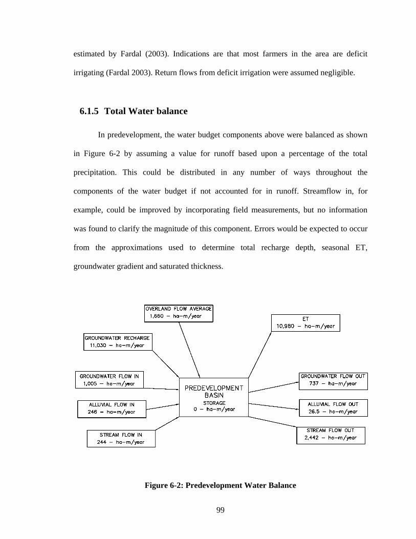
99
estimated by Fardal (2003). Indications are that most farmers in the area are deficit
irrigating (Fardal 2003). Return flows from deficit irrigation were assumed negligible.
6.1.5 Total Water balance
In predevelopment, the water budget components above were balanced as shown
in Figure 6-2 by assuming a value for runoff based upon a percentage of the total
precipitation. This could be distributed in any number of ways throughout the
components of the water budget if not accounted for in runoff. Streamflow in, for
example, could be improved by incorporating field measurements, but no information
was found to clarify the magnitude of this component. Errors would be expected to occur
from the approximations used to determine total recharge depth, seasonal ET,
groundwater gradient and saturated thickness.
Figure 6-2: Predevelopment Water Balance

100
By including well pumping for irrigation in the water budget, there is a system
deficit of approximately 7,945-ha-m/yr (64,400-acre-ft/yr) as shown in Figure 6-3. Other
outflow components would be expected to decrease or water would be released from
storage until the water budget returned to a balanced state. An evenly distributed
reduction of approximately 60% would be required from other outflow components to
balance the water budget. This would reduce the groundwater outflow from 737 to 295-
ha-m/yr (5,975 to 2,390-acre-ft/yr), the stream outflow from 1,535 to 615-ha-m/yr
(12,450 to 4,980 -acre-ft/yr) and ET from 10,980 to 4,392-ha-m/yr (89,016 to 35,610-
acre-ft/yr).
Figure 6-3: Developed Water Balance
Instead of a 60% reduction of all of these inputs, water would also be released from
storage resulting in a reduction of the basin water table to account for the water balance

101
deficit. If the entire deficit were to reduce the water table elevation, assuming an Sya of
0.2, a decline of 26.5-cm (0.89-ft) would be seen over the 149,980-ha (370,600-acre)
basin. This is consistent with the 27-cm decline found by Squires (2007). More
realistically, however there would be an unequal distribution of basin output reductions.

102
CHAPTER 7 CONCEPTUALIZATION
7.1 GENERAL ARIKAREE RIVER
CONCEPTUALIZATION
The Arikaree River Basin conceptualization includes all information available to
the author at the time of the study. Bedrock elevation, well data, geology maps, historic
water levels and model results were all considered. The basin aquifer lies within a
geologic formation that reduces in thickness as it proceeds east through Yuma County.
The separation between the ground and bedrock surfaces decreases, proceeding east. The
reduction in thickness is caused by mildly sloping bedrock as compared to the ground
surface slope (USGS 1999; Johnson et al. 2002). Characteristics of the river basin that
support this surface relationship are the discontinuity of the river upstream (west of the
Fox Ranch), the wet reach just before outcropping of bedrock at the Fox Ranch property
and the outcropping of bedrock to the east with perennial tributary flow.
Predevelopment data (Weist 1964) shows that the river is induced by a regional
groundwater basin where groundwater flow is toward the river from both lateral
directions (Figure 1-5). Transient modeling of the Arikaree River (sections 4.7 & 4.8) has
shown this to remain true after 10-years of pumping. The model shows that the river does
not change from gaining to losing groundwater. Well measurements also support that this
has currently not changed (section 3.1). A significant gradient was calculated using the

103
observed contours (Figure 3-2) of 0.014 to 0.021 directed towards the river from the
north and 0.009 to 0.014 from the south.
Transient numerical and analytical stream depletion models show that seasonal
stream depletion is negligible from most irrigation wells within the basin. This has been
shown to be true for one-year seasonal pumping schedules. Wells located more than
approximately 3,000-m away from the river were shown using the model not to directly
affect streamflow within a single growing season (appendix F). A complete discussion of
the one-year stream depletions is included in chapter 5.
The model calculated using tracer particles, that pumping does not significantly
change the location of the groundwater divide (Figure 7-1). Output head of the individual
cells along the divide drop less than 1-m after model runs with pumping included. The
output contour shape remains similar to the input contour shape. The contours are shown
at 4-m intervals so the water table elevation, after seasonal recovery from pumping would
have to have changed more than 4-m in the 10-year time interval to show changes.
The stability of the groundwater basin can be attributed in part to a high bedrock
ridge that exists to the north of the river. Figure 1-6 shows the bedrock surface and
ground surface contours along with an example point where the elevations of the ridge
and the adjacent streambed are both approximately 1,240-m. The surfaces used in the
numerical model indicate a saturated thickness of less than 5-m along the bedrock ridge
north of the river (Weist 1964; Johnson et al. 2002). Physically, if the aquifer thickness
declines, the ridge might become dry and the divide would remain, creating a gradient to
the south along that ridge.

104
Figure 7-1: Initial and 10-year Water Table Contours (Start of Pumping)
To the south of the river, there is no clear bedrock ridge. The streambed
elevations of the Arikaree River and the South Fork of the Republican River are roughly
the same near Idalia (around 1,150-m). Because of the similar elevations, while both
rivers continue to flow, a groundwater divide would occur between the two rivers. It
would be difficult to know whether this is the case if either of the rivers ceases to flow.
Model runs also show that future changes to the system will not compromise the
Arikaree River groundwater basin even if streamflow ceases. It would be difficult for the
system to become a “pass through” system, where groundwater flows either to the North
or South Republican basins without separate drainage from the Arikaree River basin. The
Initial and Output Head Contour Overlay
in GIS (No Observable Shift in
Contour Locations)
Calibration Initial Head Contours
10-year Output Head Contours
(Beginning of Growing Season)

105
model could not be forced into such a configuration for any reasonable set of input
variables.
The deep bedrock surface relative to the ground surface in southwest Yuma
County has resulted in larger declines in aquifer water-table levels compared to the
water-table level declines near the Fox Ranch. The water table decline has resulted in a
river stage below the streambed. No observable flow was present along highway 59
(Figure 1-2) during any of the visits to the river. Alluvial soils are prominent along the
river in southwest Yuma County, as indicated by aerial photo showing significant
riparian vegetation (Figure 7-2) and supported by surface geology maps (Sharps, 1980).
Figure 7-2: Satellite Photo of the Arikaree River through Southwestern Yuma County (USDA 2005)
Seasonal pumping of alluvial irrigation wells (wells within one mile of the river)
depletes the alluvial aquifer directly. In western Yuma County, this is observable using
aerial photos as shown in Figure 7-2. The decrease in riparian vegetation downstream of

106
the well in the figure shows evidence of aquifer depletion. Lower water levels in the
alluvium has a local effect of increasing the rate of groundwater influx into the alluvium
downstream of the well’s typical area of influence. Alluvial water is replaced gradually as
the river reaches south-central Yuma County and the Fox Ranch property.
Alluvial wells of southeast Yuma County also act as a drain to the alluvium but a
disconnection exists in this region between the Ogallala and alluvial aquifers. The aquifer
disconnect is caused by the outcropping of bedrock along the river (Weist 1964) and
prevents the hydraulic gradient from further increasing in the Ogallala formation because
of alluvial water table decline. The result is that the river and the alluvium are depleted
until a connected source such as a tributary or precipitation event returns enough water to
the alluvial aquifer for the water-table levels to resurface.
There is an overall water deficit in the basin created by the irrigation wells. This
results in declining winter (recovered) water-table levels and seepage to the river. Winter
water-table levels are the initial levels at the start of the growing season and therefore
affect the early season streamflow before drawdown occurs.
Evapotranspiration is very detrimental to the overall streamflow of the Arikaree
River. ET significantly reduces the amount of available water for streamflow. The total
modeled riparian ET was 2,297-ha-m (18,622-acre-ft) of water after day 258 (end of
growing season). Modeled streamflow continued but a decrease of 7,369-m3/day of
stream influx was attributed to ET after day 258 (end of growing season) from runs
without pumping. Total water use by cottonwoods, found to be around 135-cm/season
(Wachob 2005) is roughly equivalent to the water use of a single irrigation well per mile

107
of river, pumping at a rate of 2,180 to 3,270-m3/day given a riparian band of 60 to 90-m
on both sides of the river (Section 5.1).
Observed diurnal fluctuations in alluvial water table levels are shown in Figure
7-3. Fluctuations indicate that the seasonal decline of streamflow can be attributed in
large part, to local deficiencies in the water balance created by ET. Stream stage level
tracks the alluvial groundwater levels very closely (Wachob 2005). By inspection of the
graph in Figure 7-3, it is seen that large precipitation events, such as those at the
beginning of June and July, create a spike in the groundwater level that quickly returns to
a base level indicating drainage of bank storage to the stream. The spike is then followed
by a diurnal fluctuations, starting from the base level that increase in magnitude up
through July and August.
Small events create small rises in groundwater level that do not quickly decline.
Instead, diurnal fluctuations follow the rise and the groundwater level continues to
decrease at a daily rate consistent with the rate of decline before the storm. The overall
rate of decline seems to increase slightly throughout the summer.
In southwestern Yuma County, reductions in streamflow from ET and climactic
effects have historically been regulated by larger aquifer baseflow (Wachob 2005). The
baseflow would essentially buffer the streamflow ensuring continuity during summer
months. Recently water-table levels have been reduced to a point where wintertime level
recovery is possible but groundwater flow from the aquifer into the alluvium cannot
increase enough to maintain streamflow during periods of high ET.

108
Groundwater Levels in Monitoring Wells
1180.5
1181.0
1181.5
1182.0
1182.5
1183.0
1183.5
28-Apr-05
29-May-05
29-Jun-05
30-Jul-05
30-Aug-05
Date
Wat
er S
urfa
ce E
leva
tion
(m)
Well 2 Well 5 Well 7 Well 11 Well 20 Well 28 Well 30
Figure 7-3: Diurnal Alluvial Groundwater Fluctuations on the Fox Ranch (Wachob 2005)
In Southeastern Yuma County, where the aquifer is disconnected from the
alluvium, upstream inflow was historically much higher than today. The inflow would
have been high enough to accommodate riparian ET without stream depletion.
Streamflow out of Yuma County into Kansas and Nebraska was at one time continuous
through Haigler, NE (Wachob 2005). Recently total yearly flow volume has been reduced
enough to where there is essentially no flow at Haigler. A reduction to only 308,000-
m3/yr (250-acre-ft/yr) of water from an average of 23.3-Mm3/yr (18,900-acre-ft/year) was
seen at the Haigler gage station by 2002 as shown in Figure 7-4. Reduction has been
significant despite no noticeable decline in precipitation (Figure 7-5).

109
0
5,000
10,000
15,000
20,000
25,000
30,000
35,000
1933 1943 1953 1963 1973 1983 1993 2003Year
Stre
am F
low
(ac-
ft)
Major High CapacityWell Establishment
Average Flow 18,900 ac-ft/year pre-1960
Figure 7-4: Gauge Recorded Streamflow at Haigler, NE (USGS Gauge Data)
0
5
10
15
20
25
30
1932 1942 1952 1962 1972 1982 1992 2002Year
Tot
al P
reci
pita
tion
(in)
Figure 7-5: Precipitation Data, Akron Colorado Weather Station (Vigil, M. F. (2004))

110
The Arikaree River through Southern Yuma County can be thought of as being
divided by geologic features, groundwater and habitat characteristics into four distinct
regions. The regions are as follows: Upstream region, Fox Ranch region, transitional
region and downstream region. The four regions are shown in Figure 7-6.
Figure 7-6: Conceptual Regions of the Arikaree River through Southern Yuma County (Background by Weist 1964)
7.2 UPSTREAM CONCEPTUALIZATION
In the upstream region, adjacent to the Yuma and Washington County border, the
Arikaree River is ephemeral, flowing only during long precipitation events. The bedrock
is deep (~20-m) (USGS 1999, Johnson et al. 2002) in this region and groundwater
pumping is prevalent. The groundwater level is low enough so that stream channels are

111
dry except from precipitation events. Irrigation occurs mostly upstream of highway 59
(Figure 7-6) in Washington County. Proceeding eastward, toward the Fox Ranch, there is
less pumping and recharge maintains a higher water table. More riparian vegetation is
seen in aerial photos approaching the Fox Ranch.
7.3 FOX RANCH CONCEPTUALIZATION
Located in the center of Southern Yuma County, the Fox Ranch property (Figure
7-7) contains abundant wildlife habitat and is one of the remaining brassy minnow
strongholds in Colorado (Scheurer et al. 2003). The property is roughly 12.8-km wide
(East/West) and used primarily for grazing cattle, allowing much of the river habitat
through the property to remain undisturbed. A significant recharge area, composed
mostly of dune sands, is located northwest of the Fox Ranch. Two alluvial irrigation
wells are located directly upstream of the western property line. Other irrigation wells
exist to the southwest and additional alluvial irrigation wells are located starting 8-km
upstream from the ranch.

112
Figure 7-7: Fox Ranch Property Location (Base Aerial Photo by USDA 2002)
The downstream portion of the ranch (east) is usually wet and contains at least
intermittent pools throughout the summer even as the river disconnects. Other portions of
the river do not stay as wet as the ranch and many reaches dry completely, eliminating
fish habitat (Scheurer et al. 2002). The alluvial aquifer and the river itself are assumed to
be conceptually the same because of the minimal streamflow. Streamflow was
approximately 4,890-m3/day (2-cfs) on October 15, 2005 (~6-days after a major storm
event) and 11,000-m3/day (4.5-cfs) was measured March 16, 2006 (typical of early spring
flow).
During the winter, streamflow along the Fox Ranch is able to recover from ET
and irrigation, allowing the stream to become fully connected. This also occurs year-
round after significant precipitation events. During the summer months, the stream and
WELLS
DUNES

113
ET drain water stored in the upper portion of the alluvium during the winter recovery
period until the alluvial water table drops below the streambed and streamflow ceases.
This also occurs with water stored during precipitation events. After the precipitation
events, ET causes the water table to fall below the streambed (Figure 7-3). Figure 7-8
through Figure 7-11 show details of the Fox Ranch conceptualization.
Figure 7-8 is a cross-section of the Fox Ranch, extending out past a nearby
irrigation well. Since all wells surrounding the Fox Ranch are farther than 3,000-m from
the river, the cone of depression caused by the well pumping does not reach the stream.
The water table, however, reduces year to year from the water balance deficit as
described in chapter 6, as represented in the figure. A stock well as was monitored for
this study is represented in the figure. Figure 7-9 represents the alluvium and shows the
effect of ET and the stream draining water in bank storage.
Figure 7-8: N/S Cross-Section of Adjacent Well Effect on Fox Ranch Alluvium

114
Figure 7-9: N/S Cross Section of Alluvial Deposit Water Table Fluctuations at the Fox Ranch
Figure 7-10 shows a plan view of the Fox Ranch with vector arrow indicating the
magnitude of the flow rate through the alluvium, aquifer or water use by the functions of
ET. The alluvial vector after the alluvial wells is small. The well field shown impedes
base flow from the south.
Figure 7-10: Plan View of Fox Ranch Flow Concept

115
Figure 7-11 shows a profile of the alluvium along the river bed. The alluvial well
is shown draining the alluvium. Recharge from the dunes is shown filling the alluvium
until streamflow is possible. ET then is shown reducing the alluvial water table. The
result is ponding in streambed depressions with disconnection of streamflow.
Figure 7-11: W/E Profile along the Streambed of Alluvial Well Effect on Fox Ranch Stream Stage
Figure 7-11 is a profile along the streambed showing the water table as a darker
line. The notes draw attention to the effects of the dune recharge area, and riparian ET on
the alluvial water table. The lighter line is the streambed. Ponding is shown when the
streambed depression is below the water table and the stream is not connected from
depression to depression.
The groundwater gradient toward the river is higher from the northwest than from
other directions (max 0.021 from the NW vs. 0.014 from the SW) (Figure 3-2). High

116
recharge rate in the sand dunes contributes to the high hydraulic gradient. The sand dunes
to the northwest are the main recharge zone for the Arikaree Basin through the Fox
Ranch.
7.4 TRANSITIONAL CONCEPTUALIZATION
The “transitional” region is located starting just west of the confluence of Copper
Kettle Creek and the Arikaree River as shown in Figure 7-6. In this region, the alluvium
begins to disconnect from the Ogallala aquifer. A lower groundwater influx exists
because of this disconnection. Base streamflow begins to decline because the stream
base-flow is highly dependent upon upstream alluvial inflow. Alluvial flow is depleted
seasonally by at least one well (i.e. well A, Table 5-2 ) located just downstream of the
Fox Ranch. Seeps from the Ogallala Aquifer, passing over the bedrock into the alluvium
become the dominant water source of the alluvial aquifer in this area. The
conceptualization is shown in Figure 7-12.

117
Figure 7-12: Transitional Region
7.5 DOWNSTREAM CONCEPTUALIZATION
Upstream of the Blackwolf Creek and the Arikaree River confluence is the start of
the reach designated as “downstream” (Figure 7-6). Alluvial deposits in the main stretch
of the river disconnect from the Ogallala Aquifer in the direction of groundwater influx.
Intermittent connection of the alluvial soils and the Ogallala Aquifer exists southeast of
the river but water-bearing material is very shallow. For the majority of the growing
season, the alluvial water table is below the streambed. Ogallala Aquifer does not have
enough connection with the alluvium or capacity to maintain the alluvial water table.
Streamflow has all but disappeared during the summer months as shown in Figure 7-13.

118
Figure 7-13: Connectivity diagrams of the downstream stretch (from Scheurer et al. 2003)
Bedrock has been worn away along the river creating a depression under the
streambed. Weist (1964) shows that the alluvium has been deposited directly on the
surface of the bedrock. The geological relationship was confirmed by overlaying the
ground surface and the bedrock surface using GIS. Water moves downstream through the
alluvial aquifer, below the riverbed. Alluvial deposits are a sink for surface water because
of their low elevation and groundwater level.
Many alluvial irrigation wells are active on the southeast side of the Arikaree
River, both up and downstream of Blackwolf Creek. Wells are located mostly on the
southeast side of the river where there is a slight connection of the alluvial and the
Ogallala aquifers. Pumping of these wells contributes significantly to the low water levels
in the alluvium along with ET from riparian vegetation.
The groundwater gradient from the northwest side of the river remains directed
toward the river. The ground surface elevation declines at a greater slope, proceeding
eastward, than does the bedrock surface elevation. Bedrock is exposed as the two

119
surfaces intersect and the water bearing material of the Ogallala disappears. Springs and
seeps are created and tributaries such as Blackwolf Creek capture the exposed water. The
groundwater is forced to the surface, seeping into channels and becoming overland flow
as shown in Figure 7-14.
Figure 7-14: Diagram of the Downstream Arikaree River Conceptualization
The depths of the alluvium below tributary streams are generally very shallow
with bedrock directly below. Much of the water collected by the tributaries appears as
streamflow. Blackwolf Creek and other tributaries to the north of the river are typically
wet (Scheurer et al. 2002) from captured groundwater. The tributaries are expected to
remain wet until the aquifer is depleted and evapotranspiration is higher than the rate at
which groundwater is converted to streamflow. Tributary flow to the Arikaree infiltrates
into the alluvial sand as it reaches the river because the groundwater level is below the
streambed.

120
CHAPTER 8 SUMMARY AND CONCLUSIONS
8.1 SUMMARY
The objectives of this study were to improve current understanding of the
Arikaree River groundwater system and to develop a defensible conceptualization of the
river basin. The research presented was an investigation of the effects of groundwater
pumping in the Ogallala Aquifer on the Arikaree River in Southern Yuma County
Colorado. The calculated change in the Arikaree River streamflow due to pumping of
modeled wells was used to evaluate the effects of pumping on the river. A detailed
numerical groundwater model was created to examine the effects that irrigation well
pumping and declining aquifer levels have on the Arikaree River. The study was focused
specifically on the reach of the river through the Fox Ranch property but included
evaluation of the regional effects in Southern Yuma County.
The effect of well pumping on streamflow was evaluated using both the numerical
model and analytical methods to determine which would be most beneficial forbearance
targets in efforts to recover lost habitat. The results of the numerical and analytical
models are similar and were considered in the selection of target wells.
A water balance was created for the Arikaree River basin through Southern Yuma
County. The numerical model and previous studies were used to create the water budget
and determine balance criteria. A total deficit of over 7,400-ha-m/yr (60,000-acre-ft/yr)

121
was approximated from irrigation well pumping. Effects of the deficit are evident in the
change in streamflow and water levels over time. Over time, deficits in the water balance
are expected to be distributed between reductions of streamflow, ET, groundwater
outflow and water table declines throughout the basin.
A conceptualization of the river was developed to explain the groundwater trends
and seasonal habitat characteristics along the river. The conceptualization was created
using supporting studies, research of the groundwater levels, geology through Southern
Yuma County and the numerical groundwater model.
8.2 CONCLUSIONS
The Arikaree River is located in a stable groundwater basin. Conceptualization of
the river, however, must be divided into four regions where the river behaves differently
because of the geology, hydrogeology, surrounding agriculture and ecology. The effects
of evapotranspiration and groundwater pumping along the river are very detrimental to
achieving the goal of sustaining streamflow. ET is the major cause of seasonal water-
table fluctuations and seasonal streamflow declines. The year-to-year streamflow decline
is affected most by irrigation pumping and the water budget deficit reducing baseflow to
the alluvium. The decline in water table levels, found to be caused by groundwater
pumping through investigation of the water budget, must be stopped or reversed in order
to sustain or improve stream baseflow.
The Arikaree River through southern Yuma County, was divided into Upstream,
Fox Ranch, Transitional and Downstream Regions. The Upstream Region is ephemeral
and the water table receded too far too sustain streamflow. The Fox Ranch Region is wet,

122
mostly because the alluvial water table is not yet low enough to drop below the bottom of
the ponds and pools scoured out of the alluvium. This may change as time passes. This
region benefits from a nearby recharge area and lack irrigation wells in close proximity to
the river. Streamflow through the Transitional Region is intermittent as is the connection
of the alluvium to the aquifer. Other than increasing streamflow into the region by some
means of reversing the water-budget deficit upstream, there is no obvious way to improve
streamflow through the region. There are few wells that could be decommissioned in the
region and there appears to be no practical way of reducing riparian ET. The Downstream
Region passes through an area where the alluvium is disconnected from the regional
aquifer. Tributaries to the area cut off groundwater flow from east-to-west through the
regional aquifer. Water is released from aquifer storage to the tributaries where it is
conveyed via streamflow to the Arikaree River alluvium. As tributary waters enter the
Arikaree River alluvium, pools appear before water eventually dissipates into the alluvial
sands.
One season of stockwell observation along the Fox Ranch has provided some
clues as to the dynamics of the groundwater basin. The alluvial groundwater flow must
be considered in conjunction with the stream because a high percentage of the water,
relative to most rivers is conveyed through the alluvium. The stockwells are located
within two to three miles of the river within the aquifer. In this area, single-season
declines in water-table levels were not observed, suggesting that irrigation wells pumping
lateral to the river, do not have a single-season impact on streamflow around the Fox
Ranch. Numerical modeling and plotting of the groundwater contours suggest that the
stream will continue gain from the aquifer even if streamflow ceases and the water table

123
continues to decline. Riparian ET and alluvial well pumping upstream of the Fox Ranch
however, contribute to the seasonal decline of streamflow.
Well observations, drawdown calculations and the numerical model suggest that
wells located more than 3,000-m from the river generally have a negligible single-season
impact on the river. These wells have an impact on the regional water table, water
balance and ultimately the change in base-flow from year-to-year. This could be
conceptualized as the superposition of the drawdowns from all wells in the basin over
many seasons. Because of this, alluvial wells located upstream of the region where there
is a desire to increase the streamflow, should be looked at for decommissioning or
forbearance prior to wells located laterally from the river and at some distance.
Afterward, the highest capacity wells should be targeted in an attempt to improve the
basin water balance.
8.3 WELL DETAILS
Ten wells were determined to be forbearance targets. It was calculated that these
wells cause at least 5-gpm flow rate reduction in the streamflow. This was calculated
using the numerical model and by the Glover equation. A list of the top 17 wells was
compiled (Table 5-2) using the results of the numerical model analyses and Glover
equation analysis. Ten additional wells are included in Table 5-2 with notes indicating
these wells are calibration wells or create a high discrepancy with the internal model
water balance. These wells are listed but are not recommended forbearance wells.

124
8.4 RECOMMENDATIONS FOR FUTURE RESEARCH
An updated study of water levels in wells throughout the county would improve
the regional numerical model by providing more recent data for calibration. A study of
bedrock elevations, especially near the alluvium would be beneficial for quantifying total
stream and alluvial outflow. A better understanding of pumping schedules and rates
would allow a more sophisticated analysis to be completed showing actual depletions by
wells. A regional hydraulic conductivity and specific yield study would help to validate
the model inputs. Continued studies of ET, and recharge would significantly improve the
water balance and the calibration of numerical models.

125
REFERENCES
Allen, R.G., Pereira, L.S., Raes, D., Smith, M., 1998. FAO Irrigation and Drainage Paper No. 56 (guidelines for computing crop water requirements) Food and Agriculture Organization of the United Nations. Copyright 1998.
ArcMap 9.1, 2005. Environmental Systems Research Institute (ESRI), Copyright 1999-
2005. Geographical Information Systems Software (GIS). Borman, R.G., Linder, J.B., Bryn, S.M., Rutledge, J., 1983. “The Ogallala Aquifer in the
Northern High Plains of Colorado-Saturated Thickness in 1980; Saturated-Thickness Changes, Predevelopment to 1980; Hydraulic Conductivity; Specific yield; and Predevelopment and 1980 Probable Well Yields.” Hydrologic Investigation Atlas HA-671, U. S. Geological Survey. 1:500,000 and 1:1,000,000.
Bokuniewicz, H., Pavlik, B., 1990. “Groundwater Seepage along a Barrier Island.”
Biogeochemistry. Kluwer Academic Publishers. 10: 257-276 Chen, X., 2003. “Analysis of Pumping-Induced Stream-Aquifer interactions for Gaining
Streams.” Journal of Hydrology 275:1-11. Colorado Division of Water Resources (CDWR), 2002. “1942 Republican River
Compact, 2002 Stipulated Settlement.” water.state.co.us. Web. September 2006. Colorado Division of Water Resources (CDWR), 2005. Well Data Yuma County.
Database of Yuma County Registered Wells. Denver, Colorado. Colorado Department of Transportation (CDOT), 2006. “Colorado Statewide Data Set.”
www.dot.state.co.us. Web. September 2006. GIS Shapefiles. “Denver Average Temperatures.” City Rating.com. Web. June 2007. Dugan, J.T. Schild, D.E. and Kastner, W.M. 1990. “Water-Level Changes in the High
Plains Aquifer Underlying Parts of South Dakota, Wyoming, Nebraska, Colorado, Kansas, New Mexico, Oklahoma, and Texas---Predevelopment through Nonirrigation Season 1988-89.” U.S. Geological Survey Water-Resources Investigations Report 90-4153. 13 pp.

126
Falke, J.A., 2009. Effects of Groundwater Withdrawal and Drought on Native Fishes and their Habitats in the Arikaree River, Colorado. Dissertation. Department of Fish, Wildlife and Conservation Biology, Colorado State University, Fort Collins, Colorado. Print.
Fardal, L.L., 2003. Effects of groundwater pumping for irrigation on stream properties of
the Arikaree River on the Colorado Plains. MS Thesis, Department of Civil Engineering, Colorado State University. Print.
Fausch, K.D., Falke, J.A., Griscom, H., 2005. Arikaree River Plains Fish Habitat Surveys
2000-2001. Annual Research Progress Report. Department of Fishery and Wildlife Biology, Colorado State University. Print
Fetter, C.W., 2001. Applied Hydrogeology. Prentice Hall, Upper Saddle River, New
Jersey. Gaye, C.B., Edmunds, W.M., 1996. “Groundwater Recharge Estimation using Chloride,
Stable Isotopes and Tritium Profiles in the Sands of Northwestern Senegal.” Environmental Geology: 27:246-251
Glover, R. E., Balmer, C.G., 1954. “River Depletion Resulting from Pumping a Well near
a River.” Transactions-American Geophysical Union. V. 35 pt. 3, pp. 468-470. Glover, R.E., 1960. “Ground Water-surface Water Relationships.” In Ground Water
Section, Western Resources Conference, Boulder, Colorado. Colorado Ground Water Comm., Dept. Natural Resources, Colorado State Univ. Paper CER6OREG45, 8 pp. 1961.
Griffin, S., 2004. Effects of irrigation practices on stream depletion in the Arikaree River,
eastern Colorado. MS Thesis, Department of Civil Engineering, Colorado State University. Fort Collins, Colorado.
Gutentag, E.D., Heimes, F.J., Krothe, N.C, Luckey, R.R., Weeks, J.B., 1984.
Geohydrology of the High Plains Aquifer In Parts of Colorado, Kansas, Nebraska, New Mexico, Oklahoma, South Dakota, Texas, and Wyoming - U.S. Geological Survey Professional Paper 1400-B. United States Government Printing Office, Washington, pg. 4-5.
Hinderlider, M.C., Knapp, G.S., Wardner, G.S., 1942. “Republican River Compact #37-
67-101.” water.state.co.us. Colorado Division of Water Resources (CDWR). Web. September 2006.
Jackson, D., Rushton, K.R., 1987. “Assessment of Recharge Components for a Chalk
Aquifer Unit.” Journal of Hydrology 92, 1-15

127
Jenkins, C.T., 1968. “Techniques for Computing Rate and Volume of Stream Depletion by Wells.” Ground Water, March-April, 1968m Vol. 6, Num. 2.
Johnson, M.R., Cornwall, J.F., Landon, M.K., 2002. “Digital Map of the Elevation of the
Base of the High Plains Aquifer in the Republican River Basin upstream of Hardy, Nebraska, in parts of Nebraska, Kansas, and Colorado.” DEM. www.usgs.gov. Web. U.S. Geological Survey, Lincoln, Nebraska, 02-07-2002.
Katz, G.L., 2001. Fluvial Disturbance, Flood Control and Biological Invasion in Great
Plains Riparian Forests. Dissertation. Department of Geography, University of Colorado, Boulder, Colorado. Print.
Labbe, T.R., Fausch, K.D., 2000. “Dynamics of Intermittent Stream Habitat Regulate
Persistence of a Threatened Fish at Multiple Scales.” Ecological Applications, 10(6). 2000. pp 1774-1791.
Lou, W., 1994. Calibrating the SCS Blaney-Criddle Crop Coefficients for the Middle Rio
Grande Basin, New Mexico. MS Thesis. Department of Civil and Geological Engineering, New Mexico State University, Las Cruces, New Mexico. 91 pp. Print
Longenbough, R.A., 1966. Artificial Ground-Water Recharge on the Arikaree River near
Cope, Colorado, paper CER66RAL35. University publication. Civil Engineering Department, Engineering Research Center, Colorado State University, Fort Collins, Colorado. June.
Luckey, R.R., Gutentag, E.D., Heimes, F.J., Weeks, J.B., 1988. Effects of Future
Ground-Water Pumpage on the High Plains Aquifer in Parts of Colorado, Kansas, Nebraska, New Mexico, Oklahoma, South Dakota, Texas and Wyoming – U.S. Geological Survey Professional Paper 1400-E. United States Government Printing Office, Washington.
“Map of Idalia, CO”. www.mapquest.com. MapQuest Inc. NAVTEQ. Web. September
2006. Matthews, W.J., Zimmerman, E.G., 1990. “Potential Effects of Global Warming on
Native Fishes of the Southwestern Great Plains and the Southwest.” Fisheries, 15(6):26-32.
Mecham, B., 2004. “Historical Reference ET for Northern Colorado Front Range
Northern Colorado Water Conservancy District. Berthoud, CO.” Spreadsheet. Message to author. Email. [email protected].
McWhorter, D.B., Sunada, D.K., 1977. Ground-water Hydrology and Hydraulics. Water
Resources Publications, LLC. Highlands Ranch, CO. Reprinted 1999.

128
Miller, C.D., Durnford, D.S., Halstead M.R., Altenhofen, J., Flory, V., 2007. “Stream depletion in alluvial valleys using the SDF-analytical model.” Ground Water, 45 (4):506-514.
Munson, B., Young, D., and Okiishi, T., 1998. Fundamentals of Fluid Mechanics. John
Wiley and Sons, Inc., New York, NY. National Aeronautic and Space Administration (NASA), 2006. Satellite Imagery. NLT
LandSat 7, Visible Color. TIFF. NASA World Wind v. 1.3.5, 2006. Oliver, M.A., Webster, R., 1990. “Kriging: a Method of Interpolation for Geographical
Information System.” INT. J. Geographical Information Systems, VOL. 4, No. 3, 313-332
Pakaki, D.E., Bush, S.E., Gardner, P., Solomon, D.K., Ehleringer, J.R., 2005.
“Ecohydrology in a Colorado River riparian forest: Implications for the decline of Populus fremonti.” Ecological Applications, 15(3):1009-1018.
High Plains Regional Climate Center, 2006. “Period of Record Monthly Climate
Summary – Idalia 4 NNE, CO (054242). Period of Record: 8/1/1948 to 9/30/2005.” Spreadsheet. hprcc.unl.edu. Web. 20 July 2006.
Reddell, D.L., 1967. Distribution of Groundwater Discharge-Technical Report.
Department of Agricultural Engineering, Colorado State University, Fort Collins, Colorado.
Robinson, T.W., 1952. “Phreatophytes and their Relation to Water in Western United
States.” Transactions- American Geophysical Union, 33:57-66. Scheurer, J.A., Fausch, K.D., Bestgen, K.R., 2003. “Multiscale Processes Regulate
Brassy Minnow Persistence in Great Plains River.” Transactions of the American Fisheries Society, 132:840-855.
Scanlon, B.R., Healy, R.W., Cook, P.G., 2002. “Choosing Appropriate Techniques for
Quantifying Groundwater Recharge.” Hydrogeology Journal, 10:18-39 Scott, M.L., Shafroth, P.B., Auble, G.T., 1999. “Responses of riparian cottonwoods to
alluvial water table declines.” Environmental Management. Sharps, J.A., 1980. “Geologic Map of the Limon 1ox2o Quadrangle, Colorado and
Kansas, 1:250,000.” U.S. Geological Survey, Map I-1250. Solek, B., 1998. “Evaluation of Hydrogeologic Impacts Potential Nature Conservancy
Preserve Arikaree River, Yuma County, Colorado.” Consultant technical report. Louisville, CO. Print

129
Sophocleous, M., Perry, C.A., 1985. “Experimental Studies in Natural Groundwater-Recharge Dynamics: The Analysis of Observed Recharge Events.” Journal of Hydrology, 81 (1985) 297-332.
Squires, A., 2007. Groundwater response functions and water balances for parameter
estimation and stream habitat modeling. MS Thesis. Department of Civil and Environmental Engineering, Colorado State University, Fort Collins, Colorado. Print.
Theis, C.V., 1941. “The Effect of a Well on the Flow of a Nearby Stream.” Transactions-
American Geophysical Union, V. 22, pt. 3, pp. 734-738. Theis, C.V., Conover, C.S., 1963. “Chart for Determination of Pumped Water Being
Diverted from a Stream or Drain. In Bentall, Ray, compiler, Shortcuts and special problems in aquifer tests.” U.S.G.S. Water-Supply Paper 1545-C, 99. C113-C115, 1964.
USDA/FSA, 2005. “USDA-FSA-APFO Digital Ortho MrSID Mosaic.” Aerial
Photograph. USDA/FSA - Aerial Photography Field Office, Salt Lake City, Utah 09-30-2005.
U.S. Geological Survey (USGS), 2005. “USGS Arikaree River Stream Gauge Data
(1932-2003). USGS 06821500 ARIKAREE RIVER AT HAIGLER, NEBR. US Geological Survey National Water Information System.” Spreadsheet. waterdata.usgs.gov Web. September 2005.
U.S. Geological Survey (USGS), 1999. “National Elevation Dataset.” DEM. EROS Data
Center, Sioux Falls, SD. U.S. Geological Survey (USGS), 2007. “The Water Cycle: Evapotranspiration.”
ga.water.usgs.gov, Web. January 2010. Vigil, M.F., 2004. “Monthly Precipitation (from RAINHIST.xls file).” USDA-ARS
Central Great Plains Research Station Akron, Colorado. Historic Rainfall Data. Printed 01/25/2004, Unpublished.
Visual MODFLOW v. 4.0.0.131, 2003. Waterloo Hydrogeologic, distributed by Scientific
Software Group, Washington, D.C. Numerical Groundwater Modeling Software. Wachob, E.D., 2006. Irrigation Pumping, Riparian Evapotranspiration, and the Arikaree
River, Yuma County, Colorado. MS Thesis. Department of Civil Engineering, Colorado State University, Fort Collins Colorado.
Weist, W.G., 1964. Geology and Ground-Water Resources of Yuma County, Colorado –
U.S. Geological Survey Water – Supply Paper 1539-J. United States Government Printing Office, Washington, Plate 3.

130
White, W.N., 1932. “A Method of Estimating Groundwater Supplies Based on Discharge
by Plants and Evaporation from Soil.” U.S. Geological Survey Water-Supply Paper 659-A. 105 pp.
“Yuma County Colorado.” 2006. www.yumacounty.net. Hale Multimedia, Web. June
2006. Zlotnik, V.A., Tartakovsky, D.M., 2005. “Stream Depletion by Groundwater Pumping
from Leaky Aquifers.” math.lanl.gov. Web. October 2006. pdf.

131
Appendix A
Public Land Survey Coordinate System Notes

132
Public Land Survey Coordinate System Notes:
Townships are divided into 36-square mile divisions. Each township is 6-miles in
width and breadth. The north-south borders of townships are called township lines while
the east-west borders are referred to as range lines.
Labels and location descriptions in the form SC00304736AB refer to the
township, range, section and sub-section designations of the physical location.
The first letter indicates the principal meridian used to find the specific location. S
indicates the sixth principal meridian, which is used for eastern Colorado.
The second letter indicates the direction of the location from the intersection of
the baseline and the principal meridian. In eastern Colorado, C is to the south of the
baseline coinciding with the 30th mile north of the border between Yuma and Kit Carson
Counties.
The first set of three digits in the description indicates the location’s township.
The 003 indicates the location is in the third township south of the baseline, in a section
between 12 and 18 miles from the baseline.
The second set of three digits in the description indicates the location’s range. The
047 indicates the location is in the 47th range west of the 6th principal meridian in a
section between 282 and 288 miles west of the baseline.
The last two digits in the description indicate the section number of the location
within the township. Sections are numbered 1 to 6 from the northeast corner of the
township and progress to section 36 alternating back and forth proceeding south, ending
with section 36 at the southwest corner of the township.

133
The third letter indicates the location’s quarter section. Labels are assigned to
quarter sections from A to D starting in the northeast and proceeding counterclockwise.
The fourth letter indicates the location’s quarter of its quarter section. Labels are
assigned to quarters of quarter sections from A to D starting in the northeast and
proceeding counterclockwise.
The written description of a point at the PLS coordinate SC00304736AB would
be the northwest quarter of the northeast quarter of section 36, township 3 south, range 47
west of the 6th principal meridian.

134
Appendix B
Fox Ranch Windmill and Well Survey Data

135
GPS Instrument - Ashtech Locus - Ashtech 471 El Camino Real, Santa Clara, CA 95050Surveyors - Ryan Banning & Erik Wachob
Notes: Data Surveyed On or Before October 27, 2005Coordinate System UTM NAD 1983 Zone 13 N"Datum" is: Top of the Casing for wells, Ground Surface for Existing Grade SurveyDepth Measured from Top of Well CasingWindmill Locations are Shown in Figure 3-1
GPS Site Location Easting Northing Datum Depth Depth Water Surface DatumDesignation Name (m) (m) Elev. (m) (m) (ft) Elevation (m) Elev. (ft)
Base Station (Ranch Rock) 7177141.15 4403674.923 1196.524 - - - 3925.8014 Windmill 01 714900.073 4408185.063 1231.343 16.490 54.10 1214.85 4039.8312 Windmill 02 712710.188 4406522.734 1238.982 18.105 59.40 1220.87 4064.8910 Windmill 03 713971.807 4406228.529 1219.144 6.462 21.20 1212.68 3999.8013 Windmill 04 715001.081 4406360.434 1235.494 25.634 84.10 1209.86 4053.4520 Windmill 06 712901.896 4404640.746 1225.658 18.471 60.60 1207.18 4021.189 Windmill 07 714914.273 4405434.049 1219.928 18.441 60.50 1201.48 4002.388 Windmill 08 716872.398 4405405.513 1215.851 25.329 83.10 1190.52 3989.0015 Windmill 10 720226.538 4407368.989 1219.813 27.524 90.30 1192.29 4002.0016 Windmill 11 719664.425 4406019.176 1219.091 36.058 118.30 1183.03 3999.6317 Windmill 12 718108.064 4406121.697 1223.721 30.663 100.60 1193.05 4014.8218 Windmill 13 718981.166 4404978.414 1204.336 23.165 76.00 1181.17 3951.226 Windmill 14 717143.893 4400604.758 1241.088 49.957 163.90 1191.13 4071.804 Windmill 15 718074.660 4400076.588 1233.982 45.218 148.35 1188.76 4048.497 Windmill 16 (Offsite) 718993.614 4401335.229 1238.127 53.737 176.30 1184.38 4062.0824 Windmill 16 721215.151 4401311.278 1219.472 44.440 145.80 1175.03 4000.8823 Windmill 17 720966.404 4402465.37 1207.456 32.888 107.90 1174.57 3961.463 Windmill 18 716379.342 4403588.726 1199.702 9.723 31.90 1189.98 3936.025 Windmill 19 716533.111 4402053.958 1235.561 41.789 137.10 1193.77 4053.6711 Windmill 20 710765.631 4403602.102 1236.355 21.672 71.10 1214.68 4056.2721 Windmill 21 711364.77 4403886.159 1236.772 24.293 79.70 1212.48 4057.64
Observation well 1 (Wachob) 717845.732 4404284.245 1182.573 1.321 4.33 1181.25 3879.82Observation well 2 (Wachob) 717934.977 4404309.498 1182.55 1.651 5.42 1180.90 3879.74Observation well 3 (Wachob) 717877.781 4404326.226 1183.533 2.438 8.00 1181.09 3882.97Observation well 4 (Wachob) 717810.408 4404405.426 1183.742 2.032 6.67 1181.71 3883.66Observation well 5 (Wachob) 717971.709 4404383.733 1183.131 2.235 7.33 1180.90 3881.65Observation well 6 (Wachob) 717863.873 4404264.132 1182.347 1.168 3.83 1181.18 3879.08Observation well 7 (Wachob) 717888.504 4404206.632 1183.097 2.007 6.58 1181.09 3881.54Observation well 8 (Wachob) 717797.073 4404214.261 1183.396 1.880 6.17 1181.52 3882.52Observation well 9 (Wachob) 717833.762 4404118.945 1182.893 1.486 4.88 1181.41 3880.87Observation well 10 (Wachob) 717767.551 4403933.159 1183.44 1.118 3.67 1182.32 3882.67Observation well 11 (Wachob) 717920.080 4403972.893 1182.719 1.422 4.67 1181.30 3880.30Observation well 20 (Wachob) 717630.109 4404339.429 1184.521 2.362 7.75 1182.16 3886.21Observation well 21 (Wachob) 717514.810 4404261.647 1184.581 2.032 6.67 1182.55 3886.41Observation well 22 (Wachob) 717650.040 4404236.105 1183.775 1.753 5.75 1182.02 3883.76Observation well 23 (Wachob) 717595.753 4404135.426 1184.189 1.357 4.45 1182.83 3885.12Observation well 24 (Wachob) 717507.226 4404076.171 1184.471 1.638 5.38 1182.83 3886.05Observation well 25 (Wachob) 717649.818 4404062.487 1183.682 1.397 4.58 1182.28 3883.46Observation well 27 (Wachob) 717689.209 4404375.095 1182.877 2.108 6.92 1180.77 3880.82Observation well 28 (Wachob) 717612.918 4404407.108 1183.032 1.905 6.25 1181.13 3881.33Observation well 29 (Wachob) 717534.625 4404441.497 1185.456 2.794 9.17 1182.66 3889.28Observation well 30 (Wachob) 717675.207 4404490.640 1185.749 3.251 10.67 1182.50 3890.24Stage Gauge 7 (Griffin) 717625.558 4404361.716 1181.936 -0.191 -0.63 1182.13 3877.73
101 USGS Gauge (Fox Ranch) 721718.676 4403431.788 1163.018 -0.457 -1.50 1163.48 3815.6633 U Road River Bottom West 717205.554 4404217.104 1184.82 0.152 0.50 1184.67 3887.1926 Stage Guage 5 (Griffin) 720261.095 4403791.915 1169.716 0.434 1.42 1170.15 3837.6427 Obs. Well E (Griffin) 720228.723 4403799.043 1170.762 0.576 1.89 1170.19 3841.0728 Riv Btm by Gauge E (Griffin) 720233.058 4403802.297 1170.172 0.025 0.08 1170.15 3839.1429 Misc. Pond 719683.818 4404264.344 1172.528 -1.006 -3.30 1173.53 3846.8732 River Bottom 719197.998 4404503.675 1175.662 -0.165 -0.54 1175.83 3857.1534 River Bottom 720140.655 4403992.93 1170.379 -0.823 -2.70 1171.20 3839.8135 (Faulke) Well 1 718603.359 4404000.358 1180.271 1.554 5.10 1178.72 3872.2736 (Faulke) Well 1 River Bottom 718606.737 4404008.165 1178.223 -0.335 -1.10 1178.56 3865.5537 River Bottom 718292.824 4404114.086 1179.57 -0.427 -1.40 1180.00 3869.9738 River Bottom 717452.335 4404340.892 1183.572 -0.244 -0.80 1183.82 3883.1039 Beaver Pond Bottom 716779.701 4404255.248 1185.623 -1.189 -3.90 1186.81 3889.8340 River Bottom 715454.267 4404616.636 1191.509 -0.411 -1.35 1191.92 3909.14
Static Differential GPS Survey Data for the Fox Ranch Property in Southern Yuma County

136
Appendix C
Public Gauge Data

137
Akron Weather DataCummulative Precipitation for the USDA Weather Station in Akron, Colorado
Source:USDA-ARS Central Great Plains Weather StationVigil M. F. (2004)
Year Precip. (in) Precip. (cm) Year Precip. (in) Precip. (cm)1908 16.85 42.80 1956 13.3 33.91909 22.46 57.05 1957 18.0 45.81910 17.36 44.09 1958 14.4 36.61911 14.51 36.86 1959 13.6 34.51912 20.73 52.65 1960 10.9 27.71913 16.55 42.04 1961 14.3 36.41914 15.58 39.57 1962 16.4 41.81915 25 63.50 1963 16.0 40.51916 13.74 34.90 1964 12.3 31.21917 17.5 44.45 1965 22.8 58.01918 22.28 56.59 1966 14.3 36.31919 15.52 39.42 1967 18.8 47.71920 21.35 54.23 1968 12.5 31.61921 13.44 34.14 1969 14.5 36.81922 16.66 42.32 1970 11.1 28.11923 18.16 46.13 1971 13.8 35.01924 14.08 35.76 1972 14.2 36.11925 11.82 30.02 1973 21.5 54.71926 20.16 51.21 1974 9.9 25.21927 20.4 51.82 1975 17.3 44.01928 15.37 39.04 1976 10.4 26.41929 19.61 49.81 1977 12.5 31.91930 19.03 48.34 1978 15.6 39.51931 10.74 27.28 1979 21.1 53.51932 15.14 38.46 1980 15.0 38.01933 18.9 48.01 1981 19.6 49.71934 12.61 32.03 1982 18.2 46.21935 19.09 48.49 1983 17.0 43.11936 18.21 46.25 1984 18.6 47.21937 11.35 28.83 1985 17.9 45.51938 15.5 39.37 1986 13.2 33.61939 9.93 25.22 1987 19.7 50.11940 16.78 42.62 1988 16.2 41.21941 22.09 56.11 1989 13.6 34.41942 18.67 47.42 1990 20.9 53.01943 12.72 32.31 1991 14.9 37.81944 15.74 39.98 1992 16.5 42.01945 21.61 54.89 1993 17.7 45.01946 26.79 68.05 1994 12.8 32.41947 17.72 45.01 1995 20.7 52.61948 18.51 47.02 1996 18.8 47.71949 23.04 58.52 1997 16.2 41.01950 14.41 36.60 1998 12.2 30.91951 18.08 45.92 1999 20.6 52.21952 11.69 29.69 2000 14.3 36.31953 15.95 40.51 2001 16.8 42.61954 11.01 27.97 2002 9.5 24.11955 18.76 47.65 2003 17.0 43.2
AVE 16.5 41.8

138
Stream Gauge Data for the Arikaree RiverUSGS Gauge Station at Haigler, Nebraska
Source:U.S. Geological Survey National Water Information Systemhttp://waterdata.usgs.gov/nwis/help?codes_help#dv_cdUSGS 06821500 ARIKAREE RIVER AT HAIGLER, NEBR.
Year Flow (ac-ft) Flow (m3/day) Year Flow (ac-ft) Flow (m3/day)1933 23,425 79,161 1969 12,891 43,5631934 18,503 62,529 1970 7,649 25,8491935 28,469 96,207 1971 7,279 24,6001936 16,348 55,246 1972 13,849 46,8011937 11,800 39,878 1973 16,155 54,5951938 17,441 58,939 1974 12,907 43,6201939 22,397 75,688 1975 8,066 27,2581940 7,087 23,951 1976 4,934 16,6751941 29,386 99,307 1977 8,576 28,9811942 33,209 112,227 1978 2,742 9,2661943 15,868 53,624 1979 5,666 19,1481944 12,061 40,760 1980 10,875 36,7511945 11,001 37,178 1981 14,349 48,4901946 15,658 52,914 1982 10,120 34,1991947 22,258 75,219 1983 8,450 28,5551948 24,630 83,235 1984 8,198 27,7051949 20,510 69,312 1985 6,783 22,9241950 13,080 44,203 1986 6,712 22,6831951 27,554 93,117 1987 4,840 16,3561952 21,466 72,543 1988 6,527 22,0571953 8,559 28,923 1989 3,689 12,4671954 5,760 19,465 1990 5,059 17,0971955 26,666 90,116 1991 6,388 21,5871956 12,764 43,136 1992 8,683 29,3421957 26,727 90,321 1993 8,818 29,8001958 19,172 64,789 1994 8,252 27,8861959 11,854 40,059 1995 7,174 24,2451960 32,877 111,105 1996 4,678 15,8081961 9,330 31,531 1997 3,609 12,1971962 29,161 98,547 1998 2,848 9,6261963 8,974 30,325 1999 6,496 21,9521964 13,246 44,764 2000 3,223 10,8901965 14,807 50,039 2001 1,813 6,1281966 13,856 46,823 2002 206 6961967 14,093 47,625 2003 1,073 3,6251968 6,670 22,540 Average 12,623 42,659

139
Appendix D
123-Day Drawdown Comparison and
Calculations (ET vs. Irrigation Wells)

140
Tree
ET
Rat
e78
0gp
m/m
ile42
55m
3 /day
-1.6
km
K50
0ft/
day
152
m/d
ayb
30ft
9m
1/8
mile
sec
tion
Q97
.5gp
m53
2m
3 /day
T15
000
ft2 /day
1393
m2 /d
aySy
a0.
2Al
pha
7500
0ft2 /d
ay69
67m
2 /day
Tota
l Dra
wdo
wn
= su
m o
f dra
wdo
wn
x2t
123
days
Tota
l Dra
wdo
wn
3.16
ft0.
96m
Mile
s fro
m P
oint
Dis
tanc
e (ft
)E
T (g
pm)
ET
(ft3 /d
ay)
Sat
Thic
k(ft)
K (f
t/day
)T
(ft2 /d
ay)
SyU
Dra
wdo
wn
(ft)
W(u
)1/
6441
.25
12.2
2346
3050
015
000
0.2
4.6E
-05
0.11
79.
407
1/32
123.
7512
.223
4630
500
1500
00.
24.
2E-0
40.
090
7.21
01/
1624
7.5
24.4
4693
3050
015
000
0.2
1.7E
-03
0.14
55.
825
1/8
495
48.8
9385
3050
015
000
0.2
6.6E
-03
0.22
14.
444
1/4
990
97.5
1877
030
500
1500
00.
22.
7E-0
20.
306
3.07
73/
816
5097
.518
770
3050
015
000
0.2
7.4E
-02
0.20
92.
102
1/2
2310
97.5
1877
030
500
1500
00.
21.
4E-0
10.
149
1.49
65/
829
7097
.518
770
3050
015
000
0.2
2.4E
-01
0.10
71.
079
3/4
3630
97.5
1877
030
500
1500
00.
23.
6E-0
10.
078
0.78
07/
842
9097
.518
770
3050
015
000
0.2
5.0E
-01
0.05
60.
561
149
5097
.518
770
3050
015
000
0.2
6.6E
-01
0.04
00.
400
279
2078
0.0
1501
6030
500
1500
00.
21.
7E+0
00.
059
0.07
53
1320
078
0.0
1501
6030
500
1500
00.
24.
7E+0
00.
001
0.00
2
Dra
wdo
wn
from
Rip
aria
n ET
Alo
ng th
e Ar
ikar
ee R
iver
By T
heis
Equ
atio
n (S
ee E
quat
ion
5-1)

141
Wel
lsD
ista
nce
(m)
gpm
m3 /d
aySa
t Thi
ck
(m)
K (m
/day
)T
(m2 /d
ay)
S ya
UD
raw
dow
n (m
)W
(u)
13.
25N
orth
0.75
Wes
t53
6860
032
7121
4697
50.
212
.01
4.31
E-0
61.
61E
-05
23.
75N
orth
0.75
Wes
t61
5462
033
8021
4697
50.
215
.78
4.32
E-0
61.
57E
-05
32.
75So
uth
0.25
Wes
t44
4412
0065
4234
3010
220.
27.
863.
05E-
055.
99E
-05
42.
75So
uth
0.75
Wes
t45
8712
0065
4234
3010
220.
28.
372.
07E-
054.
06E
-05
52.
75So
uth
1.25
Wes
t48
6112
0065
4234
3010
220.
29.
401.
21E-
052.
37E
-05
62.
75So
uth
1.75
Wes
t52
4612
0065
4234
3010
220.
210
.95
8.74
E-0
61.
71E
-05
Tota
l Dra
wdo
wn
(m)
0.00
008
CD
WR
Yie
ld
Dis
tanc
e (m
iles)
Dra
wdo
wn
from
Irrig
atio
n W
ells
Nea
r the
Fox
Ran
ch P
rope
rty
By T
heis
Equ
atio
n (S
ee E
quat
ion
5-1)

142
Appendix E
Glover Equation Analysis

143
Com
puta
tion
Shee
t for
Glo
ver E
quat
ion
Anal
ysis
-Tab
le s
how
s th
e G
love
r equ
atio
n an
alys
is u
sing
Jen
kins
(196
8) s
df ta
bles
Glo
ver
Ran
k
(1
)
Addi
tive
Ran
k
(2
)
Subt
ract
ive
Ran
k
(3
)
Wel
l PLS
C
oord
inat
e
(4
)
Flow
C
hang
e (m
3 /day
)
(5)
Flow
C
hang
e (m
3 /day
)
(6)
61%
R
atin
g (m
3 /day
) (7
)
Oga
llala
S
at T
hick
(m
)
(8
)
Allu
vial
Sa
t Thi
ck
(m)
(9)
Ave
. Sat
. Th
ickn
ess
(m)
(10)
K Ap
prox
(m
/day
)
(11)
S
(12)
Wel
l D
ista
nce
(m
)
(1
3)t/(
sdf)
(14)
q/Q
(15)
q
(m3 /d
ay)
(1
6)1
11
SC00
3044
19C
D20
97.7
2138
.023
889.
09
9.0
152
0.22
183
22.9
30.
8821
032
23
SC00
4047
18AA
948.
712
71.8
2328
9.0
99.
015
20.
2218
322
.93
0.88
2050
313
4SC
0040
4718
BB62
4.8
849.
818
429.
09
9.0
152
0.22
183
22.9
30.
8816
234
1518
SC00
4047
14AB
421.
64.
633
2510
.09
9.5
610.
2084
60.
500.
2997
45
177
SC00
4047
17C
D65
.815
8.0
2159
24.0
916
.561
0.20
1180
0.44
0.27
577
616
6SC
0040
4719
AA81
.919
5.8
1995
28.0
918
.561
0.20
1250
0.44
0.27
533
718
8SC
0040
4712
CA
26.3
69.1
998
21.0
915
.076
0.20
1290
0.42
0.28
279
80
0SC
0040
4719
DD
N/A
N/A
3990
9.0
99.
015
20.
2224
120.
130.
0520
99
00
SC00
4048
15C
DN
/AN
/A11
6423
.09
16.0
530.
1916
000.
220.
1314
910
626
SC00
4046
18BA
784.
01.
053
2035
.09
22.0
230.
1822
000.
070.
0143
114
14SC
0040
4713
AC78
5.6
7.3
3990
38.0
923
.523
0.18
2500
0.06
0.01
2712
825
SC00
4047
15D
C75
4.3
1.6
3325
33.0
921
.023
0.17
2460
0.06
0.01
2213
4110
SC00
4045
11C
D2.
812
.739
9034
.09
21.5
610.
2141
000.
050.
0121
1414
24SC
0040
4720
CD
422.
31.
733
2546
.49
27.7
150.
1726
560.
040.
0016
159
19SC
0040
4618
AA75
2.3
4.5
3325
36.0
922
.518
0.17
2638
0.04
0.00
1616
1017
SC00
4047
29AA
744.
04.
649
8848
.89
28.9
150.
1738
000.
020.
0013
177
73SC
0040
4608
DD
766.
00
3325
35.0
922
.015
0.17
3210
0.02
0.00
918
2112
SC00
4044
04BD
11.3
69.
9539
9027
.09
18.0
530.
2057
000.
020.
008
1929
11SC
0040
4405
DD
4.49
11.8
627
2529
.19
19.0
460.
2055
000.
020.
006
2019
88SC
0040
4725
DD
17.0
027
2549
.89
29.4
230.
1853
000.
020.
005
2120
92SC
0040
4727
DD
17.0
027
2551
.29
30.1
150.
1757
500.
010.
003
2222
29SC
0010
4535
BD10
.30
5819
48.0
928
.546
0.20
1316
60.
000.
003
2323
41SC
0020
4510
AB10
.30
5320
24.7
916
.830
0.19
1195
00.
000.
001
245
5SC
0030
4703
BC78
4.0
250.
353
205.
49
7.2
530.
2010
881
0.00
0.00
125
122
SC00
3047
04AC
633.
317
79.4
5320
4.1
96.
553
0.20
1088
10.
000.
001
2611
67SC
0030
4705
AA64
3.6
033
254.
49
6.7
530.
2010
881
0.00
0.00
127
39
SC00
3047
05D
A78
6.3
61.3
3325
4.4
96.
746
0.20
1088
10.
000.
001
See
page
137
for a
n ex
plan
atio
n of
var
iabl
es

144
Glover Equation Analysis Computation Sheet Explanation (1) Glover Analysis well rank by day 257 rate of stream depletion (2) Numerical additive analysis rank by day 257 rate of stream depletion (3) Numerical subtractive analysis rank by day 257 rate of stream depletion (4) Well coordinate in public land survey coordinate system (PLS) (5) Numerical model additive analysis day 257 streamflow change due to well addition (6) Numerical model subtractive analysis day 257 streamflow change due to well addition (7) 61% of CDWR rated well capacity (8) Ogallala aquifer saturated thickness at the well from GIS (9) Assumed alluvial saturated thickness (9-m all wells) (10) Average saturated thickness between well and stream (11) Approximate hydraulic conductivity between well and stream from the calibrated numerical model (12) Approximate average specific yield between well and stream from numerical model (13) Linear distance from the well to the stream (14) Pumping time divided by Jenkins (1968) sdf
TSasdf
2
=
Where: a2 = linear distance from the well to stream - (13)2 S = specific yield of the aquifer (average used) - (12) T = transmissivity of the aquifer (average used) - (10)*(9)
(15) Stream depletion rate q (m3/day) divided by the well pumping rate Q (m3/day) from Jenkins (1968)
(16) Stream depletion rate q (m3/day) for well (15)*(7)

145
Appendix F
Numerical Model Wells Ranks Grouped by Analysis Method

146
-Table shows the comparison of the numerical model results between scenarios with no wells pumping and with individual wells added.-Influx and Outflux are based on the zone budge outputs from the model.-Influx is movement of water from the stream to the aquifer and outflux is movement of water from the aquifer to the stream.
Additive Rank
(1)
PLS Coordinate (or Run)
(2)
Capacity (m3/day)
(3)
Distance to Stream
(m) (4)
Stream Outflux
(m3/day) (5)
Stream Influx (m3/day)
(6)
Stream Flow
(m3/day) (7)
Outflux Delta
(m3/day) (8)
Influx Delta (m3/day)
(9)
Flow Change (m3/day)
(10)- All Off Steady - - 129,353 549,772 420,419 - - -1 SC00304419CD 2,388 <200 129,543 547,864 418,321 190 -1,908 -2,0982 SC00404718AA 2,159 1180 128,868 548,338 419,470 -485 -1,434 -9493 SC00304705DA 3,325 >3000 129,452 549,085 419,633 99 -687 -7864 SC00404713AC 998 1290 129,450 549,083 419,633 97 -689 -7865 SC00304703BC 5,320 >3000 129,446 549,081 419,635 93 -691 -7846 SC00404618BA 5,320 2200 129,449 549,084 419,635 96 -689 -7847 SC00404608DD 3,325 3100 129,438 549,091 419,653 84 -682 -7668 SC00404715DC 3,325 846 129,442 549,107 419,665 89 -666 -7549 SC00404618AA 3,325 2638 129,447 549,114 419,667 94 -658 -75210 SC00404729AA 4,988 >3000 129,433 549,108 419,675 80 -664 -74411 SC00304705AA 3,325 >3000 129,427 549,202 419,775 74 -570 -64412 SC00304704AC 5,320 >3000 129,394 549,180 419,786 41 -592 -63313 SC00404718BB 2,328 183 129,058 548,853 419,794 -295 -920 -62514 SC00404720CD 3,325 2656 129,417 549,414 419,997 64 -358 -42215 SC00404714AB 3,325 2916 129,325 549,323 419,997 -28 -449 -42216 SC00404719AA 1,842 <200 129,243 549,580 420,337 -110 -192 -8217 SC00404717CD 3,325 2460 129,219 549,572 420,353 -134 -200 -6618 SC00404712CA 1,995 1250 129,364 549,757 420,393 11 -16 -2619 SC00404725DD 2,725 >3000 129,352 549,754 420,402 -1 -18 -1720 SC00404727DD 2,725 >3000 129,352 549,754 420,402 -1 -18 -1721 SC00404404BD 3,990 4695 129,352 549,760 420,408 -1 -13 -1122 SC00104535BD 5,819 >3000 129,364 549,772 420,409 10 0 -1023 SC00204510AB 5,320 >3000 129,364 549,772 420,409 10 0 -1024 SC00404515DB 5,653 4462 129,353 549,762 420,409 0 -10 -1025 SC00404514CB 5,816 4903 129,355 549,765 420,410 2 -7 -926 SC00404514DB 4,361 4890 129,355 549,765 420,410 2 -7 -927 SC00404515CB 3,325 4747 129,356 549,767 420,411 3 -6 -828 SC00404407CB 5,653 4715 129,359 549,772 420,414 5 0 -529 SC00404405DD 2,725 5024 129,350 549,764 420,414 -4 -8 -430 SC00404610DC 3,325 >3000 129,353 549,776 420,423 0 4 -431 SC00404611CD 3,990 >3000 129,353 549,776 420,423 0 4 -432 SC00404611DD 3,990 >3000 129,353 549,776 420,423 0 4 -433 SC00404617CC 3,990 >3000 129,353 549,776 420,423 0 4 -434 SC00404618CD 3,325 3212 129,353 549,776 420,423 0 4 -435 SC00404618DC 3,990 >3000 129,353 549,776 420,423 0 4 -436 SC00404619AD 3,325 >3000 129,353 549,776 420,423 0 4 -437 SC00404722DC 3,325 >3000 129,353 549,776 420,423 0 4 -438 SC00404723CA 3,325 >3000 129,353 549,776 420,423 0 4 -439 SC00404729BD 2,725 >3000 129,353 549,776 420,423 0 4 -440 SC00404713DD 3,990 2500 129,349 549,772 420,422 -4 -1 -341 SC00404511CD 3,990 3955 129,349 549,765 420,416 -5 -7 -342 SC00304612CD 1,995 4917 129,352 549,768 420,416 -1 -4 -343 SC00404612CD 3,990 4349 129,352 549,768 420,416 -1 -4 -344 SC00404612DC 3,990 >3000 129,352 549,768 420,416 -1 -4 -345 SC00104534DB 4,988 >3000 129,353 549,772 420,419 0 0 046 SC00104535CA 4,988 >3000 129,353 549,772 420,419 0 0 047 SC00104535CB 3,325 >3000 129,353 549,772 420,419 0 0 048 SC00204502BA 3,990 >3000 129,353 549,772 420,419 0 0 049 SC00204502CA 3,990 >3000 129,353 549,772 420,419 0 0 050 SC00204503AA 2,993 >3000 129,353 549,772 420,419 0 0 051 SC00204503BA 3,990 >3000 129,353 549,772 420,419 0 0 052 SC00204503CA 5,320 >3000 129,353 549,772 420,419 0 0 053 SC00204503DA 3,990 >3000 129,353 549,772 420,419 0 0 054 SC00204504AC 3,990 >3000 129,353 549,772 420,419 0 0 055 SC00204509AB 3,690 >3000 129,353 549,772 420,419 0 0 056 SC00204509AC 6,650 >3000 129,353 549,772 420,419 0 0 057 SC00204510BB 5,453 >3000 129,353 549,772 420,419 0 0 058 SC00204512BA 2,660 >3000 129,353 549,772 420,419 0 0 059 SC00204519BA 2,993 >3000 129,353 549,772 420,419 0 0 060 SC00204611DD 3,821 >3000 129,353 549,772 420,419 0 0 0
Numerical Model Additive Ranks

147
-Table shows the comparison of the numerical model results between scenarios with no wells pumping and with individual wells added.-Influx and Outflux are based on the zone budge outputs from the model.-Influx is movement of water from the stream to the aquifer and outflux is movement of water from the aquifer to the stream.
Additive Rank
(1)
PLS Coordinate (or Run)
(2)
Capacity (m3/day)
(3)
Distance to Stream
(m) (4)
Stream Outflux
(m3/day) (5)
Stream Influx (m3/day)
(6)
Stream Flow
(m3/day) (7)
Outflux Delta
(m3/day) (8)
Influx Delta (m3/day)
(9)
Flow Change (m3/day)
(10)61 SC00204613BC 3,990 >3000 129,353 549,772 420,419 0 0 062 SC00204613DB 3,325 >3000 129,353 549,772 420,419 0 0 063 SC00204616CD 4,508 >3000 129,353 549,772 420,419 0 0 064 SC00204617CD 3,985 >3000 129,353 549,772 420,419 0 0 065 SC00204617DC 3,440 >3000 129,353 549,772 420,419 0 0 066 SC00204620AC 2,660 >3000 129,353 549,772 420,419 0 0 067 SC00204620DC 3,990 >3000 129,353 549,772 420,419 0 0 068 SC00204621AA 3,990 >3000 129,353 549,772 420,419 0 0 069 SC00204621BC 3,990 >3000 129,353 549,772 420,419 0 0 070 SC00204621CA 3,440 >3000 129,353 549,772 420,419 0 0 071 SC00204622DB 3,990 >3000 129,353 549,772 420,419 0 0 072 SC00204624CD 3,151 >3000 129,353 549,772 420,419 0 0 073 SC00204625BA 2,829 >3000 129,353 549,772 420,419 0 0 074 SC00204625BB 3,440 >3000 129,353 549,772 420,419 0 0 075 SC00204627BA 3,990 >3000 129,353 549,772 420,419 0 0 076 SC00204627DB 4,154 >3000 129,353 549,772 420,419 0 0 077 SC00204628AD 4,437 >3000 129,353 549,772 420,419 0 0 078 SC00204628BA 3,440 >3000 129,353 549,772 420,419 0 0 079 SC00204633CD 3,440 >3000 129,353 549,772 420,419 0 0 080 SC00304435CC 3,990 >3000 129,353 549,772 420,419 0 0 081 SC00304612BA 2,060 >3000 129,353 549,772 420,419 0 0 082 SC00404403AD 3,156 >3000 129,353 549,772 420,419 0 0 083 SC00404403CC 4,486 >3000 129,353 549,772 420,419 0 0 084 SC00404404DC 3,325 >3000 129,353 549,772 420,419 0 0 085 SC00404408DB 4,988 5819 129,353 549,772 420,419 0 0 086 SC00404410AB 4,154 >3000 129,353 549,772 420,419 0 0 087 SC00404614BC 3,658 >3000 129,353 549,772 420,419 0 0 088 SC00404622AC 3,325 >3000 129,353 549,772 420,419 0 0 089 SC00404724CA 3,325 >3000 129,353 549,772 420,419 0 0 090 SC00404725BD 3,990 >3000 129,353 549,772 420,419 0 0 091 SC00404726AD 3,990 >3000 129,353 549,772 420,419 0 0 092 SC00404726BC 3,325 >3000 129,353 549,772 420,419 0 0 093 SC00404726CD 3,325 >3000 129,353 549,772 420,419 0 0 094 SC00204621DD 3,440 >3000 129,353 549,772 420,419 0 0 095 SC00204504BC 3,990 >3000 129,353 549,772 420,419 0 0 0
Numerical Model Additive Ranks
(1) Individual well stream depletion ranking for the additive analysis method using the numerical model for model day 257
(2) Public land survey system coordinate for the well added to the model (All Off is the control run for pre-development conditions)
(3) Well pumping rate used in the numerical model (61%) of CDWR capacity rating (4) Straight line distance of the well from the stream (5) Model calculated rate of stream out-flux into the aquifer at day 257 (6) Model calculated rate of stream in-flux from the aquifer at day 257 (7) Calculated groundwater dependent stream flow at day 257 (item 6-5) (8) Calculated change in stream out-flux into the aquifer due to the well from control (Well column 5
minus All Off column 5) (9) Calculated change in stream in-flux from the aquifer due to the well from control (Well column 6
minus All Off column 6) (10) Calculated change in groundwater dependent stream flow due to well (Well column 7 minus All
Off column 7) – rates are negative because well addition has a depleting effect on stream flow

148
-Table shows the comparison of the numerical model results between scenarios with all wells pumping and with individual wells removed-Influx and Outflux are based on the zone budge outputs from the model.-Influx is movement of water from the stream to the aquifer and outflux is movement of water from the aquifer to the stream.
Subtractive Rank (1)
PLS Coordinate (or Run)
(2)
Capacity (m3/day)
(3)
Distance to Stream
(m) (4)
Stream Outflux
(m3/day) (5)
Stream Influx (m3/day)
(6)
Stream Flow
(m3/day) (7)
Outflux Change (m3/day)
(8)
Influx Change (m3/day)
(9)
Flow Change (m3/day)
(10)- All On - - 127,741 540,880 413,139 - - -- Initial - - 129,225 561,808 432,583 - - -1 SC00304419CD 2,388 <200 127,537 542,814 415,277 -205 1,933 2,1382 SC00304704AC 5,320 N/A 127,643 542,561 414,918 -98 1,681 1,7793 SC00404718AA 2,159 1180 128,224 542,634 414,411 482 1,754 1,2724 SC00404718BB 2,328 183 128,089 542,078 413,989 347 1,197 8505 SC00304703BC 5,320 N/A 127,840 541,230 413,389 99 349 2506 SC00404719AA 1,842 <200 127,992 541,327 413,335 251 447 1967 SC00404717CD 3,325 2460 127,912 541,209 413,297 170 328 1588 SC00404712CA 1,995 1250 127,780 540,988 413,208 38 107 699 SC00304705DA 3,325 N/A 127,779 540,857 413,078 38 -23 6110 SC00404511CD 3,990 3955 127,737 540,889 413,152 -4 9 1311 SC00404405DD 2,725 5024 127,744 540,871 413,127 2 -10 1212 SC00404404BD 3,990 4695 127,741 540,870 413,129 0 -10 1013 SC00404514DB 4,361 4890 127,735 540,866 413,131 -6 -14 814 SC00404713AC 998 1290 127,737 540,869 413,132 -4 -12 715 SC00404514CB 5,816 4903 127,734 540,880 413,146 -7 -1 716 SC00404407CB 5,653 4715 127,738 540,871 413,133 -4 -10 617 SC00404729AA 4,988 >3000 127,746 540,880 413,134 5 0 518 SC00404714AB 3,325 2916 127,788 540,932 413,144 47 52 519 SC00404618AA 3,325 2638 127,739 540,873 413,135 -3 -7 420 SC00404612DC 3,990 >3000 127,740 540,883 413,143 -1 3 421 SC00404515CB 3,325 4747 127,736 540,871 413,135 -6 -9 422 SC00404515DB 5,653 4462 127,737 540,879 413,142 -5 -2 323 SC00404713DD 3,990 2500 127,742 540,879 413,137 1 -2 224 SC00404720CD 3,325 2656 127,742 540,882 413,141 0 2 225 SC00404715DC 3,325 846 127,737 540,874 413,137 -5 -6 226 SC00404618BA 5,320 2200 127,750 540,888 413,138 9 8 127 SC00304612CD 1,995 4917 127,740 540,879 413,138 -1 -2 128 SC00104534DB 4,988 >3000 127,741 540,880 413,139 0 0 029 SC00104535BD 5,819 >3000 127,741 540,880 413,139 0 0 030 SC00104535CA 4,988 >3000 127,741 540,880 413,139 0 0 031 SC00104535CB 3,325 >3000 127,741 540,880 413,139 0 0 032 SC00204502BA 3,990 >3000 127,741 540,880 413,139 0 0 033 SC00204502CA 3,990 >3000 127,741 540,880 413,139 0 0 034 SC00204503AA 2,993 >3000 127,741 540,880 413,139 0 0 035 SC00204503BA 3,990 >3000 127,741 540,880 413,139 0 0 036 SC00204503CA 5,320 >3000 127,741 540,880 413,139 0 0 037 SC00204503DA 3,990 >3000 127,741 540,880 413,139 0 0 038 SC00204504AC 3,990 >3000 127,741 540,880 413,139 0 0 039 SC00204509AB 3,690 >3000 127,741 540,880 413,139 0 0 040 SC00204509AC 6,650 >3000 127,741 540,880 413,139 0 0 041 SC00204510AB 5,320 >3000 127,741 540,880 413,139 0 0 042 SC00204510BB 5,453 >3000 127,741 540,880 413,139 0 0 043 SC00204512BA 2,660 >3000 127,741 540,880 413,139 0 0 044 SC00204519BA 2,993 >3000 127,741 540,880 413,139 0 0 045 SC00204611DD 3,821 >3000 127,741 540,880 413,139 0 0 046 SC00204613BC 3,990 >3000 127,741 540,880 413,139 0 0 047 SC00204613DB 3,325 >3000 127,741 540,880 413,139 0 0 048 SC00204616CD 4,508 >3000 127,741 540,880 413,139 0 0 049 SC00204617CD 3,985 >3000 127,741 540,880 413,139 0 0 050 SC00204617DC 3,440 >3000 127,741 540,880 413,139 0 0 051 SC00204620AC 2,660 >3000 127,741 540,880 413,139 0 0 052 SC00204620DC 3,990 >3000 127,741 540,880 413,139 0 0 053 SC00204621AA 3,990 >3000 127,741 540,880 413,139 0 0 054 SC00204621BC 3,990 >3000 127,741 540,880 413,139 0 0 055 SC00204621CA 3,440 >3000 127,741 540,880 413,139 0 0 056 SC00204622DB 3,990 >3000 127,741 540,880 413,139 0 0 057 SC00204624CD 3,151 >3000 127,741 540,880 413,139 0 0 058 SC00204625BA 2,829 >3000 127,741 540,880 413,139 0 0 059 SC00204625BB 3,440 >3000 127,741 540,880 413,139 0 0 060 SC00204627BA 3,990 >3000 127,741 540,880 413,139 0 0 0
Numerical Model Subtractive Ranks
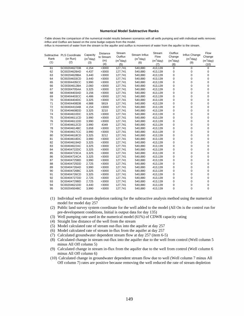
149
-Table shows the comparison of the numerical model results between scenarios with all wells pumping and with individual wells removed-Influx and Outflux are based on the zone budge outputs from the model.-Influx is movement of water from the stream to the aquifer and outflux is movement of water from the aquifer to the stream.
Subtractive Rank (1)
PLS Coordinate (or Run)
(2)
Capacity (m3/day)
(3)
Distance to Stream
(m) (4)
Stream Outflux
(m3/day) (5)
Stream Influx (m3/day)
(6)
Stream Flow
(m3/day) (7)
Outflux Change (m3/day)
(8)
Influx Change (m3/day)
(9)
Flow Change (m3/day)
(10)61 SC00204627DB 4,154 >3000 127,741 540,880 413,139 0 0 062 SC00204628AD 4,437 >3000 127,741 540,880 413,139 0 0 063 SC00204628BA 3,440 >3000 127,741 540,880 413,139 0 0 064 SC00204633CD 3,440 >3000 127,741 540,880 413,139 0 0 065 SC00304435CC 3,990 >3000 127,741 540,880 413,139 0 0 066 SC00304612BA 2,060 >3000 127,741 540,880 413,139 0 0 067 SC00304705AA 3,325 >3000 127,741 540,880 413,139 0 0 068 SC00404403AD 3,156 >3000 127,741 540,880 413,139 0 0 069 SC00404403CC 4,486 >3000 127,741 540,880 413,139 0 0 070 SC00404404DC 3,325 >3000 127,741 540,880 413,139 0 0 071 SC00404408DB 4,988 5819 127,741 540,880 413,139 0 0 072 SC00404410AB 4,154 >3000 127,741 540,880 413,139 0 0 073 SC00404608DD 3,325 3210 127,741 540,880 413,139 0 0 074 SC00404610DC 3,325 >3000 127,741 540,880 413,139 0 0 075 SC00404611CD 3,990 >3000 127,741 540,880 413,139 0 0 076 SC00404611DD 3,990 >3000 127,741 540,880 413,139 0 0 077 SC00404612CD 3,990 4349 127,741 540,880 413,139 0 0 078 SC00404614BC 3,658 >3000 127,741 540,880 413,139 0 0 079 SC00404617CC 3,990 >3000 127,741 540,880 413,139 0 0 080 SC00404618CD 3,325 3212 127,741 540,880 413,139 0 0 081 SC00404618DC 3,990 >3000 127,741 540,880 413,139 0 0 082 SC00404619AD 3,325 >3000 127,741 540,880 413,139 0 0 083 SC00404622AC 3,325 >3000 127,741 540,880 413,139 0 0 084 SC00404722DC 3,325 >3000 127,741 540,880 413,139 0 0 085 SC00404723CA 3,325 >3000 127,741 540,880 413,139 0 0 086 SC00404724CA 3,325 >3000 127,741 540,880 413,139 0 0 087 SC00404725BD 3,990 >3000 127,741 540,880 413,139 0 0 088 SC00404725DD 2,725 >3000 127,741 540,880 413,139 0 0 089 SC00404726AD 3,990 >3000 127,741 540,880 413,139 0 0 090 SC00404726BC 3,325 >3000 127,741 540,880 413,139 0 0 091 SC00404726CD 3,325 >3000 127,741 540,880 413,139 0 0 092 SC00404727DD 2,725 >3000 127,741 540,880 413,139 0 0 093 SC00404729BD 2,725 >3000 127,741 540,880 413,139 0 0 094 SC00204621DD 3,440 >3000 127,741 540,880 413,139 0 0 095 SC00204504BC 3,990 >3000 127,741 540,880 413,139 0 0 0
Numerical Model Subtractive Ranks
(1) Individual well stream depletion ranking for the subtractive analysis method using the numerical model for model day 257
(2) Public land survey system coordinate for the well added to the model (All On is the control run for pre-development conditions, Initial is output data for day 135)
(3) Well pumping rate used in the numerical model (61%) of CDWR capacity rating (4) Straight line distance of the well from the stream (5) Model calculated rate of stream out-flux into the aquifer at day 257 (6) Model calculated rate of stream in-flux from the aquifer at day 257 (7) Calculated groundwater dependent stream flow at day 257 (item 6-5) (8) Calculated change in stream out-flux into the aquifer due to the well from control (Well column 5
minus All Off column 5) (9) Calculated change in stream in-flux from the aquifer due to the well from control (Well column 6
minus All Off column 6) (10) Calculated change in groundwater dependent stream flow due to well (Well column 7 minus All
Off column 7) rates are positive because removing the well reduced the rate of stream depletion

150
Appendix G
Top 15 Additive & Subtractive Analysis Output Sheet Printouts
See Table 5-1 for Details
WELL PRINTOUT SHEETS NOTE Printout sheets contain raw mass balance output data produced by Visual Modflow v. 4.0, 2003 for model runs during well analysis (see Chapter 5). Labeled per Figure 5-6.
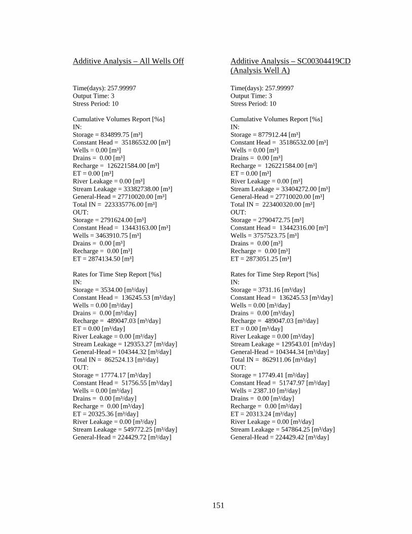
151
Additive Analysis – All Wells Off
Time(days): 257.99997 Output Time: 3 Stress Period: 10 Cumulative Volumes Report [%s] IN: Storage = 834899.75 [m³] Constant Head = 35186532.00 [m³] Wells = 0.00 [m³] Drains = 0.00 [m³] Recharge = 126221584.00 [m³] ET = 0.00 [m³] River Leakage = 0.00 [m³] Stream Leakage = 33382738.00 [m³] General-Head = 27710020.00 [m³] Total IN = 223335776.00 [m³] OUT: Storage = 2791624.00 [m³] Constant Head = 13443163.00 [m³] Wells = 3463910.75 [m³] Drains = 0.00 [m³] Recharge = 0.00 [m³] ET = 2874134.50 [m³] Rates for Time Step Report [%s] IN: Storage = 3534.00 [m³/day] Constant Head = 136245.53 [m³/day] Wells = 0.00 [m³/day] Drains = 0.00 [m³/day] Recharge = 489047.03 [m³/day] ET = 0.00 [m³/day] River Leakage = 0.00 [m³/day] Stream Leakage = 129353.27 [m³/day] General-Head = 104344.32 [m³/day] Total IN = 862524.13 [m³/day] OUT: Storage = 17774.17 [m³/day] Constant Head = 51756.55 [m³/day] Wells = 0.00 [m³/day] Drains = 0.00 [m³/day] Recharge = 0.00 [m³/day] ET = 20325.36 [m³/day] River Leakage = 0.00 [m³/day] Stream Leakage = 549772.25 [m³/day] General-Head = 224429.72 [m³/day]
Additive Analysis – SC00304419CD (Analysis Well A) Time(days): 257.99997 Output Time: 3 Stress Period: 10 Cumulative Volumes Report [%s] IN: Storage = 877912.44 [m³] Constant Head = 35186532.00 [m³] Wells = 0.00 [m³] Drains = 0.00 [m³] Recharge = 126221584.00 [m³] ET = 0.00 [m³] River Leakage = 0.00 [m³] Stream Leakage = 33404272.00 [m³] General-Head = 27710020.00 [m³] Total IN = 223400320.00 [m³] OUT: Storage = 2790472.75 [m³] Constant Head = 13442316.00 [m³] Wells = 3757523.75 [m³] Drains = 0.00 [m³] Recharge = 0.00 [m³] ET = 2873051.25 [m³]� Rates for Time Step Report [%s] IN: Storage = 3731.16 [m³/day] Constant Head = 136245.53 [m³/day] Wells = 0.00 [m³/day] Drains = 0.00 [m³/day] Recharge = 489047.03 [m³/day] ET = 0.00 [m³/day] River Leakage = 0.00 [m³/day] Stream Leakage = 129543.01 [m³/day] General-Head = 104344.34 [m³/day] Total IN = 862911.06 [m³/day] OUT: Storage = 17749.41 [m³/day] Constant Head = 51747.97 [m³/day] Wells = 2387.10 [m³/day] Drains = 0.00 [m³/day] Recharge = 0.00 [m³/day] ET = 20313.24 [m³/day] River Leakage = 0.00 [m³/day] Stream Leakage = 547864.25 [m³/day] General-Head = 224429.42 [m³/day]

152
Additive Analysis – SC00404718AA (Analysis Well B) Time(days): 257.99997 Output Time: 3 Stress Period: 10 Cumulative Volumes Report [%s] IN: Storage = 924530.06 [m³] Constant Head = 35199636.00 [m³] Wells = 0.00 [m³] Drains = 0.00 [m³] Recharge = 126221584.00 [m³] ET = 0.00 [m³] River Leakage = 0.00 [m³] Stream Leakage = 33332090.00 [m³] General-Head = 27710976.00 [m³] Total IN = 223388816.00 [m³] OUT: Storage = 2791493.25 [m³] Constant Head = 13442854.00 [m³] Wells = 3750156.75 [m³] Drains = 0.00 [m³] Recharge = 0.00 [m³] ET = 2873518.00 [m³] Rates for Time Step Report [%s] IN: Storage = 3941.48 [m³/day] Constant Head = 136370.56 [m³/day] Wells = 0.00 [m³/day] Drains = 0.00 [m³/day] Recharge = 489047.03 [m³/day] ET = 0.00 [m³/day] River Leakage = 0.00 [m³/day] Stream Leakage = 128867.91 [m³/day] General-Head = 104355.84 [m³/day] Total IN = 862582.88 [m³/day] OUT: Storage = 17772.95 [m³/day] Constant Head = 51752.93 [m³/day] Wells = 2327.20 [m³/day] Drains = 0.00 [m³/day] Recharge = 0.00 [m³/day] ET = 20318.00 [m³/day] River Leakage = 0.00 [m³/day] Stream Leakage = 548338.19 [m³/day] General-Head = 224429.58 [m³/day]
Additive Analysis – SC00304507DA (Analysis Well Y) Time(days): 257.99997 Output Time: 3 Stress Period: 10 Cumulative Volumes Report [%s] IN: Storage = 1247810.38 [m³] Constant Head = 35186532.00 [m³] Wells = 0.00 [m³] Drains = 0.00 [m³] Recharge = 126221584.00 [m³] ET = 0.00 [m³] River Leakage = 0.00 [m³] Stream Leakage = 33394116.00 [m³] General-Head = 27710024.00 [m³] Total IN = 223760064.00 [m³] OUT: Storage = 2790943.00 [m³] Constant Head = 13442995.00 [m³] Wells = 3872824.00 [m³] Drains = 0.00 [m³] Recharge = 0.00 [m³] ET = 2874041.25 [m³/day] Rates for Time Step Report [%s] IN: Storage = 6882.68 [m³/day] Constant Head = 136245.56 [m³/day] Wells = 0.00 [m³/day] Drains = 0.00 [m³/day] Recharge = 489047.03 [m³/day] ET = 0.00 [m³/day] River Leakage = 0.00 [m³/day] Stream Leakage = 129452.36 [m³/day] General-Head = 104344.45 [m³/day] Total IN = 865972.06 [m³/day] OUT: Storage = 17761.11 [m³/day] Constant Head = 51754.12 [m³/day] Wells = 3324.50 [m³/day] Drains = 0.00 [m³/day] Recharge = 0.00 [m³/day] ET = 20323.97 [m³/day] River Leakage = 0.00 [m³/day] Stream Leakage = 549085.00 [m³/day] General-Head = 224429.52 [m³/day]

153
Additive Analysis – SC00404713AC (Analysis Well K) Time(days): 257.99997 Output Time: 3 Stress Period: 10 Cumulative Volumes Report [%s] IN: Storage = 1324481.63 [m³] Constant Head = 35186532.00 [m³] Wells = 0.00 [m³] Drains = 0.00 [m³] Recharge = 126221584.00 [m³] ET = 0.00 [m³] River Leakage = 0.00 [m³] Stream Leakage = 33394084.00 [m³] General-Head = 27710028.00 [m³] Total IN = 223836704.00 [m³] OUT: Storage = 2786178.75 [m³] Constant Head = 13442995.00 [m³] Wells = 3954606.75 [m³] Drains = 0.00 [m³] Recharge = 0.00 [m³] ET = 2874041.00 [m³/day] Rates for Time Step Report [%s] IN: Storage = 7430.77 [m³/day] Constant Head = 136245.56 [m³/day] Wells = 0.00 [m³/day] Drains = 0.00 [m³/day] Recharge = 489047.03 [m³/day] ET = 0.00 [m³/day] River Leakage = 0.00 [m³/day] Stream Leakage = 129449.80 [m³/day] General-Head = 104344.61 [m³/day] Total IN = 866517.81 [m³/day] OUT: Storage = 17652.82 [m³/day] Constant Head = 51754.12 [m³/day] Wells = 3989.40 [m³/day] Drains = 0.00 [m³/day] Recharge = 0.00 [m³/day] ET = 20323.97 [m³/day] River Leakage = 0.00 [m³/day] Stream Leakage = 549083.19 [m³/day] General-Head = 224429.86 [m³/day]
Additive Analysis – SC00304703BC (Analysis Well V) Time(days): 257.99997 Output Time: 3 Stress Period: 10 Cumulative Volumes Report [%s] IN: Storage = 1493576.00 [m³] Constant Head = 35186536.00 [m³] Wells = 0.00 [m³] Drains = 0.00 [m³] Recharge = 126221584.00 [m³] ET = 0.00 [m³] River Leakage = 0.00 [m³] Stream Leakage = 33394686.00 [m³] General-Head = 27710020.00 [m³] Total IN = 224006400.00 [m³] OUT: Storage = 2790886.00 [m³] Constant Head = 13442965.00 [m³] Wells = 4118172.75 [m³] Drains = 0.00 [m³] Recharge = 0.00 [m³] ET = 2874023.75 [m³/day] Rates for Time Step Report [%s] IN: Storage = 8870.52 [m³/day] Constant Head = 136245.58 [m³/day] Wells = 0.00 [m³/day] Drains = 0.00 [m³/day] Recharge = 489047.03 [m³/day] ET = 0.00 [m³/day] River Leakage = 0.00 [m³/day] Stream Leakage = 129446.20 [m³/day] General-Head = 104344.42 [m³/day] Total IN = 867953.75 [m³/day] OUT: Storage = 17759.52 [m³/day] Constant Head = 51753.96 [m³/day] Wells = 5319.20 [m³/day] Drains = 0.00 [m³/day] Recharge = 0.00 [m³/day] ET = 20323.92 [m³/day] River Leakage = 0.00 [m³/day] Stream Leakage = 549081.13 [m³/day] General-Head = 224429.75 [m³/day]

154
Additive Analysis – SC00404618BA (Analysis Well J) Time(days): 257.99997 Output Time: 3 Stress Period: 10 Cumulative Volumes Report [%s] IN: Storage = 1491227.63 [m³] Constant Head = 35186532.00 [m³] Wells = 0.00 [m³] Drains = 0.00 [m³] Recharge = 126221584.00 [m³] ET = 0.00 [m³] River Leakage = 0.00 [m³] Stream Leakage = 33394234.00 [m³] General-Head = 27710022.00 [m³] Total IN = 224003600.00 [m³] OUT: Storage = 2789556.75 [m³] Constant Head = 13442980.00 [m³] Wells = 4118172.75 [m³] Drains = 0.00 [m³] Recharge = 0.00 [m³] ET = 2874033.50 [m³/day] Rates for Time Step Report [%s] IN: Storage = 8822.19 [m³/day] Constant Head = 136245.56 [m³/day] Wells = 0.00 [m³/day] Drains = 0.00 [m³/day] Recharge = 489047.03 [m³/day] ET = 0.00 [m³/day] River Leakage = 0.00 [m³/day] Stream Leakage = 129448.77 [m³/day] General-Head = 104344.46 [m³/day] Total IN = 867908.00 [m³/day] OUT: Storage = 17728.69 [m³/day] Constant Head = 51754.01 [m³/day] Wells = 5319.20 [m³/day] Drains = 0.00 [m³/day] Recharge = 0.00 [m³/day] ET = 20323.93 [m³/day] River Leakage = 0.00 [m³/day] Stream Leakage = 549083.75 [m³/day] General-Head = 224429.89 [m³/day]
Additive Analysis – SC00404608DD (Analysis Well Q) Time(days): 257.99997 Output Time: 3 Stress Period: 10 Cumulative Volumes Report [%s] IN: Storage = 1246582.13 [m³] Constant Head = 35186532.00 [m³] Wells = 0.00 [m³] Drains = 0.00 [m³] Recharge = 126221584.00 [m³] ET = 0.00 [m³] River Leakage = 0.00 [m³] Stream Leakage = 33389750.00 [m³] General-Head = 27710036.00 [m³] Total IN = 223754480.00 [m³] OUT: Storage = 2790225.25 [m³] Constant Head = 13443023.00 [m³] Wells = 3872824.00 [m³] Drains = 0.00 [m³] Recharge = 0.00 [m³] ET = 2874056.00 [m³/day] Rates for Time Step Report [%s] IN: Storage = 6872.48 [m³/day] Constant Head = 136245.56 [m³/day] Wells = 0.00 [m³/day] Drains = 0.00 [m³/day] Recharge = 489047.03 [m³/day] ET = 0.00 [m³/day] River Leakage = 0.00 [m³/day] Stream Leakage = 129437.63 [m³/day] General-Head = 104344.91 [m³/day] Total IN = 865947.63 [m³/day] OUT: Storage = 17748.07 [m³/day] Constant Head = 51754.25 [m³/day] Wells = 3324.50 [m³/day] Drains = 0.00 [m³/day] Recharge = 0.00 [m³/day] ET = 20324.06 [m³/day] River Leakage = 0.00 [m³/day] Stream Leakage = 549090.56 [m³/day] General-Head = 224429.89 [m³/day]

155
Additive Analysis – SC00404715DC (Analysis Well L) Time(days): 257.99997 Output Time: 3 Stress Period: 10 Cumulative Volumes Report [%s] IN: Storage = 1244320.00 [m³] Constant Head = 35186532.00 [m³] Wells = 0.00 [m³] Drains = 0.00 [m³] Recharge = 126221584.00 [m³] ET = 0.00 [m³] River Leakage = 0.00 [m³] Stream Leakage = 33385566.00 [m³] General-Head = 27710024.00 [m³] Total IN = 223748032.00 [m³] OUT: Storage = 2788107.25 [m³] Constant Head = 13443039.00 [m³] Wells = 3872824.00 [m³] Drains = 0.00 [m³] Recharge = 0.00 [m³] ET = 2874056.00 [m³/day] Rates for Time Step Report [%s] IN: Storage = 6813.58 [m³/day] Constant Head = 136245.56 [m³/day] Wells = 0.00 [m³/day] Drains = 0.00 [m³/day] Recharge = 489047.03 [m³/day] ET = 0.00 [m³/day] River Leakage = 0.00 [m³/day] Stream Leakage = 129442.02 [m³/day] General-Head = 104344.45 [m³/day] Total IN = 865892.63 [m³/day] OUT: Storage = 17694.93 [m³/day] Constant Head = 51754.28 [m³/day] Wells = 3324.50 [m³/day] Drains = 0.00 [m³/day] Recharge = 0.00 [m³/day] ET = 20324.07 [m³/day] River Leakage = 0.00 [m³/day] Stream Leakage = 549106.75 [m³/day] General-Head = 224429.91 [m³/day]
Additive Analysis – SC00404618AA (Analysis Well O) Time(days): 257.99997 Output Time: 3 Stress Period: 10 Cumulative Volumes Report [%s] IN: Storage = 1246024.88 [m³] Constant Head = 35186532.00 [m³] Wells = 0.00 [m³] Drains = 0.00 [m³] Recharge = 126221584.00 [m³] ET = 0.00 [m³] River Leakage = 0.00 [m³] Stream Leakage = 33385664.00 [m³] General-Head = 27710026.00 [m³] Total IN = 223749824.00 [m³] OUT: Storage = 2789719.75 [m³] Constant Head = 13443039.00 [m³] Wells = 3872824.00 [m³] Drains = 0.00 [m³] Recharge = 0.00 [m³] ET = 2874055.75 [m³/day] Rates for Time Step Report [%s] IN: Storage = 6858.23 [m³/day] Constant Head = 136245.56 [m³/day] Wells = 0.00 [m³/day] Drains = 0.00 [m³/day] Recharge = 489047.03 [m³/day] ET = 0.00 [m³/day] River Leakage = 0.00 [m³/day] Stream Leakage = 129447.28 [m³/day] General-Head = 104344.62 [m³/day] Total IN = 865942.75 [m³/day] OUT: Storage = 17734.78 [m³/day] Constant Head = 51754.28 [m³/day] Wells = 3324.50 [m³/day] Drains = 0.00 [m³/day] Recharge = 0.00 [m³/day] ET = 20324.07 [m³/day] River Leakage = 0.00 [m³/day] Stream Leakage = 549113.94 [m³/day] General-Head = 224429.89 [m³/day]

156
Additive Analysis – SC00404729AA (Analysis Well P) Time(days): 257.99997 Output Time: 3 Stress Period: 10 Cumulative Volumes Report [%s] IN: Storage = 1418706.75 [m³] Constant Head = 35186536.00 [m³] Wells = 0.00 [m³] Drains = 0.00 [m³] Recharge = 126221584.00 [m³] ET = 0.00 [m³] River Leakage = 0.00 [m³] Stream Leakage = 33386766.00 [m³] General-Head = 27725264.00 [m³] Total IN = 223938864.00 [m³] OUT: Storage = 2773750.75 [m³] Constant Head = 13443047.00 [m³] Wells = 4077287.00 [m³] Drains = 0.00 [m³] Recharge = 0.00 [m³] ET = 2874070.25 [m³/day] Rates for Time Step Report [%s] IN: Storage = 7954.67 [m³/day] Constant Head = 136245.61 [m³/day] Wells = 0.00 [m³/day] Drains = 0.00 [m³/day] Recharge = 489047.03 [m³/day] ET = 0.00 [m³/day] River Leakage = 0.00 [m³/day] Stream Leakage = 129433.31 [m³/day] General-Head = 104613.35 [m³/day] Total IN = 867294.00 [m³/day] OUT: Storage = 17437.40 [m³/day] Constant Head = 51754.44 [m³/day] Wells = 4986.80 [m³/day] Drains = 0.00 [m³/day] Recharge = 0.00 [m³/day] ET = 20324.19 [m³/day] River Leakage = 0.00 [m³/day] Stream Leakage = 549108.31 [m³/day] General-Head = 224428.00 [m³/day]
Additive Analysis – SC00304705AA (Analysis Well X) Time(days): 257.99997 Output Time: 3 Stress Period: 10 Cumulative Volumes Report [%s] IN: Storage = 1245621.25 [m³] Constant Head = 35186532.00 [m³] Wells = 0.00 [m³] Drains = 0.00 [m³] Recharge = 126221584.00 [m³] ET = 0.00 [m³] River Leakage = 0.00 [m³] Stream Leakage = 33385808.00 [m³] General-Head = 27710022.00 [m³] Total IN = 223749568.00 [m³] OUT: Storage = 2790971.25 [m³] Constant Head = 13443082.00 [m³] Wells = 3872824.00 [m³] Drains = 0.00 [m³] Recharge = 0.00 [m³] ET = 2874094.25 [m³/day] Rates for Time Step Report [%s] IN: Storage = 6884.06 [m³/day] Constant Head = 136245.58 [m³/day] Wells = 0.00 [m³/day] Drains = 0.00 [m³/day] Recharge = 489047.03 [m³/day] ET = 0.00 [m³/day] River Leakage = 0.00 [m³/day] Stream Leakage = 129427.07 [m³/day] General-Head = 104344.41 [m³/day] Total IN = 865948.13 [m³/day] OUT: Storage = 17762.40 [m³/day] Constant Head = 51754.73 [m³/day] Wells = 3324.50 [m³/day] Drains = 0.00 [m³/day] Recharge = 0.00 [m³/day] ET = 20324.44 [m³/day] River Leakage = 0.00 [m³/day] Stream Leakage = 549202.44 [m³/day] General-Head = 224426.03[m³/day]

157
Additive Analysis – SC00304704AC (Analysis Well W) Time(days): 257.99997 Output Time: 3 Stress Period: 10 Cumulative Volumes Report [%s] IN: Storage = 1494498.38 [m³] Constant Head = 35186532.00 [m³] Wells = 0.00 [m³] Drains = 0.00 [m³] Recharge = 126221584.00 [m³] ET = 0.00 [m³] River Leakage = 0.00 [m³] Stream Leakage = 33392144.00 [m³] General-Head = 27710020.00 [m³] Total IN = 224004784.00 [m³] OUT: Storage = 2790898.25 [m³] Constant Head = 13442942.00 [m³] Wells = 4118172.75 [m³] Drains = 0.00 [m³] Recharge = 0.00 [m³] ET = 2874010.25 [m³/day] Rates for Time Step Report [%s] IN: Storage = 8890.40 [m³/day] Constant Head = 136245.47 [m³/day] Wells = 0.00 [m³/day] Drains = 0.00 [m³/day] Recharge = 489047.03 [m³/day] ET = 0.00 [m³/day] River Leakage = 0.00 [m³/day] Stream Leakage = 129394.41 [m³/day] General-Head = 104344.43 [m³/day] Total IN = 867921.75 [m³/day] OUT: Storage = 17760.12 [m³/day] Constant Head = 51753.48 [m³/day] Wells = 5319.20 [m³/day] Drains = 0.00 [m³/day] Recharge = 0.00 [m³/day] ET = 20323.63 [m³/day] River Leakage = 0.00 [m³/day] Stream Leakage = 549180.13 [m³/day] General-Head = 224429.50 [m³/day]
Additive Analysis – SC00404718BB (Analysis Well C) Time(days): 257.99997 Output Time: 3 Stress Period: 10 Cumulative Volumes Report [%s] IN: Storage = 887912.88 [m³] Constant Head = 35263432.00 [m³] Wells = 0.00 [m³] Drains = 0.00 [m³] Recharge = 126221584.00 [m³] ET = 0.00 [m³] River Leakage = 0.00 [m³] Stream Leakage = 33350778.00 [m³] General-Head = 27710156.00 [m³] Total IN = 223433872.00 [m³] OUT: Storage = 2791543.25 [m³] Constant Head = 13442959.00 [m³] Wells = 3709259.25 [m³] Drains = 0.00 [m³] Recharge = 0.00 [m³] ET = 2873734.25 [m³] Rates for Time Step Report [%s] IN: Storage = 3773.12 [m³/day] Constant Head = 136895.89 [m³/day] Wells = 0.00 [m³/day] Drains = 0.00 [m³/day] Recharge = 489047.03 [m³/day] ET = 0.00 [m³/day] River Leakage = 0.00 [m³/day] Stream Leakage = 129058.41 [m³/day] General-Head = 104346.02 [m³/day] Total IN = 863120.50 [m³/day] OUT: Storage = 17773.21 [m³/day] Constant Head = 51754.11 [m³/day] Wells = 1994.70 [m³/day] Drains = 0.00 [m³/day] Recharge = 0.00 [m³/day] ET = 20320.58 [m³/day] River Leakage = 0.00 [m³/day] Stream Leakage = 548852.56 [m³/day] General-Head = 224429.63 [m³/day]

158
Additive Analysis – SC00404720CD (Analysis Well N) Time(days): 257.99997 Output Time: 3 Stress Period: 10 Cumulative Volumes Report [%s] IN: Storage = 1207139.38 [m³] Constant Head = 35186648.00 [m³] Wells = 0.00 [m³] Drains = 0.00 [m³] Recharge = 126221584.00 [m³] ET = 0.00 [m³] River Leakage = 0.00 [m³] Stream Leakage = 33384186.00 [m³] General-Head = 27745176.00 [m³] Total IN = 223744736.00 [m³] OUT: Storage = 2789275.25 [m³] Constant Head = 13443124.00 [m³] Wells = 3872824.00 [m³] Drains = 0.00 [m³] Recharge = 0.00 [m³] ET = 2874120.25 [m³/day] Rates for Time Step Report [%s] IN: Storage = 6353.45 [m³/day] Constant Head = 136248.83 [m³/day] Wells = 0.00 [m³/day] Drains = 0.00 [m³/day] Recharge = 489047.03 [m³/day] ET = 0.00 [m³/day] River Leakage = 0.00 [m³/day] Stream Leakage = 129417.38 [m³/day] General-Head = 104820.07 [m³/day] Total IN = 865886.75 [m³/day] OUT: Storage = 17721.05 [m³/day] Constant Head = 51755.31 [m³/day] Wells = 3324.50 [m³/day] Drains = 0.00 [m³/day] Recharge = 0.00 [m³/day] ET = 20324.87 [m³/day] River Leakage = 0.00 [m³/day] Stream Leakage = 549414.06 [m³/day] General-Head = 224429.92 [m³/day]
Additive Analysis – SC00404714AB (Analysis Well D) Time(days): 257.99997 Output Time: 3 Stress Period: 10 Cumulative Volumes Report [%s] IN: Storage = 1239232.50 [m³] Constant Head = 35186532.00 [m³] Wells = 0.00 [m³] Drains = 0.00 [m³] Recharge = 126221584.00 [m³] ET = 0.00 [m³] River Leakage = 0.00 [m³] Stream Leakage = 33390082.00 [m³] General-Head = 27710024.00 [m³] Total IN = 223747456.00 [m³] OUT: Storage = 2790712.25 [m³] Constant Head = 13442987.00 [m³] Wells = 3872824.00 [m³] Drains = 0.00 [m³] Recharge = 0.00 [m³] ET = 2874031.00 [m³/day] Rates for Time Step Report [%s] IN: Storage = 6697.35 [m³/day] Constant Head = 136245.45 [m³/day] Wells = 0.00 [m³/day] Drains = 0.00 [m³/day] Recharge = 489047.03 [m³/day] ET = 0.00 [m³/day] River Leakage = 0.00 [m³/day] Stream Leakage = 129325.48 [m³/day] General-Head = 104344.45 [m³/day] Total IN = 865659.81 [m³/day] OUT: Storage = 17754.29 [m³/day] Constant Head = 51753.95 [m³/day] Wells = 3324.50 [m³/day] Drains = 0.00 [m³/day] Recharge = 0.00 [m³/day] ET = 20323.71 [m³/day] River Leakage = 0.00 [m³/day] Stream Leakage = 549322.88 [m³/day] General-Head = 224429.89 [m³/day]

159
Subtractive Analysis – All On Time(days): 257.99997 Output Time: 3 Stress Period: 10 Cumulative Volumes Report [%s] IN: Storage = 38719736.00 [m³] Constant Head = 35379544.00 [m³] Wells = 0.00 [m³] Drains = 0.00 [m³] Recharge = 126221584.00 [m³] ET = 0.00 [m³] River Leakage = 0.00 [m³] Stream Leakage = 33223864.00 [m³] General-Head = 29713570.00 [m³] Total IN = 263258304.00 [m³] OUT: Storage = 3175298.25 [m³] Constant Head = 13440877.00 [m³] Wells = 44778600.00 [m³] Drains = 0.00 [m³] Recharge = 0.00 [m³] ET = 2870584.50 [m³/d] Rates for Time Step Report [%s] IN: Storage = 289545.59 [m³/day] Constant Head = 138234.28 [m³/day] Wells = 0.00 [m³/day] Drains = 0.00 [m³/day] Recharge = 489047.03 [m³/day] ET = 0.00 [m³/day] River Leakage = 0.00 [m³/day] Stream Leakage = 127688.86 [m³/day] General-Head = 136911.13 [m³/day] Total IN = 1181426.88 [m³/day] OUT: Storage = 80.74 [m³/day] Constant Head = 51729.55 [m³/day] Wells = 364053.66 [m³/day] Drains = 0.00 [m³/day] Recharge = 0.00 [m³/day] ET = 20278.12 [m³/day] River Leakage = 0.00 [m³/day] Stream Leakage = 540778.19 [m³/day] General-Head = 208146.25[m³/day]
Subtractive Analysis – SC00304419CD (Analysis Well A) Time(days): 257.99997 Output Time: 3 Stress Period: 10 Cumulative Volumes Report [%s] IN: Storage = 38691948.00 [m³] Constant Head = 35379544.00 [m³] Wells = 0.00 [m³] Drains = 0.00 [m³] Recharge = 126221584.00 [m³] ET = 0.00 [m³] River Leakage = 0.00 [m³] Stream Leakage = 33205762.00 [m³] General-Head = 29713568.00 [m³] Total IN = 263212400.00 [m³] OUT: Storage = 3176270.50 [m³] Constant Head = 13441747.00 [m³] Wells = 44484988.00 [m³] Drains = 0.00 [m³] Recharge = 0.00 [m³] ET = 2871682.75 [m³/d] Rates for Time Step Report [%s] IN: Storage = 289594.53 [m³/day] Constant Head = 138234.28 [m³/day] Wells = 0.00 [m³/day] Drains = 0.00 [m³/day] Recharge = 489047.03 [m³/day] ET = 0.00 [m³/day] River Leakage = 0.00 [m³/day] Stream Leakage = 127536.58 [m³/day] General-Head = 136911.09 [m³/day] Total IN = 1181323.63 [m³/day] OUT: Storage = 81.74 [m³/day] Constant Head = 51738.46 [m³/day] Wells = 361666.56 [m³/day] Drains = 0.00 [m³/day] Recharge = 0.00 [m³/day] ET = 20290.43 [m³/day] River Leakage = 0.00 [m³/day] Stream Leakage = 542813.69 [m³/day] General-Head = 208146.52[m³/day]

160
Subtractive Analysis – SC00304704AC (Analysis Well W) Time(days): 257.99997 Output Time: 3 Stress Period: 10 Cumulative Volumes Report [%s] IN: Storage = 38067116.00 [m³] Constant Head = 35379548.00 [m³] Wells = 0.00 [m³] Drains = 0.00 [m³] Recharge = 126221584.00 [m³] ET = 0.00 [m³] River Leakage = 0.00 [m³] Stream Leakage = 33233776.00 [m³] General-Head = 29713566.00 [m³] Total IN = 262615584.00 [m³] OUT: Storage = 3175306.25 [m³] Constant Head = 13441032.00 [m³] Wells = 44124340.00 [m³] Drains = 0.00 [m³] Recharge = 0.00 [m³] ET = 2870769.00 [m³/d] Rates for Time Step Report [%s] IN: Storage = 284274.63 [m³/day] Constant Head = 138234.20 [m³/day] Wells = 0.00 [m³/day] Drains = 0.00 [m³/day] Recharge = 489047.03 [m³/day] ET = 0.00 [m³/day] River Leakage = 0.00 [m³/day] Stream Leakage = 127642.98 [m³/day] General-Head = 136911.08 [m³/day] Total IN = 1176109.88 [m³/day] OUT: Storage = 80.86 [m³/day] Constant Head = 51733.04 [m³/day] Wells = 358734.47 [m³/day] Drains = 0.00 [m³/day] Recharge = 0.00 [m³/day] ET = 20282.19 [m³/day] River Leakage = 0.00 [m³/day] Stream Leakage = 542561.44 [m³/day] General-Head = 208146.64[m³/day]
Subtractive Analysis – SC00404718AA (Analysis Well B) Time(days): 257.99997 Output Time: 3 Stress Period: 10 Cumulative Volumes Report [%s] IN: Storage = 38638716.00 [m³] Constant Head = 35366476.00 [m³] Wells = 0.00 [m³] Drains = 0.00 [m³] Recharge = 126221584.00 [m³] ET = 0.00 [m³] River Leakage = 0.00 [m³] Stream Leakage = 33283036.00 [m³] General-Head = 29712602.00 [m³] Total IN = 263222416.00 [m³] OUT: Storage = 3175333.00 [m³] Constant Head = 13441267.00 [m³] Wells = 44492356.00 [m³] Drains = 0.00 [m³] Recharge = 0.00 [m³] ET = 2871307.50 [m³/d] Rates for Time Step Report [%s] IN: Storage = 289333.31 [m³/day] Constant Head = 138109.78 [m³/day] Wells = 0.00 [m³/day] Drains = 0.00 [m³/day] Recharge = 489047.03 [m³/day] ET = 0.00 [m³/day] River Leakage = 0.00 [m³/day] Stream Leakage = 128267.30 [m³/day] General-Head = 136899.47 [m³/day] Total IN = 1181656.88 [m³/day] OUT: Storage = 80.91 [m³/day] Constant Head = 51734.63 [m³/day] Wells = 361726.47 [m³/day] Drains = 0.00 [m³/day] Recharge = 0.00 [m³/day] ET = 20287.33 [m³/day] River Leakage = 0.00 [m³/day] Stream Leakage = 542717.63 [m³/day] General-Head = 208146.36[m³/day]

161
Subtractive Analysis – SC00404718BB (Analysis Well C) Time(days): 257.99997 Output Time: 3 Stress Period: 10 Cumulative Volumes Report [%s] IN: Storage = 38678100.00 [m³] Constant Head = 35302684.00 [m³] Wells = 0.00 [m³] Drains = 0.00 [m³] Recharge = 126221584.00 [m³] ET = 0.00 [m³] River Leakage = 0.00 [m³] Stream Leakage = 33263410.00 [m³] General-Head = 29713426.00 [m³] Total IN = 263179200.00 [m³] OUT: Storage = 3175320.25 [m³] Constant Head = 13441132.00 [m³] Wells = 44533256.00 [m³] Drains = 0.00 [m³] Recharge = 0.00 [m³] ET = 2871061.00 [m³/d] Rates for Time Step Report [%s] IN: Storage = 289537.31 [m³/day] Constant Head = 137584.41 [m³/day] Wells = 0.00 [m³/day] Drains = 0.00 [m³/day] Recharge = 489047.03 [m³/day] ET = 0.00 [m³/day] River Leakage = 0.00 [m³/day] Stream Leakage = 128088.85 [m³/day] General-Head = 136909.30 [m³/day] Total IN = 1181166.88 [m³/day] OUT: Storage = 80.91 [m³/day] Constant Head = 51732.97 [m³/day] Wells = 362058.97 [m³/day] Drains = 0.00 [m³/day] Recharge = 0.00 [m³/day] ET = 20284.26 [m³/day] River Leakage = 0.00 [m³/day] Stream Leakage = 542077.75 [m³/day] General-Head = 208146.31[m³/day]
Subtractive Analysis – SC00304703BC (Analysis Well V) Time(days): 257.99997 Output Time: 3 Stress Period: 10 Cumulative Volumes Report [%s] IN: Storage = 38073888.00 [m³] Constant Head = 35379544.00 [m³] Wells = 0.00 [m³] Drains = 0.00 [m³] Recharge = 126221584.00 [m³] ET = 0.00 [m³] River Leakage = 0.00 [m³] Stream Leakage = 33231514.00 [m³] General-Head = 29713568.00 [m³] Total IN = 262620096.00 [m³] OUT: Storage = 3175379.75 [m³] Constant Head = 13440950.00 [m³] Wells = 44124340.00 [m³] Drains = 0.00 [m³] Recharge = 0.00 [m³] ET = 2870679.00 [m³/d] Rates for Time Step Report [%s] IN: Storage = 284317.72 [m³/day] Constant Head = 138234.20 [m³/day] Wells = 0.00 [m³/day] Drains = 0.00 [m³/day] Recharge = 489047.03 [m³/day] ET = 0.00 [m³/day] River Leakage = 0.00 [m³/day] Stream Leakage = 127840.10 [m³/day] General-Head = 136911.13 [m³/day] Total IN = 1176350.13 [m³/day] OUT: Storage = 81.13 [m³/day] Constant Head = 51731.60 [m³/day] Wells = 358734.47 [m³/day] Drains = 0.00 [m³/day] Recharge = 0.00 [m³/day] ET = 20280.62 [m³/day] River Leakage = 0.00 [m³/day] Stream Leakage = 541229.50 [m³/day] General-Head = 208146.41[m³/day]

162
Subtractive Analysis – SC00404719AA (Analysis Well F) Time(days): 257.99997 Output Time: 3 Stress Period: 10 Cumulative Volumes Report [%s] IN: Storage = 38550776.00 [m³] Constant Head = 35363500.00 [m³] Wells = 0.00 [m³] Drains = 0.00 [m³] Recharge = 126221584.00 [m³] ET = 0.00 [m³] River Leakage = 0.00 [m³] Stream Leakage = 33243212.00 [m³] General-Head = 29713228.00 [m³] Total IN = 263092304.00 [m³] OUT: Storage = 3175303.50 [m³] Constant Head = 13440906.00 [m³] Wells = 44512808.00 [m³] Drains = 0.00 [m³] Recharge = 0.00 [m³] ET = 2870704.75 [m³/d] Rates for Time Step Report [%s] IN: Storage = 288748.81 [m³/day] Constant Head = 138016.88 [m³/day] Wells = 0.00 [m³/day] Drains = 0.00 [m³/day] Recharge = 489047.03 [m³/day] ET = 0.00 [m³/day] River Leakage = 0.00 [m³/day] Stream Leakage = 127992.41 [m³/day] General-Head = 136903.88 [m³/day] Total IN = 1180709.00 [m³/day] OUT: Storage = 80.74 [m³/day] Constant Head = 51730.24 [m³/day] Wells = 361892.75 [m³/day] Drains = 0.00 [m³/day] Recharge = 0.00 [m³/day] ET = 20280.70 [m³/day] River Leakage = 0.00 [m³/day] Stream Leakage = 541327.31 [m³/day] General-Head = 208146.25[m³/day]
Subtractive Analysis – SC00404717CD (Analysis Well E) Time(days): 257.99997 Output Time: 3 Stress Period: 10 Cumulative Volumes Report [%s] IN: Storage = 38535336.00 [m³] Constant Head = 35363500.00 [m³] Wells = 0.00 [m³] Drains = 0.00 [m³] Recharge = 126221584.00 [m³] ET = 0.00 [m³] River Leakage = 0.00 [m³] Stream Leakage = 33239144.00 [m³] General-Head = 29713228.00 [m³] Total IN = 263072800.00 [m³] OUT: Storage = 3175308.75 [m³] Constant Head = 13440904.00 [m³] Wells = 44512808.00 [m³] Drains = 0.00 [m³] Recharge = 0.00 [m³] ET = 2870682.25 [m³/d] Rates for Time Step Report [%s] IN: Storage = 288477.47 [m³/day] Constant Head = 138016.88 [m³/day] Wells = 0.00 [m³/day] Drains = 0.00 [m³/day] Recharge = 489047.03 [m³/day] ET = 0.00 [m³/day] River Leakage = 0.00 [m³/day] Stream Leakage = 127911.67 [m³/day] General-Head = 136903.88 [m³/day] Total IN = 1180356.88 [m³/day] OUT: Storage = 80.74 [m³/day] Constant Head = 51730.12 [m³/day] Wells = 361892.75 [m³/day] Drains = 0.00 [m³/day] Recharge = 0.00 [m³/day] ET = 20280.13 [m³/day] River Leakage = 0.00 [m³/day] Stream Leakage = 541208.75 [m³/day] General-Head = 208146.25[m³/day]

163
Subtractive Analysis – SC00404712CA (Analysis Well G) Time(days): 257.99997 Output Time: 3 Stress Period: 10 Cumulative Volumes Report [%s] IN: Storage = 38632892.00 [m³] Constant Head = 35379544.00 [m³] Wells = 0.00 [m³] Drains = 0.00 [m³] Recharge = 126221584.00 [m³] ET = 0.00 [m³] River Leakage = 0.00 [m³] Stream Leakage = 33229228.00 [m³] General-Head = 29713568.00 [m³] Total IN = 263176816.00 [m³] OUT: Storage = 3175302.50 [m³] Constant Head = 13440892.00 [m³] Wells = 44655924.00 [m³] Drains = 0.00 [m³] Recharge = 0.00 [m³] ET = 2870648.25 [m³/d] Rates for Time Step Report [%s] IN: Storage = 289139.78 [m³/day] Constant Head = 138234.28 [m³/day] Wells = 0.00 [m³/day] Drains = 0.00 [m³/day] Recharge = 489047.03 [m³/day] ET = 0.00 [m³/day] River Leakage = 0.00 [m³/day] Stream Leakage = 127779.61 [m³/day] General-Head = 136911.13 [m³/day] Total IN = 1181111.88 [m³/day] OUT: Storage = 80.74 [m³/day] Constant Head = 51729.98 [m³/day] Wells = 363056.31 [m³/day] Drains = 0.00 [m³/day] Recharge = 0.00 [m³/day] ET = 20279.58 [m³/day] River Leakage = 0.00 [m³/day] Stream Leakage = 540987.81 [m³/day] General-Head = 208146.25[m³/day]
Subtractive Analysis – SC00304705DA (Analysis Well Y) Time(days): 257.99997 Output Time: 3 Stress Period: 10 Cumulative Volumes Report [%s] IN: Storage = 38324876.00 [m³] Constant Head = 35379548.00 [m³] Wells = 0.00 [m³] Drains = 0.00 [m³] Recharge = 126221584.00 [m³] ET = 0.00 [m³] River Leakage = 0.00 [m³] Stream Leakage = 33228682.00 [m³] General-Head = 29713570.00 [m³] Total IN = 262868272.00 [m³] OUT: Storage = 3175369.00 [m³] Constant Head = 13440893.00 [m³] Wells = 44369688.00 [m³] Drains = 0.00 [m³] Recharge = 0.00 [m³] ET = 2870617.50 [m³/d] Rates for Time Step Report [%s] IN: Storage = 286424.88 [m³/day] Constant Head = 138234.39 [m³/day] Wells = 0.00 [m³/day] Drains = 0.00 [m³/day] Recharge = 489047.03 [m³/day] ET = 0.00 [m³/day] River Leakage = 0.00 [m³/day] Stream Leakage = 127779.34 [m³/day] General-Head = 136911.13 [m³/day] Total IN = 1178396.75 [m³/day] OUT: Storage = 81.90 [m³/day] Constant Head = 51730.25 [m³/day] Wells = 360729.16 [m³/day] Drains = 0.00 [m³/day] Recharge = 0.00 [m³/day] ET = 20279.18 [m³/day] River Leakage = 0.00 [m³/day] Stream Leakage = 540857.06 [m³/day] General-Head = 208146.67[m³/day]

164
Subtractive Analysis – SC00404511CD (Analysis Well M) Time(days): 257.99997 Output Time: 3 Stress Period: 10 Cumulative Volumes Report [%s] IN: Storage = 38352860.00 [m³] Constant Head = 35379544.00 [m³] Wells = 0.00 [m³] Drains = 0.00 [m³] Recharge = 126221584.00 [m³] ET = 0.00 [m³] River Leakage = 0.00 [m³] Stream Leakage = 33227854.00 [m³] General-Head = 29607074.00 [m³] Total IN = 262788912.00 [m³] OUT: Storage = 3175335.25 [m³] Constant Head = 13440882.00 [m³] Wells = 44287900.00 [m³] Drains = 0.00 [m³] Recharge = 0.00 [m³] ET = 2870635.25 [m³/d] Rates for Time Step Report [%s] IN: Storage = 287290.97 [m³/day] Constant Head = 138234.28 [m³/day] Wells = 0.00 [m³/day] Drains = 0.00 [m³/day] Recharge = 489047.03 [m³/day] ET = 0.00 [m³/day] River Leakage = 0.00 [m³/day] Stream Leakage = 127737.35 [m³/day] General-Head = 135487.59 [m³/day] Total IN = 1177797.25 [m³/day] OUT: Storage = 80.74 [m³/day] Constant Head = 51729.75 [m³/day] Wells = 360064.25 [m³/day] Drains = 0.00 [m³/day] Recharge = 0.00 [m³/day] ET = 20279.49 [m³/day] River Leakage = 0.00 [m³/day] Stream Leakage = 540889.13 [m³/day] General-Head = 208164.23[m³/day]
Subtractive Analysis – SC00404405DD (Analysis Well S) Time(days): 257.99997 Output Time: 3 Stress Period: 10 Cumulative Volumes Report [%s] IN: Storage = 38128448.00 [m³] Constant Head = 35379544.00 [m³] Wells = 0.00 [m³] Drains = 0.00 [m³] Recharge = 126221584.00 [m³] ET = 0.00 [m³] River Leakage = 0.00 [m³] Stream Leakage = 33227798.00 [m³] General-Head = 29734276.00 [m³] Total IN = 262691648.00 [m³] OUT: Storage = 2901950.00 [m³] Constant Head = 13440881.00 [m³] Wells = 44476128.00 [m³] Drains = 0.00 [m³] Recharge = 0.00 [m³] ET = 2870582.50 [m³/d] Rates for Time Step Report [%s] IN: Storage = 286026.03 [m³/day] Constant Head = 138234.28 [m³/day] Wells = 0.00 [m³/day] Drains = 0.00 [m³/day] Recharge = 489047.03 [m³/day] ET = 0.00 [m³/day] River Leakage = 0.00 [m³/day] Stream Leakage = 127743.68 [m³/day] General-Head = 135214.67 [m³/day] Total IN = 1176265.63 [m³/day] OUT: Storage = 75.08 [m³/day] Constant Head = 51729.70 [m³/day] Wells = 358603.66 [m³/day] Drains = 0.00 [m³/day] Recharge = 0.00 [m³/day] ET = 20278.29 [m³/day] River Leakage = 0.00 [m³/day] Stream Leakage = 540870.88 [m³/day] General-Head = 208121.52[m³/day]

165
Subtractive Analysis – SC00404404BD (Analysis Well R) Time(days): 257.99997 Output Time: 3 Stress Period: 10 Cumulative Volumes Report [%s] IN: Storage = 38189536.00 [m³] Constant Head = 35379544.00 [m³] Wells = 0.00 [m³] Drains = 0.00 [m³] Recharge = 126221584.00 [m³] ET = 0.00 [m³] River Leakage = 0.00 [m³] Stream Leakage = 33227830.00 [m³] General-Head = 29839536.00 [m³] Total IN = 262858032.00 [m³] OUT: Storage = 2743065.25 [m³] Constant Head = 13440881.00 [m³] Wells = 44826472.00 [m³] Drains = 0.00 [m³] Recharge = 0.00 [m³] ET = 2870587.25 [m³/d] Rates for Time Step Report [%s] IN: Storage = 286020.13 [m³/day] Constant Head = 138234.28 [m³/day] Wells = 0.00 [m³/day] Drains = 0.00 [m³/day] Recharge = 489047.03 [m³/day] ET = 0.00 [m³/day] River Leakage = 0.00 [m³/day] Stream Leakage = 127741.20 [m³/day] General-Head = 136573.80 [m³/day] Total IN = 1177616.50 [m³/day] OUT: Storage = 70.55 [m³/day] Constant Head = 51729.69 [m³/day] Wells = 360064.25 [m³/day] Drains = 0.00 [m³/day] Recharge = 0.00 [m³/day] ET = 20278.34 [m³/day] River Leakage = 0.00 [m³/day] Stream Leakage = 540870.31 [m³/day] General-Head = 208021.66[m³/day]
Subtractive Analysis – SC00404514DB (Analysis Well Z1) Time(days): 257.99997 Output Time: 3 Stress Period: 10 Cumulative Volumes Report [%s] IN: Storage = 38409420.00 [m³] Constant Head = 35379544.00 [m³] Wells = 0.00 [m³] Drains = 0.00 [m³] Recharge = 126221584.00 [m³] ET = 0.00 [m³] River Leakage = 0.00 [m³] Stream Leakage = 33227852.00 [m³] General-Head = 29504994.00 [m³] Total IN = 262743392.00 [m³] OUT: Storage = 3175312.00 [m³] Constant Head = 13440881.00 [m³] Wells = 44242928.00 [m³] Drains = 0.00 [m³] Recharge = 0.00 [m³] ET = 2870620.75 [m³] Rates for Time Step Report [%s] IN: Storage = 287801.63 [m³/day] Constant Head = 138234.28 [m³/day] Wells = 0.00 [m³/day] Drains = 0.00 [m³/day] Recharge = 489047.03 [m³/day] ET = 0.00 [m³/day] River Leakage = 0.00 [m³/day] Stream Leakage = 127734.91 [m³/day] General-Head = 134596.83 [m³/day] Total IN = 1177414.63 [m³/day] OUT: Storage = 80.74 [m³/day] Constant Head = 51729.70 [m³/day] Wells = 359698.56 [m³/day] Drains = 0.00 [m³/day] Recharge = 0.00 [m³/day] ET = 20279.09 [m³/day] River Leakage = 0.00 [m³/day] Stream Leakage = 540866.31 [m³/day] General-Head = 208160.47[m³/day]

166
Subtractive Analysis – SC00404713AC (Analysis Well K) Time(days): 257.99997 Output Time: 3 Stress Period: 10 Cumulative Volumes Report [%s] IN: Storage = 38244828.00 [m³] Constant Head = 35379544.00 [m³] Wells = 0.00 [m³] Drains = 0.00 [m³] Recharge = 126221584.00 [m³] ET = 0.00 [m³] River Leakage = 0.00 [m³] Stream Leakage = 33227598.00 [m³] General-Head = 29713566.00 [m³] Total IN = 262787120.00 [m³] OUT: Storage = 3175309.50 [m³] Constant Head = 13440881.00 [m³] Wells = 44287900.00 [m³] Drains = 0.00 [m³] Recharge = 0.00 [m³] ET = 2870607.00 [m³/d] Rates for Time Step Report [%s] IN: Storage = 285837.34 [m³/day] Constant Head = 138234.28 [m³/day] Wells = 0.00 [m³/day] Drains = 0.00 [m³/day] Recharge = 489047.03 [m³/day] ET = 0.00 [m³/day] River Leakage = 0.00 [m³/day] Stream Leakage = 127736.89 [m³/day] General-Head = 136911.02 [m³/day] Total IN = 1177766.50 [m³/day] OUT: Storage = 80.74 [m³/day] Constant Head = 51729.70 [m³/day] Wells = 360064.25 [m³/day] Drains = 0.00 [m³/day] Recharge = 0.00 [m³/day] ET = 20278.69 [m³/day] River Leakage = 0.00 [m³/day] Stream Leakage = 540868.69 [m³/day] General-Head = 208146.27[m³/day]
Subtractive Analysis – SC00404514CB (Analysis Well Z2) Time(days): 257.99997 Output Time: 3 Stress Period: 10 Cumulative Volumes Report [%s] IN: Storage = 38324676.00 [m³] Constant Head = 35379544.00 [m³] Wells = 0.00 [m³] Drains = 0.00 [m³] Recharge = 126221584.00 [m³] ET = 0.00 [m³] River Leakage = 0.00 [m³] Stream Leakage = 33227694.00 [m³] General-Head = 29413080.00 [m³] Total IN = 262566576.00 [m³] OUT: Storage = 3175296.75 [m³] Constant Head = 13440881.00 [m³] Wells = 44063000.00 [m³] Drains = 0.00 [m³] Recharge = 0.00 [m³] ET = 2870620.75 [m³/d] Rates for Time Step Report [%s] IN: Storage = 287302.78 [m³/day] Constant Head = 138234.28 [m³/day] Wells = 0.00 [m³/day] Drains = 0.00 [m³/day] Recharge = 489047.03 [m³/day] ET = 0.00 [m³/day] River Leakage = 0.00 [m³/day] Stream Leakage = 127734.23 [m³/day] General-Head = 133676.06 [m³/day] Total IN = 1175994.38 [m³/day] OUT: Storage = 80.74 [m³/day] Constant Head = 51729.71 [m³/day] Wells = 358235.75 [m³/day] Drains = 0.00 [m³/day] Recharge = 0.00 [m³/day] ET = 20279.09 [m³/day] River Leakage = 0.00 [m³/day] Stream Leakage = 540879.94 [m³/day] General-Head = 208200.95[m³/day]