Embed Size (px)
Citation preview

Calhoun: The NPS Institutional Archive
Theses and Dissertations Thesis Collection
1985-06
Detection of periodic signal of arbitrary shape with
random time delay
Ansari, Khalil Ahmed
http://hdl.handle.net/10945/21262


DUDLEY KNOX T.I^
NAVAL PO:
MONTEREY, C..u.^.


NAVAL POSTGRADUATE SCHOOL
Monterey, California
THESISDETECTION OF PERIODIC SIGNAL OF ARBITRARY
SHAPE WITH RANDOM TIME DELAY 1
by
Khalil Ahmed Ansari
June 1985
Thesis Advisor
:
Daniel Bukof zer
Approved for public release; distribution is unlimited
1222782

UNCLASSIFIEDSECURITY CLASSIFICATION OF THIS PAGE (Wh»n Datm Enttrmd)
REPORT DOCUMENTATION PAGE READ INSTRUCTIONSBEFORE COMPLETING FORM
1. REPORT NUMBER 2. GOVT ACCESSION NO 3. RECIPIENT'S CATALOG NUMBER
4. TITLE ("and 5ub</f/e;
Detection of Periodic Signal of ArbitraryShape with Random Time Delay
5. TYPE OF REPORT & PERIOD COVERED
Master's ThesisJune 1985
S. PERFORMING ORG. REPORT NUMBER
7. AUTHORCs;
Khalil Ahmed Ansari
8. CONTRACT OR GRANT UUMBER(a)
9. PERFORMING ORGANIZATION NAME AND ADDRESS
Naval Postgraduate SchoolMonterey, California 93943-5100
10. PROGRAM ELEMENT. PROJECT, TASKAREA & WORK UNIT NUMBERS
t1. CONTROLLING OFFICE NAME AND ADDRESS
Naval Postgraduate SchoolMonterey, California 93943-5100
12. REPORT DATE
June 19 8 513. NUMBER OF PAGES
112U. MONITORING AGENCY NAME 4 ADDRESSC/f dlllerant from Controlling OHIc») 15. SECURITY CLASS, (ol thia report)
Unclassified
15«. DECLASSIFICATION/ DOWNGRADINGSCHEDULE
16. DISTRIBUTION ST ATEMEN T ("o' (/I's ReporO
Approved for public release; distribution is unlimited
17. DISTRIBUTION STATEMENT (ol the abstract entered In Block 30. II dlllerent Irom Report)
18. SUPPLEMENTARY NOTES
19. KEY WORDS (Continue on reverse aide 11 neceaaary and identity by btocif number)
Noncoherent Receiver Design; Random Time Delay;
Periodic Signal
20. ABSTRACT (Continue on reverse aide 11 neceaaary and Identity by block number)
The detection of periodic signals of arbitrary wave shape
with random time delay in additive white Gaussian noise, is a
problem of practical significance in radar and communicationapplications
.
In this thesis, the analysis and design of optimum and
suboptimum receivers for detecting signals as described above
has been carried out. The design of optimum (m minimum
DD 1 JAN 73 1473 EDITION OF 1 NOV 65 IS OBSOLETE
S N 0102- LF- 014- 6601UNCLASSIFIED
SECURITY CLASSIFICATION OF THIS PACE (When Data Entered)

UNCLASSIFIEDSECURITY CLASSIFICATION OF THIS PAGE fWhan Data Entmr»4)
#20 - ABSTRACT - (CONTINUED)
probability of error, Pg sense) receivers is based onthe likelihood ratio test under the assumption of lowSNR conditions. The design of suboptimum receivers isbased on the heuristic approaches that intuitivelyyield reasonably good performance. Examples have beenanalyzed in order to present numerical results ingraphical form on the performance of the receivers underdifferent assumptions of wave shapes and p.d.f. on therandom time delay associated with the signal.
S N 0102- LF- 014- 66012 UNCLASSIFIED
SECURITY CLASSIFICATION OF THIS PAGErWh*n Dmim Enfrmd)
Approved for public release; distribution unlimited.
Detection of Periodic Signal of ArbitraryShape with Random Time Delay
by
Khalil Ahmed AnsariLieutenant, Pakistan Navy
B.Engg., NED University of Engineering and Technology, 1979
Submitted in partial fulfillment of therequirements for the degree of
MASTER OF SCIENCE IN ELECTRICAL ENGINEERING
from the
NAVAL POSTGRADUATE SCHOOL
June 19 8 5

ABSTRACT
The detection of periodic signals of arbitrary wave shape
with random time delay in additive white Gaussian noise, is a
problem of practical significance in radar and communication
applications.
In this thesis, the analysis and design of optimum and
suboptimum receivers for detecting signals as described above
has been carried out. The design of optimum (in minimum proba-
bility of error, P sense) receivers is based on the likelihood
ratio test under the assumption of low SNR conditions. The
design of suboptimum receivers is based on heuristic
approaches that intuitively yield reasonably good performance.
Examples have been analyzed in order to present numerical
results in graphical form on the performance of the receivers
under different assumptions of wave shapes and p.d.f. on the
random time delay associated with the signal.

TABLE OF CONTENTS
I. INTRODUCTION 11
II. NONCOHERENT RECEIVER ANALYSIS 14
A. BASIC CONCEPT 14
B. PROBABILITY DENSITY FUNCTION OF A 15
C. COMPUTATION OF LIKELIHOOD RATIO 17
D. TWO TERM APPROXIMATION • 22
1. Uniform p.d.f. 23
2. Nonuniform p.d.f. 29
E. THREE TERM APPROXIMATION 36
1. Uniform p.d.f. 37
2. Nonuniform p.d.f. 38
F. ANALYSIS OF TWO SPECIFIC SIGNAL WAVE SHAPES - 43
1. Sine Wave 44
2. Square Wave 45
G. DISCUSSION 49
III. ALTERNATIVE SUBOPTIMUM RECEIVERS 50
A. N-CORRELATOR RECEIVER 50
1. Special Case of Triangular Wave 57
B. ESTIMATOR- CORRELATOR RECEIVER 69
1. Special Case of Sine Wave 75
2. Special Case of Square Wave 76
IV. DISCUSSION OF GRAPHICAL RESULTS 79
A. GRAPHICAL RESULTS FOR OPTIMUM RECEIVERS 7 9

1. Receiver Operating on Signals withNonzero DC Component (Uniform p.d.f.on A) 79
2. Receiver Operating on ArbitrarySignals (Nonuniform p.d.f. on A) 81
B. GRAPHICAL RESULTS FOR SUBOPTIMUM RECEIVERS — 8 5
1. N-Correlator Receiver 86
2. Estimator-Correlator Receiver 87
V. CONCLUSIONS ; 103
APPENDIX A: DERIVATION OF MEAN AND VARIANCE OFR.V. A 106
APPENDIX B: INTERPRETATION OF A SMALL EXPONENTIALIN EQUATION (2.22) AND EQUATION (2.60) 10 8
LIST OF REFERENCES • 111
INITIAL DISTRIBUTION LIST 112
LIST OF TABLES
I. Probability of Error versus # of CoefficientsSummed 85

LIST OF FIGURES
2.1 PDF Of Time Delay 16
2.2 Noncoherent Receiver (Uniform p.d.f., 2 TermApproximation) 24
2.3 Probability Density Function of £ 27
2.4 Noncoherent Receiver (Nonuniform p.d.f., 2 TermApproximation) 32
2.5 Noncoherent Receiver (Uniform p.d.f., 3 TermApproximation) • 39
2.6 Noncoherent Receiver (Nonuniform p.d.f., 3 TermApproximation) 42
2.7 Periodic Square Wave 46
3.1 N-Correlator Receiver '- 51
3.2 Periodic Triangular Wave and Two of ItsDelayed Versions 58
3.3 One Period Restricted Triangular Wave and Twoof Its Delayed Versions 59
3.4 Estimator-Correlator Receiver 70
4.1 Performance (Uniform p.d.f.) 80
4.2 Performance (Sine Wave) 83
4.3 Performance (Square Wave) 84
4.4 P vs Thld (m = 0, N = 16), (SNR = -10, -5, 0,5 dB) 88
4.5 P vs Thld (m = 0, N = 16), (SNR = 10, 15,16.5 dB) 89
4.6 Pg vs Thld (m = 30, N = 16), (SNR = -10, -5, 0,5 dB) 90
4.7 P vs Thld (m = 30, N = 16) , (SNR = 10, 15,16.5 dB) 91

4.8 Pg vs Thld (m = 0, N = 2), (SNR = -10, -5, 0,5 dB) 92
4.9 Pg vs Thld (m = 0, N = 2), (SNR = 10, 15, 16.5,17 dB) 93
4.10 Pg vs Thld (m = 30, N = 2) , (SNR = -10, -5, 0,5 dB) 94
4.11 Pg vs Thld (m = 30, N = 2) , (SNR = 10, 15,16.5, 17 dB) 95
4.12 Performance (Triangular Pulse) 96
4.13 Performance (Sine Wave), (Alpha = 0) 99
4.14 Performance (Sine Wave), (Alpha = T/2) 100
4.15 Performance (Square Wave), (Alpha = 0) 101
4.16 Performance (Square Wave), (Alpha = T/2) 102

ACKNOWLEDGEMENT
I wish to gratefully express my appreciation to my
thesis advisor. Prof. Daniel Bukofzer, for his invaluable
efforts and patience in assisting me throughout my research,
10

I. INTRODUCTION
Classical noncoherent signal detection is generally under-
stood to mean the detection of a sine wave with random phase
or time delay in additive white Gaussian noise (WGN) . However,
the extension of this problem to a general noncoherent problem
involving the detection of ah arbitrary periodic signal with
random time delay in additive WGN, has received little attention.
A case of particular practical interest involves the detection
of a baseband square wave with random time delay in additive WGN
In digital communication systems, the message to be trans-
mitted is encoded into a sequence of binary digits. Typically,
these digits represented by the logical states '1' and '0' are
transmitted by sending a suitably chosen set of pulses which
are distorted during both transmission and reception. The
effect of this distortion is that at the receiver, it is no
longer possible to determine exactly which waveform was actually
transmitted. We can model the transmission as well as the
distortion introduced in the receiver itself, as random noise.
In all the analysis carried out, it will be assumed that the
random noise can be modeled as additive, white Gaussian. The
problem then is one of deciding, on the basis of noisy obser-
vations, whether the transmitted waveform corresponds to a
logical '1' or a logical '0'.
In this thesis, the analysis and design of noncoherent
receivers that optimally (and in some cases suboptimally)
11

detect an arbitrarily shaped periodic waveform with random
time delay, is carried out. The random time delay is assumed
to have some known probability density function (p.d.f.).
Two types of p.d.f. 's are assumed for the random time delay A.
Namely, a uniform p.d.f. and a (parameter varying) non-uniform
p.d.f. have been considered, and their effect on the receiver
probability of error (P ) has been studied.
The design of optimum (in minimum P sense) receivers is^ ^ e
based on the likelihood ratio and the assumption of low signal-
to-noise ratio (SNR) operations. The design of suboptimum
receivers is based on heuristic approaches that intuitively
yield reasonably good performance.
Chapter II of this thesis presents statistical communication
theoretic principles that have been applied to the analysis,
design, and performance evaluation of noncoherent receivers.
Approximations are made that lead to a decision rule or equiva-
lently a receiver structure. A justification and meaning of
such approximations is presented in Appendix B. It must be
pointed out, that at high SNR, most receivers designed strictly
from heuristic considerations perform adequately. At low SNR
however, the receiver design must be optimum so as to not
further degrade marginal operating conditions. Chapter II
addresses this issue.
Chapter III is devoted to the analysis and design of sub-
optimum receivers where simple (heuristic) techniques have
been applied to the design process. Performance evaluations
12

have been carried out, and wherever possible, comparisons are
made with optimum systems operating in similar environments.
The results of Chapters II and III involving receiver P
are analyzed and interpreted via the use of tables and graphs
in Chapter IV.
The fifth and final chapter presents some general conclu-
sions to be derived from the work carried out in preparation
of this thesis, and some suggestions for future analysis in
this general topic area are given.
13

II. NONCOHERENT RECEIVER ANALYSIS
A. BASIC CONCEPT
Detection of arbitrary periodic signals with random time
delay is a problem of significant importance in radar and
communications, which has not received a great deal of attention
in the past. The most relevant documentation related to this
problem appears in the radar literature, where the problem is
formulated as noncoherent detection of a radio frequency sine
wave burst in the presence of noise [Ref . Ij
.
In communication systems, signals are transmitted to a
receiver via some medium connecting the transmitter to the
receiver called the channel. Transmitted signals undergo
distortion in the channel as well as in the receiver itself. In
many cases this distortion is caused by physical processes
which, because of their complexity must be modeled via statis-
tical means, i.e., random variables and/or processes. As
previously pointed out in the receiver itself, noise is
unavoidably added to the signals to cause further distortion
and uncertainty. It is often found in practice, however,
that the uncertainty created by the noise in a receiver results
in the introduction of signal uncertainties, modeled as random
processes having known waveshapes but random parameters such
as random amplitudes, frequencies and/or phases. The problem
of detecting signals of random time delay has been partially
considered in Ref. 2.
14

B. PROBABILITY DENSITY FUNCTION OF A
The type of random signal parameter dealt with in this
thesis is the phase or time delay of an arbitrary periodic
waveform of period T. Generally, the period T of the signal
is very much shorter than the time duration T of the signal
and therefore it is extremely difficult to predict the time
delay at the receiver of such a signal. In such cases it is
reasonable to model the time delay 'A', as random variable
having some density function that reflects the degree of
uncertainty that exists about A.
A useful p.d.f. for the time delay [Ref. 3] is given by
27rAmcos—=—
fA*^''"' = %ip(m) ^ i l'/2| (2.1)
^ m ^ °°
where the independent parameter 'm' determines the degree of
uncertainty about the time delay A, and Ir>(ni) is a modified
Bessel function of the first kind of order zero.
For m = 0, we see that f^(A) = - for A <_ \t/2\ , so that
A is uniformly distributed over the period T. As m increases,
the uncertainty of the random variable A decreases and the
p.d.f. approaches the shape of a normal density. As m ^ °o,
f (A) tends to an impulse so that the time delay uncertainty
tends to zero and the modeled random waveform approaches that
of a deterministic or completely known signal. The shape of
the p.d.f. as a function of m is shown in Fig. 2.1.
The derivation of the mean and variance of this density func-
tion is presented in Appendix A.
15

PDF OF TIME DELAY
8-
o3-
So
d-
LEGENDa 11=0o
i
=6* sQO
s:dO
1
A
ti-
I I' B J '
Figure 2.1 PDF of Time Delay
16

C. COMPUTATION OF THE LIKELIHOOD R?^TIO
In this section, principles of statistical communication
theory are applied to the derivation of a decision rule which
will lead to the design of a receiver that optimally detects (with
minimum probability of error, P ) a periodic signal with random
time delay, in the presence of additive white Gaussian noise (WGN)
under the assumption of low signal to noise ratio conditions.
We start the problem by considering two hypotheses H-, and
Hp. such that during the observation interval (0,T ), under
hypothesis H, , we assume that the periodic signal with unknown
time delay is present and under the second hypothesis, i.e.,
H^ , there is no signal present. In both cases, the effect of
the WGN must be considered. Thus symbolically.
H^: r(t) = v(t-A) + n(t)
Hq: r(tX = n(t)
^ t ^ T (2.2)
where
r(t) = the signal at the front end of the receiver;
v(t) = the T-periodic deterministic signal withA a random variable modeling the unknowntime delay of the waveform; and
n(t) = a sample function of a white Gaussian processwith zero mean and two-sided power spectraldensity level N /2 watts/Hz.
In order to satisfy the minimum probability of error cri-
terion, the optimum decision rule is obtained by comparing the
17
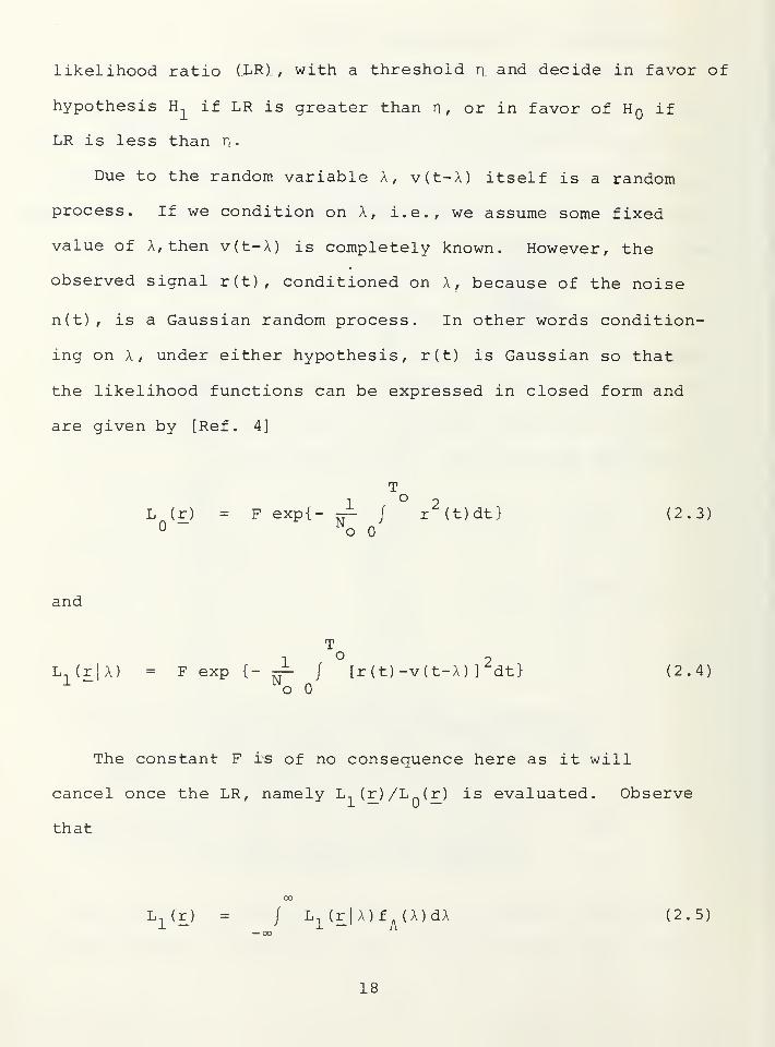
likelihood ratio (LRI, with a threshold n and decide in favor of
hypothesis E.^ if LR is greater than n , or in favor of Hq if
LR is less than ri
.
Due to the random variable A, v(t-A) itself is a random
process. If we condition on A, i.e., we assume some fixed
value of A, then v(t-A) is completely known. However, the
observed signal r(t), conditioned on A, because of the noise
n(t), is a Gaussian random process. In other words condition-
ing on A, under either hypothesis, r(t) is Gaussian so that
the likelihood functions can be expressed in closed form and
are given by [Ref. 4]
T
L (r) = F exp{- r.^ / r^(t)dt} (2.3)'^o
and
To
L^(r|A) = F exp {- ^ / [r ( t) -v ( t-A )
]
^dt
}
(2.4)o
The constant F is of no consequence here as it will
cancel once the LR, namely L, (£)/L„(r) is evaluated. Observe
that
L^(r) = / L^(r|A)f^(A)dA (2.5)
18

The likelihood ratio test is therefore
ETTrT < ^ '2-e>
«0
where
and
^ " p{H } C ^~C U.l)Fin^; ^01 ^11
P{H^} i = 1,0 (2.8)
are the prior probabilities of occurrence of hypotheses H.,
and
C. . i,j = 0,1 (2.9)13
are the costs associated with making decisions about hypotheses
H.. For a minimum probability of error receiver
(1 i 7^ J
C. = (2.10
i =j
Taking advantage of some simplifications in writing the LR, it
is simple to show that the LR becomes
19

TL, (r) °° ^ o1 = / ^^Plfr / r(t)v(t-A)dt}U ^—' -00 o
T ^1
exp{- ^ / V (t-A)dt}f^(A)dA ^ n (2.11)o „
Since v(t) is T-periodic, it can be expressed in terms of an
exponential Fourier series, namely
• 2iT, ,
:-m-ktv(t) = I v^ e " (2.12)
k=-°°
where
T/2 -j^ktV, = ^ / v(t) e dt for all k (2.13)^ ^ -T/2
Using the Fourier series expansion, we have
T 2tt T 2tto ^
c» <» -j£l(k+£)A o j4f(k+£)t/ v^(t-A)dt = I I VVe I ^ dt
k=-°° i=-oo ^ ^
(2.14)
However note that
T .2tt ,, „ , , r T if ii = -koo :— (k+£)t ) (
otherwise
/ e " dt = (2.15)
20
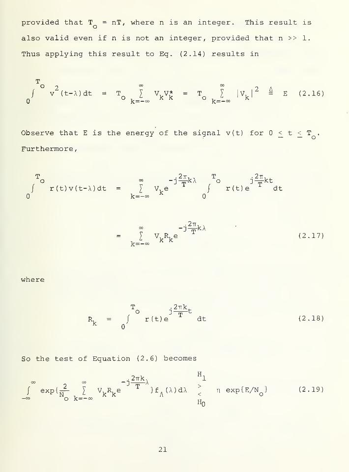
provided that T = nT, where n is an integer. This result is
also valid even if n is not an integer, provided that n >> 1.
Thus applying this result to Eq. (2.14) results in
T
/°v'(t-A)dt = T I Vj^V* = T I |VJ2A
^ ^2.16)k=-°o k=-°°
Observe that E is the energy of the signal v(t) for < t < T^ — — o
Furthermore,
T .27T, , T -Stt, ^
/ r(t)v(t-A)dt =I V,e / r(t)e " dt
k=-°° ^
• 27T, ,
-:-7TrkA
I Vj^Rj^e (2.17)
where
T .2Trk^o :i-T~^
R^ = / r(t)e dt (2.18)
So the test of Equation (2.6) becomes
.27Tk, ^1oo oo — "1 \
j exp{^ I Vj^R^e ^ }f^(A)dA ^ nexp{E/N^} (2.19-oo o k=-a)
^0
21

D. TWO TERM APPROXIMATION
In order to proceed with the analysis so as to derive a
signal processing algorithm from Equation (2.19), we will
assume that
. 2Trk,
r^ y V,R, e ^ << 1 (2.20)o k=-<»
In Appendix B, we will show under what conditions this
assumption is valid. It turns out that the assumption of
Equation (2.20) is essentially equivalent to an assumption of
low SNR, i.e., E/N << 1.o
Since
e^ - 1 + X if X << 1 (2.21)
provided Equation (2.20) is valid, it is possible to approxi-
mate the exponential term of Equation (2.19) by two terms only
so that the test can be written as
.27rk, "loo oo —
-J \
/ (1 + ^ I V,R,e "^ )f (X)dAI n exp{E/N } (2.22)
N ,^ k k ,-^v.w-» ^
o k=-°oHo.
or equivalently
.2Trk, 1 „
I V^R^ / e ^ f^(A)dXI
^[n exp{E/N^}-l] =n* (2.23k=— °o — oo
22
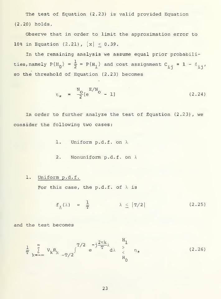
The test of Equation (2.23) is valid provided Equation
(2.2,0) holds.
Observe that in order to limit the approximation error to
10% in Equation (2.21), |xl < 0.39.
In the remaining analysis we assume equal prior probabili-
j
ties, namely P{H„} = y = P{H, } and cost assignment C. .= 1 - 6.
so the threshold of Equation (2.23) becomes
N E/N-y[e ° - 1] (2.24)
In order to further analyze the test of Equation (2.2 3) , we
consider the following two cases:
1. Uniform p.d.f. on X
2. Nonuniform p.d.f. on A
1. Uniform p.d.f.
For this case, the p.d.f. of A is
f^(A) = ^ A £ It/2| (2.25)
and the test becomes
1- T/2 -j^X "l
iI V,R, / e ^ dA : n.
,
(2.26,k=-°o -T/2
"o
23
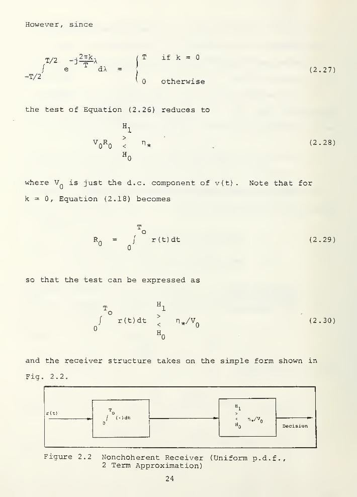
However, since
T/2 -j^AdA =
-T/2
T if k =
otherwise
(2.27)
the test of Equation (2.26) reduces to
^0^0 < ^
H
(2.28)
where V^ is just the d.c. component of v(t) . Note that for
k = 0, Equation (2.18) becomes
/ r(t)dt (2.29)
so that the test can be expressed as
T "l
/ r(t)dt ^ n*/V
H„
(2.30)
and the receiver structure takes on the simple form shown in
Fig. 2.2.
r(t)To
/ (•)dt
«1>
«0n./^o
Decision
Figure 2.2 Nonchoherent Receiver (Uniform p.d.f.,2 Terro Approximation)
24

It is clear from Equation (2.30) that this simple receiver
can only operate provided V^ 7^ 0. If Vq is indeed zero, some
other approach must be used for the purpose of deciding on
which hypothesis is true upon reception of r(t) . In the sequel
we discuss other detection approaches which will work even if
Vg = 0.
The performance of this receiver is evaluated as follows.
Let
To
£ = V / r(t) dt (2.31)" -':
Conditioning on X, we see that £ is a conditional Gaussian
random variable, where
E{£|Hq} = = m^ (2.32)
To
E{£|H,,A} = V^ / v(t-A)dt
.27Tk, T .27Tk.-D-Tp-A o :-^n-t
= V I V^ e / e dtk=-°o
= V^T = m, (2.33)o 1
Furthermore
25

Var{£|H^,A} = E{ [ (Jl|Hj_ , X ) - E{1\E^,\}]^}
T To o
^= E{[V / [v(t-A) +n(t) ]dt - V / v(t-A)dt]^}
^0 ^0
To O ^r^ 9
= V / / E{n(t)n(T) }dt dx = -^ v^ To ^ Q^ 2 o
Var{£|HQ} = a^ (2.34)
Equation (2.33) shows that the conditional mean m, is indepen-
dent of A and Equation (2.34) also shows that the conditional
variance of i is independent of A.
Hence
, -(£-m )^
f^{l\E^,X) = f^{a.\E,) = — exp{ ^} (2.35)
Also, from Equations (2.32) and (2.34)
"1 £2
f(i\E.) = —-— exp{ ^} (2.36)
The p.d.f.'s of Equations (2.35) and (2.36) are plotted in
Fig. 2.3.
26
P(i|H^)
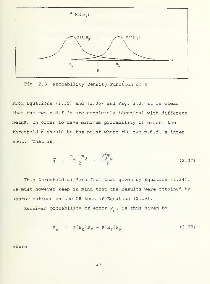
Fig. 2.3 Probability Density Function of £
From Equations (2.35) and (2.36) and Fig. 2.3, it is clear
that the two p.d.f.'s are completely identical with different
means. In order to have minimum probability of error, the
threshold n should be the point where the two p.d.f.'s inter-
sect. That is,
n =m^ +mQ
o(2.37;
This threshold differs from that given by Equation (2.24).
We must however keep in mind that the results were obtained by
approximations on the LR test of Equation (2.19).
Receiver probability of error P , is th\is given by
P = P{Hn}P^ + P{H, }P^e OF 1 M
(2.38)
where
27

P„ = Probability of false alarm;
P,, = Probability of miss; and
P{H.}, i = 0,1 are the prior probabilities.
Since we have assumed equal prior probabilities, P becomes
P^ = o" Js di + ^ e dl
2(n*-m, )/a
21 r 1 -^ /2^ ^1 r
-L^ 1 -y /2^
2" ie ^ dx + 2" J
e ^ ^ dyri*/Oj /2Tr -00 /27T
1 n* in*-my[erfc* (-— ) + erf* (
——^)
]
(2.39)
From Equations (2.24), (2.33) and (2.34), we get
Pe = i-fs'^f<^*[^7rr£r^l + erf,[^—^:£i- V-^H (2-40)
\/!!o!£ \/i!o!£V N V N
o o
Observe that if v(t) has a very strong d.c. component in
2comparison to its harmonics, then V T /N is approximately
equal to the SNR defined as E/N . Then Equation (2.40) becomes
a function of SNR only. Otherwise, it is a function of both
2the SNR and the V^T /N ratio.
o^ o
28
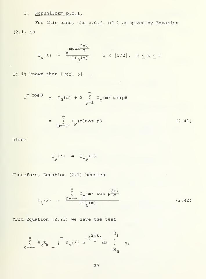
2. Nonuniform p.d.f.
For this case, the p.d.f. of A as given by Equation
(2.1) is
2-nXmoos-
^A*^' = ^TIp(I) ^ 1 1^/21, <_:a<_
It is known that [Ref. 5]
00
m cos 6 -r / \ , -^ V -r / \ .e = In(in) +2 ) I (m) cosp(u ^ , pp=l ^
P=-y I (m)cos pe (2.41)^ p^ —CO
since
I^(-) = I ^(Op -p
Therefore, Equation (2.1) becomes
00
r T- , , 2TrA2 Ip(i^) cos p^^
From Equation (2.23) we have the test
.2TTk, "l
I W ! fyv(A) e ^ dA ^ n*K= — 00 —CO
29
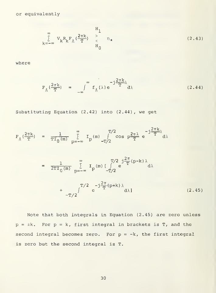
or equivalently
where
F (^) = / f (X)e ^ dA (2.44)
Substituting Equation (2.42) into (2.44), we get
o V 1°° T/2 o A -J^A
r. /27Tk> 1 V -r / ^ r^ 27tA -" T J,
1- T/2 j^(p-k)A
2TI (m) ^Ip^^) f / ^ ^^
T/2 -j^(p+k)A+ / e -^ dA] (2.45)
-T/2
Note that both integrals in Equation (2.45) are zero unless
p = ±k. For p = k, first integral in brackets is T, and the
second integral becomes zero. For p = -k, the first integral
is zero but the second integral is T.
30

Therefore
27rk> k^a'— ' = I^ ' <2-«)
since
i.^(-) = i^(-).
Hence the test of Equation (2.43) becomes
The test can be simplified further by letting
00
^ = iHHT, ^ Wk(^^^"" k=-
T T .2uk^T
O " O '^^JT-^-^{VqI (m) / r(t) + I V I (m) / r(t)e dt-^0^"^^ "
k=l ^ ^
' T .2TTk.
+ y V, I, (m) / r (t)e dt}-k=l ^ ^
To
= iTTsr'^oioC"' / ^'t)dt
T
+ 2 I |VJl (m) / r(t)cos(^t + a, )dt} (2.48)k=l ^ ^
31

where
±ja.
^±k = l^kl ^ (2.49)
Finally the test becomes
H.
V / '^ft*^^ ^ r^ J.l^l^k'"' „/r(t)cos(2ft+a^)dt
J
«0
(2.50)
and the receiver may be implemented as shown in Fig. 2.4.
r(t)
_On. To
/ ( • ) dt
V
y1
\,(r\
T
/ ( • ) dt .rr^cos (^t ..,)
V
1 \Igtm)
/ ( • ) dt r
COS(=|-t +0^1
V,
' I
<
•
•
•
Zlv^lljCm)Decision
Iglm)
Figure 2.4 Noncoherent Receiver (Nonuniform p.d.f.,2 Term Approximation)
32

Notice that this receiver can operate on signals both
with and without d.c. component. When a signal has zero d.c.
term, the receiver of Fig. 2.4 can be simplified by eliminating
the uppermost branch.
The performance of this receiver is obtained by using
the fact that conditioned on A, under either hypothesis, g
is a Gaussian random variable with
E{g|HQ} = (2.51)
and
T .2TTk.o D-;^t
E{g|H^,A} = E{^-^ I Vj^I^(m) / v(t-A)e ^ dt}k=-
k=-a' ^ = -00
(2.52)
The integral of Equation (2.52) has been analyzed in Equation
(2.15) . Therefore
^o " 2 ^~T~^ A
k=-
Furthermore
,
33
1
°° o J—^—
t
Var{g|H ,A} = E{ ( J ^ I (m) / [v ( t-A ) +n ( t) ] e '^' dt
T .27Tk^oo O 1 t
T 27Tk
T,00 00 o
~T^~ ^ ^ ^k^£^k^"'^^£^'^^ II E{n(t)n(T)}lQ(m) k=-oo l=-°o
.27Tk^ .27T£
• e e dt dT
TN - - "^o j^(k+il)t-# I I V,V T (m)T (m) / e ^ dt
W
Iq (m) k=-oo £=-oo
T N 00
2^ l\l ^k^"^^
2lQ(m) k=-oo ^ ^
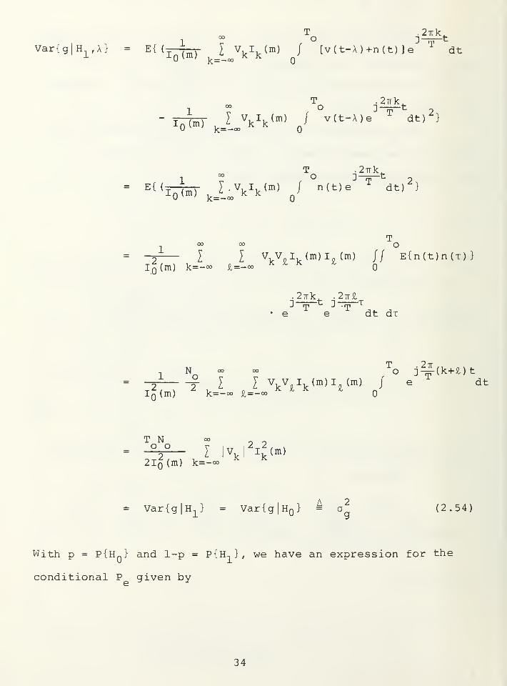
Var{g|H^} = VariglHg} = a^ (2.54)
ith p = P{Hj-,} and 1-p = P{H, } , we have an expression for the
conditional P given by
34
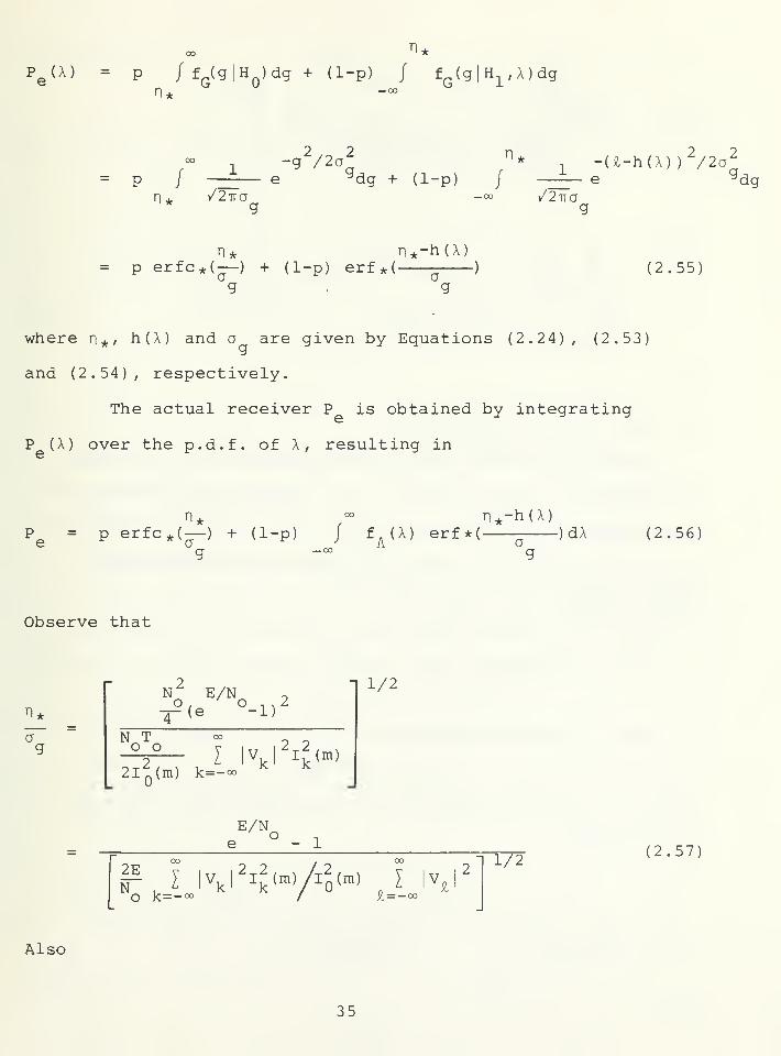
Pe(^) p /f^(g|H )dg+ (1-p) / f^(g|H^,A)dg
2 ,^ 2 1
<» , -g /2aP / -zz— e "^dg + (1-p) /
* g
2 .. 2^ -(£-h(A) )'-/2a
2710
'dg
n* n*-h(X)p erfc*(— ) + (1-p) erf*( )
g • g
(2.55)
where n*/ h(A) and a are given by Equations (2.24), (2.53)
and (2.54), respectively.
The actual receiver P is obtained by integrating
P (A) over the p.d.f. of A, resulting in
P = p erfc*(— ) + (1-p) / f (A) erf*(-n*-h(A)
-)dA (2.56)
Observe that
a
N E/N To ,-^ o , > 2
l-(e -1)
-I 1/2
N To o
2lQ(m) k=-<x>
' 'vj'i^m:
E/N- 1
2ENO K=
OO T -) / -)°°
I |vj2l2(ra)/4(m) J |v,
k.=-°° / £=-oo
1/2(2.57)
Also
35

h(A)lQ(m) k=-c» ^ ^
e'T
)
N To o
21^ (m) k=-oo''^1 |vJ^I^m)
1/2
.27Tk, /OO "1 ^ / CO
Pi |V,^l\(m)e ^ /lo(m) I jV, |
^
o k=-°° •£=-°°
2E 2,2r, I l\l ^k'^'Ao""' I V,
o k=-o° £= -00
1/2(2.58)
E. THREE TERM APPROXIMATION
Whenever Equation (2.20) is not satisfied to the degree
that Equation (2.21) is valid, it is possible to proceed with
the analysis beyond Equation (2.19), if in Equation (2.19) we
expand the exponential term and approximate it with three
terms. Since
exp{x} - 1 + X +X21
if X << 1 (2.59)
in order to have the approximation error not exceed 10%, we
must have x <_ 0.79. Using the three term approximation of
Equation (2.59) and applying it to Equation (2.19), the test
then becomes
.2Trk, .27rk, 1
~oo o k=-oo o k=-oo „"o
(2.60)
36
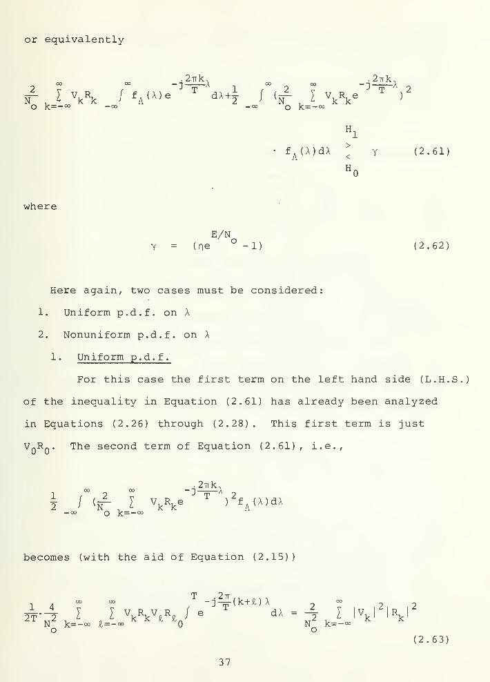
or equivalently
O K=— °o —00 —00 o k=— °o
«1
• f^(A)dAJ Y (2.61)
"0
where .
"
E/N7 = (Tie ° -1) (2.62)
Here again, two cases must be considered:
1. Uniform p.d.f. on A
2. Nonuniform p.d.f. on A
1. Uniform p.d.f.
For this case the first term on the left hand side (L.H.S.)
of the inequality in Equation (2.61) has already been analyzed
in Equations (2.26) through (2.28). This first term is just
V^R^. The second term of Equation (2.61), i.e..
.27Tk,00 00 —
"] \
-00 o k=— °°
becomes (with the aid of Equation (2.15))
14°°°°.
-D-j^(k+£)A p 0^ 2, ,2
2T-4 I I \\\\i - ^'^iJ i\i i\iN k=-<» £=-0° N k=-<»o o
(2.63)
37

The test therefore becomes
o Hq
or equivalently (using Equations (2.13) and (2.18))
T TVr. o V o ^— / r(t)dt + [/ / r(t)dt]^o o
00 V T 2
+ 2 [ l-^ , ° r(t)cos 2l!itdt)I Y* (2.65)
Hq
This test leads to the receiver structure shown in Fig. 2.5.
Note that this receiver utilizes both the d.c. and non-
d.c. components of the periodic signal. However, in practice
there are many cases where the d.c. component of the signal is zero
For those cases, the test reduces to
^ I K\'\\\' : Y* (2.66,
and the corresponding receiver can be implemented by simply
eliminating the upper most branch of the receiver in Fig. 2.5.
2 . Nonuniform p.d.f.
Our starting point here is Equation (2.11), repeated
here for convenience.
38

To
/ (•)dt C,^
C03
To
/ (.)dt (•)^
To thres-• hold for
acnparxscn
Fig. 2.5 Noncoherent Receiver (Uniform p.d.f.,3 Term Approximation)
39.

T T ^1
/ exp{j^ / r(t)v(t-A)dt}exp{- ^ / v^ (t-A ) dt }f ( A ) dA ^ n' o o „
where n is given by Equation (2,7). Note that the second
exponential of the inequality given by Equation (2.11) has
already been analyzed in Equations (2.14) through (2.16).
Furthermore, if we expand the first exponential in the above
inequality and approximate it with three terms as given by
Equation (2.59), then the test of Equation (2.11) becomes
T
/ ^ / r(t)v(t-A)dt f^(A)dA•00 GO
T 1o
+ y / [^ / r(t)v(t-A)dt]^f^(A)dAJ, y (2.67)
H,-00 O
0.
where y is given by Equation (2.62).
Interchanging the order of integration in Equation
(2.67), we obtain
T^ O 00
^ / r(t) / v(t-A)f,(A)dAdt^ o -00 ^^
T 1o °°
+ ^ // r(t)r(T) / v(t-A)v(T-A)f (A)dA dtdx ^ y (2.68)N^ -0° ^^
„o Hq
40

Note that v(t) is a deterministic signal but as mentioned
earlier, due to the r.v. A,
Ay(t) = v(t-A) (2.69)
itself is a random process with expected value
E{y(t)} = / v(t-A)f^(A)dA = m^Ct) (2.70)
and autocorrelation function
E{y(t)y(T)} = / v(t-A)v(T-A)f^(A)dA = RY(t,T) (2.71)
Substitution of Equations (2.70) and (2.71)
in Equation (2.68) leads to the following test that a receiver
has to perform
T T T ^1P
o ^ o or^ / r(t)m (t)dt + -^ / r(t)[/ r (x ) R (t
,
t ) ] dt ^ y (2.72)o ^ NO ^ „
«0
and the implementation of this receiver is shown in Fig. 2.6.
Here the autocorrelation function R (t,T) can be considered
as the impulse response of a filter that has to be designed
for detection of the signal.
Furthermore, for the uniform p.d.f. on A, the expected
value of y(t) given by Equation (2.70) becomes
41

r(t)
Q w-J '•'^'=
o
"Sr(t)
" +
0—
R^(t,T)
Decision
Fig. 2.6 Noncoherent Receiver (Nonuniform p.d.f.,3 Term Approximation)
TT/2
m^(t) = ^ / v(t-X)dX^ ^-T/2
CO j2^t T/2 -j2l]Sx
T k=_oo ^ -T/2dX
= V (2.73)
which is a constant, and the autocorrelation function of y(t)
given by Equation (2.71) turns out to be
42

3^T^t :^p-T T/2 -:]-^(k+£)Ae dA
1 J rp >- J m L
Ry^^.t) = ^ I I VV eT
^ T^^ " k=-oo £=-«> ^ -T/2
. 27Tk , , .
o :-Fn-(t-T)
I \\\ e (2.74)k=-oo
which is a function of (t-r) only. This implies that for the
uniform p.d.f. on A, the impulse response of the filter turns
out to be time invariant. That is, it depends only on the
time difference (t-i). Furthermore, m (t) being a constant
can be eliminated from the upper branch of the receiver shown
in Fig. 2.6.
F. ANALYSIS OF TWO SPECIFIC SIGNAL WAVESHAPES
It was pointed out earlier that the receiver derived using
a two term approximation on the exponential appearing in Equa-
tion (2.19), is unable to discriminate between the signal
present versus the signal absent case for signals having zero
d.c. component when the random time delay obeys a uniform
distribution. When the random time delay obeys a nonuniform
p.d.f., a receiver was derived (see Fig. 2.4) that could
detect the presence of signals having zero d.c. component.
In this section, assuming a nonuniform p.d.f. on A, the
receiver performance will be analyzed for two different signals
which are found quite often in practice and that have a zero
d.c. component. The two signals are
43

1. sine Wave
2
.
Square Wave
1. Sine Wave
For the first case let
v(t) = A cos ^t
o o (2.75)
_ A ^ T A "^ T- 2 e +2-6-
This periodic signal has only two discrete components.
In other words, it can be represented in terms of its two
Fourier coefficients, i.e..
I
I
I k = ±1
Vy. = i (2.76)
otherwise
Thus,
I IVj^l^ = (|)^ + (|)^ = ^ (2.77)k=-oo
and from Equations (2.57) and (2.58), we obtain
E/N^* (e °-l)
^a -^1^"^^ 1/2^ ^ , , (2E/N)-^^^
I (m) o'
(2.78)
44

n-hUi ^ ^ ^^ (2.79)
lQ(m) o
Thus the expression for P becomes
P^ = p erfc*, , , ^e ^\ I. (m)
, ,^/^o ,, 2E ^l(^) 2.A )
j^l-p^ T/2 I (ne -D-^^-^^^cos^ ^^^^2.^TI (m) / erf*/ .-^^ — U dA
-T/2 / -V-r (2E/N )
^^^Iq^"^) ' ^ o' I (2.80)
Computation of Equation (2.80) can be carried out as
a function of the SNR E/N , p and m. This has been carried out,
and the results are presented graphically in Chapter IV. For
the sake of computational simplicity, equal prior probabilities
were assumed, i.e.,
P = 1-P = T
resulting in n = 1
•
2 . Square Wave
For the second case, let v(t) be a periodic square
wave as shown in Fig. 2. 7.
45

' v(t)
• • # • • •
T7\
T
•-A
Fig. 2.7 Periodic Square Wave
The Fourier coefficients of v(t) are
V,, T/2 -j^liSt
Ae dt -
T/2'/ Ae ^ dt]
irk T• 1 • 1 sin —!r- 2.
2 ^^ ^ TTk ^(2.81)
Observe that V and all the even coefficients are zero, i.e.,o
V^, = for all k2k
(2.82)
and
V±k
. 2A^ kTT'
V±k
2AkTT'
V±k
(2A.2(2.83)
k odd
46

Note that
T/2 ~ 2
fv^(t)dt = A^T = T y lV,l (2.84)
-T/2 k=-oo ^
which implies that
I |Vj^|^ = A^ • (2.85)k=-oo
Furthermore
j;|V 1^1 (m) = |V ri (m) + 2 [ |V ^I (m) (2.86)
k=-oo ^ ^]^^-L
K K
so that
_.2Trk2. , .
^"1^^ ,„ ,2.
K=— CO
+ 27 IV, 1^1, (m) cos^A"
(2.87)k=l ^ ^ T
since
\l = |V_j^|; I^dn) = I_k(m;
47

Hence Equation (2.57) becomes
a
E/N(ne °-l)
(2.88)
and Equation (2.58) becomes
n*-h (A
)
N(ne -
4E/N2-nk.
l'-<V^'<JJVkl ik'"> =°-T^^'
—J IV^I Ij^(m)
o k=l2 2
Io(m)A^
(2.89)
Thus Equation (2.56) for the receiver probability of error
becomes
P = p erfc*e ^
E/N(ne -1)
4E/N^ I IVj^l^I^dn) 1/2k=l2 2
lQ(in)A^
N 4E/N2^k-
(ne -l)-( 2^ { I |Vj^| I^(m) cos-^i^-A)
+(l-p) / erflQ(m)A k=l
1/2
/
mcos-2ttA
TIq (m)dA (2.90)
48

Observe that Equation (2.90) (as well as Equations
(2.57) and (2.58)) involve summations whose index runs from
1 to infinity. In practice, it is not possible to compute
infinite sums. However, due to the fact that for all reason-
able signals v(t), the magnitude of the V, coefficients gets
smaller as k gets bigger, the infinite sum can be truncated
without introducing significant computational error. Further-
more, terms involving the magnitude squared of these coeffi-
cients will tend to decay more rapidly allowing early truncation
of the infinite sums.
G. DISCUSSION
In order to carry out the evaluation of Equation (2.90)
to a reasonable degree of accuracy, the mathematical expression
given by Equation (2.90) was evaluated by computer for fixed
SNR values. Computation of P was carried out for a fixed
value on the upper limit on the index k. Recomputation of
P was carried out everytime this upper summation limit was
incremented by 1. Recomputation of P was stopped after an
incrementation of the upper limit in the sum terms did not
yield an appreciably different value for P in comparison to
the P value before incrementation,e
The result of these evaluations has been presented in
Chapter IV in the form of tables and graphs while P has been
plotted as a function of SNR for different values of the
parameter m. Recall that m specifies our relative prior
knowledge about the signal's random time delay.
49
III. ALTERNATIVE SUBOPTIMUM RECEIVERS
In the previous chapter, optimum detectors based on
likelihood ratio tests were derived under conditions that are
equivalent to low SNR conditions for signals having random
time delay in the presence of additive white Gaussian noise.
The tests derived gave rise to different receiver structures
which, whenever possible, were analyzed in terms of their
error probability performance. Both the receiver structures
and their performance were seen to be a function of the uncer-
tainty in the signal time delay or more precisely, a function
of the p.d.f. of the signal time delay A.
In this chapter, two suboptimum receivers are analyzed.
The approach used here is different in the sense that re-
ceivers are derived via strictly heuristic means and their
performances are then analyzed. These receivers are:
A. N-correlator Receiver
B. Estimator-correlator Receiver
A. N-CORRELATOR RECEIVER
This receiver is shown in Fig. 3.1. The idea is to corre-
late the received signal r(t) with N delayed reference signals
generated at the receiver. If a signal is present, presumably
at least one correlator branch would produce a large output so
that the sum I could be guaranteed to be much larger under
50

/ (Mdt
Fig. 3.1. N-Correlator Receiver
these conditions than when the correlators are fed by low
level noise only. Thus, if £ is greater than a prescribed
threshold, then the presence of a signal with a random time
delay is declared; otherwise only the presence of noise is
declared. Here we assiome for convenience that the observation
time T is an integral multiple of T, the period of the
signal v(t). Observe furthermore that we are not required to
assume low SNR conditions as done in Chapter II.
In order to analyze this receiver in more detail, observe
that
51
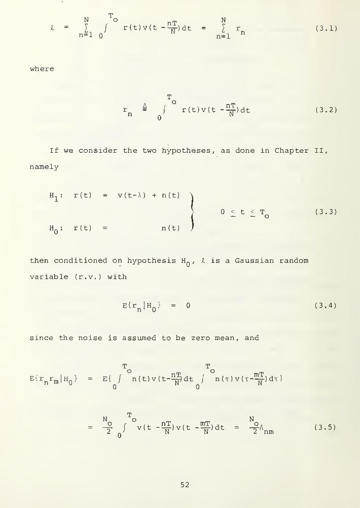
N ^O N1=11 r(t)v(t-^)dt = I r (3.1)n=l n=l ^
where
TO rn
r = / r(t)v(t -^)dt (3.2)n Q L\
If we consider the two hypotheses, as done in Chapter II,
namely
H : r(t) = v(t-A) + n(t)
Hq: r(t) = n(t)
< t < T (3.3)— — o
then conditioned on hypothesis H^ , £ is a Gaussian random
variable (r.v.) with
E{r^|HQ} = (3.4)
since the noise is assumed to be zero mean, and
T T
E{r r^|H } = E{ / n(t)v(t-^dt / n(T)v(T~)dT}
TN o ^ „ No
r/+-nT>,, mT>,. o. /ocx
-2 J^(t -—)v(t -—)dt = -^A^^ (3.5)
52

where
A„„ ^ /°v<t-!f,v(t-I^,dt ',3.6,
are the signal discrete cross correlation terms. Thus,
NE{£|Hq} =
I E{rj^|HQ} = (3.7;n=l
and
yN N
E{£'^|h„} = E{ I I r r^|H_}„ 1 ^ii n m'n=l m=l
N N N A o
^ I I A ^ a; (3.8)n=l m=l
Now conditioned on both H, and A , £ is also a Gaussian
r.v. with
T
E{r lH,,A} = / v(t-A)v(t -^)dt = a^(A) (3.9)n ' 1 p.
^ N n
and
53
N^^ f^'n -E{r^|H^,X}] [r^ -E{r^|H^,A}] |h^,A} = -f A^ (3.10)
so that
NE{£|h^,A} =
I a^(A) (3.11)n=l
and
E{ [£-E{£|Hj_,A}]^|h^,A}
T TNo o N ^
= E{[ I { I v(t-A)v(t~)dt + / n(t)v(t-^)dt) -5; a^(A)]'^}
n=l ^0 n=l
T
= E{[ I j n(t)v(t -^)dt]^}n=l
N N N ^
-T I I ^ = ^0 (3.12)2 ^
T^
,
nm £n=l in=l
Thus the conditional p.d.f.'s of Z are
2 2
f^(£|HQ) = ^: e^ (3.13)
v27Ta „
and
54
N 9-(£ - l^o.^{\))'-/2ol
f^(£|H^,A) =-^
e ^ ^ (3.14)
-fl^
with
f^(£|H^) = / f (il|H^,A)f^(A)dA (3.15)"L
The detector of Fig. 3.1 performs the test
< "^ (3.16)
«0
SO that its error probability, P is given by
P^ = P{Hq} / p^(£|HQ)d£ + P{H^} / p^(£|H^)d£ (3.17)Y — oo
Let p = P(H } and 1-p = P{H, } so that using equations
(3.13) and (3.15), equation (3.17) becomes '
N2
-(£- y a (X) ) ,
n=l ^
r 1 -^^/2^£,, , rT r 1
^^^Pg = P J -ZZ—^ d£+(l-p) j[ J
e
Y /27Ta„ -0° -°° /27Ta
• f^(A)dX]d£ (3.11
55

Interchanging the order of integration in the second
(double) integral of equation (3.18), we obtain
/ f.(^)
N-il- I a^(A))
n=l
2a?
/ fA(^)
• N
n=l
di dX
1 -x^/2 ^e ^ dx/2 7T
dA
Nfy- I a^(A)
/ f.(A) erf:n=l
n
AdA (3.19)
Thus, the receiver probability of error becomes
N
h- I a^(A)
P = p erfc*(-^) + (1-p) / f (A)erf.n=l
ndA (3.20)
The threshold y can be optimized to minimize P . Such an
approach unfortunately leads to a complicated integral equation
that is not easily solvable. in practice however, P can bee
calculated on the computer for y = , and then incrementing
|y| until an optimum value of y is found for a given SNR.
It must be pointed out that the receiver of Fig. 3.1 will
not always yield desirable results. For example, if v(t) is
56

sinusoidal, in the absence of noise, i - which means
that with noise present, the receiver is unable to detect
the presence of the signal. Fortunately for v(t) sinusoidal,
a better receiver is available and its performance is well
known [Ref . 4 J .
1. Special Case of Triangular Wave
Consider now a periodic waveform of triangular pulses
and its two arbitrarily delayed versions as shown in Fig.
3.2. If we represent one triangular pulse by p(t),then we
can express v(t) as
Mv(t) = I p(t-jT) (3.2i;
j =
In order to find the cross correlation terms Anm
required for the computation of P [eauation (3.19)],e
instead of taking all the pulses in equation (3.21) , we
simply consider the cross correlation of a single pulse of
period T with a delayed version of itself and then multiply
the result by the total number of pulses M within the interval
T , since v(t) is assumed to be periodic with MT = T .
In order to make computation simpler, Fig. 3.3 shows p(t)
,
p(t-a) and p(t-3) , where a < 6 has been assumed.
57

v(t)
T, ^
2T-//-
_(iW.U KT
*v(t-a)
-//- -*• ta T+a 2T+a (M-plLT+a MT
AV(t-0)
T+B
• •
-y/- A(M-2)T+6 -^
Fig. 3.2 Periodic Triangular Wave and Two of ItsDelayed Versions
58

p(tl
AT
At
-*• t
Ap(t-a)
AT
A(T-a)At+A(T-a)
A(t-a)
a
AT
ACT-91
v(t-6)
At+A{T-6)
A{t-6)
S T
Fig. 3.3 One Period Restricted Triangular Wave andTwo of Its Delayed Versions
59

Observe that for a < 3
/ v(t-a)v(t-3)dt = M / p[t+(T-a) ]p[t+(T-6) ]dt
3 T+ / p(t-a)p[t+(T-3) ]dt + / p(t-a)p(t-3)dt
a 3
= Ma
j [At+A(T-a) ] [At+A(T-3) ]dt
+ / A(t-a) [At+A(T-3) ]dt + / A ( t-a) A ( t-3 ) dta 3
= „A2,a!T ^ori. „gT ^ efr . sri ^ i^,
(3.22)
nT , „ mTFor a = -rr- and 3 = -rrN N , equation (3.22) becomes
2n22N ^2 2n2
2N 3= Anm (3.23)
provided n < m. For n = m or equivalently a = 3/ the quantity
inside the parenthesis in equation (3.23) becomes t^-.
Similarly for a > 3, equation (3.22) becomes
o
/ v(t-a) v(t-3)dt = MA2(4^-^-a3T+4^+eT!.^) (3.24)
60
nT mTLetting a = — and 3 = -j^ m equation (3.24) , we obtain
. 23, n n nm ,m,m,l. /-,->i-\A^^ = MA T o ~tTT T + T +tTT +T 3.25nm _^-2 2N .^2 „-^2 2N 32N N 2N
provided n > m. Here again for n = m, the quantity inside
the parenthesis in equation (3.24) becomes ^.
To proceed further with the analysis, the double
summation of equation (3.8) is broken into three summations
to account for n < m, n = m and n > m. Thus
N N N N-1 N N N-1I 1 ^
rr.= I lA+yA + y yA (3.26)
^ , ^T
nm ^,
, '^ , nm ^ , nn ^ ^ ^ ^ nmn=l m=l m=n+l n=l n=l n=m+l m=l
Observe that the L.H.S. of equation (3.26) represents
the sum of the elements of an N xn matrix. Whereas the middle
term on the R.H.S. of this equation denotes the sum of the
diagonal elements of the N xn matrix, the first term is the
sum of all the elements in the upper triangular part and the
third term is the sum of all the elements in the lower triangu-
lar part of the N xn matrix.
In order to evaluate the first term on the R.H.S. of
equation (3.26), use of equation (3.23) (n < m case) yields
61

N-1 N
I I An=l m=n+l
2„3N-1 N
nmn=l m=n+l 2N ^^ N 2N
n_ _n_ _ nm m _ m 1
2 2N .,2 ^,2 2N 3+ ^}
2 3MA T-^
^ N-1 N2 1 N-1 N
2N^ n=l m=n+l ^^ n=l m=n+l
N-1 N N-1 N
T I .1 ^^ + 7 I I~2"
N n=l m=n+lm
2N n=l m=n+l
, N-1 N , N-1 N
2Nn=l n=n+l n=l m=n+l
MAV [lM-^4f±l] (3.27)
The second term on the R.H.S. of equation (3.26)
becomes
N
I An=l
nn2 3^1
MA^T^ I In=lMA^T^ [|] (3.28)
since A = rr- for n = m.mn 3
Finally, substitution of equation (3.25) (n > m case)
in the third term on the R.H.S. of equation (3.26) yields
N N-1
I I An=m+l m=l nm
2 2
= MA^T^ [3iL^4f^] (3.29)
62
Adding the results of equations (3.27), (3.28) and
(3.29) yields
^ N 2
I I '^nn,= MAVl3»4±i] (3.30,
n=l m=l
Thus from equations (3.8) and (3.30), the conditional
variance of I becomes
2 n=l m=l ^"^ 2 12
= ^E(l^L^) (3.31)
since
To T T
/ v2(t)dt = M / v2(t)dt = M / (At)2dt
2 3MA T A^-i^V— = E (3.32)
is the energy of v(t) for £ t £ T .
In order to compute the probability of error P , weN
^
need to evaluate ^ a (A) given by equations (3.9) and (3.11n=l
as
TN No
nT,I aiX) = I j v(t-A)v(t -i^)dt (3.33)
n=l ^ n=l^^
63

nTA Fourier series expansion of v(t-A) and v(t --rr)
yields
N N ^ ^-j^kA -j2TT^ ^o j^(k+£)t
I %(A) =111 V^V^e ^ e ^ / e ^ dtn=l n=l k=-oo i=-<=o
Tq I \\\ ^ I e"^
(3.34)k=-o° n=l
Observe that for k = ±iN, where i is an integer, the
second summation involving the index n yields N, otherwise it
yields zero.
Thus, equation (3.33) can be written as
N / . -1 -:4^kNA
kN'
^/ 2 -^
n=l \ k=-oo
9 -j-^kNA
9 9 9= VdV^r + 2 I IV^^I^ cos ^kNA) (3.35)
K.— J-
since
k ' ' -k I
64

nT rnTIn equation (3.6), if we represent v(t ——) and v(t ——in terms of Fourier series, then
N N
I I An=l m=l nm
N N 00 CO
I I 1 I V^V„e ' ^'
,27Tkn .2TT£m
n=l m=l k=-<» £=-o° k rN "^o j^(k+£)t
/ e ^ dt
= T [ |V, I"- I eo 1
^ ' k ' ^,k=-°° n=l
2 N ]n(—^^) N Dm(-^^)N
m=l
N
o ,
I Iv,
k=-'
sin (kir)
sin(—
)
1 2
(3.36)
since
N
n=l
jne ^ sin(N6/2) j(N+l)e/2sin(e/2) ® (3.37)
Observe that the R.H.S. of equation (3.36) is always zero
except for k = ±iN where i is an integer. Also observe that
for k = ±iN, the R.H.S. of equation (3.36) becomes an indeter-
minate form. Due to that reason, differentiating sin (kir) and
sin(-j--) w.r.t. k and then taking the limit k ^ iN, equation
(3.36) becomes
N N
I 1 A
n=l m=lnm T N^ J |V '^
k=-<kN
= Ty(v2 + 2 IIV^^!^)k=l
(3.38)
65

so that equation (3.8) can be written as
k=l
Equations (3.35) and (3.39) are of general form and can
be applied to any signal, not just a triangular waveform.
The Fourier coefficients V, of the periodic triangular
wave are
f K.O. (
I MI^ 27Tk
V^ = / (3.40)
/ -; 7\rp
Otherwise
and
2 2
AT—^
—
y otherwise47T k
so that the use of equations (3.31) and (3.35) yields
_X = 1 = I (3.42)
^i rM Tr/3N^ +1> //^rE ,3N^ +1,t1/2o
where y* = y/N
66

N
nil ^11^
8-)
o 3N +1
2 2
N(^-^ +2
27T^2^2 cos k-^ NA
-^ 2 2k=l 47T N
2 2AT+ 2 I
2 2AT2 2 2
k=l 47T k N
o 3N +1 1 + i/3rr(3.43)
since
Ik=l
£2£_M = ll_-l.e+Q^ oie<.2Tr (3.44)
and
NY -
I a^(A)n=l X
r E,3N +1 , .,1/2
L N ^ 8 '^
o
o 3N +1
1 + 1/3N^(3.45
Finally, the expression for P , after substituting equations
(2.1), (3.42) and (3.44) in equation (3.20), becomes
67

= p erfc* Y-2 1+ (1-P) i
E (3N +1)t1/2/ -T/2
2TrA
T/2 ^"^ c°s^r-
N 8-]
Tl^dn)
erf* Y
rE_ (3N +1) .1/2
^N 8^
o
/^^<8
-)
o 3N +1
3N^+6N [|-A + (^)2]
(3N +1)
dA (3.46)
As mentioned earlier, the receiver of Fig. 3.1 has
been designed via ad-hoc methods, so that the optimum threshold
setting is not readily obtainable. The difficulty in applying
an analytical approach to the problem of finding the optimumdp
threshold arises in the solution ofdy
= for Y . Since
N
-(Y- I a^(A)
)
'^ , nn=l
dpe
dY= -P
2 21 -^ /2a^-— e ^ +
/2TTa£
(1-p) / f^(A) -^—^-T/2 '^2^^£
dA
(3.47)
dPthen, solution of
dY= is equivalent to solving
N N
-T/2
T/2
Y I a^(A) [ I a^(A)]^
T n inn=l n=l2 „ 2
o „ 2a „
dA =(1-p)
(3.48)
68

clearly, the computer could be used to search for a value of
Y that satisfies the equality prescribed in equation (3.48).
The approach that has been used in trying to obtain
the optimum threshold involves using the computer to evaluate
equation (3.46) as a function of y fo^ fixed SNR. Thus the
value of Y for which P is minimum yields the optimum thres-
hold for that particular value of SNR. This procedure is
repeated for different values of SNR. The resulting values
are then used to plot P vs. SNR. These curves have been'^ e
plotted using optimum threshold settings and the results have
been summarized and discussed in Chapter IV. (Observe that
the threshold y is SNR dependent. This situation is typical
of noncoherent signal detection problems.) .
B. ESTIMATOR-CORRELATOR RECEIVER
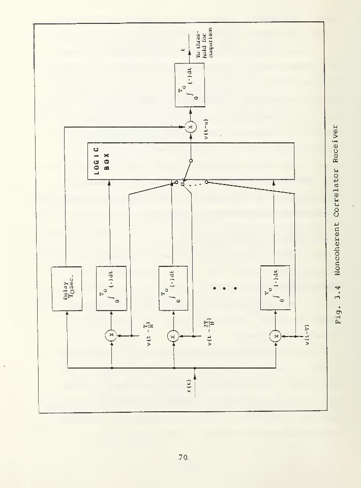
The second suboptimum receiver being proposed is the re-
ceiver structure shown in Fig. 3.4. it is basically an
estimator-correlator receiver in which first a coarse estimate
of the time delay in v(t) is made and then this information
is used to process the delayed signal r(t) coherently with
an estimated reference.
In this receiver the largest output of the N correlator
branches is used as an estimate of the signal phase by the
logic choice. This estimate is used to provide an accurate
local reference with which to perform the correlation detection
operation. The output I of the main correlator is used for
threshold comparison in order to make the decisions.
69
tn u Hi
Qi O ->
g23
o— X(9 OO flD
u
4J
-a
EilZI
U
>
'l
* *— JJ
S-l
>-HQ)
O
«
O-P(TJ
fHCU
5-1
i-l
OU4-1
a
u
ouco2
CO
•HCm
70.

Thus
To
i = j r(t)v(t-a)dt (3.49)
T 2T 3Twhere a = — , -r;-, -rr-r . . . / T and a may take on only one such
value for < t < T . In order to determine receiver perfor-— — o ^
mance , we note that £ is a conditionally Gaussian random
variable with
E{il|H } = (3.50)
To
Var{£|H } = E{ [ / n(t)v(t-a)dt] }"
T
-J- j V (t-a)dt
N^ «, a, -j^{]^+i)a '^o j2Z(k+£)t
^ k=-°° £=-«= ^
N T oo NA o^- Z IVj^l = -2- E = a^ (3.51)
k=-°°
where V are the exponential Fourier series coefficients of
v(t) , and E is the energy of v(t) for < t < T.
71

Also
E{£|H ,A} = / v(t-X)v(t-a)dt
00 CX3
I 1 V,V p .
j e ' dtk=-oo £=-< k £
o -:-=-k(A-a)
o , ^ ' k'k=-<»
Tq[|Vq|^ + 2 [ IVj^l^ cos^k(X-a)]X.— X
= m(X)
(3.52)
It can be shown without a great deal of difficulty that
Var{£|H^,A} = o^ (3.53)
Therefore the conditional p.d.f.'s of i are given by
fL<*l«0'
2 2
e/2Tra
I
(3.54)
f^(£|H^,A) = ^-[£-m(A)]^/2a^
2TTa£
(3.55)
72

so that
f^{Z\E^) =-[£-m(A)]^/2a?
f^(A)dA (3.56)
Thus the expression for P is given by
P^ = P{£ >y|Hq}P{Hq} + P{£ <y|H^}P{H^}
2 .^ 2
= P /
^ -I /2a
Y /27Ta'd£ + (1-p) / /
y - ^ -(A-m(A) )^/2a^
£oo — oo /2Tra,
X f^(A)dAd£ (3.57)
where
P = P{Hq} and (1-p) = P{Hj_}
as before.
After a change of variables, equation (3.57) can be
written as
P^ = P
2 00 [Y-m(A)]/a^
/ ^e-/2.(l-p) / /^ ^-^/^
l/O^ /27T — oo — oo '27T
e ' dxf^(A)dA
= p erfc*(-^) + (1-p) / f (A) erf*(l-^-^^)dA (3.58)
73
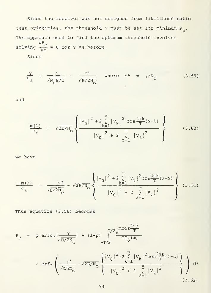
since the receiver was not designed from likelihood ratio
test principles, the threshold y must be set for minimum P .
The approach used to find the optimum threshold involvesdP
solving —5— = for y as before.
Since
Y _ Y _ Y* where y* = y/N (3.59)^£ /N E/2 /E/2N •
°o ' ^ o
and
"^-^^ = /2E/N } ^^ \ (3.60)On O
VqI^ + 2 I |V 1^
^ £ = 1 ^
we have
i::H11A)_ = y*
, /2e7n- <!^^
VqI +2 1 \V^\ cos-^(A-a)
^i /E/2N^ ° I iw |2, o y l„ |2
£=1^ol " 2 J l^£
Thus equation (3.56) becomes
27tXmcos-
T/2 TP = p erfc*(-^=L_) + (i-p) /
^
/E/2N^_T/2
0^^
( 3 . 51
)
2 ^ r I rr I
2 2TTk , , ,
V, cos -, (A -a)
X erf. (—i^-/2E7fr .' ^J:j^ ; 1 dA
(3.62)
74

As before, determination of the optimum threshold by solutiondp
eof —5— = involves solving an equation of a form similar to
that of equation (3.47).
In general, solutions in closed form do not appear tracta-
ble. A search for an optimum y may be performed or solutions
for specific cases may be possible. This is illustrated by
considering two special cases in which v(t) is a
1. sine wave
2. square wave.
1 . Sine Wave
As a first special case, let
v(t) = A cos ^t
27T .271
A ^ T,A "^ T ,-, ^^^= J e '^ J ^ ., (3.63)
so that
itk = 1
V, = (3.64)k
I
otherwise
and
k=l
2 2, ? A A
V, ^ = 2 ^ = ^V (3.65)k
'
4 2
75

Thus equation (3.60) becomes
m(A)-^ cos-=r{X-a)
- ^2E/N -^ ^° A^/2
2i\= /2E/N^ cos ^(A-a) (3.6.6)
and for p = (1-p) = ^, equation (3.58) becomes
/ T/2 27TA
1 Y* 1 .mcos-^f-
P =I erfc* (-3::^) + ^Tj-T^ / e
^ )X erf*( ^ /2E/N cos4J(A-a) )dA (3.67)
As mentioned earlier in Chapter II, m = corresponds
to a uniform p.d.f. on A, i.e. p(A) = =-, so that the error
probability expression for m = becomes
P^ = y erfc*( ^^^) +^ / erf*( '^~ /2E/N^ cos 4^( A-a) ) dA(
(3.6 8)
2 . Square VJave
Consider now the second special case in which v(t)
is a periodic square wave as shown in Fig. 2.6. In Chapter II
we showed that
(i— ) for k = oddT I KIT
for k = even
76

so that equation (3.59) becomes
"J
m(X)
^ COS KZTT {
IT ^
°H
£=1 £^
= /2E/N
^2 ,1 A-otx ^ / A-otx 2 .
TT /6
A-a>, ^ , A-a, 2,
= /2E/N^(1 - 6(^) + 6(^)") (3.69)
Therefore
27tA
1 ( Y* 1 T/2mcos-^
P = 4 erfc*( ^) + ^ -; . f e
'I
/E72F- ^0("^)T_^/2
)erf*(—:I^ - /2e7n-(1 - 6(AZ£) + 6(A^)2)d£( ^
^ * ^° ^
/E/2Nu T T j
Observe that equations (3.35) and (3.62) involve
suiranations whose indices run from 1 to infinity. In practice,
it is not possible to compute infinite sums. However, due to
the fact that for all reasonable signals v(t), the magnitude
of the V, coefficients gets smaller as k gets bigger, this
infinite sum can be truncated without introducing significant
computational error.
Fortunately for triangular and square wave signals
considered as special cases in this chapter, the argument of
77

summation in equations (3.35) and (3.61) turned out to be of
such a form that it could be expressed in closed form.
For the sine wave, summation disappeared due to the fact
that its coefficients V, exist only for k = ±1. These results
in the form of graphs are presented and discussed in Chapter
IV.
78
IV. DISCUSSION OF GRAPHICAL RESULTS
This chapter presents graphical results obtained by
applying the analytical results of the previous chapters to
specific examples and carrying out the required computations
on the computer. The plots are intended to display receiver
performance in terms of probability of error (P ) as a function
of SNR. Some curves of P versus comparator threshold level
have also been included in order to show the dependency of P^
on the threshold which in turn depends on SNR. The graphical
results displaying performance of the optimum receivers are
presented first, followed by graphical results displaying
performance of the suboptimum receivers analyzed.
A. GRAPHICAL RESULTS FOR OPTIMUM RECEIVERS
1. Receivers Operating on Signals with Nonzero DCComponent (Uniform p.d.f. on A)
In Chapter II, using statistical communication theoretic
principles, a simple integrator receiver (Fig. 2.2) was derived
that could discriminate between signal plus noise and noise
only hypotheses provided the signal had a non-zero DC component.
Recall that the receiver derivation and the subsequent per-
formance evaluation carried out was made possible by the
two-term approximation on the exponential appearing in Equation
(2.19). Equivalently, low SNR conditions were assumed so that
the P results are only valid for low SNR's.e
79
PERFORMANCE (UTORM PDF)
^ TWO TERM APPROXIMATION»^
J
oflb§2-
%.-10.0 -«UI -«J> -7.0 -4.0 -«^
SNR(DB)
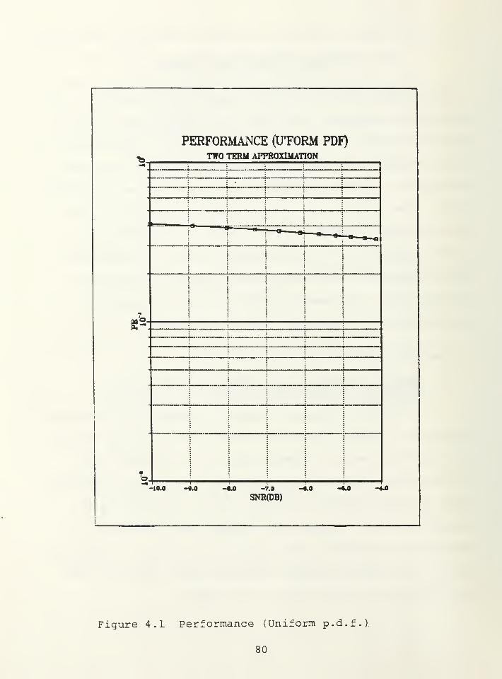
Figure 4.1 Performance (Uniform p.d.f.I
80

Figure 4.1 shows the performance of this receiver as
a function of SNR. This graph was obtained through numerical
evaluation of Equation (2.40) under the assumption that v(t)
has a strong DC component in comparison to its harmonics,
equal prior probabilities, and uniform p.d.f. on the r.v. X. Due
to the constraint imposed by Equation (2.20), Equation (2.40)
is valid up to an SNR of about -4.1 dB . Thus Fig. 4.1 is • -/- ;.
plotted only up to the SNR of -4.1 dB.. •''
Observe that P is at a very high level of about 0.3.
However, it decreases as SNR increases, as expected. While
it is clear that no receiver could operate with an error
probability of 0.3, the figure does give an indication of the
performance level that can be expected at low SNR's. For ''
'
high SNR's, it is expected that P will continue to decrease
to reasonable levels. However, for high SNR's, the receiver
of Fig. 2.2 is no longer optimum. .'
2 . Receiver Operating on Arbitrary Signals (Nonuniformp.d.f. on A)
The two-term approximation on the exponential appearing
in Equation (2.19) and application of the nonuniform p.d.f. on
X given by Equation (2.1) resulted in the receiver of Fig. 2.4
that could operate on signals having either zero or non-zero
DC component. Observe that as m ^ , the receiver of Fig.
2.4 becomes equal to the receiver of Fig. 2.2. Two specific
signals, a sine wave and square wave, both having zero DC
component, were analyzed.
81

Figure 4.2, obtained through numerical evaluation
of Equation (2.80), shows the performance of this receiver
as a function of SNR when v(t) is a sine wave. Three differ-
ent values of the independent parameter m were considered.
Recall that m controls the level of uncertainty about the time
delay A. As expected, as m increases, P decreases for a
given SNR. For example, ai SNR of -5.2 dB is required in
order to achieve aP of 0.4 at m= 2. With m = 90, we neede
an SNR of -9 dB to achieve the same Pg. Note that the m =
case has not been considered here due to the fact that m =
corresponds to a uniform p.d.f. on A. The receiver for that
case (Fig. 2.4) is unable to detect signals having zero DC
component, resulting in P equal to 0.5.
Curves shown in Fig. 4.3 are the result of numerical
evaluation of Equation (2.90) in which three different values
of the independent parameter m have been considered. The
m = case has not been considered here either due to the
same reasons presented for the sine wave case.
Observe that Equation (2.90) involves the computation
of infinite sums which can not be carried out in practice.
However, due to the fact that for all finite power signals
v(t) , the magnitude of the V, coefficients gets smaller as k
gets bigger and thus, truncation is possible. Inclusion of
more coefficients in Equation (2.90) corresponds to increased
accuracy in the results. Furthermore, P changes as k is
incremented, however up to a point only as further increase in
82

PERFORMANCE (SINE WAVE)
^ ( NONUNIFORM PDF )•i*
: i . : 1
: i i i :
ii
ii
1
|- ; ; : i !
*"1—*=T=='====r^=^|
m'O.£-^
LEGENDM=2h =5
r^ V F^O'o.
-10^
SNR(DB)
Figure 4.2 Performance (Sine Wave)
83

PERFORMANCE (SQUARE PUI^)Ts ( NONUNIFORM PDF )
WW
' ,' 1, .; _ ...
cab
i i 1i
i
S-^.
i : ! ; •
b.
LEGENDa M=:2
4 M=90
-iO,A -fl^ -7.« -«.4
SNR(DB)-«a -<a -<4
Figure 4.3 Performance (Square Wavel
84

k beyond this limit do not result in an appreciable change
in P . This phenomenon is illustrated in Table I.
TABLE I
PRQ8A8ILITY OF ERROR VS tf OF COFFICIENTS SUMMED
( SNR = -10 OB)
ff OF COFFICIENTS PROBABILITY OFSUMMED ERROR
1 0.A451 2*3TD+0a2 0.4*AJ39A7D+003 .4*-*32559D*-00<^ 0.44432543D>005 0.444325420<-006 0. 4A432 542 D<- 00r 0.44432542D>00a 0,444325420>009 0.44432542O*-00
10 0,444325420+00
We see that P keeps on decreasing until the number of
coefficients summed is 5. For k > 5, P remains unchanged.
Thus, for this example the computation of Equation (2.90) was
carried out with sums truncated to 5 terms. The performance
curves for the square wave signal are shown in Fig. 4.3
for low SNR conditions. With m = 2, ai SNR of -4.1 dB is
required in order to achieve a P of 0.4 while for the same
P , with m = 90, the SNR required is -8.8 dB
.
B. GRAPHICAL RESULTS FOR SUBOPTIMUM RECEIVERS
In Chapter III, two suboptimum receivers were analyzed.
The design approach used in that chapter was different in the
sense that receivers were derived via strictly heuristic
85

means. Therefore, the optimum threshold setting for the
receiver was not readily obtainable. However, a computational
approach was used to solve the problem of properly setting
the threshold prior to evaluating P as a function of SNR.e
1 . N-Correlator Receiver
The first suboptimum receiver analyzed in Chapter III
was the N-Correlator receiver of Fig. 3.1, and its performance
with v(t) a periodic triangular pulse was evaluated. The
graphical results corresponding to the numerical evaluation
of Equation (3.46) are shown in Figs. 4.4 through 4.12. As
mentioned earlier, using the computer. Equation (3.46) has
been evaluated as a function of the threshold y for fixed SNR
values starting at -10 dB and increasing in increments of 5
dB . For a given SNR, the threshold value for which P is^ e
minimum corresponds to the optimum threshold for that particu-
lar SNR. . These minimum points corresponding to each SNR have
been used as optimum threshold values in Equation (3.46) and
the resulting P has been plotted in Fig. 4 . 12 as P vs SNR.
Observe that Equation (3.46) involves the previously
encountered parameter m and N, namely the number of correlators
used by the receiver. Two different values of each parameter
m = 0, 90 and N = 2, 16 have been used in the computations
in order to evaluate their effect on receiver performance. An
inspection of Fig. 4.4 (m = , N = 16) and Fig. 4.6 (m = 30,
N = 16) reveal that for a given N, m has no significant effect
on P . On the other hand Fig. 4.4 (m = , N = 16) and Fig.
4.8 (m = 0, N = 2) reveal a small effect of N on P for a' e

given value of m. The actual effect of N on P is shown ine
Fig. 4.12 where P has been plotted as a function of SNR fore ^
two values of N. Observe that the higher value of N yields
better performance. To achieve a P of 10~ with N = 2, the
SNR required is ~ 13.5 dB whereas for the same P with N = 16e
we need an SNR ~ 13.2 dB . This result is once again expected
as using few correlators might result in a small output on
the correlator branches when v(t) received in r(t) has a
delay very much different than the locally generated v(t)
.
While it is possible to "see" the reason for the
independence on m in Equation (3.46), a heuristic explanation
of this observed result follows the following argument. The
receiver of Fig. 3.1 correlates the incoming signals with local
replicas of v(t) delayed by multiples of T/N. Depending on
the actual delay in v(t), upon reception of r(t), one of the
correlator branches will produce the largest output (or there
may be a tie between two branches) . The output produced,
however, namely which correlator branch is largest, should
be independent of the level of uncertainty about A. Clearly,
as m increases, it is easier to predict which correlator
branch output will be largest. But this is inconsequential
as the receiver is only trying to detect the presence of v(t)
.
2 . Estimator-Correlator Receiver
The second suboptimum receiver analyzed in Chapter III
was the Estimator-Correlator of Fig. 3.4. Its performance
for v(t) either a periodic sine wave or a square wave was
87

PEVSTHLD( 11=0. N=16 )
•*
^^x^' Jr- \
'
\
•s^<\j/ \X \ \ y^%^ \/\
Oflb\l /t
1
flu .i
^ ' /•X i^: \!i.i^
LE(SNDa SNR=-10DBo S^R=-oDB
%.-10.000 xsn tt.0«o 4«ja<
THLDSCMO
Figure 4.4 Pg vs Thld (m = 0, N = 16) ,(SNR = -10, -5,
0, 5 dBy
88

PEVSTHLD( 11=0. N=18 )
2M.01 3M.MTHLD
aM.«
Figure 4.5 Pg vs Thld (jn
16.5 dBl= 0, N = 16) , (SNR =10, 15
89.

PE VS THLD( M=30, N=16 )
-10.000 S.333 i«.aM 29.009
THLDa«.99«
Figure 4.6 Pg ^s Thld (m = 30, N0, 5 dB).
=161, (SNR = -10, -5,
90

PEVSTHLD( M=30, N=16 )
o 5NR= SDH"
-lOUM 01.07 mjU 296.01 30«.M
THLD40«.M MOJM
Figure 4.7 Pe vs Thld (m16.5 dBl
= 30, N = 16) , (SNR = 10, 15,
9_1

PEVSTHLDT3 (lfc:0,Pt=2)
^
1 \\K / /K
1 Iw'! ! /
1
wb 1i\i / 1
s-* i\ / ; ;
- ; KV : i
LE(SNDa SNR=-lpDB
A 3NR=0DB^* aNR=5DB
^.-«4 -«^ OU) 14
THLDSU) 7A IOlO
Figure 4 .
8
P
0,Q vs Thld (m = 0, N = 2)_, (SNR = -10, -5,
5 dBi
92

PEVSTHLD^^ (M=0,N=2)
v/™v™r™z:p///r-.:::::uu-^_^^v/./^^^^^^^^^^^
—-ji t**~~ —•*~
—
">" •—
»
>
b \q \ / \ i !i
•«:i^/^/i^^>^ij^^
-V"-^^- i r—f-—
\ yn
—
-f—
•b \ j\\ \ J I ^ '
---••Hu-"-^-:^;^-""^^^^^^^^ .|P=:::::::r.:r
. ^~^r^'—
i
"^i \
—r y"
• \ vV T ' 1 1 '
•b 1 \ \\ i i\
\ 1 1 \
^^H^HEiJ^H^^^^^r \ xk"
/ "• i~ T'
\ VV / • r 1 '
„^o \ T^ / 1''fc"; v?^v^^^\^ee1^^^
1
—
'ISiS^ :i^.
^ ; \]\\ ' / '
p-v^irg^^-
.^ 1.iX_..,„.i ./.;
^
•b • ^ V\ ' 1 ' ^
f^'-^^ET"'''^^
IXGENTia 9NR=10DB
V-W 4 i !
b \y / ;
^f^/i^^fci^^^SNRsiSDB1 A SNRsie.SDB r Y"/- "^ —3 * 5NTJ=iWn
—
: \r :
To.
-«JMO ll.d«7 2aJ34 4A.001
THLDS1.I 7B.SaS MkOOt
Figure 4.9 Pg ^s Thld (m = 0, N16.5, 17 dB)
= 2) , (SNR = 10, 15,
93

PEVSTHLD( M=30. N= 2 )
LEGENDSNR=-10DB3NR=-5DB~
A 5NR=0DB"
S-^--6j» •9A OJt
I
THLD
—r— —I—10.0
Figure 4.10 Pe0,
vs Thld5 dB)
(m =30, N = 2) , (SNR = -10, -5,
94

T3j
PEVSTHLD( M=30. N=2
)
^mz-•"•~'Vr-"-"r"^^^^ ,«""
• —C? : a :
b \a i / : ii
:
»^:=^;^f/H^j^^(^^|p^ jEf—?w—^—t~y-—1
—
oLJ-•
\ j\\ i / / ; / 1
«•:^^u^^Hi^iiiS^^E^ ^
• VV-^ 1" 'r~r—TT•'o W^ /• ^ 1 '
'
=iE}^H=}^mii^^ •
—
-~.—_—^—'V\X
—f""^ 'jF
—J—
'—
-.
\ W / // '
w^o \ lu / i /^ / :
S-; :::::-:u^:::^^::^:u:^;^^E^^::vL^^ n, £..iA/—1—:n....^±:. i
^ \ M ' / •'
;^;:^Ef^:^^^:^i^^^:^^ vrE
^ j—iL_.^__jL—./^ .j
•b \\ ^ 1 1 ' ^ '
p^^=^T5^ -^" ^-- r--.
•-—•—-V-Vi-V— .J....._i._——•^ LEGEND
a SNR=10DBo gNR=i5DB
W / ;
E^^EliSpi^/i^^ ::^^-
A gNR=ia.5DB ^.\^ ^1
•b.
-«UHIO 11.MT 2aj34 40.001 «1.0M
THLOTB^sas oa.001
Figure 4.11 Pq vs Thld (m = 30, N16.5, 17 dB)
= 2) , (SNR = 10, 15,
9-5

PERFORMANCE (TRIANGULAR WAVE)
?3j ( OPTIMUM THRESHOLD )
"*:'£"'}}::}}}}::^^^^
'>
':..._.Z7Tr->,^^...__^^^
..j i
b ^*'**'Vw ^
««:
==?^=iEE^^•"T r \r""^ !
•'o
i i1 \ ; ;
•^:"^^^^^E^^^^^E^^—
,
^_.J
.
^."itt^ ^
;
_
: \V :
•b i : : ; "^ i
•w:^/HEH^S^^..,.—- .^..V.*.-^^— »,^......».— >.^ »^_«. -...^..AV. .l».^^
Edb. ^ \ ^
S-^! ^^^^^^^ii^^iJl^E^^^^^^^^
\- •> 1 *• X-r- —^o \ \ \ \ %
Y""-:::-:"::::-::"-::-::::: "t:. v".v;™/^tr;;;-/".r~".r"^^^^^^^^
:\
r 1 W•b ; i ! i i\
i^Hl^^HBHiEiE^-^l^^vH^"--^^^
-r™ ~—.* •> —— -i- —
—
-».Tl.^
b Wi
LEGENDa N=2
TEEil-illi^^—
:
:\ j—
H
b.S^8
-10.0 -*ja 0.0 LOSNR(DB)
10.0 1S.0 SOUl
Figure 4.12 Performance (Triangular Pulse}.
9 6

considered as a function of SNR. As in the case for the N-
correlator receiver, this receiver does not have an optimum
threshold that is obtained from the theoretical development.
However, a procedure similar to that used for the N-correlator
receiver has been used to obtain the optimum threshold setting.
The P has been evaluated as a function of SNR except thate ^
here, plots showing P as a function of y have not been included
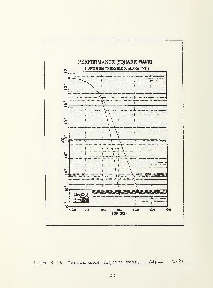
Figures 4.13 through 4.16 have been obtained through
numerical evaluation of Equations (3.67) and (3.70). Two
curves in each figure have been plotted to show the effect
of the parameter m on the receiver performance. Observe that
Equations (3.67) and (3.69) involve a parameter a which can
only take on values iT/N, where i = 1,2,...,N. Observe that
i = N corresponds to a = T or equivalently a = since v(t)
is T periodic.
Two values of a have been considered for each of the
signals, namely the sine wave and square wave, in order to
determine its effect on receiver performance. An inspection
of Fig. 4.13 and Fig. 4.14 displaying the performance of the
receiver for v(t) a sine wave, or inspection of Fig. 4.15 and
Fig. 4.16 displaying the performance of the receiver for v(t)
a square wave, it can be observed that a does not have any
significant effect on P for either case. The logic support-
ing this observation on receiver performance as a function of
a follows from the fact that a is just the estimate of the
time delay of the signal, which is obtained by choosing that
97

correlator branch that produces the largest output. The
actual value of a is irrelevant in so far as the performance
of the receiver is concerned. The receiver simply uses the
estimate of the time delay to produce a decision based on a
correlation operation. However, one of the factors that might
improve or degrade the error probability is the accuracy of
the estimate of the time delay of the signal, which is
itself a function of N and SNR.
98

PERFORMANCE (SINE WAVE)(OPTIMUM THRESHOLD. AIPHA=0)
I ' I I I 1 f
-io.oooo-s.3S9* xzaa* 10.0000 i«.8oe7 ga.aaaa aojooo
S^m(DB)
Figure 4.13 Performance (Since Wave), (Alpha = 01
9.a

PERFORMANCE (SINE WAVE)(OPTIMUM THRESHLOD. ALPHAsfl^S
)
SNR(DB)
Figure 4.14 Performance (.Sine Wave), (Alpha = T/2).
100.

PERFORMANCE (SQUARE WAVE)
^ (OPTIMUM THRESHOLD. ALPHA=0)
-i9M 0.0 10.0 SO.0 30.0
SNR (DB)
Figure 4.15 performance (.Square Wave), (Alpha - 0)
101
PERFORMANCE (SQUARE WAVE)
^J ( OPTIMUM THRESHLOD, ALPHA^/2 )
^
}?:£:E:EEE}}}F^vH::-vEr£^
b ^?N^i h- —f 1
^HiE^//s=?!^^-
r ^ ^ -r 1
•'o. i V\ i ; ;
•*: ::::..^:::::::u;u;;2^:u::::::^t5|:::^^
- ... _..^ ^.A.T—i.^
1
•'o. ; ^ \\ ^
•«:r^^/HE^;E^^=EHHj;^^
•
.j 1
—
Lz!^_ i -j—
—
Jo ; \ 5j
a."':
1
••" ~~ 1" -r ~-i--i.-t1- — - — •
•'o \ ; \ ;
; ::::::::^::-:::l::~:-:::—^^^^^
- .j, ^ —t^ \^....i
•\
; \ : i
•*: :::::::::::::::::::::::;::::::::::::::::::;:::::::::::;:^:::::::::::::::;::!y:::;:::;::::::^:::::::::::::::u^^^
;— — •• -4-' -V;-
-
^O '; \i K \
LEGENDa M=20
E=pEv^^^:^=^
•b.
o^Sm
10.0 20.0 30.0 40.0 90.0
SNR(DB)
Figure 4.16 Performance (Square Wave), (Alpha = T/21
102

V. CONCLUSIONS
In this thesis, the analysis and design of noncoherent
digital receivers that optimally (and in some cases subopti-
mally) detect an arbitrarily shaped periodic waveform with
random time delay, has been carried out. The probability
density function (p. d. f . ) of the random time delay A is assumed
to be of some known form. A uniform p.d.f. and a (parameter
varying) non-uniform p.d.f. have been considered and their
effect on the receiver performance has been studied.
The optimum (in minimum probability of error, P , sense)
receivers have been designed on the basis of likelihood ratio
test under low SNR assumptions. The design of suboptimum
receivers is based on heuristic approaches that intuitively
yield structures or algorithms that yield good performance.
The analysis carried out in this thesis, allowed for the
possibility of unequal prior probabilities of occurrence of
the hypotheses, however all examples and computations assumed
equal prior probabilities for simplicity.
The low SNR assumption allowed certain mathematical
complexities to be overcome. Therefore graphical results
involving the performance (P ) of optimum receivers are valid
and therefore presented only for SNR values less than or equal
to -4 dB . Operating at SNR values less than or equal to dB
is the basic requirement of covert communication and may
also be necessary in certain radar applications.
103

The optimum receiver operating on the signals that have
non-zero DC component, detects the signal with higher level
of error probability and it decreases with the increase of
SNR as expected. While it is clear that no receiver could
operate with such an undesirable level of error probability,
the graph displaying the performance (P ) does give an indi-
cation of the performance level that can be expected at low
SNR's. In the region of high SNR, it is expected that error
probability will continue to decrease to reasonable levels.
However, for high SNR's this receiver is no longer optimum.
The second optimum receiver operating on arbitrary sig-
nals does also yield poor performance. But here again we
must not forget that the receiver is operating in the low
SNR region. The graphs displaying the performance of this
receiver for the sine wave and square wave give an indication
of the performance that can be expected at low SNR's. Also,
they reveal an improvement in the performance with an in-
crease in the parameter ra. It is concluded that for high
SNR's, this receiver is also no longer optimum.
One of the receivers designed via heuristic means was a
(suboptimum) N-correlator receiver. Its performance was
derived and tested for the case in which v(t) was a periodic
triangular waveform. While this receiver is unable to detect
a sine wave, it is capable of detecting a square wave or some
other periodic waveform. The other receiver designed via
heuristic means, namely the Estimator-Correlator receiver,
was analyzed in terms of its P as a function of SNR.^ e
104

From the graphical results of the performance of the N-
correlator receiver, it is concluded that receiver performance
gets better as N, the number of correlators, gets bigger.
It is further concluded that m, the parameter that determines
the uncertainty about the time delay A, does not have any
effect on the receiver perfonnance. In general, it was
observed that except for the case of the N-correlator receiver,
the parameter m had a significant effect on the performance
of the receivers.
While a number of practical problems have been addressed
in this thesis, related problems and potential studies abound.
For example, the receiver obtained using a three-term approxi-
mation in the exponential of Equation (2.19) needs to be
analyzed further in terms of performance for both uniform and
non-uniform p.d.f . on X. Furthermore, other (suboptimum)
receivers need to be proposed and analyzed, such as simple
energy detection receivers.
105

APPENDIX A
DERIVATION OF MEAN AND VARIANCE OF R . V . A
The p.d.f. of r.v. A (time delay) given by Equation (2.1)
is
27T,m cos—
A
f^(A;m) = ^^J. (^)
A < 1t/2| . < m £ oo (a.1)
Substitution of Equation (2.41) into Equation (A.l) yields
2
I Ip(m) cosp^Af^(A;m) = P""°°
^-^ (^)A < |T/2| . < m < oo (a. 2)
so that the expected value or mean of r.v. A can be expressed
as
T/2E{A} = / Af.(A;m)dA
-T/2 ^^
oc T/2,., \ , J I (m) / cos(p27TA/T)dA'Iq^"^)
P=-oo P -T/2^
= (A. 3)
106

since the product of X (odd function) and cos(p27TA/T) (even
function) is an odd function and integral of an odd function
produces zero.
The variance of X is given by
T/2E{A}^ =
/ A^f.(A;m) dA-T/2 ^^
Tlo(m) _^/2
T/2f
' ,2 incos27TA/T ,, ,^ _,
,
jA e '^ dA (A. 3)
since we have a zero mean random variable.;
The variance is clearly a function of m. However, the
integral of Equation (A. 3) is not readily evaluated in closed
form. The computer has been used to evaluate
Var{A} 1 r 2 mcosrrx= T-A^ I
-' e--=°-"- dx (A. 4)
T^"Iq'™'
2and it has been clearly demonstrated that Var{A}/T becomes
smaller as m grows
.
107
APPENDIX B
INTERPRETATION OF A SMALL EXPONENTIALIN EQUATION (2.22) AND EQUATION (2.60)
In Equation (2.22) and Equation (2.60) it has been assumed
that
T2 ° A •
r^ f r(t)v(t-A)dt ^ £ << 1 (B.i:
o
This appendix is devoted to analyzing under what conditions is
this assumption valid. Observe that e is a r.v. so that
Equation (B.I) must be analyzed in a statistical sense. Recall
that
E{£1Hq} =^
(B.2)
since the noise has been assumed to be zero mean and
TE{£|H } = ^ j v^(t-A) = ^E (B.3)
o o
where E is the signal energy for £ t £ T
Thus, provided E/N << 1, e under either hypothesis on
the average takes the value zero or a value close to it. The
excursions of e away from the mean can be obtained by evaluat-
ing the conditional variances. Since
108
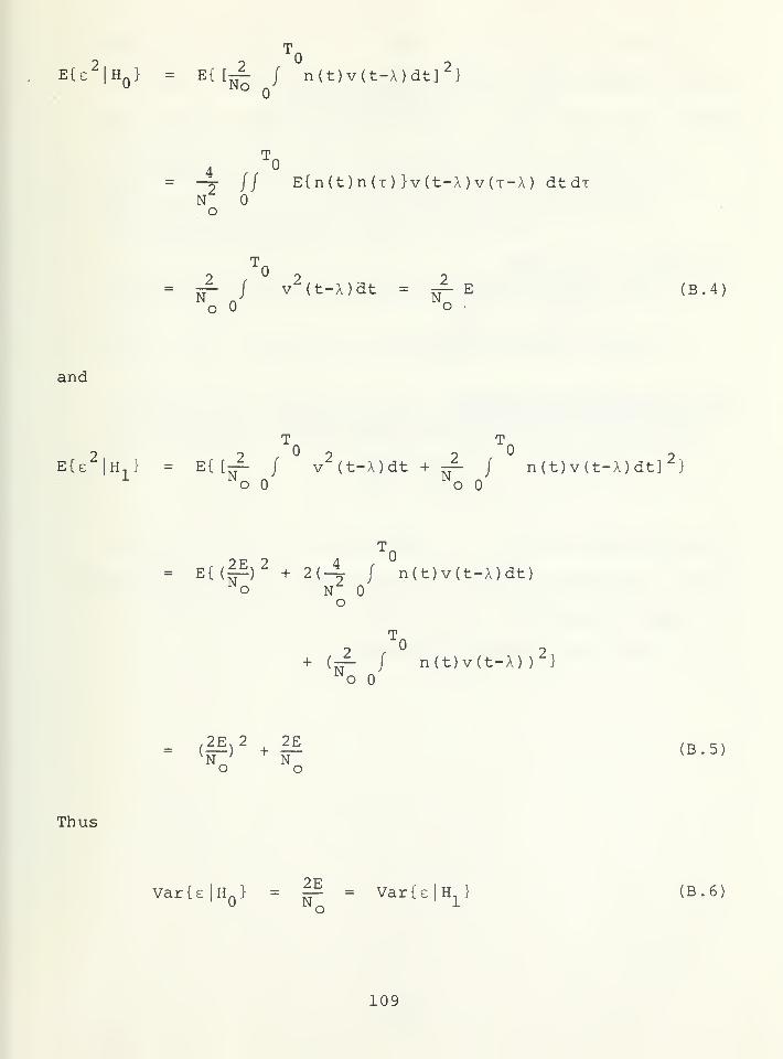
e{£^|Hq} E{ [^ / n(t)v(t-A)dt]^}
4 ./°-2 // E{n(t)n(T) }v(t-A)v(T-A) dtdTNo
? Op^ / v^(t-A)dto
N,(B.4)
and
e{£^|h^}
T T
E{ [rp- / v^(t-A)dt + -^ / n(t)v(t-A)dt]^}No
No
= E{(|^)^ + 2(4- / n(t)v(t-A)dt)N^o
+ (-f / n(t)v(t-A))^}N o
.2E>2 2E
o o(B.5)
Thus
Var{£|HQ} = ^ Var{£ 1h^} (B.6)
109

Therefore, provided that E/Nq << 1, e remains very close
to its average value which is either zero or very close to
zero. Note also that in a more rigorous sense, we can bound
2 EIe^Ih.}P{£ >6|H.} <
J^ (B.7)— ' 1 —
If we set 6=1/ then
P{£^>1|Hq} < ^ (B.8)o
and
P{e^ >1|H } <_ i^)^ + ^ (B.9)o o
In both cases if 2E/N << 1, then P{£ >1 or e < -1} is alsoo — ~
small. Therefore, a small E/N guarantees that the assumption
of a small exponential in Equations (2.22) and (2.60) is
valid with a high degree of probability.
110

LIST OF REFERENCES
1. Wainstein, L. and Zubakov, V., Extraction of Signalsfrom Noise , Englewood Cliffs, N.J., Prentice-Hall, 1962.
2. Gagliardi, R.M. , "Noncoherent Detection of PeriodicSignals," IEEE Trans. Information Theory , Vol. IT-21,pp. 282-285, May 1975.
3. Srinath, M.D. and Rajasekaran, P.K., An Introduction toStatistical Signal Processing with Applications , JohnWiley, 1979.
4. Whalen, A.D., Detection of Signals in Noise , AcademicPress, 1971.
5. Abramowitz, M. and Stegun, I.E., Handbook of MathematicalFunctions With Formulas, Graphs, and Mathematical Tables ,
U.S. Department of Commerce, National Bureau of Standards,1972.
Ill
INITIAL DISTRIBUTION LIST
No. Copies
1. Defense Technical Information Center 2
Cameron StationAlexandria, Virginia 22304-6145
2. Library, Code 0142 2
Naval Postgraduate SchoolMonterey, California 93943-5100
3. Prof. D. Bukofzer, Code 62Bh 5Naval Postgraduate SchoolMonterey, California 93943-5100
4. Prof. J.F. Chang, Code 62Cn 1
Naval Postgraduate SchoolMonterey, California 93943-5100
5. Prof. Harriet B. Rigas , Code 62 1Naval Postgraduate SchoolMonterey, California 93943-5100
6. LT Khalil A. Ansari 2
Ansari Mohalla, Hala (New) SindPakistan
7. Lt Sarfraz Hussain 1
SMC #1206Naval Postgraduate SchoolMonterey, California 93943-5100
112


J Q 7 ':• vy
ThesisA553 Ansaric.l Detection of perio-
dic signal of arbi-trary shape with ran-dom time delay.
1J87
ThesisA553c.l
AnsariDetection of perio-
dic signal of arbi-trary shape with ran-dom time delay.