UNIVERSITE TOULOUSE III - PAUL SABATIER

U.F.R Mathematiques Informatique Gestion

THESE

presentee en vue d’obtention du

DOCTORAT DE L’UNIVERSITE DE TOULOUSE

delivre par l’Universite Toulouse III - Paul Sabatier

Specialite : Mathematiques Appliquees

par

Raymond EL HAJJ

intitulee

Etude mathematique et numerique de

modeles de transport : application a la spintronique

soutenue le 3 septembre 2008 devant le jury compose de :

Naoufel Ben Abdallah Directeur de these Universite Toulouse III-Paul Sabatier

Abderrahmane Bendali Examinateur INSA de Toulouse

Thierry Goudon Rapporteur INRIA Lille, Universite de Lille 1

Ansgar Jungel Rapporteur Universite technique de Vienne

Florian Mehats Examinateur Universite de Rennes 1

Pierre Renucci Examinateur INSA de Toulouse

Jean-Michel Roquejoffre Invite Universite Toulouse III-Paul Sabatier

Institut de Mathematiques de ToulouseEquipe Mathematiques pour l’Industrie et la Physique (MIP)

Unite Mixte de Recherche CNRS - UMR 5219

UFR MIG, Universite Paul Sabatier Toulouse 3, 118 route de Narbonne,

31062 TOULOUSE cedex 09, France

Remerciements

Je tiens a remercier en premier lieu mon directeur de these Naoufel Ben Abdallah

qui m’a propose un sujet de these original et moderne. Je le remercie chaleureusement

pour sa confiance, ses conseils precieux et pour le temps qu’il m’a accorde malgre son

emploi de temps surcharge avec la direction du laboratoire. Je tiens aussi a souligner

sa gentillesse et ses qualites humaines qui m’ont permis de realiser ce travail et de

faire mes premiers pas dans la recherche dans un environnement tres agreable.

Mes remerciements les plus respectueux vont a Thierry Goudon et Ansgar Yungel

qui m’ont fait l’honneur d’etre rapporteurs de ce travail. Qu’ils trouvent ici l’expres-

sion de ma profonde reconnaissance.

J’adresse ma sincere reconnaissance a Florian Mehats pour ses conseils et pour

l’interet qu’il a toujours porte a mon travail depuis mon stage de DEA. Je suis tres

heureux de le compter parmi les membres de mon jury.

Je tiens a remercier Abderrahmane Bendali, Pierre Renucci et Jean-Michel Ro-

quejoffre pour l’interet qu’ils ont bien voulu accorder a ma these en acceptant de

participer au jury.

Les differentes reunions avec l’equipe opto-electronique du Laboratoire de Phy-

sique et Chimie de Nano-Objets (LPCNO) a l’INSA de Toulouse ont ete d’une im-

portance considerable pour la realisation de ce travail (surtout la partie principale

sur la spintronique). Je remercie vivement Xavier Marie, Thierry Amand, Pierre Re-

nucci et toute l’equipe pour le temps qu’ils nous ont accordes et pour les differentes

discussions qui ont toujours ete fructueuses.

Un grand merci a tous les membres de l’equipe MIP de l’Institut de Mathematiques

de Toulouse qui rendent l’ambiance vraiment agreable et detendue. Merci a toi Chris-

tine pour ta gentillesse et ton sourire que tu as su garder malgre la surcharge de

travail que tu avais avant de partir. Je remercie tous les collegues et amis : mon

ancien co-bureau Marc pour ta bonne humeur et pour tes blagues que je te faisais

5

6

repeter plusieurs fois (merci d’avoir libere le 3 septembre pour etre present a ma

soutenance) ; Michael avec sa grande patience pour le foot, merci pour le petit bal-

lon (c’est un beau souvenir) qui nous a accompagnes durant ces annees de these

dans les couloirs du 2 eme etage ; et desole Mounir, on t’a derange avec les parties

de foot ces derniers moments mais je t’assure qu’on ne faisait pas expres...bon cou-

rage pour la suite ; l’eternel Jean-Luc qui est toujours la pour nous rappeler l’heure

de la pause the, bon courage aussi pour la fin de these. Je salue aussi et remercie :

Laetitia, Laurent, Dominique, Benjamin, Tiphaine, Melanie, Salvador, Clement, Ali,

Sebastien, Antoine, Davuth, Aude et Olivier. Je n’oublie pas les amis a l’INSA : Elie,

Abdelkader M. et Abdelkader T. J’ai une pensee aussi pour les anciens : Claudia

(merci pour les encouragements et pour l’interet que tu portes a ce travail), Nicolas

(merci pour le code), Mehdi, Raphael ...

Enfin et surtout, tous mes remerciements vont pour mes parents, mes sœurs et

mon frere pour leur amour et leur soutien constant. Je suis heureux que vous ayez

fait le deplacement du Liban pour etre a mes cotes le jour de ma soutenance. Merci

pour tout a toi aussi Pascale et tes deux anges Etienne et My-Lihn.

Summary

This thesis is decomposed into three parts. The main part is devoted to the study

of spin polarized currents in semiconductor materials. An hierarchy of microscopic

and macroscopic models are derived and analyzed. These models takes into account

the spin relaxation and precession mechanisms acting on the spin dynamics in se-

miconductors. We have essentially two mechanisms : the spin-orbit coupling and

the spin-flip interactions. We begin by presenting a semiclassical analysis (via the

Wigner transformation) of the Schrodinger equation with spin-orbit hamiltonian.

At kinetic level, the spinor Vlasov (or Boltzmann) equation is an equation of dis-

tribution function with 2 × 2 hermitian positive matrix value. Starting then from

the spinor form of the Boltzmann equation with different spin-flip and non spin-flip

collision operators and using diffusion asymptotic techniques, different continuum

models are derived. We derive drift-diffusion, SHE and Energy-Transport models

of two-components or spin-vector types with spin rotation and relaxation effects.

Two numerical applications are then presented : the simulation of transistor with

spin rotational effect and the study of spin accumulation effect in inhomogenous

semiconductor interfaces.

In the second part, the diffusion limit of the linear Boltzmann equation with

a strong magnetic field is performed. The Larmor radius is supposed to be much

smaller than the mean free path. The limiting equation is shown to be a diffusion

equation in the parallel direction while in the orthogonal direction, the guiding

center motion is obtained. The diffusion constant in the parallel direction is obtained

through the study of a new collision operator obtained by averages of the original

one. Moreover, a correction to the guiding center motion is derived.

In the third part of this thesis, we are interested in the description of the confi-

nement potential in two-dimensional electron gases. The stationary one dimensional

Schrodinger–Poisson system on a bounded interval is considered in the limit of a

small Debye length (or small temperature). Electrons are supposed to be in a mixed

state with the Boltzmann statistics. Using various reformulations of the system as

convex minimization problems, we show that only the first energy level is asymptoti-

cally occupied. The electrostatic potential is shown to converge towards a boundary

7

8

layer potential with a profile computed by means of a half space Schrodinger–Poisson

system.

Key words. Semiclassical analysis, Wigner transformation, spin-orbit hamilto-

nian, spinor Boltzmann equation, micro-macro limit, diffusion limit, moment me-

thod, entropy minimization, drift-diffusion, SHE, Energy-Transport, two-component

models, Spin-FET, finite elements, Gummel iterations, guiding-center approxima-

tion, high magnetic field, convex minimization, min-max theorem, concentration-

compactness principle, boundary layer.

Table of contents

Remerciements 3

Summary 6

Introduction 13

I. Modeles de transport en spintronique . . . . . . . . . . . . . . . . . . . . 15

I.1 Introduction a la spintronique . . . . . . . . . . . . . . . . . . . . 15

I.2 Description des modeles utilises . . . . . . . . . . . . . . . . . . . 18

I.3 Resume des resultats . . . . . . . . . . . . . . . . . . . . . . . . . 23

II. Diffusion et champs magnetiques forts . . . . . . . . . . . . . . . . . . . 30

II.1 Introduction et position du probleme . . . . . . . . . . . . . . . . 30

II.2 Resultats obtenus . . . . . . . . . . . . . . . . . . . . . . . . . . 34

III. Confinement . . . . . . . . . . . . . . . . . . . . . . . . . . . . . . . . 36

III.1 Motivation et description du probleme . . . . . . . . . . . . . . 36

III.2 Resultats obtenus . . . . . . . . . . . . . . . . . . . . . . . . . . 38

III.3 Commentaires . . . . . . . . . . . . . . . . . . . . . . . . . . . . 39

I Transport models for semiconductor spintronics 47

1 Semiclassical analysis 49

1.1 Introduction . . . . . . . . . . . . . . . . . . . . . . . . . . . . . . . . 50

1.2 Schrodinger equation with general spin-orbit Hamiltonian . . . . . . . 51

1.2.1 Analysis of the Schrodinger equation with spin-orbit term . . . 53

1.2.2 Semiclassical limit . . . . . . . . . . . . . . . . . . . . . . . . 56

1.3 semiclassical limit and partially confining potential . . . . . . . . . . 58

1.3.1 Introduction and main result . . . . . . . . . . . . . . . . . . . 58

1.3.2 Application : subband model with Rashba spin-orbit effect . . 61

1.3.3 Proof of Theorem 1.3.7 . . . . . . . . . . . . . . . . . . . . . . 63

References . . . . . . . . . . . . . . . . . . . . . . . . . . . . . . . . . . . . 67

9

10 TABLE OF CONTENTS

2 Hierarchy of kinetic and macroscopic models 71

2.1 Introduction . . . . . . . . . . . . . . . . . . . . . . . . . . . . . . . . 72

2.2 Assumptions and notations . . . . . . . . . . . . . . . . . . . . . . . . 75

2.3 Study of spinor Boltzmann type models . . . . . . . . . . . . . . . . . 76

2.4 Two-component models . . . . . . . . . . . . . . . . . . . . . . . . . 81

2.4.1 Decoherence limit . . . . . . . . . . . . . . . . . . . . . . . . . 81

2.4.2 Diffusion limit with strong spin-orbit coupling : two-component

Drift-Diffusion model . . . . . . . . . . . . . . . . . . . . . . . 83

2.5 A general spin-vector Drift-Diffusion model . . . . . . . . . . . . . . . 91

2.5.1 Diffusion limit: formal approach . . . . . . . . . . . . . . . . 95

2.5.2 Diffusion limit: the rigorous approach . . . . . . . . . . . . . . 96

2.5.3 Maximum Principle (Proof of Theorem 2.5.3) . . . . . . . . . 100

2.6 SHE model . . . . . . . . . . . . . . . . . . . . . . . . . . . . . . . . 104

2.7 Other fluid models for semiconductor spintronics . . . . . . . . . . . . 107

2.7.1 Energy-Transport model . . . . . . . . . . . . . . . . . . . . . 110

2.7.2 Drift-Diffusion with Fermi-Dirac statistics . . . . . . . . . . . 116

References . . . . . . . . . . . . . . . . . . . . . . . . . . . . . . . . . . . . 121

3 Numerical Applications 127

3.1 Modelling and numerical implementation of spin-FET . . . . . . . . . 128

3.1.1 Introduction . . . . . . . . . . . . . . . . . . . . . . . . . . . . 128

3.1.2 A coupled quantum/drift diffusion model with spin-orbit effect 129

3.1.3 Setting of the problem and numerical results . . . . . . . . . . 133

3.2 Spin accumulation in inhomogeneous semiconductor interfaces . . . . 138

3.2.1 Presentation of the system . . . . . . . . . . . . . . . . . . . . 138

3.2.2 Numerical results . . . . . . . . . . . . . . . . . . . . . . . . . 139

3.2.3 Spin accumulation and Rashba spin-orbit effect . . . . . . . . 140

References . . . . . . . . . . . . . . . . . . . . . . . . . . . . . . . . . . . . 143

II Diffusion and high magnetic fields 145

4 Diffusion and guiding center approximation 147

4.1 Introduction . . . . . . . . . . . . . . . . . . . . . . . . . . . . . . . . 148

4.2 Setting of the problem and main results . . . . . . . . . . . . . . . . . 149

4.2.1 Scaling . . . . . . . . . . . . . . . . . . . . . . . . . . . . . . . 150

4.2.2 Notations . . . . . . . . . . . . . . . . . . . . . . . . . . . . . 153

4.2.3 Main results . . . . . . . . . . . . . . . . . . . . . . . . . . . . 154

4.3 Analysis of the operator Qη . . . . . . . . . . . . . . . . . . . . . . . 156

4.4 Expansion of Xη with respect to η . . . . . . . . . . . . . . . . . . . . 160

TABLE OF CONTENTS 11

4.4.1 Expansion of Xηz . . . . . . . . . . . . . . . . . . . . . . . . . 164

4.4.2 Expansion of X⊥η . . . . . . . . . . . . . . . . . . . . . . . . . 166

4.5 Proof of the main theorems . . . . . . . . . . . . . . . . . . . . . . . 166

4.5.1 Proof of Theorem 4.2.4 . . . . . . . . . . . . . . . . . . . . . . 168

4.5.2 Proof of Proposition 4.2.6 . . . . . . . . . . . . . . . . . . . . 170

4.5.3 Proof of Theorem 4.2.8 . . . . . . . . . . . . . . . . . . . . . . 171

4.6 Concluding remarks . . . . . . . . . . . . . . . . . . . . . . . . . . . . 173

References . . . . . . . . . . . . . . . . . . . . . . . . . . . . . . . . . . . . 173

III Confinement 177

5 High density Schrodinger-Poisson 179

5.1 Introduction and main results . . . . . . . . . . . . . . . . . . . . . . 180

5.1.1 Introduction . . . . . . . . . . . . . . . . . . . . . . . . . . . . 180

5.1.2 Main results . . . . . . . . . . . . . . . . . . . . . . . . . . . . 182

5.1.3 Remark on the scaling . . . . . . . . . . . . . . . . . . . . . . 184

5.1.4 Notation and definitions . . . . . . . . . . . . . . . . . . . . . 185

5.2 Schrodinger–Poisson system on a bounded domain . . . . . . . . . . . 187

5.3 Analysis of the limit problem . . . . . . . . . . . . . . . . . . . . . . 188

5.3.1 Properties of the fundamental mode of the Schrodinger ope-

rator on [0, +∞) . . . . . . . . . . . . . . . . . . . . . . . . . 188

5.3.2 Proof of Theorem 5.1.1 . . . . . . . . . . . . . . . . . . . . . . 193

5.4 Convergence analysis . . . . . . . . . . . . . . . . . . . . . . . . . . . 194

5.5 Comments . . . . . . . . . . . . . . . . . . . . . . . . . . . . . . . . . 198

5.5.1 Fermi–Dirac statistics . . . . . . . . . . . . . . . . . . . . . . 198

5.5.2 Boundary conditions and higher dimension . . . . . . . . . . . 200

References . . . . . . . . . . . . . . . . . . . . . . . . . . . . . . . . . . . . 200

A Appendix 205

A.1 Concentration-Compactness principle . . . . . . . . . . . . . . . . . . 205

A.1.1 Proof of Lemma 5.3.4 . . . . . . . . . . . . . . . . . . . . . . . 205

A.2 Pauli Matrices . . . . . . . . . . . . . . . . . . . . . . . . . . . . . . . 208

Introduction

Ce travail de these comporte trois parties. La partie principale porte sur l’etude

mathematique et l’analyse numerique des phenomenes de transport en spintronique.

Deux autres travaux ont ete menes en parallele. Le premier concerne l’etude de

l’asymptotique de diffusion et l’approximation centre-guide de systemes de parti-

cules en presence de champs magnetiques forts. Dans un autre travail, nous nous

interessons a la description du profil de potentiel de confinement dans des gaz

d’electrons bidimensionnels en etudiant une asymptotique forte densite du systeme

Schrodinger-Poisson unidimensionnel stationnaire. Nous resumons maintenant cha-

cune des trois parties.

Nous nous interessons dans la premiere partie de cette these au transport des cou-

rants polarises en spin dans des materiaux a base de semi-conducteur. Le mecanisme

essentiel pouvant agir sur l’orientation du spin electronique dans les semi-conducteurs

est ce que l’on appelle le couplage spin-orbite. Lorsque la structure etudiee presente

une absence de symetrie, le couplage spin-orbite se traduit par l’apparition d’un

champ effectif faisant precesser (ou tourner) le vecteur spin pendant les vols libres

des electrons. Dans les structures semi-conductrices, on a essentiellement le couplage

spin-orbite de Rashba et celui de Dresselhauss. Le terme de Rashba apparaıt dans

des couches d’accumulations a l’interface entre deux heterostructures et est due a

la forte asymetrie du puits quantique dans lequel se confine le gaz d’electrons bidi-

mensionnel. Le couplage de Dresselhauus quant a lui resulte de l’asymetrie presente

dans certains structures cristallines.

Nous derivons et analysons une hierarchie de modeles allant du niveau micro-

scopique au niveau macroscopique en tenant compte des differents mecanismes de

rotation et de relaxation du spin electronique dans les semi-conducteurs. Au niveau

microscopique, l’hamiltonien spin-orbite lie a l’absence de symetrie se represente par

la forme suivante

HSO = α~~Ω(t, x, k) · ~σ,

ou ~σ est le vecteur des matrices de Pauli (0.0.5), x, k sont respectivement la po-

sition et le vecteur d’onde d’une particule (k ≡ i~∇x), α est l’ordre du couplage

et ~Ω represente le champ effectif. Dans un premier lieu, nous effectuons une ana-

13

14 INTRODUCTION

lyse semi-classique, via la transformation de Wigner, de l’equation de Schrodinger

avec un hamiltonien spin-orbite. Suivant l’ordre du couplage spin-orbite par rapport

a la constante de Planck adimensionnee, nous derivons des modeles cinetiques a

deux composantes ou spinorielle (avec une fonction de distribution a valeur matri-

cielle). Partant ensuite de la spinor forme de l’equation de Boltzmann (avec differents

operateurs de collisions avec et sans renversement du vecteur spin) et par des tech-

niques d’asymptotiques de diffusion, nous derivons et analysons plusieurs modeles

macroscopiques. Ils sont de type derive-diffusion, SHE, Energie-Transport, a deux

composantes ou spinoriels conservant des effets de rotation et de relaxation du vec-

teur spin. Nous validons ensuite ces modeles par des cas tests numeriques. Deux

applications numeriques sont presentees : la simulation d’un transistor a effet de

rotation de spin et l’etude de l’effet d’accumulation de spin a l’interface entre deux

couches semi-conductrices differemment dopees. Cette partie de these donne lieu a

deux articles en preparation [46, 47].

Mots cles : Analyse semi-classique, transformation de Wigner, hamiltonien spin-

orbite, equation de Boltzmann spinorielle, passage cinetique fluide, limite de diffu-

sion, methode des moments, minimisation d’entropie, derive-diffusion, SHE, Energie-

Transport, modeles a deux composantes, Spin-FET, elements finis, iterations Gum-

mel.

Dans un autre travail, nous considerons une equation cinetique de type Boltz-

mann lineaire dans des domaines ou un champ magnetique fort est applique. La

presence de ce dernier introduit de fortes oscillations et donc des difficultes pour les

simulations numeriques. Nous etudions la limite de diffusion en supposant que le

champ magnetique est unidirectionnel et tend vers l’infini. Le modele obtenu est un

modele macroscopique (moins couteux numeriquement que le modele cinetique). Il

est constitue d’une equation diffusive dans la direction parallele au champ magnetique

et d’une derive representant l’effet centre-guide en presence d’un champ electrique

dans la direction perpendiculaire. Le terme de diffusion contient des moyennes de gi-

ration de l’operateur de collisions utilise. Nous prouvons la convergence en utilisant

des techniques d’entropie pour traiter le comportement diffusif, et en conjuguant

par les rotations locales induites par le champ magnetique pour tenir compte des

oscillations. Ce travail fait l’objet d’une publication [13].

Mots cles : limite de diffusion, approximation centre-guide, champ magnetique fort.

Dans la troisieme partie de cette these, nous etudions la limite faible longueur

de Debye (ou faible temperature) du systeme de Schrodinger-Poisson unidimen-

sionnel stationnaire sur un intervalle borne. Les electrons sont supposes dans un

melange d’etats avec une statistique de Boltzmann (ou de Fermi-Dirac). En utili-

sant differentes reformulations du systeme comme des problemes de minimisation

INTRODUCTION 15

convexe, nous montrons qu’asymptotiquement seul le premier niveau d’energie est

occupe. Le potentiel electrostatique converge vers une couche limite avec un pro-

fil calcule a l’aide d’un systeme de Schrodinger-Poisson sur le demi axe reel. Cette

partie est publiee dans SIAM-Multiscale Modeling and Simulations [48].

Mots cles : minimisation convexe, theoreme min-max, principe de concentration-

compacite, couche limite.

Dans la suite de cette introduction nous detaillons et presentons les principaux

resultats obtenus dans chacune des trois parties de cette these.

I. Modeles de transport en spintronique

I.1 Introduction a la spintronique

Les electrons ne sont pas seulement caracterises par leur charge electrique mais

aussi par leur moment cinetique intrinseque ou spin. Jusqu’aux annees 90’, l’electronique

ignorais quasiment le spin de l’electron. La spintronique, ou l’ electronique de spin,

est un nouveau domaine de recherche tentant d’allier l’electronique classique et les

proprietes quantiques du spin. Il vise a manipuler le spin des porteurs de charge,

et de l’utiliser comme un degre de liberte supplementaire ou comme un nouveau

vecteur de l’information.

La magnetoresistance geante (Giant Magneto-Resistance ou GMR) decouverte

par Albert Fert et al [55], et la magnetoresistance tunnel, sont les premieres mani-

festations de la spintronique.

Dans des structures electroniques composees de couches magnetiques separees

par une couche paramagnetique, la GMR se traduit par un changement de resistance

important observe dans de tels structures lorsque, sous l’effet d’un champ magnetique

exterieur (ou sous l’effet de l’accumulation des spins a l’interface M/PM), les aiman-

tations macroscopiques des couches magnetiques successives basculent d’un etat an-

tiparallele a un etat parallele aligne.

Un effet similaire a la magnetoresistance geante, appele magnetoresistance tun-

nel, a ete observe dans des jonctions tunnel metal/isolant/metal, dans lesquels les

deux electrodes metalliques sont magnetiques. Cet effet magnetoresistif a ete utilise,

dans les annees quatre-vingt dix, pour developper des memoires magnetiques a acces

aleatoire ou MRAM (Magnetic Random Access Memories). Dans ces memoires, l’in-

formation n’est plus stockee sous la forme d’une charge, comme c’est le cas des

memoires semi-conductrices de type DRAM ou Flash, mais sous la forme d’une

direction d’aimantation dans la jonction tunnel magnetique.

Pour utiliser le spin comme un porteur de l’information, il faut que cette derniere

16 INTRODUCTION

ne soit pas perdue durant son transport. En d’autres termes, il faut disposer de

porteurs dont l’orientation du spin est parfaitement definie. Cette notion conduit

naturellement aux courants polarises en spin : essentiellement liee dans les semi-

conducteurs aux differences relatives des densites de spin-up et spin-down. Notons

que dans les metaux ferromagnetiques, la notion de courants polarises en spin est sur-

tout liee a la difference de mobilite des spin-up et spin-down. Bien que les premieres

recherches dans ce domaine ont ete menees pour des structures composees de multi-

couches magnetiques, les chercheurs portent actuellement une attention particuliere

a l’etude des courants polarises en spin dans les semi-conducteurs. La raison est la

decouverte du long temps de vie du spin et la presence des mecanismes pouvant agir

sur la dynamique du spin electronique dans les semi-conducteurs.

I.1.1 Mecanismes agissant sur le spin dans les semi-conducteurs

Ces mecanismes sont dus au couplage spin-orbite qui est un effet relativiste lie

au mouvement de l’electron autour de son noyau. Ils peuvent etre classes en deux

categories.

• Mecanisme d’Elliot-Yafet. L’interaction spin-orbite melange les etats de

spin-up et down. Les interactions instantanees entre les particules et le cristal

(ou l’environnement) peuvent alors etre accompagnees d’un retournement de

l’orientation du vecteur spin, selon le mecanisme dit d’Elliot-Yafet [103, 56].

Bien que les interactions avec renversement du spin soient des evenements rares

dans les semi-conducteurs [24], elles peuvent etre suffisantes dans les zones a

faible mobilite (ou forte densite) pour faire disparaıtre la coherence en spin (ou

faire relaxer le vecteur spin). C’est le mecanisme de relaxation d’Elliot-Yafet.

• Mecanisme de relaxation de D’yakonov-Perel. Lorsque le systeme presente

une asymetrie d’inversion, le couplage spin-orbite va se traduire par l’appari-

tion d’un champ magnetique (qu’on appelle champ effectif) faisant precesser

le vecteur spin pendant les vols libres des porteurs de charge. Le couplage

spin-orbite se decompose en deux termes :

– Couplage spin-orbite de Rashba [27]. Ce couplage apparaıt dans les couches

d’accumulations a l’interface entre deux hetero-structures et du a la forte

asymetrie du puits quantique dans lequel se confine le gaz d’electrons bidi-

mensionnel (2DEG). Le vecteur de precession de spin associe au couplage

de Rashba pour un 2DEG forme dans un plan (xy) est donne par [82, 27] :

~ΩR =2a46Ez

~(−kyex + kxey) (0.0.1)

avec a46 est une constante dependant du materiel, ~ est la constante de

Planck, Ez est le champ electrique de confinement dans la direction z per-

INTRODUCTION 17

pendiculaire au plan (xy), k = (kx, ky) est le vecteur d’onde de particule

dans le plan (xy) et ex, ey denotent les vecteurs unitaires suivant les axes

des x et des y.

– Couplage de Dresselhauss [43]. C’est un couplage spin-orbite qui resulte de

l’asymetrie presente dans certaines structures cristallines. Le vecteur de

precession de Dresselhauss s’ecrit sous la forme

~ΩD =2a42

~(kxex − kyey), (0.0.2)

ou a42 est un parametre dependant de la structure.

ΩR

ΩR

ΩR

S1

S2 3S

S1 S2

3S

x1DEG

ΩR

zy

xPlan−2DEG

Source

Drain

Fig. 1 – Dynamique du vecteur spin sous l’action du vecteur de precession de Rashba dans un2DEG et dans un fil quantique 1DEG.

Le mecanisme de D’yakonov-Perel lie a l’existence d’un champ magnetique

effectif represente le mecanisme essentiel de relaxation du spin electronique

dans les hetero-structures semi-conductrices [45, 103]. Le module du champ

effectif lie au terme de Rashba (0.0.1), soit la vitesse de rotation de spin, depend

de Ez. Elle peut donc etre controlee a l’aide du champ electrique de confinement

par un potentiel exterieur applique au systeme (potentiel de grille). Neanmoins,

ce controle n’est efficace que si l’on se place dans de bonnes conditions. En

effet, dans un gaz d’electrons 2D, la direction du champ ~ΩR (0.0.1) depend

du vecteur d’onde k. Ce vecteur se redistribue de facon aleatoire dans le plan

a l’issu de chaque interaction subie par la particule (voir Figure 1). Dans

un regime fortement collisionnel, les particules subissent beaucoup de chocs.

La dynamique du champ de Rashba ressemble dans ce cas a une marche au

hasard et la coherence de spin est donc relaxee via le mecanisme de relaxation

de D’yakonov-Perel.

Pour eviter ce probleme, une solution consiste a confiner les electrons dans la

direction y en plus du confinement dans la direction z. Le transport dans le gaz

se fait alors dans une seule direction de l’espace. On definit un fil quantique

18 INTRODUCTION

ou 1DEG. Dans ce cas, le champ effectif de Rashba est donne par

~Ω1DR = αkxey,

pour un certain parametre α. Sa direction ne depend pas de k et donc ~Ω1DR

ne change pas de direction avec les interactions instantanees des particules.

L’effet de Rashba est dans ce cas efficace pour controler la dynamique du

vecteur spin dans le fil quantique. Si le vecteur spin des electrons injectes dans

le fil est parallele a ce dernier, la rotation de spin s’effectue dans un meme plan

perpendiculaire a ~Ω1DR . La periode de rotation varie avec la tension de grille

appliquee. Ce mecanisme est verifie numeriquement, voir Chapitre 3 de cette

these.

Le vecteur de Dresselhauss, quant a lui, n’est pas controlable par une voie

externe et il induit aussi un mecanisme de relaxation de spin de type D’ya-

konov Perel [45]. D’autres mecanismes de relaxation de spin existent dans la

litterature, voir [103].

I.1.2 Transistor a effet de rotation de spin

Apres le MRAM, la recherche actuelle se dirige vers la fabrication des compo-

santes integrant des materiaux magnetiques et semi-conducteurs dans une meme

hetero-structure dite ”hybride”. La possibilite de controler la vitesse de rotation

du vecteur spin dans les hetero-structures via le couplage spin-orbite de Rashba a

conduit deux chercheurs americains Datta et Das a proposer en 1990 [30] un tran-

sistor a effet de rotation de spin ou spin-FET (spin Field Effect Transistor). Il s’agit

d’un transistor a haute mobilite electronique HEMT (High Electron Mobility Tran-

sistor) dans lequel les zones fortement dopees de source et de drain sont remplacees

par des contacts ferromagnetiques. La source agit comme un polariseur en spin. Dans

le semi-conducteur, les spins vont precesser autour d’un certain champ effectif. Leur

vitesse angulaire peut etre modulee par la tension de la grille. Le contact de drain,

quant a lui, agit comme un analyseur : si le spin est oriente parallelement a l’aiman-

tation du drain, le courant dans ce dernier est important. Dans le cas contraire, le

courant est faible. A part les contraintes de dimensionnement, plusieurs obstacles

s’opposent a la realisation du spin-FET, notamment les problemes d’injection et de

collection de spin aux interfaces FM/SC, SC/FM.

I.2 Description des modeles utilises

Dans cette premiere partie de la these, nous nous interessons a la derivation des

modeles de transport tenant compte de differents mecanismes agissant sur le spin

INTRODUCTION 19

electronique dans les semi-conducteurs decrits ci-dessus. Nous derivons et analy-

sons une hierarchie de modeles allant du niveau microscopique (avec l’equation de

Schrodinger) au niveau macroscopique en passant par des modeles cinetiques (Cha-

pitre 1, 2). Nous presentons ensuite quelques applications numeriques (Chapitre 3).

Dans cette section nous presentons les modeles utilises pour decrire le transport des

courants polarises en spin dans les semi-conducteurs. Plus particulierement, nous

decrivons comment sont introduit dans les equations, pour differentes echelles de

modelisation, les mecanismes de relaxation dus aux couplages spin-orbite et aux

interactions avec renversement de spin.

I.2.1 Modele quantique

En mecanique quantique, une particule de spin 1/2 (electron) plongee dans un

potentiel V peut etre decrite par une fonction d’onde Ψ(t, x) = (ψ↑(t, x), ψ↓(t, x)) a

valeur vectoriel dans C2. Les composantes ψ↑(t, x) et ψ↓(t, x) representent les fonc-

tions d’ondes des particules avec spin-up et spin-down respectivement. La fonction

Ψ verifie l’equation de Schrodinger suivante :

i~∂tΨ = (H0 + HSO)(Ψ) (0.0.3)

ou H0 est l’hamiltonien standard de l’energie cinetique plus l’energie potentiel

H0 = (−~2

2m∆x + V )I2,

m est la masse effective d’un electron et I2 est la matrice identite de C2. L’hamilto-

nien spin-orbite, note par HSO, s’ecrit sous la forme generale suivante :

HSO = α~~Ω(t, x, k) · ~σ (0.0.4)

ou ~σ est le vecteur ~σ = (σ1, σ2, σ3) des trois celebres matrices de Pauli,

σ1 =

(0 1

1 0

), σ2 =

(0 −i

i 0

), σ3 =

(1 0

0 −1

)(0.0.5)

et α est l’ordre du couplage. Ici, k est le vecteur d’onde, k ≡ −i~∇x. En effet, selon

[76, 49] l’hamitonien de l’interaction spin-orbite, derive de l’equation de Dirac a

quatre composantes [29], est donne par

HSO =i~2

4m2c2(∇xV ×∇x) · ~σ. (0.0.6)

L’hamiltonien de Rashba s’ecrit ([27]),

HR = αi~(~σ1∂y − ~σ2∂x)

20 INTRODUCTION

pour un gas d’electrons forme dans le plan (xy) et l’hamiltonien de Dresselhauss est

donne par [43]

HD = αi~(~σ1∂x − ~σ2∂y).

Rappelons qu’en physique quantique |Ψ(t, x)|2 = |ψ↑|2 + |ψ↓|2 represente la probabi-

lite de presence d’une particule en x a l’instant t et que l’on a∫R3 ‖Ψ(t, x)‖2dx = 1.

Les quantites macroscopiques telles que la matrice densite et courant sont definies

a partir de Ψ comme suit

N(t, x) = Ψ(t, x)⊗Ψ(t, x), J(t, x) =~2i

[∇xΨ(t, x)⊗Ψ(t, x)−Ψ(t, x)⊗∇xΨ(t, x)],

ou ⊗ designe le produit tensoriel de deux vecteurs.

I.2.2 Modeles cinetiques et macroscopiques

En microelectronique classique, le transport des charges est decrit au niveau

cinetique par une grandeur statistique : la fonction de distribution scalaire f(t, x, v).

Cette fonction represente une densite dans l’espace des phases decrit par la position

x et la vitesse v a l’instant t. Autrement dit, f(t, x, v)dxdv correspond au nombre

de particules se trouvant a l’instant t dans un volume dxdv autour du point (x, v).

L’evolution de cette fonction est decrite par l’equation de Vlasov ou Boltzmann dans

un cadre collisionnel [22, 28, 65, 100].

En spintronique, un ensemble de particules de spin 1/2 est decrit au niveau

cinetique par une fonction de distribution a valeurs dans l’ensemble des matrices

carrees hermitiennes d’ordre 2 (H2(C)). L’equation de Vlasov spinorielle avec interactions

spin-orbite s’ecrit

∂tF + v · ∇xF + F · ∇vF =αi

2[~Ω · ~σ, F ], (0.0.7)

ou F(t, x) = −∇xV (t, x) est la force exterieure exercee sur les particules , et supposee

conservative donc derivant d’un certain potentiel V . Dans cette description cinetique,

le couplage spin-orbite est donne par le terme de droite de l’equation (0.0.7), ou α

est l’ordre du couplage, ~Ω(t, x, v) est le champ effectif associe et [A,B] = AB −BA

designe le commutateur des deux matrices. La fonction de distribution admet dans

ce cas quatre degres de liberte : un pour la distribution des charges et trois pour la

distribution des spins. En effet, la matrice identite I2 et les trois matrices de Pauli

(0.0.5) constituent une base deH2(C). Decomposons F dans cette base de la maniere

suivante

F (t, x, v) =1

2fc(t, x, v)I2 + ~fs(t, x, v) · ~σ (0.0.8)

et injectons la dans (0.0.7). Nous obtenons

∂tfc + v · ∇xfc −∇xV · ∇vfc = 0

∂t~fs + v · ∇x

~fs −∇xV · ∇v~fs + α~Ω× ~fs = 0.

INTRODUCTION 21

On obtient une equation scalaire sur fc = tr(F ), ou tr(F ) est la trace de F et fc

represente la fonction de distribution des charges que l’on utilise en microelectronique.

La fonction ~fs est une fonction vectorielle a valeurs dans R3. Elle represente la

fonction de distribution des spins. Avec la decomposition (0.0.8), le commutateur

representant l’effet spin-orbite dans l’equation (0.0.7) devient un produit vectoriel

entre ~Ω et ~fs. Ce dernier introduit un effet de rotation du vecteur distribution des

spins ~fs autour du champ effectif ~Ω. De plus, les valeurs propres de F (t, x, v) pour

tout (t, x, v) ∈ R+ × R6 sont donnees par

f ↑(t, x, v) =1

2fc(t, x, v) + |~fs|(t, x, v),

f ↓(t, x, v) =1

2fc(t, x, v)− |~fs|(t, x, v),

ou |~fs| est le module de ~fs. Elles representent les fonctions de distributions des par-

ticules avec ”spin-up” et ”spin-down” respectivement. Ceci montre que fc = f ↑+ f ↓

est la fonction de distribution de l’ensemble total des particules sans tenir compte de

leur spin (ou distribution des charges) et |~fs| = 12(f ↑−f ↓) est ce qu’on appelle la fonc-

tion de distribution de polarisation en spin. Cette decomposition appliquee a toute

quantite spinorielle (ou matricielle a valeur dans H2(C)) sera appelee decomposition

en partie charge et partie spin.

Si l’on veut prendre en compte, en plus des interactions spin-orbite, les collisions

entre les particules (ou avec le crystal), avec et sans retournement de spin, l’equation

de Vlasov est alors remplacee par la ”spinor” forme de l’equation de Boltzmann (ou

l’equation de Boltzmann spinorielle)

∂tF + v · ∇xF −∇xV · ∇vF =Q(F )

τ+

αi

2[~Ω · ~σ, F ] + Qsf (F )

ou Q est l’operateur de collisions sans renversement de spin et τ est le temps moyen

entre deux collisions successives. Les interactions avec renversement de spin (ou

spin-flip interactions) sont donnees par l’operateur Qsf admettant la forme reduite

suivante

Qsf =tr(F )I2 − F

τsf

, (0.0.9)

ou τsf est le temps de relaxation du vecteur spin. Cette expression nous dit que

si les interactions avec retournement de spin sont nombreuses ou si τsf est petit

et tend vers zero, alors la fonction de distribution F tend vers une distribution

scalaire. Autrement dit, Qsf fait relaxer la distribution des spins donnee par la

decomposition (0.0.8) vers zero (mecanisme de relaxation d’Elliot-Yafet). Differents

operateurs de collisions sans renversement de spin seront consideres dans la suite

comme les collisions electrons-phonons, elastiques, inelastiques, etc. . .

22 INTRODUCTION

En microelectronique, les modeles macroscopiques ou fluides s’interessent a l’evolution

des quantites moyennees en vitesse de la fonction de distribution tels que la den-

site n(t, x) =∫R3 f(t, x, v)dv, le courant j(t, x) =

∫R3 vf(t, x, v)dv, et l’energie

W(t, x) =∫R3

|v|22

f(t, x, v)dv. Ces modeles moins precis que les modeles cinetiques

(d’un point de vue physique) possedent une avantage d’etre en general moins couteux

du point de vue numerique. Differents modeles existent dans la litterature et sont

obtenus a partir des modeles cinetiques par differents processus. Les modeles hydro-

dynamiques comme les equations d’Euler et de Navier-Stokes sont obtenus avec une

limite hydrodynamique reposant sur la methode de moments [3, 22, 66, 71, 70, 99].

Une hierarchie d’autres modeles fluides existent tels que le modele SHE (Spheri-

cal Harmonic Expansion) [32, 23], ET (Energie-Transport) [10, 12, 42, 36] et le

modele de derive-diffusion [20, 95]. Ces differents modeles sont obtenus a partir de

l’equation de Boltzmann suivant le mecanisme collisionnel dominant [8] et via la

limite de diffusion. Cette limite consiste a perturber la fonction de distribution au-

tour d’un equilibre thermodynamique local (la Maxwellienne) par un petit parametre

representant le rapport entre le libre parcourt moyen et la longueur macroscopique

caracteristique. Nous citons d’autres travaux concernant l’obtention rigoureuse des

modeles macroscopiques a partir des equations cinetiques [2, 4, 40, 41, 67, 72, 73].

Modeles macroscopiques en spintronique. Les modeles macroscopiques

(et cinetiques) utilises pour decrire le transport des courants polarises en spin sont

de deux types. On a d’une part les modeles a deux composantes et d’autre part

les modeles spinoriels ou matriciels. Dans la description a deux composantes, les

electrons sont supposes avoir deux types de spin : electron avec spin-up et electron

avec spin-down. Chaque type de particules est decrit par une equation cinetique ou

macroscopique et les deux equations sont couplees par des termes d’echanges dus aux

interactions avec renversement de spin. Par exemple, le modele de derive diffusion a

deux composantes s’ecrit [89, 101, 102]

∂tn↑(↓) + divxj↑(↓) =n↓(↑) − n↑(↓)

τsf

,

j↑(↓) = −D↑(↓)(∇xn↑(↓) +∇xV n↑(↓)),

ou n↑(↓) est la densite des particules avec spin-up (spin-down), j↑(↓) est le courant

et D↑(↓) est la constante de diffusion correspondant au type de particules. Le terme

de droite de cette equation est un terme de relaxation caracterise par τsf , temps de

renversement de spin phenomenologique (spin-flip time) ou temps de relaxation, qui

peut prendre en compte a la fois la relaxation via le mecanisme d’Elliot-Yafet et la

relaxation via le mecanisme de D’yakonov-Perel. Les modeles a deux composantes

ont ete initialement utilises pour decrire le transport de spin dans les metaux fer-

romagnetiques. Ils sont ensuite utilises dans les semi-conducteurs pour etudier par

INTRODUCTION 23

exemple la propagation d’un courant polarise en spin a travers l’interface entre deux

regions semi-conductrices de differents dopages [89] (voir aussi Chapitre 3). Dans

ce type de modeles, l’effet du mecanisme de D’yakonov-Perel est pris en compte de

maniere tres simplifiee dans le temps phenomenologique τsf . L’approche spinorielle

ou matricielle, qui permet d’incorporer dans le modele le mecanisme de D’yakonov-

Perel de maniere microscopique, est une description plus generale du transport pola-

rise en spin dans les semi-conducteurs. Dans cette description, la variable de spin est

une quantite vectorielle a valeurs dans R3 et les differents mecanismes de relaxation

et de rotation decrits auparavant peuvent etre pris en compte comme on vient de

l’expliquer sur l’equation de Boltzmann.

I.3 Resume des resultats

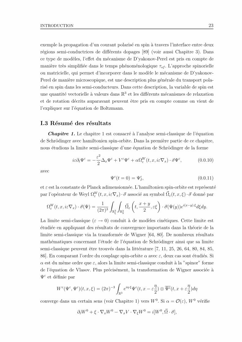
Chapitre 1. Le chapitre 1 est consacre a l’analyse semi-classique de l’equation

de Schrodinger avec hamiltonien spin-orbite. Dans la premiere partie de ce chapitre,

nous etudions la limite semi-classique d’une equation de Schrodinger de la forme

iε∂tΨε = −ε2

2∆xΨ

ε + V εΨε + αΩWε (t, x, iε∇x) · ~σΨε, (0.0.10)

avec

Ψε(t = 0) = ΨεI , (0.0.11)

et ε est la constante de Planck adimensionnee. L’hamiltonien spin-orbite est represente

par l’operateur de Weyl ΩWε (t, x, iε∇x) ·~σ associe au symbol ~Ωε(t, x, ξ) ·~σ donne par

ΩWε (t, x, iε∇x) · ~σ(Ψ) =

1

(2π)3

∫

R3ξ

∫

R3y

~Ωε

(t,

x + y

2, εξ

)· ~σ(Ψ(y))ei(x−y).ξdξdy.

La limite semi-classique (ε → 0) conduit a de modeles cinetiques. Cette limite est

etudiee en appliquant des resultats de convergence importants dans la theorie de la

limite semi-classique via la transformee de Wigner [64, 80]. De nombreux resultats

mathematiques concernant l’etude de l’equation de Schrodinger ainsi que sa limite

semi-classique peuvent etre trouves dans la litterature [7, 11, 25, 26, 64, 80, 84, 85,

86]. En comparant l’ordre du couplage spin-orbite α avec ε, deux cas sont etudies. Si

α est du meme ordre que ε, alors la limite semi-classique conduit a la ”spinor” forme

de l’equation de Vlasov. Plus precisement, la transformation de Wigner associee a

Ψε et definie par

W ε(Ψε, Ψε)(t, x, ξ) = (2π)−3

∫

R3

eiη·ξΨε(t, x− εη

2)⊗Ψε(t, x + ε

η

2)dη

converge dans un certain sens (voir Chapitre 1) vers W 0. Si α = O(ε), W 0 verifie

∂tW0 + ξ · ∇xW

0 −∇xV · ∇ξW0 = i[W 0, ~Ω · ~σ],

24 INTRODUCTION

W 0(0, x, ξ) = WI ,

ou V , ~Ω et WI sont respectivement les limites de V ε, ~Ωε et W ε(ΨεI , Ψ

εI) quand ε → 0.

Par ailleurs, si α est suppose constant par rapport a ε (α = O(1)), on obtient a la

limite un modele cinetique a deux composantes avec un ”splitting” entre les niveaux

d’energie up et down d’ordre |~Ω|. La limite est verifiee dans ce cas en dehors de

l’ensemble E des (t, x, ξ) dans R+ × R6x,ξ ou ~Ω s’annule

E =

(t, x, ξ) ∈ R+ × R6/ ~Ω(t, x, ξ) = 0

.

En d’autres termes, nous avons W 0(t, x, ξ) =1

2wc(t, x, ξ)I2 + ws(t, x, ξ)

~Ω

|~Ω|· ~σ pour

tout (t, x, ξ) ∈ R+ × R6 \ E ou E est l’adherence de E. En plus, les valeurs propres

de W 0, w↑ =wc

2+ ws et w↓ =

wc

2− ws, satisfont

∂tw↑ +∇ξλ↑ · ∇xw↑ −∇xλ↑ · ∇ξw↑ = 0 sur (R+ × R6x,ξ) \ E

∂tw↓ +∇ξλ↓ · ∇xw↓ −∇xλ↓ · ∇ξw↓ = 0 sur (R+ × R6x,ξ) \ E.

Les energies totales up et down, λ↑ and λ↓, sont respectivement donnees par

λ↑(t, x, ξ) =|ξ|22

+ V + |~Ω|, λ↓(t, x, ξ) =|ξ|22

+ V − |~Ω|.

Lorsque les courbes caracteristiques atteignent E, les deux modes d’energies λ↑ et λ↓se croisent et un probleme de transfert d’energie entre eux peut apparaıtre. Plusieurs

travaux mathematiques existent pour decrire l’evolution semi-classique d’un systeme

au dela d’un croisement de modes et pour quantifier le transfert d’energie en termes

de mesures de Wigner a double echelle et formule de Landau-Zener. Nous renvoyons

le lecteur aux travaux de Patrick Gerard et Clotilde Fermanian-Kammerer sur ce

sujet [50, 51, 52, 53, 54].

La deuxieme partie du premier chapitre est consacree a la derivation d’un modele

de sous-bande couple cinetique/quantique. Ce type de modele decrit le transport des

particules dans des systemes partiellement confines tels que les gaz d’electrons bidi-

mensionnels. Dans ces systemes de particules, les differentes directions de l’espace

ne jouent pas le meme role. Le gaz d’electrons est confine dans une (ou plusieurs

directions) et le transport s’effectue dans les autres directions. Dans la direction

du confinement l’echelle spatiale est generalement petite et une description quan-

tique est necessaire ; dans la direction du transport les electrons se comportent d’une

facon classique et un modele cinetique ou fluide peut etre utilise. Cette approche

de couplage directionnel a ete recemment developpee au sein de l’equipe MIP de

l’institut de mathematiques de Toulouse. Dans [15], un modele de sous-bande quan-

tique/cinetique est derive d’un modele entierement quantique par le biais d’une

INTRODUCTION 25

limite semi-classique partielle. L’analyse du modele obtenu a ete ensuite effectuee

dans [14]. La these de N. Vauchelet dirigee par N. Ben Abdallah et F. Mehats [98] a

ete consacree a la derivation et l’etude mathematique et numerique d’un modele

couple quantique/fluide a savoir Derive-Diffusion-Schrodinger-Poisson (voir aussi

[17, 19, 90]). D’autres modeles adiabatiques quantique/fluide sont derives comme

les modeles Schrodinger/SHE et Schrodinger/ET [18]. Notons enfin qu’une autre

strategie de couplage quantique/classique a savoir le couplage spatial existe [6, 9, 34].

Cette approche consiste a decouper le domaine d’etude en plusieurs zones. Chaque

zone est decrite par un modele quantique ou classique et le couplage se fait par des

conditions d’interfaces.

Ici, le confinement a lieu dans une seule direction de l’espace notee z et le trans-

port s’effectue dans la direction orthogonale x. Nous etudions la limite semi-classique

partielle de l’equation de Schrodinger avec terme spin-orbite en suivant [15]. Le point

de depart est l’equation de Schrodinger adimensionnee suivante

iε∂tΨε = −ε2

2∆xΨ

ε − 1

2∂2

zΨε + V εΨε + εΩW

ε (t,x, z, i∇ε) · ~σ(Ψε),

Ψε(0,x, z) = ΨεI(x, z),

(0.0.12)

avec (x, z) ∈ R2 × [0, 1], Ψε = Ψε(t,x, z) et ∇ε = (ε∇x, ∂z). Les sous bandes sont

definies par les elements propres de l’operateur de Schrodinger −12∂2

z + V ε dans la

direction z

−12∂2

zχεp + V εχε

p = εεpχ

εp

χεp(t,x, .) ∈ H1

0 (0, 1),

∫ 1

0

χεpχ

εq = δpq.

(0.0.13)

La limite ε → 0, conduit a un modele de sous bande quantique/cinetique. Plus

precisement, la matrice densite donnee par N ε = Ψε(t,x, z) ⊗ Ψε(t,x, z) converge

dans un certain sens vers N avec

N(t,x, z) =∑p≥1

(∫

R2

Fp(t,x, ξx)dξx

)|χp(t,x, z)|2

ou χp sont les fonctions propres pour ε = 0 et ξx est la variable dual associee a x.

La fonction de distribution de la pieme sous bande satisfait

∂tFp + ξx · ∇xFp −∇xεp · ∇ξxFp = i[Fp, ~Ωp · ~σ],

+ conditions initiales

ou le champ effectif du pieme sous bande, ~Ωp, est donne par

~Ωp(t,x, ξx) =

∫ 1

0

~Ω(t,x, z, ξx)|χp(t,x, z)|2dz. (0.0.14)

26 INTRODUCTION

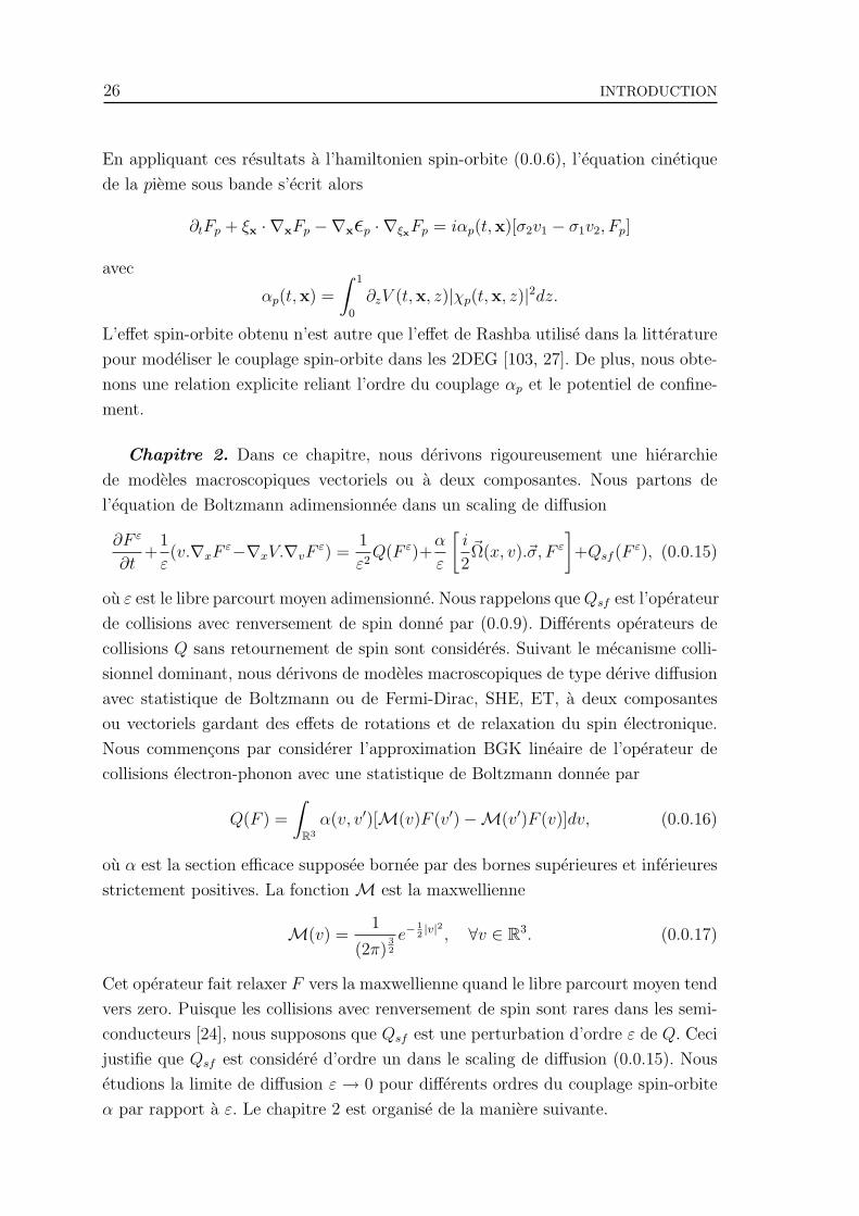
En appliquant ces resultats a l’hamiltonien spin-orbite (0.0.6), l’equation cinetique

de la pieme sous bande s’ecrit alors

∂tFp + ξx · ∇xFp −∇xεp · ∇ξxFp = iαp(t,x)[σ2v1 − σ1v2, Fp]

avec

αp(t,x) =

∫ 1

0

∂zV (t,x, z)|χp(t,x, z)|2dz.

L’effet spin-orbite obtenu n’est autre que l’effet de Rashba utilise dans la litterature

pour modeliser le couplage spin-orbite dans les 2DEG [103, 27]. De plus, nous obte-

nons une relation explicite reliant l’ordre du couplage αp et le potentiel de confine-

ment.

Chapitre 2. Dans ce chapitre, nous derivons rigoureusement une hierarchie

de modeles macroscopiques vectoriels ou a deux composantes. Nous partons de

l’equation de Boltzmann adimensionnee dans un scaling de diffusion

∂F ε

∂t+

1

ε(v.∇xF

ε−∇xV.∇vFε) =

1

ε2Q(F ε)+

α

ε

[i

2~Ω(x, v).~σ, F ε

]+Qsf (F

ε), (0.0.15)

ou ε est le libre parcourt moyen adimensionne. Nous rappelons que Qsf est l’operateur

de collisions avec renversement de spin donne par (0.0.9). Differents operateurs de

collisions Q sans retournement de spin sont consideres. Suivant le mecanisme colli-

sionnel dominant, nous derivons de modeles macroscopiques de type derive diffusion

avec statistique de Boltzmann ou de Fermi-Dirac, SHE, ET, a deux composantes

ou vectoriels gardant des effets de rotations et de relaxation du spin electronique.

Nous commencons par considerer l’approximation BGK lineaire de l’operateur de

collisions electron-phonon avec une statistique de Boltzmann donnee par

Q(F ) =

∫

R3

α(v, v′)[M(v)F (v′)−M(v′)F (v)]dv, (0.0.16)

ou α est la section efficace supposee bornee par des bornes superieures et inferieures

strictement positives. La fonction M est la maxwellienne

M(v) =1

(2π)32

e−12|v|2 , ∀v ∈ R3. (0.0.17)

Cet operateur fait relaxer F vers la maxwellienne quand le libre parcourt moyen tend

vers zero. Puisque les collisions avec renversement de spin sont rares dans les semi-

conducteurs [24], nous supposons que Qsf est une perturbation d’ordre ε de Q. Ceci

justifie que Qsf est considere d’ordre un dans le scaling de diffusion (0.0.15). Nous

etudions la limite de diffusion ε → 0 pour differents ordres du couplage spin-orbite

α par rapport a ε. Le chapitre 2 est organise de la maniere suivante.

INTRODUCTION 27

Nous nous interessons tout d’abord a l’etude des proprietes fondamentales de

l’equation de Boltzmann avec terme spin-orbite (0.0.15). Nous montrons l’existence

et l’unicite de solutions faibles verifiant le principe de maximum. Autrement dit

nous montrons que si initialement F ε(t = 0, x, v) := Fin(x, v) est une fonction a

valeurs dans l’ensemble des matrices carrees hermitiennes et positives que l’on note

par H+2 (C), alors F ε(t, x, v) ∈ H+

2 (C), ∀t > 0 et ∀(x, v) ∈ R6. Nous etablissons en

plus des estimations a priori necessaires pour passer a la limite.

La deuxieme partie est consacree a la derivation des modeles cinetiques et ma-

croscopiques a deux composantes. Nous nous placons dans un regime ou le couplage

spin-orbite est fort de sorte que la periode de rotation du vecteur spin T autour de

~Ω est petite devant le temps caracteristique t. La limite η :=T

t→ 0 est appelee

”limite de decoherence”. Cette limite fait relaxer la partie spin de la fonction de

distribution parallelement au champ effectif considere ~Ω(t, x, v). Dans le cas ou la

direction de ~Ω ne depend pas de v, nous obtenons un modele cinetique a deux com-

posantes en projetant le vecteur distribution de spin suivant la direction de ~Ω(t, x, .).

Partant ensuite de ce dernier modele cinetique et appliquant une limite de diffusion

(ou fluide), nous pouvons deriver des modeles macroscopiques a deux composantes.

Par ailleurs, si ~Ω change de direction avec la vitesse v, une limite de decoherence ap-

pliquee a la spinor forme de l’equation de Boltzmann suivie d’une limite de diffusion

fait relaxer la distribution de spin vers 0 et on obtient a la limite un modele macro-

scopique scalaire sur la densite des charges. Notons que cette relaxation de spin est

bien connue en spintronique des semi-conducteurs et n’est autre que le mecanisme de

relaxation de D’yakonov-Perel [45, 103] presente au debut de ce chapitre introduc-

toire. Ces resultats sont ensuite verifies rigoureusement en passant a la limite ε → 0

dans l’equation (0.0.15) en presence d’un couplage spin-orbite ultra-fort : supposant

α = O(1

ε). Nous montrons aussi que la limite de diffusion dans ce cas aboutit a un

modele diffusif a 2 composantes si~Ω

|~Ω|ne depend pas de v et a un modele scalaire

sinon.

Section 2.5 concerne la derivation d’un modele vectoriel de type derive-diffusion

avec des effets de rotation et de relaxation du vecteur spin. Remarquons tout d’abord

que si les interactions spin-orbite sont faibles telles que α = O(ε) alors, formellement

F ε → F0 lorsque ε tend vers 0 avec Q(F0) = 0. Ceci implique que F0 = N(t, x)M(v)

(voir Chapitre 2). En plus, en integrant l’equation (0.0.15) par rapport a v et passant

a la limite, la matrice densite N verifie

∂tN + divx(D(∇xN +∇xV N)) =i

2[ ~He · ~σ,N ] + Qsf (N)

ou D est une matrice symetrique definie positive. Le champ effectif resultant de cette

28 INTRODUCTION

limite est donne par

~He(x) =

∫

R3

~Ω(x, v)M(v)dv.

En pratique, ~Ω est impaire par rapport a v (voir vecteur de Rashba et de Dresselhauss

par exemple). Ceci implique, puisque M est paire par rapport a v, que ~He = 0 et on

perd l’effet spin-orbite a la limite dans ce cas. Ainsi, pour garder de traces de l’effet

spin-orbite au niveau macroscopique, on etudie la limite de diffusion en supposant

que le terme spin-orbite est d’ordre1

ε(α = O(1)) si ~Ω est impaire par rapport a v.

Nous derivons un modele vectoriel de type derive-diffusion conservant des effets de

rotation et de relaxation du vecteur spin et l’un de ces principaux resultats a savoir

le principe de maximum est verifie.

En suivant la meme strategie qu’on vient de presenter, d’autres modeles macro-

scopiques a deux composantes ou matriciels peuvent etre derives. Nous presentons

a la fin du 2eme chapitre un modele de type SHE dans le cas ou les collisions prises

en comptes sont les collisions elastiques. Nous discutons ensuite la construction des

operateurs de collisions non lineaires conservant certains moments tels que la masse

et l’energie par le principe de minimisation d’entropie. Nous utilisons ensuite ces

operateurs pour derives des modeles de type Energie-Transport et Derive-Diffusion

avec une statistique de Fermi-Dirac par le bias de la methode des moments.

Chapitre 3. Dans ce chapitre, deux applications numeriques sont presentees. La

premiere concerne la simulation d’un transistor a effet de rotation de spin. En suivant

le travail de [19, 90], un modele de sous-bande de derive diffusion Schrodinger-Poisson

avec effets de relaxation et de rotation du vecteur spin dus au couplage de Rashba

est derive et utilise pour la simulation. Le dispositif considere est un MOSFET

a double grille (voir [98] pour plus de details). Nous considerons un cas simple en

supposant que le transport s’effectue dans une seule direction de l’espace. Le vecteur

de precession de Rashba ne change pas de direction dans ce cas. Nous ne considerons

pas des contacts ohmic ferromagnetiques. Nous injectons un courant polarise en

spin dans le plan du dispositif avec une densite de spin parallele a la direction

du transport. Nous montrons numeriquement l’efficacite de l’effet de Rashba pour

controler l’orientation du vecteur spin dans le canal. La direction de spin a l’arrive

au drain est entierement determinee par le potentiel de grille Vgs et le courant de

drain oscille en fonction de Vgs dans ce cas.

Le deuxieme exemple etudie est l’effet de l’accumulation de spin a l’interface

entre deux regions semi-conductrices. C’est un effet bien connu en spintronique des

semi-conducteurs [89, 88]. Deux modeles sont utilises. Cet effet sera represente tout

d’abord en utilisant un modele de derive-diffusion a deux composantes couple avec

l’equation de Poisson. Nous utilisons ensuite un modele vectoriel de derive diffusion

INTRODUCTION 29

couple toujours avec l’equation de Poisson afin d’etudier l’effet de precession de

Rashba sur la densite d’accumulation.

30 INTRODUCTION

II. Diffusion et champs magnetiques forts (Chapter

4)

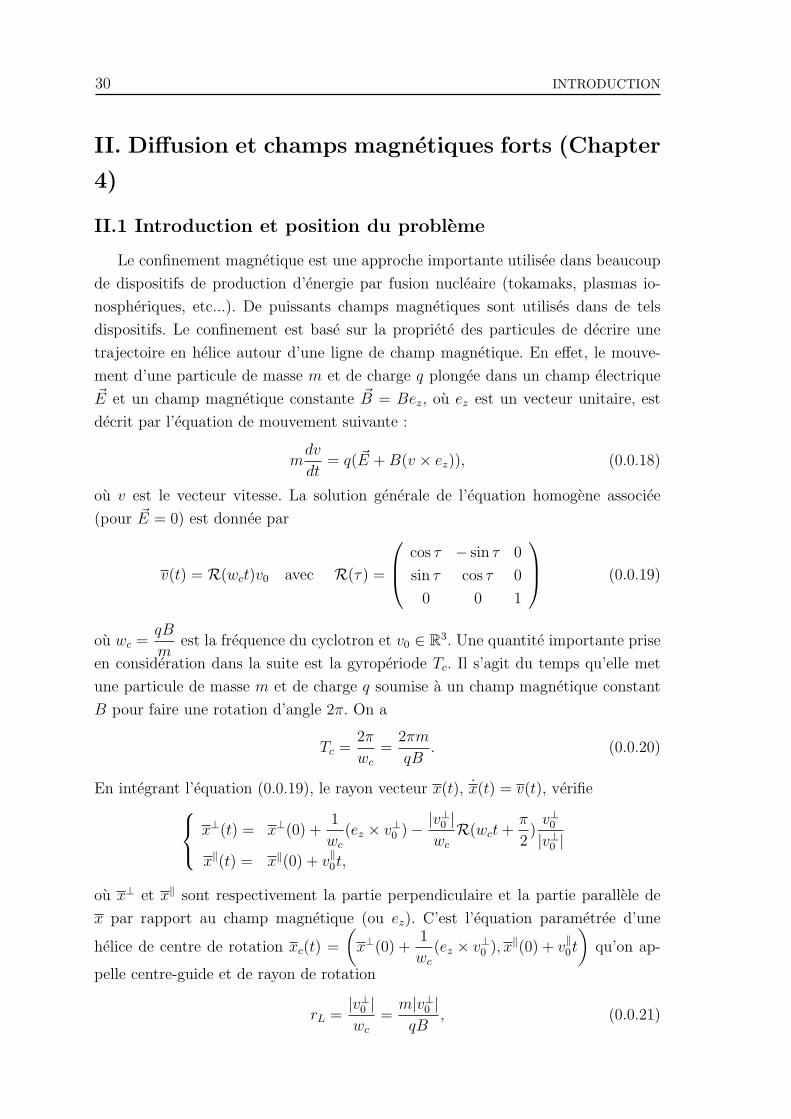
II.1 Introduction et position du probleme

Le confinement magnetique est une approche importante utilisee dans beaucoup

de dispositifs de production d’energie par fusion nucleaire (tokamaks, plasmas io-

nospheriques, etc...). De puissants champs magnetiques sont utilises dans de tels

dispositifs. Le confinement est base sur la propriete des particules de decrire une

trajectoire en helice autour d’une ligne de champ magnetique. En effet, le mouve-

ment d’une particule de masse m et de charge q plongee dans un champ electrique~E et un champ magnetique constante ~B = Bez, ou ez est un vecteur unitaire, est

decrit par l’equation de mouvement suivante :

mdv

dt= q( ~E + B(v × ez)), (0.0.18)

ou v est le vecteur vitesse. La solution generale de l’equation homogene associee

(pour ~E = 0) est donnee par

v(t) = R(wct)v0 avec R(τ) =

cos τ − sin τ 0

sin τ cos τ 0

0 0 1

(0.0.19)

ou wc =qB

mest la frequence du cyclotron et v0 ∈ R3. Une quantite importante prise

en consideration dans la suite est la gyroperiode Tc. Il s’agit du temps qu’elle met

une particule de masse m et de charge q soumise a un champ magnetique constant

B pour faire une rotation d’angle 2π. On a

Tc =2π

wc

=2πm

qB. (0.0.20)

En integrant l’equation (0.0.19), le rayon vecteur x(t), x(t) = v(t), verifie

x⊥(t) = x⊥(0) +1

wc

(ez × v⊥0 )− |v⊥0 |wc

R(wct +π

2)

v⊥0|v⊥0 |

x‖(t) = x‖(0) + v‖0t,

ou x⊥ et x‖ sont respectivement la partie perpendiculaire et la partie parallele de

x par rapport au champ magnetique (ou ez). C’est l’equation parametree d’une

helice de centre de rotation xc(t) =

(x⊥(0) +

1

wc

(ez × v⊥0 ), x‖(0) + v‖0t

)qu’on ap-

pelle centre-guide et de rayon de rotation

rL =|v⊥0 |wc

=m|v⊥0 |qB

, (0.0.21)

INTRODUCTION 31

appele rayon de Larmor et qui est inversement proportionnel au module du champ

magnetique B. Ceci implique que, lorsque B augmente et tend vers l’infini, le rayon

de Larmor tend vers zero et les particules sont piegees le long de la ligne du champ

magnetique. En presence d’un champ electrique, la solution de (0.0.18) est donnee

par la solution generale de l’equation homogene v plus une solution particuliere vpart

de (0.0.18). On a v‖part =

q ~E‖

mt et on cherche une solution particuliere stationnaire

dans la direction perpendiculaire. Ceci implique que ~B × v⊥part = ~E et donc

v⊥part =~E × ~B

B2. (0.0.22)

On en deduit que le rayon vecteur en presence d’un champ electrique est donne par

x⊥(t) = x⊥(0) + 1wc

(ez × v⊥0 ) +~E × ~B

B2t− rLR(wct +

π

2)~v⊥0v⊥0

x‖(t) = x‖(0) + (v‖0 +

q ~E‖

m)t.

Par consequent, un champ electrique perpendiculaire a ~B n’accelere pas les particules

mais cree une derive uniforme du centre-guide dans la direction ~E × ~B avec une

vitesse (appelee vitesse de derive du centre-guide) inversement proportionnelle a

B2, et donnee exactement par (0.0.22).

La presence d’un champ magnetique fort dans les equations cinetiques (Vlasov,

Boltzmann) introduit de fortes oscillations et donc des difficultes pour la simula-

tion numerique. La question de trouver des modeles approximatifs moins couteux

numeriquement que les modeles cinetiques est tres importante dans ce sujet. Differents

modeles approximatifs existent dans la litterature tels que les modeles centre-guide et

gyrocinetiques. Ces modeles consistent a moyenner le mouvement sur la gyroperiode

tout en supposant que B tend vers l’infini. Nous referons a une liste de travaux

physiques sur ce type de modeles [77, 81, 87, 44]. De point de vue mathematique, E.

Sonnendrucker et E. Frenod ont etudie la limite champ magnetique fort du systeme

Vlasov et Vlasov-Poisson par des techniques d’homogeneisation [59, 60]. Dans [59],

il a ete montre que l’approximation centre-guide de l’equation de Vlasov 3D conduit

a une equation cinetique unidimensionnelle dans la direction du champ magnetique.

La derive du centre-guide est obtenue ensuite dans [60] en etudiant la limite centre-

guide de l’equation de Vlasov 2D (dans la direction perpendiculaire au champ) dans

un echelle de temps suffisamment long. L’investigation de l’equation de Vlasov et du

systeme Vlasov-Poisson en presence d’un champ magnetique fort est intensivement

etudiee pour differents regimes asymptotiques [57, 58, 61, 62, 68, 69, 96, 97].

Dans toutes les references precedentes, le transport est suppose balistique (sans

collisions). Nous sommes interesses ici par des regimes ou les collisions sont impor-

tantes et nous etudions l’asymptotique de diffusion de l’equation de Boltzmann en

32 INTRODUCTION

presence d’un champ magnetique fort. L’equation de Boltzmann dans le scaling de

diffusion s’ecrit [95, 67]

ε∂tfε + (v · ∇rfε + E · ∇vfε) + α(v × ez) · ∇vfε =Q(fε)

ε

ou r = (x, y, z) est le vecteur position, v = (vx, vy, vz) est la variable vitesse, et ε =τ

t¿ 1 est le libre parcourt moyen adimensionne avec t et le temps caracteristique.

Le champ magnetique est suppose constant et parallele a l’axe des z de vecteur

unitaire ez. Nous notons par r⊥ = (x, y) et v⊥ = (vx, vy) les variables orthogonales.

Le parametre α−1 represente la gyroperiode adimensionnee ou

α = twc =2πt

Tc

.

Nous considerons dans ce travail pour simplifier la forme BGK lineaire de l’operateur

des collisions electron-phonon donne par (0.0.16)-(0.0.17). Le modele fluide obtenu

lorsque ε tend vers zero est alors de type derive-diffusion. Si la gyroperiode est plus

grande que le temps de relaxation τ ou si α est constante devant ε (α = O(1)) alors

l’effet du champ magnetique disparaıt a la limite. D’autre part, si Tc est du meme

ordre que le temps de relaxation ou bien si α = O(ε−1), l’equation de Boltzmann

devient

∂tfBε +

1

ε(v · ∇rf

Bε + E · ∇vfBε ) +

Bε2

(v × ez) · ∇vfBε =

Q(fBε )

ε2(0.0.23)

ou B est une constante strictement positive telle que α =Bε

. Ce scaling de diffusion

est utilise generalement pour les plasmas et les gas binaires. La matrice de diffusion

dans le modele limite admet une composante antisymetrique dans ce cas generee par

le champ magnetique. Ce resultat est prouve par P. Degond et al [31, 35, 39] pour

des collisions avec des murs. D’autres resultats formels concernant les gaz binaires

se trouvent aussi dans [33, 37, 38, 83].

Dans ce travail, nous considerons une situation ou la gyroperiode Tc est plus

petite que le temps de relaxation. Ce qui revient a supposer que B est grand et

tend vers l’infini. Nous allons voir que le scaling de diffusion standard (0.0.23) n’est

pas convenable pour decrire, quand ε → 0 et B → +∞, la dynamique du centre-

guide dans la direction perpendiculaire au champ magnetique. Il decrit seulement le

transport diffusif dans la direction parallele. Un autre scaling est propose pour lequel

la limite de diffusion avec B → +∞ conduit a un modele de derive-diffusion dans

la direction parallele au champ magnetique et dans la direction perpendiculaire, le

transport est domine par la derive du centre-guide. Afin de mieux comprendre ce

qui se passe a la limite, nous considerons l’approximation du temps de relaxation de

l’operateur de collisions

Q(f) = n(t, x)M(v)− f, n(t, x) =

∫

R3

f(t, x, v)dv. (0.0.24)

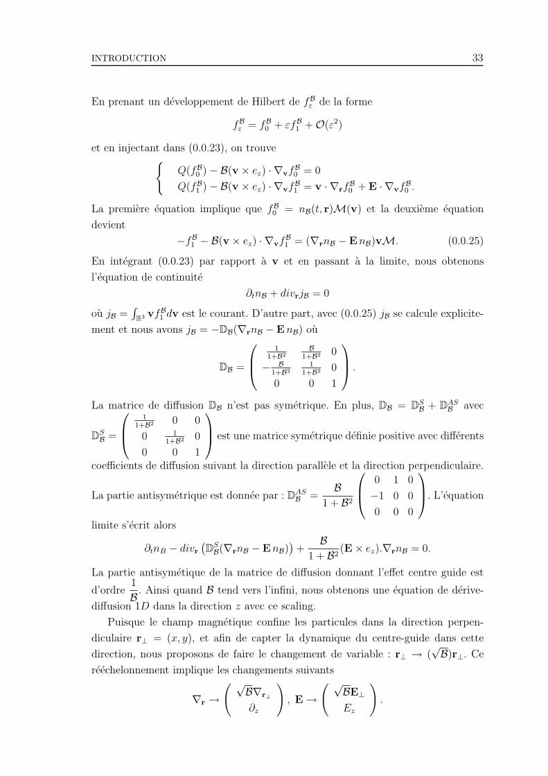
INTRODUCTION 33

En prenant un developpement de Hilbert de fBε de la forme

fBε = fB0 + εfB1 +O(ε2)

et en injectant dans (0.0.23), on trouve

Q(fB0 )− B(v × ez) · ∇vfB0 = 0

Q(fB1 )− B(v × ez) · ∇vfB1 = v · ∇rfB0 + E · ∇vfB0 .

La premiere equation implique que fB0 = nB(t, r)M(v) et la deuxieme equation

devient

−fB1 − B(v × ez) · ∇vfB1 = (∇rnB − EnB)vM. (0.0.25)

En integrant (0.0.23) par rapport a v et en passant a la limite, nous obtenons

l’equation de continuite

∂tnB + divrjB = 0

ou jB =∫R3 vfB1 dv est le courant. D’autre part, avec (0.0.25) jB se calcule explicite-

ment et nous avons jB = −DB(∇rnB − EnB) ou

DB =

11+B2

B1+B2 0

− B1+B2

11+B2 0

0 0 1

.

La matrice de diffusion DB n’est pas symetrique. En plus, DB = DSB + DAS

B avec

DSB =

11+B2 0 0

0 11+B2 0

0 0 1

est une matrice symetrique definie positive avec differents

coefficients de diffusion suivant la direction parallele et la direction perpendiculaire.

La partie antisymetrique est donnee par : DASB =

B1 + B2

0 1 0

−1 0 0

0 0 0

. L’equation

limite s’ecrit alors

∂tnB − divr

(DSB(∇rnB − EnB)

)+

B1 + B2

(E× ez).∇rnB = 0.

La partie antisymetique de la matrice de diffusion donnant l’effet centre guide est

d’ordre1

B . Ainsi quand B tend vers l’infini, nous obtenons une equation de derive-

diffusion 1D dans la direction z avec ce scaling.

Puisque le champ magnetique confine les particules dans la direction perpen-

diculaire r⊥ = (x, y), et afin de capter la dynamique du centre-guide dans cette

direction, nous proposons de faire le changement de variable : r⊥ → (√B)r⊥. Ce

reechelonnement implique les changements suivants

∇r →( √B∇r⊥

∂z

), E →

( √BE⊥Ez

).

34 INTRODUCTION

Pour simplifier la presentation, nous posons B =1

η2ou η est un petit parametre

destine a tendre vers zero. Dans ce travail, la fonction de distribution depend de

deux petits parametres ε et η. Elle verifie l’equation de Boltzmann adimensionnee

suivante

∂f εη

∂t+Tzf

εη

ε+T⊥f εη

εη+

(v × ez)

ε2η2· ∇vf εη =

Q(f εη)

ε2

f εη(t = 0) = f0(r,v).(0.0.26)

Ici, T⊥ and Tz sont respectivement les parties perpendiculaire et parallele de l’operateur

de transport

T⊥ = v⊥ · ∇r⊥ + E⊥ · ∇v⊥ , Tz = vz∂z + Ez∂vz .

II.2 Resultats obtenus

Nous etudions le cas ou ε tend vers zero pour η donne et ensuite η tend vers zero

et le cas ou ε et η tendent vers zero simultanement. Le premier resultat concerne la

limite de diffusion ε → 0 pour η fixe. Nous montrons que (f εη)ε converge dans un

certain sens (voir Chapitre 4) vers ρη(t, r)M(v) et la densite ρη verifie

∂tρη − div(Dη(∇ρη − ρηE)) = 0. (0.0.27)

La matrice de diffusion Dη est donnee par la formule

Dη =

∫ (1ηv⊥vz

)⊗

(ηXη

⊥Xη

z

)dv,

Xη =

Xη

⊥

Xηz

etant l’unique solution de

−Q(Xη)+v × ez

η2·∇v(Xη) =

1

η2v⊥

vz

M(v) and

∫

R3

Xη(v)dv = 0. (0.0.28)

Dans l’approximation du temps de relaxation σ(v,v′) = 1τ, la matrice Dη se calcule

explicitement

Dη = τ

η2

τ2+η4τ

τ2+η4 0

− ττ2+η4

η2

τ2+η4 0

0 0 1

.

A la limite η → 0, le bloc superieure de cette matrice se reduit a I =

0 1

−1 0

et sa partie symetrique est d’ordre η2. Nous obtenons ces resultats dans le cas ou

INTRODUCTION 35

la section σ est non constante. Nous developpons rigoureusement Xη par rapport a

η jusqu’a l’ordre η4. Ceci nous donne un developpement des parties symetrique et

antisymetrique de Dη en fonction de η. Nous montrons que la diffusion est d’ordre 1

dans la direction parallele et d’ordre η2 dans la direction perpendiculaire. La partie

antisymetrique Dηas agit dans la direction perpendiculaire. Elle est donnee par la

matrice I a l’ordre principale ce qui conduit a la derive du centre-guide. En plus,

le developpement de Dηas donne une correction d’ordre η a la dynamique du centre-

guide. Nous renvoyons le lecteur au Chapitre 4 pour plus de details.

Le deuxieme resultat concerne la limite simultanee ε, η → 0. Nous montrons que

f εη → ρ(t, r)M(v) avec

∂tρ + ∂zJz +∇r · (ρE× ez) = 0

ρ(0, r) =

∫

R3

f0(r,v) dv(0.0.29)

Le courant parallele est donne par

Jz = −Dz(∂zρ− Ezρ)

ou Dz est la constante de diffusion

Dz =

∫

R3

X(0)z vzdv,

et X(0)z est le terme d’ordre zero de Xη

z . C’est une fonction isotrope (invariante par

rotation autour de ez) verifiant

−Q(X(0)z ) = vzM,

∫

R3

X(0)z (v)dv = 0

avec

Q(f)(v) =

∫

R3

σ(v,v′)[M(v)f(v′)−M(v′)f(v)]dv′

et

σ (v,v′) =1

4π2

∫ 2π

0

∫ 2π

0

σ (R(τ)v,R(τ ′)v′) dτdτ ′.

L’equation limite (0.0.29) est composee d’un courant de derive-diffusion dans la di-

rection parallele et d’une derive due au mouvement du centre-guide dans la direction

perpendiculaire. Le coefficient de diffusion parallele Dz est obtenu via l’analyse d’un

operateur de collisions avec une section efficace moyennee sur les cercles de gyration

autour du champ magnetique.

36 INTRODUCTION

III. Confinement (Chapitre 5)

III.1 Motivation et description du probleme

Afin de mieux controler le transport electronique, de nombreux dispositifs electron-

iques sont bases sur la reduction de la dimensionalite en confinant les electrons dans

une ou plusieurs directions de l’espace. Parmi eux, nous avons les gas d’electrons

bidimensionnels (2DEG) [1, 74] dont les electrons sont confines dans une seule di-

rection.

Le systeme Schrodinger-Poisson est l’un des modeles les plus appropries pour

decrire le transport quantique balistique (sans collisions) des particules charges dans

les semi-conducteurs ainsi qu’en chimie quantique. Dans [94, 93, 92], la simulation

du transport electronique dans les gaz d’electrons bidimensionnels balistiques a ete

realisee grace a la derivation d’un modele approche permettant de tenir compte

de maniere moyennee de l’effet du potentiel de confinement sur le transport quan-

tique. Le modele propose admet un avantage considerable d’etre moins couteux

numeriquement et de rester en accord complet avec le model 3D de point de vue

physique. L’analyse rigoureuse de cette approximation a ensuite ete effectuee dans

[16, 91] dans le cas ou le profil du potentiel de confinement Vc et l’echelle spatiale

de ses variations ε sont supposes donnes. Dans [16], l’approximation est justifiee en

effectuant une etude asymptotique lorsque ε tend vers zero de la solution du systeme

de Schrodinger-Poisson tridimensionnel suivant

i∂tψε = −1

2∆x,zψ

ε + V εψε + V εc ψε,

V ε =1

4π√|x|2 + z2

∗ (|ψε|2),

ou x ∈ R2 et z ∈ R est la direction de confinement. Le potentiel V ε est le potentiel

auto-consistant et V εc est le potentiel de confinement impose au systeme et donne

par

V εc =

1

ε2Vc(

z

ε), (0.0.30)

ou Vc est une fonction donnee. Le cas stationnaire dans un domaine borne est traite

dans [91].

Le but de ce travail est en quelque sorte de justifier le scaling (0.0.30) par l’analyse

d’un systeme de Schrodinger-Poisson unidimensionnel (dans la direction de confine-

ment z). De ce fait, nous ignorons le transport des particules dans la direction ortho-

gonale a l’axe des z en supposant par exemple que le systeme est invariant dans cette

direction. Le parametre ε n’est pas donne mais calcule en fonction de la longueur de

Debye adimensionnee. Le systeme est suppose ferme et occupe l’intervalle [0, 1]. Les

INTRODUCTION 37

electrons se repartissent dans ce cas sur des niveaux d’energies discrets qui sont les

valeurs propres de l’operateur de Schrodinger − d2

dz2 + V . La densite totale de parti-

cules est la superposition des densites de tous les niveaux d’energies avec un facteur

d’occupation donne par la statistique de Boltzmann. Le potentiel electrostatique de

confinement est note par Vε. Le point de depart est le systeme Schrodinger-Poisson

unidimensionnel stationnaire verifie par Vε suivant

−d2ϕp

dz2+ V ϕp = Epϕp z ∈ [0, 1],

ϕp ∈ H1(0, 1), ϕp(0) = 0, ϕp(1) = 0,

∫ 1

0

ϕpϕq = δpq

−ε3d2V

dz2=

1

Z+∞∑p=1

e−Ep|ϕp|2, Z =+∞∑p=1

e−Ep

V (0) = 0,dV

dz(1) = 0.

(0.0.31)

Le scaling menant a ce systeme sera detaille. Le parametre ε est donne en fonction

de la longueur de Debye adimensionnee, λD, par

ε3 = (λD

L)2, λD =

√kBTε0εr

e2N(0.0.32)

avec L est la longueur caracteristique dans la direction z, e est la charge elementaire,

et N =Ns

Lest la densite volumique moyenne avec Ns le nombre total de particules

(ou la densite surfacique). Le parametre ε est suppose petit et tend vers zero. Ceci

correspond a la limite faible longueur de Debye ou faible temperature ou forte densite

(vu la relation (0.0.32)). A la limite (ε → 0), les fonctions d’ondes se concentrent au

point z = 0. Afin d’analyser cette couche limite, un zoom est effectue au voisinage

de z = 0 via le changement de variables suivant

ϕp(z) =1√εψp(

z

ε), Ep =

1

ε2Ep, V (z) =

1

ε2U(

z

ε), ξ =

z

ε. (0.0.33)

L’equation de Poisson dans (0.0.31) devient −d2U

dξ2=

1

Z+∞∑p=1

e−Ep

ε2 |ψp|2 avec Z =

+∞∑p=1

e−Ep

ε2 . Les valeurs propres (Ep)p sont simples, distinctes et forment une suite

croissante par rapport a p pour tout ε > 0. Nous montrerons de plus l’existence d’un

gap strictement positif separant le premier niveau d’energie E1 et les autres Ep(p ≥2) uniformement par rapport a ε. Ceci implique que les facteurs d’occupations e

−Ep

ε2

pour p ≥ 2 sont tous negligeables devant le premier (p = 1) quand ε devient petit. Il

est donc naturel de pretendre que le modele (0.0.31) est asymptotiquement proche

38 INTRODUCTION

de

−d2ϕ1

dz2+ V ϕ1 = E1ϕ1 z ∈ [0, 1],

E1 = infϕ∈H1

0 (0,1),‖ϕ‖L2=1

∫ 1

0

|ϕ′|2 +

∫ 1

0

V ϕ2

,

−ε3d2V

dz2= |ϕ1|2,

V (0) = 0,dV

dz(1) = 0

(0.0.34)

dans lequel seul le premier niveau d’energie est pris en compte. Ceci est en accord

avec les simulations numeriques [94]. Dans ce travail, nous montrons rigoureuse-

ment que ces deux modeles sont asymptotiquement proches et nous estimons leur

difference en fonction de ε. Nous montrons qu’elle decroıt exponentiellement. De

plus, nous prouvons qu’a la limite ε → 0, le potentiel Vε solution de (0.0.34) converge

vers un potentiel de couche limite de la forme1

ε2U0(

.

ε) avec un profil U0 verifiant

un systeme de Schrodinger-Poisson unidimensionnel sur le demi axe reel :

−d2ψ1

dξ2+ Uψ1 = E1ψ1 ξ ∈ [0, +∞[,

E1 = infψ∈H1

0 (R+),‖ψ‖L2=1

∫ +∞

0

|ψ′|2 +

∫ +∞

0

Uψ2

,

−d2U

dξ2= |ψ1|2,

U(0) = 0,dU

dξ∈ L2(R+).

(0.0.35)

III.2 Resultats obtenus

Les modeles (0.0.31) et (0.0.34) sont bien poses et admettent des solutions

uniques. L’etude du probleme Schrodinger-Poisson sur un domaine borne est ef-

fectuee par F. Nier [84, 85, 86] en le reformulant en un probleme de minimisation

convexe. Le systeme limite (0.0.35) quand a lui est pose sur [0,∞[. Le premier

resultat du Chapitre 5 concerne l’etude de ce modele (Theoreme 5.1.1). Nous sommes

amenes a etudier aussi un probleme de minimisation pose sur un domaine non borne.

Cette etude est realisee grace au principe de concentration-compacite introduit par

P. L. Lions [79]. Le deuxieme resultat concerne la comparaison de differents systemes

presentes ci-dessus. Nous obtenons le theoreme suivant.

Theorem 0.0.1. Soit Vε, Vε et U0 les potentiels satisfaisant (0.0.31), (0.0.34) et

(0.0.35) respectivement. Les estimations suivantes sont verifiees

‖Vε − Vε‖H1(0,1) = O(e−c

ε2 ),

REFERENCES 39

‖Vε − 1

ε2U0(

.

ε)‖H1(0,1) = O(e−

cε ),

ou c est une constante generique strictement positive et independante de ε.

III.3 Commentaires

Le choix de condition au bord de type Newmann pour le potentiel au point z = 1

est justifie dans certaines situations physiques [5]. Les conditions de Dirichlet sont

plus habituelles dans ce type de modele. Dans ce cas, l’analyse peut etre effectuee

mais comporte des complexites techniques liees au fait qu’une autre couche limite

apparaıt au point z = 1 et que les valeurs propres admettent asymptotiquement une

multiplicite double. Pour simplifier, nous avons donc impose des conditions de type

Newmann en z = 1.

Il est plus naturel d’utiliser une statistique de Fermi-Dirac dans la limite forte

densite. Cette etude peut etre generalisee au cas Fermi-Dirac avec quelques compli-

cations techniques (voir derniere section du Chapitre 5 pour plus de details).

Enfin, le probleme multidimensionnel est beaucoup plus complique. La locali-

sation de la couche limite dans ce cas peut dependre de la geometrie de bord du

domaine considere. Ce type de probleme est present dans l’etude de l’equation de

Schrodinger avec champ magnetique [21, 75].

References

[1] T. Ando, A. B. Fowler, and F. Stern, Electronic properties of two-

dimensional electron systems, Rev. Mod. Phys., 54, 2 (1982), p. 437.

[2] C. Bardos, F. Golse, and C. D. Levermore, Fluid dynamic limits of

kinetic equations. II. Convergence proofs for the Boltzmann equation, Comm.

Pure Appl. Math., 46 (1993), pp. 667–753.

[3] C. Bardos, F. Golse, and D. Levermore, Fluid dynamic limits of kinetic

equations. I. Formal derivations, J. Statist. Phys., 63 (1991), pp. 323–344.

[4] , The acoustic limit for the Boltzmann equation, Arch. Rational. Mech.

Ana., 153 (2000), pp. 177–204.

[5] G. Bastard, Wave mechanics applied to semiconductor heterostructures, Les

editions de physiques, 1996.

[6] N. Ben Abdallah, A hybrid kinetic-quantum model for stationary electron

transport, J. Stat. Phys., 90 (1998), pp. 627–662.

[7] , On a multidimensional Schrodinger-Poisson scattering model for semi-

conductors, J. Math. Phys., 41 (2000), pp. 4241–4261.

40 REFERENCES

[8] N. Ben Abdallah and P. Degond, On a hierarchy of macroscopic models

for semiconductors, J. Math. Phys., 37 (1996), pp. 3306–3333.

[9] N. Ben Abdallah, P. Degond, and I. Gamba, Coupling one dimensional

time dependent classical and quantum transport models, J. Math. Phys., 43

(2002), pp. 1–24.

[10] N. Ben Abdallah, P. Degond, and S. Genieys, An Energy-Transport

model derived from the Boltzmann equation of semiconductors, J. Stat. Phys.,

84 (1996), pp. 205–231.

[11] N. Ben Abdallah, P. Degond, and P. A. Markowich, On a One-

Dimensional Schrodinger-Poisson Scattering Model, ZAMP, 48 (1997), pp. 35–

55.

[12] N. Ben Abdallah, S. Desvillettes, and S. Genieys, On the conver-

gence of the Boltzmann for the semiconductors toward the energy transport

model, J. Stat. Phys., 98 (2000), pp. 835–870.

[13] N. Ben Abdallah and R. El Hajj, Diffusion and guiding center approxi-

mation for particle transport in strong magnetic fields, Kinetic and Related

Models, Vol. 1, No. 3 (2008), pp. 124–146.

[14] N. Ben Abdallah and F. Mehats, On a Vlasov Schrodinger Poisson

model, Comm. Partial Differential Equations, 29 (2004), pp. 173–206.

[15] N. Ben Abdallah and F. Mehats, Semiclassical analysis of the Schrodin-

ger equation with a partially confining potential, J. Math. Pures Appl. (9), 84

(2005), pp. 580–614.

[16] N. Ben Abdallah, F. Mehats, and O. Pinaud, Adiabatic approximation

of the Schrodinger-Poisson system with a partial confinement, SIAM J. Math.

Anal., 36 (2004/2005), pp. 986–1013.

[17] N. Ben Abdallah and F. Mehats, On a Vlasov-Schrodinger-Poisson Mo-

del , Comm. Partial Differential Equations, 29 (2004), pp. 173–206.

[18] N. Ben Abdallah, F. Mehats, and C. Negulescu, Adiabatic quantum-

fluid transport models, Comm. Math. Sci., 4 (2006), pp. 621–650.

[19] N. Ben Abdallah, F. Mehats, P. Pietra, and N. Vauchelet, A drift-

diffusion subband model for the simulation of the double-gate mosfet, IEEE-

NANO 2005, Conference on Nanotechnology, Nagoya.

[20] N. Ben Abdallah, F. Mehats, and N. Vauchelet, Analysis of a

Drift-Diffusion-Schrodinger-Poisson model, C.R. Acad. Sci. Paris, Ser. I 335,

pp. 1007–1012.

REFERENCES 41

[21] V. Bonnaillie, On the fundamental state energy for a Schrodinger operator

with magnetic field in domains with corners, Asymptotic Analysis, 41 (2005),

pp. 215–258.

[22] F. Bouchut, F. Golse, and M. Pulvirenti, Kinetic equations and

asymptotic theory, B. perthame, L. Desvillettes Eds, Series in Appl. Math.,

bf 4, Gauthier-Villars (2000).

[23] J. P. Bourgade, On spherical harmonics expansion type models for electron-

phonon collisions, Math. Methods Appl. Sci., 23 (2003), pp. 247–271.

[24] A. Bournel, Magneto-electronique dans des dispositifs a semiconducteurs,

Ann. Phys. Fr, 25 (2000), pp. 1–167.

[25] F. Brezzi and P. A. Markowich, A mathematical analysis of quantum

transport in three dimensional systems, Anna. di Matematica Pura Applicata,

160 (1991), pp. 171–191.

[26] , The three-dimensional Wigner-Poisson problem : existence, uniqueness

and approximation, Math. Methods Appl. Sci., 14 (1991), pp. 35–61.

[27] Y. A. Bychkov and E. I. Rashba, Oscillatory effects and the magnetic

susceptibility of carriers in inversion layers, Journal of Physics C : Solid State

Physics, 17 (1984), pp. 6039–6045.

[28] C. Cercignani, The Boltzmann equation and its applications, Springer-

Verlag, Berlin, 1988.

[29] E. U. Condon and G. H. Shortley, The theory of atomic spectra, Cam-

bridge University Press, Cambridge, 1953.

[30] S. Datta and B. Das, Electronic analog of the electro-optic modulator, Ap-

plied Physics Letters, 56 (1990), pp. 665–667.

[31] P. Degond, A model of near-wall conductivity and its application to plasma

thrusters, SIAM J. Appl. Math., 58 (1998), pp. 1138–1162 (electronic).

[32] , An infinite system of diffusion equations arising in transport theory : the

coupled Spherical Harmonic Expansion model, Math. Models Methods Appl.

Sci., 11 (2001), pp. 903–932.

[33] P. Degond, Asymptotic continuum models for plasmas and disparate mass

gaseous binary mixtures, Material Substructures in Complex Bodies, Elsevier,

(2007).

[34] P. Degond and A. El Ayyadi, A coupled Schrodinger drift-diffusion model

for quantum semiconductor device simulations, J. Comp. Phys., 181 (2002),

pp. 222–259.

42 REFERENCES

[35] P. Degond, V. Latocha, S. Mancini, and A. Mellet, Diffusion dyna-

mics of an electron gas confined between two plates, Methods Appl. Anal., 9

(2002), pp. 127–150.

[36] P. Degond, C. D. Levermore, and C. Schmeiser, A note on the energy-

transport limit of the semiconductor Boltzmann equation, IMA Vol. Math.

Appl., 135 (2004), pp. 137–153.

[37] P. Degond and B. Lucquin-Desreux, The asymptotics of collision ope-

rators for two species of particles of disparate masses, Math. Models Methods

Appl. Sci., 6 (1996), pp. 405–436.

[38] P. Degond and B. Lucquin-Desreux, Transport coefficients of plasmas

and disparate mass binary gases, Transport Theory Statist. Phys., 25 (1996),

pp. 595–633.

[39] P. Degond and S. Mancini, Diffusion driven by collisions with the boun-

dary, Asymptot. Anal., 27 (2001), pp. 47–73.

[40] P. Degond, F. Mehats, and C. Ringhofer, Quantum hydrodynamic mo-

dels derived from the entropy principle, Contemp. Math. 371, Amer. Math.

Soc., Providence RI (2005).

[41] , Quantum energy-transport and drift-diffusion models, J. Stat. Phys., 118

(2005), pp. 625–667.

[42] P. Degond and C. Schmeiser, Macroscopic models for semiconductor he-

terostructures, J. Math. Phys., 39 (1998), pp. 4634–4663.

[43] G. Dresselhaus, Spin-Orbit Coupling Effects in Zinc Blende Structures,

Phys. Rev., 100 (1955), pp. 580–586.

[44] D. H. E. Dubin, J. A. Krommes, C. Oberman, and W. W. Lee, Non-

linear gyrokinetic equations, Physics of Fluids, 26 (1983), pp. 3524–3535.

[45] M. I. D’yakonov and V. Y. Kachorovskii, spin relaxation of two-

dimensional electrons in noncentrosymmetric semiconductors, Sov. Phys. Se-

micond., 20 (1986), pp. 110–112.

[46] R. El Hajj, On an hierarchy of kinetic and macroscopic models for semicon-

ductor Spintronics, in preparation.

[47] R. El Hajj, On spin transport models and application to numerical simulation

of transistors with spin rotational effect, in preparation.

[48] R. El Hajj and N. Ben Abdallah, High density limit of the stationary

one dimensional Schrodinger–Poisson system, Multiscale Modeling and Simu-

lation, 7 (2008), pp. 124–146.

REFERENCES 43

[49] R. J. Elliott, Theory of the Effect of Spin-Orbit Coupling on Magnetic

Resonance in Some Semiconductors, Phys. Rev., 96 (1954), pp. 266–279.

[50] C. Fermanian-Kammerer and P. Gerard, Mesures semi-classiques et

croisement de modes, Seminaire Equations aux derivees partielles (Polytech-

nique) (1999-2000), Art. No. 17, 13 p.

[51] , Une formule de Landau-Zener pour un croisement non degenere et invo-

lutif de codimension 3, C. R. Math. Acad. Sci. Paris, 335 (2002), pp. 915–920.

[52] , A Landau-Zener formula for non-degenerated involutive codimension 3

crossings, Ann. Henri Poincare, 4 (2003), pp. 513–552.

[53] C. Fermanian-Kammerer and P. Gerard, A Landau-Zener formula for

two-scaled Wigner measures, in Dispersive transport equations and multiscale

models (Minneapolis, MN, 2000), vol. 136 of IMA Vol. Math. Appl., Springer,

New York, 2004, pp. 167–177.

[54] C. Fermanian-Kammerer and P. Gerard, Two-scale Wigner measures

and the Landau-Zener formulas, in Multiscale methods in quantum mechanics,

Trends Math., Birkhauser Boston, Boston, MA, 2004, pp. 59–68.

[55] A. Fert, A. Friederich, and al, Giant Magnetoresistance of

(001)Fe/(001)Cr Magnetic Superlattices, Phys. Rev. Lett., 61 (1988), p. 2472.

[56] G. Fishman and G. Lampel, Spin relaxation of photoelectrons in p-type

gallium arsenide, Phys. Rev. B, 16 (1977), pp. 820–831.

[57] E. Frenod and K. Hamdache, Homogenisation of transport kinetic equa-

tions with oscillating potentials, Proc. Roy. Soc. Edinburgh Sect. A, 126 (1996),

pp. 1247–1275.

[58] E. Frenod, P.-A. Raviart, and E. Sonnendrucker, Two-scale expan-

sion of a singularly perturbed convection equation, J. Math. Pures Appl. (9),

80 (2001), pp. 815–843.

[59] E. Frenod and E. Sonnendrucker, Homogenization of the Vlasov equa-

tion and of the Vlasov-Poisson system with a strong external magnetic field,

Asymptot. Anal., 18 (1998), pp. 193–213.

[60] E. Frenod and E. Sonnendrucker, Long time behavior of the two-

dimensional Vlasov equation with a strong external magnetic field, Math. Mo-

dels Methods Appl. Sci., 10 (2000), pp. 539–553.

[61] E. Frenod and E. Sonnendrucker, The finite Larmor radius approxima-

tion, SIAM J. Math. Anal., 32 (2001), pp. 1227–1247 (electronic).

[62] E. Frenod and F. Watbled, The Vlasov equation with strong magnetic

field and oscillating electric field as a model for isotop resonant separation,

Electron. J. Differential Equations, (2002, No. 06), p. 20 (electronic).

44 REFERENCES

[63] P. Gerard, Mesures semi-classiques et ondes de Bloch, Seminaire sur les

Equations aux Derivees Partielles, Ecole Polytech., (1991), pp. Exp. No. XVI,

19.

[64] P. Gerard, P. A. Markowich, N. J. Mauser, and F. Poupaud, Homo-

genization limits and Wigner transforms, Comm. Pure Appl. Math., 50 (1997),

pp. 323–379.

[65] R. T. Glassey, The Cauchy problem in kinetic theory, Society for Industrial

and Applied Mathematics (SIAM), Philadelphia, PA, 1996.

[66] F. Golse and D. Levermore, Stokes-Fourier and acoustic limits for the

Boltzmann equations : Convergence proofs, Comm. Pure Appl. Math., 55

(2002), pp. 336–393.

[67] F. Golse and F. Poupaud, Limite fluide des equations de Boltzmann des

semi-conducteurs pour une statistique de Fermi-Dirac, Asymptotic Anal., 6

(1992), pp. 135–160.

[68] F. Golse and L. Saint-Raymond, The Vlasov-Poisson system with strong

magnetic field, J. Math. Pures Appl. (9), 78 (1999), pp. 791–817.

[69] F. Golse and L. Saint-Raymond, The Vlasov-Poisson system with strong

magnetic field in quasineutral regime, Math. Models Methods Appl. Sci., 13

(2003), pp. 661–714.

[70] F. Golse and L. Saint-Raymond, Hydrodynamics limit for the Boltzmann

equation, Lecture Porto Ercole, (2004).

[71] , The Navier-Stokes limit of the Boltzmann equation for bounded collision

kernels, Invent Math., 155 (2004), pp. 81–161.

[72] T. Goudon, P. E. Jabin, and A. Vasseur, Hydrodynamic limit for the

Vlasov-Navier-Stokes equations, I. Light particles regime, Indiana Univ. Math.

J., 53 (2004), pp. 1495–1515.

[73] , Hydrodynamic limit for the Vlasov-Navier-Stokes equations, II. Fine par-

ticles regime, Indiana Univ. Math. J., 53 (2004), pp. 1517–1536.

[74] J. Harris, C. T. Foxon, K. Barnham, D. Lacklison, J. Hewett, and

C. White, Two-dimensional electron gas strutures with mobilities in excess

of 3.106cm2V 1S1, J. Appl. Phys., 61 (1986), p. 1219.

[75] B. Helffer and A. Mohamed, Semiclassical analysis for the ground state

energy of a Schrodinger operator with magnetic wells, J. Funct. Anal., 138

(1996), pp. 40–81.

[76] L. D. Landau and E. M. Lifshitz, Quantum Mechanics, Pergamon Press,

Oxford, 1991.

REFERENCES 45

[77] W. W. Lee, Gyrokinetic approach in particle simulation, Physics of Fluids,

26 (1983), pp. 556–562.

[78] C. D. Levermore, Moment closure hierarchies for kinetic theories, J. Stat.

Phys., 83 (1996), pp. 1021–1065.

[79] P. Lions, The concentration-compactness principle in the Calculus of Varia-

tions. The locally compact case, part 1, Ann. Inst. Henri Poincare, analyse non

lineaire, 1 (1984), pp. 109–145.

[80] P.-L. Lions and T. Paul, Sur les mesures de Wigner, Rev. Mat. Iberoame-

ricana, 9 (1993), pp. 553–618.

[81] R. G. Littlejohn, Hamiltonian formulation of guiding center motion, Phys.

Fluids, 24 (1981), pp. 1730–1749.

[82] G. Lommer, F. Malcher, and U. Rossler, spin splitting in semiconduc-

tor heterostructures for B → 0, Phys. Rev. Lett., 60 (1988), pp. 728–731.

[83] B. Lucquin-Desreux, Diffusion of electrons by multicharged ions, Math.

Models Methods Appl. Sci., 10 (2000), pp. 409–440.

[84] F. Nier, A stationary Schrodinger-Poisson System Arising from the modelling

of electronic devices, Forum Math., 2 (1990), pp. 489–510.

[85] , A variational formulation of Schrodinger-Poisson Systems in Dimension

d ≤ 3, Comm. Partial Differential Equations, 18 (1993), pp. 1125–1147.

[86] , Schrodinger-Poisson Systems in Dimension d ≤ 3 :The Whole-space

case, Proc. Roy. Soc. Edinburgh Sect. A, 123 (1993), pp. 1179–1201.

[87] T. G. Northrop, The guiding center approximation to charged particle mo-

tion, Annals of Physics, 15 (1961), pp. 79–101.

[88] Y. V. Pershin, Accumulation of electron spin polarization at semiconductor

interfaces, Phys. Rev. B, 68 (2003), p. 233309.

[89] Y. V. Pershin and V. Privman, Focusing of spin polarization in semicon-

ductors by inhomogeneous doping, Phys. Rev. Lett., 90 (2003), p. 256602.

[90] P. Pietra and N. Vauchelet, Modeling and simulation of the diffusive

transport in a nanoscale double-gate mosfet, submitted.

[91] O. Pinaud, Adiabatic approximation of the Schrodinger-Poisson system with

a partial confinement : the stationnary case, J. Math. Phys., 45 (2004), p. 2029.

[92] E. Polizzi, Modelisation et simulation numeriques du transport quantique ba-

listique dans les nanostructures semi-conductrices, PhD. Thesis, INSA, Tou-

louse, France, (2001).

46 REFERENCES

[93] E. Polizzi and N. Ben Abdallah, Self-consistent three dimensional mo-

del for quantum ballistic transport in open systems, Phys. Rev B., 66 (2002),

pp. 245301–245309.

[94] , subband decomposition approach for the simulation of quantum electron

transport in nanostructures, J. Comp. Phys., 202 (2005), pp. 150–180.

[95] F. Poupaud, Diffusion approximation of the linear semiconductor Boltzmann

equation : analysis of boundary layers, Asymptotic Anal., 4 (1991), pp. 293–

317.

[96] L. Saint-Raymond, The gyrokinetic approximation for the Vlasov-Poisson

system, Math. Models Methods Appl. Sci., 10 (2000), pp. 1305–1332.

[97] L. Saint-Raymond, Control of large velocities in the two-dimensional gyro-

kinetic approximation, J. Math. Pures Appl. (9), 81 (2002), pp. 379–399.

[98] N. Vauchelet, Modelisation mathematique du transport diffusif de charges

partiellement quantiques, Thesis, Universite Paul Sabatier-Toulouse III,

(2006).

[99] C. Villani, Limite hydrodynamiques de l’equation de Boltzmann, Seminaire

Bourbaki, 53eme annee (2000–2001), p. n0 893.

[100] , A review of mathematical topics in collisional kinetic theory, in Hand-

book of mathematical fluid dynamics 1, North-Holland Amsterdam, 2002.

[101] Z. G. Yu and M. E. Flatte, Electric-field dependent spin diffusion and

spin injection into semiconductors, Phys. Rev. B, 66 (2002), p. 201202.

[102] Z. G. Yu and M. E. Flatte, Spin diffusion and injection in semiconductor

structures : electric field effects, Phys. Rev. B, 66 (2002), p. 235302.

[103] I. Zutic, J. Fabian, and S. D. Sarma, Spintronics : Fundamentals and

applications, Reviews of Modern Physics, 76 (2004), p. 323.

Part I

Transport models for

semiconductor spintronics

47

Chapter 1

Semiclassical analysis of the

Schrodinger equation with

spin-orbit hamiltonian

Abstract

The aim of this first chapter is the derivation of kinetic type models for semi-

conductor spintronics. In the first part, a semi-classical analysis of the Schrodinger

equation with general spin-orbit hamiltonian is performed. Two situations are dis-

cussed. First, if the spin-orbit hamiltonian (HSO) is considered as a perturbative

term with order ε (the scaled planck constant) of the total energy hamiltonian (H0),

then the semi-classical limit (ε → 0) leads to the so called ”spinor” kinetic equa-

tion. However if HSO = O(H0), a two component kinetic model is obtained at the

limit. The second part of this chapter is dedicated to the study of the semi classical

limit of a partially confined electron gas in one direction of the space (z). A partial

semi-classical limit is applied following the work of N. Ben Abdallah and F. Mehats

[1]. The limit model in this case couples an infinity quasi-static Schrodinger equa-

tions describing the energy levels in the confinement direction and an infinity Vlasov

equations in the transport directions with Rashba spin-orbit coupling. Moreover, an

explicit expression relying the order of the Rashba effect and the confinement po-

tential is derived.

49

50 CHAPTER 1. SEMICLASSICAL ANALYSIS

1.1 Introduction

The study of spin related phenomenae in semi-conductor devices attracts a huge

attention by the physical community. The main reason is the possibility to control

the spin vector direction due to the existence of mechanisms acting on the spin

dynamics. The must important mechanism existing is the spin-orbit coupling. This

kind of spin-dependent interactions results generally from a lack of symmetry in

the structure. It manifests itself by the appearance of an effective magnetic field

which makes precess the spin vector during the free paths of the particles. There are

two main types of spin-orbit interactions in semiconductor heterostructures. The

Dresselhaus spin-orbit interactions [5] results from asymmetry present in certain

crystal lattices like zing blende structures. The Rashba spin-orbit interactions arises

due to the asymmetry of quantum wells formed at the interface of semiconductor

heterostructures [3]. The spin-orbit hamiltonian takes the following general form [24]

HSO = α~~Ω(t, x, k) · ~σ (1.1.1)

where ~σ is the vector of the Pauli spin matrices given by (A.2.1), (t, x, k) are res-

pectively the time, the position and the wave vector of the electron (k ≡ i~∇x),

α is the strength of the spin-orbit coupling and ~Ω represents the effective field or

the precession vector. Let us give some examples. In the Elliot-Yafet mechanism of

relaxation [24], the spin-orbit hamiltonian is given by

HSO = i~2

4m2c2(∇xV ×∇x) · ~σ. (1.1.2)

The Rashba spin-orbit hamiltonian writes as [3]

HR = αi~ (σ1∂x2 − σ2∂x1) ,

and the Dresselhauss spin-orbit interactions can be represented by the following

hamiltonian [5]

HD = αi~ (σ1∂x1 − σ2∂x2) .

In this chapter, different kinetic models describing the spin transport in semi-

conductor spintronic devices will be rigorously derived. A semi-classical analysis of

the Schrodinger equation with spin-orbit hamiltonian using the theory of Wigner

transform is performed. It leads, according to the order of the spin-orbit coupling

with respect to the scaled Planck constant, either to a spinor kinetic equation with

2 × 2 hermitian matrix value distribution function or to a two-component kinetic

model. This is the subject of the next section. The third section is concerned with

the derivation of subband kinetic/quantum model for partially confined systems.

1.2. SCHRODINGER EQUATION WITH GENERAL SPIN-ORBIT HAMILTONIAN 51

1.2 Schrodinger equation with general spin-orbit

Hamiltonian

This part is dedicated to the study of the semi classical limit of the Schrodinger

equation with spin-orbit hamiltonian. The starting equation will be the following

scaled linear Schrodinger equation :

iε∂tΨε = −ε2

2∆xΨ

ε + V εΨε + αΩWε (t, x, iε∇x) · ~σΨε (1.2.1)

subject to the following initial condition

Ψε(t = 0) = ΨεI . (1.2.2)

Here, ΩWε (t, x, iε∇x) ·~σ is the Weyl operator associated to the complex 2× 2 matrix

valued symbol ~Ωε(t, x, ξ) · ~σ on R3x × R3

ξ defined by

ΩWε (t, x, iε∇x) · ~σ(Ψ) =

1

(2π)3

∫

R3ξ

∫

R3y

~Ωε

(t,

x + y

2, εξ

)· ~σ(Ψ(y))ei(x−y).ξdξdy.

(1.2.3)

This operator represents the spin-orbit hamiltonian with ~Ωε is the effective field

and α is the spin-orbit coupling order. We recall that the wave function Ψε(t, x) =

(ψε↑(t, x), ψε

↓(t, x)) is a function of the time t ∈ R+ and the position x ∈ R3 with C2

vector value. The potential V ε is given and regular (satisfying Assumption 1.2.4).

The parameter ε is a scaled Planck constant intended to go to zero. To perform ri-

gourously this semi classical limit, we will apply some interesting convergence results

using Wigner transform techniques. A review of these techniques can be found in

[13]. The Wigner transform is a powerful tool introduced initially by Wigner in [23].

Many important convergence results for semi classical limit have been then obtained

using this transform. We cite for instance the works of Gerard [12], Lions and Paul

[15] and Markowich and Mauser [16].

The order of the spin-orbit coupling with respect to ε will obviously play an

important role in this semi classical limit. We treat here two cases : α = O(ε) and

α = O(1). In the first case (α = O(ε)), the spin-orbit coupling is considered as a

perturbation part of the total energy symbol P ε(t, x, ξ) =

( |ξ|22

+ V ε(t, x)

)I2 and

the semi classical limit leads to the spinor kinetic equation. This result is cited in

Theorem 1.2.1. However, when α = O(1), a splitting between the two energy levels

of the spin-up and spin-down species will occur with energy gap of order |~Ω| where~Ω denotes the limit of ~Ωε when ε goes to zero. The semi-classical limit leads to a

two-component kinetic model in this case. This is the subject of the second theorem

of this section, Theorem 1.2.2.

52 CHAPTER 1. SEMICLASSICAL ANALYSIS

Theorem 1.2.1 (case α = O(ε)). Under Assumptions 1.2.4, 1.2.5, 1.2.6 and

1.2.10, we have the following results.

1. The Wigner transform W ε(ΨεI , Ψ

εI), defined by (1.2.12), converges in S ′(R3

x ×R3

ξ ,M2(C)) to WI ∈Mb(R3x × R3

ξ ,M2(C)).

2. The Wigner transform W ε(Ψε, Ψε) of the solution of (1.2.1)-(1.2.2) converges

in

L∞(R+,S ′(R3x×R3

ξ ,M2(C))) weak ? topology to W 0 ∈ C0(R+,Mb(R6,H+2 (C))).

Moreover, if α = O(ε) then, W 0 satisfies the spinor Boltzmann equation :

∂tW0 + ξ · ∇xW

0 −∇xV · ∇ξW0 = i[W 0, ~Ω · ~σ] (1.2.4)

W 0(0, x, ξ) = WI (1.2.5)

where V and ~Ω denote respectively the limits of V ε and ~Ωε as ε → 0.

3. For every T > 0, the macroscopic quantities N ε, Jε given by Definition 1.2.7

converge in L∞((0, T );Mb(R3x,M2(C))) weak ? topology to :

N(t, x) =

∫

R3

W 0(t, x, ξ)dξ,

and

J(t, x) =

∫

R3

vW 0(t, x, ξ)dξ.

In this theorem as in the sequel, if E is a Banach space, S ′(R3, E) denotes the

E-valued tempered distributions and Mb(R3, E) is the space of E-valued bounded

measures. Moreover, M2(C) denotes the space of 2×2 complex matrices and H+2 (C)

is the space of hermitian positive definite matrices. The second Theorem is concerned

with the case α = O(1).

Theorem 1.2.2 (case α = O(1)). Under the same assumptions as for Theorem

1.2.1 and if α = O(1) with respect to ε, then the spin part of the Wigner measure

associated to (Ψε)ε, W 0, given by the above theorem is parallel to ~Ω outside the set

E =

(t, x, ξ) ∈ R+ × R6/ ~Ω(t, x, ξ) = 0

. (1.2.6)

In other words, we have W 0(t, x, ξ) =1

2wc(t, x, ξ)I2+ws(t, x, ξ)

~Ω

|~Ω|·~σ for all (t, x, ξ) ∈

R+×R6 \E with E is the closure of E. In addition, the eigenvalues of W 0 given by

w↑ =wc

2+ ws and w↓ =

wc

2− ws satisfy the following two-kinetic model

∂tw↑ +∇ξλ↑ · ∇xw↑ −∇xλ↑ · ∇ξw↑ = 0 on (R+ × R6x,ξ) \ E

∂tw↓ +∇ξλ↓ · ∇xw↓ −∇xλ↓ · ∇ξw↓ = 0 on (R+ × R6x,ξ) \ E.

(1.2.7)

1.2. SCHRODINGER EQUATION WITH GENERAL SPIN-ORBIT HAMILTONIAN 53

The up and down total energies, λ↑ and λ↓, are respectively given by

λ↑(t, x, ξ) =|ξ|22

+ V + |~Ω|, λ↓(t, x, ξ) =|ξ|22

+ V − |~Ω|. (1.2.8)

Remark 1.2.3. Outside E = (t, x, ξ) ∈ R+ × R6/ ~Ω(t, x, ξ) = 0, the eigenvalues

λ↑ and λ↓ are distincts and of constant multiplicity 1. The distribution functions

w↑ and w↓ propagate along the hamiltonian curves (or the characteristics curves)

associated with λ↑ and λ↓ outside E. However, when the classical trajectories reach

E, a crossing of the two energy levels occurs and some energy transfer between the

two modes is expected to happen above the crossing. Many works have been devoted

to describe the semi-classical evolution through crossings and to quantify the energy

transfer in terms of two-scale Wigner measures and Landau-Zener formula. We

refer the reader to the works of Patrick Gerard and Clotilde Fermanian-Kammerer

[6, 7, 8, 9, 10] and references therein.

1.2.1 Analysis of the Schrodinger equation with spin-orbit

term

This subsection is concerned with the analysis of (1.2.1)-(1.2.2). Some assump-

tions on the potential V ε, the initial data ΨεI and the effective field of the spin-orbit

coupling ~Ωε are needed.

Assumption 1.2.4. We assume that (ε, t, x) 7→ V ε(t, x) is a real nonnegative func-

tion belonging to C0([0, 1]ε, C1 ∩W 1,∞(R+ × R3)).

Assumption 1.2.5. We assume that the initial data (ΨεI)ε belongs to H1(R3,C2)

and satisfies the following energy estimate

Eε(ΨεI) :=

∫

R3

(|ΨεI |2 + ε2‖∇x ⊗Ψε

I‖22)dx ≤ C,

for some constant C > 0 independent on ε.

In this text, |.| and ‖.‖2 denote respectively the Euclidian vector and matrix

norms.

Assumption 1.2.6. We suppose that ~Ωε(t, x, ξ) belongs to C0([0, 1]ε, C1(R+×R6

x,ξ))3.

In addition, there exists m > 0 such that for all α, β ∈ N∗ with α+β ≤ 1, there exists

Cα,β(t) a positive continuous function independent of ε such that ∀l, k ∈ 1, 2, 3∣∣∣∣∣

∂α+β

∂xαk∂ξβ

l

~Ωε

∣∣∣∣∣ ≤ Cα,β(t)(1 + |ξ|)m−β. (1.2.9)

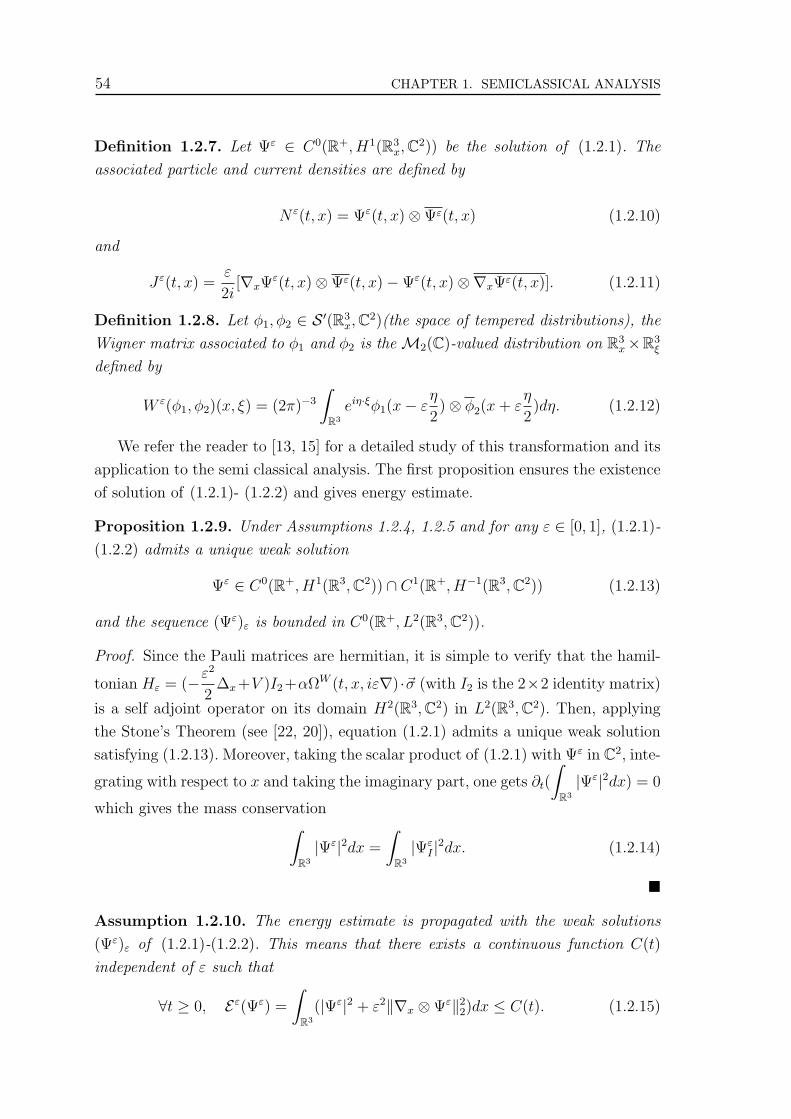
54 CHAPTER 1. SEMICLASSICAL ANALYSIS

Definition 1.2.7. Let Ψε ∈ C0(R+, H1(R3x,C2)) be the solution of (1.2.1). The

associated particle and current densities are defined by

N ε(t, x) = Ψε(t, x)⊗Ψε(t, x) (1.2.10)

and

Jε(t, x) =ε

2i[∇xΨ

ε(t, x)⊗Ψε(t, x)−Ψε(t, x)⊗∇xΨε(t, x)]. (1.2.11)

Definition 1.2.8. Let φ1, φ2 ∈ S ′(R3x,C2)(the space of tempered distributions), the

Wigner matrix associated to φ1 and φ2 is the M2(C)-valued distribution on R3x×R3

ξ

defined by

W ε(φ1, φ2)(x, ξ) = (2π)−3

∫

R3

eiη·ξφ1(x− εη

2)⊗ φ2(x + ε

η

2)dη. (1.2.12)

We refer the reader to [13, 15] for a detailed study of this transformation and its

application to the semi classical analysis. The first proposition ensures the existence

of solution of (1.2.1)- (1.2.2) and gives energy estimate.

Proposition 1.2.9. Under Assumptions 1.2.4, 1.2.5 and for any ε ∈ [0, 1], (1.2.1)-

(1.2.2) admits a unique weak solution

Ψε ∈ C0(R+, H1(R3,C2)) ∩ C1(R+, H−1(R3,C2)) (1.2.13)

and the sequence (Ψε)ε is bounded in C0(R+, L2(R3,C2)).

Proof. Since the Pauli matrices are hermitian, it is simple to verify that the hamil-

tonian Hε = (−ε2

2∆x+V )I2+αΩW (t, x, iε∇) ·~σ (with I2 is the 2×2 identity matrix)

is a self adjoint operator on its domain H2(R3,C2) in L2(R3,C2). Then, applying

the Stone’s Theorem (see [22, 20]), equation (1.2.1) admits a unique weak solution

satisfying (1.2.13). Moreover, taking the scalar product of (1.2.1) with Ψε in C2, inte-

grating with respect to x and taking the imaginary part, one gets ∂t(

∫

R3

|Ψε|2dx) = 0

which gives the mass conservation∫

R3

|Ψε|2dx =

∫

R3

|ΨεI |2dx. (1.2.14)

¥

Assumption 1.2.10. The energy estimate is propagated with the weak solutions

(Ψε)ε of (1.2.1)-(1.2.2). This means that there exists a continuous function C(t)

independent of ε such that

∀t ≥ 0, Eε(Ψε) =

∫

R3

(|Ψε|2 + ε2‖∇x ⊗Ψε‖22)dx ≤ C(t). (1.2.15)

1.2. SCHRODINGER EQUATION WITH GENERAL SPIN-ORBIT HAMILTONIAN 55

Notice that Assumption 1.2.10 is verified in practice when taking Rashba, Dres-

selhauss, or Elliot-Yafet spin-orbit hamiltonian. Indeed, taking for instance

iε∂tΨε = −ε2

2∆xΨ

ε + V εΨε + iε2(~σ ×∇xVε).∇xΨ

ε

multiplying by ∂tΨε, integrating with respect to x and taking the real part, one finds

ε2

4∂t

∫

R3

‖∇x⊗Ψε‖22dx+

1

2

∫

R3

V ε∂t(|Ψε|2)dx = ε2=(∫

R3

(~σ ×∇xVε).∇xΨ

ε.∂tΨεdx

)

(1.2.16)

where =(z) denotes the imaginary part of z ∈ C. In addition, by an integration by

part

=(∫ t

0

∫

R3

(~σ ×∇xV ε) · ∇xΨε · ∂sΨεdsdx

)(1.2.17)

=12i

∫ t

0

∫

R3

[(~σ ×∇xV ε) · ∇xΨε · ∂sΨε − (~σ ×∇xV ε) · ∇xΨε · ∂sΨε

]dsdx

=12i

∫ t

0

∫

R3

[∂s((~σ ×∇xV ε) · ∇xΨε) ·Ψε −Ψε · (~σ ×∇xV ε) · ∇x∂sΨε

]dsdx

− 12i

∫

R3

(~σ ×∇xV ε) · ∇xΨε(t, x) ·Ψε(t, x)dx +12i

∫

R3

(~σ ×∇xV ε(0, x)) · ∇xΨεI ·Ψε

Idx

=12i

∫ t

0

∫

R3

(~σ ×∇x∂sV ε) · ∇xΨε ·Ψεdsdx− 12i

∫

R3

(~σ ×∇xV ε) · ∇xΨε(t, x) ·Ψε(t, x)dx

+12i

∫

R3

(~σ ×∇xV ε(0, x)) · ∇xΨεI ·Ψε

Idx.

Moreover, it is simple to show that for any regular function U we have

∣∣∣∣i

2

∫

R3

(~σ ×∇xU) · ∇xΨε ·Ψεdx

∣∣∣∣ ≤ supR3

(|∇xU |)(∫

R3

‖∇x ⊗Ψε‖22dx

) 12(∫

R3

|Ψε|2) 1

2

.

Applying this inequality to all the terms of the right hand side of (1.2.17), one finds

thanks to Assumptions 1.2.4 and 1.2.5 and Young’s formula

ε2=(∫ t

0

∫

R3

(~σ ×∇xVε) · ∇xΨ

ε · ∂sΨεdsdx

)≤

C1(t) +ε2

8(

∫

R3

‖∇x ⊗Ψε‖22dx +

∫ t

0

∫

R3

‖∇x ⊗Ψε‖22dsdx), (1.2.18)

with a continuous function C1(t) independent of ε. Finally, integrating (1.2.16) with

respect to t and with (1.2.18), we obtain

ε2

∫

R3

‖∇x ⊗Ψε‖22dx ≤ C2(t) + ε2

∫ t

0

∫

R3

‖∇x ⊗Ψε‖22dsdx.

Applying the Gronwall’s Lemma and with the mass conservation (1.2.14), one de-

duces (1.2.15).

56 CHAPTER 1. SEMICLASSICAL ANALYSIS

1.2.2 Semiclassical limit

In this subsection, a brief proof of the two above theorems will be presented. We

use a main theorem in the semi-classical analysis due to Gerard, Markovich and al

in [13] to passing to the limit. More precisely we will use Theorem 6.1 of [13].

Proof of Theorem 1.2.1 and Theorem 1.2.2. The first point of Theorem

1.2.1 results from the boundedness of ΨεI in L2(R3,C2) (see [13]). Let Pε(t, x, ξ) =( |ξ|2

2+ V ε

)I2, then equation (1.2.1) rewrites as

ε∂tΨε + i

(PW

ε (t, x, iε∇x) + αΩWε (t, x, iε∇x) · ~σ

)(Ψε) = 0. (1.2.19)

We begin by the first case : α = O(ε) and we take α = ε for simplicity. By taking a

Hilbert expansions of V ε and ~Ωε with respect to ε

V ε = V + εV 1 + o(ε), ~Ωε = ~Ω + ε~Ω1 + o(ε),

we have

Pε + ε~Ωε · ~σ = P0(t, x, ξ) + ε(V1I2 + ~Ω · ~σ) + o(ε),

with P0(t, x, ξ) =

( |ξ|22

+ V (t, x)

)I2. Let λ(t, x, ξ) =

|ξ|22

+ V (t, x) be the unique

eigenvalue of P0(t, x, ξ) of multiplicity 2, and applying Theorem 6.1 of [13] then,

W ε(Ψε, Ψε) converges weak ? in L∞(R+,S ′(R3x × R3

v,M2(C))) to

W 0 ∈ C0(R+,Mb(R6,H+2 (C))). In addition, W 0 satisfies

∂tW0 +

λ,W 0

= [W 0, Fλ] on (R+ × R6

x,ξ) \ E, (1.2.20)

with Fλ = [Πλ, λ, Πλ] + iΠλ(V1I2 + ~Ω · ~σ)Πλ, Πλ is the orthogonal projection on

the eigenspace associated to λ, and denotes the Poisson bracket :

λ,W 0

= ∇ξλ · ∇xW

0 −∇xλ · ∇ξW0.

The set E represents a closed subset of R+×R3x×R3

ξ such that, for every (t, x, ξ) /∈ E,

the eigenvalues of P0 can be ordered as follows, see [13],

λ1(t, x, ξ) < . . . < λd(t, x, ξ)

where, for 1 ≤ q ≤ d, the multiplicity of λq(t, x, ξ) does not depend on (t, x, ξ). Here,

we have one eigenvalue λ(t, x, ξ) (d = 1) of multiplicity two for every (t, x, ξ) ∈ R+×R6. We choose then E = ∅. Moreover, we have Πλ = I2 then, Fλ = i(V1I2+~Ω ·~σ) and

equation (1.2.20) yields (1.2.4). For the convergence of the macroscopic quantities,

we refer the reader also to [13].

1.2. SCHRODINGER EQUATION WITH GENERAL SPIN-ORBIT HAMILTONIAN 57

We assume now that α = O(1) and we take α = 1, then the principal order (with

respect to ε) of the symbol of the pseudo-differential operator in equation (1.2.19)

multiplied by −i is given by P0(t, x, ξ)+~Ω(t, x, ξ)·~σ. It admits two simple eigenvalues

λ↑ and λ↓ given by

λ↑ =|ξ|22

+ V (t, x) + |~Ω(x, ξ)|, λ↓ =|ξ|22

+ V (t, x)− |~Ω(x, ξ)|.

Denoting by Π↑ and Π↓ the orthogonal projections on the eigenspaces associated to

λ↑ and λ↓ respectively, one can easily verify that

Π↑ =1

2

(I2 +

~Ω · ~σ|~Ω|

), and Π↓ =

1

2

(I2 −

~Ω · ~σ|~Ω|

)on (R+ × R6) \ E

where E is given by (1.2.6). From Theorem 6.1 of [13], the weak limit of W ε(Ψε, Ψε),

W 0, is given by W 0 = W 0↑ + W 0

↓ . The up and down functions W 0↑ and W 0

↓ are a two

continuously t-dependent positive matrix valued measures on R6x,ξ satisfying

∂tW0↑(↓) + λ↑(↓),W 0

↑(↓) = [W 0↑(↓), F↑(↓)] on (R+ × R6

x,ξ) \ E, (1.2.21)

with F↑(↓) = [Π↑(↓), λ↑(↓), Π↑(↓)] + iΠ↑(↓)(V1I2 + ~Ω1 · ~σ)Π↑(↓). Moreover, we have

W 0↑(↓) = Π↑(↓)W 0Π↑(↓) and if we pose W 0 =

wc

2I2 + ~ws · ~σ, then a straightforward

calculation gives

W 0↑ =

(wc

2+

~ws · ~Ω|~Ω|

)Π↑ and W 0

↓ =

(wc

2− ~ws · ~Ω

|~Ω|

)Π↓ on (R+ × R6

x,ξ) \ E.

(1.2.22)

We deduce that

W 0 =1

2

(wc

2+

~ws · ~Ω|~Ω|

)(I2 +

~Ω · ~σ|~Ω|

)+

1

2

(wc

2− ~ws · ~Ω

|~Ω|

)(I2 −

~Ω · ~σ|~Ω|

)

=wc

2I2 +

~ws · ~Ω|~Ω|2

~Ω · ~σ on (R+ × R6x,ξ) \ E.

This implies that the spin part of W 0, ~ws is parallel to ~Ω. Let ws(t, x, ξ) =~ws · ~Ω|~Ω|

and let w↑ =wc

2+ ws and w↓ =

wc

2− ws be the eigenvalues of W 0, we have, from

(1.2.22), W 0↑ = w↑Π↑ and W 0

↓ = w↓Π↓. Equation (1.2.21) yields (1.2.7). Indeed, we

have

∂tW0↑(↓) + λ↑(↓),W 0

↑(↓) = (∂tw↑(↓) + λ↑(↓), w↑(↓))Π↑(↓) + w↑(↓)λ↑(↓), Π↑(↓).

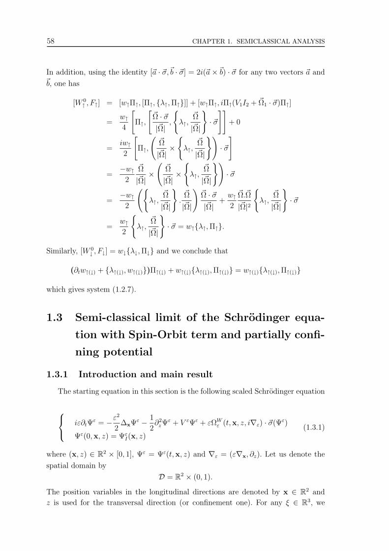
58 CHAPTER 1. SEMICLASSICAL ANALYSIS

In addition, using the identity [~a · ~σ,~b · ~σ] = 2i(~a×~b) · ~σ for any two vectors ~a and~b, one has

[W 0↑ , F↑] = [w↑Π↑, [Π↑, λ↑, Π↑]] + [w↑Π↑, iΠ↑(V1I2 + ~Ω1 · ~σ)Π↑]

=w↑4

[Π↑,

[~Ω · ~σ|~Ω|

,

λ↑,

~Ω

|~Ω|

· ~σ

]]+ 0

=iw↑2

[Π↑,

(~Ω

|~Ω|×

λ↑,

~Ω

|~Ω|

)· ~σ

]

=−w↑

2

~Ω

|~Ω|×

(~Ω

|~Ω|×

λ↑,

~Ω

|~Ω|

)· ~σ

=−w↑

2

(λ↑,

~Ω

|~Ω|

.

~Ω

|~Ω|

)~Ω · ~σ|~Ω|

+w↑2

~Ω.~Ω

|~Ω|2

λ↑,

~Ω

|~Ω|

· ~σ

=w↑2

λ↑,

~Ω

|~Ω|

· ~σ = w↑λ↑, Π↑.

Similarly, [W 0↓ , F↓] = w↓λ↓, Π↓ and we conclude that

(∂tw↑(↓) + λ↑(↓), w↑(↓))Π↑(↓) + w↑(↓)λ↑(↓), Π↑(↓) = w↑(↓)λ↑(↓), Π↑(↓)

which gives system (1.2.7).

1.3 Semi-classical limit of the Schrodinger equa-

tion with Spin-Orbit term and partially confi-

ning potential

1.3.1 Introduction and main result

The starting equation in this section is the following scaled Schrodinger equation

iε∂tΨε = −ε2

2∆xΨ

ε − 1

2∂2

zΨε + V εΨε + εΩW

ε (t,x, z, i∇ε) · ~σ(Ψε)

Ψε(0,x, z) = ΨεI(x, z)

(1.3.1)

where (x, z) ∈ R2 × [0, 1], Ψε = Ψε(t,x, z) and ∇ε = (ε∇x, ∂z). Let us denote the

spatial domain by

D = R2 × (0, 1).

The position variables in the longitudinal directions are denoted by x ∈ R2 and

z is used for the transversal direction (or confinement one). For any ξ ∈ R3, we

1.3. SEMICLASSICAL LIMIT AND PARTIALLY CONFINING POTENTIAL 59

will write ξ = (ξx, ξz) where ξx ∈ R2 and ξz ∈ R are respectively the longitudinal

and transversal parts of ξ. The Weyl operator ΩWε (t,x, z, i∇ε) · ~σ represents in this

section the following operator

ΩWε (t,x, z, i∇ε)·~σ(ψ) =

1(2π)2

∫

R2ξx

∫

R2y

~Ωε

(t,

x + y2

, z, εξx, i∂z

)·~σ(ψ(y, z))ei(x−y).ξxdξxdy.

Here, for every (t,x, z, ξx) ∈ R+ × D × R2ξx

, ~Ω(t,x, z, ξx, i∂z) is a vector valued

differential operator which is the image of i∂z by some regular vector valued function~Ω(t,x, z, ξx, .). The confinement in the z direction is modeled through the following

boundary conditions

Ψε(t,x, z = 0) = Ψε(t,x, z = 1) = 0. (1.3.2)

Thanks to this assumption, the transverse Hamiltonian (−12∂2

z +V ε)I2 has a discrete

spectrum and a complete set of eigenfunctions. Let χεp(t,x, .) and εε

p(t,x) be the

eigenfunctions and eigenvalues of −12∂2

z +V ε with homogenous boundary conditions,

they satisfy

−12∂2

zχεp + V εχε

p = εεpχ

εp

χεp(t,x, .) ∈ H1

0 (0, 1),

∫ 1

0

χεpχ

εq = δpq.

(1.3.3)

For any (t,x) ∈ R+×R2, (χεp(t,x, .))p≥1 is an orthonormal basis of L2(0, 1), (εε

p)p≥1

are simple as eigenvalues of−12∂2

z+V ε. The eigenvalues of the transverse Hamiltonian

(−12∂2

z +V ε)I2 are then εεp and are of multiplicity two. Let us denote by Hε

p(t,x) the

p-th eigenspace which is given by

Hεp(t,x) = span

(χε

p

0

),

(0

χεp

)⊂ (L2(0, 1))2

and by Πεp(t,x) the orthogonal projector on Hε

p(t,x). For ε = 0, we shall use the

notation Πp and εp instead of Π0p and ε0

p. As in the previous section we take the

following assumptions

Assumption 1.3.1. For any T > 0, (ε, t,x, z) 7→ V ε(t,x, z) is a real nonnegative

function belonging to C0([0, 1]ε, C1 ∩W 1,∞([0, T ]× R2, L∞(0, 1))).

Assumption 1.3.2. The initial data ΨεI belongs to H1

0 (D,C2) and there exists C > 0

independent of ε such that

∫ ∫

D(|Ψε

I |2 + ε2‖∇x ⊗ΨεI‖2

2 + |∂zΨεI |2)dxdz ≤ C.

60 CHAPTER 1. SEMICLASSICAL ANALYSIS

Assumption 1.3.3. The effective field ~Ωε(t,x, z, ξx, ξz) belongs to C0([0, 1]ε, C1(R+×

D × R3ξ))

3 such that (1.2.9) holds. In addition, we assume that ~Ωε satisfies the fol-

lowing expansion

~Ωε = ~Ω(t,x, z, ξx) + ε~Ω1(t,x, z, ξx, ξz) + o(ε) (1.3.4)

with ~Ω ∈ C1(R+ ×D × R2ξx

) and ~Ω1 ∈ C1(R+ ×D × R3ξx,ξz

).

Definition 1.3.4. Let

H = L2((0, 1),C2).

This is an Hilbert space equipped with the L2 norm. The unknown Ψε of (1.3.1)

is an H-valued function on R+ × R2. In the sequel, H⊗H will denote the space of

bilinear forms on H×H. It can be identified to L2((0, 1)2,M2(C)) : the set of linear

combination of simple tensors of the form (Φ1 ⊗ Φ2)(z, z′) for any Φ1, Φ2 ∈ H and

where

(Φ1 ⊗ Φ2)(Ψ1, Ψ2) =

∫ 1

0

∫ 1

0

Φ1(z)⊗ Φ2(z′) : Ψ1(z)⊗Ψ2(z′)dzdz′

=

(∫ 1

0

Φ1(z) ·Ψ1(z)dz

) (∫ 1

0

Φ2(z′) ·Ψ2(z′)dz′

)

∀Ψ1, Ψ2 ∈ H.

Definition 1.3.5. Let Φ1, Φ2 be two H-valued distribution belonging to S ′(R2x,H).

For any ε > 0, the partial Wigner transform is given by

W ε(Φ1, Φ2)(x, ξx, z′, z) = (2π)−2

∫

R2

eiη·ξxΦ1(x− εη

2, z)⊗ Φ2(x + ε

η

2, z′)dη. (1.3.5)

This defines a continuous sesquilinear mapping from S ′(R2x,H)×S ′(R2

x,H) to S ′(R2x×

R2ξx

,H⊗H).

Under Assumptions 1.3.1, 1.3.2, equation (1.3.1) admits a unique weak solution

Ψε ∈ C0(R+, H10 (D,C2))∩C1(R+, H−1(D,C2)) satisfying the mass conservation (see

the previous section). We assume moreover that the energy estimate is propagated

∀t > 0,

∫ ∫

D(|Ψε|2 + ε2‖∇x ⊗Ψε‖2

2 + |∂zΨεI |2)dxdz ≤ C(t) (1.3.6)

where C(t) is a continuous function of t independent of ε.

Definition 1.3.6. Let Ψε be the solution of (1.3.1). The associated macroscopic

quantities are now given by

N ε(t,x, z, z′) = Ψε(t,x, z)⊗Ψε(t,x, z′) (1.3.7)

and

Jε(t,x, z, z′) =ε

2i[∇xΨ

ε(t,x, z)⊗Ψε(t,x, z′)−Ψε(t,x, z)⊗∇xΨε(t,x, z′)]. (1.3.8)

1.3. SEMICLASSICAL LIMIT AND PARTIALLY CONFINING POTENTIAL 61

We are now read to give the main result of this section. This is the subject of

the next Theorem.

Theorem 1.3.7. Assume that Assumptions 1.3.1, 1.3.2 and 1.3.3 hold. Then, up

to extraction of subsequences, we have the following results at the limit ε 7→ 0.

1. For any p ∈ N∗, W ε(Πεp(0,x)Ψε

I , Πεp(0,x)Ψε

I) converges in S ′(R4x,ξx

,H⊗H) to

Fp,I(x, ξx)χp(0,x, z)χp(0,x, z′) ∈Mb(R4x,ξx ,H⊗H).

Moreover, Fp,I(x, ξx) ∈ H+2 (C) for all (x, ξx) ∈ R4.

2. The Wigner transform W ε(Ψε, Ψε) of the solution of (1.3.1) converges in

L∞(R+,S ′(R4x,ξx

,H⊗H)) weak ? to

W 0 =∑

p

Fp(t,x, ξx)χp(t,x, z)χp(t,x, z′) ∈ C0(R+,Mb(R4x,ξx ,H⊗H))

(1.3.9)

with Fp(t,x, ξx) ∈ H+2 (C). It solves

∂tFp + ξx · ∇xFp −∇xεp · ∇ξxFp = i[Fp, ~Ωp · ~σ],

Fp(0,x, ξx) = Fp,I(x, ξx),(1.3.10)

where the effective field on the p-th subband, ~Ωp, is given by

~Ωp(t,x, ξx) =

∫ 1

0

~Ω(t,x, z, ξx)|χp(t,x, z)|2dz. (1.3.11)

3. For every T > 0, the particle and current densities N ε and Jε given by (1.3.7)-

(1.3.8) converge in L∞((0, T ),Mb(R2x,H⊗H)) weak ? to

N(t,x, z, z′) =∑p≥1

(∫

R2

Fp(t,x, ξx)dξx

)χp(t,x, z)χp(t,x, z′)

J(t,x, z, z′) =∑p≥1

(∫

R2

vFp(t,x, ξx)dξx

)χp(t,x, z)χp(t,x, z′).

1.3.2 Application : subband model with Rashba spin-orbit

effect

If we consider the general spin-orbit hamiltonian given by (1.1.2), the Schrodinger

equation with physical dimensional variables writes

i~∂tΨε = − ~

2

2m∆x,zΨ

ε + V εΨε + i~2

4m2c2(~σ ×∇x,zV

ε) · ∇x,zΨε (1.3.12)

with ~ is the Planck constant, m is the effective mass of an electron and c denotes the

speed of light. Let respectively, L and l be the longitudinal and transversal length

62 CHAPTER 1. SEMICLASSICAL ANALYSIS

scales. Here, we are interested in situations where the length scale in the confinement

direction z, l, is much smaller than the length scale in the non confinement one. In

other words, let ε be the ratio between the two length scales l and L, we assume

that

ε :=l

L<< 1.

This leads, up to rescaling of equation (1.3.12), to

iε∂tΨε = −ε2

2∆xΨ

ε − 1

2∂2

zΨε + V εΨε + iβ(~σ ×∇εV

ε) · ∇εΨε (1.3.13)

where ∇ε = (ε∇x,∇z) and β =~2

4m2c2l2. If V and t denote the potential and time

scales, to obtain (1.3.13) we have taken the following hypotheses

V =h

2

ml2and

V t

~=

1

ε.

The constant β is a dimensionless quantity. We shall assume that β is small and is

of order ε and we take β = ε for simplicity. A straightforward computation gives

(~σ ×∇εVε) · ∇εψ

ε = ∂zVε(σ2(ε∂x)− σ1(ε∂y))Ψ

ε

+εσ3(∂xVε(ε∂y)− ∂yV

ε(ε∂x))Ψε

+ε(σ1∂yVε − σ2∂xV

ε)∂zΨε

where (x, y) are the components of x ∈ R2. This implies that i(~σ × ∇εVε) · ∇ε =

ΩWε (t,x, z, i∇ε) · ~σ with ~Ωε = ~Ω + ε~Ω1 + o(ε) such that

~Ω(t,x, z, ξ) = ∂zV (−ξ2x, ξ

1x, 0), ~Ω1(t,x, z, ξ) = (∂yV ξz,−∂xV ξz, ∂xV ξ2

x − ∂yV ξ1x)

and where V is the limit of V ε when ε goes to zero and ξ = (ξ1x, ξ

2x, ξz). Applying

Theorem 1.3.7, one finds the following Boltzmann equation in the p-th subband

∂tFp + ξx · ∇xFp −∇xεp · ∇ξxFp = iαp(t,x)[σ2ξ1x − σ1ξ

2x, Fp]

where

αp(t,x) =

∫ 1

0

∂zV (t,x, z)|χp(t,x, z)|2dz. (1.3.14)

Remark 1.3.8. The spin-orbit effect obtained in this limit is nothing but the Rashba

effect used generally in the literature [3, 24] to describe the spin-orbit interactions in

bidimensional gases. Moreover, an explicit relation between the confinement potential

and the strength of the Rashba spin-orbit coupling is obtained, relation (1.3.14).

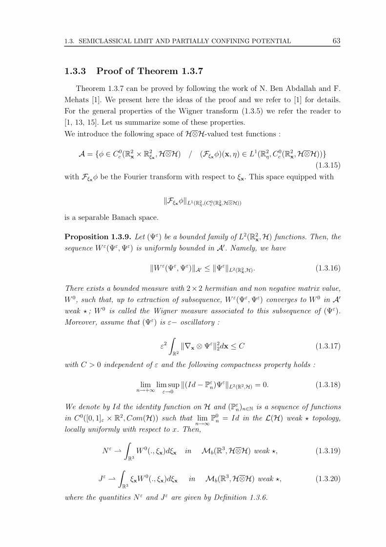
1.3. SEMICLASSICAL LIMIT AND PARTIALLY CONFINING POTENTIAL 63

1.3.3 Proof of Theorem 1.3.7

Theorem 1.3.7 can be proved by following the work of N. Ben Abdallah and F.

Mehats [1]. We present here the ideas of the proof and we refer to [1] for details.

For the general properties of the Wigner transform (1.3.5) we refer the reader to

[1, 13, 15]. Let us summarize some of these properties.

We introduce the following space of H⊗H-valued test functions :

A = φ ∈ C0c (R2

x × R2ξx ,H⊗H) / (Fξxφ)(x, η) ∈ L1(R2

η, C0c (R2

x,H⊗H))(1.3.15)

with Fξxφ be the Fourier transform with respect to ξx. This space equipped with

‖Fξxφ‖L1(R2η ,(C0

c (R2x,H⊗H))

is a separable Banach space.

Proposition 1.3.9. Let (Ψε) be a bounded family of L2(R2x,H) functions. Then, the

sequence W ε(Ψε, Ψε) is uniformly bounded in A′. Namely, we have

‖W ε(Ψε, Ψε)‖A′ ≤ ‖Ψε‖L2(R2x,H). (1.3.16)

There exists a bounded measure with 2×2 hermitian and non negative matrix value,

W 0, such that, up to extraction of subsequence, W ε(Ψε, Ψε) converges to W 0 in A′

weak ? ; W 0 is called the Wigner measure associated to this subsequence of (Ψε).

Moreover, assume that (Ψε) is ε− oscillatory :

ε2

∫

R2

‖∇x ⊗Ψε‖22dx ≤ C (1.3.17)

with C > 0 independent of ε and the following compactness property holds :

limn→+∞

lim supε→0

‖(Id− Pεn)Ψε‖L2(R2,H) = 0. (1.3.18)

We denote by Id the identity function on H and (Pεn)n∈N is a sequence of functions

in C0([0, 1]ε × R2, Com(H)) such that limn→∞

P0n = Id in the L(H) weak ? topology,

locally uniformly with respect to x. Then,

N ε

∫

R3

W 0(., ξx)dξx in Mb(R3,H⊗H) weak ?, (1.3.19)

Jε

∫

R3

ξxW0(., ξx)dξx in Mb(R3,H⊗H) weak ?, (1.3.20)

where the quantities N ε and Jε are given by Definition 1.3.6.

64 CHAPTER 1. SEMICLASSICAL ANALYSIS

Lemma 1.3.10. Let T > 0 be fixed and let (φε1(t,x)) and (φε

2(t,x)) be two families

bounded in L∞((0, T ), L2(R2x,H)). Consider an L(H)-valued function (ε, t,x, ξx) 7→

Pε(t,x, ξx) belonging to C0([0, 1], C1(R+ × R4x,ξx

,L(H))) and satisfying, for some

M ≥ 0,

∀α ∈ N3 × N3/|α| ≤ 1 : ‖∂αx,ξxPε(x, ξx)‖L(H) ≤ Cα(1 + |ξx|)M

with Cα > 0 independent of ε. Then, we have

W ε(PWε (t,x, iε∇x)φ

ε1, φ

ε2) = PεW

ε(φε1, φ

ε2) +

ε

2iPε,W

ε(φε1, φ

ε2)+ εrε

1 (1.3.21)

W ε(φε1, P

Wε (t,x, iε∇x)φ

ε2) = W ε(φε

1, φε2)P

∗ε +

ε

2iW ε(φε

1, φε2), P

∗ε + εrε

2 (1.3.22)

where rε1 0 and rε

2 0 in S ′(R4,H⊗H) weak ? uniformly with respect to t ∈ (0, T ).

Here, p, q denotes the Poisson bracket of two functions p(x, ξ) and q(x, ξ), given

by

p, q(x, ξ) = ∇ξp(x, ξ).∇xq(x, ξ)−∇xp(x, ξ).∇ξq(x, ξ). (1.3.23)

Before going on, one needs the following lemma which summarizes the regularities

of the eigenelements of the transversal Schrodinger operator.

Lemma 1.3.11. Let (εεp, χ

εp)ε satisfying (1.3.3). Then, under Assumption 1.3.1, εε

p,

χεp have the same regularity as V ε. Namely, the function (ε, t,x) 7→ εε

p(t,x) belongs

to C0([0, 1]ε, C1 ∩W 1,∞([0, T ] × R2)) and (ε, t,x, z) 7→ χε

p(t,x, z) ∈ C0([0, 1]ε, C1 ∩

W 1,∞([0, T ] × R2x, H

2(0, 1))) for any T > 0. Moreover, let Πεp be the orthogonal

projector on the p-th eigenspace and let ∂tΠεp and ∇xΠ

εp be their derivatives defined

by the following commutators :

∂tΠεp = [∂t, Π

εp], ∇xΠ

εp = [∇x, Π

εp].

For any p ≥ 1 and T > 0, Πεp is a self-adjoint operator on L(H) and the function

(ε, t,x) 7→ Πεp as well as their derivatives with respect to t and x are continuously

bounded functions of (ε, t,x) ∈ [0, 1]× [0, T ]× R2 valued in L(H).

Proof. This is a standard result using the perturbation theory of linear operators

(see for instance [14, 22]). ¥

We proceed now to the proof of the first point of Theorem 1.3.7. Under Assump-

tion 1.3.2 and by (1.3.16), we have, up to extraction of subsequence,

W ε(ΨεI , Ψ

εI) W 0

I as ε → 0

1.3. SEMICLASSICAL LIMIT AND PARTIALLY CONFINING POTENTIAL 65

in A′H weak ?, where W 0

I is a bounded measure with 2 × 2 hermitian, nonnegative

matrix value. Moreover, in view of Lemma 1.3.11, Πεp(0,x)ϕ converges strongly to

Πp(0,x)ϕ as ε → 0 in A for every ϕ ∈ A. Therefore,

Πεp(0,x)W ε(Ψε

I , ΨεI)Π

εp(0,x) Πp(0,x)W 0

I Πp(0,x) in A′ weak ?

and thanks to Lemma 1.3.10 and the self adjointness of Πεp, one obtains

W ε(Πεp(0,x)Ψε

I , Πεp(0,x)Ψε

I) Πp(0,x)W 0I Πp(0,x) in A′ weak ? .

Moreover, we have W 0I ∈ Mb(R4,H⊗H) with W 0

I (x, ξx, z, z′) ∈ H+2 (C) for all

(x, ξx, z, z′) ∈ R4× [0, 1]2. Let Fp,I =

∫ 1

0

∫ 1

0W 0

I (x, ξx, z, z′)χp(0,x, z)χp(0,x, z′)dzdz′,

then Fp,I(x, ξx) ∈ H+2 (C) and

Πp(0,x)W 0I Πp(0,x) = Fp,I(x, ξx)χp(0,x, z)χp(0,x, z′).

For the second point of the theorem, let

W εp,q = W ε(Πε

pΨε, Πε

qΨε).

An analogous analysis using (1.3.6) and (1.3.16) shows that

W εp,q W 0

p,q := ΠpW0Πq, as ε → 0

in L∞((0, T ),A′) weak ? for every T > 0, where W 0 denotes the weak ? limit of

W ε(Ψε, Ψε) in L∞((0, T ),A′). It is a bounded measure belonging to L∞((0, T ),Mb(R4,H⊗H)) with H+

2 (C) matrix value. It remains now to compute W 0p,q for every p, q ∈ N.

Lemma 1.3.12. let Ψεp = Πε

pΨε. Then,

Ψεp ∈ C0(R+, H1(R2,H)) ∩ C0(R+, L2(R2, H2((0, 1),C2)) ∩ C1(R+, L2(R2,H))

and satisfies

iε∂tΨεp = −ε2

2∆xΨ

εp + εε

pΨεp + Rε

p + εΠεpΩ

Wε (t,x, z, i∇ε).~σ(Ψε) (1.3.24)

with

Rεp = iε(∂tΠ

εp)Ψ

ε +ε2

2∇xΠ

εp · ∇xΨ

ε +ε2

2divx((∇xΠ

εp)Ψ

ε).

In addition, for any T > 0

limN→+∞

supε∈(0,1]

supt∈[0,T ]

∥∥∥∥∥∑p≥N

Ψεp(t, .)

∥∥∥∥∥L2(R2,H)

= 0. (1.3.25)

66 CHAPTER 1. SEMICLASSICAL ANALYSIS

We refer also to [1] for the proof of this lemma. We deduce that, for every p, q ∈ N,

W εp,q satisfies

∂tWεp,q = W ε(∂tΨε

p, Ψεq) + W ε(Ψε

p, ∂tΨεq)

=iε

2(W ε(∆xΨε

p, Ψεq)−W ε(Ψε

p, ∆xΨεq)

)− i

ε

(W ε(εε

pΨεp,Ψ

εq)−W ε(Ψε

p,εεqΨ

εq)

)

+ W ε((∂tΠεp)Ψ

ε, Ψεq) + W ε(Ψε

p, (∂tΠεq)Ψ

ε)− iε

2(W ε([∆x, Πε

p]Ψε,Ψε

q)−W ε(Ψεq, [∆x, Πε

q]Ψε)

)

− iW ε(ΠεpΩ

Wε (t,x, z, i∇ε).~σ(Ψε), Ψε

q) + iW ε(Ψεp,Π

εqΩ

Wε (t,x, z, i∇ε).~σ(Ψε)). (1.3.26)

Multiplying this equation by ε and getting formally ε goes to zero, one gets

(εp − εq)W0p,q = 0.

Since εp 6= εq if p 6= q, one deduces that W 0p,q = 0, or ΠpW

0Πq = 0 for p 6= q. This

result can be checked rigorously in the distribution sense. That is to wit,

W εp,q 0 if p 6= q in D′(R+

t × R4x,ξx ,H⊗H).

See [1] for details. Remark that we have, by construction of H⊗H,

W 0 =∑p,q

ΠpW0Πq

and thus

W 0 =∑

p∈N∗ΠpW

0Πp :=∑

p∈N∗ΠpW

0Πp.

Let us now calculate the equation verified by W 0p,p. For abuse of notations, we shall

use W 0p instead of W 0

p,p. For this we will perform the limit of (1.3.26) for p = q and

for a given T > 0. Applying Lemma 1.3.10 and with the boundedness of εεp, Πε

p and

all its derivatives with respect to t and x, one can pass to the limit on all the terms

of the right hand side of (1.3.26) in L∞((0, T ),A′) weak ?, to find

Πp

(∂tW

0p + ξx · ∇xW

0p −∇xεp · ∇ξxW

0p

)Πp = iΠp[W

0p , ~Ω(t,x, z, ξx)]Πp. (1.3.27)

See [1] for more details on the obtention of the left hand side of this equation. Let

us just explain the ideas for the obtention of the right hand side. View Assumption

1.3.3, the properties of Πεp (Lemma 1.3.11) and Lemma 1.3.10, one can write

W ε(ΠεpΩ

Wε (t,x, z, i∇ε) · ~σ(Ψε), Ψε

p) = ΠεpΩ

Wε (t,x, z, ξx) · ~σW ε(Ψε, Ψε)Πε

p + rε

where the both sides are bounded in L∞((0, T ),A′) and rε tends to 0 uniformly on

[0, T ] in A′ weak ?. Passing to the limit, we have

W ε(ΠεpΩ

Wε (t,x, z, i∇ε)·~σ(Ψε), Ψε

p) Πp~Ω(t,x, z, ξx)·~σW 0Πp = Πp

~Ω(t,x, z, ξx)·~σW 0p Πp

REFERENCES 67

since W 0 =∑

q∈N∗W 0

q =∑

q∈N∗ΠqW

0Πq. Using the same arguments, we have also

W ε(Ψεp, Π

εpΩ

Wε (t,x, z, i∇ε) · ~σ(Ψε)) ΠpW

0p~Ω(t,x, z, ξx) · ~σΠp.

We deduce then, by passing to the limit in (1.3.26) for p = q, that W 0p satis-

fies (1.3.27) in the sense of distributions S ′((0, T ) × R4,H⊗H) and that ∂tWεp is

bounded in L∞((0, T ),S ′(R4,H⊗H)). Thus, W εp is equicontinuous in t with va-

lues in S ′ and converges locally uniformly with respect to t. One deduces that

W 0p ∈ C0(R+,Mb(R4,H⊗H)) and for the continuity of W 0 stated in (1.3.9), it

suffices to remark that (1.3.25) and (1.3.16) imply the uniform convergence of the

series ∑

p∈N∗W ε

p ∈ C0([0, T ],A′).

Finally, since W 0p = ΠpW

0p Πp then,

W 0p (t,x, ξx, z, z′) = Fp(t,x, ξx)χp(t,x, z)χp(t,x, z′)

with Fp is an H+2 (C) matrix valued function and (1.3.27) yields the first equation of

(1.3.10).

The third item of Theorem 1.3.7 is a direct consequence of Proposition 1.3.9,

of (1.3.9) and the uniform convergence of the series. The ε-oscillatory property is

assured by the energy estimate (1.3.6) and the compactness property (1.3.18) holds

true by setting

Pεn =

∑p≤n

Πεp

and thanks to (1.3.25) and Lemma 1.3.11.

References

[1] N. Ben Abdallah and F. Mehats, Semiclassical analysis of the Schrodinger

equation with a partially confining potential, J. Math. Pures Appl. (9), 84 (2005),

pp. 580–614.

[2] J. A. Bittencourt, Fundamentals of plasma physics, Pergamon Press, Ox-

ford, 1986.

[3] Y. A. Bychkov and E. I. Rashba, Oscillatory effects and the magnetic

susceptibility of carriers in inversion layers, Journal of Physics C : Solid State

Physics, 17 (1984), pp. 6039–6045.

68 REFERENCES

[4] S. Datta and B. Das, Electronic analog of the electro-optic modulator, Ap-

plied Physics Letters, 56 (1990), pp. 665–667.

[5] G. Dresselhaus, Spin-orbit coupling effects in zinc blende structures, Phys.

Rev., 100 (1955), pp. 580–586.

[6] C. Fermanian-Kammerer and P. Gerard, Mesures semi-classiques et

croisement de modes, Seminaire Equations aux derivees partielles (Polytech-

nique) (1999-2000), Art. No. 17, 13 p.

[7] , Une formule de Landau-Zener pour un croisement non degenere et invo-

lutif de codimension 3, C. R. Math. Acad. Sci. Paris, 335 (2002), pp. 915–920.

[8] , A Landau-Zener formula for non-degenerated involutive codimension 3

crossings, Ann. Henri Poincare, 4 (2003), pp. 513–552.

[9] C. Fermanian-Kammerer and P. Gerard, A Landau-Zener formula for

two-scaled Wigner measures, in Dispersive transport equations and multiscale

models (Minneapolis, MN, 2000), vol. 136 of IMA Vol. Math. Appl., Springer,

New York, 2004, pp. 167–177.

[10] C. Fermanian-Kammerer and P. Gerard, Two-scale Wigner measures

and the Landau-Zener formulas, in Multiscale methods in quantum mechanics,

Trends Math., Birkhauser Boston, Boston, MA, 2004, pp. 59–68.

[11] A. Fert, A. Friederich, and al, Giant magnetoresistance of

(001)fe/(001)cr magnetic superlattices, Phys. Rev. Lett., 61 (1988), pp. 2472–

2475.

[12] P. Gerard, Mesures semi-classiques et ondes de Bloch, (1991), pp. Exp. No.

XVI, 19.

[13] P. Gerard, P. A. Markowich, N. J. Mauser, and F. Poupaud, Homo-

genization limits and Wigner transforms, Comm. Pure Appl. Math., 50 (1997),

pp. 323–379.

[14] T. Kato, Perturbation theory for linear operators, Springer-Verlag, Berlin, Hei-

delberg, 1966.

[15] P.-L. Lions and T. Paul, Sur les mesures de Wigner, Rev. Mat. Iberoame-

ricana, 9 (1993), pp. 553–618.

[16] P. A. Markowich and N. J. Mauser, The classical limit of a self-consistent

quantum-Vlasov equation in 3D, Math. Models Methods Appl. Sci., 3 (1993),

pp. 109–124.

[17] P. A. Markowich, N. J. Mauser, and F. Poupaud, A Wigner-function

approach to (semi)classical limits : electrons in a periodic potential, J. Math.

Phys., 35 (1994), pp. 1066–1094.

REFERENCES 69

[18] P. A. Markowich, C. A. Ringhofer, and C. Schmeiser, Semiconductor

equations, Springer-Verlag, Vienna, 1990.

[19] M. S. Mock, Analysis of mathematical models of semiconductor devices, vol. 3

of Advances in Numerical Computation Series, Boole Press, Dun Laoghaire,

1983.

[20] A. Pazy, Semigroups of linear operators and applications to partial differential

equations, vol. 44 of Applied Mathematical Sciences, Springer-Verlag, New York,

1983.

[21] Y. P. Raizer, Gas Discharge Physics, Springer, Berlin, 1997.

[22] M. Reed and B. Simon, Methods of modern mathematical physics., Academic

Press, New York, second ed., 1975. Functional analysis.

[23] E. Wigner, On the quantum correction for thermodynamic equilibrium, Phys.

Rev., 40 (1932), pp. 749–759.

[24] I. Zutic, J. Fabian, and S. D. Sarma, Spintronics : Fundamentals and

applications, Reviews of Modern Physics, 76 (2004), p. 323.

Chapter 2

On an hierarchy of kinetic and

macroscopic models for

spintronics

Abstract

In this chapter an hierarchy of kinetic and macroscopic models for semiconductor

spintronics is presented and analyzed. We begin by presenting and studying the so

called ”spinor” Boltzmann equation. Starting with a rescaled version of the Boltz-

mann equation with different spin-flip and non spin-flip collision operators, different

continuum models are derived. By comparing the strength of the spin-orbit scatte-

ring with the scaled mean free paths, we explain how some models existing in the

literature (like the two-component models) can be obtained from the spinor Boltz-

mann equation. A new spin-vector drift diffusion model keeping spin relaxation and

spin precession effects due to the spin-orbit coupling in semiconductor structures

is derived and some of its mathematical properties are checked. Other spin-vector

diffusif models like Spherical Harmonic Expansion (SHE) , Energy-Transport and

Drift-Diffusion with Fermi-Dirac statistics models are derived by means of the mo-

ment method and entropy minimization principle.

71

72 CHAPTER 2. HIERARCHY OF KINETIC AND MACROSCOPIC MODELS

2.1 Introduction

The electrons are not only characterized by their electric charge but also by their

intrinsic kinetic moment or the so called ”spin”. The spintronics is a new booming

domain of research which tries to control the spin and to use it as an additional

degree of freedom or a new vector of information. Although the first researches in

this domain were led essentially for structures based on magnetic multilayers [22], the

spin dependent properties of the electron transport in semiconductors have recently

attracted several attentions. There are typically two class of mechanisms [23] which

make relax the spin vector in semiconductors. In one side, we have according to the

Elliot-Yafet mechanism [49, 23] the instantaneous interactions of the particles with

the crystal accompanied with reversal of the spin direction. They will be called the

spin-flip interactions. These events are rare in semiconductors : typically less than

one interaction up one thousand return the spin orientation [7]. The second category

of mechanisms are relative to the effect on spin-orbit coupling of the asymmetry

inversion that can exist in the system. They can be characterized by an effective

magnetic field which makes precess the spin vector during the free path of the

particles. The ability to control this effective magnetic field could allow spin control

and manipulation in semiconductor heterostructures.

Many theoretical models are used by the physical community for spin-polarized

transport [35, 36, 38, 41, 42, 44, 46, 47, 49]. In microelectronics the drift-diffusion

system is one of the most used model for modelling the transport of charged particles

in semiconductors [32, 33], Plasma [5], Gas Discharges [39], etc. The drift-diffusion

model, which describes the macroscopic behavior of the particles, is a very well

suited model for numerical simulations. Two types of drift-diffusion approximations

are essentially used in spintronics : the so called two-component drift-diffusion model

and the spin polarization vector or density matrix based approximation. In the two-

component description, the electrons are considered to be of two types, namely,

having spin up or down. Each type of electrons is described by the usual drift-

diffusion equation with additional terms related to sources and relaxation of the

electron spin polarization, see [46, 47, 36]. The two-component model has been used

initially for spin transport in ferromagnetic metals, it was used also in studies of

propagation of spin-polarized electrons through a semiconductor region with variable

level of doping [36]. In this kind of model, the mechanism of spin relaxation (such

the spin-orbit interaction for instance) is not specified. The spin-vector (or density

matrix) approach is a more general description in which the spin variable (the density

or the distribution function for example) is a vector quantity and the mechanisms

acting on the spin dynamics can be taken into account.

The aim of this chapter is to derive and analyse macroscopic models for semi-

2.1. INTRODUCTION 73

conductor spintronics from the general spinor Boltzmann equation. The starting

equation is the following scaled Boltzmann equation

∂F ε

∂t+

1

ε(v·∇xF

ε−∇xV ·∇vFε) =

1

ε2Q(F ε)+

α

ε

[i

2~Ω(x, v) · ~σ, F ε

]+Qsf (F

ε), (2.1.1)

under the initial condition

F ε(0, x, v) = Fin(x, v), (2.1.2)

where ε > 0 is a small positive parameter. It represents the scaled mean free paths.

The parameter α is the scaled strength of the spin-orbit scattering. The operator Q

is the collision operator and Qsf represents the spin-flip interactions (or interactions

accompanied with reversal of spin’s direction). We use the following relaxation time

approximation of Qsf

Qsf (F ) =tr(F )I2 − 2F

τsf

, (2.1.3)

with τsf > 0 is the spin relaxation time. This operator makes relax, when τsf goes to

zero, the matrix distribution function to a scalar one. Since the spin-flip interactions

are not frequent in semiconductor structures as we mentioned above, τsf is not

small and we assume that Qsf is a perturbation part of the collision operator. This

is natural then to consider Qsf of order one in the diffusion scaling (2.1.1). The

diffusion limit ε → 0 leads to macroscopic diffusion models (Drift-Diffusion, SHE,

etc. . . ) according to the dominant scattering mechanisms. We refer to [1, 2, 12, 14,

19, 27, 37, 25, 43] for the rigorous derivation of macroscopic models from kinetic

equations. Different kind of scattering operators are considered in this work. We

consider first the collision operator for a Boltzmann statistics in the linear BGK

approximation given by :

Q(F ) =

∫

R3

α(v, v′)[M(v)F (v′)−M(v′)F (v)]dv′. (2.1.4)

The function M is the normalized Maxwellian

M(v) =1

(2π)32

e−12|v|2 , ∀v ∈ R3. (2.1.5)

The chapter is organized a follows. In the next section, we fix some notations

used along this chapter. The study of the Boltzmann equation is carried out in

Section 2.3. Existence and uniqueness of weak solutions of (2.1.1) is presented. It is

a standard result of Boltzmann type equations. In the spinor Boltzmann description,

the distribution function shall be a matrix valued function from R+ × R6 into the

space of 2 × 2 hermitian and positive matrices (H+2 (C)). We prove that equation

74 CHAPTER 2. HIERARCHY OF KINETIC AND MACROSCOPIC MODELS

(2.1.1) preserves the positivity and the self adjointness of the distribution function

during the time. In other terms, the following maximum principle holds :

if Fin(x, v) ∈ H+2 (C),∀(x, v) ∈ R6 then, F ε(t, x, v) ∈ H+

2 (C),∀t > 0 and (x, v) ∈ R6.

This means that if F ε satisfies (2.1.1), then (F ε)∗ is also a solution of (2.1.1). Mo-

reover, if Fin ∈ H+2 (C) and if we decompose F ε into spin-dependent and spin-

independent parts as

F ε(t, x, v) =1

2f ε

c (t, x, v)I2 + ~f εs (t, x, v) · ~σ

where f εc is the charge distribution and ~f ε

s is the spin distribution then, we have12f ε

c (t, x, v) ≥ |~fs|(t, x, v) for every (t, x, v) ∈ R× R6.

In the following sections we study the diffusion limit ε → 0 for different order

of α with respect to ε. Section 2.4 is dedicated to the derivation of two-component

models from the spinor Boltzmann equation. We begin by discussing what we call the

decoherence limit. This limit corresponds to keeping ε constant and to taking α goes

to +∞. It corresponds to taking a large spin-orbit coupling so that the ratio between

the period of rotations (T ) induced by the spin-orbit effect and the used time scale

(t) is small and goes to zero. This limit makes relax the spin part of the distribution

function to the direction parallel to ~Ω. If the direction of ~Ω does not depend on v, a

two-component kinetic model is obtained which yields two-component macroscopic

model at the diffusion limit. In the next subsection, we study the diffusion limit

of (2.1.1) with α = O(1

ε). This situation occurs in structures where the spin-orbit

coupling is high such that the rotational period T is of the same order of the mean

free path time τ and whereT

t= ε. Similarly, if the direction of ~Ω does not depend

on v, the spin vector direction tends towards ~Ω and one gets at the limit a two

component drift-diffusion model. However, if the direction of ~Ω depends on v, the

spin information is lost at the limit. In other words, the spin vector relaxes towards

zero and we obtain the standard scalar drift-diffusion model for the charge density (or

the total density) used in microelectronics. This spin relaxation corresponds to the

D’yakonov-Perel mechanism. It happens since the effective field changes frequently

direction due to the numerous interactions that a particle undergo on its trajectory

in the diffusion regime under investigation.

In Section 2.5, we are interested by the derivation of general spin-vector drift-

diffusion model with spin rotation and relaxation effects. Suppose first that α is of

the same order as ε (α = O(ε)) and take α = ε for simplicity. This means that

the order of the spin-orbit coupling is small in such a way that the rotation angle

of the spin vector around the effective field ~Ω is small during the free paths of the

2.2. ASSUMPTIONS AND NOTATIONS 75

particles. In this case, F ε converges to N(t, x)M(v) (in the weak sense see Section

2.5) such that N is a positive hermitian matrix satisfying the following equation

∂tN + divx(D(∇xN +∇xV N)) =i

2[ ~He · ~σ, N ] +

tr(N)I2 −N

τsf

,

where D is a positive definite matrix and the effective field is an M-weighted avera-

ging of ~Ω with respect to v :

~He(x) =

∫

R3

~Ω(x, v)M(v)dv.

Remark that if ~Ω is an odd vector with respect to v then ~He = 0 and no rotation

effect appears at the limit. This is generally the case of the spin-orbit effective fields

in semiconductor heterostructures (Rashba or Dresselhauss vectors). To keep trace

of the spin-orbit interactions at the diffusion limit when ~Ω is an odd vector, one has

to take a time scale such that α = O(1) with respect to ε. Applying this idea, a

general spin-vector drift-diffusion model will be rigourously derived (Theorem 2.5.2

) and one of its main property to wit the conservation of the positivity and the

self-adjointness of the density matrix during the time (maximum principle) will be

checked (see Theorem 2.5.3).

Following the same strategy, other two-component or spin-vector fluid models can

be derived. Section 2.6 is dedicated to the derivation of spin-vector SHE (Spherical

Harmonic Expansion) model when taking dominant elastic collisions. Finally, in

Section 2.7 we discuss the derivation of Energy-Transport and Drift-Diffusion with

Fermi-Dirac statistics models using the moment method and entropy minimization

principle. We note that the method used is inspired from the works of P. Degond and

C. Ringhofer [17, 18] for derivation of quantum hydrodynamic models. Other works

on derivation and numerical study of quantum fluid models exist [15, 16, 13, 24].

2.2 Assumptions and notations

Let us begin by introducing some assumptions and notations.

Assumption 2.2.1. The cross-section, α(., .), of the collision operator (2.1.4) be-

longs to W 1,∞(R6) and is assumed to be symmetric and bounded from above and

below :

∃α1, α2 > 0, 0 < α1 ≤ α(v, v′) ≤ α2, ∀v, v′ ∈ R3.

Assumption 2.2.2. For any fixed T > 0, the potential (t, x) 7→ V (t, x) is a non

negative real function belonging to C1([0, T ],W 1,∞(R3)).

76 CHAPTER 2. HIERARCHY OF KINETIC AND MACROSCOPIC MODELS

We will useM2(C) to denote the space of 2×2 complex matrices ; H2(C) denotes

the subspace of hermitian matrices and H+2 (C) the subspace of hermitian positive

matrices. We will denote by ‖.‖2 and 〈., .〉2 the Frobenuis norm and the associated

Frobenuis inner product

〈A,B〉2 = <(A : B) = <(2∑

i,j=1

AijBij), ‖A‖22 = 〈A,A〉2 =

2∑i,j=1

|Aij|2

where for z ∈ C, <(z) is the real part of z and for any two complex matrices

A,B ∈M2(C)

A : B =∑i,j

AijBij.

Definition 2.2.3. We define the space L2M by

L2M = F = F (x, v) ∈ H2(C) such that

∫

R6

‖F (x, v)‖22

M dxdv < +∞. (2.2.1)

This is an Hilbert space equipped with the following scalar product

〈F, G〉M =

∫

R6

〈F, G〉2M dxdv,

and ‖.‖M will denote the norm associated to 〈., .〉M. The same space with scalar

valued functions will be denoted by L2M instead of L2

M.

2.3 Study of spinor Boltzmann type models

The aim of this section is to study the properties of the spinor Boltzmann equa-

tion with the spin-orbit term. Existence and uniqueness of weak solution of (2.1.1)

will be shown and some a priori estimates on the solution independent of the para-

meters α and ε will be given (Theorem 2.3.2). The contents of this first part review

some well known results on linear Boltzmann type equations. We begin by defining

the notion of weak solution of (2.1.1).

Definition 2.3.1 (weak solution). For a fixed time T > 0, a function F ε ∈ L2([0, T ];L2M)

is called weak solution of (2.1.1) if it satisfies :

−∫ T

0

∫

R6

〈F ε, ∂tψ〉2dtdxdv − 1

ε

∫ T

0

∫

R6

〈F ε, v · ∇xψ −∇xV · ∇vψ〉2dtdxdv =

1

ε2

∫ T

0

∫

R6

〈Q(F ε), ψ〉2dtdxdv +α

ε

∫ T

0

∫

R6

〈 i2[~Ω(x, v) · ~σ, F ε], ψ〉2dtdxdv

+

∫ T

0

∫

R6

〈Qsf (Fε), ψ〉2dtdxdv +

∫

R6

〈Fin, ψ(0)〉2dxdv, (2.3.1)

2.3. STUDY OF SPINOR BOLTZMANN TYPE MODELS 77

for all ψ ∈ C1c ([0, T )× R6;H2(C)).

Theorem 2.3.2. For all fixed ε > 0, α > 0, T ≥ 0, Fin ∈ L2M and under As-

sumptions 2.2.1, 2.2.2, the model (2.1.1)-(2.1.2) admits a unique weak solution

F ε ∈ C0([0, T ];L2M) satisfying

‖F ε(t)‖L2M≤ C, ‖N ε‖L2

t,x([0,T ]×R3) ≤ C ∀t > 0, (2.3.2)

‖F ε − P(F ε)‖2L2

t (L2M ) ≤ Cε2, (2.3.3)

where C > 0 is a general constant independent of α and ε. Here, P is the orthogonal

projection on Ker(Q) which satisfies : P(F ε) = N εM with N ε :=∫R3 F εdv. In

addition the following maximum principle holds : if Fin(x, v) ∈ H+2 (C),∀(x, v) ∈ R6

then F (t, x, v) ∈ H+2 (C) ∀t ∈ [0, T ], (x, v) ∈ R6.

The next proposition summarizes some fundamental properties of the collision

operator (2.1.4). Since it acts only on the speed variable v, t and x are considered

as a parameters and are omitted in the next proposition for the sake of simplicity.

Proposition 2.3.3 (Properties of the collision operator (2.1.4)). Under As-

sumption 2.2.1, the collision operator given by (2.1.4) satisfies the following proper-

ties.

(i) For all F ∈ L2M, we have the mass conservation :

∫

R3

Q(F )(v)dv = 0.

(ii) The mapping Q : L2M → L2

M is a linear, continuous, selfadjoint and nonpositive

operator.

(iii) The kernel of Q is

Ker(Q) = F ∈ L2M, such that ∃N ∈ H2(C), F (v) = NM(v).

(iv) Let P be the orthogonal projection on KerQ, then we have the following coer-

civity inequality

−〈Q(F ), F 〉M ≥ α1‖F − P(F )‖2M. (2.3.4)

(v) The range of Q, R(Q), is a closed subset of L2M such that

R(Q) = Ker(Q)⊥ =

F ∈ L2

M, such that

∫

R3

F (v)dv =

(0 0

0 0

).

78 CHAPTER 2. HIERARCHY OF KINETIC AND MACROSCOPIC MODELS

Proof. The first point (i) is a direct consequence of Assumption 2.2.1. The linearity

of Q is obvious. Let F, G ∈ L2M, we have

〈Q(F ), G〉M = <(∫

R3

α(v, v′)M(v′)M(v)

[F (v′)M(v′)

− F (v)

M(v)

]:

G(v)

M(v)dvdv′

).

(2.3.5)

Using the symmetry of the cross-section α, one can write

〈Q(F ), G〉M = −12<

(∫

R3

α(v, v′)M(v′)M(v)[

F (v′)M(v′)

− F (v)M(v)

]:[

G(v′)M(v′)

− G(v)M(v)

]dvdv′

).

(2.3.6)

This implies that Q is selfadjoint and negative operator on L2M. By Assumption

2.2.1 and the fact that∫R3 ‖F (v)‖2dv ≤ ‖F‖M, (2.3.5) gives

|〈Q(F ), G〉M| ≤ C‖F‖M‖G‖M,

which yields the continuity of Q. The third point is obvious using the equality (2.3.6).

Namely, the following equivalences hold :

(F ∈ KerQ) ⇔ (〈Q(F ), F 〉M = 0) ⇔ (∃N ∈ H2(C), F (v) = NM(v)).

The orthogonal of KerQ is then given by the set :

(KerQ)⊥ =

F ∈ L2

M, such that

∫

R3

F (v)dv =

(0 0

0 0

). (2.3.7)

Let now F ∈ L2M and let G = F −PF where PF is the orthogonal projection of F

on KerQ. Then, using the self-adjointness of Q, we have

〈Q(F ), F 〉M = 〈Q(G), G〉M.

Since G ∈ (KerQ)⊥ and with Assumption 2.2.1 we get

−〈Q(F ), F 〉M =1

2

∫α(v, v′)M′M‖ G′

M′ −G

M‖22dvdv′

≥ α1

∫

R3

‖G‖22

M dv = α1‖F − PF‖2M.

For the last point, since Q is selfadjoint we have R(Q) = (KerQ)⊥. It remains to

show that R(Q) is closed. Indeed, let (Hp)p≥1 ∈ R(Q) be a sequence converging to

H ∈ L2M with respect to ‖.‖M. Writing Hp = Q(Fp) = Q(Gp), where Gp = Fp−PFp,

we have

α1‖Gp −Gq‖2M ≤ 〈Q(Gp)−Q(Gq), Gp −Gq〉M ≤ ‖Hp −Hq‖M‖Gp −Gq‖M.

2.3. STUDY OF SPINOR BOLTZMANN TYPE MODELS 79

Therefore, (Gp)p is a cauchy sequence in L2M. There exists G ∈ L2

M such that (Gp)p

converges to G. By the continuity of Q and the uniqueness of the limit, we deduce

that H = Q(G).

¥

Proof of Theorem 2.3.2. This is a standard result of the Boltzmann type

equations using a fixed point theorem and the characteristics method. Let us recall

the main ideas of the proof. For notational simplicity, we omit the presence of α and

ε (supposing α = ε = 1). We decompose the collision operator as, Q = Q+ + Q−

when Q+(F ) =

(∫

R3

α(v, v′)F (v′)dv′)M(v) and Q−(F ) = −ν(v)F with ν(v) =

∫

R3

α(v, v′)M(v′)dv′.

Lemma 2.3.4. Let L = ∂t + v · ∇x − ∇xV · ∇v, then for any Fin ∈ L2M and

S ∈ C0([0, T ];L2M), the problem

L(F )−Q−(F )− i

2[~Ω · ~σ, F ]−Qsf (F ) = S

F (t = 0) = Fin

(2.3.8)

admits a unique weak solution satisfying the following estimate

‖F (t)‖L2MV

≤ ‖Fin‖L2MV

+

∫ t

0

‖S(s)‖L2MV

ds (2.3.9)

with MV =1

(2π)32

e−12|v|2+V . In addition, the maximum principle holds which means

that if Fin, S are two hermitian positive matrices functions then the solution of

(2.3.8), F, is also in H+2 (C), ∀(t, x, v) ∈ [0, T ]× R6.

Proof. Using the decomposition of any matrix A ∈ H2(C) into spin-dependent and

spin-independent parts as A = AcI2 + ~As · ~σ, H2(C) is equivalent to R4 (we use the

identification A ≡ (Ac, ~As) for any A ∈ H2(C)). Any function F ∈ L2M is seen as

a function in (L2M)4. Let Fin ≡ (F in

c , ~F ins ) and S ≡ (Sc, ~Ss), then problem (2.3.8) is

equivalent to finding F ≡ (Fc, ~fs) in C0([0, T ], (L2M)4) such that

L(F ) + C(v)(F ) +A(x, v)(F ) = S

F (t = 0) = Fin.(2.3.10)

The function C(v) is the matrix associated to the −(Q− + Qsf ) operator given by

C(v) =

(ν(v) 0

0 (ν(v) + 1τsf

)I3

),

I3 denotes the identity matrix of order three. For all (x, v) ∈ R6, A(x, v) is an

antisymmetric 4×4 matrix associated to the spin-orbit anti-joint operator ( i2[~Ω·~σ, .]).

80 CHAPTER 2. HIERARCHY OF KINETIC AND MACROSCOPIC MODELS

It has the following form : A(x, v) =

(0 0

0 I(x, v)

)with 3 × 3 antisymmetric

matrix function I(x, v). Assuming first that Fin and S are regulars, then, thanks to

the characteristics method, the solution of (2.3.10) is given by the following integral

formula

F (t, z) = exp

(−

∫ t

0

[C(Z(s; z, t)) +A(Z(s; z, t))]ds

)· Fin

+

∫ t

0

exp

(−

∫ t

s

[C(Z(τ ; z, t)) +A(Z(τ ; z, t))]dτ

)· S(Z(s; z, t))ds,

(2.3.11)

where z = (x, v) is the variable in the phase space. For any z = (x, v) ∈ R6, t ∈ [0, T ],

the characteristics Z(s; z, t) := (X (s; z, t),V(s; z, t)) satisfy the following differential

system

dXds

= V(s),

dVds

= E(X (s)), E = −∇xV,

(X (t; z, t),V(t; z, t)) = (x, v).

In this case, F given by (2.3.11) is also the weak solution of (2.3.10). By scalar

multiplying (2.3.8) by FMV

and integrating with respect to t, x, and v (i.e. rigourously

choosing it as a test function in the weak formulation), one can find estimate (2.3.9)

since Q− and Qsf are two negative operators on H2(C) and 〈 i2[~Ω · ~σ, F ], F 〉2 = 0.

Furthermore, using the integral formula (2.3.11), one can verify straightforwardly

the maximum principle. If Fin and S belong to L2M and C0([0, T ],L2

M) respectively,

these results remain correct and can be obtained by regularization technics. The

proof of Lemma 2.3.4 is achieved.

¥

To continue the proof of Theorem 2.3.2, we define

χ : L2M × C0([0, T ],L2

M) −→ C0([0, T ],L2M)

(Fin, S) −→ χ(Fin, S) = F,

where χ(Fin, S) := F is the unique weak solution of (2.3.8) with initial condition Fin

and source term S. The mapping χ is linear, continuous (in view of estimate (2.3.9))

and satisfies the maximum principle. Moreover, a function F satisfies (2.1.1)-(2.1.2)

if and only if F = χ(Fin, Q+(F )) which is equivalent to say that F is a fixed point of

Θ : F ∈ C0([0, T ],L2M) 7→ χ(Fin, Q

+(F )) ∈ C0([0, T ],L2M). To show that Θ admits a

unique fixed point, let us define, for every δ > 0, the norm ‖.‖δ on C0([0, T ],L2M) by

2.4. TWO-COMPONENT MODELS 81

‖F‖δ = supt∈[0,T ]

(e−δt‖F‖L2

M

). All these norms are equivalent to the usual one ‖.‖0 (for

δ = 0), and one can choose δ small enough so that Θ forms a contracted mapping on

(C0([0, T ],L2M), ‖.‖δ). As a conclusion, problem (2.1.1)-(2.1.2) admits a unique weak

solution satisfying the maximum principle (since Q+(F ) conserves the positivity of

F and by Lemma 2.3.4) and we have

‖F (t)‖L2MV

≤ ‖Fin‖L2MV

+

∫ T

0

∫

R6

〈Q(F ),F

MV

〉2dsdxdv ∀t ∈ [0, T ].

Furthermore, taking into account the parameters α and ε, the weak solution, F ε, of

(2.1.1)-(2.1.2) satisfies

‖F (t)‖L2MV

≤ ‖Fin‖L2MV

+1

ε2

∫ T

0

∫

R6

〈Q(F ),F

MV

〉2dsdxdv ∀t ∈ [0, T ].

Finally, since

∫

R3

〈Q(F ),F

MV

〉2dv ≤ 0, one deduces estimates (2.3.2) and the balance

deviation inequality (2.3.3) follows from the coercivity inequality (2.3.4).

2.4 Two-component models

This section is concerned with the derivation of two-component kinetic and ma-

croscopic models from the general spinor kinetic equation.

2.4.1 Decoherence limit

We explain in this subsection how the spin-orbit interactions act on the distri-

bution function when the order of this coupling becomes large. We assume that the

period of rotation T of the spin vector distribution part around the effective field~Ω is small in front of the time scale t of the problem. The decoherence limit is the

limit η =T

t→ 0. This makes relax the spin part of the distribution function Fη of

(2.4.1) towards the effective field line. This is the subject of the next proposition.

Proposition 2.4.1. Assume that ~Ω satisfies Assumption 2.4.3, Fin ∈ L2M and that

Assumptions 2.2.1, 2.2.2 hold. Let T > 0 and Fη ∈ L2([0, T ],L2M) be the weak

solution of

∂tFη + v · ∇xFη −∇xV · ∇vFη = Q(Fη) +i

2η[~Ω · σ, Fη] + Qsf (Fη) (2.4.1)

with Fη(0, x, v) = Fin(x, v). Then, when η goes to 0, Fη tends to F0 such that

F0(t, x, v) =fc(t, x, v)

2I2+fs(t, x, v)~ω(x, v)·~σ with fc and fs belong to L2([0, T ], L2

M).

In addition, the charge and spin distribution functions, fc and fs, satisfy weakly

82 CHAPTER 2. HIERARCHY OF KINETIC AND MACROSCOPIC MODELS

∂tfc + v · ∇xfc −∇xV · ∇vfc = Q(fc) (2.4.2)

∂tfs + v · ∇xfs −∇xV · ∇vfs = Q (fs~ω) · ~ω − 2fs

τsf

(2.4.3)

and F0(0, x, v) = Fin(x, v) where for any (x, v) ∈ R6, ~ω(x, v) is the unit vector of

the effective field line.

Proof. Equation 2.4.1 admits a unique weak solution Fη ∈ L2([0, T ];L2M) such that

(Fη)η is bounded with respect to η (see Section 2.3 for details). There exists F0 ∈L2([0, T ];L2

M) such that Fη F0 weakly in L2([0, T ];L2M). This implies that i[~Ω ·

~σ, Fη] is also bounded in L2([0, T ];L2M) with respect to η and i[~Ω·~σ, Fη] i[~Ω·~σ, F0].

Multiplying the weak formulation of (2.4.1) by η and taking η tends to zero, we get

i[~Ω · ~σ, F0] = 0. This implies that the spin part of F0 is parallel to ~Ω i.e. there exist

fc and fs in L2([0, T ];L2M) such that F0 =

fc

2I2 + fs~ω · ~σ. Decomposing (2.4.1) into

charge and spin parts by setting Fη =f η

c

2+ fη

s · ~σ, one has

∂tfηc + v · ∇xf

ηc −∇xV · ∇vf

ηc = Q(fη

c )

∂tfηs + v · ∇xf

ηs −∇xV · ∇vf

ηs = Q(fη

s )− 1

η~Ω× fη

s − 2f η

s

τsf

. (2.4.4)

The weak limit of the first equation is (2.4.2). Taking the scalar multiplication of

(2.4.4) with ~ω and passing to the limit weakly in L2M([0, T ]× R6) one finds (2.4.3).

¥

Remark 2.4.2. If we suppose that the direction of ~Ω, ~ω, does not depend on v then,

we obtain at the decoherence limit a two-component kinetic model describing the

evolution of spin-up and spin-down distribution functions f ↑ and f ↓. These functions

are nothing but the eigenvalues of F0 choosing such that : f ↑ = fc + fs and f ↓ =

fc − fs. If fc, fs satisfy (2.4.2)-(2.4.3), then f ↑ and f ↓ satisfy the following two-

component kinetic model

∂tf↑ + v · ∇xf

↑ −∇xV · ∇vf↑ = Q(f ↑) +

f ↓ − f ↑

τsf

,

∂tf↓ + v · ∇xf

↓ −∇xV · ∇vf↓ = Q(f ↓) +

f ↑ − f ↓

τsf

,

(2.4.5)

subject to the initial conditions : f ↑(0) =f c

in

2+ ~f s

in · ~ω and f ↓(0) =f c

in

2− ~f s

in · ~ω,

where f cin and ~f s

in are the charge and spin parts of Fin

(Fin =

f cin

2I2 + ~f s

in.~σ

). The

model (2.4.5), leads then to a two-component macroscopic model in this case (the

case when the effective field direction is independent on v).

2.4. TWO-COMPONENT MODELS 83

In the next subsection, we will pass from a spinor Boltzmann equation to a 2-

component macroscopic (drift-diffusion) model. We will see also that this asymptotic

is possible if the effective field line does not depend on v and it corresponds to taking

a diffusion limit of the spinor Boltzmann equation with high spin-orbit coupling (case

α = O(1

ε)).

2.4.2 Diffusion limit with strong spin-orbit coupling : two-

component Drift-Diffusion model

This part is intended to the study of the diffusion limit (ε → 0) of (2.1.1) when

α = O(1

ε) with respect to ε. As mentioned in the introduction, the macroscopic

model, one obtains in this case, changes wether the direction of ~Ω depends on v or

not. We will see that if the effective field Ω does not change direction with v this

scaling gives at the limit a two-component Drift-Diffusion model. For simplicity, we

suppose that α =1

εand the starting equation is then

∂F ε

∂t+

1

ε(v · ∇xF

ε−∇xV · ∇vFε) =

1

ε2

Q(F ε) +

i

2[~Ω · ~σ, F ε]

+ Qsf (F

ε), (2.4.6)

with initial condition (2.1.2). The operators Q and Qsf are given by (2.1.4) and

(2.1.3) respectively. We will use the following form of ~Ω.

Assumption 2.4.3. We assume that ~Ω belongs to C2(R6,R3) and is given by

~Ω(x, v) = λ(x, v)~ω(x, v), such that |~ω(x, v)| = 1, ∀(x, v) ∈ R6

where λ and ~ω are two regular respectively scalar and vectorial functions. In addition,

we suppose that the following polynomially controls at infinity with respect to v hold

C1(1 + |v|)m ≤ |λ(x, v)| ≤ C2(1 + |v|)m (2.4.7)∑

η∈xi,vi|∂η

~Ω|+∑

η,η′∈xi,vi|∂2

ηη′~ω(x, v)| ≤ C(1 + |v|)m (2.4.8)

for C1 > 0, C2 > 0, C > 0 and m ∈ N.

Definition 2.4.4. We denote by QSO the following unbounded operator on L2M

QSO = Q +i

2[~Ω · ~σ, .] (2.4.9)

defined on the following domain

D(QSO) =

F ∈ L2M / i[~Ω · ~σ, F ] ∈ L2

M

(2.4.10)

=

F =

tr(F )

2I2 + ~fs · σ ∈ L2

M / ~Ω · ~fs ∈ L2M

.

Recalling that L2M denotes the space given by Definition 2.2.3.

84 CHAPTER 2. HIERARCHY OF KINETIC AND MACROSCOPIC MODELS

In view of the properties of the collision operator listed in Proposition 2.3.3, we

present in the following proposition some important properties of QSO.

Proposition 2.4.5. Under Assumptions 2.2.1, 2.4.3, the unbounded operator (QSO, D(QSO))

given by (2.4.9)-(2.4.10) satisfies the following properties.

1. It is a maximal monotone operator on L2M.

2. Let Ker(QSO) be the nul space of QSO, then we have the following characteri-

zation :

ker(QSO) =

F = N(x)M(v)/ N =

Nc

2I2 + ~Ns · ~σ ∈ L2(R3,H2(C))

and ~Ns =

0 if ~ω depends on v

ns(x)~ω if ~ω = ~ω(x) independent on v.

(2.4.11)

3. The range of QSO is given by

Im(QSO) =

G =

gc

2I2 + ~gs · ~σ ∈ L2

M /

∫

R3

gcdv = 0

and

(∫

R3

~gsdv

)· ~ω = 0 if ~ω does not depend on v

(2.4.12)

Proof. 1. The adjoint of QSO is given by

Q∗SO = Q− i

2[~Ω · ~σ, .] (2.4.13)

defined on D(Q∗SO) = D(QSO). Indeed, by definition

D(Q∗SO) =

F ∈ L2

M/ G 7→ 〈F, QSO(G)〉M is a bounded operator on D(QSO)

.

For every F ∈ D(Q∗SO), G ∈ D(QSO), we have by the self-adjointness of Q

〈F, QSO(G)〉M = 〈Q(F )− i

2[~Ω · ~σ, F ], G〉M. (2.4.14)

This implies

〈 i2[~Ω · ~σ, F ], G〉M = 〈Q(F ), G〉M − 〈F,QSO(G)〉M

for every G ∈ D(QSO). We deduce that for F ∈ D(Q∗SO),

i

2[~Ω · ~σ, F ] is a linear and

continuous operator on D(QSO) which is dense in L2M. It can be then prolonged to a

linear continuous operator on L2M which implies that (since L2

M is an Hilbert space)i

2[~Ω · ~σ, F ] ∈ L2

M and thus F ∈ D(QSO) if F ∈ D(Q∗SO). The reciprocal inclusion

(D(QSO) ⊂ D(Q∗SO)) is obvious and from (2.4.14), one deduces that Q∗

SO is given

2.4. TWO-COMPONENT MODELS 85

by (2.4.13) on D(QSO). In other side, 〈i[~Ω ·~σ, F ], F 〉M = 0 for every F ∈ L2M. Then,

since Q is a non positive operator, we have

〈QSO(F ), F 〉M = 〈Q∗SO(F ), F 〉M = 〈Q(F ), F 〉M ≤ 0

and the operators QSO and Q∗SO are monotones. Moreover, D(QSO) is dense in L2

Mand the graph of QSO, G(QSO), is closed. Indeed, let (Fn, QSO(Fn))n∈N such that

Fn ∈ D(QSO) be a sequence in G(QSO) converging to (F,G) in (L2M)2. We have to

prove that F ∈ D(QSO) and G = QSO(F ). For every H ∈ D(QSO), one has

〈Fn, Q∗SO(H)〉M = 〈QSO(Fn), H〉M.

By passing to the limit, n → +∞, one gets

〈F, Q∗SO(H)〉M = 〈G,H〉M

for every H ∈ D(QSO) and since D(QSO) = L2M, we deduce that F ∈ D(QSO) and

QSO(F ) = G. As a consequence, QSO is a densely defined closed operator such that

QSO and Q∗SO are monotones. It is then a maximal monotone operator on L2

M.

2. Let F ∈ Ker(QSO), we have

Q(F ) +i

2[~Ω · ~σ, F ] = 0. (2.4.15)

Taking the scalar product with F in L2M, one gets 〈Q(F ), F 〉M = 0. This implies

that Q(F ) = 0 and F = N(x)M(v) such that N ∈ L2(R3,H2(C)) (see Proposition

2.3.3). Writing N =Nc

2I2 + ~Ns · ~σ and inserting it in (2.4.15), we obtain

~Ω× ~Ns = 0. (2.4.16)

One can deduce simply that ~Ns = 0 if ~Ω changes direction with v and if not, the

vector ~Ns is parallel to ~Ω.

3. Since QSO is a closed and densely defined operator on L2M, we have

Im(QSO) = (KerQ∗SO)⊥.

Moreover, we have Ker(Q∗SO) = Ker(QSO) and it is simple to verify that the or-

thogonal of Ker(QSO) is nothing else but the set given (2.4.12). This implies that

Im(QSO) ⊂ Ker(QSO). In other side, let G =gc

2I2 + ~gs · ~σ ∈ ker(QSO)⊥ which

means that

∫

R3

gcdv = 0 and

(∫

R3

~gsdv

)· ~ω = 0 if ~ω = ~ω(x) does not depend on

v. Viewing the properties of the collision operator Q (Proposition 2.3.3), there is a

86 CHAPTER 2. HIERARCHY OF KINETIC AND MACROSCOPIC MODELS

unique function fc ∈ L2M(R6) such that

∫

R3

fc(x, v)dv = 0 and Q(fc) = gc. It re-

mains to verify the existence of a unique ~fs ∈ (L2M(R6))3 such that (

∫

R3

~fsdv) ·~ω = 0

if ~ω does not depend on v and

Q(~fs)− λ(~ω × ~fs) = ~gs.

Since QSO is a maximal monotone operator, then ∀δ > 0, δId − QSO is surjective,

where Id denotes the identity operator on L2M. There exists a vector function ~f δ

s

such that ~f δs · ~σ ∈ D(QSO) for any δ > 0 and (δId−QSO)(~f δ

s · ~σ) = ~gs · ~σ. Then,

δ ~f δs −Q(~f δ

s ) + λ~ω × ~f δs = ~gs,

for all δ > 0. We have to prove now that the sequence (~f δs )δ is bounded in (L2

M(R6))3.

We argue by contradiction and assume the existence of a subsequence denoted also

by (~f δs )δ such that ‖~f δ

s ‖ −−→δ→0

+∞ with ‖.‖ is the norm in (L2M(R6))3. Denoting by

~fδs =f δ

s

‖f δs ‖

, we have

δ~fδs −Q(~fδs) + λ~ω × ~fδs =~gs

‖~f δs ‖

, (2.4.17)

and ‖~fδs‖ = 1. Then, by passing to the limit weakly in (L2M)3, we have ~fδs ~fs in

(L2M)3 such that

−Q(~fs) + λ~ω × ~fs = 0

which implies that ~fs = 0 if ~ω depends on v and ~fs = ns(t, x)~ω(t, x)M if not.

Moreover, if ~ω is independent on v, ~gs satisfies (

∫

R3

~gsdv) · ~ω = 0. Then, integrating

(2.4.17) with respect to v and multiplying by ~ω, the same condition is also satisfied

by (~fδs) :

∫

R3

~fδsdv · ~ω = 0 for every δ > 0. Getting δ → 0, one deduces that ns =

(

∫

R3

~fsdv) ·~ω = 0. Hence, ~fδs ~fs = 0. In other side, let us show that ~fδs → ~fs strongly

in (L2M)3. This implies that ‖~fs‖ = 1, since ‖~fδs‖ = 1 ∀δ > 0 which is in contradiction

with ~fs = 0. Indeed, rewriting equation (2.4.17) as follows

(δ + ν(v))~fδs + λ~ω × ~fδs = ~gδs + Q+(~fδs), (2.4.18)

with ν(v) =

∫

R3

α(v, v′)M(v′)dv′, Q+(~fδs) =

∫

R3

α(v, v′)~fδs(v′)dv′M(v) and ~gδ

s =

~gs

‖~f δs ‖

. The solution of (2.4.18) can be computed explicitly. Indeed, without loss of

generality, assume that ~ω = (w1, w2, w3) is such that w3 6= 0, ‖~ω‖ = 1, and complete

it to an orthonormal basis of R3 : (ε1, ε2, ~ω). The change-of-basis matrix, P , from

2.4. TWO-COMPONENT MODELS 87

the standard euclidian basis to the new one is an orthogonal matrix (tP · P = I3)

given by

P =1

(w21 + w2

3)12

w3 −w1w2 w1(w21 + w2

3)12

0 w21 + w2

3 w2(w21 + w2

3)12

−w1 −w2w3 w3(w21 + w2

3)12

. (2.4.19)

Let ~Fδs = tP ~fδs be the new coordinates of ~fδs in the new basis (εi)i. Then, it satisfies

the following equation

Nδ(~Fδ

s) = tP (~hδs), (2.4.20)

where ~hδs = ~gδ

s + Q+(~fδs) is the second member of (2.4.18) and

Nδ = (δ + ν(v))

1 −λ 0

λ 1 0

0 0 1

, λ(x, v) =

λ(x, v)

δ + ν(v). (2.4.21)

It is simple to verify that ~hδs converges strongly in (L2

M)3 to Q+(~fs). Moreover, Nδ

is invertible and

N−1δ =

1

δ + ν(v)

11+λ2

λ1+λ2 0

−λ1+λ2

11+λ2 0

0 0 1

.

It is a bounded matrix with respect to δ uniformly with respect to (x, v) : ‖N−1δ ‖2 ≤

2

δ + α1

if the cross section α(v, v′) satisfies Assumption 2.2.1. As a conclusion, we

have~fδs = P ·N−1

δ · tP (~hδs)

with (~hδs)δ is a strongly convergent sequence in (L2

M)3 and N−1δ is a uniformly boun-

ded matrix with respect to δ. Then, (~fδs)δ converges strongly in (L2M)3. The proof of

the proposition is completed.

¥

The following lemma follows from the last proposition.

Lemma 2.4.6. There exists a unique ~χs ∈ (L2M)3 satisfying

Q(~χs) + λ(~ω × ~χs) = v · ∇x~ωM (2.4.22)

under the following condition(∫

R3

~χs(x, v)dv

)· ~ω = 0, ∀x ∈ R3. (2.4.23)

88 CHAPTER 2. HIERARCHY OF KINETIC AND MACROSCOPIC MODELS

Theorem 2.4.7. Let T > 0, Fin ∈ L2M and assume that Assumptions 2.2.1,

2.2.2, 2.4.3 hold and that the direction of the effective field ~ω is independent on v.

Then, the sequence of weak solutions, (F ε)ε>0, of (2.4.6)-(2.1.2) converges weakly in

L2([0, T ];L2M), when ε goes to zero, to N(t, x)M(v) with N ∈ L2([0, T ]×R3,H+

2 (C))

and such that

N(t, x) =nc(t, x)

2I2 + ns(t, x)~ω(x) · ~σ (2.4.24)

(the spin part of N is parallel to ~ω). In addition, the spin-up and spin-down densities,

n↑ = nc + ns and n↓ = nc − ns satisfy the following two-component drift-diffusion

model

∂tn↑ − divx(D1(∇xn

↑ +∇xV n↑)) =n↓ − n↑

τ(x)

∂tn↓ − divx(D1(∇xn

↓ +∇xV n↓)) =n↑ − n↓

τ(x)

(2.4.25)

where D1 is a symmetric positive definite matrix given by (2.5.10). We obtain at the

limit a modified spin relaxation time given by

τ(x) =2τsf

2 + τsfχ(x)

where χ(x) is a positive function

χ(x) = −∫

R3

Q(~χs) · ~χs

M dv ≥ 0 (2.4.26)

with ~χs satisfies (2.4.22).

Proof. With estimate (2.3.2), there exist F ∈ L2([0, T ],L2M) and N ∈ L2([0, T ] ×

R3;H+2 (C)) such that F ε F and N ε N in the corresponding spaces and

N =

∫

R3

Fdv (since N ε =∫R3 F εdv, ∀ε > 0). Multiplying (2.4.6) by ε2 and passing

to the weak limit ε → 0, one gets in the distribution sence

Q(F ) +i

2[~ω · ~σ, F ] = 0.

Since ~ω is independent on v and with (2.4.11), F = N(t, x)M(v) such that the

density matrix N can be written as (2.4.24). Let N ε =nε

c

2I2 + ~nε

s · ~σ and F ε =

f εc

2I2 + ~f ε

s ·~σ with nεc =

∫

R3

f εc dv and ~nε

s =

∫

R3

~f εs dv. Then, nε

c nc in L2([0, T ]×R3)

and ~nεs ns~ω in (L2([0, T ]×R3))3 (or ~nε

s · ~ω ns) where nc and ns are the charge

and spin parts of N (2.4.24). Integrating equation (2.4.6) with respect to v, one

obtains the following continuity equations

∂tnεc + divxj

εc = 0

∂t~nεs +∇x · Jε

s =−1

ε2

∫

R3

(~Ω× ~f εs )dv − 2~nε

s

τsf

(2.4.27)

2.4. TWO-COMPONENT MODELS 89

where the charge and spin currents, jεc ans Jε

s , are given by

jεc =

1

ε

∫

R3

vf εc dv Jε

s =1

ε

∫

R3

(v ⊗ ~f εs )dv.

These continuity equations can be obtained weakly by taking test functions constants

with respect to v in the weak formulation (2.3.1) (this choice of test functions

is possible, see the next section). Moreover, using estimate (2.3.3), there is Rε in

L2([0, T ];L2M) bounded with respect to ε such that F ε = N εM + εRε. In terms of

spin and charge parts, we have

~f εs = ~nε

sM+ ε~rεs, f ε

c = nεcM+ εrε

c

‖~rεs‖L2

t ((L2M)3) ≤ C, ‖rε

c‖L2t (L2

M) ≤ C(2.4.28)

where C > 0 is a general constant independent of ε. Thus, jεc =

∫

R3

vrεcdv and (jε

c )ε

is bounded with respect to ε in L2([0, T ]×R3). It converges weakly to a function jc

in L2([0, T ] × R3) and by passing to the limit on the first equation of (2.4.27), we

have

∂tnc + divxjc = 0. (2.4.29)

Moreover, multiplying the second equation of (2.4.27) by ~ω, we get

∂t(~nεs · ~ω) + divx(J

εs (~ω)) = Jε

s : (∇x ⊗ ~ω)− 2~nεs

τsf

(2.4.30)

where Jεs (~ω) =

1

ε

∫

R3

(v ⊗ ~f εs )(~ω)dv =

1

ε

∫

R3

v(~f εs · ~ω)dv =

∫

R3

v(~rεs · ~ω)dv bounded

with respect to ε. Let us denote by js the weak limit of Jεs (~ω) in L2([0, T ] × R3).

Besides, let Sε := Jεs : (∇x ⊗ ~ω). Then, Sε =

1

ε

∫

R3

(v · ∇x~ω) · ~f εs dv which is also

bounded with respect to ε in L2([0, T ] × R3) and converges weakly to a certain

function S ∈ L2([0, T ]×R3). By passing to the weak limit ε → 0, (2.4.30) yields the

following continuity equation

∂tns + divx(js) = S − 2ns

τsf

. (2.4.31)

To close this equation, one has to express js and S according to ns. For this, taking

the Frobenius inner product of (2.4.6) withθ1~ω · ~σM where θ1 is given by (2.5.8) and

integrating with respect to v yields

Jεs (w) = −ε

∫

R3

∂t(~f εs ·~ω)

θ1

Mdv−∫

R3

v·(∇x+∇xV )(~nεs·~ω)θ1dv−

∫

R3

~nεs·(v·∇x~ω)θ1dv

− ε

∫

R3

(v · ∇x −∇xV · ∇v)(~rεs · ~ω)

θ1

Mdv − ε

τsf

∫

R3

(~f εs · ~ω)θ1

M dv,

90 CHAPTER 2. HIERARCHY OF KINETIC AND MACROSCOPIC MODELS

up to straightforward computations using the self-adjointness of the collision ope-

rator Q and the expansion of ~f εs around the equilibrium (2.4.28). Taking ε goes, to

zero one obtains

Jεs (~ω) js = −D1(∇xns +∇xV ns)−

∫

R3

(v · ∇x~ω) · ~ωnsθ1dv

= −D1(∇xns +∇xV ns) (since ‖~ω‖ = 1) (2.4.32)

with D1 =

∫

R3

(θ1 ⊗ v)dv. To rigourously find the relation between js and ns, one

has to use the weak formulation of (2.4.6) withθ1~ω · ~σM φ(t, x), φ ∈ C1

c ([0, T )× R3),

as test function and passing then to the limit (see the next section for details). A

similar computation gives also

jc = −D1(∇xnc +∇xV nc). (2.4.33)

Finally, we shall express the limit of Sε :=1

ε

∫

R3

(v · ∇x~ω) · ~f εs , S, in terms of ns.

Taking the inner product of (2.4.6) with~χs · ~σM , where ~χs satisfies (2.4.22)-(2.4.23),

and integrating with respect to v, one obtains

Sε = ε

∫

R3

∂t~f εs ·

~χs

Mdv +

∫

R3

(v · ∇x~nεs + v · ∇xV ~nε

s) · ~χsdv

+ ε

∫

R3

(v · ∇x −∇xV · ∇v)~rεs ·

~χs

Mdv +ε

τsf

∫

R3

~f εs · χs

M dv.

By passing to the limit ε → 0,

S =

∫

R3

v · ∇x(ns~ω) · ~χsdv +

∫

R3

v · ∇xV ns(~ω · ~χs)dv. (2.4.34)

This limit can be rigourously verified by taking~χs · ~σM φ(t, x), with φ ∈ C1

c ([0, T ) ×

R3), as test function in (2.3.1). This choice is valid since~χs

M is polynomially increa-

sing at infinity with respect to v (see Lemma 2.4.8). Moreover, multiplying (2.4.22)

by ~ω, we have Q(~χs · ~ω) = 0 with

∫

R3

~χs · ~ωdv = 0 which implies that ~χs · ~ω = 0. In

addition, if we multiply (2.4.22) by~χs

M and integrate with respect to v, we get

∫

R3

(v · ∇x~ω) · ~χsdv =

∫

R3

Q(~χs) · ~χs

M dv = −χ(x) ≤ 0.

Consequently, the charge and spin densities nc and ns satisfy

∂tnc − divx(D1(∇xnc + nc∇xV )) = 0

∂tns − divx(D1(∇xns + ns∇xV )) = −2ns

τsf

− χ(x)ns

which yields (2.4.25).

¥

2.5. A GENERAL SPIN-VECTOR DRIFT-DIFFUSION MODEL 91

Lemma 2.4.8. Let ~χs be the solution of (2.4.22)-(2.4.23). Then under Assumption

2.2.1 and Assumption 2.4.3, one has

|~χs|M ≤ C(1 + |v|)m+1,

∑

η∈xi,vi

∂η|~χs|M ≤ C(1 + |v|)m′

,

with C is a general positive constant and m′ ∈ N.

Proof. Rewriting equation (2.4.22) as

−ν(v)~χs + λ(~ω × ~χs) = (v · ∇x~ω −Q+(~χs))M(v) (2.4.35)

with ν(v) =

∫

R3

α(v, v′)M(v′)dv′, Q+(~χs) =

∫

R3

α(v, v′)~χs(v′)dv′ and applying the

same computations we have made for resolving equation (2.4.18), one finds

~χs

M = P ·N−1 · tP (v · ∇x~ω −Q+(~χs)).

The matrix P is given by (2.4.19) and

N−1 =−1

ν

11+λ2

λ1+λ2 0

−λ1+λ2

11+λ2 0

0 0 1

, λ(x, v) =

−λ(x, v)

ν(v).

The matrices P and N−1 are uniformly bounded with respect to (x, v), ‖P‖2 =√

3

and ‖N−1‖2 ≤ 2

α1

(with Assumption 2.2.1). Therefore, using Assumption 2.4.3, we

deduce that|~χs|M ≤ C(1 + |v|)m+1. Similarly, by differentiating (2.4.35) with respect

to x or v, one can obtain the second estimates on∂η|~χs|M .

¥

2.5 A general spin-vector Drift-Diffusion model

This section is concerned with the diffusion limit when the spin-orbit coupling

is of order one with respect to ε (α = O(1)). This scaling is useful to get a spin

vector continuum model with rotation effects when the effective field of the spin-

orbit coupling is odd with respect to v. Here we take a general effective field ~Ωε as

follows~Ωε(x, v) =

1

ε~Ωo(x, v) + ~Ωe(x, v), (2.5.1)

where ~Ωo is odd with respect to v and ~Ωe is even with respect to v. For instance,~Ωo can be the effective magnetic field following from the spin-orbit interactions

(Rashba [10], Dresselhauss [20]) or the odd part of an applied magnetic field and ~Ωe

92 CHAPTER 2. HIERARCHY OF KINETIC AND MACROSCOPIC MODELS

can represent the even part of an applied field. The starting scaled spinor Boltzmann

equation is

∂F ε

∂t+

1

ε(v ·∇xF

ε−∇xV ·∇vFε) =

1

ε2Q(F ε)+

i

2[~Ωε(x, v) ·~σ, F ε]+Qsf (F

ε), (2.5.2)

with the initial condition (2.1.2) and the operators Q, Qsf are respectively given

by (2.1.4) and (2.1.3). Let us rewrite the weak formulation of (2.5.2). A function

F ε ∈ L2([0, T ];L2M) is called weak solution of (2.5.2) if it satisfies :

−∫ T

0

∫

R6

〈F ε, ∂tψ〉2dtdxdv − 1

ε

∫ T

0

∫

R6

〈F ε, v · ∇xψ −∇xV · ∇vψ〉2dtdxdv =

1

ε2

∫ T

0

∫

R6

〈Q(F ε), ψ〉2dtdxdv +

∫ T

0

∫

R6

〈 i2[~Ωε(x, v) · ~σ, F ε], ψ〉2dtdxdv

+

∫ T

0

∫

R6

〈Qsf (Fε), ψ〉2dtdxdv +

∫

R6

〈Fin, ψ(0)〉2dxdv, (2.5.3)

for all ψ ∈ C1c ([0, T )× R6;H2(C)).

Assumption 2.5.1. We assume that ~Ωo(x, v) and ~Ωe(x, v) are respectively two re-

gular odd and even vectors with respect to v. In addition, we suppose that ~Ωo is

compactly supported with respect to x and there exist a constant C0 > 0 and m ∈ Nsuch that

|~Ωo(v)|+∑

η∈xi,vi|∂η

~Ωo(v)| ≤ C0(1 + |v|)m. (2.5.4)

The main results of this section is stated in the following two theorems.

Theorem 2.5.2. Let T > 0, Fin ∈ L2M and assume that Assumption 2.2.1, As-

sumption 2.2.2 and Assumption 2.5.1 hold. Let for all ε > 0 F ε ∈ C0([0, T ];L2M) be

the weak solution of (2.5.2)-(2.1.2). Then, the matrix density N ε :=

∫

R3

F ε(t, x, v)dv

converges weakly in L2([0, T ]×R3,H2(C)) to N which satisfies the following equation

∂tN − divxD1(∇xN + N∇xV )− iD2[~σ, N ] =

i

2[~Ω · ~σ, N ] + (D4 − tr(D4))( ~Ns) · ~σ + Qsf (N) (2.5.5)

with initial condition N(0, x) =

∫

R3

Fin(x, v)dv, and where ~Ns is the spin density

part of N . In addition, if we decompose N as : N =Nc

2I2 + ~Ns · ~σ, then the charge

and spin densities satisfy

2.5. A GENERAL SPIN-VECTOR DRIFT-DIFFUSION MODEL 93

∂tNc − divx(D1(∇xNc +∇xV Nc)) = 0

∂t~Ns − divx(D1 · (∇x ⊗ ~Ns +∇xV ⊗ ~Ns) + 2(Dk

2 × ~Ns)k=1,2,3) =

−~Ω× ~Ns + (D4 − trD4)( ~Ns)− 2~Ns

τsf

.

(2.5.6)

Here

~Ω = divxD2 − D3(∇xV ) + He, He(x) =

∫

R3

~Ωe(x, v)M(v)dv (2.5.7)

and the matrices D1, D2, D3 and D4 are given by (2.5.10). For two matrices A and

B, A ·B is the product of A and B and divx(A) = ∇x ·A = (∑

k ∂kAki)i ; Dk2 is the

kth row of D2. We use ∇x ⊗ ~Ns to denote the transpose of the Jacobian matrix of~Ns : ∇x ⊗ ~Ns = (∂xi

~N js )ij.

Theorem 2.5.3 (Maximum principle). Let Nin ∈ L2(R3,H+2 (C)) be given and

under the same hypothesis as for the last theorem, there exists a unique weak solution

N(t, x) =Nc(t, x)

2I2+Ns(t, x).~σ ∈ C0([0, T ], L2(R3,H2(C)) for any T > 0 of (2.5.6)

with N(0, x) = Nin(x). In addition, for all t ≥ 0 and x ∈ R3, N(t,x) is an Hermitian

and positive matrix (N(t, x) ∈ H+2 (C)).

Remark 2.5.4. The right hand side of the limit equation (2.5.6) is the sum of a

rotational term around a certain field ~Ω (2.5.7) and a relaxation terms arising from

the spin-flip and non spin-flip scattering operators ( D4− tr(D4) is a negative matrix

since D4 is a symmetric positive definite matrix). The limiting effective field (2.5.7)

contains an averaging of the even part ~Ωe and keeps traces via the matrices D2 and

D3 from the odd part ~Ωo of the effective field in the kinetic equation.

Before beginning the proof of these theorems, we have to introduce the four

matrices D1, D2, D3 and D4 appearing in the limit model (2.5.6). These matrices

keep traces from the collision operator and the spin-orbit interactions considered.

This is the aim of the two following propositions.

Proposition 2.5.5. There exist a unique θ1 ∈ (L2M)3 and θ2 ∈ (L2

M)3 such that

−Q(θ1I2) = vM(v)I2,

∫

R3

θ1(v)dv = 0, (2.5.8)

−Q(θ2I2) = ~Ωo(v)M(v)I2,

∫

R3

θ2(v)dv = 0, (2.5.9)

where I2 is the 2× 2 identity matrix.

94 CHAPTER 2. HIERARCHY OF KINETIC AND MACROSCOPIC MODELS

Proof. Using the properties of the collision operator introduced in Proposition 2.3.3

and since

∫

R3

vM(v)I2 =

(0 0

0 0

), there exists ϑ1 ∈ (L2

M)3 such that −Q(ϑ1) =

vM(v)I2. The uniqueness of ϑ1 is guarantied under the condition∫R3 ϑ1(v)dv = 0.

It remains to prove that ϑ1 is a scalar matrix. For this, we decompose ϑ1 in the

orthogonal basis I2, σ1, σ2, σ3 of the set of 2 × 2 hermitian matrices and we use

the linearity of Q. Since ~Ωo is odd with respect to v, one can check similarly the

existence of θ2 satisfying (2.5.9).

¥

Proposition 2.5.6. Let D1, D2, D3 and D4 be the 3×3 matrices defined respectively

by

D1 =

∫

R3

(θ1(v)⊗ v)dv , D2 =

∫

R3

(v ⊗ θ2(v))dv,

D3 =

∫

R3

(~Ωo(v)⊗ θ1(v))dv , D4 =

∫

R3

(θ2(v)⊗ ~Ωo(v))dv(2.5.10)

where θ1, θ2 are given by (2.5.8), (2.5.9). The matrices D1 and D4 are symmetric

positive definite and tD3 = D2.

Proof. The components of D1 verify

Dij1 =

∫

R3

θi1(v).vjdv =

1

2

∫

R3

θi1(v)I2 : vjM(v)I2

M dv

= −1

2

∫

R3

θi1(v)I2 : Q(θj

1I2)

M dv = −1

2〈θi

1I2, Q(θj1I2)〉M.

Identically, one can calculate the components of D2,D3 and D4 to find :

Dij2 = −1

2〈θi

2I2, Q(θj1I2)〉M, Dij

3 = −1

2〈θi

1I2, Q(θj2I2)〉M, Dij

4 = −1

2〈θi

2I2, Q(θj2I2)〉M.

The selfadjointness of Q provides that D1 and D4 are symmetric and that tD3 = D2.

To prove the positivity of D1 (or D4), let X ∈ R3, and let f 1X =

3∑i=1

Xiθi1I2. Then,

since f 1X ∈ (KerQ)⊥, from (2.3.4) we have

〈D1X, X〉 =∑i,j

Dij1 XiXj = −1

2

∑i,j

〈θi1Id, Q(θj

1Id)〉MXiXj

= −1

2〈∑

i

Xiθi1Id, Q(

∑j

Xjθj1Id)〉M = −1

2〈f 1

X , Q(f 1X)〉M ≥ α1

2‖f 1

X‖2M ≥ 0.

Moreover, if X ∈ R3 such that 〈D1X,X〉 = 0 then, f 1X = 0. This implies, by the

linearity of Q, that :3∑

i=1

XiQ(θi1I2) = 0 and then

3∑i=1

XiviM = 0. Finally, since

(viM)i is a family of linearly independent elements in L2M, we deduce that X = 0.

Thus, D1 (respectively D4) is a symmetric positive definite matrix.

¥

2.5. A GENERAL SPIN-VECTOR DRIFT-DIFFUSION MODEL 95

2.5.1 Diffusion limit : formal approach

In this section, we will derive the model (2.5.6) by formally passing to the limit

ε → 0.

Proposition 2.5.7. If the solution of (2.5.2)-(2.1.2), F ε, has an Hilbert expansion

with respect to ε in the form : F ε = F 0+εF 1+O(ε), then F 0(t, x, v) = N(t, x)M(v)

and the density matrix N satisfies (2.5.5).

Proof. By inserting the expansion of F ε in (2.5.2) and comparing the terms corres-

ponding to the same order of ε, we get

Q(F 0) = 0, (2.5.11a)

Q(F 1) = (v · ∇x −∇xV · ∇v)F0 − i

2[~Ωo · ~σ, F 0]. (2.5.11b)

Therefore, F 0 = N(t, x)M(v) and

F 1 = −θ1 · (∇xN + N∇xV ) +i

2θ2 · [~σ,N ],

where θ1, θ2 are given by (2.5.8) and (2.5.9) respectively. Integrating equation (2.5.2)

with respect to v yields

∂tNε + divxJ

ε = Sε + Qsf (Nε), (2.5.12)

where N ε =

∫

R3

F εdv, Jε =1

ε

∫

R3

vF ε(t, x, v)dv and Sε =i

2

∫

R3

[~Ωε(x, v)·~σ, F ε(t, x, v)]dv.

In addition, using the Hilbert expansion of F ε, one can calculate formally the limit

of each term of the last equation. Indeed, we have

Jε =1

ε

∫

R3

vF ε(v)dv =1

ε(

∫

R3

vM(v)dv)N +

∫

R3

vF 1dv +O(ε)

= 0 +

∫

R3

vF 1(v)dv +O(ε) = −D1(∇xN + N∇xV ) +i

2D2([~σ, N ]) +O(ε),

(2.5.13)

and

2Sε =i

ε

∫

R3

[~Ωo ·~σ, F ε]+ i

∫

R3

[~Ωe ·~σ, F ε]dv = i

∫

R3

[~Ωo ·~σ, F 1]dv+ i[He ·~σ,N ]+O(ε)

= −i

∫

R3

[~Ωo·~σ, θ1·(∇xN+N∇xV )]dv−1

2

∫

R3

[~Ωo(v)·~σ, θ2·[~σ, N ]]dv+i[He·~σ, N ]+O(ε).

Then, by a straightforward computation, one finds

2Sε = −i[D3(∇x +∇xV ) · ~σ, N ]− 1

2

3∑i,j=1

Dij4 [~ei · ~σ, [~ej · ~σ,N ]] + i[He · ~σ, N ] +O(ε),

(2.5.14)

96 CHAPTER 2. HIERARCHY OF KINETIC AND MACROSCOPIC MODELS

where ~e1, ~e2, ~e3 is the euclidian basis of R3. Let N = Nc

2I2 + ~Ns · ~σ, then with

Lemma A.2.2 and the double cross product formula, ~a× (~b× ~c) = (~a · ~c)~b− (~a ·~b)~c,one obtains

3∑i,j=1

Dij4 [~ei · ~σ, [~ej · ~σ,N ]] = −4

3∑i,j=1

Dij4 ~ei × (~ej × ~Ns) · ~σ

= −43∑

i,j=1

Dij4 ( ~N i

s~ej − ~ei · ~ej~Ns) · ~σ, ( ~N i

s = ~Ns · ~ei)

= −4(D4( ~Ns)− tr(D4) ~Ns) · ~σ.

Replacing (2.5.13) and (2.5.14) in (2.5.12), passing to the limit ε → 0, and using the

fact that tD2 = D3 which implies that

divx(D2[~σ,N ]) = [(div(D2) + D3(∇x)) · ~σ,N ],

one obtains (2.5.5). ¥

2.5.2 Diffusion limit : the rigorous approach

This part is devoted to the proof of Theorem 2.5.2. The first Lemma is a conse-

quence of estimate (2.3.2).

Lemma 2.5.8. Let T > 0 and let F ε ∈ C0([0, T ];L2M) be the weak solution of

(2.5.2). There exist F ∈ L2([0, T ],L2M) and N ∈ L2([0, T ]× R3,H2(C)) such that

F ε F in L2t (L2

M)−weak and N ε N in L2t,x(H2(C))−weak. (2.5.15)

In addition, we have N(t, x) =

∫

R3

F (t, x, v)dv a.e. (t, x) ∈ R+ × R3.

Definition 2.5.9. For all ε ∈ R+, we define the current Jε and the source spin-orbit

term Sε by

Jε(t, x) =1

ε

∫

R3

vF ε(t, x, v)dv, (2.5.16)

Sε(t, x) =i

2

∫

R3

[~Ωε(x, v) · ~σ, F ε(t, x, v)]dv. (2.5.17)

Lemma 2.5.10. The current Jε and the term Sε given by (2.5.16), (2.5.17) are

respectively bounded in L2([0, T ] × R3, (H2(C))3) and L2([0, T ] × R3,H2(C)) with

respect to ε.

Proof. By (2.3.3), there exists Rε ∈ L2([0, T ],L2M) such that

F ε = N εM+ εRε and ‖Rε‖L2t (L2

M) ≤ C. (2.5.18)

2.5. A GENERAL SPIN-VECTOR DRIFT-DIFFUSION MODEL 97

The current is then equal to : Jε(t, x) =

∫

R3

vRε(t, x, v)dv, and for all (t, x) ∈R+ × R3, we have with the Cauchy-Schwartz inequality

∫ T

0

∫

R3

‖Jε(t, x)‖2(H2(C))3dtdx ≤

∫ T

0

∫

R3

(∫

R3

|v|‖Rε‖2dv

)2

dtdx

≤ ‖Rε‖2L2

t (L2M)

(∫

R3

|v|2Mdv

).

Then, with (2.5.18), Jε is bounded in L2t,x((H2(C))3). By proceeding analogously,

we obtain the boundedness of Sε in L2t,x(H2(C)).

¥

Proof of Theorem 2.5.2 : As a consequence of Lemma 2.5.10, there exist

J ∈ L2([0, T ]× R3, (H2(C))3) and S ∈ L2([0, T ]× R3,H2(C)) such that

Jε J in L2t,x((H2(C))3)− weak and Sε S in L2

t,x(H2(C))− weak.

If we pass formally to the limit in the equation (2.5.12) we get the continuity equation

∂tN + divxJ = S + Qsf (N). (2.5.19)

In order to complete the limit equation (2.5.19), we have to find the relation between

J , S and N . Indeed, multiplying equation (2.5.2) withθ1I2

M and integrating with

respect to v yields :

Jε = −∫

R3

(v·∇xF ε−∇xV ·∇vFε+ε∂tF

ε)θ1

Mdv+iε

2

∫

R3

[~Ωε·~σ, F ε]θ1

Mdv+ε

∫

R3

Qsf (F ε)θ1

Mdv.

By passing to the limit, ε → 0, we get

J = −∫

R3

v · (∇xN +∇xV N)θ1dv +i

2

∫

R3

[~Ωo · ~σ, N ]θ1dv

= −D1(∇xN +∇xV N) +i

2D2[~σ, N ]. (2.5.20)

To find the relation between S and N , we apply the operation :i

2

∫

R3

[θ2 · ~σ, .]

M dv on

(2.5.2). This yields

Sε − i

2

∫

R3

[~Ωe · ~σ, F ε]dv = − i

2

∫

R3

[θ2 · ~σ, ε∂tFε + v · ∇xF

ε −∇xV · ∇vFε]

dv

M−ε

4

∫

R3

[θ2 · ~σ, [~Ωε · ~σ, F ε]]dv

M +iε

2

∫

R3

[θ2 · ~σ, Qsf (Fε)]

dv

M .

98 CHAPTER 2. HIERARCHY OF KINETIC AND MACROSCOPIC MODELS

Taking ε goes to zero and using D3 = tD2, the last equation becomes (see the proof

of Proposition 2.5.7 for calculation details)

S = − i

2

∫

R3

[θ2 · ~σ, v · (∇xN +∇xV N)]dv − 1

4

∫

R3

[θ2 · ~σ, [~Ωo · ~σ, N ]]dv +i

2[He · ~σ, N ]

= − i

2[D3(∇x +∇xV ) · ~σ, N ] + (D4 − tr(D4))( ~Ns) · ~σ +

i

2[He · ~σ,N ]. (2.5.21)

For rigorous analysis, we have to use the weak formulation of (2.5.2) with different

test functions. Remark first that (2.5.3) is also verified for test functions lie in the

following space

T = ψ(t, x, v) ∈ C1([0, T )×R6,H2(C)) compactly supported with respect to t and x

and ψ and all its derivatives are polynomially increasing with respect to v

i.e : ∃n ∈ N, C ∈ R+/ ‖ψ(t, x, v)‖2 +∑

s∈t,xi,vi‖∂sψ‖2 ≤ C(1 + |v|)n. (2.5.22)

In particular, if we take ψ = φ(t, x) ∈ C1c ([0, T )× R3,H2(C)) in (2.5.3), we obtain

−∫ T

0

∫

R3

〈N ε, ∂tφ〉2dtdx− 1

ε

∫ T

0

∫

R6

〈F ε, v.∇xφ〉2dtdxdv =

∫ T

0

∫

R3

〈 i2

∫

R3

[~Ωε(v).~σ, F ε]dv, φ〉2dtdx +

∫ T

0

∫

R3

〈Qsf (Fε), φ〉2dtdxdv

+

∫

R6

〈Fin, φ(0, x)〉2dxdv. (2.5.23)

This is nothing else but the weak formulation of the continuity equation (2.5.12)

with initial condition

N ε(0, x) =

∫

R3

Fin(x, v)dv. (2.5.24)

Passing to the limit ε → 0 in (2.5.23), one finds the limit continuity equation (2.5.19)

in the distribution sense.

It remains now to rigorously rely the current J and the term S with the density

N . For this, one needs the following lemma which can be proved as Lemma 2.4.8.

Lemma 2.5.11. Let θ1 and θ2 be given by (2.5.8), (2.5.9). Then, under Assumption

2.2.1 and Assumption 2.5.1, we have

|θ1|M ≤ C(1 + |v|),

3∑i=1

|∂viθ1|

M ≤ C(1 + |v|2), (2.5.25)

2.5. A GENERAL SPIN-VECTOR DRIFT-DIFFUSION MODEL 99

|θ2|M +

3∑i=1

|∂xiθ2|

M ≤ C(1 + |v|)m,

3∑i=1

|∂viθ2|

M ≤ C(1 + |v|)m+1, (2.5.26)

where C stands for a generic nonnegative constant.

This lemma shows that for all φ ∈ C1c ([0, T ) × R3,H2(C)) each component of

the vectorial function ψ = φ(t, x)θ1

M belongs to T . Using it as a test function in the

weak formulation (2.5.3), we get

∫ T

0

∫

R3

〈Jε, φ(t, x)〉2dtdx = ε

∫ T

0

∫

R6

〈F ε, ∂tφ〉2 θ1

Mdtdxdv+∫ T

0

∫

R6

〈F ε, v·∇xφ−v·∇xV φ〉2 θ1

M

−∫ T

0

∫

R6

〈F ε, φ〉2∇xV · ∇vθ1

M dtdxdv + ε

∫ T

0

∫

R6

〈 i2[~Ωε(x, v) · ~σ, F ε], φ〉2 θ1

Mdtdxdv

+ ε

∫ T

0

∫

R6

〈Qsf (F ε), φ(t, x)〉2 θ1

Mdtdxdv + ε

∫

R6

〈Fin, φ(0, x)〉2 θ1

Mdxdv. (2.5.27)

Lemma 2.5.12. Let ~Ω be a general vector field (~Ω = ~Ωo or ~Ωe), then [~Ω · ~σ, F ε]

converges weakly to [~Ω · ~σ, N ]M in L2([0, T ],L2M).

Proof. For all ψ ∈ L2([0, T ],L2M), we have

∫ T

0

∫

R6

〈[~Ω · ~σ, F ε], ψ〉2M dtdxdv = −

∫ T

0

∫

R6

〈F ε, [~Ω · ~σ, ψ]〉2M dtdxdv

−−→ε→0

−∫ T

0

∫

R6

〈N, [~Ω · ~σ, ψ]〉2dtdxdv =

∫ T

0

∫

R6

〈[~Ω · ~σ, N ], ψ〉2dtdxdv.

¥

Using this lemma and with (2.5.25), it is simply to verify that we can pass to

the limit in all the terms of equation (2.5.3). We obtain at the limit

∫ T

0

∫

R3

〈J, φ(t, x)〉2dtdx =

∫ T

0

∫

R6

〈N, (∇xφ−∇xV φ) · v〉2θ1dtdxdv

+

∫ T

0

∫

R6

〈 i2[~Ωo(x, v) · ~σ, N ], φ〉2θ1dtdxdv

=

∫ T

0

∫

R3

〈N,D1(∇xφ−∇xV φ)〉2dtdx +

∫ T

0

∫

R3

〈 i2[D2 · ~σ, N ], φ〉2dtdx.

This is the weak formulation of the current (2.5.20). Finally, to find weakly the

relation between S and N given by (2.5.21), we choose now ψ =i[θ2 · ~σ, φ(t, x)]

2Mfor an arbitrary φ ∈ C1

c ([0, T )× R3,H2(C)) as a test function in (2.5.3). In view of

100 CHAPTER 2. HIERARCHY OF KINETIC AND MACROSCOPIC MODELS

(2.5.26) and Assumption 2.5.1, this is an admissible test function (i.e belongs to T ).

One has

∫ T

0

∫

R3

〈Sε, φ(t, x)〉2dtdx−∫ T

0

∫

R6

〈 i2[~Ωe·~σ, F ε], φ〉2dtdxdv = −ε

∫ T

0

∫

R6

〈F ε,i

2[θ2·~σ, ∂tφ]〉2 dtdxdv

M

−∫ T

0

∫

R6

〈F ε,i

2[(v ·∇x−v ·∇xV )θ2 ·~σ, φ]〉2 dtdxdv

M −∫ T

0

∫

R6

〈F ε,i

2[θ2 ·~σ, v ·∇xφ]〉2 dtdxdv

M

+∫ T

0

∫

R6

〈F ε,i

2[∇xV ·∇v(θ2·~σ), φ]〉2 dtdxdv

M −ε

4

∫ T

0

∫

R6

〈i[~Ωε(x, v).~σ, F ε], i[θ2·~σ, φ]〉2 dtdxdv

M

− ε

2

∫ T

0

∫

R6

(Qsf 〈F ε), i[θ2 · ~σ, φ]〉2 dtdxdv

M − ε

2

∫

R6

〈Fin, i[θ2 · ~σ, φ(0, x)]〉2 dxdv

M , (2.5.28)

where, to obtain the left hand side of this equation, we have used the self adjointness

of Q and the following identity.

Lemma 2.5.13. For each A,B and C in M2(C), we have

〈A, [B, C]〉2 = 〈C∗, [A∗, B]〉2. (2.5.29)

One verifies easily that we can pass to the limit at all the terms of (2.5.28) to

obtain

∫ T

0

∫

R3

〈S, φ(t, x)〉2dtdx−∫ T

0

∫

R3

〈 i2[He · ~σ,N ], φ〉2dtdx =

−∫ T

0

∫

R6

〈N,i

2[(v · ∇x− v · ∇xV )θ2 · ~σ, φ]〉2dtdxdv−

∫ T

0

∫

R6

〈N,i

2[θ2 · ~σ, v · ∇xφ]〉2dtdxdv

− 14

∫ T

0

∫

R6

〈[~Ωo(x, v) · ~σ, N ], [θ2 · ~σ, φ]〉2dtdxdv.

This can be rewritten, using identity (2.5.29) and the selfadjointness of all our

matrices, as follows

∫ T

0

∫

R3

〈S, φ(t, x)〉2dtdx =∫ T

0

∫

R6

〈 i2[(v · ∇x − v · ∇xV )θ2 · ~σ, N ], φ〉2dtdxdv

+∫ T

0

∫

R6

〈 i2[θ2.~σ, N ], v · ∇xφ〉2dtdxdv − 1

4

∫ T

0

∫

R3

〈[θ2 · ~σ, [~Ωo · ~σ, N ]], φ〉2dtdxdv

+∫ T

0

∫

R3

〈 i2[He · ~σ,N ], φ〉2.

This is the weak formulation of equation (2.5.21). The proof of Theorem 2.5.2 is

achieved.

2.5.3 Maximum Principle (Proof of Theorem 2.5.3)

The existence of weak solution of (2.5.5) can be readily verified using semi-groupe

technics and the fact that D1 and D4 are two symmetric definite positive matrices.

2.5. A GENERAL SPIN-VECTOR DRIFT-DIFFUSION MODEL 101

Let us just show that, for all (t, x), N(t, x) :=Nc(t, x)

2I2 + ~Ns(t, x) · ~σ is a non

negative matrix. It is sufficient to verify thatNc

2≥ ‖ ~Ns‖ since the eigenvalues of N

areNc

2± ‖ ~Ns‖. All the following computations can be made rigourously using the

weak form of (2.5.6). Taking the scalar product of the second equation of (2.5.6)

with ~Ns, we get

‖ ~Ns‖∂t(‖ ~Ns‖)− divx(D1 · (∇x ⊗ ~Ns +∇xV ⊗ ~Ns)) · ~Ns = 2(D3(∇x)× ~Ns) · ~Ns

+ (D4 − trD4)( ~Ns) · ~Ns − 2‖ ~Ns‖2

τsf

. (2.5.30)

Lemma 2.5.14. We have

divx(D1 · (∇x ⊗ ~Ns +∇xV ⊗ ~Ns)) · ~Ns = ‖ ~Ns‖divx(D1(∇x‖ ~Ns‖+∇xV ‖ ~Ns‖))− D1 · (∇x ⊗ ~Ns) : (∇x ⊗ ~Ns) +∇x‖ ~Ns‖ · D1(∇x‖ ~Ns‖).

Proof. We have

divx(D1(∇x)‖ ~Ns‖2) = divx(D1(∇x)( ~Ns · ~Ns)) =∑

i

∂i(∑

j

Dij1 ∂j( ~Ns · ~Ns))

= 2∑

i

∂i(∑

j

Dij1 (∂j

~Ns · ~Ns)) = 2∑

i,j,k

∂i(Dij1 ∂j

~Nks

~Nks )

= 2∑

i,j,k

∂i(Dij1 ∂j

~Nks ) ~Nk

s + 2∑

i,j,k

Dij1 ∂j

~Nks ∂i

~Nks

= 2∑

i,k

∂i(D1 · (∇x ⊗ ~Ns))ik~Nk

s + 2∑

i,k

(D1 · (∇x ⊗ ~Ns))ik∂i~Nk

s

= 2divx(D1 · (∇x ⊗ ~Ns)) · ~Ns + 2D1 · (∇x ⊗ ~Ns) : (∇x ⊗ ~Ns).

In other side, we have

divx(D1(∇x‖ ~Ns‖2)) = 2divx(‖ ~Ns‖D1(∇x‖ ~Ns‖))= 2∇x‖ ~Ns‖ · D1(∇x‖ ~Ns‖) + 2‖ ~Ns‖divx(D1(∇x‖ ~Ns‖)).

Identifying these two equations, one obtains

divx(D1 · (∇x ⊗ ~Ns)) · ~Ns = ‖ ~Ns‖divx(D1(∇x‖ ~Ns‖)) +∇x‖ ~Ns‖ · D1(∇x‖ ~Ns‖)−D1 · (∇x ⊗ ~Ns) : (∇x ⊗ ~Ns).

A similar calculations give

divx(D1 · (∇xV ⊗ ~Ns)). ~Ns = ‖ ~Ns‖divx(D1(∇xV )‖ ~Ns‖).¥

102 CHAPTER 2. HIERARCHY OF KINETIC AND MACROSCOPIC MODELS

Therefore, equation (2.5.30) becomes

‖ ~Ns‖

∂t‖ ~Ns‖ − divx(D1(∇x‖ ~Ns‖+∇xV ‖ ~Ns‖))

= −D1 · (∇x ⊗ ~Ns) : (∇x ⊗ ~Ns)

+ 2(D3(∇x)× ~Ns) · ~Ns + (D4 − trD4)( ~Ns) · ~Ns +∇x‖ ~Ns‖ · D1(∇x‖ ~Ns‖)− 2‖ ~Ns‖2

τsf

≤ −D1 · (∇x ⊗ ~Ns) : (∇x ⊗ ~Ns) + 2(D3(∇x)× ~Ns) · ~Ns

+ (D4 − trD4)( ~Ns) · ~Ns +∇x‖ ~Ns‖ · D1(∇x‖ ~Ns‖). (2.5.31)

Lemma 2.5.15. We have,

− D1 · (∇x ⊗ ~Ns) : (∇x ⊗ ~Ns) + 2(D3(∇x)× ~Ns) · ~Ns

+ (D4 − trD4)( ~Ns) · ~Ns +∇x‖ ~Ns‖ · D1(∇x‖ ~Ns‖) ≤ 0. (2.5.32)

Proof. Let W ∈ (L2M(R3))3 be the solution of

Q(W ) = t(∇x ⊗ ~Ns)(vM) + (~Ωo × ~Ns)M.

We have

W = −t(∇x ⊗ ~Ns)(θ1)− θ2 × ~Ns.

The operator Q is negative on L2M. Then,

∫

R3

Q(W )⊗W

M dv is a negative matrix.

Indeed, for all ξ ∈ R3, we have

(∫

R3

Q(W )⊗W

M dv

)(ξ) · ξ =

∫

R3

(Q(W ) · ξ)(W · ξ)M dv = 〈Q(W · ξ),W · ξ〉M ≤ 0.

This implies that, for all ξ ∈ R3,

〈Q(W · ξ),W · ξ〉M ≥ tr

(∫

R3

Q(W )⊗W

M dv

)‖ξ‖2 =

(∫

R3

Q(W ) ·WM dv

)‖ξ‖2.

Particularly, taking ξ = ~Ns, one gets the following inequality :

‖ ~Ns‖2

∫

R3

Q(W ) ·WM dv ≤

∫

R3

(Q(W ) · ~Ns)(W · ~Ns)

M dv, (2.5.33)

which yields (2.5.32). Indeed, we have

Q(W ) ·WM = −t(∇x ⊗ ~Ns)(v) · t(∇x ⊗ ~Ns)(θ1)− t(∇x ⊗ ~Ns)(v) · (θ2 × ~Ns)

−t(∇x ⊗ ~Ns)(θ1) · (~Ωo × ~Ns)− (~Ωo × ~Ns) · (θ2 × ~Ns)

= −(∇x ⊗ ~Ns) · t(∇x ⊗ ~Ns) : (v ⊗ θ1)− (∇x ⊗ ~Ns) : (v ⊗ (θ2 × ~Ns))

−(∇x ⊗ ~Ns) : (θ1 ⊗ (~Ωo × ~Ns))− (~Ωo × ~Ns) · (θ2 × ~Ns),

2.5. A GENERAL SPIN-VECTOR DRIFT-DIFFUSION MODEL 103

where we have used the following identity : A(v) · B(w) = (tA · B) : (v ⊗ w).

Integrating with respect to v, the first term of the right hand side of the last equation

is D1(∇x ⊗ ~Ns) : (∇x ⊗ ~Ns). In addition,

(∇x ⊗ ~Ns) :

∫

R3

v ⊗ (θ2 × ~Ns)dv =∑i,j

∂i~N j

s

∫

R3

vi(θ2 × ~Ns)jdv

=∑i,j

∂i

(~N j

s

∫

R3

vi(θ2 × ~Ns)jdv

)−

∑i,j

~N js

∫

R3

∂i(viθ2× ~Ns)jdv

=∑

j

∂i

(∫

R3

vi(θ2 × ~Ns) · ~Nsdv

)−

∑i,j

~N js

∫

R3

(vi∂iθ2× ~Ns)jdv−∑i,j

~N js

∫

R3

(viθ2×∂i~Ns)jdv

= 0−0−∑

j

((∑

i

∫

R3

viθ2∂i)× ~Ns)j~N j

s = −∑

j

(tD2(∇x)× ~Ns)j~N j

s = −(D3(∇x)× ~Ns)· ~Ns.

Similarly, one can verify that (∇x⊗ ~Ns) :

∫

R3

θ1⊗(~Ωo× ~Ns)dv = −(D3(∇x)× ~Ns)· ~Ns.

Moreover,

∫

R3

(~Ωo × ~Ns) · (θ2 × ~Ns)dv =

∫

R3

((θ2 × ~Ns)× ~Ωo) · ~Nsdv

=

((

∫

R3

~Ωo · θ2dv) ~Ns −∫

R3

(~Ωo · ~Ns)θ2

)· ~Ns = (tr(D4)− D4)( ~Ns) · ~Ns.

Finally, a straightforward computations of the right hand side of (2.5.33) yield :

Q(W ) · ~Ns = ‖ ~Ns‖v · ∇x(‖ ~Ns‖)M and W · ~Ns = −‖ ~Ns‖θ1 · ∇x(‖ ~Ns‖). Therefore,

∫

R3

(Q(W ) · ~Ns)(W · ~Ns)

M = −‖ ~Ns‖2

∫

R3

v · ∇x(‖ ~Ns‖) θ1 · ∇x(‖ ~Ns‖)dv

= −‖ ~Ns‖2D1(∇x‖ ~Ns‖) · ∇x‖ ~Ns‖.

All these computations together with inequality (2.5.33) give (2.5.32).

¥

To complete the proof of Theorem 2.5.3, (2.5.31) and (2.5.32) and the first equation

of (2.5.6) imply that (Nc − 2‖ ~Ns‖) verifies

∂t(Nc − 2‖ ~Ns‖)− divx(D1(∇x(Nc − 2‖ ~Ns‖) +∇xV (Nc − 2‖ ~Ns‖))) ≥ 0.

Moreover, sinceNc(0, x)

2I2 + ~Ns(0, x) · ~σ = Nin(x) ∈ H+

2 (C) for all x ∈ R3, then

Nc(0, .)− 2‖ ~Ns(0, .)‖ ≥ 0 and we conclude by the maximum principle satisfying by

the scalar drift diffusion equation.

104 CHAPTER 2. HIERARCHY OF KINETIC AND MACROSCOPIC MODELS

2.6 SHE model

Following the same strategy presented in the previous sections, other macrosco-

pic models of two-component or spin vector types can be derived. In this section we

are interested in the derivation of the so called SHE model. The Spherical Harmo-

nic Expansion (SHE) model represents a diffusion approximation of the Boltzmann

equation when the elastic collisions are supposed to be the dominant scattering

mechanism. We refer to [2, 19] and references therein for details about the rigorous

derivation of this model and the link with other macroscopic models (Drift-Diffusion,

Energy-Transport, etc). The elastic collision operator takes the following form :

Qel(F )(v) =

∫

R3

σ(v, v′)δ(E(v′)− E(v))(F (v′)− F (v))dv′ (2.6.1)

where, for v = (E(v), ω(v)) ∈ R3 , E(v) = |v|22

is the energy and ω(v) is the velocity

angle. This operator makes relax the distribution function towards a function de-

pending only on the energy of the particles (see Proposition 2.6.1). In other terms,

the SHE model describes a situation following the relaxation of the momentum (ω)

and preceding the energy relaxation of the particles. It describes an intermediate

situation between the kinetic and the diffusion (drift-diffusion) descriptions. Before

listing the properties of the elastic operator, we need to recall the Corea formula.

For any ψ ∈ C0(R3) and E ∈ C1(R3,R), the Corea formula says

∫

R3

ψ(v)dv =

∫ +∞

−∞

(∫

Se

ψ(v)dNe(v)

)de (2.6.2)

where, for any e ∈ R, Se = v ∈ R3, such that E(v) = e and dNe(v) =dSe(v)

∇E(v)with dSe(v) denotes the Euclidean surface element on Se. We will also denote, for

every e ∈ R, N(e) :=

∫

Se

dNe(v).

The following proposition summarizes the main properties of the elastic operator

(2.6.1). We refer to [2] for the proof.

Proposition 2.6.1. The operator Qel (2.6.1) satisfies the following properties.

1. −Q is a self-adjoint non negative operator on L2(R3,H2(C)).

2. The nul set of Qel is given by

N(Qel) =F ∈ L2(R3,H2(C)) / F (v) = G(E(v)) for some G ∈ L2

N(R)

(2.6.3)

with L2N(R) = F (E) ∈ H2(C)/

∫

R‖F (E)‖2

2N(E)dE < +∞.

2.6. SHE MODEL 105

3. −Qel is coercive on N(Qel)⊥ and the following coercivity inequality holds for

C > 0

〈−Qel(F ), F 〉L2 ≥ C‖F − P(F )‖L2 ,

where P(F )(E) =

∫

SEF (v)dNE(v) is the orthogonal projection on N(Qel).

4. Im(Qel) = N(Qel)⊥ =

F ∈ L2(R3,H2(C)) /

∫

SEF (v)dNE(v) = 0 a.e.E ∈ R+

.

As for the previous section, the starting point will be the following scaled Boltz-

mann equation

∂F ε

∂t+

1

ε(v ·∇xF

ε−∇xV ·∇vFε) =

1

ε2Qel(F

ε)+i

2[~Ωε(x, v)·~σ, F ε]+Qsf (F

ε), (2.6.4)

where ~Ωε is given by (2.5.1) and Qel by (2.6.1). Using the properties of Qel, one can

redefine the matrices Di (2.5.10) as follows.

Lemma 2.6.2. Let χ1, χ2 ∈ (L2(R3))3 be the unique solutions of

−Qel(χ1) = v,

∫

SEχ1dNE(v) = 0 a.e. E ∈ R+,

−Qel(χ2) = ~Ωo,

∫

SEχ2dNE(v) = 0 a.e. E ∈ R+,

(2.6.5)

and let D1,D2,D3 and D4 be the following matrices

D1(E) =

∫

SE(χ1 ⊗ v)dNE(v), D2(x, E) =

∫

SE(v ⊗ χ2)dNE(v),

D3(x, E) =

∫

SE(~Ωo ⊗ χ1)dNE(v), D4(x, E) =

∫

SE(χ2 ⊗ ~Ωo)dNE(v).

(2.6.6)

Then, for almost x ∈ R3 and E ∈ R+, D1(E) and D4(x, E) are two symmetric positive

definite matrices and tD2 = D3. In addition we have,

D1(E) ≥ C

∫

SE(v ⊗ v)dNE(v), D4(x, E) ≥ C

∫

SE(~Ωo ⊗ ~Ωo)dNE(v), (2.6.7)

with a constant C > 0 independent on x and E.

The proof of this lemma is straightforward, one can see [2] for details. Taking an

Hilbert expansion of F ε around ε = 0

F ε = F 0 + εF 1 + ε2F 2 + ...,

inserting it in (2.6.4) and identifying equal powers of ε, leads to the equations

Qel(F0) = 0, (2.6.8)

106 CHAPTER 2. HIERARCHY OF KINETIC AND MACROSCOPIC MODELS

Qel(F1) = v.∇xF

0 −∇xV.∇vF0 − i

2[~Ωo · ~σ, F 0], (2.6.9)

Qel(F2) = ∂tF

0 + v.∇xF1 −∇xV.∇vF

1 − i

2[~Ωo · ~σ, F 1]− i

2

[~Ωe · ~σ, F 0

]−Qsf (F

0).

(2.6.10)

The first equation implies the existence of an energy dependent function F(t, x, E)

such that

F 0(t, x, v) = F(t, x, E(v)).

The right hand side of the second equation (2.6.9) becomes

v.∇xF0 −∇xV.∇vF

0 − i

2[~Ωo · ~σ, F 0] = v · (∇xF −∇xV ∂EF)− i

2[~Ωo · ~σ,F ]

and with (2.6.5), we have

F 1 = −χ1 · (∇xF −∇xV ∂EF) +i

2[χ2 · ~σ,F ]. (2.6.11)

Using the properties of the Qel (Proposition 2.6.1), equation (2.6.10) admits a solu-

tion if and only if the averaging of its right hand side over SE is equal to zero for

almost every E ∈ R. This gives after integration over SE

N(E)∂tF+∇x.J−∇xV.∂EJ = S+i

2

[∫

SE

~Ωe(x, v)dNE(v) · ~σ,F]+Qsf (F) (2.6.12)

with

J(t, x, E) =

∫

SEvF1dNE(v) (2.6.13)

and

S =i

2

∫

SE[~Ωo · ~σ, F 1]dNE(v). (2.6.14)

To obtain the third term of (2.6.12), we proceed as follows. We write for any ψ =

ψ(E) ∈ C0(R), a continuous compactly supported function, using the Corea formula

(2.6.2),∫

R3

∇vF1ψ(E(v))dv = −∫

R3

F1∇vψ(E(v))dv = −∫

R

∫

SEvF1ψ

′(E)dNEdE

= −∫

R(

∫

SEvF1dNE)ψ′(E)dE = −

∫

RJψ′(E)dE .

One deduces that

∫

SE∇vF1dNE = ∂EJ . Moreover, an analogous computations as in

the proof of Proposition 2.5.7 lead

J = −D1(∇xF −∇xV ∂EF) +i

2[D2(~σ),F ]

and

S = − i

2[D3(∇x −∇xV ∂E) · ~σ,F ] + (D4 − tr(D4))( ~Fs) · ~σ

with ~Fs·~σ = F− tr(F)

2I2. Thus, to summarize one can deduce the following theorem.

2.7. OTHER FLUID MODELS FOR SEMICONDUCTOR SPINTRONICS 107

Theorem 2.6.3. Let T > 0, Fin ∈ L2([0, T ] × R6), then under Assumptions 2.2.1,

2.2.2, 2.5.1, the weak solutions F ε of (2.6.4)-(2.1.2) converges weakly to F in

L∞([0, T ], L2(R6,H2(C))) such that F (t, x, v) = F(t, x, |v|2

2) for some F(t, x, E) ∈

L∞([0, T ], L2N(dxdE)). In addition F satisfies the following SHE model with spin

precession and relaxation effects :

N(E)∂tF + (∇x −∇xV ∂E) · J =i

2[~ΩSHE · ~σ,F ] + (D4 − tr(D4))( ~Fs · ~σ) + Qsf (F),

with

J = −D1(∇xF −∇xV ∂EF) + i[D2(~σ),F ]

~ΩSHE(x, E) = (∇x −∇xV ∂E) · D2(x, E) +

∫

SE

~Ωe(x, v)dNE(v)

and where ~Fs · ~σ = F − tr(F)

2I2 is the spin part of F .

2.7 Other fluid models for semiconductor spintro-

nics

Review of macroscopic models and moment method. In microelectro-

nics, the macroscopic or fluid models describe the evolution of macroscopic averaged

quantities of the distribution function f . These quantities are usually the particle

number density n(t, x), the current density n(t, x)u(t, x) (where u is the mean ve-

locity) and the energy density W(t, x). They are called the moments of f and are

given by

n

nu

W

=

∫

R3

1

v|v|22

f(t, x, v)dv. (2.7.1)

These quantities evolve according to balance equations such as mass, momentum,

and energy balance. The macroscopic models (Euler, ET, SHE, Drift-Diffusion) can

be obtained from the kinetic equation

∂tf + v · ∇xf −∇xV · ∇vf = Q(f) (2.7.2)

according to the conservations of the collision operator by using the moment method

[1, 31, 6, 26, 28, 29, 45]. As an example, assume that the collision operator admits

the following conservation properties

∫

R3

Q(f)

1

v|v|22

dv = 0. (2.7.3)

108 CHAPTER 2. HIERARCHY OF KINETIC AND MACROSCOPIC MODELS

The moment method consists in multiplying the Boltzmann equation (2.7.2) by

1

v|v|22

and integrating it with respect to v. This gives with (2.7.1) and (2.7.3)

∂t

n

nu

W

+∇x ·

∫

R3

f(t, x, v)

1

v|v|22

vdv =

0

−n∇xV

−nu · ∇xV

.

It can be written also as

∂tn +∇x · (nu) = 0

∂t(nu) +∇x · Π = −n∇xV

∂tW +∇x · Φ = −nu · ∇xV,

(2.7.4)

where Π(t, x) and Φ(t, x) are respectively the pressure tensor and the energy flux

given by

Π =

∫

R3

f(v ⊗ v)dv and Φ =

∫

R3

f|v|22

vdv.

System (2.7.4) is not closed because Π and φ can not be expressed in terms of

n, nu,W . To close system (2.7.4), one needs to find a distribution function which

allows to compute these quantities in terms of the conserved variables (2.7.1). The

Levermore’s methodology [31] consists in using the entropy minimization principle.

Let n, T ∈ R+ and u ∈ R3 be fixed, the entropy minimization problem is stated as

minf

h(f)/

∫

R3

f

1

v|v|22

dv =

n

nu

W

, (2.7.5)

withW = n|u|22

+ 32nT . The entropy h is a convexe function. It describes the statistics

of the particles. In the Boltzmann statistics, h is given by

h(x) = x(ln x− 1). (2.7.6)

Problem (2.7.5) with (2.7.6) admits a unique solution given by the Maxwellian dis-

tribution

Mn,u,T (v) =n

(2πT )32

exp

(−|v − u|2

2T

). (2.7.7)

The parameters n, u and T are such that n, nu and W respectively are its density,

momentum and energy

∫

R3

Mn,u,T

1

v|v|22

dv =

n

nu

W

.

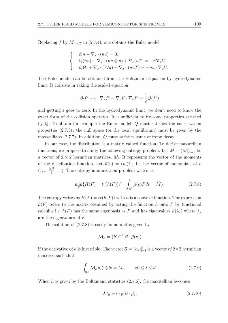
2.7. OTHER FLUID MODELS FOR SEMICONDUCTOR SPINTRONICS 109

Replacing f by Mn,u,T in (2.7.4), one obtains the Euler model

∂tn +∇x · (nu) = 0,

∂t(nu) +∇x · (nu⊗ u) +∇x(nT ) = −n∇xV,

∂tW +∇x · (Wu) +∇x · (nuT ) = −nu · ∇xV.

The Euler model can be obtained from the Boltzmann equation by hydrodynamic

limit. It consists in taking the scaled equation

∂tfε + v · ∇xf

ε −∇xV · ∇vfε =

1

εQ(f ε)

and getting ε goes to zero. In the hydrodynamic limit, we don’t need to know the

exact form of the collision operator. It is sufficient to fix some properties satisfied

by Q. To obtain for example the Euler model, Q must satisfies the conservation

properties (2.7.3) ; the null space (or the local equilibrium) must be given by the

maxwellians (2.7.7). In addition, Q must satisfies some entropy decay.

In our case, the distribution is a matrix valued function. To derive maxwellian

functions, we propose to study the following entropy problem. Let ~M = (Mi)di=1 be

a vector of 2 × 2 hermitian matrices, Mi. It represents the vector of the moments

of the distribution function. Let ~µ(v) = (µi)di=1 be the vector of monomials of v

(1, v, |v|2

2, . . .). The entropy minimization problem writes as

minFH(F ) = tr(h(F ))/

∫

R3

~µ(v)Fdv = ~M. (2.7.8)

The entropy writes as H(F ) = tr(h(F )) with h is a convexe function. The expression

h(F ) refers to the matrix obtained by acting the function h onto F by functional

calculus i.e. h(F ) has the same eigenbasis as F and has eigenvalues h(λs) where λs

are the eigenvalues of F .

The solution of (2.7.8) is easily found and is given by

M~α = (h′)−1(~α · ~µ(v))

if the derivative of h is invertible. The vector ~α = (αi)di=1 is a vector of 2×2 hermitian

matrices such that

∫

R3

M~αµi(v)dv = Mi, ∀0 ≤ i ≤ d. (2.7.9)

When h is given by the Boltzmann statistics (2.7.6), the maxwellian becomes

M~α = exp(~α · ~µ). (2.7.10)

110 CHAPTER 2. HIERARCHY OF KINETIC AND MACROSCOPIC MODELS

2.7.1 Energy-Transport model

The Energy-Transport (ET) model is a diffusion model constituted of a balance

equation for the electron density and an energy balance equation [3, 4, 14, 19]. To

derive ET Model for semiconductor spintronics, we take the Boltzmann equation in

the diffusion scaling (2.5.2). The collision operator Q must now conserve only the

mass and the energy. This means

∫

R3

Q(f)

(1|v|22

)dv = 0. (2.7.11)

Following the Levermore’s moment method, for any distribution function F (v), we

construct the maxwellian MF associated to F as the solution of (2.7.8) with h

given by (2.7.6), ~µ(v) =

(1|v|22

), and ~M =

∫R3 F~µ(v)dv. More precisely, MF is

the solution of

minG

H(G) = 〈G, (log(G)− I2)〉2/

∫

R3

(G− F )

(1|v|22

)dv = 0

.

Then, by (2.7.10)-(2.7.9), MF is given by

MF (v) = M[A,C] := exp

(A + C

|v|22

)(2.7.12)

with A ∈ H2(C) and C ∈ H2(C) are such that

∫

R3

M[A, C]

(1|v|22

)dv =

∫

R3

F

(1|v|22

)dv. (2.7.13)

Let now the collision operator be given by the following BGK simple form

Q(F ) = M[A,C]− F, (2.7.14)

where M[A,C] is defined by (2.7.12) and A and C are relied to F with (2.7.13). Let

us, before listing the properties of this operator, gives some properties satisfied by

log as function on H+2 (C).

Lemma 2.7.1. 1. For all F ∈ H+2 (C), log(F ) is the unique matrix in H2(C)

satisfying elog(F ) = F. Writing F = fcI2 + ~fs · ~σ, then we have

log(F ) =1

2log(f 2

c − |~fs|2)I2 +1

2log

(fc − |~fs|fc + |~fs|

)~fs

|~fs|· ~σ (2.7.15)

if ~fs 6= 0. Its eigenvalues are then log(fc − |~fs|) and log(fc + |~fs|).

2.7. OTHER FLUID MODELS FOR SEMICONDUCTOR SPINTRONICS 111

2. For all F,G ∈ H+2 (C), the following properties hold.

(a) If F and G commutate, then log(F ·G) = log(F ) + log(G)

(b) If F is invertible then log(F−1) = − log(F )

(c) The function log is strictly increasing which means that

〈(F −G), (log F − log G)〉2 ≥ 0 (2.7.16)

and

〈(F −G), (log F − log G)〉2 = 0 ⇔ F = G. (2.7.17)

The collision operator (2.7.14) satisfies the following properties.

(i) By (2.7.13), Q preserves the mass and the energy i.e. (2.7.11) is satisfied.

(ii) Its null space is spanned by the maxwellians. More precisely

Q(F ) = 0 ⇔ ∃(A,C) = (A(t, x), C(t, x)) s.t. F = M[A,C] = exp

(A + C

|v|22

).

(iii) By construction of MF and (2.7.16)-(2.7.17), we have the following entropy

decay ∫

R3

〈Q(F ), log F 〉2dv ≤ 0, (2.7.18)

with equality if and only if F = M[A,C]. Indeed, using (2.7.13), we have

∫

R3

〈Q(F ), log(M[A,C])〉2dv =

∫

R3

⟨M[A,C]− F, (A + C

|v|22

)

⟩

2

dv = 0.

Therefore, with (2.7.16), we have

∫

R3

〈Q(F ), log F 〉2dv =

∫

R3

〈Q(F ), log F − log(M[A,C])〉2dv

=

∫

R3

〈M[A,C]− F, log F − log(M[A,C])〉2dv ≤ 0.

We state now the main result of this subsection which consists on formal derivation

of ET model with spin rotation and relaxation effects.

Theorem 2.7.2. Let F ε be the solution of (2.5.2)-(2.1.2) with Q given by (2.7.14).

Then, formally, F ε → F0 as ε → 0, where

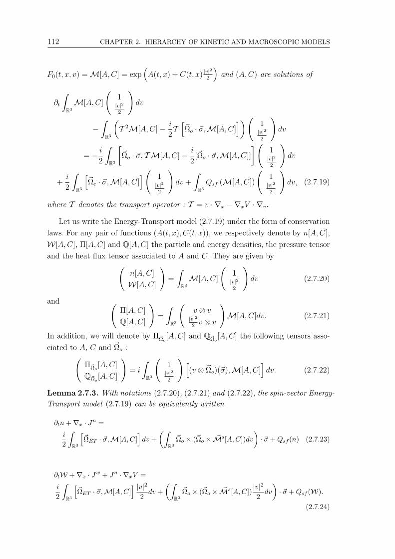
112 CHAPTER 2. HIERARCHY OF KINETIC AND MACROSCOPIC MODELS

F0(t, x, v) = M[A,C] = exp(A(t, x) + C(t, x) |v|

2

2

)and (A,C) are solutions of

∂t

∫

R3

M[A,C]

(1|v|22

)dv

−∫

R3

(T 2M[A,C]− i

2T

[~Ωo · ~σ,M[A,C]

]) (1|v|22

)dv

= − i

2

∫

R3

[~Ωo · ~σ, TM[A, C]− i

2[~Ωo · ~σ,M[A,C]]

] (1|v|22

)dv

+i

2

∫

R3

[~Ωe · ~σ,M[A,C]

](1|v|22

)dv +

∫

R3

Qsf (M[A,C])

(1|v|22

)dv, (2.7.19)

where T denotes the transport operator : T = v · ∇x −∇xV · ∇v.

Let us write the Energy-Transport model (2.7.19) under the form of conservation

laws. For any pair of functions (A(t, x), C(t, x)), we respectively denote by n[A, C],

W [A,C], Π[A,C] and Q[A,C] the particle and energy densities, the pressure tensor

and the heat flux tensor associated to A and C. They are given by(

n[A,C]

W [A,C]

)=

∫

R3

M[A,C]

(1|v|22

)dv (2.7.20)

and (Π[A,C]

Q[A,C]

)=

∫

R3

(v ⊗ v

|v|22

v ⊗ v

)M[A, C]dv. (2.7.21)

In addition, we will denote by Π~Ωo[A,C] and Q~Ωo

[A,C] the following tensors asso-

ciated to A, C and ~Ωo :(

Π~Ωo[A,C]

Q~Ωo[A, C]

)= i

∫

R3

(1|v|22

)[(v ⊗ ~Ωo)(~σ),M[A,C]

]dv. (2.7.22)

Lemma 2.7.3. With notations (2.7.20), (2.7.21) and (2.7.22), the spin-vector Energy-

Transport model (2.7.19) can be equivalently written

∂tn +∇x · Jn =

i

2

∫

R3

[~ΩET · ~σ,M[A, C]

]dv +

(∫

R3

~Ωo × (~Ωo × ~Ms[A,C])dv

)· ~σ + Qsf (n) (2.7.23)

∂tW +∇x · Jw + Jn · ∇xV =

i

2

∫

R3

[~ΩET · ~σ,M[A,C]

] |v|22

dv +(∫

R3

~Ωo × (~Ωo × ~Ms[A,C])|v|22

dv

)· ~σ + Qsf (W).

(2.7.24)

2.7. OTHER FLUID MODELS FOR SEMICONDUCTOR SPINTRONICS 113

The mass and energy fluxes are given by

Jn = −(∇x · Π + n∇xV − Π~Ωo) (2.7.25)

Jw = −(∇x ·Q+W∇xV + Π∇xV −Q~Ωo) (2.7.26)

where Π, Q, Π~Ωoand Q~Ωo

are nonlinear functionals of n and W through (2.7.21),

(2.7.22) and (2.7.20). Moreover, in the right hand side of the conservation equations

(2.7.23)-(2.7.24), the effective field ~ΩET is given by

~ΩET = divx(v ⊗ ~Ωo)−∇xV · ∇v~Ωo + ~Ωe

and ~Ms[A,C] is the spin part of M[A,C],

~Ms[A,C] = M[A,C]− 1

2tr (M[A,C]) I2.

Remark 2.7.4. The model (2.7.23)-(2.7.24) is constituted of two continuity equa-

tions on the density and the energy coupled via the maxwellian M[A,C] with addi-

tional rotational and relaxation terms as in the drift diffusion case. The first term of

the right side of (2.7.23) (or (2.7.24)) describes the precession of the spin vector part

of M[A,C] around the effective field ~ΩET . The other terms are relaxation terms.

We discuss now an important property satisfied by the Energy-Transport model

(2.7.23)-(2.7.24) : the entropy dissipation. This property is a direct consequence of

our derivation, thanks to the entropy dissipation inequality satisfied by the collision

operator (2.7.18). More precisely, we define the entropy by

S(n,W) =

∫

R6

〈M[A,C], log(M[A,C])− I2〉2dxdv

=

∫

R6

⟨M[A,C], A + C

|v|22− I2

⟩

2

dxdv

=

∫

R3

(〈A, n〉2 + 〈C,W〉2 − tr(n))dx (2.7.27)

where (A,C) and (n,W) are related through (2.7.20). The function S is a strictly

convex functional of (n,W) and we have :

Lemma 2.7.5. Let (n,W) solves the Energy-Transport model given by the previous

lemma. Then, the fluid entropy S(n,W) is a decreasing function of time

d

dtS(n,W) ≤ 0. (2.7.28)

Proof of Theorem 2.7.2. We present now the formal derivation of (2.7.19).

We assume that F ε → F0 as ε → 0 in a space of smooth functions. Multiplying

114 CHAPTER 2. HIERARCHY OF KINETIC AND MACROSCOPIC MODELS

(2.5.2) by ε2 and letting ε → 0, one obtains Q(F0) = 0. This implies that there exist

(A(t, x), C(t, x)) such that F0 = exp(A + C |v|22

). Now, we introduce the following

(Chapman-Enskog) expansion

F ε = MF ε + εF ε1 , (2.7.29)

where MF ε is the maxwellian associated to F ε. Thus, we have

F ε1 = −1

εQ(F ε). (2.7.30)

Inserting this expression into (2.5.2), we get

F ε1 = −ε∂tF

ε − T F ε +iε

2[~Ωε · ~σ, F ε] + εQsf (F

ε).

Therefore, as ε → 0, F ε1 → F1 such that

F1 = −T F0 +i

2[~Ωo · ~σ, F0]. (2.7.31)

Next, multiplying (2.5.2) by

(1|v|22

)and using the conservation properties (2.7.11),

we get

∂t

∫

R3

F ε

(1|v|22

)dv +

1

ε

∫

R3

T F ε

(1|v|22

)dv

=i

2

∫

R3

[~Ωε · ~σ, F ε]

(1|v|22

)dv +

∫

R3

Qsf (Fε)

(1|v|22

)dv

Now, using (2.7.29) and the fact that

∫

R3

TMF ε

(1|v|22

)dv = 0 and

∫

R3

[~Ωo · ~σ,MF ε ]

(1|v|22

)dv = 0 since TMF ε and ~Ωo are odd vectors with respect

to v, one obtains

∂t

∫

R3

F ε

(1|v|22

)dv +

∫

R3

T F ε1

(1|v|22

)dv =

i

2

∫

R3

[~Ωo · ~σ, F ε1 ]

(1|v|22

)dv

+i

2

∫

R3

[~Ωe · ~σ, F ε]

(1|v|22

)dv +

∫

R3

Qsf (Fε)

(1|v|22

)dv.

This gives when ε → 0

∂t

∫

R3

F0

(1|v|22

)dv +

∫

R3

T F1

(1|v|22

)dv =

i

2

∫

R3

[~Ωo · ~σ, F1]

(1|v|22

)dv

+i

2

∫

R3

[~Ωe · ~σ, F0]

(1|v|22

)dv +

∫

R3

Qsf (F0)

(1|v|22

)dv.

2.7. OTHER FLUID MODELS FOR SEMICONDUCTOR SPINTRONICS 115

Finally, inserting the expressions of F0 and F1 into the last equation leads to (2.7.19).

Proof of Lemma 2.7.5. We multiply (2.5.2) by log(F ε), integrate with respect

to x and v

∫

R6

〈∂tFε, log F ε〉2dxdv +

1

ε

∫

R6

〈T F ε, log F ε〉2dxdv =1

ε2

∫

R6

〈Q(F ε), log F ε〉2dxdv

+

∫

R6

〈 i2[~Ωε · ~σ, F ε], log F ε〉2dxdv +

∫

R6

〈Qsf (Fε), log F ε〉2dxdv. (2.7.32)

We have

d

dt

∫

R6

〈F ε, log F ε − I2〉2dxdv =d

dt

∫

R6

tr(F ε · (log F ε − I2))dxdv

=d

dt

∫

R6

tr(h(F ε))dxdv

where h = x(logx− 1). In other side we have

d

dttr(h(F ε)) = δF (trh(.))|F ε · ∂tF

ε = tr(h′(F ε) · ∂tFε)

where δF (tr(h(.))) denotes the Gateaux derivative of tr(h(.)) (see also [18] for more

details). We deduce that

d

dttr(h(F ε)) = tr(log F ε · ∂tF

ε) = 〈∂tFε, log F ε〉2.

Therefore,

∫

R6

〈∂tFε, log F ε〉2dxdv =

d

dt

∫

R6

〈F ε, log F ε − I2〉2dxdv.

A similar computations give

∫

R6

〈T F ε, log F ε〉2dxdv =

∫

R6

T (〈F ε, log F ε − I2〉2)dxdv = 0.

Moreover, we have

∫

R6

〈 i2[~Ωε · ~σ, F ε], log F ε〉2dxdv = −

∫

R6

〈(~Ωε × ~f εs ) · ~σ, log F ε〉2dxdv

= −2(~Ωε × ~f εs ) · ~gε

s,

where ~f εs is the spin part of F ε and ~gε

s the spin part of log(F ε). With (2.7.15), ~gεs is

parallel to ~f εs and we conclude that

∫

R6

〈 i2[~Ωε · ~σ, F ε], log F ε〉2dxdv = 0.

116 CHAPTER 2. HIERARCHY OF KINETIC AND MACROSCOPIC MODELS

In other side, using the entropy decay property of Q (2.7.18), the first term of the

right hand side of (2.7.32) is negative. In addition, the third term of the right hand

side of (2.7.32) is also negative. Indeed, we have

⟨tr(F ε)− 2F ε, log

(tr(F ε)

2

)I2

⟩

2

= −2 log

(tr(F ε)

2

)tr(~f ε

s · ~σ) = 0.

Then,∫

R6

〈Qsf (Fε), log F ε〉2dxdv =

1

τsf

∫

R6

〈tr(F ε)− 2F ε, log F ε〉2dxdv

=1

τsf

∫

R6

⟨tr(F ε)− 2F ε, log F ε − log

(tr(F ε)

2

)⟩

2

dxdv

=1

τsf

∫

R6

〈tr(F ε)− 2F ε, log(2F ε)− log(tr(F ε))〉2 dxdv

≤ 0 (in view of (2.7.16)).

As a conclusion, the solution of (2.5.2) with (2.7.14) satisfies

d

dt

∫

R6

〈F ε, log F ε − I2〉2dxdv ≤ 0.

To complete the proof, we pass to the limit ε → 0. This ends the proof of the

lemma since F ε converges to F0 = exp(A+C |v|22

) where (A,C) is the solution of the

spin-vector Energy-Transport model (2.7.19).

2.7.2 Drift-Diffusion with Fermi-Dirac statistics

The nonlinear BGK approximation of the collision operator for Fermi-Dirac sta-

tistics, when we consider a Boltzmann equation with scalar distribution function f ,

takes the form

Q(f) =

∫

R3

σ(v, v′) [M(v)f(v′)(1− f(v))−M(v′)f(v)(1− f(v′))] dv′ (2.7.33)

where M is given by (2.1.5). We refer to [27] for the study of such operator. We list

in the following lemma the main properties satisfied by (2.7.33).

Lemma 2.7.6. Assume that the cross-section verifies Assumption 2.2.1. Let A =

f ∈ L1(R3) ; 0 < f < 1 a.e. be the set of admissible functions. Then,

1. the operator Q given by (2.7.33) is a bounded operator on A in L1(R3).

2. For any f ∈ A, we have the following entropy inequality

H(f) =

∫

R3

Q(f) log

(f

(1− f)MV

)dv ≤ 0, (2.7.34)

2.7. OTHER FLUID MODELS FOR SEMICONDUCTOR SPINTRONICS 117

where MV is the maxwellian associated to the potential V given by

MV :=1

(2π)32

e−12|v|2−V .

.

3. The following statements are equivalent :

(i) f ∈ A and H(f) = 0

(ii) f ∈ A and Q(f) = 0

(iii) there exists µ ∈ R such that f(v) = (1 + e|v|22−µ)−1.

Inspired from the scalar case, we consider the following space of admissible func-

tions

A = F ∈ L1(R3;H2(C)) ; 0 ≺ F (v) ≺ I2 a.e.v (2.7.35)

when, for two hermitian matrices A and B, the relation A ≺ B means that (B−A)

is a positive defined matrix. We will construct a collision operator QFD with 2 × 2

hermitian matrix value admitting the following properties inspired also from the

scalar case :

1. QFD preserves the mass :∫R3 QFDdv = 0.

2. For every F ∈ A, Q admits the following entropy inequality

H(F ) =

∫

R3

QFD(F ) log(F (I2 − F )−1M−1V )dv ≤ 0

3. H(F ) = 0 ⇔ QFD(F ) = 0 ⇔ F = MF .

Here MF denotes the maxwellian associated to F with the Fermi-Dirac sta-

tistics given by

MF =

(I2 + e

|v|22−Π

)−1

(2.7.36)

where Π is a unique matrix belonging to H2(C) such that∫

R3

MF dv =

∫

R3

Fdv. (2.7.37)

We set as for the Energy-Transport case

QFD(F ) = MF − F. (2.7.38)

The maxwellian (2.7.36) with (2.7.37) can also be seen as the solution of an entropy

minimization problem. When the only conserved moment is the density or the mass ;

the convenient entropy concept is the relative entropy. It is given for Fermi-Dirac

statistics by

hFD(F ) = F

(log F +

|v|22

+ V

)+ (I2 − F ) log (I2 − F ) . (2.7.39)

118 CHAPTER 2. HIERARCHY OF KINETIC AND MACROSCOPIC MODELS

For any F ∈ A fixed, the solution of

minG∈A

tr(hFD(G))/

∫

R3

Gdv =

∫

R3

Fdv

is nothing but MF given by (2.7.36)-(2.7.37). Besides, one can verify, by direct

computations using decomposition of the matrices into charge and spin parts, that

problem (2.7.36)-(2.7.37) is well posed and admits a unique solution. This is the aim

of the following lemma and proposition where their proofs are left to the reader.

Lemma 2.7.7. Let Π = πcI + ~πs · ~σ ∈ H2(C) and F ∈ L1(R3,H+2 (C)), then MF

defined by (2.7.36) belongs to A. In addition, we have

MF = αcI2 + ~αs · ~σ (2.7.40)

such that αc = FD(πc), ~αs = 0 if ~πs = 0 and if ~πs 6= 0, we have

αc =1

2(FD(πc + |~πs|) + FD(πc − |~πs|)) (2.7.41)

~αs =1

2(FD(πc + |~πs|)− FD(πc − |~πs|)) ~πs

|~πs| . (2.7.42)

The function FD(.) on R denotes the Fermi-Dirac distribution given by

FD(φ) =

(1 + e

|v|22−φ

)−1

, ∀φ ∈ R. (2.7.43)

Proposition 2.7.8. Let F = F (v) ∈ L1(R3,H+2 (C)). Then, there exists a unique

2×2 hermitian matrix Π independent of v satisfying (2.7.37). In addition, if we write

Π = πcI2 + ~πs · ~σ and ρ :=

∫

R3

F (v)dv = ρcI2 + ~ρs · ~σ, then (2.7.37) is equivalent to

∫

R3

FD(πc + |~πs|)(v)dv = ρc + |~ρs|∫

R3

FD(πc − |~πs|)(v)dv = ρc − |~ρs|

and~πs

|~πs| =~ρs

|~ρs| if ~ρs 6= 0,

(2.7.44)

where FD is given by (2.7.43).

The newt proposition summarizes the main properties of the collision operator

(2.7.38).

Proposition 2.7.9. The operator QFD defined by (2.7.38), (2.7.36) and (2.7.37)

satisfies the following properties.

2.7. OTHER FLUID MODELS FOR SEMICONDUCTOR SPINTRONICS 119

1. QFD is bounded on L1(R3;H+2 (C)) i.e. there exists a constant C such that for

all F ∈ L1(R3;H+2 (C))

‖QFD(F )‖L1(R3;H+2 (C)) ≤ C‖F‖L1(R3;H+

2 (C)). (2.7.45)

2. For all F ∈ A, we have the following H-Theorem (or entropy decay)

H(F ) :=

∫

R3

QFD(F ) :[log(F (I2 − F )−1M−1

V )] ≤ 0. (2.7.46)

3. The following statements are equivalent

(i) F ∈ A and H(F ) = 0.

(ii) F ∈ A and QFD(F ) = 0.

(iii) there exists Π ∈ H2(C) such that F =(I2 + e

|v|22−Π

)−1

.

Proof. 1. For any Π ∈ H2(C), the matrix MF given by (2.7.40), (2.7.41), (2.7.42)

satisfies

‖MF‖22 = (αcI2 + ~αs · ~σ) : (αcI2 + ~αs · ~σ) = 2(α2

c + |~αs|2)= FD(πc + |~πs|)2 + FD(πc − |~πs|)2

≤ [FD(πc + |~πs|) + FD(πc − |~πs|)]2.

Let F ∈ L1(R3;H+2 (C)) and let Π be the solution of (2.7.37). Then, in view of

(2.7.44), we have∫

R3

‖MF‖2dv ≤∫

R3

FD(πc + |πs|)dv +

∫

R3

FD(πc − |πs|)dv

≤ ρc = |∫

R3

fcdv| ≤∫

R3

|fc|dv ≤∫

R3

‖F‖2dv.

Thus,

∫

R3

‖QFD(F )‖2 ≤∫

R3

‖MF‖2dv +

∫

R3

‖F‖2dv ≤ 2

∫

R3

‖F‖2dv.

2. For all F ∈ A, it is simple to verify that F (I2 − F )−1 belongs to H+2 (C) and F

commutate with (I2 − F )−1. Then, log(F (I2 − F )−1) is well defined and log(F (I2 −F )−1) = log(F )− log(I2−F ). Let now Π be the solution of (2.7.37). Then, we have

MF (I2 −MF )−1M−1V = (2π)

32 eΠ+V .

Indeed,

MF (I2 −MF )−1 =

(I2 + e

|v|22−Π

)−1

(I2 −MF )−1 =

[(I2 −MF )(I2 + e

|v|22−Π)

]−1

=

(I2 + e

|v|22−Π − I2

)−1

= e−|v|2

2 eΠ = (2π)32 MV eΠ+V .

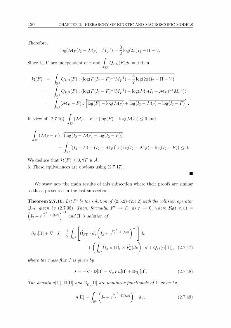
120 CHAPTER 2. HIERARCHY OF KINETIC AND MACROSCOPIC MODELS

Therefore,

log(MF (I2 −MF )−1M−1V ) =

3

2log(2π)I2 + Π + V.

Since Π, V are independent of v and

∫

R3

QFD(F )dv = 0 then,

H(F ) =

∫

R3

QFD(F ) : (log(F (I2 − F )−1M−1V )− 3

2log(2π)I2 − Π− V )

=

∫

R3

QFD(F ) : (log(F (I2 − F )−1M−1V )− log(MF (I2 −MF )−1M−1

V ))

=

∫

R3

(MF − F ) :[log(F )− log(MF ) + log(I2 −MF )− log(I2 − F )

].

In view of (2.7.16),

∫

R3

(MF − F ) : (log(F )− log(MF )) ≤ 0 and

∫

R3

(MF − F ) : (log(I2 −MF )− log(I2 − F ))

=

∫

R3

[(I2 − F )− (I2 −MF )] : (log(I2 −MF )− log(I2 − F )) ≤ 0.

We deduce that H(F ) ≤ 0,∀F ∈ A.

3. These equivalences are obvious using (2.7.17).

¥

We state now the main results of this subsection where their proofs are similar

to those presented in the last subsection.

Theorem 2.7.10. Let F ε be the solution of (2.5.2)-(2.1.2) with the collision operator

QFD given by (2.7.38). Then, formally, F ε → F0 as ε → 0, where F0(t, x, v) =(I2 + e

|v|22−Π(t,x)

)−1

and Π is solution of

∂tn[Π] +∇ · J =i

2

∫

R3

[~ΩFD · ~σ,

(I2 + e

|v|22−Π(t,x)

)−1]

dv

+

(∫

R3

~Ωo × (~Ωo × ~F so )dv

)· ~σ + Qsf (n[Π]), (2.7.47)

where the mass flux J is given by

J = −∇ · D[Π]−∇xV n[Π] + D~Ωo[Π]. (2.7.48)

The density n[Π], D[Π] and D~Ωo[Π] are nonlinear functionals of Π given by

n[Π] =

∫

R3

(I2 + e

|v|22−Π(t,x)

)−1

dv, (2.7.49)

REFERENCES 121

D[Π] =

∫

R3

(v ⊗ v)

(I2 + e

|v|22−Π(t,x)

)−1

dv,

and

D~Ωo[Π] = i

∫

R3

[(v ⊗ ~Ωo)(~σ),

(I2 + e

|v|22−Π(t,x)

)−1]

dv.

The Fermi-Dirac effective field ~ΩFD is similar to the one obtained in the derivation

of energy transport model. It is given by

~ΩFD = divx(v ⊗ ~Ωo)−∇xV · ∇v~Ωo + ~Ωe.

Finally, the ~F s0 is the spin part of F0 =

(I2 + e

|v|22−Π(t,x)

)−1

.

The entropy function is now defined by, where F0 =(I2 + e

|v|22−Π

)−1

and n =∫R3 F0dv,

S(n) =

∫

R6

〈F0, log(F0(I2 − F0)−1M−1

V )〉2dxdv +

∫

R6

tr(log(I2 − F0))dxdv

=

∫

R6

〈F0,3

2log(2π)I2 + Π + V 〉2dxdv +

∫

R6

tr(log(I2 − F0))dxdv

=

∫

R3

(3

2log(2π)tr(n) + 〈n, Π + V 〉2

)dx +

∫

R6

tr(log(I2 − F0))dxdv.

Proposition 2.7.11. Let Π and n := n[Π] solve the Drift-Diffusion system (2.7.47)-

(2.7.48). Then, the Fermi-Dirac fluid entropy S satisfies

d

dtS(n) ≤

∫

R3

∂tV tr(n)dx. (2.7.50)

If the potential V is independent of time, then S(n) is a decreasing function of time

d

dtS(n) ≤ 0.

References

[1] C. Bardos, F. Golse, and D. Levermore, Fluid dynamic limits of kinetic

equations. I. Formal derivations, J. Statist. Phys., 63 (1991), pp. 323–344.

[2] N. Ben Abdallah and P. Degond, On a hierarchy of macroscopic models

for semiconductors, J. Math. Phys., 37 (1996), pp. 3306–3333.

[3] N. Ben Abdallah, P. Degond, and S. Genieys, An Energy-Transport

model derived from the Boltzmann equation of semiconductors, J. Stat. Phys.,

84 (1996), pp. 205–231.

122 REFERENCES

[4] N. Ben Abdallah, S. Desvillettes, and S. Genieys, On the convergence

of the Boltzmann for the semiconductors toward the energy transport model, J.

Stat. Phys., 98 (2000), pp. 835–870.

[5] J. A. Bittencourt, Fundamentals of plasma physics, Pergamon Press, Ox-

ford, 1986.

[6] F. Bouchut, F. Golse, and M. Pulvirenti, Kinetic equations and asymp-

totic theory, B. perthame, L. Desvillettes Eds, Series in Appl. Math., bf 4,

Gauthier-Villars (2000).

[7] A. Bournel, Magneto-electronique dans des dispositifs a semiconducteurs,

Ann. Phys. Fr, 25 (2000), pp. 1–167.

[8] A. Bournel, V. Delmouly, P. Dollfus, G. Tremblay, and P. Hesto,

Theoretical and experimental considerations on the spin field effect transistor,

Physica E, 10 (2001), pp. 86–90.

[9] A. Bournel, P. Dollfus, E. Cassan, and P. Hesto, Monte Carlo study

of spin relaxation in AlGaAs/GaAs quantum wells, Applied Physics Letters, 77

(2000), pp. 2346–2348.

[10] Y. A. Bychkov and E. I. Rashba, Oscillatory effects and the magnetic

susceptibility of carriers in inversion layers, Journal of Physics C : Solid State

Physics, 17 (1984), pp. 6039–6045.

[11] S. Datta and B. Das, Electronic analog of the electro-optic modulator, Ap-

plied Physics Letters, 56 (1990), pp. 665–667.

[12] P. Degond, Mathematical modelling of microelectronics semiconductor de-

vices, in Some current topics on nonlinear conservation laws, vol. 15 of AMS/IP

Stud. Adv. Math., Amer. Math. Soc., Providence, RI, 2000, pp. 77–110.

[13] P. Degond, G. Gallego, and F. Mehats, Entropic discretization of a

quantum drift-diffusion model, SIAM J. Numer. Anal., 43 (2005), pp. 1828–

1849.

[14] P. Degond, C. D. Levermore, and C. Schmeiser, A note on the energy-

transport limit of the semiconductor Boltzmann equation, in Transport in tran-

sition regimes (Minneapolis, MN, 2000), vol. 135 of IMA Vol. Math. Appl.,

Springer, New York, 2004, pp. 137–153.

[15] P. Degond, F. Mehats, and C. Ringhofer, Quantum hydrodynamic mo-

dels derived from the entropy principle, Contemp. Math. 371, Amer. Math. Soc.,

Providence RI (2005).

[16] , Quantum energy-transport and drift-diffusion models, J. Stat. Phys., 118

(2005), pp. 625–667.

REFERENCES 123

[17] P. Degond and C. Ringhofer, A note on binary quantum collision ope-

rators conserving mass, momentum and energy, C. R. Acad. Sci. Paris, 336

(2003), pp. Ser I, 587–628.

[18] , Quantum moment hydrodynamics and the entropy principle, J. Stat.

Phys., 112 (2003), pp. 587–628.

[19] P. Degond and C. Schmeiser, Macroscopic models for semiconductor he-

terostructures, J. Math. Phys., 39 (1998), pp. 4634–4663.

[20] G. Dresselhaus, Spin-orbit coupling effects in zinc blende structures, Phys.

Rev., 100 (1955), pp. 580–586.

[21] R. J. Elliott, Theory of the effect of spin-orbit coupling on magnetic reso-

nance in some semiconductors, Phys. Rev., 96 (1954), pp. 266–279.

[22] A. Fert, A. Friederich, and al, Giant magnetoresistance of

(001)fe/(001)cr magnetic superlattices, Phys. Rev. Lett., 61 (1988), pp. 2472–

2475.

[23] G. Fishman and G. Lampel, Spin relaxation of photoelectrons in p-type

gallium arsenide, Phys. Rev. B, 16 (1977), pp. 820–831.

[24] G. Gallego and F. Mehats, On Quantum Hydrodynamic and Quantum

Energy Transport Models, Commun. Math. Sci., 5 (2007), pp. 887–908.

[25] I. Gasser and R. Natalini, The energy transport and the drift diffusion

equations as relaxation limits of the hydrodynamic model for semiconductors,

Quart. Appl. Math., 57 (1999), pp. 269–282.

[26] F. Golse and D. Levermore, Stokes-Fourier and acoustic limits for the

Boltzmann equations : Convergence proofs, Comm. Pure Appl. Math., 55 (2002),

pp. 336–393.

[27] F. Golse and F. Poupaud, Limite fluide des equations de Boltzmann des

semi-conducteurs pour une statistique de Fermi-Dirac, Asymptotic Anal., 6

(1992), pp. 135–160.

[28] F. Golse and L. Saint-Raymond, Hydrodynamics limit for the Boltzmann

equation, Lecture Porto Ercole, (2004).

[29] , The Navier-Stokes limit of the Boltzmann equation for bounded collision

kernels, Invent Math., 155 (2004), pp. 81–161.

[30] L. D. Landau and E. M. Lifshitz, Quantum Mechanics, Pergamon Press,

Oxford, 1991.

[31] C. D. Levermore, Moment closure hierarchies for kinetic theories, J. Stat.

Phys., 83 (1996), pp. 1021–1065.

124 REFERENCES

[32] P. A. Markowich, C. A. Ringhofer, and C. Schmeiser, Semiconductor

equations, Springer-Verlag, Vienna, 1990.

[33] M. S. Mock, Analysis of mathematical models of semiconductor devices, vol. 3

of Advances in Numerical Computation Series, Boole Press, Dun Laoghaire,

1983.

[34] A. Pazy, Semigroups of linear operators and applications to partial differential

equations, vol. 44 of Applied Mathematical Sciences, Springer-Verlag, New York,

1983.

[35] Y. Pershin, S. Saikin, and V. Privman, Semiclassical transport models for

semiconductor spintronics, Electrochem. Soc. Proc., 2004-13 (2005), pp. 183–

205.

[36] Y. V. Pershin and V. Privman, Focusing of spin polarization in semicon-

ductors by inhomogeneous doping, Phys. Rev. Lett., 90 (2003), p. 256602.

[37] F. Poupaud, Diffusion approximation of the linear semiconductor Boltzmann

equation : analysis of boundary layers, Asymptotic Anal., 4 (1991), pp. 293–317.

[38] Y. Qi and S. Zhang, Spin diffusion at finite electric and magnetic fields,

Phys. Rev. B, 67 (2003), p. 052407.

[39] Y. P. Raizer, Gas Discharge Physics, Springer, Berlin, 1997.

[40] M. Reed and B. Simon, Methods of modern mathematical physics., Academic

Press, New York, second ed., 1975. Functional analysis.

[41] S. Saikin, A drift-diffusion model for spin-polarized transport in a two-

dimensional non-degenerate electron gas controlled by spin orbit interaction,

Journal of Physics : Condensed Matter, 16 (2004), pp. 5071–5081.

[42] S. Saikin, Y. Pershin, and V. Privman, Modelling for semiconductor spin-

tronics, IEE Proceedings Circuits, Devices and Systems, 152 (2005), pp. 366–

376.

[43] C. Schmeiser and A. Zwirchmayr, Elastic and drift-diffusion limits of

electron-phonon interaction in semiconductors, Math. Models Methods Appl.

Sci., 8 (1998), pp. 37–53.

[44] T. Valet and A. Fert, Theory of the perpendicular magnetoresistance in

magnetic multilayers, Phys. Rev. B, 48 (1993), pp. 7099–7113.

[45] C. Villani, Limite hydrodynamiques de l’equation de Boltzmann, Seminaire

Bourbaki, 53eme annee, no 893 (2000–2001).

[46] Z. G. Yu and M. E. Flatte, Electric-field dependent spin diffusion and spin

injection into semiconductors, Phys. Rev. B, 66 (2002), p. 201202.

REFERENCES 125

[47] Z. G. Yu and M. E. Flatte, Spin diffusion and injection in semiconductor

structures : electric field effects, Phys. Rev. B, 66 (2002), p. 235302.

[48] I. Zutic, J. Fabian, and S. Das Sarma, Spin-Polarized Transport in Inho-

mogeneous Magnetic Semiconductors : Theory of Magnetic/Nonmagnetic p−n

Junctions, Phys. Rev. Lett., 88 (2002), p. 066603.

[49] I. Zutic, J. Fabian, and S. D. Sarma, Spintronics : Fundamentals and

applications, Reviews of Modern Physics, 76 (2004), p. 323.

Chapter 3

Numerical Applications

Abstract

The purpose of this chapter is to somewhere validate numerically the models derived

in the previous chapters. Two numerical applications are carried out. The first one

concerns the simulation of transistor with spin rotation effect (spin-FET). Following

the work of [6, 22], a subband drift-diffusion Schrodinger-Poisson model with spin

rotation and relaxation effects is derived and used for the simulation. The second

application is a well known effect in semiconductor spintronics : the accumulation of

spin polarization density at the interface between two semi-conductor regions with

different doping levels [18, 17]. This phenomena is illustrated using two-component

drift-diffusion Poisson model. Moreover, we show the action of the Rashba spin-orbit

coupling on this spin accumulation effect by means of spin vector drift-diffusion Pois-

son model.

127

128 CHAPTER 3. NUMERICAL APPLICATIONS

3.1 Modelling and numerical implementation of

spin-FET

3.1.1 Introduction

Recently, the spin-related properties of charge carries in semiconductors have

generated a huge attention leading to proposition of new magnetoelectronics devices.

The Rashba term in the spin-orbit coupling [11] appearing in a quantum well under

electric field along the growth direction makes feasible the control of electron spin

orientation through the confining electric field. This mechanism leads to the concept

of the spin Field Effect Transistor, the spin-FET [14].

The spin-FET is a High Mobility Transistor (HEMT) in which the source and

drain contacts are ferromagnetics. A HEMT transistor is composed of a channel

which is an active region connected to two electrodes called the source and drain. It is

based on the formation of electron confined gas in the channel at the heterointerface

between different semiconductor heterostructures. The confinement in the channel

is commanded by a Schottky gate. The source and drain are high doped regions

and play the role of two small reservoirs. Apply at the electrodes a drain-source

potential, VDS, a drain current can be established.

The idea of spin-FET, due to Datta and Das [14], consists in replacing the source

and drain by ferromagnetic contacts. The source then acts as polarizer and injects

a spin polarized current. In the channel, the control of electron spin orientation

is possible by the applied gate potential through the Rashba spin-orbit coupling.

The drain plays the role of selector. It collects preferentially electrons with spin

orientation depending on its magnetic moment.

The device considered here is a double gate MOSFET represented by Figure 3.1.

We do not take a ferromagnetic contacts at the source and drain. We assume that

a spin polarized current is injected from the source to the channel. The object is to

show numerically the action of the gate voltage (via the Rashba coupling) on the

spin dynamics in 1DEG. To this aim, we take a two dimension device in the (xz)

plane. We assume that the particles are confined in the z direction and the transport

is allowed in the x direction. The Rashba spin precession vector is then oriented in

the y direction (perpendicular to device plane (xz)) and does not change direction.

The aim of the simulation is to illustrate the efficiency of the gate control of the spin

orientation in this case.

The results presented here are well known in semiconductor spintronics. See for

example [8] for the study of 1DEG. However, when taking a two dimensional chan-

nel with width equal to W in the y direction, the situation is more complicated.

Indeed, in two-dimensional electron gas, the Rashba effective field direction depends

3.1. MODELLING AND NUMERICAL IMPLEMENTATION OF SPIN-FET 129

strongly on v (or on the wave vector). Then, the electron/crystal scattering ran-

domize the Rashba effective field direction. So, during the motion of one electron,

its spin orientation becomes progressively incoherent. The spin polarization of the

electron population may be thus fast relaxed (by the D’yakonov-Perel relaxation me-

chanism). Using Monte Carlo technique, A. Bournel and al study the gate induced

spin precession in 2DEG [8, 9, 10]. They studied the influence of the width W on

the spin diffusion length Ls or spin relaxation length induced by the interactions. It

is shown that the D’yakonov-Perel spin relaxation mechanism tends to vanish (or to

disappear as in the 1DEG case) when the channel width decreases. They prove that

it is sufficient to take W less than 100 nm at the room temperature to have a spin re-

laxation length exceeding 1µm. In this case, one obtains an efficient gate-controlled

spin precession in the channel as in the one dimensional case presented here. For

this, the spin orientation injected by the source contact has to be perpendicular to

the source/channel interface. We refer also to [20, 21] for the study of gate-induced

spin precession in 2DEGs. We don’t study here the 2D channel case. The study of

spin transport properties in 2DEG will be the subject of future works.

The model used for the simulation is a coupled quantum classical model. In the

confinement direction, the length scale is of the order of the electron de Broglie

wavelength and a quantum models have to be adapted in this direction. However

the length scale in the transport direction is much bigger and a classical transport

model can be used. This gives rise to the subband theory [1, 2, 15]. The subband

models are the subject of many recent works. In [3], as mentioned in the first chapter

of this thesis, a partially quantum/kinetic subband model is derived by a partially

semi-classical limit from a full quantum model. A rigorous analysis of the limit model

(Vlasov Schrodinger-Poisson model) is then investigated in [4]. We refer also to [7, 22,

5], for the derivation and study of quantum/fluid type models. The next subsection

is dedicated to give more precise description on the subband quantum/drift-diffusion

model.

3.1.2 A coupled quantum/drift diffusion model with spin-

orbit effect

In this part, we will derive a macroscopic subband model by performing a dif-

fusion limit of the Boltzmann Schrodinger system with spin-orbit term. We adapt

the work of [22]. Assume that the quantum effects take place in one direction of the

space denoted by z, z ∈ [0, 1], and in the other directions, x ∈ Rd, the particles

move classically. At a time t > 0 and a position (x, z) ∈ Rd × [0, 1], the density of

the system is given by

130 CHAPTER 3. NUMERICAL APPLICATIONS

N ε(t, x, z) =∑n>1

(

∫

Rd

F εn(t, x, v)dv)|χn(t, x, z)|2. (3.1.1)

The unknowns of the problem are (εn, χn, F εn)n>1. The subbands are characterized by

the complete set, (εn, χn)n, of the eigenelements of the one dimensional Schrodinger

operator −1

2

d2

dz2+V with homogeneous Dirichlet data. More precisely, the sequence

(εn(t, x), χn(t, x, .))n verifies

−12

d2

dz2 χn + V χn = εnχn,

χn(t, x, .) ∈ H10 (0, 1),

∫ 1

0

χnχm = δnm.(3.1.2)

The potential V (t, x, z) is supposed to be given and regular function (see Assumption

3.1.2). Generally, V is not given but satisfies the Poisson equation if one accounts the

electrostatic forces. For each subband, the distribution function, F εn(t, x, v) ∈ H+

2 (C),

satisfies the following scaled spinor Boltzmann equation

∂tFεn +

1

ε(v.∇xF

εn −∇xεn.∇vF

εn) =

1

ε2Q(F ε)n +

i

2[Ωε

n.~σ, F εn], (3.1.3)

where

Ωεn(t, x, v) =

1

εΩo

n(t, x, v) + Ωen(t, x, v) (3.1.4)

such that Ωon, Ωe

n are respectively odd and even functions with respect to v satisfying

Assumption 3.1.3. Here, the collision operator takes the form

Q(F )n =∑

n′

∫

R2

σnn′(v, v′)Mn(v)Fn′(v′)−Mn′(v

′)Fn(v)dv′ (3.1.5)

which accounts the transition between the subbands. The normalized Maxwellian

Mn is given by

Mn(v) =1

(2π)d2Z

e−( 12|v|2+εn) (3.1.6)

where Z is the repartition function

Z(t, x) =∑

n

e−εn(t,x). (3.1.7)

Initially, we will take

F εn(0, x, v) = Fin,n(x, v). (3.1.8)

We fix as in the previous chapter the following assumptions on the cross-section, the

potential and the effective field.

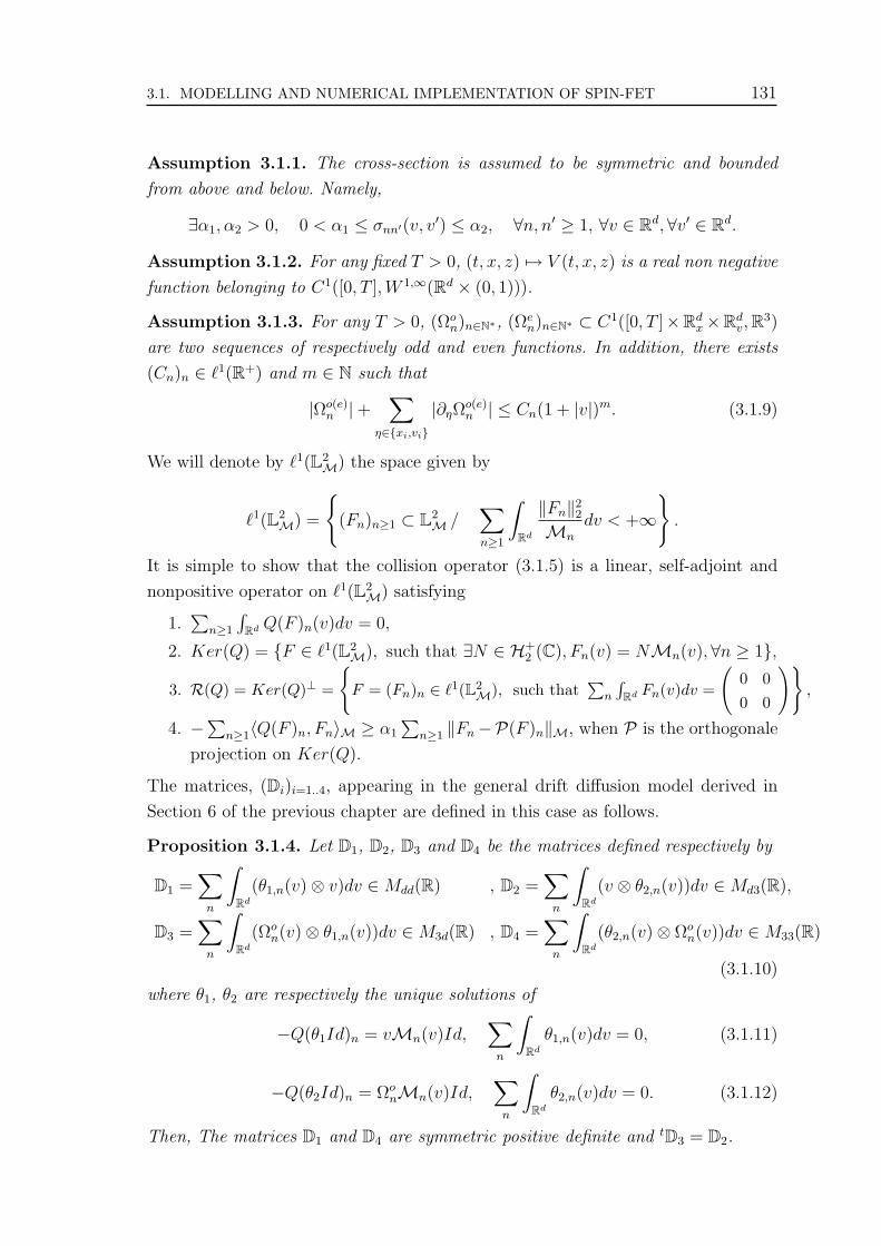
3.1. MODELLING AND NUMERICAL IMPLEMENTATION OF SPIN-FET 131

Assumption 3.1.1. The cross-section is assumed to be symmetric and bounded

from above and below. Namely,

∃α1, α2 > 0, 0 < α1 ≤ σnn′(v, v′) ≤ α2, ∀n, n′ ≥ 1, ∀v ∈ Rd,∀v′ ∈ Rd.

Assumption 3.1.2. For any fixed T > 0, (t, x, z) 7→ V (t, x, z) is a real non negative

function belonging to C1([0, T ],W 1,∞(Rd × (0, 1))).

Assumption 3.1.3. For any T > 0, (Ωon)n∈N∗, (Ωe

n)n∈N∗ ⊂ C1([0, T ]×Rdx×Rd

v,R3)

are two sequences of respectively odd and even functions. In addition, there exists

(Cn)n ∈ `1(R+) and m ∈ N such that

|Ωo(e)n |+

∑

η∈xi,vi|∂ηΩ

o(e)n | ≤ Cn(1 + |v|)m. (3.1.9)

We will denote by `1(L2M) the space given by

`1(L2M) =

(Fn)n≥1 ⊂ L2

M /∑n≥1

∫

Rd

‖Fn‖22

Mn

dv < +∞

.

It is simple to show that the collision operator (3.1.5) is a linear, self-adjoint and

nonpositive operator on `1(L2M) satisfying

1.∑

n≥1

∫Rd Q(F )n(v)dv = 0,

2. Ker(Q) = F ∈ `1(L2M), such that ∃N ∈ H+

2 (C), Fn(v) = NMn(v),∀n ≥ 1,

3. R(Q) = Ker(Q)⊥ =

F = (Fn)n ∈ `1(L2

M), such that∑

n

∫Rd Fn(v)dv =

(0 00 0

),

4. −∑n≥1〈Q(F )n, Fn〉M ≥ α1

∑n≥1 ‖Fn−P(F )n‖M, when P is the orthogonale

projection on Ker(Q).

The matrices, (Di)i=1..4, appearing in the general drift diffusion model derived in

Section 6 of the previous chapter are defined in this case as follows.

Proposition 3.1.4. Let D1, D2, D3 and D4 be the matrices defined respectively by

D1 =∑

n

∫

Rd

(θ1,n(v)⊗ v)dv ∈ Mdd(R) , D2 =∑

n

∫

Rd

(v ⊗ θ2,n(v))dv ∈ Md3(R),

D3 =∑

n

∫

Rd

(Ωon(v)⊗ θ1,n(v))dv ∈ M3d(R) , D4 =

∑n

∫

Rd

(θ2,n(v)⊗ Ωon(v))dv ∈ M33(R)

(3.1.10)

where θ1, θ2 are respectively the unique solutions of

−Q(θ1Id)n = vMn(v)Id,∑

n

∫

Rd

θ1,n(v)dv = 0, (3.1.11)

−Q(θ2Id)n = ΩonMn(v)Id,

∑n

∫

Rd

θ2,n(v)dv = 0. (3.1.12)

Then, The matrices D1 and D4 are symmetric positive definite and tD3 = D2.

132 CHAPTER 3. NUMERICAL APPLICATIONS

Passing to the limit ε → 0, we get an hybrid Drift-Diffusion Schrodinger system.

Namely, applying the same ideas as in the previous chapter, the following results

hold.

Theorem 3.1.5. Let T > 0, (Fin,n)n ∈ `1(L2M(dxdv)) and assume that Assump-

tions 3.1.1, 3.1.2 and 3.1.3 hold. Then, for all ε > 0, the model (3.1.3)...(3.1.8)

admits a unique weak solution (F εn)n ∈ C0([0, T ]; `1(L2

M(dxdv))). In addition, there

exists Ns ∈ L2([0, T ] × Rd,H+2 (C)) such that F ε

n Ns(t, x)

Z(t, x)Mn(t, x, v) weak ?

in L∞([0, T ], `1(L2M(dxdv))) and the surface density N ε

s :=∑n≥1

∫

Rd

F εn(t, x, v)dv

converges weakly to Ns in L2([0, T ]×Rd,H+2 (C)). If we decompose the density matrix

Ns into a spin independent and a spin dependent parts : Ns =nc

2I2 + ~ns.~σ then, the

charge density nc and the spin density ~ns satisfy

∂tnc − divx(D1(∇xnc +∇xVsnc)) = 0,

∂t~ns − divx(D1 · (∇x ⊗ ~ns +∇xVs ⊗ ~ns) + 2(Dk2 × ~ns)k=1,2,3) =

−Ω× ~ns + (D4 − trD4)(~ns)− 2~ns

τsf

,

Ns(0, x) = Nin :=∑n≥1

∫

Rd

Fin,n(x, v)dv,

(3.1.13)

with Ω = divxD2 − D3(∇xVs) + He, He(t, x) =∑

n

∫

Rd

Ωen(t, x, v)Mn(t, x, v)dv.

(3.1.14)

The potential Vs is given by

Vs = −Log(∑

n

e−εn).

Furthermore, the model (3.1.13) satisfies the maximum principle. i.e. if initially

Nin ∈ L2(Rd,H+2 (C)) then, Ns(t, x) is an Hermitian positive matrix for all t ∈ [0, T ]

and x ∈ Rd.

Remark 3.1.6. The total density N ε(t, x, z) given by (4.5.3) converges weakly to N

in L2([0, T ]× Rdx × [0, 1]z,H+

2 (C)) such that

N(t, x, z) =Ns(t, x)

Z(t, x)

∑n

e−εn(t,x)|χn(t, x, z)|2

and Ns(t, x) =

∫ 1

0

N(t, x, z)dz is the surface density satisfying (3.1.13).

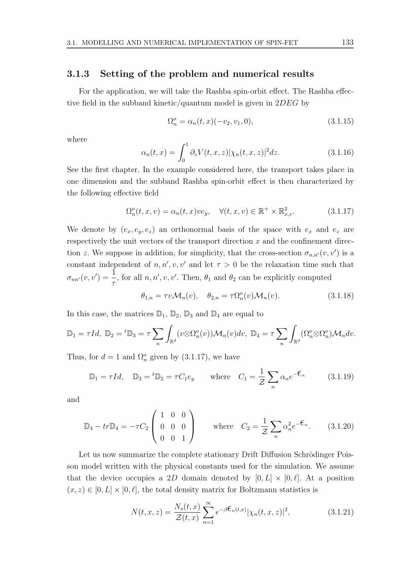
3.1. MODELLING AND NUMERICAL IMPLEMENTATION OF SPIN-FET 133

3.1.3 Setting of the problem and numerical results

For the application, we will take the Rashba spin-orbit effect. The Rashba effec-

tive field in the subband kinetic/quantum model is given in 2DEG by

Ωon = αn(t, x)(−v2, v1, 0), (3.1.15)

where

αn(t, x) =

∫ 1

0

∂zV (t, x, z)|χn(t, x, z)|2dz. (3.1.16)

See the first chapter. In the example considered here, the transport takes place in

one dimension and the subband Rashba spin-orbit effect is then characterized by

the following effective field

Ωon(t, x, v) = αn(t, x)vey, ∀(t, x, v) ∈ R+ × R2

x,v. (3.1.17)

We denote by (ex, ey, ez) an orthonormal basis of the space with ex and ez are

respectively the unit vectors of the transport direction x and the confinement direc-

tion z. We suppose in addition, for simplicity, that the cross-section σn,n′(v, v′) is a

constant independent of n, n′, v, v′ and let τ > 0 be the relaxation time such that

σnn′(v, v′) =1

τ, for all n, n′, v, v′. Then, θ1 and θ2 can be explicitly computed

θ1,n = τvMn(v), θ2,n = τΩon(v)Mn(v). (3.1.18)

In this case, the matrices D1, D2, D3 and D4 are equal to

D1 = τId, D2 = tD3 = τ∑

n

∫

Rd

(v⊗Ωon(v))Mn(v)dv, D4 = τ

∑n

∫

Rd

(Ωon⊗Ωo

n)Mndv.

Thus, for d = 1 and Ωon given by (3.1.17), we have

D1 = τId, D3 = tD2 = τC1ey where C1 =1

Z∑

n

αne−εn (3.1.19)

and

D4 − trD4 = −τC2

1 0 0

0 0 0

0 0 1

where C2 =

1

Z∑

n

α2ne−εn . (3.1.20)

Let us now summarize the complete stationary Drift Diffusion Schrodinger Pois-

son model written with the physical constants used for the simulation. We assume

that the device occupies a 2D domain denoted by [0, L] × [0, `]. At a position

(x, z) ∈ [0, L]× [0, `], the total density matrix for Boltzmann statistics is

N(t, x, z) =Ns(t, x)

Z(t, x)

∞∑n=1

e−βεn(t,x)|χn(t, x, z)|2, (3.1.21)

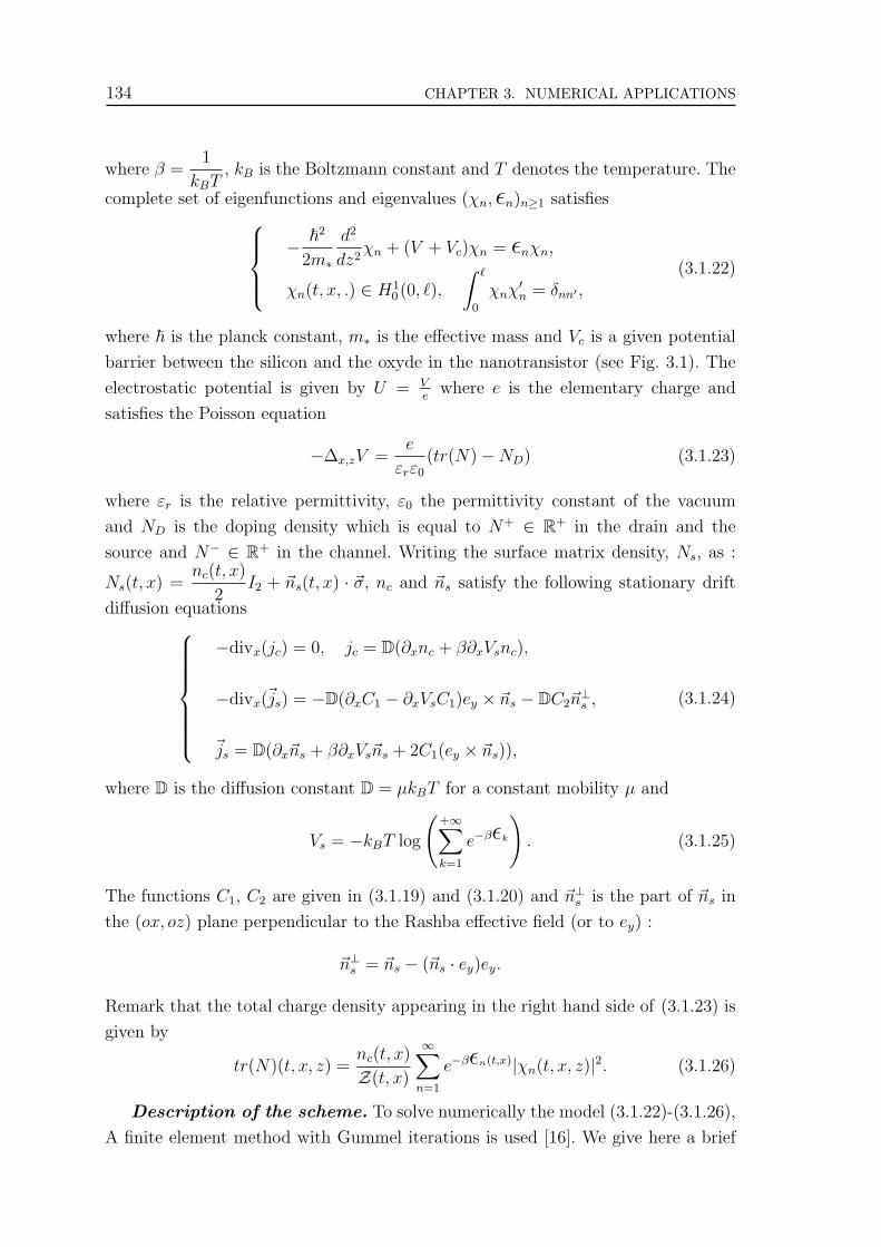
134 CHAPTER 3. NUMERICAL APPLICATIONS

where β =1

kBT, kB is the Boltzmann constant and T denotes the temperature. The

complete set of eigenfunctions and eigenvalues (χn,εn)n≥1 satisfies

− ~2

2m∗

d2

dz2χn + (V + Vc)χn = εnχn,

χn(t, x, .) ∈ H10 (0, `),

∫ `

0

χnχ′n = δnn′ ,(3.1.22)

where ~ is the planck constant, m∗ is the effective mass and Vc is a given potential

barrier between the silicon and the oxyde in the nanotransistor (see Fig. 3.1). The

electrostatic potential is given by U = Ve

where e is the elementary charge and

satisfies the Poisson equation

−∆x,zV =e

εrε0

(tr(N)−ND) (3.1.23)

where εr is the relative permittivity, ε0 the permittivity constant of the vacuum

and ND is the doping density which is equal to N+ ∈ R+ in the drain and the

source and N− ∈ R+ in the channel. Writing the surface matrix density, Ns, as :

Ns(t, x) =nc(t, x)

2I2 + ~ns(t, x) · ~σ, nc and ~ns satisfy the following stationary drift

diffusion equations

−divx(jc) = 0, jc = D(∂xnc + β∂xVsnc),

−divx(~js) = −D(∂xC1 − ∂xVsC1)ey × ~ns − DC2~n⊥s ,

~js = D(∂x~ns + β∂xVs~ns + 2C1(ey × ~ns)),

(3.1.24)

where D is the diffusion constant D = µkBT for a constant mobility µ and

Vs = −kBT log

(+∞∑

k=1

e−βεk

). (3.1.25)

The functions C1, C2 are given in (3.1.19) and (3.1.20) and ~n⊥s is the part of ~ns in

the (ox, oz) plane perpendicular to the Rashba effective field (or to ey) :

~n⊥s = ~ns − (~ns · ey)ey.

Remark that the total charge density appearing in the right hand side of (3.1.23) is

given by

tr(N)(t, x, z) =nc(t, x)

Z(t, x)

∞∑n=1

e−βεn(t,x)|χn(t, x, z)|2. (3.1.26)

Description of the scheme. To solve numerically the model (3.1.22)-(3.1.26),

A finite element method with Gummel iterations is used [16]. We give here a brief

3.1. MODELLING AND NUMERICAL IMPLEMENTATION OF SPIN-FET 135

description of the algorithm. We refer to [6, 19] for more details. We mesh the domain

by Nx ×Nz, (xi, zj)1≤i≤Nx,1≤j≤Nz , nodes.

We begin by resolving the 2D Schrodinger-Poisson system when there is no ap-

plied voltage. The boundary conditions used are as follows. At the source and the

drain, the potential does not depend on the transport direction, we take V (x =

0, z) = V (x = L, z) = Vb with Vb(z) is the solution of 1D Schrodinger-Poisson sys-

tem in the z direction. The surface density at the source and the drain is taken equal

to N+× `Si. For z = 0 or z = `, we take a Dirichlet boundary condition on the gate

contacts, V (x, z = 0) = V (x, z = l) = Vgs.

When a drain source voltage, VDS, is applied, we resolve the Schrodinger-Poisson

system coupled to the charge Drift Diffusion equation (the first equation of (3.1.24))

by Gummel iterations starting from the obtained potential in the first step and

incrementing by 0.02V . For the drift diffusion equation a Dirichlet conditions are

used at x = 0 and x = L. For the potential we impose Dirichlet boundary conditions

at the Gate and at the source and the Drain contacts : V (x = 0, z) = Vb(z), V (x =

L, z) = Vb(z) + VDS.

The Gummel iterations can be summarized as follows. For a given potential, Vold,

a diagonalization of the one dimensional Schrodinger operator (3.1.22) gives Nx sets

of eigenfunctions χk(xi, z)i=1,..Nx and eigenvalues εk(xi). The effective potential

Vs is then computed from (3.1.25). This allows to obtain the surface charge density

nc by solving the first drift diffusion equation of (3.1.24) and then to compute a

new potential Vnew thanks to the resolution of (3.1.23) with (3.1.26). We repeat

these steps until the difference ‖Vnew−Vold‖L∞ be sufficiently small. Noting that the

Poisson equation is resolved by implementing a quasi-Newton method [12].

Finally the spin part of the drift diffusion model (3.1.24) is resolved using Diri-

chlet boundary conditions. We assume that at x = 0 or x = L, the vectors ~ns(x = 0)

and ~ns(x = L) are in the plane of the domain ((xz) plane). Then, the spin vector

density ~ns remains in this plane or it has no component in the y direction (parallel

to ey) and its perpendicular part, ~n⊥s (in the (xz) plane) solves

−divx(~j⊥s ) = −D(C2~n

⊥s − (∂xC1 − ∂xVsC1)I(~n⊥s )),

~j⊥s = D(∂x~n⊥s + β∂xVs~n

⊥s + 2C1I(~n⊥s ))

with I =

(0 −1

1 0

), ~n⊥s ∈ R2 ≡ C. We resolve this equation in C, in which I is

the pur imaginary unit.

Numerical results. The geometry of the device is given by Figure 3.1. We

summarize in Table 3.1 the main values used in the simulation. We assume that

the electrons are injected into the domain with spin vector density along the x-axis.

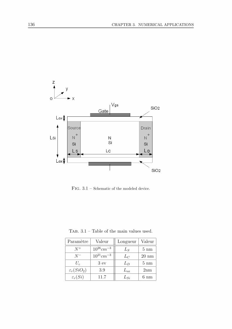
136 CHAPTER 3. NUMERICAL APPLICATIONS

Fig. 3.1 – Schematic of the modeled device.

Tab. 3.1 – Table of the main values used.

Parametre Valeur Longueur Valeur

N+ 1026cm−3 LS 5 nm

N− 1021cm−3 LC 20 nm

Uc 3 ev LD 5 nm

εr(SiO2) 3.9 Lox 2nm

εr(Si) 11.7 LSi 6 nm

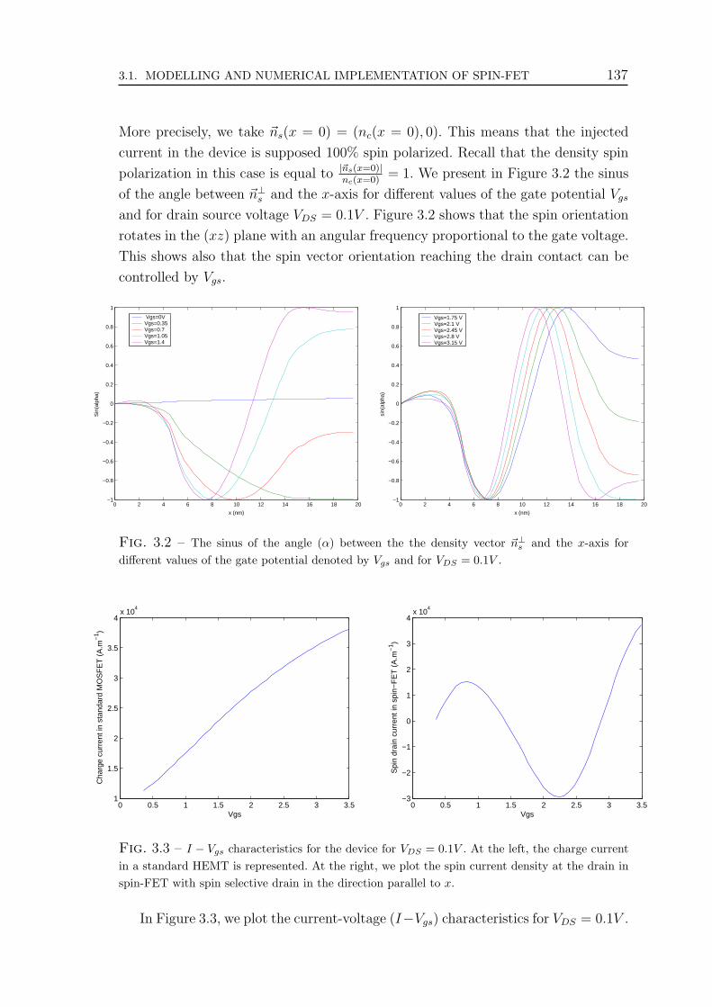
3.1. MODELLING AND NUMERICAL IMPLEMENTATION OF SPIN-FET 137

More precisely, we take ~ns(x = 0) = (nc(x = 0), 0). This means that the injected

current in the device is supposed 100% spin polarized. Recall that the density spin

polarization in this case is equal to |~ns(x=0)|nc(x=0)

= 1. We present in Figure 3.2 the sinus

of the angle between ~n⊥s and the x-axis for different values of the gate potential Vgs

and for drain source voltage VDS = 0.1V . Figure 3.2 shows that the spin orientation

rotates in the (xz) plane with an angular frequency proportional to the gate voltage.

This shows also that the spin vector orientation reaching the drain contact can be

controlled by Vgs.

0 2 4 6 8 10 12 14 16 18 20−1

−0.8

−0.6

−0.4

−0.2

0

0.2

0.4

0.6

0.8

1

x (nm)

Sin

(alp

ha)

Vgs=0VVgs=0.35Vgs=0.7Vgs=1.05Vgs=1.4

0 2 4 6 8 10 12 14 16 18 20−1

−0.8

−0.6

−0.4

−0.2

0

0.2

0.4

0.6

0.8

1

x (nm)

sin(

alph

a)

Vgs=1.75 VVgs=2.1 VVgs=2.45 VVgs=2.8 VVgs=3.15 V

Fig. 3.2 – The sinus of the angle (α) between the the density vector ~n⊥s and the x-axis fordifferent values of the gate potential denoted by Vgs and for VDS = 0.1V .

0 0.5 1 1.5 2 2.5 3 3.51

1.5

2

2.5

3

3.5

4x 10

4

Vgs

Cha

rge

curr

ent i

n st

anda

rd M

OS

FE

T (

A.m

−1 )

0 0.5 1 1.5 2 2.5 3 3.5−3

−2

−1

0

1

2

3

4x 10

4

Vgs

Spi

n dr

ain

curr

ent i

n sp

in−

FE

T (

A.m

−1 )

Fig. 3.3 – I − Vgs characteristics for the device for VDS = 0.1V . At the left, the charge currentin a standard HEMT is represented. At the right, we plot the spin current density at the drain inspin-FET with spin selective drain in the direction parallel to x.

In Figure 3.3, we plot the current-voltage (I−Vgs) characteristics for VDS = 0.1V .

138 CHAPTER 3. NUMERICAL APPLICATIONS

In standard MOSFET, the current (or charge current given by the first equation of

(3.1.24)) increases with the gate potential (left). The diffusion constant is given by

the Einstein relation : D = µkBT where µ = 0.12m2V −1s−1 and T = 300K. However,

if we assume that the drain is a selective contact of electron spin. The magnitude

of the drain current depends then on the orientation of the spin of the electrons

reaching the drain with respect to the orientation of the magnetic moment of this

contact. We consider a drain contact which selects spins parallel to the x direction.

The x-part of the spin drain current as function of Vgs is illustrated in Figure 3.3

(right). It is not any more an increasing function. It oscillates with respect to the

gate voltage Vgs. If the spin density reached the drain contact is oriented parallel

to the x axis, the drain’s current is important. In the other case, the current in the

device is weak.

3.2 Spin accumulation in inhomogeneous semicon-

ductor interfaces

The accumulation of electron spin polarization density at an interface separating

two semiconductor regions with different doping levels is a well known effect in spin-

tronics. We refer to [18, 17, 13] in which this effect was studied using two-component

type models. In this section, some numerical results illustrating the propagation of

spin polarization density through a boundary between two different doped semi-

conductor regions will be presented and interpreted. Two kind of transport models

are used : two-component and spin vector Drift-Diffusion models coupled with the

Poisson equation for self-consistent forces.

3.2.1 Presentation of the system

The geometry of the system under consideration is represented by figure 3.4. We

consider in dimension one, two semi-conductor layers with doping densities N1 and

N2 respectively such that N2 ≥ N1. Supposing that a spin-polarized electrons are

injected in the left semiconductor, under influence of the electric field, the spin pola-

rized current is driven toward the second higher doped region. It was found that, see

[18], the electron spin polarization density is accumulated near the interface between

the two regions and becomes more pronounced when N2 increases. To illustrate this

3.2. SPIN ACCUMULATION IN INHOMOGENEOUS SEMICONDUCTOR INTERFACES139

Fig. 3.4 – Schematic of the system under investigation : spin-polarized electrons are injected inthe first semiconductor (S1, N1) with doping N1 and transported under the action of the electricfield in the x direction toward another N2 doped semiconductor region (S2, N2).

phenomena, we begin by using a self consistent two-component drift-diffusion model

∂tn↑(↓) − divxj↑(↓) =n↑(↓) − n↓(↑)

τsf

,

j↑(↓) = D

(∇xn↑(↓) +

e

kBT∇xV n↑(↓)

),

−∆xV =e

εrε0

(n−Ni).

(3.2.1)

We assume that the system lies on the interval I = [−10x0, 10x0] with x0 is the

scale of the transport direction x. For the numerical simulation we will take x0 =

1.37 × 10−7m in the sequel. The boundary between the two regions is supposed

at point b ∈ I. The spin-up and spin-down densities, n↑(t, x) and n↓(t, x), sa-

tisfy the 2-component drift-diffusion system (3.2.1) with spin-flip collision term.

The constant τsf is the spin-flip relaxation time and D is the diffusion constant.

We denote by V the electrostatic potential satisfying the Poisson equation in which

n(t, x) = n↑(t, x)+n↓(t, x) is the total density of the particles (or the charge density)

and Ni(x) is the doping function

Ni(x) =

N1 if x < b,

N2 if x > b.(3.2.2)

3.2.2 Numerical results

We have solved numerically system (3.2.1) using finite elements method with

Gummel iterations and taking Dirichlet boundary conditions for the potential and

the densities. The results presented here are representative for the general idea of

140 CHAPTER 3. NUMERICAL APPLICATIONS

−1.5 −1 −0.5 0 0.5 1 1.5

x 10−6

−2

0

2

4

6

8

10

12

14

16x 10

4

x (m)

Ele

ctric

fiel

d (V

/m)

Fig. 3.5 – Electric field profil near the boundary, E = −∂xV , forN2

N1= 5.

the spin accumulation in inhomogeneous semiconductor interfaces. The values used

for the different parameters are : x0 = 1.37 × 10−7m, b = −0.8 × 10−7, N1 =

1021m−3, T = 300K. Figure 3.5 shows the electric field profile (E = −∂xV ) near the

boundary in the case when N2 = 5N1. A peak is formed at the boundary due to the

electrons diffusing from the highly doped right region to the less doped left region.

Let us now present the evolution of the spin polarization density p(t, x) defined by

p(t, x) = n↑(t, x)− n↓(t, x).

Figure 3.6 shows the evolution of p(t, x) for different values of N2 with respect to N1.

The initial spin-polarization (at t = 0) is represented by the dashed lines. In each of

the different cases presented, p(t, x) is plotted for different instances ; it converges

when t increases to an equilibrium profile. In the case N2 = N1, no accumulation of

spin-polarization is present at the boundary and p decreases exponentially to zero.

However, when N2 is greater than N1 (we give in Figure 3.6 three cases : N2 = 5N1,

N2 = 10N1 and N2 = 20N1), we see that a peak of spin polarization is formed near

the boundary in the right region and becomes more pronounced when N2 increases.

3.2.3 Spin accumulation and Rashba spin-orbit effect

The aim of this subsection is to study numerically the effect of the spin-orbit

interaction on the spin accumulation in inhomogeneous semiconductor interfaces.

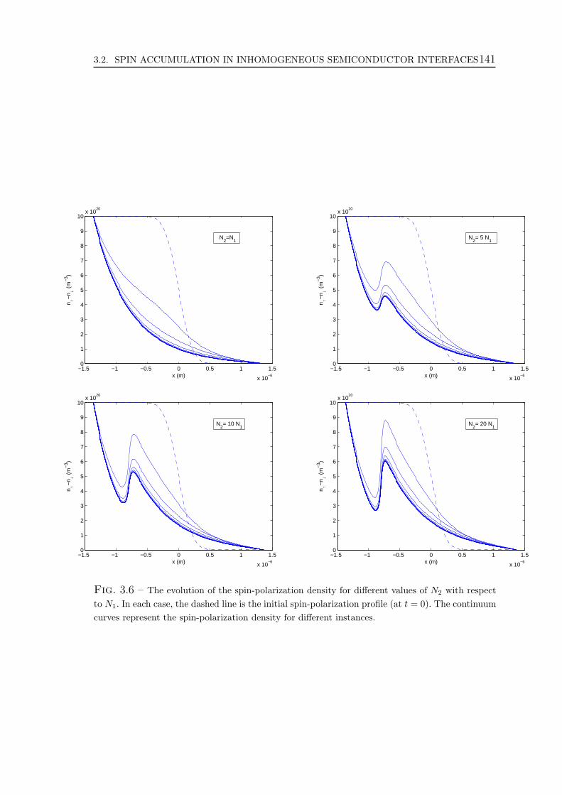
3.2. SPIN ACCUMULATION IN INHOMOGENEOUS SEMICONDUCTOR INTERFACES141

−1.5 −1 −0.5 0 0.5 1 1.5

x 10−6

0

1

2

3

4

5

6

7

8

9

10x 10

20

x (m)

n ↑−n ↓ (

m−

3 )

N2=N

1

−1.5 −1 −0.5 0 0.5 1 1.5

x 10−6

0

1

2

3

4

5

6

7

8

9

10x 10

20

x (m)

n ↑−n ↓ (

m−

3 )

N2= 5 N

1

−1.5 −1 −0.5 0 0.5 1 1.5

x 10−6

0

1

2

3

4

5

6

7

8

9

10x 10

20

x (m)

n ↑−n ↓ (

m−

3 )

N2= 10 N

1

−1.5 −1 −0.5 0 0.5 1 1.5

x 10−6

0

1

2

3

4

5

6

7

8

9

10x 10

20

x (m)

n ↑−n ↓ (

m−

3 )

N2= 20 N

1

Fig. 3.6 – The evolution of the spin-polarization density for different values of N2 with respectto N1. In each case, the dashed line is the initial spin-polarization profile (at t = 0). The continuumcurves represent the spin-polarization density for different instances.

142 CHAPTER 3. NUMERICAL APPLICATIONS

We will use the spin vector drift-diffusion model derived in the previous chapter

coupled with the Poisson equation. Let us write this model in the case of relaxation

time approximation and with one dimensional Rashba spin-orbit effect where the

effective field is given by

Ω = αvey

such that α is the order of the Rashba interaction and ey is the unit vector of

the y direction (perpendicular to the transport direction x). This effective field can

appear for example if an electric field is applied along the z direction. The model is

the following

∂tnc − divx(D(∂xnc + β∂xV nc)) = 0,

∂t~Ns − divx(D(∂x

~Ns + β∂xV ~Ns + 2αey × ~Ns)) =

αβD∂xV (ey × ~Ns)− α2D ~N⊥s −

2 ~Ns

τsf

,

−∆xV =e

εrε0

(nc −Ni),

(3.2.3)

where β =e

kBTand D is the diffusion constant. We recall that nc is the charge

density and ~Ns is the spin-vector density where ‖ ~Ns‖ represents the polarization

density (or n↑−n↓ in the 2-component description). We denoted in the second equa-

tion by ~N⊥s the perpendicular part of ~Ns with respect to the effective field direction

(or ey direction). We have plotted in figure 3.7 the polarization density profile (i.e.

the equilibrium profile of ‖N(t, x)‖ when t increases) for different values of the spin-

orbit coefficient (α). Figure 3.7 shows the variation of the spin accumulation at the

boundary with respect to α. Let us mentioned the presence of oscillation effect of

the spin accumulation due to the rotational and relaxation effects induced by the

Rashba interactions.

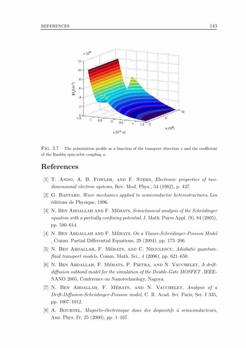
REFERENCES 143

Fig. 3.7 – The polarization profile as a function of the transport direction x and the coefficientof the Rashba spin-orbit coupling α.

References

[1] T. Ando, A. B. Fowler, and F. Stern, Electronic properties of two-

dimensional electron systems, Rev. Mod. Phys., 54 (1982), p. 437.

[2] G. Bastard, Wave mechanics applied to semiconductor heterostructures, Les

editions de Physique, 1996.

[3] N. Ben Abdallah and F. Mehats, Semiclassical analysis of the Schrodinger

equation with a partially confining potential, J. Math. Pures Appl. (9), 84 (2005),

pp. 580–614.

[4] N. Ben Abdallah and F. Mehats, On a Vlasov-Schrodinger-Poisson Model

, Comm. Partial Differential Equations, 29 (2004), pp. 173–206.

[5] N. Ben Abdallah, F. Mehats, and C. Negulescu, Adiabatic quantum-

fluid transport models, Comm. Math. Sci., 4 (2006), pp. 621–650.

[6] N. Ben Abdallah, F. Mehats, P. Pietra, and N. Vauchelet, A drift-

diffusion subband model for the simulation of the Double-Gate MOSFET , IEEE-

NANO 2005, Conference on Nanotechnology, Nagoya.

[7] N. Ben Abdallah, F. Mehats, and N. Vauchelet, Analysis of a

Drift-Diffusion-Schrodinger-Poisson model, C. R. Acad. Sci. Paris, Ser. I 335,

pp. 1007–1012.

[8] A. Bournel, Magneto-electronique dans des dispositifs a semiconducteurs,

Ann. Phys. Fr, 25 (2000), pp. 1–167.

144 REFERENCES

[9] A. Bournel, V. Delmouly, P. Dollfus, G. Tremblay, and P. Hesto,

Theoretical and experimental considerations on the spin field effect transistor,

Physica E, 10 (2001), pp. 86–90.

[10] A. Bournel, P. Dollfus, E. Cassan, and P. Hesto, Monte Carlo study

of spin relaxation in AlGaAs/GaAs quantum wells, Applied Physics Letters, 77

(2000), pp. 2346–2348.

[11] Y. A. Bychkov and E. I. Rashba, Oscillatory effects and the magnetic

susceptibility of carriers in inversion layers, Journal of Physics C : Solid State

Physics, 17 (1984), pp. 6039–6045.

[12] P. Caussignac, B. Zimmermann, and R. Ferro, Finite element approxi-

mation of electrostatic potential in one-dimensional multilayer structures with

quantized electronic charge, Computing, 45 (1990), pp. 251–264.

[13] D. Csontos and S. E. Ulloa, Spin injection and accumulation in inhomo-

geneous semiconductors, Physica E, 32 (2006), pp. 412–415.

[14] S. Datta and B. Das, Electronic analog of the electro-optic modulator, Ap-

plied Physics Letters, 56 (1990), pp. 665–667.

[15] J. H. Davies, The physiscs of low dimensional semiconductors, Cambrifge

Univ. press, 1998.

[16] H. K. Gummel, A self-consistent iterative scheme for one dimensional steady

state transistor calculations, IEEE Trans. On Elec. Dev., 11 (1964), p. 455.

[17] Y. V. Pershin, Accumulation of electron spin polarization at semiconductor

interfaces, Phys. Rev. B, 68 (2003), p. 233309.

[18] Y. V. Pershin and V. Privman, Focusing of Spin Polarization in Semicon-

ductors by Inhomogeneous Doping, Phys. Rev. Lett., 90 (2003), p. 256602.

[19] P. Pietra and N. Vauchelet, Modeling and simulation of the diffusive

transport in a nanoscale Double-Gate MOSFET , submitted.

[20] S. Saikin, Y. Pershin, and V. Privman, Modelling for semiconductor spin-

tronics, IEE Proceedings Circuits, Devices and Systems, 152 (2005), pp. 366–

376.

[21] S. Saikin, M. Shen, and M.-C. Cheng, Study of spin-polarized transport

properties for spin-FET design optimization, IEEE Trans. Nanotechnology, 3

(2004), pp. 173–179.

[22] N. Vauchelet, Modelisation mathematique du transport diffusif de charges

partiellement quantiques, Thesis, Universite Paul Sabatier-Toulouse III, (2006).

Part II

Diffusion and high magnetic

fields

145

Chapter 4

Diffusion and guiding center

approximation for particle

transport in strong magnetic

fields

Joint work with Naoufel Ben Abdallah published in KRM (Kinetic and Related

Models)-AIMS : Diffusion and guiding center approximation for particle transport

in strong magnetic fields, Kinetic and Related Models, Vol. 1, No. 3, PP. 331–354,

2008.

Abstract

The diffusion limit of the linear Boltzmann equation with a strong magnetic field is

performed. The Larmor radius is supposed to be much smaller than the mean free

path. The limiting equation is shown to be a diffusion equation in the parallel direc-

tion while in the orthogonal direction, the guiding center motion is obtained. The

diffusion constant in the parallel direction is obtained through the study of a new

collision operator obtained by averages of the original one. Moreover, a correction

to the guiding center motion is derived.

Keywords. Diffusion limit, guiding-center approximation, high magnetic field.

147

148 CHAPTER 4. DIFFUSION AND GUIDING CENTER APPROXIMATION

4.1 Introduction

The motion of charged particles under the action of a strong magnetic field is

an important phenomena encountered in artificial and natural plasmas (Tokamakas,

ionospheric plasmas, etc). In the presence of constant magnetic field ~B, a charged

particle (electron in our case) of mass m and charge q with velocity v follow a helical

trajectory around magnetic field line. The gyration radius of the particles, called

Larmor radius rL, is inversely proportional to the magnitude of the magnetic field

(rL =mv

qB). This means that when the magnetic field becomes large, the particles

get trapped along the direction of ~B. In addition, when an electric field ~E is applied,

the particles experience a drift of the instantaneous centers of Larmor circles, called

in the literature the guiding center motion, in the direction perpendicular to both

the electric and magnetic fields. The velocity of this drift is given by the following

formula

vdrift =~E × ~B

B2.

Direct simulations of Vlasov or Boltzmann equations in the presence of such large

magnetic fields requires the numerical resolutions of the small position and time

scales induced by the gyration along the magnetic field. Hence, the question of deri-

ving approximate models, numerically less expensive, is of great importance. Various

models have been developed to this aim like the “guiding-center” and the gyrokine-

tic models. The guiding center approximation consists in averaging the motion over

the gyroperiod when supposing B goes to +∞ (rL → 0) [26] and the gyrokinetic

approximation is a generalization of the guiding center one in the case of kinetic

equations. For a complete physical review, we refer for instance to [27, 15, 28, 31].

Mathematically speaking, homogenization techniques were used in [19, 20] by E.

Frenod and E. Sonnendrucker to justify the high magnetic field limit of Vlasov and

Vlasov-Poisson systems. It is proven in [19] that the tridimensional guiding center

approximation leads to a one-dimensional kinetic model in the direction of the ma-

gnetic field. The drift phenomenon perpendicular to the magnetic field is rigourously

obtained in [20] for the two dimensional Vlasov equation on a sufficiently long time

scale. Other asymptotic regimes of the Vlasov equation with strong magnetic fields

are studied [21, 18, 22, 16, 17]. The gyrokinetic approximation of the Vlasov-Poisson

system has also been intensively studied by F. Golse and L. Saint-Raymond for the

two and tridimensional motions in various asymptotic regimes [24, 33, 25, 34].

In all the above references, the transport is assumed to be ballistic, which means

that particles do not suffer any collision during their motion. We are here interested

in regimes were collisions are important and we propose to study the interplay

between the fluid limit induced by collisions and the high frequency gyrations around

4.2. SETTING OF THE PROBLEM AND MAIN RESULTS 149

the magnetic field. To simplify the study, we shall only consider collisions with a

thermal bath at a given temperature. In this case, the diffusion limit of the obtained

Boltzmann equation leads to the so-called drift diffusion equation. The question of

deriving diffusions equations from the Boltzmann equation has been widely studied

during the last three decades in the context of radiative transfer [5, 6, 35, 1, 7], in

semiconductors and plasmas [32, 23, 30, 2, 3, 4, 8, 9, 10] and many other contexts that

we do not mention here. In the presence of a magnetic field, an important quantity

to be considered is the gyroperiod measuring the time that a particle of mass m

with charge q and submitted to the constant magnetic field B makes a 2π rotation

around this field (Tc = 2πm/qB). When the gyroperiod is much larger than the

relaxation time, then the magnetic field effect disappear in the diffusion limit as will

be seen later on. When Tc is of the same order of magnitude as the relaxation time,

the diffusion matrix has an antisymmetric component, generated by the magnetic

field (this has been proven for collision with walls by P. Degond & al [8, 11, 14]).

Formal results for binary gas mixtures can also be found in [29, 12, 13, 9]. We

shall consider in this paper the situation where the gyroperiod is much smaller than

the relaxation time. In that case, one expects that the diffusion matrix is obtained

through the analysis of an averaged collision operator. Also, the high frequency

oscillations only occur in the direction perpendicular to the magnetic field while

parallel velocity stay unaffected. Therefore, the behaviours of the solutions in these

directions are expected to be different. We shall show in this paper that the transport

is diffusive along the magnetic field, while it is dominated by the guiding center drift

in the orthogonal direction. The diffusion coefficient in the parallel direction will be

obtained by averaging the collision cross section around the magnetic field.

The outline of the paper is as follows. In the next section, we introduce the

scaling, notations and state the main results. The proofs rely on the study of the

operator accounting for collisions and gyration around the magnetic field. The ana-

lysis of this operator is done in Section 3. Section 4 is devoted to the asymptotics

of this operator when the scaled gyration period tends to zero. It is shown that this

limit is well described by a collision operator with a cross section averaged around

the magnetic field. This result is then used in Section 5 in order to prove the main

results of the paper. Some concluding remarks are listed in the last section of the

paper.

4.2 Setting of the problem and main results

The problem we are interested in is a singular perturbation of the three dimensio-

nal Boltzmann equation with a constant large magnetic field. The position variable

150 CHAPTER 4. DIFFUSION AND GUIDING CENTER APPROXIMATION

is denoted by r = (x, y, z), the velocity variable is denoted v = (vx, vy, vz). The

magnetic field is assumed to be constant and parallel to the z axis. We shall denote

by r⊥ = (x, y) and v⊥ = (vx, vy), the orthogonal variables. The distribution function

is a solution of the following singularly perturbed Boltzmann equation

∂f εη

∂t+Tzf

εη

ε+T⊥f εη

εη+

(v × ez)

ε2η2· ∇vf

εη =Q(f εη)

ε2

f εη(t = 0) = f0(r,v),(4.2.1)

where T⊥ and Tz are the respectively perpendicular and parallel parts of the transport

operator

T⊥ = v⊥ · ∇r⊥ + E⊥ · ∇v⊥ , Tz = vz∂z + Ez∂vz .

The collision operator is given by

Q(f)(v) =

∫

R3

σ(v,v′)[M(v)f(v′)−M(v′)f(v)]dv′. (4.2.2)

The function M is the normalized Maxwellian :

M(v) =1

(2π)32

e−12|v|2 , (4.2.3)

and the cross section σ is symmetric and bounded from below and above by two

positive constants. The parameter ε is intended to go to zero and represents the

scaled mean free path. The scaled magnetic field is given by ez

εη2 , while E =

(E⊥Ez

)

is the scaled electric field. The gyroperiod is εη2 and we shall consider the situation

where η and ε go to zero simultaneously and the situation where ε tends to zero for

η given then η tends to zero. Since the magnetic field strongly confines the motion

of the particles in the perpendicular direction (x, y), we have rescaled this direction

with the prefactor η. This is why the orthogonal operator T⊥ comes with a different

scaling from the parallel one Tz. By doing so, we shall obtain a non trivial motion

in the orthogonal direction (guiding center).

4.2.1 Scaling

In this subsection, we shall explain the hypotheses that lead to the scaled Boltz-

mann equation (4.2.1). In particular, we highlight the differences of the position

scales in the parallel and perpendicular directions (with respect to the magnetic

field). The starting point is the diffusion scaling in the absence of a magnetic field.

The unscaled Boltzmann equation in this case reads

∂tF + V · ∇XF +q∇XΦ

m· ∇V F = Q(F )

4.2. SETTING OF THE PROBLEM AND MAIN RESULTS 151

where (t,X, V ) are the physical time position and velocity variables, while Φ is the

electrostatic potential, e is the elementary charge and m the mass of the electron

(to fix the ideas, we consider electrons). The collision operator Q has the form

Q(F ) =

∫Σ(V, V ′)[MT (V )F (V ′)−MT (V ′)F (V )] dV ′,

Σ is the transition rate and MT is the Maxwellian at the temperature T

MT (V ) = (2πKBT

m)−3/2 exp(− mv2

2KBT),

KB being the Boltzmann constant. The thermal energy and velocity are respectively

defined by

Uth = KBT, Vth =

√KBT

m.

The electrostatic energy is assumed to be of the order of the thermal energy and

varies over a macroscopic length scale L :

qΦ(X) = Uthφ(X

L).

The transition rate Σ is the inverse of a time. The typical value of this time, the

scattering time, is denoted by τs. So we write

Σ(V, V ′) ==1

τs

σ(V

Vth

,V ′

Vth

)

where σ is its scaled version assumed to be of order 1. The mean free path Ls will

be defined as the distance that a thermal electron crosses during the scattering time

τs

Ls = Vthτs.

This distance is assumed to be much smaller than the macroscopic distance L and

we shall denote it by

ε =Ls

L.

The only thing left to know is the macroscopic time scale. Since the kernel of the

collision operator is generated by the Maxwellian which carries no flux, one has to

go to the diffusion scaling and define the macroscopic time τm by

τs

τm

= (Ls

L)2 = ε2.

Using (τm, L, Vth, Uth) as units for time, position, velocity and energy, the Boltzman

equation can be written

∂tf +1

ε(v · ∇rf −∇rφ · ∇vf) =

Q(f)

ε2,

152 CHAPTER 4. DIFFUSION AND GUIDING CENTER APPROXIMATION

where Q is the scaled Boltzmann operator (4.2.2).

Let us now look at the effect of a large magnetic field B = Bez. The scaled

Boltzmann equation contains the additional term − qm

(V × B) · ∇VF . An electron

submitted to this magnetic field spins around it following the equation

mdV

dt= −qV × B.

The period of this precession, called the cyclotron period is given by

τc =m

qB.

We shall assume that this period is much smaller than the scattering time and we

write

τc = η2τs.

Of course the motion along the magnetic field stays unchanged and we shall not

change the length scale in this direction. In the orthogonal direction however, the

combined action of the electric field and the magnetic field results in the drift of

the guiding center (the electron motion is a rotation around a center which is now

drifting under the action of the electric field). The velocity of this drift is given by

Vc =E × B

B2.

Its order of magnitude is then given by

Vc =E⊥B

,

wher E⊥ is the perpendicular component of the electric field.

The last hypothesis that we make is the potential Φ varies in the orthogonal

direction on a lengthscale L⊥ which is not equal to the parallel lengthscale L. Mo-

reover, L⊥ is such that the guiding center moves during the macroscopic time by a

distance of the order of L⊥ itself. In other words, we want

E⊥ =Uth

qL⊥, Vcτm = L⊥.

Replacing the thermal energy by its expression given above in this section, we find

after straightforward computations that

L2⊥ =

τmUth

qB= η2L2.

Now rescaling the orthogonal position variable by L⊥, we obtain the Boltzmann

equation (4.2.1).

4.2. SETTING OF THE PROBLEM AND MAIN RESULTS 153

Remark 4.2.1. From the scaling hypotheses, we see that between two successive

collisions, the electron precesses a large number of times around the magnetic field.

Therefore, one might expect that the collision cross section will be averaged along

these precessions. On the other hand, since the orthogonal lengthscale has been

designed in order to see the guiding center drift, the limiting equation should exhibit

this term. Finally, since the parallel motion to the magnetic field does not feel the

magnetic field, one is entitled to expect a non vanishing diffusion in this direction.

This is exactly what we shall prove in this paper : drift in the orthogonal direction,

finite diffusion in the parallel direction governed by a collision operator averaged

over precessions around the magnetic field.

4.2.2 Notations

The analysis of the limit ε → 0 naturally leads to the study of the operator

Qη = Q− (v × ez)

η2· ∇v, (4.2.4)

while the limit η → 0, involves the cylindrical averaging around the vector ez. To

this aim, we denote by R(τ) the rotation around ez with angle τ which is the

multiplication operator by the following matrix

R(τ) =

cos τ sin τ 0

− sin τ cos τ 0

0 0 1

. (4.2.5)

The cylindrical average of a function h = h(v) is defined by

A(h)(v) := h(v) =1

2π

∫ 2π

0

h(R(τ)v) dτ. (4.2.6)

It is clear that A is the orthogonal projector (in the L2 sense) on the set of cylin-

drically invariant functions. We also define the partial average

Aτ (h)(v) := hτ (v) =1

2π

∫ τ

0

h(R(s)v) ds. (4.2.7)

We shall moreover define the averaged function σ and the symmetric average σ by

σ(v,v′) =1

2π

∫ 2π

0

σ (R(τ)v,v′) dτ

σ (v,v′) =1

4π2

∫ 2π

0

∫ 2π

0

σ (R(τ)v,R(τ ′)v′) dτdτ ′ =1

2π

∫ 2π

0

σ (v,R(τ ′)v′) dτ ′,

154 CHAPTER 4. DIFFUSION AND GUIDING CENTER APPROXIMATION

and the corresponding collision operators

Q(f)(v) =

∫

R3

σ(v,v′)[M(v)f(v′)−M(v′)f(v)]dv′, (4.2.8)

Q(f)(v) =

∫

R3

σ(v,v′)[M(v)f(v′)−M(v′)f(v)]dv′. (4.2.9)

We define the functional spaces

L2M =

f = f(v) /

∫

R3

|f(v)|2M(v)

dv < +∞

, (4.2.10)

and its cylindrically symmetric subspace

L2

M = f ∈ L2M/ f(R(τ)v) = f(v), ∀τ ∈ [0, 2π]. (4.2.11)

We also define the space

H2M = f ∈ L2

M, such that, ∂αf ∈ L2M, for |α| ≤ 2. (4.2.12)

We shall make the following hypotheses

Assumption 4.2.2. The cross-section σ belongs to W 2,∞(R6) and is supposed to be

symmetric and bounded from above and below :

∃α1, α2 > 0, 0 < α1 ≤ σ(v,v′) = σ(v′,v) ≤ α2, ∀(v,v′) ∈ R6. (4.2.13)

Assumption 4.2.3. There exists a potential V (t, r) in C1(R+; W 1,∞(R3)), such that

E = −∇rV .

We finally define the space

L2MV

=

f = f(r,v) /

∫

R6

|f(r,v)|2M(v)e−V (r)

dv < +∞

. (4.2.14)

4.2.3 Main results

The main results of this paper are summarized in the following two theorems. The

first one deals with the limit ε → 0 while η > 0 is kept fixed.

Theorem 4.2.4. Let η > 0 be fixed. Let T ∈ R∗+ and assume that the initial data of

(4.2.1), f0, belongs to L2MV

. Then, with Assumptions 4.2.2 and 4.2.3, the problem

(4.2.1) has a unique weak solution in C0([0, T ], L2MV

). Moreover, the sequence (f εη)ε

converges weakly to ρη(t, r)M(v) in L∞((0, T ); L2MV

)) weak ? where ρη satisfies

∂tρη − div(Dη(∇ρη − ρηE)) = 0 (4.2.15)

4.2. SETTING OF THE PROBLEM AND MAIN RESULTS 155

and the diffusion matrix Dη is given by the formula

Dη =

∫ (1ηv⊥vz

)⊗

(ηXη

⊥Xη

z

)dv,

Xη =

Xη

⊥

Xηz

being the only solution of (4.3.7).

Remark 4.2.5. In the relaxation time case σ(v,v′) = 1τ, the matrix Dη can be

computed explicitly :

Dη = τ

η2

τ2+η4τ

τ2+η4 0

− ττ2+η4

η2

τ2+η4 0

0 0 1

.

In the limit η → 0, the upper 2 x 2 block of the matrix reduces to the antisymmetric

matrix I =

0 1

−1 0

, whereas its symmetric part is of order η2. The following

proposition shows that these features are still valid in the case of a non constant

scattering section σ.

Proposition 4.2.6. Writing Xη =

(Xη⊥

Xηz

), we have the following expansions in

H2M as η tends to zero

Xηz = X(0)

z + η2X(1)z +O(η4),

Xη⊥ = X

(0)⊥ + η2X

(1)⊥ +O(η4).

The diffusion matrix Dη is a definite positive matrix. Its symmetric and antisymme-

tric parts, Dηs and Dη

as, have respectively the following expansions

Dηs =

η2

∫v⊥ ⊗X

(1)⊥ dv 0

0 Dz

+ η3D(1)

z⊥ +O(η4),

Dηas =

0 1 0

−1 0 0

0 0 0

+ ηD(0)

z⊥ +O(η4)

where Dz =∫

vzX(0)z dv and

D(0)z⊥ =

∫ (0

vz

)⊗

(X

(0)⊥0

)dv −

∫ (X

(0)⊥0

)⊗

(0

vz

)dv

D(1)z⊥ =

∫ (X

(1)⊥0

)⊗

(0

vz

)dv +

∫ (0

vz

)⊗

(X

(1)⊥0

)dv.

156 CHAPTER 4. DIFFUSION AND GUIDING CENTER APPROXIMATION

Remark 4.2.7. The above theorem shows that the diffusion is of order O(1) in

the parallel direction while it scales like η2 in the orthogonal one, exactly like in

the relaxation time coefficient. The antisymmetric part of the diffusion matrix acts

essentially on the orthogonal direction and leads to the guiding center motion. Ho-

wever, the above formula shows a correction of order η of the guiding center motion,

which is due to collisions. Indeed, it is readily seen that for any three dimensional

vector Z

−DηasZ = uη × Z +O(η4)

where

uη =

−η∫

X(0)y vzdv

η∫

X(0)x vzdv

1

,

and (X(0)x , X

(0)y ) are the components of X

(0)⊥ . This leads to

−∇ · (Dηas(∇rρη − ρηE)) = ∇ · (ρηE × uη) +O(η4).

Theorem 4.2.8. Under the same hypotheses as for Theorem 4.2.4, we now let ε

and η simultaneously and independently tend to zero (there is no assumption on the

relative scale between ε and η). In this case, the sequence (f εη)εη of weak solutions

of (4.2.1) converges weakly to ρ(t, r)M(v) in L∞([0, T ], L2MV

) weak *, where ρ is

the solution of

∂tρ + ∂zJz +∇ · (ρE× ez) = 0

ρ(0, r) =

∫

R3

f0(r,v) dv.(4.2.16)

The parallel current density, Jz is given by

Jz = −Dz(∂zρ− Ezρ),

where Dz is the diffusion constant given by

Dz =

∫

R3

X(0)z vzdv, (4.2.17)

and X(0)z is the zero-th order term of Xη

z (defined by (4.4.7)).

4.3 Analysis of the operator Qη

Let us consider the space L2M introduced in (4.2.10) and define the scalar product

on this space by

〈f, g〉M =

∫

R3

fg

Mdv.

4.3. ANALYSIS OF THE OPERATOR Qη 157

Let D(Qη) be defined by

D = D(Qη) := f ∈ L2M/ (v × ez) · ∇vf ∈ L2

M. (4.3.1)

We have the following result.

Proposition 4.3.1. The operator Qη given by (4.2.4) with domain D defined by

(4.3.1) satisfies the following properties.

1. For any f ∈ D, we have

∫

R3

Qη(f)dv = 0 (mass conservation).

2. (−Qη, D) is a maximal monotone operator.

3. The kernel of Qη is the real line spanned by the Maxwellian :

Ker(Qη) = f ∈ L2M/∃α ∈ R such that f(v) = αM(v).

4. Let P be the orthogonal projection on KerQη. The following coercivity inequa-

lity holds for any function f ∈ D

−〈Qη(f), f〉M ≥ α1‖f − P(f)‖2M. (4.3.2)

where α1 > 0 is the lower bound of σ (4.2.13).

5. The range of Qη, denoted by Im(Qη), is the set of functions g ∈ L2M satisfying

the solvability condition :

∫

R3

g(v)dv = 0. In addition, for all g ∈ Im(Qη) there

exists a unique function f ∈ D satisfying both Qη(f) = g and

∫

R3

f(v)dv = 0.

Proof. First of all, we recall that the operator Q satisfies all items of Proposi-

tion 4.3.1 (by substituting D by L2M). Now Items 1., 3. and 4. of the Proposition

follow immediately from these properties since we have∫R3(ez × v) · ∇v(f)dv =∫

R3 divv[(ez × v)f ]dv = 0 and 〈(ez × v) · ∇vf, f〉M = 0. In order to prove Item 2.,

we need to prove that I − Qη is one-to-one from D to L2M. In order to do so, we

rewrite the equation f −Qη(f) = g under the following form

1

η2(v × ez) · ∇vf + (1 + ν(v))f = Q+(f) + g,

where we have written

Q(f) = Q+(f)− νf, (4.3.3)

Q+(f) = (

∫

R3

σ(v,v′)f(v′)dv′)M(v) (4.3.4)

ν(v) =

∫

R3

σ(v,v′)M(v′)dv′. (4.3.5)

158 CHAPTER 4. DIFFUSION AND GUIDING CENTER APPROXIMATION

The characteristics of the equation are defined by

dv

dt=

1

η2(v × ez)

v|t=0 = v0

whose solution is v(t) = R(t

η2)v0. The solution of the equation can then be defined

by integration over the characteristics and finally leads to f = F(Q+(f) + g) where

F(h)(v) =η2

Bη(v)

∫ 2π

0

h(R(τ)v)eη2R τ0 (1+ν(R(s)v))dsdτ,

Bη(v) =eη2R 2π0 (1+ν(R(s)v)) ds − 1.

A fixed point argument leads to the existence and uniqueness of f ∈ L2M solving the

equation f − Qη(f) = g in the distributional sense. Since Q is a bounded operator

on L2M, we immediately obtain that (v × ez) · ∇vf ∈ L2

M so that the constructed

solution is in the domain D of the operator Qη. Let us now prove item 5. Consider

g ∈ L2M such that

∫

R3

g(v)dv = 0. From the maximal monotonicity of Qη, for each

λ > 0, λId − Qη is surjective. Therefore, for all λ > 0, there exists fλ ∈ D(Qη)

satisfying

λfλ −Qη(fλ) = g. (4.3.6)

Integrating this equation with respect to v gives λ

∫

R3

fλdv =

∫

R3

gdv = 0 and with

(4.3.2) we get −〈Qη(fλ), fλ〉M ≥ α1‖fλ‖2M. Taking the scalar product of (4.3.6) with

fλ in L2M, one obtains

λ‖fλ‖M + α1‖fλ‖M ≤ ‖g‖M.

This implies that (fλ)λ>0 is bounded in L2M. Up to an extraction of a subsequence,

there exists f ∈ L2M such that (fλ) converges weakly to f . By passing to the limit

λ → 0 in the weak form of equation (4.3.6), we get

1

η2(v × ez) · ∇vf −Q(f) = g in D′(R3).

In addition, Q(f) and g belong to L2M, then (v×ez)·∇vf ∈ L2

M and then f ∈ D(Qη).

Of course∫R3 fdv = 0 since this is true for fλ. Now if there is another solution of

−Q(·) = g with zero velocity average, the difference of this solution with f is in the

kernel of Qη and has a zero average. It is necessarily equal to zero.

¥

The following corollary is a direct consequence of Proposition 4.3.1.

4.3. ANALYSIS OF THE OPERATOR Qη 159

Corollary 4.3.2. For all η > 0, there exists a unique Xη =

Xη

⊥

Xηz

in (D(Qη))3

satisfying

−Qη(Xη) =

1

η2v⊥

vz

M(v) and

∫

R3

Xη(v)dv = 0 (4.3.7)

and from the coercivity inequality (4.3.2), (Xηz)η and (η2Xη

⊥)η are bounded sequences

in L2M. Namely, we have the following a priori estimates

‖Xηz‖M + ‖η2Xη

⊥‖M ≤ 1

α1

‖vM‖M. (4.3.8)

The following proposition allows to reformulate the problem Qη(f) = −g by

using the characteristics.

Proposition 4.3.3. For all g ∈ Im(Qη), we have the following equivalence

−Qη(f) = g ⇔ f − Lη(Q+(f)) = Lη(g) (4.3.9)

where Q+ is given by (4.3.4) and Lη is the operator on L2M given by the expression :

Lη(f) =η2

Cη(v)

∫ 2π

0

f(R(τ)v)eη2R τ0 ν(R(s)v)dsdτ, Cη(v) = eη2

R 2π0 ν(R(s)v)ds − 1.

(4.3.10)

Proof. Let (Sη, D(Sη)) be the unbounded operator on L2M defined by

D(Sη) = f ∈ L2M / (v × ez) · ∇vf ∈ L2

M (4.3.11)

Sη(f) =1

η2(v × ez) · ∇vf + ν(v)f ∀f ∈ D(Sη). (4.3.12)

With the decomposition (4.3.3), we have Qη = Q+−Sη. Proceeding as in the proof of

Proposition 4.3.1 (replacing ν +1 by ν), we show that Sη is invertible and its inverse

is nothing but Lη. The equation −Qη(f) = g is equivalent to f − (Sη)−1(Q+(f)) =

(Sη)−1(g) which concludes the proof. ¥

Lemma 4.3.4. For all f ∈ L1loc(R3), we have :

|Lη(f)| ≤ η2

e2πα1η2 − 1

∫ 2π

0

|f(R(τ)v)|eα2η2τdτ. (4.3.13)

Proof. This estimate follows immediately from the definition of Lη (4.3.10) using

Assumption 4.2.2. ¥

160 CHAPTER 4. DIFFUSION AND GUIDING CENTER APPROXIMATION

Proposition 4.3.5. Under Assumption 4.2.2, the solution Xη of (4.3.7) belongs to

(H2M(R3))3 and Xη and all its derivatives with respect to v of order less than or

equal 2 (up to dividing by the Maxwellian) are polynomially increasing when |v| goesto +∞. Namely, we have

|Xη(v)| ≤ Qη1(|v|)M(v), (4.3.14)

|∂αXη(v)| ≤ Qη3(|v|)M(v), (4.3.15)

for all α = (α1, α2) ∈ N2 with α1 + α2 ≤ 2 and where ∂α :=3∑

i,j=1

∂α1vi

∂α2vj

. Here, Qη1

and Qη3 are two polynomials of degrees 1 and 3 respectively (depending on η).

Proof. From (4.3.9), we deduce the identity

Xη = Lη(vηM) + Lη(Q

+(Xη)),

where

vη =

1

η2v⊥

vz

.

Moreover, we have |Q+(Xη)| ≤ α2(

∫

R3

Xη(v′)dv′)M(v) ≤ c0M(v) and with (4.3.13)

one obtains (4.3.14). Estimate (4.3.15) follows by derivation of the above equation

with respect to v and by using the fact that the cross-section σ(v, v′) belongs to

W 2,∞(R6).

¥

4.4 Expansion of Xη with respect to η

A rigourous expansion of Xη around η = 0 will be carried out in this section.

Corollary 4.3.2 provides us with bounds of order O(1) for Xηz and of order O( 1

η2 )

for Xη⊥. We shall prove in this section that Xη

⊥ is actually bounded in H2M. This

is due to the fast precession around the axis ez generated by the differential term1η2 (v × ez) · ∇v. Filtering out these oscillations is done through the reformulation

(4.3.9) of the equation satisfied by Xη. Moreover, we shall expand Xη in powers of

η2 up to the first order.

Definition 4.4.1. Let Q be the operator on L2M defined by (4.2.8) and let Q the one

defined on L2

M by (4.2.9). Then, Q restricted to L2

M coincides with Q.

We now list the properties of Q which are completely inherited from those of Q.

4.4. EXPANSION OF Xη WITH RESPECT TO η 161

Proposition 4.4.2 (Properties of Q ). The operator Q is a bounded operator on

L2

M equipped with the L2M scalar product. It satisfies the following properties whose

proof are immediate and are left to the reader.

1. For all f ∈ L2

M, we have Q(f) = Q(f) = Q(f).

2. −Q is a bounded, symmetric, non-negative operator on L2

M.

3. The null set of Q is given by

N(Q) = nM(v), n ∈ R.4. Let P : L

2

M → N(Q) be the orthogonal projection on N(Q), the following

coercivity inequality holds,

−〈Q(f), f〉M ≥ α1‖f − P(f)‖2M.

i.e −Q is coercive on N(Q)⊥.

5. The range of Q in L2

M is given by

Im(Q) = N(Q)⊥ =

f ∈ L

2

M/

∫

v

fdv = 0

= Im(Q) ∩ L

2

M.

In the sequel, we shall also need the properties of Q considered on the whole

space L2M (whereas Q is restricted to cylindrically symmetric functions). Some of

the properties of Q are inherited from those of Q but some of these properties like

the symmetry are lost. The following proposition summarizes these properties.

Proposition 4.4.3 (Properties of Q ). The operator Q is a bounded operator. It

satisfies the following properties.

1. The null set of Q is

N(Q) = N(Q) = nM(v), n ∈ R.2. The range of Q in L2

M is the following set

Im(Q) =

g ∈ L2

M/

∫

R3

νg

νdv = 0

. (4.4.1)

3. For each g ∈ Im(Q), there exists a unique function f ∈ L2M satisfying

∫

R3

fdv =

0 such that Q(f) = g. The solution can be written f = f +g − g

νwhere the

isotropic part of f, f = A(f), verifies

Q(f) = g + Q+(g − g

ν), (4.4.2)

and where we have denoted Q = Q+ − ν. In addition, there exists a constant

C > 0 independent of g (and f) such that

‖f‖M ≤ C‖g‖M. (4.4.3)

162 CHAPTER 4. DIFFUSION AND GUIDING CENTER APPROXIMATION

Proof. Let us begin with item 1. It is clear that if f is Maxwellian, it is in the kernel of

Q. Let now f ∈ N(Q). We have Q+(f)−νf = 0. Since the Maxwellian is cylindrically

symmetric, it is readily seen that Q+(f) is always cylindrically symmetric. Therefore,

f = 1νQ

+(f), is cylindrically symmetric and thus

Q(f) = Q(f) = 0.

In view of Proposition 4.4.2, f is proportional to the maxwellian.

In order to prove items 2. and 3., we consider g ∈ Im(Q), and f ∈ L2M such that

Q(f) = g. Decomposing f and g as f = f +hf (resp. g = g+hg) where hf = hg = 0,

we have

Q(f) + Q+(hf )− g = hg + νhf .

The left hand side of the above equality is cylindrically symmetric, whereas cylin-

drical averages of the right hand side vanish. Therefore, both are equal to zero. We

deduce that

hf = −hg

ν=

g − g

ν,

whereas f satisfies

Q(f) = g −Q+(hf )

which can be rewritten Q(f) = g −Q+(g−g

ν) and also

Q(f +g

ν) = Q

+(g

ν).

This equation has a solution if and only if the right hand side has zero velocity

average (see Proposition 4.4.2). A straightforward computation shows that this is

equivalent to the condition

∫

R3

νg

νdv = 0. Let us finally show estimate (4.4.3).

Remark first that for any f ∈ L2M with f = f + hf and hf = 0, we have ‖f‖2

M =

‖f‖2M + ‖hf‖2

M and then ‖f‖M ≤ ‖f‖M. Besides, equation (4.4.2) is posed on L2

Mthen, from the coercivity of −Q on N(Q)⊥ (see Proposition 4.4.2), there exists a

constant C1 > 0 such that

‖f‖M ≤ C1(‖g + Q+(g − g

ν)‖M) ≤ C1(‖g‖M + ‖Q+(

g − g

ν)‖M) ≤ C ′

1‖g‖M.

In addition, since hf =g − g

νand with (4.2.13), there exists C2 > 0 such that

‖hf‖M ≤ C2‖g‖M and estimate (4.4.3) holds.

¥

Definition 4.4.4. We define the gyration operator G by G(f) = (v×ez) ·∇vf , with

domain D.

4.4. EXPANSION OF Xη WITH RESPECT TO η 163

The kernel of this operator is nothing but the set of cylindrically symmetric

functions. It is clear that its range is contained in the set of L2M functions which

have zero cylindrical averages. The following lemma shows that both sets coincide.

Lemma 4.4.5. Let g ∈ L2M with zero cylindrical average (A(g) = 0). Then, the set

of solutions of the equation

G(f) = g, (4.4.4)

in nonempty. Any solution f can be written

f = f1 +A1(g)

where f1 si an arbitrary cylindrically symmetric function (which means that A(f1) =

f1) and the average operator A1 is defined by

A1(g) =1

ν(v)

∫ 2π

0

g(R(τ)v)ντdτ =1

2πν

∫ 2π

0

g(R(τ)v)

∫ τ

0

ν(R(s)v) ds dτ. (4.4.5)

Moreover, we have

A(νA1(g)) = 0.

Proof. Let us consider the problem

G(fη) + η2νfη = g.

This problem has a unique solution fη defined by

fη =1

η2Lη(g) =

1

Cη(v)

∫ 2π

0

g(R(τ)v)eη2R τ0 ν(R(s)v)dsdτ

=1

Cη(v)

∫ 2π

0

g(R(τ)v)[eη2R τ0 ν(R(s)v)ds − 1]dτ

where

Cη(v) = eη2R 2π0 ν(R(s)v)ds − 1 = e2πη2ν − 1.

Passing to the limit η → 0, we find that fη converges almost everywhere towards

A1(g). Moreover A(η2νfη) = A(g) = 0, which proves after passing to the limit

η → 0 that A(νA1(g)) = 0. Of course, any other solution of the equation G(f) = g

is obtained by adding an arbitrary cylindrically symmetric function.

¥

Let us now consider the problemG(f) = g

A(Q(f)) = h.(4.4.6)

It is clear that the above system does not have a solution unless A(g) = 0 and

h ∈ L2

M with∫R3 h dv = 0. The proposition below shows that these conditions are

sufficient and gives the general solution of the problem.

164 CHAPTER 4. DIFFUSION AND GUIDING CENTER APPROXIMATION

Proposition 4.4.6. Let g and h be in L2M such that A(g) = 0, A(h) = h and∫

h dv = 0. Then the problem (4.4.6) has a unique solution up to a Maxwellian (the

Maxwellian is the only solution of the homogeneous problem). The unique solution

f which has zero average is given by

f = f1 +A1(g)

Q(f) = −νA1(g) + h

with f1 is an arbitrary cylindrically symmetric function. Moreover, the mapping

(g, h) 7→ f is linear and continuous both on L2M and H2

M, i.e.

‖f‖L2M≤ C(‖h‖L2

M+ ‖g‖L2

M), ‖f‖H2

M≤ C(‖h‖H2

M+ ‖g‖H2

M).

Proof. First of all, Lemma 4.4.5 shows that f = f1 +A1(g). Besides, we have

Q(f) = A(Q(f)) +A(νf)− νf.

Since f1 is cylindrically symmetric, then A(νf1) − νf1 = 0, which leads, thanks to

the identity A(νA1(g)) = 0, to Q(f) = −νA1(g) + h. It is now enough, in view of

the solvability condition (4.4.1) to check that∫

νν(−νA1(g) + h)dv = 0, which is

readily seen.

¥

4.4.1 Expansion of Xηz

The idea is to make a Hilbert expansion of Xηz in powers of η2 :

Xηz =

∑i

η2iX(i)z .

We have the following equations

G(X(0)z ) = 0,

G(X(1)z ) = Q(X

(0)z ) + vzM,

G(X(i+1)z ) = Q(X

(i)z ), i ≥ 1,

where we have taken advantage of the fact that A(vzM) = vzM. The solvability

conditions become

A(Q(X(0)z ) + vzM) = 0

A(Q(X(i)z )) = 0, i ≥ 1.

4.4. EXPANSION OF Xη WITH RESPECT TO η 165

Therefore, the terms of the expansion can be successively computed by solving the

problems G(X

(0)z ) = 0

A(Q(X(0)z )) = −vzM

G(X

(1)z ) = Q(X

(0)z ) + vzM

A(Q(X(1)z )) = 0

G(X

(i+1)z ) = Q(X

(i)z )

A(Q(X(i+1)z )) = 0.

From Proposition 4.4.6, we deduce that X(i)z are uniquely determined by the above

equations and are in H2M.

Proposition 4.4.7. Let Xη be defined by (4.3.7). The function X(0)z is uniquely

determined by

−Q(X(0)z ) = vzM,

∫

R3

X(0)z (v)dv = 0 (4.4.7)

and X(1)z is the unique solution in L2

M of

−Q(X(1)z ) = νA1(Q(X(0)

z ) + vzM) = νA1(Q(X(0)z )−Q(X(0)

z )),

∫

R3

X(1)z (v)dv = 0

(4.4.8)

where A1 is the averaging operator defined by (4.4.5). Then the following expansion

holds in the strong topology of H2M

Xηz = X(0)

z + η2X(1)z +O(η4). (4.4.9)

Proof. We write

Xηz = X(0)

z + η2X(1)z + η4rη.

From the definitions of X(i)z , it is readily seen that

G(rη) = η2Q(rη) + Q(X(1)z )

A(Q(rη)) = 0.

Hence, we have that

Q(rη) = −νA1(η2Q(rη) + Q(X(1)

z )).

Using estimate (4.4.3), we obtain for some constant C > 0 independent of η

‖rη‖L2M≤ C(η2‖rη‖L2

M+ ‖X(1)

z ‖L2M

)

which shows the boundedness of rη in L2M. Differentiating the above identity with

respect to the velocity variable, on can show simply the boundedness of rη in H2M.

¥

166 CHAPTER 4. DIFFUSION AND GUIDING CENTER APPROXIMATION

4.4.2 Expansion of X⊥η

In this subsection, we expand the orthogonal part of Xη. We follow the same

steps as for Xηz and write the equations satisfied by the formal expansion of Xη

⊥.

Namely, we have

G(X(0)⊥ ) = v⊥M,

G(X(1)⊥ ) = Q(X

(0)⊥ ),

G(X(i+1)⊥ ) = Q(X

(i)⊥ ), i ≥ 1.

As for Xηz , the above system can be reformulated as follows

G(X

(0)⊥ ) = v⊥M

A(Q(X(0)⊥ )) = 0

G(X

(1)⊥ ) = Q(X

(0)⊥ )

A(Q(X(1)⊥ )) = 0

G(X

(i+1)⊥ ) = Q(X

(i)⊥ )

A(Q(X(i+1)⊥ )) = 0.

Proposition 4.4.8. The expansion

Xη⊥ = X

(0)⊥ + η2X

(1)⊥ +O(η4),

holds true in H2M. Morever, X

(0)⊥ satisfies

X(0)⊥ −A(X

(0)⊥ ) = −I(v⊥M),

with I =

(0 1

−1 0

).

The proof of this proposition is identical to that of Proposition 4.4.7 and is

skipped. The only thing which has to be checked is the expression of the anisotropic

part of X(0)⊥ which can be deduced from the identities

−v⊥M = G(I(v⊥M)), A(I(v⊥M)) = 0.

4.5 Proof of the main theorems

We begin this section by making precise the definition of weak solutions of the

Boltzmann equation and give quite standard a priori estimates on this solution.

For the moment, ε and η are arbitrary and all the constants are, unless specified,

independent of these parameters.

4.5. PROOF OF THE MAIN THEOREMS 167

Definition 4.5.1. Let T ∈ R∗+, a function f εη ∈ L1loc([0, T ] × R6) is called weak

solution of (4.2.1) if it satisfies

−∫ T

0

∫

R6

f εη

[∂tψ +

Tzψ

ε+T⊥ψ

εη

]dtdrdv − 1

ε2η2

∫ T

0

∫

R6

f εηG(ψ)dtdrdv

=1

ε2

∫ T

0

∫

R6

Q(f εη)ψdtdrdv +

∫

R6

f0(x, v)ψ(0, x, v)drdv, (4.5.1)

for all ψ ∈ C1c ([0, T )× R6).

Theorem 4.5.2. Assume that f0 ∈ L2MV

(drdv). Then, ∀ε, η > 0 and ∀T ∈ R∗+,

there exists a unique weak solution f εη ∈ C0([0, T ], L2MV

(drdv)) of (4.2.1). In addi-

tion, the following mass conservation equation holds

∂tρεη + divrJ

εη = 0 (4.5.2)

where

ρεη(t, x) =

∫

R3

f εηdv, Jεηz =

1

ε

∫

R3

vzfεηdv, Jεη

⊥ =1

εη

∫

R3

v⊥f εηdv, (4.5.3)

and there exists a constant C > 0 independent of ε and η such that

‖f εη(t)‖L2M(drdv) ≤ C ∀t ∈ [0, T ], (4.5.4)

‖f εη − ρεηM‖L2([0,T ],L2M(drdv)) ≤ Cε. (4.5.5)

An immediate consequence of the integrability properties of the function f εη,

with respect to v is that the weak formulation (4.5.1) is satisfied by test functions

which are not necessarily compactly supported in velocity. More precisely, we have

Corollary 4.5.3. Let f εη be the solution exhibited in Theorem 4.5.2. Then the weak

formulation (4.5.1) is satisfied by test functions lying in the set

T = ψ(t, r,v) ∈ C1([0, T )× R6) compactly supported w.r.t. t and r and

∃n ∈ N, C ∈ R+, |∇t,r,vψ(t, r,v)| ≤ C(1 + |v|)n. (4.5.6)

We shall not prove this corollary which is straightforward. The proof of Theorem

4.5.2 is also classical (see for example [32]). We show here how the a priori estimates

(4.5.4) and (4.5.5) can be obtained. We simply multiply the Boltzmann equation

(4.2.1) by fεη

MVand integrate with respect to r and v. Straightforward computations

show that this leads to the entropy inequality

168 CHAPTER 4. DIFFUSION AND GUIDING CENTER APPROXIMATION

d

dt

∫(f εη)2

2MV

drdv −∫

∂tV(f εη)2

2MV

drdv

=1

ε2

∫Qη(f εη)

f εη

MV

drdv ≤ −α1

ε2‖f εη − ρεηM‖2

L2MV

.

Thanks to the boundedness of the potential V and its derivatives, estimate (4.5.4)

follows by applying Gronwall Lemma and then the bound (4.5.5) follows immedia-

tely.

4.5.1 Proof of Theorem 4.2.4

In this section, we are interested in the limit ε → 0, while η is fixed. To this

aim, we follow the usual approach based on the moment method. Namely, thanks to

estimates (4.5.4) and (4.5.5), the sequences f εη, (ρεη), (Jεηz ) and (Jεη

⊥ ) are bounded

with respect to ε. One can find ρη(t, x) ∈ L2((0, T ) × R3) such that ρεη converges

weakly to ρη in L2((0, T )×R3) and f εη ρηM in L∞(0, T ; L2M(R6)). Similarly, Jεη

converges weakly to Jη in L2((0, T )×R3). We have of course, the mass conservation

equation

∂tρη + divrJη = 0.

Now the only thing left to show is to identify Jη. The way to proceed for identifying

Jη is standard (see for instance [1, 5, 35, 7, 32, 10, 2, 3, 4]). The Boltzmann equation

can be rewritten

ε∂f εη

∂t+ Tzf

εη +T⊥f εη

η=

Qη(fεη)

ε(4.5.7)

Let now Xη∗ be the solution of

Qη∗(Xη∗) = −

1

η2v⊥

vz

M(v) and

∫

R3

Xη∗(v)dv = 0,

where Qη∗ := (Qη)∗ is the adjoint in L2M of Qη. It is readily seen that Qη∗ has the

same expression as Qη except that η2 is replaced by −η2. We then have the following

result.

Corollary 4.5.4. The following expansion holds in H2M

Xη∗⊥ = −X

(0)⊥ + η2X

(1)⊥ +O(η4) ; Xη∗

z = X(0)z − η2X(1)

z +O(η4).

We multiply (4.5.7) byXη∗

z

M and integrate w.r.t. v. The right hand side of the

obtained equation is nothing but

1

ε

∫Qη(f εη)Xη∗

z

M dv =1

ε

∫Qη∗(Xη∗

z )f εη

M dv = −Jεηz .

4.5. PROOF OF THE MAIN THEOREMS 169

Therefore

−Jεηz = ε∂t

∫f εηXη∗

z

M dv +

∫Xη∗

z

M Tzfεηdv +

1

η

∫Xη∗

z

M T⊥f εηdv.

Thanks to the bounds (4.5.4) and (4.3.14), we can pass to the limit in the above

equation as ε tends to zero and obtain

−Jηz =

∫Xη∗

z

M Tz(ρηM)dv +1

η

∫Xη∗

z

M T⊥(ρηM)dv,

which leads to the expression

−Jηz = [

∫Xη∗

z vzdv](∂zρη + ρη∂zV ) +1

η[

∫Xη∗

z v⊥dv] · (∇r⊥ρη + ρη∇r⊥V ).

Multiplying the Boltzmann equation (4.5.7) byηXη∗

⊥M and proceeding analogously,

we find out that

−Jη⊥ = η[

∫Xη∗⊥ vzdv](∂zρη + ρη∂zV ) + [

∫Xη∗⊥ ⊗ v⊥dv](∇r⊥ρη + ρη∇r⊥V ).

Using the property∫

Xη∗z vzdv =

∫vzX

ηz dv as well as

∫Xη∗

z v⊥dv = η2∫

vzXη⊥dv

and analogous formulae for the terms appearing in the expression of Jη⊥, we finally

obtain the expression

Jη = −Dη(∇rρη + ρη∇rV )

where

Dη =

∫ (ηXη∗

⊥Xη∗

z

)⊗

(1ηv⊥vz

)dv =

∫ (1ηv⊥vz

)⊗

(ηXη

⊥Xη

z

)dv.

One can then expand Dη as

Dη = Dη⊥ + Dη

z + ηDηz⊥

where

Dη⊥ =

∫ (Xη∗⊥0

)⊗

(v⊥0

)dv =

∫ (v⊥0

)⊗

(Xη⊥

0

)dv,

Dηz =

∫ (0

Xη∗z

)⊗

(0

vz

)dv =

∫ (0

vz

)⊗

(0

Xηz

)dv,

Dηz⊥ =

∫ (0

vz

)⊗

(Xη⊥

0

)dv +

∫ (Xη∗⊥0

)⊗

(0

vz

)dv.

170 CHAPTER 4. DIFFUSION AND GUIDING CENTER APPROXIMATION

4.5.2 Proof of Proposition 4.2.6

Let us expand first Dη⊥. Following the expansion of Xη∗

⊥ and that of Xη⊥, we obtain

that

Dη⊥ = D(0)

⊥ + η2D(1)⊥ +O(η4),

where

D(0)⊥ = −

∫ (X

(0)⊥0

)⊗

(v⊥0

)dv =

∫ (v⊥0

)⊗

(X

(0)⊥0

)dv

and

D(1)⊥ =

∫ (X

(1)⊥0

)⊗

(v⊥0

)dv =

∫ (v⊥0

)⊗

(X

(1)⊥0

)dv.

It is clear that D(0)⊥ is antisymmetric while D(1)

⊥ is symmetric and we have

D(0)⊥ = −

∫ (X

(0)⊥ −A(X

(0)⊥ )

0

)⊗

(v⊥0

)dv.

Since X(0)⊥ −A(X

(0)⊥ ) = −I(v⊥M), we have

D(0)⊥ =

∫

R3

I(v⊥M)⊗ v⊥dv 0

0 0

=

I ·

∫

R3

(v⊥ ⊗ v⊥)Mdv 0

0 0

=

0 1 0

−1 0 0

0 0 0

where we have noticed that

∫

R3

v⊥ ⊗ v⊥Mdv is nothing but the identity matrix on

R2. Let us now expand Dηz . We have

Dηz = D(0)

z + η2D(1)z +O(η4)

where

D(0)z = Dz

0 0 0

0 0 0

0 0 1

which Dz =∫

vzX(0)z dv. Comparing the expansions of Xη

z and Xη∗z , we deduce that

D(1)z is equal to zero. Let us now expand Dη

z⊥. Of course we have

Dηz⊥ = D(0)

z⊥ + η2D(1)z⊥ +O(η4),

4.5. PROOF OF THE MAIN THEOREMS 171

where

D(0)z⊥ =

∫ (0

vz

)⊗

(X

(0)⊥0

)dv −

∫ (X

(0)⊥0

)⊗

(0

vz

)dv

and

D(1)z⊥ =

∫ (0

vz

)⊗

(X

(1)⊥0

)dv +

∫ (X

(1)⊥0

)⊗

(0

vz

)dv.

We can now make explicit the expansion of Dη = Dηs + Dη

as where the indices s and

as stand for the symmetric and antisymmetric parts

Dηs =

η2

∫v⊥ ⊗X

(1)⊥ dv 0

0 Dz

+ η3D(1)

z⊥ +O(η4)

Dηas =

I 0

0 0

+ ηD(0)

z⊥ +O(η4).

4.5.3 Proof of Theorem 4.2.8

Lemma 4.5.5. The density ρεη and the parallel current Jεηz (4.5.3) are bounded

in L2t,x([0, T ] × R3) with respect to ε and η. In addition, there exist ρ and Jz in

L2([0, T ]× R3) such that, up to extraction of subsequences, we have

ρεη ρ weakly in L2t,x

f εη ρM in L∞([0, T ], L2M(drdv))

Jεηz Jz in L2

t,x.

However, estimates (4.5.5) and (4.5.4) do not give a bound to Jεη⊥ and are not

sufficient to close the limit equation or to find relations between the corresponding

limits of the current and the density. To deal with this lack of compactness, we

have to filter out the oscillations generated by the magnetic field in the orthogonal

direction.

Proposition 4.5.6. Let Jεη⊥ be the perpendicular part of the current given by (4.5.3).

Then,

Jεη⊥ J⊥ in D′([0, T )× R3)

with

J⊥ = (ρE⊥ −∇r⊥ρ)× ez.

Proof. Multiplying (4.2.1) byηXη∗

⊥M and integrating with respect to v, we get

−Jεη⊥ = εη∂t

∫

R3

f εηXη∗⊥

M dv +

∫

R3

T⊥f εη Xη∗⊥M dv + η

∫

R3

Tzfεη X

η∗⊥M dv.

172 CHAPTER 4. DIFFUSION AND GUIDING CENTER APPROXIMATION

More precisely, by taking a test functionηXη∗

⊥M φ(t, x) in the weak formulation

(4.5.1), where φ(t, x) ∈ C1c ([0, T )× R3) we have

∫ T

0

∫

R3

Jεη⊥ (t, x)φ(t, x)dtdx

= εη

∫ T

0

∫

R6

f εη Xη∗⊥M ∂tφdtdrdv +

∫ T

0

∫

R6

f εηT⊥(Xη∗⊥ φ

M )dtdrdv

+η

∫ T

0

∫

R6

f εηTz(Xη∗⊥ φ

M )dtdrdv + εη

∫

R6

f0(x, v)Xη∗⊥M φ(0, x)dxdv.

In view of Corollary 4.5.4, Xη∗⊥ → −X

(0)⊥ strongly in H2

M while (f εη) converges to

ρM weakly L2(0, T, L2M(drdv)). Therefore, we can pass to the limit in the above

formula and get

limε,η→0

∫ T

0

∫

R3

Jεη⊥ (t, x)φ(t, x)dtdx = −

∫ T

0

∫

R6

ρMT⊥(X

(0)⊥ φ

M )drdvdt

=

∫ T

0

∫

R3

ρI(∇r⊥φ−∇r⊥V φ)dr dt,

where

I =

0 1

−1 0

= −

∫

R3

X(0)⊥ ⊗ v⊥ dv.

This concludes the proof of the proposition.

¥

The only thing left to do is to give the expression of the limiting parallel current.

To this aim, we use the test functionXη∗

z

M φ(t, x) in the weak formulation where φ is

a regular compactly supported function

∫ T

0

∫

R3

Jεηz (t, x)φ(t, x)dtdx

=

∫ T

0

∫

R6

f εηTz(Xη∗

z φ

M )dtdrdv + ε

∫

R6

f0(x, v)Xη∗

z

M φ(0, x)dxdv.

+ε

∫ T

0

∫

R6

f εη Xη∗z

M ∂tφdtdrdv +1

η

∫ T

0

∫

R6

f εηT⊥(Xη∗

z φ

M )dtdrdv.

(4.5.8)

The first term of the right hand side converges as ε and η tend to zero towards

∫ T

0

∫

R6

ρMTz(X

(0)z φ

M )dtdrdv =

∫ T

0

∫

R3

ρDz(∂zφ− φ∂zV ) dtdr.

4.6. CONCLUDING REMARKS 173

The second and third terms obviously tend to zero. The following lemma shows that

the last term of (4.5.8) converges to zero.

Lemma 4.5.7. Let φ(t, r) be a compactly supported C2 function. Then, we have

limε,η→0

1

η

∫ T

0

∫

R6

f εηT⊥(Xη∗

z φ

M )dtdrdv = 0.

Proof. Since we have Xη∗z = X

(0)z +O(η2) in H2

M strong, we can replace Xη∗z by X

(0)z .

Now, we remark that X(0)z is cylindrically symmetric so that

A(T⊥(X

(0)z φ

M )) = 0.

Therefore, one can find a test function ψ(t, x, v) in the set T such that

T⊥(X

(0)z φ

M ) = G(ψ).

The fact that ψ lies in T comes from the formula ψ = A1(T⊥(X(0)z φM )). Using this

function ψ in the weak formulation, we obtain

1

η

∫ T

0

∫

R6

f εηT⊥(X

(0)z φ

M )dtdrdv =1

η

∫ T

0

∫

R6

f εηG(ψ)dtdrdv.

Using the weak formulation (4.5.1), the right hand side of the above identity can be

immediately estimated as O(ε), which tends to zero as ε and η tend to zero.

¥

4.6 Concluding remarks

We have proven in this paper that the diffusion limit of the Boltzmann equation

with an ultrastrong magnetic field leads to a diffusion equation in the parallel direc-

tion and a guiding center motion in the orthogonal one. The proof has been done

for the linear Boltzmann equation and in the case of a constant magnetic field and

involved the analysis of the operator involving collisions and gyrations around the

electrostatic field. If the magnetic field has a constant direction but smoothly varies

in position and time while staying away from zero, the analysis can be carried out

without difficulty and the results can be generalized. A more difficult problem ap-

pear if one couples the Boltzmann equation to the scaled Poisson equation or when

the collision operator has nonlinear features. In this case, the method used in this

paper might not be sufficient and the use of double scale limits might be necessary

as it is for gyrokinetic limits.

174 REFERENCES

References

[1] C. Bardos, R. Santos, and R. Sentis, Diffusion approximation and com-

putation of the critical size of a transport operator, Trans. Amer. Math. Soc.,

284 (1984), pp. 617–649.

[2] N. Ben Abdallah and P. Degond, On a hierarchy of macroscopic models

for semiconductors, J. Math. Phys., 37 (1996), pp. 3306–3333.

[3] N. Ben Abdallah, P. Degond, and S. Genieys, An energy-transport mo-

del for semiconductors derived from the boltzmann equation, J. Stat. Phys., 84

(1996), pp. 205–231.

[4] N. Ben Abdallah, L. Desvillettes, and S. Genieys, On the convergence

of the boltzmann equation for semiconductors towards an energy-transport mo-

del, J. Stat. Phys., 98 (2000), pp. 835–870.

[5] A. Bensoussan, J.-L. Lions, and G. Papanicolaou, Asympototic study

of periodic structures, North Holland, Amsterdam, 1978.

[6] , Boundary layers and homogenization of transport processes, J. Pub. Res.

Inst. Math. Sci Kyoto, 15 (1979), pp. 53–157.

[7] R. Dautray and J.-L. Lions, Analyse mathematique et calcul numerique

pour les sciences et les techniques, vol. 9, Evolution : numerique, transport

INSTN : Collection Enseignement of Applied Mathematical Sciences, Masson,

Paris, 1988.

[8] P. Degond, A model of near-wall conductivity and its application to plasma

thrusters, SIAM J. Appl. Math., 58 (1998), pp. 1138–1162 (electronic).

[9] P. Degond, Asymptotic continuum models for plasmas and disparate mass

gaseous binary mixtures, Material Substructures in Complex Bodies, Elsevier,

(2007).

[10] P. Degond, T. Goudon, and F. Poupaud, Diffusion limit for non homo-

geneous and non micro-reversible processes, Indiana University Math. J., 49

(2000), pp. 1175–1198.

[11] P. Degond, V. Latocha, S. Mancini, and A. Mellet, Diffusion dyna-

mics of an electron gas confined between two plates, Methods Appl. Anal., 9

(2002), pp. 127–150.

[12] P. Degond and B. Lucquin-Desreux, The asymptotics of collision ope-

rators for two species of particles of disparate masses, Math. Models Methods

Appl. Sci., 6 (1996), pp. 405–436.

REFERENCES 175

[13] P. Degond and B. Lucquin-Desreux, Transport coefficients of plasmas

and disparate mass binary gases, Transport Theory Statist. Phys., 25 (1996),

pp. 595–633.

[14] P. Degond and S. Mancini, Diffusion driven by collisions with the boundary,

Asymptot. Anal., 27 (2001), pp. 47–73.

[15] D. H. E. Dubin, J. A. Krommes, C. Oberman, and W. W. Lee, Nonli-

near gyrokinetic equations, Physics of Fluids, 26 (1983), pp. 3524–3535.

[16] E. Frenod, Application of the averaging method to the gyrokinetic plasma,

Asymptot. Anal., 46 (2006), pp. 1–28.

[17] E. Frenod and K. Hamdache, Homogenisation of transport kinetic equa-

tions with oscillating potentials, Proc. Roy. Soc. Edinburgh Sect. A, 126 (1996),

pp. 1247–1275.

[18] E. Frenod, P.-A. Raviart, and E. Sonnendrucker, Two-scale expansion

of a singularly perturbed convection equation, J. Math. Pures Appl. (9), 80

(2001), pp. 815–843.

[19] E. Frenod and E. Sonnendrucker, Homogenization of the Vlasov equa-

tion and of the Vlasov-Poisson system with a strong external magnetic field,

Asymptot. Anal., 18 (1998), pp. 193–213.

[20] E. Frenod and E. Sonnendrucker, Long time behavior of the two-

dimensional Vlasov equation with a strong external magnetic field, Math. Mo-

dels Methods Appl. Sci., 10 (2000), pp. 539–553.

[21] E. Frenod and E. Sonnendrucker, The finite Larmor radius approxima-

tion, SIAM J. Math. Anal., 32 (2001), pp. 1227–1247 (electronic).

[22] E. Frenod and F. Watbled, The Vlasov equation with strong magnetic field

and oscillating electric field as a model for isotop resonant separation, Electron.

J. Differential Equations, (2002, No. 06), p. 20 (electronic).

[23] F. Golse and F. Poupaud, Limite fluide des equations de Boltzmann des

semi-conducteurs pour une statistique de Fermi-Dirac, Asymptotic Anal., 6

(1992), pp. 135–160.

[24] F. Golse and L. Saint-Raymond, The Vlasov-Poisson system with strong

magnetic field, J. Math. Pures Appl. (9), 78 (1999), pp. 791–817.

[25] F. Golse and L. Saint-Raymond, The Vlasov-Poisson system with strong

magnetic field in quasineutral regime, Math. Models Methods Appl. Sci., 13

(2003), pp. 661–714.

[26] H. Grad, The guiding center plasma, in Proc. Sympos. Appl. Math., Vol.

XVIII, Amer. Math. Soc., Providence, R.I., 1967, pp. 162–248.

176 REFERENCES

[27] W. W. Lee, Gyrokinetic approach in particle simulation, Physics of Fluids, 26

(1983), pp. 556–562.

[28] R. G. Littlejohn, Hamiltonian formulation of guiding center motion, Phys.

Fluids, 24 (1981), pp. 1730–1749.

[29] B. Lucquin-Desreux, Diffusion of electrons by multicharged ions, Math. Mo-

dels Methods Appl. Sci., 10 (2000), pp. 409–440.

[30] P. A. Markowich, C. A. Ringhofer, and C. Schmeiser, Semiconductor

equations, Springer-Verlag, Vienna, 1990.

[31] T. G. Northrop, The guiding center approximation to charged particle mo-

tion, Annals of Physics, 15 (1961), pp. 79–101.

[32] F. Poupaud, Diffusion approximation of the linear semiconductor Boltzmann

equation : analysis of boundary layers, Asymptotic Anal., 4 (1991), pp. 293–317.

[33] L. Saint-Raymond, The gyrokinetic approximation for the Vlasov-Poisson

system, Math. Models Methods Appl. Sci., 10 (2000), pp. 1305–1332.

[34] L. Saint-Raymond, Control of large velocities in the two-dimensional gyroki-

netic approximation, J. Math. Pures Appl. (9), 81 (2002), pp. 379–399.

[35] R. Sentis, Approximation and homogenization of a transport process, SIAM

J. Appl. Math., 39 (1980), pp. 134–141.

Part III

Confinement

177

Chapter 5

High density limit of the

stationary one dimensional

Schrodinger-Poisson system

Joint work with Naoufel Ben Abdallah published in SIAM Multiscale Model.

Simul. : High density limit of the stationary one dimensional Schrodinger-Poisson

system, SIAM Multiscale Model. Simul., Vol.7 (2008), No. 1, pp. 124-146.

Abstract

The stationary one dimensional Schrodinger–Poisson system on a bounded interval

is considered in the limit of a small Debye length (or small temperature). Electrons

are supposed to be in a mixed state with the Boltzmann statistics. Using various

reformulations of the system as convex minimization problems, we show that only

the first energy level is asymptotically occupied. The electrostatic potential is shown

to converge towards a boundary layer potential with a profile computed by means

of a half space Schrodinger–Poisson system.

Keywords. convex minimization, min-max theorem, concentration-compactness

principle, boundary layer.

179

180 CHAPTER 5. HIGH DENSITY SCHRODINGER-POISSON

5.1 Introduction and main results

5.1.1 Introduction

The Schrodinger–Poisson system is one of the most used models for quantum

transport of charged particles in semiconductors as well as for quantum chemistry

problems [3, 5, 8, 13, 14, 15, 18, 19, 20, 22, 21, 23, 30]. It describes the quantum

motion of an ensemble of electrons submitted to and interacting with an electrostatic

potential. The electron ensemble might be completely confined or in interaction with

reservoirs. In the latter case, one speaks about open systems for which the particles

are described by means of the scattering states of the Schrodinger Hamiltonian cor-

responding to the electrostatic potential which is in turn coupled to electron particle

density through the electrostatic interaction. This leads to nonlinear partial diffe-

rential equations whose analysis involves scattering theory techniques and limiting

absorption theorems [23, 4, 3] and in which the repulsive character of the electro-

static interaction plays an important role in the analysis (it provides the necessary

a priori estimates for solving the problem).

For closed systems, the particles are described thanks to the eigenstates and

eigenenergies of the Schrodinger Hamiltonian. The electron density is the superpo-

sition of the densities of the eigenstates with an occupation number decreasingly

depending on their eigenenergy. The coupling is again obtained through the Poisson

equation modeling the electrostatic interaction. This problem was reformulated by

Nier [20, 22, 21] as a minimization of a convex function (whose unknown is the elec-

trostatic potential) which allows us to prove existence and uniqueness results. In [15],

one can find generalizations including local contributions to the potential and which

can be included in the functional to be minimized. This short review partially covers

stationary problems. For evolution problems, an extended bibliography is available,

and we refer the reader to the books of Markowich, Ringhofer, and Schmeiser [19]

and Cazenave [10] for references.

In this paper we are interested in a singularly perturbed version of the Schro-

dinger–Poisson system which arises from the description of the so-called two dimen-

sional electron gases [1, 11]. The electrons, in such systems, are strongly confined

in one direction, at the interface between two material, and are free to move in

the two remaining ones. In [6], the analysis of the Schrodinger equation of strongly

confined electrons in one direction is performed. The confined direction is called z

and the confining potential is assumed to be given and scaled as 1ε2 Vc(

zε), where ε

is a small parameter. Approximate models for the transport direction (orthogonal

to z) derived heuristically in the previous works [26, 27, 25] are then analyzed in

[6, 24]. The aim of the present work is to somehow justify the scaling 1ε2 Vc(

zε) by the

5.1. INTRODUCTION AND MAIN RESULTS 181

analysis of the self-consistent Schrodinger–Poisson system in the z direction. This

is why we shall forget about the transport issues in the orthogonal direction and

assume that the considered system is invariant with respect to it. The parameter ε

in the present work is linked to the scaled Debye length as shall be explained later.

The analysis relies on the minimization formulation of the problem leading to a sin-

gularly perturbed functional. After a rescaling argument, we are led to the analysis

of a half space Schrodinger–Poisson system in which only the first eigenstate is occu-

pied. Additional estimates are obtained thanks to reformulation of the single state

Schrodinger–Poisson system as another minimization problem whose unknown is

the first eigenfunction (and not the potential). This formulation is used in quantum

chemistry [9].

Let us now come to the precise description of the problem and the results. The

system is one dimensional and occupies the interval [0, 1]. The electrostatic energy

is given by Vε(z). It satisfies the following one dimensional stationary Schrodinger–

Poisson system :

−d2ϕp

dz2+ V ϕp = Epϕp, z ∈ [0, 1],

ϕp ∈ H1(0, 1), ϕp(0) = 0, ϕp(1) = 0,

∫ 1

0

ϕpϕq = δpq,

−ε3d2V

dz2=

1

Z+∞∑p=1

e−Ep |ϕp|2, Z =+∞∑p=1

e−Ep ,

V (0) = 0,dV

dz(1) = 0.

(5.1.1)

The dimensionless parameter ε is a small parameter which is devoted to tending

to zero. The choice of the third power is done for notational convenience as shall

be understood later. This parameter is related to the Debye length and shall be

explicitly given by the rescaling of the Schrodinger–Poisson system (5.1.19) (see

subsection 1.3). The eigenvalues of the Schrodinger operator (Ep)p are the energy

levels in the potential well. The sum in the right-hand side of the Poisson equation

includes all eigenvalues of the Schrodinger operator. In the limit ε → 0, one expects

that the wave functions concentrate at z = 0. The boundary condition for the

potential at z = 1 is physically justified in some physical situations such as in bulk

materials. However, a Dirichlet condition is more commonly used in such problems.

The analysis can be carried out in that case with the cost of technical complexity

since a new boundary layer at z = 1 will appear and the eigenvalues will have

asymptotically a double multiplicity. For simplicity, we do not consider this case.

Since the density is very high in the limit ε → 0+, the Boltzmann statistics should

be replaced by the Fermi–Dirac ones. The analysis can be done in this case with

the cost of technical complications. More detailed comments about this are given in

182 CHAPTER 5. HIGH DENSITY SCHRODINGER-POISSON

the last section of this paper. In order to analyze the boundary layer, we make the

change of variables

ϕp(z) =1√εψp

(z

ε

), Ep =

1

ε2Ep, V (z) =

1

ε2U

(z

ε

), ξ =

z

ε. (5.1.2)

Then, U verifies −d2Udξ2 = 1

Z∑+∞

p=1 e−Ep

ε2 |ψp|2 with Z =∑+∞

p=1 e−Ep

ε2 . Since there is a

uniform gap with respect to ε between E1 and Ep for p ≥ 2 (see Lemma 5.4.4), the

terms e−Ep

ε2 with p ≥ 2 are expected to be negligible when compared to the first one

(p = 1). Therefore, it is natural to expect the solution of (5.1.1) to be asymptotically

close to the solution of the following Schrodinger–Poisson system in which only the

first energy level is taken into account :

−d2ϕ1

dz2+ V ϕ1 = E1ϕ1, z ∈ [0, 1],

E1 = infϕ∈H1

0 (0,1), ‖ϕ‖L2=1

∫ 1

0

|ϕ′|2 +

∫ 1

0

V ϕ2

,

−ε3d2V

dz2= |ϕ1|2,

V (0) = 0,dV

dz(1) = 0.

(5.1.3)

Moreover, when ε goes to zero, we will prove that the electrostatic potential, Vε,

solution of (5.1.3) converges towards a boundary layer potential with profile, U0,

solution of the following half line problem :

−d2ψ1

dξ2+ Uψ1 = E1ψ1, ξ ∈ [0, +∞[,

E1 = infψ∈H1

0 (R+), ‖ψ‖L2=1

∫ +∞

0

|ψ′|2 +

∫ +∞

0

Uψ2

,

−d2U

dξ2= |ψ1|2,

U(0) = 0,dU

dξ∈ L2(R+).

(5.1.4)

5.1.2 Main results

In this paper, a rigourous analysis and comparison of the systems presented above

will be provided. Namely, (5.1.1) and (5.1.3) are posed on a bounded domain. The

one dimensional Schrodinger–Poisson system on a bounded interval was studied by

Nier in [20]. Each of these systems can be reformulated as a minimization problem

(see section 2 for details). However, the limit problem (5.1.4) is posed on an unboun-

ded domain. Our first result deals with the study of (5.1.4). We also prove that it

can be formulated as a minimization problem.

5.1. INTRODUCTION AND MAIN RESULTS 183

Theorem 5.1.1. Let J0(.) be the energy functional defined on H10 (R+) (given by

(5.1.22)) by

J0(U) =1

2

∫ +∞

0

|U ′|2 − E∞1 [U ], (5.1.5)

where E∞1 [U ] is the fundamental mode of the Schrodinger operator given by (5.3.1).

The limit problem (5.1.4) has a unique solution (U0, E1,0, ψ1,0), and U0 satisfies the

following minimization problem :

J0(U0) = infU∈H1

0 (R+)J0(U). (5.1.6)

The comparison of the systems presented above is established by our second main

theorem.

Theorem 5.1.2. Let Vε, Vε, and U0 be the potentials satisfying problems (5.1.1),

(5.1.3), and (5.1.4), respectively. Then the following estimates hold :

‖Vε − Vε‖H1(0,1) = O(e−c

ε2 ) (5.1.7)

and ∥∥∥∥Vε − 1

ε2U0

( .

ε

)∥∥∥∥H1(0,1)

= O(e−cε ), (5.1.8)

where c is a general strictly positive constant independent of ε.

The paper is organized as follows. In the next subsection, we present some re-

marks on the scaling giving model (5.1.1), and we end this section by fixing some

notation and definitions. In section 5.2, we recall the spectral properties of the

Schrodinger operator on a bounded domain and state the optimization problems

corresponding to (5.1.1) and (5.1.3) (or more precisely to the intermediate systems

(5.1.10) and (5.1.11)). Section 5.3 is devoted to the analysis of the limit problem

(5.1.4) posed on the half line (proof of Theorem 5.1.1). We will first study the pro-

perties of the fundamental mode of the Schrodinger operator (Proposition 5.3.2).

The limit problem leads us to the study of a minimization problem posed on an

unbounded domain. This will be done by means of the concentration-compactness

principle introduced by Lions in [17]. Estimates (5.1.7) and (5.1.8) are proved in

section 5.4. Some comments concerning the Fermi–Dirac statistics, the choice of the

boundary conditions, and the problems of the multidimensional case are given in

section 5.5. Finally, Appendix A.1.1 is devoted to the proof of Lemma 5.3.4.

First, let us make this remark.

Remark 5.1.3. To prove (5.1.7)–(5.1.8), we use the scaled versions of (5.1.1) and

(5.1.3) when applying the changes of variables (5.1.2) and

ϕ1(z) =1√εψ1

(z

ε

), E1 =

1

ε2E1, V (z) =

1

ε2U

(z

ε

), ξ =

z

ε. (5.1.9)

184 CHAPTER 5. HIGH DENSITY SCHRODINGER-POISSON

Then the intermediate Schrodinger–Poisson models write

−d2ψp

dξ2+ Uψp = Epψp, ξ ∈

[0,

1

ε

],

ψp ∈ H1

(0,

1

ε

), ψp(0) = 0, ψp

(1

ε

)= 0,

∫ 1ε

0

ψpψq = δpq,

−d2U

dξ2=

1

Z+∞∑p=1

e−Ep

ε2 |ψp|2, Z =+∞∑p=1

e−Ep

ε2 ,

U(0) = 0,dU

dξ

(1

ε

)= 0

(5.1.10)

and

−d2ψ1

dξ2+ U ψ1 = E1ψ1, ξ ∈

[0,

1

ε

],

E1 = infψ∈H1

0 (0, 1ε), ‖ψ‖L2=1

∫ 1ε

0

|ψ′|2 +

∫ 1ε

0

Uψ2

,

−d2U

dξ2= |ψ1|2,

U(0) = 0,dU

dξ

(1

ε

)= 0.

(5.1.11)

Remark that it is natural to expect (5.1.11) to be close, when ε goes to zero, to the

limit problem (5.1.4) posed on [0, +∞).

5.1.3 Remark on the scaling

Here we show how the system (5.1.1) can be obtained by a rescaling of the

Schrodinger–Poisson system written with the physical dimensional variables. Indeed,

let (χp(Z), Λp) be the eigenfunctions and the eigenenergies of the one dimensional

Schrodinger operator (the confinement operator) − ~22m

d2

dZ2 + W with homogeneous

Dirichlet data :

− ~2

2m

d2χp

dZ2+ Wχp = Λpχp, (5.1.12)

where ~ is the Planck constant and m denotes the effective mass of the electrons in

the crystal. The (χp)p is an orthonormal basis of L2(0, L). The variable Z belongs to

[0, L], where L is the typical length of the confinement. Denoting by n the electronic

density, this can be written

n(Z) =+∞∑p=1

np|χp(Z)|2. (5.1.13)

5.1. INTRODUCTION AND MAIN RESULTS 185

In this formula, |χp(Z)|2 is the probability of presence at point Z of an electron in

the pth state. Using Boltzmann statistics, the occupation factor np is given by

np =Ns

Z exp

(− Λp

kBT

), Z =

+∞∑q=1

exp

(− Λq

kBT

), (5.1.14)

where kB is the Boltzmann constant, T denotes the temperature, and Ns is the

surface density assumed to be given. With this notation we have∫ L

0n(Z) dZ = Ns,

which means that the total number of electrons in the interval [0, L] (per unit surface

in the two remaining spatial directions) is given. The electrostatic potential W and

the electron density n are coupled through the Poisson equation :

−d2W

dZ2=

q2

ε0εr

n (5.1.15)

with boundary conditions

W (0) = 0,dW

dZ(L) = 0. (5.1.16)

In (5.1.15), the constant q is the elementary electric charge and ε0, εr are, respecti-

vely, the permittivity of the vacuum and the relative permittivity of the material.

Let us rescale the problem (5.1.12)–(5.1.16) by noticing that

z =Z

L∈ [0, 1], W (Z) = (kBT )V

(Z

L

), Λp = (kBT )Ep, χp(Z) =

1√L

ϕp

(Z

L

).

(5.1.17)

We assume that ~22mL2 is of the same order of the thermal energy (kBT ). In order to

simplify the mathematical presentation, we suppose that

~2

2mL2= kBT. (5.1.18)

By inserting (5.1.17) into the system (5.1.12)–(5.1.16), we obtain, after straight-

forward computation, the system (5.1.1) in which ε is related to the scaled Debye

length :

ε3 =

(λD

L

)2

, λD =

√kBTε0εr

q2N, (5.1.19)

where N = Ns

Lis the average volume density of electrons.

5.1.4 Notation and definitions

We summarize in this subsection the different variables and notation used in this

paper.

186 CHAPTER 5. HIGH DENSITY SCHRODINGER-POISSON

– For the Schrodinger–Poisson problems posed on [0, 1], z denotes the space

variable, V denotes the potential variable, and (E , ϕ) represents any eigen-

value and the corresponding eigenfunction of the Schrodinger operator. For

systems posed on [0, 1ε] or on R+, we use ξ, U , and (E,ψ) as variables. The

same notation with , i.e., (V , E , ϕ) or (U , E, ψ), is used for the variables of

Schrodinger–Poisson systems in which only the first eigenstate is taken into

account.

– For any real valued function V ∈ L2(0, L), where L > 0 is given (L = 1 or 1ε

here), we denote by H[V ] the Dirichlet–Schrodinger operator

H[V ] = − d2

dx2+ V (x) (x = z or ξ here) (5.1.20)

defined on the domain D(H[V ]) = H2(0, L) ∩ H10 (0, L). In addition, the se-

quence of eigenenergies and eigenfunctions of H[V ] will be denoted by (Ep[V ], ψp[V ])p∈N∗ .

We give in the next section the main properties satisfied by the functions

V 7→ Ep[V ] and V 7→ ψp[V ] for any p ∈ N∗.– The potentials satisfying (5.1.1) and (5.1.3) are denoted by Vε and Vε. In ad-

dition, (Ep,ε, ϕp,ε) and (Ep,ε, ϕp,ε), with p ∈ N∗, represent the corresponding

energy couples of H[Vε] and H[Vε], respectively. In other words, Ep,ε := Ep[Vε],

ϕp,ε := ψp[Vε], Ep,ε := Ep[Vε], and ϕp,ε := ψp[Vε]. Similarly, the solutions

of (5.1.10) and (5.1.11) will be denoted, respectively, by (Uε, Ep,ε, ψp,ε) and

(Uε, Ep,ε, ψp,ε). Finally, we fix (U0, E1,0, ψ1,0) to denote the solution of the limit

problem (5.1.4).

Let us now define some spaces which will be used throughout this paper.

Definition 5.1.4. (i) For L > 0, we define

H1,0(0, L) =U ∈ H1(0, L), U(0) = 0

. (5.1.21)

(ii) The space H10 (R+) is defined as follows :

H10 (R+) =

U ∈ L2

loc(R+), U ′ ∈ L2(R+), U(0) = 0, and U ≥ 0

. (5.1.22)

(iii) For any 0 < L ≤ +∞, we shall denote by SL the set of normalized functions

of H10 (0, L) with respect to the L2-norm

SL =

ϕ ∈ H1

0 (0, L),

∫ L

0

ϕ2 = 1

. (5.1.23)

Here H10 (0, L) is the space of H1-functions vanishing on 0 and L, and when L = +∞

H10 (R+) =

ψ ∈ H1(R+), ψ(0) = 0

.

5.2. SCHRODINGER–POISSON SYSTEM ON A BOUNDED DOMAIN 187

5.2 Schrodinger–Poisson system on a bounded do-

main

We begin this part by recalling some basic properties satisfied by the eigenvalues

and the eigenfunctions of the one dimensional Schrodinger operator (5.1.20). These

properties are standard and can be found in [16, 20, 28, 29]. The operator H[V ] is self-

adjoint, is bounded from below, and has compact resolvent. There exists a strictly

increasing sequence (Ep[V ])p of real numbers tending to +∞ and an orthonormal

basis of L2(0, L), (ψp[V ])p, such that ψp[V ] ∈ D(H[V ]) and

H[V ]ψp[V ] = Ep[V ]ψp[V ]. (5.2.1)

For V = 0, we have by a simple calculation

Ep[0] =π2p2

L2, ψp[0](x) =

√2

Lsin

(pπx

L

). (5.2.2)

The eigenvalues Ep[V ] are simple and satisfy the following characterization (min-

max principle) [29] :

Ep[V ] = minVp∈Vp(D(H[V ]))

maxϕ∈Vp, ϕ 6=0

(H[V ]ϕ, ϕ)L2

‖ϕ‖2L2

, (5.2.3)

where Vp (D(H[V ])) is the set of the subspaces of D(H[V ]) with dimension equal to

p, and (., .) denotes the scalar product in L2. In view of the min-max formula (5.2.3),

one can verify that for any p ∈ N∗, Ep[.] is an increasing function, which means that

Ep[V ] ≤ Ep[W ] if V ≤ W a.e.

Moreover, we have the Lipschitz property, for any real valued functions V, W in

L∞(0, L),

|Ep[V ]− Ep[W ]| ≤ ‖V −W‖L∞(0,L). (5.2.4)

Besides, one can prove the following lemma [20].

Lemma 5.2.1. For any p ∈ N∗, the maps

Ep[.] : L2(0, L) −→ R, ψp[.] : L∞(0, L) −→ L1(0, L)

are Gateaux differentiable, and their derivatives are given, respectively, by

dEp[V ].W =

∫ L

0

|ψp[V ]|2Wdx and

dψp[V ].W =∑

q 6=p

1

Ep[V ]− Eq[V ]

(∫ L

0

Wψpψqdx

)ψq

(5.2.5)

for any V, W ∈ L∞(0, L).

188 CHAPTER 5. HIGH DENSITY SCHRODINGER-POISSON

Using the spectral properties of the Schrodinger operator, one can prove the

following proposition. For details on the proof see [20].

Proposition 5.2.2. The systems (5.1.10) and (5.1.11) are well posed. They are

equivalent, respectively, to the following minimization problems :

Jε(Uε) = infU∈H1,0(0,Mε)

Jε(U) (5.2.6)

and

Jε(Uε) = infU∈H1,0(0,Mε)

Jε(U), (5.2.7)

where Mε = 1ε. The energy functionals Jε and Jε are given by

Jε(U) =1

2

∫ Mε

0

|U ′|2 + ε2 log

(+∞∑p=1

e−Ep[U ]

ε2

)(5.2.8)

and

Jε(U) =1

2

∫ Mε

0

|U ′|2 − E1[U ]. (5.2.9)

Each one of problems (5.2.6) and (5.2.7) admits a unique solution.

Remark 5.2.3. One can similarly study the systems (5.1.1) and (5.1.3) and prove

that each one is equivalent to an optimization problem.

5.3 Analysis of the limit problem (5.1.4)

The aim of this part is to study the well-posedness of the limit problem (5.1.4) po-

sed on the half line. Namely, this part is concerned with the proof of Theorem 5.1.1.

We begin with the study of the fundamental mode, E∞1 [.], of the Schrodinger ope-

rator. Its main properties are listed in Proposition 5.3.2.

5.3.1 Properties of the fundamental mode of the Schrodin-

ger operator on [0, +∞)

We begin by defining the fundamental mode.

Definition 5.3.1. For any real and positive function U ∈ L1loc(R+), the fundamental

mode of the Schrodinger operator is

E∞1 [U ] = inf

ψ∈S∞JU(ψ), (5.3.1)

where for any ψ ∈ S∞ (defined by (5.1.23)) we have

JU(ψ) =

∫ +∞

0

|ψ′|2 +

∫ +∞

0

Uψ2. (5.3.2)

5.3. ANALYSIS OF THE LIMIT PROBLEM 189

One difficulty due to the unboundedness of the interval [0, +∞) is that E∞1 [.]

might not be an eigenvalue but only the lower bound of the essential spectrum. The

following proposition gives some properties of E∞1 [.] and some sufficient conditions

on the potential for which E∞1 [.] is an eigenvalue.

Proposition 5.3.2. 1. The map U 7→ E∞1 [U ] is a continuous, concave, and in-

creasing function with values in R+ := [0, +∞] satisfying

E∞1 [U ] ≤ lim sup

ξ→+∞U(ξ). (5.3.3)

2. If U ∈ L1loc(R+), U ≥ 0 such that E∞

1 [U ] < lim infξ→+∞ U(ξ), then E∞1 [U ] is

reached by a unique positive function ψ1[U ], which means that there exists

a unique positive function ψ1[U ] ∈ S∞ such that E∞1 [U ] = JU(ψ1[U ]). In

addition, we havedE∞

1

dU[U ].W =

∫ +∞

0

|ψ1[U ]|2Wdξ (5.3.4)

for any function W in L∞0 (R+), the space of bounded functions with compact

support on R+.

3. Let U ∈ L1loc(R+) be a positive function such that limξ→+∞ U(ξ) exists, U ≤

limξ→+∞ U(ξ), and E∞1 [U ] = limξ→+∞ U(ξ). Then we have

dE∞1

dU[U ].W = 0

for any W ∈ L∞0 (R+).

4. Let α be an arbitrary positive constant. Then we have

E∞1 [α

√ξ] = α

45 E∞

1 [√

ξ]. (5.3.5)

Remark 5.3.3. There is quite a difference between the third case of this proposi-

tion, where E∞1 [U ] = limξ→+∞ U(ξ), and the second case, which includes E∞

1 [U ] <

limξ→+∞ U(ξ). This result is natural and can be interpreted as follows. The classically

allowed region for a particle with energy E is the set A = ξ ∈ [0, +∞); U(ξ) ≤ E.In the case E ≥ U(ξ) on [0, +∞), the set A extends to +∞ so that there is no

bound state, while in the case E < limξ→+∞ U(ξ) the set A is bounded and E is a

bounded state energy.

Lemma 5.3.4. Let U ∈ H10 (R+) such that E∞

1 [U ] < lim inf+∞ U . Then all minimi-

zing sequences (ψn)n of problem (5.3.1) are relatively compact in L2(R+).

This lemma is needed for the proof of the second point of Proposition 5.3.2. It

is proved in Appendix A.1.1. The proof is based on the concentration-compactness

principle.

190 CHAPTER 5. HIGH DENSITY SCHRODINGER-POISSON

Proof of Proposition 5.3.2. 1. Remark first that for any positive function U ,

E∞1 [U ] exists and belongs to R+. It is easy to check, from the definition of E∞

1 [.],

that it is a continuous, concave, and increasing function. To prove inequality (5.3.3),

let ψ ∈ S∞ be fixed and set ψδ =√

δψ(δξ) for any real positive δ. Then ψδ ∈ S∞,

and since E∞1 [U ] verifies (5.3.1), we have

E∞1 [U ] ≤ JU(ψδ). (5.3.6)

Moreover, we have JU(ψδ) = δ2∫ +∞0

|ψ′(ξ)|2dξ +∫ +∞

0U( ξ

δ)ψ2(ξ)dξ. Then

lim supδ→0

JU(ψδ) ≤∫ +∞

0

lim supδ→0

U

(ξ

δ

)ψ2(ξ)dξ ≤ lim sup

ξ→+∞U(ξ).

Taking the lim supδ→0 of (5.3.6), one obtains inequality (5.3.3).

2. Let (ψn)n be a minimizing sequence of E∞1 [U ] ; i.e., ψn ∈ S∞ for any n ∈ N∗

and JU(ψn) →n→+∞ E∞1 [U ]. The sequence (ψn)n is bounded in H1

0 (R+), there exist a

function ψ ∈ H10 (R+) and a subsequence also denoted (ψn) such that (ψn) converges

weakly to ψ in H10 (R+), and since JU(.) is weakly lower semicontinuous (it is strictly

convex and lower semicontinuous) we have JU(ψ) ≤ lim infn→+∞ JU(ψn). Then

JU(ψ) ≤ E∞1 [U ]. (5.3.7)

Besides, the hypothesis E∞1 [U ] < lim inf+∞ U implies that the sequence (ψn)n is

relatively compact in L2(R+) (see Lemma 5.3.4). Then, up to an extraction of sub-

sequence, (ψn)n converges strongly to ψ in L2(R+). Since ‖ψn‖2L2(R+) = 1, for all n,

we have ‖ψ‖2L2(R+) = 1, and then ψ belongs to S∞. Therefore, in view of the defini-

tion of E∞1 [U ] (5.3.1), E∞

1 [U ] ≤ JU(ψ) and with (5.3.7) we have E∞1 [U ] = JU(ψ). Let

us now show that E∞1 [U ] is a simple eigenvalue and the corresponding eigenfunction

has a constant sign. Indeed, let ψ1 and ψ2 be two minimizers of JU(.) on S∞, i.e.,

ψ1, ψ2 ∈ S∞, such that E∞1 [U ] = JU(ψ1) = JU(ψ2), and let φ =

√ψ2

1

2+

ψ22

2. The

function φ belongs to S∞, and we have

JU(φ) =1

2JU(ψ1)+

1

2JU(ψ2)−

∫ +∞

0

∣∣∣∣ψ1ψ

′2 − ψ2ψ

′1

2φ

∣∣∣∣2

= E∞1 [U ]−

∫ +∞

0

∣∣∣∣ψ1ψ

′2 − ψ2ψ

′1

2φ

∣∣∣∣2

.

Since E∞1 [U ] ≤ JU(φ) (φ ∈ S∞), we get

∫ +∞0

∣∣ψ1ψ′2−ψ2ψ′12φ

∣∣2 = 0, which implies that

ψ1 and ψ2 are proportional, and so E∞1 [U ] is simple. In particular, ψ and |ψ| are

two minimizers of E∞1 [U ] ; they are then proportional, and since

∫ +∞0

|ψ|2 = 1 we

conclude that ψ = ±|ψ|. We then choose ψ1[U ] = |ψ|, which is positive. This is

the unique positive eigenfunction corresponding to E∞1 [U ]. To end the proof of

the second point of Proposition 5.3.2, let W be a compactly supported bounded

function (W ∈ L∞0 (R+)) and remark that for a small real t we have E∞1 [U +

5.3. ANALYSIS OF THE LIMIT PROBLEM 191

tW ] ≤ E∞1 [U ] + |t|‖W‖∞ < lim infξ→+∞ U(ξ). In addition, since W ∈ L∞0 , we have

lim infξ→+∞ U = lim infξ→+∞(U(ξ) + tW (ξ)). Then, for any small real t, we have

E∞1 [U + tW ] < limξ→+∞(U(ξ) + tW (ξ)). Therefore, for all bounded and compactly

supported functions W and for all t ∈ R small, E∞1 [U + tW ] is an eigenvalue. Let

ψt be the corresponding positive eigenfunction. We have

E∞1 [U + tW ] =

∫ +∞

0

|ψ′t|2dξ +

∫ +∞

0

(U + tW )|ψt|2dξ ≥ E∞1 [U ] + t

∫ +∞

0

W |ψt|2dξ.

Similarly, one has

E∞1 [U ] ≥ E∞

1 [U + tW ]− t

∫ +∞

0

W |ψ1[U ]|2dξ.

Then, if t is a small nonnegative real (without loss of generality), one can write

∫ +∞

0

W |ψt|2dξ ≤ E∞1 [U + tW ]− E∞

1 [U ]

t≤

∫ +∞

0

W |ψ1[U ]|2dξ. (5.3.8)

Besides, since (ψt)t is bounded in H10 (R+), there exists a positive function ψ0 ∈ H1

0

such that ψt converges weakly to ψ0, when t → 0+, in H1loc(R+) and strongly in

L2loc(R+). By passing to the limit t → 0+ in

−ψ′′t + (U + tW )ψt = E∞1 [U + tW ]ψt

we obtain

−ψ′′0 + Uψ0 = E∞1 [U ]ψ0 in D′(0, +∞).

Since ψ0 is positive, we deduce that ψ0 = ψ1[U ]. Finally, to obtain (5.3.4) we just

have to take the limit t → 0+ of (5.3.8).

3. Remark first that, since E∞1 [.] is a nondecreasing real function, we have for

t ≥ 0

E∞1 [U − t|W |]− E∞

1 [U ]

t≤ E∞

1 [U + tW ]− E∞1 [U ]

t≤ E∞

1 [U + t|W |]− E∞1 [U ]

t.

Therefore, it is sufficient to provedE∞1dU

[U ].W = 0 for W ≥ 0 and W ≤ 0 (the general

case can be deduced by passing to the limit t → 0+ in the above inequalities).

(i) Let W ∈ L∞0 (R+) and W ≥ 0. Then we have E∞1 [U ] ≤ E∞

1 [U + tW ]. Besides,

by (5.3.3), we have E∞1 [U + tW ] ≤ limξ→+∞(U(ξ) + tW (ξ)) = limξ→+∞ U(ξ) =

E∞1 [U ]. Then, for all W ≥ 0 in L∞0 , E∞

1 [U + tW ] = E∞1 [U ], and the result is proved

in this case.

(ii) Let W ∈ L∞0 (R+), let W ≤ 0, and let (tn)n∈N be a sequence decreasing

towards 0+. The sequence (E∞1 [U +tnW ])n is increasing and satisfies E∞

1 [U +tnW ] ≤

192 CHAPTER 5. HIGH DENSITY SCHRODINGER-POISSON

lim+∞ U = E∞1 [U ] for all n ∈ N. Therefore, either it is stationary in the vicinity of

+∞ and in that casedE∞1dU

[U ].W = 0, or it satisfies

E∞1 [U + tnW ] < lim

+∞U ∀n ∈ N. (5.3.9)

In the latter case, E∞1 [U + tnW ] is an eigenvalue and there exists a sequence (ψn) ∈

S∞, ψn ≥ 0, such that

E∞1 [U + tnW ] = JU+tnW (ψn) = inf

ψ∈S∞JU+tnW (ψ).

Besides, we have E∞1 [U + tnW ] ≥ E∞

1 [U ] + tn∫ +∞

0Wψ2

ndξ and

∣∣∣∣E∞

1 [U + tnW ]− E∞1 [U ]

tn

∣∣∣∣ ≤ −∫ +∞

0

Wψ2ndξ. (5.3.10)

The sequence (ψn)n being bounded in H10 (R+), one can find a positive function ψ ∈

H10 (R+) and a subsequence of (ψn)n also denoted by (ψn)n such that ψn converges

weakly to ψ in H1loc(R+) and strongly in L2

loc(R+). In addition ψ satisfies, in the

sense of distributions,

−ψ′′ + Uψ = E∞1 [U ]ψ = lim

+∞(U)ψ.

This implies that ψ′′ = (U − lim+∞ U)ψ ≤ 0 with ψ ∈ H10 (R+). We deduce that

ψ = 0 a.e., and we get the result by passing to the limit in (5.3.10), W being

compactly supported.

4. Let us now verify the identity (5.3.5). Since the potential (α√

ξ) tends to +∞when ξ goes to +∞, E∞

1 [α√

ξ] is reached by a positive function ψ ∈ S∞ :

−ψ′′(ξ) + (α√

ξ)ψ = E∞1 [α

√ξ]ψ.

Setting ξ = αβζ and ψ(ζ) =√

αβψ(αβζ) for an arbitrary constant β, we get

− 1

α2βψ′′(ζ) + α1+β

2

√ζψ(ζ) = E∞

1 [α√

ξ]ψ(ζ).

By choosing β such that −2β = 1 + β2, so that β = −2

5, we obtain

−ψ′′(ζ) +

√ζψ(ζ) = α

−45 E∞

1 [α√

ξ]ψ(ζ),

which implies that E∞1 [α

√ξ] = α

45 E∞

1 [√

ξ]. The proof of Proposition 5.3.2 is achie-

ved.

5.3. ANALYSIS OF THE LIMIT PROBLEM 193

5.3.2 Proof of Theorem 5.1.1

In what follows, we will show that (5.1.6) admits a unique solution verifying

(5.1.4). Indeed, the functional J0(.) is obviously continuous and strictly convex on

H10 (R+). To prove the existence of a unique U0 ∈ H1

0 (R+) satisfying (5.1.6), it

remains to verify that J0(.) is coercive on H10 (R+). For this let U ∈ H1

0 (R+) and

write U(ξ) =∫ ξ

0U ′(t)dt. This implies that U(ξ) ≤ ‖U ′‖L2

√ξ, and since E∞

1 [.] is

an increasing function one has E∞1 [U ] ≤ E∞

1 [‖U ′‖L2

√ξ]. Applying (5.3.5) with α =

‖U ′‖L2 we get E∞1 [U ] ≤ ‖U ′‖

45

L2E∞1 [√

ξ], and finally we have

J0(U) ≥ 1

2‖U ′‖2

L2 − E∞1 [

√ξ].‖U ′‖

45

L2 −−−−−−−→‖U‖H1→+∞+∞.

Let us now prove that U0 is a solution of the limit problem (5.1.4). Namely, we have

to check that E∞1 [U0] is an eigenvalue. To this aim, we first write the Euler–Lagrange

equation for U0 :

−U ′′0 =

dE∞1

dU[U0] ≥ 0. (5.3.11)

Therefore, U0 is a concave function belonging to H10 (R+). It is thus a continuous,

increasing, and positive function on R+, and lim+∞ U0 exists in R. It now remains

to check that E∞1 [U0] < lim+∞ U0, which will ensure that E∞

1 [U0] := E1,0 is an

eigenvalue with unique positive eigenfunction ψ1,0 ∈ S∞ (see point two of Propo-

sition 5.3.2). We proceed by contradiction and assume that E∞1 [U0] = lim+∞ U0.

Applying the third point of Proposition 5.3.2, one obtainsdE∞1dU

[U0] = 0. In view of

(5.3.11) and the fact that U0 is a concave positive function in H10 (R+), we deduce

that U0 = 0 and minU∈H10 (R+) J0(U) = 0. But a simple rescaling argument shows that

J0 takes negative values, and so its minimum is negative. To prove this claim, we fix

a potential U in H10 (R+) such that

∫ +∞0

|U ′|2 = 1, lim+∞ U = +∞ and let ψ1 ∈ S∞be the eigenfunction corresponding to E∞

1 [U ]. For ε > 0, setting U ε(ξ) = ε2U(εξ)

and ψε1(ξ) =

√εψ1(εξ), we have

−d2ψε1

dξ2+ U εψε

1(ξ) = ε2E∞1 [U ]ψε

1(ξ),

which implies that E∞1 [U ε] = ε2E∞

1 [U ]. After straightforward computations, we

finally obtain

J0(Uε) =

1

2

∫ +∞

0

∣∣∣∣dU ε

dξ

∣∣∣∣2

dξ − E∞1 [U ε] =

ε5

2

∫ +∞

0

|U ′|2dξ − ε2E∞1 [U ]

= −ε2E∞1 [U ]

(1− ε3

2E∞1 [U ]

),

which is negative for ε small enough. The proof of Theorem 5.1.1 is complete.

194 CHAPTER 5. HIGH DENSITY SCHRODINGER-POISSON

5.4 Convergence analysis

The various models presented in the first section of this work are all well posed.

In this section, we shall estimate the difference between their solutions in terms of

ε. Namely, we have to prove estimates (5.1.7) and (5.1.8). The following lemma will

be useful.

Lemma 5.4.1. Let (U0, E1,0, ψ1,0) be the solution of the limit problem (5.1.4). There

exist a, b ∈ R+ independent of ε such that for all ε small we have

‖ψ1,0‖L2(Mε,+∞) ≤ ae−bMε (5.4.1)

with Mε = 1ε.

Proof. We have −ψ′′1,0 + U0ψ1,0 = E1,0ψ1,0 such that ψ1,0 ≥ 0, ψ1,0(ξ) →ξ→+∞ 0

(ψ1,0 ∈ H10 (R+)), E1,0 < lim+∞ U0, and U0 increases to its limit at +∞. Then one

can find two nonnegative constants c and δ independent of ε such that for all ε small

enough we have

−ψ′′1,0(ξ) ≤ −δψ1,0(ξ) for ξ ∈ [Mε, +∞[

and ψ1,0(Mε) ≤ ce−√

δMε . Let S(ξ) = ce−√

δξ and ψ = ψ1,0−S. Then we have S ′′ = δS

and

−ψ′′(ξ) + δψ(ξ) ≤ 0, ξ ∈ [Mε, +∞[ (5.4.2)

with

ψ(Mε) ≤ 0 and ψ(+∞) = 0.

By the maximum principle, one deduces that ψ ≤ 0 on [Mε, +∞[. Thus

ψ1,0(ξ) ≤ ce−√

δξ on [Mε, +∞[,

which yields estimate (5.4.1). ¥

We begin by proving the second estimate (5.1.8) of Theorem 5.1.2. For this we

will compare (see Proposition 5.4.3) the potentials U0 and Uε solutions of (5.1.6)

and (5.2.7), respectively. This will be done thanks to an idea consisting of the re-

formulation of the problems (5.1.4) and (5.1.11) as minimization problems whose

unknown is the first eigenfunction. This is the subject of the following remark.

Remark 5.4.2. For φ ∈ SMε(see Definition 5.1.4), where Mε = 1ε, let us set

Aε(φ) =

∫ Mε

0

|φ′(ξ)|2dξ +1

2

∫ Mε

0

∫ Mε

0

φ2(ξ)φ2(ζ) min(ξ, ζ)dξdζ (5.4.3)

and for φ ∈ S∞

A0(φ) =

∫ +∞

0

|φ′(ξ)|2dξ +1

2

∫ +∞

0

∫ +∞

0

φ2(ξ)φ2(ζ) min(ξ, ζ)dξdζ. (5.4.4)

5.4. CONVERGENCE ANALYSIS 195

The functional Aε satisfies Aε(|φ|) = Aε(φ) and the convexity property

Aε

(√tφ2

1 + (1− t)φ22

)≤ tAε(φ1) + (1− t)Aε(φ2)

for t ∈ (0, 1), the inequality being strict if |φ1| and |φ2| are not proportional (these

properties are also satisfied by A0). The functionals are obvious weakly lower se-

micontinuous on their domain of definition, in such a way that the minimization

problems

Aε(φε) = minφ∈H1

0 (0,Mε), ‖φ‖L2=1Aε(φ) (5.4.5)

and

A0(φ0) = minφ∈H1

0 (R+), ‖φ‖L2=1A0(φ) (5.4.6)

have unique positive solutions. The problems (5.4.5) and (5.4.6) are equivalent, res-

pectively, to (5.1.11) and (5.1.4). Indeed, the functions φε and φ0 satisfy

−φ′′ε + U(φε)φε = µεφε on [0,Mε],

−φ′′0 + U(φ0)φ0 = µ0φ0 on R+,

where µε (respectively, µ0) is the Lagrange multiplicator associated with the constraint

‖φ‖L2 = 1 and U(φε), U(φ0) denote, respectively,

U(φε)(ξ) =

∫ Mε

0

|φε(ζ)|2 min(ξ, ζ)dζ, U(φ0)(ξ) =

∫ +∞

0

|φ0(ζ)|2 min(ξ, ζ)dζ.

In addition, since φε and φ0 are positive and the function K(ξ, ζ) = min(ξ, ζ) is the

kernel corresponding to the Laplacian in dimension one, we have

(U(φε), µε, φε) = (Uε, E1,ε, ψ1,ε) and (U(φ0), µ0, φ0) = (U0, E1,0, ψ1,0).

Proposition 5.4.3. The solutions U0 and Uε of (5.1.6) and (5.2.7), respectively,

verify the following estimate :

∥∥∥∥d

dξ(Uε − U0)

∥∥∥∥2

L2(0,Mε)

= O(e−cε ), (5.4.7)

where c is a strictly positive constant independent of ε and Mε = 1ε. This yields

estimate (5.1.8).

Proof. We start by comparing A0(ψ1,0) and Aε(ψ1,ε). Let χε ∈ D(0, +∞) be such

that χε(ξ) = 1 on [0, Mε− 1], χε(ξ) = 0 on [Mε, +∞[, and 0 ≤ χε ≤ 1. The function

χε.ψ1,0|(0,Mε) belongs to H10 (0,Mε), and for ε small we have ‖χε.ψ1,0‖L2(0,Mε) 6= 0.

Let βε = ‖χε.ψ1,0‖L2(0,Mε). Then we have 1βε

χε.ψ1,0 ∈ SMε and, with (5.4.1), βε =

196 CHAPTER 5. HIGH DENSITY SCHRODINGER-POISSON

1+O(e−cε ). Then, in view of Remark 5.4.2, the following inequalities can be straight-

forwardly justified :

Aε(ψ1,ε) ≤ Aε

(1

βε

χε.ψ1,0

)≤ Aε(ψ1,0) +O(e−

cε ) ≤ A0(ψ1,0) +O(e−

cε ),

where c is a strictly positive constant independent of ε. Besides, we have

A0(ψ1,0) ≤ A0(ψ1,ε) = Aε(ψ1,ε).

Here and in what follows, we still denote by ψ1,ε the extension of ψ1,ε by zero on

[Mε, +∞[ when it is taken as a function on R+. Consequently, we have

|Aε(ψ1,ε)− A0(ψ1,0)| = Aε(ψ1,ε)− A0(ψ1,0) = O(e−cε ). (5.4.8)

Furthermore, A0 is uniformly convex on S∞ and ψ1,0 realizes its minimum. Then

one can find a constant c0 > 0 independent of ε such that

‖ψ1,0 − ψ1,ε‖2H1(R+) ≤ c0|A0(ψ1,0)− A0(ψ1,ε)|.

In addition, since A0(ψ1,ε) = Aε(ψ1,ε) and with (5.4.8), one deduces that

‖ψ1,0 − ψ1,ε‖2H1(R+) = O(e−

cε ). (5.4.9)

The potential U0 − Uε satisfies

− d2

dξ2(U0 − Uε)(ξ) = |ψ1,0(ξ)|2 − |ψ1,ε(ξ)|2 on [0,Mε].

Then, multiplying this equation by U0 − Uε, one obtains after integration by parts∥∥∥∥

d

dξ(U0 − Uε)

∥∥∥∥2

L2(0,Mε)

≤ dU0

dξ(Mε)(U0(Mε)− Uε(Mε))

+ supξ∈[0,Mε]

(|U0(ξ)− Uε(ξ)|)∫ Mε

0

(|ψ1,0|2 − |ψ1,ε|2)dξ.

Moreover, in view of Remark 5.4.2, we have, for every ξ ∈ [0,Mε],

(U0 − Uε)(ξ) =

∫ Mε

0

(|ψ1,0|2 − |ψ1,ε|2)(ζ) min(ξ, ζ)dζ +

∫ +∞

Mε

|ψ1,0|2 min(ξ, ζ)dζ

≤ Mε

(∫ Mε

0

(|ψ1,0|2 − |ψ1,ε|2)(ζ)dζ +

∫ +∞

Mε

|ψ1,0|2(ζ)dζ

)

and dU0

dξ(Mε) = − ∫ +∞

Mε

d2U0

dξ2 (ξ)dξ =∫ +∞

Mε|ψ1,0|2dξ. Then

∥∥∥∥d

dξ(U0 − Uε)

∥∥∥∥2

L2(0,Mε)

≤ Mε

(∫ Mε

0

(|ψ1,0|2 − |ψ1,ε|2)(ζ)dζ +

∫ +∞

Mε

|ψ1,0|2(ζ)dζ

)2

≤ 2Mε

(‖ψ1,0 − ψ1,ε‖2

L2(0,Mε)+ ‖ψ1,0‖4

L2(Mε,+∞)

),

5.4. CONVERGENCE ANALYSIS 197

and with (5.4.9) and (5.4.1) one obtains (5.4.7). Moreover, with the change of variable

Vε(.) = 1ε2 Uε(

.ε) one deduces that

∥∥∥∥d

dξ

(Vε − 1

ε2U0

( .

ε

))∥∥∥∥2

L2(0,1)

=1

ε5

∥∥∥∥d

dξ(Uε − U0)

∥∥∥∥2

L2(0,Mε)

= O(e−cε ),

and then estimate (5.1.8) holds. ¥

Let us now give the following result, which shows the existence of a uniform gap

between the first eigenvalue E1,ε := E1[Uε] and the others Ep[Uε].

Lemma 5.4.4. There exists a constant G > 0, independent of ε, such that

Ep[Uε]− E1,ε ≥ G ∀p ≥ 2. (5.4.10)

Proof. Since (Ep[Uε])p≥1 is an increasing sequence, it is sufficient to show (5.4.10)

only for p = 2. We argue by contradiction and suppose that |E2[Uε]− E1,ε| → 0 as ε

goes to zero. In view of Remark 5.4.2, we have E1,ε = Aε(ψ1,ε) and E1,0 = A0(ψ1,0).

Then, with (5.4.8), |E1,ε−E1,0| = O(e−cε ). We deduce that E2[Uε] and E1,ε converge

to E1,0 when ε → 0. Then the eigenfunctions ψ2[Uε] and ψ1,ε, corresponding, respec-

tively, to E2[Uε] and E1,ε, prolonged by zero on [1ε, +∞), are bounded in H1

0 (R+)

with respect to ε. There exists ψ1 (respectively, ψ2) ∈ H10 (R+) such that ψ1,ε (res-

pectively, ψ2[Uε]) converges weakly in H1loc(R+) to ψ1 (respectively, ψ2). By passing

to the limit ε → 0+ in D′(0, +∞), in the equations

−ψ′′1,ε + Uεψ1,ε = E1,εψ1,ε,

−(ψ2[Uε])′′ + Uεψ2[Uε] = E2[Uε]ψ2[Uε]

one deduces that ψ1 and ψ2 are two eigenfunctions corresponding to E1,0. In addition,

we have

|JU0(ψ1,ε)− E1,0| =∣∣∣∣∫ +∞

0

|ψ′1,ε|2 +

∫ +∞

0

U0|ψ1,ε|2 − E1,0

∣∣∣∣

=

∣∣∣∣∫ Mε

0

|ψ′1,ε|2 +

∫ Mε

0

Uε|ψ1,ε|2 − E1,0 +

∫ +∞

0

(U0 − Uε)|ψ1,ε|2∣∣∣∣

≤ |E1,ε − E1,0|+ sup[0,Mε]

(|U0 − Uε|) −−→ε→0

0.

Then (ψ1,ε) (and similarly (ψ2[Uε])) is a minimizing sequence of “E1,0 = infψ∈S∞ JU0(ψ).”

Moreover, since E1,0 < lim+∞ U0 (see the proof of Theorem 5.1.1) and applying

Lemma 5.3.4, (ψ1,ε) and (ψ2[Uε]) (up to extraction of subsequences) converge stron-

gly in L2(R+). Thus, since ψ1,ε and ψ2[Uε] are two normalized and orthogonal func-

tions in L2(R+) for any ε > 0, we deduce that their limits when ε → 0, ψ1 and ψ2,

which are two eigenfunctions of E1,0, are also normalized and orthogonal in L2(R+).

This contradicts the fact that E1,0 is a simple eigenvalue. ¥

198 CHAPTER 5. HIGH DENSITY SCHRODINGER-POISSON

Proposition 5.4.5. The potentials Uε and Uε solutions of (5.1.10) and (5.1.11)

verify that

‖Uε − Uε‖H1(0,Mε) = O(e−c

ε2 ), (5.4.11)

where c is a strictly positive constant independent of ε. This gives estimate (5.1.7).

Proof. Recall first that Uε and Uε verify, respectively, (5.2.6) and (5.2.7). To prove

estimate (5.4.11), it is sufficient to compare the energies Jε(Uε) and Jε(Uε) because

we have

‖Uε − Uε‖2H1(0,Mε)

≤ c0|Jε(Uε)− Jε(Uε)|, (5.4.12)

where c0 is independent of ε. A straightforward comparison gives the following in-

equalities :

Jε(Uε) ≤ Jε(Uε) ≤ Jε(Uε) ≤ Jε(Uε). (5.4.13)

Besides, we have Uε ≥ 0, and Ep[.] is an increasing function ; then Ep[Uε] ≥ Ep[0] =

ε2p2π2. Moreover, since E1,ε converges to E1,0, which is then finite, there exists a

constant c1 > 0 independent of ε such that

Ep[Uε]− E1,ε ≥ ε2p2π2 − c1. (5.4.14)

Combining (5.4.10) and (5.4.14), one finds c2 > 0 and c3 > 0 independent of ε such

that

Ep[Uε]− E1,ε ≥ c2ε2p2π2 + c3 ∀p ≥ 2.

This implies that ∑p≥2

e−Ep[Uε]−E1[Uε]

ε2 = O(e−c3ε2 ),

and since

Jε(Uε) = Jε(Uε) + ε2 log

(1 +

∑p≥2

e−Ep[Uε]−E1[Uε]

ε2

),

we obtain

Jε(Uε) = Jε(Uε) +O(ε2e−c3ε2 ),

which leads to (5.4.11) in view of (5.4.12) and (5.4.13). ¥

5.5 Comments

5.5.1 Fermi–Dirac statistics

It is more natural to consider Fermi–Dirac statistics in the high density limit

(ε → 0). Here we give some remarks and elements on the limit in this case. The

scaled occupation factor of the pth state with Fermi–Dirac statistics is given by

nFDp = fFD(Ep − EF ),

5.5. COMMENTS 199

where EF is the Fermi level and fFD is the Fermi–Dirac distribution

fFD(u) = log(1 + e−u), (5.5.1)

The scaled Boltzmann distribution function, however, is given by fB(u) = e−u. The

Poisson equation in model (5.1.1) can be written as follows :

−d2V

dξ2=

+∞∑p=1

fB(FD)(Ep − EF )|ϕp|2

under the following constraint on the Fermi energy :

+∞∑p=1

fB(FD)(Ep − EF ) =1

ε3. (5.5.2)

In the Boltzmann case, one can explicitly solve (5.5.2) with respect to EF , and we

have

eEF =1

ε3∑+∞

p=1 e−Ep,

which yields (5.1.1). The first remark we give in the Fermi–Dirac case is that eEF

cannot be expressed explicitly in terms of e−Ep . The analysis of the limit can, however,

be extended to this case but with technical complications that we have avoided in

the Boltzmann statistics case. When applying the change of variables (5.1.2) and

EF = 1ε2 εF the intermediate problem (5.1.10) becomes in the Fermi–Dirac statistics

case

−d2ψp

dξ2+ Uψp = Epψp, ξ ∈

[0,

1

ε

],

ψp ∈ H1

(0,

1

ε

), ψp(0) = 0, ψp

(1

ε

)= 0,

∫ 1ε

0

ψpψq = δpq,

−d2U

dξ2= ε3

+∞∑p=1

fFD

(Ep − εF

ε2

)|ψp|2,

+∞∑p=1

fFD

(Ep − εF

ε2

)=

1

ε3,

U(0) = 0,dU

dξ

(1

ε

)= 0.

(5.5.3)

Since fFD is a regular, positive, and decreasing function on R, the Schrodinger–

Poisson system in a bounded domain in the Fermi–Dirac case is well posed and

can also be expressed as an optimization problem ; see the work of Nier [20] in

the unidimensional case and [21] in higher dimensions. More precisely, (5.5.3) is

equivalent to

Jε(Uε) = infU∈H1,0(0, 1

ε)Jε(U), (5.5.4)

200 CHAPTER 5. HIGH DENSITY SCHRODINGER-POISSON

where

Jε(U) =1

2

∫ 1ε

0

|U ′|2−ε3

+∞∑p=1

[fFD

(Ep[U ]− εF [U ]

ε2

)εF [U ]−ε2

∫ +∞

Ep[U ]−εF [U ]

ε2

fFD(u)du

].

(5.5.5)

Replacing fFD(.) by fB(u) = e−u, Jε(.) is nothing else but the functional (5.2.8)

modulo a constant independent of the variable U . The uniform gap showed in

Lemma 5.4.4 remains correct. Then, as in the proof of Proposition 5.4.5, there are

two constants c1 > 0 and c2 > 0 such that

(Ep − εF )− (E1 − εF ) ≥ c1ε2p2π2 + c2 ∀p ≥ 2.

Since fFD is a decreasing function and log(1 + u) ∼ u when u → 0+, then for all

p ≥ 2

log(1 + e−

Ep−εFε2

)≤ log

(1 + e−

c2ε2 e−c1p2π2

e−E1−εF

ε2

)≤ ce−

c2ε2 e−c1p2π2

e−E1−εF

ε2

≤ ce−c2ε2 e−c1p2π2

log(1 + e−

E1−εFε2

),

where c > 0 is a general constant independent of ε. This implies that

∑p≥2 log

(1 + e−

Ep−εFε2

)

log(1 + e−

E1−εFε2

) ≤ c

( ∑p≥2

e−c1p2π2

)e−

c2ε2 .

Thus, a formal analysis shows that, asymptotically when ε → 0, (5.5.3) is close to a

Schrodinger–Poisson system with only the first energy level. However, the rigorous

analysis of the limit, ε → 0, of (5.5.4)–(5.5.5) is more technically complicated than

the Boltzmann case for which the functional Jε has an explicit expression given by

(5.2.8).

5.5.2 Boundary conditions and higher dimension

The choice of Neumann boundary condition at z = 1 can be justified for modula-

tion doping devices (see [2]) for which z = 1 is in the bulk of the semiconductor and

the hypothesis of a vanishing electric field is justified. This hypothesis also makes

the analysis simple because the boundary layer in the limit ε → 0+ is located at

z = 0. If V satisfies Dirichlet boundary conditions, then another boundary layer

takes place at z = 1. The analysis can probably be extended to this case, but the

first eigenvalue will have asymptotically a multiplicity 2. The multidimensional pro-

blem is more complicated, where the location of the electrons in the boundary layer

may depend on the geometry of the boundary. Such problems have been noticed for

the Schrodinger equation with a magnetic field by [7, 12] and are beyond the scope

of our work.

REFERENCES 201

References

[1] T. Ando, A. B. Fowler, and F. Stern, Electronic properties of two-

dimensional electron systems, Rev. Mod. Phys., 54, 2 (1982), p. 437.

[2] G. Bastard, Wave mechanics applied to semiconductor heterostructures, Les

editions de physiques, 1996.

[3] N. Ben Abdallah, On a multidimensional Schrodinger-Poisson scattering

model for semiconductors, J. Math. Phys., 41.

[4] N. Ben Abdallah, P. Degond, and P. Markowich, On a One-

Dimensional Schrodinger-Poisson Scattering Model, ZAMP, 48 (1997), pp. 35–

55.

[5] N. Ben Abdallah and F. Mehats, On a Vlasov-Schrodinger-Poisson model,

Comm. Partial Differential Equations, 29 (2004), pp. 173–206.

[6] N. Ben Abdallah, F. Mehats, and O. Pinaud, Adiabatic approximation

of the Schrodinger-Poisson system with a partial confinement, SIAM J. Math.

Anal., 36 (2004/2005), pp. 986–1013.

[7] V. Bonnaillie, On the fundamental state energy for a Schrodinger operator

with magnetic field in domains with corners, Asymptotic Analysis, 41 (2005),

pp. 215–258.

[8] F. Castella, L2 solutions to the Schrodinger-Poisson system : existence,

uniqueness, and approximation, Math. Models Methods Appl. Sci, 7 (1997),

pp. 1051–1083.

[9] I. Catto, C. Le Bris, and P.-L. Lions, Mathematical Theory of Thermo-

dynamic Limits Thomas-Fermi Type Models, Clarendon Press, Oxford, 1998.

[10] T. Cazenave, Semilinear Schrodinger equations, Courant Lecture Notes in

Mathematics, 10. AMS, Providence RI (2003).

[11] J. Harris, C. T. Foxon, K. Barnham, D. Lacklison, J. Hewett, and

C. White, Two-dimensional electron gas strutures with mobilities in excess of

3.106cm2V 1S1, J. Appl. Phys., 61 (1986), p. 1219.

[12] B. Helffer and A. Mohamed, Semiclassical analysis for the ground state

energy of a Schrodinger operator with magnetic wells, J. Funct. Anal., 138

(1996), pp. 40–81.

[13] R. Illner, P. Zweifel, and H. Lange, Global existence, Uniqueness and

Asymptotic Behavior of Solutions of the Wigner-Poisson and Schrodinger-

Poisson systems, Math. Methods Appl. Sci, 17 (1994), pp. 349–376.

202 REFERENCES

[14] H.-C. Kaiser and J. Rehberg, On stationary Schrodinger-Poisson equa-

tions modelling an electron gas with reduced dimension, Math. Meth. Appl. Sci,

20, Issue 15 (1997), pp. 1283–1312.

[15] , About a stationary Schrodinger-Poisson system with Kohn-Sham potential

in a bounded two- or three-dimensional domain, Nonlinear Analysis, 41 (2000),

pp. 33–72.

[16] T. Kato, Perturbation Theory for Linear Operators, Springer-Verlag, Berlin,

Heidelberg, 1966.

[17] P. Lions, The concentration-compactness principle in the Calculus of Varia-

tions. The locally compact case, part 1, Ann. Inst. Henri Poincare, analyse non

lineaire, 1 (1984), pp. 109–145.

[18] P. A. Markowich, Boltzmann distributed quantum steady states and their

classical limit, Forum Math, 6 (1994), pp. 1–33.

[19] P. A. Markowich, C. A. Ringhofer, and C. Schmeiser, Semiconductor

equations, Springer-Verlag, Vienna, 1990.

[20] F. Nier, A stationary Schrodinger-Poisson System Arising from the modelling

of electronic devices, Forum Math., 2 (1990), pp. 489–510.

[21] , A variational formulation of Schrodinger-Poisson Systems in Dimension

d ≤ 3, Comm. Partial Differential Equations, 18 (1993), pp. 1125–1147.

[22] , Schrodinger-Poisson Systems in Dimension d ≤ 3 :The Whole-space

case, Proc. Roy. Soc. Edinburgh Sect. A, 123 (1993), pp. 1179–1201.

[23] , The dynamics of some quantum open systems with short-range nonlinea-

rities, Nonlinearity, 11 (1998), pp. 1127–1172.

[24] O. Pinaud, Adiabatic approximation of the Schrodinger-Poisson system with

a partial confinement : the stationnary case, J. Math. Phys., 45 (2004), p. 2029.

[25] E. Polizzi, Modelisation et simulation numeriques du transport quantique ba-

listique dans les nanostructures semi-conductrices, PhD. Thesis, INSA, Tou-

louse, France, (2001).

[26] E. Polizzi and N. Ben Abdallah, Self-consistent three dimensional mo-

del for quantum ballistic transport in open systems, Phys. Rev B., 66 (2002),

pp. 245301–245309.

[27] , subband decomposition approach for the simulation of quantum electron

transport in nanostructures, J. Comp. Phys., 202 (2005), pp. 150–180.

[28] E. Poschel, J.and Trubowitz, Inverse spectral theory, Academic Press,

1987.

REFERENCES 203

[29] M. Reed and B. Simon, Methods of Modern Mathematical Physics, Academic

Press, New York, San Francisco and London.

[30] B. Vinter, Subbands and charge control in a two-dimensional electron gas field

effect transistor, Appl. Phys. Lett., 44 (1987), p. 307.

Annexe A

A.1 Concentration-Compactness principle

A.1.1 Proof of Lemma 5.3.4

This appendix is devoted to the proof of Lemma 5.3.4. We will use the concentration-

compactness principle. This principle is a general method introduced by Lions [17]

to solve various minimizing problems posed on unbounded domains. It is shown that

all minimizing sequences are relatively compact if and only if some strict subaddi-

tivity inequalities hold. The proof is based upon a lemma called the concentration-

compactness lemma. For more details on the principle, we refer the reader to [17].

Let us begin by recalling the concentration-compactness lemma.

Lemma A.1.1 (concentration-compactness lemma). 1. Let (ρn)n≥1 be a sequence

in L1(R) satisfying ρn ≥ 0 in R and∫R ρndx = λ for a fixed λ > 0. Then there

exists a subsequence (ρnk)k≥1 satisfying one of the three following possibilities :

(i) (Compactness) : there exists yk ∈ R such that

∀ε > 0, ∃R < +∞,

∫

yk+BR

ρnk(x)dx ≥ λ− ε,

where BR = x ∈ R; |x| ≤ R.(ii) (Vanishing) :

limk→+∞

supy∈R

∫

y+BR

ρnk(x)dx = 0.

(iii) (Dichotomy) : There exists α ∈ ]0, λ[ such that for all ε > 0, there exist

k0 ≥ 1 and ρ1k, ρ

2k ∈ L1

+(R) such that for k ≥ k0

‖ρnk− (ρ1

k + ρ2k)‖L1 ≤ ε,

∣∣∣∣∫

Rρ1

kdx− α

∣∣∣∣ ≤ ε,

∣∣∣∣∫

Rρ2

kdx− (λ− α)

∣∣∣∣ ≤ ε,

where ρ1k has compact support and dist(supp(ρ1

k), supp(ρ2k)) →k +∞.

205

206 ANNEXE A. APPENDIX

2. If ρn = |un|2 with un bounded in H1(R), there exists a subsequence (ρnk) such

that either compactness (i), vanishing (ii), or dichotomy (iii) occurs as follows :

there exists α ∈ ]0, λ[ such that for all ε > 0 there exist k0 ≥ 1, u1k, u

2k bounded

in H1(R) satisfying for k ≥ k0

‖unk− (u1

k + u2k)‖L2 ≤ δ(ε) −−→

ε→00,

∣∣∣∣∫

R|u1

k|2dx− α

∣∣∣∣ ≤ ε,

∣∣∣∣∫

R|u2

k|2dx− (λ− α)

∣∣∣∣ ≤ ε,

dist(supp(u1

k), supp(u2k)

) −−−−→k→+∞

+∞,

lim infk

∫

R|∇unk

|2 − |∇u1k|2 − |∇u2

k|2dx ≥ 0.

First, we need to give some notation. For V ∈ H10 (R+) and ε ∈ R+, we define

Iε = inf

JV (ϕ), ϕ ∈ H1

0 (R+),

∫ +∞

0

ϕ2 = ε

, (A.1.1)

where JV (ϕ) =∫ +∞

0|ϕ′|2 +

∫ +∞0

V ϕ2, and

I∞ε = inf

J∞(ϕ), ϕ ∈ H1

0 (R+),

∫ +∞

0

ϕ2 = ε

, (A.1.2)

where J∞(ϕ) =∫ +∞0

|ϕ′|2 + V ∞ ∫ +∞0

ϕ2 and V ∞ = lim inf+∞ V .

Lemma A.1.2. Let V ∈ H10 (R+) such that E∞

1 [V ] < lim inf+∞ V . Then the follo-

wing strict subadditivity inequality holds :

Iε < Iα + I∞ε−α ∀ 0 < α < ε. (A.1.3)

Proof. Take ϕ ∈ H10 (R+) such that

∫ +∞0

ϕ2 = ε and let ψ =√

α√εϕ. Then ψ ∈ H1

0 (R+),∫ +∞0

ψ2 = α, and JV (ψ) = αεJV (ϕ). This implies that εIα ≤ αIε for any arbitrary

α > 0 and ε > 0. We also deduce that εIα = αIε (and similarly εI∞α = αI∞ε ) for any

ε, α > 0. In particular, if α = 1, εI1 = Iε (or εI∞1 = I∞ε ) for any ε > 0. Moreover, by

definition we have I1 = E∞1 [V ] < V ∞. Then, for all ϕ ∈ H1

0 (R+) such that∫ +∞0

ϕ2 =

1, we have I1 <∫ +∞

0|ϕ′|2 + V ∞. This implies that I1 < I∞1 , and by multiplying by

(ε − α), which is positive if 0 < α < ε, one obtains εI1 − αI1 < (ε − α)I∞1 and

inequality (A.1.3) holds. ¥

Proof of Lemma 5.3.4. Applying the concentration-compactness lemma for (ρn)n :

ρn(x) = |ψn(x)|2 on R+ and zero elsewhere, there exists a subsequence (ρnk)k sa-

tisfying one of the three cases given by Lemma A.1.1. If vanishing (ii) occurs, i.e.,

if

limk→+∞

supy∈R

∫

y+BR

ρnk(x)dx = 0 ∀R ≥ 0,

A.1. CONCENTRATION-COMPACTNESS PRINCIPLE 207

which implies that

limk→+∞

supy∈R+

∫ y+R

y

|ψnk(x)|2dx = 0 ∀R ≥ 0,

then, for all ε > 0 small enough, one can find a sequence (Rk)k of increasing positive

real such that∫ Rk

0|ψnk

(x)|2dx ≤ ε for all k. We have

∫ +∞

0

|ψ′nk|2dx +

∫ +∞

0

V ψ2nk

dx =

∫ +∞

0

|ψ′nk|2dx +

∫ Rk

0

V ψ2nk

dx +

∫ +∞

Rk

V ψ2nk

dx

≥∫ +∞

0

|ψ′nk|2dx− ‖V ‖∞.ε + (V ∞ − ε)

∫ +∞

Rk

ψ2nk

dx.

This implies that there exists δ(ε), tending to zero when ε → 0, such that

JV (ψnk) ≥ J∞(ψnk

)− δ(ε) ≥ I∞1 − δ(ε).

Now let k go to +∞ and ε to zero. Then we obtain

I1 ≥ I∞1 ,

which contradicts the strict subadditivity inequality (A.1.3).

Now we assume that (ρnk)k verifies the dichotomy case ; i.e., there exists α ∈ ]0, 1[

such that for all ε > 0 there exist k0 ≥ 1, ψ1k, ψ

2k bounded in H1(R+) satisfying for

k ≥ k0

‖ψnk− (ψ1

k + ψ2k)‖L2 ≤ δ(ε) −−→

ε→00,

∣∣∣∣∫ +∞

0

|ψ1k(x)|2dx− α

∣∣∣∣ ≤ ε,

∣∣∣∣∫ +∞

0

|ψ2k(x)|2dx− (1− α)

∣∣∣∣ ≤ ε,

dist(supp(ψ1

k), supp(ψ2k)

) −−−−→k→+∞

+∞,

lim infk

∫

R+

|∇ψnk|2 − |∇ψ1

k|2 − |∇ψ2k|2dx

︸ ︷︷ ︸γk

≥ 0.

One can write (see [17])

ψnk= ψ1

k + ψ2k + ϕk, where ψ1

kψ2k = ψ1

kϕk = ψ2kϕk = 0 a.e.,

and without loss of generality, we suppose that supp(ψ2k) ⊂ [Rk, +∞[, where Rk

tends to +∞ with k. This implies that

∫ +∞

0

V ψ2nk

=

∫ +∞

0

V |ψ1k|2 +

∫ +∞

0

V |ψ2k|2 +

∫ +∞

0

V |ϕk|2

≥∫ +∞

0

V |ψ1k|2 + (V ∞ − ε)

∫ +∞

0

|ψ2k|2 − ‖V ‖∞.δ(ε)

208 ANNEXE A. APPENDIX

and∫ +∞

0

|ψ′nk|2 +

∫ +∞

0

V ψ2nk≥

∫ +∞

0

|ψ′nk|2 +

∫ +∞

0

V |ψ1k|2 + V ∞

∫ +∞

0

|ψ2k|2 − δ(ε).

Hence,

JV (ψnk) ≥ γk + JV (ψ1

k) + J∞(ψ2k)− δ(ε). (A.1.4)

Besides, let αk =∫ +∞0

|ψ1k(x)|2dx, βk =

∫ +∞0

|ψ2k(x)|2dx. For all fixed ε > 0, the

sequences (αk)k and (βk)k are bounded in R+. There are subsequences, still denoted

by (αk)k and (βk)k, which converge in R+ to αε and βε, respectively, where αε and

βε belong to R+ such that

|αε − α| ≤ ε and |βε − (1− α)| ≤ ε. (A.1.5)

Inequality (A.1.4) yields

JV (ψnk) ≥ γk + Iαk

+ I∞βk− δ(ε).

Taking the lim infk of the last inequality and letting ε tend to zero, we obtain in

view of (A.1.5) and the fact that lim infk γk ≥ 0

I1 ≥ Iα + I∞1−α,

which contradicts the strict subadditivity inequality (A.1.3).

Consequently, the sequence (ρnk)k verifies the compactness case of the concen-

tration-compactness lemma which yields straightforwardly that the minimizing se-

quence (ψn)n is relatively compact in L2(R+).

A.2 Pauli Matrices

Definition A.2.1. The Pauli matrices are the three matrices σ1, σ2 and σ3 defined

by

σ1 =

(0 1

1 0

), σ2 =

(0 −i

i 0

), σ3 =

(1 0

0 −1

). (A.2.1)

These matrices satisfy the following properties

Lemma A.2.2. 1. We have the following equalities

[σ1, σ2] = 2iσ3, [σ2, σ3] = 2iσ1, [σ3, σ1] = 2iσ2 and [σi, σi] = 0.

which is equivalent to (~σ × ~σ = ([σ2, σ3], [σ3, σ1], [σ1, σ2]) )

~σ × ~σ = 2i~σ.

In general, one has [~a · ~σ,~b · ~σ] = 2i(~a×~b) · ~σ.

A.2. PAULI MATRICES 209

2. The contracted product of (σi) give

σi : σj = 2δij and (~a · ~σ) : (~b · ~σ) = 2~a ·~b.

3. (~a · ~σ)(~b · ~σ) = ~a ·~bI + i(~a×~b) · ~σ.

Summary. This thesis is decomposed into three parts. The main part is

devoted to the study of spin polarized currents in semiconductor materials. An

hierarchy of microscopic and macroscopic models are derived and analyzed. These

models takes into account the spin relaxation and precession mechanisms acting on

the spin dynamics in semiconductors. We have essentially two mechanisms : the spin-

orbit coupling and the spin-flip interactions. We begin by presenting a semiclassical

analysis (via the Wigner transformation) of the Schrodinger equation with spin-

orbit hamiltonian. At kinetic level, the spinor Vlasov (or Boltzmann) equation is

an equation of distribution function with 2 × 2 hermitian positive matrix value.

Starting then from the spinor form of the Boltzmann equation with different spin-

flip and non spin-flip collision operators and using diffusion asymptotic techniques,

different continuum models are derived. We derive drift-diffusion, SHE and Energy-

Transport models of two-components or spin-vector types with spin rotation and

relaxation effects. Two numerical applications are then presented : the simulation

of transistor with spin rotational effect and the study of spin accumulation effect in

inhomogenous semiconductor interfaces.

In the second part, the diffusion limit of the linear Boltzmann equation with

a strong magnetic field is performed. The Larmor radius is supposed to be much

smaller than the mean free path. The limiting equation is shown to be a diffusion

equation in the parallel direction while in the orthogonal direction, the guiding

center motion is obtained. The diffusion constant in the parallel direction is obtained

through the study of a new collision operator obtained by averages of the original

one. Moreover, a correction to the guiding center motion is derived.

In the third part of this thesis, we are interested in the description of the confi-

nement potential in two-dimensional electron gases. The stationary one dimensional

Schrodinger–Poisson system on a bounded interval is considered in the limit of a

small Debye length (or small temperature). Electrons are supposed to be in a mixed

state with the Boltzmann statistics. Using various reformulations of the system as

convex minimization problems, we show that only the first energy level is asymptoti-

cally occupied. The electrostatic potential is shown to converge towards a boundary

layer potential with a profile computed by means of a half space Schrodinger–Poisson

system.

Key words. Semiclassical analysis, Wigner transformation, spin-orbit hamil-

tonian, spinor Boltzmann equation, micro-macro limit, diffusion limit, moment me-

thod, entropy minimization, drift-diffusion, SHE, Energy-Transport, two-component

models, Spin-FET, finite elements, Gummel iterations, guiding-center approxima-

tion, high magnetic field, convex minimization, min-max theorem, concentration-

compactness principle, boundary layer.