Embed Size (px)
Citation preview

THERMOELECTRIC SYSTEM MODELING AND DESIGN
by
Buddhima Pasindu Gamarachchi
A thesis
submitted in partial fulfillment
of the requirements for the degree of
Master of Science in Mechanical Engineering
Boise State University
August 2017

© 2017
Buddhima Pasindu Gamarachchi
ALL RIGHTS RESERVED

BOISE STATE UNIVERSITY GRADUATE COLLEGE
DEFENSE COMMITTEE AND FINAL READING APPROVALS
of the thesis submitted by
Buddhima Pasindu Gamarachchi
Thesis Title: Thermoelectric System Modeling and Design
Date of Final Oral Examination: 20 June 2017
The following individuals read and discussed the thesis submitted by student Buddhima
Pasindu Gamarachchi, and they evaluated his presentation and response to questions during
the final oral examination. They found that the student passed the final oral examination.
Yanliang Zhang, Ph.D. Chair, Supervisory Committee
John F. Gardner, Ph.D. Member, Supervisory Committee
Inanc Senocak, Ph.D. Member, Supervisory Committee
The final reading approval of the thesis was granted by Yanliang Zhang, Ph.D., Chair of
the Supervisory Committee. The thesis was approved by the Graduate College.
iv
DEDICATION
To my family, parents Asoka and Bandula, and brother Isuru

v
ACKNOWLEDGEMENTS
I would like to thank my advisor and committee chair Dr. Yanliang Zhang for
allowing me to do research at the Advanced Energy Lab, while providing me great
insight in to my research. I would like to thank my lab colleagues Joey Richardson, Nick
Kempf and Tony Varghese, without whom this work would have been difficult to
complete. I would also like to thank my former lab colleague Luke Schoensee for his help
in this work. I would also like to thank the committee members Dr. John Gardner and Dr.
Inanc Senocak. Finally, I would like to acknowledge my parents Asoka and Bandula, for
all their support throughout my life.

vi
ABSTRACT
Thermoelectric generators (TEGs) convert heat to electricity by way of the
Seebeck effect. TEGs have no moving parts and are environmentally friendly and can be
implemented with systems to recover waste heat. This work examines complete
thermoelectric systems, which include the (TEG) and heat exchangers or heat sinks
attached to the hot and cold sides of the TEG to maintain the required temperature
difference across the TEG. A 1-D steady state model is developed to predict the
performance of a TEG given the required temperatures and device dimensions. The
model is first validated using a 3-D model and then is used to examine methods to
improve the TEG performance. A numerical model is developed to predict the thermal
performance of heat exchangers to be used in combination with the TEG model. The
combined thermoelectric generator – heat exchanger model, is compared with a 3-D
model and then used to predict the performance of a TEG – heat exchanger system used
to recover waste heat from a diesel engine. Next natural convection heat sinks are
modeled and studied to be implemented with the TEG. A model is developed to predict
the performance of a system applied for power harvesting in a nuclear power plant. The
model is also used to design a system to recover waste heat from the human body.
Finally, a novel natural convection heat sink is suggested, where microwires act as the
extended surface for the heat sink. The microwire heat sink is modeled accounting for the
relevant thermal physics. The microwire heat sink is used in combination with the TEG
model to predict the performance of a system used to recover waste body heat.

vii
TABLE OF CONTENTS
DEDICATION ................................................................................................................... iv
ACKNOWLEDGEMENTS .................................................................................................v
ABSTRACT ....................................................................................................................... vi
LIST OF TABLES ............................................................................................................. xi
LIST OF FIGURES .......................................................................................................... xii
LIST OF ABBREVIATIONS ......................................................................................... xvii
INTRODUCTION ...............................................................................................................1
Thermoelectric Effect ..............................................................................................1
Seebeck Effect .........................................................................................................1
Peltier Effect ............................................................................................................2
Thomson Effect ........................................................................................................3
Thermoelectric Figure of Merit ...............................................................................3
Thermoelectric Generators and Their Applications .................................................6
Thermoelectric Materials .........................................................................................9
Objective and Organization of this Thesis .............................................................11
TEMPERATURE DEPENDENT FINITE ELEMENT MODEL FOR A
THERMOELECTRIC MODULE .....................................................................................12
Introduction ............................................................................................................12
Temperature Dependent Model .............................................................................13
Model Assumptions and Boundary Conditions .........................................13

viii
Thermoelectric Power Generation .............................................................13
Temperature Profile ...................................................................................17
Contact Resistance .....................................................................................20
Model Validation ...................................................................................................20
Thermoelectric Thin Films ....................................................................................29
Ceramic Material ...................................................................................................30
Segmented Leg Unicouples ...................................................................................36
Thermoelectric Compatibility ....................................................................37
Design of Segmented Leg Unicouples .......................................................38
THERMOELECTRIC GENERATOR – HEAT EXCHANGER MODEL .......................42
Introduction ............................................................................................................42
Model Assumptions ...............................................................................................43
Control Volume – Energy Balance ........................................................................44
Channel Convection Coefficient ............................................................................46
Model Validation ...................................................................................................48
THERMOELECTRIC GENERATORS COMBINED WITH NATURAL
CONVECTION HEAT SINKS .........................................................................................55
Introduction ............................................................................................................55
Vertical Flat Plate Heat Sink Model ......................................................................56
Vertical Base Pin Fin Heat Sink Model .................................................................59
Horizontal Base Vertical Pin Fin Heat Sink Model ...............................................61
TEG for Power Harvesting in a Nuclear Power Plant ...........................................62
Introduction ................................................................................................62
TEG – Heat Sink System Model for Powering a Wireless Sensor Node ..62

ix
Heat Sink Design .......................................................................................64
TEG Optimization ......................................................................................66
Harvesting Body Heat Using a TEG-Natural Convection Heat Sink System .......67
TEG- Heat Sink System Model for Harvesting Waste Heat from the
Body ...........................................................................................................68
Heat Sink Optimization..............................................................................70
TEG Optimization ......................................................................................71
THERMOELECTRIC GENERATORS COMBINED WITH NATURAL
CONVECTION MICROWIRE HEAT SINKS .................................................................73
Introduction ............................................................................................................73
Microwire Convection Coefficient ........................................................................74
Microwire Pin Fin Heat Sink Model ......................................................................76
Ambient Fluid Temperature ...................................................................................79
Model Assumptions ...............................................................................................82
TEG- Microwire Heat Sink Model for Harvesting Waste Heat from the Human
Body .......................................................................................................................83
Microwire Heat Sink Optimization ........................................................................83
TEG Optimization ..................................................................................................88
CONCLUSIONS AND FUTURE WORK ........................................................................91
Conclusions ............................................................................................................91
Temperature Dependent Finite Element Model for a Thermoelectric
Module .......................................................................................................91
TEG – Heat Exchanger Model ...................................................................92
TEG – Natural Convection Heat Sink Model ............................................92
Natural Convection Microwire Heat Sink .................................................93

x
Future Work ...........................................................................................................93
Temperature Dependent Finite Element Model for a Thermoelectric
Module .......................................................................................................93
TEG – Heat Exchanger Model ...................................................................93
Natural Convection Microwire Heat Sink .................................................94
REFERENCES ..................................................................................................................95
APPENDIX A ..................................................................................................................101
ANSYS Model for Thermoelectric Unicouple ....................................................102
APPENDIX B ..................................................................................................................104
Temperature Dependent Finite Element Model for a Thermoelectric Unicouple
Matlab Code .........................................................................................................105
APPENDIX C ..................................................................................................................126
TEG – Heat Exchanger Model Matlab Code .......................................................127
APPENDIX D ..................................................................................................................130
Compact Heat Exchanger Convection Coefficient Matlab Code ........................131
APPENDIX E ..................................................................................................................133
Duct Convection Coefficient Matlab Code ..........................................................134
APPENDIX F...................................................................................................................136
TEG-Combined with Flat Plate Heat Sink Matlab Code .....................................137
APPENDIX G ..................................................................................................................140
Microwire Heat Sink Matlab Code ......................................................................141

xi
LIST OF TABLES
Table 1 Dimensions of the unicouple elements ..................................................... 21
Table 2 Height of the material segments in unicouple A and B ............................ 40
Table 3 Input to the TEG – Heat Exchanger Model .............................................. 49
Table 4 Average percent error comparison between the two models. The percent
error values are obtained assuming the 3-D model values as the exact or
theoretical value. ....................................................................................... 52
Table 5 Constant input parameters......................................................................... 64
Table 6 Optimization parameters of the plate-fin heat sink ................................... 64
Table 7 Dimensions of the optimized vertical flat plate heat sink ......................... 65
Table 8 Heat sink optimization parameters............................................................ 84
Table 9 Optimized heat sink parameters of the theoretical heat sink .................... 86
Table 10 Thermal resistance comparison for a micro-scale heat sink and horizontal
base pin fin heat sink................................................................................. 87
Table 11 Optimized heat sink parameters of the practical heat sink ....................... 88
Table 12 A comparison of the power density by the base area utilized by a complete
TEG-Heat Sink device for similar works, along with a comparison of the
power density by considering the overall volume of a TEG-Heat Sink
device when a fair comparison was viable. .............................................. 90
xii
LIST OF FIGURES
Figure 1: (a) The Seebeck effect is observed when a temperature difference causes a
voltage difference across the hot and cold side. (b) The Peltier effect is
observed when an electric current causes cooling at one junction and
heating at the other of two dissimilar semiconductors................................ 2
Figure 2: (a) Thermoelectric device efficiency vs. average ZT for a TE device
operating at the maximum efficiency condition. (b) Thermoelectric device
efficiency vs. average ZT for a TE device operating at the maximum
power condition .......................................................................................... 5
Figure 3: A thermoelectric module and a thermoelectric unicouple are shown, with
the different components of the unicouple identified. ................................ 7
Figure 4: (a) A TEG applied to a car to recover waste heat from the exhaust [11] (b)
A pulse oximeter powered by a TEM [7] (c) An autonomous wireless
sensor node powered by a TEM (d) TEMs integrated into a gas-fired
boiler [10].................................................................................................... 9
Figure 5: An overview of ZT vs. Temperature for various materials [13]. .............. 10
Figure 6: Temperature dependent properties of the Half-Heusler alloy. .................. 12
Figure 7: The unicouple components labelled. QH is the heat flow into the unicouple
when the hot side temperature is maintained at a given value. Qc is the
heat leaving the cold side of the unicouple when the cold side temperature
is maintained at a fixed value. PEL is the thermoelectric power generated
by the unicouple. ....................................................................................... 14
Figure 8: (a) The division of the unicouple along its vertical length into finite
elements and the corresponding nodes, each element shares a node with its
neighboring element (b) The simplified thermal circuit for the unicouple
and the components of the unicouple........................................................ 17
Figure 9: (a) Thermoelectric unicouple that was experimentally tested with results in
Figure 11. (b) Temperature profile along unicouple for the 3-D ANSYS
model for a hot side temperature of 600°C and cold side temperature of
100 °C, the results from the ANSYS model are available in Figure 11,
Figure 14, and Figure 16 ........................................................................... 22
xiii
Figure 10: Temperature dependent properties of the Bi2Te3 material (a) Seebeck
Coefficient (b) Thermal Conductivity (c) Electrical Resistivity.
Temperature dependent properties of the PbTe material (d) Seebeck
Coefficient (e) Thermal Conductivity (f) Electrical Conductivity. .......... 23
Figure 11: (a) Peak thermoelectric power generation of a unicouple composed of the
Half-Heusler alloy compared to a 3D ANSYS Model and experimental
data. (b) Unicouple efficiency compared with a 3D ANSYS Model and
experimental data. ..................................................................................... 24
Figure 12: A cross-sectional view of the bottom surface of the n-type leg. Lateral
temperature variations are observed in the ANSYS model, which is not
accounted for in the 1-D finite element model. ........................................ 25
Figure 13: (a) Thermoelectric power generated for varying current for a unicouple
composed of the Half-Heusler alloy. (b) The TEG efficiency for varying
current for a unicouple composed of Half-Heusler alloy (c) Device voltage
vs. electric current for a unicouple composed of the Half-Heusler alloy. 25
Figure 14: (a) Peak thermoelectric power generation of a unicouple made of the
Bi2Te3 material compared to a 3D ANSYS Model (b) Unicouple efficiency
compared with a 3D ANSYS Model. ....................................................... 26
Figure 15: (a) Thermoelectric Power Generated for varying current for a unicouple
composed of the Bi2Te3 material (b) The TEG efficiency for varying
current for a unicouple composed of the Bi2Te3 material (c) Device
voltage vs. electric current for a unicouple composed of the Bi2Te3
material. .................................................................................................... 27
Figure 16: (a) Peak thermoelectric power generation of a unicouple composed of the
PbTe material compared to a 3D Ansys Model (b) Unicouple efficiency
compared with a 3D Ansys Model............................................................ 28
Figure 17: (a) Thermoelectric Power Generated for varying current for a unicouple
composed of the PbTe material (b) The TEG efficiency for varying current
for a unicouple composed of the PbTe material (c) Device voltage vs.
electric current for a unicouple composed of the PbTe material. ............. 28
Figure 18: (a) Power density vs. temperature difference compared with experimental
results. (b) Open circuit voltage vs. temperature difference compared with
experimental results [23]........................................................................... 30
Figure 19: Thermal Conductivity vs. Temperature comparison of ceramics that can be
used as an electrical insulator for a unicouple [25] ................................... 32

xiv
Figure 20: Temperature profile of the unicouple for a unicouple that has Alumina as
the ceramic and Beryllia as the ceramic; the green lines are used to
indicate the temperature along the thermoelectric legs. ............................ 33
Figure 21: (a) The temperature drop across the legs for the four different unicouples.
(b) A comparison of the open circuit voltage for the four different
unicouples (c) Power generated vs. electric current comparison for
unicouples composed of the four different ceramic material (d) Efficiency
vs. electric current for unicouples made of the different ceramic ............. 35
Figure 22: (a) ZT of the N-Type for the respective materials. (b) ZT of the P-Type for
the respective materials (c) Compatibility factor for the Half-Heusler
alloy, PbTe material, and Bi2Te3 material. ............................................... 36
Figure 23: A segmented TEG and cascaded TEG are illustrated using a single
unicouple. The primary difference is the use of two different electrical
loads connected to the different stages in the cascaded TEG and the use of
a single circuit in the segmented TEG. ..................................................... 37
Figure 24: (a) Thermoelectric power and (b) efficiency comparison for the Half-
Heusler-Bi2Te3 unicouple compared to a unicouple composed only of the
Half-Heusler alloy. (c) Thermoelectric power and (d) efficiency
comparison for the PbTe-Bi2Te3 unicouple compared to a unicouple
composed only of the PbTe material. ....................................................... 41
Figure 25: TEG – Heat Exchanger model illustrated with a 3-D view, front view and
a side view explaining the energy balance concept used in the model. QH
is the heat flow into the hot side of the TEG within the control volume and
QC is the heat flow from the cold side of the TEG to the cold-side heat
exchanger. QFH is the heat flow from the hot side heat exchanger within
the control volume and QFC is the heat flow from the cold-side heat
exchanger in the control volume. PEL is the thermoelectric power
generated by the TEG. .............................................................................. 44
Figure 26: Input parameters for the TEG – Heat exchanger model. Four modules with
a fixed cold side temperature are combined with the hot side heat
exchanger. ................................................................................................. 49
Figure 27: The average heat flow through each module compared with a 3D Model
using the TEG – Heat Exchanger Model that uses compact heat exchanger
convection coefficients and duct convection coefficients for (a) fin
thickness = 0.1 mm (b) fin thickness = 0.2 mm (c) fin thickness = 0.3
mm (d) fin thickness = 0.4 mm[3]. ........................................................... 51
Figure 28: The average temperature difference across each module compared with a
3D Model using the TEG – Heat Exchanger Model that uses compact heat

xv
exchanger convection coefficients and duct convection coefficients for (a)
fin thickness = 0.1 mm (b) fin thickness = 0.2 mm (c) fin thickness = 0.3
mm (d) fin thickness = 0.4 mm[3]. ........................................................... 53
Figure 29: (a) The average thermoelectric power generated by a module for heat
exchanger fin thicknesses of 0.1 mm, 0.2 mm, 0.3 mm and 0.4 mm (b)
Average module efficiency for heat exchanger fin thickness of 0.1mm,
0.2mm, 0.3 mm and 0.4 mm. .................................................................... 54
Figure 30: The three different types of heat sinks considered in this section. ........... 56
Figure 31: Heat Transfer model accounting for the heat flow through TEG and the
heat sink, where QH is the heat flow into the hot side of the TEG, QC is the
heat leaving the cold side of the TEG, and QHS is the heat flow from the
heat sink to the ambient. The heat sink plates are vertically oriented, and
the figure illustrates a top view. ................................................................ 63
Figure 32: a) Heat sink thermal resistance and fin efficiency for varied fin height for
a fin packing fraction of 26.25% and fin thickness of 1.5 mm. (b) Heat
sink thermal resistance for varied fin thicknesses and packing fractions for
a fin height of 15 cm. ................................................................................ 65
Figure 33: Power density vs. varied leg height for a fixed leg packing fraction of
19.85% for a TEG composed of the Half-Heusler alloy and Bi2Te3
material. .................................................................................................... 66
Figure 34: The TEG-Heat Sink heat transfer model, where QBo is the heat transferred
from the body, which is equal to the heat input to the TEG. Qs is the heat
transfer from the heat sink, which is equal to the heat leaving the cold side
of the TEG. PEL is the thermoelectric power generated by the TEG, QB is
the heat transferred from the heat sink base, and QF is the heat transfer
from the fins. The TEG is connected to an electrical load resistance RL.
The equivalent thermal network is shown in the figure with Tcore being the
core temperature of the body and Tamb being the ambient temperature. ... 69
Figure 35: (a) Thermal resistance of the plate fin heat sink for varied packing fraction
and fin thickness for a fixed fin height of 3 cm (b) Thermal resistance of
the square pin fin heat sink for varied packing fraction and fin thickness
for a fixed fin height of 3 cm. ................................................................... 71
Figure 36: The power density vs. leg height for a TEG – Heat Sink system that uses a
vertical flat plate heat sink and horizontal base pin fin heat sink. The leg
packing fraction was held constant at 0.63%. ........................................... 72

xvi
Figure 37: (a) Microwire Convection Coefficient obtained from equation 5-1 [47]. (b)
Nusselt number dependent convection coefficient obtained from equations
5-2 and 5-3 [49]. ....................................................................................... 76
Figure 38: Microwire pin fin heat sink with the thermal plume created by heat
transfer from the base in the background. QF is the heat transfer from the
microwire fins and Qb is the heat transfer from the base. ......................... 77
Figure 39: Temperature comparison along a horizontal line using the analytical
equation 5-11 and a 3-D Icepak simulation at heights above the plate of (a)
1mm (b) 2mm (c) 3mm and (d) 4mm. ...................................................... 81
Figure 40: Heat sink thermal resistance variation with fin height for a fin diameter of
10 µm and packing fraction of 1.9%. ........................................................ 85
Figure 41: Thermal resistance variation of the heat sink with fin diameter and
packing fraction variation for a fin height of 3mm (a) Base-Ambient
temperature difference of 1 °C and (b) Base – Ambient temperature
difference of 5 °C. ..................................................................................... 86
Figure 42: Thermal resistance variation of the heat sink with fin diameter and
packing fraction variation for a fin height to diameter ratio of 20 for (a)
Base-Ambient temperature difference of 1 °C and (b) Base – Ambient
temperature difference of 5 °C. ................................................................. 88
Figure 43: Power Density using the TEG Heat Sink model using the two different
heat sink designs established in Table 9 and Table 11. The thermal
resistance of the TEG was varied by changing the leg height while holding
the packing fraction constant at 0.63%. .................................................... 89
Figure 44: Mesh used in the 3-D ANSYS model. .................................................... 102
Figure 45: (a) Top surface boundary condition applied in ANSYS model (b) Bottom
surface boundary condition applied in ANSYS model. .......................... 103

xvii
LIST OF ABBREVIATIONS
TE Thermoelectric
TEG Thermoelectric Generator
TEM Thermoelectric Module
HX Heat Exchanger
HS Heat Sink

1
INTRODUCTION
Thermoelectric Effect
The thermoelectric effect is the conversion of a temperature gradient into a
voltage difference or the process of using electricity to obtain a temperature gradient
between two different materials that conduct electricity. The thermoelectric effect is
widely used in a conventional thermocouple used for temperature measurement. With the
advancement of modern semiconductor materials, the thermoelectric effect can be
utilized for thermoelectric power generation or thermoelectric cooling. The
thermoelectric effect consists of three effects, the Seebeck effect, Peltier effect and the
Thomson effect.
Seebeck Effect
The Seebeck effect named after Thomas Johann Seebeck is the phenomenon in
which a temperature gradient between two different electrical (semi)conductors produces
a voltage difference. When the semi-conductors are connected to an electric circuit in
series, heat can be converted into electricity [1]. The Seebeck coefficient, α is defined by
the following equation:
𝛼 = −
𝛥𝑉
𝛥𝑇
(1-1)
where V is the voltage and T is the temperature. The Seebeck effect results from the
diffusion of charge carriers from the hot side to the cold side in the thermoelectric
material due to the charge carriers having higher thermal energy on the hot side compared
to the cold side as illustrated in Figure 1. Charge carriers in the n-type material are

2
electrons, and electron holes constitute charge carriers in p-type materials. The gradient
of charge carrier distribution forms an electric field, which restricts the diffusion caused
by the temperature difference. Equilibrium is reached when the two opposing forces
balance each other, and an electrochemical potential known as the Seebeck voltage is
created resulting from the temperature gradient.
Peltier Effect
The Peltier effect is the reverse process of the Seebeck effect. When an electrical
current is passed through two different electrical (semi) conductors, heating at a rate of q
occurs at one end of the junction and cooling at the other end. The Peltier coefficient, π is
defined as the ratio of the current to the rate of cooling as defined by the following
equation:
𝜋 =
𝐼
𝑞
(1-2)
where I is the electric current and q is the rate of cooling. The Peltier effect is important
in solid-state cooling in thermoelectric coolers.
Figure 1: (a) The Seebeck effect is observed when a temperature difference
causes a voltage difference across the hot and cold side. (b) The Peltier effect is
observed when an electric current causes cooling at one junction and heating at the
other of two dissimilar semiconductors.

3
Thomson Effect
The Thomson effect relates to the rate of heat generation caused by the
temperature dependent nature of the Seebeck coefficient. The Thomson coefficient β,
which is dependent upon the rate of change of the Seebeck coefficient with temperature,
is defined by the following equation[1]:
𝛽 = 𝑇
𝑑𝛼
𝑑𝑇
(1-3)
where T is the temperature and α is the Seebeck coefficient.
Thermoelectric Figure of Merit
The thermoelectric figure of merit is widely used in the thermoelectric field to
estimate the performance of a thermoelectric material. The thermoelectric figure of merit
Z is defined as follows:
𝑍 =
𝜎𝛼2
𝜅
(1-4)
where α, σ and κ are the Seebeck coefficient, electrical conductivity and thermal
conductivity of the thermoelectric materials respectively. The numerator of the
thermoelectric figure of merit is defined as the thermoelectric power factor. The non-
dimensional thermoelectric figure of merit, ZT, is given as follows:
𝑍𝑇 =
𝜎𝛼2𝑇
𝜅
(1-5)
where T is the absolute temperature. A thermoelectric generator can operate under two
conditions, operate with the goal of obtaining maximum power or function with the goal
of operating at peak efficiency. The TEG efficiency can be related to the figure of merit
4
depending on the operating condition. For the peak efficiency operating condition the
heat-to-power conversion efficiency is obtained by the following equation:
𝜂𝑚𝑎𝑥 (𝐸) =
𝛥𝑇
𝑇ℎ
√1 + 𝑍 ∙ 𝑇𝑎𝑣𝑔 − 1
√1 + 𝑍 ∙ 𝑇𝑎𝑣𝑔 +𝑇𝑐𝑇ℎ
(1-6)
where ΔT is the temperature difference between the hot and cold sides, Th is the hot side
temperature measured in Kelvin. It is important to note the thermoelectric figure of merit
is a function of the Carnot efficiency ΔT/Th. Z is the thermoelectric figure of merit of the
materials, Tc is the cold side temperature measured in Kelvin and Tavg = (Th + Tc )/2. The
heat-to-power conversion efficiency is related to the thermoelectric figure of merit for the
maximum power operating condition, which is primarily used in waste heat recovery
applications by the following equation:
𝜂max (𝑃) =
𝛥𝑇
𝑇ℎ
𝑍𝑇ℎ
𝑍𝑇𝑚 + 𝑍𝑇ℎ + 4 (1-7)
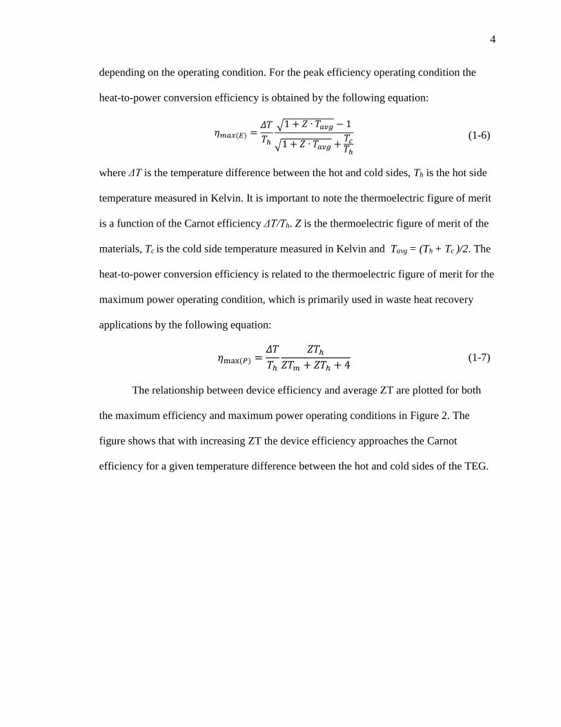
The relationship between device efficiency and average ZT are plotted for both
the maximum efficiency and maximum power operating conditions in Figure 2. The
figure shows that with increasing ZT the device efficiency approaches the Carnot
efficiency for a given temperature difference between the hot and cold sides of the TEG.

5
Figure 2: (a) Thermoelectric device efficiency vs. average ZT for a TE device
operating at the maximum efficiency condition. (b) Thermoelectric device efficiency
vs. average ZT for a TE device operating at the maximum power condition
The equation relating device efficiency to the thermoelectric figure of merit fails
to take into account any temperature dependent variations in the thermoelectric
properties, as well as any contribution from the Thomson effect, which is dependent upon
the change in the Seebeck coefficient with temperature as explained in the previous
section. Kim et al. have suggested a relationship with better accuracy [2]. The proposed
relationship accounts for the temperature dependent nature of the thermoelectric
properties and any influence from the Thomson effect. The conversion efficiency can be
related to the thermoelectric figure of merit using the following relationship [2]:
𝜂𝑚𝑎𝑥 (𝐸) = 𝜂𝑐
√1 + (𝑍𝑇)𝑒𝑛𝑔(𝑎 𝜂𝑐 − 1/2)⁄ − 1
𝑎(√1 + (𝑍𝑇)𝑒𝑛𝑔(𝑎 𝜂𝑐⁄ −12 + 1) + 𝜂𝑐
(1-8)
(𝑍𝑇)𝑒𝑛𝑔 = 𝛥𝑇
(∫ 𝑆(𝑇)𝑑𝑇𝑇ℎ
𝑇𝑐)2
∫ 𝜌(𝑇)𝑑𝑇𝑇ℎ
𝑇𝑐∫ 𝜅(𝑇)𝑑𝑇
𝑇ℎ
𝑇𝑐
(1-9)
𝑎 =
𝑆(𝑇ℎ)𝛥𝑇
∫ 𝑆(𝑇)𝑑𝑇𝑇ℎ
𝑇𝑐
(1-10)

6
where ηc is the Carnot efficiency, (ZT)eng is the engineering figure of merit, and a is the
intensity of the Thomson effect. S, ρ, and κ are the temperature dependent Seebeck
coefficient, electrical resistivity and thermal conductivity of the material. T, Th, Tc, and
ΔT are the temperature, hot side temperature, cold side temperature and the temperature
difference between the hot and cold sides measured in Kelvin.
Thermoelectric Generators and Their Applications
Thermoelectric generators consist of numerous thermoelectric unicouples
arranged electrically in series and thermally in parallel as illustrated in Figure 3. The
different components of a thermoelectric unicouple are also shown in Figure 3. The
purpose of the copper headers connected to the thermoelectric legs is to complete the
electric circuit, while the top and bottom copper headers serve the purpose of reducing
thermal stress. The ceramic layers in the unicouple act as an electrical insulator, and
prevents the electric circuit from shorting.

7
Figure 3: A thermoelectric module and a thermoelectric unicouple are shown,
with the different components of the unicouple identified.
Thermoelectric applications can be divided into energy conversion and cooling
applications. The Seebeck effect is implemented to convert heat energy into electricity,
and the Peltier effect is used for thermoelectric cooling. Thermoelectric devices require
no moving parts and are environmentally friendly, which makes it easy to be
implemented with other systems. Thermoelectric generators are a viable option for waste
heat recovery applications, and some of the applications are illustrated in Figure 4.
Thermoelectric generators have been implemented to recover waste heat from a diesel
engine [3]. Furthermore, around 70% of fuel used in automobiles is discharged as waste
heat [4], which can be employed as a heat source for thermoelectric generators, in order
to improve the fuel efficiency of the automobile. Similarly, waste heat from aircraft
engines has been utilized as a heat source for thermoelectric generators to improve the

8
overall efficiency of rotorcraft engines which can lose up to 70% of the potential
chemical energy [5]. Thermoelectric energy generation can be implemented wherever a
heat source is available and ideally, a waste heat source due to the low heat-to-electricity
conversion efficiency. The human body exudes a considerable amount of heat energy,
and thermoelectric generators have been implemented to utilize the waste heat from the
body. Thermoelectric generators that recover waste heat from the body are used to power
such devices as wireless sensor nodes, electrocardiograms, and pulse oximeters. [6-8].
Furthermore, TEGs can be integrated into residential heating systems, which require both
fuel and electricity for heat production and electricity for operating its electric
components. These heating systems are more reliable in providing heat during extreme
weather conditions than conventional systems connected to the power grid.
Thermoelectric modules can be implemented to make such systems truly self-powered
[9]. TEGs have also been incorporated with residential gas-fired boilers with a 4% heat-
to-electricity conversion efficiency [10].

9
Figure 4: (a) A TEG applied to a car to recover waste heat from the exhaust [11]
(b) A pulse oximeter powered by a TEM [7] (c) An autonomous wireless sensor node
powered by a TEM (d) TEMs integrated into a gas-fired boiler [10]
Thermoelectric Materials
As suggested by the thermoelectric figure of merit, the three critical properties for
a thermoelectric material are its Seebeck coefficient, electrical conductivity, and thermal
conductivity. Thermoelectric effects are predominantly observable in semiconductor
materials. The Seebeck coefficient, which is critical to the thermoelectric effect, is
inversely proportional to charge carrier concentration, whereas the electrical conductivity
is proportional to the charge carrier concentration. The thermal conductivity in
semiconductors is dominated by phonons, which are atomic vibrations [12].
Thermoelectric materials are classified into three categories based on the operation
temperature. Bismuth based alloys combined with Antimony, Tellurium, and Selenium
have high ZT as illustrated in Figure 5 are used for low-temperature applications up to

10
around 450K. The intermediate temperature range used for heat recovery applications up
to around 850 K consist primarily of lead Chalcogenides, Skutterudites, and Half-
Heuslers. While thermoelements employed in high-temperature applications up to 1300
K consist of silicon Germanium alloys [1]. Lead based thermoelectric materials are
highly toxic and have weak mechanical strength. Skutterudites, which are rare earth
metal-based minerals, suffer from having poor thermal stability as well as being of
limited supply in nature. On the other hand, Half-Heusler alloys are environmentally
friendly, mechanically and thermally robust and the cost is dependent upon the Hafnium
material. Half-Heuslers alloys consist of a XYZ chemical composition, where X can be a
transition metal, a noble metal, or a rare-earth element, where Y is a transition metal or a
noble metal, and Z is a main group element [13].
Figure 5: An overview of ZT vs. Temperature for various materials [13].

11
Objective and Organization of this Thesis
The purpose of this thesis research is to examine and model thermoelectric
systems. Thermoelectric systems are composed of a thermoelectric generator, which is
accompanied by heat exchangers or heat sinks on the hot and cold side of the TEG. The
first task that was accomplished was the development of a finite element model to predict
the performance of a thermoelectric unicouple, which is then extended to a thermoelectric
module. The work done in developing the finite element model for a thermoelectric
unicouple is detailed in Chapter 2, along with suggestions for improving the unicouple
performance. Chapter 3 describes the development of a TEG – Heat exchanger model.
The heat exchanger model developed in Chapter 3 utilizes forced convection. The TEG –
Heat exchanger model builds on the TEG model developed in Chapter 2. Natural
convection heat sinks and their application with TEGs are examined in Chapter 4, with
the development of a TEG-Heat Sink model. The work culminates in the development of
a microwire heat sink model, which is developed to be used in collaboration with the
TEG model to recover waste heat from the human body. As each chapter focuses on
somewhat varied topics, the literature review is done on a per chapter basis. Additionally,
the equation variables for each chapter are independent of each other, stemming from the
fact that heat flow and heat transfer coefficients are used throughout this work in different
context.

12
TEMPERATURE DEPENDENT FINITE ELEMENT MODEL FOR A
THERMOELECTRIC MODULE
Introduction
Thermoelectric material properties are temperature dependent, and in practical
use, there is a significantly large temperature gradient along a thermoelectric unicouple.
As indicated in Figure 6, the P-type Half-Heusler material is particularly sensitive to
temperature. With a temperature change from 100 °C to 600 °C, a 100%, 174% and 32 %
changes are observed in the Seebeck coefficient, electrical resistivity, and thermal
conductivity respectively.
Figure 6: Temperature dependent properties of the Half-Heusler alloy.
Much of the work done on modeling thermoelectric unicouples has been done in
an ANSYS environment [14] or COMSOL environment [15]. Similar thermoelectric
models do not take into account the temperature dependence of the material properties
[16] or the influence of the headers attached to the unicouple [17 -20]. With the goal of
accurately predicting, the thermoelectric power generation and heat-to-power conversion

13
efficiency of a thermoelectric module a steady-state finite element model was developed
in a MATLAB environment.
Temperature Dependent Model
Model Assumptions and Boundary Conditions
The following assumptions were made to simplify the model.
1) The temperature variation was assumed one-dimensional through the unicouple.
The reasoning for this assumption was that the temperatures at the hot and cold
side of a unicouple are fixed and assumed constant. Furthermore, there are no
significant heat losses from the lateral sides of the unicouple.
2) The energy generation or absorption was assumed constant throughout the finite
element, and material properties are assumed to be constant within a given finite
element.
3) Convection and radiation heat transfer from the external surfaces of the unicouple
were ignored in the model.
4) The whole of the top surface of the unicouple is assumed to be at the constant hot-
side temperature, and the bottom surface is assumed that of the cold-side
temperature. This assumption is utilized as the boundary condition for the model.
5) The module power output and voltage were obtained by the product of the
number of unicouples and the power output and voltage of a single unicouple
respectively.
Thermoelectric Power Generation
The energy generation terms are significant for the finite element solution. The
two primary energy generation/absorption are the Peltier heat generation/absorption at the
14
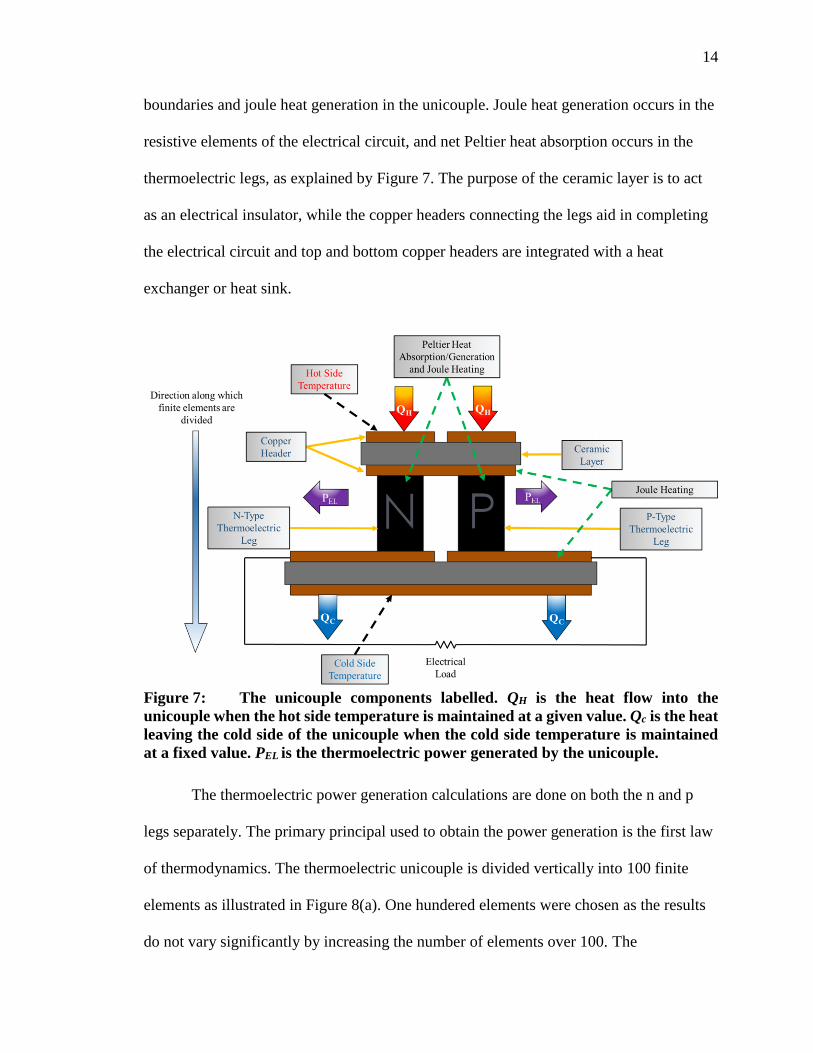
boundaries and joule heat generation in the unicouple. Joule heat generation occurs in the
resistive elements of the electrical circuit, and net Peltier heat absorption occurs in the
thermoelectric legs, as explained by Figure 7. The purpose of the ceramic layer is to act
as an electrical insulator, while the copper headers connecting the legs aid in completing
the electrical circuit and top and bottom copper headers are integrated with a heat
exchanger or heat sink.
Figure 7: The unicouple components labelled. QH is the heat flow into the
unicouple when the hot side temperature is maintained at a given value. Qc is the heat
leaving the cold side of the unicouple when the cold side temperature is maintained
at a fixed value. PEL is the thermoelectric power generated by the unicouple.
The thermoelectric power generation calculations are done on both the n and p
legs separately. The primary principal used to obtain the power generation is the first law
of thermodynamics. The thermoelectric unicouple is divided vertically into 100 finite
elements as illustrated in Figure 8(a). One hundered elements were chosen as the results
do not vary significantly by increasing the number of elements over 100. The

15
thermoelectric power generated by the unicouple is equal to the sum of the difference
between the heat input and heat leaving each segment in the thermo-electric leg. It is
important to note that for the thermoelectric power generation calculation, only segments
covering the thermoelectric legs are considered, although the complete unicouple is
segmented in the model.
The heat transferred into a finite element containing a thermoelectric leg is given
by the following equation:
𝑄ℎ,𝑝,𝑛 = 𝑎𝑏𝑠(𝛼𝑝,𝑛(𝑇)) ∙ (𝑇𝑛𝑜,𝑝,𝑛)∙ 𝐼 + 𝐾𝑝,𝑛(𝑇𝑛𝑜,𝑝,𝑛 − 𝑇𝑛𝑜+2,𝑝,𝑛) − 1
2𝐼2 ∙ 𝑅𝑒𝑙,𝑝,𝑛
(2-1)
The heat leaving a finite element containing a thermoelectric leg is given by the
following equation:
𝑄𝑐,𝑝,𝑛 = 𝑎𝑏𝑠(𝛼𝑝,𝑛(𝑇)) ∙ (𝑇𝑛𝑜+2,𝑝,𝑛)∙ 𝐼 + 𝐾𝑝,𝑛(𝑇𝑛𝑜,𝑝,𝑛 − 𝑇𝑛𝑜+2,𝑝,𝑛) + 1
2𝐼2 ∙ 𝑅𝑒𝑙,𝑝,𝑛
(2-2)
where Qh,p,n is the heat transferred in to the p-leg and n-leg segments, and Qc,p,n is the heat
transferred from the cold side of the p-leg and n-leg segments. The first terms on the right
hand side of equations 2-1 and 2-2 account for the Peltier heat at the boundaries of the
segment, where αp,n (T) is the temperature dependent Seebeck coefficient of each
segment. Tno,p,n is the temperature of each element at the upper node of the element and
Tno+2,p,n is the temperature of the bottommost node of each element, the nodes, and
elements of the model are shown in Figure 8(a). I is the current through the two legs,
which are connected in series. The second term on the right side of equations 2-1 and 2-2
account for the thermal conduction through the thermoelectric legs, where Tno, p,n and
Tno+2,p,n are defined as above. Kp,n is the thermal conductance of each element which is
given by the following equation:
𝐾𝑝,𝑛 = 𝜅𝑝,𝑛(𝑇)∙𝐴𝑝,𝑛
𝑙𝑝,𝑛 (2-3)
16
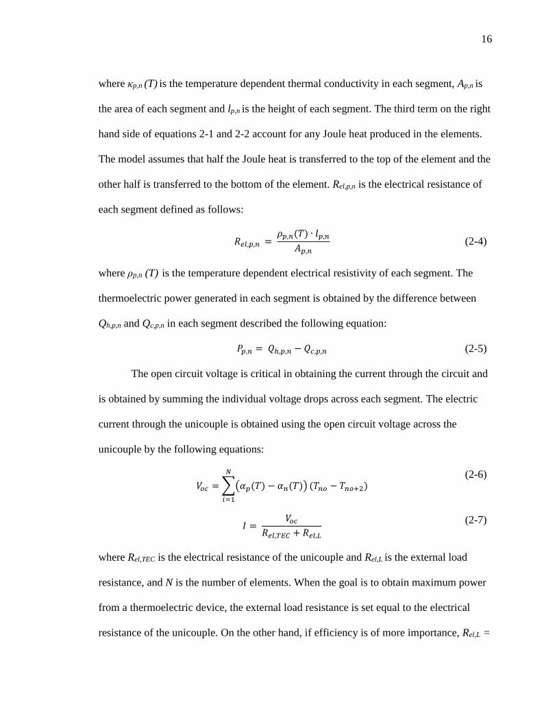
where κp,n (T) is the temperature dependent thermal conductivity in each segment, Ap,n is
the area of each segment and lp,n is the height of each segment. The third term on the right
hand side of equations 2-1 and 2-2 account for any Joule heat produced in the elements.
The model assumes that half the Joule heat is transferred to the top of the element and the
other half is transferred to the bottom of the element. Rel,p,n is the electrical resistance of
each segment defined as follows:
𝑅𝑒𝑙,𝑝,𝑛 =
𝜌𝑝,𝑛(𝑇) ∙ 𝑙𝑝,𝑛
𝐴𝑝,𝑛
(2-4)
where ρp,n (T) is the temperature dependent electrical resistivity of each segment. The
thermoelectric power generated in each segment is obtained by the difference between
Qh,p,n and Qc,p,n in each segment described the following equation:
𝑃𝑝,𝑛 = 𝑄ℎ,𝑝,𝑛 − 𝑄𝑐,𝑝,𝑛 (2-5)
The open circuit voltage is critical in obtaining the current through the circuit and
is obtained by summing the individual voltage drops across each segment. The electric
current through the unicouple is obtained using the open circuit voltage across the
unicouple by the following equations:
𝑉𝑜𝑐 = ∑(𝛼𝑝(𝑇) − 𝛼𝑛(𝑇))
𝑁
𝑖=1
(𝑇𝑛𝑜 − 𝑇𝑛𝑜+2)
(2-6)
𝐼 =
𝑉𝑜𝑐
𝑅𝑒𝑙,𝑇𝐸𝐶 + 𝑅𝑒𝑙,𝐿
(2-7)
where Rel,TEC is the electrical resistance of the unicouple and Rel,L is the external load
resistance, and N is the number of elements. When the goal is to obtain maximum power
from a thermoelectric device, the external load resistance is set equal to the electrical
resistance of the unicouple. On the other hand, if efficiency is of more importance, Rel,L =

17
Rel,TEC(1 +ZT)1/2, where ZT is the thermoelectric figure of merit of the material at the
average temperature of the unicouple. The model is also setup to simulate a current
swipe, where the load resistance is varied from 0 to a value greater than Rel,TEC. As
indicated by the equations above, it is necessary to obtain the temperature profile along
the thermoelectric unicouple; this process is explained in the following section.
Figure 8: (a) The division of the unicouple along its vertical length into finite
elements and the corresponding nodes, each element shares a node with its
neighboring element (b) The simplified thermal circuit for the unicouple and the
components of the unicouple
Temperature Profile
The temperature profile of the thermoelectric unicouple was obtained by solving a
one-dimensional finite element model of the unicouple, which requires the assembly of a

18
global stiffness matrix and a forcing vector. The temperature profile can be obtained by
the matrix solution as follow:
𝑇 = 𝐾−1𝐹 (2-8)
where T is the temperature vector, K-1 is the inverse global stiffness matrix, and F is the
forcing vector. The assembly of the global stiffness matrix requires elemental stiffness
matrix, which is obtained as follows [21]:
𝐾𝑒 = ∫ [𝐵]𝑇[𝐷][𝐵]𝐴𝑒𝑑𝑥
𝑘
𝑙
(2-9)
where B is a term borrowed from structural mechanics called the strain displacement
matrix, the D matrix contains the elemental thermal conductivity terms, and Ae is the area
of the element. The model uses one-dimensional quadratic elements, which allows an
accurate solution to be obtained with a smaller number of elements in comparison to
linear elements. The elemental stiffness matrix for this model simplifies to the following
equation:
𝐾𝑒 =
𝐴𝑒𝑘𝑒
𝑙𝑒[
14 −16 2−16 32 −16
2 −16 14]
(2-10)
where le is the element thickness. It is important to note that each element will have its
own, temperature dependent thermal conductivity term, κe. The elemental area would
change according to the geometry of the headers and the thermoelectric legs. The global
stiffness matrix is assembled using the individual stiffness matrix while taking into
consideration that each element has three temperature nodes illustrated in Figure 8(a).
The elemental loading vector was developed taking into consideration energy generation

19
or absorption in the element, which is the Peltier heat absorption/generation and Joule
heat produced in each element:
𝐹𝑒 = ∫ 𝐺[𝑁]𝑇𝐴𝑑𝑥
𝑘
𝑙
(2-11)
where G is the volumetric energy generation/absorption, N is the shape function, and A is
the elemental area. For a one-dimensional quadratic element, the forcing vector reduces
to the following vector:
𝐹𝑒 =
𝐺𝑒𝐴𝑒𝑙𝑒
6[141
]
(2-12)
where Ge is the elemental volumetric energy generation/absorption, Ae and le are defined
as above. Once again, the global loading vector was assembled using each of the
elemental loading vectors while considering that each element has three temperature
nodes.
It must be noted that an initial temperature profile (initial guess) is needed to
obtain the required terms for the elemental stiffness matrix (temperature dependent
thermal conductivity) and forcing vector (thermoelectric power generation in an
element). The thermal circuit illustrated in Figure 8(b) is used to obtain the temperatures
at critical boundaries along the unicouple, and a linear profile is assumed between those
boundaries to obtain the initial temperature profile (intial guess). The temperature
dependent properties and energy generation terms are evaluated using the initial
temperature profile. Once the temperature profile is obtained using equation 2-8, it is
used to obtain the temperature dependent global stiffness matrix and forcing vector. This
process is repeated until the difference between the temperature profiles is less than the
convergence criteria as explained by the following equation:

20
∑ 𝑎𝑏𝑠(𝑇𝑜𝑙𝑑(𝑖) − 𝑇𝑛𝑒𝑤(𝑖))
𝑒𝑙𝑒𝑚𝑠
𝑖=1
< 𝐶𝐶
(2-13)
where Told is the temperature profile obtained from the previous iteration, Tnew is the new
temperature profile, elems is the number of elements and CC is the convergence criteria
set equal to 1°C. Once the final temperature profile is obtained, it is used in equations 2-1
through 2-7 to obtain the thermoelectric power generated by a unicouple.
Contact Resistance
The brazing process between the thermoelectric legs and headers can induce an
electrical resistance. The electrical contact resistance is captured into the overall circuit,
by adding it as an additional resistor, using an electrical resistivity of 1*10-9Ω-m2 [22].
The electrical contact resistivity was obtained from experimental data and numerical
simulations. The electrical contact resistance is obtained using the following equation:
𝑅𝑐𝑜𝑛𝑡 =𝜌𝑐𝑜𝑛𝑡
𝐴𝑐
(2-14)
where ρcont is the electrical contact resistivity value of 1*10-9Ω-m2, and Ac is the area of
contact between the legs and the copper headers.
Model Validation
The one-dimensional model was compared with a 3-D model developed in an
ANSYS environment for three different material types. The ANSYS model was
developed for a unicouple with the dimensions in Table 1. The ANSYS model used a fine
mesh with 19359 elements and 98186 nodes and further details regarding the ANSYS
model can be found in Appendix I. The finite element model results were also compared
with available experimental data for the Half-Heusler alloy. The experimental data
compared is expected to be published in 2017 and was obtained using a similar

21
experimental setup that is described by Zhang et al.[10]. Table 1 illustrates the
dimensions of the unicouple components, which are the dimensions used for the
experimental data obtained. The unicouple that was experimentally tested is illustrated in
Figure 9, as well as the temperature profile of the unicouple obtained from the 3-D
ANSYS model.
Table 1 Dimensions of the unicouple elements
Component Thickness/Height [mm] Area [mm x mm]
Copper Header 1 0.203 [1.93 * 1.96]*2
Ceramic 1 0.635 2.26 * 4.51
Copper Header 2 0.203 1.96 * 4.21
P-Leg 2.400 1.50 * 1.50
N-Leg 2.400 1.50 * 1.50
Copper Header 3 0.203 [1.96 * 4.07]*2
Ceramic 2 0.635 2.26 * 8.81
Copper Header 4 0.203 [1.96 * 8.50]*2

22
Figure 9: (a) Thermoelectric unicouple that was experimentally tested with
results in Figure 11. (b) Temperature profile along unicouple for the 3-D ANSYS
model for a hot side temperature of 600°C and cold side temperature of 100 °C, the
results from the ANSYS model are available in Figure 11, Figure 14, and Figure 16
The ANSYS model developed was used to compare results from the finite
element model for two additional materials, Bi2Te3 and PbTe with the temperature
dependent materials shown in Figure 10.

23
Figure 10: Temperature dependent properties of the Bi2Te3 material (a) Seebeck
Coefficient (b) Thermal Conductivity (c) Electrical Resistivity. Temperature
dependent properties of the PbTe material (d) Seebeck Coefficient (e) Thermal
Conductivity (f) Electrical Conductivity.
The results for the Half-Heusler alloy unicouple was compared for hot side
temperatures of 200 °C, 300 °C, 400 °C, 500 °C and 600 °C while maintaining the cold
side temperature at 100 °C as illustrated in Figure 11. The power results for the Half-
Heusler material compare fairly well with the ANSYS model with an average percent error
of 11.93%. The discrepancies in the power values are due to differing values of the leg hot
and cold side temperatures. The temperature difference between the leg hot and cold sides
influence the open circuit voltage of the unicouple, which in turn affects the power
produced by the unicouple. The leg hot side temperature (T3 from Figure 8) is lower in the
3-D model compared to the 1-D model. Similarly, the leg cold side temperature (T4 from
Figure 8) is smaller in the 1-D model. Therefore, a larger temperature difference is
observed across the legs for the 1-D model, which results in larger power being produced.
The discrepancies in the temperatures of the legs are due to heat spreading effects in the 3-
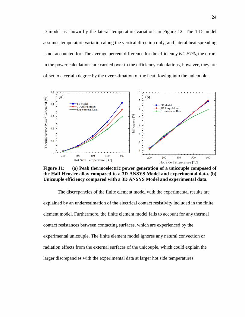
24
D model as shown by the lateral temperature variations in Figure 12. The 1-D model
assumes temperature variation along the vertical direction only, and lateral heat spreading
is not accounted for. The average percent difference for the efficiency is 2.57%, the errors
in the power calculations are carried over to the efficiency calculations, however, they are
offset to a certain degree by the overestimation of the heat flowing into the unicouple.
Figure 11: (a) Peak thermoelectric power generation of a unicouple composed of
the Half-Heusler alloy compared to a 3D ANSYS Model and experimental data. (b)
Unicouple efficiency compared with a 3D ANSYS Model and experimental data.
The discrepancies of the finite element model with the experimental results are
explained by an underestimation of the electrical contact resistivity included in the finite
element model. Furthermore, the finite element model fails to account for any thermal
contact resistances between contacting surfaces, which are experienced by the
experimental unicouple. The finite element model ignores any natural convection or
radiation effects from the external surfaces of the unicouple, which could explain the
larger discrepancies with the experimental data at larger hot side temperatures.

25
Figure 12: A cross-sectional view of the bottom surface of the n-type leg. Lateral
temperature variations are observed in the ANSYS model, which is not accounted for
in the 1-D finite element model.
The power and efficiency curves obtained by varying the load resistance are
displayed in Figure 13 (a) and (b) for the five different hot side temperatures. The device
voltage decreases from the open circuit voltage to zero as the current is increased by
varying the load resistance as shown in Figure 13(c). The maximum power is obtained at
a device voltage that is equal to half the open circuit voltage.
Figure 13: (a) Thermoelectric power generated for varying current for a
unicouple composed of the Half-Heusler alloy. (b) The TEG efficiency for varying
current for a unicouple composed of Half-Heusler alloy (c) Device voltage vs. electric
current for a unicouple composed of the Half-Heusler alloy.

26
Similarly, the power generated and efficiency was compared for a unicouple
composed of Bi2Te3. The hot side temperature was increased from 50°C, 100°C, 150 °C,
200°C and 250°C, which is its operating limit while maintaining the cold side temperature
at 20 °C. The power and efficiency results are compared in Figure 14. The average percent
error in the power calculations is 2.73% for the Bi2Te3 material, whereas the average
percent error for the efficiency calculation is 14.2%. The better accuracy in the power
calculations are accounted for by smaller discrepancies in the leg hot (T3 from Figure 8)
and cold side temperatures( T4 from Figure 8) when compared with the 3-D ANSYS model.
The discrepancies in the heat flow are attributed to the model underestimating the heat flow
into the model, considering 3-D heat spreading effects are not accounted for in the model.
Figure 14: (a) Peak thermoelectric power generation of a unicouple made of the
Bi2Te3 material compared to a 3D ANSYS Model (b) Unicouple efficiency compared
with a 3D ANSYS Model.
The power and efficiency curves obtained by varying the load resistance is
displayed in Figure 15. The electrical current values are restricted by the open circuit
voltage values, which are smaller for the unicouple composed of the Bi2Te3 material
compared to the unicouple composed of the Half-Heusler material.

27
Figure 15: (a) Thermoelectric Power Generated for varying current for a
unicouple composed of the Bi2Te3 material (b) The TEG efficiency for varying current
for a unicouple composed of the Bi2Te3 material (c) Device voltage vs. electric current
for a unicouple composed of the Bi2Te3 material.
Finally, the thermoelectric power and efficiency of a unicouple composed of PbTe
was compared for hot side temperatures of 200 °C, 300 °C, 400°C, 500°C and 600°C, while
the cold side temperature was held at 100 °C as shown in Figure 16. The average percent
error in the power calculations for the PbTe material are 4.85% and 7.85% for the
efficiency calculations. The better accuracy in the PbTe unicouple model is possibly
explained by the smaller variations in thermal conductivity of PbTe in the operating
temperature of the material.

28
Figure 16: (a) Peak thermoelectric power generation of a unicouple composed of
the PbTe material compared to a 3D Ansys Model (b) Unicouple efficiency compared
with a 3D Ansys Model
Similar to the Half-Heusler alloy unicouple and Bi2Te3 unicouple, the power and
efficiency curves were obtained by varying the load resistance, which resulted in the power
and efficiency curves in Figure 17 (a) and (b). The accompanying voltage vs. current curves
are displayed in Figure 17(c).
Figure 17: (a) Thermoelectric Power Generated for varying current for a
unicouple composed of the PbTe material (b) The TEG efficiency for varying current
for a unicouple composed of the PbTe material (c) Device voltage vs. electric current
for a unicouple composed of the PbTe material.

29
Thermoelectric Thin Films
Bulk thermoelectric modules are difficult to implement with or in small-scale
devices. Furthermore, it is challenging to design flexible bulk thermoelectric modules.
Thin film thermoelectrics uses semiconductor processing to create nano-structured thin
films used as the thermoelectric legs. These films have a thickness of around 10 µm,
compared to the leg heights of 1-2 mm discussed previously. The miniature scale of the
thin film devices results in flexible thermoelectric devices, which can be beneficial when
the heat source has a contoured surface, such as the human body. Flexible thermoelectric
devices are an attractive option for powering power sensors, biomedical devices and
wearable electronics [23]. The thermoelectric model was used to predict the performance
of a thin film thermoelectric device with an area of 2mm by 0.01mm and height of 10.5
mm, consisting of five thin films for a cold side temperature of 20 °C with the material
properties detailed in [23]. The power density is the ratio of the total thermoelectric
power generated to the surface area occupied by the TEG. The experimental power
density and open circuit voltage results in [23] are compared with the finite element
model results in Figure 18. An average percent difference of 11.5% is observed for the
power density, and an average percent difference of 5.4% is observed for the open circuit
voltage.

30
Figure 18: (a) Power density vs. temperature difference compared with
experimental results. (b) Open circuit voltage vs. temperature difference compared
with experimental results [23].
Ceramic Material
The thermoelectric power generated by a unicouple can be increased by having the
largest possible temperature difference between the thermoelectric legs (temperatures T3
and T4 from Figure 8). For the Half-Heusler material model described in the previous
section, the temperature difference across the legs is 463.05°C, when the temperature
difference across the unicouple is 500°C. The temperature drop across the copper and
ceramic components of the unicouple accounts for the 36.95°C difference. As copper is an
effective thermal conductor, the temperature drop across the copper header is negligible.
However, there is a 30.968°C temperature drop across ceramic 1 and a 4.99°C temperature
drop across ceramic 2. If a larger ratio of the 500°C temperature difference can be had over
the thermoelectric legs, the unicouple performance could be improved by having a larger
open-circuit voltage resulting in more thermoelectric power generated. The performance
of the unicouple can be improved by eliminating the ceramic component of the unicouple;
however, the ceramic element serves to act as an electrical insulator, which is essential for
the unicouple. A larger temperature difference could be obtained across the thermoelectric

31
legs by reducing the thermal resistance of the ceramic component, which could be
accomplished by:
a) Using a thinner ceramic component
b) Using an electrical insulator with a larger thermal conductivity
In this thesis, the latter option was examined. The thermal conductivity of the
ceramic currently used Alumina (Al2O3) varies from 24.7 W/m-K at room temperature to
6.59 W/m-K at 600°C as illustrated in Figure 19. Three other electrical insulators with
better thermal conductivities are considered in this section. The three materials of interest
are Aluminum Nitride, Silicon nitride, and Beryllium oxide. Alumina is the industry
standard for electronic substrates [24] and is the ceramic chosen in the model in the
previous section. It offers the advantages of having relatively high strength, a high service
temperature, being chemically inert and having a lower cost when compared to the other
materials. Beryllia (BeO) has the highest thermal conductivity values of 259.4 W/m-K at
room temperature and 46.79 W/m-K at 600°C among the materials considered. However,
it is extremely expensive due to high powder costs. Furthermore, it is also considered a
toxic substance, which limits its application. Aluminum nitride (AlN) has a thermal
conductivity of 200 W/m-K at room temperature and 40.46 W/m-K at 600°C, which is
comparable to the thermal conductivity of Beryllia. It offers a non-toxic alternative to
Beryllia and has good oxidation resistance, which is significant at high temperatures.
However, similar to Beryllia it is expensive and is only feasible in limited applications.
Silicon nitride (Si3N4) has thermal conductivity values of 63.5 W/m-K at room temperature
and 38.31 W/m-K at 600 °C; additionally, it offers high-temperature strength and thermal

32
shock resistance, which makes it an attractive material for high-temperature applications
[25].
Figure 19: Thermal Conductivity vs. Temperature comparison of ceramics that
can be used as an electrical insulator for a unicouple [25]
As the goal of this section is to show the significance of the ceramic layer,
thermoelectric legs with lower thermal resistance are chosen compared to the values in
Table 1. The updated values leg heights are 1.7mm and leg area of 2mm by 2mm, while
the copper and ceramic header dimensions are as in Table 1. For the comparison between
the ceramics, the unicouple dimensions were kept the same, and the Half-Heusler material
was chosen for the unicouple legs. As illustrated in Figure 20 there is a temperature

33
difference of 479.6 °C across the legs when Beryllia is used as the electrical insulator when
compared to a temperature difference of 417.3°C when Alumina is used. It should be noted
that unicouples with Aluminum Nitride and Silicon Nitride as the ceramic exhibit relatively
similar temperature profiles to that of the unicouple with Beryllia as the ceramic, and were
not included in the figure to improve clarity.
Figure 20: Temperature profile of the unicouple for a unicouple that has Alumina
as the ceramic and Beryllia as the ceramic; the green lines are used to indicate the
temperature along the thermoelectric legs.
The larger temperature differences across the thermoelectric legs for the
unicouples with Beryllia, Aluminum Nitride and Silicon Nitride illustrated in Figure
21(a) induce a larger open circuit voltage across the unicouple shown in Figure 21 (b).

34
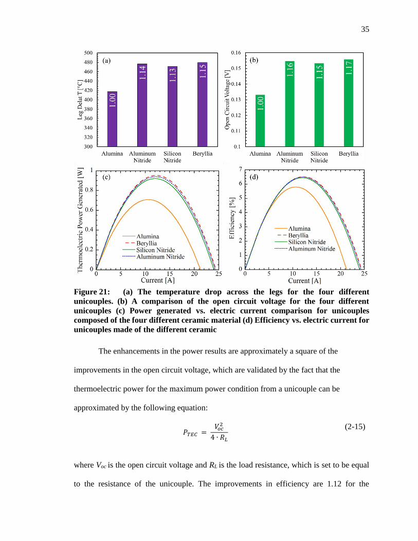
The improvements in the open circuit voltages are 1.16 for Aluminum Nitride, 1.15 for
Silicon Nitride and 1.17 for Beryllia when compared with the open circuit voltage of the
unicouple with Alumina as the ceramic. The enhancements in the power results are 1.33
for Aluminum Nitride, 1.30 for Silicon Nitride and 1.34 for Beryllia when compared with
the power output of the unicouple with Alumina as the ceramic as shown in Figure 21(c).
It is interesting to note that although the Beryllia material has a higher overall thermal
conductivity compared to Aluminum Nitride and Silicon Nitride, the improvements in the
thermoelectric power are comparable to the unicouples with AlN and Si3N4 as the
ceramic. This observation is explained by the fact that the temperature the top ceramic
experiences is in the 500°C -600°C range. The average thermal conductivities of Beryllia,
Aluminum Nitride, and Silicon Nitride is 56.13 W/m-K, 44.28 W/m-K, and 39.78 W/m-k
respectively in the 500°C to 600 °C temperature range.
35
Figure 21: (a) The temperature drop across the legs for the four different
unicouples. (b) A comparison of the open circuit voltage for the four different
unicouples (c) Power generated vs. electric current comparison for unicouples
composed of the four different ceramic material (d) Efficiency vs. electric current for
unicouples made of the different ceramic
The enhancements in the power results are approximately a square of the
improvements in the open circuit voltage, which are validated by the fact that the
thermoelectric power for the maximum power condition from a unicouple can be
approximated by the following equation:
𝑃𝑇𝐸𝐶 =
𝑉𝑜𝑐2
4 ∙ 𝑅𝐿
(2-15)
where Voc is the open circuit voltage and RL is the load resistance, which is set to be equal
to the resistance of the unicouple. The improvements in efficiency are 1.12 for the
36
unicouple with a ceramic composed of Aluminum Nitride, 1.11 for one with Silicon
Nitride, and 1.12 for one with Beryllia, which corresponds to the increase in the
temperature difference across the legs.
Segmented Leg Unicouples
One of the major limitations of thermoelectric generators holding it back from
large-scale production is their low heat-to-power conversion efficiencies. The conversion
efficiency is itself capped by the Carnot efficiency η = (Th –Tc)/Th as demonstrated by
equations 1-6 and 1-7. The conversion efficiency is dependent upon the thermoelectric
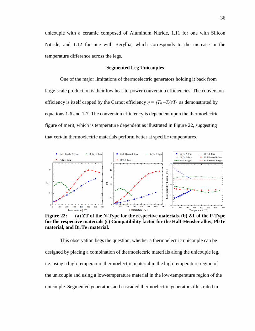
figure of merit, which is temperature dependent as illustrated in Figure 22, suggesting
that certain thermoelectric materials perform better at specific temperatures.
Figure 22: (a) ZT of the N-Type for the respective materials. (b) ZT of the P-Type
for the respective materials (c) Compatibility factor for the Half-Heusler alloy, PbTe
material, and Bi2Te3 material.
This observation begs the question, whether a thermoelectric unicouple can be
designed by placing a combination of thermoelectric materials along the unicouple leg,
i.e. using a high-temperature thermoelectric material in the high-temperature region of
the unicouple and using a low-temperature material in the low-temperature region of the
unicouple. Segmented generators and cascaded thermoelectric generators illustrated in

37
Figure 23 are utilized to achieve this goal. The primary difference between a segmented
and cascaded thermoelectric generator is that a cascaded generator uses an independent
electrical circuit for each stage (material), whereas a segmented generator uses one
electrical circuit.
Figure 23: A segmented TEG and cascaded TEG are illustrated using a single
unicouple. The primary difference is the use of two different electrical loads
connected to the different stages in the cascaded TEG and the use of a single circuit
in the segmented TEG.
Thermoelectric Compatibility
Utilizing segmented thermoelectric legs puts forward the problem of
thermoelectric compatibility. From equation 2-7, it is shown that peak power of a
thermoelectric unicouple is dependent upon the electric current through it, for the peak
power condition this is obtained by setting the load resistance equal to the electrical
resistance of the unicouple. When two materials are segmented the same current flows
through both materials, however, the optimum electric current will be different for both

38
materials as they would have different electrical resistivites. Furthermore, each material
has its own optimum relative current density defined by the following equation [26]:
𝑢 =
𝐽
𝜅𝛻𝑇
(2-16)
where J is the electric current density, κ is the thermal conductivity and 𝛻T is the
temperature gradient. If the relative current density of the two-segmented materials
differs significantly, the thermoelectric efficiency may decrease when compared to using
a single material [26]. The thermoelectric compatibility equation may be utilized to select
materials, which can be used for segmentation:
𝑠 =
√1 + 𝑧𝑇 − 1
𝛼𝑇
(2-17)
where ZT is the thermoelectric figure of merit, α is the Seebeck coefficient, and T is the
absolute temperature. Initially, it was suggested that two materials with compatibility
factors differing by a factor of 2 would decrease efficiency when segmented [27, 28].
However, Ouyang and Li suggest that it is the smooth transition of the compatibility
factors at the temperature boundaries that is significant [29]. A smooth transition is
observed in the compatibility factor for the p-type at 200°C for Bi2Te3 and PbTe, and a
similar transition can be witnessed for Bi2Te3 and Half-Heusler at 250 °C in Figure 22(c).
For the n-type material, the transition is observed at the limit of the Bi2Te3 operating
temperature of 250 °C. Additionally, it is also observed that the thermoelectric figure of
merit of Bi2Te3 is larger than that of the Half-Heusler and PbTe materials from 20°C to
approximately 225 °C for the n-type material and 200°C for the p-type material.
Design of Segmented Leg Unicouples
The thermoelectric unicouple model was modified to predict the performance of a
unicouple containing a Half-Heusler segment and a Bi2Te3 segment (unicouple A).

39
Additionally, a unicouple containing a PbTe segment and a Bi2Te3 segment (unicouple B)
was designed. The two newly designed unicouples were then compared with
conventional unicouples containing only a single material of PbTe and Half-Heusler alloy
for a hot side temperature of 600°C and cold side temperature of 20°C.
Taking into consideration the transition of the compatibility factor between Bi2Te3
and the Half-Heusler material and the thermoelectric figure of merit of both materials,
250°C appears to be a suitable interface temperature. This observation means that the
segmented unicouple would be designed such that the Bi2Te3 segment of the unicouple
will experience a temperature from 250 °C to 20 °C. Similarly, the Half-Heusler alloy
segment will have a hot side temperature of 600°C, and a cold side temperature of 250°C.
The total height of the unicouple was kept similar to that in Table 1. In order to obtain the
required interface temperature, the thermal resistances of the segments have to be
adjusted according to the required interface temperature. While keeping the leg areas
constant, the following equation can be utilized to obtain the ratio of the two segment
heights [30]:
𝑙𝑝1
𝑙𝑝2=
∫ 𝜆𝑝,1(𝑇)𝑑𝑇𝑇ℎ
𝑇𝑖𝑛𝑡
∫ 𝜆𝑝,2(𝑇)𝑑𝑇𝑇𝑖𝑛𝑡
𝑇𝑐
(2-18)
𝑙𝑛1
𝑙𝑛2=
∫ 𝜆𝑛,1(𝑇)𝑑𝑇𝑇ℎ
𝑇𝑖𝑛𝑡
∫ 𝜆𝑛,2(𝑇)𝑑𝑇𝑇𝑖𝑛𝑡
𝑇𝑐
(2-19)
𝑙 = 𝑙𝑝1 + 𝑙𝑝2 = 𝑙𝑛1 + 𝑙𝑛2 (2-20)
where lp,n,1 is the length of the p and n type top segment, lp,n,2 is the height of the p and n
type bottom segment. Th is the temperature at the interface between the top copper header
and the top segment; Tint is the temperature at the segment interface, Tc is the temperature

40
at the interface between the bottom copper segment and the bottom segment, and l is the
total height of the combined leg. The leg heights of each segment obtained by equations
2-18 through 2-20 and are shown in Table 2.
Table 2 Height of the material segments in unicouple A and B
Segment Unicouple A Unicouple B
Half-Heusler alloy segment 2.106 mm -
PbTe segment - 1.618 mm
Bi2Te
3 segment 0.294 mm 0.782 mm
Total Height 2.4 mm 2.4 mm
The power and efficiency curves are compared in Figure 24 for both the Half-
Heusler-Bi2Te3 segmented unicouple (unicouple A) and the PbTe-Bi2Te3 segmented
unicouple (unicouple B) compared with only using a single material. The models were
run for a hot side temperature of 600°C and cold side temperature of 20°C and compared
using similar geometric properties with the difference being leg heights defined in Table
2. For the segmented Half-Heusler unicouple there was a 16 % increase in the power
output, while there was 61 % increase in the peak efficiency. The higher increase in the
efficiency is explained by the fact that the compatibility factor is utilized to find matching
materials, which can be used to improve efficiency. While improvements in power
generation are expected with improved efficiency, the primary improvement is in the heat
to power conversion efficiency. Similarly, for the PbTe-Bi2Te3, segmented unicouple a
49.5% improvement was observed for power, and an increase of 65.5% was observed for
the efficiency.
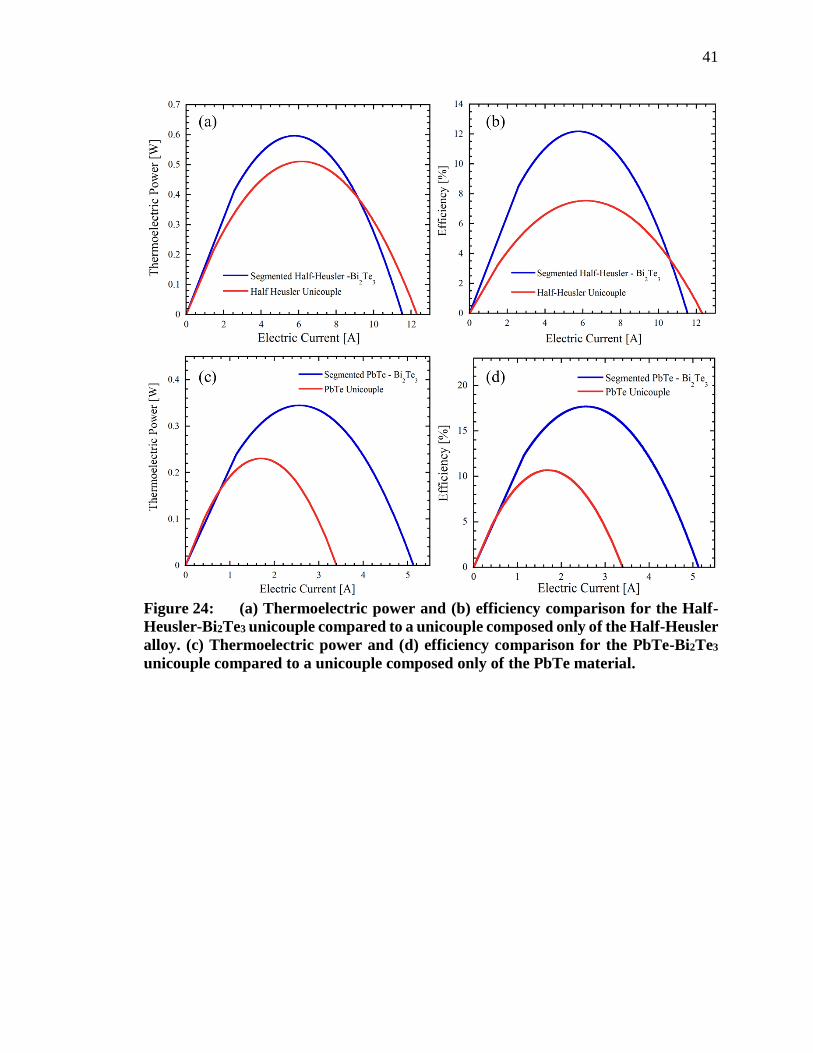
41
Figure 24: (a) Thermoelectric power and (b) efficiency comparison for the Half-
Heusler-Bi2Te3 unicouple compared to a unicouple composed only of the Half-Heusler
alloy. (c) Thermoelectric power and (d) efficiency comparison for the PbTe-Bi2Te3
unicouple compared to a unicouple composed only of the PbTe material.

42
THERMOELECTRIC GENERATOR – HEAT EXCHANGER MODEL
Introduction
Thermoelectric generators are often accompanied by heat exchangers with the
goal of maintaining the required temperature difference across a thermoelectric module.
Compact heat exchangers are used in waste heat recovery when there is a restriction on
the available space, for instance in automotive waste heat recovery applications [3].
Further, applications of compact heat exchangers include high-temperature polymer
electrolyte membrane fuel cell exhaust heat recovery [19] and waste heat reclamation
from jet engines[5]. Heat exchangers, which utilize forced convection, are often used, as
the waste heat is often available as a flowing hot fluid.
Heat exchanger models have been developed to be used in combination with
thermoelectric generator models. A plate-fin heat exchanger model has been developed in
combination with a TEG model to predict the electrical power output and overall heat
transferred to be implemented for automotive waste heat recovery [16]. The model uses
the hot exhaust gas as the hot side fluid and the liquid coolant for the cold side fluid. A
similar numerical model has been developed for a TEG to be used with a parallel-plate
heat exchanger [17]. Cylindrical shell and straight fin heat exchangers offer an alternative
to parallel plate heat exchangers to recover waste heat from an automotive. A numerical
heat transfer model has been developed along with a TEG model to predict the heat
transfer and electrical power performance of a combined system [20].

43
A heat exchanger model is developed to complement the thermoelectric module
model for steady state operation. The model developed in a MATLAB environment is
solved by considering the first law of thermodynamics in every finite control volume
illustrated in Figure 25. The inputs to the heat exchanger-TEG model are the geometry of
the heat exchanger and the inlet temperatures of the working fluids as well as the
temperature dependent fluid and thermoelectric properties.
Model Assumptions
The following assumptions were made to simplify the heat exchanger model.
1) The model divides each spacing in the heat exchanger as an individual channel,
which leads to the following assumptions
a. The mass flowrate in each channel is identical and is obtained by dividing
the total flowrate by the number of channels.
b. The heat transfer coefficient and friction factor in each section of the
channel is constant for the control volume.
2) Lateral variations in temperature are ignored.
3) The model assumes the flow is fully developed when entering each channel. The
heat exchangers are usually accompanied by a diffuser, which is not included in
the model.
4) Constant fluid temperatures are assumed in each control volume and a constant
fin base temperature is assumed for each control volume.
5) The lateral sides of the heat exchanger are assumed to be perfectly insulated.

44
Control Volume – Energy Balance
The model is solved by portioning each segment of the TEG-heat exchanger
system into finite control volumes as illustrated in Figure 22. The fundamental principal
used to solve the model is the first law of thermodynamics, by equating the heat flow
through the fins to be equal to the heat flow through the thermoelectric modules. The
TEG-Heat exchanger model is split into two symmetric components as shown in Figure
25 and calculations are performed on one section to minimize computational expense.
The length of one control volume needs to be the length of the thermoelectric module.
Figure 25: TEG – Heat Exchanger model illustrated with a 3-D view, front view
and a side view explaining the energy balance concept used in the model. QH is the
heat flow into the hot side of the TEG within the control volume and QC is the heat
flow from the cold side of the TEG to the cold-side heat exchanger. QFH is the heat
flow from the hot side heat exchanger within the control volume and QFC is the heat
flow from the cold-side heat exchanger in the control volume. PEL is the
thermoelectric power generated by the TEG.
The heat flow through the heat exchanger in the control volume is given by the
following equation by using the adiabatic fin tip condition [31]:
𝑄𝑓 = 𝑀 ∙ 𝑡𝑎𝑛ℎ (𝑚 ∙
𝑓ℎ
2) ∙ (𝑁𝑓 − 1) + 𝐴𝑢𝑓 ∙ ℎ ∙ (𝑇𝑏 − 𝑇𝑓)
(3-1)

45
𝑀 = √ℎ ∙ 𝑃 ∙ 𝑘 ∙ 𝐴𝑐 ∙ (𝑇𝑏 − 𝑇𝑓) (3-2)
𝑚 = √
ℎ ∙ 𝑃
𝑘 ∙ 𝐴𝑐
(3-3)
where fh is the fin height, Nf is the number of fins, Auf is the un-finned area, Tb is the fin
base temperature of the control volume, Tf is the fluid temperature within the control
volume and h is the channel convection coefficient which will be discussed in detail in
the next section. P is the fin perimeter, k is the thermal conductivity of the fin material,
and Ac is the cross-sectional area of the fin. The heat flow into the module, Qh is equal to
the heat transferred through the fins in the control volume, while the heat flow leaving the
cold side of the module, Qc is equal to the heat transferred through the cold side heat
exchanger, QFC. The difference between the heat entering and leaving the module is
equal to the thermoelectric power generated by the module as explained in the previous
chapter. An iterative process solves the TEG-Heat Exchanger model, and the energy
balance criteria have to be met for each control volume. The difference between the heat
flow through the hot side of the heat exchanger (QFH) and the heat flow into the module
(QH) has to be less than the required convergence criteria of 10-4W. Similarly, the
difference between the heat flow leaving the cold side of the module (TC) and the heat
flow through the cold side heat exchanger (QFC) has to be smaller than the convergence
criteria. The iterative process requires solving the base temperature of both the hot and
cold side heat exchangers for the control volume. The exit temperature of the fluid in the
control volume will be the inlet temperature of the next one and is obtained by the
following equation:

46
𝑇𝑓,𝑜𝑢𝑡 = 𝑇𝑓,𝑖𝑛 −
𝑄𝑓
�̇� ∙ 𝑐𝑝
(3-4)
where Tf,out is the exit temperature of the fluid in the control volume, Qf is the heat
transferred by the heat exchanger within the control volume, �̇� is the mass flowrate and
cp is the specific heat of the fluid.
Channel Convection Coefficient
The channel convection coefficient utilized in the model are obtained from
available empirical correlations. Similar numerical models [16, 17] have used Reynolds
number dependent empirical correlations for the convection coefficients for channel flow.
The current model uses convection coefficients for smooth rectangular ducts, which are
dependent upon the channel width to height ratio. The hydraulic diameter, dh dependent
Reynolds number for the channel flow is obtained by the following equations:
𝑅𝑒 =
𝑣𝑐ℎ ∙ 𝑑ℎ
𝜈𝑓
(3-5)
𝑑ℎ =
4 ∙ 𝐴
𝑃
(3-6)
where vch is the channel velocity, νf is the kinematic viscosity, P is the wetted perimeter,
and A is the channel cross-sectional area. The critical Reynolds number for a rectangular
inlet geometry varies from 2000 to 3100 with the upper limit at 10000 [32]. For this
model, laminar and turbulent flow is analyzed with the critical Reynolds number being
2500 based on the empirical correlation used. The convection coefficient evaluated using
the Nusselt number relationships for the laminar and turbulent regions are obtained using
the following equations [32]:
𝑁𝑢 = 7.541 ∙ (1 − 2.61𝛼 + 4.970𝛼2 − 5.199𝛼3 + 2.702𝛼4 − 0.548𝛼5)
𝑅𝑒 ≤ 2500
(3-7)

47
𝑁𝑢 = 0.024 ∙ 𝑅𝑒𝑑ℎ0.8𝑃𝑟0.4 Re ≥ 2500 ( Ts > Tf ) (3-8)
𝑁𝑢 = 0.026 ∙ 𝑅𝑒𝑑ℎ0.8𝑃𝑟0.3
Re ≥ 2500 ( Tf > Ts ) (3-9)
ℎ =
𝑁𝑢 ∙ 𝑘𝑓
𝑑ℎ
(3-10)
where α is the height to spacing ratio, Re is the hydraulic diameter dependent Reynolds
number, Pr is the Prandtl number, kf is the fluid thermal conductivity,dh is the hydraulic
diameter defined above, Ts is the surface temperature, and Tf is the fluid temperature.
Compact heat exchangers defined as having a surface area of 650 m2 per cubic
meter [33] are widely used in applications such as automotive waste heat recovery due to
spatial constraints. The following equations developed by Weiting [34] for compact
rectangular offset plate fin heat exchangers are considered in the model as well:
𝑗 = 0.483 ∙ (ℎ𝑥𝑙
𝑑ℎ)−0.162 ∙ 𝛼−0.184 ∙ 𝑅𝑒−0.536 Re ≤ 1000 (3-11)
𝑗 = 0.242 ∙ (ℎ𝑥𝑙
𝑑ℎ)−0.322 ∙ (
𝑡𝑓
𝑑ℎ)−0.089 ∙ 𝑅𝑒−0.368 Re > 1000 (3-12)
ℎ = 𝑗 ∙ 𝑅𝑒 ∙ 𝑃𝑟1/3 ∙
𝑘𝑓
𝑑ℎ
(3-13)
where j is the Colburn factor, hxl is the heat exchanger length, tf is the fin thickness, and
the other variables are similar to that defined above. The Colburn factor is a modified
version of the Stanton number taking into consideration variations in the fluid Prandtl
number [32]. There are certain limitations in extending these empirical correlations to
compact channel flow. The empirical correlations are obtained for offset plate fin heat
exchangers, which means that there is a boundary layer developing on the thickness of
the plate. In addition, there is turbulence generated by the plate thickness at the leading
edge and wake flow developed at the trailing edge. However, the influence of the fin

48
thickness is not included in the correlation for the laminar region, suggesting the
influence of the fin thickness is limited in laminar flow [34].
Model Validation
The TEG heat exchanger model was compared with an available computational
fluid dynamics and ANSYS model, which was developed for a TEG-Heat Exchanger
system for automotive waste heat recovery from a diesel engine [3]. The model was
compared using the convection coefficients for duct flow using equations 3-10 and the
convection coefficients for compact offset fin heat exchangers using equation 3-13. The
model was compared for fin packing fractions of 10%, 15%, 20%, 25%, and 30 % and fin
thicknesses of 0.1mm, 0.2mm, 0.3mm and 0.4 mm encompassing in 20 different designs.
The exhaust of a car resemble the properties of air, and the temperature dependent
properties of air were used in the model. The hot-side heat exchanger is composed of
Nickel as it has a high thermal conductivity, high service temperature and corrosion
resistance [3]. The cold side temperature of the TEG was assumed constant at 94°C,
which can be accomplished by using water as the cold side fluid. The following figure
illustrates the input into the model and Table 3 lists the parameters.

49
Figure 26: Input parameters for the TEG – Heat exchanger model. Four modules
with a fixed cold side temperature are combined with the hot side heat exchanger.
Table 3 Input to the TEG – Heat Exchanger Model
Input Value
Exhaust Inlet Temperature 558 °C
Hot Side Fluid Exhaust gas (Air)
Number of Modules 4
Module Size 40mm x 40 mm x 4.9 mm
TEM Cold Side Temperature 94 °C
Heat Exchanger Width 40 mm
Heat Exchanger Length 160 mm
Heat Exchanger Height 20 mm
Heat Exchanger Material Nickel
The average heat flow through each TEG is compared in Figure 27 for a TEG –
Heat exchanger model that uses convection coefficient of (a) duct and (b) compact heat
exchanger with a 3-D model developed in ANSYS Icepak. The 3-D model results are
available in [3]. The heat exchangers with a fin thickness of 0.1mm provide more

50
channels and a larger fin surface area, resulting in better heat flow compared to the other
heat exchanger designs. However, the better thermal performance comes at the cost of a
larger pressure drop across the heat exchanger. The model using the compact heat
exchanger convection coefficient appears to show more consistent results when compared
with the model using the duct convection coefficient. The discrepancies between the two
models developed can be attributed to the limitations of the empirical convection
coefficients used and the lateral heat spreading that is captured in the 3-D model. The
mismatch in convection coefficients between the models results in a mismatch in the heat
transferred through the heat exchanger, which can be used to explain the discrepancies
observed in Figure 27. Furthermore, the model accuracy could be improved by
accounting for the heat spreading within the heat exchanger. The model assumes that the
base temperature in each control volume is maintained at the same temperature, this is
not the case in the 3-D ANSYS model.
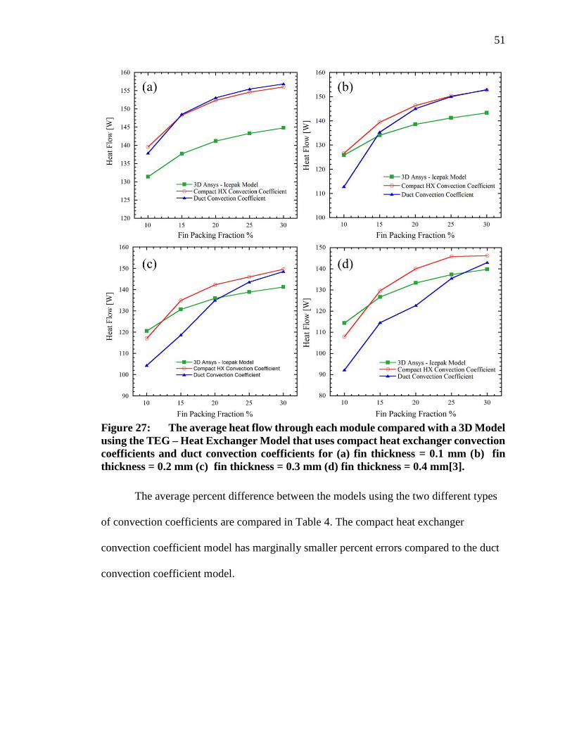
51
Figure 27: The average heat flow through each module compared with a 3D Model
using the TEG – Heat Exchanger Model that uses compact heat exchanger convection
coefficients and duct convection coefficients for (a) fin thickness = 0.1 mm (b) fin
thickness = 0.2 mm (c) fin thickness = 0.3 mm (d) fin thickness = 0.4 mm[3].
The average percent difference between the models using the two different types
of convection coefficients are compared in Table 4. The compact heat exchanger
convection coefficient model has marginally smaller percent errors compared to the duct
convection coefficient model.

52
Table 4 Average percent error comparison between the two models. The
percent error values are obtained assuming the 3-D model values as the exact or
theoretical value.
Fin Thickness Duct Convection
Coefficient model Compact Heat-Exchanger
Convection Coefficient
model
0.1 mm 7.60 % 7.50 %
0.2 mm 5.79 % 4.63 % 0.3 mm 6.37 % 4.36 %
0.4 mm 8.13 % 4.76 %
The temperature difference between the TEG hot and cold side is critical to the
thermoelectric performance of the TEG. The average temperature difference between the
TEGs are compared for the different heat exchanger designs evaluated. The results follow
similar trends to the average heat flow results shown in Figure 27.

53
Figure 28: The average temperature difference across each module compared
with a 3D Model using the TEG – Heat Exchanger Model that uses compact heat
exchanger convection coefficients and duct convection coefficients for (a) fin thickness
= 0.1 mm (b) fin thickness = 0.2 mm (c) fin thickness = 0.3 mm (d) fin thickness = 0.4
mm[3].
The average module power generation and efficiency are shown in Figure 29 for
the different heat exchanger designs. The largest TEG power generation of 7.75 W is
obtained for the heat exchanger design with a fin thickness of 0.1mm and packing
fraction of 30%. This design has the largest heat flow through it resulting in more power
generated. Additionally, this design resulted in the largest temperature difference between
the TEG, corresponding to the largest TEG efficiency of 4.96 %. It should be noted that
the 0.1mm – 30% packing fraction heat exchanger has a significantly larger pressured

54
drop compared to the other designs. When the heat exchanger design is considered both
pressure drop and heat transfer capabilities of the heat exchanger should be evaluated.
Figure 29: (a) The average thermoelectric power generated by a module for heat
exchanger fin thicknesses of 0.1 mm, 0.2 mm, 0.3 mm and 0.4 mm (b) Average module
efficiency for heat exchanger fin thickness of 0.1mm, 0.2mm, 0.3 mm and 0.4 mm.

55
THERMOELECTRIC GENERATORS COMBINED WITH NATURAL
CONVECTION HEAT SINKS
Introduction
Natural convection heat sinks can be incorporated with TEGs to maintain the cold
side temperature of the TEG. There are many instances when it is not possible to
integrate a forced convection heat sink with a TEG, for instance when a TEG is used to
recover waste heat from the body. Furthermore, natural convection heat sinks are much
more reliable than forced convection heat exchangers. Natural convection heat sinks
require almost no maintenance, which makes them ideal to be implemented with TEG
devices that are used to self-power electric devices. Additionally, natural convection heat
sinks require no pumping power, as compared to forced convection heat sinks, which
means that all the power generated by a TEG can be used to power devices, and none of
the energy is expended on pumping power. However, heat transfer coefficients for natural
convection heat sinks are much smaller than forced convection heat exchangers.
Buoyancy effects drive natural convection, which is dependent upon density variations of
the fluid, which in turn require a significant temperature difference between the surface in
consideration and the ambient fluid. Natural convection heat sinks are classified into
plate fin heat sinks and pin fin heat sinks, whose performance is influenced by the heat
sink orientation with regard to the gravitational field. This section looks at vertical plate
and pin fin heat sinks, as well as horizontal base pin fin heat sinks, where the primary
difference in the models are the convection coefficients of the heat sinks. The three
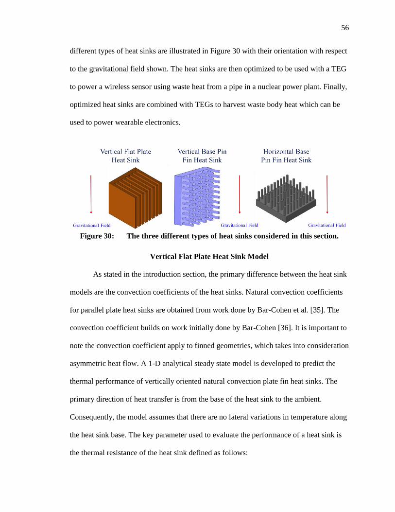
56
different types of heat sinks are illustrated in Figure 30 with their orientation with respect
to the gravitational field shown. The heat sinks are then optimized to be used with a TEG
to power a wireless sensor using waste heat from a pipe in a nuclear power plant. Finally,
optimized heat sinks are combined with TEGs to harvest waste body heat which can be
used to power wearable electronics.
Figure 30: The three different types of heat sinks considered in this section.
Vertical Flat Plate Heat Sink Model
As stated in the introduction section, the primary difference between the heat sink
models are the convection coefficients of the heat sinks. Natural convection coefficients
for parallel plate heat sinks are obtained from work done by Bar-Cohen et al. [35]. The
convection coefficient builds on work initially done by Bar-Cohen [36]. It is important to
note the convection coefficient apply to finned geometries, which takes into consideration
asymmetric heat flow. A 1-D analytical steady state model is developed to predict the
thermal performance of vertically oriented natural convection plate fin heat sinks. The
primary direction of heat transfer is from the base of the heat sink to the ambient.
Consequently, the model assumes that there are no lateral variations in temperature along
the heat sink base. The key parameter used to evaluate the performance of a heat sink is
the thermal resistance of the heat sink defined as follows:

57
𝑅𝑡ℎ =
𝑇𝑏 − 𝑇𝑎𝑚𝑏
𝑄𝐻𝑆
(4-1)
where Tb is the temperature of the heat sink base. Tamb is the ambient temperature, and
QHS is the heat flow through the heat sink. The heat flow through the heat sink by heat
convection was obtained as follows:
𝑄𝐻𝑆 = 𝑛𝑓𝑖𝑛 ∙ 𝑞𝑓𝑖𝑛 + ℎ𝑏𝑎𝑠𝑒 ∙ 𝐴𝑏 ∙ (𝑇𝑏 − 𝑇𝑎𝑚𝑏)
(4-2)
where nfin is the number of fins, Ab is the unfinned base area, Tb is the heat sink base
temperature, and hbase and qfin are defined by the following equations. The unfinned base
area is treated as a vertical flat plate, and the convection heat transfer coefficient is
obtained as follows:
ℎ𝑏𝑎𝑠𝑒 = 0.59 ∙ 𝑅𝑎𝐿1/4
∙ 𝑘𝑓 𝐿⁄
(4-3)
where kf is the thermal conductivity of air, and L is the vertical length of the heat sink,
and the Rayleigh number, RaL is obtained as follows:
𝑅𝑎𝐿 = 𝑔 ∙ 𝛽 ∙ 𝜃𝑏 ∙ 𝑃𝑟 ∙ 𝐿3 𝜈2⁄
(4-4)
where g is gravity, β is the coefficient of thermal expansion, θb is the temperature
difference between the heat sink base and the ambient, Pr is the Prandtl number, and ν is
the kinematic viscosity of the fluid. The heat transfer from each of the individual plate-
fins, qfin, is obtained as follows[31]:
𝑞𝑓𝑖𝑛 = 𝑀 ∙ 𝑡𝑎𝑛ℎ (𝑚 ∙ 𝐻)
(4-5)
where H is the height of the plate fins extruding in the horizontal direction, M and m are
fin parameters defined as follows:
𝑀 = √ℎ ∙ 𝑃 ∙ 𝑘 ∙ 𝐴𝑐 ∙ (𝑇𝑏 − 𝑇𝑎𝑚𝑏) (4-6)

58
𝑚 = √(ℎ ∙ 𝑃) (𝑘 ∙ 𝐴𝑐)⁄ (4-7)
where k is the thermal conductivity of the fin material, P is the fin perimeter, and Ac is the
cross-sectional area. The convection heat transfer coefficient, h from non-isothermal
asymmetric plates, take into account the two limiting spacing conditions for flat plate
heat sinks, small fin spacing, and large fin spacing. The convection coefficient
considering the spacing limits above is obtained as follows [35]:
ℎ𝑓𝑖𝑛 =
𝑘𝑎
𝑠∙ (
576
(𝜂𝑓𝑖𝑛 ∙ 𝐸𝑙)2 +
2.873
(𝜂𝑓𝑖𝑛 ∙ 𝐸𝑙)12
)1/2
(4-8)
where s is the spacing between the plate fins, ηfin is the fin efficiency, and El, the
Elenbaas number, which is a modified version of the Rayleigh number, is obtained as
follows:
𝐸𝑙 = (𝑔 ∙ 𝛽 ∙ 𝜃𝑏 ∙ 𝑃𝑟 ∙ 𝑠4) 𝐿𝜐2⁄ (4-9)
The first term in parentheses in equation 4-8 accounts for the small fin spacing
condition, while the second term represents the large spacing condition. When the heat
sink is used for applications with large temperature differences, radiation effects become
significant and are considered in the heat sink model. Radiation heat transfer from the
outer surfaces of the heat sink was considered in the model, as these surfaces have a view
factor of 1 with the ambient. The heat transfer by radiation is given by the following
equation:
𝑄𝑟 = 𝐴𝑟 ∙ 𝜎 ∙ 휀 ∙ (𝑇𝐻𝑆4 − 𝑇𝑎𝑚𝑏
4 ) (4-10)

59
where Ar is the heat sink area transferring heat by radiation to the ambient, σ is the
Boltzmann constant, ε is the emissivity of the heat sink material, and THS is the average
heat sink temperature. It is important to note that the model uses absolute temperature
values for the radiation analysis.
Vertical Base Pin Fin Heat Sink Model
Vertical base pin fin heat sinks are another viable option to be used along with
TEGs to harvest waste thermal energy. Pin fin heat sinks have better thermal performance
compared to flat plate heat sinks when the mass of the heat sink is considered [37]. A
one-dimensional heat transfer model is developed similar to the vertical flat plate heat
sink model. The primary differences between the two models are the fin geometry, the fin
cross-sectional area, and the fin perimeter. In addition to the fin geometry, the convection
coefficient for pin fin heat sinks is different to that of the vertical plate heat sinks. The
convection coefficient for pin fin heat sinks are influenced by four limiting conditions,
which are listed below:
1) Small vertical spacing with small horizontal spacing
2) Small vertical spacing with large horizontal spacing.
3) Large vertical spacing with small horizontal spacing.
4) Large vertical spacing with large horizontal spacing.
The work done by Joo et al. [37] consider convection coefficients for each limiting
case and combine them to match empirical data. The convection coefficient for limiting
case 1 looks at densely packed heat sink with a large number of pins in both the
horizontal and vertical directions. The convection coefficient for the densely packed
condition is obtained by modeling the fin array as a porous medium:

60
ℎ𝑓𝑖𝑛,1 =
𝑆ℎ𝑆𝑣
𝜋𝑑𝐿∙
4𝑆ℎ𝑆𝑣 − 𝜋𝑑2
48 ∙
𝜌𝑓𝑐𝑝𝑔𝛽𝜂𝑓𝑖𝑛(𝑇𝑏 − 𝑇∞)
𝜐𝑓
(4-11)
where Sh and Sv are the horizontal and vertical spacing, d is the fin diameter, L is the heat
sink length, ρf is the fluid density, cp is the specific heat of the fluid, g is the acceleration
of gravity, β is the thermal coefficient of expansion, ηfin is the fin efficiency, νf is the
kinematic viscosity of the fluid, Tb is the base temperature and T∞ is the ambient
temperature. For the second limiting case, the pins are arranged in a vertical direction
with large horizontal spacing and can be modelled as an isolated vertical array of
cylinders by the following equation:
ℎ𝑓𝑖𝑛,2 =
𝑘𝑓
𝐿∙ [0.3669
𝑆𝑣
𝑑− 0.0494] 𝐺𝑟𝐿
1/4
(4-12)
𝐺𝑟𝐿 =
𝑔𝛽𝜂𝑓𝑖𝑛(𝑇𝑏 − 𝑇∞)𝐿3
𝜐𝑓2
(4-13)
where GrL is the length dependent Grashof number and the other variables as defined
above. For the third limiting case, pins are arranged in a single horizontal direction with
large vertical spacing, and the convection coefficient is obtained by the following
equation:
ℎ𝑓𝑖𝑛,3 =
𝑘𝑓
𝑑∙ [2.132𝑆ℎ
∗ − 0,4064](𝑔𝛽(𝑇𝑏 − 𝑇∞)
𝛼𝑓𝜐𝑓𝑑)0.188
(4-14)
𝑆ℎ
∗ =𝑆ℎ
∗
𝑑3/4𝐿1/4
(4-15)
where Sh* is the non-dimensional horizontal spacing and αf is the thermal diffusivity of the
fluid, and the other variables are defined as above. The final limiting condition accounts
for a pin fin with large horizontal and vertical spacing, which is an isolated horizontal
cylinder with the convection coefficient given by the following equation:

61
ℎ𝑓𝑖𝑛,4 =
𝑘𝑓
𝑑∙ 0.85𝑅𝑎𝑑
0.188
(4-16)
𝑅𝑎𝑑 =
𝑔𝛽𝜂𝑓𝑖𝑛(𝑇𝑏 − 𝑇∞)𝑑3
𝛼𝑓𝜈𝑓
(4-17)
where Rad is the fin diameter dependent Rayleigh number and the other variables as defined
above. The four convection coefficients are combined to match experimental data and
reduces to the following equation:
ℎ𝑓𝑖𝑛 = [(ℎ𝑓𝑖𝑛,1
−1.3 + ℎ𝑓𝑖𝑛,2−1.3 ℎ𝑓𝑖𝑛,3
−1.3 )8
1.3 + ℎ𝑓𝑖𝑛,4−8 ]
1−8
(4-18)
Horizontal Base Vertical Pin Fin Heat Sink Model
Initial work on pin fin heat sinks was done by Sparrow and Vemuri [38]. They
performed experiments in air to measure the combined convection and radiation heat
transfer from (1) horizontal fins with a vertical base plate, (2) vertical fins with a
downward facing base plate and (3) vertical fins for an upward facing base plate.
Horizontal base plate vertical pin fin heat sinks have been numerically and
experimentally been studied by Sahray et al. [39]. A mean convection coefficient for a
heat sink is obtained taking into consideration fin height, fin packing fraction (which
considers fin spacing) and heat sink base area. The convection relation is obtained for
vertical square pin fins on a horizontal base. The Nusselt number correlation and
convection coefficient are given by the following equations:
ℎ𝑐 =
𝑘𝑓 ∙ 𝑁𝑢𝑠
𝑆
(4-19)
𝑁𝑢𝑠 = 0.0285 {1 − 𝑒𝑥𝑝 (−𝐻
𝑊)} …
…{1 + 1.50𝑒𝑥𝑝 (−0.07𝐿
𝐻)} 𝑅𝑎𝑠
1/2{1 − 𝑒𝑥𝑝 [−
7000
𝑅𝑎𝑠]}
1/3
(4-20)

62
𝑅𝑎𝑠 =
𝑔𝛽𝛥𝑇𝑆3𝑃𝑟
𝜈2
(4-21)
𝑆 = 𝑃 − 𝑊 (4-22)
where kf is the fluid thermal conductivity, Nus is the spacing dependent Nusselt number, S
is fin spacing defined by equation 4-22. L is the heat sink base width, H is the pin height,
Ras is the spacing dependent Rayleigh number, P is fin pitch, W is the pin width and the
variables in equation 4-21 are similar to that defined in the previous sections.
TEG for Power Harvesting in a Nuclear Power Plant
Introduction
Constant monitoring of temperature, pressure, and radiation levels are critical to the
safe operation of a nuclear power plant. Wireless sensor nodes are used to monitor the
temperature pressure and radiation levels in a nuclear power plant. When natural disasters
such as the Fukushima Daiichi nuclear incident in March 2011 occur, where power
supply from both the on-site and off-site power depletes, monitoring systems lose
function and cannot collect critical information regarding the nuclear plant status. The
loss of off-site power in nuclear plants is a frequent occurrence where 42 power outages
have been recorded from 1997 to 2004 [40]. Thermoelectric generators can be utilized to
self-power wireless sensor nodes making nuclear power plants safer. Furthermore, cost
savings can be observed by eliminating cable installation and maintenance. The lack of
required maintenance and reliability of natural convection heat sinks make them an ideal
candidate to be used with a thermoelectric generator to power wireless sensor nodes.
TEG – Heat Sink System Model for Powering a Wireless Sensor Node
A one-dimensional model was developed in a MATLAB environment combining
the thermoelectric model from chapter two and the corresponding heat sink model. The

63
primary direction of heat transfer is from the pipe (Heat Source) to the ambient.
Therefore 1-D heat flow through the TEG and heat sink is considered as illustrated in
Figure 31. The inputs into the heat transfer model are the TEG hot side temperature (TH ),
and the ambient temperature (Tamb). The combined model is solved by an iterative
process, which requires that the heat leaving the cold side of the TEG (Qc) match the heat
flow through the heat sink (QHS) as explained by the following equation:
abs(𝑄𝑐 − 𝑄𝐻𝑆) < 𝐶𝐶 (4-23)
where CC is the convergence criteria equal to 10-6 W. When the convergence criterion is
met, the model will solve for the cold side temperature. Eventually, the model will output
the heat flow through the TEG, while obtaining the cold side temperature of the TEG, the
power output of the TEG, as well as the operational current and voltage. The external
temperature of a nuclear power plant piping system can vary from 200°C – 350°C, the
lower limit of 200 °C was used in the model.
Figure 31: Heat Transfer model accounting for the heat flow through TEG and
the heat sink, where QH is the heat flow into the hot side of the TEG, QC is the heat

64
leaving the cold side of the TEG, and QHS is the heat flow from the heat sink to the
ambient. The heat sink plates are vertically oriented, and the figure illustrates a top
view.
Heat Sink Design
A vertical flat plate heat sink was chosen to be placed on the cold side of the
TEG. Vertical flat plate heat sinks have better thermal performance compared to a
vertical base –horizontal pin fin heat sink when the overall mass of the heat sink is
insignificant [37]. The design of the vertical flat plate heat sink was optimized with the
goal of obtaining the smallest thermal resistance. Table 5 lists the conditions that were
held constant for each optimization.
Table 5 Constant input parameters
Parameter Value
Base Thickness 1 cm
Base Area 4 cm x 4 cm
Base Temperature 110 °C
Ambient Temperature 20 °C
The vertical flat plate heat sink was optimized for fin thickness, fin packing
fraction and fin height with the heat sink optimization parameters listed in the table
below.
Table 6 Optimization parameters of the plate-fin heat sink
Parameter Value
Fin Thickness 1mm – 10 mm with 0.5 mm increments
Fin Height 1cm – 30 cm with 1 cm increments
Fin Packing Fraction 10% - 50 %

65
At a fin height of 15 cm, the thermal resistance of the heatsink approaches an
asymptotic value as illustrated in Figure 32(a). The diminishing returns in thermal
resistance with fin height are explained by the reduction in fin efficiency of an individual
fin. A fin height of 15 cm provides considerable heat flow without extruding out
significantly. A fin thickness of 1.5 mm provides the smallest thermal resistance of 1.67
K/W at a packing fraction of 25 % as shown in Figure 32(b).
Figure 32: a) Heat sink thermal resistance and fin efficiency for varied fin height
for a fin packing fraction of 26.25% and fin thickness of 1.5 mm. (b) Heat sink thermal
resistance for varied fin thicknesses and packing fractions for a fin height of 15 cm.
The minimum thermal resistance of the optimized heat sink is 1.67 K/W, and the
relevant fin parameters are listed in Table 7.
Table 7 Dimensions of the optimized vertical flat plate heat sink
Parameter Value
Heat Exchanger Base Area 4 cm x 4 cm
Fin Height 15 cm
Fin Thickness 1.5 mm
Fin Packing Fraction 26.25%

66
TEG Optimization
The optimized heat sink described in Table 7 was combined with a TEG. The
TEG was optimized by increasing the TE leg height from 0.4 mm to 4 mm while holding
the leg fill factor to 19.85 %. The thermoelectric power generated was compared for two
modules, one composed of the Half-Heusler alloy and the other composed of the Bi2Te3
material. A peak power density of 101.79 mW/cm2 is obtained for at leg height of 1.5mm
for the Half-Heusler alloy, and a peak power density of 133 mW/cm2 is obtained at a leg
height of 0.8mm for the Bi2Te3 material as illustrated in Figure 33. The TEG made of
Half-Heusler produces a total power of 1.63 W and the one composed of Bi2Te3 produces
2.128 W. The larger power produced by the Bi2Te3 material stems from its superior
performance at the device operation temperature range.
Figure 33: Power density vs. varied leg height for a fixed leg packing fraction of
19.85% for a TEG composed of the Half-Heusler alloy and Bi2Te3 material.
67
Harvesting Body Heat Using a TEG-Natural Convection Heat Sink System
The human body emits significant quantities of waste heat with an average heat
flow from the human body found to be 19 mW/cm2 for data collected from 100 persons
[41]. Many wearable electronic devices use much less power than ever before and could
be powered by waste heat from the human body. There has been a considerable amount
of work done to demonstrate the potential of harvesting body heat using TEGs. The
concept of using body heat to power electronic devices was pioneered to power an
electronic watch [42] producing 22.5 µW of power. Further applications of TEGs
harvesting body heat have been used to power wireless sensor nodes [6] where a pin fin
heat sink is used to improve heat transfer from the cold side of the TEG. Further
applications examine using TEGs to power autonomous wireless sensors for body area
networks. Additional applications include utilizing a TEG to power a pulse oximeter,
which measures the oxygen level in the body [7, 43]. Experimental work has been done
on a TEG used to harvest body heat, where copper heat spreaders were used to extract
body heat [44]. Experimental work done has examined the best location to recover waste
heat from the human body, when no airflow is considered the wrist is the best position to
extract waste body heat. Interestingly, the work does not use a heat sink but uses copper
heat spreaders on both the hot and cold side of the TEG[45]. To obtain a larger
temperature difference across the TEG, the thermal resistance of the TEG has to be
increased; this has been accomplished by stacking commercially available TEGs on top
of each other [46].

68
TEG- Heat Sink System Model for Harvesting Waste Heat from the Body
The TEG- Heat sink heat transfer model for harvesting body heat is illustrated in
Figure 34. The known inputs into the model are the body core temperature, which is
assumed to be 37°C and the ambient temperature of 22°C. The body regulates the heat
flow from itself by adjusting the thermal resistance between the core and the skin. The
thermal resistance of the skin is obtained by the following equation:
𝑅𝑡ℎ =
1
𝑈 ∙ 𝐴𝑏
(4-24)
where Ab is the cross sectional area of the TEG placed on the skin, U is the heat transfer
coefficient accounting for heat transfer through the skin, which was found to be equal to
25 W/m2∙K [46]. The model also considers the contact resistance between the human skin
and the TEG. The contact resistance between the skin and the TEG is given by the
following equation [8]:
𝑅𝑡ℎ(𝑐𝑜𝑛𝑡𝑎𝑐𝑡) =
1
ℎ𝑐 ∙ 𝐴𝑏
(4-25)
ℎ𝑐 = 1.25
𝜅𝑠𝛥𝑎
𝜎(
𝑃
𝐻𝑐)0.95
(4-26)
where κs is the harmonic mean thermal conductivity, 𝛥a is the surface roughness, P is the
applied pressure, Hc is the micro-hardness of the skin and Ab is as defined above. The
smallest contact resistance value is obtained for the forearm, where the hc value varies
from 50 -75 Wm-2K-1[8]. The conservative value of 50 Wm-2K-1 was used in the model.
The two thermal resistances connected in series were combined into one thermal
resistance with an overall heat transfer coefficient of 16.67 Wm-2K-1.

69
Figure 34: The TEG-Heat Sink heat transfer model, where QBo is the heat
transferred from the body, which is equal to the heat input to the TEG. Qs is the heat
transfer from the heat sink, which is equal to the heat leaving the cold side of the
TEG. PEL is the thermoelectric power generated by the TEG, QB is the heat
transferred from the heat sink base, and QF is the heat transfer from the fins. The
TEG is connected to an electrical load resistance RL. The equivalent thermal network
is shown in the figure with Tcore being the core temperature of the body and Tamb being
the ambient temperature.
The model is solved in a similar iterative manner to the TEG-Heat Sink model for
the wireless sensor node. However, this model requires two iterative conditions to be
satisfied. Firstly, the heat flow through the human skin (QBo) has to match the heat flow
in to the hot side of the TEG, QH as explained by the following equation:
𝑎𝑏𝑠(𝑄𝐵𝑂 − 𝑄𝐻) < 𝐶𝐶 (4-27)
where CC is the convergence criteria and is equal to 10-6 W. The second condition is that
the heat leaving the cold side of the TEG, Qc has to match the heat flow through the
micro-wire heat sink (QS) as explained by the following equation:

70
𝑎𝑏𝑠(𝑄𝑠 − 𝑄𝐶) < 𝐶𝐶 (4-28)
The hot side temperature of the TEG (TH) and the cold side temperature of the
TEG (TC) are unknown and will be solved by satisfying the aforementioned iterative
conditions. Eventually, the model will solve for the heat flow from the body, in the
process obtaining the total power output of the TEG, along with the hot side temperature,
cold side temperature, operational current and voltage.
Heat Sink Optimization
Two types of heat sinks were considered to be implemented with a TEG to
recover waste body heat. A vertical flat plate heat sink and a horizontal base square pin
fin heat sink, it is interesting to note that these two heat sinks are oriented perpendicular
to each other as illustrated in Figure 30. The fin height was capped at 3 cm, as a design
that is bulky is not desirable for waste heat recovery from the body. A base area of 4 cm x
4 cm is selected to match a conventional base area of a TEG. A flat plate heat sink and
square pin fin heat sink were optimized to obtain the smallest thermal resistance. The
thermal resistance of both the plate fin heat sink and the square pin fin heat sink are
illustrated in Figure 35 for varied packing fractions and fin thickness. A minimum
thermal resistance of 19.25 K/W is obtained for the flat plate heat sink for a fin thickness
of 1 mm and packing fraction of 12.5%. For the square pin fin heat sink, diminishing
returns in thermal resistance is observed at a packing fraction of 42.5% for a fin thickness
of 1 mm where a minimum thermal resistance of 17.3 K/W is observed.

71
Figure 35: (a) Thermal resistance of the plate fin heat sink for varied packing
fraction and fin thickness for a fixed fin height of 3 cm (b) Thermal resistance of the
square pin fin heat sink for varied packing fraction and fin thickness for a fixed fin
height of 3 cm.
TEG Optimization
The principle of thermal impedance matching is used to design the thermoelectric
generator. For small temperature differences, the TEG thermal resistance should match
the sum of the external thermal resistances. Such a condition is required to obtain the
highest possible heat flow through the TEG while having the largest possible temperature
difference across the module. If the thermal resistance of the module is much smaller
than the external thermal resistance, the temperature drop across the module will be
small, resulting in smaller thermoelectric power. On the other hand, if the thermal
resistance of the module is much larger than the external thermal resistance the heat flow
through the module is restricted. The thermal resistance of the module composed of the
Bi2Te3 material described in chapter 2, is varied by adjusting the thermoelectric leg
height. The leg packing fraction, which is the ratio of the leg area to the base area, was
held constant. For the TEG combined with a flat plate heat sink a total power output of
0.717 mW at a power density of 44.82 µW/cm2 is obtained for a leg height of 0.65 mm

72
for a leg packing fraction of 0.63% as shown in Figure 36. Similarly, for the TEG
combined with a horizontal base square pin fin heat sink a total power output of 0.731
mW at a power density of 45.69 µW/cm2 was obtained for a leg height of 0.6mm.
Figure 36: The power density vs. leg height for a TEG – Heat Sink system that uses
a vertical flat plate heat sink and horizontal base pin fin heat sink. The leg packing
fraction was held constant at 0.63%.
73
THERMOELECTRIC GENERATORS COMBINED WITH NATURAL
CONVECTION MICROWIRE HEAT SINKS
Introduction
Natural convection heat transfer is driven by buoyancy effects, which require a
large temperature difference for effective heat transfer. Natural convection heat sinks
offer the advantages of not requiring any pumping power, low cost, and high reliability.
As established in Chapter 4, natural convection heat sinks have limited heat flow, and
convection coefficients are largely dependent upon the temperature difference between
the heat sink and the ambient temperature. Heat transfer in microscale structures (sub 100
µm) experience much larger natural convection coefficients when compared with its
macro-scale counterparts. Natural convection heat transfer in micro-structures is
dominated by heat conduction to the ambient air, and buoyancy effects have a limited
effect [47], this conclusion has been reached by the observed phenomenon that
orientation of the microstructure with regard to gravitational fields has no effect on the
heat transfer performance of a microstructure. Further explanations of the enhanced heat
transfer suggest that the increased surface area to volume allow for much larger heat
conduction with the ambient fluid [48]. It should also be noted that the thermal boundary
layer created by heat transfer from micro-structures is thin, which leads to better heat
transfer [49]. This chapter examines the development of a natural convection heat sink,
which uses micro-wires as its extended surface. A proposed heat sink that utilizes micro-
scale extended surfaces can be manufactured by additive manufacturing methods.

74
Flat plate heat sinks with fin heights of 200µm have been experimentally
investigated by Mahmoud et al. [50]. However, the smallest fin thickness is 1mm, which
cannot be considered to be of micro-scale. Similarly, the thermal performance of heat
sinks with a minimum thickness of 200 µm and a maximum height of 0.8 mm have been
examined, while considering the orientation of the heat sink with respect to the
gravitational field [51]. Heat transfer of square micro pin fin with the smallest dimension
of 0.4 mm under natural convection has been examined [52]. The work mentioned above
do not fully exploit the micro-scale effects, which are observed at dimensions smaller
than a 100 µm. Additionally, flat plate heat sinks with micro-scale dimensions of 40 µm
have been examined by Kim et. al [53]. The heat sink heights are capped at 200 µm that
limit their performance as will be explained in the following sections.
Microwire Convection Coefficient
Convection coefficients for micro-wires with diameters in the range from 10.6 µm
to 95.6 µm are experimentally obtained [47]. The convection coefficient is obtained for
microwires of both horizontal and vertical orientations with respect to the gravitational
field. The convection coefficient for natural convection in a micro-wire is given by the
following equation [47]:
ℎ =
𝑘𝑎
1 + 𝐾𝑛(
1
𝑑) [
1
16𝑙𝑛2 (
𝛼𝑎
𝑑2) − 0.292 𝑙𝑛 (
𝛼𝑎
𝑑2) + 0.958]
−1/2
(5-1)
where d is the pin diameter, ka is the thermal conductivity of air, αa is the thermal
diffusivity of air and Kn is the Knudsen number which is the ratio of the mean free path of
air to the pin diameter. As evidenced by equation 5-1, the convection coefficient is
independent of the temperature difference between the surface and the ambient. The

75
equation suggests an inverse relationship between the convection coefficient and the fin
diameter. Furthermore, experimental data indicate that the microwire orientation has no
influence on the convection coefficient. The length or the length to diameter ratio has no
impact on the convection coefficient as confirmed by the experimental data in the source.
A similar experimental convection coefficient has been obtained for natural
convection from copper microwires using both air and water as the ambient fluid [49].
The experimental results have been confirmed by a 3-D numerical model, which also
revealed details about the thin boundary layer thickness around the microwire. The
convection coefficient follows the form of conventional natural convection Nusselt
numbers, and is given by the following equation:
𝑁𝑢 = 1.03 ∙ (𝐺𝑟 ∙ 𝑃𝑟)0.035
30 µm < D < 120 µm
0.0001 < Gr < 2.5
(5-2)
𝐺𝑟 =
𝑔 ∙ 𝛽 ∙ (𝑇𝑠 − 𝑇∞)𝑑3
𝜐2
(5-3)
where Pr is the Prandtl number, g is the gravitational acceleration, Ts is the surface
temperature, T∞ is the ambient temperature, d is the microwire diameter, and ν is the
kinematic viscosity. The experimental results were obtained for microwire diameters of
39.9 µm, 65.9 µm, and 119.1 µm. The inclusion of the temperature difference between
the microwire surface and the ambient fluid resulting from the inclusion of the Grashof
number may suggest the importance of the temperature difference. However,
experimental results from the source show a weak relationship between the convection
coefficient and the temperature dependence, which is also illustrated in Figure 37(b).

76
Figure 37: (a) Microwire Convection Coefficient obtained from equation 5-1 [47].
(b) Nusselt number dependent convection coefficient obtained from equations 5-2 and
5-3 [49].
Microwire Pin Fin Heat Sink Model
The enhanced heat transfer from the microwires can be exploited in natural
convection applications. A steady state numerical model is built in a MATLAB
environment utilizing the microwires as extended surfaces on a heat sink. For this model,
the ambient temperature of the fluid adjacent to a fin and the ambient temperature of the
fluid further away from the heat sink base is treated differently as shown in Figure 38.
The ambient temperature away from the heat sink base will be referred to as T∞ and the
ambient temperature adjacent to the fin will be denoted by Tamb.

77
Figure 38: Microwire pin fin heat sink with the thermal plume created by heat
transfer from the base in the background. QF is the heat transfer from the microwire
fins and Qb is the heat transfer from the base.
Each microwire is treated as an individual fin, conventionally fins in a natural
convection heat sink can be treated as an individual fin if the boundary layers of the
adjacent fins do not mix [31]. A similar principle is applied which limits the packing
fraction of the microwire heat sink governed by a minimum spacing requirement between
the microwires. The spacing requirement is obtained by using the microwire diameter
dependent boundary layer thickness data from Guan et al. [49]. The purpose of
incorporating the spacing limit into the model is to be able to treat the microwires as
individual fins. Each microwire fin is solved for by a finite element model with a varied
ambient temperature adjacent to each fin and each fin finite element. The ambient
temperature surrounding the fin will be influenced by heat transfer from the horizontal
base as illustrated in Figure 38. The ambient temperature surrounding the fins are
obtained in the next section and is used as an input into the fin model. The model
assumes an adiabatic tip and a constant base temperature and is solved by a one-

78
dimensional linear finite element model. The temperature profile along the fin is required
to obtain the heat transfer from an individual microwire and is obtained by the following
equation [21]:
𝑇 = 𝐾−1𝐹
(5-4)
where T is the temperature vector, K-1 is the inverse global stiffness matrix, and F is the
forcing vector. The assembly of the global stiffness matrix requires elemental stiffness
matrix similar to that in Chapter 2, which is obtained as follows:
𝐾𝑒 = ∫ [𝐵]𝑇[𝐷][𝐵]𝐴𝑑𝑥 +
𝑘
𝑙
∫ ℎ𝑃[𝑁]𝑇[𝑁]𝑑𝑥𝑘
𝑙
(5-5)
where B is the strain displacement matrix, the D matrix contains the elemental thermal
conductivity terms and A is the area of the element, h is the microwire convection
coefficient obtained from equation 5-1, P is the circumference of the fin and N is the
shape function for the linear element. The model uses one-dimensional linear elements,
which simplify to the following elemental stiffness matrix:
𝐾𝑒 =
𝐴𝑒𝑘𝑒
𝑙𝑒[
1 −1−1 1
] +ℎ𝑃
𝑙𝑒[2 11 2
]
(5-6)
where Ae is the elemental area, ke is the thermal conductivity, le is the elemental length, h
and P are as defined above. The elemental loading vector was developed taking into
consideration heat transfer from the surface of the fin by the following equation:
𝐹𝑒 = ∫ ℎ𝑇𝑎𝑚𝑏[𝑁]𝑇𝑑𝑆
𝑘
𝑆
(5-7)
where Tamb is the ambient temperature adjacent to the fluid, once again the forcing vector
simplifies to the following equation for a one-dimensional linear element:
𝐹𝑒 =
ℎ𝑃𝑇𝑎𝑚𝑏𝑙𝑒
2[11
] (5-8)

79
Once the temperature profile T is obtained, it is used to obtain the convection heat
transfer from each element and is summed to obtain the total heat transfer from the fin.
𝑄𝑇_𝐹𝑖𝑛 = ∑ ℎ ∙ 𝐴𝑒_𝑠 ∙ (
𝑇𝑛 + 𝑇𝑛+1
2− 𝑇𝑎𝑚𝑏(𝑛))
𝑒𝑙𝑒𝑚𝑠
𝑖=1
(5-9)
where elems is the total number of elements, Ae_s is the elemental surface area, Tn is the
nodal temperature and Tamb(n) is the ambient temperature for each element. The total heat
transfer from the heat sink sums up the heat transferred by all of the fins as well as heat
transferred from the unfinned base area obtained by the following equation:
𝑄𝐻𝑆 = ∑ 𝑄𝑇_𝐹𝑖𝑛
𝐹𝑖𝑛𝑠
𝑖=1
+ ℎℎ𝑝 ∙ 𝐴𝑢𝑓 ∙ (𝑇𝑏 − 𝑇∞) (5-10)
where Fins is the total number of fins, hhp is the convection coefficient for an upward
facing horizontal plate, Auf is the unfinned area, Tb is the base temperature, and T∞ is the
ambient temperature away from the base of the heat sink.
Ambient Fluid Temperature
The fluid temperature adjacent to a fin is used as an input into the model as
evidenced by equations 5-8 and 5-9. Heat transfer from the base of the heat sink produces
a thermal plume for a horizontal upward facing orientation [54]. The thermal boundary
layer produced by the heat transfer from the base results in much warmer ambient
temperatures for the microwire fins when compared to temperatures further away from
the base (T∞ ). This phenomenon is particularly apparent near the base of the heat sink up
to a height of around 5 mm. If the model were to use the ambient temperature away from
the heat sink base, T∞ illustrated in Figure 38; it would significantly overestimate the
performance of the heatsink. To capture the influence of the thermal boundary layer
80
developed by the heat sink base, the temperature profile over a horizontal flat plate was
obtained and implemented in the model. The temperature profile over a horizontal flat
plate for laminar natural convection was obtained from Guha et al.[55], where an
analytical solution for a horizontal plate for a varied surface temperature is available. The
available equation was adjusted for a constant surface temperature condition, which
realizes in the following equations:
𝑇𝑥,𝑦 − 𝑇∞
𝑇𝑠 − 𝑇∞= (1 − 𝑦/𝛿)2
(5-11)
𝛿 = 4.317𝑥 [𝑃𝑟 + (16
21⁄ )
𝑃𝑟 ∙ 𝐺𝑟𝑥]
1/5
(5-12)
𝐺𝑟𝑥 =
𝑔 ∙ 𝛽 ∙ (𝑇𝑠 − 𝑇∞)𝑥3
𝜐2
(5-13)
where Tx,y is the temperature along the surface, T∞ is the ambient temperature away from
the plate, Ts is the plate surface temperature, and y is the vertical distance from the base of
the plate. The thermal boundary layer thickness δ is given by equation 5-12, x is the
horizontal distance from the edge of the base, Pr is the Prandtl number, Grx is the local
Grashof number, β is the thermal coefficient of expansion and ν is the kinematic
viscosity. Equation 5-11 only provides the temperature profile for a surface above the
horizontal plate from the edge towards the midpoint of the plate. To obtain the complete
temperature profile above the horizontal plate, equation 5-11 was rotated around the
center of the plate, which sweeps the complete horizontal plate. The temperature profile
obtained from equation 5-11 was compared with a 3D model developed in Ansys Icepak
for laminar natural convection as illustrated in Figure 39. The temperature profile above
the heat sink compares fairly well with the 3-D model temperature profiles up until a

81
height of approximately 6 mm. The temperature profile obtained using equation 5-11
mostly overestimates the ambient temperature compared to the 3-D model, which serves
to make the overall model more conservative. The corresponding temperature above the
base was used as the input into the ambient temperature for the fin model, which was
established based on the location of the fin. A microwire located at the edge of the base
would experience adjacent fluid temperature smaller than that of a microwire located at
the center of the base.
Figure 39: Temperature comparison along a horizontal line using the analytical
equation 5-11 and a 3-D Icepak simulation at heights above the plate of (a) 1mm (b)
2mm (c) 3mm and (d) 4mm.

82
Model Assumptions
The model has some simplifying assumptions, which are listed below.
1) The model assumes the heat source is a thermal reservoir, such that the base of the
heat sink can be maintained at a constant temperature, this means that there is no
lateral heat spreading effects along the base. This assumption is required as more
heat is transferred from the corner fins, as they are influenced less by the thermal
plume of the base. As the corner fins transfer more heat, lateral heat variations are
to be expected if the heat sink is not attached to a thermal reservoir.
2) The boundary layer of the microwire has little influence on the ambient
temperature surrounding the fins, which is justified based on the small thicknesses
of the boundary layer data available from Guan et al.[49].
3) Each heat sink fin is treated as an individual fin, where the convection coefficient
of one fin is not influenced by the heat transfer from the adjacent fin. To make
this assumption a minimum fin spacing condition was established allowing each
fin to be treated as an individual extended surface.
4) The microwire convection coefficients are used as the convection coefficient for
the heat sink fins, which are of microscale order.
5) The heat transfer from the unfinned base area affects the ambient temperature and
is captured in the model.
6) The model does not take into account the structural stability of the microwires and
only considers the heat transfer process.

83
TEG- Microwire Heat Sink Model for Harvesting Waste Heat from the Human
Body
The heat sinks designed in Chapter 4 provide limited heat transfer and are quite
bulky. The microwire heat sinks provide better thermal performance while providing a
compact heat sink which can be implemented with a TEG to harvest waste heat from the
body. The following sections detail the design of a microwire heat sink to be placed on
the cold side of the TEG to harvest waste body heat. A theoretical microwire heat sink
design is suggested with a large fin height-to-diameter ratio. A more practical design is
suggested while capping the height-to-diameter ratio to 20. The TEG-Microwire Heat
Sink model is similar to the model described in section 0 and described in Figure 34,
where this model uses microwires as the heat sink fins.
Microwire Heat Sink Optimization
The microwire heat sink was optimized to minimize thermal resistance, for
temperature differences of 1°C and 5°C. Copper was chosen as the heat sink base and
microwire material as it has a thermal conductivity of approximately 401 W/m-K at room
temperature. Similar to the previous section, a heat sink base area of 4 cm x 4 cm was
chosen to match the surface area of a conventional module. The microwire fin height,
diameter and fin packing fraction were optimized to obtain the lowest possible thermal
resistance for the heat sink. The following table lists the optimization parameters.
84
Table 8 Heat sink optimization parameters
Parameter Value
Fin Diameter 10 µm, 50µm, 100 µm
Fin Height 1 mm , 2 mm, 3 mm, 4 mm, 5 mm
Fin Packing Fraction [10 µm, 50 µm
and 100 µm] 0.9 % - 1.9 %, 1.2%, 2.2%
The fin height was optimized for a fixed fin diameter of 10 µm and packing fraction
of 1.9%. As shown in Figure 40, the thermal resistance reaches diminishing returns for a
fin height of 3 mm. This observation is explained by shrinking fin efficiencies, although
the fin material is composed of Copper, the large convection coefficients and small cross-
sectional areas result in smaller fin efficiencies. At a fin height of 3 mm, a thermal
resistance of 0.821 K/W is obtained for a temperature difference of 1°C compared to
thermal resistances of 0.776 K/W at 4 mm and 0.760 K/W at 5 mm. Similarly, for a
temperature difference of 5°C a fin height of 3 mm results in a thermal resistance of
0.706 K/W compared to thermal resistances of 0.673 K/W at 4 mm and 0.664 at 5 mm.
The proposed fin heights for a fin diameter of 10 µm suggest fin diameter to height ratios
of 100 to 500 for the optimized fin heights. These height-to-diameter ratios could be
difficult to manufacture and have little structural integrity.

85
Figure 40: Heat sink thermal resistance variation with fin height for a fin diameter
of 10 µm and packing fraction of 1.9%.
Similarly, the fin diameter and packing fractions were optimized for a fixed fin
height of 3 mm. The fin packing fraction is capped to a maximum of 1.9% for the 10 µm
heat sink and 2.2 % for the 50 µm and 100 µm heat sinks. The packing fraction is
restricted by the spacing limit requirement between the fins, which was explained
previously. The thermal resistances of varied fin diameters and packing fractions are
compared for a temperature difference of 1 °C and 5°C. The heat sinks with a pin
diameter of 10µm provide smaller thermal resistances compared to the 50 µm and 100
µm heat sink as shown in Figure 41. This is attributable to the much larger convection
coefficient for the 10 µm fin diameter of 982.4 W/m2-K compared to 277.5 W/m2-K for
the 50 µm fin diameter and 166.4 W/m2-K for the 100 µm fin diameter.

86
Figure 41: Thermal resistance variation of the heat sink with fin diameter and
packing fraction variation for a fin height of 3mm (a) Base-Ambient temperature
difference of 1 °C and (b) Base – Ambient temperature difference of 5 °C.
A minimum thermal resistance of 0.820 K/W is obtained for a temperature
difference of 1°C, and a minimum thermal resistance of 0.706 K/W is obtained for a
temperature difference of 5°C for the optimized heat sink design parameters listed in
Table 9.
Table 9 Optimized heat sink parameters of the theoretical heat sink
Parameter Value
Heat Exchanger Base Area 40 mm x 40 mm
Heat Exchanger Base Thickness 0.5 mm
Fin Diameter 10 µm
Fin Height 3 mm
Fin Packing Fraction 1.9 %
A comparison of the microwire heat sink to the horizontal base pin fin heat sink can
be found in Table 10. It is important to note that the macro-scale heat sink had a pin
height of 3 cm compared to the micro-scale pin height of 3mm; therefore, a normalizing

87
parameter was developed by accounting for the different fin heights. The adjusted
thermal resistance was obtained by multiplying the thermal resistance by the fin height.
Table 10 Thermal resistance comparison for a micro-scale heat sink and
horizontal base pin fin heat sink
Heat Sink
Type
Thermal
Resistance ΔT = 1°C
Adjusted
Thermal
Resistance ΔT = 1°C
Thermal
Resistance ΔT = 5°C
Adjusted
Thermal
Resistance ΔT = 5°C
Macro-scale 28.68 K/W 77.05 K-cm/W 12.90 K/W 38.70 K-cm/W
Micro-scale 0.820 K/W 0.246 K-cm/W 0.706 K/W 0.212 K-cm/W
The microwire heat sink design suggested in Table 9 has a fin height to diameter
ratio of 300, which could be difficult to manufacture through additive manufacturing. A
practical heat sink design is implemented by restricting the pin height to diameter ratio to
20. The thermal resistances are significantly higher than the theoretical minimum as
displayed by Figure 42. The 10-µm diameter fin heat sinks are now ineffective, as at their
height of 200 µm is fully bathed in the thermal plume created by heat transfer from the
base. The lack of a significant temperature difference limits heat flow from the fins,
regardless of the high convection coefficient. The 100 µm heat sink has the lowest
thermal resistance with a packing fraction of 2.2%, as the pin height is 2mm, where it is
not affected by the thermal plume of the base to the extent the 10µm diameter heatsinks
are.
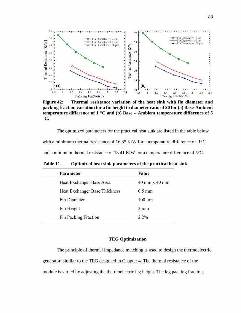
88
Figure 42: Thermal resistance variation of the heat sink with fin diameter and
packing fraction variation for a fin height to diameter ratio of 20 for (a) Base-Ambient
temperature difference of 1 °C and (b) Base – Ambient temperature difference of 5
°C.
The optimized parameters for the practical heat sink are listed in the table below
with a minimum thermal resistance of 16.35 K/W for a temperature difference of 1°C
and a minimum thermal resistance of 13.41 K/W for a temperature difference of 5°C.
Table 11 Optimized heat sink parameters of the practical heat sink
Parameter Value
Heat Exchanger Base Area 40 mm x 40 mm
Heat Exchanger Base Thickness 0.5 mm
Fin Diameter 100 µm
Fin Height 2 mm
Fin Packing Fraction 2.2%
TEG Optimization
The principle of thermal impedance matching is used to design the thermoelectric
generator, similar to the TEG designed in Chapter 4. The thermal resistance of the
module is varied by adjusting the thermoelectric leg height. The leg packing fraction,
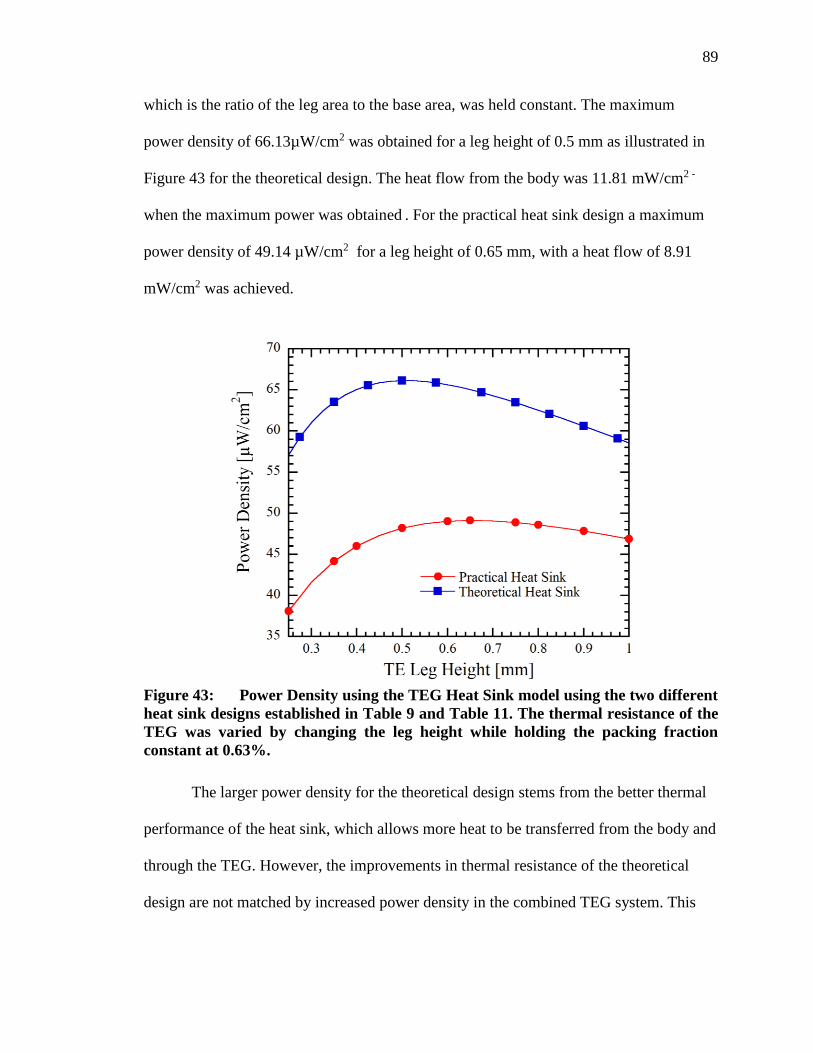
89
which is the ratio of the leg area to the base area, was held constant. The maximum
power density of 66.13µW/cm2 was obtained for a leg height of 0.5 mm as illustrated in
Figure 43 for the theoretical design. The heat flow from the body was 11.81 mW/cm2 -
when the maximum power was obtained . For the practical heat sink design a maximum
power density of 49.14 µW/cm2 for a leg height of 0.65 mm, with a heat flow of 8.91
mW/cm2 was achieved.
Figure 43: Power Density using the TEG Heat Sink model using the two different
heat sink designs established in Table 9 and Table 11. The thermal resistance of the
TEG was varied by changing the leg height while holding the packing fraction
constant at 0.63%.
The larger power density for the theoretical design stems from the better thermal
performance of the heat sink, which allows more heat to be transferred from the body and
through the TEG. However, the improvements in thermal resistance of the theoretical
design are not matched by increased power density in the combined TEG system. This

90
observation is explained by the thermal resistance of the human skin (and the contact
resistance between the TEG and skin) limiting heat flow from the human body.
The power density of the practical design is larger than the maximum power
density obtained by combining a macro-scale natural convection heat sink to a TEG
which was obtained in section 0. Furthermore, the microwire heat sink occupies a smaller
volume when compared to the macro-scale heat sink. The results from this work are
compared to that of other similar works. Table 12 compares both the base area power
density and volumetric power density. The base area power density is the ratio of the
thermoelectric power generated to the base area of the TEG-heat sink, while the
volumetric power density is the ratio of the thermoelectric power generated to the volume
of the complete TEG-heat sink system.
Table 12 A comparison of the power density by the base area utilized by a
complete TEG-Heat Sink device for similar works, along with a comparison of the
power density by considering the overall volume of a TEG-Heat Sink device when a
fair comparison was viable.
Ref. Base Area Power
Density [µW/cm2]
Volumetric Power Density
[µW/cm3]
Theoretical HS 66.13 165.33 Practical HS 49.137 156.0
[6] 20.00 22.22 [7] 30.00 20.00 [41] 0.44 0.30 [44] 28.50 57.00 [45] 6.1 50.83 [46] 60.00 10.00

91
CONCLUSIONS AND FUTURE WORK
Conclusions
Temperature Dependent Finite Element Model for a Thermoelectric Module
The temperature dependent finite element model developed can be used as a
starting point for the design of a thermoelectric module. The model was validated using a
3-D model in an ANSYS environment for three popular thermoelectric materials and a
number of temperature differences pertaining to the operating temperature of the
materials. The thermoelectric power estimation of the model performs reasonably well
considering the assumptions made in the model with the largest average percent error of
11.93 % obtained for the Half-Heusler alloy model.
Improvements to the unicouple design are suggested by using a ceramic material
composed of a higher thermal conductivity compared to the standard ceramic material
used in a unicouple. The power generated was found to be improved by a factor of 1.34
for a unicouple with a ceramic composed of Beryllia compared to a unicouple with a
ceramic of Alumina, when a temperature difference of 500°C is applied across the
unicouple.
The model developed was used to examine segmented unicouples, which can be
used to obtain increased power and efficiency. For a temperature difference of 580 °C a
unicouple composed of the Half-Heusler alloy and Bi2Te3 material produced 16% more
power and was 61% more efficient compared to a unicouple composed of only the Half-
Heusler alloy. Similarly, a unicouple made of the PbTe material and Bi2Te3 material

92
produced 49.5 % more power and was 65.5 % more efficient compared to a unicouple
made of only the PbTe material.
TEG – Heat Exchanger Model
The heat exchanger model developed is used in combination with the
thermoelectric module model to compose a complete thermoelectric system. The heat
exchanger model was compared to a 3D model developed in ANSYS Icepak. The work
done on the heat exchanger model examines the convection heat transfer coefficient used
in heat exchangers by implementing a duct convection coefficient for the model and a
compact heat exchanger convection coefficient. The results using the two convection
coefficients are compared, where the results indicate that the compact heat exchanger
convection coefficient provides more accurate results compared to the model using the
duct convection coefficient.
TEG – Natural Convection Heat Sink Model
Natural convection heat sinks to be implemented with TEGs are examined. Three
different natural convection heat sinks are examined considering the fin type and
orientation with regards to the gravitational field. The heat sinks are then optimized and
applied to harvest waste heat from a pipe in a nuclear power plant. The optimized TEG-
Heat Sink system produces a power density of 133 mW/cm2 for a module composed of
Bi2Te3 which can be used to power a wireless sensor node making the sensor node fully
autonomous. Further application of a TEG-Heat Sink system is used to harvest waste
body heat. An optimized system produces a power density of 44.82 µW/cm2 for a TEG
attached to a vertical plate fin heat sink and a power density of 45.69 µW/cm2 for a TEG
attached to a horizontal base pin fin heat sink.

93
Natural Convection Microwire Heat Sink
A numerical model for a heat sink composed of microwires has been developed.
The heat sink model was then used to optimize a heat sink to harvest waste heat from the
human body by placing the heat sink on the cold side of TEG. Two heat sink designs are
suggested, one a theoretical design, and a more practical design whose height is restricted
by a fin height to diameter ratio. When the theoretical heat sink design is used with a
TEG a maximum power density of 66.13 µW/cm2 is acquired, while the TEG combined
with the practical design suggested acheieves a maximum power density of 49.14
µW/cm2. The power density from both TEG- Heat sink designs are larger than the power
density obtained from a TEG- Macro scale heat sink obtained in Chapter 4. Furthermore,
the microwire heat sink provides a more compact design, which is important when
harvesting waste heat from the human body.
Future Work
Temperature Dependent Finite Element Model for a Thermoelectric Module
The available model could be improved to account for radiation and convection
losses from the surfaces of the unicouple. Furthermore, the model could be improved to
incorporate 3-D heat diffusion effects, which diminish the accuracy of the model.
Furthermore, the available model could be used to study the thermal stress developed in
the unicouple due to the large temperatures experienced.
TEG – Heat Exchanger Model
The pressure drop across the heat exchanger is an important parameter in the heat
exchanger design. The model could be improved to perform pressure drop calculations
for a given heat exchanger design. Using the pressure drop values the net power

94
generated from a complete heat exchanger system could be obtained to evaluate the
complete TEG – Heat exchanger design.
Natural Convection Microwire Heat Sink
The natural convection microwire heat sink has a number of limiting assumptions.
The model developed is only valid when the heat sink base can be maintained at a constant
temperature. The model could be improved to account for when this condition cannot be
met. Which would require the model to consider lateral heat spreading in the base.
Furthermore, the current model considers a heat sink with a horizontal base with vertical
pins. Future work could examine the model for a vertical base plate, where the microwire
fins are horizontal to the gravitational field. Although it was stated that the convection
microwire convection coefficient are not influenced by orientation, the thermal boundary
layer developed by the base plate is dependent upon its orientation to the gravitational field.
Finally, the model could be used to obtain data for numerous designs with varied fin
diameters, packing fractions and fin heights. Using the collected data, convection heat
transfer coefficients could be developed for the complete heat sink considering heat flow,
base to ambient temperature difference and total heat sink surface area.

95
REFERENCES
[1] D. Rowe, Thermoelectrics handbook, 1st ed. Boca Raton: CRC/Taylor & Francis,
2006.
[2] H. S. Kim, W. S. Liu, G. Chen, C. W. Chua, and Z. F. Ren, "Relationship
between thermoelectric figure of merit and energy conversion efficiency,"
Proceedings of the National Academy of Sciences of the United States of America,
vol. 112, pp. 8205-8210, Jul 7 2015.
[3] Y. L. Zhang, M. Cleary, X. W. Wang, N. Kempf, L. Schoensee, J. Yang, et al.,
"High-temperature and high-power-density nanostructured thermoelectric
generator for automotive waste heat recovery," Energy Conversion and
Management, vol. 105, pp. 946-950, Nov 15 2015.
[4] J. H. Yang and F. R. Stabler, "Automotive Applications of Thermoelectric
Materials," Journal of Electronic Materials, vol. 38, pp. 1245-1251, Jul 2009.
[5] V. Lee, "Waste heat reclamation in aircraft engines", M.S. thesis, Massachusetts
Institute of Technology, 2014.
[6] V. Leonov, T. Torfs, P. Fiorini, and C. Van Hoof, "Thermoelectric converters of
human warmth for self-powered wireless sensor nodes," Ieee Sensors Journal,
vol. 7, pp. 650-657, May-Jun 2007.
[7] T. Torfs, V. Leonov and R. Vullers, "Pulse Oximeter Fully Powered by Human
Body Heat", Sensors & Transducers, vol. 80, no. 6, pp. 1230-1238, 2007.
[8] F. Suarez, A. Nozariasbmarz, D. Vashaee, and M. C. Ozturk, "Designing
thermoelectric generators for self-powered wearable electronics," Energy &
Environmental Science, vol. 9, pp. 2099-2113, 2016.

96
[9] K. Qiu and A. C. S. Hayden, "Development of a thermoelectric self-powered
residential heating system," Journal of Power Sources, vol. 180, pp. 884-889, Jun
1 2008.
[10] Y. L. Zhang, X. W. Wang, M. Cleary, L. Schoensee, N. Kempf, and J.
Richardson, "High-performance nanostructured thermoelectric generators for
micro combined heat and power systems," Applied Thermal Engineering, vol. 96,
pp. 83-87, Mar 5 2016.
[11] G. Snyder, "Small Thermoelectric Generators", The Electrochemical Society
Interface, pp. 54-56, 2008.
[12] L. Jiji, Heat conduction, 1st ed. [Place of publication not identified]: Springer,
2014.
[13] S. Chen and Z. F. Ren, "Recent progress of half-Heusler for moderate temperature
thermoelectric applications," Materials Today, vol. 16, pp. 387-395, Oct 2013.
[14] E. Antonova and D. Looman, "Finite Elements for Thermoelectric Device
Analysis in ANSYS", in IEEE International Conference on Thermoelectrics,
Clemson, SC, 2005, pp. 215-218.
[15] X. Hu, A. Yamamoto and K. Nagase, "Characterization of half-Heusler unicouple
for thermoelectric conversion", Journal of Applied Physics, vol. 117, 2015.
[16] S. Kumar, S. D. Heister, X. F. Xu, J. R. Salvador, and G. P. Meisner,
"Thermoelectric Generators for Automotive Waste Heat Recovery Systems Part I:
Numerical Modeling and Baseline Model Analysis," Journal of Electronic
Materials, vol. 42, pp. 665-674, Apr 2013.
[17] J. L. Yu and H. Zhao, "A numerical model for thermoelectric generator with the
parallel-plate heat exchanger," Journal of Power Sources, vol. 172, pp. 428-434,
Oct 11 2007.
[18] M. Chen, H. Lund, L. A. Rosendahl, and T. J. Condra, "Energy efficiency
analysis and impact evaluation of the application of thermoelectric power cycle to
today's CHP systems," Applied Energy, vol. 87, pp. 1231-1238, Apr 2010.

97
[19] X. Gao, S. J. Andreasen, M. Chen, and S. K. Kaer, "Numerical model of a
thermoelectric generator with compact plate-fin heat exchanger for high
temperature PEM fuel cell exhaust heat recovery," International Journal of
Hydrogen Energy, vol. 37, pp. 8490-8498, May 2012.
[20] M. F. Zhou, Y. L. He, and Y. M. Chen, "A heat transfer numerical model for
thermoelectric generator with cylindrical shell and straight fins under steady-state
conditions," Applied Thermal Engineering, vol. 68, pp. 80-91, Jul 2014.
[21] P. Nithiarasu, R. Lewis and K. Seetharamu, Fundamentals of the finite element
method for heat and mass transfer, 1st ed. Chichester, West Sussex: Wiley, 2016.
[22] S. R. Annapragada, T. Salamon, P. Kolodner, M. Hodes, and S. V. Garimella,
"Determination of Electrical Contact Resistivity in Thermoelectric Modules
(TEMs) from Module-Level Measurements," Ieee Transactions on Components
Packaging and Manufacturing Technology, vol. 2, pp. 668-676, Apr 2012.
[23] T. Varghese, C. Hollar, J. Richardson, N. Kempf, C. Han, P. Gamarachchi, et al.,
"High-performance and flexible thermoelectric films by screen printing solution-
processed nanoplate crystals," Scientific Reports, vol. 6, Sep 12 2016.
[24] Borland W (1989) In: Electronic materials handbook: packaging, vol 1. ASM
International, New York
[25] D. de Faoite, D. J. Browne, F. R. Chang-Diaz, and K. T. Stanton, "A review of the
processing, composition, and temperature-dependent mechanical and thermal
properties of dielectric technical ceramics," Journal of Materials Science, vol. 47,
pp. 4211-4235, May 2012.
[26] G. Snyder and T. Ursell, "Thermoelectric efficiency and compatability", Physics
Review Letters, vol. 91, no. 14, 2003.
[27] B.Y. Moizhes, Y. P. Shishkin, A.V. Petrov, and L. A.Kolomoets, Sov. Phys.
Tech. Phys. 7, 336 (1962).
[28] T. S. Ursell and G. J. Snyder, in Proceedings of the 21st International Conference
on Thermoelectrics (IEEE, New York, 2002), p. 412. Figures and tables in [15]
calculate u a factor of 2 smaller than defined here.

98
[29] Z. L. Ouyang and D. W. Li, "Modelling of segmented high-performance
thermoelectric generators with effects of thermal radiation, electrical and thermal
contact resistances," Scientific Reports, vol. 6, Apr 7 2016.
[30] G. B. Zhang, L. H. Fan, Z. Q. Niu, K. Jiao, H. Diao, Q. Du, et al., "A
comprehensive design method for segmented thermoelectric generator," Energy
Conversion and Management, vol. 106, pp. 510-519, Dec 2015.
[31] F. Incropera and D. DeWitt, Fundamentals of heat transfer, 1st ed. New York:
Wiley, 1981.
[32] R. Shah and D. Sekulic, Fundamental of Heat Exchanger Design, 1st ed.
Hoboken, NJ: John Wiley & Sons, Inc, 2003.
[33] A. Kraus, A. Aziz and J. Welty, Extended Surface Heat Transfer, 1st ed. New
York, NY: John Wiley & Sons, Inc., 2001.
[34] A. R. Wieting, "Empirical Correlations for Heat-Transfer and Flow Friction
Characteristics of Rectangular Offset-Fin Plate-Fin Heat-Exchangers," Journal of
Heat Transfer-Transactions of the Asme, vol. 97, pp. 488-490, 1975.
[35] A. Bar-Cohen, M. Iyengar, and A. D. Kraus, "Design of optimum plate-fin natural
convective heat sinks," Journal of Electronic Packaging, vol. 125, pp. 208-216,
Jun 2003.
[36] A. Bar-Cohen and W. M. Rohsenow, "Thermally Optimum Spacing of Vertical,
Natural-Convection Cooled, Parallel Plates," Journal of Heat Transfer-
Transactions of the Asme, vol. 106, pp. 116-123, 1984.
[37] Y. Joo and S. Kim, "Comparison of thermal performance between plate-fin and
pin-fin heat sinks in natural convection", International Journal of Heat and Mass
Transfer, vol. 83, pp. 345-356, 2015.
[38] E. M. Sparrow and S. B. Vemuri, "Orientation Effects on Natural-Convection
Radiation Heat-Transfer from Pin-Fin Arrays," International Journal of Heat and
Mass Transfer, vol. 29, pp. 359-368, Mar 1986.

99
[39] D. Sahray, G. Ziskind, and R. Letan, "Scale-Up and Generalization of Horizontal-
Base Pin-Fin Heat Sinks in Natural Convection and Radiation," Journal of Heat
Transfer-Transactions of the Asme, vol. 132, Nov 2010.
[40] J. Chen, "Design and Analysis of a Thermoelectric Energy Harvesting System for
Powering Sensing Nodes in Nuclear Power Plant", M.S. thesis, Viginia
Polytechnic Institute and State University, 2015.
[41] V. Leonov, P. Fiorini, S. Sedky, T. Torfs, and C. Van Hoof, Proceedings of 13th
International Conference on Solid-State Sensors, Actuators and Microsystems,
Vol. 1 (Seoul, Korea, 2005), pp. 291–294.
[42] M. Kishi, H. Nemoto, T. Hamao, M. Yamamoto, S. Sudou, M. Mandai, and S.
Yamamoto,Proceedings of International Conference on
Thermoelectrics (Baltimore, USA, 1999), pp. 301–307.
[43] T. Torfs, V. Leonov, and R. Vullers, Sensors Transducers J. 80, 1230 (2007).
[44] K. T. Settaluri, H. Y. Lo, and R. J. Ram, "Thin Thermoelectric Generator System
for Body Energy Harvesting," Journal of Electronic Materials, vol. 41, pp. 984-
988, Jun 2012.
[45] M. Hyland, H. Hunter, J. Liu, E. Veety, and D. Vashaee, "Wearable
thermoelectric generators for human body heat harvesting," Applied Energy, vol.
182, pp. 518-524, Nov 15 2016.
[46] M. Lossec, B. Multon, and H. Ben Ahmed, "Sizing optimization of a
thermoelectric generator set with heatsink for harvesting human body heat,"
Energy Conversion and Management, vol. 68, pp. 260-265, Apr 2013.
[47] Z. L. Wang and D. W. Tang, "Investigation of heat transfer around microwire in
air environment using 3 omega method," International Journal of Thermal
Sciences, vol. 64, pp. 145-151, Feb 2013.
[48] X. J. Hu, A. Jain, and K. E. Goodson, "Investigation of the natural convection
boundary condition in microfabricated structures," International Journal of
Thermal Sciences, vol. 47, pp. 820-824, Jul 2008.

100
[49] N. Guan, Z. G. Liu, C. W. Zhang, and G. L. Jiang, "Natural convection heat
transfer on surfaces of copper micro-wires," Heat and Mass Transfer, vol. 50, pp.
275-284, Feb 2014.
[50] S. Mahmoud, R. Al-Dadah, D. K. Aspinwall, S. L. Soo, and H. Hemida, "Effect
of micro fin geometry on natural convection heat transfer of horizontal
microstructures," Applied Thermal Engineering, vol. 31, pp. 627-633, Apr 2011.
[51] L. Micheli, K. S. Reddy, and T. K. Mallick, "General correlations among
geometry, orientation and thermal performance of natural convective micro-
finned heat sinks," International Journal of Heat and Mass Transfer, vol. 91, pp.
711-724, Dec 2015.
[52] N. Matsumoto, T. Tomimura and Y. Koito, "Heat Transfer Characteristics of
Square Micro Pin Fins under Natural Convection", Journal of Electronics Cooling
and Thermal Control, vol. 04, no. 03, pp. 59-69, 2014.
[53] J. S. Kim, B. K. Park, and J. S. Lee, "Natural convection heat transfer around
microfin arrays," Experimental Heat Transfer, vol. 21, pp. 55-72, 2008.
[54] A. Bejan, Convection heat transfer, 1st ed.
[55] A. Guha and S. Samanta, "Closed-Form Analytical Solutions for Laminar Natural
Convection on Horizontal Plates," Journal of Heat Transfer-Transactions of the
Asme, vol. 135, Oct 2013.

101
APPENDIX A

102
ANSYS Model for Thermoelectric Unicouple
The ANSYS model developed in Chapter 2 is described as follows. The
dimensions of the individual components are the same as that listed in Table 1. A mesh
with 98186 nodes and 19359 elements was used, a refined mesh was used as the
calculations were used to validate the 1-D finite element model. The following figure
illustrates the mesh used.
Figure 44: Mesh used in the 3-D ANSYS model.
The boundary conditions applied to the finite element were applied to the ANSYS
model, where the top of the unicouple is assumed to be at a constant hot side temperature,
and the bottom of the unicouple is assumed to be at a constant cold side temperature as
shown in the following figure. Additionaly, the bottom copper header attached to the n-
leg was assigned a zero voltage boundary condition.

103
Figure 45: (a) Top surface boundary condition applied in ANSYS model (b)
Bottom surface boundary condition applied in ANSYS model.

104
APPENDIX B

105
Temperature Dependent Finite Element Model for a Thermoelectric Unicouple
Matlab Code
%% Finite Element Model for TE Unicouple % Pasindu Gamarachchi - Email: [email protected]
clc clear all
% Naming Convention % property/leg/otherconsideration no slashes
% Nodes and Elements elems =100; % numn = 2*elems +1;
% Input Temperatures Th = 600; Tc = 100;
% Dimensions
% N - Leg hn = (1.7*10^-3); ln = 2.0*10^-3; tn = 2.0*10^-3; % P - Leg
hp = (1.7*10^-3); lp = 2.0*10^-3; tp = 2.0*10^-3 ;
% T3 - Copper t3w = 1.93*10^-3; t3l = 1.96*10^-3; t3t = 0.2032*10^-3;
% T2 - Ceramic t2w = 4.51*10^-3; t2l = 2.26*10^-3; t2t = 0.635*10^-3; % it2t = t2t;
% T1 - Copper t1w = 4.21*10^-3; t1l = 1.96*10^-3; t1t = 0.2032*10^-3;
% B3 - Copper b3w = 8.50*10^-3;

106
b3l = 1.96*10^-3; b3t = 0.2032*10^-3;
% B2- Ceramic b2w = 8.81*10^-3; b2l = 2.26*10^-3; b2t = 0.635*10^-3;
% B1 - Copper b1w = 4.07*10^-3; b1l = 1.96*10^-3; b1t = 0.2032*10^-3;
ws = warning('off', 'all');
% Temperature Dependent properties syms T
% Seebeck - N TNS = [ 20 ,50, 100, 200, 300, 400, 500, 600 ]; SN = [ -0.000135243, -0.000142471, -0.000153643, -0.000171607, -
0.000187049, -0.000202244, -0.000211448, -0.000217053]; CNS = polyfit( TNS, SN, 6); snf = int ( CNS(1)*T^6 + CNS(2)*T^5 + CNS(3)*T^4 + CNS(4)*T^3 +
CNS(5)*T^2 + CNS(6)*T + CNS(7));
% Electrical - N TNP = [ 20 ,50, 100, 200, 300, 400, 500, 600 ]; PN = [ 6.56786E-06, 6.7325E-06, 7.03657E-06, 7.60784E-06, 8.0957E-06,
8.4766E-06, 8.6924E-06, 8.77723E-06]; CNP = polyfit( TNS, PN, 6); pnf = int ( CNP(1)*T^6 + CNP(2)*T^5 + CNP(3)*T^4 + CNP(4)*T^3 +
CNP(5)*T^2 + CNP(6)*T + CNP(7));
% Theramal - N TNK = [ 20 ,50, 100, 200, 300, 400, 500, 600 ]; KN = [ 5.308966362, 5.001685214, 4.609217214, 4.251736671, 4.069193415,
3.95510388, 3.962709849, 4.175676981]; CNK = polyfit( TNK, KN, 6); knf = int ( CNK(1)*T^6 + CNK(2)*T^5 + CNK(3)*T^4 + CNK(4)*T^3 +
CNK(5)*T^2 + CNK(6)*T + CNK(7));
% Seebeck - P TPS = [ 20 ,50, 100, 200, 300, 400, 500, 600 ]; SP = [7.39928E-05, 7.95446E-05, 8.87751E-05, 0.00010694, 0.000125184,
0.000142737, 0.000161509, 0.00017735 ]; CPS = polyfit( TPS, SP, 6); spf = int ( CPS(1)*T^6 + CPS(2)*T^5 + CPS(3)*T^4 + CPS(4)*T^3 +
CPS(5)*T^2 + CPS(6)*T + CPS(7));
% Electrical - P TPP = [ 20 ,50, 100, 200, 300, 400, 500, 600 ]; PP = [1.97399E-06, 2.13811E-06, 2.46366E-06, 3.18329E-06, 4.01544E-06,
4.92E-06, 5.85437E-06, 6.7556E-06 ]; CPP = polyfit( TPP, PP, 6);

107
ppf = int ( CPP(1)*T^6 + CPP(2)*T^5 + CPP(3)*T^4 + CPP(4)*T^3 +
CPP(5)*T^2 + CPP(6)*T + CPP(7));
% Thermal - P TPK = [ 20 ,50, 100, 200, 300, 400, 500, 600 ]; KP = [7.533937719, 7.251196645, 6.711129425, 5.980450245, 5.438397484,
5.05121694, 4.773241165, 4.550860545]; CPK = polyfit( TPK, KP, 6); kpf = int ( CPK(1)*T^6 + CPK(2)*T^5 + CPK(3)*T^4 + CPK(4)*T^3 +
CPK(5)*T^2 + CPK(6)*T + CPK(7));
% Conductivity Copper 102 TCK = [2.85, 27.85, 77.85, 127.85, 177.85, 227.85, 277.85 , 327.85,
377.85, 427.85, 477.85, 527.85, 577.85, 627.85, 677.85, 727.85, 777.85,
827.85, 877.85, 927.85, 977.85, 1027.85, 1077.85, 1084.85 ]; KC = [388.23 ,386.52 ,385.47, 384.59, 383.6, 382.34, 380.69, 378.59,
376.06, 373.12, 369.85, 366.33, 362.67, 358.98, 355.33, 351.8, 348.44,
345.26, 342.2, 339.16, 335.98, 332.39, 328.07,327.39]; CCK = polyfit( TCK, KC, 4); kcf = int ( CCK(1)*T^4 + CCK(2)*T^3 + CCK(3)*T^2 + CCK(4)*T + CCK(5));
% Resistivity Copper 102 TCP = [0, 19.85, 26.85, 76.85, 126.85, 226.85, 326.85, 426.85, 526.85,
626.85, 726.85, 826.85, 926.85, 1026.85, 1084.45 ]; PC = [1.5430E-08 1.6780E-08 1.7250E-08 2.0630E-08 2.4020E-08
3.0900E-08 3.7920E-08 4.5140E-08 5.2620E-08 6.0410E-08 6.8580E-08
7.7170E-08 8.6260E-08 9.5920E-08 1.0171E-07]; CCP = polyfit( TCP, PC, 4); pcf = int ( CCP(1)*T^4 + CCP(2)*T^3 + CCP(3)*T^2 + CCP(4)*T + CCP(5));
% Conductivity Al2O3 TAK = [19.85 ,37.8298, 55.8096, 73.78939, 91.76919, 109.749, 127.7288,
145.7086, 163.6884, 181.6682, 199.648, 217.6278, 235.6076, 253.5874,
271.5672, 289.547, 307.5268, 325.5066, 343.4864, 361.4662 ... 379.446, 397.4258, 415.4056, 433.3854, 451.3652, 469.3449,
487.3247, 505.3045, 523.2843, 541.2641, 559.2439,577.2237, 595.2035,
613.1833, 631.1631, 649.1429, 667.1227, 685.1025, 703.0823, 721.0621
... 739.0419, 757.0217, 775.0015, 792.9813, 810.9611, 828.9409,
846.9207, 864.9005, 882.8803, 900.8601, 918.8399, 936.8197, 954.7995,
972.7793, 990.7591, 1008.739, 1026.719, 1044.698, 1062.678
... 1080.658 1098.638 1116.618 1134.597 1152.577
1170.557 1188.537 1206.517 1224.496 1242.476 1260.456
1278.436 1296.416 1314.395 1332.375 1350.355 1368.335
... 1386.315 1404.294 1422.274 1440.254 1458.234
1476.214 1494.193 1512.173 1530.153 1548.133 1566.113
1584.092 1602.072 1620.052 1638.032 1656.012 1673.991
... 1691.971 1709.951 1727.931 1745.911 1763.89 1781.87
1799.85];
KA = [35.4396 33.51727 31.9325 30.42353 28.98777 27.6227
26.32582 25.0947 23.92694 22.82018 21.77212 20.78048

108
19.84306 18.95768 18.1222 17.33454 16.59267 15.89457
15.23832 ... 14.62198 14.04371 13.50169 12.99413 12.51932
12.07557 11.66125 11.27474 10.91452 10.57906 10.26692
9.976668 9.70694 9.456409 9.223791 9.007849 8.80739
8.621267 ... 8.448375 8.287655 8.138092 7.998718 7.868607
7.746878 7.632696 7.525269 7.42385 7.327738 7.236275
7.148849 7.064891 6.983877 6.90533 6.828814 6.75394
6.680364 6.607784 ... 6.535945 6.464636 6.393691 6.322987 6.252448 6.18204
6.111777 6.041714 5.971953 5.902639 5.833964 5.766163
5.699515 5.634345 5.571022 5.509959 5.451616 5.396494
... 5.345142 5.298152 5.25616 5.219848 5.189943 5.167214
5.152478 5.146594 5.150467 5.165047 5.191326 5.230344
5.283184 5.350973 5.434884 5.536134 5.655984 5.795741
... 5.956756 6.140425 6.348187 6.581527 6.841975
7.131104 7.450535 7.801928 ]; CAK = polyfit( TAK, KA, 4); kaf = int ( CAK(1)*T^4 + CAK(2)*T^3 + CAK(3)*T^2 + CAK(4)*T + CAK(5));
syms kn kp sn sp pp pn T % k: Conductivity, s: Seebeck, p: resistivity,
p: p-leg, n:n-leg
kn = symfun( knf, T); % Temperature dependent k for n-leg kp = symfun (kpf, T); % Temperature dependent k for p-leg sn = symfun (snf, T); % Temperature dependent s for n-leg sp = symfun (spf, T); % Temperature dependent k for p-leg pp = symfun (ppf, T); % Temperature dependent k for p-leg pn = symfun (pnf, T); % Temperature dependent k for p-leg kc = symfun (kcf, T); % Temperature dependent k for Copper 102 pc = symfun (pcf, T); % Temperature dependent p for Copper 102 ka = symfun (kaf, T); % Temperature dependent k for Al2O3
% Integral Averages for initial Temperature profile
knm = (kn(Th) - kn (Tc))/(Th-Tc); knm = double(knm); kpm = (kp(Th) - kp (Tc))/(Th-Tc); kpm = double(kpm); snm = (sn(Th) - sn(Tc))/(Th-Tc); snm = double(snm); spm = (sp(Th) - sp(Tc))/(Th-Tc); spm = double(spm); ppm = (pp(Th) - pp(Tc))/(Th-Tc); ppm = double(ppm); pnm = (pn(Th) - pn(Tc))/(Th-Tc); pnm = double(pnm);
kcm = (kc(Th) - kc(Tc))/(Th-Tc);

109
kcm = double(kcm); pcm = (pc(Th) - pc(Tc))/(Th-Tc); pcm = double(pcm);
kam = (ka(Th) - ka(Tc))/(Th-Tc); kam = double(kam);
% Thermal Circuit for initial temperature profile rc1 = (t3t/(kcm*t3l*t3w/2)); ra1 = (t2t/(kam*t2l*t2w/2)); rc2 = (t1t/(kcm*t1l*t1w/2)); cp = (kpm* lp*tp)/hp; rthp = 1/cp; cn = (knm* ln*tn)/hn; rthn = 1/cn; RLegs = 1/(cp +cn);
ra2 = (b2t/(kam.*b2l*b2w/2)); rc3 = (b1t/(kcm*b1l*b1w/2)); rc4 = (b3t/(kcm*b3l*b3w/2));
Rtot = rc1 + ra1 + rc2 + RLegs + rc3 + ra2 + rc4;
P1 = rc1/Rtot; P2 = ra1/Rtot; P3 = rc2/Rtot; P4 = rLegs/Rtot; P5 = rc3/Rtot; P6 = ra2/Rtot; P7 = rc4/Rtot;
DelTP1 = (P1*(Th-Tc)); DelTP2 = (P2*(Th-Tc)); DelTP3 = (P3*(Th-Tc)); DelTP4 = (P4*(Th-Tc)); DelTP5 = (P5*(Th-Tc)); DelTP6 = (P6*(Th-Tc)); DelTP7 = (P7*(Th-Tc));
DeltT = DelTP1+ DelTP2 + DelTP3+ DelTP4+ DelTP5+ DelTP6 + DelTP7;
Tcu1 = Th - DelTP1; Ta1 = Tcu1 - DelTP2; Tcu2 = Ta1 - DelTP3; Tpleg = Tcu2 - DelTP4; Tcu3 = Tpleg - DelTP5; Ta2 = Tcu3 - DelTP6; Tcu4 = Ta2 - DelTP7;
Tp = [ Th Tcu1 Ta1 Tcu2 Tpleg Tcu3 Ta2 Tc];

110
TotalHeight = t3t + hp + t2t + t1t + b3t + b2t + b1t;
t3telems = round((t3t/TotalHeight)*elems); t2telems = round((t2t/TotalHeight)*elems); t1telems = round((t1t/TotalHeight)*elems); hpelems = round((hp/TotalHeight)*elems); b3telems = round((b3t/TotalHeight)*elems); b2telems = round((b2t/TotalHeight)*elems); b1telems = round((b1t/TotalHeight)*elems); summedelems = sum([t3telems , t2telems, t1telems, hpelems, b3telems,
b2telems ,b1telems]);
while ( summedelems ~= elems)
if (summedelems > elems & t3telems > b3telems) t3telems = t3telems -1; summedelems = sum([t3telems , t2telems, t1telems, hpelems,
b3telems, b2telems ,b1telems]); elseif (summedelems > elems) b3telems = b3telems -1; summedelems = sum([t3telems , t2telems, t1telems, hpelems,
b3telems, b2telems ,b1telems]); elseif (summedelems < elems & t3telems > b3telems) b3telems = b3telems +1; summedelems = sum([t3telems , t2telems, t1telems, hpelems,
b3telems, b2telems ,b1telems]); else t3telems = t3telems +1; summedelems = sum([t3telems , t2telems, t1telems, hpelems,
b3telems, b2telems ,b1telems]);
end end
for i = 1: t3telems
dt = (Th - Tcu1)/t3telems; T_t3t(i+1) = Th - dt*(i);
end T_t3t(1) = Th;
for i = 1: t2telems
dt = (Tcu1 - Ta1)/t2telems; T_t2t(i+1) = Tcu1 - dt*(i);
end T_t2t(1) = Tcu1;
for i = 1: t1telems

111
dt = (Ta1 - Tcu2)/t1telems; T_t1t(i+1) = Tcu2 - dt*(i);
end T_t1t(1) = Ta1;
for i = 1: hpelems
dt = (Tcu2 - Tpleg)/hpelems; T_hp(i+1) = Tcu2 - dt*(i);
end T_hp(1) = Tcu2;
for i = 1: b1telems
dt = (Tpleg - Tcu3)/b1telems; T_b1t(i+1) = Tpleg - dt*(i);
end T_b1t(1) = Tpleg;
for i = 1: b2telems
dt = (Tcu3 - Ta2)/b2telems; T_b2t(i+1) = Tcu3 - dt*(i);
end T_b2t(1) = Tcu3;
for i = 1: b3telems
dt = (Ta2 - Tc)/b3telems; T_b3t(i+1) = Ta2 - dt*(i);
End
T_b3t(1) = Ta2; T_b3t(end) = Tc;
Tp = [ T_t3t T_t2t T_t1t T_hp T_b1t T_b2t T_b3t ];
ppm = (pp(T_hp(1)) - pp(T_hp(end)))/(T_hp(1)-T_hp(end)); ppm = double(ppm); pnm = (pn(T_hp(1)) - pn(T_hp(end)))/(T_hp(1)-T_hp(end)); pnm = double(pnm);
rp = (ppm * hp )/(lp*tp); rn = (pnm * hn )/(ln*tn);
112
pt1tm = (pc(T_t1t(1)) - pc(T_t1t(end)))/(T_t1t(1) - T_t1t(end) ); pt1tm = double(pt1tm);
pb1tpm = (pc(T_b1t(1)) - pc(T_b1t(end)))/(T_b1t(1) - T_b1t(end) ); pb1tpm = double(pb1tpm);
pb1tnm = (pc(T_b1t(1)) - pc(T_b1t(end)))/(T_b1t(1) - T_b1t(end) ); pb1tnm = double(pb1tnm);
snm = (sn(T_hp(1)) - sn(T_hp(end)))/(T_hp(1)-T_hp(end)); snm = double(snm); spm = (sp(T_hp(1)) - sp(T_hp(end)))/(T_hp(1)-T_hp(end)); spm = double(spm);
% Contact Resistance C_pho = 10*(10^-6); CR_n = C_pho/(tp*100)*(lp*100); CR_p = C_pho/(tp*100)*(lp*100); CR = 2*(CR_n + CR_p);
Rt1t = (pt1tm* t1w)/(t1l*t1t); Rb1tp = (pb1tpm* b1w)/(b1l*b1t); Rb1tn = (pb1tnm* b1w)/(b1l*b1t) ; Rt = rp +rn + Rt1t + Rb1tp +Rb1tn + CR; RL = Rt ; R = RL + Rt ; S = spm -snm ; I = (S*(T_hp(1) -T_hp(end)))/(R);
t1te_h = t1t/t1telems;
Jh_t1t = (I^2)* Rt1t; Jh_b1tp = (I^2)*Rb1tp; Jh_b1tn = (I^2)*Rb1tn;
Jh_t1t_e = Jh_t1t/(t1telems*2); Jh_b1tp_e = Jh_t1t/(b1telems); Jh_b1tn_e = Jh_t1t/(b1telems);
shp = hp/hpelems; shn = hn/hpelems;
%% Thermoelectric Energy Generation calculations using initial
temperature profile guess %% to be input into FE calculations for j = 1:hpelems
knm(j) = (kn(T_hp(j)) - kn(T_hp(j+1)))/(T_hp(j)-T_hp(j+1)); kpm(j) = (kp(T_hp(j)) - kp(T_hp(j+1)))/(T_hp(j)-T_hp(j+1));

113
snm(j) = (sn(T_hp(j)) - sn(T_hp(j+1)))/(T_hp(j)-T_hp(j+1)); spm(j) = (sp(T_hp(j)) - sp(T_hp(j+1)))/(T_hp(j)-T_hp(j+1)); ppm(j) = (pp(T_hp(j)) - pp(T_hp(j+1)))/(T_hp(j)-T_hp(j+1)); pnm(j) = (pn(T_hp(j)) - pn(T_hp(j+1)))/(T_hp(j)-T_hp(j+1));
rp1(j) = (ppm(j)* shp )/(lp*tp); rn1(j) = (pnm(j)* shn )/(ln*tn); cp(j) = (kpm(j)* lp*tp)/shp; cn(j) = (knm(j)* ln*tn)/shn;
Qhp(j) = spm(j)*T_hp(j)*I + cp(j)*(T_hp(j)-T_hp(j+1))-
(0.5)*(I^2)*rp1(j); Qcp(j) = spm(j)*T_hp(j+1)*I + cp(j)*(T_hp(j)-T_hp(j+1))+
0.5*(I^2)*rp1(j); Pp(j) = double((Qhp(j)- Qcp(j))) ;
Qhn(j) = abs(snm(j))*T_hp(j)*I + cn(j)*(T_hp(j)-T_hp(j+1)) -
(0.5)*(I^2)*rn1(j) ; Qcn(j) = abs(snm(j))*T_hp(j+1)*I + cn(j)*(T_hp(j)-T_hp(j+1)) +
0.5*(I^2)*rn1(j) ; Pn(j) = double(Qhn(j)- Qcn(j));
end
% Temperature Dependent elemental k - matrix for i = 1:t3telems
k_t3tp_e(i) = double((kc(T_t3t(i)) - kc(T_t3t(i+1)))/(T_t3t(i) -
T_t3t(i+1))); k_t3tn_e(i) = double((kc(T_t3t(i)) - kc(T_t3t(i+1)))/(T_t3t(i) -
T_t3t(i+1))); A_t3t(i) = t3w*t3l;
end
for i = 1:t2telems
k_t2tp_e(i) = double((ka(T_t2t(i)) - ka(T_t2t(i+1)))/(T_t2t(i) -
T_t2t(i+1))); k_t2tn_e(i) = double((ka(T_t2t(i)) - ka(T_t2t(i+1)))/(T_t2t(i) -
T_t2t(i+1))); A_t2tp(i) = 0.5*(t2w*t2l); A_t2tn(i) = 0.5*(t2w*t2l);
end
for i = 1:t1telems
k_t1tp_e(i) = double((kc(T_t1t(i)) - kc(T_t1t(i+1)))/(T_t1t(i) -
T_t1t(i+1)));

114
k_t1tn_e(i) = double((kc(T_t1t(i)) - kc(T_t1t(i+1)))/(T_t1t(i) -
T_t1t(i+1))); A_t1tp(i) = 0.5*(t1w*t1l); A_t1tn(i) = 0.5*(t1w*t1l); end
for i = 1:hpelems
k_hp_e(i) = double((kp(T_hp(i)) - kp(T_hp(i+1)))/(T_hp(i) -
T_hp(i+1))); k_hn_e(i) = double((kn(T_hp(i)) - kn(T_hp(i+1)))/(T_hp(i) -
T_hp(i+1))); A_p(i) = lp*tp; A_n(i) = ln*tn;
end
for i = 1:b1telems
k_b1tp_e(i) = double((kc(T_b1t(i)) - kc(T_b1t(i+1)))/(T_b1t(i) -
T_b1t(i+1))); k_b1tn_e(i) = double((kc(T_b1t(i)) - kc(T_b1t(i+1)))/(T_b1t(i) -
T_b1t(i+1))); A_b1t(i) = b1w*b1l; end
for i = 1:b2telems
k_b2tp_e(i) = double((ka(T_b2t(i)) - ka(T_b2t(i+1)))/(T_b2t(i) -
T_b2t(i+1))); k_b2tn_e(i) = double((ka(T_b2t(i)) - ka(T_b2t(i+1)))/(T_b2t(i) -
T_b2t(i+1))); A_b2tp(i) = 0.5*(b2w*b2l); A_b2tn(i) = 0.5*(b2w*b2l); end
for i = 1:b3telems
k_b3tp_e(i) = double((kc(T_b3t(i)) - kc(T_b3t(i+1)))/(T_b3t(i) -
T_b3t(i+1))); k_b3tn_e(i) = double((kc(T_b3t(i)) - kc(T_b3t(i+1)))/(T_b3t(i) -
T_b3t(i+1))); A_b3tp(i) = 0.5*(b3w*b3l); A_b3tn(i) = 0.5*(b3w*b3l);
end
kp_elems = [ k_t3tp_e, k_t2tp_e, k_t1tp_e, k_hp_e, k_b1tp_e, k_b2tp_e,
k_b3tp_e]; kn_elems = [ k_t3tn_e, k_t2tn_e, k_t1tn_e, k_hn_e, k_b1tn_e, k_b2tn_e,
k_b3tn_e];

115
Ap_elems = [ A_t3t, A_t2tp, A_t1tp, A_p, A_b1t, A_b2tp, A_b3tp]; An_elems = [ A_t3t, A_t2tn, A_t1tn, A_n, A_b1t, A_b2tn, A_b3tn];
Kp = sparse(numn, numn); Kn = sparse(numn, numn);
el_l = TotalHeight/elems;
%% Global K- Matrix Assembly for i=1:2:numn-2
if (i == 1) j = i ; else j =i-(prvj); end prvj = j;
ke_p = (kp_elems(j))*(Ap_elems(j))/(6*el_l)*[14, -16, 2; -16, 32, -
16; 2, -16, 14]; ke_n = (kn_elems(j))*(An_elems(j))/(6*el_l)*[14, -16, 2; -16, 32, -
16; 2, -16, 14];
dof = [ i, i+1, i+2]; Kp(dof, dof) = ke_p + Kp(dof, dof); Kn(dof, dof) = ke_n + Kn(dof, dof);
end
% F - Vector assembly using TE energy generation and joule heating C0 = t3telems; C1 = t3telems + t2telems; C2 = C1 + t1telems; C3 = C2 + hpelems; C4 = C3 + b1telems; C5 = C4 + b2telems;
for i = C1+1: C2
E_gen_t1t(i) = Jh_t1t_e/(Ap_elems(i) * el_l);
end
for i = 1:hpelems
E_genp(i) = -Pp(i)/(Ap_elems(i+C2)*el_l); E_genn(i) = -Pn(i)/(Ap_elems(i+C2)*el_l);
end
for i = C3+1: C4
j= i -C3; E_gen_b1tp(j) = Jh_b1tp_e/(Ap_elems(i)* el_l);

116
E_gen_b1tn(j) = Jh_b1tn_e/(Ap_elems(i)* el_l);
end E_gen_b2t = zeros(b2telems,1)'; E_gen_b3t = zeros(b3telems,1)';
E_Gen_pL = [ E_gen_t1t, E_genp, E_gen_b1tp, E_gen_b2t, E_gen_b3t]; E_Gen_nL = [ E_gen_t1t, E_genn, E_gen_b1tn, E_gen_b2t, E_gen_b3t];
prvj =1; for i = 3:2: numn-2
j = i - prvj; prvj =j; fe_p = (E_Gen_pL(j)*Ap_elems(j)*el_l/6)*[1, 4, 1]'; fe_n = (E_Gen_nL(j)*An_elems(j)*el_l/6)*[1, 4, 1]';
dof = [i, i+1, i+2]; F_p(dof) =fe_p; F_p(i) = fe_p(1) + fe_p(3);
F_n(dof) =fe_n; F_n(i) = fe_n(1) + fe_n(3); end
%% Adjusing for Boundary Conditions F_p(1) = Th; F_n(1) = Th; F_p(2) = F_p(2) - Kp(2,1)*Th; F_n(2) = F_n(2) - Kn(2,1)*Th; F_p(3) = F_p(3) - Kp(3,1)*Th; F_n(3) = F_n(3) - Kn(3,1)*Th;
F_p(end-2) = F_p(end -2) - Kp(end-2,end)*Tc; F_p(end -1) = F_p(end -1) - Kp(end-1,end)*Tc; F_p(end) = Tc;
F_n(end-2) = F_n(end -2) - Kn(end-2,end)*Tc; F_n(end -1) = F_n(end -1) - Kn(end-1,end)*Tc; F_n(end) = Tc;
for i = 1: numn Kp(numn,i) = 0; Kp(i,numn) = 0; Kp(numn,numn) =1; Kp(1,i) = 0; Kp(i,1) = 0;
Kn(numn,i) = 0; Kn(i,numn) = 0; Kn(numn,numn) =1; Kn(1,i) = 0; Kn(i,1) = 0;

117
end Kp(1,1) =1; Kn(1,1) =1;
Tempr_p = Kp\F_p'; Tempr_n = Kn\F_n';
F_nold = F_n; F_pold = F_p;
ppm = (pp(Tempr_p(C2*2 +1)) - pp(Tempr_p(C3*2 +1)))/(Tempr_p(C2*2 +1)-
Tempr_p(C3*2 +1)); ppm = double(ppm); pnm = (pn(Tempr_p(C2*2 +1)) - pn(Tempr_p(C3*2 +1)))/(Tempr_p(C2*2 +1)-
Tempr_p(C3*2 +1)); pnm = double(pnm);
pt1tm = (pc(Tempr_p(C1*2 +1 )) - pc(Tempr_p(C2*2 +1)))/(Tempr_p(C1*2
+1) - Tempr_p(C2*2 +1) ); pt1tm = double(pt1tm);
pb1tpm = (pc(Tempr_p(C3*2 +1)) - pc(Tempr_p(C4*2 +1)))/(Tempr_p(C3*2
+1) - Tempr_p(C4*2 +1) ); pb1tpm = double(pb1tpm);
pb1tnm = (pc(Tempr_n(C3*2 +1)) - pc(Tempr_n(C4*2 +1)))/(Tempr_n(C3*2
+1) - Tempr_n(C4*2 +1) ); pb1tnm = double(pb1tnm);
snm = (sn(Tempr_n(C2*2 +1)) - sn(Tempr_n(C3*2 +1)))/(Tempr_n(C2*2 +1)-
Tempr_n(C3*2 +1)); snm = double(snm); spm = (sp(Tempr_p(C2*2 +1)) - sp(Tempr_p(C3*2 +1)))/(Tempr_p(C2*2 +1)-
Tempr_p(C3*2 +1)); spm = double(spm);
Rt1t = (pt1tm* t1w)/(t1l*t1t); Rb1tp = (pb1tpm* b1w)/(b1l*b1t); Rb1tn = (pb1tnm* b1w)/(b1l*b1t) ; Rt = rp +rn + Rt1t + Rb1tp +Rb1tn + CR ; RL = Rt ; R = RL + Rt ;
S = spm -snm ; Voc_av = S*(Tempr_p(C2*2 +1) -Tempr_p(C3*2 +1)); I = S*(Tempr_p(C2*2 +1) -Tempr_p(C3*2 +1))./(R);
for k = 1:hpelems
if ( k ==1) j = C2*2 + 1;

118
else j = C2*2 +1 + (k-1)*2; end
knm(k) = (kn(Tempr_p(j)) - kn(Tempr_p(j+2)))/(Tempr_p(j)-
Tempr_p(j+2)); kpm(k) = (kp(Tempr_p(j)) - kp(Tempr_p(j+2)))/(Tempr_p(j)-
Tempr_p(j+2));
snm(k) = (sn(Tempr_n(j)) - sn(Tempr_n(j+2)))/(Tempr_n(j)-
Tempr_n(j+2)); spm(k) = (sp(Tempr_p(j)) - sp(Tempr_p(j+2)))/(Tempr_p(j)-
Tempr_p(j+2)); ppm(k) = (pp(Tempr_p(j)) - pp(Tempr_p(j+2)))/(Tempr_p(j)-
Tempr_p(j+2)); pnm(k) = (pn(Tempr_n(j)) - pn(Tempr_n(j+2)))/(Tempr_n(j)-
Tempr_n(j+2));
rp1(k) = (ppm(k)* shp )/(lp*tp); rn1(k) = (pnm(k)* shn )/(ln*tn); cp(k) = (kpm(k)* lp*tp)/shp; cn(k) = (knm(k)* ln*tn)/shn;
V_oc_e(k) = (spm(k)-snm(k))*(Tempr_p(j) -Tempr_p(j+2));
Qhp(k) = spm(k)*Tempr_p(j)*I + cp(k)*(Tempr_p(j)-Tempr_p(j+2))-
(0.5)*(I^2)*rp1(k) ; Qcp(k) = spm(k)*Tempr_p(j+2)*I + cp(k)*(Tempr_p(j)-Tempr_p(j+2))+
0.5*(I^2)*rp1(k) ; Pp(k) = double((Qhp(k)- Qcp(k))) ;
Qhn(k) = abs(snm(k))*Tempr_p(j)*I + cn(k)*(Tempr_p(j)-Tempr_p(j+2))
- (0.5)*(I^2)*rn1(k); Qcn(k) = abs(snm(k))*Tempr_p(j+2)*I + cn(k)*(Tempr_p(j)-
Tempr_p(j+2)) + 0.5*(I^2)*rn1(k); Pn(k) = double(Qhn(k)- Qcn(k));
end
%% Iterative Process for Temperature profiles to converge it =1; cc = 1; err = cc*3; % Initalize Error value while err > cc
if it ==1 Tempr_p = Tempr_p; Tempr_n = Tempr_n; else Tempr_p = Tempr_p2; Tempr_n = Tempr_n2; end

119
%% Temperature Dependent elemental k - matrix using new Temperature
profile for i = 1:t3telems % t3t (Very Top Cu Layer) Copper Conductivity and
Area
if ( i ==1) j = 1; else j = (i-1)*2 +1; end
k_t3tp_e(i) = double((kc(Tempr_p(j)) -
kc(Tempr_p(j+2)))/(Tempr_p(j) - Tempr_p(j+1))); k_t3tn_e(i) = double((kc(Tempr_n(j)) -
kc(Tempr_n(j+2)))/(Tempr_n(j) - Tempr_n(j+2)));
end
for i = 1:t2telems % t22 Top Alumina Conductivity and Area
if ( i ==1) j = C0 + 1; else j = C0 +(i-1)*2 +1; end
k_t2tp_e(i) = double((ka(Tempr_p(i)) -
ka(Tempr_p(i+1)))/(Tempr_p(i) - Tempr_p(i+1))); k_t2tn_e(i) = double((ka(Tempr_n(i)) -
ka(Tempr_n(i+1)))/(Tempr_n(i) - Tempr_n(i+1)));
end
for i = 1:t1telems % t1t ( Copper Layer Connecting Legs ) Conductivity
and Area
if ( i ==1) j = C1 + 1; else j = C1 +(i-1)*2 +1; end
k_t1tp_e(i) = double((kc(Tempr_p(i)) -
kc(Tempr_p(i+1)))/(Tempr_p(i) - Tempr_p(i+1))); k_t1tn_e(i) = double((kc(Tempr_n(i)) -
kc(Tempr_n(i+1)))/(Tempr_n(i) - Tempr_n(i+1)));
end
for i = 1:hpelems % Leg conductivity and area
if ( i ==1)

120
j = C2 + 1; else j = C2 +(i-1)*2 +1; end
k_hp_e(i) = double((kp(Tempr_p(i)) - kp(Tempr_p(i+1)))/(Tempr_p(i)
- Tempr_p(i+1))); k_hn_e(i) = double((kn(Tempr_n(i)) - kn(Tempr_n(i+1)))/(Tempr_n(i)
- Tempr_n(i+1)));
end
for i = 1:b1telems % Bottom Copper Conductivity and Area
if ( i ==1) j = C3 + 1; else j = C3 +(i-1)*2 +1; end
k_b1tp_e(i) = double((kc(Tempr_p(i)) -
kc(Tempr_p(i+1)))/(Tempr_p(i) - Tempr_p(i+1))); k_b1tn_e(i) = double((kc(Tempr_n(i)) -
kc(Tempr_n(i+1)))/(Tempr_n(i) - Tempr_n(i+1)));
end
for i = 1:b2telems % Bottom Alumina Conductivity and Area
if ( i ==1) j = C3 + 1; else j = C3 +(i-1)*2 +1; end
k_b2tp_e(i) = double((ka(Tempr_p(i)) -
ka(Tempr_p(i+1)))/(Tempr_p(i) - Tempr_p(i+1))); k_b2tn_e(i) = double((ka(Tempr_n(i)) -
ka(Tempr_n(i+1)))/(Tempr_n(i) - Tempr_n(i+1)));
end
for i = 1:b3telems % Bottomost Copper Conductivity and Area
if ( i ==1) j = C4 + 1; else j = C4 +(i-1)*2 +1; end

121
k_b3tp_e(i) = double((kc(Tempr_p(i)) -
kc(Tempr_p(i+1)))/(Tempr_p(i) - Tempr_p(i+1))); k_b3tn_e(i) = double((kc(Tempr_n(i)) -
kc(Tempr_n(i+1)))/(Tempr_n(i) - Tempr_n(i+1)));
end
kp_elems = [ k_t3tp_e, k_t2tp_e, k_t1tp_e, k_hp_e, k_b1tp_e, k_b2tp_e,
k_b3tp_e]; kn_elems = [ k_t3tn_e, k_t2tn_e, k_t1tn_e, k_hn_e, k_b1tn_e, k_b2tn_e,
k_b3tn_e];
Ap_elems = [ A_t3t, A_t2tp, A_t1tp, A_p, A_b1t, A_b2tp, A_b3tp]; An_elems = [ A_t3t, A_t2tn, A_t1tn, A_n, A_b1t, A_b2tn, A_b3tn];
Kp = sparse(numn, numn); Kn = sparse(numn, numn);
el_l = TotalHeight/elems;
%% Global K- Matrix Assembly for i=1:2:numn-2
if (i == 1) j = i ; else j =i-(prvj); end prvj = j;
ke_p = (kp_elems(j))*(Ap_elems(j))/(6*el_l)*[14, -16, 2; -16, 32, -
16; 2, -16, 14]; ke_n = (kn_elems(j))*(An_elems(j))/(6*el_l)*[14, -16, 2; -16, 32, -
16; 2, -16, 14];
dof = [ i, i+1, i+2]; Kp(dof, dof) = ke_p + Kp(dof, dof); Kn(dof, dof) = ke_n + Kn(dof, dof);
end F_p = sparse(1,numn); F_n = sparse(1,numn);
% F - Vector assembly using TE energy generation and joule heating C0 = t3telems; C1 = t3telems + t2telems; C2 = C1 + t1telems; C3 = C2 + hpelems; C4 = C3 + b1telems; C5 = C4 + b2telems;
for i = C1+1: C2
E_gen_t1t(i) = Jh_t1t_e/(Ap_elems(i) * el_l);
122
end
for i = 1:hpelems
E_genp(i) = -Pp(i)/(Ap_elems(i+C2)*el_l); E_genn(i) = -Pn(i)/(Ap_elems(i+C2)*el_l);
end
for i = C3+1: C4
j= i -C3; E_gen_b1tp(j) = Jh_b1tp_e/(Ap_elems(i)* el_l); E_gen_b1tn(j) = Jh_b1tn_e/(Ap_elems(i)* el_l);
end E_gen_b2t = zeros(b2telems,1)'; E_gen_b3t = zeros(b3telems,1)';
E_Gen_pL = [ E_gen_t1t, E_genp, E_gen_b1tp, E_gen_b2t, E_gen_b3t]; E_Gen_nL = [ E_gen_t1t, E_genn, E_gen_b1tn, E_gen_b2t, E_gen_b3t];
prvj =1; for i = 3:2: numn-2
j = i - prvj; prvj =j; fe_p = (E_Gen_pL(j)*Ap_elems(j)*el_l/6)*[1, 4, 1]'; fe_n = (E_Gen_nL(j)*An_elems(j)*el_l/6)*[1, 4, 1]';
dof = [i, i+1, i+2]; F_p(dof) =fe_p; F_p(i) = fe_p(1) + fe_p(3);
F_n(dof) =fe_n; F_n(i) = fe_n(1) + fe_n(3); end
%% Adjusing for Boundary Conditions F_p(1) = Th; F_n(1) = Th; F_p(2) = F_p(2) - Kp(2,1)*Th; F_n(2) = F_n(2) - Kn(2,1)*Th; F_p(3) = F_p(3) - Kp(3,1)*Th; F_n(3) = F_n(3) - Kn(3,1)*Th;
F_p(end-2) = F_p(end -2) - Kp(end-2,end)*Tc; F_p(end -1) = F_p(end -1) - Kp(end-1,end)*Tc; F_p(end) = Tc;
F_n(end-2) = F_n(end -2) - Kn(end-2,end)*Tc; F_n(end -1) = F_n(end -1) - Kn(end-1,end)*Tc; F_n(end) = Tc;

123
for i = 1: numn Kp(numn,i) = 0; Kp(i,numn) = 0; Kp(numn,numn) =1; Kp(1,i) = 0; Kp(i,1) = 0;
Kn(numn,i) = 0; Kn(i,numn) = 0; Kn(numn,numn) =1; Kn(1,i) = 0; Kn(i,1) = 0;
end Kp(1,1) =1; Kn(1,1) =1;
Tempr_p2 = Kp\F_p'; Tempr_n2 = Kn\F_n';
diffp = abs(Tempr_p -Tempr_p2) ; diffn = abs(Tempr_n -Tempr_n2);
err = sum(diffp + diffn) it = it +1
end
%% Thermoelectric Calculations using Final Temperature Profile ppm = (pp(Tempr_p2(C2*2 +1)) - pp(Tempr_p2(C3*2 +1)))/(Tempr_p2(C2*2
+1)-Tempr_p2(C3*2 +1)); ppm = double(ppm); pnm = (pn(Tempr_p2(C2*2 +1)) - pn(Tempr_p2(C3*2 +1)))/(Tempr_p2(C2*2
+1)-Tempr_p2(C3*2 +1)); pnm = double(pnm);
pt1tm = (pc(Tempr_p2(C1*2 +1 )) - pc(Tempr_p2(C2*2
+1)))/(Tempr_p2(C1*2 +1) - Tempr_p2(C2*2 +1) ); pt1tm = double(pt1tm);
pb1tpm = (pc(Tempr_p2(C3*2 +1)) - pc(Tempr_p2(C4*2
+1)))/(Tempr_p2(C3*2 +1) - Tempr_p2(C4*2 +1) ); pb1tpm = double(pb1tpm);
pb1tnm = (pc(Tempr_n2(C3*2 +1)) - pc(Tempr_n2(C4*2
+1)))/(Tempr_n2(C3*2 +1) - Tempr_n2(C4*2 +1) ); pb1tnm = double(pb1tnm);
snm = (sn(Tempr_n2(C2*2 +1)) - sn(Tempr_n2(C3*2 +1)))/(Tempr_n2(C2*2
+1)-Tempr_n2(C3*2 +1)); snm = double(snm);

124
spm = (sp(Tempr_p2(C2*2 +1)) - sp(Tempr_p2(C3*2 +1)))/(Tempr_p2(C2*2
+1)-Tempr_p2(C3*2 +1)); spm = double(spm);
Rt1t = (pt1tm* t1w)/(t1l*t1t); Rb1tp = (pb1tpm* b1w)/(b1l*b1t); Rb1tn = (pb1tnm* b1w)/(b1l*b1t) ; Rt = rp +rn + Rt1t + Rb1tp +Rb1tn + CR ; RL = Rt ; R = RL + Rt ;
S = spm -snm ; Voc_av = S*(Tempr_p2(C2*2 +1) -Tempr_p2(C3*2 +1)); I = S*(Tempr_p2(C2*2 +1) -Tempr_p2(C3*2 +1))./(R);
for k = 1:hpelems
if ( k ==1) j = C2*2 + 1; else j = C2*2 +1 + (k-1)*2; end
knm(k) = (kn(Tempr_p2(j)) - kn(Tempr_p2(j+2)))/(Tempr_p2(j)-
Tempr_p2(j+2)); kpm(k) = (kp(Tempr_p2(j)) - kp(Tempr_p2(j+2)))/(Tempr_p2(j)-
Tempr_p2(j+2));
snm(k) = (sn(Tempr_n2(j)) - sn(Tempr_n2(j+2)))/(Tempr_n2(j)-
Tempr_n2(j+2)); spm(k) = (sp(Tempr_p2(j)) - sp(Tempr_p2(j+2)))/(Tempr_p2(j)-
Tempr_p2(j+2)); ppm(k) = (pp(Tempr_p2(j)) - pp(Tempr_p2(j+2)))/(Tempr_p2(j)-
Tempr_p2(j+2)); pnm(k) = (pn(Tempr_n2(j)) - pn(Tempr_n2(j+2)))/(Tempr_n2(j)-
Tempr_n2(j+2));
rp1(k) = (ppm(k)* shp )/(lp*tp); rn1(k) = (pnm(k)* shn )/(ln*tn); cp(k) = (kpm(k)* lp*tp)/shp; cn(k) = (knm(k)* ln*tn)/shn;
V_oc_e(k) = (spm(k)-snm(k))*(Tempr_p(j) -Tempr_p(j+2));
Qhp(k) = spm(k)*Tempr_p2(j)*I + cp(k)*(Tempr_p2(j)-Tempr_p2(j+2))-
(0.5)*(I^2)*rp1(k) ; Qcp(k) = spm(k)*Tempr_p2(j+2)*I + cp(k)*(Tempr_p2(j)-
Tempr_p2(j+2))+ 0.5*(I^2)*rp1(k) ; Pp(k) = double((Qhp(k)- Qcp(k))) ;

125
Qhn(k) = abs(snm(k))*Tempr_p2(j)*I + cn(k)*(Tempr_p2(j)-
Tempr_p2(j+2)) - (0.5)*(I^2)*rn1(k); Qcn(k) = abs(snm(k))*Tempr_p2(j+2)*I + cn(k)*(Tempr_p2(j)-
Tempr_p2(j+2)) + 0.5*(I^2)*rn1(k); Pn(k) = double(Qhn(k)- Qcn(k));
end
Qhin = max(Qhp) + max(Qhn); TotalP = sum(Pp); TotalN = sum(Pn); Power = TotalP + TotalN - (Rt1t + Rb1tn + Rb1tp + CR)*I^2 V_oc = sum(V_oc_e); Eff = Power*100/Qhin;

126
APPENDIX C

127
TEG – Heat Exchanger Model Matlab Code
% Hot Side Heat Exchanger and TE Unicouple model combined % Pasindu Gamarachchi - Email: [email protected] clc clear all
global hxl hxh hxw N Tin tf TEMW TEML TempC cvl Thg Tbg mf
% HX Dimensions & Input hxl = 0.16; hxh = 0.02; hxw = 0.04; N = 30; mf = 0.5*9.7*10^-3; Tin = 558; tf = 0.1*10^-3; s = (hxw - (N.*tf))./(N+1); % Fin Spacing
% TEM Dimensions
TEMW = 40*10^-3; % [m] TEML = 40*10^-3; % [m]
TempC = 94; % [C]
cvl = 40*(10^-3); cv = round(hxl./(cvl)); % Number of control volumes
% Guesses and Error Err = 0.005; % Convergence Error Thg = 5; % Temperature Outlet Guess Tbg = 180; % Base/TEM Hot Side Temperature Tdg = 10; TempCh = Err*0.9; ErrMult = 5; DiffLim = 1;
% Fin Material and Fluid Properties syms x caf = int( 3.134242E-10*x^4 - 8.519344E-07*x^3 + 7.480582E-04*x^2 -
3.006360E-02*x + 1.007301E+03); % specific Heat of air ca = symfun(caf,x); % knif = int( -9.32400932E-11*x^4 + 1.13247863E-07*x^3 + 6.33449883E-
05*x^2 -9.47163947E-02*x + 8.13811189E+01); % Thermal Conductivity of
Nickel kni = symfun(knif,x);
%% T = zeros(cv,1);

128
T(1) = Tin;
% Calculations for each control volume for j = 1:length(T)
Tin = T(j); Th = Tin; Thi = Tin -Thg; Ti =Tin;
cam = (ca(Th) - ca(Thi))./(Th-Thi); cam = double(cam);
cp = cam;
Tog = Ti - Tdg;
if j==1; Tb = Ti-Tbg; else end
[Q,P,Eff] = TEModule(Tb,TempC, Un);% Function with finite element
unicouple function and number of unicouples
To = Ti - (Q/(mf*cp)); Pf = 2*(cvl); Af = cvl*tf;
Tfl = (Ti + To)/2;
kNim = (kni(Tb) -kni(Tb-10))./(10); kNim = double(kNim);
% Fin Heat Transfer Calcs [h, v, Re] = convcoeff(Tfl,mf); % Function with Duct Convection
Coefficient
M = (sqrt(h*Pf*kNim*Af))*(Ti - Tb); Un_ar = (hxw- tf*N)*cvl;
m = sqrt((h*Pf)/(kNim*Af)); Qf = M*tanh(m*hxh/2)*((N-1)) + Un_ar*h*(Tb - Tfl) ;
[QTET, P, Eff] = TEModule(Tb,TempC, Un);
i=0;
% Convergence Requirement while abs(Qf-QTET)>Err
Tb = Tb+(Err);

129
[h, v, Re]= convcoeffv3(T(j),mf); M = (sqrt(h*Pf*kNim*Af))*((Ti- Tb)); m = sqrt((h*Pf)/(kNim*Af)); Qf = M*tanh(m*hxh/2)*((N-1)) + Un_ar*h*(Tb - Tfl) ; [QTET, P, Eff] = TEModule(Tb,TempC, Un);
if Qf - QTET> Err & Qf -QTET< (Err*DiffLim) Tb = Tb +(TempCh); elseif Qf - QTET> (Err*DiffLim) Tb = Tb + (ErrMult*TempCh); elseif (Qf -QTET ) < (Err*-1) & Qf -QTET > (Err*- DiffLim) Tb = Tb -(TempCh); elseif (Qf - QTET) < (Err*- DiffLim) Tb = Tb -(ErrMult*TempCh); end diff = Qf-QTET;
end
progress = j/length(T) QTETv(j) = QTET; Pv (j) = P; Effv(j) = Eff;
hv(j) = h; vv(j) = v; Rev(j) = Re;
To = Ti - (Qf./(mf*cp)); Tbv(j) = Tb; Qhv(j) = Qf; T(j+1) = To;
end

130
APPENDIX D

131
Compact Heat Exchanger Convection Coefficient Matlab Code
% Function calculates the convection coefficient along with Velocity
and % Reynolds Number for the hot side of the heat exchanger % Pasindu Gamarachchi - Email : [email protected] function [h, v, Re] = convcoeff(Th, mf)
global hxl hxh hxw N tf Thg
Thi = Th - Thg;
%% Temperature dependent properties
% Density of steam/ Hot side fluid syms x % ps cs ms ks ps daf = int(2.876602E-12*x^4 - 7.350893E-09*x^3 + 7.284062E-06*x^2 -
3.760334E-03*x + 1.251051E+00); % Specific Heat Capacity of steam caf = int( 3.134242E-10*x^4 - 8.519344E-07*x^3 + 7.480582E-04*x^2 -
3.006360E-02*x + 1.007301E+03); % Dynamic viscocity of Steam maf = int(-1.17230617E-17*x^4 +3.14251436E-14*x^3 -3.87294440E-11*x^2
+4.96283182E-08*x + 1.71301016E-05); % Thermal Cond of Steam kaf = int(1.146049E-14*x^4 + 5.825050E-12*x^3 - 4.412201E-08*x^2 +
8.330657E-05*x + 2.396400E-02); % Prandtl Number of Steam paf = int( 1.946038E-13*x^4 - 8.530084E-10*x^3 + 9.958116E-07*x^2 -
3.351574E-04*x + 7.176453E-01); % Thermal Conductivity of Fin Material knf = int(-9.32400932E-11*x^4 + 1.13247863E-07*x^3 +6.33449883E-05*x^2
+ -9.47163947E-02*x + 8.13811189E+01);
da = symfun(daf,x); ca = symfun(caf,x); ma = symfun(maf,x); ka = symfun(kaf,x); pa = symfun(paf,x);
kb = symfun(knf,x); % Integral averages
cam = (ca(Th) - ca (Thi))/(Th-Thi); cam = double(cam);
mam = (ma(Th) - ma (Thi))/(Th-Thi); mam = double(mam);
kam = (ka(Th) - ka (Thi))/(Th-Thi); kam = double(kam);
pam = (pa(Th) - pa (Thi))/(Th-Thi);

132
pam = double(pam);
% Intermediate Calculations s = (hxw - (N*tf))/(N+1); % Fin Spacing dh = (4*s*(hxh/2))/(s + hxh ); % Hydraulic Diameter, hxh is divided by
2, because of adiabatic tip v = mf/(dam*s*(hxh/2)*(N-1)); Re = v*dam*dh/(mam); Pr = (cam*mam)/(kam);
% Colburn and pressure factors al = s/(hxh/2); if Re<=1000 j_f = 0.483*(hxl/dh)^(-0.162)*al^(-0.184)*Re^(-0.536); else j_f =0.242*(hxl/dh)^(-0.322)*(tf/dh)^0.089*Re^(-0.368); end
h = j_f*Re*(Pr^(1/3))*kam/(dh);
end

133
APPENDIX E

134
Duct Convection Coefficient Matlab Code
% Function calculates the convection coefficient along with Velocity
and % Reynolds Number for the hot side of the heat exchanger % Pasindu Gamarachchi - Email : [email protected] function [h, v, Re] = convcoeffv_Duct(Th, mf)
global hxh hxw N tf Thg
Thi = Th - Thg;
%% Temperature dependent properties
% Density of steam/ Hot side fluid syms x % ps cs ms ks ps daf = int(2.876602E-12*x^4 - 7.350893E-09*x^3 + 7.284062E-06*x^2 -
3.760334E-03*x + 1.251051E+00); % Specific Heat Capacity of steam caf = int( 3.134242E-10*x^4 - 8.519344E-07*x^3 + 7.480582E-04*x^2 -
3.006360E-02*x + 1.007301E+03); % Dynamic viscocity of Steam maf = int(-1.17230617E-17*x^4 +3.14251436E-14*x^3 -3.87294440E-11*x^2
+4.96283182E-08*x + 1.71301016E-05); % Thermal Cond of Steam kaf = int(1.146049E-14*x^4 + 5.825050E-12*x^3 - 4.412201E-08*x^2 +
8.330657E-05*x + 2.396400E-02); % Prandtl Number of Steam paf = int( 1.946038E-13*x^4 - 8.530084E-10*x^3 + 9.958116E-07*x^2 -
3.351574E-04*x + 7.176453E-01);
% Thermal Conductivity of Fin Material knf = int(-9.32400932E-11*x^4 + 1.13247863E-07*x^3 +6.33449883E-05*x^2
+ -9.47163947E-02*x + 8.13811189E+01);
da = symfun(daf,x); ca = symfun(caf,x); ma = symfun(maf,x); ka = symfun(kaf,x); pa = symfun(paf,x);
kb = symfun(knf,x); % Integral averages
dam = (da(Th) - da (Thi))/(Th-Thi); dam = double(dam);
cam = (ca(Th) - ca (Thi))/(Th-Thi); cam = double(cam);
mam = (ma(Th) - ma (Thi))/(Th-Thi); mam = double(mam);

135
kam = (ka(Th) - ka (Thi))/(Th-Thi); kam = double(kam);
pam = (pa(Th) - pa (Thi))/(Th-Thi); pam = double(pam);
% Intermediate Calculations s = (hxw - (N*tf))/(N+1); dh = (4*s*(hxh/2))/(s + hxh ); v = mf/(dam*s*(hxh)*(N-1));
Re = v*dam*dh/(mam); Pr = (cam*mam)/(kam);
% Colburn and pressure factors al = s/(hxh/2);
if Re < 2500 Nu = 7.541*(1- 2.61*al +4.97*al^2 -5.199*al^3 + 2.702*al^4 -
0.548*al^5); else Nu = 0.026*Re^(0.8)*Pr^(0.3); end
h = Nu*kam/dh;
end

136
APPENDIX F

137
TEG-Combined with Flat Plate Heat Sink Matlab Code
% TEG Combined with Vertical Flat Plate Heat Sink % Pasindu Gamarachchi - Email : [email protected] clc clear all
global hxl cvl NC tf_C Tcg Tcbg hxhC hxwC hxlC Cb hn ln tn hp lp tp
Th =200; % Hot Side Temperature Tamb= 120;
hnv = 0.2*(10^-3): (0.1*(10^-3)): 2.0*(10^-3); leng = length(hnv) %%
%%Heat Sink Dimensions NC = 7; tf_C = 1.50*(10^-3); hxhC = 0.15; hxwC = 0.04; hxl = 0.04; hxlC = hxl; Cb = 1*10^-2; cvl = hxl; PackFracColdSide = (tf_C*NC/hxwC) sC = (hxwC - (NC.*tf_C))./(NC-1)
% TC Dimensions ln = 1.8*(10^-3); tn = 1.8*(10^-3); lp = 1.8*(10^-3); tp = 1.8*(10^-3); F =7; G =7; C = F*G; FillFactor = (tn*ln*2*C)/(hxwC*hxlC)
% Guesses and Error Err = 10^-6; Tcg = 1; Tcbg =35; ErrMult = 3.5; DiffLim = 800; ErrMult = 500; TempCh = 0.5*Err;
if TempCh > Err fprintf('Unlikely to converge\n') return end

138
% For each unicouple height for i = 1:length(hnv)
hn = hnv(i); hp = hn;
if i ==1 Tb = Tamb + Tcbg; TempC = Tb + Tcg; else end
[QHT, QCT, P, n, Volt, I, Qm] = TEModuleDOE_Bi2Te3(Th,TempC,C); QTE = QCT; [Qc, Q_b, h_f, h_b ,TEMC ,TTip ,et_f, Qr] = HXFreeConvFlat(Tb,
Tamb);
%% Iterative Condition while ( abs(Qc -QTE)> Err )
[QHT, QCT, P, n, Volt, I, Qm] = TEModuleDOE_Bi2Te3(Th,TempC,C); QTE = QCT; [Qc, Q_b, h_f, h_b ,TEMC ,TTip ,et_f, Qr] = HXFreeConvFlat(Tb,
Tamb);
TempC = TEMC; if Qc -QTE> Err & Qc -QTE< (Err*DiffLim) Tb = Tb -(TempCh); elseif Qc - QTE> (Err*DiffLim) Tb = Tb -(ErrMult*TempCh); elseif (Qc -QTE) < (Err*-1) & Qc -QTE > (Err*-DiffLim) Tb = Tb +(TempCh); elseif (Qc -QTE) < (Err*-ErrMult) Tb = Tb +(ErrMult*TempCh); end
diffcs = Qc-QTE Tb;
end
progress = i/length(hnv)
TotalP = P; Eff = (TotalP*100)/QTE; TotalPv(i) = P; QHTv(i) = QHT; QCTv(i) = QCT; nv(i) =n; Voltv(i) = Volt; Iv(i) = I; Tbv(i) =Tb; TEMCv(i) = TEMC;

139
end

140
APPENDIX G

141
Microwire Heat Sink Matlab Code
% Micro-wire Heat Sink to calculate heat transferred from Heat Sink for % varied ambient temperature using finite elements for fins % Pasindu Gamarachchi - Email : [email protected]
function QTot = HXMicroFinsFiniteElement(Tb, Tamb)
global hxlC hxwC NCx NCz fd fh
temprfile = ['Base', num2str(Tb),'Amb', num2str(Tamb),
'FluidTempDat.mat']; % Load Temperature File based on base and ambient
temperature
load(temprfile);
Nx = floor(NCx/2); Nz = floor(NCz/2);
elemsize = y(2)-y(1); elems = ceil(fh/elemsize) -1; numn =elems+1; len = size(Tempr);
Nx_norm = round((1:1:Nx).*(len(1))./(Nx)); Nz_norm = round((1:1:Nz).*(len(2))./(Nz));
%% TambM = zeros(Nx,Nz,length(y));
% for j = 1:Nz for i = 1:Nx for j = 1:Nz
p = Nx_norm(i); q = Nz_norm(j); TambM(i,j,:) = Tempr(p,q,:);
end end
for i = 1:Nx for j = 1:Nz
[Qf_fe, TTip, Tempr] = FEFinV(TambM(i,j,:),Tb, Tamb, elemsize
); % Function for heat transfer from fins Qf_feM(i,j) = Qf_fe; TtipM(i,j) = TTip;
142
end end
% Heat Transfer from Base
h_b = convec_hotplate(Tb, Tamb); % Function to obtain convection coeff
for Heat Transfer from Base Fin_Ar = 0.25*pi*(fd^2)*(NCx*NCz); Un_Ar = (hxwC*hxlC) - Fin_Ar;
Q_b = Un_Ar*(h_b)*(Tb-Tamb); % Heat transfer from Base Area
Qf_Tot = sum(sum((Qf_feM))); QTot = Qf_Tot*4 + Q_b;
end
% Finite Element Model for heat transfer from microwire fins % Pasindu Gamarachchi - Email : [email protected]
function [Qf_fe, Ttip, Tempr] = FEFinVFTemp(AmbTemp, Tb, Tamb,
elemsize)
global fd fh
elems = ceil(fh/elemsize) -1; % Number of Elements
numn =elems+1;
h = convectionmicro(Tb,Tamb); kCupf = (5.25E-15*x^6 - 1.34E-11*x^5 + 1.26E-08*x^4 - 5.19E-06*x^3 +
8.71E-04*x^2 - 9.61E-02*x + 3.99E+02); kCup = symfun(kCupf,x);
kCupm = kCup(Tb) ; kCupm = double(kCupm);
k = kCupm;
l = fh/elems; % Element length Tambv = AmbTemp(1:numn);
% Element K Matrix

143
A = pi*(fd^2)*0.25; P = pi*fd;
C1 = k*A/l; C2 = h*P*l/6;
ke = C1*[1, -1; -1,1] + C2*[2,1; 1,2];
K = sparse(numn, numn); F = sparse(numn,1);
for i = 1:elems
dof = [ i, i+1]; K(dof, dof) = ke + K(dof, dof);
end
% Calculates Thermal Load for each node for i = 1:numn fe(i) = h*P*l*Tambv(i)/2;
end
% Combines the Thermal Loads from previous element for i = 2:numn-1 F(i) = fe(i)+ fe(i-1);
end
F(end) = fe(end); % Last node only has thermal load from itself F(2) = F(2) - Tb*(ke(2,1));
for i=1:numn K(i,1) =0; K(1,i) =0; F(1) = Tb; end
K(1,1) =1;
Tempr = K\F;
for i = 1:elems Tavg(i) = (Tempr(i) +Tempr(i+1))*0.5; Q_elem(i) = h*P*l*(Tavg(i) - Tambv(i)); end

144
Qf_fe = sum(Q_elem); Ttip = Tempr(end);
end
% Microfins convection coefficient
function h = convectionmicro(Tcb, Tamb)
global fd
g = 9.81; lam = 68*10^-9;
% Fin Material syms x
knif = ( -9.32400932E-11*x^4 + 1.13247863E-07*x^3 + 6.33449883E-05*x^2
-9.47163947E-02*x + 8.13811189E+01); % Thermal Conductivity of Nickel kni = symfun(knif,x);
kAlpf = ( 7.00000000E-09*x^4 - 6.18933333E-06*x^3 + 1.25071800E-03*x^2
+ 1.47795093E-02*x + 2.28807284E+02); kAlp = symfun(kAlpf,x);
kCupf = (5.25E-15*x^6 - 1.34E-11*x^5 + 1.26E-08*x^4 - 5.19E-06*x^3 +
8.71E-04*x^2 - 9.61E-02*x + 3.99E+02); kCup = symfun(kCupf,x);
kAlpm = kAlp(Tcb); kAlpm = double(kAlpm);
kCupm = kCup(Tcb) ; kCupm = double(kCupm);
k = kCupm;
Tcold = Tamb;
%% Temperature dependent properties
syms x

145
daf = (2.876602E-12*x^4 - 7.350893E-09*x^3 + 7.284062E-06*x^2 -
3.760334E-03*x + 1.251051E+00);
caf = ( 3.134242E-10*x^4 - 8.519344E-07*x^3 + 7.480582E-04*x^2 -
3.006360E-02*x + 1.007301E+03);
maf = (-1.17230617E-17*x^4 +3.14251436E-14*x^3 -3.87294440E-11*x^2
+4.96283182E-08*x + 1.71301016E-05);
kaf = ( 1.146049E-14*x^4 + 5.825050E-12*x^3 - 4.412201E-08*x^2 +
8.330657E-05*x + 2.396400E-02);
paf = ( 1.946038E-13*x^4 - 8.530084E-10*x^3 + 9.958116E-07*x^2 -
3.351574E-04*x + 7.176453E-01);
faf = ( 1.093417E-16*x^4 - 1.924826E-13*x^3 + 1.754598E-10*x^2 +
1.375914E-07*x + 1.847226E-05);
% Kinematic Viscocity of Air vaf = ( 9.471589E-18*x^4 - 3.915231E-14*x^3 + 1.054041E-10*x^2 +
8.961175E-08*x + 1.340998E-05);
da = symfun(daf,x); ca = symfun(caf,x); ma = symfun(maf,x); ka = symfun(kaf,x); pa = symfun(paf,x); fa = symfun(faf,x); va = symfun(vaf,x);
Tfilm = (Tamb + Tcb)/2;
% Air dam = da(Tfilm) ; dam = double(dam);
cam = ca(Tfilm); cam = double(cam);
mam = ma(Tfilm) ; mam = double(mam);
kam = ka(Tfilm) ; kam = double(kam);
pam = pa(Tfilm) ; pam = double(pam);
fam = fa(Tfilm) ; fam = double(fam);
vam = va(Tfilm); vam = double(vam);

146
TfilmK = Tfilm +273.15; Be = 1/TfilmK;
% Intermediate Calculations Kn = lam/fd; C = fam/(fd^2); C1 = (log(C))^2; C2 = log(C);
h = (kam/(1+Kn))*(1/fd)*((1/16)*C1 -0.292*C2 +0.958)^(-0.5);
end