1

ThermodynamicallyReversibleProcessesinStatisticalPhysics

JohnD.Norton

Department of History and Philosophy of Science, University of Pittsburgh, Pittsburgh,

PA 15222

(Dated: June 15, 2016)

Equilibrium states are used as limit states to define thermodynamically reversible

processes. When these processes are implemented in statistical physics, these

limit states become unstable and can change with time, due to thermal

fluctuations. For macroscopic systems, the changes are insignificant on ordinary

time scales and what little there is can be suppressed by macroscopically

negligible, entropy-creating dissipation. For systems of molecular sizes, the

changes are large on short time scales and can only sometimes be suppressed with

significant entropy-creating dissipation. As a result, at molecular scales,

thermodynamically reversible processes are impossible in principle. Unlike the

macroscopic case, they cannot be realized even approximately, when we account

for all sources of dissipation.

I.INTRODUCTION

In ordinary thermodynamics, a reversible process is, loosely speaking, one whose driving

forces are so delicately balanced around equilibrium that only a very slight disturbance to them

can lead the process to reverse direction. Since the process is arbitrarily close to a perfect balance

of driving forces, they proceed arbitrarily slowly while their states remain arbitrarily close to

equilibrium states. They can never become equilibrium states. For otherwise, there would be no

imbalance of driving forces, no change and no process. Equilibrium states remain as they are.

This circumstance changes when we allow that thermal systems consist of very many

interacting components, such as molecules, whose behavior is to be analyzed statistically. Then

what were the limiting equilibrium states of ordinary thermodynamics are no longer unchanging.

Molecular scale thermal fluctuations, that is, thermal noise, move them to neighboring states and,

2

since there are no directed imbalances of driving forces, these migrations meander indifferently

in a random walk. The very slight imbalance of forces of a reversible process must overcome this

meandering if the process is to complete.

On macroscopic scales, the fluctuation-derived meandering is negligible and what little

there is can easily be overcome by very slight imbalances in the driving forces. On molecular

scales, however, fluctuations are large and significant imbalances in the driving forces are

needed to bring any process to completion. Since such imbalances are dissipative, creating

entropy, reversible processes are impossible on molecular scales. Completion of a process is only

assured probabilistically, with higher probabilities requiring greater entropy creation.

The principal goal of this paper is to demonstrate these last claims at the general level and

to provide an illustration of them in the isothermal expansion of an ideal gas. Section II

introduces the essential but neglected idea that one cannot properly assess the dissipation

associated with a process unless one accounts for all sources of dissipation. For reversible

processes, that includes the normally suppressed devices that guide the process in its slow

advance. Section III contains the main results for the cases of processes in both isolated and in

isothermal systems. These results are illustrated in Section IV with the case of an isothermal

expansion of an ideal gas.

II.SELF-CONTAINEDTHERMODYNAMICALLYREVERSIBLEPROCESSES

If our treatment of thermodynamically reversible processes is to be consistent, then we

must consider the thermal and statistical properties of all the components involved in the process.

This may seem like a minor point. However fully implementing it is essential to all that follows.

A full implementation is rare since many common goals can be met without it. We may merely

wish, for example, to determine the thermodynamic properties of some system, such as the

volume dependence of the entropy of a gas. Then we can take shortcuts.

In a common case of the shortcut, the gas is confined to a cylinder under a weighted

piston; and the entirety of the system is within a heat bath that maintains all components at a

fixed temperature T. Following a familiar textbook treatment,1 the piston is weighted by a pile of

sand whose mass is just enough to balance the gas pressure. No process will ensue, unless

something changes. Tiny grains of sand are removed, one by one, successively lightening the

load on the piston. With each removal, the gas expands slightly and the gas pressure drops

3

slightly, until the pressure is once again balanced by the slightly less weighty piston. Repeated

removals realizes a thermodynamically reversible expansion of the confined gas. The entropy

change in the gas ΔS can now be determined by tracking the heat Qrev gained by the gas,

according to the Clausius formula ΔS = ∫ dQrev/T.

In common treatments of thermodynamically reversible processes in statistical physics,

all details of the machinery that slowly carries the process forward are omitted. In its place is the

abstract notion of the manipulation of a variable, such as the volume of the expanding gas. The

variable may be identified as an “external parameter” whose manipulation comprises a

“switching process”;2 or as a “control parameter” that is “controlled by an external agent.”3

In assuming that the external agent can slowly advance the control parameter, these

reduced treatments neglect dissipation in the physical processes implementing the external

manipulation. It is assumed tacitly, for example, that the mechanism that lightens the load on the

piston can be implemented in some reversible, non-dissipative manner that is consistent with the

fuller thermodynamic and statistical theory.

In principle, an explicit determination of compatibility of the process with our fuller

theory would require examinations of the details of the external agent’s physical processes. Just

what are the details of the non-dissipative machinery that picks off the sand grains one at a time?

Only then have we shown that the process is theoretically self-contained, that is, relies only on

the components manifestly conforming to our thermodynamic and statistical theory.

For macroscopic systems, neglecting these details is usually benign, especially if our

concern is merely computing thermodynamic properties. The need to attend to these details

becomes acute when we investigate processes on molecular scales. For fluctuations within

molecular scale machinery are large and can disrupt the intended operation. As we shall see

below, entropy creating disequilibria are required to overcome the fluctuations and bring any

process in a molecular scale device to completion.

The discussion that follows is limited to self-contained thermodynamically reversible

processes, since these are the only processes fully licensed by thermodynamic and statistical

theory.

4

III.THERMODYNAMICALLYREVERSIBLEPROCESSES:GENERAL

RESULTS

III.1LimitStatesinOrdinaryThermodynamics

In ordinary thermodynamics, a thermodynamically reversible process is one whose states

come arbitrarily close to limiting equilibrium states. For isolated systems, the equilibrium states

approached have constant thermodynamic entropy. That is, if the stages of the process are

parametrized by λ, proceeding from an initial value λinit to a final value λfin, we have for the

total entropy Stot of the total system “tot” that

dStot/dλ = 0 and Stot(λinit) = … = Stot(λ) = … = Stot(λfin). (1)

An important special case is an isothermal reversible process, where the subsystem “sys” is

maintained as a constant temperature T by heat exchange with a heat bath environment “env, ”

with which it exchanges no work. For this process, the constancy of total entropy Eq. (1) is

equivalent to the constancy of the free energy F = U – TS of the system, where U is internal

energy:4

dFsys/dλ = 0 and Fsys(λinit) = … = Fsys (λ) = … = Fsys(λfin). (2)

A generalized force X and associated displacement variable x are defined so that the amount of

work done dW by the system in a small constant temperature change is dW = Xdx. If X is the total

generalized force and we use the displacement variable x to track the degree of completion of the

process, so that x = λ, then X is given by5

€

X = −∂Fsys∂x T

= −dFsysdλ

. (3)

An equivalent formulation of Eq. (2) is

X = 0. (4)

The most familiar example of one component of this generalized force is pressure P and its

associated displacement variable is volume V. For a reversible expansion of a gas, the total

generalized force will be the suitably formulated sum of the pressure force of the gas and the

restraining forces on the piston that hold the system in equilibrium. They will sum to zero, as

required by Eq. (4).

5

III.2LimitStatesinStatisticalPhysics

If a system is in one of the limiting equilibrium states of Eq. (1) and Eq. (2) of ordinary

thermodynamics, it is unchanging. If we allow for its molecular constitution, then the

equilibrium is dynamic with its components interacting under the Hamiltonian evolution of a

phase space. Through this internal dynamics, these states—now just called “limit states”—are no

longer unchanging. They can migrate to neighboring states through what manifests

macroscopically as thermal fluctuations. We will consider two cases.

First, consider an isolated system. It is microcanonical. That is, its probability density is

uniform over its classical phase space. As it migrates over the phase space, the probability that

the system is in some region of the phase space is proportional to its phase volume

probability ∝ phase volume. (5)

System states can be associated with regions of the phase space. The entropy S assigned to them

is

S ∝ k ln (phase volume), (6)

where k is Boltzmann’s constant. Combining we have

S ∝ k ln (probability) or probability ∝ exp(S/k) . (7)

Einstein6 called Eq. (7) “Boltzmann’s principle” when he introduced it in his analysis of

fluctuations. It tells us that isolated thermal systems can fluctuate from high to low entropy

states, but only with very small probability.

Second, consider a system in a heat bath, with which it exchanges heat but no work, and

is maintained by the bath at constant temperature T. The system will be canonically distributed

over its phase space. That means that the probability density of finding the system at a phase

point with energy E, in the course if its migration over the phase space, is proportional to

exp(-E/kT). Hence, the probability that it is found in some subvolume Vph of its whole phase

space is proportional to the partition integral Z(Vph), so that

probability ∝ Z(Vph) = ∫ Vphexp(-E/kT) dΩ, (8)

where dΩ is the phase space volume element.7 If we associate states with volumes of the phase

space, we have the canonical definition of free energy F is

F = - kT ln Z. (9)

Combining we have

6

F ∝ - kT ln (probability) or probability ∝ exp(-F/kT) . (10)

The limit states of a reversible process in an isolated system Eq. (1) have equal entropy S. It

follows from Eq. (7) that thermal fluctuations can bring the system spontaneously to any of the

limit states with equal probability:

P(λinit) = … = P(λ) = … = P(λfin) . (11)

This result of equal probability obtains also for the limit states of a reversible process Eq. (2) in

an isothermal system. For each state has equal free energy F and thus by Eq. (10) equal

probability.

A familiar illustration of Eq. (11) is provided by a microscopically visible Brownian

particle suspended in water in a dish. If λ if the position of the particle as it moves about, then

each λ state has equal entropy S (if the dish is isolated); or equal free energy F (if the dish is in a

heat bath). Over time, as it executes a random walk, the Brownian particle will visit each

position and, according to Eq. (11), with equal probability. The time needed to realize these

motions depends on the scale. For smaller Brownian particles, as their size approaches molecular

scales, the motions become rapid, comparable to those of individual water molecules. For larger

particles, approaching macroscopic sizes, the motions become so slow as to be negligible. A pea

suspended in quiescent broth will eventually explore the complete bowl through its Brownian

motion, but its migration will require eons and be undetectable on all normal time scales.

Allowing for the statistical character of the limiting equilibrium states of a

thermodynamically reversible process thus reveals that they are no longer equilibrium states.

Rather they are pseudo-equilibrium states in the sense that they are no longer unchanging and

can migrate spontaneously through thermal fluctuations to other states. In macroscopic

applications, this pseudo-equilibrium character can be ignored since the time scales needed for it

to manifest are enormous. On molecular scales, this pseudo-equilibrium character can no longer

be ignored.

III.3FluctuationsMakeReversibleProcessesImpossibleonMolecularScales

To be a reversible process in ordinary thermodynamics, the states of the process must

come arbitrarily close to limit states. As they do so, the states become ever more delicately

balanced. In ordinary thermodynamics, these limit states are equilibrium states and there are no

disturbing forces present to upset the delicate balance. This is no longer so once we allow for the

7

statistical character of the limiting states. They are now pseudo-equilibrium states, confounded

by fluctuations. If the system is in one of the limit states of Eq. (1) or Eq. (2) of some process,

the effect of thermal fluctuations is to migrate the system through the other limit states of the

process. These other limit states will be occupied with equal probability according to Eq. (11).

With macroscopic systems, the migration can be neglected since the time scales needed

to realize it are enormous. The pea in quiescent broth mentioned above will eventually migrate

over the entire bowl, but not in our lifetimes. With molecular scale systems, the migration will be

rapid and completely disrupt the intended reversible process. We may initiate a molecular scale

process in or very near to some state corresponding to λinit and then expect that the system will

very slowly migrate through the states of intermediate λ values, terminating in that of λfin.

However thermal fluctuations will defeat these expectations and move the system rapidly among

all the states. Termination will be impossible. If the system occupies a state at or near that of λfin,

fluctuations will immediately divert it to other, earlier states in the process. Thermodynamically

reversible processes on molecular scales are impossible.

III.4DissipationSuppressesFluctuationsProbabilistically

Once we allow that the limiting states are in pseudo-equilibrium, we see that an attempt

at a reversible process can only be brought to completion if we introduce some dissipative,

entropy creating disequilibrium that suppresses the fluctuations. The dissipation replaces the

uniform probability distribution Eq. (11) by one that favors completion, which can only be

assured to some nominated probability. That is, we set the ratio P(λfin)/P(λinit), which

determines how much more likely the system is to settle into the final state λfin as opposed to

reverting by fluctuations to the initial state λinit. The corresponding dissipation is computed

through equations Eq. (7) and Eq. (10). For an isolated system, the entropy change ΔS between

initial and final states is

ΔS = k ln (P(λfin)/P(λinit)) or P(λfin)/P(λinit) = exp(ΔS/k). (12)

For a system in a heat bath at temperature T with which it exchanges no work, the free energy

change ΔF between initial and final states is

ΔF = - kT ln (P(λfin)/P(λinit)) or P(λfin)/P(λinit) = exp(-ΔF/kT). (13)

8

These equations apply to a system that it initially set up in state λinit, then released and the

system allowed to equilibrate. P(λfin) is the probability that it will subsequently be found in state

λfin. P(λinit) is not the probability that the system was initially set up in state λinit. It is the

probability that the system, after achieving its new equilibration, reverts by a fluctuation to the

initial state.

These two formulae Eqs. (12) and (13) do not give the total entropy and free energy

changes directly for most processes. Commonly processes can only arrive at the final state if

many other intermediate states are also accessible, such as the intermediate states of the

expansion of a gas. Their accessibility leads to further dissipative creation of entropy or further

free energy decreases. Since these intermediate states remain accessible, this further dissipation

must be included in the computation of the total dissipation. To arrive at the minimum

dissipation, all these other intermediate states, incompatible with the initial and final states, must

be rendered highly improbable by careful design of the process. That is achievable but not done

in most standard processes. If we do contrive the process so that that the initial and final states

only are accessible,8 then

P(λinit) + P(λfin) = 1. (14)

With this contrivance, the minimum entropy creation in an isolated system is9

€

ΔSmin = k lnP(λinit )+P(λ fin )

P(λinit )⎛

⎝ ⎜

⎞

⎠ ⎟ = k ln 1+

P(λ fin )P(λinit )

⎛

⎝ ⎜

⎞

⎠ ⎟ . (15)

For a system in a heat bath at temperature T with which it exchanges no work, the minimum free

energy change in executing the process is

€

ΔFmin = −kT lnP(λinit )+P(λ fin )

P(λinit )⎛

⎝ ⎜

⎞

⎠ ⎟ = −kT ln 1+

P(λ fin )P(λinit )

⎛

⎝ ⎜

⎞

⎠ ⎟ . (16)

A modest probability ratio for success is:

P(λfin)/P(λinit) = 20 for which ΔS = 3k and ΔF = -3kT.

In molecular scale systems, a dissipation of entropy 3k and free energy 3kT is comparable to the

entire amounts of entropy and free energy changing. It is a significant departure from

equilibrium. Thus the conditions for completion of thermodynamically reversible process cannot

be met at molecular scales: completion requires that the system not approach the limit states too

closely, which entails that the process cannot be thermodynamically reversible.

9

For macroscopic systems with component numbers of the order of Avogadro’s number N

= 6.022x1023, quantities of entropy are of the order of Nk and quantities of free energy of NkT.

The dissipation required is negligible. If completion is required with very high probability, we

might choose the ratio:

P(λfin)/P(λinit) = 7.2x1010, for which ΔS = 25k and ΔF = -25kT.

This level of dissipation is still insignificant for macroscopic systems. Thus molecular-scale

dissipation provides no obstacle to thermodynamically reversible processes at macroscopic

scales.

If our intended process is the migration of a Brownian particle from one side of dish to

the other, the entropy creating disequilibrium needed to suppress fluctuations is introduced by

inclining the dish so that the Brownian particle is driven in the intended direction by gravity.

The quantities of entropy produced and the associated probabilities of completion are

computed in the appendix of an extended version of this paper.10 It also illustrates a simple way

in which the intermediate states can be made probabilistically inaccessible, in order to arrive at

the case of minimum dissipation.

IV.SELF-CONTAINED,ISOTHERMALEXPANSIONOFAIDEALGAS

The general results of Section III can be illustrated in the case of a self-contained,

reversible, isothermal expansion of an ideal gas. For the results of Section III to apply, the

analysis must include the mechanism through which the expanding gas is kept in near perfect

equilibrium with the restraining piston. If that mechanism is the device of Section II that removes

sand grains one at a time, its operation would have to be analyzed for dissipative processes. This

analysis would be complicated. It would also be unnecessary, since there are simpler ways of

achieving the same effect of a self-contained process. One way is to replace the homogeneous

gravitational field acting on the piston by another, inhomogeneous field. It weakens as the piston

rises by just the amount needed to maintain a mechanical balance of forces, without any

manipulation of the weighting of the piston itself.11 Another approach is computed in detail

below. Through a simple mechanical contrivance described in Section IV.11, the piston area

increases as the gas expands in such a way that the total upward force exerted by the gas on the

piston remains constant, balancing the constant weight of the piston.

10

IV.1TheConfinedGasandtheStagesofItsExpansion

An ideal gas of n monatomic molecules is contained in a chamber under a horizontal,

weighted piston in a heat bath that maintains the system of gas and piston at a constant

temperature T. The gas expands reversibly by raising the piston, passing work energy to the

rising weight. The expansion is made self-contained by ensuring that the piston area A(h) of the

piston at height h increases by just the right amount that the weight of the piston always balances

the mean pressure force of the gas for the limiting states. The expansion begins with the piston at

h = h0 when the gas has spatial volume V(h0) and ends at h = h1with gas spatial volume V(h1).

The stages of the process of expansion are, loosely speaking, parameterized by the height

to which the gas has lifted the piston. This is not precisely correct since the fluctuating thermal

energy of the piston will allow it to rise above the maximum extension of the gas. We shall see

that this effect is negligible for a macroscopic gas, but is marked for a gas of one or few

molecules. To accommodate this effect, the limiting equilibrium states associated with the

expansion are parameterized by the height h above the chamber floor that demarcates the region

accessible to the gas and the region accessible to the piston. That is, if the height of the i-th

molecule is given by xi and the height of the piston by xpist, then the limiting equilibrium states

are characterized by

0<xi<h, for all i and xpist≥h . (17)

The resulting “h-states” are not completely disjoint in the sense that two may share some of the

same microstates.

For example, states h and 2h may share the same microstate as follows. In state h, a

thermal fluctuation may bring the piston to height 2h, leaving all the gas molecules below height

h. The same microstate may be associated with state 2h if all the gas molecules collect below

height h through a thermal fluctuation.

This example makes clear that an extensive overlap of the microstates attached to h-states

is improbable for a macroscopic gas of large n. For, as we shall see in calculations below, large

volume fluctuations are extremely improbable in the short-term. Correspondingly, for large n,

the mass of the piston will be great, so that the spatial extent of its short-term fluctuations will be

small. However for a gas of one or few molecules, the fluctuations will be large in relation to the

system size. As a result, a single microstate, specified by the position of the gas molecules and

11

piston, can correspond to a wide range of h-states. This ambiguity in the h-states is part of the

breakdown of reversible processes at molecular scales: there is a failure of distinctness of the

individual stages through which we would like to the process to pass.

Figure 1 illustrates how h-states for heights h and 2h are almost certainly realized by

distinct microstates, if the gas is macroscopic. However, just one microstate can realize both h-

states for a gas of very few molecules.

gas

h

2h

piston

gas

h

piston

gas

piston 2h

gas

piston

FIG. 1. Microstates of h-states are distinct only for macroscopic gases.

IV.2Gas-PistonHamiltonian

The n monatomic gas molecules, each of mass m, have canonical position and

momentum coordinates x = (xi, yi, zi), p = (pxi, pyi, pzi), where i = 1, … , n. The piston of mass M

has two relevant degrees of freedom, its vertical canonical position xpist and its vertical canonical

momentum ppist. The combined Hamiltonian of the gas-piston system is

Egas-piston(x, p; xpist,ppist) = Egas(x, p) + Episton(xpist, ppist), where xpist>xi, all i,

Egas(x, p) = Σi=1,n p2/2m Episton(xpist, ppist) = ppist2/2M + Mgxpist . (18)

The constant g is the acceleration due to gravity. It is assumed that the individual molecules do

not feel the gravitational force acting on the piston.

The condition xpist>xi asserts that the piston never falls to or below the height of the

highest molecule. It expresses the coupling between gas and piston. The fact of this coupling

would mean normally that the gas-piston partition function does not factor. However the h-state

of Eq. (17) has the fortunate property of breaking the coupling for each fixed value of h, so that

12

the gas-piston partition integral for state h, Zgas-piston(h) is the product of the partition integrals

for the individual gas and piston systems:

Zgas-piston(h) = Zgas (h) . Zpiston(h), (19)

and their free energies F, as given by the canonical formula F = -kT ln Z, will sum

Fgas-piston(h) = Fgas (h) + Fpiston(h). (20)

This means that we can compute the thermodynamic properties of the gas and piston

independently for these states.

IV.3.GasProperties

The gas partition integral is

€

Zgas (h) = exp −E(x,p)kT

⎛

⎝ ⎜

⎞

⎠ ⎟

all x,p∫ dxdp

€

= exp −pxi

2 + pyi2 + pzi

2

2mkT

⎛

⎝ ⎜ ⎜

⎞

⎠ ⎟ ⎟ all pi

∫i=1,n∏ dpxi dpyi dpzi dxidyidziaccessible yi ,zi

∫∫xi =0

h∫i=1,n

∏

€

= 2πmkT( )3n /2 A(xi )dxixi =0

h∫i=1,n

∏ = 2πmkT( )3n /2V (h)n , (21)

where A(xi) is the gas chamber cross-sectional area at height xi and V(h) is the spatial volume

accessible to the gas molecules between the chamber floor and height h. The canonical free

energy is

Fgas(h) = - kT ln Zgas(h) = -nkT ln V(h) + constgas(T), (22)

where constgas(T) is a constant independent of h. Since V is a monotonic function of h, we can

use it as the path parameter λ to define the generalized force

€

Xgas (V ) = −∂∂V T

Fgas (V ) =nkTV

. (23)

That is, the generalized force is just the ordinary pressure of the gas according to the ideal gas

law.

IV.4PistonProperties

The piston partition integral is

€

Zpiston(h) = exp −Episton(x, p)

kT⎛

⎝ ⎜

⎞

⎠ ⎟ all p,x∫ dxdp

13

€

= exp −p2

2MkT⎛

⎝ ⎜

⎞

⎠ ⎟ dp ⋅ exp −

MgxkT

⎛

⎝ ⎜

⎞

⎠ ⎟ dx

x=h

∞

∫all p∫ = 2πMkT kTMg⎛

⎝ ⎜

⎞

⎠ ⎟ exp −

MghkT

⎛

⎝ ⎜

⎞

⎠ ⎟ . (24)

The canonical free energy is

Fpiston(h) = - kT ln Zpiston(h) = Mgh + constpiston(T), (25)

where constpiston(T) is a constant independent of h. Using V as the path parameter, the

generalized force is

€

Xpiston(V ) = −∂∂V T

Fpiston(V ) = −∂∂h T

Fpiston(h) ⋅dh

dV (h)= −

MgA(h)

. (26)

It is the ordinary gravitational force exerted per unit area by the weight of the piston.

IV.5.BalanceofForces

During the expansion, the piston rises from height h= h0 to h= h1. Associated with each

height is a limit state in which the mean gas pressure force and piston weight are equal, in the

correlate of the equilibrium of ordinary thermodynamics. We recover this equality from the

condition for equilibrium: the free energy of the gas and piston system remains constant as in Eq.

(2); or, equivalently, that the total generalized force vanishes as in Eq. (4). Setting the sum of the

generalized forces of Eqs. (23) and (26) to zero, we have

€

nkTV (h)

−MgA(h)

= 0 . (27)

Since A(h) = dV(h)/dh, this last condition gives the differential equation

€

A(h) =dV (h)dh

=MgnkT

V (h), (28)

for h0 < h < h1. The solution is

€

V (h) =V (h0 )expMg(h − h0 )

nkT⎛

⎝ ⎜

⎞

⎠ ⎟ (29)

and

€

A(h) =dV (h)dh

=MgnkT

V (h0 )expMg(h − h0 )

nkT⎛

⎝ ⎜

⎞

⎠ ⎟ = A(h0 )exp

Mg(h − h0 )nkT

⎛

⎝ ⎜

⎞

⎠ ⎟ . (30)

Equations (28) and (30) tell us that the gas volume and piston area must each grow exponentially

with height h during the expansion h0 < h < h1 for equilibrium to be maintained.

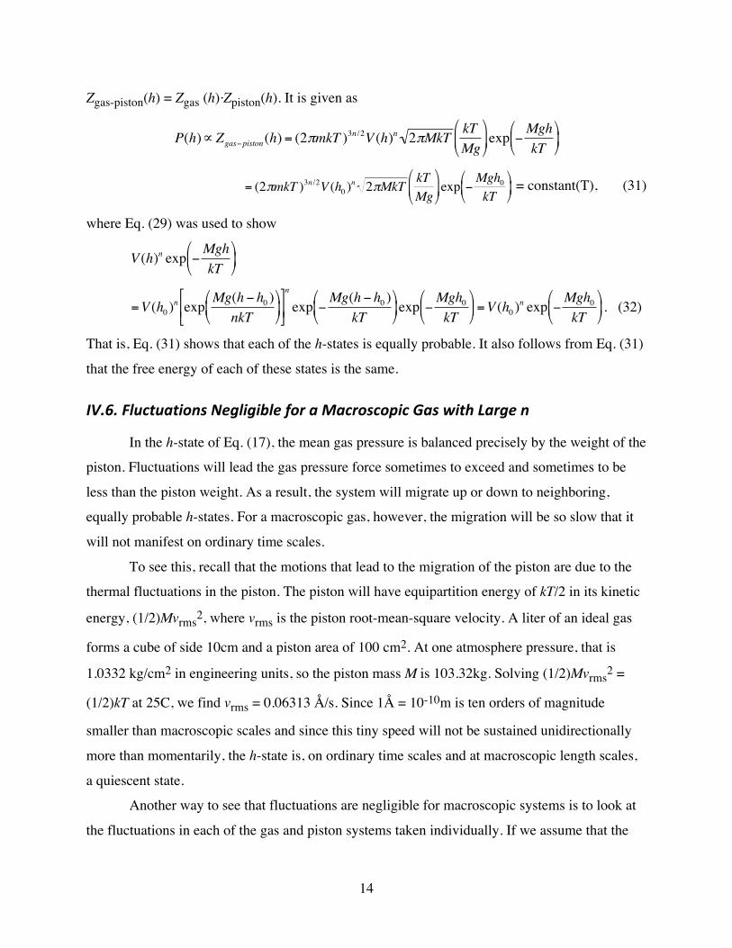
The probability of P(h) of each h-state is proportional to the partition integral

14

Zgas-piston(h) = Zgas (h).Zpiston(h). It is given as

€

P(h)∝ Zgas−piston(h) = (2πmkT )3n /2V (h)n 2πMkT kTMg⎛

⎝ ⎜

⎞

⎠ ⎟ exp −

MghkT

⎛

⎝ ⎜

⎞

⎠ ⎟

€

= (2πmkT )3n /2V (h0 )n 2πMkT kT

Mg⎛

⎝ ⎜

⎞

⎠ ⎟ exp −

Mgh0kT

⎛

⎝ ⎜

⎞

⎠ ⎟ = constant(T), (31)

where Eq. (29) was used to show

€

V (h)n exp −MghkT

⎛

⎝ ⎜

⎞

⎠ ⎟

€

=V (h0 )n exp Mg(h − h0 )

nkT⎛

⎝ ⎜

⎞

⎠ ⎟

⎡

⎣ ⎢

⎤

⎦ ⎥

n

exp −Mg(h − h0 )kT

⎛

⎝ ⎜

⎞

⎠ ⎟ exp −

Mgh0kT

⎛

⎝ ⎜

⎞

⎠ ⎟ =V (h0 )

n exp −Mgh0kT

⎛

⎝ ⎜

⎞

⎠ ⎟ . (32)

That is, Eq. (31) shows that each of the h-states is equally probable. It also follows from Eq. (31)

that the free energy of each of these states is the same.

IV.6.FluctuationsNegligibleforaMacroscopicGaswithLargen

In the h-state of Eq. (17), the mean gas pressure is balanced precisely by the weight of the

piston. Fluctuations will lead the gas pressure force sometimes to exceed and sometimes to be

less than the piston weight. As a result, the system will migrate up or down to neighboring,

equally probable h-states. For a macroscopic gas, however, the migration will be so slow that it

will not manifest on ordinary time scales.

To see this, recall that the motions that lead to the migration of the piston are due to the

thermal fluctuations in the piston. The piston will have equipartition energy of kT/2 in its kinetic

energy, (1/2)Mvrms2, where vrms is the piston root-mean-square velocity. A liter of an ideal gas

forms a cube of side 10cm and a piston area of 100 cm2. At one atmosphere pressure, that is

1.0332 kg/cm2 in engineering units, so the piston mass M is 103.32kg. Solving (1/2)Mvrms2 =

(1/2)kT at 25C, we find vrms = 0.06313 Å/s. Since 1Å = 10-10m is ten orders of magnitude

smaller than macroscopic scales and since this tiny speed will not be sustained unidirectionally

more than momentarily, the h-state is, on ordinary time scales and at macroscopic length scales,

a quiescent state.

Another way to see that fluctuations are negligible for macroscopic systems is to look at

the fluctuations in each of the gas and piston systems taken individually. If we assume that the

15

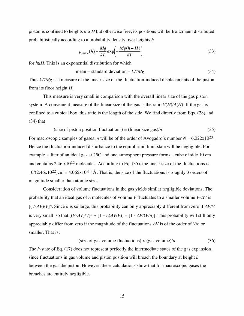
piston is confined to heights h ≥ H but otherwise free, its positions will be Boltzmann distributed

probabilistically according to a probability density over heights h

€

ppiston(h) =MgkT

exp −Mg(h −H )kT

⎛

⎝ ⎜

⎞

⎠ ⎟ (33)

for h≥H. This is an exponential distribution for which

mean = standard deviation = kT/Mg. (34)

Thus kT/Mg is a measure of the linear size of the fluctuation-induced displacements of the piston

from its floor height H.

This measure is very small in comparison with the overall linear size of the gas piston

system. A convenient measure of the linear size of the gas is the ratio V(H)/A(H). If the gas is

confined to a cubical box, this ratio is the length of the side. We find directly from Eqs. (28) and

(34) that

(size of piston position fluctuations) = (linear size gas)/n. (35)

For macroscopic samples of gases, n will be of the order of Avogadro’s number N = 6.022x1023.

Hence the fluctuation-induced disturbance to the equilibrium limit state will be negligible. For

example, a liter of an ideal gas at 25C and one atmosphere pressure forms a cube of side 10 cm

and contains 2.46 x1022 molecules. According to Eq. (35), the linear size of the fluctuations is

10/(2.46x1022)cm = 4.065x10-14 Å. That is, the size of the fluctuations is roughly 3 orders of

magnitude smaller than atomic sizes.

Consideration of volume fluctuations in the gas yields similar negligible deviations. The

probability that an ideal gas of n molecules of volume V fluctuates to a smaller volume V-ΔV is

[(V-ΔV)/V]n. Since n is so large, this probability can only appreciably different from zero if ΔV/V

is very small, so that [(V-ΔV)/V]n ≈ [1 – n(ΔV/V)] = [1 - ΔV/(V/n)]. This probability will still only

appreciably differ from zero if the magnitude of the fluctuations ΔV is of the order of V/n or

smaller. That is,

(size of gas volume fluctuations) < (gas volume)/n. (36)

The h-state of Eq. (17) does not represent perfectly the intermediate states of the gas expansion,

since fluctuations in gas volume and piston position will breach the boundary at height h

between the gas the piston. However, these calculations show that for macroscopic gases the

breaches are entirely negligible.

16

Hence, a reversible gas expansion is quite achievable in the sense that its states can be

brought arbitrarily close by macroscopic standards to the equilibrium states. Nonetheless, just as

in the case of the Brownian motion of a macroscopic body, tiny fluctuations will accumulate

over long times and eventually enable the gas-piston system to migrate over the full extent of

configurations available to it. This migration is represented by the equal probabilities of all states

of Eq. (11).

IV.7.Fluctuationsforn=1

Matters change when we take small values of n. The extreme case of a one-molecule gas

is dominated by fluctuations. The formulae developed above still apply. However we must now

set n = 1 in them. In place of Eq. (35), we have a piston whose thermal fluctuations fling the

piston through distances of the order of the size of the entire gas

(size of piston position fluctuations) = (linear size gas). (37)

It is also evident without calculation that a gas of a single molecule is undergoing massive

density fluctuations as the molecule moves from region to region. If we associate the volume of a

gas with the places where its density is high, these in turn can be understood as volume

fluctuations of the size of the gas confining chamber:

(size of gas volume fluctuations) ≈ (gas volume). (38)

That fluctuations will dominate is apparent from brief reflections without calculations. It

is assumed that the pressure of the one molecule gas is sufficient to support the weight of the

piston. That is, in molecular terms, repeated collisions with a single rapidly moving molecule are

enough to support the mass of piston. This can only be the case if the piston mass itself is

extremely light. If that is so, then its own thermal motion will be considerable.

These fluctuations defeat attempts to realize a thermodynamically reversible expansion of

a gas of one or few molecules. In such an expansion, the gas state is always arbitrarily close to

the limit states and it is supposed to migrate indefinitely slowly through them, under the delicate

and very slight imbalance of pressure and weight forces. This circumstance is unrealizable. The

fluctuations just described will completely destabilize the delicate imbalance. If the gas-piston

system has arrived at any height, fluctuations will immediately move it to a different height. A

near completed expansion may be flung back to the start of the expansion, just as an unexpanded

17

gas can be rapidly expanded by a fluctuation. Instead of rising serenely, the piston will jump

about wildly with no discernible start or finish to the process.

IV.8SuppressingFluctuations:ARoughEstimate

An assured expansion, not confounded by fluctuations, will only be possible if we

introduce enough disequilibrium to suppress the fluctuations. A very rough first estimate

confirms that the dissipation will be considerable in relation to the quantities of entropy

associated with the expansion of a one-molecule gas, but negligible for a macroscopic gas.

If the motion of expansion is to dominate the random thermal motions, then the vertical

velocity of the piston in the overall process must greatly exceed the random thermal motions of

the piston. Assume that the mass M of the piston is slightly smaller than the equilibrium value

required in Eq. (28), so that there is a small, net upward force on the piston. This upward force

gradually accelerates the piston until, at the end of its expansion, it has acquired the vertical

speed vproc and then slams to a halt. This process speed “proc” is a rough measure of the overall

vertical motion of the piston.

The associated kinetic energy (1/2)Mvproc2 is derived from work done on the piston. It is

potentially usable work energy that is lost as heat to the environment at the conclusion of the

process. Had the process been carried out non-dissipatively, that is, reversibly, the only

difference in the end state is that this lost work would have been stored as extra potential energy

in the ascent of a weightier piston and the corresponding quantity of heat would not have been

passed irreversibly to the environment.

The dissipation is represented most compactly in terms of free energy. The free energy

change of the gas-piston system is

ΔF = ΔFgas + ΔFpist = ΔUgas - T ΔSgas + ΔUpist - T ΔSpist (39)

For a reversible, non-dissipative expansion, we have ΔF = 0. Most of the terms in this expression

remain the same if we now consider the dissipative expansion. The internal energy Ugas and

entropy Sgas of the gas are functions of state, so they remain the same. The entropy of the piston

is unaltered; it is just a raised mass. So ΔSpist = 0. Overall, in the transition to a dissipative

expansion, the free energy change ΔF is depressed from its zero value merely by the decrease in

ΔUpist below its reversible value in the amount of the lost work (1/2)Mvproc2. That is, we have

18

ΔF = -(1/2)Mvproc2. (40)

The dissipation can also be measured by an entropy change, but now we must consider

the entropy of the gas, piston and environment together. If ΔUenv,rev is the change of internal

energy of the environment in the case of the reversible process, then we have

ΔUenv = ΔUenv,rev + (1/2)Mvproc2. (41)

Hence the total entropy change in the environment is

ΔSenv = ΔUenv,rev/T + (1/2)Mvproc2/T. (42)

Since the start and end states of the gas are the same for the reversible and the irreversible

processes and entropy is a function of state, the entropy change in the gas is the same for both

processes. It follows that

ΔSgas = - ΔUenv,rev/T, (43)

so that the total entropy change for gas, piston and environment together is

ΔS = ΔSgas + ΔSenv = (1/2)Mvproc2/T. (44)

Thus the net increase in entropy results entirely from the irreversible transfer of the potentially

usable work as heat Q = (1/2)Mvproc2 to the environment, which creates entropy Q/T.

The random thermal motion of the piston is measured by its root-mean-square vertical

speed, vtherm, that satisfies

(1/2)Mvtherm2 = (1/2)kT. (45)

The condition that random thermal motions not confound the process is

vproc >> vtherm. (46)

It follows immediately from the two preceding equations that

ΔF << -(1/2)kT and ΔS >> (1/2)k. (47)

On molecular scales, this decrease in free energy or increase of entropy represents a considerable

dissipation and departure from equilibrium. For comparison, the free energy and entropy changes

usually attributed to a two-fold, reversible isothermal expansion of a one molecule gas are just

ΔF = -kT ln 2 = -0.69 kT and ΔS = k ln 2 = 0.69 k.

19

IV.9SuppressingFluctuations:FreeEnergyChanges

Lightening the piston mass so that vproc >> vtherm enables the expansion to complete with

dissipation Eq. (47) with a reasonably high, but unquantified, probability. A closer analysis using

Eq. (13) provides quantitative relations among the amount of lightening of the mass, the

dissipation and the probability of completion. We will find that negligible lightening and

dissipation can assure completion with high probability for a macroscopic gas, but that no

amount of lightening can achieve this for a one-molecule gas.

If Meq is the equilibrium mass defined through Eq. (28), then we introduce a slight

disequilibrium by setting the piston mass M to be slightly smaller

M = Meq - ΔM, (48)

where ΔM > 0. Instead of Eq. (31), we have for the probabilities P(h) of the h-states

€

P(h)∝ Zgas−piston(h) = (2πmkT )3n /2V (h)n 2πMkT kTMg⎛

⎝ ⎜

⎞

⎠ ⎟ exp −

MghkT

⎛

⎝ ⎜

⎞

⎠ ⎟

€

= (2πmkT )3n /2V (h0 )n 2πMkT kT

Mg⎛

⎝ ⎜

⎞

⎠ ⎟ exp −

Mgh0kT

⎛

⎝ ⎜

⎞

⎠ ⎟ exp

ΔMg(h − h0 )kT

⎛

⎝ ⎜

⎞

⎠ ⎟ , (49)

since now

€

V (h)n exp −MghkT

⎛

⎝ ⎜

⎞

⎠ ⎟

=V (h0 )n exp

Meqg(h − h0 )nkT

⎛

⎝ ⎜

⎞

⎠ ⎟

⎡

⎣ ⎢

⎤

⎦ ⎥

n

exp −(Meq −ΔM )g(h − h0 )

kT⎛

⎝ ⎜

⎞

⎠ ⎟ exp −

Mgh0kT

⎛

⎝ ⎜

⎞

⎠ ⎟

=V (h0 )n exp −Mgh0

kT⎛

⎝ ⎜

⎞

⎠ ⎟ exp

ΔMg(h − h0 )kT

⎛

⎝ ⎜

⎞

⎠ ⎟ ⋅

Most of the terms in Eq. (49) are independent of h, so it can be re-expressed more usefully as:12

€

P(h1)P(h0 )

= exp ΔMg(h1 − h0 )kT

⎛

⎝ ⎜

⎞

⎠ ⎟ =

Z(h1)Z(h0 )

= exp − ΔFkT

⎛

⎝ ⎜

⎞

⎠ ⎟ . (50)

The free energy change between the two states ΔF is introduced using the canonical formula F =

-kT ln Z. It follows that the free energy change is

ΔF = -ΔMg(h1- h0). (51)

This relation admits the obvious reading: in reducing the piston mass by ΔM below the

equilibrium mass Meq, we lose the possibility of recovering work ΔMg(h1- h0) when the piston is

20

raised from height h0 to h1. That work would otherwise appear as a corresponding increase in the

potential energy of the unreduced piston of mass M.

We have already seen from Section III.4 that a macroscopically negligible free energy

change ΔF = -25kT is sufficient to ensure a very favorable probability of completion. From Eq.

(51), we see that this free energy change will correspond to a macroscopically negligible mass

reduction. For a height difference of (h1- h0)=10 cm and a gas at 300K, the mass reduction is ΔM

= 25kT/g(h1- h0) = 1.05x10-19 kg, which is considerably less than the 103.32 kg piston mass of

Section IV.6.

In sum, a thermodynamically reversible expansion of a macroscopic gas is possible in

this sense. The gas-piston system can expand slowly through a sequence of states that are, by

macroscopic standards, very close to limit states that are stable in the shorter term. Fluctuations

introduce negligible complications.

IV.10FailuretoSuppressFluctuationsfortheOne-MoleculeGas

The suppression of fluctuations breaks down completely, however, for a gas of one or

few molecules. For the maximum suppression is achieved by reducing the mass of the piston

arbitrarily close to zero mass. That is, we achieve the maximum probability ratio favoring

completion in Eq. (50) when ΔM approaches its maximum value Meq. This maximum is the case

of a massless piston, which is no piston at all. It is simply releasing the gas freely into an infinite

space. Then, a canonical probability distribution is not established and the probabilistic analysis

used here does not apply. To preserve its applicability, consider instead the limiting behavior as

ΔM approaches Meq arbitrarily closely but never actually equals Meq. Using Eq. (29) with Eq.

(50), we have

€

P(h1)P(h0 )⎛

⎝ ⎜

⎞

⎠ ⎟ ΔM→Meq

= expMeqg(h1 − h0 )

kT⎛

⎝ ⎜

⎞

⎠ ⎟ = exp

Meqg(h1 − h0 )nkT

⎛

⎝ ⎜

⎞

⎠ ⎟

⎡

⎣ ⎢

⎤

⎦ ⎥

n

=V (h1)V (h0 )⎛

⎝ ⎜

⎞

⎠ ⎟

n

. (52)

The probability ratio Eq. (52) is just the probability ratio associated with a spontaneous

recompression of the gas of n independently moving molecules from volume V(h1) to V(h0).

For gases of one or few molecules, the maximum of Eq. (52) presents serious problems.

For the one-molecule gas undergoing a two-fold volume expansion, the largest probability ratio

possible is just 2:1. Even in the most dissipative case, with the piston reduced to its lightest mass,

21

the expanding one-molecule gas is just twice as likely to be in the intended final state than in the

initial state.

In sum, a thermodynamically reversible expansion of a gas of one or few molecules is

impossible. Fluctuations prevent the states of the expansion migrating very close to and very

slowly past the requisite sequence of pseudo-equilibrium states. In the system described, even

dissipation in significant measure at molecular scales is unable to suppress the fluctuations. This

in turn results from the limiting pseudo-equilibrium states themselves being so confounded by

fluctuations that they cannot persist even briefly as stable states.

IV.11HowPistonAreaIncreases

It is not so straightforward to devise ordinary mechanical devices that can achieve the

increase of piston area required by Eq. (30). The simplest arrangement, illustrated in Fig. 2, is to

have a gas chamber of rectangular section that flares out horizontally in one direction with

heights h > h0. The chamber is fitted with a horizontal, rectangular piston that increases in area

as it ascends, so it can keep the gas confined. The piston consists of two rectangular parts that

slide frictionless over each other and are guided apart by rails as the piston ascends.

h1

h0

FIG. 2. A Weighted Piston that Maintains Equilibrium with an Expanding Gas

The sliding of the parts of the piston introduces new thermal degrees of freedom. They

can be neglected since they are independent of the expansion. At all piston heights, each sliding

part has the same slight horizontal motion corresponding to whatever slack is in the fitting of the

rails to the parts. Since this slack will be the same at all stages of the expansion, they will

22

contribute an additive term to the piston Hamiltonian that is independent h and thus will not

figure in the h dependence of the piston free energy of Eq. (25) or in the generalized force of Eq.

(26).

Finally, the expansion under this scheme cannot continue indefinitely. Otherwise the gas

-piston system can access an infinity of equally accessible stages of expansion, which means that

it will never achieve equilibrium. The probability distributions used above, however, depend on

the assumption that equilibrium has been achieved. The expansion could be halted by placing a

maximum stop on the piston at some maximum height. This, however, would introduce

complicating thermal effects. As the piston approaches the stop, it would behave like a one-

molecule gas and resist compression. The simplest remedy is to assume that, at some height

Hmax ≥ h1, the chamber-piston system reverts to one with constant piston area. Then achieving

greater stages of expansion ceases to be equally easy and an equilibration is possible.

V.CONCLUSION

The accommodation of the molecular constitution of matter by ordinary thermodynamics

introduces negligible complications for the thermodynamic analysis of macroscopic systems.

However, as a matter of principle, once we take into account all the processes involved, thermal

fluctuations preclude thermodynamically reversible processes in systems at molecular scales.

This has been shown in Section 3 for the general case of any isolated system and for any system

maintained at constant temperature by a heat bath with which it exchanges no work.

In standard treatments of molecular scale systems, thermodynamically reversible

processes are described as advancing very slowly under the guidance of a parameter that is

manipulated externally by unspecified processes. The requisite precise, external control of the

parameter is only possible through considerable dissipation in those unspecified processes. It

renders the overall process irreversible. The neglect of this additional dissipation masks the

impossibility described here.

The most general result is the impossibility of a reversible process for any isolated,

molecular scale system since it covers all other cases. Imagine that somehow we could realize a

reversible process in some part of an isolated system. Since reversibility is unachievable for the

total isolated system, there must be an unaccounted dissipation in some other part of the system.

23

The impossibility of molecular scale, thermodynamically reversible processes derives

from Eqs. (11), (12) and (13) of Sections III.2 and III.4, which apply quite generally. If we have

a process that is intended to be thermodynamically reversible, Eq. (11) tells us that thermal

fluctuations lead the system to meander back and forth indefinitely if its states are in or

arbitrarily near the limiting states. They will eventually realize a uniform probability distribution

over the process stages. Such a process does not complete. Eq. (12) and (13) determine the order

of magnitude of the dissipation needed to overcome the fluctuations and assure probabilistic

completion of the intended process. Eqs. (15) and (16) give the minimum dissipation in a special

circumstance contrived to be least dissipative. The dissipation is negligible on macroscopic

scales and significant on molecular scales.

The idea that one could undertake a thermodynamically reversible expansion of a gas of a

single molecule was introduced by Szilard13 as part of his celebrated analysis of Maxwell’s

demon. The idea has become standard in the now voluminous literature that develops Szilard’s

work.14 Szilard15 briefly recognized the problem that the gas pressure is wildly fluctuating, as it

acts to lift a weight coupled to the piston. The problem is dismissed with the parenthetically

inserted remark:

The transmission of force to the weight is best arranged so that the force exerted

by the weight on the piston at any position of the latter equals the average

pressure of the gas.

We have now seen here in detail that this is an inadequate response. There is no arrangement that

can convey the work done by the expanding one-molecule gas to a raised weight in a way that

maintains thermodynamic reversibility of the entire process. Any arrangement, no matter how

simple or complicated in design, is subject to the above general relations. They affirm that

fluctuations will disrupt the intended operation, unless the fluctuations can be suppressed by the

dissipative creation of entropy in quantities significant at molecular scales.

1 Such as in Hendrick C. Van Ness, Understanding Thermodynamics. (New York: McGraw-Hill,

1969; reprinted, New York: Dover, 1983), pp. 19-22. 2 Christopher Jarzynski, “Nonequilibrium Equality for Free Energy Differences,” Physical

Review Letters, 78(No. 14), 2690-2693 (1997) on p. 2690.

24

3 R. Kawai, J. M. R. Parrondo, and C. Van den Broeck, “Dissipation: The Phase-Space

Perspective,” Physical Review Letters, 98, 080602 (2007) on p. 080602-1. 4 To see this, for small changes, we have

dFsys = d(Usys – TSsys) = dUsys – TdSsys = dUsys + dUenv = dUtot = 0

where the heat passed to the environment in the reversible process is dQsys = TdSsys, which

equals the energy change in the environment dUenv.

5 For a small, reversible change, we have dFsys = dUsys − Τ dUsys = dUsys − dQ = − dW, so that

−dFsys/dx = dW/dx = X.

6 Albert Einstein, "On a Heuristic Viewpoint Concerning the Production and Transformation of

Light." Annalen der Physik, 17, 132-148 (1905) in §5. 7 To connect with the usual statement of the canonical distribution, if Vph,tot is the volume of the

full phase space accessible to the system, then the canonical distribution is

p = exp(-E/kT)/ Z(Vph,tot) and the probability that the system is in subvolume Vph is equal to

Z(Vph)/ Z(Vph,tot).

8 The intermediate states can never be completely inaccessible or the process could not proceed.

Rather the process design must be such as to make them accessible only with arbitrarily small

probability. 9 Eqs. (15) and (16) with a term ln(1 + P(λfin)/P(λinit)) give slightly higher dissipation than the

corresponding formulae (22) and (23) of an earlier paper (John D. Norton, “All Shook Up:

Fluctuations, Maxwell’s Demon and the Thermodynamics of Computation,” Entropy, 15, pp.

4432-83 (2013).), which instead have a term ln(P(λfin)/P(λinit)). The latter formulae presumed

that the process ends in a way that prevents return to the initial state. In the absence of a non-

dissipative way of preventing this return, the newer formulae provide a better limit. 10 Available at http://philsci-archive.pitt.edu/12202/ 11 See §7.5 of John D. Norton, “Waiting for Landauer,” Studies in History and Philosophy of

Modern Physics, 42, 184-98 (2011).

25

12 These two probabilities are to be read as follows: over the longer term in which the gas-piston

system fully explores the phase space accessible to it, it comes to an equilibrium with probability

P(h0) of the initial compressed h-state and probability P(h1) of the final, expanded h-state.

13 Leo Szilard, “On the Decrease of Entropy in a Thermodynamic System by the Intervention of

Intelligent Beings,” (1929) in The Collected Works of Leo Szilard: Scientific Papers. (MIT Press:

Cambridge, MA, 1972), pp. 120–129. 14 For a survey and collection of works, see Harvey S. Leff and Andrew Rex, eds. Maxwell’s

Demon 2: Entropy, Classical and Quantum Information, Computing. (Bristol and Philadelphia:

Institute of Physics Publishing, 2003). 15 Ref. 13, p. 122.