Thermodynamic Studies in Anhydrous Ethanol. The Hydrogen

Louisiana State UniversityLSU Digital Commons

LSU Historical Dissertations and Theses Graduate School

1960

Thermodynamic Studies in Anhydrous Ethanol.The Hydrogen - Silver - Silver-Bromide GalvanicCell.Loys Joseph Nunez JrLouisiana State University and Agricultural & Mechanical College

Follow this and additional works at: https://digitalcommons.lsu.edu/gradschool_disstheses

This Dissertation is brought to you for free and open access by the Graduate School at LSU Digital Commons. It has been accepted for inclusion inLSU Historical Dissertations and Theses by an authorized administrator of LSU Digital Commons. For more information, please [email protected].

Recommended CitationNunez, Loys Joseph Jr, "Thermodynamic Studies in Anhydrous Ethanol. The Hydrogen - Silver - Silver-Bromide Galvanic Cell."(1960). LSU Historical Dissertations and Theses. 585.https://digitalcommons.lsu.edu/gradschool_disstheses/585

https://digitalcommons.lsu.edu?utm_source=digitalcommons.lsu.edu%2Fgradschool_disstheses%2F585&utm_medium=PDF&utm_campaign=PDFCoverPages

https://digitalcommons.lsu.edu/gradschool_disstheses?utm_source=digitalcommons.lsu.edu%2Fgradschool_disstheses%2F585&utm_medium=PDF&utm_campaign=PDFCoverPages

https://digitalcommons.lsu.edu/gradschool?utm_source=digitalcommons.lsu.edu%2Fgradschool_disstheses%2F585&utm_medium=PDF&utm_campaign=PDFCoverPages

https://digitalcommons.lsu.edu/gradschool_disstheses?utm_source=digitalcommons.lsu.edu%2Fgradschool_disstheses%2F585&utm_medium=PDF&utm_campaign=PDFCoverPages

https://digitalcommons.lsu.edu/gradschool_disstheses/585?utm_source=digitalcommons.lsu.edu%2Fgradschool_disstheses%2F585&utm_medium=PDF&utm_campaign=PDFCoverPages

mailto:[email protected]

Thermodynamic Studies in Anhydrous Ethanol. 'The Hydrogen - Silver - Silver Bromide

Galvanic Cell

A Dissertation

Submitted to the Graduate Faculty of the Louisiana State University and

Agricultural and Mechanical College in partial fulfillment of the requirements for the degree o:

Doctor of Philosophyin

The Department of Chemistry

byLoys Joseph NunezjM.S., Louisiana State University, 1955

January I960

Acknowledgment

The author wishes to express his appreciation for the advice of Dr. Marion C. Day. He is also grateful for the financial aid received as the recipient of a Lewis Gottlieb Fellowship.

TABLE OF CONTENTSPage

LIST OF TABLES....................................... ivLIST OF FIGURES..................................... vABSTRACT............................................. viI INTRODUCTION ................................... 1II THE IONIZATION CONSTANT OF HYDROGEN BROMIDE

IN ETHANOL..................................... 7III PURIFICATION OF ETHANOL

A, Methods......... 13B. Experimental Procedure 14

IV EXPERIMENTAL APPARATUS AND PROCEDUREA. The Galvanic Cell................. 17B. Preparation of the Silver, Silver-

Bromide Electrodes . . . . . . . . . . . . 20C. Reagents Used* . • . .......................21D. Procedure....... * ....................... 22

V THE DETERMINATION OF THE STANDARD POTENTIAL. . . . 25VI IONIZATION CONSTANTS OF WEAK ACIDS IN ETHANOL. . . 32VII DISCUSSION OF RESULTS............................. 35BIBLIOGRAPHY ....................................... 78VITA....................... 81

LIST OF TABLESTABLE PAGE

I Conductivity Data of H. Goldschmidtand P. Dahll......................... 38

II Functions calculated from the dataof H. Goldschmidt and P. Dahll . . . . 39

III Physical Properties of AnhydrousEthanol....................... 40Observed electromotive force of the cell

IV-XV Runs 1 - 1 2 .......................... 41-52(Eq - E*) and (E* - E*)* as a function of the concentration for the value of the parameter a :

XVI ft = 4 . 0 ......................... . 53XVII X = 5.0 55XVIII X Z 6 . 5 .................... 57XIX X - 8 . 0 ............................. 59

XX-XXVII Observed electromotive force of thecell. Runs A-l - A-G............... 61-68

XXVIII-XXXV Observed electromotive force of thecell. Runs B-l-B-8...................69-76

XXXVI The function -0.0591 log as dependent on the Ionic Strength,UJ, for Acetic Acid........................... 77

LIST OF FIGURES FIGURE PAGE1. The Data of Goldschmidt. Equivalent

Conductivity vs. the Square Root of the Concentration ............................... &

2. The Data of GoldschmidtF{Z)//i vs. Cf2A/F(Z).........................11

3. Schematic Diagram of Potentiometer-CellCircuitry • • • • • • • . ................... 18

4. The Galvanic Cell............................ 195. Corrected Eobs> vs. 4- log Molality...........246. Corrected Eobs vs. — log Normality...........267. Concentration vs. — {Eq — E ) ........... 29S. Concentration vs. — (Eq — E^)*. . . . . . . . 319. The Ionic Strength,U) , vs. 0.0591 log k !

for Acetic Acid ..................... *3310. The Ionic Strength, IV, vs. 0.0591 log

for Benzoic Acid............................. 34

v

ABSTRACT

The standard electrode potential of the silver- silver bromide electrode was determined in anhydrous ethanol for the first time. The value was found to be — 0.1940 +1 0.0005 volts on the molar concentration scale and — 0.1S60 — 0.0005 volts on the molal concentration scale, the standard potential being expressed as an oxidation potential. The silver-silver bromide standard electrode potential in ethanol is more negative than the silver-silver chloride standard electrode potential in ethanol, when both are determined by the method used by H. Taniguchi and G.Janz (23). The difference in these two standard potentials in ethanol is 0.1002 volts as contrasted to 0.1493 volts in water.

Potentiometric measurements were made at a temperature of 25°C on a galvanic cell without liquid junction consisting of a silver-silver bromide electrode and a platinum black hydrogen electrode.

The silver-silver bromide electrodes were prepared by a new modification of existing procedures, which eliminated the need for platinum wire in the electrodes.

The conductivity data of H. Goldschmidt and P. Dahll (10) were independently evaluated in order to obtain an approximation for the molar thermodynamic ionization constant of hydrogen bromide in ethanol. This was found to be 0.01S7.

vi

The thermodynamic molal ionization constants of acetic and benzoic acids in anhydrous ethanol were evaluated.The ionization constants of benzoic and acetic acids in ethanol were found to be 1.01x10“^ and 2*05x10"’'^ respectively. The value of the ionization' constant of benzoic acid in ethanol is in substantial agreement with that found by other workers using conductivity methods. No value for the ionization constant of acetic acid in ethanol is available in the literature for comparison.

vii

I

INTRODUCTION

The measurement of the electromotive force of galvanic cells without liquid junction has been frequently- reported in the litejâture of the recent past for aqueous systems, particularly in connection with the determination of the ionization constant of dissolved weak acids (20). Until recently non-aqueous measurements have been less frequently reported and are more difficult to interpret due to the lack of an adequate theoretical approach and a clear understanding of the effects of solvent impurities.

A recent study of a non-aqueous galvanic cell without liquid junction was made by H. Taniguchi and G.Janz (23) using anhydrous ethanol as the solvent with reversible hydrogen and silver-silver chloride electrodes. These authors used the best known procedures to ensure the purity of ethanol, although small quantities of benzene may well have been present in their solvent, and they were the first ones to consider the degree of dissociation of hydrogen chloride in ethanol in evaluating the standard electrode potential of their system. They accepted the value of the ionization constant of hydrogen chloride in ethanol as calculated by the method of R. Fuoss and G. Kraus (8), (9) from the conductivity data of I. Bezman and F. Verhoek (2). By using the extended terms of the Debye-

1

Huckel Theory, as tabulated by T. Gronwell, V. La Mer and K„ Sandved (11), Taniguchi and Janz calculated the activity coefficients of the ions, evaluated the degree of dissociation of hydrogen chloride in ethanol, and computed the standard electrode potential, E0, for the cell by a method which is illustrated by H. Earned and B. Owen (14). Taniguchi and Janz obtained an EQ value of -0.09383 in terms of the molar concentration scale. This value differs somewhat from previously reported values which varied from -0.0864 volts (20) to 0.00977 volts (21).

C. Le Bas (18) has shown that some of the discrepancies in E0 values may be attributed to the prescence of small quantities of water in the ethanol. Other discrepancies may be due to methods of graphical extrapolation which place emphasis on points in regions,of high dilution where experimental error tends to be high.

Attention was drawn to the bromide system by the fact that the salts, sodium bromide and potassium bromide, are considerably more soluble in anhydrous ethanol than the corresponding chlorides as shown in Table I. It was felt that practical applications of anhydrous ethanol as a solvent may favor the bromide system rather than the chloride system due to solubility considerations, but it was found that t-hese advantages are off-set by the instability found in the regions of relatively high concentration of the bromide system in ethanol.

The aqueous cell:Ag; AgBr (s), HBr (m), H^; Pt

has been investigated by A. Keston (17) and by H. Harned,A. Keston, and J. Donelson (12), (13)* The present inves— tigation is concerned with a cell analogous to the oneshown above, using anhydrous ethanol as the solvent. Thecell reaction is:

AgBr 4- l/2H£=* Ag + HBrConsiderable attention has been paid to the

purification of ethanol; the small quantities of benzene which may have been present in the solvent of Taniguchi and Janz have been carefully removed, even though their effect on the potential of the cell is not accurately known.

It was felt that the theoretical approach of Taniguchi and Janz was the most desirable even though the value of E0 will be dependent on the value of K, the ionization constant of hydrogen bromide in ethanol, which must be obtained from conductivity data.

The conductivity data of H. Goldschmidt and P. Dahll (10), presented in the literature of 1925* allows an approximation of the ionization constant of hydrogen bromide in ethanol to be obtained by a method unknown to those workers at the time of publication.

The method of determining the standard electrode potential of the cell, the same as that used by Taniguchi

and Janz, essentially reduces to plotting the function

4, t{E0 — E^J versus the concentration of hydrogen bromide for a given value of the parameter a where (E — Ew) is defined as:

(Eq - E j = Eobs<+ 0.1163 logoCf^C (1-1)where Eobs z Corrected observed E.M.F. of cell

Ot, Z degree of dissociation HBr in ethanolfK z activity coefficient, dependent on <xC r concentration HBr, moles/liter.

and a = mean distance of closest approach of theDebye - Huckel Theory.

When the correct value of a has been chosen, the left hand term reduces to the true EQ value of the cell and the plot becomes a straight line of zero slope, at least forthe region of low concentration* An extrapolation to zeroconcentration yields the best value of EQ.

Once the standard potential of the cell is known other thermodynamic properties of the system may be determined by means of potentiometric measurements. The thermodynamic dissociation constants of benzoic and acetic acids in ethanol may be obtained from consideration of the cell below:

Ag; AgBr(s), HA{m-), NaAfir^), NaBrfm^), H£J Pt where HA represents a weak acid and NaA its sodium salt.We may define the dissociation constant, K& as:

Ka - m^ m£_ . Yh* Ta”

mHA YHA

where m = molalityV ~ molal activity coefficient

The expression for the electromotive force of the cell may be written as follows:

E = Ec - ET In mH+V H+mBr_ YBr-

Combining the two equations yields:E— E0+RT In mHAmBr- Z- -RT In Yh+ Br" HAF--------- - F--- -------------

mA- Yh+ Ya~

— RT In k ! (1-4)F A

The left hand side of the equation may be readily evaluated. As the dilution approaches infinite dilution, the activity coefficients approach unity and the first term on the right becomes zero. According to D. A,Mac Innes (20) the left hand side of the equation has been found to be a linear function of the ionic strength. Therefore, when the left hand side of the equation is plottedversus the ionic strength, the intercept is proportional to the thermodynamic dissociation constant, KA.

In dilute aqueous solution it is frequently possible to neglect the extended terms of the Debye - Hiickel Theory and use only the Debye approximation for calculating the activity coefficient. This equation is of the general form:

— log f = a n r -1 + Bai TfT

where C = Concentrationf = activity coefficientA = constantB = constanta^ = mean distance of closest approach

For very dilute aqueous solutions the equation reduces to:— log f = A VTTDue to the low dielectric constant of alcohol, it

is not possible to neglect the extended terms of the Debye- Huckel Theory when working with this solvent in concentrations comparable to dilute aqueous systems. Therefore, all calculations of the activity coefficient presented in this investigation have used two extended terms, that is, the terms of the 5th power have been included in the calculations.

Once the E0 value has been obtained the activity coefficient may be calculated from the experimental data at any concentration by means of Eq. (I—1)•

In lieu of a formal section on review of the literature, the pertinent references appear in this section and the body of the dissertation.

II

THE IONIZATION CONSTANT OF HYDROGEN BROMIDE IN ETHANOL

The conductivity data of H. Goldschmidt and P. Dahll (10) have been used to determine the ionization constant, K, of HBr in ethanol by the method of R. Fuoss and C. Kraus (8), (9)* These data are presented in Table I. The value of conductivity at infinite dilution reported by Goldschmidt was not used in the calculations. The method allows an approximate value to be used, based on a simple extrapolation to zero concentration. A plot of the conductivity data is shown in Fig.l.

Essentially, the method is based on a solution by successive approximation of the Onsager Equation. This equation is believed to hold exactly up to concentrations where ionic interactions of higher order than pairwise become appreciable. According to R. Fuoss and C. Kraus the equation may be written:

A =Y(A> —«3cr) (ii-Dwhere: A z equivalent conductance

Aor equivalent conductance at infinite dilution C z concentration, m/1.Y = degree of dissociation.

and oCamay be defined as:X - S. 18x105A0 4. 82

(DT) 3/2 tl (DT) 1/2where: D I dielectric constant

T z absolute temperature = viscosity of the solvent

7

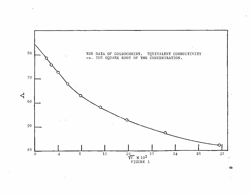
80 THE DATA OF GOLDSCHMIDT. EQUIVALENT CONDUCTIVITY vs. THE SQUARE ROOT OF THE CONCENTRATION.

70

60

50

400 4 8 12 16 20 24 28 32YcT x io2

FIGURE 1ca

We may define the ionization constant, K:K : C V 2 f 2

-L±

whereand

& -

(II-2)

activity coefficient of the positive ion.

In order to facilitate the solution of the various equations R. Fuoss has defined a function Z such that:

Z 5 OCAZ3^2 NfCA (II—3)and F(Z) = 1 - Z(l-Z(l-Z(l-...)-£)-4)-l (II-4)

Then the solution for ^ , that is, the best approximation of Y , is given immediately by:

Y = — A (n-5)A 0 (F <Z))

The activity coefficient may be evaluated, approximately, by using the Debye Expression:

- log f : b J jjT

where: B = 0.4343 e2 N e2 \l/22DkT \1000 Dkt /

/8-IT N e2 \ 1/2 \1COO Dkt )

andwhere

[H*] = [fir-]e Z electronic chargeN Z Avogadrofs Numberk Z- Boltzmann ConstantD z Dielectric constant of solventT = absolute temperatureaj_ = ionic radius

10For our purposes it was possible to neglect the

term in the denominator, Eq.(II-6) reducing to:- iog10 = 2B'ire_

as an approximation. For ethanol:2 B : $.90Substituting Eq.(II-5) into Eq.(II-2) the following

expression is obtained:k ( l — A ^ = cf2 / A 2V A 0F(Z) ) \ A § F(z)2

Upon rearrangement this reduces to:F (Z) = 1______ f Cf2A S|. 1A lKA02) { F (Z) A 0

Thus if F(Z )/A is plotted versus GfÂ/F{Z) a straightline of slope ( V kA o and intercept V A 0 should beobtained. Such a plot is shown for the data of Goldschmidtin Fig.2. A 0 was found to be S3.47 and the value of themolar ionization constant, was calculated to be 0.0187.Numerical values of the functions plotted in Fig.2 aretabulated in Table II. F(Z) values were taken as thoseconveniently tabulated by Fuoss (8) for any given value of Z.

The value of the molar ionization constant K^gr = 0.0187 in ethanol may be compared to the molar ionization constant « 0*0113 in ethanol, both calculated by thesame method. Since both HBr and HC1 have long been assumed to be strong acids in ethanol, it is not surprising that the ionization constants are of the same order of magnitude. Qualitatively, at least, it would be expected that HBr would

THE DATA OF GOLDSCHMIDT

1300

LOo

1200

14129 10 11 c A f 2 xioo

FFIGURE 2

F Xl

O5

THE DATA OF GOLDSCHMIDTF(z)

1300

1200

1211F

FIGURE 2

12be a stronger acid than HC1 due to the greater size of the bromide ion, which would allow greater dissociation of the proton.

Ill

PURIFICATION OF ETHANOLA. Methods

Traces of benzene present in commercially available U.S.I. absolute ethyl alcohol, U.S.P. grade, are of sufficient quantity to prevent the use of this grade of alcohol as a glass in phosphorescence studies and as a solvent where the highest degree of purity is required. Spectroscopic data of the author indicate that benzene may be present in quantities higher than 0.001%.

Anhydrous alcohol may be prepared from 95% ethanol by a variety of methods some of which depend on depressing the vapor pressure of water (6). Usually the starting material is sufficiently free from benzene so that this impurity does not show up in the final product, but the removal of other impurities often necessitates considerable effort. Calcium oxide treatment (22) and various modifications of this method have been used for purifying 95% alcohol. J. Woolcock and H. Hartley {2k) as well as P. Danner and J. Hildebrand (5) used ethanol treated in this manner for potentiometric studies. Other workers have followed calcium oxide treatment by the Bjerrum method (19), which involves the addition of magnesium.

By combining known procedures a simplified method has been obtained, using U.S.I. absolute ethyl alcohol as a

13

Ik

starting material, which produces ethanol of a high degree of purity that may be used as a solvent in potentiometric studies. The physical properties of this alcohol compare favorably with data reported in the literature. Some of the results obtained are presented in Table III.

Taniguchi and Janz (23) report a density of 0.73056 at 25°C for pure ethanol, although it is probable that this value is a misprint since a density of 0.73506 at 25°C is reported for pure ethanol in the International Critical Tables (16).

A. Clow and G. fearson (3), L. Mukherjee (21), and L. Harris (15) determined the purity of alcohol by means of spectroscopic data, observing transmission of ultraviolet light in the region 210 — 250 m)i. Transmission in both the infrared and ultraviolet regions, as measured by the Beckman DK Spectrophotometer, have been regarded as the most important criteria of purity of alcohol prepared by the method described below:

B. Experimental Procedure

Modifying the method of Bjerrum, magnesium alcoholate was prepared by adding 25g of magnesium metal and 5g< of iodine to 150 ml of dry ethanol (pre-purified and containing less than 1% water). The mixture was allowed to react for 3-10 hours ar room temperature until no liquid remained in the flask.

15Two per cent water by volume was added to U.S.I.

ethyl alcohol, U.S.P. grade, and the mixture was fractionally distilled. When a fractionating column of approximately ten theoretical plates was used, the first 25%> of distillate contained most of the benzene as the azeotropic mixture of the following composition: water, 7.5%; ethanol, 18,5%;benzene, 74.0$. The distillation was stopped at this point and the solid magnesium alcoholate mixture introduced into 900 ml of the distillation residue. This was refluxed for approximately one-half hour until free of water, followed immediately by fractional distillation. The first and last 10%o cuts of the distillate were discarded and the intermediate fraction of pure ethanol was retained. Absorption of water from the atmosphere was prevented during refluxing and distillation by the use of silica gel drying towers.

The distillation which removes benzene as well as the final distillation of pure ethanol was monitored by means of the Beckman Model DK Spectrophotometer. Using water as a blank less than 0.000B$ of benzene in ethanol may be easily detected in the ultraviolet region with a cell path length of 1 cm. An impurity in the first and last cuts of the final distillation also appears in the region 335—200 mj*.

The same instrument will also detect small quantities of water in ethanol in the wavelength region of 1950 mjju A cell path length of 0.5 cm. may be used with

16anhydrous ethanol as a blank. It was found that less than 0.02 w t o f water in ethanol could be easily detected in this manner.

It is important that once the magnesium alcoholate is introduced into the alcohol-water mixture, the resulting distillation be conducted without interruption and as rapidly as possible; otherwise undesirable side reactions will considerably reduce the yield of pure ethanol.

Best results were obtained using magnesium turnings of 99.6$ purity, marketed for use in the Grignard Reaction by the J. T. Baker Chemical Co., Phillipsburg, N. J.

IVEXPERIMENTAL APPARATUS AND PROCEDURE

A. The Galvanic Cell

A schematic diagram of the cell circuitry is presented in Fig.3* A. Leeds and Northrup Potentiometer was used. The cell itself, illustrated in Fig.4* consisted of a four neck flask in which a hydrogen electrode of the Hildebrand type occupied the center position. Silver- silver bromide electrodes were in adjacent positions.Thus the same hydrogen electrode served as "reference" when potentiometric measurements were made alternately on both silver-silver bromide electrodes. The platinum black surface of the hydrogen electrode was immersed approximately one inch below the surface of the liquid, the bubbles emerging from the electrode at about the same height. The rate of flow of hydrogen was 1-2 bubbles/second.

The platinum black was deposited on the surface of the electrode from a chloroplatinic acid solution containing a little lead acetate. A platinum electrode was used as the anode and a current of 200-400 ma. was passed for 3 minutes. The electrode was replatinized every 2 or 3 runs or whenever the system showed signs of instability.

Prepurified hydrogen, sold by the Matheson Co., Inc., passed first through a hydrogen catalytic purifier marketed by Engelhard Industries, Inc., Newark, N. J.

17

POTENTIOMETERCIRCUIT

FIGURE 3

TO HYDROGEN

HYDROGENELECTRODE

Ag,AgBrELECTRODE

19

THE CELL

FIGURE 4

20It then went through a silica gel column and into a bubbling tower filled with a liquid of identical composition as that present in the celle From the bubbling tower the hydrogen entered the cell and passed over the platinum surface of the electrode. Exit of the gas into the atmosphere was through a capillary tube.

The cell was immersed in a Sargent constant temperature water bath, maintained at a temperature of 25,25°C i 0,05°. As room temperature exceeded 25°C, a Sargent water bath cooler was employed which circulated cool water through coils immersed in the constant temperature bath,

B, Preparation of the Silver-Silver BromideElectrodes

Silver-silver bromide electrodes of the thermal electrolytic type were prepared initially by use of a platinum wire as a holder, A mass of porous silver was deposited on a helix of platinum wire by the thermal decomposition of a paste of silver oxide. The silver was then converted to silver bromide by electrolysis. Elec— • trodes of this type showed marked instability, presumably due to cracks in the silver surface exposing areas of platinum which may function as small hydrogen electrodes.

The following adaptation was therefore chosen. Silver wire of 1 ram. diameter was sealed in one end of a

21glass tube of slightly larger diameter than the silver wire* Approximately one centimeter of silver wire was allowed to protrude from the glass tube on both ends, one end serving as a means of electrical contact to the external circuit and the other end serving as the surface of the electrode. One end was heated in a flame until molten, a spherical droplet being formed. After cooling, a paste of very pure silver-oxide (1) was applied to the silver surface and this was heated again until a spongy surface of very pure metallic silver had covered the surface. The electrode was then anodized in dilute KBr solution as usual, until a spongy layer of AgBr had covered the surface of the electrode. All silver-silver bromide electrodes used in this investigation were prepared in this manner.

C. Le Bas (IB) has shown that these electrodes gave results identical to those observed with electrodes prepared by the thermal electrolytic method using the platinum wire spiral.

C. Reagents Used

Anhydrous hydrogen bromide as obtained from the Matheson Co., Inc. was used directly from the cylinder.

Anhydrous acetic acid was prepared by distilling a mixture containing 1% acetic anhydride and glacial acetic acid of 99,1% purity. A middle fraction of 20-40% was collected and used as anhydrous acetic acid.

22Benzoic acid, sodium bromide and sodium benzoate

were all of U.S.P. or Analytical Reagent grade and were recrystallized from anhydrous ethanol. Sodium acetate •3H2O was heated until molten in order to obtain the anhydrous salt.

All operations which would expose anhydrous materials to the atmosphere were conducted in a nitrogen atmosphere dry box desiccated with phosphorous pentoxide.

The fractional distillation apparatus used was of approximately 10 theoretical plates. All connections were glass to glass with no stopcock grease. Drying towers of silica gel were placed on all openings to the atmosphere.

D. Procedure

After completion of a run, aliquots of the ethanol-hydrogen bromide solution were withdrawn by pipette from the cell and titrated with standardized sodium hydroxide solution using phenolphthalein as an indicator. The normality was then converted to molality by the appropriate conversion factor.

The concentrations of salts and weak acids were determined directly on a weight basis. Both salts and alcohol were weighed on an analytical balance in a desiccated atmosphere. The salts and weak acids were added to the anhydrous ethanol in a dry box and were allowed to remain there, stoppered, for several hours until all solid particles

c

23went into solution.

No electromotive force measurements were recorded until the system had reached an apparent equilibrium, which usually required several hours after initiation of hydrogen bubbling. The criterion of equilibrium was that no appreciable drift in readings in one direction could be observed during a period of one hour, although most measurements recorded in the tables extended over a period of time considerably greater than one hour.

It was found impossible to obtain reliable readings in regions of concentration greater than that shown in Fig.5.

V

THE DETERMINATION OF THE STANDARD POTENTIAL

The observed potential of the cell, corrected to one atmosphere pressure of hydrogen, is presented in Fig.6 as a function of the logarithm of the concentration of hydrogen bromide expressed as m/l. The raw data from which this curve was obtained are presented in Tables IV-XV.The empirical equations of the line within the concentration ranges studied may be expressed as:

E E — 0.1021 log Molarity — 0.1327 (V-l)E = — 0.1021 log Molality — 0.1221 ,The above equations were obtained by the method

of least squares, the standard deviation being: 0.00165. Considerable deviation from a straight line is to be expected in the more concentrated regions but the instability of the system did not permit an accurate evaluation of points in this area.

The expression for the density of HBr- ethanol mixtures as a function of the normality is as follows:

D = 0.07993 (N)-f0.7855 (V-2)where D z density, g/cc

N = normalityThe above expression, which was obtained from a

least squares treatment of experimental density points, holds in the range of concentration from 0.0 to 0.5 normal.

25

obsCORRECTED E0bs. vs. -log MOLALITY

120

80

. 40

ta

-40

-802.8 2.4 2.0

-log m FIGURE 5

1.6 1.2

JO-e-

X 10

160CORRECTED Eobs vs. -log NORMALITY

120CO

“ 80ou

40

-402.8 2.6 2.4 2.2 2.0 1.8

-log NORMALITY FIGURE 6

1.6 1.4 1.2 1.0

roo

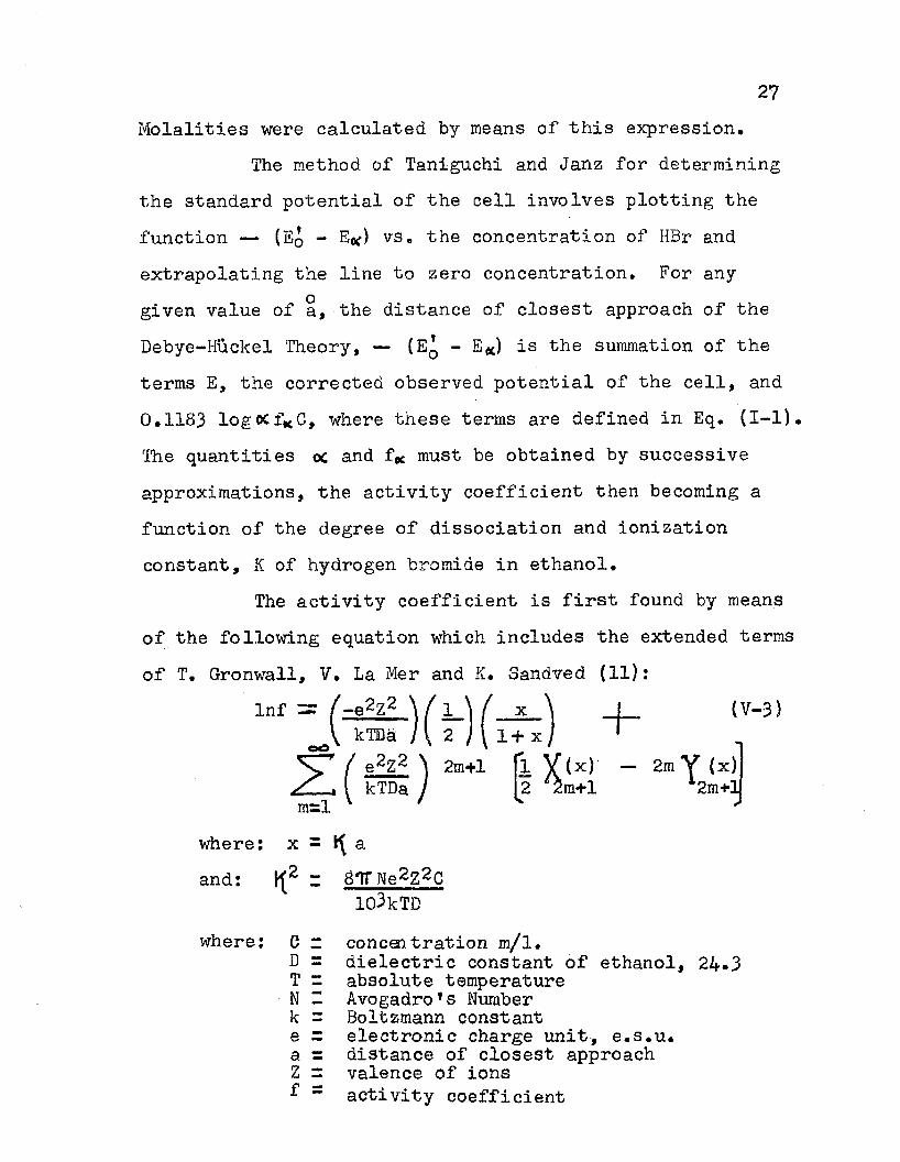
Molalities were calculated by means of this expression.The method of Taniguchi and Janz for determining

the standard potential of the cell involves plotting the function — (Eq - E*) vs. the concentration of HBr and extrapolating the line to zero concentration. For any given value of a, the distance of closest approach of the Debye-Huckel Theory, — (E^ - E*) is the summation of the terms E, the corrected observed potential of the cell, and 0.1183 logocfKC, where these terms are defined in Eq. (1-1). The quantities oc and fee must be obtained by successive approximations, the activity coefficient then becoming a function of the degree of dissociation and ionization constant, K of hydrogen bromide in ethanol.

The activity coefficient is first found by means of the following equation "which includes the extended terms of T. Gronwall, V. La Mer and K. Sandved (11):

Inf =: /-e2Z2 \ / 1 U x \ I (V-3)J [ 2 j [ 1+x/ '

e2Z2 'N 2m+l (l Y(x) — 2m V (x) kTDa I [2 2m+l l2m+l

m=l 'where: x = 1 aand: \[2 z 8TTNe2Z2C

103kTDwhere: C z concaitration m/l.

D = dielectric constant of ethanol, 24-3 T r absolute temperatureN Z Avogadrofs Numberk = Boltzmann constante = electronic charge unit, e.s.u.a = distance of closest approach Z = valence of ions£ = activity coefficient

28and x< x) and Y W are complicated functions of x

tabulated by Gronwall, LaMer, and Sandved.Once the activity coefficient has been evaluated

for a given value of the parameter a, the degree of dissociation, <X , may be determined by means of the following equation:

DC - 12 )1/2]•_K \l/2\ (V-4)

Cf± *where: K = thermodynamic ionization constant.

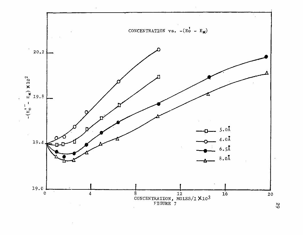
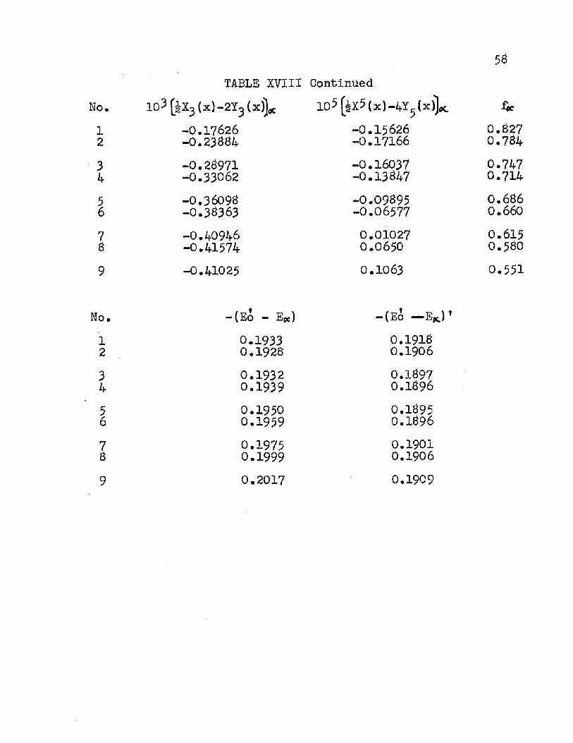
Once DC has been calculated, the activity coefficient, f*, may be recalculated on the basis ofotC to give a better approximation of the function f*. These data are presented in Tables XVI —-XIX for values of a 5, 6.5, and 8.0angstrom units. Plots of these data are shown in Fig.7.The theoretical line of zero slope is exhibited by the function only in the region of concentration less than 3 m/1. Therefore this plot is not as unambiguous as that presented by Taniguchi and Janz, as their function exhibited a straight line of zero slope over a larger concentration range. This is perhaps because the hydrogen bromide system is less ideal since the bromide ion is considerable larger than the chloride ion.

Since it was observed that OC, the degree of dissociation approaches unity as the concentration approaches zero, a new function was defined by the author such that:

(E* - E«)' = E-f 0.1183 log foe C.This makes DC--1, but f* is still calculated as a function of

20.2

cso3—IXw 19.8

► ow

19.4

19.0

5.0A4.0A. o6.5A8.0A

18 12 16 20 CONCENTRATION, MOLES/l XlO^

FIGURE 7

30the approximate values of ot given by the ionization constant expression, Eq. (V-4)« This function is plotted at values of a equal to 4, 5* and 6.5 angstroms in Fig.8. It can be seen that the curves are smooth and extrapolate to the same value of E0 as shown in Fig.7. The value of E0 has been taken as — 0.1940 on the molar concentration scale and — 0.1816 on the molal concentration scale. The reliability may be estimated to be + 0.0005.

Once the E0 value has been determined, the mean molal activity coefficients may readily be calculated from the following equation:

log Xt " Eo — E molality (V-5)0.1183

where I mean molal activity coefficientEq = standard electrode potential E z corrected observed E.M.F.

zoi X4(*a - o3)-

20.00CONCENTRATION vs. -(Eq - E*)5.0A

6. 5A

4.0A

19.00__

18.802010

CONCENTRATION, MOLES/l. X103 FIGURE 8

VI

IONIZATION CONSTANTS OF WEAK ACIDS IN ETHANOL

Once the standard potential of the cell has been obtained, the ionization constant of a weak acid dissolved in ethanol may be determined by potentiometric measurements. These data are presented in Tables XI - XXXVI for benzoic and acetic acids. The method utilizes Eq. (1-4). When the left hand side of the equation, the function 0.0591 log K^, is plotted versus the ionic strength,Ui, at regions of high dilution the activity coefficients reduce to unity and the intercept equals — ^/F lnK^. The thermodynamic ionization constant, K^, may then be readily calculated from the intercept. The ionic strength,60 , is defined as:

10 = l / 2 Z c ± Z?(VI-1)

where C I- concentrationZ = valence = 1 for HBr

These data are presented in Figs.9 and 10 and Tables XXXVII and XXXVIII. Considerable scattering is observed in the points of Figs.9 and 10. The function was assumed to be a straight line and a least squares treatment was used. Extrapolation to zero ionic strength gave an intercept equal to — > RT InK^. Values of the molal

HFionization constant calculated from the intercept were 1.01 x 10*"^ for benzoic acid and 2.05 x 10”^ for acetic acid.

32

.0591

log

THE IONIC STRENGTH,CO vs.0.0591 log Ka ACETIC ACID

61.0o

- <60.5

0 60.0 I

59.5

80 164 2012IONIC STRENGTH , U3 X 10 FIGURE 9

VjJ

.05915

log

60.0

59.5(MO

- <

58.0

THE IONid STRENGTH, U), vs. 0.0591 log KA for BENZOIC ACID.

oi

58.5

O

i i I i i i i i i i i i i i i i i7 8 9 10 11 12

IONIC STRENGTH, ii> , X |0? FIGURE 10

13 14 15 16 17

U)-P-

VII

DISCUSSION OF RESULTS

Evaluation of the data of Goldschmidt has yielded 0.01&7 for the molar ionization constant of hydrogen bromide in ethanol. This constant is reasonable compared to 0,0113, the molar ionization constant of hydrogen chloride in ethanol used by Taniguchi and Janz. D. A. Mac Innes (20) has done an independent evaluation of the data of Goldschmidt and arrived at an ionization constant of 0.022 for hydrogen bromide in ethanol. He also reported however, an ionization constant of 0.015 for hydrogen chloride in ethanol, a value somewhat higher than that used by Taniguchi and Janz. Therefore,the values used in this investigation, 0.01S7, appears to be a very reasonable approximation.

The standard electrode potentials in aqueous solutions as reported by Fc Daniels (4) give values of— 0.2223 volts for the Ag,AgCl;Cl- electrode reaction and— 0.073 volts for the Ag,AgBr;Br- electrode reaction. This is to be compared in ethanol with — 0.1940 volts for the Ag,AgBr;Br- electrode reaction and — 0.093&3 volts for the Ag,AgCl;Cl- electrode reaction as determined by Taniguchi and Janz. Thus there is a difference of 0.1493 volts in water and 0.1002 volts in ethanol. The silver-silver bromide standard electrode potential is the more negative in both aqueous and ethanol systems.

35

The determination of the ionization constant of benzoic acid affords an indirect check on the value of the standard potential of the silver-silver bromide electrode.A pK value of 10.0 was obtained by the author which may be compared to a pk value of 10.13 used by J. Elliott and M. Kilpatrick (7) in their studies, although these authors mention there is still some disagreement on the correct value of the pK of benzoic acid in ethanol* Another value of 10.43 has been reported. The experimentally determined pK of benzoic acid in ethanol (as calculated with the value of Eq found in this investigation) appears to be in good agreement with the most acceptable value of the pK of benzoic acid as determined by other workers using different systems.

The ionization constants of acetic and benzoic acids in water are 1.753x10“ ^ and 6.30x10“ ^ respectively as tabulated by D. A. Mac Innes (20). The values found in this investigation in ethanol were 2.05x10“^ for acetic and l.OlxlO”10 for benzoic acids. Thus in ethanol, acetic acid has a slightly smaller ionization constant, just as it has the smaller ionization constant in water.

A major drawback of the silver-silver bromide, hydrogen electrode galvanic cell is the inability to obtain reliable results in HBr concentration regions greater than 0.07 molar. The exact cause of instability has not been determined but it is not improbable that silver bromide

itself becomes more soluble due to complex formation.The greatest source of error in applying the method

for calculating the standard potential of the cell was the departure from ideality of the system at relatively low concentrations as shown in Fig.7* Thus, emphasis had to be placed on points which had been determined at low concentrations, necessitating the extrapolation of the straight line presented in Fig.6. The extrapolation to infinite dilution was not as unambiguous as in the hydrogen chloride system, however the results appear to be entirely reasonable.

38TABLE I

Conductivity Data of H. Goldschmidt and P. Dahll

The Conductivity of hydrogen bromide in absolute ethyl alcohol.

V X X10 42.2 42.220 47.6 47.640 52.7 52.980 53.1 58.3

160 63.0 63.2320 67.3 68.0640 72.6 72.9

1230 75.6 75.82560 78.4 73.3160-640 38.9 89.4320-1230 88.9 89.1640-2560 88.8 88.8Average 88.9

concentration, gram equivalent weights/1.Equivalent Conductance

1 - x where: x = v

X Z

39TABLE II

No.1234

Functions Calculated from the data ofH. Goldschmidt and P. Dahll

C j m/1 •0.006250.003120.001560,00781

0.16240.11940.08700.0629

F(Z)0.820730.372140.908730.93495

Y » degree of dissociation

0.9110.9230.9470.959

0.00391 0.0453 0.95362 0.976

No. f2 F/A CA^/F1 0.359 0.01301 0.17232 0.483 0.01284 0.11743 0.593 0.01250 0.07374 0.690 0.01235 0.04365 0.767 0.01213 0.0247

Intercept z 1198A o = 33.47 9Limiting Slope = 0.767x10“^

K 0.0187 m/1

TABLE IIIPhysical Properties of Anhydrous Ethanol

DensityViscosityRefractive Index

15^9.3ju )

Experimentally Determined, 25°CO.7S5O1.077 Gentipoises

1.3635 at 20.0°C.

LiteratureValues0.7S506*1.07^**

1.3624** at 13°C

* J. Woolcock and H. Hartley (24)** International Critical Tables (16)

TABLE IVObserved Electromotive Force of the Cell

Run 1Normality HBr 1 0.00255 Molality HBr r 0.00325

Corrected Barometric Pressure - 767.1 mm HgEquilibrium Time, Observed E.M.F., volt

minutes Ag-AgBr Electrode#5 #2

0 0.1325 0.132515 0.1315 0.131530 0.1320 0.132045 0.1319 0.131960 0.1325 0.1325Average: 0.1321

0.13210.1321

Corrected E, volts 0.1330

TABLE VObserved Electromotive Force of the Cell

Run 2Normality HBr “ 0.0119 Molality HBr = 0.0151

Corrected Barometric pressure — 766.£ mm HgEquilibrium Time,

minutes0102030405060Average:

Observed E.M.F., volts Ag, AgBr Electrode

#5 0.0620¥0.06200.06230.06210.06210.06210.06200.06220.06210.0621

0.06230.06210.06210.06210.06200.06220.0621

Corrected E, Volts 0.0630

43TABLE VI

Observed Electromotive Force of the CellRun 3

Normality HBr z 0.01B04 Molality HBr = 0.0230

Corrected barometric pressure 762.0 mm Hgbrium Time, nutes010

ObservedAg-AgBrULr\

0.04390.0441

E.M.F., volts Electrode

#5 0.0439 0.0441

2030

LfM>OO * .

o o oo

• • .

oo -P--P-

O O 0.0441

0.04440.04410.0444

oo 1—1 0.04390.0441

0.04410.0446

2030 0.0444

0.04430.04460.0446

40 0.0444 0.0446Average 0.0443

0.044350.0444


TABLE VIIObserved Electromotive Force of the Cell

Run 4Normality HBr = 0.0536 Molality HBr z 0.0682

Corrected Barometric Pressure 762.0 mm HgEquilibrium Time,

minutes015

ObservedAg-AgBr#2-0.0022-0.0022


#5-0.0022-0.0021

2540-0.0021-0.0022

-0.0021-0.0022

6085

-0.0020-0.0020

-0.0020-0.0020

Average: i I

oo

. .

oo

oo

ro i«o

MH-0.0021

Corrected E, volts —0.0011

TABLE VIIIObserved Electromotive Force of the Cell

Run ■5Normality HBr = 0.0286Molality HBr = 0.0364

Corrected barometric pressure 760.5 mm HgLlibrium Time, Observed E.M.!F., voltsminutes Ag-AgBr Electrode

#2 #50 0.0200 0.020415 0.0198 0.020640 0.0196 0.020465 0.0198 0.020275 0.0195 0.02000 0.0200 0.020020 0,0204 0.020430 0.0204 0.0204Average: 0.0199

0.0201C.0203


46TABLE IX

Observed Electromotive Force of the CellRun 6

Normality HBr I 0,0416 Molality HBr = 0.0530

Corrected barometric pressure 764*5 mm Hgilibrium Time, .minutes

025

ObservedAg-AgBr$2

0.00900.0088


#50.00890.0069

35125

0.00690.0064

0.00690.0060

135150

0.00660.0093

0.0089O.OO65

020

0.0065O.OO65

0.00850.0085

85 0.0063 0.0063Average 0.006?

0.006650.0086


TABLE XObserved Electromotive Force of the Cell

Run 7Normality HBr r 0.0346 Molality HBr = 0.0440

Corrected barometric pressure 764.5 mm HgEquilibrium Time,

minutes015

ObservedAg-AgBr

$20.01260.0127


#50.01260.0127

3555

0.01270.0128

0.01270.0126

70 0.0123 0.0127Average 0.0127

0.01270.0127


TABLE XIObserved Electromotive Force of the Cell

Run 8Normality HBr = 0.0692 Molality HBr Z 0.0881

Corrected barometric pressure 755*4 m HgEquilibrium Time

minutes015

ObservedAg-AgBr#2

-0.0147-0.0145


#5-0.0147-0.0146

2540

-0.0143 —0.0144 i

i o o

• •

oo H H

5565

-0.0142-0.0145

-0.0142-0.0145

75 -0.0143 -0.0143AverageCorrected E, volts

-0.0144-0.01445-0.0134

-0.0145

TABLE XIIObserved Electromotive Force of the Cell

Run 9Normality HBr z 0.0496 Molality HBr = 0.0631

Corrected barometric pressure 763 mm HgEquilibrium Time, Observed" E.M.F., volts


0 0.0002 0.000225 0.0004 0.000440 -0.0004 -0.000455 -0.0009 —0.000475 -0.0003 -0.000495 -0.0004 -0.0004

110 -0.0004 0.0005125 0.0012 0.0012Average 0.0000

0.00000.0001


TABLE XIIIObserved Electromotive Force of the cell

Run 10Normality HBr = 0.022$Molality HBr =: 0.0290

Corrected barometric pressure 757-$ mm HgEquilibrium Time,

minutes040558095110120130Average

Corrected E, volts

Observed E.M.F., volts Ag-AgBr Electrode

:20.033$0.03420.033$0.03390.03410.03410.03400.03420.03400.034050.0351

#5 0.0333 0.03420.033$0.03410.03440.03440.03440.03440.0341

TABLE XIVObserved Electromotive Force of the Cell

Run HNormality HBr = 0.00807 Molality HBr = 0.0103


minutes040

Observed E.M.F., volts Ag-AgBr Electrodeh #60.0S06 0.08100.0310 0.0818

5065

0.03070.0807

0.08070.0807

651200.03100.0336

0.08080.0836

130150

0.08100.0810

0.08100.0810

160170

0.08140.0314

0.08140.0814

Average 0.08120.08125

0.0813


TABLE XVObserved Electromotive Force of the Cell

Run 12Normality HBr r 0.00229 Molality HBr = 0.00291


minutes015

ObservedAg-AgBrh

0.13550.1348

E.M.F., volts electrode

#6 0.1375 0.1348

55900.13500.1345

0.13570.1350

1051300.13500.1344

0.13500.1344

150175

0.13500.1352

0.13500,1364

200 0.1351 0.1360Average 0.1349

0.13520.1355


TABLE XVI(Eo - Eot) and (Eo - EpJâs a function

of the concentrationa — 4*0

No. C,moles/l x leP [gX^ (x)-21 (x)] 10^ Jj X (x)-4X^ (x:)J1 0.0009 0.07092 -0.09594 -0.10302 0.0016 0.09456 -0.14105 -0.13713 0.0025 0.1182 -0.18476 -0.15994 0.0036 0.1416 -0.22530 -0.17055 0.0049 0.1655 -0.26194 -0.17016 0.0064 0.1961 -0.2941 -0.1608

7 0.0100 0.2364 -0.3453 -0.12326 0.0144 0.2837 -0.3805 -0.07289 0.0196 0.3310 -0.4023 -0.0202

No. -■>J. oc x* Eobs. (Calculated)1 0.806 0.970 0.06984 0.17832 0.752 0.955 0.09240 0.15283 0.704 0.940 0.1146 0.13304 0.662’ 0.925 0.1364 0.11685 0.624 0.915 0.1583 0.10316 0.591 0.900 0.1794 0.09137 0.535 0.880 0.2217 0.07158 0.469 0.865 0.2636 0.05539 0.451 0.845 0.3043 0.0417

54TABLE XVI Continued

No.12

lo3[iX3tx)-2Y3(x)]0C-0.09373-0.13687

105[&X5(x )-4Y5U-)|*-0.10110-0.13443

ur»

0.8080.757

34

-0.17825-0.21633

-0.15710-0.16680

0.7100.672

56

-0.25130 -0.28148

-0.17123-0.16543

0.6350.60476

-0.33121-0.36747

-0.13847-0.09895

0.5510.507

9 -0.39144 -0,05453 0.472

No. -(Eo-E*) -(Eo-E*)112 0.19450.1946

0.19290.1923

34

0.19550.19680.19230.1928

560.19800.1995

0.19340.1941

780.20230.2049

0.19570.1974

9 0.2076 0.1989

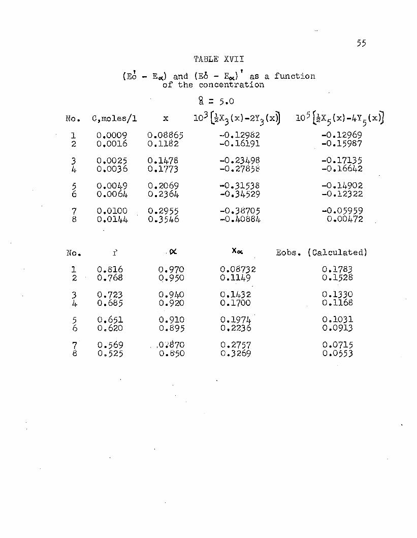
TABLE XVII(Eo - E*) and (E6 - Eot)1 as a function

of the concentration& = 5.0

lo. C,moles/l X 10^ [iX^ (x)-2Xcj (x)J 10 [j X5(x)-4Yt1 0.0009 0.08865 -0.12982 -0.129692 0,0016 0.1182 -0.16191 -0.159873 0.0025 0.1478 -0.23498 -0.171354 0.0036 0.1773 -0.27858 -0.166425 0.0049 0.2069 -0.31538 -0.149026 0.0064 0.2364 -0.34529 -0.123227 0.0100 0.2955 -0.38705 -0.059598 0.0144 0.3546 -0.40884 0.00472

No. f oc Xot Eobs. (Calculated)1 0.816 0.970 0.08732 0.17832 0.768 0.950 0.1149 0.15283 0.723 0.940 0.1432 0.13304 0.685 0.920 0.1700 0.11685 0.651 0.910 0.1974' 0.10316 0.620 0.895 0.2236 0.09137 0.569 , ,0.870 0.2757 0.07158 0.525 0.&50 0.3269 0.0553

TABLE XVII No. 103[jX3(x)-2Y3(x)J(<1 -0.127142 -0.173793 -0.22756k -0.263515 -0.304336 -0.333097 -0.375553 -0.40030

No. -(Eo - E*)1 0.19392 0.19393 0.19424 0.19535 0.19636 0.19747 0.19993 0.2022

56Continued105[lX5{x)-4Y5(x))«

-0.12771 0.313-0.15733 0.772-0.17069 0.730-0.16910 0.694-0.15572 0.661-0.13521 O'. 633-0.03172 0.534-0.02469 0.544

-(e£t- E*)'0.19230.19130.19100.19110.19140.19170.192?0.1933

TABLE XVIII(Eo - E*) and (Eo - E*) * as a function

of the concentrationa r 6.5

No. G,moles/1 X 10? (x)-2X3 (xj) 10^ [|x5 (x)-4Y5(xj)1 0.0009 0.1152 -0.17933 -0.157562 0.0016 0.1537 -0•24422 -0.171503 0.0025 0.1921 -0.29786 -0.159054 0.0036 0.2305 -0.33989 -0.126945 0.0049 0.2689 -0.37109 -0.089246 0.0064 0.3073 -0.39284 -0.046377 0.0100 0.3842 -0.41385 0.033778 0.0144 0.4610 -0.41335 0.09479 0.0196 0.5378 -0.39937 0.1334

No. f oc x* Eobs. (Calculated)1 0.825 0.970 0.1135 0.17832 0.780 0.955 0.1502 0.15283 0.741 0.935 0.1857 0.13304 0.706 0.920 0.2211 0.11685 0.675 0.900 0.2551 0.10316 0.647 O.885 0.2891 0.09137 0.600 0.865 0.3573 0.07158 0.561 0.835 0.4213 0.05539 0.529 0.810 0•4840 0.0417

58

TABLE XVIII Continued No. 103[|X3(x )-2Y3(x ))<iC1 - 0.176262 -0.236643 -0.269714 -0.330625 -0.360966 -0.363637 -0.409466 -0.415749 -0.41025

No. -(Eo - Epc)1 0.19332 0.19283 0.19324 0.19395 0.19506 0.19597 0.19758 0.19999 0.2017

lO^xSfxJÎ^xj}* lie-0.15626 0.827-0.17166 0.764-0.16037 0.747-0.13647 0.714-0.09695 0.686-0.06577 0.6600.01027 0.6150.0650 0.5800.1063 0.551

-(Eo — Ek)»0.19180.19060.18970.18960,18950.18960.19010.19060.1909

59TABLE XIX

(Eo - E*) as a function of the concentrationg = 3.0

No. C,moles/l x 10^ [|X^ (x)-2Y^ (x)J l O ^ X ^ (x)-4X(xjj1 0.0009 0.1418 -0.22530 -0.170492 0.0016 0.1891 -0.29413 -0.160833 0.002$ 0.2364 -0.34529 -0.123224 0.0036 0.2837 -0.38048 -0.072825 0.0049 0.3310 -0.40225 -0.020236 0.0064 0.3782 -0.41313 -0.028127 0.0100 0.i?28 -0.41184 -0.010198 0.0144 0.5674 -0.39164 0.014309 0.0196 0.6619 -0.36205 0.01581

No. f OC Eobs. (Calculated)1 0.831 0.970 0.1397 0.17832 0.789 0.950 0.1844 0.15283 0.753 0.930 0.2279 0.13304 0.720 0.915 0.2712 0.11685 0.692 0.895 0.3131 0.10316 0.666 0.885 0.3559 0.09137 0.623 0.850 0.4359 0.07158 0.$88 0.820 0.5141 0.05539 0.558 0.790 0.5884 0.0417

60TABLE XIX

No. 103 [£x3(x)-2Y3(x)]1 -0.221892 -0.288033 -0.337354 -0.372645 -0.395406 -0.409147 -0.41559s -0.404699 -0.3&563

No. -(E; - Ej1 0.19292 0.19253 0.19264 0.19325 0.19406 0.19457 0.19648 0.19849 0.2003

Continued105[iX5(x)-4Y5(x)]

-0.17023 0.833-0.16543 0.793-0.12942 0.759-0.08804 0.729-0.04335 0.702-0.01027 0.6780.0803 0.6390.1264 0.6070.1464 0.581

TABLE XXObserved Electromotive Force of the Cell

Run A-lMolality NaBr = 0.00610 Molality HAc “ 0.00539 Molality NaAc = 0.00626

Corrected Barometric Pressure 760.2 mm HgEquilibrium Time, Observed E.M.F., volts


0 0.5520 0.552520 0.5490 0.550060 0.5518 0.551690 0.5490 0.5488120 0.5486 0.5466140 0.5486 0.5481165 0.5473 0.5477180 0.5492 0.5481215 0.5480 0.5483245 0.5498 0.5486300 0.5482 0.5490Average. 0.5492 0.5492

0.5492Corrected E, volts 0.5502

TABLE XXIObserved Electromotive Force of the Cell

Run A-2Molality NaBr - 0.00721 Molality HAc = 0.00662 Molality NaAc = 0.00748

Corrected Barometric Pressure 759*7 mm HgEquilibrium Time

minutesObserved E.M.F., voltsAg-AgBr Electrode

#60.5361 0.53840.5378 0.5405

0153045

0.5381 0.54050.5378 0.5390

6075

0.5378 0.54000.5375 0.5386

90110 0.5385 0.54040.5375 0.5405

125150

0.5401 0.54150.5381 0.5386

Average 0.5379 0.53980.5389


TABLE XXIIObserved Electromotive Force of the Cell

Run A—3Molality NaBr = 0.01019 Molality HAc = 0.00891 Molality NaAc = 0.00953

Corrected barometric pressure 756.8 mm HgEquilibrium Time, Observed E.M.F., vo3

minutes Ag-AgBr Electrode. h #60 0.5283 0.527310 0.5277 0.5284

30 0.5290 0,528140 0.5283 0.528665 0.5300 0.5290BO 0.5290 0.5293

100 0.5290 0.5281125 0.5290 0.5305145 0.5294 0.5291160 0.5275 0.5300170 0.5301 0.5296180 0.5280 0.5295190 0.5286 0.5280Average 0.5288

0.52880.5289


TABLE XXIII Observed Electromotive Force of the Cell

Rim A-4Corre Molality NaBr s: 0.00190

Molality HAc s 0.00220Molality NaAc = 0.00212

Corrected barometric Pressure 757.7 mm HgEquilibrium Time, Observed E.M.F., volts

minutes Ag-AgBr Electrode|?2 $50 0.5781 0.580415 0.5796 0.580530 0.5794 0.581145 0.5804 0.580075 0.5804 O.58OO90 0.5810 0.5796105 0.5602 0.5804125 0.5813 0.5798140 O.58O5 0.5605155 0.5810 0.5802170 0.5804 0.5811190 0.5806 O.58OI210 0.5811 0.5810Average O.5803 O.5804

0.5803Corrected E, volts O.58I5

TABLE XXIVObserved Electromotive Force of the Cell

Run A-5Molality NaBr = 0,00373 Molality HAc = 0.00375 Molality NaAc = 0.00411

Corrected barometric pressure 758*3 nun HgEquilibrium Time, Observed E.M.F., vo]

minutes Ag-AgBr Electrode#5 n0 0.5676 0.565020 0.5666 0.5650

55 0.5674 0.565175 0.5673 0.5660

130 0.5668 0.5654145 0.5671 0.5650165 0.5662 0.5652ISO 0,5654 0.5644195 0.5650 0.5645210 0.5670 0.5660230 0.5645 0.5645245 0.5645 0.5648260 O.566O 0.5650Average 0.5663

0.56570.5651


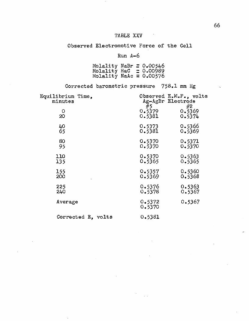
TABLE XXVObserved Electromotive Force of the Cell

Run A-6Molality NaBr z 0.00546 Molality HaC = 0.00939 Molality NaAc = 0.00576

Corrected barometric pressure 753.1 mm HgEquilibrium Time, Observed E.M.F., volts


0 0.5379 0.536920 0.5331 0.537440 0.5373 0.536665 0.5331 0.536930 0.5370 0.537195 0.5370 0.5370

110 0.5370 0.5363135 0.5365 0.5365153 0.5357 0.5360200 , 0.5369 0.5363225 0.5376 0.5363240 0.5373 0.5367Average O.5372 0.5367


TABLE XXVIObserved Electromotive Force of the Cell

Run A-7Molality NaBr z 0.00458 Molality HAc Z 0,00457 Molality NaAc = 0.00517

Corrected barometric pressure 757#5 mm HgEquilibrium Time, Observed E.M.F., volts


0 0.5539 0.559520 0.5592 0.553055 0.5535 0.553475 0.5564 0.553485 0.5533 0.5531

100 0.5571 0.5564120 0.5533 0.5594135 0.5535 0.55321555 0.5530 0.5532170 0.5534 0.5535205 0.5576 0.5590220 0.5599 0.5594Average 0.5536 0*5536


TABLE XXVIIObserved Electromotive Force of the Cell

Run A-8Molality NaBr = 0.00297 Molality HAc = 0.00238 Molality NaAc = 0.00302


minutes Ag-AgBr Electroder r2 r r ?

0 0.5758 0.576415 0.5765 0.575560 0.5760 0.576075 0.5778 0.579090 0.5775 0.5788

105 0.5784 0.5778120 0.5776 0.5784135 0.5776 0.5775150 0.5770 0.5786165 0.5775 0.5770180 0.5766 0.5783195 0.5784 0.5786Average 0.5772 0.5777


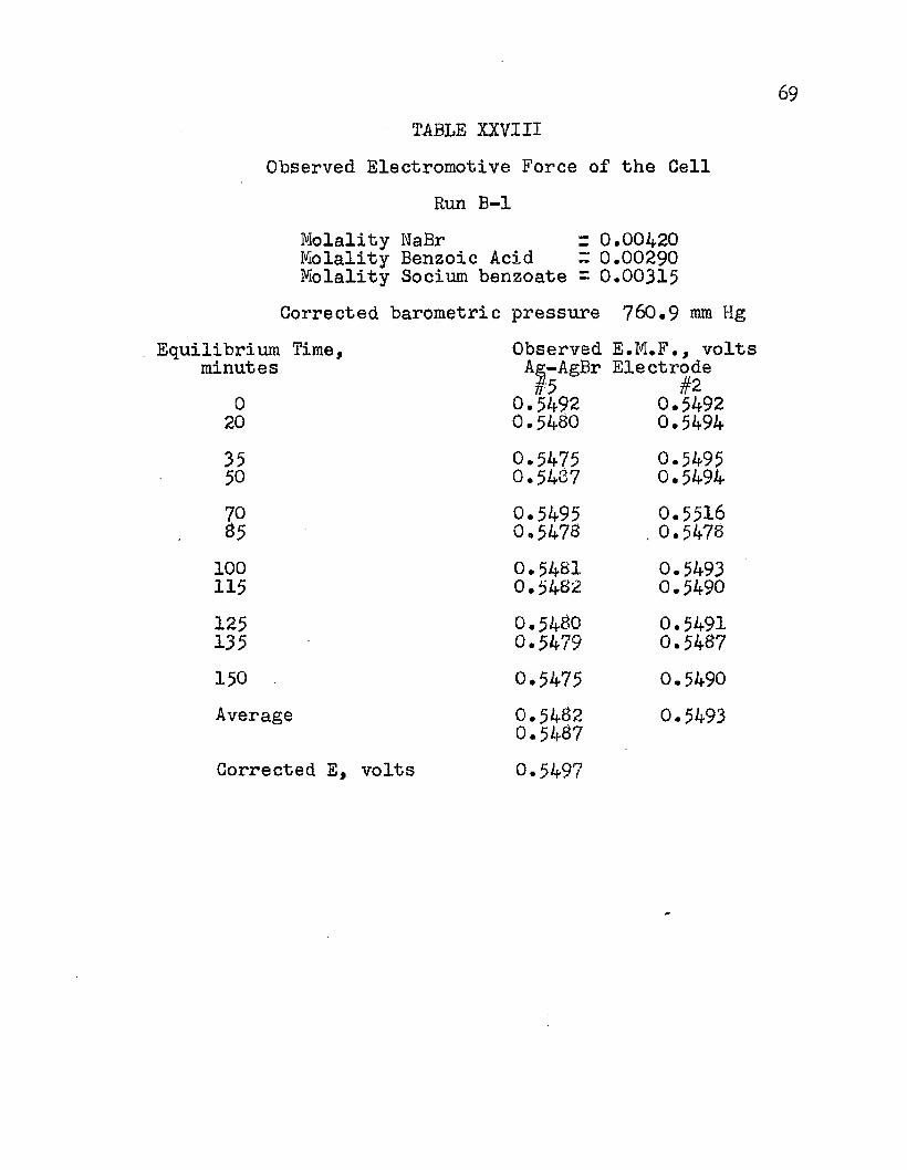
TABLE XXVIII Observed Electromotive Force of the Cell

Run B-lMolality NaBr z 0.00420Molality Benzoic Acid ~ 0.00290 Molality Socium benzoate = 0.00315


minutes Ag-AgBr Electrodeif 5 $20 0.5492 0.5492

20 0.5430 0.549435 0.5475 0.549550 0.5437 0.549470 0.5495 0.551635 0.5473 . 0.5473100 0.5431 0.5493115 0.5482 0.5490125 0.5430 0.5491135 0.5479 0.5437150 0.5475 0.5490Average 0.5432 0.5493


TABLE XXIXObserved Electromotive Force of the Cell

Run B-2Molality NaBr = 0.00709Molality benzoic acid - 0.00554 Molality sodium benzoate = O.OO5I6

Corrected barometric pressure 757*6 mm Hg.librium Time, Observed E.M.F., vojminutes Ag-AgBr Electrode

#5 #20 0.5263 0.527420 0.5270 0.527030 0.5268 0.528540 0.5271 0.527150 0.5260 0.526065 0.5255 0.525075 O.5263 0.527090 0.5261 0.5261105 0.5260 0.5270125 0.5250 0.5250195 0.5250 0.5259235 0.5250 0.5250Average 0.5260

0.5262 0.5264


TABLE XXXObserved Electromotive Force of the Cell

Run 13-3Molality NaBr - 0.00999Molality benzoic acid I 0.00828Molality sodium benzoate - 0.00701


minutes Ag-AgBr Electrodeir5 $2

0 0.5203 0.519830 0.5200 0.519050 0.5193 0.519065 0.5195 O.518685 0.5204 0.5194

120 0.5198 0.5198240 0.5193 0.5190Average 0.5198 0.5192


TABLE XXXIObserved Electromotive Force of the Cell

Run B-4Molality NaBr = 0.00221Molality benzoic acid = 0.00140 Molality sodium benzoate = 0.00132

Corrected barometric pressure 762.0 mm HgEquilibrium Time, Observed E.M.F., vo]

minutes Ag-AgBr Electrode#5:0 0.5627 0.5634

15 0.5644 0.562530 0.5635 0.563445 0.5636 0.563660 O.56I6 0.563985 0.5644 0.5644

110 0.5635 0.5649130 0.5629 0.5625155 0.5664 0.5650175 O.5625 O.5627205 O.5630 0.5640Average 0.5635O.5636 0.5637


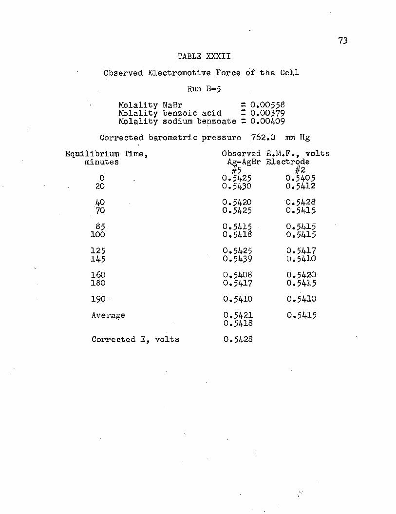
TABLE XXXII Observed Electromotive Force of the Cell

Run B-5Molality NaBr = 0.00558Molality benzoic acid I 0.00379 Molality sodium benzoate = 0.00409


minutes020407085.100125145160180190Average

Observed E.M.F., volts Ag-AgBr Electrode#5

0.5425 0.54300.54200.54250.54150.54180.54250.54390.54080.54170.54100.54210.5418

#2 0.5405 0.54120.5428 0.54150.54150.54150.54170.54100.54200.54150.54100.5415


TABLE XXXIII Observed Electromotive Force of the Cell

Run B-6Molality NaBr " 0.00715Molality benzoic acid z 0.00640 Molality sodium benzoate = 0.00541

Corrected barometric pressure 762.0 mm HgEquilibrium Time, Observed E.M.F., vo3


0 0.5250 0.527320 0.5242 0.526935 0.5240 0.526750 0.5240 0.526465 0.5243 0.526095 0.5236 0.5263335 0.5256 0.5265345 0.5247 0.5264360 0.5258 0*5260375 0.5251 0.5263410 0.5264 0.5264425 0.5255 0.5264445 0.5260 0.5260470 0.5256 0.5264485 0.5284 0.5279Average 0.5252

0.52590.5265


TABLE XXXIV Observed Electromotive Force of the Cell

Run B-7Molality NaBr Z.0.002S4Molality benzoic acid = 0.00242 Molality sodium benzoate = 0.00203



0 0.5525 0.550520 0.5510 0.550535 0.5525 0.551545 0.551S 0.551460 0.5520 0.552075 0.5515 0.551^S5 0.5520 0.551595 0.5515 0.5525105 0.5505 0.5521115 0.5515 0.5520125 0.5519 0.5515135 0.551S 0.5512Average 0.5517 0.5515


TABLE XXXVObserved Electromotive Force of the Cell

Run B-3Molality NaBr r 0,00377Molality benzoic acid - 0,00391 Molality sodium benzoate “ 0,00339

Corrected barometric pressure 760,$ mm HgEquilibrium Time, Observed E.M.F., vo]


0 0.5440 0.545015 0.5452 0.544530 0.5451 0.544645 0.5456 0•544460 0.5456 0.544690 0.5456 0.544610$ 0.5452 0•5444H 5 0.5445 0.5445135 0,5443 0.5443165 0.5455 0.5440Average 0.5451

0.5453 .0.5445


Run No.

TABLE XXXVIThe function -0.0591 log as

dependent on the ionic strength,

mHA mBr mAc

ACETIC ACID

60

A-l 0.00525 0.01236 0.5969A-2 0.00638 0,014699 0.5917A-3 0.00948 0.01977 0.5919A-4 0.00197 0.00402 0.6031A-5 0.00340 0.00784 0.6024A-6 0.00937 0.01122 0.5997A—7 0.00405 0.00975 0.5998A-8 0.00234 0.00599 0.6046

77

-0.0591 log

Âcetic Acid, Ethanol z 2.05x10“^-

BENZOIC ACIDB-l 0.00387 0.00735 0.5886B—2 0.00761 0.01225 0.5836B-3 0.0117 0.01702 0.5878B-4 0.00234 0.00353 0.5906B-5 0.00517 0.00967 0.5892B-6 0.00846 0.01256 0.5859B-7 0.00339 0.00487 0.5881B-8 0.00435 0*00716 0.5882

^Benzoic Acid, Ethanol = l.OlxlO” -0

BIBLIOGRAPHY

Bates, Roger G.Electrometric pH DeterminationsNew York: Johnwiiey and Sons, Inc., 1954*p. 202

Bez-man, I. I. and Verhock, F. H.The Conductance of Hydrogen Chloride and Ammonium Chloride in Ethanol-Water Mixtures.J. Am. Chem. Soc.. 67. 1330 (1945)

Clow, A. and Pearson, G.Pure Ethyl Alcohol for Absorption Spe ctrophotometry.Nature. 144. 208 (1939)

Daniels, FarringtonOutlines of Physical ChemistryNew Yorki”"3ohn Wiley and Sons, Inc., 1952p. 447

Danner, P. S. and Hildebrand, J. H.The Degree of Ionization of Ethyl Alcohol.1. From Measurements of Conductivity J. Am. Chem. Soc., 44* 2824 -{1922)

Encvlopedia of Chemical TechnologyTJew York: Tnterscience Publishers, Inc., 1947

Elliott, J. H. and Kilpatrick, M.The Effect of Substituents on the Acid Strength of Benzoic Acid. II. in Ethyl Alcohol J. Phys. Chem. 45* 466 (1941)

Fuoss, R. M.Solution of the Conductance Equation.

Soc.. ££, 488 (1935)Fuoss, R. M. and Kraus, C. A.

Properties of Electrolytic Solutions. II.The Evaluation of « and of K for Incompletely Dissociated Electrolytes.J. Am. Chem. Soc.. 55_. 476 (1933)

Goldschmidt, H. and Dahll, P.Die Leitfahigkeit und die katalytische Wirkung der drei starken Halogen- Wasserstoffsauren in methyl - und athylalkolischer Losung.2. physik. Chem. Leipsig. 114. 1 (192$)

7911. Gronwall, T. H., LaMer, V. K. and Sandved, K.

Uber den Einfluss der sogennantenhoheren Glieder in der Debye-Huckelschen Theorie der losungen starker Elektrolyte Phvsik. Zi, 22, 358 (1923)

12. Harned, H. S. and Donelson, J. G.The Thermodynamics of Ionized Water in LithiumBromide Solutions.

Chem. Soc.. 1230 (1937)13* Harned, H. S., Keston, A. S. and Donelson, J. G.

The Thermodynamics of Hydrobromic Acid in Aqueous Solutions from Electromotive Force Measurements.

Anu Chem. Soc. j>3, 989 (1936)14. Harned, H. S. and Owen, B. B.

The Physical Chemistry of Electrolytic Solutions.New York: Reinhold Publishing Corporation, 1950, ( Second Edition)

15* Harris, L.Purification arid Ultraviolet Transmission of Ethyl Alcohol.ii Anu Chem. Soc.. ££, 1940 (1933)

16. International Critical TablesNew York: McGraW-Hill Book Company, 1923

17- Keston, A. S.A Silver-Silver Bromide Electrode Suitable for Measurements in Very Dilute Solutions.

Chem. Soc. j>2, 1671 (1935)18s LeBas, Carlyle.

Master*s ThesisLouisiana State University, 1959

19* Lund, H. and Bjerrum, J,Eine einfache Methods Zur Darstellung wasserfreier Alkohole Ber.. 64B, 210 (1931)

20. Maclnnes, D. A.The Principles of ElectrochemistryNew York: Reinhold Publishing Corporation1939

go21. Mukherjee, L. M.

The Standard Potential of the Silver- Silver Chloride Electrode in Ethanol, it Phys. Chem.. £8, 1042 (1954)

22. Osborne, N» S., McKelvy, E. C. and Bearce, H. W.Density and Thermal Expansion of Ethyl Alcohol and its mixtures with water.Bull. Bur. Standards. £ (Mo. 3), 327 (1913)

23. Taniguchi, H. and Janz, G. T.The Thermodynamics of Hydrogen Chloride in Ethyl Alcohol from Electromotive Force Measurements.J. Phys. Chem.. 61, 688 (1957)

24. Woolcock, J. W. and Hartley, H.The Activity coefficients of Hydrogen Chloride in Ethyl Alcohol.Phil. Mag.. 5 (7th Series), 1133 (1928)

VITA

Loys Joseph Nunez, Jr. was born in New Orleans, Louisiana on March 18, 1926. He received his elementary education in the parochial schools of New Orleans and Madisonville, Louisiana.

He was graduated with honors from St. Paul*s College (high school), Covington, Louisiana, in May 1944 and in August, 1947 he received the Bachelor of Science Degree from Tulane University, majoring in Chemistry.

He was then in the employment of Cities Service Refining Corporation and Cities Service Research and Development Corporation for six years.

In September of 1953 he entered the Graduate School of Louisiana State University and received the Master of Science degree in Chemistry in May, 1955* He spent the academic year of 1957-5# as a Fulbright Student at the University of Tubingen, Ttibingen, West Germany. He is at present a candidate for the degree of Doctor of Philosophy.

81

EXAMINATION AND THESIS REPORT

Candidate: Loys J. Nunez

Major Field: Chemistry

Title of Thesis: Thermodynamic Studies in Anhydrous Ethanol - Silver^ Silver Bromide Galvanic Cell

Approved:

if, IMajor Professor and C h a i r m a n //

the Graduate School

EXAMINING COMMITTEE:

Date of Examination: August 3, 19^9

Documents

Thermodynamic Studies in Anhydrous Ethanol. The Hydrogen