Embed Size (px)
Citation preview

RICE UNIVERSITY Thermodynamic Stability and Phase Behavior of Asphaltenes in Oil and of
Other Highly Asymmetric Mixtures
by
P. David Ting
A THESIS SUBMITTED IN PARTIAL FULFILLMENT OF THE
REQUIREMENTS FOR THE DEGREE
Doctor of Philosophy
APPROVED, THESIS COMMITTEE: _____________________________ Walter Chapman, Professor, Chair Chemical Engineering _____________________________ George Hirasaki, A.J.Hartsook Professor, co-Chair Chemical Engineering _____________________________ Clarence Miller, Louis Calder Professor Chemical Engineering _____________________________ Matthias Heinkenschloss, Associate Professor Computational & Applied Mathematics
HOUSTON, TEXAS
MAY 2003

Copyright
P. David Ting
2003

ABSTRACT
Thermodynamic Stability and Phase Behavior of Asphaltenes in Oil
and of Other Highly Asymmetric Mixtures
by
P. David Ting
Asphaltenes are the polydisperse fraction of heavy organics from
petroleum whose phase behavior is important in petroleum production and
processing because of its potential to precipitate and plug tubulars.
The molecular framework used in this work is that van der Waals
(dispersion) interactions dominate asphaltene phase behavior in oil. Using a
proposed reservoir fluid fractionation method and an equation of state (EOS)
asphaltene characterization method that requires only ambient condition titration
data, the Statistical Associating Fluid Theory (SAFT) EOS was extended to
model/predict asphaltene phase behavior in oil. Studies on model asphaltene
systems (polystyrene-hexane, polystyrene-toluene-ethane, long-chain and short-
chain n-alkanes, and phenanthrene-decane-methane mixtures) show that SAFT
can describe the phase behavior of fluids dominated by molecular size and
shape interactions.

Comparison between predicted and experimental asphaltene stability and
oil bubble point curves of a recombined oil and a model live oil measured in this
work show good agreement. The asphaltene stability and the bubble point
measurements for the two oils were made under reservoir conditions as functions
of pressure, temperature, and dissolved gas concentration. Both theory and
experiment show significant temperature effects on asphaltene stability and the
asphaltene instability onset pressures are nearly linear functions of dissolved gas
concentration at each temperature. Furthermore, both SAFT-calculated and
experiment derived mixture solubility parameters/refractive indices along the
asphaltene instability curves are nearly constant at each temperature.
A SAFT investigation into the effects of asphaltene polydispersity shows
that the lower molecular weight (MW) asphaltenes (including resins) play a
significant role in stabilizing higher MW asphaltenes in oil, despite the inclusion
of only dispersion interactions in the model. Resin’s stabilizing effects on
(polydisperse) asphaltene is greatest in the region of incipient asphaltene
instability. In n-alkane titrations, SAFT shows that the heaviest asphaltenes will
precipitate first, followed by the precipitation of smaller asphaltenes on further oil
dilution. The ability to calculate changes in asphaltene MW distribution may be
useful in deposition models.

DEDICATION
To my loving parents
For their unwavering support and their sound advice

ACKNOWLEDGEMENTS
I thank my parents and Christine for their love and support and my parents
for instilling in me the discipline and work ethics that guided me through the worst
times.
I am very grateful for the guidance and advice of Professors Walter
Chapman and George Hirasaki, my two co-advisors. This work would have been
impossible without their insights, their patience and their encouragements. I
especially enjoyed the many Blimpie’s and Wendy’s runs with Dr. Chapman.
I thank the Chapman research group for their help and support, and am
especially grateful for the friendships of Sharon Sauer, Prasanna Jog, and
Auleen Ghosh. I would like to thank Steve Yang, Raymond Joe, and T-C Lee for
their friendship and for many fruitful discussions on a variety of topics from critical
scaling to surface physics.
I am grateful to the many people that made my stay here so enjoyable.
These include: Rebecca Daprato, Ming He, Elizabeth Hedberg, Erik Hughes,
Johnna Temenoff, and Heidi Thornquist.
I would like to thank our collaborators at New Mexico Institute of Mining
and Technology, especially Jill Buckley and Jianxin Wang, for fruitful discussions

vi
on asphaltenes and for providing us with valuable experimental data. I also like
to thank Ahmed Hamammi, John Ratulowski, Kunal Karan, and Kurt Schmidt of
DB Robinson and Nancy Burke and Jeff Creek of ChevronTexaco for many
discussions concerning my thesis research. The experimental portion of this
thesis would have been impossible without the equipment and support of the
people in these organizations. I especially enjoyed the company of Kunal and
Kurt in the brew pubs of Edmonton.
I gratefully acknowledge the Department of Energy, DeepStar,
ChevronTexaco, DB Robinson, and the Consortium of Processes in Porous
Media at Rice University for their financial support. The financial, equipment, and
technical supports of ChevronTexaco and DB Robinson were especially
valuable.

TABLE OF CONTENTS
CHAPTER 1. INTRODUCTION ………………………………………………. 1
CHAPTER 2. BACKGROUND INFORMATION ………………………….….
4
2.1 Physical Properties and Characteristics of Asphaltenes ………. 4
2.2 Economic Significance ……………………………………………. 9
2.3 The Phase Behavior of Asphaltenes in Crude Oil ……………… 10
2.4 Our Hypothesis …………………………………………………….. 13
2.5 Asphaltene Thermodynamic Models …………………………….. 15
2.5.1 Classical Thermodynamic Models …………………….. 16
2.5.2 Colloidal Models …………………………………………. 19
CHAPTER 3. EXPERIMENTS OF ASPHALTENE STABILITY ……………
23
3.1 Introduction …………………………………………………………. 23
3.2 Experimental ………………………………………….……………. 26
3.2.1 Stock Tank Oil Properties ………………………………. 26
3.2.2 Model Oil Preparation .………………………………….. 28
3.2.3 Recombined Oil Preparation ………..………………….. 29
3.2.4 High Pressure and Temperature Apparatus ………….. 29
3.2.5 Procedure ………………………………………………… 31
3.3 Results ……………………………………………..……………….. 34

viii
3.4 Discussions ………………………………………………………… 38
3.5 Summary ……………………………………………………………. 45
CHAPTER 4. EQUATION OF STATE ALGORITHMS ……………………..
47
4.1 Introduction …………………………………………………………. 47
4.2 The SAFT Equation of State ……………………………………… 48
4.3 Reference State Conversions ……………………………………. 57
4.4 SAFT Equation of State Parameters …………………………….. 58
4.5 Phase Stability and Flash Algorithm …………………………….. 62
CHAPTER 5. APPLICATION OF SAFT TO MODEL SYSTEMS ………….
77
5.1 Introduction …………………………………………………………. 77
5.2 Long-Chain Short-Chain Alkane Mixtures ………………………. 78
5.2.1 Background Information ………………………………… 78
5.2.2 Results and Discussions ………………………………... 82
5.2.3 Section Summary ………………………………………... 87
5.3 Polystyrene-Solvent/Precipitant Mixtures ……….………………. 88
5.3.1 Background Information ………………………………… 88
5.3.2 Results and Discussions ………………………………... 89
5.3.3 Section Summary ………………………………………... 97
5.4 Phenanthrene-Solvent/Precipitant Mixtures ……..……………… 98
5.4.1 Background Information ………………………………… 98
5.4.2 Results and Discussions ………………………………... 99
viii

ix
5.4.3 Section Summary ………………………………………... 102
CHAPTER 6. MODELING OF ASPHALTENE PHASE BEHAVIOR ………
103
6.1 Introduction …………………………………………………………. 103
6.2 Model Oil Investigations …… …………………………...………... 104
6.2.1 Determination of Asphaltene SAFT Parameters ……... 104
6.2.2 Comparison of Predicted and Measured Asphaltene
Instability Onsets ………………………………………...
110
6.3 Recombined Oil Investigations ……………………….………….. 113
6.3.1 Separator Gas Characterization ……………………….. 114
6.3.2 Stock-Tank Oil Characterization ……………………….. 115
6.3.3 Recombined Oil Properties …………………………….. 127
6.3.4 Comparison of Predicted and Measured Asphaltene
Instability Onsets ………………………………………...
130
6.4 Summary ………………..………………………………………….. 131
CHAPTER 7. ASPHALTENE SAFT PARAMETER SELECTION RULES .. 133
7.1 Introduction …………………………………………………………. 133
7.2 Effects of Variations in SAFT Parameters on Solubility
Parameter ………………………………….……………………..
133
7.3 Effects of Variations in SAFT Parameters on Molar Volume …. 135
7.4 Effects of Variations in Asphaltene SAFT Parameters on
Mixture Composition at Asphaltene Instability Onset ………..
136
ix

x
7.5 Uniqueness of the Asphaltene SAFT Parameters ……………... 140
7.6 Summary ……………………………………………………………. 143
CHAPTER 8. EFFECTS OF ASPHALTENE POLYDISPERSITY
(INCLUDING RESIN ADDITION) ……………………………
146
8.1 Introduction …………………………………………………………. 146
8.2 Selection of SAFT Parameters for Polydisperse Asphaltenes &
Resins …………………………………………………………….
147
8.3 Effects of Asphaltene Polydispersity and Resin Addition ……… 155
8.4 Summary ……………………………………………………………. 161
CHAPTER 9. REFORMULATION OF THE SAFT DISPERSION TERM
FOR POLYDISPERSITY ……………………..………………
163
9.1 Introduction ……..………………………………….………………. 163
9.2 Algorithm Extension ……………………………………………….. 164
CHAPTER 10. MODIFICATIONS TO THE SAFT ASSOCIATION TERM –
IMPLICATIONS TO MIXTURES CONTAINING WATER …
172
10.1 Introduction ……………………………………….………………. 172
10.2 Theory Modifications ….…………………………………………. 175
CHAPTER 11. CONCLUSIONS AND FUTURE RESEARCH ……………
186
x

xi
REFERENCES ………………………………………………………………….. 193
xi

LIST OF TABLES
CHAPTER 3
Table 3.1 Properties of the oil samples used in this study. 24
Table 3.2 Precipitant volume fractions (φvppt) and mixture
refractive indices (PRI) at the onset of asphaltene
instability for the stock-tank oil mixture and the model
oil.
24
Table 3.3 Stock-tank oil and separator gas compositions. 27
Table 3.4 Asphaltene instability onset and bubble point pressures
of the model live oil.
34
Table 3.5 Asphaltene instability onset and bubble point pressures
of the recombined oil.
36
Table 3.6 Comparison of molar refractions of some compounds
of interest calculated using measured refractive indices
and densities and using group contribution method.
40
CHAPTER 4
Table 4.1 SAFT pure component parameters. 58
Table 4.2 SAFT pure component parameters correlations. 61
Table 4.3 Comparison of flash algorithms on some nonideal
systems.
73
xiii
CHAPTER 5
Table 5.1 Experimentally obtained and regressed pure
component parameters for the Peng-Robinson and
SAFT equations.
83
Table 5.2 Optimum binary interaction parameters for the tested
EOS and average absolute percent deviations between
experimental and calculated phase compositions.
84
Table 5.3 Average absolute percent deviations between
experimental and predicted phase compositions for
SAFT with kij = 0.
87
Table 5.4 SAFT parameters used to model polystyrene phase
behavior.
90
Table 5.5 Select solid, solid-solid, and solid-liquid phase
transition properties of pure phenanthrene.
100
Table 5.6 Pressure-solubility behavior of phenanthrene in toluene
at 293K.
102
CHAPTER 6
Table 6.1 Composition of the separator gas and the pseudo-
component SAFT parameters.
115
Table 6.2 Binary interaction parameters for the separator gas
sub-fractions.
115
Table 6.3 Estimated compositions of each stock-tank oil sub- 118
xiii

xiv
fraction.
Table 6.4 SAFT parameters for the non-asphaltene stock-tank oil
pseudo-components.
119
Table 6.5 SAFT parameter correlations for the saturates and
aromatics+resins oil sub-fractions.
121
Table 6.6 Binary interaction parameters used to fit the stock-tank
oil asphaltenes in SAFT.
125
Table 6.7 Comparison of stock-tank oil SAFT asphaltene
parameters and the n-C7 insoluble model oil SAFT
asphaltene parameters.
126
Table 6.8 Binary interaction parameters between pseudo-
component species in SAFT.
128
CHAPTER 8
Table 8.1 SAFT Parameters for the various asphaltene sub-
fractions (including resins).
152
Table 8.2 Oil and asphaltene properties of four representative
model oils tested to study the effects of asphaltene
polydispersity and resin addition.
157
xiv

LIST OF FIGURES
CHAPTER 2
Figure 2.1 Fractionation of stock-tank oil into saturates, aromatics,
resins, and asphaltenes according to the ASTM D2007-
80 method.
5
Figure 2.2 Relationship between crude oil sub-fractions and coke.
The polydisperse nature of petroleum asphaltenes is
also shown.
6
Figure 2.3 One group’s proposed structures of asphaltene
molecules.
6
CHAPTER 3
Figure 3.1 PRI and φvppt at asphaltene instability onsets for the
model oil and the stock tank oil mixture as a function of
the square root of the precipitant molar volume (vp1/2) at
20°C.
25
Figure 3.2 Diagram of the DB Robinson PVT apparatus used in
this study.
31
Figure 3.3 The onset of asphaltene instability for the model oil at
65.5°C as detected by the light transmittance
apparatus.
32
Figure 3.4 Experimental procedure used in the high pressures
asphaltene instability studies.
33

xvi
Figure 3.5 (a) Asphaltene instability onsets and bubble points for
the model live oil at 20.0°C and 65.5°C. (b) Asphaltene
instability onsets and bubble points for the recombined
oil at 71.1°C.
35
Figure 3.6 Comparison of asphaltene instability onsets and bubble
points for model oil at 65.5°C and recombined oil at
71.1°C.
37
Figure 3.7 Effects of pressure on mass density for (a) model live
oil at 20.0°C and 65.5°C and (b) recombined oils.
38
Figure 3.8 Mixture refractive indices on the asphaltene instability
boundaries (PRI) for model oil at 20.0°C, model oil at
65.5°C, and recombined oil at 71.1°C.
42
Figure 3.9 Measured PRI vs. vp1/2 of n-alkane titrants for the model
oil and calculated PRI vs. vp1/2 of methane for the model
live oil at 20.0°C.
43
Figure 3.10 Mixture refractive indices during pressure depletion for
the model live oil at 20.0°C with 0.143 mass fraction
methane above the bubble point. Asphaltenes are
unstable below the asphaltene instability line.
45
CHAPTER 4
Figure 4.1 Assumptions and limitations of the SAFT EOS. 50
Figure 4.2 In SAFT, fluids are initially considered to be a mixture
of independent segments that are then bonded to form
51

xvii
chains.
Figure 4.3 Comparison of SAFT-predicted compressibility factor Z
as a function of packing fraction η with simulation
results.
53
Figure 4.4 Comparison of SAFT-predicted and experimental
solubility parameters at 25°C and 1 bar.
56
Figure 4.5 Comparison of SAFT-predicted, Peng-Robinson EOS-
predicted, and experimental liquid molar volumes at 1
bar.
56
Figure 4.6 Plots of SAFT pure component parameters with
molecular weight.
61
Figure 4.7 Variation of m with molecular weight for various
compounds.
62
Figure 4.8 Calculation procedure in a typical TP flash algorithm. 65
Figure 4.9 Change in the Gibbs energy of mixing for a binary
mixture at various pressures and compositions. The
pressure-composition diagram is given on the left and
the energy-composition diagrams for various pressure
cuts on the right.
67
Figure 4.10 Proposed phase equilibria calculation procedure. 70
Figure 4.11 Illustration of the tangent plane distance approach to
determine phase stability.
75

xviii
CHAPTER 5
Figure 5.1 Peng-Robinson fits to C6-C16, C6-C24, and C6-C36
mixture phase equilibria data at 622 K or 623 K. The
vapor compositions are expanded on the right and the
mixture critical points are filled.
85
Figure 5.2 SAFT fits to C6-C16, C6-C24, and C6-C36 mixture phase
equilibria data at 622 K or 623 K. The vapor
compositions are expanded on the right and the
mixture critical points are filled.
85
Figure 5.3 Experiment and SAFT-predicted cloud point pressures
for 4% polystyrene solution in n-hexane. The
molecular weights of the polystyrene range from 8,000
to 50,000.
90
Figure 5.4 Experiment and SAFT-predicted cloud point pressures
for 8,000 MW polystyrene in n-hexane. The mass
composition of polystyrene range from 1% to 8%.
91
Figure 5.5 Experiment and SAFT-predicted polystyrene-ethane-
toluene phase diagram at 343K and 62 bar or 117.2
bar.
94
Figure 5.6 SAFT-predicted polystyrene-ethane-toluene phase
diagram at 500 K and 300 or 500 bar.
95
Figure 5.7 Experiment and SAFT-predicted pressure-temperature
diagrams for the system polystyrene-ethane-toluene
with 17.8% mass ethane (78.3% mass toluene) and
97

xix
with 22.5% mass ethane (73.8% mass toluene).
Figure 5.8 Experiment and SAFT+solid fugacity model-calculated
solid-liquid-vapor equilibria for the system
phenanthrene-decane-methane at various pressures
and temperatures.
101
CHAPTER 6
Figure 6.1 Asphaltene SAFT parameters fitting procedure. 107
Figure 6.2 SAFT fits to model oil asphaltene aggregates PRI and
volume fraction precipitants data.
109
Figure 6.3 Ternary phase diagram at 20°C and 1 bar for a mixture
of asphaltene, toluene, and n-pentane.
110
Figure 6.4 Experimental and SAFT-predicted asphaltene
instability onsets and bubble points for the model oil at
20.0°C and 65.5°C.
111
Figure 6.5 Calculated refractive index and SAFT calculated
mixture solubility parameter during pressure depletion
for the model live oil at 20.0°C with 0.143 mass fraction
methane above the bubble point. Asphaltenes are
unstable below the asphaltene instability line.
113
Figure 6.6 Molecular weight distribution of the C10+ saturates. 117
Figure 6.7 Comparison of SAFT-calculated densities for the
mixture of saturates using the one-fluid treatment and
the 26-components treatment.
120

xx
Figure 6.8 Relationship between solubility parameter (at 25°C)
and refractive index (at 20°C) for some select
compounds.
124
Figure 6.9 SAFT fits to stock-tank oil asphaltene aggregates PRI
data.
126
Figure 6.10 Experimental and SAFT-predicted one-phase
recombined oil densities with two different gas-oil
ratios.
129
Figure 6.11 Comparison of SAFT-predicted and measured bubble
points for the recombined oils
130
Figure 6.12 SAFT-predicted and measured asphaltene instability
onset and mixture bubble points for the recombined oil
at 71.1°C.
131
CHAPTER 7
Figure 7.1 Effects of variations in m, σ, and ε/k on the calculated
solubility parameters at 20°C and 1 bar.
134
Figure 7.2 Effects of variations in m, σ, and ε/k on calculated
molar volumes at 20°C and 1 bar. All else being equal,
molecules with lower ε/k have larger molar volumes.
136
Figure 7.3 Effects of changing (a) m, (b) ε/k, and (c) σ for
asphaltenes on the amount of n-alkane precipitants
needed to induce asphaltene instability in the
137

xxi
asphaltene-toluene-n-alkane mixtures.
Figure 7.4 Effects of m and ε/k for asphaltenes on calculated
volume fraction of precipitants at the onset of
asphaltene instability at 20°C and 1 bar.
140
Figure 7.5 Calculated precipitant volume fractions at asphaltene
instability onset using different sets of asphaltene
SAFT parameters. m = 54 in all cases.
141
Figure 7.6 ε/k vs. σ for six sets of asphaltene SAFT parameters
(m=54 in all cases). Different sets of SAFT parameters
that give similar φvppt vs. n-alkane carbon number
curves are connected by lines.
142
Figure 7.7 Asphaltene-toluene-n-heptane ternary phase diagram
for two different asphaltenes that give similar φvppt vs. n-
alkane carbon number curves at 20°C and 1 bar.
143
CHAPTER 8
Figure 8.1 Fitting procedure for polydisperse asphaltenes with
polydispersity captured using three asphaltene pseudo-
components.
150
Figure 8.2 Comparison of SAFT and measured precipitant volume
fraction and mixture refractive index at asphaltene
instability onset for Lagrave asphaltene-toluene-n-
alkane mixtures at 20°C and 1 bar. The initial
asphaltene/toluene ratio is 1g/100mL.
151
xxii
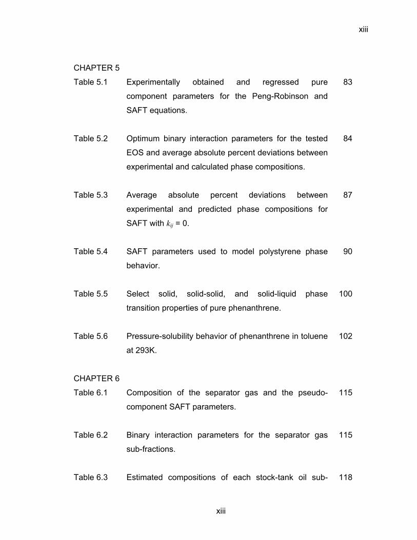
Figure 8.3 Comparison of SAFT and experimental mass
distribution of each asphaltene sub-fraction in Lagrave
asphaltenes.
153
Figure 8.4 Plot of ε/k vs. m for the various SAFT asphaltene sub-
fractions and resin.
155
Figure 8.5 Solubility of monodisperse asphaltenes in model
Lagrave oil (7.5g asphaltenes/100mL toluene) mixed
with n-alkanes at 20°C and 1 bar.
158
Figure 8.6 Solubility of polydisperse asphaltenes (with or without
resins) in model Lagrave oil (7.5g total
asphaltenes/100mL toluene) mixed with n-alkanes at
20°C and 1 bar.
159
Figure 8.7 Normalized distributions of the asphaltene sub-
fractions in the precipitated phase as a function of
volume fraction precipitant in the model oil mixtures.
161
CHAPTER 10
Figure 10.1 Intermolecular potential model for molecules with
square-well sites with angular cutoffs.
177
Figure 10.2 The hard spheres + association model of water used in
this work can qualitatively describe the local structure
of bulk water.
178
Figure 10.3 Comparison of the pair correlation functions obtained
from different methods at a reduced density of 0.39
(η=0.2042).
182

1
CHAPTER 1. INTRODUCTION
The ability to model the thermodynamic phase behavior of mixtures with
large disparities in molecular size and/or shape dominated by nonpolar
dispersion interactions is of considerable interest because of the large number of
industrial processes associated with the mixing and separation of these mixtures.
While the reader can probably think of a few polymer systems as examples of
mixtures with large size/shape disparities, it is not often that one will associate
asphaltenes in crude oil as an example in this category. However, asphaltene
phase behavior in crude oil is an important area of research because crude oil is
the feedstock to most petrochemical processes and asphaltenes are one of the
main culprits behind production and transportation delays. The main focus of this
work is to model and predict the phase behavior of asphaltenes in crude oil under
ambient and reservoir conditions using a statistical mechanical perturbation
theory called SAFT (the Statistical Associating Fluid Theory).
This study contains an experimental and a theoretical component. In the
experimental work (Chapter 3), asphaltene stability boundaries of a model live oil
and a recombined oil were measured under reservoir conditions as functions of
pressure, temperature, and dissolved gas concentration. While much had been
reported on asphaltene stability, most of the studies reported in literature were
performed under ambient conditions. In the theoretical work, an algorithm that is
both robust and efficient was developed (Chapter 4) to calculate phase

2
equilibrium compositions. Using a proposed reservoir fluid fractionation method
and a monodisperse SAFT asphaltene characterization method that requires only
ambient condition titration data, SAFT-predicted asphaltene phase stability
boundaries were compared with experimental data in Chapter 6. In Chapter 7,
the sensitivity and the uniqueness of the fitted SAFT asphaltene parameters
were investigated and a set of asphaltene parameter selection guidelines was
formulated. Since asphaltene exists in nature as a polydisperse mixture of
structurally related molecules, an analysis of the effects of resins (which are
essentially the lowest molecular weight asphaltenes) and asphaltene
polydispersity on SAFT-calculated asphaltene phase behavior in oil is given in
Chapter 8. In Chapter 9, we reformulated the various terms in SAFT so that the
equation of state can more robustly and efficiently account for molecular
polydispersity. Finally, in Chapter 10, a more rigorous implementation of the
SAFT equation of state was introduced to improve SAFT’s ability to model
systems containing water and hydrocarbons.
As the title suggests, a considerable amount of work in this thesis
(Chapter 5) deals with other systems with large disparities in molecular size and
shape. One goal of these investigations is to show that SAFT can be used to
describe the phase behavior of a variety of systems with large size/shape
discrepancies dominated by nonpolar dispersion interactions. The other, more
important, reason for these investigations is to show the reader the connection
between asphaltene and polymer phase behaviors; many “peculiar” behaviors of

3
asphaltenes in oil can be described in terms of the much better understood
polymer thermodynamics.

4
CHAPTER 2. BACKGROUND INFORMATION
2.1 Physical Properties and Characteristics of Asphaltenes
The study of the heavy fractions of petroleum known as asphaltenes and
resins first garnered interests in the 1930s when it was realized that asphaltenes
are widely distributed throughout nature. They are found in native asphalts,
crude oil, bitumen, tar mats, and in dispersed organic matters in sediments.
Coined in 1837 by Boussingault,[1] asphaltene was used to describe the black,
alcohol-insoluble and essence of turpentine-soluble material from crude oil
distillation residues. In modern operations, its definition evolved to loosely
describe the fraction of heavy organics from carbonaceous sources such as
petroleum, coal, and shale oil that is insoluble in low molecular weight n-paraffins
and soluble in aromatic solvents such as benzene and toluene.[2]
The currently accepted definition of asphaltenes is an operational one
based on solubility (Figure 2.1). As such, it reveals little about the structure of
asphaltenes. Considering that oil can contain 100,000+ different molecules[3],
the exact structural definition may never be known. However, most researchers
agree that asphaltenes are a polydisperse mixture of molecules containing
polynuclear aromatics, aliphatics, and alicyclic moieties with small amounts of
dispersed heteroelements such as oxygen, sulfur, vanadium, and nitrogen.
Furthermore, asphaltenes are the heaviest fraction of a distribution (in molecular

5
weight and aromaticity) of compounds that include aromatics and resins in the
lower molecular weight sub-fractions. The accepted definition for asphaltenes is,
in essence, an arbitrarily divided sub-fraction of this distribution. The relationship
between asphaltenes and other classes of compounds in oil is shown in Figure
2.2. As shown in the figure, asphaltenes are more aromatic (low weight percent
hydrogen) than the other oil fractions, are larger in molecular weight, and have
higher solubility parameters. In terms of solubility, resins are often defined as the
propane-insoluble and heptane- and toluene-soluble fraction of the crude oil.
Figure 2.3 shows one set of proposed structures for asphaltene molecules; there
is considerable disagreement on the size and the degree of aromaticity of these
molecules in literature.
Figure 2.1 Fractionation of stock-tank oil into saturates, aromatics, resins, and asphaltenes according to the ASTM D2007-80 method[4]. The figure is reproduced from Wang[5].

6
Figure 2.2 Relationship between crude oil sub-fractions and coke from Wiehe and Liang.[3] The solubility parameter in the figure is given in units of (calories/cm3)1/2.
Figure 2.3 One group’s proposed structures of asphaltene molecules.[6]
Unlike other crude oil components, asphaltenes are unique because they
have a strong tendency to self-aggregate with changes in temperature, pressure,
or mixture composition. Hence, the extent of aggregation may differ depending

7
on the solvent used in the analyses to determine molecular weights and
structures. This (together with asphaltene’s polydispersity in composition) is the
reason why there is considerable difference in the reported molecular weight and
structural properties of asphaltenes. For example, Speight and Plancher[7]
reported an average asphaltene molecular weight of about 2,000 using vapor
pressure osmometry, whereby asphaltenes were dissolved in highly polar
solvents. On the other hand, Wiehe[8] reported an average asphaltene molecular
weight of between 500 and 4,000 using the same technique but with o-
dichlorobenzene as the solvent.
Using fluorescence depolarization (which can detect the size of fused
aromatic clusters), Groenzin and Mullins[9] concluded that each asphaltene
monomer (which can be thought of as a tambourine with dangling arms because
of its large polynuclear aromatic cores) has an average molecular weight of
between 500 to 1,000 and contains 1 or 2 fused polynuclear aromatic clusters
per molecule. These monomer molecules form asphaltene “stacks” in toluene
solution even with asphaltene concentrations as low as 0.06 g/L.[9] There is
considerable variation in the reported number of asphaltene “monomer
molecules” in a stack, and computer simulations show a stack size of about 5
monomer molecules if each monomer molecule is about 10 Angstrom in
diameter.[10]

8
One of the simple techniques that have been used to estimate asphaltene
solubility is to plot the surface tension of a mixture containing asphaltenes
against asphaltene concentration. A break in the surface tension vs. asphaltene
concentration curve can be measured for solutions containing dissolved
asphaltenes.[11] Some researchers call this point of singularity the critical micelle
concentration (cmc) of asphaltenes, with the view that asphaltenes form micelles
in solution (to be discussed in more detail in Section 2.4). The occurrence of a
point singularity in the surface tension vs. asphaltene concentration curve may
simply signal the onset of a phase transition. In either case, the cmc is a
measurable quantity that has been used to estimate the stability of asphaltenes
in different mixtures (such as crude oil blends) and to investigate the
effectiveness of asphaltene inhibitors.
Several other properties of interest include the mass density, the solubility
parameter, and the refractive index of asphaltenes. The mass density of
asphaltenes is estimated by several authors to be between 1.13 g/cm3 and 1.20
g/cm3 using Archimedean techniques, with most authors reporting values closer
to 1.20 g/cm3 than 1.13 g/cm3.[5] Estimated solubility parameters (at 25°C) of
between 19 and 24 MPa0.5 have been reported for asphaltenes based on
solvent-solute mutual solubility.[3,12,13] And refractive indices (at 25°C ) of
between 1.70 and 1.8 have been extrapolated for asphaltenes from diluted
asphaltene solutions in toluene.[5]

9
2.2 Economic Significance
Asphaltene is suitably termed the “cholesterol of petroleum”[14] because of
its ability to precipitate with changes in crude oil temperature, pressure, and
composition. These precipitates may in turn adhere to surfaces or change crude
oil rheology. The economic implications of asphaltene precipitation from crude
oils are significant in petroleum production and refining because of this
precipitation/adhesion potential. Deposition and subsequent fouling, occlusion,
or damage have been observed in all aspects of petroleum recovery and
processing, from near wellbore formations to well bores and well tubings to
pipelines to refinery units. Furthermore, the asphaltene problem shows no
geographic boundaries. Asphaltene related problems have been encountered in
all parts of the world, from the North Sea to North Africa to the Americas.[15-18]
And depositions may occur even in fields that have very little asphaltenes. For
instance, depositions were reported in well tubings and production processing
facilities of the Ula reservoir in the North sea despite the crude oil having only
0.57% mass asphaltene.[17] Finally, asphaltene problems may disappear in later
stages of primary depletion (as in the case of Ventura Avenue field in
California[16]) because normal production tends to produce the lighter fractions
first (due to higher mobility) and the residual asphaltene fractions are gradually
stabilized (the reasons for this will be discussed in the next section).
In spite of nearly 70 years of asphaltene research, our understanding of
the material is still at its infancy. This is due partly to the complex nature of

10
asphaltene and partly to the difficulties involved in conducting asphaltene
research in its natural reservoir environment. As the industry moves towards
deeper reservoirs and relies more on integrated production systems (both sub-
sea and on-shore), the probability of encountering asphaltene precipitation
problems will only increase and the economic implications will become more
significant.
2.3 The Phase Behavior of Asphaltenes in Crude Oil
The behavior of asphaltenes in oil can be deduced by examining a few
representative examples of field experiences with asphaltene problems.[15,16,19-
22] From these experiences, it can be concluded that pressure contribution to
asphaltene phase separation is most pronounced for light oil near its bubble
point. Asphaltenes are usually stable in highly under-saturated oils. And at
pressures well below the bubble point, asphaltenes tend to be stable since most
of the precipitants (methane, ethane, nitrogen, etc.) have escaped from the
liquid. Furthermore, light oils with little asphaltenes are the most susceptible to
asphaltene problems. Compositional changes such as oil blending or miscible
flooding sometimes result in asphaltene precipitation. And temperature changes
may result in either asphaltene precipitation or solubilization. For instance, in the
propane deasphalting process, asphaltenes become increasingly unstable with
temperature increase.[23] However, for n-alkane (n-C5+) titrations, asphaltene
stability improves with increasing temperature.[23]

11
These observations concerning asphaltene precipitation can be explained
in terms of changes to crude oil cohesive energy density (CED) with changes in
temperature, pressure, and/or composition. CED is defined by Hildebrand and
Scatchard for regular (i.e. nonpolar) fluids as the square of the solubility
parameter δ and can be approximated as[24]
i
rsmi
ii vU
CED−
=≡ 2δ (2.1)
where rsmiU is the residual internal energy (the internal energy obtained by
subtracting the ideal gas contribution from that of the real fluid) and vi is the liquid
volume of pure species i. For binary mixtures, the residual internal energy can
be approximated as[24]
jjii
jijijijjjiiirsmmix vxvx
xxvvCEDCEDxvCEDxvCEDU
+
++−=
22222
(2.2)
where xi is the mole fraction of the ith species. Equations 2.1 and 2.2 show the
dependence of mixture CED on density and on the CED (or solubility parameter)
of the component species.
Alternatively, from statistical mechanics, we can approximate[25]
∑∑ ∫+
=
+
=
∞
=ba
a
ba
b
rsmmix drrrgrNN
vU
α βαβαββα φπ
0
2)()(2 (2.3)
where a and b denote species type, Nα and Nβ are the number of α and β
molecules, gαβ is the pair correlation function, r is distance, and φαβ is the
molecular interaction potential. Eqn. 2.3 provides more insight to the behavior of

12
fluids at the molecular level (than Eqn. 2.2) because it relates molecular
interaction potentials to bulk properties.
For mixtures dominated by van der Waals’ interactions (also called
dispersion or non-polar interactions), φab in Eqn. 2.3 has an attraction contribution
proportional to the product of the interacting species’ electronic polarizabilities
and inversely proportional to the sixth power of molecular distance.[26] Hence for
non-polar mixtures, the mixture’s CED is a function of density and the electronic
polarizabilities of the mixture’s constituent species. As a measure of the
displacement of a molecule’s electron clouds under the influence of external
electric fields, electronic polarizability is dependent on the structure of the
molecule and on the frequency of the external electric field but is, to the first
order, independent of thermodynamic state. The polarizability of molecules
dominated by nonpolar interactions are insensitive to the frequencies of the
external electric field below those of visible light.[26]
The behavior of asphaltenes in crude oil can be described in terms of
changes to the oil’s cohesive energy density. Above the bubble point, further
pressure increases lead to increasing oil density, which increases the oil’s CED
and makes asphaltenes more stable. Below the bubble point, there is a net
increase in density with pressure decrease due to the release of lighter
hydrocarbons from the oil. Again the oil becomes a better solvent for
asphaltenes. An increase in temperature decreases the oil density but at the

13
same time increases the entropy of the solution, resulting in a counter balancing
effect. Composition changes that increase density may improve asphaltene
solubility, and composition changes that decrease density may have the opposite
effect. The inclusion to the oil of species with lower polarizabilities (e.g. addition
of methane or blending with lighter oils) will decrease the oil’s CED and increase
the likelihood of asphaltene flocculation. And the inclusion of species that are
similar in polarizability (e.g. addition of toluene) will keep asphaltenes from
becoming unstable. Because both density and component polarizability affect a
mixture’s CED, opposing effects may be observed. For example, CO2 may be
more dense than oil at high pressures but may act as a precipitant because of its
low polarizability. Evidence of the important role of cohesive energy density (or
solubility parameter) on asphaltene behavior points to the significance of
nonpolar interactions in determining asphaltene phase behavior in crude oil.
2.4 Our Hypothesis
The underlying hypothesis of our approach is that molecular size and
nonpolar van der Waals interactions dominate asphaltene phase behavior in
reservoir fluids. We have described in the previous section how asphaltene
phase behavior can be qualitatively explained in terms of nonpolar interactions.
Our hypothesis is also supported by other evidence:
(1) The intermolecular interaction energies due to the polynuclear
aromatic cores (which are plate-like structures with large surface areas) may be

14
similar or larger in magnitude than the energies due to polar interactions. For
instance, Khryaschchev, et al.[27] calculated the energy between the polynuclear
aromatic cores of asphaltenes to be about 80 kJ/mol, which is much larger than
the hydrogen bonding interaction energy in water (~15 kJ/mol).
(2) An investigation of asphaltene solubility in over 40 polar and nonpolar
solvents by Wiehe[8] shows that asphaltenes are soluble in solvents with high
field force solubility parameters (which is a measure of nonpolar, mean field
interaction strength) and insoluble in solvents with moderate and high
complexing solubility parameters (which is a measure of hydrogen bonding and
polar interaction strengths).
(3) One traditional viewpoint on asphaltene behavior relies on a micellar
model in which asphaltenes are stabilized by resins via polar-polar interactions.
The basis of this viewpoint is that asphaltenes and resins are the most polar
fractions of crude oil because they contain heteroatoms of various proportions.
When resins are added, less asphaltenes will precipitate. And when n-alkanes
are added, asphaltenes will precipitate because of the dilution of resins in the
mixture. The argument is similar to the explanation given for the addition of
surfactants (resins) to an oil/water mixture to stabilize the dispersion; stable
micro-emulsions would form with sufficient surfactant addition. However,
nonpolar diluents of similar size and structure can be either precipitants or
solvents for asphaltenes. For instance, toluene (C6H5CH3) is a good nonpolar

15
solvent for asphaltenes while n-heptane (C7H16) is a nonpolar precipitant.
Similarly, both carbon disulfide (CS2) and carbon dioxide (CO2) are nonpolar and
of similar molecular structure but CS2 is a good solvent for asphaltenes while
CO2 is a precipitant.
In a few situations, the role of polar or hydrogen bonding interactions may
become important. For example, asphaltenes may aggregate on the water-oil
interface and stabilize water emulsions.[28] And addition of a sufficiently large
amount of alkyl-benzene derived amphiphiles (such as dodecyl benzene sulfonic
acid) would inhibit asphaltene aggregation.[29] While polar interactions may play
a role, our hypothesis is that asphaltene phase behavior in the reservoir is
shaped to a larger extent by the nonpolar interactions in the oil.
2.5 Asphaltene Thermodynamic Models
Thermodynamic models of asphaltene phase behavior in crude oil
generally fall under one of two molecular thermodynamic frameworks, mirroring
the two prevalent schools of thought regarding how asphaltenes are stabilized in
crude oil. The first approach assumes that asphaltenes are solvated in crude oil
and that these asphaltenes will precipitate if the oil solubility drops below a
certain threshold. The Flory-Huggins-regular-solution based models and the
cubic equation of state based models are some examples of this
approach.[5,13,30-32] Thermodynamic models in the second category take the
colloidal approach to describe asphaltene behavior and the presence of resins

16
becomes critical in stabilizing asphaltenes. The solid-asphaltene colloidal model
proposed by Leontaritis and Mansoori[33], the reversible micellization model
proposed by Victorov and Firoozabadi[34], and the McMillan-Mayer-SAFT based
theory proposed by Wu[23] are some examples in this category.
2.5.1 Classical Thermodynamic Models
One of the most widely used classical thermodynamic models to describe
asphaltene behavior is the Flory-Huggins-regular-solution theory:[24]
( ) )(lnln 21*2
*1
221
1*22
*11 rNN
RTvNN
RTGmix +ΦΦ−+Φ+Φ=
∆ δδ (2.4)
where
21
2*2
21
1*1 ;
rNNrN
rNNN
+=Φ
+=Φ (2.5)
In Eqn. 2.4, ∆Gmix is the change in Gibbs energy on mixing, R is the gas constant,
T is temperature, v1 is the molar volume of the solvent, N1, N2 are the number of
solvent and solute molecules, respectively, r is the ratio of solute to solvent
volume, and δ1, δ2 are the solubility parameter of the solvent and solute at T. Φ*
in Eqn. 2.5 is the volume fraction of either the solvent or the solute species.
The application of this model to describe asphaltene phase behavior was
first proposed by Hirschberg, et al.[13] In the Hirschberg implementation, the
asphaltene-rich phase is assumed to be pure asphaltenes (i.e. Φ2* = 1 where the
subscript 2 denotes asphaltenes). Furthermore, the amount of asphaltenes in
the asphaltene-lean phase is assumed to be very small (i.e. 1*2 <<Φ ). With

17
these assumptions and applying the condition of chemical potential equality at
equilibrium (see Chapter 4), the composition of asphaltenes in the asphaltene-
lean phase becomes
( )
−−+−=Φ −
212
1*,2 1exp δδ
RTrvrleanasphaltene (2.6)
If the solvent (crude oil) and asphaltene solubility parameters and the solvent
molar volume can be measured, the volume fraction of asphaltenes in the
asphaltene-lean phase becomes a function of asphaltene molar volume only.
Other models based on the Flory-Huggins-regular-solution theory
change/relax the assumptions made by Hirschberg, et al.[13] For instance, in the
implementation of Cimino, et al.[31], a pure solvent phase is assumed to form
upon phase separation. And in the implementation of Wang[5], each of the
coexisting phases can have asphaltenes as well as solvents.
While the Flory-Huggins-regular solution based approaches have been
used with varying success to model asphaltene solubility with n-alkane titrations
under ambient conditions, it is difficult to extend the approach to model
asphaltene solubility under reservoir conditions. In a sense, the theory is not a
“complete” equation of state; unless the volumes and solubility parameters are
measured under reservoir conditions, these values must be obtained from
another equation of state or estimated from empirical correlations. Furthermore,
the model cannot reproduce/predict certain classes of phase diagrams unless
extremely temperature dependent energy modification parameters are
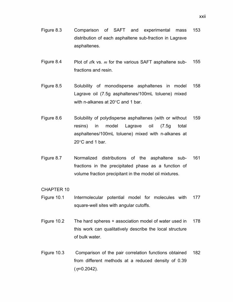
18
introduced. For instance, the model is incapable of showing lower critical
solution behavior in systems of large size differences unless extremely
temperature dependent binary interaction parameters are used.
Another popular approach in the classical thermodynamics framework to
model asphaltene behavior is to use the cubic equations of state. A description
of one of the cubic equations (the Peng-Robinson equations) is given in Chapter
5. In the method proposed by Nghiem, et al.[35], the C31+ heavy end of crude oil
is first divided into nonprecipitating and precipitating sub-fractions. Different
interaction parameters (between these sub-fractions and light ends) are then
assigned to reproduce experimental results. In another example, Akbarzadeh, et
al.[30] modified the Soave-Redlich-Kwong cubic equations by adding an additional
aggregation size parameter to asphaltenes.
The cubic equations have relatively simple functional forms and are easy
to implement into existing reservoir simulators because cubic equations have
been used extensively to describe the thermodynamic behavior of reservoir
fluids. However, their major shortcomings are that the equations of state cannot
describe the phase behavior of systems with large size disparities and that they
cannot accurately describe fluid densities. While the calculated densities can be
modified using volume translation techniques, volume translations do not affect
phase equilibria calculations. These issues will be addressed in more detail in
Chapter 5.

19
As mentioned above, the Flory-Huggins-regular-solution model is not a
“complete” equation of state because it requires as input physically-based
parameters that must be obtained using other methods. Hence the Flory-
Huggins-regular-solution model has been often used in conjunction with other
equations of state to model asphaltene solubility. For example, in the work of
Chung, et al.[36], the Flory-Huggins-regular-solution model is combined with the
Peng-Robinson cubic equations to model asphaltene solubility in oil. And in the
work of Burke, et al.[37], the Flory-Huggins-regular-solution model parameters
were obtained from the Zudkevitch-Joffe-Redlich-Kwong equations.
2.5.2 Colloidal Models
The colloidal models assume that crude oil can be divided into polar and
nonpolar sub-fractions; the saturate and aromatic components make up the
nonpolar sub-fraction while asphaltenes and resins comprise the polar sub-
fraction. The model due to Leontaritis and Mansoori[33] is one of the earliest
models using this approach. In this model, asphaltenes are assumed to be
insoluble solid particles suspended in oil and kept in solution by resins (which
adsorb onto the surfaces of asphaltene molecules). For asphaltenes to stay in
solution, resins must be present. Dilution of the resins below a certain threshold
will cause asphaltenes to precipitate.

20
In the approach due to Pan and Firoozabadi and Victorov and
Firoozabadi[38] (the reversible-micellization approach), the assumption that
asphaltenes are insoluble solid particles is relaxed. In this approach, the total
Gibbs energy of a system consisting of a liquid phase and a precipitated phase is
minimized to calculate equilibrium phase compositions. The liquid phase
consists of a mixture of monomer asphaltenes, monomer resins, asphaltene-
resin micelles, and other oil species. And the precipitated phase is assumed to
consist solely of asphaltenes and resins that do not associate with each other.
An equation of state (such as the Peng-Robinson cubic equations) is used to
calculate the fugacity coefficients of each species (including those of asphaltenes
and resins).
To calculate the Gibbs energy of the liquid phase, an expression for the
energy change due to asphaltene-resin micelle formation is needed:
( ) ( )[ ] ( ) ( ) ( ) ( )[ ]defradsrtrrmdefatram GGGGGGG 000int
00000 ∆+∆+∆+∆+∆+∆=∆ (2.6)
( )traG 0∆ is the Gibbs energy change due to the transfer of asphaltene (subscript
a) molecules from an infinitely dilute solution to an aggregated, pure asphaltene
state. ( )defaG 0∆ is the Gibbs energy of deformation of asphaltene molecules and
( )int0aG∆ is the interfacial Gibbs energy of the formation of micellar cores. Since
resins also take part in the formation of micelles, their energy contributions are
accounted for in the terms with the subscript r. Additionally, an energy

21
contribution due to the adsorption of resins onto asphaltene micellar cores is
needed ( )adsrG 0∆ .
While the reversible-micellization model has shown some success in
describing the effects of pressure and concentration on asphaltene
precipitation[38], a large number of parameters are needed in the model. Each
species in the model (including asphaltenes and resins) requires a set of
equation of state parameters. If the cubic equations are used (i.e. the Peng-
Robinson equations), 3 pure species parameters plus a set of interaction
parameters are needed for each pure component. To calculate the energy of
micellization, parameters such as the size of the micellar core, the average
characteristic length of the oil (non-asphaltene) molecules, the interfacial tension
between the asphaltene in the micellar core and the bulk oil, the thickness of
each asphaltenes-resins micelle, and the adsorption energy of the resins onto
the asphaltene micellar core, among others, are needed. It is not clear how
some of these parameters vary with changes in pressure, temperature, and oil
composition.
In a third approach due to Wu and Prausnitz[23], asphaltenes are assumed
to be large spherical molecules with multiple association sites that can bind to
other asphaltenes and to resins (which are smaller molecules with only one
association site per molecule). The theory is presented in the McMillan-Mayer
framework using the Statistical Associating Fluid Theory (SAFT) to describe the

22
free energy of association between asphaltenes and resins. Hence, only
asphaltenes and resins exist as real molecular species; other components in the
oil exist solely as “background” contributions to the free energy of the mixture.
An advantage of the McMillan-Mayer-SAFT approach is that the
complexity of the problem can be significantly reduced by formulating the theory
in the McMillan-Mayer framework. Furthermore, the theory can account for the
effects of resins addition and asphaltene solvent addition on the solubility of
asphaltenes. The addition of resins would “tie” up bonding sites on asphaltenes
that otherwise would bind to other asphaltenes, and the addition of asphaltene
solvents would improve asphaltene solubility by changing the magnitude of the
“background” energy. One potential issue with this approach is that it is not clear
how the McMillan-Mayer approximations affect the energies calculated by SAFT.
As a statistical mechanical equation of state based on the perturbation of
molecular segment densities (see Chapter 4 and 10), even molecular species
that do not associate contribute to the association energy calculations indirectly
in SAFT by their contribution to the correlation functions. In the approach
proposed by Wu and Prausnitz[23], only asphaltenes and resins are “real”
molecules and the presence of the nonassociating species (that exist in the oil
and affect the extent of association) are ignored.

23
CHAPTER 3. EXPERIMENTS OF ASPHALTENE STABILITY
3.1 Introduction
The objective of this experimental study is to provide a set of data to test
models of asphaltene precipitation from crude oil. We performed experiments
simulating reservoir depressurization on a model live oil (mixture of toluene,
methane, and n-heptane insoluble asphaltenes) and on a recombined oil (stock-
tank oil with its separator gas). The asphaltene stability boundaries and mixture
bubble point curves of these oils were measured as functions of pressure,
temperature, and dissolved gas concentration. The effects of pressure on
mixture density were also monitored from constant composition volume
expansion measurements.
A set of titration experiments with n-heptane, n-undecane, and n-
pentadecane titrants were also performed on the model oil and stock-tank oil
described above. These ambient condition titration experiments were performed
by J.X. Wang at New Mexico Institute of Mining and Technology (NMT) using
different oil samples (but all are from the same reservoir, see Table 3.1). The
titration procedure is described in Ting, et al.[39] and the titration results are given
in Table 3.2 and Figure 3.1 in terms of the n-alkane precipitant volume fraction
(φvppt) and the refractive indices at the onsets of asphaltene instability (PRI). Note
that equi-volume of α-methyl-naphthalene was added to the stock-tank oil before

24
the ambient condition titration experiments to dissolve any preexisting solids in
the oil. For a given oil/precipitant pair, the addition of asphaltene solvents (such
as α-methyl-naphthalene) to the oil changes the amount of precipitant needed to
induce asphaltene precipitation but has little effect on the mixture’s refractive
index at precipitation onset. [40]
Table 3.1 Properties of the oil samples (all from the same reservoir) used in the study.
stock-tank oil used in this
study to make the recombined
oil
stock-tank oil used in titration
study at ambient
conditionsa
source of extracted
asphaltenes used to make the model
oila
density at 20°C (g/cm3) 0.857 0.8673 0.8679 saturates (mass %) 72.3 70.6 70.6 aromatics (mass %) 16 16.3 15
resins (mass %) 9.2 11.4 12.9 asphaltenes (mass %) 2.5 1.7 1.5
a Measured by Jianxin Wang at New Mexico Institute of Technology.
Table 3.2 Precipitant volume fractions (φvppt) and mixture refractive indices (PRI)
at the onset of asphaltene instability for the stock-tank oil mixture and the model oil.a
model Oil equi-volume & α-methyl
stock-tank oil -naphthalene
precipitant φv
ppt PRI φvppt PRI
n-C7 0.45 1.4477 0.66 1.4444 n-C11 0.42 1.4618 0.65 1.4632 n-C15 0.36 1.4721 0.59 1.4795
a Measured by Jianxin Wang at New Mexico Institute of Technology.

25
Figure 3.1 PRI and φvppt at asphaltene instability onsets for the model oil (square)
and the stock-tank oil mixture (triangle) as a function of the square root of the precipitant molar volume (vp
1/2) at 20°C.
The reservoir condition depressurization experiments (performed in this
work) and the ambient condition titration experiments (performed by NMT)
provide a set of data on asphaltene stability in a wide range of nonpolar
precipitants from methane and separator gas (which is primarily methane,
ethane, and propane) to n-pentadecane. Our hypothesis is that the mechanism
responsible for asphaltene precipitation under reservoir depressurization is
consistent with the mechanism in titration experiments. If this is true, we expect
that thermodynamic models that account for van der Waals interactions,
molecular size, and pressure effects should be able to predict the

26
depressurization results based on matching the results of the titration
experiments.
3.2 Experimental
3.2.1 Stock-Tank Oil Properties
The stock-tank oil used in this study has a density of 0.857 g/cm3 at 293K
and 0.848 g/cm3 at 328K (both at 14.5 psi). This corresponds to an API gravity
of 33.6° at 293K. Using the ASTM D2007-80 method[4], the stock-tank oil was
fractionated into 72.3% (mass) saturates, 16.0% (mass) aromatics, 9.2% (mass)
resins, and 2.5% (mass) n-heptane insoluble asphaltenes (Table 3.1). A
breakdown of the oil composition is shown in Table 3.3. The composition was
determined using gas-chromatography. A generalized single carbon number
correlation due to Katz and Firoozabadi[41] was used to estimate the molecular
weight of C10+ petroleum sub-fractions. The correlation is based on normal
boiling point distillation data of more than 26 condensates and liquid
hydrocarbons.

27
Table 3.3 Stock-tank oil and separator gas compositions.
reservoir gas stock-tank oil
component molecular mass mass weight fraction fraction
CO2 44.01 0.019 N2 28.01 0.136 C1 16.04 0.285 C2 30.07 0.139 C3 44.10 0.141 C4 58.12 0.147 C5 72.15 0.080 0.001 C6 86.20 0.027 0.004
m-cyclopentane 84.16 0.001 benzene 78.11 0.000
cyclohexane 84.16 0.001 C7 100.20 0.016 0.009
m-cyclohexane 98.19 0.004 toluene 92.14 0.001
C8 114.23 0.008 0.020 ethyl-benzene 106.17 0.001
xylene 106.17 0.005 C9 128.30 0.002 0.027 C10 134.00 0.041 C11 147.00 0.041 C12 161.00 0.040 C13 175.00 0.045 C14 190.00 0.042 C15 206.00 0.044 C16 222.00 0.038 C17 237.00 0.035 C18 251.00 0.035 C19 263.00 0.034 C20 275.00 0.031 C21 291.00 0.028 C22 305.00 0.025 C23 318.00 0.024 C24 331.00 0.021 C25 345.00 0.022 C26 359.00 0.017 C27 374.00 0.020 C28 388.00 0.017 C29 402.00 0.017 C30+ 580.00 0.307

28
3.2.2 Model Oil Preparation
Asphaltenes were extracted from a slightly different stock-tank oil from the
same reservoir (Table 3.1) using a modified ASTM-D2007-80 procedure. [4] The
extraction was performed by J.X. Wang at New Mexico Institute of Mining and
Technology. A 40:1 excess volume of n-heptane was mixed with the oil for two
days and the solution filtered through a range of filters from 8 down to 0.22 µm.
The collected solids were redissolved in excess toluene (to a concentration of
about 0.5%) and the solution filtered (with 0.22 µm filter) to remove any
nonasphaltic solids. The filtrate was then concentrated using a rotary evaporator
and the asphaltenes reprecipitated with 40:1 excess volume of n-heptane. After
filtration with 0.22 µm filter, the solids were dried at ambient conditions for two
days.
To prepare the model oil, the extracted asphaltenes were dissolved in
degassed toluene (Fisher Scientific, Certified ACS Grade) at a ratio of 1 g
asphaltenes per 100 mL toluene at 20°C and atmospheric pressure. The mixture
was stirred constantly and aged for two days before being filtered through a 0.20
µm (Osmonics Inc. Silver Membrane) filter. The mass of undissolved solids
removed equaled 7% to 8% of the mass of asphaltenes initially present in the
model oil mixture.
29
3.2.3 Recombined Oil Preparation
Separator gas (0.378 g/cm3 at 293K and 3,500 psi) with the composition
given in Table 3.3 was prepared and mixed with the stock-tank oil to create a
recombined oil with a targeted gas-oil-ratio (GOR) between 140 and 150 m3/m3.
The recombined oil was first aged for four days at 71.1°C and 6,000 psi outside
the PVT cell and then kept at 71.1°C and 8,588 psi inside the PVT cell for 24
hours before use. The GOR of the prepared recombined oil was determined to
be 152 m3/m3 using a DB Robinson Gasometer. Since the total mass of the one
phase fluid in the PVT cell, the stock-tank oil density at ambient conditions, and
the gas-oil-ratio were known, the mass of the dissolved gas could be calculated.
The ideal gas equation of state was used to estimate gas density at ambient
conditions using an average molecular weight of 28.5 obtained from composition
data.
Asphaltene problems that occurred in the field from which this oil sample
was taken were associated with injection of CO2. Because asphaltene related
problems were not observed in the field prior to the introduction of CO2, it is
unlikely that asphaltene precipitation would be observed if the oil were
recombined to a GOR representative of down-hole samples. Therefore more
separator gas was added in all experiments than the amount observed in down-
hole samples.
3.2.4 High Pressure and Temperature Apparatus

30
A near infrared laser (2.0 milliwatts) transmittance device mounted on a
visual PVT cell was used to detect phase instability onsets (Figure 3.2). The
apparatus was designed and manufactured by DB Robinson. With this system,
asphaltene instability and bubble point onsets could be observed as sudden
decreases in light transmittance (due to increased light scattering caused by the
formation of a second phase). The PVT cell had a maximum operating pressure
of 15,000 psi and was mounted in an air temperature bath. The fluid of interest
was placed inside a Pyrex glass cylinder (maximum sample volume of about 113
cc) and stirred using a magnetically coupled mixer. A volume displacement
pump (DBR Series II Pump) controlled system pressure by adjusting the amount
of overburden fluid based on readings from a digital Heise pressure gauge
(accurate to ±0.15% of 15,000 psi). The pressure gauge was located on the
overburden side of the apparatus. The cell temperature was measured using a
platinum RTD (accurate to ±0.05°C). During each experiment, the fluid volume
was monitored using an external CCD camera (accurate to ±0.002 cc).
Additional fluid or gas could be added into the cell using a mercury displacement
pump (accurate to ±0.005 cc) via a port next to the magnetic stirrer.

31
Figure 3.2 Diagram of the DB Robinson PVT apparatus used in the study.
3.2.5 Procedure
For the model oil investigations, a measured amount of the asphaltene-
toluene mixture was fed into the PVT cell and pressurized to 5,500 psig. After
temperature equilibration, a known amount of Air Product Ultra High Purity
methane (at 6,000 psig, 20°C) was injected and the mixture pressurized to
between 8,000 and 14,000 psig (depending on the amount of methane in the
system) for up to 24 hours to redissolve any of the asphaltenes that might have
precipitated during methane injection. While such pressurization led initially to
dramatic increases in light transmittance, transmittance reached a plateau after
about 12 hours and the change in transmittance became negligible after that
point.

32
To trace out the asphaltene instability and bubble point boundaries, the
model live oil was slowly depressurized at 45 minutes per pressure step until
asphaltene instability onset. We defined the onset asphaltene instability
pressure as the average between the first pressure (i.e. the highest pressure in a
depressurization experiment) at which transmittance decreased continuously with
time and the pressure step before that (see Figure 3.3). As a polydisperse
mixture, some asphaltenes could have already phase separated at even higher
pressures but were not observed due to instrument limitations.
Figure 3.3 The onset of asphaltene instability for the model oil at 65.5°C.
Below the asphaltene instability onset pressure, the system was
depressurized quickly until the mixture bubble point was reached (as determined
by light transmittance and corroborated with sudden change in overall system
onset of asphalteneinstability
onset of asphalteneinstability
33
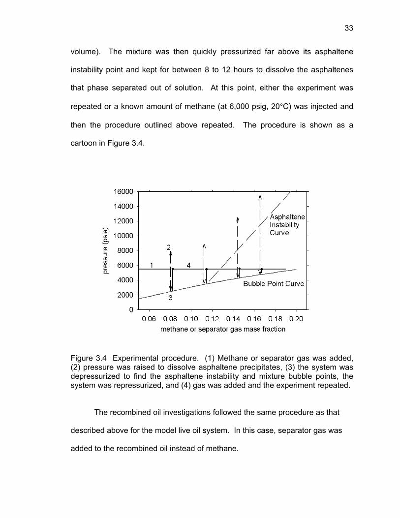
volume). The mixture was then quickly pressurized far above its asphaltene
instability point and kept for between 8 to 12 hours to dissolve the asphaltenes
that phase separated out of solution. At this point, either the experiment was
repeated or a known amount of methane (at 6,000 psig, 20°C) was injected and
then the procedure outlined above repeated. The procedure is shown as a
cartoon in Figure 3.4.
Figure 3.4 Experimental procedure. (1) Methane or separator gas was added, (2) pressure was raised to dissolve asphaltene precipitates, (3) the system was depressurized to find the asphaltene instability and mixture bubble points, the system was repressurized, and (4) gas was added and the experiment repeated.
The recombined oil investigations followed the same procedure as that
described above for the model live oil system. In this case, separator gas was
added to the recombined oil instead of methane.

34
3.3 Results
The measured asphaltene instability onset and bubble point pressures of
the model live oil at 20.0°C and 65.5°C are listed in Table 3.4 and plotted in
Figure 3.5(a). At lower methane concentrations, asphaltene instability was not
observed during depressurization. However, as the amount of dissolved
methane increased, asphaltenes phase separated at increasingly higher
pressures. The observed instability onset pressures were nearly linear functions
of dissolved gas concentration at each temperature (solid and dashed lines fitted
to the asphaltene instability points are shown in Figure 3.5(a). Significant
temperature effects on asphaltene stability were observed, with the fitted
instability lines for the two temperatures having very similar slopes.
Table 3.4 Asphaltene instability onset and bubble point pressures of the model live oil.
methane mixture bubble point asphaltene instability onset mass frac. (psia) (psia)
T=20.0°C
0.063 ± 0.001 1915 ± 30 Not Observed 0.103 ± 0.001 3153 ± 30 Not Observed 0.118 ± 0.002 3609 ± 40 4358 ± 130 0.132 ± 0.002 3960 ± 40 5747 ± 250 0.143 ± 0.002 4241 ± 40 7812 ± 100 0.153 ± 0.003 9786 ± 150
T=65.5°C
0.061 ± 0.001 2038 ± 30 Not Observed 0.100 ± 0.001 3043 ± 30 Not Observed 0.116 ± 0.002 3468 ± 30 Not Observed 0.140 ± 0.002 3911 ± 23 4296 ± 100 0.159 ± 0.003 6514 ± 200 0.169 ± 0.003 4383 ± 23 7883 ± 150 0.180 ± 0.003 4556 ± 40 9899 ± 150

35
Figure 3.5 (a) Asphaltene instability onsets (open symbols) and bubble points (filled symbols) for the model live oil at 20.0°C (triangles) and 65.5°C (squares). (b) Asphaltene instability onsets (open squares) and bubble points (filled squares) for the recombined oil at 71.1°C.
The asphaltene instability onset and bubble points for the recombined oil
at 71.1°C are listed in Table 3.5 and plotted in Figure 3.5(b). As seen in Figure
3.5(b), we would expect asphaltene precipitation problems to occur at higher

36
separator gas concentrations. Comparison of the model and recombined oil
results shows that in the limited dissolved gas concentration range investigated,
the behavior of asphaltenes to dissolved gas concentration and pressure
changes are qualitatively similar. While the bubble point curve for the
recombined oil was similar to that of the model oil at 65.5°C in the region
investigated, the asphaltenes seemed to be more stable in the recombined oil. If
we assumed that the asphaltene instability points for the recombined oil was a
linear function of separator gas mass fraction, this line would have a smaller
slope than those for the model oils (Figure 3.6). It is interesting to note that if the
asphaltene instability points for the recombined oil were plotted as a function of
methane plus nitrogen mass fraction (the components in separator gas most
dissimilar to asphaltenes in their polarizabilities and densities), the resulting
instability “line” has a slope similar to those of the model oil system.
Table 3.5 Asphaltene instability onset and bubble point pressures of the recombined oil.
separator gas bubble point asphaltene instability onset gas-oil-ratio
mass frac. (psia) (psia) (m3/m3)
0.174 4250 ± 30 6034 ± 50 152 0.227 4900 ± 23 9266 ± 150 212

37
Figure 3.6 Comparison of asphaltene instability onsets (open symbols) and bubble points (filled symbols) for model oil (squares) at 65.5°C and recombined oil (triangles) at 71.1°C.
The effect of pressure on mass density (from constant composition
expansion measurements) for some compositions of model live oil and for the
recombined oil is shown in Figure 3.7. The density information was used in
conjunction with composition data to calculate fluid properties discussed in the
next section.

38
Figure 3.7 Effects of pressure on mass density for (a) model live oil at 20.0°C (triangles, methane mass fraction labeled above data) and 65.5°C (squares, methane mass fraction labeled below data) and (b) recombined oil (GOR labeled above data).
3.4 Discussions
The difference in magnitude between a solvent and a solute’s solubility
parameter is a measure of miscibility because this difference can be related to
the enthalpies of mixing (for instance, see the expressions for Flory-Huggins-

39
regular-solution equation in Chapter 2.5.1). Demixing would occur if the mixture
solubility parameter becomes much smaller than the solubility parameter of the
most polarizable species in the mixture (of course, entropy effects would also
play a role). A solubility threshold can then be established in terms of the mixture
solubility parameter. For van der Waals fluids, a function of the refractive index,
( ))2()1( 22 +− nn , is approximately linearly proportional to solubility parameter.[40]
Hence the solubility threshold for nonpolar mixtures can be estimated by
measuring the refractive index at the threshold of phase separation.
For the systems studied, we can determine approximately (using the
Clausius-Mossotti-Lorenz-Lorentz equation[42,43]) the refractive indices at the
points of asphaltene instability onset from composition and density data:
∑=
+−
iii
mix
mix RCnn
21
2
2
(3.1)
+−
=i
i
i
ii d
MWnn
R21
2
2
(3.2)
In the above equations, n is the refractive index of the mixture or of the ith
species and Ci, Ri, MWi, di are the molar concentration, molar refraction,
molecular weight, and pure component mass density of the ith species,
respectively. In using Eqn. 3.1, we assume that the excess volume on mixing is
zero for all components in the mixture. Ri is, to a first approximation,
independent of temperature or physical states, and the molar refraction of pure
species used in this work were obtained from group contribution methods
tabulated in the Handbook of Chemistry and Physics.[44] A comparison of the

40
molar refractions of some compounds of interest in this work calculated using the
group contribution method and the molar refractions calculated with Eqn. 3.2
(using measured refractive indices) show good agreement (see Table 3.6). We
used an asphaltene molar refraction of 1317 cm3/mol (assuming MW = 3750, n =
1.75 at 20°C, and density = 1.16 g/cm3 at 20°C) but the contribution of
asphaltenes was extremely small due to their low concentrations. In the
recombined oil calculations, the stock-tank oil was treated as a single species
and its molar refraction (R = 83.6 cm3/mol) was obtained from GC derived
average molecular weight (MW = 250), measured mixture density (ρ = 0.857
g/cm3), and measured refractive index (n = 1.485) at ambient conditions. The
components in the separator gas were treated explicitly (not as lumped pseudo-
components) and the experimental densities in Fig. 3.7 were used to calculate
the density contribution from each species.
Table 3.6 Comparison of molar refractions of some compounds of interest calculated using measured refractive indices and densities and using group contribution method.
compound refractive
indexa (20°C)
molar refraction, Eqn. 3.2 (cm3/mol)
molar refraction, group contributionb
(cm3/mol)
absolute deviation (percent)
n-C5 1.3575 25.27 25.29 0.08 n-C6 1.3751 29.88 29.94 0.18 n-C7 1.3878 34.57 34.59 0.05 n-C8 1.3974 39.19 39.23 0.10 n-C9 1.4054 43.85 43.88 0.08 n-C10 1.4102 48.31 48.53 0.45 n-C11 1.4165 53.05 53.17 0.23 n-C12 1.4216 57.77 57.82 0.09 n-C13 1.4251 62.34 62.47 0.21 n-C14 1.429 67.05 67.11 0.09
41
n-C15 1.4314 71.60 71.76 0.23 n-C16 1.4345 76.33 76.41 0.10
Toluene 1.4964 31.07 31.14 0.22 α-methyl naph. 1.6170 48.77 48.68 0.20
Methane -- -- 6.70 -- a from [45] b from [44]
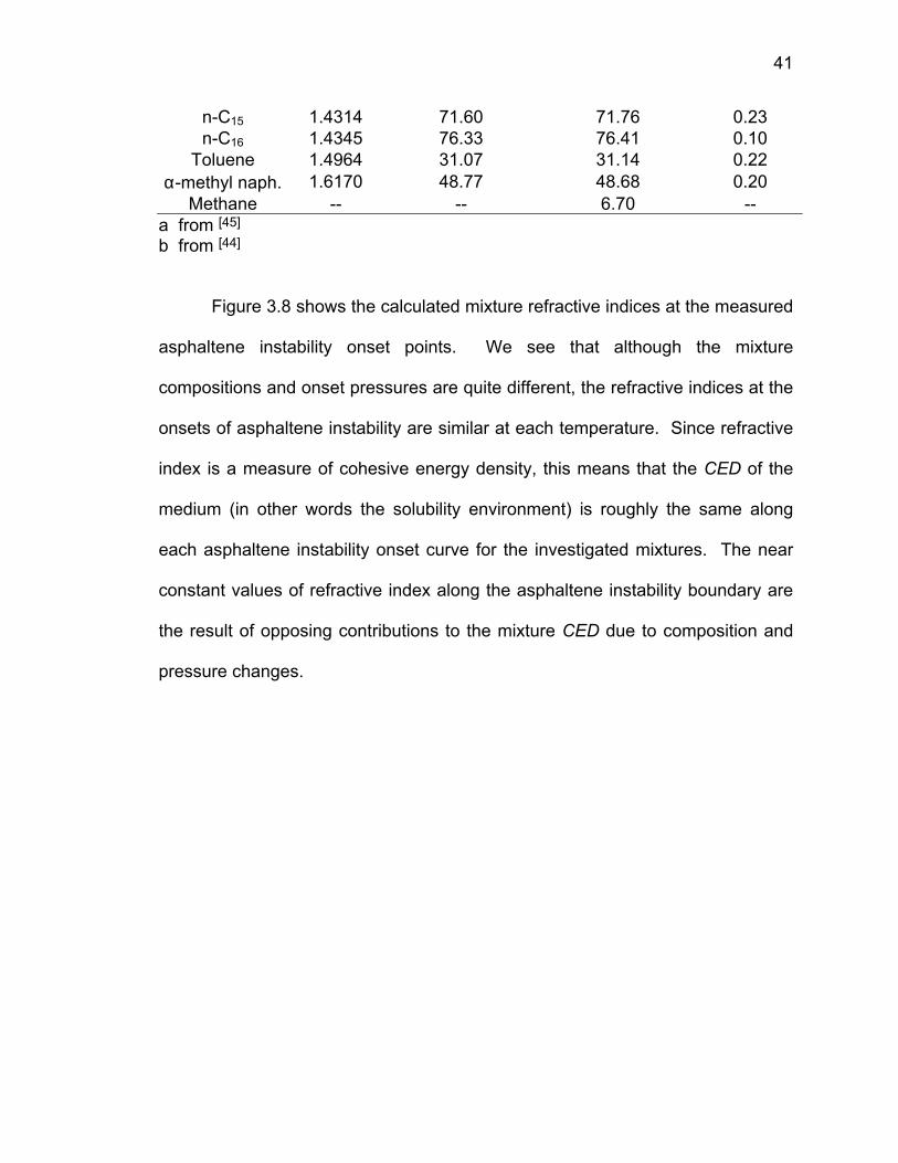
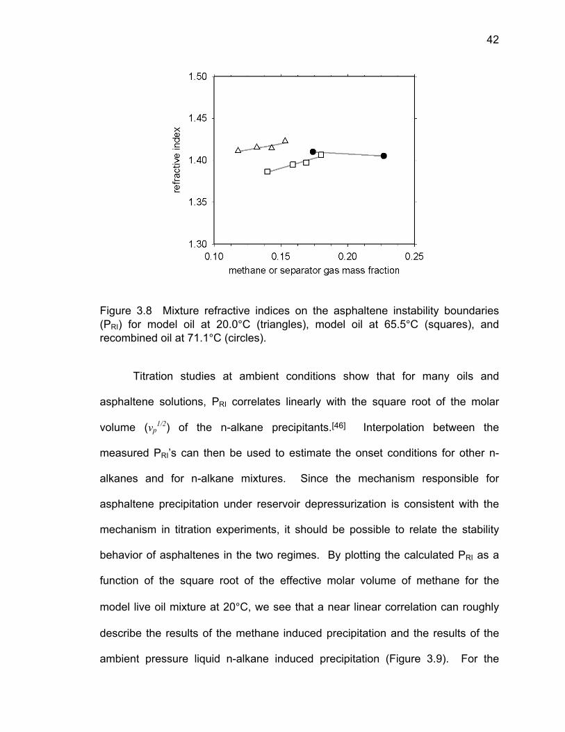
Figure 3.8 shows the calculated mixture refractive indices at the measured
asphaltene instability onset points. We see that although the mixture
compositions and onset pressures are quite different, the refractive indices at the
onsets of asphaltene instability are similar at each temperature. Since refractive
index is a measure of cohesive energy density, this means that the CED of the
medium (in other words the solubility environment) is roughly the same along
each asphaltene instability onset curve for the investigated mixtures. The near
constant values of refractive index along the asphaltene instability boundary are
the result of opposing contributions to the mixture CED due to composition and
pressure changes.
42
Figure 3.8 Mixture refractive indices on the asphaltene instability boundaries (PRI) for model oil at 20.0°C (triangles), model oil at 65.5°C (squares), and recombined oil at 71.1°C (circles).
Titration studies at ambient conditions show that for many oils and
asphaltene solutions, PRI correlates linearly with the square root of the molar
volume (vp1/2) of the n-alkane precipitants.[46] Interpolation between the
measured PRI’s can then be used to estimate the onset conditions for other n-
alkanes and for n-alkane mixtures. Since the mechanism responsible for
asphaltene precipitation under reservoir depressurization is consistent with the
mechanism in titration experiments, it should be possible to relate the stability
behavior of asphaltenes in the two regimes. By plotting the calculated PRI as a
function of the square root of the effective molar volume of methane for the
model live oil mixture at 20°C, we see that a near linear correlation can roughly
describe the results of the methane induced precipitation and the results of the
ambient pressure liquid n-alkane induced precipitation (Figure 3.9). For the

43
model live oil at 20°C, the value of vp1/2 of methane varies with pressure and
mass fraction of methane and can be approximated by an effective methane
volume
effectivemethanemethane
effectivetoluenetoluenemixture vxvxv += (3.3)
where vmixture is the mixture molar volume determined from experiment, xtoluene and
xmethane are the toluene and methane mole fractions, and veffective are the effective
molar volumes. The molar volume of pure toluene was used in place of effectivetoluenev .
Note that effectivemethanev is an “effective” methane volume and is not the partial molar
volume of methane calculated by an equation of state such as SAFT. Hence by
fitting to the asphaltene stability results from titration experiments at ambient
conditions, we may be able to estimate the onset of asphaltene precipitation as a
function of pressure, provided that we know the effective molar volume of the
precipitants as a function of pressure.
Figure 3.9 Measured PRI vs. vp1/2 of n-alkane titrants (squares) for the model oil
and calculated PRI vs. vp1/2 of methane (triangles) for the model live oil at 20.0°C.

44
Because the observed instability onset pressures are nearly linear
functions of mixture gas concentration at each temperature, it may be possible to
trace out the asphaltene stability boundaries with only a small set of instability
onset data. Furthermore, for this particular source asphaltenes, the effect of
temperature on the asphaltene instability boundary seems to be systematic (i.e.
increasing temperature improves asphaltene solvency in oil) and temperature
extrapolation may be possible.
From an operational standpoint, results of this study suggest that the oil
refractive index may be used to estimate whether or not asphaltenes would
precipitate. Along the asphaltene instability boundaries, these properties should
vary little regardless of pressure and composition. At a constant temperature,
asphaltenes would be stable as long as the mixture was above a certain solubility
threshold, as indicated by the mixture refractive index or solubility parameter. In
an isothermal pressure depletion operation, asphaltenes would be initially stable
at pressures high above the bubble point pressure due to high solvent density.
As pressure decreases, the density of the oil will decrease (which can be seen by
the lowering of the oil refractive index) as the solubility environment becomes
increasingly unfavorable for asphaltene dissolution. Asphaltenes may precipitate
out of solution below a certain refractive index threshold near the oil bubble point.
Finally, as the pressure decreases further below the bubble point, the oil
refractive index would increase (due to composition changes) and asphaltenes
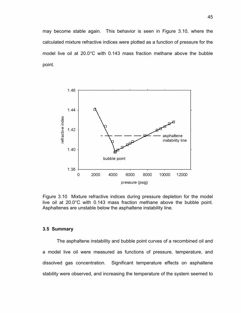
45
may become stable again. This behavior is seen in Figure 3.10, where the
calculated mixture refractive indices were plotted as a function of pressure for the
model live oil at 20.0°C with 0.143 mass fraction methane above the bubble
point.
Figure 3.10 Mixture refractive indices during pressure depletion for the model live oil at 20.0°C with 0.143 mass fraction methane above the bubble point. Asphaltenes are unstable below the asphaltene instability line.
3.5 Summary
The asphaltene instability and bubble point curves of a recombined oil and
a model live oil were measured as functions of pressure, temperature, and
dissolved gas concentration. Significant temperature effects on asphaltene
stability were observed, and increasing the temperature of the system seemed to

46
improve asphaltene stability. At each temperature, the asphaltene instability
onset pressures were nearly linear functions of mixture gas concentration. This
suggests that the asphaltene instability boundaries can be roughly estimated
from a few data points.
An analysis of the data shows that at a constant temperature, the mixture
refractive indices do not change much along the asphaltene instability curves.
From an operational stand point, this means that it may be possible to estimate
the degree of asphaltene stability from a crude oil’s refractive index (or solubility
parameter).
Finally, for the systems tested, there is a clear connection between
asphaltene precipitation in the titration experiments at ambient conditions and in
the reservoir depressurization experiments. This is indicated at 20°C by the near
linear relationship between the mixture PRI and the square root of the effective
molar volume of the precipitants. Hence an equation of state that can match the
results of the titration experiments at ambient conditions should be able to
estimate the effects of pressure on asphaltene stability in crude oil.

47
CHAPTER 4. EQUATION OF STATE ALGORITHMS
4.1 Introduction
In this chapter, we will develop the theoretical tools to be used in the
asphaltene phase behavior investigations. We will start with a description of the
Statistical Associating Fluid Theory (SAFT) equation of state that includes a
discussion on its limitations. SAFT-predicted thermodynamic properties of some
pure fluids will be compared with experimental data or molecular simulation data
to show the equation of state’s ability to accurately model the thermodynamic
properties of molecular species relevant in this work. A list of pure component
SAFT parameters for compounds relevant in this work is also presented together
with the methodology used to obtain them. An analysis of these parameters
shows distinct trends in their behavior with molecular weight. The implications of
these observed trends are discussed.
Since the SAFT equation of state is used to describe fluids and fluid
mixtures in all phases, an algorithm is needed to determine equilibrium phase
compositions from calculated free energies. Issues associated with mixture
phase equilibrium calculations will be discussed and several algorithms
investigated in terms of their speed and range of applicability. Finally, a hybrid
phase stability-modified flash algorithm that is both robust and efficient is
presented. This algorithm is used in all calculations presented in this thesis.

48
4.2 The SAFT Equation of State
A variety of approaches have been developed to describe the
thermodynamic phase behavior of molecular fluids and fluid mixtures. These
approaches include the use of perturbation theory, integral equation theory,
scaled particle theory, molecular simulations, lattice theory, local composition
theory, and correlative models such as the van Laar equations to describe fluid
properties.[24,47,48] Of these approaches, the use of thermodynamic perturbation
theory is especially popular because of its theoretical basis, its fast computation
time, its accuracy, and its wide range of applicability.
In perturbation theory, the properties of a fluid are obtained by expanding
about the same properties of a reference fluid. It is assumed that the reference
fluid roughly describes the fluid of interest; the perturbation is a series of small
corrections to the reference. For instance, in one of the most well known (and
together with virial expansion method the earliest) examples of this approach,
van der Waals added a perturbation to the pressure of a hard-sphere fluid to
account for intermolecular attraction:[48]
kTa
bkTP 2
1ρ
ρρ −
−= (4.1)
In Eqn. 4.1, P is pressure, k is the Boltzmann constant, T is temperature, ρ is
density, and a, b are constants that account for intermolecular attraction and
hard-sphere fluid repulsion, respectively.

49
Since van der Waals published his monumental work in 1873[49], much
activity have been devoted to the application of perturbation theory methods to
model dense fluids. These activities fall under one of two categories: (1) semi-
empirical modifications to Eqn. 4.1 to better reproduce experimental data of real
fluids and (2) application of statistical mechanics to the perturbation expansions
of molecular pair potentials to obtain fluid properties. An example of the first
approach is the Peng-Robinson (PR) equation[50]. And an example of the
second approach is the thermodynamic perturbation theory for square-well fluids
and for Lennard-Jones fluids due to Barker and Henderson.[51,52] While the first
approach is popular in industry because of its wide applicability and
mathematical simplicity, the second approach is favored by academics because
it allows one to test the effects of different pair potential functions on bulk fluid
properties. However, the second approach is complicated for molecules that
have anisotropic potentials.
SAFT, an acronym for Statistical Associating Fluid Theory, is a statistical
mechanical equation of state developed from Wertheim’s first order perturbation
theory (TPT1).[53-59] By treating a mixture of associating spheres as a mixture of
differently associated species (monomers, dimers, etc.), Wertheim used a
perturbation expansion in terms of the monomer and overall fluid density (about
the hard sphere reference) to calculate the free energy contribution due to
bonding. The assumptions used in TPT1 are (see Figure 4.1): (1) the hard cores

50
of two molecules bonded at sites A (a site on one molecule) and B (a site on the
second molecule) would prevent sites on a third molecule from bonding with
these sites, (2) no double bonding can occur, (3) a site on a molecule cannot
simultaneously bond to two sites on another molecule, and (4) each molecular
segment does not know the location of other segments not directly bonded to it
(and thus SAFT cannot explicitly model ring formation). The last assumption is
the result of first order approximation. Derivation of Wertheim’s theory can be
found in Joslin, et al[60] or in the works by Wertheim.[56-59]
Figure 4.1 Assumptions and limitations of the SAFT EOS.
As a perturbation theory, SAFT considers the fluid of interest to be initially
a mixture of independent segments. The theory predicts the change in free
energy upon bonding these segments to form chains and on the further
association of the chain-like molecules (Figure 4.2) using TPT1 theory. In this
work, we use a hard-sphere contribution from the Mansoori-Carnahan-Starling-
Leland (MCSL) hard-spheres equation of state[61], chain formation and
association contributions from Wertheim theory[55], and mean field contribution
from Gross and Sadowski[62]. SAFT requires three parameters for each
nonassociating component. These parameters are the temperature independent

51
diameter of each molecular segment (σ), the number of segments per molecule
(m), and the segment-segment dispersion energy (ε/k).
A = Asegment + ∆Achain + ∆Aassoc
Figure 4.2 In SAFT, fluids are initially considered to be a mixture of independent segments that are then bonded to form chains.
The residual Helmholtz energy Ares of a fluid mixture is described by SAFT
as
RT
ART
ARTA
mRTA
mRT
ART
ARTA
RTA assocchaindisphs
oassocchainsegres
+++=++= 0 (4.2)
where Aseg, Achain, Aassoc, Aohs, Ao
disp are the segment, chain, association, segment
hard sphere, and segment dispersion contributions to the residual Helmholtz
energy. Ares is called a residual property because it is defined as the energy of
the fluid minus that of an ideal gas at the same temperature and density. The
average segment number of the mixture m is an average of the pure species
segment numbers mi weighted by their compositions:
∑=i
iimxm (4.3)

52
The free energy contribution of the hard-sphere mixtures (from the MCSL
EOS) is
−
−−
−−+
= )1ln()1(336
323
32
233
2321321
32 ζ
ζζζ
ζζζζζζζζζ
πρ o
hso
RTA (4.4)
where ∑
= k
iiiik dmxρπζ6
(4.5)
and [ ])/3exp(12.01 kTd iiii εσ −−= (4.6)
Here, ρ is the number density (molecules/A3), σi is the temperature-independent
segment diameter of species i in units of Angstroms, and dii is the temperature-
dependent segment diameter. The contribution to A due to chain formation is
given by[53]
∑ −= )(ln)1( iihsiiii
Chain
dgmxRT
A (4.7)
where
−
+
−+
−= 3
3
22
2
23
2
3 )1(22
)1(23
11)(
ζζ
ζζ
ζiiii
iihsii
dddg (4.8)
A comparison of SAFT-predicted compressibility factor (Z) with simulation results
for flexible hard-sphere chains show good agreement[53] (Figure 4.3), indicating
that SAFT is a good model for hard-chain molecules.

53
Figure 4.3 Comparison of SAFT-predicted compressibility factor Z as a function of packing fraction η with simulation results.[53] The simulation data are from Dickman and Hall[63] (dimer to 16-mer) and from Gao and Weiner[64] (201-mer).
For fluid or fluid mixtures that are not comprised of hard-sphere chains, an
energy contribution is added to account for dispersion interactions. As
mentioned earlier, the dispersion contribution of Gross and Sadowski[65] is used
in this work. This particular dispersion term was initially developed for alkanes by
incorporating the effects of chain length on the segment dispersion energy ε/k.
Thus
RTA
RTA
RTAdisp
o 21 += (4.9)
∑∑−=i j
ijijjiji kTmmxxmIRTA /),(2 3
11 εσηπρ (4.10)
∑∑−−=i j
ijijjiji kTmmxxWmmIRTA 231
22 )/(),( εσηρπ (4.11)
[ ]2
432
4
2
)2)(1(2122720)1(
)1(281
ηηηηηη
ηηη
−−−+−−+
−−+= mmW (4.12)

54
)()1( jjiiijij sqrtk εεε −= (4.13)
( )jiij σσσ += 5.0 (4.14)
where I1 and I2 are functions of the system packing fraction and average segment
number m and can be found in the work by Gross and Sadowski[65]. kij corrects
for deviations in the mixing of the pure component energies ε from that predicted
by the geometric mixing rule. Equation 4.9 was derived in the spirit of Barker-
Henderson perturbation theory and, as such, A1 and A2 correspond to the first
and second order contributions to A0disp, respectively. Other dispersion
contributions can be used instead of the one given in Eqns. 4.9 to 4.14. The
form of SAFT described above is sometimes referred to in literature as PC-SAFT
(perturbed-chain SAFT) because the dispersion contribution accounts for the
effects of chain length on the segment dispersion energy.
Because of our assumption that nonpolar van der Waals interactions
dominate asphaltene phase behavior in crude oil (Chapter 2), the association
term in SAFT will not be used in our asphaltene modeling work. A detailed
discussion of the SAFT association term will be deferred to Chapter 10, where
we present some modifications to model hydrogen bonding interactions in water.
With the expressions for Ares given in Eqns. 4.2 to 4.14, all other residual
thermodynamic properties can be calculated. For instance,
nvTRTARS ,)/(/ ∂∂−= where S is entropy, RSRTARTU /// += where U is
internal energy, and ( ) 5.0RTU rsm ρδ ≈ where δ is the solubility parameter.[24]

55
SAFT and its various modifications and extensions have demonstrated the
ability to accurately predict the phase behavior of simple, hydrogen bonding,
polar, and polymeric mixtures.[66,67] It is particularly useful for modeling systems
with significant size, shape, and/or association effects. One reason for this
success is due to SAFT’s ability to reproduce and predict accurately the
thermophysical properties of pure species and of mixtures. For example, a
comparison of SAFT-predicted and experimental[45] solubility parameters of
some n-alkanes, polynuclear aromatics, cycloalkanes, benzene derivatives, and
carbon disulfide at 25°C and 1 bar shows good agreement (Figure 4.4). A
comparison of SAFT-predicted and experimental liquid volumes of hexadecane
(n-C16), tetracosane (n-C24), and hexatriacontane (n-C36) at 1 bar also shows
good agreement[68] (Figure 4.5). In contrast, a cubic equation of state such as
Peng-Robinson equations does not predict the correct volumes for the longer n-
alkanes because it does not correctly account for the effects of molecular size.

56
Figure 4.4 Comparison of SAFT-predicted and experimental[45] solubility parameters at 25°C and 1 bar.
Figure 4.5 Comparison of SAFT-predicted, Peng-Robinson EOS-predicted, and experimental liquid molar volumes at 1 bar[68].
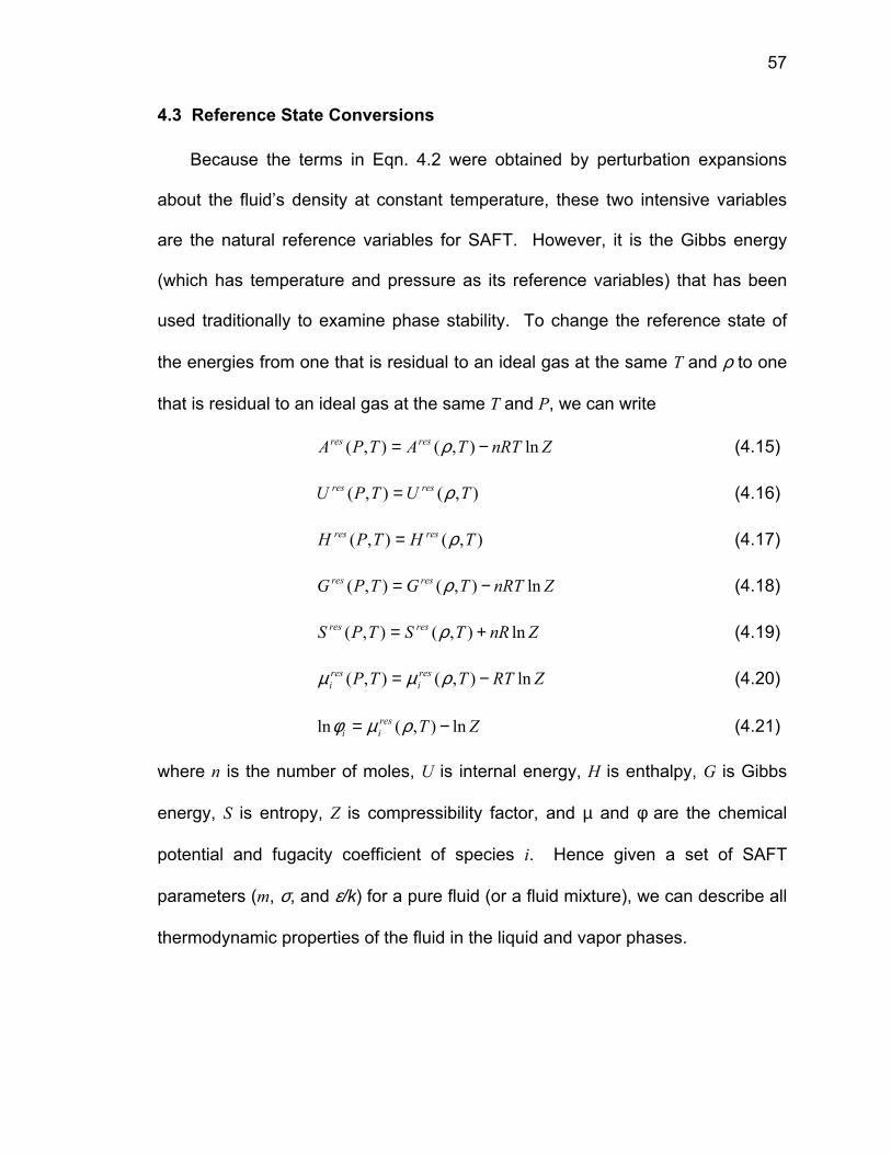
57
4.3 Reference State Conversions
Because the terms in Eqn. 4.2 were obtained by perturbation expansions
about the fluid’s density at constant temperature, these two intensive variables
are the natural reference variables for SAFT. However, it is the Gibbs energy
(which has temperature and pressure as its reference variables) that has been
used traditionally to examine phase stability. To change the reference state of
the energies from one that is residual to an ideal gas at the same T and ρ to one
that is residual to an ideal gas at the same T and P, we can write
ZnRTTATPA resres ln),(),( −= ρ (4.15)
),(),( TUTPU resres ρ= (4.16)
),(),( THTPH resres ρ= (4.17)
ZnRTTGTPG resres ln),(),( −= ρ (4.18)
ZnRTSTPS resres ln),(),( += ρ (4.19)
ZRTTTP resi
resi ln),(),( −= ρµµ (4.20)
ZTresii ln),(ln −= ρµφ (4.21)
where n is the number of moles, U is internal energy, H is enthalpy, G is Gibbs
energy, S is entropy, Z is compressibility factor, and µ and φ are the chemical
potential and fugacity coefficient of species i. Hence given a set of SAFT
parameters (m, σ, and ε/k) for a pure fluid (or a fluid mixture), we can describe all
thermodynamic properties of the fluid in the liquid and vapor phases.

58
4.4 SAFT Equation of State Parameters
The pure component SAFT parameters used in this work are listed in
Table 4.1. These parameters were either tabulated by Gross and Sadowski[65] or
obtained in this work by regressing to the substance’s experimental saturated
vapor pressures ( satiP ) and liquid densities ( liq
iρ ):
∑+
=
ndpndp
i
liqi
satiikm
orPkmf1
2
/,,),,,(
21min ρεσ
εσ (4.22)
where exp,
exp,,
sati
sati
calcsati
i PPP
f−
= for i = 1 to ndp
exp,
exp,,
liqi
liqi
calcliqi
ifρ
ρρ −= for i = ndp+1 to ndp+ ndp
The experimental data used in the regression were obtained from the DIPPR
database[69]. As is typical of analytic equations of state, SAFT tends to
overpredict critical temperatures and pressures. Because of this, data in the
critical region were not used in the fitting procedure.
Table 4.1 SAFT pure component parameters. For substances fitted in this work, the AAPDsa and temperature range of the experimental data[69] are given. All other SAFT parameters are from Gross and Sadowski.[65]
AAPDa Substance MW (g/mol) m σ
(A) ε/k (K)
T range (K) Psat ρliq
n-alkanes methane 16.04 1.0000 3.7039 150.03 ethane 30.07 1.6069 3.5206 191.42 propane 44.09 2.0020 3.6184 208.11 butane 58.12 2.3316 3.7086 222.88 pentane 72.15 2.6896 3.7729 231.20 hexane 86.18 3.0576 3.7983 236.77 heptane 100.20 3.4831 3.8049 238.40 octane 114.23 3.8176 3.8373 242.78 nonane 128.25 4.2079 3.8448 244.51

59
decane 142.29 4.6627 3.8384 243.87 undecane 156.31 4.9082 3.8893 248.82 dodecane 170.34 5.3060 3.8959 249.21 tridecane 184.37 5.6877 3.9143 249.78 tetradecane 198.39 5.9002 3.9396 254.21 pentadecane 212.42 6.2855 3.9531 254.14 hexadecane 226.45 6.6485 3.9552 254.70 eicosane 282.55 7.9849 3.9869 257.75
cycloalkanes cyclopentane 70.13 2.3655 3.7114 265.83 methyl-cyclopentane 84.16 2.6130 3.8253 265.12 ethyl-cyclopentane 98.18 2.9062 3.8873 270.50 cyclohexane 84.15 2.5303 3.8499 278.11 methyl-cyclohexane 98.18 2.6637 3.9993 282.33 ethyl-cyclohexane 112.22 2.8256 4.1039 294.04 cyclopheptane 98.19 2.6870 3.9352 296.15 300-570 0.44 0.21 cyclooctane 112.22 2.9222 4.0028 304.67 300-620 0.71 1.06
polynuclear aromatics
benzene 78.11 2.4653 3.6478 287.35 naphthalene 128.17 3.0915 3.8333 348.40 373-633 1.45 0.77 anthracene 178.23 3.5291 4.0922 402.13 500-830 1.81 1.57 phenanthrene 178.23 3.4890 4.1053 403.06 330-780 1.51 1.39 naphthacene 228.29 4.6432 3.8942 407.60 660-940 0.88 4.23 chrysene 228.29 5.1201 3.8400 385.73 580-940 0.81 3.61 pyrene 202.26 3.6847 4.1151 427.35 450-850 1.37 3.76
aromatic & polynuclear aromatics derivatives
toluene 92.14 2.8149 3.7169 285.69 ethylbenzene 106.17 3.0799 3.7974 287.35 propylbenzene 120.19 3.3438 3.8438 288.13 butylbenzene 134.22 3.7662 3.8727 283.07 tetralin 132.21 3.3131 3.8750 325.07 biphenyl 154.21 3.8877 3.8151 327.42 1-methylnaphthalene 142.20 3.4064 3.8961 345.71 393-673 0.29 0.50 1-phenylnaphthalene 204.27 4.7634 3.8582 336.53 330-780 1.51 1.39 m-terphenyl 228.29 5.6273 3.7967 329.18 420-840 1.52 0.26
gases
nitrogen 28.01 1.2053 3.3130 90.96 carbon dioxide 44.01 2.0729 2.7852 169.21 carbon disulfide 76.14 1.6919 3.6172 334.82
a Average absolute percent deviation = %1001 ∑ −ndp alExperiment
alExperimentCalculatedndp

60
An important feature of SAFT is that the fitted pure component parameters
behave in a systematic manner with molecular weight for each class of
compounds[62,70] (Figure 4.6, Table 4.2). Furthermore, species with both
aromatic and aliphatic characteristics have EOS parameters that lie in between
the aromatic and n-alkane correlations in a systematic manner depending on
their degree of aromaticity. For instance, the variation of m with molecular weight
for some benzene derivatives and cyclo-alkanes are shown in Figure 4.7; as the
degree of aliphaticity increases, the pure component parameters more closely
resembles those for the n-alkanes. These correlations between the pure
component parameters and molecular weight have three implications. (1) The
correlations can be used to estimate the SAFT parameters for substances whose
vapor pressures and/or liquid densities are difficult to measure. For example, the
SAFT-predicted liquid molar volumes of hexatriacontane (n-C36) in Figure 4.5
were calculated using n-C36 SAFT parameters extrapolated from the n-alkane
correlations. In the case of asphaltenes, these correlations provide the upper
and lower bounds of the asphaltene SAFT parameters. (2) Systems that are
polydisperse in molecular size (with molecular weight) can be modeled in SAFT
as a single pseudo-component. And (3) the pure component SAFT correlations
imply that the EOS can be extended to explicitly model (rather than using a
pseudo-component scheme) the effects of polydispersity. Each of these will be
discussed in more detail in the following chapters.

61
Table 4.2 SAFT pure component parameter correlations.
n-alkane saturates polynuclear aromatics m 0.0253MW+0.9263 0.0139MW+1.2988
mσ 0.1037MW+2.7985 0.0597MW+4.2015
ε/k 32.81ln(MW)+80.398 119.41ln(MW)-230.21
Figure 4.6 Plots of SAFT pure component parameters with molecular weight. The parameter correlations in Table 4.2 are shown as lines.

62
Figure 4.7 Variation of m with molecular weight for various compounds.
4.5 Phase Stability and Flash Algorithms
Equilibrium is a condition in which the system’s macroscopic properties do
not change with time because all the energy that may cause change are
balanced.[49] The necessary and sufficient condition for thermodynamic phase
equilibrium (at a fixed T and P) is that the overall Gibbs energy of the mixture is
at its global minimum[49]:
∑=ji
jijijn
nPTnGij ,
),,(min µ (4.23)
where the underscore denotes vector quantities and the summation is over all
components i and all phases j. The necessary condition at equilibrium is
πβα TTT === ...
πβα PPP === ...

63
πβα µµµ iii === ... (i=1,2,…,n) (4.24)
where α, β, ... , π are the different phases and n is the total number of
components. Eqn. 4.24 is the first order necessary condition of Eqn. 4.23
obtained by first differentiating Eqn. 4.23 and then applying the Gibbs-Duhem
relation. Eqn. 4.24 can also be expressed as an equality of fugacities
πβα iii fff === ... (4.24’)
because
),(ln),,(ln),(),,( 00 PTfRTPTnfRTPTPTn iiii −+= µµ (4.25)
and the fugacity and chemical potential of the pure components fi0, µi
o depend
only on temperature and pressure. The second order derivatives of the Gibbs
energy with composition (which provides the sufficiency condition) depends on
the EOS used to calculate the thermodynamic properties and are difficult to
determine analytically for SAFT.
The direct minimization of the function G in (4.23) is difficult because the
number of phases present is not known a priori and the equations of state used
to calculate the chemical potentials of these nonideal mixtures are nonlinear.
Optimization methods such as interval analysis[71], simulated annealing[38], the
RAND method[72], genetic algorithms[73], and random search algorithms[74] have
all been used to solve (4.23) directly. The application of the interval analysis
method seems especially promising, as the authors claim that their algorithm is
guaranteed to find the global minimum.[71] However, the robustness that these
algorithms offer comes at the expense of efficiency. For instance, equilibrium

64
(binary) phase compositions of a mixture of ethane and eicosane (outside the
mixture critical region) took about a minute of CPU time while a mixture of
heptane and propanol (outside the mixture critical region) took more than 6
minutes on a Sun Ultra 10/440.[71]
An alternative approach to determine equilibrium phase compositions is to
use the constant temperature and pressure flash (also called the successive-
substitution method). This approach is called a flash because it simulates the
flashing of a one-phase mixture into a tank at T and P to see if the fluid would
phase separate. The number of phases at equilibrium, the feed composition, an
initial estimate of the compositions of all phases, T, and P must be given a priori.
The algorithm for a vapor-liquid flash[49,75] is shown in Figure 4.8. In the figure,
{z}, {x}, and {y} are the set of feed, liquid, and vapor phase compositions. Ki is
the partition coefficient of the ith species, V is the ratio of the amount of vapor to
the feed, and φi is the fugacity coefficient (recall Eqn. 4.24’ and ( )Pxf iii φ= ). The
equations shown in the figure to evaluate V, {x}, and {y} are mass balance
constraints. Since the function used to determine V is a monotonically
decreasing function between V=0 and V=1, it can be evaluated easily. An
extension of the algorithm to three phase calculations can be found in the work of
Nelson[76].

65
Figure 4.8 Calculation procedure in a typical TP flash algorithm[49].
Unlike the direct Gibbs energy minimization approaches, the correct
number of phases at equilibrium must be specified a priori for the solution of the
flash to be meaningful. Furthermore, an initial guess for the equilibrium
composition may return a trivial solution (which indicates a stable state) even if
the state point is not stable, and multiple initial guesses for the equilibrium
composition may be needed to determine stability. These and other problems
are illustrated in Figure 4.9, where compositions at phase equilibrium are
connected by tangents to the ∆Gmix curves (on the right hand side figures). Since
the first derivative of ∆Gmix with respect to a component’s mole number is its

66
chemical potential, the lines in Figure 4.9 satisfy the requirement of Equation
4.24. At pressure P2, a feed of composition z2 would phase split into 3 phases.
However, if one specified the number of phases to be 2, then the incorrect binary
phase compositions of x2Lb and x2
G would be obtained. At pressure P1, the
system exists as either a single gas phase, a single liquid phase, or as a liquid
and gas in equilibrium. The flash would converge to the solution x2La and x2
G if a
feed z2 is used but would return the trivial solution if a feed of z2* is used. At
pressure P4, the flash would converge to the trivial solution regardless of the feed
composition. Finally, the tangent lines at P3 illustrate the difficulties one may
encounter in obtaining the correct phase equilibria compositions. While all three
tangent lines at P3 satisfy Eqn. 4.24, the compositions on the solid line are the
only real solution.
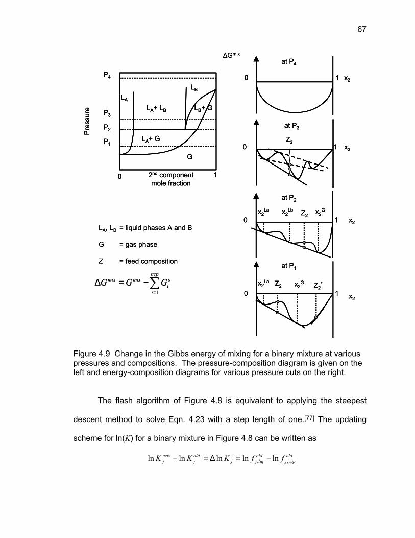
67
2nd componentmole fraction
0
LA
LA+ LB
LB
G
LA+ G
LB+ G
P1
P2
P3
P4
1
Pres
sure
∆Gmix
0 1
at P2
x2La Z2x2
Lb x2G
x2
at P3
Z20 1 x2
at P4
0 1 x2
LA, LB = liquid phases A and B
G = gas phase
Z = feed composition
∑=
−=∆ncp
i
oi
mixmix GGG1
at P1
x20 1
x2La Z2 x2
G Z2*
2nd componentmole fraction
0
LA
LA+ LB
LB
G
LA+ G
LB+ G
P1
P2
P3
P4
1
Pres
sure
2nd componentmole fraction
0
LA
LA+ LB
LB
G
LA+ G
LB+ G
P1
P2
P3
P4
1
Pres
sure
∆Gmix
0 1
at P2
x2La Z2x2
Lb x2G
x20 1
at P2
x2La Z2x2
Lb x2G
x2
at P3
Z20 1 x2
at P3
Z20 1 x2
Z20 1 x2
at P4
0 1 x2
at P4
0 1 x2
LA, LB = liquid phases A and B
G = gas phase
Z = feed composition
∑=
−=∆ncp
i
oi
mixmix GGG1
at P1
x20 1
x2La Z2 x2
G Z2*
at P1
x20 1
x2La Z2 x2
G Z2*
Figure 4.9 Change in the Gibbs energy of mixing for a binary mixture at various pressures and compositions. The pressure-composition diagram is given on the left and energy-composition diagrams for various pressure cuts on the right.
The flash algorithm of Figure 4.8 is equivalent to applying the steepest
descent method to solve Eqn. 4.23 with a step length of one.[77] The updating
scheme for ln(K) for a binary mixture in Figure 4.8 can be written as
oldvapj
oldliqjj
oldj
newj ffKKK ,, lnlnlnlnln −=∆=−

68
(using Eqn. 4.23 and 4.25) jliqj
gn
RTG
−=∂
∂−=
,
so that
kkk gBK 1ln −−=∆ α (4.26)
In Eqn. 4.26, k is the iteration number, the single underscore denotes vectors,
and the double underscore denotes matrices. 1−kB in this case is the identity
matrix I and αk is one. Moreover, since the mole numbers jn for phase j is
related to the equilibrium ratios K (because the feed was specified a priori), we
can rewrite Eqn. 4.26 for a two phase mixture as
gBUn j11 −−−=∆ α (4.26’)
Since U and its inverse are positive definite, the flash algorithm would always
move in the direction of decreasing Gibbs energy.
While Gibbs energy minimization is superior to the flash formulation
because the latter cannot guarantee convergence to the global solution, the
computation costs associated with the global methods are often much higher.
For instance, the interval method would give reliable solutions to (4.23) while a
quasi-Newton method would be more efficient but does not guarantee
convergence to the global solution. Ohanomah and Thompson[78] compared
more than ten algorithms and reported that direct Gibbs energy minimization
schemes are not competitive in practice because of their added complexity and
computation time.

69
In this work, we used a two-prong approach to improve the algorithm in
Figure 4.8. A phase stability algorithm was added to a modified flash algorithm
to improve efficiency and robustness. The proposed procedure is shown in
Figure 4.10. Succinctly, a given feed is first checked for phase stability using the
tangent plane method (to be discussed shortly). If the feed is unstable, the
composition given by the stability algorithm (with which the feed are unstable to)
is used with the feed composition to determine K guesses for the two-phase
flash. After the two-phase flash has converged, the calculated equilibrium phase
compositions are tested for stability. If they are unstable, the process is first
repeated with new feed compositions. If subsequent stability-flash calculations
return the same false “equilibrium” compositions, the feed and the compositions
calculated by the two-phase flash are then used to construct initial K estimates
for the three-phase flash. This cycle of flash calculation followed by stability
check continues until a stable solution has been obtained. The notion of coupling
a phase stability algorithm with a local optimization algorithm was first proposed
by Michelsen[79,80]. And the idea of modifying the flash with line search, trust
region, or quasi-Newton methods was first investigated in the 1970s with the
development of reservoir and plant simulators.

70
Figure 4.10 Proposed phase equilibria calculation procedure.

71
Three modifications to the flash algorithm were investigated. (1) We kept
the steepest descent algorithm of Eqn. 4.26 with IB k =−1 but optimized α at each
iteration k: ),,(min0 kkk gnPTG α
α+
> using the golden section algorithm with a
tolerance of 10-5 and 200 ≤<α . (2) We set IB k =−1 and calculated the step
length at each iteration after the first using[77]
1
1
1
1
1
1
1
)( −
−
−
−
−
−
−
−= k
kk
T
k
k
T
kk ggUg
gUgαα (4.27)
where the elements of 1−U are
[ ]
−
+
−=
∑−
n
kkkk
j
jjij
i
iiij
zyxzyx
zyxVVu
1
11
)1(1 δ (4.28)
for the two phase system. Eqn. 4.27 was obtained by first Taylor expanding the
Gibbs energy and then setting the derivative of the truncated expansion with α to
0. Eqn. 4.28 relates changes in composition to changes in K values assuming
that the total amount of vapor and liquid is one mole. (3) We used the golden
section algorithm to optimize α (as in the first approach) and updated 1−kB using
the Broyden-Fletcher-Goldfarb-Shanno method[81]
k
T
k
T
kk
kkTk
kTkkk
kk Kg
gg
KBK
BKKBBB
lnlnln
lnln1 ∆
+∆∆
∆∆−=
+ (4.29)
with IB =0 . B was calculated once every 4 iterations to reduce computation
time.

72
A comparison of the various flash algorithms on some representative,
extremely nonideal binary mixtures is given in Table 4.3. The systems
investigated include binary mixtures of hexane and hexatriacontane, hexane and
25,000 MW polystyrene, hexane and 33,000 MW polyethylene-octene, and
methanol and pentane. The effectiveness of these algorithms in the mixture
critical region is also tested. Keep in mind that all perturbation methods will fail at
the critical point.
As seen in Table 4.3, the second modification was overall the most robust
and the fastest. The algorithm of Modification 1 required few iterations but was
CPU intensive because it needed to search for an optimum α at every iteration
step. The original flash formulation, on the other hand, required many iterations
but was not CPU intensive because few calculations were done at each step.
For some systems, the original flash formulation would not converge because it
would start to cycle between several compositions. Finally, the algorithm of
Modification 3 was expensive because of the required line search plus the
various matrix manipulations. It was also not reliable; the optimum α at some
iteration k would sometimes push ln(K) of a specie to a very large number and
hence force the specie out of a particular phase. It was decided that the
algorithm of Modification 2 would be used in the stability-flash algorithm shown in
Figure 4.10.

73
Table 4.3 Comparisonf of the flash algorithms on some nonideal systems.
temperature, pressure (feed composition)
(TPD composition)a
traditional flash algorithm
(Figure 4.7)mod. 1 mod. 2 mod. 3
(1) n-C6 and (2) n-C36
equil. comp. (0.7804, 0.2196)b (0.9915, 0.0085)b
623K, 50 Bar (0.85, 0.15)b
(0.9943, 0.0057)b
# iterations
CPU time (s)
10
0.07
6
0.80
7
0.05
11
1.52
(1) n-C6 and (2) n-C36 In Critical Region equil. comp. (0.9251, 0.0749)b and (0.9618, 0.0382)b
623K, 73 Bar (0.93, 0.07)b
(0.9675, 0.0325)b
# iterations
CPU time (s)
125
0.87
5
0.63
8
0.06
4
0.51
(1) n-C6 and (2) Polystyrene (25,000 MW) equil. comp. (0.8011, 0.1989)c and (0.9841, 0.0159)c
407K, 380 Bar (0.90, 0.10)c
(0.99999995, 5e-8)b
# iterations
CPU time (s)
86
0.98
13
2.04
50
0.54
27
3.82
(1) n-C6 and (2) Polystyrene (25,000 MW) In Critical Region equil. comp. (0.8952, 0.1048)c and (0.9407, 0.0593)c
407K, 485 Bar (0.92, 0.08)c
(0.99959, 4.1e-4)b
# iterations
CPU time (s)
280
3.44
35
4.70
13
0.20 N/Ad
(1) n-C6 and (2) Polyethylene-octene (33,000 MW) equil. comp. (0.8848, 0.1152)c and (0.9977, 0.0023)c
450K, 42 Bar (0.96, 0.04)c
(0.999993, 7e-6)b
# iterations
CPU time (s) N/Ae N/Ad
283
3.50 N/Ad
(1) methanol and (2) n-C5
equil. comp. (0.3831, 0.6169)b and (0.5479, 0.4521)b
288K, 50 Bar (0.45, 0.55)b
(0.5543, 0.4457)b
# iterations
CPU time (s)
3888
25.15
77
13.0
11
0.09 N/Ad
(1) Methanol and (2) n-C5
equil. comp. (0.1025, 0.8975)b and (0.7681, 0.2319)b
270K, 50 Bar (0.50, 0.50)b
(0.0891, 0.9109)b
# iterations
CPU time (s)
311
1.95
15
1.77
11
0.08 N/Ad

74
a composition given by stability analysis to be unstable to the feed. b mole fraction c mass fraction d did not complete e did not converge after 20,000 iterations f comparisons were made on a 700 MHz Intel Pentium III computer
The phase stability algorithm used in the method of Figure 4.10 is based
on the tangent plane distance (TPD) analysis of Baker, et al.[82] and
Michelsen[79]. Essentially, a tangent to the Gibbs energy curve at the feed is
constructed (see the cartoon in Figure 4.11). If the difference
( ) ( )( )∑=
−≡ncp
iiii zPTxPTxTPD
1,,,, µµ (4.30)
is nonnegative for all composition x , then the feed is stable (as in the case for
2z in Figure 4.11). The feed is unstable if any x can be found that will make
(4.30) negative (as in the case for 1z in Figure 4.11); a negative TPD is a
necessary and sufficient condition for phase instability.

75
Figure 4.11 Illustration of the tangent plane distance approach to determine phase stability.
In this work, we used the golden section algorithm with the BFGS update
to minimize the tangent plane distance. The set of x that minimizes the TPD
was then used (with the feed composition) to calculate initial estimates of K .
Note that in our approach, we do not perform an exhaustive search for all the
stationary points to (4.30). Instead, we stop the TPD minimization program as
soon as a negative TPD is found and rely on the stability check-flash calculation
cycle to find the global solution. While our approach is less rigorous, it is faster
because we are not interested in finding all the stationary points (the number of
which is not known a priori) to the tangent plane distance, just a set of points in
composition space that is a good enough initial guess for the flash.

76
The following mole fraction initial guesses are fed into (4.30):
999999.0=ix (4.31)
( ))(lnlnexp zzx iii φ+= (4.32)
satj
sati
i PPPx−
= for sati
satj PPP ≤≤ (4.33)
Equation 4.31 is effective for systems containing polymers and Eqn. 4.32 was
proposed by Michelsen[79] that seems to work well for a variety of systems. In
another check, if the stability algorithm cannot find an unstable point at T, P, the
system pressure is reduced until an unstable point emerges and the equilibrium
compositions at this lower pressure are used as initial guesses in (4.30). An
exhaustive grid search on composition space is performed as a last resort.
Because of the nature of the stability algorithm, it is much easier to map out the
phase diagram of a mixture by operating inside the unstable regions than
searching explicitly for the stable regions.

77
CHAPTER 5. APPLICATION OF SAFT TO MODEL SYSTEMS
5.1 Introduction
Using the tools developed in the previous chapter, we will apply the SAFT
equation of state (EOS) to some model mixtures to test the EOS’ range of
applicability. We will investigate SAFT’s ability to model the thermodynamic
phase behavior of long-chain short-chain alkane mixtures in Section 5.2, of
polystyrene-hexane and polystyrene-toluene-ethane mixtures in Section 5.3, and
of phenanthrene-methane-decane mixtures in Section 5.4. The systems in
Section 5.2 and 5.3 will test SAFT’s ability to model the effects of size on
solubility. The system in Section 5.4 will test SAFT’s ability to describe the
solubility behavior of polynuclear aromatics, which share structural similarities
with asphaltenes. Since asphaltenes differ from other oil components in both
size and shape, how well SAFT predicts the phase behavior of these systems
provides insights to its ability to relate these molecular features to macroscopic
thermodynamic properties. Furthermore, these model systems will provide us
with insights regarding asphaltene phase behavior in oil. The system
polystyrene-toluene-ethane is particularly interesting because it resembles the
model live oil system (asphaltene-toluene-methane) described in Chapter 3.
Finally, we are also interested in SAFT’s ability to model long-chain short-chain
alkane mixtures because the bulk of crude oil is made up of alkanes (see Table
3.1).
78
Aside from serving as model systems in our investigation of asphaltene
phase behavior, these model systems are important in other areas of research.
For example, the thermodynamic phase behavior of long-chain short-chain
alkane mixtures is important in the recovery of wax products from the Fischer-
Tropsch slurry reactor[83], in determining wax precipitation in natural gas
pipelines[84], and in the design of the ROSE process which uses light, near
critical solvents to recover oils from residua[85]. The thermodynamic phase
behavior of polymer-solvent systems is important in polymer synthesis and
processing, and the phase behavior of mixtures containing polynuclear aromatics
is important in refining, in environmental remediation, and in the recovery of tar
oil.
5.2 Long-Chain Short-Chain Alkane Mixtures
5.2.1 Background Information
The goal of this investigation is to determine the extent to which SAFT is
applicable to highly asymmetric mixtures of alkanes (and hence how well it
accounts for the effects of size on mixture phase behavior). The Peng-Robinson
(PR) equation[50] was also evaluated for comparison. These EOS were tested for
their predictive and their correlative abilities, with the experimental vapor-liquid
equilibrium (VLE) data of Joyce and Thies[86] and Joyce et al.[87] for hexane-
hexadecane (C6-C16), hexane-tetracosane (C6-C24), and hexane-hexatriacontane

79
(C6-C36) being used for analysis. The PR equation was chosen because of its
widespread use in industry and simplicity.
The Peng-Robinson equation[50] for pure fluids can be written as
( )22 2 bbvv
Tabv
RTP−+
−−
= (5.1)
where P denotes pressure, T temperature, v molar volume, and R the ideal gas
constant. The temperature-independent repulsion parameter b is
c
c
PRT
b07780.0
= (5.2)
where Tc and Pc are the critical temperature and pressure, respectively. The
temperature dependent attraction parameter a(T) is given by
[ ]25.0 )1(1)( rc TTaa −+= κ (5.3)
where
c
cc P
TRTa
2245724.0)( = (5.4)
In Eqn. 5.3, κ is correlated to vapor pressure data over a range of reduced
temperature Tr. For aromatics, n-alkanes (but only up to n-decane), and other
light nonpolar compounds, Peng and Robinson correlated κ to the acentric factor
ω:
226992.054226.137464.0 ωωκ −+= (5.5)
For other species, κ can be regressed from vapor pressure data.
To extend this EOS to mixtures, van der Waals one-fluid mixing rules are
typically applied:
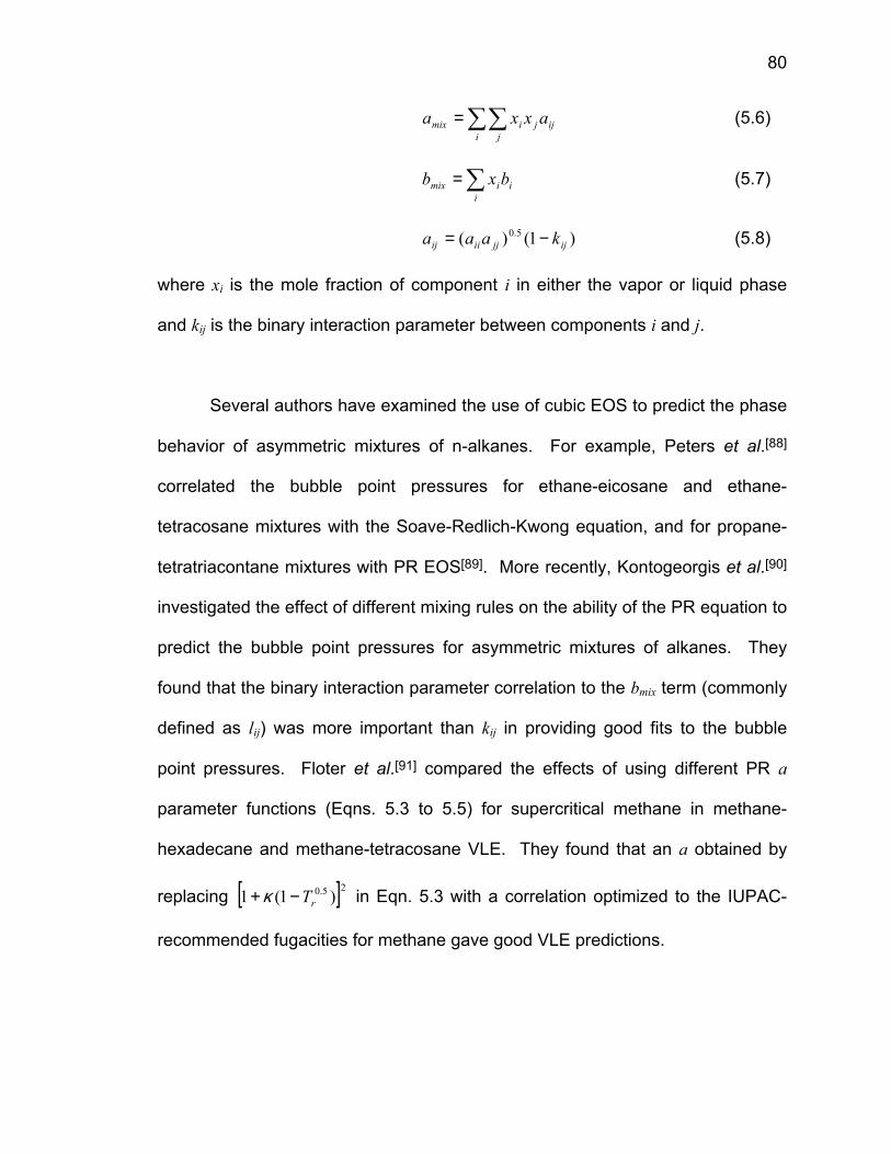
80
∑∑=i j
ijjimix axxa (5.6)
∑=i
iimix bxb (5.7)
)1()( 5.0ijjjiiij kaaa −= (5.8)
where xi is the mole fraction of component i in either the vapor or liquid phase
and kij is the binary interaction parameter between components i and j.
Several authors have examined the use of cubic EOS to predict the phase
behavior of asymmetric mixtures of n-alkanes. For example, Peters et al.[88]
correlated the bubble point pressures for ethane-eicosane and ethane-
tetracosane mixtures with the Soave-Redlich-Kwong equation, and for propane-
tetratriacontane mixtures with PR EOS[89]. More recently, Kontogeorgis et al.[90]
investigated the effect of different mixing rules on the ability of the PR equation to
predict the bubble point pressures for asymmetric mixtures of alkanes. They
found that the binary interaction parameter correlation to the bmix term (commonly
defined as lij) was more important than kij in providing good fits to the bubble
point pressures. Floter et al.[91] compared the effects of using different PR a
parameter functions (Eqns. 5.3 to 5.5) for supercritical methane in methane-
hexadecane and methane-tetracosane VLE. They found that an a obtained by
replacing [ ]25.0 )1(1 rT−+κ in Eqn. 5.3 with a correlation optimized to the IUPAC-
recommended fugacities for methane gave good VLE predictions.

81
A few authors have investigated the ability of SAFT to model alkane
mixtures with significant degrees of size asymmetry. For example, Pan and
Radosz[92] used a version of SAFT (proposed by Huang and Radosz[70,93]) with a
single, temperature-independent kij = 0.03 to give reasonable predictions of liquid
compositions for ethane-eicosane, ethane-docosane, and ethane-tetracosane
systems (no experimental vapor-phase compositions were available for these
systems). Benzaghou et al.[94] investigated another approach: using the original
version of SAFT proposed by Chapman et al.[55], they regressed vapor pressures
and liquid densities for n-C2 to n-C8 as a group to obtain constant, unique values
for the segment diameter and the segment energy; only the segment number
was allowed to vary with carbon number. Thus, no kij was used. Except in the
vicinity of the mixture critical points, reasonable predictions of VLE for hexane-
hexadecane and hexane-squalane were obtained. In another example,
Gregorowicz and de Loos[95] reported that the version of SAFT with the
dispersion contribution proposed by Huang and Radosz[70,93] gave poor
predictions for ethane-eicosane liquid-liquid-vapor equilibria; similarly poor
predictions were obtained for the critical end points for the ternary systems
ethane-eicosane-methane and ethane-eicosane-propane.
For all EOS used in this study, the kij’s were obtained by minimizing the
total absolute deviation between measured and calculated liquid and vapor
compositions summed over all ndp data points:

82
∑∑ −−
+−
−=
ndp
i ii
icalcindp
i ii
icalci
k yyyy
xxxx
fij )1,min()1,min(
minexp,exp,
exp,,
exp,exp,
exp,, (5.9)
As indicated in Eqn. 5.9, the calculation was always carried out with the minor
component in a given phase. Thus low vapor phase solubilities were weighted
approximately the same as other data points. We also omitted the mixture
critical points in the determination of the optimal binary interaction parameters.
5.2.2 Results and Discussions
The pure component parameters used in this study are given in Table 5.1.
Critical properties and ω for hexane and hexadecane were obtained from Reid et
al.[96], with κ obtained from Eqn. 5.5. Critical properties for tetracosane and
hexatriacontane were obtained from Ambrose and Tsonopoulous[97] and from
Nikitin, et al.[98], respectively. κ for tetracosane was obtained by regressing the
vapor pressure data of Morgan and Kobayashi[99] and API-42[100]. And κ for
hexatriacontane was obtained by regressing the vapor pressure correlation of
Stephenson and Malanowski[101]. In the case of hexatriacontane, the correlation
of Stephenson and Malanowski[101] gives vapor pressures that are in best
agreement with the results of an enhancement factor[102] analysis (i.e., to better
than ±10%). The SAFT parameters for hexane and hexadecane were obtained
from Table 4.1. As described in Chapter 4, these parameters were fit to pure
component vapor pressures and saturated liquid densities. The SAFT
parameters for tetracosane and hexatriacontane were calculated from
correlations in Table 4.2.

83
Table 5.1 Experimentally obtained and regressed pure component parameters for the Peng-Robinson and SAFT equations.
PR SAFT component
Tc (K) Pc (bar) κ σ (A) ε/k (K) m hexane 507.5 30.1 0.812 3.798 236.77 3.058
hexadecane 722.0 14.1 1.371 3.955 254.70 6.648 tetracosane 800.0 8.7 1.781 3.937 253.18 9.822
hexatriacontane 872.0 4.7 2.224 4.014 256.37 13.8600
Each of the tested EOS was fit to three asymmetric mixtures of n-alkanes
(C6-C16, C6-C24, and C6-C36) for which both VLE compositions and mixture critical
points are available[86,87]. The temperature of these systems range from 472K to
623K. For each measured pressure-composition isotherm, optimum binary
interaction parameters were determined. These optimum binary interaction
parameters and the average absolute percent deviation (AAPD) between
experimental and calculated phase compositions are listed in Table 5.2.
Representative pressure-composition isotherms generated by each EOS are
compared with measurements at 622K or 623K in Figures 5.1 and 5.2.

84
Table 5.2 Optimum binary interaction parameters for the tested EOS and deviations (AAPDa) between experimental[86,87] and calculated phase compositions
PR SAFT mixture T (K) opt. kij AAPDx AAPDy opt. kij AAPDx AAPDyC6-C16 473 -0.01 8.3 2.8 0.005 3.8 4.0
524 0.00 7.7 2.0 0.031 14.5 6.1 573 0.00 5.2 4.9 0.006 4.9 13.2 623 0.02 5.0 8.4 0.007 3.7 8.8
C6-C24 473 -0.01 11.1 14.4 0.021 16.4 8.17 524 -0.04 11.0 7.5 0.015 16.2 14.3 573 -0.11 22.1 5.1 -0.009 4.8 16.5 623 -0.20 33.0 2.2 -0.011 3.8 10.3
C6-C36 522 -0.14 39.6 20.4 0.008 9.1 45.0 573 -0.24 42.7 25.6 0.006 6.4 19.7 622 0.12 31.9 56.8 -0.002 6.2 14.5
a 100))1,(min(
)(1
expexp
exp
×−
−
=∑
=
ndpxx
xx
AAPD
ndp
i ii
calcii
, x is either the liquid or
vapor composition

85
Figure 5.1 PR fits to mixture data at T=622K or 623K. The vapor compositions are expanded on the right and the mixture critical points are filled. Experimental data are from Joyce and Thies[86] and Joyce, et al.[87].
Figure 5.2 SAFT fits to mixture data at T=622K or 623K. The vapor compositions are expanded on the right and the mixture critical points are filled. Experimental data are from Joyce and Thies[86] and Joyce, et al.[87].

86
With the Peng-Robinson equations, a good fit to experimental data can be
obtained for the C6-C16 system at all investigated temperatures (Table 5.2, Figure
5.1). Furthermore, for this system, the kij can be set to 0 with little loss in
accuracy. However, as the chain length of the wax component increases, the
goodness of fit deteriorates significantly. Moreover, for the C6-C24 and C6-C36
binaries the optimum kij’s exhibit large changes in magnitude as a function of
temperature. Part of the reason for the poor fits to liquid phase compositions is
that PR does not correctly predict the liquid density behavior of pure long-chain
n-alkanes. As seen in Figure 4.5, PR EOS predicts molar volumes of long-chain
n-alkanes that are significantly larger than the measured values. Techniques
such as volume translation would correct this discrepancy in molar volumes but
would not improve the phase equilibrium results.
Comparison of SAFT calculated phase equilibrium compositions and
experimental results are given in Table 5.2 and Figure 5.2. At low to moderate
pressures (i.e. far away from the critical region), SAFT provides a good fit to both
the liquid and vapor phase compositions; the higher temperature fits are
especially good. Furthermore, the optimized kij’s are very close to 0. One
problem with SAFT is that the mixture critical pressures are significantly over-
predicted; this deficiency is responsible for most of the reported deviations from
the experimental data. For example, if the highest-pressure VLE compositions
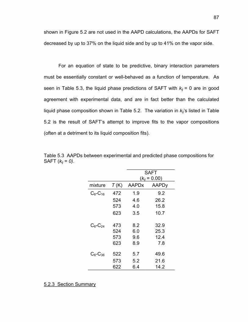
87
shown in Figure 5.2 are not used in the AAPD calculations, the AAPDs for SAFT
decreased by up to 37% on the liquid side and by up to 41% on the vapor side.
For an equation of state to be predictive, binary interaction parameters
must be essentially constant or well-behaved as a function of temperature. As
seen in Table 5.3, the liquid phase predictions of SAFT with kij = 0 are in good
agreement with experimental data, and are in fact better than the calculated
liquid phase composition shown in Table 5.2. The variation in kij‘s listed in Table
5.2 is the result of SAFT’s attempt to improve fits to the vapor compositions
(often at a detriment to its liquid composition fits).
Table 5.3 AAPDs between experimental and predicted phase compositions for SAFT (kij = 0).
SAFT (kij = 0.00)
mixture T (K) AAPDx AAPDy C6-C16 472 1.9 9.2
524 4.6 26.2 573 4.0 15.8 623 3.5 10.7
C6-C24 473 8.2 32.9 524 6.0 25.3 573 9.6 12.4 623 8.9 7.8
C6-C36 522 5.7 49.6 573 5.2 21.6 622 6.4 14.2
5.2.3 Section Summary

88
In spite of its deficiencies in vapor phase predictions and modeling of the
critical region, SAFT is a better equation of state for predicting the phase
behavior of highly asymmetric mixtures of alkanes compared to the conventional
cubic equations. Because SAFT parameters correlate with molecular weight, we
can avoid uncertainties in the critical points for long-chain alkanes that figure in
the cubic equations of state calculations. Using a kij of 0, SAFT will provide good
estimates of liquid phase compositions up to within 5 to 10 bars of the predicted
mixture critical point. This means that we should be able to obtain good
predictions of crude oil thermodynamic properties using SAFT if we set the kij‘s
between all alkanes in oil (with the exception of the light gases) to 0.
5.3 Polystyrene-Solvent/Precipitant Mixtures
5.3.1 Background Information
The goal of this section is to investigate the effects of asphaltene size on
solubility via the behavior of various molecular weight polystyrenes in hexane
and in mixtures of toluene and ethane. Polystyrene is chosen as an “asphaltene”
model compound because it shares structural similarities (i.e., very large and
possessing a certain degree of aromaticity) with asphaltenes and interacts mainly
through dispersion forces.
Unlike mixtures of long-chain alkanes with solvents, mixtures containing
polymers are less well defined (the polymers will exhibit at least some
polydispersity) and the polymers do not have quantifiable vapor compositions.

89
The phase behavior of polymer solutions are often given in terms of the mixtures’
cloud point pressures. This is the pressure at which a polymer in a mixture at
fixed temperature, composition, and polymer molecular weight distribution first
becomes unstable and is equivalent to the onset instability pressure for
asphaltenes in oil described in Chapter 3.
The SAFT equation of state used to calculate polystyrene properties is
slightly different than that used in the other calculations presented in this work.
More specifically, the dispersion contribution developed by Chen and
Kreglewski[103] (as proposed by Huang and Radosz[70,93]) is used in the
polystyrene investigations. Recall that the SAFT EOS described in Chapter 4
(which is used in the rest of this work) has its dispersion contribution from Gross
and Sadowski[62]. While the pure component parameters and the mixture binary
interaction parameters vary depending on the dispersion contribution used, the
two different forms of SAFT will reproduce and show the same phase behaviors.
5.3.2 Results and Discussions
Using the pure component parameters listed in Table 5.4, we generated
the cloud point pressures for a 4% mass polystyrene in n-hexane solution. The
polystyrene used in the experiment is nearly monodisperse. As shown in Figure
5.3, SAFT predicts accurately the phase behavior of the polystyrene-hexane
binary mixture over a wide range of pressures and temperatures from a low
molecular weight of 8,000 to a high polystyrene molecular weight of 50,000.

90
These calculations were made using a single binary interaction parameter of
0.017. As the molecular weight of the polymer increases, so does the size of the
two phase region. And at a given temperature, pressure increases will eventually
move the system from a two-phase region into a one phase region due to the
increase in the solvent’s cohesive energy density with increasing pressure.
Table 5.4 SAFT parameters used to model polystyrene phase behavior. These parameters were obtained using the dispersion contribution developed by Chen and Kreglewski. [103]
Compound σ (A) ε/k (K) m ethane 3.2382 191.44 1.941 hexane 3.0827 202.72 4.724
polystyrene 3.0430 226.50 MW/21.9696 toluene 3.0251 245.27 4.373
Figure 5.3 Cloud point pressures for 4% polystyrene solution in n-hexane. Experimental data are from Xiong and Kiran[104].

91
We compared experimental cloud point pressures with SAFT predictions
for 1%, 4%, and 8% mass polystyrene (8,000 MW) in hexane in Figure 5.4. As
seen in the figure, SAFT qualitatively predicts the effects of different polymer
concentrations on cloud point pressures. A large shift in the cloud point curves
from 1% to 4% mass polystyrene is observed while a considerably smaller shift in
the cloud point curve is observed between 4% and 8% mass polystyrene. A
constant kij of 0.017 was used in all calculations.
Figure 5.4 Cloud point pressures for 8,000 MW polystyrene solution in n-hexane. Experimental data are from Xiong and Kiran[104].
An interesting observation from Figure 5.3 and 5.4 is that SAFT predicts
the presence of a lower critical solution temperature (LCST) region at the higher

92
temperatures. In this region, an increase in temperature (at a fixed pressure) will
result in the demixing of the polystyrene solution; the more typically observed
behavior of increasing solubility with increasing temperature occurs in the upper
critical solution temperature, or UCST region. While polystyrene-pentane and
polystyrene-butane systems are known to exhibit LCST behaviors at higher
temperatures, the presence of the LCST region has only been conjectured for the
polystyrene-hexane system due to insufficient data.[104]
The existence of the UCST and LCST regions can be explained in terms
of contributions to the Gibbs energy. At lower temperatures, entropy effects
dominate and polystyrene solubility increases with increasing temperature. At
the higher temperatures (i.e., as the critical temperature of the solvent is
approached), enthalpy effects dominate due to increasing differences in the rate
of free volume expansion of the components, which effects large changes in the
cohesive energy density of the solvent. In the case of the polystyrene-hexane
system investigated here, the critical temperature of hexane is about 507.5K.[96]
Although the polystyrene-hexane mixture is only a model system for
asphaltenes, it elucidates characteristics typical of asphaltenes in crude oil. For
instance, operations that decrease pressure (at fixed temperature and
composition, as in the case when the mixture is above its bubble point) may lead
to asphaltene phase separation due to increasing differences in the species’ free
volumes. And the opposing solubility behavior of asphaltenes with changes in

93
temperature, similar to the polystyrene mixing/demixing behaviors with
temperature change in the UCST and LCST regions, has been reported in
literature. From the free energy description given above, we can expect the
onset of LCST behavior to shift to lower temperatures with increasing
concentration of light gases in the asphaltene-containing solution (this behavior is
observed in Figure 5.4 and in Figure 5.7 for the mixture polystyrene-toluene-
ethane, which will be discussed in the next section). Indeed, it has been
discussed in literature[23] that with propane (Tc~100°C) addition, asphaltenes
become increasingly unstable with temperature increase. On the other hand, for
n-alkane (n-C5+) titrations, asphaltenes become more stable with increasing
temperature.[23] Of course, whether or not LCST behavior will be observed
depends on the temperature range investigated.
A comparison of experimental and SAFT calculated phase equilibrium
compositions (and tie lines) for a mixture of polystyrene, toluene, and ethane at
343K shows that SAFT can accurately account for the effects of pressure and
composition changes (Figure 5.5). The polystyrene used in this experiment has
a number average MW of 68,000 and MWw/MWn = 2.21. A single binary
interaction parameter for ethane-polystyrene listed in Figure 5.5 was fit to
equilibrium composition data at 62 bar. This system is similar to the model live
oil described in Chapter 3 in that we have polystyrene (the model asphaltene)
dissolved in a mixture of solvent (toluene) and precipitant (ethane). Like
asphaltenes, varying the amounts of toluene (solvent) and ethane (precipitant)

94
changes the stability of polystyrene (at a fixed polymer concentration) in the
system. Addition of toluene makes the system miscible, while ethane addition
eventually results in phase separation (Fig. 5.5).
Figure 5.5 Ethane-toluene-polystyrene phase diagram at 343K and 62 or 117.2 bar. The compositions are in mass fractions and the regions of liquid-liquid (L-L), liquid-liquid-vapor (L-L-V), and liquid-vapor (L-V) equilibria are demarcated. Experimental data are from Seckner, et al.[105].
SAFT-predicted pressure effects on the phase stability of the ethane,
toluene, and polystyrene system at 500K is plotted in Figure 5.6. When the
pressure is increased from 300 to 500 bars, we see an increase of the single
phase region. This is expected because increasing pressure increases the
density and thus the cohesive energy density of the solvent. It is interesting to
note in Figures 5.5 and 5.6 that at a given pressure, the stability boundary is
approximately a function of ethane mass fraction and is nearly independent of
the amount of polystyrene. This is analogous to saying that asphaltene stability
is dominated by the solution gas-oil-ratio rather than the amount of asphaltenes

95
in the solution. It is also interesting to note that a plait point is observed at each
of the pressures; when ethane is added to the system to induce precipitation, the
precipitated phase can be either polymer lean or polymer rich depending on the
polymer concentration with respect to the plait point. Both the formation of a light
phase (asphaltene-lean) and the formation of a heavy phase (asphaltene-rich)
have been observed at asphaltene instability onset in the field.[106]
Figure 5.6 SAFT-predicted polysytrene-toluene-ethane phase diagram at 500K and 300 or 500 bars.
In Figure 5.7, we compared SAFT-predicted pressure-temperature
diagrams for a system containing 17.8% mass ethane (in toluene and 68,000
number average MW polystyrene) and a system containing 22.5% mass ethane
with experimental data of Seckner, et al.[105]. The binary interaction parameters
for the polystyrene-toluene-ethane system fitted to equilibrium composition data

96
at 343K and 62 bar were used in these calculations. To obtain these data,
Seckner, et al. slowly added ethane to a mixture with initially 5% mass
polystyrene dissolved in toluene until the onset of phase instability. This is
similar to the methane titration of a 1g asphaltene/100mL toluene mixture until
asphaltene instability onset in our experimental studies.
As seen in Figure 5.7, SAFT qualitatively describes the liquid-liquid and
liquid-vapor equilibrium phase behavior of the polystyrene-toluene-ethane
mixture with 17.8% mass ethane. The predicted phase envelopes are
consistently lower than the experimental values. For the polystyrene-toluene-
ethane mixture with 22.5% mass ethane, SAFT predictions for the liquid-liquid
instability onset do not agree well with experimental data; SAFT shows the
“breaking off” of the LCST/UCST curve from the LV curve at a much higher
temperature than measured. According to Seckner, et al.[105], the location of the
LCST curve becomes very sensitive to ethane concentration at levels of 20%
mass or greater. For example, the behavior predicted by SAFT is seen
experimentally for the system with 24.9% mass ethane[105]. The poor prediction
given by SAFT is partly due to uncertainties in concentration measurements, to
the effects of polymer polydispersity, and to the fact that the binary interaction
parameters were not optimized.
We expect the “peculiar” temperature dependence of asphaltenes (i.e. the
behavior in the LCST region) to be most apparent in systems with a large

97
concentration of light gas components and in reservoirs with higher
temperatures.
Figure 5.7 Experiment and SAFT-predicted pressure-temperature diagrams for the system polystyrene, toluene, and ethane. L=one liquid phase, L-L=two liquid phases in coexistence, L-V=liquid and vapor phases in coexistence. Experimental data are from Seckner, et al.[105].
5.3.3 Section Summary
In this section, we showed that SAFT is capable of describing and
predicting the phase behavior of binary and ternary systems consisting of
species with very large size disparities. Various molecular weight polystyrenes

98
were used as model asphaltenes and their behaviors in solvents and precipitants
investigated. The effects of pressure, temperature, and composition changes on
phase stability can be accurately described using SAFT. Furthermore, because
of similarities in phase behavior between asphaltenes and polystyrene, we were
able to describe many asphaltene behaviors in crude oil in the framework of
polymer thermodynamics.
5.4 Phenanthrene-Solvent/Precipitant Mixtures
5.4.1 Background Information
The phase behavior of the system phenanthrene-methane-decane at
solid-liquid-vapor equilibrium (SLVE) was modeled to investigate whether SAFT
can describe the solubility behavior of polynuclear aromatics. In this
investigation, SAFT was used to describe fluid behavior in the liquid phase only;
the solid phase was described using Eqn. 5.10. Phenanthrene, a three-ring
polynuclear aromatics, was the model asphaltene in this work. Recall from
Chapter 2 that the polynuclear aromatic cores of asphaltene molecules are
structurally similar to a phenanthrene molecule. The conjugated benzene rings
in the polynuclear aromatics (PNAs) make PNAs much more polarizable than
linear or branched molecules of similar molecular weights (due to the
delocalization of the π electrons).

99
When a (pure) solid phase is in equilibrium with a liquid phase, the
fugacity of the solid (fi,solid) is related to that specie’s subcooled (pure) liquid
fugacity (fi,liq) by the ratio[107,108]
( ) λ+−∆+∆
+
−
∆−
−∆= sattptpt
t
f
solidi
liqi PPRT
vTT
Rc
TT
Rc
TT
RTh
ff
ln11ln,
, (5.10)
In Eqn. 5.10, ∆hf is the enthalpy of fusion, ∆cp is the change in heat capacity from
the liquid to the solid phase, ∆v is the change in volume from the liquid to the
solid phase, and λ is the change in Gibbs energy due to solid-solid phase
transition divided by RT. The solid properties ∆hf, cpsolid, vsolid, and λ are
determined from experiments. The triple point temperature Tt can be
approximated with the melting point temperature. Furthermore, the two terms
containing the heat capacities are approximately equal in magnitude and
opposite in sign in this investigation and can be dropped from Eqn. 5.10. For
example, the magnitudes of the two terms containing the heat capacities differ by
at most about 3% in the temperature range investigated. In this investigation, the
fugacity of the subcooled liquid phenanthrene, the molar volume of the subcooled
liquid phenanthrene, and the saturation pressure of the subcooled liquid
phenanthrene were calculated using SAFT; the value for ∆hf and λ and the molar
volume of solid phenanthrene were obtained from experiment. The condition of
equi-fugacity between the solid and liquid phases was enforced at a given T and
P to obtain the equilibrium compositions.
5.4.2 Results and Discussions

100
The solid and phase transition properties of phenanthrene are listed in
Table 5.5 and the SAFT pure component parameters are listed in Table 4.1.
Note that a solid-solid phase transition exists for phenanthrene at 347.5K. [109]
Table 5.5 Select solid, solid-solid and solid-liquid phase transition properties of pure phenanthrene.[109]
vsolid 151.7 cm3/mol Tm 372.4 K ∆hf 16,463 J/mol
λ transition energy 217 J/mol
The calculated and experimental SLVE compositions at pressures
between 20.2 and 60.8 bar and temperatures between 350 K and 362K are
plotted in Figure 5.8. The binary interaction parameters between phenanthrene-
methane (kij = 0.094) and methane-decane (kij = 0.015) were fit to two-
component vapor-liquid equilibrium data[110-112] while the kij between
phenanthrene and decane (kij = 0.012) was fit to the SLV equilibrium
compositions at 350K. Comparison of the calculations with experimental data
shows good agreement. As expected, the size of the SLVE region decreases as
the temperature of the system approaches the melting temperature of
phenanthrene. At a given temperature, increasing the system’s pressure will
decrease the size of the SLVE region but will increase the size of the SLE region.
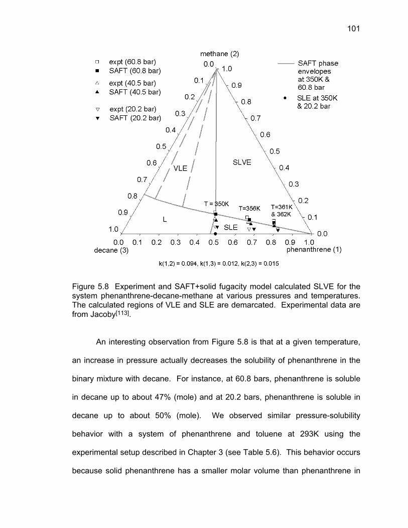
101
Figure 5.8 Experiment and SAFT+solid fugacity model calculated SLVE for the system phenanthrene-decane-methane at various pressures and temperatures. The calculated regions of VLE and SLE are demarcated. Experimental data are from Jacoby[113].
An interesting observation from Figure 5.8 is that at a given temperature,
an increase in pressure actually decreases the solubility of phenanthrene in the
binary mixture with decane. For instance, at 60.8 bars, phenanthrene is soluble
in decane up to about 47% (mole) and at 20.2 bars, phenanthrene is soluble in
decane up to about 50% (mole). We observed similar pressure-solubility
behavior with a system of phenanthrene and toluene at 293K using the
experimental setup described in Chapter 3 (see Table 5.6). This behavior occurs
because solid phenanthrene has a smaller molar volume than phenanthrene in

102
solution. When the system is pressurized, more liquid phenanthrene would go
into the solid phase to minimize system volume. As seen in Table 5.6, although
our model qualitatively describes the same pressure-solubility behavior, the
predicted solubility is less sensitive to pressure than what was observed in
experiments. We do not expect this type of pressure-solubility behavior to occur
for asphaltenes because their polydispersity and the side groups surrounding
their polynuclear aromatic cores prevent crystallization.
Table 5.6 Pressure-solubility behavior of phenanthrene in toluene at 293K.
solubility pressure (psi)a
exp. mole frac. Phenanthrene
SAFT mole frac. phenanthrene
(kij=0.008) ~4200 0.147 0.152 ~4500 ~5100
0.145 0.143
0.151 0.151
a phenanthrene is soluble below the solubility pressure.
5.4.3 Section Summary
In this section, we showed that SAFT (together with a solid fugacity
model) is able to describe the solubility behavior of polynuclear aromatics
through an investigation of the SLVE phase behavior of phenanthrene in decane
and methane. The size of the SLVE region decreases with increasing
temperature and pressure, and the size of the one-phase (liquid) region
increases with increasing pressure. Furthermore, the model is able to predict the
pressure-solubility behavior of phenanthrene in which increasing pressure leads
to lower solubility.

103
CHAPTER 6. MODELING OF ASPHALTENE PHASE BEHAVIOR
6.1 Introduction
The SAFT equation of state will be used to model asphaltene phase
behavior in a model live oil and a recombined oil under reservoir conditions, with
the asphaltenes modeled as a monodisperse species. Recall from Chapter 3
that the model live oil is a mixture of n-heptane insoluble asphaltenes in toluene
and methane, and that the recombined oil is a mixture of stock-tank oil with its
separator gas. We will compare the theory results with asphaltene precipitation
data from n-alkane titrations at ambient conditions and from reservoir
depressurization described in Chapter 3.
Two issues that will be addressed in this chapter are: (1) how to model
asphaltenes in SAFT and (2) how to model the other oil components in SAFT.
The equation of state parameters for asphaltenes are fit to ambient condition
precipitation data from oil titrations with n-alkanes. If the mechanism responsible
for asphaltene precipitation under reservoir depressurization is consistent with
the mechanism in titration experiments, thermodynamic models that correctly
account for the interaction forces should be able to predict the depressurization
results based on matching the results of the titration experiments. To model
reservoir fluids in SAFT, a lumping scheme that divides the recombined oil into
six pseudo-components based on composition (from gas chromatography),

104
saturates-aromatics-resins-asphaltenes (SARA) fractionation, and gas-oil-ratio
(GOR) is introduced.
As discussed in Chapter 2, the underlying hypothesis of our approach is
that molecular size and nonpolar van der Waals interactions dominate
asphaltene phase behavior in crude oil. This view is supported by: (1) the large
effects on intermolecular interactions due to the polynuclear aromatic cores; (2)
by the solubility parameter mapping arguments[8]; (3) by the contrasting solvating
and precipitating abilities of non-polar materials of similar sizes and structures
(i.e. toluene vs. n-heptane and CS2 vs. CO2); and (4) by the success of using
refractive index to estimate the stability of asphaltenes in oil-precipitant mixtures
(see Chapter 3). Within this molecular thermodynamic framework, SAFT is a
good candidate for asphaltene phase behavior modeling because it accurately
describes and predicts the phase behavior of nonpolar fluids where molecular
size and shape interactions dominate (see Chapter 5).
6.2 Model Oil Investigations
6.2.1 Determination of Asphaltene SAFT Parameters
Since the model oil is a mixture of well defined species with n-C7 insoluble
asphaltenes, all SAFT parameters except those for the asphaltenes can be found
in Table 4.1. We will fit the SAFT parameters for asphaltenes to the measured
composition and mixture refractive index data at the onset of asphaltene
instability with n-alkane titration (Table 3.2). The procedure is outlined in Figure

105
6.1. Essentially, a set of SAFT asphaltene parameters is chosen such that (1)
the calculated solubility parameter (δ) is in the range reported for asphaltenes,
(2) the SAFT asphaltene parameters are within the correlation space bound by
the n-alkanes and PNA correlations (see Fig. 4.6), and (3) the asphaltenes are
soluble in toluene. The parameters that meet the above criteria are then used to
calculate the mixture composition and refractive index (PRI) at the onset of
asphaltene instability for a range of n-alkane precipitants at ambient conditions.
If the calculated compositions and PRIs’ do not agree with experimental
measurements, another set of asphaltene SAFT parameters that satisfies the
aforementioned constraints (refer to Chapter 7 for the selection guidelines) is
used and the procedure repeated until satisfactory agreement (determined, for
instance, with average absolute percent deviations between measured and
calculated compositions or PRIs) is obtained.
The refractive index of the asphaltene-toluene-precipitant mixture at the
onset of asphaltene instability can be calculated from instability onset
compositions using Eqn. 3.1. As described in Chapter 3.4, we use an asphaltene
molar refraction of 1317 cm3/mol in our calculations but the contribution of
asphaltenes is extremely small due to their low concentrations. The molar
refraction of other species (toluene and n-alkanes) are calculated from group
contribution methods given in the CRC Handbook of Chemistry and Physics.[44]
For these compounds, the molar refractions calculated using the group
106
contribution method are in good agreement with those calculated from measured
pure species’ refractive indices and densities (see Table 3.6).
To satisfy the mass density requirement of pure asphaltenes (i.e.
asphaltenes having densities between 1.13 g/cm3 and 1.20 g/cm3), the molecular
weight of the asphaltene needs to be recalculated every time the set of SAFT
asphaltene parameters is changed. This is important because SAFT requires
molar compositions as inputs. Since the asphaltene/toluene ratio in the model oil
is 1g asphaltenes per 100mL toluene at 293 K and 1 bar, failure to update the
asphaltene molecular weight whenever the SAFT asphaltene parameters are
changed effectively will change the ratio of asphaltenes to toluene between the
iterations.

107
Figure 6.1 Asphaltene SAFT parameters fitting procedure.
To reduce the number of fitted parameters, all binary interaction
parameters between asphaltenes and other species are set to zero. The kijs’
between toluene and n-alkanes (from pentane to hexadecane) are also set to 0
because SAFT adequately describes the VLE behavior of these systems with
zero kij.
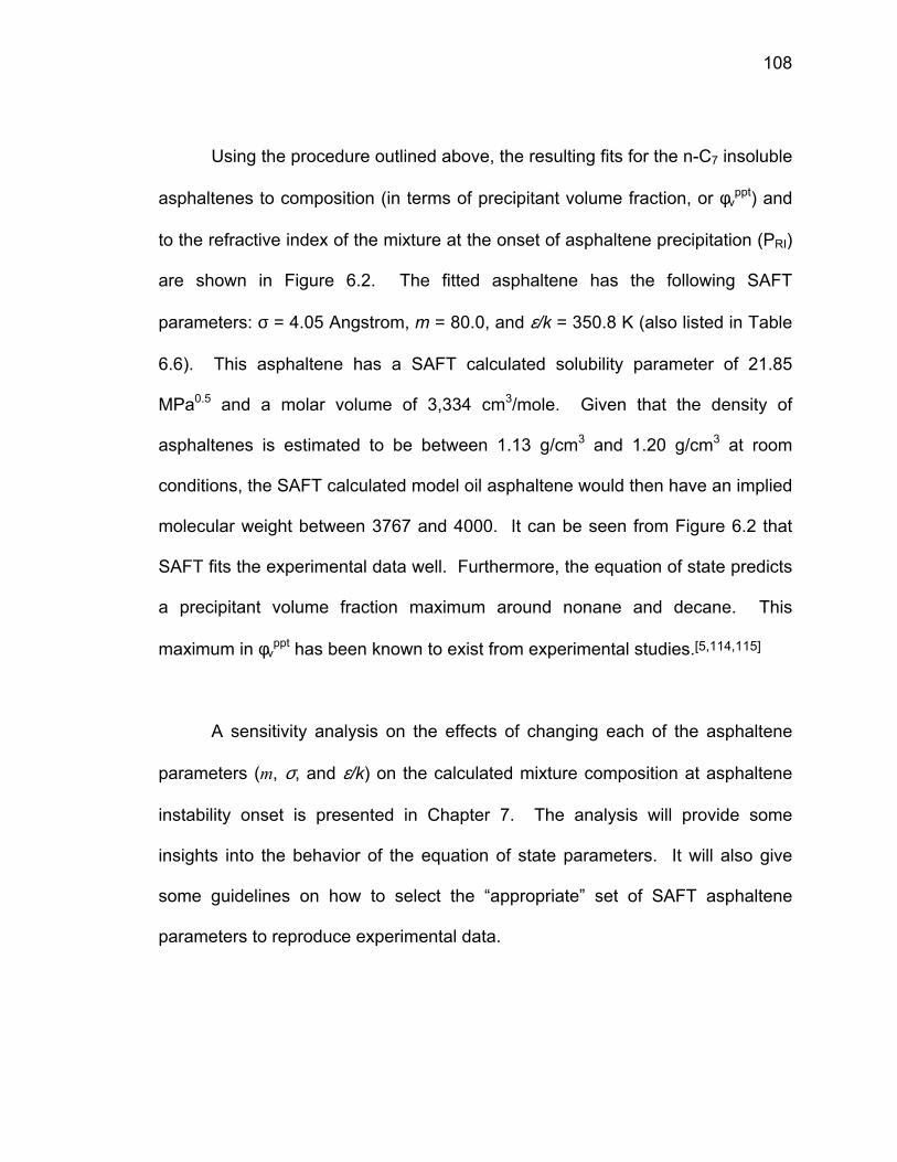
108
Using the procedure outlined above, the resulting fits for the n-C7 insoluble
asphaltenes to composition (in terms of precipitant volume fraction, or φvppt) and
to the refractive index of the mixture at the onset of asphaltene precipitation (PRI)
are shown in Figure 6.2. The fitted asphaltene has the following SAFT
parameters: σ = 4.05 Angstrom, m = 80.0, and ε/k = 350.8 K (also listed in Table
6.6). This asphaltene has a SAFT calculated solubility parameter of 21.85
MPa0.5 and a molar volume of 3,334 cm3/mole. Given that the density of
asphaltenes is estimated to be between 1.13 g/cm3 and 1.20 g/cm3 at room
conditions, the SAFT calculated model oil asphaltene would then have an implied
molecular weight between 3767 and 4000. It can be seen from Figure 6.2 that
SAFT fits the experimental data well. Furthermore, the equation of state predicts
a precipitant volume fraction maximum around nonane and decane. This
maximum in φvppt has been known to exist from experimental studies.[5,114,115]
A sensitivity analysis on the effects of changing each of the asphaltene
parameters (m, σ, and ε/k) on the calculated mixture composition at asphaltene
instability onset is presented in Chapter 7. The analysis will provide some
insights into the behavior of the equation of state parameters. It will also give
some guidelines on how to select the “appropriate” set of SAFT asphaltene
parameters to reproduce experimental data.
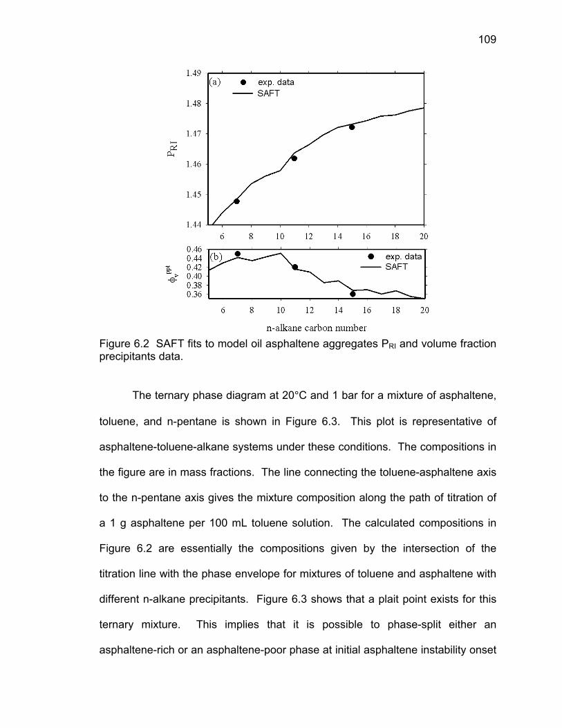
109
Figure 6.2 SAFT fits to model oil asphaltene aggregates PRI and volume fraction precipitants data.
The ternary phase diagram at 20°C and 1 bar for a mixture of asphaltene,
toluene, and n-pentane is shown in Figure 6.3. This plot is representative of
asphaltene-toluene-alkane systems under these conditions. The compositions in
the figure are in mass fractions. The line connecting the toluene-asphaltene axis
to the n-pentane axis gives the mixture composition along the path of titration of
a 1 g asphaltene per 100 mL toluene solution. The calculated compositions in
Figure 6.2 are essentially the compositions given by the intersection of the
titration line with the phase envelope for mixtures of toluene and asphaltene with
different n-alkane precipitants. Figure 6.3 shows that a plait point exists for this
ternary mixture. This implies that it is possible to phase-split either an
asphaltene-rich or an asphaltene-poor phase at initial asphaltene instability onset

110
depending on the amount of asphaltenes initially present in the system. In the
field, both “light” (asphaltene-lean) and “heavy” (asphaltene-rich) precipitated
phases have been observed at the onset of asphaltene instability.[106]
Furthermore, information on the compositions along the tie lines may provide
insights into the morphology of the various phases. It is interesting to note that
the mass fraction of pentane in the asphaltene-rich (“heavy”) phase is relatively
constant.
Figure 6.3 Ternary phase diagram at 20°C and 1 bar for a mixture of asphaltene, toluene, and n-pentane. The compositions are in mass fractions.
6.2.2 Comparison of Predicted and Measured Asphaltene Instability Onsets
With the asphaltene parameters determined above, SAFT can be used to
predict the phase behavior of the model live oil system (mixture of toluene,
methane, and asphaltenes). Comparison between SAFT predictions and

111
experimental data shows qualitative agreement (Figure 6.4). In these
calculations, a temperature independent methane-toluene binary interaction
parameter of 0.029 (determined from methane-toluene vapor-liquid equilibria
determined in this work and by Elbishlawi and Spencer[116]) was used and all
other binary interaction parameters were set to zero. While SAFT predicts the
correct temperature dependence of the asphaltene instability curves, its
predictions become worse at higher methane concentrations. In the most part,
SAFT calculated asphaltenes are less stable than experimental observations. We
believe that the inclusion of asphaltene polydispersity will improve the quality of
these predictions.
Figure 6.4 Experimental and SAFT-predicted asphaltene instability onsets and bubble points for the model oil at 20.0°C and 65.5°C.

112
Since the SAFT equation of state provides accurate solubility parameters,
we can plot the change in the mixture solubility parameter during pressure
depletion. As seen in Figure 6.5 (for the model live oil at 20.0°C with 0.143 mass
fraction methane above the bubble point), asphaltenes in the model oil are stable
above a certain solubility threshold. Asphaltenes are unstable below the
asphaltene instability line shown in Figure 6.5 and are stable above that line.
Above the bubble point, asphaltenes are stable at high pressures because of
high solvent density. Below the bubble point, asphaltenes are stable at lower
pressures because of changing composition (i.e. the light ends start to leave the
liquid mixture). As expected, the plot of mixture solubility parameter and the plot
of refractive index (the same RI plot in Figure 3.10) show the same behavior
because refractive index is a measure of solubility parameter for fluids dominated
by nonpolar interactions. The presence of the solubility threshold means that at
each temperature, we can estimate whether a reservoir will encounter
asphaltene related problems by examining how far the solubility parameter (or
refractive index) of the reservoir fluid is from its solubility threshold.

113
Figure 6.5 Calculated refractive index and SAFT calculated mixture solubility parameter during pressure depletion for the model live oil at 20.0°C with 0.143 mass fraction methane above the bubble point. Asphaltenes are unstable below the asphaltene instability line.
6.3 Recombined Oil Investigations
To model the phase behavior of the recombined oil (stock-tank oil plus its
separator gas with compositions given in Table 3.3), the oil is treated as a six
pseudo-components mixture. Three sub-fractions (methane, N2+CO2, and light
n-alkanes) are used to describe the separator gas and three sub-fractions
(saturates, aromatics+polynuclear aromatics, and asphaltenes) are used to

114
describe the stock-tank oil. The relative amount of each sub-fraction can be
calculated based on composition data from gas chromatography (GC), SARA
fractionation data, and GOR data listed in Chapter 3.
6.3.1 Separator Gas Characterization
The molar composition of the separator gas is listed in Table 6.1 together
with each sub-fraction’s pseudo-component SAFT parameters. As seen in the
table, the average molecular weight of the light n-alkane sub-fraction is similar to
that of propane, and a correlation described in the footnote to Table 6.1 is used
to calculate the light n-alkane sub-fraction SAFT parameters. Note also that N2
and CO2 are modeled as a separate pseudo-component. The SAFT calculated
density of 0.3708 g/cm3 obtained from the three pseudo-component treatment of
the separator gas compares well with the experimentally determined density of
0.3773 g/cm3 at 241.3 bar and 293K. The binary interaction parameters used
between the separator gas sub-fractions are listed in Table 6.2.

115
Table 6.1 Composition of the separator gas and the pseudo-component SAFT parameters.
SAFT parameters
component MW mole frac.pseudo-comp.
mole frac.MWn σ (A) m ε/k (K)
CO2 44.01 0.0126 N2 28.01 0.1385
0.1510 29.34 3.3130a 1.2053a 90.96a
methane 16.04 0.5063 0.5063 16.04 3.7039f 1.0000d 150.03s
ethane 30.07 0.1320 propane 44.09 0.0913 butane 58.12 0.0719 pentane 72.15 0.0315 hexane 86.17 0.0090 heptane 100.21 0.0045 octane 114.23 0.0021 nonane 128.26 0.0005
0.3427 46.61 3.6917b 1.9854b 206.12b
Total 1.0000 1.00000
MWn 28.524 a SAFT parameters for N2 is used because of low CO2 composition. b Obtained from molecular weight correlations similar to the n-alkane correlations in
Table 4.2, with the exception that the correlation used here was only based on parameters from ethane to decane.
Table 6.2 Binary interaction parameters for the separator gas sub-fractions.
methane N2+CO2 light n-alkanes methane 0.000z 0.000a 0.011b N2+CO2 0.000a 0.000z 0.071c
light n-alkanes 0.011b 0.071c 0.000z a based on methane-N2 binary data of Kidnay, et al.[117] b based on methane-propane binary data of Reamer, et al.[118] c based on N2-propane binary data of Grauso, et al.[119]
6.3.2 Stock-Tank Oil Characterization
The stock-tank oil is treated as a mixture of 3 pseudo-components
(saturates, aromatics+resins, and asphaltenes). The following assumptions are
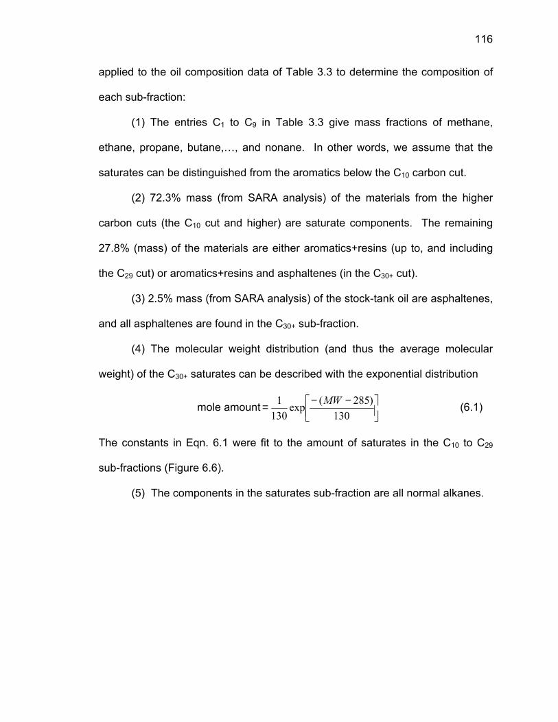
116
applied to the oil composition data of Table 3.3 to determine the composition of
each sub-fraction:
(1) The entries C1 to C9 in Table 3.3 give mass fractions of methane,
ethane, propane, butane,…, and nonane. In other words, we assume that the
saturates can be distinguished from the aromatics below the C10 carbon cut.
(2) 72.3% mass (from SARA analysis) of the materials from the higher
carbon cuts (the C10 cut and higher) are saturate components. The remaining
27.8% (mass) of the materials are either aromatics+resins (up to, and including
the C29 cut) or aromatics+resins and asphaltenes (in the C30+ cut).
(3) 2.5% mass (from SARA analysis) of the stock-tank oil are asphaltenes,
and all asphaltenes are found in the C30+ sub-fraction.
(4) The molecular weight distribution (and thus the average molecular
weight) of the C30+ saturates can be described with the exponential distribution
mole amount
−−=
130)285(exp
1301 MW (6.1)
The constants in Eqn. 6.1 were fit to the amount of saturates in the C10 to C29
sub-fractions (Figure 6.6).
(5) The components in the saturates sub-fraction are all normal alkanes.
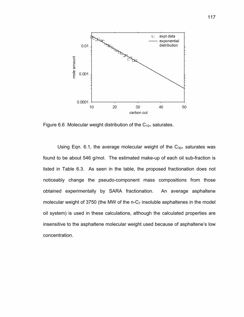
117
Figure 6.6 Molecular weight distribution of the C10+ saturates.
Using Eqn. 6.1, the average molecular weight of the C30+ saturates was
found to be about 546 g/mol. The estimated make-up of each oil sub-fraction is
listed in Table 6.3. As seen in the table, the proposed fractionation does not
noticeably change the pseudo-component mass compositions from those
obtained experimentally by SARA fractionation. An average asphaltene
molecular weight of 3750 (the MW of the n-C7 insoluble asphaltenes in the model
oil system) is used in these calculations, although the calculated properties are
insensitive to the asphaltene molecular weight used because of asphaltene’s low
concentration.

118
Table 6.3 Estimated compositions of each stock-tank oil sub-fraction.
SCN properties saturates sub-fraction aromatics+resins sub-fraction
Component MWn mass frac. MWsat
mass frac.
norm. mole frac. MWaro+res
mass frac.
norm. mole frac.
C5 072.15 0.001 072.15 0.001 0.004 C6 086.20 0.004 086.18 0.004 0.016
Cyclopentane 084.16 0.001 084.16 0.001 0.007 Benzene 078.11 0.000 078.11 2.3E-4 0.003
Cyclohexane 084.16 0.001 084.16 0.001 0.013 Heptane 100.20 0.009 100.20 0.009 0.031
Cyclohexane 098.19 0.004 098.19 0.004 0.035 Toluene 092.14 0.001 092.14 0.001 0.010 Octane 114.23 0.020 114.23 0.020 0.062
Ethylbenzene 106.17 0.001 106.17 0.001 0.012 Xylene 106.17 0.005 106.17 0.005 0.038
C9 128.30 0.027 128.25 0.020 0.054 128.43 0.008 0.052 C10 134.00 0.041 142.29 0.030 0.074 116.31 0.011 0.087 C11 147.00 0.041 156.31 0.030 0.067 127.21 0.011 0.079 C12 161.00 0.040 170.34 0.029 0.060 140.84 0.011 0.069 C13 175.00 0.045 184.37 0.033 0.063 154.51 0.013 0.071 C14 190.00 0.042 198.39 0.031 0.055 171.10 0.012 0.060 C15 206.00 0.044 212.42 0.032 0.053 190.93 0.012 0.056 C16 222.00 0.038 226.45 0.027 0.043 211.17 0.010 0.044 C17 237.00 0.035 240.47 0.025 0.037 228.39 0.010 0.037 C18 251.00 0.035 254.50 0.025 0.035 242.30 0.010 0.035 C19 263.00 0.034 268.53 0.024 0.032 249.58 0.009 0.033 C20 275.00 0.031 282.55 0.022 0.028 257.06 0.008 0.029 C21 291.00 0.028 296.56 0.020 0.024 277.41 0.008 0.025 C22 305.00 0.025 310.59 0.018 0.021 291.31 0.007 0.021 C23 318.00 0.024 324.61 0.017 0.019 301.93 0.007 0.020 C24 331.00 0.021 338.64 0.015 0.016 312.58 0.006 0.017 C25 345.00 0.022 352.67 0.016 0.016 326.47 0.006 0.017 C26 359.00 0.017 366.69 0.012 0.012 340.36 0.005 0.012 C27 374.00 0.020 380.72 0.014 0.013 357.53 0.005 0.013 C28 388.00 0.017 394.74 0.012 0.011 371.43 0.005 0.011 C29 402.00 0.017 408.77 0.013 0.011 385.33 0.005 0.011
C30+ 580.00 0.307 546.00 0.222 0.145 640.75 0.060 0.083 Total mass/mole frac. 1.000 0.723 1.000 0.252 1.000 Average MW 255.00 222.00
The SAFT parameters for the saturates sub-fraction can be calculated
from the sub-fraction’s average molecular weight using the n-alkane correlations
first given in Table 4.2 and reproduced in Table 6.5. The correlated SAFT

119
parameters of the saturates sub-fraction are listed in Table 6.4. In using these
correlations, we assume (assumption 5) that all saturates are normal alkanes.
Comparison of SAFT calculated densities of the saturates-only mixture at
representative pressures and temperatures using the one-fluid (pseudo-
component) and the full 26-components treatment is shown in Figure 6.7. As
expected, the results of the one-fluid and the full 26-components treatment are
similar because SAFT uses the conformal solution mixing rule to describe
mixture properties.
Table 6.4 SAFT parameters for the non-asphaltene stock-tank oil pseudo-components.
saturates aromatics + resins
MWn 255 222 m 7.377 5.335
σ (A) 3.964 3.764 ε/k(K) 257.1 323.7

120
Figure 6.7 Comparison of SAFT calculated densities for the mixture of saturates using the one-fluid treatment and the 26-components treatment.
The SAFT parameters for the aromatics+resins sub-fraction (listed in
Table 6.4) depend not only on the average molecular weight but also on the
average aromaticity of the sub-fraction. This is because the aromatics+resins
sub-fraction is a mixture of aromatics, polynuclear aromatics (PNA), PNA
derivatives, and resins that span a range in terms of the aromaticity of each
molecular constituents. For instance, if a mixture contains a lot of alkyl-benzenes
and very little polynuclear aromatics, it is, on average, less “aromatic” than a
mixture consisting mostly of polynuclear aromatics. Since the SAFT parameters
for compounds in each of these classes follow different parameter correlation
curves (see Figure 4.7), it is important to quantify this “degree of aromaticity”.
We have defined a fitting parameter γ, which we call the aromaticity parameter,
that would relate the degree of aromaticity of the aromatics+resins sub-fraction to
the SAFT parameter correlations used to calculate the sub-fraction’s SAFT

121
parameters (see Table 6.5). With γ = 0, the correlation for the aromatics+resins
sub-fraction reduces to the correlation for PNAs’. With γ = 1, the correlation
reduces to the correlation for benzene, biphenyl, and ter-phenyl.
Table 6.5 SAFT parameter correlations for the saturates and aromatics+resins oil sub-fractions. γ is a ratio parameter related to the degree of aromaticity.a
saturates aromatics + resinsa
correlation for m 0.0253MW+0.9263 γ(0.0201MW+0.7860)+ (1-γ)(0.0139MW + 1.2988)
Correlation for mσ 0.1037MW+2.7985 γ(0.0782MW+2.466) + (1-γ)(0.0597MW + 4.2015)
Correlation for ε/k 32.81ln(MW)+80.398 γ(40.65ln(MW)+112.4) + (1-γ)(119.41ln(MW)-230.21)
a The ratio γ = 1.1 was chosen so that (1) the recombined oil would reproduce the correct bubble point and (2) asphaltenes would be soluble in the aromatics+resins pseudo-component fluid. The two sets of bracketed correlations are those for the polynuclear aromatics and those for benzene, biphenyl, and terphenyl.
We grouped aromatics and resins into one single pseudo-component
because they form a part of the same distribution (that actually extends out to the
asphaltenes).
To pin down a set of parameters for the aromatics+resins sub-fraction, the
following procedure can be used. Starting with the set of SAFT parameters for n-
alkanes at MWn=222, we slowly increase γ, the aromaticity parameter, until (1)
the predicted stock-tank oil density at ambient conditions matches the

122
experimental density and (2) the n-C7 insoluble asphaltene in the model oil
investigations becomes completely soluble in a fluid composed of only the
aromatics+resins sub-fraction. Since the SAFT parameters for the stock-tank oil
asphaltenes have not yet been determined, the n-C7 insoluble asphaltene used
in the model oil investigations can be used in the density calculations. Recall
that the parameters for the model oil asphaltenes were determined from ambient
condition titration in n-alkane precipitants + toluene. The binary interaction
parameter between the saturates and the aromatics+resins pseudo-components
are set to –0.01 based on the optimal kij for toluene-dodecane and toluene-
hexadecane VLE data[120] at 353K and 333K.
The SAFT equation of state parameters for the aromatics+resins pseudo-
component are listed in Table 6.4 and were obtained using the listed correlations;
the γ parameter adjusts for the degree of aromaticity and has a value of 1.1 for
this oil. With γ = 0, the correlation reduces to the correlation for PNAs’. With γ =
1, the correlation reduces to the correlation for benzene, biphenyl, and ter-
phenyl. A comparison of the calculated and experimental stock-tank oil densities
show good agreement; the deviation at 293K and 1 bar between experimental
(0.857 g/cm3) and calculated (0.864 g/cm3) densities is about 0.8% and the
deviation at 328K and 1 bar between experimental (0.848 g/cm3) and calculated
(0.839 g/cm3) densities is about -1%. The good agreement is not surprising
because the density data at 293K and 1 bar was used to fit the pseudo-
component SAFT parameters for the aromatics+resins sub-fraction. Comparison
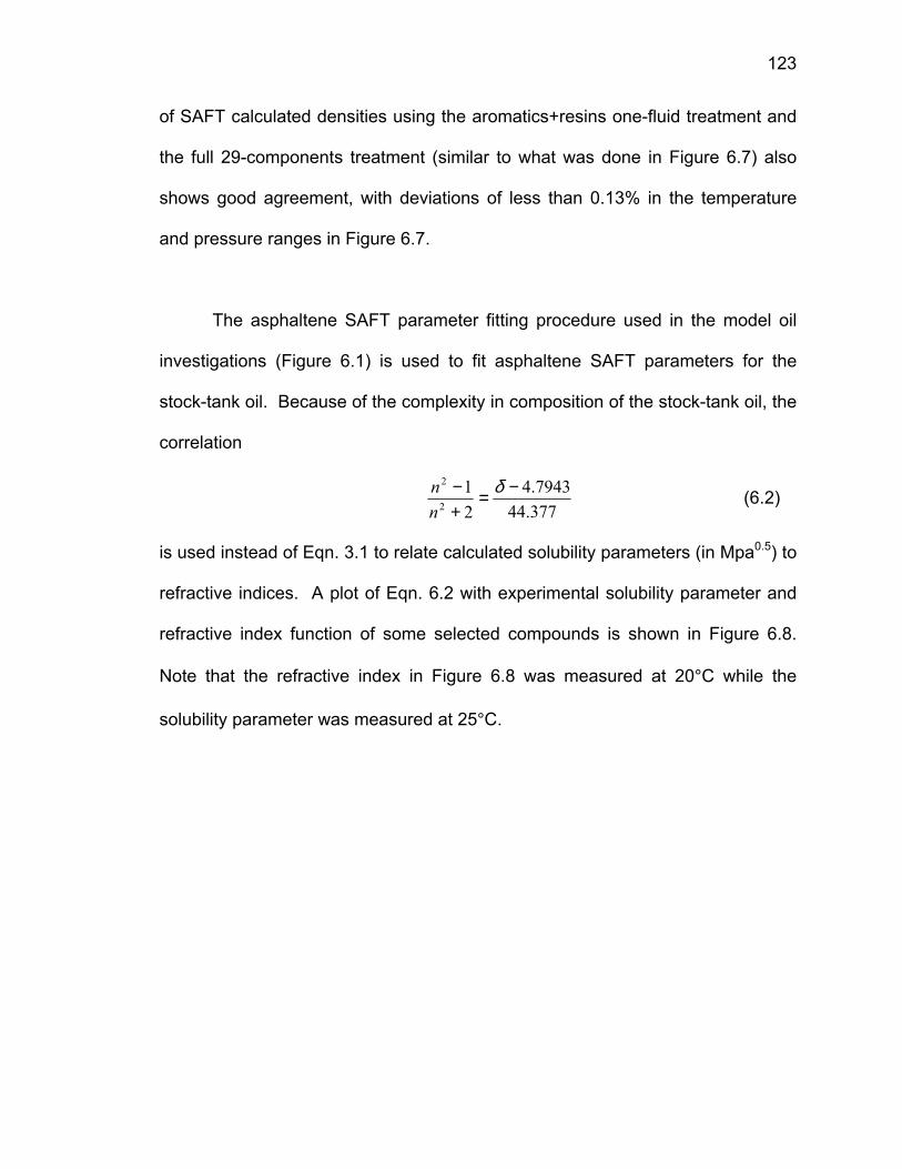
123
of SAFT calculated densities using the aromatics+resins one-fluid treatment and
the full 29-components treatment (similar to what was done in Figure 6.7) also
shows good agreement, with deviations of less than 0.13% in the temperature
and pressure ranges in Figure 6.7.
The asphaltene SAFT parameter fitting procedure used in the model oil
investigations (Figure 6.1) is used to fit asphaltene SAFT parameters for the
stock-tank oil. Because of the complexity in composition of the stock-tank oil, the
correlation
377.447943.4
21
2
2 −=+− δ
nn (6.2)
is used instead of Eqn. 3.1 to relate calculated solubility parameters (in Mpa0.5) to
refractive indices. A plot of Eqn. 6.2 with experimental solubility parameter and
refractive index function of some selected compounds is shown in Figure 6.8.
Note that the refractive index in Figure 6.8 was measured at 20°C while the
solubility parameter was measured at 25°C.

124
Figure 6.8 Relationship between solubility parameter[121] (δ, at 25°C) and refractive index[44] (at 20°C) for some select compounds.
As described in Chapter 3 (see Table 3.2), the stock-tank oil was initially
mixed with equi-volume of α-methyl naphthalene. For a given oil/precipitant pair,
the addition of asphaltene solvents to the oil shifts the amount of precipitant
needed to induce asphaltene precipitation but does not significantly alter the
refractive index at precipitation onset.[40] As in the model oil asphaltene fits, the
binary interaction parameters between asphaltenes and the other stock-tank oil
components (and α-methyl-naphthalene) are set to zero. The set of kijs’ used
between the various components are listed in Table 6.6. These interaction
parameters were based on kijs’ between representative species of the oil sub-
fractions described in the footnotes of Table 6.6.

125
Table 6.6 Binary interaction parameters used to fit the stock-tank oil asphaltenes in SAFT.
saturates aromatics+resins
α-methyl naph.b
n-alkane ppt.c asphaltenes
Saturates -0.00a -0.01a -0.01 -0.00 0.00 aromatics+ resins -0.01a -0.00a -0.00 -0.01 0.00 α-methyl naph.b -0.01 -0.00 -0.00 -0.01 0.00
n-alkane ppt.c -0.00 -0.01 -0.01 -0.00 0.00
Asphaltenes -0.00 -0.00 -0.00 -0.00 0.00 a based on toluene-dodecane and toluene-hexadecane binary data of Messow and
Engel[120] b the kijs’ between α-methyl naphthalene and other species are the same as those between
aromatics+resins and other species. c the kijs’ between n-alkane precipitants and other species are the same as those between
saturates and other species.
The fitted stock-tank oil asphaltenes has the following parameters: σ =
4.30 Angstrom, m = 29.5, ε/k = 395 K. This asphaltene has a SAFT calculated
solubility parameter of 21.85 MPa0.5 and a molar volume of 1,437 cm3/mol.
Given that the density of asphaltenes is estimated to be between 1.13 g/cm3 and
1.20 g/cm3, the SAFT calculated stock-tank oil asphaltene has an implied MW
between 1624 and 1724. Results of the fits are given in Figure 6.9. A
comparison of the stock-tank oil SAFT asphaltene parameters and the n-C7
insoluble model oil SAFT asphaltene parameters is given in Table 6.7.

126
Figure 6.9 SAFT fits to stock-tank oil asphaltene aggregates PRI data.
Table 6.7 Comparison of stock-tank oil SAFT asphaltene parameters and the n-C7 insoluble model oil asphaltene parameters.
stock-tank oil asphaltene
n-C7 insoluble model oil asphaltene
m 29.5 80.0
σ (Angstrom) 4.30 4.05
ε/k (K) 395 350.8
δ (MPa0.5) 21.85 21.85 molar volume
(cm3/mol) 1,437 3,334
MW (range) 1,624-1,724 3,767-4,000
A comparison of the SAFT parameters for the stock-tank oil asphaltenes
and the n-C7 extracted asphaltenes used in the model live oil (Table 6.7) shows
that the stock-tank oil asphaltenes are, on average, smaller and more
polarizable. This is expected. We recognize that the stock-tank oil asphaltenes
are polydisperse in size, shape, and molecular composition. We modeled the

127
asphaltenes as a monodisperse species with the SAFT parameters giving
average properties. The n-C7 insoluble product of the extraction process is a high
molecular weight sub-fraction of the stock-tank oil asphaltenes. The difference in
the two sets of SAFT parameters reflects the difference in physical properties
between the average n-C7 insoluble and stock-tank oil asphaltenes. This
information can be used together with data on the precipitation behavior of other
n-alkane extracted asphaltenes to estimate the stock-tank oil asphaltene’s
degree of polydispersity.
6.3.3 Recombined Oil Properties
Before the pure component SAFT parameters listed above can be used to
model the recombined oil system, the binary interaction parameters between the
pseudo-components in oil need to be determined. These binary interaction
parameters are given in Table 6.8 and were obtained from kijs’ between the sub-
fractions’ representative species (see table footnotes). For instance, the
interaction parameter between propane (MW = 44.1) and hexadecane (MW =
226.4) can be used in place of the interaction parameter between saturates
(MWn = 255) and light alkanes (MWn = 46.6) sub-fractions. Although the MWn of
the saturates sub-fraction is closer to the molecular weight of octadecane than
hexadecane, hexadecane is used as the representative species for saturates
because of constraints in the availability of published data. Whenever strongly
temperature-dependent kijs’ were observed, the values listed in Table 6.8 were
interpolated/extrapolated to the kij values between 300K and 350K.

128
Table 6.8 Binary interaction parameters between pseudo-component species in SAFT.
methane N2+CO2light n-alkanes saturates aromatics
+resins asphaltenesk
methane 0.00z 0.00a 0.01b 0.03d 0.03e 0.03 N2+CO2 0.00a 0.00z 0.07c 0.01f 0.13h 0.13
light n-alkanes 0.01b 0.07c 0.00z 0.006g 0.02i 0.00 saturates 0.03d 0.01f 0.006g 0.00z -0.01j 0.00 aromatics +resins 0.03e 0.13h 0.02i -0.01j 0.00z 0.00
asphaltenesk 0.03z 0.13z 0.00z 0.00z 0.00z 0.00
a based on methane-N2 binary data of Kidnay, et al.[117] b based on methane-propane binary data of Reamer, et al.[118] c based on N2-propane binary data of Grauso, et al.[119] d based on methane-decane data of Reamer, et al.[111] e based on methane-toluene binary data reported in this work and from Elbishlawi and
Spencer[116] f based on N2-decane binary data of Azarnoosh and McKetta[122] g based on propane-hexadecane binary data of Joyce[102] h based on N2-benzene binary data of Miller and Dodge[123] i based on propane-benzene binary data of Glanville, et al.[124] j based on toluene-dodecane and toluene-hexadecane binary data of Messow and
Engel[120] k the kijs’ between asphaltenes and separator gas sub-fractions are assumed to be the
same as the kijs’ between aromatics+resins and separator gas sub-fractions.
To calculate the amount of separator gas in the recombined oil, the gas-oil
ratio can be converted to molar quantities (of gas) per mass stock-tank oil:
gas20C,1bar
3bar20C,1 MW
m100cmGOR
STOmassgasmoles
gasρ
= (6.3)
where GOR is in m3/m3, the average molecular weight of the separator gas is
28.52, and the density of the separator gas at 293 K and 1 bar is approximately
0.0012 g/cm3 using the ideal gas equation of state.

129
A comparison of SAFT-predicted and experimental densities (along the
depressurization experiments) for the one-phase recombined oil with a gas-oil
ratio of 152 m3/m3 and a GOR of 212 m3/m3 is shown in Figure 6.10. Although
SAFT slightly under-predicts the recombined oil densities, the predicted densities
are in good agreement with experimental values. As described in Chapter 3 (see
Figure 3.7b), the experimental densities were obtained from constant-
composition volume-expansion data.
Figure 6.10 Experimental and SAFT-predicted (lines) one-phase recombined oil densities with two different gas-oil ratios.
Comparison of SAFT-predicted and measured bubble points for the
recombined oil with the two different gas-oil ratios is shown in Figure 6.11. As
seen in the figure, SAFT accurately describes the effect of gas concentration on
bubble point pressures. The predicted mixture bubble points for two limiting
scenarios of separator gas compositions are also plotted in the figure. In the first
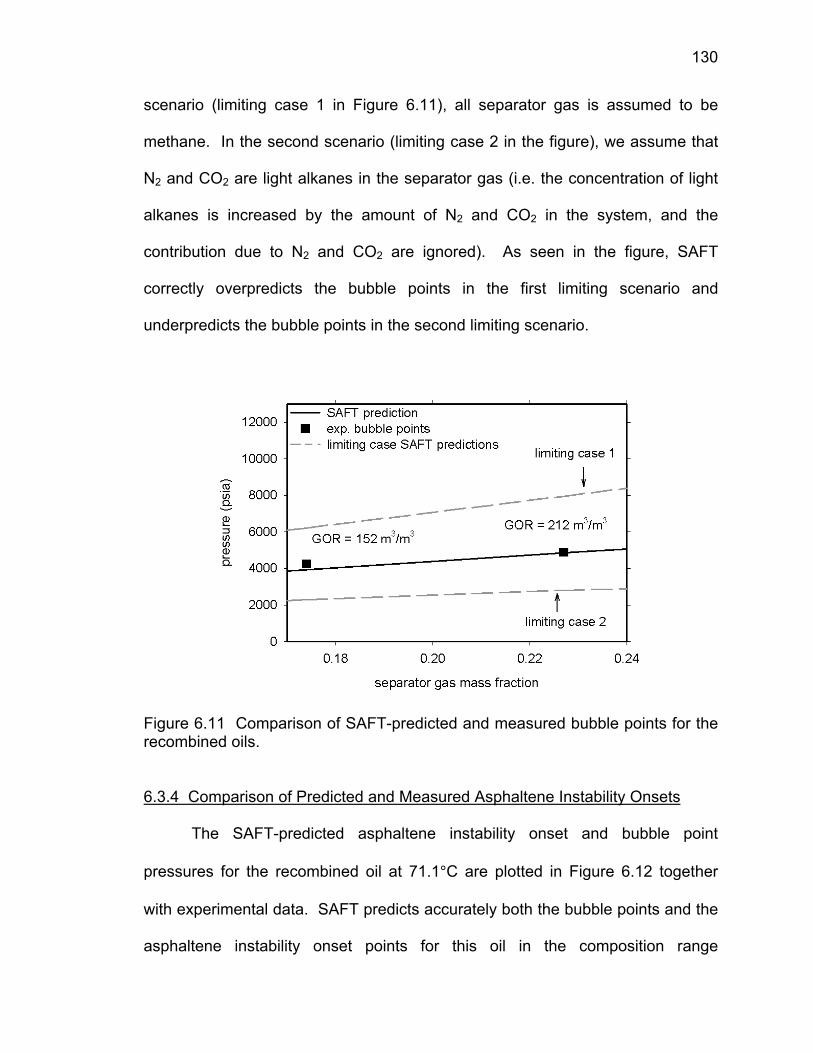
130
scenario (limiting case 1 in Figure 6.11), all separator gas is assumed to be
methane. In the second scenario (limiting case 2 in the figure), we assume that
N2 and CO2 are light alkanes in the separator gas (i.e. the concentration of light
alkanes is increased by the amount of N2 and CO2 in the system, and the
contribution due to N2 and CO2 are ignored). As seen in the figure, SAFT
correctly overpredicts the bubble points in the first limiting scenario and
underpredicts the bubble points in the second limiting scenario.
Figure 6.11 Comparison of SAFT-predicted and measured bubble points for the recombined oils.
6.3.4 Comparison of Predicted and Measured Asphaltene Instability Onsets
The SAFT-predicted asphaltene instability onset and bubble point
pressures for the recombined oil at 71.1°C are plotted in Figure 6.12 together
with experimental data. SAFT predicts accurately both the bubble points and the
asphaltene instability onset points for this oil in the composition range

131
investigated. According to the equation of state calculations, we would expect
asphaltene precipitation problems to occur at higher separator gas
concentrations.
Figure 6.12 SAFT-predicted and measured asphaltene instability onset and mixture bubble points for the recombined oil at 71.1°C.
6.4 Summary
A method has been presented to characterize the recombined oil and the
asphaltenes for use in the SAFT equation of state. The recombined oil was
modeled as a six-component mixture, with three pseudo-components for the
stock-tank oil and three pseudo-components for the separator gas. The average
molecular weight and the amount of each sub-fraction was determined from gas-
chromatography, saturates-aromatics-resins-asphaltenes fractionation, and gas-
oil-ratio information. SAFT parameters for each sub-fraction (except for the

132
asphaltenes) were obtained from correlations with molecular weight for each
class of compounds. The SAFT-predicted densities for the stock-tank oil and the
recombined oils agree very well with experimental measurements.
PRI data was used to fit the asphaltene’s SAFT parameters. Essentially,
the SAFT asphaltene parameters were optimized so that SAFT would reproduce
the composition of the mixture (or the refractive index of the mixture) at the onset
of asphaltene precipitation. For both the model oil and the stock-tank oil, good
agreements were obtained between experimental and fitted PRI even with a
binary interaction parameter of zero between asphaltenes and the other species.
While the stock-tank oil and the model oil asphaltenes thus obtained have almost
the same solubility parameter, according to SAFT, the stock-tank oil asphaltenes
are much smaller and more aromatic.
For both the model and the recombined oil systems, SAFT-predicted
asphaltene instability and bubble points agree well with experimental
measurements.

133
CHAPTER 7. ASPHALTENE SAFT PARAMETERS SELECTION RULES
7.1 Introduction
As described in Chapter 6, the SAFT equation of state parameters for
asphaltenes (m, σ, and ε/k) are fit to ambient condition precipitation data from oil
titrations with n-alkanes. In this section, we will investigate the effects of varying
one or more of these parameters on the calculated asphaltene instability onset
compositions. We will also look at the effects of changing these parameters on a
pure species’ solubility parameter (δ) and molar volume (v). These investigations
will provide some general guidelines on selecting the appropriate set of
asphaltene SAFT parameters to fit the ambient condition titration data.
7.2 Effects of Variations in SAFT Parameters on Solubility Parameter
The effects of varying a pure specie’s chain length (m), segment diameter
(σ), and segment energy (ε/k) on the calculated solubility parameter (20°C, 1 bar)
are shown in Figures 7.1(a) to 7.1(c). The range of SAFT parameters
investigated ( 9014 ≤≤ m ; A1.4A9.3 ≤≤ σ ; K400/K280 ≤≤ kε ) roughly span the
parameter space where we expect asphaltenes to lie. Compared to the range of
m and ε/k investigated, the range of σ investigated is small because σ does not
vary much between species (see Table 4.1). The gray horizontal lines in Figures
7.1(a)-(c) demarcate the measured upper and lower values of solubility

134
parameter for asphaltenes; these lines mark the boundaries within which
potential asphaltene SAFT parameters would be found.
Figure 7.1 Effects of variations in m, σ, and ε/k on the calculated solubility parameters at 20°C and 1 bar. The three plots contain the same data.
As seen in Figure 7.1, with all other parameters held constant, the
solubility parameters are not very sensitive to changes in molecular chain length.
For instance, at σ = 4.0A and ε/k = 340K, a 50% increase in m from 44 to 66
results in a 0.4% increase in δ. This implies that for a given set of segment
properties (ε/k and σ) in the region of SAFT parameter space investigated, the
ratio of the residual internal energy to the molecular volume (i.e. the solubility
parameter) is relatively independent of chain length. Since the residual internal

135
energy is approximately proportional to chain length at fixed mass density and
temperature, the molar volume is also proportional to chain length.
Unlike the case with m, the solubility parameters are sensitive to small
changes in the segment properties ε/k and σ. A decrease in the segment energy
will decrease the solubility parameter (see Figure 7.1(c)), and a decrease in the
segment diameter will increase the solubility parameter (see Figure 7.1(b)). For
instance, at m = 50 and σ = 4.0A, a 2.5% decrease in ε/k from 400K to 390K
results in a 2.2% decrease in δ. And at m = 50 and ε/k = 400K, a 2.5% decrease
in σ from 4.0A to 3.9A results in a 3.7% increase in δ. In both instances, the
molecule’s energy density has been altered.
7.3 Effects of Variations in SAFT Parameters on Molar Volume
The effects of varying a pure specie’s chain length, segment diameter,
and segment energy on its molar volume (at 20°C, 1 bar) can be seen in Figure
7.2. The range of SAFT parameters investigated is the same as those in the
previous section. As seen in the figure, molar volume is a linear function of m.
As expected, increasing the segment diameter σ increases the molar volume
while increasing the segment energy ε/k has the opposite effect. It is interesting
that the effects of changes in the segment properties (σ and ε/k) are more
pronounced in molecules with longer chains (larger values of m). Because of the

136
large differences in the reported asphaltene molecular weights, an asphaltene
molecule would fall within the range of molar volumes in Figure 7.2.
Figure 7.2 Effects of variations in m, σ, and ε/k on calculated molar volumes at 20°C, 1 bar. All else being equal, molecules with lower ε/k have larger molar volumes.
7.4 Effects of Variations in Asphaltene SAFT Parameters on Mixture Composition at Asphaltene Instability Onset
The effects of varying each of the asphaltene SAFT parameters on the
calculated asphaltene-toluene-n-alkane mixture composition at asphaltene
instability onset are shown in Figure 7.3. As described earlier, φvppt is the volume
fraction of the precipitant in a mixture of asphaltene-toluene-n-alkane at the onset
of asphaltene instability. The concentration of asphaltenes in these calculations
is fixed at 1g asphaltenes per 100mL toluene (at 20°C, 1 bar). Since the
asphaltene molar volume calculated using each set of SAFT parameters is

137
different, the molecular weight of the asphaltenes are allowed to vary to maintain
an asphaltene mass density of 1.126 g/cc. As detailed in Chapter 6, the binary
interaction parameters between all species are set to zero. To check for phase
stability of the asphaltene-toluene-n-alkane mixtures, we use, as initial guesses,
a composition grid of 0.04 in each direction. An unstable phase is defined
(numerically) as one in which the tangent plane distance (see Chapter 4) has a
value more negative than -1.0x10⁻¹⁴.
Figure 7.3 Effects of changing (a) m, (b) ε/k, and (c) σ for asphaltenes on the amount of n-alkane precipitants needed to induce asphaltene instability in the asphaltene-toluene-n-alkane mixtures.
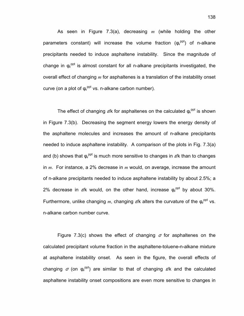
138
As seen in Figure 7.3(a), decreasing m (while holding the other
parameters constant) will increase the volume fraction (φvppt) of n-alkane
precipitants needed to induce asphaltene instability. Since the magnitude of
change in φvppt is almost constant for all n-alkane precipitants investigated, the
overall effect of changing m for asphaltenes is a translation of the instability onset
curve (on a plot of φvppt vs. n-alkane carbon number).
The effect of changing ε/k for asphaltenes on the calculated φvppt is shown
in Figure 7.3(b). Decreasing the segment energy lowers the energy density of
the asphaltene molecules and increases the amount of n-alkane precipitants
needed to induce asphaltene instability. A comparison of the plots in Fig. 7.3(a)
and (b) shows that φvppt is much more sensitive to changes in ε/k than to changes
in m. For instance, a 2% decrease in m would, on average, increase the amount
of n-alkane precipitants needed to induce asphaltene instability by about 2.5%; a
2% decrease in ε/k would, on the other hand, increase φvppt by about 30%.
Furthermore, unlike changing m, changing ε/k alters the curvature of the φvppt vs.
n-alkane carbon number curve.
Figure 7.3(c) shows the effect of changing σ for asphaltenes on the
calculated precipitant volume fraction in the asphaltene-toluene-n-alkane mixture
at asphaltene instability onset. As seen in the figure, the overall effects of
changing σ (on φvppt) are similar to that of changing ε/k and the calculated
asphaltene instability onset compositions are even more sensitive to changes in

139
σ than to ε/k. This is not surprising because unlike changes in ε/k (which directly
changes the molecular energy density but only indirectly changes the molar
volume), changing σ directly changes the molar volume and the molecular
energy density. Since changing ε/k and σ for asphaltenes have qualitatively
similar effects on φvppt, the issue of parameter uniqueness becomes important.
This issue will be addressed in the following section.
An example of the combined effects of changing ε/k and m on the
calculated φvppt is given in Figure 7.4. In these calculations, the segment
diameter of the asphaltenes is fixed at 4.0 A. As seen in the figure, one way to
increase the curvature of the φvppt vs. n-alkane carbon number plot is to first
decrease the segment energy of the asphaltene and then increase its segment
number to reduce the volume fraction of precipitants needed to induce
asphaltene instability.

140
Figure 7.4 Effects of m and ε/k for asphaltenes on calculated volume fraction of precipitants at the onset of asphaltene instability at 20°C and 1 bar.
7.5 Uniqueness of the Asphaltene SAFT Parameters
Since changing ε/k and σ for asphaltenes have qualitatively similar
influences on the calculated amount of precipitants needed to induce asphaltene
instability, the issue of parameter uniqueness becomes important. In other
words, can we fit an experimental φvppt (and hence PRI) curve using different sets
of asphaltene SAFT parameters?
In Figure 7.5, the φvppt vs. n-alkane carbon number curve is plotted for six
sets of asphaltene SAFT parameters, all with m = 54. As seen in the figure, in
three cases, two independent sets of parameters produce nearly identical results.
This suggests that, in modeling the ambient condition φvppt and PRI curves, it is
possible to fit the experimental data using multiple sets of asphaltene SAFT
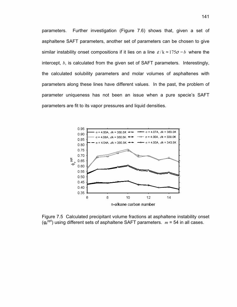
141
parameters. Further investigation (Figure 7.6) shows that, given a set of
asphaltene SAFT parameters, another set of parameters can be chosen to give
similar instability onset compositions if it lies on a line b−≈ σε 175k/ where the
intercept, b, is calculated from the given set of SAFT parameters. Interestingly,
the calculated solubility parameters and molar volumes of asphaltenes with
parameters along these lines have different values. In the past, the problem of
parameter uniqueness has not been an issue when a pure specie’s SAFT
parameters are fit to its vapor pressures and liquid densities.
Figure 7.5 Calculated precipitant volume fractions at asphaltene instability onset (φv
ppt) using different sets of asphaltene SAFT parameters. m = 54 in all cases.

142
Figure 7.6 ε/k vs. σ for six sets of asphaltene SAFT parameters (m = 54 in all cases). Different sets of SAFT parameters that give similar φv
ppt vs. n-alkane carbon number curves are connected by lines.
To investigate whether the region in parameter space of an asphaltene’s
SAFT parameters can be further restricted, the asphaltene-toluene-n-heptane
ternary phase diagrams (at 20°C, 1 bar) for two different asphaltenes that give
similar φvppt vs. n-alkane carbon number curves are plotted in Figure 7.7. As
seen in the figure, the mixture compositions at the onset of asphaltene
instabilities for a 1g asphaltene per 100mL toluene mixture (the intersection of
the titration line with the phase boundaries) are similar for both asphaltenes.
Furthermore, the slope of the tie lines are similar for the two systems and the
phase envelopes are similar away from the mixtures’ plait points. Because of the
similarities in the phase envelopes away from the plait points, the effects of the
non-uniqueness of ε/k and σ for asphaltenes on asphaltene phase behavior
should be small for similar mixtures away from the plait points. We should be
able to further restrict the region in parameter space of an asphaltene’s SAFT

143
parameters if asphaltene instability onset data are available for systems that
originally (i.e. before any precipitant titration) had much more asphaltenes
dissolved in toluene. In situations where this addition information is not available,
one should arbitrarily set σ to a constant value in the fitting procedure and then
vary ε/k because a species’ thermodynamic phase behavior is much more
sensitive to changes in σ.
Figure 7.7 Asphaltene-toluene-n-heptane ternary phase diagram for two different asphaltenes that give similar φv
ppt vs. n-alkane carbon number curves at 20°C and 1 bar.
7.6 Summary
We investigated the effects of changes in SAFT parameters on the pure
species’ solubility parameter and molar volume. In the region of parameter
144
space where we expect asphaltenes to lie, the calculated solubility parameter is
not sensitive to changes in m but is very sensitive to changes in the segment
properties ε/k and σ. On the other hand, the calculated molar volume is a linear
function of m and is less sensitive to changes in ε/k and σ.
The effect of changing the asphaltene SAFT parameters on the φvppt vs. n-
alkane carbon number curve is also explored. The overall effect of changing m
for asphaltenes is a translation of the asphaltene instability onset curve (on a plot
of φvppt vs. n-alkane carbon number). The volume fraction of precipitants needed
to induce asphaltene instability decreases with increasing m for asphaltenes.
Unlike changes in m, changes in ε/k and σ also alter the curvature of the φvppt vs.
n-alkane carbon number curve. Using different combinations of m, σ, and ε/k for
asphaltenes, we can fit a wide range of φvppt vs. n-alkane carbon number data.
In the last section, we investigated the issue of uniqueness of the
asphaltene SAFT parameters. It is shown that SAFT can fit the ambient
condition φvppt (and hence the PRI) data using multiple sets of ε/k and σ.
Furthermore, different sets of ε/k and σ for asphaltenes that would fit the same
ambient condition φvppt data are linearly related. Away from the mixture plait
point, the phase envelope calculated using these different (but related) sets of
asphaltene parameters are similar and we believe the effects of the non-
uniqueness of ε/k and σ for asphaltenes on asphaltene phase behavior in oil
should be small. Asphaltene instability onset data for systems containing much

145
more asphaltenes (where the mixture is closer to its plait point) can be used to
further pin down a set of unique asphaltene parameters. In situations where this
additional information is not available, one should arbitrarily set σ to a constant
value in the fitting procedure.

146
CHAPTER 8. EFFECTS OF ASPHALTENE POLYDISPERSITY (INCLUDING
RESIN ADDITION)
8.1 Introduction
The results on asphaltene stability presented thus far were calculated in
SAFT by treating asphaltenes as a single, monodisperse component. As
discussed in Chapter 2, asphaltenes are, in actuality, a polydisperse class of
compounds with resins as their lower molecular weight sub-fraction; what is
commonly termed asphaltenes in literature is a solubility cut (toluene soluble, n-
pentane or n-heptane insoluble) of this distribution. As an example, Yarranton
and Masliyah[125] are able to describe the molar mass distribution (determined
using plasma desorption mass spectrometry[126]) for Athabasca bitumen using an
exponential distribution. Since asphaltenes are a polydisperse class of
compounds, the effects of asphaltene polydispersity need to be incorporated.
The goal of this chapter is to examine the effects of asphaltene
polydispersity on its thermodynamic phase behavior in oil. One of the questions
we will try to answer is whether the lowest molecular weight asphaltenes
(including the resins) can stabilize, via nonpolar interactions, the higher
molecular weight asphaltenes. Another question we will try to address is whether
SAFT can describe the correct partitioning of the asphaltene pseudo-components
between the oil and the precipitated phases at equilibrium. Since deposition

147
tendencies onto pipeline surfaces have often been associated with variations in
the morphology and the composition of the precipitated asphaltene phase, an
understanding of the molecular weight distribution of polydisperse asphaltenes in
equilibrium phases will help us estimate asphaltene’s deposition tendencies.
At this stage of the research, polydisperse asphaltene will be represented
as four pseudo-components in SAFT: the n-C3-5, the n-C5-7, the n-C7-15, and the
n-C15+ n-alkane insoluble sub-fraction. The reader should keep in mind that,
traditionally, the n-C3-5 fraction is called resins and that conventional asphaltene
extraction techniques generally identify asphaltenes as the n-C5+ or n-C7+
insoluble (and toluene/benzene soluble) fractions of heavy organics.
8.2 Selection of SAFT Parameters for Polydisperse Asphaltenes & Resins
In experiments performed by Wang[5], the asphaltenes for Lagrave oil (the
oil modeled in this chapter) were first separated into various solubility fractions
using excess n-pentane, n-heptane, and n-pentadecane precipitants; these sub-
fractions are called n-C5 insoluble asphaltenes (7.5g/100mL stock-tank oil), the
n-C7 insoluble asphaltenes (6.7g/100mL oil), and the n-C15 insoluble asphaltenes
(5.1g/100mL oil), respectively. The asphaltene instability onsets for mixtures of
asphaltenes, toluene, and n-alkanes (at ambient condition and initially with an
asphaltene/toluene ratio of 1 gram per 100mL toluene) were then measured for
each asphaltene fraction. The experimental asphaltene fractionation and
148
instability onset data that we use in this chapter to fit the SAFT model are those
for Lagrave oil and are taken from Wang[5].
The method used to obtain the SAFT parameters for polydisperse
asphaltenes is similar to the monodisperse SAFT asphaltene characterization
procedure given in Chapter 6. Within the SAFT model, polydisperse asphaltenes
are modeled as three or four pseudo-components (depending on whether the
resin fraction, which is the n-C3-5 asphaltene sub-fraction, is included): an n-C15+
sub-fraction, an n-C7-15 sub-fraction, an n-C5-7 sub-fraction, and an n-C3-5 sub-
fraction. SAFT parameters are fit for the n-C15+ asphaltene sub-fraction to
reproduce the experimental data on the minimum volume fraction precipitant
needed to induce asphaltene instability (φvppt) or, equivalently, to reproduce the
experimental data on the mixture refractive index at asphaltene instability onset
(PRI) for mixtures of n-C15 insoluble asphaltene, toluene, and various n-alkanes.
The asphaltenes made from the combination of n-C15+ and n-C7-15 sub-fractions
are assumed to represent the n-C7 insoluble asphaltenes; a second set of SAFT
parameters is fit for the n-C7-15 sub-fraction to reproduce (together with the
previously fitted n-C15+ sub-fraction) the experimental φvppt (or PRI) data for a
mixture of n-C7 insoluble asphaltene, toluene, and n-alkane. Finally, a third set
of SAFT parameters is fit to the n-C5-7 sub-fraction so that the combination of the
n-C15+ (previous fit), n-C7-15 (previous fit), and n-C5-7 sub-fractions represent the
n-C5 insoluble asphaltenes and will reproduce the experimental φvppt (or PRI) data
for a mixture of n-C5 insoluble asphaltene, toluene, and n-alkanes. Due to lack of

149
precipitation data, the SAFT parameters for the resin (n-C3-5) sub-fraction are
obtained by decreasing the SAFT parameters (m and ε/k) of the n-C5-7
asphaltene sub-fraction until a set of parameter is obtained that will make the
resins insoluble in propane (tested at 10 bars) and soluble in n-pentane.
A flow chart of the fitting procedure is given in Figure 8.1. Note that inside
the solid bracket “A”, the ratio of m/MW and the n-C15+ SAFT asphaltene
parameters are not changed. And inside the dashed bracket “B”, the ratio of
m/MW, the mass ratio of n-C15+ to n-C7-15 asphaltenes, the n-C15+ SAFT
asphaltene parameters, and the n-C7-15 SAFT asphaltene parameters are not
changed. Once a value has been assigned for the molecular weight of the n-C15+
asphaltene, the molecular weight of the other asphaltene sub-fractions depend
only on the chain lengths of the pseudo-components representing those
particular sub-fractions. As in the case for monodisperse asphaltenes, all binary
interaction parameters between all species are set to zero. Furthermore, in light
of the parameter uniqueness issues discussed in Chapter 7, the segment
diameters of all asphaltene pseudo-components are set to the same value.

150
Figure 8.1 Fitting procedure for polydisperse asphaltenes with polydispersity captured using three asphaltene pseudo-components.
A comparison of the equation-of-state fitted and the experimental φvppt and
PRI data is shown in Figure 8.2, with the fitted SAFT asphaltene parameters listed
in Table 8.1. The SAFT PRIs’ in Figure 8.2 were calculated using the method
described in Chapter 3.4. Compared to other SAFT calculated φvppt and PRI plots
shown in the previous chapters, the curves in Figure 8.2 appear to be smoother
because only results for the odd carbon number n-alkane precipitants are
Follow the procedure in Fig. 6.1 to fit a set of SAFT parameters to the φvppt (or
PRI) data for the mixture toluene, n-alkane, and n-C15 insol. asph.
Calculate a where mC15+=aMWC15+
Estimate w1 (the ratio of the n-C15+ to the n-C7-15 asphaltenes)
Follow the procedure in Fig. 6.1 to fit mC7-15, σC7-15, and (ε/k)C7-15 to the φvppt
(or PRI) data for the toluene, n-alkane, and n-C7 insol. asph. All other parameters are kept constant
is deviation > tolerance
Choose mC7-15, σC7-15, and (ε/k)C7-15
Calculate MWC7-15 = a/mC7-15
YES NO
Estimate w2 (the ratio of the n-C15+ to the n-C5-7 asphaltenes)
Choose mC5-7, σC5-7, and (ε/k)C5-7
Calculate MWC5-7 = a/mC5-7
Follow the procedure in Fig. 6.1 to fit mC5-7, σC5-7, and (ε/k)C5-7 to the φvppt (or
PRI) data for the toluene, n-alkane, and n-C5 insol. asph. All other parameters are kept constant
is deviation > toleranceYES NO
DONE
A
B

151
presented. As seen in the figure, the agreement between SAFT calculated and
measured φvppt (and PRI) is qualitative. SAFT is able to describe the change in
magnitude (and to a lesser extent, the curvature) of the φvppt vs. n-alkane carbon
number curve between n-C15 insoluble and n-C5 insoluble asphaltenes. For the
precipitation onsets with n-C7 and n-C5 extracted asphaltenes, SAFT does not
accurately describe the experimental φvppt (and PRI) data in cases where larger n-
alkanes (undecane and higher) are used to induce asphaltene precipitation;
SAFT consistently under-predicts the volume fraction of n-alkane precipitants
needed to induce asphaltene instability.
Figure 8.2 Comparison of SAFT and measured precipitant volume fraction and mixture refractive index (PRI) at asphaltene instability onset for Lagrave asphaltene-toluene-n-alkane mixtures (20°C and 1 bar). The asphaltene/toluene ratio is 1g/100mL. Experimental data are from Wang[5].

152
Table 8.1 SAFT parameters for the various asphaltene sub-fractions (including resins).
SAFT Parameters Asph sub-fraction MW M σ (A) ε/k (K) δ (MPa0.5) ρ (g/cm3)
n-C15+ 2500 54 4.00 350.5 22.17 1.150 n-C7-15 1852 40 4.00 340.0 21.52 1.137 n-C5-7 1806 39 4.00 335.0 21.25 1.133 Resin 556 12 4.00 330.0 20.41 1.103
A comparison of SAFT and measured mass distribution of the asphaltene
sub-fractions is shown in Figure 8.3. For the column labeled “experimental”, the
mass of each asphaltene sub-fraction was inferred from the difference in the
measured amount of asphaltenes precipitated with different precipitants. Within
the SAFT model, the amount of each asphaltene sub-fraction was optimized
(together with the sub-fraction’s asphaltene SAFT parameters) to fit the
experimental φvppt (PRI) data in Figure 8.2. It is interesting to note the large
discrepancy in the amount of n-C5-7 asphaltene sub-fraction between
experimental inferred and SAFT calculated n-C5 extracted asphaltenes; to get a
reasonable fit to experimental φvppt (PRI) data, SAFT requires three times as much
low molecular weight asphaltenes (n-C5-7 sub-fraction) as was inferred from
experiments.

153
0
2
4
6
8
10
12
14
expt
SAFT
mas
s of
eac
h as
phal
tene
su
b-fra
ctio
n (g
/100
mL
oil)
n-C5
asph n-C7
asph n-C15
asph
n-C15+ fraction
n-C15+ fraction
n-C15+ fraction
n-C15+ fraction
n-C15+ fraction
n-C15+ fraction
n-C7-15 fraction
n-C7-15 fraction
n-C7-15 fraction
n-C7-15 fraction
n-C5-7 fraction
n-C5-7 fraction
n-C5
asph
n-C7
asph n-C15
asph
Figure 8.3 Comparison of SAFT and experimental mass distribution of each asphaltene sub-fraction in Lagrave asphaltenes. The column label above the columns identify the precipitants used to extract the asphaltenes. Experimental data are from Wang[5].
Several factors may contribute to the poor agreement in the amount of low
molecular weight asphaltenes in the asphaltene fraction shown in Figure 8.3.
Experimentally, the measured amount of asphaltenes precipitated may contain
not only asphaltenes that should precipitate with the precipitant used but also
small amounts of entrained resins, oil, and other asphaltene fractions; variations
in the amount of asphaltenes precipitated exist even for the same oil using the
same extraction procedure. On the modeling side, because there are insufficient
data to uniquely fit all of the model parameters for polydisperse asphaltenes,
certain approximations and relationships have to be made. For instance, the

154
molecular weights of all SAFT asphaltene sub-fractions were set to be linearly
dependent on chain length. This was done because the experimental molecular
weight of each asphaltene sub-fraction is not known and because chain length
has been shown to be roughly linearly dependent on molecular weight for
polynuclear aromatics (see Chapter 4). The constant of proportionality
(MW=m/0.0216) used in this work was set to give the n-C15+ asphaltene sub-
fraction a molecular weight of 2,500. In another approximation, the segment
diameters of all asphaltene sub-fractions were set to 4 Angstroms. The rationale
behind setting the segment diameter to 4 was that for most polynuclear
aromatics and polynuclear aromatics derivatives, the average value for the SAFT
parameter σ is about 4.
A plot of the SAFT parameters ε/k vs. m for the various SAFT asphaltene
fractions and resin (the n-C3-5 sub-fraction) shows a well-defined trend between
ε/k and m (Figure 8.4). The asphaltene precipitated by the lower molecular
weight n-alkanes tend to be smaller in size and have lower segment energy.

155
Figure 8.4 Plot of ε/k vs. m for the various SAFT asphaltene sub-fractions and resin.
8.3 Effects of Asphaltene Polydispersity and Resin Addition
To investigate the roles resins and asphaltene polydispersity play on
asphaltene phase behavior in oil, the asphaltene solubility behavior of four model
oil mixtures with monodisperse or polydisperse asphaltenes are compared. In
these model systems, toluene is used as the model oil (with different amounts of
n-alkane precipitants added) and the asphaltene parameters were fit to
experimental φvppt data for Lagrave asphaltenes. The properties and
asphaltene/resin contents of these systems are listed in Table 8.2 and are
discussed in the following paragraph. We use a mixture of 7.5g asphaltenes in
100mL of toluene in these investigations because the total amount of n-pentane
insoluble asphaltenes in Lagrave oil is 7.5g. All binary interaction parameters
between all species used in the SAFT calculations in this section are set to zero.

156
The biggest difference between the various systems in Table 8.2 is that
asphaltenes in Systems 1 and 2 are monodisperse, while the asphaltenes in
Systems 3 and 4 are polydisperse. More specifically, the asphaltene used in
Model System 1 is monodisperse and was fit to experimental φvppt (PRI) data for
the n-C15 insoluble Lagrave asphaltenes (also called the n-C15+ asphaltene
fraction in this work). The asphaltene used in Model System 2 is monodisperse
and was fit to experimental φvppt (PRI) data for the n-C5 insoluble Lagrave
asphaltenes. The asphaltene used in Model System 3 is polydisperse and the
SAFT parameters for each asphaltene sub-fraction was fit to the experimental
φvppt (PRI) data of the fractionated asphaltenes. Model System 4 is similar to
Model System 3 with the exception that 10g of resin per 100mL oil (about 2
moles resin/100moles toluene) is added to the system. The amount of resin
added (10g resin per 100mL oil) is arbitrary because the actual amount of resin
in Lagrave oil is not available in literature.
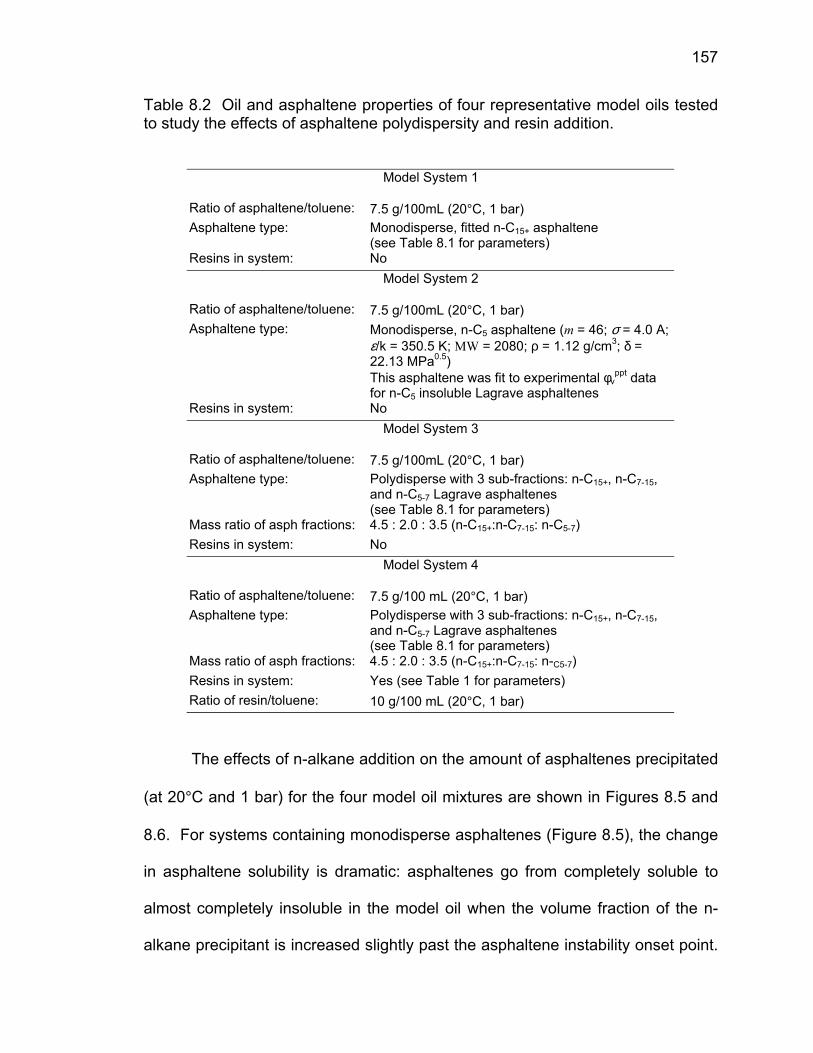
157
Table 8.2 Oil and asphaltene properties of four representative model oils tested to study the effects of asphaltene polydispersity and resin addition.
Model System 1
Ratio of asphaltene/toluene: 7.5 g/100mL (20°C, 1 bar) Asphaltene type: Monodisperse, fitted n-C15+ asphaltene
(see Table 8.1 for parameters) Resins in system: No
Model System 2
Ratio of asphaltene/toluene: 7.5 g/100mL (20°C, 1 bar) Asphaltene type: Monodisperse, n-C5 asphaltene (m = 46; σ = 4.0 A;
ε/k = 350.5 K; MW = 2080; ρ = 1.12 g/cm3; δ = 22.13 MPa0.5) This asphaltene was fit to experimental φv
ppt data for n-C5 insoluble Lagrave asphaltenes
Resins in system: No Model System 3
Ratio of asphaltene/toluene: 7.5 g/100mL (20°C, 1 bar) Asphaltene type: Polydisperse with 3 sub-fractions: n-C15+, n-C7-15,
and n-C5-7 Lagrave asphaltenes (see Table 8.1 for parameters)
Mass ratio of asph fractions: 4.5 : 2.0 : 3.5 (n-C15+:n-C7-15: n-C5-7) Resins in system: No
Model System 4 Ratio of asphaltene/toluene: 7.5 g/100 mL (20°C, 1 bar) Asphaltene type: Polydisperse with 3 sub-fractions: n-C15+, n-C7-15,
and n-C5-7 Lagrave asphaltenes (see Table 8.1 for parameters)
Mass ratio of asph fractions: 4.5 : 2.0 : 3.5 (n-C15+:n-C7-15: n-C5-7) Resins in system: Yes (see Table 1 for parameters) Ratio of resin/toluene: 10 g/100 mL (20°C, 1 bar)
The effects of n-alkane addition on the amount of asphaltenes precipitated
(at 20°C and 1 bar) for the four model oil mixtures are shown in Figures 8.5 and
8.6. For systems containing monodisperse asphaltenes (Figure 8.5), the change
in asphaltene solubility is dramatic: asphaltenes go from completely soluble to
almost completely insoluble in the model oil when the volume fraction of the n-
alkane precipitant is increased slightly past the asphaltene instability onset point.

158
As expected, the lower molecular weight asphaltenes (the monodisperse
asphaltene fit to the n-C5 insoluble asphaltene φvppt data) are more soluble than
the higher molecular weight asphaltene (the monodisperse, n-C15 insoluble
asphaltene) in terms of the amount of precipitant needed to induce asphaltene
instability. When sufficiently large amount of n-alkanes are added to the model
oil, all asphaltenes will precipitate.
0
0.2
0.4
0.6
0.8
1
0 0.2 0.4 0.6 0.8 1precipitant volume fraction
amou
nt a
spha
ltene
pre
cipi
tate
dov
er to
tal a
mou
nt a
spha
ltene
(mas
s)
n-C15 precipitantModel System 1
n-C5 precipitantModel System 1
n-C15 precipitantModel System 2
n-C5 precipitantModel System 2
Unstable RegionStable Region
Figure 8.5 Solubility of monodisperse asphaltenes in model Lagrave oil (7.5g asphaltene/100mL toluene) mixed with n-alkanes at 20°C and 1 bar.

159
0
0.2
0.4
0.6
0.8
1
0 0.2 0.4 0.6 0.8 1
precipitant volume fraction
amou
nt a
spha
ltene
pre
cipi
tate
d ov
er to
tal a
mou
nt a
spha
ltene
(m
ass)
precipitant = n-C15
polydisperse asphaltenesModel System 3
precipitant = n-C5
polydisperse asphaltenesModel System 3
precipitant = n-C5
polydisperse asphaltenes + resinsModel System 4
precipitant = n-C15
polydisperse asphaltenes + resinsModel System 4
UnstableRegion
StableRegion
Figure 8.6 Solubility of polydisperse asphaltenes (with or without resins) in model Lagrave oil (7.5g total asphaltene/100mL toluene) mixed with n-alkanes at 20°C and 1 bar.
A large change in the amount of precipitated asphaltene vs. precipitant
volume fraction can be seen when the effect of asphaltene polydispersity (and
resin addition) is taken into consideration (Figure 8.6). By treating asphaltene as
a polydisperse species, the amount of asphaltenes precipitated increases much
more gradually with precipitant addition. A significant amount of asphaltenes will
stay in solution even at high precipitant volume fractions, and more asphaltenes
can be precipitated using lower molecular weight n-alkanes. It is interesting to
note that when n-C15 is used as the precipitant, SAFT predicts the existence of a
solubility minimum around φvppt=0.9.
160
A comparison of the SAFT-predicted behavior of polydisperse asphaltenes
with and without resins show that the presence of resins will increase the amount
of precipitant needed to induce the onset of asphaltene instability (Figure 8.6).
Furthermore, at lower precipitant volume fractions in the oil, the amount of
asphaltenes that will precipitate is less when resins are present. Even though
only dispersion interactions are considered in our models, the lower molecular
weight asphaltenes and especially resins will stabilize the heavier asphaltenes in
the oil. It can be seen in Figure 8.6 that the effects of resins on asphaltene
phase behavior in the oil become less pronounced as the oil becomes more
dilute with precipitants.
A plot of the mass distribution of the asphaltene sub-fractions as a
function of precipitant volume fraction is shown in Figure 8.7. As seen in the
figure, near the initial asphaltene instability onset, the precipitated phase is
composed mostly of the heaviest asphaltene fractions (in this case, the n-C15+
sub-fraction). As the amount of precipitant is increased further, more and more
lower molecular weight asphaltenes will precipitate.

161
0
0.2
0.4
0.6
0.8
1
0 0.2 0.4 0.6 0.8 1
precipitant volume fraction
amou
nt a
spha
ltene
pre
cipi
tate
dov
er to
tal a
mou
nt a
spha
ltene
(m
ass)
precipitant = n-C15
dashed lines = polydisperse asph (Model System 3)solid lines = polydisperse asph + resins (Model System 4)
n-C15+ sub-fraction
n-C7-15 sub-fraction
n-C5-7 sub-fraction
0
0.2
0.4
0.6
0.8
1
0 0.2 0.4 0.6 0.8 1
precipitant volume fraction
amou
nt a
spha
ltene
pre
cipi
tate
dov
er to
tal a
mou
nt a
spha
ltene
(m
ass)
precipitant = n-C5
dashed lines = polydisperse asph (Model System 3)solid lines = polydisperse asph + resins (Model System 4)
n-C15+ sub-fraction
n-C7-15 sub-fraction
n-C5-7 sub-fraction
Figure 8.7 Normalized distribution of the asphaltene sub-fractions in the precipitated phase as a function of volume fraction precipitant in the model oil mixtures.
8.4 Summary
In this chapter, we investigated the effects of asphaltene polydispersity on
the thermodynamic phase behavior of oil. At this stage of the research, we
represented polydisperse asphaltene in SAFT with four pseudo-components: the

162
n-C3-5 (the resins), the n-C5-7, the n-C7-15, and the n-C15+ sub-fractions. Using an
extension of the monodisperse SAFT asphaltene parameter fitting procedure, we
were able to assign a set of SAFT parameters to represent each of the four sub-
fractions. The volume fractions of precipitants at asphaltene instability onset
calculated using these parameters qualitatively agree with experimental findings.
SAFT calculations show that the lower molecular weight asphaltenes and
resins play a large role in stabilizing higher molecular weight asphaltenes in oil.
This is despite the inclusion of only dispersion interactions in the SAFT model.
Resin’s stabilizing effects on polydisperse asphaltene is greatest in the region of
incipient asphaltene instability; when sufficiently large amounts of n-alkane
precipitants are added, similar amounts of asphaltenes would precipitate
regardless of the presence of resins in the oil. An analysis of the mass
distribution of the asphaltene sub-fractions in the precipitated phase shows that
the largest asphaltenes will precipitate first, followed by the precipitation of
smaller asphaltenes upon further oil dilution.

163
CHAPTER 9. REFORMULATION OF THE SAFT DISPERSION TERM FOR
POLYDISPERSITY
9.1 Introduction
Thermodynamic phase equilibria calculations for systems containing many
species are computationally expensive and difficult because the number of
equations that need to be solved increases with the number of species present.
For example, in an iteration of the flash calculation, the chemical potential of
each species in each phase must be calculated. To address this issue, Jog and
Chapman[127] proposed a reformulated cloud point algorithm that takes
advantage of the form of the SAFT equation of state using the Chen and
Kreglewski[103] dispersion term. In the reformulation, the chemical potentials of
the pseudo-components in a polydisperse mixture are shown to be linearly
related to chain length m of the pseudo-components. Hence, computation time
for systems with polydisperse species becomes independent of the number of
pseudo-components in the polydisperse species. The simplification follows from
the assumptions that all pseudo-components in a polydisperse species have the
same segment diameter σ and have m that are linearly proportional to their
molecular weight.
In this chapter, we will show that the SAFT equation of state with the
dispersion contribution of Gross and Sadowski[62] can be similarly extended to

164
include an arbitrary number of pseudo-components with minimal impact on
computation time. Since the hard-sphere and the chain contributions are the
same for SAFT with Chen & Kreglewski and SAFT with Gross & Sadowski
dispersions, the reader should refer to Jog and Chapman[127] for the hard-sphere
and chain terms.
9.2 Algorithm Extension
The extension of the Gross and Sadowski[62] dispersion contribution
described below assumes that: (1) m for a pseudo-component is linear with
molecular weight (i.e. bMWm +=α where MW is the molecular weight of a
pseudo-component, and α, b are constants), (2) the segment properties (σ and
ε/k) are the same for all pseudo-components in a polydisperse species, and (3)
the binary interaction parameters kij between pseudo-components of the same
polydisperse species are zero. With these assumptions, we can write, for the
overall mixture
∑∑→
+==solventsj
jjpi
ii mxMnmxmxm )( (9.1)
∑→
+=solventsj
jjjjppp dmxdMnmx 33)(6
ρπη (9.2)
where
∑→
=pseudocompj
jp xx (9.3)
p
pseudocompjjj
x
MWxMn
∑→= (9.4)

165
In the above equations, η is the packing fraction, ρ is the mixture’s density,
)(Mnm is m for a pseudo-component with the average molecular weight Mn , and
d is the temperature-dependent segment diameter. The subscript p denotes
polydisperse species and over-line bars are added to show average properties.
Equations in this chapter are written with the assumption that the mixture has
only one polydisperse specie (with many pseudo-components); the extension to
multiple polydisperse species is straightforward.
The Gross and Sadowski dispersion contribution to the residual
compressibility factor Zdisp,res can be written as[62]
32222
21
132, )()(2 σεηη
ηπρη
ηεσπρ mICICmImZ resdisp
+
∂∂
−∂
∂−= (9.5)
using the notations in their work. With the assumptions listed above, Eqn. 9.5
can be simplified for systems containing polydisperse species:
∑ ∑
∑
→ →
→
++=
solvi solvjij
ijjiji
solvjpj
pjjjpppp
pp
kTmmxx
kTmxxMnmMnmx
kTm
3
322332 )(2))((
σε
σε
σε
εσ (9.6)
∑ ∑
∑
→ →
→
+
+
=
solvi solvjij
ijjiji
solvjpj
pjjjpppp
pp
kTmmxx
kTmxxMnmMnmx
kTm
32
32
2232
322 )(2))((
σε
σε
σε
σε (9.7)
[ ]
1
2
432
4
2
1 )2)(1(2122720)1(
)1(281
−
−−−+−−+
−−+=
ηηηηηη
ηηη mmC (9.8)

166
[ ]
−−+−+−+
−++−−= 3
23
5
22
12 )2)(1(4048122)1(
)1(8204
ηηηηη
ηηη mmCC (9.9)
∑=
=6
02 )(
ii
i mbI η (9.10)
∑=
+=∂
∂ 6
0
1 )1)(()(j
jj jmaI η
ηη (9.11)
∑=
+=∂
∂ 6
0
2 )1)(()(j
jj jmbI η
ηη (9.12)
jjjj am
mm
mam
mama 210211)( −−+−+= (9.13)
jjjj bm
mm
mbm
mbmb 210211)( −−+−+= (9.14)
In Eqns. 9.13 and 9.14, a and b are fixed constants given in Gross and
Sadowski[62]. A close look at the various contributions to Eqn. 9.5 shows that the
only variables for the polydisperse component needed in the calculations are the
segment properties (which are independent of the distribution of the pseudo-
components), xp, and Mn . Hence, at a fixed temperature, the dispersion
contribution to the compressibility factor can be calculated given xp, {xsolvents}, Mn ,
and the segment properties of all components.
The residual chemical potential for each (polydisperse or monodisperse)
component in a mixture can be written as
∑→ ∂
∂−∂
∂++=speciesallj j
resdisp
jk
resdispresdisp
resdispresdispk
xax
xaZ
NkTA
kTvT
)ˆ
(ˆ),( ,,
,,,µ (9.15)
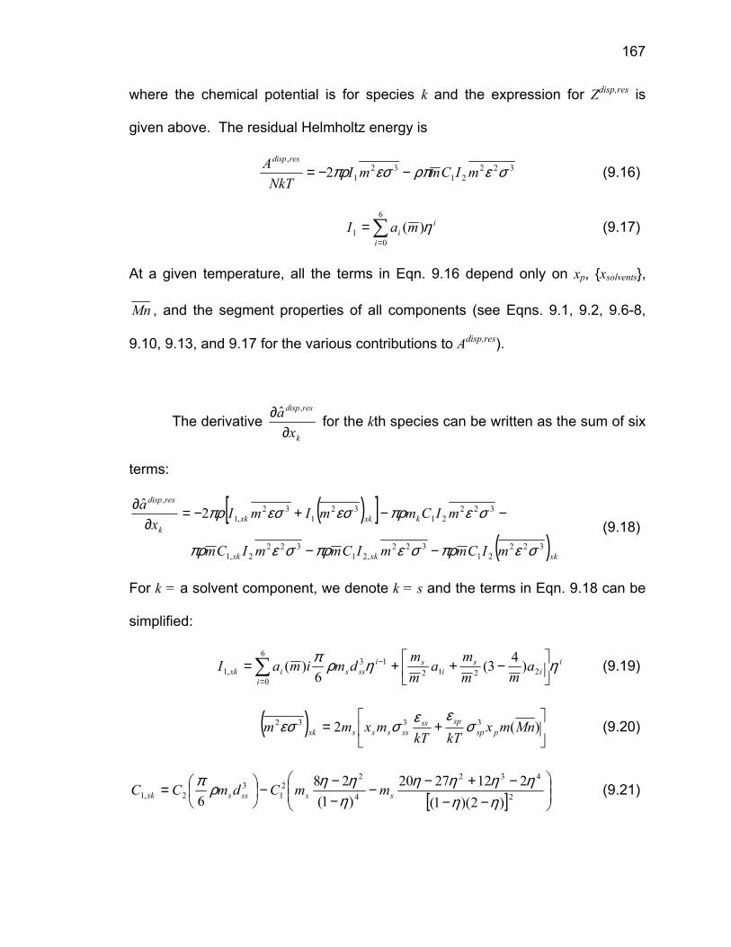
167
where the chemical potential is for species k and the expression for Zdisp,res is
given above. The residual Helmholtz energy is
32221
321
,
2 σερπεσπρ mICmmINkT
A resdisp
−−= (9.16)
∑=
=6
01 )(
i
ii maI η (9.17)
At a given temperature, all the terms in Eqn. 9.16 depend only on xp, {xsolvents},
Mn , and the segment properties of all components (see Eqns. 9.1, 9.2, 9.6-8,
9.10, 9.13, and 9.17 for the various contributions to Adisp,res).
The derivative k
resdisp
xa∂
∂ ,ˆ for the kth species can be written as the sum of six
terms:
( )[ ]( )xkxkxk
kxkxkk
resdisp
mICmmICmmICm
mICmmImIx
a
32221
322,21
3222,1
32221
321
32,1
,
2ˆ
σεπρσεπρσεπρ
σεπρεσεσπρ
−−
−−+−=∂
∂ (9.18)
For k = a solvent component, we denote k = s and the terms in Eqn. 9.18 can be
simplified:
∑=
−
−++=
6
02212
13,1 )43(
6)(
i
ii
si
sisssixk a
mmm
amm
dmimaI ηηρπ (9.19)
( )
+= )(2 3332 Mnmx
kTkTmxmm psp
spsssssssxk σ
εεσεσ (9.20)
[ ]
−−−+−−
−−−
= 2
432
4
22
13
2,1 )2)(1(2122720
)1(28
6 ηηηηηη
ηηηρπ
sssssxk mmCdmCC (9.21)

168
∑=
−
−++=
6
02212
13,2 )43(
6)(
i
ii
si
sisssixk b
mmm
bmm
dmimbI ηηρπ (9.22)
( )
+
= )(2 3
223322 Mnmx
kTkTmxmm psp
spsssssssxk σ
εεσσε (9.23)
As seen from Eqns. 9.6-10, 9.17, and 9.19-23, at a given temperature, each term
in Eqn. 9.18 depends only on xp, {xsolvents}, Mn , and the segment properties (σ and
ε/k) of all components. Recall that d is the temperature dependent σ given in
Eqn. 4.6.
For k = a pseudo-component (in the polydisperse species), we let k = pn
for the nth pseudo-component and the terms in Eqn. 9.18 can be written as
∑=
−
−++=
6
02
22
113,1 )43(
6)(
i
iiiippipxk mm
ama
dimamIn
ηηρπ (9.24)
( )
+= ∑
→solventsj
pjpjjj
ppppppxk kT
mxkT
Mnmxmmn
εσ
εσεσ 3332 )(2 (9.25)
[ ]
−−−+−−
−−−= 2
432
4
22
13
2,1 )2)(1(2122720
)1(28
6 ηηηηηη
ηηηρπ CdCmC pppxk n
(9.26)
∑=
−
−++=
6
02
22
113,2 )43(
6)(
i
iiiippipxk mm
bmb
dimbmIn
ηηρπ (9.27)
( )
+= ∑ 2323322 )()()(2
kTmx
kTMnmxmm pj
pjjjpp
ppppxk n
εσ
εσσε (9.28)
Hence, for each pseudo-component in a polydisperse mixture, each term in Eqn.
9.18 depends explicitly on the chain length of that pseudo-component and on xp,
{xsolvents}, Mn , and the segment properties (σ and ε/k) of all components.

169
To recap, we have
∑→ ∂
∂−∂
∂++=speciesallj j
resdisp
jk
resdispresdisp
resdispresdispk
xax
xaZ
NkTA
kTvT
)ˆ
(ˆ),( ,,
,,,µ (9.15)
which, for a pseudo-component in the polydisperse species, has the following
dependency in each of its terms:
( )ppsolventssolventssolventsp
resdispresdisp
kkMnxxTNkT
ANkT
A )/(,},)/{(},{,,},{,,,,,
εσεσαρ= (9.29)
( )ppsolventssolventssolventspresdispresdisp kkMnxxTZZ )/(,},)/{(},{,,},{,,,,, εσεσαρ= (9.30)
k
resdisp
pk
resdisp
xam
xa
n ∂∂=
∂∂ ,, ˆ̂ˆ (9.31)
where
( )ppsolventssolventssolventspk
resdisp
k
resdisp
kkMnxxTx
ax
a )/(,},)/{(},{,,},{,,,ˆ̂ˆ̂ ,,
εσεσαρ∂
∂=∂
∂
(9.32)
and
)()ˆ̂
()ˆ
()ˆ
(,,,
Mnmxx
ax
axx
ax pp
resdisp
solventsj j
resdisp
jspeciesallj j
resdisp
j ∂∂+
∂∂=
∂∂ ∑∑
→→
(9.33)
In Eqn. 9.33, the terms in the summation over all solvents all depend only on (T,
ρ, xp, {xsolvents}, Mn , α, {σsolvents}, {(ε/k)solvents}, σp, (ε/k)p). Furthermore, the derivative
in the second term of the right hand side of Eqn. 9.33 is constant for all pseudo-
components and also depend only on (T, ρ, xp, {xsolvents}, Mn , α, {σsolvents},
{(ε/k)solvents}, σp, (ε/k)p).

170
For a solvent (a monodisperse species), the residual chemical potential
has the following dependency in each of its terms:
( )ppsolventssolventssolventsp
resdispresdisp
kkMnxxTNkT
ANkT
A )/(,},)/{(},{,,},{,,,,,
εσεσαρ= (9.34)
( )ppsolventssolventssolventspresdispresdisp kkMnxxTZZ )/(,},)/{(},{,,},{,,,,, εσεσαρ= (9.35)
( )ppsolventssolventssolventspk
resdisp
k
resdisp
kkMnxxTx
ax
a )/(,},)/{(},{,,},{,,,ˆˆ ,,
εσεσαρ∂
∂=∂
∂ (9.36)
)()ˆ̂
()ˆ
()ˆ
(,,,
Mnmxx
ax
axx
ax pp
resdisp
solventsj j
resdisp
jspeciesallj j
resdisp
j ∂∂+
∂∂=
∂∂ ∑∑
→→
(9.33)
The dependencies of the various terms in Eqn. 9.33 has been described above.
Finally, if we are to lump the various terms together, we get
BA
resdispk WWkT
+=,µ for k = solvents (9.34)
and ckA
resdispk WmWkT
+=,µ for k = pseudo-components (9.34’)
where the Ws’ are function only of (T, ρ, xp, {xsolvents}, Mn , α, {σsolvents}, {(ε/k)solvents},
σp, (ε/k)p). Jog and Chapman[127] showed similar dependencies in the chain and
hard-sphere contributions to the chemical potential:
D
reshsk WkT
=,µ for k = solvent
Ek
reshsk WmkT
=,µ for k = pseudo-components
and

171
F
reschaink WkT
=,µ for k = solvent
HkG
reschaink WmWkT
+=,µ for k = pseudo-components
Since Eqns. 9.34 and 9.34’ have the same functional form as the dispersion term
in Jog and Chapman[127], the cloud point curve acceleration algorithm proposed
in their work can be applied here. Furthermore, since the residual chemical
potential for the pseudo-components in each polydisperse species is a linear
function of chain length mi, the natural logarithm of the partition coefficient Ki for
the ith pseudo-component (see Chapter 4) is also a linear function of mi. Hence,
only two parameters need to be solved for each polydisperse species (having an
arbitrary number of pseudo-components) in the flash calculations.

172
CHAPTER 10. MODIFICATIONS TO THE SAFT ASSOCIATION TERM –
IMPLICATIONS TO MIXTURES CONTAINING WATER
10.1 Introduction
The main focus of our investigation so far has been on mixtures
dominated by molecular size and van der Waals interactions. For these systems,
the local fluid structures are dominated by the species’ repulsive interactions and
to a lesser degree by nonpolar interactions. However, for mixtures containing
associating species such as water, intermolecular attraction (due to hydrogen
bonding) plays a larger role in determining the structure of the fluid. These
attraction forces are highly orientation dependent and will constrain the
orientations of the interacting molecules.
Of all the mixtures containing associating species, we are especially
interested in modeling the thermodynamic phase behavior of water-hydrocarbon
mixtures. We are interested in this system because (1) it is of considerable
importance in refining and petrochemical operations; (2) it is important in the
treatment of industrial waste water and in other environmental engineering
operations; (3) considerable amounts of water are present in some oil and gas
reservoirs whose presence may affect the phase behavior of other reservoir
components; and (4) at its present state, SAFT cannot describe the solubility of
hydrocarbon in a water-rich phase[128,129].

173
Water-hydrocarbon mixtures are difficult to model because of the unique
properties of water due to its strong hydrogen bonding tendencies. For instance,
the solubility of water in hydrocarbon is orders of magnitude larger than the
solubility of hydrocarbon in water. Furthermore, there is a minimum solubility of
hydrocarbons in water (as a function of temperature) while water solubility in
hydrocarbon is a monotonic function of temperature.[129-133] The extremely
nonideal behaviors in these systems are due to extensive cooperative bonding of
water (which forms a space-filling, open network[134]) in the water-rich phase.
Thus, to be able to model the phase behavior of water-hydrocarbon systems, an
equation of state must be able to take into account the considerable degree of
long range order (due to hydrogen bonding) in the water-rich phase. This long
range structural order in water is responsible for such unique properties as the
density maximum of water (0.999972 g/cm3 at 3.98°C and atmospheric pressure)
and the isothermal compressibility minimum near 46.5°C and atmospheric
pressure.[135]
Traditionally, the phase behavior of mixtures containing water are
modeled using either an excess Gibbs energy model such as the Wilson
equations[24] or a cubic equation of state model with modifications to include the
energy effects due to hydrogen bonding[136,137]. The main advantage of the
excess Gibbs energy models is their ability to represent experimental data with
simple empirical equations. These models are not predictive because they are
174
empirical in nature and the equations work well only within a range of
temperatures and pressures. The cubic equation of state models rely on
elaborate mixing rules (such as the local composition mixing rule of Huron and
Vidal[138]) or large binary interaction parameters with questionable predictive
capabilities. For instance, Economou, et al.[130] showed that while the Peng-
Robinson equations with the Huron-Vidal mixing rule provided qualitative
improvement over the van der Waals mixing rule in modeling 1-hexene solubility
in water, its prediction for water in 1-hexene became worse. Because of the low
solubility of hydrocarbons in water, experimental phase equilibrium data are often
described in terms of Henry’s constants and it is common to recast theory
calculations in terms of theory-calculated Henry’s constants.
In the last decade, theories based on Wertheim’s TPT1 theory[56-59]
(namely SAFT) have been used to model systems containing water. For
instance, Economou and Tsonopoulos[139] found that while SAFT adequately
describes the solubility of water in various hydrocarbons, the equation of state
fails to describe the solubility of hydrocarbons in water. This is true regardless of
whether a 3-site or 4-site model is used to describe water in SAFT. The results
of this and other similar studies[128,129,139,140] are surprising. Truskett, et al.[141]
attributed this in part to the theory’s inability to reproduce the distinguishing
thermodynamic features of liquid water (such as its density maxima), which are
indications that SAFT cannot adequately describe the long range cooperative
bonding behavior of liquid water. In the following section, we will discuss some

175
potential reasons for SAFT’s shortcomings and introduce a more rigorous form of
the equation of state that explicitly accounts for the longer-range interactions in
the hydrogen bonding term.
10.2 Theory Modifications
The association contribution to the Helmholtz energy (Aassoc) for a pure fluid
with multiple bonding sites can be written as[55]
22ln MXX
RTA
A
AA
assoc
+
−=∑ (10.1)
from Wertheim’s first order perturbation theory[56-59] where M is the number of
association sites on each molecule, XA is the mole fraction of molecules not
bonded at site A, R is the gas constant, and T is temperature. The other terms in
the Helmhotz energy expression can be found in Chapter 4. XA is calculated
from the recursive relationship
1]1[ −∑ ∆+=B
ABBA XX ρ (10.2)
where ∫=∆ )12()12()12( dfg ABR
AB (10.3)
∫ ∫ ∫∫ ∫=
cr AB
R drdd
ddfrrg
σ ϖϖ
ϖϖπ
21
212)12(
)(4
and 1)/)(exp( −−= kTrf ABABAB φ (10.4)
In Eqn. 10.2, ρ is the number density of molecules and the summation is over all
sites B. In Eqn. 10.2 to 10.4, ∆AB is the strength of association, fAB is the Mayer f-
function, gR(12) is the reference fluid pair correlation function,

176
∫∫=
21
2124)12(
ϖϖϖϖπ
dddrddrd where ω denotes the orientation contributions, and φAB is
the intermolecular potential between molecules A and B. d(12) is an unweighted
angle average of the orientations. The pair correlation function (also called the
radial distribution function) is a factor that multiplies the bulk density of the fluid to
give the local fluid density about some fixed molecule. The integral in Eqn. 10.3
is taken from the surface of the molecule to a cutoff distance rc and the equation
requires the radial distribution of the reference fluid in the range where bonding
occurs. The free energy relationship (Eqns. 10.1 to 10.4) is exact within the first
order molecular framework described by Wertheim. The assumptions and
limitations of the first order perturbation theory are given in Chapter 4.
If one assumes that the reference fluid consists of hard spheres (with a
spherical diameter of σ) and that the site-site intermolecular interaction has the
form given in Figure 10.1, then the integral in Eqn. 10.3 can be simplified and
renormalized:[142]
∫=∆*
1
23 )(r
hsABAB drrgrFKσ (10.5)
where 4
)cos1(4
2cK
θπ −= (10.6)
and 1)/exp( −= kTF ABAB ε (10.7)
In Eqn. 10.6, θc is the angle cutoff of the associating “cone” (see Fig. 10.1). The
form of the SAFT association term used in literature is the result of an additional

177
simplification made by Chapman, et al.[55]; they assumed that ≈refgr 2 constant
since association is effective only in a small region near the molecular surface so
that
)(σκ refAB gF≈∆ (10.8)
The volume parameter κ and energy parameter εAB can be determined by fits to
the fluid’s liquid densities and vapor pressures.
Figure 10.1 Intermolecular potential model for molecules with square-well sites with angular cutoff. The figure is reproduced from Jackson, et al.[142]
The idea of treating water as hard spheres with multiple bonding sites
(similar to that shown in Figure 10.1) is similar to the simple point charge (SPC)
model for water used in literature. In the SPC models, water is treated as a
Lennard-Jones sphere located on the oxygen atom with two positive partial
charges and one or two negative charges. As shown in Figure 10.2, the hard
spheres + association model for water used in this study can qualitatively
Molecule 1 Molecule 2
r12
Site A Site B θ2
θ1
φAB(r12) =-εAB, if |r12| ≤ r12,cutoff and |θ1| ≤ θ1,cutoff and |π - | θ2 | ≤ θ2,cutoff
0 , if |r12| > r12,cutoff or |θ1| > θ1,cutoff or |π - | θ2 | > θ2,cutoff
Molecule 1 Molecule 2
r12
Site A Site B θ2
θ1
Molecule 1 Molecule 2
r12
Site A Site B θ2
θ1
φAB(r12) =-εAB, if |r12| ≤ r12,cutoff and |θ1| ≤ θ1,cutoff and |π - | θ2 | ≤ θ2,cutoff
0 , if |r12| > r12,cutoff or |θ1| > θ1,cutoff or |π - | θ2 | > θ2,cutoff
φAB(r12) =-εAB, if |r12| ≤ r12,cutoff and |θ1| ≤ θ1,cutoff and |π - | θ2 | ≤ θ2,cutoff
0 , if |r12| > r12,cutoff or |θ1| > θ1,cutoff or |π - | θ2 | > θ2,cutoff

178
describe the radial distribution of bulk water. The experimental data in Figure
10.2 were obtained at 25°C by Soper and Phillips[143] for the oxygen-oxygen
distribution. The simulation was run using 864 hard spheres with 4 bonding sites
per molecule for 100 million configurations. Each molecule has a bonding ε of 6,
a θcutoff of 27°, a hard sphere diameter of 2.55 Angstrom, and a reduced density
of 0.555 (equivalent to 1 g/cm3 with the aforementioned σ). The van der Waals
diameter of water molecule was found to be between 2.8 and 3.9 Angstroms,
depending on orientation.[134]
Figure 10.2 The hard spheres + association model of water used in this work can qualitatively describe the local structure of bulk water.
To improve the equation of state’s ability to model strongly associating
fluids such as water, we can (1) apply Wertheim’s second order perturbation
179
theory[144] and/or (2) remove the assumptions used to obtain Eqn. 10.8 and use
the expression for ∆AB in Eqn. 10.5 instead. Although calculations made with the
second order theory show better agreement with simulation results, the
improvements made in going from first to second order theory is small. [142]
Furthermore, the inclusion of the second order terms would require analytic
expressions for the triplet correlation functions that are much more complex than
the expressions for the pair correlations. This will become apparent in the next
few paragraphs. Thus we will concentrate our effort on the second approach. By
considering the fluid structure over a large distance in the calculation of the
strength of association between two potential bonding sites, we should be able to
capture the long range bonding behavior of liquid water.
To use Eqn. 10.5 to calculate the strength of association between two
bonding sites, we need an analytic expression for g(r) of the reference hard
sphere fluid. While g(r) can be tabulated in computer simulations, its exact
solution cannot be determined analytically. An approximation to g(r) for hard
spheres was solved by Wertheim[145] and Thiele[146] using Percus-Yevick (PY)
equation. (The solution is exact in the PY framework.) Succinctly, they applied
the PY equation
)()()( ryrgrc −= (10.9)
where )()/)(exp()( rgkTrry φ≡ (10.10)
to the Ornstein-Zernike (OZ) integral equation to “close” the OZ equation:
∫+= 323131212 )()()()( drrhrcrcrh ρ (10.11)

180
In the above equations, c(r), y(r), and h(r) are the direct, the cavity, and the total
correlation function, respectively. The OZ equation essentially says that the total
correlation between two molecules is the sum of a direct contribution and an
indirect contribution that depends on all other molecules. Note that the solution
to the PY equations is exact but the integral equation theory is only approximate.
The solution to g(r) given by Wertheim and Thiele is difficult to use
because the radial distribution function is given in terms of its Laplace transforms
and the function itself contains imaginary terms. Using Baxter’s factorization
method[147], Chang and Sandler[148] parameterized these expressions in terms of
real functions. We will use the form given by Chang and Sandler but limit the
range of integration to within 2σ because of the presence of poles at integral
multiples of σ (i.e. at σ, 2σ, 3σ …). This cutoff distance is about 6.3 Angstroms in
terms of SPC water diameter (Figure 10.2).
Comparison between computer simulations and the solution to g(r) given
by Wertheim and Thiele shows that the latter suffers from three defects at higher
fluid densities.[149] These are: (1) the pair correlation function is too small near
the core )( σ→r , (2) the pair correlation function oscillates slightly out of phase
with respect to simulation results, and (3) the main maximum is too high
compared to simulation results. We will use an empirical shifting algorithm
proposed by Verlet and Weis[149] to “correct” for these defects in the Wertheim-
Thiele solutions (Figure 10.3). If we denote g(r/σ, η) as the true pair correlation

181
function and gwt(r/σ, η) as the pair correlation function calculated using the
Wertheim-Thiele solution, then
)(),/(),/( 1 rgrgrg wtwtwt δησησ += (10.12)
where 2
161 ηηη −=wt (10.13)
)(cos)](exp[)/()(1 σµσµδ −−−= rrrArg (10.14)
4
22
)1()114.07117.01(
43
wt
wtwtwtAη
ηηησ −
−−= (10.15)
and ),1(
)/(24
wtwtwt gA
ηησµσ = (10.16)
As seen in Figure 10.3, the Verlet-Weis correction agrees very well with
simulation data.

182
Figure 10.3 Comparison of the pair correlation functions obtained from different methods at a reduced density of 0.39 (η = 0.2042). r* is the reduced distance. The simulation was run for 4 million configurations with 256 molecules.
Using the Chang and Sandler parameterization with the Verlet-Weis shift,
the integral in Eqn. 10.5 becomes
*)***()( 32 BAdrrgrcr
ref +=∫ σσ
(10.17)
where
−−−++
=
−))1(cos(
21))1(sin()1(
21
21**
]1[
σσσσσσ ccccrC r
CC
rrC
rCe
CAB
σA is given in Eqn. 10.15

183
),1(
)/(24
wtwtwt gAC
ηησ=
wtη is given in Eqn. 10.13
4
2
4
2
4
2
)1(2)21(
)1()2/1(6
)1()21(
),1(wt
wtwt
wt
wtwt
wt
wtwtwtg
ηηη
ηηη
ηηη
−+
−−+
+−+−
=
and where
321** IIIA ++=
−−−=
−
)1)(()1)()(()/(
3/1)/(3/1)/()/(3/22
11
3/13/1
w
Ac
w
rA
wt
A
Aer
AeA
eaI wtcwt
ηη
σηη
ηηηησηη
−++−= − ))1)()((cos())()()()(( 3/123/1223/13)/()/(
22
3/1
σηη
σηη
σηησηη c
w
c
w
c
w
rBB rCC
rBCB
rBeeaI cwt
−+−+ ))1)()((sin())()(2)()(( 3/13/123/12
σηη
σηη
σηη c
w
c
wt
c
wt
rC
rCB
rBC
−++−− ))1)((cos())()(( 3/123/1223/13)/( 3/1
wtwtwt
B CCBCBBe wt
ηη
ηη
ηηηη
+
−+−+ 2223/23/13/123/12 )()(/))1)((sin())(2)(( CBCCBBC
wtwtwtwt ηη
ηη
ηη
ηη
−+−= − ))1)((cos())(2)(( 3/13/123/12)/(
33
3/1
wtwtwt
BB CCBBCeeaI wt
ηη
ηη
ηηηη
++−−− ))()())(1)((sin( 2223/133/1 CBCBBC
wtwtwt ηη
ηη
ηη
))1)()((sin()))(()()(( 3/12223/13)/()/( 3/1
−++−
+
σηη
σηη
σηησηη c
wt
c
wt
c
wt
rB rCC
rBCB
rBe cwt

184
+
+−−− 2223/23/123/123/1 )()(/)()(2)()())(1)()((cos( CB
rCB
rB
rCC
wt
c
wt
c
wt
c
wt ηη
σηη
σηη
σηη
The variables used in I1, I2, and I3 are
w
dw ZA
ηη−
+−=
12
w
dw ZB
ηη
−−−
=1
2/2
)1(23
wt
sZC
η−=
−+ −= yyZ d
−+ += yyZ s
3/12/1
2
43/1 1)12()2(
±+=± f
fy ηη
233 wtwtf ηη −+=
222
222
1 )1)(2(3)2/1()431()31(2
wtdwt
dwtdwtwtwtwtwt
ZZZ
aηη
ηηηηηη−+
++−−+−−−=
222
222
2 )1)(2(3)2/1(2)431()342(
wtdw
dwtdwtwtwtwt
ZZZ
aηη
ηηηηηη−+
++−−−−+=
3)1)(2()52()4)(431(
222
2222
3wtdwts
dwtwtdwtwtwt
ZZZZ
aηη
ηηηηη−+
−++−−=
The variables (rc/σ) and θc, which is the dimensionless cutoff distance and the
cutoff angle, can be determined from fits to saturated vapor pressures and liquid

185
densities of water. The various derivatives of ∆AB such as ( ) NT ,ρ∂∆∂ can be
determined numerically.
186
CHAPTER 11. CONCLUSIONS AND FUTURE RESEARCH
The main focus of this research is to develop an equation of state model
that can describe and predict the phase behavior of asphaltenes in crude oil
under both ambient and reservoir conditions. The hypothesis underlying this
work is that molecular size and nonpolar van der Waals interactions dominate
asphaltene phase behavior in reservoir fluids. We chose the SAFT equation of
state (with the inclusion of only van der Waals interactions) as our starting point
because of its theoretical basis and its ability to model systems dominated by
large differences in molecular size. Along the way, a robust and efficient
stability-flash algorithm was developed (Chapter 4) to calculate equilibrium phase
compositions for systems of interest in this work (namely multi-component
systems with large differences in molecular properties and/or composition).
To trace out the asphaltene stability boundary under reservoir conditions
for comparison with SAFT predictions, the asphaltene stability and bubble point
curves of a recombined oil (stock-tank oil with separator gas added back in) and
a model live oil (asphaltene-toluene-methane mixture) were measured as
functions of pressure, temperature, and dissolved gas concentration (Chapter 3).
Significant temperature effects on asphaltene stability were observed, and
increasing the temperature of the system seemed to improve asphaltene stability.
Furthermore, at each temperature, the asphaltene instability onset pressures
were nearly linear functions of mixture gas concentration. This suggested that
187
the asphaltene instability boundaries could be roughly estimated from a few data
points. Finally, an analysis of the experimental data showed that at a constant
temperature, the mixture refractive indices do not change much along the
asphaltene instability onset curves.
To investigate the applicability of the SAFT equation of state for use in
asphaltene phase behavior modeling, SAFT’s ability to describe the
thermodynamic phase behavior of a variety of model systems were tested
(Chapter 5). In the first set of investigation, we tested SAFT’s ability to describe
the phase behavior of long-chain short-chain alkane mixtures. We were
interested in this system because the bulk of crude oil is made up of saturates
components and because these mixtures will test SAFT’s ability to model the
effects of size on solubility. In spite of its deficiencies in modeling of the critical
region, SAFT was clearly the better equation of state for predicting the phase
behavior of highly asymmetric mixtures of alkanes compared to conventional
cubic equations. Using a binary interaction parameter of 0, SAFT provided good
estimates of liquid phase compositions up to within 5-10 bars of the predicted
mixture critical points. This meant that good predictions of crude oil
thermodynamic properties should be possible using SAFT with binary interaction
parameters set to 0 between all alkanes in oil (with the exception of the lighter
fractions).
188
In the second set of model system investigations, we tested SAFT’s ability
to describe the phase behavior of polystyrene-hexane and polystyrene-toluene-
ethane. The system polystyrene-toluene-ethane was particularly interesting
because it resembled our model live oil system (asphaltene-toluene-methane).
Comparison between theory and experiments showed that SAFT was capable of
describing and predicting the phase behavior of these binary and ternary
systems (which consisted of species with very large size disparities); the effects
of pressure, temperature, and composition changes on phase stability were
accurately described using SAFT. Furthermore, by comparing the phase
behavior of asphaltenes with that of polystyrene, we could explain many
asphaltene behaviors in the framework of polymer thermodynamics (such as the
L/UCST behavior).
In the last set of model system investigations, we looked at the phase
behavior (solid-liquid-vapor equilibria) of phenanthrene-methane-decane mixture.
This system was of significant interest because phenanthrene shares structural
similarities with asphaltene and this system would provide insights into SAFT’s
ability to describe the solubility behavior of polynuclear aromatics. An analysis
showed that SAFT (together with a solid fugacity model) was able to describe the
solubility behavior of polynuclear aromatics. Furthermore, the combination of
SAFT (in modeling of the fluid phases) and the solid fugacity model (in modeling
of the solid phase) was able to predict the pressure-solubility behavior of
phenanthrene in which increasing pressure leads to lower solubility.

189
Before SAFT could be applied to model crude oil systems containing
asphaltenes, a lumping scheme needed to be developed to divide the
recombined oil into pseudo-components and a characterization scheme needed
to be developed to model asphaltenes for use in SAFT. In this work, the
recombined oil was modeled as a six-component mixture, with three pseudo-
components for the stock-tank oil fraction and three pseudo-components for the
separator gas. The average molecular weight and the amount of each sub-
fraction were determined from gas-chromatography, saturates-aromatics-resins-
asphaltenes fractionation, and gas-oil-ratio information. The SAFT parameters
for each sub-fraction (except for the asphaltenes) were obtained from
correlations with molecular weight for each class of compounds. The SAFT-
predicted densities for the stock-tank oil and the recombined oils agree very well
with experimental measurements.
The mixture refractive indices at the onset of asphaltene precipitation
during ambient condition titrations (PRI) were used to characterize asphaltene’s
SAFT parameters; the parameters were optimized so that SAFT would reproduce
the mixture’s PRI (alternatively the composition of the mixture) at the onset of
asphaltene precipitation. If the mechanism responsible for asphaltene
precipitation under reservoir depressurization is consistent with the mechanism in
titration experiments, thermodynamic models that correctly account for the
interaction forces should be able to predict the depressurization results based on

190
matching the results of the titration experiments. For both the model oil and the
stock-tank oil, good agreements were obtained between experimental and fitted
PRI even with a binary interaction parameter of zero between asphaltenes and
the other species.
For both the model live oil and the recombined oil systems, SAFT
predicted asphaltene instability, oil bubble points, and other fluid properties agree
well with experiments. Good agreements were obtained between experiment
and model predictions on the effects of temperature, pressure, and dissolved gas
concentration on asphaltene stability. Furthermore, both SAFT calculated and
experiment derived mixture solubility parameters/refractive indices along the
asphaltene instability curves were nearly constant at a given temperature.
Since asphaltene is actually a polydisperse collection of molecules, the
effects of asphaltene polydispersity on the thermodynamic phase behavior of oil
need to be examined. At this stage, we represented polydisperse asphaltene in
SAFT using four pseudo-components: the n-C3-5 (the resins), the n-C5-7, the n-C7-
15, and the n-C15+ sub-fractions. Using an extension of the monodisperse SAFT
asphaltene parameter fitting procedure, we were able to assign a set of SAFT
parameters to represent each of the four sub-fractions.
A SAFT investigation into the effects of asphaltene polydispersity showed
that the lower molecular weight asphaltenes and resins played a significant role

191
in stabilizing higher molecular weight asphaltenes in oil. This was despite the
inclusion of only dispersion interactions in the SAFT model. Resin’s stabilizing
effects on polydisperse asphaltene was greatest in the region of incipient
asphaltene instability; when sufficient n-alkane precipitants were added, similar
amounts of asphaltenes would precipitate regardless of the presence of resins in
the oil. An analysis of the mass distribution of the asphaltene sub-fractions in the
precipitated phase showed that the largest asphaltenes would precipitate first,
followed by the precipitation of smaller asphaltenes upon further oil dilution. It is
important to keep in mind that although the SAFT predicted asphaltene mass
distributions are qualitatively correct, no experimental data is available at this
point to quantitatively validate these numbers.
The underlying hypothesis of our approach is that molecular size and
nonpolar van der Waals interactions dominate asphaltene phase behavior in
reservoir fluids. A comparison of our monodisperse and polydisperse modeling
results with experimental observations supports this hypothesis. An equation of
state that can correctly account for the nonpolar van der Waals interactions in
titration experiments should be able to also predict asphaltene stability during
depressurization.
The next logical step for the research program is to further validate the
monodisperse and polydisperse models presented in this work. The asphaltene
instability boundaries of at least a few more oils need to be calculated and

192
compared with experimental results to gauge the model’s abilities. It will also be
interesting to look at oils whose asphaltene precipitation problems are due to
CO2 injection.
While the monodisperse asphaltene precipitation model is relatively
straightforward to implement, two issues need to be resolved for the polydisperse
asphaltene model. One should concurrently work on implementing the
modifications made in Chapter 9 (so that the equation of state can be made to
accept an arbitrary number of asphaltene pseudo-components) and on finding
better ways to isolate the various asphaltene pseudo-components for use in
SAFT characterization.
Finally, since asphaltene problems are ultimately only problems if they
deposit onto pipeline surfaces, the bulk phase precipitation model presented in
this work need to be combined with a deposition model. While deposition may or
may not occur with asphaltene precipitation, asphaltene precipitation is mostly
likely a pre-requisite for deposition.

193
REFERENCES
1 Boussingault, M., Ann. Chim. Phys. 64, 141 (1837).
2 Mansoori, G. A., Jiang, T. S., and Kawanaka, S., Arabian J. Sci. Eng. 13,
17-34 (1988).
3 Wiehe, I. A. and Liang, K. S., Fluid Phase Equil. 117, 201-221 (1996).
4 ASTM, (American Society for Testing and Materials, 1980).
5 Wang, J. X., Predicting Asphaltene Flocculation in Crude Oils. Ph.D.
Thesis, New Mexico Institute of Mining & Technology, 2000.
6 Artok, L., Su, Y., Hirose, Y., Hosokawa, M., Murata, S., and Nomura, M.,
Energy & Fuels 13, 287-296 (1999).
7 Speight, J. G. and Plancher, H., in Intl. Symp. on the Chem. of Bitumens
(1991), pp. 154.
8 Wiehe, I. A., Fuel Sci. Tech. Intl. 14, 289-312 (1996).
9 Groenzin, H. and Mullins, O. C., J. Phys. Chem. A. 103, 11237-11245
(1999).
10 Brandt, H. C., Hendriks, E. M., Michels, M. A. J., and Visser, F., J. Phys.
Chem. 99, 10430-10432 (1995).
11 Mohamed, R. S., Ramos, A. C. S., and Loh, W., Energy & Fuels 13, 323
(1999).
12 Burke, N. E., Hobbs, R. D., and Kashou, S. F., in Soc. Pet. Eng. Annual
Tech. Conf. and Exhib. (Houston, TX, 1988).
194
13 Hirschberg, A., deJong, L. N. J., Schipper, B. A., and Meijer, J. G., Soc.
Pet. Eng. J. 24, 283-293 (1984).
14 Kokal, S. L. and Sayegh, S. G., in Soc. Pet. Eng. Middle East Oil Show
(Bahrain, 1995).
15 Haskett, C. E. and Tartera, M., J. Pet. Tech. 17, 387-391 (1965).
16 Tuttle, R. N., J. Pet. Tech. 35, 1192-1196 (1983).
17 Thaver, R., Nicoll, D. C., and Dick, G., in Soc. Pet. Eng. Intl. Symp. Oilfield
Chem. (Houston, TX, 1989).
18 Lichaa, P. M., in CIM Conf. on Oil Sands of Canada and Venezuela
(1977), pp. 609-624.
19 Adialalis, S., Investigation of physical and chemical criteria as related to
the prevention of asphalt deposition in oil well tubings. Ph.D. Thesis,
Imperial College, 1982.
20 Chavez, A. J. L. and Lory, M. A., Revista del Instituto Mexicano del
Petroleo 23, 1 (1991).
21 Escobedo, J. and Mansoori, G. A., in SPE Annual Technical Conference
and Exhibition (Dallas, TX, 1995).
22 von Albrecht, C., Salathiel, W. M., and Nierode, D. E., CIM Special
Volume , 55-62 (1977).
23 Wu, J., Molecular Thermodynamics of Some Highly Asymmetric Liquid
Mixtures. Ph.D. Thesis, University of California at Berkeley, 1998.
195
24 Prausnitz, J. M., Lichtenthaler, R. N., and de Azevedo, E. G., Molecular
Thermodynamics of Fluid-Phase Equilibria, 2nd ed. P T R Prentice-Hall,
Inc., 1986.
25 Reed, T. M. and Gubbins, K. E., Applied Statistical Mechanics
Butterworth-Heinemann, 1973.
26 Israelachvili, J., Intermolecular & Surface Forces, 2nd ed. Academic Press
Inc., 1992.
27 Khryaschchev, A. N., Popov, O. G., Posadov, N. A., and Rozental, D. A.,
Pet. Chem. 31, 601-604 (1991).
28 Moore, E. W., Crowe, C. W., and Hendrickson, A. R., J. Pet. Tech. 17,
1023-1028 (1965).
29 Chang, C. L. and Fogler, H. S., in Soc. Pet. Eng. Intl. Symp. on Oilfield
Chem. (New Orleans, LA, 1993).
30 Akbarzadeh, K., Ayatollahi, S., Moshfeghian, M., Alboudwarej, H., Svrcek,
W. Y., and Yarranton, H. W., in Amer. Inst. Chem. Eng. Spring National
Meeting (New Orleans, LA, 2002), pp. 218-224.
31 Cimino, R., Correra, S., and Sacomani, P. A., in Soc. Pet. Eng. Intl. Symp.
on Oilfield Chem. (San Antonio, TX, 1995).
32 Nghiem, L. X., Hassam, M. S., Nutakki, R., and George, A. E. D., in Soc.
Pet. Eng. Annual Tech. Conf. and Exhib. (Houston, TX, 1993), pp. 375-
384.

196
33 Leontaritis, K. J. and Mansoori, G. A., in Soc. Pet. Eng. Intl. Symp. on
Oilfield Chem. (San Antonio, TX, 1987).
34 Victorov, A. I. and Firoozabadi, A., Amer. Inst. Chem. Eng. J. 42, 1753-
1764 (1996).
35 Nghiem, L. X. and Coombe, D. A., Soc. Pet. Eng. J. 2 (1997).
36 Chung, F., Sarathi, P., and Jones, R., (National Institute for Petroleum and
Energy Research, Bartlesville, 1991).
37 Burke, N. E., Hobbs, R. E., and Kashou, S. F., J. Pet. Tech. 42, 1440-
1446 (1990).
38 Firoozabadi, A., Thermodynamics of hydrocarbon reservoirs McGraw-Hill,
New York, 1999.
39 Ting, P. D., Wang, J., Buckley, J. S., Creek, J., Hamammi, A., Hirasaki, G.
J., and Chapman, W. G., In Preparation (2003).
40 Buckley, J. S., Hirasaki, G. J., Liu, Y., von Drasek, S., Wang, J., and Gill,
B. S., Pet. Sci. Tech. 16, 251-285 (1998).
41 Katz, D. L. and Firoozabadi, A., J. Pet. Tech. , 1649 (1978).
42 Feynman, R. P., Leighton, R. B., and Sands, M., The Feynman Lectures
on Physics Addison-Wesley Publishing Co., 1989.
43 Vedam, K. and Limsuwan, P., J. Chem. Phys. 69, 4772-4778 (1978).
44 CRC Handbook of Chemistry and Physics, Vol. , edited by Weast, R. C.,
Astle, M. J., and Beyer, W. H. (CRC Press, Inc., Boca Raton, 1987).

197
45 Barton, A. F. M., CRC Handbook of Solubility Parameters and Other
Cohesion Parameters, 2nd ed. CRC Press, Boca Raton, 1991).
46 Wang, J. X. and Buckley, J. S., in OCS (Houston, TX, 2001).
47 Gray, C. G. and Gubbins, K. E., Theory of Molecular Fluids I. Clarendon
Press, Oxford, 1984.
48 McQuarrie, D. A., Statistical Mechanics. Harper & Row Publishers, New
York, 1976.
49 Smith, J. M. and van Ness, H. C., Introduction to Chemical Engineering
THermodynamics, 4th ed. McGraw-Hill, Inc., 1987.
50 Peng, D. Y. and Robinson, D. B., Ind. Eng. Chem. Fund. 15, 59-63 (1976).
51 Barker, J. A. and Henderson, D. J., J. Chem. Phys. 47, 2856-2861 (1967).
52 Barker, J. A. and Henderson, D. J., J. Chem. Phys. 47, 4714-4721 (1967).
53 Chapman, W. G., Jackson, G., and Gubbins, K. E., Mol. Phys. 65, 1057-
1079 (1988).
54 Chapman, W. G., Gubbins, K. E., Jackson, G., and Radosz, M., Fluid
Phase Equil. 52, 31-38 (1989).
55 Chapman, W. G., Gubbins, K. E., Jackson, G., and Radosz, M., Ind. Eng.
Chem. Res. 29, 1709-1721 (1990).
56 Wertheim, M. S., J. Stat. Phys. 35, 19 (1984).
57 Wertheim, M. S., J. Stat. Phys. 35, 35 (1984).
58 Wertheim, M. S., J. Stat. Phys. 42, 459 (1986).
59 Wertheim, M. S., J. Stat. Phys. 42, 477 (1986).

198
60 Joslin, C. G., Gray, C. G., Chapman, W. G., and Gubbins, K. E., Mol.
Phys. 62, 843-860 (1987).
61 Mansoori, G. A., Carnahan, N. F., Starling, K. E., and Leland, T. W., J.
Chem. Phys. 54, 1523 (1971).
62 Gross, J. and Sedowski, G., Ind. Eng. Chem. Res. 40, 1244-1260 (2001).
63 Dickman, R. and Hall, C., J. Chem. Phys. 89, 3168-3174 (1988).
64 Gao, J. and Weiner, J. H., J. Chem. Phys. 91, 3168-3173 (1989).
65 Gross, J. and Sadowski, G., Ind. Eng. Chem. Res. 40, 1244-1260 (2001).
66 Economou, I. G., Ind. Eng. Chem. Res. 41, 953-962 (2002).
67 Muller, E. A. and Gubbins, K. E., Ind. Eng. Chem. Res. 40, 2193-2212
(2001).
68 Ting, P. D., Joyce, P. C., Jog, P. K., Chapman, W. G., and Thies, M. C.,
Fluid Phase Equil. (2002).
69 DIPPR, (AIChE, ).
70 Huang, S. H. and Radosz, M., Ind. Eng. Chem. Res. 29, 2284-2294
(1990).
71 Xu, G., Brennecke, J. F., and Stadtherr, M. A., Ind. Eng. Chem. Res. 41,
938-952 (2002).
72 Dluzniewski, J. H. and Adler, S. B., Chem. E. Symp. Ser. 35, 4 (1972).
73 Genetic algorithms in engineering and computer science, edited by
Quagliarella, D., Periaux, J., Poloni, C., and Winter, G. (John Wiley &
Sons, New York, 1997).
199
74 Banga, J. R. and Seider, W. D., Nonconvex optimization and its
applications 7, 563-584 (1996).
75 Rachford, H. H. and Rice, J. D., J. Pet. Tech. 4, 19 (1952).
76 Nelson, P. A., Comp. Chem. Eng. 11, 581-591 (1987).
77 Mehra, R. K., Heidemann, R. A., and Aziz, K., Can. J. Chem. Eng. 61,
590-596 (1983).
78 Ohanomah, M. O. and Thompson, D. W., Comp. Chem. Eng. 8, 163
(1984).
79 Michelsen, M. L., Fluid Phase Equil 9, 1-19 (1982).
80 Michelsen, M. L., Fluid Phase Equil 9, 21-40 (1982).
81 Nocedal, J. and Wright, S. J., Numerical Optimization Springer, New York,
1999.
82 Baker, L. E., Pierce, A. C., and Luks, K. D., Soc. Pet. Eng. J. , 731 (1982).
83 Marano, J. J. and Holder, G. D., Fluid Phase Equil. 138, 1-21 (1997).
84 Voulgaris, M. E., Peters, C. J., and de Swaan Arons, J., Intl. J.
Thermophys. 16, 629-642 (1995).
85 McHugh, M. A. and Krukonis, V. J., Supercritical Fluid Extraction -
Principles and Practice, Butterworths, Boston, 1986.
86 Joyce, P. C. and Thies, M. C., J. Chem. Eng. Data 43, 819-822 (1998).
87 Joyce, P. C., Gordon, J., and Thies, M. C., J. Chem. Eng. Data 45, 424-
427 (2000).

200
88 Peters, C. J., de Swaan Arons, J., Levelt Sengers, J. M. H., and
Gallagher, J. S., AIChE J. 34, 834-839 (1988).
89 Peters, C. J., de Roo, J. L., and de Swaan, A. J., Fluid Phase Equil. 72,
251-266 (1992).
90 Kontogeorgis, G. M., Coutsikos, P., Harismiadis, V. I., Fredenslund, A.,
and Tassios, D. P., Chem. Eng. Sci. 53, 541-552 (1998).
91 Floter, E., de Loos, T. W., and de Swaan Arons, J., Ind. Eng. Chem. Res.
37, 1651-1992 (1998).
92 Pan, C. and Radosz, M., Ind. Eng. Chem. Res., 37, 3169-3179 (1998).
93 Huang, S. H. and Radosz, M., Ind. Eng. Chem. Res., 30, 1994-2005
(1991).
94 Benzaghou, S., Passarello, J. P., and Tobaly, P., Fluid Phase Equil. 180,
1-26 (2001).
95 Gregorowicz, J. and de Loos, T. W., Ind. Eng. Chem. Res. 40, 444-451
(2001).
96 Reid, R. C., Prausnitz, J. M., and Poling, B. E., The Properties of Gases &
Liquids, McGraw-Hill, Singapore, 1987.
97 Ambrose, D. and Tsonopoulos, C., J. Chem. Eng. Data 40, 531-546
(1995).
98 Nikitin, E. D., Pavlov, P. A., and Popov, A. P., Fluid Phase Equil. 141, 155-
164 (1997).
99 Morgan, D. L. and Kobayashi, R., Fluid Phase Equil. 97, 211-242 (1994).

201
100 API-42, (American Petroleum Institute, University Park, 1940-1966), pp.
1.
101 Stephenson, R. M. and Malanowski, S., Handbook of the
Thermodynamics of Organic Compounds, Elsevier, New York, 1987.
102 Joyce, P. C., Vapor-Liquid Equilibria for Long-Chain Hydrocarbons in
Supercritical Alkane Solvents. Ph.D. Thesis, Clemson University, 1999.
103 Chen, S. S. and Kreglewski, A., Bunsen-Ges. Phys. Chem. 51, 1048
(1977).
104 Xiong, Y. and Kiran, E., Polymer 38, 5185-5193 (1997).
105 Seckner, A. J., McClellan, A. K., and McHugh, M. A., Amer. Inst. Chem.
Eng. J. 34, 9-16 (1988).
106 Ratulowski, J., Personal Correspondence.
107 Coon, J. E., Troth, M., and McLaughlin, E., J. Chem. Eng. Data 32, 233-
240 (1987).
108 Pan, C. and Radosz, M., Fluid Phase Equil. 155, 57-73 (1999).
109 API-708, (American Petroleum Institute, Washington, D.C., 1979).
110 Malone, P. V. and Kobayashi, R., Fluid Phase Equil. 55, 193-205 (1990).
111 Reamer, H. H., Olds, R. H., Sage, B. H., and Lacey, W. N., Ind. Eng.
Chem. 34, 1526-1531 (1942).
112 Darwish, N. A., Gasem, K. A. M., and Robinson, R. L., J. Chem. Eng. Data
39, 781-784 (1994).

202
113 Jacoby, R. H., in Heavy Crude Oil Recovery, Vol. 76, edited by E.
Okandar (NATO, 1984), pp. 1-47.
114 Wiehe, I. A., Personal Correspondence.
115 Wu, J., Personal Correspondence.
116 Elbishlawi, M. and Spencer, J. R., Ind. Eng. Chem. 43, 1811-1815 (1951).
117 Kidnay, A. F., Miller, R. C., Parrish, W. R., and Hiza, M. J., Cryogenics 15,
531-540 (1975).
118 Reamer, H. H., Sage, B. H., and Lacey, W. N., Ind. Eng. Chem. 42, 534
(1950).
119 Grauso, L., Fredenslund, A., and Mollerup, J., Fluid Phase Equil. 1, 13-26
(1977).
120 Messow, U. and Engel, I., Z. Phys. Chem. 258, 798 (1977).
121 Barton, A. F. M., Handbook of Solubility Parameters & Other Cohesion
Parameters, 2nd ed. CRC Press, Boca Raton, 1991.
122 Azarnoosh, A. and McKetta, J. J., J. Chem. Eng. Data 8, 494-496 (1963).
123 Miller, P. and Dodge, B. F., Ind. Eng. Chem. 32, 434-438 (1940).
124 Glanville, J. W., Sage, B. H., and Lacey, W. N., Ind. Eng. Chem. 42, 508
(1950).
125 Yarranton, H. and Masliyah, J. H., AIChE J. 42, 3533-3543 (1996).
126 Larsen, J. W. and Li, S., Energy Fuels 9, 760-764 (1995).
127 Jog, P. K. and Chapman, W. G., Macromolecules 35, 1002-1011 (2002).

203
128 Boulougouris, G. C., Voutsas, E. C., Economou, I. G., Theodorou, D. N.,
and Tassios, D. P., J. Phys. Chem. B 105, 7792-7798 (2001).
129 Voutsas, E. C., Boulougouris, G. C., Economous, I. G., and Tassios, D. P.,
Ind. Eng. Chem. Res. 39, 797-804 (2000).
130 Economou, I. G., Heidman, J. L., Tsonopoulos, C., and Wilson, G. M.,
AIChE J. 43, 535-546 (1997).
131 Dhima, A., de Hemptinne, J. C., and Jose, J., Ind. Eng. Chem. Res. 38,
3144-3161 (1999).
132 Kobayashi, R. and Katz, D., Ind Eng Chem 45, 440-451 (1953).
133 Tsonopoulos, C., Fluid Phase Equil. 156, 21-33 (1999).
134 Nemethy, G. and Scheraga, H. A., J. Chem. Phys. 36, 3382-3400 (1962).
135 Kell, G. S., in Water, a comprehensive treatise, Vol. 1, edited by F.
Franks, Plenum Press, New York, 1972, pp. 363-404.
136 Poole, P. H., Sciortino, F., Grande, T., Stanley, H. E., and Angell, C. A.,
Phys. Rev. Lett. 73, 1632-1635 (1994).
137 Zudkevitch, D. and Joffe, J., AIChE J. 16, 112-119 (1970).
138 Huron, M. J. and Vidal, J., Fluid Phase Equil. 3, 255 (1979).
139 Economou, I. G. and Tsonopoulos, C., Chem. Eng. Sci. 52, 511-525
(1997).
140 Yakoumis, I. V., Kontogeorgis, G. M., Voutsas, E. C., Hendriks, E. M., and
Tassios, D. P., Ind. Eng. Chem. Res. 37, 4175-4182 (1998).

204
141 Truskett, T. M., Debenedetti, P. G., and Sastry, S., J. Chem. Phys. 111,
2647-2656 (1999).
142 Jackson, G., Chapman, W. G., and Gubbins, K. E., Mol. Phys. 65, 1-31
(1988).
143 Soper, A. K. and Phillips, M. G., Chem. Phys. 107, 47-60 (1986).
144 Wertheim, M. S., J. Chem. Phys. 87, 7323-7331 (1987).
145 Wertheim, M. S., Phys. Rev. Let. 10, 321-323 (1963).
146 Thiele, E. J., J. Chem. Phys. 38, 1959 (1963).
147 Baxter, R. J., Aust. J. Phys. 21, 563 (1968).
148 Chang, J. and Sandler, S. I., Mol. Phys. 81, 735-744 (1994).
149 Verlet, L. and Weis, J. J., Phys. Rev. A 5, 939-952 (1972).