THERMODYNAMIC MODELING AND OPTIMIZATION OF A

SCREW COMPRESSOR CHILLER AND COOLING TOWER

SYSTEM

A Thesis

by

RHETT DAVID GRAVES

Submitted to the Office of Graduate Studies ofTexas A&M University

in partial fulfillment of the requirements for the degree of

MASTER OF SCIENCE

December 2003

Major Subject: Mechanical Engineering

THERMODYNAMIC MODELING AND OPTIMIZATION OF A

SCREW COMPRESSOR CHILLER AND COOLING TOWER

SYSTEM

A Thesis

by

RHETT DAVID GRAVES

Submitted to Texas A&M Universityin partial fulfillment of the requirements

for the degree of

MASTER OF SCIENCE

Approved as to style and content by:

Charles H. Culp(Co-Chair of Committee)

Calvin B. Parnell, Jr.(Member)

Warren M. Heffington(Co-Chair of Committee)

Dennis L. O’Neal(Head of Department)

December 2003

Major Subject: Mechanical Engineering

iii

ABSTRACT

Thermodynamic Modeling and Optimization of a Screw Compressor Chiller and

Cooling Tower System. (December 2003)

Rhett David Graves, B.S., Mississippi State University

Co-Chairs of Advisory Committee: Dr. Charles H. Culp Dr. Warren M. Heffington

This thesis presents a thermodynamic model for a screw chiller and cooling

tower system for the purpose of developing an optimized control algorithm for the

chiller plant. The thermodynamic chiller model is drawn from the thermodynamic

models developed by Gordon and Ng (1996). However, the entropy production in the

compressor is empirically related to the pressure difference measured across the

compressor. The thermodynamic cooling tower model is the Baker & Shryock cooling

tower model that is presented in ASHRAE Handbook – HVAC Systems and Equipment

(1992). The models are coupled to form a chiller plant model which can be used to

determine the optimal performance. Two correlations are then required to optimize the

system: a wet-bulb/setpoint correlation and a fan speed/pump speed correlation. Using

these correlations, a “quasi-optimal” operation can be achieved which will save 17% of

the energy consumed by the chiller plant.

iv

DEDICATION

Soli Deo Gloria.

v

TABLE OF CONTENTS

ABSTRACT...................................................................................................................... iii

DEDICATION .................................................................................................................. iv

TABLE OF CONTENTS................................................................................................... v

LIST OF FIGURES .......................................................................................................... vi

LIST OF TABLES.......................................................................................................... viii

INTRODUCTION ............................................................................................................. 1

LITERATURE REVIEW OF CHILLER & COOLING TOWER MODELS .................. 5

APPLICATION ................................................................................................................. 9

CHILLER MODEL DEVELOPMENT........................................................................... 15

COOLING TOWER MODEL DEVELOPMENT .......................................................... 31

COUPLING THE MODELS ........................................................................................... 39

OPTIMIZATION STRATEGY AND ANALYSIS ........................................................ 47

CONCLUSIONS.............................................................................................................. 54

REFERENCES................................................................................................................. 56

APPENDIX A. COMPLETE CHILLER DERIVATION .............................................. 59

APPENDIX B. TEMPERATURE-ENTROPY DIAGRAM EXPLANATION............. 88

VITA ................................................................................................................................ 97

vi

LIST OF FIGURES

FIGURE Page

Figure 1.1. 205-ton Installed Screw Chiller...................................................................... 2

Figure 3.1. Test Facility .................................................................................................. 10

Figure 3.2. First-Floor Layout of the Test Facility ......................................................... 10

Figure 3.3. Second-Floor Layout of the Test Facility..................................................... 11

Figure 3.4. Building Automation System Diagram ........................................................ 13

Figure 4.1. Chiller Energy Balance Diagram ................................................................. 17

Figure 4.2. Measured Power vs. Calculated Power (Gordon-Ng Model) ...................... 20

Figure 4.3. Measured Power vs. Calculated Power (Derived Evaporator Model) ......... 22

Figure 4.5. Change in Pressure vs. Change in Coolant Leaving Temperatures ............. 28

Figure 4.6. Change in Refrigerant Temperature vs. Change in Pressure ....................... 28

Figure 4.7. Chiller Model Flow Chart ............................................................................ 30

Figure 5.1. Test Facility Cooling Tower......................................................................... 31

Figure 5.2. Cooling Tower Diagram............................................................................... 36

Figure 5.3. Condenser Water Entering Temperature Comparison ................................. 38

Figure 6.1. Chiller Plant Power Comparison (without offsets) ...................................... 41

Figure 6.2. Chiller Plant Power Comparison (with offsets) ........................................... 42

Figure 6.3. Condenser Water Entering Temperature Error ............................................ 43

Figure 6.4. Condenser Water Leaving Temperature Error ............................................. 44

Figure 6.5. Condenser Refrigerant Temperature Error................................................... 44

vii

FIGURE Page

Figure 6.6. Condenser Refrigerant Pressure Error.......................................................... 45

Figure 6.7. Compressor Power Error .............................................................................. 45

Figure 7.1. Optimized Chiller Plant Power Comparison ................................................ 48

Figure 7.2. Typical Cooling Tower Fan VFD Control Loop.......................................... 49

Figure 7.3. Cooling Tower Setpoint vs. Wet-Bulb Temperature ................................... 50

Figure 7.4. Condenser Water Pump Speed vs. Cooling Tower Fan Speed .................... 51

Figure 7.5. Quasi-Optimal Control Loop........................................................................ 52

Figure 7.6. Quasi-Optimal Chiller Plant Power Comparison ......................................... 53

viii

LIST OF TABLES

TABLE Page

Table 5.1. Cooling Tower Node Values ......................................................................... 37

Table 6.1. Inputs and Outputs of Chiller-Tower Model ................................................. 39

Table 6.2. Output Offsets................................................................................................ 41

Table 6.3. Standard Deviations for Each Component .................................................... 46

1

INTRODUCTION

The performance of the air conditioning system in most facilities can be

improved by 10% to 30% (Braun 1988, Weber 1988). Large industrial and commercial

facilities often employ a chilled water system to provide cooling to the space. These

systems typically consist of air handling units, chillers and cooling towers. Figure 1.1

shows the 205-ton screw chiller installed in the test facility.

In order to effectively evaluate and improve the performance of these devices, a

thermodynamic model of each component has been developed to analyze changes in

energy consumption with respect to changes in control variables. As such models have

developed over time, certain variables have been treated as constant in order to simplify

the mathematical complexity. This is certainly true of modeling chilled-water and

condenser-water flow rates. Few chiller plants modulate the chilled-water and

condenser-water flow rates, and so, the assumption of constant values for these

parameters is valid for the modeling of a chiller (Hartman 2001). This approach also

allows the modeling of air-conditioning systems by treating each component

individually. However, to calculate the lowest possible energy consumption for the

system, the coupling between the chiller and the cooling tower, including the power

consumption by the chilled-water and condenser-water pumps must be considered. 1

This thesis follows the style and format of the International Journal of Heating,Ventilating, Air-Conditioning and Refrigerating Research.

2

Reducing the chilled-water flow rate has energy-reduction advantages in

variable-air-volume systems, but these advantages are limited for a constant-volume

system (Cascia 2000). Cooling coils are designed to cool the air in the space and to

provide humidity removal.

Figure 1.1. 205-ton Installed Screw Chiller

Reducing the chilled-water flow in a constant-volume system will raise the

average temperature leaving the cooling coil, thus reducing the amount of latent heat

3

removed from the air. For this reason, the chilled-water flow rate is typically not varied

in a chiller plant.

On the other hand, reducing the condenser-water flow rate has two advantages.

The first advantage is the obvious reduction in pumping power associated with moving

the condenser water between the cooling tower and chiller. The second advantage is an

increase in cooling tower effectiveness. As the condenser-water flow rate is decreased,

the temperature of the water entering the tower is increased. This elevated water

temperature provides the tower with a greater enthalpy difference between the entering

air and water streams, which means there is more driving potential for heat transfer in

the cooling tower (Kirsner 1996). As the condenser-water flow rate is reduced, the

compressor power will increase due to the elevation in average condenser temperature.

However, there is an optimal operating point where the sum of the compressor power,

the condenser-water pumping power, and the cooling tower fan power is a minimum.

Simply modeling the components in a chilled water system will not reveal the savings in

pumping power unless the chiller and cooling tower models are coupled with varying

condenser water flow rate.

In Section 2, a literature review of chiller models, cooling tower models, and

combinations of these models will be presented. The particular modeling application

will be described in Section 3. This work will develop a thermodynamically coupled

model of a chiller and cooling tower including variable condenser-water flow rate in

Sections 4 and 5, respectively. Section 6 will discuss the coupling of the chiller and

cooling tower model. The model allows optimization of the system by minimizing

4

power consumption. It was validated using measured data from a commercial building

installation. The model can then be used to predict the behavior of the chiller plant

under a variety of conditions, which then will be used to implement control algorithms

for the chiller plant as discussed in Section 7.

5

LITERATURE REVIEW OF CHILLER & COOLING TOWER

MODELS

A literature search revealed that much work has been done in the area of chiller

plant component modeling, but it did not yield a satisfactory model of coupled chillers

and cooling towers. Most cross-flow cooling tower models employ a nodal analysis that

looks at the change in tower water temperature versus the change in air enthalpy across

the tower fill (ASHRAE Handbook 1992, Weber 1988). This particular model assumes

that there is no water loss due to evaporation. An improvement to include the water loss

due to evaporation shows that there is only a 1% to 3% change in cooling tower water

flow if the evaporation is considered (Braun 1988). Another popular cooling tower

model was developed at the Environmental Engineering Laboratory of the Chamber of

Mines of South Africa (Whillier 1976). This model introduces a tower capacity factor

that is used to predict tower performance. Also presented is the idea that there is an

optimal water flow rate for a given set of outside conditions to minimize the average

water temperature across the cooling tower.

Thermodynamic models of reciprocating chillers (Chua et al. 1996) and

centrifugal chillers (Gordon et al. 1995) have been developed, but a thermodynamic

model of a screw chiller was not found. However, a universal thermodynamic model for

chillers is available with fundamental characteristics that apply to all chiller models:

vapor compression, absorption, thermoelectric, and thermoacoustic (Gordon and Ng

1995). Chiller models have been used to predict the performance of thermal storage

6

systems (Henze et al. 1997) and whole chiller plant systems (Lau et al. 1985). Chiller

models have also been used to aid in the development of control algorithms for chiller

plants (Flake et al. 1997).

There have been several attempts to generate an “optimal” operating scheme

using the Whillier cooling tower model, a chiller model, or a combination of both.

Many authors present “optimized” operation by considering the speed of the compressor,

particularly in centrifugal and screw compressors (Braun 1988, Rolfsman and Wihlborg

1996, Gordon and Ng 2000, Hartman 2001). Within a screw compressor, there are two

methods for controlling the mass flow rate of refrigerant through the compressor. One

controls compressor speed and the second uses a “slider”, essentially a gate valve on top

of the compressor compartment, to control the flow of refrigerant. An “optimized”

screw chiller control strategy using the “slider” is presented by Hitachi (Aoyama and

Izushi 1990). Further chiller optimization compares multiple-input, multiple-output

(MIMO) and single-input, single-output (SISO) control of the compressor speed and

expansion valve settings (He et al. 1998). Multiple-chiller plants can be optimized by

ensuring that each chiller is operating near its own optimal point (Austin 1991).

An “optimized” control of a cooling tower has been developed utilizing

condenser water flow rate and cooling tower fan speed as the control variables (Van Dijk

1985). The idea that the average water temperature determines the capacity of the tower

was used to suggest that, during a retrofit, a cooling tower’s capacity may be increased

by increasing the average water temperature (Schwedler and Bradley 2001). Another

strategy for “optimized” control utilizes a fixed-approach tower setpoint (Burger 1993).

7

Another study showed that the fixed-approach tower setpoint method of optimization

was not as effective as an optimization technique based on tower range (Stout and Leach

2002). Although these control strategies do optimize the operation of one component,

they do not optimize the system.

Trane engineers have shown that reducing cooling tower fan power, although

that action may increase chiller compressor power, actually results in a lower overall

power consumption operating point (Schwedler 1998). This work was a natural

extension of the idea that controlling cooling tower leaving temperature setpoint and

compressor power would provide “near optimal” control of a chiller plant (Braun and

Didderich 1990). In an effort to control electrical demand, thermal storage systems have

been designed to take advantage of the relationship between chiller power and electrical

rate structures (Henze et al. 1997). Controlling the condenser water flow rate has been

discussed (Lau et al. 1985), but a useful thermodynamic model has not been published.

The effect of controlling the chilled water side of operations has been investigated as

well (Cascia 2000). These efforts were attempts to optimize the system rather than

individual components, but none of these included the three components compressor

power, cooling tower fan power, and condenser water pumping power.

Artificial neural networks have been used with building automation systems to

optimize the performance of a system (Gibson 1997), however, this optimization

technique is very complicated to understand and employ. With the exception of the

papers mentioning condenser water flow rate as a control variable for reducing the

power consumption of the entire chiller plant (Lau et al. 1985) and the effect of varying

8

the condenser water flow rate on the chiller (Gordon 2000), little has been done to

explain the relationship between compressor power, cooling tower fan power and

condenser water pumping power. Currently a single model that represents all three

components does not exist in the published literature.

9

APPLICATION

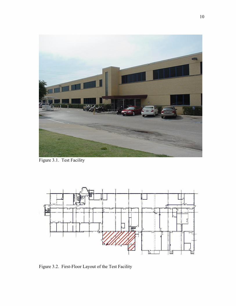
The test facility for this thesis is an office and laboratory building located on the

campus of a defense contractor in Fort Worth, Texas. The building is a two-story

building of brick construction with windows in the perimeter walls. The approximate

window area is 2,888 square feet. The exterior wall area, not including the window area,

is 13,112 square feet. The roof is of modified bitumen construction and covers an area

of 35,553 square feet. The first-floor conditioned floor space is 30,400 square feet,

while the second-floor conditioned floor space is 25,600 square feet. Figure 3.1 shows a

picture of the test facility. Figures 3.2 and 3.3 show the first- and second-floor layouts

of the building, respectively. The crosshatched area is the unconditioned mechanical

room.

10

Figure 3.1. Test Facility

Figure 3.2. First-Floor Layout of the Test Facility

11

Figure 3.3. Second-Floor Layout of the Test Facility

The air conditioning load on the first floor of the building is divided into two

distinct types of areas: office and lab. The load in the office area is attributed to

lighting, computers, people and solar heat gain through the exterior walls and windows.

The lab area is located on the south side of the building in a single story building

addition with approximately 10-ft. high ceilings. The load in the lab area is attributed to

two autoclaves, hydraulic pumping equipment, lighting, computers, people and solar

heat gain through the exterior walls and roof. The second floor of the building is office

space. The load in this area is attributed to lighting, computers, people and solar heat

gain through the exterior walls, windows and roof. The building is occupied between

the hours of 6 a.m. and 6 p.m. during weekdays.

There are seven air-handling units that serve the building. There are four large

multi-zone air-handling units that serve the large office areas and three small single-zone

air-handling units that control the lab areas of the building. These air-handling units

feature blow-through coils with the heating coil located upstream of the cooling coil.

12

There are a number of fan-coil cooling units for individual offices throughout the

building. The chiller plant in this building also provides chilled water for two air-

handling units in the cafeteria of an adjoining building and the fan-coil units for the

office area of an adjacent building.

The chiller plant includes two identical 205-ton helical rotary screw chillers,

Trane model RTHC-B2C2D2 of the type shown in Figure 1.1. The chillers are designed

to produce 43 ºF water with a chilled water return temperature of 53 ºF and a condenser

entering water temperature of 85 ºF. The chiller plant is designed to operate in a

primary-secondary format so that the second chiller will only operate when the chilled

water temperature exceeds 47 ºF.

A 400-ton cooling tower cools the condenser water for both chillers. The cooling

tower fan is powered by a 25-hp motor that is equipped with a variable-speed drive. The

variable-speed drive works to maintain a tower leaving set point, when attainable.

Currently the cooling tower set point is 80 ºF.

Two 20-hp, 600-gpm condenser water pumps circulate water between the cooling

tower and chillers. Each condenser pump is assigned to a particular chiller so that the

pump only operates when its designated chiller operates. Two 25-hp, 410-gpm chilled

water pumps circulate water between the chillers and the air-handling units. Like the

condenser pumps, each chilled water pump is assigned to a particular chiller.

A proprietary automated building software program controls the building. This

control system consists of programmable control modules (PCMs), building control units

(BCUs), and an operator-interface workstation as shown in Figure 3.4.

13

Figure 3.4. Building Automation System Diagram

System measurements are made with devices that are connected to the PCMs.

The PCM is capable of receiving 4-20mA signals. The conversion of this signal to a

digital value takes place in the PCM. Time-keeping and the trending of data takes place

in the BCU. The BCU is only capable of trending data with a resolution of 1 minute

(Stagg 2003). A scheduled data trend is initiated by an operator using the interface

software and then uploaded to the BCU. The data trend will then run continuously and

replace data on a first-in-first-out basis. The BCU is capable of storing 244 samples per

trend. The number of trends that the BCU is capable of recording is limited by the

memory card space available in the BCU. The time is applied to the trend when the data

is requested by the BCU. The time between the trend request and the actual time that the

data is recorded is separated by the scan rate between the BCU and PCM (Stagg 2003).

The BCU periodically scans each PCM for every input in the PCM. The scan rate is

dependent upon the load on the communications system. The BCU will scan a fully-

loaded system every 63 seconds. At the current communications loading, the BCU will

14

scan the PCMs for new data every 18 seconds. This means that a trend that is scheduled

to record every minute will have data that is no older than 18 seconds. For the purpose

of generating a steady-state model, the data acquisition capabilities of this system are

adequate.

In order to obtain the data, the operator must initiate the reporting feature. The

report is stored in the BCU and collects the specified trends into one document, which is

uploaded to the operator-interface workstation. Each upload takes place on a schedule

specified by the operator. The uploaded data is then added to a data file that is stored on

the workstation. The data storage on the workstation is limited by the hard-drive space

available on the workstation.

15

CHILLER MODEL DEVELOPMENT

The First Law equation that describes the refrigerant-side operation of a chiller is

leakcompin

leakevapevap

leakcondcond QPQQQQ0∆E +−−−+== (4.1)

where

condQ = heat transfer in the condenser (refrigerant to water), kW,

leakcondQ = heat transfer from the condenser piping to the environment, kW,

condQ = heat transfer in the evaporator (water to refrigerant) , kW,

leakevapQ = heat transfer from the evaporator piping to the environment, kW,

inP = compressor power input, kW,

leakcompQ = heat transfer from the compressor to the environment, kW.

The Second Law equation is

ernalintrefrevap

leakevapevap

refrcond

leakcondcond S

TQQ

TQQ

0S ∆−⎟⎟⎠

⎞⎜⎜⎝

⎛ +−⎟⎟

⎠

⎞⎜⎜⎝

⎛ +==∆ (4.2)

where

refrcondT = temperature of the condensing refrigerant, R,

refrevapT = temperature of the evaporating refrigerant, R,

16

ernalintS∆ = internal entropy production, kW/R.

Equations (4.1) and (4.2) are combined to give:

⎥⎥⎦

⎤

⎢⎢⎣

⎡⎟⎟⎠

⎞⎜⎜⎝

⎛−++∆++−= refr

condrefrevap

leakevaprefr

cond

leakcomprefr

condernalintrefrcondrefr

evap

refrcondevap

evapin T1

T1Q

TQ

TSTT

TQQP (4.3)

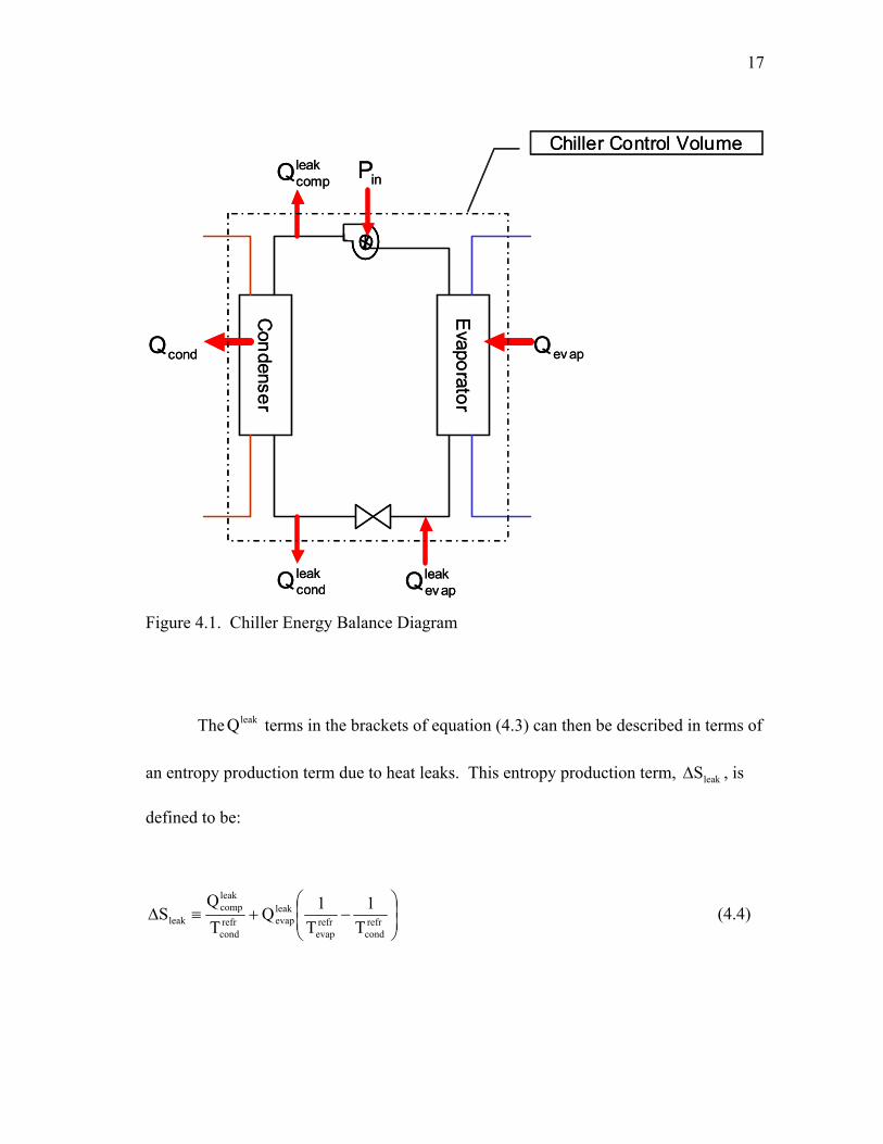
A more detailed derivation of equation (4.3) is shown in Appendix A. A

graphical representation of equation (4.3) is shown in Figure 4.1.

17

Con

denser

Evapo

rator

leakcondQ leak

evapQ

leakcompQ

condQ ev apQ

inPChiller Control Volume

Con

denser

Evapo

rator

leakcondQ leak

evapQ

leakcompQ

condQ ev apQ

inPChiller Control Volume

Figure 4.1. Chiller Energy Balance Diagram

The leakQ terms in the brackets of equation (4.3) can then be described in terms of

an entropy production term due to heat leaks. This entropy production term, leakS∆ , is

defined to be:

⎟⎟⎠

⎞⎜⎜⎝

⎛−+≡∆ refr

condrefrevap

leakevaprefr

cond

leakcomp

leak T1

T1Q

TQ

S (4.4)

18

Inserting equation (4.4) into equation (4.3) gives a simplified thermodynamic

equation that governs chiller performance:

leakrefrcondernalint

refrcondrefr

evap

refrcondevap

evapin STSTT

TQQP ∆+∆++−= (4.5)

evapQ can be expressed in terms of evaporator water inlet and outlet temperatures

and the mass flow of water through the evaporator

( ) ( )out_wevap

in_wevapevappwevap TTcmQ −= & (4.6)

where

wm& = coolant (water) mass flow rate, lb/min,

pc = coolant (water) specific heat, Btu/lb*R,

out_wevapT = evaporator leaving water temperature, R,

in_wevapT = evaporator entering water temperature, R.

Inserting equation (4.6) into equation (4.5) gives

19

( ) ( ) ( ) ( )

totalrefrcond

refrevap

refrcond

out_wevap

in_wevapevappwout_w

evapin_w

evapevappwin

ST

T

TTTcmTTcmP

∆+

−+−−=

&&

(4.7)

where

leakernalinttotal SSS ∆+∆≡∆ . (4.8)

Equation (4.7) is an expression for inP in terms of the chiller coolant

temperatures, refrigerant temperatures, entropy changes, and the mass flow of coolant

through the evaporator. Gordon and Ng claim that totalS∆ is approximately constant for

reciprocating and centrifugal chillers over a wide range of chiller loads (Gordon 2000).

In order to calculate a constant totalS∆ , the power, temperatures and mass flows were

measured and equation (4.7) was solved for each set of values. The totalS∆ terms for

each individual point were averaged to arrive at a constant totalS∆ term. Figure 4.2

shows the comparison of the calculated chiller power versus the measured chiller power

if the assumption of a constant totalS∆ is employed for the screw chiller. The data points

represent the calculated power using equation (4.7) and the constant totalS∆ term. Also

shown is the ideal power line, where measured power equals calculated power. The use

of a constant totalS∆ term yields calculated values that are 4-5% lower than the ideal

power line when the measured power is less than 45 kW. The calculated value varies

20

slightly (± 2%) from the ideal power line over the range of 45-55 kW. Above 55 kW,

the calculated values are 10-12% higher than the ideal power line.

Figure 4.2. Measured Power vs. Calculated Power (Gordon-Ng Model)

For a screw compressor, the change in pressure across the compressor will

impact the entropy change (Gordon and Ng 2000). Since the evaporation and

condensation processes occur at constant pressures and temperatures, there is a strong

correlation between the refrigerant condensation and evaporation temperatures and the

refrigerant condensation and evaporation pressures, respectively. Consequently, there is

a strong correlation between the change in pressure across the compressor and the

difference between the condenser and evaporator refrigerant temperatures. Since the

change in the log-mean temperature difference will change the effectiveness of the heat

21

exchanger, the difference in chilled water entering and leaving temperatures will also

have an effect on totalS∆ . These are the two physical mechanisms that will be considered

in empirically determining an equation to describe totalS∆ . An explanation of entropy

production mechanisms from the Rankine Cycle diagram can be found in Appendix B.

In order to account for these effects, equation (4.8) is solved for totalS∆ and a multiple-

linear regression for totalS∆ as a function of chilled water temperature change and

refrigerant temperature difference is performed. This line is described by:

( ) 05605.0TT00176.0)TT(0001608.0S out_wevap

in_wevap

refrevap

refrcondtotal +−−−−=∆ (4.9)

Combining equations (4.7) and (4.9) yields an expression for inP which allows

the computation of chiller power using the evaporator coolant temperatures, refrigerant

temperatures, and the mass flow of coolant through the evaporator. Figure 4.3 shows the

power comparison using these variables and the temperature-entropy correlation for the

evaporator side. The data points represent the calculated power using equations (4.7)

and (4.9). The ideal power line again represents the series of points that would be

obtained with a perfect chiller model. The use of the temperature-entropy correlation in

equation (4.9) shows a calculated chiller power that are 3-5% higher than the ideal line

for measured power values less than 48 kW. The calculated power is 2-3% lower than

the measured power over the range of 48-55 kW. Above 55 kW, the calculated power is

only 2-3% higher than the ideal line. The shape of the calculated power plot is due to

22

entropy effects that were not considered in this analysis. The effect of boiling and

condensing refrigerant on the heat transfer in the evaporator and condenser is not

considered. Also, the effect of the outside air conditions on the heat leaks to the

environment is not considered. While these considerations would provide a more

accurate chiller model, they only improve the model’s accuracy by 2-3%. The added

complexity is not necessary for the purpose of determining an algorithm to provide

optimal chiller plant control.

Figure 4.3. Measured Power vs. Calculated Power (Derived Evaporator Model)

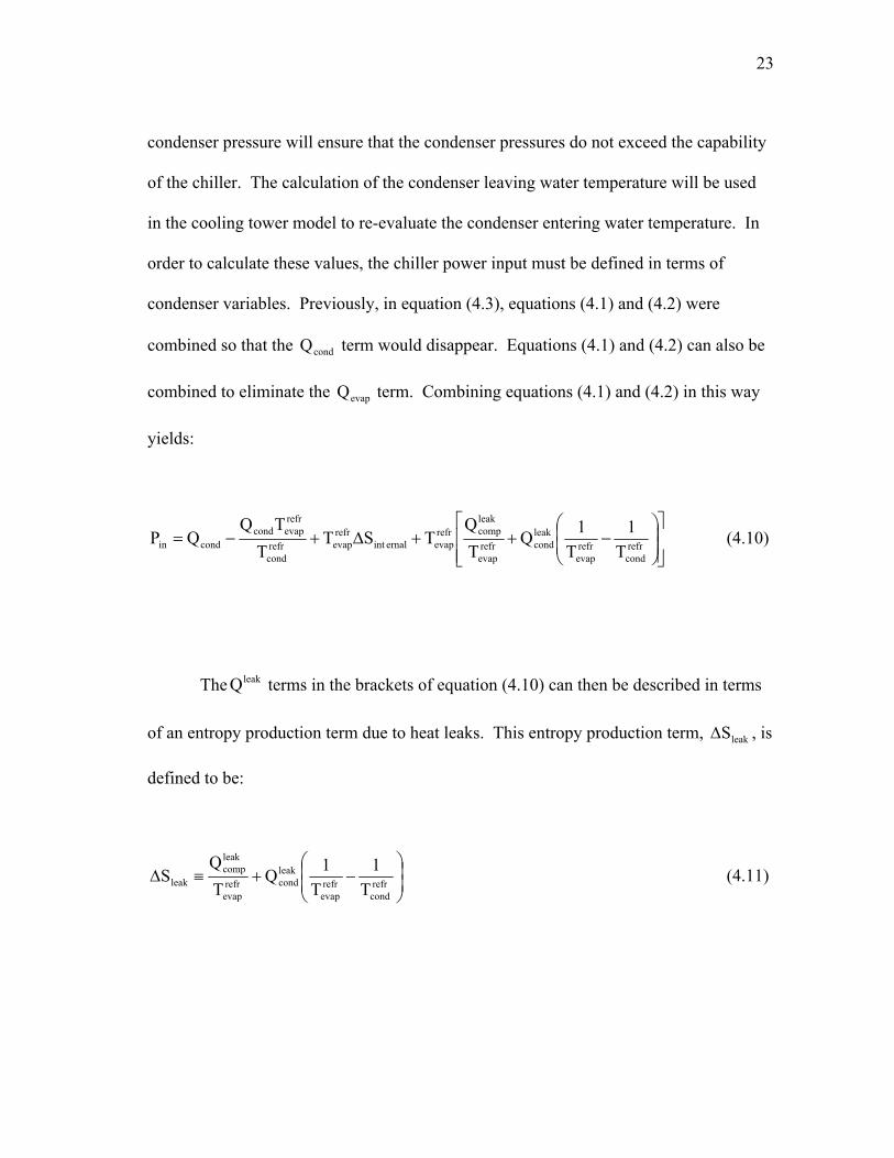
In addition to the compressor power, the condenser pressure and condenser

leaving water temperature are desired variables for calculation. The calculation of the

23

condenser pressure will ensure that the condenser pressures do not exceed the capability

of the chiller. The calculation of the condenser leaving water temperature will be used

in the cooling tower model to re-evaluate the condenser entering water temperature. In

order to calculate these values, the chiller power input must be defined in terms of

condenser variables. Previously, in equation (4.3), equations (4.1) and (4.2) were

combined so that the condQ term would disappear. Equations (4.1) and (4.2) can also be

combined to eliminate the evapQ term. Combining equations (4.1) and (4.2) in this way

yields:

⎥⎥⎦

⎤

⎢⎢⎣

⎡⎟⎟⎠

⎞⎜⎜⎝

⎛−++∆+−= refr

condrefrevap

leakcondrefr

evap

leakcomprefr

evapernalintrefrevaprefr

cond

refrevapcond

condin T1

T1Q

TQ

TSTT

TQQP (4.10)

The leakQ terms in the brackets of equation (4.10) can then be described in terms

of an entropy production term due to heat leaks. This entropy production term, leakS∆ , is

defined to be:

⎟⎟⎠

⎞⎜⎜⎝

⎛−+≡∆ refr

condrefrevap

leakcondrefr

evap

leakcomp

leak T1

T1Q

TQ

S (4.11)

24

Inserting equation (4.11) into equation (4.10) gives:

leakrefrevapernalint

refrevaprefr

cond

condrefrevap

condin STSTT

QTQP ∆+∆+−= (4.12)

condQ can be expressed as

( ) ( )in_wcond

out_wcondcondpwcond TTcmQ −= & (4.13)

where

wm& = coolant (water) mass flow rate through condenser, lb/min,

pc = coolant (water) specific heat, Btu/lb*R,

out_wcondT = condenser leaving water temperature, R,

in_wcondT = condenser entering water temperature, R.

Inserting equation (4.13) into equation (4.12) gives

( ) ( ) ( ) ( )

totalrefrevap

refrcond

in_wcond

out_wcondcondpw

refrevapin_w

condout_w

condcondpwin

ST

TTTcmT

TTcmP

∆+

−−−=

&&

(4.14)

25

where the S∆ terms have again been combined using equation (4.8). As with the

evaporator model, equation (4.15) is used to calculate totalS∆ using the condenser

measurements. A linear regression for totalS∆ as a function of condenser water

temperature change and refrigerant temperature difference is performed. This line is

described by:

( ) 05132.0TT00291.0)TT(0000666.0S in_wcond

out_wcond

refrevap

refrcondtotal +−−−=∆ (4.15)

Combining equations (4.14) and (4.15) allows the computation of chiller power

using the condenser coolant temperatures, refrigerant temperatures, and the mass flow of

coolant through the condenser. Figure 4.4 shows the power comparison using these

variables and the temperature-entropy correlation for the condenser side. The data

points represent the calculated power using equations (4.14) and (4.15). Also shown is

the ideal power line. The condenser model shows a calculated chiller power values that

are within 5% of the values shown on the ideal chiller power line.

26

Figure 4.4. Measured Power vs. Calculated Power (Derived Condenser Model)

One of the desired outputs of this chiller model is the condenser leaving water

temperature. The derived condenser model is used to predict the condenser leaving

water temperature by rearranging the combination of equations (4.14) and (4.15). In

order to calculate the condenser pressure, calculating the change in pressure across the

compressor is necessary. As mentioned before, there is a strong correlation between the

refrigerant condensation and evaporation temperatures and the refrigerant condensation

and evaporation pressures, respectively. The leaving condenser and leaving evaporator

coolant temperatures approach the condenser and evaporator refrigerant temperatures

such that:

out_wevap

out_wcondrefr TTT −≈∆ (4.16)

27

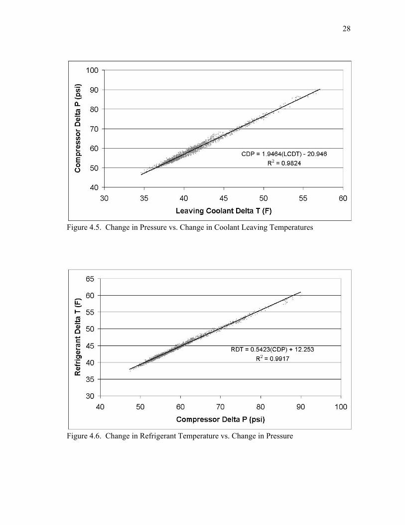
Since refrT∆ is related to out_wevap

out_wcond TT − , there is a relationship between

out_wevap

out_wcond TT − and P∆ . This empirical relationship is shown in Figure 4.5. A linear

regression of the data in Figure 4.5 provides the empirical correlation between the

changes in refrigerant temperature and pressure. This line is described by:

946.20)TT(9464.1P out_wevap

out_wcond −−=∆ (4.17)

The change in pressure is then added to the measured evaporator pressure to

calculate the pressure in the condenser of the chiller. The pressure in the condenser must

be calculated since exceeding the chiller’s maximum condenser pressure will cause a

chiller failure. The empirical correlation between the change in refrigerant temperature

and the change in pressure is shown in Figure 4.6. A linear regression of the data in

Figure 4.6 gives:

253.12)P(5423.0Trefr +∆=∆ (4.18)

28

Figure 4.5. Change in Pressure vs. Change in Coolant Leaving Temperatures

Figure 4.6. Change in Refrigerant Temperature vs. Change in Pressure

29

At this point an iterative solution is employed to calculate the chiller power

consumption, the leaving condenser water temperature and the condenser pressure.

Initial estimate values for the change in pressure across the compressor and the

condenser refrigerant temperature are employed with measured evaporator temperatures

and pressures to calculate the compressor power using equation (4.7). This compressor

power is then used in equation (4.14) to calculate the condenser coolant leaving

temperature. This temperature is used in equation (4.17) to calculate a new value for the

change in pressure across the compressor. Equation (4.18) is employed to calculate the

change in refrigerant temperatures. The condenser refrigerant temperature is given by:

refrrefrevap

refrcond TTT ∆+= (4.19)

Equation (4.19) is used to calculate a new condenser refrigerant temperature.

The new condenser refrigerant temperature and pressure is used in subsequent iterations.

The model typically converges to 0.0025% with five iterations. A flow chart depicting

the order of the chiller model calculations is shown in figure 4.7 on the following page.

30

CalculateEvaporator ModelEntropy ChangeEquation (4.9)

CalculateChiller PowerEquation (4.7)

CalculateCondenser ModelEntropy ChangeEquation (4.16)

CalculateCondenser Water

Leaving TemperatureEquation (4.15)

CalculateCoolant Leaving

Delta TEquation (4.17)

CalculateCompressor Delta P

Equation (4.18)

CalculateRefrigerant Delta T

Equation (4.18)

CalculateCondenserRefrigerant

TemperatureEquation (4.18)

Input Units

Condenser Pump Flow gpmEvaporator Pump Flow gpmChilled Water Entering Temperature RChilled Water Leaving Temperature REvaporator Refrigerant Temperature REvaporator Refrigerant Pressure psiCondenser Water Entering Temperature RCondenser Refrigerant Temperature Estimate R

Output Units

Chiller Power kWCondenser Water Leaving Temperature RCondenser Refrigerant Temperature R

Figure 4.7. Chiller Model Flow Chart

31

COOLING TOWER MODEL DEVELOPMENT

Figure 5.1. Test Facility Cooling Tower

Figure 5.1 shows the installed cross-flow cooling tower to be modeled. The first

step in examining the performance of a cooling tower is to develop the mass balance

equations for each flow stream:

out_ain_aair mm0m &&& −==∆ (5.1)

32

outout_aout_winin_ain_wwater mmmm0m ω−−ω+==∆ &&&&& (5.2)

Setting equation (5.1) equal to equation (5.2) and solving for out_wm& gives:

( )outinin_ain_wout_w mmm ω−ω+= &&& (5.3)

Equation (5.3) is the governing mass balance equation for the cooling tower. The

next step is to develop the energy balance equation for each flow stream:

( )( ) ( )( )out_aout_ain_ain_aair hmhm0E && −==∆ (5.4)

( )( ) ( )( )out_wout_win_win_wwater hmhm0E && −==∆ (5.5)

The total energy balance for the cooling tower is:

airwatertotal EE0E ∆+∆==∆ (5.6)

33

Combining equations (5.3), (5.4), (5.5) and (5.6) gives:

( )( ) ( )( )( )[ ]( )out_woutinin_ain_w

in_win_wout_ain_ain_atotal

hmm

hmhhm0E

ω−ω+−

+−==∆

&&

&&(5.7)

The enthalpy of the water can be expressed as:

( )ww_pw Tch = (5.8)

Combining equations (5.7) and (5.8) and simplifying yields

( )( ) ( )( )( )out_win_ww_pin_win_aout_ain_a TTcmYhhm −=−− && (5.9)

where

( )( )( )( )out_ww_pinoutin_a TcmY ω−ω= & .

For this cooling tower model, the assumptions made by Merkel in 1925 will be

employed. These assumptions are:

1. Mass of water evaporated from the water stream is negligible.

2. Lewis number = 1.

Because the mass flow of water evaporated is on the order of 1% of the total

mass flow entering the tower, the first Merkel assumption seems valid. Utilizing this

34

assumption, the Y term in equation (5.9) is reduced to zero. The assumption of a Lewis

number equal to one means that there is a coefficient that utilizes the enthalpy difference

as its driving force to account for both mass and sensible heat transfer (ASHRAE

Handbook 1992). This allows equation (5.9) to be equated to

( )( ) ( )( )( ) dV)hh(KTTcmhhm avgairmout_win_ww_pin_win_aout_ain_a −′=−=− && (5.10)

where

h′ = enthalpy of air at the bulk water temperature, Btu/lb,

airh = enthalpy of air at the dry bulb temperature, Btu/lb,

mK = overall heat and mass transfer coefficient,

dV = change in tower volume.

35

If a unit volume is considered, equation (5.10) becomes:

( )( ) ( )( )( ) dA)hh(KTTcmhhm avgairmout_win_ww_pin_win_aout_ain_a −′=−=− && (5.11)

The number of transfer units (NTU) is a term that is used to describe the physical

size of the heat transfer area in a cooling tower. NTU is defined as:

in_a

m

mAK

NTU&

= (5.12)

Inserting equation (5.12) into equation (5.11) and simplifying gives:

( ) ( )( ) avgairout_win_ww_pin_a

in_win_aout_a )hh(NTUTTc

mm

hh −′=−⎟⎟⎠

⎞⎜⎜⎝

⎛=−

&&

(5.13)

Equation (5.13) is the governing equation for cooling tower performance. The

value for NTU must be empirically determined. The value for NTU depends on the

number of nodes used for analyzing the tower. A 10x10-node configuration was utilized

for this model. The calculations begin in the upper left hand corner and proceed down

and to the right. The enthalpy of the air changes from right to left while the temperature

36

of the water changes from top to bottom. Figure 5.2 shows a diagram of the cooling

tower that shows how the air and water flows across the nodes.

Tower Leaving Water

(to Chiller)

Tower Entering Water

(from Chiller)

Tower Airflow

������������������������������������������������������������������

������������������������������������������������������������������

���������������������������������������������������������������������������������������������������������������������������������������������������������������������������������������������������������������������������������������������������������������������������������������������������������������������������������������������������������������������������������������������������������������������������������������

Node 1,1

Tower Leaving Water

(to Chiller)

Tower Entering Water

(from Chiller)

Tower Airflow

������������������������������������������������������������������

������������������������������������������������������������������

���������������������������������������������������������������������������������������������������������������������������������������������������������������������������������������������������������������������������������������������������������������������������������������������������������������������������������������������������������������������������������������������������������������������������������������

Node 1,1

Tower Airflow

������������������������������������������������������������������

������������������������������������������������������������������

���������������������������������������������������������������������������������������������������������������������������������������������������������������������������������������������������������������������������������������������������������������������������������������������������������������������������������������������������������������������������������������������������������������������������������������

Node 1,1

Figure 5.2. Cooling Tower Diagram

The entering water temperature for each node is equal to the leaving water

temperature from the node above. Likewise, the entering air enthalpy is equal to the

leaving air enthalpy from the node to the left. The entering air enthalpy and water

temperature are used to estimate the change in air enthalpy and water temperature for the

entering conditions. These values are then used to estimate the leaving air enthalpy and

37

water temperature. The leaving air enthalpy and water temperature are used to estimate

the change in air enthalpy and water temperature for the leaving conditions. The

changes in air enthalpy and water temperature for the entering and leaving conditions are

averaged to provide the change across the node. Table 5.1 shows the set of values that

are calculated in one node of the cooling tower model.

Table 5.1. Cooling Tower Node ValuesNode 1,1

Name Abbrev. Value UnitsTower Entering Water Temperature TWET 95 °FEnthalpy of Entering Air ha_in 42.63 Btu/lbSaturation pressure of water @ TWET Pw_ws 0.825 psiSaturation humidity ratio @ TWET Ws_wb 0.037 Enthalpy of air @ TWET h'_in 63.58 Btu/lbEnthalpy Difference at inlet conditions (h'-ha)in 20.95 Btu/lbWater to Air Ratio L/G 1.055 Temperature Change based on inlet conditions dTw inlet 3.06 °FEnthalpy Change based on inlet conditions dHah 3.22 Btu/lbTower Leaving Water Temperature TWLT 91.94 °FEnthalpy of Leaving Air ha_out 45.85 Btu/lbSaturation pressure of water @ TWLT Pw_ws 0.750 psiSaturation humidity ratio @ TWLT Ws_wb 0.033 Enthalpy of leaving air @ TWLT h'_out 58.92 Btu/lbEnthalpy Difference at outlet conditions (h'-ha)out 13.08 Btu/lbAverage Enthalpy Difference (h'-ha)av 17.01 Btu/lbChange in Water Temperature dTw 2.48 °FChange in Air Enthalpy dHah 2.62 Btu/lb

The value for NTU is determined by setting the boundary conditions to those

established by the tower manufacturer and adjusting the value for NTU until the

appropriate leaving water temperature is obtained. The NTU for the tower in this

application is 14.60, or 0.1460 NTU/node. Once the NTU for the tower is determined,

38

the model can be used to predict the tower leaving water temperature for a variety of

entering water temperatures and weather conditions. Figure 5.3 shows a comparison

between the measured and calculated condenser water entering temperatures, i.e. the

tower leaving water temperatures. These values were measured at the chiller and the

temperature rise due to the cooling tower pump was neglected. The ideal CWET line

represents the set of points that would be generated by a “perfect” tower model.

Figure 5.3. Condenser Water Entering Temperature Comparison

Figure 5.3 shows that the cooling tower model can calculate the condenser water

entering temperature within ± 4 ºF. During the process of coupling the chiller and

cooling tower models, offsets will be employed to improve the accuracy of the model.

39

COUPLING THE MODELS

In order to generate a complete chiller-tower model, the chiller and cooling tower

models developed previously must be coupled together. The inputs and outputs of this

model are shown in Table 6.1.

Table 6.1. Inputs and Outputs of Chiller-Tower ModelInput Units Output Units

Cooling Tower Airflow cfm Condenser Refrigerant Temperature °F

Condenser Pump Flow gpm Condenser Refrigerant Pressure Psi

Evaporator Pump Flow gpm Condenser Water Entering Temperature °F

Ambient Dry-bulb Temperature °F Condenser Water Leaving Temperature °F

Ambient Wet-bulb Temperature °F Chiller Power kW

Chilled Water Entering Temperature °F Cooling Tower Fan Power kW

Chilled Water Leaving Temperature °F Condenser Pump Power kW

Evaporator Refrigerant Temperature °F

Evaporator Refrigerant Pressure psi

The chiller model calculates the condenser refrigerant temperature, condenser

refrigerant pressure, condenser leaving water temperature, and chiller power. The

cooling tower model calculates the condenser entering water temperature. The cooling

tower fan power and condenser pump power are calculated from the pump flow and

airflow inputs using the fan laws. An iterative method was employed, beginning with

the chiller model, measured data for the inputs, and initial estimate values for the cooling

tower leaving water temperature, condenser refrigerant temperature, and change in

pressure across the compressor. The condenser leaving water temperature is then used

40

for the cooling tower entering water temperature. The leaving water temperature from

the cooling tower model is used for the entering condenser coolant temperature for a

subsequent chiller iteration. In this way, the cooling tower models and chiller model are

coupled to create a chiller-tower model that will investigate the concomitant

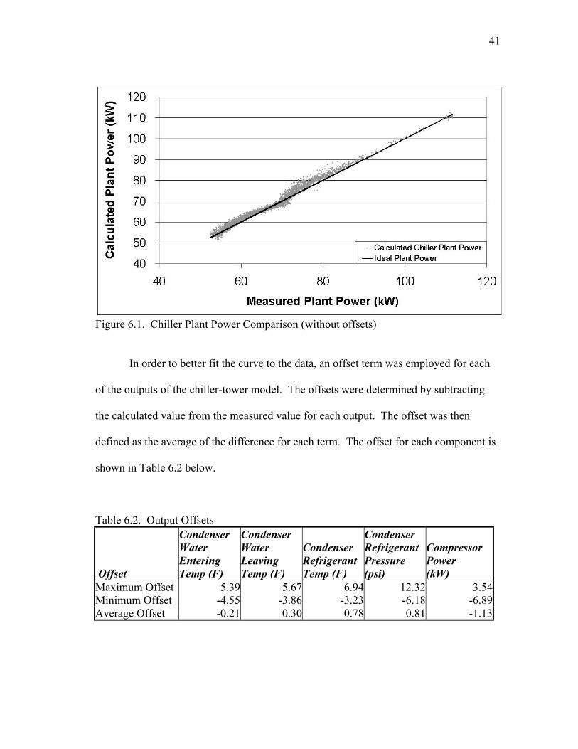
performance of both systems. Figure 6.1 shows a comparison of the calculated chiller

plant power with the measured plant power. Also shown on this graph is the ideal plant

power line. The data points were calculated using inputs measured every fifteen minutes

over the period from 5/13/03 to 6/30/03. There were 4,101 total input points that were

used in this calculation. The chiller contributes 75% of the energy consumed by the

chiller plant, so the chiller plant power comparison is closely related in shape to the

chiller model curve shown in Figure 4.3. Figure 6.1 shows that the model without the

offsets can predict the power consumption of the chiller plant within ± 5% over the

entire range of the measured power.

41

Figure 6.1. Chiller Plant Power Comparison (without offsets)

In order to better fit the curve to the data, an offset term was employed for each

of the outputs of the chiller-tower model. The offsets were determined by subtracting

the calculated value from the measured value for each output. The offset was then

defined as the average of the difference for each term. The offset for each component is

shown in Table 6.2 below.

Table 6.2. Output Offsets

Offset

CondenserWaterEnteringTemp (F)

CondenserWaterLeavingTemp (F)

CondenserRefrigerantTemp (F)

CondenserRefrigerantPressure(psi)

CompressorPower(kW)

Maximum Offset 5.39 5.67 6.94 12.32 3.54Minimum Offset -4.55 -3.86 -3.23 -6.18 -6.89Average Offset -0.21 0.30 0.78 0.81 -1.13

42

Utilizing the average offsets for each component, the chiller-tower model is run

again for the same data set. The results of the model, including the offsets, are shown in

Figure 6.2. The model with the offsets included is capable of calculating the plant power

within ± 3% of the ideal plant power line. This chart shows that the coupling the chiller

and cooling tower models produces a reasonably accurate chiller-tower model. This

model will be used with an optimization strategy to minimize the energy consumption of

the chiller plant.

Figure 6.2. Chiller Plant Power Comparison (with offsets)

Figures 6.3 through 6.7 show the error associated with each calculated output.

Taking the difference between the calculated value and the measured value generated

these errors. The spread between the maximum and minimum errors was divided into

43

one hundred bins. The number of error points in each bin was summed and then plotted

versus the bin value to generate a bell curve to describe the error associated with each

measurement. Table 6.3 shows the standard deviation associated with each bell curve.

Figure 6.3. Condenser Water Entering Temperature Error

44

Figure 6.4. Condenser Water Leaving Temperature Error

Figure 6.5. Condenser Refrigerant Temperature Error

45

Figure 6.6. Condenser Refrigerant Pressure Error

Figure 6.7. Compressor Power Error

46

Table 6.3. Standard Deviations for Each Component

Component Standard Deviation UnitsCondenser Water Entering Temperature 1.04 FCondenser Water Leaving Temperature 1.01 FCondenser Refrigerant Temperature 1.04 FCondenser Refrigerant Pressure 2.01 psiCompressor Power 1.38 kW

Since the standard deviation of the error of each calculated value is within the

error bands of the device used to measure these values, the model is capable of

accurately predicting the performance of the system.

47

OPTIMIZATION STRATEGY AND ANALYSIS

In order to optimize the chiller plant, the chiller-tower model is utilized to

determine the optimal cooling tower fan speed and condenser water pump flow. The

cooling tower fan speed and condenser pump flow are the only two inputs that are

directly related to the optimization of the chiller plant from the condenser side. The

remaining chiller-tower model inputs pertain either to weather conditions or to building

load and are independent with respect to the varying of condenser water flow rate.

The sum of the chiller power, cooling tower fan power, and condenser water

pumping power is minimized using an iterative method with the cooling tower fan speed

and condenser pump flow as the variables. This is accomplished by using a

mathematical equation solver that performs the iterations using a quasi-Newtonian

method to achieve the minimum value. The cooling tower fan speed is first solved for

the minimum value, then the condenser pump flow. A second iteration of the cooling

tower fan speed and condenser pump flow is performed to ensure that the true minimum

value is obtained. Figure 7.1 shows a comparison of the current simulated chiller plant

power to the optimized chiller plant power over the period of time between 5/17/03 and

5/27/03. Also shown is the power difference, i.e. power savings, realized by the

installation of the optimized system.

48

Figure 7.1. Optimized Chiller Plant Power Comparison

The optimizer returns the ideal values for the cooling tower fan speed and

condenser water pump flow as well as the other outputs supplied by the simulator. In

order to optimize the real system, a correlation between the optimized cooling tower fan

speed and the condenser water pump flow must be implemented. One of the most

popular methods for controlling cooling tower fan variable-frequency drives (VFD)

involves a cooling tower leaving water temperature setpoint. This setpoint, typically an

operator-specified value, is subtracted from the measured cooling tower leaving water

temperature to provide a differential for controlling the cooling tower VFD. The control

loop for a typical cooling tower fan VFD is shown in Figure 7.2.

49

Cooling Tower Fan VFD

Cooling Tower System

CT Setpoint Temp. (F)

Cooling Tower

Leaving Water Temp (F)

+ -

Cooling Tower Fan Speed (% Full Speed)

Cooling Tower Fan VFD

Cooling Tower System

CT Setpoint Temp. (F)

Cooling Tower

Leaving Water Temp (F)

+ -+ -

Cooling Tower Fan Speed (% Full Speed)

Figure 7.2. Typical Cooling Tower Fan VFD Control Loop

Since this type of VFD control is currently installed on the system and the

building owner does not want to change the operation of a working device, the setpoint

becomes the only variable that can be adjusted with regard to the cooling tower fan

controls. In order to exercise the abilities of the VFD, the cooling tower setpoint must

be above the wet-bulb temperature. If the cooling tower setpoint is below the wet-bulb

temperature, the cooling tower fan will run full speed in an effort to reach a tower

leaving water temperature that is thermodynamically impossible. It has been suggested

that setting the cooling tower setpoint to a constant value above the wet-bulb

temperature will provide “near optimal” tower operation (Burger 1993, Hartman 2001).

The output data provided by the chiller-tower model optimization shows the ideal

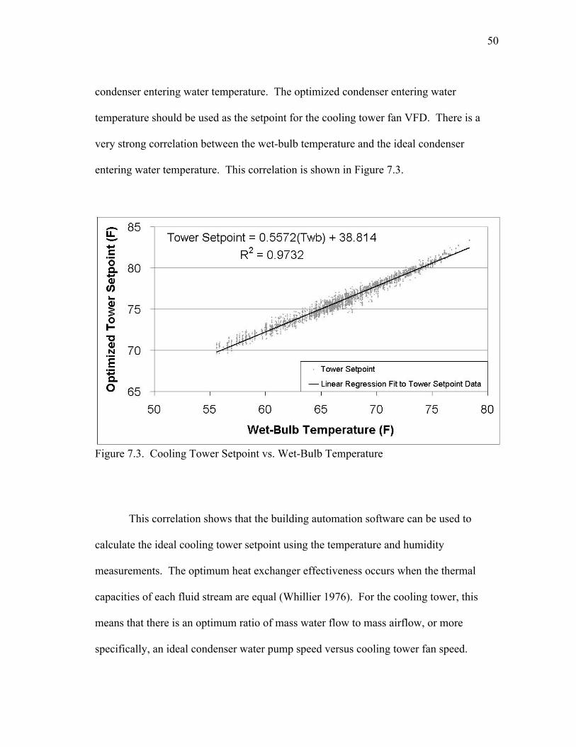
50

condenser entering water temperature. The optimized condenser entering water

temperature should be used as the setpoint for the cooling tower fan VFD. There is a

very strong correlation between the wet-bulb temperature and the ideal condenser

entering water temperature. This correlation is shown in Figure 7.3.

Figure 7.3. Cooling Tower Setpoint vs. Wet-Bulb Temperature

This correlation shows that the building automation software can be used to

calculate the ideal cooling tower setpoint using the temperature and humidity

measurements. The optimum heat exchanger effectiveness occurs when the thermal

capacities of each fluid stream are equal (Whillier 1976). For the cooling tower, this

means that there is an optimum ratio of mass water flow to mass airflow, or more

specifically, an ideal condenser water pump speed versus cooling tower fan speed.

51

Indeed, comparing the optimal cooling tower fan speed to the ideal condenser water

pump speed shows a strong correlation between these two values. This comparison is

shown in Figure 7.4. The R-square value for the linear regression fit is 0.88. This is

primarily due to the effect that air density has on the relationship between cooling tower

fan speed and cooling tower mass airflow. An R-square value of 0.98 can be obtained

by adding a wet-bulb correction factor. However, the added complexity results in a

three percent change in the energy savings, which is not significant enough to warrant

the added complexity.

Figure 7.4. Condenser Water Pump Speed vs. Cooling Tower Fan Speed

Utilizing the correlations developed in Figures 7.3 and 7.4 will result in a “quasi-

optimal” operation of the chiller plant. In order to define the losses incurred by using the

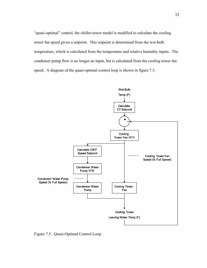
52

“quasi-optimal” control, the chiller-tower model is modified to calculate the cooling

tower fan speed given a setpoint. This setpoint is determined from the wet-bulb

temperature, which is calculated from the temperature and relative humidity inputs. The

condenser pump flow is no longer an input, but is calculated from the cooling tower fan

speed. A diagram of the quasi-optimal control loop is shown in figure 7.5.

Cooling Tower Fan VFD

Condenser WaterPump VFD

Cooling Tower Fan

Calculate CWP Speed Setpoint

Calculate CT Setpoint

Wet-Bulb

Temp (F)

Cooling Tower

Leaving Water Temp (F)

+ -

Cooling Tower Fan Speed (% Full Speed)

Condenser Water Pump Speed (% Full Speed)

Condenser WaterPump

Cooling Tower Fan VFD

Condenser WaterPump VFD

Cooling Tower Fan

Calculate CWP Speed Setpoint

Calculate CT Setpoint

Wet-Bulb

Temp (F)

Cooling Tower

Leaving Water Temp (F)

+ -+ -

Cooling Tower Fan Speed (% Full Speed)

Condenser Water Pump Speed (% Full Speed)

Condenser WaterPump

Figure 7.5. Quasi-Optimal Control Loop

53

The results of the “quasi-optimal” operation versus the optimal operation are

shown in Figure 7.6. The “quasi-optimal” operation proposed yields a power

consumption that is approximately 1% higher than a truly optimal operation.

Figure 7.6. Quasi-Optimal Chiller Plant Power Comparison

Implementing new method for controlling the cooling tower setpoint and the

condenser water pump flow shows an 18% average reduction in chiller plant power.

54

CONCLUSIONS

The development of the combined chiller-tower model allows the opportunity to

explore what will occur in a real system without endangering the equipment in that

system. In this case, the chiller-tower model was used to predict the performance of the

chiller plant under the conditions of variable condenser water flow rate and variable

tower airflow. The model is able to estimate the energy consumption with enough

accuracy to ensure that energy savings over 5% of the current total will indeed occur.

However, this model will need some refinement before it can be used to definitively

predict energy savings.

One task that was not undertaken was the validation of the optimized model.

This is due to the lack of an existing VFD on the condenser water pumps. The primary

goal of this thesis was to develop a thermodynamic chiller-tower model that could be

used to predict the energy savings allowed by a retrofit. This was to provide an

economic justification for the retrofit without actually having to implement the retrofit.

In to truly validate the model’s optimization capability, the retrofit must be made to an

existing system and post-retrofit measurements taken.

Another particular weakness of this combined chiller-tower model is the cooling

tower model that was employed. This model is very good for systems in which the

cooling tower is matched to the chiller. In this situation the cooling tower capacity was

twice the capacity of the one chiller that normally operates. This resulted in tower water

flow rates that were one-half that for which the cooling tower was designed. Further

55

reducing the tower water flow rate affects the tower nozzles’ ability to disperse the water

evenly over the tower. This can result in a lower effective evaporation surface area,

which would effectively reduce the tower NTU. There was no simple correlation found

between the tower NTU and any of the independent variables. Because many chiller

plants are designed with one large cooling tower, the ability to model the effects of a

cooling tower at less than 50% tower airflow and water flow rates is very valuable.

A third area that deserves some attention is the area of controls. For simplicity’s

sake, the chiller plant in this situation is controlled using coupled single-input-single-

output loops. The truly optimal relationship between the condenser pump flow and

cooling tower fan speed may be realized by utilizing a multiple-input-multiple-output

control sequence.

The combined chiller-tower model shows that there are two simple correlations

that can be used to optimize a chiller plant. The first is the correlation between cooling

tower setpoint and the wet-bulb temperature. The second is the correlation between the

cooling tower fan speed and the condenser water pump speed. These two correlations

can be used to provide “quasi-optimal” operation of a chiller plant.

56

REFERENCES

Aoyama, M. and M. Izushi. 1990. Continuous capacity control type screw chiller unit.Hitachi Review 39(3):149-154.

ASHRAE. 1992. ASHRAE Handbook – HVAC Systems and Equipment. Atlanta:American Society of Heating, Refrigerating and Air-Conditioning Engineers, Inc.

Austin, S.B. 1991. Optimum chiller loading. ASHRAE Journal 33(7):40-43.

Braun, J.E. 1988. Methodologies for the design and control of central cooling plants.Ph.D. dissertation, University of Wisconsin-Madison.

Braun, J.E. and G.T. Diderrich. 1990. Near-optimal control of cooling towers forchilled-water systems. ASHRAE Transactions 96(2):806-813.

Burger, R. 1993. Wet bulb temperature: The misunderstood element. HPACEngineering 65(9):29-34.

Cascia, M.A. 2000. Implementation of a near-optimal global set point control methodin a DDC controller. ASHRAE Transactions 106(1):249-263.

Chua, H.T., K.C. Ng and J.M. Gordon. 1996. Experimental study of the fundamentalproperties of reciprocating chillers and their relation to thermodynamic modelingand chiller design. International Journal of Heat and Mass Transfer39(11):2195-2204.

Flake, B.A., J.W. Mitchell and W.A. Beckman. 1997. Parameter estimation formultiresponse nonlinear chilled-water plant models. ASHRAE Transactions103(1):470-485.

Gibson, G.L. 1997. A supervisory controller for optimization of building centralcooling systems. ASHRAE Transactions 103(1):486-493.

Gordon, J.M. and K.C. Ng. 1995. Predictive and diagnostic aspects of a universalthermodynamic model for chillers. International Journal of Heat and MassTransfer 38(5):807-818.

Gordon, J.M. and K.C. Ng. 2000. Cool Thermodynamics. London: CambridgeInternational Science Publishing. 2000.

57

Gordon, J.M., K.C. Ng, H.T. Chua. 1995. Centrifugal chillers: Thermodynamicmodeling and a diagnostic case study. International Journal of Refrigeration18(4):253-257.

Gordon, J.M., K.C. Ng, H.T. Chua and C.K. Lim. 2000. How varying condenser coolantflow rate affects chiller performance: Thermodynamic modeling andexperimental confirmation. Applied Thermal Engineering 20(13):1149-1159.

Hartman, T. 2001. All-variable speed centrifugal chiller plants. ASHRAE Journal43(9):43-51.

He, X., S. Liu, H.H. Asada and H. Itoh. 1998. Multivariable control of vaporcompression systems. HVAC&R Research 4(3):205-230.

Henze, G.P.,R.H. Dodier and M. Krarti. 1997. Development of a predictive optimalcontroller for thermal energy storage systems. HVAC&R Research 3(3):233-264.

Kirsner, W. 1996. 3 GPM/Ton condenser water flow rate: Does it waste energy?ASHRAE Journal 38(2):63-69.

Lau, A.S., W.A. Beckman and J.W. Mitchell. 1985. Development of computerizedcontrol strategies for a large chilled water plant. ASHRAE Transactions91(1B):766-780.

Ng, K.C., H.T. Chua, W. Ong, S.S. Lee and J.M. Gordon. 1997. Diagnostics andoptimization of reciprocating chillers: Theory and experiment. Applied ThermalEngineering 17(3):263-276.

Rolfsman, L. and S. Wihlborg. 1996. Screw compressor capacity regulated by steplessspeed control. ABB Review (4):18-23.

Schwedler, M. 1998. Take it to the limit…Or just halfway? ASHRAE Journal40(7):32-39.

Schwedler, M. and B. Bradley. 2001. Uncover the hidden assets in your condenserwater system. HPAC Engineering 73(11):68,75.

Stagg, J. Trane – Tracer Summit Applications Technician. Fort Worth, Texas. Personalcommunication concerning the communications and storage capabilities of theTrane Tracer BCUs.

Stout, M.R., Jr. and J.W Leach. 2002. Cooling tower fan control for energy efficiency.Energy Engineering 99(1):7-31.

58

Van Dijk, H. 1985. Investment in cooling tower control pays big dividends. ProcessEngineering 66(10):57, 59-60.

Weber, E.D. 1988. Modeling and generalized optimization of commercial buildingchiller/cooling tower systems. Master’s thesis, Georgia Institute of Technology.

Whillier, A. 1976. A fresh look at the calculation of performance of cooling towers.ASHRAE Transactions 82(1):269-282.

59

APPENDIX A

COMPLETE CHILLER DERIVATION

The First Law equation that describes the refrigerant-side operation of a chiller is

leakcompin

leakevapevap

leakcondcond QPQQQQ0E +−−−+==∆ (A.1)

where

condQ = heat transfer in the condenser, kW,

leakcondQ = heat transfer from the condenser piping to the environment, kW,

evapQ = heat transfer in the evaporator, kW,

leakevapQ = heat transfer from the evaporator piping to the environment, kW,

inP = compressor power input, kW,

leakcompQ = heat transfer from the compressor to the environment, kW.

The Second Law equation is

ernalintrefrevap

leakevapevap

refrcond

leakcondcond S

TQQ

TQQ

0S ∆−⎟⎟⎠

⎞⎜⎜⎝

⎛ +−⎟⎟

⎠

⎞⎜⎜⎝

⎛ +==∆ (A.2)

60

where

refrcondT = temperature of the condensing refrigerant, R,

refrevapT = temperature of the evaporating refrigerant, R,

ernalintS∆ = internal entropy production, kW/R.

Solving equation (A.2) for condQ gives the following:

( ) leakcondenserernalint

refrcond

leakevapevaprefr

evap

refrcond

cond QSTQQTTQ −∆++= (A.3)

Inserting condQ obtained in equation (A.3) into equation (A.1) yields:

( )leakcompin

leakevapevap

leakcond

leakcondernalint

refrcond

leakevapevaprefr

evap

refrcond

QP

QQQQSTQQTT0

+−

−−+−∆++=(A.4)

The leakcondQ term cancels out and equation (A.4) is solved for inP to obtain:

( ) leakcomp

leakevapevapernalint

refrcond

leakevapevaprefr

evap

refrcond

in QQQSTQQTTP +−−∆++= (A.5)

61

By combining the evapQ and leakevapQ terms, equation (A.5) becomes:

ernalintrefrcond

leakevaprefr

evap

refrcondleak

evaprefrevap

refrcond

evapin STQ1TT

Q1TT

QP ∆++⎟⎟⎠

⎞⎜⎜⎝

⎛−+⎟

⎟⎠

⎞⎜⎜⎝

⎛−= (A.6)

Dividing both sides of equation (A.6) by evapQ gives:

evap

ernalintrefrcond

evap

leakcomp

refrevap

refrcond

evap

leakevap

refrevap

refrcond

evap

in

QST

QQ

1TT

QQ

TT

1QP ∆

++⎟⎟⎠

⎞⎜⎜⎝

⎛−++−= (A.7)

The coefficient of performance (COP) of a chiller is defined as:

in

evap

PQ

COP = (A.8)

62

Inserting the reciprocal of equation (A.8) into equation (A.7) and moving

the leakQ terms to the end of the equation gives:

evap

leakevap

refrevap

refrcond

evap

leakevap

evap

ernalintrefrcond

refrevap

refrcond

QQ

1TT

QQ

QST

TT

1COP

1+⎟

⎟⎠

⎞⎜⎜⎝

⎛−+

∆++−= (A.9)

The leakQ terms in equation (A.9) can be further combined to yield:

⎥⎥⎦

⎤

⎢⎢⎣

⎡+⎟

⎟⎠

⎞⎜⎜⎝

⎛−+

∆++−= leak

comprefrevap

refrcondleak

evapevapevap

ernalintrefrcond

refrevap

refrcond Q1

TT

QQ

1Q

STTT

1COP

1 (A.10)

The leakQ terms in equation (A.10) are multiplied by unity in the form of cond

cond

TT

to obtain:

⎥⎥⎦

⎤

⎢⎢⎣

⎡+⎟

⎟⎠

⎞⎜⎜⎝

⎛−+

∆++−= refr

cond

leakcomp

refrevap

refrcond

refrcond

leakevap

evap

refrcond

evap

ernalintrefrcond

refrevap

refrcond

TQ

1TT

TQ

QT

QST

TT

1COP

1 (A.11)

63

The terms inside the brackets of equation (A.11) are rearranged to give:

⎥⎥⎦

⎤

⎢⎢⎣

⎡⎟⎟⎠

⎞⎜⎜⎝

⎛−++

∆++−= refr

condrefrevap

leakevaprefr

cond

leakcomp

evap

refrcond

evap

ernalintrefrcond

refrevap

refrcond

T1

T1Q

TQ

QT

QST

TT1

COP1 (A.12)

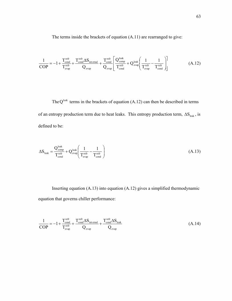
The leakQ terms in the brackets of equation (A.12) can then be described in terms

of an entropy production term due to heat leaks. This entropy production term, leakS∆ , is

defined to be:

⎟⎟⎠

⎞⎜⎜⎝

⎛−+=∆ refr

condrefrevap

leakevaprefr

cond

leakcomp

leak T1

T1Q

TQ

S (A.13)

Inserting equation (A.13) into equation (A.12) gives a simplified thermodynamic

equation that governs chiller performance:

evap

leakrefrcond

evap

ernalintrefrcond

refrevap

refrcond

QST

QST

TT1

COP1 ∆

+∆

++−= (A.14)

64

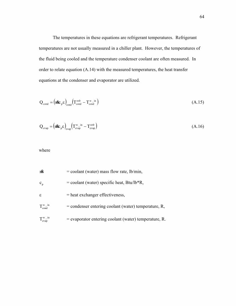
The temperatures in these equations are refrigerant temperatures. Refrigerant

temperatures are not usually measured in a chiller plant. However, the temperatures of

the fluid being cooled and the temperature condenser coolant are often measured. In

order to relate equation (A.14) with the measured temperatures, the heat transfer

equations at the condenser and evaporator are utilized.

( ) ( )in_wcond

refrcondcondpcond TTcmQ −ε= & (A.15)

( ) ( )refrevap

in_wevapevappevap TTcmQ −ε= & (A.16)

where

m& = coolant (water) mass flow rate, lb/min,

pc = coolant (water) specific heat, Btu/lb*R,

ε = heat exchanger effectiveness,

in_wcondT = condenser entering coolant (water) temperature, R,

in_wevapT = evaporator entering coolant (water) temperature, R.

65

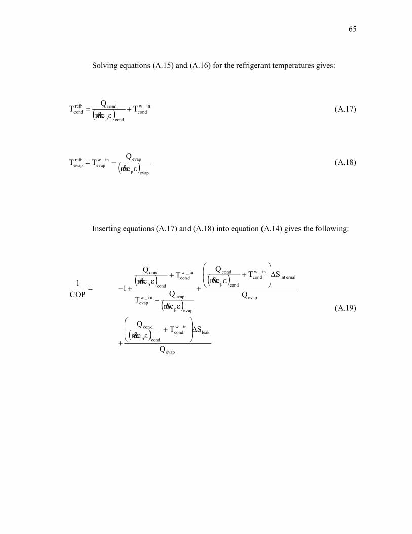
Solving equations (A.15) and (A.16) for the refrigerant temperatures gives:

( )in_w

condcondp

condrefrcond T

cmQT +ε

=&

(A.17)

( )evapp

evapin_wevap

refrevap cm

QTT

ε−=

&(A.18)

Inserting equations (A.17) and (A.18) into equation (A.14) gives the following:

( )

( )

( )

( )evap

leakin_w

condcondp

cond

evap

ernalintin_w

condcondp

cond

evapp

evapin_wevap

in_wcond

condp

cond

Q

STcmQ

Q

STcmQ

cmQ

T

TcmQ

1COP

1

∆⎟⎟⎠

⎞⎜⎜⎝

⎛+

ε+

∆⎟⎟⎠

⎞⎜⎜⎝

⎛+

ε+

ε−

+ε

+−=

&

&

&

&

(A.19)

66

The condQ term reappears in equation (A.19). Gordon and Chua insert equation

(A.3) into equation (A.19) to eliminate the condQ term. However, this results in condQ

terms of higher order which are then neglected. If the condenser coolant entering and

leaving temperatures are known, condQ can be expressed as follows

( ) ( )in_wcond

out_wcondcondpcond TTcmQ −= & (A.20)

where

m& = coolant (water) mass flow rate, lb/min,

pc = coolant (water) specific heat, Btu/lb*R,

out_wcondT = condenser leaving water temperature, R,

in_wcondT = condenser entering water temperature, R.

67

In the same way, evapQ can be expressed as

( ) ( )out_wevap

in_wevapevappevap TTcmQ −= & (A.21)

where

m& = coolant (water) mass flow rate, lb/min,

pc = coolant (water) specific heat, Btu/lb*R,

out_wevapT = evaporator leaving water temperature, R,

in_wevapT = evaporator entering water temperature, R .

Inserting equations (A.20) and (A.21) into equation (A.19) gives:

( ) ( )( )( ) ( )

( )( ) ( )

( )( ) ( )

( ) ( )( )( ) ( )out_w

evapin_w

evapevapp

leakin_w

condcondp

in_wcond

out_wcondcondp

out_wevap

in_wevapevapp

ernalintin_w

condcondp

in_wcond

out_wcondcondp

evapp

out_wevap

in_wevapevappin_w

evap

in_wcond

condp

in_wcond

out_wcondcondp

TTcm

STcm

TTcm

TTcm

STcm

TTcm

cm

TTcmT

Tcm

TTcm

1COP

1

−

∆⎟⎟⎠

⎞⎜⎜⎝

⎛+

ε

−

+

−

∆⎟⎟⎠

⎞⎜⎜⎝

⎛+

ε

−

+

ε

−−

+ε

−

+−=

&

&&

&

&&

&

&

&&

(A.22)

68

Simplifying the equation (A.22) by dividing out the common mass flow rates and

specific heats yields:

( )

( )

( ) ( )

( ) ( )out_wevap

in_wevapevapp

leakin_w

condcond

in_wcond

out_wcond

out_wevap

in_wevapevapp

ernalintin_w

condcond

in_wcond

out_wcond

evap

out_wevap

in_wevapin_w

evap

in_wcond

cond

in_wcondenser

out_wcond

TTcm

STTT

TTcm

STTT

TTT

TTT

1COP

1

−

∆⎟⎟⎠

⎞⎜⎜⎝

⎛+

ε−

+

−

∆⎟⎟⎠

⎞⎜⎜⎝

⎛+

ε−

+

ε

−−

+ε−

+−=

&

&(A.23)

Equation (A.23) can be used to determine the COP of a chiller using only the

chiller coolant temperatures, effectiveness of each heat exchanger, entropy changes, and

the mass flow of coolant through the evaporator.

69

The equation for the compressor input power can be obtained by multiplying

both sides of equation (A.23) by evapQ , giving:

( )

( )

( ) ( )

( ) ( )out_wevap

in_wevapevapp

leakin_w

condcond

in_wcond

out_wcond

evap

out_wevap

in_wevapevapp

ernalintin_w

condcond

in_wcond

out_wcond

evap

evap

out_wevap

in_wevapin_w

evap

in_wcond

cond

in_wcond

out_wcond

evap

evapin

TTcm

STTTQ

TTcm

STTTQ

TTT

TTTQQP

−

∆⎟⎟⎠

⎞⎜⎜⎝

⎛+

ε−

+

−

∆⎟⎟⎠

⎞⎜⎜⎝

⎛+

ε−

+

ε

−−

+ε−

+−=

&

&(A.24)

By inserting equation (A.21) into equation (A.24) gives the following:

( ) ( )

( ) ( ) ( )

( )

( ) ( )( ) ( )

( ) ( )( ) ( )out_w

evapin_w

evapevapp

leakin_w

condcond

in_wcond

out_wcondout_w

evapin_w

evapevapp

out_wevap

in_wevapevapp

ernalintin_w

condcond

in_wcond

out_wcondout_w

evapin_w

evapevapp

evap

out_wevap

in_wevapin_w

evap

in_wcond

cond

in_wcond

out_wcondout_w

evapin_w

evapevapp

out_wevap

in_wevapevappin

TTcm

STTT

TTcm

TTcm

STTT

TTcm

TTT

TTT

TTcm

TTcmP

−

∆⎟⎟⎠

⎞⎜⎜⎝

⎛+

ε−

−

+

−

∆⎟⎟⎠

⎞⎜⎜⎝

⎛+

ε−

−

+

ε

−−

⎟⎟⎠

⎞⎜⎜⎝

⎛+

ε−

−

+

−−=

&

&

&

&

&

&

(A.25)

70

Dividing out the common terms on the right-hand side of equation (A.25) yields:

( ) ( )

( ) ( ) ( )

( )

leakin_w

condcond

in_wcond

out_wcond

ernalintin_w

condcond

in_wcond

out_wcond

evap

out_wevap

in_wevapin_w

evap

in_wcond

cond

in_wcond

out_wcondout_w

evapin_w

evapevapp

out_wevap

in_wevapevappin

STTT

STTT

TTT

TTT

TTcm

TTcmP

∆⎟⎟⎠

⎞⎜⎜⎝

⎛+

ε−

+

∆⎟⎟⎠

⎞⎜⎜⎝

⎛+

ε−

+

ε

−−

⎟⎟⎠

⎞⎜⎜⎝

⎛+

ε−

−

+

−−=

&

&

(A.26)

Equation (A.26) is an expression for inP in terms of the chiller coolant

temperatures, effectiveness of each heat exchanger, entropy changes, and the mass flow

of coolant through the evaporator.

If both the refrigerant and coolant temperatures are measured, then equation

(A.21) can be substituted directly into equation (A.14) to give the following:

( ) ( ) ( ) ( )out_wevap

in_wevapevapp

leakrefrcond

out_wevap

in_wevapevapp

ernalintrefrcond

refrevap

refrcond

TTcmST

TTcmST

TT1

COP1

−∆

+−

∆++−=

&&(A.27)

71

Equation (A.27) can be used to determine the COP of a chiller using only the

chiller coolant temperatures, refrigerant temperatures, entropy changes, and the mass

flow of coolant through the evaporator. The equation for the compressor input power

can be obtained by multiplying both sides of equation (A.14) by evapQ , giving:

leakrefrcondernalint

refrcondrefr

evap

refrcondevap

evapin STSTT

TQQP ∆+∆++−= (A.28)

Inserting equation (A.21) into equation (A.23) gives:

( ) ( ) ( ) ( )

leakrefrcondernalint

refrcond

refrevap

refrcond

out_wevap

in_wevapevappout_w

evapin_w

evapevappin

STST

T

TTTcmTTcmP

∆+∆+

−+−−=

&&

(A.29)

Equation (A.29) is an expression for inP in terms of the chiller coolant

temperatures, refrigerant temperatures, entropy changes, and the mass flow of coolant

through the evaporator. Combining the S∆ terms in equation (A.29) gives:

( ) ( ) ( ) ( )total

refrcondrefr

evap

refrcond

out_wevap

in_wevapevappout_w

evapin_w

evapevappin STT

TTTcmTTcmP ∆+

−+−−=

&& (A.30)

72

Solving equation (A.30) for totalS∆ yields:

( ) ( ) ( ) ( )refrevap

out_wevap

in_wevapevapp

refrcond

out_wevap

in_wevapevapp

refrcond

intotal T

TTcm

T

TTcm

TPS

−−

−+=∆

&&(A.31)

Equation (A.31) is used to calculate the change in entropy using the evaporator

measurements. A multiple linear regression of the change in entropy versus the

difference in refrigerant temperatures and the change in water temperature across the

evaporator provides:

( ) 05605.0TT00176.0)TT(0001608.0S out_wevap

in_wevap

refrevap

refrcondtotal +−−−−=∆ (A.32)

Inserting equation (A.32) into equation (A.30) gives:

( ) ( ) ( ) ( )

( )[ ]05605.0TT00176.0)TT(0001608.0T

T

TTTcmTTcmP

out_wevap

in_wevap

refrevap

refrcond

refrcond

refrevap

refrcond

out_wevap

in_wevapevappout_w

evapin_w

evapevappin

+−−−−+

−+−−=

&&

(A.33)

73

Equation (A.33) allows the computation of chiller power using the evaporator

coolant temperatures, refrigerant temperatures, pressure change across the compressor,

and the mass flow of coolant through the evaporator. In addition to the compressor

power, the condenser pressure and condenser leaving water temperature are desired

variables for calculation. The calculation of the condenser pressure will ensure that the

condenser pressures do not exceed the capability of the chiller. The calculation of the

condenser leaving water temperature will be used in the cooling tower model to re-

evaluate the condenser entering water temperature. In order to calculate these values,

the chiller power input must be defined in terms of condenser variables. Returning to

the 1st and 2nd Law and solving equation (A.2) for evapQ gives the following:

( ) leakevapernalint

refrevap

leakcondcondrefr

cond

refrevap

evap QSTQQTT

Q −∆−+= (A.34)

Inserting evapQ obtained in equation (A.34) into equation (A.1) yields:

( )leakcompin

leakevap

leakevapernalint

refrevap

leakcondcondrefr

cond

refrevapleak

condcond

QP

QQSTQQTT

QQ0

+−

−+∆++−+=(A.35)

74

The leakevapQ term cancels out and equation (A.35) is solved for inP to obtain:

( ) leakcompressorernalint

refrevap

leakcondcondrefr

cond

refrevapleak

condcondin QSTQQTT

QQP +∆++−+= (A.36)

By combining the evapQ and leakevapQ terms, equation (A.36) becomes:

ernalintrefrevap

leakcomprefr

cond

refrevapleak

condrefrcond

refrevap

condin STQTT

1QTT

1QP ∆++⎟⎟⎠

⎞⎜⎜⎝

⎛−+⎟

⎟⎠

⎞⎜⎜⎝

⎛−= (A.37)

Dividing both sides of equation (A.37) by condQ gives:

cond

ernalintrefrevap

cond

leakcomp

refrcond

refrevap

cond

leakcond

refrcond

refrevap

cond

in

QST

QQ

TT

1QQ

TT

1QP ∆

++⎟⎟⎠

⎞⎜⎜⎝

⎛−+−= (A.38)

Moving the leakQ terms to the end of the equation (A.38) gives:

cond

leakcomp

refrcond

refrevap

cond

leakcond

cond

ernalintrefrevap

refrcond

refrevap

cond

in

QQ

TT

1QQ

QST

TT

1QP

+⎟⎟⎠

⎞⎜⎜⎝

⎛−+

∆+−= (A.39)

75

The leakQ terms in equation (A.39) can be further combined to yield:

⎥⎥⎦

⎤

⎢⎢⎣

⎡+⎟

⎟⎠

⎞⎜⎜⎝

⎛−+

∆+−= leak

comprefrcond

refrevapleak

condcondcond

ernalintrefrevap

refrcond

refrevap

cond

in QTT

1QQ

1Q

STTT

1QP (A.40)

The leakQ terms in equation (A.40) are multiplied by unity in the form of evap

evap

TT

to

obtain:

⎥⎥⎦

⎤

⎢⎢⎣

⎡+⎟

⎟⎠

⎞⎜⎜⎝

⎛−+

∆+−= refr

evap

leakcomp

refrcond

refrevap

refrevap

leakcond

cond

refrevap

cond

ernalintrefrevap

refrcond

refrevap

cond

in

TQ

TT

1TQ

QT

QST

TT

1QP (A.41)

The terms inside the brackets of equation (A.41) are rearranged to give:

⎥⎥⎦

⎤

⎢⎢⎣

⎡⎟⎟⎠

⎞⎜⎜⎝

⎛−++

∆+−= refr

condrefrevap

leakcondrefr

evap

leakcomp

cond

refrevap

cond

ernalintrefrevap

refrcond

refrevap

cond

in

T1

T1Q

TQ

QT

QST

TT

1QP (A.42)

76

The leakQ terms in the brackets of equation (A.42) can then be described in terms

of an entropy production term due to heat leaks. This entropy production term, leakS∆ , is

defined to be:

⎟⎟⎠

⎞⎜⎜⎝

⎛−+=∆ refr

condrefrevap

leakcondrefr

evap

leakcomp

leak T1

T1Q

TQ

S (A.43)

Inserting equation (A.43) into equation (A.42) gives:

cond

leakrefrevap

cond

ernalintrefrevap

refrcond

refrevap

cond

in

QST

QST

TT

1QP ∆

+∆

+−= (A.44)

Solving equation (A.44) for inP gives a simplified equation that will govern

chiller performance:

leakrefrevapernalint

refrevaprefr

cond

condenserrefrevap

condin STSTTQT

QP ∆+∆+−= (A.45)

The temperatures in these equations are refrigerant temperatures. Refrigerant

temperatures are not usually measured in a chiller plant. However, the temperatures of

77

the fluid being cooled and the temperature condenser coolant are often measured. In

order to relate equation (A.45) with the measured temperatures, the heat transfer

equations at the condenser and evaporator are utilized.

( ) ( )in_wcond

refrcondcondpcond TTcmQ −ε= & (A.46)

( ) ( )refrevap

in_wevapevappevap TTcmQ −ε= & (A.47)

where

m& = coolant (water) mass flow rate, lb/min,

pc = coolant (water) specific heat, Btu/lb*R,

ε = heat exchanger effectiveness,

in_wcondT = condenser entering coolant (water) temperature, R,

in_wevapT = evaporator entering coolant (water) temperature, R.

78

Solving equations (A.46) and (A.47) for the refrigerant temperatures gives:

( )in_w

condcondp

condrefrcond T

cmQT +ε

=&

(A.48)

( )evapp

evapin_wevap

refrevap cm

QTT

ε−=

&(A.49)

Inserting equations (A.48) and (A.49) into equation (A.45) gives the following:

( )

( )( )

( ) leakevapp

evapin_wevap

ernalintevapp

evapin_wevap

in_wcond

condp

cond

condevapp

evapin_wevap

condin

ScmQ

T

ScmQ

TT

cmQ

QcmQ

T

QP

∆⎟⎟

⎠

⎞

⎜⎜

⎝

⎛

ε−+

∆⎟⎟

⎠

⎞

⎜⎜

⎝

⎛

ε−+

+ε

⎟⎟

⎠

⎞

⎜⎜

⎝

⎛

ε−

−=

&

&&

&

(A.50)

79

The evapQ term reappears in equation (A.50). If the evaporator coolant entering

and leaving temperatures are known, evapQ can be expressed as

( ) ( )out_wevap

in_wevapevappevap TTcmQ −= & (A.51)

where

m& = coolant (water) mass flow rate, lb/min,

pc = coolant (water) specific heat, Btu/lb*R,

out_wevapT = evaporator leaving water temperature, R,

in_wevapT = evaporator entering water temperature, R.

80

In the same way, condQ can be expressed as

( ) ( )in_wcond

out_wcondcondpcond TTcmQ −= & (A.52)

where

m& = coolant (water) mass flow rate, lb/min,

pc = coolant (water) specific heat, Btu/lb*R,

out_wcondT = condenser leaving water temperature, R,

in_wcondT = condenser entering water temperature, R.

Inserting equations (A.51) and (A.52) into equation (A.50) gives:

( ) ( )( ) ( )

( ) ( ) ( )

( ) ( )( )

( ) ( )( )

( ) ( )( ) leak

evapp

out_wevap

in_wevapevappin_w

evap

ernalintevapp

out_wevap

in_wevapevappin_w

evap

in_wcond

condp

in_wcond

out_wcondcondp

in_wcond

out_wcondcondp

evapp

out_wevap

in_wevapevappin_w

evap

in_wcond

out_wcondcondpin

Scm

TTcmT

Scm

TTcmT

Tcm

TTcm

TTcmcm

TTcmT

TTcmP

∆⎟⎟

⎠

⎞

⎜⎜

⎝

⎛

ε

−−+

∆⎟⎟

⎠

⎞

⎜⎜

⎝

⎛

ε

−−+

+ε

−

−⎟⎟

⎠

⎞

⎜⎜

⎝

⎛

ε

−−

−

−=

&

&

&

&

&&

&&

&

&

(A.53)

81

Simplifying the equation (A.53) by dividing out the common mass flow rates and

specific heats yields:

( ) ( )

( ) ( ) ( )

( )

( ) ( )leak

evap

out_wevap

in_wevapin_w

evapernalintevap

out_wevap

in_wevapin_w

evap

cond

in_wcond

out_wcondin_w

cond

evap

out_wevap

in_wevapin_w

evapin_w

condout_w

condcondp

in_wcond

out_wcondcondpin

STT

TSTT

T

TTT

TTTTTcm

TTcmP

∆⎟⎟⎠

⎞⎜⎜⎝

⎛

ε

−−+∆⎟

⎟⎠

⎞⎜⎜⎝

⎛

ε

−−+

ε−

+

⎟⎟⎠

⎞⎜⎜⎝

⎛

ε

−−−

−

−=

&

&

(A.54)

Equation (A.54) can be used to determine the compressor power input to a chiller

using only the chiller coolant temperatures, effectiveness of each heat exchanger,

entropy changes, and the mass flow of coolant through the condenser. If both the

refrigerant temperatures and coolant temperatures are measured, then equation (A.52)

can be substituted directly into equation (A.45) giving:

( ) ( ) ( ) ( )

leakrefrevapernalint

refrevap

refrcond

in_wcond

out_wcondcondp

refrevapin_w

condout_w

condcondpin

STST

TTTcmT

TTcmP

∆+∆+

−−−=

&&

(A.55)

82

Combining the S∆ terms in equation (A.55) gives:

( ) ( ) ( ) ( )total

refrevaprefr

cond

in_wcond

out_wcondcondp

refrevapin_w

condout_w

condcondpin STT

TTcmTTTcmP ∆+

−−−=

&& (A.56)

Solving equation (A.56) for totalS∆ yields:

( ) ( ) ( ) ( )refrcond

in_wcond

out_wcondcondp

refrevap

in_wcond

out_wcondcondp

refrevap

intotal T

TTcmT

TTcmTPS

−+

−−=∆

&&(A.57)

Equation (A.57) is used to calculate the change in entropy using the condenser

measurements. A multiple-linear regression of the data provides the empirical

correlation between the changes in entropy, refrigerant temperature and evaporator water

temperature. This line is described by:

( ) 05132.0TT00291.0)TT(0000666.0S in_wcond

out_wcond

refrevap

refrcondtotal +−−−=∆ (A.58)

83

Inserting equation (A.58) into equation (A.56) gives:

( ) ( ) ( ) ( )

( )[ ]05132.0TT00291.0)TT(0000666.0T

TTTcmT

TTcmP

in_wcond

out_wcond

refrevap

refrcond

refrevap

refrcond

in_wcond

out_wcondcondenserp

refrevapin_w

condout_w

condcondenserpin

+−−−+

−−−=

&&

(A.59)

Equation (A.59) allows the computation of chiller power using the condenser

coolant temperatures, refrigerant temperatures, pressure change across the compressor,

and the mass flow of coolant through the condenser. To solve for the condenser coolant

leaving temperature, equation (A.45) is first solved for the condenser heat load:

refrcond

condrefrevap

condleakrefrevapernalint

refrevapin T

QTQSTSTP −=∆−∆− (A.60)

Combining the S∆ terms and factoring out condQ gives:

⎟⎟⎠

⎞⎜⎜⎝

⎛−=∆− refr

cond

refrevap

condtotalrefrevapin T

T1QSTP (A.61)

84

Solving equation (A.61) for condQ yields:

⎟⎟⎠

⎞⎜⎜⎝

⎛−

∆−=

refrcond

refrevap

totalrefrevapin

cond

TT

1

STPQ (A.62)

Inserting equation (A.52) into equation (A.62) gives:

( ) ( )⎟⎟⎠

⎞⎜⎜⎝

⎛−

∆−=−

refrcond

refrevap

totalrefrevapinin_w

condout_w

condcondenserp

TT

1

STPTTcm& (A.63)

Solving equation (A.63) for out_wcondT obtains:

( )in_w

cond

refrcond

refrevap

condp

totalrefrevapinout_w

cond T

TT

1cm

STPT +

⎟⎟⎠

⎞⎜⎜⎝

⎛−

∆−=

&(A.64)

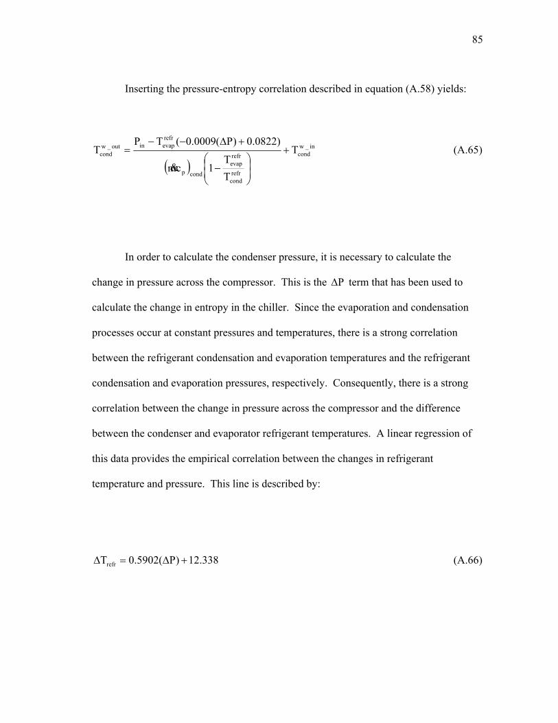
85

Inserting the pressure-entropy correlation described in equation (A.58) yields:

( )in_w

cond

refrcond

refrevap

condp

refrevapinout_w

cond T

TT

1cm

)0822.0)P(0009.0(TPT +

⎟⎟⎠

⎞⎜⎜⎝

⎛−

+∆−−=

&(A.65)

In order to calculate the condenser pressure, it is necessary to calculate the

change in pressure across the compressor. This is the P∆ term that has been used to

calculate the change in entropy in the chiller. Since the evaporation and condensation

processes occur at constant pressures and temperatures, there is a strong correlation

between the refrigerant condensation and evaporation temperatures and the refrigerant

condensation and evaporation pressures, respectively. Consequently, there is a strong

correlation between the change in pressure across the compressor and the difference

between the condenser and evaporator refrigerant temperatures. A linear regression of

this data provides the empirical correlation between the changes in refrigerant

temperature and pressure. This line is described by:

338.12)P(5902.0Trefr +∆=∆ (A.66)

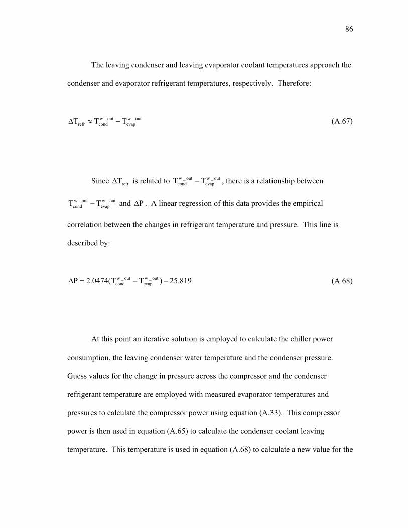
86

The leaving condenser and leaving evaporator coolant temperatures approach the

condenser and evaporator refrigerant temperatures, respectively. Therefore:

out_wevap

out_wcondrefr TTT −≈∆ (A.67)

Since refrT∆ is related to out_wevap

out_wcond TT − , there is a relationship between

out_wevap

out_wcond TT − and P∆ . A linear regression of this data provides the empirical

correlation between the changes in refrigerant temperature and pressure. This line is

described by:

819.25)TT(0474.2P out_wevap

out_wcond −−=∆ (A.68)

At this point an iterative solution is employed to calculate the chiller power

consumption, the leaving condenser water temperature and the condenser pressure.

Guess values for the change in pressure across the compressor and the condenser

refrigerant temperature are employed with measured evaporator temperatures and

pressures to calculate the compressor power using equation (A.33). This compressor

power is then used in equation (A.65) to calculate the condenser coolant leaving

temperature. This temperature is used in equation (A.68) to calculate a new value for the

87

change in pressure across the compressor. Equation (A.66) is employed to calculate the

change in refrigerant temperatures. The condenser refrigerant temperature is given by:

refrrefrevap

refrcond TTT ∆+= (A.69)

Equation (A.69) is used to calculate a new condenser refrigerant temperature.

The new condenser refrigerant temperature and pressure is used in subsequent iterations.

The model shows convergence after five iterations.

88

APPENDIX B

TEMPERATURE-ENTROPY DIAGRAM EXPLANATION

In describing the operation of a chiller, the temperature-entropy diagram can be a

useful diagnostic tool. To provide an explanation of real chiller operation, the ideal case

will be considered and the inefficiencies associated with real operation will be added as

the idea is developed. The Carnot Cycle consists of four internally reversible processes

and may be used to describe chiller operations. These four processes are an adiabatic

compression, isothermal condensation, adiabatic expansion, and isothermal evaporation.

These four processes are shown in Figure B.1.

89

Figure B.1. Ideal Carnot Cycle

The capacity of the chiller is the area under the evaporation line (4-1). The

amount of work done by the cycle is the area under the condensation line (2-3) minus the

capacity. These definitions for capacity and work will continue to hold true for the other

cycles in this investigation.

The first problem encountered with the Carnot Cycle in an explanation of a real

refrigeration system is the determination of Point 1. Point 1 exists in the fluid-vapor

region of the refrigerant. Point 1 is not distinguishable from the other points along the

90

Process 4-1 line using readily measured variables such as temperature or pressure. The

second problem is that condensation and evaporation take place at the temperature of the

hot and cold reservoirs. This would physically mean that no temperature difference

exists to drive the heat transfer.

In order to address these problems, the Carnot Cycle is modified to move Point 1

to a measurable condition and to account for the temperature differences between the

refrigerant and the reservoirs in the evaporator and condenser. The resulting diagram is

shown in Figure B.2.

Figure B.2. Modified Carnot Cycle

91

Point 1 has been moved to the saturated vapor line. This point can be measured

using a temperature sensor since the temperature will rise sharply if Point 1 is exceeded.

This would indicate that the refrigerant is fully evaporated and has entered a superheated

state. The evaporation line has been moved below the cold reservoir temperature while

the condensation line has been moved above the hot reservoir temperature. The cold

reservoir represents the chilled water temperature and the hot reservoir represents the

condenser water temperature. The areas between the reservoir temperatures and the

evaporation and condensation lines physically represent the losses due to finite-rate heat

transfer in the evaporator and condenser, respectively. Extending Point 1 to the

saturated vapor line increases the effective capacity of the chiller with respect to the

chiller cycle shown in Figure 1. It should also be noted that the area between the

condensation and evaporation lines increased. This physically corresponds to the

amount of work required to realize the increased capacity.

The Carnot Cycle shown in Figure B.2 is not without problems. The first

problem occurs in moving along the condensation line (2-3). In the superheated vapor

region, an isothermal decrease in entropy would correspond to an increase in pressure,

i.e. isothermal compression in the condenser. This condition violates the assumption of

isentropic compression. A better assumption would be a decrease in temperature and

entropy at a constant pressure. The second problem occurs in the assumption of an

isentropic expansion. The amount of work that can be obtained by using a turbine in the

expansion of the refrigerant is very small for most refrigeration systems. An expansion

valve is used in place of the turbine. An isenthalpic expansion is a more realistic

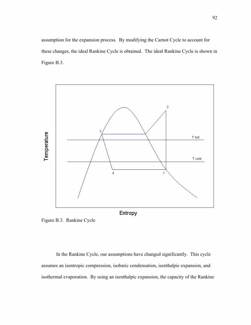
92

assumption for the expansion process. By modifying the Carnot Cycle to account for

these changes, the ideal Rankine Cycle is obtained. The ideal Rankine Cycle is shown in

Figure B.3.

Figure B.3. Rankine Cycle

In the Rankine Cycle, our assumptions have changed significantly. This cycle

assumes an isentropic compression, isobaric condensation, isenthalpic expansion, and

isothermal evaporation. By using an isenthalpic expansion, the capacity of the Rankine

93

Cycle decreases in comparison to the capacity of the Carnot Cycle. The combination of

an isentropic compression and isobaric condensation results in a superheated refrigerant

vapor at the discharge of the compressor. This is graphically represented as the

“superheat spike” that is characteristic of the Rankine Cycle. The amount of work

required increases since the area under the condensation line now includes the

“superheat spike” and the previously mentioned reduction in capacity.

The ideal Rankine Cycle begins to account for work that is done to overcome

non-isentropic inefficiencies in the expansion valve. In a real chiller, the compressor

behaves in a non-isentropic manner as well. Entropy is produced in the compressor due

to frictional losses. In order to ensure that no liquid refrigerant enters the compressor,

the refrigerant is allowed to enter the superheated vapor region before compression.

Another departure from the ideal Rankine Cycle is the sub-cooling of the refrigerant in

the condenser. Accounting for these changes, the diagram in Figure B.4 is obtained.

94

Figure B.4. Modified Rankine Cycle

The chiller capacity may increase depending on whether the superheating of the

vapor occurs in the evaporator or in the pipe connecting the evaporator and compressor.

If an increase in capacity due to superheating is realized, it should be very small in

comparison with the capacity due to evaporation. For practical purposes, the capacity

will still be the area under the evaporation line (4-1). The work now becomes the area

under the line 2-3b minus the capacity. The relationship between capacity and work is

shown in Figure B.5.

95

Figure B.5. Rankine Cycle with capacity emphasized

Figure B.5 may also be used to show the work associated with individual stages

in the cycle. For instance, the area under the line 1b-2 is the amount of work done to

overcome compressor irreversibilities. The area under the line 1-1b is the work

associated with the superheating of the refrigerant vapor. By using the temperature-

entropy diagram, each component that contributes to the work required to achieve the

capacity may be investigated. The breakdown of these individual components is shown

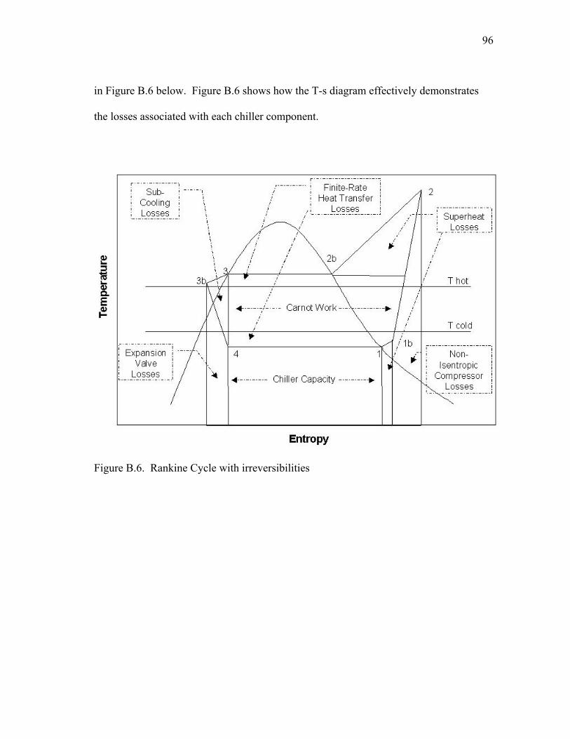
96

in Figure B.6 below. Figure B.6 shows how the T-s diagram effectively demonstrates

the losses associated with each chiller component.

Figure B.6. Rankine Cycle with irreversibilities

97

VITA

Rhett David Graves

Project Analyst, Energy Solutions

TAC Americas

Carrollton, TX 75006

Personal Data

Birth Date and Place:September 03, 1977, Sweetwater, TN

Home Address:342 White Road WestCollierville, TN 38017

Marital Status:Single

Education

Master of Science, Mechanical Engineering, Texas A&M University,College Station. December 2003.

Bachelor of Science, Mechanical Engineering, Mississippi State University,Mississippi State. May 2001.