Embed Size (px)
Citation preview

Thermo Vertical Drains for in-situ
consolidation of soils
Hugo Manuel Milheiro Martins Diogo
Dissertação para obtenção do Grau de Mestre em
Engenharia Civil
Júri Presidente: Prof. Jaime Alberto dos Santos Orientador: Profª Maria Rafaela Pinheiro Cardoso Vogais: Profª Teresa Maria Bodas de Araújo Freitas
Dezembro – 2009

Master Project – Study Report Thermo Vertical Drains for in-situ consolidation of soils
1
ABSTRACT
The aim of this master project is to evaluate and to improve an innovative technique that reduces the
time required to return to pore-water pressure equilibrium and, consequently, increases the rate of settlement. This technique consists of using Prefabricated Vertical Drains fitted with a heat source named T-PVD. This increase of the soil temperature around the drains leads to an increase of the permeability due to the heat effect on the water viscosity.
The effect of temperature on the settlement process was analyzed through experimental tests
performed on a large oedometer apparatus incorporating a centered T-PVD which was designed for this study. This apparatus allowed the measurement of pore pressure and temperature at different points of the sample, besides the vertical displacements and the water volume released during the test. Numerical simulations of the experimental tests were performed to analyze the processes involved at the local scale.
In the second part of the study the advantages of using the T-PVD technique were analyzed through
numerical simulations of a real embankment on which complete experimental data was available. In situ and numerical data were compared. A final analysis was done to evaluate the practical application of T-PVD technique by estimating the time saved and its energetic cost.
The main conclusion of the study is that T-PVD is a promising technique in terms of time saved due to
25-50% of time saved registered for temperature increments ranging between 10-30ºC. This was verified with the experimental and numerical programs developed. Nevertheless, the practical implementation of the T-PVD technique requires a better knowledge of the conditions on which it could be successfully used, mainly due to the high energetic costs involved.
Keywords
Pre-fabricated Vertical Drains; Thermo-mechanical behavior of soils; Large oedometer consolidations; Time saved in embankment constructions.

Master Project – Study Report Thermo Vertical Drains for in-situ consolidation of soils
2
RESUMO
O objectivo desta tese de mestrado é a avaliação e o desenvolvimento de uma técnica inovadora que
permite a redução do tempo de retorno ao equilíbrio de pressão intersticial e, consequentemente, o aumento do ritmo de assentamento. Esta técnica consiste no uso de drenos verticais pré-fabricados munidos de uma fonte de aquecimento, T-PVD. Este aumento da temperatura do solo em torno dos drenos leva a um aumento da permeabilidade devido ao efeito da temperatura na viscosidade da água.
Este efeito da temperatura no processo de assentamento será analisado experimentalmente usando
um aparelho específico de laboratório desenhado para este estudo. Este aparelho permitirá a medição da pressão intersticial e temperatura em diferentes pontos da amostra, o deslocamento total e o volume de água libertado.
De seguida, simulações numéricas serão realizadas para o trabalho experimental de forma a analisar o processo à escala local. Para demonstrar a vantagem da técnica T-PVD, simulações numéricas serão igualmente efectuadas para aterros reais sobre os quais existem medições completas retiradas do plano de instrumentação.
Uma análise final avaliará a aplicação prática desta técnica estimando o tempo ganho e os seus custos energéticos.
Concluindo, esta técnica é promissora em termos de tempo ganho, obtendo-se cerca de 25 -50% para
∆T entre 10-30ºC. A verificação destes resultados foi obtida nos programas experimentais e numéricos desenvolvidos. Por fim, esta técnica tem ainda um longo caminho a ser percorrido sendo que as condições onde deverá ser implementada com sucesso não são ainda totalmente conhecidas, o que será essencial devido aos elevados custos energéticos envolvidos.
Palavras-chave
Drenos verticais pré-fabricados; Comportamento termo-mecânico de solos; Consolidações em oedómetros de grandes dimensões; Tempo ganho em construções de aterros.

Master Project – Study Report Thermo Vertical Drains for in-situ consolidation of soils
3
ACKNOWLEGMENTS
This study was developed in École polytechnique Féderal de Lausanne, EPFL during the scholar year
of 2008/2009. The host laboratory was Laboratoire des Mécaniques des Sols, LMS from the Environnement Naturel, Architectural et Construit faculty (ENAC). The master project responsible was Professor Lyesse Laloui, director of the LMS and the designated tutor was the researcher Doctor Simon Salager also from LMS.
The applicant wishes to also express his gratitude to Dr. Mathieu Nuth for the help provided with the
numerical simulation software and Patrick Dubey. A special thank for Doctor Rafaela Cardoso from Instituto Superior Técnico, IST which permitted the development of this study.
A final thanks to my parents and family that supported me during this year in all aspects, for my friends
back home and the ones made during my stay in Switzerland.
Master Project – Study Report Thermo Vertical Drains for in-situ consolidation of soils
4
INDEX
1. Introduction .................................................................................................................................... 10
2. Experimental program ................................................................................................................... 19
2.1 Consolidation tests .................................................................................................................... 19
2.2 Experimental apparatus ............................................................................................................ 20
2.2.1 Main components ............................................................................................................. 21
2.2.1.1 Piston ........................................................................................................................... 22
2.2.1.2 Drain ............................................................................................................................. 23
2.2.2 Equipment description – Measured variables ................................................................... 26
2.2.2.1 Displacement................................................................................................................ 27
2.2.2.2 Pore pressure ............................................................................................................... 29
2.2.2.3 Temperature ................................................................................................................. 29
2.2.2.4 Water volume ............................................................................................................... 30
2.3 Soil – Kaolin clay ....................................................................................................................... 32
2.4 Test protocol .............................................................................................................................. 33
2.4.1 Calculations ...................................................................................................................... 33
2.4.2 Test preparation ............................................................................................................... 33
2.5 Experimental results .................................................................................................................. 36
2.5.1 Consolidation at ambient temperature – Reference test ................................................... 36
2.5.1.1 Mechanical loading ....................................................................................................... 36
2.5.1.2 Mechanical unloading ................................................................................................... 39
2.5.2 Test at 40ºC ...................................................................................................................... 41
2.5.2.1 Thermal loading ............................................................................................................ 41
2.5.2.2 Mechanical loading ....................................................................................................... 43
2.5.2.3 Mechanical unloading ................................................................................................... 46
2.5.2.4 Thermal unloading ........................................................................................................ 48
2.5.3 Test at 60ºC ...................................................................................................................... 51

Master Project – Study Report Thermo Vertical Drains for in-situ consolidation of soils
5
2.5.3.1 Thermal loading ............................................................................................................ 51
2.5.3.2 Mechanical loading ....................................................................................................... 53
2.5.3.3 Thermal unloading ........................................................................................................ 56
2.5.4.4 Mechanical unloading ................................................................................................... 58
2.5.4 Permeability tests ............................................................................................................. 61
2.5.4.1 Before consolidation ..................................................................................................... 62
2.5.4.2 After consolidation ........................................................................................................ 62
2.5.4.3 Experimental cell conditions ......................................................................................... 63
2.5.4.4 Conclusions .................................................................................................................. 64
2.6 Tests analysis – Temperature effects in consolidation .............................................................. 65
2.6.1 Displacements .................................................................................................................. 66
2.6.2 Pore pressure ................................................................................................................... 70
2.6.3 Temperature ..................................................................................................................... 71
2.6.4 Water exchanged.............................................................................................................. 72
2.6.4.1 Soil sample ................................................................................................................... 72
2.6.4.2 Experimental cell .......................................................................................................... 73
3. Finite elements simulations ........................................................................................................... 76
3.1 Thermo-hydro-mechanical model .............................................................................................. 77
3.1.1 Mechanical law ................................................................................................................. 78
3.1.2 Hydraulic law .................................................................................................................... 79
3.1.2.1 Radial permeability – Equivalent plane strain ............................................................... 80
3.1.2.2 Equivalent vertical permeability .................................................................................... 81
3.1.2.3 Well resistance ............................................................................................................. 82
3.1.2.4 Conclusions .................................................................................................................. 82
3.1.3 Thermal law ...................................................................................................................... 83
4. Results of numerical simulations ................................................................................................... 85
4.1 Oedometric cell simulations ....................................................................................................... 85
4.1.1 Definition ........................................................................................................................... 85

Master Project – Study Report Thermo Vertical Drains for in-situ consolidation of soils
6
4.1.2 Mesh ................................................................................................................................. 87
4.1.3 Analysis type .................................................................................................................... 87
4.1.3.1 Displacements .............................................................................................................. 88
4.1.3.2 Pore pressure ............................................................................................................... 89
4.1.3.3 Effective stress ............................................................................................................. 90
4.1.3.4 Temperature ................................................................................................................. 90
4.1.3.5 Conclusions .................................................................................................................. 90
4.1.4 Soil parameters definition ................................................................................................. 91
4.1.4.1 Soil’s general properties ............................................................................................... 91
4.1.4.2 Mohr-Coulomb parameters – simulation model ............................................................ 93
4.1.5 Experimental data for each temperature .......................................................................... 95
4.1.6 Results .............................................................................................................................. 95
4.1.6.1 Ambient temperature test – Mechanical consolidation ................................................. 96
4.1.6.2 Test at 40ºC ............................................................................................................... 103
4.1.6.3 Test at 60ºC ............................................................................................................... 107
4.1.7 Conclusions .................................................................................................................... 108
4.2 Embankments simulations....................................................................................................... 110
4.2.1 Definition of the analysed cases ..................................................................................... 110
4.2.2 Chosen Mesh ................................................................................................................. 111
4.2.2.1 Two drains mesh ........................................................................................................ 111
4.2.2.2 Full scale mesh .......................................................................................................... 112
4.2.3 Type of analysis made .................................................................................................... 114
4.2.4 Soil parameters .............................................................................................................. 114
4.2.5 Drain simulation – PVD solution ..................................................................................... 115
4.2.6 Consolidation simulation ................................................................................................. 119
5. Analysis for T-PVD practical application ...................................................................................... 120
5.1 Evaluation for time saved with T-PVD ..................................................................................... 120
5.1.1 Horizontal permeability ................................................................................................... 121
Master Project – Study Report Thermo Vertical Drains for in-situ consolidation of soils
7
5.1.1.1 Consolidation period ................................................................................................... 124
5.1.1.2 Rate of construction ................................................................................................... 126
5.1.2 Equivalent vertical permeability ...................................................................................... 129
5.2 T-PVD technique energetic cost .............................................................................................. 131
5.2.1 Soil’s heat energy ........................................................................................................... 131
6. Conclusions and future work ....................................................................................................... 133
REFERENCES .................................................................................................................................... 135
APPENDIX .......................................................................................................................................... 137

Master Project – Study Report Thermo Vertical Drains for in-situ consolidation of soils
8
List of symbols
Experimental cell’s central drain diameter Horizontal permeability in smear zone
Liquid limit Equivalent axisymmetric vertical drainage ( , )
Plastic limit Drainage length
Plasticity index Cell diameter
Unit weight of the soil particles Equivalent PVD rayon
Compression index , Geometric ratios
Slope of the swelling line Smear zone rayon
Coefficient of secondary compression Vertical permeability in plane strain
Friction angle at critical state Axisymmetric drain discharge capacity
Elastic modulus Vertical permeability (equal to in this study)
Poisson’s ratio Well resistance
Non-linear elasticity exponent Permeability multiplication coefficient at temperature
Water content Permeability at reference temperature of 22ºC
Soil volume Water density
Water volume Water cinematic viscosity
Total volume Water dynamic viscosity
Water mass Coefficient related to viscosity
Soil particules mass ∆ Temperature variation
Total mass (Soil sample for test consolidations) ´ Isotropic thermal expansion coefficient of the solid skeleton
Volumetric strain variation ´ Thermal expansion coefficient of the solid skeleton
∆ Height variation (Consolidation tests displacement) Slope for the variation of ´
Sample initial height Ratio between and
Final void ratio Reference consolidation pressure
Initial void ratio Effective net mean stress
Permeability ´ Thermal expansion coefficient of water
Horizontal permeability Phase compressibility ; Energy per degree celsius
Diameter of the permeability recipient base Volume thermical dilatation at constant pressure phase
Stress ( – vertical stress in this study) , Pore water pressure

Master Project – Study Report Thermo Vertical Drains for in-situ consolidation of soils
9
Time Position vector of the material point
² Minimum square method error Displacement vector of the solid matrix
, Volume of water exited at temperature Initial porosity ( initial porosity )
, Displacement of the piston at temperature Hydrostatic pore pressure
, Velocity of water exited at temperature Density of the solid particules
, Velocity of the piston displacement at temperature Specific gravity of soil grains
Cell area Total volumetric mass of the material
Cell rayon Water’s density
Drain rayon Relation between total and intergranular stress
/ Ration between , and , , Total stress
Maximum shear stress in rupture , Intergranular stress
Cohesion Kronecker symbol
Effective stress Poisson’s ratio
Attrition angle CSL gradient
Difference between and Dilatancy angle
Radial stress Initial earth pressure coefficient
Tangent modulus ( ) Final displacement in the consolidation tests
Strain variation (equal to in this study) , , Adjusted horizontal permeability at temperature
Final stress (before rupture) Average degree of consolidation at percentage
Equivalent PVD diameter ∆ Time variation in percentage
, Dimensions of PVD rectangular section Soil layer depth under embankment
Mandrel diameter ∆ Time saved in days
Smear zone diameter ∆ , Time saved by consolidation level
Equivalent radius of the PVD influence zone ∆ , Accumulated final time saved
Space between two vertical drains Specific heat capacity
Axisymmetric horizontal permeability Mass

Master Project – Study Report Thermo Vertical Drains for in-situ consolidation of soils
10
INDEX
i. Figures
Figure 1 Experimental apparatus (Left: Initial device; Right: Device after modifications) ...................... 20 Figure 2 Experimental cylinder vertical section ..................................................................................... 21 Figure 3 Piston components .................................................................................................................. 22 Figure 4 Torsion cases: loads (Left) and water expansion (Right) ........................................................ 23 Figure 6 Drain components and hot water movement inside the drain ................................................. 23 Figure 5 Piston: rigid elements .............................................................................................................. 23 Figure 7 Drain : Superior detail ............................................................................................................. 24 Figure 8 Drain: Inferior detail ................................................................................................................. 24 Figure 9 Schematics for the filter’s solution (dimensions and adhesive positions) ................................ 25 Figure 10 Description of the filter’s behaviour in time when compression starts ................................... 26 Figure 11 Oedometer: measurement devices ....................................................................................... 27 Figures 12 and 13 Previous displacement measurement apparatus (left) and displacement
measurement device (right) ........................................................................................................................ 28 Figure 14 Measurement apparatus solution for displacements ............................................................. 28 Figure 15 Pressure sensors disposition (cylinder mid-section) and data input device .......................... 29 Figure 16 Temperature sensors disposition (cylinder mid-section) and data input device .................... 30 Figure 17 Water volume exchange apparatus ...................................................................................... 31 Figure 18 Water exchange dispositive detail ......................................................................................... 31 Figure 19 Soil-water mixture ................................................................................................................. 34 Figure 20 Central drain installation ........................................................................................................ 34 Figure 21 Installed piston and central drain heating system ................................................................. 35 Figure 22 Soil sample: air voids detail ................................................................................................... 35 Figure 23 Permeability test (Right) and sample recipient (Left) ............................................................ 61 Figure 24 Mechanical unloading paths: T22 and T35 (linear line) and T53 (levelled line) .................... 67 Figure 25 Water filling the area above the piston during a consolidation test ....................................... 73 Figure 26 Mohr-Coulomb criterion in Mohr’s plan ................................................................................. 77 Figure 27 Kondner model in ( ; ) plan ................................................................................................ 78
Figure 28 Axisymmetric unit cell (oedometer) to an equivalent plane strain unit cell (embankment) .... 79 Figure 29 Simulation graphical representation ...................................................................................... 86

Master Project – Study Report Thermo Vertical Drains for in-situ consolidation of soils
11
Figure 30 Description of the elements chosen to define the cell’s mesh (Left: Material element; Right: Loading element) ........................................................................................................................................ 87
Figure 31 Points and sections for displacements analysis .................................................................... 88 Figure 32 Points and sections for pore pressure analysis ..................................................................... 89 Figure 33 R375.1 simple profile type (defined with the available information) .................................... 110 Figure 34 R375.2 simple profile type (defined with the available information) .................................... 110 Figure 36 Optimal mesh: complete embankment analysis .................................................................. 112 Figure 35 Proposed boundaries for simulation of the interaction between two drains at variable
distances ................................................................................................................................................... 112 Figure 37 Practical mesh: influence of PVD under the embankment (Central part of optimal mesh) .. 113 Figure 38 Embankments proposed boundaries for simulation (vertical lines correspond to PVD with a
imposed) .................................................................................................................................. 113
Figure 39 Drainage path: 1 side (up) and 2 side (down) ..................................................................... 115
ii. Plots Plot 1 Displacement vs Time : Mechanical loading at ambient temperature ......................................... 37 Plot 2 Pore pressure vs Time : Mechanical loading at ambient temperature ........................................ 37 Plot 3 Variation of void ratio in time (function of water exchange volume) ............................................ 38 Plot 4 Variation of water content in time (function of water exchange volume) ..................................... 38 Plot 5 Displacement in time: Mechanical unloading at ambient temperature ........................................ 39 Plot 6 Pore pressure vs Time : Mechanical unloading at ambient temperature .................................... 40 Plot 7 Temperature in time: Thermal loading until 40ºC ........................................................................ 42 Plot 8 Displacement in time: Thermal loading until 40ºC ....................................................................... 42 Plot 9 Pressure in time: Thermal loading until 40ºC .............................................................................. 43 Plot 10 Temperature in time: Mechanical consolidation ........................................................................ 44 Plot 11 Displacement in time: Mechanical consolidation at 40ºC .......................................................... 45 Plot 12 Pressure in time: Mechanical consolidation at 40ºC ................................................................. 45 Plot 13 Temperature in time: Mechanical unloading at 40ºC ................................................................ 46 Plot 14 Displacement in time: Mechanical unloading at 40ºC ............................................................... 47 Plot 15 Pressure in time: Mechanical unloading at 40ºC ....................................................................... 48 Plot 16 Temperature in time: Thermal unloading from 40ºC ................................................................. 49 Plot 17 Displacement in time: Thermal unloading from 40ºC ................................................................ 49 Plot 18 Pressure in time: thermal unloading from 40ºC ......................................................................... 50 Plot 19 Temperature in time: Thermal loading until 60ºC ...................................................................... 52 Plot 20 Displacement in time: Thermal loading until 60ºC ..................................................................... 52

Master Project – Study Report Thermo Vertical Drains for in-situ consolidation of soils
12
Plot 21 Pressure in time: Thermal loading until 60ºC ............................................................................ 53 Plot 22 Temperature in time: Mechanical consolidation ........................................................................ 54 Plot 23 Displacement in time: Mechanical consolidation at 60ºC .......................................................... 55 Plot 24 Pressure in time: Mechanical consolidation at 60ºC ................................................................. 55 Plot 25 Temperature in time: Thermal unloading from 60ºC ................................................................. 56 Plot 26 Displacement in time: Thermal unloading from 60ºC ................................................................ 57 Plot 27 Pressure in time: thermal unloading from 60ºC ......................................................................... 58 Plot 28 Temperature in time: Mechanical unloading ............................................................................. 58 Plot 29 Displacement in time: Mechanical unloading ............................................................................ 59 Plot 30 Pressure in time: Mechanical unloading ................................................................................... 60 Plot 31 Permeability in time: Test with sample before consolidation ..................................................... 62 Plot 32 Permeability in time: test with sample before consolidation ...................................................... 63 Plot 33 Permeability in time: test in oedometer conditions .................................................................... 64 Plot 34 Average degree of consolidation for mechanical loading in all tests – T22, T35 and T53 ........ 66 Plot 35 Mean displacement for mechanical unloading in all tests: T22, T35 and (T53 – T=22ºC) ........ 67 Plot 36 Temperature featuring displacement for thermal loading in T35 and T53 ................................. 68
Plot 37 Mean displacement in Thermal Unloading: T35 – 5 (Left) and T53 – 57
(Right) ......................................................................................................................................................... 69 Plot 38 Pore pressure measurements in T53 – ML (left) and T53 – MU (right) ..................................... 70 Plot 39 Pore pressure measurements for T22 – ML and T35 – ML ...................................................... 71 Plot 40 Temperature measurements for thermal unloading in T35 and T53 ......................................... 71 Plot 41 Water volume in time: Mechanical consolidation experimental tests ........................................ 72 Plot 42 Water volume in time: Mechanical consolidation at ambient temperature and 40ºC tests (Detail)
.................................................................................................................................................................... 74 Plot 43 Displacement vs Time: Mechanical consolidation at ambient temperature and at 40ºC tests
(Initial displacements detail) ........................................................................................................................ 74 Plot 44 Tangent modulus parameter function of final displacement (cylinder simulation) ..................... 96 Plot 45 Displacement values at t=1,40E+05 seconds for different simulated permeabilities ................. 98 Plot 46 Displacement in time for different testing permeabilities ( 1,64 105 ) ....... 99
Plot 47 Plot A (D,22): Experimental and final simulation consolidation paths in time, Lx,1 for ambient temperature (22,5ºC) .................................................................................................................................. 99
Plot 48 Plot B (D,22): Absolute variation of displacement, Lx,1 (h=0,57m) with radial distance for five pre-defined times ...................................................................................................................................... 100
Plot 49 Plot C (D,22): Variation of displacement with depth in different radial pre-defined distances (t4) .................................................................................................................................................................. 100
Master Project – Study Report Thermo Vertical Drains for in-situ consolidation of soils
13
Plot 50 Plot A (PP,22): Experimental and final simulation pore pressure evolution in time for ambient temperature (22,5ºC) ................................................................................................................................ 101
Plot 51 Plot B (PP,22): Variation of pore pressure (h=0,25m) with radial distance Lx,2 for the five pre-defined times (t0 to t4) ................................................................................................................................ 102
Plot 52 Plot C (PP,22): Variation of pore pressure with depth in different radial pre-defined distances (t1) ............................................................................................................................................................. 102
Plot 53 Plot C (PP,22): Variation of pore pressure with depth in different radial pre-defined distances (t4) ............................................................................................................................................................. 102
Plot 54 Plot A (D,35): Experimental and final simulation consolidation paths in time for heated test at 40ºC (Average 35ºC) ................................................................................................................................ 103
Plot 55 Plot B (D,35): Absolute variation of displacement (h=0,53m) in radial distance at five pre-defined times ............................................................................................................................................ 104
Plot 56 Plot C (D,35): Variation of displacement with depth in different radial pre-defined distances (t4) .................................................................................................................................................................. 104
Plot 57 A (PP,35): Experimental and final simulation pore pressure evolution in time for consolidation at 40ºC (35ºC) ........................................................................................................................................... 105
Plot 58 Adjustment of simulation temperature field, S.Ti to reproduce the experimental case, E.Ti for thermal loading until 40ºC ......................................................................................................................... 106
Plot 59 Plot A (D,53): Final simulation consolidation path in time for heated test at 60ºC (Average 53ºC) ......................................................................................................................................................... 107
Plot 60 Displacement comparison in time between simulation results and experimental measurements .................................................................................................................................................................. 108
Plot 61 Pore pressure comparison in time between simulation results and experimental measurements .................................................................................................................................................................. 109
Plot 62 Embankment height in time: Field data ................................................................................... 115
Plot 63 Validation of drainage hypotheses in simulation: Settlement vs Time (R375.1 – 1,3 ) 116
Plot 64 Validation of Young modulus in simulation: Settlement vs Time (R375.1) .............................. 117 Plot 65 Validation of vertical permeability hypothesis in simulation for two side drainage: Settlement vs
Time (R375.1) ........................................................................................................................................... 117 Plot 66 Validation of permeability hypothesis (vertical and horizontal) in simulation: Settlement vs Time
(R375.1) .................................................................................................................................................... 118 Plot 67 Validation of permeability hypothesis (smear zone) in simulation: Settlement vs Time (R375.1)
.................................................................................................................................................................. 118 Plot 68 Permeability vs Drain spacing [Equivalent vertical permeability] ............................................ 120 Plot 69 Average degree of consolidation: Evaluation of time saved using T-PVD solution (R375.1
example) ................................................................................................................................................... 121
Master Project – Study Report Thermo Vertical Drains for in-situ consolidation of soils
14
Plot 70 Final displacement simulated at different charges for R375.1 case and typical consolidation degrees ..................................................................................................................................................... 122
Plot 71 Average degrees of consolidation for R375.1 ......................................................................... 122 Plot 72 Consolidation check points for T-PVD time saved evaluation ................................................. 123 Plot 73 Consolidation check levels for T-PVD time saved evaluation ................................................. 123
Plot 74 Check points for T-PVD solution at ∆ 30 (Example) ................................................... 125
Plot 75 Average degree of consolidation controls for T-PVD solution time saved analysis ................. 125 Plot 76 Final embankment construction steps for verification of structural security with T-PVD solution
at ∆ 10 .......................................................................................................................................... 126
Plot 77 Final embankment construction steps for verification of structural security with T-PVD solution
at ∆ 20 .......................................................................................................................................... 127
Plot 78 Final embankment construction steps for verification of structural security with T-PVD solution
at ∆ 30 .......................................................................................................................................... 128
Plot 79 Evaluation of time saved using T-PVD solution: R375.1 example (Equiv. vertical permeability) .................................................................................................................................................................. 129
Plot 80 Difference between T-PVD simulations: ∆ (Vertical permeability) – (Radial
permeability) ............................................................................................................................................. 130
Tables Table 1 Consolidation test steps in time ................................................................................................ 20 Table 2 Identification properties of Kaolin clay ...................................................................................... 32 Table 3 Mechanical properties of Kaolin Clay ....................................................................................... 32 Table 4 Liquidity limit and water content to obtain a fully saturated state ............................................. 33 Table 5 Total mass values for each consolidation test .......................................................................... 33 Table 6 Permeability tests values function of sample consolidation and recipient base configuration .. 64 Table 7 Resume of the relevant test parameters: Charge, Time (to equilibrium), Average displacement
and Temperature ........................................................................................................................................ 65 Table 8 Ratios of movement between piston and exiting water ............................................................ 75 Table 9 Solid skeleton values at each simulated temperature .............................................................. 92 Table 10 Resume of general material properties for simulation ............................................................ 92 Table 11 Multiplier coefficient for different simulated temperatures: Ambient temperature as reference
.................................................................................................................................................................... 94 Table 12 Resume of Mohr-Coulomb material properties for simulation ................................................ 94 Table 13 Coefficient for uniform displacement analysis in simulation ................................................... 95

Master Project – Study Report Thermo Vertical Drains for in-situ consolidation of soils
15
Table 14 General Young modulus values for Kaolin soil simulation ...................................................... 96 Table 15 Detailed values approximation for Kaolin soil simulation .................................................. 97
Table 16 General permeability values for Kaolin soil simulation ........................................................... 98 Table 17 Evaluation of time saved with different T-PVD solutions for the oedometer tests simulation108 Table 18 Simulation soil parameters for embankment R375.1 (average soil characteristics from 1,7 to 3
meters ) ..................................................................................................................................................... 114 Table 19 Total displacements for R375.1 simulations ......................................................................... 115 Table 20 Simulations for embankment R375.1 ................................................................................... 115 Table 21 Permeability values used to validate the hydraulic hypothesis ............................................. 116
Table 22 Permeability values for radial permeability with 1,3 ................................................ 120
Table 23 Minimum displacement to be observed at each check point ................................................ 123 Table 24 Security displacement values in time for different T-PVD temperatures .............................. 124 Table 25 Time saved at each temperature increment ......................................................................... 124 Table 26 Primary time saved with T-PVD vs PVD solution for test embankment R375.1 (consolidation
period adjustment) .................................................................................................................................... 124 Table 27 Consolidation period adjustment check point verification ..................................................... 125 Table 28 Time saved adjustments to verify security at all check points: ∆ 10 ........................ 126
Table 29 Time saved adjustments to verify security at all check points: ∆ 20 ........................ 127
Table 30 Time saved adjustments to verify security at all check points: ∆ 30 ........................ 128
Table 31 Total time saved using T-PVD solution instead of PVD solution at three different temperatures for R375.1 ........................................................................................................................... 129
Table 32 Equivalent vertical permeability values for several temperatures with 1,3 .............. 129
Table 33 Heating capacity values: unconsolidated samples ............................................................... 131 Table 34 Costs for soil heating at different temperatures per drain in Switzerland ............................. 131 Table 35 Total energetic costs for T-PVD technique ........................................................................... 132 iii. Equations [1] .......................................................................................................................................................... 33 [2] .......................................................................................................................................................... 33 [3] .......................................................................................................................................................... 38 [4] .......................................................................................................................................................... 73 [5] .......................................................................................................................................................... 73 [6] .......................................................................................................................................................... 74 [7] .......................................................................................................................................................... 74 [8] .......................................................................................................................................................... 75
Master Project – Study Report Thermo Vertical Drains for in-situ consolidation of soils
16
[9] .......................................................................................................................................................... 77 [10] ........................................................................................................................................................ 80 [11] ........................................................................................................................................................ 80 [12] ........................................................................................................................................................ 80 [13] ........................................................................................................................................................ 81 [14] ........................................................................................................................................................ 81 [15] ........................................................................................................................................................ 81 [16] ........................................................................................................................................................ 82 [17] ........................................................................................................................................................ 83 [18] ........................................................................................................................................................ 83 [19] ........................................................................................................................................................ 83 [20] ........................................................................................................................................................ 84 [21] ........................................................................................................................................................ 84 [22] ........................................................................................................................................................ 84 [23] ........................................................................................................................................................ 91 [24] ........................................................................................................................................................ 91 [25] ........................................................................................................................................................ 91 [26] ........................................................................................................................................................ 91 [27] ........................................................................................................................................................ 92 [28] ........................................................................................................................................................ 93 [29] ........................................................................................................................................................ 96 [30] ........................................................................................................................................................ 98 [31] ...................................................................................................................................................... 131
Master Project – Study Report Thermo Vertical Drains for in-situ consolidation of soils
17
1. Introduction
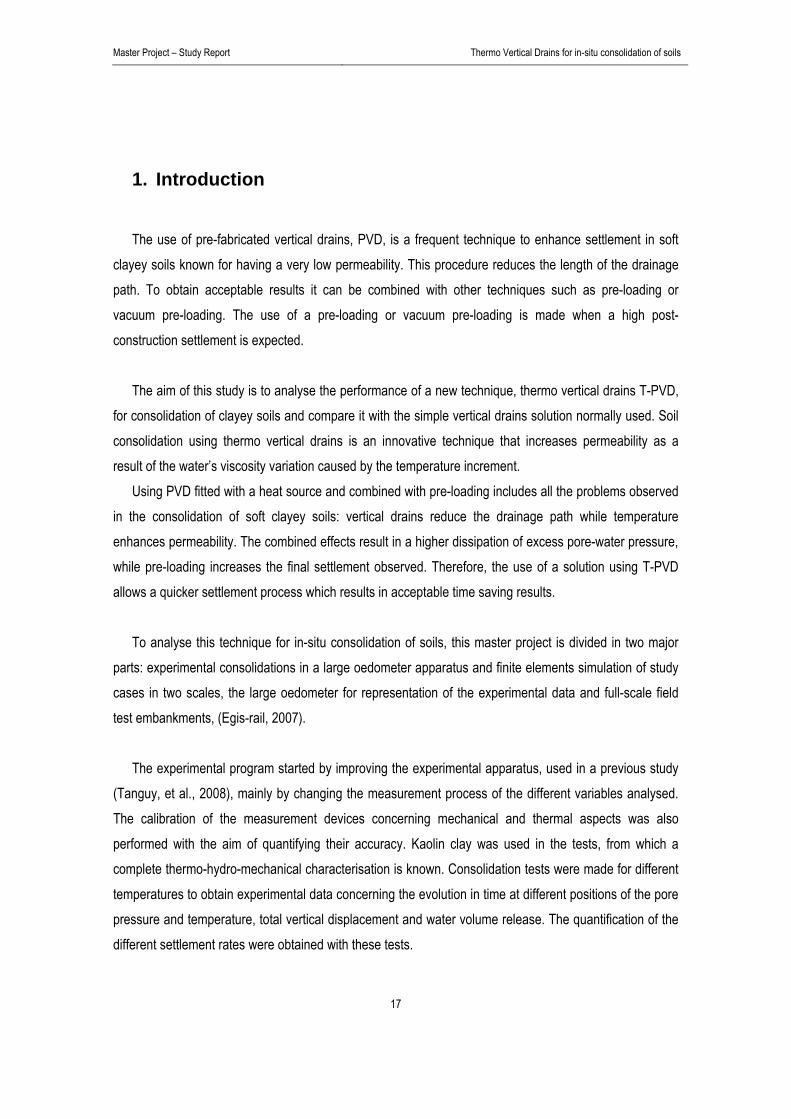
The use of pre-fabricated vertical drains, PVD, is a frequent technique to enhance settlement in soft
clayey soils known for having a very low permeability. This procedure reduces the length of the drainage path. To obtain acceptable results it can be combined with other techniques such as pre-loading or vacuum pre-loading. The use of a pre-loading or vacuum pre-loading is made when a high post-construction settlement is expected.
The aim of this study is to analyse the performance of a new technique, thermo vertical drains T-PVD,
for consolidation of clayey soils and compare it with the simple vertical drains solution normally used. Soil consolidation using thermo vertical drains is an innovative technique that increases permeability as a result of the water’s viscosity variation caused by the temperature increment.
Using PVD fitted with a heat source and combined with pre-loading includes all the problems observed in the consolidation of soft clayey soils: vertical drains reduce the drainage path while temperature enhances permeability. The combined effects result in a higher dissipation of excess pore-water pressure, while pre-loading increases the final settlement observed. Therefore, the use of a solution using T-PVD allows a quicker settlement process which results in acceptable time saving results.
To analyse this technique for in-situ consolidation of soils, this master project is divided in two major
parts: experimental consolidations in a large oedometer apparatus and finite elements simulation of study cases in two scales, the large oedometer for representation of the experimental data and full-scale field test embankments, (Egis-rail, 2007).
The experimental program started by improving the experimental apparatus, used in a previous study
(Tanguy, et al., 2008), mainly by changing the measurement process of the different variables analysed. The calibration of the measurement devices concerning mechanical and thermal aspects was also performed with the aim of quantifying their accuracy. Kaolin clay was used in the tests, from which a complete thermo-hydro-mechanical characterisation is known. Consolidation tests were made for different temperatures to obtain experimental data concerning the evolution in time at different positions of the pore pressure and temperature, total vertical displacement and water volume release. The quantification of the different settlement rates were obtained with these tests.

Master Project – Study Report Thermo Vertical Drains for in-situ consolidation of soils
18
Finite elements simulations of the previous experimental case were made, as well as the simulation of
a real case test embankment where PVD are used and from which complete experimental data is known. The simulation of the experimental tests was used to validate the model so it could be used to reproduce the T-PVD solution adopted for the test embankment for different temperatures.
The simulations performed for the embankment were the basis for the evaluation of time saved using this new technique. They allowed the analysis of the energetic costs involving this procedure.
The study performed allowed a better understanding of T-PVD technique including the definition of
bases for following studies. This report proposes a complete description of the improved experimental apparatus, analysis of the experimental tests regarding the improvements made and a comparative evaluation of the simulations made concluding with a clear assessment of the time saved using a T-PVD solution and its energetic costs.

Master Project – Study Report Thermo Vertical Drains for in-situ consolidation of soils
19
2. Experimental program
After the calibration process that prepared all the measurement devices, presented in Appendix 1, the
experimental consolidation tests are executed. These tests consist in consolidation of a saturated preparation of Kaolin clay at three different temperatures.
In this chapter, each component of the experimental apparatus will be described and explained followed by the procedure to prepare the soil for an experiment and the results obtained in the experimental tests at ambient and high temperatures (22ºC, 40ºC and 60ºC). The results are going to be analyzed in all aspects with special attention to the temperature effects observed.
2.1 Consolidation tests
To evaluate the behavior of consolidation at different temperatures an experimental test is made and three effective tests are proposed:
Experimental Test (TT) – A test was conducted after a briefing on the equipment used. The objective was to have a first contact with the device, understand how it works by assembling all components, guarantee that all steps are correctly made and finally define the modifications needed to improve the initial device. These modifications are described in chapter 2.2 Experimental apparatus.
Ambient temperature (T22) – A test at ambient temperature is made to evaluate the final displacement obtained and determine a reference time to arrive to this displacement by compaction of a clay soil sample at a pre-defined charge.
Test at 40ºC (T35) – This test is made as it will probably represent the variation that it´s actually possible to apply to a soil (variation of 20ºC). Even if the maximum temperature registered in the soil is around 36,5ºC (and average of 35ºC) this test had a 40ºC level to be achieved. Temperature has a clear dissipative gradient from the cell’s center.
Test at 60ºC (T53) – With this test a higher stage will give a framing for the thermal study. An analysis of the soil with a variation of approximately 30ºC is thought to be achieved.
For each test the measurements are initiated after the cell is closed with the piston and stabilization is achieved. The piston has a combined weight of 33, 65 Kg which means approximately 5,25 kN/m2. This stabilization ensures a final homogenization for the soil before initiating the test.
The mechanical loading is applied on each test in approximately one and a half minutes and it’s kept constant during the test. The weight of the charges applied is 365,96 Kg which results in 57,07 kN/m2.
Master Project – Study Report Thermo Vertical Drains for in-situ consolidation of soils
20
Application of mechanical and thermal loadings is made separately in order to distinguish (uncouple) the consequences of each. It’s important to refer that equilibrium in all measurements (displacement, temperature and pore pressure) is always achieved before the initiation of each step. The steps proposed for the tests are graphically presented in Table 1.
Test Pre-consolidation
Thermal loading
Mechanical loading
Mechanical unloading
Thermal unloading
Table 1 Consolidation test steps in time
The measurements made for the tests described here are going to be presented in chapter 2.5 Experimental results. The data registered for each step of the tests is available in the appendix CD.
2.2 Experimental apparatus
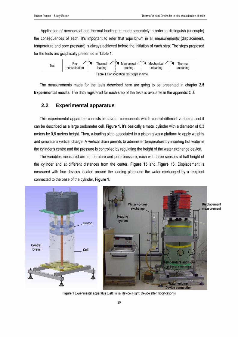
This experimental apparatus consists in several components which control different variables and it can be described as a large oedometer cell, Figure 1. It’s basically a metal cylinder with a diameter of 0,3 meters by 0,6 meters height. Then, a loading plate associated to a piston gives a platform to apply weights and simulate a vertical charge. A vertical drain permits to administer temperature by inserting hot water in the cylinder's centre and the pressure is controlled by regulating the height of the water exchange device.
The variables measured are temperature and pore pressure, each with three sensors at half height of the cylinder and at different distances from the center, Figure 15 and Figure 16. Displacement is measured with four devices located around the loading plate and the water exchanged by a recipient connected to the base of the cylinder, Figure 1.
Figure 1 Experimental apparatus (Left: Initial device; Right: Device after modifications)
Piston
Central Drain Cell
Water volume exchange
Heating system
Temperature and Pore pressure sensors
Displacement measurement
Water volume: Device connection

Master Project – Study Report Thermo Vertical Drains for in-situ consolidation of soils
21
The device is described in the next chapter with general views for main components in Figure 2 and the equipment used in Figure 11. The modifications made are also mentioned and they were all concluded before the consolidation tests that are part of this study. These modifications were defined in the experimental test made in order to improve the quality of the measurements and to have a better approximation of these tests to a real case.
2.2.1 Main components The oedometer itself is divided in three main components: the metal cylinder, the piston and the central
drain. These components have a crucial part in reproducing a soil consolidation case using thermo vertical drains as they control the variables that will reproduce these behaviours.
Figure 2 Experimental cylinder vertical section
Each of these main components is described next with special attention to the problems observed in the experimental test that will culminate in the solutions executed to solve them.
Piston
Drain
Cell wall

Master Project – Study Report Thermo Vertical Drains for in-situ consolidation of soils
22
2.2.1.1 Piston The piston is the connection platform between the loads that apply a vertical charge to the system and
the soil where this charge is distributed. It’s composed from two rings, for stability, where rigid metal bars give connection to a loading plate. In this metal loading plate charges can be applied to simulate a distributed vertical stress in the soil. The rigid bars exist so the heating water system in the central drain can be operational during the consolidation tests and also to give some space between the rectangular loading plate and the cylinder (so different scales of displacements can occur). The heating system links with the superior part of the drain which passes by the central hole in the piston.
Figure 3 Piston components
Consequently, the piston has the capacity to transmit a chosen load to the soil, homogeneous and constant, and therefore control the effective stress applied to the sample.
In the experimental test it was observed that the piston and loading plate had a torsion component that
caused variations and unconformities in the values registered for displacement as they’re measured from the loading plate, Figure 15. The vertical liaisons of the piston, part in contact with the cylinder’s interior, are rigid and they’re not heated. Therefore, they conduct these variations directly to the loading plate.
A part of this torsion can also happen when the cell is heated, Figure 15 (Right). The heating system is in the centre of the cylinder and the water is consequently hotter there. This is deducted from the empirical observation only, as the cylinder temperature was also significantly bigger in the top of the cell, where the hot water enters, in comparison with the bottom. There’re also torsions due to charges non-centred which will induce negative variations in the displacement, Figure 15 (Left). Also the application of these charges with different weights gives different variations.
Loading plate
O-rings Stability ring
Sealing ring
Load groups
Metal liaison bars
Master Project – Study Report Thermo Vertical Drains for in-situ consolidation of soils
23
Figure 4 Torsion cases: loads (Left) and water expansion (Right)
Therefore, the charges must be placed with equal weights in groups of three to decrease the torsion problem to the minimum and an improved displacement system will be executed, 2.2.2.1 Displacement.
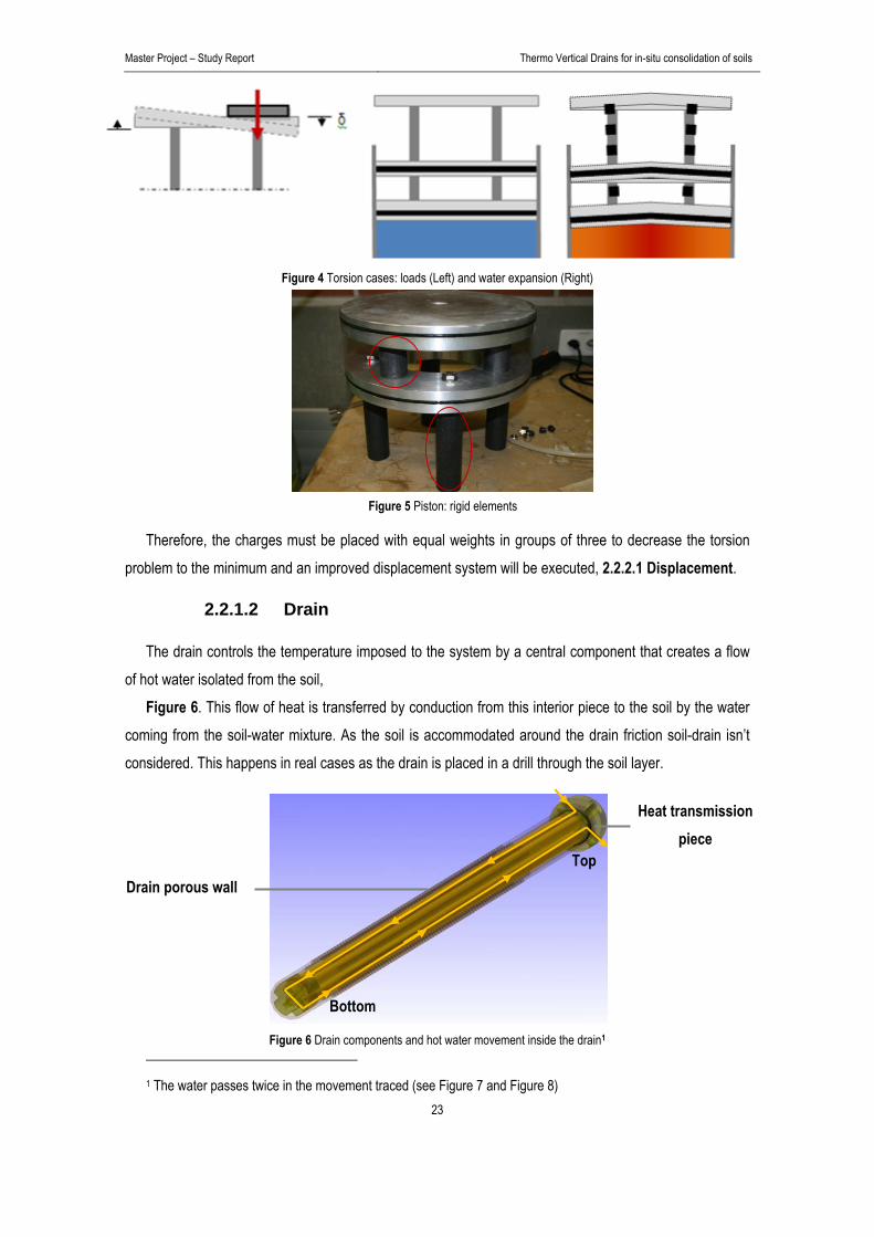
2.2.1.2 Drain
The drain controls the temperature imposed to the system by a central component that creates a flow of hot water isolated from the soil,
Figure 6. This flow of heat is transferred by conduction from this interior piece to the soil by the water coming from the soil-water mixture. As the soil is accommodated around the drain friction soil-drain isn’t considered. This happens in real cases as the drain is placed in a drill through the soil layer.
Figure 6 Drain components and hot water movement inside the drain1
1 The water passes twice in the movement traced (see Figure 7 and Figure 8)
Drain porous wall
Heat transmission piece
Top
Bottom
Figure 5 Piston: rigid elements

Master Project – Study Report Thermo Vertical Drains for in-situ consolidation of soils
24
The hot water flows two times from up to down and two times in the inversed way, Figure 8 until it exits from the upper part of the drain, Figure 7.
Figure 7 Drain : Superior detail
With this movement, and as hot water circulates by means of a pump, there is time for the heat transfer to occur while this imposed heat is renovated. To help maintaining this heat in the system an isolation mousse surrounds the cylinder’s exterior.
Figure 8 Drain: Inferior detail
So, the central drain gives the control of the temperature imposed to the system. With the installed cork in the end of the drain the water from the soil’s mixture is also controlled and measured by the water exchange device, Figure 17. This device, explained in 2.2.2.4 Water volume, permits also to control the water level.
Water evacuation Water alimentation
Water from sample
Heated water movement

Master P
ThIn
compfilter’sthis pr
Th
preve In
displaloose.10. Itassumthe ch
Th
Project – Study Re
he porous part the previous ression starte
s design that, croblem. his solution co
(wnt the soil from
the filter’s upacement begin. The whole fi’s considered
med because harges appliedhe geometry o
F
eport
t of the drain i studies the lo
ed. So, in ordecomplemented
onsists in a filtith
m passing in t
per part a shans. And also alter shall slide
d that the effeof the filter’s r
d. of the filter and
Figure 9 Schema
s covered withost of some ser to avoid thid with the imp
ter diameter d) and it
he non adhes
ape of funnel avoiding the o
e below the pisects from thisresistance wh
d improvemen
atics for the filter’s
25
h a geotextile soil in the cenis lost, a solutproved water e
design that va now ends in
sive parts (adh
is proposed toopening of theston while disps solution arehich is conside
t of the heatin
s solution (dimen
Thermo
filter to maintantral drain haption was founexchange dev
aries with heig the top of thehesive parts ar
o also prevente non adhesivplacement adve negligible foered null when
ng system wer
nsions and adhes
Vertical Drains for
ain the soil in ppened in thed in the expeice, 2.2.2.4 W
ght so it doesne porous partre represented
t the soil fromve parts as itsvances with cor the resultsn compared w
ren’t a target o
sive positions)
r in-situ consolidatio
place. e experimentserimental test
Water volume
n't need three, Figure 9. Thd by yellow st
m exiting theres upper part
compression, Fs measured. Twith the greatn
of this study.
on of soils
s when for the solves
e rows, his will ripes).
, when is now Figure This is ness of
Master P
Th
Th
measdescrregardfilled w
Project – Study Re
2.2.2 E
he equipment
Displacem Pressure; Temperat Water vol
he solutions urements of tibe the equipding the conclwith water hea
eport
Equipmen
description re
ment; ; ture; ume.
that improvethese variablepment used alusions obtainated at differe
Figure 10 Des
t descript
esumes the va
ed the expees from the laare mentioneed from an exnt temperature
scription of the filt
26
tion – Mea
ariables to be m
erimental devast version, aed as they exxperimental tees.
ter’s behaviour in
Thermo
asured var
measured dur
vice, giving are described xisted and thst and thermo
n time when comp
Vertical Drains for
riables
ring the tests:
the possibilit next. Each ohen the modio-mechanical b
pression starts
r in-situ consolidatio
ty to develoof the variableifications are behaviour of t
on of soils
op the es that made the cell
Master Project – Study Report Thermo Vertical Drains for in-situ consolidation of soils
27
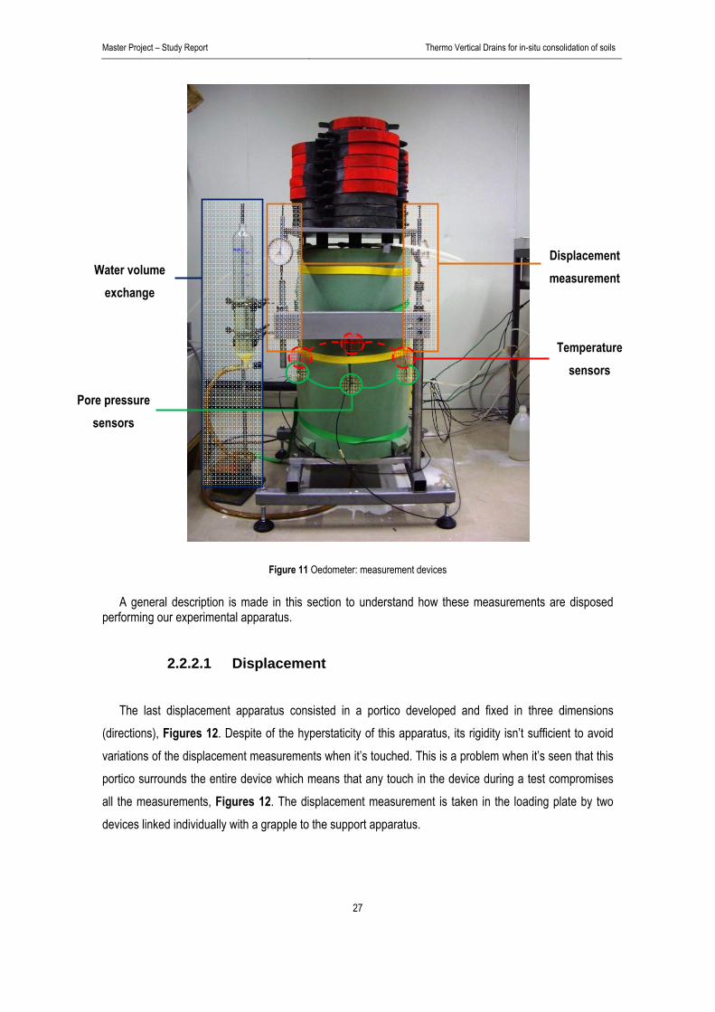
Figure 11 Oedometer: measurement devices
A general description is made in this section to understand how these measurements are disposed performing our experimental apparatus.
2.2.2.1 Displacement The last displacement apparatus consisted in a portico developed and fixed in three dimensions
(directions), Figures 12. Despite of the hyperstaticity of this apparatus, its rigidity isn’t sufficient to avoid variations of the displacement measurements when it’s touched. This is a problem when it’s seen that this portico surrounds the entire device which means that any touch in the device during a test compromises all the measurements, Figures 12. The displacement measurement is taken in the loading plate by two devices linked individually with a grapple to the support apparatus.
Displacement measurement Water volume
exchange
Temperature sensors
Pore pressure sensors

Master P
Th
attachmetal differetime tbe ad
Wgood isn’t sneareconsis
Project – Study Re
he improvemehed around th welded to thent heights ashe screw is aded.
When the thermapproximation
sufficiently rigest device regsts in consolid
Figures 12 and
eport
ent of this mhe loading plahe cylinder bas we can havedjusted the fin
mal calibrationn is obtained. id. So, as loa
gisters a positdation) which i
13 Previous disp
F
easurement cate, Figure 20ase support. almost 15cmnal measure a
n was made, Variations onads aren’t petive displacems solved, as a
placement measu
Figure 14 Measu
28
consists in fo0. This measuThis bar has of displacem
and the new o
this apparatu measuremenrfectly centred
ment and thealready mentio
urement apparatu
urement apparatu
Thermo
our displacemurement is tak a screw in thent and each
one have to be
us was testednts are due to d, Figure 20 other a neg
oned, by using
us (left) and displ
us solution for dis
Vertical Drains for
ment devices. ken from a righe end that c device has a e registered s
, and from th torsion of the each time a ative one (po
g the mean va
lacement measu
splacements
r in-situ consolidatio
Each of themgid cylindrical can be regulat range of 5cmo the differenc
eir average v loading plate level is placositive displacalue of all devic
rement device (ri
on of soils
m was bar in ted for
m. Each ce can
value a e which ed the
cement ces.
ight)

Master P
Someascornethe so
Th
the cycalibrapresspressthe cyknown
Th6,5 cmvaries0,05 kimporreturn
Tediffereadmisaccura
Project – Study Re
o, in conclusiourements will rs of the load
oil’s sample. T
2.2.2
hree pore presylinder’s baseation due to thure sensors, ure variationsylinder’s mid-n.
he pressure sem and sensor s from each sekPa. Despite rtant effect in tning to ambien
2.2.2
emperature isent radial distassible accuracacy is admitte
Data indevic
eport
on, to contou correspond t
ding plate, FigThis measurem
2.2 Pore
ssure sensorse) at differenthe values obt Appendix 1s. Nevertheles-section. With
Figure 15 Pres
ensors are loc 3 at 11,7 cm ensor due to tof the calibratheir measure
nt temperature
2.3 Tem
s measured uances, Figure
cy for this variaed equal to the
put ce
ur the problemo four devices
gure 11. The ment results in
e pressure
s are located it radial distaained from the one of the
ss, this sensor this configur
ssure sensors dis
cated at threemeasuring frotheir sensibilit
ation made to ements but it he.
mperature
using three se 16. These sable in the teme scale provide
29
m of torsion ds with an accdisplacement
n the total disp
e
n the mid-secnces, Figure e last study msensors didn
r was used anration the ran
sposition (cylinde
e different radiom the cylindety to pressure the sensors has been prov
sensors also sensors werenmperature ranged, 0,1ºC.
Thermo
due to the loacuracy of 1/10 is therefore m
placement obs
ction of the cy 15. The sen
made in the oen’t demonstrand was locatenge of pressu
er mid-section) an
al positions: ser’s wall in dire variation but a long term e
ven that they
located at thn’t calibrated age of the cons
Prese
P1
P3: 4
P2: 6,5 cm
Vertical Drains for
ads disposition0th millimetresmeasured for served for the
linder (25cm hnsors were oedometer. In tate an acceped in the middure inside the
nd data input dev
sensor 1 is at ection of the c its around 0,2exposition to tregain the sam
he cylinder’s as their perforsolidation tests
essure ensors
: 11,7 cm
4,6 cm
m
r in-situ consolidatio
n, the displacs located in th the superior soil.
high measureobject of a sethe calibrationptable sensibidle radial posie cylinder is a
vice
4,6 cm, senscentre. The ac25 kPa in a sctemperature hme calibration
mid-section armance is withs (20 to 60ºC)
on of soils
cement he four part of
ed from ensible of the lity for ition of always
or 2 at curacy cale of has an n when
and at hin the ). Their
Master P
Thand se
Fo
the cySo
Th
recipievolumrecipieto rep
Thlost oalso meastests a
Project – Study Re
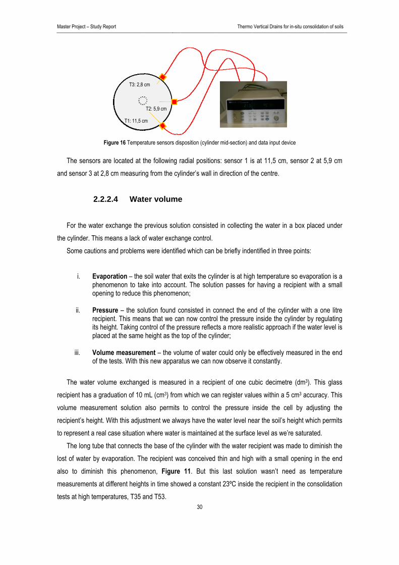
Fi
he sensors arensor 3 at 2,8
2.2.2
or the water eylinder. This mome cautions
i. Evapophenoopenin
ii. Pressrecipieits heiplaced
iii. Volumof the
he water voluent has a grad
me measurement’s height. W
present a real che long tube thf water by evto diminish turements at dat high tempe
eport
gure 16 Temper
re located at t8 cm measurin
2.4 Wat
exchange the means a lack o
and problems
oration – the omenon to takng to reduce t
sure – the solent. This meaght. Taking cod at the same
me measurem tests. With th
me exchangeduation of 10
ment solution With this adjuscase situationhat connects taporation. Ththis phenomedifferent heightratures, T35 a
T3: 2,8
T1: 11,5 c
ature sensors dis
the following rng from the cy
er volume
previous soluof water exchas were identifie
soil water thatke into accouhis phenomen
lution found cns that we caontrol of the pr height as the
ment – the volis new appara
ed is measuremL (cm3) fromalso permits
stment we alwn where water the base of the recipient wa
enon, Figure ts in time showand T53.
cm
m
T2: 5,9 cm
30
sposition (cylinde
radial positionlinder’s wall in
e
tion consistedange control. ed which can
t exits the cylint. The solutinon;
consisted in coan now controressure reflec top of the cyli
lume of wateratus we can no
ed in a recipim which we ca to control th
ways have the is maintained
he cylinder witas conceived 11. But thiswed a constan
Thermo
er mid-section) an
ns: sensor 1 isn direction of t
d in collecting
be briefly inde
nder is at highon passes fo
onnect the enl the pressurets a more reainder;
r could only beow observe it
ient of one cuan register valhe pressure water level ne
d at the surfaceh the water re thin and highs last solutiont 23ºC inside
Vertical Drains for
nd data input dev
s at 11,5 cm, he centre.
the water in
entified in thre
h temperaturer having a re
nd of the cyline inside the cylistic approach
e effectively m constantly.
ubic decimetrues within a 5inside the ceear the soil’s he level as we’ecipient was mh with a small on wasn’t nee the recipient
r in-situ consolidatio
vice
sensor 2 at 5
a box placed
e points:
e so evaporatioecipient with a
nder with a onylinder by regh if the water l
measured in th
re (dm3). This5 cm3 accuracyell by adjustinheight which pre saturated.
made to dimin opening in thed as tempe in the consol
on of soils
5,9 cm
under
on is a a small
ne litre ulating level is
he end
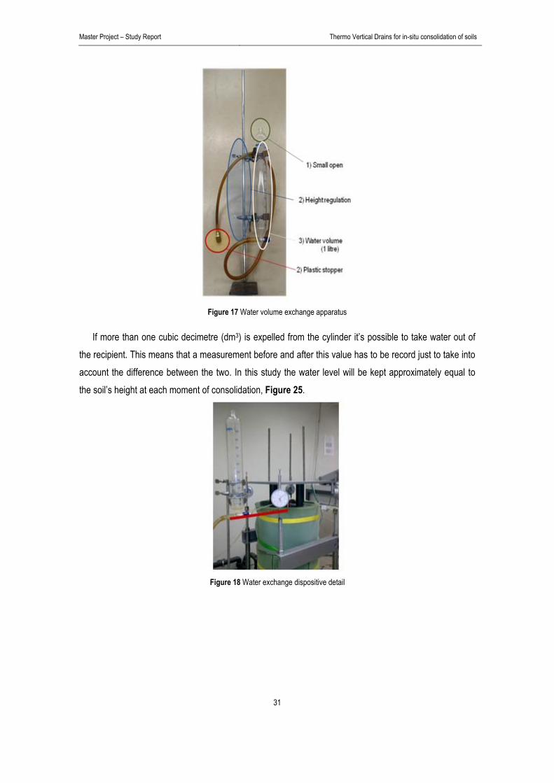
s glass y. This ng the permits
ish the he end erature idation
Master Project – Study Report Thermo Vertical Drains for in-situ consolidation of soils
31
Figure 17 Water volume exchange apparatus
If more than one cubic decimetre (dm3) is expelled from the cylinder it’s possible to take water out of the recipient. This means that a measurement before and after this value has to be record just to take into account the difference between the two. In this study the water level will be kept approximately equal to the soil’s height at each moment of consolidation, Figure 25.
Figure 18 Water exchange dispositive detail
Master Project – Study Report Thermo Vertical Drains for in-situ consolidation of soils
32
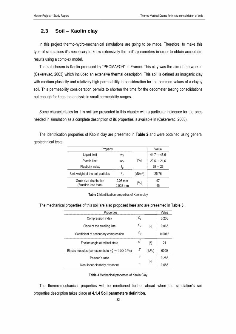
2.3 Soil – Kaolin clay
In this project thermo-hydro-mechanical simulations are going to be made. Therefore, to make this type of simulations it’s necessary to know extensively the soil’s parameters in order to obtain acceptable results using a complex model.
The soil chosen is Kaolin produced by “PROMAFOR” in France. This clay was the aim of the work in (Cekerevac, 2003) which included an extensive thermal description. This soil is defined as inorganic clay with medium plasticity and relatively high permeability in consideration for the common values of a clayey soil. This permeability consideration permits to shorten the time for the oedometer testing consolidations but enough for keep the analysis in small permeability ranges.
Some characteristics for this soil are presented in this chapter with a particular incidence for the ones
needed in simulation as a complete description of its properties is available in (Cekerevac, 2003). The identification properties of Kaolin clay are presented in Table 2 and were obtained using general
geotechnical tests. Property Value
Liquid limit [%]
44,7 45,6 Plastic limit 20,6 21,6
Plasticity index 25 23
Unit weight of the soil particles [kN/m3] 25,76
Grain-size distribution (Fraction less than)
0,06 mm [%] 97 0,002 mm 45
Table 2 Identification properties of Kaolin clay
The mechanical properties of this soil are also proposed here and are presented in Table 3. Properties Value
Compression index
[-]
0,236
Slope of the swelling line 0,065
Coefficient of secondary compression 0,0012
Friction angle at critical state [º] 21
Elastic modulus (corresponds to 100 ) [kPa] 6000
Poisson’s ratio [-]
0,285
Non-linear elasticity exponent 0,685
Table 3 Mechanical properties of Kaolin Clay
The thermo-mechanical properties will be mentioned further ahead when the simulation’s soil properties description takes place at 4.1.4 Soil parameters definition.
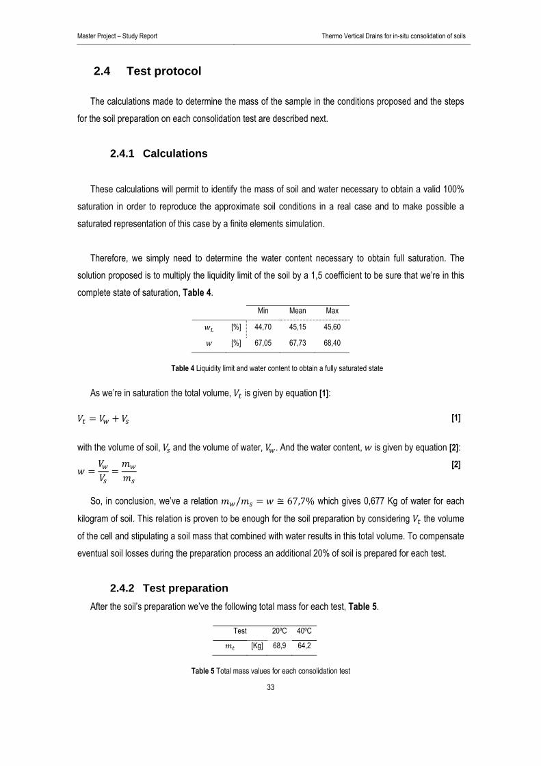
Master Project – Study Report Thermo Vertical Drains for in-situ consolidation of soils
33
2.4 Test protocol
The calculations made to determine the mass of the sample in the conditions proposed and the steps for the soil preparation on each consolidation test are described next.
2.4.1 Calculations These calculations will permit to identify the mass of soil and water necessary to obtain a valid 100%
saturation in order to reproduce the approximate soil conditions in a real case and to make possible a saturated representation of this case by a finite elements simulation.
Therefore, we simply need to determine the water content necessary to obtain full saturation. The
solution proposed is to multiply the liquidity limit of the soil by a 1,5 coefficient to be sure that we’re in this complete state of saturation, Table 4.
Min Mean Max
[%] 44,70 45,15 45,60
[%] 67,05 67,73 68,40
Table 4 Liquidity limit and water content to obtain a fully saturated state
As we’re in saturation the total volume, is given by equation [1]:
[1] with the volume of soil, and the volume of water, . And the water content, is given by equation [2]:
[2]
So, in conclusion, we’ve a relation / 67,7% which gives 0,677 Kg of water for each
kilogram of soil. This relation is proven to be enough for the soil preparation by considering the volume
of the cell and stipulating a soil mass that combined with water results in this total volume. To compensate eventual soil losses during the preparation process an additional 20% of soil is prepared for each test.
2.4.2 Test preparation After the soil’s preparation we’ve the following total mass for each test, Table 5.
Test 20ºC 40ºC
[Kg] 68,9 64,2
Table 5 Total mass values for each consolidation test

Master Project – Study Report Thermo Vertical Drains for in-situ consolidation of soils
34
Using the quantities calculated in the last chapter we arrive to a malleable sample with traces of water, practically non consistent but with a high cohesion. The sample was mixed in a laboratory machine and vibrated to free any air bubbles that may have been kept inside, Figure 19.
Figure 19 Soil-water mixture
With the sample ready the cylinder is assembled in the following order:
1. Central drain installation – the drain is installed covered with a geotextile prepared as described in 2.2.1.2 Drain;
Figure 20 Central drain installation
2. Cell filling and sensors installation – The cell is half full and the sensors are installed. A first measure for all sensors is taken (first zero). The cell is completely filled and another round of measurements is taken (second zero). Friction soil-drain isn’t considered as already mentioned;
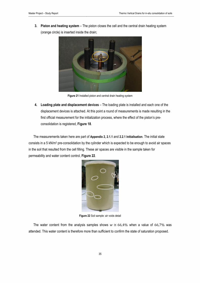
Master Project – Study Report Thermo Vertical Drains for in-situ consolidation of soils
35
3. Piston and heating system – The piston closes the cell and the central drain heating system (orange circle) is inserted inside the drain;
Figure 21 Installed piston and central drain heating system
4. Loading plate and displacement devices – The loading plate is installed and each one of the displacement devices is attached. At this point a round of measurements is made resulting in the first official measurement for the initialization process, where the effect of the piston’s pre-consolidation is registered, Figure 18.
The measurements taken here are part of Appendix 2, 2.1.1 and 2.2.1 Initialisation. The initial state
consists in a 5 kN/m2 pre-consolidation by the cylinder which is expected to be enough to avoid air spaces in the soil that resulted from the cell filling. These air spaces are visible in the sample taken for permeability and water content control, Figure 22.
Figure 22 Soil sample: air voids detail
The water content from the analysis samples shows 66,4% when a value of 66,7% was
attended. This water content is therefore more than sufficient to confirm the state of saturation proposed.

Master Project – Study Report Thermo Vertical Drains for in-situ consolidation of soils
36
2.5 Experimental results
The experimental results are presented in this chapter followed by the permeability tests conducted in reference samples collected after and before the consolidation tests. These permeability tests will permit to develop a better understanding around the soil’s behaviour in different confinements.
2.5.1 Consolidation at ambient temperature – Reference test The test at ambient temperature is divided in mechanical loading, ML and mechanical unloading, MU.
The measurements taken for this test are presented in Appendix 2.1. The displacement and pore pressure values for the mechanical loading and unloading in the ambient
temperature test are presented next and are used as a reference for the heated cases analysis.
2.5.1.1 Mechanical loading During the mechanical loading the maximum temperature registered was 23,4ºC near the drain at the
end of the consolidation and the smallest was 21,7ºC near the cylinder’s wall at the beginning of the test. The average temperature registered was 22,5ºC.
The final displacement measured was 135,66 mm within approximately 0,57 m of initial soil’s height.
This gives a compression ratio around, 135,66/0,57 0,238 which means that the sample’s height
diminishes from a quarter, 25% in 7 days for a charge of 50,75 kN/m2. This high compression is mainly
due to the small pre-compaction of the soil’s mixture which is prepared from powder. The high void ratio of this clay is also a reason for these large values of displacement observed.
The displacement showed in Plot 1 is the result of a mean value obtained by the four measurement
devices.

Master Project – Study Report Thermo Vertical Drains for in-situ consolidation of soils
37
0
20
40
60
80
100
120
140
0 1 105 2 105 3 105 4 105 5 105 6 105 7 105 8 105
Mean displacement : T22 - ML
Dis
plac
emen
t [m
m]
Time [sec] Plot 1 Displacement vs Time : Mechanical loading at ambient temperature
The positional solution found to register the displacements observed has proved to give accurate results which permits to observe the curve in Plot 1. One day corresponds to 8,64x10⁴ seconds which is approximately 1x10⁵ seconds for time grading solution in Plot 1.
Pore pressure was also registered and is given in Plot 2.
0
10
20
30
40
50
0 1 105 2 105 3 105 4 105 5 105 6 105 7 105 8 105
P3: T22 - ML (Cell wall)
P1: T22 - ML (Drain)
Pre
ssur
e [k
Pa]
Time [sec] Plot 2 Pore pressure vs Time : Mechanical loading at ambient temperature
Day 2
Day 1
Day 3
Day 4
Day 5
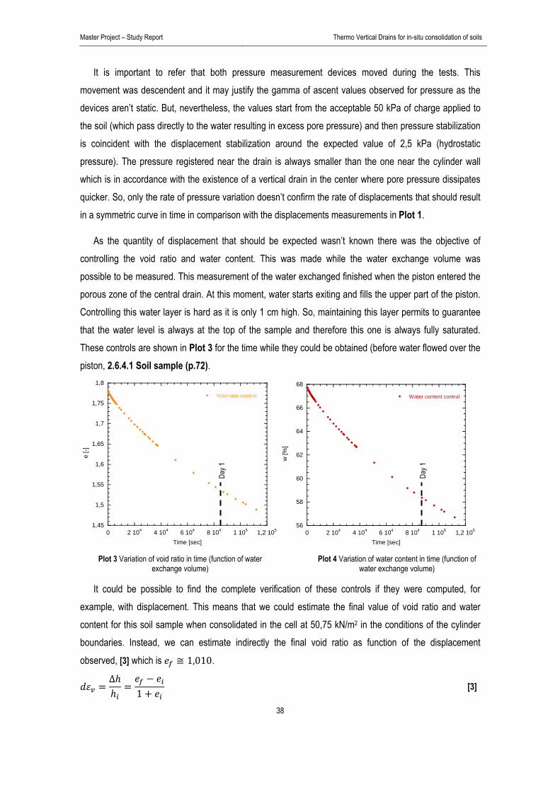
Master Project – Study Report Thermo Vertical Drains for in-situ consolidation of soils
38
It is important to refer that both pressure measurement devices moved during the tests. This movement was descendent and it may justify the gamma of ascent values observed for pressure as the devices aren’t static. But, nevertheless, the values start from the acceptable 50 kPa of charge applied to the soil (which pass directly to the water resulting in excess pore pressure) and then pressure stabilization is coincident with the displacement stabilization around the expected value of 2,5 kPa (hydrostatic pressure). The pressure registered near the drain is always smaller than the one near the cylinder wall which is in accordance with the existence of a vertical drain in the center where pore pressure dissipates quicker. So, only the rate of pressure variation doesn’t confirm the rate of displacements that should result in a symmetric curve in time in comparison with the displacements measurements in Plot 1.
As the quantity of displacement that should be expected wasn’t known there was the objective of controlling the void ratio and water content. This was made while the water exchange volume was possible to be measured. This measurement of the water exchanged finished when the piston entered the porous zone of the central drain. At this moment, water starts exiting and fills the upper part of the piston. Controlling this water layer is hard as it is only 1 cm high. So, maintaining this layer permits to guarantee that the water level is always at the top of the sample and therefore this one is always fully saturated. These controls are shown in Plot 3 for the time while they could be obtained (before water flowed over the piston, 2.6.4.1 Soil sample (p.72).
1,45
1,5
1,55
1,6
1,65
1,7
1,75
1,8
0 2 104 4 104 6 104 8 104 1 105 1,2 105
Void ratio control
e [-]
Time [sec]
56
58
60
62
64
66
68
0 2 104 4 104 6 104 8 104 1 105 1,2 105
Water content control
w [%
]
Time [sec] Plot 3 Variation of void ratio in time (function of water
exchange volume) Plot 4 Variation of water content in time (function of
water exchange volume)
It could be possible to find the complete verification of these controls if they were computed, for example, with displacement. This means that we could estimate the final value of void ratio and water content for this soil sample when consolidated in the cell at 50,75 kN/m2 in the conditions of the cylinder boundaries. Instead, we can estimate indirectly the final void ratio as function of the displacement observed, [3] which is 1,010.
∆1
[3]
Day 1
Day 1

Master Project – Study Report Thermo Vertical Drains for in-situ consolidation of soils
39
A final experimental value wasn’t measured and therefore there’s no comparison possible. The water content control is also shown here in Plot 4 (also before water flowed over the piston,
2.6.4.1 Soil sample (p.72). The relevant measurements taken during the mechanical loading of the cylinder were presented in
this chapter and all the values registered are available in Appendix 2.1.2 A) and B) for consultation.
2.5.1.2 Mechanical unloading In the mechanical unloading the temperature was approximately equal to 22,8ºC. It’s important to refer
that a variation of temperature inside the cell exists even at ambient temperature. This variation is around 0,3ºC, starting from the center at 23ºC to the cylinder’s wall at 22,7ºC.
The recovered displacement with the mechanical unloading, also made in one and half minutes, is
around 2 mm (1,93mm). This means that practically all displacement observed in consolidation is plastic being the elastic part in the order of 1,5% considering the total displacement (135,66mm).
The displacement measured is presented in Plot 5.
-2
-1,5
-1
-0,5
0
0 2 104 4 104 6 104 8 104 1 105
Mean displacement: T22 - MU
Dis
plac
emen
t [m
m]
Time [sec] Plot 5 Displacement in time: Mechanical unloading at ambient temperature
The unloading displacement curve is also well defined just like in the loading case but, as mentioned, with a quite smaller value. This means that this displacement measurement solution not only gives good results in big displacements but also in small ones.
Day 1

Master Project – Study Report Thermo Vertical Drains for in-situ consolidation of soils
40
For pressure measurements a particular case has occurred. As soon as the charge was removed a negative pressure is obtained near the cylinder’s wall but not in the center where this one is still positive.
This can be the reason to a small elastic recover of the soil. As negative pressure exists, the piston will
be retained and the soil obliged to rearrange itself without giving the chance for a normal elastic recover. Pressure measurements are presented next, Plot 6.
-10
-5
0
5
10
15
20
0 2 104 4 104 6 104 8 104 1 105
P3: T22 - MU (Cell wall)P1: T22 - MU (Drain)
Pres
sure
[kPa
]
Time [sec]
Plot 6 Pore pressure vs Time : Mechanical unloading at ambient temperature
It also seems that time may have provoked some variation in the pressure measures. In the end of the unloading process we arrive to a final value of pressure of 17 kPa (Pressure 1) near the drain and a smaller pressure around 6 kPa (Pressure 3) near the cylinder’s wall. These values are very far from the 2,5 kPa encountered at the end of the mechanical consolidation step and even from the ones where the unloading started, with 4 kPa for sensor 3 and 9 kPa for sensor 1.
The relevant measurements taken during the mechanical unloading of the cylinder were presented in
this chapter and all the values registered are available in Appendix 2.1.3 A) and B).
Day 1

Master Project – Study Report Thermo Vertical Drains for in-situ consolidation of soils
41
2.5.2 Test at 40ºC This test at high temperature is divided in four separated tests:
Thermal loading, TL – a thermal load is applied to the soil in order to simulate a thermo vertical drain. The calibration made for the cylinder can now be used to justify the behavior of the cylinder when heated;
Mechanical loading, ML – loads are applied to simulate a vertical charge of 50 kN/m2 with the same procedure for the ambient temperature test in order to represent the same conditions;
Mechanical unloading, MU – the loads are removed and elastic displacement is observed;
Thermal unloading, TU – the foam that involves the cylinder in order to enhance the heat
retention is removed and the heating system is turned off. These test measurements at all steps are presented in Appendix 2.2. The displacement and pore
pressure values for the four steps of this test are presented next. As the pressure values obtained in the mechanical unloading, for the test at ambient temperature,
were different from the ones expected, in this test the sensors position is inverted. The first sensor is now located near the drain and the second sensor near the cylinder’s wall.
2.5.2.1 Thermal loading
To apply an average 35ºC inside the cylinder it takes one and a half days with a temperature of 42ºC in the water inside the heating device. The solution proposed for the control of the water exchange also enhanced the capacity to maintain the temperature imposed in the soil. As water saturates the drain in all its length it gives a platform for heat conduction to the soil. Before, the water fell from the cylinder and the drain was occupied by air which made difficult this heat maintenance as soon as the water from the soil’s mixture started to flow (Tanguy, et al., 2008) resulting in a considerable decrease of temperature during the test. Even with this solution the heat capacity of the soil is still the same. This means that temperature isn’t constant and has a radial variation of 2,8ºC.

Master Project – Study Report Thermo Vertical Drains for in-situ consolidation of soils
42
22
24
26
28
30
32
34
36
38
0 5 104 1 105 1,5 105 2 105
T1: T35 - TL (Drain)
T2: T35 - TL (Middle)
T3: T35 - TL (Cell wall)
Mean temperature
Tem
pera
ture
[ºC
]
Time [sec] Plot 7 Temperature in time: Thermal loading until 40ºC
For the displacements during the heating phase we get Plot 8. The expansion observed is extremely small (0,07 mm) but it’s important to refer that this soil expansion value is affected by the dilatation of the cell when induced by heat.
-0,07
-0,06
-0,05
-0,04
-0,03
-0,02
-0,01
0
0,01
0 5 104 1 105 1,5 105 2 105
Mean displacement: T35 - TL
Dis
plac
emen
t [m
m]
Time [sec] Plot 8 Displacement in time: Thermal loading until 40ºC
Day 1
Da
y 1
Day 2
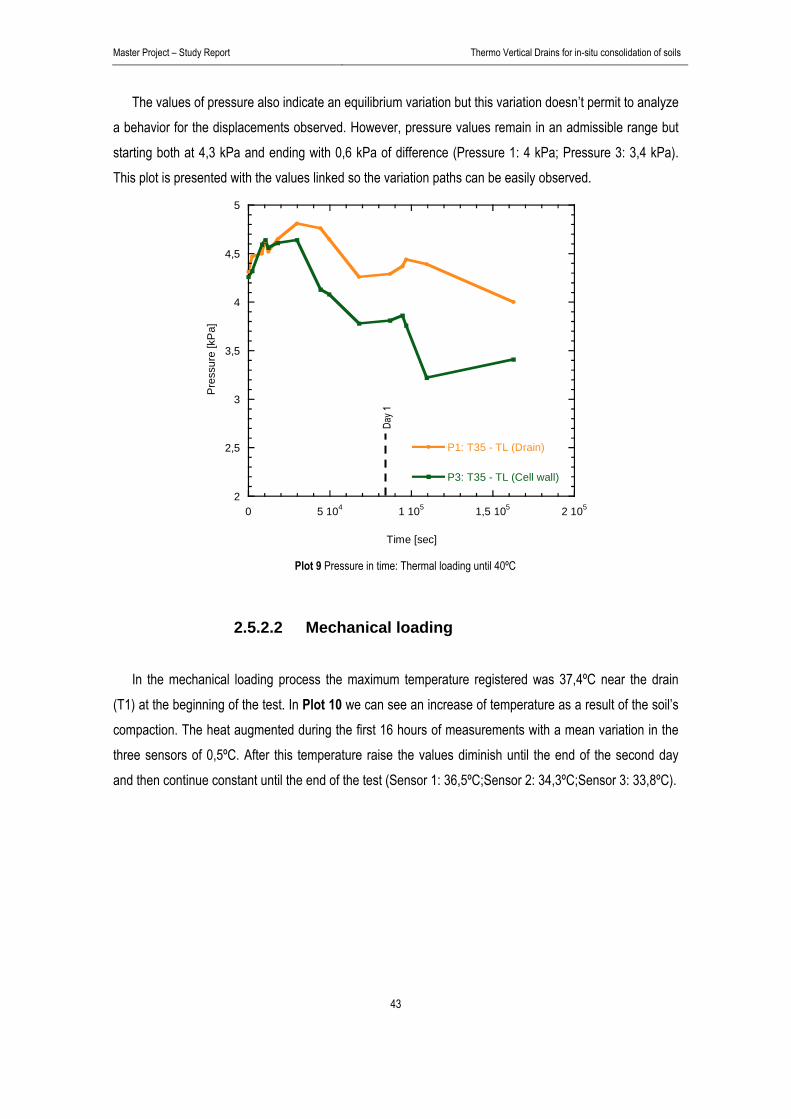
Master Project – Study Report Thermo Vertical Drains for in-situ consolidation of soils
43
The values of pressure also indicate an equilibrium variation but this variation doesn’t permit to analyze a behavior for the displacements observed. However, pressure values remain in an admissible range but starting both at 4,3 kPa and ending with 0,6 kPa of difference (Pressure 1: 4 kPa; Pressure 3: 3,4 kPa). This plot is presented with the values linked so the variation paths can be easily observed.
2
2,5
3
3,5
4
4,5
5
0 5 104 1 105 1,5 105 2 105
P1: T35 - TL (Drain)
P3: T35 - TL (Cell wall)
Pre
ssur
e [k
Pa]
Time [sec] Plot 9 Pressure in time: Thermal loading until 40ºC
2.5.2.2 Mechanical loading In the mechanical loading process the maximum temperature registered was 37,4ºC near the drain
(T1) at the beginning of the test. In Plot 10 we can see an increase of temperature as a result of the soil’s compaction. The heat augmented during the first 16 hours of measurements with a mean variation in the three sensors of 0,5ºC. After this temperature raise the values diminish until the end of the second day and then continue constant until the end of the test (Sensor 1: 36,5ºC;Sensor 2: 34,3ºC;Sensor 3: 33,8ºC).
Day 1

Master Project – Study Report Thermo Vertical Drains for in-situ consolidation of soils
44
30
32
34
36
38
40
0 1 105 2 105 3 105 4 105 5 105 6 105 7 105 8 105
T1: T35 - TL (Drain)
T2: T35 - TL (Middle)
T3: T35 - TL (Cell wall)
Tem
pera
ture
[ºC
]
Time [sec] Plot 10 Temperature in time: Mechanical consolidation
The final displacement measured was 125,38 mm within approximately 0,53 m of initial soil’s height.
For this final displacement we get a compression ratio around, 125,38/0,53 0,237 which means that
the sample’s height diminishes also from a quarter, 25% like the test at ambient temperature but now
in 5 days for an equal charge of 50,75 kN/m2. The displacement showed in Plot 11 is the result of a mean value obtained by four measurement
devices. The curve is well defined which is similar to the case at ambient temperature. For pressure we get now, in our understanding, a better approximation for the second half of the
consolidation process. The explanation for this may be the 50 kPa variation that the sensors suffered which now, at 40ºC, has a quicker recover due to the induced heat. Therefore, the sensors don’t have enough time to adjust for this variation and give an accurate value which is then corrected in time. For the case at ambient temperature, the pressure values seem to give a worst approximation in the second half of the mechanical consolidation. This may be due to the slow variation of pressure in time which interferes with the sensor’s accuracy. The pressure values obtained are presented in Plot 12.
Day 2
Day 1
Day 3
Day 4
Day 5
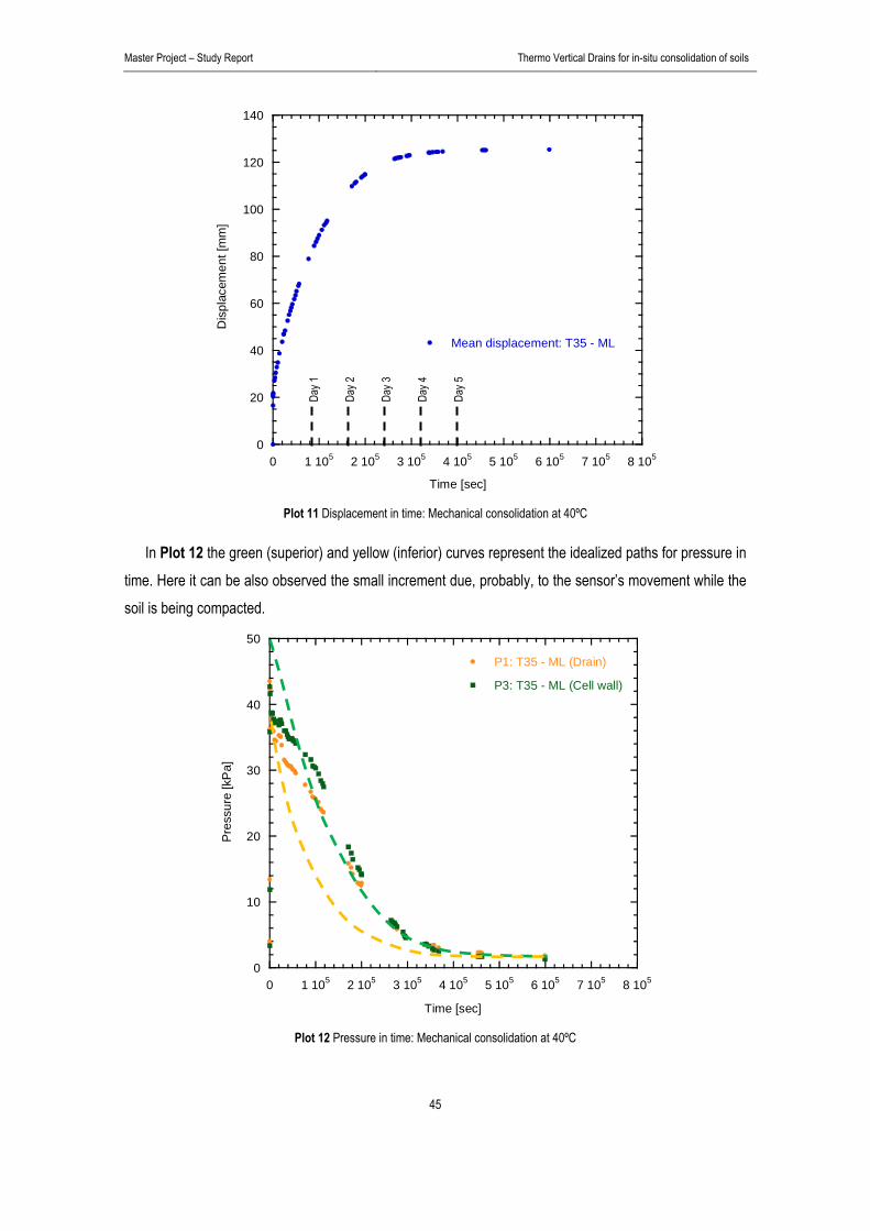
Master Project – Study Report Thermo Vertical Drains for in-situ consolidation of soils
45
0
20
40
60
80
100
120
140
0 1 105 2 105 3 105 4 105 5 105 6 105 7 105 8 105
Mean displacement: T35 - ML
Dis
plac
emen
t [m
m]
Time [sec] Plot 11 Displacement in time: Mechanical consolidation at 40ºC
In Plot 12 the green (superior) and yellow (inferior) curves represent the idealized paths for pressure in time. Here it can be also observed the small increment due, probably, to the sensor’s movement while the soil is being compacted.
0
10
20
30
40
50
0 1 105 2 105 3 105 4 105 5 105 6 105 7 105 8 105
P1: T35 - ML (Drain)
P3: T35 - ML (Cell wall)
Pre
ssur
e [k
Pa]
Time [sec] Plot 12 Pressure in time: Mechanical consolidation at 40ºC
Day 2
Day 1
Day 3
Day 4
Day 5

Master Project – Study Report Thermo Vertical Drains for in-situ consolidation of soils
46
In the end of this test it’s clear that two equal soil samples in equivalent conditions, the one on which temperature is imposed have a considerable higher rate of consolidation. All values that are the basis of the plots presented on this chapter are presented in Appendix 2.2.3 A) and B).
2.5.2.3 Mechanical unloading In the mechanical unloading temperature was practically constant and equal to 36,5ºC in sensor 1,
34,3ºC in sensor 2 and 33,8ºC in sensor 3. So, the same variation is always observed between sensors at this high temperature.
30
32
34
36
38
40
0 2 104 4 104 6 104 8 104 1 105
T1: T35 - MU (Drain)
T2: T35 - MU (Middle)
T3: T35 - MU (Cell wall)
Tem
pera
ture
[ºC
]
Time [sec] Plot 13 Temperature in time: Mechanical unloading at 40ºC
Displacements seen during the mechanical unloading are presented in Plot 14. The recovered
displacement with the mechanical unloading is similar to the one obtained at ambient temperature. The charges were removed also in one and half minutes and the displacement observed is around 1,5 mm (1,56mm). Again we get an elastic displacement around 1,2% considering the total displacement observed (125,38mm).
This value of displacement is, however, smaller than the one registered for the case at ambient
temperature which may be related to the expansion observed in the cylinder at this temperature that also affects its radius.

Master Project – Study Report Thermo Vertical Drains for in-situ consolidation of soils
47
In pressure measurements we’ve again negative pressures registered, Plot 15. But the negative pressure is now in all mid-section of the cylinder. Again, as soon as the charge was removed a negative pressure is obtained in the cylinder that goes up to minus 10 kPa. At ambient temperature the variation of pressure between sensors was around 9 kPa with only the sensor near the cylinder’s wall giving a negative pressure. In this test the variation between both sensors is practically constant to 1 kPa and the values obtained in the end are around the same ones observed in the beginning.
It can be said that, despite of the values difference, the type of behavior observed for the pressure
sensors in the mechanical unloading at different temperatures is quite similar. This higher negative pressure can also be the cause for a smaller value of displacement recovered in
comparison with the test at ambient temperature.
-1,6
-1,4
-1,2
-1
-0,8
-0,6
-0,4
-0,2
0
0 2 104 4 104 6 104 8 104 1 105
Mean displacement: T35 - MU
Dis
plac
emen
t [m
m]
Time [sec] Plot 14 Displacement in time: Mechanical unloading at 40ºC
Day 1

Master Project – Study Report Thermo Vertical Drains for in-situ consolidation of soils
48
-12
-10
-8
-6
-4
-2
0
2
4
0 2 104 4 104 6 104 8 104 1 105
P1: T35 - MU (Drain)
P3: T35 - MU (Cell wall)
Pres
sure
[kPa
]
Time [sec]
Plot 15 Pressure in time: Mechanical unloading at 40ºC
All values that are the basis of the plots presented on this chapter are presented in Appendix 3.2.4 A)
and B).
2.5.2.4 Thermal unloading The values for thermal unloading at different temperatures are presented in Plot 16. If the isolation mousse that involves the cell is removed the temperature unloading takes approximately
2 days. The unloading starts with a high temperature gradient at different radial distances and after a few hours temperature becomes similar decreasing equally in time.
In the end we’ve an average 23ºC in the cylinder with the normal temperature gradient of 0,4ºC at ambient temperature.

Master Project – Study Report Thermo Vertical Drains for in-situ consolidation of soils
49
22
24
26
28
30
32
34
36
38
0 5 104 1 105 1,5 105 2 105
T1: T35 - TU (Drain)
T2: T35 - TU (Middle)
T3: T35 - TU (Cell wall)
Tem
pera
ture
[ºC
]
Time [sec] Plot 16 Temperature in time: Thermal unloading from 40ºC
The values observed in thermal unloading are presented in Plot 17.
-0,04
-0,03
-0,02
-0,01
0
0,01
0,02
0 5 104 1 105 1,5 105 2 105
Mean displacement: T35 - TU
Dis
plac
emen
t [m
m]
Time [sec] Plot 17 Displacement in time: Thermal unloading from 40ºC
Day 1
Day 2
Day 1
Day 2

Master Project – Study Report Thermo Vertical Drains for in-situ consolidation of soils
50
It can be seen that displacement is within the same scale as in thermal loading. In this step we’ve initially compression with an inversion followed by expansion. This expansion has the same displacement modulus as in the case of thermal loading.
Pressure values are presented in Plot 18. We found again negative pressure for this case but only
near the cylinder’s wall. In the thermal unloading we find in the beginning a concave curve that becomes convex after approximately half a day. This inflection point coincides approximately with the highest compression displacement observed in Plot 17.
The variation of pressure between sensors is approximately equal during the thermal unloading and
around 0,5 kPa. The values at the end correspond to the ones observed in the beginning which means that the same equilibrium state was obtained.
-1
-0,5
0
0,5
1
1,5
2
2,5
0 5 104 1 105 1,5 105 2 105
P1: T35 - TU (Drain)
P3: T35 - TU (Cell wall)
Pres
sure
[kPa
]
Time [sec] Plot 18 Pressure in time: thermal unloading from 40ºC
The values presented on these plots are available in Appendix 3.2.5 A) and B).
Day 1

Master Project – Study Report Thermo Vertical Drains for in-situ consolidation of soils
51
2.5.3 Test at 60ºC The soil used on this test is recovered from the one used in the test at 40ºC. In this case we’ve a soil
layer of 33 cm high with a water content of 71% and a layer of 12 cm with a water content of 74%. This test at high temperature will be used to confirm some of the phenomena observed in the cell and
is divided in:
Thermal loading, TL – a thermal load is applied to the soil as in the case of the test at 40ºC;
Mechanical loading, ML – loads are applied to simulate a vertical charge of 50 kN/m2 with the same procedure for the last two tests in order to represent the same conditions;
Thermal unloading, TU – the foam that involves the cylinder, in order to enhance the heat
retention, is removed and the heating system is turned off. This step comes first than mechanical unloading in this test so we can identify the changes between thermal unloading with a mechanical charge of 50 kN/m2 and 5 kN/m2;
Mechanical unloading, MU – the loads are removed in 9 steps so negative pressures aren’t
observed as in the last two tests. With this we can now verify the total displacement due to the elastic recovery of the soil.
These test measurements at all steps are presented in Appendix 2.3. The displacement and pore
pressure values for the four steps of this test at 60ºC are presented next. The pore pressure sensors are located in the same place as in the test at 40ºC. The first is near the
drain and the second sensor is near the cylinder’s wall.
2.5.3.1 Thermal loading To impose an average 53ºC inside the cylinder it takes two days with a temperature level of 62ºC
during one day and 71ºC during another day in the water inside the heating device. Temperature isn’t constant and has a radial variation of 5,1ºC. This variation increases with the
increase of the temperature imposed.

Master Project – Study Report Thermo Vertical Drains for in-situ consolidation of soils
52
20
25
30
35
40
45
50
55
60
0 5x10⁴ 1x10⁵ 1,5x10⁵ 2x10⁵
T1: T53 - TL (Drain)
T2: T53 - TL (Middle)
T3: T53 - TL (Cell wall)
Mean temperature
Tem
pera
ture
[ºC
]
Time [sec] Plot 19 Temperature in time: Thermal loading until 60ºC
For the displacements during the heating phase we get Plot 20. The expansion observed is around 0,007 mm but it’s important to refer that this soil expansion value is affected by the quicker increase of the temperature. The value is ten times smaller than the one observed for the test at 40ºC.
-0,14
-0,12
-0,1
-0,08
-0,06
-0,04
-0,02
0
0,02
0 5 104 1 105 1,5 105 2 105
Mean displacement: T53 - TL
Dis
plac
emen
t [m
m]
Time [sec] Plot 20 Displacement in time: Thermal loading until 60ºC
Day 1
Da
y 1
Day 2

Master Project – Study Report Thermo Vertical Drains for in-situ consolidation of soils
53
The values of pressure also indicate an equilibrium variation but this variation doesn’t permit to analyze a behavior for the displacements observed. However, pressure values remain in an admissible range but starting both at 1,8 kPa and ending with 1,3 kPa. This plot is presented with the values linked so the variation paths can be easily observed.
0
1
2
3
4
5
6
7
8
0 5 104 1 105 1,5 105 2 105 2,5 105 3 105
P1: T53 - TL (Cell wall)
P3: T53 - TL (Drain)
P2: T53 - TL (Middle)
Pre
ssur
e [k
Pa]
Time [sec] Plot 21 Pressure in time: Thermal loading until 60ºC
2.5.3.2 Mechanical loading In the mechanical loading process the maximum temperature registered was 56,6ºC near the drain
during the test. In Plot 44 we can see an increase of temperature as a result of the soil’s compaction. The heat augmented during the first 14 hours of measurements with a mean variation in the three sensors of 1ºC. After this temperature raise the values diminish until the end of the second day and then continue constant until the end of the test (Sensor 1: 53,4ºC;Sensor 2: 48,8ºC;Sensor 3: 47,3ºC).
Day 2
Day 1
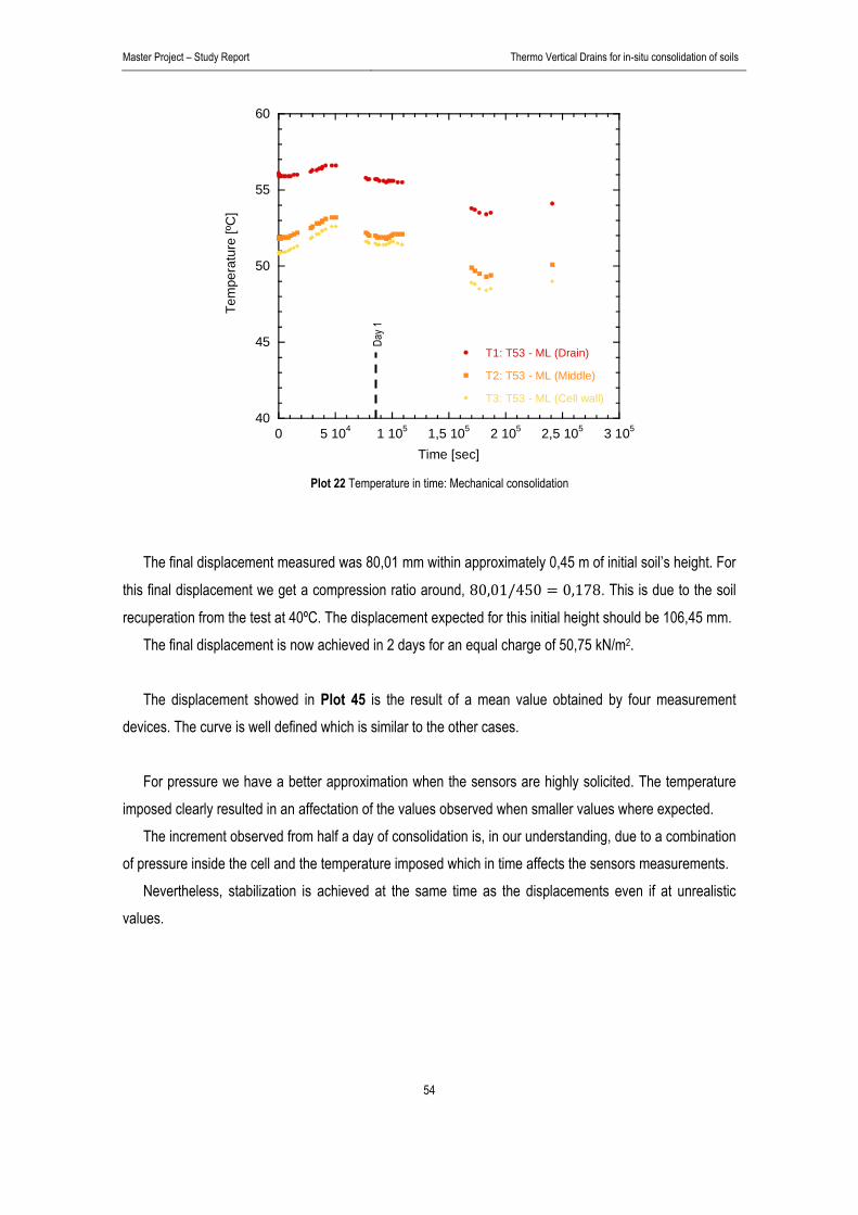
Master Project – Study Report Thermo Vertical Drains for in-situ consolidation of soils
54
40
45
50
55
60
0 5 104 1 105 1,5 105 2 105 2,5 105 3 105
T1: T53 - ML (Drain)
T2: T53 - ML (Middle)
T3: T53 - ML (Cell wall)
Tem
pera
ture
[ºC
]
Time [sec] Plot 22 Temperature in time: Mechanical consolidation
The final displacement measured was 80,01 mm within approximately 0,45 m of initial soil’s height. For
this final displacement we get a compression ratio around, 80,01/450 0,178. This is due to the soil
recuperation from the test at 40ºC. The displacement expected for this initial height should be 106,45 mm. The final displacement is now achieved in 2 days for an equal charge of 50,75 kN/m2. The displacement showed in Plot 45 is the result of a mean value obtained by four measurement
devices. The curve is well defined which is similar to the other cases. For pressure we have a better approximation when the sensors are highly solicited. The temperature
imposed clearly resulted in an affectation of the values observed when smaller values where expected. The increment observed from half a day of consolidation is, in our understanding, due to a combination
of pressure inside the cell and the temperature imposed which in time affects the sensors measurements. Nevertheless, stabilization is achieved at the same time as the displacements even if at unrealistic
values.
Day 1
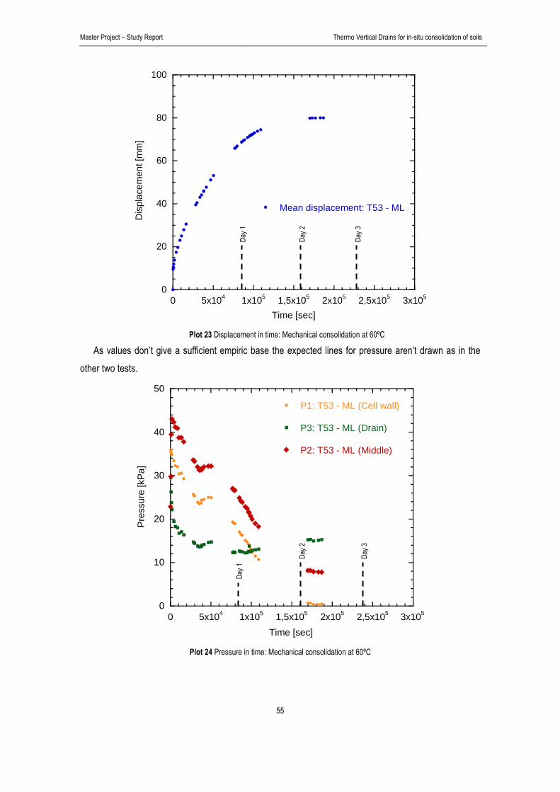
Master Project – Study Report Thermo Vertical Drains for in-situ consolidation of soils
55
0
20
40
60
80
100
0 5x10⁴ 1x10⁵ 1,5x10⁵ 2x10⁵ 2,5x10⁵ 3x10⁵
Mean displacement: T53 - ML
Dis
plac
emen
t [m
m]
Time [sec] Plot 23 Displacement in time: Mechanical consolidation at 60ºC
As values don’t give a sufficient empiric base the expected lines for pressure aren’t drawn as in the other two tests.
0
10
20
30
40
50
0 5x10⁴ 1x10⁵ 1,5x10⁵ 2x10⁵ 2,5x10⁵ 3x10⁵
P1: T53 - ML (Cell wall)
P3: T53 - ML (Drain)
P2: T53 - ML (Middle)
Pres
sure
[kPa
]
Time [sec] Plot 24 Pressure in time: Mechanical consolidation at 60ºC
Day 1
Day 2
Day 3
Day 2
Day 1
Day 3

Master Project – Study Report Thermo Vertical Drains for in-situ consolidation of soils
56
All values that are the basis of the plots presented on this chapter are presented in Appendix 2.3.3 A) and B).
2.5.3.3 Thermal unloading The values for thermal unloading at different temperatures are presented in Plot 25. If the isolation mousse that involves the cell is removed the temperature unloading takes approximately
one and a half days. The unloading starts with a high temperature gradient at different radial distances and after a few hours temperature becomes similar diminishing equally in time.
In the end we’ve an average 23ºC in the cylinder with the normal temperature gradient of 0,4ºC at ambient temperature.
20
25
30
35
40
45
50
55
0 5 104 1 105 1,5 105 2 105
T1: T53 - TU (Drain)
T2: T53 - TU (Middle)
T3: T53 - TU (Cell wall)
Tem
pera
ture
[ºC
]
Time [sec] Plot 25 Temperature in time: Thermal unloading from 60ºC
The values observed for the displacements during thermal unloading are presented in Plot 26.
Day 1
Day 2

Master Project – Study Report Thermo Vertical Drains for in-situ consolidation of soils
57
0
0,5
1
1,5
2
0 5 104 1 105 1,5 105 2 105
Mean displacement: T53 - TU
Dis
plac
emen
t [m
m]
Time [sec] Plot 26 Displacement in time: Thermal unloading from 60ºC
It can be seen, as expected, that displacement isn’t within the same scale as in thermal loading. The
inversion of the process in this test can be used to understand how the cell reacts with a thermal unloading at different mechanical charges.
Pressure values are presented in Plot 27. We found again negative pressure for this case but only
near the cylinder’s wall. In the thermal unloading we find that the sensors records shouldn’t be interpreted as with the temperature decrease we see a recovery of the values approximately to the initial values.
The variation of pressure between sensors is approximately equal during the thermal unloading and around 0,5 kPa. The values at the end differ from the ones at the beginning with high variations (Sensor 1: +3 kPa; Sensor 3: -10 kPa; Sensor 2: -1 kPa) which means that the same equilibrium state wasn’t obtained.
Observing now the values of pore pressure before the thermal loading we even see that none of the pressure sensors returns to the approximately the same values.
Day 1
Day 2

Master Project – Study Report Thermo Vertical Drains for in-situ consolidation of soils
58
-4
0
4
8
12
0 5 104 1 105 1,5 105 2 105 2,5 105 3 105
P1: T53 - TU (Cell wall)
P3: T53 - TU (Drain)
P2: T53 - TU (Middle)
Pres
sure
[kPa
]
Time [sec] Plot 27 Pressure in time: thermal unloading from 60ºC
The values presented on these plots are available in Appendix 2.3.5 A) and B).
2.5.4.4 Mechanical unloading In the mechanical unloading temperature was practically constant and equal to 22,8ºC in sensor 1,
22,7ºC in sensor 2 and 22,6ºC in sensor 3.
20
21
22
23
24
25
0 2 104 4 104 6 104 8 104 1 105
T1: T53 - MU (Drain)
T2: T53 - MU (Middle)
T3: T53 - MU (Cell wall)
Tem
pera
ture
[ºC
]
Time [sec] Plot 28 Temperature in time: Mechanical unloading
Day 2
Day 3
Day 1

Master Project – Study Report Thermo Vertical Drains for in-situ consolidation of soils
59
Displacements seen during the mechanical unloading are presented in Plot 29. The recovered displacement with the mechanical unloading was made in a different form than in the other tests. The charges were removed in 6 levels so pressure inside the cell could be maintained positive. This would be useful to verify if the elastic recovery of the soil was affected by negative pressures which result on suction and rearrangement of the soil inside the cell.
The final displacement observed is around 1,0 mm (0,95 mm). Again we get an elastic displacement
around 1,2% considering the total displacement observed (80,01mm). So, it seems that even with negative pressures in time reduced we arrive to the same elastic recovery of the soil but in a smaller time as the soil recovers more quickly.
In pressure measurements the variations due to the different levels are clearly seen, Plot 15. It seems
that negative pressures still occurre if we consider that the sensors give accurate variations of pressure.. In this test the first two variations correspond to a line of three loads and the following two to two lines (6 loads).
At this final step the values for pressure sensors 1 and 2 are approximately equal to the initial values.
-1
-0,8
-0,6
-0,4
-0,2
0
0 2 104 4 104 6 104 8 104 1 105
Mean displacement: T53 - MU
Dis
plac
emen
t [m
m]
Time [sec] Plot 29 Displacement in time: Mechanical unloading
Day 1
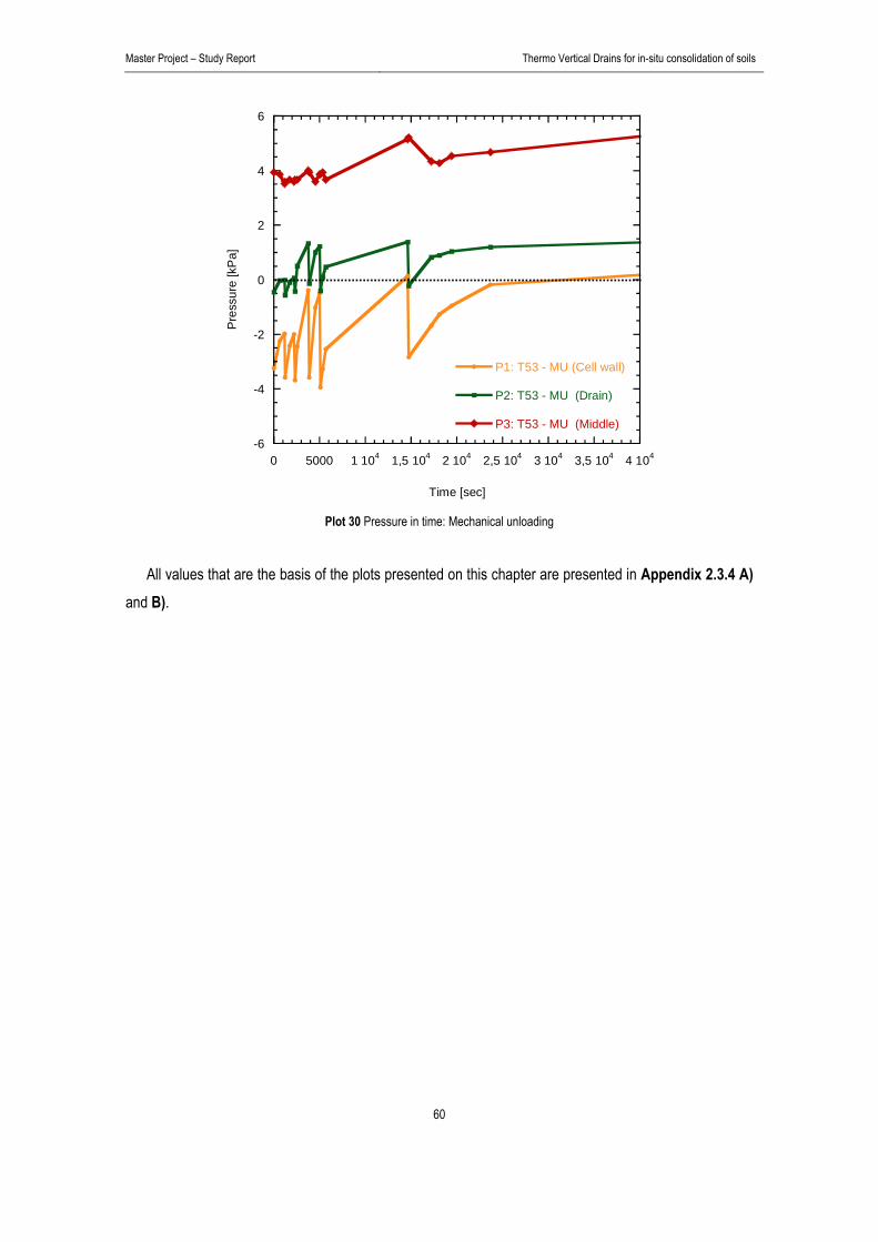
Master Project – Study Report Thermo Vertical Drains for in-situ consolidation of soils
60
-6
-4
-2
0
2
4
6
0 5000 1 104 1,5 104 2 104 2,5 104 3 104 3,5 104 4 104
P1: T53 - MU (Cell wall)
P2: T53 - MU (Drain)
P3: T53 - MU (Middle)
Pre
ssur
e [k
Pa]
Time [sec] Plot 30 Pressure in time: Mechanical unloading
All values that are the basis of the plots presented on this chapter are presented in Appendix 2.3.4 A)
and B).
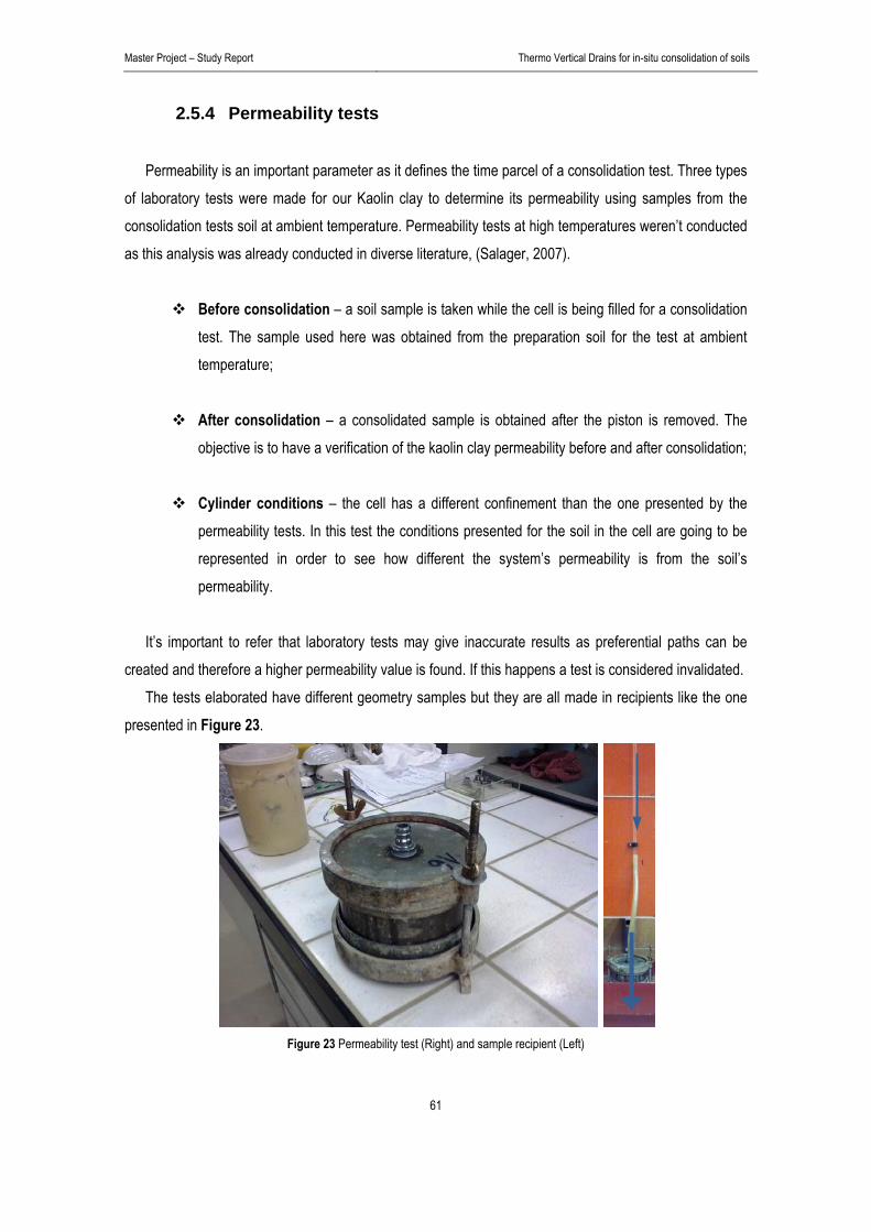
Master Project – Study Report Thermo Vertical Drains for in-situ consolidation of soils
61
2.5.4 Permeability tests Permeability is an important parameter as it defines the time parcel of a consolidation test. Three types
of laboratory tests were made for our Kaolin clay to determine its permeability using samples from the consolidation tests soil at ambient temperature. Permeability tests at high temperatures weren’t conducted as this analysis was already conducted in diverse literature, (Salager, 2007).
Before consolidation – a soil sample is taken while the cell is being filled for a consolidation
test. The sample used here was obtained from the preparation soil for the test at ambient temperature;
After consolidation – a consolidated sample is obtained after the piston is removed. The objective is to have a verification of the kaolin clay permeability before and after consolidation;
Cylinder conditions – the cell has a different confinement than the one presented by the
permeability tests. In this test the conditions presented for the soil in the cell are going to be represented in order to see how different the system’s permeability is from the soil’s permeability.
It’s important to refer that laboratory tests may give inaccurate results as preferential paths can be
created and therefore a higher permeability value is found. If this happens a test is considered invalidated. The tests elaborated have different geometry samples but they are all made in recipients like the one
presented in Figure 23.
Figure 23 Permeability test (Right) and sample recipient (Left)
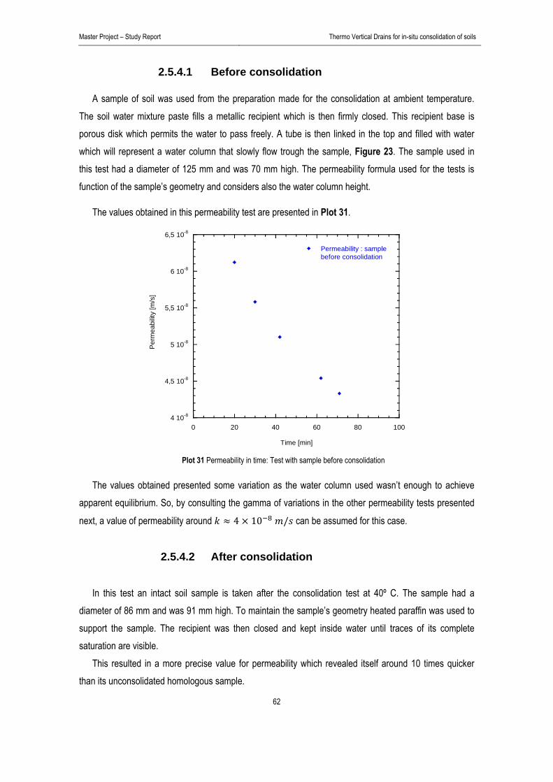
Master Project – Study Report Thermo Vertical Drains for in-situ consolidation of soils
62
2.5.4.1 Before consolidation
A sample of soil was used from the preparation made for the consolidation at ambient temperature. The soil water mixture paste fills a metallic recipient which is then firmly closed. This recipient base is porous disk which permits the water to pass freely. A tube is then linked in the top and filled with water which will represent a water column that slowly flow trough the sample, Figure 23. The sample used in this test had a diameter of 125 mm and was 70 mm high. The permeability formula used for the tests is function of the sample’s geometry and considers also the water column height.
The values obtained in this permeability test are presented in Plot 31.
4 10-8
4,5 10-8
5 10-8
5,5 10-8
6 10-8
6,5 10-8
0 20 40 60 80 100
Permeability : samplebefore consolidation
Per
mea
bilit
y [m
/s]
Time [min] Plot 31 Permeability in time: Test with sample before consolidation
The values obtained presented some variation as the water column used wasn’t enough to achieve apparent equilibrium. So, by consulting the gamma of variations in the other permeability tests presented
next, a value of permeability around 4 10 / can be assumed for this case.
2.5.4.2 After consolidation In this test an intact soil sample is taken after the consolidation test at 40º C. The sample had a
diameter of 86 mm and was 91 mm high. To maintain the sample’s geometry heated paraffin was used to support the sample. The recipient was then closed and kept inside water until traces of its complete saturation are visible.
This resulted in a more precise value for permeability which revealed itself around 10 times quicker than its unconsolidated homologous sample.

Master Project – Study Report Thermo Vertical Drains for in-situ consolidation of soils
63
The values for this test are presented in Plot 32. Vertical permeability for a consolidated sample with
50 kPa is now around 2,5 10 / .
2,4 10-7
2,5 10-7
2,6 10-7
2,7 10-7
2,8 10-7
2,9 10-7
3 10-7
0 20 40 60 80 100
Permeability : Consolidated sample
Per
mea
bilit
y [m
/s]
Time [min] Plot 32 Permeability in time: test with sample before consolidation
2.5.4.3 Experimental cell conditions As permeability values changed between samples for consolidated and unconsolidated cases another
test was conducted to see if a different value could be obtained. When simulations were run, 4.1.6.1 Ambient temperature test – Mechanical consolidation (p.96)
the optimal value found, for horizontal permeability, to represent the experimental results at ambient
temperature, 2.5.1.1 Mechanical loading (p.36) was 8,21 10 / .
So, we’ve an optimal value within the 10 base which is ten to twenty times smaller than the values
already obtained. Therefore, a representation of the cylinder conditions is proposed in order to determine if the system’s permeability is different from the soil’s permeability.
The cylinder has a diameter of 31 cm with a central drain having a diameter of 2,7 cm which
represents a ratio between both around 0,1. With this geometry defined one of the recipients used is going to be sealed in the base leaving a centre opening respecting the same ratio. This test doesn’t represent in reality all the conditions observed for the cylinder. Its objective is mainly to show that permeability in this case is function of the soil’s confinement in the cell.
Results show a value for permeability 1,2 10 / which reveals that the conditions found
in our case affect the value of permeability to be used in the simulations to reproduce the experimental tests.

Master Project – Study Report Thermo Vertical Drains for in-situ consolidation of soils
64
1 10-9
1,5 10-9
2 10-9
2,5 10-9
3 10-9
0 50 100 150 200 250 300 350
Permeability: Cylinder conditions
Per
mea
bilit
y [m
/s]
Time [min] Plot 33 Permeability in time: test in oedometer conditions
The results obtained by these permeability tests are merely representative as more tests are needed so values can be filtered and a concrete value determined.
2.5.4.4 Conclusions
The objective of these permeability tests is to understand the variation of permeability with the conditions on which the soil is accommodated in the laboratory cell. Therefore, it can be concluded that the permeability obtained, Table 6 is higher when compacted which normally happens when the soil is loose. This shows the difficulty for obtaining accurate values for soil permeability in laboratory.
Finally, a variation of the base configuration demonstrates that, in the cell, the geometry of the system where the soil is confined influences the capacity for the water to flow. So, the actual value for permeability in the cell is going to be defined from the mechanical consolidation in the test at ambient temperature, T22 – ML and used as reference for the simulations. This value is similar to the one obtained in the permeability test for the experimental cell conditions.
Sample Base Permeability (m/s)
Unconsolidated
4 10
Consolidated 2,5 10
Unconsolidated
1,2 10
Table 6 Permeability tests values function of sample consolidation and recipient base configuration
Db
Db /10
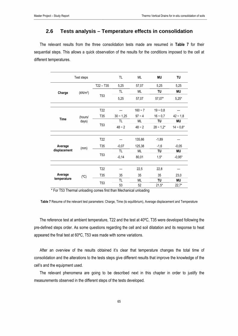
Master Project – Study Report Thermo Vertical Drains for in-situ consolidation of soils
65
2.6 Tests analysis – Temperature effects in consolidation
The relevant results from the three consolidation tests made are resumed in Table 7 for their sequential steps. This allows a quick observation of the results for the conditions imposed to the cell at different temperatures.
Test steps TL ML MU TU
Charge (kN/m2)
T22 – T35 5,25 57,07 5,25 5,25
T53 TL ML TU MU
5,25 57,07 57,07* 5,25*
Time (hours/ days)
T22 --- 160 ~ 7 19 ~ 0,8 --- T35 30 ~ 1,25 97 ~ 4 16 ~ 0,7 42 ~ 1,8
T53 TL ML TU MU
48 ~ 2 48 ~ 2 28 ~ 1,2* 14 ~ 0,6*
Average displacement (mm)
T22 --- 135,66 -1,89 ---
T35 -0,07 125,38 -1,6 -0,05
T53 TL ML TU MU
-0,14 80,01 1,5* -0,95*
Average temperature (ºC)
T22 --- 22,5 22,8 ---
T35 35 35 35 23,0
T53 TL ML TU MU 53 52 21,5* 22,7*
* For T53 Thermal unloading comes first than Mechanical unloading
Table 7 Resume of the relevant test parameters: Charge, Time (to equilibrium), Average displacement and Temperature
The reference test at ambient temperature, T22 and the test at 40ºC, T35 were developed following the
pre-defined steps order. As some questions regarding the cell and soil dilatation and its response to heat appeared the final test at 60ºC, T53 was made with some variations.
After an overview of the results obtained it’s clear that temperature changes the total time of
consolidation and the alterations to the tests steps give different results that improve the knowledge of the cell’s and the equipment used.
The relevant phenomena are going to be described next in this chapter in order to justify the measurements observed in the different steps of the tests developed.

Master Project – Study Report Thermo Vertical Drains for in-situ consolidation of soils
66
2.6.1 Displacements As already explained, the main purpose of this study is to demonstrate the evolution of consolidation
velocity in fully saturated media, in particular for clays, when temperature is applied as the water viscosity changes. In Plot 34 this phenomenon is clearly observed with consolidation rate increasing for higher temperatures inside the cell. It’s important to refer again that temperature loading is applied before mechanical consolidation and this one only starts when temperature equilibrium is achieved.
0
20
40
60
80
100
0 1 105 2 105 3 105 4 105 5 105 6 105 7 105 8 105
Mean displacement: T22 - MLMean displacement: T35 - MLMean displacement: T53 - ML
Aver
age
degr
ee o
f con
solid
atio
n [%
]
Time [sec] Plot 34 Average degree of consolidation for mechanical loading in all tests – T22, T35 and T53
The different initial heights of the soil samples and the re-use in T53 of the soil in T35 result in different
initial conditions and therefore the results are shown in average degree of consolidation so they can be compared.
It was also mentioned before that some soil blocked the water exchanged device tube which decreased the initial rate of consolidation in T53 until the water started to be expelled from the piston, Figure 25.

Master Project – Study Report Thermo Vertical Drains for in-situ consolidation of soils
67
-2
-1,5
-1
-0,5
0
0 2 104 4 104 6 104 8 104 1 105
Mean displacement: T22 - MU
Mean displacement: T35 - MU
Mean displacement: T53 - MU
Dis
plac
emen
t [m
m]
Time [sec] Plot 35 Mean displacement for mechanical unloading in all tests: T22, T35 and (T53 – T=22ºC)
For T22 and T35 the mechanical unloading consisted in removing all weights at the same rate during one and a half minutes and for T53 the removal was phased as shown in Figure 24. Therefore, the elastic recovery of the soil has a similar path for T22 and T35 but with different final values due to the different initial heights of the samples, Plot 35. It is important to see that this path is the same even with mechanical unloading at high temperatures. So, by approximation and using T22 as reference, a variation of 0,1 mm for each 0,01 meters of sample initial height is expected (in a range of initial heights around 0,45 to 0,55 meters).
Therefore, with this approximation it should be expected an expansion of 0,75 mm or less for T53
(sample with initial height of 0,45 meters) but the total recuperation of the soil is around 0,95 mm. The phased mechanical unloading had the objective of decreasing the time where negative pore pressures occurre inside the cell due to vacuum caused by a quick load removal, Plot 15 and see if this was related to the soil elastic recovery. So, a higher recovery can be said to be observed but remaining cautious on the magnitude of the values in the tests due to the characteristics of the soil used in T53 (soil recovered from T35).
57 kPa
(sec) 90
1000
2500
4000
5000
1500
0
5 kPa
Figure 24 Mechanical unloading paths: T22 and T35 (linear line) and T53 (levelled line)

Master Project – Study Report Thermo Vertical Drains for in-situ consolidation of soils
68
A calibration of the cell behaviour to high temperatures, when completely filled with water, was conducted before initiating the tests and the results are shown in Appendix 1. But, analysing the results obtained in thermal loading and unloading with the soil can be more effective than extrapolating them from a water calibration.
While applying thermal loading to the soil in T53 the heating system was aimed for two levels. So, by comparing the temperature in the cell with the displacements response, Plot 36 it can admitted a real-time response to heat by the cell. It can be also said that a 0,02 mm expansion is observed for each 5ºC temperature increase. This expansion is a combination of the soil’s and cell dilatation. The first results in an expansion slightly bigger than the contraction of the cell (do to the radius increase).
For T53 thermal unloading comes first than mechanical unloading. As observed before, Plot 35 the mechanical unloading path can be assumed equal at high or ambient temperature.
Plot 36 Temperature featuring displacement for thermal loading in T35 and T53
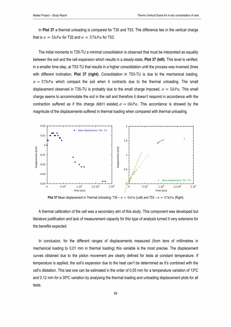
Master Project – Study Report Thermo Vertical Drains for in-situ consolidation of soils
69
In Plot 37 a thermal unloading is compared for T35 and T53. The difference lies in the vertical charge that is 5 for T35 and 57 for T53.
The initial moments in T35-TU a minimal consolidation is observed that must be interpreted as equality
between the soil and the cell expansion which results in a steady-state, Plot 37 (left). This level is verified, in a smaller time step, at T53-TU that results in a higher consolidation until the process was inversed (lines with different inclination, Plot 37 (right). Consolidation in T53-TU is due to the mechanical loading,
57 which compact the soil when it contracts due to the thermal unloading. The small
displacement observed in T35-TU is probably due to the small charge imposed, 5 . This small
charge seems to accommodate the soil in the cell and therefore it doesn’t respond in accordance with the
contraction suffered as if this charge didn’t existed, 0 . This accordance is showed by the
magnitude of the displacements suffered in thermal loading when compared with thermal unloading.
-0,04
-0,03
-0,02
-0,01
0
0,01
0,02
0 5 104 1 105 1,5 105 2 105
Mean displacement: T35 - TU
Dis
plac
emen
t [m
m]
Time [sec]
0
0,5
1
1,5
2
0 5 104 1 105 1,5 105 2 105
Mean displacement: T53 - TU
Dis
plac
emen
t [m
m]
Time [sec] Plot 37 Mean displacement in Thermal Unloading: T35 – 5 (Left) and T53 – 57 (Right)
A thermal calibration of the cell was a secondary aim of this study. This component was developed but
literature justification and lack of measurement capacity for this type of analysis turned it very extensive for the benefits expected.
In conclusion, for the different ranges of displacements measured (from tens of millimetres in
mechanical loading to 0,01 mm in thermal loading) this variable is the most precise. The displacement curves obtained due to the piston movement are clearly defined for tests at constant temperature. If temperature is applied, the soil’s expansion due to the heat can’t be determined as it’s combined with the cell’s dilatation. This last one can be estimated in the order of 0,05 mm for a temperature variation of 13ºC and 0,12 mm for a 30ºC variation by analysing the thermal loading and unloading displacement plots for all tests.

Master Project – Study Report Thermo Vertical Drains for in-situ consolidation of soils
70
2.6.2 Pore pressure The pore pressure sensors represent the most sensible of the measured variables. The sensors were
the aim of a calibration process before the tests in order to obtain the best values as possible, Appendix 1.
From the tests made, we can say that:
the sensors give good records when highly solicited (immediately after mechanical charge variations);
variations are still registered while displacements occurre;
when equilibrium is achieved the sensors stabilise. This stabilisation is observed at the expected values for measurements at ambient temperature and 35ºC but a discrepancy is observed for T53. This divergence of values at 53ºC is observed in all sensors but all conclusions traced remain the same;
the values measured are also function of the water’s level in the exchange water device which needs to be kept as soon as possible near the soil’s layer surface and before taking pressure measurements;
These conclusions can be observed for the two cases shown in that are: T53 – ML which corresponds
to the pore pressure measurements taken at T=53ºC with 57 and T53 – MU which are related to
the phased mechanical unloading with the cell at ambient temperature.
0
10
20
30
40
50
0 5x10⁴ 1x10⁵ 1,5x10⁵ 2x10⁵ 2,5x10⁵ 3x10⁵
Pressure 1 (Cell wall)
Pressure 2 (Drain)
Pressure 3 (Middle)
Pres
sure
[kPa
]
Time [sec]
-6
-4
-2
0
2
4
6
0 5000 1 104 1,5 104 2 104 2,5 104 3 104 3,5 104 4 104
Pressure 1 (Cell wall)
Pressure 2 (Drain)
Pressure 3 (Middle)
Pre
ssur
e [k
Pa]
Time [sec] Plot 38 Pore pressure measurements in T53 – ML (left) and T53 – MU (right)

Master Project – Study Report Thermo Vertical Drains for in-situ consolidation of soils
71
Even with the difficulties mentioned the values of pore pressure are in accordance with the ones expected for the case studied. In Plot 39 the higher rate of pore pressure return to equilibrium is easily observed while pressure also becomes equal more quickly in radial direction for the heated case.
0
10
20
30
40
50
0 1 105 2 105 3 105 4 105 5 105 6 105 7 105 8 105
P1: T22 - ML
P2: T22 - ML
P2: T35 - ML
P1: T35 - ML
Pre
ssur
e [k
Pa]
Time [sec] Plot 39 Pore pressure measurements for T22 – ML and T35 – ML
2.6.3 Temperature
Temperature was the aim of this chapter and in this section the comments developed are regarding the thermal unloading which was quite quicker for T53 then T35. The conditions for TU are the same for both tests with the isolating mousse being removed as soon as the heating system is turned off. The only
apparent difference is in the loading applied, for T35 – 5 and for T53 – 57 . Therefore,
it seems that for higher charges, higher is the temperature dissipation.
20
25
30
35
40
45
50
55
0 5 104 1 105 1,5 105 2 105
T1: T53 - TUT2: T53 - TUT3: T53 - TU
T1: T35 - TUT2: T35 - TUT3: T35 - TU
Tem
pera
ture
[ºC
]
Time [sec] Plot 40 Temperature measurements for thermal unloading in T35 and T53

Master Project – Study Report Thermo Vertical Drains for in-situ consolidation of soils
72
The heating system efficiency is a problematic to be considered. To heat the cell at the pre-defined temperatures the heating system was aimed for higher ones. To reach a temperature of an average 35ºC inside the cell the heating system was set to 44ºC and to have an average 53ºC it was set to 70ºC. When temperature in the laboratory decreases from 23ºC to 21,5ºC the cell register’s a greater heat loss resulting in a decrease of temperature to an average 50ºC which is never recovered to the initial values. Nevertheless, this heating solution is enough for the temperature scope studied resulting in a clear radial temperature field which will surely occurre in real cases.
2.6.4 Water exchanged Following the analysis of the experimental values obtained in the tests made the water exchanged
during them is here studied to evaluate how the cell behaves in different temperature conditions.
2.6.4.1 Soil sample As observed the piston is completely impermeable even with heating dilation phenomena.
Consolidation, for the same applied charge, is demonstrated to be influenced by temperature as already concluded in 2.6.1 Displacements (p.66). This phenomenon is again identified by the exiting water flow rate which initiates as soon as loading is applied and it’s represented in Plot 41 for T22 and T35.
0
1000
2000
3000
4000
5000
0 5 104 1 105 1,5 105 2 105
Water volume: T22 - ML
Water volume: T35 - ML
Wat
er v
olum
e [m
L]
Time [sec] Plot 41 Water volume in time: Mechanical consolidation experimental tests
The concave part, as already explained, represents the limit where the drain porous passes the pistons
centre o-ring which makes a thin water layer above the piston. After the piston is filled the water exchange stabilises.
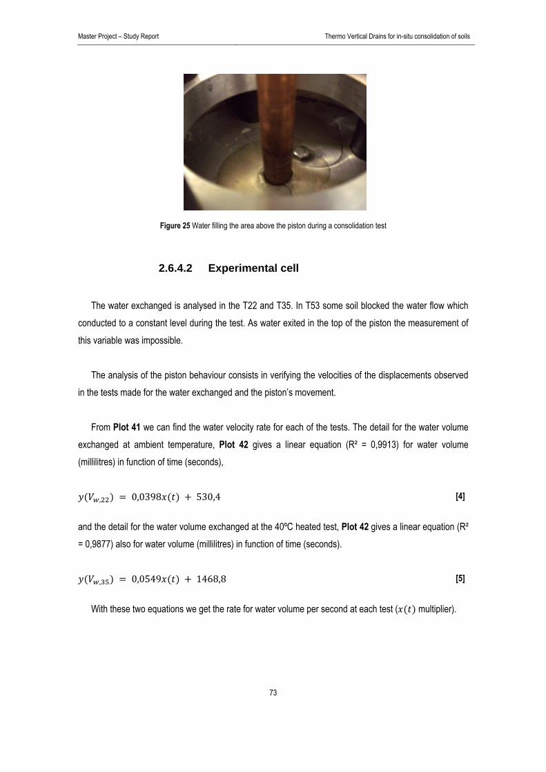
Master Project – Study Report Thermo Vertical Drains for in-situ consolidation of soils
73
Figure 25 Water filling the area above the piston during a consolidation test
2.6.4.2 Experimental cell
The water exchanged is analysed in the T22 and T35. In T53 some soil blocked the water flow which conducted to a constant level during the test. As water exited in the top of the piston the measurement of this variable was impossible.
The analysis of the piston behaviour consists in verifying the velocities of the displacements observed
in the tests made for the water exchanged and the piston’s movement. From Plot 41 we can find the water velocity rate for each of the tests. The detail for the water volume
exchanged at ambient temperature, Plot 42 gives a linear equation (R² = 0,9913) for water volume (millilitres) in function of time (seconds),
, 0,0398 530,4 [4]
and the detail for the water volume exchanged at the 40ºC heated test, Plot 42 gives a linear equation (R² = 0,9877) also for water volume (millilitres) in function of time (seconds).
, 0,0549 1468,8 [5]
With these two equations we get the rate for water volume per second at each test ( multiplier).
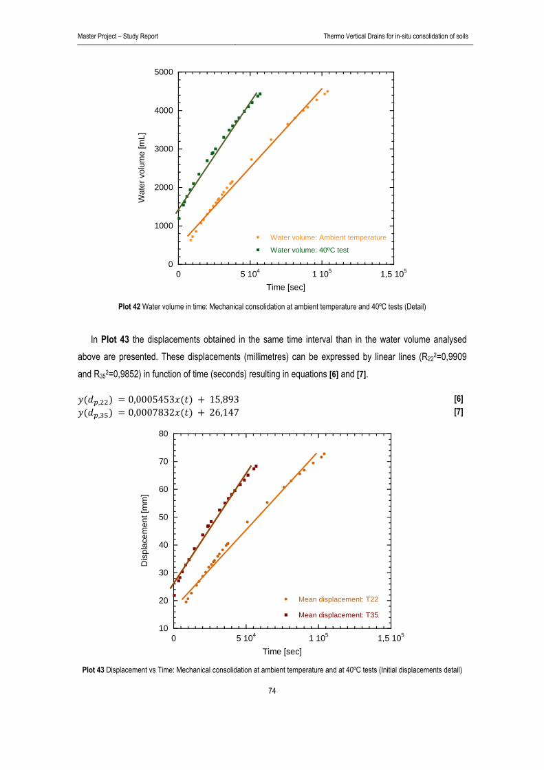
Master Project – Study Report Thermo Vertical Drains for in-situ consolidation of soils
74
0
1000
2000
3000
4000
5000
0 5 104 1 105 1,5 105
Water volume: Ambient temperature
Water volume: 40ºC test
Wat
er v
olum
e [m
L]
Time [sec]
Plot 42 Water volume in time: Mechanical consolidation at ambient temperature and 40ºC tests (Detail)
In Plot 43 the displacements obtained in the same time interval than in the water volume analysed
above are presented. These displacements (millimetres) can be expressed by linear lines (R222=0,9909 and R352=0,9852) in function of time (seconds) resulting in equations [6] and [7].
, 0,0005453 15,893 [6] , 0,0007832 26,147 [7]
10
20
30
40
50
60
70
80
0 5 104 1 105 1,5 105
Mean displacement: T22
Mean displacement: T35
Dis
plac
emen
t [m
m]
Time [sec] Plot 43 Displacement vs Time: Mechanical consolidation at ambient temperature and at 40ºC tests (Initial displacements detail)
Master Project – Study Report Thermo Vertical Drains for in-situ consolidation of soils
75
This water represents approximately a total volume of 4,71 just before apparent stabilisation
on both cases. With the lines defined in Plot 42 and after conversion the velocity of the water exiting is,
, 0,2278 / which is higher than the piston’s velocity, , 0,1963 / obtained from
the line in Plot 43 and considering the cylinder’s area given by equation [8].
[8]
This means that the displacement observed is slower than the one that should be expected. So the consolidation time will also be slower. In fact, this exiting water stabilizes immediately which means that the rest of the water’s imposed displacement will smoothly be absorbed by the piston displacement rate.
For the experimental test at 40ºC we can see that the piston speed increases and is practically equal
to the displacement rate observed for the water volume. Using the same approach as before, by analysis
of Plot 43, we get , 0,3142 / and , 0,2820 / .
So, if we heat the cylinder the consolidation occurs quickly only due to the higher rate of exiting water
but if we do a test at ambient temperature it occurs slower also due to the slower piston’s movement. The ratios for the velocity of the piston in comparison with the velocity of the exiting water are presented next, Table 8.
Test 22ºC 35ºC
/ 0,86 0,90
Table 8 Ratios of movement between piston and exiting water
So, for a higher temperature inside the cell the consolidation time will be better represented with the cylinder moving in accordance with the exiting water’s volume imposed displacement.
Master Project – Study Report Thermo Vertical Drains for in-situ consolidation of soils
76
3. Finite elements simulations
The finite element software chosen for this study is Gefdyn, which was developed by LMSS-Mat at
Ecole Central de Paris in 2003. This software was chosen as it provides temperature analysis and a vast variety of models for geotechnical studies. An overview of this software, description of the contents of each file and how to generate a calculus from a pre-processor mesh to a post-processor results analysis is presented in (Nuth, 2004).
The pre-processor and post-processor used is GID. The choice of this software was made as it’s easily combined with Gefdyn results files. In this study, regarding pre-processing, GID wasn’t used and all meshes were created manually and partially aided by Microsoft Office EXCEL. This mesh creation was possible due to the elements quadrangular format and it wasn’t difficulted by the quantity of elements or the complexity of the mesh (variation of elements size). It can be said that creating a mesh manually is easier than use GID as a pre-processor as it was initially used to build a test mesh. But concerning GID as a post-processor its importance to analyse results isn’t questioned.
The numerical simulations made had a constant evolution during this study and were object of an
intensive work as these cases have never been simulated before with this software. In order to assist and smooth the progress of further studies with GEFDYN software a document will be added in the Appendix CD.
These numerical simulations are divided in two parts: 1. Cylinder – Thermo-Hydro-Mechanical simulations
Firstly, the simulations will be run to reproduce the behaviour of a single vertical drain based in the
experimental tests made with clayey soil, Kaolin in the oedometric cell. As it will be mentioned further ahead, an elastic model is used. This is related to its simplicity in the software, shorten time to run a calculus and the capacity for having several tests calculating at the same time.
2. Embankments – Thermo-Hydro-Mechanical simulations
Secondly, the LGV Rhin-Rhône East branch is a high speed train project managed by Egis society,
Egis Rail. The project includes 57 Km of new line which will connect Dijon and Mulhouse, in France, with a high public interest due to Mulhouse proximity to Basel, Switzerland. This project started at January, 2003 and its conclusion date is expected for October, 2011.
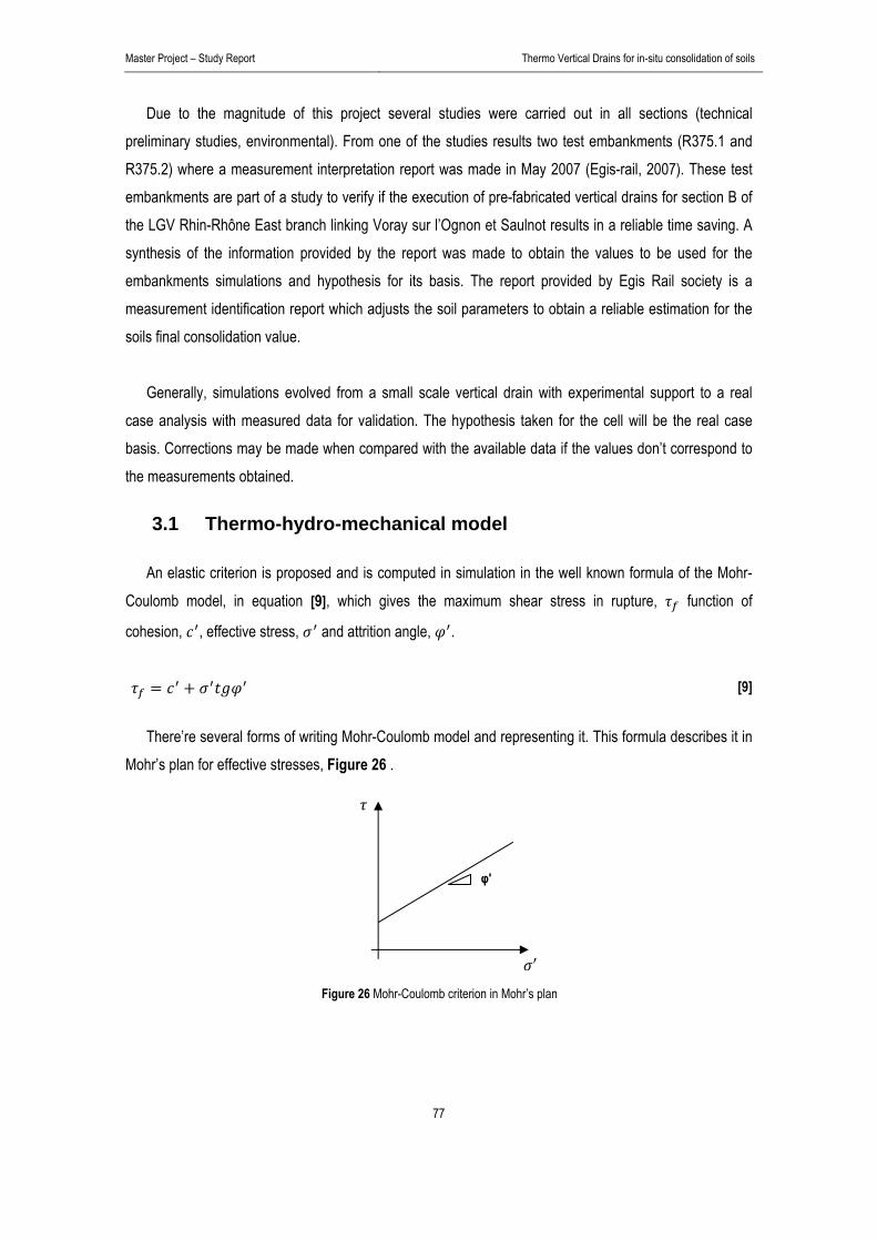
Master Project – Study Report Thermo Vertical Drains for in-situ consolidation of soils
77
Due to the magnitude of this project several studies were carried out in all sections (technical preliminary studies, environmental). From one of the studies results two test embankments (R375.1 and R375.2) where a measurement interpretation report was made in May 2007 (Egis-rail, 2007). These test embankments are part of a study to verify if the execution of pre-fabricated vertical drains for section B of the LGV Rhin-Rhône East branch linking Voray sur l’Ognon et Saulnot results in a reliable time saving. A synthesis of the information provided by the report was made to obtain the values to be used for the embankments simulations and hypothesis for its basis. The report provided by Egis Rail society is a measurement identification report which adjusts the soil parameters to obtain a reliable estimation for the soils final consolidation value.
Generally, simulations evolved from a small scale vertical drain with experimental support to a real
case analysis with measured data for validation. The hypothesis taken for the cell will be the real case basis. Corrections may be made when compared with the available data if the values don’t correspond to the measurements obtained.
3.1 Thermo-hydro-mechanical model
An elastic criterion is proposed and is computed in simulation in the well known formula of the Mohr-Coulomb model, in equation [9], which gives the maximum shear stress in rupture, function of
cohesion, , effective stress, and attrition angle, .
[9]
There’re several forms of writing Mohr-Coulomb model and representing it. This formula describes it in
Mohr’s plan for effective stresses, Figure 26 .
c’
φ'
Figure 26 Mohr-Coulomb criterion in Mohr’s plan

Master Project – Study Report Thermo Vertical Drains for in-situ consolidation of soils
78
1
The choice of this model is its suitable capacity to reproduce the behaviour of geomaterials even if it may cause some difficulties to obtain convergence in simulation when plasticity is encountered and also because it can easily represent our elastic model.
It’s because of this plasticity problem that cohesion, is considered infinite. With this strong
assumption, we reproduce the elasto-plastic behaviour of the soil with an elastic law. This type of analysis is strongly used in current civil engineering problems as we get a simple and reliable evaluation of the soil’s behaviour with sufficient accuracy to verify well documented problems. This process is minutely described in the mechanical law chapter presented next.
3.1.1 Mechanical law Despite of the geomaterials rarely demonstrate a pure elastic behaviour this approximation is correct if
we consider small displacements or we’ve a monotonous loading, for example. In the cases where this approach is admissible, by using secant elastic modules, we can substitute the elasto-plastic curve that reproduces the soil behaviour by an elastic one.
This doesn’t constitute a problem if discharge isn’t considered and if it is, a new secant modulus should be encountered to reproduce this discharge by counting only with the elastic recovery of the soil.
It is important to refer that, in these cases, the modules found for this approach are no longer a constant of the material but a function of deformation and that an isotropic media is admitted.
Therefore, elastic theories represent an important and useful tool even in circumstances where elasticity is no longer observed.
A linear elastic law was chosen for our modelled cases. This approach can be determined by several
models. The one that, in our understanding, describes well the way to find this equivalent modulus is by computing the Young modulus with the final displacements observed in simulation.
This model can be described with and and the tangent module, . A
schematic graphical representation is shown in Figure 27.
Figure 27 Kondner model in ( ; ) plan

Master Project – Study Report Thermo Vertical Drains for in-situ consolidation of soils
79
In the oedometer simulations, this tangent module will be calculated in function of the final
displacement observed for the charge applied as shown in 4.1.6.1 Ambient temperature test – Mechanical consolidation (p.96). In the case of the embankment simulation the value used is the one presented in the laboratory tests made for the soil’s layer in study for the charge value induced by the embankment, (Egis-rail, 2007).
3.1.2 Hydraulic law Evolving from a simple laboratory case (with clear pre-defined conditions) to a real scale embankment
implies some variations in the defined parameters that have to be studied. The objective is to find justified permeabilities that can represent the correct evolution of settlement for our studied cases that have different geometry configurations and physical assumptions, Figure 28. These hydraulic formulations are described next and final conclusions are traced for them with reference to the values to be used in the oedometer and embankments simulations.
The smear zone presented around the drain in Figure 28 results from the soil affected by the drilling process inherent to the drain installation. This smear zone is important to be considered as the soil characteristics are clearly altered. The geometry of this zone is defined in the next chapter.
Figure 28 Axisymmetric unit cell (oedometer) to an equivalent plane strain unit cell (embankment)2
2 (Tran, et al., 2008)
Master Project – Study Report Thermo Vertical Drains for in-situ consolidation of soils
80
3.1.2.1 Radial permeability – Equivalent plane strain
In the oedometer there’s no consideration of smear zone due to the soil’s accommodation around the filter so the permeability will be considered simply in the horizontal direction and equal to the value determined for the soil. Further, this analysis proposes an equivalent plane strain unit cell to be used for the embankments simulations. Here, two solutions are presented for a plane strain cell: radial permeability with smear zone and radial permeability without smear zone.
The following parameters are calculated for the embankments simulation as they’ll define the smear zone and the geometry for the case studied:
Determination of the equivalent diameter, d of the PVD solution is made by equation [10],
2 [10]
and regarding the PVD regular dimensions used in the embankments a 10 cm and
0,4 cm we get d 5 cm.
To define the smear zone diameter, d we apply the following equation [11] with a common
mandrel diameter, d 12 cm,
3 [11]
and we get 36 cm.
The equivalent radius of the influence zone, is defined in equation [12], being a relation between
circle and rectangular areas:
1.1282
[12]
and defines the space between two vertical drains. This influence zone formula will be used,
(Egis-rail, 2007) in all permeability formulations. With these definitions, simulations can be run for constant radial permeability ( 4 10 / )
with for a 2D cell with and without smear zone. There, permeability in the undisturbed zone will be
and in the smear zone 5⁄ . With this case, horizontal permeability will be multiplied
by the permeability factor defined in equation [17] so it defines the temperature effects in a T-PVD solution.

Master Project – Study Report Thermo Vertical Drains for in-situ consolidation of soils
81
3.1.2.2 Equivalent vertical permeability Again, as the cylinder has no possibility for evacuation of water in the vertical direction we’re obliged,
as already mentioned, to follow a horizontal permeability approach for its simulation. Therefore, the following formulation for vertical permeability will be tested for the embankments analysis.
This formulation combines the horizontal and vertical permeability interaction in an equivalent vertical
drainage to reproduce both permeability directions as radial hypothesis is only verified while the effects of the vertical charge are highly felt by the excess pore water pressure (Jin-Chun Chai, 2001). The proposed method gives the following equation for the equivalent axisymmetric vertical drainage, :
12.5
[13]
where is the drainage length,
1 as horizontal and vertical permeabilities are considered equal
(isotropy) and is the cell diameter which is considered to be equal to . With these assumptions this
formula becomes applicable to plain strain. The parameter is defined by equation [14].
ln34
23
[14]
Where 22,56 · , ratio 7,2 between smear zone, 18 and drain
rayon, 2,5 , ratio between horizontal and smear zone axisymmetric permeability, 5 and
the drain’s discharge capacity axisymmetrically.
So, we arrive to the final equation for function of :
12.5
ln 3
423 . 0,564 ·
[15]
These three permeability solutions give several combinations which may justify the values obtained for
the settlement of the test embankment.

Master Project – Study Report Thermo Vertical Drains for in-situ consolidation of soils
82
3.1.2.3 Well resistance The well resistance isn’t considered for the oedometer due to the characteristics of the experimental
test mainly evolving time, as we only have a maximum of 8 days of experimental consolidation on each test.
For the embankments case, the discharge capacity of the drains (Egis-rail, 2007), used is equal to
0,4 ⁄ 50,5 ⁄ in plane flow rate at 200 of charge.
[16] Using equation [16] it’s shown that no well resistance for the case analysed is reasonable due to the
extremely small permeability of our soil that gives an extremely high 1,23 10 20 limit from
which Mesri and Lo, (Jin-Chun Chai, 2001) define no well resistance.
3.1.2.4 Conclusions In the oedometer simulations there isn’t any consideration of smear zone effect as the soil was
stowage around the filter. The consolidation rate is influenced by the piston’s settlement which is inconsistent with the water flow rate. This and the confinement provoked by oedometer system invalidate the permeability values obtained by simple laboratory tests as already shown. It’s proposed a similar approach for this equivalent permeability value as the one used for the mechanical law.
For the embankments simulations several formulations are possible and they will be applied and
validated when possible. All values for permeability are now well defined just like the zones where these values should be observed (smear zone).
Master Project – Study Report Thermo Vertical Drains for in-situ consolidation of soils
83
3.1.3 Thermal law To obtain the best approximation possible with this elastic model the permeability and the thermal
expansion coefficient for the solid skeleton are adjusted for each test at different temperatures.
Permeability is adjusted using the multiplier coefficient in equation [17] from (Salager, 2007),
which is going to be defined 4.1.6.1Ambient temperature test – Mechanical
consolidation (p.96). This parameter has been chosen as a changing one because temperature affects mainly the water’s viscosity in saturated conditions.
1 ∆ [17]
where is the water’s density, is the water’s cinematic viscosity, is the dynamic viscosity and
is a coefficient related to viscosity. For temperatures between 20ºC and 60ºC the coefficient is
equal to 0,03 . This formula shows a linear augmentation of permeability with temperature variation,
∆ .
In the model used the thermal expansion coefficients from both soil solid skeleton and water can be
used and the first one is clearly shown as function of temperature. Therefore, the thermal expansion coefficient for our soil is going to be also modified as it can be simply adjusted by equation [19].
The average value for the isotropic thermal expansion coefficient of the solid skeleton for clays is
given in handbook of Chemistry and Physics (2000) and it’s around ´ 3 · 10 . The thermal
expansion coefficient of the solid skeleton, ´ is given by equation [18] and is highly influenced by
temperature.
´ ´ [18]
where is the slope for the variation of ´ at 1. This parameter has been defined as being
´ /100 and equation [19] is finally written as:
´ 0,99 · ´ · · [19]
Master Project – Study Report Thermo Vertical Drains for in-situ consolidation of soils
84
The value proposed for the thermal expansion coefficient of water is assumed to be adjusted for the
temperature range and pressure of this study and it’s equal to ´ 4 · 10 .
These parameters are introduced in the mass conservation equation [20] for the water/soil mixture by
the phase compressibility, in equation [21] and volume thermical dilatation at constant pressure phase, in equation [22]:
0 [20] with being pore water pressure, the temperature, the position vector of the material point and
the displacement vector of the solid matrix. 1
1 [21]
11 [22]
with being the initial porosity.
Thermal expansion coefficients are only influent in thermal loading and unloading simulations and are
defined here for those cases. In simulations where temperature is constant they don’t have an active part. Therefore, the thermal component of the simulations made, with constant temperature, are a result of the manual variation in the permeability values.
Master Project – Study Report Thermo Vertical Drains for in-situ consolidation of soils
85
4. Results of numerical simulations
This chapter combines firstly, cylinder simulations to reproduce the results from experimental tests and
then, regarding the conclusions from these results, the embankments simulations take place. For the embankments case several hydraulic hypothesis are made to reproduce different scenarios and support the calculated time saved for the thermal application into pre-fabricated drains consolidation solution.
4.1 Oedometric cell simulations
Modelling using thermo-elasto-plastic cyclic Hujeux law was an aim of this study in order to provide a comparison with the results presented. This model was chosen as it was the one available by the software that considered thermo-plasticity for our simulated cases. The difficulty of determining some of the parameters needed induced a level of complexity on this simulation’s resulting in a complete divergence and the time associated to each simulation was finally too high. The cyclicality of the model wasn’t considered interesting too as the mechanical loading applied is monotonic.
The objective of simulating the laboratory’s oedometric cell is to achieve an evaluation of the soil’s
response to a vertical drain implementation and also to a thermical load applied in a vertical drain. Then, have the possibility of extrapolate this model to every day cases where pre-fabricated vertical drains are executed in soils where permeability is very low.
4.1.1 Definition
The case analysed is a cylinder with variable height depending on each test, (0,53 and 0,57
meters and being the temperature on which the experimental tests are run), an exterior vertical border
at 0,156 cm and an interior border at 0,0145 m are used to reproduce the drains thickness, Figure 29. In the ambient temperature test it was seen that a high displacement could happen due to the high
void ratio of the soil, therefore an additional quantity of soil was adjusted due to the small pre-defined length of the solid connection between the piston and the loading plate, Figure 3. This proved to be correct and adjustments were made to the piston for the consolidations at high temperature so a bigger displacement could be measured.
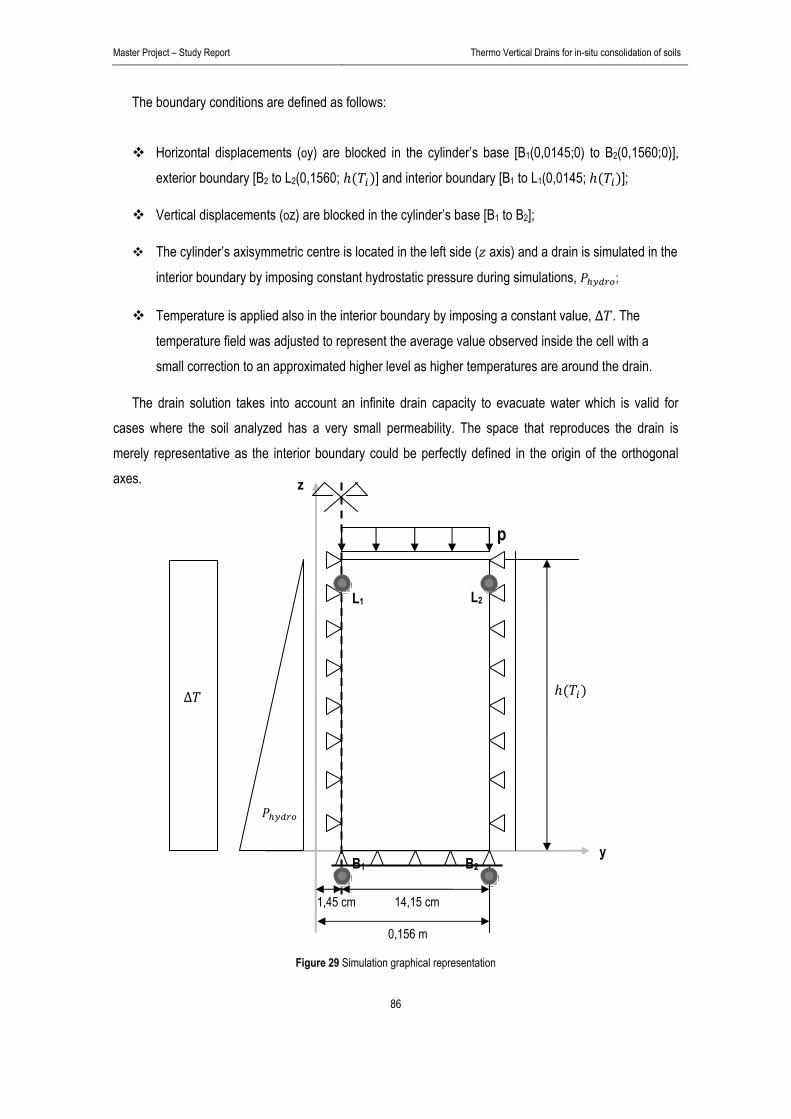
Master Project – Study Report Thermo Vertical Drains for in-situ consolidation of soils
86
The boundary conditions are defined as follows:
Horizontal displacements (oy) are blocked in the cylinder’s base [B1(0,0145;0) to B2(0,1560;0)], exterior boundary [B2 to L2(0,1560; ] and interior boundary [B1 to L1(0,0145; ];
Vertical displacements (oz) are blocked in the cylinder’s base [B1 to B2];
The cylinder’s axisymmetric centre is located in the left side ( axis) and a drain is simulated in the
interior boundary by imposing constant hydrostatic pressure during simulations, ;
Temperature is applied also in the interior boundary by imposing a constant value, ∆ . The
temperature field was adjusted to represent the average value observed inside the cell with a small correction to an approximated higher level as higher temperatures are around the drain.
The drain solution takes into account an infinite drain capacity to evacuate water which is valid for cases where the soil analyzed has a very small permeability. The space that reproduces the drain is merely representative as the interior boundary could be perfectly defined in the origin of the orthogonal axes.
∆
z
y
1,45 cm 14,15 cm
0,156 m
p
B1 B2
L1 L2
Figure 29 Simulation graphical representation

Master Project – Study Report Thermo Vertical Drains for in-situ consolidation of soils
87
4.1.2 Mesh To reproduce the soil in the cylinder a rectangular element mesh was made. This mesh consists in 21
nodal points high and 11 nodal points large resulting in a matrix of 231 points defining a total of 210 elements from which 200 are soil elements and 10 are loading elements. Each element has 14,15
millimetres large and 25,00 millimetres height performing a ratio of / 1,77.
The soil elements are isoparametric quadrilateral 2D volume elements defined by 4 nodal points. The
description and local numbering of the elements nodal points for our integration order (2) is presented in Figure 30. For the 2D surface loading elements the description is also in Figure 30 being n the direction of the charge applied. These elements definition is equal in all simulations.
4.1.3 Analysis type Before running the final simulations it is important to define which parameters will be studied and how
they will be presented in the report. Therefore, homogeneity in all cases will permit to analyse them and extract combined conclusions. But this doesn’t mean that, if necessary, some remarks and other positions may be taken into account to express encountered exceptions.
S
R
x
I V
x I I
x
I I I
x I
1 2
3 4
n
1 2 s
Figure 30 Description of the elements chosen to define the cell’s mesh (Left: Material element; Right: Loading element)
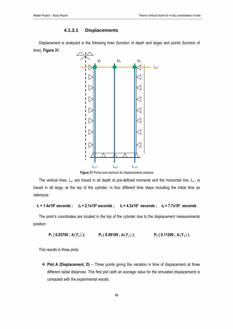
Master Project – Study Report Thermo Vertical Drains for in-situ consolidation of soils
88
4.1.3.1 Displacements Displacement is analyzed in the following lines (function of depth and large) and points (function of
time), Figure 31.
The vertical lines, Ly,i are traced in all depth at pre-defined moments and the horizontal line, Lx,1 is
traced in all large, at the top of the cylinder, in four different time steps including the initial time as reference:
t1 = 1.4x10⁵ seconds ; t2 = 2.1x10⁵ seconds ; t3 = 4.2x10⁵ seconds ; t4 = 7.7x10⁵ seconds
The point’s coordinates are located in the top of the cylinder due to the displacement measurements position:
P1 ( 0.03700 ; ); P2 ( 0.09100 ; ); P3 ( 0.11200 ; ).
This results in three plots:
Plot A (Displacement, D) – Three points giving the variation in time of displacement at three different radial distances. This first plot (with an average value for the simulated displacement) is computed with the experimental results.
Lx,1
Ly,2 L y,3 L y,1
P1 P2 P3
Figure 31 Points and sections for displacements analysis

Master Project – Study Report Thermo Vertical Drains for in-situ consolidation of soils
89
After this first plot analysis other two plots will be traced with the adjusted soil parameters.
Plot B (D) – Horizontal line giving displacement radial variation at the top of the cylinder in four pre-determined time steps;
Plot C (D) – Vertical lines giving displacement variation in depth at three different radial distances from the centre drain (defined by the points x coordinate).
These plots are the basis of the cylinder’s simulation results analysis where conclusions will be traced
for all tests.
4.1.3.2 Pore pressure The pore pressure is analyzed in the following lines (function of depth and large) and points (function
of time), Figure 32. Pore pressure gives the information about the consolidation evolution and if stabilisation is achieved in a test.
Lx,2
Ly,2 L y,3 L y,1
P1 P2 P3
Figure 32 Points and sections for pore pressure analysis

Master Project – Study Report Thermo Vertical Drains for in-situ consolidation of soils
90
The vertical lines, Ly,i are traced as for the displacement case. The horizontal line, Lx,2 is now traced at half height and in the same four different time steps.
The point’s coordinates are located in the same place as the pore pressure sensors at half height of the cylinder:
P1 ( 0.03700 ; 0.25000) ; P2 ( 0.09100 ; 0.25000) ; P3 ( 0.11200 ; 0.25000)
The same three plots are proposed. The first plot, now for the pore pressure, Plot A (PP) will be
computed with the experimental results but there won’t be any soil parameters variation.
4.1.3.3 Effective stress
If pore pressure is simulated correctly the effective stress values, analysed by Terzaghi’s theory in the software, will only depend on the simulation reading of the soil’s characteristics. Therefore, this analysis doesn’t bring a new understanding of the case if the displacement and pore pressure values are validated.
It is possible that the simulation of effective stress shows some localised interesting behaviours resulting on the interpretation of the conditions imposed by the software. As a comparison with experimental data can’t be made, effective stress won’t be analysed.
4.1.3.4 Temperature Temperature won’t be analysed either as the sensor’s experimental values obtained were used to
calibrate the propagation of the temperature’s field for a mean value of temperature registered in the cell. This was made because no flow lost is previewed for the cylinder’s boundaries in the software (isothermal hypothesis).
4.1.3.5 Conclusions A saturation observation was made to confirm that complete saturation was obtained during the
simulations as defined in the code. As that is confirmed, no evaluation will be made forward about this parameter. Neither for deformation as we obligate the problem to be always in the elastic domain.
Each case must be analysed regarding the values obtained. If necessary, due to the almost
instantaneous charged applied, a more detailed analysis can be made for the beginning of the tests. The analysis of some plots may be repetitive and, if a lack of physical interest is seen or a parameter
behaviour is clearly well defined, Plot C (D., P.P. or E.S.) analysis may not be imperatively presented.

Master Project – Study Report Thermo Vertical Drains for in-situ consolidation of soils
91
4.1.4 Soil parameters definition In the simulation, the soil parameters are divided in general properties, common for all models, and the
parameters that support the studied criterion. The definition of the parameters is made but only the tangent modulus and permeability will have an influence in the results. Justifications for those parameters are held so clear fundaments can stand the values used (if plasticity is somehow achieved the model may continue to give adjusted results). Kaolin soil properties are extracted from (Cekerevac, 2003).
4.1.4.1 Soil’s general properties Further in Table 10 a resume of the soil’s general properties is presented.
Density,
The soil’s unit weight of the solid particles is 25,76 / . Therefore, the particles density
can be expressed as
25,76 9,81 1000⁄ 2626 / [23]
It’s used to calculate the material’s mass matrix and the gravity forces.
Initial porosity,
Porosity can also change regarding the void ratio in temperature but this parameter will be kept constant. It’s obtained from the void ratio, and this one from the water content, and the specific gravity
of soil grains, at 22 for a complete constant saturation, equal to 1.
[24]
1 [25]
From [24] we get 1,778 and from [25] we get 0,640.
The initial porosity is used to obtain the total volumetric mass of the material. This value is given, in a saturated coupled analysis, by [26].
1 [26]
Grain compressibility
The grain compressibility is considered in complete Biot’s formulation. For our case, simple Biot’s formulation, the grain compressibility isn’t used which means that grains are defined as incompressible. This supposition is common in soil analysis.

Master Project – Study Report Thermo Vertical Drains for in-situ consolidation of soils
92
Biot’s formulation factor
This parameter is also considered in complete Biot’s formulation. The factor gives the relation
between total stress, , and intergranular stress, , given by equation [27],
, , [27]
where is the pore pressure and the Kronecker symbol. So, for 1, we’ve effective stress instead
of intergranular stress which is the norm in soils mechanics.
Initial saturation ratio
Initial saturation is used to calculate the pore pressure. In this simulation initial conditions are given by a restart calculation where equilibrium of displacements and hydrostatic pressure is achieved before starting each test. For initial saturation equal to 1 pressure is null at the beginning and complete saturation is achieved.
Thermal expansion coefficients
i) Solid skeleton – The average value for the isotropic thermal expansion coefficient of the solid
skeleton for clays is around ´ 3 · 10 . The thermal expansion coefficient of the
solid skeleton, ´ is highly influenced by temperature and its values are presented in Table 9.
[ºC] 22,5ºC 35ºC 53ºC ´ [ºC-1] 3 · 10 3,7 · 10 9,1 · 10
Table 9 Solid skeleton values at each simulated temperature
ii) Water – The value proposed for the thermal expansion coefficient of water is assumed to be
adjusted for the temperature range and pressure of this study and it’s equal to ´ 4 ·
10 .
All the defined parameters in this section are resumed in the following table, Table 10.
Definition Value Density 2626.0
Initial porosity 0.640 Grain compressibility 0.0
ALFA factor for Biot’s formulation 1.0 Initial saturation ratio 1.0
Thermal expansion coefficient of the solid skeleton ´ Thermal expansion coefficient of water 4e-4
Table 10 Resume of general material properties for simulation
Master Project – Study Report Thermo Vertical Drains for in-situ consolidation of soils
93
4.1.4.2 Mohr-Coulomb parameters – simulation model The criterion chosen to simulate our elastic model is Mohr-Coulomb. As said before, only the tangent
compression modulus and permeability will have an influence in this simulation as cohesion is defined as infinite.
Young’s modulus
This parameter is the most important as it influences completely the values obtained for displacement.
The value defined by (Cekerevac, 2003) is 100 6 10 Pa . But this elastic analysis
proposes a tangent modulus which is calculated further ahead in the simulations, 4.1.6.1 Ambient temperature test – Mechanical consolidation (p.96) and therefore this value will only state here for comparison.
Poisson’s ratio
It was determined with a mean value of 0,285 in the initial slope of the radial strain, versus
axial strain (Cekerevac, 2003).
Friction angle
The friction angle at critical state, for triaxial compression is given by equation [28].
63
[28]
And from the projection of the critical state line onto : plane defined by , where
0,80 is the gradient of the CSL, we get 21 .
Cohesion
In order to have the elastic behavior as defined, cohesion has to be assumed as infinite ( 3
10 ) and therefore we’ll have a pure elastic comportment for the soil.
Dilatancy angle
The dilatancy angle value is 22,5° which means that admit a non associated flow law ( ).
Initial earth pressure coefficient
Initial earth pressure coefficient, is used to determine the initial stresses by using the supported
soil’s weight at each height, when this function is activated in the simulation code. Relations are
given by with 1 sin .
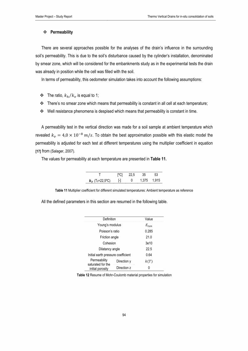
Master Project – Study Report Thermo Vertical Drains for in-situ consolidation of soils
94
Permeability
There are several approaches possible for the analyses of the drain’s influence in the surrounding soil’s permeability. This is due to the soil’s disturbance caused by the cylinder’s installation, denominated by smear zone, which will be considered for the embankments study as in the experimental tests the drain was already in position while the cell was filled with the soil.
In terms of permeability, this oedometer simulation takes into account the following assumptions: The ratio, ⁄ is equal to 1;
There’s no smear zone which means that permeability is constant in all cell at each temperature; Well resistance phenomena is despised which means that permeability is constant in time.
A permeability test in the vertical direction was made for a soil sample at ambient temperature which
revealed 4,0 10 / . To obtain the best approximation possible with this elastic model the
permeability is adjusted for each test at different temperatures using the multiplier coefficient in equation [17] from (Salager, 2007).
The values for permeability at each temperature are presented in Table 11.
T [ºC] 22,5 35 53 (T0=22,5ºC) [-] 0 1,375 1,915
Table 11 Multiplier coefficient for different simulated temperatures: Ambient temperature as reference
All the defined parameters in this section are resumed in the following table.
Definition Value Young’s modulus
Poisson’s ratio 0.285 Friction angle 21.0
Cohesion 3e10 Dilatancy angle 22.5
Initial earth pressure coefficient 0.64 Permeability
saturated for the initial porosity
Direction y Direction z 0
Table 12 Resume of Mohr-Coulomb material properties for simulation
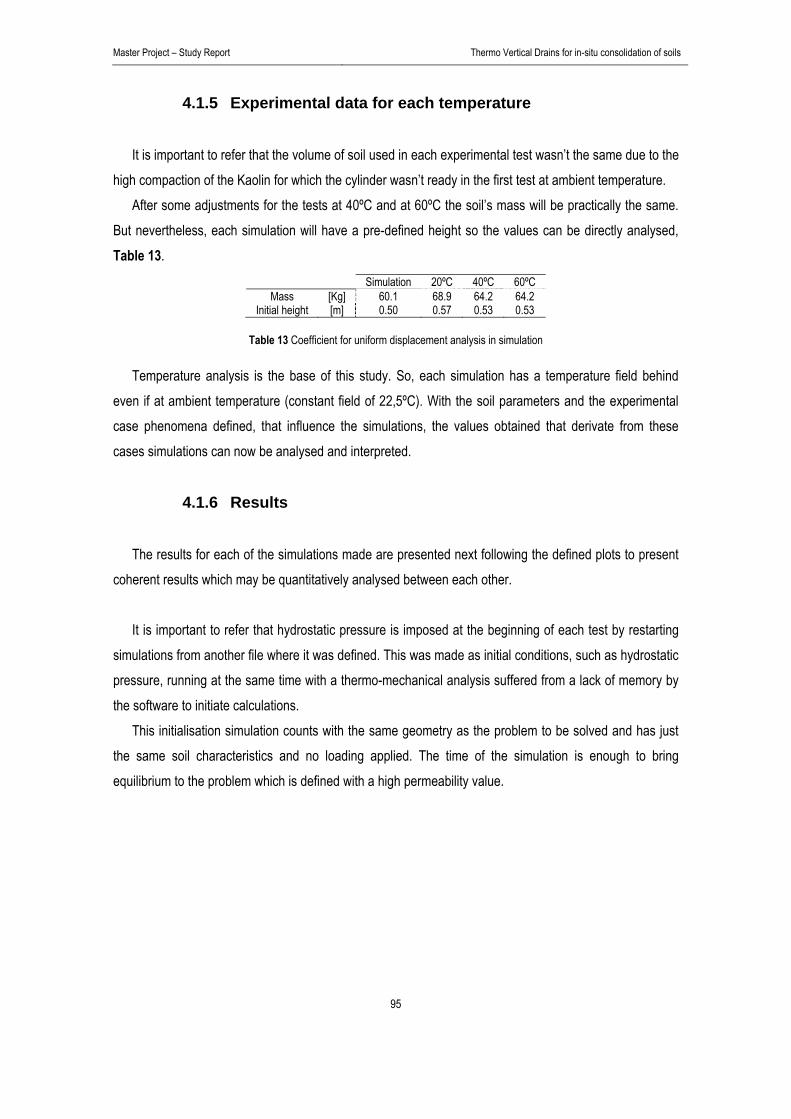
Master Project – Study Report Thermo Vertical Drains for in-situ consolidation of soils
95
4.1.5 Experimental data for each temperature It is important to refer that the volume of soil used in each experimental test wasn’t the same due to the
high compaction of the Kaolin for which the cylinder wasn’t ready in the first test at ambient temperature. After some adjustments for the tests at 40ºC and at 60ºC the soil’s mass will be practically the same.
But nevertheless, each simulation will have a pre-defined height so the values can be directly analysed, Table 13.
Simulation 20ºC 40ºC 60ºC Mass [Kg] 60.1 68.9 64.2 64.2
Initial height [m] 0.50 0.57 0.53 0.53
Table 13 Coefficient for uniform displacement analysis in simulation
Temperature analysis is the base of this study. So, each simulation has a temperature field behind even if at ambient temperature (constant field of 22,5ºC). With the soil parameters and the experimental case phenomena defined, that influence the simulations, the values obtained that derivate from these cases simulations can now be analysed and interpreted.
4.1.6 Results The results for each of the simulations made are presented next following the defined plots to present
coherent results which may be quantitatively analysed between each other. It is important to refer that hydrostatic pressure is imposed at the beginning of each test by restarting
simulations from another file where it was defined. This was made as initial conditions, such as hydrostatic pressure, running at the same time with a thermo-mechanical analysis suffered from a lack of memory by the software to initiate calculations.
This initialisation simulation counts with the same geometry as the problem to be solved and has just the same soil characteristics and no loading applied. The time of the simulation is enough to bring equilibrium to the problem which is defined with a high permeability value.

Master Project – Study Report Thermo Vertical Drains for in-situ consolidation of soils
96
4.1.6.1 Ambient temperature test – Mechanical consolidation
The formulation adopted has a tangent compression modulus to be defined all along with an equivalent
permeability. These two parameters are defined next:
Young modulus – Tangent modulus determination
In this simulation, as already mentioned, the cohesion is very high in order to have the Mohr-Coulomb’s model simplified in elasticity. In reality we’ve an elasto-plastic behaviour which is here simulated by an elastic criterion. So, a tangent module is found that will represent the total displacement, 3.1.1 Mechanical law (p.78).
104
105
106
107
0 50 100 150 200 250 300 350 400
Test values : Et
E [M
Pa]
Final Displacement [mm]
With these three values an exponential line is easily traced and is obtained by equation [29]. This
equation gives the relation between the tangent modulus, and the final displacement observed for the
Kaolin in the cylinder’s conditions.
2,3036 10 · , [29]
E [MPa] 6x10⁶ 6x10⁵ 6x10⁴
Displacement [mm] 3,82 37,09 369,78
Table 14 General Young modulus values for Kaolin soil simulation
Plot 44 Tangent modulus parameter function of final displacement (cylinder simulation)

Master Project – Study Report Thermo Vertical Drains for in-situ consolidation of soils
97
Therefore, for the observed final displacement at ambient temperature 135,66 mm the
1,64 10 is obtained and a final simulation is run to adjust this parameter, Table 15.
As this parameter will kept unchanged for the following simulations with temperature it was here an objective to give the best accurate value possible to describe the ambient temperature simulation.
This formulation may be defined as a strong assumption but necessary as simulations with a more
complex model weren’t possible in the pre-defined time for this thesis. The curves for each shown in
Table 15 weren’t traced because only the final displacement values were necessary to obtain the optimal curve for this parameter adjustment.
Permeability adjustment
The values obtained by the permeability tests executed with samples of the soil and even the values
obtained by (Cekerevac, 2003) overestimated the consolidation time observed in the experimental test [range from 4x10⁻⁸ m/s in a sample before consolidation and 2,5x10⁻⁷m/s for a sample after consolidation]. This is due to the influence of the oedometer boundaries. In the oedometer we’ve a closed environment where water can only be expelled by the centred drain and in the permeability tests we’ve a water flow which doesn’t find any blockage at all.
To obtain the best value to describe the simulation we proceed similarly as with . Three values of
displacement are taken at three different permeability values at a pre-defined time during the test to obtain the best fit for the experimental case.
E [MPa] 1,64x10⁵ 1,63x10⁵ Displacement [mm] 134,93 135,74
Table 15 Detailed values approximation for Kaolin soil simulation

Master Project – Study Report Thermo Vertical Drains for in-situ consolidation of soils
98
20
40
60
80
100
120
140
0 1 10-8 2 10-8 3 10-8 4 10-8 5 10-8
Test values :Radial permeability
Dis
plac
emen
t [m
m]
kr [m/s] Plot 45 Displacement values at t=1,40E+05 seconds for different simulated permeabilities
With these three values an exponential line is easily traced and equation [30] is obtained. This
equation gives the relation between the Young modulus, and the final displacement observed for the
Kaolin in the cylinder’s conditions.
5,5395 10 · , · , [30] Therefore, for the observed displacement at ambient temperature , 85,60 the
radial permeability is , 8,21 10 / .
Kh [m/s] 4x10⁻⁸ 4x10⁻⁹ 1,5x10⁻⁹ Displacement [mm] 135,45 63,42 19,08
Table 16 General permeability values for Kaolin soil simulation

Master Project – Study Report Thermo Vertical Drains for in-situ consolidation of soils
99
0
20
40
60
80
100
120
140
0 1 105 2 105 3 105 4 105 5 105 6 105 7 105 8 105
kr=4,0E-08kr=4,0E-09kr=1,5E-09Experimental displacement
Dis
plac
emen
t [m
m]
Time [sec] Plot 46 Displacement in time for different testing permeabilities ( , )
With these adjustments the final simulation parameters give the following pre-defined plots for the ambient temperature test:
i) Displacements
The displacement evolution in time is plotted with the experimental displacement observed for the cylinder, Plot 47.
0
20
40
60
80
100
120
140
0 1 105 2 105 3 105 4 105 5 105 6 105 7 105 8 105
SimulationDisplacementExperimentalDisplacement
Dis
plac
emen
t [m
m]
Time [sec]
Plot 47 Plot A (D,22): Experimental and final simulation consolidation paths in time, Lx,1 for ambient temperature (22,5ºC)
Lx 1
Ly 2 L y 3 L y 1

Master Project – Study Report Thermo Vertical Drains for in-situ consolidation of soils
100
The simulation proposes a higher rate of displacement between the end of the first day and the beginning of the fourth day. This may be not only due to the basic model analysis used here but also due to the ratio between the exiting water’s velocity and the velocity of the piston displacement as described in 2.6.4.2 Experimental cell (p.73).
This assumption gains even more fundaments as we have water exiting with a high rate until 1,5x10⁵
seconds from which divergence, between simulation and experimental measurements, ends. Then, both rates tend to equality finishing with smooth convergence as we’re in ambient temperature.
To validate this simulation Plot 48 and Plot 49 are proposed. The first one gives the variation of
displacement in radial direction at different moments in time and the second the final displacements observed in depth.
From Plot 48 we can see the clear influence of the drain that causes a bigger displacement in the centre. This is due to the higher dissipation of pore pressure which increases the displacements observed. This phenomenon is the basis of the PVD technique and ensures that the solution found for simulation of a vertical drain represents it correctly. We can see here that the variation of displacement can go up to 6 mm or more depending on the time step analysed. In the case of Plot 49 we’ve a displacement analysis in depth at different radial distances. This analysis shows that total equilibrium hasn’t been achieved as in the top (and bottom) of the cylinder the displacement is slightly higher near the drain. But a clear linear displacement variation is observed with departure from zero. This linear displacement shows that we’ve a homogeneous soil layer which can be considered as correct for this case due to the soil’s preparation made.
0
1
2
3
4
5
6
0,02 0,04 0,06 0,08 0,1 0,12 0,14
t0
t1
t2
t3
t4
Dis
plac
emen
t var
iatio
n [m
m]
Radial distance [m]
-0,56
-0,48
-0,4
-0,32
-0,24
-0,16
-0,08
0
0 10 20 30 40 50 60 70
Ly,1 (Drain)
Ly,2 (Center)
Ly,3 (Wall)
Dep
th [m
]
Displacement [mm] Plot 48 Plot B (D,22): Absolute variation of displacement,
Lx,1 (h=0,57m) with radial distance for five pre-defined times Plot 49 Plot C (D,22): Variation of displacement with
depth in different radial pre-defined distances (t4)

Master Project – Study Report Thermo Vertical Drains for in-situ consolidation of soils
101
ii) Pore pressure The pore pressure evolution in time is compared with the experimental values obtained in the cylinder
test and is shown in Plot 50.
0
10
20
30
40
50
60
0 1 105 2 105 3 105 4 105 5 105 6 105 7 105 8 105
P1: T22 - ML (Cell wall)
P3: T22 - ML (Drain)
Sim P1: Drain
Sim P2: Center
Sim P3: Wall
Pres
sure
[kPa
]
Time [sec] Plot 50 Plot A (PP,22): Experimental and final simulation pore pressure evolution in time for ambient temperature (22,5ºC)
In this plot we can clearly see the idealized behaviour of a vertical drain with pore pressure dissipating in accordance with displacements. This observed delay for pore pressure dissipation is in accordance with the smaller rate of displacement seen in Plot 47 for the experimental test when compared with the simulation.
The variation of pressure in radial direction, Plot 51 shows again this idealized behaviour with pressure
being constant to the hydrostatic value in the drain line. This may not be necessarily true but it’s, even so,
a valid assumption. The pore pressure values at and are presented in Plot 51 which shows the
intermediary higher dissipation of pore pressure in time with the spacing between lines ( ; and
, ; , ) being practically three times bigger for simulation. This is caused by the accumulated delay
in the water exiting and the adjustment of the pore pressure sensors to the variations observed. In Plot 52 and Plot 53 we’ve the pore pressure variation in depth. For Plot 52 the pore pressure
variation confirms the radial values spacing and also shows that pressure in depth varies within approximately 6 kPa which is in accordance with the expected value corresponding the height of the sample. Again this value is verified in Plot 53 for the final time step with equilibrium practically achieved.
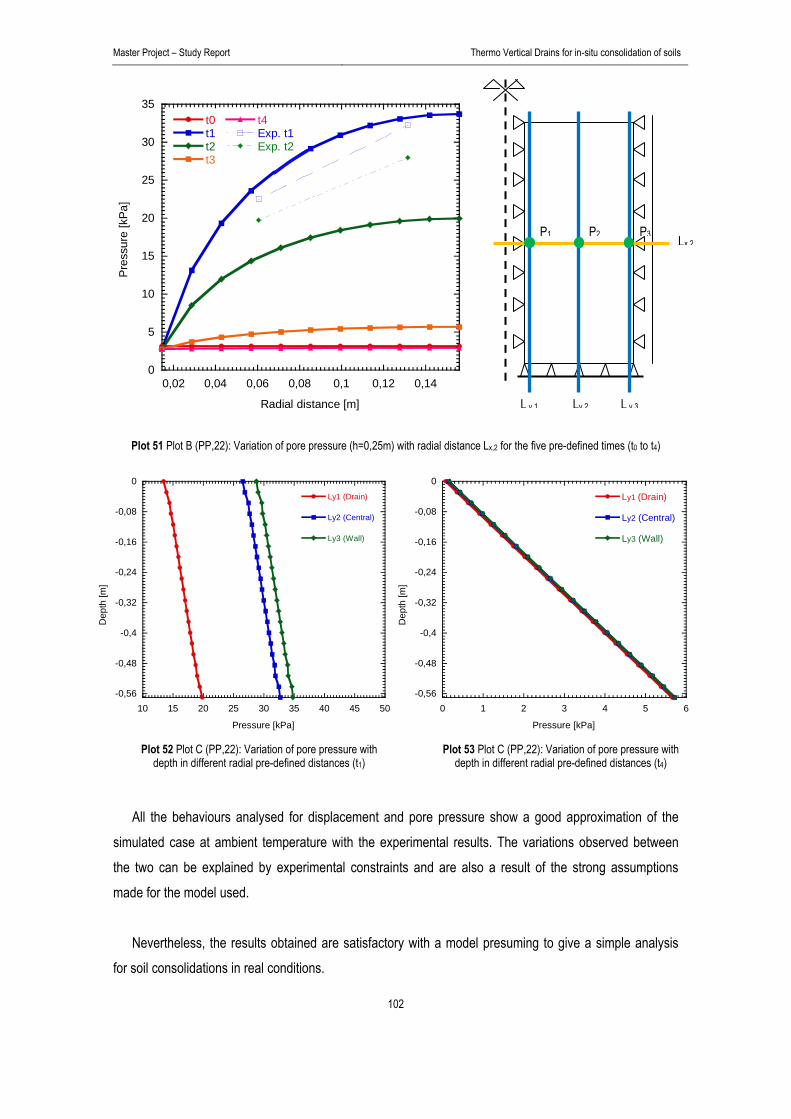
Master Project – Study Report Thermo Vertical Drains for in-situ consolidation of soils
102
0
5
10
15
20
25
30
35
0,02 0,04 0,06 0,08 0,1 0,12 0,14
t0t1t2t3
t4Exp. t1Exp. t2
Pres
sure
[kPa
]
Radial distance [m]
Plot 51 Plot B (PP,22): Variation of pore pressure (h=0,25m) with radial distance Lx,2 for the five pre-defined times (t0 to t4)
-0,56
-0,48
-0,4
-0,32
-0,24
-0,16
-0,08
0
10 15 20 25 30 35 40 45 50
Ly1 (Drain)
Ly2 (Central)
Ly3 (Wall)
Dep
th [m
]
Pressure [kPa]
-0,56
-0,48
-0,4
-0,32
-0,24
-0,16
-0,08
0
0 1 2 3 4 5 6
Ly1 (Drain)
Ly2 (Central)
Ly3 (Wall)
Dep
th [m
]
Pressure [kPa] Plot 52 Plot C (PP,22): Variation of pore pressure with
depth in different radial pre-defined distances (t1) Plot 53 Plot C (PP,22): Variation of pore pressure with
depth in different radial pre-defined distances (t4)
All the behaviours analysed for displacement and pore pressure show a good approximation of the
simulated case at ambient temperature with the experimental results. The variations observed between the two can be explained by experimental constraints and are also a result of the strong assumptions made for the model used.
Nevertheless, the results obtained are satisfactory with a model presuming to give a simple analysis
for soil consolidations in real conditions.
Lx,2
Ly,2 L y,3 L y,1
P1 P2 P3

Master Project – Study Report Thermo Vertical Drains for in-situ consolidation of soils
103
4.1.6.2 Test at 40ºC
As the oedometer suffers variations due to the metal expansion the thermal loading won’t be simulated and the mechanical loading simulation will start at constant temperature.
For a simulation with T=22,5ºC or a simulation with T=35ºC the values obtained are practically equal in
terms of displacement with an approximation to 0,01 mm as they show variations of the same scale which means that temperature is slightly present in the simulations. So, simulate in thermo-hydro-mechanical conditions with our soil characteristics including expansion or simply use a hydro-mechanical simulation has the same results. Consequently, only permeability will be adjusted in a hydro-mechanical simulation to consider the application of temperature in this experiment.
Permeability will be adjusted regarding [17] and for the optimal value 8,21 10 /
calculated at ambient temperature which gives an adjusted permeability of , 1,13
10 / .
i) Displacement
The displacement results obtained in simulation and those from the experimental test are presented in
Plot 54. For this heated case simulation proposes initially a higher rate than the one observed and then a good approximation practically in the end of the first day of consolidation and until the end of the test.
0
20
40
60
80
100
120
140
0 1 105 2 105 3 105 4 105 5 105 6 105 7 105 8 105
SimulationDisplacementExperimentalDisplacement
Dis
plac
emen
t [m
m]
Time [sec]
Plot 54 Plot A (D,35): Experimental and final simulation consolidation paths in time for heated test at 40ºC (Average 35ºC)
Lx 1
Ly 2 L y 3 L y 1
P1 P2 P3
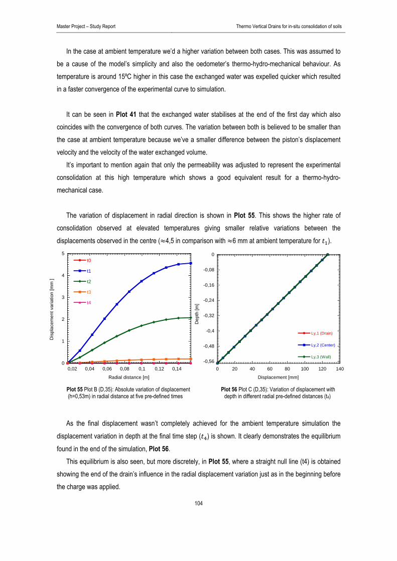
Master Project – Study Report Thermo Vertical Drains for in-situ consolidation of soils
104
In the case at ambient temperature we’d a higher variation between both cases. This was assumed to be a cause of the model’s simplicity and also the oedometer’s thermo-hydro-mechanical behaviour. As temperature is around 15ºC higher in this case the exchanged water was expelled quicker which resulted in a faster convergence of the experimental curve to simulation.
It can be seen in Plot 41 that the exchanged water stabilises at the end of the first day which also
coincides with the convergence of both curves. The variation between both is believed to be smaller than the case at ambient temperature because we’ve a smaller difference between the piston’s displacement velocity and the velocity of the water exchanged volume.
It’s important to mention again that only the permeability was adjusted to represent the experimental consolidation at this high temperature which shows a good equivalent result for a thermo-hydro-mechanical case.
The variation of displacement in radial direction is shown in Plot 55. This shows the higher rate of
consolidation observed at elevated temperatures giving smaller relative variations between the displacements observed in the centre ( 4,5 in comparison with 6 mm at ambient temperature for ).
0
1
2
3
4
5
0,02 0,04 0,06 0,08 0,1 0,12 0,14
t0
t1
t2
t3
t4
Dis
plac
emen
t var
iatio
n [m
m ]
Radial distance [m]
-0,56
-0,48
-0,4
-0,32
-0,24
-0,16
-0,08
0
0 20 40 60 80 100 120 140
Ly,1 (Drain)
Ly,2 (Center)
Ly,3 (Wall)
Dep
th [m
]
Displacement [mm] Plot 55 Plot B (D,35): Absolute variation of displacement (h=0,53m) in radial distance at five pre-defined times
Plot 56 Plot C (D,35): Variation of displacement with depth in different radial pre-defined distances (t4)
As the final displacement wasn’t completely achieved for the ambient temperature simulation the
displacement variation in depth at the final time step ( ) is shown. It clearly demonstrates the equilibrium
found in the end of the simulation, Plot 56. This equilibrium is also seen, but more discretely, in Plot 55, where a straight null line (t4) is obtained
showing the end of the drain’s influence in the radial displacement variation just as in the beginning before the charge was applied.
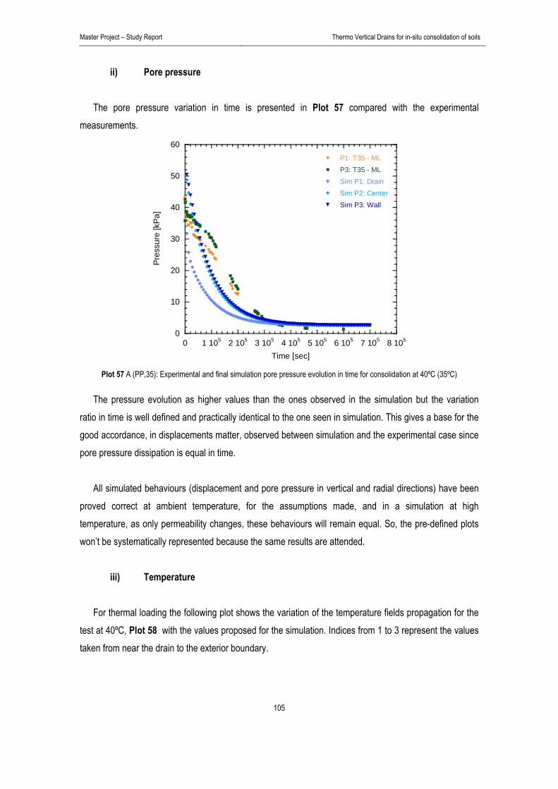
Master Project – Study Report Thermo Vertical Drains for in-situ consolidation of soils
105
ii) Pore pressure The pore pressure variation in time is presented in Plot 57 compared with the experimental
measurements.
0
10
20
30
40
50
60
0 1 105 2 105 3 105 4 105 5 105 6 105 7 105 8 105
P1: T35 - ML
P3: T35 - MLSim P1: Drain
Sim P2: CenterSim P3: Wall
Pres
sure
[kPa
]
Time [sec] Plot 57 A (PP,35): Experimental and final simulation pore pressure evolution in time for consolidation at 40ºC (35ºC)
The pressure evolution as higher values than the ones observed in the simulation but the variation ratio in time is well defined and practically identical to the one seen in simulation. This gives a base for the good accordance, in displacements matter, observed between simulation and the experimental case since pore pressure dissipation is equal in time.
All simulated behaviours (displacement and pore pressure in vertical and radial directions) have been
proved correct at ambient temperature, for the assumptions made, and in a simulation at high temperature, as only permeability changes, these behaviours will remain equal. So, the pre-defined plots won’t be systematically represented because the same results are attended.
iii) Temperature
For thermal loading the following plot shows the variation of the temperature fields propagation for the
test at 40ºC, Plot 58 with the values proposed for the simulation. Indices from 1 to 3 represent the values taken from near the drain to the exterior boundary.

Master Project – Study Report Thermo Vertical Drains for in-situ consolidation of soils
106
22
24
26
28
30
32
34
36
38
0 5 104 1 105 1,5 105 2 105
Exp. T1
Exp. T2
Exp. T3
Sim. T1
Sim. T2
Sim. T3
Tem
pera
ture
[ºC
]
Time [sec] The simulation reproduction of the average value for the temperature fields in comparison with the
experimental case can be considered practically equal varying only in the end as temperature is imposed constant and equal to 35ºC in all cell. The parameters to obtain this temperature field have the following values:
Average heat capacity – 40 J/m3.ºC;
Thermal conductivity – 1x10⁻⁴ W/m/ºC.
with an imposed temperature of 35ºC for the heating test at 40ºC. A temperature field is generated using a pure hydraulic calculation where the parameters listed before are inputted instead of the hydraulic ones. The detailed description of the temperature field’s execution can be found in Appendix B of Gefdyn user’s manual (July 2005).
Plot 58 Adjustment of simulation temperature field, S.Ti to reproduce the experimental case, E.Ti for thermal loading until 40ºC

Master Project – Study Report Thermo Vertical Drains for in-situ consolidation of soils
107
4.1.6.3 Test at 60ºC
For a simulation with T=35ºC or a simulation with T=53ºC the values obtained are also practically equal in terms of displacement just as before. So, the same procedure is adopted.
Permeability will be adjusted regarding equation [17] and for the optimal value 8,21
10 / calculated at ambient temperature.
Therefore, the adjusted permeability is , 1,55 10 / .
The displacement obtained is presented in Plot 59.
0
20
40
60
80
100
120
140
0 1 105 2 105 3 105 4 105 5 105 6 105 7 105 8 105
SimulationDisplacement
Dis
plac
emen
t [m
m]
Time [sec]
Plot 59 Plot A (D,53): Final simulation consolidation path in time for heated test at 60ºC (Average 53ºC)
This simulation is presented here as a test at 60ºC was expected for this master thesis. The good approximation of the simulation at 35ºC also suggests the presentation of this simulation’s displacement in time.
No further analyses are made as there isn’t any data for comparison. This simulation will be presented to stipulate the time saved for the experimental test at these three temperatures in the next chapter. The complete analysis is made in 5.1 Evaluation for time saved with T-PVD (p.120) for the test embankment R375.1.
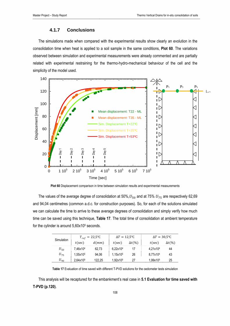
Master Project – Study Report Thermo Vertical Drains for in-situ consolidation of soils
108
4.1.7 Conclusions
The simulations made when compared with the experimental results show clearly an evolution in the consolidation time when heat is applied to a soil sample in the same conditions, Plot 60. The variations observed between simulation and experimental measurements were already commented and are partially related with experimental restraining for the thermo-hydro-mechanical behaviour of the cell and the simplicity of the model used.
0
20
40
60
80
100
120
140
0 1 105 2 105 3 105 4 105 5 105 6 105 7 105
Mean displacement: T22 - ML
Mean displacement: T35 - ML
Sim. Displacement T=22ºC
Sim. Displacement T=35ºC
Sim. Displacement T=53ºCDis
plac
emen
t [m
m]
Time [sec] Plot 60 Displacement comparison in time between simulation results and experimental measurements
The values of the average degree of consolidation at 50%, and at 75% are respectively 62,69
and 94,04 centimetres (common a.d.c. for construction purposes). So, for each of the solutions simulated we can calculate the time to arrive to these average degrees of consolidation and simply verify how much time can be saved using this technique, Table 17. The total time of consolidation at ambient temperature for the cylinder is around 5,60x10⁵ seconds.
Simulation 22,5 ∆ 12,5 ∆ 30,5
sec sec ∆ % sec ∆ %
50 7,46x10⁴ 62,73 6,22x10⁴ 17 4,21x10⁴ 44 75 1,55x10⁵ 94,06 1,15x10⁵ 26 8,77x10⁴ 43 90 2,64x10⁵ 122,25 1,92x10⁵ 27 1,99x10⁵ 25
Table 17 Evaluation of time saved with different T-PVD solutions for the oedometer tests simulation
This analysis will be recaptured for the embankment’s real case in 5.1 Evaluation for time saved with T-PVD (p.120).
Day 2
Day 1
Day 3
Day 4
Day 5
Lx 1
P1 P2 P3

Master Project – Study Report Thermo Vertical Drains for in-situ consolidation of soils
109
The comparison of simulated pore pressure and experimental measurements is presented in Plot 61.
0
10
20
30
40
50
60
0 1 105 2 105 3 105 4 105 5 105 6 105 7 105 8 105
P1: T22 - MLP3: T22 - MLP3: T35 - MLP1: T35 - MLSim. P3 T=25ºCSim. P1 T=25ºCSim. P3 T=35ºCSim. P1 T=35ºC
Pres
sure
[kPa
]
Time [sec] Plot 61 Pore pressure comparison in time between simulation results and experimental measurements
A superposition of values is clearly seen in the beginning and end of the test. The experimental values are presented with filled marks and its correspondent has the same mark format but unfilled.
It’s clear that experimental pore pressure doesn’t seem to follow the same path as simulated pore
pressure. This may be due to the inaccuracy of the sensors combined with the ideal hydrostatic imposition of water pressure all along the drain that gives a higher dissipation for the simulated case. In reality, water pressure is approximated to hydrostatic and its dissipation is related with the speed of the exiting water. This is why experimental values for pore pressure at high temperature dissipate quickly than the ones at ambient temperature and consolidation is faster. The thin water layer over the piston, to ensure saturation, can also be part of these higher values of pore pressure.
Finally, the main barrier of the oedometer simulations is obviously the necessity of having a final value
of total displacement so an elastic analysis may be reproduced as an elasto-plastic behaviour, which is clearly the case for the Kaolin soil.
The acceptable reality simulated derivates from the linearity applied into these calculations as final
values for displacement are manipulated by the tangent modulus, and time adjusted by permeability.
For the oedometer’s simulation it’s here by proposed a comparison of these results with a thermo-elasto-plastic model that could take directly into account the effects of temperature in the soil.
Lx,2 P3 P2 P1

Master Project – Study Report Thermo Vertical Drains for in-situ consolidation of soils
110
4.2 Embankments simulations
These embankments simulations bring a new scale to this study. Here, several combinations are tested with different numbers of vertical drains and application of temperature. A study of temperature fields is made to have an idea how the soil behaves when heated in a non isothermal environment. This temperature analysis is made as permeability is highly influenced by temperature and if temperature is different in several zones this will clearly change the consolidation time. The cases analysed are the two test embankments from which displacement and pore pressure measurement data is available.
4.2.1 Definition of the analysed cases The test embankments are defined using the information from (Egis-rail, 2007). After the analysis of
this information we arrive to the following geometry profiles for the embankments, Figure 33 and Figure 34. Taking this information as base several meshes were drawn until the final one was defined. The next paragraph gives an overview of this mesh evaluation which finished in a compact simple mesh for total displacement analysis below the embankment due to the software elements limit (around 1600 elements).
11,5 m
9 m
∞
Alluvial clays / Altered marls
Iridescent marls (Incompressible layer)
11 m
4 m
∞
Alluvial clays / Altered marls
Iridescent marls (Incompressible layer)
Figure 33 R375.1 simple profile type (defined with the available information)
Figure 34 R375.2 simple profile type (defined with the available information)

Master Project – Study Report Thermo Vertical Drains for in-situ consolidation of soils
111
4.2.2 Chosen Mesh For this embankment analysis two mesh types were made and are presented next. The first one is a
two drain mesh where the behaviour of two drains side by side can be studied to validate the hydraulic and mechanic hypotheses and may also be used to verify the alterations suffered for different drain spacing. The second mesh is a full scale model of the embankment where the optimal solution, found for the first mesh to represent the embankment’s settlement, may be modelled.
4.2.2.1 Two drains mesh This mesh is similar to the cylinder but now emphasis is given to horizontal phenomena. It has 11
nodal points high and 21 large resulting in a mesh with 200 elements defined by 231 nodal points. It has 4 meters of height, as the compressible soil layer under embankment R375.1, and its largeness depends on
the space between two drains, . As described in 3.1.2 Hydraulic law (p.79) the width of this mesh is
given by equation [12] multiplied by 2. This defines it equal to 1,128 · with corresponding to 1,3
meters in this embankment study. The boundary conditions are defined as follows:
Horizontal displacements (oy) are blocked in the soil’s layer base [B1(0;0) to B2(1,128 · ;0)], right boundary [B2 to L2(1,128 · ; 4)] and left boundary [B1 to L1(0;4];
Vertical displacements (oz) are blocked in the soil’s layer base [B1 to B2];
Drains are simulated by imposing constant hydrostatic pressure during simulations, .
Hydrostatic pressure is imposed in the left and right boundary. Drainage may be made in two sides which mean constant hydrostatic pressure under the soil layer; Pressure is considered equal to zero in the top (atmospheric pressure).
Temperature is applied in each drain with a constant, ∆ in depth.
These boundary conditions are represented in Figure 35. It is important to refer again that the drain
solution takes into account an infinite drain capacity to evacuate water which is valid for cases where the soil analyzed has a very small permeability.
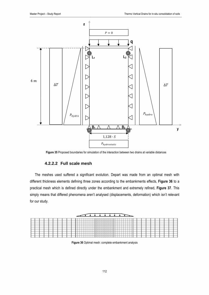
Master Project – Study Report Thermo Vertical Drains for in-situ consolidation of soils
112
4.2.2.2 Full scale mesh The meshes used suffered a significant evolution. Depart was made from an optimal mesh with
different thickness elements defining three zones according to the embankments effects, Figure 36 to a practical mesh which is defined directly under the embankment and extremely refined, Figure 37. This simply means that differed phenomena aren’t analysed (displacements, deformation) which isn’t relevant for our study.
Figure 36 Optimal mesh: complete embankment analysis
z
y
1,128 ·
q
0
∆ 4
∆
B1 B2
L1 L2
Figure 35 Proposed boundaries for simulation of the interaction between two drains at variable distances

Master Project – Study Report Thermo Vertical Drains for in-situ consolidation of soils
113
Figure 37 Practical mesh: influence of PVD under the embankment (Central part of optimal mesh)
This last mesh, Figure 37 has 11 nodal points high by 101 points large resulting in 1111 points defining 1000 elements. It will have 4 m depth, for R375.1 and 9 m depth, for R375.2 with
pre-defined 13 meters large so drains can be installed in 1,3x1,3 meters mesh. This simulation is made in plane strain with no thickness defined (standard one meter thick). The boundary conditions are defined as:
Horizontal displacements (oy) are blocked in the soil’s layer base [B1(0;0) to B2(13,0;0)], right
boundary [B2 to L2(13,0; ] and left boundary [B1 to L1(0; ];
Vertical displacements (oz) are blocked in the soil’s layer base [B1 to B2];
Drains are simulated by imposing constant hydrostatic pressure during simulations, .
Hydrostatic pressure isn’t imposed in the left and right boundary as all loading is defined in the upper layer [L1 to L2]; Drainage may be made in two sides which mean constant hydrostatic pressure under the soil layer. Pressure is considered equal to zero in the top (atmospheric pressure);
Temperature is applied in each drain with a constant, ∆ in depth. Temperature is imposed equal
to 15ºC in left and right boundaries so it represents reality for the drains thermal scope.
This full-scale mesh was initially used to confirm the values obtained by the two drain mesh. In this
study this mesh may be used to verify the sustenance of imposing a constant temperature between drains.
15
15
Figure 38 Embankments proposed boundaries for simulation (vertical lines correspond to PVD with a imposed)
L1 L2
B1 B2
13
0
1,3
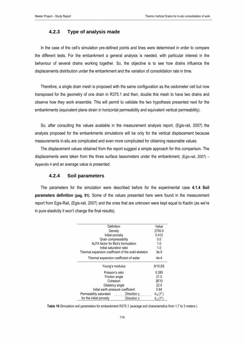
Master Project – Study Report Thermo Vertical Drains for in-situ consolidation of soils
114
4.2.3 Type of analysis made
In the case of the cell’s simulation pre-defined points and lines were determined in order to compare the different tests. For the embankment a general analysis is needed, with particular interest in the behaviour of several drains working together. So, the objective is to see how drains influence the displacements distribution under the embankment and the variation of consolidation rate in time.
Therefore, a single drain mesh is proposed with the same configuration as the oedometer cell but now
transposed for the geometry of one drain in R375.1 and then, double this mesh to have two drains and observe how they work ensemble. This will permit to validate the two hypothesis presented next for the embankments (equivalent plane strain in horizontal permeability and equivalent vertical permeability).
So, after consulting the values available in the measurement analysis report, (Egis-rail, 2007) the
analysis proposed for the embankments simulations will be only for the vertical displacement because measurements in-situ are complicated and even more complicated for obtaining reasonable values.
The displacement values obtained from the report suggest a simple approach for this comparison. The displacements were taken from the three surface tassometers under the embankment, (Egis-rail, 2007) –
Appendix 4 and an average value is presented.
4.2.4 Soil parameters
The parameters for the simulation were described before for the experimental case 4.1.4 Soil parameters definition (pag. 91). Some of the values presented here were found in the measurement report from Egis-Rail, (Egis-rail, 2007) and the ones that are unknown were kept equal to Kaolin (as we’re in pure elasticity it won’t change the final results).
Definition Value Density 2700.0
Initial porosity 0.412 Grain compressibility 0.0
ALFA factor for Biot’s formulation 1.0 Initial saturation ratio 1.0
Thermal expansion coefficient of the solid skeleton 3e-5 Thermal expansion coefficient of water 4e-4
Young’s modulus 9/10.E6 Poisson’s ratio 0.285 Friction angle 21.0
Cohesion 3E10 Dilatancy angle 22.5
Initial earth pressure coefficient 0.64 Permeability saturated for the initial porosity
Direction y Direction z
Table 18 Simulation soil parameters for embankment R375.1 (average soil characteristics from 1,7 to 3 meters )

Master Project – Study Report Thermo Vertical Drains for in-situ consolidation of soils
115
4.2.5 Drain simulation – PVD solution
So, with these values we get the total displacements in Table 19 which, facing the value expected of 8 cm for this soil layer, gives an underestimated final displacement error around 5% if we consider the measured Young modulus for the soil’s compressive range with the embankment charge (Egis-rail, 2007) instead of the approximated value [Appendix 5 – Resume from Egis measurement report] for this 4 meters layer, .
Thickness is considered to be equal to 2 so it works as a rectangular section and simulations are
made for the two drain mesh, 4.2.2.1 Two drains mesh (p.111). In terms of permeability the two hypotheses presented had to be validated for our real case. Therefore,
the displacements observed for R375.1 were plotted with a space between drains, of 1,3 meters and
using the following embankment construction steps, Plot 65 and drainage path, Figure 39.
0
2
4
6
8
10
12
0 50 100 150 200 250
R375.1 Simulation
R375.1 Field measurement
Hei
ght [
m]
Time [days]
Plot 62 Embankment height in time: Field data Figure 39 Drainage path: 1 side (up) and 2 side (down)
The simulations proposed pretend to cover the hydraulic formulations enounced in 3.1.2 Hydraulic law (p.79).
Simulation E [MPa]
Drainage [side(s)] Permeability
1 10
1 , 2 2 , 3 1 4
9
2 , 5 1 6 2 7 1 , 8 1 , and ,
Table 20 Simulations for embankment R375.1
E [MPa] 10 9 Total displacement [mm] 68,0 75,5
Table 19 Total displacements for R375.1 simulations
Permeable
Permeable
Permeable
Impermeable
/2
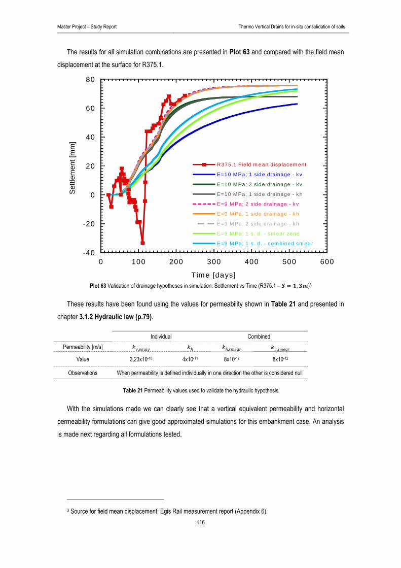
Master Project – Study Report Thermo Vertical Drains for in-situ consolidation of soils
116
The results for all simulation combinations are presented in Plot 63 and compared with the field mean displacement at the surface for R375.1.
-40
-20
0
20
40
60
80
0 100 200 300 400 500 600
R375.1 F ie ld m ean displacem ent
E=10 MPa; 1 side drainage - kv
E=10 MPa; 2 side drainage - kv
E=10 MPa; 1 side drainage - kh
E=9 M Pa; 2 side drainage - kv
E=9 M Pa; 1 side drainage - kh
E=9 M Pa; 2 side drainage - kh
E=9 M Pa; 1 s. d. - sm ear zone
E=9 M Pa; 1 s. d. - com bined sm ear
Settl
emen
t [m
m]
T im e [days]
Plot 63 Validation of drainage hypotheses in simulation: Settlement vs Time (R375.1 – , )3
These results have been found using the values for permeability shown in Table 21 and presented in chapter 3.1.2 Hydraulic law (p.79).
Individual Combined Permeability [m/s] , , ,
Value 3,23x10⁻¹⁰ 4x10-11 8x10-12 8x10-12
Observations When permeability is defined individually in one direction the other is considered null
Table 21 Permeability values used to validate the hydraulic hypothesis
With the simulations made we can clearly see that a vertical equivalent permeability and horizontal permeability formulations can give good approximated simulations for this embankment case. An analysis is made next regarding all formulations tested.
3 Source for field mean displacement: Egis Rail measurement report (Appendix 6).

Master Project – Study Report Thermo Vertical Drains for in-situ consolidation of soils
117
Regarding to Plot 63 the following conclusions can be traced:
The tangent modulus, equal to 9MPa, as already mentioned, gives the best approximation
for the total settlement of the soil’s layer analysed. This value can be found in the laboratory oedometer test from a sample of soil extracted between 1,7 and 3 meters in (Egis-rail, 2007);
0
10
20
30
40
50
60
70
80
0 100 200 300 400 500 600
R375.1 Mean field displacement
E=10 MPa; 2 side drainage - kv
E=9 MPa; 2 side drainage - kv
Dis
plac
emen
t [m
m]
Time [sec] Plot 64 Validation of Young modulus in simulation: Settlement vs Time (R375.1)
The vertical equivalent permeability, , has an excellent approximation to the final
values measured for the embankments settlement if a two side drainage is assumed with 9 . For this permeability hypothesis assuming one side drainage our two side
drainage affects clearly the time for settlement as shown for 10 .
0
10
20
30
40
50
60
70
80
0 100 200 300 400 500 600
R375.1 Mean field displacement
E=10 MPa; 1 side drainage - kv
E=10 MPa; 2 side drainage - kv
E=9 MPa; 1 side drainage - kv
Dis
plac
emen
t [m
m]
Time [days]Time [days] Plot 65 Validation of vertical permeability hypothesis in simulation for two side drainage: Settlement vs Time (R375.1)

Master Project – Study Report Thermo Vertical Drains for in-situ consolidation of soils
118
Assuming that, when installing a PVD, the permeability simply changes its direction from vertical to horizontal (with the same value) also gives an excellent approximation, for both one side drainage and two side drainage, and practically equal to the vertical equivalent permeability with two side drainage at 9 , Plot 66.
To simulate the true drainage path a smear zone is added in the elements surrounding the drain with permeability 5 times smaller than in the rest of the soil. Thus, a combination of permeabilities was made assuming that vertical drainage wasn’t despised and having then both directions for permeability with the same value, Plot 67. By regarding Plot 67 we can see clearly that the assumption of constant radial permeability with the value of the vertical permeability seems to give a good equivalent value from a smear and undisturbed
zones within a solution improved with PVD.
0
10
20
30
40
50
60
70
80
0 100 200 300 400 500 600
R375.1 Mean field displacement
E=9 MPa; 2 side drainage - kv
E=9 MPa; 1 side drainage - kh
E=9 MPa; 2 side drainage - kh
Dis
plac
emen
t [m
m]
Time [days]
0
10
20
30
40
50
60
70
80
0 100 200 300 400 500 600
R375.1 Mean field displacement
E=9 MPa; 1 side drainage - k smear
E=9 MPa; 1 s. d. - combined smear
E=9 MPa; 1 s. d. - combined smear
Dis
plac
emen
t [m
m]
Time [days] Plot 66 Validation of permeability hypothesis (vertical and
horizontal) in simulation: Settlement vs Time (R375.1) Plot 67 Validation of permeability hypothesis (smear
zone) in simulation: Settlement vs Time (R375.1)
As a conclusion, two out of the three hypotheses for permeability tested resulted in good
representations of the embankments settlement:
1. Vertical equivalent permeability, , 3,23 10 / at 9 and two side
drainage path;
2. Horizontal permeability, 4 10 / at 9 with both one side and two side
drainage paths.
These two hypotheses will be used to define the time saved using T-PVD technique.

Master Project – Study Report Thermo Vertical Drains for in-situ consolidation of soils
119
As shown for the cylinder in 3.1.3 Thermal law (p.83) the permeability variation, in saturated media, when temperature is applied mainly derivates from the augmentation of the water’s viscosity. So, for the embankments case the permeability will also be enhanced by a factor depending on the variation of temperature suffered, Equation [17]. This formula was validated for the oedometer consolidations at different temperatures and is used here too if temperature is maintained constant during consolidation. This can be assumed for a drain spacing of 1,3 meters.
It is important to refer that these validations are made for a space between drains of 1,3 .
Therefore, for a larger distance the second option won’t represent the displacement observed as it will be overestimated. So, as the vertical equivalent permeability formula changes with drain spacing, this simple method will be used for the costs evaluation at 5.1.2 Equivalent vertical permeability (pag. 129) where a single T-PVD cost will be calculated.
4.2.6 Consolidation simulation With the hydraulic hypothesis defined it was an objective to verify if this two drain mesh confirmed the
values obtained for the embankment test R375.2. This embankment didn’t have a PVD solution and was executed to confront the results from the test embankment R375.1 on which this solution was used. With these two embankments it would be then possible to verify if using a T-PVD solution would increase the rate of settlement enough to justify its usage.
The measurement report indicates the existence of drainage paths spaced from 8 to 9 meters in the alluvial clays and altered marls. This section corresponds to our soil layer analysed and the simulation made showed a longer time of consolidation than the one observed in the field.
The report also mentions that a cautious approach should be made due to the results obtained for this
embankment’s vertical consolidation as the expected time for consolidation and the consolidation time really obtained are extremely different.
With the results encountered only verification between the time saved using T-PVD or PVD techniques
is going to be made. This analysis is made next for the test embankment R375.1.
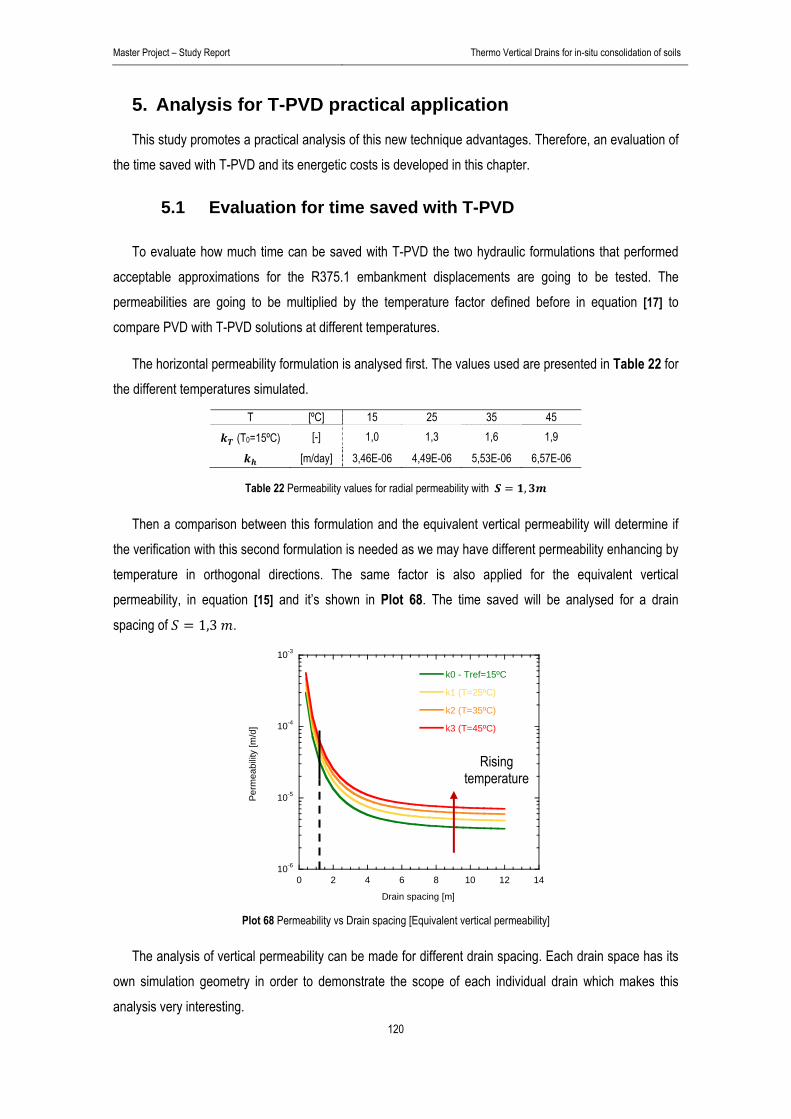
Master Project – Study Report Thermo Vertical Drains for in-situ consolidation of soils
120
5. Analysis for T-PVD practical application
This study promotes a practical analysis of this new technique advantages. Therefore, an evaluation of the time saved with T-PVD and its energetic costs is developed in this chapter.
5.1 Evaluation for time saved with T-PVD
To evaluate how much time can be saved with T-PVD the two hydraulic formulations that performed acceptable approximations for the R375.1 embankment displacements are going to be tested. The permeabilities are going to be multiplied by the temperature factor defined before in equation [17] to compare PVD with T-PVD solutions at different temperatures.
The horizontal permeability formulation is analysed first. The values used are presented in Table 22 for the different temperatures simulated.
Table 22 Permeability values for radial permeability with ,
Then a comparison between this formulation and the equivalent vertical permeability will determine if the verification with this second formulation is needed as we may have different permeability enhancing by temperature in orthogonal directions. The same factor is also applied for the equivalent vertical permeability, in equation [15] and it’s shown in Plot 68. The time saved will be analysed for a drain
spacing of 1,3 .
10-6
10-5
10-4
10-3
0 2 4 6 8 10 12 14
k0 - Tref=15ºC
k1 (T=25ºC)
k2 (T=35ºC)
k3 (T=45ºC)
Perm
eabi
lity
[m/d
]
Drain spacing [m] Plot 68 Permeability vs Drain spacing [Equivalent vertical permeability]
The analysis of vertical permeability can be made for different drain spacing. Each drain space has its own simulation geometry in order to demonstrate the scope of each individual drain which makes this analysis very interesting.
T [ºC] 15 25 35 45 (T0=15ºC) [-] 1,0 1,3 1,6 1,9
[m/day] 3,46E-06 4,49E-06 5,53E-06 6,57E-06
Rising temperature

Master Project – Study Report Thermo Vertical Drains for in-situ consolidation of soils
121
5.1.1 Horizontal permeability
Using this formulation the average degree of consolidation in percentage is plotted, at four different temperatures, for the R375.1 embankment construction, Plot 69. The permeability values are shown in
Table 22.
0
20
40
60
80
100
0 100 200 300 400 500 600
R375.1 Sim T=15ºC
R375.1 Sim T=25ºC
R375.1 Sim T=35ºC
R375.1 Sim T=45ºC
U [%
]
Time [days] Plot 69 Average degree of consolidation: Evaluation of time saved using T-PVD solution (R375.1 example)
At day 159 the embankment’s construction is finished. When Plot 69 is observed it seems that a T-PVD solution doesn’t bring a significant evolution of consolidation. This is due to the phased embankment construction which waited for the soil’s stabilization before initiating each step. These stabilization periods can be diminished and then a higher time will be saved.
To understand which consolidation stage determined the embankments construction several charges
were applied in simulation to find the final displacements associated that resulted in the crossed linear line at Plot 70.

Master Project – Study Report Thermo Vertical Drains for in-situ consolidation of soils
122
0
20
40
60
80
100
120
0 50 100 150 200 250 300 350
Total displacement
U50
U70
U75
Dis
plac
emen
t [m
m]
Charge [kN/m2]
0
10
20
30
40
50
60
70
80
0 100 200 300 400 500 600
R375.1 Sim T=15ºC
U50
U75
Dis
plac
emen
t [m
m]
Time [days] Plot 70 Final displacement simulated at different charges
for R375.1 case and typical consolidation degrees Plot 71 Average degrees of consolidation for R375.1
The variable represents the average degree of consolidation at percent of consolidation observed.
This value is function of the charge applied in the soil’s layer.
It can be clearly observed that as soon as was achieved for small displacements (until around 25
mm) the next stage of the embankment is executed. After this assumed limit (25 mm) the average degree
of consolidation is increased for . Taking this into account, we use the stages for the construction of
the embankment shown in Plot 62. Considering that this test embankment may represent a section of a LGV project, with an embankment
construction of this type (alternated pairs of similar construction rate interacting with the waiting time to achieve the degree of consolidation necessary for stability) all the machinery used can be successfully mobilized for the next section of the embankment. This means that the time saved must be multiplied by the number of sections as the one representing this embankment.
Therefore, to make T-PVD a valuable option we most diminish the waiting time of the embankment construction to see effectively how much time can be saved to execute it.
So, for each of the three temperatures presented in Plot 69: 25 , 35 and 45 which represent
respectively ∆ 10 , 20 and 30 the maximum time possible to be saved for this study case will
be determined.
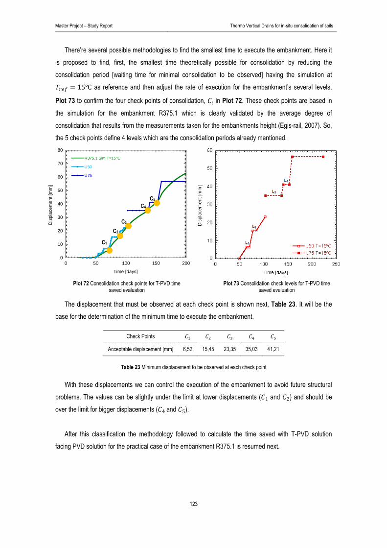
Master Project – Study Report Thermo Vertical Drains for in-situ consolidation of soils
123
There’re several possible methodologies to find the smallest time to execute the embankment. Here it is proposed to find, first, the smallest time theoretically possible for consolidation by reducing the consolidation period [waiting time for minimal consolidation to be observed] having the simulation at
15 as reference and then adjust the rate of execution for the embankment’s several levels,
Plot 73 to confirm the four check points of consolidation, in Plot 72. These check points are based in
the simulation for the embankment R375.1 which is clearly validated by the average degree of consolidation that results from the measurements taken for the embankments height (Egis-rail, 2007). So, the 5 check points define 4 levels which are the consolidation periods already mentioned.
0
10
20
30
40
50
60
70
80
0 50 100 150 200
R375.1 Sim T=15ºC
U50
U75
Dis
plac
emen
t [m
m]
Time [days] Plot 72 Consolidation check points for T-PVD time
saved evaluation Plot 73 Consolidation check levels for T-PVD time
saved evaluation
The displacement that must be observed at each check point is shown next, Table 23. It will be the base for the determination of the minimum time to execute the embankment.
Check Points
Acceptable displacement [mm] 6,52 15,45 23,35 35,03 41,21
Table 23 Minimum displacement to be observed at each check point
With these displacements we can control the execution of the embankment to avoid future structural problems. The values can be slightly under the limit at lower displacements ( 1 and 2) and should be over the limit for bigger displacements ( 4 and 5).
After this classification the methodology followed to calculate the time saved with T-PVD solution
facing PVD solution for the practical case of the embankment R375.1 is resumed next.
C1
C2
C4
C5
C3

Master Project – Study Report Thermo Vertical Drains for in-situ consolidation of soils
124
5.1.1.1 Consolidation period
The adjustments for each of the temperatures variations are presented next in Table 24. The reference base at this first calculation step will be the own embankments displacement at 15 .
Time Displacement [mm]
Level (j)
[days] 15 ∆ 10 ∆ 20 ∆ 30 Initial Final ∆
1 63 70 7 70 5,24 67 5,31 65 5,40 63,5 5,29 2 77 84 7 84 13,31 81 13,56 79 13,64 77,5 13,94 3 103 137 34 137 35,48 127 35,60 118,5 35,57 113 35,58 4 140 153 13 153 42,11 144,5 42,12 139 42,25 136,5 42,40
Table 24 Security displacement values in time for different T-PVD temperatures
The time, is marked when the values for displacement reference are observed, . Then, the
variations from each test are registered so we can calculate the time,
where the same value of displacement is observed at different temperatures, com 10,20,30.
With these values we obtain, at each level, how many days can be saved, ∆ . Then, ∆ , (j levels) is obtained by subtracting ∆ from the days already saved in the levels before.
Finally the time saved is accumulated resulting in the initial total brut time saved, ∆ , . These values
are presented in Table 25. It’s important to say that time is approximated to 0,5 day (as we’re studying an expensive procedure). In simulation, time is registered every 5 days and within this interval of time displacement is considered constant. The values of displacement are evaluated in the equilibrium moments, where charge is constant from a determined period of time before being augmented. This augments the error assumed in linear interpolation between 5 days but this one is neglected and a conservative approach is taken instead for the values of displacement observed.
Time Time saved [days]
Level [days] ∆ 10 ∆ 20 ∆ 30
Initial Final ∆ ∆ ∆ , ∆ , ∆ ∆ , ∆ , ∆ ∆ , ∆ ,
1 63 70 7 3 3 3 5 5 5 6,5 6,5 7 2 77 84 7 3 0 6 5 0 10 6,5 0 14 3 103 137 34 10 7 16 18,5 13,5 28,5 24 17,5 38 4 140 153 13 8,5 1,5 24,5 14 0,5 42,5 16,5 -1 54,5
Table 25 Time saved at each temperature increment
As the consolidation period at the last level was around 13 days for ∆ 20 and ∆ 30 the
last level is eliminated resulting in a continuous execution of the embankment. This means that the time saved for each solution at different temperatures is:
∆ 10 ∆ 20 ∆ 30
Total time saved [days] 24,5 41,5 51
Table 26 Primary time saved with T-PVD vs PVD solution for test embankment R375.1 (consolidation period adjustment)
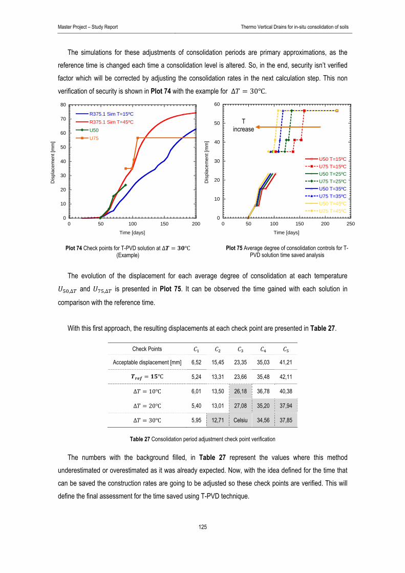
Master Project – Study Report Thermo Vertical Drains for in-situ consolidation of soils
125
The simulations for these adjustments of consolidation periods are primary approximations, as the reference time is changed each time a consolidation level is altered. So, in the end, security isn’t verified factor which will be corrected by adjusting the consolidation rates in the next calculation step. This non verification of security is shown in Plot 74 with the example for ∆ 30 .
0
10
20
30
40
50
60
70
80
0 50 100 150 200
R375.1 Sim T=15ºCR375.1 Sim T=45ºCU50U75
Dis
plac
emen
t [m
m]
Time [days]
0
10
20
30
40
50
60
0 50 100 150 200 250
U50 T=15ºCU75 T=15ºCU50 T=25ºCU75 T=25ºCU50 T=35ºCU75 T=35ºCU50 T=45ºCU75 T=45ºC
Dis
plac
emen
t [m
m]
Time [days]
Plot 74 Check points for T-PVD solution at ∆ (Example)
Plot 75 Average degree of consolidation controls for T-PVD solution time saved analysis
The evolution of the displacement for each average degree of consolidation at each temperature
,∆ and ,∆ is presented in Plot 75. It can be observed the time gained with each solution in
comparison with the reference time. With this first approach, the resulting displacements at each check point are presented in Table 27.
Check Points
Acceptable displacement [mm] 6,52 15,45 23,35 35,03 41,21
5,24 13,31 23,66 35,48 42,11
∆ 10 6,01 13,50 26,18 36,78 40,38
∆ 20 5,40 13,01 27,08 35,20 37,94
∆ 30 5,95 12,71 Celsiu 34,56 37,85
Table 27 Consolidation period adjustment check point verification
The numbers with the background filled, in Table 27 represent the values where this method underestimated or overestimated as it was already expected. Now, with the idea defined for the time that can be saved the construction rates are going to be adjusted so these check points are verified. This will define the final assessment for the time saved using T-PVD technique.
T increase

Master Project – Study Report Thermo Vertical Drains for in-situ consolidation of soils
126
5.1.1.2 Rate of construction As seen in Table 27 the last level suppression provoked a non verification of safety at this stage. This
is due to the adjustments made at the first levels, which changed the reference displacement observed for the embankment in the following levels as the charges were applied quicker. This is a consequence of the methodology followed which will be corrected by adjusting the rate of construction that is controlled by
and then apply again a 4th level of construction to absorb the displacements observed which are controlled by . These adjustments will be made for each temperature at a time.
i) T-PVD simulation at ∆
As already described the check points will be adjusted to verify security which may diminish the intermediary values already observed. The adjustments made for this case are presented in Table 28.
Check Points
Acceptable displacement [mm] 6,52 15,45 23,35 35,03 41,21
5,24 13,31 23,66 35,48 42,11
Saved Time
∆ 10 67 6,01 78 13,50 97 26,18 121 36,78 128,5 40,38
∆ 10 66 5,57 75 12,05 91 23,68 117 35,39 127 41,24
Table 28 Time saved adjustments to verify security at all check points: ∆
The line for ∆ 10 corresponds to the values obtained in the consolidation period verification and the ∆ 10 to the values after a final adjustment of both consolidation period and construction rate.
These values lead to Plot 44 where the final embankment rate is defined. This probably results in a construction not phased in an optimal point of view but other solutions can be traced and also verifying the check points made.
0
10
20
30
40
50
60
70
80
0 50 100 150 200
R375.1 Sim T=15ºCR375.1 Sim T=25ºCU50U75
Dis
plac
emen
t [m
m]
Time [days] Plot 76 Final embankment construction steps for verification of structural security with T-PVD solution at ∆
C1
C2
C4
C5
C3

Master Project – Study Report Thermo Vertical Drains for in-situ consolidation of soils
127
ii) T-PVD simulation at ∆
The values for this test are presented in Table 29 always facing the results with the reference temperature assumed for the soil, 15 .
Check Points Acceptable
displacement [mm] 6,52 15,45 23,35 35,03 41,21
5,24 13,31 23,66 35,48 42,11
Saved Time
∆ 20 65 5,40 74 13,01 93 27,08 108,5 35,20 111,5 37,94
∆ 20 65 5,40 74 13,09 87 24,19 107 35,31 116 41,27
Table 29 Time saved adjustments to verify security at all check points: ∆
The values presented in Table 29 result in Plot 77. Most of the time saved from this solution in
comparison with the one at ∆ 10 is related to the intermediary check point, that permitted a
quite higher rate of construction.
0
10
20
30
40
50
60
70
80
0 50 100 150 200
R375.1 Sim T=15ºC
R375.1 Sim T=35ºC
U50
U75
Dis
plac
emen
t [m
m]
Time [days]
Plot 77 Final embankment construction steps for verification of structural security with T-PVD solution at ∆
The variation observed at this temperature clearly shows a grater evolution of consolidation than the case at ambient temperature. The adjustment made to the permeability in temperature clearly augments the soil response to consolidation ending practically with the waiting periods for the embankment execution.
C1
C2
C4
C5
C3
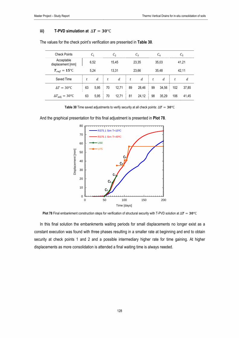
Master Project – Study Report Thermo Vertical Drains for in-situ consolidation of soils
128
iii) T-PVD simulation at ∆
The values for the check point’s verification are presented in Table 30.
Check Points Acceptable
displacement [mm] 6,52 15,45 23,35 35,03 41,21
5,24 13,31 23,66 35,48 42,11
Saved Time
∆ 30 63 5,95 70 12,71 89 28,46 99 34,56 102 37,85
∆ 30 63 5,95 70 12,71 81 24,12 98 35,29 106 41,45
Table 30 Time saved adjustments to verify security at all check points: ∆
And the graphical presentation for this final adjustment is presented in Plot 78.
0
10
20
30
40
50
60
70
80
0 50 100 150 200
R375.1 Sim T=15ºC
R375.1 Sim T=45ºC
U50
U75
Dis
plac
emen
t [m
m]
Time [days] Plot 78 Final embankment construction steps for verification of structural security with T-PVD solution at ∆
In this final solution the embankments waiting periods for small displacements no longer exist as a constant execution was found with three phases resulting in a smaller rate at beginning and end to obtain security at check points 1 and 2 and a possible intermediary higher rate for time gaining. At higher displacements as more consolidation is attended a final waiting time is always needed.
C1
C2
C4
C5
C3

Master Project – Study Report Thermo Vertical Drains for in-situ consolidation of soils
129
Finally, following the initial configuration for the embankment’s construction, the time saved for using a T-PVD solution, at three different variations of temperature, instead of a simple PVD solution is presented in Table 31.
15 ∆ 10 ∆ 20 ∆ 30
Final date 159 133 122 112
Total time saved [days] - 26 37 47
Time saved [%] - 24% 34% 43%
Table 31 Total time saved using T-PVD solution instead of PVD solution at three different temperatures for R375.1
These values are theoretic and can oscillate in function of the case study. The time saved can still be adjusted depending on the type of embankment execution made. The values obtained are also in accordance with the ones obtained for the simple oedometer simulation, 4.1.7 Conclusions (p.108).
5.1.2 Equivalent vertical permeability As we’ve two different formulations that give good approximations for our study case we’ll now verify if
an equivalent vertical permeability with temperature enhancing gives a similar saved time for T-PVD technique. The variation with temperature for this formulation was shown in Plot 68. So, by observing Plot 68 we get the values for vertical permeability at different temperatures which are presented in Table 32.
Simulations 15 ∆ 10 ∆ 20 ∆ 30
, [m/s] 3,23x10⁻¹⁰ 4,20x10⁻¹⁰ 5,17x10⁻¹⁰ 6,14x10⁻¹⁰
[m/d] 2,79x10⁻⁵ 3,63x10⁻⁵ 4,47x10⁻⁵ 5,30x10⁻⁵
Table 32 Equivalent vertical permeability values for several temperatures with ,
With these values, simulations are run and the evolution in time is shown in Plot 79.
0
10
20
30
40
50
60
70
80
0 100 200 300 400 500 600
R375.1 Sim T=15ºC
R375.1 Sim T=25ºC
R375.1 Sim T=35ºC
R375.1 Sim T=45ºC
Dis
plac
emen
t [m
m]
Time [days]
Plot 79 Evaluation of time saved using T-PVD solution: R375.1 example (Equiv. vertical permeability)

Master Project – Study Report Thermo Vertical Drains for in-situ consolidation of soils
130
The evaluation for the time saved with T-PVD solution in this hydraulic formulation will only be made if a significant variation is seen when comparing the simulations with the radial permeability formulation that was already object of this evaluation.
Therefore, if the evolution in time is similar, it means that both formulations represent equally the
application of temperature in a T-PVD solution and therefore the results found in the end, for the time saved, will be quite similar.
In Plot 80 the variations in time between equivalent vertical permeability and radial permeability
formulations in the three pre-defined temperatures are shown.
0
0,5
1
1,5
2
0 100 200 300 400 500 600
R375.1 Sim T=15ºCVertical vs RadialR375.1 Sim T=25ºCVertical vs RadialR375.1 Sim T=35ºCVertical vs RadialR375.1 Sim T=45ºCVertical vs Radial
Dis
plac
emen
t [m
m]
Time [days] Plot 80 Difference between T-PVD simulations: ∆ (Vertical permeability) – (Radial permeability)
By observing Plot 80 equivalent vertical drainage gives higher displacements when the soil is charged and this variation diminishes when temperature is imposed. In equilibrated states the contrary is observed but 100 times smaller ( 2 mm in vertical compared with 0,02 mm in radial). The time for recuperation
of these variations is almost equal as the one that induced them. So, the biggest variation that can be observed between these cases at different temperatures is around 1 mm. But this highest variation is seen
for the charging part where is the average degree of consolidation to be observed. This means that, if
calculations were made trough for the equivalent vertical permeability formulation we would save at least
one day and then security wouldn’t be verified for the radial case as at a small overestimation is
always attended. Therefore, it can be concluded that the methodology chosen for the radial permeability gave safety
values for the time saved with T-PVD technique which can be shorten from approximately a day when compared with the vertical permeability simulations. The final time saved is therefore the one previously shown in Table 31.
T increase

Master Project – Study Report Thermo Vertical Drains for in-situ consolidation of soils
131
5.2 T-PVD technique energetic cost
The time saved with this technique is clearly motivating but now an evaluation of the energetic costs involved is necessary to estimate this technique’s pertinence.
The heating capacity of saturated clay is calculated in the conditions of the experimental study and then the same is made for our test embankment case.
5.2.1 Soil’s heat energy
The soil-water mixture equivalent heating capacity can be simply determined considering the specific heat capacity for a dry clayey soil which is adjusted to the water content present in the soil.
We get 800 J.Kg-1ºC-1 for soil and 4181 J.Kg-1ºC-1 for water which combined with the water content on each case gives our equivalent heating capacity, Table 33.
Soil w
[%] [J.Kg-1.ºC-1] Kaolin clay 66 3031 Alluvial clay 26 1679
Table 33 Heating capacity values: unconsolidated samples
Using the energy formula relating heat energy to specific heat capacity, [31] and knowing the mass of soil in the domain of each drain we get the energy necessary per degree Celsius.
· · ∆ [31]
The soil’s mass for the heated test in the oedometer was defined in Table 13. For the test embankment we’ve a mesh of 1,3x1,3 m of proposed T-PVD drains in a 4 meters depth soil layer which means a volume of 6,76 m3 and with a density of 2000 Kg/m3 the mass of soil dedicated to each drain is 13,52 ton.
With these relations we get the final values for energy necessary on each case while considering that we’ve an ideal situation without heat losses. With the price of electric energy in Switzerland (around 0,1 CHF/kWh4 0,67 €/kWh) we get the price per drain, Table 34.
Soil ∆ Heating cost [Kg] [ºC] [MJ] [€/drain]
Kaolin clay 64,2 7 1,36 0,33 12 2,34 0,57 30 5,84 1,41
Alluvial clay 13 517
3 6,81 1,65 10 226,95 54,75 20 453,90 109,48 30 680,85 164,22
Table 34 Costs for soil heating at different temperatures per drain in Switzerland
4 approximated value for constant electric service

Master Project – Study Report Thermo Vertical Drains for in-situ consolidation of soils
132
It’s important to refer that these values will still suffer a coefficient related to the efficiency, of the
heating system which will increase this value in around 15-30% as this value is normally located around 80-90%.
With these values we can now specify the cost of this technique per drain in function of the time of
application and temperature applied. In the work developed for an embankment real case where T-PVD technique was used (Marques, et
al., 2003) the heating system had an efficiency of 81%. In the same work after the heating system was turned off the loss of temperature was 3ºC/day and in the experimental oedometer the heat lost was around 7ºC/day. The quantity of energy lost per day was already calculated in Table 34 and if we consider that this energy corresponds to the one necessary to maintain the temperature in the soil constant we can define the costs for the cases studied.
Soil ∆ Heating time Energetic cost
[ºC] [days] [€/drain] [€/Km]
Kaolin clay 12 5 2,21 - 30 2,5 2,59 -
Alluvial clay 10 133 273,96 260.167,43 20 122 310,57 294.933,62 30 112 348,82 331.265,05
Table 35 Total energetic costs for T-PVD technique
In the test embankment we consider a drain’s mesh of 1,3x1,3 meters with 13 meters of large which gives lines of 9 PVD. The cost of this technique per kilometre considers the efficiency of a system around 81% for all temperatures.

Master Project – Study Report Thermo Vertical Drains for in-situ consolidation of soils
133
6. Conclusions and future work
The project developed here gives a general progress in the experimental analysis of thermo-vertical
drains as consolidations at different temperatures in the LMS large oedometer were executed using Kaolin clay.
Regarding the experimental program the tests executed (T22, T35 and T53) gave well traced
displacement curves in mechanical loading with an acceptable capacity to maintain temperature inside the cell and coherence with the pore pressure measurements. The quality of the results obtained is due to the calibration made for all experimental apparatus which culminated in some alterations. This quality is not only linked to the approximation to real cases obtained (hydrostatic pressure along the drain) but also to the acknowledgment gained of the cell’s behaviour with temperature (using now the average displacement of four devices eliminating torsion problems caused by mechanical loading and temperature).
Kaolin clay mixture used had a high void ratio ( 1,76) which clearly resulted in a high
consolidation ratio with displacements reaching 24% of consolidation ratio (example: T22: 125 mm for an initial sample of 0,53) for a 57 kPa charge.
The equilibrium of pore water pressure is achieved quickly in the heated cases also shown by the higher rate of the water volume exit flow. This phenomenon verifies the water’s viscosity decrease which directly accelerates the rate of displacement resulting in a total consolidation achieved approximately 3 days earlier for a temperature variation of 13ºC in T35 test.
The water exchange device was blocked in T53 test by a considerable quantity of soil that escaped into the drain during the preparation of the sample. This only invalidated a comparison with the other tests as the same increase of the displacement rate was observed.
Simulations for the laboratorial test were kept in an elastic model solution. This permitted to conduct
several simulations confronting different solutions for representing a vertical drain. The results obtained are satisfactory even using a simple model with maximum differences smaller than 5% on both tests. Differences observed demonstrate a practically continuous simulation overestimation during the consolidation at ambient temperature and an underestimation at the beginning of the heated case followed by a clear accordance between simulation and the experimental consolidation in all duration of the test.
The formulation used for the permeability’s enhancing, in order to reproduce the thermal fraction of the simulation, demonstrates a good reproduction of the laboratory tests reality. Variations observed between experimental values and simulation decrease with temperature and may be related to the simplicity of the model used and to the thermo-mechanical behaviour of the large oedometer.

Master Project – Study Report Thermo Vertical Drains for in-situ consolidation of soils
134
In the analysis of the real cases the same model was used for simulations but now with different
hydraulic formulations based in the values offered by the laboratory tests presented in the measurement report available, (Egis-rail, 2007). The suitable apparent reproduction of the measured displacement values (there were clear field displacement measurement problems during consolidation) is sustained by a good representation between the expected average degrees of consolidation for the soil at each step of the embankment construction extrapolated from field measurements and the simulation model proposed. This shows the general applicability in civil engineering for a model as the one used in this study.
The conclusion of this project suggested an investigation of the time saved using T-PVD technique and
its energetic cost. For the oedometer a simple comparison of time to arrive to several average degrees of consolidation
was made. This analysis showed a linear time saving for a single monotonous charge which is in accordance with the linear increase of permeability with temperature The time saved is extremely satisfactory as the reference time for consolidation in T22 is almost 8 days and for a variation of 13ºC in T35 the same consolidation is achieved 3 days earlier.
The test embankment case analysis for time saved was also conducted and even for a combination of several construction steps, typical in an embankment execution, a practically linear time saving was achieved. This was due to the easiness found on adjusting the construction rates and steps so the check points proposed by simulation could be achieved. Starting from 24% of time saved using T-PVD technique for a temperature increase of 10ºC this value increases linearly 10% for each temperature increment of 10ºC (temperature variations were analysed until ∆ =30ºC).
The energetic cost determined showed a value around 5700 €/drain to apply a ∆ of 10ºC to the soil.
This value was based in the geometry used in the field case where this technique was adopted and considering the heating capacity of the soil’s mass involved, maintenance of the energy imposed, due to the heat lost, and the efficiency of a selected heating system. Using a simple scale relation the geometry of a field thermo-vertical drain is also defined and the heating capacity determined for the system. Some energetic considerations were made which demonstrates the several possibilities for an embankment heating system.
The developments made on this subject demonstrate the vastness of variables from which to deal with.
There are still several unknowns that cause drastic variations from the real cases analysed and the theoretical ideal solutions sustained by laboratory tests and numerical simulations. Thermo-vertical drains technique has a long way to be developed as the conditions on which to be successfully implemented aren’t totally known.

Master Project – Study Report Thermo Vertical Drains for in-situ consolidation of soils
135
REFERENCES
Abuel-Naga, H.M., Bergado, D.T. & Chaiprakaikeow, S. (2006a). Innovative thermal technique for
enhancing the performance of prefaricated vertical drain during the preloading process. pp. 359-370.
Cekerevac, Cane. 2003. Thermal effects on the mechanical behaviour of saturated clays: an
experimental and constitutive study. Lausanne, EPFL : s.n., 2003.
Egis-rail. 2007. LGV Rhin Rhône Branche Est Troçon B - Voray sur l'Ognin - Saulnot. 2007. Mesri G, Lo DOK. 1991. performance of prefabricated vertical drains. Proceedings of the international
conference on geotechnical engineering for coastal development - theory and practice on soft ground
Yokohama. Japan : s.n., 1991, Vols. vol. 1, p. 231-6. GEFDYN user's manual : Thermo-hydro-mechanical simulations. July 2005. p. Appendix B. H., ABU-HAMDEH Nidal. 2003. Thermal properties of soils as affected by density and water content.
2003. pp. Vol. 86, no1, pp. 97-102. Jin-Chun Chai, Shui-Long Shen, Norihiko Miura and Dennes T. Bergardo. 2001. Simple method of
modeling PVD-Improved subsoil. 2001. pp. 965-972. Marques, M.E.S. and Leroueil, S. e Almeida, M.S.S. 2003. Performance of instrumentation under
vacuum consolidation and heating. Boston : Eds. Culligan, Einstein and Whittle, 2003. pp. vol.2 pp.2641-2648.
Nuth, Mathieu. 2004. Thermal ground improvement : Application to heat exchanger piles. LMS -
EPFL : s.n., 2004. R. Robert Goughnour, A.M.ASCE. Flow capacity effect on vertical drain performance. p. Vol. 2 No. 30. S.-A., TAN and S.-H., CHEW. 1996. Comparison of the hyperbolic and Asaoka observational method
of monitoring consolidation with vertical drains. 1996. pp. vol. 36, no3, pp. 31-42 (12 ref.). Salager, Simon. 2007. Etude de la retention d'eau et de la consolidation de sols dans un cadre thermo-
hydro-mecanique. 2007.
Master Project – Study Report Thermo Vertical Drains for in-situ consolidation of soils
136
Tanguy, Mathieu, et al. 2008. Evaluation de la méthode des drains verticaux préfabriqués thermiques
pour la consolidation in-situ des sols. LMS - EPFL : s.n., 2008. Tran, Tuan Anh and Mitachi, Toshiyuki. 2008. Equivalent plane strain modeling of vertical drains in soft
ground under embankment combined with vacuum preloading. 2008. pp. 655-672. Vulliet, L. Février 2001. Géomécanique: Notes de cours. Lausanne : Laboratoire de mécanique des
sols (LMS) - Institut des sols, roches et fondations (IRSF) - EPFL, Février 2001.
WEBSITES American wick drain company. www.americanwick.com (accessed Mai 26, 2009). EGIS Rail. www.egis-rail.ch (accessed April 20, 2009). NDS company. www.ndspro.com (accessed Mai 26, 2009). Nilex construction company. www.nilexconstruction.com (accessed Mai 27, 2009). Thermo scientific. www.thermo.com (accessed June 16, 2009).

Master Project – Study Report Thermo Vertical Drains for in-situ consolidation of soils
137
APPENDIX
APPENDIX 1 – Experimental device calibration report APPENDIX 2 – Experimental tests data APPENDIX 3 – Resume from Egis-Rail measurement report

APPENDIX 1

Master Project – Appendix 2 Thermo Vertical Drains for in-situ consolidation of soils
i.1
APPENDIX 1 – CALIBRATION OF THE EXPERIMENTAL DEVICE
INDEX
1. Introduction .............................................................................................................. 2
1.1 Pressure sensors ................................................................................................. 3
1.1.1 Pressure calibration process ........................................................................ 3
1.1.2 Mechanical loading calibration ...................................................................... 7
1.1.2.1 Test at ambient temperature ..................................................................... 7
1.1.2.2 Test at 40ºC .............................................................................................. 8
1.1.2.3 Test at 60ºC .............................................................................................. 9
1.1.3 Results after heating process ..................................................................... 10
1.2 Displacement ..................................................................................................... 12
1.2.1 Test at ambient temperature ....................................................................... 12
1.2.1.1 Laboratory’s temperature variation ......................................................... 15
1.2.2 Test at 40ºC ................................................................................................ 16
1.2.3 Test at 60ºC ................................................................................................ 18
1.3 Conclusions ....................................................................................................... 20
1.3.1 Theoretical approach for thermal loading ................................................... 20
1.3.2 Pressure and displacement for high temperature cases ............................ 22
1.3.2.1 Test at ambient temperature ................................................................... 23
1.3.2.2 Test at 40ºC ............................................................................................ 24
1.3.2.3 Test at 60ºC ............................................................................................ 24

Master Project – Appendix 2 Thermo Vertical Drains for in-situ consolidation of soils
i.2
1. Introduction
This calibration will consist in the evaluation of the displacement and pressure variations due to the inducted heat of water and mechanical loading for the big size oedometer cell in the LMS laboratory, Figure 1. The main objective is to register and understand the cell’s effects due to temperature so they can be corrected in the studies that involve this experimental apparatus. The complete device is described in the technical report, 1.1 Experimental apparatus.
Figure 1 Experimental apparatus: Oedometer cell
This study is based in tests at different temperatures, which influence the displacements of the piston and the cell’s behaviour, when this one is full of water. A displacement analysis will be complemented with the pressure sensors calibration. This calibration consists in registering its variation with temperature induced and in time (as high temperatures in time may also influence the pressure measurements). In the case of the displacement analysis, the values obtained will be used to isolate the displacement component due to the cell’s dilation when heated.
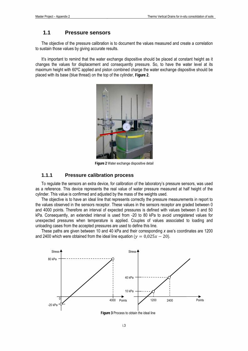
Master Project – Appendix 2 Thermo Vertical Drains for in-situ consolidation of soils
i.3
0
Stress
-20 kPa
80 kPa
4000 Points
40 kPa
10 kPa
1200 2400
Stress
Points
1.1 Pressure sensors
The objective of the pressure calibration is to document the values measured and create a correlation to sustain those values by giving accurate results.
It’s important to remind that the water exchange dispositive should be placed at constant height as it
changes the values for displacement and consequently pressure. So, to have the water level at its maximum height with 60ºC applied and piston combined charge the water exchange dispositive should be placed with its base (blue thread) on the top of the cylinder, Figure 2.
1.1.1 Pressure calibration process To regulate the sensors an extra device, for calibration of the laboratory’s pressure sensors, was used
as a reference. This device represents the real value of water pressure measured at half height of the cylinder. This value is confirmed and adjusted by the mass of the weights used.
The objective is to have an ideal line that represents correctly the pressure measurements in report to the values observed in the sensors receptor. These values in the sensors receptor are graded between 0 and 4000 points. Therefore an interval of expected pressures is defined with values between 0 and 50 kPa. Consequently, an extended interval is used from -20 to 80 kPa to avoid unregistered values for unexpected pressures when temperature is applied. Couples of values associated to loading and unloading cases from the accepted pressures are used to define this line.
These paths are given between 10 and 40 kPa and their corresponding x axe’s coordinates are 1200 and 2400 which were obtained from the ideal line equation ( 0,025 20).
Figure 3 Process to obtain the ideal line
Figure 2 Water exchange dispositive detail
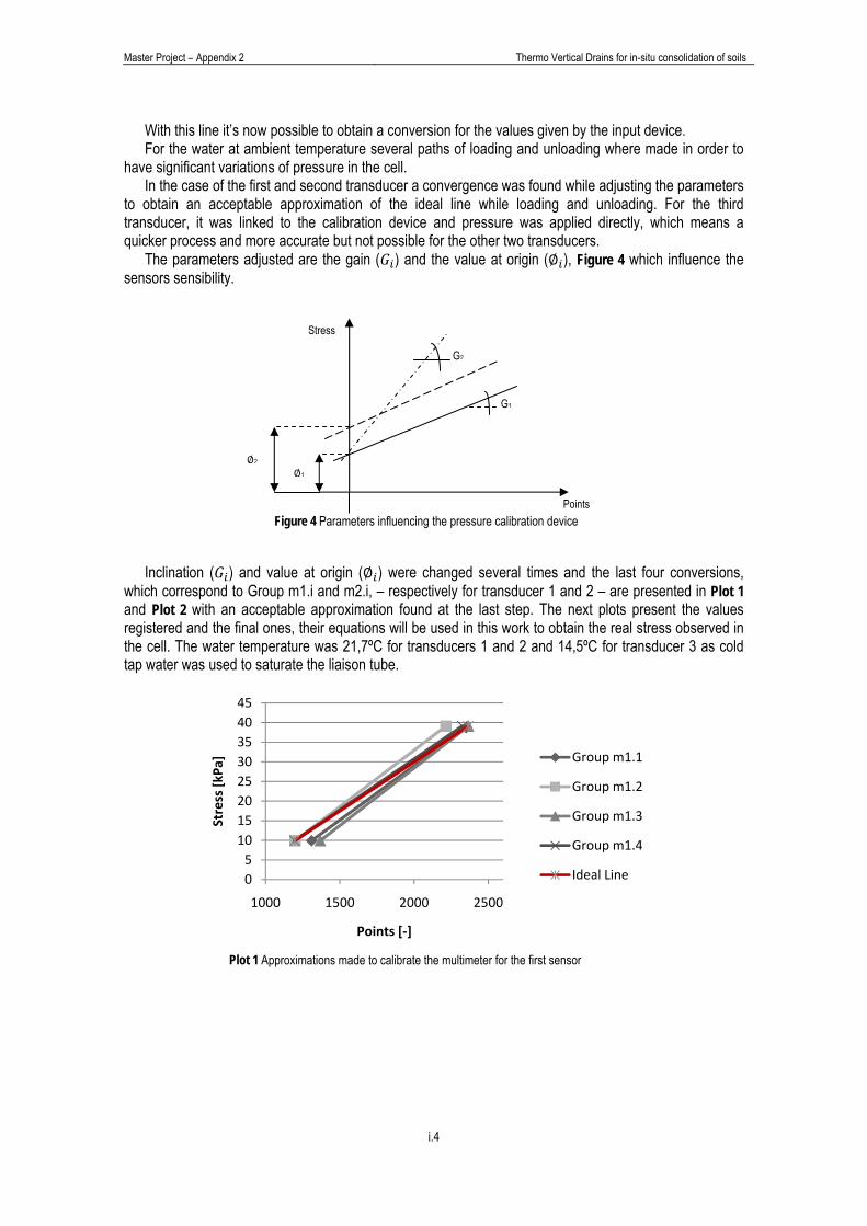
Master Project – Appendix 2 Thermo Vertical Drains for in-situ consolidation of soils
i.4
With this line it’s now possible to obtain a conversion for the values given by the input device. For the water at ambient temperature several paths of loading and unloading where made in order to
have significant variations of pressure in the cell. In the case of the first and second transducer a convergence was found while adjusting the parameters
to obtain an acceptable approximation of the ideal line while loading and unloading. For the third transducer, it was linked to the calibration device and pressure was applied directly, which means a quicker process and more accurate but not possible for the other two transducers.
The parameters adjusted are the gain ( ) and the value at origin ( ), Figure 4 which influence the sensors sensibility.
Inclination ( ) and value at origin ( ) were changed several times and the last four conversions,
which correspond to Group m1.i and m2.i, – respectively for transducer 1 and 2 – are presented in Plot 1 and Plot 2 with an acceptable approximation found at the last step. The next plots present the values registered and the final ones, their equations will be used in this work to obtain the real stress observed in the cell. The water temperature was 21,7ºC for transducers 1 and 2 and 14,5ºC for transducer 3 as cold tap water was used to saturate the liaison tube.
051015202530354045
1000 1500 2000 2500
Stress [kPa
]
Points [‐]
Group m1.1
Group m1.2
Group m1.3
Group m1.4
Ideal Line
1
G1
Stress
Points
G2
2
Figure 4 Parameters influencing the pressure calibration device
Plot 1 Approximations made to calibrate the multimeter for the first sensor
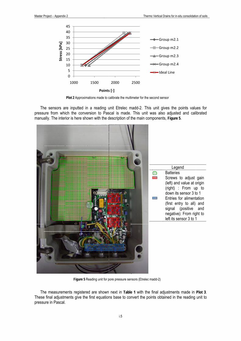
Master P
Thpressmanu
Th
Thesepress
Project – Appendix
he sensors aure from whially. The inter
he measureme final adjustmure in Pascal.
Stress [kPa
]
x 2
re inputted inch the conve
rior is here sho
ents registerements give the
051015202530354045
1000
Plot 2 Approxim
Figure 5 R
n a reading uersion to Pasown with the d
ed are showne first equation
1500
Points
mations made to c
Reading unit for p
i.5
unit Etrelec mscal is made.description of t
next in Tablens base to co
2000
s [‐]
calibrate the mult
pore pressure sen
Thermo
madd-2. This This unit wthe main com
e 1 with the fnvert the poin
2500
timeter for the se
nsors (Etrelec ma
Vertical Drains for
unit gives thas also adjusponents, Figu
final adjustments obtained in
LeBatterScrew(left) a(right)down Entrie(first signalnegatleft its
Group m2
Group m2
Group m2
Group m2
Ideal Line
cond sensor
add-2)
r in-situ consolidatio
e points valusted and cali
ure 5.
ents made in n the reading
egend ries ws to adjust and value at o) : From up its sensor 3 to
es for alimententry to all) l (positive tive): From rigs sensor 3 to 1
2.1
2.2
2.3
2.4
e
on of soils
ues for ibrated
Plot 3. unit to
gain origin p to o 1 ation and
and ght to 1

Master Project – Appendix 2 Thermo Vertical Drains for in-situ consolidation of soils
i.6
Case Stress Reading m1 m2 Case Stress Reading m3 Read Ajusted Parameter Variation Read Ajusted Parameter Variation Read Ajusted Parameter Variation
--- 38,7 2348 --- 2350 --- --- 2353 --- --- 10,1 1204 --- 1206 (-Gain) --- Unload 9,9 1196 1310 1199 (-Gain / -φ) 111 1284 1200 (-Gain / +φ) 84 Unload 23,5 1740 1910 1746 (-Gain / +φ) 164 Load 39,1 2364 2214 2366 (-Gain / +φ) -152 2215 2365 (-Gain / +φ) -150 Load 34,2 2168 2239 2171 (-Gain / +φ) 68
Unload 9,9 1196 1368 1199 (-Gain / +φ) 169 1369 1195 (-Gain / +φ) 174 Unload 46,8 2672 2733 2671 (-Gain / +φ) 62 Load 39,1 2364 2151 2368 (+Gain / -φ) -217 2156 2368 (+Gain / -φ) -212 Load 10 1200 1100 1202 (-Gain / +φ) -102
Unload 9,9 1196 1304 1196 (+Gain / -φ) 108 1304 1196 (+Gain / -φ) 108 Unload 40 2400 2434 2399 (+Gain / +φ) 35 Load 39,1 2364 2325 39 2311 2311 Load 30,1 2004 2022 2000 (-Gain / -φ) 22
Unload 20 1600 1609 1593 (+Gain / -φ) 16
Load 10 1200 1202 1195 7 Table 1 Values registered for the final calibration of the pore pressure transducers
yreal = 0,0259x ‐ 21,033
yideal = 0,025x ‐ 20
01020304050
1000 2000
Pressure [k
Pa]
Points [‐]
Transducer 1 (3)[Final pressure calibration]
Group m1.4
Ideal Line yreal = 0,0262x ‐ 21,421
yideal = 0,025x ‐ 200
1020304050
1000 2000
Pressure [k
Pa]
Points [‐]
Transducer 2 (1)[Final pressure calibration]
Group m2.4
Ideal Line
y real= 0,0256x ‐ 20,742
yideal = 0,025x ‐ 20
01020304050
1000 1500 2000 2500
Pressure [k
Pa]
Points [‐]
Transducer 3[Final pressure calibration]
Group m3.7
Ideal Line
Plot 3 Final lines with equations for conversion between pressure and points given by multimeter

Master Project – Appendix 2 Thermo Vertical Drains for in-situ consolidation of soils
i.7
1.1.2 Mechanical loading calibration In the following tests pressure values were taken at high temperature but without the reference device.
This means that variation of the sensors caused directly by temperature can’t be measured. Therefore calibration confirmations will be made after the heating tests and characteristic lines will be traced to confirm the values obtained.
1.1.2.1 Test at ambient temperature
Two loading tests were made due to some dispersion in the displacement values measured in a first approach of this case. Both tests are presented in Plot 4 and Plot 5. The values for these tests are presented in Appendix 1.
If the displacement behaviour wasn’t clearly defined the charge applied in function of pressure shows a
clear linear relation. This demonstrates that pressure and displacement for calibration are two factors that can be studied independently but when comparisons are made between tests, they’re proportionally related.
It can be seen again a plain linear relation between the charges applied and pressure.
0,0
50,0
100,0
150,0
200,0
250,0
300,0
350,0
400,0
990 1190 1390 1590 1790 1990 2190 2390 2590
Charge
[Kg]
Points [‐]
Pressure 1
Pressure 2
Pressure 3
0,0
50,0
100,0
150,0
200,0
250,0
300,0
350,0
400,0
990 1190 1390 1590 1790 1990 2190 2390 2590
Stress [K
g]
Points [‐]
Pressure 1
Pressure 2
Pressure 3
Plot 4 Test 1 – Charge vs Pressure results
Plot 5 Test 2 – Charge vs Pressure results
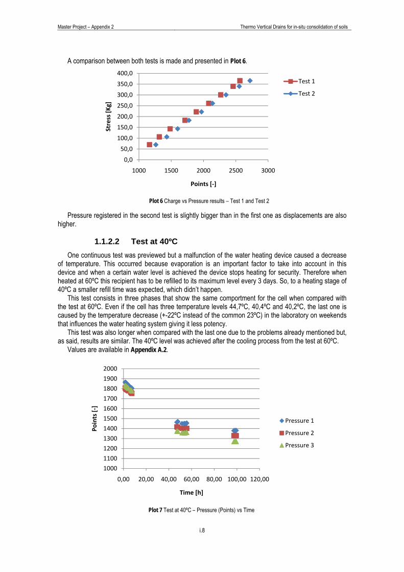
Master Project – Appendix 2 Thermo Vertical Drains for in-situ consolidation of soils
i.8
A comparison between both tests is made and presented in Plot 6. Pressure registered in the second test is slightly bigger than in the first one as displacements are also
higher.
1.1.2.2 Test at 40ºC One continuous test was previewed but a malfunction of the water heating device caused a decrease
of temperature. This occurred because evaporation is an important factor to take into account in this device and when a certain water level is achieved the device stops heating for security. Therefore when heated at 60ºC this recipient has to be refilled to its maximum level every 3 days. So, to a heating stage of 40ºC a smaller refill time was expected, which didn’t happen.
This test consists in three phases that show the same comportment for the cell when compared with the test at 60ºC. Even if the cell has three temperature levels 44,7ºC, 40,4ºC and 40,2ºC, the last one is caused by the temperature decrease (+-22ºC instead of the common 23ºC) in the laboratory on weekends that influences the water heating system giving it less potency.
This test was also longer when compared with the last one due to the problems already mentioned but, as said, results are similar. The 40ºC level was achieved after the cooling process from the test at 60ºC.
Values are available in Appendix A.2.
0,0
50,0
100,0
150,0
200,0
250,0
300,0
350,0
400,0
1000 1500 2000 2500 3000
Stress [K
g]
Points [‐]
Test 1
Test 2
1000
1100
1200
1300
1400
1500
1600
1700
1800
1900
2000
0,00 20,00 40,00 60,00 80,00 100,00 120,00
Points [‐]
Time [h]
Pressure 1
Pressure 2
Pressure 3
Plot 6 Charge vs Pressure results – Test 1 and Test 2
Plot 7 Test at 40ºC – Pressure (Points) vs Time
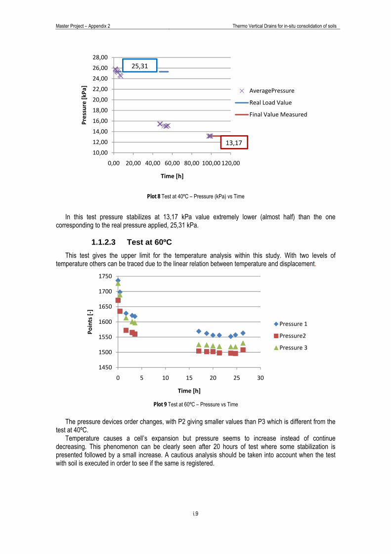
Master Project – Appendix 2 Thermo Vertical Drains for in-situ consolidation of soils
i.9
10,00
12,00
14,00
16,00
18,00
20,00
22,00
24,00
26,00
28,00
0,00 20,00 40,00 60,00 80,00 100,00 120,00
Pressure [kPa
]
Time [h]
AveragePressure
Real Load Value
Final Value Measured
13,17
25,31
1450
1500
1550
1600
1650
1700
1750
0 5 10 15 20 25 30
Points [‐]
Time [h]
Pressure 1
Pressure2
Pressure 3
In this test pressure stabilizes at 13,17 kPa value extremely lower (almost half) than the one
corresponding to the real pressure applied, 25,31 kPa.
1.1.2.3 Test at 60ºC This test gives the upper limit for the temperature analysis within this study. With two levels of
temperature others can be traced due to the linear relation between temperature and displacement.
The pressure devices order changes, with P2 giving smaller values than P3 which is different from the
test at 40ºC. Temperature causes a cell’s expansion but pressure seems to increase instead of continue
decreasing. This phenomenon can be clearly seen after 20 hours of test where some stabilization is presented followed by a small increase. A cautious analysis should be taken into account when the test with soil is executed in order to see if the same is registered.
Plot 8 Test at 40ºC – Pressure (kPa) vs Time
Plot 9 Test at 60ºC – Pressure vs Time
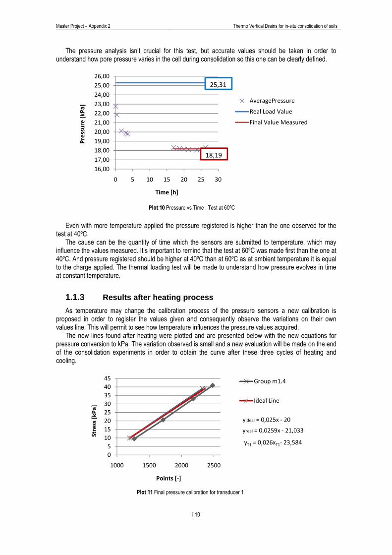
Master Project – Appendix 2 Thermo Vertical Drains for in-situ consolidation of soils
i.10
The pressure analysis isn’t crucial for this test, but accurate values should be taken in order to understand how pore pressure varies in the cell during consolidation so this one can be clearly defined.
Even with more temperature applied the pressure registered is higher than the one observed for the
test at 40ºC. The cause can be the quantity of time which the sensors are submitted to temperature, which may
influence the values measured. It’s important to remind that the test at 60ºC was made first than the one at 40ºC. And pressure registered should be higher at 40ºC than at 60ºC as at ambient temperature it is equal to the charge applied. The thermal loading test will be made to understand how pressure evolves in time at constant temperature.
1.1.3 Results after heating process As temperature may change the calibration process of the pressure sensors a new calibration is
proposed in order to register the values given and consequently observe the variations on their own values line. This will permit to see how temperature influences the pressure values acquired.
The new lines found after heating were plotted and are presented below with the new equations for pressure conversion to kPa. The variation observed is small and a new evaluation will be made on the end of the consolidation experiments in order to obtain the curve after these three cycles of heating and cooling.
yreal = 0,0259x ‐ 21,033
yideal = 0,025x ‐ 20
yT1 = 0,026xT1‐ 23,584
05
1015202530354045
1000 1500 2000 2500
Stress [kPa
]
Points [‐]
Group m1.4
Ideal Line
16,0017,0018,0019,0020,0021,0022,0023,0024,0025,0026,00
0 5 10 15 20 25 30
Pressure [kPa
]
Time [h]
AveragePressure
Real Load Value
Final Value Measured
18,19
25,31
Plot 11 Final pressure calibration for transducer 1
Plot 10 Pressure vs Time : Test at 60ºC
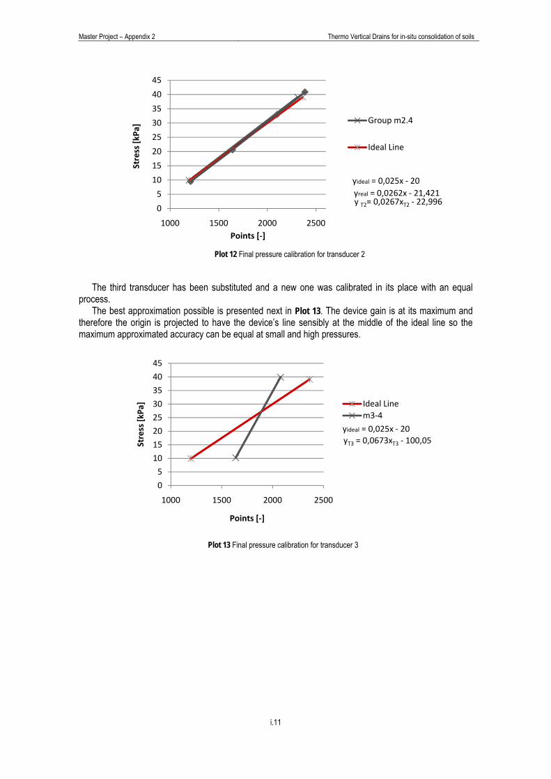
Master Project – Appendix 2 Thermo Vertical Drains for in-situ consolidation of soils
i.11
The third transducer has been substituted and a new one was calibrated in its place with an equal
process. The best approximation possible is presented next in Plot 13. The device gain is at its maximum and
therefore the origin is projected to have the device’s line sensibly at the middle of the ideal line so the maximum approximated accuracy can be equal at small and high pressures.
yreal = 0,0262x ‐ 21,421yideal = 0,025x ‐ 20
y T2= 0,0267xT2 ‐ 22,9960
5
10
15
20
25
30
35
40
45
1000 1500 2000 2500
Stress [kPa
]
Points [‐]
Group m2.4
Ideal Line
yideal = 0,025x ‐ 20yT3 = 0,0673xT3 ‐ 100,05
0
5
10
15
20
25
30
35
40
45
1000 1500 2000 2500
Stress [kPa
]
Points [‐]
Ideal Linem3‐4
Plot 12 Final pressure calibration for transducer 2
Plot 13 Final pressure calibration for transducer 3
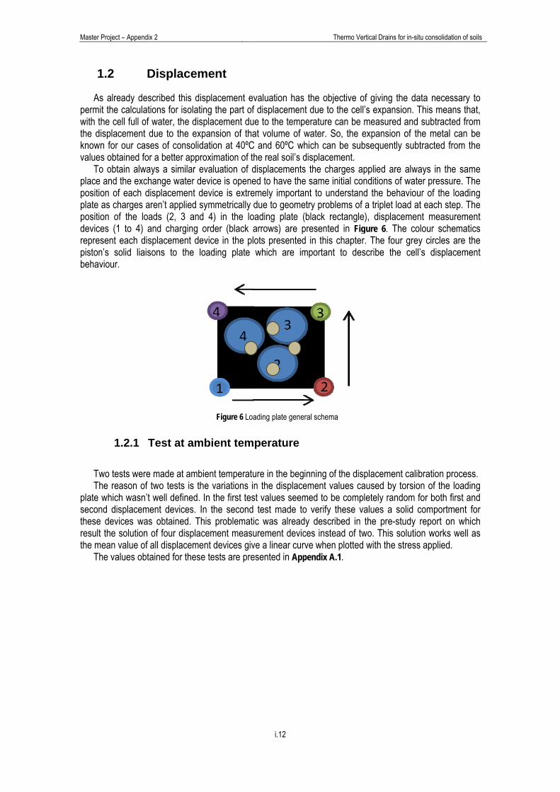
Master P
1
Aspermiwith ththe diknownvalues
Toplace positioplate positiodevicereprespistonbehav
TwTh
plate seconthese result the m
Th
Project – Appendix
1.2 D
s already dest the calculatihe cell full of wisplacement dn for our cases obtained foro obtain alway and the exchon of each dias charges aron of the loaes (1 to 4) asent each disn’s solid liaisoviour.
1.2.1 T
wo tests were he reason of twhich wasn’t
nd displaceme devices was the solution oean value of a
he values obta
x 2
Displacem
cribed this disons for isolatiwater, the dis
due to the expes of consolidr a better apprys a similar eange water desplacement dren’t applied sads (2, 3 andnd charging oplacement deons to the lo
Test at am
made at ambtwo tests is thwell defined.
ent devices. Is obtained. Thof four displacall displacemeained for these
ment
splacement eng the part of
splacement dupansion of thadation at 40ºCroximation of tevaluation of device is opene
device is extresymmetrically d 4) in the loorder (black
evice in the ploading plate
mbient tem
ient temperatuhe variations iIn the first tesn the secondhis problematcement measuent devices give tests are pre
Figure 6 Lo
i.12
valuation hasf displacemenue to the tempat volume of
C and 60ºC whe real soil’s ddisplacementsed to have theemely importadue to geome
oading plate (arrows) are plots presentedwhich are im
mperature
ure in the begn the displacest values seemd test made toic was alreadurement devicve a linear curesented in App
ading plate gene
Thermo
s the objectivent due to the cperature can bwater. So, thehich can be sdisplacement.s the chargese same initial cant to understaetry problems (black rectangpresented in d in this chapmportant to d
inning of the dement values med to be como verify thesedy described ces instead ofrve when plottpendix A.1.
eral schema
Vertical Drains for
e of giving thecell’s expansiobe measured ae expansion osubsequently
s applied are conditions of wand the behaof a triplet loagle), displaceFigure 6. Theter. The four describe the
displacement caused by tompletely randoe values a soin the pre-stuf two. This soed with the st
r in-situ consolidatio
e data necesson. This meanand subtracteof the metal csubtracted fro
always in thewater pressur
aviour of the load at each stement measur
e colour schegrey circles acell’s displac
calibration proorsion of the loom for both firlid comportme
udy report on olution works wress applied.
on of soils
sary to ns that, ed from can be om the
e same re. The oading
ep. The rement matics
are the cement
ocess. oading rst and ent for which well as

Master P
In Th
the cestudieconso
In devicethe chfind ebehavD4.
Project – Appendix
0,0
50,0
100,0
150,0
200,0
250,0
300,0
350,0
400,0
Stress[Kg]
0
50
100
150
200
250
300
350
400
Stress [K
g]
Plot 14 it is clhis thematic well behaviour wed, as displacolidation settle
this second te D2 has a clharge applied equal behaviovior and displa
x 2
0
0
0
0
0
0
0
0
0
‐0,40 ‐0,20
0,0
0,0
0,0
0,0
0,0
0,0
0,0
0,0
0,0
‐0,4 ‐0,2
ear the undefiwould be a prowill be similarcement will b
ement.
est (Appendixlear loading d (200Kg) and or for all dispacement can
0 0,00 0Displace
0 0,2 0Displac
ined behaviouoblem, if a char to the one shbe corrected
x A.2) we can displacement w then inversioplacement debe classified
Plot 14 Test 1
Plot 15 Test
i.13
0,20 0,40ement [mm]
,4 0,6 0,8cement [mm]
ur of the cell’s arge is appliedhowed above.in time for a
clearly see a which shows n of behavior.vices. After tin two groups
– Charge vs Dis
t 2 – Charge vs D
Thermo
0,60 0,
1 1,2 1
displacementd for a soil at . But this hypo
a constant loa
pattern for theload transfer . It can be seethis level the s: equal to D1
splacement result
Displacement res
Vertical Drains for
80
Disp
Disp
Disp
Disp
1,4
Disp
Disp
Disp
Disp
t for a constan a first attempothesis isn’t read in order t
e loading plateto the piston en that until th loading plate and D3 and
ts
ults
r in-situ consolidatio
placement 1
placement 2
placement 3
placement 4
placement 1
placement 2
placement 3
placement 4
nt loading procpt, which meanelevant for theto achieve th
e comportmensolid links aft
his level, 200Ke shows a m opposite to D
on of soils
cess. ns that e case e final
nt. The ter half Kg, we marked D2 and

Master Project – Appendix 2 Thermo Vertical Drains for in-situ consolidation of soils
i.14
Positive conclusions can be traced for both tests with linear relations that simplify the cell’s
comportment analysis.
Even with the cells comportment not well defined in the first test it is well demonstrated to be equal for both tests.
0,0
50,0
100,0
150,0
200,0
250,0
300,0
350,0
400,0
0 0,1 0,2 0,3 0,4 0,5
Stress [K
g]
Displacement [mm]
Test 1
Test2
Plot 16 Charge vs Displacement results – Test 1 and Test 2

Master Project – Appendix 2 Thermo Vertical Drains for in-situ consolidation of soils
i.15
1.2.1.1 Laboratory’s temperature variation The laboratory’s air temperature near the cell was registered during the week while calibrations were made.
Plot 17 Weekly temperature in the laboratory
The stabilization process of the cylinder seems to be related to the temperature registered in the laboratory so a complementary study was made to give an approximation
of the laboratory’s temperature during a normal week. At night and weekends the laboratory is one or two degrees colder (approx. 21ºC) and at around 18h it tends to be hotter during the week (23,5ºC). It also seems that the heating system works when lights are turned on. These variation cases are enough to make a difference in the cylinder’s temperature at ambient temperature as stabilization of pressure and displacement is never achieved. This variation will consist in the incertitude of our study case.
21,621,822,022,222,422,622,823,023,223,423,623,8
23‐3‐09 0:00 24‐3‐09 0:00 25‐3‐09 0:00 26‐3‐09 0:00 27‐3‐09 0:00 28‐3‐09 0:00 29‐3‐09 0:00 30‐3‐09 0:00
Tempe
rature [˚C]
Time [dd‐m‐yy h:mm]
Laboratory Temperature
Monday Tuesday Wednesday Thursday Friday Saturday Sunday

Master P
Astempe
Th
with thigheheatinbehav
Thhighe
Ththe te
Project – Appendix
0
0,2
0,4
0,6
0,8
1
1,2
1,4
1,6
1,8
0
Displacem
ent [mm]
1.2.2 Ts already meerature: 44,7ºC
he same tendhe mechanicar values than ng that can beviour is transmhe non inversr values than
his behaviour mperature eff
0
0,02
0,04
0,06
0,08
0,
0,12
0,14
0,16
0,18
Displacem
ent [mm]
x 2
0,00 20,00
Test at 40ºntioned each C, 40,4ºC and
ency in time ial loading casD4 and D1 hig
e understood mitted to the lo
ed behaviour D2 and the sa
is then lost infect.
0
2
4
6
8
1
2
4
6
8
0,00
Plot
40,00 60,
Time
ºC group of val
d 40,2ºC. This
is observed fose at ambient gher values thas a force act
oading plate by can be seename for D1 an
n time with inv
2,00 4,
Tim
Plot 18 Test at
19 Test at 40ºC
i.16
00 80,00 1
e [h]
lues, that can temperature v
or the displace temperature,han D3, Plot 18ting in opposiy the solid liaisn in the beginnd D3, Plot 19.
version arrivin
,00 6,0
me [h]
t 40ºC – Displace
– Displacement v
Thermo
100,00 120,00
n be clearly svariation is sh
ement measu as D2 and D8. This is due te direction thsons in the pisning of the m
g as soon as
00 8,00
ement vs Time
vs Time (Initial de
Vertical Drains for
0
Displac
Displac
Displac
Displac
seen in Plot own in Plot 21
urement devicD4 but now in to the cell’s ehan a charge ston
mechanical ch
mechanical l
0
Displace
Displace
Displace
Displace
etail)
r in-situ consolidatio
ement 1
ement 2
ement 3
ement 4
18 correspon1.
es, when comversed as D2
expansion cau(compression
arge with D4
oad is annula
ement 1
ement 2
ement 3
ement 4
on of soils
d to a
mpared 2 gives sed by
n). This
giving
ated by
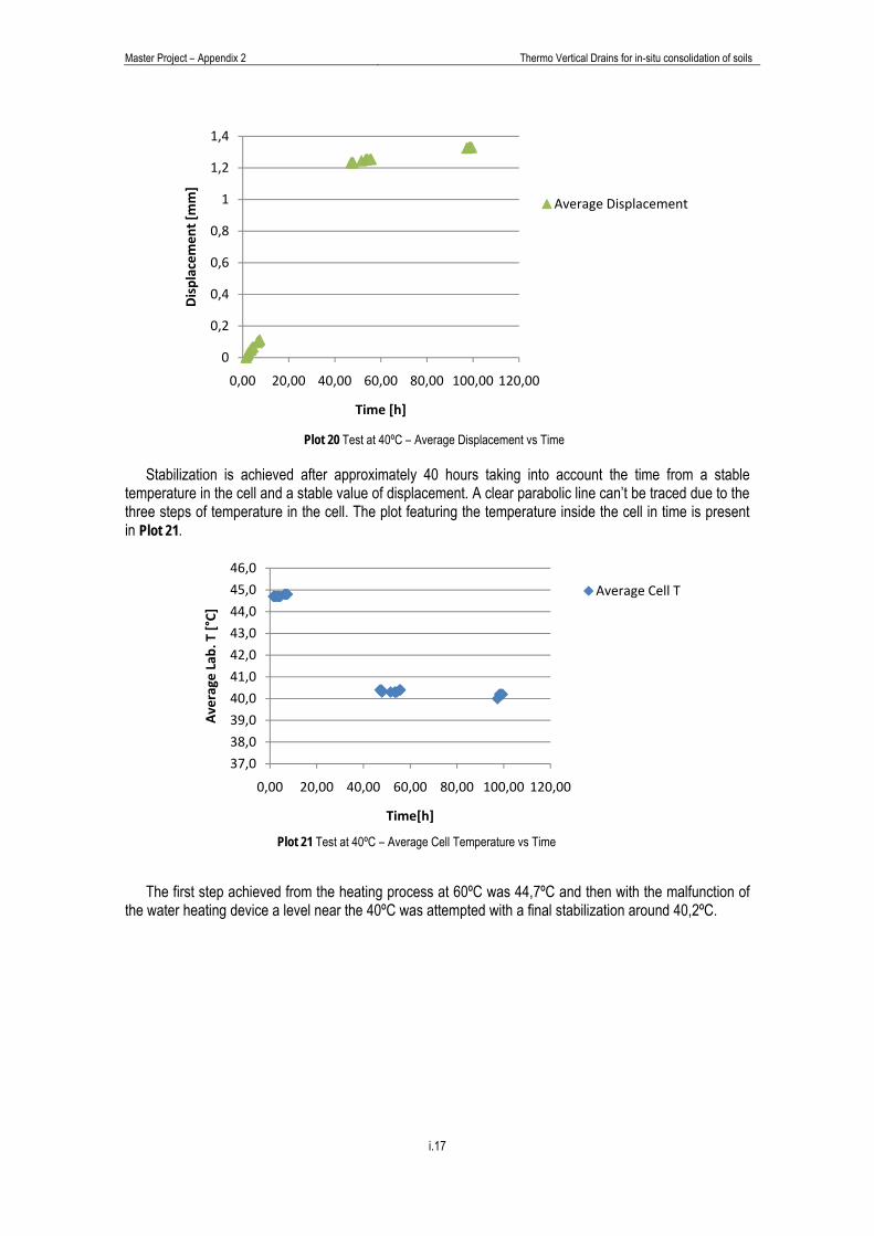
Master Project – Appendix 2 Thermo Vertical Drains for in-situ consolidation of soils
i.17
Stabilization is achieved after approximately 40 hours taking into account the time from a stable temperature in the cell and a stable value of displacement. A clear parabolic line can’t be traced due to the three steps of temperature in the cell. The plot featuring the temperature inside the cell in time is present in Plot 21.
The first step achieved from the heating process at 60ºC was 44,7ºC and then with the malfunction of
the water heating device a level near the 40ºC was attempted with a final stabilization around 40,2ºC.
37,0
38,0
39,0
40,0
41,0
42,0
43,0
44,0
45,0
46,0
0,00 20,00 40,00 60,00 80,00 100,00 120,00
Average
Lab
. T [°C]
Time[h]
Average Cell T
0
0,2
0,4
0,6
0,8
1
1,2
1,4
0,00 20,00 40,00 60,00 80,00 100,00 120,00
Displacem
ent [mm]
Time [h]
Average Displacement
Plot 20 Test at 40ºC – Average Displacement vs Time
Plot 21 Test at 40ºC – Average Cell Temperature vs Time

Master P
Af
in the
Thvaluesgives
Opthis si
Project – Appendix
1.2.3 T
fter a heating next chapter)
he device D1 s (related to t the highest dipposite happede). But with
0
0,02
0,04
0,06
0,08
0,1
0,12
0,14
0,16
0,18
0,2
Displacem
ent [mm]
0
0,02
0,04
0,06
0,08
0,1
0,12
0,14
0,16
0,18
0,2
Displacem
ent [mm]
x 2
Test at 60º
process from ) a test at this
when chargetorsion) so, it isplacements.ens for D3 andD3 positioned
0
2
4
6
8
1
2
4
6
8
2
0 5
0
2
4
6
8
1
2
4
6
8
2
0 5
Plot 23 Te
ºC
ambient temp last temperatu
d at ambient seems logica
d D4 that seemd in a place wh
10 1
Tim
10 15
Time
Plot 22 Test at
est at 60ºC – Dis
i.18
perature to 60ure will be exe
temperature ial that when e
m to demonsthere more wei
15 20
me [h]
5 20
[h]
60ºC – Displace
splacement vs Tim
Thermo
0ºC (values foecuted with a
is the one thaexpansion cau
rate the sameight is concen
25 30
25 30
ement vs Time
me (Tendency ev
Vertical Drains for
or this heatingconstant mec
at gives the smused by temp
e behavior for trated.
Displacem
Displacem
Displacem
Displacem
Displace
Displace
Displace
Displace
volution)
r in-situ consolidatio
case will be hanical charg
maller displacperature is app
the loading pl
ment 1
ment 2
ment 3
ment 4
ement 1
ement 2
ement 3
ement 4
on of soils
shown e.
cement plied it
late (in

Master Project – Appendix 2 Thermo Vertical Drains for in-situ consolidation of soils
i.19
These plots seem to present a stabilization followed by a sudden augmentation but this augmentation, in all displacement devices, is only 0,01 mm which means a smooth stabilization around this value as soon as the operator thinks it can adjust another 0,01 mm in each device. This is shown next in the average displacement Plot 24. For this test, stabilization is achieved at 25 hours as a more than 4 hours passed without increasing of displacement.
0,00
0,02
0,04
0,06
0,08
0,10
0,12
0,14
0,16
0 5 10 15 20 25 30
Displacem
ent [mm]
Time [h]
Average Displacement
Plot 24 Test at 60ºC – Displacement vs Time

Master Project – Appendix Thermo Vertical Drains for in-situ consolidation of soils
i.20
1.3 Conclusions
As this calibration is a process to reduce the influences of the material used in the cylinder on the real boundary conditions, even if the values deducted aren’t extremely accurate we’ll always have a relative approach for each case.
The values obtained here will be the base for a more profound study when the complete behaviour of the cell may be necessary to be known. After the project developed here the thermal loading behaviour regarding the cylinder’s expansion wasn’t relevant enough to search deeper on this matter. A theoretical approach is, however, presented.
1.3.1 Theoretical approach for thermal loading Calibration for loading and unloading cases was conducted as a non drained case. This means a new
approach for the displacements as they won’t be the same for our drained case. Therefore, it can be assumed that the differences between a drained and non drained case will be the pressure registered and the exchange of water volume. Water was chosen because its characteristics are well documented and therefore its behaviour can be well defined. For this case the volume-temperature relationship is taken into account. Characteristics such as vapour pressure curves for liquid water and pressure-density aren’t considered valid for the range of values of this study.
Volume-temperature [%] 0,272√
[1]
The pressure will be smaller and always well known and the water volume increase at each
temperature and pressure is given by equation [1] represented in Figure 7. So, the following parameters at the three temperatures which are taken into account in this study give
the following values presented in Table 2. The fixed variables in these formulas have the following values: reference pressure, 85 and 0,03605 the quantity of water in the cylinder. As the pressures that are observed in the cylinder are around 50 kPa the water density variation won’t be taken into account.
∆
20° 0
40° 0,3 %
60° 0,95 %
Table 2 Volume variation for different temperatures [20ºC as base]
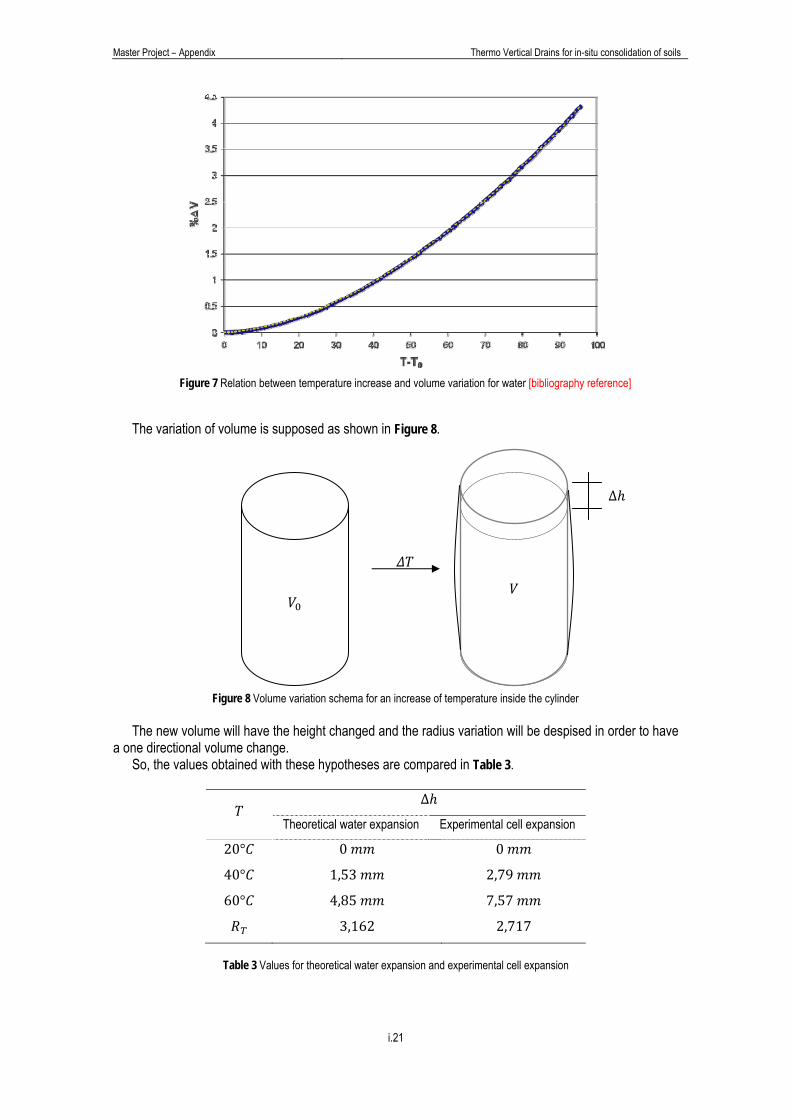
Master Project – Appendix Thermo Vertical Drains for in-situ consolidation of soils
i.21
Figure 7 Relation between temperature increase and volume variation for water [bibliography reference]
The variation of volume is supposed as shown in Figure 8.
The new volume will have the height changed and the radius variation will be despised in order to have
a one directional volume change. So, the values obtained with these hypotheses are compared in Table 3.
∆
Theoretical water expansion Experimental cell expansion
20° 0 0
40° 1,53 2,79
60° 4,85 7,57
3,162 2,717
Table 3 Values for theoretical water expansion and experimental cell expansion
∆
Figure 8 Volume variation schema for an increase of temperature inside the cylinder

Master Project – Appendix Thermo Vertical Drains for in-situ consolidation of soils
i.22
1.3.2 Pressure and displacement for high temperature cases The values that were obtained have to be compared in order to verify their validity. The following table
resumes the values registered when stabilization was achieved for constant mechanical charge.
Variables Test
20ºC 40ºC 60ºC
Stabilization [h] --- 40 25
Pressure [Points]
P1 --- 1380 1559 P2 --- 1330 1501 P3 --- 1270 1522
Displacement [mm]
D1 --- 1,45 0,18 D2 --- 1,63 0,14 D3 --- 1,17 0,10 D4 --- 1,07 0,14
Mean --- 1,33 [0,23] 0,14
Table 4 Stabilization values for the calibration tests with constant mechanical load
The displacement will always be presented for a mean value as this one shall represent the accurate displacement of the cell. For the pressure each device is analysed separately as they will give pressure values at different positions inside the cell. A mean value for pressure is only used to evaluate the behaviour of the cell when featured with displacement.
We can clearly see that the prolonged time on which the test at 40ºC took place shows a big displacement which doesn’t correspond to a reality. The problem is that, with a new level of temperature the reference level changes. In this test the temperature that should have been obtained can be calculated by plotting the first results and tracing a parabolic tendency line.
With this approach for a time of consolidation around 40 hours a displacement of 0,23 mm is expected.
This value is probably smaller but it is achieved with a really prolonged time of temperature applied. If this value and also pressure measurements, where the same case is observed, was extremely important a new test should be done with beginning from ambient temperature.
So, the temperature effect diminishes the values of displacement as it causes expansion of the cell which contraries the charge effect. This means that less temperature gives less important displacement correction effects.
y1 = 0,0759ln(x1) ‐ 0,0244R1² = 0,9932
y2 = 0,0388ln(x2) ‐ 0,0067R2² = 0,9594
y3 = 0,0585ln(x3) ‐ 0,0396R3² = 0,9195
y4 = 0,1029ln(x4) ‐ 0,0554R4² = 0,97510
0,02
0,04
0,06
0,08
0,1
0,12
0,14
0,16
0,18
0,00 2,00 4,00 6,00 8,00
Displacem
ent [mm]
Time [h]
Displacement 1
Displacement 2
Displacement 3
Displacement 4
Plot 25 Test at 40ºC – Displacement vs Time (Tendency lines for initial detail)

Master Project – Appendix Thermo Vertical Drains for in-situ consolidation of soils
i.23
y = ‐0,0009x + 1,9773R² = 0,9941
0,00
0,10
0,20
0,30
0,40
0,50
0,60
1550 1600 1650 1700 1750 1800 1850
Displacem
ent [mm]
Pressure [points]
Average Displacement
1.3.2.1 Test at ambient temperature
In this case a mechanical loading was applied at ambient temperature and the two tests are plotted
bellow to relate displacement with pressure evolution.
Plot 26 Displacement vs Pressure – Test 1 and Test 2 at ambient temperature
In this plot it can be seen that accuracy of measurements taken won’t increase sufficiently if more tests are done as the first results are already extremely satisfying and taking into account the devices scales more accuracy isn’t relevant. The pressure sensors accuracy is fixed to 5 points resulting in 0,25 kPa.
Plot 27 Displacement vs Pressure – Constant mechanical load at ambient temperature
y1 = 0,0003x ‐ 0,2486R1² = 0,9937
y2= 0,0002x ‐ 0,2545R2² = 0,99770,00
0,050,100,150,200,250,300,350,400,45
1000 1500 2000 2500 3000
Displacem
ent [mm]
Pressure [points]
Test 1
Test 2
Linear (Test 1)
Linear (Test 2)
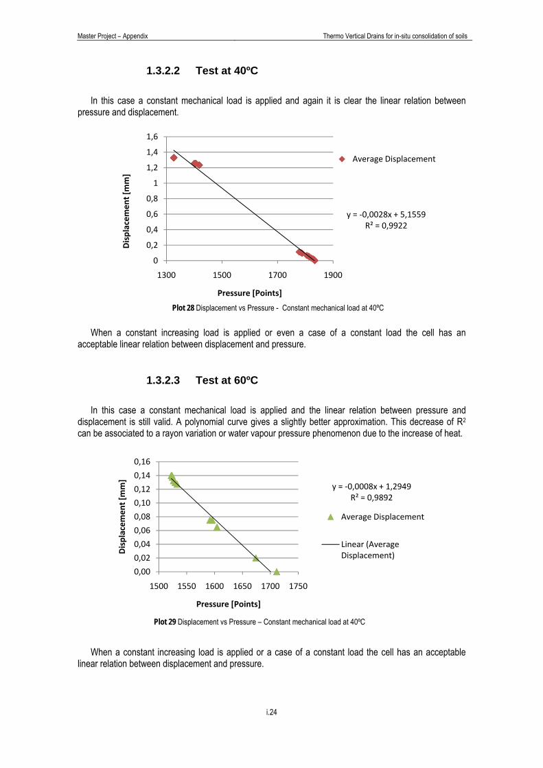
Master Project – Appendix Thermo Vertical Drains for in-situ consolidation of soils
i.24
1.3.2.2 Test at 40ºC In this case a constant mechanical load is applied and again it is clear the linear relation between
pressure and displacement.
When a constant increasing load is applied or even a case of a constant load the cell has an
acceptable linear relation between displacement and pressure.
1.3.2.3 Test at 60ºC In this case a constant mechanical load is applied and the linear relation between pressure and
displacement is still valid. A polynomial curve gives a slightly better approximation. This decrease of R2 can be associated to a rayon variation or water vapour pressure phenomenon due to the increase of heat.
When a constant increasing load is applied or a case of a constant load the cell has an acceptable
linear relation between displacement and pressure.
y = ‐0,0028x + 5,1559R² = 0,9922
0
0,2
0,4
0,6
0,8
1
1,2
1,4
1,6
1300 1500 1700 1900
Displacem
ent [mm]
Pressure [Points]
Average Displacement
Plot 28 Displacement vs Pressure - Constant mechanical load at 40ºC
y = ‐0,0008x + 1,2949R² = 0,9892
0,00
0,02
0,04
0,06
0,08
0,10
0,12
0,14
0,16
1500 1550 1600 1650 1700 1750
Displacem
ent [mm]
Pressure [Points]
Average Displacement
Linear (Average Displacement)
Plot 29 Displacement vs Pressure – Constant mechanical load at 40ºC

Master Project – Appendix 1 Thermo Vertical Drains for in-situ consolidation of soils
i.A1
APPENDIX 1 – Mechanical loading calibration 1. Test at ambient temperature i) Test 1
Loading
Time Charge Pressure
Position Displacement
Piston 18,995 18,995 1 2 3 4 Plate 14,655 33,650 1 2 3 29 29 29 29 1 2 3 4 M 11h45 12,064 45,7 1121 1093 998 28,85 29 29,15 29,02 ‐0,15 0,00 0,15 0,02 11h50 12,086 57,8 1166 1138 1046 28,89 28,89 29,14 29,16 ‐0,11 ‐0,11 0,14 0,16 11h54 12,057 69,9 1211 1181 1098 28,99 29,02 29,07 29,07 ‐0,01 0,02 0,07 0,07 0,04 13h44 12,096 82,0 12,089 94,0 12,078 106,1 1360 1328 1259 29 29,095 29,15 29,11 0,00 0,09 0,15 0,11 0,09 12,092 118,2 13,102 131,3 11,925 143,2 1523 1491 1435 29,01 29,15 29,24 29,18 0,01 0,15 0,24 0,18 0,15 13,105 156,3 13,102 169,4 13,103 182,5 1750 1715 1676 28,82 29,06 29,39 29,40 ‐0,18 0,06 0,39 0,40 0,17 13,1 195,6 13,1 208,7 14h46 13,102 221,9 1918 1884 1862 28,84 29,06 29,48 29,51 ‐0,16 0,06 0,48 0,51 0,22 13,101 235,0 13,09 248,0

Master Project – Appendix 1 Thermo Vertical Drains for in-situ consolidation of soils
i.A2
14h55 13,099 261,1 2107 2070 2066 28,96 29,11 29,47 29,57 ‐0,04 0,11 0,47 0,57 0,28 13,102 274,2 13,104 287,3 13,1 300,4 2288 2249 2263 28,925 29,2 29,58 29,62 ‐0,07 0,20 0,58 0,62 0,33 16h22 13,102 313,5 13,102 326,7 13,104 339,8 2475 2435 2465 28,93 29,28 29,65 29,63 ‐0,07 0,28 0,65 0,63 0,37 13,101 352,9 13,105 366,0 2577 2536 2576 28,93 29,27 29,70 29,69 ‐0,07 0,27 0,70 0,69 0,40
Unloading
Time Charge
Pressure Position
Displacement
1 2 3 4 T=22,3ºC 1 2 3 29,060 29,380 29,830 29,860 1 2 3 4 13,105 13,105 17h06 13,101 26,206 2520 2471 2513 29,420 29,620 29,560 29,680 0,42 0,62 0,56 0,68 13,104 39,310 13,102 52,412 17h13 13,102 65,514 2352 2317 2349 29,380 29,570 29,550 29,650 0,38 0,57 0,55 0,65 13,100 78,614 13,104 91,718 17h15 13,102 104,820 2194 2153 2166 29,340 29,520 29,530 29,610 0,34 0,52 0,53 0,61 13,099 117,919 13,090 131,009 17h18 13,101 144,110 2018 1990 1987 29,330 29,510 29,480 29,540 0,33 0,51 0,48 0,54

Master Project – Appendix 1 Thermo Vertical Drains for in-situ consolidation of soils
i.A3
13,102 157,212 13,100 170,312 17h20 13,100 183,412 1845 1815 1795 29,300 29,480 29,420 29,270 0,30 0,48 0,42 0,27 13,103 196,515 13,102 209,617 17h22 13,105 222,722 1669 1641 1608 29,270 29,440 29,370 29,400 0,27 0,44 0,37 0,40 11,925 234,647 13,102 247,749 17h24 12,092 259,841 1493 1467 1413 29,240 29,410 29,320 29,310 0,24 0,41 0,32 0,31 12,078 271,919 12,089 284,008 12,096 296,104 1314 1291 1224 ‐29,00 ‐29,00 ‐29,00 ‐29,00 12,057 308,161 12,086 320,247
12,064 332,312 ‐29,00 ‐29,00 ‐29,00 ‐29,00

Master Project – Appendix 1 Thermo Vertical Drains for in-situ consolidation of soils
i.A4
ii) Test 2 – Loading Time Charge
Pressure Position
Displacement Piston 18,995 18,995 1 2 3 4 Plate 14,655 33,650 1 2 3 29,3 29,36 29,07 29,14 1 2 3 4 M 12,064 45,7 12,086 57,8 17h06 12,057 69,9 1302 1277 1206 29,31 29,39 29,14 29,21 0,01 0,03 0,07 0,07 0,04 12,096 82,0 12,089 94,0
17h13 12,078 106,1 1466 1442 1385 29,38 29,45 29,17 29,26 0,08 0,09 0,10 0,12 0,10 12,092 118,2 13,102 131,3
17h15 11,925 143,2 1631 1603 1565 29,41 29,47 29,22 29,35 0,11 0,11 0,15 0,21 0,15 13,105 156,3 13,102 169,4
17h18 13,103 182,5 1802 1772 1750 29,44 29,5 29,27 29,43 0,14 0,14 0,20 0,29 0,19 13,1 195,6 13,1 208,7
17h20 13,102 221,9 1992 1961 1953 29,26 29,52 29,50 29,51 ‐0,04 0,16 0,43 0,37 0,23 13,101 235,0 13,09 248,0
17h22 13,099 261,1 2156 2127 2135 29,28 29,54 29,55 29,60 ‐0,02 0,18 0,48 0,46 0,27 13,102 274,2 13,104 287,3
17h24 13,1 300,4 2365 2326 2354 29,35 29,475 29,57 29,77 0,05 0,12 0,50 0,63 0,32 13,102 313,5 13,102 326,7 13,104 339,8 2565 2526 2570 29,36 29,4 29,64 29,95 0,06 0,04 0,57 0,81 0,37 13,101 352,9 13,105 366,0 2734 2682 2743 29,4 29,14 29,70 30,28 0,10 ‐0,22 0,63 1,14 0,41

Master Project – Appendix 1 Thermo Vertical Drains for in-situ consolidation of soils
i.A5
2. Test at 40ºC
Time Time T Pressure Position Displacement
25/03/2009 ‐ 13h35
182,55 kg Lab. Cell 1 2 3 M Real 1 2 3 4 1 2 3 4 M 25,31 kN/m2 Close valvule and charge 1,48 23,0 44,7 1865 1807 1830 1834 25,85 27,15 27 27,41 27,86 0 0 0 0 0
25-3-09 13:55 1,82 23,1 44,7 1863 1802 1831 1832 25,80 27,17 27,02 27,41 27,87 0,02 0,02 0,00 0,01 0,01 25-3-09 14:16 2,17 23,0 44,7 1860 1797 1826 1828 25,69 27,19 27,03 27,41 27,88 0,04 0,03 0,00 0,02 0,02 25-3-09 14:45 2,65 22,9 44,7 1852 1793 1821 1822 25,55 27,2 27,03 27,42 27,90 0,05 0,03 0,01 0,04 0,03 25-3-09 15:30 3,40 23,0 44,7 1844 1787 1814 1815 25,38 27,22 27,04 27,43 27,92 0,07 0,04 0,02 0,06 0,05
25-3-09 15:55 3,82 23,0 44,7 1841 1785 1810 1812 25,30 27,23 27,05 27,44 27,93 0,08 0,05 0,03 0,07 0,06 25-3-09 16:35 4,48 23,0 44,7 1833 1779 1804 1805 25,13 27,24 27,05 27,45 27,95 0,09 0,05 0,04 0,09 0,07 25-3-09 18:25 6,32 23,3 44,8 1813 1764 1788 1788 24,71 27,26 27,06 27,48 28,00 0,11 0,06 0,07 0,14 0,10 25-3-09 19:00 6,90 23,3 44,8 1810 1759 1783 1784 24,60 27,27 27,07 27,49 28,01 0,12 0,07 0,08 0,15 0,11 25-3-09 19:30 7,40 23,3 44,8 1803 1753 1777 1778 24,44 27,28 27,07 27,50 28,02 0,13 0,07 0,09 0,16 0,11
Malfunction
27-3-09 11:10 47,07 23,2 40,4 1463 1417 1374 1418 15,45 28,5 28,52 28,48 28,85 1,35 1,52 1,07 0,99 1,23 27-3-09 11:45 47,65 23,1 40,4 1468 1414 1373 1418 15,46 28,5 28,52 28,48 28,85 1,35 1,52 1,07 0,99 1,2325 27-3-09 12:00 47,90 23,1 40,3 1470 1412 1372 1418 15,45 28,5 28,53 28,48 28,85 1,35 1,53 1,07 0,99 1,24 27-3-09 15:40 51,57 22,8 40,3 1450 1402 1358 1403 15,08 28,51 28,54 28,49 28,86 1,36 1,54 1,08 1,00 1,25 27-3-09 17:25 53,32 22,8 40,3 1449 1400 1356 1402 15,04 28,52 28,54 28,50 28,87 1,37 1,54 1,09 1,01 1,25 27-3-09 17:45 53,65 23,0 40,3 1451 1398 1356 1402 15,04 28,52 28,54 28,50 28,87 1,37 1,54 1,09 1,01 1,25 27-3-09 18:20 54,23 23,2 40,3 1448 1397 1356 1400 15,01 28,52 28,55 28,50 28,87 1,37 1,55 1,09 1,01 1,26 27-3-09 19:35 55,48 23,3 40,4 1452 1402 1362 1405 15,13 28,52 28,55 28,50 28,87 1,37 1,55 1,09 1,01 1,26 27-3-09 19:50 55,73 23,4 40,4 1455 1402 1362 1406 15,16 28,52 28,55 28,50 28,87 1,37 1,55 1,09 1,01 1,26 29-3-09 13:25 97,32 21,9 40,0 1379 1330 1269 1326 13,15 28,59 28,63 28,57 28,93 1,44 1,63 1,16 1,07 1,33 29-3-09 14:20 98,23 22,2 40,2 1381 1330 1270 1327 13,18 28,6 28,63 28,58 28,93 1,45 1,63 1,17 1,07 1,33 29-3-09 14:50 98,73 22,1 40,2 1379 1330 1270 1326 13,16 28,6 28,63 28,58 28,93 1,45 1,63 1,17 1,07 1,33 29-3-09 15:30 99,40 22,2 40,2 1381 1329 1270 1327 13,17 28,6 28,63 28,58 28,93 1,45 1,63 1,17 1,07 1,33

Master Project – Appendix 1 Thermo Vertical Drains for in-situ consolidation of soils
i.A6
3. Test at 60ºC
Charge applied at
Time Time T Pressure
Position Displacement 23/03/2009 ‐ 17h15
182,55 kg 1 2 3 4
25,31 kN/m2 Lab. Cell 1 2 3 M Real 23,34 23,18 23,56 23,88 1 2 3 4 M
23‐3‐09 17:16 0 22,9 59,8 1736 1671 1727 1711 22,78 23,34 23,18 23,56 23,88 0 0 0,00 0,00 0,00 23‐3‐09 17:40 0 22,7 59,8 1698 1635 1689 1674 21,85 23,38 23,2 23,56 23,90 0,04 0,02 0,00 0,02 0,02 23‐3‐09 18:57 2 23,3 59,8 1628 1572 1613 1604 20,11 23,43 23,24 23,60 23,95 0,09 0,06 0,04 0,07 0,07 23‐3‐09 20:15 3 23,1 59,8 1621 1565 1601 1596 19,89 23,44 23,25 23,61 23,96 0,10 0,07 0,05 0,08 0,08 23‐3‐09 20:49 4 23,0 59,8 1618 1560 1597 1592 19,79 23,44 23,25 23,61 23,96 0,10 0,07 0,05 0,08 0,08 24‐3‐09 10:16 17 23,1 59,7 1569 1504 1525 1533 18,32 23,5 23,31 23,65 24,01 0,16 0,13 0,09 0,13 0,13 24‐3‐09 11:56 19 23,0 59,8 1562 1502 1524 1529 18,23 23,51 23,31 23,65 24,01 0,17 0,13 0,09 0,13 0,13 24‐3‐09 13:15 20 23,0 59,8 1556 1502 1521 1526 18,16 23,51 23,32 23,65 24,01 0,17 0,14 0,09 0,13 0,13 24‐3‐09 14:36 21 23,0 59,8 1556 1498 1519 1524 18,11 23,51 23,32 23,66 24,02 0,17 0,14 0,10 0,14 0,14 24‐3‐09 17:00 24 22,9 59,8 1552 1497 1518 1522 18,06 23,52 23,32 23,66 24,02 0,18 0,14 0,10 0,14 0,14 24‐3‐09 18:00 25 23,3 59,8 1557 1496 1518 1524 18,09 23,52 23,32 23,66 24,02 0,18 0,14 0,10 0,14 0,14 24‐3‐09 19:35 26 23,2 59,8 1563 1508 1530 1534 18,34 23,52 23,32 23,66 24,02 0,18 0,14 0,10 0,14 0,14

APPENDIX 2

Master Project – Appendix 2 Thermo Vertical Drains for in-situ consolidation of soils
ii.1
APPENDIX 2 – Experimental data
2.1 Experimental test at ambient temperature
2.1.1 Pre-consolidation
A) Temperature and water volume measurements – Void ratio and water content calculation controls
Charge applied at
Case Time T Water 17/04/2009 ‐ 17h00
33,65 kg
5,25 kN/m2 1 2 3 Level Volume
Half cell full 17,5 19,3 20,2 ‐‐‐ ‐‐‐ Cell full 19,8 19,8 20,1 ‐‐‐ ‐‐‐ Cell closed 20,1 20,1 20,2 370 ‐‐‐ First zero 20,2 20,2 20,2 370 ‐‐‐ Second zero 16‐4‐09 17:00 20,6 20,7 20,6 205 ‐‐‐
16‐4‐09 20:00 20,7 20,7 20,7 210 ‐‐‐ 16‐4‐09 20:20 20,8 20,8 20,7 215 ‐‐‐ 16‐4‐09 20:40 20,9 20,8 20,7 220 ‐‐‐ 16‐4‐09 21:00 20,9 20,8 20,8 220 ‐‐‐ 16‐4‐09 21:30 20,9 20,9 20,8 220 ‐‐‐
3rd pressure sensor at the cilinder's top 17‐4‐09 14:15 22,0 21,9 21,8 235 ‐‐‐
3rd pressure sensor at cilinder's half height 17‐4‐09 15:15 22,0 21,9 21,8 235 ‐‐‐

Master Project – Appendix 2 Thermo Vertical Drains for in-situ consolidation of soils
ii.2
B) Pressure and position measurements – Pressure and displacement calculations
Charge applied at
Case Time Pressure Position
Displacement 17/04/2009 - 17h00
33,65 kg Points Real 1 2 3 4 5,25 kN/m2 1 2 3 1 2 3 1 2 3 4 M
Half cell full 926 900 1488 0,49 1,03 0,09 Cell full 1030 1003 1490 3,20 3,78 0,23 Cell closed 1127 1092 1490 5,72 6,16 0,23 33,00 34,31 41,12 40,71 First zero 1110 1068 1491 5,28 5,52 0,29 1,00 1,00 1,00 1,00 Second zero 16-4-09 17:00 1130 1095 1490 5,80 6,24 0,23 1,40 0,57 1,00 1,02 0,00 0,00 0,00 0,00 0,00
16-4-09 20:00 1149 1079 1489 6,29 5,81 0,16 1,41 0,60 1,04 1,05 0,01 0,03 0,04 0,03 0,03 16-4-09 20:20 1134 1073 1488 5,90 5,65 0,09 1,42 0,61 1,06 1,07 0,02 0,04 0,06 0,05 0,04 16-4-09 20:40 1146 1072 1489 6,21 5,63 0,16 1,43 0,62 1,07 1,08 0,03 0,05 0,07 0,06 0,05 16-4-09 21:00 1150 1074 1488 6,32 5,68 0,09 1,44 0,63 1,08 1,08 0,04 0,06 0,08 0,06 0,06 16-4-09 21:30 1170 1070 1486 6,84 5,57 -0,04 1,44 0,64 1,08 1,08 0,04 0,07 0,08 0,06 0,06
3rd pressure sensor at the cilinder's top 17-4-09 14:15 1260 1070 1488 9,18 5,57 0,09 1,46 0,64 1,10 1,09 0,06 0,07 0,10 0,07 0,08 3rd pressure sensor at cilinder's half height 17-4-09 15:15 1269 1053 1502 9,41 5,12 1,03 1,46 0,64 1,10 1,09 0,06 0,07 0,10 0,07 0,08
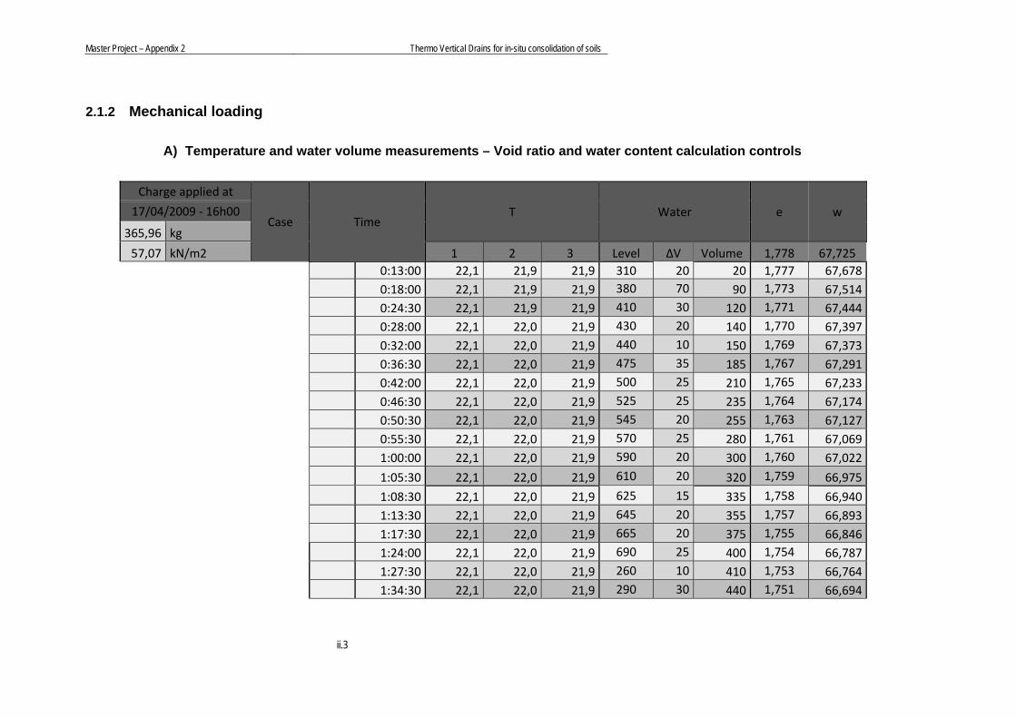
Master Project – Appendix 2 Thermo Vertical Drains for in-situ consolidation of soils
ii.3
2.1.2 Mechanical loading A) Temperature and water volume measurements – Void ratio and water content calculation controls
Charge applied at
Case Time T Water e w 17/04/2009 ‐ 16h00
365,96 kg
57,07 kN/m2 1 2 3 Level ∆V Volume 1,778 67,725 0:13:00 22,1 21,9 21,9 310 20 20 1,777 67,678 0:18:00 22,1 21,9 21,9 380 70 90 1,773 67,514 0:24:30 22,1 21,9 21,9 410 30 120 1,771 67,444 0:28:00 22,1 22,0 21,9 430 20 140 1,770 67,397 0:32:00 22,1 22,0 21,9 440 10 150 1,769 67,373 0:36:30 22,1 22,0 21,9 475 35 185 1,767 67,291 0:42:00 22,1 22,0 21,9 500 25 210 1,765 67,233 0:46:30 22,1 22,0 21,9 525 25 235 1,764 67,174 0:50:30 22,1 22,0 21,9 545 20 255 1,763 67,127 0:55:30 22,1 22,0 21,9 570 25 280 1,761 67,069
1:00:00 22,1 22,0 21,9 590 20 300 1,760 67,022
1:05:30 22,1 22,0 21,9 610 20 320 1,759 66,975
1:08:30 22,1 22,0 21,9 625 15 335 1,758 66,940 1:13:30 22,1 22,0 21,9 645 20 355 1,757 66,893 1:17:30 22,1 22,0 21,9 665 20 375 1,755 66,846
1:24:00 22,1 22,0 21,9 690 25 400 1,754 66,787 1:27:30 22,1 22,0 21,9 260 10 410 1,753 66,764 1:34:30 22,1 22,0 21,9 290 30 440 1,751 66,694

Master Project – Appendix 2 Thermo Vertical Drains for in-situ consolidation of soils
ii.4
1:39:30 22,1 22,0 21,9 310 20 460 1,750 66,647 1:51:30 22,2 22,1 22,0 360 50 510 1,747 66,529 2:23:30 22,2 22,1 22,0 485 125 635 1,739 66,236 2:45:30 22,2 22,1 22,0 570 85 720 1,734 66,037
Piston enters in the cylinder 3:25:00 22,2 22,1 22,0 375 140 860 1,725 65,709
4:25:00 22,3 22,2 22,1 585 210 1070 1,713 65,217
4:54:00 22,3 22,2 22,1 320 90 1160 1,707 65,006 5:35:00 22,3 22,2 22,1 465 145 1305 1,698 64,666 6:07:30 22,4 22,2 22,1 565 100 1405 1,692 64,431 6:45:00 22,4 22,3 22,2 350 110 1515 1,685 64,174 7:15:00 22,4 22,3 22,2 440 90 1605 1,680 63,963 7:38:00 22,4 22,3 22,2 510 70 1675 1,675 63,799 7:50:00 22,4 22,3 22,2 270 35 1710 1,673 63,716 8:26:00 22,5 22,4 22,2 375 105 1815 1,667 63,470 8:46:00 22,5 22,4 22,3 440 65 1880 1,663 63,318 9:25:00 22,5 22,4 22,3 550 110 1990 1,656 63,060 10:05:00 22,5 22,4 22,3 340 105 2095 1,649 62,814
10:20:00 22,5 22,4 22,3 380 40 2135 1,647 62,720
10:26:00 22,5 22,4 22,3 400 20 2155 1,646 62,673 14:10:00 22,7 22,6 22,5 790 390 2725 1,611 61,337 17:57:00 22,7 22,6 22,5 750 515 3240 1,579 60,130 21:10:00 22,8 22,6 22,5 635 405 3645 1,554 59,181 22:34:00 22,8 22,7 22,6 370 160 3805 1,544 58,805Day 2 0:12:00 22,8 22,7 22,6 560 190 3995 1,532 58,360 1:02:00 22,8 22,7 22,6 300 90 4085 1,527 58,149 2:46:00 22,9 22,8 22,7 490 190 4275 1,515 57,704 4:15:00 22,9 22,8 22,7 360 155 4430 1,506 57,340

Master Project – Appendix 2 Thermo Vertical Drains for in-situ consolidation of soils
ii.5
4:53:00 22,9 22,8 22,7 425 65 4495 1,502 57,188 7:03:00 22,6 22,7 22,8 410 210 4705 1,489 56,696 9:31:00 23,0 22,9 22,8 4510 1,501 57,153 9:40:00 23,0 22,9 22,8 4510 1,501 57,153 10:00:00 23,0 22,9 22,8 4550 1,498 57,059 10:38:00 23,0 22,9 22,8 4605 1,495 56,930 11:18:00 23,0 22,9 22,8 4670 1,491 56,778 11:50:00 23,0 22,9 22,8 4715 1,488 56,672 12:25:00 23,1 22,9 22,8 4715 1,488 56,672 12:54:00 23,1 22,9 22,8 4715 1,488 56,672 18:10:00 22,5 22,7 22,7 4715 1,488 56,672 23:21:00 22,4 22,6 22,6 4715 1,488 56,672Day 3 0:00:00 22,9 22,8 22,6 4710 1,488 56,684 1:25:00 22,8 22,7 22,6 4710 1,488 56,684 2:53:00 22,8 22,7 22,6 4710 1,488 56,684 3:17:00 22,8 22,7 22,5 4710 1,488 56,684 20:28:00 22,4 22,5 22,5 4710 1,488 56,684 23:10:00 22,7 22,6 22,5 4710 1,488 56,684Day 4 1:52:00 22,8 22,6 22,5 4710 1,488 56,684 5:32:00 22,7 22,6 22,5 4710 1,488 56,684 5:40:00 22,7 22,6 22,5 4710 1,488 56,684 18:27:00 22,3 22,4 22,5 4710 1,488 56,684 21:22:00 22,7 22,6 22,4 4715 1,488 56,672Day 5 2:22:00 22,8 22,6 22,5 4715 1,488 56,672 7:22:00 22,4 22,5 22,6 4715 1,488 56,672 21:22:00 22,5 22,6 22,7 4710 1,488 56,684 23:11:00 22,5 22,7 22,7 4710 1,488 56,684

Master Project – Appendix 2 Thermo Vertical Drains for in-situ consolidation of soils
ii.6
23:52:00 23,0 22,9 22,8 4710 1,488 56,684Day 6 0:30:00 23,0 22,9 22,8 4710 1,488 56,684 1:48:00 22,6 22,7 22,8 4710 1,488 56,684 2:04:00 23,0 23,0 23,0 4710 1,488 56,684 18:34:00 22,8 23,0 23,0 4715 1,488 56,672 22:11:00 22,9 23,0 23,1 4715 1,488 56,672 22:41:00 23,3 23,2 23,1 4715 1,488 56,672Day 7 0:40:00 23,3 23,1 23,0 4715 1,488 56,672 6:28:00 23,3 23,2 23,1 4715 1,488 56,672 7:13:00 23,4 23,3 23,1 4715 1,488 56,672 20:33:00 22,8 23,0 23,1 4715 1,488 56,672 21:58:00 22,8 23,0 23,0 4715 1,488 56,672Day 8 2:04:00 23,0 23,0 22,9 4715 1,488 56,672Day 9 0:51:00 23,0 22,8 22,7 4705 1,489 56,696

Master Project – Appendix 2 Thermo Vertical Drains for in-situ consolidation of soils
ii.7
B) Pressure and position measurements – Pressure and displacement calculations
Charge applied at
Case Time
Pressure Position Displacement 17/04/2009 ‐ 16h00
365,96 kg Points Real 1 2 3 4
57,07 kN/m2 1 2 3 1 2 3 1,47 4,44 1,09 6,85 1 2 3 4 M
0:13:00 2763 2523 1500 48,25 44,37 0,90 12,00 4,99 12,81 7,59 10,53 11,05 11,72 10,27 10,89
0:18:00 2783 2514 1500 48,77 44,13 0,90 12,42 5,34 13,35 8,10 10,95 11,40 12,26 10,78 11,35
0:24:30 2785 2493 1500 48,83 43,57 0,90 12,93 6,09 14,00 8,61 11,46 12,15 12,91 11,29 11,95
0:28:00 2787 2478 1501 48,88 43,17 0,97 13,21 6,38 14,31 8,93 11,74 12,44 13,22 11,61 12,25
0:32:00 2783 2465 1500 48,77 42,82 0,90 13,53 6,68 14,63 9,26 12,06 12,74 13,54 11,94 12,57
0:36:30 2784 2452 1501 48,80 42,47 0,97 13,88 7,00 14,97 9,63 12,41 13,06 13,88 12,31 12,92
0:42:00 2773 2432 1499 48,51 41,94 0,83 14,29 7,39 15,39 10,08 12,82 13,45 14,30 12,76 13,33
0:46:30 2780 2423 1499 48,70 41,70 0,83 14,59 7,62 15,74 10,43 13,12 13,68 14,65 13,11 13,64
0:50:30 2781 2414 1500 48,72 41,46 0,90 14,84 7,91 16,05 10,85 13,37 13,97 14,96 13,53 13,96
0:55:30 2789 2407 1497 48,93 41,27 0,70 15,15 8,21 16,42 11,12 13,68 14,27 15,33 13,80 14,27
1:00:00 2790 2400 1499 48,96 41,08 0,83 15,45 8,53 16,74 11,43 13,98 14,59 15,65 14,11 14,58
1:05:30 2755 2386 1496 48,05 40,71 0,63 15,83 8,89 17,07 11,78 14,36 14,95 15,98 14,46 14,94
1:08:30 2781 2376 1497 48,72 40,44 0,70 16,03 9,10 17,26 11,96 14,56 15,16 16,17 14,64 15,13
1:13:30 2778 2363 1497 48,64 40,10 0,70 16,36 9,42 17,56 12,26 14,89 15,48 16,47 14,94 15,45
1:17:30 2776 2357 1500 48,59 39,94 0,90 16,61 9,69 17,80 12,49 15,14 15,75 16,71 15,17 15,69
1:24:00 2764 2346 1498 48,28 39,64 0,77 16,98 10,06 18,21 12,89 15,51 16,12 17,12 15,57 16,08
1:27:30 2774 2344 1501 48,54 39,59 0,97 17,21 10,30 18,44 13,12 15,74 16,36 17,35 15,80 16,31
1:34:30 2758 2327 1498 48,12 39,13 0,77 17,66 10,75 18,84 13,52 16,19 16,81 17,75 16,20 16,74
1:39:30 2766 2320 1497 48,33 38,95 0,70 17,97 11,06 19,15 13,83 16,50 17,12 18,06 16,51 17,05
1:51:30 2736 2298 1501 47,55 38,36 0,97 18,66 11,73 19,82 14,52 17,19 17,79 18,73 17,20 17,73
2:23:30 2694 2265 1496 46,46 37,48 0,63 20,45 13,52 21,58 16,28 18,98 19,58 20,49 18,96 19,50

Master Project – Appendix 2 Thermo Vertical Drains for in-situ consolidation of soils
ii.8
2:45:30 2698 2245 1499 46,56 36,95 0,83 21,62 14,69 22,72 17,42 20,15 20,75 21,63 20,10 20,66
Piston enters in the cylinder 3:25:00 2685 2216 1496 46,23 36,17 0,63 23,62 16,71 24,72 19,40 22,15 22,77 23,63 22,08 22,66
4:25:00 2659 2182 1498 45,55 35,26 0,77 26,46 19,57 27,60 22,26 24,99 25,63 26,51 24,94 25,52
4:54:00 2658 2170 1496 45,52 34,94 0,63 27,81 20,93 28,96 23,62 26,34 26,99 27,87 26,30 26,88
5:35:00 2628 2151 1496 44,74 34,44 0,63 29,70 22,82 30,86 25,52 28,23 28,88 29,77 28,20 28,77
6:07:30 2626 2139 1494 44,69 34,12 0,50 31,05 24,19 32,22 26,91 29,58 30,25 31,13 29,59 30,14
6:45:00 2615 2116 1496 44,41 33,50 0,63 32,66 25,79 34,85 28,50 31,19 31,85 33,76 31,18 32,00
7:15:00 2605 2094 1495 44,15 32,91 0,56 33,93 27,06 35,10 29,75 32,46 33,12 34,01 32,43 33,01
7:38:00 2595 2082 1495 43,89 32,59 0,56 34,91 28,03 36,03 30,69 33,44 34,09 34,94 33,37 33,96
7:50:00 2610 2066 1493 44,28 32,17 0,43 35,41 28,52 36,53 31,20 33,94 34,58 35,44 33,88 34,46
8:26:00 2580 2049 1495 43,50 31,71 0,56 36,89 30,02 38,00 32,66 35,42 36,08 36,91 35,34 35,94
8:46:00 2580 2042 1494 43,50 31,53 0,50 37,70 30,80 38,80 33,48 36,23 36,86 37,71 36,16 36,74
9:25:00 2577 2036 1494 43,42 31,37 0,50 39,19 32,31 40,31 34,96 37,72 38,37 39,22 37,64 38,24
10:05:00 2560 2020 1493 42,98 30,94 0,43 40,75 33,89 41,90 36,44 39,28 39,95 40,81 39,12 39,79
10:20:00 2570 2018 1494 43,24 30,88 0,50 41,33 34,47 42,48 37,12 39,86 40,53 41,39 39,80 40,40
10:26:00 2578 2017 1494 43,44 30,86 0,50 3,15 3,25 3,52 2,98 40,02 40,65 41,47 39,85 40,50
14:10:00 2432 1934 1490 39,65 28,64 0,23 10,85 11,00 11,38 10,80 47,72 48,40 49,33 47,67 48,28
17:57:00 2332 1881 1489 37,05 27,23 0,16 17,86 18,01 18,39 17,81 54,73 55,41 56,34 54,68 55,29
21:10:00 2284 1849 1490 35,80 26,37 0,23 23,32 23,46 23,88 23,31 60,19 60,86 61,83 60,18 60,77
22:34:00 2280 1827 1490 35,70 25,78 0,23 25,64 25,79 26,17 25,59 62,51 63,19 64,12 62,46 63,07
Day 2 0:12:00 2256 1822 1493 35,07 25,65 0,43 28,16 28,28 28,71 28,15 65,03 65,68 66,66 65,02 65,60
1:02:00 2253 1810 1493 34,99 25,33 0,43 29,47 29,60 30,00 29,42 66,34 67,00 67,95 66,29 66,90
2:46:00 2220 1798 1493 34,14 25,01 0,43 32,04 32,22 32,59 31,97 68,91 69,62 70,54 68,84 69,48
4:15:00 2202 1758 1492 33,67 23,94 0,36 34,18 34,37 34,70 34,07 71,05 71,77 72,65 70,94 71,60
4:53:00 2204 1748 1492 33,72 23,68 0,36 35,07 35,25 35,60 35,97 71,94 72,65 73,55 72,84 72,75
7:03:00 2129 1730 1487 31,77 23,20 0,03 37,96 38,10 38,50 37,90 74,83 75,50 76,45 74,77 75,39
9:31:00 2162 1731 1491 32,63 23,22 0,29 41,25 41,43 41,79 41,17 78,12 78,83 79,74 78,04 78,68

Master Project – Appendix 2 Thermo Vertical Drains for in-situ consolidation of soils
ii.9
9:40:00 2172 1713 1490 32,89 22,74 0,23 41,49 41,68 42,01 41,38 78,36 79,08 79,96 78,25 78,91
10:00:00 2165 1711 1491 32,71 22,69 0,29 41,95 42,13 42,45 41,82 78,82 79,53 80,40 78,69 79,36
10:38:00 2150 1700 1492 32,32 22,39 0,36 42,84 43,04 43,29 42,64 79,71 80,44 81,24 79,51 80,23
11:18:00 2162 1713 1491 32,63 22,74 0,29 43,74 43,95 44,18 43,53 80,61 81,35 82,13 80,40 81,12
11:50:00 2146 1702 1491 32,21 22,45 0,29 44,45 44,66 44,87 44,21 81,32 82,06 82,82 81,08 81,82
12:25:00 2166 1718 1492 32,73 22,87 0,36 45,18 45,43 45,66 45,02 82,05 82,83 83,61 81,89 82,60
12:54:00 2146 1702 1490 32,21 22,45 0,23 1,64 1,63 1,68 1,61 82,68 83,46 84,19 82,51 83,21
18:10:00 2096 1681 1486 30,91 21,89 ‐0,04 8,23 8,20 8,01 7,96 89,27 90,03 90,52 88,86 89,67
23:21:00 2020 1636 1485 28,94 20,69 ‐0,11 14,07 13,99 13,73 13,72 95,11 95,82 96,24 94,62 95,45
Day 3 0:00:00 2026 1636 1485 29,09 20,69 ‐0,11 14,69 14,70 14,44 14,39 95,73 96,53 96,95 95,29 96,13
1:25:00 2006 1622 1485 28,57 20,31 ‐0,11 16,22 16,14 15,90 15,89 97,26 97,97 98,41 96,79 97,61
2:53:00 1996 1620 1486 28,31 20,26 ‐0,04 17,71 17,62 17,36 17,36 98,75 99,45 99,87 98,26 99,08
3:17:00 1983 1600 1486 27,97 19,72 ‐0,04 18,12 18,02 17,77 17,78 99,16 99,85 100,28 98,68 99,49
20:28:00 1777 1464 1483 22,62 16,09 ‐0,24 32,61 32,43 32,29 32,36 113,65 114,26 114,80 113,26 113,99
23:10:00 1722 1442 1482 21,19 15,51 ‐0,31 34,42 34,23 34,09 34,17 115,46 116,06 116,60 115,07 115,80
Day 4 1:52:00 1674 1404 1482 19,94 14,49 ‐0,31 36,12 35,92 35,75 35,84 117,16 117,75 118,26 116,74 117,48
5:32:00 1633 1378 1481 18,87 13,80 ‐0,38 38,27 38,07 37,86 37,95 119,31 119,90 120,37 118,85 119,61
5:40:00 1635 1394 1482 18,93 14,22 ‐0,31 10,12 10,04 10,14 9,98 119,38 119,94 120,41 118,90 119,66
18:27:00 1463 1274 1477 14,45 11,02 ‐0,65 16,19 16,01 16,13 16,05 125,45 125,91 126,40 124,97 125,68
21:22:00 1415 1249 1476 13,21 10,35 ‐0,72 17,28 17,08 17,18 17,11 126,54 126,98 127,45 126,03 126,75
Day 5 2:22:00 1338 1206 1479 11,20 9,20 ‐0,51 18,87 18,68 18,77 18,69 128,13 128,58 129,04 127,61 128,34
7:22:00 1289 1174 1473 9,93 8,35 ‐0,92 20,25 20,06 20,15 20,05 129,51 129,96 130,42 128,97 129,72
21:22:00 1167 1083 1473 6,76 5,92 ‐0,92 22,95 22,76 22,85 22,75 132,21 132,66 133,12 131,67 132,42
23:11:00 1144 1055 1473 6,16 5,17 ‐0,92 23,20 23,02 23,10 23,00 132,46 132,92 133,37 131,92 132,67
23:52:00 1141 1048 1475 6,08 4,99 ‐0,78 23,30 23,12 23,19 23,09 132,56 133,02 133,46 132,01 132,76
Day 6 0:30:00 1142 1045 1475 6,11 4,91 ‐0,78 23,38 23,19 23,27 23,17 132,64 133,09 133,54 132,09 132,84
1:48:00 1125 1040 1474 5,67 4,77 ‐0,85 23,53 23,34 23,44 23,34 132,79 133,24 133,71 132,26 133,00

Master Project – Appendix 2 Thermo Vertical Drains for in-situ consolidation of soils
ii.10
2:04:00 1120 1040 1473 5,54 4,77 ‐0,92 23,56 23,37 23,47 23,37 132,82 133,27 133,74 132,29 133,03
18:34:00 1030 988 1470 3,20 3,38 ‐1,12 25,01 24,83 24,89 24,79 134,27 134,73 135,16 133,71 134,47
22:11:00 1029 996 1472 3,17 3,60 ‐0,98 25,21 25,02 25,07 24,97 134,47 134,92 135,34 133,89 134,66
22:41:00 1033 986 1472 3,27 3,33 ‐0,98 25,23 25,05 25,10 24,99 134,49 134,95 135,37 133,91 134,68
Day 7 0:40:00 1025 978 1473 3,07 3,12 ‐0,92 25,33 25,14 25,19 25,08 134,59 135,04 135,46 134,00 134,77
6:28:00 1012 966 1474 2,73 2,80 ‐0,85 25,54 25,36 25,40 25,30 134,80 135,26 135,67 134,22 134,99
7:13:00 1011 965 1475 2,70 2,77 ‐0,78 25,57 25,38 25,42 25,32 134,83 135,28 135,69 134,24 135,01
20:33:00 997 969 1472 2,34 2,88 ‐0,98 25,89 25,70 25,73 25,63 135,15 135,60 136,00 134,55 135,33
21:58:00 996 963 1470 2,31 2,72 ‐1,12 25,92 25,72 25,75 25,65 135,18 135,62 136,02 134,57 135,35
Day 8 2:04:00 995 964 1473 2,29 2,74 ‐0,92 25,97 25,77 25,80 25,70 135,23 135,67 136,07 134,62 135,40
Day 9 0:51:00 1096 960 1482 4,91 2,64 ‐0,31 26,24 26,04 26,04 25,95 135,50 135,94 136,31 134,87 135,66

Master Project – Appendix 2 Thermo Vertical Drains for in-situ consolidation of soils
ii.11
2.1.3 Mechanical unloading
A) Temperature and water volume measurements – Void ratio and water content calculation controls
Mechanical uncharge applied
Case Time T Water e w 27/04/2009 ‐ 14h45
33,65 kg 5,25 kN/m2 1 2 3 Level Volume 1,778 67,725
0:00:00 23,0 22,8 22,7 600 0 1,778 67,725 0:01:30 23,0 22,8 22,7 600 0 1,778 67,725 0:16:30 23,0 22,8 22,7 600 0 1,778 67,725 0:37:30 23,0 22,8 22,7 600 0 1,778 67,725 0:55:30 23,0 22,8 22,7 600 0 1,778 67,725 1:10:30 22,9 22,8 22,6 600 0 1,778 67,725 1:23:00 22,9 22,8 22,6 600 0 1,778 67,725 1:38:00 22,9 22,8 22,6 600 0 1,778 67,725 2:03:00 23,0 22,8 22,7 600 0 1,778 67,725 2:40:00 23,0 22,8 22,7 600 0 1,778 67,725 3:10:00 23,0 22,8 22,7 600 0 1,778 67,725 4:02:00 23,0 22,8 22,7 600 0 1,778 67,725 4:40:00 23,0 22,8 22,7 600 0 1,778 67,725 5:44:00 23,0 22,8 22,7 600 0 1,778 67,725 6:40:00 23,0 22,8 22,7 600 0 1,778 67,725
7:26:00 23,0 22,9 22,7 600 0 1,778 67,725 8:30:00 23,0 22,9 22,8 600 0 1,778 67,725 19:22:00 23,0 22,9 22,7 600 0 1,778 67,725 19:40:00 23,0 22,9 22,8 600 0 1,778 67,725 21:04:00 23,0 22,9 22,7 600 0 1,778 67,725 22:47:00 23,0 22,8 22,7 600 0 1,778 67,725

Master Project – Appendix 2 Thermo Vertical Drains for in-situ consolidation of soils
ii.12
B) Pressure and position measurements – Pressure and displacement calculations
27/04/2009 ‐ 14h45
Case Time
Pressure Position Displacement
33,65 kg Points Real 1 2 3 4
5,25 kN/m2 1 2 3 1 2 3 27,24 26,95 27,08 26,99 1 2 3 4 M
0:00:00 1060 1212 1474 3,98 9,36 -0,85 27,24 26,95 27,08 26,99 0,00 0,00 0,00 0,00 0,00 0:01:30 688 1003 1473 -5,70 3,78 -0,92 27,02 26,58 26,79 26,56 -0,22 -0,37 -0,29 -0,43 -0,33 0:16:30 706 1124 1478 -5,23 7,01 -0,58 26,86 26,39 26,57 26,35 -0,38 -0,56 -0,51 -0,64 -0,52 0:37:30 750 1194 1476 -4,08 8,88 -0,72 26,78 26,26 26,42 26,21 -0,46 -0,69 -0,66 -0,78 -0,65 0:55:30 784 1220 1476 -3,20 9,58 -0,72 26,64 26,17 26,32 26,11 -0,60 -0,78 -0,76 -0,88 -0,75 1:10:30 799 1230 1475 -2,81 9,85 -0,78 26,58 26,10 26,24 26,03 -0,66 -0,85 -0,84 -0,96 -0,83 1:23:00 811 1236 1475 -2,50 10,01 -0,78 26,53 26,05 26,19 25,98 -0,71 -0,90 -0,89 -1,01 -0,88 1:38:00 831 1247 1475 -1,98 10,30 -0,78 26,47 25,99 26,12 25,91 -0,77 -0,96 -0,96 -1,08 -0,94 2:03:00 850 1265 1476 -1,48 10,78 -0,72 26,39 25,91 26,03 25,81 -0,85 -1,04 -1,05 -1,18 -1,03 2:40:00 881 1280 1477 -0,68 11,18 -0,65 26,28 25,80 25,91 25,69 -0,96 -1,15 -1,17 -1,30 -1,15 3:10:00 899 1295 1476 -0,21 11,58 -0,72 26,20 25,72 25,82 25,60 -1,04 -1,23 -1,26 -1,39 -1,23
4:02:00 915 1307 1477 0,21 11,90 -0,65 26,10 25,61 25,69 25,48 -1,14 -1,34 -1,39 -1,51 -1,35 4:40:00 932 1321 1479 0,65 12,27 -0,51 26,03 25,54 25,61 25,40 -1,21 -1,41 -1,47 -1,59 -1,42 5:44:00 962 1339 1480 1,43 12,76 -0,45 25,92 25,44 25,50 25,29 -1,32 -1,51 -1,58 -1,70 -1,53 6:40:00 975 1351 1480 1,77 13,08 -0,45 25,84 25,36 25,42 25,21 -1,40 -1,59 -1,66 -1,78 -1,61
7:26:00 989 1354 1481 2,13 13,16 -0,38 25,79 25,30 25,38 25,16 -1,45 -1,65 -1,70 -1,83 -1,66 8:30:00 1012 1370 1481 2,73 13,58 -0,38 25,73 25,23 25,32 25,11 -1,51 -1,72 -1,76 -1,88 -1,72 19:22:00 1135 1463 1478 5,93 16,07 -0,58 25,54 25,03 25,12 24,92 -1,70 -1,92 -1,96 -2,07 -1,91 19:40:00 1130 1466 1479 5,80 16,15 -0,51 25,54 25,03 25,11 24,92 -1,70 -1,92 -1,97 -2,07 -1,92 21:04:00 1142 1445 1478 6,11 15,59 -0,58 25,53 25,02 25,11 24,92 -1,71 -1,93 -1,97 -2,07 -1,92 22:47:00 1155 1483 1475 6,45 16,60 -0,78 25,53 25,01 25,10 24,91 -1,71 -1,94 -1,98 -2,08 -1,93

Master Project – Appendix 2 Thermo Vertical Drains for in-situ consolidation of soils
ii.13
2.2 Experimental test at high temperature: 40ºC
2.2.1 Pre-consolidation A) Temperature and water volume measurements – Void ratio and water content calculation controls
Charge applied at
Case Time T Water
01/05/2009 ‐ 15h00
33,65 kg
5,25 kN/m2 1 2 3 Level Volume
Half cell full 20,6 21,0 21,3 ‐‐‐ ‐‐‐ Cell full 21,3 21,5 21,6 ‐‐‐ ‐‐‐ Cell closed 21,5 21,4 21,5 420 ‐‐‐ First zero 0:00:00 21,6 21,5 21,5 450 ‐‐‐
1:08:00 21,7 21,6 21,6 470 ‐‐‐ 1:31:00 21,8 21,7 21,6 470 ‐‐‐ 4:09:00 21,5 21,7 21,8 470 ‐‐‐ 22:05:00 22,1 22,3 22,4 470 ‐‐‐

Master Project – Appendix 2 Thermo Vertical Drains for in-situ consolidation of soils
ii.14
B) Pressure and position measurements – Pressure and displacement calculations
Charge applied at
Case Time
Pressure Position Displacement 01/05/2009 ‐ 15h00
33,65 kg Points Real 1 2 3 4
4,67 kN/m2 1 2 3 1 2 3 1 2 3 4 M
Half cell full 892 865 1556 -0,39 0,10 4,67 Cell full 1078 1014 1556 4,44 4,08 4,67 Cell closed 1160 1097 1558 6,58 6,29 4,80 First zero 0:00:00 1193 1132 1555 7,43 7,23 4,60 1,69 36,59 1,88 33,30 0,00
1:08:00 1082 1036 1556 4,55 4,67 4,67 1,77 36,65 1,94 33,37 -0,08 -0,06 -0,06 -0,07 -0,07 1:31:00 1084 1038 1556 4,60 4,72 4,67 1,77 36,65 1,95 33,37 -0,08 -0,06 -0,07 -0,07 -0,07 4:09:00 1076 1035 1552 4,39 4,64 4,40 1,78 36,65 1,95 33,37 -0,09 -0,06 -0,07 -0,07 -0,07 22:05:00 1060 1023 1539 3,98 4,32 3,52 1,78 36,65 1,95 33,37 -0,09 -0,06 -0,07 -0,07 -0,07

Master Project – Appendix 2 Thermo Vertical Drains for in-situ consolidation of soils
ii.15
2.2.2 Thermal loading A) Temperature and water volume measurements – Void ratio and water content calculation controls
Charge applied at
Case Time T Water e w 17/04/2009 ‐ 16h00
33,65 kg
4,67 kN/m2 1 2 3 M H Level Volume 1,778 67,725
0:00:00 22,3 22,4 22,5 22,4 24,3 480 10 1,778 67,702 0:40:00 25,0 22,6 22,4 23,3 39,7 490 20 1,777 67,678 2:20:00 28,9 24,5 23,8 25,7 42,3 515 45 1,776 67,620 2:55:00 29,5 25,2 24,5 26,4 42,3 525 55 1,775 67,596 3:25:00 30,0 25,8 25,1 27,0 42,3 535 65 1,774 67,573 5:02:00 31,4 27,6 26,9 28,6 42,3 555 85 1,773 67,526 8:18:00 33,0 30,1 29,6 30,9 42,3 580 110 1,772 67,467 12:18:00 34,6 32,1 31,7 32,8 42,3 485 115 1,771 67,455 13:46:00 35,4 32,8 32,1 33,4 42,3 480 110 1,772 67,467 18:52:00 35,8 33,7 33,2 34,2 42,3 450 80 1,773 67,537
Day 2 0:10:00 36,1 34,2 33,7 34,7 42,3 435 65 1,774 67,573
2:17:00 36,7 34,5 33,8 35,0 42,3 435 65 1,774 67,573 2:53:00 36,8 34,5 33,9 35,1 41,5 430 60 1,775 67,584 6:25:00 36,9 34,7 34,0 35,2 42,3 430 60 1,775 67,584
21:10:00 36,9 34,8 34,1 35,3 42,3 435 65 1,774 67,573
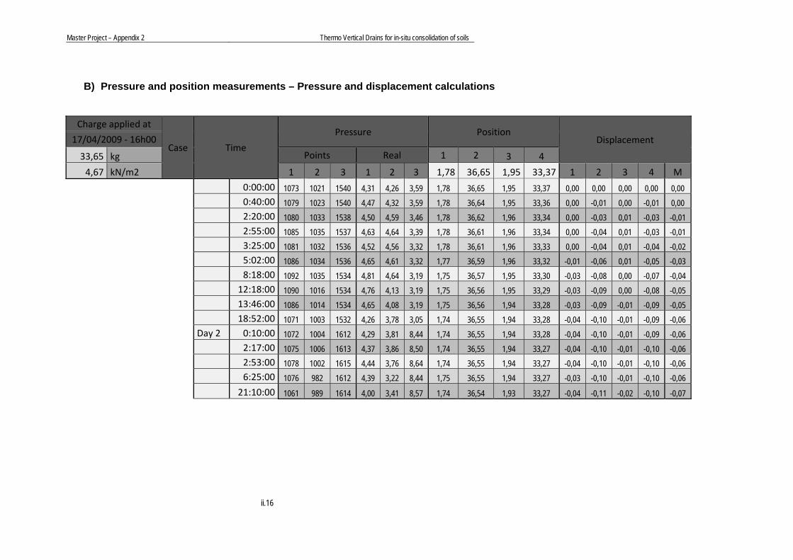
Master Project – Appendix 2 Thermo Vertical Drains for in-situ consolidation of soils
ii.16
B) Pressure and position measurements – Pressure and displacement calculations
Charge applied at
Case Time
Pressure Position Displacement 17/04/2009 ‐ 16h00
33,65 kg Points Real 1 2 3 4
4,67 kN/m2 1 2 3 1 2 3 1,78 36,65 1,95 33,37 1 2 3 4 M
0:00:00 1073 1021 1540 4,31 4,26 3,59 1,78 36,65 1,95 33,37 0,00 0,00 0,00 0,00 0,00 0:40:00 1079 1023 1540 4,47 4,32 3,59 1,78 36,64 1,95 33,36 0,00 -0,01 0,00 -0,01 0,00 2:20:00 1080 1033 1538 4,50 4,59 3,46 1,78 36,62 1,96 33,34 0,00 -0,03 0,01 -0,03 -0,01 2:55:00 1085 1035 1537 4,63 4,64 3,39 1,78 36,61 1,96 33,34 0,00 -0,04 0,01 -0,03 -0,01 3:25:00 1081 1032 1536 4,52 4,56 3,32 1,78 36,61 1,96 33,33 0,00 -0,04 0,01 -0,04 -0,02 5:02:00 1086 1034 1536 4,65 4,61 3,32 1,77 36,59 1,96 33,32 -0,01 -0,06 0,01 -0,05 -0,03 8:18:00 1092 1035 1534 4,81 4,64 3,19 1,75 36,57 1,95 33,30 -0,03 -0,08 0,00 -0,07 -0,04 12:18:00 1090 1016 1534 4,76 4,13 3,19 1,75 36,56 1,95 33,29 -0,03 -0,09 0,00 -0,08 -0,05 13:46:00 1086 1014 1534 4,65 4,08 3,19 1,75 36,56 1,94 33,28 -0,03 -0,09 -0,01 -0,09 -0,05 18:52:00 1071 1003 1532 4,26 3,78 3,05 1,74 36,55 1,94 33,28 -0,04 -0,10 -0,01 -0,09 -0,06 Day 2 0:10:00 1072 1004 1612 4,29 3,81 8,44 1,74 36,55 1,94 33,28 -0,04 -0,10 -0,01 -0,09 -0,06 2:17:00 1075 1006 1613 4,37 3,86 8,50 1,74 36,55 1,94 33,27 -0,04 -0,10 -0,01 -0,10 -0,06 2:53:00 1078 1002 1615 4,44 3,76 8,64 1,74 36,55 1,94 33,27 -0,04 -0,10 -0,01 -0,10 -0,06 6:25:00 1076 982 1612 4,39 3,22 8,44 1,75 36,55 1,94 33,27 -0,03 -0,10 -0,01 -0,10 -0,06 21:10:00 1061 989 1614 4,00 3,41 8,57 1,74 36,54 1,93 33,27 -0,04 -0,11 -0,02 -0,10 -0,07

Master Project – Appendix 2 Thermo Vertical Drains for in-situ consolidation of soils
ii.17
2.2.3 Mechanical loading A) Temperature and water volume measurements – Void ratio and water content calculation controls
Charge applied at
Case Time T Water e w
04/04/2009 ‐ 12h00
365,96 kg
50,79 kN/m2 1 2 3 Level Volume 1,778 67,725
0:00:00 36,9 34,8 34,1 435 0 1,778 67,725 0:01:30 36,9 34,8 34,1 1300 865 1,725 65,697 0:02:40 36,8 34,8 34,1 440 1105 1,710 65,135 0:03:20 36,8 34,7 34,1 500 1165 1,707 64,994 0:07:20 36,8 34,7 34,1 230 1195 1,705 64,924 0:57:00 37,0 34,8 34,1 580 1545 1,683 64,103 1:12:00 37,0 34,8 34,1 275 1625 1,678 63,916 1:40:00 37,0 34,8 34,1 335 1765 1,670 63,588 2:17:00 37,0 34,7 34,1 360 1940 1,659 63,177 2:57:00 37,0 34,8 34,1 355 2100 1,649 62,802
3:59:00 37,0 34,8 34,1 440 2350 1,634 62,216
5:34:00 37,1 34,8 34,2 530 2700 1,612 61,396
6:32:00 37,1 34,9 34,2 360 2880 1,601 60,974 6:40:00 37,1 34,9 34,2 210 2905 1,600 60,915 7:11:00 37,2 34,9 34,3 310 3005 1,593 60,681
8:47:00 37,3 35,0 34,3 485 3305 1,575 59,978 9:49:00 37,3 35,0 34,3 350 3495 1,563 59,532
10:29:00 37,3 35,0 34,4 280 3605 1,556 59,274 11:07:00 37,3 35,0 34,4 280 3715 1,550 59,016

Master Project – Appendix 2 Thermo Vertical Drains for in-situ consolidation of soils
ii.18
11:43:00 37,4 35,1 34,4 270 3810 1,544 58,794 12:46:00 37,3 35,1 34,4 340 3980 1,533 58,395 13:33:00 37,3 35,1 34,4 280 4100 1,526 58,114
14:15:00 37,4 35,1 34,5 265 4210 1,519 57,856
15:22:00 37,4 35,1 34,5 320 4375 1,509 57,469
15:48:00 37,4 35,1 34,5 210 4435 1,505 57,329 21:31:00 37,2 34,9 34,1 310 4595 1,496 56,954Day 2 0:57:00 36,9 34,5 33,8 370 4825 1,481 56,414 2:00:00 36,9 34,4 33,7 230 4685 1,490 56,743 2:55:00 36,8 34,4 33,7 190 4645 1,492 56,836
3:52:00 36,8 34,4 33,7 180 4635 1,493 56,860 5:30:00 36,7 34,3 33,6 230 4685 1,490 56,743 6:56:00 36,7 34,3 33,6 340 4795 1,483 56,485 7:52:00 36,7 34,3 33,6 280 4875 1,478 56,297 8:30:00 36,7 34,3 33,6 335 4930 1,475 56,168 23:36:00 36,2 34,2 33,8 20 4800 1,483 56,473
Day 3 1:10:00 36,5 34,2 33,7 335 4800 1,483 56,473
2:15:00 36,5 34,2 33,7 335 4800 1,483 56,473 5:15:00 36,6 34,3 33,7 335 4800 1,483 56,473 6:10:00 36,5 34,3 33,7 330 4795 1,483 56,485 7:18:00 36,6 34,3 33,8 330 4795 1,483 56,485 7:37:00 36,6 34,3 33,8 330 4795 1,483 56,485
Day 4 1:14:00 36,1 34,2 33,9 320 4785 1,484 56,508 2:04:00 36,5 34,3 33,8 320 4785 1,484 56,508 3:15:00 36,5 34,3 33,8 320 4785 1,484 56,508 4:05:00 36,5 34,3 33,8 320 4785 1,484 56,508 4:49:00 36,5 34,3 33,8 320 4785 1,484 56,508

Master Project – Appendix 2 Thermo Vertical Drains for in-situ consolidation of soils
ii.19
8:28:00 36,6 34,4 33,9 320 4785 1,484 56,508 9:48:00 36,6 34,5 34,0 320 4785 1,484 56,508 10:19:00 36,6 34,5 34,0 320 4785 1,484 56,508 21:51:00 36,7 34,5 34,0 310 4775 1,484 56,532
22:46:00 36,6 34,5 34,0 310 4775 1,484 56,532Day 5 0:07:00 36,6 34,5 34,0 310 4775 1,484 56,532 2:28:00 36,6 34,4 33,9 310 4775 1,484 56,532 3:28:00 36,5 34,4 33,9 310 4775 1,484 56,532 6:08:00 36,5 34,4 33,9 305 4770 1,485 56,543Day 6 6:03:00 36,4 34,5 34,2 295 4760 1,485 56,567
7:12:00 36,7 34,6 34,1 295 4760 1,485 56,567
8:24:00 36,7 34,6 34,1 290 4755 1,486 56,578Day 7 22:21:00 36,6 34,4 33,9 270 4735 1,487 56,625

Master Project – Appendix 2 Thermo Vertical Drains for in-situ consolidation of soils
ii.20
B) Pressure and position measurements – Pressure and displacement calculations
Charge applied at
Case Time
Pressure Position Displacement
04/04/2009 ‐ 12h00
365,96 kg Points Real 1 2 3 4
50,79 kN/m2 1 2 3 1 2 3 1,74 36,54 1,93 33,27 1 2 3 4 M
0:00:00 1062 988 1614 4,03 3,38 8,57 1,74 36,54 1,93 33,27 0,00 0,00 0,00 0,00 0,00 0:01:30 1423 1307 1637 13,41 11,90 10,12 17,82 0,77 18,67 0,62 16,08 16,56 16,74 16,98 16,59 0:02:40 2300 2204 1818 36,22 35,85 22,30 21,35 4,52 22,55 4,38 19,61 20,31 20,62 20,74 20,32 0:03:20 2581 2460 1861 43,52 42,69 25,20 22,17 5,32 23,42 5,35 20,43 21,11 21,49 21,71 21,19 0:07:20 2535 2420 1923 42,33 41,62 29,37 22,85 6,09 24,15 6,07 21,11 21,88 22,22 22,43 21,91 0:57:00 2365 2313 1941 37,91 38,76 30,58 28,05 11,32 29,38 11,24 26,31 27,11 27,45 27,60 27,12 1:12:00 2357 2310 1940 37,70 38,68 30,51 29,27 12,53 30,59 12,47 27,53 28,32 28,66 28,83 28,34 1:40:00 2333 2310 1941 37,07 38,68 30,58 31,33 14,58 32,68 14,55 29,59 30,37 30,75 30,91 30,41 2:17:00 2288 2277 1942 35,90 37,80 30,65 33,77 17,01 35,10 17,00 32,03 32,80 33,17 33,36 32,84 2:57:00 2239 2254 1941 34,63 37,19 30,58 34,18 19,42 37,50 19,40 32,44 35,21 35,57 35,76 34,75 3:59:00 2231 2266 1940 34,42 37,51 30,51 39,64 22,90 41,00 22,88 37,90 38,69 39,07 39,24 38,73
5:34:00 2264 2243 1939 35,28 36,89 30,44 44,54 27,80 45,93 27,79 42,80 43,59 44,00 44,15 43,64 6:32:00 2260 2272 1938 35,18 37,67 30,38 47,62 30,95 49,07 30,95 45,88 46,74 47,14 47,31 46,77 6:40:00 2255 2263 1940 35,05 37,43 30,51 3,95 31,10 2,54 31,07 46,09 46,89 47,28 47,43 46,92 7:11:00 2207 2250 1941 33,80 37,08 30,58 5,45 32,61 4,04 32,57 47,59 48,40 48,78 48,93 48,43
8:47:00 2121 2211 1935 31,56 36,04 30,18 9,59 36,77 8,18 36,70 51,73 52,56 52,92 53,06 52,57 9:49:00 2107 2210 1933 31,20 36,01 30,04 12,16 39,35 10,75 39,26 54,30 55,14 55,49 55,62 55,14 10:29:00 2099 2189 1934 30,99 35,45 30,11 13,76 40,95 12,34 40,85 55,90 56,74 57,08 57,21 56,73 11:07:00 2091 2174 1931 30,78 35,05 29,91 15,24 42,44 13,82 42,32 57,38 58,23 58,56 58,68 58,21 11:43:00 2085 2163 1932 30,63 34,76 29,97 16,61 43,80 15,18 43,69 58,75 59,59 59,92 60,05 59,58
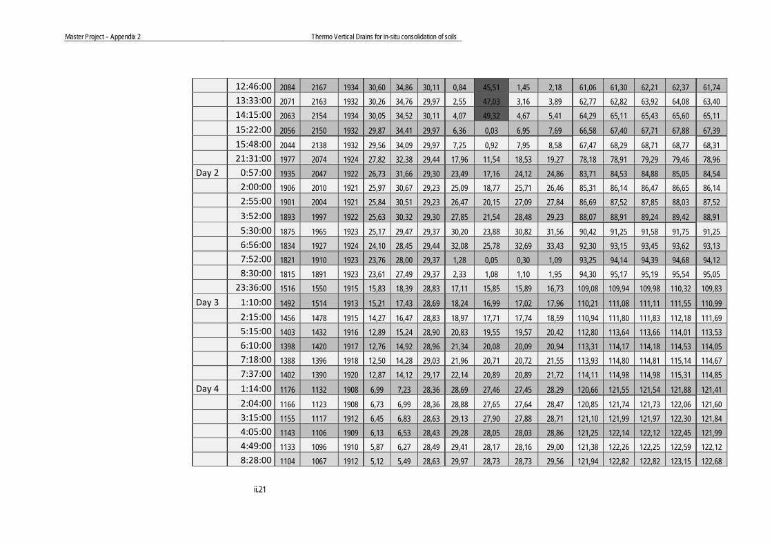
Master Project – Appendix 2 Thermo Vertical Drains for in-situ consolidation of soils
ii.21
12:46:00 2084 2167 1934 30,60 34,86 30,11 0,84 45,51 1,45 2,18 61,06 61,30 62,21 62,37 61,74 13:33:00 2071 2163 1932 30,26 34,76 29,97 2,55 47,03 3,16 3,89 62,77 62,82 63,92 64,08 63,40
14:15:00 2063 2154 1934 30,05 34,52 30,11 4,07 49,32 4,67 5,41 64,29 65,11 65,43 65,60 65,11 15:22:00 2056 2150 1932 29,87 34,41 29,97 6,36 0,03 6,95 7,69 66,58 67,40 67,71 67,88 67,39
15:48:00 2044 2138 1932 29,56 34,09 29,97 7,25 0,92 7,95 8,58 67,47 68,29 68,71 68,77 68,31 21:31:00 1977 2074 1924 27,82 32,38 29,44 17,96 11,54 18,53 19,27 78,18 78,91 79,29 79,46 78,96 Day 2 0:57:00 1935 2047 1922 26,73 31,66 29,30 23,49 17,16 24,12 24,86 83,71 84,53 84,88 85,05 84,54 2:00:00 1906 2010 1921 25,97 30,67 29,23 25,09 18,77 25,71 26,46 85,31 86,14 86,47 86,65 86,14 2:55:00 1901 2004 1921 25,84 30,51 29,23 26,47 20,15 27,09 27,84 86,69 87,52 87,85 88,03 87,52 3:52:00 1893 1997 1922 25,63 30,32 29,30 27,85 21,54 28,48 29,23 88,07 88,91 89,24 89,42 88,91 5:30:00 1875 1965 1923 25,17 29,47 29,37 30,20 23,88 30,82 31,56 90,42 91,25 91,58 91,75 91,25 6:56:00 1834 1927 1924 24,10 28,45 29,44 32,08 25,78 32,69 33,43 92,30 93,15 93,45 93,62 93,13 7:52:00 1821 1910 1923 23,76 28,00 29,37 1,28 0,05 0,30 1,09 93,25 94,14 94,39 94,68 94,12 8:30:00 1815 1891 1923 23,61 27,49 29,37 2,33 1,08 1,10 1,95 94,30 95,17 95,19 95,54 95,05 23:36:00 1516 1550 1915 15,83 18,39 28,83 17,11 15,85 15,89 16,73 109,08 109,94 109,98 110,32 109,83 Day 3 1:10:00 1492 1514 1913 15,21 17,43 28,69 18,24 16,99 17,02 17,96 110,21 111,08 111,11 111,55 110,99 2:15:00 1456 1478 1915 14,27 16,47 28,83 18,97 17,71 17,74 18,59 110,94 111,80 111,83 112,18 111,69 5:15:00 1403 1432 1916 12,89 15,24 28,90 20,83 19,55 19,57 20,42 112,80 113,64 113,66 114,01 113,53 6:10:00 1398 1420 1917 12,76 14,92 28,96 21,34 20,08 20,09 20,94 113,31 114,17 114,18 114,53 114,05 7:18:00 1388 1396 1918 12,50 14,28 29,03 21,96 20,71 20,72 21,55 113,93 114,80 114,81 115,14 114,67 7:37:00 1402 1390 1920 12,87 14,12 29,17 22,14 20,89 20,89 21,72 114,11 114,98 114,98 115,31 114,85 Day 4 1:14:00 1176 1132 1908 6,99 7,23 28,36 28,69 27,46 27,45 28,29 120,66 121,55 121,54 121,88 121,41 2:04:00 1166 1123 1908 6,73 6,99 28,36 28,88 27,65 27,64 28,47 120,85 121,74 121,73 122,06 121,60 3:15:00 1155 1117 1912 6,45 6,83 28,63 29,13 27,90 27,88 28,71 121,10 121,99 121,97 122,30 121,84 4:05:00 1143 1106 1909 6,13 6,53 28,43 29,28 28,05 28,03 28,86 121,25 122,14 122,12 122,45 121,99 4:49:00 1133 1096 1910 5,87 6,27 28,49 29,41 28,17 28,16 29,00 121,38 122,26 122,25 122,59 122,12 8:28:00 1104 1067 1912 5,12 5,49 28,63 29,97 28,73 28,73 29,56 121,94 122,82 122,82 123,15 122,68

Master Project – Appendix 2 Thermo Vertical Drains for in-situ consolidation of soils
ii.22
9:48:00 1091 1041 1911 4,78 4,80 28,56 30,15 28,91 28,90 29,73 122,12 123,00 122,99 123,32 122,86 10:19:00 1091 1033 1910 4,78 4,59 28,49 30,22 28,97 28,97 29,80 122,19 123,06 123,06 123,39 122,93 21:51:00 1046 997 1900 3,61 3,62 27,82 31,36 30,12 30,09 30,93 123,33 124,21 124,18 124,52 124,06 22:46:00 1049 995 1900 3,69 3,57 27,82 31,43 30,18 30,11 30,99 123,40 124,27 124,20 124,58 124,11 Day 5 0:07:00 1041 983 1900 3,48 3,25 27,82 31,52 30,27 30,25 31,08 123,49 124,36 124,34 124,67 124,22 2:28:00 1036 971 1900 3,35 2,93 27,82 31,61 30,41 30,39 31,22 123,58 124,50 124,48 124,81 124,34 3:28:00 1040 963 1899 3,46 2,72 27,75 31,71 30,47 30,44 31,27 123,68 124,56 124,53 124,86 124,41 6:08:00 1026 956 1896 3,09 2,53 27,55 31,83 30,59 30,56 31,40 123,80 124,68 124,65 124,99 124,53 Day 6 6:03:00 996 926 1888 2,31 1,73 27,01 32,40 31,12 31,13 31,96 124,37 125,21 125,22 125,55 125,09 7:12:00 995 925 1889 2,29 1,70 27,08 32,42 31,18 31,14 31,98 124,39 125,27 125,23 125,57 125,12 8:24:00 994 925 1887 2,26 1,70 26,95 32,43 31,20 31,16 31,99 124,40 125,29 125,25 125,58 125,13 Day 7 22:21:00 977 911 1863 1,82 1,33 25,33 32,68 31,44 31,40 32,24 124,65 125,53 125,49 125,83 125,38

Master Project – Appendix 2 Thermo Vertical Drains for in-situ consolidation of soils
ii.23
2.2.4 Mechanical unloading A) Temperature and water volume measurements – Void ratio and water content calculation controls
Mechanical uncharge
applied
Case Time T Water e w 11/05/2009 ‐
10h00
365,96 kg
50,79 kN/m2 1 2 3 Level Volume 1,778 67,725
0:00:00 36,6 34,4 33,9 270 0 1,778 67,725 0:01:30 36,5 34,4 33,8 270 0 1,778 67,725 0:05:00 36,5 34,4 33,8 270 0 1,778 67,725 0:10:00 36,5 34,4 33,8 270 0 1,778 67,725 0:20:00 36,5 34,4 33,8 270 0 1,778 67,725 0:31:00 36,5 34,4 33,8 270 0 1,778 67,725 0:50:00 36,5 34,4 33,8 270 0 1,778 67,725 1:07:00 36,5 34,3 33,8 270 0 1,778 67,725 1:29:00 36,5 34,3 33,8 270 0 1,778 67,725 2:30:00 36,4 34,2 33,7 270 0 1,778 67,725
3:50:00 36,3 34,2 33,6 265 ‐5 1,779 67,737
4:48:00 36,4 34,2 33,7 265 ‐5 1,779 67,737
6:19:00 36,3 34,2 33,6 265 ‐5 1,779 67,737
7:05:00 36,4 34,2 33,7 265 ‐5 1,779 67,737
9:04:00 36,4 34,2 33,7 260 ‐10 1,779 67,748
21:47:00 36,1 34,3 34,0 255 ‐15 1,779 67,760
22:56:00 36,5 34,4 33,8 255 ‐15 1,779 67,760
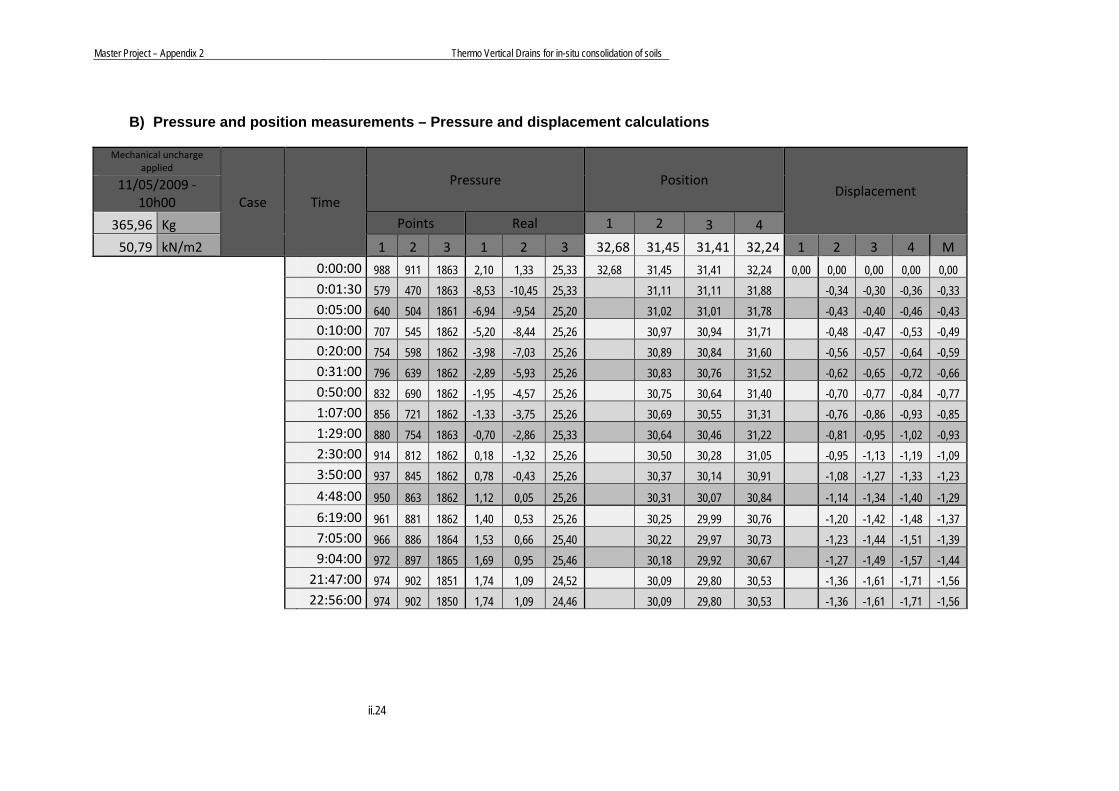
Master Project – Appendix 2 Thermo Vertical Drains for in-situ consolidation of soils
ii.24
B) Pressure and position measurements – Pressure and displacement calculations Mechanical uncharge
applied
Case Time
Pressure Position Displacement 11/05/2009 ‐
10h00
365,96 Kg Points Real 1 2 3 4
50,79 kN/m2 1 2 3 1 2 3 32,68 31,45 31,41 32,24 1 2 3 4 M
0:00:00 988 911 1863 2,10 1,33 25,33 32,68 31,45 31,41 32,24 0,00 0,00 0,00 0,00 0,00 0:01:30 579 470 1863 -8,53 -10,45 25,33 31,11 31,11 31,88 -0,34 -0,30 -0,36 -0,33 0:05:00 640 504 1861 -6,94 -9,54 25,20 31,02 31,01 31,78 -0,43 -0,40 -0,46 -0,43 0:10:00 707 545 1862 -5,20 -8,44 25,26 30,97 30,94 31,71 -0,48 -0,47 -0,53 -0,49 0:20:00 754 598 1862 -3,98 -7,03 25,26 30,89 30,84 31,60 -0,56 -0,57 -0,64 -0,59 0:31:00 796 639 1862 -2,89 -5,93 25,26 30,83 30,76 31,52 -0,62 -0,65 -0,72 -0,66 0:50:00 832 690 1862 -1,95 -4,57 25,26 30,75 30,64 31,40 -0,70 -0,77 -0,84 -0,77 1:07:00 856 721 1862 -1,33 -3,75 25,26 30,69 30,55 31,31 -0,76 -0,86 -0,93 -0,85 1:29:00 880 754 1863 -0,70 -2,86 25,33 30,64 30,46 31,22 -0,81 -0,95 -1,02 -0,93 2:30:00 914 812 1862 0,18 -1,32 25,26 30,50 30,28 31,05 -0,95 -1,13 -1,19 -1,09 3:50:00 937 845 1862 0,78 -0,43 25,26 30,37 30,14 30,91 -1,08 -1,27 -1,33 -1,23
4:48:00 950 863 1862 1,12 0,05 25,26 30,31 30,07 30,84 -1,14 -1,34 -1,40 -1,29
6:19:00 961 881 1862 1,40 0,53 25,26 30,25 29,99 30,76 -1,20 -1,42 -1,48 -1,37 7:05:00 966 886 1864 1,53 0,66 25,40 30,22 29,97 30,73 -1,23 -1,44 -1,51 -1,39 9:04:00 972 897 1865 1,69 0,95 25,46 30,18 29,92 30,67 -1,27 -1,49 -1,57 -1,44 21:47:00 974 902 1851 1,74 1,09 24,52 30,09 29,80 30,53 -1,36 -1,61 -1,71 -1,56 22:56:00 974 902 1850 1,74 1,09 24,46 30,09 29,80 30,53 -1,36 -1,61 -1,71 -1,56
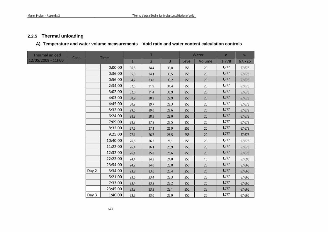
Master Project – Appendix 2 Thermo Vertical Drains for in-situ consolidation of soils
ii.25
2.2.5 Thermal unloading A) Temperature and water volume measurements – Void ratio and water content calculation controls
Thermal unload
12/05/2009 ‐ 11h00 Case Time
T Water e w
1 2 3 Level Volume 1,778 67,725
0:00:00 36,5 34,4 33,8 255 20 1,777 67,678 0:36:00 35,3 34,1 33,5 255 20 1,777 67,678
0:56:00 34,7 33,8 33,2 255 20 1,777 67,678 2:34:00 32,5 31,9 31,4 255 20 1,777 67,678 3:02:00 32,0 31,4 30,9 255 20 1,777 67,678 4:03:00 30,9 30,3 29,9 255 20 1,777 67,678 4:45:00 30,2 29,7 29,3 255 20 1,777 67,678 5:32:00 29,5 29,0 28,6 255 20 1,777 67,678 6:24:00 28,8 28,3 28,0 255 20 1,777 67,678 7:09:00 28,3 27,8 27,5 255 20 1,777 67,678 8:32:00 27,5 27,1 26,9 255 20 1,777 67,678
9:25:00 27,1 26,7 26,5 255 20 1,777 67,678 10:40:00 26,6 26,3 26,1 255 20 1,777 67,678 11:22:00 26,4 26,1 25,9 255 20 1,777 67,678 12:32:00 26,1 25,8 25,6 255 20 1,777 67,678
22:22:00 24,4 24,2 24,0 250 15 1,777 67,690 23:54:00 24,2 24,0 23,8 250 25 1,777 67,666 Day 2 3:34:00 23,8 23,6 23,4 250 25 1,777 67,666 5:21:00 23,6 23,4 23,3 250 25 1,777 67,666 7:33:00 23,4 23,3 23,2 250 25 1,777 67,666 23:45:00 23,3 23,2 23,1 250 25 1,777 67,666 Day 3 1:40:00 23,2 23,0 22,9 250 25 1,777 67,666

Master Project – Appendix 2 Thermo Vertical Drains for in-situ consolidation of soils
ii.26
B) Pressure and position measurements – Pressure and displacement calculations Thermal unload
12/05/2009 ‐ 11h00
Case Time Pressure Position
Displacement Points Real 1 2 3 4
1 2 3 1 2 3 28,60 30,09 30,88 30,52 1 2 3 4 M
0:00:00 991 903 1849 2,18 1,11 24,39 28,60 30,09 30,88 30,52 0,00 0,00 0,00 0,00 0,00 0:36:00 928 848 1848 0,54 -0,35 24,32 28,60 30,10 30,88 30,53 0,00 0,01 0,00 0,01 0,01 0:56:00 923 839 1848 0,41 -0,59 24,32 28,60 30,10 30,88 30,53 0,00 0,01 0,00 0,01 0,01 2:34:00 917 841 1846 0,26 -0,54 24,19 28,60 30,11 30,88 30,54 0,00 0,02 0,00 0,02 0,01 3:02:00 922 845 1845 0,39 -0,43 24,12 28,60 30,11 30,88 30,54 0,00 0,02 0,00 0,02 0,01 4:03:00 928 854 1846 0,54 -0,19 24,19 28,60 30,12 30,88 30,54 0,00 0,03 0,00 0,02 0,01 4:45:00 935 860 1848 0,73 -0,03 24,32 28,60 30,12 30,88 30,54 0,00 0,03 0,00 0,02 0,01 5:32:00 939 865 1846 0,83 0,10 24,19 28,60 30,12 30,88 30,54 0,00 0,03 0,00 0,02 0,01 6:24:00 941 871 1846 0,88 0,26 24,19 28,60 30,12 30,87 30,54 0,00 0,03 -0,01 0,02 0,01 7:09:00 947 875 1845 1,04 0,37 24,12 28,60 30,12 30,87 30,54 0,00 0,03 -0,01 0,02 0,01 8:32:00 955 886 1844 1,25 0,66 24,05 28,60 30,13 30,87 30,54 0,00 0,04 -0,01 0,02 0,01
9:25:00 957 889 1845 1,30 0,74 24,12 28,59 30,13 30,87 30,54 -0,01 0,04 -0,01 0,02 0,01 10:40:00 961 894 1842 1,40 0,87 23,92 28,59 30,13 30,86 30,54 -0,01 0,04 -0,02 0,02 0,01 11:22:00 965 895 1842 1,51 0,90 23,92 28,59 30,13 30,86 30,54 -0,01 0,04 -0,02 0,02 0,01 12:32:00 964 897 1840 1,48 0,95 23,78 28,59 30,13 30,86 30,53 -0,01 0,04 -0,02 0,01 0,00
22:22:00 971 905 1832 1,66 1,17 23,24 28,57 30,12 30,84 30,51 -0,03 0,03 -0,04 -0,01 -0,01 23:54:00 973 907 1830 1,71 1,22 23,11 28,56 30,12 30,83 30,51 -0,04 0,03 -0,05 -0,01 -0,02 Day 2 3:34:00 975 910 1830 1,77 1,30 23,11 28,56 30,12 30,83 30,50 -0,04 0,03 -0,05 -0,02 -0,02 5:21:00 976 911 1829 1,79 1,33 23,04 28,56 30,12 30,82 30,50 -0,04 0,03 -0,06 -0,02 -0,02 7:33:00 980 914 1829 1,90 1,41 23,04 28,56 30,12 30,82 30,50 -0,04 0,03 -0,06 -0,02 -0,02 23:45:00 981 917 1823 1,92 1,49 22,64 28,54 30,11 30,81 30,48 -0,06 0,02 -0,07 -0,04 -0,04 Day 3 1:40:00 982 916 1821 1,95 1,46 22,50 28,54 30,11 30,81 30,48 -0,06 0,02 -0,07 -0,04 -0,04

Master Project – Appendix 2 Thermo Vertical Drains for in-situ consolidation of soils
ii.27
2.3 Experimental test at ambient temperature
2.3.1 Pre-consolidation
A) Temperature and water volume measurements – Void ratio and water content calculation controls
Charge applied at
Case Time T Water
01/05/2009 ‐ 15h00
33,65 kg
4,67 kN/m2 1 2 3 Level Volume
Half cell full 21,7 22,9 22,1 ‐‐‐ ‐‐‐ Cell full 21,7 22,0 21,4 ‐‐‐ ‐‐‐ Cell closed 21,8 21,7 21,7 380 ‐‐‐ First zero 0:00:00 21,7 21,6 21,5 385 ‐‐‐
0:35:00 21,8 21,6 21,5 385 ‐‐‐ 2:08:00 21,7 21,6 21,5 385 ‐‐‐ 2:40:00 21,7 21,6 21,5 385 ‐‐‐ 21:47:00 21,2 21,3 21,4 385 ‐‐‐
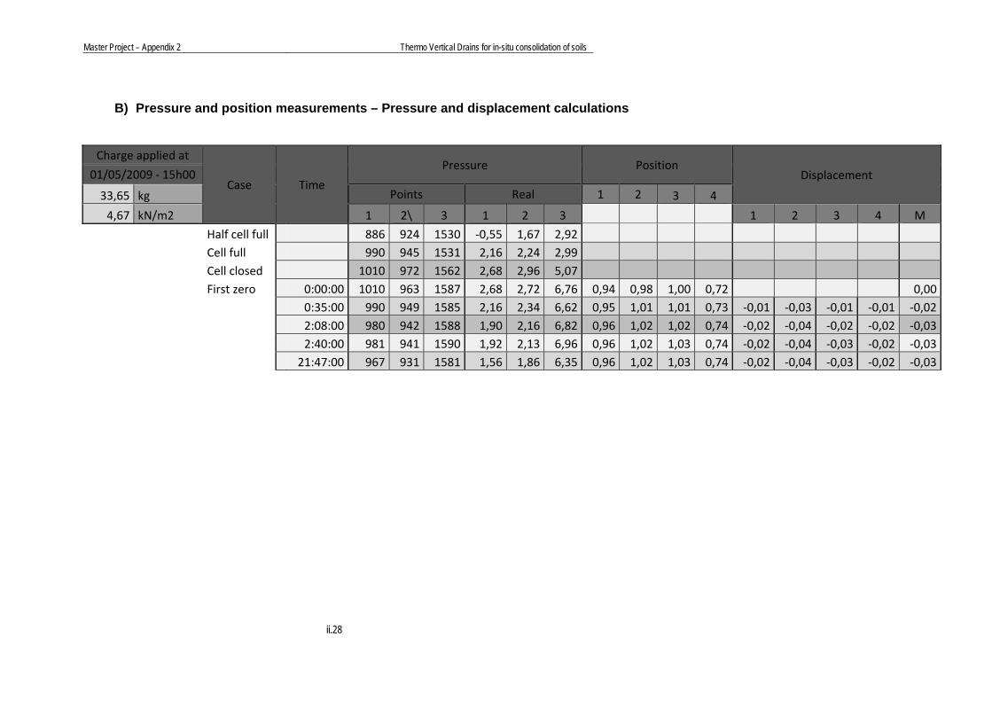
Master Project – Appendix 2 Thermo Vertical Drains for in-situ consolidation of soils
ii.28
B) Pressure and position measurements – Pressure and displacement calculations
Charge applied at
Case Time
Pressure Position Displacement 01/05/2009 ‐ 15h00
33,65 kg Points Real 1 2 3 4
4,67 kN/m2 1 2\ 3 1 2 3 1 2 3 4 M
Half cell full 886 924 1530 ‐0,55 1,67 2,92 Cell full 990 945 1531 2,16 2,24 2,99 Cell closed 1010 972 1562 2,68 2,96 5,07 First zero 0:00:00 1010 963 1587 2,68 2,72 6,76 0,94 0,98 1,00 0,72 0,00
0:35:00 990 949 1585 2,16 2,34 6,62 0,95 1,01 1,01 0,73 ‐0,01 ‐0,03 ‐0,01 ‐0,01 ‐0,02 2:08:00 980 942 1588 1,90 2,16 6,82 0,96 1,02 1,02 0,74 ‐0,02 ‐0,04 ‐0,02 ‐0,02 ‐0,03 2:40:00 981 941 1590 1,92 2,13 6,96 0,96 1,02 1,03 0,74 ‐0,02 ‐0,04 ‐0,03 ‐0,02 ‐0,03 21:47:00 967 931 1581 1,56 1,86 6,35 0,96 1,02 1,03 0,74 ‐0,02 ‐0,04 ‐0,03 ‐0,02 ‐0,03
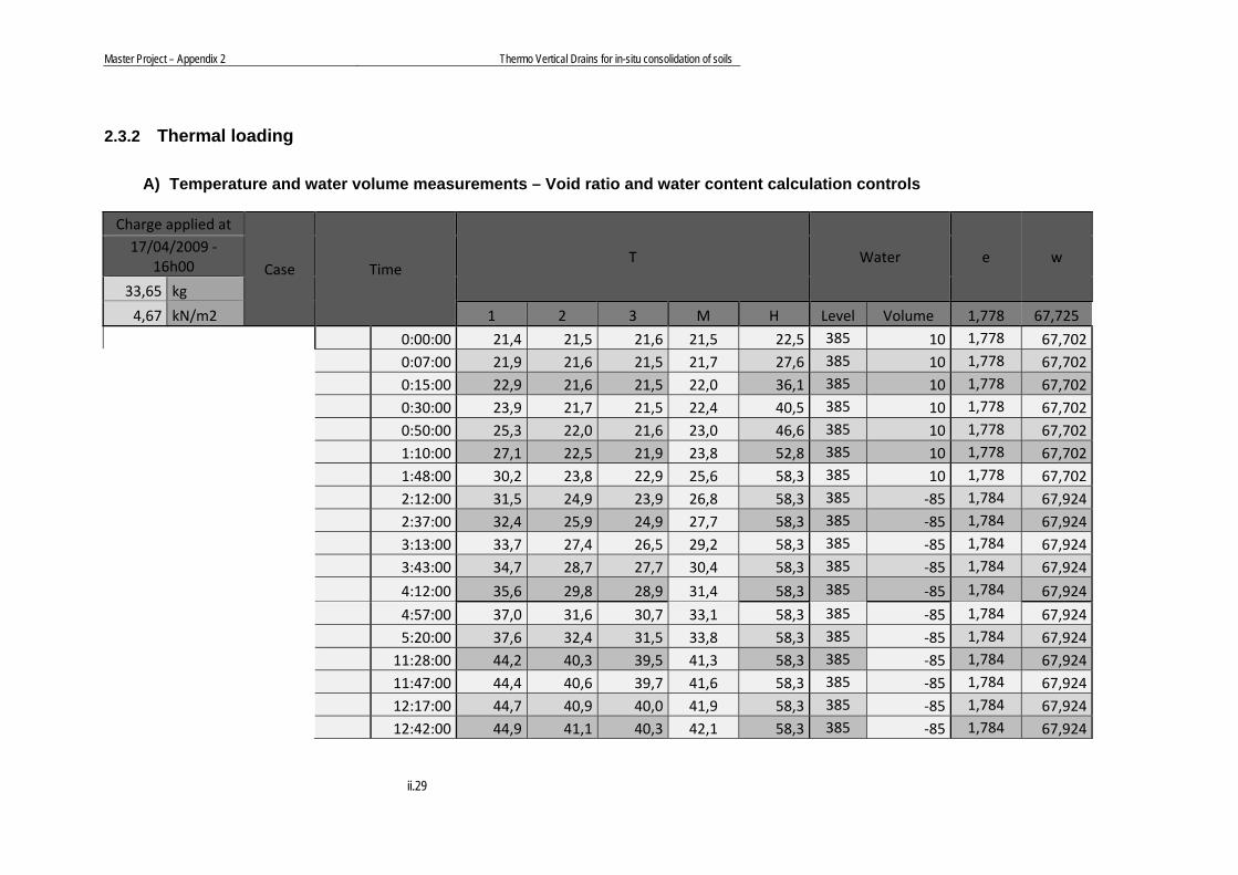
Master Project – Appendix 2 Thermo Vertical Drains for in-situ consolidation of soils
ii.29
2.3.2 Thermal loading
A) Temperature and water volume measurements – Void ratio and water content calculation controls
Charge applied at
Case Time T Water e w
17/04/2009 ‐ 16h00
33,65 kg
4,67 kN/m2 1 2 3 M H Level Volume 1,778 67,725
0:00:00 21,4 21,5 21,6 21,5 22,5 385 10 1,778 67,702 0:07:00 21,9 21,6 21,5 21,7 27,6 385 10 1,778 67,702 0:15:00 22,9 21,6 21,5 22,0 36,1 385 10 1,778 67,702 0:30:00 23,9 21,7 21,5 22,4 40,5 385 10 1,778 67,702 0:50:00 25,3 22,0 21,6 23,0 46,6 385 10 1,778 67,702 1:10:00 27,1 22,5 21,9 23,8 52,8 385 10 1,778 67,702 1:48:00 30,2 23,8 22,9 25,6 58,3 385 10 1,778 67,702 2:12:00 31,5 24,9 23,9 26,8 58,3 385 ‐85 1,784 67,924 2:37:00 32,4 25,9 24,9 27,7 58,3 385 ‐85 1,784 67,924 3:13:00 33,7 27,4 26,5 29,2 58,3 385 ‐85 1,784 67,924 3:43:00 34,7 28,7 27,7 30,4 58,3 385 ‐85 1,784 67,924
4:12:00 35,6 29,8 28,9 31,4 58,3 385 ‐85 1,784 67,924
4:57:00 37,0 31,6 30,7 33,1 58,3 385 ‐85 1,784 67,924 5:20:00 37,6 32,4 31,5 33,8 58,3 385 ‐85 1,784 67,924 11:28:00 44,2 40,3 39,5 41,3 58,3 385 ‐85 1,784 67,924 11:47:00 44,4 40,6 39,7 41,6 58,3 385 ‐85 1,784 67,924 12:17:00 44,7 40,9 40,0 41,9 58,3 385 ‐85 1,784 67,924 12:42:00 44,9 41,1 40,3 42,1 58,3 385 ‐85 1,784 67,924
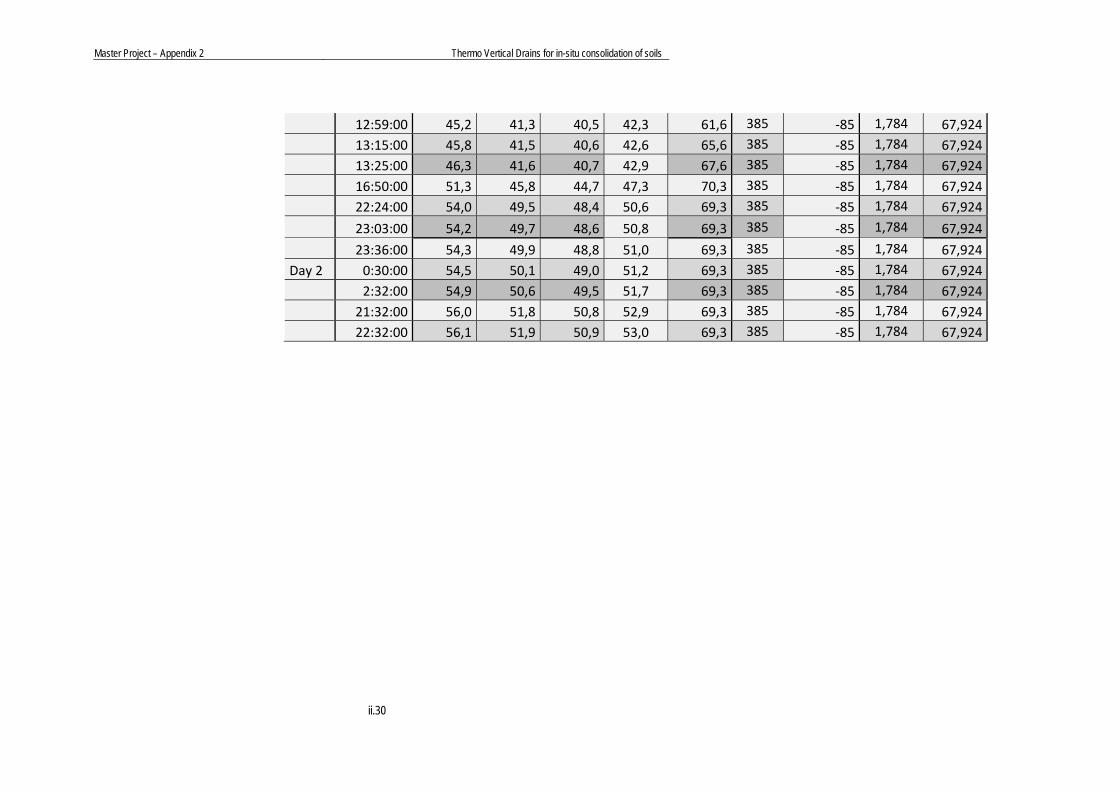
Master Project – Appendix 2 Thermo Vertical Drains for in-situ consolidation of soils
ii.30
12:59:00 45,2 41,3 40,5 42,3 61,6 385 ‐85 1,784 67,924 13:15:00 45,8 41,5 40,6 42,6 65,6 385 ‐85 1,784 67,924 13:25:00 46,3 41,6 40,7 42,9 67,6 385 ‐85 1,784 67,924 16:50:00 51,3 45,8 44,7 47,3 70,3 385 ‐85 1,784 67,924
22:24:00 54,0 49,5 48,4 50,6 69,3 385 ‐85 1,784 67,924
23:03:00 54,2 49,7 48,6 50,8 69,3 385 ‐85 1,784 67,924
23:36:00 54,3 49,9 48,8 51,0 69,3 385 ‐85 1,784 67,924 Day 2 0:30:00 54,5 50,1 49,0 51,2 69,3 385 ‐85 1,784 67,924 2:32:00 54,9 50,6 49,5 51,7 69,3 385 ‐85 1,784 67,924 21:32:00 56,0 51,8 50,8 52,9 69,3 385 ‐85 1,784 67,924 22:32:00 56,1 51,9 50,9 53,0 69,3 385 ‐85 1,784 67,924

Master Project – Appendix 2 Thermo Vertical Drains for in-situ consolidation of soils
ii.31
B) Pressure and position measurements – Pressure and displacement calculations
Charge applied at
Case Time
Pressure Position Displacement
17/04/2009 ‐ 16h00
33,65 kg Points Real 1 2 3 4
4,67 kN/m2 1 2 3 1 2 3 0,96 1,02 1,03 0,74 1 2 3 4 M
0:00:00 978 934 1582 1,84 1,94 6,42 0,96 1,02 1,03 0,74 0,00 0,00 0,00 0,00 0,0000 0:07:00 978 934 1582 1,84 1,94 6,42 0,96 1,02 1,03 0,74 0,00 0,00 0,00 0,00 0,0000 0:15:00 982 944 1581 1,95 2,21 6,35 0,98 1,02 1,04 0,74 0,02 0,00 0,01 0,00 0,0075 0:30:00 993 949 1582 2,23 2,34 6,42 0,98 1,02 1,04 0,74 0,02 0,00 0,01 0,00 0,0075 0:50:00 1006 953 1585 2,57 2,45 6,62 0,97 1,01 1,04 0,73 0,01 ‐0,01 0,01 ‐0,01 0,0000 1:10:00 1012 966 1587 2,73 2,80 6,76 0,98 1,01 1,04 0,73 0,02 ‐0,01 0,01 ‐0,01 0,0025 1:48:00 1020 961 1589 2,94 2,66 6,89 0,98 1,00 1,04 0,72 0,02 ‐0,02 0,01 ‐0,02 ‐0,0025 2:12:00 1031 987 1590 3,22 3,36 6,96 0,98 0,99 1,04 0,71 0,02 ‐0,03 0,01 ‐0,03 ‐0,0075 2:37:00 1037 989 1595 3,38 3,41 7,29 0,98 0,98 1,04 0,71 0,02 ‐0,04 0,01 ‐0,03 ‐0,0100 3:13:00 1029 969 1595 3,17 2,88 7,29 0,98 0,97 1,04 0,70 0,02 ‐0,05 0,01 ‐0,04 ‐0,0150 3:43:00 1029 974 1595 3,17 3,01 7,29 0,97 0,96 1,04 0,69 0,01 ‐0,06 0,01 ‐0,05 ‐0,0225
4:12:00 1029 976 1591 3,17 3,06 7,02 0,97 0,95 1,04 0,68 0,01 ‐0,07 0,01 ‐0,06 ‐0,0275
4:57:00 1023 1007 1594 3,01 3,89 7,23 0,96 0,94 1,04 0,67 0,00 ‐0,08 0,01 ‐0,07 ‐0,0350 5:20:00 1034 1016 1596 3,30 4,13 7,36 0,96 0,94 1,03 0,67 0,00 ‐0,08 0,00 ‐0,07 ‐0,0375 11:28:00 1019 989 1589 2,91 3,41 6,89 0,93 0,89 1,02 0,63 ‐0,03 ‐0,13 ‐0,01 ‐0,11 ‐0,0700 11:47:00 1012 989 1591 2,73 3,41 7,02 0,93 0,89 1,02 0,63 ‐0,03 ‐0,13 ‐0,01 ‐0,11 ‐0,0700 12:17:00 1007 992 1591 2,60 3,49 7,02 0,93 0,89 1,02 0,63 ‐0,03 ‐0,13 ‐0,01 ‐0,11 ‐0,0700 12:42:00 1013 982 1592 2,75 3,22 7,09 0,93 0,89 1,02 0,63 ‐0,03 ‐0,13 ‐0,01 ‐0,11 ‐0,0700 12:59:00 1022 985 1592 2,99 3,30 7,09 0,92 0,88 1,02 0,62 ‐0,04 ‐0,14 ‐0,01 ‐0,12 ‐0,0775 13:15:00 1011 990 1592 2,70 3,44 7,09 0,91 0,88 1,02 0,60 ‐0,05 ‐0,14 ‐0,01 ‐0,14 ‐0,0850
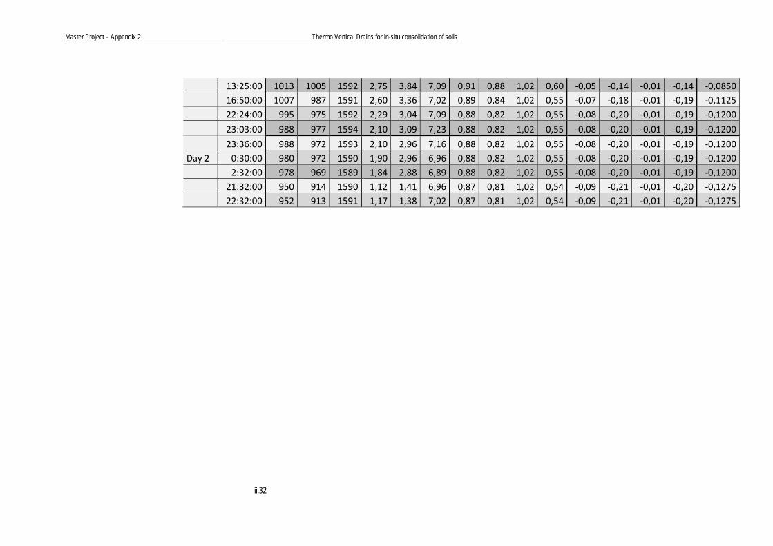
Master Project – Appendix 2 Thermo Vertical Drains for in-situ consolidation of soils
ii.32
13:25:00 1013 1005 1592 2,75 3,84 7,09 0,91 0,88 1,02 0,60 ‐0,05 ‐0,14 ‐0,01 ‐0,14 ‐0,0850 16:50:00 1007 987 1591 2,60 3,36 7,02 0,89 0,84 1,02 0,55 ‐0,07 ‐0,18 ‐0,01 ‐0,19 ‐0,1125
22:24:00 995 975 1592 2,29 3,04 7,09 0,88 0,82 1,02 0,55 ‐0,08 ‐0,20 ‐0,01 ‐0,19 ‐0,1200
23:03:00 988 977 1594 2,10 3,09 7,23 0,88 0,82 1,02 0,55 ‐0,08 ‐0,20 ‐0,01 ‐0,19 ‐0,1200
23:36:00 988 972 1593 2,10 2,96 7,16 0,88 0,82 1,02 0,55 ‐0,08 ‐0,20 ‐0,01 ‐0,19 ‐0,1200 Day 2 0:30:00 980 972 1590 1,90 2,96 6,96 0,88 0,82 1,02 0,55 ‐0,08 ‐0,20 ‐0,01 ‐0,19 ‐0,1200 2:32:00 978 969 1589 1,84 2,88 6,89 0,88 0,82 1,02 0,55 ‐0,08 ‐0,20 ‐0,01 ‐0,19 ‐0,1200 21:32:00 950 914 1590 1,12 1,41 6,96 0,87 0,81 1,02 0,54 ‐0,09 ‐0,21 ‐0,01 ‐0,20 ‐0,1275 22:32:00 952 913 1591 1,17 1,38 7,02 0,87 0,81 1,02 0,54 ‐0,09 ‐0,21 ‐0,01 ‐0,20 ‐0,1275

Master Project – Appendix 2 Thermo Vertical Drains for in-situ consolidation of soils
ii.33
2.3.3 Mechanical loading
A) Temperature and water volume measurements – Void ratio and water content calculation controls
Charge applied at
Case Time T Water e w
04/04/2009 ‐ 12h00
365,96 kg
50,79 kN/m2 1 2 3 Level Volume 1,778 67,725
0:00:00 56,1 51,9 50,9 385 0 1,778 67,725 0:04:15 55,9 51,8 50,8 385 0 1,778 67,725 0:10:00 56,0 51,8 50,8 385 185 1,767 67,291 0:19:00 55,9 51,8 50,9 385 185 1,767 67,291 0:33:30 55,9 51,8 50,9 385 370 1,756 66,858 1:11:30 55,9 51,9 50,9 385 370 1,756 66,858 1:40:00 55,9 51,9 50,9 385 560 1,744 66,412 2:25:30 55,9 51,9 51,0 385 750 1,732 65,967 2:58:30 55,9 52,0 51,1 385 950 1,720 65,498 3:47:00 56,0 52,1 51,2 385 1140 1,708 65,053
4:35:00 56,0 52,2 51,3 385 1335 1,696 64,596
7:52:00 56,2 52,5 51,8 385 1540 1,684 64,115
8:17:00 56,3 52,6 51,9 385 1745 1,671 63,634 9:22:00 56,3 52,8 52,1 385 1945 1,659 63,166 9:53:00 56,4 52,8 52,1 385 1945 1,659 63,166
10:35:30 56,4 52,9 52,3 385 2145 1,646 62,697 10:45:00 56,5 53,0 52,3 385 2370 1,632 62,169 11:32:00 56,6 53,1 52,4 385 2585 1,619 61,665

Master Project – Appendix 2 Thermo Vertical Drains for in-situ consolidation of soils
ii.34
13:04:00 56,6 53,2 52,6 385 2800 1,606 61,161 14:01:00 56,6 53,2 52,6 385 3010 1,593 60,669 21:21:00 55,8 52,2 51,6 385 3225 1,580 60,165 21:45:00 55,7 52,1 51,6 385 3450 1,566 59,638
22:11:00 55,7 52,0 51,5 385 3680 1,552 59,098
23:41:00 55,7 52,0 51,5 385 3910 1,538 58,559
Day 2 0:10:00 55,7 51,9 51,4 385 4145 1,523 58,008 0:40:00 55,6 51,9 51,4 380 4375 1,509 57,469 1:41:00 55,6 51,9 51,4 380 4615 1,494 56,907 2:19:30 55,5 51,8 51,4 380 4615 1,494 56,907 2:54:00 55,6 51,9 51,5 380 4615 1,494 56,907 3:00:00 55,6 51,9 51,5 380 4615 1,494 56,907 3:34:00 55,6 52,0 51,6 380 4615 1,494 56,907 4:08:00 55,6 52,1 51,6 380 4615 1,494 56,907 5:13:00 55,5 52,1 51,5 380 4795 1,483 56,485 6:16:00 55,5 52,1 51,4 380 4795 1,483 56,485 23:19:30 53,8 49,9 48,9 380 5025 1,469 55,946
Day 3 0:00:00 53,7 49,7 48,8 380 5070 1,466 55,840
1:07:00 53,5 49,5 48,5 380 5070 1,466 55,840 2:42:00 53,4 49,3 48,4 380 5070 1,466 55,840 3:58:00 53,5 49,4 48,5 380 5070 1,466 55,840 19:02:00 54,1 50,1 49,0 380 5070 1,466 55,840Day 4 23:11:00 53,4 48,8 47,3 380 5070 1,466 55,840

Master Project – Appendix 2 Thermo Vertical Drains for in-situ consolidation of soils
ii.35
B) Pressure and position measurements – Pressure and displacement calculations
Charge applied at
Time
Pressure Position Displacement
04/04/2009 ‐ 12h00
365,96 kg Points Real 1 2 3 4
50,79 kN/m2 1 2 3 1 2 3 0,86 0,81 1,01 0,53 1 2 3 4 M
0:00:00 957 916 1592 1,30 1,46 7,09 0,86 0,81 1,01 0,53 0,00 0,00 0,00 0,00 0,00 0:04:15 2289 1970 1826 35,93 29,60 22,84 9,89 10,05 10,73 10,44 9,03 9,24 9,72 9,91 9,48 0:10:00 2272 1846 1930 35,49 26,29 29,84 10,96 11,11 11,77 11,49 10,10 10,30 10,76 10,96 10,53 0:19:00 2255 1753 2073 35,05 23,81 39,46 12,35 12,51 13,17 12,89 11,49 11,70 12,16 12,36 11,93 0:33:30 2248 1691 2126 34,86 22,15 43,03 14,19 14,36 15,01 14,72 13,33 13,55 14,00 14,19 13,77 1:11:30 2193 1591 2115 33,43 19,48 42,29 17,85 17,97 18,64 18,39 16,99 17,16 17,63 17,86 17,41 1:40:00 2148 1546 2098 32,26 18,28 41,15 20,08 20,21 20,88 20,59 19,22 19,40 19,87 20,06 19,64 2:25:30 2141 1536 2094 32,08 18,02 40,88 23,43 23,57 24,23 23,95 22,57 22,76 23,22 23,42 22,99 2:58:30 2076 1490 2062 30,39 16,79 38,72 25,50 25,62 26,25 25,99 24,64 24,81 25,24 25,46 25,04 3:47:00 2082 1501 2062 30,55 17,08 38,72 28,35 28,49 29,12 28,85 27,49 27,68 28,11 28,32 27,90
4:35:00 2034 1475 2048 29,30 16,39 37,78 31,02 31,14 31,79 31,54 30,16 30,33 30,78 31,01 30,57
7:52:00 1896 1413 1986 25,71 14,73 33,61 39,96 40,09 40,72 40,48 39,10 39,28 39,71 39,95 39,51
8:17:00 1880 1402 1981 25,30 14,44 33,27 40,95 41,09 41,71 41,47 40,09 40,28 40,70 40,94 40,50 9:22:00 1826 1379 1962 23,89 13,82 31,99 43,43 43,55 44,20 43,95 42,57 42,74 43,19 43,42 42,98 9:53:00 1812 1370 1951 23,53 13,58 31,25 44,54 44,65 45,30 45,06 43,68 43,84 44,29 44,53 44,09
10:35:30 1819 1375 1951 23,71 13,72 31,25 46,08 46,38 46,99 46,75 45,22 45,57 45,98 46,22 45,75 10:45:00 1843 1386 1956 24,33 14,01 31,59 1,94 1,28 1,73 1,09 45,54 45,75 46,09 46,32 45,93 11:32:00 1850 1393 1962 24,52 14,20 31,99 3,71 3,04 3,50 2,88 47,31 47,51 47,86 48,11 47,70 13:04:00 1869 1410 1965 25,01 14,65 32,19 7,12 6,43 6,90 6,28 50,72 50,90 51,26 51,51 51,10 14:01:00 1866 1413 1964 24,93 14,73 32,13 9,13 8,43 8,90 8,29 52,73 52,90 53,26 53,52 53,10

Master Project – Appendix 2 Thermo Vertical Drains for in-situ consolidation of soils
ii.36
21:21:00 1651 1322 1888 19,34 12,30 27,01 21,77 20,99 21,52 21,00 65,37 65,46 65,88 66,23 65,74 21:45:00 1642 1327 1883 19,11 12,43 26,68 22,31 21,53 22,05 21,54 65,91 66,00 66,41 66,77 66,27 22:11:00 1634 1324 1882 18,90 12,35 26,61 22,89 22,11 22,62 22,11 66,49 66,58 66,98 67,34 66,85
23:41:00 1562 1335 1856 17,03 12,65 24,86 24,73 23,93 24,45 23,96 68,33 68,40 68,81 69,19 68,68
Day 2 0:10:00 1542 1331 1846 16,51 12,54 24,19 25,26 24,45 24,98 24,50 68,86 68,92 69,34 69,73 69,21 0:40:00 1532 1328 1841 16,25 12,46 23,85 25,80 25,00 25,51 25,04 69,40 69,47 69,87 70,27 69,75 1:41:00 1488 1320 1826 15,10 12,25 22,84 26,85 26,02 26,54 26,09 70,45 70,49 70,90 71,32 70,79 2:19:30 1473 1323 1820 14,71 12,33 22,44 27,46 26,63 27,15 26,70 71,06 71,10 71,51 71,93 71,40 2:54:00 1449 1333 1808 14,09 12,60 21,63 27,98 27,14 27,66 27,21 71,58 71,61 72,02 72,44 71,91 3:00:00 1447 1377 1806 14,04 13,77 21,49 28,07 27,22 27,75 27,30 71,67 71,69 72,11 72,53 72,00 3:34:00 1410 1331 1794 13,08 12,54 20,69 28,55 27,69 28,22 27,80 72,15 72,16 72,58 73,03 72,48 4:08:00 1382 1341 1783 12,35 12,81 19,95 29,04 28,15 28,73 28,28 72,64 72,62 73,09 73,51 72,97 5:13:00 1348 1346 1769 11,46 12,94 19,00 29,85 28,94 29,48 29,08 73,45 73,41 73,84 74,31 73,75 6:16:00 1320 1351 1758 10,74 13,08 18,26 30,60 29,69 30,23 29,83 74,20 74,16 74,59 75,06 74,50 23:19:30 933 1433 1608 0,67 15,27 8,17 36,04 34,99 35,48 35,25 79,64 79,46 79,84 80,48 79,86
Day 3 0:00:00 932 1435 1608 0,65 15,32 8,17 36,08 35,02 35,51 35,29 79,68 79,49 79,87 80,52 79,89
1:07:00 921 1423 1604 0,36 15,00 7,90 36,13 35,06 35,55 35,33 79,73 79,53 79,91 80,56 79,93 2:42:00 919 1429 1603 0,31 15,16 7,83 36,18 35,10 35,58 35,38 79,78 79,57 79,94 80,61 79,98 3:58:00 923 1434 1602 0,41 15,29 7,76 36,19 35,12 35,59 35,38 79,79 79,59 79,95 80,61 79,99 19:02:00 897 1470 1588 ‐0,26 16,25 6,82 36,20 35,11 35,59 35,38 79,80 79,58 79,95 80,61 79,99 Day 4 23:11:00 861 1385 1576 ‐1,20 13,98 6,01 36,24 35,13 35,60 35,42 79,84 79,60 79,96 80,65 80,01
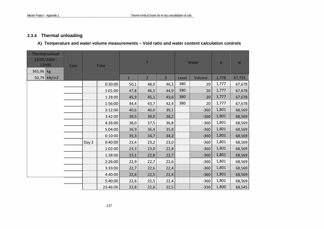
Master Project – Appendix 2 Thermo Vertical Drains for in-situ consolidation of soils
ii.37
2.3.4 Thermal unloading A) Temperature and water volume measurements – Void ratio and water content calculation controls
Thermal unload
Case Time T Water e w
12/05/2009 ‐ 11h00
365,96 kg
50,79 kN/m2 1 2 3 Level Volume 1,778 67,725
0:30:00 50,1 48,0 46,3 380 20 1,777 67,678
1:01:00 47,8 46,5 44,9 380 20 1,777 67,678
1:28:00 45,9 45,1 43,6 380 20 1,777 67,678
1:56:00 44,4 43,7 42,4 380 20 1,777 67,678
3:12:00 40,6 40,0 39,1 ‐360 1,801 68,569
3:42:00 39,5 39,0 38,2 ‐360 1,801 68,569
4:26:00 38,0 37,5 36,8 ‐360 1,801 68,569
5:04:00 36,9 36,4 35,8 ‐360 1,801 68,569
6:10:00 35,3 34,7 34,2 ‐360 1,801 68,569
Day 2 0:40:00 23,4 23,2 23,0 ‐360 1,801 68,569
1:02:00 23,3 23,0 22,8 ‐360 1,801 68,569
1:38:00 23,1 22,8 22,7 ‐360 1,801 68,569
2:26:00 22,9 22,7 22,6 ‐360 1,801 68,569
3:33:00 22,7 22,6 22,4 ‐360 1,801 68,569
4:40:00 22,6 22,5 22,4 ‐360 1,801 68,569
5:40:00 22,6 22,5 22,4 ‐360 1,801 68,569
23:46:00 22,8 22,6 22,5 ‐350 1,800 68,545

Master Project – Appendix 2 Thermo Vertical Drains for in-situ consolidation of soils
ii.38
B)Pressure and position measurements – Pressure and displacement calculations Thermal unload
Time
Pressure Position Displacement
12/05/2009 ‐ 11h00
365,96 kg Points Real 1 2 3 4
50,79 kN/m2 1 2 3 1 2 3 36,24 35,11 35,60 35,38 1 2 3 4 M
0:30:00 735 1249 1561 ‐4,47 10,35 5,01 36,30 35,23 35,62 35,49 0,06 0,12 0,02 0,11 0,0775
1:01:00 736 1243 1548 ‐4,45 10,19 4,13 36,31 35,31 35,67 35,57 0,07 0,20 0,07 0,19 0,1325
1:28:00 723 1202 1531 ‐4,79 9,10 2,99 36,40 35,36 35,70 35,62 0,16 0,25 0,10 0,24 0,1875
1:56:00 720 1160 1529 ‐4,86 7,98 2,85 36,44 35,40 35,73 35,67 0,20 0,29 0,13 0,29 0,2275
3:12:00 732 1081 1527 ‐4,55 5,87 2,72 36,52 35,49 35,80 35,78 0,28 0,38 0,20 0,40 0,3150
3:42:00 738 1057 1533 ‐4,40 5,23 3,12 36,55 35,51 35,83 35,81 0,31 0,40 0,23 0,43 0,3425
4:26:00 744 1023 1532 ‐4,24 4,32 3,05 36,58 35,55 35,86 35,86 0,34 0,44 0,26 0,48 0,3800
5:04:00 748 1002 1534 ‐4,14 3,76 3,19 36,62 35,59 35,89 35,89 0,38 0,48 0,29 0,51 0,4150
6:10:00 754 968 1531 ‐3,98 2,85 2,99 36,67 35,64 35,94 35,96 0,43 0,53 0,34 0,58 0,4700
Day 2 0:40:00 812 877 1543 ‐2,47 0,42 3,79 37,55 36,64 36,88 36,90 1,31 1,53 1,28 1,52 1,4100
1:02:00 813 875 1542 ‐2,45 0,37 3,73 37,57 36,65 36,88 36,91 1,33 1,54 1,28 1,53 1,4200
1:38:00 815 873 1542 ‐2,39 0,31 3,73 37,58 36,68 36,90 36,93 1,34 1,57 1,30 1,55 1,4400
2:26:00 814 870 1542 ‐2,42 0,23 3,73 37,61 36,70 36,93 36,95 1,37 1,59 1,33 1,57 1,4650
3:33:00 819 850 1542 ‐2,29 ‐0,30 3,73 37,63 36,73 36,95 36,98 1,39 1,62 1,35 1,60 1,4900
4:40:00 819 850 1544 ‐2,29 ‐0,30 3,86 37,65 36,75 36,98 37,00 1,41 1,64 1,38 1,62 1,5125
5:40:00 823 851 1546 ‐2,19 ‐0,27 4,00 37,67 36,77 36,99 37,01 1,43 1,66 1,39 1,63 1,5275 23:46:00 838 860 1544 ‐1,80 ‐0,03 3,86 37,70 36,81 37,03 37,05 1,46 1,70 1,43 1,67 1,5650

Master Project – Appendix 2 Thermo Vertical Drains for in-situ consolidation of soils
ii.39
2.3.5 Mechanical unloading
A) Temperature and water volume measurements – Void ratio and water content calculation controls
Mechanical uncharge applied
Case Time T Water e w 11/05/2009 ‐
10h00
365,96 kg
50,79 kN/m2 1 2 3 Level Volume 1,778 67,725
30 0:00:30 22,80 22,70 22,60 0,00 1,78 67,73 660 0:11:00 22,80 22,70 22,60 0,00 1,78 67,73 1200 0:20:00 22,80 22,70 22,60 0,00 1,78 67,73 1260 0:21:00 22,80 22,70 22,50 0,00 1,78 67,73 1740 0:29:00 22,80 22,60 22,50 0,00 1,78 67,73 2220 0:37:00 22,80 22,60 22,50 0,00 1,78 67,73 2340 0:39:00 22,80 22,60 22,50 0,00 1,78 67,73 2580 0:43:00 22,80 22,60 22,50 0,00 1,78 67,73 3780 1:03:00 22,80 22,60 22,60 0,00 1,78 67,73 3900 1:05:00 22,80 22,70 22,60 0,00 1,78 67,73
4560 1:16:00 22,80 22,70 22,50 0,00 1,78 67,73
5040 1:24:00 22,80 22,70 22,50 0,00 1,78 67,73
5130 1:25:30 22,80 22,70 22,50 0,00 1,78 67,73
5370 1:29:30 22,80 22,70 22,50 0,00 1,78 67,73
5700 1:35:00 22,80 22,70 22,50 0,00 1,78 67,73
14640 4:04:00 22,80 22,60 22,50 0,00 1,78 67,73
14760 4:06:00 22,80 22,60 22,50 0,00 1,78 67,73
17220 4:47:00 22,80 22,60 22,50 0,00 1,78 67,73
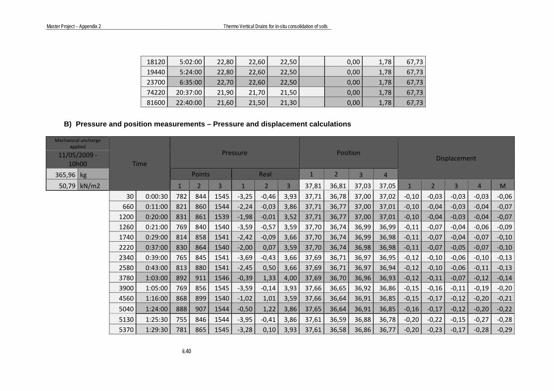
Master Project – Appendix 2 Thermo Vertical Drains for in-situ consolidation of soils
ii.40
18120 5:02:00 22,80 22,60 22,50 0,00 1,78 67,73
19440 5:24:00 22,80 22,60 22,50 0,00 1,78 67,73
23700 6:35:00 22,70 22,60 22,50 0,00 1,78 67,7374220 20:37:00 21,90 21,70 21,50 0,00 1,78 67,7381600 22:40:00 21,60 21,50 21,30 0,00 1,78 67,73
B) Pressure and position measurements – Pressure and displacement calculations
Mechanical uncharge
applied
Time
Pressure Position Displacement 11/05/2009 ‐
10h00
365,96 kg Points Real 1 2 3 4
50,79 kN/m2 1 2 3 1 2 3 37,81 36,81 37,03 37,05 1 2 3 4 M
30 0:00:30 782 844 1545 ‐3,25 ‐0,46 3,93 37,71 36,78 37,00 37,02 ‐0,10 ‐0,03 ‐0,03 ‐0,03 ‐0,06 660 0:11:00 821 860 1544 ‐2,24 ‐0,03 3,86 37,71 36,77 37,00 37,01 ‐0,10 ‐0,04 ‐0,03 ‐0,04 ‐0,07 1200 0:20:00 831 861 1539 ‐1,98 ‐0,01 3,52 37,71 36,77 37,00 37,01 ‐0,10 ‐0,04 ‐0,03 ‐0,04 ‐0,07 1260 0:21:00 769 840 1540 ‐3,59 ‐0,57 3,59 37,70 36,74 36,99 36,99 ‐0,11 ‐0,07 ‐0,04 ‐0,06 ‐0,09 1740 0:29:00 814 858 1541 ‐2,42 ‐0,09 3,66 37,70 36,74 36,99 36,98 ‐0,11 ‐0,07 ‐0,04 ‐0,07 ‐0,10 2220 0:37:00 830 864 1540 ‐2,00 0,07 3,59 37,70 36,74 36,98 36,98 ‐0,11 ‐0,07 ‐0,05 ‐0,07 ‐0,10 2340 0:39:00 765 845 1541 ‐3,69 ‐0,43 3,66 37,69 36,71 36,97 36,95 ‐0,12 ‐0,10 ‐0,06 ‐0,10 ‐0,13 2580 0:43:00 813 880 1541 ‐2,45 0,50 3,66 37,69 36,71 36,97 36,94 ‐0,12 ‐0,10 ‐0,06 ‐0,11 ‐0,13 3780 1:03:00 892 911 1546 ‐0,39 1,33 4,00 37,69 36,70 36,96 36,93 ‐0,12 ‐0,11 ‐0,07 ‐0,12 ‐0,14 3900 1:05:00 769 856 1545 ‐3,59 ‐0,14 3,93 37,66 36,65 36,92 36,86 ‐0,15 ‐0,16 ‐0,11 ‐0,19 ‐0,20
4560 1:16:00 868 899 1540 ‐1,02 1,01 3,59 37,66 36,64 36,91 36,85 ‐0,15 ‐0,17 ‐0,12 ‐0,20 ‐0,21
5040 1:24:00 888 907 1544 ‐0,50 1,22 3,86 37,65 36,64 36,91 36,85 ‐0,16 ‐0,17 ‐0,12 ‐0,20 ‐0,22
5130 1:25:30 755 846 1544 ‐3,95 ‐0,41 3,86 37,61 36,59 36,88 36,78 ‐0,20 ‐0,22 ‐0,15 ‐0,27 ‐0,28
5370 1:29:30 781 865 1545 ‐3,28 0,10 3,93 37,61 36,58 36,86 36,77 ‐0,20 ‐0,23 ‐0,17 ‐0,28 ‐0,29

Master Project – Appendix 2 Thermo Vertical Drains for in-situ consolidation of soils
ii.41
5700 1:35:00 809 879 1541 ‐2,55 0,47 3,66 37,60 36,57 36,85 36,75 ‐0,21 ‐0,24 ‐0,18 ‐0,30 ‐0,31
14640 4:04:00 912 913 1563 0,13 1,38 5,14 37,55 36,47 36,70 36,64 ‐0,26 ‐0,34 ‐0,33 ‐0,41 ‐0,45
14760 4:06:00 798 853 1564 ‐2,84 ‐0,22 5,21 37,53 36,44 36,67 36,58 ‐0,28 ‐0,37 ‐0,36 ‐0,47 ‐0,49
17220 4:47:00 842 892 1551 ‐1,69 0,82 4,33 37,46 36,37 36,57 36,48 ‐0,35 ‐0,44 ‐0,46 ‐0,57 ‐0,61
18120 5:02:00 858 895 1550 ‐1,28 0,90 4,27 37,44 36,35 36,55 36,46 ‐0,37 ‐0,46 ‐0,48 ‐0,59 ‐0,63
19440 5:24:00 870 900 1554 ‐0,96 1,03 4,53 37,42 36,33 36,52 36,43 ‐0,39 ‐0,48 ‐0,51 ‐0,62 ‐0,67
23700 6:35:00 900 906 1556 ‐0,18 1,19 4,67 37,37 36,28 36,46 36,36 ‐0,44 ‐0,53 ‐0,57 ‐0,69 ‐0,74 74220 20:37:00 943 926 1583 0,93 1,73 6,49 37,22 36,14 36,30 36,18 ‐0,59 ‐0,67 ‐0,73 ‐0,87 ‐0,95 81600 22:40:00 944 928 1582 0,96 1,78 6,42 37,22 36,14 36,30 36,18 ‐0,59 ‐0,67 ‐0,73 ‐0,87 ‐0,95

APPENDIX 3

LGV Embankment Simulation LGV RHIN RHÔNE – BRANCH EAST – R375.1 /.2
iii.1
Report: Resume the information available in the measurement interpretation report from EGIS rail to prepare the test embankments simulation in GEFDYN software. This report is available integrally in the CD annexed to this study.
1.1 OBJECTIFS
Acquire correct values for the estimation of the consolidation time in laboratory by readjusting the compressibility parameters with the measurements taken in 2 test embankments.
One will be equipped with vertical drains (R375.1) and compared with another without drains (R375.2) to study the possibility of not using them in this work.
The analysis of the embankment materials reuse isn’t taken into account in this document.
1.2 GEOTECHNICAL ACKNOWLEDGEMENTS
To achieve the readjustment of the geotechnical model in function of the instrumentation measurements, geotechnical acknowledgement profiles were made along the instrumentation profiles resulting on the following report elaborated in 31/05/2007 by Egis Rail.
1.3 EMBANKMENT GEOMETRY, DRAIN CHARACTERISTICS AND INSTRUMENTATION
Description of drain characteristics and number/ type of instrumentation used for both embankments is available in the report. The attachment number three of this report shows the evolution of settlement (at the surface and deep) in time for R375.1 and evolution of pore pressure and settlement for R375.2. These values are plotted with the evolution in time of the embankment’s height.
1.4 GEOTECHNICAL MODEL ALONG THE EMBANKMENT
This chapter will define the geotechnical model to be used.
i. Geological formations The existing formations between PK37+622 and PK37+740 are:
Alluvial clays (formation 44): 5 to 6 meters of maximum deep. The highest thickness exists between 37+620 and 37+770;
Altered marls (formation 15.1): 8 to 9 meters of maximum deep. The highest thickness exists between 37+600 and 37+800;
Inferior iridescent marls (formation 18.5)
[Attachment 6: Profile in length may be important for material definition in simulation]
ii. Hydrogeology
The piezometers and the pore pressure cells made near the test embankments give coherent results
for a ground water level constantly near the surface.
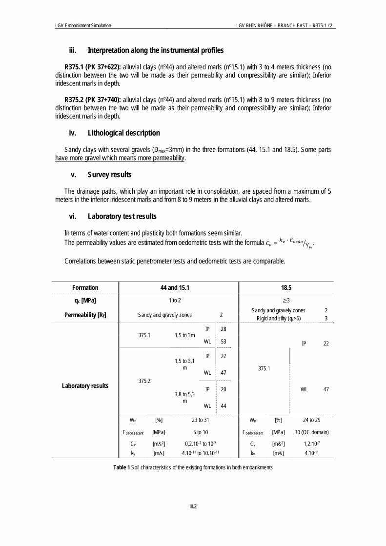
LGV Embankment Simulation LGV RHIN RHÔNE – BRANCH EAST – R375.1 /.2
iii.2
iii. Interpretation along the instrumental profiles R375.1 (PK 37+622): alluvial clays (nº44) and altered marls (nº15.1) with 3 to 4 meters thickness (no
distinction between the two will be made as their permeability and compressibility are similar); Inferior iridescent marls in depth.
R375.2 (PK 37+740): alluvial clays (nº44) and altered marls (nº15.1) with 8 to 9 meters thickness (no
distinction between the two will be made as their permeability and compressibility are similar); Inferior iridescent marls in depth.
iv. Lithological description
Sandy clays with several gravels (Dmax=3mm) in the three formations (44, 15.1 and 18.5). Some parts
have more gravel which means more permeability.
v. Survey results The drainage paths, which play an important role in consolidation, are spaced from a maximum of 5
meters in the inferior iridescent marls and from 8 to 9 meters in the alluvial clays and altered marls.
vi. Laboratory test results In terms of water content and plasticity both formations seem similar. The permeability values are estimated from oedometric tests with the formula · .
Correlations between static penetrometer tests and oedometric tests are comparable.
Formation 44 and 15.1 18.5
qc [MPa] 1 to 2 3
Permeability [Rf] Sandy and gravely zones 2 Sandy and gravely zones 2
Rigid and silty (qc>6) 3
Laboratory results
375.1 1,5 to 3m IP 28
375.1
IP 22 WL 53
375.2
1,5 to 3,1 m
IP 22
WL 47
WL 47 3,8 to 5,3
m
IP 20
WL 44
Wn [%] 23 to 31 Wn [%] 24 to 29
Eoedo secant [MPa] 5 to 10 Eoedo secant [MPa] 30 (OC domain)
Cv [m/s2] 0,2.10-7 to 10-7 Cv [m/s2] 1,2.10-7 kv [m/s] 4.10-11 to 10.10-11 kv [m/s] 4.10-11
Table 1 Soil characteristics of the existing formations in both embankments
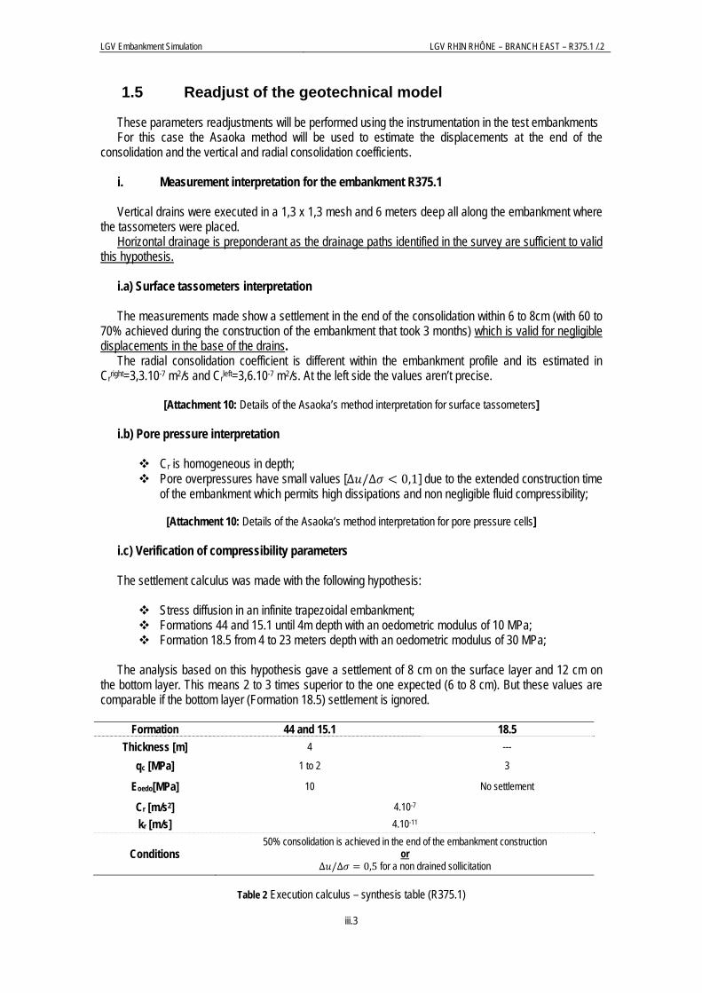
LGV Embankment Simulation LGV RHIN RHÔNE – BRANCH EAST – R375.1 /.2
iii.3
1.5 Readjust of the geotechnical model
These parameters readjustments will be performed using the instrumentation in the test embankments For this case the Asaoka method will be used to estimate the displacements at the end of the
consolidation and the vertical and radial consolidation coefficients. i. Measurement interpretation for the embankment R375.1 Vertical drains were executed in a 1,3 x 1,3 mesh and 6 meters deep all along the embankment where
the tassometers were placed. Horizontal drainage is preponderant as the drainage paths identified in the survey are sufficient to valid
this hypothesis. i.a) Surface tassometers interpretation
The measurements made show a settlement in the end of the consolidation within 6 to 8cm (with 60 to
70% achieved during the construction of the embankment that took 3 months) which is valid for negligible displacements in the base of the drains.
The radial consolidation coefficient is different within the embankment profile and its estimated in Crright=3,3.10-7 m2/s and Crleft=3,6.10-7 m2/s. At the left side the values aren’t precise.
[Attachment 10: Details of the Asaoka’s method interpretation for surface tassometers]
i.b) Pore pressure interpretation
Cr is homogeneous in depth; Pore overpressures have small values [∆ /∆ 0,1] due to the extended construction time
of the embankment which permits high dissipations and non negligible fluid compressibility;
[Attachment 10: Details of the Asaoka’s method interpretation for pore pressure cells] i.c) Verification of compressibility parameters The settlement calculus was made with the following hypothesis:
Stress diffusion in an infinite trapezoidal embankment; Formations 44 and 15.1 until 4m depth with an oedometric modulus of 10 MPa; Formation 18.5 from 4 to 23 meters depth with an oedometric modulus of 30 MPa;
The analysis based on this hypothesis gave a settlement of 8 cm on the surface layer and 12 cm on
the bottom layer. This means 2 to 3 times superior to the one expected (6 to 8 cm). But these values are comparable if the bottom layer (Formation 18.5) settlement is ignored.
Formation 44 and 15.1 18.5 Thickness [m] 4 ---
qc [MPa] 1 to 2 3
Eoedo[MPa] 10 No settlement
Cr [m/s2] 4.10-7 kr [m/s] 4.10-11
Conditions 50% consolidation is achieved in the end of the embankment construction
or ∆ /∆ 0,5 for a non drained sollicitation
Table 2 Execution calculus – synthesis table (R375.1)

LGV Embankment Simulation LGV RHIN RHÔNE – BRANCH EAST – R375.1 /.2
iii.4
ii. Measurement interpretation for the embankment R375.2 The Cv parameter is estimated with a drainage path of 4 meters (a layer of 8 meters drained at the
surface and base) which is coherent with the analysis of the dissipation of pore overpressure. The Cv and Cr value are now both equal to 4.10-7 m2/s. This value is conservative and different from the
one measured in laboratory. The final settlement is around 16 cm and the consolidation degree around 85% can be considered
accurate. ii.a) Verification of compressibility parameters The settlement calculus was made with the following hypothesis:
Stress diffusion in an infinite trapezoidal embankment; Formations 44 and 15.1 until 8 meters depth with an oedometric modulus of 10 MPa; Formation 18.5 from 8 to 23 meters depth with an oedometric modulus of 30 MPa;
The analysis based on these hypothesis give a settlement of 17 cm on the surface layer and 8 cm on
the bottom layer. This means a 25cm settlement to the 16 cm expected. But these values are comparable if the bottom layer (Formation 18.5) settlement is ignored as already observed for the R375.1.
Formation 44 and 15.1 18.5 Thickness [m] 8 to 9 ---
qc [MPa] 1 to 2 3 Eoedo[MPa] 10 No settlement
Cv = Cr [m/s2] 4.10-7 kv = kr [m/s] 4.10-11
Conditions Layer of 8 meters drained in two sides (drainage path never exceeds 4m); 50% consolidation is achieved in the end of the embankment construction
or ∆ /∆ 0,5 for a non drained sollicitation
Table 3 Execution calculus – synthesis table (R375.2)
1.6 CONCLUSIONS
In the case of vertical consolidation (embankment without drains) the consolidation times calculated are superior to the ones from the test embankment. But the incertitude in the interpretation of some parameters suggests a cautious approach in this case as concluded by the engineer responsible for the measurement response.