Thermodynamics of the Heat Engine

Waqas Mahmood, Salman Mahmood Qazi� and Muhammad Sabieh Anwar

May 10, 2011

The experiment provides an introduction to thermodynamics. Our principle objec-

tive in this experiment is to understand and experimentally validate concepts such

as pressure, force, work done, energy, thermal e�ciency and mechanical e�ciency.

We will verify gas laws and make a heat engine using glass syringes. A highly inter-

esting background resource for this experiment is selected material from Bueche's

book [1]. The experimental idea is extracted from [2].

KEYWORDS

Temperature � Pressure � Force � Work � Internal Energy � Thermal E�ciency �

Mechanical E�ciency � Data Acquisition � Heat Engine � Carnot Cycle � Transducer

� Second law of thermodynamics

APPROXIMATE PERFORMANCE TIME 6 hours

1 Conceptual Objectives

In this experiment, we will,

1. learn about the �rst and second laws of thermodynamics,

2. learn the practical demonstration of gas laws,

3. learn how to calculate the work done on and by the system,

4. correlate proportionalities between pressure, volume and temperature by

equations and graphs,

5. make a heat engine using glass syringes, and

6. make a comparison between thermodynamic and mechanical e�ciencies.

2 Experimental Objectives

The experimental objectives include,

�Salman, a student of Electronics at the Government College University worked as an intern

in the Physics Lab.

1

1. a veri�cation of Boyle's and Charles's laws,

2. use of the second law of thermodynamics to calculate the internal energy of

a gas which is impossible to directly measure,

3. making a heat engine,

4. using transducers for measuring pressure, temperature and volume, and

5. tracing thermodynamical cycles.

3 Theoretical introduction

3.1 First law of thermodynamics

We know from our lessons in science that energy is always conserved. Applying the

same principle to thermodynamics, we can write an equation that relates di�erent

variables such as heat entering a system, work done on the system and the system's

internal energy. Heat is de�ned as the energy transferred from a warm or to a

cooler body as a result of the temperature di�erence between the two.

Consider a gas contained in a cylinder. We call the gas our 'system'. If we heat

it, this energy may appear in two forms. First, it can increase the internal energy

U of the system. The change in the internal energy is given by,

UB � UA = �U (1)

where UB and UA represent the �nal and initial internal energies. Second, the

heat input to the system, can cause the gas to expand. This increases the volume

and work is done by the system on its surroundings, reducing the internal energy

content of the system itself. Therefore heat entering the system Q manifests as

an increase in internal energy and work done by the system on its surroundings.

Expressing this mathematically, we obtain,

Q = �U �W; (2)

or

�U = Q+W; (3)

We will revisit the concept in section 3.3. Note that the work done by the system

is conventionally taken to be negative �W .

Equation (3), which is simply rearrangement of (2) is another way of saying that

the internal energy can increase in two ways; �rst by heat entering the system and

second, by work done on the system.

Equations (2) and (3) are called the �rst law of thermodynamics relating heat,

internal energy and work. If a small amount of heat dQ results in a tiny change

in the internal energy dU as well as some in�nitesimal work dW , then Equation

(2) can be also written in its di�erential form,

2

U UA B

= A

(a) (c)

mg

Area

A

(b)

V L

L

Q

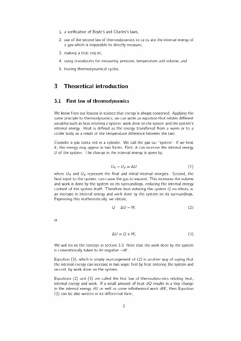
Figure 1: (a) System with internal energy UA. (b) Heat Q enters the system.

(c) Work done by the system as the gas expands. W = �P�V , is negative

by convention. The internal energy also increases to UB. The �rst law states

�U = Q+W = Q� P�V .

dQ = dU � dW: (4)

In summary, heating a system has two e�ects, �rst, on the internal energy, and

second, on the mechanical work done by the system.

3.2 E�ect of heat on internal energy

Suppose we have n moles of gas inside a container with rigid and �xed boundaries

implying that the gas cannot contract or expand, hence W = 0. The volume of

the gas in such a container remains constant. Now if we supply heat, the thermal

energy input will only increase the internal energy of the system. Since, there is

no change in volume, dV = 0, dW = 0, we can write Equation (4) as,

dQ = dU; (5)

meaning that all the heat added brings a change in the internal energy of the

system. The heat required to raise the temperature of n moles of gas at constant

volume is given by,

dQ = nCvdT; (6)

where Cv is the speci�c heat capacity of the gas at constant volume, and dT

is the small change in temperature. A constant-volume process is also called an

isochoric process.

3.3 Work done as a result of heating

Now suppose that the gas at atmospheric pressure is instead contained in a cylinder

�tted with a moveable piston. Since the piston can freely move, the volume of the

gas is variable but the pressure remains constant. If we now heat the container, the

3

internal energy of the gas molecules increases. The gas molecules perform work

on the piston by pushing it upwards and bring about an increase in the volume dV .

By our de�nition, the work done on the system, W , is negative. This is called

an isobaric (constant-pressure) process. The heat absorbed by n moles of gas at

constant pressure is given by,

dQ = nCpdT: (7)

where Cp is the speci�c heat capacity of gas at constant pressure.

Thermodynamic processes are commonly drawn on PV diagrams, where the pres-

sure is plotted on the y -axis and volume on the x-axis. The PV diagrams for some

representative processes are shown in Figure 2.

VA VB V

P

. .

V

P

..

V

P .

.

(a) (b)

(c)

i

f

i f

i

f

Figure 2: Typical PV curves for (a) isobaric, (b) isochoric and (c) isothermal

processes, i and f represent initial and �nal states.

The calculation for the work done is easy. For example, consider Figure 2 (a)

which shows an expansion process at constant pressure. The initial volume is VA.

Expansion results in an increase to a new volume VB. Since, work is given by Force

x distance = Pressure x area x distance = Pressure x change in volume, we have

the relationship,

W = �P�V = �P (VB � VA): (8)

Here the negative sign is introduced to ensure compliance with our convention.

(�V is positive, and work done on the system W is negative). Now P (VB � VA)

4

is just the area of the shaded rectangle shown, or the area under the PV curve.

This rule is in general true, work done can be calculated by measuring the area

under the PV curve. Let's illustrate this through a numerical example.

Example

Suppose a gas contracts in the way shown by the PV diagram in Figure 3. We

are asked to �nd the work done by the gas in going from the situation represented

by point A, through point B, to point C.

2

5

3 5 8

AB

C

00

P (

Pa

)

V (cm ) 3

x 102

x 105

3

4

1

1 2 4 6 7

...

Figure 3: An example for calculating the area under the curve when a system

traverses the path A ! B ! C.

As expected, we must compute the area under the curve. Notice that this irregular

shape consists of three simple shapes: two rectangles and one triangle. We can

calculate these three simple areas and add them to get the total area we need.

The area under the portion AB is given by,

(5:0 x 105Pa)[(800� 500)x10�6 m3] = 150 J: (9)

Similarly, the area under the curve from B to C is,

(2:0 x 105Pa)(200 x 10�6 m3) +1

2(3:0 x 105Pa)(200 x 10�6m3) = 70 J (10)

where we have used the fact that the area of a triangle is one-half the base times

the height. Therefore, the total area under PV curve = 150 J + 70 J = 220

J. Since, the process we are considering involves a decrease in volume, the work

done on the system �P�V is positive.

Q 1. Substitute Equations (7) and (8) into Equation (4) and show that,

nCpdT = dU + PdV: (11)

5

In an ideal gas, the internal energy U depends only on the temperature. Therefore,

if the temperature change at constant pressure has the same value as the tem-

perature change at constant volume, the increase dU must be the same between

an isobaric and isochoric process. Hence, substituting Equation (6) into Equation

(11) yields,

nCpdT = nCvdT + PdV: (12)

Q 2. Using the ideal gas law equation PV = nRT and Equation (12), show

that,

Cp = Cv + R; (13)

where R is called the molar gas constant. It has the value 8:31 J kg�1 K�1. Equa-

tion (13) relates the heat capacities of a gas at constant pressure and constant

volume.

3.4 Adiabatic processes

Suppose the gas is now contained in a cylinder that is �tted with a moveable

piston but in addition, the cylinder is perfectly insulated from the surroundings.

No exchange of heat is possible between the gas and the surroundings, dQ =

0. The idealized process in which no heat is absorbed or released is called an

adiabatic process. Consider Figure 4 which shows an isolated system with internal

energy UA. A weight is rapidly dropped onto the piston, compressing the gas and

increasing its internal energy to UB. The work done on the system is now positive

and given by,

U UA B

= A

(a) (b)

mg

Area

A V L

L

V

P

..

.

i

f

f.

Rapidly place an additional weight

insulation

(c)

.

.

Figure 4: (a) An insulated cylinder with gas inside. (b) Rapid placement of the

weight makes the process adiabatic. (c) The PV diagrams for isothermal and

adiabatic curves, shown respectively by i ! f and i ! f 0.

dW = �PdV: (14)

6

Remember the negative sign: it ensure dW is positive when dV is negative! Since

no heat enters or leaves the system we have,

dQ = 0; (15)

and using Equation (12) we obtain,

nCvdT + PdV = 0: (16)

Rearranging the terms and using PV = nRT ,

nCvdT + nRTdV

V= 0: (17)

The solution of the above equation can be found in [1], and in your higher classes

you will learn how to solve such equations, but let's su�ce for the time being to

stating just the result. The solution is,

PV = constant: (18)

Here, =Cp

Cv

is the ratio of the speci�c heats at constant pressure and volume.

Figure 5 shows the values of for di�erence materials. Figure 4(c) shows how

an adiabatic process looks like on a PV diagram. For a comparison, an isothermal

process for which PV 1 = constant is also shown. Notice the steeper slope for the

adiabatic process.

r

Figure 5: = CP =CV for various gases.

Q 3. Derive the solution (17) or show that Equation (18) is indeed a solution.

4 Introduction to the Apparatus

A photograph of the experimental assembly is presented in Figure (6).

1. Beakers and Hot plate for heating water. The heating is achieved by the

provided hot plate. The maximum temperature of the hot plate is around

400 �C.

7

potentiometer

positive

sliding contact

GND

clamp stand

glass syringe

Figure 6: Photograph of the experimentally assembly.

2. Conical asks We will use 37 and 50 mL conical asks. The small volume

of the asks provides the essential pressure required to lift the piston of the

syringe.

3. Piezoresistive pressure transducer

A pressure sensor (MPXH6400, Freescale Semiconductor) [3] is used to

monitor the pressure variation inside the conical ask. The sensor is con-

nected to a glass syringe through luer connectors (Harvard Apparatus).

Three wires labeled VIN , GND and VOUT are attached to the terminals 2,

3 and 4. The numbering starts from the end with a notch. A �xed DC

8

voltage of +5 volts is applied at pin 2 by a 30 Vdc power supply and the

output is read at pin number 4 using a digital multi-meter. The pin number

4 is also connected to the data acquisition system (DAQ) to record the

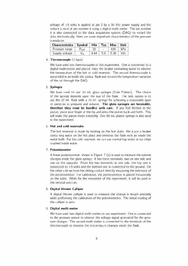
data electronically. Here are some important characteristics of the pressure

transducer.

Characteristics Symbol Min Typ Max Unit

Pressure range POP 20 - 400 kPa

Supply voltage VS 4.64 5.0 5.36 Vdc

4. Thermocouple (J type)

We have used two thermocouples in this experiment. One is connected to a

digital multi-meter and placed inside the beaker containing water to observe

the temperature of the hot or cold reservoir. The second thermocouple is

suspended in air inside the conical ask and records the temperature variation

of the air through the DAQ.

5. Syringes

We have used 10 and 20 mL glass syringes (Cole Palmer). The choice

of the syringe depends upon the size of the ask. The best option is to

use the 37 mL ask with a 20 mL syringe for achieving a reasonable span

of variation in pressure and volume. The glass syringes are breakable,

therefore they must be handled with care. If you feel friction in the

piston, place your �nger at the tip and press the piston back and forth. This

will make the piston move smoothly. One 60 mL plastic syringe is also used

in the experiment.

6. Hot and cold reservoirs

The hot reservoir is made by heating on the hot plate. We place a beaker

containing water on the hot plate and immerse the ask with air inside the

water bath. For the cold reservoir, we can use normal tap water or ice chips

crushed inside water.

7. Potentiometer

A linear potentiometer, shown in Figure 7 (a) is used to measure the volume

changes inside the glass syringe. It has three terminals, two on one side and

one on the opposite. From the two terminals at one side, the top one is

connected to +5 volts and the bottom one is connected to the ground. On

the other side we have the sliding contact directly measuring the extension of

the potentiometer. For calibration, the potentiometer is placed horizontally

on the table. While for the remainder of the experiment, it will be used in

the vertical position.

8. Digital Vernier Calliper

A digital Vernier calliper is used to measure the change in length precisely

while performing the calibration of the potentiometer. The initial reading of

the calliper is zero.

9. Digital multi-meter

We have used two digital multi-meters in our experiment. One is connected

to the pressure sensor to observe the voltage signal generated for the pres-

sure changes. The second multi-meter is connected to the terminals of the

thermocouple to monitor the temperature changes inside the ask.

9

positive

GND

sliding contact

(a)

(b)

Figure 7: (a) Connections to the potentiometer. (b) Fixation of the digital Vernier

calliper to measure the increase in length

10. Power supply for potentiometer and pressure transducer One 30 V DC

power supply is used to provide a �xed +5 V to the pressure transducer.

The second is connected to the potentiometer and provides a +5 V �xed

DC voltage.

5 The Experiment

5.1 Calibration of the potentiometer

A potentiometer is a three-terminal device with one sliding contact that acts as

a voltage divider. The other two terminals are connected to voltage and ground

through a power supply. In our experiment, we will use a linear potentiometer

to measure the volume change of air in a glass syringe. The change in volume

of air in a syringe is recorded in terms of voltage that is recorded electronically

using DAQ and we can convert it into volume using a calibration equation of the

potentiometer. The �rst step is this calibration.

Q 4. Place the potentiometer horizontally on the table and �x it with the

help of scotch tape such that it does not move. Connect a multi-meter to the

potentiometer and using the provided support and tape, �x the calliper as shown

10

in Figure 7 (b). Try to keep the Vernier calliper and the potentiometer at the

same level and �x the sliding bar of the calliper to the potentiometer using tape.

Make sure that the calliper does not move but its length can be changed.

Q 5. Make connections to the power supply.

Q 6. Note down the initial reading of the voltage when the displacement of

the sliding contact is zero.

Q 7. Now start increasing the displacement and measure the corresponding

voltage. Try to increase the length in small increments to get a large number

of readings. The reading on the calliper directly measures the length and the

voltmeter shows the corresponding voltage.

Q 8. Plot the voltage versus displacement and using the curve �tting tool in

MATLAB, obtain the calibration equation for the potentiometer. Find the slope

and intercept of this curve, paying close attention to the units. You will use the

slope (V=mL) and intercept (mL) in the LabView codes.

5.2 Verifying Charles's law

In the present section, we aim at verifying the Charles's law and predicting the

absolute zero of temperature. If you are not sure, what the law is, look up [1].

Q 9. Write a mathematical equation for the Charles's law.

Q 10. Connect a 10 mL glass syringe to a 37 or 50 mL ask with the help

of plastic tubing as shown in Figure 8 (a). Make sure there is no droplet of

water inside the ask. This may produce extra pressure due to the evaporation

of the water molecule and not due to the expansion of air. Guided by the �gure,

complete the assembly.

Q 11. To make the ask sealed properly, use silicone or te on tape. Place the

ask in a beaker containing water and heat it on a hot plate.

Q 12. Open the LabView �le temperatureversusvolume.vi and click Run.

The data will be saved in a �le charleslaw.lvm in the Z drive containing the folder

heat engine.

Q 13. As the water is heated, you will notice a change in the volume of

the gas, making the piston of the syringe to move upwards. This change in

volume is recorded using the linear potentiometer whose output is a variable voltage

connected to the DAQ.

Q 14. The change in temperature is monitored using the thermocouple placed

in the water and connected to the DAQ.

Q 15. Open the saved �le in Matlab and using the recorded data, plot the

curve between volume and temperature and calculate the value of the absolute

zero by extrapolation. The predicted value is �273 �C. For this part use the

calibration equation achieved in Q8.

Q 16. Repeat the same experiment by directly heating the ask on a hot plate

11

Hot Plate

Hot Plate

Air

Thermocouple

Pressure

Sensor

(a) (b)

To power supplyTo DAQ

GND

Thermocouple to DAQ

waterAir

glass syringe

Figure 8: (a) Experimental scheme for the veri�cation of Charles's law. (b) Setup

to see the behavior of pressure versus temperature when the volume is �xed.

and calculate the absolute zero temperature.

Q 17. Explain the di�erence between the two methods. Which method pro-

vides more reliable readings?

5.3 Verifying the change in pressure versus temperature at

constant volume

Q 18. Connect a 37 mL ask using plastic tubing directly to the pressure

sensor as shown in Figure 8 (b). Prefer using the smaller volume ask to have

su�cient expansion of the syringe. Make the connections tight using silicone or

te on tape to avoid any leakage.

Q 19. Place the ask in water. Open the LabView �le named as pressure-

versustemperature.vi and click Run after setting the hot plate on for heating.

The values for temperature and pressure will be recorded in the �le pressurever-

sustemperature.lvm in the same folder as described in section 5:2. Plot a curve

for pressure versus temperature.

Q 20. Estimate the value of absolute zero temperature.

Note: Do not heat the ask directly for a long time. The maximum temper-

ature should not exceed 90 �C.

12

6 The heat engine

The industrial revolution in the late eighteenth century catalyzed the formation of

a machine that could e�ciently convert thermal energy into mechanical work [1].

Initially, these were low e�ciency machines but with time a su�cient increase in

e�ciency was made possible. A device that converts thermal energy to mechanical

work is called as a heat engine.

In principle, heat is taken in from a hot reservoir and used to do work. There is

also some on ow of energy to a cold body. We know from our daily experiences

that the conversion of work to heat is easy but it is more challenging to obtain

work from thermal energy. Kelvin formulated this perception in his second law of

thermodynamics.

No process is possible whose sole result is the complete conversion of heat

into work.

An alternative statement of the second law is, it is impossible experimentally

to convert thermal energy into work with out any loss of energy to a cold

environment.

Now let's try to understand the above statement using heat engines, such as steam

and petrol engines. Steam and automobile engines convert heat into mechanical

energy. The steam engine obtains heat from the combustion of coal in a boiler

whereas the automobile engine obtains heat from the combustion of petrol in

its cylinders. A substantial amount of heat is lost to surroundings through the

condenser of the steam engine and the radiator of an automobile engine.

Consider the owchart of a simple heat engine shown in Figure 9. An amount

of heat QH is given to the engine by the hot reservoir held at the temperature

TH. This amount of input energy will be utilized in doing some work W and the

remaining energy will the transferred to the cold reservoir QC at temperature TC , in

line with the energy conservation principle. Using the �rst law of thermodynamics

we can write,

Qnet = QH �QC = W; (19)

whereW is the mechanical work done by the engine in one complete cycle, implying

�U = 0.

Now we de�ne the thermodynamic e�ciency, the ratio of work done to the input

thermal energy, given by,

� =W

Qnet

: (20)

Substituting Equation ( 19) in the above equation we obtain,

� = 1�QC

QH

; (21)

13

Cold reservoir

Tc

Hot reservoir

TH

Heat engine Output in the form of Work

Q H

Q C

Figure 9: Working principle of a heat engine.

which can also be written in terms of absolute temperatures as,

� = 1�TC

TH: (22)

The above equation shows that the e�ciency of any heat engine is de�ned by the

di�erence in temperatures of the cold and hot reservoir.

Q 21. Derive Equation (21) and Equation (22).

Q 22. Under what conditions is the thermodynamic e�ciency � = 100 %?

Before moving to the experimental part of making a simple heat engine using a

glass syringe, we discuss an ideal engine working in a cyclic process.

6.1 The Carnot cycle

Sadi Carnot in 1824 proposed an ideal heat engine capable of converting thermal

energy into work. When a system performs work with the application of the

thermal energy, the variables such as pressure and temperature, de�ning the state

of the system change. If at the end of the processes, the initial state is resotred,

it is called a thermodynamical cycle.

To understand how the Carnot cycle works, consider an example of a gas contained

in a cylinder that is �tted with a piston as shown in Figure 10.

If we place the cylinder in contact with a high temperature thermal reservoir at

14

Work done by the gas

Gas continues to do work

Work done on the gas

Work done on the gas

Cold reservoir (TC)Hot reservoir (TH)

Step I Step II Step III Step IV

Piston

Isothermal expansion Adiabatic expansion Isothermal compression Adiabatic compression

A B B C C D D A

InsulationInsulation

Figure 10: Demonstration of di�erent phases of the Carnot cycle.

temperature TH, the gas expands and does some work on the piston by moving it

to a new position as shown in step I. The temperature of the gas does not change

in this process. This process in which the engine absorbs heat and performs work

at a constant temperature is known as the isothermal process and leads to the

trajectory, A ! B as shown in Figure 11.

V

P ..

.

isothermal expansion

.

isothermal compression

adiabatic expansion

adiabatic

compresssion

A

B

C

D

Figure 11: PV diagram for the Carnot cycle.

If we now remove the cylinder from the heat reservoir, the gas will continue to

expand. This is an adiabatic process in which the gas does work while being

insulated from its surroundings. As the gas is expanding, its temperature will

continue to decrease. The adiabatic curve representing step II is shown in Figure

11 by the path B ! C.

Now we place the cylinder in contact with a low temperature reservoir at temper-

ature TC . The heat now ows from the gas to the reservoir thus decreasing its

energy. As the temperature remains constant, therefore, this is also an isothermal

15

process and is shown in Figure 11 from C ! D.

Now, if we sever the contact between the low temperature reservoir and the cylin-

der, the gas will continue to reduce its volume. Since no heat is added or taken

out of the system, this is adiabatic compression. The original volume has been

restored and initial pressure value is achieved. The path D ! A in Figure 11

depicts this process and completes the Carnot cycle.

In the following experiment, we will employ the above principles and construct a

simple heat engine that operates in a cyclic process between two temperatures

TH and TC . You will be able to calculate the thermodynamic and mechanical and

e�ciencies and see how they di�er from each other. The mechanical e�ciency is

de�ned later.

6.2 Practical demonstration of the heat engine

Q 23. Connect a 20 mL glass syringe to the pressure sensor, 37 ml conical

ask and a linear potentiometer as shown in Figure 12. The position of the

potentiometer should be vertical allowing the free movement of the sliding contact.

Cold water

Pressure

sensor

To DAQ

To power supply

To power supply

GND

To DAQ

GND

Potentiometer

Glass syringe

Small mass

Flask

Air

Thermocouple to DAQ

(a) (d)(b) (c)

Hot water

D A A B B C C D

Cold water

Figure 12: Steps depicting the implementation of the Carnot cycle.

Q 24. Place the ask in the cold reservoir whose temperature is monitored

using the thermocouple. Open the LabView �le heatengine.vi and click Run.

The values of pressure and volume will be stored in a �le heatengine.lvm in the

heat engine folder in the Z drive. Now place a small mass (e.g. 50 or 100 g) at

the top of the syringe slowly, without displacing the assembly, see Figure 12 (a).

The gas inside the ask contracts adiabatically and moves the potentiometer. The

relevant change in the position is monitored using the DAQ system. Now move

16

the ask to a hot reservoir with known temperature, as shown in Figure 12 (b)and

observe the changes. Next, remove the mass slowly from the piston, making the

piston to expand more, Figure 12 (c) representing the expansion. Last, place the

ask back in the cold reservoir as shown in Figure 12 (d). The gas achieves its

original volume. Stop the vi �le.

Q 25. Open the saved �le in Matlab and plot the pressure versus volume curve.

Q 26. Discuss your result with the demonstrator and give reasoning why is it

di�erent from the ideal curve?

Q 27. Calculate the total work done and heat added during the process.

Q 28. Calculate the thermodynamic e�ciency.

Q 29. Calculate the mechanical e�ciency de�ned as,

�mech =Work output

Work input: (23)

Q 30. Make a semi-logarithmic plot for the data obtained in the adiabatic

process of the heat engine cycle and calculate the value for for air. Compare

your value with the published value of 1:31 [4].

Q 31. Calculate the uncertainty in ?

References

[1] Fredrick J. Bueche and David A. Jerde, Principles of Physics, (McGraw Hill,

1995), pp. 352-391.

[2] David P. Jackson and Priscilla W. Laws, Syringe thermodynamics: The many

uses of a glass syringe, American Journal of Physics, 74, 94-101, (2005).

[3] Date sheet of MPXH6400 pressure sensor is downloadble from

http://www.freescale.com/.

[4] Paul F. Rebillot, Determining the Ratio Cp=Cv us-

ing Rucchart's Method, Wooster, Ohio, April (1998),

http://www3.wooster.edu/physics/jris/Files/Rebillot.pdf.

17